Fisheries Research 73 (2005) 323–339

Gill-net selectivity off the Portuguese western coast

Paulo Fonsecaa,∗, Rogelia Martinsa, Aida Camposa, Preciosa Sobralb

a INIAP/IPIMAR, Portuguese Institute for Agriculture and Fisheries Research, Avenida de Bras´ılia, 1449-006 Lisboa, Portugalb INIAP/IPIMAR (CRIPCentro), Regional Centre for Fisheries Research, Aveiro, Canal das Pirˆamides, 3800 Aveiro, Portugal

Received 9 July 2004; received in revised form 9 January 2005; accepted 18 January 2005

Abstract

Fishing with experimental gill-nets was carried out during 1994 and 1995 off the western coast of Portugal, using mesh sizesbetween 40 and 90 mm. Most sets were concentrated in the region between Setubal and Lisbon in shallow waters up to 100 m,with about 1/4 being carried out at greater depths. A total of 88 species were captured over the 2 years, of which the majorityhad small or no commercial value. The most important commercial species (hake,Merluccius merluccius, pouting,Trisopterusluscus, axillary seabream,Pagellus acarne, red mullet,Mullus surmuletus, and horse mackerel,Trachurus trachurus) accountedfor about 12% of the catch weight in the 40 mm mesh panels, between 32 and 44% for mesh panels ranging between 60 and80 mm, and 70% in the 90 mm mesh panels. The estimation of selectivity was carried out for the latter five species and also forthe dogfish,Scyliorhinus canicula, wedge sole,Dicologlossa cuneata, and spotted flounder,Citharus linguatula, applying theSELECT method to the data pooled over both years. In the case of hake, pouting and dogfish, sufficient data were available toestimate selectivity on a yearly basis. Four different uni-modal and a bi-modal (bi-normal) models were fitted, with the bi-normal

n was thest fit. Thee panels ofavailable,ere poor,

ased only

mackerel;

g inent’

of

always providing the best fit as given by the smallest value of the ratio deviance/degrees-of-freedom. The exceptiowedge sole where the bi-normal model did not converge and the gamma was the unimodal model providing the be40 mm mesh panels mostly retained species of low or no commercial value and undersized hake and pouting. Mesh siz60, 70 and 80 mm proved to be the most efficient in catching the commercially valuable species over the length rangewith virtually no catch of undersized fish. The 90 mm panels retained mainly valuable species, but the overall catches wwith the exception of the axillary seabream. These results highlight the difficulties of managing multispecies fisheries bon mesh size, since the optimal mesh varies considerably among the target species.© 2005 Elsevier B.V. All rights reserved.

Keywords: Gill-net; Size selection; Portuguese western coast; Axillary seabream; Small-spotted dogfish; European hake; HorsePouting; Striped red mullet; Spotted flounder; Wedge sole

∗ Corresponding author. Tel.: +351 213 027163;fax: +351 213 015948.

E-mail addresses:pfonseca@ipimar.pt (P. Fonseca),rmartins@ipimar.pt (R. Martins), acampos@ipimar.pt (A. Campos),

1. Introduction

Most of the Portuguese fishing vessels operatincoastal waters are included in the so-called ‘polyval(multi-gear, multi-species) fleet. This fleet consists

cripc@ipimar.pt (P. Sobral). almost 7000 vessels, most of them between 7 and 9 m

0165-7836/$ – see front matter © 2005 Elsevier B.V. All rights reserved.doi:10.1016/j.fishres.2005.01.015

324 P. Fonseca et al. / Fisheries Research 73 (2005) 323–339

overall length with open-deck, and thus only fishingwithin a limited area off the coastline. The economicand social importance of this fleet is evidenced by thecontribution to the total landings and revenue, about30 and 60%, respectively, and the number of fishermeninvolved, nearly 80% of the total.1

The gears used by this fleet include gill-nets andtrammels, longlines, traps, pots, dredges, beam-trawlsand beach seines. Although most of the fishing is car-ried out in shallow waters, often corresponding to nurs-ery zones, some of the fishing grounds are located atgreater depths. This is the case of longlining for theblack scabbard,Aphanopus carboand the Europeanhake,Merluccius merluccius, and the gill-net and tram-mels fisheries for the hake and monkfish,Lophiusspp.,respectively.

Gill-nets and trammels comprise almost 50% of thetotal licences issued every year (a vessel can be licensedfor the use of multiple gears). Current Portuguese leg-islation, Decree-law no. 7/2000 and Act 1102H/2000,limits the use of these gears in oceanic waters by re-stricting fishing areas and seasons, duration of sets andgear characteristics such as total length, and panel max-imum height and mesh size.

Gill-nets are highly selective for those species cap-tured mainly by gilling (i.e., captured behind the gill-cover) or wedged (being held by a mesh around theirmaximum body girth). For these, retention is supposedto increase with size up to a length of maximum catchand decrease thereafter, and consequently the range ofs witha ddi-t sticsr ines avea ion.S re-t ce ofw dyp inga shb

ent st ofP 98,

lture(

2003; Erzini et al., 2003), the information available forthe western coast is scarce (Martins et al., 1990). Thepresent study represents the first attempt to describegear selection patterns for a number of species caughtin the coastal waters off the western coast.

2. Materials and methods

2.1. Survey areas and gears

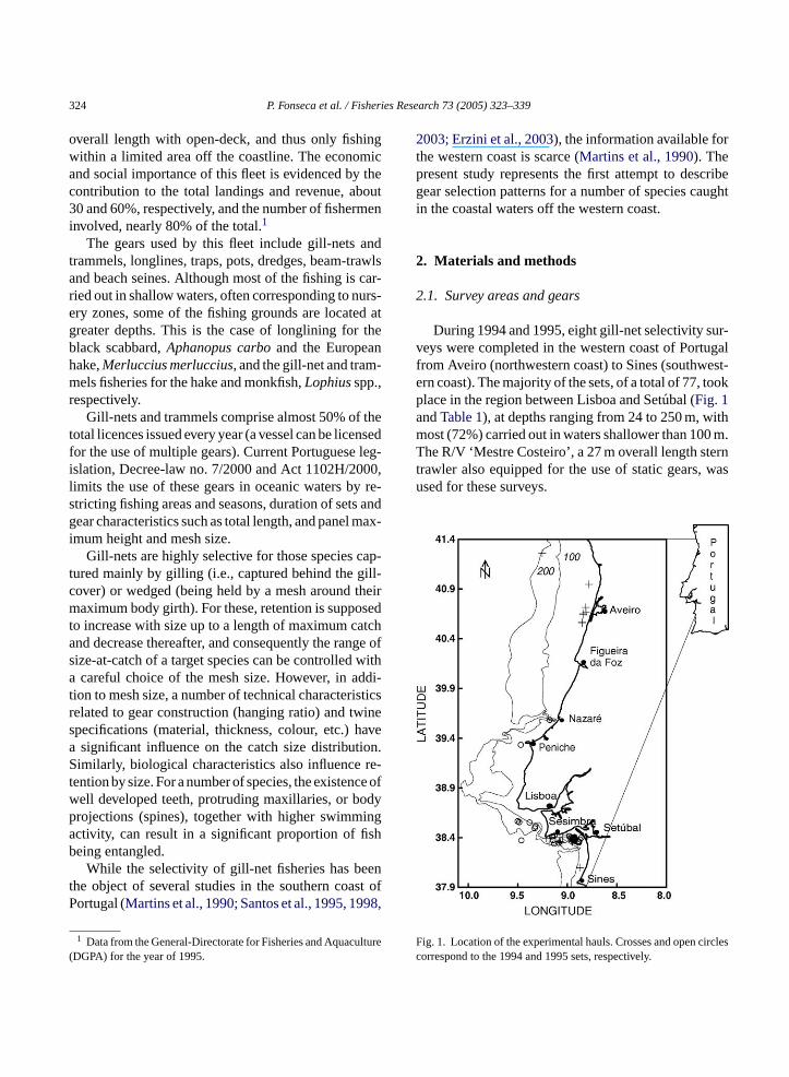
During 1994 and 1995, eight gill-net selectivity sur-veys were completed in the western coast of Portugalfrom Aveiro (northwestern coast) to Sines (southwest-ern coast). The majority of the sets, of a total of 77, tookplace in the region between Lisboa and Setubal (Fig. 1andTable 1), at depths ranging from 24 to 250 m, withmost (72%) carried out in waters shallower than 100 m.The R/V ‘Mestre Costeiro’, a 27 m overall length sterntrawler also equipped for the use of static gears, wasused for these surveys.

F irclesc

ize-at-catch of a target species can be controlledcareful choice of the mesh size. However, in a

ion to mesh size, a number of technical characterielated to gear construction (hanging ratio) and twpecifications (material, thickness, colour, etc.) hsignificant influence on the catch size distributimilarly, biological characteristics also influence

ention by size. For a number of species, the existenell developed teeth, protruding maxillaries, or borojections (spines), together with higher swimmctivity, can result in a significant proportion of fieing entangled.

While the selectivity of gill-net fisheries has behe object of several studies in the southern coaortugal (Martins et al., 1990; Santos et al., 1995, 19

1 Data from the General-Directorate for Fisheries and AquacuDGPA) for the year of 1995.

ig. 1. Location of the experimental hauls. Crosses and open correspond to the 1994 and 1995 sets, respectively.

P. Fonseca et al. / Fisheries Research 73 (2005) 323–339 325

Table 1Description of the different surveys carried out in 1994 and 1995, including number of sets by survey, mesh sizes used and total fishing time

Year Month Nb sets Total duration (h) Mesh size (mm)

1994 April 19–26 5 515 40/60/70/80June 09–29 12 40/60/70/80July 06–13 5 40/60/70/80November 1–16 6 40/60/70/80

1995 April 19–May 02 8 640 40/60/70/80/90May 23–31 9 40/60/70/80/90July 19–August 10 18 40/60/70/80/90September 13–27 14 40/60/70/80/90

During the experiments carried out in 1994, the gearwas composed of ten panels of each mesh size, 40, 60,70 and 80 mm stretched (nominal) length, disposed al-ternately, with about 30 cm spacing between adjacentpanels. In 1995 a similar number of 90 mm panels wereadded to the experimental fleet. Panel dimensions were50 m× 3 m in length and in height, respectively. Hang-ing coefficients were kept constant at about 0.5 (seeTable 2for gear details).

2.2. Experimental procedures

The most productive period for gill-net fishing isbetween dusk and dawn, and therefore the gears arenormally set during the few hours before sunset andhauled early in the morning. However, the effectiveduration of fishing and deployment period is depen-dent on the target species and local conditions. In thepresent study, the soaking time varied from about 3 toover 24 h, either due to biological factors (occurrenceof scavengers) or operational constraints (e.g., weatherconditions preventing haul-up), with an average of 18 hfor 1994 and 13 h during 1995. Most often the fleet wasset 1 or 2 h before sunset or in the evening, and hauled

in the morning. Although on a few occasions the fish-ing started before noon and lasted until the followingmorning, only three sets occurred entirely during theday. Independently of the soaking time for each set, allmesh sizes were fished the same total time, since a sin-gle fleet was deployed with all the experimental panelsat the same time.

2.3. Catch handling

All species, whether commercial or not, were sortedout by mesh size, identified to species level, sexed andweighed to the nearest 0.1 g. Total length, as well asopercula and maximum girth, were measured to thenearest millimetre.

2.4. Selectivity estimation

The estimation of the selectivity of static gears,namely gill-nets, has been the object of a number of dif-ferent approaches: inference from girth measurements,direct estimates, mortality estimates, and indirect esti-mates (Hamley, 1975). In the latter, the structure ofthe population being fished is not known, and has to

Table 2Technical characteristics of the gill-nets used during the different surveys

Mesh size (mm) Length Nb of meshes Side line (m) Twine material Diameter (mm)

Floatline (m) Leadline (m) Length Height

46789

0 50.7 52.3 25360 51.8 53.2 16800 49.3 50.8 14500 49.5 50.8 12700 49.7 50.8 1130

74.0 3.0 PAmono 0.3549.0 3.0 PAmono 0.3543.5 3.0 PAmono 0.3537.5 3.0 PAmono 0.3533.0 3.0 PAmono 0.35

326 P. Fonseca et al. / Fisheries Research 73 (2005) 323–339

be inferred from the catches taken during comparativefishing experiments that simultaneously deploy multi-ple gill-net panels of different mesh sizes.

Assumptions on the equal availability of fishes of allsizes to the different mesh sizes and on the functionalform of the selection curves have to be made. A usefulsimplification is to assume that selection curves of thedifferent mesh sizes follow the ‘principle of geometricsimilarity’, introduced byBaranov (1948). Accordingto this assumption, the catch process is only dependenton the relative geometry of the fish and the mesh size.In other words, the selectivity of different mesh sizesis equal when the ratio of fish length to mesh size isthe same. This assumption implies that all mesh sizesare equally selective for the size of fish they catch mostefficiently (i.e., all the selection curves have the sameheight). Also, the curve spread will increase propor-tionally with mesh size. Although the ‘principle’ is anoversimplification of the retention process, since it doesnot take into account potentially distinct fish behaviouraccording to size class, or allometric growth or differ-ences in fishing power among the different mesh sizepanels, it is still the basis of most of the commonlyused methods. Other approaches have been tried, in-cluding the models used byHolt (1963)andKirkwoodand Walker (1986)which assume that the spread of theselection curve is the same for all mesh-sizes used.

From the early 1990s, a new methodologicalapproach for the analysis of gear selectivity data, theSELECT method (Millar, 1992) has arisen. First used inttTg y ofa ove( oni es )a ra sedo LS).A t invt eousp andm fort2

The SELECT method assumes that catches (nlj )by length class (l) and gear size (j) follow a Poissondistribution with parameterspj(l) (the relative fishingintensity, a combined measure of fishing effort andfishing power, representing the probability that afish of lengthl contacts the gear sizej given that itcontacts the combined gear),λl (the abundance oflength l fish contacting the combined gear) andrj(l)(the contact-selection curve; i.e., the probability ofretention of a fish of lengthl in gear sizej):

nlj ≈ Pois(pj(l)λlrj(l)) (1)

For model simplificationpj is usually taken as lengthindependent, and therefore, the log-likelihood ofexpression(1) is given by:

∑

l

∑

j

{nlj loge[pjλlrj(l)

] − pjλlrj(l)} (2)

where the term not depending on any of the parameterswas excluded.

By using the proportions of the total catch (foreach length class) taken by each mesh size panels(ylj =nlj /nl+), and considering that they follow a multi-nomial distribution with parametersnl+ and φlj =pjrj(l)/

∑jpjrj(l), the model can be further reduced as

λl is eliminated from the maximization process (Millarand Fryer, 1999). The log-likelihood ofylj can then bewritten:∑

w -t -l dt um-b andn dalm heset s)h on ofcb ta vet -t vesh

he context of trawling (Millar and Walsh, 1992), it washen extended to static gears (Millar and Holst, 1997).ogether with the work byFryer (1991)it constitutes aeneral framework for the analysis of the selectivitll types of fishing gears, both at haul-level and abMillar and Fryer, 1999) where parameter estimatis carried out by maximum likelihood (ML). In thtrict context of gillnet selectivity,Hovgard (1996ndHovgard et al. (1999)brought forward a similapproach to selectivity parameter estimation ban, either linear or non-linear, least squares (lthough both estimation procedures may resulery close estimates (seeErzini and Castro, 1998),he SELECT approach carries all the advantagroperties of maximum likelihood (e.g., unbiasedinimum variance estimators), further allowing

he incorporation of between-haul variability (Millar,000), and therefore will be used herein.

l

∑

j

nlj loge(φlj) (3)

hich depends only on parameterspj and the parameers of the selection curvesrj(l). For gill-net (and longine) selectivity,Millar and Holst (1997)demonstratehat the model reduces to a log-linear model for a ner of uni-modal selection curves (normal scaleormal location, lognormal and gamma). Multimoodels are also available under SELECT. Among t

he ‘bi-normal’ model (a mixture of two normal curveas often been used to accommodate a combinatilearly different catch processes (Hovgard, 1996) oreen found to provide an overall better fit (Madsen el., 1999; Moth-Poulsen, 2003). These models obser

he ‘principle of geometric similarity’, with the excepion of the ‘normal location’, where the selection curave a fixed spread.

P. Fonseca et al. / Fisheries Research 73 (2005) 323–339 327

A proprietary software (GILLNET, Constat, DK)was used here for selectivity estimation (equal powerover mesh sizes was assumed). The model providingthe best fit, corresponding to the smallest value for theratio deviance/degrees-of-freedom, was adopted.

2.5. Comparison between selection curves

The data were too scarce for haul-by-haul selec-tivity estimation or even for a survey based analysis,and therefore data from both years were pooled forall species. However, for three of the species (pout-ing, Trisopterus luscus, hake,Merluccius merluccius,and dogfish,Scyliorhinus canicula), a yearly estima-tion of the selectivity could be carried out. In thesecases, a likelihood ratio test (LRT) (see, for exam-ple, McCullagh and Nelder, 1989) was used to testfor significant differences in selectivity between the2 years. For this purpose, the deviances resulting fromthe fits to individual years are summed up and thencompared to the deviance resulting from the model fit-ted to the combined data. The combined dataset wasconstructed by appending the 1995 dataset to the 1994dataset.

The value of [deviance(1994 + 1995)− (deviance(1994) + deviance(1995))] is distributed approximatelyχ2

d.f. where d.f. (the degrees of freedom) is given bythe change in the number of parameters when fittingthe separate and the joint selection curves. The sig-nificance level was set at 0.01, that is, the differenceb canti

3

overt gheri ostp phi-c eciesa lowm eco-n -isT et)w

Table 3presents the total catches by mesh size, innumber and in weight, for the most captured species,along with the proportions of high-valued species andtotal commercial species. It provides a basis for com-parison among the fishing characteristics of the differ-ent mesh size panels. The 40 mm mesh panels caughtmainly low or non-commercial species, along withsmall individuals of the most valuable ones. On theother hand, for mesh sizes from 60 to 80 mm, theproportion of highly valuable fish is within a rela-tively close range (0.32–0.44). Also, the proportion of(high + low) commercial fish shows an increasing trendwith mesh size, both in number and in weight, attainingalmost one for the largest mesh size. The 90 mm pan-els presented the highest proportion, both in numberand in weight, of the highly valuable species (0.6 and0.7, respectively). They retained virtually no by-catchand caught the largest individuals of the highly valu-able species. However, no direct comparisons could becarried out with the other mesh size panels, since the90 mm panels were only used during 1995. The ex-ception is for the axillary seabream which was onlycaptured in 1995.

The most valuable species were mainly capturedwithin the mesh size range from 60 to 80 mm. Smallermesh sizes (40 mm) were observed to catch a high pro-portion of undersized fish, while the largest mesh size(90 mm) retained mainly valuable species, but had con-siderably lower yields.

3

ciesa r-r ctionc weret fora

dfl na sin-g eda ize( reda ingm thed ft the

etween years was considered statistically signifif the above value exceededχ2

d.f.,0.01.

. Results

Altogether, 88 different species were capturedhe 2 years, with the number of species being hin 1994 (74) than in 1995 (66). This difference is mrobably related to the much more restricted geograal area surveyed during 1995. Among these, 41 spre potentially commercialized, but most are ofarket value. Only five species can be consideredomically important for thismetier (hake, pouting, ax

llary seabream,Pagellus acarne, red mullet,Mullusurmuletus, and horse mackerel,Trachurus trachurus).he average yield (for the whole experimental fleas about 31.5 kg per set, or 2.1 kg h−1.

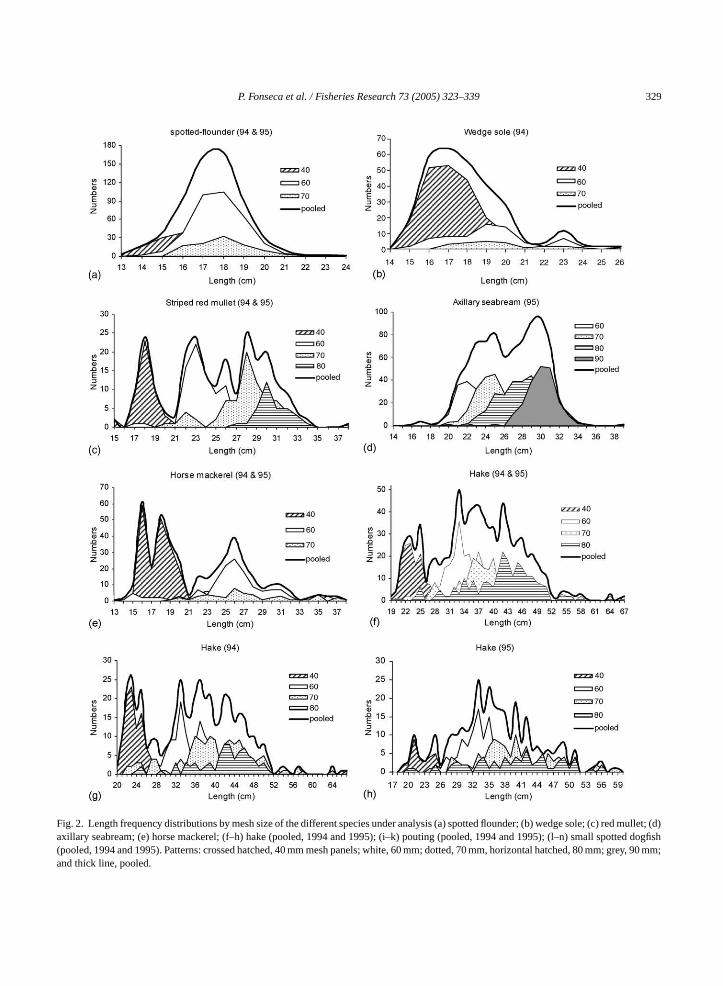
.1. Length frequency distributions

The length frequency distributions for the spenalyzed are shown inFig. 2(a)–(n). These plots coespond to the cases where the estimation of seleurves was possible. Hake, pouting and dogfishhe only species for which there was enough datan analysis by year.

Wedge sole,Dicologlossa cuneata, and spotteounder,Citharus linguatula, were captured withipproximately the same length range with similarle modes (Fig. 2(a) and (b)). The former was capturlmost exclusively above its minimum landing sMLS) of 15 cm. The red mullet was always captubove the MLS (15 cm), its size distribution beulti-modal and denoting a sharp selection byifferent mesh size panels (Fig. 2(c)). The majority o

he axillary seabreams were concentrated within

328 P. Fonseca et al. / Fisheries Research 73 (2005) 323–339

Table 3Catches in number (a) and weight (kg) (b) for high, low and non commercially valuable species, by mesh size

Catch/mesh size 40 60 70 80 90a

(a) High commercial valueEuropean hake 142 260 254 156 55Axillary seabream 6 192 256 285 218Red mullet 46 83 77 41 4Pouting 229 670 390 135 17Horse mackerel 229 153 48 20 2

Low commercial valueWedge sole 203 73 24 9Dogfish 111 701 1033 926 41

Other 4079 1186 1379 1187 141

Non commercialSpotted flounder 174 349 111 41 5Other 1132 323 148 98 54

Proportion of high commercial value 0.11 0.42 0.39 0.32 0.60Proportion of commercial value 0.78 0.79 0.90 0.93 0.88

(b) High commercial valueEuropean hake 21 89 131 94 32Axillary seabream 1 33 64 94 90Red mullet 3 15 25 16 1Pouting 12 90 72 32 5Horse mackerel 16 24 9 4 0

Low commercial valueWedge sole 9 5 2 1Dogfish 13 157 424 428 18Other 304 259 513 500 47

Non commercialSpotted flounder 6 15 6 2 0Other 75 46 26 14 7

Proportion of high commercial value 0.12 0.44 0.36 0.32 0.70Proportion of commercial value 0.81 0.89 0.96 0.98 0.96

a 90 mm nets were only used in 1995.

range of 21–31 cm, thus above the MLS of 18 cm; tworelatively close modes of similar importance can beperceived, one at 25 and the other at 30 cm (Fig. 2(d)).Similarly, practically no horse mackerel below theMLS (15 cm) were caught, but the catch lengthdistribution is distinctly broken in two (Fig. 2(e)),with the individuals from 16 to 20 cm correspondingbasically to those retained by the 40 mm mesh panels,and those from 22 to about 32 cm, with modes at 16and 26 cm, respectively.

Hake catches varied from 19 to 67 cm in length,with most fish concentrated in the range of 21–51 cm(Fig. 2(f)–(h)). Individuals below the MLS (27 cm)

were caught in considerable numbers in the 1994 sets.They were mostly captured in the 40 mm mesh panels,with about 84% of the catch constituted by undersizedfish, whereas for 60–80 mm panels this percentage wasat the most about 5%. For pouting, a bi-modal distribu-tion clearly split at the MLS (17 cm) can be observed(Fig. 2(i)). Undersized individuals (71% of the total)were exclusively retained by the smallest mesh sizeand presented a mode at 15 cm, while for commerciallysized catches the mode is situated at 23 cm. The dog-fish, ranging in size from 21 to 71 cm, were caught witha mode at 50 cm, but the most abundant length classeswere within the range of 38–55 cm (Fig. 2(l)).

P. Fonseca et al. / Fisheries Research 73 (2005) 323–339 329

Fig. 2. Length frequency distributions by mesh size of the different species under analysis (a) spotted flounder; (b) wedge sole; (c) red mullet; (d)axillary seabream; (e) horse mackerel; (f–h) hake (pooled, 1994 and 1995); (i–k) pouting (pooled, 1994 and 1995); (l–n) small spotted dogfish(pooled, 1994 and 1995). Patterns: crossed hatched, 40 mm mesh panels; white, 60 mm; dotted, 70 mm, horizontal hatched, 80 mm; grey, 90 mm;and thick line, pooled.

330 P. Fonseca et al. / Fisheries Research 73 (2005) 323–339

Fig. 2. (Continued).

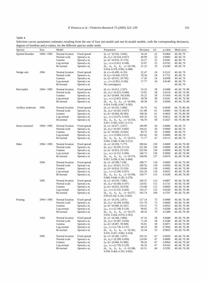
3.2. Selectivity estimation

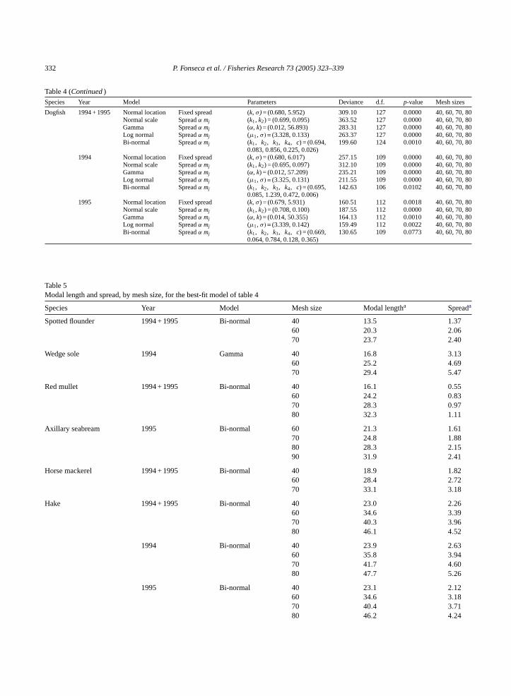
Table 4displays the results of the fits for the fouruni-modal and the single bi-modal (bi-normal) mod-els, while the modal lengths and spread values of theselection curves corresponding to the best-fit modelare shown inTable 5. For the majority of the datasetsthe bi-normal model provided the best fit, presentingthe smallest value for the ratio deviance/d.f. The ex-ception was for the wedge sole where no convergence

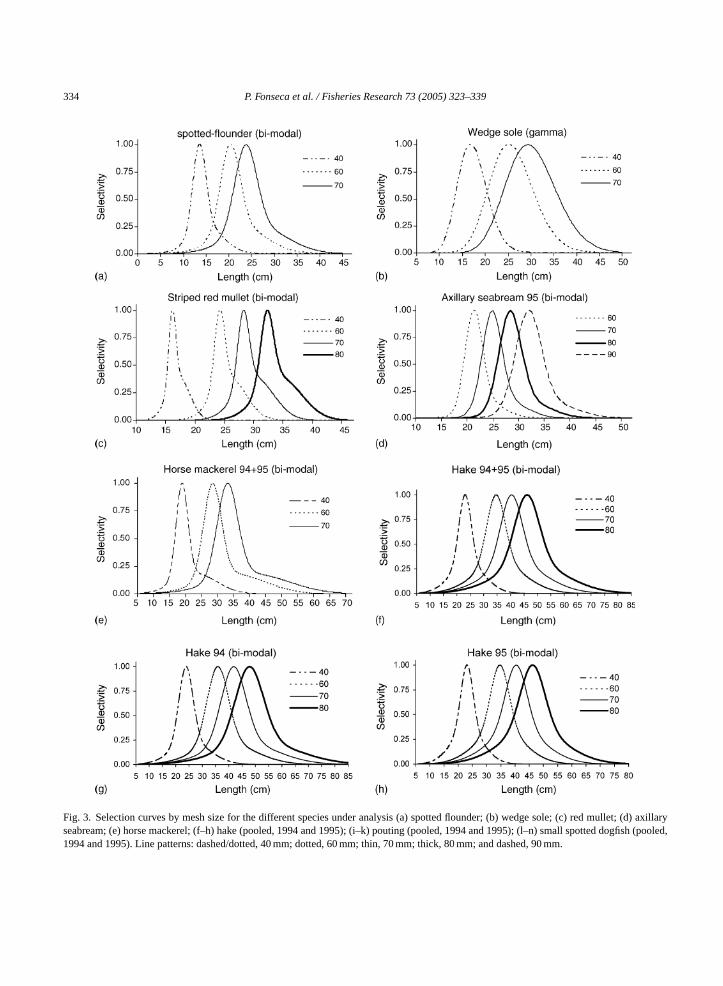
could be obtained and the Gamma presented the bestfit among the unimodal models. In all of the bi-normalfits, the two modes of the fitted bi-normal curves wereinsufficiently separated to appear as two separate peaksin selection probability (Fig. 3). Instead, the fitted bi-normal curves were all uni-modal with varying degreesof right-skewness.

Both flatfish species (spotted flounder and wedgesole) were caught approximately within the samelength range, attaining a maximum size of 30 cm.

P. Fonseca et al. / Fisheries Research 73 (2005) 323–339 331

Table 4Selection curves parameters estimates resulting from the use of four uni-modal and one bi-modal models, with the corresponding deviances,degrees of freedom andp-values, for the different species under studySpecies Year Model Parameters Deviance d.f. p-value Mesh sizes

Spotted flounder 1994 + 1995 Normal location Fixed spread (k, σ) = (0.332, 3.045) 34.24 22 0.0464 40, 60, 70Normal scale Spreadα mj (k1, k2) = (0.354, 0.057) 40.99 22 0.0083 40, 60, 70Gamma Spreadα mj (α, k) = (0.010, 37.270) 33.27 22 0.0581 40, 60, 70Log normal Spreadα mj (µ1, σ) = (2.612, 0.168) 32.07 22 0.0762 40, 60, 70Bi-normal Spreadα mj (k1, k2, k3, k4, c) = (0.338,

0.034, 0.378, 0.091, 0.308)21.23 19 0.3240 40, 60, 70

Wedge sole 1994 Normal location Fixed spread (k, σ) = (0.409, 4.135) 22.47 24 0.5512 40, 60, 70Normal scale Spreadα mj (k, k2) = (0.426, 0.072) 18.56 24 0.7751 40, 60, 70Gamma Spreadα mj (α, k) = (0.015, 29.795) 17.20 24 0.8399 40, 60, 70Log normal Spreadα mj µ1, σ) = (2.851, 0.196) 17.77 24 0.8140 40, 60, 70Bi-normal Spreadα mj No convergence – – – 40, 60, 70

Red mullet 1994 + 1995 Normal location Fixed spread (k, σ) = (0.412, 2.507) 53.32 58 0.6498 40, 60, 70, 80Normal scale Spreadα mj (k1, k2) = (0.423, 0.040) 53.81 58 0.6319 40, 60, 70, 80Gamma Spreadα mj (α, k) = (0.004, 102.639) 56.22 58 0.5418 40, 60, 70, 80Log normal Spreadα mj (µ1, σ) = (2.823, 0101) 58.58 58 0.4541 40, 60, 70, 80Bi-normal Spreadα mj (k1, k2, k3, k4, c) = (0.404,

0.014, 0.430, 0.047, 0.582)40.38 55 0.9300 40, 60, 70, 80

Axillary seabream 1995 Normal location Fixed spread (k, σ) = (0.355, 2.684) 95.70 61 0.0030 60, 70, 80, 90Normal scale Spreadα mj (k1, k2) = (0.362, 0.037) 131.88 61 0.0000 60, 70, 80, 90Gamma Spreadα mj (α, k) = (0.004, 96.583) 108.36 61 0.0002 60, 70, 80, 90Log normal Spreadα mj (µ1, σ) = (3.075, 0.102) 100.33 61 0.0011 60, 70, 80, 90Bi-normal Spreadα mj (k1, k2, k3, k4, c) = (0.354,

0.027, 0.395, 0.057, 0.171)66.70 58 0.2027 60, 70, 80, 90

Horse mackerel 1994 + 1995 Normal location Fixed spread (k, σ) = (0.477, 5.027) 100.99 50 0.0000 40, 60, 70Normal scale Spreadα mj (k1, k2) = (0.507, 0.091) 104.41 50 0.0000 40, 60, 70Gamma Spreadα mj (α, k) = (0.020, 25.816) 99.75 50 0.0000 40, 60, 70Log normal Spreadα mj (µ1, σ) = (3.004, 0.211) 102.62 50 0.0000 40, 60, 70Bi-normal Spreadα mj (k1, k2, k3, k4, c) = (0.473,

0.045, 0.580, 0.166, 0.212)71.77 47 0.0115 40, 60, 70

Hake 1994 + 1995 Normal location Fixed spread (k, σ) = (0.559, 7.177) 290.64 130 0.0000 40, 60, 70, 80Normal scale Spreadα mj (k1, k2) = (0.592, 0.113) 221.06 130 0.0000 40, 60, 70, 80Gamma Spreadα mj (α, k) = (0.023, 25.510) 225.96 130 0.0000 40, 60, 70, 80Log normal Spreadα mj (µ1, σ) = (3.152, 0.206) 240.73 130 0.0000 40, 60, 70, 80Bi-normal Spreadα mj (k1, k2, k3, k4, c) = (0.576,

0.057, 0.599, 0.161, 0.409)168.96 127 0.0076 40, 60, 70, 80

1994 Normal location Fixed spread (k, σ) = (0.589,7.238) 188.77 118 0.0000 40, 60, 70, 80Normal scale Spreadα mj (k1, k2) = (0.621, 0.117) 160.56 118 0.0056 40, 60, 70, 80Gamma Spreadα mj (α, k) = (0.024, 25.510) 158.00 118 0.0082 40, 60, 70, 80Log normal Spreadα mj (µ1, σ) = (3.200, 0.207) 163.59 118 0.0035 40, 60, 70, 80Bi-normal Spreadα mj (k1, k2, k3, k4, c) = (0.596,

0.066, 0.646, 0.185, 0.278)129.77 115 0.1639 40, 60, 70, 80

1995 Normal location Fixed spread (k, σ) = (0.554, 7.082) 166.27 112 0.0007 40, 60, 70, 80Normal scale Spreadα mj (k1, k2) = (0.584, 0.107) 120.61 112 0.2725 40, 60, 70, 80Gamma Spreadα mj (α, k) = (0.022, 26.974) 133.08 112 0.0850 40, 60, 70, 80Log normal Spreadα mj (µ1, σ) = (3.141, 0.202) 143.37 112 0.0244 40, 60, 70, 80Bi-normal Spreadα mj (k1, k2, k3, k4, c) = (0.577,

0.053,0.142, 0.142, 0.502)105.74 109 0.5707 40, 60, 70, 80

Pouting 1994 + 1995 Normal location Fixed spread (k, σ) = (0.376, 2.871) 117.14 73 0.0008 40, 60, 70, 80Normal scale Spreadα mj (k1, k2) = (0.394, 0.050) 151.79 73 0.0000 40, 60, 70, 80Gamma Spreadα mj (α, k) = (0.006, 61.567) 110.31 73 0.0032 40, 60, 70, 80Log normal Spreadα mj (µ1, σ) = (2.748, 0.129) 99.65 73 0.0208 40, 60, 70, 80Bi-normal Spreadα mj (k1, k2, k3, k4, c) = (0.377,

0.035, 0.434, 0.074, 0.165)68.19 70 0.5389 40, 60, 70, 80

1994 Normal location Fixed spread (k, σ) = (0.368, 2.866) 47.16 58 0.8448 40, 60, 70, 80Normal scale Spreadα mj (k1, k2) = (0.387, 0.050) 71.20 58 0.1049 40, 60, 70, 80Gamma Spreadα mj (α, k) = (0.007, 59.508) 55.01 58 0.5871 40, 60, 70, 80Log normal Spreadα mj (µ1, σ) = (2.730, 0.131) 49.33 58 0.7843 40, 60, 70, 80Bi-normal Spreadα mj (k1, k2, k3, k4, c) = (0.362,

0.032, 0.427, 0.062, 0.324)35.34 55 0.9819 40, 60, 70, 80

1995 Normal location Fixed spread (k, σ) = (0.382, 2.875) 105.25 67 0.0020 40, 60, 70, 80Normal scale Spreadα mj (k1, k2) = (0.399, 0.050) 124.06 67 0.0000 40, 60, 70, 80Gamma Spreadα mj (α, k) = (0.006, 61.996) 99.26 67 0.0064 40, 60, 70, 80Log normal Spreadα mj (µ1, σ) = (2.759, 0.129) 94.10 67 0.0162 40, 60, 70, 80Bi-normal Spreadα mj (k1, k2, k3, k4, c) = (0.386,

0.038, 0.464, 0.105, 0.042)62.51 64 0.5292 40, 60, 70, 80

332 P. Fonseca et al. / Fisheries Research 73 (2005) 323–339

Table 4 (Continued)Species Year Model Parameters Deviance d.f. p-value Mesh sizes

Dogfish 1994 + 1995 Normal location Fixed spread (k, σ) = (0.680, 5.952) 309.10 127 0.0000 40, 60, 70, 80Normal scale Spreadα mj (k1, k2) = (0.699, 0.095) 363.52 127 0.0000 40, 60, 70, 80Gamma Spreadα mj (α, k) = (0.012, 56.893) 283.31 127 0.0000 40, 60, 70, 80Log normal Spreadα mj (µ1, σ) = (3.328, 0.133) 263.37 127 0.0000 40, 60, 70, 80Bi-normal Spreadα mj (k1, k2, k3, k4, c) = (0.694,

0.083, 0.856, 0.225, 0.026)199.60 124 0.0010 40, 60, 70, 80

1994 Normal location Fixed spread (k, σ) = (0.680, 6.017) 257.15 109 0.0000 40, 60, 70, 80Normal scale Spreadα mj (k1, k2) = (0.695, 0.097) 312.10 109 0.0000 40, 60, 70, 80Gamma Spreadα mj (α, k) = (0.012, 57.209) 235.21 109 0.0000 40, 60, 70, 80Log normal Spreadα mj (µ1, σ) = (3.325, 0.131) 211.55 109 0.0000 40, 60, 70, 80Bi-normal Spreadα mj (k1, k2, k3, k4, c) = (0.695,

0.085, 1.239, 0.472, 0.006)142.63 106 0.0102 40, 60, 70, 80

1995 Normal location Fixed spread (k, σ) = (0.679, 5.931) 160.51 112 0.0018 40, 60, 70, 80Normal scale Spreadα mj (k1, k2) = (0.708, 0.100) 187.55 112 0.0000 40, 60, 70, 80Gamma Spreadα mj (α, k) = (0.014, 50.355) 164.13 112 0.0010 40, 60, 70, 80Log normal Spreadα mj (µ1, σ) = (3.339, 0.142) 159.49 112 0.0022 40, 60, 70, 80Bi-normal Spreadα mj (k1, k2, k3, k4, c) = (0.669,

0.064, 0.784, 0.128, 0.365)130.65 109 0.0773 40, 60, 70, 80

Table 5Modal length and spread, by mesh size, for the best-fit model of table 4

Species Year Model Mesh size Modal lengtha Spreada

Spotted flounder 1994 + 1995 Bi-normal 40 13.5 1.3760 20.3 2.0670 23.7 2.40

Wedge sole 1994 Gamma 40 16.8 3.1360 25.2 4.6970 29.4 5.47

Red mullet 1994 + 1995 Bi-normal 40 16.1 0.5560 24.2 0.8370 28.3 0.9780 32.3 1.11

Axillary seabream 1995 Bi-normal 60 21.3 1.6170 24.8 1.8880 28.3 2.1590 31.9 2.41

Horse mackerel 1994 + 1995 Bi-normal 40 18.9 1.8260 28.4 2.7270 33.1 3.18

Hake 1994 + 1995 Bi-normal 40 23.0 2.2660 34.6 3.3970 40.3 3.9680 46.1 4.52

1994 Bi-normal 40 23.9 2.6360 35.8 3.9470 41.7 4.6080 47.7 5.26

1995 Bi-normal 40 23.1 2.1260 34.6 3.1870 40.4 3.7180 46.2 4.24

P. Fonseca et al. / Fisheries Research 73 (2005) 323–339 333

Table 5 (Continued)

Species Year Model Mesh size Modal lengtha Spreada

Pouting 1994 + 1995 Bi-normal 40 15.1 1.4160 22.6 2.1270 26.4 2.4780 30.2 2.83

1994 Bi-normal 40 14.5 1.2960 21.7 1.9470 25.4 2.2780 29.0 2.59

1995 Bi-normal 40 15.4 1.5260 23.2 2.2870 27.0 2.6680 30.9 3.05

Dogfish 1994 + 1995 Bi-normal 40 27.8 3.3060 41.7 4.9570 48.6 5.7880 55.6 6.60

1994 Bi-normal 40 27.8 3.4060 41.7 5.1070 48.7 5.9480 55.6 6.79

1995 Bi-normal 40 26.8 2.5460 40.1 3.8170 46.8 4.4580 53.5 5.08

a For the bi-normal model data corresponds to the curve associated with the primary mode.

However, their selection curves are considerably differ-ent. For spotted flounder, the best fit was provided bythe bi-normal model (Fig. 3(a)), while for wedge solethe Gamma model fitted better (Fig. 3(b)). The formerspecies systematically displayed smaller modal lengths(13.5, 20.3 and 23.7 cm) than the latter (16.8, 25.2 and29.4 cm) and smaller spreads (1.37, 2.06, 2.40 cm ver-sus 3.13, 4.69, 5.47 cm), for the 40, 60 and 70 mmmesh sizes, respectively. The analysis ofFig. 3(a) andFig. 2(a) together suggests that an intermediate meshsize between 40 and 60 mm would be the most effec-tive for the capture of the spotted flounder. For wedgesole (Fig. 3(b)), the most captured size class coincideswith the modal length of the 40 mm mesh size panels.

For the red mullet, as mentioned above, the dif-ferences in size distribution by mesh size were moreevident, with clear modes and narrow intervals. As aconsequence, the bi-normal selection curves (Fig. 3(c))appear very narrow. Modal lengths for the 40–80 mmmesh size panels varied from 16.1 to 32.3 cm. Although

all mesh sizes only caught commercially sized individ-uals, the 70 mm panels were more efficient at catch-ing the bigger fish of the available length range, whilecatches in the 80 mm panels were much lower due toscarcity of fish above 30 cm. The axillary seabream wasthe only species with sufficiently high catches in the90 mm mesh panels to allow selectivity estimation forthis mesh size (Fig. 3(d)). Modal lengths in the 60, 70,80 and 90 mm mesh sizes, using the bi-normal model,were 21.3, 24.8, 28.3 and 31.9 cm, respectively. Thecatch of undersized fish was negligible and restrictedto the 60 mm panels. Although the 70 and 80 mm pan-els were the most efficient, by number, if catches areanalysed by weight then both the 80 and 90 mm hadsimilar yields. For horse mackerel, bi-modal selectioncurves estimated for 40, 60 and 70 mesh size panels pre-sented modal lengths of 18.9, 28.4 and 33.1 cm, respec-tively (Fig. 3(e)). Hake selectivity was estimated forboth years (Fig. 3(f)–(h)) by fitting a bi-normal modelto the 40, 60, 70 and 80 mm panels. Modal lengths of

334 P. Fonseca et al. / Fisheries Research 73 (2005) 323–339

Fig. 3. Selection curves by mesh size for the different species under analysis (a) spotted flounder; (b) wedge sole; (c) red mullet; (d) axillaryseabream; (e) horse mackerel; (f–h) hake (pooled, 1994 and 1995); (i–k) pouting (pooled, 1994 and 1995); (l–n) small spotted dogfish (pooled,1994 and 1995). Line patterns: dashed/dotted, 40 mm; dotted, 60 mm; thin, 70 mm; thick, 80 mm; and dashed, 90 mm.

P. Fonseca et al. / Fisheries Research 73 (2005) 323–339 335

Fig. 3. (Continued).

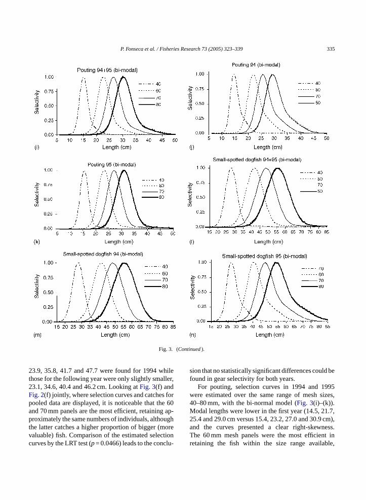
23.9, 35.8, 41.7 and 47.7 were found for 1994 whilethose for the following year were only slightly smaller,23.1, 34.6, 40.4 and 46.2 cm. Looking atFig. 3(f) andFig. 2(f) jointly, where selection curves and catches forpooled data are displayed, it is noticeable that the 60and 70 mm panels are the most efficient, retaining ap-proximately the same numbers of individuals, althoughthe latter catches a higher proportion of bigger (morevaluable) fish. Comparison of the estimated selectioncurves by the LRT test (p= 0.0466) leads to the conclu-

sion that no statistically significant differences could befound in gear selectivity for both years.

For pouting, selection curves in 1994 and 1995were estimated over the same range of mesh sizes,40–80 mm, with the bi-normal model (Fig. 3(i)–(k)).Modal lengths were lower in the first year (14.5, 21.7,25.4 and 29.0 cm versus 15.4, 23.2, 27.0 and 30.9 cm),and the curves presented a clear right-skewness.The 60 mm mesh panels were the most efficient inretaining the fish within the size range available,

336 P. Fonseca et al. / Fisheries Research 73 (2005) 323–339

without catching undersized individuals. The LRT testindicated a significant difference (p< 0.01) in gearselectivity between 1994 and 1995.

Similarly to hake and pouting, both yearly andpooled datasets for dogfish were best fitted by a bi-normal model (Fig. 3(l)–(n)). In 1994, modal lengthswere 27.8, 41.7, 48.7 and 55.6 cm for the 40–80 mmmesh size panels. In the following year, when smallerfish were caught, slightly lower values were obtained(26.8, 40.1, 46.8 and 53.5 cm). Differences in selec-tivity between both years were statistically significant(p< 0.01).

4. Discussion and conclusions

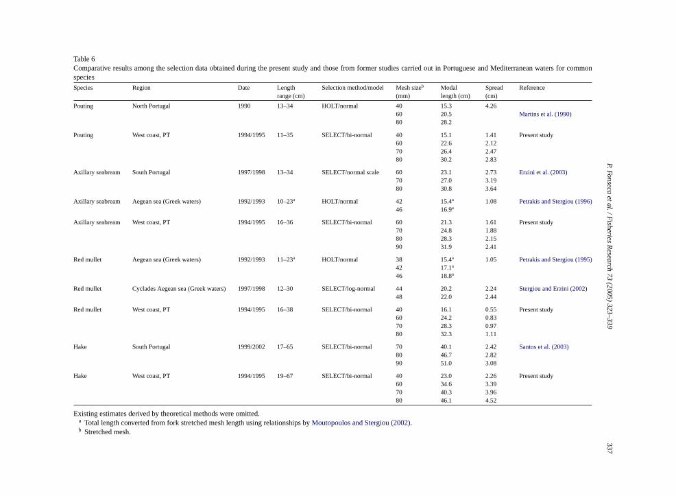
Previous results had already been obtained for someof the species analysed within this study, both in thePortuguese coast (Martins et al., 1990; Santos et al.,2003; Erzini et al., 2003) and in Greek waters (Petrakisand Stergiou, 1995, 1996; Stergiou and Erzini, 2002)(Table 6). However, not only the methods of estimat-ing the selectivity parameters varied among experi-ments, but the estimation was always carried out overpooled datasets. In such conditions the difficulty ofdistinguishing between real differences in selectivityand method-induced results is aggravated by the poten-tial masking of between-set variability. For the axillaryseabream and the hake (in Portuguese southern waters)and the red mullet (in Greek waters), the SELECT ap-p , thusp ooda fort theo lling( xil-l ateda mostc r redm p ofm

eret theM tionf ith

thea

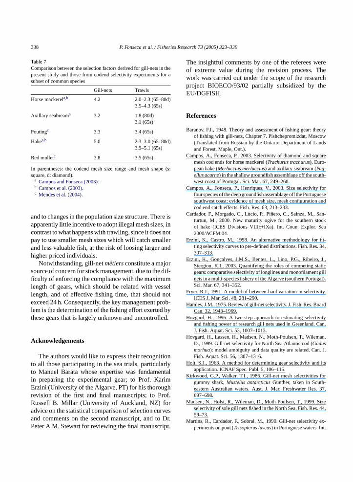
those from trawls using 65 mm, or larger, diamond andsquare mesh codends (Table 7), it can be concludedthat gill-nets of similar mesh size are much more se-lective. Actually, the SF values are equal or even largerthan those found for square mesh codends. A furtheradvantage of gill-nets is that by a careful choice of themesh size it is not only possible to tackle the problem ofcatch of undersized fish, but also to control the catch ofbigger fish in situations where recruitment overfishingis at issue.

From the catch (in weight) of the most importantcommercial species (Table 3(b)), it is noticeable thatthe mesh size providing the best yields varied accord-ing to the species. Pouting and horse mackerel werepreferentially retained by the 60 mm mesh size panels,which is in line with the current Portuguese legisla-tion that enforces the use of a mesh size in the rangeof 60–79 mm for fisheries targeting these species. Forthe red mullet and the axillary seabream, also caught bythe same mesh size range, the best yields were observedin the 70 and 80 mm nets, respectively. Therefore, forthe latter species, the use of mesh sizes smaller than80 mm will result in catches constituted by smaller andless valuable fish. In contrast, for hake the 70 mm netsproved to be the most efficient, catching about 47 and40% more than the 60 and 80 mm nets, respectively.The legislation enforces the use of a minimum meshsize equal or higher than 80 mm, which is justifiablesince the length at first maturity for females is 45.3 cm(Cardador et al., 2000), and therefore a smaller meshs di-v sizep pu-l tudyw ecu-t sizer

emt nt oft . Ac-c izeda us-i om-m roma otherfi tivityo size( ies

roach had previously been used in recent studiesroviding a more reliable basis for comparison. A ggreement in the selectivity estimates was found

he hake, where an almost total coincidence in bothperational condition (mesh size range) and modebi-normal model) took place. Conversely, for the aary seabream the modal lengths previously estimre higher than those of the present study, for an aloincident range of mesh sizes, and so are those foullet in Greek waters, although here the overlaesh sizes is very restricted.With the exception of the 40 mm mesh panels, wh

he majority of hake and pouting catch was belowLS, no undersized fish was caught. If the selec

actors2 (SF =L50/m) are estimated and compared w

2 For gill-nets, the length of 50% retention was calculated onscending arm of the curve;m is the stretched mesh size.

ize would retain a large quantity of immature iniduals. The comparative yields of different meshanels will depend on the size distribution of the po

ation fished. However, the catches in the present sere pooled over different seasons and two cons

ive years, and therefore should closely reflect theange captured by the commercial boats.

Overall, gill-nets from 60 to 80 mm mesh size seo be the most adequate for the correct managemehe majority of the species targeted by these gearsording to the present study, the discards of undersnd/or immature individuals would be small when

ng these mesh sizes, consisting mainly of low cercial value species or damaged fish resulting fn excessive set duration, e.g., by consumption bysh and scavenging amphipods. Due to the selecf these gears, fishermen can easily adapt meshwithin the legal framework) to specific target spec

P.Fonse

caeta

l./Fish

erie

sR

ese

arch

73

(2005)323–339

Table 6Comparative results among the selection data obtained during the present study and those from former studies carried out in Portuguese and Mediterranean waters for commonspecies

Species Region Date Lengthrange (cm)

Selection method/model Mesh sizeb

(mm)Modallength (cm)

Spread(cm)

Reference

Pouting North Portugal 1990 13–34 HOLT/normal 40 15.3 4.2660 20.5 Martins et al. (1990)80 28.2

Pouting West coast, PT 1994/1995 11–35 SELECT/bi-normal 40 15.1 1.41 Present study60 22.6 2.1270 26.4 2.4780 30.2 2.83

Axillary seabream South Portugal 1997/1998 13–34 SELECT/normal scale 60 23.1 2.73 Erzini et al. (2003)70 27.0 3.1980 30.8 3.64

Axillary seabream Aegean sea (Greek waters) 1992/1993 10–23a HOLT/normal 42 15.4a 1.08 Petrakis and Stergiou (1996)46 16.9a

Axillary seabream West coast, PT 1994/1995 16–36 SELECT/bi-normal 60 21.3 1.61 Present study70 24.8 1.8880 28.3 2.1590 31.9 2.41

Red mullet Aegean sea (Greek waters) 1992/1993 11–23a HOLT/normal 38 15.4a 1.05 Petrakis and Stergiou (1995)42 17.1a

46 18.8a

Red mullet Cyclades Aegean sea (Greek waters) 1997/1998 12–30 SELECT/log-normal 44 20.2 2.24Stergiou and Erzini (2002)48 22.0 2.44

Red mullet West coast, PT 1994/1995 16–38 SELECT/bi-normal 40 16.1 0.55 Present study60 24.2 0.8370 28.3 0.9780 32.3 1.11

Hake South Portugal 1999/2002 17–65 SELECT/bi-normal 70 40.1 2.42 Santos et al. (2003)80 46.7 2.8290 51.0 3.08

Hake West coast, PT 1994/1995 19–67 SELECT/bi-normal 40 23.0 2.26 Present study60 34.6 3.3970 40.3 3.9680 46.1 4.52

Existing estimates derived by theoretical methods were oma Total length converted from fork stretched mesh lengthb Stretched mesh.

337

itted.using relationships byMoutopoulos and Stergiou (2002).

338 P. Fonseca et al. / Fisheries Research 73 (2005) 323–339

Table 7Comparison between the selection factors derived for gill-nets in thepresent study and those from codend selectivity experiments for asubset of common species

Gill-nets Trawls

Horse mackerela,b 4.2 2.0–2.3 (65–80d)3.5–4.3 (65s)

Axillary seabreama 3.2 1.8 (80d)3.1 (65s)

Poutingc 3.3 3.4 (65s)

Hakea,b 5.0 2.3–3.0 (65–80d)3.9–5.1 (65s)

Red mulletc 3.8 3.5 (65s)

In parentheses: the codend mesh size range and mesh shape (s:square, d: diamond).

a Campos and Fonseca (2003).b Campos et al. (2003).c Mendes et al. (2004).

and to changes in the population size structure. There isapparently little incentive to adopt illegal mesh sizes, incontrast to what happens with trawling, since it does notpay to use smaller mesh sizes which will catch smallerand less valuable fish, at the risk of loosing larger andhigher priced individuals.

Notwithstanding, gill-netmetiersconstitute a majorsource of concern for stock management, due to the dif-ficulty of enforcing the compliance with the maximumlength of gears, which should be related with vesselength, and of effective fishing time, that should notexceed 24 h. Consequently, the key management problem is the determination of the fishing effort exerted bythese gears that is largely unknown and uncontrolled.

Acknowledgements

The authors would like to express their recognitionto all those participating in the sea trials, particularlyto Manuel Barata whose expertise was fundamentin preparing the experimental gear; to Prof. KarimErzini (University of the Algarve, PT) for his thoroughrevision of the first and final manuscripts; to ProfRussell B. Millar (University of Auckland, NZ) foradvice on the statistical comparison of selection curveand comments on the second manuscript, and to DPeter A.M. Stewart for reviewing the final manuscript

The insightful comments by one of the referees wereof extreme value during the revision process. Thework was carried out under the scope of the researchproject BIOECO/93/02 partially subsidized by theEU/DGFISH.

References

Baranov, F.I., 1948. Theory and assessment of fishing gear: theoryof fishing with gill-nets, Chapter 7. Pishchepromizdat, Moscow(Translated from Russian by the Ontario Department of Landsand Forest, Maple, Ont.).

Campos, A., Fonseca, P., 2003. Selectivity of diamond and squaremesh cod ends for horse mackerel (Trachurus trachurus), Euro-pean hake (Merluccius merluccius) and axillary seabream (Pag-ellus acarne) in the shallow groundfish assemblage off the south-west coast of Portugal. Sci. Mar. 67, 249–260.

Campos, A., Fonseca, P., Henriques, V., 2003. Size selectivity forfour species of the deep groundfish assemblage off the Portuguesesouthwest coast: evidence of mesh size, mesh configuration andcod end catch effects. Fish. Res. 63, 213–233.

Cardador, F., Morgado, C., Lucio, P., Pinero, C., Sainza, M., San-turtun, M., 2000. New maturity ogive for the southern stockof hake (ICES Divisions VIIIc+IXa). Int. Coun. Explor. Sea2000/ACFM:04.

Erzini, K., Castro, M., 1998. An alternative methodology for fit-ting selectivity curves to pre-defined distributions. Fish. Res. 34,307–313.

Erzini, K., Goncalves, J.M.S., Bentes, L., Lino, P.G., Ribeiro, J.,Stergiou, K.I., 2003. Quantifying the roles of competing staticgears: comparative selectivity of longlines and monofilament gillnets in a multi-species fishery of the Algarve (southern Portugal).

ty.

rd

ityan.

J. Fish. Aquat. Sci. 53, 1007–1013.,

.

7,

,

al

.

sr.

.

Hovgard, H., Lassen, H., Madsen, N., Moth-Poulsen, T., WilemanD., 1999. Gill-net selectivity for North Sea Atlantic cod (Gadusmorhua): model ambiguity and data quality are related. Can. JFish. Aquat. Sci. 56, 1307–1316.

Holt, S.J., 1963. A method for determining gear selectivity and itsapplication. ICNAF Spec. Publ. 5, 106–115.

Kirkwood, G.P., Walker, T.I., 1986. Gill-net mesh selectivities forgummy shark,Mustelus antarcticusGunther, taken in South-eastern Australian waters. Aust. J. Mar. Freshwater Res. 3697–698.

Madsen, N., Holst, R., Wileman, D., Moth-Poulsen, T., 1999. Sizeselectivity of sole gill nets fished in the North Sea. Fish. Res. 4459–73.

Martins, R., Cardador, F., Sobral, M., 1990. Gill-net selectivity ex-periments on pout (Trisopterus luscus) in Portuguese waters. Int.

l

-

Sci. Mar. 67, 341–352.Fryer, R.J., 1991. A model of between-haul variation in selectivi

ICES J. Mar. Sci. 48, 281–290.Hamley, J.M., 1975. Review of gill-net selectivity. J. Fish. Res. Boa

Can. 32, 1943–1969.Hovgard, H., 1996. A two-step approach to estimating selectiv

and fishing power of research gill nets used in Greenland. C

P. Fonseca et al. / Fisheries Research 73 (2005) 323–339 339

Coun. Explor. Sea, Fish Capture Committee, C.M. 1990/B:26,Session U.

McCullagh, P., Nelder, J.A., 1989. Generalized linear models. In:Monographs on Statistics and Applied Probability, vol. 37, sec-ond ed. Chapman & Hall, London, 511 pp.

Mendes, B., Fonseca, P., Campos, A., 2004. Selectividade em sacosde redes de arrasto para seis especies de peixes na costa su-doeste Portuguesa. Relat. Cient. Tec. IPIMAR. Serie Digital(http://www.ipimar-iniap.ipimar.pt) no. 11, 19 pp. (in Portuguesewith an English abstract).

Millar, R.B., 1992. Estimating the size-selectivity of fishing gear byconditioning on the total catch. J. Am. Stat. Assoc. 87, 962–968.

Millar, R.B., 2000. Untangling the confusion surrounding the esti-mation of gillnet selectivity. Can. J. Fish Aquat. Sci. 57, 507–511.

Millar, R.B., Walsh, S.J., 1992. Analysis of trawl selectivity studieswith an application to trouser trawls. Fish. Res. 13, 205–220.

Millar, R.B., Holst, R., 1997. Estimation of gill-net and hook selec-tivity using log-linear models. ICES J. Mar. Sci. 54, 471–477.

Millar, R.B., Fryer, R.J., 1999. Estimating the size-selection curvesof towed gears, traps, nets and hooks. Rev. Fish Biol. Fish. 9,89–116.

Moth-Poulsen, T., 2003. Seasonal variations in selectivity of plaicetrammel nets. Fish. Res. 61, 87–94.

Moutopoulos, D.K., Stergiou, K.I., 2002. Length–weight andlength–length relationships of fish species from Aegean Sea(Greece). J. Appl. Ichthyol. 18, 200–203.

Petrakis, G., Stergiou, K.I., 1995. Gill net selectivity forDiplodusannularisandMullus surmuletusin Greek waters. Fish. Res. 21,455–464.

Petrakis, G., Stergiou, K.I., 1996. Gill net selectivity for four species(Mullus barbatus, Pagellus erythrinus, Pagellus acarneandSpicara flexuosa) in Greek waters. Fish. Res. 27, 17–27.

Santos, M.N., Monteiro, C.C., Erzini, K., 1995. Aspects of the bi-ology and gill-net selectivity of the axillary seabream (Pagellusacarne, Risso) and common Pandora (Pagellus erythrinus, Lin-naeus) from the Algarve (south Portugal). Fish. Res. 23, 223–236.

Santos, M.N., Monteiro, C.C., Erzini, K., Lasserre, G., 1998. Mat-uration and gill-net selectivity of two small seabreams (genusDiplodus) from the Algarve coast (south Portugal). Fish. Res.36, 185–194.

Santos, M.N., Gaspar, M., Monteiro, C.C., Erzini, K., 2003. Gill-net selectivity for European hakeMerluccius merlucciusfromsouthern Portugal: implications for fishery management. Fish.Sci. 69, 873–882.

Stergiou, K.I., Erzini, K., 2002. Comparative fixed gear studies in theCyclades (Aegean Sea): size selectivity of small-hook longlinesand monofilament gill nets. Fish. Res. 58, 25–40.