This content has been downloaded from IOPscience. Please scroll down to see the full text.

Download details:

IP Address: 134.76.225.142

This content was downloaded on 26/08/2014 at 07:31

Please note that terms and conditions apply.

Investigation of the imaging quality of synchrotron-based phase-contrast mammographic

tomography

View the table of contents for this issue, or go to the journal homepage for more

2014 J. Phys. D: Appl. Phys. 47 365401

(http://iopscience.iop.org/0022-3727/47/36/365401)

Home Search Collections Journals About Contact us My IOPscience

Journal of Physics D: Applied Physics

J. Phys. D: Appl. Phys. 47 (2014) 365401 (18pp) doi:10.1088/0022-3727/47/36/365401

Investigation of the imaging quality ofsynchrotron-based phase-contrastmammographic tomography

T E Gureyev1,2, S C Mayo1, Ya I Nesterets1,2, S Mohammadi3,4, D Lockie5,R H Menk3, F Arfelli3, K M Pavlov2,6, M J Kitchen6, F Zanconati7,C Dullin8 and G Tromba3

1 Commonwealth Scientific and Industrial Research Organisation, Melbourne, Australia2 School of Science and Technology, University of New England, Armidale, Australia3 Elettra-Sincrotrone, Trieste, Italy4 The Abdus Salam ICTP, Trieste, Italy5 Maroondah BreastScreen, Melbourne, Australia6 School of Physics, Monash University, Melbourne, Australia7 Department of Medical Science-Unit of Pathology, University of Trieste, Trieste, Italy8 University Hospital Goettingen, Goettingen, Germany

E-mail: Tim.Gureyev@csiro.au

Received 29 May 2014, revised 11 July 2014Accepted for publication 21 July 2014Published 20 August 2014

AbstractWe report the results of a systematic study of phase-contrast x-ray computed tomography inthe propagation-based and analyser-based modes using specially designed phantoms andexcised breast tissue samples. The study is aimed at the quantitative evaluation and subsequentoptimization, with respect to detection of small tumours in breast tissue, of the effects of phasecontrast and phase retrieval on key imaging parameters, such as spatial resolution,contrast-to-noise ratio, x-ray dose and a recently proposed ‘intrinsic quality’ characteristicwhich combines the image noise with the spatial resolution. We demonstrate that some of themethods evaluated in this work lead to substantial (more than 20-fold) improvement in thecontrast-to-noise and intrinsic quality of the reconstructed tomographic images compared withconventional techniques, with the measured characteristics being in good agreement with thecorresponding theoretical estimations. This improvement also corresponds to anapproximately 400-fold reduction in the x-ray dose, compared with conventionalabsorption-based tomography, without a loss in the imaging quality. The results of this studyconfirm and quantify the significant potential benefits achievable in three-dimensionalmammography using x-ray phase-contrast imaging and phase-retrieval techniques.

Keywords: phase-contrast imaging, phase retrieval, computed tomography, mammography

(Some figures may appear in colour only in the online journal)

1. Introduction

Phase-contrast x-ray imaging is currently transitioning fromearlier general theoretical and experimental research usinglaboratory and synchrotron-based setups to a stage wherethe first medical trials with live patients are likely tobecome reasonably widespread and lead to refinement ofthese techniques and their implementation in routine medicalpractice using commercial instrumentation [1, 2]. X-ray

mammography, in particular, has been recognized as thearea of medical radiography which stands to gain the mostfrom the application of phase-contrast techniques [3]. Alarge number of publications have appeared in recent years,in which the advantages of different methods of phase-contrast imaging of soft biological tissues have been studiedboth theoretically and experimentally [4–11]. Several recentreviews have summarized the current state of the art in

0022-3727/14/365401+18$33.00 1 © 2014 IOP Publishing Ltd Printed in the UK

J. Phys. D: Appl. Phys. 47 (2014) 365401 T E Gureyev et al

this area and provided useful ideas for further development[1, 12, 13]. A small number of early trials of phase-contrastmammography with live patients have been reported withpromising results [14]. Although some results in this areahave been reported using specially designed laboratory x-rayimaging equipment [15–18], most of the relevant experimentsso far have been conducted at synchrotron facilities. TheSYRMEP beamline of the Elettra synchrotron is unique in thisrespect in that it has been designed and constructed specificallywith mammographic applications in mind [19–21]. This isthe only synchrotron beamline so far where human patienttrials have been conducted in 2D projection mammographymode, and active preparations are underway for trials of 3Dmammographic imaging. This work is part of this targetedresearch which aims at the quantification and optimization ofimaging conditions for mammographic computed tomography(CT) of live patients.

With regard to the advantages that 3D imaging candeliver in the context of mammography, a large number ofpublications is already available which confirm that x-raytomosynthesis is capable of considerable improvement in thesensitivity and specificity of breast cancer diagnosis comparedwith conventional 2D mammography [22–27]. The relevantadvantages are achieved primarily due to the removal of thetissue overlap effect that is inevitable in 2D projection imaging,which can lead to the ‘masking’ of small tumours by texturefrom overlying tissue in conventional mammographic imagesor to the creation of suspiciously looking areas in the imageconducive to false positive results [26]. It is well known that CTis generally superior to tomosynthesis in terms of the fidelityof 3D reconstruction due to the fundamental difference in theunderlying mathematical frameworks for image reconstructionbetween the two techniques. The main issue for the applicationof CT in breast imaging is that of the dose delivered to thepatient. If the dose could be kept at a level comparable to that inthe present-day clinical 2D mammography or tomosynthesis,while ensuring sufficient spatial resolution and signal-to-noise ratio (SNR), mammographic CT is likely to outperformthe other imaging techniques in terms of image quality anddiagnostic value. In that respect a remarkable developmentwas reported by Zhao et al [28], who showed that the useof phase contrast can deliver 3D mammographic CT imageswith sufficient spatial resolution and contrast at a dose severaltimes lower than in conventional mammography. These resultshave demonstrated that the use of phase contrast can indeedsubstantially enhance the sensitivity of breast x-ray imaging tosmall variations in the density and composition of soft tissuesmaking the method attractive for clinical applications.

We have recently reported [29] the results of aninvestigation of quantitative accuracy and noise sensitivity ofreconstruction of the 3D distribution of complex refractiveindex, n(r) = 1 − δ(r) + iβ(r), in samples containingmaterials with significantly different refractive indices using amethod combining propagation-based phase-contrast imagingand computed tomography (PBI-CT) with phase retrievalbased on the so-called homogeneous version of the transportof intensity equation (TIE-Hom) [30]. We demonstrated thatwhile the distribution of the imaginary part of the refractive

index, β(r) (which is responsible for attenuation of x-raysin the sample), can be accurately reconstructed from a singleprojection image per view angle with this method, the accuracyof reconstruction of δ(r) (that determines the refraction ofx-rays in the sample) depends strongly on the choice of the‘regularization’ parameter in TIE-Hom. In particular, wedemonstrated that for some multi-material samples a directapplication of the TIE-Hom method in PBI-CT producesqualitatively incorrect results for δ(r). On a related issue, ithas been observed [29, 31–33] that it is possible to significantlyimprove the SNR in the reconstructed images by increasingthe sample-to-detector distance in combination with TIE-Hom phase retrieval in PBI-CT compared with conventional(‘contact’) CT. We have shown [33] that the relevant maximumachievable gain is of the order of 0.3δ/β, which, given thatthe δ/β ratio of soft tissues at x-ray energies typical formammography is of the order of 103, can lead to significantlyimproved image quality and/or reduction of the x-ray dosedelivered to patients in medical imaging.

In this work, we extend the results of our previousresearch in this area in three different ways. Firstly, weconduct quantitative PBI-CT experiments using not only thespecially designed plastic phantoms, but also six differentexcised breast tissue samples, with and without tumours, freshor fixed in formalin. Secondly, we compare the quantitativeaccuracy of the reconstruction of the phantoms and tissuesamples using two different phase-contrast CT techniques,analyser-based imaging combined with CT (ABI-CT) andPBI-CT. For both techniques, we evaluate CT-reconstructedimages obtained from ‘raw’ phase-contrast projections, as wellas from processed projections obtained with the use of therelevant phase-retrieval techniques. Thirdly, apart from usingstandard image characteristics, such as spatial resolution, SNRand others, we introduce and evaluate a recently proposednew ‘intrinsic’ imaging quality characteristic [34], whichsimultaneously takes into account both the spatial resolutionand the noise sensitivity of the imaging setup. We provide asimple theoretical expression for this new characteristic in thecase of imaging that combines PBI-CT with TIE-Hom phaseretrieval, and demonstrate that the obtained theoretical valuesagree reasonably well with the corresponding experimentaldata. This approach allows one to assess and theoreticallyoptimize an imaging setup, maximizing the quality of producedPBI-CT images at a given x-ray dose.

2. Image characteristics and imaging setups

2.1. Imaging performance characteristics

The quantitative analysis presented in this work includes theevaluation of accuracy and precision of the measurement ofx-ray attenuation (determined by the imaginary part β ofthe refractive index), spatial resolution, contrast-to-noise ratio(CNR), figure-of-merit (FOM), as well as the new imagingquality characteristic, QS, for the main components of thesamples. The CNR was defined as follows:

CNR = A1/2feature

∣∣〈βfeature〉 − ⟨βbackground

⟩∣∣[(σ 2

feature + σ 2background)/2

]1/2 , (1)

2

J. Phys. D: Appl. Phys. 47 (2014) 365401 T E Gureyev et al

where Afeature = Sfeature/h2 is the area of the correspondingimage feature measured in pixels (Sfeature is the area of thefeature and h is the pixel size), 〈βfeature〉 and

⟨βbackground

⟩are

the average values of the imaginary part of the refractive indexin the feature and in the background, respectively, and σ 2

featureand σ 2

background are the variance of noise in the feature and thebackground, respectively. Note that according to the definitionof CNR, if the pixel size h is increased (e.g. by binning), thevalue of CNR generally will not change, as the decrease inthe first factor (feature area) is compensated by the decreasein the noise level in the denominator (due to the improvedphoton statistics), at least in the case of uncorrelated Poissonnoise (photon-counting detectors). Note also that due tothe fact that we are considering not ‘raw’ detected images,but the output of certain ‘computational imaging’ systems,the contrast in the above CNR behaves differently from the‘signal’ in a similarly defined SNR. For example, while thestandard deviation of noise in the denominator of equation (1)is inversely proportional to the square root of the photonfluence (in the case of Poisson statistics and flat-field correctedimages), the average contrast (which plays the role of the signalhere) is essentially independent of the incident fluence, unlikethe case for intensity-type ‘signals’ in ‘raw’ (not corrected forthe flat field) images. Indeed, zero contrast in the numeratorof equation (1) may be produced at high fluences, if the x-rayattenuation is the same in the ‘feature’ and in the ‘background’.The definition of CNR in equation (1) coincides with theSNR of the naıve observer introduced in [35] for the simplestdetection task when the signal is known exactly and thebackground is known exactly (SKE/BKE) [36], which treatsnoise in reconstructed slices as uncorrelated (so that the noisepower spectrum W is the same for all spatial frequencies,W(u) ≡ W(0)) and can be written as follows:

SNR2naive = W−1(0)

∫|βfeature(u) − βbackground(u)|2 du

= (hσ)−2∫

|βfeature(x) − βbackground(x)|2 dx,

where σ is the standard deviation of noise in the image(assuming that the noise in the image is approximately spatiallystationary, i.e. in particular σfeature = σbackground = σ) andthe hat symbol denotes the Fourier transform. Note also thatif noise in the reconstructed slices were uncorrelated, thenthe CNR would coincide with the SNR of the ideal observer[36, 37]. For correlated noise, the CNR is expected to be lessthan the SNR of the ideal observer.

The FOM was defined as the CNR normalized by the x-raydose (and, hence, by the photon fluence in particular):

FOM = CNR/D1/2abs , (2)

where the mean absorbed dose (in mGy) was calculatedaccording to the formula [38]:

Dabs = Ninc,pxl1.602 × 10−10ERabs

h2Lρ, (3)

where Ninc,pxl is the number of incident photons per pixel, h2

is the pixel area in cm2, L and ρ are the average projected

thickness and the mass density of the sample measured in cmand g cm−3, respectively, E is the x-ray energy in keV, and Rabs

is the dimensionless material and energy specific coefficientof x-ray absorption (a fraction of the incident x-ray energyabsorbed by the sample). We calculated Rabs using Monte-Carlo simulations with numerical phantoms that model theanalysed samples (see details below).

In this work, we also use the following normalizedversions of the above quantities:

CNR′ = CNR/A1/2feature, (4)

FOM′ = FOM/A1/2feature = CNR′/D1/2

abs . (5)

These values correspond to a single pixel, rather than to animage feature of a certain size. They allow one to estimate,if desired, the corresponding CNR and FOM for featuresof different sizes in the image, simply by multiplying thecorresponding dashed values by the square root of the featurearea expressed in pixels.

Gain factors were introduced in the context of PBI asquantities that characterize the effect of phase retrieval onthe standard deviation of noise in the reconstructed projectionimages and in the axial CT slices of the object [33]. Thegain factor most relevant to our present experiments can bedefined as the ratio of the standard deviation of error in a CTslice reconstructed from contact projections to the standarddeviation of error in the corresponding CT slice obtained fromphase-retrieved projections collected at a defocus distancez = R:

Gexp(R) = σfeature(raw; z = 0)

σfeature(TIE − Hom;z = R). (6)

In this work, we evaluate the gain factor Gexp(R) in CT slicesobtained from experimental images, and also compare it withthe corresponding values of the gain factor Gtheor(R), whichwas defined in [33] as a ratio of the standard deviation ofnoise-induced errors in a raw CT slice to the correspondingstandard deviation of noise-induced errors in a phase-retrievedCT slice. Note that by definition this theoretical gain factorignores any reconstruction artefacts. For this reason, one mustbe careful when comparing Gtheor(R) with Gexp(R) definedin equation (6). Indeed, the latter one also incorporates theeffect of the reconstruction artefacts originating, e.g., fromthe limited number of projections, etc. The variance of errorin a conventional reconstructed CT slice can be expressed asσ 2

feature(raw; z = 0) = σ 2noise + σ 2

artefact, where the first termdescribes the noise propagated from projections and the secondterm corresponds to deterministic imperfections of the imagingsystem (e.g. insufficient number of projections which resultsin streak artefacts in the reconstructed CT slice). These twosources of error are usually independent of each other (hence asimple sum of the corresponding variances) and only the noiseterm, σnoise, is affected by the phase retrieval. The reductionof the noise-induced component of the reconstruction erroris quantified by the gain factor Gtheor. Accordingly, thevariance of noise in a phase-retrieved CT slice can be writtenas σ 2

feature(TIE − Hom;z = R) = σ 2noiseG

−2theor + σ 2

artefact. Then

Gexp(R) = Gtheor(R)

(1 + α2

1 + G2theor(R)α2

)1/2

, (7)

3

J. Phys. D: Appl. Phys. 47 (2014) 365401 T E Gureyev et al

’

y

y

z

x

x

zsample

detector

x

z

analysercrystal

incident beam

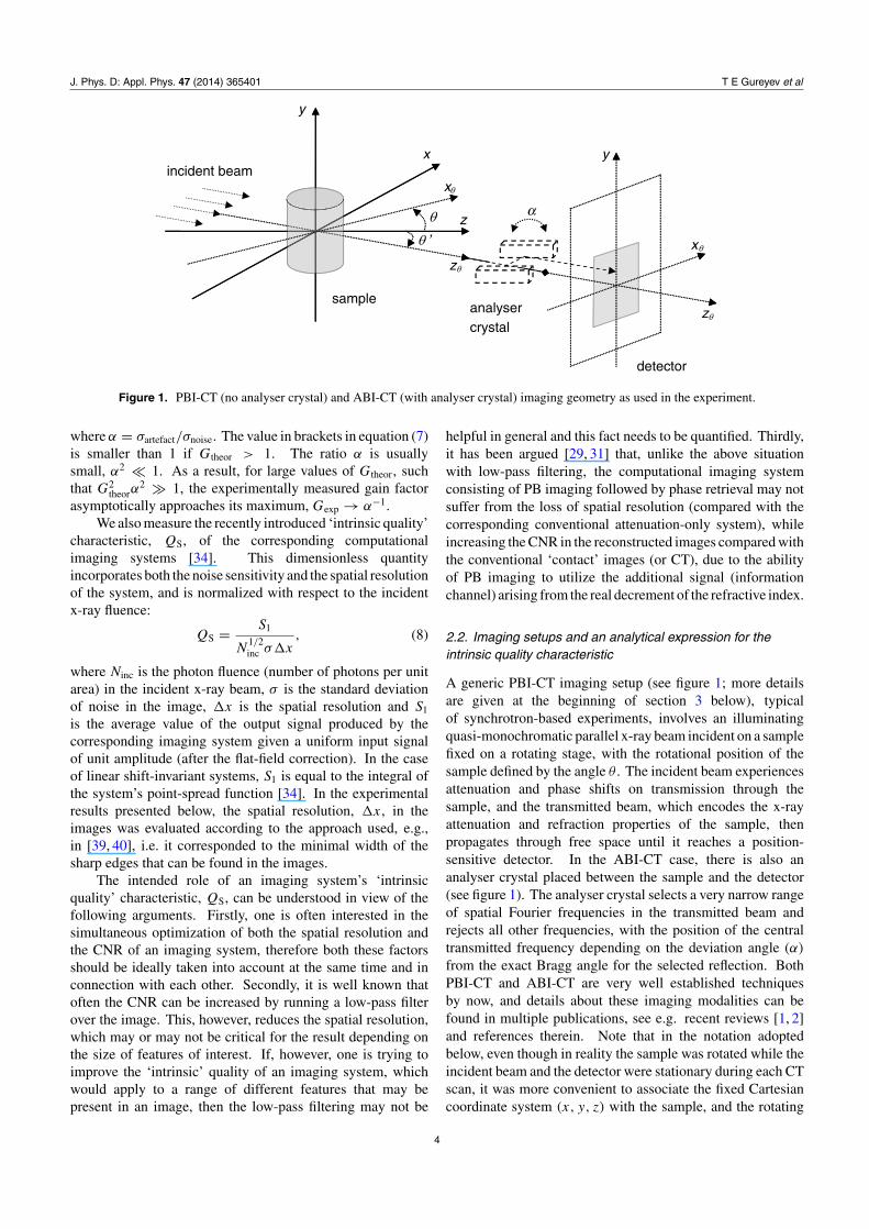
Figure 1. PBI-CT (no analyser crystal) and ABI-CT (with analyser crystal) imaging geometry as used in the experiment.

where α = σartefact/σnoise. The value in brackets in equation (7)is smaller than 1 if Gtheor > 1. The ratio α is usuallysmall, α2 � 1. As a result, for large values of Gtheor, suchthat G2

theorα2 � 1, the experimentally measured gain factor

asymptotically approaches its maximum, Gexp → α−1.We also measure the recently introduced ‘intrinsic quality’

characteristic, QS, of the corresponding computationalimaging systems [34]. This dimensionless quantityincorporates both the noise sensitivity and the spatial resolutionof the system, and is normalized with respect to the incidentx-ray fluence:

QS = S1

N1/2inc σ�x

, (8)

where Ninc is the photon fluence (number of photons per unitarea) in the incident x-ray beam, σ is the standard deviationof noise in the image, �x is the spatial resolution and S1

is the average value of the output signal produced by thecorresponding imaging system given a uniform input signalof unit amplitude (after the flat-field correction). In the caseof linear shift-invariant systems, S1 is equal to the integral ofthe system’s point-spread function [34]. In the experimentalresults presented below, the spatial resolution, �x, in theimages was evaluated according to the approach used, e.g.,in [39, 40], i.e. it corresponded to the minimal width of thesharp edges that can be found in the images.

The intended role of an imaging system’s ‘intrinsicquality’ characteristic, QS, can be understood in view of thefollowing arguments. Firstly, one is often interested in thesimultaneous optimization of both the spatial resolution andthe CNR of an imaging system, therefore both these factorsshould be ideally taken into account at the same time and inconnection with each other. Secondly, it is well known thatoften the CNR can be increased by running a low-pass filterover the image. This, however, reduces the spatial resolution,which may or may not be critical for the result depending onthe size of features of interest. If, however, one is trying toimprove the ‘intrinsic’ quality of an imaging system, whichwould apply to a range of different features that may bepresent in an image, then the low-pass filtering may not be

helpful in general and this fact needs to be quantified. Thirdly,it has been argued [29, 31] that, unlike the above situationwith low-pass filtering, the computational imaging systemconsisting of PB imaging followed by phase retrieval may notsuffer from the loss of spatial resolution (compared with thecorresponding conventional attenuation-only system), whileincreasing the CNR in the reconstructed images compared withthe conventional ‘contact’ images (or CT), due to the abilityof PB imaging to utilize the additional signal (informationchannel) arising from the real decrement of the refractive index.

2.2. Imaging setups and an analytical expression for theintrinsic quality characteristic

A generic PBI-CT imaging setup (see figure 1; more detailsare given at the beginning of section 3 below), typicalof synchrotron-based experiments, involves an illuminatingquasi-monochromatic parallel x-ray beam incident on a samplefixed on a rotating stage, with the rotational position of thesample defined by the angle θ . The incident beam experiencesattenuation and phase shifts on transmission through thesample, and the transmitted beam, which encodes the x-rayattenuation and refraction properties of the sample, thenpropagates through free space until it reaches a position-sensitive detector. In the ABI-CT case, there is also ananalyser crystal placed between the sample and the detector(see figure 1). The analyser crystal selects a very narrow rangeof spatial Fourier frequencies in the transmitted beam andrejects all other frequencies, with the position of the centraltransmitted frequency depending on the deviation angle (α)

from the exact Bragg angle for the selected reflection. BothPBI-CT and ABI-CT are very well established techniquesby now, and details about these imaging modalities can befound in multiple publications, see e.g. recent reviews [1, 2]and references therein. Note that in the notation adoptedbelow, even though in reality the sample was rotated while theincident beam and the detector were stationary during each CTscan, it was more convenient to associate the fixed Cartesiancoordinate system (x, y, z) with the sample, and the rotating

4

J. Phys. D: Appl. Phys. 47 (2014) 365401 T E Gureyev et al

coordinate system (xθ , y, zθ ) with the imaging system, so thatthe optic axis direction coincided with zθ and the image planewas (xθ , y, R) (see figure 1).

We calculated analytically the value of S1 in equation (8)for the computational imaging system employed in thepresent experiments, which consisted of CT reconstruction(producing the imaginary part of the refractive index β,rather than the linear attenuation coefficient µ = 4πβ/λ),optionally preceded by the TIE-Hom phase retrieval [29]. Thecorresponding mathematical expressions are as follows. Forthe TIE-Hom phase retrieval, we have [30]

I0(xθ , y) = T −1[IR(xθ , y)], (9)

where T −1[f ](x, y) = [1 − γR/(2k)∇2]−1f (x, y), ∇2⊥ =

∂2x +∂2

y , IR(xθ , y) is the (flat and dark field corrected) measuredintensity distribution in the image plane z = R at the rotationalposition of the sample defined by the angle θ , I0(xθ , y) is thereconstructed intensity distribution in the object plane, and γ

is the regularization parameter that is usually taken to be equalto the δ/β ratio in the case of homogeneous samples (wherethis ratio is constant across the sample). In the case of the CTreconstruction part of the imaging system, we have [41]

β(x, y, z) = X−1[ln(Iin(xθ , y)/I0(xθ , y)], (10)

where X−1[g](x, y, z) = 1/(2k)∫ π

0

∫ ∞−∞

∫ ∞−∞ exp{−i2π

×[ξθ (x sin θ + z cos θ) + ηy]}g(ξθ , η)|ξθ | dξθ dη dθ, g(ξθ , η)

denotes the 2D Fourier transform of the function g(xθ , y), andIin(xθ , y) is the transverse intensity distribution in the beamincident on the object (as measured in the flat-field images).It is obvious from energy conservation and can also be shownmathematically that T −1[1] = 1, where the bold ‘1’ symboldenotes a function identically equal to one at all points insidethe relevant domain. The response of the CT reconstructionoperator X−1 to unit input signal can also be found from energyconservation considerations. Indeed, it is easy to understandthat the total x-ray attenuation integrated over any row in a(parallel-beam) x-ray projection is equal to the x-ray attenua-tion integrated over the corresponding 2D slice of the object.Mathematically, this can be written as 2k

∫∫�r

β(x, y, z) dx dz

= ∫∫�r

µ(x, y, z) dx dz = ∫ r

−rPθ [µ](t, y)dt = ∫ r

−rln[Iin×

(xθ , y)/I0(xθ , y)] dxθ , where r is the radius of the correspond-ing reconstruction circle �r in the 2D plane y = const andPθ [µ](t, y) = ∫ ∞

−∞∫ ∞−∞ µ(x, y, z)δ(t − x sin θ − z cos θ)×

dx dz is the projection of the function µ(x, y, z) along thestraight lines xθ = t . Accordingly, for a unit input we get∫∫

�rX−1[1] dx dz = (2k)−1

∫ r

−r1 dxθ = r/k. Finally, taking

into account that X−1[1] is actually a constant (see e.g. [41]),we obtain

S1 = X−1[1] = 1/(πkr). (11)

It can be shown [33] that in the case of an imaging systemwhich combines the TIE-Hom phase retrieval with FBP CTreconstruction (referred to as TIE-Hom+PBI-CT below), thevariance of noise in the output images (axial CT-reconstructedslices containing β values) can be expressed as σ 2 =σ 2

inF(A, b)(2k)−2π2/(12Nah2), where σ 2

in = 1/(Ninch2) is the

variance of white noise in individual CT projections, Ninc is

the incident photon fluence, Na is the number of (equispaced)projections in the CT scan, and F(A, b) is a function givenin [33] that depends on the dimensionless parameters A =πγλR/(4h2), which determines the behaviour of the TIE-Hom phase retrieval, and b that depends only on the detectormodulation transfer function (MTF) (b = σdet/(2h) in thecase of a Gaussian MTF with standard deviation σdet). Inturn, the spatial resolution in the axial slices obtained by FBPCT reconstruction from TIE-Hom retrieved projections can beapproximately expressed as �x = (h2 + H 2)1/2, where H

lies in the range between zero for homogeneous samples withδ(r)/β(r) ≡ γ, and (2γ λR)1/2 for samples with (spatiallyvariable) δ/β ratio that is very different from the constant γ

used in TIE-Hom [34]. Then, in accordance with equation (8),we obtain

QS[X−1T −1] = 8√

3

π2

N1/2a

NpixF 1/2(A, b)(1 + H 2/h2)1/2,

(12)

where Npix = 2r/h is the number of pixels in the detector row.Note that if the number of projections Na satisfies the optimalsampling condition for CT, Na = (π/2)Npix [41], then thequality characteristic in equation (12) is inversely proportionalto N

1/2pix . This result is in agreement with the well-known

behaviour of singular values of the inverse Radon transform in2D, whose magnitudes increase in proportion to the square rootof the radial index [41]. Note that, if we used the total incidentphoton fluence (integrated over all projections), instead of thefluence in a single projection, Ninc, in the definition of QS

for this system, the latter characteristic would be inverselyproportional to Npix, which corresponds to the squares ofthe singular values of the Radon transform. On the otherhand, as F(A, b) decreases as a function of parameter A [33],and can typically reach values as small as 10−3–10−5 forlarge A achievable under realistic experimental conditions, thequality characteristic of the TIE-Hom+FBP imaging systemcan improve significantly for large propagation distances R.This fact is consistent with the experimental results presentedbelow.

3. Experimental results and discussion

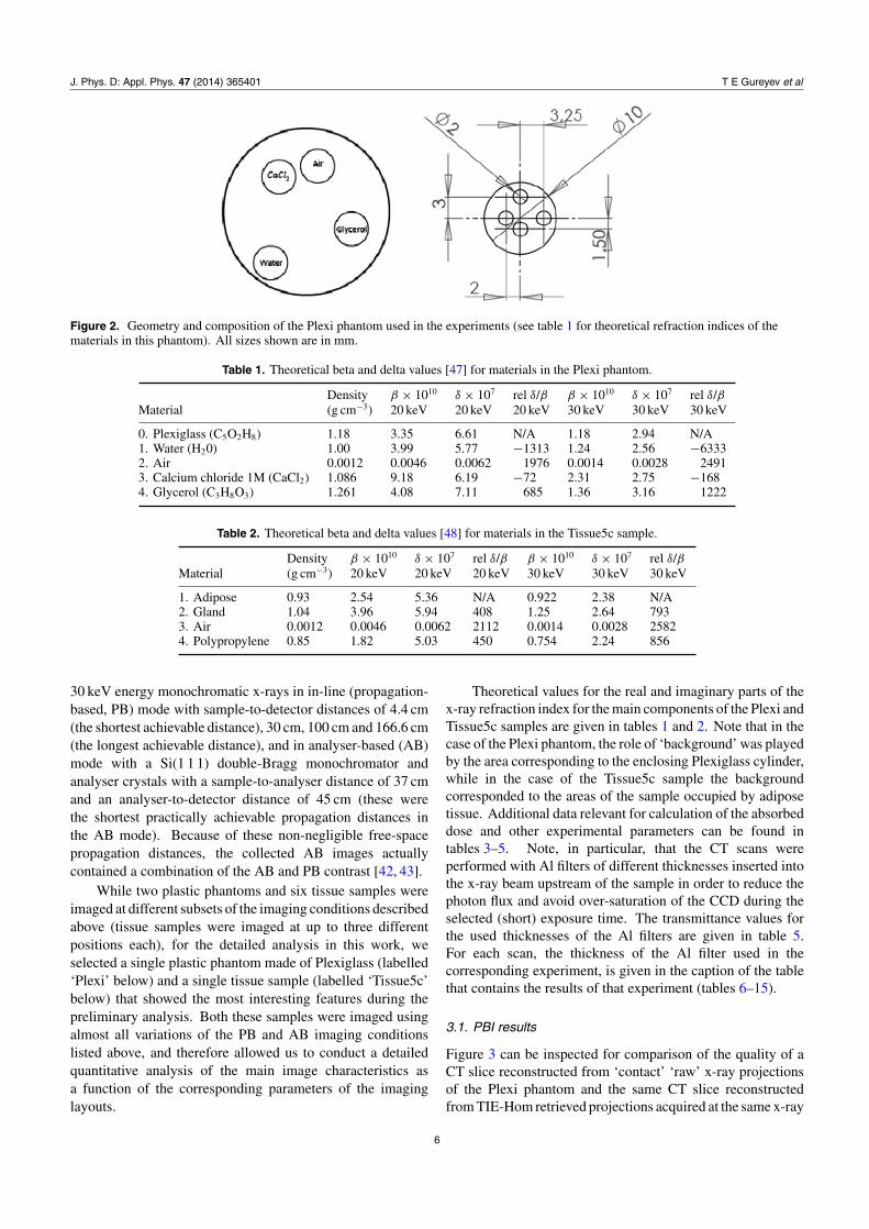
We have conducted phase-contrast CT imaging experimentsat the SYRMEP beamline of the Elettra synchrotron [19–21].The detector used was a water-cooled CCD camera by PhotonicScience, model VHR, 4008 × 2672 full frame, used in 2 × 2binning mode (resulting in pixel size = 9 µm), coupled toa gadolinium oxysulfide scintillator placed on a fibre optictaper. Two classes of samples (phantoms) were used inthese experiments: (a) plastic phantoms of overall cylindricalshape made of Plexiglass or polyoxymethylene (POM), 1 cmdiameter and with four holes of 2 mm diameter filled withwater, air, glycerol and (nominally) 1M solution of CaCl2(figure 2); (b) excised breast tissue samples, either healthyor containing tumours, fresh or fixed in formalin, containedin polypropylene tubes with 1 mm thick walls and an outerdiameter of 12 mm. The samples were imaged with 20 or

5

J. Phys. D: Appl. Phys. 47 (2014) 365401 T E Gureyev et al

Figure 2. Geometry and composition of the Plexi phantom used in the experiments (see table 1 for theoretical refraction indices of thematerials in this phantom). All sizes shown are in mm.

Table 1. Theoretical beta and delta values [47] for materials in the Plexi phantom.

Density β × 1010 δ × 107 rel δ/β β × 1010 δ × 107 rel δ/βMaterial (g cm−3) 20 keV 20 keV 20 keV 30 keV 30 keV 30 keV

0. Plexiglass (C5O2H8) 1.18 3.35 6.61 N/A 1.18 2.94 N/A1. Water (H20) 1.00 3.99 5.77 −1313 1.24 2.56 −63332. Air 0.0012 0.0046 0.0062 1976 0.0014 0.0028 24913. Calcium chloride 1M (CaCl2) 1.086 9.18 6.19 −72 2.31 2.75 −1684. Glycerol (C3H8O3) 1.261 4.08 7.11 685 1.36 3.16 1222

Table 2. Theoretical beta and delta values [48] for materials in the Tissue5c sample.

Density β × 1010 δ × 107 rel δ/β β × 1010 δ × 107 rel δ/βMaterial (g cm−3) 20 keV 20 keV 20 keV 30 keV 30 keV 30 keV

1. Adipose 0.93 2.54 5.36 N/A 0.922 2.38 N/A2. Gland 1.04 3.96 5.94 408 1.25 2.64 7933. Air 0.0012 0.0046 0.0062 2112 0.0014 0.0028 25824. Polypropylene 0.85 1.82 5.03 450 0.754 2.24 856

30 keV energy monochromatic x-rays in in-line (propagation-based, PB) mode with sample-to-detector distances of 4.4 cm(the shortest achievable distance), 30 cm, 100 cm and 166.6 cm(the longest achievable distance), and in analyser-based (AB)mode with a Si(1 1 1) double-Bragg monochromator andanalyser crystals with a sample-to-analyser distance of 37 cmand an analyser-to-detector distance of 45 cm (these werethe shortest practically achievable propagation distances inthe AB mode). Because of these non-negligible free-spacepropagation distances, the collected AB images actuallycontained a combination of the AB and PB contrast [42, 43].

While two plastic phantoms and six tissue samples wereimaged at different subsets of the imaging conditions describedabove (tissue samples were imaged at up to three differentpositions each), for the detailed analysis in this work, weselected a single plastic phantom made of Plexiglass (labelled‘Plexi’ below) and a single tissue sample (labelled ‘Tissue5c’below) that showed the most interesting features during thepreliminary analysis. Both these samples were imaged usingalmost all variations of the PB and AB imaging conditionslisted above, and therefore allowed us to conduct a detailedquantitative analysis of the main image characteristics asa function of the corresponding parameters of the imaginglayouts.

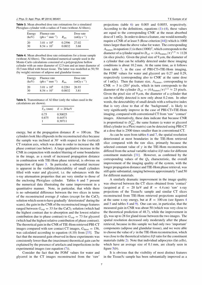
Theoretical values for the real and imaginary parts of thex-ray refraction index for the main components of the Plexi andTissue5c samples are given in tables 1 and 2. Note that in thecase of the Plexi phantom, the role of ‘background’ was playedby the area corresponding to the enclosing Plexiglass cylinder,while in the case of the Tissue5c sample the backgroundcorresponded to the areas of the sample occupied by adiposetissue. Additional data relevant for calculation of the absorbeddose and other experimental parameters can be found intables 3–5. Note, in particular, that the CT scans wereperformed with Al filters of different thicknesses inserted intothe x-ray beam upstream of the sample in order to reduce thephoton flux and avoid over-saturation of the CCD during theselected (short) exposure time. The transmittance values forthe used thicknesses of the Al filters are given in table 5.For each scan, the thickness of the Al filter used in thecorresponding experiment, is given in the caption of the tablethat contains the results of that experiment (tables 6–15).

3.1. PBI results

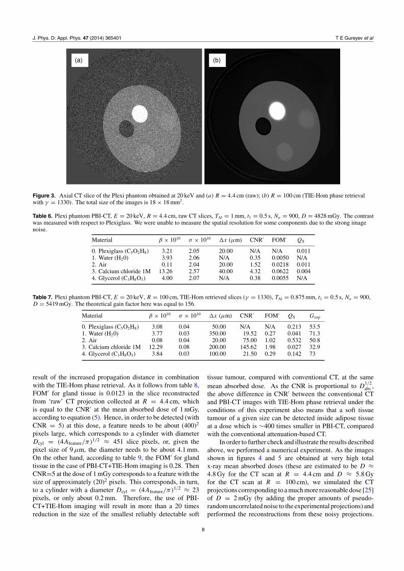
Figure 3 can be inspected for comparison of the quality of aCT slice reconstructed from ‘contact’ ‘raw’ x-ray projectionsof the Plexi phantom and the same CT slice reconstructedfrom TIE-Hom retrieved projections acquired at the same x-ray

6

J. Phys. D: Appl. Phys. 47 (2014) 365401 T E Gureyev et al

Table 3. Mean absorbed dose rate estimations for a simulatedPlexiglass cylinder with a radius of 5 mm (without Al filters).

Energy Fluence rate Dose rate(keV) (ph s−1 mm−2) Rabs (mGy s−1)

20 3.01 × 108 0.2596 27.0230 8.54 × 107 0.0832 3.68

Table 4. Mean absorbed dose rate estimations for a tissue sample(without Al filters). The simulated numerical sample used in theMonte-Carlo calculations consisted of a polypropylene hollowcylinder with an outer diameter of 12.5 mm and an inner diameter of10.5 mm filled with breast tissue. The latter was modelled as 50/50(by weight) mixture of adipose and glandular tissues.

Energy Fluence rate Dose rate(keV) (ph s−1 mm−2) Rabs (mGy s−1)

20 3.01 × 108 0.2261 26.9330 8.54 × 107 0.0832 3.81

Table 5. Transmittance of Al filter (only the values used in thecalculations are shown).

TAl (mm) E = 20 keV

0.75 0.500250.875 0.445711 0.39711

energy, but at the propagation distance R = 100 cm. Thecylinders look like ellipsoids in the reconstructed slice becausethe sample was inclined at 30◦ with respect to the (vertical)CT rotation axis, which was done in order to increase the ABphase contrast (see below). A large qualitative increase in theCNR in conjunction with modest blurring of some boundariesin the image, as a result of increased propagation distancein combination with TIE-Hom phase retrieval, is obvious oninspection of figure 3. In particular, a substantial increaseis apparent in the visibility/detectability of small cylindersfilled with water and glycerol, i.e. the substances with thex-ray attenuation properties that are very similar to those ofthe enclosing Plexiglass cylinder. Tables 6 and 7 presentthe numerical data illustrating the same improvement in aquantitative manner. Note, in particular, that while thereis no substantial difference between the two slices in termsof the reconstructed average β values (except for the CaCl2solution which seem to have gradually ‘deteriorated’ during thescans), the gain in the CNR of the reconstructed image featuresranged between Gexp = 33 for the CaCl2 solution (which hadthe highest contrast due to absorption and the lowest relativecontribution due to phase contrast) to Gexp = 73 for glycerol(which had the highest relative contribution of phase contrast).The theoretical gain in the CNR of TIE-Hom retrieved PBI-CTimages compared with raw contact CT images, Gtheor = 156,was calculated according to equation (4.10) from [33]. Thefact that the measured gain observed in these experiments wasconsistently lower than the (maximum) theoretical gain can beexplained by the presence of artefacts and imperfections in theexperimental images (see equation (7)).

Consider the fact that the FOM′ values for water andglycerol in the CT images reconstructed from the ‘raw’

projections (table 6) are 0.005 and 0.0055, respectively.According to the definitions, equations (1)–(4), these valuesare equal to the corresponding CNR′ at the mean absorbeddose of 1 mGy. In order to detect a feature, one would normallyrequire a CNR of at least 5 (Rose criterion [44]) which is 1000times larger than the above value for water. The correspondingAfeature in equation (1) is then (1000)2, which corresponds to thediameter of a cylinder equal to Dcyl = (4Afeature/π)1/2 ≈ 1128(in slice pixels). Given the pixel size of 9 µm, the diameter ofa cylinder that can be reliably detected under these imagingconditions is about 10.2 mm. At the same time, as it followsfrom table 7, in the case of PBI-CT+TIE-Hom imaging,the FOM′ values for water and glycerol are 0.27 and 0.29,respectively (corresponding also to CNR′ at the same doseof 1 mGy). Then the feature size, Afeature, corresponding toCNR = 5 is (20)2 pixels, which in turn corresponds to thediameter of the cylinder Dcyl = (4Afeature/π)1/2 ≈ 23 pixels.Given the pixel size of 9 µm, the diameter of a cylinder thatcan be reliably detected is now only about 0.2 mm. In otherwords, the detectability of small details with a refractive indexthat is very close to that of the ‘background’, is likely tovery significantly improve in the case of PBI-CT+TIE-Homimaging, compared with conventional CT from ‘raw’ ‘contact’images. Alternatively, these data indicate that because CNRis proportional to D

1/2abs , the same feature (a water or glycerol

filled cylinder in a Plexi matrix) can be detected using PBI-CTat a dose that is 2500 times smaller than in conventional CT.

As can be seen from tables 6 and 7, the spatial resolutiondeteriorated at most boundaries in the TIE-Hom retrievedslice compared with the raw slice, primarily because theselected constant value of γ in the TIE-Hom reconstructiondiffered from the actual variable relative δ/β ratio for differentconstituent materials [31]. However, as confirmed by thecorresponding values of the QS characteristic, the overallimprovement of the imaging quality of the system, with thelonger propagation distance and TIE-Hom phase retrieval, wasstill quite substantial, ranging between approximately 7 and 50for different materials.

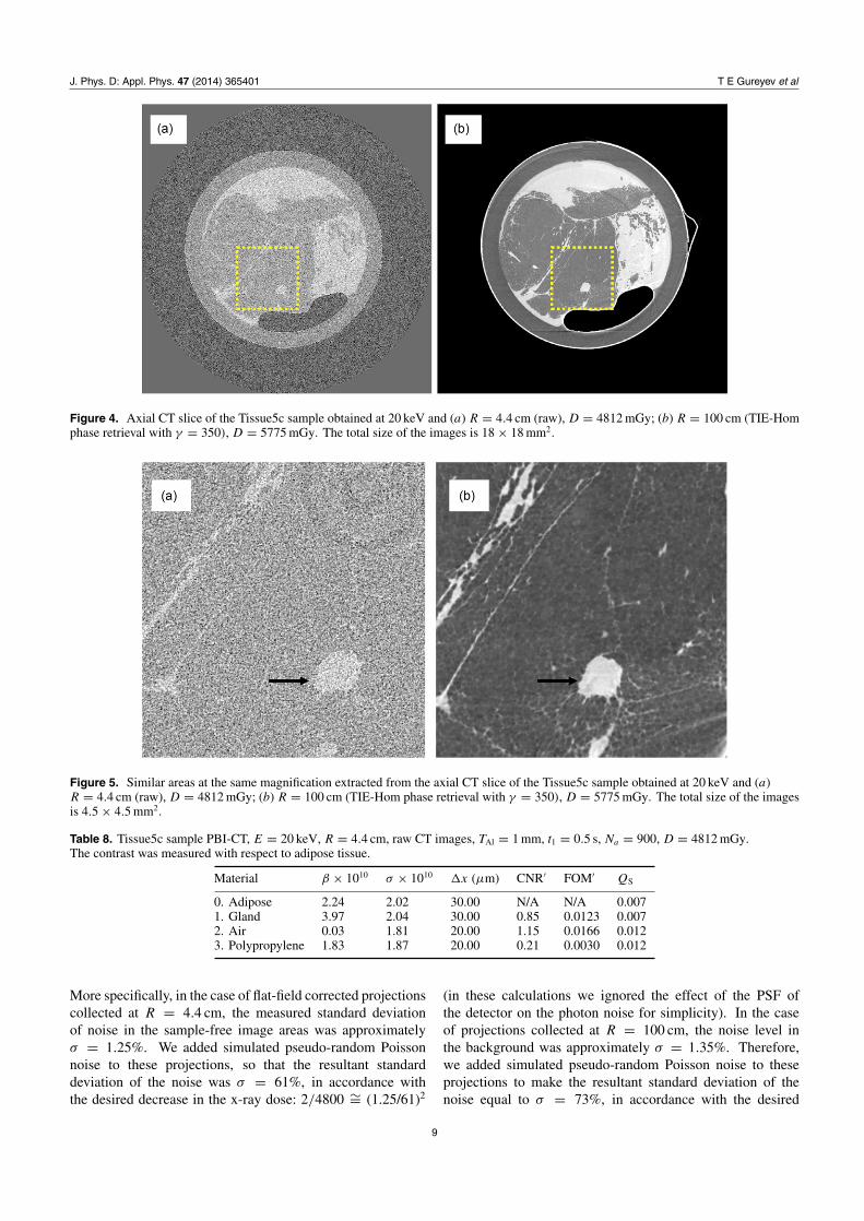
A similarly dramatic improvement in the image qualitywas observed between the CT slices obtained from ‘contact’(acquired at E = 20 keV and R = 4.4 cm) ‘raw’ x-rayprojections of the Tissue5c sample and similar CT slicesreconstructed from TIE-Hom retrieved projections acquiredat the same x-ray energy, but at R = 100 cm (see figures 4and 5 and tables 8 and 9). One can see, in particular, that themeasured gain in CNR was about 50 (which was very close tothe theoretical prediction of 48.7), while the improvement inQS was up to 28 for gland tissue between the two images. Thespatial resolution decreased only moderately after the phaseretrieval, because in this sample we had only two ‘important’components (adipose and glandular tissue), and we were ableto choose the value of γ in the TIE-Hom reconstruction, whichwas close to the theoretical relative δ/β ratio for the constituentmaterials (table 2). Note that individual adipocytes (fat cells),which have an average size of 0.1 mm, are clearly seen infigure 5(b).

It is obvious that the visibility of most distinct featuresin the Tissue5c sample has been substantially improved as a

7

J. Phys. D: Appl. Phys. 47 (2014) 365401 T E Gureyev et al

Figure 3. Axial CT slice of the Plexi phantom obtained at 20 keV and (a) R = 4.4 cm (raw); (b) R = 100 cm (TIE-Hom phase retrievalwith γ = 1330). The total size of the images is 18 × 18 mm2.

Table 6. Plexi phantom PBI-CT, E = 20 keV, R = 4.4 cm, raw CT slices, TAl = 1 mm, t1 = 0.5 s, Na = 900, D = 4828 mGy. The contrastwas measured with respect to Plexiglass. We were unable to measure the spatial resolution for some components due to the strong imagenoise.

Material β × 1010 σ × 1010 �x (µm) CNR′ FOM′ QS

0. Plexiglass (C5O2H8) 3.21 2.05 20.00 N/A N/A 0.0111. Water (H20) 3.93 2.06 N/A 0.35 0.0050 N/A2. Air 0.11 2.04 20.00 1.52 0.0218 0.0113. Calcium chloride 1M 13.26 2.57 40.00 4.32 0.0622 0.0044. Glycerol (C3H8O3) 4.00 2.07 N/A 0.38 0.0055 N/A

Table 7. Plexi phantom PBI-CT, E = 20 keV, R = 100 cm, TIE-Hom retrieved slices (γ = 1330), TAl = 0.875 mm, t1 = 0.5 s, Na = 900,D = 5419 mGy. The theoretical gain factor here was equal to 156.

Material β × 1010 σ × 1010 �x (µm) CNR′ FOM′ QS Gexp

0. Plexiglass (C5O2H8) 3.08 0.04 50.00 N/A N/A 0.213 53.51. Water (H20) 3.77 0.03 350.00 19.52 0.27 0.041 71.32. Air 0.08 0.04 20.00 75.00 1.02 0.532 50.83. Calcium chloride 1M 12.29 0.08 200.00 145.62 1.98 0.027 32.94. Glycerol (C3H8O3) 3.84 0.03 100.00 21.50 0.29 0.142 73

result of the increased propagation distance in combinationwith the TIE-Hom phase retrieval. As it follows from table 8,FOM′ for gland tissue is 0.0123 in the slice reconstructedfrom ‘raw’ CT projection collected at R = 4.4 cm, whichis equal to the CNR′ at the mean absorbed dose of 1 mGy,according to equation (5). Hence, in order to be detected (withCNR = 5) at this dose, a feature needs to be about (400)2

pixels large, which corresponds to a cylinder with diameterDcyl = (4Afeature/π)1/2 ≈ 451 slice pixels, or, given thepixel size of 9 µm, the diameter needs to be about 4.1 mm.On the other hand, according to table 9, the FOM′ for glandtissue in the case of PBI-CT+TIE-Hom imaging is 0.28. ThenCNR=5 at the dose of 1 mGy corresponds to a feature with thesize of approximately (20)2 pixels. This corresponds, in turn,to a cylinder with a diameter Dcyl = (4Afeature/π)1/2 ≈ 23pixels, or only about 0.2 mm. Therefore, the use of PBI-CT+TIE-Hom imaging will result in more than a 20 timesreduction in the size of the smallest reliably detectable soft

tissue tumour, compared with conventional CT, at the samemean absorbed dose. As the CNR is proportional to D

1/2abs ,

the above difference in CNR′ between the conventional CTand PBI-CT images with TIE-Hom phase retrieval under theconditions of this experiment also means that a soft tissuetumour of a given size can be detected inside adipose tissueat a dose which is ∼400 times smaller in PBI-CT, comparedwith the conventional attenuation-based CT.

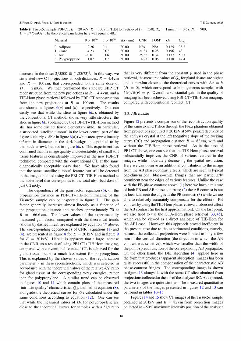
In order to further check and illustrate the results describedabove, we performed a numerical experiment. As the imagesshown in figures 4 and 5 are obtained at very high totalx-ray mean absorbed doses (these are estimated to be D ≈4.8 Gy for the CT scan at R = 4.4 cm and D ≈ 5.8 Gyfor the CT scan at R = 100 cm), we simulated the CTprojections corresponding to a much more reasonable dose [25]of D = 2 mGy (by adding the proper amounts of pseudo-random uncorrelated noise to the experimental projections) andperformed the reconstructions from these noisy projections.

8

J. Phys. D: Appl. Phys. 47 (2014) 365401 T E Gureyev et al

Figure 4. Axial CT slice of the Tissue5c sample obtained at 20 keV and (a) R = 4.4 cm (raw), D = 4812 mGy; (b) R = 100 cm (TIE-Homphase retrieval with γ = 350), D = 5775 mGy. The total size of the images is 18 × 18 mm2.

Figure 5. Similar areas at the same magnification extracted from the axial CT slice of the Tissue5c sample obtained at 20 keV and (a)R = 4.4 cm (raw), D = 4812 mGy; (b) R = 100 cm (TIE-Hom phase retrieval with γ = 350), D = 5775 mGy. The total size of the imagesis 4.5 × 4.5 mm2.

Table 8. Tissue5c sample PBI-CT, E = 20 keV, R = 4.4 cm, raw CT images, TAl = 1 mm, t1 = 0.5 s, Na = 900, D = 4812 mGy.The contrast was measured with respect to adipose tissue.

Material β × 1010 σ × 1010 �x (µm) CNR′ FOM′ QS

0. Adipose 2.24 2.02 30.00 N/A N/A 0.0071. Gland 3.97 2.04 30.00 0.85 0.0123 0.0072. Air 0.03 1.81 20.00 1.15 0.0166 0.0123. Polypropylene 1.83 1.87 20.00 0.21 0.0030 0.012

More specifically, in the case of flat-field corrected projectionscollected at R = 4.4 cm, the measured standard deviationof noise in the sample-free image areas was approximatelyσ = 1.25%. We added simulated pseudo-random Poissonnoise to these projections, so that the resultant standarddeviation of the noise was σ = 61%, in accordance withthe desired decrease in the x-ray dose: 2/4800 ∼= (1.25/61)2

(in these calculations we ignored the effect of the PSF ofthe detector on the photon noise for simplicity). In the caseof projections collected at R = 100 cm, the noise level inthe background was approximately σ = 1.35%. Therefore,we added simulated pseudo-random Poisson noise to theseprojections to make the resultant standard deviation of thenoise equal to σ = 73%, in accordance with the desired

9

J. Phys. D: Appl. Phys. 47 (2014) 365401 T E Gureyev et al

Table 9. Tissue5c sample PBI-CT, E = 20 keV, R = 100 cm, TIE-Hom retrieved (γ = 350), TAl = 1 mm, t1 = 0.6 s, Na = 900,D = 5775 mGy. The theoretical gain factor here was equal to 48.7.

Material β × 1010 σ × 1010 �x (µm) CNR′ FOM′ QS Gexp

0. Adipose 2.26 0.11 30.00 N/A N/A 0.125 38.21. Gland 4.23 0.07 30.00 21.37 0.28 0.196 482. Air −0.01 0.06 50.00 25.62 0.34 0.137 50.73. Polypropylene 1.87 0.07 50.00 4.23 0.06 0.118 47.4

decrease in the dose: 2/5800 ∼= (1.35/73)2. In this way, wesimulated new CT projections at both distances, R = 4.4 cmand R = 100 cm, that corresponded to the same dose ofD = 2 mGy. We then performed the standard FBP CTreconstruction from the new projections at R = 4.4 cm, and aTIE-Hom phase retrieval followed by FBP CT reconstructionfrom the new projections at R = 100 cm. The resultsare shown in figures 6(a) and (b), respectively. One caneasily see that while the slice in figure 6(a), obtained bythe conventional CT method, shows very little structure, theslice in figure 6(b) obtained by the PBI-CT+TIE-Hom methodstill has some distinct tissue elements visible. In particular,a suspected ‘satellite tumour’ in the lower central part of thefigure is clearly visible in figure 6(b) (white area approximately0.6 mm in diameter on the dark background, pointed to bythe black arrow), but not in figure 6(a). This experiment hasconfirmed that the image quality and detectability of small softtissue features is considerably improved in the new PBI-CTtechnique, compared with the conventional CT, at the samediagnostically acceptable x-ray dose. We have also foundthat the same ‘satellite tumour’ feature can still be detectedin the image obtained using the PBI-CT+TIE-Hom method atthe noise level that corresponds to the total absorbed dose ofjust 0.2 mGy.

The dependence of the gain factor, equation (6), on thepropagation distance in PBI-CT+TIE-Hom imaging of theTissue5c sample can be inspected in figure 7. The gainfactor generally increases almost linearly as a function ofthe propagation distance and reaches approximately 70 atR = 166.6 cm. The lower values of the experimentallymeasured gain factor, compared with the theoretical trends(shown by dashed lines), are explained by equation (7) above.The corresponding dependences of CNR′, equations (1) and(4), are presented in figure 8 for E = 20 keV and in figure 9for E = 30 keV. Here it is apparent that a large increasein the CNR, as a result of using PBI-CT+TIE-Hom imaging,compared with conventional ‘contact’ CT, is achieved for thegland tissue, but to a much less extent for polypropylene.This is explained by the chosen values of the regularizationparameter γ in these reconstructions, which was selected inaccordance with the theoretical values of the relative δ/β ratiofor gland tissue at the corresponding x-ray energies, ratherthan for polypropylene. A similar trend can be observedin figures 10 and 11 which contain plots of the measured‘intrinsic quality’ characteristic, QS, defined in equation (8),alongside the theoretical curves for QS calculated under thesame conditions according to equation (12). One can seethat while the measured values of QS for polypropylene areclose to the theoretical curves for samples with a δ/β ratio

that is very different from the constant γ used in the phaseretrieval, the measured values of QS for gland tissues are higherand somewhat closer to the theoretical curves with �x = h

(H = 0), which correspond to homogeneous samples withδ(r)/β(r) = γ . Overall, a substantial gain in the quality ofimaging has been achieved using PBI-CT+TIE-Hom imaging,compared with conventional ‘contact’ CT.

3.2. ABI results

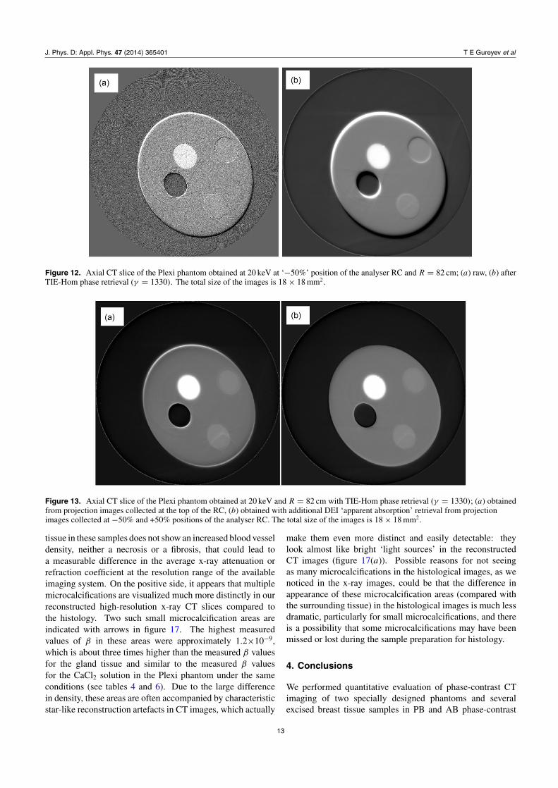
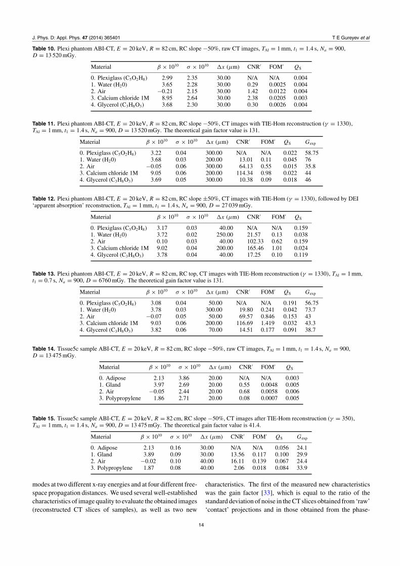
Figure 12 presents a comparison of the reconstruction qualityof the same axial CT slice through the Plexi phantom obtainedfrom projections acquired at 20 keV at 50% peak reflectivity ofthe analyser crystal at the left (negative) slope of the rockingcurve (RC) and propagation distance R = 82 cm, with andwithout the TIE-Hom phase retrieval. As in the case ofPBI-CT above, one can see that the TIE-Hom phase retrievalsubstantially improves the CNR of various features in theimages, while moderately decreasing the spatial resolution.Here we can observe an additional contribution to the imagefrom the AB phase-contrast effects, which are seen as typicalone-dimensional black–white fringes that are particularlyprominent near the edges of various features. Unlike the casewith the PB phase contrast above, (1) here we have a mixtureof both PB and AB phase contrasts; (2) the AB contrast is notas localized near the edges as the PB contrast; (3) while we areable to relatively accurately compensate for the effect of PBcontrast by using the TIE-Hom phase retrieval, it does not affectthe AB contrast (in the first approximation). On the last point,we also tried to use the GOA-Hom phase retrieval [33, 45],which can be viewed as a direct analogue of TIE-Hom forthe ABI case. However, this approach proved inefficient inthe present case due to the experimental conditions, namely,because the collected projections were limited to only a fewmm in the vertical direction (the direction to which the ABcontrast was sensitive), which was smaller than the width ofthe point-spread function of the corresponding AB propagator.On the other hand, the DEI algorithm [4] applied here inthe form that produces ‘apparent absorption’ images has beenquite successful in the compensation of the characteristic ABphase-contrast fringes. The corresponding image is shownin figure 13 alongside with the same CT slice obtained fromprojections collected at the top of the analyser RC. As expected,the two images are quite similar. The measured quantitativeparameters of the images presented in figures 12 and 13 canbe found in tables 10–15.

Figures 14 and 15 show CT images of the Tissue5c sampleobtained at 20 keV and R = 82 cm from projection imagescollected at −50% maximum intensity position of the analyser

10

J. Phys. D: Appl. Phys. 47 (2014) 365401 T E Gureyev et al

Figure 6. Axial CT slice of the Tissue5c sample obtained from in-line projections at 20 keV with added simulated Poisson noisecorresponding to the total dose D = 2 mGy and (a) R = 4.4 cm (raw); (b) R = 100 cm (TIE-Hom phase retrieval with γ = 350). Bothimages were filtered with a Gaussian filter with a standard deviation equal to 9.5 pixels. The total size of the images is 18 × 18 mm2. Thedark arrow points to the suspected small tumour (a denser area inside the adipose tissue) which is about 0.6 mm in diameter.

0 20 40 60 80 100 120 140 160Propagation distance (cm)

0

10

20

30

40

50

60

70

80

90

G

Figure 7. Theoretical and experimental values of the gain factor(defined in equation (6)) for the reconstructed CT slices of theTissue5c sample as a function of propagation distance. Solid lines:circles—gland tissue, squares—polypropylene; dashed lines andtriangles—theoretical values; empty symbols—20 keV, filledsymbols—30 keV.

RC and at the top of the RC with TIE-Hom phase retrieval(γ = 350), respectively. Tables 14 and 15 contain the mainparameters of these images. Although, as in the case ofPBI-CT, the numbers in these tables indicate a substantialimprovement in FOM′ by a factor of about 24 for gland tissue,as well as in CNR′ by a factor of about 25 and a similar factor ofimprovement inQS between the images with and without phaseretrieval, the visual inspection of the two images in figure 14,

0 20 40 60 80 100 120 140 160Propagation distance (cm)

0

5

10

15

20

25

30

CN

R'

Figure 8. Experimental values of contrast-to-noise CNR′ (definedin equation (4)) for the reconstructed CT slices of the Tissue5csample at E = 20 keV as a function of the propagation distance.Circles—gland tissue, squares—polypropylene; emptysymbols—raw projections, filled symbols—phase-retrievedprojections.

and particularly the zoomed images in figure 15, indicates thatthe difference is not as clear-cut as in the case of PBI-CT.While the phase-retrieved image is obviously less noisy, it alsoappears to have a lower visibility of small features, comparedwith the ‘raw’ AB+PB image. A comparison of the likelydiagnostic value between these two types of images may needto be investigated further in the future.

11

J. Phys. D: Appl. Phys. 47 (2014) 365401 T E Gureyev et al

0 20 40 60 80 100 120 140 160Propagation distance (cm)

0

5

10

15

20

CN

R'

Figure 9. Experimental values of contrast-to-noise CNR′ (definedin equation (4)) for the reconstructed CT slices of the Tissue5csample at E = 30 keV as a function of the propagation distance.Circles—gland tissue, squares—polypropylene; emptysymbols—raw projections, filled symbols—phase-retrievedprojections.

0 20 40 60 80 100 120 140 160Propagation distance (cm)

0

0.2

0.4

0.6

0.8

1

QS

Figure 10. Experimental and theoretical values of the intrinsicimaging quality QS (defined in equation (7)) for the reconstructedCT slices of the Tissue5c sample at E = 20 keV as a function of thepropagation distance. Circles—gland tissue,squares—polypropylene; empty symbols—raw projections, filledsymbols—phase-retrieved projections; solid lines—experiment,dashed lines—theory, equation (12), with H equal to zero (circles)and H = (2γ λR)1/2 (squares).

0 20 40 60 80 100 120 140 160Propagation distance (cm)

0

0.2

0.4

0.6

0.8

1

1.2

1.4

1.6

QS

Figure 11. Experimental and theoretical values of the intrinsicimaging quality QS (defined in equation (7)) for the reconstructedCT slices of the Tissue5c sample at E = 30 keV as a function of thepropagation distance. Circles—gland tissue,squares—polypropylene; empty symbols—raw projections, filledsymbols—phase-retrieved projections; solid lines—experiment,dashed lines—theory, equation (12), with H equal to zero (circles)and H = (2γ λR)1/2 (squares).

3.3. Comparison with histology

As demonstrated above, x-ray PBI-CT reconstructed slicesof excised breast tissue samples containing tumours acquiredat high spatial resolution and low noise demonstratedsignificant improvement in the achieved CNR compared withconventional CT under similar conditions. However, in theseimages it has not been possible to conclusively detect thedifference between neoplastic and normal tissue. We havecollected multiple histological images of the same tissuesamples (after x-ray CT experiments). The samples, afterfixation in formalin, were prepared for the optical microscopyevaluation by embedding them into paraffin blocks followinga routine histological procedure. Paraffin blocks were thensectioned using a microtome in 4 µm thick sections which wereplaced on glass slides. Subsequently, the histological sectionswere stained using hematoxylin and eosin for microscopyexamination [46]. As an example, in the histological image ofTissue5c shown in figure 16, a breast cancer (purple colouredregions) with moderate desmoplasia and infiltration in theadipose tissue (white spots) is highlighted. Because the samplewas kept ‘squeezed’ inside the enclosing Plexiglass cylinderduring the CT scans, when it was extracted from the containerit assumed the original shape. This change in the shape ofthe specimens has made it more complicated to compare thetwo techniques. While neoplastic cells are clearly visible aspurple-stained regions in the histological images (figure 16),we could not find any consistent difference between the normaland cancerous regions in the reconstructed CT images. Themost likely explanation for the last fact is that the cancerous

12

J. Phys. D: Appl. Phys. 47 (2014) 365401 T E Gureyev et al

Figure 12. Axial CT slice of the Plexi phantom obtained at 20 keV at ‘−50%’ position of the analyser RC and R = 82 cm; (a) raw, (b) afterTIE-Hom phase retrieval (γ = 1330). The total size of the images is 18 × 18 mm2.

Figure 13. Axial CT slice of the Plexi phantom obtained at 20 keV and R = 82 cm with TIE-Hom phase retrieval (γ = 1330); (a) obtainedfrom projection images collected at the top of the RC, (b) obtained with additional DEI ‘apparent absorption’ retrieval from projectionimages collected at −50% and +50% positions of the analyser RC. The total size of the images is 18 × 18 mm2.

tissue in these samples does not show an increased blood vesseldensity, neither a necrosis or a fibrosis, that could lead toa measurable difference in the average x-ray attenuation orrefraction coefficient at the resolution range of the availableimaging system. On the positive side, it appears that multiplemicrocalcifications are visualized much more distinctly in ourreconstructed high-resolution x-ray CT slices compared tothe histology. Two such small microcalcification areas areindicated with arrows in figure 17. The highest measuredvalues of β in these areas were approximately 1.2×10−9,which is about three times higher than the measured β valuesfor the gland tissue and similar to the measured β valuesfor the CaCl2 solution in the Plexi phantom under the sameconditions (see tables 4 and 6). Due to the large differencein density, these areas are often accompanied by characteristicstar-like reconstruction artefacts in CT images, which actually

make them even more distinct and easily detectable: theylook almost like bright ‘light sources’ in the reconstructedCT images (figure 17(a)). Possible reasons for not seeingas many microcalcifications in the histological images, as wenoticed in the x-ray images, could be that the difference inappearance of these microcalcification areas (compared withthe surrounding tissue) in the histological images is much lessdramatic, particularly for small microcalcifications, and thereis a possibility that some microcalcifications may have beenmissed or lost during the sample preparation for histology.

4. Conclusions

We performed quantitative evaluation of phase-contrast CTimaging of two specially designed phantoms and severalexcised breast tissue samples in PB and AB phase-contrast

13

J. Phys. D: Appl. Phys. 47 (2014) 365401 T E Gureyev et al

Table 10. Plexi phantom ABI-CT, E = 20 keV, R = 82 cm, RC slope −50%, raw CT images, TAl = 1 mm, t1 = 1.4 s, Na = 900,D = 13 520 mGy.

Material β × 1010 σ × 1010 �x (µm) CNR′ FOM′ QS

0. Plexiglass (C5O2H8) 2.99 2.35 30.00 N/A N/A 0.0041. Water (H20) 3.65 2.28 30.00 0.29 0.0025 0.0042. Air −0.21 2.15 30.00 1.42 0.0122 0.0043. Calcium chloride 1M 8.95 2.64 30.00 2.38 0.0205 0.0034. Glycerol (C3H8O3) 3.68 2.30 30.00 0.30 0.0026 0.004

Table 11. Plexi phantom ABI-CT, E = 20 keV, R = 82 cm, RC slope −50%, CT images with TIE-Hom reconstruction (γ = 1330),TAl = 1 mm, t1 = 1.4 s, Na = 900, D = 13 520 mGy. The theoretical gain factor value is 131.

Material β × 1010 σ × 1010 �x (µm) CNR′ FOM′ QS Gexp

0. Plexiglass (C5O2H8) 3.22 0.04 300.00 N/A N/A 0.022 58.751. Water (H20) 3.68 0.03 200.00 13.01 0.11 0.045 762. Air −0.05 0.06 300.00 64.13 0.55 0.015 35.83. Calcium chloride 1M 9.05 0.06 200.00 114.34 0.98 0.022 444. Glycerol (C3H8O3) 3.69 0.05 300.00 10.38 0.09 0.018 46

Table 12. Plexi phantom ABI-CT, E = 20 keV, R = 82 cm, RC slope ±50%, CT images with TIE-Hom (γ = 1330), followed by DEI‘apparent absorption’ reconstruction, TAl = 1 mm, t1 = 1.4 s, Na = 900, D = 27 039 mGy.

Material β × 1010 σ × 1010 �x (µm) CNR′ FOM′ QS

0. Plexiglass (C5O2H8) 3.17 0.03 40.00 N/A N/A 0.1591. Water (H20) 3.72 0.02 250.00 21.57 0.13 0.0382. Air 0.10 0.03 40.00 102.33 0.62 0.1593. Calcium chloride 1M 9.02 0.04 200.00 165.46 1.01 0.0244. Glycerol (C3H8O3) 3.78 0.04 40.00 17.25 0.10 0.119

Table 13. Plexi phantom ABI-CT, E = 20 keV, R = 82 cm, RC top, CT images with TIE-Hom reconstruction (γ = 1330), TAl = 1 mm,t1 = 0.7 s, Na = 900, D = 6760 mGy. The theoretical gain factor value is 131.

Material β × 1010 σ × 1010 �x (µm) CNR′ FOM′ QS Gexp

0. Plexiglass (C5O2H8) 3.08 0.04 50.00 N/A N/A 0.191 56.751. Water (H20) 3.78 0.03 300.00 19.80 0.241 0.042 73.72. Air −0.07 0.05 50.00 69.57 0.846 0.153 433. Calcium chloride 1M 9.03 0.06 200.00 116.69 1.419 0.032 43.34. Glycerol (C3H8O3) 3.82 0.06 70.00 14.51 0.177 0.091 38.7

Table 14. Tissue5c sample ABI-CT, E = 20 keV, R = 82 cm, RC slope −50%, raw CT images, TAl = 1 mm, t1 = 1.4 s, Na = 900,D = 13 475 mGy.

Material β × 1010 σ × 1010 �x (µm) CNR′ FOM′ QS

0. Adipose 2.13 3.86 20.00 N/A N/A 0.0031. Gland 3.97 2.69 20.00 0.55 0.0048 0.0052. Air −0.05 2.44 20.00 0.68 0.0058 0.0063. Polypropylene 1.86 2.71 20.00 0.08 0.0007 0.005

Table 15. Tissue5c sample ABI-CT, E = 20 keV, R = 82 cm, RC slope −50%, CT images after TIE-Hom reconstruction (γ = 350),TAl = 1 mm, t1 = 1.4 s, Na = 900, D = 13 475 mGy. The theoretical gain factor value is 41.4.

Material β × 1010 σ × 1010 �x (µm) CNR′ FOM′ QS Gexp

0. Adipose 2.13 0.16 30.00 N/A N/A 0.056 24.11. Gland 3.89 0.09 30.00 13.56 0.117 0.100 29.92. Air −0.02 0.10 40.00 16.11 0.139 0.067 24.43. Polypropylene 1.87 0.08 40.00 2.06 0.018 0.084 33.9

modes at two different x-ray energies and at four different free-space propagation distances. We used several well-establishedcharacteristics of image quality to evaluate the obtained images(reconstructed CT slices of samples), as well as two new

characteristics. The first of the measured new characteristicswas the gain factor [33], which is equal to the ratio of thestandard deviation of noise in the CT slices obtained from ‘raw’‘contact’ projections and in those obtained from the phase-

14

J. Phys. D: Appl. Phys. 47 (2014) 365401 T E Gureyev et al

Figure 14. Axial CT slice of the Tissue5c sample at 20 keV and R = 82 cm; (a) obtained from projection images collected at −50%position of the analyser RC, (b) obtained from projection images collected at the top of the RC with TIE-Hom phase retrieval (γ = 350).The total size of the images is 18×18 mm2.

Figure 15. Magnified images of the area corresponding to the dotted square in figures 14(a) and (b), respectively. The total size of theimages is 4.5 × 4.5 mm2.

Figure 16. Region of a histology slice of the Tissue5c sample around a ductal in situ cancer component (violet rounded area). Breast cancercells are stained with dark violet colour, adipose tissue appears white and glandular tissue mostly appears pink.

15

J. Phys. D: Appl. Phys. 47 (2014) 365401 T E Gureyev et al

Figure 17. Zoomed region from the x-ray CT image shown in figure 4(b), given here in the original contrast (a), as well as in invertedcontrast (b) to facilitate the comparison with the histology images in figure 16. A cross-section of a duct is clearly visible in lower rightcorner. The regions inside the duct indicated by white arrows correspond to two microcalcifications.

retrieved projections collected in a phase-contrast regime. Thesecond new characteristic was the ‘intrinsic’ imaging qualityQS [34], which, by definition, is inversely proportional tothe product of the standard deviation of noise and the spatialresolution in the image. We have demonstrated that forall the measured imaging characteristics a generally similarimprovement is achievable using the two phase-contrast imageacquisition modalities with subsequent phase retrieval based onthe ‘homogeneous’ version of the TIE. Overall, the measuredgain in all image characteristics was equal to 20 or more, whichtranslates into at least a 20 times reduction in the minimalsize of reliably detectable soft tissue tumours compared withconventional CT imaging at the same mean absorbed x-raydose (or, alternatively, to a 400 times reduction in the dose at thesame image quality level). Our theoretical estimations showthat although even larger gains (up to approximately 0.3δ/β

[33]) in the image quality may be possible in principle usingthe same methods with different experimental parameters(e.g. longer propagation distances), such gains will likely berestricted in practice by factors such as CT reconstructionartefacts due to the limited number of projections or instabilityof the incident illumination. Note that the application of TIE-Hom phase retrieval to PBI and ABI images led to somedeterioration of the spatial resolution, which was higher fordetails whose δ/β ratio was very different from the value ofγ used in the TIE-Hom reconstruction. For the breast tissuesamples, the spatial resolution decreased only moderately asin this case there are mainly two components, adipose andglandular tissue, with similar compositions and consequentlysimilar values of δ/β, and the reconstructions were performedusing γ ∼= δ/β. Regarding the comparison between the PB andAB phase-contrast imaging modes in combination with TIE-hom phase retrieval, we observed a similar improvement in themeasured image quality characteristics in the two methods.Given that (a) the PBI-CT method is easier to implement inpractice (as it does not require an analyser crystal, whichbecomes particularly important for larger samples), and (b)the corresponding quantitatively accurate phase retrieval is alsoeasier to implement in the PB imaging case, it appears that thePBI-CT method should be preferred in these circumstances. Atthe next stage of our research we plan to scale up the phantoms

and breast tissue samples to a size comparable to full-breastimaging. The results obtained in this study indicate that asimilar quantitative improvement in the imaging quality at afixed x-ray dose, or a similar reduction in the x-ray dose at afixed image quality, should be achievable for larger samples.

Acknowledgments

The authors would like to thank Dr Diego Dreossi andDr Nicola Sodini for their help during the experiments atthe SYRMEP beamline. They are also very grateful toMrs Cristina Bottin for expertly preparing the histologicalsamples. The authors acknowledge travel funding providedby the International Synchrotron Access Program (ISAP)managed by the Australian Synchrotron and funded by theAustralian Government. MJK acknowledges support of theAustralian Research Council (ARC) and is the recipientof an ARC Australian Research Fellowship (DP110101941;DP130104913). KMP acknowledges financial support fromthe University of New England.

References

[1] Bravin A, Coan P and Suortti P 2013 X-ray phase-contrastimaging: from pre-clinical applications towards clinicsPhys. Med. Biol. 58 R1–35

[2] Wilkins S W, Nesterets Y I, Gureyev T E, Mayo S C, PoganyA and Stevenson A W 2014 On the evolution and relativemerits of hard x-ray phase-contrast imaging methods Phil.Trans. R. Soc. A 372 20130021

[3] Raupach R and Flohr T 2012 Performance evaluation of x-raydifferential phase contrast computed tomography (PCT)with respect to medical imaging Med. Phys. 39 4761–74

[4] Chapman D, Thomlinson W, Arfelli F, Gmur N, Zhong Z,Menk R, Johnson R E, Washburn D, Pisano E and Sayers D1996 Mammography imaging studies using a Laue crystalanalyzer Rev. Sci. Instrum. 67 1–5

[5] Pani S et al 2004 Breast tomography with synchrotronradiation: preliminary results Phys. Med. Biol. 49 1739–54

[6] Abrami A et al 2005 Medical applications of synchrotronradiation at the SYRMEP beamline of ELETTRA Nucl.Instrum. Methods Phys. Res. A 548 221–7

[7] Pagot E, Fiedler S, Cloetens P, Bravin A, Coan P, Fezzaa K,Baruchel J and Hartwig J 2005 Quantitative comparison

16

J. Phys. D: Appl. Phys. 47 (2014) 365401 T E Gureyev et al

between two phase contrast techniques: diffractionenhanced imaging and phase propagation imaging Phys.Med. Biol. 50 709–24

[8] Keyrilainen J et al 2011 Comparison of in vitro breast cancervisibility in analyser-based computed tomography withhistopathology, mammography, computed tomography andmagnetic resonance imaging J. Synchrotron Radiat. 18689–96

[9] Sztrokay A, Diemoz P C, Schlossbauer T, Brun E, Bamberg F,Mayr D, Reiser M F, Bravin A and Coan P 2012High-resolution breast tomography at high energy: afeasibility study of phase contrast imaging on a wholebreast Phys. Med. Biol. 57 2931–42

[10] Diemoz P C, Bravin A and Coan P 2012 Theoreticalcomparison of three x-ray phase-contrast imagingtechniques: propagation-based imaging, analyzer-basedimaging and grating interferometry Opt. Express20 2789–805

[11] Diemoz P C, Bravin A, Langer M and Coan P 2012 Analyticaland experimental determination of signal-to-noise ratio andfigure of merit in three phase-contrast imaging techniquesOpt. Express 20 27670–90

[12] Keyrilainen J, Bravin A, Fernandez M, Tenhunen M,Virkkunen P and Suortti P 2010 Phase-contrast x-rayimaging of breast Acta Radiol. 51 866–84

[13] Coan P, Bravin A and Tromba G 2013 Phase-contrast x-rayimaging of the breast: recent developments towards clinicsJ. Phys. D: Appl. Phys. 46 494007

[14] Castelli E et al 2011 Mammography with synchrotronradiation: first clinical experience with phase-detectiontechnique Radiology 259 684–94

[15] Honda C and Ohara H 2008 Advantages of magnification indigital phase-contrast mammography using a practical x-raytube Eur. J. Radiol. 68 S69–72

[16] Parham C, Zhong Z, Connor D M, Chapman L D andPisano E D 2009 Design and implementation of a compactlow-dose diffraction enhanced medical imaging systemAcad. Radiol. 16 911–17

[17] Munro P R, Ignatyev K, Speller R D and Olivo A 2010Design of a novel phase contrast x-ray imagingsystem for mammography Phys. Med. Biol.55 4169–85

[18] Stampanoni M, Wang Z, Thurling T, David C, Roessl E,Trippel M, Kubik-Huch R A, Singer G, Hohl M K andHauser N 2011 The first analysis and clinical evaluation ofnative breast tissue using differential phase-contrastmammography Invest. Radiol. 46 801–6

[19] Dreossi D et al 2008 The mammography project at theSYRMEP beamline Eur. J. Radiol. 68 S58–62

[20] Tromba G et al 2010 The SYRMEP beamline of Elettra:clinical mammography and bio-medical applications AIPConf. Proc. 1266 18–23

[21] Tromba G, Cova M A and Castelli E 2011 Phase-contrastmammography at the SYRMEP beamline of ElettraSynchrotron Radiat. News 24 3–7

[22] Dobbins J T III and Godfrey D J 2003 Digital x-raytomosynthesis: current state of the art and clinical potentialPhys. Med. Biol. 48 R65–106

[23] Michell M J, Iqbal A, Wasan R K, Evans D R, Peacock C,Lawinski C P, Douiri A, Wilson R and Whelehan P 2012 Acomparison of the accuracy of film-screen mammography,full-field digital mammography, and digital breasttomosynthesis Clin. Radiol. 67 976–81

[24] Malliori A, Bliznakova K, Speller R D, Horrocks J A,Rigon L, Tromba G and Pallikarakis N 2012 Image qualityevaluation of breast tomosynthesis with synchrotronradiation Med. Phys. 39 5621–34

[25] Skaane P et al 2013 Comparison of digital mammographyalone and digital mammography plus tomosynthesis in a

population based screening program Radiology267 47–56

[26] Ciatto S et al 2013 Integration of 3D digital mammographywith tomosynthesis for population breast-cancer screening(STORM): a prospective comparison study Lancet Oncol.14 583–9

[27] Friedewald S M et al 2014 Breast cancer screening usingtomosynthesis in combination with digital mammographyJ. Am. Med. Assoc. 311 2499–507

[28] Zhao Y Z et al 2012 High-resolution, low-dose phase contrastx-ray tomography for 3D diagnosis of human breast cancersProc. Natl Acad. Sci. USA 109 18290–4

[29] Gureyev T, Mohammadi S, Nesterets Y, Dullin C andTromba G 2013 Accuracy and precision of reconstructionof complex refractive index in near-field single-distancepropagation-based phase-contrast tomography J. Appl.Phys. 114 144906

[30] Paganin D, Mayo S C, Gureyev T E, Miller P R andWilkins S W 2002 Simultaneous phase and amplitudeextraction from a single defocused image of a homogeneousobject J. Microsc. 206 33–40

[31] Beltran M A, Paganin D M, Uesugi K and Kitchen M J 20102D and 3D x-ray phase retrieval of multi-material objectsusing a single defocus distance Opt. Express18 6423–36

[32] Beltran M A, Paganin D M, Siu K K, Fouras A, Hooper S B,Reser D H and Kitchen M J 2011 Interface-specific x-rayphase retrieval tomography of complex biological organsPhys. Med. Biol. 56 7353–69

[33] Nesterets Y I and Gureyev T E 2014 Noise propagation inx-ray phase-contrast imaging and computed tomographyJ. Phys. D: Appl. Phys. 47 105402

[34] Gureyev T E, Nesterets Y I, de Hoog F, Schmalz G, Mayo S C,Mohammadi S and Tromba G 2014 Duality between noiseand spatial resolution in linear systems Opt. Express22 9087–94

[35] Nesterets Y I 2014 Quantitative evaluation of in-line x-rayphase contrast for a class of edge objects Opt. Express22 5937–49

[36] Barrett H H and Myers K J 2004 Foundations of ImageScience (Hoboken, NJ: Wiley)

[37] Anastasio M A, Chou C Y, Zysk A M and Brankov J G 2010Analysis of ideal observer signal detectability inphase-contrast imaging employing linear shift-invariantoptical systems J. Opt. Soc. Am. A 27 2648–59

[38] Johns P C and Yaffe M J 1985 Theoretical optimization ofdual-energy x-ray imaging with application tomammography Med. Phys. 12 289–96

[39] Nesterets Y I, Wilkins S W, Gureyev T E, Pogany A andStevenson A W 2005 On the optimization of experimentalparameters for x-ray in-line phase-contrast imaging Rev.Sci. Instrum. 76 093706

[40] Gureyev T E, Nesterets Y I, Stevenson A W, Miller P R,Pogany A and Wilkins S W 2008 Some simple rules forcontrast, signal-to-noise and resolution in in-line x-rayphase-contrast imaging Opt. Express 16 3223–41

[41] Natterer F 1986 The Mathematics of ComputerizedTomography (Stuttgart: B G Teubner)

[42] Pavlov K M et al 2005 Unification of analyser-based andpropagation-based x-ray phase-contrast imaging Nucl.Instrum. Methods Phys. Res. A 548 163–8

[43] Coan P, Pagot E, Fiedler S, Cloetens P, Baruchel J and BravinA 2005 Phase-contrast x-ray imaging combining free spacepropagation and Bragg diffraction J. Synchrotron Radiat.12 241–5

[44] Rose A 1948 The sensitivity performance of the human eye onan absolute scale J. Opt. Soc. Am. 38 196–208

[45] Paganin D, Gureyev T E, Pavlov K M, Lewis R A andKitchen M 2004 Phase retrieval using coherent imaging

17

J. Phys. D: Appl. Phys. 47 (2014) 365401 T E Gureyev et al

systems with linear transfer functions Opt. Commun.234 87–105

[46] Carson F L 1990 Histotechnology, A Self-Instructional Text(Chicago, IL: American Society of ClinicalPathologists)

[47] www.ts-imaging.net/Services/Simple/Default.aspx, accessed 1February 2014

Brennan S and Cowan P L 1992 A suite of programs forcalculating x-ray absorption, reflection, and diffraction

performance for a variety of materials at arbitrarywavelengths Rev. Sci. Instrum. 63 850–3

Stevenson A W 1993 X-ray integrated intensities fromsemiconductor substrates and epitaxic layers—acomparison of kinematical and dynamical theories withexperiment Acta Crystallogr. A 49 174–83

[48] Hammerstein G R, Miller D W, White D R, Masterson M E,Woodard H Q and Laughlin J S 1979 Absorbed radiationdose in mammography Radiology 130 485–91

18