c o m p u t e r m e t h o d s a n d p r o g r a m s i n b i o m e d i c i n e 1 0 2 ( 2 0 1 1 ) 47–63

journa l homepage: www. int l .e lsev ierhea l th .com/ journa ls /cmpb

A fully automated scheme for mammographic segmentationand classification based on breast density and asymmetry

Stylianos D. Tzikopoulosa,∗, Michael E. Mavroforakisb, Harris V. Georgioua,Nikos Dimitropoulosc, Sergios Theodoridisa

a National and Kapodistrian University of Athens, Dept. of Informatics and Telecommunications, Panepistimiopolis,Ilissia, Athens 15784, Greeceb University of Houston, Department of Computer Science, 501 P.G. Hoffman Hall, Houston, TX 77204-3010, USAc Delta Digital Imaging, Semitelou 6, Athens 11528, Greece

a r t i c l e i n f o

Article history:

Received 11 February 2010

Received in revised form

23 November 2010

Accepted 30 November 2010

Keywords:

Automated mammogram

segmentation

Breast boundary

Pectoral muscle

Breast density

Breast asymmetry

Nipple detection

a b s t r a c t

This paper presents a fully automated segmentation and classification scheme for mam-

mograms, based on breast density estimation and detection of asymmetry. First, image

preprocessing and segmentation techniques are applied, including a breast boundary

extraction algorithm and an improved version of a pectoral muscle segmentation scheme.

Features for breast density categorization are extracted, including a new fractal dimension-

related feature, and support vector machines (SVMs) are employed for classification,

achieving accuracy of up to 85.7%. Most of these properties are used to extract a new set

of statistical features for each breast; the differences among these feature values from the

two images of each pair of mammograms are used to detect breast asymmetry, using an

one-class SVM classifier, which resulted in a success rate of 84.47%. This composite method-

ology has been applied to the miniMIAS database, consisting of 322 (MLO) mammograms

-including 15 asymmetric pairs of images-, obtained via a (noisy) digitization procedure.

The results were evaluated by expert radiologists and are very promising, showing equal

or higher success rates compared to other related works, despite the fact that some of

them used only selected portions of this specific mammographic database. In contrast, our

methodology is applied to the complete miniMIAS database and it exhibits the reliability

ired

1

Bciccc

of radiologists. In addition, when observing a mammographic

0d

that is normally requ

. Introduction

reast cancer, i.e., a malignant tumor developed from breastells, is considered to be one of the major causes for thencrease in mortality among women, especially in developed

ountries. More specifically, breast cancer is the second mostommon type of cancer and the fifth most common cause ofancer death according to Nishikawa [1].

∗ Corresponding author. Tel.: +30 210 7275104; fax: +30 210 7275214.E-mail address: stzikop@di.uoa.gr (S.D. Tzikopoulos).URL: http://www.di.uoa.gr/ stzikop (S.D. Tzikopoulos).

169-2607/$ – see front matter © 2010 Elsevier Ireland Ltd. All rights resoi:10.1016/j.cmpb.2010.11.016

for clinical use in CAD systems.

© 2010 Elsevier Ireland Ltd. All rights reserved.

While mammography has been proven to be the mosteffective and reliable method for the early detection of breastcancer, as indicated by Siddiqui et al. [2], the large numberof mammograms, generated by population screening, mustbe interpreted and diagnosed by a relatively small number

image, abnormalities are often embedded in and camouflagedby varying densities of breast tissue structures, resulting inhigh rates of missed breast cancer cases as mentioned by

erved.

m s i n

48 c o m p u t e r m e t h o d s a n d p r o g r a

Wroblewska et al. [3]. In order to reduce the increasing work-load and improve the accuracy of interpreting mammograms,a variety of computer-aided diagnosis (CAD) systems, thatperform computerized mammographic analysis have beenproposed, as stated by Rangayyan et al. [4]. These systemsare usually employed as a second reader, with the final deci-sion regarding the presence of a cancer left to the radiologist.Thus, their role in modern medical practice is considered tobe significant and important in the early detection of breastcancer.

All of the CAD systems require, as a first stage, the segmen-tation of each mammogram into its representative anatomicalregions, i.e., the breast border, the pectoral muscle and thenipple, as in the work by Ferrari et al. [5]. The breast borderextraction is a necessary and cumbersome step for typical CADsystems, as it must identify the breast region independentlyof the digitization system, the orientation of the breast in theimage and the presence of noise, including imaging artifacts.The goal is to exclude the background from the subsequentprocessing steps, reducing the image file size without losinganatomic information. It should also have a fast running timeand be sufficiently precise, in order to improve the accuracy ofthe overall CAD system.

The pectoral muscle is a high-intensity, approximately tri-angular region across the upper posterior margin of theimage, appearing in all the medio-lateral oblique (MLO)view mammograms and in 30–40% of the cranio-caudal (CC)mammograms, as described by Andolina et al. [6]. Auto-matic segmentation of the pectoral muscle can be usefulin many ways, according to Kwok et al. [7] and Ferrariet al. [8]. One example is the reduction of the false posi-tives in a mass detection procedure, because of the similaritybetween the pectoral region and the mammographic glan-dular parenchyma. In addition, the pectoral muscle must beexcluded in an automated breast tissue density quantificationmethod. The location of the nipple is also of great importance, asit is the only anatomical landmark of the breast, as mentionedby Andolina et al. [6], and can therefore serve as a key pointfor the whole mammographic image. Most CAD systems usethe nipple as a registration point for comparison, when try-ing to detect possible asymmetry between the two breasts ofa patient, according to Yin et al. [9]. These automatic methodscan also use the nipple as a starting point for cancer detec-tion, as cancer appears in the glandular/ductal (not the fatty)tissue of the breast, which ends at the nipple and appears as a“cone” to the remaining breast area, as mentioned by Knauer-hase et al. [10]. In addition, radiologists pay specific attentionto the nipple, when examining a mammogram, according toChandrasekhar and Attikiouzel [11] and Méndez et al.[12].

Another important characteristic of a mammogram is thebreast parenchymal density with regard to the prevalence offibroglandular tissue in the breast as it appears on a mam-mogram. The relation between mammographic parenchymaldensity levels and high risk of breast cancer was first shown byWolfe [13], using four distinct classes for breast parenchymaldensity categorization, leading later to the BI-RADS classifica-

tion scheme proposed by De Orsi et al. [14] from the AmericanCollege of Radiology (ACR). Thus, mammographic images withhigh breast density value should be examined more carefullyby radiologists, for both physiological and imaging risk fac-

b i o m e d i c i n e 1 0 2 ( 2 0 1 1 ) 47–63

tors, creating a need for automatic breast parenchymal densityestimation algorithms. In Masek [15], such algorithms are pre-sented and a new technique, introducing a histogram distancemetric, achieves good results. Some existing algorithms, e.g.,Bosch et al. [16] and Oliver et al. [17], use the texture infor-mation of mammograms, in order to extract more features forbreast density estimation.

Radiologists try also to detect possible asymmetry betweenthe left and the right breast in a pair of mammograms, as it canprovide clues about the presence of early signs of tumors suchas parenchymal distortion, according to Homer [18]. ManyCAD systems analyze automatically the images of a mammo-gram pair and provide results for the detection of asymmetricabnormalities by applying some type of alignment and directcomparison, as implemented by Yin et al. [9]. In the works ofFerrari et al. [19] and Rangayyan et al. [20], directional analy-sis methods are proposed, using Gabor wavelets, in order todetect possible asymmetry.

In this work, we propose a fully automated and completesegmentation methodology as the first stage of a multi-stageprocessing procedure for mammographic images. Specifically,we have chosen to implement and apply the algorithm pre-sented by Masek [15] for breast boundary extraction, as thefirst step of the composite processing procedure; for the sec-ond step of pectoral muscle estimation, we enhanced thealgorithm presented by Kwok et al. [7] in order to achieveimproved results; as a third step, we propose a new nippledetection technique, using the output of the breast bound-ary extraction procedure, when the nipple is in profile; thatis, when it is projected on the background area of the mam-mogram, which is the recommended and usual case. The lastalgorithm, that is proposed in this work, besides locating thenipple point, can also serve as an improvement for the exist-ing breast boundary algorithm, which misses the nipple ifit is in profile. The improvement is obtained when updatingthe breast boundary, in order to include the detected nip-ple. Furthermore, as a fourth step, a new breast parenchymaldensity estimation algorithm is proposed, using segmenta-tion, first-order statistics and fractal-based analysis of themammographic image for the extraction of new statisticalfeatures, while the classification task is performed using sup-port vector machines (SVMs). Finally, a new algorithm isproposed for breast asymmetry detection, using the featurevalues already extracted from the breast parenchymal den-sity estimation step, using an one-class SVM classifier. Bothtechniques achieve high success rates, often higher than thecorresponding values of other algorithms in the relevant lit-erature, while simpler and faster feature extraction methodshave been employed. Our methodology has been tested on allthe 322 mediolateral oblique view mammograms of the com-plete miniMIAS database, which is provided by Suckling et al.[21], giving prominent results according to specific statisticalmeasures and evaluation by expert radiologists, even in thecase of such a difficult (very noisy) mammographic dataset.

The rest of this paper is organized as follows: In Section2, the mammographic image database used is described. The

pre-processing techniques, the segmentation algorithms, thebreast parenchymal density estimation method and the asym-metry detection scheme are described in Section 3. Section4 presents the results obtained by the proposed algorithms,

s i n b i o m e d i c i n e 1 0 2 ( 2 0 1 1 ) 47–63 49

wS

2

TcfeoiTaoFitwdaTn

pidtg0Attbif

3

3

Ifiatni

3Tittpeocta

Fig. 1 – Images of the database used: (a) types of noise

c o m p u t e r m e t h o d s a n d p r o g r a m

hile the discussion and the conclusions are summarized inection 5.

. Dataset

he methodology presented in this work was applied on theomplete miniMIAS database [21]. It is available online freelyor scientific purposes and consists of 161 pairs of mediolat-ral oblique view mammograms. The images of the databaseriginate from a film-screen mammographic imaging process

n the United Kingdom National Breast Screening Program.he films were digitized and the corresponding images werennotated according to their breast density by expert radi-logists, using three distinct classes: Fatty (F) (106 images),atty-Glandular (G) (104 images) and Dense-Glandular (D) (112mages), similar to Mavroforakis et al. [22]. Any abnormali-ies were also detected and described, including calcifications,ell-defined, spiculated or ill-defined masses, architecturalistortion or asymmetry. Each pair of images in the database isnnotated as Symmetric (146 pairs) or Asymmetric (15 pairs).he severity of each abnormality is also provided, i.e., benig-ancy or malignancy.

Typical mammographic images are shown in Fig. 1. Theresence of high levels of noise and imaging artifacts is read-

ly observed; this makes the segmentation of the image aemanding task. Moreover, speckle noise was added throughhe original digitization processing of the film mammo-rams. The original 0.2 mm/pixel images were resized to.4 mm/pixel, as in Kwok et al. [7] and Chandrasekhar andttikiouzel [11], in order to reduce the required computational

ime, whereas the initial bit depth of 8 bits was preservedhoughout all the experiments and processing steps. It shoulde noted that the very high noise levels introduced in the dig-

tal images makes the miniMIAS dataset a very hard testbedor our methodology and this is a major reason of adopting it.

. Methodology

.1. Mammogram image pre-processing

mage pre-processing techniques are necessary, in order tond the orientation of the mammogram, remove the noisend enhance the quality of the image. Thus, (i) an algorithmo deduce the orientation of the image is implemented, (ii) theoise is estimated according to a specific scheme and (iii) an

mage filtering technique is adopted for enhancement.

.1.1. Image orientationhe orientation of the mammogram is determined accord-

ng to Masek [23]. The image is rotated and reflected, so thathe chest wall location, i.e., the side of the image containinghe pectoral muscle, is on the left side of the image and theectoral muscle is at the upper-left corner of the image. Anxample is shown in Fig. 2. In Fig. 2a, the initial image is shown,

n which the algorithm is applied. In order to determine thehest wall location, the decreasing pixel intensity of the breastissue near the skin-air interface (breast boundary) is used,s Fig. 2b displays. This tissue is located by employing the

observed at a mammogram and (b) an example of amammogram with the breast cut off.

minimum cross-entropy thresholding technique, proposed byBrink and Pendock [24], twice in the original image. By esti-mating the first derivatives in these pixel transition areas,

using the appropriate convolution masks, we can determinethe chest wall location. The image is rotated, in order for thechest wall location to be placed on the left side of the image,resulting to the image of Fig. 2c. Next, the top of the image

50 c o m p u t e r m e t h o d s a n d p r o g r a m s i n b i o m e d i c i n e 1 0 2 ( 2 0 1 1 ) 47–63

Fig. 2 – The different steps of the image orientation procedure: (a) initial image, (b) the pixels of the breast tissue near theskin-air interface, (c) initial image rotated, (d) the vertical centroid extracted, (e) the asymmetric regions, (f) the final

reflected image.

is determined: At first, we extract the vertical centroid of theimage, as the row dividing the skin tissue mask into two equalparts, as Fig. 2d shows. Then, the asymmetric regions withrespect to the vertical centroid are estimated (Fig. 2e). Weassert that the asymmetric region closest to the right sideof the vertical centroid is the tip of the breast. The image isflipped vertically, if needed, to place this asymmetric regionbelow the vertical centroid, resulting in an image the rightway up as in Fig. 2f.

3.1.2. Noise estimationAs in typical film scanned mammographic images, in theimages of miniMIAS database several types of noise and imag-ing artifacts are present, as Fig. 1a shows. Our methodologyestimates those regions and excludes them from the remain-

ing process.

Noise corresponding to high values of optical densities isrefered to as “high intensity noise”. Examples are the labelsor the scanning artifacts of Fig. 1a. In order to detect these

regions, an existing algorithm, that uses a combination of the2-level minimum cross entropy thresholding technique [24]as well as of logical and morphological operations, is imple-mented.

In Fig. 1a, we can also observe “tape” artifacts. These aredefined as markings left by tapes or other shadows present-ing themselves as horizontally running strips. This horizontalline, corresponding to their edges, is used for the segmenta-tion of this type of “noise” as in [15]. The methodology firstdetects the high intensity noise and determines the orienta-tion of the image. Then the image is rotated and flipped, so asto enclose the pectoral muscle on the upper left corner, accord-ing to the procedure described in the previous subsection.Then, the horizontal edges of the image are enhanced, usinga 3 × 3 horizontal Sobel mask, described in detail by Sobel [25].

The tape artifact detection is completed by adopting the Radontransform proposed by Radon [26] and performing it on theleft-half of the edge-enhanced image containing the pectoralmuscle. Obviously, the rotation angle theta of the Radon trans-

s i n

fi

qinst

3Dcohtiraac

3

3Tmttmcefrti

FR

c o m p u t e r m e t h o d s a n d p r o g r a m

orm is set to (�/2), in order to compute the projection of themage onto the y-axis.

The already mentioned noise removal techniques are ade-uate for the separation of the human tissue region from the

mage background. Other types of noise (besides of the speckleoise, which is discussed separately in the next subsection),uch as low intensity noise, are not considered, as their con-ribution is negligible to the context of this work.

.1.3. Image enhancementue to the digitization process, the images of the databaseontain also speckle noise. In order to enhance the qualityf the image and achieve better resulting image quality and,ence, better boundary detection and segmentation results,his type of noise should be eliminated. After trying specificmage filtering techniques, the method that was selected toemove this type of noise, preserve the edges of the image andchieve the best segmentation results, is the median filtering,s described by Gonzalez and Woods [27]. The median filter isalculated over a neighborhood of 3 × 3 pixels.

.2. Mammogram segmentation

.2.1. Breast boundary detectionhe adopted method to detect the breast boundary of eachammogram is described in detail in [15]. In this algorithm,

wo interfaces are estimated and then combined in ordero obtain the final one: the row-wise interface, which esti-

ates one pixel from each row as a boundary pixel and theolumn-wise interface, which also estimates one pixel fromach column as a boundary pixel. Each one of the two inter-

aces is divided into two parts, as shown in Fig. 3a and b,esulting, at the end, to four estimates to be combined in ordero obtain the final one (Fig. 3c). Each of them is transformednto a function having one value for each row or column.

ig. 3 – The row-wise and the column-wise interfaces estimatedow-wise interfaces, (b) column-wise interfaces, (c) final interfac

b i o m e d i c i n e 1 0 2 ( 2 0 1 1 ) 47–63 51

The algorithm relies on the idea that the skin-air interfaceis the smoothest section of identical pixels near the breastboundary. Based on that, we segment the image using a spe-cific threshold, extract the interface and fit polynomials ofdegree 5 to 10, in order to extract each one of the above fourinterfaces. Then the square error between the fitted curve andthe interface is calculated, “punishing” high values of inten-sities, in order not to detect contours internal to the breast.This procedure is repeated for several values of the thresholdand the final estimate is chosen as the one that results in theminimum error, when compared with the inherently smoothpolynomial.

3.2.2. Pectoral muscle detectionThe region of the pectoral muscle of a mammogram is pre-sented magnified at Fig. 4. In order to detect this region indetail, we used the technique described by Kwok et al. [7],which adopts a two-step segmentation scheme. The first stepis called straight line estimation and validation and approxi-mates the boundary as a straight line, as Fig. 4a shows. Thisline is given as input to the second step of processing, namediterative cliff detection. This procedure iteratively refines thestraight line to a curve that depicts the pectoral margin moreaccurately (Fig. 4b).

At the end of this process, if the bottom end of the esti-mate is not aligned with the left edge of the image, RegionEnclosing is performed. According to this technique, the bot-tom end is extended by a straight line parallel to the initialstraight line estimation. In order to use the updated estimateof the pectoral muscle and not the initial straight line esti-mation, we extend the bottom end – if needed – by a straight

line parallel to the straight line, which best fits the iterativelyrefined estimate. Using this improvement of the existing algo-rithm, we achieve better results, as it is obvious from Fig. 4 andanalytically presented in subsection 4.1. The initial straight

(a and b) and combined to determine the final one (c). (a)e.

52 c o m p u t e r m e t h o d s a n d p r o g r a m s i n b i o m e d i c i n e 1 0 2 ( 2 0 1 1 ) 47–63

linehe p

Fig. 4 – Pectoral muscle segmentation procedure: (a) straightbibliography, (c) improvement we propose, (d) difference of t

line estimation, which is used for the Region Enclosing pro-cedure is not the best one. Thus, the bottom end of the finalestimate of Fig. 4b is not aligned with the actual boundary.In Fig. 4c, the line used for the Region Enclosing is not theinitial one, but the straight line that best fits the iterativelyrefined estimate, which results to a better estimate. The dif-ference of the pixels of the two techniques is observed inFig. 4d.

3.2.3. Nipple detectionIt is evident from Fig. 3c that the nipple boundary is character-ized by high curvature or corner lines. This is the main reasonfor the inadequacy of the breast boundary estimation algo-rithm to detect the nipple, when it is in profile. We propose anew technique to detect the nipple whenever this is in profile,using the already estimated boundary.

The regions of a mammogram, which may contain thenipple, correspond to the right-column, bottom-row and top-row interfaces of the breast boundary detection algorithm,as Fig. 3a and b shows. The algorithm uses the thresholdsselected for these interfaces. Considering a threshold value,we assume a search area of 10 mm width, which is located onthe right of the already detected breast boundary (of a mam-mogram facing right, Fig. 5a) and we threshold the search area,after performing a 3 × 3 gaussian filter of 0.5 standard devia-tion in order to minimize the noise of the background pixels.For each row of the search area, the first zero pixel (the pixelwhose value in the initial image is smaller or equal with thethreshold value) is detected and all the previous columns aregiven the value 1, creating a new binary mask ST, where Tis the threshold value. S is assumed to be an area that may

T

contain a nipple. The previous procedure is repeated for theminimum and maximum values of the thresholds, as well asfor the intermediate values, resulting to several binary masks,some of which are shown in Fig. 5b and c.

estimation, (b) the final estimate of the algorithm of theixels of the two techniques.

Considering a binary mask ST, an ellipse with moving cen-ter at each pixel of the boundary and with variable semi-majorand semi-minor axis from 2 mm to 10 mm is drawn, trying tomodel the possible presence of the nipple, as Fig. 5d showsan ellipse having a 10 mm semi-major axis and 4 mm semi-minor axis, which tries without success to model the nipple.The major axis is considered to be the tangent of the boundaryat the specific point. Note that the smallest value of the axis issmaller than the one in Chandrasekhar and Attikiouzel [11], inorder to be able to detect smaller nipples. If the pixels of theellipse, which are located on the right of the boundary havealso non-zero values in the binary image ST, then a possiblenipple is detected and those pixels are considered as a regionof interest (nippleROI).

Subsequently, we use the area STmax , defined as the binarymask obtained by the largest value of the thresholds, in orderto avoid detecting possible noise pixels as being the nip-ple. The basic idea is that the segmented mask, which isobtained by the largest value of threshold Tmax should con-tain at least one pixel of the nipple; otherwise, we havedetected noise as possible nipple area. Thus, a logical ANDoperator is performed between each region of interest nip-pleROI and STmax and the corresponding nippleRoi is discardedif the result is a black binary image not containing any whitepixels.

By repeating the previous procedure for all the binaryimages ST, we obtain several nippleROI’s and we consider thelargest of them as the possible nipple, as Fig. 5e indicates.

3.3. Mammogram classification

3.3.1. Breast density estimationAfter the implementation of the complete segmentationscheme, which was previously presented, we adopt a newimage pre-processing stage, in order to improve the overall

c o m p u t e r m e t h o d s a n d p r o g r a m s i n b i o m e d i c i n e 1 0 2 ( 2 0 1 1 ) 47–63 53

F or an le e

qc

•

•

ig. 5 – Nipple detection procedure: (a) defined search area fipple, (d) an ellipse trying to model the nipple, (e) final nipp

uality of the images of the database for the breast densitylassification. This stage includes:

a gaussian smoothing filter, as described by Gonzalez andWoods [27], with variable kernel size hsize and standarddeviation sigma, in order to remove the noise of the imagean unsharp filter, as declared by Gonzalez and Woods [27],with custom convolution mask

nipple, (b) S2, (c) S3 binary masks searched for containing astimate.

hUNSHARP = 11 + a

·[ −a a − 1 −a

a − 1 a + 5 a − 1−a a − 1 −a

]of variable

parameter alpha, in order to enhance the edges inside

the image

The previous parameters were automatically tuned accord-ing to an experimentation scheme. Specifically, the followingvalues were given to the variables and, for each combination

m s i n b i o m e d i c i n e 1 0 2 ( 2 0 1 1 ) 47–63

Fig. 6 – Different regions for the feature extraction of thebreast density classification: (a) initial image I, (b)

54 c o m p u t e r m e t h o d s a n d p r o g r a

of values, the success rate of the breast density estimationtechnique was recorded:

• hsize: 3 × 3, 5 × 5, 7 × 7, 9 × 9, 11 × 11 (pixels × pixels)• sigma: 0.1, 0.4, 0.7, 1.0• alpha: 0.1, 0.4, 0.7, 1.0

The values that achieved the best success rate were:hsize = 7 × 7, sigma = 0.4 and alpha = 0.7; these optimal valueswere used as the baseline for enhancing all the images in thedatabase prior to any breast segmentation and parenchymalanalysis.

For the estimation of the features used for the breastdensity classification scheme, we start from the completesegmentation technique described above. According to thisprocess, each mammogram is analyzed to the followingregions, as Fig. 6 shows:

• The initial I image (Fig. 6a).• The background area, labels and artifacts have been

excluded, to obtain the Back area (Fig. 6b).• The human-tissue HuT area (Fig. 6c), which has been

obtained after extracting background, labels, artifacts andnoise from the initial image.

• The segmented breast tissue BrT area (Fig. 6d), which hasbeen obtained after extracting the pectoral muscle from thehuman-tissue HuT area.

The first two features, used for breast density estimation,are extracted from the Back area (no tissue or artifacts). Theyanalyze and model the overall noise levels of the image byestimating the mean and variance of the pixel intensity valuesof this specific area, as Eqs. (1) and (2) show:

F1 = �Back =

∑(i,j) ∈ Back

I (i, j)

N (Back)(1)

F2 = �2Back =

∑(i,j) ∈ Back

(I (i, j) − �Back)2

N (Back)(2)

where N (R) is the number of pixels in region R.The features F3 and F4 are estimated from the breast tissue

(BrT) area, according to Eqs. (3) and (4):

F3 = SBrT

N (BrT)(3)

F4 = PBrT

�2BrT

(4)

where SBrT is the graylevel-sensitive surface and PBrT the powerof the BrT area (Eqs. (5) and (6)):

(

SBrT =

∑(x,y) ∈ BrT

I (x, y) + 1 +∣∣I (x + 1, y) − I (x, y)

∣∣

+∣∣I (x, y + 1) − I (x, y)

∣∣) (5)

background Back, (c) tissue-rich area HuT and (d) breasttissue area BrT.

PBrT =∑

(x,y) ∈ BrT

∣∣I (x, y)∣∣2

(6)

Next, an algorithm based on the power spectrum isemployed for the computation of a fractal-related feature, asdescribed in Refs. [27,28]. The initial image is resized from0.4 mm/pixel to the lower resolution of 1.6 mm/pixel (Fig. 7a),after placing black (zero-valued) pixels to the non-HuT area.The absolute values of the Discrete Fourier Transform (DFT)of the derived image are estimated and averaged over the

four 2-D spectrum quarters. The estimated image is croppedto become square and the logarithmic values over the maindiagonal of the spectral image are extracted (Fig. 7b). An expo-nential function f (x) = A exp (Bx) + C is fitted to the extracted

c o m p u t e r m e t h o d s a n d p r o g r a m s i n

Fig. 7 – The estimation of the fractal-related feature: (a)Initial image resized to lower resolution, (b) logarithmicvalues of the cropped image of the absolute values of theFd

1th

fptmas

•

•

•

cam

3 1

• ROI4: the pixels I (x, y) with T1 < I (x, y) ≤ 2q − 1.• ROI5: the pixels I (x, y) with T1 < I (x, y) ≤ T2.

ourier transform, (c) fitting an exponential function to theata.

-D data as Fig. 7c shows and the feature F5 = B is obtained, ashe feature related to the fractal exponent of the texture of theuman tissue according to Kaplan [29].

Next, an inner-breast segmentation technique is per-ormed, in order to detect the fibroglandular tissue and itsroportion to the whole breast area. For this procedure,he human tissue area HuT is used to perform the mini-

um cross entropy (MCE) thresholding, provided by Brinknd Pendock [24], three times, according to the followingcheme:

T is the (baseline) threshold derived from MCE at gray levelrange [1, 2q − 1]T1 is the threshold derived from MCE at gray level range[T + 1, 2q − 1]T2 is the threshold derived from MCE at gray level range[T1 + 1, 2q − 1], where q is the current graylevel depth (q = 8)

The value of the threshold T2 is used to segment the mainore of the glandular tissue from the remaining breast area,s Fig. 8b shows. The lower threshold T1 results to a larger,ore detailed description of the glandular tissue, as observed

b i o m e d i c i n e 1 0 2 ( 2 0 1 1 ) 47–63 55

at Fig. 8c. Note that all the possible regions combining the twothresholds T1 and T2 are extracted, as Fig. 8a shows. This is dueto the importance of the remaining fatty tissue after each seg-mentation (corresponding to the two thresholds), with regardto shape and size information of the glandular tissue com-pared to the remaining breast area. Thus, we extract thefollowing regions:

• ROI1: the pixels I (x, y) with 0 ≤ I (x, y) ≤ T2.• ROI2: the pixels I (x, y) with T2 < I (x, y) ≤ 2q − 1.• ROI : the pixels I (x, y) with 0 ≤ I (x, y) ≤ T .

Fig. 8 – Inner-breast segmentation scheme: (a) thresholdselection, (b) ROI1 and ROI2, (c) ROI3 and ROI4 and (d) ROI5.

56 c o m p u t e r m e t h o d s a n d p r o g r a m s i n

Table 1 – Features used for breast density estimation.

F1 = �Back F8 = �ROI2 F15 = �2ROI4

F2 = �2Back

F9 = �2ROI2

F16 = r4

F3 = SBrTN(BrT) F10 = r2 F17 = wr4

F4 = PBrT

�2BrT

F11 = wr2 F18 = �ROI5

F5 = FE (HuT) F12 = �ROI3 F19 = �2ROI5

pixels in ROIi as ‘on’ pixels. In order to find the x-axis cum-mulative projection in the form of a histogram, estimatethe number (sum) of ‘on’ pixels in every row of the image. Inthe same way, we obtain the y-axis histogram (cummulative

Table 2 – Features used for asymmetry detection.

F1 = FBRD10 F14 = �Y−AXIS

ROI2F27 = kuY−AXIS

ROI4

F2 = FBRD11 F15 = �Y−AXIS

ROI2F28 = mY−AXIS

ROI4

F3 = FBRD16 F16 = skY−AXIS

ROI2F29 = �X−AXIS

ROI5

F4 = FBRD17 F17 = kuY−AXIS

ROI2F30 = �X−AXIS

ROI5

F5 = FBRD20 F18 = mY−AXIS

ROI2F31 = skX−AXIS

ROI5

F6 = FBRD21 F19 = �X−AXIS

ROI4F32 = kuX−AXIS

ROI5

F7 = FBRD5 F20 = �X−AXIS

ROI4F33 = mX−AXIS

ROI5

F8 = N (BrT) F21 = skX−AXISROI4

F34 = �Y−AXISROI5

F9 = �X−AXISROI2

F22 = kuX−AXISROI4

F35 = �Y−AXISROI5

F10 = �X−AXISROI2

F23 = mX−AXISROI4

F36 = skY−AXISROI5

F6 = �ROI1 F13 = �2ROI3

F20 = r5

F7 = �2ROI1

F14 = �ROI4 F21 = wr5

Finally, for each one of the above regions ROIi, the mean�ROIi and the variance �2

ROIiof the pixel intensities are esti-

mated, according to Eqs. (1) and (2); for the regions ROI2, ROI4and ROI5 a set of features are also estimated using Eqs. (7)and (8):

ri = N (ROIi)N (BrT)

(7)

wri =

∑(x,y) ∈ ROIi

I (x, y)

∑(x,y) ∈ BrT

I (x, y)(8)

where BrT is the segmented breast tissue referred above. Thisresults to a total number of 21 features, as Table 1 shows. Forthe classification of the images according to the breast den-sity, Classification and Regression Trees (CARTs) as describedby Breiman [30] are used. The main motivation for adoptingthis base classifier was the simplicity of these decision trees.We used three CARTs, equal to the number of the classes.The CART Tri is trained to output the value 1 for the images ofclass i and the value 0 for all the remaining images. Thus, weuse an unknown pattern as input to all the CARTs and classifyto class j, so that output(Trj) = max{output

1≤k≤3(Trk)}, according to

the “one-against-all” classification scheme as described byTheodoridis and Koutroumbas [31]. Another classifier used isthe k nearest neighbor classifier, as described by Theodoridisand Koutroumbas [31], whose results are compared with theprevious one.

Besides the CARTs and k-nn, the SVM classifier, as pre-sented algorithmically by Mavroforakis and Theodoridis [32]and Mavroforakis [33], was used, in order to classify all theimages to the three breast density classes. This classifier mapsthe data to a high-dimensional space, where the training dataare expected to be linearly separable with high probability,and the goal is to design an optimal hyperplane that separatesthem so that the margin between classes is maximized. SVMspresent attractive advantages, such as the uniqueness andsparseness of the solution, and have therefore been success-fully applied to a number of applications in various fields, asdescribed by Byun and Lee [34] and Mavroforakis [35], includ-ing medical diagnosis, face detection and signal processing.

For the SVM classification task, the radial basis function(RBF) kernel was selected. The one-against-one approach wasadopted in order to deal with a 3-class problem, using thetwo class SVM classifier, as described by [31]. For choice of the

b i o m e d i c i n e 1 0 2 ( 2 0 1 1 ) 47–63

hyperparameters �2 (for the RBF) and the C constant associ-ated with the terms in the SVM’s loss function, a grid searchtecnhique was adopted.

In order to evaluate the proposed procedure, the leave-one-out methodology was implemented, as described byTheodoridis and Koutroumbas [31]. Accordingly, each one pat-tern is selected as the unknown one and extracted from thedata, resulting to the training set. The classifier is trained andthen tested for the unknown pattern. The previous procedureis repeated for all the available data, obtaining the classifica-tion results. Apart from the leave-one-out methodology, theleave-one-woman-out algorithm is also used for the evalua-tion of the system, as presented by Bosch et al. [16]. Accordingto this technique, we leave the two images (left and rightbreasts) from the same woman out of the training set and usethem as the testing set, based on the assumption of the similartissue features of the both breasts of one woman.

For the sake of reproducibility of the results we men-tion the optimal values of the parameters � = (1/2�2) and C,associated with the SVM classifier. Using the leave-one-outevaluation technique we selected � = 2−3 and C = 8 for the auto-matic segmentation and � = 2−2 and C = 10 for the manualsegmentation method correspondingly. Using the leave-one-woman-out evaluation technique the values are � = 2−3 andC = 8 for the automatic segmentation and � = 2−6 and C = 16 forthe manual segmentation method.

3.3.2. Asymmetry detectionThe basic idea in the feature extraction phase is to usethe inner segmentation of the breast, already obtained fromthe mammographic breast density estimation steps, to pro-vide the necessary means for detecting possible asymmetrybetween a pair of mammograms. For each mammogram, thefeatures described in Table 2 are calculated. Note that:

• For each one of the regions ROI2, ROI4, ROI5, consider the

F11 = skX−AXISROI2

F24 = �Y−AXISROI4

F37 = kuY−AXISROI5

F12 = kuX−AXISROI2

F25 = �Y−AXISROI4

F38 = mY−AXISROI5

F13 = mX−AXISROI2

F26 = skY−AXISROI4

c o m p u t e r m e t h o d s a n d p r o g r a m s i n b i o m e d i c i n e 1 0 2 ( 2 0 1 1 ) 47–63 57

Fig. 9 – The segmentation mask and the x-axis (red) andytw

•

iamcshrscm

F

Fig. 10 – One-class classification at a 2-dimensional featurespace (x1, x2). The classifier is trained according to the

-axis (blue) generated histograms. (For interpretation ofhe references to color in text, the reader is referred to theeb version of the article.)

projection), as shown in Fig. 9. Subsequently, estimate thefirst-order statistics for each of these histograms, meaningthe mean value �, the standard deviation �, the skewnesssk, the kurtosis ku and the median m.The value FBRD

icorresponds to the feature i of the mammo-

graphic breast density estimation step (Table 1).

The feature vector of length N = 38, described in Table 2,s estimated for each mammogram. However, in our case, were interested in detecting asymmetry between a pair of mam-ograms. Thus, we should detect the cases where the values

orresponding to the left and the right mammograms differignificantly. Suppose that for the left breast mammogram weave estimated the feature vector f and for the correspondingight breast mammogram the feature vector g. Then, we con-truct the following differential features of Eqs. (9)–(11), thatan be used to detect possible asymmetry between a pair of

ammographic images:

ASYMMD1−38 =

∣∣fi − gi

∣∣max (fi, gi)

(9)

target patterns (yi = + 1); everything outside is considered asan outlier (yi = − 1).

FASYMMD39−76 =

∣∣fi − gi

∣∣ (10)

FASYMMD77−114 =

∣∣fi − gi

∣∣3(11)

where 1 ≤ i ≤ 38, resulting to a feature space of 114 features intotal.

For the classification of a pair of mammograms accordingto a possible asymmetry, one-class classification is adopted, asdescribed by Tax [36]. An example of the one-class classifica-tion scheme, using a 2-dimensional feature space, is shown inFig. 10. One-class classification has been used in other appli-cations successfully, e.g., in audio classification, described byRabaoui et al. [37]. We train the one-class SVM classifier usingthe patterns of the asymmetric cases; then, we classify all thepatterns using the trained classifier.

Using this classification scheme we try to model the classcontaining the asymmetric cases, as the patterns of thisclass tend to be close between themselves. All the symmetriccases can be considered as outliers and generally as non-asymmetric cases.

The features were processed through univariate signifi-cance analysis, specifically T-test, as stated by Cooley andLohnes [38], resulting to a feature vector of pre-defined lengthof 18. For the one-class SVM classification, the libSVM softwarewas used, as given by Chang and Lin [39]. For the kernel con-figuration, the radial basis function (RBF) was used. In order totest our system, the leave-one-out methodology was imple-mented, as described by Theodoridis and Koutroumbas [31].

4. Experiments and results

4.1. Mammogram pre-processing

The pre-processing techniques were applied to the imagesof the database. All the steps were successful, except for the

image orientation algorithm, which failed in 3 of the images,where the breast was cut off, meaning that a large part ofbreast tissue is not included in the image, as Fig. 1b shows.However, this is a case of a non-acceptable mammographic

58 c o m p u t e r m e t h o d s a n d p r o g r a m s i n

Fig. 11 – Segmentation scheme: (a) initial image and (b)breast boundary, pectoral muscle and nipple detected.

image. The noise is correctly detected and the tape artifactsare excluded from the subsequent processing of the image.

4.2. Mammogram segmentation

4.2.1. Breast boundary detectionThe fully automatic breast boundary detection algorithm wastested on the images of the complete miniMIAS database.For the evaluation of the results, the images in Wirth [40]were used, as they correspond to the manual segmentationmasks of the same images. The statistical measures adoptedare the Tannimoto Coefficient (TC), as provided by Duda andHart [41] and the Dice Similarity Coefficient (DSC), as pro-posed by Dice [42]. Considering two overlapping regions, Aand B, these indices can be defined as TC = (N(A ∩ B))/(N(A ∪ B))and DSC = (2N(A ∩ B))/(N(A) + N(B)), having unity as the opti-mal value. A search area of 10mm around the “ground truth”boundary is defined, using the morphological operation ofdilation and the TC and DSC metrics between the ground truthmask and the mask, obtained by the fully automatic breastborder detection method, are estimated, at the search areadefined before. In this way, only the region around the bound-ary is considered, so that to obtain a more reliable measure.We obtained the mean values of 0.900 and 0.945, for the TC andDSC respectively, for the 322 images of the database, whereasthe corresponding standard deviations were 0.079 and 0.055.In other words, the fully automated segmentation algorithmgives significant results, similar to the manual segmentationmethod. An example is shown in Fig. 11b.

In order to ensure the fact, that the results of thisstage are acceptable, we perform a direct comparison withthe work of Wirth et al. [43]. There, a new algorithm

for breast region segmentation using fuzzy reasoning wasproposed. The evaluation is performed by comparing theextracted results with the same ground truth masks thatwe used. The metrics that are estimated in this work are

b i o m e d i c i n e 1 0 2 ( 2 0 1 1 ) 47–63

completeness, correctness and quality, which are defined ascompleteness = TP/(TP + FN), correctness = TP/(TP + FP) and qual-ity = TP/(TP + FP + FN) correspondingly, where TP, FN and FP arethe True-Positive, False-Negative and False-Positive pixels ofthe boundary. The mean values of the previous metrics of theresults of the work of Wirth et al. [43] on the 322 images of theminiMIAS database were estimated as: completeness = 0.996,correctness = 0.981 and quality = 0.980. The corresponding val-ues for the algorithm that we adopted are: completeness = 0.993,correctness = 0.996 and quality = 0.989. The obtained values arevery similar and we will employ the method of Section 3.2.1for the remaining processing steps.

4.2.2. Pectoral muscle detectionThe pectoral muscle detection algorithm described in Section3.2.2 was tested on the images of the database and the resultswere very promising. From Fig. 4, we can observe the outputobtained via the already existing algorithm. Obviously, the ini-tial straight line approximation (Fig. 4a) is refined to a moredetailed estimate (Fig. 4b). However, the bottom end obtainedis still not aligned with the actual boundary. Using our pro-posed modification, we achieve the estimate shown in Fig. 4c,which improves the detection of the boundary at this specificarea. The difference of the pixels of the existing methodologyand our approach is shown at Fig. 4d from which it is readilyobserver that our modified algorithm improves the estimateat the bottom end of the curve.

For the evaluation of the proposed algorithm, the follow-ing scheme is adopted: The existing algorithm is performedon the image i of the database, resulting to an estimate Pi,1.Then, our modified algorithm is performed on the same image,resulting to another estimate Pi,2. If the difference Di of thetwo estimates is more than a specific number of pixels, Diff-Pxls, then the image is added to a set of images DiffImgs,which, at the end, corresponds to the images on which theproposed pectoral muscle detection algorithm gives signif-icantly different results compared to the existing one. Wechose to set the value of DiffPxls to 20 pixels and, as theimage resolution used is 0.4mm /pixel, this results to an area ofE = 20 × 0.4 × 0.4 = 3.2mm2, which is an adequate and reason-able threshold area to differentiate between the two methods.At the end of this procedure, the DiffImgs set has a size ofND = 79 images. All these images were given to an expertradiologist for evaluation. For each image i of this set, theradiologist gave a value to the variable Marki, according to thefollowing marking scheme:

• Marki = − 2, in case that the existing algorithm achievedsurely a better pectoral estimate.

• Marki = − 1, in case that the existing algorithm achieved aslightly better pectoral estimate.

• Marki = 0, in case that both algorithms succeeded or failedat the detection of the pectoral muscle.

• Marki = + 1, in case that the proposed algorithm achieved aslightly better pectoral estimate.

• Mark = + 2, in case that the proposed algorithm achieved

i

surely a better pectoral estimate.

Then, the values of the metrics of average a =(1/ND)

∑ND

i=1Marki and weighted average wa = (1/ND)∑ND

i=1Di ·

c o m p u t e r m e t h o d s a n d p r o g r a m s i n b i o m e d i c i n e 1 0 2 ( 2 0 1 1 ) 47–63 59

Table 3 – Truth table of the nipple detection algorithm.

M

apt

4FrrifsttcgcpdntdAth

condu0ubnct

4

4TrfSspmu[rmwa

Table 4 – Classification results of each classifier for thebreast density estimation step using the leave-one-outevaluation methodology.

Segmentation method Classifier used

CART k-nn SVM

Automatic 67.39% 78.57% 85.71%Manual 68.01% 78.57% 84.16%

Table 5 – Results of the proposed breast densityestimation algorithm using the leave-one-out evaluationmethodology. Values inside parentheses are the resultsobtained when using the manual segmentation method.

Breast density True class

F G D

Predicted class F 95 (92) 5 (9) 1 (1)G 11 (11) 89 (85) 19 (17)D 0 (3) 10 (10) 92 (94)

Table 6 – Classification results of each classifier for thebreast density estimation step using theleave-one-woman-out evaluation methodology.

Segmentation method Classifier used

CART k-nn SVM

Automatic 65.84% 76.40% 77.02%Manual 65.84% 76.40% 77.33%

Table 7 – Results of the proposed breast densityestimation algorithm using the leave-one-woman-outevaluation methodology. Values inside parentheses arethe results obtained when using the manualsegmentation method.

Breast density True class

F G D

sented in Table 4. It is noteworthy that the SVM classificationscheme outperformed by far the rest of the classifiers used,achieving a success rate of 85.71% for the automatic segmenta-tion and 84.16% for the manual segmentation method. Table 5.

Table 8 – Results of the proposed asymmetry detectionalgorithm. Values inside parentheses are the resultsobtained when using the manual segmentation method.

Breast pair True class

Nipple Not visible Visible

Not detected 189 30Detected 15 88

arki are estimated. The corresponding values are a = 0.6329nd wa = 62.2 pixels. The fact that both metrics are clearlyositive, results to an evidence of the better performance ofhe proposed algorithm.

.2.3. Nipple detectionor the evaluation of the nipple detection algorithm, expertadiologists annotated all the images in the database withegard to the visibility of the nipple. If it is in profile and visible,ts exact location was given, using a customized user inter-ace program. The proposed nipple detection algorithm, whichhould detect a nipple, in case it is in profile, was tested andhe corresponding truth table is presented in Table 3. Fromhe 118 mammograms, with a visible nipple, the nipple wasorrectly detected in the 88 of them, whereas in 30 mammo-rams no nipple was detected. These 30 mammograms werearefully observed and in 25 of them the nipple was recognizedartly in profile (less than 1 mm). In these cases, the alreadyetected breast boundary has succeeded in segmenting theipple, i.e., including it inside the breast boundary itself. Fromhe 204 mammograms with no nipple in profile, a nipple wasetected to only 15 of them, resulting to false positive cases.fter careful observation of these cases, it became apparent

hat the algorithm failed primarily due to the presence of veryigh noise levels.

An example of the results from the nipple detection pro-ess is shown in Fig. 11b. In order to evaluate the improvementbtained by the nipple detection technique, we estimate theew values of the TC and DSC measures, after including theetected nipple to the breast boundary estimation; their val-es were 0.903 and 0.947 with standard deviations 0.078 and.055, respectively. Although the increase with respect to val-es derived previously, is not large in absolute value, it muste noted that the boundary changes only in cases where theipple is detected (103 images) and the area of the boundaryhange, due to the nipple presence, is too small compared tohe whole breast boundary of the image.

.3. Mammogram classification

.3.1. Breast density estimationhe proposed mammographic breast density estimation algo-ithm was tested on all the images of the miniMIAS database,ully annotated according to the 3 breast density classes, as inection 2 was explained. We preserved the initial classificationcheme of 3 classes of the experts, in order to be able to com-are directly with the algorithms of the literature. Note thatasks capable of extracting the background, obtained by man-

al segmentation of the tissue-related areas given by Wirth40], have been used. Thus, it was possible to compare the

esults derived by the fully automated and the manually seg-

entated techniques. For the evaluation of the algorithm, theork in Masek [15] was used, where the Closest Point Distancelgorithm achieved 66.15% success rate, while a previous work

Predicted class F 93 (94) 11 (15) 3 (4)G 12 (12) 72 (70) 26 (23)D 1 (0) 21 (19) 83 (85)

of Blot and Zwiggelaar [44] reported 65%, when applied to aselected subset of the miniMIAS database. Both of these tech-niques use the leave-one-out methodology for the evaluation,so for the sake of a fair comparison we selected, in the firststage, this technique. For the classification step, we used sev-eral classifiers. The success rate for each one of the differentclassifiers, using the leave-one-out evaluation criterion is pre-

Symm. Asymm.

Predicted class Symm. 124(119) 3 (4)Asymm. 22(27) 12 (11)

60 c o m p u t e r m e t h o d s a n d p r o g r a m s i n b i o m e d i c i n e 1 0 2 ( 2 0 1 1 ) 47–63

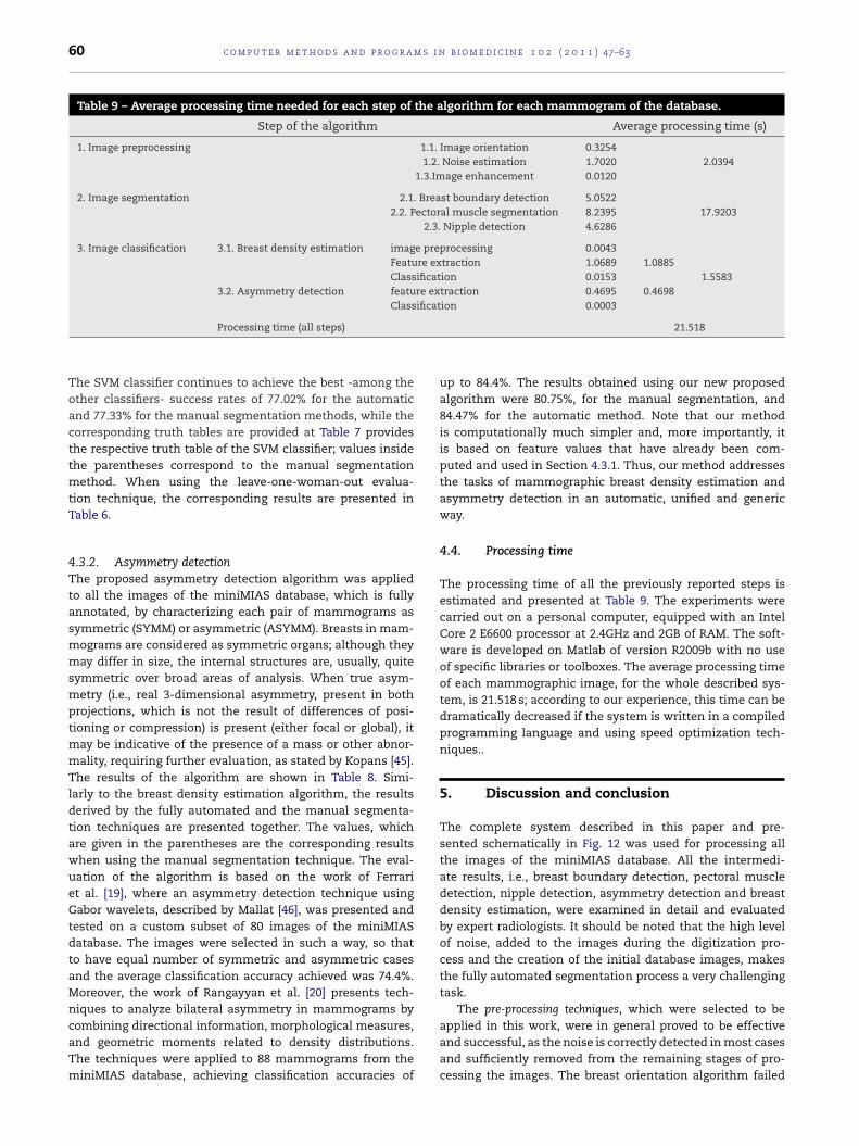
Table 9 – Average processing time needed for each step of the algorithm for each mammogram of the database.

Step of the algorithm Average processing time (s)

1. Image preprocessing 1.1. Image orientation 0.32541.2. Noise estimation 1.7020 2.0394

1.3.Image enhancement 0.0120

2. Image segmentation 2.1. Breast boundary detection 5.05222.2. Pectoral muscle segmentation 8.2395 17.9203

2.3. Nipple detection 4.6286

3. Image classification 3.1. Breast density estimation image preprocessing 0.0043Feature extraction 1.0689 1.0885Classification 0.0153 1.5583

3.2. Asymmetry detection feature extraction 0.4695 0.4698Classification 0.0003

Processing time (all steps)

The SVM classifier continues to achieve the best -among theother classifiers- success rates of 77.02% for the automaticand 77.33% for the manual segmentation methods, while thecorresponding truth tables are provided at Table 7 providesthe respective truth table of the SVM classifier; values insidethe parentheses correspond to the manual segmentationmethod. When using the leave-one-woman-out evalua-tion technique, the corresponding results are presented inTable 6.

4.3.2. Asymmetry detectionThe proposed asymmetry detection algorithm was appliedto all the images of the miniMIAS database, which is fullyannotated, by characterizing each pair of mammograms assymmetric (SYMM) or asymmetric (ASYMM). Breasts in mam-mograms are considered as symmetric organs; although theymay differ in size, the internal structures are, usually, quitesymmetric over broad areas of analysis. When true asym-metry (i.e., real 3-dimensional asymmetry, present in bothprojections, which is not the result of differences of posi-tioning or compression) is present (either focal or global), itmay be indicative of the presence of a mass or other abnor-mality, requiring further evaluation, as stated by Kopans [45].The results of the algorithm are shown in Table 8. Simi-larly to the breast density estimation algorithm, the resultsderived by the fully automated and the manual segmenta-tion techniques are presented together. The values, whichare given in the parentheses are the corresponding resultswhen using the manual segmentation technique. The eval-uation of the algorithm is based on the work of Ferrariet al. [19], where an asymmetry detection technique usingGabor wavelets, described by Mallat [46], was presented andtested on a custom subset of 80 images of the miniMIASdatabase. The images were selected in such a way, so thatto have equal number of symmetric and asymmetric casesand the average classification accuracy achieved was 74.4%.Moreover, the work of Rangayyan et al. [20] presents tech-niques to analyze bilateral asymmetry in mammograms by

combining directional information, morphological measures,and geometric moments related to density distributions.The techniques were applied to 88 mammograms from theminiMIAS database, achieving classification accuracies of

21.518

up to 84.4%. The results obtained using our new proposedalgorithm were 80.75%, for the manual segmentation, and84.47% for the automatic method. Note that our methodis computationally much simpler and, more importantly, itis based on feature values that have already been com-puted and used in Section 4.3.1. Thus, our method addressesthe tasks of mammographic breast density estimation andasymmetry detection in an automatic, unified and genericway.

4.4. Processing time

The processing time of all the previously reported steps isestimated and presented at Table 9. The experiments werecarried out on a personal computer, equipped with an IntelCore 2 E6600 processor at 2.4GHz and 2GB of RAM. The soft-ware is developed on Matlab of version R2009b with no useof specific libraries or toolboxes. The average processing timeof each mammographic image, for the whole described sys-tem, is 21.518 s; according to our experience, this time can bedramatically decreased if the system is written in a compiledprogramming language and using speed optimization tech-niques..

5. Discussion and conclusion

The complete system described in this paper and pre-sented schematically in Fig. 12 was used for processing allthe images of the miniMIAS database. All the intermedi-ate results, i.e., breast boundary detection, pectoral muscledetection, nipple detection, asymmetry detection and breastdensity estimation, were examined in detail and evaluatedby expert radiologists. It should be noted that the high levelof noise, added to the images during the digitization pro-cess and the creation of the initial database images, makesthe fully automated segmentation process a very challengingtask.

The pre-processing techniques, which were selected to be

applied in this work, were in general proved to be effectiveand successful, as the noise is correctly detected in most casesand sufficiently removed from the remaining stages of pro-cessing the images. The breast orientation algorithm failed

c o m p u t e r m e t h o d s a n d p r o g r a m s i n

is4io

wrbsrmpbnaatmovoua

r

Fig. 12 – The complete system described.

n only three images, because in these cases the breast tis-ue is cut off from the image, as already explained in Section.1. These cases, however, are non-acceptable mammographicmages, according to best practice and to the radiologist’spinion.

The implemented breast boundary detection technique,hich is based on a simple inference, gives satisfactory

esults. This is obvious by a careful observation of the detectedoundary of the images and also verified accordingly, usingpecific statistic measures. The pectoral muscle estimate is accu-ate and further improved, according to specific statistical

easures, through the modification we propose. The new nip-le detection technique tries to overcome the drawback of thereast boundary estimation method, i.e., not detecting theipple, when this is in profile. In this way, it can serve asn improvement for the already established breast bound-ry, and in addition as a key point for further processing ofhe image, due to the importance of the nipple area in a

ammographic image. Note that this technique can not bebjectively compared to the algorithms proposed in the pre-

iously published relevant literature, since the most similarne is the work by Chandrasekhar and Attikiouzel [11], whichses only a small subset of the miniMIAS database and hasdifferent target than ours. The results were evaluated by

b i o m e d i c i n e 1 0 2 ( 2 0 1 1 ) 47–63 61

expert radiologists and are promising enough to expect evenbetter results, when applied to high quality digital mammo-grams.

The proposed algorithm for mammographic breast densityestimation achieves better results compared to the work ofMasek [15] and of Oliver et al. [17], although the latter one usesonly a selected small portion of the miniMIAS database. Thework of Bosch et al. [16] achieves higher success rates, albeit ituses a different approach with higher-order textural features,which are computationally very expensive. The work we pro-pose in this paper uses simple first-order statistical featuresand a new technique for the power spectrum estimation, mak-ing the whole process suitable for on-line training updates andreal-time applications.

The asymmetry detection scheme uses the segmentationalready obtained via the breast density estimation procedure.It achieves a success rate similar to or even higher than thelevels reported in the relevant literature, although it uses thecomplete set of images of the miniMIAS database, instead ofa small subset, as the work of Ferrari et al. [19] and Rangayyanet al. [20]. Therefore, our experimental results can be consid-ered more reliable and consistent. Furthermore, the use of theone-class classification algorithm turned out to be a simpleyet effective way to overcome the problem of the imbalancedclasses, as the asymmetric cases are about 10% of the symmet-ric cases. The idea of the classification is to model as “target”the asymmetric cases and consider as “outliers” all the othercases, leading to an one-class scheme. The symmetric casesare not specifically modelled, but simply considered as non-asymmetric.

All the previously reported techniques can be combinedand integrated to a clinical-level CAD system. All the algo-rithms are fully-automated and there is no need for externalassistance. In addition, the processing time is not largeenough, so each mammogram can be analyzed online; thatis, on the fly as it is inserted the system. Moreover, the pro-posed scheme is considered to be robust against noise, as ithas been verified by its application to the miniMIAS mammo-graphic images database, in which the noise levels are veryhigh and of varying nature.

Conflict of interest

There are no conflict of interest.

e f e r e n c e s

[1] R. Nishikawa, Current status and future directions ofcomputer-aided diagnosis in mammography, ComputerizedMedical Imaging and Graphics 31 (4–5) (2007) 224–235.

[2] M. Siddiqui, M. Anand, P. Mehrotra, R. Sarangi, N. Mathur,Biomonitoring of organochlorines in women with benignand malignant breast disease, Environmental Research 98(2) (2005) 250–257.

[3] A. Wroblewska, P. Boninski, A. Przelaskowski, M. Kazubek,

Segmentation and feature extraction for reliableclassification of microcalcifications in digital mammograms,Opto-Electronics Review 11 (3) (2003) 227–235.

[4] R. Rangayyan, F. Ayres, J. Leo Desautels, A review ofcomputer-aided diagnosis of breast cancer: toward the

m s i n

[41] R.O. Duda, P.E. Hart, Pattem Classification and Scene

62 c o m p u t e r m e t h o d s a n d p r o g r a

detection of subtle signs, Journal of the Franklin Institute344 (3–4) (2007) 312–348.

[5] R. Ferrari, R. Rangayyan, R. Borges, A. Frère, Segmentation ofthe fibro-glandular disc in mammogrms using Gaussianmixture modelling, Medical and Biological Engineering andComputing 42 (3) (2004) 378–387.

[6] V. Andolina, S. Lillé, K. Willison, Mammographic Imaging: APractical Guide, Williams & Wilkins, Lippincott, 2001.

[7] S. Kwok, R. Chandrasekhar, Y. Attikiouzel, M. Rickard,Automatic pectoral muscle segmentation on mediolateraloblique view mammograms, IEEE Transactions on MedicalImaging 23 (9) (2004) 1129–1140.

[8] R. Ferrari, R. Rangayyan, J. Desautels, R. Borges, A. Frere,Automatic identification of the pectoral muscle inmammograms, IEEE Transactions on Medical Imaging 23 (2)(2004) 232–245.

[9] F. Yin, M. Giger, K. Doi, C. Vyborny, R. Schmidt,Computerized detection of masses in digital mammograms:automated alignment of breast images and its effect onbilateral-subtraction technique, Medical Physics 21 (1994)445.

[10] H. Knauerhase, M. Strietzel, B. Gerber, T. Reimer, R. Fietkau,Tumor location, interval between surgery and radiotherapy,and boost technique influence local control afterbreast-conserving surgery and radiation: retrospectiveanalysis of monoinstitutional long-term results,International Journal of Radiation Oncology, Biology,Physics 72 (4) (2008) 1048–1055.

[11] R. Chandrasekhar, Y. Attikiouzel, A simple method forautomatically locating the nipple on mammograms, IEEETransactions on Medical Imaging 16 (5) (1997) 483–494.

[12] A. Méndez, P. Tahoces, M. Lado, M. Souto, J. Correa, J. Vidal,Automatic detection of breast border and nipple in digitalmammograms, Computer Methods and Programs inBiomedicine 49 (3) (1996) 253–262.

[13] J. Wolfe, Risk for breast cancer development determined bymammographic parenchymal pattern, Cancer 37 (5) (1976)2486–2492.

[14] C. De Orsi, L. Bassett, S. Feig, et al., Illustrated BreastImaging Reporting and Data System: Illustrated BI-RADS,American College of Radiology, Reston, VA, 1998.

[15] M. Masek, Hierarchical Segmentation of MammogramsBased on Pixel Intensity, Ph.D. Thesis, University of WesternAustralia School of Electrical, Electronic and ComputerEngineering and University of Western Australia Centre forIntelligent Information Processing Systems, URLhttp://citeseerx.ist.psu.edu/viewdoc/summary?doi=10.1.1.128.1245, 2004.

[16] A. Bosch, X. Munoz, A. Oliver, J. Martı, Modeling andclassifying breast tissue density in mammograms, in:Proceedings of the 2006 IEEE Computer Society Conferenceon Computer Vision and Pattern Recognition-Volume 2, IEEEComputer Society Washington, DC, USA, 2006, pp.1552–1558.

[17] A. Oliver, J. Freixenet, A. Bosch, D. Raba, R. Zwiggelaar,Automatic classification of breast tissue, in: IberianConference on Pattern Recognition and Image Analysis,Springer, 2005, pp. 431–438.

[18] M. Homer, Mammographic Interpretation: A PracticalApproach, McGraw-Hill Companies, 1991.

[19] R. Ferrari, R. Rangayyan, J. Desautels, A. Frere, Analysis ofasymmetry in mammograms via directional filteringwithGabor wavelets, IEEE Transactions on Medical Imaging20 (9) (2001) 953–964.

[20] R. Rangayyan, R. Ferrari, A. Frere, Analysis of bilateral

asymmetry in mammograms using directional,morphological, and density features, Journal of ElectronicImaging 16 (1) (2007) 13003–113003.

b i o m e d i c i n e 1 0 2 ( 2 0 1 1 ) 47–63

[21] J. Suckling, J. Parker, D. Dance, S. Astley, I. Hutt, C. Boggis, I.Ricketts, E. Stamatakis, N. Cerneaz, S. Kok, et al., Themammographic image analysis society digital mammogramdatabase, in: Exerpta Medica. International Congress Series,1994, pp. 375–378.

[22] M. Mavroforakis, H. Georgiou, N. Dimitropoulos, D.Cavouras, S. Theodoridis, Significance analysis of qualitativemammographic features, using linear classifiers, neuralnetworks and support vector machines, European Journal ofRadiology 54 (1) (2005) 80–89.

[23] M. Masek, J. deSilva, Y. Christopher, Attikiouzel, Automaticbreast orientation in mediolateral oblique viewmammograms, in: 6th International Workshop onDigital Mammography, Greece, Springer-Verlag, 2003, pp.207–209.

[24] A.D. Brink, N.E. Pendock, Minimum cross-entropy thresholdselection, Pattern Recognition 29 (1) (1996) 179–188.

[25] I. Sobel, Camera Models and Machine Perception AIM-21,1970.

[26] J. Radon, Über die Bestimmung von Funktionen durchihre Integralwerte längs gewisser Mannigfaltigkeiten,Berichte Sächsische Akademie der Wissenschaften,Leipzig, Mathematisch-Physikalische Klasse 69 (1917)262–277.

[27] R. Gonzalez, R. Woods, Digital Image Processing, PrenticeHall, 2007.

[28] A. Penn, M. Loew, Estimating fractal dimension with fractalinterpolation function models, IEEE Transactions on MedicalImaging 16 (6) (1997) 930–937.

[29] L. Kaplan, Extended fractal analysis for texture classificationandsegmentation, IEEE Transactions on Image Processing 8(11) (1999) 1572–1585.

[30] L. Breiman, Classification and Regression Trees, CRC,Chapman & Hall, 1998.

[31] S. Theodoridis, K. Koutroumbas, Pattern Recognition, 4thedn., Academic Press, 2009.

[32] M.E. Mavroforakis, S. Theodoridis, A geometric approach tosupport vector machine (SVM) classification, IEEETransactions on Neural Network 17 (3) (2006) 671–682.

[33] M. Mavroforakis, M. Sdralis, S. Theodoridis, A geometricnearest point algorithm for the efficient solution of the SVMclassification task, IEEE Transactions on Neural Networks 18(5) (2007) 1545–1549.

[34] H. Byun, S. Lee, A survey on pattern recognitionapplications of support vector machines, InternationalJournal of Pattern Recognition and Artificial Intelligence 17(3) (2003) 459–486.

[35] M. Mavroforakis, M. Sdralis, S. Theodoridis, A novel SVMgeometric algorithm based on reduced convex hulls, in:Pattern Recognition, 2006. ICPR 2006. 18th InternationalConference, vol. 2, IEEE, 2006, pp. 564–568.

[36] D. Tax, One-class classification; Concept-learning in theabsence of counter-examples, Ph.D. Thesis, 2001.

[37] A. Rabaoui, H. Kadri, Z. Lachiri, N. Ellouze, One-class SVMschallenges in audio detection and classificationapplications, EURASIP Journal on Advances in SignalProcessing (2008) (19).

[38] W. Cooley, P. Lohnes, Multivariate Data Analysis, John Wiley& Sons Inc., 1971.

[39] C.-C. Chang, C.-J. Lin, LIBSVM: A Library for Support VectorMachines, Software available athttp://www.csie.ntu.edu.tw/cjlin/libsvm, 2001.

[40] M. Wirth, MIAS Mask Database, University of Guelph,Canada, 2005.

Analysis, Wiley, New York, 1973.[42] L. Dice, Measures of the amount of ecologic association

between species, Ecology 26 (3) (1945) 297–302.

s i n

c o m p u t e r m e t h o d s a n d p r o g r a m

[43] M. Wirth, D. Nikitenko, J. Lyon, Segmentation of the breast

region in mammograms using a rule-based fuzzy reasoningalgorithm, ICGST International Journal on Graphics, Visionand Image Processing 05 (2005) 45–54.

[44] L. Blot, R. Zwiggelaar, Background texture extraction for theclassification of mammographic parenchymal patterns, in:

b i o m e d i c i n e 1 0 2 ( 2 0 1 1 ) 47–63 63

Medical Image Understanding and Analysis, 2001, pp.

145–148.

[45] D. Kopans, Breast Imaging, Williams & Wilkins, Lippincott,2007.

[46] S. Mallat, A Wavelet Tour of Signal Processing, AcademicPress, 1999.