MNRAS 497, 2455–2468 (2020) doi:10.1093/mnras/staa1990Advance Access publication 2020 July 9

Gamma-ray counterparts of 2WHSP high-synchrotron-peaked BL Lacobjects as possible signatures of ultra-high-energy cosmic ray emission

Michael W. Toomey ,1,2,3,4‹ Foteini Oikonomou 3,5,6,7 and Kohta Murase3,4,8

1Brown Theoretical Physics Center, Brown University, Providence, RI 02912, USA2Department of Physics, Brown University, Providence, RI 02912, USA3Department of Physics, The Pennsylvania State University, University Park, PA 16802, USA4Department of Astronomy and Astrophysics, The Pennsylvania State University, University Park, PA 16802, USA5Physik-Department, Technische Universitat Munchen, James-Frank-Str. 1, D-85748 Garching bei Munchen, Germany6European Southern Observatory, Karl-Schwarzschild-Str. 2, D-85748 Garching bei Munchen, Germany7Institutt for fysikk, NTNU, Trondheim, 7491 Norway8Yukawa Institute for Theoretical Physics, Kyoto University, Kyoto 606-8502, Japan

Accepted 2020 June 29. Received 2020 June 23; in original form 2020 March 4

ABSTRACTWe present a search for high-energy γ -ray emission from 566 Active Galactic Nuclei at redshift z > 0.2, from the 2WHSPcatalogue of high-synchrotron peaked BL Lac objects with 8 yr of Fermi-LAT data. We focus on a redshift range whereelectromagnetic cascade emission induced by ultra-high-energy cosmic rays can be distinguished from leptonic emission basedon the spectral properties of the sources. Our analysis leads to the detection of 160 sources above ≈5σ (TS ≥25) in the 1–300 GeVenergy range. By discriminating significant sources based on their γ -ray fluxes, variability properties, and photon index in theFermi-LAT energy range, and modelling the expected hadronic signal in the TeV regime, we select a list of promising sourcesas potential candidate ultra-high-energy cosmic ray emitters for follow-up observations by Imaging Atmospheric CherenkovTelescopes.

Key words: galaxies: active – galaxies: high-redshift – gamma rays: galaxies.

1 IN T RO D U C T I O N

The Fermi Gamma-ray Space Telescope (Atwood et al. 2009)and Imaging Atmospheric Cherenkov Telescopes (IACTs) havedramatically increased the number of known γ -ray sources, aswell as our knowledge of the non-thermal Universe. Among theobserved extragalactic γ -ray sources, blazars, active galactic nuclei(AGNs) with jets aligned with the observer’s line of sight (e.g.Urry & Padovani 1995), are by far the most numerous. Theyexhibit superluminal motion, and are some of the most powerfulsteady sources in the Universe. Additionally, they dominate theγ -ray sky and play an important role in the energy budget of theUniverse (Murase & Fukugita 2019).

Categorized as either BL Lacertae (BL Lac) objects or FlatSpectrum Radio Quasars (FSRQs), based on the properties of theiroptical spectra, blazars are among the brightest objects in theUniverse. Blazars possess spectral energy distributions (SEDs) with acharacteristic double hump shape. The lower energy peak is generallythought to be powered by the synchrotron emission of electrons in theblazar jet. The origin of the high-energy peak is a subject of debate.In conventional leptonic scenarios, the γ -ray emission is assumed tobe powered by inverse Compton radiation (Maraschi, Ghisellini &Celotti 1992; Sikora, Begelman & Rees 1994), but it could also have ahadronic origin (Aharonian 2000; Mucke & Protheroe 2001). BL Lac

� E-mail: michael toomey@brown.edu

objects are further sub-classified according to the value of the fre-quency (in the source rest-frame) at which the synchrotron peak of theSED occurs. Low-energy (νS < 1014 Hz), intermediate-energy (1014

<νS < 1015 Hz) and high-energy (νS > 1015 Hz) synchrotron peaked,referred to in short as LSP, ISP, and HSP respectively (Padovani &Giommi 1995; Fermi-LAT Collaboration 2010).

More recently, observations with IACTs have revealed an addi-tional class of BL Lac objects, whose spectrum in the Fermi-LATenergy range is hard (meaning that the spectral index in this energyrange γ < 2), placing their peak of the high-energy ‘hump’ inthe SED, after accounting for absorption during their extragalacticpropagation, in the TeV energy range. Additionally, these sourcestypically possess νS > 1017 Hz. These properties are suggestive ofextreme particle acceleration which has led to them being referred toas extreme HSPs (Costamante et al. 2001, 2018; Biteau et al. 2020).

One of the greatest mysteries in particle astrophysics todayis the origin of ultra-high-energy cosmic-rays (UHECRs). Suchparticles are observed with energies in excess of ≈1020 eV (see e.g.reviews by Kotera & Olinto 2011; Mollerach & Roulet 2018; AlvesBatista et al. 2019; Anchordoqui 2019). Since the Larmor radiusfor cosmic-rays above the ankle, at ∼4 × 1018 eV, exceeds that ofthe Galaxy, these UHECRs are very likely of extragalactic origin.One of the most promising candidates proposed as the sources ofUHECRs are AGNs (Ginzburg & Syrovatskii 1964; Hillas 1984).Blazars, specifically, have often been proposed as sites of UHECRacceleration (see e.g. Dermer & Razzaque 2010; Murase et al. 2012b;Rodrigues et al. 2018, and references therein).

C© 2020 The Author(s)Published by Oxford University Press on behalf of the Royal Astronomical Society

Dow

nloaded from https://academ

ic.oup.com/m

nras/article/497/2/2455/5869263 by guest on 04 July 2022

2456 M. W. Toomey, F. Oikonomou and K. Murase

This is particularly true for extreme HSP BL Lac objects. Attemptsto describe the origin of their hard TeV spectra with standard leptonicmodels often require extreme parameters (e.g. Katarzynski et al.2006). An alternative scenario for the observed γ -ray emissionof extreme HSPs is that it is secondary emission from UHECRs(e.g. Essey & Kusenko 2010; Essey et al. 2011; Murase et al.2012b; Aharonian et al. 2013; Takami, Murase & Dermer 2013;Oikonomou, Murase & Kotera 2014; Takami, Murase & Dermer2016; Tavecchio et al. 2019). If these sources produce UHECRs,these will interact with photons from the extragalactic backgroundlight (EBL) and the cosmic microwave background (CMB), andproduce electron–positron pairs (Bethe-Heitler) emission, and pionicγ -rays. However, the spectrum of UHECR-induced secondary γ -raysis expected to extend to higher energies than in standard leptonicscenarios due to the continuous injection of high-energy leptons viathe Bethe-Heitler (BH) pair-production process during intergalacticpropagation, leading to a natural explanation for the observed hardTeV spectra.

Primary and secondary γ -rays with energy Eγ ∼ (m2ec

4)/εγ ∼260 (1 eV/εγ ) GeV, interact with photons of the EBL and the CMBwith energy εγ , which results in the production of electron–positronpairs (Gould & Schreder 1966; Stecker, de Jager & Salamon 1992).Electrons and positrons produced in interactions of γ -rays withthe EBL/CMB inverse Compton upscatter background photons, andgenerate secondary γ -rays. The two processes (pair-production andinverse Compton emission) produce an electromagnetic ‘cascade’ inthe intergalactic medium, until the γ -rays drop below the thresholdfor pair production on the EBL. During the intergalactic propagationof the cascade emission, the electrons (and positrons) get deflected inthe presence of intergalactic magnetic fields (IGMFs), causing eithermagnetic broadening of the cascade emission, or, in the presenceof a stronger field, a suppression of the observed GeV cascadeflux from the source (Gould & Rephaeli 1978; Aharonian, Coppi& Volk 1994). The detection (or absence of) the cascade emissionfrom TeV emitting blazars can result in the measurement of (orlower bound on) the IGMF in the line of sight from these sources.Similarly the detection of magnetic broadening, ‘halo’ emission,can result in a measurement of the strength of IGMFs (e.g. Elyiv,Neronov & Semikoz 2009; Neronov & Semikoz 2009; H. E. S. S.Collaboration 2014; Archambault et al. 2017). High-redshift, hard-spectrum blazars, whose intrinsic spectrum extends beyond TeVenergies are thus ideal sources to look for the signatures of the effectsof the IGMF (cascade flux, and halo component), as the cascadeemission in the GeV spectrum dominates the observed emission inthis energy band. This combination of parameters maximizes theexpected cascade emission in these sources, and in the case of non-observation of the expected cascade emission, can result in lowerlimits on the IGMF strength. For the same reason, the expectedhalo component is maximal for high-redshift, hard-spectrum sources(although at the disadvantage of having an overall fainter source). Thehighest redshift blazars that have been detected to date with IACTsare PKS 1441+25 (Abeysekara et al. 2015) and S3 0218+35 (Ahnenet al. 2016). These are of the FSRQ type, and were detected up to∼200 GeV energy. They are thus not expected to exhibit the signatureof UHECR emission which has been proposed for extreme HSPs intheir γ -ray spectra, but demonstrate the possible reach of future,deeper, IACT observations.

1.1 Time variability

An important observational distinction between leptonic andUHECR-induced intergalactic cascade emissions is related to the

different deflections experienced by the leptonic and UHECR beamin the IGMF. As a result, one expects different variability properties ofthe γ -ray emission in these two cases. In the case of a leptonic beam,time delays are only relevant for the secondary (cascade) emission,and come from the deflections of the electrons produced in the inter-actions of the primary γ -rays with background photons. Electronswith energy E′

e (in the cosmic rest frame at redshift z), and Lorentzfactor γ ′

e = E′e/(mec

2), traversing a region with magnetic fieldstrength B, have a Larmor radius rL ≈ eB/E′

e, where e is the chargeof the electron. Such electrons will experience deflections of orderθIC ≈ √

2/3(λIC/rL) before inverse Compton upscattering CMBphotons, after, on average, one inverse Compton cooling length λIC =3mec

2/(4σT UCMBγ ′e) ≈ 70 kpc (E′

e/5 TeV)−1(1 + z)−4, where σ T isthe Thompson cross-section and UCMB � 0.26 eV (1 + z)4 is theenergy density of the CMB at redshift z.

The typical time delay experienced by cascade photons due to thedeflections of the electrons is of order, (e.g. Murase et al. 2008;Takahashi et al. 2008; Dermer et al. 2011), tIC,IGMF/(1 + z) ≈θ2

IC(λIC + λγγ )/2c. Here, λγγ ∼ 20 Mpc (nEBL/0.1 cm3)−1 is theaverage distance travelled by a primary γ -ray before it interactswith an EBL photon to create an electron–positron pair. In theabove expression, nEBL is the number density of EBL photons,normalized to the value relevant for interactions with 10 TeV γ -rays.The electrons subsequently upscatter CMB photons via the inverse-Compton process, typically to energy Eγ ≈ (4/3)γ ′2

e εCMB, whereεCMB ≈ 2.8kBTCMB,0 and kB the Boltzmann constant, and T0,CMB thetemperature of the CMB at z = 0. For such γ -rays with energy Eγ

from a source at z 1, we obtain a characteristic time delay (e.g.Murase, Meszaros & Zhang 2009),

tIC,IGMF

(1 + z)≈ θ2

IC

2c(λIC + λγγ ) ∼ 4 × 105 yr

(Eγ

0.1 TeV

)−2

×(

B

10−14 G

)2 (λγγ

20 Mpc

). (1)

Thus, any detectable variable emission in short time-scales is likelyprimary in origin. An additional, slowly variable component mayexist, due to the reprocessed emission, if the IGMF is sufficientlylow (B � 10−17 G).

In the UHECR-induced intergalactic cascade scenario, there isno primary γ -ray component. The main energy loss channel forprotons with energy less than 1019 eV is through the Bethe–Heitlerpair-production process. The trajectory of the protons may beregarded as a random walk through individual scattering centresof size, lc ∼ O(Mpc). The Larmor radius of an UHECR withenergy Ep is, rL,p ∼ eB/Ep ∼ 800 Mpc(B/1017 G)(Ep/1017 eV)−1.After crossing a scattering centre of size lc the proton experi-ences a deflection of order θp ≈ √

2/3lc/rL,p and a time delayof order t0 ∼ (lc/c)θ2

p . Thus, the total time delay experiencedafter travelling the characteristic energy loss length of the Bethe–Heitler process, λBH, is of order, tp ∼ (λBH/lc)t0 ∼ (λBH/c)θ2

p ∼20 yr (Ep/1017 eV)(B/10−14 G)2(λBH/1 Gpc)(1 + z) (Murase et al.2012b; Prosekin et al. 2012). At every interaction the proton produceselectrons (and positrons) which cascade down to GeV energies overa length scale of order λIC. Thus, in this case, the relevant time delayis max(tIC,IGMF, tp), i.e. the maximum of the delays experiencedby the protons and those of the leptonic cascade emission given byequation (1). As a result, we expect that the sources whose emissionis dominated by UHECR cascades should be non-variable or at mostslowly variable.

The search for variability is a strong motivation for this work.However, though the absence or weakness of the variability is one

MNRAS 497, 2455–2468 (2020)

Dow

nloaded from https://academ

ic.oup.com/m

nras/article/497/2/2455/5869263 by guest on 04 July 2022

A candidate list of HECR accelerating blazars 2457

of the crucial signatures of the UHECR-induced cascade scenario,negative detection itself is not proof for the UHECR origin of theemission. This is because, even if the variability is present, it maysimply be below the experimental sensitivity.

Our goal is to identify sources which have a hard spectrum inthe GeV energy range. Such sources are good candidates for veryhigh-energy (VHE) follow-up observations, which can reveal TeVspectra of extreme HSP blazars, and possibly the signatures ofUHECR acceleration and information on IGMFs. Additionally, weinvestigate variability properties of our source sample. The presenceof the variability can rule out hadronic origin of the γ -ray emission.The non-detection of variability is harder to interpret in this context,as it can be caused by either intergalactic propagation effects orinsufficient sensitivities of the instruments. Nevertheless, we makeinferences by examining the entire sample, and trends as a functionof redshift and γ -ray flux.

The layout of the paper is as follows. In Section 2 we discussthe selection of our catalogue and the analysis of Fermi-LAT data,including the calculation of the time variability. In Section 3 wediscuss our modelling of the leptonic and hadronic emissions in theTeV regime. In Section 4 we present the results of our work andin Section 5 we discuss our results and propose avenues for furtherstudy.

2 A NA LY SIS

2.1 Data selection

For our analysis we opt to use the 2WHSP catalogue of HSPblazars (Chang et al. 2017), which was, until recently, the mostcomplete catalogue of HSP and candidate extreme-HSP sources (seediscussion in Section 5). All sources from the catalogue with redshifts≥0.2 were selected and submitted to a full Fermi analysis, a total of566 sources. This was the only cut made on the 2WHSP catalogue,motivated by the theoretical prediction that UHECR-induced cascadeemission can be more prominent for higher redshift HSPs (Muraseet al. 2012b; Takami et al. 2013). Note that some sources in thecatalogue only have a redshift with a lower limit. We still includethese in the analysis but interpret results differently where relevant.

This sample of high redshift blazars from the 2WHSP catalogueforms the basis of the sources studied in this analysis. An analysissearching for γ -ray emission was conducted by the authors of the1BIGB catalogue (Arsioli & Chang 2017) (see also Arsioli et al.2018). However, these analyses did not include a study of sourcevariability. In order to determine potential cosmic-ray acceleratorsbased on VHE γ -rays, this information can be critical. In Section 4we elaborate further on how our results compare to and differ fromthose of Arsioli & Chang (2017).

Many of the sources studied in this analysis have a counter-part in the 3FGL (Acero et al. 2015) and the recently released4FGL catalogue (The Fermi-LAT collaboration 2019). However,the variability analysis from the 4FGL, or the previous 3FGL, isnot appropriate for our work due to the inclusion of sub-GeVphotons. In the UHECR-induced cascade scenario, cascade emissionis expected to be dominant in the 10–100 GeV range as we show inthe following sections. At the sub-GeV energy range, because of theIGMF suppression of the cascade component, primary photons thatare intrinsically variable would dominate the spectrum for blazars.However, we would not have sufficient statistics for the variabilityanalysis if we focused on the high-energy data in the 30–100 GeVrange only. Therefore in this work we have chosen the 1–100 GeVenergy range for our analysis. This is not ideal but still useful to see

the variability and discriminate between the leptonic and hadronicscenarios. We further note that since the sources of interest in ourstudy have a hard spectrum in the Fermi energy range, it would bemore challenging to detect the variability in the 100 MeV–1 GeVenergy range than for the average of 4FGL sources.

2.2 Data analysis

An unbinned maximum-likelihood approach was used in this workfor spectral analysis utilizing Fermi Science Tools v10r0p5. For eachblazar candidate, a region of interest 8◦ in radius was created fromPass 8 SOURCE class (evclass = 128) photons that where detected onboth the FRONT and BACK of the LAT detectors (evtype = 3). Datawere filtered temporally from 2008 August 5 (239587201 MET) to2016 September 24 (496426332 MET) culminating in a total of 8.2 yrof data. Data were additionally filtered by considering photons ofenergies 1.0–300 GeV and setting a maximum zenith angle of 100◦ toavoid atmospheric background. Periods where data taken from LATwere of poor quality were removed utilizing the tool gtmktime. At thisstep, the LAT team’s recommended filter expression for SOURCEclass photons (DATA QUAL>0)&&(LAT CONFIG==1) was used.

For each source an exposure hypercube was calculated – a measureof the amount of time a position on the sky has spent at a certaininclination angle. The exposure hypercube was computed withgtltcube by binning the off-axis angle in increments of 0.025 cosθOA

and setting the spatial grid size to 1◦. For our analysis, we followthe Fermi-LAT recommendation to implement the zenith angle cutfor exposure during the calculation of the exposure hypercube asopposed to during the determination of good time intervals withgtmktime. The exposure map was then calculated for a region18◦ in radius, with 72 latitudinal and longitudinal points, and 24logarithmically uniform energy bins.

We conducted a sanity check of our own implementation of FermiTools used in this analysis by utilizing the FERMIPY package (Woodet al. 2017). The results obtained with the two methods were foundto be consistent. We did not use the FERMIPY package for our resultsas an unbinned analysis method was not available.

2.3 Modelling

For each candidate γ -ray blazar, a model was constructed us-ing known 3FGL sources, the Galactic diffuse emission modelgll iem v06, and isotropic diffuse model iso P8R2 SOURCE V6 v06with make3FGLxml. Non-3FGL sources were added to the model asa simple power law,

dN

dE= N0

[E

E0

]−γ

. (2)

The photon index, γ , and normalizations, N0, were set free to be fitbut the pivot energy, E0, was fixed at 3.0 GeV for non-3FGL sourcesand set to 3FGL catalogue values otherwise. The normalizations ofthe Galactic and isotropic diffuse emissions were fit, in addition to thenormalization of all sources within 3◦ and variable sources out to 5◦.The maximum likelihood for each source was then computed using anunbinned technique with the NEWMINUIT minimizer implementedby the UnbinnedAnalysis module from Fermi Tools.

2.4 Time variability

A detailed variability analysis was conducted for significant sources– those above a TS of 25. Variability was determined by analysingthe sources at 60 d intervals with two different models. The first

MNRAS 497, 2455–2468 (2020)

Dow

nloaded from https://academ

ic.oup.com/m

nras/article/497/2/2455/5869263 by guest on 04 July 2022

2458 M. W. Toomey, F. Oikonomou and K. Murase

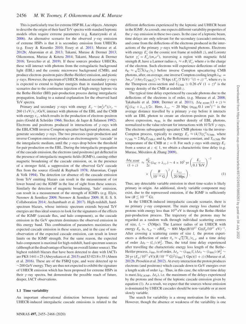
Table 1. Results from the analysis of 2WHSP sources. Included is the name from the 2WHSP catalogue, whether it is a Class I or II source, the luminosity from1–300 GeV, L44, in units of 1044 erg s−1, the 1–300 GeV photon flux, (dN/dt)−10, in units of 10−10 cm−2 s−1, the test statistic from the likelihood fit, T S, thenormalization and its error scaled by 10−11 cm−2 s−1 GeV−1, N−11 and σN, the photon index γ and its error σγ , the variability index TSV (> 63.17 is a variablesource), the source redshift z, alternative identifier, and the logarithm of the synchrotron peak frequency, log νS,pk in units of log Hz. The latter three entriesare obtained from the 2WHSP catalogue. Listed here are the results based on our source selection criteria. The full table, with all sources from the analysis, isavailable in the Appendix.

2WHSP name Class L44 ( dNdt

)−10 T S N−11 σN γ σγ T SV z Other name log νS,pk

J011904.6-145858 II 45.54 2.82 134.42 1.82 0.29 1.77 0.12 27.0 >0.530 3FGL J0118.9-1457 16.1J050657.7-543503 I 25.07 5.05 488.2 2.21 0.21 1.56 0.07 40.6 >0.260 RBS 621 16.2J060408.5-481725 II 20.5 2.69 132.76 0.26 0.05 1.73 0.11 37.1 >0.370 1ES 0602-482 16.2J101244.2+422957 19.77 2.78 157.36 1.01 0.14 1.74 0.11 29.3 0.365 3FGL J1012.7+4229 16.8J103118.4+505335 I 41.89 9.22 1014.9 7.26 0.48 1.74 0.05 52.7 0.360 1ES 1028+511 17.0J112453.8+493409 II 93.35 4.89 362.65 2.91 0.29 1.78 0.08 63.9 >0.570 RBS 981 16.5J124312.7+362743 II 99.06 21.98 2594.8 33.10 1.52 1.78 0.03 62.1 1.065 Ton 116 16.2J141756.5+254324 I 10.14 2.86 147.3 7.2 1.65 1.63 0.08 24.6 0.237 RBS 1366 17.4J143657.7+563924 II 57.3 5.79 522.39 8.28 0.8 1.77 0.06 47.4 >0.430 RBS 1409 16.9J150340.6-154113 I 65.09 9.18 439.69 5.04 0.42 1.79 0.07 52.0 >0.380 RBS 1457 17.6J175615.9+552218 II 45.88 3.68 223.86 3.85 0.5 1.76 0.08 32.0 >0.470 RGB J1756+553 17.3J205528.2-002116 32.19 2.96 92.1 0.8 0.14 1.75 0.13 27.7 0.440 3FGL J2055.2-0019 18.0

model allows the source normalization to be optimized for each bin.In the second model the source spectrum is fixed to correspond tothe null hypothesis, i.e. the source not being variable. For the firstmodel, if the flux in a temporal bin was not significant (TS < 9) orif errors were larger than Fi/Fi, a 90 per cent confidence Bayesianupper limit was calculated with the IntegralUpperLimit module. Ourvariability index corresponds to that defined by Fermi in their 2FGLpaper (Nolan et al. 2012),

T SV = 2∑

i

F 2i

F 2i + f 2F 2

c

V 2i , (3)

where Fi is defined as the as the flux error, Fc the flux for thesource if it was not variable, V 2

i the difference in log-likelihoods forthe null and alternative hypothesis, and f is a systematic correctionfactor determined by the Fermi team to be 0.02 in this calculation.For bins with low TS the variability was calculated using a similarstatistic,

T SUL = 2∑

i

0.5(FUL − Fi)2

0.5(FUL − Fi)2 + f 2F 2c

V 2i . (4)

The variability index is distributed as a χ2 distribution where thedegree of freedom corresponds to the number of bins, here 50. Thus,a total TSV > 63.17 implies less than 10 per cent chance for thesource to exhibit non-variability. For this analysis, a source with anindex above this value is considered to be variable.

2.5 Source selection criteria

In choosing promising sources for follow-up, a set of criteria wereplaced on the sources to establish merit. A primary cut was imposedon the flux of each source, F > 2.5 × 10−10 cm−2 s−1, to eliminatedim sources. It is also important that the sources have a hard photonindex, γ < 1.8, and have low variability, TSV < 70. From thesecuts a list of 12 potentially promising sources was compiled (seeTable 1). As a final means of selecting the most promising sourcesfor observation, the hadronic and leptonic spectrum for each sourcewas calculated and classified based on their detectability with IACTs.Sources which are detectable are put into two merit classes. Class Iare likely detectable with current generation IACT detectors. Class IIsources will likely take much longer for detection and are therefore

better candidates for next-generation detectors like CTA. Sources aremarked as belonging to one of these two classes in Table 1.

3 TEV SPECTRUM MODELLI NG

3.1 Leptonic scenario

With knowledge of the spectrum in the GeV regime, it is possible topredict the expected spectrum at TeV energies. For leptonic emissionthis can be done by assuming that the spectral index derived at GeVenergies and extending the maximum energy while accounting forattenuation of γ -rays due to pair production on the EBL. In thisscenario, the optical depth for EBL photons, τ γ γ (E), is dependent onthe redshift of the source. Thus, we can model the expected energyflux out to TeV energy,

EFE = Nlep · E−γLAT+2 · e−τγ γ (E), (5)

where Nlep and γ LAT are the flux normalization and spectral index inthe LAT energy range as determined in our analysis. We have useddata from Inoue et al. (2013) to calculate the attenuation of primaryleptonic γ -rays.

3.2 UHECR-induced cascade scenario

Similar to primary γ -rays, cascades occur for UHECRs travellingthrough intergalactic space. The observed TeV spectrum, however,should be harder than in the leptonic case due to the injection ofhigh-energy leptons from the Bethe–Heitler process. We adopt theanalytic formula from Murase, Beacom & Takami (2012a) for suchcascades (see also Berezinsky & Smirnov 1975). The approximatespectrum for the cascade emission is given by,

EGE ∝{

(E/Ebr)1/2 (E ≤ Ebr),(E/Ebr)2−β (Ebr ≤ E ≤ Ecut),

(6)

where the normalization is set by∫

dEGE = 1, with Ecut, the criticalenergy at which τ γ γ (E) = 1 due to the EBL absorption,for pair-production on the EBL, Ebr ≈ 4εCMBE′2

e /(3m2e) the energy below

which the number of electrons remains constant, where E′e ≈ (1 +

z)Ecut/2 and εCMB ≈ 2.8kBTCMB,0, and the cascade photon index β ≈1.9 (Murase et al. 2012a).

MNRAS 497, 2455–2468 (2020)

Dow

nloaded from https://academ

ic.oup.com/m

nras/article/497/2/2455/5869263 by guest on 04 July 2022

A candidate list of HECR accelerating blazars 2459

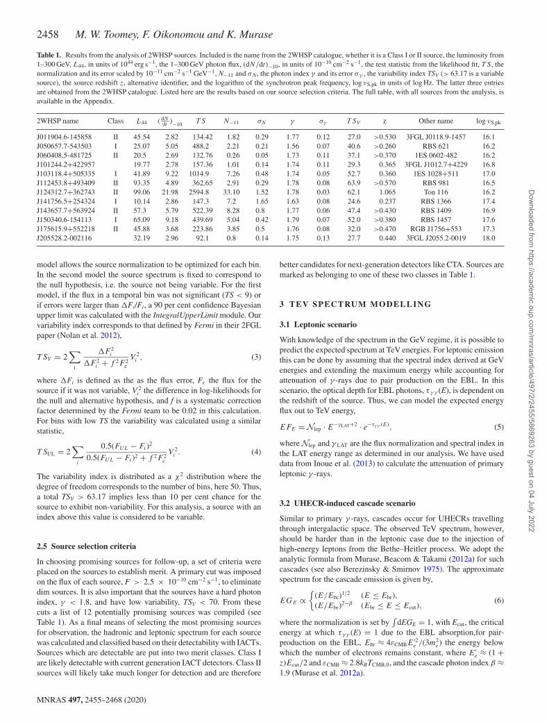
Figure 1. Distribution of the source variability index. The variability indexfor this analysis follows a χ2 distribution with 50 degrees of freedom. Thusa source with a variability index in excess of 63.17 exhibits variability with90 per cent confidence.

The optical depth to BH pair-production, τBH for cosmic raysaround 1019 eV, is given by the approximate expression,

τBH ≈ d

1000 Mpc, (7)

where d is the particle travel distance. Thus, the expected observedspectrum is given by,

EFE = Chad · EGE

min[1, τBH]

τγ γ (E)(1 − exp−τγ γ (E)), (8)

where Chad is the normalization factor and this equation is imple-mented without a cutoff (because the cutoff shape is taken intoaccount via τ γ γ ). In addition, the low-energy spectrum is suppressedby IGMFs. The comparison with the point spread function of theFermi-LAT (e.g. Neronov & Semikoz 2009; Murase et al. 2012a)suggests that the cascade emission is suppressed below ∼30 GeV forB ∼ 3 × 10−17 G (see also equation 6 of Kotera, Allard & Lemoine2011, and discussion).

In practice, our procedure provides the shape of the UHECR-induced cascade spectrum but does not encode the expected differen-tial energy flux. Thus, we normalize our hadronic cascade spectrumusing the normalization obtained through the Fermidata in the 10–100 GeV range.

4 R ESULTS

4.1 Likelihood and variability results

In our analysis of 566 VHE γ -ray blazar candidates above z ≥ 0.2from the 2WHSP catalogue of HSP BL Lac objects, we detected 160sources above ≈5σ (TS ≥ 25). Our best-fitting spectral parametersand TS values are in agreement with previous analyses of thesesources (Acero et al. 2015; Arsioli & Chang 2017).

Of the 160 γ -ray detected sources, 26 were found to exhibitvariability with greater than 90 per cent confidence while 134 didnot present variability (see Fig. 1). Based upon our criterion, the

Figure 2. Distribution of fluxes over the 1–300 GeV band for non-variableand variable sources.

majority of our sources do not exhibit significant variability. Table 1contains the results from the analysis for the most promising sourcesidentified. The entire table with all sources from the analysis can befound in the Appendix.

Many of the sources in the 2WHSP catalogue do not have firmredshifts. While some sources have precise measurements, some haveonly lower limits, and others have measurements but uncertaintiesare still large. Where relevant, we separate data based on the natureof the redshift measurement.

The photon flux and luminosity distributions for non-variableand variable sources are plotted in Figs 2 and 3 respectively. Forcalculation of the luminosity we adopt the following cosmology, � = 0.7, m = 0.3, k = 0, and H0 = 70 km s−1 Mpc−1.

These distributions clearly show that our non-variable sourcesare less bright than those which exhibit stronger variability. It is,however, less clear whether there is a correlation between variabilityand source luminosity. Our result could simply be due to the fact thatvariability is more easily seen for nearby sources.

In Fig. 4 the measured photon index is plotted against the calcu-lated luminosity. For variable sources there appears to be a weak trendbetween these two parameters. A correlation test on the data revealsthat the photon index is anticorrelated with source luminosity at ≈2σ

confidence. On the other hand, there is no apparent correlation fornon-variable data. Characteristic error bars are depicted in Fig. 4 forvariable and non-variable sources which corresponds to the averageerror for each class. Additionally plotted was variability index againstthe photon index in Fig. 5 to see if there was a correlation. If oneconsiders the data set as a whole, there is no apparent correlation.Even further consideration of the strongest sources implies there is nocorrelation between hardness and variability. In Fig. 5 we make thisdistinction by considering sources with a TS < 450 as being sourceswith less confident variability. Note that a non-variable source withTS = 450 with a variability index calculated over 50 time intervalswill have a test statistic for a per bin in the light-curve, correspondingto ≈3σ .

Indeed, the true nature of the variability for each source should beconsidered. It is more than likely that many of the sources from this

MNRAS 497, 2455–2468 (2020)

Dow

nloaded from https://academ

ic.oup.com/m

nras/article/497/2/2455/5869263 by guest on 04 July 2022

2460 M. W. Toomey, F. Oikonomou and K. Murase

Figure 3. Distribution of luminosity over the 1–300 GeV band for non-variable (blue) and variable (green) sources. The light colour correspondsto sources with confident redshift measurements. Variable and non-variablesources are represented by ‘V’ and ‘NV’, respectively.

Figure 4. Source luminosities against the photon index. The open circlescorrespond to sources of uncertain redshift. The legend at the lower rightcorner shows the characteristic error bars for sources of confident redshift.

analysis do exhibit some variability, to which our analysis is not yetsensitive. In Fig. 6, where we plot the source luminosity as a functionof redshift, it is interesting to note that the variable and non-variablesources can be roughly partitioned by plotting the luminosity for agiven energy flux over a range of redshifts. In Fig. 7 we plot thevariability as a function of test statistic. There is, unsurprisingly, astrong apparent correlation between the two.

Figure 5. Plot of the variability versus the photon index. Note that we haveartificially split the data by choosing TS ≥ 450. This corresponds to an averageTS per temporal bin of 3. The red vertical line indicates a photon index n =2 and the red horizontal line indicates the 90 per cent confidence limit onsource variability. Characteristic error bars for both classes are given in thelegend of the upper left of the figure.

Figure 6. Luminosity is plotted against redshift for the sources where opencircles correspond to uncertain redshift. The thick dashed line correspondsto the 8 yr, 5σ Fermi-LAT detection threshold. Characteristic error bars aregiven in the legend on the lower left of the figure.

4.2 Promising sources

From the results of the likelihood and variability analyses, significantsources were discriminated based on their variability, redshift,and brightness, to establish the best candidates with the potentialfor a hadronic signature to be observed by IACTs, including theCherenkov Telescope Array (CTA) (Cherenkov Telescope ArrayConsortium 2019), Major Atmospheric Gamma Imaging Cherenkov

MNRAS 497, 2455–2468 (2020)

Dow

nloaded from https://academ

ic.oup.com/m

nras/article/497/2/2455/5869263 by guest on 04 July 2022

A candidate list of HECR accelerating blazars 2461

Figure 7. Source variability index plotted against its TS value. The solidblack line indicates the 90 per cent confidence limit on source variability andthe vertical dashed line the TS ≥ 25, ≈5σ , detection threshold. Note that thereare no sources below a TS = 25 as these did not meet the detection threshold.

Telescopes (MAGIC) (Aleksic et al. 2016a), High Energy Stereo-scopic System (H.E.S.S) (H. E. S. S. Collaboration 2017), and VeryEnergetic Radiation Imaging Telescope Array System (VERITAS)(Holder et al. 2008).

We have identified four sources as Class I, based on the criterionthat they may be detectable with current IACTs. We present them inturn, below.

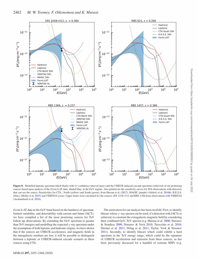
4.2.1 1ES 1028+511

Source 2WHSP J103118.4+505335, 3FGL J1031.2+5053, alsoknown with the name 1ES 1028+511, shown in Fig. 8, is apromising candidate for observation by CTA and potentially MAGICand VERITAS, based on our Fermi analysis. This source hasbeen observed by VERITAS for 24.1 h, yielding an upper limit of7.7 × 10−12 erg−1 cm−2 s−1 (Archambault et al. 2016). Interestingly,for this source the VERITAS upper limit constrains the hadronicmodel for the level of flux predicted with the best-fitting Fermi index.Thus additional observations of this source may be very sensitive toor otherwise very constraining of the hadronic model. Additionally,with log νS = 17.0 it is interesting as a possible extreme-HSP source.

4.2.2 RBS 1366

With a detection significance of ≈12σ , a very low variabilityindex, and a firm redshift determination (Ahn et al. 2012), 2WHSPJ141756.5+254324, 3FGL J1417.8+2540, also known as RBS 1366,is also a promising candidate for detecting with TeV instruments.The large uncertainties in the Fermi-LAT analysis however meanthat we cannot conclusively determine whether the source will bedetectable. Under optimistic assumptions (upper 1σ uncertaintyrange) it is a good candidate for observation by CTA or VERI-TAS and also possibly by MAGIC. A differential upper limit of1.7 × 10−11 erg−1cm−2s−1 at 327 GeV was calculated for this sourceby VERITAS based on 10 h of observations, but is not sufficient toconstrain the hadronic origin model (Archambault et al. 2016). With

synchrotron peak frequency at log νS = 17.4, this source is possiblyan extreme-HSP, and thus interesting to study at VHE even if it ispurely leptonic, for the purpose of furthering our knowledge of this,small and extreme source population. It was also flagged as a TeVblazar candidate by the analysis of Costamante (2020).

4.2.3 RBS 621

The blazar RBS 621 (3FGL J0506.9-5435, 2WHSP J050657.7-543503), with Fermi-LAT detection significance of around 23.0 σ

and low variability TSV = 40.6, is another source promising for TeVdetection and for the detection of the UHECR hadronic signature.The redshift is uncertain with a lower limit of z > 0.26. To the best ofour knowledge this source has not yet been observed with H.E.S.S.,but it is our most promising source for detection with a 50 h exposureif the true redshift is close to the lower limit and certainly promisingfor observations with CTA.

4.2.4 RBS 1457

The blazar RBS 1457 (3FGL J1503.7-1540,2WHSP J150340.6-154113) is also one of the sources most promising for TeV detectionand for detection of the hadronic cascade signature in our sample,with Fermi-LAT detection significance of around 21.0 σ and lowvariability TSV = 52. There is only a lower limit on the redshift ofthis source, z > 0.38, but if the true redshift is not much higher thanthe lower limit, this source, at declination δ = −15.4◦ is possiblydetectable with H.E.S.S. and it is certainly a promising source forCTA South.

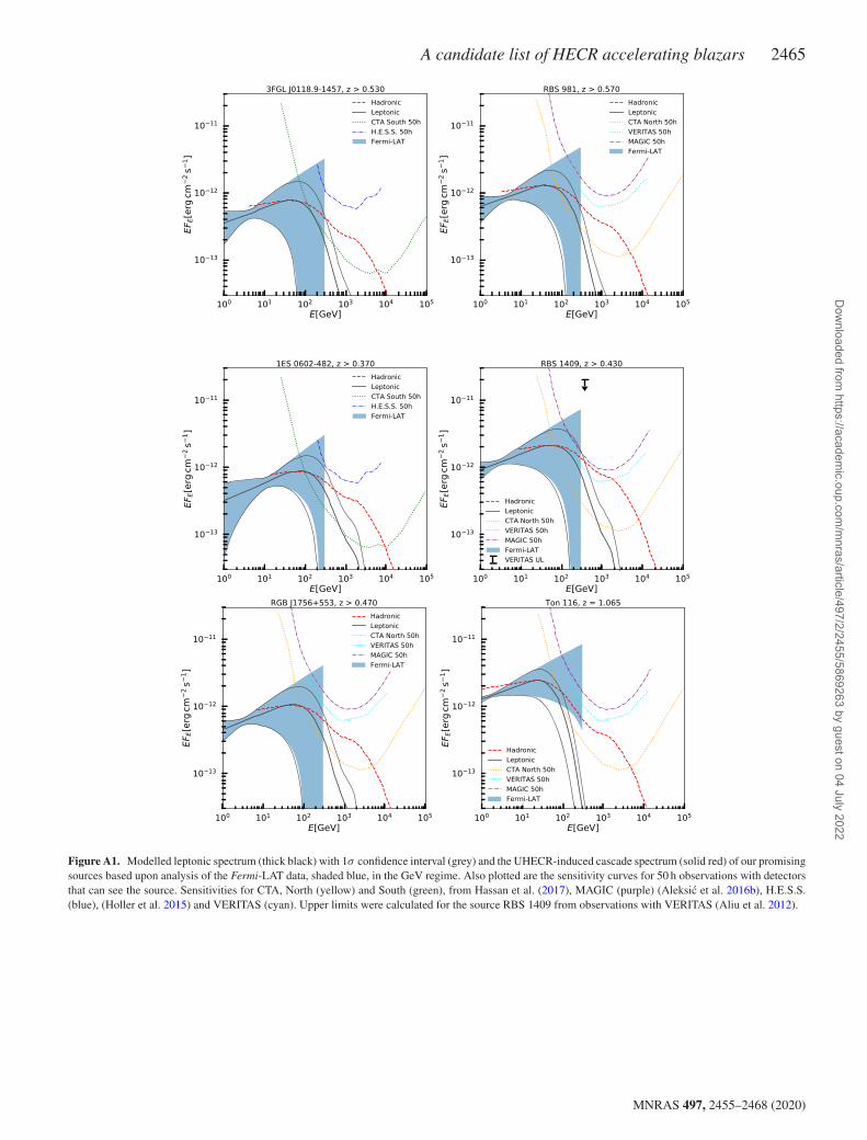
4.2.5 Other promising sources

We have found a number of additional promising sources, whichwe categorized as Class II because they likely require an instrumentwith sensitivity comparable to that of CTA for detection. We showtheir γ -ray spectra in Fig. A1, in the Appendix. The source 2WHSPJ143657.7+563924, or RBS 1409, or RX J1436.9+5639, is oneof these sources. An upper limit was obtained based on a 13 hobservation of the source with VERITAS (Aliu et al. 2012). A redshiftof z = 0.15 has been quoted based on the redshift of a galaxy clusterwithin the same region of the sky (Bauer et al. 2000). However,the optical spectrum of the galaxy is featureless (Aliu et al. 2012).We thus assumed a redshift value equal to the lower limit quotedby the more recent work of Chang et al. (2017) in this work. TheClass II sample additionally contains Ton 116, which at redshift z =1.065, if detected with CTA could give unambigious evidence of thehadronic cascade. The additional notable candidates include 3FGLJ1124.9+4932-RBS 981, at redshift z > 0.57, and RGB 1756+553at redshift z > 0.57, both suitable with observations with North skyinstruments, as well as 3FGL J0118.9-145 at redshift z > 0.530 and1ES 0602-482 in the Southern sky.

Two sources from Table 1, 3FGL J2055.2-0019 and 3FGLJ1012.7+4229, are not included as promising sources for observationeven though they met the initial selection criteria. It was clear thatcurrent and future IACTs lack the sensitivity to detect the hadroniccomponent of these sources in a reasonable observation period.

5 D I SCUSSI ON AND C ONCLUSI ONS

We have analysed the Fermi data for 566 HSP blazars fromthe 2WHSP catalogue. By discriminating significant sources with

MNRAS 497, 2455–2468 (2020)

Dow

nloaded from https://academ

ic.oup.com/m

nras/article/497/2/2455/5869263 by guest on 04 July 2022

2462 M. W. Toomey, F. Oikonomou and K. Murase

Figure 8. Modelled leptonic spectrum (thick black) with 1σ confidence interval (grey) and the UHECR-induced cascade spectrum (solid red) of our promisingsources based upon analysis of the Fermi-LAT data, shaded blue, in the GeV regime. Also plotted are the sensitivity curves for 50 h observations with detectorsthat can see the source. Sensitivities for CTA , North (yellow) and South (green), from Hassan et al. (2017), MAGIC (purple) (Aleksic et al. 2016b), H.E.S.S.(blue), (Holler et al. 2015) and VERITAS (cyan). Upper limits were calculated for the sources 1ES 1218+511 and RBS 1366 from observations with VERITAS(Archambault et al. 2016).

Fermi-LAT data in the GeV band based on the hardness of spectrum,limited variability, and detectability with current and future IACTs,we have compiled a list of the most promising sources for TeVfollow-up observations. By extending the GeV spectrum to greaterthan TeV energies and modelling the expected γ -ray spectrum underthe assumption of both leptonic and hadronic origins, we have shownthat if the sources are UHECR accelerators, and magnetic fields inthe intergalactic medium are low, it will be possible to distinguishbetween a leptonic or UHECR-induced cascade scenario in thesesources using CTA.

The motivation for our analysis has been twofold. First, to identifyblazars whose γ -ray spectra can be used, if a detection with IACTs isachieved, to constrain the extragalactic magnetic field by consideringtheir combined GeV–TeV spectra (e.g. Murase et al. 2008; Neronov& Semikoz 2009; Neronov & Vovk 2010; Tavecchio et al. 2010;Dermer et al. 2011; Dolag et al. 2011; Taylor, Vovk & Neronov2011). Secondly, to identify blazars which could exhibit a hardspectrum in the TeV energy range, which could be the signatureof UHECR acceleration and emission from these sources, as hasbeen previously discussed for a handful of extreme HSPs (e.g.

MNRAS 497, 2455–2468 (2020)

Dow

nloaded from https://academ

ic.oup.com/m

nras/article/497/2/2455/5869263 by guest on 04 July 2022

A candidate list of HECR accelerating blazars 2463

Essey & Kusenko 2010; Essey et al. 2011; Murase et al. 2012b;Aharonian et al. 2013; Takami et al. 2013; Oikonomou et al. 2014;Tavecchio 2014; Dzhatdoev et al. 2017; Cherenkov Telescope ArrayConsortium 2019; Khalikov & Dzhatdoev 2019; Tavecchio et al.2019). Recently the MAGIC Collaboration announced the detectionof 2WHSP J073326.7+515354 (Acciari et al. 2019) at �1 TeVenergies. The source does not form part of our sample, since itlies at z = 0.06 and doesn’t satisfy the z ≥ 0.2 cut. However, thesearch for TeV emission from this source demonstrates the interestfor detectable HSP and extreme HSP sources, as well as some ofthe open questions on blazar emission which can be addressed withsimilar IACT observations.

In our analysis the majority of sources were found to lack anysignificant variability. While blazars as a class are well known fortheir variability, this result cannot exclude the presence of variability,since these are relatively faint sources, and any intrinsic variabilitymay be below the experimental sensitivity of Fermi. As expected inthis statistically limited regime, the sources that do exhibit significantvariability in our analysis are the brightest sources in terms offlux. Therefore, our results are not conclusive in regards to thequestion whether some of the sources examined could be poweredby secondary γ -rays from UHECR primaries. In the latter case,there should be no detectable variability in the γ -ray energy rangesince UHECRs get delayed by magnetic fields. Given that the brightsources in our sample are all consistent with being variable, ourresults are consistent with all sources being intrinsically variable andthus powered by leptonic emission mechanisms, giving no conclusivesupport to the UHECR-induced cascade scenario.

It is important to emphasize again how our variability results differfrom those which accompany the 4FGL catalogue. The most impor-tant difference is the energy range over which the variability indexwas calculated. In our analysis we used a higher energy thresholdof 1 GeV than the 100 MeV threshold of the 4FGL, which is bettersuited for the hard spectrum sources of interest in our analysis andmight allow us, to better isolate the the hadronic component which,if present, should be dominant above ∼10–100 GeV as demonstratedin previous sections. The present analysis was conducted using datafrom the Fermi launch to late 2016. An updated analysis shouldreach the same conclusion, but surely with improved uncertainties(≈10 per cent with 2 more years of data).

While this work was being finalized, the 3HSP catalogue, whichis the largest and most complete HSP catalogue available to date,became available (Chang et al. 2019). With respect to the 2WHSPit contains 395 additional HSP blazars. In the future, our analysiscould be extended to include these additional sources.

AC K N OW L E D G E M E N T S

This work was initiated in 2016 for the honors thesis ‘BLAZARSAS A SOURCE FOR ULTRA-HIGH-ENERGY COSMIC RAYS?A SEARCH FOR THE ELUSIVE HADRONIC SIGNATURE’ atthe Schreyer Honors College of Penn State University in 2018. Wethank Gordana Tesic for fruitful input during the early stages ofthis work. We also thank Akira Okumura for useful comments onsensitivity curves. The work of KM is supported by the Alfred P.Sloan Foundation, NSF Grant No. AST-1908689, and KAKENHINo. 20H01901.

DATA AVAILABILITY

The data underlying this article are available in the article.

REFERENCES

Abeysekara A. U. et al., 2015, ApJ, 815, L22Acciari V. A. et al., 2019, MNRAS, 490, 2284Acero F. et al., 2015, ApJS, 218, 23Aharonian F. A., 2000, New Astron., 5, 377Aharonian F. A., Coppi P. S., Volk H. J., 1994, ApJ, 423, L5Aharonian F., Essey W., Kusenko A., Prosekin A., 2013, Phys. Rev. D, 87,

063002Ahn C. P. et al., 2012, ApJS, 203, 21Ahnen M. L. et al., 2016, A&A, 595, A98Aleksic J. et al., 2016a, Astropart. Phys., 72, 61Aleksic J. et al., 2016b, Astropart. Phys., 72, 76Aliu E. et al., 2012, ApJ, 759, 102Alves Batista R. et al., 2019, Front. Astron. Space Sci., 6, 23Anchordoqui L. A., 2019, Phys. Rep., 801, 1Archambault S. et al., 2016, AJ, 151, 142Archambault S. et al., 2017, ApJ, 835, 288Arsioli B., Chang Y. L., 2017, A&A, 598, A134Arsioli B., Barres de Almeida U., Prandini E., Fraga B., Foffano L., 2018,

MNRAS, 480, 2165Atwood W. B. et al., 2009, ApJ, 697, 1071Bauer F. E., Condon J. J., Thuan T. X., Broderick J. J., 2000, ApJS, 129,

547Berezinsky V. S., Smirnov A. Yu., 1975, Ap&SS, 32, 461Biteau J. et al., 2020, Nat. Astron., 4, 124Chang Y. L., Arsioli B., Giommi P., Padovani P., 2017, A&A, 598, A17Chang Y.-L., Arsioli B., Giommi P., Padovani P., Brandt C. H., 2019, A&A,

632, A77Cherenkov Telescope Array Consortium, 2019, Science with the Cherenkov

Telescope Array. WSP, SingaporeCostamante L., 2020, MNRAS, 491, 2771Costamante L. et al., 2001, A&A, 371, 512Costamante L., Bonnoli G., Tavecchio F., Ghisellini G., Tagliaferri G.,

Khangulyan D., 2018, MNRAS, 477, 4257Dermer C. D., Razzaque S., 2010, ApJ, 724, 1366Dermer C. D., Cavadini M., Razzaque S., Finke J. D., Chiang J., Lott B.,

2011, ApJ, 733, L21Dolag K., Kachelriess M., Ostapchenko S., Tomas R., 2011, ApJ, 727, L4Dzhatdoev T. A., Khalikov E. V., Kircheva A. P., Lyukshin A. A., 2017, A&A,

603, A59Elyiv A., Neronov A., Semikoz D. V., 2009, Phys. Rev. D, 80, 023010Essey W., Kusenko A., 2010, Astropart. Phys., 33, 81Essey W., Kalashev O., Kusenko A., Beacom J. F., 2011, ApJ, 731, 51Fermi-LAT Collaboration, 2010, ApJ, 716, 30Ginzburg V. L., Syrovatskii S. I., 1964, The Origin of Cosmic Rays. Pergamon,

New YorkGould R. J., Rephaeli Y., 1978, ApJ, 225, 318Gould R., Schreder G., 1966, Phys. Rev. Lett., 16, 252H. E. S. S. Collaboration, 2014, A&A, 562, A145H. E. S. S. Collaboration, 2017, A&A, 600, A89Hassan T. et al., 2017, Astropart. Phys., 93, 76Hillas A. M., 1984, ARA&A, 22, 425Holder J. et al., 2008, in Aharonian F. A., Hofmann W., Rieger F., eds,

AIP Conf. Proc. Vol. 1085, Proceedings of the 4th International Meetingon High Energy Gamma-Ray Astronomy. Am. Inst. Phys., New York,p. 657

Holler M. et al., 2015, Proc. Sci., International Cosmic Ray Conference(ICRC2015). SISSA, Trieste, PoS#847

Inoue Y., Inoue S., Kobayashi M. A. R., Makiya R., Niino Y., Totani T., 2013,ApJ, 768, 197

Katarzynski K., Ghisellini G., Tavecchio F., Gracia J., Maraschi L., 2006,MNRAS, 368, L52

Khalikov E. V., Dzhatdoev T. A., 2019, preprint (arXiv:1912.10570)Kotera K., Olinto A. V., 2011, ARA&A, 49, 119Kotera K., Allard D., Lemoine M., 2011, A&A, 527, A54Maraschi L., Ghisellini G., Celotti A., 1992, ApJ, 397, L5Mollerach S., Roulet E., 2018, Prog. Part. Nucl. Phys., 98, 85

MNRAS 497, 2455–2468 (2020)

Dow

nloaded from https://academ

ic.oup.com/m

nras/article/497/2/2455/5869263 by guest on 04 July 2022

2464 M. W. Toomey, F. Oikonomou and K. Murase

Mucke A., Protheroe R. J., 2001, Astropart. Phys., 15, 121Murase K., Fukugita M., 2019, Phys. Rev. D, 99, 063012Murase K., Takahashi K., Inoue S., Ichiki K., Nagataki S., 2008, ApJ, 686,

L67Murase K., Meszaros P., Zhang B., 2009, Phys. Rev., D79, 103001Murase K., Beacom J. F., Takami H., 2012a, J. Cosmol. Astropart. Phys., 8,

030Murase K., Dermer C. D., Takami H., Migliori G., 2012b, ApJ, 749, 63Neronov A., Semikoz D., 2009, Phys. Rev., D80, 123012Neronov A., Vovk I., 2010, Science, 328, 73Nolan P. L. et al., 2012, ApJS, 199, 31Oikonomou F., Murase K., Kotera K., 2014, A&A, 568, A110Padovani P., Giommi P., 1995, ApJ, 444, 567Prosekin A., Essey W., Kusenko A., Aharonian F., 2012, ApJ, 757, 183Rodrigues X., Fedynitch A., Gao S., Boncioli D., Winter W., 2018, ApJ, 854,

54Sikora M., Begelman M. C., Rees M. J., 1994, ApJ, 421, 153Stecker F. W., de Jager O. C., Salamon M. H., 1992, ApJ, 390, L49

Takahashi K., Murase K., Ichiki K., Inoue S., Nagataki S., 2008, ApJ, 687,L5

Takami H., Murase K., Dermer C. D., 2013, ApJ, 771, L32Takami H., Murase K., Dermer C. D., 2016, ApJ, 817, 59Tavecchio F., 2014, MNRAS, 438, 3255Tavecchio F., Ghisellini G., Foschini L., Bonnoli G., Ghirlanda G., Coppi P.,

2010, MNRAS, 406, L70Tavecchio F., Romano P., Landoni M., Vercellone S., 2019, MNRAS, 483,

1802Taylor A. M., Vovk I., Neronov A., 2011, A&A, 529, A144The Fermi-LAT collaboration, 2019, ApJS, 247, 33Urry C. M., Padovani P., 1995, PASP, 107, 803Wood M., Caputo R., Charles E., Di Mauro M., Magill J., Perkins J. S.,

Fermi-LAT Collaboration, 2017, Proc. Sci., International Cosmic RayConference (ICRC2017), SISSA, Trieste, PoS#824

APPENDI X A :

MNRAS 497, 2455–2468 (2020)

Dow

nloaded from https://academ

ic.oup.com/m

nras/article/497/2/2455/5869263 by guest on 04 July 2022

A candidate list of HECR accelerating blazars 2465

Figure A1. Modelled leptonic spectrum (thick black) with 1σ confidence interval (grey) and the UHECR-induced cascade spectrum (solid red) of our promisingsources based upon analysis of the Fermi-LAT data, shaded blue, in the GeV regime. Also plotted are the sensitivity curves for 50 h observations with detectorsthat can see the source. Sensitivities for CTA, North (yellow) and South (green), from Hassan et al. (2017), MAGIC (purple) (Aleksic et al. 2016b), H.E.S.S.(blue), (Holler et al. 2015) and VERITAS (cyan). Upper limits were calculated for the source RBS 1409 from observations with VERITAS (Aliu et al. 2012).

MNRAS 497, 2455–2468 (2020)

Dow

nloaded from https://academ

ic.oup.com/m

nras/article/497/2/2455/5869263 by guest on 04 July 2022

2466 M. W. Toomey, F. Oikonomou and K. Murase

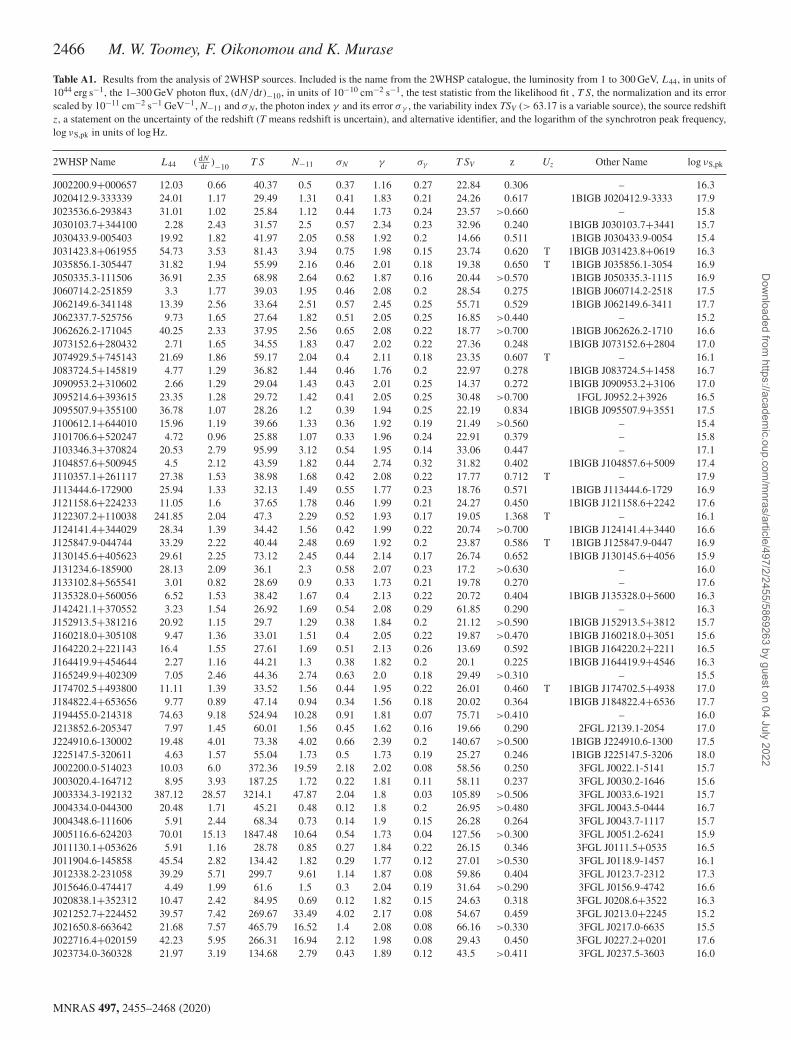
Table A1. Results from the analysis of 2WHSP sources. Included is the name from the 2WHSP catalogue, the luminosity from 1 to 300 GeV, L44, in units of1044 erg s−1, the 1–300 GeV photon flux, (dN/dt)−10, in units of 10−10 cm−2 s−1, the test statistic from the likelihood fit , T S, the normalization and its errorscaled by 10−11 cm−2 s−1 GeV−1, N−11 and σN, the photon index γ and its error σγ , the variability index TSV (> 63.17 is a variable source), the source redshiftz, a statement on the uncertainty of the redshift (T means redshift is uncertain), and alternative identifier, and the logarithm of the synchrotron peak frequency,log νS,pk in units of log Hz.

2WHSP Name L44 ( dNdt

)−10 T S N−11 σN γ σγ T SV z Uz Other Name log νS,pk

J002200.9+000657 12.03 0.66 40.37 0.5 0.37 1.16 0.27 22.84 0.306 – 16.3J020412.9-333339 24.01 1.17 29.49 1.31 0.41 1.83 0.21 24.26 0.617 1BIGB J020412.9-3333 17.9J023536.6-293843 31.01 1.02 25.84 1.12 0.44 1.73 0.24 23.57 >0.660 – 15.8J030103.7+344100 2.28 2.43 31.57 2.5 0.57 2.34 0.23 32.96 0.240 1BIGB J030103.7+3441 15.7J030433.9-005403 19.92 1.82 41.97 2.05 0.58 1.92 0.2 14.66 0.511 1BIGB J030433.9-0054 15.4J031423.8+061955 54.73 3.53 81.43 3.94 0.75 1.98 0.15 23.74 0.620 T 1BIGB J031423.8+0619 16.3J035856.1-305447 31.82 1.94 55.99 2.16 0.46 2.01 0.18 19.38 0.650 T 1BIGB J035856.1-3054 16.9J050335.3-111506 36.91 2.35 68.98 2.64 0.62 1.87 0.16 20.44 >0.570 1BIGB J050335.3-1115 16.9J060714.2-251859 3.3 1.77 39.03 1.95 0.46 2.08 0.2 28.54 0.275 1BIGB J060714.2-2518 17.5J062149.6-341148 13.39 2.56 33.64 2.51 0.57 2.45 0.25 55.71 0.529 1BIGB J062149.6-3411 17.7J062337.7-525756 9.73 1.65 27.64 1.82 0.51 2.05 0.25 16.85 >0.440 – 15.2J062626.2-171045 40.25 2.33 37.95 2.56 0.65 2.08 0.22 18.77 >0.700 1BIGB J062626.2-1710 16.6J073152.6+280432 2.71 1.65 34.55 1.83 0.47 2.02 0.22 27.36 0.248 1BIGB J073152.6+2804 17.0J074929.5+745143 21.69 1.86 59.17 2.04 0.4 2.11 0.18 23.35 0.607 T – 16.1J083724.5+145819 4.77 1.29 36.82 1.44 0.46 1.76 0.2 22.97 0.278 1BIGB J083724.5+1458 16.7J090953.2+310602 2.66 1.29 29.04 1.43 0.43 2.01 0.25 14.37 0.272 1BIGB J090953.2+3106 17.0J095214.6+393615 23.35 1.28 29.72 1.42 0.41 2.05 0.25 30.48 >0.700 1FGL J0952.2+3926 16.5J095507.9+355100 36.78 1.07 28.26 1.2 0.39 1.94 0.25 22.19 0.834 1BIGB J095507.9+3551 17.5J100612.1+644010 15.96 1.19 39.66 1.33 0.36 1.92 0.19 21.49 >0.560 – 15.4J101706.6+520247 4.72 0.96 25.88 1.07 0.33 1.96 0.24 22.91 0.379 – 15.8J103346.3+370824 20.53 2.79 95.99 3.12 0.54 1.95 0.14 33.06 0.447 – 17.1J104857.6+500945 4.5 2.12 43.59 1.82 0.44 2.74 0.32 31.82 0.402 1BIGB J104857.6+5009 17.4J110357.1+261117 27.38 1.53 38.98 1.68 0.42 2.08 0.22 17.77 0.712 T – 17.9J113444.6-172900 25.94 1.33 32.13 1.49 0.55 1.77 0.23 18.76 0.571 1BIGB J113444.6-1729 16.9J121158.6+224233 11.05 1.6 37.65 1.78 0.46 1.99 0.21 24.27 0.450 1BIGB J121158.6+2242 17.6J122307.2+110038 241.85 2.04 47.3 2.29 0.52 1.93 0.17 19.05 1.368 T – 16.1J124141.4+344029 28.34 1.39 34.42 1.56 0.42 1.99 0.22 20.74 >0.700 1BIGB J124141.4+3440 16.6J125847.9-044744 33.29 2.22 40.44 2.48 0.69 1.92 0.2 23.87 0.586 T 1BIGB J125847.9-0447 16.9J130145.6+405623 29.61 2.25 73.12 2.45 0.44 2.14 0.17 26.74 0.652 1BIGB J130145.6+4056 15.9J131234.6-185900 28.13 2.09 36.1 2.3 0.58 2.07 0.23 17.2 >0.630 – 16.0J133102.8+565541 3.01 0.82 28.69 0.9 0.33 1.73 0.21 19.78 0.270 – 17.6J135328.0+560056 6.52 1.53 38.42 1.67 0.4 2.13 0.22 20.72 0.404 1BIGB J135328.0+5600 16.3J142421.1+370552 3.23 1.54 26.92 1.69 0.54 2.08 0.29 61.85 0.290 – 16.3J152913.5+381216 20.92 1.15 29.7 1.29 0.38 1.84 0.2 21.12 >0.590 1BIGB J152913.5+3812 15.7J160218.0+305108 9.47 1.36 33.01 1.51 0.4 2.05 0.22 19.87 >0.470 1BIGB J160218.0+3051 15.6J164220.2+221143 16.4 1.55 27.61 1.69 0.51 2.13 0.26 13.69 0.592 1BIGB J164220.2+2211 16.5J164419.9+454644 2.27 1.16 44.21 1.3 0.38 1.82 0.2 20.1 0.225 1BIGB J164419.9+4546 16.3J165249.9+402309 7.05 2.46 44.36 2.74 0.63 2.0 0.18 29.49 >0.310 – 15.5J174702.5+493800 11.11 1.39 33.52 1.56 0.44 1.95 0.22 26.01 0.460 T 1BIGB J174702.5+4938 17.0J184822.4+653656 9.77 0.89 47.14 0.94 0.34 1.56 0.18 20.02 0.364 1BIGB J184822.4+6536 17.7J194455.0-214318 74.63 9.18 524.94 10.28 0.91 1.81 0.07 75.71 >0.410 – 16.0J213852.6-205347 7.97 1.45 60.01 1.56 0.45 1.62 0.16 19.66 0.290 2FGL J2139.1-2054 17.0J224910.6-130002 19.48 4.01 73.38 4.02 0.66 2.39 0.2 140.67 >0.500 1BIGB J224910.6-1300 17.5J225147.5-320611 4.63 1.57 55.04 1.73 0.5 1.73 0.19 25.27 0.246 1BIGB J225147.5-3206 18.0J002200.0-514023 10.03 6.0 372.36 19.59 2.18 2.02 0.08 58.56 0.250 3FGL J0022.1-5141 15.7J003020.4-164712 8.95 3.93 187.25 1.72 0.22 1.81 0.11 58.11 0.237 3FGL J0030.2-1646 15.6J003334.3-192132 387.12 28.57 3214.1 47.87 2.04 1.8 0.03 105.89 >0.506 3FGL J0033.6-1921 15.7J004334.0-044300 20.48 1.71 45.21 0.48 0.12 1.8 0.2 26.95 >0.480 3FGL J0043.5-0444 16.7J004348.6-111606 5.91 2.44 68.34 0.73 0.14 1.9 0.15 26.28 0.264 3FGL J0043.7-1117 15.7J005116.6-624203 70.01 15.13 1847.48 10.64 0.54 1.73 0.04 127.56 >0.300 3FGL J0051.2-6241 15.9J011130.1+053626 5.91 1.16 28.78 0.85 0.27 1.84 0.22 26.15 0.346 3FGL J0111.5+0535 16.5J011904.6-145858 45.54 2.82 134.42 1.82 0.29 1.77 0.12 27.01 >0.530 3FGL J0118.9-1457 16.1J012338.2-231058 39.29 5.71 299.7 9.61 1.14 1.87 0.08 59.86 0.404 3FGL J0123.7-2312 17.3J015646.0-474417 4.49 1.99 61.6 1.5 0.3 2.04 0.19 31.64 >0.290 3FGL J0156.9-4742 16.6J020838.1+352312 10.47 2.42 84.95 0.69 0.12 1.82 0.15 24.63 0.318 3FGL J0208.6+3522 16.3J021252.7+224452 39.57 7.42 269.67 33.49 4.02 2.17 0.08 54.67 0.459 3FGL J0213.0+2245 15.2J021650.8-663642 21.68 7.57 465.79 16.52 1.4 2.08 0.08 66.16 >0.330 3FGL J0217.0-6635 15.5J022716.4+020159 42.23 5.95 266.31 16.94 2.12 1.98 0.08 29.43 0.450 3FGL J0227.2+0201 17.6J023734.0-360328 21.97 3.19 134.68 2.79 0.43 1.89 0.12 43.5 >0.411 3FGL J0237.5-3603 16.0

MNRAS 497, 2455–2468 (2020)

Dow

nloaded from https://academ

ic.oup.com/m

nras/article/497/2/2455/5869263 by guest on 04 July 2022

A candidate list of HECR accelerating blazars 2467

Table A1 – continued

2WHSP Name L44 ( dNdt

)−10 T S N−11 σN γ σγ T SV z Uz Other Name log νS,pk

J023832.3-311656 22.59 10.19 835.93 14.51 1.1 1.8 0.05 63.3 0.233 3FGL J0238.4-3117 16.3J024440.1-581954 18.05 5.29 411.39 1.82 0.17 1.72 0.08 88.32 0.260 3FGL J0244.8-5818 16.8J030326.3-240710 127.67 55.28 7499.57 340.74 12.35 1.93 0.02 672.76 0.266 3FGL J0303.4-2407 15.7J030416.3-283217 61.21 1.56 62.22 0.45 0.1 1.68 0.16 26.51 >0.700 3FGL J0304.3-2836 17.7J032523.5-563544 67.9 4.9 262.21 31.81 4.85 1.99 0.07 40.94 0.600 3FGL J0325.2-5634 16.5J032540.9-164615 35.67 10.75 754.22 10.94 0.8 1.85 0.06 67.4 0.291 3FGL J0325.6-1648 15.6J033812.4-244350 4.95 0.96 43.72 0.05 0.02 1.52 0.19 23.79 0.251 3FGL J0338.1-2443 17.1J041652.3+010522 23.01 6.7 317.69 2.76 0.28 1.82 0.08 36.76 0.287 3FGL J0416.8+0104 16.5J050534.6+041553 41.26 6.32 204.81 3.17 0.38 1.95 0.11 39.44 0.424 3FGL J0505.5+0416 15.7J050657.7-543503 25.07 5.05 488.15 2.21 0.21 1.56 0.07 40.57 >0.260 3FGL J0506.9-5435 16.2J050756.0+673723 265.31 17.08 2720.35 5.27 0.23 1.54 0.03 95.0 0.416 T 3FGL J0508.0+6736 17.9J053628.9-334301 55.09 19.18 1336.69 379.34 33.18 2.12 0.03 156.11 >0.340 3FGL J0536.4-3347 16.0J054357.1-553207 54.18 15.6 1592.31 15.17 0.83 1.76 0.04 77.78 0.273 3FGL J0543.9-5531 16.7J055806.4-383830 21.14 6.14 347.52 8.0 0.84 1.87 0.08 42.16 0.302 3FGL J0558.1-3838 16.7J060408.5-481725 20.5 2.69 132.76 0.26 0.05 1.73 0.11 37.13 >0.370 3FGL J0604.1-4817 16.2J064443.6-285115 28.03 2.53 67.3 4.2 0.96 1.86 0.12 22.47 >0.490 3FGL J0644.6-2853 16.1J065046.3+250258 58.54 32.21 3411.1 25.7 0.96 1.75 0.03 188.73 0.203 T 3FGL J0650.7+2503 16.8J074405.2+743357 21.21 4.58 372.66 7.65 0.87 1.78 0.07 47.18 0.314 3FGL J0744.3+7434 16.7J080457.7-062425 36.6 4.97 166.99 2.57 0.34 1.91 0.11 37.46 >0.430 3FGL J0805.0-0622 16.9J080625.9+593106 7.68 2.51 110.66 1.73 0.28 1.93 0.13 40.34 0.300 T 3FGL J0806.6+5933 15.3J081627.1-131152 114.61 18.07 1336.78 17.85 1.01 1.81 0.04 114.91 >0.370 3FGL J0816.4-1311 16.4J082706.1-070844 9.54 4.04 155.31 7.63 1.25 1.84 0.09 36.62 0.247 T 3FGL J0827.2-0711 16.3J090534.9+135805 48.19 9.5 651.36 13.0 1.07 1.82 0.06 44.29 >0.340 3FGL J0905.5+1358 15.1J091037.0+332924 58.77 14.17 1143.74 15.9 0.91 1.95 0.05 107.14 0.350 T 3FGL J0910.5+3329 15.0J091230.5+155527 3.47 2.62 82.34 0.1 0.03 1.95 0.11 50.43 0.212 3FGL J0912.7+1556 16.9J091714.5-034314 9.99 1.44 48.02 0.62 0.17 1.59 0.17 28.02 0.308 3FGL J0917.3-0344 16.6J092542.7+595815 44.5 1.67 67.85 0.43 0.08 1.86 0.15 17.95 >0.700 3FGL J0925.6+5959 15.5J094022.3+614825 3.56 3.47 146.74 25.57 4.66 2.07 0.09 40.55 0.210 3FGL J0941.0+6151 16.2J094620.2+010450 34.71 1.71 44.65 0.33 0.08 1.76 0.19 21.72 0.577 3FGL J0946.2+0103 17.9J095805.8-031739 34.06 0.88 25.94 0.18 0.06 1.53 0.22 26.24 >0.600 3FGL J0958.3-0318 16.4J101244.2+422957 19.77 2.78 157.36 1.01 0.14 1.74 0.11 29.31 0.365 3FGL J1012.7+4229 16.8J102339.7+300056 12.89 1.55 49.01 0.51 0.12 1.86 0.19 27.66 0.433 3FGL J1023.7+3000 15.8J103118.4+505335 41.89 9.22 1014.96 7.26 0.48 1.74 0.05 52.72 >0.360 3FGL J1031.2+5053 17.0J104149.0+390118 2.05 1.85 53.25 2.71 0.59 2.03 0.17 48.69 0.210 3FGL J1041.8+3901 16.5J104651.4-253544 4.98 2.04 56.87 1.29 0.28 1.83 0.16 30.21 0.250 3FGL J1046.9-2531 18.0J105125.3+394324 30.66 2.58 101.98 1.19 0.19 1.84 0.14 32.63 0.497 3FGL J1051.4+3941 16.8J110124.7+410847 41.2 2.18 101.33 0.79 0.14 1.8 0.14 29.06 >0.580 3FGL J1101.5+4106 15.7J110747.9+150209 11.18 6.18 305.15 14.09 1.6 1.98 0.08 37.98 0.250 T 3FGL J1107.8+1502 15.6J111224.5+175120 8.97 1.14 25.7 0.07 0.03 1.85 0.22 25.04 0.420 3FGL J1112.6+1749 16.9J111939.4-304720 13.95 0.62 28.6 0.1 0.04 1.38 0.23 23.38 0.412 3FGL J1119.7-3046 17.1J112453.8+493409 93.35 4.89 362.65 2.91 0.29 1.78 0.08 63.95 >0.570 3FGL J1124.9+4932 16.5J112551.9-074220 6.16 1.86 47.16 1.78 0.47 1.81 0.16 22.16 0.279 3FGL J1125.8-0745 15.7J114930.3+243925 9.84 1.35 31.19 1.28 0.43 1.84 0.19 23.45 0.402 3FGL J1149.5+2443 17.1J115034.6+415439 79.88 19.26 2122.31 29.82 1.46 1.85 0.04 85.54 >0.320 3FGL J1150.5+4155 15.6J115404.5-001009 13.36 3.99 202.3 1.47 0.2 1.71 0.1 46.77 0.254 3FGL J1154.2-0010 16.6J115853.2+081942 5.86 1.84 50.53 1.12 0.25 1.87 0.19 25.99 0.290 3FGL J1158.9+0818 16.1J120412.1+114555 9.78 3.91 125.3 3.26 0.47 2.01 0.13 46.81 0.296 3FGL J1204.0+1144 16.6J121945.7-031422 15.32 5.15 200.41 9.2 1.3 1.94 0.09 51.71 0.299 3FGL J1219.7-0314 16.0J122424.1+243623 20.61 14.18 1081.89 16.98 1.02 1.93 0.05 226.87 0.218 3FGL J1224.5+2436 16.1J122644.2+063853 55.02 2.04 94.42 0.37 0.07 1.65 0.14 22.51 0.583 3FGL J1226.8+0638 15.8J123123.8+142124 10.65 3.27 128.07 4.74 0.87 1.73 0.09 22.81 0.256 3FGL J1231.8+1421 15.4J123738.9+625841 3.23 0.8 27.79 0.42 0.13 1.78 0.22 29.47 0.297 3FGL J1237.9+6258 16.0J124312.7+362743 99.06 21.98 2594.81 33.1 1.52 1.78 0.03 62.08 >1.065 3FGL J1243.1+3627 16.2J131532.5+113330 44.19 2.44 63.8 1.83 0.36 1.88 0.15 39.18 >0.610 3FGL J1315.4+1130 16.7J132301.0+043951 2.69 2.22 49.54 0.76 0.16 2.06 0.19 22.21 0.224 3FGL J1322.9+0435 16.8J132358.3+140558 53.68 5.75 271.93 13.23 1.65 1.89 0.08 36.22 >0.470 3FGL J1323.9+1405 15.4J134029.8+441004 39.93 1.62 74.83 0.7 0.16 1.61 0.14 36.4 0.540 3FGL J1340.6+4412 17.3J140450.8+040202 25.64 4.39 183.09 7.71 1.14 1.85 0.09 24.03 >0.370 3FGL J1404.8+0401 15.7J140659.1+164206 26.99 1.46 44.26 0.33 0.08 1.73 0.18 24.55 >0.540 3FGL J1406.6+1644 17.0J141756.5+254324 10.14 2.86 147.3 7.2 1.65 1.63 0.08 24.58 0.237 3FGL J1417.8+2540 17.4J141826.2-023333 127.76 28.2 2765.72 57.51 2.33 1.48 nan 134.68 >0.356 3FGL J1418.4-0233 15.5J141900.3+773229 12.81 4.34 328.47 5.14 0.53 1.83 0.07 32.38 >0.270 3FGL J1418.9+7731 16.0J143657.7+563924 57.3 5.79 522.39 8.28 0.8 1.77 0.06 47.4 >0.430 3FGL J1436.8+5639 16.9

MNRAS 497, 2455–2468 (2020)

Dow

nloaded from https://academ

ic.oup.com/m

nras/article/497/2/2455/5869263 by guest on 04 July 2022

2468 M. W. Toomey, F. Oikonomou and K. Murase

Table A1 – continued

2WHSP Name L44 ( dNdt

)−10 T S N−11 σN γ σγ T SV z Uz Other Name log νS,pk

J143917.3+393242 18.93 5.28 289.04 3.68 0.37 2.01 0.1 42.05 0.344 3FGL J1439.2+3931 15.9J144037.7-384654 40.0 5.42 285.18 1.5 0.16 1.68 0.08 36.35 >0.350 3FGL J1440.4-3845 17.2J144506.1-032612 27.6 6.55 281.39 10.13 1.24 1.81 0.07 35.43 >0.310 3FGL J1445.0-0328 17.4J145127.7+635419 52.03 1.61 96.65 1.03 0.2 1.68 0.13 29.58 0.650 3FGL J1451.2+6355 17.0J150101.7+223806 17.13 11.95 746.59 25.58 1.81 2.03 0.06 106.44 0.235 3FGL J1500.9+2238 15.1J150340.6-154113 65.09 9.18 439.69 5.04 0.42 1.79 0.07 52.0 >0.380 3FGL J1503.7-1540 17.6J150716.3+172102 56.74 3.44 131.85 1.5 0.21 1.83 0.11 43.84 0.565 3FGL J1507.4+1725 15.7J150842.5+270908 6.95 1.54 58.39 0.48 0.11 1.64 0.16 23.28 0.270 3FGL J1508.6+2709 17.8J153311.2+185429 12.93 2.56 117.52 1.86 0.35 1.71 0.11 28.7 0.305 3FGL J1533.2+1852 17.2J153500.7+532036 39.18 1.48 68.96 1.78 0.44 1.67 0.12 32.12 >0.590 3FGL J1534.4+5323 17.2J154604.2+081913 28.91 6.47 318.97 2.55 0.25 1.91 0.08 65.78 >0.350 3FGL J1546.0+0818 15.1J154712.1-280221 53.33 3.12 80.1 0.93 0.16 1.83 0.14 30.87 >0.570 3FGL J1547.1-2801 15.8J155424.1+201125 5.85 2.15 64.0 6.92 1.95 1.88 0.11 26.73 0.273 3FGL J1554.4+2010 17.4J155543.0+111123 878.53 140.08 26507.02 468.11 7.41 1.42 nan 224.09 >0.443 3FGL J1555.7+1111 15.6J160620.8+563016 15.78 1.48 63.57 0.88 0.2 1.78 0.16 32.23 0.450 3FGL J1606.1+5630 16.0J162625.8+351341 21.79 1.64 61.92 0.48 0.1 1.79 0.16 29.82 0.498 3FGL J1626.1+3512 16.0J170238.5+311542 39.15 3.54 180.58 0.51 0.07 1.81 0.09 37.09 >0.470 3FGL J1702.6+3116 15.4J175615.9+552218 45.88 3.68 223.86 3.85 0.5 1.76 0.08 32.04 >0.470 3FGL J1756.3+5523 17.3J175713.0+703337 17.18 2.45 90.8 0.31 0.06 1.87 0.13 34.16 0.407 3FGL J1756.9+7032 17.3J183849.0+480234 81.84 20.04 2206.35 20.22 0.93 1.79 0.04 216.67 0.300 T 3FGL J1838.8+4802 15.8J201428.6-004721 7.47 4.92 133.66 3.21 0.44 1.98 0.12 48.3 0.231 T 3FGL J2014.3-0047 15.2J201624.0-090333 49.24 11.68 589.46 27.26 2.22 2.0 0.06 51.79 0.367 T 3FGL J2016.4-0905 15.0J203649.3-332830 7.66 2.31 77.87 0.12 0.03 1.62 0.12 24.53 0.230 3FGL J2036.6-3325 16.3J205528.2-002116 32.19 2.96 92.1 0.8 0.14 1.75 0.13 27.67 0.440 3FGL J2055.2-0019 18.0J213103.1-274656 49.59 8.82 543.82 4.85 0.38 1.9 0.07 49.09 >0.380 3FGL J2130.8-2745 16.1J213135.3-091523 56.54 6.51 291.27 14.19 1.76 1.88 0.07 56.71 0.449 3FGL J2131.5-0915 16.4J213151.4-251557 151.09 3.49 136.81 5.01 0.82 1.86 0.11 24.51 >0.860 3FGL J2131.8-2516 16.9J214552.1+071927 3.13 2.75 61.8 89.18 37.36 2.18 0.09 31.31 0.237 3FGL J2145.7+0717 17.5J214636.9-134359 120.94 12.42 901.51 6.88 0.46 1.75 0.05 72.84 >0.420 3FGL J2146.6-1344 15.7J215015.4-141049 8.47 3.92 157.35 2.51 0.36 1.76 0.1 28.71 0.220 3FGL J2150.2-1411 17.8J215305.2-004229 11.43 2.66 61.44 2.04 0.47 1.9 0.16 35.95 0.341 3FGL J2152.9-0045 18.0J222129.2-522527 39.59 8.71 634.52 16.4 1.36 1.87 0.06 66.99 >0.340 3FGL J2221.6-5225 15.8J225818.9-552536 19.73 2.97 123.74 19.87 4.03 2.1 0.1 38.22 0.479 3FGL J2258.3-5526 15.7J230722.0-120517 15.01 1.13 30.63 0.57 0.19 1.73 0.21 23.05 >0.470 3FGL J2307.4-1208 16.5J232444.5-404049 27.82 10.72 866.67 7.26 0.51 1.76 0.06 84.18 >0.240 3FGL J2324.7-4040 15.5J235034.3-300603 6.06 3.93 153.56 8.61 1.3 1.96 0.11 51.19 0.230 3FGL J2350.4-3004 15.7J235612.1+403643 14.84 4.02 147.69 1.19 0.16 1.95 0.11 41.97 0.331 3FGL J2356.0+4037 16.3

This paper has been typeset from a TEX/LATEX file prepared by the author.

MNRAS 497, 2455–2468 (2020)

Dow

nloaded from https://academ

ic.oup.com/m

nras/article/497/2/2455/5869263 by guest on 04 July 2022