Research Article

Received 31 October 2008 Published online 14 October 2009 in Wiley InterScience

(www.interscience.wiley.com) DOI: 10.1002/mma.1238MOS subject classification: 30 G 35

Clifford analysis versus its quaternioniccounterparts

Juan Bory Reyesa∗† and Michael Shapirob

Communicated by K. Gürlebeck

For a positive integer n let Cl0,n be the universal Clifford algebra with the signature (0, n). The name Clifford analysisis usually referred to the function theories for functions in the kernels of the two operators: the (Cliffordian) Cauchy–Riemann operator and the Dirac operator. For n=2, Cl0,2 becomes the skew-field of Hamilton’s quaternions for which thetwo operators are widely known: the Moisil–Théodoresco and the Fueter operators. We establish the precise relationsbetween the Moisil–Théodoresco operator and the Dirac operator for Cl0,3. It turns out that the case of the Cauchy–Riemann operator for Cl0,3 and the Fueter operator is more sophisticated, and we describe the peculiarities emerginghere. Copyright © 2009 John Wiley & Sons, Ltd.

Keywords: quaternionic and Clifford analysis; Moisil–Théodoresco and Fueter operators

1. Introduction and preliminaries

1.1. When it is said about Clifford analysis, it is typically referred to the following situations. Let n be a positive integer, denote byCl0,n the universal Clifford algebra of signature (0, n). We shall freely use the well-known properties of Clifford algebras which thereader can find in many sources such as for instance [1, 2] but many others as well.

We will denote by e1,. . . , en the imaginary units of Cl0,n which means that e2k =−1 for any k ∈{1, . . . , n}, that ekej +ejek =0 for

k �= j, and that any Clifford number (equal to an element of Cl0,n) is of the form

a=∑A

aAeA, eA :=ei1 · · ·eik, 1�i1<i2< · · ·<ik�n

aA are real numbers.Let �n+1 be a domain in Rn+1 and let �n be a domain in Rn, consider the sets C1(�n+1, Cl0,n) and C1(�n, Cl0,n). The operator

Dn :=∑nk=0 ek� / �xk acts on the former and is frequently called the (Cliffordian) Cauchy–Riemann operator meanwhile the operator

Dn :=∑nk=1 ek� / �xk is usually termed the Dirac operator, and it acts on the latter set. Thus the two Clifford analyses have arisen, one

related to the Cauchy–Riemann operator, and the other related to the Dirac operator; normally it is meant that we are interestedin the study of null-solutions of the corresponding operators which is the most part of the truth; at the same we believe that it isimportant to emphasize that the other properties of both operators are also quite relevant; it is enough to recall the Borel–Pompeiu(equal to the Cauchy–Green) formula.

We will call the null-solutions of the Cliffordian Cauchy–Riemann operator, the C-R-hyperholomorphic functions, for the Diracoperator the name will be the Dirac-hyperholomorphic. The adjectives monogenic, regular, etc. are used as well.

1.2. Hence, as a matter of fact the term Clifford analysis refers to a family of theories parameterized by the parameter n for eachvalue of which there are two theories: the first of them is in Rn+1 being determined by the Cauchy–Riemann operator and thesecond that corresponds to the Dirac operator is in Rn.

Let us see what happens in low-dimensional cases, namely, for n=1 and n=2. For n=1, there holds: Cl0,1 =C, the field of complexnumbers, D1 =� / �x0 +e1� / �x1 ≈2� / �z for z =x0 +e1x1. Hence, D1-hyperholomorphic functions f are just usual holomorphicfunctions of one-dimensional complex analysis. The Dirac operator D1 becomes D1 =� / �x1, and the condition D1[f ]=0 in a domain�1 ⊂R shows that the class of D1-hyperholomorphic functions is trivial.

1.3. For n=2, there holds: Cl0,2 =H, the skew-field of Hamilton’s quaternions; the Cauchy–Riemann operator is D2 =� / �x0 +e1� /�x1 +e2� / �x2 and the Dirac operator is D2 =e1� / �x1 +e2� / �x2. Here e1 and e2 are the first two, traditionally considered quaternionic

aDepartamento de Matemáticas, Universidad de Oriente, Santiago de Cuba 90500, CubabEscuela Superior de Física y Matemáticas, IPN, Mexico City, Mexico∗Correspondence to: Juan Bory Reyes, Departamento de Matemáticas, Universidad de Oriente, Santiago de Cuba 90500, Cuba.†E-mail: juanboryreyes@yahoo.com, jbory@rect.uo.edu.cu

Copyright © 2009 John Wiley & Sons, Ltd. Math. Meth. Appl. Sci. 2010, 33 1089–1101

10

89

J. B. REYES AND M. SHAPIRO

imaginary units that coincide with what we called above the imaginary units of the Clifford algebra Cl0,2; hence the third quaternionicimaginary unit is e12 :=e1e2 =−e2e1. Each of the three generates a copy of the field C within H which we denote as C(e1), C(e2),C(e12).

1.3.1. We begin with the Dirac operator D2, which can be written as

D2 =e1

(�

�x0−e12

��x1

)=

(�

�x0+e12

��x1

)e1

Writing z :=x0 +e12x1 we endow the real space R2 where the functions from C1(�2, H) live with a complex structure where theimaginary unit is i :=e12; in other words we identify R2 with C(e12). This implies the notation:

��x0

+e12�

�x1=: 2

��z

��x0

−e12�

�x1=: 2

��z

hence

D2 =2��z

e1 =2e1��z

Take f ∈C1(�2, H) then f = f0 +e1f1 +e2f2 +e12f12 = (f0 +e12f12)+(f1 +e12f2)e1 =: F1 +F2e1 where F1, F2 are in C1(�2 ⊂C(e12), C(e12)), that is, F1 and F2 can be seen as a pair of complex functions.

What does the hyperholomorphy in the sense of D2 mean in terms of the functions F1, F2 and the operator � / �z? As D2[f ]=2� /�z[F1e1 − F2] the condition D2[f ]=0 is equivalent to a pair of conditions �F1 / �z =0, �F2 / �z =0, that is, the Dirac-hyperholomorphyfor quaternion-valued functions is nothing more than a usual holomorphy for pairs of complex functions, so that it makes no senseto develop the whole theory.

1.3.2. Of course the case of the Cauchy–Riemann operator D2 is not degenerated, i.e. it does not reduce to a well-known theory;thus, a rich in content Clifford analysis of quaternion-valued functions is that of the operator D2, and one may ‘reasonably’ thinkthat an appropriate name for it should be ‘quaternionic analysis’.

1.4. Paradoxically, this is not what is normally understood by ‘quaternionic analysis’, the most renowned examples are Sudbery’spaper [3] and the books [4--6] but there are some others also.

Let �m, m=3, 4, be as before a domain in Rm; on C1(�4, H) there is defined the operator

DF := ��x0

+e1�

�x1+e2

��x2

+e12�

�x3

called the Fueter operator, and on C1(�3, H) there is defined the operator

DMT :=e1�

�x1+e2

��x2

+e12�

�x3

called the Moisil–Théodoresco operator, see [7, 8]. Historically the function theories for them are referred to as quaternionic analysis.A fine point here is that in the definitions of both operators not only the Cliffordian imaginary units e1 and e2 take part but

also their product e12 that is a bi-vector in H, in Clifford algebras language, which makes a significant difference from an algebraicviewpoint; in particular, in domains of R3 we have now both Clifford analysis of H-valued functions that is determined by theoperator D2 and quaternionic analysis of H-valued functions determined by the operator DMT; they are quite similar but notcoinciding, for instance, meanwhile the Cauchy–Riemann operator factorizes, together with its conjugate D2, the Laplace operator:D2 ◦D2 =�R3 , the Moisil–Théodoresco operator is a square root of that Laplacian: D2

MT =−�R3 .What is more, the only Clifford algebra Cl0,n that admits the same dimension for the domains and for the range of its functions is

Cl0,1 ≈C; the case of quaternionic functions becomes similar if we complement the Clifford analysis with the quaternionic analysisfor the Fueter operator.

1.5. One of the conclusions from the afore-presented reasonings is that for functions with range in Cl0,n for any n�3 there arethe two types of Clifford analysis, namely, the Cauchy–Riemann and Dirac versions. For n=2 there are four kinds of ‘Clifford-type’analysis: the Cauchy–Riemann and Dirac versions of Clifford analysis of quaternion-valued functions, and quaternionic analysiswith its Fueter and Moisil–Théodoresco versions. What is more, for no value of n any version of Clifford analysis coincides withquaternionic analysis.

The aim of the present work is to show that there does exist a precise relationship between both versions of quaternionic analysisand Clifford analysis for the algebra Cl0,3, thus refining what has been established in [9].

10

90

Copyright © 2009 John Wiley & Sons, Ltd. Math. Meth. Appl. Sci. 2010, 33 1089–1101

J. B. REYES AND M. SHAPIRO

1.6. It is worth mentioning that there are two systems of equations that bear the name of Moisil–Théodoresco system; the firstone was introduced in [8] (see also [6, 10, 11]), and it has the form⎧⎪⎪⎪⎪⎪⎪⎪⎪⎪⎪⎪⎪⎪⎨⎪⎪⎪⎪⎪⎪⎪⎪⎪⎪⎪⎪⎪⎩

0− �f1

�x1− �f2

�x2− �f3

�x3=0

�f0

�x1+0− �f2

�x3+ �f3

�x2=0

�f0

�x2+ �f1

�x3+0− �f3

�x1=0

�f0

�x3− �f1

�x2+ �f2

�x1+0=0

(1)

the second is ⎧⎨⎩div�f =0

grad f0 +curl�f =0(2)

the solutions (f0, f1, f2, f3) for (1) and (f0,�f ) for (2) are looked for in the class C1 in �3 ⊂R3.As the vectorial operations div, grad, and curl take the following form in cartesian coordinates:

div�f :=3∑

k=1

�fk

�xk, grad f0 :=

3∑k=1

ek�f0

�xk, curl�f :=

∣∣∣∣∣∣∣∣∣∣

e1 e2 e3

��x1

��x2

��x3

f1 f2 f3

∣∣∣∣∣∣∣∣∣∣one can easily see that both systems are formally equivalent. But in the numerous applications they are used differently; for instance,it is well known that the operations div, grad, and curl, can be defined invariantly, without appealing to any cartesian coordinates;besides they have deep physical meanings: the solutions of (2) with constant f0 determine the class of irrotational and solenoidalvector fields, that is, those fields �f with ⎧⎨⎩div�f =0

curl�f =0(3)

1.6.1. Slight modifications of both systems will be used bellow as well:⎧⎪⎪⎪⎪⎪⎪⎪⎪⎪⎪⎪⎪⎪⎨⎪⎪⎪⎪⎪⎪⎪⎪⎪⎪⎪⎪⎪⎩

0− �f1

�x1− �f2

�x2− �f3

�x3=0

�f0

�x1+0+ �f2

�x3− �f3

�x2=0

�f0

�x2− �f1

�x3+0+ �f3

�x1=0

�f0

�x3+ �f1

�x2− �f2

�x1+0=0

(4)

⎧⎨⎩div�f =0

grad f0 −curl�f =0(5)

1.7. Although the majority of the authors work with the systems (1) and (2), and especially with (3), without any reference to theMoisil–Théodoresco operator DMT, there is a deep relationship between on one hand the quaternionic equation

DMT[f ]=0 (6)

with an H-valued function

f = f0 +e1f1 +e2f2 +e12f3 (7)

and the system of partial differential Equations (1) or the system of equations for the pair of a scalar and a vector field (2) (inparticular, the system (3) for vector fields only). Indeed, the system (1) is just a component-wise form of writing the Equation (6);this can be seen also in a different way if one recalls the left regular representation of quaternions as 4-by-4 matrices with realentries (see, e.g. [6], Appendices): the system (1) proceeds directly from such a representation of the ‘vectorial quaternion’ DMT.

Copyright © 2009 John Wiley & Sons, Ltd. Math. Meth. Appl. Sci. 2010, 33 1089–1101

10

91

J. B. REYES AND M. SHAPIRO

As for (2), writing a quaternion-valued f as f = f0 +�f , �f =e1f1 +e2f2 +e12f3, it follows that

DMT[f ]=−div�f +curl�f +grad f0

making the Equation (6) equivalent to (2).One may conclude that (1) and (2) are the two forms of the Cauchy–Riemann equations for DMT-hyperholomorphic H-valued

functions; in particular, the system (3) forms the Cauchy–Riemann equations for vector-valued DMT-hyperholomorphic functions.1.7.1. As usual, the Moisil–Théodoresco operator can act on the right in which case the notation [f ]DMT for the same f = f0 +�f

means that:

[f ]DMT =−div�f −curl�f +grad f0

Hence (5) is the system of the Cauchy–Riemann equations for the right-DMT-hyperholomorphic functions in vectorial form. Analo-gously, (4) is another form of those equations derived from the right regular representation of the quaternions as 4-by-4 matriceswith real entries. Notice that we shall write, sometimes, DMT,r[f ] instead of [f ]DMT.

1.8. In order to facilitate the usage of the properties of the algebra Cl0,3 we will recall now some of them, see e.g. [2, 12].Let e= (e1, e2, e3) be an orthogonal basis of R0,3, R0,3 being the vector space R3 provided with a quadratic form of signature

(0, 3). Then a basis of the Clifford algebra Cl0,3 constructed over R0,3 is given by the elements

e0 =1; e1, e2, e3; e2e3; e3e1; e1e2; e1e2e3

Hereby 1 is the identity element in Cl0,3 and R is identified with R1 in Cl0,3, R1 being the so-called set of scalars.Putting for r ∈{0,. . . , 3} fixed,

Cl(r)0,3 :=spanR{eA : |A|= r}

it is clear that

Cl0,3 =3∑

r=0

⊕Cl(r)

0,3 (8)

The subspace Cl(r)0,3 of Cl0,3 is called the space of r-vectors and the projection operator from Cl0,3 onto Cl(r)

0,3 is denoted by [ ]r .

The conjugation a→a in Cl0,3 is defined by ei →ei :=−ei , i=1, 2, 3; and ab=ba for a, b∈Cl0,3. We write a=: Z[a].A norm | | may be introduced on Cl0,3 by putting |a|2 =(aa), a∈Cl0,3, where for b∈Cl0,3, (b) denotes the scalar part of b.Inside Cl0,3, the even subalgebra Cl+0,3 of Cl0,3 is given by

Cl+0,3 =spanR(1, e2e3, e3e1, e1e2)

i.e. all linear combinations of scalars and bivectors. The bivectors e23 :=e2e3, e31 :=e3e1, e12 :=e1e2 behave exactly as quaternionicimaginary units that leads to an isomorphism between Cl+0,3 and H : Cl+0,3

∼=H. Note that the conjugation on Cl0,3 restricted to Cl+0,3coincides with the conjugation induced from H.

Consider also

Cl−0,3 := spanR(e1, e2, e3)⊕spanR(e1e2e3)

∼= R0,3 ⊕e1e2e3R

Clearly

Cl0,3 =Cl+0,3 ⊕Cl−0,3 (9)

1.8.1. It is known from the book [2] that the centre C(Cl0,3) of the algebra Cl0,3 is given by

C(Cl0,3)=R+Re123 (10)

and that

Cl−0,3 =Cl+0,3 ·e123 =e123 ·Cl+0,3 (11)

or equivalently

Cl+0,3 =Cl−0,3 ·e123 =e123 ·Cl−0,3 (12)

It is useful to realize how the sets Cl+0,3 and Cl−0,3 are multiplied inside Cl0,3. The following equalities hold:

(a) Cl+0,3 ·Cl+0,3 =Cl+0,3.

(b) Cl−0,3 ·Cl−0,3 =Cl+0,3.

(c) Cl+0,3 ·Cl−0,3 =Cl−0,3 ·Cl+0,3 =Cl−0,3.

10

92

Copyright © 2009 John Wiley & Sons, Ltd. Math. Meth. Appl. Sci. 2010, 33 1089–1101

J. B. REYES AND M. SHAPIRO

Indeed, (a) is true because of Cl+0,3 ≈H. In case of (b) one has

Cl−0,3 ·Cl−0,3 =Cl+0,3 ·e123 ·e123 ·Cl+0,3 =Cl+0,3

as

e2123 =1

A proof of (c) is quite similar.1.9. All this implies that given a quaternion-valued function f in �3 ⊂R3, with components f0, f1, f2, f3, it generates the Cl+0,3-valued

C1-function F in �3:

F := f0 +e2e3f1 +e3e1f2 +e1e2f3 (13)

such that saying that f is DMT-hyperholomorphic is equivalent to saying that F satisfies the equation:

D3[F]=0 (14)

The latter means that F is Dirac–hyperholomorphic in the sense of Clifford analysis of Cl0,3; denote by Ml(�3; Cl0,3) the set of allsuch functions.

1.9.1. Roughly speaking, the above assumptions say that the space of solutions of the system (1) in �3 ⊂R3 may be identifiedwith the space of Cl+0,3-valued left-Dirac-hyperholomorphic functions, denoted henceforth by MTl(�3, Cl+0,3). The identification ismade through (13).

The mapping a→ae1e2e3, a∈Cl+0,3, is an isomorphism of Cl+0,3 onto Cl−0,3, its inverse being given by b→be1e2e3, b∈Cl−0,3.As multiplication by e1e2e3 does not affect left-Dirac-hyperholomorphy of functions, it thus means that the solutions of the

system (1) may also be considered as elements of the space MTl(�3, Cl−0,3), consisting of all Cl−0,3-valued left-Dirac-hyperholomorphicfunctions.

There are also right-handed versions for the spaces. When necessary we shall indicate by employing the scripts l or r respectively.The whole reasoning has led to the following1.9.2. Theorem (Bory Reyes and Delanghe [9]) Let f ∈C1(�3, Cl0,3). Then the following statements are equivalent:

(i) f ∈Ml(�3, Cl0,3).(ii) There exists a pair (F+, F+) in MTl(�3, Cl+0,3) such that

f =F++ F+e1e2e3

2. The Moisil–Théodoresco operator versus the Dirac operator D3

2.1. Our aim in this section is to establish a direct relation between both operators in the title. We begin with considering the actionfrom the left of the Dirac operator D3:

D3 =e1�

�x1+e2

��x2

+e3�

�x3

on a function f ∈C1(�3, Cl0,3) given by

f = f0 +3∑

k=1ekfk + ∑

p<qepeqfpq +e1e2e3f123 (15)

Direct computation gives

D3[f ] =3∑

k=1ek

�f0

�xk+

3∑m=1

em

�[∑3

k=1 ekfk

]�xm

+3∑

m=1em

�[∑

p<q epeqfpq

]�xm

+3∑

k=1ek

�[f123]

�xke1e2e3 =: J1 +J2 +J3 +J4

where

J1 := e1�f0

�x1+e2

�f0

�x2+e3

�f0

�x3

J2 := − �f1

�x1− �f2

�x2− �f3

�x3+ ∑

1�m<k�3emek

(�fk

�xm− �fm

�xk

)

Copyright © 2009 John Wiley & Sons, Ltd. Math. Meth. Appl. Sci. 2010, 33 1089–1101

10

93

J. B. REYES AND M. SHAPIRO

J3 :=3∑

m=1,p<qemepeq

�fpq

�xm

= e1∑

p<qepeq

�fpq

�x1+e2

∑p<q

epeq�fpq

�x2+e3

∑p<q

epeq�fpq

�x3=: J1

3 +J23 +J3

3

with

J13 := −e2

�f12

�x1−e3

�f13

�x1+e1e2e3

�f23

�x1

J23 := e1

�f12

�x2−e1e2e3

�f13

�x2−e3

�f23

�x2

J33 := e1e2e3

�f12

�x3+e1

�f13

�x3+e2

�f23

�x3

As

J3 :=e1e2e3

(�f23

�x1− �f13

�x2+ �f12

�x3

)+e1

(�f13

�x3+ �f12

�x2

)+e2

(�f23

�x3− �f12

�x1

)−e3

(�f13

�x1+ �f23

�x2

)and

J4 :=−e2e3�f123

�x1+e1e3

�f123

�x2−e1e2

�f123

�x3

the Clifford number D3[f ] becomes decomposed into r-vector components as

D3[f ]= [D3[f ]]0 +[D3[f ]]1 +[D3[f ]]2 +[D3[f ]]3

where

[D3[f ]]0 = − �f1

�x1− �f2

�x2− �f3

�x3

[D3[f ]]1 = e1�f0

�x1+e2

�f0

�x2+e3

�f0

�x3+e1

(�f13

�x3+ �f12

�x2

)+e2

(�f23

�x3− �f12

�x1

)−e3

(�f13

�x1+ �f23

�x2

)[D3[f ]]2 = −e2e3

�f123

�x1+e1e3

�f123

�x2−e1e2

�f123

�x3+ ∑

1�m<k�3emek

(�fk

�xm− �fm

�xk

)

[D3[f ]]3 = e1e2e3

(�f23

�x1− �f13

�x2+ �f12

�x3

)Let us introduce the temporary notation fA for −fA, A⊂{1, 2, 3}.

Omitting the multiplicative structure in Cl0,3, the equation D3[f ]=0 turns out to be a system of the eight real equations thatdissolve into the two independent systems: ⎧⎪⎪⎪⎪⎪⎪⎪⎪⎪⎪⎪⎪⎪⎨⎪⎪⎪⎪⎪⎪⎪⎪⎪⎪⎪⎪⎪⎩

0− �f1

�x1− �f2

�x2− �f3

�x3=0

�f123

�x1+0− �f2

�x3+ �f3

�x2=0

�f123

�x2+ �f1

�x3+0− �f3

�x1=0

�f123

�x3− �f1

�x2+ �f2

�x1+0=0⎧⎪⎪⎪⎪⎪⎪⎪⎪⎪⎪⎪⎪⎪⎪⎪⎨⎪⎪⎪⎪⎪⎪⎪⎪⎪⎪⎪⎪⎪⎪⎪⎩

0− �f23

�x1− �f13

�x2− �f12

�x3=0

�f0

�x1+0+ �f13

�x3− �f12

�x2=0

�f0

�x2− �f23

�x3+0+ �f12

�x1=0

�f0

�x3+ �f23

�x2− �f13

�x1+0=0

(16)

the solutions being given by (f123, f1, f2, f3) and (f0, f23, f13, f12), respectively.

10

94

Copyright © 2009 John Wiley & Sons, Ltd. Math. Meth. Appl. Sci. 2010, 33 1089–1101

J. B. REYES AND M. SHAPIRO

In an equivalent vector form, ⎧⎨⎩div�fl =0

grad f123 +curl�fl =0⎧⎨⎩div�fr =0

grad f0 −curl�fr =0

(17)

where

�fl = (f1, f2, f3)

�fr = (f23, f13, f12)

2.2. As a matter of fact, that the system (16) is a union of the two independent systems is related to the formula (9). In effect,formula (9) says that there exists an isomorphism (of R-linear spaces) between Cl0,3 and Cl+0,3 ×Cl−0,3. Denote it by �, i.e.

� : a∈Cl0,3 → (a+, a−)∈Cl+0,3 ×Cl−0,3

The isomorphism � extends naturally onto C1(�, Cl0,3) and C(�, Cl0,3) as

� : f ∈C1(�, Cl0,3) → (F+, F−)∈C1(�, Cl+0,3)×C1(�, Cl−0,3)

the same for C(�, Cl0,3).The operator D3 acts from C1(�, Cl0,3) into C(�, Cl0,3); hence (9) generates a new operator �◦D3 ◦�−1 acting from C1(�, Cl+0,3)×

C1(�, Cl−0,3) into C(�, Cl+0,3)×C(�, Cl−0,3) and which is of the form

D3 :=⎛⎝D1,1

3 D1,23

D2,13 D2,2

3

⎞⎠ (18)

where D1,13 acts from C1(�, Cl+0,3) into C(�, Cl+0,3), meanwhile D2,2

3 from C1(�, Cl−0,3) into C(�, Cl−0,3), D1,23 from C1(�, Cl+0,3) into C(�, Cl−0,3),

and D2,13 from C1(�, Cl−0,3) into C(�, Cl+0,3).

The system (16) hints that two of the entries of the matrix D3 are the zero operators, and indeed, a direct computation showsthat D11

3 =D223 , and hence

D3 =⎛⎝ 0 D1,2

3

D2,13 0

⎞⎠ (19)

2.3. The above can be seen in a different, quite useful way.Let f ∈C1(�3, Cl0,3) be decomposed following (9), i.e.

f =F++F−where F± is Cl±0,3-valued. Consider the R-linear operators

P± : C1(�3, Cl0,3) −→C1(�3, Cl±0,3)

defined by the relations

f −→P±[f ] :=F±Hence, (P±)2 =P±; P++P− = Id, the identity operator, P+◦P− =P−◦P+ =0, the zero operator; all this means that P+ and P− aremutually complementary projectors.

Therefore

D3 = Id◦D3 ◦ Id= (P++P−)◦D3 ◦(P++P−)

= P+◦D3 ◦P++P−◦D3 ◦P++P+◦D3 ◦P−+P−◦D3 ◦P−

For f being as in (15) and taking into account the formulas (a)–(c) in Section 1.8.1, we have after a direct computation:

P+◦D3 ◦P+ = P−◦D3 ◦P− =0

P−◦D3 ◦P+[f ] = [D3[f ]]1 +[D3[f ]]3

P+◦D3 ◦P−[f ] = [D3[f ]]0 +[D3[f ]]2

Copyright © 2009 John Wiley & Sons, Ltd. Math. Meth. Appl. Sci. 2010, 33 1089–1101

10

95

J. B. REYES AND M. SHAPIRO

Thus

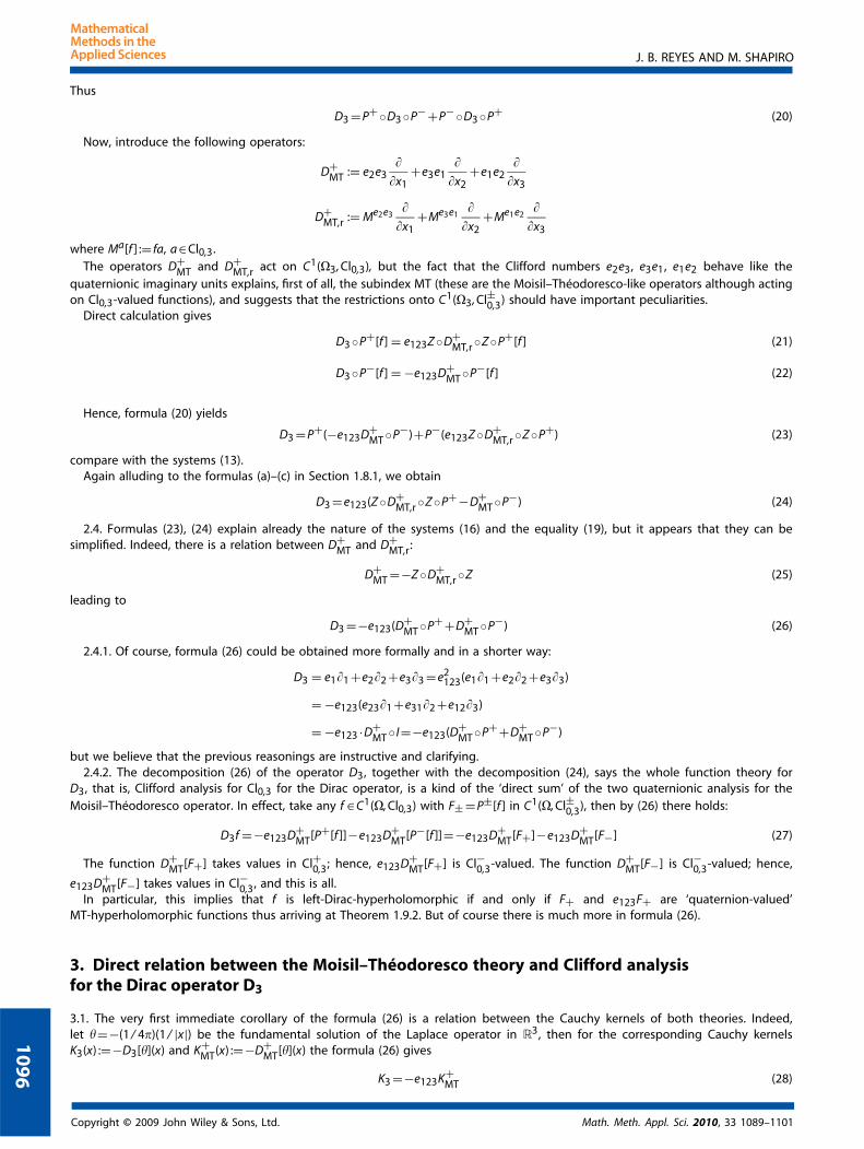
D3 =P+◦D3 ◦P−+P−◦D3 ◦P+ (20)

Now, introduce the following operators:

D+MT := e2e3

��x1

+e3e1�

�x2+e1e2

��x3

D+MT,r := Me2e3

��x1

+Me3e1�

�x2+Me1e2

��x3

where Ma[f ] := fa, a∈Cl0,3.The operators D+

MT and D+MT,r act on C1(�3, Cl0,3), but the fact that the Clifford numbers e2e3, e3e1, e1e2 behave like the

quaternionic imaginary units explains, first of all, the subindex MT (these are the Moisil–Théodoresco-like operators although actingon Cl0,3-valued functions), and suggests that the restrictions onto C1(�3, Cl±0,3) should have important peculiarities.

Direct calculation gives

D3 ◦P+[f ] = e123Z ◦D+MT,r ◦Z ◦P+[f ] (21)

D3 ◦P−[f ] = −e123D+MT ◦P−[f ] (22)

Hence, formula (20) yields

D3 =P+(−e123D+MT ◦P−)+P−(e123Z ◦D+

MT,r ◦Z ◦P+) (23)

compare with the systems (13).Again alluding to the formulas (a)–(c) in Section 1.8.1, we obtain

D3 =e123(Z ◦D+MT,r ◦Z ◦P+−D+

MT ◦P−) (24)

2.4. Formulas (23), (24) explain already the nature of the systems (16) and the equality (19), but it appears that they can besimplified. Indeed, there is a relation between D+

MT and D+MT,r:

D+MT =−Z ◦D+

MT,r ◦Z (25)

leading to

D3 =−e123(D+MT ◦P++D+

MT ◦P−) (26)

2.4.1. Of course, formula (26) could be obtained more formally and in a shorter way:

D3 = e1�1 +e2�2 +e3�3 =e2123(e1�1 +e2�2 +e3�3)

= −e123(e23�1 +e31�2 +e12�3)

= −e123 ·D+MT ◦ I=−e123(D+

MT ◦P++D+MT ◦P−)

but we believe that the previous reasonings are instructive and clarifying.2.4.2. The decomposition (26) of the operator D3, together with the decomposition (24), says the whole function theory for

D3, that is, Clifford analysis for Cl0,3 for the Dirac operator, is a kind of the ‘direct sum’ of the two quaternionic analysis for theMoisil–Théodoresco operator. In effect, take any f ∈C1(�, Cl0,3) with F± =P±[f ] in C1(�, Cl±0,3), then by (26) there holds:

D3f =−e123D+MT[P+[f ]]−e123D+

MT[P−[f ]]=−e123D+MT[F+]−e123D+

MT[F−] (27)

The function D+MT[F+] takes values in Cl+0,3; hence, e123D+

MT[F+] is Cl−0,3-valued. The function D+MT[F−] is Cl−0,3-valued; hence,

e123D+MT[F−] takes values in Cl−0,3, and this is all.

In particular, this implies that f is left-Dirac-hyperholomorphic if and only if F+ and e123F+ are ‘quaternion-valued’MT-hyperholomorphic functions thus arriving at Theorem 1.9.2. But of course there is much more in formula (26).

3. Direct relation between the Moisil–Théodoresco theory and Clifford analysisfor the Dirac operator D3

3.1. The very first immediate corollary of the formula (26) is a relation between the Cauchy kernels of both theories. Indeed,let �=−(1 / 4�)(1 / |x|) be the fundamental solution of the Laplace operator in R3, then for the corresponding Cauchy kernelsK3(x) :=−D3[�](x) and K+

MT(x) :=−D+MT[�](x) the formula (26) gives

K3 =−e123K+MT (28)

10

96

Copyright © 2009 John Wiley & Sons, Ltd. Math. Meth. Appl. Sci. 2010, 33 1089–1101

J. B. REYES AND M. SHAPIRO

A similar relation holds for the two representations of the (geometric) unit normal vector for domains under consideration.Because the formulation of surface integration over a highly non-smooth domain boundary is considered, the standard unit

normal cannot be defined and we have to consider that in the Federer sense, see [13].Indeed, let ϑ(x)= (ϑ1(x),ϑ2(x),ϑ3(x)) stand for the outward pointing Federer’s unit normal vector, then it is seen as Cl−0,3-valued

Clifford number ϑ�3 (x) :=∑3k=1 ekϑk(x) in Clifford analysis, while it is seen as ϑ+

�3(x) :=e23ϑ1(x)+e31ϑ2(x)+e12ϑ3(x) in the Moisil–

Théodoresco quaternionic analysis, thus giving

ϑ+�3

=−e123ϑ�3 (29)

3.2. From now on, we will denote by �3 a Jordan domain in R3, with the boundary � that is assumed to be a two-dimensionalcompact topological and oriented surface, �3 :=�3 ∪�.

We require � to be an Ahlfors David regular surface (see [14]), that is, there exists C>0 such that for all x ∈� and all 0<r�diam�,

C−1r2�H2(�∩{|y−x|�r})�Cr2

where H2 denotes the two-dimensional Hausdorff measure.Let us introduce the temporary notation �±

3 for the corresponding internal and external domains bounded by � in R3.Below we present the basic integral formulas of Clifford analysis in the non-smooth context assumed in the paper. Although the

form in general of those do not differ to what one usually sees in references on Clifford analysis, it is important to remark that theproofs of these, in particular formula (40), differ significantly from the traditionalists.

3.2.1. Theorem (Stokes’ formula compatible with the Dirac-hyperholomorphy). Let f and g be functions in C1(�3, Cl0,3). Then∫�

g(x)ϑ�3 (x)f (x) dH2(x)=∫

�3

(D3,r[g](x)f (x)+g(x)D3[f ](x)) dx (30)

where D3,r denotes the action of the Dirac operator from the right-hand side.3.2.2. Theorem (an analogue of the Cauchy integral theorem). Let the functions f and g be, respectively, left and right Dirac-

hyperholomorphic in �3, continuous in �3. Then ∫�

g(x)ϑ�3 (x)f (x) dH2(x)=0

Analogously to the classical complex analysis in the Clifford analysis, the integral representation formulas are deduced from theStokes theorem.

3.2.3. Theorem. For f ∈C1(�3, Cl0,3) we have

∫�

K3(x−y)ϑ�3 (y)f (y) dH2(y)−∫

�3

K3(x−y)D3[f ](y) dy ={

f (x) if x ∈�+3

0 if x ∈�−3

In particular, we obtain the Cauchy formula.3.2.4. Corollary. Let f ∈C1(�3, Cl0,3)∩C(�3, Cl0,3) such that D3[f ]=0 in �3, then∫

�K3(x−y)ϑ�3 (y)f (y) dH2(y)= f (x), x ∈�3

3.3. In order to transform the formula (30), we take into account (26), (29) and (9); thus the left-hand side of (30) is∫�

g(x)ϑ�3 f (x) dH2(x) = −e123

∫�

[G+(x)ϑ+�3

(x)F+(x)+G−(x)ϑ+�3

(x)F−(x)

+G+(x)ϑ+�3

(x)F−(x)+G−(x)ϑ+�3

(x)F+(x)] dH2(x) (31)

meanwhile for the right-hand side one has∫�3

(D3,r[g](x)f (x)+g(x)D3[f ](x)) dx = −e123

∫�3

(D+MT,r[G+](x)F+(x)+G−(x)D+

MT[F−](x)+D+MT,r[G+](x)F−(x)+G−(x)D+

MT[F+](x)

+D+MT,r[G−](x)F+(x)+D+

MT,r[G−](x)F−(x)+G+(x)D+MT[F+](x)+G+(x)D+

MT[F−](x)) dx (32)

Substituting (31) and (32) into (30) and recalling the decomposition (9) we get∫�

[G+(x)ϑ+�3

(x)F+(x)+G−(x)ϑ+�3

(x)F−(x)] dH2 =∫

�3

(D+MT,r[G+](x)F+(x)+G−(x)D+

MT[F−](x)

+D+MT,r[G−](x)F−(x)+G+(x)D+

MT[F+](x)) dx (33)

Copyright © 2009 John Wiley & Sons, Ltd. Math. Meth. Appl. Sci. 2010, 33 1089–1101

10

97

J. B. REYES AND M. SHAPIRO∫�

[G+(x)ϑ+�3

(x)F−(x)+G−(x)ϑ(x)F+(x)] dH2 =∫

�3

(D+MT,r[G+](x)F−(x)+G−(x)D+

MT[F+](x)

+G+(x)D+MT[F−](x)+D+

MT,r[G−](x)F+(x)) dx

AS the functions F+, F−, G+, G− can be chosen arbitrarily in their respective classes, the system (33) is equivalent to the systemof the four identities: ∫

�G+(x)ϑ+

�3(x)F+(x) =

∫�3

(D+MT,r[G+](x)F+(x)+G+(x)D+

MT[F+](x)) dx (34)

∫�

G−(x)ϑ+�3

(x)F−(x) =∫

�3

(D+MT,r[G−](x)F−(x)+G−(x)D+

MT[F−](x)) dx (35)

∫�

G+(x)ϑ+�3

(x)F−(x) =∫

�3

(DMT,r[G+](x)F−(x)+G+(x)D+MT[F−](x)) dx (36)

∫�

G−(x)ϑ+�3

(x)F+(x) =∫

�3

(DMT,r[G−](x)F+(x)+G−(x)D+MT[F+](x)) dx (37)

The formula (34) is already the Stokes theorem for the Moisil–Théodoresco theory. The three remaining formulas are just slightmodifications of it. Indeed, for the formulas (36) and (37), it is enough to multiply them by e123 and to take into account that thefunctions F+ :=e123F− and G+ :=e123G− take values in Cl+0,3. The formula (35) should be multiplied by 1= (e123)2.

3.4. So it has been shown that the formula (30) that expresses the essence of the Stokes Theorem compatible with the Dirac-hyperholomorphy is completely equivalent to the four ‘copies’ of the corresponding formula for the MT-hyperholomorphy. In thesame way one can show that each of the formulas from Sections 3.2.2, 3.2.3, and 3.2.4 is completely equivalent to several ‘copies’of their MT-hyperholomorphic analogues. In particular, this means that if we have proved the above facts for one of the theories,their counterparts for the other follow immediately by an algebraic reasoning.

The situation can be characterized in different words, depending on a personal taste; for example, one can say that quaternionicanalysis for the Moisil–Théodoresco operator ‘is’ just Clifford analysis. It is our opinion that such a characterization would be toostrong and it does not correspond to our above-described reasoning: strictly speaking, the theories are equivalent although theMT-theory may have an advantage as the other one is its ‘double repetition’.

3.5. We illustrate now all this with a more elaborated example.The Cauchy-type integral is a well-known integral operator, which has been thoroughly studied in the Clifford analysis framework,

and whose properties are similar to their famous complex prototypes. From theoretical reasons and in connection with variousbranches of applied sciences, much work in the study of its properties has been done. For brevity, will be only indicated thecomprehensive exposition of the theory of three-dimensional Cauchy-type integral analogues and its application to direct andinverse problems of the three-dimensional potential theory, as well as to integral transforms of three-dimensional geopotentialfields developed in [15] and the utility in geophysics and magnetism presented in [16].

A great deal of modern Clifford analysis is to ask for what kind of boundaries and functions the Cauchy-type integral hascontinuous limit values. The existence literature in this topic is classically known in the case of considering sufficiently smoothsurfaces and Hölder continuous functions, but for the case of considering surfaces with an irregular geometry, the literature is fewscattered, see [17--21].

One very important reason for needing to know that the singular integral operator associated with the limits values of theCauchy-type integral represent a continuous functions on the boundary is to be able to solve boundary value problems in a localbehaviour of continuous setting, i.e. near any specific point of the surface, ignoring their global behaviour (non-tangential boundaryvalues).

The classical singular integral operator that appears mostly in the literature is

S3[f ](x)=2

∫�

K3(x−y)ϑ�3 (y)f (y) dH2(y), x ∈�

which is not appropriated for the continuous context. Notice that for rough surface �, the particular case S3[1] does not representin general a continuous function for every point of �.

Thus, to treat existence and properties of the boundary values of Cauchy-type integral we need to understand what sort ofsurface we are interested in together with what kind of continuous densities we can take so that such conditions allow us to havea striking development and here again it is worth noting that the geometry of the boundary plays a basic role.

If f is a continuous function defined on the Ahlfors David regular surface �, then the Cauchy-type integral of f is the functiongiven by

C3[f ](x)=∫

�K3(x−y)ϑ�3 (y)f (y) dH2(y), x ∈R3 \� (38)

It immediately follows that C3[f ] is a left-Dirac-hyperholomorphic function in R3 \� and vanishes at infinity.

10

98

Copyright © 2009 John Wiley & Sons, Ltd. Math. Meth. Appl. Sci. 2010, 33 1089–1101

J. B. REYES AND M. SHAPIRO

To put way out of the difficulties mentioned before, we consider the singular version of the Cauchy-type integral (taking it in thesense of Cauchy’s principal value) defined by

S3[f ](x)=2

∫�

K3(x−y)ϑ�3 (y)(f (y)−f (x)) dH2(y)+f (x), x ∈� (39)

However, when � is sufficiently smooth, then the singular integral (39) coincides with the previously mentioned.Suppose that f belongs to the Hölder space C0,�(�, Cl0,3), 0<�<1. Then

(C±3 [f ])(x) := lim

�±3 �y→x

C3[f ](y)= 12 (S3[f ](x)±f (x)), x ∈� (40)

Moreover, the following results are extensions to the case of Clifford analysis of those obtained for complex-valued functions ofone complex variable.

(i) The singular integral operator S3 is an involution on C0,�(�, Cl0,3), 0<�<1, i.e.

S23[f ]= f

for all f ∈C0,�(�, Cl0,3).(ii) S3f is a bounded operator mapping C0,�(�, Cl0,3) into itself.

We must remark that Plemelj–Sokhotski formulae (40) is obtained (see the aforementioned references) for a wider class ofrectifiable surfaces, which contains those differentiable, chord-arc, piece-wise smooth, Liapunov, Lipschitz, and simple Lipschitzgraphs as proper subclasses.

3.5.1. Take the formula (38) and apply (39) and (34); this gives

C3[f ](x) =∫

�K+

MT(x−y)ϑ+�3

(y)F+(y) dH2(y)+∫

�K+

MT(x−y)ϑ+�3

(y)F−(y) dH2(y)

=∫

�K+

MT(x−y)ϑ+�3

(y)F+(y) dH2(y)+e123

∫�

K+MT(x−y)ϑ+

�3(y)F+(y) dH2(y)

=: CMT[F+]+e123CMT[F+]

where the integral

CMT[f ](x) :=∫

�K+

MT(x−y)ϑ+�3

(y)f (y) dH2(y), x ∈R3 \�

defining a continuous map from C(�, Cl±0,3) onto MTl(�±3 , Cl±0,3) plays the role of an analog of a Cauchy-type integral in the theory

of the Moisil–Théodoresco system; of course we have set also F+ :=e123F−.3.5.2. Introducing the singular version of CMT as

SMT[f ] :=2

∫�

K+MT(x−y)ϑ+

�3(y)(f (y)−f (x)) dH2(y)+f (x), x ∈�

we obtain in the same way that

S3[F+]=SMT[F+]+e123SMT[F+]

Hence, one sees that, again, the whole theory of the Clifford Cauchy-type integral, both in its hyperholomorphic and singularversions, is completely equivalent to the theory of its (quaternionic) Moisil–Théodoresco counterpart, and the conclusions identicalto the ones presented above can be made.

4. Considerations about the relationship between the Fueter and the Cauchy–Riemannoperators

One may think that in case of the Fueter and the Cauchy–Riemann operators, the situation is quite similar to the preceding sectionbut it turns out that, surprisingly for us, it is not.

The matter is that the algebraic structure of the Clifford numbers associated with the ‘authentic’ Fueter and Cauchy–Riemannoperators, i.e.

D+F = �

�x0+e23

��x1

+e31�

�x2+e12

��x3

D3 = ��x0

+e1�

�x1+e2

��x2

+e3�

�x3

Copyright © 2009 John Wiley & Sons, Ltd. Math. Meth. Appl. Sci. 2010, 33 1089–1101

10

99

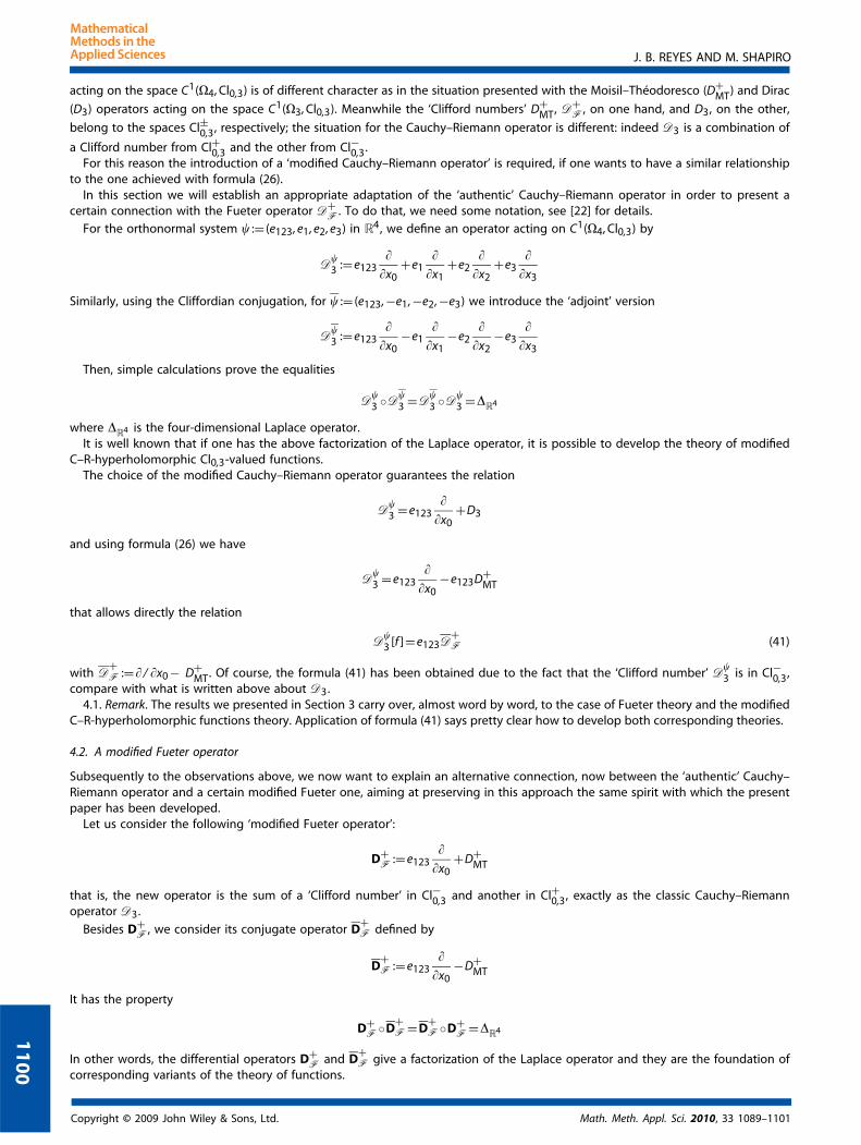
J. B. REYES AND M. SHAPIRO

acting on the space C1(�4, Cl0,3) is of different character as in the situation presented with the Moisil–Théodoresco (D+MT) and Dirac

(D3) operators acting on the space C1(�3, Cl0,3). Meanwhile the ‘Clifford numbers’ D+MT, D+

F, on one hand, and D3, on the other,

belong to the spaces Cl±0,3, respectively; the situation for the Cauchy–Riemann operator is different: indeed D3 is a combination of

a Clifford number from Cl+0,3 and the other from Cl−0,3.For this reason the introduction of a ‘modified Cauchy–Riemann operator’ is required, if one wants to have a similar relationship

to the one achieved with formula (26).In this section we will establish an appropriate adaptation of the ‘authentic’ Cauchy–Riemann operator in order to present a

certain connection with the Fueter operator D+F. To do that, we need some notation, see [22] for details.

For the orthonormal system � := (e123, e1, e2, e3) in R4, we define an operator acting on C1(�4, Cl0,3) by

D�3 :=e123

��x0

+e1�

�x1+e2

��x2

+e3�

�x3

Similarly, using the Cliffordian conjugation, for � := (e123,−e1,−e2,−e3) we introduce the ‘adjoint’ version

D�3 :=e123

��x0

−e1�

�x1−e2

��x2

−e3�

�x3

Then, simple calculations prove the equalities

D�3 ◦D�

3 =D�3 ◦D�

3 =�R4

where �R4 is the four-dimensional Laplace operator.It is well known that if one has the above factorization of the Laplace operator, it is possible to develop the theory of modified

C–R-hyperholomorphic Cl0,3-valued functions.The choice of the modified Cauchy–Riemann operator guarantees the relation

D�3 =e123

��x0

+D3

and using formula (26) we have

D�3 =e123

��x0

−e123D+MT

that allows directly the relation

D�3 [f ]=e123D

+F (41)

with D+F :=� / �x0 − D+

MT. Of course, the formula (41) has been obtained due to the fact that the ‘Clifford number’ D�3 is in Cl−0,3,

compare with what is written above about D3.4.1. Remark. The results we presented in Section 3 carry over, almost word by word, to the case of Fueter theory and the modified

C–R-hyperholomorphic functions theory. Application of formula (41) says pretty clear how to develop both corresponding theories.

4.2. A modified Fueter operator

Subsequently to the observations above, we now want to explain an alternative connection, now between the ‘authentic’ Cauchy–Riemann operator and a certain modified Fueter one, aiming at preserving in this approach the same spirit with which the presentpaper has been developed.

Let us consider the following ‘modified Fueter operator’:

D+F :=e123

��x0

+D+MT

that is, the new operator is the sum of a ‘Clifford number’ in Cl−0,3 and another in Cl+0,3, exactly as the classic Cauchy–Riemannoperator D3.

Besides D+F, we consider its conjugate operator D

+F defined by

D+F :=e123

��x0

−D+MT

It has the property

D+F◦D

+F=D

+F◦D+

F=�R4

In other words, the differential operators D+F and D

+F give a factorization of the Laplace operator and they are the foundation of

corresponding variants of the theory of functions.

11

00

Copyright © 2009 John Wiley & Sons, Ltd. Math. Meth. Appl. Sci. 2010, 33 1089–1101

J. B. REYES AND M. SHAPIRO

Finally, by using again the formula (26) we obtain

D+F=e123

��x0

−e123D3

Then, we have

D+F=e123D3

where, again, D3 means the Clifford conjugate to the Cauchy–Riemann operator:

D3 := ��x0

−e1�

�x1−e2

��x2

−e3�

�x3

4.3. Remark. It follows immediately that an associated theory for the modified Fueter operator is completely equivalent to theClifford analysis for the ‘authentic’ Cauchy–Riemann operator. In the same way, results on function theory associated with theCauchy kernel of modified Fueter operator completely coincide in structure with similar statements of the Clifford analysis forthe ‘authentic’ Cauchy–Riemann operator.

References1. Brackx F, Delanghe R, Sommen F. Clifford Analysis. Research Notes in Mathematics. vol. 76. Pitman (Advanced Publishing Program): Boston, MA,

1982; x+308.2. Delanghe R, Sommen F, Soucek V. Clifford Algebra and Spinor-valued Functions, vol. 53. Kluwer: Dordrecht, 1992.3. Sudbery A. Quaternionic analysis. Mathematical Proceedings of the Cambridge Philosophical Society 1979; 85:199--225.4. Gürlebeck K, Sprössig W. Quaternionic Analysis and Elliptic Boundary Value Problems. Birkhäusser: Boston, 1990.5. Gürlebeck K, Sprössig W. Quaternionic and Clifford calculus for physicists and engineers. Mathematical Methods in Practice. Wiley: Chichester,

1997, xi, 371.6. Kravchenko V, Shapiro M. Integral Representations for Spatial Models of Mathematical Physics. Pitman Research Notes in Mathematics Series,

vol. 351. Longman: Harlow, 1996; vi+247.7. Füter R. Analytische funktionen einer quaternionen variablen. Commentarii Mathematici Helvetici 1932; 4:9--20.8. Moisil Gr, Théodoresco N. Functions holomorphes dans l’espace. Mathematica, Cluj 1931; 5:142--159.9. Bory Reyes J, Delanghe R. On the solution of the Moisil Théodoresco system. Mathematical Methods in the Applied Sciences 2008; 31(12):

1427--1439.10. Bitsadze AV. Boundary Value Problems for Second Order Equations. North-Holland, Interscience: Amsterdam, NY, 1968.11. Dzhuraev AD. Singular Integral Equation Method. Nauka: Moscow, 1987 (in Russian); English translation—Longman Scientific and Technical,

Wiley: Harlow, NY, 1992.12. Gilbert JE, Murray MAM. Clifford Algebras and Dirac Operators in Harmonic Analysis. Cambridge Studies in Advanced Mathematics, vol. 26.

Cambridge University Press: Cambridge, 1991; viii+334.13. Federer H. Geometric Measure Theory. Die Grundlehren der mathematischen Wissenschaften, Band 153. Springer, New York Inc.: New York,

1969; xiv+676.14. David G, Semmes S. Analysis of and on uniformly rectifiable sets. Mathematical Surveys and Monographs, vol. 38. American Mathematical Society:

Providence, RI, 1993.15. Zhdanov MS. Integral Transforms in Geophysics. Springer: Berlin, 1988; xxiv+367.16. Nicolaide A. Three-dimensional analog of the Cauchy integral formula for solving magnetic field problems. IEEE Transactions on Magnetics 1998;

34(3):608--612.17. Abreu Blaya R, Bory Reyes J, Moreno García T. Cauchy transform on non-rectifiable surfaces in Clifford Analysis. Journal of Mathematical Analysis

and Applications 2008; 339:31--44.18. Abreu Blaya R, Bory Reyes J, Peña Peña D. Clifford Cauchy type integrals on Ahlfors–David regular surfaces in Rm+1. Advances in Applied

Clifford Algebras 2003; 13(2):133--156.19. Abreu Blaya R, Bory Reyes J, Moreno García T. Minkowski dimension and Cauchy transform in Clifford analysis. Complex Analysis and Operator

Theory 2007; 1(3):301--315.20. Bory Reyes J, Abreu Blaya R. Cauchy transform and rectifiability in Clifford Analysis. Zeitschrift für Analysis und ihre Anwendungen 2005;

24(1):167--178.21. Abreu Blaya R, Bory Reyes J, Shapiro M. The Clifford Cauchy transform with a continuous density; N. Davydov theorem. Mathematical Methods

in the Applied Sciences 2005; 28(7):811--825.22. Shapiro M. Some remarks on generalizations of the one-dimensional complex analysis: hypercomplex approach. Functional Analytic Methods in

Complex Analysis and Applications to Partial Differential Equations. World Scientific: Singapore, 1995; 379--401.

Copyright © 2009 John Wiley & Sons, Ltd. Math. Meth. Appl. Sci. 2010, 33 1089–1101

11

01