Spatial and spectral Quaternionic approaches

for Colour Images

Patrice DENIS a,∗, Philippe CARRE a,Christine FERNANDEZ-MALOIGNE a

aUniversity of Poitiers - SIC Laboratory - Bat SP2MI - Bd Marie et Pierre CurieB.P. 30179 - 86962 Futuroscope Chasseneuil Cedex - FRANCE

Abstract

Hypercomplex or quaternions numbers have been used recently for both greyscaleand colour image processing. Fast, numerous hypercomplex 2D Fourier transformswere presented as a generalization of the complex 2D Fourier transform to this newhypercomplex space. Thus, the major problem was to put an interpretation of whatinformation the Fourier coefficients could provide. In this paper, we first define theconditions on the spectrum coefficients needed to reconstruct a colour image with-out loss of information through the inverse quaternionic Fourier transform process.The result is used to interpret the quaternionic spectrum coefficients of this specificcolour Fourier transform. Secondly, with this apprehension of the quaternion num-bers and the corresponding colour spectrum space, we define spatial and frequentialstrategies to filter colour images.

Key words: quaternions, quaternionic Fourier transform, colour image processing,filter, symmetry conditions

NOTICE: this is the author’s version of a work that was accepted for publi-cation in Computer Vision and Image Understanding. Changes resulting fromthe publishing process, such as peer review, editing, corrections, structural for-matting, and other quality control mechanisms may not be reflected in thisdocument. Changes may have been made to this work since it was submit-ting for publication. A definitive version was subsequently published in PatriceDENIS, Philippe CARRE and Christine FERNANDEZ-MALOIGNE, Spatial

∗ Corresponding author.Email addresses: denis@sic.sp2mi.univ-poitiers.fr (Patrice DENIS),

carre@sic.sp2mi.univ-poitiers.fr (Philippe CARRE),fernandez@sic.sp2mi.univ-poitiers.fr (ChristineFERNANDEZ-MALOIGNE).

Preprint submitted to Computer Vision and Image Understanding

hal-0

0278

008,

ver

sion

1 -

7 M

ay 2

008

Author manuscript, published in "Computer Vision and Image Understanding 107, Issues 1-2 (2007) 74-87" DOI : 10.1016/j.cviu.2006.11.019

and spectral Quaternionic approaches for Colour Images, Computer Visionand Image Understanding, In Press, Accepted Manuscript, Available online8 February 2007, . (http://www.sciencedirect.com/science/article/B6WCX-4N0X5Y6-1/2/ebc9f4fb65da13b0c696dd3857391dfb)

Nowadays, as multimedia devices and internet are becoming accessible to moreand more people, image processing must take colour information into accountbecause colour processing is needed everywhere for new technologies. Severalapproaches have been submitted to deal with colour images, one of the old-est is to process each channel of the colour image separately. Implementingsuch programs often creates colour shifts and artefacts, so different approachesshould be used to produce visually pleasing colour images. A quite recent ap-proach is to encode the three channel components on the three imaginary partsof a quaternion as proposed by S.T. Sangwine and T. Ell in [20,14,13]. Quater-nions have been used for both greyscale images by Bulow [1] and colour onesby Sangwine et al. [20]. An introduction of quaternionic Fourier transformshas been made independently by both the teams above but in different defini-tions. In this paper, we study the Quaternionic Fourier spectrum in order todefine precisely the properties of this new colour representation. In this way,we want to explain the colour information contained in the new domain thatis to say how the different real and imaginary parts of the spectral quater-nionic domain interact with the pure quaternion component chosen to encodecolours in spatial domain. The other fundamental studied topic in the paper isthe filtering aspect. Indeed, we review spatial colour filter approaches, intro-duce a new spatial gradient approach using quaternions, and validate a newquaternionic spectral colour filter.

The first section of this paper reminds what the quaternions are and howto use them to process colour information. Then we study how quaternionscan be used to make R

3 transformations such as projections, rotations, etc.As an example, these transformations are used to switch from RGB to HSVcolour spaces. The second section introduces the discrete quaternionic Fouriertransform proposed by Sangwine and by Bulow, and we define the conditionson the quaternionic spectrum to enable manipulations into this frequencydomain without loosing information when going back to the spatial domain.This is also the subject of the second section which gives a new interpretationof the influence of Dirac initialization on the quaternionic Fourier space. Thethird section starts by surveying existing colour image filtering approachesbased on quaternions. Then, we use the R

3 transformations defined in the firstsection and the analysis of the quaternionic frequency domain in the secondsection to propose the definitions of a new quaternionic vector gradient anda frequency quaternionic filter. Finally, the appendix gives more details withformulas and graphics to help understand the information included in thequaternionic colour spectrum.

2

hal-0

0278

008,

ver

sion

1 -

7 M

ay 2

008

1 Quaternions

1.1 Concept

A quaternion q ∈ H (H refers to Hamilton[8] who was first to discover thesenumbers) is a generalization of a complex number and is defined as q = qr +qii + qjj + qkk where:

• qr, qi, qj and qk are real numbers.• i, j and k are three new imaginary numbers, asserting:

i2 = j2 = k2 = −1 ij = −ji = k jk = −kj = i and ki = −ik = j

With q = qr + qii + qjj + qkk any quaternion:

• q = qr − qii − qjj − qkk is q’s conjugate.

• q’s modulus or norm is√

q2r + q2

i + q2j + q2

k =√

qq noted |q|.• if q 6= 0, then q−1 = q

|q|2 is q’s inverse.

• ℜ(q) = qr is q’s real part . If ℜ(q) = q, then q is real .• ℑ(q) = ib + jc + kd is q’s imaginary part . If ℑ(q) = q, then q is pure.• P = {q ∈ H | q = ℑ(q)} is the Pure Quaternion set.• S = {q ∈ H | |q| = 1} is the Unitary Quaternion set.

Note that the quaternion product is anti-commutative.

Quaternions can be expressed using scalar part S(q) and vector part V (q),q = S(q) + V (q) with S(q) = qr and V (q) = qii + qjj + qkk. Sangwine andEll [20,14,13,21,22,4] were the first to use this vector part of quaternions toencode colour images. They took the three imaginary parts to code the r (red),g (green) and b (blue) colour components of an image. A colour image I withthe spatial resolution of N ×M pixels is in this way represented by an N ×M

matrix as follow:

q(s, t) = r(s, t)i + g(s, t)j + b(s, t)k

where s = 1, 2, ..., N and t = 1, 2, ...,M are the spatial coordinates of the pixelq.

3

hal-0

0278

008,

ver

sion

1 -

7 M

ay 2

008

1.2 R3 Transformations with Quaternions

As pure quaternions are used analogously to describe R3 vectors, the classical

R3 transformations such as translations, reflections, projections, rejections and

rotations can be defined with only additions and multiplications as explainedby Sangwine in [22] (cf. Figure 1). With two pure quaternions (q1, q2) ∈ P

2,the translation vector is supported by the quaternion qtrans = q1 + q2. If q ∈ P

and µ ∈ S ∩ P then qrefl = −µqµ is the q’s reflection vector with µ axis. Ifq ∈ P and µ ∈ S ∩ P then qproj = 1

2(q − µqµ) is the q’s projection vector on

µ axis. If q ∈ P and µ ∈ S ∩ P then qrej = 1

2(q + µqµ) is the q’s orthogonal

projection vector on µ axis’s orthogonal plane or the q’s rejection of the µ

axis. And eventually if q ∈ P, φ ∈ R and µ ∈ S ∩ P then qrot = eµφ

2 qe−µφ

2 isthe q’s rotation vector around µ axis with φ angle.

Fig. 1. Geometric Transformations in R3 with Quaternion: q denotes the

original vector, µ denotes the axis vector, qrefl is the q’s reflection vector with µ

axis, qrej is the q’s rejection of the µ axis and qproj is q’s projection vector on µ

axis.

For each colour pixel described in RGB colour space using a quaternion vectorq ∈ P, HSV (hue, saturation, value) colour space coordinates can be foundusing operations on quaternions. We consider that the value component ofthe HSV vector represents the norm of the colour’s orthogonal projectionvector (q.µgrey)µgrey on the grey axis µgrey (this axis can be defined such thatµgrey = i+j+k√

3). Saturation and hue are represented on the plane orthogonal

to the grey axis which crosses (q.µgrey)µgrey. The saturation is the distancebetween the colour vector q and the grey axis µgrey, and hue is the anglebetween the colour vector q and a colour vector ν taken anywhere on theplane orthogonal to µgrey and which sets the zero hue reference angle. Thisreference hue value is often taken to represent the red colour vector, so wedecided arbitrarily to associate the red colour vector to the ν vector and gave

4

hal-0

0278

008,

ver

sion

1 -

7 M

ay 2

008

it a zero hue value (cf. Figure 2). Hue is the angle between this reference colourvector and the colour vector q.

For a colour vector q, the corresponding H, V, and S components can beobtained using the grey-axis µ = µgrey ∈ S∩P and the reference colour vectorν ∈ S ∩ P with the following elementary quaternionic operations [7]

H=tan−1 |q−µνqνµ||q−νqν|

S=|12(q + µqµ)|

V =|12(q − µqµ)|

(1)

which will be used later in this paper to define a new gradient operator.

Fig. 2. Hue, Saturation and Value given with reference µGrey and H(ν) = 0

2 Discrete Quaternion Fourier Transform

2.1 Definition

Different works introduced the quaternionic Fourier Transform, [1,21]. TheDiscrete Quaternion Fourier Transform (DQFT) in µ = µii+µjj+µkk ∈ S∩P

direction analysis allows us to give the frequency equivalence of a N×M spatial

5

hal-0

0278

008,

ver

sion

1 -

7 M

ay 2

008

colour image in a matrix defined by

Q(S, T ) =1√MN

N2∑

s=−N2

+1

M2∑

t=−M2

+1

exp−2µπ(SsN

+TtM ) q(s, t) (2)

Here, the term Q(S, T ) represents the frequency coordinates and q(s, t) =r(s, t)i + g(s, t)j + b(s, t)k is a pure quaternion used to represent the threedifferent colour channels of the pixel at the coordinates (s, t) of the colourimage. Since the quaternion product is not commutative, DQFT can havedifferent forms [15]. Note that in this paper we will follow the DQFT definitiongiven in (2).

The inverse DQFT (IDQFT) to the transform presented in (2) is given by

q(s, t) = 1√MN

∑N2

S=−N2

+1

∑M2

T=−M2

+1exp2πµ(Ss

N+

TtM ) Q(S, T )

It is proved [15,5] that DQFT or its inverse (IDQFT) for a square matrix ofdimension 2n × 2n could be simplified by processing two fast complex Fouriertransforms.

2.2 Colour quaternion spectrum properties

In order to understand what the Fourier coefficients stand for, we studiedthe digital characterization of the DQFT. We first discovered that the colourFourier spectrum exhibits some symmetries due to zero scalar spatial partof any colour image. This observation follows the well-known fact that thespectrum of a real signal by a complex Fourier transform (CFT) has hermitianproperties of symmetry.

Even if the spatial information of a colour image is using pure quaternions only,applying a DQFT on an image results in full quaternions (i.e. with nonzeroscalar part). We wanted to find, after IDQFT, a space where scalar part iszero in order to avoid any loss of information as the spatial colour image iscoded on a pure quaternions matrix.

LetQ(S, T ) = Qr(S, T ) + Qi(S, T )i + Qj(S, T )j + Qk(S, T )k

be the spectral quaternion at coordinates (S, T ) ∈ ([−N2

+1..N2], [−M

2+1..M

2]).

In addition, letq(s, t) = qi(s, t)i + qj(s, t)j + qk(s, t)k

6

hal-0

0278

008,

ver

sion

1 -

7 M

ay 2

008

denote the IDQFT quaternion of (s, t) spatial coordinates.

Developping this,with µ = µii + µjj + µkk, the cartesian real part form of thespatial domain leads to

qr(s, t) = 1√MN

∑ ∑ [cos(2π

(SsN

+ TtM

))Qr(S, T )

−µi sin(2π(

SsN

+ TtM

))Qi(S, T ) − µj sin(2π

(SsN

+ TtM

))Qj(S, T )

−µk sin(2π(

SsN

+ TtM

))Qk(S, T )

](3)

where qr(s, t) is null when

Qr(−S,−T ) = −Qr(S, T ) ; Qi(−S,−T ) = Qi(S, T )

Qj(−S,−T ) = Qj(S, T ) ; Qk(−S,−T ) = Qk(S, T )

As it can be seen from the symmetries contained in the Fourier spectrum, thereal part must be odd and all the imaginary parts must be even. This is a directextension of the antihermitian property of the complex Fourier transform ofimaginary signal. Any transform in the quaternionic colour spectrum mustobey to these rules to keep spatial information safe.

2.3 Digital study of the colour spectrum

In this section, we try to give an interpretation of the information containedin the quaternionic spectrum of colour images. To do this, we propose toinitialize the discrete spectrum with a constant which will represent a Dirac(an infinetely short pulse) and study the response in the spatial domain afterIDQFT. Note that the details of the calculus are presented in appendix.

Initialization could be done in two different ways:

• On the real part of the spectrum, this leads to odd oscillations on thespatial domain linked to the µ direction parameter of the Fourier transform.Complex colours are obtained in the RGB colour space after modifying µ

and normalizing it in order to obtain a pure unit quaternion.

If Qr(S0, T0) = Kr; Qr(−S0,−T0) = −Kr then

q(s, t) = 2Kr(µi sin(2π

(S0sN

+ T0tM

))+ µj sin

(2π

(S0sN

+ T0tM

))+ µk sin

(2π

(S0sN

+ T0tM

))

• On an imaginary part of the spectrum, this results to even oscillations onthe spatial domain independently from the µ parameter of the Fourier trans-

7

hal-0

0278

008,

ver

sion

1 -

7 M

ay 2

008

form. A proper initialization on the different imaginary components with re-spect to the additive colour synthesis theory allows to reach complex colours.For example to get yellow oscillations the red and green components (i andj) should be initialised (with e=i,j or k).

If Qe(S0, T0) = Qe(−S0,−T0) = Ke then qe(s, t) = 2Keµe cos(2π

(S0sN

+ T0tM

))

2.4 Quaternionic Graphical Spectrum Illustration

Figure 3 illustrates the different possible initializations on the quaternionicspectrum. A pair of constants has been set on the quaternionic spectrumfollowing the properties for spatial reconstruction, then IDQFT has been per-formed to make the following subfigures (for more graphical illustrations reportto section A.2 in the appendix).

• Initializing a pair of constants on any imaginary component with any direc-tion µ leads to a spatial oscillation on the same component (Figure 3(a)).

• Initializing a pair of constants on the real component leads to a spatialoscillation following the same imaginary component(s) as those included inthe direction µ (Figure 3(b)).

• The coordinates (S0, T0) and (−S0,−T0) of the two initialization points inthe Fourier domain affect the orientation and the frequency of the oscil-lations in the spatial domain as it does so for greyscale image in complexFourier domain. Orientation of the oscillations can be changed as shown inFigure 3(c).

(a) (b) (c)

Fig. 3. Spectrum Initialization examples: (a) µGrey = i+j+k√3

and Qi(2, 2) = Qi(−2,−2) = Ki; (b) µMagenta = i+k√2

and

Qr(2, 2) = −Qr(−2,−2) = Kr; (c) µY ellow = i+j√2

and Qr(0, 2) = −Qr(0,−2) = Kr

The following focuses on the use of quaternions in filtering which is one of themost frequently used low level image processing operations. We first reviewspatial colour image approaches and get a new spatial colour filter. Thenstarting from the interpretation of the quaternionic Fourier space that wemade in this previous section, we introduce a quaternionic spectrum filter.

8

hal-0

0278

008,

ver

sion

1 -

7 M

ay 2

008

3 Quaternionic filtering

In this section, we focus on the colour filtering aspect and study discontinuitydetection which is a fundamental issue of colour image processing such asedge detection and image analysis. A number of approaches can be used todetect the edges and fine details in colour images. The following briefly surveyswell-known approaches.

3.1 Spatial filtering

3.1.1 Marginal methods

Marginal methods, adopted directly from greyscale image processing, processeach channel of the colour image separately (Figure 4a). Thus, they are compu-tationally simple and easy to implement. On the other hand, due to the omis-sion of the essential spectral information during processing, many marginalmethods have insufficient performance [11,12]. As presented in [10,11], edgescan be detected in a component-wise manner or by applying the processingsolution to the luminance signal. However, neither approach can detect thediscontinuities in colour information.

3.1.2 Vectorial methods

To avoid the drawbacks of marginal solutions, vectorial methods, such as thosebased on robust order statistics [12,16], process colour pixels as vectors (Figure4b). In the design proposed by Di Zenzo [3], edges are detected using colourvectorial gradients. The vectorial methods usually have better performancecompared to marginal solutions, however, the performance improvements areobtained at expense of the increased computational complexity.

(a) (b)

Fig. 4. (a)Marginal and (b) Vectorial methods

9

hal-0

0278

008,

ver

sion

1 -

7 M

ay 2

008

3.1.3 Perceptual methods

Perceptuals methods [6,9,23,17] are based on the human visual system (HVS)characteristics. For example, in [2], Carron used a marginal gradient methodbut based on a weight factor : the hue coefficient of each pixel, more relevantthan saturation or intensity to split colours. In a second approach, when thehue information is not enough to detect edges, the gradient is given using in-tensity and/or saturation. The contribution in this approach relies on the factthat if the difference between two colours is detected with a high saturation,the colours seem farther than if they have smaller saturation (i.e. nearer fromthe grey axis) but the same hues. Figure 5 shows that the two green vectorsq1 and q2, near the grey axis, seem to have a smaller hue difference than thetwo red vectors q3 and q4, far from the grey axis. This is not true but there isa difference: q1 and q2 have a smaller saturation (distance from the grey axis)than q3 and q4. The perceptual methods because using the HVS character-istics give better results than the marginal and vectorial ones. Moreover thechromatic information of pixels is used to avoid artefacts and a major advan-tage is the integration of colour shadows. Nevertheless, by working in propercolour spaces and using thresholds for instance for hue relevance, algorithmscomplexity is raised.

Fig. 5. The distance between q1 and q2 (green vectors) seems to be smaller thanbetween q3 and q4 (red vectors) but the hue difference is the same: q1q2 = q3q4

3.1.4 Sangwine’s quaternionic approach

Sangwine proposed the convolution on a quaternionic colour image can bedefined by [20,14,21]:

qfiltered(s, t) =n1∑

τ1=−n1

m1∑

τ2=−m1

hl(τ1, τ2)q((s − τ1)(t − τ2))hr(τ1, τ2) (4)

10

hal-0

0278

008,

ver

sion

1 -

7 M

ay 2

008

where hl and hr are the two conjugate filters of dimension N1 × M1 whereN1 = 2n1 + 1 ∈ N and M1 = 2m1 + 1 ∈ N.

From this definition of the convolution product, Sangwine proposed a colouredge detector in [19]. In this method, the two filters h1 and h2 are conjugatedin order to fullfill a rotation operation of every pixel around the greyscale axisby an angle of π and compare it to its neighbours (cf. Figure 6).

qfilt(s, t) = l ⋆ q ⋆ r(s, t) (5)

Fig. 6. Sangwine’s Edge Detector Scheme: µ is the grey axis; µq1µ (resp. µq3µ)is the rotated vector of q1 (resp. q3) around µ with an angle of π; the comparisonvector between q1 and q2 (resp. between q3 and q4) is given by q2 + µq1µ (resp.q4 + µq3µ); q4 + µq3µ is near from the grey axis so the colour seems grey butq2 + µq1µ is far from the grey axis so Sangwine’s filter has detect an edge as thisvector is more coloured.

The filter composed by a pair of quaternion conjugated filters is defined asfollows

l =1

6

1 1 1

0 0 0

Q Q Q

and r =1

6

1 1 1

0 0 0

Q Q Q

(6)

where Q = eµ π2 and µ = µGrey = i+j+k√

3the greyscale axis.

The filtered image (cf. Figure 6) is a greyscale image almost everywhere, be-cause in homogeneous regions the vector sum of one pixel to its neighboursrotated by π around the grey axis has a low saturation (cf. q4 + µq3µ forinstance). However, pixels in colour opposition (like q1 and q2 for example)

11

hal-0

0278

008,

ver

sion

1 -

7 M

ay 2

008

represent a colour edge. Therefore, they present a vector sum far from thegrey axis. Edges are thus coloured due to this high distance.

Although this detector has a good performance, it often produces false colours,for example, when the vector sum is out of the colour space domain. Figure7 shows that the edge of the hat is not detected by the same colour in c or dwhere the horizontal filtering convolution is applied rightwise or leftwise.

(a) (b)

(c) (d)

Fig. 7. Sangwine edge detector result: (a) original image; (b) Sangwine’s filterapplied from left to right horizontally; (c) zoom on the hat edge of the (b) picture;(d) same zoom but with the filter applied from right to left. Thus applying the filterleftwise in one same direction (horizontal, vertical or diagonal) leads to differentresults than applying it rightwise.

3.1.5 A new gradient detector

Starting with the result of Sangwine filter, we get for each pixel q1 and q3 avector of itself rotated by π around the greyscale axis and compared to itsneighbours q2 and q4. We saw that the more the colour vector of a pixel isfar from its neighbours (colour edge), the more the vector sum in Sangwine’s

12

hal-0

0278

008,

ver

sion

1 -

7 M

ay 2

008

filter is far from the grey axis. Our approach also gives us a colour gradient.We propose to determine the distance qdist of Sangwine’s comparison colourvector sum qsum = q2 + µq1µ or qsum = q4 + µq3µ from the grey axis µ (cf.Figure 8). This distance can be calculated with quaternionic operations (referto section 1.2) and is the norm of the rejection of the vector of the grey axis.This distance is defined from a colour vector to the grey axis and we work inthe RGB colour space. Thus, equation (1) implies that this is the saturationof the colour vector sum given by Sangwine’s filter.

qdist =1

2(qsum + µqsumµ) (7)

Fig. 8. Proposed quaternionic edge detector: µ is the grey axis; µq1µ (resp.µq3µ) is the rotated vector of q1 (resp. q3) around µ with an angle of π; our com-parison vector between q1 and q2 (resp. between q3 and q4) is given by the dis-tance qdist = 1

2(qsum + µqsumµ) of Sangwine’s vector sum qsum = q2 + µq1µ (resp.

qsum = q4 +µq3µ) from the grey axis (orange arrows); An edge is detected by a highdistance from the grey axis like the orange arrow between µ and q2 + µq1µ.

Figure 9 shows that the two distances S1 and S2 are equal. Sangwine’s filtergives two different colour vectors q1 + µq2µ and q2 + µq1µ for the same twooriginal colours q1 and q2 comparison. Note that our new method is thusindependent from the path (leftwise or rightwise) applied to convolute thefilter with the image whereas Sangwine’s is not.

This saturation filter is applied to the horizontal, vertical and both diagonaldirections. The maximum of these values of saturation at each pixel of theimage is then selected to make the final colour gradient filter by maximumdistance. Note that this quaternionic filtering operation is linear but the totalprocess is not linear as the ”maximum” operator interferes.

Figure 10 shows the results of our experiment where in each row there arefirst the original image, then the colour gradient and log colour gradient (inorder to amplify the edges detected by the colour gradient) and finally theedge map images. This last image is a thresholding on the colour gradient

13

hal-0

0278

008,

ver

sion

1 -

7 M

ay 2

008

Fig. 9. Difference between Sangwine and our edge detector: µ is the greyaxis; µq1µ (resp. µq2µ) is the rotated vector of q1 (resp. q2) around µ with an angle ofπ; the same colours q1 and q2 can give two different colour vectors qsum = q2 +µq1µ

and qsum = q1 + µq2µ by the Sangwine’s method. Note that our approach leads tothe same distance because S1 = S2.

image. The results show that the method detect colour edges quite properlyfor example with the house image where walls, roof and sky are well separated.The same observation can be done with the well detected separation betweenLenna’s shoulder and chin. Process our method on images such as the mandrillseparates correctly the homogeneous and textures areas. Even if there is stillan edge detected between the roof and the top right side of the chimney, wecan say that our approach handles shadows quite well. However,because ourmethod uses a comparison of saturation only, the differences of luminancebetween colours is not detected, see for instance the details of the window’shouse.

3.1.6 Edge detection performance

Figure 11 shows the edge maps obtained using the different methods. Themarginal (Figure 11b) and Di Zenzo (Figure 11c) approaches seem to be moresensitive to noise. The edges obtained by our approach (Figure 11f and g) aremuch thicker and closed. Remember that the first Carron method (Figure 11d)is based on a measure of the hue to weight the marginal gradient; the secondmethod uses as well the saturation and the luminance measures to weight thegradient when hue is not enough relevant. These methods give closed contoursand are not sensitive to noise as the marginal and Di Zenzo ones. RegardingCarron2 approach (Figure 11e), our method cannot distinguish as efficiently

14

hal-0

0278

008,

ver

sion

1 -

7 M

ay 2

008

(a) (b) (c) (d)

(e) (f) (g) (h)

(i) (j) (k) (l)

Fig. 10. From left to right, original images, colour gradient, log colour gradient andedge map from our new spatial method

shadows to real contours because our method is based on the saturation only.But this result depends on the thresholding done on the colour gradient. Indeedthe shadows contours can be erased from our edge map but at the price ofthinner edges everywhere else (see Figure 10d for example).

To improve our algorithm and take shadows into account we need to check ifthe saturation measure is self-sufficient. Indeed, two different colours can havethe same saturation. It is the case for instance with q1 and q2 on one handand q3 and q4 on the other hand as we saw in Figure 5. Even so, q1 and q2

are different colours as well as q3 and q4, fortunately they can be disjoined bytheir difference of luminance and/or hue. Implementing these luminance andchromaticity measures (as the Carron2 method does) when saturation is not

15

hal-0

0278

008,

ver

sion

1 -

7 M

ay 2

008

enough relevant should enhance the performance of our approach.

Even with this lack of improvement, our edge detector is quite efficient with animplementation using quaternion formalism and the results are given withoutperforming any change of colour space so imprecisions due to these digitalmanipulations of colours are avoided. Moreover, it should be noted that ouredge detector is based on a vectorial approach and does not need any additionaldefinition to sort colours. Our distance is a saturation one that does not givemore importance for a specified colour than for another one, speaking at thesame saturation level. Finally, our method is more similar to a perceptual onethan those based on RGB colour space as it uses geometric concepts fromHSV colour space for example.

3.1.7 Computational complexity

To compare the computational complexity of the proposed approach and thetraditional marginal colour gradient operator, the quaternionic operationshave to be expressed in terms of the traditional real operations such as multi-plications and additions. Let multq (resp. multr) stand for quaternionic (resp.real) multiplication, addq (resp. addr) quaternionic (resp. real) addition:

• addq = 4 addr

• multq = 4 ∗ 4 multr + 4*3 addr

We apply Sangwine algorithm and then we calculate the distance of the coloursum vector results from the grey axis. Note that the calculations will be per-formed for a N × N image.

• Sangwine algorithm :Remember that for each pixel we apply two convolutions by a 3 × 3

window, one with the quaternion Q and one with Q (cf. equations (5) and(6)).

nSang = N2(2 ∗ (6multq + 5addq))

In fact, since each convolution implies three zero coefficients, only 6quaternionic multiplications and 5 quaternionic additions are needed.

• Distance calculation :For each pixel again we calculate the saturation distance as seen in equa-

tion (7).

nDist = N2(addq + 2multq)

16

hal-0

0278

008,

ver

sion

1 -

7 M

ay 2

008

Then as we process the Sangwine filter on horizontal, vertical and both diag-onal directions :

nTotal = 4 ∗ (nSang + nDist)

= 4 ∗ (N2(2 ∗ (6 multq + 5 addq)) + N2(addq + 2 multq))

= N2(832 multr + 768 addr)

For a classical marginal gradient, the same kind of Prewitt filter is needed,but we only apply it one time on each colour component. We then apply iton the same four directions and the number of operations needed is aboutN2(28multr + 20addr).

We can see that our method is using much more operations than the classi-cal one so the computation time is increased (linearly and not exponentially).However, it should be noted that the complexity is not changed as both meth-ods are in O(N2) and the results obtained using the proposed approach arebetter than the ones obtained using a marginal method.

3.2 Frequency filtering

Our approach is built on the same idea used to filter greyscale images: DQFTis performed on a colour image leading to its the frequential information. Wethen apply a mask on this Fourier information by setting its either low orhigh frequency coefficients to zero. Eventually, the result is processed throughIDQFT to give the filtered image.

We use the quaternion formalism to encode colour images but we need tostay aware on the fact that the quaternionic product is not commutative.Indeed, the well known theorem which states that a convolution product inspatial domain is equal to the product in the Fourier space is not true withquaternions [15].

By definition, the formulation of our Fourier filtering approach is given by

qFilt = IDQFT{H.Q} (8)

with Q = DQFT (q) denotes the quaternionic Fourier transform of the originalimage and H the frequency behavior of the filter.

To compare the frequential filtering to the spatial one, we focus on the high-

17

hal-0

0278

008,

ver

sion

1 -

7 M

ay 2

008

(a) (b)

(c) (d)

(e)

(f) (g)

Fig. 11. Different spatial gradients on the ”house” image : (a) ”House”original image; (b) Marginal approach; (c) Di Zenzo approach; (d) First Carronapproach; (e) Second Carron approach; (f) our method; (g) our method with loga-rithmic approach.

18

hal-0

0278

008,

ver

sion

1 -

7 M

ay 2

008

pass filtering

H(S, T ) = 1 for (|S| > a, |T | > b) and 0 otherwise, with a, b ∈ R

Indeed we notice through the quaternionic spectrum study that there is alikeness of organisation as in the classical complex spectrum. As a consequence,high frequency selection will give weight to ruptures and thus contours.

Figure 12 shows that frequency filtering preserves the original colours and thehigh frequency content is really isolated from the rest of the image. In fact,the contours of the top and bottom boxes appear green and white in Figure12g and the circle and quadrilateral are red and blue in Figure 12h as inthe original image (Figure 12e). These remarks are also valid on the contoursmade on the Lenna image as we can see the details of her hat in Figure 12cand mouth in Figure 12d. We see that information on edges is vectorial as itappears in colours. A scaling process between 0 and 255 has been made afterIDQFT using the min and max of each component. As the method uses thewindowing concept to filter the image in the frequency domain, we can observethat there are some oscillations on edges detected in the high-pass filteredpictures. This windowing process in the quaternionic spectral domain leads toequivalent artefacts than those produced if it was done on a greyscale imagespectrum : the Fourier transform of the rectangle function is the sinc (sinecardinal) function. However, even if this statement is not true anymore withthe formalism of quaternions (from the anti-commutativity of the product),we observe that it still remains the same kind of border effects. Note that thecolour artefacts are just the conjugate colours of the edges in the RGB colourdomain as we see in Figure 12h where the red (resp. blue) colour of the circle(resp. quadrilateral) is oscillating with green (resp. yellow).

Figure 13 shows that this spectrum strategy is at least good enough to detectcolour edges properly. A edge map is made by thresholding the absolute valuesof the filtered images. This method seems however more sensitive to smalldetails than the one presented on the spatial filtering section but it may givemore details than the spatial approach with not saturated colours. Indeed wecan see in Figure 13c that the gutters and drainpipes of the roof are welldetected by the frequential method. They are not detected by the spatial onebecause they are quite white (white has a zero saturation level). Furthermore,this approach can filter both in low-pass and high-pass bands and it can begeneralized to band-pass by selecting the proper windowing scheme in thespectrum domain.

Notice that the experiments show only results with the µ parameter of theDQFT and IDQFT equal to µgrey. Finally taking the interpretation of thequaternionic spectrum of the first section we may be able to make spectrumfilters which can extract only one component or any combinaison of them.

19

hal-0

0278

008,

ver

sion

1 -

7 M

ay 2

008

(a) (b) (c)

(d) (e) (f)

(g) (h)

Fig. 12. Quaternionic high-pass filtering results: (a) Lenna original image;(b) highpass filter applied on (a); (c) details of the hat; (d) details of the face; (e)hand-made colour image; (f) high-pass filter applied on (e); (g) details of the greenand white boxes edges; (h) details of the red circle and blue quadrilateral edges.Frequency filtering preserves the original colours.

Speaking about performances, it takes two classical complex fast Fourier trans-forms to perform a DQFT or IDQFT. To process both DQFT and IDQFTis so equivalent to a complexity in O(N2ln(N2)). The windowing process isa product term by term between the spectrum and a 2D rectangle function.This process has a complexity in O(N2). The all method uses the two previousalgorithms leading the total complexity of the process in O(N2+N2ln(N2)) =

20

hal-0

0278

008,

ver

sion

1 -

7 M

ay 2

008

O(N2ln(N2)). This is a bit slower than the spatial method.

(a) (b) (c)

(d) (e) (f)

(g) (h) (i)

Fig. 13. Comparison between high-pass and spatial filtering: (a) Lenna orig-inal image; (b) highpass filtering’s edge map; (c) spatial gradient’s edge map; (d)mandrill original image; (e) highpass filtering’s edge map; (f) spatial gradient’s edgemap; (g) house original image; (h) highpass filtering’s edge map; (i) spatial gradi-ent’s edge map.

4 Conclusion

In this paper, we analysed the properties of the quaternionic Fourier spec-trum. This contributed first, to reconstruct after IDQFT and without any lossof information a quaternionic spatial colour image composed of three imagi-nary components only. Secondly, this gave us an interpretation of quaternionicFourier coefficients influence on the spatial domain with both calculus andgraphical illustrations. When initializing the real part of the spectrum with

21

hal-0

0278

008,

ver

sion

1 -

7 M

ay 2

008

a pair of constants respecting proper symmetries, the corresponding spatialdomain presents odd oscillations dependent on the µ parameter of the trans-formation. However, spectrum pairs of Dirac initialization made on imaginarycomponent influences the spatial domain with even oscillations independentlyfrom the µ parameter. As in the complex Fourier analysis, the quaternionicspectrum can be used to detect spatial orientations. Then in a second part,we applied the previous digital concepts to propose a new quaternionic colourvectorial gradient. This gave enthusiastic results as its takes advantages ofboth vectorial and perceptual approaches of spatial filtering for a RGB colourspace approach. In addition, we used the interpretation of the spectrum tocreate frequency quaternionic filters that gave similar results than complexfrequency filters on greyscale images. In that way, both spatial and spectrumapproaches have been discussed to get a wider vision on filtering with quater-nions. Perspectives are first to enhance the spatial vectorial filter in order totake the saturation reluctance into account, thus achieving higher efficiencyby giving more power to intensity and hue values when needed. The frequen-tial approach can as well be improved first by using a smoother function thanthe rectangle one to process the spectrum filtering and soften the border ef-fects leading to colour artefacts. Secondly, we can select in the Fourier domainthe wanted components as described by the spectrum interpretation of thefirst section. Finally, as quaternions do not seem to give information to com-pare colour components between themselves but more independent componentanalysis, geometric algebra which manipulates vectors but also multivectorsmay represent a useful tool to achieve new results.

A Appendix

A.1 Digital study of the colour spectrum

This section shows more details on how, an initialization made in the quater-nionic spectrum, influences the spatial domain after IDQFT.

A problem relies on the fact that the spectrum must present the previoussymmetry conditions (refer to section 2.2), and thus the pixel at coordinates(−S0,−T0) must be initialized with amplitude that respects the conditions.Eventually there are two points initialized in the spectrum in order to find aspatial image after IQFT without any loss of information. There are differentcases for initialization, as reported in the following.

• Initialization on the real component

In this case, the initialization requires the Qr(S0, T0) = Kr and Qr(−S0,−T0) =

22

hal-0

0278

008,

ver

sion

1 -

7 M

ay 2

008

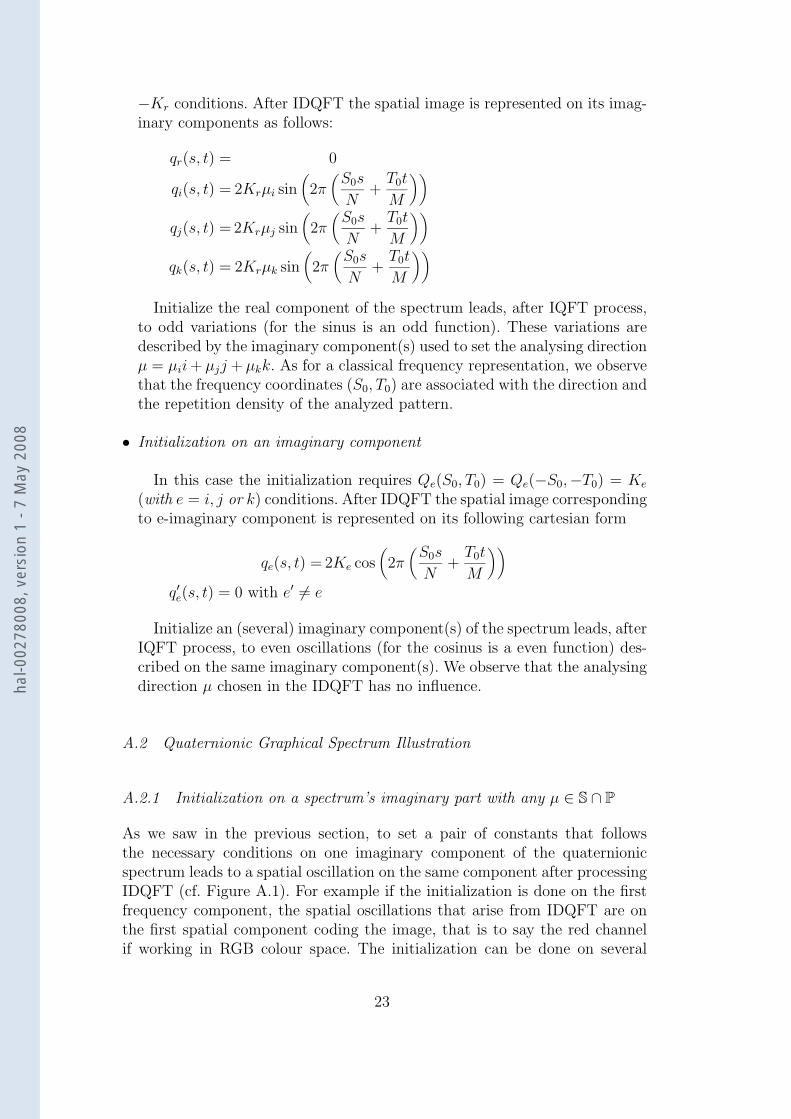
−Kr conditions. After IDQFT the spatial image is represented on its imag-inary components as follows:

qr(s, t) = 0

qi(s, t) = 2Krµi sin(2π

(S0s

N+

T0t

M

))

qj(s, t) = 2Krµj sin(2π

(S0s

N+

T0t

M

))

qk(s, t) = 2Krµk sin(2π

(S0s

N+

T0t

M

))

Initialize the real component of the spectrum leads, after IQFT process,to odd variations (for the sinus is an odd function). These variations aredescribed by the imaginary component(s) used to set the analysing directionµ = µii + µjj + µkk. As for a classical frequency representation, we observethat the frequency coordinates (S0, T0) are associated with the direction andthe repetition density of the analyzed pattern.

• Initialization on an imaginary component

In this case the initialization requires Qe(S0, T0) = Qe(−S0,−T0) = Ke

(with e = i, j or k) conditions. After IDQFT the spatial image correspondingto e-imaginary component is represented on its following cartesian form

qe(s, t) = 2Ke cos(2π

(S0s

N+

T0t

M

))

q′e(s, t) = 0 with e′ 6= e

Initialize an (several) imaginary component(s) of the spectrum leads, afterIQFT process, to even oscillations (for the cosinus is a even function) des-cribed on the same imaginary component(s). We observe that the analysingdirection µ chosen in the IDQFT has no influence.

A.2 Quaternionic Graphical Spectrum Illustration

A.2.1 Initialization on a spectrum’s imaginary part with any µ ∈ S ∩ P

As we saw in the previous section, to set a pair of constants that followsthe necessary conditions on one imaginary component of the quaternionicspectrum leads to a spatial oscillation on the same component after processingIDQFT (cf. Figure A.1). For example if the initialization is done on the firstfrequency component, the spatial oscillations that arise from IDQFT are onthe first spatial component coding the image, that is to say the red channelif working in RGB colour space. The initialization can be done on several

23

hal-0

0278

008,

ver

sion

1 -

7 M

ay 2

008

components, in that case, the result affects the same components that havebeen modified. In our case as the following examples are taken from a RGBcolour space, multiple initializations (always under the conditions for correctspatial reconstruction) on the spectrum produce spatial oscillations followingthe rules of the addivive synthesis of colours. So if we initialize the spectrum oneach imaginary component with the same couple of constants, the spatial resultafter IDQFT on a RGB colour space is grey oscillations. The µ parameter doesnot interfere in this case.

A.2.2 Initialization on the spectrum’s real part with any µ ∈ S ∩ P but µ 6=µGrey

It was shown in Section 2.3 that the initialization on the spectrum could bedone on the real component. In that case, we can also get different kindsof oscillations after IDQFT was performed, thus showing that the conditionsenunciated before are preserved. Oscillations after IQFT process are on thesame imaginary components involved in the initialization of the pure unitquaternion direction µ. In other words, working in RGB colour space impliesthat, to get red oscillations, the µ parameter must be equal to i (cf. FigureA.2). Oscillations composed of numerous colours can be achieved in settingthe µ parameter properly, for instance µ = i+j√

2leads to yellow variations in

the RGB colour space after IDQFT.

A.2.3 Geometric Variations

In the complex plane, coordinates of the spectrum coefficients involved in thequaternionic Fourier space’s initialization are really important parameters.Indeed, the resulting oscillations by IDQFT process have a geometric orien-tation linked to this. Supposing that coordinates are given in Z

2 with thepixel O(0, 0) in the image centre (whereas on the top-left corner as often), theinitialization of the spectrum at coordinates (S0, T0) and (−S0,−T0) results,through IDQFT process, in a 2D oscillation (sinus and cosinus) following theaxis made by this two pixels.

In Figure A.3, numerous geometric oscillations are shown by modifying thecoordinates of the pixels pair implicated by the initialization but with thesame way to set the spectrum components.

24

hal-0

0278

008,

ver

sion

1 -

7 M

ay 2

008

(a) (b) (c)

(d) (e) (f)

(g)

Fig. A.1. Initialization examples with µ = µGrey = i+j+k√3

: (a)

Qi(2, 2) = Qi(−2,−2) = Ki; (b) Qj(2, 2) = Qj(−2,−2) = Kj ;(c) Qk(2, 2) = Qk(−2,−2) = Kk; (d) Qi(2, 2) = Qi(−2,−2) = Ki

and Qi(2, 2) = Qi(−2,−2) = Ki; (e) Qj(2, 2) = Qj(−2,−2) = Kj

and Qj(2, 2) = Qj(−2,−2) = Kj ; (f) Qk(2, 2)Qk(−2,−2) = Kk andQk(2, 2) = Qk(−2,−2) = Kk; (g) Qi(2, 2) = Qi(−2,−2) = Ki,Qj(2, 2) = Qj(−2,−2) = Kj and Qk(2, 2) = Qk(−2,−2) = Kk.

B Acknowledgments

The author thanks Emeric Rollo[18] for his contribution to the spatial colourgradient part of this work. Thanks as well to Poitou-Charentes Region boardand PIMHAI, INTERREG IIIB ”Arc Atlantique” project, which have fundedthis work.

25

hal-0

0278

008,

ver

sion

1 -

7 M

ay 2

008

(a) (b) (c)

Fig. A.2. Initialization examples with µ 6= µGrey and

Qr(2, 2) = −Qr(−2,−2) = Kr (a) µGrey = i+j+k√3

; (b) µRed = i; (c) µMagenta = i+k√2.

(a) (b)

(c) (d)

Fig. A.3. Geometric oscillation examples initialization with µY ellow = i+j√2

(a) Qr(2, 2) = −Qr(−2,−2) = Kr; (b) Qr(4,−4) = −Qr(−4, 4) = Kr; (c)Qr(0, 2) = −Qr(0,−2) = Kr; (d) Qr(2, 0) = −Qr(−2, 0) = Kr.

References

[1] Thomas Bulow, Hypercomplex Spectral Signal Representations for the processingand Analysis of Images, p.22, PhD Thesis, August 1999

[2] T. Carron, Segmentation d’images couleur dans la base Teinte-Luminance-Saturation : approche numerique et symbolique, These de doctorat, Universitede Savoie, decembre 1995

26

hal-0

0278

008,

ver

sion

1 -

7 M

ay 2

008

[3] S. Di Zenzo, A note on the gradient of multi-image, in Computer Vision,Graphics, and Image Processing, vol.33, pp116-125,1986.

[4] T.A. Ell and S.J. Sangwine,Decomposition of 2D hypercomplex Fouriertransforms into pairs of Fourier transforms,in Proc. EUSIPCO,2000,pp.151-154

[5] M. Felsberg and G. Sommer,Optimized fast algorithms for the quaternionicFourier transform,in 8th Int. Conference on Computer Analysis of Images andPatterns, Ljubljana,1999,vol.1689,p209-216

[6] C. Fernandez-Maloigne, M.-C. Larabi, B. Bringier B, and N. Richard., Spatial-temporal characteristics of the visual brain and their effects on colour qualityevaluation, in AIC International Conference, Granada, Spain, 813 May 2005.

[7] P.H. Gosselin, Quaternions et Images Couleurs, DEA study with SIC laboratoryin 2002, p.25-27

[8] W.R. Hamilton, Elements of Quaternions. London, U.K.: Longman, 1866

[9] Kelly D.H.,Spatiotemporal variation of chromatic and achromatic contrastthresholds. J. Opt. Soc. Am. 73(6):742750, 1983.

[10] R. Lukac, K.N. Plataniotis, A.N. Venetsanopoulos, R. Bieda, and B. Smolka,Color edge detection techniques, in Signaltheorie und Signalverarbeitung,Akustik und Sprachakustik, Informationstechnik, W.E.B. Universitt Verlag,Dresden, vol. 29, pp. 21-47, 2003.

[11] R. Lukac, B. Smolka, K. Martin, K.N. Plataniotis, and A.N. Venetsanopoulos,Vector filtering for color imaging, in IEEE Signal Processing Magazine, vol. 22,no. 1, pp. 74-86, January 2005.

[12] R. Lukac and K.N. Plataniotis, A taxonomy of color image filtering andenhancement solutions, in Advances in Imaging and Electron Physics, (eds.)P.W. Hawkes, Elsevier, vol. 140, 2006, 187-264.

[13] C.E. Moxey, S.J. Sangwine and T.A. Ell, Vector Correlation of colour ImagesinFirst European Conference on Colour in Graphics, Imaging and Vision (CGIV2002), University of Poitiers, France, 2-5 April 2002, The society for ImageScience and Technology, pages 343-347.

[14] C.E. Moxey, S.J. Sangwine and T.A. Ell, Hypercomplex Correlation Techniquesfor Vector Images in IEEE Transactions on Signal Processing, vol.51, July 2003,pages 1941-1953

[15] Soo-Chang Pei, Jian-Jiun Ding and Ja-Han Chang,Efficient Implementation ofQuaternion Fourier Transform, Convolution, and Correlation by 2-D ComplexFFT, IEEE Trans. Signal Processing, vol.49, p2783-2797, Nov 2001

[16] K.N. Plataniotis and A.N. Venetsanopoulos, Color Image Processing andApplications, Springer Verlag, 2000.

[17] A.B. Poirson and B.A. Wandell. Pattern-color separable pathways predictsensitivity to simple colored patterns. in Vision research, march 1996.

27

hal-0

0278

008,

ver

sion

1 -

7 M

ay 2

008

[18] E. Rollo, N. Richard, C. Fernandez Maloigne, A perceptual colour imagewatershed, SIC laboratory, internal report, may 2006

[19] Sangwine, S.J., Colour image edge detector based on quaternion convolution, inElectronics Letters, 34, (10), May 14 1998, 969-971.

[20] Sangwine, S.J., Colour in Image Processing, in Electronics and CommunicationEngineering Journal, 12, (5), October 2000, 211-219.

[21] S.J. Sangwine and T. Ell, Hypercomplex Fourier transforms of colour images.In Proc. ICIP, volume 1, pages 137-140, Thessaloniki, Greece, 2001

[22] S.J. Sangwine and T.A. Ell, Mathematical Approaches to Linear Vector Filteringof colour Imagesin First European Conference on Colour in Graphics, Imagingand Vision (CGIV 2002), University of Poitiers.

[23] Wandell, Color appearance : the effects of illumination and spatial patterns,Nat. Acad. Sci. USA 90, pp.9778-9784, 1993.

28

hal-0

0278

008,

ver

sion

1 -

7 M

ay 2

008