om sharan salafia

S H O RT G A M M A - R AY B U R S T S A S E L E C T R O M A G N E T I C C O U N T E R PA RT SO F C O M PA C T B I N A RY M E R G E R S

The revolution just started

Dottorato di Ricerca in Fisica e AstronomiaDipartimento di Fisica “G. Occhialini”

Facoltà di Scienze Matematiche, Fisiche e NaturaliUniversità degli Studi di Milano-Bicocca

Fall 2017 – v 1.0

Om Sharan Salafia: Short gamma-ray bursts as electromagnetic counterparts of compactbinary mergers, The revolution just started, © Fall 2017

supervisors:Gabriele GhiselliniMonica ColpiGiancarlo Ghirlanda

location:Università degli Studi di Milano-Bicocca, piazza della Scienza 3, 20124 Milano,Italy

time frame:Fall 2017

Dedico questo lavoro a Ilaria, l’unica persona capace di capirmi veramente, disostenermi con pazienza, e di far emergere il meglio di me.

A B S T R A C T

Gamma-ray bursts (GRBs) are brief flashes of photons that trigger current space-based hard X-ray and gamma-ray detectors every two or three days. During atime ranging from less than one to several thousand seconds, a highly variablephoton flux with an unpredictable time structure is recorded by the detector. Fiftyyears have flown since the first observation of this kind, during which a long se-ries of technological and theoretical breakthroughs paved the way for the current,widely-accepted paradigm that relates these flashes to accretion of matter on anewborn stellar-mass black hole or neutron star. Two are the natural birthplacesof such relativistic beasts: the collapse of a massive star and the coalescence of twocompact objects. The latter, perhaps the most intriguing of the two, was the firstto be proposed as a candidate progenitor of GRBs, but in 1998 the association ofGRB 980425 with supernova 1998bw provided compelling evidence for the former.Nevertheless, no supernova has been associated so far – in some cases down tovery stringent limits – to members of a particular subclass of these events, knownas short gamma-ray bursts (SGRBs).

Several pieces of evidence support the idea that the progenitor of SGRBs isindeed the coalescence of two neutron stars, or of a black hole and a neutron star.If this is true, then SGRBs are also intimately related to gravitational waves (GW).The advanced network of ground-based GW detectors – which at present consistsof the two Advanced LIGO interferometers in the USA and of Advanced Virgoin Italy – is especially sensitive in the frequency range of GW produced by theinspiral and merger of a stellar mass compact object binary, so that we are right inthe position to start testing the SGRB–GW connection.

In August of this year, the first observation of GW from a neutron star binarycoalescence, followed by the first observation of a kilonova – the UV/Optical/In-frared emission from the expanding material ejected during the merger and post-merger phases of the coalescence, powered by nuclear decay of unstable nucleisynthesized by the r-process – and an associated SGRB-like transient marked thestart of a revolution, whose effect on our understanding of these subjects stillneeds to be completely unfolded. For this reason, in this thesis I do not to drawfirm conclusions about these observations, but rather I discuss some possible inter-pretations and implications, leaving many questions open to future investigation.

In the first part of this thesis I show the results of a detailed modeling of theSGRB population, with a careful handling of selection effects. The model satisfiesfor the first time all available observational constraints. Despite the model beingagnostic about the progenitor, the shape of the resulting redshift distribution repro-duces well that expected in the compact binary progenitor scenario. The predictedlocal density of SGRBs, though, is very low, and the implied rate of joint detec-tions of SGRBs and GWs from compact binary mergers is less than one event perdecade. The low rate is in part due to the need for the SGRB jet to be aligned withthe line of sight in order for the gamma-ray emission to be detected. Somewhatbetter prospects are found for the joint detection of GW and an SGRB orphanafterglow.

v

These results triggered my interest in maximizing the effectiveness of the elec-tromagnetic follow-up of GW detections. In the subsequent chapter, I describe amethod to optimize the electromagnetic follow-up of a GW event which makesuse of the information about compact binary parameters that can be extractedfrom the GW signal through parameter estimation. The compact binary parame-ter posterior distributions – and their correlations – are used to build a family ofpossible SGRB afterglow and kilonova light curves. These are the basis to constructa time-dependent sky-position-conditional probability of detection that guides theoptimization of the follow-up strategy.

The second part of the thesis is devoted to GRB170817A, the SGRB-like burstdetected by Fermi/GBM and INTEGRAL/SPI-ACS in temporal and spatial associ-ation with the gravitational wave event GW170817, which has been interpreted asthe spacetime perturbation due to the inspiral of a double neutron star binary. De-spite the electromagnetic burst appears as a rather ordinary SGRB from a purelyobservational point of view, the very low luminosity and energy implied by thesmall distance are absolutely unprecedented. The community is still in the processof finding a consensus on the interpretation of this event. Most proposed scenar-ios involve the presence of a jet misaligned with the line of sight, whose emissionwould have been that of an ordinary SGRB if seen on-axis. The extremely low en-ergy and luminosity of the burst (with respect to any previous SGRB for which aredshift has been measured) is either interpreted as emission from the border ofthe jet, or from a slower and less energetic sheath surrounding the jet, or from a“cocoon” of plasma heated by the jet while it had been excavating its way throughthe merger ejecta. Since it is unclear whether a jet should be always producedafter this kind of merger, and not even if it can always successfully break outof the region polluted by the merger ejecta, I tried to imagine a jet-less scenarioable to explain the properties of GRB170817A – knowing that the absence of ajet would affect the impact that this observation has on the rate of SGRBs. In thefinal part of this thesis I describe such a scenario, in which the SGRB is producedby an isotropic fireball powered by reconnection of a very strong magnetic fieldsurrounding the merging binary, produced by amplification of the neutron starmagnetic field due to magnetohydrodynamic turbulence. I set up a simple phys-ical model to predict the properties of such emission, and I show that there isa set of parameters for which the model fits the properties of both the promptgamma-ray emission and the late X-ray and radio data. The model predicts thefuture evolution of the radio and X-ray light curve, which will be soon put on testby new observations. I finally discuss some possible difficulties related to the verylow electron fraction needed in the fireball according to the fit parameters.

vi

P U B L I C AT I O N S

Most of the ideas and figures in this thesis appeared previously in articles I gotpublished on peer-reviewed journals during my three year PhD course. Neverthe-less, this work is not a simple collection of previously published papers, but ratherelaborates on selected works in order to provide a coherent picture of the SGRB–GW connection and of my personal view about the interpretation of GRB170817A.Here is a complete list of my publications as of February 13, 2018:

• D’Avanzo, P., Campana, S., Ghisellini, G., et al. (2018). Evidence for a decreas-ing X-ray afterglow emission of GW170817A and GRB 170817A in XMM-Newton. Submitted to A&A. e-print arXiv:1801.06164

• Ghirlanda, G., Nappo, F., Ghisellini, G., et al. (2017). Bulk Lorentz factorsof gamma-ray bursts. Astronomy & Astrophysics, 609, A112. https://doi.org/10.1051/0004-6361/201731598

• Melandri, A., Covino, S., Zaninoni, E., et al. (2017). Colour variations in theGRB 120327A afterglow. Astronomy & Astrophysics, 607, A29. https://doi.org/10.1051/0004-6361/201731759

• Salafia, O. S., Ghisellini, G., Ghirlanda, G., et al. (2017). GRB170817A: a giantflare from a jet-less double neutron-star merger? Submitted to A&A. e-printarXiv:1711.03112

• Salafia, O. S., Ghisellini, G., and Ghirlanda, G. (2017). Jet-driven and jet-less fireballs from compact binary mergers. Monthly Notices of the RoyalAstronomical Society: Letters, 474(1), L7-L11. http://dx.doi.org/10.1093/mnrasl/slx189

• Chhotray, A., Nappo, F., Ghisellini, G., et al. (2017). On radiative acceler-ation in spine-sheath structured blazar jets. Monthly Notices of the RoyalAstronomical Society, 466(3), 3544–3557. https://doi.org/10.1093/mnras/stw3002

• Pian, E., D’Avanzo, P., Benetti, et al. (2017). Spectroscopic identification of r-process nucleosynthesis in a double neutron-star merger. Nature, 551(7678),67–70. https://doi.org/10.1038/nature24298

• Nappo, F., Pescalli, A., Oganesyan, G., et al. (2017). The 999th Swift gamma-ray burst: Some like it thermal. A multiwavelength study of GRB 151027A.Astronomy & Astrophysics, 598, A23. https://doi.org/10.1051/0004-6361/201628801

• Salafia, O. S., Colpi, M., Branchesi, M., et al. (2017). Where and When: Op-timal Scheduling of the Electromagnetic Follow-up of Gravitational-waveEvents Based on Counterpart Light-curve Models. The Astrophysical Jour-nal, 846(1), 62. https://doi.org/10.3847/1538-4357/aa850e

vii

• Abbott, B. P., Abbott, R., Abbott, T. D., et al. (2017). Multi-messenger Obser-vations of a Binary Neutron Star Merger. The Astrophysical Journal Letters,848(2), L12. https://doi.org/10.3847/2041-8213/aa91c9

• Perri, L., and Salafia, O. S. (2016). An unexpected new explanation of season-ality in suicide attempts: Grey’s Anatomy broadcasting. e-print arXiv:1603.09590

• Salafia, O. S., Ghisellini, G., Pescalli, A., et al. (2016). Light curves and spectrafrom off-axis gamma-ray bursts. Monthly Notices of the Royal AstronomicalSociety, 461(4), 3607–3619. https://doi.org/10.1093/mnras/stw1549

• Campana, S., Braito, V., D’Avanzo, P., et al. (2016). Searching for narrow ab-sorption and emission lines in XMM-Newton spectra of gamma-ray bursts.Astronomy & Astrophysics, 592, A85. https://doi.org/10.1051/0004-6361/201628402

• Ghirlanda, G., Salafia, O. S., Pescalli, A., et al. (2016). Short gamma-ray burstsat the dawn of the gravitational wave era. Astronomy & Astrophysics, 594,A84. https://doi.org/10.1051/0004-6361/201628993

• Pescalli, A., Ghirlanda, G., Salvaterra, R., et al. (2016). The rate and luminos-ity function of long gamma ray bursts. Astronomy & Astrophysics, 587, A40.https://doi.org/10.1051/0004-6361/201526760

• Salafia, O. S., Pescalli, A., Nappo, F., et al. (2015). Gamma-ray burst jets:uniform or structured?. PoS(SWIFT 10), 96. https://pos.sissa.it/archive/conferences/233/096/SWIFT10_096.pdf

• Pescalli, A., Ghirlanda, G., Salafia, O. S., et al. (2015). Luminosity functionand jet structure of Gamma-Ray Burst. Monthly Notices of the Royal Astro-nomical Society, 447(2), 1911-1921. https://doi.org/10.1093/mnras/stu2482

• Salafia, O. S., Ghisellini, G., Pescalli, A., et al. (2015). Structure of gamma-rayburst jets: intrinsic versus apparent properties. Monthly Notices of the RoyalAstronomical Society, 450(4), 3549–3558. https://doi.org/10.1093/mnras/stv766

• Ghirlanda, G., Salvaterra, R., Campana, S., et al. (2015). Unveiling the pop-ulation of orphan -ray bursts. Astronomy & Astrophysics, 578, A71. https://doi.org/10.1051/0004-6361/201526112

viii

C O N T E N T S

1 introduction 1

i short gamma-ray bursts 3

2 gamma-ray burst astronomy 5

2.1 The discovery 5

2.2 The prompt emission 5

2.3 The afterglow 10

2.4 Presence of a jet 12

2.5 Progenitors 14

3 trying to get a grasp of the short grb population 15

3.1 Briefing 15

3.2 Introduction 15

3.3 Selecting a good sample 17

3.4 A sensible parametrization of the φ(L) and Ψ(z) 19

3.5 From population properties to observables 22

3.6 A too steep luminosity function is at odds with the observer-frameconstraints 23

3.7 A Monte Carlo simulation of the SGRB population 24

3.8 Looking for the best fit parameters 26

3.9 The results 28

3.10 The local SGRB rate 32

3.11 Summing up 35

4 waw : a gw-informed em follow-up strategy 37

4.1 The EM follow-up problem 37

4.2 Where and when to look 41

4.3 Detectability maps 49

4.4 Test of the IDW method 50

4.5 Test example: injection 28840 56

4.6 Discussion 63

4.7 Conclusions 67

ii light and gravitational waves from a single source : gw170817

69

5 a revolution started on the 17th of august 2017 71

5.1 The short gamma-ray burst GRB170817A 71

5.2 Observational properties of GRB170817A 72

5.3 Some possible interpretations of GRB170817A 73

5.4 Impact on the rate of SGRBs 73

6 prompt emission from an off-axis jet 75

6.1 Pulses: building blocks of GRB light curves 75

6.2 Pulse overlap and light curve variability 76

6.3 Pulses in the internal shock scenario 79

6.4 Pulse light curves and time dependent spectra in the shell-curvaturemodel 80

ix

x contents

6.5 Characteristics of pulses from an off-axis jet 93

6.6 Multi-pulse light curves 96

6.7 The number of off-axis Short GRBs seen by Fermi/GBM 99

6.8 The time delay between GW170817 and GRB170817A 101

7 the jet-less fireball scenario 105

7.1 Set up of the isotropic fireball model 105

7.2 Comparison of the afterglow emission from the three scenarios 108

7.3 Application to GRB170817A and estimation of the model parame-ters 111

7.4 The physical picture that emerges from the results 113

7.5 Future light curve evolution 115

7.6 Can the fireball retain the low electron fraction up to the trans-parency radius? 115

8 conclusions 117

bibliography 119

1I N T R O D U C T I O N

Our knowledge of the Universe has expanded dramatically during the last century.The new theory of gravity and spacetime, born after a formidable intellectual ef-fort by Albert Einstein and several other visionary minds, has survived severaltests and is now mature. Among many other mind-boggling products, this theorypredicts the existence of black holes and, when coupled with our understand-ing of degenerate matter from quantum mechanics, of neutron stars. When twosuch compact objects orbit each other, the theory predicts that the perturbationof spacetime due to their motion propagates at the speed of light and can pro-duce measurable effects at cosmological distances: these perturbations are knownas gravitational waves. During the last few decades, new techniques for solvingthe Einstein equations both analytically and numerically allowed theorists to buildan increasingly refined understanding of these phenomena. Moreover, we are ina golden age for what concerns the development of instruments and facilities forthe detection of cosmic signals, which allowed observations to keep the pace withthe theoretical advancement.

The existence of compact relativistic stars, with a gravitational binding energy ofthe order of 1053 erg or more, is also the basis for the understanding of extremelyluminous sources of radiation such as quasars and gamma-ray bursts. No processother than the extraction of gravitational energy from a black hole or a neutronstar is able to reach the efficiency required to explain the observations of thesekinds of sources.

For these reasons, gamma-ray bursts are intimately related to strong gravity.More specifically, their short duration and extreme luminosity both point to a cat-aclysmic event where a large amount of matter is accreted in a short time ontoa compact object: the most natural setting is thus the birth of a black hole or aneutron star after the collapse of a massive star or the coalescence of two com-pact objects. Incidentally, these events also produce gravitational waves. The twophenomena are thus inseparable.

In this thesis, I explore this connection from the point of view of gamma-raybursts, which are the physical phenomena I had the chance to study in greatest de-tail during my PhD. In particular, I focus on the connection between short gamma-ray bursts and the coalescence of two neutron stars. After a brief introduction tothe observational features of gamma-ray bursts in general (Chapter 2), I presentthe results of a study of the properties of the population of short gamma-ray burstsI realized together with Giancarlo Ghirlanda and other co-authors (Chapter 3). Inthe chapter that follows, I describe a method I developed to use the informationon the neutron star binary that can be extracted from the gravitational wave sig-nal, combined with models of the short gamma-ray burst afterglow and of thekilonova, to optimize the electromagnetic follow-up of a gravitational wave de-tection of that kind of source. All the subsequent chapters (Chapters 5–7) focuson the first ever association of a gamma-ray burst (GRB170817A) to a detectionof gravitational waves (GW170817), which took place just a few months ago, on

1

2 introduction

the interpretation of the properties of that particular gamma-ray burst, and on itsimpact on our understanding of the population of short gamma-ray bursts.

Part I

S H O RT G A M M A - R AY B U R S T S

2G A M M A - R AY B U R S T A S T R O N O M Y

the discovery

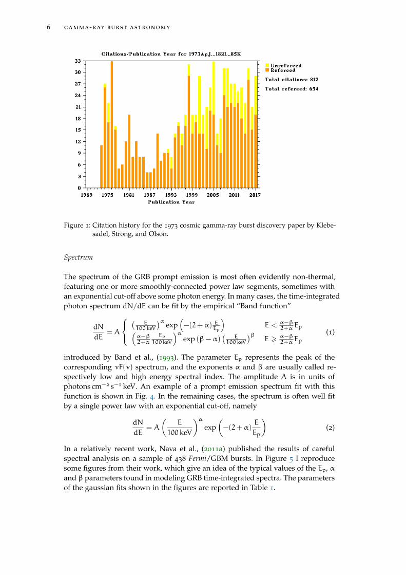
The first observation of a Gamma Ray Burst dates back to 1967 (Bonnell and Klebe-sadel, 1996), but its announcement was made only in 1973 in a letter to ApJ by R.W. Klebesadel (Klebesadel, Strong, and Olson, 1973), due to the initial difficultiesin discriminating this and some other similar events from the frequent false trig-gers of the instruments aboard the Vela satellites - a series of US satellites inspiredby a nuclear test ban treaty, which serendipitously allowed for this discovery - andto the need of more data to confirm the cosmic origin of such events. The newsignited the astronomical community, as can be evinced from Figure 1, where the ci-tation history for the original work by Klebesadel and collaborators is shown (thefigure was produced by querying the SAO/NASA Astrophysics Data System1).The Compton Gamma Ray Observatory (CGRO), launched in 1991, collected thefirst large sample of gamma-ray bursts, providing strong evidence for a uniformsky distribution (see Figure 2) and showing that their cumulative fluence distribu-tion does not follow the -3/2 power law expected for a homogeneous populationof sources in Euclidean space (Meegan et al., 1992). This was the first compellingevidence against a Galactic origin.

No search for optical counterparts of GRBs had been successful at that time,though, so that no redshift measurement (and thus no intrinsic energy estimate)was available yet. If GRBs were extragalactic, the huge energy release and the fastvariability suggested (Paczynski and Rhoads, 1993) that a slowly fading emission(called afterglow) at longer wavelengths (from X-ray down to Radio) should fol-low the main event. The search for such emission did not produce results until1997, when the first X-ray afterglow was observed by BeppoSAX 3 following theburst GRB970228 (Costa et al., 1997). Soon later the afterglow of another event,GRB970508, was observed and finally led to the first redshift measurement (Re-ichart, 1998; Metzger et al., 1997) of a GRB, namely z = 0.835. This showed thatGRBs are among the most powerful photon-emitters known in the Universe.

the prompt emission

After the discovery of the afterglow, a distinction between the initial gamma-raysand the subsequent longer wavelength counterpart became necessary. Hereafter, Iadopt the name “prompt emission” to indicate the initial highly variable, short du-ration (less than 1000 seconds in the vast majority of cases) hard-X-ray and gamma-ray signal detected by instruments such as Swift/BAT, Fermi/GBM, CGRO/BATSE,INTEGRAL/SPI-ACS and the like. Some example light curves constructed usingCGRO/BATSE data are shown in Figure 3.

1 http://adsabs.harvard.edu/

5

6 gamma-ray burst astronomy

Figure 1: Citation history for the 1973 cosmic gamma-ray burst discovery paper by Klebe-sadel, Strong, and Olson.

Spectrum

The spectrum of the GRB prompt emission is most often evidently non-thermal,featuring one or more smoothly-connected power law segments, sometimes withan exponential cut-off above some photon energy. In many cases, the time-integratedphoton spectrum dN/dE can be fit by the empirical “Band function”

dN

dE= A

(

E100 keV

)αexp

(−(2+α) EEp

)E < α−β

2+αEp(α−β2+α

Ep100 keV

)αexp (β−α)

(E

100 keV

)βE > α−β

2+αEp(1)

introduced by Band et al., (1993). The parameter Ep represents the peak of thecorresponding νF(ν) spectrum, and the exponents α and β are usually called re-spectively low and high energy spectral index. The amplitude A is in units ofphotons cm−2 s−1 keV. An example of a prompt emission spectrum fit with thisfunction is shown in Fig. 4. In the remaining cases, the spectrum is often well fitby a single power law with an exponential cut-off, namely

dN

dE= A

(E

100 keV

)αexp

(−(2+α)

E

Ep

)(2)

In a relatively recent work, Nava et al., (2011a) published the results of carefulspectral analysis on a sample of 438 Fermi/GBM bursts. In Figure 5 I reproducesome figures from their work, which give an idea of the typical values of the Ep, αand β parameters found in modeling GRB time-integrated spectra. The parametersof the gaussian fits shown in the figures are reported in Table 1.

2.2 the prompt emission 7

+90

-90

-180+

180

2704 BA

TS

E G

amm

a-Ray B

ursts

10-7

10-6

10-5

10-4

Fluence, 50-300 keV

(ergs cm-2)

Figure 2: Sky distribution of GRBs detected by CGRO/BATSE, from https://gammaray.

nsstc.nasa.gov/batse/grb/skymap/.

8 gamma-ray burst astronomy

150

100

50

0−5 60 −5 40

Time (s)

50

Time (s) Time (s)

−5 20

Time (s)

−20 80 −2 8

−5 20

Time (s)

−2 40 −2 50

−2 50

−5 100

50 300

Time (s)

Time (s)

Time (s)

Time (s)

Time (s)

Time (s)

Time (s)

20

15

10

5

0

20

15

10

5

0

30

25

20

15

10

5

0

18

16

14

12

10

8

6

12

10

8

6

4

2

2

400

300

200

100

0

9

8

7

6

5

4

3

6

5

4

3

100

80

60

40

20

0

12

10

8

6

4

2

150

100

50

0

GRB 910503Trig #143

GRB 910711Trig #512

GRB 920216BTrig #1406

GRB 920221Trig #1425

GRB 921003ATrig #1974

GRB 921022BTrig #1997

GRB 921123ATrig #2067

GRB 930131ATrig #2151

GRB 931008CTrig #2571

GRB 940210Trig #2812

GRB 990316ATrig #7475

GRB 991216Trig #7906

Figure 3: Light curves of 12 bright gamma-ray bursts detected by CGRO/BATSE. Thevertical axes are in units of thousands of detector counts per second. Figurecreated by Daniel Perley with data from the public BATSE archive (https://gammaray.nsstc.nasa.gov/batse/grb/catalog/).

2.2 the prompt emission 9

Figure 4: The datapoints (coloured crosses in the right-hand panel) represent Fermi/GBMobservations of a GRB spectrum, corresponding to the photons in the hatchedpart of the light curve shown in the left-hand panel. The black solid line is afit with the Band function described in the text. Reproduced from Tierney et al.,(2013).

Figure 5: Distributions of spectral parameters in a sample of 438 GRBs detected byFermi/GBM analyzed by Nava et al., (2011a). Blue histograms refer to LongGRBs (duration longer than 2 s), red histograms refer to Short GRBs, and blackhistograms refer to the whole sample.

Parameter Type # of GRBs Central value σ

Log(Ep) All 318 2.27 0.40

Short 44 2.69 0.19

Long 272 2.21 0.36

α All 318 –0.86 0.39

Short 44 –0.50 0.40

Long 274 –0.92 0.35

Table 1: Parameters of the gaussian fits to the distributions of Fermi/GBM burst spectralparameters as analyzed in Nava et al., (2011a).

10 gamma-ray burst astronomy

Short Long

Figure 6: Distribution of T90 for all GRBs detected by CGRO/BATSE. From https://

gammaray.nsstc.nasa.gov/batse/grb/duration/.

Duration

When I learnt about the existence of gamma-ray bursts, I was amazed by theirshort duration. I had been told that astronomical time scales were huge comparedto our lives – but these events, instead, can be as fast as lightning! A precise mea-surement of their duration is not trivial, because of many practical issues suchas the relatively narrow band of the detectors, the uncertainty in distinguishingthe signal from the background in the dim part of the lightcurve, the presenceof quiescent phases. A simple and widely adopted definition of their duration isthe time T90 over which 90 percent of the detector counts above the backgroundare recorded, leaving out the first and the last five percent. Such definition clearlydepends on the instrument band, on its sensitivity, and on the background model,but it is practical in many cases, and it is a standard piece of information givenin catalogues. Figure 6 shows the distribution of T90 for all bursts detected byCGRO/BATSE. The distribution is clearly bimodal, and can be fit by a mixture oftwo log-normal distributions (Kouveliotou et al., 1993), which overlap at approx-imately 2 s. This is the historical reason of the distinction between Short GRBs(T90 < 2 s) and Long GRBs (T90 > 2 s).

the afterglow

Since its discovery in 1997, afterglow emission has been routinely observed in thefollow-up of many GRBs. The observed behaviour is rather diverse, but I will tryto identify some general features in order to get to a broad description of theirobservational appearance.

Temporal evolution

Let me divide the afterglow evolution into four stages: early afterglow (minutesto hours after the prompt emission), normal decay phase (few days), steep decayphase (from one week to few months), late afterglow (months to years). Before thelaunch of Swift, the “normal decay phase” was the one most commonly observed:

2.3 the afterglow 11

102 103 104 105 106

Time after prompt [seconds]

10 4

10 3

10 2

10 1

100

101F

lux

dens

ity

[Jy

]

10 14

10 13

10 12

10 11

10 10

10 9

erg

s1 c

m2 k

eV1

10 1 100 101 102 103

Time after prompt [hours]

10 1

100

101

102

103

104

Flu

x de

nsit

y [

Jy]

14

16

18

20

22

24

26

AB

mag

nitu

de

10 1 100 101 102

Time after prompt [days]

101

102

Flux

den

sity

[Jy

]

Figure 7: Observed afterglows of short gamma-ray bursts. In all panels, grey triangles rep-resent 3 sigma upper limits, while solid lines represent detections. For radioobservations only the one sigma uncertainty is represented by the error bars.Upper panel: flux densities from spacecraft X-ray observations at 1 keV. Middlepanel: flux densities and corresponding AB magnitudes from Earth-based obser-vations in the optical and near-infrared. Lower panel: flux densities from radioobservations between 1 and 10 GHz. All data are from the catalogues of Fonget al., (2015).

12 gamma-ray burst astronomy

not many bursts were well localized, and hours to days were usually needed tostart the follow-up, during which the emission faded significantly. When observedin X-ray and in optical, this phase usually features a power law behaviour bothin frequency and in time, i. e. Fν ∝ ναtβ, with the temporal decay index beingβ ∼ −1. The automatic, rapid repointing system of Swift (Gehrels, Ramirez-Ruiz,and Fox, 2009) enabled observations of the “early” phase, where a more complexbehaviour is often found (see e. g. Kann et al., 2010), which often involves thepresence of an early peak and a subsequent steeper (or sometimes shallower) decaywith respect to the normal decay phase. If the afterglow is sufficiently bright, itcan still be observable after a few days or weeks, after which often it shows anachromatic steepening of the temporal decay index (the “steep decay phase”). The“late afterglow” phase is uniquely observed in the Radio, and it usually shows noevident temporal evolution.

Afterglow spectra

GRB afterglows have been detected in a very wide range of frequencies, fromGeV gamma-rays (with instruments such as LAT onboard Fermi) down to lessthan 1 GHz in radio. As stated in the preceding paragraph, GRB afterglow spectrafeature a non-thermal spectrum. Broadband simultaneous spectral energy distri-butions (SEDs) reveal the presence of spectral breaks, showing that the spectrumis composed of multiple, smoothly connected power law branches. The spectralbreak frequencies are seen to evolve during time, and the peak of the spectrum tomove towards lower frequencies.

The blastwave interpretation

The above observations are most commonly interpreted as being caused by a blast-wave expanding into the interstellar medium (ISM) surrounding the GRB progeni-tor. After producing the prompt emission, the GRB ejecta move at relativistic speedand they expand into the ISM, sweeping it. As soon as the rest mass of the collectedISM becomes comparable to the kinetic energy of the ejecta, a strong shock waveis formed. At the shock, electrons are accelerated by the Fermi process and radi-ate mainly by synchrotron emission. As long as the expansion is ultra-relativistic,the structure of the blastwave and its deceleration evolve in a self-similar fash-ion (Blandford and McKee, 1976). When the blastwave becomes mildly relativistic(Lorentz factor Γ . 3) a slow transition to the Newtonian regime takes place, afterwhich the system resembles a supernova remnant.

presence of a jet

Right after the discovery of the first GRB afterglow, Rhoads, (1997) argued thatif the afterglow emission comes from material collimated into a jet, rather thanfrom an isotropic explosion, then the behaviour of the light curve must changequalitatively after the reciprocal of the bulk Lorentz factor Γ−1 becomes compa-rable to the jet half-opening angle θjet. The qualitative change corresponds to anachromatic steepening of the decay of the light curve, usually called “jet break”.

2.4 presence of a jet 13

1 101 102 103 104 105 106 107

Time since BAT trigger (s)

Flux

(arb

itrar

ily s

cale

d)

GRB050315GRB050319GRB050505

GRB050713B

GRB050814GRB050820A

GRB051016BGRB051109A

GRB051221A

GRB060109GRB060204B

GRB060428AGRB060510A

GRB060605

GRB060614

GRB060707

GRB060729

GRB060807

GRB060813

GRB060814GRB061019

GRB061021

GRB061222A

GRB070129

GRB070306

GRB070328

GRB070419B

GRB070420

Figure 8: Possible jet breaks in the X-ray afterglow light curves of a sample of Swift gamma-ray bursts. The break time is shown by a vertical bar. Reproduced from Racusinet al., (2009).

14 gamma-ray burst astronomy

Quantitative predictions for the afterglow of jetted GRBs were published two yearslater (Rhoads, 1999), just before the first clear observation of a jet break in the op-tical and radio light curve of GRB990510 (Harrison et al., 1999). Despite quiteconvincing jet breaks have been found in several afterglow light curves in the fol-lowing years (see Fig. 8 for some examples), some afterglows do not show anyachromatic steepening up to several days after the prompt emission, suggestingthat the distribution of jet opening angles could be wide, or that some ingredientsare missing in standard afterglow modeling.

progenitors

A typical Long GRB has a fluence of the order of 10−5 erg cm−2 and it is lo-cated at a redshift z ∼ 1.5. This implies an isotropic equivalent energy releaseof 1052 erg. The presence of afterglow radiation indicates that the energy radi-ated in the prompt emission is only a fraction of the kinetic energy of the ejecta,which can be 10 times as energetic. If the ejecta are collimated, though, the actual(collimation-corrected) kinetic energy content is lowered by a factor ∼ θ2jet. The re-sult is still of the order of 1051 erg. This huge energy must be liberated in a processthat produces variability on the millisecond time-scale. Accretion on a stellar blackhole has a high enough efficiency and happens in a compact enough region to becompatible with the energy and variability time-scale requirements. The transientnature of GRBs, moreover, suggests that such accretion must be linked to a catas-trophic event. All these pieces of information, when gathered together, suggestthat GRBs are linked to the birth of a stellar black hole.

Long versus Short, Collapsar versus Non-Collapsar

The natural birthplaces of stellar black holes are two: the collapse of a massive starand the coalescence of two compact objects. The latter was the first to be identifiedas a promising GRB progenitor candidate (Eichler et al., 1989), followed a few yearslater by the former (Woosley, 1993). In 1998, the observation of supernova 1998bwassociated to the close-by GRB980425 (Galama et al., 1998) provided compellingevidence for the collapse of a massive star (later dubbed the “collapsar scenario”MacFadyen and Woosley, 1999). In the following years, several secure associationsbetween GRBs and supernovae have been made. On the other hand, the searchfor supernovae associated to nearby short GRBs always led to (sometimes verystringent) upper limits so far (Berger, 2014a). For this class of GRBs the coalescenceof two compact objects is thus the favoured scenario.

3T RY I N G T O G E T A G R A S P O F T H E S H O RT G R B P O P U L AT I O N

briefing

When somewhat more than a few events of a particular class have been observed, afundamental question is whether the properties of the observed sample can informus, in a statistical sense, about the instrinsic properties of the whole population.In astronomy there is usually no guarantee that a sample is representative, so thatparticular care has to be put in modeling selection effects and trying to keep themunder control. Moreover, in most cases only incomplete information is available:for example, most known GRBs have no redshift measurement, thus their intrinsicluminosity or energy cannot be derived. In this chapter I will present how theseproblems have been dealt with, in the case of short gamma-ray bursts (SGRBs),in a recent work led by Giancarlo Ghirlanda and me (Ghirlanda et al., 2016). Ourapproach led us to define the first model of the SGRB population able to explain allthe statistical properties of the observed population. Based on this model, we madepredictions for the rate of SGRBs to be observed in association with gravitationalwaves (GW) from compact binary mergers in the upcoming runs of AdvancedLIGO and Virgo. In the following sections, I present the approach and results. Atthe end of the chapter, I comment on the results in light of the recent developmentfollowing the observation of GW170817 and its electromagnetic counterparts.

introduction

The instrinsic properties of the SGRB population are still poorly understood, partlybecause of the small number of events with measured redshift (see e.g. Berger,2014b; D’Avanzo, 2015, for recent reviews). Rather sparse information about theorigin of these events is available, but the low density of the circum-burst medium(Fong and Berger, 2013; Fong et al., 2015a), the variety of galaxy morphologies(e.g. D’Avanzo, 2015), the lack of any associated supernova in nearby SGRBs, andthe possible recent detection of a “kilonova” (Eichler et al., 1989; Li and Paczynski,1998; Yang et al., 2015a; Yang et al., 2015b; Jin et al., 2016; Jin et al., 2015) signature(Berger, Fong, and Chornock, 2013; Tanvir et al., 2013), all hint at the merger oftwo compact objects (e.g. double neutron stars) rather than a single massive starcollapse as in long GRBs.

On the other hand, the prompt γ-ray emission properties of SGRBs (Ghirlandaet al., 2009; Ghirlanda et al., 2015), the sustained long-lasting X-ray emission (al-though not ubiquitous in short GRBs; Sakamoto and Gehrels 2009) and flaringactivity suggest that the central engine and radiation mechanisms are similar tothose of long GRBs. Despite this is based on a few breaks in the optical light curves,it seems also that SGRBs have jets: current measures of θjet are between 3

and 15,

while lower limits seem to suggest a wider distribution (e.g. Berger, 2014b; Fonget al., 2015b).

15

16 trying to get a grasp of the short grb population

If the progenitors are compact object binaries (made of two neutron stars – “NS-NS” – or of a neutron star and a black hole – “NS-BH”), SGRBs are among the mostpromising electromagnetic counterparts of GW events detectable by advanced in-terferometers. The rate of association of GW events with SGRBs is mainly deter-mined by the rate of SGRBs within the relatively small horizon set by the sensitiv-ity of aLIGO and Advanced Virgo (Abbott et al., 2016). However, estimates of thelocal SGRB rates vary from 0.1–0.6 Gpc−3 yr−1 (e.g. Guetta & Piran 2005; 2006) to1–10 Gpc−3 yr−1 (Guetta and Piran, 2006; Guetta and Stella, 2009; Coward et al.,2012; Siellez, Boër, and Gendre, 2014; Wanderman and Piran, 2015) to even largervalues, e.g. 40-240 Gpc−3 yr−1 (Nakar, Gal-Yam, and Fox, 2006; Guetta and Piran,2006). These rates are not corrected for the collimation angle, i.e. they represent thefraction of bursts whose jets are pointed towards the Earth, whose γ–ray promptemission can be detected.

These rate estimates depend mainly on the luminosity function φ(L) and red-shift distribution Ψ(z) of SGRBs. These functions are usually derived by fittingthe peak flux distribution of SGRBs detected by BATSE (Guetta and Piran, 2005;Guetta and Piran, 2006; Nakar, Gal-Yam, and Fox, 2006; Hopman et al., 2006; Sal-vaterra et al., 2008). Owing to the degeneracies in the parameter space (whenboth φ(L) and Ψ(z) are parametric functions), the redshift distribution is also con-strained by comparison with that constructed from the few SGRBs with measuredz.

The luminosity function φ(L) is typically modelled as a single or broken powerlaw, and in most cases it is found to be similar to that of long GRBs (i.e. propor-tional to L−1 and L−2 below and above a characteristic break ∼ 1051−52 erg s−1;Guetta and Piran, 2006; Salvaterra et al., 2008; Virgili et al., 2011; D’Avanzo et al.,2014, hereafter D14) or much steeper (L−2 and L−3; Wanderman and Piran, 2015,hereafter WP15). Aside from the mainstream, Shahmoradi and Nemiroff, 2015

modelled all the distributions with lognormal functions.The redshift distribution Ψ(z) (the number of SGRBs per comoving unit vol-

ume and time, as a function of redshift z) has always been assumed to followthe cosmic star formation rate convolved with a delay time distribution, which ac-counts for the time necessary for the progenitor binary system to merge. With thisassumption, various authors derived the delay time τ distribution, which couldbe a single power law P(τ) ∝ τ−δ (e.g. with δ = 1 − 2; Guetta and Piran 2005,2006; D14; WP15) with a minimum delay time τmin = 10− 20 Myr, or a peaked(lognormal) distribution with a considerably large delay (e.g. 2–4 Gyr, Nakar andGal-Yam 2005; WP15). Alternatively, the population could be described by a com-bination of prompt mergers (small delays) and large delays (Virgili et al., 2011) orto the combination of two progenitor channels, i.e. binaries formed in the field ordynamically within globular clusters (e.g. Salvaterra et al., 2008).

Many past works feature a common approach: parametric forms are assumedfor the compact binary merger delay time distribution and for the SGRB luminos-ity function; free parameters of these functions are then constrained through thesmall sample of SGRBs with measured redshift, and through the distribution ofthe γ–ray peak fluxes of SGRBs detected by past and/or present GRB detectors.A number of other observer frame properties, though, are available and have notbeen used: fluence distribution, duration distribution, observer frame peak energy.The last of these has been considered in Shahmoradi and Nemiroff, (2015) which,

3.3 selecting a good sample 17

however, lacks a comparison with rest–frame properties of SGRBs as is done inthis chapter. Another relevant issue with many previous works is the compari-son of the model predictions with small and incomplete samples of SGRBs withmeasured z. Indeed, only recently D14 have constructed a flux-limited completesample of SGRBs detected by Swift.

The aim of this chapter is to present a model of the SGRB population, whoseredshift distribution Ψ(z) and luminosity function φ(L) are constrained using allthe available observational constraints of the large sample of bursts detected byFermi/GBM. These constraints are the (1) peak flux, (2) fluence, (3) observer frameduration and (4) observer frame peak energy distributions. Additionally, I alsoconsider as constraints (5) the redshift distribution, (6) the isotropic energy, and(7) the isotropic luminosity of a complete sample of SGRBs detected by Swift(D14). This is the first time that the φ(L) and Ψ(z) of SGRBs are constrained using2–4 and 6–7. In the formulation of the model, I do not assume any delay timedistribution for SGRBs, but I assume a quite general parametric form and derivedirectly its parameters.

In §3.3 I describe a sample of SGRBs (without measured redshifts) detected byFermi/GBM, which provides the observer-frame constraints 1–4, and the complete(though smaller) sample of Swift SGRBs of D14, which provides the rest-frameconstraints 5–7. In §3.6 I show that that a steep φ(L) is excluded when all theavailable constraints (1–7) are considered. In §3.7 I show a Monte Carlo approachto derive the parameters describing the φ(L) and Ψ(z) of SGRBs. In §3.9 the resultson the φ(L) and Ψ(z) of SGRBs are presented and discussed. I assume a standardflat ΛCDM cosmology with H0 = 70 km s−1 Mpc−1 and Ωm = 0.3 throughoutthis chapter.

selecting a good sample

As stated in the preceding section, the luminosity function and redshift distribu-tion of SGRBs have been derived by many authors by taking into account thefollowing two constraints:

1. the peak flux distribution of large samples of SGRBs detected by CGRO/BATSEor Fermi/GBM;

2. the redshift distribution of the SGRBs with measured z.

However, a considerable amount of additional information on the prompt γ-rayemission of SGRBs can be extracted from the BATSE and GBM samples. In par-ticular, we can learn more about these sources by considering the distributionsof

3. the peak energy Ep,o of the observed νFν spectrum;

4. the fluence F;

5. the duration T90.

Moreover, for the handful of events with known redshift z, we have also access tothe1

1 To avoid too much redundancy, throughout this chapter I will sometimes drop the “iso” subscript,so that Liso and Eiso will be equivalently written as L and E. For the same reason, the peak energy

18 trying to get a grasp of the short grb population

6. isotropic luminosity Liso;

7. isotropic energy Eiso.

Observer-frame constraints: a flux-limited Fermi/GBM sample

For the distributions of the observer frame prompt emission properties (constraints1, 3, 4, 5) I consider the sample of 1767 GRBs detected by Fermi/GBM (from 080714

to 160118) as reported in the online spectral catalogue2. It contains most of theGRBs published in the second spectral catalogue of Fermi/GBM bursts (relativeto the first four years) (Gruber et al., 2014), plus events detected by the satellite in2015 and 2016. 295 events in the sample are SGRBs (i.e. with T90 6 2 s). Accordingto Bromberg et al., 2013, for both the Fermi and CGRO GRB populations, this du-ration threshold should limit the contamination from collapsar-GRBs to less than10% (see also WP15).

I only select bursts with a peak flux (computed on 64ms timescale in the 10-1000

keV energy range) larger than 5 ph cm−2 s−1 in order to work with a well-definedsample, less affected by the incompleteness close to the detector limiting flux. Withthis selection, the sample reduces to 211 SGRBs, detected by Fermi/GBM in 7.5years within its field of view of ∼70% of the sky.I consider the following prompt emission properties of the bursts in the sample tobe used as constraints of the population synthesis model:

• the distribution of the 64ms peak flux P64 (integrated in the 10-1000 keVenergy range). This is shown by black symbols in the top left panel of Fig. 9;

• the distribution of the observed peak energy of the prompt emission spec-trum Ep,o (black symbols, bottom left panel in Fig. 9);

• the distribution of the fluence F (in the 10–1000 keV energy range) (blacksymbols, bottom middle panel in Fig. 9);

• the distribution of the duration T90 of the prompt emission (black symbols,bottom right panel in Fig. 9);

Short GRB spectra have a typical observer frame peak energy Ep,o distribution(e.g. Ghirlanda et al., 2009; Nava et al., 2011b; Gruber et al., 2014) centred at rel-atively large values (∼ 0.5 − 1 MeV), as is also shown by the distribution in thebottom left panel of Fig. 9. For this reason, I adopt here the peak flux P64 andfluence F computed in the wide 10–1000 keV energy range as provided in the spec-tral catalogue of Fermi bursts rather than the typically adopted 50–300 keV peakflux (e.g. from the BATSE archive), which would sample only a portion of the fullspectral curvature.

The distributions of the peak flux, fluence, peak energy, and duration are shownin Fig. 9 with black symbols. Error bars are computed by resampling each mea-surement (P, F, Ep,o, and T90) from a normal distribution with a sigma equal tothe measurement uncertainty. For each bin, the vertical error bars represent thestandard deviations of the bin heights of the resampled distributions.

Epeak,obs (Epeak,rest) of the νF(ν) spectrum in the observer frame (in the local cosmological rest frame)will be sometimes written as Ep,o (Ep).

2 https://heasarc.gsfc.nasa.gov/W3Browse/fermi/fermigbrst.html

3.4 a sensible parametrization of the φ(L) and Ψ(z) 19

Rest-frame constraints: the Swift SBAT4 sample

For the redshift distribution and the rest frame properties of SGRBs (constraints 2,6, and 7) I consider the sample published in D14. It consists of bursts detected bySwift, selected with criteria similar to those adopted for long GRBs in Salvaterraet al., 2012, with a peak flux (integrated in the 15–150 keV energy range and com-puted on a 64 ms timescale) P64 > 3.5 photons cm−2 s−1. This corresponds toa flux which is approximately four times larger than the Swift–BAT minimumdetectable flux on this timescale; for this reason, I call this sample SBAT4 (ShortBAT 4). The redshift distribution of the SBAT4 sample is shown in the top rightpanel of Fig. 9 (solid black line). Within the SBAT4 sample I consider the 11 GRBswith known z and determined Liso and Eiso (the distributions of these quantitiesare shown in the inset of Fig. 9, top right panel, with black and grey lines re-spectively). The grey shaded region shows how the distribution changes when thefive SGRBs in the sample with unknown z are all assigned the minimum or themaximum redshift of the sample.

a sensible parametrization of the φ(L) and Ψ(z)

Given the incompleteness of the available SGRB samples, particularly with mea-sured z, no direct method as for the population of long GRBs; see e.g. Pescalliet al., 2016 can be applied to derive the shape of the SGRB luminosity functionφ(L) and redshift distribution Ψ(z) from the observations. The typical approachin this case consists in assuming some simple analytical shape for both functions,with free parameters to be determined by comparison of model predictions withobservations.

For the luminosity function, a power law

φ(L) ∝ L−α (3)

or a broken power law

φ(L) ∝

(L/Lb)

−α1 L < Lb

(L/Lb)−α2 L > Lb

(4)

normalized to its integral is usually assumed. I will assume the latter.If SGRBs are produced by the merger of compact objects, their redshift distribu-

tion should follow a “retarded” star formation,

Ψ(z) =

∫∞z

ψ(z ′)P [t(z) − t(z ′)]dt

dz ′dz ′ (5)

where ψ(z) represents the formation rate of SGRB progenitors per comovingGpc−3 yr−1 , and P(τ) is the delay time distribution, i.e. the probability den-sity function of the delay τ between the formation of the progenitors and theirmerger (which produces the SGRB). Adopting the point of view that SGRBs areproduced by the coalescence of a NS-NS (or BH-NS) binary, one can assume adelay time distribution and convolve it with a ψ(z) of choice to obtain the corre-sponding SGRB formation rate Ψ(z). Theoretical considerations and population

20 trying to get a grasp of the short grb population

Figure 9: Black dots show the distributions obtained from the Fermi/GBM and SwiftSBAT4 samples (§3.3). Horizontal error bars are the bin widths, while verticalerror bars are 1σ errors on the bin heights accounting for experimental errorson single measurements. The results of the Monte Carlo population synthesiscode are shown by solid red lines (for the model in which Ep − Liso and Ep −Eisocorrelations are assumed to hold) and by triple dot-dashed orange lines (for themodel with no correlations). Predictions based on the models of D14 and WP15

are shown by dashed blue and dot-dashed cyan lines, respectively (the latter onlyin the first three panels; see the text). These are obtained by analytical methodsof §3.5. Top left panel: Distribution of the peak flux P of the Fermi/GBM sample.Top right panel: Normalized cumulative redshift distribution of the SBAT4 sample.The grey shaded area represents the change in the distribution if the remainingbursts with unknown z are all assigned the largest or the lowest z of the sam-ple. The inset shows the cumulative distributions of the isotropic luminosity Liso(solid black line) and energy Eiso (solid grey line) of the same sample. Bottompanels: From left to right, distributions of peak energy Ep,o, fluence, and durationof SGRBs of the Fermi/GBM sample.

3.4 a sensible parametrization of the φ(L) and Ψ(z) 21

synthesis (Portegies Zwart and Yungelson, 1998; Schneider et al., 2001; Belczyn-ski et al., 2006; O’Shaughnessy, Belczynski, and Kalogera, 2008; Dominik et al.,2013) suggest that compact binary coalescences should typically follow a delaytime distribution P(τ) ∝ τ−1 with τ & 10 Myr. Equation 5 is actually a simpli-fication, in that it implicitly assumes that the fraction of compact binaries withrespect to all stars formed does not depend on redshift. The actual fraction verylikely depends on metallicity and on the initial mass function, and thus indirectlyon redshift. Moreover, the star formation history itself is affected by uncertainties,which affect the result of the convolution. To make the analysis as general as pos-sible, I thus prefer to adopt a generic parametric form for the redshift distributionΨ(z) of SGRBs. A posteriori, the delay time distribution (in the compact binaryprogenitor scenario) can be recovered by direct comparison of the result with thestar formation history of choice. I parametrize the Ψ(z) following Cole et al., 2001,namely

Ψ(z) =1+ p1z

1+(z/zp

)p2 (6)

which rises and then decays (for p1 > 0, p2 > 1), with a peak roughly3 correspond-ing to zp;

Two past works

Let me now consider the works of D14 and WP15 in more detail, which will beuseful as a comparison.

D’Avanzo et al. (2014) assume a power law shape for both the φ(L) and thedelay time distribution P(τ), and they adopt the parametric form of Cole et al.,2001 for the cosmic star formation history, with parameter values taken from Hop-kins and Beacom, 2006. They assume that SGRBs follow the Ep − Liso correlationEpeak = 337keV(Liso/2× 1052ergs−1)0.49 and that their spectrum is a Band function(Band et al., 1993) with low and high energy photon spectral indices -0.6 and -2.3,respectively. They constrain the free parameters by fitting the BATSE peak flux dis-tribution and the redshift distribution of bright Swift short bursts with measured z.They find φ(L) ∝ L−2.17 between 1049 erg s−1 and 1055 erg s−1, and P(τ) ∝ τ−1.5

with a minimum delay of 20 Myr. The blue dashed lines in Fig. 9 are obtainedthrough Eq. 4 and Eq. 5 using the same parameters as D14: their model (limitedto Plim > 5 ph cm−2 s−1 in order to be compared with the sample selected in thiswork) reproduces correctly the peak flux distribution (top left panel of Fig. 9) ofFermi SGRBs and the redshift distribution of the bright SGRBs detected by Swift(top right panel).

The preferred model for φ(L) in WP15 is a broken power law, with a break at2× 1052 erg s−1 and pre- and post-break slopes of −1.9 and −3.0, respectively.Their preferred models are either a power law delay time distribution P(τ) ∝τ−0.81 with a minimum delay of 20 Myr or a lognormal delay time distributionwith central value 2.9 Gyr and sigma 6 0.2. Differently from D14, rather thanassuming the Ep − Liso correlation they assign to all SGRBs a fixed rest frame

3 The exact peak is not analytical, but a good approximation is zpeak ≈zpp2[1+ 1/

(p1 zp

)]− 1−1/p2 .

22 trying to get a grasp of the short grb population

Ep,rest = 800 keV. The dot-dashed cyan lines in Fig. 9 are the model of WP15 (forthe lognormal P(τ) case).

In the following I show how the results of WP15 and D14, both representativeof a relatively steep luminosity function, compare with the other additional con-straints (bottom panels of Fig. 9) that I consider in this chapter.

from population properties to observables

Given the two functions φ(L) and Ψ(z), the peak flux distribution can be derivedas

N(P1 < P < P2) =∆Ω

4π

∫∞0

dzdV(z)

dz

Ψ(z)

1+ z

∫L(P2,z)L(P1,z)

φ(L)dL, (7)

where ∆Ω/4π is the fraction of sky covered by the instrument/detector (whichprovides the real GRB population with which the model is to be compared) anddV(z)/dz is the differential comoving volume. The flux P corresponding to theluminosity L at redshift z is4

P(L, z, Epeak, α) =L

4πdL(z)2

∫ε2(1+z)ε1(1+z)

N(E|Epeak, α)dE∫∞0 EN(E|Epeak, α)dE

, (8)

where dL(z) is the luminosity distance at redshift z and N(E|Epeak, α) is the restframe photon spectrum of the GRB. The photon flux P is computed in the restframe energy range [(1+ z)ε1, (1+ z)ε2], which corresponds to the observer frame[ε1, ε2] band.

The SGRB spectrum is often assumed to be a cut-off power law, i.e.N(E|Epeak, α) ∝E−α exp(−E(2− α)/Epeak), or a Band function (Band et al., 1993). Typical parame-ter values are α ∼ 0.6 (i.e. the central value of the population of SGRBs detectedby BATSE and Fermi - Ghirlanda et al., 2009; Nava et al., 2011b; Goldstein andPreece, 2010; Gruber et al., 2014) and, for the Band function, β ∼ 2.3 − 2.5. Thepeak energy is either taken as fixed (e.g. 800 keV in WP15) or derived assumingthat SGRBs follow a Ep −Liso correlation in analogy to long bursts (e.g. D14; Virgiliet al., 2011). Recent evidence supports the existence of such a correlation amongSGRBs (see e.g. D14; Calderone et al., 2015; Tsutsui et al., 2013; Ghirlanda et al.,2009) with similar parameters to those present in the population of long GRBs(Yonetoku et al., 2004).

In order to compare the model peak flux distribution obtained from Eq. 7 withthe real population of GRBs, only events with peak flux above a certain thresholdPlim are considered. The integral in Eq. 7 is thus performed over the (L, z) rangewhere the corresponding flux is larger than Plim.

In D14 the assumption of the correlation (Ep − Liso) between the isotropic lumi-nosity Liso and the rest frame peak energy Ep also allows one to derive, from Eq. 7,the expected distribution of the observer frame peak energy Ep,o,

N(E1,p,o < E < E2,p,o) =

∫∞0

dzC(z)

∫L(E2,p,o,z)L(E1p,o,z)

φ(L)dL, (9)

4 The assumption of a spectrum is required to convert the bolometric flux into a characteristic energyrange for comparison with real bursts.

3.6 a too steep luminosity function is at odds with the observer-frame constraints 23

where Ep,o is the peak energy of the observed ν F(ν) spectrum, and I set C(z) =

[∆Ω/4π][Ψ(z)/(1 + z)][dV(z)/dz]. The limits of the luminosity integral are com-puted by using the rest frame correlation Ep = Y Lmy , namely

L(Ep,o, z) =

(Ep

Y

)1/my

=

((1+ z)Ep,o

Y

)1/my

. (10)

In order to compare the distribution of Ep,o with real data, the integral in Eq. 9,similarly to Eq. 7, is performed over values of L(Ep,o, z) corresponding to fluxesabove the limiting flux adopted to extract the real GRB sample (e.g. 5 ph cm−2

s−1 for SGRBs selected from the Fermi sample).Similarly, by assuming a Ep −Eiso correlation to hold in SGRBs (see D14; Tsutsui

et al., 2013; Amati, 2006; Calderone et al., 2015), i.e. Ep = AEma , one can derive arelation between luminosity and energy (Liso–Eiso), which reads

L(E) =

(A

Y

)1/my

Ema/my . (11)

This can then be used to compute the fluence distribution, where the fluence isrelated to the isotropic energy as F = E(1+ z)/4πdL(z)2,

N(F1 < F < F2) =

∫∞0

dzC(z)

∫L(E2)L(E1)

φ(L)dL, (12)

again by limiting the integral to luminosities which correspond to fluxes above thegiven limiting flux.

Finally, since the light curves of SGRBs are usually single spikes, one can assumea triangular shape and thus let 2E/L ∼ T in the rest frame of the source. Therefore,it is possible to combine the Ep −Eiso and Ep −Liso correlations to derive the modelpredictions for the distribution of the duration to be compared with the observeddistribution,

N(T1,o < T < T2,o) =

∫∞0

dzC(z)

∫L(T2,o,z)L(T1,o,z)

φ(L)dL, (13)

where

L(To, z) =

[(Y

A

)1/ma 2(1+ z)

To

]1/(1−my/ma)

. (14)

a too steep luminosity function is at odds with the observer-frame

constraints

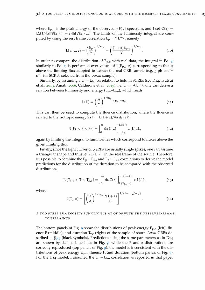
The bottom panels of Fig. 9 show the distributions of peak energy Ep,o (left), flu-ence F (middle), and duration T90 (right) of the sample of short Fermi GRBs de-scribed in §3.3 (black symbols). Predictions using the same parameters as in D14

are shown by dashed blue lines in Fig. 9: while the P and z distributions arecorrectly reproduced (top panels of Fig. 9), the model is inconsistent with the dis-tributions of peak energy Ep,o, fluence F, and duration (bottom panels of Fig. 9).For the D14 model, I assumed the Ep − Eiso correlation as reported in that paper

24 trying to get a grasp of the short grb population

i-th GRB

ϕ(Ep)

z

Ep - Eiso

Ep Eiso Liso

PF T

spectrum

Ep,o

Ep - Liso

Figure 10: Scheme of the procedure followed in the MC to generate the observables ofeach synthetic GRB.

to derive the fluence and (in combination with the Ep − Liso correlation) the dura-tion distribution. Since WP15 assume a unique value of the peak energy Ep,o, itis not possible to derive the fluence and duration of their model unless indepen-dent functions for these parameters are assumed. Therefore, the model of WP15

(dot-dashed cyan line in Fig. 9) is compared only with the peak flux, redshift (toppanels), and observed peak energy (bottom left panel of Fig. 9) distributions.

The figure shows that a steep φ(L) combined with either a power law distri-bution of delay times favouring short delays (as in D14) or a nearly unique longdelay time (as in the log–normal model of WP15) correctly reproduce the observerframe peak flux distribution of Fermi GRBs5 and the redshift distribution of Swiftbright short bursts. However, they do not reproduce the peak energy, fluence, andduration distributions of the same population of Fermi SGRBs.

Motivated by these results, Giancarlo Ghirlanda and I implemented a MonteCarlo (MC) code aimed at deriving the φ(L) and Ψ(z) of SGRBs which satisfyall the constraints (1–7) described above. The reason to choose a MC method isthat it allows for an easy implementation of the dispersion of the correlations (e.g.Ep − Liso and Ep − Eiso) and of any distribution assumed (which are less trivial toaccount for in an analytic approach as that shown above).

a monte carlo simulation of the sgrb population

In this section I describe the Monte Carlo (MC) approach adopted in Ghirlandaet al., (2016) to generate the model population. The approach is based on thefollowing choices:

1. Customarily, Eq. 5 has been used to compute the redshift distribution Ψ(z)of SGRBs from an assumed star formation history ψ(z) and a delay timedistribution P(τ). As stated in §3.4, this approach implies simplifications wewanted to avoid, so the more general form given in Eq. 6 was assumed;

5 Here I consider as a constraint the population of Fermi/GBM GRBs. Nava et al., 2011 showed thatthe BATSE SGRB population has similar prompt emission properties as Fermi SGRBs (peak flux,fluence, and duration distribution).

3.7 a monte carlo simulation of the sgrb population 25

2. In order to avoid inducing spurious correlations, it is convenient to extractEp from an assumed probability distribution and then use the correlationsto associate to it a luminosity and an energy. We considered a broken powerlaw shape for the Ep distribution:

φ(Ep) ∝

(Ep/Ep,b

)−a1 Ep 6 Ep,b(Ep/Ep,b

)−a2 Ep > Ep,b

. (15)

Through the Ep − Liso and Ep − Eiso correlations, also accounting for theirscatter, one can then associate to Ep a luminosity Liso and an energy Eiso. Theluminosity function of the population is then constructed as a result of thisprocedure;

3. We assumed the correlations Ep − Liso and Ep − Eiso written as

log10(Ep/670 keV) = qY +mY log10(L/1052erg s−1) (16)

andlog10(Ep/670 keV) = qA +mA log10(Eiso/10

51erg). (17)

For each GRB, after sampling Ep from Eq. 15, we associated a luminosity(resp. energy) sampled from a lognormal distribution whose central valueis given by Eq. 16 (resp. 17), with σ = 0.2. There are still too few SGRBswith known redshift to measure the scatter of the corresponding correlations.We thus assumed the same scatter found in the correlations holding for thepopulation of long GRBs (Nava et al., 2012);

4. For each GRB, a typical Band function prompt emission spectrum was as-sumed, with low and high photon spectral index −0.6 and −2.5, respectively.We kept these two parameters fixed after checking that our results were un-affected by sampling them from distributions centred around these values6.

For each synthetic GRB, the scheme in Fig. 10 was followed: a redshift z is sam-pled from Ψ(z) and a rest frame peak energy Ep is sampled from φ(Ep); throughthe Ep − Liso (resp. Ep − Eiso) correlation a luminosity Liso (resp. energy Eiso) withlognormal scatter is assigned; using the redshift and luminosity (energy), the peakflux P (fluence F) in the observer frame energy range 10–1000 keV is derived via theassumed spectral shape. The observer frame duration T is obtained as 2(1+ z)E/L,i.e. the light curve is approximated with a triangle. This scheme reflects the proce-dure followed to compute the observer frame quantities in “model (a)”.

The minimum and maximum values of Ep admitted are Ep,min = 0.1 keV andEp,max = 105 keV. These limiting values correspond to a minimum luminosityLmin and a maximum luminosity Lmax which depend on the Ep − Liso correlation.While the maximum luminosity is inessential (in all solutions the high luminosityslope α2 & 2), the existence of a minimum luminosity might affect the observeddistributions. We thus implemented an alternative scheme (“model (b)”) in whichthe minimum luminosity Lmin is a parameter, and values of Ep which correspondto smaller luminosities are rejected.

6 We also made sure that our results were not sensitive to a slightly different choice of the spectralparameters, i.e. low and high energy spectral index −1.0 and −3.0, respectively.

26 trying to get a grasp of the short grb population

In order to investigate the dependence of the results on the assumption of theEp − Liso and Ep − Eiso correlations, we also implemented a third MC scheme(“model (c)”) where independent probability distributions (i.e., independent fromthe peak energy) were assumed for the luminosity and duration. A broken powerlaw

P(L) ∝

(L/Lb)

−α1 L 6 Lb

(L/Lb)−α2 L > Lb

(18)

was assumed for the luminosity distribution, and a lognormal shape

P(Tr) ∝ exp

[−1

2

((log(Tr) − log(Tc)

σTc

)2](19)

was assumed for the rest frame duration Tr = T/(1+ z) probability distribution.Again, the energy of each GRB was computed as E = LTr/2, i.e. the light curvewas approximated with a triangle.

looking for the best fit parameters

In model (a) there are ten free parameters: three (p1, zp, p2) define the redshiftdistribution (Eq. 6), three (a1, a2, Ep,b) define the peak energy distribution (Eq. 15),and four (qY ,mY , qA,mA) define the Ep − Liso and Ep − Eiso correlations (Eqs. 16

and 17). Our constraints are the seven distributions shown in Fig. 9 (including theinsets in the top right panel).

In order to find the best fit values and confidence intervals of our parame-ters, we employed a Markov chain Monte Carlo (MCMC) approach based on theMetropolis-Hastings algorithm (Hastings, 1970). At each step of the MCMC

• we displace each parameter7 pi from the last accepted value. The displace-ment is sampled from a uniform distribution whose maximum width is care-fully tuned in order to avoid the random walk remaining stuck in local max-ima;

• we compute the Kolmogorov-Smirnov (KS) probability PKS,j of each observeddistribution to be drawn from the corresponding model distribution;

• we define the goodness of fit G of the model as the sum of the logarithms ofthese KS probabilities, i.e. G =

∑7j=1 logPKS,j;

• we compare g = exp(G) with a random number r sampled from a uniformdistribution within 0 and 1: if g > r the set of parameters is “accepted”,otherwise it is “rejected”.

We performed tests of the MCMC with different initial parameters, to verify thata unique global maximum of G could be found. Once properly set up, 200,000 stepsof the MCMC were run. After removing the initial burn in, the posterior density

7 For parameters corresponding to slopes, like mY and mA, we actually displace the correspondingangle φ = arctan(m), otherwise a uniform sampling of the displacement would introduce a biastowards high (i.e. steep) slopes.

3.8 looking for the best fit parameters 27

2.55.07.5

10.0

a 2

800

1600

2400

3200

E p,b

0.81.21.62.0

mY

2

1

0

1

2

mA

0.50

0.25

0.00

0.25

q Y

0.30.00.30.60.9

q A

2

4

6

8

p 1

0.81.62.43.2

z p

0.4 0.0 0.4 0.8 1.2

a1

2.55.07.5

10.0

p 2

2.5 5.0 7.5 10.0

a280

016

0024

0032

00

Ep, b

0.8 1.2 1.6 2.0

mY

2 1 0 1 2

mA0.5

00.2

50.0

00.2

5

qY

0.3 0.0 0.3 0.6 0.9

qA

2 4 6 8

p10.8 1.6 2.4 3.2

zp

2.5 5.0 7.5 10.0

p2

Figure 11: Marginalized densities of sampled parameters in model (a) (i.e. with corre-lations and no minimum luminosity). Red lines indicate the means of themarginalized distributions.

28 trying to get a grasp of the short grb population

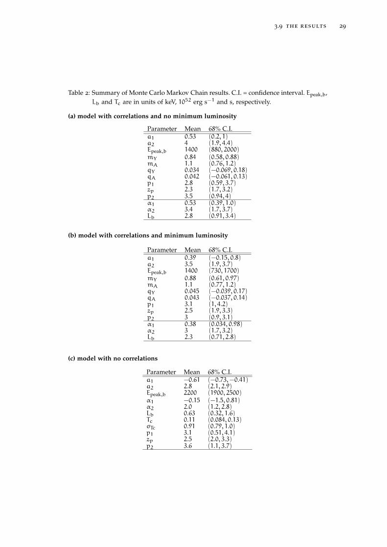
distribution of each parameter (and the joint distribution of each couple of pa-rameters) was extracted with the getDist python package8. The resulting 1D and2D marginalized distributions are shown in Fig. 11, where red lines indicate theposition of the mean of the marginalized density of each parameter. The contoursrepresent the 68% and 95% probability areas of the joint density distributions. Themeans and 68% probability intervals of the 1D marginalized distributions are sum-marized in Table 2.a, where the corresponding luminosity function parameters arealso reported.

For the solution represented by the mean values in Table 2.a, the minimumluminosity is Lmin ∼ 1047 erg s−1. For comparison, we tested case (b) fixing Lmin =

1050 erg s−1. This is the highest minimum luminosity that can be assumed, sincethe lowest SGRB measured luminosity in the Swift sample considered is L =

1.2 × 1050 erg s−1 (D14). Table 2.b summarizes the results of the analysis after200,000 MCMC steps. The two cases are consistent within one sigma. The best fitluminosity function in case (b) is slightly shallower at low luminosities (i.e. thereis a slight decrease in α1) than in case (a), and it remains much shallower than inD14 and WP15.

Finally, we tested model (c) performing 200,000 MCMC steps. In this case, thereare 11 free parameters: three (p1, zp, p2) for Ψ(z) and three (a1, a2, Ep,b) for φ(Ep)

as before, plus three (α1, α2, Lb) for the luminosity function (Eq. 18) and two(Tc, σTc) for the intrinsic duration distribution (Eq. 19). Consistently with model(a) and model (b), we assumed two broken power laws for φ(Ep) and φ(L). The re-sults are listed in Table 2.c. We found that if no correlations are assumed betweenthe spectral peak energy and the luminosity or energy, the luminosity functionand the peak energy distributions become peaked around characteristic values.This result is reminiscent of the findings of Shahmoradi and Nemiroff, 2015 whoassumed lognormal distributions for these quantities.

the results

Luminosity function

In model (a) we found that the luminosity function is shallow (α1 = 0.53+0.47−0.14,

and flatter than 1.0 within the 68% confidence interval) below a break luminosity∼ 3× 1052 erg s−1 and steeper (α2 = 3.4+0.3

−1.7) above this characteristic luminosity.The minimum luminosity ∼ 5× 1047 erg s−1 is set by the minimum Ep coupledwith the Ep −Liso correlation parameters (see §3.7). Similar parameters for the φ(L)are obtained in model (b), where a minimum luminosity was introduced, thusshowing that this result is not strongly dependent on the choice of the minimumluminosity of the φ(L).

Relaxing the assumption about the correlations (model (c)), we found that thedistributions of the peak energy and luminosity are peaked. However, the 68%confidence intervals of some parameters, common to cases (a) and (b), are largerin case (c). In particular, the slope α1 of the luminosity function below the break

8 getDist is a python package written by Antony Lewis of the University of Sussex. It is a set oftools to analyse MCMC chains and to extract posterior density distributions using Kernel DensityEstimation (KDE) techniques. Details can be found at http://cosmologist.info/notes/GetDist.

pdf.

3.9 the results 29

Table 2: Summary of Monte Carlo Markov Chain results. C.I. = confidence interval. Epeak,b,Lb and Tc are in units of keV, 1052 erg s−1 and s, respectively.

(a) model with correlations and no minimum luminosity

Parameter Mean 68% C.I.a1 0.53 (0.2, 1)a2 4 (1.9, 4.4)Epeak,b 1400 (880, 2000)mY 0.84 (0.58, 0.88)mA 1.1 (0.76, 1.2)qY 0.034 (−0.069, 0.18)qA 0.042 (−0.061, 0.13)p1 2.8 (0.59, 3.7)zp 2.3 (1.7, 3.2)p2 3.5 (0.94, 4)α1 0.53 (0.39, 1.0)α2 3.4 (1.7, 3.7)Lb 2.8 (0.91, 3.4)

(b) model with correlations and minimum luminosity

Parameter Mean 68% C.I.a1 0.39 (−0.15, 0.8)a2 3.5 (1.9, 3.7)Epeak,b 1400 (730, 1700)mY 0.88 (0.61, 0.97)mA 1.1 (0.77, 1.2)qY 0.045 (−0.039, 0.17)qA 0.043 (−0.037, 0.14)p1 3.1 (1, 4.2)zp 2.5 (1.9, 3.3)p2 3 (0.9, 3.1)α1 0.38 (0.034, 0.98)α2 3 (1.7, 3.2)Lb 2.3 (0.71, 2.8)

(c) model with no correlations

Parameter Mean 68% C.I.a1 −0.61 (−0.73,−0.41)a2 2.8 (2.1, 2.9)Epeak,b 2200 (1900, 2500)α1 −0.15 (−1.5, 0.81)α2 2.0 (1.2, 2.8)Lb 0.63 (0.32, 1.6)Tc 0.11 (0.084, 0.13)σTc 0.91 (0.79, 1.0)p1 3.1 (0.51, 4.1)zp 2.5 (2.0, 3.3)p2 3.6 (1.1, 3.7)

30 trying to get a grasp of the short grb population

0 1 2 3 4 5 6z

10-1

100

101

102Ψ

(z) [

Gpc−

3yr−

1]

MD14 * P(τ)∝ τ−1

Dominik+13D14

WP15This work (a)

This work (c)

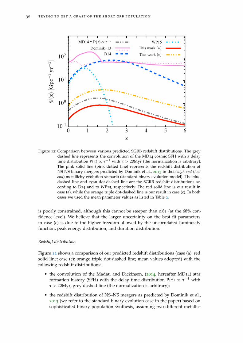
Figure 12: Comparison between various predicted SGRB redshift distributions. The greydashed line represents the convolution of the MD14 cosmic SFH with a delaytime distribution P(τ) ∝ τ−1 with τ > 20Myr (the normalization is arbitrary).The pink solid line (pink dotted line) represents the redshift distribution ofNS-NS binary mergers predicted by Dominik et al., 2013 in their high end (lowend) metallicity evolution scenario (standard binary evolution model). The bluedashed line and cyan dot-dashed line are the SGRB redshift distributions ac-cording to D14 and to WP15, respectively. The red solid line is our result incase (a), while the orange triple dot-dashed line is our result in case (c). In bothcases we used the mean parameter values as listed in Table 2.

is poorly constrained, although this cannot be steeper than 0.81 (at the 68% con-fidence level). We believe that the larger uncertainty on the best fit parametersin case (c) is due to the higher freedom allowed by the uncorrelated luminosityfunction, peak energy distribution, and duration distribution.

Redshift distribution

Figure 12 shows a comparison of our predicted redshift distributions (case (a): redsolid line; case (c): orange triple dot-dashed line; mean values adopted) with thefollowing redshift distributions:

• the convolution of the Madau and Dickinson, (2014, hereafter MD14) starformation history (SFH) with the delay time distribution P(τ) ∝ τ−1 withτ > 20Myr, grey dashed line (the normalization is arbitrary);

• the redshift distribution of NS–NS mergers as predicted by Dominik et al.,2013 (we refer to the standard binary evolution case in the paper) based onsophisticated binary population synthesis, assuming two different metallic-

3.9 the results 31

ity evolution scenarios: high-end (pink solid line) and low-end (pink dottedline);

• the SGRB redshift distribution found by D14, which is obtained convolvingthe SFH by Hopkins and Beacom, 2006 with a delay time distribution P(τ) ∝τ−1.5 with τ > 20Myr, blue dashed line;

• the SGRB redshift distribution found by WP15, which is obtained convolv-ing an SFH based on Planck results (“extended halo model” in Planck Col-laboration et al., 2014) with a lognormal delay time distribution P(τ) ∝exp

[−(ln τ− ln τ0)

2 /(2σ2

)]with τ0 = 2.9Gyr and σ < 0.2 (we used σ =

0.1), cyan dot-dashed line.

The redshift distribution by D14 peaks between z ∼ 2 and z ∼ 2.5, i.e. at a higherredshift than the MD14 SFH (which peaks at z ∼ 1.9). This is due to the short delayimplied by the delay time distribution assumed in D14, and because the (Hopkinsand Beacom, 2006) SFH peaks at higher redshift than the MD14 SFH. On the otherhand, the redshift distribution by WP15 peaks at very low redshift (∼ 0.8) andpredicts essentially no SGRBs with redshift z & 2 because of the extremely largedelay implied by their delay time distribution.

Assuming the MD14 SFH (which is the most recent SFH available) to be repre-sentative, our result using model (a) seems to be compatible with the P(τ) ∝ τ−1delay time distribution (grey dashed line), theoretically favoured for compact bi-nary mergers. For model (c), the redshift distribution we find seems to be indica-tive of a slightly smaller average delay with respect to model (a). Since the cosmicSFH is still subject to some uncertainty, and since the errors on our parameters(p1, zp, p2) are rather large, no strong conclusion about the details of the delaytime distribution can be drawn.

Ep − Liso and Ep − Eiso correlations

Our approach allowed us, in cases (a) and (b), to derive the slope and normaliza-tion of the intrinsic Ep − Liso and Ep − Eiso correlations of SGRBs. For the Ep − Eiso

and Ep − Liso correlations of SGRBs, Tsutsui et al., 2013 finds slope values of0.63± 0.05 and 0.63± 0.12, respectively. Although our mean values for mY andmA (Table 1) are slightly steeper, the 68% confidence intervals reported in Tab. 1

are consistent with those reported by Tsutsui et al., 2013. In order to limit the freeparameter space, we assumed a fixed scatter for the correlations and a fixed nor-malization centre for both (see Eq. 14 and Eq. 15). This latter choice, for instance,introduces the small residual correlation between the slope and normalization ofthe Ep − Liso parameters (as shown in Fig. 11).

Inspection of Fig. 11 reveals another correlation in the MCMC chain between theparameters qY and qA of the Ep − Liso and Ep − Eiso correlations. This is expected,as can be seen by taking the difference between Eqs. 17 and 16

qY − qA = log(EmA

LmY

)+ 52mY − 51mA. (20)

Since EmA and LmY are both proportional to Ep, this induces a linear correlationbetween qA and qY.

32 trying to get a grasp of the short grb population

the local sgrb rate

The local rate of SGRBs is clearly of great importance for the connection with grav-itational wave events to be detected by the advanced interferometers (AdvancedLIGO - LIGO Scientific Collaboration et al. 2015; Abbott et al. 2016; AdvancedVirgo - Acernese et al. 2015). The work done in Ghirlanda et al., (2016) enabledus to make new (and somewhat surprising) predictions about the local SGRB rateand the prospects for association with GW from compact binary mergers. The lo-cal rate R0 of SGRBs, defined as the number of events with a jet pointing towardsthe Earth per comoving Gpc3 and yr at redshift zero, is found by imposing thatthe total number of SGRBs in the flux-limited Fermi/GBM sample is equal to thenumber of events with the corresponding characteristics predicted by the model,namely

NGBM/TGBM = R0

∫∞0

C(z)

∫Ep,max

Ep,min

[φ(Ep)

∫∞Llim(Ep,z,Plim)

P(L|Ep)dL

]dEp

dz (21)

where:

• NGBM = 211 is the number of events in our GBM sample;

• TGBM = 7.5 yr is the time over which the events have been observed;

• the simultaneous sky coverage ∆Ω/4π in the definition of C(z) (see §3.5) is70 percent;

• Llim is the luminosity that corresponds (at a given redshift and for a givenEp) to the flux cut Plim = 5ph cm−2s−1 of the sample;

• P(L|Ep) in model (a) is a lognormal distribution centered at the luminosityL(Ep) given by the Ep − Liso relation, with σ = 0.2, while in model (c) it is theluminosity distribution given in Eq. 15.

The integral can be computed both analytically or via the same Monte Carlo ap-proach described in §3.7, in which case it corresponds to the fraction of SGRBs inthe synthetic sample for which the photon flux in the Fermi/GBM band is P > Plim.To find out how the uncertainty on the model parameters propagates to the rateestimate, one can simply compute the local rate for (a randomly selected subsam-ple of) the posterior samples from the MCMC, and derive the uncertainty from theresulting distribution of local rates. The result is that both model (a) and model(c) predict a quite low local rate, namely9 R0 = 0.36+0.53

−0.17Gpc−3yr−1 for the for-mer and R0 = 0.32+0.98

−0.17Gpc−3yr−1 for the latter (one sigma uncertainties). Thisis about one order of magnitude lower than WP15 and D14, which seems daunt-ing for the GW-SGRB association prospects, as can be seen by the correspondingnumber of events per year expected within the aLIGO detection volume shown inTable 3. A somewhat more promising prediction comes from the fact that the lumi-nosity function is shallower than previous ones, which implies that on average jets

9 These estimates are updated with respect to those given in Ghirlanda et al., (2016), where we usedonly the best fit parameters of the luminosity function and redshift distribution, and we only tookinto account the uncertainty on a subsample of the parameters. The results are compatible withthose given in that paper, but now the uncertainties are estimated in a more rigorous way.

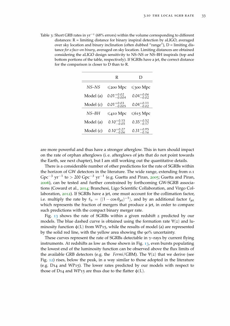
3.10 the local sgrb rate 33

Table 3: Short GRB rates in yr−1 (68% errors) within the volume corresponding to differentdistances: R = limiting distance for binary inspiral detection by aLIGO, averagedover sky location and binary inclination (often dubbed “range”), D = limiting dis-tance for a face–on binary, averaged on sky location. Limiting distances are obtainedconsidering the aLIGO design sensitivity to NS–NS or NS–BH inspirals (top andbottom portions of the table, respectively). If SGRBs have a jet, the correct distancefor the comparison is closer to D than to R.

R D

NS–NS 6200 Mpc 6300 Mpc

Model (a) 0.01+0.02−0.004 0.04+0.06

−0.02

Model (c) 0.01+0.03−0.005 0.04+0.11

−0.02

NS–BH 6410 Mpc 6615 Mpc

Model (a) 0.10+0.15−0.05 0.35+0.52

−0.17

Model (c) 0.10+0.27−0.06 0.31+0.95

−0.16

are more powerful and thus have a stronger afterglow. This in turn should impacton the rate of orphan afterglows (i. e. afterglows of jets that do not point towardsthe Earth, see next chapter), but I am still working out the quantitative details.

There is a considerable number of other predictions for the rate of SGRBs withinthe horizon of GW detectors in the literature. The wide range, extending from 0.1Gpc−3 yr−1 to > 200 Gpc−3 yr−1 (e.g. Guetta and Piran, 2005; Guetta and Piran,2006), can be tested and further constrained by forthcoming GW-SGRB associa-tions (Coward et al., 2014; Branchesi, Ligo Scientific Collaboration, and Virgo Col-laboration, 2012). If SGRBs have a jet, one must account for the collimation factor,i.e. multiply the rate by fb = 〈(1 − cos θjet)

−1〉, and by an additional factor fjet

which represents the fraction of mergers that produce a jet, in order to comparesuch predictions with the compact binary merger rate.

Fig. 13 shows the rate of SGRBs within a given redshift z predicted by ourmodels. The blue dashed curve is obtained using the formation rate Ψ(z) and lu-minosity function φ(L) from WP15, while the results of model (a) are representedby the solid red line, with the yellow area showing the 90% uncertainty.

These curves represent the rate of SGRBs detectable in γ–rays by current flyinginstruments. At redshifts as low as those shown in Fig. 13, even bursts populatingthe lowest end of the luminosity function can be observed above the flux limits ofthe available GRB detectors (e.g. the Fermi/GBM). The Ψ(z) that we derive (seeFig. 12) rises, below the peak, in a way similar to those adopted in the literature(e.g. D14 and WP15). The lower rates predicted by our models with respect tothose of D14 and WP15 are thus due to the flatter φ(L).

34 trying to get a grasp of the short grb population

0.02 0.04 0.06 0.08 0.10Redshift

10 3

10 2

10 1

100

101

102

103

N(<

z) [y

r1 ]

NS­NS RateO2 O3 Design

Ghirlanda+16Wanderman+15

100 200 300 400Distance [Mpc]

Figure 13: Event rates within redshift z. The solid red line represents the SGRB rate formodel (a); the filled yellow area represents the corresponding 90% uncertainty.The results for model (c) are very similar. The SGRB rate according to the bestfit model of WP15 is also shown (dashed blue line). The rate of NS-NS mergersbased on GW170817 (Abbott et al., 2017a) is shown by the pink hatched region.The vertical stripes represent the ranges of aLIGO for the detection of NS–NSmergers in O2 and O3 (i. e. the second and third scientific runs of the aLIGOdetectors, Abbott et al. 2016), and for the design sensitivity. The turquoise rect-angle represents the sky-averaged limiting distance for the detection of a face-onNS-NS binary inspiral with the aLIGO design sensitivity.

3.11 summing up 35

summing up

In Ghirlanda et al., (2016), we derived the luminosity function φ(L), redshift dis-tribution Ψ(z), and local rate of SGRBs. In a way similar (to some extent) to pre-vious works present in the literature, we fitted the properties of a synthetic SGRBpopulation, described by the parametric φ(L) and Ψ(z), to a set of observationalconstraints derived from the population of SGRBs detected by Fermi and Swift.Any acceptable model of the SGRB population must reproduce their prompt emis-sion properties and their redshift distributions. Our approach featured a series ofimprovements with respect to previous works present in the literature:

• (observer frame) constraints: we extended the classical set of observationalconstraints (peak flux and – for a few events – redshift distribution) requir-ing our model to reproduce the peak flux P, fluence F, peak energy Ep,o, andduration T distributions of 211 SGRBs with P64 > 5ph s−1 cm−2 detectedby the GBM instrument on board the Fermi satellite. The uniform responseof the GBM over a wide energy range (10 keV – few MeV) ensures a goodcharacterization of the prompt emission spectral properties of the GRB pop-ulation and, therefore, of the derived quantities, i.e. the peak flux and thefluence;

• (rest frame) constraints: we also required our model to reproduce the distri-butions of redshift, luminosity, and energy of a small sample (11 events) ofSwift SGRBs with P64 > 3.5ph s−1 cm−2 (selected by D14). This sample is70% complete in redshift and therefore it ensures a less pronounced impactof redshift-selection biases in the results;

• method: we derived our results assuming the existence of intrinsic Ep − Liso

and Ep − Eiso correlations in SGRBs (model (a)), similarly to what has beenobserved in the population of long GRBs. However, since evidence of theexistence of such correlations in the population of SGRBs is still based ona limited number of bursts, we also explored the case of uncorrelated peakenergy, luminosity and energy (model (c)).

Our main results are as follows:

1. The luminosity function of SGRBs in both models (a) and (c) is shallow,with a low luminosity slope α1 . 0.5 (68% confidence interval) below abreak luminosity Lb ∼ 3× 1052 erg s−1 and falls steeply above the break. Theassumption of a minimum luminosity does not change the qualitative results(as shown with model (b));

2. The redshift distribution of SGRBs Ψ(z) peaks at z ∼ 1.5 and falls rapidlyabove the peak. This result is intermediate between those reported in theliterature which assume either a constant large delay or a power law distri-bution favouring small delays. Our Ψ(z) is consistent with the MD14 SFHretarded with a power law delay time distribution ∝ τ−1;

3. We estimated the rate of SGRBs as a function of z, finding a rather low localrate R0 ∼ 0.3Gpc−3yr−1, which corresponds to a very low number of events

36 trying to get a grasp of the short grb population

per year within the explorable volume of advanced LIGO, as quantified inTable 3.

4WAW : A G R AV I TAT I O N A L - WAV E - I N F O R M E DE L E C T R O M A G N E T I C F O L L O W- U P S T R AT E G Y

According to the results described in the preceding chapter, the rate of SGRBs witha jet pointing towards the Earth that can be associated to GW events from NS-NSinspirals should be very low. On the other hand, the same results suggest thatSGRB jets are rather energetic on average, so there could be better prospects for thedetection of an orphan afterglow associated to such a GW event. For these reasons,in the following months I tried to find a method to set up an optimal strategy forthe follow-up of GW events, aimed especially at discovering the orphan afterglow.The idea of the “where and when” method (WAW for short) came as an epiphanywhen I was half-sleeping on an old, slow bus traveling from the Kotor bay to theDurmitor mountains in Montenegro. The subsequent work resulted in an article,published by the Astrophysical Journal (Salafia et al., 2017b), whose results andmethods are described in this chapter.

the em follow-up problem

The first detection (The LIGO Scientific Collaboration and the Virgo Collaboration,2016b) of gravitational waves (GW hereafter) from the inspiral and merger of ablack hole binary suddenly turned these fascinating, theoretical objects into realastronomical sources.

When such a compact binary coalescence is detected, analysis of the GW signaland comparison with carefully constructed templates of the waveform (The LIGOScientific Collaboration and the Virgo Collaboration, 2016a; Abbott et al., 2016b)enables the extraction of precious information about the parameters of the binaryand of the remnant. The identification of an electromagnetic (EM) counterpartwould increase further the scientific outcome of the detection, e.g. by enablingthe identification of the host galaxy, by providing hints about the environmentsurrounding the merger, by constraining theoretical models of EM counterpartsand by reducing degeneracies in the GW extrinsic parameter space (Pankow et al.,2016).

Several observatories, covering a large fraction of the EM spectrum, recentlydeveloped dedicated programs for the EM follow-up of GW events. The presentmain limitation for the detection of a possible EM counterpart is the large uncer-tainty on the sky localization of the GW source (see e. g. Singer et al. 2014; Berryet al. 2014). The problem might be alleviated by targeting bright galaxies withinthe localization uncertainty region (Nuttall and Sutton, 2010; Abadie et al., 2012),and the selection of target galaxies can also take into account the sky-position-conditional posterior distribution of the source luminosity distance (Hanna, Man-del, and Vousden, 2013; Nissanke, Kasliwal, and Georgieva, 2013; Gehrels et al.,2016; Singer et al., 2016a). The aim of this work is to propose an additional wayto use information encoded in the GW signal to optimize the follow-up strategy

37

38 waw : a gw-informed em follow-up strategy

for each single event, namely to combine posterior distributions of the compactbinary parameters and available models of the EM emission to predict the besttiming for the observation of different parts of the GW skymap. Such an approachcan be applied in cases when a model of the expected EM counterpart is available,and it is especially useful when the lightcurve predicted by the model depends on(some of) the compact binary parameters.

The first electromagnetic follow-ups

The observation campaigns that followed up the first detections of GWs werevery extensive. Hundreds of square degrees within the GW sky localization werecovered by wide-field telescopes (Abbott et al., 2016a). Target areas were selectedin order to maximize the contained GW source posterior sky position probability,incorporating telescope visibility constraints (e. g. Kasliwal et al., 2016). In somecases, models of the expected EM counterpart emission were used to estimate theoptimal search depth (e. g. Soares-Santos et al., 2016); other searches combinedthe posterior sky position probability map with the areal density and luminosityof nearby galaxies to select the best target fields (e. g. Evans et al., 2016; Díazet al., 2016). Observations were concentrated during the first days after the eventsand repeated weeks to months later to search for both rapid and slowly evolvingpossible counterparts.

Candidate EM counterparts

It is not clear whether an EM counterpart should be expected in the case of a binaryof black holes (BH-BH), due to the unlikely presence of matter surrounding thebinary (but see Yamazaki, Asano, and Ohira 2016; Perna, Lazzati, and Giacomazzo2016; Loeb 2016); on the other hand, if the merger involves a black hole and aneutron star (BH-NS) or two neutron stars (NS-NS), there are solid reasons tobelieve that EM emission should take place. The most popular mechanisms forsuch an emission in both BH-NS and NS-NS cases include prompt (gamma-ray)and afterglow (panchromatic) emission from a short gamma-ray burst (SGRB) jet,and “macronova” (optical/infrared) emission from ejecta launched during andafter the merger, powered by the decay of unstable heavy nuclei resulting fromr-process nucleosynthesis taking place within the neutron-rich ejecta during theearly expansion phase.

Many other promising EM counterparts have been proposed, e. g. the long last-ing radio transient (Nakar and Piran, 2011) arising from the deceleration of the dy-namical ejecta due to interaction with the interstellar medium (ISM), the jet cocoonemission (Lazzati et al., 2017b; Gottlieb, Nakar, and Piran, 2018) or the spindown-powered emission described by Siegel and Ciolfi, (2016) in the case when a (meta-)stable neutron star is left after the merger. To keep the discussion as simple aspossible, in this chapter I will only consider the (Optical and Radio) SGRB after-glow and the dynamical ejecta macronova as examples, leaving the possibility toapply the present approach to other EM counterparts to future works.

4.1 the em follow-up problem 39

The SGRB afterglow

The detectability of the SGRB prompt emission depends crucially on the jet view-ing angle θv, i. e. the angle between the jet axis and our line of sight. If the viewingangle is larger than the jet half opening angle θjet (in other words, if the jet pointsaway from the Earth), the prompt emission flux received by an observer on Earthis severely suppressed (e. g. Salafia et al., 2016) due to relativistic beaming (bythe compactness argument, the bulk Lorentz factor in GRB jets must be compara-ble to or larger than one hundred – e. g. Lithwick and Sari 2001 – and estimatesbased on observations are sometimes even larger than a thousand – as in theshort burst GRB090510, see Ghirlanda, Ghisellini, and Nava 2009; Ackermann etal. 2010). Since the typical half opening angle θjet is somewhere between 5 and 15

(e. g. Berger, 2014a), the prompt emission goes undetected in the majority of cases(for an isotropic population, the probability that θv < 15

is less than 2 percent).Soon after producing the prompt emission, the jet starts interacting significantlywith the ISM, and a shock develops (Meszaros and Rees, 1996). Electrons in theshocked ISM produce synchrotron radiation, giving rise to a fading afterglow (ob-served fo the first time by Beppo-SAX, Costa et al., 1997). Since the consequentdeceleration of the jet reduces the relativistic beaming, an off-axis observer (whomissed the prompt emission) could in principle detect the afterglow before it fades(Rhoads, 1997): in this case, the afterglow is said to be orphan. No convincing detec-tion of such a transient has been claimed to date, consistently with predictions forcurrent and past surveys (Ghirlanda et al., 2015; Ghirlanda et al., 2014), but futuredeep surveys (e. g. MeerKAT in the Radio – Booth et al. 2009, LSST in the Optical– Ivezic et al. 2008, eROSITA in the X-rays – Merloni et al. 2012) are anticipated todetect tens to thousands of such events per year.

Given the large uncertainty on the expected rate of NS-NS and BH-NS detectionsby the aLIGO and Advanced Virgo facilities in the near future (LIGO ScientificCollaboration et al., 2010; Kim, Yoon, and Koo, 2015; Dominik et al., 2015; Minkand Mandel, 2016; Abbott et al., 2016) and the rather low expected fraction of GWevents with an associated SGRB jet pointing at the Earth (Ghirlanda et al., 2016;Patricelli et al., 2016; Wanderman and Piran, 2014; Metzger and Berger, 2011), theinclusion of orphan afterglows as potential counterparts is of primary importanceto test the SGRB-compact binary coalescence connection.

The dynamical ejecta macronova

Despite the idea dates back to almost twenty years ago (Li and Paczynski, 1998),the understanding of the possible macronova emission following a compact binarymerger has been expanded relatively recently, as a result of the combined effort ofresearchers with expertise in a wide range of areas. A non-exhaustive list of themain contributions should include:

• numerical simulations of the merger dynamics (relativistic simulations bymany groups using different approaches – e. g. Dietrich et al. 2017; Ciolfiet al. 2017; Radice et al. 2016; Sekiguchi et al. 2016; Ruiz et al. 2016; Giaco-mazzo et al. 2015; Bauswein and Stergioulas 2015; Just et al. 2016; East et al.2015; Sekiguchi et al. 2015; Wanajo et al. 2014; Kiuchi et al. 2014; Tanaka

40 waw : a gw-informed em follow-up strategy

and Hotokezaka 2013; Rezzolla et al. 2010 – and non relativistic simulations,especially by Stephan Rosswog and collaborators – e. g. Rosswog et al. 2014);

• studies to assess the efficiency of r-process nucleosynthesis and the conse-quent heating rate due to heavy element decay in the various ejecta (Freiburghaus,Rosswog, and Thielemann, 1999; Rosswog, Freiburghaus, and Thielemann,2000; Korobkin et al., 2012; Wanajo et al., 2014; Lippuner and Roberts, 2015;Hotokezaka et al., 2015; Eichler et al., 2016; Rosswog et al., 2016);

• atomic structure modeling which revealed the role of lanthanides in theejecta opacity evolution (Kasen, Badnell, and Barnes, 2013);

• simulations including neutrino physics to model the neutrino-driven windand the associated macronova (Dessart et al., 2008; Martin et al., 2015; Perego,Yasin, and Arcones, 2017);

Results (especially for the dynamical ejecta) from various research groups beginto converge, and the dependence of the emission features on the parameters of thebinary is in the process of being understood. Both analytical and numerical modelscapable to predict the lightcurve have been developed recently (Barnes and Kasen,2013; Grossman et al., 2013; Kawaguchi et al., 2016; Dietrich and Ujevic, 2017;Barnes et al., 2016; Rosswog et al., 2016). The emission from the dynamical ejecta isgenerally thought to be isotropic, which is an advantage with respect to the SGRBafterglow (which is instead beamed) from the point of view of the EM follow-up.The energy reservoir is the ejected mass Mej, which depends most prominently onthe mass ratio q = M1/M2 of the binary and on the neutron star compactness,which in turn reflects the mass of the neutron star and its equation of state (EoS).Exciting claims of the detection of possible macronova signatures in the afterglowsof few short GRBs (Tanvir et al., 2013; Yang et al., 2015; Jin et al., 2015; Jin etal., 2016) are in the process of being tested by intensive observational campaigns.All this makes the macronova emission an extremely interesting candidate EMcounterpart.

Outline of this chapter

In §4.2.1 I introduce the idea of a follow-up strategy as a collection of observationsthat partially fill a “search volume” (search sky area × typical transient duration),stressing that the GW “skymap” (the sky position probability density) gives in-formation about where to observe, but not about when. In §4.2.1.1 I show how apriori information about the EM counterpart can be used to quantitatively definehow likely the detection of the EM emission is if the observation is performed attime t, thus providing some information about how to explore the temporal di-mension of the “search volume”. In §4.2.2 I suggest that the same approach can beextended to use a posteriori information extracted from the GW signal, providedthat we have a way to link the properties of the inspiral to those of the EM coun-terpart (as shown in §4.2.2.2). In §4.2.2.4 I go one step further by introducing theidea that the information on the inspiral parameters that we can extract from theGW signal has a dependence on sky position, and thus the clues (that we obtainfrom the GW signal analysis) about when to observe can also depend on the sky

4.2 where and when to look 41

position. In §4.3 I introduce a method to extract such information from the “pos-terior samples” obtained from the analysis of a GW signal, and in §4.5 I apply itto a synthetic example to show how it optimizes the follow-up strategy. Finally, Idiscuss the results in §4.6 and I draw some conclusions in §4.7.

where and when to look

A sketch of the design of a follow-up observation strategy

A short time after the detection of a compact binary coalescence signal, the LIGOScientific Collaboration and Virgo Collaboration share information about the eventwith a network of astronomical facilities interested in the EM follow-up. The mostfundamental piece of information for the follow-up is the so-called “skymap”,i. e. the posterior sky position probability density, which I denote as P(α | S). Itrepresents the probability per unit solid angle that the source is at sky positionα, say α = (RA, Dec), given the GW signal S detected by the interferometers (Shere represents all information contained in the strain amplitudes measured byall interferometers in the network). In what follows, I will most often call thisprobability density “skymap probability”. Imagine the EM counterpart appearsat the GW position right after the event and never turns off. Assume that it canbe found by comparison with previously available images of the sky, and that itcan be easily identified by its spectrum or by another method. An ultra-simplifiedsketch of the obvious follow-up strategy would then be the following:

1. find the smallest sky area Aω containing a large fraction ω (say ω = 90%)of the skymap probability P(α | S);

2. divide such area into patches of size AFoV corresponding to the field of viewof the instrument;

3. observe the patches in decreasing order of skymap probability1;

4. for each patch:

a) identify the new sources by comparison with archive images;

b) perform a set of operations, including e. g. cross-matching with cata-logues and spectral charachterization, to discard known variable sourcesand unrelated transients in order to identify the counterpart.

The expected EM counterparts are transients, thus a first modification to theabove sketch must take into account the time constraints coming from our a prioriknowledge of the transient features. If we have a physical or phenomenologicalmodel of the transient and we have some hint about the distribution of the param-eters of such model, we can construct a prior probability P(F(t) > Flim) that thetransient flux (in a chosen band) F is above some limiting flux Flim at a given timet after the GW event. Hereafter, I will call such quantity “a priori detectability”.

1 to keep the discussion as simple as possible, I am neglecting the limitations due to observing condi-tions.

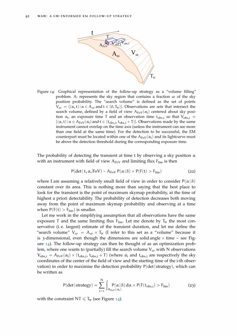
42 waw : a gw-informed em follow-up strategy

tVobs,2Vobs,1

VωAω

Ttr

AFoV

T

Figure 14: Graphical representation of the follow-up strategy as a “volume filling”problem. A! represents the sky region that contains a fraction ω of the skyposition probability. The “search volume” is defined as the set of pointsVω = (α, t) |α ∈ Aω and t ∈ (0, Ttr). Observations are sets that intersect thesearch volume, defined by a field of view AFoV(αi) centered about sky posi-tion αi, an exposure time T and an observation time tobs,i so that Vobs,i =

(α, t) |α ∈ AFoV(αi) and t ∈ (tobs,i, tobs,i + T). Observations made by the sameinstrument cannot overlap on the time axis (unless the instrument can see morethan one field at the same time). For the detection to be successful, the EMcounterpart must be located within one of the AFoV(αi) and its lightcurve mustbe above the detection threshold during the corresponding exposure time.

The probability of detecting the transient at time t by observing a sky position αwith an instrument with field of view AFoV and limiting flux Flim is then

P(det | t, α, FoV) ∼ AFoV P(α | S)× P(F(t) > Flim) (22)

where I am assuming a relatively small field of view in order to consider P(α | S)

constant over its area. This is nothing more than saying that the best place tolook for the transient is the point of maximum skymap probability, at the time ofhighest a priori detectability. The probability of detection decreases both movingaway from the point of maximum skymap probability and observing at a timewhen P(F(t) > Flim) is smaller.

Let me work in the simplifying assumption that all observations have the sameexposure T and the same limiting flux Flim. Let me denote by Ttr the most con-servative (i. e. largest) estimate of the transient duration, and let me define the“search volume” Vω = Aω × Ttr (I refer to this set as a “volume” because itis 3-dimensional, even though the dimensions are solid angle × time – see Fig-ure 14). The follow-up strategy can then be thought of as an optimization prob-lem, where one wants to (partially) fill the search volume Vω with N observationsVobs,i = AFoV(αi)× (tobs,i, tobs,i + T) (where αi and tobs,i are respectively the skycoordinates of the center of the field of view and the starting time of the i-th obser-vation) in order to maximise the detection probability P(det | strategy), which canbe written as

P(det | strategy) =N∑

i=1

∫AFoV(αi)P(α | S)dα× P(F(tobs,i) > Flim) (23)

with the constraint NT 6 Ttr (see Figure 14).

4.2 where and when to look 43

The above paragraphs are essentially a formal description of the most basicfollow-up strategy one can think of, which can be reduced to the principle “tryto arrange the observations in order to cover the largest possible fraction of theGW skymap around the time when the flux is expected to be high enough for adetection”. In this approach, the proper construction of the a priori detectabilityP(F(t) > Flim) is the key: it defines the time span within which the observationsare to be performed, while the posterior sky position probability density definesthe search area.

How to construct the a priori detectability

In order to construct the a priori detectability P(F(t) > Flim), one must assumesome prior probability density of the model parameters. Let me consider a simple,illustrative example. First, I construct a synthetic population of NS-NS inspiralswhose properties roughly reproduce those expected for the population detected byAdvanced LIGO; then I associate to each of them a jet afterglow and a macronova,under some assumptions. The detectable fraction of lightcurves in a given band, ata given time, will then constitute our estimate of the a priori detectability for thisparticular case. For the jet afterglow, I assume2 that all SGRB jets have an isotropickinetic energy EK = 1050 erg and a half-opening angle θjet = 0.2 radians (11.5 deg),and that they are surrounded by a relatively tenuous interstellar medium withconstant number density nISM = 0.01 cm−3. I fix the microphysical parameters3

so that the only remaining parameters needed to predict the afterglow lightcurveof the SGRB are the distance dL and the viewing angle θv. I will link the viewingangle to the binary orbit inclination, and the distance will be obviously set equalto that of the binary. Assuming two opposite jets launched perpendicular to thebinary orbital plane, we have that

θv(ι) =

ι 0 6 ι < π/2

π− ι π/2 6 ι < π(24)

where ι is the angle between the normal to the orbital plane and the line of sight.For the dynamical ejecta macronova, I evaluate the disk mass and the ejecta ve-

locity using the fitting formulas of Dietrich and Ujevic, (2017), and I use them asinputs to compute the lightcurve following Grossman et al., (2013) (using a con-stant grey opacity κ = 10 cm2 g−1), assuming a blackbody spectrum with effectivetemperature equal to that of the photosphere. The input compact binary parame-ters in this case are the masses M1 and M2. To determine the compactness andthe baryon mass of the neutron stars, which are necessary to associate the dynam-ical ejecta mass Mej and velocity vej to the merger through the fitting formulasof Dietrich and Ujevic, (2017), I assume the H4 equation of state (Lackey, Nayyar,and Owen, 2006; Glendenning and Moszkowski, 1991) which has a mid-range stiff-

2 these are typical reference values for short GRBs, though they suffer from the still limited numberof reliable measurements available.

3 I refer here to the standard synchrotron afterglow model, and I set the microphysical parametersp = 2.5, εe = 0.1 and εB = 0.01. Such values, typical of Long GRBs (e. g. Panaitescu and Kumar,2002; Ghisellini et al., 2009; Ghirlanda et al., 2015), seem to be representative for SGRBs as well (Fonget al., 2015), despite the much smaller sample of broadband lightcurves available.

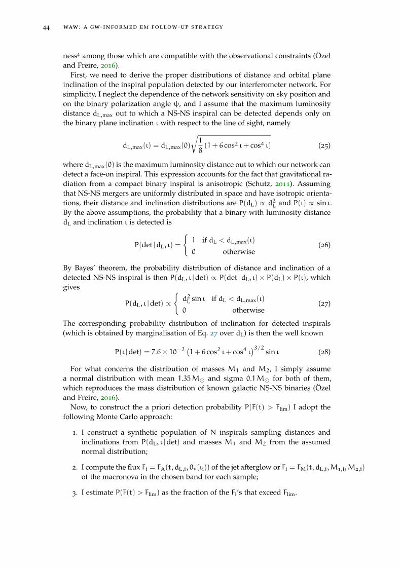
44 waw : a gw-informed em follow-up strategy

ness4 among those which are compatible with the observational constraints (Özeland Freire, 2016).

First, we need to derive the proper distributions of distance and orbital planeinclination of the inspiral population detected by our interferometer network. Forsimplicity, I neglect the dependence of the network sensitivity on sky position andon the binary polarization angle ψ, and I assume that the maximum luminositydistance dL,max out to which a NS-NS inspiral can be detected depends only onthe binary plane inclination ι with respect to the line of sight, namely

dL,max(ι) = dL,max(0)

√1

8(1+ 6 cos2 ι+ cos4 ι) (25)

where dL,max(0) is the maximum luminosity distance out to which our network candetect a face-on inspiral. This expression accounts for the fact that gravitational ra-diation from a compact binary inspiral is anisotropic (Schutz, 2011). Assumingthat NS-NS mergers are uniformly distributed in space and have isotropic orienta-tions, their distance and inclination distributions are P(dL) ∝ d2L and P(ι) ∝ sin ι.By the above assumptions, the probability that a binary with luminosity distancedL and inclination ι is detected is

P(det |dL, ι) =

1 if dL < dL,max(ι)

0 otherwise(26)

By Bayes’ theorem, the probability distribution of distance and inclination of adetected NS-NS inspiral is then P(dL, ι |det) ∝ P(det |dL, ι)× P(dL)× P(ι), whichgives

P(dL, ι |det) ∝

d2L sin ι if dL < dL,max(ι)

0 otherwise(27)

The corresponding probability distribution of inclination for detected inspirals(which is obtained by marginalisation of Eq. 27 over dL) is then the well known

P(ι |det) = 7.6× 10−2(1+ 6 cos2 ι+ cos4 ι

)3/2sin ι (28)

For what concerns the distribution of masses M1 and M2, I simply assumea normal distribution with mean 1.35M and sigma 0.1M for both of them,which reproduces the mass distribution of known galactic NS-NS binaries (Özeland Freire, 2016).

Now, to construct the a priori detection probability P(F(t) > Flim) I adopt thefollowing Monte Carlo approach:

1. I construct a synthetic population of N inspirals sampling distances andinclinations from P(dL, ι |det) and masses M1 and M2 from the assumednormal distribution;

2. I compute the flux Fi = FA(t, dL,i, θv(ιi)) of the jet afterglow or Fi = FM(t, dL,i,M1,i,M2,i)

of the macronova in the chosen band for each sample;

3. I estimate P(F(t) > Flim) as the fraction of the Fi’s that exceed Flim.

4.2 where and when to look 45

100 101 102

t [days]

10­3

10­2

10­1

100

Prob

abili

ty th

at Fν o

bs>F

lim Macronova IR

Jet Radio

Jet Opt

νobs Flim

1. 4 GHz 0. 5 mJyJ filter 22. 4mAB

r filter 22. 4mAB

Figure 15: “A priori detectability”, i. e. a priori probability that the EM counterpart of acompact binary inspiral is detected if the observation is performed at a time tafter the merger, for observations in Radio at 1.4 GHz, in Infrared (IR) in theJ band, and in Optical in the r band, with limiting fluxes of 0.5 mJy in Radioand 22.4 AB magnitude in IR and Optical. The Radio and Optical probabilitiesaccount only for the jet afterglow, while the IR probability accounts only for thedynamical ejecta macronova. Based on a series of simplifying assumptions, see§4.2.1.1.

46 waw : a gw-informed em follow-up strategy

Figure 15 shows the a priori detectability computed with the above method fordL,max(0) = 100 Mpc (which corresponds roughly to the sky-position averagedaLIGO range for an optimally oriented NS-NS inspiral with the sensitivity of thefirst Advanced LIGO observing run, see Abbott et al., 2016) for Radio, Infraredand Optical observations (see the caption for details). The sensitivity of Opticalobservations has been chosen to match the limiting magnitude of the VST follow-up of GW150914, see Abbott et al. 2016a. The flux of the jet afterglow has beencomputed using BOXFIT v. 1.0 (Eerten, Horst, and MacFadyen, 2012).

A more accurate a priori detectability would require us to use astrophysicallymotivated priors on the other model parameters, such as the kinetic energy EK, theISM number density nISM, etc. Moreover, the actual intrinsic mass distribution ofneutron stars that merge within the frequency band of GW detectors might differsignificantly from the assumed one. The curves shown in Fig. 15, thus, must betaken as illustrative.

The definitely higher detectability of the macronova is due to the fact that itsemission is assumed to be isotropic, while the jet is fainter for off-axis observers.

Two steps further: how to improve the strategy using posterior information about otherparameters of the binary

The full posterior probability density in parameter space

Parameter estimation techniques applied to a compact binary coalescence signalS result in a posterior probability density P(ξ | S), where ξ ∈ Rn is a point in then-dimensional parameter space. The “skymap probability”, i. e. the posterior skyposition probability density P(α | S), is essentially the P(ξ | S) marginalised over allparameters but the sky position. Much more information is contained in the fullposterior probability density, though, and some of it can be used to improve thedesign of the EM follow-up strategy.

Relevant parameters in our case

In §4.2.1.1 we already made use of two extrinsic parameters of the compact binaryinspiral which are relevant for the SGRB afterglow and the macronova, namely theluminosity distance dL and the binary inclination5 ι.

Recent works based on numerical simulations of NS-NS and BH-NS mergers(e. g. Foucart, 2012; Giacomazzo et al., 2013; Hotokezaka and Piran, 2015; Kawaguchiet al., 2016; Dietrich and Ujevic, 2017) seem to indicate that the amount of matterin the remnant disk and in the dynamical ejecta, plus some other properties of thelatter such as the velocity profile, depend in a quite simple way (once an equationof state is assumed) on the parameters of the binary prior to the merger, especiallythe masses M1 and M2 and the effective spin χeff of the black hole in the BH-NS

4 This translates into mid-range values of the corresponding Mej and vej.5 the inclination of the orbital plane with respect to the line of sight can also be relevant for the

neutrino-driven wind (Martin et al., 2015) and the disk wind (Kasen, Fernandez, and Metzger, 2014)macronovas, due to their axial geometry and to the possibility that the dynamical ejecta act as a“lanthanide curtain” obscuring their optical emission (Rosswog et al., 2016) if the binary is observededge-on.

4.2 where and when to look 47

efficiency?

M1

M2

χeff

EK jetSGRBAfterglow

Dyn. ejectaMacronova

Mej

εBpεenISM θjet

κ

dmdvej

EoS

Mergerdynamics

ε(t)

lightcurve

Mdisk

dL

ι

GW signal(intrinsic)

Numerical simulations Physical models

(assumptions)

(assumptions)

(assumption)

GW signal(extrinsic)

Figure 16: Sketch of the dependence of some parameters of the SGRB and dynamical ejectamacronova on the progenitor binary parameters. The masses and spin of the bi-nary components, through the dynamics and assuming an equation of state(EoS), determine the masses Mej (Kawaguchi et al., 2016; Dietrich and Ujevic,2017) and Mdisk (Foucart, 2012; Giacomazzo et al., 2013) of the dynamical ejectaand the accretion disk on the remnant compact object, respectively. The dynam-ics also determine the velocity profile dm/dvej of the ejecta. Accretion on theremnant converts disk rest mass (with some unknown efficiency) into jet kineticenergy EK (e. g. Giacomazzo et al., 2013), which constitutes the energy reservoirof the SGRB afterglow. By making assumptions on the remaining parameters,the lightcurves of the macronova and SGRB afterglow (possibly) associated tothe merger can be predicted, taking into account the luminosity distance dLand the inclination ι of the binary.

case. Such information can be used to predict the observed lightcurve of the as-sociated macronovas (e. g. Kawaguchi et al., 2016; Dietrich and Ujevic, 2017) and,with greater uncertainty, the energy in the GRB jet (as in Giacomazzo et al., 2013).

Summarizing, at least the following compact binary coalescence parameters arerelevant in order to predict the lightcurve of the SGRB and/or of the dynamicalejecta macronova associated to the merger:

1. the luminosity distance dL and the associated redshift z;

2. the orbital plane inclination ι with respect to the line of sight;

3. the component masses M1 and M2;

4. the effective spin χeff of the black hole in the BH-NS case.

Figure 16 represents a sketch of how the above parameters influence the prop-erties of the SGRB afterglow and the dynamical ejecta macronova associated tothe merger. The same approach can be adopted to link the properties of other EMcounterparts (such as the long lasting radio transient described by Nakar and Pi-ran 2011 or the X-ray spindown-powered transient described by Siegel and Ciolfi2016) to those of the binary, whose distributions can be constrained by the GWsignal.

In §4.5, I will use the fitting formulas provided in Dietrich and Ujevic, (2017) tocompute the posterior ejecta mass distribution associated to the example NS-NSinspiral treated in that section. I will refrain from deriving the SGRB jet energyfrom disk mass as suggested in Fig. 16, though, because that would require a

48 waw : a gw-informed em follow-up strategy

detailed discussion about the proper disk mass energy conversion efficiency to beused, which is outside the scope of this work. I leave such a discussion to a futurework.

A posteriori detectability

In §4.2.1 I introduced the idea of “a priori detectability” P(F(t) > Flim), which canbe regarded as the basic tool to set the timing of observations for the EM follow-up if no specific information about the source is available. Once the GW signalS is observed, information it carries can be used to construct a posterior probabil-ity P(F(t) > Flim | S) to better plan such observations. I will call it “a posterioridetectablity”. If the a priori detectability P(F(t) > Flim) is constructed using theprior distributions of the parameters of the EM transient model, the a posterioridetectability P(F(t) > Flim | S) is obtained exactly the same way (as exemplified in§4.2.1.1), but using the posterior distributions of the relevant parameters.

Detectability maps

Several parameters of a compact binary inspiral are degenerate to some degree,i. e. the same signal S can be produced by different combinations of the parametervalues. These combinations, though, are not just uniformly distributed in somesubset of the parameter space, but rather they follow fundamental relations whichdepend both on the nature of the source (the binary inspiral) and on the prop-erties of the detector network (the locations and orientations of the interferom-eters, their antenna patterns, the noise power spectrum). In particular, distance,inclination, polarization angle, chirp mass and sky position of the binary share acertain degree of degeneracy: the same signal S can be produced by different com-binations of values of these parameters and different realizations of the detectornoises, which is the obvious reason why the sky position uncertainty is so large.For this reason, if we restrict the posterior probability density in parameter spaceto a certain point of the skymap, i. e. we take the sky-position-conditional posteriordistribution of the physical parameters of the binary, in principle it will dependon the chosen sky-position. Knowing the sky-position-conditional posterior prob-ability distribution P(dL, ι,M1,M2, ... |α, S) of the relevant binary parameters atsky position α, we can thus derive the corresponding distribution of the proper-ties of the EM counterpart at that particular sky position, which means that wecan construct a sky-position-conditional posterior detectability P(F(t) > Flim |α, S)

which can be used as the basis of the EM follow-up strategy. I call this quantity“detectability map”.

Recap

It is useful to summarize here the steps of increasing complexity that led us to thedefinition of the detectability maps:

• I started by assuming an unrealistic model of the EM counterpart: a sourcethat turns on at the GW time and never turns off. In this case, no timinginformation is needed for the follow-up strategy, which simply consists of

4.3 detectability maps 49

scanning the localization uncertainty area, starting from the most probablesky location, until the source is found;

• If a model of the counterpart is available and prior distributions of the modelparameters can be assumed (based on available astrophysical data or on aneducated guess), the “a priori detectability” P(F(t) > Flim) can be constructed,as shown in §4.2.1.1. This is the best follow-up timing information that canbe constructed based on a priori knowledge only;

• After a GW signal S is detected and parameter estimation has been per-formed, prior distributions of the model parameters can be (partly) replacedwith posterior distributions derived from the signal: the “a posteriori de-tectability” P(F(t) > Flim | S) can be constructed. This exploits informationcontained in the GW signal, but it is still independent of the sky position;

• If the counterpart is assumed to be located at a certain sky position, the cor-responding sky-position-conditional posterior distributions can be used inplace of the full posterior distributions. Indeed, given a signal S, compactbinary inspiral parameters compatible with S and a particular sky positionare in general different from those compatible with S and another sky pos-tion. By varying the assumed sky position on a grid that covers the wholeskymap, one can then construct the “detectability map” P(F(t) > Flim |α, S).

Let me now introduce a method to compute the detectability maps and apply itto a practical example.

how to construct and how to use the detectability maps

Extraction of the sky-position-conditional posterior distributions using a simple methodbased on “inverse distance weighting”

The extraction of the sky-position-conditional posterior distribution requires somemulti-dimensional kernel density estimation (KDE) technique, to be applied to theposterior samples obtained from a parameter estimation pipeline run on the grav-itational wave signals recorded by the detectors. Since the aim of this work is topropose a new approach in the design of the EM follow-up, rather than to discussthe technical subtleties of such multi-dimensional KDE, I adopt the following sim-ple and intuitive method, which can be replaced with a more accurate one in apossible application of our approach to a real case.

Our simplified method to extract the sky-position-conditional posterior distri-bution P(q |α, S) of a quantity q at sky position α is based on the concept of“inverse distance weighting” (Shepard, 1968): I assume that each posterior sampleαi, qi, dL,i, ιi, ... contributes to the P(q |α, S) with a weight which is a decreasingfunction of the angular distance δ(α,αi) between the posterior sample and the skyposition α. In particular, I assign a Gaussian weight to each posterior sample

wi ∝ exp

[−1

2

(δ(α,αi)

σ(α)

)2](29)

50 waw : a gw-informed em follow-up strategy

where the bandwidth σ(α) is taken as

σ(α) =

√∑Ni=1

[δ(α,αi) − 〈δ〉]2

N− 1×N−1/5 (30)

where 〈δ〉 is the arithmetic mean of the δ(α,αi). The normalization of the weightsis given by

∑Ni=1wi = 1.

The ideas behind this method are simply that the closer the posterior sample isto sky-position α, the more it contributes to the conditional posterior distributionat that sky position, and that the influence of the posterior sample decreases as aGaussian with increasing angular distance. The choice of the bandwidth (Eq. 30)is just “Silverman’s rule of thumb” (Silverman, 1982) for Gaussian KDE in a onedimensional parameter space (namely, the angular distance space).

The mean of q at sky position α is thus computed as

〈q〉α =

N∑i=1

wi qi (31)

and similarly the variance

Varα(q) =

(N∑

i=1

wi qi

)2−

N∑i=1

wi q2i (32)

More generally, the sky-position-conditional posterior distribution of q at sky po-sition α is approximated as

P(q |α, S) ∼

N∑i=1

wi K(q− qi

σq

)(33)

where K(x) is some kernel function, and σq is its bandwidth.In the next section, I describe tests I performed to ensure that the above method

yields consistent results. As one might expect, the results are accurate in sky re-gions where the distribution of posterior samples is sufficiently dense.

testing our inverse-distance-weighting-based method of sky-position-conditional density estimation

Test 1: reconstruction of the position-conditional mean and standard deviation of a knowndistribution

As a first test, I constructed a set of 10000 mock posterior samples whose un-derlying probability distribution in parameter space has a known analytic form.The parameter space is 4-dimensional, the parameters being right ascension RA,declination Dec, luminosity distance dL and a fourth quantity q with no physicalmeaning. The RA, Dec and dL parameters are independent. The right ascension isnormally distributed with mean 12h and sigma 30min; the declination is uniformlydistributed between −730′ and +730′; the luminosity distance is normally dis-tributed with mean 100 Mpc and sigma 20 Mpc; the distribution of quantity q

4.4 test of the idw method 51

0.0

0.2

0.4

0.6

0.8

1.0

µq(R

A)

10 11 12 13 14right ascension [hours]

­0.3­0.15

0.00.15

resi

dual

s

0.1

0.2

0.3

0.4

σq(R

A)

10 11 12 13 14right ascension [hours]

­0.3­0.15

0.00.15

resi

dual

s

Figure 17: Test to assess the capability of our method to recover the mean and the stan-dard deviation of the sky-position-conditional posterior distribution of a quan-tity. Left panel: the blue line represents the position-conditional mean of thetrue underlying distribution of quantity q, while the red dots are the position-conditional means derived with our method. The black dotted line shows thedensity of samples around each point normalized to the maximum density,while the black dashed vertical lines show the approximate right ascension lim-its of the 90% position probability area. The red crosses in the lower panelare the residuals of the computed means with respect to the true values. Theaccuracy in the reconstruction of the means clearly depends on the density ofsamples in the surrounding area. Right panel: same as the left panel, but for theposition-conditional standard deviation. The reconstruction accuracy is clearlylower than in the case of the mean, but it remains acceptable in the region ofhigh sample density.

depends on right ascension: its position-conditional distribution is normal, withmean and sigma given by

µq(RA) = sin2[8π

(RA12h

− 1

)]σq(RA) =

1

5+2

3

(RA12h

− 1

) (34)

The 90% position probability area of the posterior samples is about 435 deg2

wide and its shape is approximately a rectangle extending in right ascension from11 to 13 hours and in declination from −75′ to +75′. Figure 17 shows the re-constructed position-conditional means and standard deviations computed in aset of points along the Dec = 0 axis. Both moments are reconstructed with anacceptable accuracy within the 90% sky position probability area.

Test 2: comparison with the “Going the Distance” study

The “Going the Distance” study (Singer et al., 2016a, GTD hereafter) and especiallythe related Supplement (Singer et al., 2016b) represent an important practical steptowards the use of posterior distributions of parameters other than the sky positionto inform and improve the electromagnetic follow-up. In their approach, distanceinformation encoded in the signal is used in conjunction with galaxy cataloguesas the basis for a follow-up strategy based on pointing candidate host galaxiesto maximise the counterpart detection probability. In the Supplement, Singer and

52 waw : a gw-informed em follow-up strategy

8h10h12h14hRA [h]

­75

­60

­45

­30

­15

0

Dec

[deg

]

0 0.125 0.25 0.375 0.5|µGTD −µ|/µGTD

8h10h12h14hRA [h]

­75

­60

­45

­30

­15

0

Dec

[deg

]

0 0.125 0.25 0.375 0.5|σGTD − σ|/σGTD

Figure 18: Comparison between the mean of the sky-position-conditional posterior distri-bution of luminosity distance of injection 18951 of Singer et al., (2014) as com-puted with our method and that given in Singer et al., (2016b). Left panel: Thecolor coding shows the fractional deviation of the mean luminosity distance ofour method compared to that of Singer et al., (2016b) (“GTD” stands for “Goingthe Distance”, i. e. the title of Singer and collaborators’ work). The outer (inner)red boundary represents the contour of the sky area containing 90% (50%) ofthe posterior sky position probability. The star marks the actual position of theinjection. Right panel: Same as the left panel, but the comparison is on thestandard deviation.

collaborators show a step-by-step procedure to download and visualize the sky-position-conditional posterior distribution of the luminosity distance of injection18951 from the “First two years of electromagnetic follow-up with Advanced LIGOand Virgo” study (Singer et al., 2014, F2Y hereafter). I took that procedure asa starting point, and used it to compare the sky-position-conditional mean andstandard deviation of luminosity distance derived with our method to those ofthe GTD study. Figure 18 shows the relative difference between the quantitiescomputed with the two methods. Again, the difference is very small except forregions where the density of posterior samples is small, i. e. at the borders andoutside the 90% sky-position confidence region.

The detectability map

By the above method, we can thus define the sky-position-conditional posteriordetectability estimate (i. e. the detectability map) as

P(F(t) > Flim |α, S) =

N∑i=1

wi

∫∞Flim

K(F− Fi(t)

σF

)dF (35)

where Fi(t) represents the flux (in the chosen band) at time t of the lightcurvecomputed using the i-th posterior sample parameter values, Fi(t) = F(t, dL,i, ιi, ...).If we approximate the kernel functions with delta functions K(x) ∼ δ(x), the ex-pression becomes

P(F(t) > Flim |α, S) ∼

N∑i=1

wiH(Fi(t) − Flim) (36)

where H(x) is the Heaviside function.

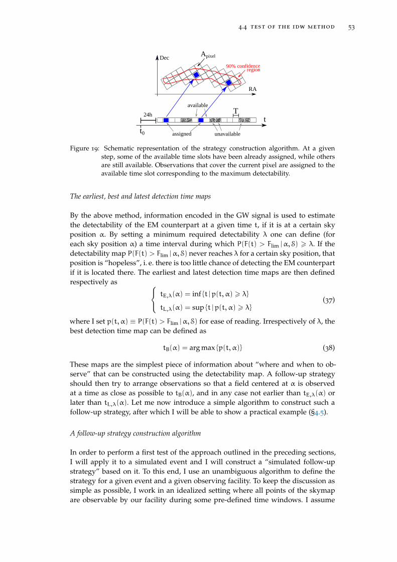
4.4 test of the idw method 53

90% confidenceregion

t

assigned unavailable

Apixel

Tavailable

24h

t0

RA

Dec

Figure 19: Schematic representation of the strategy construction algorithm. At a givenstep, some of the available time slots have been already assigned, while othersare still available. Observations that cover the current pixel are assigned to theavailable time slot corresponding to the maximum detectability.

The earliest, best and latest detection time maps

By the above method, information encoded in the GW signal is used to estimatethe detectability of the EM counterpart at a given time t, if it is at a certain skyposition α. By setting a minimum required detectability λ one can define (foreach sky position α) a time interval during which P(F(t) > Flim |α, S) > λ. If thedetectability map P(F(t) > Flim |α, S) never reaches λ for a certain sky position, thatposition is “hopeless”, i. e. there is too little chance of detecting the EM counterpartif it is located there. The earliest and latest detection time maps are then definedrespectively as tE,λ(α) = inf t |p(t, α) > λ

tL,λ(α) = sup t |p(t, α) > λ(37)

where I set p(t, α) ≡ P(F(t) > Flim |α, S) for ease of reading. Irrespectively of λ, thebest detection time map can be defined as

tB(α) = arg max p(t, α) (38)

These maps are the simplest piece of information about “where and when to ob-serve” that can be constructed using the detectability map. A follow-up strategyshould then try to arrange observations so that a field centered at α is observedat a time as close as possible to tB(α), and in any case not earlier than tE,λ(α) orlater than tL,λ(α). Let me now introduce a simple algorithm to construct such afollow-up strategy, after which I will be able to show a practical example (§4.5).

A follow-up strategy construction algorithm

In order to perform a first test of the approach outlined in the preceding sections,I will apply it to a simulated event and I will construct a “simulated follow-upstrategy” based on it. To this end, I use an unambiguous algorithm to define thestrategy for a given event and a given observing facility. To keep the discussion assimple as possible, I work in an idealized setting where all points of the skymapare observable by our facility during some pre-defined time windows. I assume

54 waw : a gw-informed em follow-up strategy

that each observation covers an area AFoV at observing frequency νobs and that thelimiting flux Flim for detection is independent of sky position and is always reachedafter an integration time Tint. The outline of the algorithm is the following:

• I divide the skymap in patches, each representing a potential field to beobserved;

• I define a list of available time slots (i. e. possible observing time windows)on the time axis, starting 24 hours after the event (posterior samples are typ-ically obtained after several hours or even days, so an earlier start would beunrealistic. Note that this does not mean that I discourage an earlier follow-up – which is of great importance especially for the Optical and X-ray af-terglow – but only that this method may not be applicable with very lowlatency6);

• starting from the patch with highest sky position probability, I check if thedetectability map P(F(t) > Flim |α, S) within that patch exceeds λ at sometime within the available time slots: if it does not, I discard the patch (I choosenot to observe it); if it does, I schedule the observations that cover that patchat the time when the detectability is highest, and I mark the correspondingtime slots as not available anymore;

• I proceed to the next patch in descending order of skymap probability untilthe available time is over, or until all patches have been processed.

To keep the implementation of the above steps as simple as possible, I use aHEALPix tessellation of the sky (Gorski et al., 2005) to define the observablefields: it is a way to divide the sky (i. e. a sphere) into equal area patches, called“pixels”. The “order” Nside of the HEALPix tessellation defines the number ofpixels the sky is divided into, namely Npixels = 12N2side. The pixel area is thenApixel = 3438N−2

side deg2. Thus I replace the actual observations of duration Tint

and field of view AFoV with “pseudo observations” of area Apixel and effectiveduration T = Tint×Apixel/AFoV, choosing Nside in order to minimize the differencebetween Apixel and AFoV. The algorithm is thus implemented as follows:

1. I consider the posterior samples produced by a parameter estimation sam-pler (multiple sampling algorithms are implemented in LALINFERENCE, i. e.LIGO’s parameter estimation tool7) applied to a simulated signal S. Theseare points in the compact binary inspiral parameter space distributed ac-cording to the posterior probability density;

2. I find the 90% sky position confidence region of the source based on theposterior samples;

3. I divide the sky into pixels according to a HEALPix tessellation of orderNside, and I consider only those pixels which fall inside the 90% sky positionconfidence region of the simulated signal;

6 In the example of §4.5, actually, the only parameters needed to predict the possible SGRB afterglowlight curves are dL and ι. Posterior distributions of these parameters (so called “extrinsic”) can beobtained with a low latency analysis tool such as BAYESTAR (Singer and Price, 2016).

7 http://software.ligo.org/docs/lalsuite/lalinference/

4.4 test of the idw method 55

4. I associate to each pixel p the integral of the skymap probability densityPp =

∫Apixel(p)

P(α | S)dΩ over the pixel area;

5. I associate to each pixel p the earliest and latest detection times tE,λ(p)

and tL,λ(p) averaged over that pixel; pixels for which the detectability neverreaches λ are excluded from the list of possible observations;

6. I divide the time axis into contiguous intervals (slots) of duration T (theeffective time needed to cover one pixel) and I mark some of the slots as“available” for the follow-up (based on the characteristics of the instrument);

7. I sort the pixels in order of decreasing Pp and, starting from the first (p = 1)pixel, I do the following:

a) I check that at least one available time slot is comprised between tE,λ(p)

and tL,λ(p): if not, no observation of the pixel is scheduled; otherwise,the available time slot where the detectability is maximum is assignedto the observation of the pixel;

b) I proceed to the next pixel, until all available time slots are assigned, oruntil all pixels have been processed.

Figure 19 shows a schematic representation of the algorithm described above.The output of the above algorithm is thus a list of observation times tobs(p) that

cover (part of) the skymap, giving priority to pixels with high skymap probabilityand trying to use the available time in a way that maximizes the probability todetect the transient. The inputs of the algorithm are:

1. the posterior sample list based on S;

2. the detectability threshold λ;

3. the available time windows;

4. the instrument observing frequency νobs, the field of view area AFoV, thelimiting flux Flim and the corresponding integration time Tint (which shouldalso include the slew time);

5. the HEALPix tessellation order Nside, which should give a pixel area Apixel

close to AFoV.

The observations are given in order of decreasing “importance” (skymap prob-ability). Once the list of observations is produced, one can decide to perform onlythe first N observations that fit into the available telescope time. If all observationssuggested by the algorithm can be performed within the available time, the ex-cess time can be used e. g. to take comparison images of some fields at differenttimes (for the identification of transients or uncatalogued variable sources, in ab-sence of previously available images) or to perform deeper observations for thecharacterization of the candidates.

We are now ready to construct an example of how the use of sky-position-conditional posterior probabilities can help in the definition of an EM follow-upstrategy.

56 waw : a gw-informed em follow-up strategy

100 101 102

t [days]

10­5

10­4

10­3

10­2

10­1

100Fl

ux [m

Jy]

0.5 mJy

1. 4 GHz

17

19

21

23

25

27

AB

mag

nitu

de

22.4 mAB

24.5 mAB

J filterr filter

Figure 20: Light curves of the EM counterparts associated to injection 28840 of F2Y. Jet af-terglow: Radio (1.4 GHz – blue line) and optical (r filter – red line); macronova:Infrared (J filter – yellow line). The same assumptions as in S4.2.1.1 wereadopted. The limiting fluxes for detection adopted in the test example (§4.5)are shown with horizontal black dashed lines.

test example : injection 28840 , a ns-ns merger with an associated

orphan afterglow

As a test example, I consider injection number 28840 from the F2Y study. The in-jection simulates the inspiral of a neutron star binary with M1 = 1.59M andM2 = 1.53M at a luminosity distance dL = 75 Mpc, with orbital plane inclina-tion ι = 14, at sky position (RA,Dec) = (23h 27m 12s, −10 30′ 0′′), detected by thetwo-detector Advanced LIGO network on MJD 55483.27839 (i. e. at 06:40:53 of the14

th of October 2010 – this is just a simulated event) adopting an early sensitivitycurve corresponding to a binary NS range of 55 Mpc (Barsotti and Fritschel, 2012).Assuming that a relativistic jet with isotropic equivalent kinetic energy EK = 1050

erg and half-opening angle θjet = 0.2 rad (which is less than the viewing an-

Table 4: Algorithm input parameters used to construct the example follow-up strategies.Instrument νobs Flim AFoV Tint λ Avail. timea Det. timeb

[Hz] [µJy] [deg2] [s] [h]VST-like (shallow) 4.8×1014 (r filter) 4 (22.4 mAB) 1 100 0.01 3 h/night -

VST-like (deep) 4.8×1014 (r filter) 0.58 (24.5 mAB) 1 1000 0.05 3 h/night 7

MeerKAT-like 1.4×109 500 1.7 1000 0.05 20% 4.7VISTA-like 2.4×1014 (J filter) 4 (22.4 mAB) 1.5 1200 0.5 3 h/night 14.5

aavailable observing time starts 24h after the event.bminimum observation time needed for detection.

4.5 test example : injection 28840 57

0h2h4h6h8h10h12h14h16h18hRA [h]

­75

­60

­45

­30

­15

0

15

30

45

60

75

Dec

[deg

]

3.5 5 6.5 8 9.5tB(α) [days]

Figure 21: Mercator projection of the best detection time map tB(α) at νobs = 1.4 GHzfor injection 28840 of F2Y. Red lines represent the contours of the 50 and 90

percent sky position confidence areas; the black solid line is the locus of skypositions that yield a GW signal arrival time delay of ∆t = 0.359 ms (the “true”arrival time difference associated to the injection position) between the twoLIGO detectors, and the black dashed lines correspond to ∆t± 1 ms. The whitecontours are isolines of the average antenna pattern of the aLIGO network (thefour smaller closed circular contours enclose the local and absolute minima,while the two large closed contours near the lower left and the upper right cor-ners enclose the absolute maxima). The injection true position is marked witha star symbol. Regions marked by blue contours are those where the posteriordetectability of the EM counterpart of our test example reaches the required 5

percent threshold.

gle, thus the afterglow is orphan) is launched perpendicular to the orbital planeright after the merger, I computed its afterglow lightcurve assuming an ISM num-ber density nISM = 0.01 cm−3, adopting the same microphysical parameters as in§4.2.1.1, using BOXFIT v. 1.0 (Eerten, Horst, and MacFadyen, 2012). The lightcurvesat νobs = 1.4 GHz and in the r filter are shown in Figure 20.

To produce our sky-position-conditional posterior distributions, I use 7962 pos-terior samples produced by one of the LALINFERENCE parameter estimation sam-plers. Since I fixed the jet isotropic equivalent kinetic energy EK = 1050 erg, in thisexample the only binary parameters which are relevant to the posterior detectabil-ity of the jet afterglow are the luminosity distance and the binary plane inclination.Figure 21 shows the best detection time map at νobs = 1.4 GHz produced usingthese samples (see the caption for additional information). The 90 percent sky posi-tion confidence area (represented by the larger red contours) covers approximately1500 deg2.

58 waw : a gw-informed em follow-up strategy

Optical search

For our virtual optical EM follow-up, I adopt parameters inspired by the VSTfollow-up of GW150914 (Abbott et al., 2016a). I consider observations in the r band(νobs = 4.8× 1014 Hz) with a detection limit Flim = 22.4 AB magnitude, reachedafter Tint = 100 seconds (slew + integration). The field of view is AFoV = 1 deg2.With the adopted flux limit, the optical lightcurve (Fig. 20) becomes too faint fordetection after a few hours. Consistently, the detectability P(F(t) > Flim |α, S) is be-low 1 percent at all times t > 1 d over the whole skymap except for a subregion ofthe skymap with a total area of 185 deg2. I run the follow-up strategy constructionalgorithm allowing 3 hours of available time per night from day 1 to day 15. I setNside = 64 which gives Apixel = 0.84 deg2 and T = 84 s. Even adopting the verylow detectability limit λ = 0.01 (i. e. allowing for observations with a detectabilityas low as 1 percent), only 24 “pseudo observations” (corresponding to 22 observa-tions) are scheduled (all during the first available night), totalling 36 minutes oftelescope time. The position of the EM counterpart is not contained in any of theobserved fields.

The short integration time and the relatively shallow detection limit of the VSTfollow-up of GW150914 are good in order to cover the largest possible area duringthe next few nights after the event; if we wish to have some chance to detect arelatively dim optical afterglow like that in Fig. 20, though, we need to go deeper,i. e. we need longer integration times. I thus repeat the optical search with thesame parameters as above, but with Tint = 1000 s and Flim = 24.5 mAB. I also raisethe minimum detectability to λ = 0.05, to avoid pointing fields with a very lowdetectability. The algorithm outputs 54 “pseudo observations”, corresponding to46 observations, totalling 15 hours of telescope time. The p = 25 observation (i. e.the 25th observation in descending order of Pp), scheduled 2d 2h 34m 45s after theevent, contains the EM counterpart. The flux at that time is 24.58 mAB, slightlydimmer than the required detection threshold, but detectable with a thresholdS/N ratio of 5 under optimal observing conditions.

As explained in §4.4.5, the follow-up observations suggested by the algorithmare given in descending order of sky position probability, thus astronomers canchoose to perform only the first N observations if not enough telescope time isavailable to complete them all. The field containing the counterpart is at p =

25 in this case. To complete the first 25 observations, 7 hours of telescope timeare needed: this represents the minimum amount of telescope time for the EMcounterpart to be detected by this facility in this case.

Figure 22 shows the positions and times of the observations scheduled by the al-gorithm in this case. During the first night, essentially all points of the detectabilitymap are above the limit λ, thus observations are concentrated around the centresof the two large uncertainty regions (see Fig. 21 for an all-sky view), which are thepoints of largest skymap probability. During the second night, the detectability hasfallen below the limit in most of the central parts of the two uncertainty regions,thus the algorithm moves towards points of lower skymap probability, but higherdetectability. The evolution of the detectability map proceeds in a similar fashionuntil the fifth night, when the detectability at all points of the skymap eventuallyfalls below λ.

4.5 test example : injection 28840 59

10h30m11h30m12h30m13h30m­50°

­35°

­20°

­5°

10°

25°

Dec

22h30m23h30m0h30m1h30mRA

­30°

­20°

­10°

0°

10°

20°

30°

40°

Dec

1 2 3.01 4.01 5.01scheduled time of observation [days]

Figure 22: Time and position of the Optical follow-up observations of our test example(§4.5). The star marks the injection position.

60 waw : a gw-informed em follow-up strategy

Radio search

The parameters of our virtual radio follow-up are inspired by MeerKAT, the SouthAfrican SKA precursor. Sixteen (of the eventual 64) 13.5 m dishes have alreadybeen integrated into a working radio telescope and produced their “first light” im-age8 in July 2016. I assume a field of view AFoV = 1.7 deg2 at νobs = 1.4 GHz. Iconservatively estimate 50 µJy rms noise for a Tint = 1000 s observation (slew + in-tegration), assuming 16 working dishes. In a large area survey, usually a 10 sigmadetection is required to avoid a large number of false alarms, thus I set Flim = 0.5mJy, i. e. I require the flux to be ten times the rms noise for the detection to beconsidered confident. I allow a maximum of 20 percent of the available time fromday 1 to day 100 to be dedicated to the follow-up (in practice, I allow an availabletime window of 4.8 hours each day), and I adopt a λ = 0.05 detectability limit. Thebest detection time map with the chosen parameters is shown in Figure 21, wherethe blue contours represent regions where the detectability reaches the requireddetectability limit at some time t > 1 d (382 deg2 in total). Setting Nside = 64, thefollow-up construction algorithm outputs 337 “pseudo observations” (correspond-ing to 169 pointings, totalling 47 hours of telescope time), which are representedin Figure 23. The p = 35 observation contains the counterpart. It is scheduled5d 0h 9min 27s after the event, when the flux of the EM counterpart is 0.52 mJy(see Fig. 20), which means that the afterglow is detected at better than 10 sigma.The first 35 (pseudo) observations make up 4.7 hours of telescope time: only thisamount needs to be actually allocated for the follow-up to successfully detect theradio counterpart.

Infrared search of the associated macronova

For the same event, I computed the Infrared (J band) lightcurve (see Figure 20)of the associated macronova with the same assumptions as in §4.2.1.1. Due to therather large masses of the binary components and to their similar mass, the dy-namically ejected mass is small (Mej ≈ 5.6×10−3M according to the Dietrich andUjevic, (2017) fitting formula assuming the H4 equation of state). The lightcurveis thus quite dim. It peaks between the second and the third day, slightly brighterthan 22.4 mAB in the J band. The effective temperature of the photosphere at peakis Tpeak ∼ 2900 K. To detect such a transient with a telescope like VISTA, an inte-gration time of the order of 1000 s is needed. I thus perform our virtual follow upstrategy with the following parameters inspired to VISTA: I choose a limiting fluxFlim = 22.4 mAB in the J band with Tint = 1200 s, and I set AFoV = 1.5 deg2. Again,I assume that 3 hours per night are dedicated to the follow-up. The a priori de-tectability (see Figure 15) of the macronova for this limiting flux is high, meaningthat most of the possible lightcurves exceed 22.4 mAB, thus I set λ = 0.5 to limitthe search to points of the skymap which reach a detectability at least as good asthe a priori one.

Adopting the above parameters, the algorithm outputs 123 “pseudo observa-tions” (corresponding to 69 pointings, totalling 23 hours of telescope time), whichare represented in Figure 24. The 79th observation in descending order of Pp con-

8 Media release at http://www.ska.ac.za/media-releases/

4.5 test example : injection 28840 61

10h15m30m45m11h15m30m45m12h­10°

0°

10°

20°

Dec

22h30m45m23h15m30m45m0hRA

­30°

­20°

­10°

0°

Dec

1 3.77 6.54 9.32 12.1scheduled time of observation [days]

Figure 23: Time and position of the Radio follow-up observations of our test example(§4.5). The star marks the injection position.

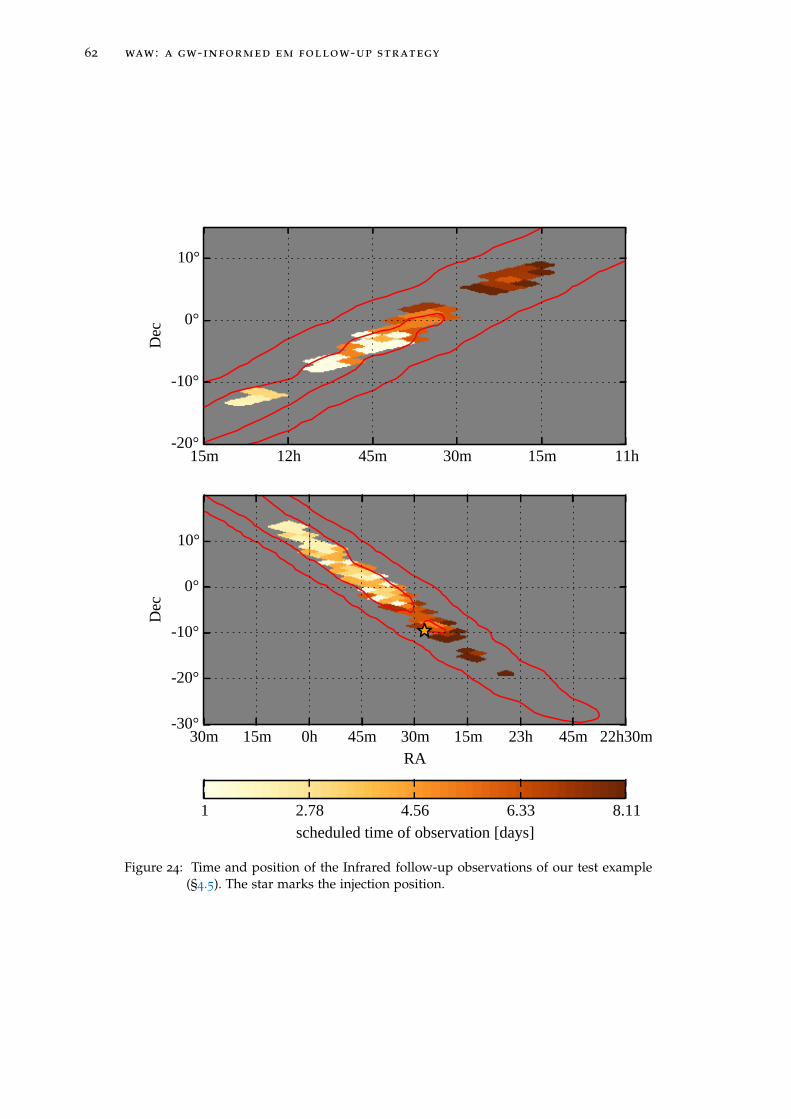
62 waw : a gw-informed em follow-up strategy

11h15m30m45m12h15m­20°

­10°

0°

10°

Dec

22h30m45m23h15m30m45m0h15m30mRA

­30°

­20°

­10°

0°

10°

Dec

1 2.78 4.56 6.33 8.11scheduled time of observation [days]

Figure 24: Time and position of the Infrared follow-up observations of our test example(§4.5). The star marks the injection position.

4.6 discussion 63

tains the counterpart. It is scheduled 6d 0h 18min 27s after the event, when theflux of the macronova in the J band is just below the 22.9 mAB and the effectivetemperature of the spectrum is around 2600 K. The flux is lower than Flim (whichwas chosen to represent an indicative limit for achieving a S/N ratio ∼ 10), butaccording to ESO’s exposure time calculator9, such emission would be detectedthrough the VISTA telescope at ESO in the J band with a S/N ratio of 6, assuminga 1000 s integration, in optimal observing conditions. Our virtual Infrared follow-up would thus again result in a detection in a search with a threshold at S/N ∼ 5.To achieve it, 14.5 hours of telescope time are needed (the amount of time for thefirst 79 most important observations to be performed).

Comparison with follow-up strategies based on the a priori detectability only

For comparison, I performed additional Optical, Radio and Infrared searches us-ing the same parameters as before (listed in Table 4), but replacing the a posterioridetectability P(F(t) > Flim |α, S) with the a priori detectability P(F(t) > Flim) com-puted in §4.2.1.1. This should simulate a search based on a priori information only.The results are the following:

• Optical search: the counterpart is in the field of view 5d 22h 53m 32s afterthe event, when the flux of the jet afterglow in the r band is as low as 26 mAB,which is definitely too faint for a detection;

• Radio search: the counterpart is in the field of view 20d 2h 18m 0s after theevent, when the flux of the jet afterglow at 1.4 GHz is 120 µJy, which is signif-icantly below our required limiting flux. Even assuming that the sensitivitywas good enough for a detection, the facility should have allocated at least77.6 hours of telescope time for this single follow-up in order to include theobservation that contains the counterpart;

• Infrared search: none of the 122 fields of view whose observation is sched-uled by the algorithm contains the counterpart.

I conclude that the use of posterior information from the GW signal has a deci-sive impact on the EM follow-up in our example test case.

discussion

In Salafia et al., (2017b), my co-authors and I proposed the new idea that infor-mation on compact binary inspiral parameters extracted from a GW signal can beused to predict (to some extent) the best timing for observation of the possibleEM counterpart. In practice, the probability distributions of the binary parametersinferred from the GW signal are fed to a model of the candidate EM counterpartin order to define a family of possible lightcurves. The possible lightcurves arethen used to construct the “detectability maps”, which represent an estimate ofhow likely is the detection of the EM counterpart with a given instrument, if theobservation is performed at time t looking at sky position α = (RA,Dec). In order

9 I queried the VIRCAM ETC at http://www.eso.org assuming a 1.2 airmass and a seeing of 0.8arcsec.

64 waw : a gw-informed em follow-up strategy

to apply the idea to a practical example, we introduced an explicit method to con-struct the detectability maps (§4.3.1) and an algorithm which uses these maps todefine an EM follow-up observing strategy (§4.4.5). We then applied the methodto a synthetic example, showing that it improves significantly the effectiveness ofthe EM follow-up (§4.5).

In order to keep the treatment as simple as possible, we adopted many sim-plifications at various stages of the discussion, and we intentionally avoided tomention some secondary details or to include too much complexity. Let me brieflyaddress some of the points that were not discussed in the preceding sections.

Model dependence and inclusion of priors on unknown parameters

The approach clearly relies on the availability of models of the EM counterparts,and on our confidence in the predictions of these models. On the other hand, sincethe lightcurves are treated in a statistical sense, the models only need to representcorrectly the peak flux and lightcurve general evolution. Fine details are lost inthe processing of the lightcurves, and are thus unnecessary. Moreover, it is verystraightforward to include our uncertainty on model parameters unrelated to theGW signal. In all examples discussed in Salafia et al., (2017b), we fixed the valuesof such parameters (e. g. the kinetic energy EK and ISM density nISM of the SGRBafterglow, or the NS equation of state). A better approach (at the cost of a highercomputational cost) would be to assume priors for these parameters, i. e. to assigna probability distribution to the values of these parameters based on some priorinformation (e. g. available astrophysical data, if any) or on theoretical arguments.In this case, multiple lightcurves of the counterpart must be computed for eachposterior sample, using different values of the unknown parameters sampled fromthe assumed priors. This should be the most effective way of incorporating theuncertainty on these parameters in the computation of the detectability maps (itapplies as well to the a priori detectability and to the a posteriori detectability).We will explore the effect of the inclusion of such priors in the construction of apriori detectabilities, a posteriori detectabilities and detectability maps for a rangeof potential EM counterpart models in a future work.

Sky position dependence of the parameters

In §4.2.2.4 I stated that, in general, the sky-position-conditional posterior distribu-tion of the inspiral parameters depends on the assumed sky position. The maindriver of this dependence is the sky projection of the antenna patterns (i. e. thesensitivity to different polarizations) of the interferometers of the network: the dis-tribution of distances, inclinations and mass ratios compatible with a given signal,assuming that the source is at a particular sky position, is especially constrainedby what the interferometers can or cannot detect if the source is at that sky po-sition. As an intuitive example, say that a particular sky position corresponds tothe maximum sensitivity of one of the detectors with respect to a particular po-larization, and say that the incident GW that yields the signal picked up by thatdetector contains no such polarization: only combinations of parameters for whichthe corresponding component of the strain is smaller than the limit set by the sen-

4.6 discussion 65

sitivity are admissible if that sky location is assumed. If another sky location isassumed, the constraints change accordingly. As a general trend, points of the skywhere the network has a higher sensitivity will correspond to a larger averagedistance of the source, thus implying a lower detectability for both the macronovaand the SGRB afterglow. If the sky position uncertainty region is smaller than thetypical angular scale over which the antenna pattern varies, the dependence of theposterior distributions of the parameters on sky position becomes less important:the a posteriori detectability contains most of the relevant information in that case.With Advanced Virgo joining the network, in many cases the sky position uncer-tainty region will still extend over a few hundreds of square degrees (Abbott et al.,2016); on the other hand, better information on the two polarization states of theGW signal will be available (the two interferometers of the aLIGO network arealmost anti-aligned, thus the ability of the network to distinguish between the twopolarization states is rather poor as of now). In the next decades, third generationinterferometers will face again the same issues about sky localization. The use ofdetectability maps instead of the a posteriori detectability alone is thus likely toremain useful with more advanced networks as well.

The choice of injection 28840

The injection event used to construct the example presented in the last section wasselected among those of the F2Y study. We considered a two-detector case (LIGOonly), as it leads in general to larger localization uncertainties. We looked throughthe list for an event which was quite distant and whose orbit inclination was suf-ficiently inclined for the jet to be off-axis. The 28840 injection event luminositydistance is indeed rather large (dL = 75 Mpc), the jet is slightly off-axis (ι = 14),the sky position uncertainty is large (more than 1500 deg2) and the injection po-sition is rather far away from the maximum of the skymap probability. The lattercondition makes a search based only on the a priori information particularly in-effective, because the exploration of the skymap proceeds slowly (using relativelysmall field instruments) from the centre of the skymap (where the skymap prob-ability is high) to the periphery (where the source is actually located). In caseswhen the sky location is better reconstructed (i. e. the source is closer to the pointof maximum skymap probability), the improvement in the EM follow-up effec-tiveness thanks to the detectability maps (with respect to a strategy based onlyon the skymap probability and on a priori information on the EM counterpartcharacteristics) could be less striking. We plan to study systematically the relativeimprovement in a future work.

A better strategy construction algorithm

The algorithm (§4.4.5) used to construct the virtual EM follow-up strategy of ourexample is admittedly oversimplified. An algorithm suited for real applicationshould be able to:

1. take into account the actual observability constraints on all points of theskymap at a given time, e. g. the setting of tiles below the horizon;

66 waw : a gw-informed em follow-up strategy

2. use a better (instrument specific) way of dividing the sky into potentiallyobservable fields;

3. consider the impact of airmass, expected seeing, dust extinction, stellar den-sity in the field and other variables on the detectability;

4. potentially use a different integration time for each tile, in order to maximizethe detection probability;

5. avoid sequences of widely separated pointings, that would result in a wasteof time in slewing.

Some recent works already addressed, at least in part, some of the above points.Ghosh et al., (2015) discussed an algorithm for the optimization of the tiling, whichis totally compatible with our approach, since the detectability maps do not set apreferred tiling. Rana et al., (2017) developed and compared some ingenious algo-rithms that aim at maximizing the sky position probability in the search, takinginto account per-tile setting and rising times. Their approach does not account forthe time evolution of the EM counterpart luminosity, though, and it can result inthe paradoxical situation in which the highest probability tile is observed before thetime at which the flux is high enough for a detection. Incorporating the informa-tion from the detectability maps in their method could be the starting point for arealistic automated strategy construction algorithm based on the ideas presentedin this work. For what concerns point (4) above, both Coughlin and Stubbs, (2016)and Chan et al., (2017) found that an equal integration time in all observationscould be sub-optimal with respect to the EM counterpart detection probability.Their assumptions, though, are significantly different from ours: both assume aconstant luminosity of the EM counterpart (i. e. they ignore the time variation ofthe flux), and they do not use astrophysically motivated priors on luminosity (theformer use a flat prior, while the latter use Jeffrey’s prior L−1/2 limited to therange span by the peak luminosities of the macronova model in Barnes and Kasen2013). It is not straightforward to figure out if their results are applicable to ourmore general case as well.

As an additional caveat, we only considered the case where one epoch obser-vation per field is enough to identify transient sources. Realistically, this is onlyfeasible when previous images can be used as reference, or where source catalogsare complete up to the survey limit. The identification of interesting transientsand the removal of those unrelated to the GW source require at least two epochsof observations, which are not taken into account in our example algorithm.

Use in conjunction with the “galaxy targeting” approach

The use of detectability maps is entirely compatible with a search based on tar-geting candidate host galaxies. The observation of each target galaxy would sim-ply need to be performed as close to the corresponding best detection time (asdefined in §4.4.4) as possible. Since choosing a target galaxy corresponds to as-suming a known distance to the source, an intriguing further refinement of thepresent method could be to consider the posterior distribution of binary parame-ters conditioned on both sky position and distance. This would have a great impact

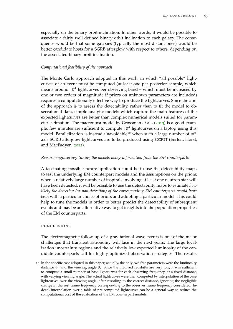
4.7 conclusions 67

especially on the binary orbit inclination. In other words, it would be possible toassociate a fairly well defined binary orbit inclination to each galaxy. The conse-quence would be that some galaxies (typically the most distant ones) would bebetter candidate hosts for a SGRB afterglow with respect to others, depending onthe associated binary orbit inclination.

Computational feasibility of the approach

The Monte Carlo approach adopted in this work, in which “all possible” light-curves of an event must be computed (at least one per posterior sample, whichmeans around 104 lightcurves per observing band – which must be increased byone or two orders of magnitude if priors on unknown parameters are included)requires a computationally effective way to produce the lightcurves. Since the aimof the approach is to assess the detectability, rather than to fit the model to ob-servational data, simple analytic models which capture the main features of theexpected lightcurves are better than complex numerical models suited for param-eter estimation. The macronova model by Grossman et al., (2013) is a good exam-ple: few minutes are sufficient to compute 104 lightcurves on a laptop using thismodel. Parallelization is instead unavoidable10 when such a large number of off-axis SGRB afterglow lightcurves are to be produced using BOXFIT (Eerten, Horst,and MacFadyen, 2012).

Reverse-engineering: tuning the models using information from the EM counterparts

A fascinating possible future application could be to use the detectability mapsto test the underlying EM counterpart models and the assumptions on the priors:when a relatively large number of inspirals involving at least one neutron star willhave been detected, it will be possible to use the detectability maps to estimate howlikely the detection (or non-detection) of the corresponding EM counterparts would havebeen with a particular choice of priors and adopting a particular model. This couldhelp to tune the models in order to better predict the detectability of subsequentevents and may be an alternative way to get insights into the population propertiesof the EM counterparts.

conclusions

The electromagnetic follow-up of a gravitational wave events is one of the majorchallenges that transient astronomy will face in the next years. The large local-ization uncertainty regions and the relatively low expected luminosity of the can-didate counterparts call for highly optimized observation strategies. The results

10 In the specific case adopted in this paper, actually, the only two free parameters were the luminositydistance dL and the viewing angle θv. Since the involved redshifts are very low, it was sufficientto compute a small number of base lightcurves for each observing frequency, at a fixed distance,with varying viewing angle. The actual lightcurves were then computed by interpolation of the baselightcurves over the viewing angle, after rescaling to the correct distance, ignoring the negligiblechange in the rest frame frequency corresponding to the observer frame frequency considered. In-deed, interpolation over a table of pre-computed lightcurves can be a general way to reduce thecomputational cost of the evaluation of the EM counterpart models.

68 waw : a gw-informed em follow-up strategy

of this work showed that information from the GW signal can be used to makeevent-specific adjustments to the EM follow-up strategy, and that such adjustmentscan improve significantly the effectiveness of the search at least in some cases, asshown in the example in §4.5. Advances in the theoretical understanding of theEM counterparts (e. g. in our ability to predict the amount of mass ejected duringthe merger) will increase the effectiveness of this approach, and are thus of greatimportance for the astronomy community as well.

Part II

L I G H T A N D G R AV I TAT I O N A L WAV E S F R O M A S I N G L ES O U R C E : G W 1 7 0 8 1 7

5A R E V O L U T I O N S TA RT E D O N T H E 1 7 T H O F A U G U S T 2 0 1 7

Not many people have had the chance to witness a revolution. Only few have hadthe luck, and the responsibility, to be part of it. I feel right in between the two cases:I was just entering the field, I had just started to understand some of the aspectsof this exciting world, when I suddenly found myself witnessing the first ever de-tection of gravitational waves from a binary neutron star merger, event GW170817

(Abbott et al., 2017b), and the subsequent discovery of associated electromagneticemission in several bands (Abbott et al., 2017d). The infrared, optical and ultravi-olet emission (Coulter et al., 2017; Valenti et al., 2017; Pian et al., 2017; Andreoniet al., 2017; Arcavi et al., 2017; Chornock et al., 2017; Covino et al., 2017; Díaz et al.,2017; Drout et al., 2017; Evans et al., 2017; Hallinan et al., 2017; Pozanenko et al.,2017; Utsumi et al., 2017; Cowperthwaite et al., 2017; Gall et al., 2017; Kilpatricket al., 2017; McCully et al., 2017; Nicholl et al., 2017; Smartt et al., 2017) leaveslittle doubt about its origin: a kilonova1, i. e. a supernova-like emission powered bythe decay of heavy nuclei produced by r-process nucleosynthesis in the expand-ing material ejected during the NS-NS merger and post-merger phases (Metzger,2017). The gamma-ray burst detected by Fermi/GBM (Goldstein et al., 2017) andINTEGRAL/SPI-ACS (Savchenko et al., 2017) and the late-time X-ray (Haggard etal., 2017; Margutti et al., 2017; Troja et al., 2017) and Radio (Hallinan et al., 2017;Alexander et al., 2017) data, instead, have been interpreted in different ways bydifferent groups. It is important to note here that the local rate of NS-NS mergersthat can be estimated from this single observation is R0 = 1540+3200−1220Gpc−3 yr−1

(Abbott et al., 2017b), which is three to four orders of magnitude larger than thelocal rate of SGRBs as estimated in chapter 3. This clearly has implications thatmust be discussed. Hereafter, I will try to examine some of the possible interpre-tations of these observations, both from the point of view of the physics behindthe emission, and from that of the implications concerning rate associated to thisevent.

the short gamma-ray burst grb170817a

Before the 17th of August 2017, events like GRB170817A have probably been de-tected several times by instruments such as Fermi and possibly Swift without at-tracting too much attention. Due to the low flux and fluence, this kind of bursthardly becomes a candidate for a follow-up aimed at searching for the afterglowand identifying the host galaxy. These events simply end up populating the highlyincomplete part of the “logN− logS” (the fluence distribution of the sample), andthey are usually cut off the flux limited samples used for population studies.

The association with the gravitational wave event GW170817 reveals though thatat least some of these low flux events might represent extremely precious pieces ofinformation about one of the most interesting class of phenomena astrophysicists

1 In chapter 4 I referred to the same phenomenon using the term macronova.

71

72 a revolution started on the 17th of august 2017

have been dreaming of: binary neutron star (NS-NS) mergers (Abbott et al., 2017b;Abbott et al., 2017d; Abbott et al., 2017c).

The fact that such an association entered the scene so early is astonishing undermany points of view: even though NS-NS mergers have been among the best candi-date short gamma-ray burst progenitors since a long time (Eichler et al., 1989), themost recent predictions of the rate of SGRBs within the Advanced LIGO/Virgo net-work range during the first and second run were very low (Ghirlanda et al., 2016;Wanderman and Piran, 2014). Moreover, all measurements of SGRB half-openingangles to date (Soderberg et al., 2006; Nicuesa Guelbenzu et al., 2011; Fong et al.,2012; Fong et al., 2013; Troja et al., 2016) point to narrow jets (θjet . 10 – eventhough serious selection effects could be at play), implying that the probability tohave an on-axis or slightly off-axis jet associated with the very first GW from a NS-NS merger should be very small. Last but not least, several studies (e. g. Ruiz andShapiro, 2017; Murguia-Berthier et al., 2017; Margalit, Metzger, and Beloborodov,2015) seem to indicate that not all NS-NS mergers are capable of producing a jet,making the association even more unlikely.

It can certainly be the case that all or some of the above expectations and prej-udices about SGRB jets are simply wrong. On the other hand, many features ofGRB170817A suggest quite naturally that it does not belong to the SGRB popula-tion we are used to. Its isotropic equivalent energy is several orders of magnitudebelow the least energetic SGRB known so far, despite the spectral peak energy be-ing only moderately low with respect to the known population (Nava et al., 2011a;Zhang et al., 2017). Indeed, these facts have been taken by many as hints thatGRB170817A is an ordinary or structured SGRB jet seen off-axis (e. g. Pian et al.,2017; Ioka and Nakamura, 2017; Burgess et al., 2017; Zhang et al., 2017; Lamb andKobayashi, 2017; He, Tam, and Shen, 2017; Kathirgamaraju, Duran, and Giannios,2017), while others interpret it as emission from the jet cocoon (e. g. Kasliwal et al.,2017; Bromberg et al., 2017; Piro and Kollmeier, 2017; Gottlieb et al., 2017; Lazzatiet al., 2017a).

observational properties of grb170817a

The GRB triggered Fermi/GBM on 2017-08-17 12:41:06, just 1.74 s after the esti-mated merger time of GW170817 (Abbott et al., 2017c). The duration of the bursthas been estimated as T90 = 2.0± 0.5 s. The 64 ms peak flux in the 10–1000 keVband was 3.7 ± 0.9ph cm−2s−1, and the fluence was (2.8± 0.2) × 10−7 erg cm−2.A detailed analysis (Goldstein et al., 2017; Zhang et al., 2017) indicates the pres-ence of two components: a non-thermal component, which dominates the earlypart of the lightcurve, whose spectrum is fit by a power-law with an exponentialcut-off with Epeak = 185± 62 keV, and has a fluence (1.8± 0.4)× 10−7 erg cm−2;a thermal component, visible in the tail of the lightcurve, which is fit by a black-body with kBT = 10.3 ± 1.5 keV (where kB is Boltzmann’s constant) and has afluence (0.61± 0.12)× 10−7 erg cm−2, which corresponds to an isotropic equiva-lent energy (1.20± 0.23)× 1046 erg at dL ≈ 40Mpc (i. e. the distance to the hostgalaxy NGC4993, Hjorth et al. 2017; Im et al. 2017). According to Goldstein et al.,(2017), the thermal component could be present since the beginning, being initiallymasked by the non-thermal emission.

5.3 some possible interpretations of grb170817a 73

some possible interpretations of grb170817a

As mentioned in §5.1, the majority of the works published after the announcementof the discovery of GW170817 recognize GRB170817A as a “special” SGRB, i. e.they see the need to add some ingredient to the standard GRB picture in orderto explain its properties. Almost all authors seem to agree on the fact that, if a jetwas present, it was not seen on-axis, i. e. it was not pointing towards the Earth.The most widespread views are the following:

• the emission was due to a standard SGRB jet seen off-axis (e.g. Burgess et al.,2017; Fraija et al., 2017; Granot et al., 2017; Granot, Guetta, and Gill, 2017;Hallinan et al., 2017; Ioka and Nakamura, 2017; Lamb and Kobayashi, 2017);

• the emission was due to a structured SGRB jet seen off-axis (e.g. Kathirgama-raju, Duran, and Giannios, 2017; He, Tam, and Shen, 2017; Troja et al., 2017;Zhang et al., 2017);

• the emission was from an off-axis jet that was slower than average (e.g. Pianet al., 2017);

• the emission came from a mildly relativistic jet cocoon (e.g. Lazzati et al.,2017a; Bromberg et al., 2017; Gottlieb et al., 2017; Kasliwal et al., 2017; Piroand Kollmeier, 2017);

• aside from the mainstream, I proposed an alternative solution: emission froman isotropic fireball, powered by the strong magnetic field amplified by mag-netohydrodynamic turbulence at the beginning of the merger phase (Salafia,Ghisellini, and Ghirlanda, 2018; Salafia et al., 2017a).

First of all, let me comment briefly on how these scenarios relate to the followingquestion: is the rate of SGRBs, as derived in chapter 3, in tension with this event?

impact on the rate of sgrbs

All the interpretations listed above seek a way out of the same two problems: (1) itis improbable for the first NS-NS merger to be associated to an SGRB jet pointingtowards the Earth (if jets are narrow), and (2) the luminosity of GRB170817A isextremely low compared to the known SGRB population. As a byproduct, all theseinterpretations also imply that the rate of this kind of event does not match thatof “normal” SGRBs, i. e. of relatively energetic jets seen on-axis. Let me focus nowon the interpretations that require the presence of a jet. Let RSGRB be the localrate of SGRBs pointing towards the Earth, and RNS−NS the local rate of doubleneutron-star mergers. The two are linked by

RSGRB = fjfbRNS−NS (39)

where fb =⟨1− cos θj

⟩is the collimation factor (the mean is over the half-opening

angles θj of all SGRBs), which gives the fraction of jets that point towards the Earthover the total, and fj is the fraction of NS-NS mergers that produce a successful jet(I am neglecting BH-NS mergers for simplicity). Since the orbital plane inclinationof the GW170817 binary with respect to the line of sight was . 30 (Abbott et al.,

74 a revolution started on the 17th of august 2017

2017b), we can neglect to first order the possible anisotropy of the cocoon or theweakness at very large angles of the emission from a structured jet, and concludethat the probability to associate such emission to GW170817 was essentially fj

(because a jet is needed in both scenarios). If we require this probability to be atleast, say, fj = 0.3, and we use RNS−NS = 1540+3200−1220Gpc−3 yr−1 as estimated fromthis single event (Abbott et al., 2017b), from Eq. 39 we have that

⟨θj⟩. 2.3+5.5

−1.0 degif we take RSGRB = 0.36+0.53

−0.17Gpc−3 yr−1 as in Ghirlanda et al., (2016), or⟨θj⟩.

7.6+13.4−4.4 deg if we take RSGRB = 4.1+2.3

−1.9Gpc−3 yr−1 as in Wanderman and Piran,(2014).

The above argument can be summarized by saying that, adopting an off-axis jetor cocoon interpretation of GRB170817A, the relatively low rate of SGRBs found inrecent population studies can be reconciled with the association of GRB170817Awith GW170817 provided that a large fraction fj & 0.3 of NS-NS mergers producea jet (which must be a successful jet in the structured jet scenario, but may be achoked jet in the cocoon scenario), and that jets feature narrow half-opening angles⟨θj⟩. few degrees.

In the isotropic fireball scenario proposed in Salafia, Ghisellini, and Ghirlanda,(2018) and Salafia et al., (2017a), on the other hand, no jet is needed to explainthe emission: it thus implies no requirements on fb and fj; it simply requires theisotropic fireball to be produced in most NS-NS mergers. In chapter 7, I describesuch scenario and show that it could be present in most or even all NS-NS mergers.Before, in chapter 6, I discuss some expected properties of emission from an off-axis jet, and use them to show that an off-axis jet interpretation of GRB170817Apresents some difficulties.

6P R O M P T E M I S S I O N F R O M A N O F F - A X I S J E T

pulses : building blocks of grb light curves

The diversity and complexity of GRB prompt emission light curves is often usedto illustrate the difficulty in the classification of these sources and in the unifica-tion of their properties. A natural approach to get insight into such complexityis to look for global and average properties, like flux time integral (i. e. fluence),total duration, average spectrum, peak flux. Alternatively, one can try to breakdown the light curve into simpler parts following some pattern. If a fundamen-tal building block was identified, the analysis of single blocks could be the keyto the unification and disentanglement of properties of the underlying processes.Many authors (e. g. Imhof et al., 1974; Golenetskii et al., 1983; Norris et al., 1986;Link, Epstein, and Priedhorsky, 1993; Ford et al., 1995; Kargatis and Liang, 1995;Liang and Kargatis, 1996; Preece et al., 1998; Ramirez-Ruiz and Fenimore, 1999;Lee, Bloom, and Petrosian, 2000; Ghirlanda, Celotti, and Ghisellini, 2002; Hakkilaand Preece, 2011; Lu et al., 2012; Basak and Rao, 2014) performed careful analysesof light curves and time resolved spectra looking for patterns and for hints aboutsuch fundamental building blocks. As early as 1983, Golenetskii et al. found evi-dence of a correlation between spectral peak energy and photon flux during thedecay of pulses. Such correlation was later confirmed by Kargatis et al., (1994),Kargatis and Liang, (1995) and Borgonovo and Ryde, (2001) and became known asthe hardness-intensity correlation (Ryde and Svensson, 1998). Norris et al., (1986) waspresumably the first to systematically decompose the light curves into pulses andto look for patterns in the properties of these putative building blocks. Some yearslater, Woods and Loeb, (1999) developed tools to calculate the emission from arelativistically expanding jet, including the case of an off-axis viewing angle. Iokaand Nakamura, (2001) took advantage of this formulation to model the singlepulse, finding that the spectral lag-luminosity and variability-luminosity correla-tions found by Norris, Marani, and Bonnell, (2000) and Reichart et al., (2001) canbe explained as viewing angle effects. The pulse model at that stage assumed emis-sion from a unique radius and from an infinitesimally short time interval (i. e. adelta function in radius and time). In the following years, other authors proposedincreasingly refined models of the pulse (e. g. Dermer, 2004; Genet and Granot,2009), but neglected the possibility for the jet to be observed off-axis.

Off-axis pulses and the interpretation of low-luminosity GRBs

The viewing angle, i. e. the angle between the jet axis and the line of sight, isusually assumed to be smaller than the jet semi-aperture, in which case the jetis said to be on-axis. For larger viewing angles, i. e. for off-axis jets, the flux isseverely suppressed because of relativistic beaming. Nevertheless, it can be stillabove detection threshold if the viewing angle is not much larger than the jet

75

76 prompt emission from an off-axis jet

semi-aperture, especially if the burst is at low redshift. Pescalli et al., (2015) haveshown that off-axis jets might indeed dominate the low luminosity end of theobserved population.

The idea that nearby low luminosity GRBs could be off-axis events has been asubject of debate since the observation of GRB980425. Soderberg et al., (2004) re-jected such possibility, based on radio observations of GRB980425 and GRB031203,but soon later Ramirez-Ruiz et al., (2005) presented an off-axis model for the af-terglow of GRB031203 which seems to fit better the observations (including radio)with respect to the usual on-axis modelling. Using the same off-axis afterglowmodel, Granot, Ramirez-Ruiz, and Perna, (2005) extended the argument to twoX-Ray Flashes, thus including them in the category of off-axis GRBs. Based onprompt emission properties, an off-axis jet interpretation of X-Ray Flashes hadbeen already proposed by Yamazaki, Ioka, and Nakamura, (2002) and Yamazaki,Ioka, and Nakamura, (2003), following the work by Ioka and Nakamura, (2001).Ghisellini et al., (2006a) argued that the off-axis interpretation of GRB031203 andGRB980425 is not practicable, because their true energy would then be on the veryhigh end of the distribution, implying a very low likelihood when combined withthe low redshift of these two events. More recently, the idea that such events aremembers of a separate class (e. g. Liang, Zhang, and Zhang, 2007; Zhang, 2008; Heet al., 2009; Bromberg, Nakar, and Piran, 2011; Nakar, 2015) has gained popularity.Recent results about the GRB luminosity function (Pescalli et al., 2015), though,still point towards the unification of these events with ordinary GRBs based onthe off-axis viewing angle argument. In this chapter, I will address the issue fromanother point of view, by focusing on the apparently single pulsed, smooth be-haviour of prompt emission light curves of these bursts, trying to figure out ifsuch behaviour is expected in the case of an off-axis viewing angle.

pulse overlap and light curve variability

For a light curve to be highly variable, pulses must be short and not overlaptoo much. If pulses are produced at a typical radius by material moving closeto the speed of light, then the amount of overlap can depend on the viewingangle. To see this, consider two point sources moving at equal constant speedβc along the z axis, separated by a distance βc∆T , as in Fig. 25. Each sourcestarts emitting at radius Ron and stops emitting at Roff. An observer along the zaxis (viewing angle θv = 0) sees two separated pulses of equal duration ∆t0 andpeak flux F0, the second starting a time ∆T after the start of the first. Becauseof relativistic Doppler effect, an observer with another θv 6= 0 measures a lower(bolometric) peak flux F = F0/b

4 and a longer pulse duration ∆t = b∆t0, whereb = (1 − β cos θv)/(1 − β) is the ratio of the on-axis relativistic Doppler factorδ(0) = Γ−1 (1−β)−1 to the off-axis one δ(θv) = Γ

−1 (1−β cos θv)−1 (Rybicki and

Lightman, 1979; Ghisellini, 2013). The difference in pulse start times ∆T , on theother hand, is not affected by the viewing angle, because the emission of bothpulses begins at the same radius: it can be thought of as emission from a sourceat rest (for what concerns arrival times). The pulses overlap if ∆t > ∆T , whichcorresponds to θv > θov ≈ Γ−1

√∆T/∆t0 − 1. Consider the case in which the

pulse separation is equal to the pulse duration, i. e. ∆T = 2∆t0 and θov ≈ Γ−1.

6.2 pulse overlap and light curve variability 77

Ron Roff

F0/b4

overlap

t

F

Δt0

F0

on axis off axis

ΔT

ΔT

Δt0 b

cΔT

Figure 25: Upper left panel: two point sources (blue and red dots) move at equal con-stant speed along the z axis, separated by a distance βc∆T . Each starts emittingat z = Ron and stops emitting at z = Roff. The blue and red circles representwavefronts of the emitted light. The first blue wavefront and the first red wave-front reach any observer with a time difference ∆T . Upper right panel: closeup. Depending on the viewing angle θv, a distant observer sees the blue andred signal separated (θv < θov) or overlapped (θv > θov). The angle θov is theangle between the z axis and the normal to a plane tangent to both the firstred wavefront and the last blue wavefront. Lower panel: sketch of the bolomet-ric light curve as seen by on-axis (θv = 0) and off-axis (θv > θov) observers.Letting b = (1−β cos θv)/(1−β), the single pulse flux as measured by the off-axis observer is decreased by a factor b4 with respect to the on-axis one, whilethe duration is increased by a factor b. The pulse separation ∆T , though, doesnot depend on the viewing angle, being the emission time difference at a fixedradius. This causes the pulses to overlap as seen by the off-axis observer.

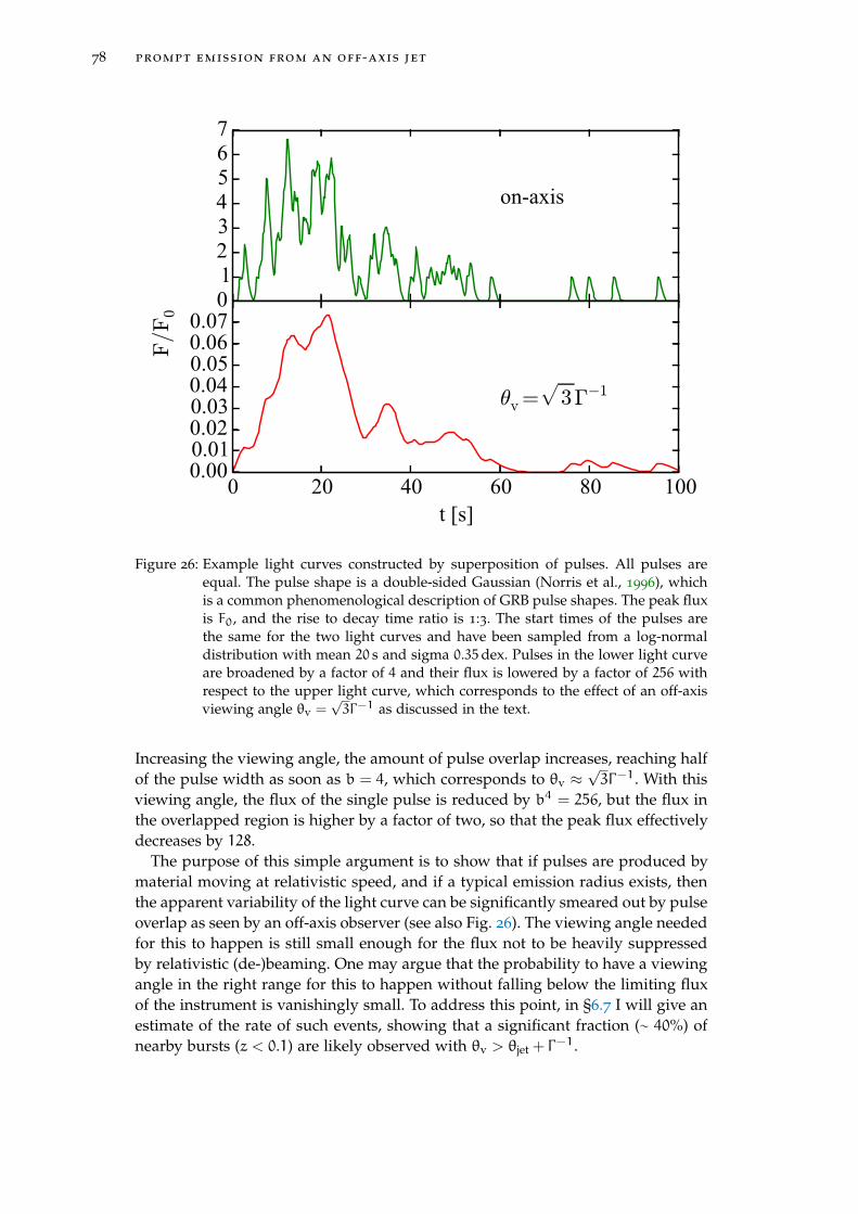
78 prompt emission from an off-axis jet

01234567

on-axis

0 20 40 60 80 100t [s]

0.000.010.020.030.040.050.060.07

θv =√

3Γ−1

F/F

0

Figure 26: Example light curves constructed by superposition of pulses. All pulses areequal. The pulse shape is a double-sided Gaussian (Norris et al., 1996), whichis a common phenomenological description of GRB pulse shapes. The peak fluxis F0, and the rise to decay time ratio is 1:3. The start times of the pulses arethe same for the two light curves and have been sampled from a log-normaldistribution with mean 20 s and sigma 0.35dex. Pulses in the lower light curveare broadened by a factor of 4 and their flux is lowered by a factor of 256 withrespect to the upper light curve, which corresponds to the effect of an off-axisviewing angle θv =

√3Γ−1 as discussed in the text.

Increasing the viewing angle, the amount of pulse overlap increases, reaching halfof the pulse width as soon as b = 4, which corresponds to θv ≈

√3Γ−1. With this

viewing angle, the flux of the single pulse is reduced by b4 = 256, but the flux inthe overlapped region is higher by a factor of two, so that the peak flux effectivelydecreases by 128.

The purpose of this simple argument is to show that if pulses are produced bymaterial moving at relativistic speed, and if a typical emission radius exists, thenthe apparent variability of the light curve can be significantly smeared out by pulseoverlap as seen by an off-axis observer (see also Fig. 26). The viewing angle neededfor this to happen is still small enough for the flux not to be heavily suppressedby relativistic (de-)beaming. One may argue that the probability to have a viewingangle in the right range for this to happen without falling below the limiting fluxof the instrument is vanishingly small. To address this point, in §6.7 I will give anestimate of the rate of such events, showing that a significant fraction (∼ 40%) ofnearby bursts (z < 0.1) are likely observed with θv > θjet + Γ

−1.

6.3 pulses in the internal shock scenario 79

Being based solely on geometry and relativity, the above argument does notrely on a specific scenario, e. g. internal shocks. Any model in which photons areproduced at a typical radius, being the photospheric radius (e. g. subphotosphericdissipation models like those described in Rees and Mészáros, 2005; Giannios,2006; Beloborodov, 2010) or beyond (e. g. magnetic reconnection models, Lazarianet al., 2003; Zhang and Yan, 2010) eventually must take into account the pulseoverlap as seen by off-axis observers.

pulses in the internal shock scenario

The pulse width in GRB light curves is roughly constant throughout the burstduration (Ramirez-Ruiz and Fenimore, 1999). The internal shock scenario (Reesand Meszaros, 1994) provides a natural framework for the understanding of thiskind of behaviour. In this scenario, discontinuous activity in the central engine pro-duces a sequence of shells with different Lorentz factors. When faster shells catchup with slower ones, shocks develop and particles are heated. If the plasma is op-tically thin and some magnetic field is present, the energy gained by the electronsis promptly and efficiently radiated away by synchrotron (and inverse Compton)emission. Each pulse is thus the result of the merger of two shells beyond thephotospheric radius Rph. The strength of the shock, and thus the efficiency of theelectron heating, depends strongly on the relative Lorentz factor of the mergingshells (a radiative efficiency of a few percent is achieved only for Γrel & 3, Lazzati,Ghisellini, and Celotti 1999). Shell pairs with small relative Lorentz factors mergelater (they need more time to catch up with each other), thus the highest efficiencyis achieved for shells merging just after the photospheric radius. This explains,within this framework, why the typical pulse width is not seen to grow with time:the bulk of the emission happens at a fixed radius, regardless of the expansion ofthe jet head.

Time scales

Three main time scales arise in the internal shock scenario:

• the electron cooling time τcool, i. e. the time needed by electrons to radiateaway most of the energy gained from the shock;

• the angular time scale τang, i. e. the difference in arrival time between photonsemitted at different latitudes;

• the shell crossing time τsc, i. e. the time needed for the two shells to merge.

The electron cooling time scale, as measured in the lab frame, is τcool ∼ Γ−1γ/γ,

where Γ is the bulk Lorentz factor, γ is the typical electron Lorentz factor as mea-sured in the comoving frame, and γ is the cooling rate. For synchrotron emission,it is of the order of τcool ∼ 10

−7 s for typical parameters1 (Ghisellini, Celotti, andLazzati, 2000).

1 by typical parameters I mean Γ = 100, Γrel = a few, Urad = UB, a typical synchrotron frequency of1 MeV and I assume equipartition. See Ghisellini, Celotti, and Lazzati, (2000) and references thereinfor a complete treatment.

80 prompt emission from an off-axis jet

The angular time scale arises when one takes into account the arrival time differ-ence of photons emitted at the same time by parts of the shell at different latitudes.It is defined as the arrival time difference between a pair of photons, one emittedat zero latitude and the other at Γ−1 latitude at the same time. Given a typical pho-tospheric radius (Daigne and Mochkovitch, 2002a) Rph ∼ 1012 cm, this differenceis τang ∼ R/Γ2c ≈ 3× 10−3 s R12/Γ22 (we adopt the notation Qx = Q/10x in cgsunits).

The shell crossing time is τsc ∼ w/c, where w is the typical shell width. Beinglinked to the central engine activity, one may assume w to be of the order of afew Schwarzschild radii. The Schwarzschild radius of a 5M black hole is Rs ≈1.5 × 106 cm, thus an estimate might be τsc ∼ 5 × 10−5 s w6. In this case, wehave τang > τsc, i. e. the effect of shell curvature dominates over (i. e. smears out)intrinsic luminosity variations due to shock dynamics, which take place over theτsc time scale or less.

Temporal analysis of GRB light curves, though, along with simple modelling ofinternal shocks (Nakar and Piran, 2002a; Nakar and Piran, 2002b), seem to indi-cate that the shell width must be comparable to the initial shell separation. Takingthe two as equal, the time needed for two shells to collide is the same as the shellcrossing time, and thus the shell merger is completed within a doubling of theradius. In this case, the shell crossing time and the angular time scale are the same(Piran, 2005). This means that details of the pulse shape and spectral evolutioncannot be explained as just being due to the shell curvature effect. Indeed, discrep-ancies between predictions based on shell curvature only and observations havebeen pointed out (e. g. Dermer, 2004).

Nevertheless, the description of the pulse in terms of shell curvature qualita-tively reproduces the main features of many long GRB pulses, namely the fastrise and slower decay, the hard-to-soft spectral evolution, and the presence of ahardness-intensity correlation (Ryde and Petrosian, 2002). For this reason, since Ifocus on the effect of the viewing angle rather than on details of the pulse, in whatfollows I will set up a simple model of the pulse based on the shell curvature effectonly.

pulse light curves and time dependent spectra in the shell-curvature

model

Main assumptions

Based on the arguments outlined in §6.3.1, I assume that the variation of the fluxseen by the observer during a single pulse is due only to the angular time delaydescribed above. The luminosity L of the shell is assumed constant during anemission time T and zero before and after this time interval. The emitting regionis assumed geometrically and optically thin. The emitted spectrum, as measuredby a locally comoving observer, is assumed to be the same for any shell fluidelement.

Woods and Loeb, 1999 and other authors already provided the necessary for-mulas for the computation of the pulse shape in this case. Nevertheless, I will go

6.4 pulse light curves and time dependent spectra in the shell-curvature model 81

through an alternative derivation, which will allow us to set up an independentnotation and a physical understanding of the process.

Let the radius of the shell be R at the beginning of the emission and R+∆R at theend of it. The bolometric flux F(t) (specific flux Fν(t)) is computed by integrationof the intensity I (specific intensity Iν) over the appropriate equal arrival timesurface (EATS hereafter) S(t) (i. e. the locus of points of the source whose emittedphotons reach the observer at t), namely

F(t) =

∫S(t)

I(s)ds/r2 (40)

where r is the distance between the element ds of S(t) and the observer.In our situation, it is convenient to use spherical coordinates centred on the

emitting sphere, so that (assuming cylindrical symmetry of the intensity) we haveds = 2π sin θdθR(te)2, where te = t− r/c is the emission time. The distance r ofthe point (θ,φ, te) from the detector is r ≈ d− R(te) cos θ where d is the distanceof the sphere centre from the detector, thus

F(t) = 2π

∫S(t)

I(θ, te) sin θdθR(te)

2

(d− R(te) cos θ)2(41)

Since d R(te), the last term is well approximated by R(te)2/d2, thus we canwrite

F(t) =2π

d2

∫S(t)

I(θ, te)R(te)2 sin θdθ (42)

Let me now assume that the luminosity L of the sphere is constant in the timeinterval t0 < t < t0 + T . This is different from assuming that the intensity isconstant, in that it prevents the expansion of the surface area from causing a risein the luminosity (this alternative assumption would be more appropriate in thedescription of an external shock). In terms of intensity, this assumption impliesthat I ∝ R−2, which I write as

I(θ, te) = I0(θ)R2

R2(te)(43)

Inserting this definition into Eq. 42 allows us to bring the radius outside the inte-gral.

Assuming isotropic emission in the comoving frame, in the approximation ofinfinitesimal shell thickness, the intensity is related to the comoving one (primedquantities throughout the paper will always refer to the comoving frame) throughI = δ4I ′ (or Iν(ν) = δ3I ′ν(ν/δ) for the specific intensity). Note that the constant lu-minosity assumption implies I ′ ∝ R−2: this is consistent if the number of emittingparticles is constant despite the increase of the surface area with the expansion. Itwould not be appropriate e. g. for external shocks, where the number of emittingparticles instead increases with increasing surface area.

In what follows, I will show a simple way to work out the shape of the EATS inour case.

82 prompt emission from an off-axis jet

x

z

ct

θ to observer

x

z

cT

to observerθ

θoff

onon

R

R

Figure 27: A sphere starts emitting radiation at t = t0 and stops at t = t0 + T . The lineof sight of a distant observer is parallel to the z axis. Left: a time t < T afterthe arrival of the first photon, the observer has received radiation from theportion of the sphere with z > R− ct = R cos θon; Right: later when t > T , theobserver has stopped receiving radiation from the portion of the sphere withz > R− c(t− T) = R cos θoff. Thus the effective emitting surface is the portionof the sphere with R cos θon < z < R cos θoff.

Equal arrival time surfaces

a sphere Consider a sphere of radius R. The surface of the sphere starts emit-ting electromagnetic radiation at t = t0 and stops suddenly at t = t0 + T (asmeasured in the inertial frame at rest with respect to the centre of the sphere).Emitted photons reach a distant observer at different arrival times. Let the line ofsight be parallel to the z axis (as in Fig. 27). The first photon to reach the observeris the one emitted at t = t0 from the tip of the sphere at z = R. Let t = 0 beits arrival time as measured by the observer. A photon emitted at the same timet = t0 by a point of the surface at z = R cos θon reaches the observer at a latertime t = R(1− cos θon)/c. Thus, despite the surface turned on all at the same timet = t0, at a given time t the observer has received radiation only from the portionwith z/R > cos θon = 1 − ct/R (left panel of Fig. 27). This can be visualized aseach point on the sphere being turned on by the passage of a plane traveling inthe −z direction with speed c, starting from z = R at t = 0. The same reasoningapplies to the turning-off of the sphere: each point is turned off by the passage ofa plane traveling in the −z direction with speed c, starting from z = R at t = T .As a result, if T < R/c, at some time t the observer will “see” only the portion ofsphere comprised between cos θon = 1− ct/R and cos θoff = 1− c(t− T)/R (rightpart of Fig. 27). Thus, the EATS at time t is this portion of the sphere.

an expanding sphere If the sphere is expanding, the above argument is stillvalid, with some modification. The radius now is R(t) = R + βc(t − t0) so thatthe lighting up takes place at R(0) = R and the turning-off at R(T) = R+ βcT ≡R + ∆R. Since the lighting up happens all at the same radius, the angle θon upto which the observer sees the surface on is still given by cos θon = 1 − ct/R

6.4 pulse light curves and time dependent spectra in the shell-curvature model 83

x

y

z

y

EATS

Top viewFront view

RR

ΔR ΔR

θon θoff

Figure 28: The shaded regions represent the equal arrival time surface (EATS) of theexpanding sphere at t > toff. The line of sight is parallel to the z-axis. Thesphere started emitting when its radius was R, and stopped when it was R+∆R.

(the photons emitted at t = t0 all come from the sphere with radius R). Sincethe sphere is expanding, its surface “runs after” the emitted photons, causingthe arrival time difference between the first and the last photon to contract. Inparticular, for the first and last photon emitted from z = R(t), the arrival timedifference is toff = T(1− β) = T/(1+ β)Γ2 where Γ = (1− β2)−1/2 is the Lorentzfactor of the expansion. For this reason, the angle up to which the observer seesthe surface turned off is given by cos θoff = 1− c(t− toff)/(R+∆R).

The resulting geometry is not spherical (see Fig. 28), but the assumption ofconstant luminosity greatly simplifies the mathematical treatment in that it allowsone to perform all integrations over angular coordinates only.

Light curve of the pulse from an expanding sphere

In sections §6.4.2 and §6.4.2, we found that the EATS are the portions of the spherecomprised between cos θon and cos θoff, so that we have, for t > 0

F(t) =2πR2

d2

∫θon(t)

θoff(t)I0(θ) sin θdθ (44)

The intensity is related to the comoving one by I0(θ) = δ4(θ) I ′0, where δ(θ) =

[Γ(1−β cos θ)]−1 is the Doppler factor, and I ′0 is the comoving intensity, assumedisotropic. The flux is then

F(t) =2πR2

d2I ′0Γ4

∫ cosθoff(t)

cosθon(t)

d cos θ

(1−β cos θ)4(45)

84 prompt emission from an off-axis jet

which yields, after substitution of the expressions for cos θon and cos θoff derivedabove, the light curve of the pulse

F(t) = Fmax ×

1−

(1+

t

τ

)−3

t 6 toff(1+

t− toff

τ+ toff

)−3

−

(1+

t

τ

)−3

t > toff

(46)

where

Fmax =2πR2

3d2(1+β)3 Γ2 I ′0

β(47)

is the (saturation) peak flux if the pulse lasts T R/c,

τ =R

βc(1+β)Γ2(48)

andtoff =

T

(1+β)Γ2=

∆R

βc(1+β)Γ2≡ tpeak (49)

The fluence, i. e. integral of the flux over time, from t = 0 to t→∞ is

F = Fmax ×3

2toff =

πR2

d2(1+β)2

βI ′0T (50)

It is worth noting that the light curve parameters are three, i. e. τ, toff and Fmax,while the underlying physical parameters are four, namely R, T , Γ and I ′0. Thisdegeneracy leads to the impossibility to determine all the physical parameters byfitting the pulse shape to an observed light curve.

Figure 29 shows light curves of pulses from an expanding sphere. If the jetviewing angle θv is small enough so that the angular distance θjet − θv of theline of sight from the jet border is much larger than 1/Γ , the jet pulse lightcurvesare just the same as those from an expanding sphere. Since the typical expectedLorentz factor of GRB jets is Γ ∼ 100, this means that a viewing angle a few 0.01radians smaller than θjet allows one to consider the jet practically on-axis. On theother hand, if the jet is very narrow, or if the Lorentz factor is low enough (i. e.if θjet is comparable with 1/Γ ), then the finite half opening angle must come intoplay. In the next section I will show this latter case.

Light curve of the pulse from an on-axis jet with θjet . 1/Γ

To compute the pulse light curve of a jet of semiaperture θjet, we can just take thepulse of the sphere and “trim” the unwanted part. If the jet is seen on-axis, thisamounts to limit the integral of Eq. 45 to angles θ < θjet. It is straightforward towork out at what time the EATS borders reach the jet border, i. e.

θon(t) = θjet =⇒ t = R(1− cos θjet)/c ≡ tjet (51)

and similarly

θoff(t) = θjet =⇒ t = toff + Roff(1− cos θjet)/c ≡ tjet,off (52)

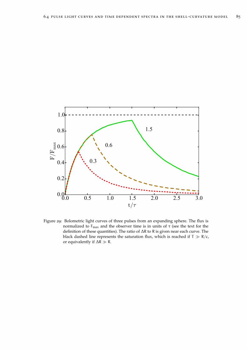
6.4 pulse light curves and time dependent spectra in the shell-curvature model 85

0.0 0.5 1.0 1.5 2.0 2.5 3.0t/τ

0.0

0.2

0.4

0.6

0.8

1.0

F/F

max

0.3

0.6

1.5

Figure 29: Bolometric light curves of three pulses from an expanding sphere. The flux isnormalized to Fmax and the observer time is in units of τ (see the text for thedefinition of these quantities). The ratio of ∆R to R is given near each curve. Theblack dashed line represents the saturation flux, which is reached if T R/c,or equivalently if ∆R R.

86 prompt emission from an off-axis jet

0.0 0.5 1.0 1.5 2.0 2.5 3.0t/τ

0.0

0.2

0.4

0.6

0.8

1.0F/F

max

0.3

0.6

1.5tjet

Figure 30: Bolometric light curves of three pulses from an on-axis jet with θjet = 1/Γ . Theratio of ∆R to R is reported near each curve. The black dashed line representsthe time tjet at which the jet border first comes into sight. In this case tjet equalsτ.

where Roff ≡ R+∆R. It is then easy to see that the light curve becomes

F(t)

Fmax= 1−

(1+

min(t, tjet)

τ

)−3

(53)

for t 6 toff, then

F(t)

Fmax=

(1+

t− toff

τoff

)−3

−

(1+

min(t, tjet)

τ

)−3

(54)

for toff < t < tjet,off, and zero for t > tjet,off. This light curve is the same as that ofthe expanding sphere up to t = tjet. After that, if tjet < toff the flux saturates (thewhole jet is visible) until t = toff, then it drops and reaches zero at t = tjet,off. Iftjet > toff no saturation is reached. The difference between the expanding sphereand the on-axis jet is relevant only if tjet . τ, i. e. if θjet . 1/Γ , as expected.

Figure 30 shows light curves (Eqs. 53 & 54) of pulses from an on-axis jet withθjet = 1/Γ .

Off-axis jet

If the jet is off-axis, it is still possible to compute an expression for the light curve.I propose here an approach to the computation, based on geometrical arguments.Let me call θv the angle between the jet axis and the line of sight, θjet the jet half-opening angle, and let me set the coordinate system so that the jet axis lies in the

6.4 pulse light curves and time dependent spectra in the shell-curvature model 87

x

y

z

y

annulus

jet

θvjetθyi

yi

S

Sθ

Rsinθ

Front view Top view

Figure 31: The off-axis jet can be thought of as being part of an expanding sphere. Theaxes in the figures above are chosen so that the jet axis lies on the z-x plane.Jet surface elements in the S shaded part all share the same Doppler factor δ,and thus they all give the same contribution (per unit emitting area) to the flux.For this reason, the ratio of the flux from the annulus to the flux from S is justequal to the ratio of the corresponding surface areas. Left: the jet is seen fromthe z-axis. The y-coordinate yi of the intersections between the annulus and thejet border is shown. Right: the jet is seen from the x-axis. Angles θv, θjet and θare reported.

z− x plane, as in Fig. 31. This is what one would obtain by rotating an on-axisjet counter-clockwise by an angle θv around the x axis. Let me now consider thering-shaped part of the sphere surface (“annulus” hereafter) comprised betweenθ and θ+ dθ. If θ > |θv − θjet|, a portion S of the annulus lies on the jet surface(shaded part in Fig. 31). Since the annulus width dθ is infinitesimal, the ratio ofthe area of S to the total annulus area is equal to the ratio between the length l ofS and the total annulus length 2πR cos θ. Moreover, this is also equal to the ratioof the flux dFS from S to the flux dFa from the whole annulus, namely

dFS(θ)

dFa(θ)=

l(θ)

2πR cos θ(55)

The flux due to the annulus is easily obtained by deriving the flux of the sphere,Eq. 45, with respect to θ, which gives

dFa(θ) =dF

dθdθ =

2πR2

d2I ′0Γ4

sin θdθ

(1−β cos θ)4(56)

To compute the length l(θ), we must first find the intersections between theannulus and the jet border. Both are circles on the sphere surface, i. e. they lie onthe surface x2 + y2 + z2 = R2. The annulus is the circle given by the intersectionbetween the plane z = R cos θ and the sphere; in a coordinate system K ′ wherethe z ′ axis coincides with the jet axis, the jet border is the circle given by theintersection between the plane z ′ = R cos θjet and the sphere. Applying a rotationof an angle θv around the x axis, this plane becomes z cos θv − y sin θv = R cos θjet.

88 prompt emission from an off-axis jet

The intersections between the two circles are then found by solving the linearsystem

x2 + y2 + z2 = R2

z = R cos θ

z cos θv − y sin θv = R cos θjet

(57)

The y coordinate of the intersections (see Fig. 31) is found to be

yi =cos θ cos θv − cos θjet

sin θvR (58)

Consider now the annulus as a circle whose center lies on the z = R cos θ plane.Its radius is R sin θ, and the angle α that subtends S is α = 2 arccos (−yi/R sin θ).The length l(θ) is then

l(θ) = 2R sin θ arccos(

cos θjet − cos θ cos θv

sin θ sin θv

)(59)

Substituting Eqs. 56 and 59 into Eq. 55, I conclude that

dFS(θ) =dF

dθdθ× 1

πarccos

(cos θjet − cos θ cos θv

sin θ sin θv

)(60)

This is valid as long as the intersections between the annulus and S exist, i. e. for|θv − θjet| < θ < θv + θjet. Let me work out the remaining cases:

• if θv < θjet, i. e. if line of sight is inside the jet border, then for θ < θjet − θv

also the annulus is inside the jet border, thus dFS(θ) = dFa(θ);

• if θv > θjet, i. e. if line of sight is outside the jet border, then for θ < θv − θjet

the annulus is too small to intercept the jet border, thus dFS(θ) = 0; in eithercase, if θ > θv + θjet the annulus is too large to intercept the jet border, thusagain dFS(θ) = 0.

Summing up, we can define the function a(θ, θv, θjet) by

a =

H(θjet − θv) θ 6 |θv − θjet|

0 θ > θv + θjet1

πarccos

(cos θjet − cos θ cos θv

sin θ sin θv

)otherwise

(61)

where H(x) is the Heaviside function, i. e.

H(x) =

0 x < 0

1 x > 0(62)

and writedFS(θ, θv, θjet) = a(θ, θv, θjet)

dF

dθdθ (63)

The light curve of the pulse from the off-axis jet is then obtained by integration ofthis expression between θon(t) and θoff(t), namely

F(t, θv, θjet) =2πR2

d2I ′0Γ4

∫θon(t)

θoff(t)a(θ, θv, θjet)

sin θdθ

(1−β cos θ)4(64)

6.4 pulse light curves and time dependent spectra in the shell-curvature model 89

x

z

ct

θ to observer

x

z

ctoff

to observerθon

on

R

θoff

actual emittingsurface

jet

θv

θA A

Figure 32: The off-axis jet can be thought of as being part of an expanding sphere. Forsimplicity, the EATS of the expanding sphere (hatched area) is represented asin Figure 27, but it is actually the same as in Figure 28. The actual EATS of thejet is the intersection between the jet surface and the sphere EATS.

Note that here t = 0 is the arrival time of the first photon from the sphere, thus ifθv > θjet the actual light curve of the off-axis jet starts a little later. The actual starttime of the off-axis light curve is

tstart(θv, θjet) =R

βc

(1−β cos(θv − θjet)

)(65)

Equation 64 can be easily integrated with a simple numerical procedure. Some ex-ample light curves computed using a RK4 integration scheme are given in Fig. 33.

light curves Figure 33 shows plots of bolometric light curves of the samepulse seen at different viewing angles, computed by numerical integration ofEq. 64 using a Runge-Kutta IV order scheme. Both the peak flux decrease andthe duration increase discussed in §6.5 and §6.5 are apparent. The overall shape isqualitatively insensitive of the viewing angle, apart from the peak being sharperin the on-axis case.

Spectra and hardness-intensity correlation

All the above arguments can be also applied to the derivation of the observedspectrum. All we need to do is to compute the flux density

dF

dν(ν, t) ≡ Fν(ν, t) =

∫S(t)

dI

dν(ν, t) cosαds/r2 (66)

over the same EATS as before, using the transformation

dI

dν(ν) = δ3

dI ′

dν ′(ν/δ) (67)

to express the intensity density in terms of the comoving one. It is convenient towrite dI ′/dν ′ as follows

dI ′

dν ′(ν ′) =

I ′0ν ′0f(ν ′/ν ′0) (68)

90 prompt emission from an off-axis jet

0

0.05

0.1

0.15

0.2

0.25

0.3

0.35

0.4

0.45

0 1 2 3 4 5 6

F/F

max

t/τ

1

10-4

10-3

10-2

10-1

0.1 1 10

Figure 33: Light curves of a pulse from a jet with θjet = 5o and Γ = 100. Each curve refers

to a different viewing angle in the sequence (from green to red) θv = 5o, 5.2o,5.4o, 5.6o, 5.8o and 6o. Fmax refers to the on-axis jet. The inset shows the samecurves plotted with logarithmic axes.

6.4 pulse light curves and time dependent spectra in the shell-curvature model 91

where I ′0 is the total intensity, ν ′0 is some frequency, and f(x) is a function whichdescribes the comoving spectral shape, and whose integral is normalized to unity.As an example, we can set a power law spectral shape

f(ν ′/ν ′0) = (1−α)

(ν ′

ν ′0

)−α

(69)

for ν ′ > ν ′0 and zero otherwise, with α > 1. Since the integral of f(x) is normalizedto unity, we have ∫∞

0

dI ′

dν ′(ν ′)dν ′ =

I ′0ν ′0

∫∞0

f(ν ′/ν ′0)dν′ = I ′0 (70)

The equation for the observed spectrum of a off-axis jet is then

dF

dν(ν, t) =

2πR2

d2I ′0ν ′0Γ

3

∫θon(t)

θoff(t)a(θ, θv, θjet)

f(ν/δν ′0) sin θdθ

(1−β cos θ)3(71)

For the simplest case of an on-axis jet, with power law comoving spectral shape,the integral is analytic and it gives

dF

dν(ν, t) =

2πR2

d2I ′0 (1+β)

2+α Γ1+α

βν ′1−α0

(1−α)ν−α×

×

(1+

t− toff

τ+ toff

)−2−α

−

(1+

t

τ

)−2−α (72)

which reproduces the well-known 2+α decay slope due to high latitude emission(Kumar and Panaitescu, 2000; Dermer, 2004). For more general spectral shapes, anumerical approach is necessary to compute the integral in Eq. 71.

Since we are mainly interested in how the peak of the observed spectrum evolveswith time, let me assume a simple form of the comoving spectral shape, namely

I ′ν(ν′) = n(a, b)

I ′0ν ′0

[(ν ′

ν ′0

)−a

+

(ν ′

ν ′0

)−b]−1

(73)

where n(a, b) is a normalization constant which depends upon the high and lowspectral indices a and b; clearly I ′ν ∝ ν ′a for ν ′ ν ′0 and I ′ν ∝ ν ′b for ν ′ ν ′0. Ifa > 0 and b < −1, the normalization n(a, b) can be defined so that

I ′0 =

∫∞0

I ′ν(ν′)dν ′ (74)

The break frequency ν ′0 is related to the comoving ν ′F ′ν peak energy E ′peak through

E ′peak =

(−a+ 1

b+ 1

) 1a−b

hν ′0 (75)

where h is Planck’s constant. All the examples in the figures assume the abovecomoving spectral shape, with a = 0.2 and b = −1.3, which represent averagehigh and low spectral indices of Fermi GRB spectra (Nava et al., 2011b).

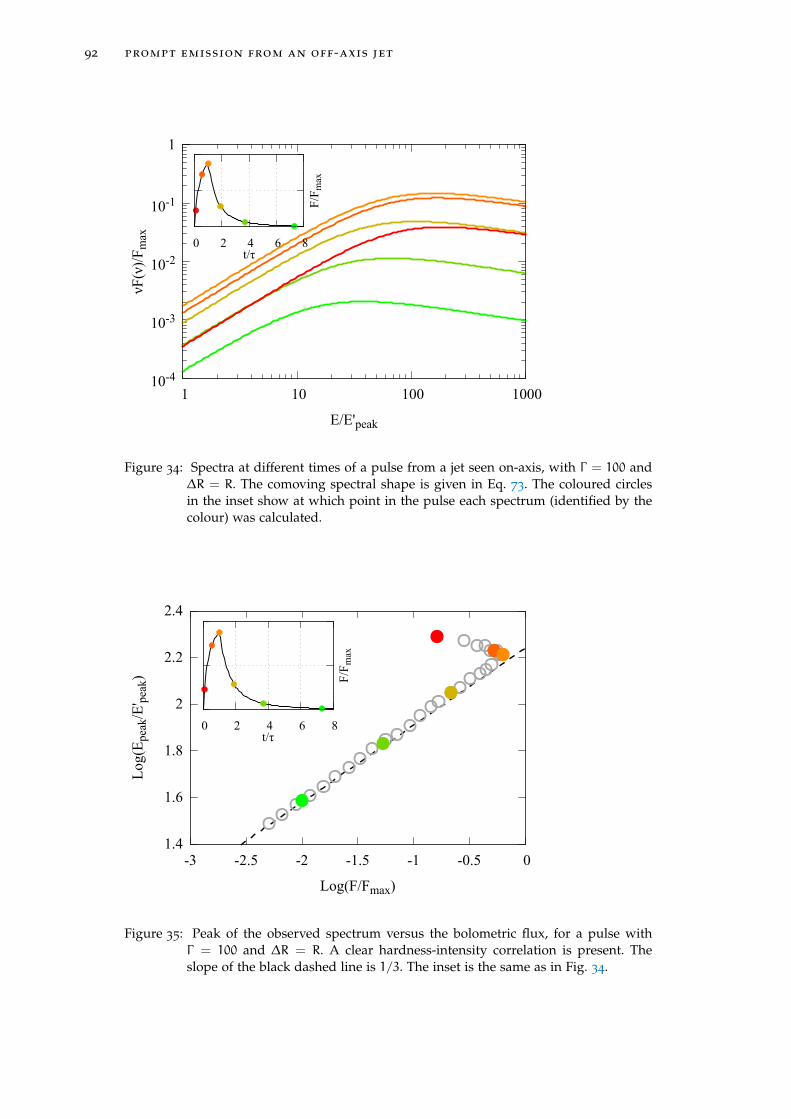
92 prompt emission from an off-axis jet

1

10-4

10-3

10-2

10-1

1 10 100 1000

νF(ν

)/F

max

E/E'peak

0 2 4 6 8

F/F

max

t/τ

Figure 34: Spectra at different times of a pulse from a jet seen on-axis, with Γ = 100 and∆R = R. The comoving spectral shape is given in Eq. 73. The coloured circlesin the inset show at which point in the pulse each spectrum (identified by thecolour) was calculated.

1.4

1.6

1.8

2

2.2

2.4

-3 -2.5 -2 -1.5 -1 -0.5 0

Log

(Epe

ak/E

' pea

k)

Log(F/Fmax)

0 2 4 6 8

F/F

max

t/τ

Figure 35: Peak of the observed spectrum versus the bolometric flux, for a pulse withΓ = 100 and ∆R = R. A clear hardness-intensity correlation is present. Theslope of the black dashed line is 1/3. The inset is the same as in Fig. 34.

6.5 characteristics of pulses from an off-axis jet 93

Figure 34 shows spectra from an on-axis jet at six representative times, com-puted using Eq. 71. The evolution is clearly hard-to-soft (i. e. the peak energy de-creases monotonically with time), and the low and high energy spectral indicesare the same as those of the comoving spectrum. Figure 35 shows that after thepeak of the light curve the peak energy Epeak of the observed νFν spectrum varieswith the bolometric flux F following roughly Epeak ∝ F1/3, i. e. the model predictsa hardness intensity correlation with index 1/3 during the decay of the pulse. Letme interpret these results:

1. Pulse rise: the maximum of Epeak(t) is at the very beginning of the pulse,when only a small area pointing directly towards the observer (the “tip” ofthe jet at zero latitude) is visible. As the visible area increases, less beamedcontributions from parts at increasing latitude come into sight, reducingEpeak slightly.

2. Pulse decay: after the pulse peak, the tip of the jet turns off, causing Epeak

to drop. At this time the visible part of the jet is an annulus (see Fig. 28):the spectral peak is determined mainly by the maximum Doppler factorδmax(t) = Γ−1 [1−β cos θoff(t)]

−1 of the visible area, which corresponds tothe innermost circle of the annulus, so that Epeak ∼ δmaxE

′peak. The flux F in

turn decreases approximately as δ4max times the angular size of the annulus.The latter is proportional to cos θoff − cos θon, which can be shown to be

cos θoff − cos θon ≈∆R

R

1

βΓδmax(76)

As a result, we have that F ∝ δ3max, which explains why Epeak ∝ F1/3.

characteristics of pulses from an off-axis jet

a longer pulse duration If the jet is off-axis, relativistic beaming of theemitted radiation causes both the flux and Epeak to be much lower than the on-axis counterparts. For the same reason, the duration of the pulse becomes longer.This can be understood intuitively as follows: as in the on-axis case, the jet surfaceis not seen to turn on all at the same time, but progressively from the nearest-to-the-observer point (point A in Fig. 32) down to the farthest. The same holds forthe turning off. Thus point A is the first to turn on, and also the first to turn off.As a consequence, the effective emitting area increases as long as point A is seenemitting, then it decreases. In other words, the peak time equals the emission timeof point A, which is given by

tpeak(θv, θjet) = T[1−β cos(θv − θjet)

](77)

thus its ratio to the on-axis peak time is

tpeak(θv, θjet)

tpeak=1−β cos(θv − θjet)

1−β(78)

Figure 36 shows a plot of this ratio as a function of θv − θjet for different values ofΓ . The off-axis pulse is thus intrinsically broader than its on-axis counterpart. Theeffective duration as seen by the observer, though, depends on the limiting fluxand on the amount of overlap with other pulses.

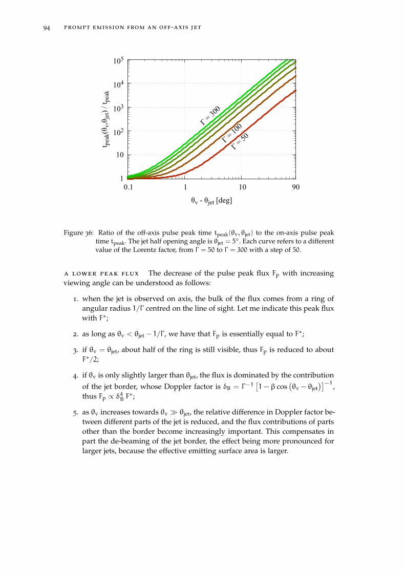
94 prompt emission from an off-axis jet

1

10

102

103

104

105

90 0.1 1 10

t pea

k(θ v

,θje

t) /

t pea

k

θv - θjet [deg]

Γ = 50Γ

= 100Γ

= 300

Figure 36: Ratio of the off-axis pulse peak time tpeak(θv, θjet) to the on-axis pulse peaktime tpeak. The jet half opening angle is θjet = 5

. Each curve refers to a differentvalue of the Lorentz factor, from Γ = 50 to Γ = 300 with a step of 50.

a lower peak flux The decrease of the pulse peak flux Fp with increasingviewing angle can be understood as follows:

1. when the jet is observed on axis, the bulk of the flux comes from a ring ofangular radius 1/Γ centred on the line of sight. Let me indicate this peak fluxwith F∗;

2. as long as θv < θjet − 1/Γ , we have that Fp is essentially equal to F∗;

3. if θv = θjet, about half of the ring is still visible, thus Fp is reduced to aboutF∗/2;

4. if θv is only slightly larger than θjet, the flux is dominated by the contribution

of the jet border, whose Doppler factor is δB = Γ−1[1−β cos

(θv − θjet

)]−1,thus Fp ∝ δ4B F∗;

5. as θv increases towards θv θjet, the relative difference in Doppler factor be-tween different parts of the jet is reduced, and the flux contributions of partsother than the border become increasingly important. This compensates inpart the de-beaming of the jet border, the effect being more pronounced forlarger jets, because the effective emitting surface area is larger.

6.5 characteristics of pulses from an off-axis jet 95

3 5 10 15 40θv [deg]

10-1010-910-810-710-610-510-410-310-210-1100

Fpea

k(θ

v,θ

jet)/F

max

Figure 37: Peak fluxes of pulses from jets with four different half opening angles, namelyθjet = 3

, 5, 10, and 15 (indicated by the thin vertical dotted lines), assumingΓ = 100 and ∆R = R. The orange dashed curves represent the correspondingempirical parametrization given in Eq. 79.

Based on these considerations, an empirical analytical formula can be constructedto describe how the peak flux depends on the viewing angle θv and on the jet halfopening angle θjet. An example of such an empirical formula is

Fp/F∗ ≈

1 θv 6 θ∗jet

1− Γ(θv − θ∗jet)/2 θ∗jet < θv 6 θjet

1

2

(δB

(1+β)Γ

)(4−√2θ1/3jet )

θv > θjet

(79)

where θ∗jet = θjet − 1/Γ . The definition for θ∗jet < θv 6 θjet is just a linear decreasefrom F∗ to F∗/2; the exponent of δB in the definition for θv > θjet is 4 reducedby an amount2 which depends on θjet, in order to take into account the flux losscompensation explained in point (v) above.

The flux at time t of the pulse from an off-axis jet is given by the integral inEq. 64, which however has no analytical solution for θv > 0. The coloured solidlines in Figure 37 represent Fp as computed by numerical integration of Eq. 64

at t = tpeak(θv, θjet), for five jets with different half opening angles. The orangedashed lines are plots of Eq. 79 for the corresponding parameter values, showingthat the best agreement is for half opening angles 5 . θjet . 10.

2 The coefficient and exponent of θjet in Eq. 79 have been chosen to get a good agreement with theresults from the semi-analytical formulation developed in the preceding sections.

96 prompt emission from an off-axis jet

-2.5

-2

-1.5

-1

-0.5

0

5 15 10

Log

[Epe

ak(t

peak

)/2Γ

E' p

eak]

θv [deg]

Γ = 30

Γ = 100

Γ = 300

Figure 38: Epeak at the pulse peak time for three jets with R = 1013 cm, θjet = 5 and three

values of Γ , namely (from red to green) Γ = 30, 100 and 300. The black dashedlines are plots of δB/2Γ for the corresponding values of Γ .

spectral peak energy, hardness-intensity correlation With the sameassumptions as in the on-axis case, I computed the spectra from the off-axis pulseat different times. The spectrum at each time is dominated by the part of the EATSwith the strongest beaming. At time tpeak, such part is the border of the jet nearestto the observer, thus one expects Epeak(tpeak) to decrease with θv as the Dopplerfactor of the jet border, i. e. Epeak(tpeak) ∝ δB. Figure 38 is a plot of Epeak(tpeak) forthree values of Γ , obtained by using Eq. 71 to compute the spectra, and it showsthat indeed Epeak is approximately proportional to δB. In general, Epeak is a littlelower than δBE ′peak because of the “blending in” of softer spectra from less beamedparts of the jet.

Figure 39 shows the evolution of Epeak as a function of the flux F during thepulse, for four different off-axis viewing angles. A “hardness-intensity” correla-tion during the pulse decay is still apparent, with a slightly steeper slope (∼ 0.5)just after the pulse peak, getting shallower as the flux decreases and eventuallyreaching ∼ 1/3 as in the on-axis case.

multi-pulse light curves

Now that we have a detailed (though simple) model of the single pulse, we canproceed to construct a “synthetic” GRB light curve by superposition of pulses.Some non-trivial features emerge from such superposition. Figure 40 shows fourlight curves of the same series of N = 100 pulses seen at four different viewingangles. All pulses are equal in duration and peak flux. Their starting times havebeen sampled from a uniform distribution within a 2 seconds time span. The jetparameters are Γ = 100, θjet = 5, R = 1013 cm and ∆R = R. The viewing angles

6.6 multi-pulse light curves 97

0

0.5

1

1.5

2

2.5

-7 -6 -5 -4 -3 -2 -1 0

Log

(Epe

ak/E

' pea

k)

Log(F/Fmax)

F1/3

0.35

0.4

0.45

0.5

slopes

Figure 39: Logarithmic plot of Epeak versus Flux of the same pulse seen at different off-axis viewing angles. The jet has θjet = 5, Γ = 100 and R = 1013 cm. The fourseries of points (from green to red) correspond to θv = 5.1, 5.5, 6 and 7.The inset shows the slope of the relation during the decay of the pulse for eachviewing angle.

are θv = 0, θjet + 1/Γ , θjet +√3/Γ and θjet + 2/Γ . The comoving spectral shape

is the same as before (Eq. 73). The resulting light curves have been binned at32 ms resolution for a better comparison with actual GRB light curves. For eachlight curve, the Epeak of the spectrum in each time bin is also given (thin orangehistograms). The following features should be apparent:

1. as the viewing angle increases, variability is smeared out by the pulse broad-ening;

2. the shape of the overall light curve tends to resemble a (long) single pulsewhen the viewing angle is large enough;

3. the superposition of pulses masks the hard-to-soft spectral evolution of thesingle pulses, turning it into an intensity tracking behaviour: this is due tothe superposition of spectra with different peak energies;

4. the variation of Epeak leads slightly the variation in flux, because of the hard-to-soft nature of the single pulses;

5. there is a general softening of Epeak in time over the entire light curve.

These features are strikingly similar to those found in time resolved spectral anal-ysis of real gamma-ray bursts (e. g. Ford et al., 1995; Ghirlanda, Celotti, and Ghis-ellini, 2002). I do not advocate this as a proof of the correctness of our model,which is certainly oversimplified, but rather as a further indication that some fea-tures of GRB light curves might be explained admitting that the jet is seen at

98 prompt emission from an off-axis jet

0.0 0.5 1.0 1.5 2.0 2.5

50

100

150

200

0.0 0.5 1.0 1.5 2.0 2.50.0

0.2

0.4

0.6

0.8

1.0

L/L

max

0.0 0.5 1.0 1.5 2.0 2.5

20

40

60

80

100

Epea

k[k

eV]

0.0 0.5 1.0 1.5 2.0 2.50.00

0.01

0.02

0.03

0.04

0.05

0.06

0.0 0.5 1.0 1.5 2.0 2.5 3.0

10

20

30

40

50

0.0 0.5 1.0 1.5 2.0 2.5 3.0t [s]

0.000

0.002

0.004

0.006

0.008

0.010

L/L

max

0.0 0.5 1.0 1.5 2.0 2.5 3.0 3.5

5

10

15

20

25

30

35

40

Epea

k[k

eV]

0.0 0.5 1.0 1.5 2.0 2.5 3.0 3.5t [s]

0.000

0.001

0.002

0.003

0.004

0.005

0.006

Figure 40: Light curves (thick histograms) and spectral peak evolution (thin orange his-tograms) of a sequence of 100 pulses from a jet with θjet = 5

o, Γ = 100, R = 1013

cm and ∆R = R. The peak of the νFν comoving spectrum is E ′p = 1 keV. Thepulse start times are sampled from a uniform distribution within the first 2 s ofthe observer time. Each panel refers to a different viewing angle in the sequenceθv = 0, θjet + 1/Γ , θjet +

√3/Γ , θjet + 2/Γ (from left to right, top to bottom). Lmax

refers to the peak luminosity of the on-axis light curve.

6.7 the number of off-axis short grbs seen by fermi/gbm 99

least slightly off-axis. The off-axis viewing angle favours the broadening and su-perposition of pulses, which is the necessary ingredient to some of the featuresenumerated above. It can also contribute in a simple way to explain why the slopeof the hardness-intensity correlation changes from burst to burst, being influencedby the viewing angle (§6.5).

Figure 40 shows that the simple arguments outlined in §6.2 are valid not only ifpulses are produced by point sources, but also in presence of an extended geome-try.

the number of off-axis short grbs seen by fermi/gbm

We can obtain an estimate of the fraction of off-axis SGRBs in the observed popula-tion by the simplifying assumption that all jets share the same intrinsic properties,and that their flux in an observer band is uniquely determined by the viewing an-gle and the redshift. I assume that the majority of SGRBs are observed on-axis, andI choose the following parameters in an attempt to match the average propertiesof the on-axis population:

1. Epeak,0 = 700keV as the typical (on-axis, rest frame) peak spectral energy;

2. α = −0.5 and β = −2.3 as typical low- and high-energy spectral indices(Nava et al., 2011b);

3. the redshift distribution as given in Ghirlanda et al., 2016;

4. L0 = 2.5× 1052erg s−1 as the typical (on-axis) luminosity, which correspondsto the break of the broken power law luminosity function of Ghirlanda etal., 2016. This choice is motivated by the fact that if GRBs can be observedoff-axis, then their luminosity function is indeed well described by a brokenpower law, with the break around the average on-axis luminosity (Pescalliet al., 2015);

5. since the result is sensitive to the assumed typical Lorentz factor Γ and half-opening angle θjet, I explore the cases Γ = 50, 100 and 300, and θjet = 5

and10.

I then define the effective luminosity L(θv) following Eq. 79, namely

L(θv) = L0 ×

1 θv 6 θ∗jet

1− Γ(θv − θ∗jet)/2 θ∗jet 6 θv < θjet

1

2

(δB

(1+β)Γ

)(4−√2θ1/3jet

)θv > θjet

(80)

with θ∗jet = θjet − Γ−1, and the effective peak energy

Epeak(θv) =Epeak,0

1+ z×

1 θv 6 θjetδB

(1+β)Γ θv > θjet(81)

100 prompt emission from an off-axis jet

0.01 0.1 1 2 3z

0.0

0.2

0.4

0.6

0.8

N off/

N tot

(<z) = 100,

jet = 5= 100,jet = 10= 300, jet = 5

= 50,jet = 5

= 300, jet = 10

P64 > 2 ph s 1cm 2

[10 1000 keV band]

Epeak, 0 = 700keVL0 = 2.5 × 1052erg s 1

Figure 41: Fraction of off-axis GRBs over the total within a given redshift. The curves repre-sent an estimate of the fraction of SGRBs with redshift lower than z observableby Fermi/GBM (assuming a 64-ms peak photon flux p > 2ph s−1cm−2 in the10–1000 keV band) whose viewing angle is larger than θjet + Γ

−1.

6.8 the time delay between gw170817 and grb170817a 101

as in §6.5. With these assumptions and prescriptions, one can compute the ob-served rate of GRBs with a viewing angle in the range (θv, θv +dθv), in the redshiftrange (z, z+ dz), assuming a limiting photon flux plim in a given band, as

dN

dθv dzdθv dz =

Ψ(z)

1+ z

dV

dzP(θv, z, plim)dθv dz (82)

where P(θv, z, plim) is the viewing angle probability, dV/dz is the differential co-moving volume, and the factor 1+ z accounts for cosmological time dilation. Theviewing angle probability is

P(θv, z, plim) =

sin θv θv 6 θv,lim(z, plim)

0 θv > θv,lim(z, plim)(83)

The limiting viewing angle θv,lim corresponds (through Eq. 80) to the limitingluminosity Llim computed as

Llim = 4πd2L plim

∫∞0dNdE EdE∫(1+z)Ehigh

(1+z)Elow

dNdE dE

(84)

where Elow (Ehigh) is the lower (upper) limit of the observer band, dL is the lumi-nosity distance, and dN/dE(Epeak, α, β) is the rest frame spectrum.

Let me define the total rate Ntot(< z) of observable GRBs within redshift z as theintegral of Eq. 82 over redshift from 0 to z and over θv from 0 to π/2; similarly, therate Noff(< z) of off-axis GRBs within redshift z is the integral over redshift from 0

to z and over the viewing angle from θv + Γ−1 to π/2. Since we are interested in the

ratio of these two quantities, we do not need to bother about the normalization.In Fig. 41 I show the fraction of bursts with θv > θjet + Γ

−1 at redshift lower thanz for various choices of Γ and θjet, assuming a limiting flux plim = 2ph s−1 cm−2 inthe 10-1000 keV band. Standard flat ΛCDM cosmology was assumed, with Planckparameters H0 = 67.3 km s−1 Mpc−1 and Ωm,0 = 0.315 (Planck Collaboration etal., 2013). These results clearly indicate that at low redshift a large fraction ofSGRBs is likely seen off-axis.

the time delay between gw170817 and grb170817a : too short for an

off-axis jet

The picture of off-axis GRBs developed in this chapter seems to be compatible withthe interpretation of GRB170817A as an off-axis jet: it is much less luminous thanaverage, it shows no significant variability, and it is at low redshift. As shown in§6.4.5, though, the delay with respect to the jet launch time (and thus the mergertime in our case) increases with the viewing angle (see Eq. 65). I will show in whatfollows that it is hard to reconcile a ∼2 seconds delay time with emission from ajet seen under a large viewing angle.

In order to shine in gamma-rays, the jet must expand enough to become trans-parent.

Let me estimate the transparency radius Rt as (e. g. Daigne and Mochkovitch,2002b)

Rt =LK,isoσT8πmpc3Γ3

(85)

102 prompt emission from an off-axis jet

Rt

NS-NSmerger

JET

θ - θv jet

gamma-rayphotons

gravitationalwaves

timedelay

to observer

Figure 42: If the gamma-ray prompt emission is due to an off-axis jet, the arrival time dif-ference between the last gravitational waves and the first gamma-ray photons isdominated by the time it takes for the jet to become transparent in the observerframe.

where σT is the Thomson cross-section, mp is the proton mass, and we are assum-ing an electron fraction of unity. LK,iso in this expression is the isotropic equivalentkinetic luminosity of the outflow, i. e. LK,iso = ΓMisoc

2. If we assume that the jet islaunched a short time ( 1 s) after the merger, the arrival time difference betweenthe latest gravitational waves and the first photons is

tγ − tGW ≈Rt

βc

(1−β cos

(θv − θjet

))(86)

This accounts for the fact that fluid elements on the jet border must travel up toRt at speed βc before being able to emit the gamma-ray photons (see Fig. 42).

We can relate the kinetic luminosity of the jet to the on-axis gamma-ray lumi-nosity by assuming that 10 percent of the kinetic luminosity is converted intophotons, i. e. Liso(θv = 0) = 0.1 LK,iso (as in e. g. Kathirgamaraju, Duran, and Gian-nios 2017; see also Beniamini et al. 2015 who show that this is a typical conversionefficiency). I compute the corresponding off-axis luminosity Liso(θv) using Eq. 80.If we require that Liso(θv) = 1047 erg/s as in GRB170817A (Goldstein et al., 2017),and we assume a jet half-opening angle θjet, we can compute the correspondingon-axis luminosity Liso(0) and arrival time delay tγ − tGW for various combina-tions of the bulk Lorentz factor Γ and off-axis viewing angle θv − θjet. Figure 43

shows the contours of these quantities for θjet = 0.2 rad = 11.5 (the figure wouldbe very similar for θjet = 0.1 rad or θjet = 0.3 rad). The red solid contour corre-sponds to the actual 1.7 s delay time as observed in GRB170817A, while the dottedcontours represent the on-axis luminosities. The figure shows that a “standard” jetwith a large Lorentz factor Γ & 70 and an on-axis luminosity Liso(0) ∼ 10

51 erg/sis formally compatible with the observed time delay, but it requires fine-tuningof the viewing angle, which implies an extremely small probability. Moreover, theafterglow in this case would be very bright and visible very early. A structured

6.8 the time delay between gw170817 and grb170817a 103

5 10 20 30 50 70 1002

3

4

5

6

vje

t [de

g]

0.7 s

1.7 s2.7 s

3×10 4710 48

10 49 10 50 10 5110 52 10 53

Figure 43: The solid red and dashed brown lines represent contours of the gamma-rayphoton arrival time delay with respect to the last gravitational waves for a givenjet bulk Lorentz factor Γ and off-axis viewing angle θv − θjet. The dotted linesrepresent contours of the on-axis jet luminosity Liso(0) corresponding to an off-axis luminosity of Liso(θv) = 10

47 erg/s.

104 prompt emission from an off-axis jet

jet with slower (but still narrow) wings moving at Γ ∼ 10 does not solve the issue,since the viewing angle cannot be large. A “slow” fireball with a Lorentz factoraround Γ ≈ 7 and a much smaller energy, instead, would give the correct timedelay both if seen on-axis or a few degrees off-axis. For these reasons, I believethat GRB170817A is more naturally explained by slow material moving towardsthe observer (which is the case for the jet cocoon, for a structured jet whose struc-ture extends at large angles, and for the isotropic giant flare described in the nextchapter) than by a fast off-axis jet.

7T H E J E T- L E S S F I R E B A L L S C E N A R I O

The possible interpretations of GRB170817A mentioned in the preceding chaptersall require the presence of a jet. In this chapter I investigate the possibility to have adetectable isotropic emission in hard X-rays in NS-NS and BH-NS mergers withouta jet. I am guided by the fact that isolated magnetars can produce giant flareswith Eiso ∼ 1046 erg (e.g. Hurley et al., 2005; Lazzati, Ghirlanda, and Ghisellini,2005) in non-catastrophic events, probably due to some re-configuration of theirmagnetic field (Thompson and Duncan, 1995). In NS-NS and BH-NS mergers, thegravitational energy available during the last phase of the coalescence is more thanEG ∼ 1053 erg, and only a very small fraction of this needs to be used.

To explore this possibility, I postulate that a small fraction (e.g. less than 0.1%)of EG can be used, e.g. through magnetic field amplification and subsequent con-version of magnetic field energy into thermal and/or kinetic energy, during theinitial phase of the coalescence. The magnetic field in the NS material during themerger can be amplifieid to values larger than B ∼ 1015 G (Ruiz and Shapiro, 2017;Giacomazzo et al., 2015; Kiuchi et al., 2014; Zrake and MacFadyen, 2013; Price,2006). This is enough to form a fireball, that can produce an important isotropicemission in hard X-rays, as first suggested by Zrake and MacFadyen, (2013) andGiacomazzo et al., (2015).

Various recent numerical simulations (e.g. Ruiz and Shapiro, 2017; Murguia-Berthier et al., 2017; Just et al., 2016) and theoretical works (e.g. Margalit, Metzger,and Beloborodov, 2015) suggest that the conditions for launching a relativisticjet after a NS-NS or BH-NS merger are not always satisfied, thus the fraction ofmergers without jets might be significant. An alternative mechanism to producea prompt, isotropic, high-energy component is thus particularly relevant to theinterpretation of GRB170817A.

set up of the isotropic fireball model

The binding energy difference between an isolated neutron star and a black holeof the same mass is

∆EG ∼3

10MNSc

2

(1−

RS

RNS

)∼ 5× 1053 erg (87)

where RS is the Schwarzschild radius, MNS and RNS are the mass and radius ofthe NS, and the numerical value assumes MNS = 1.4M and RNS = 14 km.

This energy is of the same order as that released in a supernova explosion. Inthat case, most of it goes into neutrinos. In a compact binary merger it powers sev-eral other processes, such as emission of gravitational waves, dynamical ejectionof matter and magnetic field amplification. The latter process is widely believedto produce a magnetic field of order B ∼ 1015–1016 G, which in turn can containan energy of order ∼ 1051 erg (Giacomazzo et al., 2015).

105

106 the jet-less fireball scenario

As first suggested by Zrake and MacFadyen, 2013, if just 1 percent of this en-ergy, E0 ∼ 1049 erg, is converted into photons in a relatively baryon–free volumesurrounding the merger (e.g. with a mechanism similar to that responsible for gi-ant flares in magnetars, see e.g. Thompson and Duncan, 1995), a fireball initiallydominated by electron-positron pairs can form and produce a short, high-energytransient.

From this point on, the evolution resembles that of the classical, standard isotropicfireball of gamma-ray bursts: the fireball accelerates to relativistic speed, up tosome saturation radius Ra where the bulk kinetic energy becomes of the sameorder as the initial internal energy. Thereafter, the fireball coasts with constant ve-locity. At some point, the transparency radius Rt is reached, after which the fireballcan release radiation.

The origin of the emission is still a controversial issue in the field of GRBs. Onone hand, the release of “relic” thermal photons (i.e. the photons that constitutedthe initial source of pressure of the fireball, diluted by the expansion) at the trans-parency (photospheric) radius is expected (Meszaros and Rees, 2000). On the otherhand, in the case of GRBs the observed spectra suggest a non-thermal origin of theradiation, which could be the result of internal shocks (Rees and Meszaros, 1994)or reconnection of the carried magnetic field (Thompson, 1994) transforming partof the kinetic energy of the fireball back into radiation.

These processes may be present in our isotropic case as well, but let me firstconsider the thermal photospheric radiation.

The temperature of the initial blackbody can be estimated by equating the en-ergy density of photons to that of the source magnetic field, i.e. aT40 ∼ B2/(8π),giving T0 ∼ 4.8× 1010B1/215 K. The acceleration ends when the bulk Lorentz factorequals E0/(Mc2), i.e. when Γ ∼ 11 E0,49/M27 (here and in what follows I employthe usual notation Qx ≡ Q/10x in cgs units). This occurs at Ra = ΓR0, and therethe comoving temperature is T ′a = T0(R0/Ra). Beyond Ra the temperature decreasesas T ′ = (R/Ra)

−2/3 and Γ is constant. During these phases, the main radiativeprocesses (pair creation and annihilation and Compton scatterings) conserve thenumber of blackbody photons. This implies that the total energy contained in this“fossil” thermal component is

EBB(Rt) ≈ E0 ΓT ′(Rt)

T0= E0

[Rt

Ra

]−2/3(88)

The transparency radius depends on the thickness of the fireball (Daigne andMochkovitch, 2002b). In our case the fireball is thin (Rt/2Γ

2 > ctinj, where tinj .10−3 s, Γ . 10 and Rt & 1012 cm) so that Rt is given by (see Eq. 15 of Daigne andMochkovitch 2002b):

Rt =

[YeσTE04πmpc2Γ

]1/2∼ 1.9× 1012

[Ye,−1E0,49

Γ1

]1/2cm (89)

where Ye = ne/(np+nn) is the electron fraction of the fireball at the transparency.In this case the final blackbody energy (Eq. 88) can be written in terms of the freeparameters as:

EBB = E0TBB

T0≈ 1.2× 1046 E5/30,49R

2/30,7 T0,11M

−127 Y

−1/3e,−1 erg (90)

7.1 set up of the isotropic fireball model 107

and the observed temperature is

kBTBB = kBT0R0

R1/3a R

2/3t

≈ 10 E2/30,49R2/30,7 T0,11M

−127 Y

−1/3e,−1 keV (91)

With the fiducial values of the parameters, this emission is a very small fractionof the initial energy. As discussed above, there can be another mechanism ableto convert a larger fraction of the bulk kinetic energy into radiation, just as inGRBs. Since there is no general consensus about this process, I leave it unspecified.This ignorance is encapsulated in the efficiency parameter η, such that the energyreleased in this additional, non-thermal component is:

E‚ = ηE0 (92)

With η = 10−2η−2 we have E‚ = 1047η−2E0,49 erg. Assuming a limiting sensitivity

of 10−7 erg cm−2, such a fireball can be detected up to a distance of ∼90 Mpc,close to the current horizon of LIGO/Virgo. This holds assuming that most of theelectromagnetic radiation falls into the observed band of the current instruments(i.e. between 10 and 1000 keV). This requires a radiation mechanism not only ableto transform a fraction η & 10−2 of E0 into radiation, but also able to do that inthe hard X-rays. Quasi thermal Comptonization and/or synchrotron emission arethe first candidates, as they are in “standard” GRBs.

Delay and pulse duration

A point not always appreciated, in the GRB standard fireball theory, is that thedelay time between the initial formation and the arrival of the fireball at the trans-parency radius Rt is equal to the duration of the pulse, if the fireball is thin (namelyits width ∆R Rt).

Indeed, for a thin fireball the pulse duration is comparable to the angular time-scale

tang =Rt

2Γ2c≈ 0.38 E−20,49M

5/227 Y

1/2e,−1 s (93)

The delay with respect to the initial formation, on the other hand, is given by:

∆tdelay =Rt

βc(1−β) ≈ Rt

2cΓ2(94)

The two time scales are thus equal. In general, in GRBs the delay time is not mea-surable, but in the case of the detection of gravitational waves, it can be taken asthe time difference ∆tdelay between the merger and the arrival of the first photonsof the prompt.

Afterglow

After the prompt emission phase, a cold shell is left, which continues its expansionat a constant rate, sweeping the circum-binary medium (CBM). The interactionwith the CBM produces a shock, where electrons are accelerated and give rise toan afterglow by synchrotron radiation. The afterglow rises as t2 at all frequencies(Sari and Piran, 1999) until the shell has swept up a CBM rest mass comparable

108 the jet-less fireball scenario

Layer

Spine

θv iew

θv iewθjet

100 101 102

Time [days]

8

6

4

2

0

Log(

Flux

den

sity

/mJy

)

R band

1keV

5 GHz

Isotropic fireball

100 101 102

Time [days]

Structured jet

layer/cocoon

core

100 101 102

Time [days]

26 AB mag

10 15erg cm 2s 1

100 Jy

Off­beam slow jet

Figure 44: Indicative afterglow light curves in radio (5 GHz), optical (R band) and X-ray(1 keV) for the three scenarios. Parameters in Table 5. Left panel: isotropic fire-ball. Mid panel: the spine/layer model (which I consider equivalent also to thejet plus cocoon scenario), where the spine is the assumed to have parameterstypical of a standard SGRB jet. The layer contributes to the light curve at earlytimes, since θlayer = θview = 30. Right panel: off-beam slow jet model. Thedotted lines show representative detection limits for the three bands. The corre-sponding flux values are shown on the figure. The optical and X-ray fluxes areuncertain, since they depend on the presence of high energy electrons. For allmodels, the behaviour of the light curve is almost the same regardless of theobserver frequency: this is due to all three frequencies being between νm andνc (for the chosen parameters) at all times shown on the plot, except for theearly rising part of the off-beam slow jet and of the core.

to its own energy, after which it starts to fade as the shell decelerates (Nava et al.,2013). The afterglow peak time is given by

tonset ≈ 1.6 E1/30,49n−1/3−4 Γ

−8/31 d (95)

comparison of the afterglow emission from the three scenarios

It is instructive to compare the general features of the afterglow of the isotropicfireball with the other competing models able to explain the prompt emission ofsub-energetic short GRBs, i. e. the quasi-isotropic cocoon plus relativistic jet modelby Lazzati et al., (2017a) and Lazzati et al., (2017b) which is essentially equivalentto the structured jet model by Kathirgamaraju, Duran, and Giannios, (2017), andthe off-beam slow jet of Pian et al., (2017), namely a rather weak and homogeneousjet, with moderate Γ , seen off-beam. In order to describe the general behaviour ofthe afterglow in the three scenarios, I construct example light curves with repre-

7.2 comparison of the afterglow emission from the three scenarios 109

Model Ek,iso Γ θjet θview

[erg] [deg] [deg]

Isotropic fireball 1049 5 — —

spine 1052 100 10 30

layer 1049 5 30 30

off–beam 1051 10 10 30

Table 5: Parameters used for the models shown in Fig. 44. For all models, I assumed anISM number density n0 = 10−3 cm−3 and microphysical parameters p = 2.3,εe = 0.1, εB = 0.01. The source is located at a luminosity distance of 60 Mpc.

sentative parameters. For all models I use the same microphysical parameters (seeTable 5), and I assume that the number density of interstellar medium (ISM) is con-stant and equal for all models. For definiteness, I locate the source at a luminositydistance dL = 60Mpc which is comparable to the LIGO interferometer networkrange at the end of the O1 observing run (Abbott et al., 2016) and represents aconservative estimate of the range during O2. This is also the limiting distance atwhich a strong magnetar giant flare as the one described in Lazzati, Ghirlanda,and Ghisellini, (2005) (which I take as a prototype for the isotropic fireball sce-nario) can be detected by a Fermi-like instrument, assuming a limiting fluence of10−7 erg cm−2. I compute the light curves of the jetted components using the pub-lic code BOXFIT (Eerten, Horst, and MacFadyen, 2012), and those of the isotropiccomponent with SPHEREFIT (Leventis et al., 2012). Since neither code accounts forthe dynamics before the deceleration time, I effectively correct the light curves bysmoothly joining, at the peak time given by Eq. 95, a power law rising as t2 at allfrequencies (Sari and Piran, 1999).

Isotropic fireball

Fig. 44 shows (left panel) a representative afterglow (in the radio, optical and X-rays) of the isotropic fireball. The onset time is close to 5 days, after which the fluxdecays as a power law. If a jet is not present, this is all we see. If there is a jet withstandard parameters (middle panel), it becomes visible at later times (∼ 100 days),when it has slowed down so that 1/Γ & (θview − θjet), i.e. when we start to see itsborder. Its emission in the optical and X-rays depends on the uncertain presence,at late times, of very high energy electrons. Emission in the radio, instead, is moresecure. This late emission can be used as a diagnostic to distinguish between thejet-less, isotropic fireball scenario and the cocoon model by Lazzati et al., (2017b),which has similar features, but requires the presence of a jet.

Jet plus cocoon

To my understanding, the mildly relativistic layer/sheath described in the struc-tured jet model of Kathirgamaraju, Duran, and Giannios, (2017) is essentially thesame as the cocoon described in Lazzati et al., (2017a). I thus consider the core-

110 the jet-less fireball scenario

layer and the jet-plus-cocoon scenarios as equivalent. The middle panel of Fig. 44

mimics the expected afterglow from this scenario, obtained by summing the emis-sion from a fast, narrow jet and that from a slower, wider jet, which representsthe layer or the cocoon (parameters in Table 5). Since the latter has a wider half-opening angle, it is more likely seen within its beam. The layer afterglow peaksearlier (∼ 5 days for the chosen parameters, which are the same as for the isotropicfireball), with the spine contributing after ∼100 days. As studied in Rossi et al.,(2004), in this case a rather strong linear polarization should be present aroundthe time when the light curve peaks, in contrast with the isotropic fireball sce-nario. This can be used as a diagnostic.

Off-beam slow jet

The energy distribution of SGRB jets may have a low energy tail, accompaniedby a corresponding low Γ tail. In this case a jet with θjet ∼ 10, Ek,iso ∼ 1051 ergand Γ ∼5–15 could be seen also at a relatively large θview ∼ 30. If seen on-axis,such a jet would produce Eγ,iso = ηEk,iso = 1050η−1Ek,iso,51

erg. These values ofEk,iso and Γ are roughly consistent (i.e. they are within the rather large dispersion)with the relation shown in Ghirlanda et al., (2012) and Liang et al., (2013). UsingEq. 2 and Eq. 3 in Ghisellini et al., (2006b) one can calculate the observed Eγ,iso

for any θview. It turns out that for θview = 30, the de-beaming factor is 1/2500,and then Eγ,iso(30

) ≈ 4× 1046η−1Ek,iso,51erg, detectable up to ∼60 Mpc if the

fluence limit is 10−7 erg cm−2. For θview > 30 the de-beaming makes the source

undetectable. The probability to see a burst within 30 is P = (1 − cos 30) ∼

0.13: small, but not impossible. Taking into account the anisotropy of the GWemission (Schutz, 2011), the probability to see the jet within 30 after the progenitorNS-NS binary has been detected in GW is significantly larger1, being ∼ 0.38. With theparameters listed in Table 5, I calculated the expected afterglow, shown in the rightpanel of Fig. 44. The peak flux corresponds approximately to the time when theLorentz factor 1/Γ ∼ (θview − θjet), namely when we start to see the border of thejet. This occurs at tpeak ∼ 60 days for the parameters shown in Tab. 5, and it goesas tpeak ∝ (Ek,iso/n0)

1/3 for a given viewing angle, i.e. it is independent from theinitial Lorentz factor, due to the self-similar nature of the deceleration (Blandfordand McKee, 1976).

After tpeak, the flux decreases monotonically. After the peak, the light curve issimilar to an isotropic fireball with the same Ek,iso and initial Γ . However, there isan important difference: the flux of an off-beam jet should be strongly polarizedat tpeak, because the observer sees only the border of the jet (Rossi et al., 2004).

1 This relies upon the assumption that the jet is launched perpendicular to the orbital plane of thebinary. This most likely holds in NS-NS mergers, while it is less certain for BH-NS mergers, becausethe BH spin might cause the accretion disk plane in the post-merger phase to be tilted with respectto the original orbital plane.

7.3 application to grb170817a and estimation of the model parameters 111

application to grb170817a and estimation of the model parame-ters

Let me now see if the isotropic fireball model is able to account for the observedfeatures of GRB170817A. In order to estimate the model parameters, I performeda Markov Chain Monte Carlo using a simple chi-squared likelihood, employingthe emcee Python package (Foreman-Mackey et al., 2013). To reduce the dimen-sions of the parameter space, I fixed εe = 0.1, following the evidence (Nava et al.,2014; Beniamini and Horst, 2017) that in GRB afterglows this parameter clustersaround this value. Tje set of free parameters is thus E0,M, R0, T0, Ye, n, εB, p. Theobservables are:

1. the duration T90 = 2.0± 0.5 s of the prompt emission and the delay (∼1.74 s)between the merger and the prompt emission. Both are predicted by themodel to be approximately equal to the angular timescale tang given byEq. 93;

2. the temperature of the blackbody component in the prompt emission, i. e.kBT = 10.3± 1.5 keV, to be compared with the prediction given by Eq. 91;

3. the energy in the blackbody component, namely (1.3 ± 0.23) × 1046 erg asestimated in §5.2, to be compared with Eq. 90;

4. The observed flux of the afterglow, which I model as described in the pre-ceding section. The radio and X-ray observations, published in the literature,that I use to constrain the model parameters are listed in Table 6.

The log-likelihood I use for the fit is given by

lnL = −1

2

N∑i=1

[(Pi −Oiσi

)2− ln

(2πσ2i

)](96)

where the index i runs over the observables listed above, the Oi and σi repre-sent respectively the measurements and their one-sigma uncertainties (assumedsymmetric), and Pi represent the model predictions. I assume uniform priors onlog(E0), log(M), log(R0), log(T0), Ye, log(n), log(εB), p, and I impose the followingconstraints:

• Γ > 2 to avoid breaking the fundamental assumption that the fireball isrelativistic;

• Ye < 1 to keep the fireball electric charge neutral, and Ye > 0.01 since this isthe lowest value of the electron fraction found in NS-NS merger simulationswhich account for neutrino interaction (e. g. Radice et al., 2016);

• 10−6 cm−3 < n < 102 cm−3 to allow for the widest possible range of ISMnumber densities;

• εB < 0.2;

• 2 < p < 4 not to fall off the validity range of the synchrotron afterglowmodel used;

• T0 < 4.1× 104 keV, which corresponds to B < 1017G.

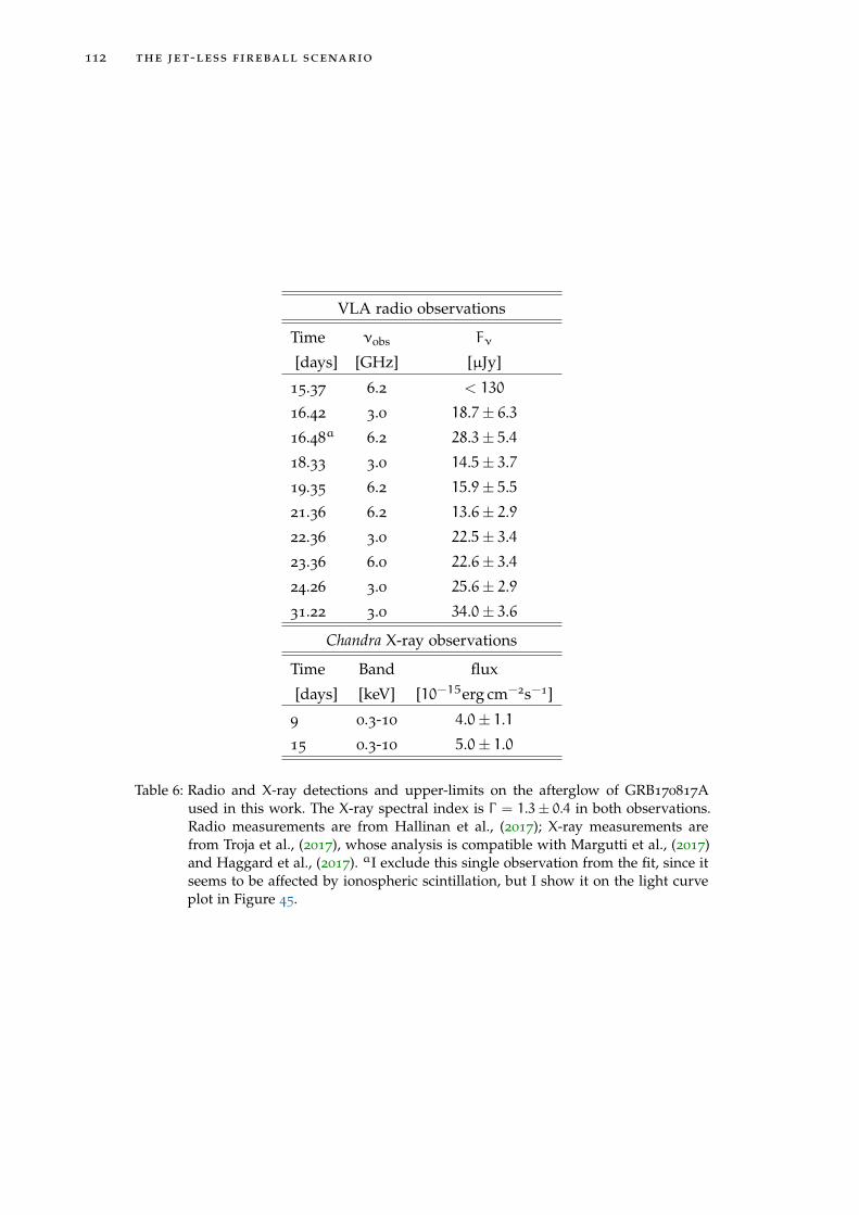
112 the jet-less fireball scenario

VLA radio observations

Time νobs Fν

[days] [GHz] [µJy]

15.37 6.2 < 130

16.42 3.0 18.7± 6.316.48

a6.2 28.3± 5.4

18.33 3.0 14.5± 3.719.35 6.2 15.9± 5.521.36 6.2 13.6± 2.922.36 3.0 22.5± 3.423.36 6.0 22.6± 3.424.26 3.0 25.6± 2.931.22 3.0 34.0± 3.6

Chandra X-ray observations

Time Band flux

[days] [keV] [10−15erg cm−2s−1]

9 0.3-10 4.0± 1.115 0.3-10 5.0± 1.0

Table 6: Radio and X-ray detections and upper-limits on the afterglow of GRB170817Aused in this work. The X-ray spectral index is Γ = 1.3± 0.4 in both observations.Radio measurements are from Hallinan et al., (2017); X-ray measurements arefrom Troja et al., (2017), whose analysis is compatible with Margutti et al., (2017)and Haggard et al., (2017). aI exclude this single observation from the fit, since itseems to be affected by ionospheric scintillation, but I show it on the light curveplot in Figure 45.

7.4 the physical picture that emerges from the results 113

Table 7: I summarize here the results of the parameter estimation procedure decribed in§7.3.

Parameter estimation results

Fireball parameters

Kinetic energy E0 = (3.1+2.1−1.3)× 10

49 erg

Starting radius R0 = 54+50−25 km

Initial temperature T0 = (2.6+1.5−1.0)× 10

11K

Baryonic mass M = (3.6+1.6−1.1)× 10

−6M

Electron fraction Ye = 0.06+0.04−0.04

Afterglow parameters

ISM number density n = (0.9+3.0−0.7)× 10

−5 cm−3

Shock energy fraction to electrons εe = 0.1 (fixed)

Shock energy fraction to magnetic field εB = 0.09+0.08−0.04

Electron power-law index p = 2.11+0.02−0.02

Derived quantities

Fireball Lorentz factor Γ = 5.0+1.2−1.2

Non-thermal emission efficiency η = (0.85+0.60−0.35)× 10

−3

Magnetic field driving the fireball B = (3.0+4.5−1.85)× 10

16G

Results

The results of the parameter estimation are summarized in Table 7 and in Figure 45,where a corner plot showing the posterior densities in the parameter space isshown. In the upper right panel of the same figure I show the afterglow lightcurves corresponding to the best fit values of the parameters (thick lines), whichhave been estimated as the means of the marginalized posteriors, along with 100

light curves corresponding to random posterior samples (thin lines) to give anidea of how the uncertainty on the parameters propagates to the light curves. Theuncertainties reported in Table 7 correspond to the 16th and 84th percentiles ofthese posteriors.

the physical picture that emerges from the results

The fit results are generally consistent with the physical picture proposed: themagnetic field is B ∼ 3× 1016G (which matches the predictions by Zrake and Mac-Fadyen 2013 and Giacomazzo et al. 2015); the mass of the fireball is very small(M ∼ 3× 10−6M), it is located close to the merging binary (R0 ∼ 54 km) and ishighly neutron rich (Ye ∼ 0.06), all of which suggests it constitutes the very first dy-namically ejected material at the beginning of the merger phase (see e. g. Radice et

114 the jet-less fireball scenario

6.05.75.45.1

log(

M/M

)

6.06.57.07.58.0

log(

R 0/c

m)

3.33.63.94.24.5

log(

T 0/k

eV)

0.15

0.30

0.45

Y e

5.64.84.03.2

log(

n/cm

3 )

2.42.01.61.20.8

log(

B)

48.4

48.8

49.2

49.6

50.0

log(E0/erg)

2.08

2.16

2.24

2.32

p

6.0 5.7 5.4 5.1

log(M/M )

6.0 6.5 7.0 7.5 8.0

log(R0/cm)

3.3 3.6 3.9 4.2 4.5

log(T0/keV)

0.15

0.30

0.45

Ye

5.6 4.8 4.0 3.2

log(n/cm 3)

2.4 2.0 1.6 1.2 0.8

log( B)

2.08

2.16

2.24

2.32

p

101 102

time [days]

10 3

10 2

Flux

den

sity

[mJy

]

3 GHz

6 GHz

1 keV (×10 4)

Figure 45: The corner plot in the figure shows the marginalized posterior densities of allmodel parameters and the joint densities of all couples of parameters. The redlines and squares pinpoint the best fit values, estimated by taking the meansof the marginalized posteriors. The upper right panel shows the radio and X-ray afterglow light curves of the model with the best fit parameters. Circles,squares and stars represent respectively the 3 GHz, 6 GHz and 1 keV flux den-sities corresponding to the observations listed in Table 6. The thick solid linesrepresent the light curves corresponding to the best fit parameter values, whilethe thin lines are light curves corresponding to 100 random posterior samples,that I draw to show how the uncertainty on the model parameters propagatesto the light curves. The X-ray light curves and data are multiplied by 104 forpresentation purposes.

7.5 future light curve evolution 115

al., 2016). The Lorentz factor of the fireball after the accelerated explansion phaseis Γ = E0/Mc

2 ∼ 5. At the photospheric radius Rt ∼ 4×1012 cm (Eq. 89), the fireballreleases relic photons from the radiation dominated phase (which are seen in thethermal tail of the Fermi/GBM signal) plus non-thermal radiation from an addi-tional mechanism (e. g. internal shocks or magnetic reconnection) which dissipatesa tiny fraction η ∼ 10−3 (§7.1) of the fireball energy. The cold shell left after theprompt emission contains a large number of free neutrons, which undergo (mainlyβ−) decay after a while (the comoving time is approximately Γ times the observertime). The decay of neutrons takes place after the prompt emission (the comovingtime at Rt is Rt/(cΓ) ∼ 27 s) but long before the deceleration radius (the mean decayradius is 1.3× 1014 cm for a mean lifetime of 900 s), so that the afterglow shouldnot be affected by the presence of neutrons (Beloborodov, 2003a). The afterglowfit requires the number density of the CBM to be very low (n ∼ 10−5 cm−3): thiscan be caused by the binary being outside the host galaxy in our direction (whichis supported by the lack of ISM absorption features in the optical spectra of theassociated Kilonova, see Levan et al., 2017), or alternatively could be due to thebinary being surrounded by a cavity blown by its own Poynting flux (Medvedevand Loeb, 2013).

future light curve evolution

As shown in Figure 45, these results imply that the radio and X-ray light curvesshould stop rising between 30 and 50 days, after which they should decay ap-proximately as t−0.9 (assuming no CBM density gradient is encountered by theblastwave as it expands, and provided that the microphysical parameters εB, εeand p remain constant throughout the afterglow evolution). The alternative scenar-ios, namely the off-axis (possibly structured) jet and the jet cocoon, should featurea shallower decay (see e. g. the figures in Granot et al., 2017; Hallinan et al., 2017;Troja et al., 2017) or even a further rise of the light curve (depending on the prop-erties of the jet) and polarization should be present near the peak of the afterglow(Rossi et al., 2004), contrary to our case. Future radio and X-ray flux measurements,possibly complemented by polarimetry, can thus be used to falsify or support thediscussed scenario.

can the fireball retain the low electron fraction up to the trans-parency radius?

A possible difficulty of the physical picture I described in the preceding sectionscomes from the very low electron fraction of the fireball. The small number of elec-trons per baryon is essentially needed to reduce the Thomson opacity of the fire-ball, allowing it to become transparent early enough to produce a short ∼2 secondsprompt emission pulse, while having the right energy and Lorentz factor to pro-duce the observed X-ray and Radio afterglow. Studies of the nuclear compositionof relativistic outflows from compact objects (e.g. Pruet, Woosley, and Hoffman,2003; Beloborodov, 2003b; Metzger, Thompson, and Quataert, 2008), though, showthat lepton (i. e. electron and positron) and neutrino (in presence of a strong neu-trino source) captures by free neutrons and protons can rapidly raise the outflow

116 the jet-less fireball scenario

electron fraction to Ye ∼ 0.5 short after the onset of the acceleration. Our fireballstarts expanding at the very beginning of the merger, thus the neutrino flux isprobably unimportant in our case, but the presence of a huge density of electron-positron pairs seems inevitable. Moreover, the reaction rates are very high becauseof the large starting temperature of the fireball, which would suggest that the de-neutronization proceeds very rapidly. A way out is represented by the possibilitythat leptons are degenerate, in which case the positron density is exponentiallyreduced, and the equilibrium electron fraction is shifted towards a neutron-richcomposition (Beloborodov, 2003b). Such degeneracy happens when the density ρand temperature T in the fireball satisfy

kBT . 7.7(

ρ

1011 g cm−3

)1/3MeV (97)

The starting temperature of our fireball (Table 7) is T ∼ 2.6× 1011K = 22.4MeV,so that a density ρ & 2.5 × 1012 g cm−3 is needed. This is not an unreasonabledensity for the shock-compressed neutron-star crust material which is ejected atthe beginning of the merger, but I admit that it is unclear to me if these conditionsare realistic. I need more time to study and think about the feasibility of thisscenario.

An alternative way to avoid the de-neutronization would be a Poynting fluxdominated outflow (Metzger, Thompson, and Quataert, 2008). In this case, the ac-celeration is not driven by internal pressure, but by the magnetic field (Drenkhahn,2001; Drenkhahn and Spruit, 2002), so that the plasma does not need to be radiation-dominated at the beginning and no copious pair production is necessary.

8C O N C L U S I O N S

The first ever double neutron-star merger witnessed by human kind, GW170817,has been also the first event ever to be observed through both GW and EM radi-ation. This clearly represents a huge scientific achievement, and marks the begin-ning of a new era in multi-messenger astronomy. The community is glowing withexcitement, and I feel very lucky for being part of it right now. In the near future,all of us are required to work towards constructing the best possible understand-ing of this observation and its consequences. The quality of the observations isvery high, and despite the very large number of articles that have been alreadypublished about them, there is still much to learn.

On the SGRB side, I would like to solve the question if GRB170817A can beinterpreted as off-axis emission from a GRB jet, or as something else. The interpre-tation described in thep revious chapter seems promising, despite the difficultiesrelated to the low electron fraction, but new radio and X-ray observations mightdisprove it. As I have shown in this thesis, the presence or absence of a jet inGW170817 impacts directly on our understanding of the SGRB population andof the conditions that are needed for a jet to be launched after the merger. I amworking right now on a quantitative assessment of how the luminosity functionof SGRBs is modified by adding a slower, low-energy component, such as the jetcocoon. I am also working on a comprehensive model of the SGRB populationwhich enables predictions on the rate of orphan afterglows that will be possiblydetected in future large surveys.

On the EM follow-up side, GW170817 clearly represents a huge success of cur-rent strategies, especially of the “galaxy targeting” approach, and provided thefirst direct information on the observational appearance of the EM counterparts as-sociated to double neutron-star mergers. This clearly impacts on future strategies.As the horizon of the GW detector network grows larger, the optimal strategieswill certainly need to evolve accordingly. As an example, our galaxy cataloguesare highly incomplete beyond 100 Mpc, so the galaxy targeting approach will soonbecome less effective. Moreover, GRB170817A would not have triggered Fermi if ithad been twice as far away, so we must not expect the EM follow-up to be alwaysso lucky. I will certainly devote some time in the near future to think about theseissues, with the possibility to update and improve the “where and when” method.

For what concerns longer-term research plans, I would like both to continueworking on EM counterpart physics and follow-up strategies, and also to expandmy research to include other astrophysical transients, such as fast radio burstsand tidal disruption events. In a few years, I would like to find myself havinga much more comprehensive understanding of high-energy processes, especiallythose linked to black-hole accretion, and be able to contribute with new ideas andinterpretations in the upcoming era of extremely large facilities and surveys.

117

B I B L I O G R A P H Y

Abadie, J et al. (2012). «Implementation and testing of the first prompt search for gravitational wave transients with electromagnetic counterparts.»In: Astronomy & Astrophysics 539.September, A124. issn: 0004-6361. doi: 10.1051/0004-6361/201118219. arXiv: 1109.3498.

Abbott, B. P. et al. (2016a). «LOCALIZATION AND BROADBAND FOLLOW-UP OF THE GRAVITATIONAL-WAVE TRANSIENT GW150914.» In:The Astrophysical Journal Letters 826. issn: 0004-637X. doi: 10.3847/2041-8205/826/1/L13. arXiv: 1602.08492.

Abbott, B. P. et al. (2016b). «Properties of the Binary Black Hole Merger GW150914.» In: Physical Review Letters 116.24, p. 241102. issn: 0031-9007. doi:10.1103/PhysRevLett.116.241102. arXiv: 1602.03840.

Abbott, B. P. et al. (2016). «Prospects for Observing and Localizing Gravitational-Wave Transients with Advanced LIGO and Advanced Virgo.» In:Living Reviews in Relativity 19. doi: 10.1007/lrr-2016-1. arXiv: 1304.0670 [gr-qc].

Abbott, B. P. et al. (2016). «Prospects for Observing and Localizing Gravitational-Wave Transients with Advanced LIGO and Advanced Virgo.» In:Living Reviews in Relativity 19.1, p. 1. issn: 2367-3613. doi: 10.1007/lrr-2016-1. arXiv: 1304.0670.

Abbott, B. P. et al. (2016). «Tests of General Relativity with GW150914.» In: Physical Review Letters 116.22, 221101, p. 221101. doi: 10.1103/PhysRevLett.116.221101. arXiv: 1602.03841 [gr-qc].

Abbott, B. P. et al. (2016). «UPPER LIMITS ON THE RATES OF BINARY NEUTRON STAR AND NEUTRON STAR–BLACK HOLE MERGERS FROMADVANCED LIGO’S FIRST OBSERVING RUN.» In: The Astrophysical Journal 832.2, p. L21. issn: 2041-8213. doi: 10.3847/2041-8205/832/2/L21.arXiv: 1607.07456.

Abbott, B. P. et al. (2017a). «GW170817: Observation of Gravitational Waves from a Binary Neutron Star Inspiral.» In: Physical Review Letters 119.16,p. 161101. issn: 0031-9007. doi: 10.1103/PhysRevLett.119.161101.

Abbott, B. P. et al. (2017b). «GW170817: Observation of Gravitational Waves from a Binary Neutron Star Inspiral.» In: Physical Review Letters 119.16,p. 161101. issn: 0031-9007. doi: 10.1103/PhysRevLett.119.161101. arXiv: 1710.05832.

Abbott, B. P. et al. (2017c). «Gravitational Waves and Gamma-Rays from a Binary Neutron Star Merger: GW170817 and GRB 170817A.» In: TheAstrophysical Journal 848.2, p. L13. issn: 2041-8213. doi: 10.3847/2041-8213/aa920c. arXiv: 1710.05834.

Abbott, B. P. et al. (2017d). «Multi-messenger Observations of a Binary Neutron Star Merger.» In: The Astrophysical Journal 848.2, p. L12. issn: 2041-8213.doi: 10.3847/2041-8213/aa91c9. arXiv: 1710.05833.

Acernese, F. et al. (2015). «Advanced Virgo: a second-generation interferometric gravitational wave detector.» In: Classical and Quantum Gravity 32.2,024001, p. 024001. doi: 10.1088/0264-9381/32/2/024001. arXiv: 1408.3978 [gr-qc].

Ackermann, M. et al. (2010). «Fermi Observations of GRB 090510: A Short Hard Gamma-Ray Burst with an Additional, Hard Power-Law Componentfrom 10 keV to GeV Energies.» In: The Astrophysical Journal, Volume 716, Issue 2, pp. 1178-1190 (2010). 716, pp. 1178–1190. issn: 0004-637X. doi:10.1088/0004-637X/716/2/1178. arXiv: 1005.2141.

Alexander, K. D. et al. (2017). «The Electromagnetic Counterpart of the Binary Neutron Star Merger LIGO/Virgo GW170817. VI. Radio Constraints ona Relativistic Jet and Predictions for Late-time Emission from the Kilonova Ejecta.» In: The Astrophysical Journal 848.2, p. L21. issn: 2041-8213.doi: 10.3847/2041-8213/aa905d.

Amati, L (2006). «The E_p,i-E_iso correlation in gamma-ray bursts: updated observational status, re-analysis and main implications.» In: Mon.Not.Roy.Astron.Soc.372, pp. 233–245. doi: 10.1111/j.1365-2966.2006.10840.x.

Andreoni, I. et al. (2017). «Follow up of GW170817 and its electromagnetic counterpart by Australian-led observing programs.» In: ArXiv e-prints.arXiv: 1710.05846.

Arcavi, Iair et al. (2017). «Optical Follow-up of Gravitational-wave Events with Las Cumbres Observatory.» In: The Astrophysical Journal 848.2, p. L33.issn: 2041-8213. doi: 10.3847/2041-8213/aa910f. arXiv: 1710.05842.

Band, D et al. (1993). «BATSE observations of gamma-ray burst spectra. I - Spectral diversity.» In: The Astrophysical Journal 413, p. 281. issn: 0004-637X.doi: 10.1086/172995.

Barnes, Jennifer and Daniel Kasen (2013). «EFFECT OF A HIGH OPACITY ON THE LIGHT CURVES OF RADIOACTIVELY POWERED TRANSIENTSFROM COMPACT OBJECT MERGERS.» In: The Astrophysical Journal 775.1, p. 18. issn: 0004-637X. doi: 10.1088/0004-637X/775/1/18. arXiv:1303.5787.

Barnes, Jennifer, Daniel Kasen, Meng-Ru Wu, and Gabriel Martinez-Pinedo (2016). «Radioactivity and thermalization in the ejecta of compact objectmergers and their impact on kilonova light curves.» In: The Astrophysical Journal, Volume 829, Issue 2, article id. 110, 20 pp. (2016). 829. issn:0004-637X. doi: 10.3847/0004-637X/829/2/110. arXiv: 1605.07218.

Barsotti, Lisa and Peter Fritschel (2012). Early aLIGO Configurations: example scenarios toward design sensitivity. Tech. rep.Basak, R. and A. R. Rao (2014). «Time-resolved spectral study of Fermi gamma-ray bursts having single pulses.» In: Monthly Notices of the Royal

Astronomical Society 442.1, pp. 419–427. issn: 0035-8711. doi: 10.1093/mnras/stu882. arXiv: 1405.0119.Bauswein, A. and N. Stergioulas (2015). «Unified picture of the post-merger dynamics and gravitational wave emission in neutron star mergers.» In:

Physical Review D - Particles, Fields, Gravitation and Cosmology 91.12. issn: 15502368. doi: 10.1103/PhysRevD.91.124056. arXiv: 1502.03176.Belczynski, K., R. Perna, T. Bulik, V. Kalogera, N. Ivanova, and D. Q. Lamb (2006). «A Study of Compact Object Mergers as Short Gamma-Ray Burst

Progenitors.» In: ApJ 648, pp. 1110–1116. doi: 10.1086/505169. eprint: astro-ph/0601458.Beloborodov, Andrei M. (2003a). «Neutron-fed Afterglows of Gamma-Ray Bursts.» In: The Astrophysical Journal 585.1, pp. L19–L22. issn: 0004637X. doi:

10.1086/374258.Beloborodov, Andrei M. (2003b). «Nuclear Composition of GammaRay Burst Fireballs.» In: The Astrophysical Journal 588.2, pp. 931–944. issn: 0004-637X.

doi: 10.1086/374217.Beloborodov, Andrei M. (2010). «Collisional mechanism for gamma-ray burst emission.» In: Monthly Notices of the Royal Astronomical Society 407.2,

pp. 1033–1047. issn: 00358711. doi: 10.1111/j.1365-2966.2010.16770.x.Beniamini, Paz and Alexander J. van der Horst (2017). «Electrons’ energy in GRB afterglows implied by radio peaks.» In: Monthly Notices of the Royal

Astronomical Society 472.3, pp. 3161–3168. issn: 0035-8711. doi: 10.1093/mnras/stx2203. arXiv: 1706.07817.Beniamini, Paz, Lara Nava, Rodolfo Barniol Duran, and Tsvi Piran (2015). «Energies of GRB blast waves and prompt efficiencies as implied by

modeling of X-ray and GeV afterglows.» In: Monthly Notices of the Royal Astronomical Society 454.1, pp. 1073–1085. issn: 0035-8711. doi: 10.1093/mnras/stv2033. arXiv: 1504.04833.

Berger, E., W. Fong, and R. Chornock (2013). «An r-process Kilonova Associated with the Short-hard GRB 130603B.» In: ApJ 774, L23, p. L23. doi:10.1088/2041-8205/774/2/L23. arXiv: 1306.3960 [astro-ph.HE].

Berger, Edo (2014a). «Short-Duration Gamma-Ray Bursts.» In: Annual Review of Astronomy and Astrophysics 52.1, pp. 43–105. issn: 0066-4146. doi:10.1146/annurev-astro-081913-035926. arXiv: 1311.2603 [astro-ph.HE].

Berger, Edo (2014b). «Short-Duration Gamma-Ray Bursts.» In: Annual Review of Astronomy and Astrophysics 52.1, pp. 43–105. issn: 0066-4146. doi:10.1146/annurev-astro-081913-035926. arXiv: 1311.2603 [astro-ph.HE].

Berry, Christopher P. L. et al. (2014). «Parameter estimation for binary neutron-star coalescences with realistic noise during the Advanced LIGO era.»In: The Astrophysical Journal, Volume 804, Issue 2, article id. 114, 24 pp. (2015). 804. issn: 0004-637X. doi: 10.1088/0004-637X/804/2/114. arXiv:1411.6934.

Blandford, R. D. and C. F. McKee (1976). «Fluid dynamics of relativistic blast waves.» In: Physics of Fluids 19.8, p. 1130. issn: 00319171. doi: 10.1063/1.861619.

Bonnell, J. T. and R. W. Klebesadel (1996). «A brief history of the discovery of cosmic gamma-ray bursts.» In: AIP Conference Proceedings. Ed. by CKouveliotou, M.˜F. Briggs, and G.˜J. Fishman. Vol. 384. American Institute of Physics Conference Series. AIP, pp. 977–980. doi: 10.1063/1.51630.

Booth, R. S., W. J. G. de Blok, J. L. Jonas, and B. Fanaroff (2009). «MeerKAT Key Project Science, Specifications, and Proposals.» In: eprint arXiv:0910.2935.arXiv: 0910.2935.

Borgonovo, Luis and Felix Ryde (2001). «On the HardnessIntensity Correlation in GammaRay Burst Pulses.» In: The Astrophysical Journal 548.2, pp. 770–786. issn: 0004-637X. doi: 10.1086/319008.

Branchesi, M., Ligo Scientific Collaboration, and Virgo Collaboration (2012). «Electromagnetic follow-up of gravitational wave transient signal candi-dates.» In: Journal of Physics Conference Series 375.6, 062004, p. 062004. doi: 10.1088/1742-6596/375/1/062004. arXiv: 1202.4421 [astro-ph.IM].

119

120 Bibliography

Bromberg, O., E. Nakar, and T. Piran (2011). «Are low luminosity GRBs generated by relativistic jets?» In: The Astrophysical Journal 739.2, p. L55. issn:2041-8205. doi: 10.1088/2041-8205/739/2/L55. arXiv: 1107.1346.

Bromberg, O., E. Nakar, T. Piran, and R. Sari (2013). «Short versus Long and Collapsars versus Non-collapsars: A Quantitative Classification ofGamma-Ray Bursts.» In: ApJ 764, 179, p. 179. doi: 10.1088/0004-637X/764/2/179. arXiv: 1210.0068 [astro-ph.HE].

Bromberg, Omer, Alexander Tchekhovskoy, Ore Gottlieb, Ehud Nakar, and Tsvi Piran (2017). «The gamma-rays that accompanied GW170817 and theobservational signature of a magnetic jet breaking out of NS merger ejecta.» In: ArXiv e-prints. arXiv: 1710.05897.

Burgess, J. Michael, Jochen Greiner, Damien Begue, Dimitrios Giannios, Francesco Berlato, and Vladimir M. Lipunov (2017). «Viewing short Gamma-ray Bursts from a different angle.» In: ArXiv e-prints. arXiv: 1710.05823.

Calderone, G. et al. (2015). «There is a short gamma-ray burst prompt phase at the beginning of each long one.» In: MNRAS 448, pp. 403–416. doi:10.1093/mnras/stu2664. arXiv: 1408.1608 [astro-ph.HE].

Chan, Man Leong, Yi-Ming Hu, Chris Messenger, Martin Hendry, and Ik Siong Heng (2017). «Maximizing the detection probability of kilonovaeassociated with gravitational wave observations.» In: The Astrophysical Journal 834.1, p. 84. issn: 1538-4357. doi: 10.3847/1538-4357/834/1/84.

Chornock, R. et al. (2017). «The Electromagnetic Counterpart of the Binary Neutron Star Merger LIGO/Virgo GW170817. IV. Detection of Near-infraredSignatures of r -process Nucleosynthesis with Gemini-South.» In: The Astrophysical Journal 848.2, p. L19. issn: 2041-8213. doi: 10.3847/2041-8213/aa905c. arXiv: 1710.05454.

Ciolfi, Riccardo, Wolfgang Kastaun, Bruno Giacomazzo, Andrea Endrizzi, Daniel M. Siegel, and Rosalba Perna (2017). «General relativistic magne-tohydrodynamic simulations of binary neutron star mergers forming a long-lived neutron star.» In: Physical Review D 95.6, p. 063016. issn:2470-0010. doi: 10.1103/PhysRevD.95.063016. arXiv: 1701.08738.

Cole, S. et al. (2001). «The 2dF galaxy redshift survey: near-infrared galaxy luminosity functions.» In: MNRAS 326, pp. 255–273. doi: 10.1046/j.1365-8711.2001.04591.x. eprint: astro-ph/0012429.

Costa, E. et al. (1997). «Discovery of an X-ray afterglow associated with the γ-ray burst of 28 February 1997.» In: Nature 387.6635, pp. 783–785. issn:0028-0836. doi: 10.1038/42885. arXiv: 9706065 [astro-ph].

Coughlin, Michael and Christopher Stubbs (2016). «Maximizing the probability of detecting an electromagnetic counterpart of gravitational-waveevents.» In: Experimental Astronomy 42.2, pp. 165–178. issn: 0922-6435. doi: 10.1007/s10686-016-9503-4. arXiv: 1604.05205.

Coulter, D. A. et al. (2017). «Swope Supernova Survey 2017a (SSS17a), the optical counterpart to a gravitational wave source.» In: Science, eaap9811.issn: 0036-8075. doi: 10.1126/science.aap9811. arXiv: 1710.05452.

Covino, S. et al. (2017). «The unpolarized macronova associated with the gravitational wave event GW 170817.» In: Nature Astronomy. issn: 2397-3366.doi: 10.1038/s41550-017-0285-z. arXiv: 1710.05849.

Coward, D. M., E. J. Howell, T. Piran, G. Stratta, M. Branchesi, O. Bromberg, B. Gendre, R. R. Burman, and D. Guetta (2012). «The Swift shortgamma-ray burst rate density: implications for binary neutron star merger rates.» In: MNRAS 425, pp. 2668–2673. doi: 10.1111/j.1365-2966.2012.21604.x. arXiv: 1202.2179.

Coward, D. M., M. Branchesi, E. J. Howell, P. D. Lasky, and M. Böer (2014). «The detection efficiency of on-axis short gamma-ray burst opticalafterglows triggered by aLIGO/Virgo.» In: MNRAS 445, pp. 3575–3580. doi: 10.1093/mnras/stu1863. arXiv: 1409.2600 [astro-ph.HE].

Cowperthwaite, P. S. et al. (2017). «The Electromagnetic Counterpart of the Binary Neutron Star Merger LIGO/Virgo GW170817. II. UV, Optical, andNear-infrared Light Curves and Comparison to Kilonova Models.» In: The Astrophysical Journal 848.2, p. L17. issn: 2041-8213. doi: 10.3847/2041-8213/aa8fc7. arXiv: 1710.05840.

D’Avanzo, P. (2015). «Short gamma-ray bursts: A review.» In: Journal of High Energy Astrophysics 7, pp. 73–80. doi: 10.1016/j.jheap.2015.07.002.D’Avanzo, P. et al. (2014). «A complete sample of bright Swift short gamma-ray bursts.» In: MNRAS 442, pp. 2342–2356. doi: 10.1093/mnras/stu994.

arXiv: 1405.5131 [astro-ph.HE].Daigne, F. and R. Mochkovitch (2002a). «The expected thermal precursors of gamma-ray bursts in the internal shock model.» In: Monthly Notices of the

Royal Astronomical Society 336.4, pp. 1271–1280. issn: 0035-8711. doi: 10.1046/j.1365-8711.2002.05875.x.Daigne, Frédéric and Robert Mochkovitch (2002b). «The expected thermal precursors of gamma-ray bursts in the internal shock model.» In: Monthly

Notices of the Royal Astronomical Society 336.4, pp. 1271–1280. issn: 00358711. doi: 10.1046/j.1365- 8711.2002.05875.x. arXiv: 0207456[astro-ph].

Dermer, Charles D. (2004). «Curvature Effects in GammaRay Burst Colliding Shells.» In: The Astrophysical Journal 614.1, pp. 284–292. issn: 0004-637X.doi: 10.1086/426532.

Dessart, Luc, Christian Ott, Adam Burrows, Stefan Rosswog, and Eli Livne (2008). «Neutrino signatures and the neutrino-driven wind in BinaryNeutron Star Mergers.» In: The Astrophysical Journal, Volume 690, Issue 2, pp. 1681-1705 (2009). 690, pp. 1681–1705. issn: 0004-637X. doi: 10.1088/0004-637X/690/2/1681. arXiv: 0806.4380.

Díaz, M. C. et al. (2017). «Observations of the First Electromagnetic Counterpart to a Gravitational-wave Source by the TOROS Collaboration.» In: TheAstrophysical Journal 848.2, p. L29. issn: 2041-8213. doi: 10.3847/2041-8213/aa9060. arXiv: 1710.05844.

Díaz, Mario C. et al. (2016). «GW150914: FIRST SEARCH FOR THE ELECTROMAGNETIC COUNTERPART OF A GRAVITATIONAL-WAVE EVENTBY THE TOROS COLLABORATION.» In: The Astrophysical Journal 828.2, p. L16. issn: 2041-8213. doi: 10.3847/2041-8205/828/2/L16.

Dietrich, Tim and Maximiliano Ujevic (2017). «Modeling dynamical ejecta from binary neutron star mergers and implications for electromagneticcounterparts.» In: Classical and Quantum Gravity 34.10, p. 105014. issn: 0264-9381. doi: 10.1088/1361-6382/aa6bb0. arXiv: 1612.03665.

Dietrich, Tim, Maximiliano Ujevic, Wolfgang Tichy, Sebastiano Bernuzzi, and Bernd Brügmann (2017). «Gravitational waves and mass ejecta frombinary neutron star mergers: Effect of the mass ratio.» In: Physical Review D 95.2, p. 024029. issn: 2470-0010. doi: 10.1103/PhysRevD.95.024029.

Dominik, M., K. Belczynski, C. Fryer, D. E. Holz, E. Berti, T. Bulik, I. Mandel, and R. O’Shaughnessy (2013). «Double Compact Objects. II. CosmologicalMerger Rates.» In: ApJ 779, 72, p. 72. doi: 10.1088/0004-637X/779/1/72. arXiv: 1308.1546 [astro-ph.HE].

Dominik, Michal, Emanuele Berti, Richard O’Shaughnessy, Ilya Mandel, Krzysztof Belczynski, Christopher Fryer, Daniel E. Holz, Tomasz Bulik, andFrancesco Pannarale (2015). «DOUBLE COMPACT OBJECTS. III. GRAVITATIONAL-WAVE DETECTION RATES.» In: The Astrophysical Journal806.2, p. 263. issn: 1538-4357. doi: 10.1088/0004-637X/806/2/263.

Drenkhahn, G and H. C. Spruit (2002). «Efficient acceleration and radiation in Poynting flux powered GRB outflows.» In: Astronomy & Astrophysics391.3, pp. 1141–1153. issn: 0004-6361. doi: 10.1051/0004-6361:20020839.

Drenkhahn, Georg (2001). «Acceleration of GRB outflows by Poynting flux dissipation.» In: Astronomy and Astrophysics 387.2, p. 10. issn: 0004-6361.doi: 10.1051/0004-6361:20020390. arXiv: 0112509 [astro-ph].

Drout, M. R. et al. (2017). «Light curves of the neutron star merger GW170817/SSS17a: Implications for r-process nucleosynthesis.» In: Science, eaaq0049.issn: 0036-8075. doi: 10.1126/science.aaq0049. arXiv: 1710.05443.

East, William E., Vasileios Paschalidis, Frans Pretorius, and Stuart L. Shapiro (2015). «Relativistic Simulations of Eccentric Binary Neutron StarMergers: One-arm Spiral Instability and Effects of Neutron Star Spin.» In: Physical Review D, Volume 93, Issue 2, id.024011 93.2. issn: 0556-2821.doi: 10.1103/PhysRevD.93.024011. arXiv: 1511.01093.

Eerten, Hendrik van, Alexander van der Horst, and Andrew MacFadyen (2012). «GAMMA-RAY BURST AFTERGLOW BROADBAND FITTINGBASED DIRECTLY ON HYDRODYNAMICS SIMULATIONS.» In: The Astrophysical Journal 749.1, p. 44. issn: 0004-637X. doi: 10.1088/0004-637X/749/1/44. arXiv: 1110.5089.

Eichler, D., M. Livio, T. Piran, and D. N. Schramm (1989). «Nucleosynthesis, neutrino bursts and gamma-rays from coalescing neutron stars.» In:Nature 340, pp. 126–128. doi: 10.1038/340126a0.

Eichler, David, Mario Livio, Tsvi Piran, and David N. Schramm (1989). «Nucleosynthesis, neutrino bursts and γ-rays from coalescing neutron stars.»In: Nature 340.6229, pp. 126–128. issn: 0028-0836. doi: 10.1038/340126a0.

Eichler, M et al. (2016). «The Impact of Fission on R-Process Calculations.» In: Journal of Physics: Conference Series 665.1, p. 012054. issn: 1742-6588. doi:10.1088/1742-6596/665/1/012054.

Evans, P. A. et al. (2016). «Swift follow-up of gravitational wave triggers: results from the first aLIGO run and optimization for the future.» In: MonthlyNotices of the Royal Astronomical Society 462.2, pp. 1591–1602. doi: 10.1093/mnras/stw1746.

Evans, P. A. et al. (2017). «Swift and NuSTAR observations of GW170817: Detection of a blue kilonova.» In: Science, eaap9580. issn: 0036-8075. doi:10.1126/science.aap9580. arXiv: 1710.05437.

Fong, W. and E. Berger (2013). «The Locations of Short Gamma-Ray Bursts as Evidence for Compact Object Binary Progenitors.» In: ApJ 776, 18, p. 18.doi: 10.1088/0004-637X/776/1/18. arXiv: 1307.0819 [astro-ph.HE].

Fong, W. et al. (2012). «A JET BREAK IN THE X-RAY LIGHT CURVE OF SHORT GRB 111020A: IMPLICATIONS FOR ENERGETICS AND RATES.»In: The Astrophysical Journal 756.2, p. 189. issn: 0004-637X. doi: 10.1088/0004-637X/756/2/189.

Fong, W. et al. (2013). «SHORT GRB 130603B: DISCOVERY OF A JET BREAK IN THE OPTICAL AND RADIO AFTERGLOWS, AND A MYSTERIOUSLATE-TIME X-RAY EXCESS.» In: The Astrophysical Journal 780.2, p. 118. issn: 0004-637X. doi: 10.1088/0004-637X/780/2/118.

Fong, W., E. Berger, R. Margutti, and B. A. Zauderer (2015a). «A Decade of Short-duration Gamma-Ray Burst Broadband Afterglows: Energetics, Cir-cumburst Densities, and Jet Opening Angles.» In: ApJ 815, 102, p. 102. doi: 10.1088/0004-637X/815/2/102. arXiv: 1509.02922 [astro-ph.HE].

Bibliography 121

Fong, W., E. Berger, R. Margutti, and B. A. Zauderer (2015b). «A Decade of Short-duration Gamma-Ray Burst Broadband Afterglows: Energetics, Cir-cumburst Densities, and Jet Opening Angles.» In: ApJ 815, 102, p. 102. doi: 10.1088/0004-637X/815/2/102. arXiv: 1509.02922 [astro-ph.HE].

Fong, Wen-fai, Edo Berger, Raffaella Margutti, and B. Ashley Zauderer (2015). «A DECADE OF SHORT-DURATION GAMMA-RAY BURST BROAD-BAND AFTERGLOWS: ENERGETICS, CIRCUMBURST DENSITIES, AND JET OPENING ANGLES.» In: The Astrophysical Journal 815.2, p. 102.issn: 1538-4357. doi: 10.1088/0004-637X/815/2/102. arXiv: 1509.02922.

Ford, L. A. et al. (1995). «BATSE observations of gamma-ray burst spectra. 2: Peak energy evolution in bright, long bursts.» en. In: Astrophysical Journal439, p. 307. issn: <null>. doi: 10.1086/175174. arXiv: 9407090 [astro-ph].

Foreman-Mackey, Daniel, David W. Hogg, Dustin Lang, and Jonathan Goodman (2013). «emcee : The MCMC Hammer.» In: Publications of the Astro-nomical Society of the Pacific 125.925, pp. 306–312. issn: 00046280. doi: 10.1086/670067.

Foucart, Francois (2012). «Black-hole–neutron-star mergers: Disk mass predictions.» In: Physical Review D 86.12, p. 124007. issn: 1550-7998. doi:10.1103/PhysRevD.86.124007. arXiv: 1207.6304.

Fraija, N., P. Veres, F. De Colle, S. Dichiara, R. Barniol Duran, W. H. Lee, and A. Galvan-Gamez (2017). «The short GRB 170817A: Modelling the off-axisemission and implications on the ejecta magnetization.» In: ArXiv e-prints. arXiv: 1710.08514.

Freiburghaus, C., S. Rosswog, and F.-K. Thielemann (1999). «R-Process in Neutron Star Mergers.» In: The Astrophysical Journal, Volume 525, Issue 2, pp.L121-L124. 525, pp. L121–L124. issn: 0004-637X. doi: 10.1086/312343.

Galama, T. J. et al. (1998). «An unusual supernova in the error box of the γ-ray burst of 25 April 1998.» In: Nature 395.6703, pp. 670–672. issn: 0028-0836.doi: 10.1038/27150.

Gall, Christa, Jens Hjorth, Stephan Rosswog, Nial R. Tanvir, and Andrew J. Levan (2017). «Lanthanides or dust in kilonovae: lessons learned fromGW170817.» In: ArXiv e-prints. arXiv: 1710.05863.

Gehrels, N, E Ramirez-Ruiz, and D.˜B. Fox (2009). «Gamma-Ray Bursts in the Swift Era.» In: Annual Review of Astronomy and Astrophysics 47.1, pp. 567–617. issn: 0066-4146. doi: 10.1146/annurev.astro.46.060407.145147. arXiv: 0909.1531 [astro-ph.HE].

Gehrels, Neil, John K. Cannizzo, Jonah Kanner, Mansi M. Kasliwal, Samaya Nissanke, and Leo P. Singer (2016). «Galaxy Strategy for LIGO-VirgoGravitational Wave Counterpart Searches.» In: The Astrophysical Journal, Volume 820, Issue 2, article id. 136, 9 pp. (2016). 820. issn: 0004-637X. doi:10.3847/0004-637X/820/2/136. arXiv: 1508.03608.

Genet, F. and J. Granot (2009). «Realistic analytic model for the prompt and high-latitude emission in GRBs.» In: Monthly Notices of the Royal AstronomicalSociety 399.3, pp. 1328–1346. issn: 00358711. doi: 10.1111/j.1365-2966.2009.15355.x.

Ghirlanda, G., A. Celotti, and G. Ghisellini (2002). «Time resolved spectral analysis of bright gamma ray bursts.» en. In: Astronomy and Astrophysics393.2, pp. 409–423. issn: 0004-6361. doi: 10.1051/0004-6361:20021038. arXiv: 0206377 [astro-ph].

Ghirlanda, G., G. Ghisellini, and L. Nava (2009). «The onset of the GeV afterglow of GRB 090510.» In: Astronomy and Astrophysics, Volume 510, id.L7, 4pp. 510. issn: 0004-6361. doi: 10.1051/0004-6361/200913980. arXiv: 0909.0016.

Ghirlanda, G., L. Nava, G. Ghisellini, A. Celotti, and C. Firmani (2009). «Short versus long gamma-ray bursts: spectra, energetics, and luminosities.»In: A&A 496, pp. 585–595. doi: 10.1051/0004-6361/200811209. arXiv: 0902.0983 [astro-ph.HE].

Ghirlanda, G, L Nava, G Ghisellini, A Celotti, D Burlon, S Covino, and A Melandri (2012). «Gamma-ray bursts in the comoving frame.» In: MonthlyNotices of the Royal Astronomical Society 420.1, pp. 483–494. issn: 00358711. doi: 10.1111/j.1365-2966.2011.20053.x. arXiv: 1107.4096.

Ghirlanda, G. et al. (2014). «GRB orphan afterglows in present and future radio transient surveys.» In: Publications of the Astronomical Society of Australia31, e022. issn: 1323-3580. doi: 10.1017/pasa.2014.14. arXiv: 1402.6338.

Ghirlanda, G., M. G. Bernardini, G. Calderone, and P. D’Avanzo (2015). «Are short Gamma Ray Bursts similar to long ones?» In: Journal of High EnergyAstrophysics 7, pp. 81–89. doi: 10.1016/j.jheap.2015.04.002.

Ghirlanda, G. et al. (2015). «Unveiling the population of orphan γ -ray bursts.» In: Astronomy & Astrophysics 578, A71. issn: 0004-6361. doi: 10.1051/0004-6361/201526112. arXiv: 1504.02096 [astro-ph.HE].

Ghirlanda, G. et al. (2016). «Short gamma-ray bursts at the dawn of the gravitational wave era.» In: Astronomy & Astrophysics 594, A84. issn: 0004-6361.doi: 10.1051/0004-6361/201628993. arXiv: 1607.07875.

Ghisellini, G (2013). Radiative Processes in High Energy Astrophysics. Vol. 873. Lecture Notes in Physics, Berlin Springer Verlag. doi: 10.1007/978-3-319-00612-3. arXiv: 1202.5949 [astro-ph.HE].

Ghisellini, G., A. Celotti, and D. Lazzati (2000). «Constraints on the emission mechanisms of gamma-ray bursts.» In: Monthly Notices of the RoyalAstronomical Society 313.1, pp. L1–L5. issn: 0035-8711. doi: 10.1046/j.1365-8711.2000.03354.x.

Ghisellini, G, G Ghirlanda, S Mereghetti, Z Bosnjak, F Tavecchio, and C Firmani (2006a). «Are GRB 980425 and GRB 031203 real outliers or twins of GRB060218?» In: Monthly Notices of the Royal Astronomical Society 372.4, pp. 1699–1709. issn: 0035-8711. doi: 10.1111/j.1365-2966.2006.10972.x.

Ghisellini, G, G Ghirlanda, S Mereghetti, Z Bosnjak, F Tavecchio, and C Firmani (2006b). «Are GRB 980425 and GRB 031203 real outliers or twins of GRB060218?» In: Monthly Notices of the Royal Astronomical Society 372.4, pp. 1699–1709. issn: 0035-8711. doi: 10.1111/j.1365-2966.2006.10972.x.

Ghisellini, G, M Nardini, G Ghirlanda, and A Celotti (2009). «A unifying view of gamma-ray burst afterglows.» In: Mon. Not. R. Astron. Soc 393,pp. 253–271. doi: 10.1111/j.1365-2966.2008.14214.x.

Ghosh, Shaon, Steven Bloemen, Gijs Nelemans, Paul J. Groot, and Larry R. Price (2015). «Tiling strategies for optical follow-up of gravitational wavetriggers by wide field of view telescopes.» In: Astronomy & Astrophysics, Volume 592, id.A82, 10 pp. 592. issn: 0004-6361. doi: 10.1051/0004-6361/201527712. arXiv: 1511.02673.

Giacomazzo, Bruno, Rosalba Perna, Luciano Rezzolla, Eleonora Troja, and Davide Lazzati (2013). «COMPACT BINARY PROGENITORS OF SHORTGAMMA-RAY BURSTS.» In: The Astrophysical Journal 762.2, p. L18. issn: 2041-8205. doi: 10.1088/2041-8205/762/2/L18.

Giacomazzo, Bruno, Jonathan Zrake, Paul C. Duffell, Andrew I. MacFadyen, and Rosalba Perna (2015). «Producing Magnetar Magnetic Fields inthe Merger of Binary Neutron Stars.» In: The Astrophysical Journal 809.1, p. 39. issn: 1538-4357. doi: 10.1088/0004- 637X/809/1/39. arXiv:1410.0013.

Giannios, D. (2006). «Prompt emission spectra from the photosphere of a GRB.» In: Astronomy and Astrophysics 457.3, pp. 763–770. issn: 0004-6361. doi:10.1051/0004-6361:20065000.

Glendenning, N. and S. Moszkowski (1991). «Reconciliation of neutron-star masses and binding of the Λ in hypernuclei.» In: Physical Review Letters67.18, pp. 2414–2417. issn: 0031-9007. doi: 10.1103/PhysRevLett.67.2414.

Goldstein, A. and R. Preece (2010). «The BATSE 5B Spectral Catalog and the First Year Results from FermiGBM.» In: Eighth Integral Workshop. TheRestless Gamma-ray Universe (INTEGRAL 2010), p. 94.

Goldstein, A. et al. (2017). «An Ordinary Short Gamma-Ray Burst with Extraordinary Implications: Fermi -GBM Detection of GRB 170817A.» In: TheAstrophysical Journal 848.2, p. L14. issn: 2041-8213. doi: 10.3847/2041-8213/aa8f41. arXiv: 1710.05446.

Golenetskii, S. V., E. P. Mazets, R. L. Aptekar, and V. N. Ilyinskii (1983). «Correlation between luminosity and temperature in ??-ray burst sources.» In:Nature 306.5942, pp. 451–453. issn: 00280836. doi: 10.1038/306451a0.

Gorski, K. M., E. Hivon, A. J. Banday, B. D. Wandelt, F. K. Hansen, M. Reinecke, and M. Bartelman (2005). «HEALPix – a Framework for HighResolution Discretization, and Fast Analysis of Data Distributed on the Sphere.» In: The Astrophysical Journal, Volume 622, Issue 2, pp. 759-771.622, pp. 759–771. issn: 0004-637X. doi: 10.1086/427976. arXiv: 0409513 [astro-ph].

Gottlieb, Ore, Ehud Nakar, and Tsvi Piran (2018). «The cocoon emission – an electromagnetic counterpart to gravitational waves from neutronstar mergers.» In: Monthly Notices of the Royal Astronomical Society 473.1, pp. 576–584. issn: 0035-8711. doi: 10.1093/mnras/stx2357. arXiv:1705.10797.

Gottlieb, Ore, Ehud Nakar, Tsvi Piran, and Kenta Hotokezaka (2017). «A cocoon shock breakout as the origin of the gamma-ray emission inGW170817.» In: ArXiv e-prints. arXiv: 1710.05896.

Granot, Jonathan, Dafne Guetta, and Ramandeep Gill (2017). «Lessons from the short GRB170817A - the First Gravitational Wave Detection of a BinaryNeutron Star Merger.» In: ArXiv e-prints. arXiv: 1710.06407.

Granot, Jonathan, Enrico Ramirez-Ruiz, and Rosalba Perna (2005). «Afterglow Observations Shed New Light on the Nature of XRay Flashes.» In: TheAstrophysical Journal 630.2, pp. 1003–1014. issn: 0004-637X. doi: 10.1086/431477.

Granot, Jonathan, Ramandeep Gill, Dafne Guetta, and Fabio De Colle (2017). «Off-Axis Emission of Short GRB Jets from Double Neutron Star Mergersand GRB 170817A.» In: ArXiv e-prints. arXiv: 1710.06421.

Grossman, Doron, Oleg Korobkin, Stephan Rosswog, and Tsvi Piran (2013). «The long-term evolution of neutron star merger remnants - II. Radioac-tively powered transients.» In: Monthly Notices of the Royal Astronomical Society, Volume 439, Issue 1, p.757-770 439, pp. 757–770. issn: 0035-8711.doi: 10.1093/mnras/stt2503. arXiv: 1307.2943.

Gruber, D. et al. (2014). «The Fermi GBM Gamma-Ray Burst Spectral Catalog: Four Years of Data.» In: ApJS 211, 12, p. 12. doi: 10.1088/0067-0049/211/1/12. arXiv: 1401.5069 [astro-ph.HE].

Guetta, D. and T. Piran (2005). «The luminosity and redshift distributions of short-duration GRBs.» In: A&A 435, pp. 421–426. doi: 10.1051/0004-6361:20041702. eprint: astro-ph/0407429.

122 Bibliography

Guetta, D. and T. Piran (2006). «The BATSE-Swift luminosity and redshift distributions of short-duration GRBs.» In: A&A 453, pp. 823–828. doi:10.1051/0004-6361:20054498. eprint: astro-ph/0511239.

Guetta, D. and L. Stella (2009). «Short γ-ray bursts and gravitational waves from dynamically formed merging binaries.» In: A&A 498, pp. 329–333.doi: 10.1051/0004-6361:200810493. arXiv: 0811.0684.

Haggard, Daryl, Melania Nynka, John J Ruan, Vicky Kalogera, S Bradley Cenko, Phil Evans, and Jamie A Kennea (2017). «A Deep Chandra X-RayStudy of Neutron Star Coalescence GW170817.» In: The Astrophysical Journal 848.2, p. L25. issn: 2041-8213. doi: 10.3847/2041-8213/aa8ede.

Hakkila, Jon and Robert D. R.˜D. Preece (2011). «Unification of Pulses in Long and Short Gamma-Ray Bursts: Evidence from Pulse Properties andTheir Correlations.» In: Astrophys.J. 740.2, p. 104. issn: 0004-637X. doi: 10.1088/0004-637X/740/2/104. arXiv: 1103.5434 [astro-ph.HE].

Hallinan, G. et al. (2017). «A Radio Counterpart to a Neutron Star Merger.» In: Science, eaap9855. issn: 0036-8075. doi: 10.1126/science.aap9855.arXiv: 1710.05435.

Hanna, Chad, Ilya Mandel, and Will Vousden (2013). «Utility of galaxy catalogs for following up gravitational waves from binary neutron star mergerswith wide-field telescopes.» In: The Astrophysical Journal, Volume 784, Issue 1, article id. 8, 7 pp. (2014). 784. issn: 0004-637X. doi: 10.1088/0004-637X/784/1/8. arXiv: 1312.2077.

Harrison, F.˜A. A. et al. (1999). «Optical and Radio Observations of the Afterglow from GRB 990510: Evidence for a Jet.» In: The Astrophysical Journal523.2, pp. L121–L124. issn: 0004637X. doi: 10.1086/312282.

Hastings, W Keith (1970). «Monte Carlo sampling methods using Markov chains and their applications.» In: Biometrika 57.1, pp. 97–109.He, Hao-Ning, Xiang-Yu Wang, Yun-Wei Yu, and Peter Mészáros (2009). «HIGH-ENERGY GAMMA-RAY AFTERGLOWS FROM LOW-LUMINOSITY

GAMMA-RAY BURSTS.» In: The Astrophysical Journal 706.2, pp. 1152–1162. issn: 0004-637X. doi: 10.1088/0004-637X/706/2/1152.He, Xin-Bo, Pak-Hin Thomas Tam, and Rong-Feng Shen (2017). «GRB 170817A: a short GRB seen off-axis.» In: ArXiv e-prints. arXiv: 1710.05869.Hjorth, Jens, Andrew J. Levan, Nial R. Tanvir, Joe D. Lyman, Radosław Wojtak, Sophie L. Schrøder, Ilya Mandel, Christa Gall, and Sofie H. Bruun

(2017). «The Distance to NGC 4993: The Host Galaxy of the Gravitational-wave Event GW170817.» In: The Astrophysical Journal 848.2, p. L31.issn: 2041-8213. doi: 10.3847/2041-8213/aa9110. arXiv: 1710.05856.

Hopkins, A. M. and J. F. Beacom (2006). «On the Normalization of the Cosmic Star Formation History.» In: ApJ 651, pp. 142–154. doi: 10.1086/506610.eprint: astro-ph/0601463.

Hopman, C., D. Guetta, E. Waxman, and S. Portegies Zwart (2006). «The Redshift Distribution of Short Gamma-Ray Bursts from Dynamically FormedNeutron Star Binaries.» In: ApJ 643, pp. L91–L94. doi: 10.1086/505141. eprint: astro-ph/0603440.

Hotokezaka, Kenta and Tsvi Piran (2015). «Mass ejection from neutron star mergers: Different components and expected radio signals.» In: MonthlyNotices of the Royal Astronomical Society 450.2, pp. 1430–1440. issn: 13652966. doi: 10.1093/mnras/stv620. arXiv: 1501.01986.

Hotokezaka, Kenta, Shinya Wanajo, Masaomi Tanaka, Aya Bamba, Yukikatsu Terada, and Tsvi Piran (2015). «Radioactive decay products in neutronstar merger ejecta: heating efficiency and gamma-ray emission.» In: Monthly Notices of the Royal Astronomical Society, Volume 459, Issue 1, p.35-43459, pp. 35–43. issn: 0035-8711. doi: 10.1093/mnras/stw404. arXiv: 1511.05580.

Hurley, K. et al. (2005). «An exceptionally bright flare from SGR 1806–20 and the origins of short-duration γ-ray bursts.» In: Nature 434.7037, pp. 1098–1103. issn: 0028-0836. doi: 10.1038/nature03519.

Im, Myungshin et al. (2017). «Distance and properties of NGC 4993 as the host galaxy of a gravitational wave source, GW170817.» In: ArXiv e-prints.arXiv: 1710.05861.

Imhof, W. L., G. H. Nakano, R. G. Johnson, J. R. Kilner, J. B. Regan, R. W. Klebesadel, and I. B. Strong (1974). «Spectra Measurements of a CosmicGamma-Ray Burst with Fast Time Resolution.» In: The Astrophysical Journal 191, p. L7. issn: 0004-637X. doi: 10.1086/181529.

Ioka, Kunihito and Takashi Nakamura (2001). «Peak Luminosity–Spectral Lag Relation Caused by the Viewing Angle of the Collimated Gamma-RayBursts.» en. In: The Astrophysical Journal 554.2, pp. L163–L167. issn: 0004637X. doi: 10.1086/321717. arXiv: 0105321 [astro-ph].

Ioka, Kunihito and Takashi Nakamura (2017). «Can an Off-axis Gamma-Ray Burst Jet in GW170817 Explain All the Electromagnetic Counterparts?»In: ArXiv e-prints. arXiv: 1710.05905.

Ivezic, Z. et al. (2008). «LSST: from Science Drivers to Reference Design and Anticipated Data Products.» In: eprint arXiv:0805.2366. arXiv: 0805.2366.Jin, Z.-P., X. Li, Z. Cano, S. Covino, Y.-Z. Fan, and D.-M. Wei (2015). «The Light Curve of the Macronova Associated with the Long-Short Burst GRB

060614.» In: ApJ 811, L22, p. L22. doi: 10.1088/2041-8205/811/2/L22. arXiv: 1507.07206 [astro-ph.HE].Jin, Z.-P., K. Hotokezaka, X. Li, M. Tanaka, P. D’Avanzo, Y.-Z. Fan, S. Covino, D.-M. Wei, and T. Piran (2016). «The 050709 macronova and the

GRB/macronova connection.» In: ArXiv e-prints. arXiv: 1603.07869 [astro-ph.HE].Jin, Zhi-Ping, Xiang Li, Zach Cano, Stefano Covino, Yi-Zhong Fan, and Da-Ming Wei (2015). «The lightcurve of the macronova associated with the

long-short burst GRB 060614.» In: p. 12. doi: 10.1088/2041-8205/811/2/L22. arXiv: 1507.07206.Jin, Zhi-Ping, Kenta Hotokezaka, Xiang Li, Masaomi Tanaka, Paolo D’Avanzo, Yi-Zhong Fan, Stefano Covino, Da-Ming Wei, and Tsvi Piran (2016).

«The Macronova in GRB 050709 and the GRB-macronova connection.» In: Nature Communications 7, p. 12898. issn: 2041-1723. doi: 10.1038/ncomms12898.

Just, Oliver, Martin Obergaulinger, H.-T. Janka, Andreas Bauswein, and Nicole Schwarz (2016). «Neutron-Star Merger Ejecta As Obstacles To Neutrino-Powered Jets of Gamma-Ray Bursts.» In: The Astrophysical Journal 816.2, p. L30. issn: 2041-8213. doi: 10.3847/2041-8205/816/2/L30. arXiv:1510.04288.

Kann, D. A. et al. (2010). «THE AFTERGLOWS OF SWIFT -ERA GAMMA-RAY BURSTS. I. COMPARING PRE- SWIFT AND SWIFT -ERA LONG/-SOFT (TYPE II) GRB OPTICAL AFTERGLOWS.» In: The Astrophysical Journal 720.2, pp. 1513–1558. issn: 0004-637X. doi: 10.1088/0004-637X/720/2/1513. arXiv: 0712.2186.

Kargatis, V. E. and E. P. Liang (1995). «Spectral evolution of GRB pulses.» In: Astrophysics and Space Science 231.1-2, pp. 177–180. issn: 0004-640X. doi:10.1007/BF00658611.

Kargatis, Vincent E., Edison P. Liang, Kevin C. Hurley, C. Barat, E. Eveno, and M. Niel (1994). «Spectral evolution of gamma-ray bursts detected bythe SIGNE experiment. 1: Correlation between intensity and spectral hardness.» In: The Astrophysical Journal 422, p. 260. issn: 0004-637X. doi:10.1086/173724.

Kasen, Daniel, N. R. Badnell, and Jennifer Barnes (2013). «OPACITIES AND SPECTRA OF THE r -PROCESS EJECTA FROM NEUTRON STARMERGERS.» In: The Astrophysical Journal 774.1, p. 25. issn: 0004-637X. doi: 10.1088/0004-637X/774/1/25. arXiv: 1303.5788.

Kasen, Daniel, Rodrigo Fernandez, and Brian Metzger (2014). «Kilonova Light Curves from the Disk Wind Outflows of Compact Object Mergers.» In:Monthly Notices of the Royal Astronomical Society, Volume 450, Issue 2, p.1777-1786 450, pp. 1777–1786. issn: 0035-8711. doi: 10.1093/mnras/stv721.arXiv: 1411.3726.

Kasliwal, M. M. et al. (2016). «iPTF Search for an Optical Counterpart to Gravitational Wave Trigger GW150914.» In: The Astrophysical Journal Letters,Volume 824, Issue 2, article id. L24, 9 pp. (2016). 824. issn: 0004-637X. doi: 10.3847/2041-8205/824/2/L24. arXiv: 1602.08764.

Kasliwal, M. M. et al. (2017). «Illuminating gravitational waves: A concordant picture of photons from a neutron star merger.» In: Science, eaap9455.issn: 0036-8075. doi: 10.1126/science.aap9455. arXiv: 1710.05436.

Kathirgamaraju, Adithan, Rodolfo Barniol Duran, and Dimitrios Giannios (2017). «Off-axis short GRBs from structured jets as counterparts to GWevents.» In: Monthly Notices of the Royal Astronomical Society: Letters slx175. issn: 1745-3925. doi: 10.1093/mnrasl/slx175. arXiv: 1708.07488.

Kawaguchi, Kyohei, Koutarou Kyutoku, Masaru Shibata, and Masaomi Tanaka (2016). «Models of Kilonova/macronova emission from black hole-neutron star mergers.» In: The Astrophysical Journal, Volume 825, Issue 1, article id. 52, 12 pp. (2016). 825. issn: 0004-637X. doi: 10.3847/0004-637X/825/1/52. arXiv: 1601.07711.

Kilpatrick, Charles D. et al. (2017). «Electromagnetic evidence that SSS17a is the result of a binary neutron star merger.» In: Science, eaaq0073. issn:0036-8075. doi: 10.1126/science.aaq0073. arXiv: 1710.05434.

Kim, Hyun-Jeong, Sung-Chul Yoon, and Bon-Chul Koo (2015). «OBSERVATIONAL PROPERTIES OF TYPE Ib/c SUPERNOVA PROGENITORS INBINARY SYSTEMS.» In: The Astrophysical Journal 809.2, p. 131. issn: 1538-4357. doi: 10.1088/0004-637X/809/2/131. arXiv: 1506.06354.

Kiuchi, Kenta, Koutarou Kyutoku, Yuichiro Sekiguchi, Masaru Shibata, and Tomohide Wada (2014). «High resolution numerical-relativity simulationsfor the merger of binary magnetized neutron stars.» In: Physical Review D, Volume 90, Issue 4, id.041502 90.4. issn: 0556-2821. doi: 10.1103/PhysRevD.90.041502. arXiv: 1407.2660.

Klebesadel, Ray W., Ian B. Strong, and Roy A. Olson (1973). «Observations of Gamma-Ray Bursts of Cosmic Origin.» In: The Astrophysical Journal 182,p. L85. issn: 0004-637X. doi: 10.1086/181225.

Korobkin, O., S. Rosswog, A. Arcones, and C. Winteler (2012). «On the astrophysical robustness of the neutron star merger r-process.» In: MonthlyNotices of the Royal Astronomical Society 426.3, pp. 1940–1949. issn: 00358711. doi: 10.1111/j.1365-2966.2012.21859.x. arXiv: 1206.2379.

Kouveliotou, Chryssa, Charles A. Meegan, Gerald J. Fishman, Narayana P. Bhat, Michael S. Briggs, Thomas M. Koshut, William S. Paciesas, andGeoffrey N. Pendleton (1993). «Identification of two classes of gamma-ray bursts.» In: The Astrophysical Journal 413, p. L101. issn: 0004-637X.doi: 10.1086/186969.

Kumar, Pawan and Alin Panaitescu (2000). «Afterglow Emission from Naked Gamma-Ray Bursts.» In: The Astrophysical Journal 541.2, pp. L51–L54.issn: <null>. doi: 10.1086/312905. arXiv: 0006317 [astro-ph].

Bibliography 123

LIGO Scientific Collaboration et al. (2010). «Predictions for the Rates of Compact Binary Coalescences Observable by Ground-based Gravitational-waveDetectors.» In: Classical and Quantum Gravity 27.17, p. 173001. issn: 0264-9381. doi: 10.1088/0264-9381/27/17/173001. arXiv: 1003.2480.

LIGO Scientific Collaboration et al. (2015). «Advanced LIGO.» In: Classical and Quantum Gravity 32.7, 074001, p. 074001. doi: 10.1088/0264-9381/32/7/074001. arXiv: 1411.4547 [gr-qc].

Lackey, Benjamin D., Mohit Nayyar, and Benjamin J. Owen (2006). «Observational constraints on hyperons in neutron stars.» In: Physical Review D73.2, p. 024021. issn: 1550-7998. doi: 10.1103/PhysRevD.73.024021.

Lamb, Gavin P and Shiho Kobayashi (2017). «GRB 170817A as a jet counterpart to gravitational wave trigger GW 170817.» In: ArXiv e-prints. arXiv:1710.05857.

Lazarian, a., V. Petrosian, H. Yan, and J. Cho (2003). «Physics of Gamma-Ray Bursts: Turbulence, Energy Transfer and Reconnection.» In: eprintarXiv:astro-ph/0301181, p. 18. arXiv: 0301181 [astro-ph].

Lazzati, D., G. Ghirlanda, and G. Ghisellini (2005). «Soft gamma-ray repeater giant flares in the BATSE short gamma-ray burst catalogue: constraintsfrom spectroscopy.» In: Monthly Notices of the Royal Astronomical Society: Letters 362.1, pp. L8–L12. issn: 1745-3925. doi: 10.1111/j.1745-3933.2005.00062.x.

Lazzati, D., G. Ghisellini, and A. Celotti (1999). «Constraints on the bulk Lorentz factor in the internal shock scenario for gamma-ray bursts.» In:Monthly Notices of the Royal Astronomical Society 309.2, pp. L13–L17. issn: 0035-8711. doi: 10.1046/j.1365-8711.1999.02970.x.

Lazzati, Davide, Diego López-Cámara, Matteo Cantiello, Brian J. Morsony, Rosalba Perna, and Jared C. Workman (2017a). «Off-axis Prompt X-RayTransients from the Cocoon of Short Gamma-Ray Bursts.» In: The Astrophysical Journal 848.1, p. L6. issn: 2041-8213. doi: 10.3847/2041-8213/aa8f3d. arXiv: 1709.01468.

Lazzati, Davide, Alex Deich, Brian J. Morsony, and Jared C. Workman (2017b). «Off-axis emission of short γ-ray bursts and the detectability of electro-magnetic counterparts of gravitational-wave-detected binary mergers.» In: Monthly Notices of the Royal Astronomical Society 471.2, pp. 1652–1661.issn: 0035-8711. doi: 10.1093/mnras/stx1683. arXiv: 1610.01157.

Lee, Andrew, Elliott D. Bloom, and Vahe Petrosian (2000). «Properties of GammaRay Burst Time Profiles Using Pulse Decomposition Analysis.» In:The Astrophysical Journal Supplement Series 131.1, pp. 1–19. issn: 0067-0049. doi: 10.1086/317364.

Levan, A. J. et al. (2017). «The Environment of the Binary Neutron Star Merger GW170817.» In: The Astrophysical Journal 848.2, p. L28. issn: 2041-8213.doi: 10.3847/2041-8213/aa905f. arXiv: 1710.05444.

Leventis, K., H. J. van Eerten, Z. Meliani, and R. A. M. J. Wijers (2012). «Practical flux prescriptions for gamma-ray burst afterglows, from early to latetimes.» In: Monthly Notices of the Royal Astronomical Society 427.2, pp. 1329–1343. issn: 00358711. doi: 10.1111/j.1365-2966.2012.21994.x.

Li, L.-X. and B. Paczynski (1998). «Transient Events from Neutron Star Mergers.» In: ApJ 507, pp. L59–L62. doi: 10.1086/311680. eprint: astro-ph/9807272.

Li, Li-Xin and Bohdan Paczynski (1998). «Transient Events from Neutron Star Mergers.» In: The Astrophysical Journal 507.1, pp. L59–L62. issn: 0004637X.doi: 10.1086/311680. arXiv: 9807272 [astro-ph].

Liang, Edison and Vincent Kargatis (1996). «Dependence of the spectral evolution of γ-ray bursts on their photon fluence.» en. In: Nature 381.6577,pp. 49–51. issn: 0028-0836. doi: 10.1038/381049a0.

Liang, En-Wei et al. (2013). «A COMPREHENSIVE STUDY OF GAMMA-RAY BURST OPTICAL EMISSION. II. AFTERGLOW ONSET AND LATERE-BRIGHTENING COMPONENTS.» In: The Astrophysical Journal 774.1, p. 13. issn: 0004-637X. doi: 10.1088/0004-637X/774/1/13. arXiv:1210.5142.

Liang, EnWei, BinBin Zhang, and Bing Zhang (2007). «A Comprehensive Analysis of Swift XRT Data. II. Diverse Physical Origins of the Shallow DecaySegment.» In: The Astrophysical Journal 670.1, pp. 565–583. issn: 0004-637X. doi: 10.1086/521870.

Link, Bennett, Richard I. Epstein, and William C. Priedhorsky (1993). «Prevalent properties of gamma-ray burst variability.» In: The AstrophysicalJournal 408, p. L81. issn: 0004-637X. doi: 10.1086/186836.

Lippuner, Jonas and Luke F. Roberts (2015). «r-Process Lanthanide Production and Heating Rates in Kilonovae.» In: The Astrophysical Journal, Volume815, Issue 2, article id. 82, 18 pp. (2015). 815. issn: 0004-637X. doi: 10.1088/0004-637X/815/2/82. arXiv: 1508.03133.

Lithwick, Yoram and Re’em Sari (2001). «Lower Limits on Lorentz Factors in Gamma-Ray Bursts.» In: The Astrophysical Journal 555, p. 540. issn: <null>.doi: 10.1086/321455. arXiv: 0011508v2 [arXiv:astro-ph].

Loeb, Abraham (2016). «ELECTROMAGNETIC COUNTERPARTS TO BLACK HOLE MERGERS DETECTED BY LIGO.» In: The Astrophysical Journal819.2, p. L21. issn: 2041-8213. doi: 10.3847/2041-8205/819/2/L21. arXiv: 1602.04735.

Lu, Rui-Jing, Jun-Jie Wei, En-Wei Liang, Bin-Bin Zhang, Hou-Jun Lü, Lian-Zhong Lü, Wei-Hua Lei, and Bing Zhang (2012). «A COMPREHEN-SIVE ANALYSIS OF FERMI GAMMA-RAY BURST DATA. II. E p EVOLUTION PATTERNS AND IMPLICATIONS FOR THE OBSERVEDSPECTRUM-LUMINOSITY RELATIONS.» In: The Astrophysical Journal 756.2, p. 112. issn: 0004-637X. doi: 10.1088/0004- 637X/756/2/112.arXiv: 1204.0714 [astro-ph.HE].

MacFadyen, A. I. and S. E. Woosley (1999). «Collapsars: GammaRay Bursts and Explosions in “Failed Supernovae”.» In: The Astrophysical Journal 524.1,pp. 262–289. issn: 0004-637X. doi: 10.1086/307790.

Madau, P. and M. Dickinson (2014). «Cosmic Star–Formation History.» In: ARA&A 52, pp. 415–486. doi: 10.1146/annurev-astro-081811-125615.arXiv: 1403.0007.

Margalit, Ben, Brian D. Metzger, and Andrei M. Beloborodov (2015). «Does the Collapse of a Supramassive Neutron Star Leave a Debris Disk?» In:Physical Review Letters 115.17, p. 171101. issn: 0031-9007. doi: 10.1103/PhysRevLett.115.171101. arXiv: 1505.01842.

Margutti, R et al. (2017). «The Electromagnetic Counterpart of the Binary Neutron Star Merger LIGO/Virgo GW170817. V. Rising X-Ray Emissionfrom an Off-axis Jet.» In: The Astrophysical Journal 848.2, p. L20. issn: 2041-8213. doi: 10.3847/2041-8213/aa9057.

Martin, Dirk, Albino Perego, Almudena Arcones, Friedrich-Karl Thielemann, Oleg Korobkin, and Stephan Rosswog (2015). «Neutrino-driven windsin the aftermath of a neutron star merger: nucleosynthesis and electromagnetic transients.» In: The Astrophysical Journal, Volume 813, Issue 1,article id. 2, 14 pp. (2015). 813. issn: 0004-637X. doi: 10.1088/0004-637X/813/1/2. arXiv: 1506.05048.

McCully, Curtis et al. (2017). «The Rapid Reddening and Featureless Optical Spectra of the Optical Counterpart of GW170817, AT 2017gfo, during theFirst Four Days.» In: The Astrophysical Journal 848.2, p. L32. issn: 2041-8213. doi: 10.3847/2041-8213/aa9111. arXiv: 1710.05853.

Medvedev, Mikhail V. and Abraham Loeb (2013). «On Poynting-flux-driven bubbles and shocks around merging neutron star binaries.» In: MonthlyNotices of the Royal Astronomical Society 431.3, pp. 2737–2744. issn: 1365-2966. doi: 10.1093/mnras/stt366.

Meegan, C. A., G. J. Fishman, R. B. Wilson, W. S. Paciesas, G. N. Pendleton, J. M. Horack, M. N. Brock, and C Kouveliotou (1992). «Spatial distributionof γ-ray bursts observed by BATSE.» In: Nature 355.6356, pp. 143–145. issn: 0028-0836. doi: 10.1038/355143a0.

Merloni, A. et al. (2012). «eROSITA Science Book: Mapping the Structure of the Energetic Universe.» In: eprint arXiv:1209.3114. arXiv: 1209.3114.Meszaros, P. and M. J. Rees (1996). «Optical and Long Wavelength Afterglow from Gamma-Ray Bursts.» In: The Astrophysical Journal, Volume 476, Issue

1, pp. 232-237. 476, pp. 232–237. issn: 0004-637X. doi: 10.1086/303625. arXiv: 9606043 [astro-ph].Meszaros, P. and M. J. Rees (2000). «Steep Slopes and Preferred Breaks in GammaRay Burst Spectra: The Role of Photospheres and Comptonization.»

In: The Astrophysical Journal 530.1, pp. 292–298. issn: 0004-637X. doi: 10.1086/308371.Metzger, Brian D. (2017). «Kilonovae.» In: Living Reviews in Relativity 20.1, p. 3. issn: 2367-3613. doi: 10.1007/s41114-017-0006-z. arXiv: 1610.09381.Metzger, Brian D. and Edo Berger (2011). «What is the Most Promising Electromagnetic Counterpart of a Neutron Star Binary Merger?» In: The

Astrophysical Journal 746, p. 16. issn: 0004-637X. doi: 10.1088/0004-637X/746/1/48. arXiv: 1108.6056.Metzger, Brian D., Todd A. Thompson, and Eliot Quataert (2008). «On the Conditions for Neutronrich GammaRay Burst Outflows.» In: The Astrophys-

ical Journal 676.2, pp. 1130–1150. issn: 0004-637X. doi: 10.1086/526418.Metzger, M. R., S. G. Djorgovski, S. R. Kulkarni, C. C. Steidel, K. L. Adelberger, D. A. Frail, E. Costa, and F. Frontera (1997). «Spectral constraints on

the redshift of the optical counterpart to the γ-ray burst of 8 May 1997.» In: Nature 387.6636, pp. 878–880. issn: 0028-0836. doi: 10.1038/43132.Mink, S. E. de and I. Mandel (2016). «The chemically homogeneous evolutionary channel for binary black hole mergers: rates and properties of

gravitational-wave events detectable by advanced LIGO.» In: Monthly Notices of the Royal Astronomical Society, Volume 460, Issue 4, p.3545-3553460, pp. 3545–3553. issn: 0035-8711. doi: 10.1093/mnras/stw1219. arXiv: 1603.02291.

Murguia-Berthier, Ariadna, Enrico Ramirez-Ruiz, Gabriela Montes, Fabio De Colle, Luciano Rezzolla, Stephan Rosswog, Kentaro Takami, AlbinoPerego, and William H. Lee (2017). «The Properties of Short Gamma-Ray Burst Jets Triggered by Neutron Star Mergers.» In: The AstrophysicalJournal 835.2, p. L34. issn: 2041-8213. doi: 10.3847/2041-8213/aa5b9e. arXiv: 1609.04828.

Nakar, E. and A. Gal-Yam (2005). «Are the Properties of Host Galaxies of Short-Hard GRBs Consistent With an Origin of NS-NS Mergers?» In:American Astronomical Society Meeting Abstracts. Vol. 37. Bulletin of the American Astronomical Society, p. 1418.

Nakar, E., A. Gal-Yam, and D. B. Fox (2006). «The Local Rate and the Progenitor Lifetimes of Short-Hard Gamma-Ray Bursts: Synthesis and Predictionsfor the Laser Interferometer Gravitational-Wave Observatory.» In: ApJ 650, pp. 281–290. doi: 10.1086/505855. eprint: astro-ph/0511254.

Nakar, E. and T. Piran (2002a). «Gamma-Ray Burst Light Curves—Another Clue on the Inner Engine.» In: The Astrophysical Journal 572.2, pp. L139–L142. issn: 0004637X. doi: 10.1086/341748.

124 Bibliography

Nakar, Ehud (2015). «A unified picture for low-luminosity and long gamma-ray bursts based on the extended progenitor of ll GRB 060218/SN2006AJ.» In: The Astrophysical Journal 807.2, p. 172. issn: 1538-4357. doi: 10.1088/0004-637X/807/2/172. arXiv: 1503.00441.

Nakar, Ehud and Tsvi Piran (2002b). «Time-scales in long gamma-ray bursts.» In: Monthly Notices of the Royal Astronomical Society 331.1, pp. 40–44. issn:00358711. doi: 10.1046/j.1365-8711.2002.05158.x.

Nakar, Ehud and Tsvi Piran (2011). «Radio Remnants of Compact Binary Mergers - the Electromagnetic Signal that will follow the GravitationalWaves.» In: Nature 478.7367, pp. 82–84. issn: 0028-0836. doi: 10.1038/nature10365. arXiv: 1102.1020.

Nava, L., G. Ghirlanda, G. Ghisellini, and A. Celotti (2011). «Fermi/GBM and BATSE gamma-ray bursts: comparison of the spectral properties.» In:MNRAS 415, pp. 3153–3162. doi: 10.1111/j.1365-2966.2011.18928.x. arXiv: 1012.3968 [astro-ph.HE].

Nava, L, G Ghirlanda, G Ghisellini, and A Celotti (2011a). «Spectral properties of 438 GRBs detected by Fermi /GBM.» In: Astronomy & Astrophysics530, A21. issn: 0004-6361. doi: 10.1051/0004-6361/201016270. arXiv: 1012.2863.

Nava, L, G Ghirlanda, G Ghisellini, and A Celotti (2011b). «Spectral properties of 438 GRBs detected by Fermi/GBM.» In: Astronomy and Astrophysics530, A21. doi: 10.1051/0004-6361/201016270. arXiv: 1012.2863 [astro-ph.HE].

Nava, L. et al. (2012). «A complete sample of bright Swift long gamma-ray bursts: testing the spectral-energy correlations.» In: MNRAS 421, pp. 1256–1264. doi: 10.1111/j.1365-2966.2011.20394.x. arXiv: 1112.4470 [astro-ph.HE].

Nava, L, L Sironi, G Ghisellini, A Celotti, and G Ghirlanda (2013). «Afterglow emission in gamma-ray bursts - I. Pair-enriched ambient medium andradiative blast waves.» In: Monthly Notices of the Royal Astronomical Society 433.3, pp. 2107–2121. issn: 0035-8711. doi: 10.1093/mnras/stt872.arXiv: 1211.2806 [astro-ph.HE].

Nava, L., G. Vianello, N. Omodei, G. Ghisellini, G. Ghirlanda, A. Celotti, F. Longo, R. Desiante, and Rodolfo Barniol Duran (2014). «Clustering ofLAT light curves: a clue to the origin of high-energy emission in gamma-ray bursts.» In: Monthly Notices of the Royal Astronomical Society 443.4,pp. 3578–3585. issn: 0035-8711. doi: 10.1093/mnras/stu1451. arXiv: 1406.6693.

Nicholl, M. et al. (2017). «The Electromagnetic Counterpart of the Binary Neutron Star Merger LIGO/Virgo GW170817. III. Optical and UV Spectraof a Blue Kilonova from Fast Polar Ejecta.» In: The Astrophysical Journal 848.2, p. L18. issn: 2041-8213. doi: 10.3847/2041-8213/aa9029. arXiv:1710.05456.

Nicuesa Guelbenzu, A. et al. (2011). «GRB 090426: Discovery of a jet break in a short burst afterglow.» In: Astronomy & Astrophysics 531, p. L6. issn:0004-6361. doi: 10.1051/0004-6361/201116657.

Nissanke, Samaya, Mansi Kasliwal, and Alexandra Georgieva (2013). «Identifying Elusive Electromagnetic Counterparts to Gravitational Wave Merg-ers: an end-to-end simulation.» In: The Astrophysical Journal, Volume 767, Issue 2, article id. 124, 21 pp. (2013). 767. issn: 0004-637X. doi: 10.1088/0004-637X/767/2/124. arXiv: 1210.6362.

Norris, J. P., G. F. Marani, and J. T. Bonnell (2000). «Connection between Energydependent Lags and Peak Luminosity in GammaRay Bursts.» In: TheAstrophysical Journal 534.1, pp. 248–257. issn: 0004-637X. doi: 10.1086/308725.

Norris, J. P., G. H. Share, D. C. Messina, B. R. Dennis, U. D. Desai, T. L. Cline, S. M. Matz, and E. L. Chupp (1986). «Spectral evolution of pulsestructures in gamma-ray bursts.» In: The Astrophysical Journal 301, p. 213. issn: 0004-637X. doi: 10.1086/163889.

Norris, J. P., R. J. Nemiroff, J. T. Bonnell, J. D. Scargle, C. Kouveliotou, W. S. Paciesas, C. A. Meegan, and G. J. Fishman (1996). «Attributes of Pulses inLong Bright Gamma-Ray Bursts.» In: The Astrophysical Journal 459, p. 393. issn: 0004-637X. doi: 10.1086/176902.

Nuttall, Laura K and Patrick J Sutton (2010). «Identifying the Host Galaxy of Gravitational Wave Signals.» In: Physical Review D, vol. 82, Issue 10, id.102002 82.10. issn: 0556-2821. doi: 10.1103/PhysRevD.82.102002. arXiv: 1009.1791.

O’Shaughnessy, R., K. Belczynski, and V. Kalogera (2008). «Short Gamma-Ray Bursts and Binary Mergers in Spiral and Elliptical Galaxies: RedshiftDistribution and Hosts.» In: ApJ 675, 566-585, pp. 566–585. doi: 10.1086/526334. arXiv: 0706.4139.

Özel, Feryal and Paulo Freire (2016). «Masses, Radii, and Equation of State of Neutron Stars.» In: Annual Review of Astronomy and Astrophysics, vol. 54,p.401-440 54, pp. 401–440. issn: 0066-4146. doi: 10.1146/annurev-astro-081915-023322. arXiv: 1603.02698.

Paczynski, Bohdan and James E. Rhoads (1993). «Radio Transients from Gamma-Ray Bursters.» In: The Astrophysical Journal 418, p. L5. issn: 0004-637X.doi: 10.1086/187102.

Panaitescu, A. and P. Kumar (2002). «Properties of Relativistic Jets in GammaRay Burst Afterglows.» In: The Astrophysical Journal 571.2, pp. 779–789.issn: 0004-637X. doi: 10.1086/340094.

Pankow, Chris, Laura Sampson, Leah Perri, Eve Chase, Scott Coughlin, Michael Zevin, and Vassiliki Kalogera (2016). «Astrophysical Prior Informationand Gravitational-wave Parameter Estimation.» In: The Astrophysical Journal, Volume 834, Issue 2, article id. 154, 7 pp. (2017). 834. issn: 0004-637X.doi: 10.3847/1538-4357/834/2/154. arXiv: 1610.05633.

Patricelli, Barbara, Massimiliano Razzano, Giancarlo Cella, Francesco Fidecaro, Elena Pian, Marica Branchesi, and Antonio Stamerra (2016). «Prospectsfor joint observations of gravitational waves and gamma rays from merging neutron star binaries.» In: Journal of Cosmology and AstroparticlePhysics 2016.11, pp. 056–056. issn: 1475-7516. doi: 10.1088/1475-7516/2016/11/056. arXiv: 1606.06124.

Perego, Albino, Hannah Yasin, and Almudena Arcones (2017). «Neutrino pair annihilation above merger remnants: implications of a long-livedmassive neutron star.» In: Journal of Physics G: Nuclear and Particle Physics 44.8, p. 084007. issn: 0954-3899. doi: 10.1088/1361-6471/aa7bdc.arXiv: 1701.02017.

Perna, Rosalba, Davide Lazzati, and Bruno Giacomazzo (2016). «SHORT GAMMA-RAY BURSTS FROM THE MERGER OF TWO BLACK HOLES.»In: The Astrophysical Journal 821.1, p. L18. issn: 2041-8213. doi: 10.3847/2041-8205/821/1/L18. arXiv: 1602.05140.

Pescalli, A, G Ghirlanda, O S Salafia, G Ghisellini, F Nappo, and Others (2015). «Luminosity function and jet structure of Gamma-Ray Burst.» In:Mon.Not.Roy.Astron.Soc. 447, pp. 1911–1921. doi: 10.1093/mnras/stu2482. arXiv: 1409.1213 [astro-ph.HE].

Pescalli, A., G. Ghirlanda, R. Salvaterra, G. Ghisellini, S. D. Vergani, F. Nappo, O. S. Salafia, A. Melandri, S. Covino, and D. Götz (2016). «Therate and luminosity function of long gamma ray bursts.» In: A&A 587, A40, A40. doi: 10.1051/0004- 6361/201526760. arXiv: 1506.05463[astro-ph.HE].

Pian, E. et al. (2017). «Spectroscopic identification of r-process nucleosynthesis in a double neutron-star merger.» In: Nature 551.7678, pp. 67–70. issn:0028-0836. doi: 10.1038/nature24298. arXiv: 1710.05858.

Piran, Tsvi (2005). «The physics of gamma-ray bursts.» In: Reviews of Modern Physics 76.4, pp. 1143–1210. issn: 0034-6861. doi: 10.1103/RevModPhys.76.1143.

Piro, Anthony L. and Juna A. Kollmeier (2017). «Evidence for Cocoon Emission from the Early Light Curve of SSS17a.» In: ArXiv e-prints. arXiv:1710.05822.

Planck Collaboration et al. (2013). «Planck 2013 results. XVI. Cosmological parameters.» In: Astronomy & Astrophysics 571. Ed. by Jan Tauber, A16. issn:0004-6361. doi: 10.1051/0004-6361/201321591. arXiv: 1303.5076.

Planck Collaboration et al. (2014). «Planck 2013 results. XXX. Cosmic infrared background measurements and implications for star formation.» In:A&A 571, A30, A30. doi: 10.1051/0004-6361/201322093. arXiv: 1309.0382.

Portegies Zwart, S. F. and L. R. Yungelson (1998). «Formation and evolution of binary neutron stars.» In: A&A 332, pp. 173–188. eprint: astro-ph/9710347.

Pozanenko, Alexei, Maxim V. Barkov, Pavel Yu. Minaev, Alina A. Volnova, Elena D. Mazaeva, Alexander S. Moskvitin, Maxim A. Krugov, Vladimir A.Samodurov, Vladimir M. Loznikov, and Maxim Lyutikov (2017). «GRB170817A associated with GW170817: multifrequency observations andmodeling of prompt gamma-ray emission.» In: ArXiv e-prints. arXiv: 1710.05448.

Preece, Robert D., Geoffrey N. Pendleton, Michael S. Briggs, Robert S. Mallozzi, William S. Paciesas, David L. Band, James L. Matteson, and C. A.Meegan (1998). «BATSE Observations of GammaRay Burst Spectra. IV. Timeresolved HighEnergy Spectroscopy.» In: The Astrophysical Journal496.2, pp. 849–862. issn: 0004-637X. doi: 10.1086/305402.

Price, D. J. (2006). «Producing Ultrastrong Magnetic Fields in Neutron Star Mergers.» In: Science 312.5774, pp. 719–722. issn: 0036-8075. doi: 10.1126/science.1125201. arXiv: 0603845 [astro-ph].

Pruet, Jason, S. E. Woosley, and R. D. Hoffman (2003). «Nucleosynthesis in GammaRay Burst Accretion Disks.» In: The Astrophysical Journal 586.2,pp. 1254–1261. issn: 0004-637X. doi: 10.1086/367957.

Racusin, J. L., E. W. Liang, D. N. Burrows, A. Falcone, T. Sakamoto, B. B. Zhang, B. Zhang, P. Evans, and J. Osborne (2009). «JET BREAKS ANDENERGETICS OF Swift GAMMA-RAY BURST X-RAY AFTERGLOWS.» In: The Astrophysical Journal 698.1, pp. 43–74. issn: 0004-637X. doi:10.1088/0004-637X/698/1/43.

Radice, David, Filippo Galeazzi, Jonas Lippuner, Luke F. Roberts, Christian D. Ott, and Luciano Rezzolla (2016). «Dynamical Mass Ejection fromBinary Neutron Star Mergers.» In: Monthly Notices of the Royal Astronomical Society, Volume 460, Issue 3, p.3255-3271 460.3, pp. 3255–3271. issn:0035-8711. doi: 10.1093/mnras/stw1227. arXiv: 1601.02426.

Ramirez-Ruiz, E. and E. E. Fenimore (1999). «Temporal evolution of the pulse width in GRBs.» In: Astronomy and Astrophysics Supplement Series 138.3,pp. 521–522. issn: 0365-0138. doi: 10.1051/aas:1999336.

Ramirez-Ruiz, Enrico, Jonathan Granot, Chryssa Kouveliotou, S. E. Woosley, Sandy K. Patel, and Paolo A. Mazzali (2005). «An Off-Axis Model ofGRB 031203.» In: The Astrophysical Journal 625.2, pp. L91–L94. issn: 0004-637X. doi: 10.1086/431237.

Bibliography 125

Rana, Javed, Akshat Singhal, Bhooshan Gadre, Varun Bhalerao, and Sukanta Bose (2017). «An Enhanced Method for Scheduling Observations ofLarge Sky Error Regions for Finding Optical Counterparts to Transients.» In: The Astrophysical Journal 838.2, p. 108. issn: 1538-4357. doi:10.3847/1538-4357/838/2/108. arXiv: 1603.01689.

Rees, M. J. and P. Meszaros (1994). «Unsteady outflow models for cosmological gamma-ray bursts.» en. In: Astrophys.J.L. 430, p. L93. issn: 0004-637X.doi: 10.1086/187446. arXiv: 9404038 [astro-ph].

Rees, M.˜J. and P Mészáros (2005). «Dissipative Photosphere Models of Gamma-Ray Bursts and X-Ray Flashes.» In: Astrophys.J. 628, pp. 847–852. doi:10.1086/430818.

Reichart, Daniel E. (1998). «The Redshift of GRB 970508.» In: The Astrophysical Journal 495.2, pp. L99–L101. issn: 0004637X. doi: 10.1086/311222.Reichart, Daniel E., Donald Q. Lamb, Edward E. Fenimore, Enrico Ramirez-Ruiz, Thomas L. Cline, and Kevin Hurley (2001). «A Possible Cepheidlike

Luminosity Estimator for the Long GammaRay Bursts.» In: The Astrophysical Journal 552.1, pp. 57–71. issn: 0004-637X. doi: 10.1086/320434.Rezzolla, Luciano, Luca Baiotti, Bruno Giacomazzo, David Link, and José A. Font (2010). «Accurate evolutions of unequal-mass neutron-star binaries:

properties of the torus and short GRB engines.» In: Classical and Quantum Gravity 27.11, p. 114105. issn: 0264-9381. doi: 10.1088/0264-9381/27/11/114105. arXiv: 1001.3074.

Rhoads, J. E. (1997). «How to Tell a Jet from a Balloon: A Proposed Test for Beaming in Gamma-Ray Bursts.» In: ApJ 487, pp. L1–L4. doi: 10.1086/310876. eprint: astro-ph/9705163.

Rhoads, James E. (1997). «How to Tell a Jet from a Balloon: A Proposed Test for Beaming in Gamma-Ray Bursts.» In: The Astrophysical Journal 487.1,pp. L1–L4. issn: 0004637X. doi: 10.1086/310876.

Rhoads, James E. (1999). «The Dynamics and Light Curves of Beamed GammaRay Burst Afterglows.» In: The Astrophysical Journal 525.2, pp. 737–749.issn: 0004-637X. doi: 10.1086/307907.

Rossi, Elena M., Davide Lazzati, Jay D. Salmonson, and Gabriele Ghisellini (2004). «The polarization of afterglow emission reveals γ-ray bursts jetstructure.» In: Monthly Notices of the Royal Astronomical Society 354.1, pp. 86–100. issn: 00358711. doi: 10.1111/j.1365-2966.2004.08165.x.

Rosswog, S., C. Freiburghaus, and F. K. Thielemann (2000). «Nucleosynthesis Calculations for the Ejecta of Neutron Star Coalescences.» In: NuclearPhysics A, Volume 688, Issue 1-2, p. 344-348. 688, pp. 344–348. issn: 0375-9474. doi: 10.1016/S0375-9474(01)00724-2. arXiv: 0012046 [astro-ph].

Rosswog, S., O. Korobkin, A. Arcones, F. K. Thielemann, and T. Piran (2014). «The long-term evolution of neutron star merger remnants-I. The impact ofr-process nucleosynthesis.» In: Monthly Notices of the Royal Astronomical Society 439.1, pp. 744–756. issn: 00358711. doi: 10.1093/mnras/stt2502.arXiv: arXiv:1307.2939v2.

Rosswog, S., U. Feindt, O. Korobkin, M. R. Wu, J. Sollerman, A. Goobar, and G. Martinez-Pinedo (2016). «Detectability of compact binary mergermacronovae.» In: arXiv preprint arXiv:1611.09822 34.10. issn: 0264-9381. doi: 10.1088/1361-6382/aa68a9. arXiv: 1611.09822.

Ruiz, Milton and Stuart L. Shapiro (2017). «General relativistic magnetohydrodynamics simulations of prompt-collapse neutron star mergers: Theabsence of jets.» In: Physical Review D 96.8, p. 084063. issn: 2470-0010. doi: 10.1103/PhysRevD.96.084063. arXiv: 1709.00414.

Ruiz, Milton, Ryan N. Lang, Vasileios Paschalidis, and Stuart L. Shapiro (2016). «BINARY NEUTRON STAR MERGERS: A JET ENGINE FOR SHORTGAMMA-RAY BURSTS.» In: The Astrophysical Journal 824.1, p. L6. issn: 2041-8213. doi: 10.3847/2041-8205/824/1/L6. arXiv: 1604.02455.

Rybicki, George B. and Alan P. Lightman (1979). Radiative Processes in Astrophysics. First. Vol. 25. A Wiley-Interscience publication 4. Wiley-Interscience,p. 432. isbn: 9781139171083. doi: 10.1016/0031-9201(81)90057-1.

Ryde, Felix and Vahe Petrosian (2002). «GammaRay Burst Spectra and Light Curves as Signatures of a Relativistically Expanding Plasma.» en. In: TheAstrophysical Journal 578.1, pp. 290–303. issn: 0004-637X. doi: 10.1086/342271.

Ryde, Felix and Roland Svensson (1998). «On the Shape of Pulse Spectra in Gamma-Ray Bursts.» In: The Astrophysical Journal 512, p. 7. issn: 0004-637X.doi: 10.1086/306818. arXiv: 9808213 [astro-ph].

Sakamoto, T. and N. Gehrels (2009). «Indication of Two Classes in the Swift Short Gamma-Ray Bursts from the XRT X-Ray Afterglow Light Curves.»In: American Institute of Physics Conference Series. Ed. by C. Meegan, C. Kouveliotou, and N. Gehrels. Vol. 1133. American Institute of PhysicsConference Series, pp. 112–114. doi: 10.1063/1.3155860. arXiv: 0901.4920 [astro-ph.HE].

Salafia, O. S., G. Ghisellini, A. Pescalli, G. Ghirlanda, and F. Nappo (2016). «Light curves and spectra from off-axis gamma-ray bursts.» In: MonthlyNotices of the Royal Astronomical Society 461.4, pp. 3607–3619. issn: 0035-8711. doi: 10.1093/mnras/stw1549. arXiv: 1601.03735.

Salafia, Om S., Gabriele Ghisellini, and Giancarlo Ghirlanda (2018). «Jet-driven and jet-less fireballs from compact binary mergers.» In: Monthly Noticesof the Royal Astronomical Society: Letters 474.1, pp. L7–L11. issn: 1745-3925. doi: 10.1093/mnrasl/slx189. arXiv: 1710.05859.

Salafia, Om S., Gabriele Ghisellini, Giancarlo Ghirlanda, and Monica Colpi (2017a). «GRB170817A: a giant flare from a jet-less double neutron-starmerger?» In: submitted to A&A. arXiv: 1711.03112.

Salafia, Om Sharan, Monica Colpi, Marica Branchesi, Eric Chassande-Mottin, Giancarlo Ghirlanda, Gabriele Ghisellini, and Susanna D. Vergani(2017b). «Where and When: Optimal Scheduling of the Electromagnetic Follow-up of Gravitational-wave Events Based on Counterpart Light-curve Models.» In: The Astrophysical Journal 846.1, p. 62. issn: 1538-4357. doi: 10.3847/1538-4357/aa850e. arXiv: 1704.05851.

Salvaterra, R., A. Cerutti, G. Chincarini, M. Colpi, C. Guidorzi, and P. Romano (2008). «Short Gamma-ray bursts: a bimodal origin?» In: MNRAS 388,pp. L6–L9. doi: 10.1111/j.1745-3933.2008.00488.x. arXiv: 0710.3099.

Salvaterra, R et al. (2012). «A COMPLETE SAMPLE OF BRIGHT SWIFT LONG GAMMA-RAY BURSTS. I. SAMPLE PRESENTATION, LUMINOSITYFUNCTION AND EVOLUTION.» In: The Astrophysical Journal 749.1, p. 68. issn: 0004-637X. doi: 10.1088/0004- 637X/749/1/68. arXiv:1112.1700 [astro-ph.CO].

Sari, Re’em and Tsvi Piran (1999). «Predictions for the Very Early Afterglow and the Optical Flash.» In: The Astrophysical Journal 520.2, pp. 641–649.issn: 0004-637X. doi: 10.1086/307508.

Savchenko, V. et al. (2017). «INTEGRAL Detection of the First Prompt Gamma-Ray Signal Coincident with the Gravitational-wave Event GW170817.»In: The Astrophysical Journal 848.2, p. L15. issn: 2041-8213. doi: 10.3847/2041-8213/aa8f94.

Schneider, R., V. Ferrari, S. Matarrese, and S. F. Portegies Zwart (2001). «Low-frequency gravitational waves from cosmological compact binaries.» In:MNRAS 324, pp. 797–810. doi: 10.1046/j.1365-8711.2001.04217.x. eprint: astro-ph/0002055.

Schutz, Bernard F (2011). «Networks of gravitational wave detectors and three figures of merit.» In: Classical and Quantum Gravity 28.12, p. 125023.issn: 0264-9381. doi: 10.1088/0264-9381/28/12/125023. arXiv: 1102.5421.

Sekiguchi, Yuichiro, Kenta Kiuchi, Koutarou Kyutoku, and Masaru Shibata (2015). «The dynamical mass ejection from binary neutron star mergers:Radiation-hydrodynamics study in general relativity.» In: Physical Review D, Volume 91, Issue 6, id.064059 91.6. issn: 0556-2821. doi: 10.1103/PhysRevD.91.064059. arXiv: 1502.06660.

Sekiguchi, Yuichiro, Kenta Kiuchi, Koutarou Kyutoku, Masaru Shibata, and Keisuke Taniguchi (2016). «Dynamical mass ejection from the merger ofasymmetric binary neutron stars: Radiation-hydrodynamics study in general relativity.» In: Physical Review D, Volume 93, Issue 12, id.12404693.12. issn: 0556-2821. doi: 10.1103/PhysRevD.93.124046. arXiv: 1603.01918.

Shahmoradi, A. and R. J. Nemiroff (2015). «Short versus long gamma-ray bursts: a comprehensive study of energetics and prompt gamma-raycorrelations.» In: MNRAS 451, pp. 126–143. doi: 10.1093/mnras/stv714. arXiv: 1412.5630 [astro-ph.HE].

Shepard, Donald (1968). «A two-dimensional interpolation function for irregularly-spaced data.» In: Proceedings of the 1968 23rd ACM national conferenceon -. New York, New York, USA: ACM Press, pp. 517–524. doi: 10.1145/800186.810616.

Siegel, D.M.a and R.b c Ciolfi (2016). «ELECTROMAGNETIC EMISSION FROM LONG-LIVED BINARY NEUTRON STAR MERGER REMNANTS. I.FORMULATION OF THE PROBLEM.» In: Astrophysical Journal 819.1, p. 14. issn: 0004637X. doi: 10.3847/0004-637X/819/1/14.

Siellez, K., M. Boër, and B. Gendre (2014). «Simultaneous event detection rates by electromagnetic and gravitational wave detectors in the advancedera of LIGO and Virgo.» In: MNRAS 437, pp. 649–655. doi: 10.1093/mnras/stt1915. arXiv: 1310.2106 [astro-ph.HE].

Silverman, B W (1982). «On the Estimation of a Probability Density Function by the Maximum Penalized Likelihood Method.» In: The Annals ofStatistics 10.3, pp. 795–810. issn: 0090-5364. doi: 10.1214/aos/1176345872.

Singer, Leo P and Larry R Price (2016). «Rapid Bayesian position reconstruction for gravitational-wave transients.» In: Physical Review D 93.2, p. 024013.issn: 2470-0010. doi: 10.1103/PhysRevD.93.024013.

Singer, Leo P. et al. (2014). «THE FIRST TWO YEARS OF ELECTROMAGNETIC FOLLOW-UP WITH ADVANCED LIGO AND VIRGO.» In: TheAstrophysical Journal 795.2, p. 105. issn: 1538-4357. doi: 10.1088/0004-637X/795/2/105. arXiv: 1404.5623.

Singer, Leo P. et al. (2016a). «GOING THE DISTANCE: MAPPING HOST GALAXIES OF LIGO AND VIRGO SOURCES IN THREE DIMENSIONSUSING LOCAL COSMOGRAPHY AND TARGETED FOLLOW-UP.» In: The Astrophysical Journal 829.1, p. L15. issn: 2041-8213. doi: 10.3847/2041-8205/829/1/L15.

Singer, Leo P. et al. (2016b). «SUPPLEMENT: “GOING THE DISTANCE: MAPPING HOST GALAXIES OF LIGO AND VIRGO SOURCES IN THREEDIMENSIONS USING LOCAL COSMOGRAPHY AND TARGETED FOLLOW-UP” (2016, ApJL, 829, L15).» In: The Astrophysical Journal Sup-plement Series 226.1, p. 10. issn: 1538-4365. doi: 10.3847/0067-0049/226/1/10.

Smartt, S. J. et al. (2017). «A kilonova as the electromagnetic counterpart to a gravitational-wave source.» In: Nature. issn: 0028-0836. doi: 10.1038/nature24303. arXiv: 1710.05841.

126 Bibliography

Soares-Santos, M. et al. (2016). «A Dark Energy Camera Search for an Optical Counterpart to the First Advanced LIGO Gravitational Wave EventGW150914.» In: The Astrophysical Journal Letters, Volume 823, Issue 2, article id. L33, 6 pp. (2016). 823. issn: 0004-637X. doi: 10.3847/2041-8205/823/2/L33. arXiv: 1602.04198.

Soderberg, A M et al. (2004). «The sub-energetic gamma-ray burst GRB 031203 as a cosmic analogue to the nearby GRB 980425.» In: Nature 430.7000,pp. 648–50. issn: 1476-4687. doi: 10.1038/nature02757.

Soderberg, A. M. et al. (2006). «The Afterglow, Energetics, and Host Galaxy of the ShortHard GammaRay Burst 051221a.» In: The Astrophysical Journal650.1, pp. 261–271. issn: 0004-637X. doi: 10.1086/506429.

Tanaka, Masaomi and Kenta Hotokezaka (2013). «Radiative Transfer Simulations for Neutron Star Merger Ejecta.» In: The Astrophysical Journal, Volume775, Issue 2, article id. 113, 16 pp. (2013). 775. issn: 0004-637X. doi: 10.1088/0004-637X/775/2/113. arXiv: 1306.3742.

Tanvir, N. R., A. J. Levan, A. S. Fruchter, J. Hjorth, R. A. Hounsell, K. Wiersema, and R. L. Tunnicliffe (2013). «A ‘kilonova’ associated with theshort-duration γ-ray burst GRB 130603B.» In: Nature 500, pp. 547–549. doi: 10.1038/nature12505. arXiv: 1306.4971 [astro-ph.HE].

Tanvir, N. R., A. J. Levan, A. S. Fruchter, J. Hjorth, R. A. Hounsell, K. Wiersema, and R. L. Tunnicliffe (2013). «A ‘kilonova’ associated with theshort-duration γ-ray burst GRB130603B.» In: Nature 500.7464, pp. 547–549. issn: 0028-0836. doi: 10.1038/nature12505.

The LIGO Scientific Collaboration and the Virgo Collaboration (2016a). «Binary Black Hole Mergers in the First Advanced LIGO Observing Run.» In:Physical Review X 6.4, p. 041015. issn: 2160-3308. doi: 10.1103/PhysRevX.6.041015. arXiv: 1606.04856.

The LIGO Scientific Collaboration and the Virgo Collaboration (2016b). «Observation of Gravitational Waves from a Binary Black Hole Merger.» In:Physical Review Letters 116.6, p. 061102. issn: 0031-9007. doi: 10.1103/PhysRevLett.116.061102. arXiv: 1602.03837.

Thompson, Christopher (1994). «A model of gamma-ray bursts.» In: Monthly Notices of the Royal Astronomical Society 270.3, pp. 480–498. issn: 0035-8711.doi: 10.1093/mnras/270.3.480.

Thompson, Christopher and Robert C. Duncan (1995). «The soft gamma repeaters as very strongly magnetized neutron stars - I. Radiative mechanismfor outbursts.» In: Monthly Notices of the Royal Astronomical Society 275.2, pp. 255–300. issn: 0035-8711. doi: 10.1093/mnras/275.2.255.

Tierney, D. et al. (2013). «Anomalies in low-energy gamma-ray burst spectra with the Fermi Gamma-ray Burst Monitor.» In: Astronomy & Astrophysics550, A102. issn: 0004-6361. doi: 10.1051/0004-6361/201220710.

Troja, E. et al. (2016). «AN ACHROMATIC BREAK IN THE AFTERGLOW OF THE SHORT GRB 140903A: EVIDENCE FOR A NARROW JET.» In:The Astrophysical Journal 827.2, p. 102. issn: 1538-4357. doi: 10.3847/0004-637X/827/2/102. arXiv: 1605.03573.

Troja, E. et al. (2017). «The X-ray counterpart to the gravitational-wave event GW170817.» In: Nature. issn: 0028-0836. doi: 10.1038/nature24290. arXiv:1710.05433.

Tsutsui, R., D. Yonetoku, T. Nakamura, K. Takahashi, and Y. Morihara (2013). «Possible existence of the Ep-Lp and Ep-Eiso correlations for shortgamma-ray bursts with a factor 5-100 dimmer than those for long gamma-ray bursts.» In: MNRAS 431, pp. 1398–1404. doi: 10.1093/mnras/stt262. arXiv: 1208.0429 [astro-ph.HE].

Utsumi, Yousuke et al. (2017). «OUP accepted manuscript.» In: Publications of the Astronomical Society of Japan. issn: 0004-6264. doi: 10.1093/pasj/psx118. arXiv: 1710.05848.

Valenti, Stefano, David J. Sand, Sheng Yang, Enrico Cappellaro, Leonardo Tartaglia, Alessandra Corsi, Saurabh W. Jha, Daniel E. Reichart, JoshuaHaislip, and Vladimir Kouprianov (2017). «The Discovery of the Electromagnetic Counterpart of GW170817: Kilonova AT 2017gfo/DLT17ck.»In: The Astrophysical Journal 848.2, p. L24. issn: 2041-8213. doi: 10.3847/2041-8213/aa8edf. arXiv: 1710.05854.

Virgili, F. J., B. Zhang, P. O’Brien, and E. Troja (2011). «Are All Short-hard Gamma-ray Bursts Produced from Mergers of Compact Stellar Objects?» In:ApJ 727, 109, p. 109. doi: 10.1088/0004-637X/727/2/109. arXiv: 0909.1850 [astro-ph.HE].

Wanajo, Shinya, Yuichiro Sekiguchi, Nobuya Nishimura, Kenta Kiuchi, Koutarou Kyutoku, and Masaru Shibata (2014). «Production of all the r-processnuclides in the dynamical ejecta of neutron star mergers.» In: The Astrophysical Journal Letters, Volume 789, Issue 2, article id. L39, 6 pp. (2014).789. issn: 0004-637X. doi: 10.1088/2041-8205/789/2/L39. arXiv: 1402.7317.

Wanderman, D. and T. Piran (2015). «The rate, luminosity function and time delay of non-Collapsar short GRBs.» In: MNRAS 448, pp. 3026–3037. doi:10.1093/mnras/stv123. arXiv: 1405.5878 [astro-ph.HE].

Wanderman, David and Tsvi Piran (2014). «The rate, luminosity function and time delay of non-Collapsar short GRBs.» en. In: Monthly Notices of theRoyal Astronomical Society 000.May, p. 10. issn: 0035-8711. doi: 10.1093/mnras/stv123. arXiv: 1405.5878.

Woods, Eric and Abraham Loeb (1999). «Constraints on OffAxis XRay Emission from Beamed GammaRay Bursts.» In: The Astrophysical Journal 523.1,pp. 187–191. issn: 0004-637X. doi: 10.1086/307738.

Woosley, S. E. (1993). «Gamma-ray bursts from stellar mass accretion disks around black holes.» In: The Astrophysical Journal 405, p. 273. issn: 0004-637X.doi: 10.1086/172359.

Yamazaki, Ryo, Katsuaki Asano, and Yutaka Ohira (2016). «Electromagnetic afterglows associated with gamma-ray emission coincident with binaryblack hole merger event GW150914.» In: Progress of Theoretical and Experimental Physics 2016.5, 051E01. issn: 2050-3911. doi: 10.1093/ptep/ptw042. arXiv: 1602.05050.

Yamazaki, Ryo, Kunihito Ioka, and Takashi Nakamura (2002). «X-Ray Flashes from Off-Axis Gamma-Ray Bursts.» en. In: The Astrophysical Journal571.1, pp. L31–L35. issn: 0004637X. doi: 10.1086/341225. arXiv: 0203224 [astro-ph].

Yamazaki, Ryo, Kunihito Ioka, and Takashi Nakamura (2003). «Cosmological XRay Flashes in the OffAxis Jet Model.» en. In: The Astrophysical Journal593.2, pp. 941–945. issn: 0004-637X. doi: 10.1086/376677. arXiv: 0212557 [astro-ph].

Yang, B., Z.-P. Jin, X. Li, S. Covino, X.-Z. Zheng, K. Hotokezaka, Y.-Z. Fan, T. Piran, and D.-M. Wei (2015a). «A possible macronova in the late afterglowof the long-short burst GRB 060614.» In: Nature Communications 6, 7323, p. 7323. doi: 10.1038/ncomms8323. arXiv: 1503.07761 [astro-ph.HE].

Yang, B., Z.-P. Jin, X. Li, S. Covino, X.-Z. Zheng, K. Hotokezaka, Y.-Z. Fan, T. Piran, and D.-M. Wei (2015b). «A possible macronova in the late afterglowof the long-short burst GRB 060614.» In: Nature Communications 6, 7323, p. 7323. doi: 10.1038/ncomms8323. arXiv: 1503.07761 [astro-ph.HE].

Yang, Bin, Zhi-Ping Jin, Xiang Li, Stefano Covino, Xian-Zhong Zheng, Kenta Hotokezaka, Yi-Zhong Fan, Tsvi Piran, and Da-Ming Wei (2015). «Apossible macronova in the late afterglow of the long–short burst GRB 060614.» In: Nature Communications 6, p. 7323. issn: 2041-1723. doi:10.1038/ncomms8323. arXiv: 1503.07761.

Yonetoku, D, T Murakami, T Nakamura, R Yamazaki, A.˜K. Inoue, and K Ioka (2004). «Gamma-Ray Burst Formation Rate Inferred from the SpectralPeak Energy-Peak Luminosity Relation.» In: Astrophys.J. 609, pp. 935–951. doi: 10.1086/421285.

Zhang, B. B. et al. (2017). «A peculiar low-luminosity short gamma-ray burst from a double neutron star merger progenitor.» In: ArXiv e-prints. arXiv:1710.05851.

Zhang, Bing and Huirong Yan (2010). «The Internal-Collision-Induced Magnetic Reconnection and Turbulence (ICMART) Model of Gamma-RayBursts.» In: The Astrophysical Journal 726.2, p. 90. issn: 0004-637X. doi: 10.1088/0004-637X/726/2/90. arXiv: 1011.1197.

Zhang, FuWen (2008). «Broadband lightcurve characteristics of GRBs 980425 and 060218 and comparison with long-lag, wide-pulse GRBs.» en. In: TheAstrophysical Journal 685.2, pp. 1052–1062. issn: 0004-637X. doi: 10.1086/590951. arXiv: 0806.1278.

Zrake, Jonathan and Andrew I. MacFadyen (2013). «MAGNETIC ENERGY PRODUCTION BY TURBULENCE IN BINARY NEUTRON STAR MERG-ERS.» In: The Astrophysical Journal 769.2, p. L29. issn: 2041-8205. doi: 10.1088/2041-8205/769/2/L29. arXiv: 1303.1450.

R I N G R A Z I A M E N T I

Questi tre anni di dottorato hanno coinvolto, stravolto e trasformato ogni centi-metro cubo del mio essere. Durante questo periodo straordinario mi sono trovatoa sperimentare un sacco di cose nuove e sempre molto emozionanti. Alcune diqueste sono documentate e visibili “dall’esterno”: ad esempio ho scritto e parteci-pato a un discreto numero di articoli, ho presentato il mio lavoro in molti luoghi,diverse decine di volte, di fronte a centinaia di persone provenienti da ogni angolodel globo, ho guidato tre studenti nel loro percorso di laurea triennale, ho tenutolezioni all’Università, ho fatto laboratori e interventi di divulgazione in scuole diogni grado e in altri luoghi di conoscenza, ho prodotto non so quanti resoconti delmio lavoro di ricerca e delle attività di dottorato, ho partecipato a scuole e work-shop, ho passato diversi brevi periodi all’estero. Ci sono poi innumerevoli altreesperienze che non rimangono nella documentazione “ufficiale”, ma che conservonei miei archivi interiori, come la meraviglia di alcune scoperte, il senso di am-mirazione verso le persone straordinarie con cui ho lavorato e che ho conosciuto,la paura di confrontarmi con i pari e con me stesso, la fatica della competizione,molte discussioni animate, le frustrazioni, le risate...

È strano e sembra forse un po’ riduttivo pensare che tutto questo percorso possaessere suggellato da una tesi, come se un libretto del genere potesse contenere eattestare la sostanza di quello che significano questi anni. Mi rendo conto peròche questa tesi, la sua preparazione e la sua discussione, sono elementi di unpassaggio rituale che ha bisogno di prendere una forma esplicita e visibile. Senzauno spartiacque netto, il percorso di dottorato si confonderebbe con il prima econ il dopo: rischierebbe di non essere contenuto (deborderebbe) e di non essereesorcizzato (ne rimarrebbe il daimon frammentato nel mio cuore, nella mia pancia,nelle mie giornate); rischierebbe anche di non essere celebrato, non esprimendo apieno il suo potenziale catartico e metamorfico.

Sono contento dunque di poter arrivare alla fine di questo cammino, e di poter-mi voltare indietro un momento, prendendo fiato. Ripercorrendolo mentalmente,vedo molte persone camminare accanto a me, per tratti più o meno lunghi.

Ilaria è stata la mia compagna di viaggio prima ancora di iniziare: era con mequando ho lasciato i lavori precedenti e ho colto l’occasione di poter tornare all’U-niversità. Quando ho vacillato di fronte alle difficoltà legate alla ripresa degli studi,lei mi ha saputo comprendere e sostenere senza mai stancarsi, accompagnandomiattraverso passaggi anche molto dolorosi, incrollabile e coraggiosa come Durga.Ha lottato al mio fianco contro i miei demoni e le mie paure, come se fossero statii suoi, e credo che possiamo dire di aver vinto molte grandi battaglie insieme. Du-rante il dottorato, ha visto cambiare radicalmente le mie abitudini, ha accettato lalontananza imposta dalle missioni in giro per il mondo, ha fatto da sponda a tuttii dubbi e le questioni esistenziali che un lavoro come questo apre continuamente,ha ascoltato con pazienza interminabili spiegzioni di strani fenomeni lontani, avolte difficili da immaginare e spesso incredibili, cogliendone il lato affascinante esuggestivo. So di non esagerare se dico che senza di lei non sarei mai arrivato finqui. Grazie Ilaria, anche se so che non potrò mai ringraziarti abbastanza.

127

128 Bibliography

Giancarlo ha saputo guidarmi e accompagnare la mia crescita, umana e scienti-fica, con una sensibilità, un ascolto e una pazienza inestimabili. È stato un puntodi riferimento, un mentore, un amico, e un grande esempio. Il suo è stato unregalo raro e prezioso: mi ha fatto sentire libero di essere me stesso, di accetta-re anche le mie debolezze, facendole diventare spunti per una crescita ulteriore.Grazie Giancarlo.

Gabriele è una forza della Natura, uno tsunami, capace di portare la sua ener-gia, il suo entusiasmo, la sua visione penetrante del mondo, la sua genialità conl’umiltà e l’ironia di una persona illuminata. In questi anni ho avuto il privilegiodi confrontarmi con lui su questioni scientifiche, politiche, filosofiche ed esisten-ziali, imparando ogni volta molto più di quanto potessi mai immaginare. GrazieGabriele.

Monica mi ha dimostrato come si possa unire una grande conoscenza, un’ampiavisione scientifica, una grande capacità di insegnare e trasmettere, e una genuinadolcezza. Ci vorrebbero più persone come lei – competenti e umane, idealiste,ma anche pragmatiche – nel mondo, non solo quello della ricerca. In questi anniha sempre mostrato di credere in me, dandomi fiducia anche quando ero più indifficoltà. Grazie Monica.

Marica ha portato la sua vitalità radiosa nel mio ultimo anno di dottorato, di-ventando per me un punto di riferimento e aiutandomi tantissimo durante duepassaggi: l’entrata nella collaborazione LIGO/Virgo, e la fine del dottorato. È sta-to un aiuto pratico, ma anche umano, indispensabile. Il suo esempio mi mostral’esistenza di una rete di persone che non vivono la scienza come una competi-zione tra eroi sovrumani, ma come un’impresa corale e comunitaria, in cui si puòtrovare anche un equilibrio con una propria vita più semplice e quotidiana. GrazieMarica.

Éric è un altro esempio di genialità e umanità che mi ha ispirato in questi an-ni. Mi ha accolto durante tre periodi a Parigi, accompagnando con pazienza lamia entrata nel mondo delle onde gravitazionali, dando valore alle mie idee e aiu-tandomi a svilupparle. Ma non è stato solo un mentore scientifico: il suo sorriso,accanto a quelli di Thibault e di Maria, sono stati la chiave per scoprire un lato piùdolce di Parigi, anche in momenti tristi. Grazie Éric.

Mery è stata la prima studentessa che ho avuto l’onore di seguire come co-relatore della sua tesi. È una delle persone più esplosivamente positive e luminoseche abbia mai conosciuto, una supernova di entusiasmo, curiosità e intrapren-denza. In quel percorso siamo cresciuti insieme, ed è bellissimo adesso vederlacontinuare un percorso di travolgente crescita personale e scientifica, senza maiperdere queste sue preziose qualità. Grazie Mery.

Tra le altre persone con cui ho condiviso fisicamente e simbolicamente gli spa-zi di questi tre anni, non posso non ringraziare Alessio, compagno di avventuree sventure dottorali e parigine; Tullia, che assieme a Federico ha fatto da fulcroper creare un’atmosfera allegra di condivisione e collaborazione che ha coinvoltotutti gli studenti del corso di astrofisica, e ha permesso di realizzare degli spetta-colari eventi di divulgazione al Meet Me Tonight; Federico, stella nascente dellaradioastronomia e della scultura del legno, paziente compagno di ufficio; MatteoBormio, simpaticissimo orso che porta un po’ di rigore nel caos del secondo pianodell’U2; i “bulli” Massimo, Francesco, Beppo, Guido e Tommy, che scardinanol’aplomb del suddetto secondo piano con un po’ di sana goliardia, talvolta alcolica,

Bibliography 129

più spesso nerd; il “gruppo Swift” all’Osservatorio di Brera-Merate, le cui riunionisono continua fonte di ispirazione e crescita, e dalle quali sono nate molte idee.

Ci sono poi alcune persone non direttamente coinvolte in questo percorso, mache voglio ringraziare perché sono stati parte del percorso parallelo nella mia sferapiù intima. Innanzitutto, Renata e Paolo, che sono i pilastri – i punti fermi – perme e Ilaria, ci sostengono quotidianamente, sono il nostro rifugio, ci donano sere-nità e un sacco di cose buone. Ringrazio mia mamma, Linda, che anche se siamolontani mi ascolta e mi accompagna sempre, con la sua dolcezza, la sua creativi-tà, la sua forza inarrestabile, la sua devozione e la sua saggezza. Ringrazio i mieifratelli Ram e Nara, che hanno avuto il coraggio di vivere una vita di musica e diviaggi, alla scoperta continua di sé stessi: sono sempre felice quando li posso riab-bracciare e ascoltare affascinato tutte le loro storie magiche. Ringrazio mio papà,Claudio, che va sempre più verso la dolcezza, e che mi ha trasmesso l’amore perla conoscenza. Ringrazio mia zia Marcella e mio cugino Josè per il loro preziososostegno, il loro esempio meraviglioso, il loro sprone a continuare.

Ringrazio i miei compagni musicali, Ivan, la Fra, Teo e Alby, per avemri aiutato,nonostante tutte le difficoltà di questi ultimi anni, a mantenere in vita la mia animamusicale, che voglio nutrire per sempre. Grazie amici.

Ringrazio le colorate persone del Cortile, Laura, Nadia, Manu e Marta, i nostricompagni di danza (Laura, Simone, Giancarlo, Mauro, Monica, Monica, Eleono-ra, Eleonora, Valerio, e tanti altri), e il nostro guru Urs perché con loro ho potutoprendermi cura del mio corpo e della mia anima, condizione indispensabile perpoter portare avanti questo percorso.

Grazie a tutti i compagni di Servizio Civile Internazionale, Stefania, Francesca,Sara, Alberto, e tutti gli altri.

Grazie anche a tutti gli amici preziosi che non ho ancora nominato, come Laurae Diego, Diana e Ale, Manu, Laura, Lale e Roby, Pilo e Chiara, Marzia, Ishtiaq,Rici e Claudia, Chiara e Marcello, Chiara e Alberto, Fabrizia e Leonardo, Cri-stina e Paolo, Lucia e Andrea, e mi sto dimenticando sicuramente qualcuno, mamancano dieci minuti alla scadenza per la consegna della tesi ed è meglio andare.Vi abbraccio tutti, siete la mia vita. Grazie.

colophon

This document was typeset using the typographical look-and-feel classicthesisdeveloped by André Miede. The style was inspired by Robert Bringhurst’s seminalbook on typography “The Elements of Typographic Style”. classicthesis is availablefor both LATEX and LYX:

https://bitbucket.org/amiede/classicthesis/

Happy users of classicthesis usually send a real postcard to the author, a collec-tion of postcards received so far is featured here:

http://postcards.miede.de/

Final Version as of February 13, 2018 (classicthesis v 1.0).