Interaction of two-dimensional spots with a heat releasing ...

HAL Id: hal-02142649https://hal.archives-ouvertes.fr/hal-02142649

Submitted on 28 May 2019

HAL is a multi-disciplinary open accessarchive for the deposit and dissemination of sci-entific research documents, whether they are pub-lished or not. The documents may come fromteaching and research institutions in France orabroad, or from public or private research centers.

L’archive ouverte pluridisciplinaire HAL, estdestinée au dépôt et à la diffusion de documentsscientifiques de niveau recherche, publiés ou non,émanant des établissements d’enseignement et derecherche français ou étrangers, des laboratoirespublics ou privés.

Interaction of two-dimensional spots with a heatreleasing/absorbing shock wave: linear interaction

approximation resultsG. Farag, Pierre Boivin, P. Sagaut

To cite this version:G. Farag, Pierre Boivin, P. Sagaut. Interaction of two-dimensional spots with a heat releas-ing/absorbing shock wave: linear interaction approximation results. Journal of Fluid Mechanics,Cambridge University Press (CUP), 2019, 871, pp.865-895. 10.1017/jfm.2019.324. hal-02142649

https://hal.archives-ouvertes.fr/hal-02142649

https://hal.archives-ouvertes.fr

This draft was prepared using the LaTeX style file belonging to the Journal of Fluid Mechanics 1

Interaction of 2D spots with a heatreleasing/absorbing shock wave: Linear

Interaction Approximation results

G. Farag1 P. Boivin1†, and P. Sagaut1

1Aix Marseille Univ, CNRS, Centrale Marseille, M2P2 UMR 7340, Marseille, France

(Received xx; revised xx; accepted xx)

The canonical interaction between a two-dimensional weak Gaussian disturbance (en-tropy spot, density spot, weak vortex) with an exothermic/endothermic planar shockwave is studied via the Linear Interaction Approximation. To this end, a unified frame-work based on an extended Kovasznay decomposition that simultaneously accounts fornon-acoustic density disturbances along with a poloidal-toroidal splitting of the vorticitymode and for heat-release is proposed. An extended version of Chu’s definition for theenergy of disturbances in compressible flows encompassing multi-component mixtures ofgases is also proposed. This new definition precludes spurious non-normal phenomenawhen computing the total energy of extended Kovasznay modes. Detailed results areprovided for three cases, along with fully general expressions for mixed solutions thatcombine incoming vortical, entropy and density disturbances.

1. Introduction

The propagation of a hydrodynamic shock wave across an heterogeneous medium isa very important topic in many fields of application, e.g. aerospace engineering, nuclearengineering but also astrophysics. Such an interaction is known to emit a complex field,which is a mixture of acoustic, entropy and vortical waves according to Kovasznay’sdecomposition (see Kovasznay (1953); Chu & Kovasznay (1958); Sagaut & Cambon(2018)). In the limit of small disturbances, the emitted field can be accurately predictedconsidering a linearized theory, namely the Linear Interaction Approximation (LIA), seeSagaut & Cambon (2018) for an exhaustive discussion. This approximation is relevant inthe wrinkled shock regime, in which the shock front corrugation by upstream disturbancesis small enough to leave its topology unchanged, so that it can be decomposed as a linearsum of sinusoidal contributions. Several semi-empirical criteria of validity of LIA havebeen proposed on the ground of Direct Numerical Simulation results. In the case of aturbulent upstream flow, Lee et al. (1993) proposed

M2t < 0.1(M2

1 − 1) (1.1)

where Mt and M1 are the upstream turbulent and mean Mach numbers, respectively.This criterion was later refined using DNS with higher resolution by Ryu & Livescu(2014), yielding

Mt2 6 0.1M2 (1.2)

with Mt2 and M2 the downstream (LIA-predicted) turbulent Mach number and the

† Email address for correspondence: [email protected]

2 G. Farag, P. Boivin and P. Sagaut

downstream mean flow based Mach number, respectively. In the laminar case of theinteraction between an entropy spot and a normal shock, (Fabre et al. 2001) reportedan excellent agreement within 1% error up to M1 = 4 for disturbances with relativeamplitude lesser or equal to 0.01.This theory was pioneered in the 1950s by Ribner (1954a,b, 1959); Moore (1953) and is

still under development. The most complete formulation of the normal mode analysis forcanonical interaction was given by Fabre et al. (2001), which was further extended to thecase of the non-reacting binary mixture of perfect gas (Griffond 2005; Griffond et al. 2010)and to rarefaction waves (Griffond & Soulard 2012). Following this approach, wave vectorsof emitted waves are obtained analytically thanks to the dispersion relation stemmingfrom the linearized Euler equations, while wave amplitudes are solution of a linear system.A deeper physical insight is obtained by grouping upstream disturbances according to theKovasznay normal-mode decomposition of small compressible fluctuations into acoustic,vorticity and entropy mode. This decomposition has been extended by splitting thevorticity mode as the sum of a poloidal and a toroidal components (Griffond & Soulard2012), and also considering a binary mixture of perfect gas (Griffond 2005, 2006). Severalcases have been succesfully investigated using LIA, among which the case of an upstreamentropy spot (Fabre et al. 2001), upstream vortical isotropic turbulent field (Lee et al.1993, 1997; Quadros et al. 2016), upstream isotropic acoustic turbulent field (Maheshet al. 1995), upstream isotropic mixed vortical-entropy turbulent field (Mahesh et al.1997).An alternative complete analytical treatment of the linearized problem based on the

Laplace transform has been developed by Wouchuk, Huete and coworkers in a series ofpapers (e.g. Wouchuk et al. 2009; de Lira 2010; Huete et al. 2012a,b, 2013). Here, atelegraphist equation is obtained for each type of incident wave whose analytical solutiongives the amplitude of emitted disturbances. This approach has not been explicitly recastinto Kovasznay framework up to now, but acoustic and vortical upstream fluctuationshave been considered in a series of papers, along with density fluctuations. The analysishas been recently extended to the case of thin detonation waves (Huete et al. 2013,2014), which are described as shock wave associated to a heat release phenomenon.That approach has also been applied to many cases, e.g. incident isotropic adiabaticturbulence (Wouchuk et al. 2009), pure incident acoustic turbulence (Huete et al. 2012b),pure incident isotropic density fluctuations including the re-shock problem (Huete et al.2012a).Selected studies carried out within these two general frameworks are listed in Table 1

in an attempted summary, sorting the studies referred to in the two previous paragraphsaccording to the perturbation modes considered, the possibility to account for heatreleasing/absorbing shock, as well as the upstream perturbations and the approachfollowed. It is worth noting that in the case of an upstream turbulent field, LIA canbe rewritten in terms of turbulent fluxes, leading to a linear problem for the jump ofthese quantities across the shock. These relations can be used to derive RANS modelswell suited for the simulation of the shock-turbulence interaction (Sinha et al. 2003;Griffond et al. 2010; Soulard et al. 2012; Sinha 2012; Quadros et al. 2016).The goal of the present paper is three-fold. First, it aims at providing a complete,

unified formulation of the normal-mode-based LIA approach that encompasses all pre-vious developments, namely binary mixture of perfect gas interacting with a non-adiabatic shock wave considering the poloidal/toroidal splitting of vorticity. The variousextensions mentioned above have not been gathered into a single unified frameworkup to now. In particular, accounting for the non-adiabatic character of a shock wavesimultaneously with these extensions has not been done up to now, although it was

Interaction of 2D spots with a heat releasing/absorbing shock 3

ω s p Y ∆Q Turb. Spot ApproachFabre et al. (2001) X X OGriffond (2005) X X X OGriffond (2006) X OGriffond et al. (2010) X X X OGriffond & Soulard (2012) X X X X OHuete et al. (2012a) X X X LHuete et al. (2012b) X X LHuete et al. (2013) X X X LHuete et al. (2014) X X X X OLee et al. (1993) X X OLee et al. (1997) X X Ode Lira (2010) X X LMahesh et al. (1995) X X OMahesh et al. (1997) X X X OMoore (1953) X X OQuadros et al. (2016) X X X X ORibner (1954a) X X ORibner (1954b) X X ORibner (1959) X X ORyu & Livescu (2014) X X OSinha (2012) X X OWouchuk et al. (2009) X X LThis study X X X X X O

Table 1: Summary of the LIA literature. ω, s, p and Y indicate the considered incidentKovasznay modes, and ∆Q the presence of a heat releasing and/or absorbing shock. Turb(turbulent) and Spot refer to the nature of the upstream field. The approach followedis also indicated as L/O, referring respectively studies articles based/not based on theLaplace transform.

carried out in the case of density fluctuations through detonations (Huete et al. 2013,2014). Heat-release/absorption will be described as a punctual source/sink at the shock,to encompass thin reactive shock waves, shock-induced condensation or radiative loss(see e.g. Zel’Dovich & Raizer 2012). In this general formulation, all types of upstreamdisturbances will be considered within an extended Kovasznay decomposition framework.

The second goal of the paper is to extend Chu’s definition for disturbance energy (Chu1965) to a multi-component fluid: a physically relevant and mathematically consistentdefinition well-suited for small perturbations definition of the disturbance energy is ofprimary importance to analyze the effect of the interaction with the shock wave, and istherefore a prerequisite to the next paper’s goal.The last goal of the present paper is to analyze the interaction of a Gaussian pertur-

bation spot with a shock wave in the presence of phenomena mentioned above. Threedifferent cases are investigated: a density spot, an entropy spot and a vorticity spot (i.e.a weak vortex). It is worth noting that the case of upstream density heterogeneities hasbeen considered in the case of non-reactive shock waves and thin strong detonations byHuete et al. (2013). Such a simple configuration can be considered as an idealized modelof the interaction of a shock wave with a two-phase heterogeneity (bubble, droplet) withsmall density ratio. To the knowledge of the authors, such general cases have never beenconsidered in the open literature up to now. Using the three elementary cases consideredin the present papers, an infinite number of cases can be derived by linear combination


of the LIA results. As an example, the interaction between a shock wave and a cold weakvortex is obtained in a straightforward way by linear combination of the solutions relatedto the isentropic vortex case and a cold entropy spot. Multiple spot solutions can also befound in the same way, introducing a space-time shift in the solution associated to eachspot. The optimal combination of these elementary spots to minimize the radiated noiseis investigated in the present paper.The paper is organized as follows. The basic physical model and associated govern-

ing equations are displayed in Section 2. The decomposition of both upstream anddownstream fields according to the present extended Kovasznay modal decompositionis then presented in Section 3. The extended definition of disturbance energy and itsrelation to the energy of Kovasznay modes are discussed in Section 4. Then the proposedgeneral formulation of the normal-mode-based LIA approach is discussed in Section 5.The application to the interaction of a heat releasing/absorbing shock wave with a varietyof Gaussian spots (for density, entropy and vorticity fluctuations) is then addressed inSection 6, with most of the technical details regarding the treatment of 2D Gaussianspots given in Appendix. Conclusions are drawn in Section 7.

2. Physical model

The physical model addressed in the present paper is related to the case of 2D canonicalshock/disturbance interaction in a binary mixture of perfect gas, in the presence ofheat release/absorption on the shock wave. Viscous effects are neglected. Upstream anddownstream of the normal shock, the flow is governed by the Euler equations:

∂ρ

∂t+ div(ρu) = 0,

∂ρu

∂t+ div

(ρu⊗ u+ pI

)= 0,

∂ρE

∂t+ div ((ρE + p)u) = 0,

∂ρY

∂t+ div(ρY u) = 0,

(2.1)

where p, ρ,u and E denote the mixture pressure, density, velocity, and total energy; andY is the mass fraction of the first component in the binary mixture (see e.g. Williams1985).The mixture equation of state for the binary mixture reads

p = ρR

WT , (2.2)

where R and W denote the perfect gas constant and the molar weight of the mixture,respectively. The classical relations for ideal gas mixtures yields the following relationsbetween the component properties and the mixture properties:

1/W = Y/Wa + (1 − Y )/Wb,

cv = Y cv,a + (1− Y )cv,b, and cp = Y cp,a + (1− Y )cp,b,

γa =cp,acv,a

, γb =cp,bcv,b

, γ =cpcv

,

Art =

ra − rbr

, and Acvt =

cva − cvbcv

. (2.3)


W , cv, cp and γ denote respectively the mixture molecular weight, mass heat capacityat constant volume and constant pressure, the heat capacity ratio, as well as twoAtwood numbers, to be used hereafter. Subscripts a and b denote the correspondingcomponent thermodynamic properties in the binary mixture, one being inert and onepossibly reactive. Note however that they do not intervene in the following, where indicesexclusively serve as to identify the upstream and downstream states.Considering the case of an 1D flow along the x axis and a normal shock wave

and denoting (ux, ur, uφ) the component of velocity in cylindrical coordinates (in thediscontinuity reference frame, the x axis being taken normal to the planar shock wave),the upstream and downstream mean quantities (resp. subscripts 1,2) relate through theHugoniot jump conditions for mass, momentum and energy:

ρ1ux1 = ρ2ux2,

p1 + ρ1u2x1 = p2 + ρ2u

2x2,

h1 +u2x1

2= h2 +

u2x2

2, (2.4)

with ur, uφ and Ya being conserved through the shock:

ur1 = ur1, uφ1 = uφ2, Ya,1 = Ya,2.

The enthalpy h jump condition may be reformulated as

cpT1 +u2x1

2= cpT2 +

u2x2

2−∆Q, (2.5)

where ∆Q accounts for heat release/heat absorption at the shock wave.∆Q > 0 was considered by Huete et al. (2013) to model thin detonations, while∆Q < 0

should be used to account for physical mechanisms restricted to a thin region downstreamthe shock front that act as an energy sink, e.g. radiative losses or condensation (Zel’Dovich& Raizer 2012).Note that, while ∆Q is here formulated as an independent parameter, a classical

assumption for strong detonations (see, e.g. Williams 1985) , the heat absorption typicallydepends on the shock strength for endothermic processes (which typically ends whensaturation is reached), as is the case in ionizing, nuclear dissociating shocks as thoseoccurring in core collapsing supernovae (Huete et al. 2018; Abdikamalov et al. 2018;Huete & Abdikamalov 2019), shock-induced condensation in vapor-liquid two-phase flow(Zhao et al. 2008) or cooling induced by radiative loss (Narita 1973).Introducing the sound speeds on either side of the shock c1, c2 in the jump conditions

lead to the following relation between the upstream and downstream Mach Numbers,respectively M1 and M2:

M22 =

1 + γM21 − (M2

1 − 1)√1− β

1 + γM21 + γ(M2

1 − 1)√1− β

, β =2(γ2 − 1)M2

1 q

(1−M21 )

2, (2.6)

where the normalized heat coefficient has been introduced

q =∆Q

c21. (2.7)

The compression factor m = ρ2/ρ1 = u1/u2 is obtained through

1

m=

1 + γM21

(γ + 1)M21

+1−M2

1

(γ + 1)M21

√1− β. (2.8)

Note that cp and γ, appearing in the above relations are identical on both side of the


0.1

0.2

0.3

0.4

0.5

0.6

0.70.8

0.9

-20 0 20

2

4

6

8

10

M1

q

2

3

3

4

4

5

68

10

15

30

-20 0 20

2

4

6

8

10

M1

q

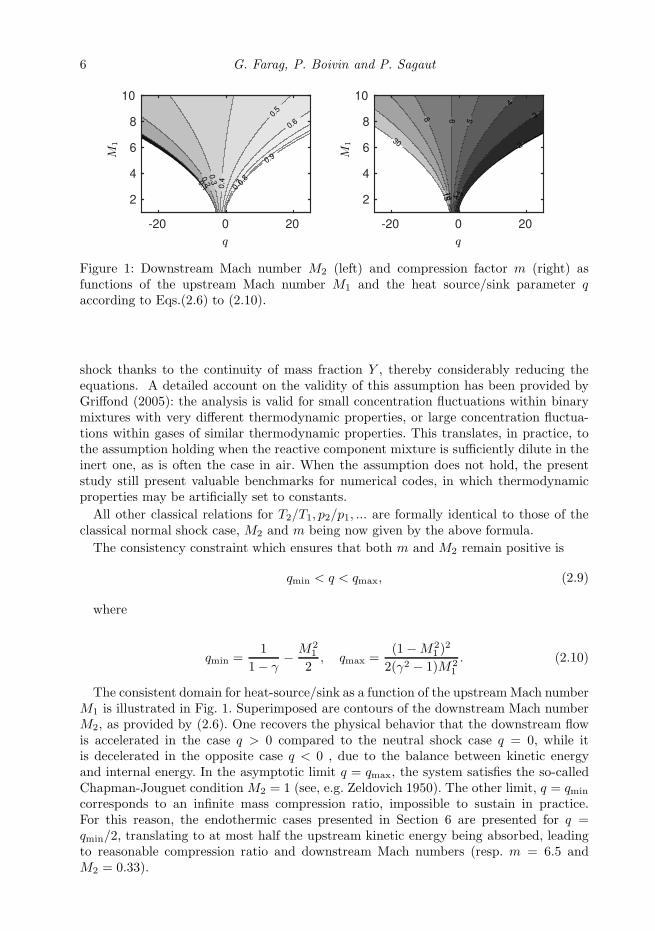
Figure 1: Downstream Mach number M2 (left) and compression factor m (right) asfunctions of the upstream Mach number M1 and the heat source/sink parameter qaccording to Eqs.(2.6) to (2.10).

shock thanks to the continuity of mass fraction Y , thereby considerably reducing theequations. A detailed account on the validity of this assumption has been provided byGriffond (2005): the analysis is valid for small concentration fluctuations within binarymixtures with very different thermodynamic properties, or large concentration fluctua-tions within gases of similar thermodynamic properties. This translates, in practice, tothe assumption holding when the reactive component mixture is sufficiently dilute in theinert one, as is often the case in air. When the assumption does not hold, the presentstudy still present valuable benchmarks for numerical codes, in which thermodynamicproperties may be artificially set to constants.

All other classical relations for T2/T1, p2/p1, ... are formally identical to those of theclassical normal shock case, M2 and m being now given by the above formula.

The consistency constraint which ensures that both m and M2 remain positive is

qmin < q < qmax, (2.9)

where

qmin =1

1− γ− M2

1

2, qmax =

(1−M21 )

2

2(γ2 − 1)M21

. (2.10)

The consistent domain for heat-source/sink as a function of the upstreamMach numberM1 is illustrated in Fig. 1. Superimposed are contours of the downstream Mach numberM2, as provided by (2.6). One recovers the physical behavior that the downstream flowis accelerated in the case q > 0 compared to the neutral shock case q = 0, while itis decelerated in the opposite case q < 0 , due to the balance between kinetic energyand internal energy. In the asymptotic limit q = qmax, the system satisfies the so-calledChapman-Jouguet condition M2 = 1 (see, e.g. Zeldovich 1950). The other limit, q = qmin

corresponds to an infinite mass compression ratio, impossible to sustain in practice.For this reason, the endothermic cases presented in Section 6 are presented for q =qmin/2, translating to at most half the upstream kinetic energy being absorbed, leadingto reasonable compression ratio and downstream Mach numbers (resp. m = 6.5 andM2 = 0.33).


3. The Kovasznay modal decomposition for disturbances in a binarymixture of ideal gas

The Linear Interaction Approximation relies on a small disturbance hypothesis andthe use of linearized equations to described fluctuation propagation on either side of theshock.

For each quantity (e.g. u), let us identify the fluctuation part (u′) and the mean (u) as

u = u+ u′, p = p+ p′, . . .

and assume the fluctuation part is small (u′/u ≪ 1), a classical assumption provided:

• Linearization of Y , for which Y = 0 is acceptable, is valid (Griffond 2005). This isin practice related to the continuity of cp and γ discussed after Eq. (2.8).• Similarly, the linearization for the normal shock velocity is questionable in the limit

u → 0, attainable when q → qmin. To avoid this, the present study should not be carriedout for M2 < 0.25, or, alternatively, q < qmin/2.

In the reference frame tied to the planar shock front the 2D perturbation field thensatisfies

∂ρ′

∂t+ u

∂ρ′

∂x+ ρ

∂u′j

∂xj= 0,

∂u′i

∂t+ u

∂u′i

∂x+

1

ρ

∂p′

∂xi= 0,

∂Y ′

∂t+ u

∂Y ′

∂x= 0,

∂p′

∂t+ u

∂p′

∂x+ γp

∂u′j

∂xj= 0,

(3.1)

which can be recast as a system of evolution equations for Kovasznay’s physical modes:

∂s′

∂t+ u

∂s′

∂x= 0,

∂ω′‖

∂t+ u

∂ω′‖

∂x= 0,

∂ω′⊥

∂t+ u

∂ω′⊥

∂x= 0,

( ∂

∂t+ u

∂

∂x

)2p′ = c2∇2p′,

∂Y ′

∂t+ u

∂Y ′

∂x= 0,

(3.2)

where ω′ = ∇×u′ denotes the fluctuating vorticity, and ω′⊥ = (ω′·n)n and ω′

‖ = ω′−ω′⊥

are the shock-normal and the shock-parallel components of vorticity, respectively, withn the unit normal vector of the planar shock wave. The shock-normal and the shock-tangential components correspond to the toroidal and poloidal components of the velocityfield in the reference frame tied to the planar shock front, respectively.

One recognizes the entropy mode, the toroidal and poloidal vorticity modes, the fastand slow acoustic modes and the concentration mode. It is worth noting that Kovasznay’smodes correspond to the eigenmodes of the linearized propagation operator, which areorthonormal according to the inner product associated to Chu’s definition of compressibledisturbance energy.


ka

ks

k

x

y

αa

αsα

xs(y, t)

Figure 2: Sketch of the configuration. The corrugated shock mean front position is atx = 0. The incident perturbation has wave vector k, at angle α with respect to the shocknormal. Emitted waves may be acoustic waves, with wave vector ka, or non-acousticones, with wave vector ks.

Let us now introduce propagating plane wave disturbances of the general form

φ′ = Ai(k) exp [i(k · x−Ωt)]. (3.3)

Here, Ai(k) denotes the amplitude of upstream Kovasznay mode of type i, with i =s, a, Y, v, t for entropy, acoustic, concentration and poloidal/toroidal vorticity mode,respectively. k is the perturbation wave vector, associated with pulsation Ω = u1k cosα,where α is the angle of the incident perturbation with respect to the shock, as illustratedin Fig. 2.

The upstream fluctuating field can then be decomposed as follows

τ ′1/τ1u′x1/u1

u′r1/u1

u′φ1/u1

p′1/γp1Y ′1

T ′1/T1

s′1/Cp1

= Ai(k)ei(k·x−Ωt)

δis − δia + δiY Art

δiv sinα+ δiacosαM1

−δiv cosα+ δiasinαM1

δitδiaδiY

δis + (γ − 1)δiaδis

, (3.4)

where δij is the Kronecker symbol, and τ = 1/ρ is the specific volume.

Now introducing the transfer function Zij between upstream Kovasznay mode of typei and downstream Kovasznay mode of type j, the emitted fluctuating field downstreamthe shock is given by:


τ ′2/τ2u′x2/u2

u′r2/u2

u′φ2/u2

p′2/γp2Y ′2

T ′2/T2

s′2/Cp2

= Ai(k)e−ka ηxei(ka·x−Ωt)

−Zia

Zia(cosαa + iη)/(M2ζ)Zia sinαa/(M2ζ)

0Zia

0(γ − 1)Zia

0

+Ai(k)ei(ks·x−Ωt)

Zis + ZiY Art

Ziv sinαs

−Ziv cosαs

Zit

0ZiY

Zis

Zis

,

(3.5)

where

ζ =√1− η2 + 2iη cosαa. (3.6)

Acoustic and non-acoustic emitted fluctuations are separated into two contributions inEq. (3.5), as they correspond to different wave vectors, resp. ka (possibly associated toattenuation η) and ks. These wave vectors are explicited hereafter. The transfer functionZij coefficients are explicitly given in Section 5.

Emitted acoustic and non-acoustic wave vectors

Evaluation of the wave vectors ka, ks and the associated angles αa, αs and attenuationη is classical (see Fabre et al. 2001; Sagaut & Cambon 2018), but is nonetheless recalledfor the sake of completness.The effect of α being different whether the incident perturbation is acoustic (i = a) or

non-acoustic (i 6= a), it is convenient to introduce the modified incident angle β as

β = δiaα′ + (1 − δia)α, (3.7)

where α′ is defined as

cotα′ = cotα+1

M1 sinα. (3.8)

Wave vectors and angles are then related through the relation:

ka,sk

=sinβ

sinαa,s, (3.9)

valid for both acoustic and non-acoustic emitted waves.The emitted non-acoustic wave vector angle simply reads

cotαs = m cotβ, (3.10)

where m is the compression factor (2.8).Obtaining the emitted acoustic wave vector ka and associated attenuation η is not as

straightforward. If the incident perturbation is non-acoustic (i 6= a), a singularity appears


56

60

64

646

6

66

66

70

70

80

-5 0 5

1.5

2

2.5

3

3.5

4

4.5

5

q

M1

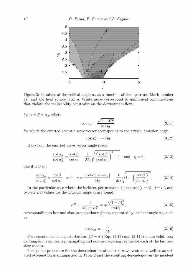
Figure 3: Isovalues of the critical angle αc as a function of the upstream Mach numberM1 and the heat source term q. White areas correspond to unphysical configurationsthat violate the realizability constraint on the downstream flow.

for α = β = αc, where

cotαc =

√1−M2

2

mM2, (3.11)

for which the emitted acoustic wave vector corresponds to the critical emission angle

cosαca = −M2. (3.12)

If α < αc, the emitted wave vector angle reads

cotαa

cotαca

=cotβ

cotαc− 1

M2

√(cotβ

cotαc

)2

− 1 and η = 0, (3.13)

else if α > αc:

cotαa

cotαca

=cotβ

cotαcand η =

| cotαca sinαa |M2

− 1

M2

√

1−(

cotβ

cotαc

)2

, (3.14)

In the particular case where the incident perturbation is acoustic (i = a), β = α′, andtwo critical values for the incident angle α are found:

α±c +

1

M1 sinα±c

= ∓√1−M2

2

mM2, (3.15)

corresponding to fast and slow propagation regimes, separated by incident angle αM suchas

cosαM = − 1

M1. (3.16)

For acoustic incident perturbations (β = α′) Eqs. (3.13) and (3.14) remain valid, nowdefining four regimes: a propagating and non-propagating regime for each of the fast andslow modes.The global procedure for the determination of emitted wave vectors as well as associ-

ated attenuation is summarized in Table 2 and the resulting dependence on the incident


non-acoustic perturbation

∀α, αs from Eq. (3.10) with β = α

α < αc, (αa, η) from Eq. (3.13) with β = α

α > αc, (αa, η) from Eq. (3.14) with β = α

acoustic perturbation

∀α, αs from Eq. (3.10) with β = α′

0 < α < α−

c , (αa, η) from (3.13) with β = α′

α−

c < α < αM , (αa, η) from (3.14) with β = α′

αM < α < α+c , (αa, η) from (3.14) with β = α′

α+c < α < π, (αa, η) from (3.13) with β = α′

Table 2: Computation of the emitted acoustic and non acoustic wave vectors throughthe corresponding angles αa and αs, for non-acoustic and acoustic incident perturbation.Also included is the determination of attenuation η for emitted acoustic waves.

acoustic perturbation

α

angle

andatten

uation

π

π

2

0

−π

2

−π0 π/2 π

α

non-acoustic perturbation

π

2

π

4

0 0 π/4 π/2

Figure 4: Emission angles and attenuation factor η, obtained following the proceduresummarized in Tab. 2, for γ = 1.4, M1 = 2 and q = −2.25. Plain line: αa, dashed-line:αs, dotted-line: attenuation η. In the left plot, the additional dot-dashed line representsthe non-linear dependence of β as a function of α (3.7) in the case of an acoustic incidentperturbation.

angle is illustrated in Fig. 4.

4. Extension of Chu’s definition for disturbance energy tomulticomponent gas

An important issue is the derivation of a physically relevant and mathematicallyconsistent definition of the energy of the disturbances in compressible flows. Chu’sdefinition (Chu 1965) for the disturbance energy around a base flow has the advantageto define an inner product, with respect to which the linearized Euler equations abouta uniform base flow are self-adjoint, and Kovasznay modes correspond to orthogonaleigenmodes of the linearized operator. The orthogonality of eigenmodes prevents spuriousnon-normality-induced phenomenon in the computation of the energy of the fluctuatingfield (George & Sujith 2011; Sagaut & Cambon 2018) As a matter of fact, the use ofa non-normal basis may lead to unphysical growth of the energy of the system becauseof the contributions of non-zero cross-products of basis vectors. Therefore, one can split


the total energy as the sum Etot =∑

iEi, with i = v, a, s for the vorticity mode, theacoustic mode and the entropy mode, respectively.

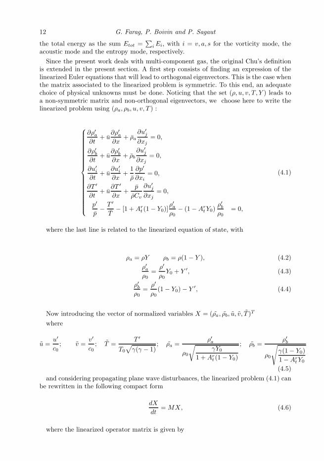
Since the present work deals with multi-component gas, the original Chu’s definitionis extended in the present section. A first step consists of finding an expression of thelinearized Euler equations that will lead to orthogonal eigenvectors. This is the case whenthe matrix associated to the linearized problem is symmetric. To this end, an adequatechoice of physical unknowns must be done. Noticing that the set (ρ, u, v, T, Y ) leads toa non-symmetric matrix and non-orthogonal eigenvectors, we choose here to write thelinearized problem using (ρa, ρb, u, v, T ) :

∂ρ′a∂t

+ u∂ρ′a∂x

+ ρa∂u′

j

∂xj= 0,

∂ρ′b∂t

+ u∂ρ′b∂x

+ ρb∂u′

j

∂xj= 0,

∂u′i

∂t+ u

∂u′i

∂x+

1

ρ

∂p′

∂xi= 0,

∂T ′

∂t+ u

∂T ′

∂x+

p

ρCv

∂u′j

∂xj= 0,

p′

p− T ′

T− [1 +Ar

t (1− Y0)]ρ′aρ0

− (1−ArtY0)

ρ′bρ0

= 0,

(4.1)

where the last line is related to the linearized equation of state, with

ρa = ρY ρb = ρ(1 − Y ), (4.2)

ρ′aρ0

=ρ′

ρ0Y0 + Y ′, (4.3)

ρ′bρ0

=ρ′

ρ0(1− Y0)− Y ′, (4.4)

Now introducing the vector of normalized variables X = (ρa, ρb, u, v, T )T

where

u =u′

c0; v =

v′

c0; T =

T ′

T0

√γ(γ − 1)

; ρa =ρ′a

ρ0

√γY0

1 +Art (1− Y0)

; ρb =ρ′b

ρ0

√γ(1− Y0)

1−ArtY0

(4.5)

and considering propagating plane wave disturbances, the linearized problem (4.1) canbe rewritten in the following compact form

dX

dt= MX, (4.6)

where the linearized operator matrix is given by


M =

−ikxu0 0 − ikxc0√γ K1 − ikyc0√

γ K1 0

0 −ikxu0 − ikxc0√γ K2 − ikyc0√

γ K2 0

− ikxc0√γ K1 − ikxc0√

γ K2 −ikxu0 0 − ikxc0√γ−1√

γ

− ikyc0√γ K1 − ikyc0√

γ K2 0 −ikxu0 − ikyc0√γ−1√

γ

0 0 − ikxc0√γ−1√

γ − ikyc0√γ−1√

γ −ikxu0

(4.7)

where the two positive parameters K1 and K2 are defined as

K1 =√

Y0[1 +Art (1− Y0)], K2 =

√(1− Y0)(1 −Ar

tY0), (4.8)

The five eigenvalues are

−ikxu0, −ikxu0, −ikxu0, −i (kxu0 ∓ kc0) , (4.9)

which correspond to the normalized propagation speeds of (from the left to the right)the entropy mode, the vorticity mode, the concentration mode and the fast and slowacoustic modes. The associated set of orthogonal eigenvectors is

Xs =

√γ−1

γ+K2

1−1

000

−K1√γ+K2

1−1

, Xv =

00ky

k−kx

k0

, Xa± =

K1√2γ

K2√2γ

±kx

k√2

±ky

k√2√

γ−12γ

, (4.10)

XY =

−K1K2√(γ+K2

1−1)γ√

γ+K2

1−1

γ

00

−K2

√γ−1

(γ+K2

1−1)γ

. (4.11)

All possible solutions of the linearized problem can be expressed as a linear combinationof the eigenvectors: X(t) =

∑i=s,v,a±,Y Ci(t)Xi. Therefore a local definition of the total

energy E(t) of the disturbance is given by the square of L2 norm of X(t). Thanks to theorthogonality property, one has ‖X(t)‖2 = X(t) ·X(t) =

∑i=s,v,a±,Y C2

i (t)‖Xi‖2, whichappears as the sum of the energy of each mode. The associated energy in a volume V isobtained in a straightforward way as:

Etot(t) =γp02

∫

V

(K2

1ρ′2a

γρ20Y20

+K2

2ρ′2b

γρ20(1 − Y0)2+

u′iu

′i

c20+

T ′2

γ(γ − 1)T 20

)dV , (4.12)

which can be rewritten as a function of u′i, p

′, s′ and Y ′ as follows:


Etot(t) =γp02

∫

V

M2

0

(u′i

u0

)2

+

(p′

γp0

)2

+1

γ

[K2

1

Y 20

+K2

2

(1− Y0)2+

(Art )

2

γ − 1

](Y ′)

2(4.13)

+1

γ − 1

(s′

Cp

)2dV.

The original formula given by Chu for single-species fluids is recovered taking Y0 = 1(which leads to K1 = 1, K2 = 0) along with Y ′ = 0.

5. A general formulation of the normal-mode-based LIA

The shock jump relations for a normal planar shock wave with possible heat re-lease/absorption and change in specific heats across the shock read

ρ1(u′x1 −

∂xs

∂t) + u1ρ

′1 = ρ2(u

′x2 −

∂xs

∂t) + u2ρ

′2, (5.1)

p′1 + ρ′1u21 + 2ρ1u1u

′x1 = p′2 + ρ′2u

22 + 2ρ2u2u

′x2,

h′1 + u1(u

′x1 −

∂xs

∂t) = h′

2 + u2(u′x2 −

∂xs

∂t),

u1∂xs

∂y+ u′

r1 = u2∂xs

∂y+ u′

r2,

u′φ1 = u′

φ2,

Y ′1 = Y ′

2 .

As in Eq. (3.4), all prime quantities (e.g. p′1) correspond to the fluctuations around theaverage base flow (e.g. p1), and

xs = xs(y, t) = Axei(k sin βy−Ωt), (5.2)

denotes the shock displacement with respect to its equilibrium position, as depicted inFig. 2. Ax is the perturbation amplitude.


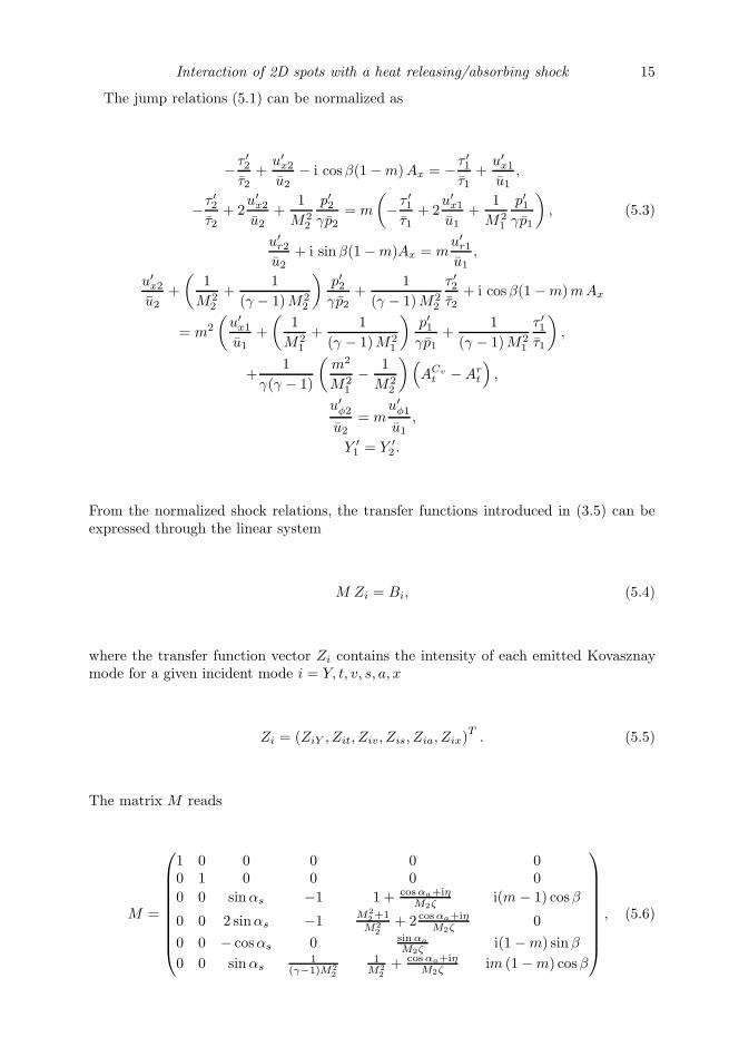
The jump relations (5.1) can be normalized as

−τ ′2τ2

+u′x2

u2− i cosβ(1 −m)Ax = −τ ′1

τ1+

u′x1

u1,

−τ ′2τ2

+ 2u′x2

u2+

1

M22

p′2γp2

= m

(−τ ′1τ1

+ 2u′x1

u1+

1

M21

p′1γp1

), (5.3)

u′r2

u2+ i sinβ(1 −m)Ax = m

u′r1

u1,

u′x2

u2+

(1

M22

+1

(γ − 1)M22

)p′2γp2

+1

(γ − 1)M22

τ ′2τ2

+ i cosβ(1 −m)mAx

= m2

(u′x1

u1+

(1

M21

+1

(γ − 1)M21

)p′1γp1

+1

(γ − 1)M21

τ ′1τ1

),

+1

γ(γ − 1)

(m2

M21

− 1

M22

)(ACv

t −Art

),

u′φ2

u2= m

u′φ1

u1,

Y ′1 = Y ′

2 .

From the normalized shock relations, the transfer functions introduced in (3.5) can beexpressed through the linear system

M Zi = Bi, (5.4)

where the transfer function vector Zi contains the intensity of each emitted Kovasznaymode for a given incident mode i = Y, t, v, s, a, x

Zi = (ZiY , Zit, Ziv, Zis, Zia, Zix)T. (5.5)

The matrix M reads

M =

1 0 0 0 0 00 1 0 0 0 0

0 0 sinαs −1 1 + cosαa+iηM2ζ

i(m− 1) cosβ

0 0 2 sinαs −1M2

2+1

M2

2

+ 2 cosαa+iηM2ζ

0

0 0 − cosαs 0 sinαa

M2ζi(1−m) sinβ

0 0 sinαs1

(γ−1)M2

2

1M2

2

+ cosαa+iηM2ζ

im (1−m) cosβ

, (5.6)


and the right-hand term, dependent on the incident wave’s nature:

Bs =

00−1−m0m2

(γ−1)M2

1

, Bv =

00

sinα2m sinα−m cosαm2 sinα

, Ba =

00

1 + cosαM1

m(

M2

1+1

M2

1

+ 2 cosαM1

)

m sinαM1

m2(

1M2

1

+ cosαM1

)

,

Bt =

0m0000

, BY =

100

(1−m)Art

0(m2

M2

1

− 1M2

2

)(1

γ(γ−1)ACv

t + 1γA

rt

)

. (5.7)

From the above system, the transfer function vector can be deduced as

(ZiY , Zit, Ziv, Zis, Zia, Zix)T= M−1Bi, (5.8)

where the inverse matrix is a block diagonal matrix of the same form as M . It can thenbe inferred that the toroidal mode is fully decoupled from the others

Ztj = Bt,

Zit = 0 for i 6= t.(5.9)

A similar behavior is obtained for the concentration mode Y , when (Art , A

Cv

t ) = (0, 0)and BY comprises of a single non-zero component. For arbitrary values of (Ar

t , ACv

t ),however,

ZY j 6= BY ,

ZiY = 0 for i 6= Y,(5.10)

so that an upstream mass concentration perturbation can produce a combination of vari-ous modes downstream of the shock. Downstream, however, a mass fraction perturbationcan only arise from an upstream mass fraction perturbation. These comments allow toconsider a reduced number of Zij terms in the following Figures.

The transfer functions obtained for acoustic, poloidal and entropy incident perturba-tions are plotted in Fig. 5 as functions of the incident angle α. The associated emittedwave vectors are found in Fig. 4 (αa for Zai and αs for Zvi and Zsi).

Incident mass fraction perturbations can vary in nature depending on the value ofAtwood’s numbers (Ar

t , ACv

t ) defined earlier (2.3). The associated transfer function ZY i

are therefore provided separately, in Fig. 6, with associated emitted wave angle αs inFig. 4. Note that BY is linear in Ar

t and ACv

t , so that providing solutions ZY i for thetwo base vectors (Ar

t , ACv

t ) = (0, 1) and (Art , A

Cv

t ) = (1, 0) suffice to describe the transferfunction for any (Ar

t , ACv

t ).


0 50 100 150−2

−1

0

1

2

3

n

Zaa

0 50 100 150−15

−10

−5

0

5

10

15

n

Zav

0 50 100 150−2

−1

0

1

2

n

Zas

0 50 100 150−4

−2

0

2

4

n

Zax

0 20 40 60 80−1

−0.5

0

0.5

1

1.5

n

Zva

0 20 40 60 80−10

−5

0

5

10

15

20

n

Zvv

0 20 40 60 80−1

−0.5

0

0.5

1

1.5

n

Zvs

0 20 40 60 80−2

−1

0

1

2

3

n

Zvx

0 20 40 60 80−1

−0.5

0

0.5

n

α

Zsa

0 20 40 60 80−15

−10

−5

0

5

10

n

α

Zsv

0 20 40 60 80−1

0

1

2

3

n

α

Zss

0 20 40 60 80−2.5

−2

−1.5

−1

−0.5

0

n

α

Zsx

Figure 5: Real part (plain line) and imaginary part (dashed) of Zii as a function of theincident wave angle α, for γ = 1.4, M1 = 2 and q = −2.25. The corresponding emittedwave vectors angles αa and αs are those represented in Fig 4.

0 20 40 60 80−1

−0.5

0

0.5

n

ZY a

0 20 40 60 80−15

−10

−5

0

5

10

n

ZY v

0 20 40 60 80−1

−0.5

0

0.5

1

1.5

n

ZY s

0 20 40 60 80−2.5

−2

−1.5

−1

−0.5

0

n

ZY x

0 20 40 60 80−0.1

−0.05

0

0.05

0.1

0.15

n

α

ZY a

0 20 40 60 80−1

−0.5

0

0.5

1

n

α

ZY v

0 20 40 60 80−0.1

0

0.1

0.2

0.3

n

α

ZY s

0 20 40 60 80−0.3

−0.2

−0.1

0

0.1

n

α

ZY x

Figure 6: Real part (plain line) and imaginary part (dashed) of ZY i as a function of theincident wave angle α, for different incident mass fraction wave: (Ar

t , ACv

t ) = (1,0) (top),(0,1) (bottom). The remaining parameters are identical to Fig. 5: γ = 1.4, M1 = 2 andq = −2.25. The corresponding emitted wave vector angle αs can be found in Fig 4.

6. Interaction with Gaussian spots

This section is dedicated to the interaction between 2D Gaussian spots advected atthe uniform speed U1 in the shock-normal direction and a planar shock wave.


Y s ω Σ

Figure 7: Emitted vorticity for incident gaussian density Y , entropy s, and vorticity ωspots. The fourth spot corresponds to the sum Σ of the three gaussian spots, resultingin yet another vorticity pattern. The dashed line illustrates the corrugated shock.

The Gaussian spots are introduced as perturbations of the form

G′ = ǫ e−r2, (6.1)

where r is the radial coordinate relative to the centre of the spot, and the Gaussianperturbation G′ is successively set as three elemental perturbations

G′ =τ ′

Art τ

for the density spot,

G′ =s′

cpfor the entropy spot,

G′ =ω′

Ufor the vorticity spot.

(6.2)

For each perturbation, the emitted flow will systematically be studied through compar-isons of acoustic, entropy and vorticity fields.Note that, owing to the linear character of this study, it is straight-forward to combine

these three elemental Gaussian perturbations into more complex ones, and obtain theemitted flow-field. This is illustrated in Fig. 7, which displays the vorticity field emittedfrom the combination of the three elemental spots presented hereafter.In the following ǫ, appears as a mere scaling and is therefore set to 1. Typical results

are shown for Art = 2, ACv

t = 1, M1 = 2 and γ = 1.4. To illustrate the effect of theheat-release, results are plotted for adiabatic (q = 0), endothermic (q = −2.25) andexothermic (q = 0.59). The numeric values for endothermic and exothermic shocks werechosen to be qmin/2 and qmax/2 at M1 = 2.

6.1. Gaussian density spot

Let us now consider a density spot, e.g . G′ = τ ′

Art τ in (6.2), which can be considered

as an idealized model for shock/dropplet interaction.The choice of a positive ǫ in (6.2) corresponds to the definition of a heavy perturbation

with respect to the upstream fluid, which can be interpreted as an ideal model for adroplet of heavy fluid. A negative value would correspond a pocket of light fluid. It is


-0.1

0.05

0.05

0.050.9

0 1 2 3

-1.5

-1

-0.5

0

0.5

1

1.5

0.0

2

0.02

0.0

2

0.05

0.05

0.0

5

0.30.6

0.6

-3 -2 -1 0

-1.5

-1

-0.5

0

0.5

1

1.5x x

q < 0s′

Cp

0.0

2

0.0

2

0.02

0.05

0.05

0.3

0.6

0.6

0 1 2 3

-1.5

-1

-0.5

0

0.5

1

1.5

0.0

2

0.02

0.0

2

0.05

0.05

0.0

5

0.30.6

0.6

-3 -2 -1 0

-1.5

-1

-0.5

0

0.5

1

1.5

x x

q > 0q = 0

-7

-3 -3

2

2

2

10

0 2 4

-2

-1

0

1

2

-1

-0.6

-0.2

-0.20.2

0.2

0.2

0.2

0.6

0.6

2 4

-4 -2 0

-2

-1

0

1

2

x x

q < 0aω′

u

-0.3

-0.1

-0.1 0.0

25

0.025

0.0

25

0.0

25

0.2

0.21

1

0 2 4

-2

-1

0

1

2-1

-0.6

-0.2

-0.20.2

0.2

0.2

0.2

0.6

0.6

2 4

-4 -2 0

-2

-1

0

1

2

x x

q > 0q = 0

-0.1

-0.05

-0.05

-0.01

-0.0

1

-0.0

1

0.02

0.02

0.03

0 2 4 6

0

2

4

6

-0.0

7

-0.07

-0.0

3

-0.0

3

0.01

0.0

1

0.0

2

-6 -4 -2 0

0

2

4

6

x x

q < 0p′

γp

y

-0.0

7

-0.05

-0.05

-0.03

-0.0

3

-0.03

-0.01

-0.0

1

-0.01

0.010.0

1

0.01

0.02

0 2 4 6

0

2

4

6

-0.0

7

-0.07

-0.0

3

-0.0

3

0.01

0.0

1

0.0

2

-6 -4 -2 0

0

2

4

6

x x

q > 0

y

q = 0

Figure 8: Incident Gaussian density spot: emitted entropy, vorticity and acousticperturbations (from top to bottom). Left: adiabatic vs endothermic case. Right: adiabaticvs exothermic.

worth noting that pure density heterogeneities without acoustic perturbation, i.e. pure ρ-waves, are obtained considering concentration fluctuations. The solution is then computedanalytically thanks to the formulas given in the Appendix.The emitted fields of normalized entropy s′

Cpand vorticity aω′

u are displayed in the first

4 plots of Figure. 8. Since the emitted patterns are advected at the constant speed U2,they are plotted in the reference frame associated to the perturbation centre, in whichthey are frozen thanks to the fact that diffusive effects are not taken into account in thepresent inviscid model. The presented patterns are related to the far field solution, i.e.intermediary solutions that are found at times at which the incoming fluctuation spothas not totally crossed the shock are not presented for the sake of brevity (but can becomputed).It is seen that the topology of the emitted vorticity field is qualitatively the same

in the three cases: a quadripolar pattern made of two counter-rotating vortex pairs isgenerated. This can be qualitatively interpreted as the result of a baroclinic effect of theform −(∇p ×∇ρ)/ρ2, in which the positive pressure gradient is related to the pressurejump across the shock wave. From that expression, it is seen that the case of a lightdisturbance with a negative amplitude parameter ǫ would lead to a vorticity patternwith opposite sign, i.e. a pattern made of four vortices rotating in the opposite sense tothose found for a heavy density spot.The main effects of the heat source term being i) an amplification (resp. damping)

of the amplitude of the emitted perturbations and ii) an increase (resp. decrease) of


-5 0 5

1.5

2

2.5

3

3.5

4

4.5

5

0

0.5

1

1.5

2

2.5

q

M1

log10 Etot

-5 0 5

1.5

2

2.5

3

3.5

4

4.5

5

-1

-0.5

0

0.5

q

M1

log10 Ey

-5 0 5

1.5

2

2.5

3

3.5

4

4.5

5

-2

-1

0

1

2

q

M1

log10 Ev

-5 0 5

1.5

2

2.5

3

3.5

4

4.5

5

-5

-4

-3

-2

-1

0

q

M1

log10 Ea

-5 0 5

1.5

2

2.5

3

3.5

4

4.5

5

-4

-3

-2

-1

0

1

2

q

M1

log10 Es

Figure 9: Energy of the emitted disturbances in the case of an incident Gaussian densityspot in the (M1, q) plane. Total energy Etot and the part associated to each Kovasznaymode are displayed, with Ey: energy of the concentration mode;Ev: energy of the vorticitymode; Ea: energy of the acoustic mode; Es: energy of the entropy mode.

the anisotropy of the emitted pattern for endothermic (resp. exothermic) case, whencompared to the adiabatic case. In the strong endothermic case the amplitude of the fourvortices are nearly equal, while the second vortex pair is weaker in other cases. This isconsistent with the fact that the effective shock-induced compressive effect is stronger inthe endothermic case, as observed in Section 2.The emitted acoustic field is illustrated here in the bottom plots of Fig. 8, in which

the acoustic pressure field p′

γp is plotted at time t = 4ac2.

A more global view at the interaction physics is obtained looking at the energy of theemitted waves along with the part associated to each Kovasznay mode, according to theextended definition derived in Section 4. The area used to compute the sum in Eq.(4.13)is taken equal to 12D × 12D, which was checked to be large enough to get fully convergedvalues, with D defined as the radius of the incident Gaussian spot (see Appendix).Results in the (M1, q) plane normalized by the energy of the incident density spot are

displayed in Fig. 9 for the far-field solution, i.e. the transient contribution of acousticnon-propagative waves is omitted. Profiles along the q = 0 and the M1 = 2 lines are alsoshown in Fig. 10.It is observed that the total emitted energy is an increasing function of the incoming

Mach numberM1, and that the respective importance of each mode is strongly influencedby the heat source term q. In the neutral case q = 0, the emitted energy is mainly dueEy and Ev, i.e. to the concentration mode and the vorticity mode, the former beingdominant for M1 < 4. It is worth noting that the energy of all emitted modes is anincreasing function of M1, excepted Es which decreases for 1 6 M1 6 2.6 Varying qat fixed M1 makes a more complex behavior to appear. The emitted energy is mostlyrelated to the vorticity mode in the endothermic case, the solution being dominated bythe concentration mode for sligthly negative q and exothermic cases. This is due to thecase that the concentration mode is the only one which exhibit an increase for increasing


1.5 2 2.5 3 3.5 4 4.5 510

-4

10-3

10-2

10-1

100

101

E

q = 0

M1

-4 -3 -2 -1 010

-6

10-4

10-2

100

102

104

E

M1 = 2

q

Figure 10: Energy of the emitted disturbances in the case of an incident Gaussian densityspot versus M1 for the adiabatic case (q = 0) and versus q for M1 = 2. Total energyand the part associated to each Kovasznay mode are displayed. Etot (solid thick line),Ey (solid), Ev (dotted), Ea (dashed), Es (dotted-dashed).

q, while a decrease of the total emitted energy Etot associated to a monotonic decreaseof all other modes is observed. A very fast decrease of Es is observed, leading to thefact that the entropy mode is very strong in the highly endothermic case, while it is theweakest mode in the neutral and and exothermic cases.

6.2. Gaussian entropy spot

This Section is dedicated to the interaction with a Gaussian entropy spot, and thereforeis an extension of the previous analysis provided in Fabre et al. (2001) for the adiabatic

case q = 0. The upstream entropy spot is defined by setting G′ = s′

cpin (6.2).

The emitted entropy far field, vorticity far field and acoustic pressure far field aredisplayed in Fig. 11. The emitted disturbance topology is the same as in the density case: aquadrupolar pattern made of two counter-rotating vortex pairs is generated downstreamthe shock, whose intensity and anisotropy are decreasing functions of the heat sourceterm q. The key mechanisms for vorticity generation can again be interpreted as a kindof baroclinic production term associated to the pressure jump across the shock and thedensity gradient associated to the entropy disturbance, see Eq. (3.4).The total energy of the emitted far-field solution (normalized by the energy of the

incident spot) and the part associated to each Kovasznay component are plotted in Fig.12 in the (M1, q) plane, while profiles along the M1 = 2 and q = 0 lines are shown inFig. 13. It is worth noting that the concentration mode energy remains null downstreamthe shock, i.e. Ey = 0, since it is null upstream the shock and the the concentrationfluctuation is continuous at the shock according to Eq. (5.1).Some interesting differences with the density spot case are observed, which are due

to the fact that the entropy spot combines a density disturbance and a temperaturedisturbance. First, in the adiabatic case q = 0, the normalized total emitted energy isnot a monotonous function of the upstream Mach number M1. A decrease is observed forM1 < Mcrit ≃ 2.7, which is due to a decrease of the energy of the emitted entropy mode,which is a monotonic decaying function of M1. The emitted acoustic and vorticity energycomponent, Ea and Ev, are growing with M1, Ea being negligible in all cases. Therefore,the emitted field is dominated by the entropy mode for M1 < Mcrit, while the vorticitymode is dominant at higher Mach number. This picture is very different from the oneobserved for the density spot, and it it stable with respect to a change in the parameter


0.05

0.05

0.05

0.3

0.3

0.6

0 1 2 3

-1.5

-1

-0.5

0

0.5

1

1.5

0.0

1

0.01

0.0

1

0.05

0.05

0.30.3

0.6

-3 -2 -1 0

-1.5

-1

-0.5

0

0.5

1

1.5x x

q < 0s′

Cp

0.01

0.0

1

0.01

0.05

0.050.3

0.6

0 1 2 3

-1.5

-1

-0.5

0

0.5

1

1.5

0.0

1

0.01

0.0

1

0.05

0.05

0.30.3

0.6

-3 -2 -1 0

-1.5

-1

-0.5

0

0.5

1

1.5

x x

q > 0q = 0

-3

-1

-1

-1

11

1

5

0 2 4

-2

-1

0

1

2

-0.4

-0.2

0.2

0.2

1 2

-4 -2 0

-2

-1

0

1

2

x x

q < 0aω′

u

-0.1

0.0

5

0.0

5

0.05

0.2

0.2

0.6 1

0 2 4

-2

-1

0

1

2

-0.4

-0.2

0.2

0.2

1 2

-4 -2 0

-2

-1

0

1

2

x x

q > 0q = 0

-0.07

-0.0

5

-0.03

-0.03

-0.01

-0.01

-0.01

0.01

0.01

0.02

0 2 4 6

0

2

4

6

-0.05

-0.05

-0.0

3

-0.03

-0.0

1

-0.0

1

-0.01

0.01

0.0

1

0.02

-6 -4 -2 0

0

2

4

6

x x

q < 0p′

γp

y

-0.05

-0.0

3

-0.03

-0.01

-0.0

1

-0.0

1

0.0

1

0.01

0.02

0 2 4 6

0

2

4

6

-0.05

-0.05

-0.0

3

-0.03

-0.0

1

-0.0

1

-0.01

0.01

0.0

1

0.02

-6 -4 -2 0

0

2

4

6

x x

q > 0

y

q = 0

Figure 11: Incident Gaussian entropy spot: emitted entropy, vorticity and acousticperturbations (from top to bottom). Left: adiabatic vs endothermic case. Right: adiabaticvs exothermic.

q. Here, the energy of all emitted modes decays when increasing q, including the emittedvortical energy which was an increasing function of q in the density spot case.

6.3. Gaussian vorticity spot

The last case deals with the interaction between a planar shock wave and a Gaussianvorticity spot, which is a model of a weak vortex. The shock/vortex interaction has beenaddressed by several authors, mainly via Direct Numerical Simulation, but the presentanalysis is the first one to cover the full (M1, q) plane within the LIA framework.Results for the emitted non-acoustic fields are shown in the first 4 plots of Fig. 14.

The concentration field remains uniform, as in the case of the entropy spot. A firstobservation is that the topology of the emitted field is different from the one observed forboth incident density and entropy spot. As a matter of fact, while two vortex pairs withvariable intensity were found previously, the present field is made of a strong counter-rotating vortex pair, with two companion pairs of much weaker vortical structures.The topology of the downstream acoustic field is investigated in the bottom plots of Fig.

14 which displays the generated pressure. A compression wave followed by a dilatationwave is observed, while in the two other cases the dilatation wave is emitted first.The energy of the emitted field split into model components, normalized by the energy

of the incident spot, is displayed in Figs. 15 and 16. It is observed that, in all cases,the emitted energy is dominated by the vortical component. In the adiabatic case, theacoustic energy remains larger than the entropy mode energy at all Mach number. The


-5 0 5

1.5

2

2.5

3

3.5

4

4.5

5

0

0.5

1

1.5

2

2.5

q

M1

log10 Etot

-5 0 5

1.5

2

2.5

3

3.5

4

4.5

5

-3

-2

-1

0

1

2

q

M1

log10 Ev

-5 0 5

1.5

2

2.5

3

3.5

4

4.5

5

-5

-4

-3

-2

-1

0

q

M1

log10 Ea

-5 0 5

1.5

2

2.5

3

3.5

4

4.5

5

-0.5

0

0.5

1

1.5

2

2.5

q

M1

log10 Es

Figure 12: Energy of the emitted disturbances in the case of an incident Gaussian entropyspot in the (M1, q) plane. Total energy Etot and the part associated to each Kovasznaymode are displayed, with Ev: energy of the vorticity mode; Ea: energy of the acousticmode; Es: energy of the entropy mode.

1.5 2 2.5 3 3.5 4 4.5 510

-4

10-3

10-2

10-1

100

E

q = 0

M1

-4 -3 -2 -1 010

-3

10-2

10-1

100

101

102

103

E

M1 = 2

q

Figure 13: Energy of the emitted disturbances in the case of an incident Gaussian entropyspot versus M1 for in the adiabatic case (q = 0) (top) and versus q for M1 = 2 (bottom).Total energy and the part associated to each Kovasznay mode are displayed. Etot (solidthick line), Ev (dotted), Ea (dashed), Es (dotted-dashed).

opposite trend can be observed in strongly endothermic cases. All energy componentsare growing functions of M1 and decreasing functions of q.

6.4. Optimal mixed disturbances with minimal radiated noise

The purpose of this section is to illustrate the possibility of finding upstream distur-bances associated with peculiar emitted field. To this end, it is chosen to find the optimalcombination of the three above elementary spots for minimal radiated noise.Let us identify the emitted pressure perturbation as p′Y , p

′s and p′ω for the density,


-0.06

-0.02-0.02

-0.02

-0.02

0.02

0.0

2

0.0

2

0.02

0.0

6

0.06

0.1

4

0 1 2 3

-1.5

-1

-0.5

0

0.5

1

1.5

-0.0

2

-0.0

2

0.0

2

0.04

0.0

4

0.0

60.0

8

-3 -2 -1 0

-1.5

-1

-0.5

0

0.5

1

1.5x x

q < 0s′

Cp

0.0

20.0

4

0 1 2 3

-1.5

-1

-0.5

0

0.5

1

1.5

-0.0

2

-0.0

2

0.0

2

0.04

0.0

4

0.0

60.0

8

-3 -2 -1 0

-1.5

-1

-0.5

0

0.5

1

1.5

x x

q > 0q = 0

-25-7-7

-71

1

1

1

11

1

44

44

0 2 4

-2

-1

0

1

2

-6-3.5

-1.5

-1.5

0.2

0.2

0.2

0.20.2

0.2

0.6

0.6

0.6

1

-4 -2 0

-2

-1

0

1

2

x x

q < 0aω′

u

-4-3

-1

-1

0.2

0.2

0.2

0.2

0.2

0.4

0.4

0.6

0 2 4

-2

-1

0

1

2

-6-3.5

-1.5

-1.5

0.2

0.2

0.2

0.20.2

0.2

0.6

0.6

0.6

1

-4 -2 0

-2

-1

0

1

2

x x

q > 0q = 0

-0.02

-0.0

2

-0.02

0.0

3

0.0

3

0.03

0.07

0.0

7

0.09

0.09

0 2 4 6

0

2

4

6

-0.0

1

-0.0

1

-0.0

1

0.0

1

0.0

1

0.0

1

0.03

0.03

0.0

3

-6 -4 -2 0

0

2

4

6

x x

q < 0p′

γp

y

-0.0

1

-0.01

-0.01

0.0

1 0.0

1

0.0

1

0.0

3

0 2 4 6

0

2

4

6

-0.0

1

-0.0

1

-0.0

10.0

1

0.0

1

0.0

1

0.03

0.03

0.0

3

-6 -4 -2 0

0

2

4

6

x x

q > 0

y

q = 0

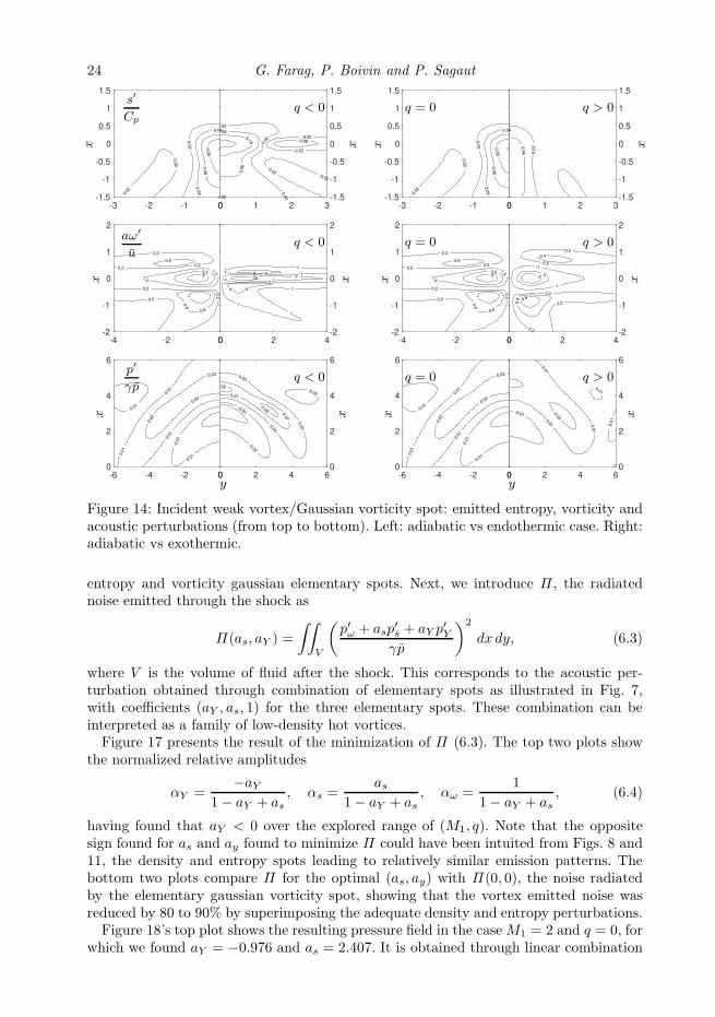
Figure 14: Incident weak vortex/Gaussian vorticity spot: emitted entropy, vorticity andacoustic perturbations (from top to bottom). Left: adiabatic vs endothermic case. Right:adiabatic vs exothermic.

entropy and vorticity gaussian elementary spots. Next, we introduce Π , the radiatednoise emitted through the shock as

Π(as, aY ) =

∫∫

V

(p′ω + asp

′s + aY p

′Y

γp

)2

dx dy, (6.3)

where V is the volume of fluid after the shock. This corresponds to the acoustic per-turbation obtained through combination of elementary spots as illustrated in Fig. 7,with coefficients (aY , as, 1) for the three elementary spots. These combination can beinterpreted as a family of low-density hot vortices.Figure 17 presents the result of the minimization of Π (6.3). The top two plots show

the normalized relative amplitudes

αY =−aY

1− aY + as, αs =

as1− aY + as

, αω =1

1− aY + as, (6.4)

having found that aY < 0 over the explored range of (M1, q). Note that the oppositesign found for as and ay found to minimize Π could have been intuited from Figs. 8 and11, the density and entropy spots leading to relatively similar emission patterns. Thebottom two plots compare Π for the optimal (as, ay) with Π(0, 0), the noise radiatedby the elementary gaussian vorticity spot, showing that the vortex emitted noise wasreduced by 80 to 90% by superimposing the adequate density and entropy perturbations.Figure 18’s top plot shows the resulting pressure field in the case M1 = 2 and q = 0, for

which we found aY = −0.976 and as = 2.407. It is obtained through linear combination


-5 0 5

1.5

2

2.5

3

3.5

4

4.5

5

0.4

0.6

0.8

1

1.2

q

M1

log10 Etot

-5 0 5

1.5

2

2.5

3

3.5

4

4.5

5

0.4

0.6

0.8

1

1.2

q

M1

log10 Ev

-5 0 5

1.5

2

2.5

3

3.5

4

4.5

5

-5.5

-5

-4.5

-4

-3.5

-3

-2.5

-2

q

M1

log10 Ea

-5 0 5

1.5

2

2.5

3

3.5

4

4.5

5

-7

-6

-5

-4

-3

-2

-1

q

M1

log10 Es

Figure 15: Energy of the emitted disturbances in the case of an incident weakvortex/Gaussian vorticity spot in the (M1, q) plane. Total energy Etot and the partassociated to each Kovasznay mode are displayed, with Ev: energy of the vorticity mode;Ea: energy of the acoustic mode; Es: energy of the entropy mode.

1.5 2 2.5 3 3.5 4 4.5 5

10-4

10-2

100

102

E

q = 0

M1

-4 -3 -2 -1 0

10-4

10-2

100

102

E

M1 = 2

q

Figure 16: Energy of the emitted disturbances in the case of an weak vortex/Gaussianvorticity spot versus M1 for in the adiabatic case and versus q for M1 = 2. Total energyand the part associated to each Kovasznay mode are displayed. Etot (solid thick line),Ev (dotted), Ea (dashed), Es (dotted-dashed).

of the emitted pressure for the elementary spots of Figs 8, 11 and 14 with weights(aY , as, 1). From the levels of the emitted pressure, it is clear that the radiated noise issignificantly reduced compared to either elementary spot – by 82.6%, as seen in Fig. 17.The bottom plot of Fig. 18 shows the vorticity pattern downstream of the shock for thesame perturbation, following Fig. 7.

Following the above procedure, it is straight-forward to minimize other fluctuations,such as vorticity, temperature, etc.


1.6 1.7 1.8 1.9 20

0.2

0.4

0.6

0.8

1

αω

αs

αY

M1

-0.4 -0.2 0 0.2 0.40

0.2

0.4

0.6

0.8

1

αω

αs

αY

q

1.6 1.7 1.8 1.9 20

0.002

0.004

0.006

0.008

0.01

0.012

0.76

0.78

0.8

0.82

0.84

M1

-0.4 -0.2 0 0.2 0.40

0.005

0.01

0.015

0.8

0.81

0.82

0.83

0.84

0.85

0.86

noise

reductio

n

q

Figure 17: Relative spots amplitudes minimizing the radiated noise Π (top) dependencewith M1 for q = 0 (left), and with q for M1 = 2 (right). The corresponding integralradiated noise Π (6.3) is shown for the elementary vortex Π(0, 0) (dashed) and theoptimal combination Π(as, aY ) (solid) in the bottom two plots. The dot-dashed line,

plotted in the right axes, shows the noise reduction Π(as,aY )−Π(0,0)Π(0,0) .

7. Concluding remarks

A complete LIA framework for the interaction between a planar shock and a Gaussiandisturbance including thermal effects at the shock front was proposed, along with ade-quate extension of the energy of the disturbances. General expressions for the emittedfield are also provided, allowing for a straightforward reconstruction of the solution. Sucha framework can provide a deep insight into shock/mixed disturbances interaction, butalso very acurate benchmark solutions for numerical scheme validation. Another results isthe extension of Chu’s definition of disturbance energy to the present framework, leadingto a mathematically-grounded meaningful definition of the energy of both upstream anddownstream fields. It is worth noting that mixed solutions based on the combination ofthe three elementary solutions analyzed in the previous section can also be very easilyobtained by linear combinations of the instantaneous elementary fields. This way, somesolutions with peculiar features can be obtained. This is illustrated by the search ofupstream vortex-like disturbances with minimal emitted pressure perturbations. In asimilar way, combining an heavy density spot with a cold entropy spot one can obtain anemitted field with a very small residual vorticity. Solutions that minimize or maximizethe energy of a given emitted Kovasznay mode can be obtained, the relative weight ofeach upstream mode being a function of the upstream Mach number and the heat sourceparameter q.

Strong of a wide variety of covered shock/spot interaction configurations, this workmay serve as benchmark for the development of shock-capturing numerical methods.


0

2

4

6

-6 -4 -2 0 2 4 6

-0.01

-0.0

1

-0.0

1

-0.0

1

-0.0

1

-0.0

05

-0.005-0

.005

-0.005

-0.005

0.005

0.005

0.005

0.005

0.005

0.005

0.005

0.01

0.01

0.01

0.01

0.01

0.0

15 0.015

-2

-1

0

1

2

-4 -2 0 2 4

y

xx

Figure 18: Emitted pressure (top) and vorticity (bottom) fields for the optimized vortexperturbation minimizing the radiated noise Π , in the case M1 = 2 and q = 0.

Acknowledgements

This work was supported by Labex MEC (ANR-10-LABX-0092) and the A*MIDEXproject (ANR-11-IDEX-0001-02), funded by the “Investissements d’Avenir”.

8. Appendix: Mathematical formulation for Gaussian spot/shockinteraction

One addresses here the general formulation for the upstream and downstream fieldassociated to the interaction between a 2D Gaussian non-acoustic disturbance and aplanar shock within the Kovasznay decomposition framework. The upstream disturbancesare advected at the constant speed U , and are then frozen in the reference frame movingwith the base flow far from the shock wave.Considering an upstream perturbation of Kovasznay mode i of the form (in cylindrical

coordinates (r, φ))

fi(r) = ǫe−r2/D2

, (8.1)

where D denotes the radius (taken equal to 1) of the Gaussian profile and fi thefluctuation of the physical quantity associated to the Kovasznay mode (e.g. density orspecific volume for a density spot, entropy for an entropy spot, vorticity for a vortex),its decomposition into Fourier modes obtained via a 2D polar Fourier transform is (seeFabre et al. (2001) for a full description of intermediary algebra, with (k, α) the polarcoordinates in the Fourier space)


fi(r) =ǫ

2π

∫ π2

α=−π2

K(r)dα, (8.2)

where

K(z) =

∫ ∞

k=0

k

2e−(

k2 )

2

cos(kz)dk = 1−√πze−z2

erfi(z), (8.3)

r = r cos(α− φ). (8.4)

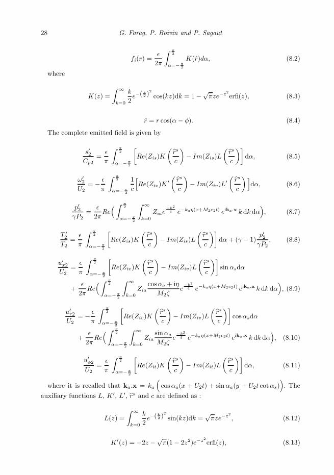
The complete emitted field is given by

s′2Cp2

=ǫ

π

∫ π2

α=−π2

[Re(Zis)K

(rs

c

)− Im(Zis)L

(rs

c

)]dα, (8.5)

ω′2

U2= − ǫ

π

∫ π2

α=−π2

1

c

[Re(Ziv)K

′(rs

c

)− Im(Ziv)L

′(rs

c

)]dα, (8.6)

p′2γP2

=ǫ

2πRe(∫ π

2

α=−π2

∫ ∞

k=0

Ziae−k2

4 e−kaη(x+M2c2t) eika.x k dk dα), (8.7)

T ′2

T2=

ǫ

π

∫ π2

α=−π2

[Re(Zis)K

(rs

c

)− Im(Zis)L

(rs

c

)]dα+ (γ − 1)

p′2γP2

, (8.8)

u′x2

U2=

ǫ

π

∫ π2

α=−π2

[Re(Ziv)K

(rs

c

)− Im(Ziv)L

(rs

c

)]sinαsdα

+ǫ

2πRe(∫ π

2

α=−π2

∫ ∞

k=0

Ziacosαa + iη

M2ζe

−k2


u′r2

U2= − ǫ

π

∫ π2

α=−π2

[Re(Ziv)K

(rs

c

)− Im(Ziv)L

(rs

c

)]cosαsdα

+ǫ

2πRe(∫ π

2

α=−π2

∫ ∞

k=0

Ziasinαa

M2ζe

−k2


u′φ2

U2=

ǫ

π

∫ π2

α=−π2

[Re(Zit)K

(rs

c

)− Im(Zit)L

(rs

c

)]dα, (8.11)

where it is recalled that ka.x = ka

(cosαa(x + U2t) + sinαa(y − U2t cotαs)

). The

auxiliary functions L, K ′, L′, rs and c are defined as :

L(z) =

∫ ∞

k=0

k

2e−(

k2 )

2

sin(kz)dk =√πze−z2

, (8.12)

K ′(z) = −2z −√π(1− 2z2)e−z2

erfi(z), (8.13)


L′(z) =√π(1 − 2z2)e−z2

, (8.14)

c =sinαs

sinα, rs = r cos(αs − φ). (8.15)

The emitted density field ρ′2 and specific volume τ ′2 = 1/ρ′2 are computed for eachcomponent from T ′, Y ′ and p′ in a straightforward way using the linearized equation ofstate, i.e.

p′

P=

ρ′

ρ+

T ′

T+Ar

tY′. (8.16)


REFERENCES

Abdikamalov, Ernazar, Huete, Cesar, Nussupbekov, Ayan & Berdibek, Shapagat 2018Turbulence generation by shock-acoustic-wave interaction in core-collapse supernovae.Particles 1 (1), 97–110.

Chu, Boa-Teh 1965 On the energy transfer to small disturbances in fluid flow (part i). ActaMechanica 1 (3), 215–234.

Chu, Boa-Teh & Kovasznay, Leslie SG 1958 Non-linear interactions in a viscous heat-conducting compressible gas. Journal of Fluid Mechanics 3 (5), 494–514.

Fabre, David, Jacquin, Laurent & Sesterhenn, Jorn 2001 Linear interaction of acylindrical entropy spot with a shock. Physics of Fluids 13 (8), 2403–2422.

George, K Joseph & Sujith, RI 2011 On chu’s disturbance energy. Journal of Sound andVibration 330 (22), 5280–5291.

Griffond, J 2005 Linear interaction analysis applied to a mixture of two perfect gases. Physicsof Fluids 17 (8), 086101.

Griffond, J 2006 Linear interaction analysis for richtmyer-meshkov instability at low atwoodnumbers. Physics of Fluids 18 (5), 054106.

Griffond, Jerome & Soulard, Olivier 2012 Evolution of axisymmetric weakly turbulentmixtures interacting with shock or rarefaction waves. Physics of Fluids 24 (11), 115108.

Griffond, J, Soulard, O & Souffland, D 2010 A turbulent mixing reynolds stress modelfitted to match linear interaction analysis predictions. Physica Scripta 2010 (T142),014059.

Huete, Cesar & Abdikamalov, Ernazar 2019 Response of nuclear-dissociating shocks tovorticity perturbations. Physica Scripta .

Huete, Cesar, Abdikamalov, Ernazar & Radice, David 2018 The impact of vorticitywaves on the shock dynamics in core-collapse supernovae. Monthly Notices of the RoyalAstronomical Society 475 (3), 3305–3323.

Huete, Cesar, Sanchez, Antonio L & Williams, Forman A 2013 Theory of interactionsof thin strong detonations with turbulent gases. Physics of Fluids 25 (7), 076105.

Huete, Cesar, Sanchez, Antonio L & Williams, Forman A 2014 Linear theory forthe interaction of small-scale turbulence with overdriven detonations. Physics of Fluids26 (11), 116101.

Huete, C, Wouchuk, JG, Canaud, B & Velikovich, AL 2012a Analytical linear theory forthe shock and re-shock of isotropic density inhomogeneities. Journal of Fluid Mechanics700, 214–245.

Huete, C, Wouchuk, JG & Velikovich, AL 2012b Analytical linear theory for the interactionof a planar shock wave with a two-or three-dimensional random isotropic acoustic wavefield. Physical Review E 85 (2), 026312.

Kovasznay, Leslie SG 1953 Turbulence in supersonic flow. Journal of the AeronauticalSciences 20 (10), 657–674.

Lee, Sangsan, Lele, Sanjiva K & Moin, Parviz 1993 Direct numerical simulation of isotropicturbulence interacting with a weak shock wave. Journal of Fluid Mechanics 251, 533–562.

Lee, Sangsan, Lele, Sanjiva K & Moin, Parviz 1997 Interaction of isotropic turbulencewith shock waves: effect of shock strength. Journal of Fluid Mechanics 340, 225–247.

de Lira, C Huete Ruiz 2010 Turbulence generation by a shock wave interacting with a randomdensity inhomogeneity field. Physica Scripta 2010 (T142), 014022.

Mahesh, Krishnan, Lee, Sangsan, Lele, Sanjiva K & Moin, Parviz 1995 The interactionof an isotropic field of acoustic waves with a shock wave. Journal of Fluid Mechanics 300,383–407.

Mahesh, Krishnan, Lele, Sanjiva K & Moin, Parviz 1997 The influence of entropyfluctuations on the interaction of turbulence with a shock wave. Journal of FluidMechanics 334, 353–379.

Moore, Franklin K 1953 Unsteady oblique interaction of a shock wave with a planedisturbance .

Narita, Shinji 1973 The radiative energy loss from the shock front. Progress of TheoreticalPhysics 49 (6), 1911–1931.

Quadros, Russell, Sinha, Krishnendu & Larsson, Johan 2016 Turbulent energy flux


generated by shock/homogeneous-turbulence interaction. Journal of Fluid Mechanics 796,113–157.

Ribner, H.S. 1954a Shock-turbulence interaction and the generation of noise. NACA TechnicalNote 3255.

Ribner, Herbert S 1954b Convection of a pattern of vorticity through a shock wave .Ribner, Herbert S 1959 The sound generated by interaction of a single vortex with a shock

wave. Tech. Rep.. University of Toronto.Ryu, Jaiyoung & Livescu, Daniel 2014 Turbulence structure behind the shock in canonical

shock–vortical turbulence interaction. Journal of Fluid Mechanics 756.Sagaut, P. & Cambon, C. 2018 Homogeneous turbulence dynamics, 2nd edition. Springer.Sinha, Krishnendu 2012 Evolution of enstrophy in shock/homogeneous turbulence interaction.

Journal of Fluid Mechanics 707, 74–110.Sinha, Krishnendu, Mahesh, Krishnan & Candler, Graham V 2003 Modeling shock

unsteadiness in shock/turbulence interaction. Physics of Fluids 15 (8), 2290–2297.Soulard, Olivier, Griffond, Jerome & Souffland, Denis 2012 Pseudocompressible

approximation and statistical turbulence modeling: Application to shock tube flows.Physical Review E 85 (2), 026307.

Williams, Forman Arthur 1985 Combustion Theory, second edition.. Cummings Publ. Co.Wouchuk, JG, de Lira, C Huete Ruiz & Velikovich, AL 2009 Analytical linear theory for

the interaction of a planar shock wave with an isotropic turbulent vorticity field. PhysicalReview E 79 (6), 066315.

Zeldovich, Yakov Borissovich 1950 On the theory of the propagation of detonation ingaseous systems .

Zel’Dovich, Ya B & Raizer, Yu P 2012 Physics of shock waves and high-temperaturehydrodynamic phenomena. Courier Corporation.

Zhao, Liangju, Wang, Fei, Gao, Hong, Tang, Jingwen & Yuan, Yuexiang 2008 Shockwave of vapor-liquid two-phase flow. Front. Energy Power Eng. China 2 (3), 344–347.

Interaction of two-dimensional spots with a heat releasing ...

Documents

Transcript of Interaction of two-dimensional spots with a heat releasing ...