�����������������

Citation: Zhang, G. Detecting and

Visualizing Observation Hot-Spots in

Massive Volunteer-Contributed

Geographic Data across Spatial Scales

Using GPU-Accelerated Kernel

Density Estimation. ISPRS Int. J.

Geo-Inf. 2022, 11, 55. https://

doi.org/10.3390/ijgi11010055

Academic Editor: Wolfgang Kainz

Received: 27 November 2021

Accepted: 7 January 2022

Published: 12 January 2022

Publisher’s Note: MDPI stays neutral

with regard to jurisdictional claims in

published maps and institutional affil-

iations.

Copyright: © 2022 by the author.

Licensee MDPI, Basel, Switzerland.

This article is an open access article

distributed under the terms and

conditions of the Creative Commons

Attribution (CC BY) license (https://

creativecommons.org/licenses/by/

4.0/).

International Journal of

Geo-Information

Article

Detecting and Visualizing Observation Hot-Spots in MassiveVolunteer-Contributed Geographic Data across Spatial ScalesUsing GPU-Accelerated Kernel Density EstimationGuiming Zhang

Department of Geography & the Environment, University of Denver, Denver, CO 80208, USA;guiming.zhang@du.edu; Tel.: +1-303-871-7908

Abstract: Volunteer-contributed geographic data (VGI) is an important source of geospatial big datathat support research and applications. A major concern on VGI data quality is that the underlyingobservation processes are inherently biased. Detecting observation hot-spots thus helps betterunderstand the bias. Enabled by the parallel kernel density estimation (KDE) computational tool thatcan run on multiple GPUs (graphics processing units), this study conducted point pattern analyses ontens of millions of iNaturalist observations to detect and visualize volunteers’ observation hot-spotsacross spatial scales. It was achieved by setting varying KDE bandwidths in accordance with thespatial scales at which hot-spots are to be detected. The succession of estimated density surfaceswere then rendered at a sequence of map scales for visual detection of hot-spots. This study offersan effective geovisualization scheme for hierarchically detecting hot-spots in massive VGI datasets,which is useful for understanding the pattern-shaping drivers that operate at multiple spatial scales.This research exemplifies a computational tool that is supported by high-performance computingand capable of efficiently detecting and visualizing multi-scale hot-spots in geospatial big data andcontributes to expanding the toolbox for geospatial big data analytics.

Keywords: volunteered geographic information (VGI); geospatial big data; point pattern analysis;kernel density estimation; hot-spot detection and visualization; spatial bias; multiple spatial scales;iNaturalist; graphics processing unit (GPU); parallel computing

1. Introduction

Volunteer-contributed geographic data, often termed ‘volunteered geographic in-formation’ (VGI) [1], have flourished over the past two decades or so due to the vastadvancements in geospatial and communication technologies (e.g., location-aware smartphones, social media) that enable ordinary citizens to collect and share georeferenced obser-vations of the world [2]. Broadly speaking, VGI encompasses geographic data generatedand shared (actively or passively) by volunteers participating in geographic citizen science,participatory mapping, public participation geographic information systems, neogeogra-phy, social media, crowdsourcing, etc. [2]. Prominent VGI examples, among others, includeOpenStreetMap, a platform for volunteers to collaboratively map all kinds of geographicfeatures across the globe with great details [3], and biodiversity citizen science projectssuch as eBird and iNaturalist to which nature observers submit tens of thousands of speciessightings on a daily basis [4,5]. Notably, citizen science [6] has existed for centuries, andgeographic citizen science [7,8] has been a major source of volunteer-contributed geo-graphic data (e.g., biodiversity observations), even long before the term VGI was coinedin 2007 [1]. VGI has risen to become an important source of geospatial data supportingscientific research and applications (e.g., biodiversity monitoring, disaster response) largelydue to its low cost, extensive coverage, high spatiotemporal resolution, and data updatetimeliness [9–13]. In a larger context, VGI represents a paradigm shift in how geographicdata is created and shared and in its content and characteristics [14]. It may have great

ISPRS Int. J. Geo-Inf. 2022, 11, 55. https://doi.org/10.3390/ijgi11010055 https://www.mdpi.com/journal/ijgi

ISPRS Int. J. Geo-Inf. 2022, 11, 55 2 of 15

influence on geography and its relationship to society [1,15]. VGI (particularly citizen sci-ence), due to its active engagement of the general public in scientific research activities (e.g.,data collection), is regarded as a bridge between geography (and other disciplines) andsociety that helps harness the power of the public to advance scientific discoveries throughcarefully designed projects [16] and, at the same time, increase scientific awareness of thepublic [17,18]. In fact, VGI is an important source of geospatial big data which is propellinggeographic research towards emerging paradigms such as ‘data-driven geography’ [19]and ‘data-intensive science’ [20].

VGI data quality issues, nonetheless, are under constant scrutiny [21]. Spatial datacollected and shared by volunteer communities may or may not be as of high quality asdata compiled by professional agencies. Data quality therefore is always an importantconsideration when using VGI for any applications. A variety of methods and frameworkshave been proposed for assessing VGI data quality from the perspectives of source credi-bility [22,23] and the fundamental dimensions of spatial data quality (positional accuracy,attribute accuracy, temporal accuracy, semantic accuracy, logical consistency, completeness,and lineage) [24–31], and for assuring VGI data quality [24,32–35]. Despite the qualityassessment or assurance measures, VGI datasets are often subject to various forms ofbiases (e.g., spatial bias, temporal bias, demographic bias) [21,36–38]. A useful first step to-wards better understanding such biases is simply visualizing where VGI observations wereoriginated, as the spatial distribution of VGI observations has implications on ‘representa-tiveness’ of the resulted VGI datasets [36]. Individual volunteers driven by self-interest orself-motivation often choose sites for observation on their own, in contrast to traditionalgeographic data collection efforts conducted by trained professionals following establishedprotocols and geographic sampling schemes (e.g., stratified random sampling) [39]. Itis widely recognized observation efforts of volunteers tend to concentrate in certain ge-ographic areas (e.g., areas of better accessibility) and VGI datasets, as a result, are oftenspatially biased [40–42].

Examining the spatial pattern of volunteers’ observation efforts can shed light uponthe driving spatial processes that often operate at multiple spatial scales [37]. A bettercomprehension of the patterns in observation efforts across spatial scales helps understandthe inherent spatial biases embedded in VGI datasets, and could also inform devisingappropriate bias mitigation strategies [43–46]. Geographic locations where volunteersconducted observations can be taken as a spatial point pattern consisting of point events(i.e., observation was conducted at individual locations). Therefore, spatial point patternanalysis [47], a classic spatial analysis method widely used across many domains (e.g.,geography, ecology, spatial epidemiology, crime analysis, and traffic accident analysis), canbe applied to detect any interesting spatial patterns in volunteer’s observation efforts.

Kernel density estimation (KDE) is a common approach to explanatory spatial pointpattern analysis [47,48]. It is capable of estimating a continuous probability density surfaceof the point event over geographic space based on a set of discrete sample event loca-tions [49]. The density surface can be used to detect and visualize event hot-spots (i.e.,clusters) to facilitate qualitative investigation of the point pattern. Moreover, hot-spotsin the point pattern can be detected and visualized at varied spatial scales with the KDEapproach by setting appropriate kernel bandwidths, a parameter controlling the smooth-ness (i.e., level of generalization) of the estimated density surface [49–51]. Furthermore,the density surface serves as a basis for conducting further quantitative analysis, for in-stance, delineating cluster zones [51,52] and testing statistical significance through MonteCarlo simulations [47], and correcting for geographic sampling bias [44]. Such characteris-tics render the KDE approach desirable for visualizing and analyzing spatial patterns involunteer’s observation efforts.

Applying the KDE approach on massive VGI datasets, however, faces computationalchallenges [50,51]. First, as the number of data points (i.e., locations) increases (e.g., mil-lions or even billions of locations), there are significant computational costs associatedwith simple spatial queries (e.g., finding nearby locations to compute their kernel density

ISPRS Int. J. Geo-Inf. 2022, 11, 55 3 of 15

contributions towards a foci location). Second, determining the optimal kernel bandwidth(s) for KDE is computationally intensive as the iterative optimization process involvesiterations of complex computations [49]. Lastly, computing kernel density based on numer-ous data points on a high-resolution grid of raster cells over extensive geographic area iscomputationally expensive. As a result, traditional software tools implementing the KDEmethod are not able to handle massive datasets.

Until recently, high-performance computational tools have been developed to enablepoint pattern analysis on geospatial big data [53–55], especially with the KDE method [50,51].The tools utilize spatial indexing techniques such as k-dimensional tree and quad-tree tospeed up spatial queries, implement algorithmic optimizations to reduce computationalcomplexity, and adopt parallel computing on multi-core CPUs (central processing units) ormany-core GPUs (graphics processing units) to further accelerate KDE computations. As aresult, these newly developed high-performance computational tools have made it feasibleto complete point pattern analysis on massive point event datasets within a reasonableamount of time. The largest experiment datasets used to test computing performance ofthe tools contain about one million point locations [50,51].

Empowered by the big data-enabled point pattern analysis tools, this study aims todetect and visualize multi-scale observation hot-spots in massive volunteer-contributedgeographic data (e.g., tens of millions of points) to the global extent using the KDE methodaccelerated with GPU parallel computing [50]. This endeavor advances understandingof the spatial pattern of VGI contributor’s data contribution activities, sheds light uponthe inherent spatial biases in global-coverage VGI datasets at various spatial scales, andultimately informs designing proper methods to mitigate the impacts of such biases whenVGI is used in spatial analysis and modeling (e.g., species distribution modeling).

To the best of the author’s knowledge, this is the first attempt to detect and visualizeVGI contributors’ observation hot-spots across spatial scales on a global scale using theKDE approach. Existing efforts of visualizing spatial patterns in large-scale VGI datasetsavoided the KDE approach despite its advantages for both visualization and quantitativeanalysis and, instead, adopted other less computationally demanding methods for fasteron-the-fly visualization. For instance, eBird (ebird.org/hotspots, accessed on 6 January2022) and iNaturalist (www.inaturalist.org/observations, accessed on 6 January 2022)both adopt a quadrat-based approach to simply count the number of observations (i.e.,intensity) within a grid of rectangular quadrats for visualizing observation hot-spotsin data submissions. Although the quadrat-based approach can visualize hot-spots atmultiple spatial scales by adjusting quadrat size depending on the current viewing zoomlevel, it introduces artificial abrupt intensity change across quadrat boundaries and, moreimportantly, quadrats delineation is subject to the modifiable areal unit problem [56,57]. TheKDE approach would overcome such drawbacks [58] as continuous probability surfacesestimated with scale-dependent kernel bandwidths are used to detect and visualize multi-scale observation hot-spots. This study examines the applicability and usefulness of theKDE method for analyzing massive point datasets for hot-spot detection and visualization,using VGI datasets with over 30 million points obtained from iNaturalist as an example.The remainder of this article is organized as follows. Section 2 introduces data and methods,Section 3 presents results and related discussion, and Section 4 concludes the article.

2. Materials and Methods2.1. Datasets2.1.1. VGI Data

VGI datasets containing locations where volunteers conducted observations wereobtained from iNaturalist, the world’s largest citizen science project (in terms of the numberof participants) with global coverage aiming to engage nature observers in uploading,identifying, and sharing species observations of all taxa [5,59]. In this study, iNaturalistwas used as an example to illustrate to usefulness of the GPU-accelerated KDE approachfor visualizing multi-scale observation hot-spots in massive VGI datasets, although the

ISPRS Int. J. Geo-Inf. 2022, 11, 55 4 of 15

approach itself is applicable to any spatial point datasets. Users upload geo-referencedand time-stamped photos of species observations, along with auxiliary information (e.g.,suggested species identification) through the iNaturalist website or mobile app. Userscan also choose whether to obscure the observation’s geographic coordinates (latitudeand longitude) to protect geoprivacy (if obscuring, the observation location is replacedwith a random location selected from a 0.2◦ latitude × 0.2◦ longitude cell containingthe true location), and whether to make a submission public and hence visible to thecommunity of contributors. The community collaboratively identify or confirm species forpublic observations through a voting mechanism. As of November 2021, nearly 2 millioncontributors have contributed over 85 million observations on more than 345,000 speciesaround the world [60]. All public observations are available on the iNaturalist websitefor download (www.inaturalist.org/observations/export, accessed on 6 January 2022).Observations meeting certain data quality criteria are labeled as ‘Research Grade’ [61] anda dataset containing only such observations are published and updated periodically on theGlobal Biodiversity Information Facility website [62].

Observations conducted in 2019 and 2020 with latitude between 60◦ S and 75◦ N(very few observations were beyond this latitude range) and non-obscured geographiccoordinates were downloaded from iNaturalist and loaded into a spatial database. Datain these two years were chosen due to the fact that applying the GPU-accelerated KDEapproach to visualize observation hot-spots in individual years makes it feasible to iden-tify any pattern change across the two years. Obscured observations were excluded asthey were associated with too high positional uncertainty for meaningful point patternanalysis. Geographically distinct observation locations (i.e., point locations with uniquelatitude longitude coordinates) were then extracted. The above processing steps resultedin 11,986,484 and 19,022,923 observation locations in 2019 and 2020, respectively. Simplyplotting the point locations on a global scale creates visually cluttered point maps that aresimilar across the two years (Figure 1), although there were 7 million more point locationsin 2020 and spatial pattern of the locations might have changed over the years, e.g., dueto the ongoing COVID-19 pandemic [10]. With such point maps, it is difficult to visuallydetect iNaturalist contributors’ observation hot-spots in a single year across spatial scales,nor visually identify any spatial pattern change over time.

ISPRS Int. J. Geo-Inf. 2022, 11, x FOR PEER REVIEW 5 of 16

Figure 1. iNaturalist observation locations in 2019 (left) and 2020 (right).

2.1.2. Land Boundaries Density surfaces in this study were estimated only for the world’s land areas for hot-

spot detection and visualization, as the vast majority of iNaturalist observation locations are on land and excluding oceans greatly reduces KDE computational workload. The 1:10 million land polygons (including major islands) downloaded from the Natural Earth web-site (www.naturalearthdata.com (accessed on 13 September 2021)) were used to depict boundaries of the world’s land mass. The land polygons were converted to rasters at var-ied spatial resolutions (5 km, 1 km, 500 m, etc.) for estimating density surfaces.

2.2. Methods The KDE approach to exploratory point pattern analysis, accelerated with parallel

computing on GPUs, was adopted to estimate density surfaces for detecting and visualiz-ing observation hot-spots across spatial scales in the massive iNaturalist datasets.

2.2.1. GPU-Accelerated KDE Approach The KDE approach assumes that an event occurred at a given location Xi could occur

at another location x at a lower probability, which is inversely related to the distance from Xi to x. The distance-decaying probability is represented by a kernel function 𝐾 ∙ . The typical Gaussian kernel was adopted in this study [63]:

𝐾 |𝒙 − 𝑿 |ℎ = 12𝜋 𝑒 |𝒙 𝑿 | (1)

where |𝒙 − 𝑿 | is the distance between the two locations, and hi is the bandwidth param-eter controlling how quickly the probability decays as the distance to Xi increases. Con-ceptually, the kernel can be thought of as a three-dimensional probability density surface (i.e., a bell) with a fixed volume of 1 centered at each sample event location. Bandwidth hi determines the shape of the kernel at sample location 𝑿 and a larger bandwidth indicates wider but shorter kernel. The KDE method then computes the probability density of the event occurring at any location x as the mean of density contributions from all sample locations [49]: 𝑓 𝒙 = 1𝑛 1ℎ 𝐾 |𝒙 − 𝑿 |ℎ (2)

where 𝑓 𝒙 is the estimated density at location 𝒙, and 𝑛 is the total number of sample locations. Applying Equation (2) to everyone of the cell locations in the study area results in a probability density surface.

Figure 1. iNaturalist observation locations in 2019 (left) and 2020 (right).

2.1.2. Land Boundaries

Density surfaces in this study were estimated only for the world’s land areas for hot-spot detection and visualization, as the vast majority of iNaturalist observation locationsare on land and excluding oceans greatly reduces KDE computational workload. The1:10 million land polygons (including major islands) downloaded from the Natural Earth

ISPRS Int. J. Geo-Inf. 2022, 11, 55 5 of 15

website (www.naturalearthdata.com (accessed on 13 September 2021)) were used to depictboundaries of the world’s land mass. The land polygons were converted to rasters at variedspatial resolutions (5 km, 1 km, 500 m, etc.) for estimating density surfaces.

2.2. Methods

The KDE approach to exploratory point pattern analysis, accelerated with parallelcomputing on GPUs, was adopted to estimate density surfaces for detecting and visualizingobservation hot-spots across spatial scales in the massive iNaturalist datasets.

2.2.1. GPU-Accelerated KDE Approach

The KDE approach assumes that an event occurred at a given location Xi could occurat another location x at a lower probability, which is inversely related to the distance fromXi to x. The distance-decaying probability is represented by a kernel function K(·). Thetypical Gaussian kernel was adopted in this study [63]:

K(|x−Xi|

hi

)=

12π

e− |x−Xi |

2

2hi2 (1)

where |x−Xi| is the distance between the two locations, and hi is the bandwidth parametercontrolling how quickly the probability decays as the distance to Xi increases. Conceptually,the kernel can be thought of as a three-dimensional probability density surface (i.e., abell) with a fixed volume of 1 centered at each sample event location. Bandwidth hidetermines the shape of the kernel at sample location Xi and a larger bandwidth indicateswider but shorter kernel. The KDE method then computes the probability density of theevent occurring at any location x as the mean of density contributions from all samplelocations [49]:

f (x) =1n ∑n

i=11h2

iK(|x−Xi|

hi

)(2)

where f (x) is the estimated density at location x, and n is the total number of samplelocations. Applying Equation (2) to every one of the cell locations in the study area resultsin a probability density surface.

Smoothness of the estimated density surface is largely influenced by the band-widths [49,63]. Bandwidths can be the same at all sample locations (fixed KDE). Gen-erally speaking, larger bandwidths tend to smooth out local density variations and theestimated density surface thus could only reveal large-scale density variations. With smallbandwidths, KDE is able to reveal local density variations but may fail to capture thegeneral trend. The bandwidth for fixed KDE can be conveniently computed followingthe simple ‘rule-of-thumb’ heuristic that takes into account the spatial distribution (i.e.,standard distance) of the sample locations [63], or through optimization with the objectiveof maximizing the likelihood (probability) of observing the event across the sample loca-tions [49]. Bandwidths could also vary across sample locations (adaptive KDE). AdaptiveKDE flexibly employs larger bandwidths at sparsely distributed sample locations andsmaller bandwidths at dense sample locations, and thus is capable of discern subtle densityvariations in areas of dense sample locations [49]. Spatially adaptive bandwidths can bedetermined based on simple heuristics (e.g., K-nearest neighbor distance) [64] or throughoptimization [49]. In general, determining bandwidth (s) using optimization is much morecomputationally expensive than using simple heuristics (e.g., ‘rule-of-thumb’, K-nearestneighbor distance).

When the KDE method is used on very large datasets, determining bandwidths forKDE, especially through optimization, and subsequently estimating the probability densitysurface (on a fine-resolution raster grid over a large geographic area) can both be computa-tionally demanding [50,51]. To overcome the computational challenges, the GPU-parallelKDE tool developed in [50] enabling point pattern analysis on geospatial big data wasadopted to detect and visualize observation hot-spots in the massive iNaturalist datasets.

ISPRS Int. J. Geo-Inf. 2022, 11, 55 6 of 15

The original implementation of the KDE tool with parallel computing on multiple GPUsimplemented based on the CUDA parallel programming library [65] runs only on a singleGPU [50]. This study improved the tool so that it can utilize parallel computing power onany number of GPUs available on the computing platform. The new version (source codesavailable on GitHub at https://rb.gy/mv0z5m, accessed on 26 November 2021) splits KDEcomputation workload into smaller parts and dispatch them to multiple GPUs to be carriedout collaboratively. Besides, the new version implemented the less computationally de-manding K-nearest neighbor distance heuristic for determining adaptive bandwidths [64],in addition to the existing option of determining adaptive bandwidths based on optimiza-tion [50]. The improvements further expand the upper limit of the problem size of pointpattern analysis tasks which the GPU-parallel KDE tool can tackle.

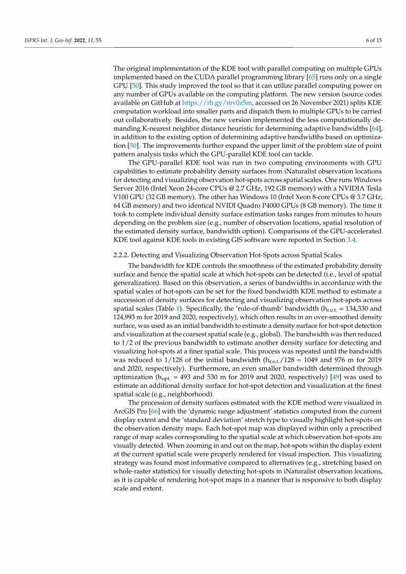
The GPU-parallel KDE tool was run in two computing environments with GPUcapabilities to estimate probability density surfaces from iNaturalist observation locationsfor detecting and visualizing observation hot-spots across spatial scales. One runs WindowsServer 2016 (Intel Xeon 24-core CPUs @ 2.7 GHz, 192 GB memory) with a NVIDIA TeslaV100 GPU (32 GB memory). The other has Windows 10 (Intel Xeon 8-core CPUs @ 3.7 GHz,64 GB memory) and two identical NVIDI Quadro P4000 GPUs (8 GB memory). The time ittook to complete individual density surface estimation tasks ranges from minutes to hoursdepending on the problem size (e.g., number of observation locations, spatial resolution ofthe estimated density surface, bandwidth option). Comparisons of the GPU-acceleratedKDE tool against KDE tools in existing GIS software were reported in Section 3.4.

2.2.2. Detecting and Visualizing Observation Hot-Spots across Spatial Scales

The bandwidth for KDE controls the smoothness of the estimated probability densitysurface and hence the spatial scale at which hot-spots can be detected (i.e., level of spatialgeneralization). Based on this observation, a series of bandwidths in accordance with thespatial scales of hot-spots can be set for the fixed bandwidth KDE method to estimate asuccession of density surfaces for detecting and visualizing observation hot-spots acrossspatial scales (Table 1). Specifically, the ‘rule-of-thumb’ bandwidth (hr.o.t. = 134,330 and124,993 m for 2019 and 2020, respectively), which often results in an over-smoothed densitysurface, was used as an initial bandwidth to estimate a density surface for hot-spot detectionand visualization at the coarsest spatial scale (e.g., global). The bandwidth was then reducedto 1/2 of the previous bandwidth to estimate another density surface for detecting andvisualizing hot-spots at a finer spatial scale. This process was repeated until the bandwidthwas reduced to 1/128 of the initial bandwidth (hr.o.t./128 = 1049 and 976 m for 2019and 2020, respectively). Furthermore, an even smaller bandwidth determined throughoptimization (hopt. = 493 and 530 m for 2019 and 2020, respectively) [49] was used toestimate an additional density surface for hot-spot detection and visualization at the finestspatial scale (e.g., neighborhood).

The procession of density surfaces estimated with the KDE method were visualized inArcGIS Pro [66] with the ‘dynamic range adjustment’ statistics computed from the currentdisplay extent and the ‘standard deviation’ stretch type to visually highlight hot-spots onthe observation density maps. Each hot-spot map was displayed within only a prescribedrange of map scales corresponding to the spatial scale at which observation hot-spots arevisually detected. When zooming in and out on the map, hot-spots within the display extentat the current spatial scale were properly rendered for visual inspection. This visualizingstrategy was found most informative compared to alternatives (e.g., stretching based onwhole-raster statistics) for visually detecting hot-spots in iNaturalist observation locations,as it is capable of rendering hot-spot maps in a manner that is responsive to both displayscale and extent.

ISPRS Int. J. Geo-Inf. 2022, 11, 55 7 of 15

Table 1. Bandwidths used in fixed-bandwidth KDE for detecting hot-spots across spatial scales.hr.o.t. and hopt. are the bandwidths determined based on the ‘rule-of-thumb’ heuristic and throughoptimization, respectively. Smaller bandwidths are associated with finer spatial resolutions, largerdisplay map scales, and increasingly fine spatial scales at which hot-spots are detected and visualized.

Bandwidth Resolution Display Map Scale Spatial Scale

hr.o.t. 5 km ≤1:40 million Globalhr.o.t./2 5 km ≤1:20 million Continentalhr.o.t./4 5 km ≤1:10 million Regionalhr.o.t./8 1 km ≤1:5 million Countryhr.o.t./16 1 km ≤1:2.5 million Stateshr.o.t./32 500 m ≤1:1.2 million Metropolitanhr.o.t./64 500 m ≤1:600,000 City

hr.o.t./128 100 m ≤1:300,000 Sub-cityhopt. 100 m ≤1:180,000 Neighborhood

In addition, a web map for visually detecting observation hot-spots across spatialscales was published through the ArcGIS Online platform [67]. Map tiles rendering multi-scale observation hot-spots across a sequence of map zoom levels (i.e., display map scales)were created using the Create Map Tile Package geoprocessing tool in ArcGIS Pro. The tilepackages were then uploaded to ArcGIS Online and published as a web map that can beviewed freely at https://rb.gy/1cjyey, accessed on 26 November 2021. Zooming in andout triggers the web map to load tiles at the proper zoom level for visualizing observationhot-spots across spatial scales.

3. Results and Discussion3.1. Visual Detection of Observation Hot-Spots across Spatial Scales

Globally, North America and Europe are the two largest iNaturalist observation hot-spots in the world (Figure 2A). Western Europe and eastern, western, and southern UnitedStates are obvious regional observation hot-spots. European countries such as the UnitedKingdom, Germany, Belgium, Netherland, Switzerland, and Italy, and US states includingCalifornia, Washington, Texas, Florida, Maryland, New Jersey, New York, Connecticut,and Massachusetts stand out as country- or state-level hot-spots. At a finer spatial scale,iNaturalist observation hot-spots well coincide with large metropolitan areas (e.g., SanFrancisco, Los Angeles, Dallas, Denver, Chicago, Minneapolis, New York, Mexico City,Quito, London, Milan, Madrid, Moscow, Cape Town, Sydney, Melbourne, Hong Kong,Tokyo, and Seoul). Observation hot-spots are also detected at finer scales. For example,within the Denver metropolitan area (Figure 2), city- to neighborhood-level observationhot-spots (e.g., in parks, along trails) are readily visible on the density maps with increasingspatial details.

Visualization of the kernel density raster maps in ArcGIS Pro and on the ArcGISOnline web map (https://rb.gy/1cjyey, accessed on 26 November 2021) can be utilized tovisually detect observation hot-spots across spatial scales in iNaturalist data for any part ofthe world (e.g., from global to neighborhood scales). Such a geovisual tool for hierarchicallydetecting and visualizing observation hot-spots across spatial scales in massive VGI datasetsoffers many benefits, as discussed in more detail in Section 3.3.

ISPRS Int. J. Geo-Inf. 2022, 11, 55 8 of 15

ISPRS Int. J. Geo-Inf. 2022, 11, x FOR PEER REVIEW 8 of 16

Kingdom, Germany, Belgium, Netherland, Switzerland, and Italy, and US states includ-ing California, Washington, Texas, Florida, Maryland, New Jersey, New York, Connecti-cut, and Massachusetts stand out as country- or state-level hot-spots. At a finer spatial scale, iNaturalist observation hot-spots well coincide with large metropolitan areas (e.g., San Francisco, Los Angeles, Dallas, Denver, Chicago, Minneapolis, New York, Mexico City, Quito, London, Milan, Madrid, Moscow, Cape Town, Sydney, Melbourne, Hong Kong, Tokyo, and Seoul). Observation hot-spots are also be detected at finer scales. For example, within the Denver metropolitan area (Figure 2), city- to neighborhood-level ob-servation hot-spots (e.g., in parks, along trails) are readily visible on the density maps with increasing spatial details.

Figure 2. iNaturalist observation hot-spots (2020) in the Denver metropolitan area across spatial scales. (A–I) corresponds to the increasingly large map scales at which hot-spots are detected and visualized. On each map, red color represents high observation density, and the inner box indi-cates the display extent of the next map in sequence rendering finer-scale hot-spots.

Visualization of the kernel density raster maps in ArcGIS Pro and on the ArcGIS Online web map (https://rb.gy/1cjyey, accessed on 26 November 2021) can be utilized to visually detect observation hot-spots in iNaturalist data for any part of the world across spatial scales (e.g., from global to neighborhood scales). Such a geovisual tool for hierar-chically detecting and visualizing observation hot-spots across spatial scales in massive VGI datasets offer many benefits, as discussed in more detail in Section 3.3.

Figure 2. iNaturalist observation hot-spots (2020) in the Denver metropolitan area across spatialscales. (A–I) corresponds to the increasingly large map scales at which hot-spots are detected andvisualized. On each map, red color represents high observation density, and the inner box indicatesthe display extent of the next map in sequence rendering finer-scale hot-spots.

3.2. Hot-Spot Detection and Visualization at Even Finer Spatial Scales

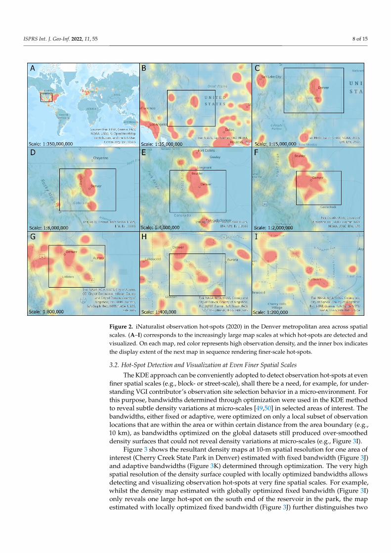
The KDE approach can be conveniently adopted to detect observation hot-spots at evenfiner spatial scales (e.g., block- or street-scale), shall there be a need, for example, for under-standing VGI contributor’s observation site selection behavior in a micro-environment. Forthis purpose, bandwidths determined through optimization were used in the KDE methodto reveal subtle density variations at micro-scales [49,50] in selected areas of interest. Thebandwidths, either fixed or adaptive, were optimized on only a local subset of observationlocations that are within the area or within certain distance from the area boundary (e.g.,10 km), as bandwidths optimized on the global datasets still produced over-smootheddensity surfaces that could not reveal density variations at micro-scales (e.g., Figure 3I).

Figure 3 shows the resultant density maps at 10-m spatial resolution for one area ofinterest (Cherry Creek State Park in Denver) estimated with fixed bandwidth (Figure 3J)and adaptive bandwidths (Figure 3K) determined through optimization. The very highspatial resolution of the density surface coupled with locally optimized bandwidths allowsdetecting and visualizing observation hot-spots at very fine spatial scales. For example,whilst the density map estimated with globally optimized fixed bandwidth (Figure 3I)only reveals one large hot-spot on the south end of the reservoir in the park, the mapestimated with locally optimized fixed bandwidth (Figure 3J) further distinguishes two

ISPRS Int. J. Geo-Inf. 2022, 11, 55 9 of 15

smaller hot-spots (one hot-spot on the southeast side and another larger hot-spot on thesouthwest side), and the map estimated with locally optimized adaptive bandwidths(Figure 3K) was able to detect and visualize several hot-spots with more precise spatialextent. Detecting and visualizing hot-spots at such fine spatial scales provides usefulinformation for understanding volunteer’s observation preferences in a micro-environment(e.g., more observations were concentrated in the woods along the east shore) (Figure 3K).

ISPRS Int. J. Geo-Inf. 2022, 11, x FOR PEER REVIEW 9 of 16

3.2. Hot-Spot Detection and Visualization at Even Finer Spatial Scales The KDE approach can be conveniently adopted to detect observation hot-spots at

even finer spatial scales (e.g., block- or street-scale), shall there be a need, for example, for understanding VGI contributor’s observation site selection behavior in a micro-environ-ment. For this purpose, bandwidths determined through optimization were used in the KDE method to reveal subtle density variations at micro-scales [49,50] in selected areas of interest. The bandwidths, either fixed or adaptive, were optimized on only a local subset of observation locations that are within the area or within certain distance from the area boundary (e.g., 10 km), as bandwidths optimized on the global datasets still produced over-smoothed density surfaces that could not reveal density variations at micro-scales (e.g., Figure 3I).

Figure 3. Observation hot-spots (2020) detected and rendered at micro-scales in a park in Denver. (I–K) corresponds to the increasingly large map scales at which hot-spots are detected and visual-ized.

Figure 3 shows the resultant density maps at 10-m spatial resolution for one area of interest (Cheery Creek State Park in Denver) estimated with fixed bandwidth (Figure 3J) and adaptive bandwidths (Figure 3K) determined through optimization. The very high spatial resolution of the density surface coupled with locally optimized bandwidths al-lows detecting and visualizing observation hot-spots at very fine spatial scales. For exam-ple, whilst the density map estimated with globally optimized fixed bandwidth (Figure 3I) only reveals one large hot-spot on the south end of the reservoir in a state park, the map estimated with locally optimized fixed bandwidth (Figure 3J) further distinguishes two smaller hot-spots (one hot-spot on the southeast side and another larger hot-spot on the southwest side), and the map estimated with locally optimized adaptive bandwidths (Figure 3K) was able to detect and visualize several hot-spots with more precise spatial extent. Detecting and visualizing hot-spots at such fine spatial scales provides useful in-formation for understanding volunteer’s observation preferences in a micro-environment (e.g., more observations were concentrated in the woods along the east shore) (Figure 3K)

3.3. Usefulness for Exploratory Point Pattern Analysis and Beyond Backed by the GPU-accelerated KDE took, the proposed hierarchical detection and

visualization of hot-spots within massive point datasets across spatial scales offers a pow-erful geovisual tool for exploratory point pattern analysis, which enables formulating hy-potheses to uncover the spatial processes that operate at multiple spatial scales to have shaped the point pattern [47,58]. Intuitions regarding the multi-scale pattern-shaping spa-tial processes are easier to develop from visually exploring the hot-spot maps across spa-tial scales and comparing the hot-spot maps against maps depicting the spatial variation of environmental and cultural factors that could play a role in shaping the patterns (e.g., population density, land cover, accessibility to mobile technologies). For instance, conti-nental-, regional-, and country-scale observation hot-spots in VGI datasets may be mainly attributed to cultural and socio-economic factors. As explored in [37], nature observing

Figure 3. Observation hot-spots (2020) detected and rendered at micro-scales in a park in Denver.(I–K) corresponds to the increasingly large map scales at which hot-spots are detected and visualized.

3.3. Usefulness for Exploratory Point Pattern Analysis and Beyond

Backed by the GPU-accelerated KDE tool, the proposed scheme for hierarchical detec-tion and visualization of hot-spots within massive point datasets across spatial scales offersa powerful geovisual tool for exploratory point pattern analysis, which enables formulatinghypotheses to uncover the spatial processes that operate at multiple spatial scales to haveshaped the point pattern [47,58]. Intuitions regarding the multi-scale pattern-shaping spatialprocesses are easier to develop from visually exploring the hot-spot maps across spatialscales and comparing the hot-spot maps against maps depicting the spatial variation ofenvironmental and cultural factors that could play a role in shaping the patterns (e.g., popu-lation density, land cover, accessibility to mobile technologies). For instance, continental-,regional-, and country-scale observation hot-spots in VGI datasets may be mainly attributedto cultural and socio-economic factors. As explored in [37], nature observing has a longerhistory and is a more popular activity in western English-speaking countries, which are alsoon the high end of United Nations Human Development Index (e.g., longer life expectancy,more years of education, higher gross national income per capita). States, metropolitan, andcity-scale observation hot-spots, reflecting an urban-rural divide, could be linked mostly tohuman population distribution, infrastructure availability (e.g., road, Internet), and by ex-tension, the digital divide [37,68]. For sub-city- to neighborhood-level observation hot-spots,however, the dominant driving factors may be more related to human behavior patterns.For example, people tend to report species sightings in open green spaces such as parks,botanic gardens, and trails [37] while enjoying the benefits of human-nature interactions [69].Such intuitions could well inform formulating hypotheses to explain the hot-spot patternsacross spatial scales. Beyond, they are also informative for devising methodologies to modelsampling biases in VGI observations [37], which could be a basis for correcting for suchbiases when VGI observations are used in spatial analysis and modeling [12,70,71].

The hot-spot maps could also be used to discover point pattern change over time.Visually comparing hot-spot maps at the same spatial scale but from different times helpsqualitatively identify changes in spatial pattern across time and facilitates understandingthe underlying causes. As an example, Figure 4 shows hot-spot maps on the Universityof Denver (DU) campus in 2019 and 2020. There was a large hot-spot on campus in2019 but it was no longer the case in 2020. This change was due to that the DU NatureChallenge, an annual event where participants survey biodiversity on DU campus andreport species observations to iNaturalist, was cancelled due to the ongoing COVID-19pandemic. More broadly, the visualizations are helpful for identifying observation hot-spot

ISPRS Int. J. Geo-Inf. 2022, 11, 55 10 of 15

pattern change across spatial scales to reveal impacts of the pandemic on VGI contributors’data contribution patterns. It could offer new evidence to consolidate findings regardingCOVID-19 effects on citizen science projects and therefore contribute to forming guidelineson how to account for data anomalies caused by the pandemic [72–75].

ISPRS Int. J. Geo-Inf. 2022, 11, x FOR PEER REVIEW 10 of 16

has a longer history and is a more popular activity in western English-speaking countries, which are also on the high end of United Nations Human Development Index (e.g., longer life expectancy, more years of education, higher gross national income per capita). States, metropolitan, and city-scale observation hot-spots, reflecting an urban-rural divide, could be linked mostly to human population distribution, infrastructure availability (e.g., road, Internet), and by extension, the digital divide [37,68]. For sub-city- to neighborhood-level observation hot-spots, however, the dominant driving factors may be more related to hu-man behavior patterns. For example, people tend to report species sightings in open green spaces such as parks, botanic gardens, and trails [37] while enjoying the benefits of hu-man-nature interactions [69]. Such intuitions could well inform formulating hypotheses to explain the hot-spot patterns across spatial scales. Beyond, they are also informative for devising methodologies to model sampling biases in VGI observations [37], which could be a basis for correcting for such biases when VGI observations are used in spatial analysis and modeling [12,70,71].

The hot-spot maps could also be used to discover point pattern change over time. Visually comparing hot-spot maps at the same spatial scale but from different times helps qualitatively identify changes in spatial pattern across time and facilitates understanding the underlying causes. As an example, Figure 4 shows hot-spot maps on the University of Denver (DU) campus in 2019 and 2020. There was a large hot-spot on campus in 2019 but it was no longer the case in 2020. This change was due to that the DU Nature Challenge, an annual event where participants survey biodiversity on DU campus and report species observations to iNaturalist, was cancelled due to the ongoing COVID-19 pandemic. More broadly, the visualizations are helpful for identifying observation hot-spot pattern change across spatial scales to reveal impacts of the pandemic on VGI contributors’ data contri-bution patterns. It could offer new evidence to consolidate findings regarding COVID-19 effects on citizen science projects and therefore contribute to forming guidelines on how to account for data anomalies caused by the pandemic [72–75].

Figure 4. Changes in observation hot-spots across 2019 and 2020 on the University of Denver cam-pus. (I–K) corresponds to the increasingly large map scales at which hot-spots are detected and visualized.

Figure 4. Changes in observation hot-spots across 2019 and 2020 on the University of Denver campus.(I–K) corresponds to the increasingly large map scales at which hot-spots are detected and visualized.

This study used only iNaturalist data in two individual years (2019 and 2020) todemonstrate the usability and usefulness of the GPU-accelerated KDE tool and the geo-visualization scheme (Section 2.2.2) for visualizing hot-spots in point data across spatialscales and identifying yearly pattern change. A full investigation regarding what haveshaped the hot-spots and what have caused pattern change in iNaturalist observationsis out of the scope of this article and deserves a separate treatment (an example of suchstudies can be found in [37]). Nonetheless, one could easily apply the GPU-accelerated KDEtool and the geovisualization scheme with customized spatial and temporal resolutions(e.g., weekly, monthly) on other (big) point datasets to visualize multi-scale hot-spots andidentify any patter change as a starting point for answering research questions pertinent tothe specific datasets.

3.4. Comparison of the GPU-Accelerated KDE Tool and KDE Tools in Existing GIS Software

The GPU-accelerated KDE tool used in this study was compared with KDE toolsin existing GIS software, specifically, the proprietary ArcGIS Pro (version 2.9) [66] andthe open-source QGIS (version 3.22) [76]. KDE results are known to be more sensitive tothe bandwidth than to the kernel function [63]. The KDE tool in Pro implemented theQuartic kernel function with a ‘rule-of-thumb’ algorithm to calculate a default bandwidthbased on the standard distance of the points. The KDE tool in QGIS does not compute adefault bandwidth (i.e., user must specify a bandwidth) for any of the five implementedkernel functions (Quartic, Triangular, Uniform, Triweight, Epanechnikov). Moreover, bothtools implement only fixed-bandwidth KDE with no support for adaptive-bandwidth KDE.Compared to KDE with a fixed bandwidth, KDE with adaptive bandwidths can betterreveal subtle density variations in areas of dense point events (e.g., Section 3.2) [49,50].For example, when applying KDE to analyze disease cases, the bandwidth can be set to

ISPRS Int. J. Geo-Inf. 2022, 11, 55 11 of 15

inversely relate to population density to account for inhomogeneous background [77,78].In this regard, the GPU-accelerated KDE tool is superior to the KDE tools in Pro andQGIS, as it supports both adaptive-bandwidth KDE and fixed-bandwidth KDE and itimplemented (parallelized) algorithms to automatically determine the optimal bandwidthsfor the Gaussian kernel function (Section 2.2.1) [50].

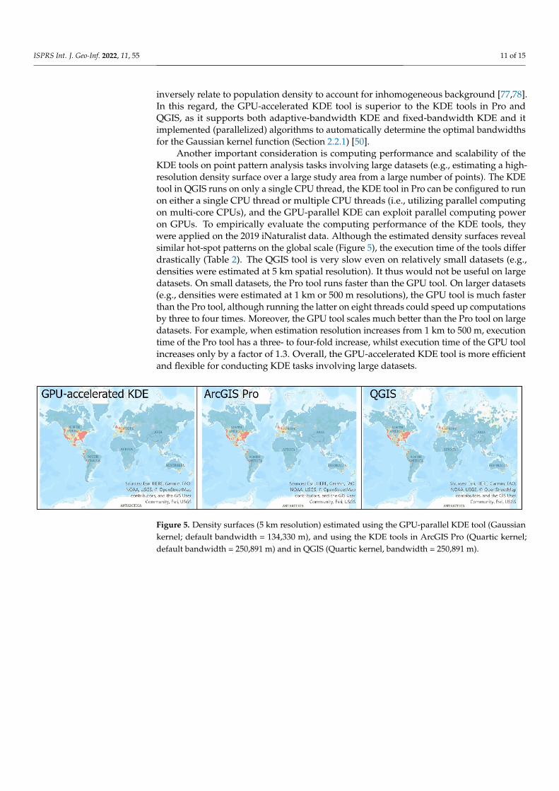
Another important consideration is computing performance and scalability of theKDE tools on point pattern analysis tasks involving large datasets (e.g., estimating a high-resolution density surface over a large study area from a large number of points). The KDEtool in QGIS runs on only a single CPU thread, the KDE tool in Pro can be configured to runon either a single CPU thread or multiple CPU threads (i.e., utilizing parallel computingon multi-core CPUs), and the GPU-parallel KDE can exploit parallel computing poweron GPUs. To empirically evaluate the computing performance of the KDE tools, theywere applied on the 2019 iNaturalist data. Although the estimated density surfaces revealsimilar hot-spot patterns on the global scale (Figure 5), the execution time of the tools differdrastically (Table 2). The QGIS tool is very slow even on relatively small datasets (e.g.,densities were estimated at 5 km spatial resolution). It thus would not be useful on largedatasets. On small datasets, the Pro tool runs faster than the GPU tool. On larger datasets(e.g., densities were estimated at 1 km or 500 m resolutions), the GPU tool is much fasterthan the Pro tool, although running the latter on eight threads could speed up computationsby three to four times. Moreover, the GPU tool scales much better than the Pro tool on largedatasets. For example, when estimation resolution increases from 1 km to 500 m, executiontime of the Pro tool has a three- to four-fold increase, whilst execution time of the GPU toolincreases only by a factor of 1.3. Overall, the GPU-accelerated KDE tool is more efficientand flexible for conducting KDE tasks involving large datasets.

ISPRS Int. J. Geo-Inf. 2022, 11, x FOR PEER REVIEW 12 of 16

Figure 5. Density surfaces (5 km resolution) estimated using the GPU-parallel KDE tool (Gaussian kernel; default bandwidth = 134,330 m), and using the KDE tools in ArcGIS Pro (Quartic kernel; default bandwidth = 250,891 m) and in QGIS (Quartic kernel, bandwidth = 250,891 m).

Table 2. Execution time of the KDE tools to estimate density surfaces at varied spatial resolutions using the 2019 iNaturalist data (n = 11,986,484 points) with a fixed bandwidth. Higher spatial reso-lution represents KDE task involving larger datasets. The KDE tool in Pro were run with both one thread and eight threads. Experiments were conducted on the server computer running Windows Server 2016 with a NVIDIA Tesla GPU.

KDE Tool Resolution Execution Time QGIS 5 km 5 h 40 min 2 s

GPU-parallel KDE 5 km 7 min 11 s 1 km 7 min 51 s 500 m 10 min 5 s

ArcGIS Pro

1 thread 8 threads 5 km 5 min 10 s 1 min 15 s 1 km 1 h 33 min 20 s 18 min 11 s 500 m 5 h 51 min 51 s 1 h 9 min 3 s

4. Conclusions Enabled by the multi-GPU parallel KDE computational tool, this study presents a

geovisualization scheme to conduct point pattern analyses on massive VGI datasets (e.g., tens of millions of iNaturalist observations with a global coverage) for detecting and vis-ualizing volunteers’ observation hot-spots across spatial scales. It was achieved by setting varying bandwidths for the KDE method in accordance with the spatial scales at which hot-spots are to be detected (e.g., from continental to neighborhood and even finer scales) to estimate a succession of density raster surfaces. The density rasters were then rendered and displayed at a sequence of map scales for visually detecting hot-spots. The geovisu-alization scheme built upon the GPU-accelerated KDE tool offers a hierarchical mecha-nism for visualizing volunteers’ observation hot-spots in massive data across spatial scales. It effectively facilitates visually detecting observation hot-spots and identifying pattern changes over time. As an exploratory data analysis tool, it is helpful for exploring the underlying drivers that have shaped the pattern in volunteer’s observation efforts and the causes of any pattern change. One can easily apply the GPU-accelerated KDE tool and the geovisualization scheme to other big point datasets (not necessarily VGI data) to vis-ualize multi-scale hot-spots and identify any patter change as a starting point for answer-ing research questions pertinent to the datasets. This research exemplifies a high-perfor-mance computing-backed and big data-capable tool for conducting exploratory point pat-tern analysis on massive point datasets. It is an invaluable addition to the expanding toolbox for geospatial big data analytics.

Figure 5. Density surfaces (5 km resolution) estimated using the GPU-parallel KDE tool (Gaussiankernel; default bandwidth = 134,330 m), and using the KDE tools in ArcGIS Pro (Quartic kernel;default bandwidth = 250,891 m) and in QGIS (Quartic kernel, bandwidth = 250,891 m).

ISPRS Int. J. Geo-Inf. 2022, 11, 55 12 of 15

Table 2. Execution time of the KDE tools to estimate density surfaces at varied spatial resolutionsusing the 2019 iNaturalist data (n = 11,986,484 points) with a fixed bandwidth. Higher spatialresolution represents KDE task involving larger datasets. The KDE tool in Pro were run with both onethread and eight threads. Experiments were conducted on the server computer running WindowsServer 2016 with a NVIDIA Tesla GPU.

KDE Tool Resolution Execution Time

QGIS 5 km 5 h 40 min 2 s

GPU-parallel KDE5 km 7 min 11 s1 km 7 min 51 s500 m 10 min 5 s

ArcGIS Pro

1 thread 8 threads5 km 5 min 10 s 1 min 15 s1 km 1 h 33 min 20 s 18 min 11 s500 m 5 h 51 min 51 s 1 h 9 min 3 s

4. Conclusions

Enabled by the multi-GPU parallel KDE computational tool, this study presents ageovisualization scheme to conduct point pattern analyses on massive VGI datasets (e.g.,tens of millions of iNaturalist observations with a global coverage) for detecting andvisualizing volunteers’ observation hot-spots across spatial scales. It was achieved bysetting varying bandwidths for the KDE method in accordance with the spatial scales atwhich hot-spots are to be detected (e.g., from continental to neighborhood and even finerscales) to estimate a succession of density raster surfaces. The density rasters were thenrendered and displayed at a sequence of map scales for visually detecting hot-spots. Thegeovisualization scheme built upon the GPU-accelerated KDE tool offers a hierarchicalmechanism for visualizing volunteers’ observation hot-spots in massive data across spatialscales. It effectively facilitates visually detecting observation hot-spots and identifyingpattern changes over time. As an exploratory data analysis tool, it is helpful for exploringthe underlying drivers that have shaped the pattern in volunteer’s observation efforts andthe causes of any pattern change. One can easily apply the GPU-accelerated KDE tooland the geovisualization scheme to other big point datasets (not necessarily VGI data)to visualize multi-scale hot-spots and identify any patter change as a starting point foranswering research questions pertinent to the datasets. This research exemplifies a high-performance computing-backed and big data-capable tool for conducting exploratory pointpattern analysis on massive point datasets. It is an invaluable addition to the expandingtoolbox for geospatial big data analytics.

Funding: This research was partially supported by the Faculty Start-up Funds and the FacultyResearch Fund at the University of Denver. The APC was sponsored by the University of Denver’sOpen Access Publication Equity Fund.

Data Availability Statement: iNaturalist observations were downloaded from the iNaturalist websiteat http://www.inaturalist.org/observations/export (accessed on 5 January 2021). Source codes ofthe multi-GPU parallel KDE algorithm are available on GitHub at https://rb.gy/mv0z5m, accessedon 26 November 2021. A web map for visually detecting observation hot-spots across spatial scales in2019 and 2020 iNaturalist data used in this study is freely available at https://rb.gy/1cjyey, accessedon 26 November 2021.

Acknowledgments: The author thanks the iNaturalist project for making its data freely available forresearch and the many nature observers for contributing species observations to iNaturalist.

Conflicts of Interest: The funders had no role in the design of the study; in the collection, analyses,or interpretation of data; in the writing of the manuscript; or in the decision to publish the results.Shall this article be included in a Special Issue the author is guest-editing in this journal, decisionsregarding the review process are referred to the editor-in-chief.

ISPRS Int. J. Geo-Inf. 2022, 11, 55 13 of 15

References1. Goodchild, M.F. Citizens as sensors: The world of volunteered geography. GeoJournal 2007, 69, 211–221. [CrossRef]2. Zhang, G. Volunteered Geographic Information. In The Geographic Information Science & Technology Body of Knowledge; 2021.

Available online: https://gistbok.ucgis.org/bok-topics/volunteered-geographic-information (accessed on 6 January 2022).3. Haklay, M.; Weber, P. OpenStreetMap: User-generated street maps. Pervasive Comput. IEEE 2008, 7, 12–18. [CrossRef]4. Sullivan, B.L.; Wood, C.L.; Iliff, M.J.; Bonney, R.E.; Fink, D.; Kelling, S. eBird: A citizen-based bird observation network in the

biological sciences. Biol. Conserv. 2009, 142, 2282–2292. [CrossRef]5. Altrudi, S. Connecting to nature through tech? The case of the iNaturalist app. Convergence 2021, 27, 124–141. [CrossRef]6. Haklay, M.; Dörler, D.; Heigl, F.; Manzoni, M.; Hecker, S.; Vohland, K. What Is Citizen Science? The Challenges of Definition.

In The Science of Citizen Science; Vohland, K., Land-Zandstra, A., Ceccaroni, L., Lemmens, R., Perelló, J., Ponti, M., Samson, R.,Wagenknecht, K., Eds.; Springer Nature: Berlin/Heidelberg, Germany, 2021; pp. 13–33. ISBN 9783030582784.

7. Haklay, M. Geographic Citizen Science: An overview. In Geographic Citizen Science Design; UCL Press: London, UK, 2021;pp. 15–37.

8. Haklay, M. Citizen science and volunteered geographic information: Overview and typology of participation. In CrowdsourcingGeographic Knowledge: Volunteered Geographic Information (VGI) in Theory and Practice; Sui, D., Elwood, S., Goodchild, M., Eds.;Springer: Dordrecht, The Netherlands, 2013; pp. 105–122. ISBN 978-94-007-4586-5.

9. Fink, D.; Auer, T.; Johnston, A.; Ruiz-Gutierrez, V.; Hochachka, W.M.; Kelling, S. Modeling avian full annual cycle distributionand population trends with citizen science data. Ecol. Appl. 2020, 30, e02056. [CrossRef]

10. Basile, M.; Russo, L.F.; Russo, V.G.; Senese, A.; Bernardo, N. Birds seen and not seen during the COVID-19 pandemic: The impactof lockdown measures on citizen science bird observations. Biol. Conserv. 2021, 256, 109079. [CrossRef]

11. Zook, M.; Graham, M.; Shelton, T.; Gorman, S. Volunteered Geographic Information and Crowdsourcing Disaster Relief: A CaseStudy of the Haitian Earthquake. World Med. Health Policy 2010, 2, 6–32. [CrossRef]

12. Johnston, A.; Moran, N.; Musgrove, A.; Fink, D.; Baillie, S.R. Estimating species distributions from spatially biased citizen sciencedata. Ecol. Modell. 2020, 422, 108927. [CrossRef]

13. Yan, Y.; Feng, C.; Huang, W.; Fan, H.; Wang, Y. Volunteered geographic information research in the first decade: A narrativereview of selected journal articles in GIScience. Int. J. Geogr. Inf. Sci. 2020, 34, 1765–1791. [CrossRef]

14. Elwood, S. Volunteered geographic information: Key questions, concepts and methods to guide emerging research and practice.GeoJournal 2008, 72, 133–135. [CrossRef]

15. Trojan, J.; Schade, S.; Lemmens, R.; Frantál, B. Citizen science as a new approach in Geography and beyond: Review andreflections. Morav. Geogr. Rep. 2019, 27, 254–264. [CrossRef]

16. Skarlatidou, A.; Haklay, M. Geographic Citizen Science Design: No One Left Behind; UCL Press: London, UK, 2020.17. Silvertown, J. A new dawn for citizen science. Trends Ecol. Evol. 2009, 24, 467–471. [CrossRef]18. Vohland, K.; Land-Zandstra, A.; Ceccaroni, L.; Lemmens, R.; Perelló, J.; Ponti, M.; Samson, R.; Wagenknecht, K. The Science of

Citizen Science; Springer Nature: Berlin/Heidelberg, Germany, 2021.19. Miller, H.J.; Goodchild, M.F. Data-driven geography. GeoJournal 2014, 80, 449–461. [CrossRef]20. Kelling, S.; Hochachka, W.M.; Fink, D.; Riedewald, M.; Caruana, R.; Ballard, G.; Hooker, G. Data-intensive science: A new

paradigm for biodiversity studies. Bioscience 2009, 59, 613–620. [CrossRef]21. Basiri, A.; Haklay, M.; Foody, G.; Mooney, P. Crowdsourced geospatial data quality: Challenges and future directions. Int. J. Geogr.

Inf. Sci. 2019, 33, 1588–1593. [CrossRef]22. Hung, K.-C.; Kalantari, M.; Rajabifard, A. Methods for assessing the credibility of volunteered geographic information in flood

response: A case study in Brisbane, Australia. Appl. Geogr. 2016, 68, 37–47. [CrossRef]23. Flanagin, A.; Metzger, M. The credibility of volunteered geographic information. GeoJournal 2008, 72, 137–148. [CrossRef]24. Goodchild, M.F.; Li, L. Assuring the quality of volunteered geographic information. Spat. Stat. 2012, 1, 110–120. [CrossRef]25. Barrington-Leigh, C.; Millard-Ball, A. The world’s user-generated road map is more than 80% complete. PLoS ONE 2017,

12, e0180698. [CrossRef]26. Senaratne, H.; Mobasheri, A.; Ali, A.L.; Capineri, C.; Haklay, M. A review of volunteered geographic information quality

assessment methods. Int. J. Geogr. Inf. Sci. 2017, 31, 139–167. [CrossRef]27. Barron, C.; Neis, P.; Zipf, A. A Comprehensive Framework for Intrinsic OpenStreetMap Quality Analysis. Trans. GIS 2014, 18,

877–895. [CrossRef]28. Haklay, M. How good is volunteered geographical information? A comparative study of OpenStreetMap and Ordnance Survey

datasets. Environ. Plann. B Plann. Des. 2010, 37, 682–703. [CrossRef]29. Wu, H.; Lin, A.; Clarke, K.C.; Shi, W.; Cardenas-Tristan, A.; Tu, Z. A comprehensive quality assessment framework for linear

features from Volunteered Geographic Information. Int. J. Geogr. Inf. Sci. 2021, 35, 1826–1847. [CrossRef]30. Xu, Y.; Chen, Z.; Xie, Z.; Wu, L. Quality assessment of building footprint data using a deep autoencoder network. Int. J. Geogr. Inf.

Sci. 2017, 31, 1929–1951. [CrossRef]31. Chehreghan, A.; Ali Abbaspour, R. An evaluation of data completeness of VGI through geometric similarity assessment. Int. J.

Image Data Fusion 2018, 9, 319–337. [CrossRef]32. Salk, C.F.; Sturn, T.; See, L.; Fritz, S.; Perger, C. Assessing quality of volunteer crowdsourcing contributions: Lessons from the

Cropland Capture game. Int. J. Digit. Earth 2016, 9, 410–426. [CrossRef]

ISPRS Int. J. Geo-Inf. 2022, 11, 55 14 of 15

33. Ali, A.L.; Schmid, F. Data quality assurance for volunteered geographic information. In Proceedings of the Geographic InformationScience: 8th International Conference, GIScience 2014, Vienna, Austria, 24–26 September 2014; Springer: Berlin/Heidelberg, Germany,2014; Volume 8728, pp. 126–141.

34. Yan, Y.; Feng, C.-C.; Wang, Y.-C. Utilizing fuzzy set theory to assure the quality of volunteered geographic information. GeoJournal2017, 82, 517–532. [CrossRef]

35. Haklay, M. Volunteered Geographic Information: Quality Assurance. In International Encyclopedia of Geography: People, the Earth,Environment and Technology; John Wiley & Sons: Hoboken, NJ, USA, 2016; pp. 1–6.

36. Zhang, G.; Zhu, A.-X. The representativeness and spatial bias of volunteered geographic information: A review. Ann. GIS 2018,24, 151–162. [CrossRef]

37. Zhang, G. Spatial and Temporal Patterns in Volunteer Data Contribution Activities: A Case Study of eBird. ISPRS Int. J. Geo-Inf.2020, 9, 597. [CrossRef]

38. Hecht, B.; Stephens, M. A tale of cities: Urban biases in volunteered geographic information. In Proceedings of the EighthInternational Conference on Web and Social Media (ICWSM), Ann Arbor, MI, USA, 1–4 June 2014; pp. 197–205.

39. Jensen, R.R.; Shumway, J.M. Sampling our world. In Research Methods in Geography: A Critical Introduction; Gomez, B., Jones, J.P.,III, Eds.; John Wiley & Sons: Hoboken, NJ, USA, 2010; pp. 77–90.

40. Millar, E.E.; Hazell, E.C.; Melles, S.J. The “cottage effect” in citizen science? Spatial bias in aquatic monitoring programs. Int. J.Geogr. Inf. Sci. 2018, 33, 1612–1632. [CrossRef]

41. Fan, C.; Esparza, M.; Dargin, J.; Wu, F.; Oztekin, B.; Mostafavi, A. Spatial biases in crowdsourced data: Social media contentattention concentrates on populous areas in disasters. Comput. Environ. Urban Syst. 2020, 83, 101514. [CrossRef]

42. Boakes, E.H.; McGowan, P.J.K.; Fuller, R.A.; Ding, C.; Clark, N.E.; O’Connor, K.; Mace, G.M. Distorted views of biodiversity:Spatial and temporal bias in species occurrence data. PLoS Biol. 2010, 8, e1000385. [CrossRef]

43. Zhang, G.; Zhu, A.-X. A representativeness directed approach to spatial bias mitigation in VGI for predictive mapping. Int. J.Geogr. Inf. Sci. 2019, 33, 1873–1893. [CrossRef]

44. Fourcade, Y.; Engler, J.O.; Rödder, D.; Secondi, J. Mapping species distributions with MAXENT using a geographically biasedsample of presence data: A performance assessment of methods for correcting sampling bias. PLoS ONE 2014, 9, e97122.[CrossRef]

45. Phillips, S.J.; Dudík, M.; Elith, J.; Graham, C.H.; Lehmann, A.; Leathwick, J.; Ferrier, S. Sample selection bias and presence-onlydistribution models: Implications for background and pseudo-absence data. Ecol. Appl. 2009, 19, 181–197. [CrossRef]

46. Fink, D.; Hochachka, W.M.; Zuckerberg, B.; Winkler, D.W.; Shaby, B.; Munson, M.A.; Hooker, G.; Riedewald, M.; Sheldon, D.;Kelling, S. Spatiotemporal exploratory models for broad-scale survey data. Ecol. Appl. 2010, 20, 2131–2147. [CrossRef]

47. Baddeley, A.; Rubak, E.; Turner, R. Spatial Point Patterns: Methodology and Applications with R; CRC Press: Boca Raton, FL, USA,2015; ISBN 1482210215.

48. Gatrell, A.C.; Bailey, T.C.; Diggle, P.J.; Rowlingson, B.S. Spatial Point Pattern Analysis and Its Application in GeographicalEpidemiology. Trans. Inst. Br. Geogr. 1996, 21, 256–274. [CrossRef]

49. Brunsdon, C. Estimating probability surfaces for geographical point data: An adaptive kernel algorithm. Comput. Geosci. 1995, 21,877–894. [CrossRef]

50. Zhang, G.; Zhu, A.-X.; Huang, Q. A GPU-accelerated adaptive kernel density estimation approach for efficient point patternanalysis on spatial big data. Int. J. Geogr. Inf. Sci. 2017, 31, 2068–2097. [CrossRef]

51. Yuan, K.; Chen, X.; Gui, Z.; Li, F.; Wu, H. A quad-tree-based fast and adaptive Kernel Density Estimation algorithm for heat-mapgeneration. Int. J. Geogr. Inf. Sci. 2019, 33, 2455–2476. [CrossRef]

52. Yu, W.; Ai, T.; Shao, S. The analysis and delimitation of Central Business District using network kernel density estimation. J.Transp. Geogr. 2015, 45, 32–47. [CrossRef]

53. Tang, W.; Feng, W.; Jia, M. Massively parallel spatial point pattern analysis: Ripley’s K function accelerated using graphicsprocessing units. Int. J. Geogr. Inf. Sci. 2015, 29, 412–439. [CrossRef]

54. Zhang, G.; Huang, Q.; Zhu, A.-X.; Keel, J. Enabling point pattern analysis on spatial big data using cloud computing: Optimizingand accelerating Ripley’s K function. Int. J. Geogr. Inf. Sci. 2016, 30, 2230–2252. [CrossRef]

55. Wang, Y.; Gui, Z.; Wu, H.; Peng, D.; Wu, J.; Cui, Z. Optimizing and accelerating space-time Ripley ’s K function based on ApacheSpark for distributed spatiotemporal point pattern analysis. Futur. Gener. Comput. Syst. 2020, 105, 96–118. [CrossRef]

56. Kwan, M.P. The Uncertain Geographic Context Problem. Ann. Assoc. Am. Geogr. 2012, 102, 958–968. [CrossRef]57. Openshaw, S. The Modifiable Areal Unit Problem; Geo Books: Norwich, UK, 1984.58. Fotheringham, A.S.; Brunsdon, C.; Charlton, M. Quantitative Geography: Perspectives on Spatial Data Analysis; Sage: Thousand

Oaks, CA, USA, 2000; ISBN 1847876412.59. Unger, S.; Rollins, M.; Tietz, A.; Dumais, H. iNaturalist as an engaging tool for identifying organisms in outdoor activities. J. Biol.

Educ. 2020, 55, 537–547. [CrossRef]60. iNaturalist iNaturalist Observations. Available online: https://www.inaturalist.org/observations (accessed on 12 July 2021).61. iNaturalist iNaturalist Help. Available online: https://www.inaturalist.org/pages/help (accessed on 11 November 2021).62. iNaturalist Contributors, iNaturalist. iNaturalist Research-Grade Observations. iNaturalist.org. Occurrence Dataset. 2021.

Available online: https://www.gbif.org/dataset/50c9509d-22c7-4a22-a47d-8c48425ef4a7 (accessed on 5 January 2021).63. Silverman, B.W. Density Estimation for Statistics and Data Analysis; Chapman and Hall: London, UK, 1986.

ISPRS Int. J. Geo-Inf. 2022, 11, 55 15 of 15

64. Breiman, L.; Meisel, W.; Purcell, E. Variable kernel estimates of multivariate densities. Technometrics 1977, 19, 135–144. [CrossRef]65. Luebke, D. CUDA: Scalable parallel programming for high-performance scientific computing. In Proceedings of the 2008 5th

IEEE International Symposium on Biomedical Imaging: From Nano to Macro, Paris, France, 14–17 May 2008; pp. 836–838.66. ESRI Development Team. ArcGIS Pro. 2021. Available online: https://www.esri.com/en-us/arcgis/products/arcgis-pro/

overview (accessed on 5 January 2021).67. ESRI Development Team. ArcGIS Online. 2021. Available online: https://www.esri.com/en-us/landing-page/product/2019

/arcgis-online/overview (accessed on 5 January 2021).68. Sui, D.; Goodchild, M.; Elwood, S. Volunteered geographic information, the exaflood, and the growing digital divide. In

Crowdsourcing Geographic Knowledge: Volunteered Geographic Information (VGI) in Theory and Practice; Sui, D., Elwood, S., Goodchild,M., Eds.; Springer: Dordrecht, The Netherlands, 2013; pp. 1–12. ISBN 978-94-007-4586-5.

69. Keniger, L.E.; Gaston, K.J.; Irvine, K.N.; Fuller, R.A. What are the benefits of interacting with nature? Int. J. Environ. Res. PublicHealth 2013, 10, 913–935. [CrossRef]

70. Johnston, A.; Hochachka, W.M.; Strimas-Mackey, M.E.; Ruiz Gutierrez, V.; Robinson, O.J.; Miller, E.T.; Auer, T.; Kelling, S.T.;Fink, D. Analytical guidelines to increase the value of community science data: An example using eBird data to estimate speciesdistributions. Divers. Distrib. 2021, 27, 1265–1277. [CrossRef]

71. Zhu, A.-X.; Zhang, G.; Wang, W.; Xiao, W.; Huang, Z.-P.; Dunzhu, G.-S.; Ren, G.; Qin, C.-Z.; Yang, L.; Pei, T.; et al. A citizendata-based approach to predictive mapping of spatial variation of natural phenomena. Int. J. Geogr. Inf. Sci. 2015, 29, 1864–1886.[CrossRef]

72. Sánchez-Clavijo, L.M.; Martínez-Callejas, S.J.; Acevedo-Charry, O.; Diaz-Pulido, A.; Gómez-Valencia, B.; Ocampo-Peñuela, N.;Ocampo, D.; Olaya-Rodríguez, M.H.; Rey-Velasco, J.C.; Soto-Vargas, C.; et al. Differential reporting of biodiversity in two citizenscience platforms during COVID-19 lockdown in Colombia. Biol. Conserv. 2021, 256, 109077. [CrossRef]

73. Crimmins, T.M.; Posthumus, E.; Schaffer, S.; Prudic, K.L. COVID-19 impacts on participation in large scale biodiversity-themedcommunity science projects in the United States. Biol. Conserv. 2021, 256, 109017. [CrossRef]

74. Kishimoto, K.; Kobori, H. COVID-19 pandemic drives changes in participation in citizen science project “City Nature Challenge”in Tokyo. Biol. Conserv. 2021, 255, 109001. [CrossRef] [PubMed]

75. Hochachka, W.M.; Alonso, H.; Guti, C.; Miller, E.; Johnston, A. Regional variation in the impacts of the COVID-19 pandemic onthe quantity and quality of data collected by the project eBird. Biol. Conserv. 2021, 254, 108974. [CrossRef]

76. QGIS Development Team. QGIS Geographic Information System. 2021. Available online: https://www.qgis.org (accessed on26 November 2021).

77. Shi, X. Selection of bandwidth type and adjustment side in kernel density estimation over inhomogeneous backgrounds. Int. J.Geogr. Inf. Sci. 2010, 24, 643–660. [CrossRef]

78. Carlos, H.A.; Shi, X.; Sargent, J.; Tanski, S.; Berke, E.M. Density estimation and adaptive bandwidths: A primer for public healthpractitioners. Int. J. Health Geogr. 2010, 9, 39. [CrossRef]