Integrating Sustainable Hunting in Biodiversity Protection in Central Africa: Hot Spots, Weak Spots,...

Integrating Sustainable Hunting in BiodiversityProtection in Central Africa: Hot Spots, Weak Spots, andStrong SpotsJohn E. Fa1,2*, Jesus Olivero2, Miguel Angel Farfan2, Ana Luz Marquez2, Juan Mario Vargas2,

Raimundo Real2, Robert Nasi3

1 ICCS, Division of Biology, Imperial College London, Silwood Park Campus, Ascot, United Kingdom, 2 Universidad de Malaga, Grupo de Biogeografıa, Diversidad y

Conservacion, Departamento de Biologıa Animal, Facultad de Ciencias, Campus de Teatinos s/n, Malaga, Spain, 3 Consultative Group on International Agricultural

Research (CGIAR), CIFOR Headquarters, Jalan CIFOR, Situ Gede, Bogor, Indonesia

Abstract

Wild animals are a primary source of protein (bushmeat) for people living in or near tropical forests. Ideally, the effect ofbushmeat harvests should be monitored closely by making regular estimates of offtake rate and size of stock available forexploitation. However, in practice, this is possible in very few situations because it requires both of these aspects to bereadily measurable, and even in the best case, entails very considerable time and effort. As alternative, in this study, we usehigh-resolution, environmental favorability models for terrestrial mammals (N = 165) in Central Africa to map areas of highspecies richness (hot spots) and hunting susceptibility. Favorability models distinguish localities with environmentalconditions that favor the species’ existence from those with detrimental characteristics for its presence. We develop anindex for assessing Potential Hunting Sustainability (PHS) of each species based on their ecological characteristics(population density, habitat breadth, rarity and vulnerability), weighted according to restrictive and permissive assumptionsof how species’ characteristics are combined. Species are classified into five main hunting sustainability classes using fuzzylogic. Using the accumulated favorability values of all species, and their PHS values, we finally identify weak spots, defined ashigh diversity regions of especial hunting vulnerability for wildlife, as well as strong spots, defined as high diversity areas ofhigh hunting sustainability potential. Our study uses relatively simple models that employ easily obtainable data of aspecies’ ecological characteristics to assess the impacts of hunting in tropical regions. It provides information formanagement by charting the geography of where species are more or less likely to be at risk of extinction from hunting.

Citation: Fa JE, Olivero J, Farfan MA, Marquez AL, Vargas JM, et al. (2014) Integrating Sustainable Hunting in Biodiversity Protection in Central Africa: Hot Spots,Weak Spots, and Strong Spots. PLoS ONE 9(11): e112367. doi:10.1371/journal.pone.0112367

Editor: Francisco Moreira, Institute of Agronomy, University of Lisbon, Portugal

Received June 23, 2014; Accepted October 10, 2014; Published November 5, 2014

Copyright: � 2014 Fa et al. This is an open-access article distributed under the terms of the Creative Commons Attribution License, which permits unrestricteduse, distribution, and reproduction in any medium, provided the original author and source are credited.

Data Availability: The authors confirm that all data underlying the findings are fully available without restriction. All relevant data are within the paper and itsSupporting Information files.

Funding: This work is supported by the KnowFor (International Forestry Knowledge) initiative of the UK Department for International Development (UKAID). Thefunders had no role in study design, data collection and analysis, decision to publish, or preparation of the manuscript. This paper is a contribution of the CIFORBushmeat Research Initiative.

Competing Interests: The authors have declared that no competing interests exist.

* Email: [email protected]

Introduction

Wildlife is a primary source of protein (bushmeat or wild meat)

for many rural inhabitants in poor countries, particularly for

people living in or near tropical forests [1]. However, unsustain-

able hunting of bushmeat can result in dramatic declines of local

wild animal populations [2,3]. The unsustainable harvest of

mammals and birds can also have negative effects on forest

structure and regeneration [4], ecosystem functioning [5,6], and

species diversity [7].

In West and Central Africa, many mammals (which include

endemic and endangered species) are the main source of bushmeat

protein in the region [4]. Due to the increase in human

population, commercial trade of bushmeat has increased dramat-

ically in the last three decades in these areas [2]. Such trade in wild

animals for meat may have reached unsustainable levels, as the

natural regeneration ability of wildlife populations may not be

high enough to match the demand for bushmeat [2]. Hence,

unsustainable extraction of wild meat in many tropical forests

threatens the survival of a wide range of wildlife species as well as

the food security of forest-dwellers [8]. However, areas that are

more prone to species extinctions due to hunting are yet to be

identified.

Empirical data on bushmeat harvest rates in large regions such

as the Congo Basin are available for an increasing number of sites

although these are still fragmentary [9]. So far these data alone

cannot be used to advance strategies to mitigate the problem of

wildlife exploitation and resolve food scarcity issues [2].

Bushmeat hunting sustainability has been defined and assessed

most commonly via the use of indices [10,11]. A number of

sustainability indices have been published, and the production

model (RR model) is the most commonly used [12]. The RR

model employs literature values of a target species’ carrying

capacity and intrinsic population growth rate to calculate a

maximum annual production, a fraction of which is then taken to

PLOS ONE | www.plosone.org 1 November 2014 | Volume 9 | Issue 11 | e112367

http://creativecommons.org/licenses/by/4.0/

http://crossmark.crossref.org/dialog/?doi=10.1371/journal.pone.0112367&domain=pdf

be the species’ maximum sustainable yield. Although the RR

model has been applied to wildlife use studies at specific localities,

it has also been used to assess production and extraction of

bushmeat species at a landscape level [13]. A number of

shortcomings have been noted in the application of production

models to real-world situations [14].

Given that reliable monitoring of offtake (across all prey species

at the necessary spatial and temporal scales) is notoriously hard,

alternative methods to visualize hunting sustainability over large

areas are urgently required. Species distribution modeling offers a

mean for determining what environmental conditions are suitable

for an animal or plant in geographic space [15–17], that can be

coupled with classification of species according to some character

of interest (e.g. their potential to withstand hunting pressure).

In this paper, we use favorability models to map the distribution

of favorable areas for all hunted mammals in Central Africa.

Topographic, hydrographic, climatic, land-cover, human and

spatial variables are employed. Favorability modeling is a modality

of species distribution modeling that reflects environmental

favorability values rather than presence probability [18]. Favor-

ability models have been successfully used for conservation

purposes [19–22]. Then we combine the species’ environmental

favorability with their potential hunting sustainability to identify

areas of high species diversity, as well as zones where future loss of

wildlife is likely to be high, if hunting persists. We base

sustainability on four species’ ecological traits: population density,

habitat breadth, rarity and vulnerability. This contribution is the

first to present a hunting vulnerability map for bushmeat species in

a large biodiversity-rich tropical region.

Material and Methods

Study AreaOur study area (10uN, 16uS, 8uE, 36uE) stretches from the coast

of the Gulf of Guinea to the mountains of the Albertine Rift

(Fig. 1) covering about seven degrees of latitude on either side of

the Equator [23]. The central rainforest zone encompasses six

main countries (the Democratic Republic of the Congo, the

Republic of the Congo, Central African Republic, Cameroon,

Gabon and Equatorial Guinea), as well as parts of another three

(Angola, Burundi and Rwanda) (Fig. 1). The region contains the

second largest and the least degraded area of contiguous moist

tropical forest in the world, close to 2 million km2 [24]. The main

vegetation types include evergreen/deciduous broadleaf forests

and woody savannas, as well as areas of savanna and cropland-

natural vegetation mosaic [25].

Species DatasetWe first compiled a list of all terrestrial mammal species occurring

within the geographical limits of our study region, using Kingdon etal. [26]. We also enumerated those species whose distributions

overlapped with the Rainforest Biotic Zone, as defined by Kingdon

et al. [26], following White [27], and inhabited habitats including

rainforest. In order to select species for which there were records of

being hunted for bushmeat, we used the list of species, recorded

from the literature by Taylor et al. [28], with additional species

included after consultation with another 4 experts working in the

field. A total of 141 monotypic species and 24 other including 67

subspecies, belonging to 11 Orders, were finally used in our analyses

(see Appendix S1 in File S1).

Distribution maps of all species in this list were downloaded as

polygon shapefiles from the IUCN website [29] (maps compiled or

modified in 2008). We considered only polygons of extant

populations of the species that coincided with maps of those

species in Kingdon et al. [26]. Polygons were then rasterized at a

0.01u60.01u spatial resolution. The resulting raster maps were

used to extract presence/absence values within a 1u61u grid for

the whole African continent.

Species Distribution Modeling‘‘Extent of occurrence’’ range maps, such as those provided by

IUCN, are only suitable for analysis at a maximum of 1u61uspatial resolution [30]. This constraint can be overcome using

distribution modeling and model downscaling [31–36]. We thus

obtained maps describing distributions of environmentally favor-

able areas for species in 0.1u60.1u resolution squares. Favorability

models can show how the probability of a species’ local presence

differs from that expected by chance in the whole study area, and

so can distinguish those localities with environmental conditions

that favor the species’ existence from those with detrimental

characteristics for its presence [37]. In contrast to modeling

techniques providing probability values, favorability models can

distinguish between the effect of environmental conditions and the

probability of presence derived from the species prevalence within

the study area [37]. This enables direct comparison between

models when several species are involved in the analytical design

[37], and allows for model combinations through fuzzy logic

[38,39].

We built environmental favorability models for 141 species and

67 subspecies belonging to 24 other species. We attempted to

develop independent models for every subspecies but environ-

mental models were not found for most of them. This is because

these subspecies have highly circumscribed distributions within

which spatial autocorrelations predominated. Hence, we built a

favorability model for each of the 165 species.

Models were executed for the entire African continent for the

following reasons (see [40]): (1) some predictor factors considered

in the models (climate, spatial historical constraints) required a

Figure 1. Map of the study region showing: rainforest (darkgreen), woody savannas (light green) extracted from [25]. Theblack line indicates the Rainforest Biotic Zone [27]. Countries: A Angola;B Burundi; Ca Cameroon; CAR Central African Republic; Ch Chad; CoCongo; DRC Democratic Republic of the Congo; E Ethiopia; EGEquatorial Guinea; G Gabon; IT Ilemi Triangle; K Kenya; Ma Malawi;Mo Mozambique; N Nigeria; R Rwanda; S Sudan; U Uganda; URT UnitedRepublic of Tanzania; Za Zambia; Zi Zimbabwe.doi:10.1371/journal.pone.0112367.g001

Sustainable Hunting in Central Africa


large-scale modeling approach; (2) many species were broadly

distributed throughout the continent, and so we had to include an

environmentally significant geographical context for distinguishing

between presences and absences; and (3) a large extent was

required because we used a coarse spatial resolution. Model

outputs, initially with a spatial resolution of 1u61u, were later

downscaled to 0.1u60.1u resolution squares within our study area.

For this, we employed the ‘‘direct downscaling approach’’ [33],

classified by Bierkens et al. [32] as ‘‘downscaling based on

mechanistic models through a deterministic [favorability] func-

tion’’. Using the ArcGIS 10.0 raster calculator, the favorability

model was thus projected to a 0.1u60.1u resolution grid across the

study area by applying the favorability equations to predictor

variables at this resolution (see examples in [34–36]). A 10-fold

shortening of the grain size (referring to pixel side length) does not

severely affect predictions of species distributions [33,41].

Models were built on the species’ presence/absence in 1u61usquares as the response variable, and were based on a list of 27

predictor variables describing topography, hydrography, climate,

land cover/use and other indicators of anthropogenic pressure

(Appendices S2 and S3 in File S1). Variables likely to have

changed over time, such as farming, land cover and transport

infrastructure, were taken for years within the decade before 2008,

when species distribution maps were compiled or modified. A

spatial descriptor was added to these variables to account for

autocorrelation. This descriptor was defined for every species

following the ‘‘trend surface approach’’ [42], and may account for

the impact of dispersal barriers, geological history and biotic

interactions. For this, a series of combinations of average longitude

(Lo) and average latitude (La) for every square of the grid were

entered in a stepwise logistic regression: Lo, La, Lo2, La2, Lo6La,

Lo3, La3, Lo6La2, Lo26La. The ‘‘trend surface variable’’ was

then considered to be the resulting spatial y, i.e. the logit, or ‘‘y’’

lineal combination resulting from the logistic regression.

Type I errors, arising from the large number of variables used,

were controlled using Benjamini & Hochberg’s [43] procedure for

controlling the False Discovery Rate (FDR). This control was

performed before building each multivariate model, and we

accepted only those variables that were significant under an FDRof q,0.05. In order to avoid multicollinearity, when the Pearson’s

correlation between two variables within a model was.0.8, only

the variable most significantly predicting the species presence was

retained.

Forward-backward stepwise logistic regression was run with the

resulting set of variables [44], and probability outputs were finally

transformed into favorability values [37]. The estimation of the

relative weight of each variable in the model was tested using

Wald’s [45] test.

An alternative approach was used when the spatial-y had

extremely high predictive value within the model. This was

interpreted as a species distribution being constrained mostly by

the spatial, possibly historical factor, and happened in two cases: 1)

when the spatial-y was the only factor entered in the model; 2)

when the Wald’s parameter for the spatial-y was more than 10

times higher than the following variable in order of importance. In

these cases, the niche theory [46,47] advocates that the ‘‘realized

ecological niche’’ of a species can be better explained by factors

that imply spatial constraints on its distribution than by the

ecological characteristics of the species itself. In these cases, a

spatial model — based only on the spatial y — was intersected

with an environmental model — in which the spatial y was not

considered — using the fuzzy intersection. This intersection

describes simultaneous spatial and environmental favorability for

the presence of the species [39]. The fuzzy intersection was

calculated as the minimum favorability value in any of the two

models [48].

Highly favorable sites where a species can be present are

possible outside their current distribution ranges [47]. In our

analysis, we derived favorability values for the species only where it

is known to occur, because we were interested on how sustainable

present populations are likely to be. Thus, species can persist

within their current distribution area if populations of that species

are sustainable. The distribution areas for subspecies were

considered separately, hence a total of 208 species maps of 141

monotypic species and 67 subspecies were obtained.

Describing a Species’ Potential Hunting SustainabilityIn this study, we used the fuzzy logic approach to avoid

subjective thresholds when describing a species’ ‘‘Potential

Hunting Sustainability’’ (PHS), that is, the species’ potential

resilience to hunting according to ecological traits that are linked

with extinction proneness [49]. The logic behind fuzzy sets states

that the membership of any element to a set is neither completely

true nor false, whereas a membership function, assigning to each

element a real number in the interval [0, 1], describes the degree

to which it meets the definition of the set [48]. Thus, the fuzzy

approach allowed to consider all species as members of the set of

species whose hunting is sustainable, each one having, however, a

different degree of membership.

The first step for estimating PHS was to calculate, for each

taxon, a ‘‘Sustainability Index’’ (SI) based on its population density

weighted by a combination of other ecological traits - habitat

breadth, rarity and vulnerability (see below). SI was calculated by

considering two different fuzzy-logic operations:

Fuzzy union

SI~

logD|Max HB=HBmax, 1{Rð Þ= 1{Rð Þmax, VS=VSmax½ � ð1Þ

Fuzzy intersection

SI~

logD|Min HB=HBmax, 1{Rð Þ= 1{Rð Þmax, VS=VSmax½ � ð2Þ

where D is population density, HB is habitat breadth, R rarity and

VS vulnerability status of a given species. D was log-transformed

for linearizing its highly pronounced exponential behavior. SIincreases with all these traits, hence 1-rarity, and not rarity, is

used. The fuzzy union allowed a ‘‘permissive’’ approach for

incorporating the relevance of the three later factors in SI, i.e. a

high value in a single factor enabled a high weighing of logD.

Instead, the fuzzy intersection related to a ‘‘restrictive’’ weighting

in which high values are required in the three factors for a high

weighting of logD.

We derived population densities for all taxa in our list from

various sources: data for 53 (32%) species directly as in

PanTHERIA [50]; 15 (9%) as in Fa & Purvis [51]; and 97

(59%) from the expected values derived from a linear regression of

log(population density) on the basis of log(body mass), performed

by us using the worldwide data in PanTHERIA (N = 949 species,

R2 = 0.5743, P,0.05). Habitat breadth was defined as the number

of main habitats occupied by a taxon. Ten habitats were

considered: forest, fragmented forest, forest-savanna/pasture

mosaic, woody savanna, savanna/pasture, scrubland, bareland,

moorland, mangrove and farmland; we scored each taxon with

one point per occupied habitat according to Kingdon et al. [26].



Rarity reports on the size range of each species and was measured

as 1 - the proportion of the total surface area of the African

continent occupied by the taxon from distribution data from

IUCN [29]. ArcGIS 10.0 Raster Calculator was employed.

Vulnerability of a taxon was the conservation status category

according to the IUCN Red List. We distributed points in this

way: 0 = Critically Endangered, 1 = Endangered, 2 = Vulnera-

ble, 3 = Near Threatened, 4 = Least Concern. We used the latest

version of the IUCN Red List [29].

We then estimated the Potential Hunting Sustainability (PHS)

score of each taxon:

PHS~ SI{SImin½ �= SImax{SImin½ � ð3Þ

PHS is, in practice, a rescaling of SI in the interval [0, 1]. The

essential tenet of this index is based on the observation that body

size is inversely correlated with population density, making large-

bodied animals less abundant and more vulnerable to human

activities like hunting [49]. The extinction proneness of large-

bodied animals is further enhanced because of other correlated

traits, such as their requirement of large area, greater food intake,

high habitat specificity, and lower reproductive rate. Species in our

data set include taxa where hunting is more sustainable, mostly the

smaller species, and species that are more extinction prone from

hunting, the larger-bodied species. Thus, PHS ranged from 0

when sustainability equaled the minimum value observed in any

species of our data set [SI = SImin] to 1 when sustainability equaled

the maximum value observed [SI = SImax].

Fuzzy Sets for Mapping Hunting SustainabilityMaps representing the favorability for every species/subspecies

within their distributions were integrated by employing an index

hereinafter referred to as the ‘‘Accumulated Favorability’’ (AFj),

which constitutes a surrogate of biodiversity [38]. High values of

this index represent fuzzy favorability hot spots, and have been

considered in the assessment of site networks for the protection of

biodiversity [38]. The accumulated favorability is the result of

adding up the favorability (Fi) value for all i taxa in each j cell in

the study area:

AFj~X

Fi ð4Þ

We obtained a measure of ‘‘Sustainable Accumulated Favor-

ability’’ (SAFj) by weighting F, in equation 4, according to the

PHS as defined in equation 3:

SAFj~X

Fi|PHSið Þ ð5Þ

We also calculated the ‘‘Unsustainable Accumulated Favor-

ability’’ (UAFj) by weighting Fi according to 1-PHSi:

UAFj~X

Fi| 1{PHSið Þ½ � ð6Þ

Both SAFj and UAFj are complementary indices the sum of

which equals AFj. Theoretically, these three indices could range

from 0 to the number of species included in the analysis. Just like

AFj represents the total diversity of hunted mammals, SAFj

quantifies the diversity of species of high hunting sustainability

potential; instead, UAFj quantifies the diversity of highly

vulnerable species to hunting. This complementarity is, thus,

consistent with the geographical overlap of high SAFj and high

UAFj areas, because vulnerable and resilient species to hunting

can coexist. The fuzzy logic approach allowed us, however, to

avoid subjectively classifying species as sustainable or unsustain-

able. This way of weighting the constituents of a diversity index (in

our case, Fi) with a factor representing degrees of fuzzy

membership (in our case, in the set of species whose hunting is

sustainable), has been a successful procedure as demonstrated in

Olivero et al. [52,53].

Geographical hot spots (areas of high species richness), strong

spots (high diversity areas of high hunting sustainability potential)

and weak spots (high diversity regions of especial hunting

vulnerability for wildlife) were defined by selecting grid cells with

the highest 5% of AFj, SAFj and UAFj values, respectively. This

arbitrary cutoff was selected to match the proportion of our study

area that is currently protected within rainforest reserves according

to the World Database on Protected Areas [54]. This threshold

was also used in Cardillo et al. [55] and Estrada et al. [38].

Defining Sustainability CategoriesOnce species and subspecies were ordered according to PHS

(equation 3), we divided the list into five taxon clusters

representing categories of sustainability (1 = minimum sustain-

ability and 5 = maximum sustainability. Our purpose here was to

facilitate the interpretation of our results (see Figs. 2 and 3),

without using these categories as fixed classifiers of sustainable

hunting. Cutoffs for the central category were based on the

standard deviation of the mean PHS (mean PHS6 standard

error). We calculated the cutoff for the highest sustainability

category by accumulating PHS, from the highest to the lowest

value, until the maximum local SAFj (equation 5) observed within

our study areas was reached. This threshold allowed the grouping

of species whose accumulation would equal the maximum

observed SAFj, should completely favorable areas for all of them

overlap geographically. For the lowest sustainability category,

PHS was accumulated from the lowest to the highest value until

the maximum local UAFj (equation 6) was reached. Two sets of

sustainability categories were then developed, depending whether

the fuzzy union (equation 1) or the fuzzy intersection (equation 2)

was applied to calculate SI.

Results

Potential Hunting Sustainability (PHS)For all taxa, we constructed separate listings of the PHS values

derived for the permissive or restrictive weighting (Appendix S1 in

File S1). We found that for the permissive weighting, PHS was

significantly positively correlated with species population density

(R2 = 0.780; P,0.01) and then with their vulnerability status

(R2 = 0.558; P,0.01) (Fig. 2). Thus, species likely to be unsus-

tainable in the permissive weighting were those with low

population densities, but also taxa that were threatened even

having a relatively higher abundance. In contrast, PHS values for

the restrictive weighting were significantly associated with species’

rarity (R2 = 0.877; P,0.01), followed by their vulnerability status

(R2 = 0.631; P,0.01) and habitat breadth (R2 = 0.467; P,0.01).

Unsustainability here was related to small home ranges, threat

status, and by a more limited habitat breadth (Fig. 2).

The distribution of all Central African mammals (N = 208)

differed significantly by PHS category according to whether we

applied permissive or restrictive weightings to calculate the PHS(Fig. 3, Appendix S4 in File S1). A total of 51.4% of taxa belonged



to the low PHS categories (1 and 2) according to the permissive

weighting, but this proportion was higher (72.6%) for the

restrictive weighting. In contrast, 42.8% and 26.0% of all taxa

were included in the high sustainability categories (4 and 5)

according to the two criteria, respectively.

For the four most represented mammalian orders, clear

differences between PHS classes appeared in the frequency

distribution of taxa (Fig. 3). For primates, PHS was skewed

towards the less sustainable classes (1 and 2) for the strict weighting

criterion, but was more evenly distributed in the permissive

Figure 2. Boxplots linking potential hunting sustainability (PHS) categories and species’ ecological traits used to calculate PHS. Traitsconsidered are: a) log-transformed population density; b) habitat breadth; c) 1-rarity; d) vulnerability status; e) union and intersection of habitatbreadth, 1-rarity and vulnerability status (combinations driving the permissive and the restrictive approaches, respectively). PHS increases with alltraits. Spearman correlations, in brackets, are shown between PHS and each sustainability factor for the permissive and restrictive weighting(** = P,0.01).doi:10.1371/journal.pone.0112367.g002



approach. By comparison, most Rodentia were found within the

two most sustainable categories (4 and 5) regardless of the

weighting used. No significant groupings were found for Carnivora

although there was a slight tendency towards least sustainable

PHS categories. Finally, most Cetartiodactyla were grouped

around PHS categories 1 and 2, regardless of the weighting used.

Weak Spots, Strong Spots and Hot SpotsFavorability models were obtained for the 165 mammal species

included in our analyses. Only two variables, ‘‘Forest’’ and ‘‘Intact

Forest’’, showed Pearson’s correlations.0.8; thus, we avoided

these to enter together in the same model. The distributions of

19% of the species were explained mostly by the spatial factor,

possibly denoting historical constraints; in these cases, the

intersection of a purely spatial and a purely environmental model

provided complete environmental favorability models. Finally, 208

favorability maps with a 0.1u60.1u spatial resolution were

obtained: 141 for monotypic species and 67 for subspecies. All

maps were integrated with each other according to the formulas

defining accumulated favorability values (equations 4–6).

Maps representing the Accumulated Favorability (AFj) values

for all taxa show that the highest values were found within the

main rainforest block between the Albertine Rift and the Atlantic

Ocean (Fig. 4a), but both north of the Congo River. Two

biodiversity hot spots are clear, one in the northwest in the study

area stretching from the Atlantic coast north to the Sanaga River

and east towards the Sangha and Congo Rivers. The second hot

spot nestles in the eastern most part of the study area, West of the

Mitumba Mountain range in the Western Rift Valley (Democratic

Republic of Congo), and to the south of the upper course of the

Ubangi River.

Sustainable and unsustainable accumulated favorability for the

permissive criterion were located within the rainforest region

where hot spots, strong and weak spots largely coincide (90.2% of

weak spots and 88.8% of strong spots are also hot spots, Figs. 4b

and 4c). The coincidence is almost perfect in the case of the weak

spots, though the eastern strong spot boundaries are slightly

contracted northward along the southern parts. Distribution of

weak, strong and hot spots for the restrictive approach show that

weak spots, not strong spots, overlap with hot spots (97.1% of weak

spots but only 56.3% of strong spots are also hot spots, Fig. 4c).

Strong spots and hot spots coincide in the eastern part of the study

area; strong spots spread eastward along rainforest areas east of the

Mitumba Mountains, but also occupy crop mosaic, woody

savanna and grassland habitats around Lake Victoria, as well as

woody savannas to the north and south (Fig. 4d). Maps showing

the overlap between strong spots and weak spots defined by the

permissive and restrictive approaches are shown in Fig. 5a and 5b,

respectively.

Figure 3. Number of taxa associated with the five potential hunting sustainability (PHS) classes. a) Primates; b) Rodentia; c) Carnivora; d)Cetartiodactyla. Asterisks indicate medians. Sustainability increases from class 1 to 5.doi:10.1371/journal.pone.0112367.g003



Figure 4. Distribution of hot spots, strong spots and weak spots in the study region. a) Hot spots derived from the AccumulatedFavorability (AFj) of all mammals (208 taxa) in the analysis (AFj range: 60.1–74.0). b) Strong spots (permissive), Sustainable Accumulated Favorability(SAFj) according to the permissive weighting of the potential hunting sustainability (PHS) (SAFj range: 20.1–26.2). c) Weak spots (permissive),Unsustainable Accumulated Favorability (UAFj) according to the permissive weighting (UAFj range: 40.0–48.7). d) Strong spots (restrictive),Sustainable Accumulated Favorability (SAFj) according to restrictive weighting (SAFj range: 8.6–11.4). e) Weak spots (restrictive) UnsustainableAccumulated favorability (UAFj) according to the restrictive weighting (UAFj range: 53.5–63.2). White lines outline hot spots, pale green lines outlinestrong spots, and pink lines outline weak spots. The black line delimits the Rainforest Biotic Zone [27].doi:10.1371/journal.pone.0112367.g004

Figure 5. Maps showing the spatial overlap between weak spots and strong spots. a) permissive weighting; b) restrictive weighting. Weakspots are areas of highest unsustainable accumulated favorability, and strong spots are areas of highest sustainable accumulated favorability.doi:10.1371/journal.pone.0112367.g005



For both permissive and restrictive approaches, our results

showed that most taxa (over 97%) within the most sustainable

classes (i.e. 4 and 5) were those of Least Concern [VS/VSmax = 1,

Appendix S1 in File S1], with the remaining 3% being Vulnerable

[VS/VSmax = 0.75]. In contrast, around 65% of taxa in the least

sustainable categories (classes 1 and 2), were Near Threatened,

Endangered or Critically Endangered. Moreover, almost all (92%)

of the rainforest taxa [HB/HBmax = 0.14, Appendix S1 in File S1]

were classified within the least sustainable classes in the restrictive

approach, whereas only 54% of these were included in these

classes in the permissive approach.

Weak spots contained a high concentration of high conservation

value taxa like western lowland gorilla Gorilla gorilla gorilla,

eastern lowland gorilla G. beringei graueri, the two subspecies of

chimpanzee Pan troglodytes, Adolf Friedrichs’s Angola colobus

Colobus angolensis ruwenzorii, golden-bellied crowned monkey

Cercopithecus pogonias pogonias, owl-faced monkey C. hamlyni,Western putty-nosed monkey C. nictitans martini, L’hoest’s

monkey Allochrocebus lhoesti, okapi Okapia johnstoni, forest

elephant Loxodonta cyclotis and savanna elephant L. africana.

However, more than half of the Near Threatened, Endangered

and Critically Endangered taxa lay outside the limits of our weak

spots; over 80% of these have highly restricted distributions

[(1-R)/(1-R)max,0.01, see Appendix S1 in File S1]. This group

included Critically Endangered mammals like the mountain

gorilla Gorilla beringei beringei, Cross River gorilla G. gorilladiehli, Schouteden’s blue monkey Cercopithecus mitis schoutedeni,Dryad monkey C. dryas, Bouvier’s red colobus Procolobuspennantii bouvieri and Preuss’s red colobus P. preussi.

Discussion

Use of spatial modeling in hunting sustainabilitySome studies have used direct estimates of carrying capacity of

catchment areas and actual or predicted population densities to

establish hunting sustainability [56]. Such high quality empirical

data can inform better models, but these are currently not

available for large-scale projections. These data limitations

typically mean that only simpler models can be generated

presently. Although better data on local species composition and

densities of individual species are becoming available [57,58], the

urgency of the problem of overhunting in the tropics means that

heuristic tools are useful to offer an immediate solution, even if not

optimal.

Our study is the first to use spatial modeling tools for assessing

geographical distributions of hunted mammals at a large scale. We

employed favorability models to assess ecological responses of

species to environmental conditions. These models differ from

other modeling approaches since they do not reflect presence

probability, but rather environmental favorability values, which

are of greatest interest to distribution modelers [18,37]. Unlike

probabilities, favorability describes local deviations from the

overall probability of presence; this provides a model output that

is independent from the species’ prevalence, which allows models

of different species to be compared and combined. The Fi value

may be considered as the degree of membership of the fuzzy set of

areas favorable for species i, so that it may be used to apply the

concepts, operations and rules of fuzzy logic to environmental

modeling: for example, 12Fi corresponds to the degree of

membership of the complementary fuzzy set of sites whose

environmental conditions are unfavorable to the species. These

values also allow for directly comparing the degree of favorability,

for instance, of sustainable and unsustainable taxa, which is more

difficult to achieve using the original logistic functions, as the

different proportions of presences for the two species bias their

random expectations in opposite directions. A region may be

equally favorable for both species, even if one of them is much less

frequent due to its biology or behavior. Favorability models are

useful to elucidate biogeographical trends, as well as for practical

purposes such as the selection of the most suitable locations for

species reintroductions.

In this paper, we developed a new approach in which we

combined models defining local environmental favorability for

hunted species with their potential for a sustainable hunting. Our

index essentially draws from a considerable body of research

relating to how intrinsic characteristics of mammals [49] can be

used to derive a measure of their vulnerability to hunting. In

particular, we focus on the negative relationship between body

mass and ecological characteristics (population density, reproduc-

tive rates) based on the observations that large-bodied mammals

are most at risk from hunting [59], and are often the preferred by

hunters [60]. Thus, we employed the actual or derived population

density estimates for each species as the basis for our hunting

sustainability index.

We used different weightings for quantifying PHS as a guide to

provide policy makers with the choice of two different set of

criteria at varying levels of ‘‘zeal’’ i.e. a more lenient ‘‘one criterion

is sufficient’’ permissive approach vs. a sterner restrictive one ‘‘all

criteria must be enforced’’ (see equations 1 and 2). The permissive

approach was clearly influenced principally by species population

density and vulnerability status, whilst the restrictive one was

mostly linked to rarity. These effects are not ad hoc but are

explicable by the nature of the weightings we employed.

Moreover, the restrictive approach classified more species within

the lowest PHS categories (i.e. taxa at greater risk of overhunting)

compared with the permissive approach. This means that the

difference between both criteria is also qualitative, since species

appear ordered in distinct ways in both lists (Appendix S1 in File

S1). This weighting-based differential ordering of species also

resulted in the identification of distinct geographical locations for

strong spots. Thus, in the permissive weighting, weak and strong

spots widely overlapped within the rainforest region (Fig. 5a),

whereas for the restrictive weighting sustainable diversity moved

towards extensive ecotonal regions between the rainforest and

more open lands in the East (Fig. 5b). This is a result of the

restrictive weighting considering almost all forest-bound species as

unsustainable (93% of the 73 rainforest taxa in classes 1 and 2) and

thus delimiting strong spots outside the rainforest block. In

contrast, 42% of the forest-bound taxa (i.e. 33 species and

subspecies) were classified amongst the most sustainable classes by

the permissive approach, contributing to strong spots within the

rainforest area.

Use of IUCN species distribution mapsWe used the species distribution range maps published by the

IUCN as the basis of our analyses. Favorability models based on

these may have some limitations, which we have tried to overcome

by: (1) training the models by employing a spatial resolution at

which ‘extent of occurrence’ range maps are still informative [30];

(2) downscaling models to a spatial resolution for which high

quality environmental data are widely available (see Appendix S2

in File S1); and (3) applying only a 10-fold shortening of the grain

size, which should not severely affect predictions of species

distributions [33,41]. Moreover, we account for the impact of

dispersal barriers, geological history, and biotic interactions by

following a suitable approach to deal with autocorrelation [42].



Visualizing areas at risk from huntingThe advantage of accumulated favorability as a surrogate of

diversity, compared to just summing species presences as

employed in other studies [61], is that favorability is positively

correlated with the abundance of a species at a given site [62,63].

This approach has been used before by Estrada et al. [38] in which

the accumulated favorability was used as part of a fuzzy set

method for detecting diversity hot spots. Moreover, basing hot

spots on favorability models have further allowed us to extrapolate

observed patterns in this study to future human and climate

scenarios. These will be published in a subsequent paper.

We delimited geographical clusters of taxa in the Central

African region capable of sustaining variable levels of hunting

extraction by singling out discrete weak spots or places of especial

hunting vulnerability for wildlife, but also areas of high potential

sustainability, such as strong spots. This approach is novel and can

become a more realistic method for understanding where

conservation efforts should be targeted. Hitherto, most spatial

analyses of biodiversity in the Congo Basin have concentrated on

the selection of conservation landscapes based on expert-driven

assessments of the region’s biological importance e.g. by the

Congo Basin Forest Partnership [23]. Our approach goes beyond

defining areas on the basis of species richness alone, focusing on

what is the main form of human disturbance affecting many

mammal species, hunting, and especially commercial hunting [64–

67]. Moreover, areas that are considered completely irreplaceable

for the conservation of African mammals are positively correlated

with high human population density [68] and by association will

be areas of highest hunting pressure.

Hot spots detected in our analysis coincide with areas of highest

mammal richness in Africa as described by Rondinini et al. [61].

However, here we have gone a step further by applying fuzzy logic

to turn a surrogate of diversity into a measurement of how

sustainable this diversity is under hunting pressure. By weighting

each species’ favorability with an index of hunting sustainability

(PHS, which, in fact, is a degree of membership into the fuzzy set

of sustainable species), while keeping all species within the analysis,

we have extracted information on how much the existing diversity

at a location is subject to sustainable extraction (SAFj). Strong

spots, the areas with highest SAFj values, are thus interpreted as a

qualified hot spot for hunting. In contrast, by weighting species

favorability values with the complementary fuzzy set of unsustain-

able species (12PHS), we determine how much of the existing

diversity at a location is unsustainable if subjected to hunting

(UAFj). Weak spots point out areas where special policies should

be implemented in order to protect species from overexploitation.

Strong spots and weak spots can, nonetheless, overlap under some

circumstances; these areas represent hot spots in which hunting is

highly sustainable, on condition that only taxa with high PHS are

the main quarry.

Concluding remarksA crucial part of the global policy agenda is the search for

methods to understand the links between natural resources,

economic activity and human well-being [69]. Among the priority

issues is the attainment of hunting sustainability at a global scale

[70]. This remains a key challenge because achieving equilibrium

between hunter and quarry requires knowledge of the behavior,

ecology and demography of the target species, but also of the

economic costs and benefits, and institutional frameworks

regulating animal harvests.

Similar to hot spots, weak spots — in spite of being qualified

according to hunting sustainability of species — are nonetheless

determined by high diversity. Rarity affected our analyses, but

spatially restricted distributions often occupy areas with low

overlap with other species. A clear example of this effect is the case

of the Cross-Sanaga coastal forest region between Nigeria and

Cameroon where high numbers of endemic species overlap,

though not enough to be included within a weak spot (Fig. 4e).

Thus, clusters of taxa with highly restricted distributions will

require conservation policies that complement those targeting

weak spots. These policies could be based on b-diversity, by

focusing on enforcing representativeness of all species at risk of

overhunting within the protected area network in Central Africa

[71]; indeed, our main goal. Furthermore, our weak spots overlap

with areas of high latent extinction risk for the Congo Basin shown

in Cardillo et al. [55].

Additional analyses are needed to ascertain how weak and

strong spots identified in our study are linked to anthropogenic

pressures other than hunting, and how these may change in

response to climate change. Moreover, how hunted mammal

diversity is associated to human nutrition may advance our

understanding of the importance of wild meat in the food security

of forest inhabitants [8]. These topics are contemplated in

subsequent papers.

Supporting Information

File S1 This file contains supporting appendices for thisarticle. Appendix S1, List of species included in the study, listed

according to potential hunting sustainability (PHS). Appendix S2,

Predictor variables (and primary sources) used to construct

favorability models for all species in our study. Appendix S3,

Detailed description of predictor variable design. Appendix S4,

Number and percentage of taxa (species and subspecies) included

in the five sustainability categories defined by potential hunting

sustainability (PHS).

(DOC)

Acknowledgments

We are most grateful to P. Mayaux, J. Nackoney, D. Wilkie, F. Moreira, N.

van Vliet and an anonymous reviewer for comments on first drafts of the

paper. We thank M. Svenssen, J. Head, O. Terao and C. Hicks for further

information on hunted rainforest mammals in the Congo Basin.

Author Contributions

Conceived and designed the experiments: JEF JO JMV RR RN.

Performed the experiments: JEF JO MAF ALM RR JMV. Analyzed the

data: JO ALM RR MAF JEF. Wrote the paper: JEF JO ALM MAF RR

RN.

References

1. Fa JE, Peres CA, Meeuwig J (2002) Bushmeat exploitation in tropical forests: an

intercontinental comparison. Conserv Biol 16: 232–237.

2. Milner-Gulland EJ, Bennett EL (2003) Wild meat: the bigger picture. Trends

Ecol Evol 18: 351–357.

3. Brashares JS, Arcese P, Sam MK, Coppolillo PB, Sinclair ARE, et al. (2004)

Bushmeat hunting, wildlife declines, and fish supply in West Africa. Science 306:

1180–1183.

4. Fa JE, Brown D (2009) Impacts of hunting on mammals in African tropical moist

forests: a review and synthesis. Mamm Rev 39: 231–264.

5. Stoner KE, Vulinec K, Wright SJ, Peres CA (2007) Hunting and plant

community dynamics in tropical forests: a synthesis and future directions.

Biotropica 39: 385–392.

6. Brodie JF, Helmy OE, Brockelman WY, Maron JL (2009) Bushmeat poaching

reduces the seed dispersal and population growth rate of a mammal-dispersed

tree. Ecol Appl 19: 854–863.



7. Cullen L, Bodmer RE, Valladares-Padua C (2001) Ecological consequences of

hunting in Atlantic forest patches, Sao Paulo, Brazil. Oryx 35: 137–144.

8. Fa JE, Currie D, Meeuwig J (2003) Bushmeat and food security in the Congo

Basin: linkages between wildlife and people’s future. Environ Conserv 1: 71–78.

9. Robinson JG, Bennett EL (2000) Hunting for sustainability in tropical forests.

New York: Columbia University Press. 582p.

10. Milner-Gulland EJ, Akcakaya HR (2001) Sustainability indices for exploited

populations under uncertainty. Trends Ecol Evol 16: 686–692.

11. Stephens PA, Frey-Roos F, Arnold W, Sutherland WJ (2002) Model complexity

and population predictions. The alpine marmot as a case study. J Anim Ecol 71:

343–361.

12. Robinson JG, Redford KH (1991) Sustainable harvest of Neotropical mammals.

In Robinson, JG, Redford, KH editors. Neotropical wildlife use and

conservation. Chicago: Chicago University Press. pp. 415–429.

13. Fa JE, Peres CA, Meeuwig J (2002) Bushmeat exploitation in tropical forests: an

intercontinental comparison. Conserv Biol 16: 232–237.

14. Levi T, Shepard GH, Ohl-Schacherer J, Peres CA, Yu DW (2009) Modelling

the long-term sustainability of indigenous hunting in Manu National Park, Peru:

landscape-scale management implications for Amazonia. J Appl Ecol 46: 804–

814.

15. Fielding AH, Haworth PF (1995) Testing the generality of bird-habitat models.

Conserv Biol 9: 1466–1481.

16. Peterson AT (2007) Uses and requirements of ecological niche models and

related distributional models. Biodiversity Informatics 3: 59–72.

17. Franklin J (2009) Mapping species distributions: spatial inference and prediction.

Cambridge: Cambridge University Press.

18. Real R, Barbosa AM, Vargas JM (2006) Obtaining environmental favourability

functions from logistic regression. Environmental Ecology Statistics 12: 237–245.

19. Munoz AR (2013) Distribution models for Bonelli’s Eagle (Aquila fasciata) at

different spatio-temporal scales. Implications for management and conservation.

PhD thesis, University of Malaga, Malaga, Spain.

20. Real R, Barbosa AM, Rodrıguez A, Garcıa FJ, Vargas JM, et al. (2008)

Conservation biogeography of ecologically interacting species: the case of the

Iberian lynx and the European rabbit. Divers Distrib 15: 390–400.

21. Acevedo P, Farfan MA, Marquez AL, Delibes-Mateos M, Real R, et al. (2011)

Past, present and future of wild ungulates in relation to changes in land use.

Landsc Ecol 26: 19–31.

22. Delibes-Mateos M, Farfan MA, Olivero J, Vargas JM (2012) Impact of land-use

changes on red-legged partridge conservation in the Iberian Peninsula. Environ

Conserv 39: 337–346.

23. Congo Basin Forest Partnership (CBFP) (2014). Congo Basin Forest Partnership.

Available: http://pfbc-cbfp.org/home.html. Accessed 2013 Jul 8.

24. De Wasseige C, Devers D, de Marcken P, Eba’a Atyi R, Nasi R, et al. (2012) Les

Forets du Bassin du Congo – Etat des Forets 2010. Luxembourg: Office des

publications de l’Union Europeenne. 276 p.

25. Friedl MA, Sulla-Menashe D, Tan B, Schneider A, Ramankutty N, et al. (2010)

MODIS Collection 5 global land cover: Algorithm refinements and character-

ization of new datasets. Remote Sens Environ 114: 168–182.

26. Kingdon J, Happold D, Hoffman M, Butynski T, Happold M, et al. (Eds) (2013)

Mammals of Africa: 6 Vols. London: Bloomsbury Publishing. 3760 p.

27. White F (1983) The vegetation of Africa: A descriptive memoir to accompany

the UNESCO/AETFAT/UNS Vegetation Map of Africa. UNESCO, Paris.

356p.

28. Taylor G, Scharlemann JPW, Rowcliffe M, Kumpel N, Harfoot M, et al. (2014)

Synthesising bushmeat research effort in West and Central Africa: an

introduction to a new regional database. Biol Conserv. In Press.

29. IUCN (2014) IUCN red list of threatened species. Version 2012.1. Available:

http://www.iucnredlist.org. Accessed 2013 July8.

30. Hurlbert AH, Jetz W (2007) Species richness, hotspots, and the scale dependence

of range maps in ecology and conservation. Proc Natl Acad Sci USA 104:

13384–13389.

31. Keil P, Belmaker J, Wilson AM, Unitt P, Jetz W (2013) Downscaling of species

distribution models: a hierarchical approach. Methods Ecol Evol 4: 82–94.

32. Bierkens MFP, Finke PA, de Willigen P (2000) Upscaling and downscaling

methods for environmental research. Dordrecht: Kluwer Academic Publishers.

190 p.

33. Bombi P, d’Amen M (2012) Scaling down distribution maps from atlas data: a

test of different approaches with virtual species. J Biogeogr 39: 640–651.

34. Araujo MB, Thuiller W, Williams PH, Regisnster I (2005) Downscaling

European species atlas distributions to a finer resolution: implications for

conservation planning. Global Ecol Biogeogr 14: 17–30.

35. Barbosa AM, Real R, Olivero J, Vargas JM (2003) Otter (Lutra lutra)

distribution modeling at two resolution scales suited to conservation planning in

the Iberian Peninsula. Biol Conserv 114: 377–387.

36. Barbosa AM, Real R, Vargas JM (2010) Use of coarse-resolution models of

species’ distributions to guide local conservation inferences. Conserv Biol 24:

1378–1387.

37. Acevedo P, Real R (2012) Favourability: concept, distinctive characteristics and

potential usefulness. Naturwissenschaften 99: 515–522.

38. Estrada A, Real R, Vargas JM (2008) Using crisp and fuzzy modelling to identify

favourability hotspots useful to perform gap analysis. Biodivers Conserv 17: 857–

871.

39. Barbosa AM, Real R (2012) Applying fuzzy logic to comparative distribution

modelling: a case study with two sympatric amphibians. Scientific World JournalID 428206, doi: 10.1100/2012/428206.

40. Soberon J, Peterson AT (2005) Interpretation of models of fundamental

ecological niches and species’ distributional areas. Biodiversity Informatics 2: 1–

10.

41. Guisan A, Graham CH, Elith J, Huettmann F, the NCEAS Species Distribution

Modelling Group (2007) Sensivity of predictive species distribution models to

change in grain size. Divers Distrib 13: 332–340.

42. Legendre P (1993) Spatial autocorrelation: trouble or new paradigm? Ecology

74: 1659–1673.

43. Benjamini Y, Hochberg Y (1995) Controlling the false discovery rate: a practical

and powerful approach to multiple testing. J R Stat Soc Series B 57: 289–300.

44. Romero D, Olivero J, Real R (2012) Comparative assessment of differentmethods for using land-cover variables for distribution modelling of Salamandra

salamandra longirostris. Environ Conserv 40: 48–59.

45. Wald A (1943) Tests of statistical hypotheses concerning several parameters with

applications to problems of estimation. Trans Am Math Soc 54: 426–482.

46. Hutchinson GE (1957) Concluding remarks. Cold Spring Harbor Symposia on

Quant Biol 22: 415–427.

47. Austin MP (2002) Spatial prediction of species distribution: an interface between

ecological theory and statistical modelling. Ecol Modell 157: 101–118.

48. Zadeh LA (1965) Fuzzy sets. Information and Control 8: 338–353.

49. Cardillo M, Mace GM, Jones KE, Bielby J, Bininda-Emonds ORP, et al. (2005)

Multiple causes of high extinction risk in large mammal species. Science Express

10.1126/science.1116030

50. Jones KE, Bielby J, Cardillo M, Fritz SA, O’Dell J, et al. (2009) PanTHERIA: a

species-level database of life history, ecology, and geography of extant and

recently extinct mammals. Ecology 90: 2648.

51. Fa JE, Purvis A (1997) Body size, diet and population density in Afrotropicalforest mammals: a comparison with Neotropical species. J Anim Ecol 66: 98–

112.

52. Olivero J, Real R, Marquez AL (2011) Fuzzy chorotypes as a conceptual tool to

improve insight into biogeographic patterns. Syst Biol 60: 645–660.

53. Olivero J, Marquez AL, Real R (2013) Integrating fuzzy logic and statistics to

improve the reliable delimitation of biogeographic regions and transition zones.

Syst Biol 62: 1–21.

54. UNEP-WCMC (2012) Data standards for the world database on protected

areas. UNEP-WCMC, Cambridge. Available at: http://protectedplanet.net.(Accessed 13 March 2014).

55. Cardillo M, Mace GM, Gittleman JL, Purvis A (2006). Latent extinction risk and

the future battlegrounds of mammal conservation. Proc Natl Acad Sci USA 103:

4157–4161.

56. Peres CA (2000) Evaluating the impact and sustainability of subsistence hunting

at multiple Amazonian forest sites. In: Robinson, J.G., Bennett, E.L. (Eds.),

Hunting for Sustainability in Tropical Forests, Columbia University Press, pp.

31–56.

57. Robinson JG, Redford KH (1986a) Body size, diet, and population density of

neotropical forest mammals. Am Nat 128: 665–680.

58. Robinson JG, Redford KH (1986b) Intrinsic rates of increase in neotropical

forest mammals. Oecologia, 68: 516–520.

59. Remis MJ, Jost Robinson CA (2012) Reductions in primate abundance and

diversity in a multiuse protected area: Synergistic impacts of hunting and logging

in a Congo Basin forest. Amer J Primatol 74: 602–612.

60. Cowlishaw G, Mendelson S, Rowcliffe JM (2005) Evidence for post-depletion

sustainability in a mature bushmeat market. J Appl Ecol 42: 460–468.

61. Rondinini C, Di Marco M, Hoffmann M, Schipper J, Stuart SN, et al. (2011)

Global habitat suitability models of terrestrial mammals Phil. Trans. R. Soc.

B 2011 366, doi: 10.1098/rstb.2011.0113

62. VanDerWal J, Shoo LP, Johnson CN, Williams SE (2009) Abundance and theenvironmental niche: environmental suitability estimated from niche models

predicts the upper limit of local abundance. Am Nat 174: 282–291.

63. Munoz AR, Real R (2006) Assessing the potential range expansion of the exotic

monk parakeet in Spain. Divers Distrib 12: 656–665.

64. Wilkie DS, Carpenter JF (1999) Bushmeat hunting in the Congo Basin: an

assessment of impacts and options for mitigation. Biodivers Conserv 8: 927–955.

65. Blake S, Strindberg S, Boudjan P, Makombo C, Bila-Isia I, et al. (2007) Forest

elephant crisis in Congo Basin. PLoS Biol 5(4): e222 doi:10.1371/journal.pbio.0050111.

66. Kuhl HS, Nzeingui C, Le Duc Yeno S, Huijbregts B, Boesch C, et al. (2009)

Discriminating between village and commercial hunting of apes. Biol Conserv

142: 1500–1506.

67. Allebone-Webb SM, Kumpel NF, Rist J, Cowlishaw G, Rowcliffe JM, et al.

(2011) Use of market data to assess bushmeat hunting sustainability in Equatorial

Guinea. Conservation Biology 25: 597–606

68. Rondinini C, Chiozza F, Boitani L (2006) High human density in the

irreplaceable sites for African vertebrate conservation. Biol Conserv 133: 358–363.

69. TEEB (2010) The economics of ecosystems and biodiversity: mainstreaming the

economics of nature: a synthesis of the approach, conclusions and recommen-

dations of TEEB. Available at: http://www.teebweb.org/wp-content/uploads/

Study%20and%20Reports/Reports/Synthesis%20report/TEEB%20Synthesis%20Report%202010.pdf (Accessed 17 May 2014).



http://pfbc-cbfp.org/home.html

http://www.iucnredlist.org

http://protectedplanet.net

http://www.teebweb.org/wp-content/uploads/Study%20and%20Reports/Reports/Synthesis%20report/TEEB%20Synthesis%20Report%202010.pdf



70. Balmford A, Rodrigues ASL, Walpole M, ten Brink P, Kettunen M, et al. (2008)

The economics of biodiversity and ecosystems: scoping the science. Cambridge,UK: European Commission (contract: ENV/070307/2007/486089/ETU/B2)

71. Margules CR (1986) Conservation evaluation in practice. In: Usher M.B.

(Ed.), Wildlife conservation evaluation, Chapman & Hall, London, pp. 298–314.



Appendix S1. List of species included in the study, listed according to potential hunting

sustainability (PHS): CS: category of sustainability (sustainability increases from 1 to 5); LogD:

decimal logarithm of density; HB: habitat breadth; R: rarity; VS: Vulnerability status. The black line

indicates category limits; - : No data. Numbers in bold indicate threatened species and subspecies

[VS/VSmax < 0.75, including vulnerable, endangered and critically endangered taxa] from classes 3, 4 and

5 whose distributions lay outside the limits of strong spots, and those in classes 1, 2 and 3 whose

distributions were outside weak spot limits; most of these taxa are highly scored for rarity [(1-R)/(1-

R)max < 0.01]. Species and subspecies whose populations occur only in rainforests have an HB/HBmax =

0.14.

Permissive weighting

Order Species PHS CS LogD HB/HBmax (1-R)/(1-R)max VS/VSmax

Hyracoidea Procavia capensis 1.0000 5 3.44 0.43 0.57 1.00

Rodentia Funisciurus congicus 0.8722 5 3.00 0.14 0.07 1.00

Rodentia Myosciurus pumilio 0.8698 5 2.99 0.14 0.01 1.00

Rodentia Paraxerus alexandri 0.7630 5 2.63 0.14 0.01 1.00

Primates Galagoides demidovii 0.7410 5 2.55 0.43 0.17 1.00

Rodentia Paraxerus boehmi 0.7322 5 2.52 0.29 0.04 1.00

Primates Galagoides thomasi 0.7098 5 2.45 0.29 0.18 1.00

Rodentia Paraxerus poensis 0.6988 5 2.41 0.29 0.06 1.00

Rodentia Funisciurus isabella 0.6904 5 2.38 0.14 0.02 1.00

Rodentia Funisciurus lemniscatus 0.6664 5 2.30 0.14 0.02 1.00

Primates Galago moholi 0.6489 5 2.24 0.57 0.17 1.00

Primates Galago matschiei 0.6280 5 2.17 0.14 0.00 1.00

Rodentia Paraxerus cepapi 0.6232 5 2.15 0.14 0.11 1.00

Rodentia Funisciurus anerythrus 0.6229 5 2.15 0.14 0.09 1.00

Primates Arctocebus aureus 0.6185 5 2.13 0.14 0.03 1.00

Rodentia Cricetomys emini 0.6174 5 2.13 0.14 0.15 1.00

Rodentia Funisciurus pyrropus 0.6149 5 2.12 0.14 0.08 1.00

Rodentia Heliosciurus gambianus 0.6130 5 2.12 0.29 0.18 1.00

Rodentia Funisciurus leucogenys 0.6123 5 2.11 0.29 0.02 1.00

Primates Sciurocheirus gabonensis 0.6086 5 2.10 0.14 0.02 1.00

Rodentia Funisciurus carruthersi 0.6027 5 2.08 0.14 0.00 1.00

Primates Euoticus pallidus talboti 0.6026 5 2.08 0.14 0.00 1.00

Carnivora Helogale parvula 0.6011 5 2.07 0.29 0.27 1.00

Rodentia Heliosciurus ruwenzorii 0.5980 5 2.06 0.43 0.01 1.00

Carnivora Poecilogale albinucha 0.5927 5 2.05 0.57 0.22 1.00

Primates Cercopithecus ascanius

ascanius

0.5876 5 2.03 0.29 0.02 1.00


katangae

0.5876 5 2.03 0.29 0.02 1.00


schmidti

0.5876 5 2.03 0.29 0.04 1.00


whitesidei

0.5876 5 2.03 0.29 0.02 1.00

Rodentia Heliosciurus rufobrachium 0.5854 5 2.02 0.29 0.11 1.00

Primates Colobus guereza occidentalis 0.5795 5 2.00 0.29 0.08 1.00

Primates Sciurocheirus alleni

cameronensis

0.5793 5 2.00 0.29 0.00 1.00

Primates Galago senegalensis 0.5669 5 1.96 0.57 0.33 1.00

Primates Otolemur crassicaudatus 0.5644 5 1.95 0.29 0.19 1.00

Rodentia Anomalurus beecrofti 0.5512 5 1.90 0.29 0.13 1.00

Carnivora Herpestes sanguineus 0.5458 5 1.89 1.00 0.65 1.00

Rodentia Epixerus ebii 0.5434 5 1.88 0.14 0.02 1.00

Primates Cercopithecus mitis doggeti 0.5363 5 1.85 0.14 0.00 1.00

Primates Cercopithecus mitis

stuhlmanni

0.5363 5 1.85 0.14 0.02 1.00

Rodentia Xerus erythropus 0.5298 5 1.83 0.86 0.34 1.00

Rodentia Protoxerus stangeri 0.5255 5 1.82 0.29 0.13 1.00

Afrosoricida Potamogale velox 0.5197 4 1.80 0.14 0.15 1.00

Afrosoricida Micropotamogale ruwenzorii 0.5163 4 2.38 0.14 0.00 0.75

Rodentia Atherurus africanus 0.5055 4 1.75 0.29 0.14 1.00

Carnivora Ictonyx striatus 0.5020 4 1.74 0.71 0.60 1.00

Rodentia Anomalurus derbianus 0.4946 4 1.71 0.29 0.22 1.00

Carnivora Crossarchus platycephalus 0.4730 4 1.64 0.57 0.02 1.00

Primates Miopithecus talapoin 0.4721 4 1.63 0.14 0.02 1.00

Primates Miopithecus ogouensis 0.4615 4 1.60 0.14 0.02 1.00

Rodentia Cricetomys gambianus 0.4606 4 1.59 0.29 0.33 1.00

Cetartiodactyla Philantomba monticola 0.4527 4 1.57 0.43 0.25 1.00

Carnivora Genetta thierryi 0.4514 4 1.56 0.29 0.10 1.00

Carnivora Crossarchus alexandri 0.4448 4 1.54 0.14 0.06 1.00

Carnivora Bdeogale crassicauda 0.4323 4 1.50 0.14 0.06 1.00

Primates Cercopithecus neglectus 0.4262 4 1.48 0.29 0.09 1.00

Carnivora Genetta maculata 0.4209 4 1.46 0.71 0.50 1.00


heymansi

0.4006 4 1.85 0.14 0.00 0.75

Lagomorpha Poelagus marjorita 0.3979 4 1.38 0.29 0.01 1.00

Hyracoidea Dendrohyrax arboreus 0.3959 4 1.37 0.29 0.10 1.00

Primates Cercopithecus nictitans

nictitans

0.3950 4 1.37 0.29 0.04 1.00

Pholidota Phataginus tetradactyla 0.3884 4 1.35 0.43 0.11 1.00

Primates Chlorocebus tantalus 0.3879 4 1.35 0.29 0.16 1.00

Primates Cercopithecus cephus 0.3869 4 1.34 0.14 0.03 1.00

Carnivora Xenogale naso 0.3847 4 1.34 0.29 0.10 1.00

Carnivora Herpestes ichneumon 0.3823 4 1.33 0.43 0.55 1.00

Hyracoidea Dendrohyrax dorsalis 0.3766 4 1.31 0.43 0.12 1.00

Primates Cercopithecus pogonias

grayi

0.3748 4 1.30 0.14 0.03 1.00


nigripes

0.3748 4 1.30 0.14 0.01 1.00

Primates Cercopithecus wolfi

pyrogaster

0.3743 4 1.30 0.14 0.00 1.00

Primates Cercopithecus wolfi wolfi 0.3743 4 1.30 0.14 0.02 1.00

Primates Cercopithecus denti 0.3678 4 1.28 0.14 0.02 1.00

Rodentia Thryonomys swinderianus 0.3616 4 1.26 0.43 0.29 1.00

Carnivora Mungos mungo 0.3610 4 1.25 0.29 0.41 1.00

Primates Lophocebus aterrimus 0.3600 4 1.67 0.14 0.02 0.75

Primates Euoticus elegantulus 0.3573 4 1.24 0.14 0.03 1.00

Primates Chlorocebus pygerythrus 0.3525 4 1.23 0.43 0.18 1.00

Cetartiodactyla. Cephalophus callipygus 0.3461 4 1.20 0.14 0.03 1.00

Primates Lophocebus albigena 0.3450 4 1.20 0.29 0.03 1.00

Primates Lophocebus johnstoni 0.3450 4 1.20 0.29 0.03 1.00

Primates Lophocebus osmani 0.3450 4 1.20 0.29 0.00 1.00

Primates Lophocebus ugandae 0.3450 4 1.20 0.29 0.00 1.00

Primates Chlorocebus cynosuros 0.3443 4 1.20 0.29 0.12 1.00

Primates Allenopithecus nigroviridis 0.3405 4 1.18 0.14 0.02 1.00

Primates Procolobus rufomitratus

parmentieri

0.3390 4 1.18 0.29 0.00 1.00

Carnivora Hydrictix maculicollis 0.3360 4 1.17 0.43 0.40 1.00


oustaleti

0.3303 4 1.15 0.29 0.02 1.00

Primates Cercopithecus mona 0.3292 4 1.15 0.29 0.02 1.00

Cetartiodactyla Cephalophus ogilbyi

crusalbum

0.3292 4 1.15 0.29 0.01 1.00


lulindicus

0.3210 4 1.12 0.29 0.00 1.00


langi

0.3109 3 1.08 0.29 0.00 1.00

Primates Papio anubis 0.3074 3 1.07 0.43 0.31 1.00

Primates Cercocebus agilis 0.3052 3 1.06 0.14 0.04 1.00

Primates Procolobus rufomitratus foai 0.2999 3 1.05 0.29 0.00 1.00

Pholidota Phataginus tricuspis 0.2976 3 1.38 0.57 0.23 0.75

Carnivora Bdeogale jacksoni 0.2970 3 1.38 0.29 0.00 0.75

Primates Cercopithecus erythrotis

camerunensis

0.2905 3 2.03 0.14 0.00 0.50


erythrotis

0.2905 3 2.03 0.14 0.00 0.50


ellioti

0.2880 3 1.01 0.29 0.00 1.00

Primates Colobus angolensis

angolensis

0.2849 3 1.00 0.29 0.07 1.00

Primates Colobus angolensis cottoni 0.2849 3 1.00 0.29 0.01 1.00

Carnivora Mellivora capensis 0.2848 3 0.99 1.00 1.00 1.00

Primates Perodicticus potto potto 0.2794 2 0.98 0.29 0.02 1.00

Primates Perodicticus potto ibeanus 0.2794 2 0.98 0.29 0.03 1.00

Primates Perodicticus potto edwardsi 0.2794 2 0.98 0.29 0.09 1.00

Primates Cercopithecus wolfi elegans 0.2791 2 1.30 0.14 0.00 0.75

Primates Cercocebus chrysogaster 0.2734 2 0.96 0.14 0.01 1.00

Cetartiodactyla Hyemoschus aquaticus 0.2690 2 0.94 0.14 0.10 1.00


tholloni

0.2645 2 1.23 0.29 0.02 0.75

Carnivora Caracal caracal 0.2608 2 0.91 0.71 0.63 1.00

Carnivora Leptailurus serval 0.2606 2 0.91 0.86 0.49 1.00

Rodentia Hystrix cristata 0.2514 2 0.88 0.86 0.20 1.00

Rodentia Anomalurus pusillus 0.2449 2 0.86 0.14 0.02 1.00

Primates Arctocebus calabarensis 0.2446 2 0.86 0.29 0.01 1.00

Rodentia Hystrix africaeaustralis 0.2425 2 0.85 0.57 0.30 1.00

Primates Papio cynocephalus 0.2384 2 0.84 0.43 0.17 1.00

Cetartiodactyla Syncerus caffer brachyceros 0.2381 2 0.84 0.43 0.04 1.00

Cetartiodactyla Syncerus caffer nanus 0.2381 2 0.84 0.43 0.10 1.00

Cetartiodactyla Syncerus caffer caffer 0.2381 2 0.84 0.43 0.14 1.00

Cetartiodactyla Syncerus caffer

aequinoctialis

0.2381 2 0.84 0.43 0.05 1.00

Cetartiodactyla Cephalophus weynsi 0.2306 2 0.81 0.14 0.06 1.00

Primates Cercocebus torquatus 0.2299 2 1.61 0.43 0.01 0.50

Carnivora Nandinia binotata 0.2212 2 0.78 0.57 0.24 1.00

Primates Colobus angolensis cordeiri 0.2121 2 1.00 0.29 0.00 0.75

Carnivora Genetta cristata 0.2093 2 1.47 0.14 0.00 0.50

Carnivora Aonyx congicus 0.2049 2 0.72 0.29 0.10 1.00

Primates Colobus satanas anthracinus 0.2044 2 1.44 0.14 0.01 0.50

Cetartiodactyla Cephalophus leucogaster 0.2007 2 0.71 0.14 0.05 1.00


martini

0.1943 2 1.37 0.29 0.01 0.50

Cetartiodactyla Cephalophus dorsalis 0.1930 2 0.68 0.29 0.12 1.00

Primates Mandrillus sphinx 0.1912 2 1.35 0.14 0.01 0.50

Carnivora Ichneumia albicauda 0.1904 2 0.67 0.43 0.53 1.00

Rodentia Funisciurus bayonii 0.1870 2 2.31 0.29 0.02 -

Primates Cercopithecus sclateri 0.1866 2 1.32 0.14 0.00 0.50


pogonias

0.1842 2 1.30 0.14 0.00 0.50

Cetartiodactyla Cephalophus rufilatus 0.1754 2 0.62 0.57 0.11 1.00

Primates Cercopithecus hamlyni 0.1689 2 1.20 0.14 0.01 0.50

Primates Allochrocebus lhoesti 0.1666 2 1.18 0.29 0.01 0.50

Carnivora Civettictis civetta 0.1633 2 0.58 0.43 0.60 1.00


atrinasus

0.1633 2 2.03 0.29 0.00 -

Cetartiodactyla Cephalophus ogilbyi ogilbyi 0.1614 2 1.15 0.29 0.00 0.50

Primates Colobus guereza matschiei 0.1609 2 2.00 0.29 0.00

Primates Allochrocebus solatus 0.1609 2 1.14 0.14 0.00 0.50

Primates Sciurocheirus alleni alleni 0.1605 2 2.00 0.29 0.00 0.25

Carnivora Dologale dybowskii 0.1604 2 1.99 0.29 0.02 -

Primates Cercopithecus lomamiensis 0.1601 2 1.14 0.14 0.00 0.50

Primates Lophocebus opdenboschi 0.1532 2 1.09 0.14 0.01 0.50

Carnivora Atilax paludinosus 0.1529 2 0.54 0.14 0.55 1.00

Primates Euoticus pallidus pallidus 0.1458 2 2.08 0.14 0.00 0.25

Tubulidentata Orycteropus afer 0.1440 2 0.51 0.71 0.75 1.00

Proboscidea Loxodonta africana 0.1421 2 0.89 0.57 0.10 0.50


ruwenzorii

0.1392 2 1.00 0.29 0.00 0.50

Pholidota Smutsia gigantea 0.1350 2 0.64 0.57 0.13 0.75

Cetartiodactyla Cephalophus nigrifrons 0.1333 2 0.48 0.14 0.12 1.00

Carnivora Genetta genetta 0.1281 2 0.46 0.71 0.53 1.00

Cetartiodactyla Phacochoerus africanus 0.1198 2 0.43 0.43 0.43 1.00

Cetartiodactyla Tragelaphus spekii 0.1180 2 0.42 0.57 0.17 1.00

Cetartiodactyla Tragelaphus scriptus 0.1111 2 0.40 0.71 0.47 1.00

Cetartiodactyla Hylochoerus meinertzhageni 0.1101 1 0.40 0.43 0.08 1.00

Cetartiodactyla Neotragus batesi batesi 0.1101 1 0.40 0.14 0.02 1.00

Cetartiodactyla Neotragus batesi harrisoni 0.1101 1 0.40 0.14 0.01 1.00

Cetartiodactyla Hippopotamus amphibius 0.1060 1 0.77 0.43 0.07 0.50

Primates Colobus satanas satanas 0.0990 1 1.44 0.14 0.00 0.25


tephrosceles

0.0946 1 1.21 0.29 0.00 0.25

Carnivora Genetta servalina 0.0938 1 0.34 0.14 0.12 1.00

Primates Pan paniscus 0.0933 1 0.48 0.71 0.02 0.25

Rodentia Funisciurus duchaillui 0.0849 1 2.18 0.14 0.00 -

Rodentia Paraxerus cooperi 0.0819 1 2.11 0.14 0.00 -

Carnivora Poiana richardsonii 0.0817 1 0.30 0.14 0.08 1.00

Primates Allochrocebus preussi ins 0.0815 1 1.20 0.14 0.00 0.25

Primates Allochrocebus preussi pre 0.0815 1 1.20 0.14 0.00 0.25

Cetartiodactyla Hippotragus equinus 0.0791 1 0.29 0.29 0.22 1.00


prigoginei

0.0768 1 1.00 0.29 0.00 0.25

Primates Cercopithecus mitis mitis 0.0711 1 1.85 0.14 0.00 -


schoutedeni

0.0711 1 1.85 0.14 0.00 0.00

Carnivora Crossarchus ansorgei 0.0681 1 1.78 0.14 0.02 -

Primates Procolobus pennantii

pennantii

0.0665 1 1.00 0.14 0.00 0.25

Primates Mandrillus leucophaeus

leucophaeus

0.0658 1 0.86 0.29 0.00 0.25


poensis

0.0658 1 0.86 0.29 0.00 0.25

Carnivora Genetta piscivora 0.0568 1 1.51 0.14 0.01 -

Primates Cercopithecus dryas 0.0500 1 1.35 0.14 0.00 0.00

Carnivora Genetta poensis 0.0486 1 1.32 0.14 0.01 -

Perissodactyla Equus quagga 0.0471 1 0.18 0.43 0.09 1.00

Cetartiodactyla Tragelaphus oryx 0.0456 1 0.18 0.43 0.26 1.00

Cetartiodactyla Cephalophus silvicultor 0.0451 1 0.18 0.43 0.24 1.00

Primates Procolobus preussi 0.0377 1 1.06 0.14 0.00 0.00

Cetartiodactyla Potamochoerus larvatus 0.0363 1 0.15 0.43 0.23 1.00

Carnivora Genetta victoriae 0.0363 1 0.15 0.14 0.02 1.00

Carnivora Bdeogale nigripes 0.0363 1 0.15 0.14 0.08 1.00


bouvieri

0.0333 1 0.95 0.14 0.00 0.00

Carnivora Felis silvestris 0.0327 1 0.13 0.57 0.88 1.00

Cetartiodactyla Tragelaphus derbianus 0.0326 1 0.13 0.29 0.01 1.00

Carnivora Aonyx capensis 0.0317 1 0.13 0.43 0.46 1.00

Primates Pan troglodytes

schweinfurthii

0.0287 1 0.42 0.29 0.04 0.25

Primates Pan troglodytes troglodytes 0.0287 1 0.42 0.29 0.03 0.25

Primates Pan troglodytes ellioti 0.0287 1 0.42 0.29 0.01 0.25

Cetartiodactyla Tragelaphus eurycerus 0.0256 1 0.15 0.57 0.09 0.75

Cetartiodactyla Potamochoerus porcus 0.0199 1 0.09 0.43 0.20 1.00

Proboscidea Loxodonta cyclotis 0.0193 1 0.18 0.43 0.03 0.50

Carnivora Canis adustus 0.0188 1 0.09 0.57 0.42 1.00

Primates Gorilla beringei graueri 0.0170 1 0.32 0.14 0.00 0.25

Cetartiodactyla Okapia johnstoni 0.0159 1 0.31 0.14 0.01 0.25

Carnivora Profelis aurata 0.0109 1 0.08 0.57 0.16 0.75

Carnivora Crocuta crocuta 0.0080 1 0.05 1.00 0.57 1.00

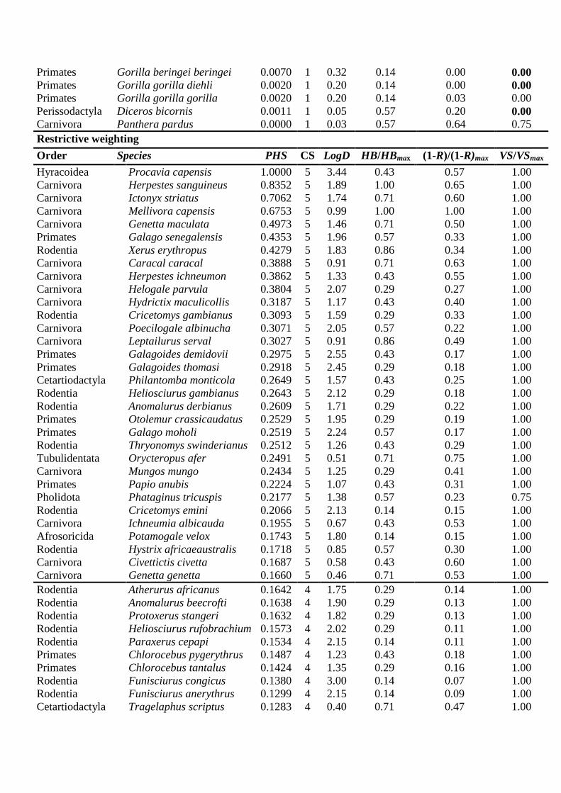
Primates Gorilla beringei beringei 0.0070 1 0.32 0.14 0.00 0.00

Primates Gorilla gorilla diehli 0.0020 1 0.20 0.14 0.00 0.00

Primates Gorilla gorilla gorilla 0.0020 1 0.20 0.14 0.03 0.00

Perissodactyla Diceros bicornis 0.0011 1 0.05 0.57 0.20 0.00

Carnivora Panthera pardus 0.0000 1 0.03 0.57 0.64 0.75

Restrictive weighting

Order Species PHS CS LogD HB/HBmax (1-R)/(1-R)max VS/VSmax

Hyracoidea Procavia capensis 1.0000 5 3.44 0.43 0.57 1.00

Carnivora Herpestes sanguineus 0.8352 5 1.89 1.00 0.65 1.00

Carnivora Ictonyx striatus 0.7062 5 1.74 0.71 0.60 1.00

Carnivora Mellivora capensis 0.6753 5 0.99 1.00 1.00 1.00

Carnivora Genetta maculata 0.4973 5 1.46 0.71 0.50 1.00

Primates Galago senegalensis 0.4353 5 1.96 0.57 0.33 1.00

Rodentia Xerus erythropus 0.4279 5 1.83 0.86 0.34 1.00

Carnivora Caracal caracal 0.3888 5 0.91 0.71 0.63 1.00

Carnivora Herpestes ichneumon 0.3862 5 1.33 0.43 0.55 1.00

Carnivora Helogale parvula 0.3804 5 2.07 0.29 0.27 1.00

Carnivora Hydrictix maculicollis 0.3187 5 1.17 0.43 0.40 1.00

Rodentia Cricetomys gambianus 0.3093 5 1.59 0.29 0.33 1.00

Carnivora Poecilogale albinucha 0.3071 5 2.05 0.57 0.22 1.00

Carnivora Leptailurus serval 0.3027 5 0.91 0.86 0.49 1.00

Primates Galagoides demidovii 0.2975 5 2.55 0.43 0.17 1.00

Primates Galagoides thomasi 0.2918 5 2.45 0.29 0.18 1.00

Cetartiodactyla Philantomba monticola 0.2649 5 1.57 0.43 0.25 1.00

Rodentia Heliosciurus gambianus 0.2643 5 2.12 0.29 0.18 1.00

Rodentia Anomalurus derbianus 0.2609 5 1.71 0.29 0.22 1.00

Primates Otolemur crassicaudatus 0.2529 5 1.95 0.29 0.19 1.00

Primates Galago moholi 0.2519 5 2.24 0.57 0.17 1.00

Rodentia Thryonomys swinderianus 0.2512 5 1.26 0.43 0.29 1.00

Tubulidentata Orycteropus afer 0.2491 5 0.51 0.71 0.75 1.00

Carnivora Mungos mungo 0.2434 5 1.25 0.29 0.41 1.00

Primates Papio anubis 0.2224 5 1.07 0.43 0.31 1.00

Pholidota Phataginus tricuspis 0.2177 5 1.38 0.57 0.23 0.75

Rodentia Cricetomys emini 0.2066 5 2.13 0.14 0.15 1.00

Carnivora Ichneumia albicauda 0.1955 5 0.67 0.43 0.53 1.00

Afrosoricida Potamogale velox 0.1743 5 1.80 0.14 0.15 1.00

Rodentia Hystrix africaeaustralis 0.1718 5 0.85 0.57 0.30 1.00

Carnivora Civettictis civetta 0.1687 5 0.58 0.43 0.60 1.00

Carnivora Genetta genetta 0.1660 5 0.46 0.71 0.53 1.00

Rodentia Atherurus africanus 0.1642 4 1.75 0.29 0.14 1.00

Rodentia Anomalurus beecrofti 0.1638 4 1.90 0.29 0.13 1.00

Rodentia Protoxerus stangeri 0.1632 4 1.82 0.29 0.13 1.00

Rodentia Heliosciurus rufobrachium 0.1573 4 2.02 0.29 0.11 1.00

Rodentia Paraxerus cepapi 0.1534 4 2.15 0.14 0.11 1.00

Primates Chlorocebus pygerythrus 0.1487 4 1.23 0.43 0.18 1.00

Primates Chlorocebus tantalus 0.1424 4 1.35 0.29 0.16 1.00

Rodentia Funisciurus congicus 0.1380 4 3.00 0.14 0.07 1.00

Rodentia Funisciurus anerythrus 0.1299 4 2.15 0.14 0.09 1.00

Cetartiodactyla Tragelaphus scriptus 0.1283 4 0.40 0.71 0.47 1.00

Cetartiodactyla Phacochoerus africanus 0.1251 4 0.43 0.43 0.43 1.00

Carnivora Nandinia binotata 0.1241 4 0.78 0.57 0.24 1.00

Rodentia Hystrix cristata 0.1224 4 0.88 0.86 0.20 1.00

Rodentia Funisciurus pyrropus 0.1211 4 2.12 0.14 0.08 1.00

Primates Colobus guereza

occidentalis

0.1084 4 2.00 0.29 0.08 1.00

Carnivora Genetta thierryi 0.1071 4 1.56 0.29 0.10 1.00

Hyracoidea Dendrohyrax dorsalis 0.1068 4 1.31 0.43 0.12 1.00

Rodentia Paraxerus poensis 0.1003 4 2.41 0.29 0.06 1.00

Primates Chlorocebus cynosuros 0.0979 4 1.20 0.29 0.12 1.00

Pholidota Phataginus tetradactyla 0.0969 4 1.35 0.43 0.11 1.00

Primates Papio cynocephalus 0.0951 4 0.84 0.43 0.17 1.00

Carnivora Xenogale naso 0.0941 4 1.34 0.29 0.10 1.00

Primates Cercopithecus neglectus 0.0897 3 1.48 0.29 0.09 1.00

Hyracoidea Dendrohyrax arboreus 0.0891 3 1.37 0.29 0.10 1.00

Cetartiodactyla Syncerus caffer caffer 0.0815 3 0.84 0.43 0.14 1.00

Rodentia Paraxerus boehmi 0.0639 2 2.52 0.29 0.04 1.00

Primates Perodicticus potto

edwardsi

0.0616 2 0.98 0.29 0.09 1.00

Proboscidea Loxodonta africana 0.0615 2 0.89 0.57 0.10 0.50


schmidti

0.0613 2 2.03 0.29 0.04 1.00

Cetartiodactyla Hyemoschus aquaticus 0.0611 2 0.94 0.14 0.10 1.00

Carnivora Bdeogale crassicauda 0.0577 2 1.50 0.14 0.06 1.00

Carnivora Crossarchus alexandri 0.0577 2 1.54 0.14 0.06 1.00

Pholidota Smutsia gigantea 0.0561 2 0.64 0.57 0.13 0.75

Cetartiodactyla Syncerus caffer nanus 0.0552 2 0.84 0.43 0.10 1.00

Cetartiodactyla Cephalophus dorsalis 0.0536 2 0.68 0.29 0.12 1.00

Carnivora Atilax paludinosus 0.0528 2 0.54 0.14 0.55 1.00

Carnivora Felis silvestris 0.0518 2 0.13 0.57 0.88 1.00

Carnivora Aonyx congicus 0.0511 2 0.72 0.29 0.10 1.00

Cetartiodactyla Tragelaphus spekii 0.0495 2 0.42 0.57 0.17 1.00

Cetartiodactyla Cephalophus rufilatus 0.0482 2 0.62 0.57 0.11 1.00


angolensis

0.0447 2 1.00 0.29 0.07 1.00

Cetartiodactyla Hippotragus equinus 0.0432 2 0.29 0.29 0.22 1.00

Cetartiodactyla Cephalophus nigrifrons 0.0404 2 0.48 0.14 0.12 1.00

Cetartiodactyla Hippopotamus amphibius 0.0383 2 0.77 0.43 0.07 0.50

Carnivora Aonyx capensis 0.0379 2 0.13 0.43 0.46 1.00

Primates Arctocebus aureus 0.0378 2 2.13 0.14 0.03 1.00

Rodentia Funisciurus lemniscatus 0.0372 2 2.30 0.14 0.02 1.00

Rodentia Funisciurus isabella 0.0360 2 2.38 0.14 0.02 1.00


nictitans

0.0351 2 1.37 0.29 0.04 1.00

Cetartiodactyla Tragelaphus oryx 0.0319 2 0.18 0.43 0.26 1.00

Cetartiodactyla Cephalophus weynsi 0.0319 2 0.81 0.14 0.06 1.00


katangae

0.0318 2 2.03 0.29 0.02 1.00

Primates Cercocebus agilis 0.0297 2 1.06 0.14 0.04 1.00

Primates Sciurocheirus gabonensis 0.0296 2 2.10 0.14 0.02 1.00

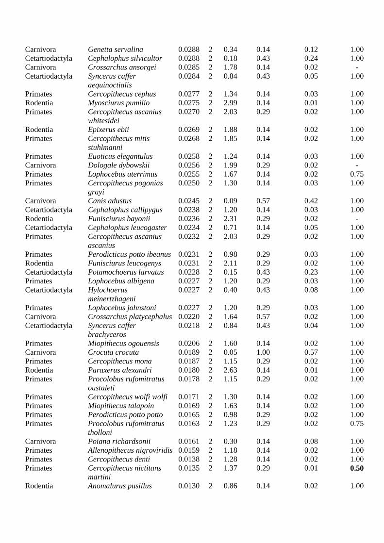
Carnivora Genetta servalina 0.0288 2 0.34 0.14 0.12 1.00

Cetartiodactyla Cephalophus silvicultor 0.0288 2 0.18 0.43 0.24 1.00

Carnivora Crossarchus ansorgei 0.0285 2 1.78 0.14 0.02 -


aequinoctialis

0.0284 2 0.84 0.43 0.05 1.00

Primates Cercopithecus cephus 0.0277 2 1.34 0.14 0.03 1.00

Rodentia Myosciurus pumilio 0.0275 2 2.99 0.14 0.01 1.00


whitesidei

0.0270 2 2.03 0.29 0.02 1.00

Rodentia Epixerus ebii 0.0269 2 1.88 0.14 0.02 1.00


stuhlmanni

0.0268 2 1.85 0.14 0.02 1.00

Primates Euoticus elegantulus 0.0258 2 1.24 0.14 0.03 1.00

Carnivora Dologale dybowskii 0.0256 2 1.99 0.29 0.02 -

Primates Lophocebus aterrimus 0.0255 2 1.67 0.14 0.02 0.75


grayi

0.0250 2 1.30 0.14 0.03 1.00

Carnivora Canis adustus 0.0245 2 0.09 0.57 0.42 1.00

Cetartiodactyla Cephalophus callipygus 0.0238 2 1.20 0.14 0.03 1.00

Rodentia Funisciurus bayonii 0.0236 2 2.31 0.29 0.02 -

Cetartiodactyla Cephalophus leucogaster 0.0234 2 0.71 0.14 0.05 1.00


ascanius

0.0232 2 2.03 0.29 0.02 1.00

Primates Perodicticus potto ibeanus 0.0231 2 0.98 0.29 0.03 1.00

Rodentia Funisciurus leucogenys 0.0231 2 2.11 0.29 0.02 1.00

Cetartiodactyla Potamochoerus larvatus 0.0228 2 0.15 0.43 0.23 1.00

Primates Lophocebus albigena 0.0227 2 1.20 0.29 0.03 1.00

Cetartiodactyla Hylochoerus

meinertzhageni

0.0227 2 0.40 0.43 0.08 1.00

Primates Lophocebus johnstoni 0.0227 2 1.20 0.29 0.03 1.00

Carnivora Crossarchus platycephalus 0.0220 2 1.64 0.57 0.02 1.00


brachyceros

0.0218 2 0.84 0.43 0.04 1.00

Primates Miopithecus ogouensis 0.0206 2 1.60 0.14 0.02 1.00

Carnivora Crocuta crocuta 0.0189 2 0.05 1.00 0.57 1.00

Primates Cercopithecus mona 0.0187 2 1.15 0.29 0.02 1.00

Rodentia Paraxerus alexandri 0.0180 2 2.63 0.14 0.01 1.00


oustaleti

0.0178 2 1.15 0.29 0.02 1.00

Primates Cercopithecus wolfi wolfi 0.0171 2 1.30 0.14 0.02 1.00

Primates Miopithecus talapoin 0.0169 2 1.63 0.14 0.02 1.00

Primates Perodicticus potto potto 0.0165 2 0.98 0.29 0.02 1.00


tholloni

0.0163 2 1.23 0.29 0.02 0.75

Carnivora Poiana richardsonii 0.0161 2 0.30 0.14 0.08 1.00

Primates Allenopithecus nigroviridis 0.0159 2 1.18 0.14 0.02 1.00

Primates Cercopithecus denti 0.0138 2 1.28 0.14 0.02 1.00


martini

0.0135 2 1.37 0.29 0.01 0.50

Rodentia Anomalurus pusillus 0.0130 2 0.86 0.14 0.02 1.00

Primates Colobus satanas

anthracinus

0.0125 2 1.44 0.14 0.01 0.50

Primates Cercocebus torquatus 0.0123 2 1.61 0.43 0.01 0.50

Cetartiodactyla Potamochoerus porcus 0.0119 2 0.09 0.43 0.20 1.00

Primates Mandrillus sphinx 0.0116 2 1.35 0.14 0.01 0.50

Carnivora Panthera pardus 0.0114 2 0.03 0.57 0.64 0.75

Perissodactyla Equus quagga 0.0112 2 0.18 0.43 0.09 1.00


schweinfurthii

0.0107 2 0.42 0.29 0.04 0.25

Carnivora Genetta piscivora 0.0090 2 1.51 0.14 0.01 -

Carnivora Profelis aurata 0.0086 2 0.08 0.57 0.16 0.75

Cetartiodactyla Tragelaphus eurycerus 0.0086 2 0.15 0.57 0.09 0.75


nigripes

0.0082 2 1.30 0.14 0.01 1.00

Carnivora Bdeogale nigripes 0.0082 2 0.15 0.14 0.08 1.00


troglodytes

0.0079 2 0.42 0.29 0.03 0.25

Rodentia Heliosciurus ruwenzorii 0.0077 2 2.06 0.43 0.01 1.00

Primates Allochrocebus lhoesti 0.0068 2 1.18 0.29 0.01 0.50

Cetartiodactyla Neotragus batesi batesi 0.0063 2 0.40 0.14 0.02 1.00

Primates Colobus angolensis cottoni 0.0061 2 1.00 0.29 0.01 1.00

Primates Cercopithecus hamlyni 0.0059 2 1.20 0.14 0.01 0.50

Primates Cercocebus chrysogaster 0.0058 2 0.96 0.14 0.01 1.00


crusalbum

0.0058 1 1.15 0.29 0.01 1.00

Primates Pan paniscus 0.0053 1 0.48 0.71 0.02 0.25

Primates Euoticus pallidus talboti 0.0052 1 2.08 0.14 0.00 1.00

Lagomorpha Poelagus marjorita 0.0052 1 1.38 0.29 0.01 1.00

Rodentia Funisciurus carruthersi 0.0051 1 2.08 0.14 0.00 1.00

Primates Cercopithecus mitis mitis 0.0051 1 1.85 0.14 0.00 -

Primates Galago matschiei 0.0050 1 2.17 0.14 0.00 1.00

Primates Sciurocheirus alleni

cameronensis

0.0050 1 2.00 0.29 0.00 1.00

Carnivora Genetta poensis 0.0045 1 1.32 0.14 0.01

Primates Lophocebus opdenboschi 0.0041 1 1.09 0.14 0.01 0.50

Carnivora Genetta cristata 0.0039 1 1.47 0.14 0.00 0.50


pogonias

0.0037 1 1.30 0.14 0.00 0.50

Proboscidea Loxodonta cyclotis 0.0034 1 0.18 0.43 0.03 0.50

Primates Arctocebus calabarensis 0.0034 1 0.86 0.29 0.01 1.00

Afrosoricida Micropotamogale

ruwenzorii

0.0033 1 2.38 0.14 0.00 0.75


lulindicus

0.0029 1 1.12 0.29 0.00 1.00


camerunensis

0.0029 1 2.03 0.14 0.00 0.50


heymansi

0.0025 1 1.85 0.14 0.00 0.75

Carnivora Bdeogale jacksoni 0.0023 1 1.38 0.29 0.00 0.75

Cetartiodactyla Neotragus batesi harrisoni 0.0022 1 0.40 0.14 0.01 1.00


langi

0.0021 1 1.08 0.29 0.00 1.00


doggeti

0.0021 1 1.85 0.14 0.00 1.00

Carnivora Genetta victoriae 0.0021 1 0.15 0.14 0.02 1.00


ogilbyi

0.0020 1 1.15 0.29 0.00 0.50

Cetartiodactyla Okapia johnstoni 0.0020 1 0.31 0.14 0.01 0.25


pyrogaster

0.0020 1 1.30 0.14 0.00 1.00

Primates Pan troglodytes ellioti 0.0019 1 0.42 0.29 0.01 0.25

Primates Colobus guereza matschiei 0.0018 1 2.00 0.29 0.00 -


cordeiri

0.0018 1 1.00 0.29 0.00 0.75


atrinasus

0.0017 1 2.03 0.29 0.00 -


elegans

0.0015 1 1.30 0.14 0.00 0.75

Cetartiodactyla Tragelaphus derbianus 0.0013 1 0.13 0.29 0.01 1.00

Primates Cercopithecus sclateri 0.0013 1 1.32 0.14 0.00 0.50

Primates Lophocebus ugandae 0.0010 1 1.20 0.29 0.00 1.00


leucophaeus

0.0010 1 0.86 0.29 0.00 0.25


foai

0.0008 1 1.05 0.29 0.00 1.00

Primates Cercopithecus

lomamiensis

0.0006 1 1.14 0.14 0.00 0.50

Rodentia Paraxerus cooperi 0.0006 1 2.11 0.14 0.00 -


parmentieri

0.0006 1 1.18 0.29 0.00 1.00


ellioti

0.0006 1 1.01 0.29 0.00 1.00

Primates Gorilla beringei graueri 0.0005 1 0.32 0.14 0.00 0.25

Primates Allochrocebus preussi pre 0.0005 1 1.20 0.14 0.00 0.25

Primates Allochrocebus solatus 0.0004 1 1.14 0.14 0.00 0.50


ruwenzorii

0.0003 1 1.00 0.29 0.00 0.50

Rodentia Funisciurus duchaillui 0.0002 1 2.18 0.14 0.00 -


tephrosceles

0.0001 1 1.21 0.29 0.00 0.25

Primates Sciurocheirus alleni alleni 0.0001 1 2.00 0.29 0.00 0.25

Primates Euoticus pallidus pallidus 0.0001 1 2.08 0.14 0.00 0.25

Primates Lophocebus osmani 0.0001 1 1.20 0.29 0.00 1.00


erythrotis

0.0001 1 2.03 0.14 0.00 0.50

Primates Colobus satanas satanas 0.0000 1 1.44 0.14 0.00 0.25


prigoginei

0.0000 1 1.00 0.29 0.00 0.25


poensis

0.0000 1 0.86 0.29 0.00 0.25

Primates Allochrocebus preussi ins 0.0000 1 1.20 0.14 0.00 0.25


pennantii

0.0000 1 1.00 0.14 0.00 0.25

Primates Procolobus preussi 0.0000 1 1.06 0.14 0.00 0.00


bouvieri

0.0000 1 0.95 0.14 0.00 0.00

Primates Cercopithecus dryas 0.0000 1 1.35 0.14 0.00 0.00


schoutedeni

0.0000 1 1.85 0.14 0.00 0.00

Primates Gorilla gorilla diehli 0.0000 1 0.20 0.14 0.00 0.00

Primates Gorilla gorilla gorilla 0.0000 1 0.20 0.14 0.03 0.00

Primates Gorilla beringei beringei 0.0000 1 0.32 0.14 0.00 0.00

Perissodactyla Diceros bicornis 0.0000 1 0.05 0.57 0.20 0.00

Appendix S2. Predictor variables (and primary sources) used to construct favorability

models for all species in our study: A species’ distribution is influenced by multiple causal

factors such as climate, topography, human activity, history, and the population dynamics of the

species itself, among others (Lomolino et al., 2005; Guisan & Thuiller, 2005; Márquez et al.,

2011). Climate, topo-hydrography and land cover/land use, in particular, have a dominant

influence on species distributions at scales ranging from site (10-1000 m) to global levels (>10000

km) (Mackey & Lindenmayer, 2001; Pearson & Dawson, 2005). However, the inclusion of

anthropogenic variables in distribution modeling is also important, since human presence is a

primary factor impacting species distributions (Corsi et al., 1999). Spatial descriptors need also to

be included in the variable set to account for autocorrelation, and because it may explain the effect

of dispersal barriers, geological history and biotic interactions (Legendre, 1993). For further

details on variable building and data sources see Appendix S3.

Climate (WorldClim, IPCC5/CMIP5) (representative of 1950-2000)

Maximum temperature of July

Minimum temperature of January

Annual temperature range

Annual precipitation

Pluviometric irregularity

Topography (GlobDEM50; GTOPO30)

Elevation

Slope

Hydrography (HydroSHEDS; Global Land Cover 2000)

Distance to water masses

Distance to minor rivers

Land cover / land use

Forest (Collection 5 MODIS Global Land Cover Type, which processed data for each year

for the period 2001-2005)

Grassland-shrubland-savanna (Collection 5 MODIS Global Land Cover Type)

Woody savanna (Collection 5 MODIS Global Land Cover Type)

Cropland-natural vegetation mosaic (Collection 5 MODIS Global Land Cover Type)

Desert (Collection 5 MODIS Global Land Cover Type)

Occurrence of cropland (FGGD Digital Atlas for the year 2000)

Occurrence of pasture and browse (FGGD Digital Atlas for the year 2000)

Intact forest (IFL) in 2000

Other anthropogenic pressure variables

Percentage of area equipped for irrigation (Global Map of Irrigation Areas v.4.0.1) around

the year 2000

Global climate, soil and terrain slope constraints for cropping activities (FAO & IIASA,

2007)

Density of poultry farms (FAO's Gridded Livestock of the World, derived from various

national census reports, livestock surveys and data archives from 1992 to 2003)

Density of pigs (FAO's Gridded Livestock of the World)

Density of cattle (FAO's Gridded Livestock of the World)

Density of small ruminants (FAO's Gridded Livestock of the World)

Distance to roads (FAO/GIS, DCW) in 2002

Distance to rail-roads (FAO/GIS, DCW) in 2002

Distance to populated places (RWDB2) in 2000

Rural population density (LandScan™ 2008 High Resolution Global Population Data Set;

MODIS 500-m Map of Global Urban Extent, produced using data circa 2001-2002)

Spatial descriptors: these two variables were combined, following the trend surface approach

described in the main text.

Geographic latitude

Geographic longitude

References

Corsi, F., Duprè, E., Boitani, L. (1999) A large-scale model of wolf distribution in Italy for

conservation planning. Conservation Biology 13:150-159.

FAO and IIASA (2007). Mapping Biophysical Factors that Influence Agricultural Production and

Rural Vulnerability [van Velthuizen, H., Huddleston, B., Fischer, G., Salvatore, M.,

Ataman, E., Nachtergaele, F., Zanetti, M., Bloise, M.]. Environmental and Natural

Resources Series No. 11. Rome.

Guisan, A., Thuiller, W. (2005) Predicting species distribution: offering more than simple habitat

models. Ecology Letters 8: 993-1009.

Legendre, P. (1993) Spatial autocorrelation: trouble or new paradigm? Ecology 74:1659-1673.

Lomolino, M.V., Riddle, B.R., Brown, J.H. (2005) Distributions of species. In: Lomolino, M.V.,

Riddle, B.R., Brown, J.H. (eds) Biogeography, 3rd edn. Sinauer, Sunderland, pp 65-96.

Mackey, B.G., Lindenmayer, D.B. (2001) Towards a hierarchical framework for modelling the

spatial distribution of animals. Journal of Biogeography 28: 1147-1166.

Márquez, A.L., Real, R., Olivero, J., Estrada, A. (2011) Combining climate with other influential

factors for modelling the impact of climate change on species distribution. Climatic Change

108: 135-157.

Pearson, R.G., Dawson, T.P. (2005) Predicting the impacts of climate change on the distribution

of species: are bioclimate envelope models useful? Global Ecology & Biogeography 12:

361-371.

Appendix S3. Detailed description of predictor variable design.

Climate

Five climate variables were used: "maximum temperature of July", "minimum temperature

of January", "annual temperature range", "annual precipitation", and "pluviometric irregularity"

―i.e. annual variation coefficient of monthly precipitation. We built these variables using 30 arc-

second-resolution layers for maximum temperature of July, minimum temperature of January and

monthly precipitation regarding current conditions (~1950-2000), which were downloaded from

WorldClim (http://www.worldclim.org). These measures were chosen as variable sources in order

to match with the set of variables with available predictions for 2050.

Topography

"Elevation" and "slope" values for model training, including the entire African continent,

were derived from GTOPO30 (US Geological Survey, 1996), with a 30 arc-second-resolution. The

GlobDEM50 3-arc-second-resolution digital elevation model, based on raw data from the Shuttle

Radar Topography Mission (SRTM) (Farr & Kobrick, 2000), was alternatively used for model

downscaling within our study area.

Hydrography

Two variables measuring "distance to water masses" and "distance to minor rivers" were

calculated using the hydrologically conditioned 3-arc-second-resolution elevation layer

distributed with HydroSHEDS (http://hydrosheds.cr.usgs.gov). Water masses were referred to as

lakes (delimited as in http://www.naturalearthdata.com) and main river courses, which were

defined as river courses whose water flow was higher than 106 according to HydroSHEDS. These

rivers included Zambezi, Limpopo, Cubango, Nile, Niger, Congo, Senegal, Chari, Orange, and

some principal tributaries. Instead, we considered minor rivers to be those ones whose water flow

was between 104 and 10

6, which included most tributaries and other main courses not cited above.

Rivers outlined within the Sahara Desert in HydroSHEDS were eliminated from the data set by

intersecting with the Bare Areas (19) land cover class in Global Land Cover 2000 (Bartholomé &

Belward, 2005). This layer was chosen because it allowed respecting river courses running across

the desert, as Nile and Niger.

http://hydrosheds.cr.usgs.gov/

Land cover / land use

Land-cover / land use variable describing the proportion of surface area covered with the

corresponding classes within each cell were calculated (see Romero et al., 2012).

Five variables were extracted from the Collection 5 MODIS Global Land Cover Type

product, which processed data for each year during the period 2001-2005 (Friedl et al., 2010):

"forest" ―land-cover classes 1 to 5―, "grassland-shrubland-savanna" ―classes 6, 7, 9 and 10―,

"woody savanna" ―class 8―, "cropland-natural vegetation mosaic" ―class14― and "desert"

―class 16.

The source for the "occurrence of cropland" and for the "occurrence of pasture and

browse" was the Food Insecurity, Poverty and Environment Global GIS Database (FGGD Digital

Atlas for the year 2000) (FAO & IIASA, 2007).

"Intact forest" surface was calculated using the World Intact Forest Landscapes (IFL) Map in the

year 2000 (Potapov et al., 2008).

Other anthropogenic pressure variables

Two more agriculture variables were included in the analysis. The "percentage of area

equipped for irrigation" was got from the Global Map of Irrigation Areas (version 4.0.1) around

the year 2000 (http://www.fao.org/nr/water); maps to calculate the area with "global climate, soil

and terrain slope constraints for cropping activities" was extracted from FAO & IIASA (2007).

Livestock was represented by four variables: "density of poultry farms", "density of pigs",

"density of cattle" and "density of small ruminants". Data were extracted from FAO's Gridded

Livestock of the World maps, derived from various national census reports, livestock surveys and

data archives from 1992 to 2003 (Robinson et al., 2007).

We calculated "distance to roads" and "distance to rail-roads" with ArcGIS 10.0, using the

maps extracted by FAO/GIS (http://www.fao.org/geonetwork) from Vector Map Level 0 at the

Digital Chart of the World (DCW, http://worldmap.harvard.edu), updated in 2002.

http://worldmap.harvard.edu/

The "distance to populated places" was calculated with ArcGIS 10.0, using the Administrative

Centres & Populated Places shapefile at the Relational World Database II (RWDB2) updated in

2000 (http://www.fao.org/geonetwork) as a reference.

"Rural population density" was estimated by combining two data sources: (1) population

density, calculated utilizing the LandScan™ 2008 High Resolution Global Population Data Set

(copyrighted by UT-Battelle, LLC, operator of Oak Ridge National Laboratory); and (2) urban

areas, taken from MODIS 500-m Map of Global Urban Extent (produced using data circa 2001-

2002, see Schneider et al., 2009, 2010). Using ArcGIS 10.0, population density was valued as 0

within a 2-km buffer around urban areas.

How variables were prepared for modeling

Values of all the above-described variables had, initially, spatial resolutions finer than 0.1º

x 0.1º. We then calculated variable values for all 1º x 1º-resolution grid cells in Africa, and for all

0.1º x 0.1º-resolution grid cells in our study area (see main text). The former were used for

favorability-model training, whereas the latter were used for model downscaling. These variable

values were estimated as the average of the initial values within each cell, for which we used

Zonal Statistic tools of ArcGIS 10.0.

References

Bartholomé, E., Belward, A. S. (2005). GLC2000: a new approach to global land cover mapping

from Earth observation data. International Journal of Remote Sensing 26:1959-1977.

FAO and IIASA (2007). Mapping Biophysical Factors that Influence Agricultural Production and

Rural Vulnerability [van Velthuizen, H., Huddleston, B., Fischer, G., Salvatore, M.,

Ataman, E., Nachtergaele, F., Zanetti, M., Bloise, M.]. Environmental and Natural

Resources Series No. 11. Rome.

Farr, T. G., Kobrick, M. (2000). Shuttle Radar Topography Mission produces a wealth of data.

Transactions of the American Geophysical Union 81:583-585.

Friedl, M. A., Sulla-Menashe, D., Tan, B., Schneider, A., Ramankutty, N., Sibley, A., Huang, X.

(2010). MODIS Collection 5 global land cover: Algorithm refinements and characterization

of new datasets. Remote Sensing of Environment 114:168-182.

Potapov, P., Yaroshenko, A., Turubanova, S., Dubinin, M., Laestadius, L., Thies, C., Aksenov, D.,

Egorov, A., Yesipova, Y., Glushkov, I., Karpachevskiy, M., Kostikova, A., Manisha, A.,

Tsybikova, E., Zhuravleva, I. (2008). Mapping the World's Intact Forest Landscapes by

Remote Sensing. Ecology and Society 13:51-66.

Robinson, T.P., Franceschini, G., Wint, W. (2007). The Food and Agriculture Organization's

Gridded Livestock of the World. Veterinaria Italiana 43:745-751.

Romero, D., Olivero, J., Real, R. (2012). Comparative assessment of different methods for using

land-cover variables for distribution modelling of Salamandra salamandra longirostris.

Environmental Conservation 40:48-59.

Schneider, A., Friedl, M. A., Potere, D. (2009). A new map of global urban extent from MODIS

data. Environmental Research Letters 4:044003.

Schneider, A., Friedl, M. A., Potere, D. (2010). Monitoring urban areas globally using MODIS

500m data: New methods and datasets based on urban ecoregions. Remote Sensing of

Environment 114:1733-1746.

US Geological Survey (1996). GTOPO30. Land processes distributed active archive center (LP

DAAC), EROS data center. https://lta.cr.usgs.gov/GTOPO30

Appendix S4. Number (N) and percentage (%) of taxa (species and subspecies) included in the

five sustainablility categories defined by potential hunting sustainability (PHS). Sustainability

increases from 1 to 5.

Permissive weighting

Family 1 2 3 4 5 Total

Procaviidae N 0 0 0 2 1 3

% 0.0 0.0 0.0 66.7 33.3 100.0

Elephantidae N 1 1 0 0 0 2

% 50.0 50.0 0.0 0.0 0.0 100.0

Tenrecidae N 0 0 0 2 0 2

% 0.0 0.0 0.0 100.0 0.0 100.0

Orycteropodidae N 0 1 0 0 0 1

% 0.0 100.0 0.0 0.0 0.0 100.0

Hominidae N 8 0 0 0 0 8

% 100.0 0.0 0.0 0.0 0.0 100.0

Cercopithecidae N 13 19 9 24 7 72

% 18.1 26.4 12.5 33.3 9.7 100.0

Lorisidae N 0 4 0 0 1 5

% 0.0 80.0 0.0 0.0 20.0 100.0

Galagidae N 0 2 0 1 9 12

% 0.0 16.7 0.0 8.3 75.0 100.0

Sciuridae N 2 1 0 0 18 21

% 9.5 4.8 0.0 0.0 85.7 100.0

Nesomyidae N 0 0 0 1 1 2

% 0.0 0.0 0.0 50.0 50.0 100.0

Anomaluridae N 1 0 0 1 1 3

% 33.3 0.0 0.0 33.3 33.3 100.0

Hystricidae N 0 2 0 1 0 3

% 0.0 66.7 0.0 33.3 0.0 100.0

Thryonomyidae N 0 0 0 1 0 1

% 0.0 0.0 0.0 100.0 0.0 100.0

Leporidae N 0 0 0 1 0 1

% 0.0 0.0 0.0 100.0 0.0 100.0

Canidae N 1 0 0 0 0 1

% 100.0 0.0 0.0 0.0 0.0 100.0

Mustelidae N 1 1 1 2 1 6

% 16.7 16.7 16.7 33.3 16.7 100.0

Nandiniidae N 0 1 0 0 0 1

% 0.0 100.0 0.0 0.0 0.0 100.0

Felidae N 3 2 0 0 0 5

% 60.0 40.0 0.0 0.0 0.0 100.0

Viverridae N 5 3 0 2 0 10

% 50.0 30.0 0.0 20.0 0.0 100.0

Hyaenidae N 1 0 0 0 0 1

% 100.0 0.0 0.0 0.0 0.0 100.0

Herpestidae N 2 3 1 6 2 14

% 14.3 21.4 7.1 42.9 14.3 100.0

Manidae N 0 1 1 1 0 3

% 0.0 33.3 33.3 33.3 0.0 100.0

Equidae N 1 0 0 0 0 1

% 100.0 0.0 0.0 0.0 0.0 100.0

Rhinocerotidae N 1 0 0 0 0 1

% 100.0 0.0 0.0 0.0 0.0 0.0

Suidae N 3 1 0 0 0 4

% 75.0 25.0 0.0 0.0 0.0 100.0

Hippopotamidae N 1 0 0 0 0 1

% 100.0 0.0 0.0 0.0 0.0 100.0

Tragulidae N 0 1 0 0 0 1

% 0.0 100.0 0.0 0.0 0.0 100.0

Giraffidae N 1 0 0 0 0 1

% 100.0 0.0 0.0 0.0 0.0 100.0

Bovidae N 7 12 0 3 0 22

% 31.8 54.5 0.0 13.6 0.0 100.0

Restrictive weighting

Family 1 2 3 4 5 Total

Procaviidae N 0 0 1 1 1 3

% 0.0 0.0 33.3 33.3 33.3 100.0

Elephantidae N 1 1 0 0 0 2

% 50.0 50.0 0.0 0.0 0.0 100.0

Tenrecidae N 1 0 0 0 1 2

% 50.0 0.0 0.0 0.0 50.0 100.0

Orycteropodidae N 0 0 0 0 1 1

% 0.0 0.0 0.0 0.0 100.0 100.0

Hominidae N 6 2 0 0 0 8

% 75.0 25.0 0.0 0.0 0.0 100.0

Cercopithecidae N 35 30 1 5 1 72

% 48.6 41.7 1.4 6.9 1.4 100.0

Lorisidae N 1 4 0 0 0 5

% 20.0 80.0 0.0 0.0 0.0 100.0

Galagidae N 5 2 0 0 5 12

% 41.7 16.7 0.0 0.0 41.7 100.0

Sciuridae N 3 9 0 7 2 21

% 14.3 42.9 0.0 33.3 9.5 100.0

Nesomyidae N 0 0 0 0 2 2

% 0.0 0.0 0.0 0.0 100.0 100.0

Anomaluridae N 0 1 0 1 1 3

% 0.0 33.3 0.0 33.3 33.3 100.0

Hystricidae N 0 0 0 2 1 3

% 0.0 0.0 0.0 66.7 33.3 100.0

Thryonomyidae N 0 0 0 0 1 1

% 0.0 0.0 0.0 0.0 100.0 100.0

Leporidae N 1 0 0 0 0 1

% 100.0 0.0 0.0 0.0 0.0 100.0

Canidae N 0 1 0 0 0 1

% 0.0 100.0 0.0 0.0 0.0 100.0

Mustelidae N 0 2 0 0 4 6

% 0.0 33.3 0.0 0.0 66.7 100.0

Nandiniidae N 0 0 0 1 0 1

% 0.0 0.0 0.0 100.0 0.0 100.0

Felidae N 0 3 0 0 2 5

% 0.0 60.0 0.0 0.0 40.0 100.0

Viverridae N 3 3 0 1 3 10

% 30.0 30.0 0.0 10.0 30.0 100.0

Hyaenidae N 0 1 0 0 0 1

% 0.0 100.0 0.0 0.0 0.0 100.0

Herpestidae N 1 7 0 1 5 14

% 7.1 50.0 0.0 7.1 35.7 100.0

Manidae N 0 1 0 1 1 3

% 0.0 33.3 0.0 33.3 33.3 100.0

Equidae N 0 1 0 0 0 1

% 0.0 100.0 0.0 0.0 0.0 100.0

Rhinocerotidae N 1 0 0 0 0 1

% 100.0 0.0 0.0 0.0 0.0 0.0

Suidae N 0 3 0 1 0 4

% 0.0 75.0 0.0 25.0 0.0 100.0

Hippopotamidae N 0 1 0 0 0 1

% 0.0 100.0 0.0 0.0 0.0 100.0

Tragulidae N 0 1 0 0 0 1

% 0.0 100.0 0.0 0.0 0.0 100.0

Giraffidae N 1 0 0 0 0 1

% 100.0 0.0 0.0 0.0 0.0 100.0

Bovidae N 4 15 1 1 1 22

% 18.2 68.2 4.5 4.5 4.5 100.0

Integrating Sustainable Hunting in Biodiversity Protection in Central Africa: Hot Spots, Weak Spots,...

Documents

Transcript of Integrating Sustainable Hunting in Biodiversity Protection in Central Africa: Hot Spots, Weak Spots,...