Integrated conditional global optimisation for discrete fracture network modelling

$: Integrated conditional global optimisation for discrete fracture network modelling$
ARTICLE IN PRESS

0098-3004/$ - se

doi:10.1016/j.ca

�CorrespondE-mail addr

Computers & Geosciences 32 (2006) 17–27

www.elsevier.com/locate/cageo

Integrated conditional global optimisation for discrete fracturenetwork modelling

Nam H. Tran�, Zhixi Chen, Sheik S. Rahman

School of Petroleum Engineering, The University of New South Wales, Sydney NSW 2052, Australia

Received 2 February 2005; received in revised form 31 March 2005; accepted 31 March 2005

Abstract

This paper presents a methodology to simulate discrete fracture networks for naturally fractured reservoirs by

combining statistical and spatial analyses, object-based modelling and conditional global optimisation. The

methodology examines and utilises both continuum and discrete fracture information, such as spatial distribution of

fracture density, statistical and geostatistical distributions of fracture size and orientation. The output is a network of

discrete fractures, with their corresponding details of location, size and orientation. The methodology is illustrated by a

case study on the surface fault system in New York region. The results show that it is able to produce discrete fracture

network that match closely to the target fault map, even in the case where data are limited. The results show that it is

also able to improve results of several recent fracture models, such as integrated stochastic simulations as well as grid-

based simulations.

r 2005 Elsevier Ltd. All rights reserved.

Keywords: Naturally fractured reservoir; Stochastic simulation; Object-based; Geostatistics; Simulated annealing

1. Introduction

Comprehensive understanding of fracture systems is

critical to economical development of oil and gas

reservoirs, generation of heat and vapour from geother-

mal reservoirs, management of groundwater resources

and underground nuclear wastes (National Research

Council, 1996; Bonnet et al., 2001). In these naturally

fractured reservoirs (NFR), reliable discrete fracture

networks (DFN) are required to portray both fracture

spatial distribution and details of individual fracture

properties such as location, orientation, size, density and

conductivity. In petroleum engineering, such DFN can

be combined with conventional geological reservoir

models as inputs for reservoir simulation and stimula-

e front matter r 2005 Elsevier Ltd. All rights reserve

geo.2005.03.019

ing author. Fax: +612 9385 5182.

ess: [email protected] (N.H. Tran).

tion studies. They allow us to select the best locations for

production wells, assess the response of natural fractures

under stimulation pressure, hence, develop the best

scenarios for hydraulic fracture treatments, design

optimum production methods and evaluate reservoir

potentials (National Research Council, 1996).

Many mathematical and geo-mechanical techniques

are available to simulate underground fracture networks

(Oda et al., 1987; Carrera et al., 1990). They, however,

mostly use only single source of data (either seismic maps

or well logs) and rely on simplistic geometrical descrip-

tions of fracture systems (e.g. homogeneous settings,

parallel plate fractures). Due to the heterogeneous and

multi-scaled nature of NFR, comprehensive fracture

modelling requires utilisation of available data sources

in integrated manners (Rawnsley and Wei, 2001).

Stochastic simulation represents a comparatively

more versatile and integrated approach. To some

d.

www.elsevier.com/locate/cageo

ARTICLE IN PRESSN.H. Tran et al. / Computers & Geosciences 32 (2006) 17–2718

extents, it succeeds in combining multiple data sources,

such as core descriptions and well logs (Willis-Richards,

1996; Cacas et al., 2001; Tran et al., 2002). Nevertheless,

because data are mostly available at well locations,

fracture distributions away from the wellbores are

uncertain. In other words, the unconditioned random

filling of the inter-well regions limits applications of such

simulations beyond the near-wellbore regions. In addition,

it remains a major problem to validate DFN from

stochastic simulations (National Research Council, 1996).

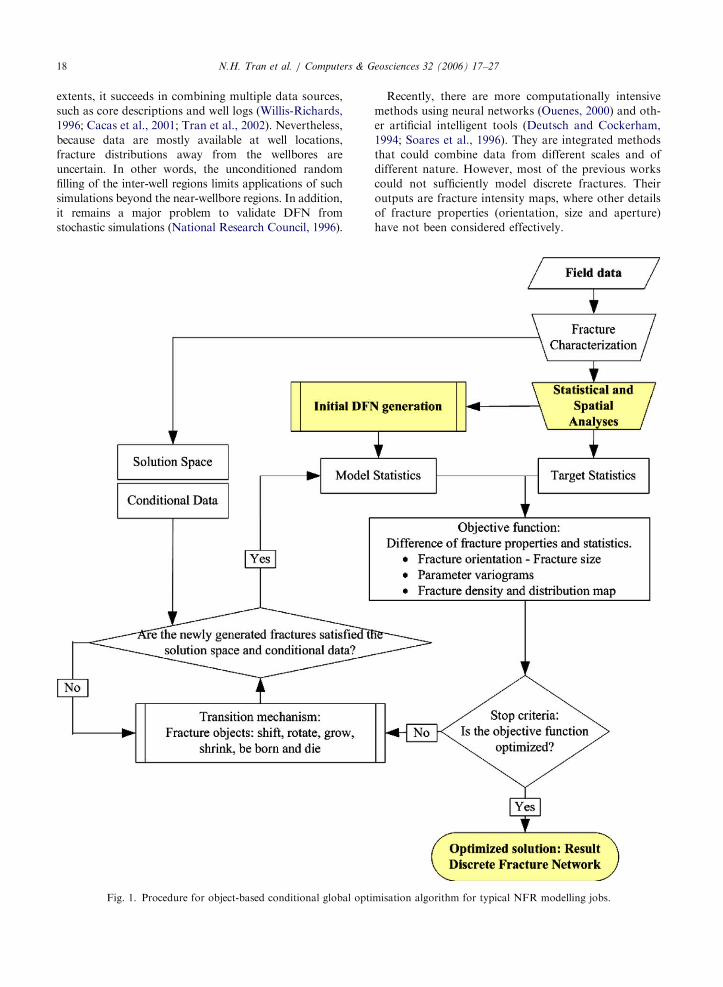
Fig. 1. Procedure for object-based conditional global opti

Recently, there are more computationally intensive

methods using neural networks (Ouenes, 2000) and oth-

er artificial intelligent tools (Deutsch and Cockerham,

1994; Soares et al., 1996). They are integrated methods

that could combine data from different scales and of

different nature. However, most of the previous works

could not sufficiently model discrete fractures. Their

outputs are fracture intensity maps, where other details

of fracture properties (orientation, size and aperture)

have not been considered effectively.

misation algorithm for typical NFR modelling jobs.

ARTICLE IN PRESSN.H. Tran et al. / Computers & Geosciences 32 (2006) 17–27 19

The objective of this work is to present a hybrid

methodology for simulating DFN of NFR. It involves

statistical and spatial analyses, object-based conditional

modelling, stochastic simulation and global optimisa-

tion. An object-based model treats fractures as discrete

objects. A global optimisation algorithm brings about

many advantages compared to the previously cited

methods, such as the ability to simultaneously and

sequentially integrate fracture data of different scales

and nature. Assumptions on distributions of fracture

properties and their variogram fitting as in conventional

geostatistics are not required. First, characteristic

statistics and spatial distributions of the reservoir

fracture properties (target) are determined. This process

can be performed in conjunction with or after the

process of characterisation in a typical reservoir study.

Next, an initial DFN (a realisation) is stochastically

generated. The differences between the target and any

generated realisation are formulated in an ‘‘objective

function’’. A conditional global optimisation algorithm

is applied to modify the realisation, in such a way that

the objective function is minimised. By doing so, the

realisation becomes more and more representative of the

target. Fig. 1 presents the methodological procedure.

In order to put this work in the correct perspective

and to demonstrate its advantages over the previous

methods, a brief review of each technique’s components

is presented, followed by a case study of a fault network

in the New York region, USA.

2. Integrated methodology for modelling discrete fracture

networks

2.1. Object-based modelling

Most of the previously cited fracture models are grid-

based, yielding only fracture intensity maps. These maps

could only indicate the fracture presence while details of

fracture properties such as orientation, size and aperture

are not available. An extensive study of NFR, however,

requires knowledge of not only fracture intensity

distribution, but also details of individual fractures.

Only then, comprehensive simulations for different

stimulation scenarios and fluid flows become possible

(National Research Council, 1996). In addition, an

object-based model gives more accurate results, by

allowing analyses on individual fracture properties and

their inter-relationships.

In this work, each single fracture is treated as a

discrete object. The fracture object is characterised by

properties such as location, orientation and size. Each

object possesses a variety of rules for behaviour in space

such as shift, rotate, grow, shrink, multiply or disappear.

Mathematically, a fracture network model (M) is

defined as a composite of total number of fractures

(NF), individual fracture (MF) and their attributes

(Kumar et al., 1999). Single fracture object, being the

base attribute, serves as base model for fracture location

(ML), size (MS) and orientation (MO) attributes:

M ¼MF �NF fMLðMF Þ �MOðMF Þ �MSðMF Þg. (1)

2.2. Statistical and spatial analyses

The aim of the optimisation modelling is to develop a

DFN, whose statistical and spatial measurements match

those of the target NFR. Thus, defining the representa-

tive and assessable measurements of fracture properties

is essential.

Farmer (1992) and Soares et al. (1996) employ

histogram, correlation, multi-histogram, spatial covar-

iance, fractal dimension, intersections and fracture

density. Deutsch and Cockerham (1994), in their pixel-

based simulated annealing, use semi-variogram (either

experimental or model) of fracture intensity. However,

the use of single fractal dimension value implies

assumptions on fractal characteristics of fracture net-

works, which is usually not adequate. Fracture networks

are more likely to possess multi-fractal characteristics

(Berkowitz and Hadad, 1997; Belfield, 1998; Stach et al.,

2001). Moreover, in a typical NFR, it is just impossible

to count the number of fracture intersections and their

statistics.

A statistical analysis on the fracture data gives general

understandings of individual properties. Generally,

natural fractures tend to be distributed in more than

one dominant directions, which correspond to the field

maximum and minimum stresses and litho-static,

tectonic and thermal history. Stronger stresses tend to

make fractures propagate out on the orthogonal planes.

Thus, fracture orientation is expected to belong to multi-

modal distributions (as opposed to simple one-modal

normal distributions described in the previous mathe-

matical methods and stochastic simulations, e.g. Willis-

Richards, 1996). Distributions for fracture lengths could

be lognormal, power law and (multi) fractal (Belfield,

1998; Bonnet et al., 2001; Stach et al., 2001). The

correlations between fracture orientation and size are

also important. In this approach, fractures are divided

into different sets based on their orientations. Natural

fractures with similar directions tend to have similar

characteristics (as they were created and influenced by

similar stresses). The statistical analysis is performed

using a statistical package S-PLUS.

A spatial analysis provides broad information on

fracture distribution in space and identifies the possible

specific patterns, clustering or regularity. Quantitative

spatial analysis is achieved by using various geostatis-

tical tools and developed in S-PLUS and Fortran 90.

The FORTRAN source codes are based on GSLIB: a


geostatistical software library (Deutsch and Journel,

1992).

Variogram, a second-order moment, is used for

visualising, modelling and exploiting spatial continuity

and spatial variability of regionalised variables. Vario-

gram is also a generalised variable characterised by both

generalisation and randomness. This has made it

possible to be used widely in geostatistical modelling,

especially in spatial distribution characterisation

(Deutsch and Cockerham, 1994). A semi-variogram

(gðhÞ) describes how a parameter (z) varies in space as a

function of lag distance between two measuring loca-

tions (xi) and (xi þ h) (separated by a vector h):

gðhÞ ¼1

2NðhÞ

XNðhÞi¼1

½zðxi þ hÞ � zðxiÞ�2, (2)

where NðhÞ is total number of the data pairs. A cross-

variogram (gcðhÞ) represents variogram between two

different variables z1 and z2:

gcðhÞ

¼1

2NðhÞ

XNðhÞi¼1

½z1ðxi þ hÞ � z1ðxiÞ�½z2ðxi þ hÞ � z2ðxiÞ�. ð3Þ

In this work, geostatistical analysis also involves a

modified multi-histogram, which originates from histo-

gram and variogram measurements. Multi-histogram

mean vector (HmðhÞ) is defined as

HmðhÞ ¼1

NðhÞ

XNðhÞi¼1

½zðxiÞ�. (4)

Finally, fracture density is defined as the total fracture

area per unit volume in 3D (P32) or total fracture trace

length per unit area in 2D (P21). Fracture intensity

refers to the number of fractures per unit volume in 3D

(P30) or area in 2D (P20) (Dershowitz and Herda,

1992). Fracture density is one of the most important

fracture network characteristics, being directly propor-

tional to the number of fractures per unit volume and

their relative size distribution. Spatial distributions of

both fracture density and intensity are continuum (grid-

based) measurements. For a grid-block, the quantities

are determined by counting only the portion of fractures

crossing. In this work, both overall fracture density and

intensity maps of a fracture network are considered and

developed into discrete models.

2.3. Global optimisation

Global optimisation has effectively solved complex

problems in combinatorial optimisation, acquiring

optimum values of a function of very large number of

independent variables (Sen and Stoffa, 1995). It is

especially suitable for such complicated problems as

modelling fracture networks, where there are many

parameters and statistics to optimise. Procedure for

global optimisation modelling of DFN is presented in

Fig. 1.

The first step of global optimisation for DFN

modelling is problem representation. The actual DFN

to be modelled is represented as ‘‘target’’ of the

optimisation program. The differences between the

target and any generated realisation are formulated in

‘‘objective function’’. The objective function represents

the mathematical difference between the DFN realisa-

tion and the target (the actual fracture data from the

field) (*). It is composed of a weighted average of

positive functions:

E ¼X

i

wizi � z�i

z�i

� �2, (5)

where zi denotes arbitrary components of the objective

function. wi are the weighting factors (Swi ¼ 1:0).The optimisation algorithm will continuously modify

DFN realisations, guiding the objective function to

minimisation. The minimum value is equivalent to

achieving the DFN, which is expected to be closed to

the target.

In the modification step, the global optimisation

algorithm systematically transfers a DFN realisation

from one state to another. It starts from an initial

realisation and finishes with the minimised objective

function. During the transition, each fracture, as an

individual object, exercises one or combination of the

possible behaviours (shift, rotate, grow or shrink), while

still stays within the defined solution space. The

algorithm continually observes overall fracture density

to be within its pre-defined range. At any point where

the density value gets higher than the upper limit,

fractures are forced to shrink or disappear (die).

Similarly, if the fracture density falls below the lower

limit, fracture size is enlarged or more fractures are

inserted (be born).

For each modification, a new realisation of DFN is

obtained. Global optimisation algorithm determines

whether the modification is counted or not. If not, the

program generates another realisation. This process is

called generation-acceptance, guiding the algorithm to a

global optimal. Unlike simple algorithm (e.g. exhaustive

search), advanced global optimisation algorithm (simu-

lated annealing) accepts all generations with a prob-

ability. This mechanism facilitates the speed of

convergence and avoids being trapped at local optima.

If the objective function is reduced, the probability of

acceptance equals one.

The generation-acceptance process repeats, until there

has not been any significant improvement or the

objective function becomes small enough. In the former

case, the objective function could reach the required

level of minimisation. Then, it is necessary to check if the


chosen statistics and their relative weighting factors are

representative for the target fracture network data. In

the later case, the minimum objective function results in

a DFN, which is most mathematically representative to

the target fracture data?.

One of the remarkable advantages of global optimisa-

tion is the flexibility of the objective function. Fracture

data of different scales and nature are integrated as

independent components of the objective function.

Formulation of the objective function is an essential

step and should follow data analysis, so that the

characteristic statistical and spatial measurements could

be assessed. In this work, the objective function contains

the overall fracture density (global indicator), fracture

density and intensity distribution maps (continuum

indicators). It also includes semi-variogram, cross-

variogram, modified multi-histograms and representa-

tive statistics of fracture size and orientation (discrete

indicators). It is also important to consider the

program’s accuracy and speed. More and/or different

components could be included into the objective

function. However, the speed of convergence would

have to be considered.

The weighting factors are chosen proportionally to

the importance of each measurement on the convergence

of the optimisation process. General observations

indicate that first-order statistics (e.g. mean, modified

multi-histogram mean and variogram distance) should

correspond to small weighting factors, compared to

other second-order moments (e.g. semi-variogram and

cross-variogram) and fracture densities.

Through iterations, the new objective function is

updated rather than computed. For example, when a

fracture zðxiÞ is perturbed to z0ðx0iÞ and the total number

of fractures is unchanged, the variogram is updated as

gnewðhÞ ¼ gold ðhÞ � f½zðxi þ hÞ � zðxiÞ�2 � ½zðxi � hÞ

� zðxiÞ�2 þþ½zðxi þ hÞ � z0ðx0 iÞ�

2

þ ½zðxi � hÞ � z0ðx0iÞ�2g. ð6Þ

When a region of large number of fractures is

considered, this process drastically reduces computa-

tional time and resources.

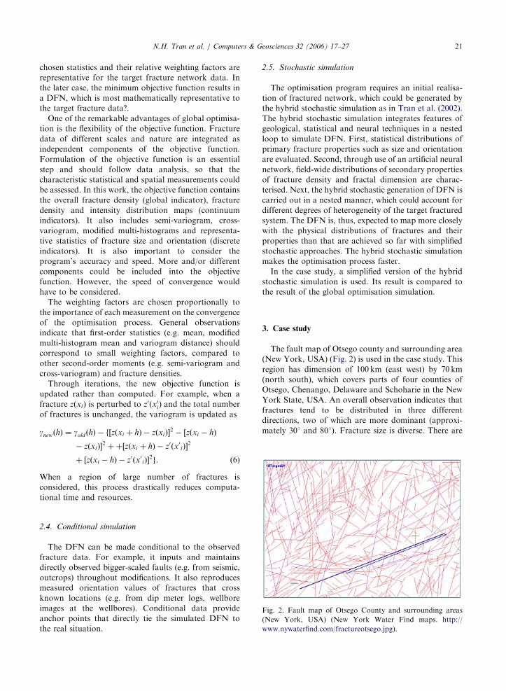
Fig. 2. Fault map of Otsego County and surrounding areas

(New York, USA) (New York Water Find maps. http://

www.nywaterfind.com/fractureotsego.jpg).

2.4. Conditional simulation

The DFN can be made conditional to the observed

fracture data. For example, it inputs and maintains

directly observed bigger-scaled faults (e.g. from seismic,

outcrops) throughout modifications. It also reproduces

measured orientation values of fractures that cross

known locations (e.g. from dip meter logs, wellbore

images at the wellbores). Conditional data provide

anchor points that directly tie the simulated DFN to

the real situation.

2.5. Stochastic simulation

The optimisation program requires an initial realisa-

tion of fractured network, which could be generated by

the hybrid stochastic simulation as in Tran et al. (2002).

The hybrid stochastic simulation integrates features of

geological, statistical and neural techniques in a nested

loop to simulate DFN. First, statistical distributions of

primary fracture properties such as size and orientation

are evaluated. Second, through use of an artificial neural

network, field-wide distributions of secondary properties

of fracture density and fractal dimension are charac-

terised. Next, the hybrid stochastic generation of DFN is

carried out in a nested manner, which could account for

different degrees of heterogeneity of the target fractured

system. The DFN is, thus, expected to map more closely

with the physical distributions of fractures and their

properties than that are achieved so far with simplified

stochastic approaches. The hybrid stochastic simulation

makes the optimisation process faster.

In the case study, a simplified version of the hybrid

stochastic simulation is used. Its result is compared to

the result of the global optimisation simulation.

3. Case study

The fault map of Otsego county and surrounding area

(New York, USA) (Fig. 2) is used in the case study. This

region has dimension of 100 km (east west) by 70 km

(north south), which covers parts of four counties of

Otsego, Chenango, Delaware and Schoharie in the New

York State, USA. An overall observation indicates that

fractures tend to be distributed in three different

directions, two of which are more dominant (approxi-

mately 301 and 801). Fracture size is diverse. There are

http://www.nywaterfind.com/fractureotsego.jpg

http://www.nywaterfind.com/fractureotsego.jpg


many segmented fractures that propagate in lines. They

used to be long faults before being fragmented. These

evidences also suggest that the region has been through

several tectonic regime changes. Fracture distribution is

rather even, except to the northwest where it is visibly

denser.

There are 442 fracture traces in the target fault map.

Each trace could be portrayed by x and y coordinates of

centre (X, Y), orientation (y) and radius (R) (radius is

equivalent to half length of the fault trace):

M ¼MF � 442fX � Y � y� Rg. (7)

Following the optimisation procedure (Fig. 1), the

first step is to identify behaviours of the target network

and define a characteristic objective function. The

formulation of the objective function is a data-driven

process, adding versatility and accuracy to the overall

simulation. A simplified version of the hybrid stochastic

simulation is then used to generate an initial realisation.

The global optimisation algorithm continuously modi-

fies the initial realisation to minimise the objective

function. The final DFN is compared with the target

original.

Two different scenarios are designed to assess the

object-based conditional global optimisation methodol-

ogy. In the first scenario, it is assumed that all necessary

information on the fault map is obtainable, including a

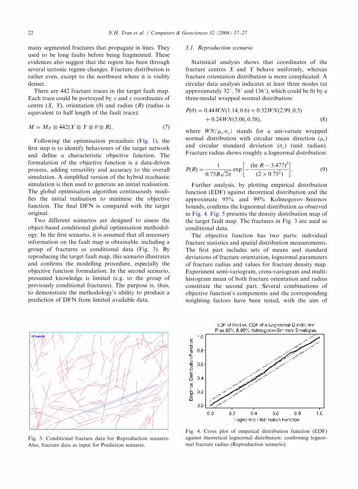
group of fractures as conditional data (Fig. 3). By

reproducing the target fault map, this scenario illustrates

and confirms the modelling procedure, especially the

objective function formulation. In the second scenario,

presumed knowledge is limited (e.g. to the group of

previously conditional fractures). The purpose is, thus,

to demonstrate the methodology’s ability to produce a

prediction of DFN from limited available data.

Fig. 3. Conditional fracture data for Reproduction scenario.

Also, fracture data as input for Prediction scenario.

3.1. Reproduction scenario

Statistical analysis shows that coordinates of the

fracture centres X and Y behave uniformly, whereas

fracture orientation distribution is more complicated. A

circular data analysis indicates at least three modes (at

approximately 321, 781 and 1361), which could be fit by a

three-modal wrapped normal distribution:

PðyÞ ¼ 0:44WNð1:14; 0:6Þ þ 0:32WNð2:99; 0:5Þ

þ 0:24WNð5:06; 0:58Þ, ð8Þ

where WN(mc,sc) stands for a uni-variate wrapped

normal distribution with circular mean direction (mc)

and circular standard deviation (sc) (unit radian).

Fracture radius shows roughly a lognormal distribution:

PðRÞ ¼1

0:75Rffiffiffiffiffiffi2pp exp �

ðln R� 3:477Þ2

ð2� 0:752Þ

� �. (9)

Further analysis, by plotting empirical distribution

function (EDF) against theoretical distribution and the

approximate 95% and 99% Kolmogorov–Smirnov

bounds, confirms the lognormal distribution as observed

in Fig. 4. Fig. 5 presents the density distribution map of

the target fault map. The fractures in Fig. 3 are used as

conditional data.

The objective function has two parts: individual

fracture statistics and spatial distribution measurements.

The first part includes sets of means and standard

deviations of fracture orientation, lognormal parameters

of fracture radius and values for fracture density map.

Experiment semi-variogram, cross-variogram and multi-

histogram mean of both fracture orientation and radius

constitute the second part. Several combinations of

objective function’s components and the corresponding

weighting factors have been tested, with the aim of

Fig. 4. Cross plot of empirical distribution function (EDF)

against theoretical lognormal distribution: confirming lognor-

mal fracture radius (Reproduction scenario).


minimising the final objective function and the speed of

convergence. The sensitivity analysis outputs an opti-

mised range for the weighting factors, as in Table 1. It

can be noted that the first-order statistics do correspond

to small weighting factors (0.01–0.1) while the second-

order moments and fracture density embody bigger

values (0.1–0.8). Each weighting factor represents the

importance of each statistics, towards characterising

DFN.

Fig. 5. Fracture density distribution map (Reproduction

scenario). Density unit m/m2. Lighter shades indicate denser

fracture distribution.

Table 1

Objective function components and their relative optimised ranges for

weighting factors (Reproduction scenario)

Objective function components Fracture properties

First-order statistics Size

Orientation

Size

Orientation

Size

Orientation

Size+orientation

Second-order moments Size

Orientation

Size+Orientation

Density

Density

Fig. 6 demonstrates how objective function decreases

through iterations, showing an approximately logarith-

mic trend. In the beginning, the objective function

decreases faster, since it is easier to get away from local

minima. Towards the end, it requires a much greater

number of iterations. This graph displays typical

behaviour of an optimisation process (Deutsch and

Cockerham, 1994).

Since the objective function quantifies the differences

between characteristics of the output realisation and

target DFN, a final value as small as 1.0e�5 reduces

their difference to minimum. It means that all of its

components have been matched. Table 2 illustrates the

matching of simple statistical measurements of fracture

location, orientation and radius. Fig. 7 presents the

Statistics and measurements Weighting factor range

Logmean 0.01–0.1

Log std dev

Mean 0.01–0.1

Std dev

Proportion

Multi-histogram mean vector 0.01–0.1

Multi-histogram mean vector

Variogram distance vector 0.01–0.1

Variogram distance vector

Covariance 0.01–0.05

Semi-variogram vector 0.5–0.8

Semi-variogram vector

Cross-variogram vector

Grided densities 0.1–0.3

Total density

Fig. 6. Logarithmic declination of objective function (Repro-

duction scenario).

ARTICLE IN PRESS

Table 2

Comparison of objective function components

Simple statistics comparison

Target (0) FraCGOM

(2)

Percentage

error (%)

Stochastic

simulation (1)

Percentage

error (%)

Radius (m)

Lognormal mean 42.87 41.55 3.085 40.42 5.719

Lognormal std dev 37.23 35.76 3.948 31.92 14.281

Orientation (radian)

Set 1: Mean 1.140 1.131 0.756 1.054 7.506

Std dev 0.600 0.600 0.000 0.435 27.434

Probability factor 0.440 0.439 0.287 0.428 2.726

Set 2: Mean 2.990 3.007 0.553 3.165 5.864

Std dev 0.500 0.510 1.953 0.727 45.313


Set 3: Mean 5.060 5.027 0.654 4.722 6.685

Std dev 0.580 0.586 0.977 0.369 36.373


Total fracture density (m/m�m) 0.0792 0.0793 0.076 0.0794 0.252

For target DFN (0), initial realisation by stochastic simulation (1), and final DFN (2) (Reproduction scenario).

Fig. 7. Comparison of experiment semi-variogram vectors for target DFN (0), initial realisation by stochastic simulation (1), and final

DFN (FraCGOM 2) (Reproduction scenario). (A) Fracture radius; (B) fracture orientation.

N.H. Tran et al. / Computers & Geosciences 32 (2006) 17–2724

matching of experimental semi-variogram of fracture

radius and orientation, respectively. The final DFN

realisation for this scenario and its corresponding

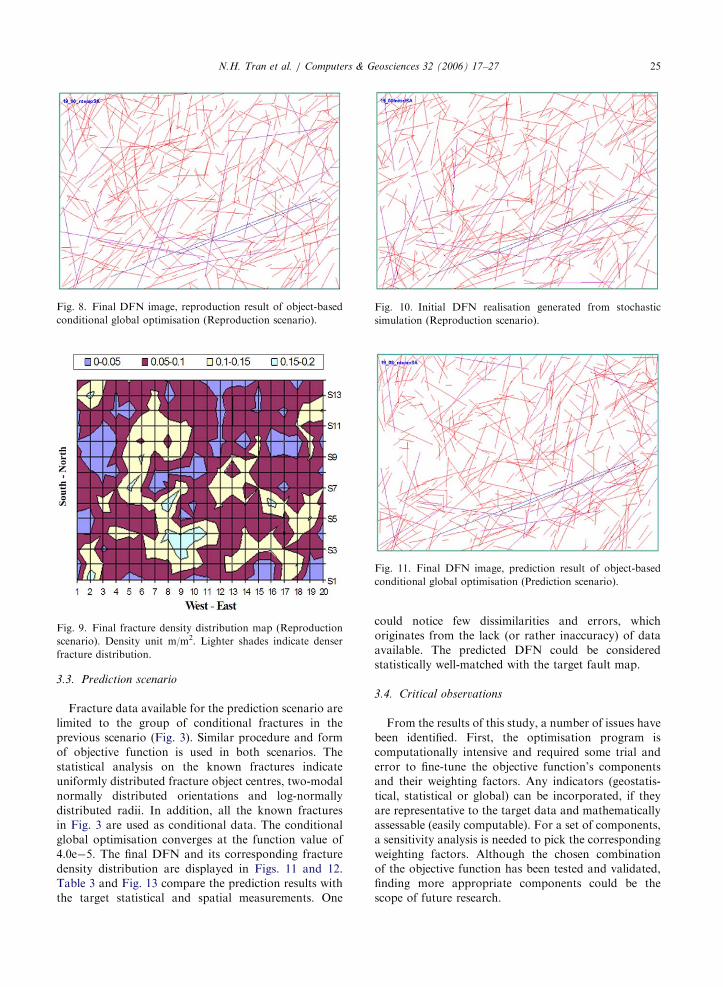
density distribution map are shown in Figs. 8 and 9.

The results are quite comparable to the target fault map,

which confirm the reproduction ability of the object-

based conditional global optimisation methodology.

3.2. Comparison to stochastic simulation

Since a current stochastic simulation is used to

generate the initial DFN, a comparison between results

of the stochastic simulation (Fig. 10) and global

optimisation methodology (Fig. 8) is possible. By visual

comparison, it is observed that the global optimisation

methodology results in a closer matched with the target

fault map. In fact, the objective function is improved

from 0.40 to 1.0e�5. Details of the objective function

components are compared in Table 2 and Fig. 7. This

comparison reaffirms that stochastic simulations could

not effectively utilise such sophisticated spatial statistics

as experimental variograms. Moreover, the global

optimisation methodology does not assume prior data

distribution and requires no variogram fitting. It

provides one effective solution to improve results of

the previous integrated stochastic simulations.

ARTICLE IN PRESS

Fig. 8. Final DFN image, reproduction result of object-based

conditional global optimisation (Reproduction scenario).

Fig. 9. Final fracture density distribution map (Reproduction



Fig. 10. Initial DFN realisation generated from stochastic

simulation (Reproduction scenario).

Fig. 11. Final DFN image, prediction result of object-based

conditional global optimisation (Prediction scenario).

N.H. Tran et al. / Computers & Geosciences 32 (2006) 17–27 25

3.3. Prediction scenario

Fracture data available for the prediction scenario are

limited to the group of conditional fractures in the

previous scenario (Fig. 3). Similar procedure and form

of objective function is used in both scenarios. The

statistical analysis on the known fractures indicate

uniformly distributed fracture object centres, two-modal

normally distributed orientations and log-normally

distributed radii. In addition, all the known fractures

in Fig. 3 are used as conditional data. The conditional

global optimisation converges at the function value of

4.0e�5. The final DFN and its corresponding fracture

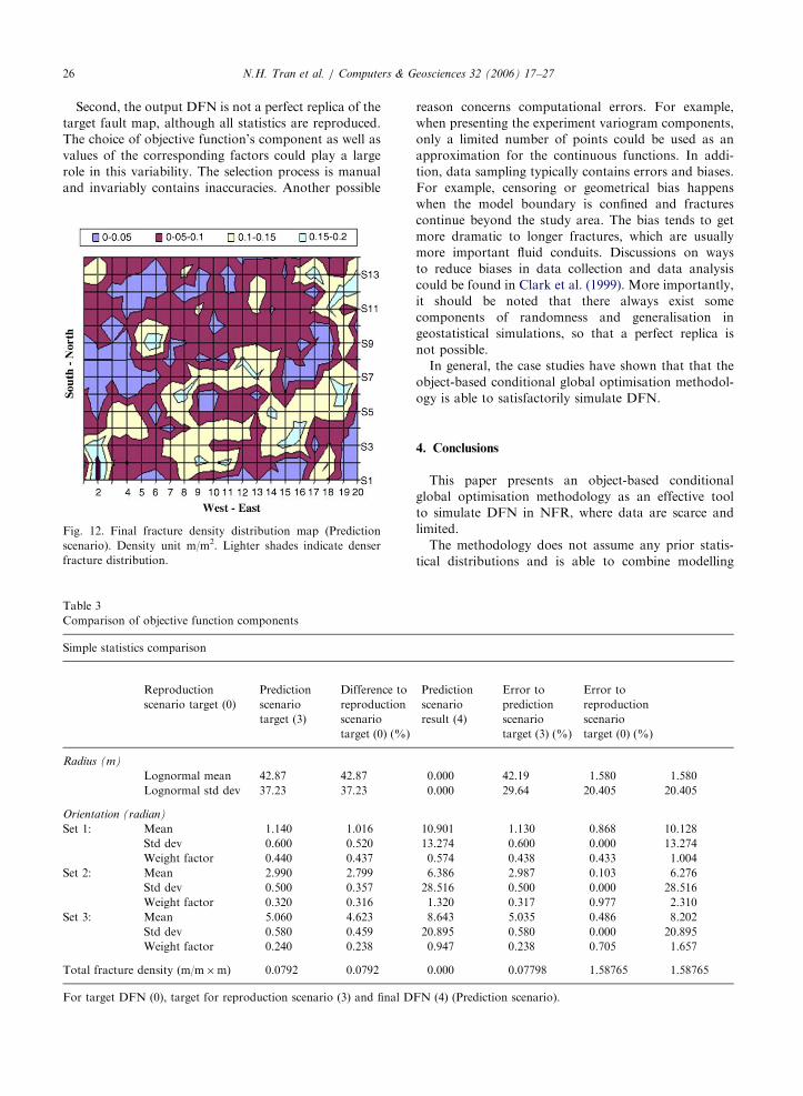
density distribution are displayed in Figs. 11 and 12.

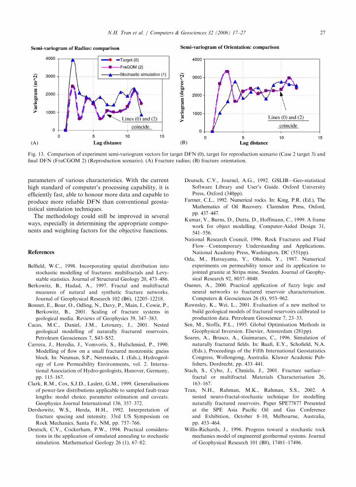
Table 3 and Fig. 13 compare the prediction results with

the target statistical and spatial measurements. One

could notice few dissimilarities and errors, which

originates from the lack (or rather inaccuracy) of data

available. The predicted DFN could be considered

statistically well-matched with the target fault map.

3.4. Critical observations

From the results of this study, a number of issues have

been identified. First, the optimisation program is

computationally intensive and required some trial and

error to fine-tune the objective function’s components

and their weighting factors. Any indicators (geostatis-

tical, statistical or global) can be incorporated, if they

are representative to the target data and mathematically

assessable (easily computable). For a set of components,

a sensitivity analysis is needed to pick the corresponding

weighting factors. Although the chosen combination

of the objective function has been tested and validated,

finding more appropriate components could be the

scope of future research.


Second, the output DFN is not a perfect replica of the

target fault map, although all statistics are reproduced.

The choice of objective function’s component as well as

values of the corresponding factors could play a large

role in this variability. The selection process is manual

and invariably contains inaccuracies. Another possible

Fig. 12. Final fracture density distribution map (Prediction



Table 3

Comparison of objective function components

Simple statistics comparison

Reproduction

scenario target (0)

Prediction

scenario

target (3)

Difference to

reproduction

scenario

target (0) (%)

Radius (m)

Lognormal mean 42.87 42.87

Lognormal std dev 37.23 37.23

Orientation (radian)

Set 1: Mean 1.140 1.016

Std dev 0.600 0.520

Weight factor 0.440 0.437

Set 2: Mean 2.990 2.799

Std dev 0.500 0.357


Set 3: Mean 5.060 4.623

Std dev 0.580 0.459


Total fracture density (m/m�m) 0.0792 0.0792

For target DFN (0), target for reproduction scenario (3) and final D

reason concerns computational errors. For example,

when presenting the experiment variogram components,

only a limited number of points could be used as an

approximation for the continuous functions. In addi-

tion, data sampling typically contains errors and biases.

For example, censoring or geometrical bias happens

when the model boundary is confined and fractures

continue beyond the study area. The bias tends to get

more dramatic to longer fractures, which are usually

more important fluid conduits. Discussions on ways

to reduce biases in data collection and data analysis

could be found in Clark et al. (1999). More importantly,

it should be noted that there always exist some

components of randomness and generalisation in

geostatistical simulations, so that a perfect replica is

not possible.

In general, the case studies have shown that that the

object-based conditional global optimisation methodol-

ogy is able to satisfactorily simulate DFN.

4. Conclusions

This paper presents an object-based conditional

global optimisation methodology as an effective tool

to simulate DFN in NFR, where data are scarce and

limited.

The methodology does not assume any prior statis-

tical distributions and is able to combine modelling

Prediction

scenario

result (4)

Error to

prediction

scenario

target (3) (%)

Error to

reproduction

scenario

target (0) (%)

0.000 42.19 1.580 1.580

0.000 29.64 20.405 20.405

10.901 1.130 0.868 10.128

13.274 0.600 0.000 13.274

0.574 0.438 0.433 1.004

6.386 2.987 0.103 6.276

28.516 0.500 0.000 28.516

1.320 0.317 0.977 2.310

8.643 5.035 0.486 8.202

20.895 0.580 0.000 20.895

0.947 0.238 0.705 1.657

0.000 0.07798 1.58765 1.58765

FN (4) (Prediction scenario).

ARTICLE IN PRESS

Fig. 13. Comparison of experiment semi-variogram vectors for target DFN (0), target for reproduction scenario (Case 2 target 3) and

final DFN (FraCGOM 2) (Reproduction scenario). (A) Fracture radius; (B) fracture orientation.

N.H. Tran et al. / Computers & Geosciences 32 (2006) 17–27 27

parameters of various characteristics. With the current

high standard of computer’s processing capability, it is

efficiently fast, able to honour more data and capable to

produce more reliable DFN than conventional geosta-

tistical simulation techniques.

The methodology could still be improved in several

ways, especially in determining the appropriate compo-

nents and weighting factors for the objective functions.

References

Belfield, W.C., 1998. Incorporating spatial distribution into

stochastic modelling of fractures: multifractals and Levy-

stable statistics. Journal of Structural Geology 20, 473–486.

Berkowitz, B., Hadad, A., 1997. Fractal and multifractal

measures of natural and synthetic fracture networks.

Journal of Geophysical Research 102 (B6), 12205–12218.

Bonnet, E., Bour, O., Odling, N., Davy, P., Main, I., Cowie, P.,

Berkowitz, B., 2001. Scaling of fracture systems in

geological media. Reviews of Geophysics 39, 347–383.

Cacas, M.C., Daniel, J.M., Letouzey, J., 2001. Nested

geological modelling of naturally fractured reservoirs.

Petroleum Geosciences 7, S43–S52.

Carrera, J., Heredia, J., Vomvoris, S., Hufschmied, P., 1990.

Modelling of flow on a small fractured monzonitic gneiss

block. In: Neuman, S.P., Neretnieks, I. (Eds.), Hydrogeol-

ogy of Low Permeability Environments, vol. 2. Interna-

tional Association of Hydro-geologists, Hanover, Germany,

pp. 115–167.

Clark, R.M., Cox, S.J.D., Laslett, G.M., 1999. Generalisations

of power-law distributions applicable to sampled fault-trace

lengths: model choice, parameter estimation and caveats.

Geophysics Journal International 136, 357–372.

Dershowitz, W.S., Herda, H.H., 1992. Interpretation of

fracture spacing and intensity. 33rd US Symposium on

Rock Mechanics, Santa Fe, NM, pp. 757–766.

Deutsch, C.V., Cockerham, P.W., 1994. Practical considera-

tions in the application of simulated annealing to stochastic

simulation. Mathematical Geology 26 (1), 67–82.

Deutsch, C.V., Journel, A.G., 1992. GSLIB—Geo-statistical

Software Library and User’s Guide. Oxford University

Press, Oxford (340pp).

Farmer, C.L., 1992. Numerical rocks. In: King, P.R. (Ed.), The

Mathematics of Oil Recovery. Clarendon Press, Oxford,

pp. 437–447.

Kumar, V., Burns, D., Dutta, D., Hoffmann, C., 1999. A frame

work for object modelling. Computer-Aided Design 31,

541–556.

National Research Council, 1996. Rock Fractures and Fluid

Flow—Contemporary Understanding and Applications.

National Academy Press, Washington, DC (551pp).

Oda, M., Hatsuyama, Y., Ohnishi, Y., 1987. Numerical

experiments on permeability tensor and its application to

jointed granite at Stripa mine, Sweden. Journal of Geophy-

sical Research 92, 8037–8048.

Ouenes, A., 2000. Practical application of fuzzy logic and

neural networks to fractured reservoir characterisation.

Computers & Geosciences 26 (8), 953–962.

Rawnsley, K., Wei, L., 2001. Evaluation of a new method to

build geological models of fractured reservoirs calibrated to

production data. Petroleum Geoscience 7, 23–33.

Sen, M., Stoffa, P.L., 1995. Global Optimisation Methods in

Geophysical Inversion. Elsevier, Amsterdam (281pp).

Soares, A., Brusco, A., Guimaraes, C., 1996. Simulation of

naturally fractured fields. In: Baafi, E.Y., Schofield, N.A.

(Eds.), Proceedings of the Fifth International Geostatistics

Congress, Wollongong, Australia. Kluwer Academic Pub-

lishers, Dordrecht, pp. 433–441.

Stach, S., Cybo, J., Chmiela, J., 2001. Fracture surface—

fractal or multifractal. Materials Characterisation 26,

163–167.

Tran, N.H., Rahman, M.K., Rahman, S.S., 2002. A

nested neuro-fractal-stochastic technique for modelling

naturally fractured reservoirs. Paper SPE77877 Presented

at the SPE Asia Pacific Oil and Gas Conference

and Exhibition, October 8–10, Melbourne, Australia,

pp. 453–464.

Willis-Richards, J., 1996. Progress toward a stochastic rock

mechanics model of engineered geothermal systems. Journal

of Geophysical Research 101 (B8), 17481–17496.

Integrated conditional global optimisation for discrete fracture network modelling

Documents

Transcript of Integrated conditional global optimisation for discrete fracture network modelling