INFLUENCE OF NOISE ON SUBWAVELENGTH IMAGING OF TWO CLOSE SCATTERERS USING TIME REVERSAL METHOD:...

Progress In Electromagnetics Research, PIER 98, 333–358, 2009

INFLUENCE OF NOISE ON SUBWAVELENGTH IMAG-ING OF TWO CLOSE SCATTERERS USING TIME RE-VERSAL METHOD: THEORY AND EXPERIMENTS

M. Davy

Institut Langevin, ESPCI Paris Tech, CNRS UMR 7587Laboratoire Ondes et AcoustiqueUniversite Denis Diderot Paris10 rue Vauquelin 75231 Paris cedex 05, France

J.-G. Minonzio

Laboratoire Imagerie ParametriqueUMPC Universite Paris 06, UMR 762315 Rue de l’Ecole de medecine, 75006 Paris, France

J. de Rosny, C. Prada, and M. Fink

Institut Langevin, ESPCI Paris Tech, CNRS UMR 7587Laboratoire Ondes et AcoustiqueUniversite Denis Diderot Paris10 rue Vauquelin 75231 Paris cedex 05, France

Abstract—Although classical imaging is limited by the Rayleighcriterion, it has been demonstrated that subwavelength imaging of twopoint-like scatterers can be achieved with probing sensors arrays, evenif the scatterers are located in the far field of the sensors. However,the role of noise is crucial to determine the resolution limit. Thispaper proposes a quantitative study of the influence of noise on thesubwavelength resolution obtained with the DORT-MUSIC method.The DORT method, French acronym for decomposition of the timereversal operator, consists in studying the invariants of the timereversal operator. The method is combined here with the estimatorMUSIC (MUltiple SIgnal Classification) to detect and image two closemetallic wires. The microwaves measurements are performed between2.6GHz and 4GHz. Two wires of λ/100 diameters separated by λ/6are imaged and separated experimentally. To interpret this result in

Corresponding author: M. Davy ([email protected]).

334 Davy et al.

terms of noise level, the analytical expression of the eigenvectors of thetime reversal operator perturbed by the noise is established. We thendeduce the noise level above which the subwavelength resolution fails.Numerical simulations and experimental results validate the theoreticaldevelopments.

1. INTRODUCTION

A dramatic issue for all detection and imaging techniques concernsthe resolution. Here by resolution, we mean the capacity to separatetwo close point-like, or isotropic scatterers. Indeed, in the far fieldapproximation, the diffraction limit is given by the Rayleigh criterion.If the array of probing sensors is used to focus the waves, theclassical resolution is limited by λ/2, where λ is the wavelength ofthe illuminating field. However, some methods lead to overcome thislimit in imaging. Multiple Signal Classification (MUSIC) is one ofthem. This method was investigated by Cheney [1]. Lev-Avri andDevaney combined first Time Reversal and MUSIC to achieve super-resolution [2]. This method is however very sensitive to the noise.Far field subwavelength resolution is consequently very challengingexperimentally.

Without noise, unlimited resolution can be achieved. Neverthelessincreasing the noise level degrades the quality of subwavelengthimaging. Some papers underlined the sensitivity of the DORT-MUSICmethod to the noise level, but, at our knowledge, no systematic studyhas been conducted. In particular no analytical expression of theresolution limit in presence of noise has been provided. The aim ofthis paper is thus to explore the influence of the noise level on thesubwavelength imaging both experimentally and theoretically, usingisotropic electromagnetic scatterers.

The DORT method has been developed in acoustics since 1994 [3].It consists in studying the Time Reversal Invariants (TRI) of the TimeReversal Operator. This latter is built from the inter-element responsesmatrix between an emitting and a receiving array. The DORT methodhas been first applied to detect and focus selectively on differentscatterers in a medium [3]. Till now it has been studied in differentdomains such as radar imaging [4], non-destructive evaluation [5, 6]or underwater acoustics [7]. The studies about the application ofDORT method with microwaves began in 1999 with the work of Tortelet al.. They investigated the role of different polarizations for dielectricscatterers [8]. They showed experimentally that the DORT methodleads to localize dielectric cylinders with a high precision and a lowsensitivity to noise.

Progress In Electromagnetics Research, PIER 98, 2009 335

In 1996, Prada et al. performed the first study of the time reversalinvariants to separate scatterers echoes and focus selectively on eachof them [9]. Regarding subwavelength imaging, in 2003 Prada et al.showed that the DORT method leads to detect two wires distant fromless than half a wavelength [10]. At best, they experimentally resolvedλ/3 distant wires. To achieve such sub-wavelength resolution, theysuggested combining the DORT method with two different non-linearsignal processings: Maximum Likehood and MUSIC (Multiple SignalClassification). The DORT-MUSIC algorithm gave the best results.

In an unpublished work [11], Devaney developed the formalismof DORT-MUSIC method, assuming isotropic scatterers. Specialcare was given to the maximum rank of the DORT matrix. Later,Lehman and Devaney [12] focused on the detection of point-likescatterers using DORT-MUSIC with two distinct arrays: one for theemission and one for the reception. In the same way, Miwa andArai studied MUSIC algorithm in the case of the cross-borehole radararrangement [13]. Baussard introduced a numerical method basedon the recursively applied and projected (RAP) MUSIC to improvedetection and localization of close targets [14]. Besides the early works,most of the surveys on this topic are theoretical and numerical. Alongthe few ones that are experimental, there is the Simonetti’s work [15–17]. The aim was to resolve two 2 small holes with elastic surface wavesor two small scattering with acoustic waves. Simonetti investigated theinfluence of multiple scattering on subwavelength imaging. Howeverthe first interpretation of the results [15] leads to a controversy [18].In all these papers, scatterers are supposed to be isotropic: the rankof the problem is equal to the numbers of scatterers. Consideringthe two small elastic cylinders problem, Minonzio et al. showed theanisotropy of the scattering can modify greatly the singular values [19].That is why scatterers, which scattering is experimentally isotropic, areconsidered in this paper.

The originality of this paper is twofold. First, no microwavesexperiments have been performed with two close point-like scatterers.Second, thanks to the expansion of the singular vectors into powerseries with respect to the noise variance, the super-resolution limitis quantified. Concretely, a criterion describing the noise level abovewhich the subwavelength resolution fails will be worked out. Thiscriterion is very important experimentally to know if subwavelengthresolution can be achieved.

After a brief description of the decomposition of the time reversaloperator in Section 2, the experimental microwave setup is presentedin details in Section 3. In Section 4, the experimental results areshown with two wires separated from less than half a wavelength.

336 Davy et al.

We successfully resolve two copper wires, with λ/200 diameter andseparated by λ/6. Section 5 is devoted to the development of thetheoretical expressions of the Time Reversal Invariants obtained withtwo different antenna arrays: a transmit one and a receive one. InSection 6, thanks to a perturbation approach, the TRI are deducedin presence of external noise. Then the TRI are used to build upthe projection operator that is the heart of the MUSIC method.The theoretical results are then compared to numerical simulationsand to the experiment. It will be shown that the DORT-MUSICsubwavelength imaging imposes the noise to be inferior to a certainlevel given in this paper. From this study, a new resolution criterionis introduced.

2. TIME REVERSAL INVARIANTS AND SINGULARVALUE DECOMPOSITION

In the present paper, as seen in several previous work [5, 12, 20, 21],DORT method is applied to distinct antenna arrays labelled A and B.The number of antennas of arrays A and B are equal to NA and NB,respectively. The receive vector R on array B is linearly linked to thetransmit vector E on array A through the linear relation R = KE. TheNB ×NA matrix K is the frequency dependent matrix containing theinter-element response kij(ω) between element #j of the array A andelement #i of the array B. After time reversal, i.e., phase conjugationof R at one frequency, the signal is emitted back by array B to thearray A. The signal received on array A writes KR∗ which is equal to(KH KE)∗, where superscript ∗, T and H means conjugate, transposeand transpose-conjugate respectively. If array B emits first the signalE, the receive signal on array B after time reversal by array A is(KKHE)∗.

Two matrices KKH and KHK appear, the so-called TimeReversal Operators (TRO). They are diagonalizable because they areHermitian. We write vj the jth eigenvector of KHK and uj . the oneof KKH. These eigenvectors can be interpreted as the Invariants ofthe Time Reversal (TRI) process. For instance, after emission of vj byarray A and time reversal by array B, the signals on array A is simplygiven by λ2

jvj . The time reversal invariants can be also directly workedout from the singular value decomposition (SVD) of the matrix K

K =min(NA,NB)∑

j=1

(uj)λj (vj)H (1)


Hence the singular vectors of matrix K are the eigenvectors of the TRO.As for the singular values, they are the square root of the eigenvalues.

Practically speaking, the K matrix is recorded between a transmit(Tx) array and a receive (Rx) array. The vj will hence be also referredas Tx singular vectors (or Tx-TRI) and the uj the Rx singular vectors(or Rx-TRI).

3. EXPERIMENTAL SETUP

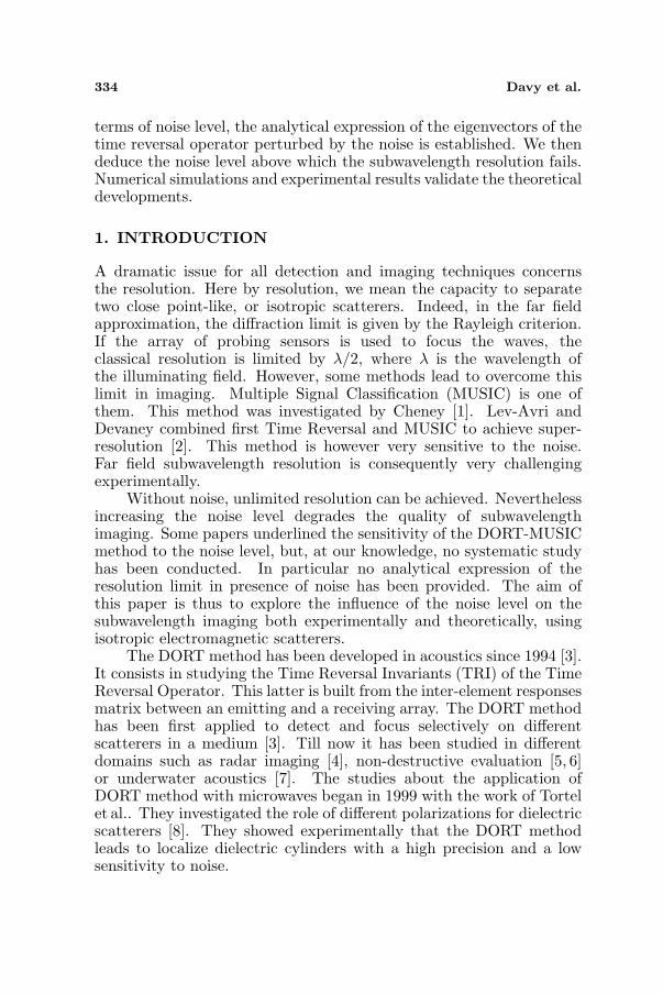
In our experiments, the receiving array is linear and continuous. Theemitting array is also linear but splits into two parts over the bothsides of the receiving array (see Fig. 1). We will see further thatthis configuration is used to improve the imaging from the Rx TimeReversal Invariants.

Two horn antennas, which are 96 cm long and have a 58◦ apertureangle, move along the x-axis on a rail. The antennas are workingbetween 2.6GHz and 4 GHz. They are automated in rotation in orderto take aim to the wires at each position. The response between thefirst and the second antenna is recorded on a vector spectral analyserwith a frequency step of 87.5 kHz. To minimize parasitic echoes, thewall behind the wire is covered with anechoic material. The distance F

Figure 1. Experimental set-up.

338 Davy et al.

from the rail on which the antennas are mounted to the wires is equalto 1.35 m. As the reception array aperture, denoted D, is of the sameorder as F , the resolution λF/D is about λ.

The scatterers consist of two copper wires with 0.6 mm diameter,corresponding to about 1/200λ. The distance 2dx between the twowires is denoted d and ranges from λ/10 to λ/4.

4. EXPERIMENTAL RESULTS

4.1. Singular Values

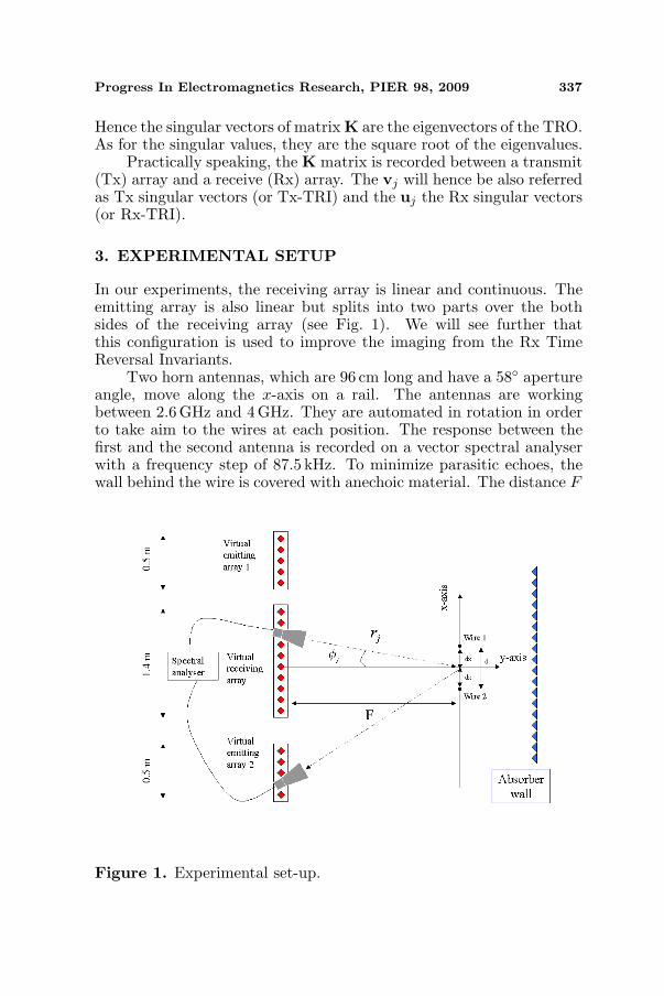
To improve our results, the inter element responses of the mediumwithout the wires are subtracted. Consequently the remainingparasitic echoes are therefore significantly reduced. The plot of thesingular values on Fig. 2 lets appear a dominant one. The secondsingular value λ2 increases with respect to frequency, whereas the thirdone λ3 that keeps steady is attributed to noise. We will see that theratio between the second singular value and the third one, i.e., λ2/λ3,is a key parameter in order to perform sub-wavelength imaging.

4.2. Back-propagation of the Singular Vectors with theMUSIC Algorithm

The resolution of a simple (linear) match filtering method (such asbeamforming) is limited to λ/2. So we choose a non-linear method, theMUSIC algorithm to resolve close wires. The MUSIC method requires

Figure 2. Experimental singular values λn for a distance between thetwo wires d equal to 22 mm.


the knowledge of the medium Green’s function. Considering the systemas equivalent to a bi-dimensional one, the far field expression of theGreen’s function can be approximated by

G(r, r′

)=

√2

iπk |r− r′|eik|r−r′| (2)

In the horizontal plane, the two wires are considered as pointlike andthe field transmitted by the horn antennas is vertically polarized. Asshown in the Appendix of [22], the scattering of a small metalliccylinder in E parallel polarization corresponds to the Dirichletcondition and it is equivalent to the acoustical soft boundary conditionas an air bubble in water. It implies that for diameter small comparedto the wavelength, the scattering is purely isotropic and non negligible.

In such a case, the dimension p of the signal subspace, i.e., therank of K, is equal to the number of scatterers. Here p = 2. TheMUSIC estimator writes:

IMU (r) =1

1−2∑

n=1

∣∣∣⟨un

∣∣∣ G (r)⟩∣∣∣

2(3)

The vector G (r) stands for the normalized vector (G (r) / ‖G (r)‖) andthe ith component of vector G(r) is given by G(r, ri). The antennapositions rj must be accurately known to be able to resolve close wire.

(a) (b)

Figure 3. (a) Normalized classical back-propagation of the firstsingular vector (continuous) and the second one (dashed line). (b)Normalized MUSIC estimators obtained with the two first singularvalues in case of: Two wires (continuous line), left wire (dashed line)and right wire (circle).

340 Davy et al.

In Fig. 3 are plotted the results of the MUSIC estimation obtainedfor 3 configurations: The left wire alone, the right wire alone and bothof them. We see that MUSIC estimator enables to localize the wiresthat are spaced by λ/3.5.

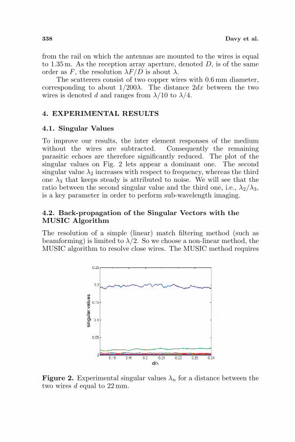
At best, the resolution of wires separated by d = λ/6 is achieved.As it can be seen on Fig. 4, the smaller d is, the weaker the doublemaxima relative amplitude is.

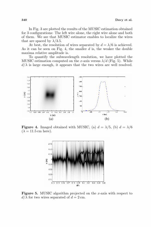
To quantify the subwavelength resolution, we have plotted theMUSIC estimation computed on the x-axis versus λ/d (Fig. 5). Whiled/λ is large enough, it appears that the two wires are well resolved.

(a) (b)

Figure 4. Imaged obtained with MUSIC, (a) d = λ/5, (b) d = λ/6(λ = 11.5 cm here).

Figure 5. MUSIC algorithm projected on the x-axis with respect tod/λ for two wires separated of d = 2 cm.


Two spots appear on the image at the wires location. When d/λdecreases, the interpretation becomes less obvious. Above (d/λ)lim =0.195, the system is no more resolved and only one spot appears onthe image, localized between the two wires.

The two wires are not resolved although the second singular valueis still above the noise background. In the next sections, we propose atheoretical analysis to explain this effect.

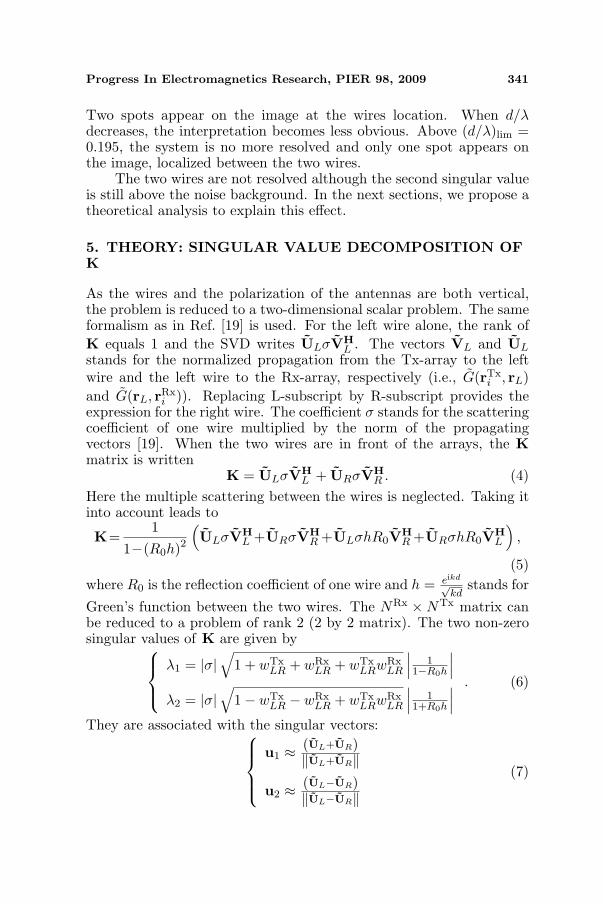
5. THEORY: SINGULAR VALUE DECOMPOSITION OFK

As the wires and the polarization of the antennas are both vertical,the problem is reduced to a two-dimensional scalar problem. The sameformalism as in Ref. [19] is used. For the left wire alone, the rank ofK equals 1 and the SVD writes ULσVH

L . The vectors VL and UL

stands for the normalized propagation from the Tx-array to the leftwire and the left wire to the Rx-array, respectively (i.e., G(rTx

i , rL)and G(rL, rRx

i )). Replacing L-subscript by R-subscript provides theexpression for the right wire. The coefficient σ stands for the scatteringcoefficient of one wire multiplied by the norm of the propagatingvectors [19]. When the two wires are in front of the arrays, the Kmatrix is written

K = ULσVHL + URσVH

R . (4)Here the multiple scattering between the wires is neglected. Taking itinto account leads to

K=1

1−(R0h)2(ULσVH

L +URσVHR +ULσhR0VH

R +URσhR0VHL

),

(5)where R0 is the reflection coefficient of one wire and h = eikd√

kdstands for

Green’s function between the two wires. The NRx ×NTx matrix canbe reduced to a problem of rank 2 (2 by 2 matrix). The two non-zerosingular values of K are given by

λ1 = |σ|√

1 + wTxLR + wRx

LR + wTxLRwRx

LR

∣∣∣ 11−R0h

∣∣∣

λ2 = |σ|√

1− wTxLR − wRx

LR + wTxLRwRx

LR

∣∣∣ 11+R0h

∣∣∣. (6)

They are associated with the singular vectors:

u1 ≈ (UL+UR)‖UL+UR‖

u2 ≈ (UL−UR)‖UL−UR‖

(7)

342 Davy et al.

In Eq. (6), the term wTxLR (resp. wRx

LR) stands for the scalar productsbetween VL and VR (resp. UL and UR). As the distance between thetwo wires decreases, wRx

LR and wTxLR increase towards 1. As a result, the

first singular value increases and the second one decreases. Hence, thesecond one can be very sensitive to noise, which degrades the qualityof the imaging. As the wires are considered to be in the far field fromthe arrays, {

UL

}j

=1√NTx

eikrRxjL (8)

where rRxjL is the distance for Rx-antenna #j and the left wire. Same

expressions are obtained for the right wire and the Tx-array. In thefollowing the Rx superscript is omitted because only the Rx-array isconsidered. In Eq. (8), the aperture of the antennas is not taken intoaccount because the antennas take aim to the wires location. Thanksto the symmetric configuration of the receiving array (Fig. 6), thepositions are well approximated by{

rRj ≈ rj − dx sin (φj)

rLj ≈ rj + dx sin(φj)(9)

From Eqs. (7) and (9) the singular vectors can then be written

u1j = 1

‖UL+UR‖eikrj cos (kdx sin (φj))

u2j = 1

‖UL−UR‖eikrj sin (kdx sin (φj))(10)

Figure 6. Experimental configuration of the Tx-array in front of thetwo wires that are 2dx distant.


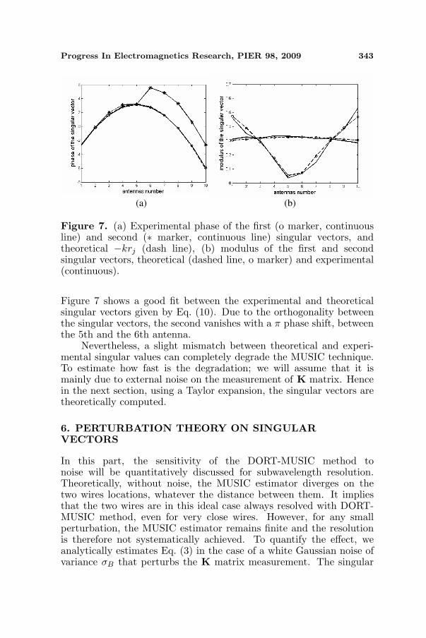
(a) (b)

Figure 7. (a) Experimental phase of the first (o marker, continuousline) and second (∗ marker, continuous line) singular vectors, andtheoretical −krj (dash line), (b) modulus of the first and secondsingular vectors, theoretical (dashed line, o marker) and experimental(continuous).

Figure 7 shows a good fit between the experimental and theoreticalsingular vectors given by Eq. (10). Due to the orthogonality betweenthe singular vectors, the second vanishes with a π phase shift, betweenthe 5th and the 6th antenna.

Nevertheless, a slight mismatch between theoretical and experi-mental singular values can completely degrade the MUSIC technique.To estimate how fast is the degradation; we will assume that it ismainly due to external noise on the measurement of K matrix. Hencein the next section, using a Taylor expansion, the singular vectors aretheoretically computed.

6. PERTURBATION THEORY ON SINGULARVECTORS

In this part, the sensitivity of the DORT-MUSIC method tonoise will be quantitatively discussed for subwavelength resolution.Theoretically, without noise, the MUSIC estimator diverges on thetwo wires locations, whatever the distance between them. It impliesthat the two wires are in this ideal case always resolved with DORT-MUSIC method, even for very close wires. However, for any smallperturbation, the MUSIC estimator remains finite and the resolutionis therefore not systematically achieved. To quantify the effect, weanalytically estimates Eq. (3) in the case of a white Gaussian noise ofvariance σB that perturbs the K matrix measurement. The singular

344 Davy et al.

vectors are expanded in Taylor’s series of the noise variance. The aim isto work out an analytical expression of the noise level above which theMUSIC estimator fails to resolve the wires. In fact, contrary to whatone would expect at first thought, the subwavelength resolution of thetwo wires does not always occurs when the second signal singular valueis higher than the third one associated to noise. We will show that,in the far field limit, an explicit criterion between those two singularvalues can be worked out in order to achieve subwavelength imaging.

To validate the theoretical expressions, they are compared tosimple numerical simulations developed under Matlab. In thenumerical simulations, the propagation between the antennas and thewires are modelled by the Green’s function. The scattering coefficientsof the two wires are equal. An additive white Gaussian noise is added tothe K matrix. The number of antennas of the emitting and receivingarrays is chosen to be large enough to allow a statistical approach(NRx = NTx = N = 100). The wavelength λ equals 0.1m. Thedistance between the wires is noted d, with d = 2dx, and the noisevariance σ2

B. The aperture D of the receiving array is 0.2m, and thewires are located at a distance F = 5 m from the arrays. The distancebetween the wires varies between λ/10 and λ/2 in the simulations.

6.1. Expansion of the Singular Values into ConvergentPower Series

Consider the previous theoretical matrix K perturbed by a noiserandom matrix:

Kp = K + σB∆K =2∑

i=1

(ui)λi(vi)H + σB∆K (11)

From now a p superscript indicates perturbed values to distinguishthem from their unperturbed values. The matrix ∆K is a randommatrix. Its Frobenius norm equals 1. By definition, the Frobeniusnorm of a matrix A is given by:

‖A‖F =√∑

i,j

|Aij |2 (12)

Similarly to Eq. (11), the SVD of K is given by

Kp =N∑

i=1

(up

i

)λp

i

(vp

i

)H (13)

In this section the singular vectors of Kp will be established in orderto use them, in the next section, in the MUSIC estimator. The


perturbation analysis on singular vectors and singular values has beenwell documented in literature [23–27]. The perturbation of the singularvectors that span the signal subspace was especially established at firstand second order [24, 25].

Due to the noise perturbation, the singular vectors can beexpanded into convergent power series of the noise variance. Developedat the second order in small parameter σB, the singular vectors of theperturbed matrix Kp can be written as:

upi = ui + σBw(1)

i + σ2Bw(2)

i + o(σ2

B

)(1 ≤ i ≤ 2) (14)

The approximation made to develop the singular vectors into powerseries and the expression of the vectors w1 and w2 are given inAppendix A. The expected (mean) values of their different componentsare also expressed. Their expected values will be used in the followingto estimate the mean perturbation on the MUSIC estimator.

When the wires are close, we have seen that the first singularvalue is much bigger than second one. As a result, according to theexpression provided par Jun et al. [26], the expected perturbation onthe first singular vector is roughly null at the second order:

up1 ' u1 + o

(σ2

B

)(15)

Only the perturbation on the second singular vector will thensignificantly modify the MUSIC estimator.

6.2. Application to the MUSIC Estimator

To simplify the results of the MUSIC algorithm, let us define the Lfunction as:

L(G (r)

)=

∣∣∣⟨up

1

∣∣∣ G (r)⟩∣∣∣

2+

∣∣∣⟨up

2

∣∣∣ G (r)⟩∣∣∣

2. (16)

L represents the square of the distance of G from the subspace builtfrom u1 and u2. Then the MUSIC estimator becomes:

IMU

(G (r)

)=

1

1− L(G (r)

) (17)

The IMU estimator only increases the contrast of the L estimatorthanks to a strong non-linear relation. In the upcoming calculations,we use UL, UR as in the previous section. Furthermore, we define UM

as the propagating vector between the receiving array and the positionexactly between the two wires. Indeed, we will show that the wires arenot anymore resolved when the expected value on the wires becomesinferior to the expected value between the wires.

346 Davy et al.

The vector UL can be expressed in terms of the signal subspace{u1,u2} as:

UL =12

(u1

∥∥∥UL + UR

∥∥∥ + u2

∥∥∥UL − UR

∥∥∥)

(18)

with∥∥∥UL + UR

∥∥∥ =√

2 (1 + w) and∥∥∥UL − UR

∥∥∥ =√

2 (1− w). The

scalar w stands for the scalar cross product between UL and UR, w isreal in the far field approximation.

The expected value of the estimator L applied to the vectors UL

can now be calculated. The first order perturbation has no effect onthe mean value of L. The expected value of L is computed at thesecond order in Appendix A. It leads to

E[L

(UL

)]=

1 + w

2+

1− w

2

(1− (N − 2)σ2

B

λ22

)+ o

(σ2

B

). (19)

The expected value of L(UL) decreases from 1 when noise increases.Between the two wires, the contribution of the second singular vector,associated to an antisymetric field, is null, so L(UM ) is given by:

E[L

(UM

)]=

∣∣∣⟨u1

∣∣∣ UM

⟩∣∣∣2

(20)

To express the third singular value, one should use some results of therandom matrix theory. Assuming the noise completely decorrelatedfrom antenna to antenna, the singular values λn of which index islarger than 2 are the same ones, in a statistical point of view, as theones of a (N − 2) ∗ (N − 2) random matrix. The quadrant law givesthe distribution of the singular values of such a matrix. Especially, thelargest singular value (i.e., λ3), is given by:

λ3 = 2√

N − 2σB (21)

Fig. 8 displays the evolution of the L estimator for UM and for UL withrespect to λ3/λ2. The analytical formula in Eq. (19) fits the simulatedcurve very well.

The standard deviation normalized by the mean value of L(UL)is small compared to its expected value (roughly equal to λ2/λ1). As aconsequence, its value in one experimental measurement will be closeto the analytical expected value.

In Paragraph 6.4, the threshold value of λ3 above which the wiresare not anymore resolved will be worked out.


Figure 8. Simulated 1 − L(UM) (continuous) and 1− L(UL) (dots)compared to the analytical formula in (19) (markers). The simulationparameter d is: d = 0.39λ.

6.3. Estimated Profile

We can also predict the expected profile of the DORT-MUSICestimator between the two wires. For a point of coordinates r =[x, F ], the vector (Ux)i = eik(ri−x sin(φi))√

Nis very close to UL and

UR. Consequently, when computing E[L(Uδ)], the contribution tothe scalar products in (16) mainly comes from the components u1 andu2 (the signal sub-space) of Eq. (14). We neglect in particular thecontribution of the noise subspace perturbation in |〈Ux|up

2〉|2.In such a case, assuming that the wires are in the far-field and

that the array aperture and the step between two antenna positionsare sufficiently small, the L estimator writes from Appendix B:

E[L

(Ux

)]

= 12(1+sinc(kdxD/F ))

[sinc

(k(dx−x)D

2F

)+sinc

(k(dx+x)D

2F

)]2

+ 12(1−sinc(kdxD/F ))

[sinc

(k(dx−x)D

2F

)− sinc

(k(dx+x)D

2F

)]2(1− λ2

3

4λ22

)

(22)This formula is consistent with the expected values computedpreviously. Using Eq. (22), the DORT-MUSIC image can be built. Thecomparison between numerical simulation and the theoretical shapeconfirms the validity of our approach.

The theoretical IMU is also compared to the experimental resultsin Fig. 10.

348 Davy et al.

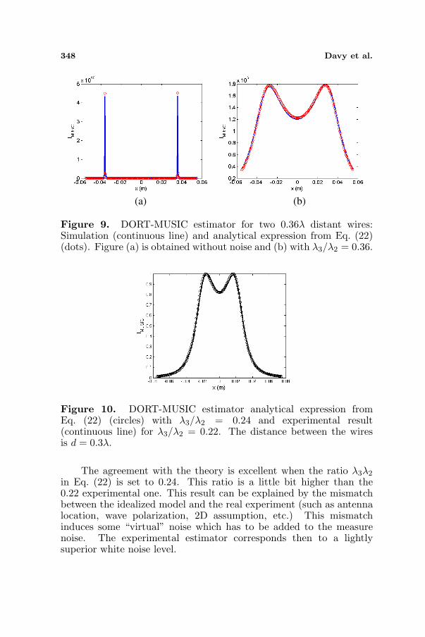
(a) (b)

Figure 9. DORT-MUSIC estimator for two 0.36λ distant wires:Simulation (continuous line) and analytical expression from Eq. (22)(dots). Figure (a) is obtained without noise and (b) with λ3/λ2 = 0.36.

Figure 10. DORT-MUSIC estimator analytical expression fromEq. (22) (circles) with λ3/λ2 = 0.24 and experimental result(continuous line) for λ3/λ2 = 0.22. The distance between the wiresis d = 0.3λ.

The agreement with the theory is excellent when the ratio λ3λ2

in Eq. (22) is set to 0.24. This ratio is a little bit higher than the0.22 experimental one. This result can be explained by the mismatchbetween the idealized model and the real experiment (such as antennalocation, wave polarization, 2D assumption, etc.) This mismatchinduces some “virtual” noise which has to be added to the measurenoise. The experimental estimator corresponds then to a lightlysuperior white noise level.


6.4. Criterion to Resolve the System, Resolution Limit inPresence of Noise

To finish, from a given noise level, the expected value of L on the wiresbecomes inferior to the value between the wires. The subwavelengthresolution cannot then be achieved because only one peak appears onthe image. A resolution criterion can then be introduced:

E[L

(UL

)]> E

[L

(UM

)]. (23)

Using Eqs. (19), (20) and (21), the ratio between the third and thesecond singular value providing the super-resolution limit becomes

λ3

λ2≤ λ3

λ2

∣∣∣∣lim

' 2

√√√√√2(

1−⟨u1|UM

⟩2)

1− w. (24)

However, the expression in Eq. (24) is very general. Assuming thesame small aperture hypothesis used in the previous section, we showin Appendix C that Eq. (24) is simplified into

λ3

λ2

∣∣∣∣lim

=π√15

D

F

d

λ+ o

(D

F

d

λ

). (25)

This linear evolution is displayed in Fig. 11, where the expressionin (25) is compared to numerical simulations.

Figure 11. Simulated (markers) and analytical (continuous line)ratios λ3

λ2

∣∣∣lim

with respect to DF

dλ .

350 Davy et al.

Equation (25) leads to quantify the noise level above which thesubwavelength resolution fails. The main result is that the super-resolution is not achieved when the criterion is not verified evenif the second singular value is higher than third one. Indeed thesecond singular vectors can be too much perturbed in order to achievesubwavelength resolution. Hence, the DORT-MUSIC algorithm is thenvery sensitive to noise. However, for a distance between the wires closeto or larger than λ/2, the super-resolution limit ratio is close to 1, thatmeans the two wires are resolved as soon as the second singular valueemerges from the noise background.

7. DISCUSSION

From Eq. (4), we deduce the transfer response between antenna #iand #j in a free space medium:

Kij = 2eik(rTx

i +rRxj )

rTxi rRx

j

cos

(kdx

(XRx

i

F+

XTxj

F

))(26)

Here, for simplicity, we neglect multiple scattering. The phase of theresponse Kij in Eq. (26) only depends on the barycentre of the wireswhile the distance dx between them only affects the amplitude termthrough the cosine function. Integrating this cosinus function over thewhole array aperture lets appear a sinc function of the distance dxdivided by the resolution cell λF/D. This integral is used to calculatethe scalar product w developed in Appendix B, Eq. (41), which is akey parameter for resolution. As the slope of the sinc function varieslinearly with dx, the sensitivity to a variation of dx also decreaseslinearly with dx. This fact explains the difficulty to separate closetargets. As shown in Eq. (25), the smaller the distance between thewires is, the more sensitive the DORT-MUSIC estimator becomes.

Concretely, two concomitant effects explain this consideration.First, the second singular value decreases when the wires become close,because the scalar product w increases and becomes close to 1 (seeEq. (6)). Second, for a small distance between the wires, followingthe criterion in Eq. (25), the second singular value should be muchlarger than the third one. To understand this point, if we used aclassical beam-forming method for each wires, the two focal spotswould overlap and the level between them would increase when ddecreases. The DORT-MUSIC method overcomes this difficulty bythe way of a strongly non-linear relation. However, the drawback isthe dramatic sensitivity to noise. The subwavelength resolution inpresence of noise becomes thus all the more difficult to achieve that dis small.


Note that the perturbation theory on the singular vectors is stillvalid whether multiple scattering occurs between the wires. Withoutnoise, single scattering and multiple scattering singular vectors are thesame. With noise, multiple scattering can either increase or decreasethe second singular value. Simonetti et al. proposed that multiplescattering can be really helpful in case of large noise levels [17]. Infact, in the case of the DORT-MUSIC method, multiple scattering willonly change the singular values. The interaction between the noiselevel and the associated singular vectors used to image the scatterersis then a key point to achieve super-resolution. As the criterion is stillvalid, multiple scattering will either improve or degrade the resolutionlimit.

In DORT-MUSIC method, a key point concerns the number ofsingular vectors that are taken into account in the signal subspace.It has been shown that including the first noise singular vectorscan improve the DORT-MUSIC. Prada et al. observed that theperformance of the MUSIC algorithm could be improved by selectingthe first seven singular vectors [10], for an emitting-receiving array of128 transducers. Experimentally, we observed a similar phenomenon,whereas the number of antennas was much smaller (N = 10). But thosenoise singular vectors that improved the resolution were not necessarilythe same at each frequency. In fact, the singular vectors up

k, k > 2,of the perturbed matrix Kp depend also on the 2 singular vectors ofthe unperturbed matrix K. Hence the noise subspace contains alsouseful information. This fact explains that including more singularvectors can improve the DORT-MUSIC performances. A future workwill consist in studying the resolution property of the DORT methodcombined with other estimators such as minimum variance or whitenoise constrained where all the singular vectors are taken into accountwith different weight for each of them.

8. CONCLUSION

This study results from the need to interpret experimental resultsobtained with the DORT-MUSIC method applied to two close metallicwires. Hence, the efficiency of the DORT method to image asubwavelength system of two small scatterers has been proved. Thisstudy is based on the analysis of the singular vectors in terms of Taylorpower series. From this analysis, the performance of the DORT-MUSIC method has been studied in details. Special care has beengiven to the limit of the method in terms of signal to noise ratio.Especially it has been shown that even if the second singular value islarger than the noise singular values, it might be still impossible to

352 Davy et al.

resolve the two wires. Our approach has been validated numericallyand experimentally.

ACKNOWLEDGMENT

This work was financially supported by the French Army, DGA/MRIS,under the grant REI — AORTE — #0634002.

APPENDIX A.

Considering that the expansion in power series is valid for

E [‖σB∆K‖F ] ¿∥∥∥∥∥

2∑

i=1

(ui)λi(vi)H∥∥∥∥∥

F

,

it means that the second order perturbation holds true as long as:

NσB ¿√

λ21 + λ2

2 (A1)

As we are interested in configurations where the distance between thewires is small compared to the wavelength, the second singular valueλ2 is small compared to the first singular value. The noise variance isalso considered as inferior to the second singular value but of the sameorder: λ1 À λ2 > σB. In such a case, an other hypothesis is done inthe following calculations:

λ21 + λ2

2(λ2

1 − λ22

)2 '1λ2

1

¿ N − 2λ2

2

(A2)

According to the SVD properties (projection on signal subspace andorthogonality of the new singular vectors), the first order perturbationis given by:

w(1)1 =

uH2

(∆KKH + K∆KH

)u1

λ21 − λ2

2

u2

+N∑

k=3

uHk

(∆KKH + K∆KH

)u1

λ21

uk (A3)

w(1)2 =

uH1

(∆KKH + K∆KH

)u2

λ22 − λ2

1

u1

+N∑

k=3

uHk

(∆KKH + K∆KH

)u2

λ22

uk (A4)


Vectors w(1)1 and w(1)

2 are composed of two contributions: the firstone stands for the contribution of the signal subspace (generated byu1 and u2), whereas the second one for the contribution of the “noise”subspace. This last one is responsible of the degradation of the MUSICestimator.

Considering the expected value of their components, Jun Liu et al.in [26] showed that:

E[⟨

w(1)2 |u1

⟩]= 0 (A5)

E

[∥∥∥⟨w(1)

2 |u1

⟩u1

∥∥∥2]

=λ2

1 + λ22(

λ21 − λ2

2

)2 ≈ 0 (A6)

E

∥∥∥∥∥N∑

k=3

⟨w(1)

2 |uk

⟩uk

∥∥∥∥∥

2 =

N − 2λ2

2

, (A7)

where E stands for the expected value (mean). Due to theapproximation made in Eq. (A2), the expected signal subspacecontribution on the second singular vectors perturbation in Eq. (A6)is far less than the one of the noise subspace, expressed in Eq. (A7).

The second order expansions of up1 and up

2 are much more complex.The exact expression of the second order perturbation is given inreference [25]. Nevertheless w(2)

1 and w(2)2 can be expressed in terms

of the uk vectors:

w(2)i =

N∑

k=1

akiuk (A8)

For the second singular vector, the two first coefficients at the secondorder are:

a12 =λ1uH

1 ∆Kw(1)2 + λ2uH

1 ∆KHw(1)2 − (λ1c1 + λ2c2)

λ22 − λ2

1

(A9)

a22 = −12

(w(1)

2

Hw(1)

2

)(A10)

where c1 and c2 in Eq. (A9) stands for two coefficients verifyingE[ck] = 0 (1 ≤ k ≤ 2). The other coefficients are not necessary toapply the MUSIC estimator.

Their expected values become:

E [a12] ' 0 and E [a22] = −12

N − 2λ2

2

(A11)

354 Davy et al.

In order to apply the MUSIC algorithm, the norm of the perturbedsingular vectors at the second order has to equal 1. If the norm of thefirst singular vector is obvious, concerning the second one, it verifies:

‖up2‖2 = (up

2/up2)

= 〈u2|u2〉+ 2σB

⟨w(1)

2 |u2

⟩

+ σ2B

(∥∥∥w(1)2

∥∥∥2+ 2

⟨w(2)

2 |u2

⟩)+ o

(σ2

B

)(A12)

As {uk} constitutes an orthonormal basis and due to Eq. (33) andEq. (37), it becomes:

∥∥up2

∥∥2 ' 1 + o(σ2

B

)(A13)

The two wires are then well orthogonal and normalized, even at thesecond order.

APPENDIX B.

If the wires are in the far field and the array pitch sufficiently small,the scalar product between UL and UR becomes:

w ≈ 1N

∫ D/2

−D/2e2ikdx s

Fds

p, (B1)

The integration is done along the x-axis, but we use the index s fornot confounding with the distance dx. It leads to:

w ≈ sinc(

kdD

2F

). (B2)

Moreover, in the same way, the expected value of the scalar productsbetween the singular vectors and Uδ can be computed:

E

[∣∣∣⟨up

1|Ux

⟩∣∣∣2]

=

(√2

1 + w

∫ D/2

−D/2

cos(kdx s

F

)e−ikx s

F

N

ds

p

)2

(B3)

which gives:

E

[∣∣∣⟨up

1|Ux

⟩∣∣∣2]

=1

2 (1 + w)

[sinc

(k (dx− x) D

2F

)+ sinc

(k (dx + x) D

2F

)]2

(B4)


In the same way,

E

[∣∣∣⟨up

2|Ux

⟩∣∣∣2]

=(

1− λ23

4λ22

)(√2

(1− w)

∫ D/2

−D/2

sin(kdx s

F

)e−ikx s

F

Nds

)2

(B5)

which results to

E

[∣∣∣⟨up

2|Ux

⟩∣∣∣2]

=1

2(1− w)

[sinc

(k(dx− x)D

2F

)−sinc

(k(dx + x)D

2F

)]2(1− λ2

3

4λ22

)(B6)

Finally, it leads to

E[L

(Ux

)]

=1

2(1 + w)

[sinc

(k(dx− x)D

2F

)+sinc

(k(dx + x)D

2F

)]2

+1

2(1− w)

[sinc

(k(dx− x)D

2F

)−sinc

(k(dx + x)D

2F

)]2(1− λ2

3

4λ22

)(B7)

This formula gives the expected profile between the two wires.

APPENDIX C.

First we remain that the scalar product of the first singular value ofthe vector of the point between the wires is:

⟨u1|U0

⟩≈

√2

1 + wsinc

(kdx

D

2F

)(C1)

Using Eq. (24) and Eq. (C1), the threshold ratio giving the resolutioncriterion in (24) becomes:

λ3

λ2

∣∣∣∣lim

= 2

√√√√2{

1− 2[sinc

(kdx D

2F

)]2/

[1 + sinc

(kdxD

F

)]}

1− sinc(kdxD

F

) (C2)

By developing the sinc function at the fourth order with respect to(kdxD

F ), we finally obtain:

λ3

λ2

∣∣∣∣lim

=2π√15

D

F

dx

λ+ o

(D

F

dx

λ

)(C3)

356 Davy et al.

REFERENCES

1. Cheney, M., “The linear sampling method and the MUSICalgorithm,” Inverse Problems, Vol. 17, 591–595, 2001.

2. Lev-Ari, H. and A. J. Devancy, “The time-reversal techniquere-interpreted: Subspace-based signal processing for multi-statictarget location,” Sensor Array and Multichannel Signal ProcessingWorkshop, 2000, Proceedings of the 2000 IEEE, 509–513, 2000.

3. Prada, C. and M. Fink, “Eigenmodes of the time reversal operator:A solution to selective focusing in multiple-target media,” WaveMotion, Vol. 20, 151–163, 1994.

4. Kerbrat, E., R. K. Ing, C. Prada, D. Cassereau, and M. Fink,“The D. O. R. T. method applied to detection and imaging inplates using Lamb waves,” Review of Progress in QuantitativeNondestructive Evaluation, 934–940, Ames, Iowa (USA), 2001.

5. Prada, C., M. Tanter, and M. Fink, “Flaw detection in solid withthe D. O. R. T. method,” Ultrasonics Symposium, Vol. 1, 679–683,1997.

6. Kerbrat, E., D. Clorennec, C. Prada, D. Royer, D. Cassereau, andM. Fink, “Detection of cracks in a thin air-filled hollow cylinderby application of the DORT method to elastic components of theecho,” Ultrasonics, Vol. 40, 715–720, 2002.

7. Mordant, N., C. Prada, and M. Fink, “Highly resolved detectionand selective focusing in a waveguide using the D. O. R. T.method,” The Journal of the Acoustical Society of America,Vol. 105, 2634–2642, 1999.

8. Tortel, H., G. Micolau, and M. Saillard, “Decomposition of thetime reversal operator for electromagnetic scattering,” Journal ofElectromagnetic Waves and Applications, Vol. 13, No. 5, 687–719,1999.

9. Prada, C., S. Manneville, D. Spoliansky, and M. Fink,“Decomposition of the time reversal operator: Detection andselective focusing on two scatterers,” The Journal of the AcousticalSociety of America, Vol. 99, 2067–2076, 1996.

10. Prada, C. and J.-L. Thomas, “Experimental subwavelengthlocalization of scatterers by decomposition of the time reversaloperator interpreted as a covariance matrix,” The Journal of theAcoustical Society of America, Vol. 114, 235–243, 2003.

11. Devaney, A. J., “Super-resolution processing of multi-static datausing time reversal and MUSIC,” http://www.ece.neu.edu/facu-lty/devaney/preprints/paper02n 00.pdf.

12. Lehman, S. K. and A. J. Devaney, “Transmission mode time-


reversal super-resolution imaging,” The Journal of the AcousticalSociety of America, Vol. 113, 2742–2753, 2003.

13. Miwa, T. and I. Arai, “Super-resolution imaging for point reflec-tors near transmitting and receiving array,” IEEE Transactionson Antennas and Propagation, Vol. 52, 220–229, 2004.

14. Baussard, A. and T. Boutin, “Time-reversal RAP-MUSICimaging,” Waves in Random and Complex Media, Vol. 18, 151–160, 2008.

15. Simonetti, F., “Multiple scattering: The key to unravel thesubwavelength world from the far-field pattern of a scatteredwave,” Physical Review E (Statistical, Nonlinear, and Soft MatterPhysics), Vol. 73, 036619-13, 2006.

16. Simonetti, F., “Pushing the boundaries of ultrasound imagingto unravel the subwavelength world,” Proceedings of IEEEInternational Ultrasonics Symposium, Vancouver, Canada, 313–316, 2006.

17. Simonetti, F., M. Fleming, and E. A. Marengo, “Illustration of therole of multiple scattering in subwavelength imaging from far-fieldmeasurements,” J. Opt. Soc. Am. A, Vol. 25, 292–303, 2008.

18. De Rosny, J. and C. Prada, “Multiple scattering: The key tounravel the subwavelength world from the far-field pattern of ascattered wave,” Physical Review E (Statistical, Nonlinear, andSoft Matter Physics), Vol. 75, 048601-2, 2007.

19. Minonzio, J.-G., C. Prada, A. Aubry, and M. Fink, “Multiplescattering between two elastic cylinders and invariants of the time-reversal operator: Theory and experiment,” The Journal of theAcoustical Society of America, Vol. 120, 875–883, 2006.

20. Moura, J. M. F. and J. Yuanwei, “Detection by time reversal:Single antenna,” IEEE Transactions on Signal Processing, Vol. 55,187–201, 2007.

21. Moura, J. M. F. and J. Yuanwei, “Time reversal imaging byadaptive interference canceling,” IEEE Transactions on SignalProcessing, Vol. 56, 233–247, 2008.

22. Minonzio, J.-G., M. Davy, J. de Rosny, C. Prada, and M. Fink,“Theory of the time-reversal operator for the dielectric cylinderusing separate transmit and received arrays,” IEEE Transactionson Antennas and Propagation, August 2009.

23. Stewart, G. W., “Perturbation theory for the singular valuedecomposition,” SVD and Signal Processing, II: Algorithms,Analysis and Applications, 99–109, 1990.

24. Xu, Z., “Perturbation analysis for subspace decomposition with

358 Davy et al.

applications in subspace-based algorithms,” IEEE Transactionson Signal Processing, Vol. 50, 2820–2830, 2002.

25. Zhenhua, L., “Direct perturbation method for reanalysis ofmatrix singular value decomposition,” Applied Mathematics andMechanics, Vol. 18, 471–477, 1997.

26. Liu, J., X. Liu, and X. Ma, “First-order perturbation analysisof singular vectors in singular value decomposition,” IEEETransactions on Signal Processing, Vol. 56, 3044–3049, 2008.

27. De Moor, B., “The singular value decomposition and long andshort spaces of noisy matrices,” IEEE Transactions on SignalProcessing, Vol. 41, 2826–2838, 1993.

INFLUENCE OF NOISE ON SUBWAVELENGTH IMAGING OF TWO CLOSE SCATTERERS USING TIME REVERSAL METHOD:...

Documents

Transcript of INFLUENCE OF NOISE ON SUBWAVELENGTH IMAGING OF TWO CLOSE SCATTERERS USING TIME REVERSAL METHOD:...