Momentum, reversal, and the trading behaviors of institutions
28
Journal of Financial Markets 10 (2007) 48–75 Momentum, reversal, and the trading behaviors of institutions $ Roberto C. Gutierrez Jr. a, , Christo A. Prinsky b a Lundquist College of Business, 1208 University of Oregon, Eugene, OR 97403-1208, USA b College of Business and Economics, 2600 E. Nutwood, Suite 1060, California State University, Fullerton, CA 92831, USA Available online 1 December 2006 Abstract We identify two types of momenta in stock returns—one due to returns relative to other stocks and one due to firm-specific abnormal returns, where abnormal is determined by a stock’s idiosyncratic return variation. Despite similar performances over the first year, these momentum portfolios perform dramatically differently beyond year one. Relative-return momentum reverses strongly; abnormal-return momentum continues for years. This complexity in return momentum challenges the current theories of momentum. We propose that both momenta are consequences of agency issues in the money management industry and provide empirical support for this economic rationale of momentum in returns. Incentives induce institutions to chase relative returns and to underreact to firm-specific abnormal returns. r 2006 Elsevier B.V. All rights reserved. JEL classification: G14; G11; G20 Keywords: Momentum; Reversal; Institutions; Money manager incentives ARTICLE IN PRESS www.elsevier.com/locate/finmar 1386-4181/$ - see front matter r 2006 Elsevier B.V. All rights reserved. doi:10.1016/j.finmar.2006.09.002 $ We thank John Chalmers, Jennifer Conrad, Mike Cooper, Larry Dann, Diane Del Guercio, Greg Kadlec, Eric Kelley, Wayne Mikkelson, Megan Partch, Jon Reuter, and Avanidhar Subrahmanyam (Editor) for their helpful comments as well as numerous participants in seminars at the Chicago Quantitative Alliance Fall 2002 Conference, the 2003 Pacific Northwest Finance Conference at the University of Washington, Penn State University, Purdue University, Rice University, Southern Methodist University, Texas A&M University, Tulane University, University of Arizona, University of Georgia, and University of Oregon. Part of this study was completed while both authors were on faculty at Mays Business School, Texas A&M University. Any errors are ours. Corresponding author. Tel.: +1 541 346 3254; fax: +1 541 346 3341. E-mail address: [email protected] (R.C. Gutierrez Jr.).
-
Upload
independent -
Category
Documents
-
view
1 -
download
0
Transcript of Momentum, reversal, and the trading behaviors of institutions

ARTICLE IN PRESS
Journal of Financial Markets 10 (2007) 48–75
1386-4181/$ -
doi:10.1016/j
$We than
Eric Kelley,
helpful comm
Conference,
University, P
University, U
completed wh
ours.�CorrespoE-mail ad
www.elsevier.com/locate/finmar
Momentum, reversal, and the trading behaviorsof institutions$
Roberto C. Gutierrez Jr.a,�, Christo A. Prinskyb
aLundquist College of Business, 1208 University of Oregon, Eugene, OR 97403-1208, USAbCollege of Business and Economics, 2600 E. Nutwood, Suite 1060, California State University, Fullerton,
CA 92831, USA
Available online 1 December 2006
Abstract
We identify two types of momenta in stock returns—one due to returns relative to other stocks and
one due to firm-specific abnormal returns, where abnormal is determined by a stock’s idiosyncratic
return variation. Despite similar performances over the first year, these momentum portfolios
perform dramatically differently beyond year one. Relative-return momentum reverses strongly;
abnormal-return momentum continues for years. This complexity in return momentum challenges
the current theories of momentum. We propose that both momenta are consequences of agency
issues in the money management industry and provide empirical support for this economic rationale
of momentum in returns. Incentives induce institutions to chase relative returns and to underreact to
firm-specific abnormal returns.
r 2006 Elsevier B.V. All rights reserved.
JEL classification: G14; G11; G20
Keywords: Momentum; Reversal; Institutions; Money manager incentives
see front matter r 2006 Elsevier B.V. All rights reserved.
.finmar.2006.09.002
k John Chalmers, Jennifer Conrad, Mike Cooper, Larry Dann, Diane Del Guercio, Greg Kadlec,
Wayne Mikkelson, Megan Partch, Jon Reuter, and Avanidhar Subrahmanyam (Editor) for their
ents as well as numerous participants in seminars at the Chicago Quantitative Alliance Fall 2002
the 2003 Pacific Northwest Finance Conference at the University of Washington, Penn State
urdue University, Rice University, Southern Methodist University, Texas A&M University, Tulane
niversity of Arizona, University of Georgia, and University of Oregon. Part of this study was
ile both authors were on faculty at Mays Business School, Texas A&M University. Any errors are
nding author. Tel.: +1 541 346 3254; fax: +1 541 346 3341.
dress: [email protected] (R.C. Gutierrez Jr.).

ARTICLE IN PRESSR.C. Gutierrez Jr., C.A. Prinsky / Journal of Financial Markets 10 (2007) 48–75 49
1. Introduction
Momentum in stock returns presents one of the strongest challenges to the efficiency andrationality of financial markets. Why does buying stocks with the highest returns over theprior six to twelve months and shorting stocks with the lowest returns generate robustprofits?1 Thus far, risk-based explanations have had little empirical success. As aconsequence, most theories of momentum rely on behavioral and cognitive biases ofinvestors.2
We present findings that challenge the most prominent theories of momentum whileproviding support for a new agency-based rational explanation suggesting that institutionsplay a role in generating momentum in returns. First, we document that there are twotypes of momenta—one due to returns relative to other stocks and one due to firm-specificabnormal returns, where abnormal is determined by a stock’s own idiosyncratic returnvariation. Our motivation for isolating these types of momenta is based on two findings inthe literature. One, the profits to the standard relative-return momentum portfolios reverseon average in the long run (two to five years after formation), suggesting an overreactionto relative returns. Two, abnormal returns following corporate events such as earningssurprises, dividend changes, share repurchases, stock splits, and seasoned equity offeringscontinue for years without reversing, suggesting an underreaction to firm-specific news.3
Consistent with these other results, the two types of momenta we identify performdramatically differently after the first year of their holding periods, revealing a complexityto momentum that current theories cannot accommodate. Second, we show that thetrading of institutions contributes to both types of momenta in ways that are consistentwith their incentives as money managers, thereby supporting an economic rationale formomentum in returns. Agency issues provide a parsimonious and rational theory ofmomentum that is consistent with our new empirical facts.
To examine the two types of momenta, we construct portfolios based on firm-specificabnormal returns and raw returns independently and then separate the stocks withabnormal-return momentum from the stocks with relative-return momentum. Relative-return-momentum stocks are identified as those in the extreme deciles of prior six-monthreturns, as introduced by Jegadeesh and Titman (1993). Abnormal-return-momentumstocks are identified as those with firm-specific residual returns more than one standarddeviation from zero. Both momentum portfolios generate significant and robustprofitability in the first twelve months of their holding periods. We find that relative-return momentum reverses strongly in months thirteen through sixty with average profitsaround negative 40 basis points per month. In contrast, abnormal-return momentum
1Following Jegadeesh and Titman’s (1993) seminal study, Rouwenhorst (1998, 1999), Griffin et al. (2005),
Grundy and Martin (2001), and Schwert (2003) find momentum in stock returns throughout the world, in U.S.
returns before 1960, and even in U.S. returns after the publication of Jegadeesh and Titman’s (1993) results.2Fama and French (1996), Moskowitz (2003), Cooper et al. (2004), and Liu et al. (2003) find that momentum
cannot be captured by various measures of factor risks. Lewellen and Shanken (2002) and Brav and Heaton (2002)
note that rational learning under uncertainty can generate momentum, but this theory has yet to be tested. Chan
et al. (1996) and Grinblatt and Han (2005) suggest that momentum is due to underreaction to firm-specific news.
On the other hand, Daniel et al. (1998), Hong and Stein (1999), and Barberis et al. (1998) suggest that momentum
is due to overreaction to firm-specific news.3Lee and Swaminathan (2000) and Jegadeesh and Titman (2001) find long-run reversal for momentum
portfolios. A list of studies finding post-event continuation in returns is provided in the appendix of Daniel et al.
(1998). In addition, Chan (2003) finds long-run continuation in returns following headline media news.

ARTICLE IN PRESSR.C. Gutierrez Jr., C.A. Prinsky / Journal of Financial Markets 10 (2007) 48–7550
persists on average for at least four years, generating profits in months thirteen throughsixty around positive 20 basis points per month. The five-year difference in cumulativereturns across the abnormal-return-momentum and relative-return-momentum portfoliosis roughly 30%, revealing a stark distinction between abnormal-return and relative-returnmomenta.The finding of two types of momenta is important for several reasons. First, we find that
the long-run profitability of momentum portfolios depends critically on the type ofmomentum present. Relative-return momentum reverses and is consistent with over-reaction. Abnormal-return momentum persists and is consistent with underreaction.Current theories do not predict these differences. Second, the long-run momentum inabnormal returns extends the empirical evidence of underreaction to firm-specific newsbeyond the distinct news announcements in corporate events and media headlines. We findthat underreaction extends more broadly to include even the firm-specific informationcaptured in returns. Such a pervasive phenomenon deserves further attention and suggestsan avenue of research away from event-specific explanations of underreaction.We continue our analysis by examining how changes in the institutional ownership of
stocks relate to our momentum findings. Do institutions overreact to extreme relativereturns and underreact to firm-specific abnormal returns? First, we find that institutionsbuy relative-return winners and sell relative-return losers at rates far above average, butinstitutions buy abnormal-return winners and sell abnormal-return losers as if they wereany other stock. These results suggest that institutions chase relative returns, possiblyresulting in an overreaction, but institutions ignore firm-specific abnormal returns,possibly resulting in an underreaction. Second, we examine how changes in institutionalownership affect the profits of each type of momentum portfolio. We find that the relative-return-momentum stocks that institutions most support (i.e., winners they buy the most ofand losers they sell the most of) reverse strongly in the long run, while the relative-return-momentum stocks that institutions least support (i.e., winners they buy the least of andlosers they sell the least of) do not reverse. This variation in long-run profits is consistentwith institutions’ overreacting to relative returns. On the other hand, the abnormal-return-momentum stocks that institutions least support display momentum that persists for years,while the abnormal-return-momentum stocks that institutions most support do not. Thisvariation in profits is consistent with institutions’ underreacting to firm-specific abnormalreturns. In sum, institutions are empirically linked to both types of momenta.We propose that the incentives of money managers can induce managers to underreact
to firm-specific abnormal returns and to overreact to relative returns. Lakonishok et al.(1994), Shleifer and Vishny (1997), and others note that agency issues in delegated moneymanagement can have consequences for asset pricing. The general notion is that, on onehand, institutions keep their portfolios near a market index, for reputation and careerconcerns, which hinders managers from fully exploiting firm-specific information, possiblygenerating an underreaction to firm-specific news. On the other hand, when institutions dodeviate from an index, they tend to tilt toward stocks with higher prior returns becausetheir clientele demands relative returns. Chasing relative returns may generate anoverreaction.4 Our analysis of institutional trading supports these agency explanations
4Chan et al. (2002) document that mutual funds tend to cluster near an index but deviate in the direction of
stocks with higher prior returns. Gruber (1996), Sirri and Tufano (1998), and Del Guercio and Tkac (2002)
ARTICLE IN PRESSR.C. Gutierrez Jr., C.A. Prinsky / Journal of Financial Markets 10 (2007) 48–75 51
of momentum in returns and dovetails with the recent literature on the limits of arbitrage,surveyed by Barberis and Thaler (2003).
Throughout the paper we consider numerous robustness checks of our findings. Withregard to the construction of our abnormal-return-momentum portfolios, we considersingle-index and multifactor models of expected returns to estimate abnormal returns aswell as several ways of defining abnormal-return winners and losers. With regard to theperformance evaluation of our momentum portfolios, we employ several unconditionalfactor models, conditional versions of the CAPM, estimates of an empirical stochasticdiscount factor similar to Chen and Knez (1996), and size-and-book-to-market-matchedreturns. To alleviate concerns that the changes in portfolio composition each month mightresult in changes in risk that we are not otherwise capturing, we also use the average of thefactor loadings from the individual stocks as the proxies for potentially dynamic portfolioloadings. With regard to robustness across stock size, we examine equal-weighted andvalue-weighted portfolios as well as large-stock subsets. Our findings are robust across allthese alternatives and across subperiods.
In Section 2, we define abnormal-return momentum and examine the profits toabnormal-return-momentum portfolios. We highlight the disparate performances ofrelative-return momentum and abnormal-return momentum in Section 3. In Section 4, weexamine the relations between institutional trading, momentum, and long-run reversal.Section 5 presents robustness checks of the momentum and reversal patterns, and Section 6provides characteristics of the stocks in the various momentum portfolios we construct.We conclude in Section 7.
2. Isolating momentum due to abnormal returns
Our sample is constructed from all stocks traded on the NYSE, AMEX, and NASDAQfrom 1960 through 2000. For all portfolios, the first holding period begins January of 1963.We exclude stocks priced below $5 at the end of the formation periods to reducemicrostructure concerns.
2.1. Construction of the abnormal-return momentum portfolios
The momentum first identified by Jegadeesh and Titman (1993) is based on relative rawreturns. Stocks with the highest returns are the winners and are held in a long position;stocks with the lowest returns are the losers and are held in a short position. As noted inthe introduction, we seek to compare momentum due to relative returns with momentumdue to firm-specific abnormal returns (i.e., firm-specific news). To do so, we first mustestimate abnormal returns. Using a market-index model, we calculate the firm-specificreturn of a given stock.
For each stock i and each month t, we estimate Eq. (1) over the previous five years:½t� 60; t� 1�, requiring at least 24 monthly observations during that window.
rit � rft ¼ ai þ biðrMt � rftÞ þ �it, (1)
(footnote continued)
examine capital flows into mutual funds and find that fund investors chase relative returns in addition to, or
possibly in lieu of, risk-adjusted (firm-specific) returns.

ARTICLE IN PRESSR.C. Gutierrez Jr., C.A. Prinsky / Journal of Financial Markets 10 (2007) 48–7552
where rit is the return on stock i in month t, rft is the one-month T-bill rate in month t, rMt
is the return on the CRSP value-weighted index in month t, ai and bi are parameters to beestimated, and �it is the residual return for stock i in month t. Afterwards, we calculate thefirm-specific abnormal return of the stock in month t based on the estimated parameters.
�it ¼ rit � rft � ai � biðrMt � rftÞ. (2)
For each stock and each month, this procedure identifies two quantities, the residualreturn of the stock in month t, �it, and the estimated variance of the residual over the priorfive years, s�2it. Note that the alpha from the estimation period serves as a general controlfor misspecification in the model of expected returns. We have also estimated residualsusing the Fama and French (1993) three-factor model, using a two-factor model comprisedof the market portfolio and the appropriate industry portfolio for stock i from the 48industry portfolios of Fama and French (1997), and using a sixty-month moving averageof an individual stock’s return.5 The findings are unchanged.We identify abnormal-return winners and losers over the J-month formation period½t� J; t� 1� by first cumulating the monthly residual returns of each stock over the J
months and also cumulating the variances of the monthly residuals over the J months. Theparameters of (1) and the stock-specific return variances are updated each month over theJ-month formation period. Stock i is a J-month winner during months ½t� J; t� 1� if itscumulative residual return over the period is greater than or equal to the square root ofits cumulative variance. Stock i is a J-month loser during months ½t� J; t� 1� if itscumulative residual return over the period is less than or equal to the negative square rootof its cumulative variance. Standardizing the residual return yields an improved measure ofthe extent to which a given firm-specific return shock is actually news, as opposed to noise,thereby facilitating a better interpretation of the residual as firm-specific information. Weuse the one-standard-deviation threshold to maintain a sufficient number of stocks permonth in subsequent analyses, but we have also implemented the strategies based on one-and-a-half and two standard deviations, and all findings remain unchanged. In short,abnormal-return momentum behaves consistently no matter how we measure it.Following the above procedure, we identify two groups of stocks, abnormal-return
winners and abnormal-return losers, and we hold them for K months, ½tþ 1; tþ K �; werefer to these months as the holding period. We skip a month between the formationperiod and the holding period to mitigate the negative serial correlation due to bid-askbounce. Following Jegadeesh and Titman (1993), we employ a calendar-time method toincrease the power of the tests but to avoid the pitfalls induced by overlapping returns. Inany particular calendar month, we identify K portfolios of winner and loser stocksrespectively. Each of the K portfolios represents a different vintage of the J-month strategywhich is currently open in that month. The return in a given calendar month is the equally-weighted return of the component stocks across the K portfolios. This produces a time-series of monthly returns to the respective winner and loser portfolios for the holdingperiod ½tþ 1; tþ K �. Afterwards, we subtract the return of the loser portfolio each monthfrom the return of the winner portfolio. The resulting profits represent a zero-cost tradingstrategy which is long in the winners and short in the losers.
5We thank Kenneth French for providing these data on his website. The definitions of the industries are
provided on the website as well.

ARTICLE IN PRESSR.C. Gutierrez Jr., C.A. Prinsky / Journal of Financial Markets 10 (2007) 48–75 53
Our measure of firm-specific abnormal return differs from raw return by a function of ai,s�i
, and bi, though bi is not expected to generate any cross-sectional differences. For thosereaders who are already wondering about the relative extent to which ai and s�i
drive theforthcoming results, we can state that both measures contribute to our findings, with ai
playing the larger role. In addition, we can confirm that our results are qualitatively similarif we do not standardize the residual return and instead define abnormal-return winnersand losers using a cross-sectional decile sort of residual returns. Measuring expectedreturns with ai estimated over only the prior 12 months or with ai set to zero also generatesqualitatively similar results to those reported in later sections.
2.2. Performance evaluation
We consider various formation and holding periods for the abnormal-return momentumportfolios (and the relative-return momentum portfolios defined later). To evaluateperformance during the holding period, we follow the calendar-time procedure ofJegadeesh and Titman (1993) which is also the long-run procedure recommended for theevent-study literature by Fama (1998) and Mitchell and Stafford (2001). Since there is noclear consensus on what model of expected returns is best, though, we consider a widevariety. In the tables, we report three performance metrics: raw returns, CAPM alphas,and Fama and French (1993) three-factor alphas. We also evaluate portfolio performanceusing a conditional CAPM, a conditional CAPM with human capital, and severalestimates of the stochastic discount factor of Chen and Knez (1996). The findings areunchanged and are not provided for the sake of brevity. These alternative models ofexpected returns are detailed in Sections A.1, A.2, and A.3 of the Appendix.
Mitchell and Stafford (2001) raise additional concerns regarding long-run performanceevaluation. Following their suggestions, we address potential concerns. First, we controlfor the inability of the Fama-French three-factor model to fully explain average returnsacross size and book-to-market categories (for example, small value stocks) by subtractingthe returns to matching size/book-to-market stocks from the returns of the selectedmomentum stocks. Second, the factor loadings of the momentum portfolio might changeover time as the composition of the portfolio changes. We allow for this by using averagefactor loadings of the individual stocks comprising each portfolio as proxies for theportfolio’s loadings. Third, we consider value-weighted portfolios as well as equal-weighted portfolios. The inferences about abnormal profit spreads between winner andloser stocks documented in the upcoming tables are unaffected by the comprehensive set ofperformance-evaluation procedures we consider, and are not provided for brevity’s sake.Different procedures, however, can affect inferences on whether the winners or the losersare primarily responsible for the abnormal return spread between the two sets of stocks.Details of the matching technique and of the factor-loadings procedure are provided inSections A.4 and A.5 of the Appendix. In short, our findings for abnormal-returnmomentum and for relative-return momentum are remarkably robust.
2.3. Momentum profits of abnormal-return portfolios
We begin our examination by documenting the performances of portfolios of stocksexperiencing firm-specific abnormal returns (denoted as ‘‘ABN’’) for J ¼ 6 and J ¼ 12.Table 1 displays the performances of these portfolios during three holding periods

ARTICLE IN PRESS
Table 1
Abnormal-return momentum
For each stock i and each month t, we estimate Eq. (1) over the previous five years: ½t� 60; t� 1�, requiring at
least 24 monthly observations. We obtain the residual return of the stock using Eq. (2). To identify abnormal
performance over the J-month formation period ½t� J ; t� 1�, we first cumulate the residual monthly returns of
each stock over the J months and cumulate the variances of the monthly residuals over the J months. Winner
(loser) stocks over months ½t� J ; t� 1� are identified when the cumulative residual return over the period is
greater (less) than or equal to the square root (negative square root) of its cumulative variance. We report below
the performances of the equally-weighted calendar-time portfolios during the holding periods ½tþ 1; tþ K� for
K ¼ 6; 12, and ½tþ 13; tþ K� for K ¼ 60. Panels A and B give the mean performances for the 6-month and 12-
month formation periods ðJ ¼ 6; 12Þ, respectively, over the 1963:01 to 2000:12 period, with the t-statistics in
parentheses. The columns correspond to the three performance metrics and three holding-period windows.
Mean return CAPM alpha Fama-French alpha
Months Months Months Months Months Months Months Months Months
1–6 1–12 13–60 1–6 1–12 13–60 1–6 1–12 13–60
Panel A: Formation period ½�6;�1�Winners� Losers 1.14 0.84 0.03 1.11 0.80 0.03 1.20 0.94 0.09
(8.01) (6.87) (0.65) (7.80) (6.59) (0.59) (8.66) (7.97) (1.87)
Winners 1.26 1.09 0.77 0.66 0.49 0.21 0.53 0.36 �0.01
(4.75) (4.14) (3.13) (5.20) (4.07) (1.92) (8.29) (6.52) (�0.29)
Losers 0.13 0.25 0.74 �0.45 �0.32 0.18 �0.67 �0.57 �0.11
(0.50) (1.00) (2.96) (�3.58) (�2.55) (1.52) (�6.96) (�6.55) (�1.78)
Panel B: Formation period ½�12;�1�Winners� Losers 1.08 0.72 �0.01 1.03 0.68 �0.02 1.22 0.88 �0.06
(6.63) (4.99) (�0.24) (6.34) (4.66) (�0.31) (7.85) (6.43) (�1.01)
Winners 1.24 1.04 0.74 0.62 0.42 0.17 0.55 0.35 �0.04
(4.51) (3.84) (2.99) (4.67) (3.35) (1.60) (7.16) (4.99) (�0.77)
Losers 0.16 0.32 0.75 �0.41 �0.25 0.19 �0.67 �0.53 �0.10
(0.63) (1.24) (3.00) (�3.13) (�1.93) (1.59) (�6.68) (�5.77) (�1.65)
R.C. Gutierrez Jr., C.A. Prinsky / Journal of Financial Markets 10 (2007) 48–7554
½tþ 1; tþ 6�, ½tþ 1; tþ 12�, and ½tþ 13; tþ 60�. In month tþ 1, each of the abnormal-return portfolios contains on average more than 800 stocks, over 400 in the winner andloser component portfolios respectively, which is roughly 15% of the stock universeselected for each side of the portfolio in a given month.6 Including such a large number ofstocks in the portfolios reduces the power of our tests and decreases our ability to findabnormal profits to these strategies since the selected stocks are also components of thefactor-mimicking portfolios used for performance evaluation.Over the 1963:01 to 2000:12 period, the 6-month ABN portfolio, reported in Panel A,
generates significant monthly profits between 0.80% and 1.20% per month during the firstsix and twelve months of the holding period across the three measures of performance.Profits are higher in the first six months. The CAPM alphas and the Fama-French alphasindicate that both sides of the portfolio contribute to the momentum profits. The resultsfor the 12-month ABN portfolio in Panel B are similar.
6The two-standard-deviation filter is much more restrictive. Requiring that each calendar month have at least
10 stocks in the portfolios results in roughly 100 stocks on average in the winner portfolios and 70 stocks on
average in the loser portfolios using the two-standard-deviation filter. So, roughly three percent of the stock
universe is on either side of the portfolio when using the two-standard-deviation filter.

ARTICLE IN PRESSR.C. Gutierrez Jr., C.A. Prinsky / Journal of Financial Markets 10 (2007) 48–75 55
These abnormal-return momentum findings are similar to the relative-return momentumresults of Jegadeesh and Titman (1993) and others. There is a notable difference, however,between abnormal-return momentum identified here and relative-return momentumexamined in prior studies. Jegadeesh and Titman (2001) and Lee and Swaminathan (2000)find that the profits to a six-month relative-return-momentum strategy reverse significantlyfrom two to five years following portfolio formation.7 Panels A and B of Table 1 show thatthe profits to the 6-month and 12-month abnormal-return portfolios do not reverse by anymetric in the long-run holding period of two to five years.
The lack of reversal in abnormal-return momentum suggests that abnormal returns are asource of information for future returns that is separate from relative returns. Examiningonly the first year of the holding periods masks the distinction between abnormal andrelative returns. We fully clarify this distinction in the next section by separating abnormal-return-momentum stocks from relative-return-momentum stocks.
3. Long-run differences between abnormal-return and relative-return momentum
To compare the performances of the abnormal-return-momentum and relative-return-momentum strategies, we must identify the relative-return winners and losers. FollowingJegadeesh and Titman (1993), in each month t, we rank all stocks into deciles based ontheir compounded returns over the formation period ½t� J; t� 1�. We refer to the top-decile stocks as winners and to the bottom-decile stocks as losers, and we hold them for K
months, ½tþ 1; tþ K �. Again, we employ a calendar-time method and also skip one monthbetween the formation period and the testing period. The relative-return (denoted as‘‘REL’’) momentum portfolios are constructed as long positions in the winning stocks andshort positions in the losing stocks.
We then identify three subset portfolios of momentum stocks. The ‘‘REL-only’’portfolio is comprised of the subset of the relative-return portfolio that does not alsoexperience a firm-specific abnormal return during the formation period (i.e., does notexperience a standardized residual greater than or equal to one in absolute value). The‘‘ABN-only’’ portfolio is comprised of the subset of the stocks in the abnormal-return-momentum portfolio from the previous section which are not also in the top or bottomdeciles of lagged returns during the formation period.8 Finally, we identify the‘‘REL\ABN’’ portfolio which is the intersection of the stocks in the relative-return-momentum portfolio with the stocks in the abnormal-return-momentum portfolio. For thesake of brevity, we report only the results for the 6-month formation periods. The 12-month results are very similar. On average, the number of stocks in the REL-only, ABN-only, and REL\ABN portfolios in month tþ 1 is about 150, 440, and 400 respectively,with an equal split between the winner and loser sides for each portfolio.
Table 2 presents the mean profits for the three subset 6-month portfolios (REL-only,ABN-only, and REL\ABN). The REL-only portfolio generates greater profits on averagethan the ABN-only portfolio in the first six months, but this difference is statistically
7These reversal findings are for the full sample. Jegadeesh and Titman (2001) and Lee and Swaminathan (2000)
find that reversal depends on risk adjustments, stock size, subperiods, and trading volume.8There is a handful of stocks throughout the entire sample period that can be classified as ‘‘conflicting’’—a
relative-return winner (loser) with a negative (positive) abnormal return. For example, 35 conflicting stocks are
discovered from 1963 to 2000 in the 6-month-formation-period results. We disregard these stocks.

ARTICLE IN PRESS
Table 2
Subsets of 6-month momentum portfolios
Following the procedure described in Table 1, we identify the abnormal-return winners and losers over the
formation months ½t� 6; t� 1�. We then identify the relative-return winners and losers as the stocks in the highest
(lowest) decile of raw returns over the formation period ½t� 6; t� 1�. We then identify the ‘‘REL-only’’ portfolio
which is comprised of the subset of the relative-return winners and losers that are not also abnormal-return
winners or losers during the formation period. The ‘‘ABN-only’’ portfolio is comprised of the subset of the
abnormal-return winners and losers that are not also in the top or bottom decile of lagged raw returns during the
formation period. Finally, we identify the ‘‘REL\ABN’’ portfolio which is the intersection of the stocks in the
relative-return momentum portfolio with the stocks in the abnormal-return–momentum portfolio. The subset
portfolios are each long in winners and short in losers. We report below the performances of the equally-weighted
calendar-time portfolios during the holding periods ½tþ 1; tþ K� for K ¼ 6, 12 and ½tþ 13; tþK � for K ¼ 60.
Below are the mean performances for the 6-month portfolios, respectively, with the t-statistics in parentheses. The
columns correspond to the three performance metrics and three holding-period windows.
Winners� losers Mean return CAPM alpha Fama-French alpha
Months Months Months Months Months Months Months Months Months
1–6 1–12 13–60 1–6 1–12 13–60 1–6 1–12 13–60
REL-only 1.00 0.48 �0.40 0.97 0.43 �0.43 1.29 0.78 �0.24
(4.78) (2.65) (�4.14) (4.60) (2.40) (�4.43) (6.35) (4.66) (�3.03)
ABN-only 0.70 0.60 0.19 0.70 0.59 0.20 0.66 0.57 0.18
(6.51) (6.59) (3.73) (6.44) (6.47) (3.92) (6.27) (6.35) (3.48)
REL\ABN 1.52 1.06 �0.14 1.49 1.01 �0.15 1.72 1.28 �0.01
(7.36) (6.04) (�1.92) (7.16) (5.75) (�2.16) (8.48) (7.68) (�0.22)
-0.20
-0.15
-0.10
-0.05
0.00
0.05
0.10
0.15
0.20
1 6 11 16 21 31 36 41 46 51 56
Event Month
Cum
ulat
ive
Alp
ha
REL-only REL∩ABNABN-only
26
Fig. 1. Cumulative CAPM alphas of the 6-month subset portfolios. The cumulative performances from the
CAPM are plotted for the 6-month subset portfolios, REL-only, ABN-only, and REL\ABN (described in Table
2) for the 60 months following formation of the portfolios.
R.C. Gutierrez Jr., C.A. Prinsky / Journal of Financial Markets 10 (2007) 48–7556
significant only using the Fama-French alphas (t-statistic of 3.1, not in tables). We see alsothat the REL-only profits dissipate more quickly than the ABN-only profits as evidencedby the large decline in REL-only monthly profits from ½tþ 1; tþ 6� to ½tþ 1; tþ 12�. What

ARTICLE IN PRESSR.C. Gutierrez Jr., C.A. Prinsky / Journal of Financial Markets 10 (2007) 48–75 57
is most revealing, however, are the striking differences in the long-run performances ofthese portfolios. The REL-only portfolio reverses dramatically during months 13 to 60 byall performance measures (�0:24 to �0:43%) while the ABN-only portfolio generatessignificant profits during months 13–60 using all three performance measures (0.18 to0.20%).
So, once we control for the overlap between the relative-return and abnormal-returnportfolios, we find that these two seemingly similar strategies behave dramaticallydifferently. Fig. 1 plots the cumulative CAPM alphas for the subset portfolios based on a6-month formation period.9 The plots of the cumulative mean raw returns and of thecumulative Fama-French alphas are similar. The REL-only portfolio reverses sharply afterthe first year, while the ABN-only profits drift upward for four years before becoming flat.On average after 60 months, the REL-only portfolio generates a cumulative abnormalreturn of �15% while the ABN-only portfolio generates þ15%. The gulf between theirlong-run performances is astounding given that both portfolios are momentum strategiesthat generate relatively similar levels of momentum profits in the short-run.
We also see in Fig. 1 that the short-run momentum profits of the REL\ABN portfolioare markedly higher than the short-run profits of the other two portfolios, and the long-run performance of the REL\ABN portfolio falls between the performances of the othertwo subsets. These findings for the REL\ABN portfolio are detailed in Table 2. Theprofits of the 6-month REL\ABN portfolio during the first twelve months significantlyexceed the profits for both the REL-only and ABN-only groups using the raw, CAPM, andFama-French performance metrics by at least 0.41% per month with a t-statistic of at least3.1 (not in table). This is likely because the formation-period residuals of the REL\ABNstocks are much larger than the residuals of the other two groups; in other words, theformation-period news is larger. The mean residual of the 6-month REL\ABN winners(losers) is 57% ð�45%Þ while those of the REL-only and ABN-only winners (losers) are25% ð�26%Þ and 26% ð�25%Þ, respectively.10 The profits of the REL\ABN portfolioeither reverse mildly or not at all in months 13–60, depending on which performancemeasure is used.
Overall, we find that stocks experiencing firm-specific abnormal returns continue toperform well for several years, once the influence of relative returns is removed.Conversely, the stocks in the relative-return extremes that are without firm-specificabnormal returns display dramatic long-run reversal in returns.11
Additionally, Table 3 shows that both sides of the subset 6-month portfolios (winnersand losers) contribute to the short-run momentum profits of the REL-only, ABN-only,and REL\ABN winners-minus-losers portfolios. Which side contributes more to the
9To produce Fig. 1, we estimate the alphas and betas for each holding-period month in a separate regression,
which means that the profits and losses are robust when allowing the factor loadings to vary month-by-month
through event time.10The average standard deviation of the residuals to the 6-month REL\ABN winners (losers) is 30% (28%), to
the REL-only winners (losers) is 41% (37%), and to the ABN-only winners (losers) is 19% (19%).11Abnormal-return momentum is not simply momentum in less extreme relative returns. Additional tests
confirm this. First, the less extreme REL-only portfolio long in decile 9 of the cross section of prior returns and
short in decile 2, but not containing abnormal-return winners or losers, displays long-run reversal across all three
performance metrics (between �0:25% and �0:11% per month in ½tþ 13; tþ 60�). Second, the ABN-only
portfolio excluding stocks in the cross-sectional deciles 10, 9, 2, and 1 displays long-run momentum across all
three metrics (between 0.23% and 0.31% per month in ½tþ 13; tþ 60�).

ARTICLE IN PRESS
Table 3
Decomposition of 6-month subset momentum portfolios into winners and losers
For the 6-month formation period, we form three subset portfolios, REL-only, ABN-only, and REL\ABN
(described in Table 2). Reported below are the performances of the equally-weighted winner and loser portfolios
during the holding periods ½tþ 1; tþK � for K ¼ 6, 12, and ½tþ 13; tþK � for K ¼ 60. Panels A, B, and C give the
mean performances for the respective subsets, with the t-statistics in parentheses. The columns correspond to the
three performance metrics and three holding-period windows.
Mean return CAPM alpha Fama-French alpha
Months Months Months Months Months Months Months Months Months
1–6 1–12 13–60 1–6 1–12 13–60 1–6 1–12 13–60
Panel A: REL-only
Winners 1.14 0.83 0.56 0.41 0.10 �0.14 0.53 0.21 �0.20
(3.27) (2.47) (1.79) (2.03) (0.55) (�0.88) (4.29) (2.17) (�2.54)
Losers 0.14 0.36 0.96 �0.56 �0.34 0.30 �0.76 �0.57 0.04
(0.40) (1.03) (2.89) (�2.52) (�1.55) (1.43) (�5.51) (�4.48) (0.43)
Panel B: ABN-only
Winners 1.07 1.02 0.85 0.56 0.50 0.35 0.30 0.25 0.05
(4.73) (4.55) (3.88) (5.29) (5.11) (3.56) (5.79) (5.47) (1.02)
Losers 0.37 0.42 0.66 �0.15 �0.09 0.16 �0.36 �0.32 �0.12
(1.63) (1.88) (2.99) (�1.41) (�0.91) (1.61) (�4.18) (�4.03) (�2.10)
Panel C: REL\ABN
Winners 1.42 1.14 0.68 0.73 0.45 0.05 0.74 0.46 �0.10
(4.41) (3.61) (2.40) (4.08) (2.71) (0.35) (6.90) (5.06) (�1.63)
Losers �0.10 0.08 0.82 �0.76 �0.56 0.20 �0.98 �0.82 �0.09
(�0.34) (0.26) (2.82) (�4.52) (�3.46) (1.26) (�7.72) (�7.44) (�1.12)
R.C. Gutierrez Jr., C.A. Prinsky / Journal of Financial Markets 10 (2007) 48–7558
long-run reversal of profits of the REL-only winners-minus-losers portfolio and to thelong-run momentum of the ABN-only winners-minus-losers portfolio is less clear and candepend upon which metric is used. For example, the CAPM alphas indicate that the long-run momentum of the ABN-only winners-minus-losers portfolio is mostly due to thecontinued positive performance of the winners while the Fama-French alphas indicate thatthe momentum is due predominantly to the continued negative performance of the losers.Thus far, we find that momentum from firm-specific abnormal returns persists for
several years and does not reverse. In contrast, momentum from relative returns reversesstrongly in the long run. The long-run findings reveal that abnormal-return momentumand relative-return momentum are separate phenomena. Abnormal-return momentum isconsistent with underreaction. Relative-return momentum is consistent with overreaction.These findings are robust and are unaltered when employing other definitions of abnormal-return winners and losers (different expected-return models and different filters) and whenemploying other metrics of performance evaluation (as detailed in the Appendix). Asshown later in Section 5, the disparate long-run performances of abnormal-return andrelative-return momenta are also present in subperiods and in large-cap stocks.As an additional robustness check, we also employ cross-sectional regressions, in lieu of
the preceding portfolio methods, to disentangle the information regarding future returnscontained in REL from the information contained in ABN. To avoid the statisticalconcerns that would arise from overlapping the returns on the left-hand side of the
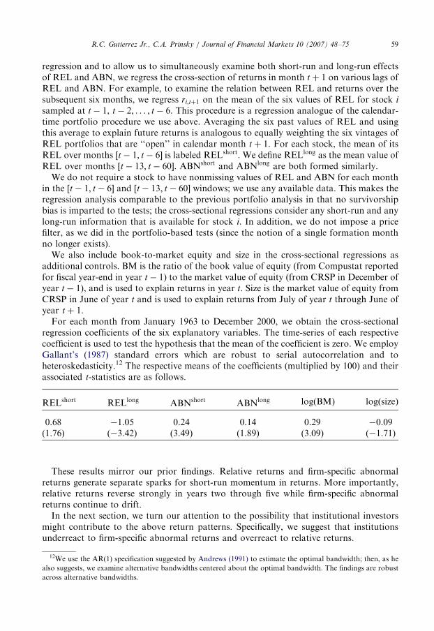
ARTICLE IN PRESSR.C. Gutierrez Jr., C.A. Prinsky / Journal of Financial Markets 10 (2007) 48–75 59
regression and to allow us to simultaneously examine both short-run and long-run effectsof REL and ABN, we regress the cross-section of returns in month tþ 1 on various lags ofREL and ABN. For example, to examine the relation between REL and returns over thesubsequent six months, we regress ri;tþ1 on the mean of the six values of REL for stock i
sampled at t� 1, t� 2; . . . ; t� 6. This procedure is a regression analogue of the calendar-time portfolio procedure we use above. Averaging the six past values of REL and usingthis average to explain future returns is analogous to equally weighting the six vintages ofREL portfolios that are ‘‘open’’ in calendar month tþ 1. For each stock, the mean of itsREL over months ½t� 1; t� 6� is labeled RELshort. We define RELlong as the mean value ofREL over months ½t� 13; t� 60�. ABNshort and ABNlong are both formed similarly.
We do not require a stock to have nonmissing values of REL and ABN for each monthin the ½t� 1; t� 6� and ½t� 13; t� 60� windows; we use any available data. This makes theregression analysis comparable to the previous portfolio analysis in that no survivorshipbias is imparted to the tests; the cross-sectional regressions consider any short-run and anylong-run information that is available for stock i. In addition, we do not impose a pricefilter, as we did in the portfolio-based tests (since the notion of a single formation monthno longer exists).
We also include book-to-market equity and size in the cross-sectional regressions asadditional controls. BM is the ratio of the book value of equity (from Compustat reportedfor fiscal year-end in year t� 1) to the market value of equity (from CRSP in December ofyear t� 1), and is used to explain returns in year t. Size is the market value of equity fromCRSP in June of year t and is used to explain returns from July of year t through June ofyear tþ 1.
For each month from January 1963 to December 2000, we obtain the cross-sectionalregression coefficients of the six explanatory variables. The time-series of each respectivecoefficient is used to test the hypothesis that the mean of the coefficient is zero. We employGallant’s (1987) standard errors which are robust to serial autocorrelation and toheteroskedasticity.12 The respective means of the coefficients (multiplied by 100) and theirassociated t-statistics are as follows.
12We use the AR(
also suggests, we exa
across alternative ba
1) specification sugg
mine alternative ba
ndwidths.
ested by Andrews (1
ndwidths centered ab
991) to estimate the
out the optimal ban
optimal bandwidth;
dwidth. The findings
RELshort
RELlong ABNshort ABNlong log(BM) log(size)0.68
�1.05 0.24 0.14 0.29 �0.09 (1.76) (�3.42) (3.49) (1.89) (3.09) (�1.71)These results mirror our prior findings. Relative returns and firm-specific abnormalreturns generate separate sparks for short-run momentum in returns. More importantly,relative returns reverse strongly in years two through five while firm-specific abnormalreturns continue to drift.
In the next section, we turn our attention to the possibility that institutional investorsmight contribute to the above return patterns. Specifically, we suggest that institutionsunderreact to firm-specific abnormal returns and overreact to relative returns.
then, as he
are robust

ARTICLE IN PRESSR.C. Gutierrez Jr., C.A. Prinsky / Journal of Financial Markets 10 (2007) 48–7560
4. Institutional trading and momentum
Delegated money managers have incentives that can lead them to underreact to firm-specific news and to overreact to relative returns. Assuming institutional investors are themarginal traders, their incentives can result in the return patterns that we find in the priorsection. On one hand, managers have incentives to keep their fund portfolios close to anindex. Chan et al. (2002) document that mutual fund portfolios tend to cluster around abroad index, i.e., to closet index. The desire to remain near an index can hinder a managerfrom fully exploiting any firm-specific information he might have, since generating positivealpha requires him to tilt his portfolio toward individual stocks. This behavior can result inan underreaction to firm-specific news. There are various incentives for managers to keeptheir portfolios near an index. Scharfstein and Stein (1990) note reputation concerns. Inaddition, Shleifer and Vishny (1997) recognize that arbitrage can be riskier for moneymanagers when the principals have short horizons. Consistent with both of these notions,Del Guercio and Tkac (2002) find that pension funds with high tracking error relative tothe S&P 500 index are punished with fund outflows, documenting the downside ofdeviating from an index benchmark. Admati and Pfleiderer (1997) and Dybvig et al.(2004), among others, show that benchmark-adjusted compensation structures can lead toreduced managerial effort. For any of these reasons, money managers might stay close toan index, thus possibly generating an underreaction to firm-specific news.On the other hand, Chan et al. (2002) document that when mutual funds do deviate
from an index, they tilt toward stocks with higher prior returns. This behavior presumablyreflects the preferences of their investing clientele to chase relative returns. For example,Gruber (1996), Sirri and Tufano (1998), and Del Guercio and Tkac (2002) find thatmutual-fund flows chase prior relative returns in addition to, and possibly in lieu of, risk-adjusted returns. Funds with the best recent performance based on relative returns receivethe largest inflows. Our conjecture is that money managers give their clients what theywant—higher relative returns. By chasing relative returns, institutions possibly generate anoverreaction.13
The upshot of all this is that agency issues in money management can provide a rationalexplanation for institutions’ underreacting to firm-specific news (abnormal returns) andoverreacting to relative returns. Although the empirical evidence we have highlighted tosupport our framework is for mutual and pension funds, we believe the same forces arelikely to apply to money managers in general.To test our hypotheses, we first examine the stock holdings of institutional money
managers to see if managers pursue relative returns while relatively ignoring firm-specificabnormal returns. We then test if the abnormal-return momentum stocks that institutionspursue the least are the stocks whose momentum is greatest and does not reverse,consistent with underreactions to firm-specific news. We also examine if the relative-return
13Interestingly, Evans (2004) provides evidence that investors’ (naive) demand for relative returns affects more
than just the asset-selection decisions of money managers. He finds that the more externally relevant decisions of
mutual funds, namely the choices of which incubated funds to bring to market and which funds to terminate, are
based upon relative returns. In contrast, the more internally relevant decisions such as manager promotion or
demotion are based upon risk-adjusted returns. The second finding recognizes the sophistication of institutions; it
also indicates a possible mitigating effect for a portfolio manager’s pursuit of relative returns since internal
monitoring relies on alpha. However, Farnsworth and Taylor (2004) provide survey evidence that the majority of
a fund manager’s compensation is linked to the profitability of the firm rather than to investment performance.
ARTICLE IN PRESS
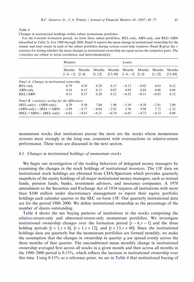
Table 4
Changes in institutional holdings within subset momentum portfolios
For the 6-month formation period, we form three subset portfolios, REL-only, ABN-only, and REL\ABN
(described in Table 2). For 1980 through 2000, Panel A reports the mean change in institutional ownership for the
winner and loser stocks in each of the subset portfolios during various event-time windows. Panel B gives the t-
statistics for testing whether the mean changes in institutional ownership are equal across the respective pairs. The
t-statistics are robust to serial correlation and heteroskedasticity.
Winners Losers
Months Months Months Months Months Months Months Months
½�6;�1� ½1; 6� ½1; 12� ½13; 60� ½�6;�1� ½1; 6� ½1; 12� ½13; 60�
Panel A: Changes in institutional ownership
REL-only 0.79 0.39 0.29 0.13 �0.13 �0.02 0.03 0.12
ABN-only 0.16 0.15 0.13 0.07 0.05 0.05 0.06 0.08
REL\ABN 0.51 0.37 0.28 0.12 �0.32 �0.11 �0.03 0.12
Panel B: t-statistics testing for the differences
ðREL-onlyÞ � ðABN-onlyÞ 4.29 8.50 7.04 1.90 �5.10 �4.58 �2.61 2.09
ðABN-onlyÞ � ðREL \ABNÞ �2.89 �4.77 �4.84 �2.92 5.36 9.98 7.72 �2.32
ðREL \ABNÞ � ðREL-onlyÞ �8.02 �0.63 �0.21 �0.74 �6.03 �4.73 �4.15 0.89
R.C. Gutierrez Jr., C.A. Prinsky / Journal of Financial Markets 10 (2007) 48–75 61
momentum stocks that institutions pursue the most are the stocks whose momentumreverses most strongly in the long run, consistent with overreactions to relative-returnperformance. These tests are discussed in the next section.
4.1. Changes in institutional holdings of momentum stocks
We begin our investigation of the trading behaviors of delegated money managers byexamining the changes in the stock holdings of institutional investors. The 13F data oninstitutional stock holdings are obtained from CDA/Spectrum which provides quarterlysnapshots of the equity holdings of all major institutional money managers, such as mutualfunds, pension funds, banks, investment advisors, and insurance companies. A 1978amendment to the Securities and Exchange Act of 1934 requires all institutions with morethan $100 million under discretionary management to report their equity portfolioholdings each calendar quarter to the SEC on form 13F. Our quarterly institutional dataare for the period 1980–2000. We define institutional ownership as the percentage of thenumber of shares outstanding.
Table 4 shows the net buying patterns of institutions in the stocks comprising therelative-return-only and abnormal-return-only momentum portfolios. We investigateinstitutional ownership changes over the formation period ½t� 6; t� 1� and the threeholding periods ½tþ 1; tþ 6�, ½tþ 1; tþ 12�, and ½tþ 13; tþ 60�. Since the institutionalholdings data are quarterly but the momentum portfolios are formed monthly, we makethe assumption that the changes in ownership in quarter q are spread evenly across thethree months of that quarter. The unconditional mean monthly change in institutionalownership averaged first across all stocks in a given month and then across all months inthe 1980–2000 period is 0.15%, which reflects the increase in institutional ownership overthis time. Using 0.15% as a reference point, we see in Table 4 that institutional buying of

ARTICLE IN PRESSR.C. Gutierrez Jr., C.A. Prinsky / Journal of Financial Markets 10 (2007) 48–7562
the REL-only and REL\ABN winners is far above average in the six-month formationperiod and in the first twelve months of the holding period. Institutions are net buyers ofthe relative-return winners over ½t� 6; t� 1� and ½tþ 1; tþ 12� at a rate which is at leastdouble the 0.15% mean rate across all stocks. Accordingly, institutional buying of theREL-only and REL\ABN losers is far below average, and is actually negative over ½t�6; t� 1� and ½tþ 1; tþ 6�. These differences between the relative-return winners and losersand the market-wide averages are statistically significant (not in tables) and are consistentwith prior studies that document the tendency of institutions to chase prior relativereturns.14
The more novel finding is that institutions are buying the ABN-only winners and sellingthe ABN-only losers substantially less than the relative-return-momentum stocks. Panel Bprovides the t-statistics comparing the mean changes in institutional ownership across themomentum subsets. Since we detect serial correlation in these differences, we employstandard errors that are robust to serial autocorrelation and to heteroskedasticity (Gallant(1987)).15 Given that 0.15% is the average change in institutional ownership per monthacross all stocks, we can see that institutions treat the ABN-only stocks much like anyother stocks despite the momentum profits these stocks generate. Institutions are buyingthe ABN-only winners in the six-month formation period and in the first twelve months ofthe holding period nearly exactly at the 0.15% average rate for all stocks. Hence,institutions are ignoring firm-specific abnormal returns.Note also that institutions are buying fewer REL\ABN winners than REL-only winners
over ½t� 6; t� 1� despite the fact that the REL\ABN winners generate greater profits inthe future, as shown in Table 3. Institutional trading seems more related to a stock’scharacteristic of being a relative-return extreme than to the future alpha a stock generates.In short, Table 4 shows that institutions tend to aggressively pursue relative returns and
to ignore firm-specific abnormal returns. Hence, institutions might be overreacting torelative returns and underreacting to abnormal returns. We provide further evidence thatinstitutions contribute to both types of momenta in the next section by examining therelations between institutional trading and momentum profits.16
4.2. Profits to stocks that institutions most and least support
For the momentum in the ABN-only stocks to be due to an underreaction byinstitutions to firm-specific returns in ½t� 6; t� 1�, the ABN-only stocks that institutionsleast support during the formation period, i.e., winners they buy least and losers they sellleast, should display the strongest momentum in the holding periods. In other words, the
14Sias (2004) confirms this finding using quarterly holdings data and provides a reference list of prior studies. In
addition, Griffin et al. (2005) provide high-frequency evidence.15We use the AR(1) specification suggested by Andrews (1991) to estimate the optimal bandwidth; then, as he
also suggests, we examine alternative bandwidths centered about the optimal bandwidth. The results are robust
across alternative bandwidths.16It is interesting to note that institutions seemingly ignore the strong reversal in returns for the REL-only
stocks over months ½tþ 13; tþ 60� and continue to relatively ignore the return continuation for the ABN-only
stocks over this subsequent period. As a side note, institutions’ participation in the presumed long-run corrections
occurring over ½tþ 13; tþ 60� is not necessary to support the overreaction or the underreaction hypothesis. First,
no one needs to participate in the correction since prices can adjust to news without trading (i.e., dealers adjust
their quotes in response to news). Second, if institutions contribute to the mispricing, why should they necessarily
be expected to contribute to the correction?

ARTICLE IN PRESSR.C. Gutierrez Jr., C.A. Prinsky / Journal of Financial Markets 10 (2007) 48–75 63
ABN-only stocks that institutions ignore most should experience the greatest momentumprofits as the market corrects the underreaction.
For overreaction by institutions to explain the REL-only return pattern of short-runmomentum and long-run reversal, we should find evidence that overreaction in theformation period continues into the early part of the holding period. If institutions areoverreacting in the formation period, the REL-only stocks that institutions most supportduring ½t� 6; t� 1�, i.e., winners they buy most and losers they sell most, should reversemost strongly in the long run over ½tþ 13; tþ 60�, as the overreaction is corrected. Ifinstitutions continue to overreact in the early part of the holding period, the REL-onlystocks that institutions most support during ½tþ 1; tþ 6� should reverse most strongly inthe long run over ½tþ 13; tþ 60�.
Table 5 provides the profits for the respective most-supported and least-supportedsubsets of the ABN-only and REL-only portfolios. In Panels A and B respectively, thewinner stocks in the ABN-only and REL-only portfolios are sorted into thirds based onthe changes in institutional ownership over ½t� 6; t� 1�. The loser stocks are also sorted
Table 5
Profits to momentum portfolios most supported and least supported by institutions
For the 6-month formation period, we form three subset portfolios, REL-only, ABN-only, and REL\ABN
(described in Table 2). For 1980–2000, we further divide the REL-only and ABN-only portfolios into portfolios
that are most-supported and least-supported by institutions. The stocks in the REL-only and ABN-only
portfolios are sorted separately into thirds based on changes in institutional ownership over the formation period
½t� 6; t� 1�. The most-supported portfolios are formed by taking long positions in the winner stocks in the
highest third of institutional changes and taking short positions in the loser stocks in the lowest third of
institutional changes. The least-supported portfolios are formed by taking long positions in the winner stocks in
the lowest third of institutional changes and taking short positions in the loser stocks in the highest third of
institutional changes. Panel A gives the mean performances for the most-supported and least-supported ABN-
only stocks, with the t-statistics in parentheses. Panel B provides the same for REL-only stocks. Panel C provides
the mean performances for the most-supported and least-supported REL-only stocks defining institutional
support over the holding period ½tþ 1; tþ 6�, instead of over the formation period ½t� 6; t� 1�.
Winners� losers Mean return CAPM alpha Fama-French alpha
Months Months Months Months Months Months Months Months Months
1–6 1–12 13–60 1–6 1–12 13–60 1–6 1–12 13–60
Panel A: ABN-only, support defined over ½t� 6; t� 1�
Most supported 0.50 0.32 0.07 0.44 0.28 0.10 0.58 0.43 0.11
(2.56) (2.07) (1.05) (2.23) (1.78) (1.54) (3.05) (2.81) (1.54)
Least supported 0.59 0.53 0.19 0.67 0.60 0.31 0.66 0.62 0.31
(3.70) (3.94) (2.40) (4.21) (4.49) (4.76) (4.27) (4.67) (4.59)
Panel B: REL-only, support defined over ½t� 6; t� 1�
Most supported 1.41 0.76 �0.33 1.17 0.51 �0.47 1.67 0.98 �0.36
(4.07) (2.53) (�2.12) (3.45) (1.76) (�3.21) (5.15) (3.67) (�2.58)
Least supported 1.32 0.53 �0.12 1.30 0.50 �0.12 1.47 0.68 �0.11
(5.42) (2.53) (�0.73) (5.26) (2.32) (�0.71) (5.83) (3.12) (�0.71)
Panel C: REL-only, support defined over ½tþ 1; tþ 6�
Most supported 4.88 2.70 �0.42 4.60 2.40 �0.56 5.07 2.86 �0.45
(12.80) (7.95) (�2.24) (12.21) (7.33) (�3.03) (14.34) (9.18) (�2.63)
Least supported �2.59 �1.55 �0.12 �2.63 �1.62 �0.13 �2.38 �1.39 �0.09
(�8.98) (�7.06) (�0.82) (�8.98) (�7.32) (�0.90) (�8.12) (�6.21) (�0.60)

ARTICLE IN PRESSR.C. Gutierrez Jr., C.A. Prinsky / Journal of Financial Markets 10 (2007) 48–7564
into thirds. In Panel C, the REL-only stocks are sorted according to changes ininstitutional ownership over ½tþ 1; tþ 6�. The most-supported portfolio is defined as longin the winner stocks in the upper third of changes in institutional ownership and short inthe loser stocks in the bottom third. The least-supported portfolio is defined as long in thewinner stocks in the lower third of changes in institutional ownership and short in theloser stocks in the upper third. That is, the most-supported stocks are those thatinstitutions trade most strongly in the direction of formation-period returns, i.e.,momentum strategies. The least-supported stocks are those that institutions trade theleast in the direction of formation-period returns, which in fact are contrarian strategies onaverage.Panel A of Table 5 shows that the least-supported ABN-only stocks generate the most
momentum profits. The differences in profits over ½tþ 1; tþ 12� between the least-supported and the most-supported ABN-only stocks are significant with t-statistics at least1.70 across the three profit metrics (not in the tables). The long-run profit differences over[t+13, t+60] are also significant. In fact, the least-supported ABN-only stocks displaymomentum for years while the most-supported stocks do not. These findings suggest thatinstitutions in aggregate contribute to momentum in the ABN-only stocks by under-reacting to firm-specific news.The profits to the REL-only stocks that are most-supported and least-supported over
the formation period ½t� 6; t� 1� are shown in Panel B of Table 5. The most-supportedREL-only stocks reverse most strongly in the long-run over ½tþ 13; tþ 60�. In fact, thereversals in the most-supported stocks are quite strong and are at least 0.33% per monthacross the three metrics. However, the REL-only stocks with the least institutional supportdo not reverse. In addition, the profit differences across the most-supported and least-supported REL-only stocks are significant in the CAPM alphas, not provided in the tables.These REL-only results are consistent with institutions overreacting to the REL-onlystocks during the formation period.Panel C of Table 5 is consistent with institutions’ continuing their overreactions into the
first six months of the holding period. The REL-only stocks that institutions most supportover ½tþ 1; tþ 6� display the greatest reversals over the long-run of at least 0.42% permonth across all performance metrics over ½tþ 13; tþ 60�. The profit differences across themost-supported and least-supported portfolios are significant using the CAPM and Fama-French models, and are not reported in the tables. And once again, the least-supportedREL-only stocks do not reverse in the long-run. The findings in Panels B and C suggestthat the aggressive pursuit of relative-return winners by institutions and the aggressiveavoidance of relative-return losers, as shown in Table 4, generate a prolonged overreactionin the REL-only stocks.As a side note, the profits in Panel C of Table 5 for the ½tþ 1; tþ 6� and ½tþ 1; tþ 12�
holding periods are extreme because changes in institutional ownership are highlycorrelated contemporaneously with returns. By ranking on changes in institutionalownership over the holding periods, we are de facto ranking on returns over the sameperiod. The profit differences across the most-supported and least-supported stocks arepositive in the first twelve months and are consistent with momentum on average for theREL-only portfolio in the short-run.In sum, Table 5 supports both the notion that the tendency of institutions to pursue relative
returns contributes to overreactions and the notion that the tendency of institutions to ignorefirm-specific abnormal returns contributes to underreactions. Institutions appear to play a role

ARTICLE IN PRESSR.C. Gutierrez Jr., C.A. Prinsky / Journal of Financial Markets 10 (2007) 48–75 65
in explaining the performances of relative-return–momentum portfolios and of abnormal-return–momentum portfolios, respectively.
5. Subperiods, large stocks, and January seasonals
We examine the strength of the abnormal-return–momentum and relative-return-momentum patterns within the 1963–1981 and 1982–2000 subperiods and within the subsetof large stocks. Jegadeesh and Titman (2001) find that the long-run performance ofrelative-return–momentum portfolios varies across roughly these same subperiods andacross stock size. We also examine the performances of the various momentum portfoliosin January and non-January. Prior studies find strong losses in the profits to relative-return–momentum portfolios in January even in the first twelve months of the holdingperiod and attribute this brief reversal at least in part to tax effects (Grinblatt andMoskowitz, 2004). To the extent that January losses to momentum portfolios are due totaxes, abnormal-return-only momentum portfolios should not display the January effectthat the relative- return–momentum portfolios display, since taxes are based on rawreturns.
5.1. Subperiods and large-stock results
Panels A and B of Table 6 show the profits to the REL-only and the ABN-onlyportfolios in the 1963–1981 and 1982–2000 subperiods. In each subperiod, the returns ofthe REL-only stocks reverse in the long-run, while the returns of the ABN-only stocks donot. Panel C of Table 6 shows that the long-lasting continuations in abnormal returns arealso present in large stocks, defined as stocks whose market value is above the median forNYSE stocks. The long-run reversal of relative-return–momentum is also robust in largestocks according to the raw-return and CAPM metrics, but not according to the Fama-French model. In sum, the momentum and reversal patterns we find in the full sample arerobust across the subperiods and within large-cap stocks.
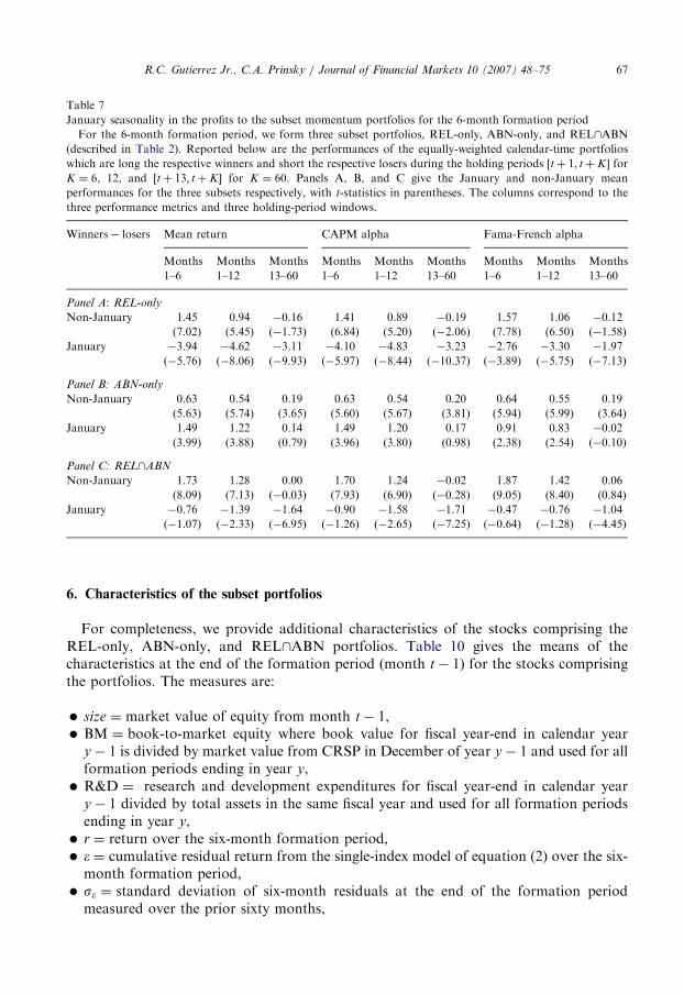
5.2. January seasonality
Table 7 shows that the REL-only and REL\ABN portfolios incur large losses inJanuary regardless of the holding-period horizon, a well-documented result for relative-return strategies (though the losses are insignificant in the REL\ABN portfolio due to thelarge variability in profits). The ABN-only strategy, however, shows no evidence ofreversal in January, and in fact, generates large profits in January in the first twelve monthsof the holding period. Return reversal in January is only an attribute of the relative-returnportfolios.
The lack of even a January reversal for the ABN-only strategy is roughly consistent witha tax-loss selling hypothesis for January effects. Taxes are paid according to raw returns,not abnormal returns. Since the ABN-only loser stocks, by definition, are not among theworst stocks according to raw returns, these stocks are not the most advantageous to sellfor realizing a capital loss. Tables 8 and 9 report the January and non-Januaryperformances of the subset portfolios for the winner and loser sides of the portfoliosrespectively. They indicate that the January losses of the REL-only portfolio are due to the

ARTICLE IN PRESS
Table 6
Momentum profits in subperiods and in large stocks for the 6-month formation period
For the 6-month formation period, we form the REL-only and ABN-only subset portfolios (described in Table
2). Reported below are the performances of the equally-weighted calendar-time portfolios which are long the
respective winners and short the respective losers during the holding periods ½tþ 1; tþK � for K ¼ 6; 12, and½tþ 13; tþ K� for K ¼ 60. Panels A, B, and C give the mean performances, with t-statistics in parentheses. Panels
A and B report the profits for the subperiods 1963:01–1981:12 and 1982:01–2000:12, respectively. Panel C reports
the profits to the subset portfolios formed from the set of stocks whose market capitalization is greater than the
median market capitalization on the NYSE in month t� 1. The columns correspond to the three performance
metrics and the three holding-period windows.
Winners� losers Mean return CAPM alpha Fama-French alpha
Months Months Months Months Months Months Months Months Months
1–6 1–12 13–60 1–6 1–12 13–60 1–6 1–12 13–60
Panel A: 1963:01– 1981:12
REL-only 0.69 0.34 �0.55 0.70 0.34 �0.55 1.12 0.82 �0.20
(2.10) (1.20) (�3.71) (2.13) (1.22) (�3.69) (3.57) (3.25) (�1.80)
ABN-only 0.79 0.70 0.29 0.79 0.70 0.29 0.61 0.56 0.25
(5.28) (5.44) (3.50) (5.29) (5.40) (3.42) (4.23) (4.41) (2.95)
Panel B: 1982:01– 2000:12
REL-only 1.31 0.62 �0.25 1.18 0.46 �0.34 1.49 0.77 �0.29
(5.06) (2.73) (�2.03) (4.53) (2.07) (�2.78) (5.89) (3.54) (�2.61)
ABN-only 0.63 0.50 0.08 0.61 0.49 0.14 0.68 0.59 0.14
(3.97) (3.88) (1.48) (3.77) (3.71) (2.64) (4.51) (4.66) (2.67)
Panel C: Large stocks only
REL-only 0.66 0.34 �0.28 0.60 0.26 �0.36 1.06 0.76 �0.08
(2.69) (1.61) (�2.74) (2.43) (1.24) (�3.57) (4.63) (4.18) (�1.01)
ABN-only 0.41 0.37 0.12 0.42 0.38 0.15 0.37 0.36 0.13
(3.28) (3.62) (2.07) (3.33) (3.60) (2.69) (2.95) (3.43) (2.27)
R.C. Gutierrez Jr., C.A. Prinsky / Journal of Financial Markets 10 (2007) 48–7566
extremely good performances of the losers, consistent with a rebound following tax-lossselling.However, Table 7 demonstrates that there is more to the January performances than just
tax-loss selling. The profits for the ABN-only portfolio in the first twelve months of theholding period are greater in January than in non-January, with t-statistics of at least 2.0for the raw and CAPMmetrics (not in the tables). Hence, abnormal-return momentum hasits own January effect, opposite that of the relative-return momentum. In sum, there existlarge profit differences in January across relative-return-momentum and abnormal-return-momentum portfolios, part of which is consistent with taxation effects.17
17Although we have not pursued this further, the increased profits in January to the ABN-only portfolio might
be consistent with institutions’ being responsible for a portion of these turn-of-the-year effects. If the incentives of
money managers to chase relative returns is highest right before the turn of the year and lowest right after, the
incentives of institutions might also be capable of explaining the January reversal in relative-return momentum
(due to the release of price pressure from chasing relative returns at the end of the year) and the increased January
profitability of abnormal-return momentum (due to institutions’ tilting their portfolios toward positive-alpha
stocks in January in response to within-firm incentives—see footnote 13).
ARTICLE IN PRESS
Table 7
January seasonality in the profits to the subset momentum portfolios for the 6-month formation period
For the 6-month formation period, we form three subset portfolios, REL-only, ABN-only, and REL\ABN
(described in Table 2). Reported below are the performances of the equally-weighted calendar-time portfolios
which are long the respective winners and short the respective losers during the holding periods ½tþ 1; tþ K� for
K ¼ 6, 12, and ½tþ 13; tþ K� for K ¼ 60. Panels A, B, and C give the January and non-January mean
performances for the three subsets respectively, with t-statistics in parentheses. The columns correspond to the
three performance metrics and three holding-period windows.
Winners� losers Mean return CAPM alpha Fama-French alpha
Months Months Months Months Months Months Months Months Months
1–6 1–12 13–60 1–6 1–12 13–60 1–6 1–12 13–60
Panel A: REL-only
Non-January 1.45 0.94 �0.16 1.41 0.89 �0.19 1.57 1.06 �0.12
(7.02) (5.45) (�1.73) (6.84) (5.20) (�2.06) (7.78) (6.50) (�1.58)
January �3.94 �4.62 �3.11 �4.10 �4.83 �3.23 �2.76 �3.30 �1.97
(�5.76) (�8.06) (�9.93) (�5.97) (�8.44) (�10.37) (�3.89) (�5.75) (�7.13)
Panel B: ABN-only
Non-January 0.63 0.54 0.19 0.63 0.54 0.20 0.64 0.55 0.19
(5.63) (5.74) (3.65) (5.60) (5.67) (3.81) (5.94) (5.99) (3.64)
January 1.49 1.22 0.14 1.49 1.20 0.17 0.91 0.83 �0.02
(3.99) (3.88) (0.79) (3.96) (3.80) (0.98) (2.38) (2.54) (�0.10)
Panel C: REL\ABN
Non-January 1.73 1.28 0.00 1.70 1.24 �0.02 1.87 1.42 0.06
(8.09) (7.13) (�0.03) (7.93) (6.90) (�0.28) (9.05) (8.40) (0.84)
January �0.76 �1.39 �1.64 �0.90 �1.58 �1.71 �0.47 �0.76 �1.04
(�1.07) (�2.33) (�6.95) (�1.26) (�2.65) (�7.25) (�0.64) (�1.28) (�4.45)
R.C. Gutierrez Jr., C.A. Prinsky / Journal of Financial Markets 10 (2007) 48–75 67
6. Characteristics of the subset portfolios
For completeness, we provide additional characteristics of the stocks comprising theREL-only, ABN-only, and REL\ABN portfolios. Table 10 gives the means of thecharacteristics at the end of the formation period (month t� 1) for the stocks comprisingthe portfolios. The measures are:
�
size ¼ market value of equity from month t� 1, � BM ¼ book-to-market equity where book value for fiscal year-end in calendar yeary� 1 is divided by market value from CRSP in December of year y� 1 and used for allformation periods ending in year y,
� R&D ¼ research and development expenditures for fiscal year-end in calendar yeary� 1 divided by total assets in the same fiscal year and used for all formation periodsending in year y,
� r ¼ return over the six-month formation period, � � ¼ cumulative residual return from the single-index model of equation (2) over the six-month formation period,
� s� ¼ standard deviation of six-month residuals at the end of the formation periodmeasured over the prior sixty months,

ARTICLE IN PRESS
Table 8
January seasonality in the profits to the subset momentum portfolios for the 6-month formation period: the
winners
For the 6-month formation period, we form three subset portfolios, REL-only, ABN-only, and REL\ABN
(described in Table 2). Reported below are the performances of the equally-weighted calendar-time portfolios
which are only long the respective winners during the holding periods ½tþ 1; tþ K � for K ¼ 6, 12, and ½tþ
13; tþ K� for K ¼ 60. Panels A, B, and C give the January and non-January mean performances for the three
subsets respectively, with the t-statistics in parentheses. The columns correspond to the three performance metrics
and three holding-period windows.
Winners Mean return CAPM alpha Fama-French alpha
Months Months Months Months Months Months Months Months Months
1–6 1–12 13–60 1–6 1–12 13–60 1–6 1–12 13–60
Panel A: REL-only
Non-January 0.88 0.57 0.14 0.31 0.01 �0.41 0.54 0.22 �0.31
(2.43) (1.63) (0.44) (1.48) (0.01) (�2.67) (4.25) (2.18) (�3.97)
January 4.02 3.71 5.29 1.54 1.22 3.05 0.38 0.09 1.41
(3.35) (3.19) (4.93) (2.21) (1.96) (5.92) (0.85) (0.26) (5.14)
Panel B: ABN-only
Non-January 0.79 0.74 0.59 0.40 0.34 0.20 0.30 0.25 0.06
(3.42) (3.23) (2.62) (3.73) (3.46) (1.95) (5.70) (5.28) (1.00)
January 4.12 4.06 3.81 2.39 2.32 2.2 0.25 0.27 0.05
(5.35) (5.34) (5.05) (6.78) (7.08) (6.56) (1.31) (1.67) (0.24)
Panel C: REL\ABN
Non-January 1.16 0.86 0.29 0.63 0.32 �0.21 0.77 0.47 �0.18
(3.47) (2.63) (1.00) (3.35) (1.88) (�1.55) (6.98) (4.96) (�2.94)
January 4.23 4.22 5.10 1.97 1.90 3.06 0.32 0.40 1.09
(3.87) (3.91) (5.24) (3.16) (3.34) (6.71) (0.81) (1.20) (4.98)
R.C. Gutierrez Jr., C.A. Prinsky / Journal of Financial Markets 10 (2007) 48–7568
�
1
cou
NA1
acr
tha
com
Th
los
VOL ¼mean monthly trading volume per share outstanding over the six-monthformation period for NYSE stocks only.18
Table 10 also provides the mean decile ranks of the characteristics for the stocks in thesubset portfolios. For size and turnover, we use the NYSE breakpoints; for all othervariables we use the NYSE-AMEX-NASDAQ breakpoints.We see that the ABN-only stocks (winners and losers) tend to be larger than the REL-
only and REL\ABN stocks; they tend to have lower R&D, and lower turnover.19 No clearpattern emerges for BM across the subset portfolios. Note that the return characteristicsare as expected given our definitions of REL-only and ABN-only. The raw returns of
8Volume cannot be directly compared across the NYSE and NASDAQ markets because of the double
nting of inter-dealer trades on NASDAQ. The turnover characteristics are qualitatively the same, though, for
SDAQ stocks.9The lower volume for the ABN-only stocks persists across formation and later holding periods as well as
oss Decembers and Januarys. The turnover in these portfolios implies that we are identifying a return effect
t is different from the patterns found by Lee and Swaminathan (2000). The REL-only portfolio is typically
prised of high-volume stocks, while the ABN-only portfolio is typically comprised of medium-volume stocks.
e ‘‘late’’ portfolio of Lee and Swaminathan, which reverses, combines high-volume winners with low-volume
ers. Their ‘‘early’’ strategy, which does not reverse, combines low-volume winners with high-volume losers.

ARTICLE IN PRESS
Table 9
January seasonality in the profits to the subset momentum portfolios for the 6-month formation period: the losers
For the 6-month formation period, we form three subset portfolios, REL-only, ABN-only, and REL\ABN
(described in Table 2). Reported below are the performances of the equally-weighted calendar-time portfolios
which are only long the respective losers during the holding periods ½tþ 1; tþ K� for K ¼ 6, 12, and ½tþ 13; tþ K�
for K ¼ 60. Panels A, B, and C give the January and non-January mean performances for the three subsets
respectively, with t-statistics in parentheses. The columns correspond to the three performance metrics and three
holding-period windows.
Losers Mean return CAPM alpha Fama-French alpha
Months Months Months Months Months Months Months Months Months
1–6 1–12 13–60 1–6 1–12 13–60 1–6 1–12 13–60
Panel A: REL-only
Non-January �0.57 �0.37 0.31 �1.10 �0.89 �0.22 �1.03 �0.84 �0.18
(�1.63) (�1.09) (0.91) (�5.18) (�4.36) (�1.10) (�7.83) (�7.09) (�2.02)
January 7.96 8.33 8.40 5.64 6.05 6.28 3.14 3.40 3.38
(6.88) (7.38) (7.58) (7.96) (8.87) (9.49) (6.81) (8.12) (10.6)
Panel B: ABN-only
Non-January 0.16 0.20 0.40 �0.24 �0.20 �0.01 �0.34 �0.31 �0.14
(0.69) (0.86) (1.75) (�2.23) (�1.91) (�0.04) (�3.83) (�3.73) (�2.25)
January 2.64 2.85 3.67 0.91 1.12 2.03 �0.66 �0.55 0.07
(3.42) (3.73) (4.81) (2.55) (3.26) (6.20) (�2.12) (�1.91) (0.30)
Panel C: REL\ABN
Non-January �0.57 �0.43 0.29 �1.07 �0.92 �0.19 �1.10 �0.96 �0.24
(�1.85) (�1.42) (1.01) (�6.46) (�5.77) (�1.26) (�8.58) (�8.68) (�3.20)
January 5.05 5.62 6.74 2.86 3.48 4.77 0.78 1.16 2.12
(4.92) (5.64) (6.93) (5.18) (6.59) (9.34) (1.73) (2.99) (8.10)
R.C. Gutierrez Jr., C.A. Prinsky / Journal of Financial Markets 10 (2007) 48–75 69
ABN-only stocks are, by definition, less extreme cross-sectionally, but interestingly, theresidual returns of ABN-only and REL-only stocks are equivalent. ABN-only stocks havesmaller standard deviations of residuals (and returns).
The finding that the ABN-only stocks tilt away from the smallest stocks is interesting.First, many return anomalies tend to concentrate in the smallest stocks, perhaps because ofgreater information asymmetries and/or greater microstructural issues. Second, thelikelihood of realizing the holding-period returns of the abnormal-return-only portfolioshould be greater than that for the relative-return portfolios, since trading costs typicallydecrease with stock size.20
7. Conclusion
We find that momentum in stock returns is more complex than previously recognized.Both firm-specific abnormal returns and relative returns contribute separately tomomentum. These two types of momenta display starkly different long-run performances.Abnormal-return–momentum persists for years without reversing and is consistent withunderreaction. Relative-return momentum reverses strongly after one year and is
20Korajczyk and Sadka (2002) and Lesmond et al. (2004) estimate the trading costs to various momentum
strategies.

ARTICLE IN PRESS
Table 10
Characteristics of the stocks comprising the subset momentum portfolios for a 6-month formation period
Mean levels of the following measures are reported for the stocks comprising the three subset portfolios, REL-
only, ABN-only, and REL\ABN (described in Table 2). For the six-month formation period ending in month
t� 1 of year y, size is market capitalization in month t� 1 in millions of dollars; BM is the book-to-market equity
ratio with book value from year t� 1 and market value from December of year y� 1; R&D is research and
development expenditures over total assets from year t� 1; and INST is institutional ownership at the most recent
calendar quarter-end. r is the six-month return, � is the cumulative six-month residual return from equation (2),
and VOL is mean monthly trading volume per share for NYSE stocks only during the formation period. s� is thestandard deviation of six-month residual returns measured over the prior sixty months. All stocks are also sorted
each month into deciles according to each one of the above characteristics. For size and volume, we use the NYSE
breakpoints; for all other measures, we use the NYSE-AMEX-NASDAQ breakpoints. The mean decile of each
measure that the component stocks belong to at the end of the formation period is reported. Panels A and B give
the mean characteristics for the winners, and Panels C and D give the mean characteristics for the losers.
Size BM R&D r � s� VOL
Winners
Panel A: Mean values
REL-only 594 0.61 0.07 0.57 0.25 0.41 0.07
ABN-only 1378 1.03 0.03 0.29 0.26 0.19 0.04
REL\ABN 628 0.94 0.05 0.83 0.57 0.30 0.07
Panel B: Mean decile ranks
REL-only 3.36 3.78 6.18 9.94 8.80 7.73 7.33
ABN-only 4.61 6.21 5.25 8.50 8.89 3.32 5.34
REL\ABN 3.54 5.52 5.71 9.97 9.82 5.98 7.21
Losers
Panel C: Mean values
REL-only 118 0.89 0.07 �0.24 �0.26 0.37 0.06
ABN-only 1590 0.65 0.03 �0.10 �0.25 0.19 0.04
REL\ABN 451 0.74 0.04 �0.30 �0.45 0.28 0.06
Panel D: Mean decile ranks
REL-only 2.26 5.21 6.32 1.64 2.37 7.34 6.71
ABN-only 5.22 4.39 5.14 3.22 2.36 3.32 4.92
REL\ABN 3.54 4.58 5.57 1.39 1.34 5.61 6.63
R.C. Gutierrez Jr., C.A. Prinsky / Journal of Financial Markets 10 (2007) 48–7570
consistent with overreaction. These findings are robust across alternative performancemetrics, across alternative measures of abnormal returns, across subperiods, and withinlarge-cap stocks.We offer an agency-based explanation of our stock-return findings that provides an
economic rationale for momentum in returns. Moreover, the agency explanation that wepropose for these newly identified complexities in return momentum is parsimonious in thatthe single underlying source of momentum is the agency relation between money managersand their clients. Delegated money managers have incentives to chase relative returns yieldingan overreaction and to ignore firm-specific news yielding an underreaction. The tradingbehaviors of institutions confirm these tendencies. We find that institutions aggressively buystocks with the highest prior returns and avoid stocks with the lowest prior returns. We alsofind that the long-run reversal of relative-return momentum occurs only for winner stocksthat institutions buy the most and for loser stocks that institutions sell the most. Thesefindings suggest that institutions overreact to relative returns. On the other hand, institutionstrade stocks with high and low firm-specific abnormal returns as if these stocks were any other

ARTICLE IN PRESSR.C. Gutierrez Jr., C.A. Prinsky / Journal of Financial Markets 10 (2007) 48–75 71
stocks. Moreover, abnormal-return momentum persists for years only for the winner stocksthat institutions buy the least and for the loser stocks that institutions sell the least. Thesefindings suggest that institutions underreact to abnormal returns (firm-specific news). In short,institutions seem to contribute to both types of the momenta we identify.
In addition, the persistence of abnormal-return momentum contributes to the growingevidence that the market underreacts to firm-specific news. Prior studies find evidence ofunderreaction to corporate events and to headline news. The finding that the market alsounderreacts to the general firm-specific information in returns reinforces and extends theprior evidence. Underreaction to firm-specific news is a pervasive phenomenon. Ouragency explanation for momentum also serves as an economic rationale for the specificunderreactions found in prior studies.
Finally, our institutional results complement the recent literature on the limits ofarbitrage, surveyed in Barberis and Thaler (2003). As such, they offer possibleexplanations for the notorious inability of institutions to beat the market.21 Our findingthat institutions appear to underreact to firm-specific news is consistent with the VARresults of Cohen et al. (2002). The subtle difference is that we suggest that institutionscontribute to underreaction while they suggest that institutions fail to fully exploit theunderreaction. Our results on overreaction, however, provide a sharper contrast to recentstudies. This is the first finding of a negative relation between institutional trading andlong-run returns that we are aware of. This finding suggests that institutional tradingpossibly destabilizes prices, driving them away from fundamental values. In contrast,recent studies by Wermers (1999) and Sias (2004), among others, find only a positivecorrelation between institutional trading and future returns. However, these studies limittheir analysis to just twelve months after they measure institutional trading. We find returnreversals in months 13–60.
Appendix
We describe here the other metrics and procedures we employ to evaluate theperformances of the portfolios. The findings are robust across all of these variations.Abnormal-return momentum persists for several years and does not reverse; relative-returnmomentum reverses strongly in the long-run.
A.1. Stochastic discount factor
Assuming that the law of one price holds, there exists a stochastic discount factor (SDF)that satisfies the following pricing equation:
EðmxÞ ¼ 1, (A.1)
where x is a future payoff (expressed as a gross return). Assuming that there exists ariskless (unobservable) asset, Hansen and Jagannathan (1991) show how an estimator of m
can be retrieved from a basis set of traded assets. The estimate is obtained by finding theN � 1 vector c such that
Eðxx0cÞ ¼ 1N , (A.2)
21Berk and Green (2004) and Wermers (2000) suggest other possible and complementary reasons.

ARTICLE IN PRESSR.C. Gutierrez Jr., C.A. Prinsky / Journal of Financial Markets 10 (2007) 48–7572
where x is the N � 1 vector of payoffs for the basis assets and m ¼ x0c is the estimate ofthe SDF.Since the portfolios we examine are winner-minus-loser portfolios, the SDF should price
the profits to zero.
EðmrW�LÞ ¼ 0, (A.3)
where rW�L is the payoff to the winner portfolio minus the payoff to the loser portfolio.Following Chen and Knez (1996), we can estimate the pricing error, or alpha, using themean of the time-series of the discounted payoffs, which should be zero. The advantage ofthis method is that it does not rely on any specific model of the pricing kernel. The pricingkernel is obtained directly from return data on the basis assets.We employ four sets of assets to serve as the basis sets, and thus form four estimates of
the SDF. From Kenneth French’s website we obtain value-weighted and equal-weightedreturns to sets of 12 and 30 industry portfolios, respectively.22 The equal-weightedportfolios reflect more of the performance of smaller stocks and increasing the number ofindustry portfolios reflects more of the non-systematic components of stock returns.Following the advice of Dahlquist and Soderlind (1999) and Farnsworth et al. (2002), weadd the one-month T-bill rate to the set of basis assets to better estimate the mean of m.
A.2. Conditional CAPM
Jagannathan and Wang (1996, hereafter JW) and Lettau and Ludvigson (2001a,hereafter LL) find that allowing betas to change as a function of the state of the marketimproves the ability of the CAPM to explain the cross section of stock returns. FollowingLL, we employ cay as the conditioning variable.23 The variable cay is the log consumption-wealth ratio and is shown by Lettau and Ludvigson (2001b) to predict stock returns.24 Theform of the CAPM we estimate is
rW�Lt ¼ aþ b1ðrMt � rftÞ þ b2ðcayÞðrMt � rftÞ þ �t. (A.4)
The macro data are quarterly. The findings in this specification, and in the following withhuman capital, are the same when using quarterly frequency for the momentum portfolios’profits or when using monthly frequency and updating the macro variables every thirdmonth.
A.3. Conditional CAPM with human capital
JW and LL find that adding the return on human capital to the CAPM improves theconditional CAPM’s ability to explain the cross section of stock returns even further. Sowe consider a conditional CAPM with the market portfolio expanded to include humancapital. We use the growth rate in per capita labor income as the proxy for the return on
22Professor French’s website is at http://mba.tuck.dartmouth.edu/pages/faculty/ken.french. We thank him for
generously providing these data. The definitions of the industries are provided on the website.23We thank Martin Lettau for generously providing the cay data as well as the labor income data on his website
at http://pages.stern.nyu.edu/�mlettau.24Brennan and Xia (2005) and Lee (2002) argue that the estimates of cay provided by Lettau and Ludvigson are
biased. Lee re-estimates the series and finds that cay is unable to predict future returns. Lettau and Ludvigson
(2005) respond to the criticisms.

ARTICLE IN PRESSR.C. Gutierrez Jr., C.A. Prinsky / Journal of Financial Markets 10 (2007) 48–75 73
human capital as JW and LL do. The model is then
rW�Lt ¼ aþ b1ðrMt � rftÞ þ b2ðcayÞðrMt � rftÞ þ b3Dyþ b4ðcayÞDyþ �t, (A.5)
where Dy is the change in the log of labor income.
A.4. Size and book-to-market matches
For each month in the holding period, we subtract from the returns of our selectedmomentum stocks the returns of a matching size/book-to-market portfolio. The portfoliosare formed by first sorting all stocks into quintiles using market values of equity at the endof the prior month. These five portfolios are then sorted further into quintiles using thebook-to-market ratios of equity, where book value is from the fiscal-year end of the priorcalendar year and market value is from December of the prior calendar year. The sizebreakpoints are determined using only NYSE stocks; the book-to-market breakpoints aredetermined using all stocks. The calendar-time series of adjusted returns are then evaluatedusing mean raw returns and Fama-French alphas. We also examine 10� 10 matchingportfolios and find similar results.
A.5. Using individual-stock factor loadings to construct proxies for portfolio loadings
Since the composition of stocks in these momentum portfolios is changing through time,the factor loadings of the portfolios might also be changing through time. Estimating time-invariant factor loadings, as we do in the reported tables, might lead to poor estimates ofperformance. This source of potential time variation is different from the time variationthat we consider in the conditional CAPM models. To allow for the possibility thatchanges in portfolio composition will lead to changes in factor loadings, we follow thesuggestion of Mitchell and Stafford (2001) and Grundy and Martin (2001) to use theloadings of the individual stocks comprising the portfolios each month to construct proxiesfor portfolio loadings. We estimate each stock’s CAPM and Fama-French factor loadingsin months ½tþ 1; tþ 60�, requiring at least twenty-four months of available data. (Thelook-ahead bias this imposes does not affect our empirical findings.) To estimatethe portfolio factor loadings each calendar month, we average the factor loadings of theindividual stocks that are in each portfolio that calendar month.
References
Admati, A.R., Pfleiderer, P., 1997. Does it all add up? Benchmarks and the active compensation of portfolio
managers. Journal of Business 70, 323–350.
Andrews, D.K., 1991. Heteroskedastic and autocorrelation consistent covariance matrix estimation. Econome-
trica 59, 817–858.
Barberis, N., Shleifer, A., Vishny, R., 1998. A model of investor sentiment. Journal of Financial Economics 49 (3),
307–343.
Barberis, N., Thaler, R.H., 2003. A survey of behavioral finance. In: Constantinides, G.M., Harris, M., Stultz, R.
(Eds.), Handbook of the Economics of Finance. Elsevier Science, Amsterdam.
Berk, J.B., Green, R.C., 2004. Mutual fund flows and performance in rational markets. Journal of Political
Economics 112, 1269–1295.
Brav, A., Heaton, J.B., 2002. Competing theories of financial anomalies. Review of Financial Studies 15, 575–606.
Brennan, M.J., Xia, Y., 2005. Tay’s as good as cay. Finance Research Letters 2, 1–14.

ARTICLE IN PRESSR.C. Gutierrez Jr., C.A. Prinsky / Journal of Financial Markets 10 (2007) 48–7574
Chan, L.K.C., Chen, H., Lakonishok, J., 2002. On mutual fund investment styles. Review of Financial Studies 15,
1407–1437.
Chan, L.K.C., Jegadeesh, N., Lakonishok, J., 1996. Momentum strategies. Journal of Finance 51,
1681–1713.
Chan, W.S., 2003. Stock price reaction to news and no-news: drift and reversal after headlines. Journal of
Financial Economics 70, 223–260.
Chen, Z., Knez, P., 1996. Portfolio performance measurement: theory and applications. Review of Financial
Studies 9, 511–555.
Cohen, R.B., Gompers, P.A., Vuolteenaho, T., 2002. Who underreacts to cash-flow news? Evidence from trading
between individuals and institutions. Journal of Financial Economics 66, 409–462.
Cooper, M., Gutierrez Jr., R.C., Hameed, A., 2004. Market states and momentum. Journal of Finance 59,
1345–1365.
Dahlquist, M., Soderlind, P., 1999. Evaluating portfolio performance with stochastic discount factors. Journal of
Business 72, 347–384.
Daniel, K., Hirshleifer, D., Subrahmanyam, A., 1998. Investor psychology and investor security market under-
and overreactions. Journal of Finance 53, 1839–1886.
Del Guercio, Diane, Tkac, Paula A., 2002. The determinants of the flow of funds of managed portfolios: mutual
funds versus pension funds. Journal of Financial and Quantitative Analysis 37, 523–557.
Dybvig, P.H., Farnsworth, H.K., Carpenter, J.N., 2004. Portfolio performance and agency. Working paper,
Washington University in Saint Louis.
Evans, R., 2004. Does alpha really matter? Evidence from mutual fund incubation, termination, and manager
change. Working paper, Boston College.
Fama, E.F., 1998. Market efficiency, long-term returns and behavioral finance. Journal of Financial Economics
49, 283–307.
Fama, E.F., French, K.R., 1993. Common risk factors in the returns on stocks and bonds. Journal of Financial
Economics 33, 3–56.
Fama, E.F., French, K.R., 1996. Multifactor explanations of asset pricing anomalies. Journal of Finance 51,
55–84.
Fama, E.F., French, K.R., 1997. Industry costs of equity. Journal of Financial Economics 43, 153–193.
Farnsworth, H., Ferson, W., Jackson, D., Todd, S., 2002. Performance evaluation with stochastic discount
factors. Journal of Business 75, 473–504.
Farnsworth, H., Taylor, J., 2004. Evidence on the compensation of portfolio managers. Working paper,
Washington University in St. Louis.
Gallant, A.R., 1987. Nonlinear Statistical Models. Wiley, New York.
Griffin, J.M., Harris, J., Topaloglu, S., 2005. The dynamics of institutional and individual trading. Journal of
Finance 58, 2285–2320.
Grinblatt, M., Han, B., 2005. Prospect theory, mental accounting and momentum. Journal of Financial
Economics 78, 311–339.
Grinblatt, M., Moskowitz, T.J., 2004. Predicting stock price movements from past returns: the role of consistency
and tax-loss selling. Journal of Financial Economics 71, 541–579.
Gruber, M.J., 1996. Another puzzle: the growth of actively managed mutual funds. Journal of Finance 51,
783–810.
Grundy, B., Martin, S., 2001. Understanding the nature of the risks and the source of the rewards to momentum
investing. Review of Financial Studies 14, 29–78.
Hansen, L.P., Jagannathan, R., 1991. Implications of security market data for models of dynamic economies.
Journal of Political Economy 99, 225–262.
Hong, H., Stein, J., 1999. A unified theory of underreaction, momentum trading, and overreaction in asset
markets. Journal of Finance 54, 2143–2184.
Jagannathan, R., Wang, Z., 1996. The conditional CAPM and the cross-section of expected returns. Journal of
Finance 51, 353.
Jegadeesh, N., Titman, S., 1993. Returns to buying winners and selling losers: implications for stock market
efficiency. Journal of Finance 48, 65–91.
Jegadeesh, N., Titman, S., 2001. Profitability of momentum strategies: an evaluation of alternative explanations.
Journal of Finance 56, 699–720.
Korajczyk, R., Sadka, R., 2002. Are momentum profits robust to trading costs? Journal of Finance 59,
1039–1082.

ARTICLE IN PRESSR.C. Gutierrez Jr., C.A. Prinsky / Journal of Financial Markets 10 (2007) 48–75 75
Lakonishok, J., Shleifer, A., Vishny, R.W., 1994. Contrarian investment, extrapolation, and risk. Journal of
Finance 49, 1541–1578.
Lee, H., 2002. Deterministic trend and biases in the estimated consumption-wealth ratio. Working paper,
Columbia University.
Lee, C.M.C., Swaminathan, B., 2000. Price momentum and trading volume. Journal of Finance 55, 2017–2069.
Lesmond, D.A., Schill, M.J., Zhou, C., 2004. The illusory nature of momentum profits. Journal of Financial
Economics 71, 349–380.
Lettau, M., Ludvigson, S.C., 2001a. Resurrecting the (C)CAPM: a cross-sectional test when risk premia are time-
varying. Journal of Political Economy 109, 1238–1287.
Lettau, M., Ludvigson, S.C., 2001b. Consumption, aggregate wealth and expected stock returns. Journal of
Finance 56, 815–849.
Lettau, M., Ludvigson, S.C., 2005. Tay’s as good as cay: a reply. Finance Research Letters 2, 15–22.
Lewellen, J., Shanken, J., 2002. Learning, asset-pricing tests, and market efficiency. Journal of Finance 57,
1113–1145.
Liu, L.X.L., Warner, J.B., Zhang, L., 2003. Economic fundamentals, risk, and momentum profits. Working
paper, University of Rochester.
Mitchell, M., Stafford, E., 2001. Managerial decisions and long-term stock price performance. Journal of Business
73, 287–329.
Moskowitz, T.J., 2003. An analysis of covariance risk and pricing anomalies. Review of Financial Studies 16,
417–457.
Rouwenhorst, K.G., 1998. International momentum strategies. Journal of Finance 53, 267–284.
Rouwenhorst, K.G., 1999. Local return factors and turnover in emerging stock markets. Journal of Finance 54,
1439–1464.
Scharfstein, D.S., Stein, J.S., 1990. Herd behavior and investment. American Economic Review 80, 465–479.
Schwert, G.W., 2003. Anomalies and market efficiency. In: Constantinides, G., Harris, M., Stulz, R. (Eds.),
Handbook of the Economics of Finance. North-Holland, Amsterdam, pp. 937–972.
Shleifer, A., Vishny, R.W., 1997. The limits of arbitrage. Journal of Finance 52, 35–55.
Sias, R.W., 2004. Institutional herding. Review of Financial Studies 17, 165–206.
Sirri, E.R., Tufano, P., 1998. Costly search and mutual fund flows. Journal of Finance 53, 1589–1622.
Wermers, R., 1999. Mutual fund herding and the impact on stock prices. Journal of Finance 54, 581–622.
Wermers, R., 2000. Mutual fund performance: an empirical decomposition into stock-picking talent, style,
transactions costs, and expenses. Journal of Finance 55, 1655–1695.