Web Book of Regional Science Regional Research Institute

2020

Industrial Location Industrial Location

Michael J. Webber

Follow this and additional works at: https://researchrepository.wvu.edu/rri-web-book

Recommended Citation Recommended Citation Webber, M.J. (1985). Industrial Location. Reprint. Edited by Grant Ian Thrall. WVU Research Repository, 2020.

This Book is brought to you for free and open access by the Regional Research Institute at The Research Repository @ WVU. It has been accepted for inclusion in Web Book of Regional Science by an authorized administrator of The Research Repository @ WVU. For more information, please contact ian.harmon@mail.wvu.edu.

The Web Book of Regional ScienceSponsored by

Industrial LocationBy

Michael J. Webber

Scientific Geography

Series Editor:Grant Ian Thrall

Sage Publications: 1985Web Book Version: May, 2020

Web Series Editor: Randall JacksonDirector, Regional Research InstituteWest Virginia University

<This page blank>

The Web Book of Regional Science is offered as a service to the regional research community in an effortto make a wide range of reference and instructional materials freely available online. Roughly three dozenbooks and monographs have been published as Web Books of Regional Science. These texts covering diversesubjects such as regional networks, land use, migration, and regional specialization, include descriptionsof many of the basic concepts, analytical tools, and policy issues important to regional science. The WebBook was launched in 1999 by Scott Loveridge, who was then the director of the Regional Research Instituteat West Virginia University. The director of the Institute, currently Randall Jackson, serves as the Series editor.

When citing this book, please include the following:

Webber, M.J. (1985). Industrial Location. Reprint. Edited by Grant Ian Thrall. WVU Research Repository,2020.

<This page blank>

SCIENTIFIC GEOGRAPHY SERIES

EditorGRANT IAN THRALLDepartment of Geography

University of Florida, Gainesville

Editorial Advisory Board

EMILIO CASETTIDepartment of GeographyOhio State University

MASAHISA FUJITARegional Science DepartmentUniversity of Pennsylvania

LESLIE J. KINGVice President, AcademicMcMaster University

ALLEN SCOTTDepartment of Geography

University of California, Los Angeles

<This page blank>

ContentsINTRODUCTION TO THE SCIENTIFIC GEOGRAPHY SERIES 4

SERIES EDITOR’S INTRODUCTION 5

1 MOTIVATION 71.1 Location Problems . . . . . . . . . . . . . . . . . . . . . . . . . . . . . . . . . . . . . . . . . . 71.2 Significance of Industrial Location . . . . . . . . . . . . . . . . . . . . . . . . . . . . . . . . . 81.3 Plan . . . . . . . . . . . . . . . . . . . . . . . . . . . . . . . . . . . . . . . . . . . . . . . . . . 91.4 Further Reading . . . . . . . . . . . . . . . . . . . . . . . . . . . . . . . . . . . . . . . . . . . 9

2 CONTEXT 102.1 Objects of Study . . . . . . . . . . . . . . . . . . . . . . . . . . . . . . . . . . . . . . . . . . . 10

2.1.1 WORK . . . . . . . . . . . . . . . . . . . . . . . . . . . . . . . . . . . . . . . . . . . . 102.1.2 MANUFACTURING . . . . . . . . . . . . . . . . . . . . . . . . . . . . . . . . . . . . . 112.1.3 INDUSTRIES . . . . . . . . . . . . . . . . . . . . . . . . . . . . . . . . . . . . . . . . 152.1.4 ORGANIZATIONS . . . . . . . . . . . . . . . . . . . . . . . . . . . . . . . . . . . . . 17

2.2 Evolution of Manufacturing . . . . . . . . . . . . . . . . . . . . . . . . . . . . . . . . . . . . . 182.3 Further Reading . . . . . . . . . . . . . . . . . . . . . . . . . . . . . . . . . . . . . . . . . . . 22

3 PROFITS AND LOCATION 233.1 Location in Theory . . . . . . . . . . . . . . . . . . . . . . . . . . . . . . . . . . . . . . . . . . 23

3.1.1 MANAGERIALISM . . . . . . . . . . . . . . . . . . . . . . . . . . . . . . . . . . . . . 243.1.2 UNCERTAINTY . . . . . . . . . . . . . . . . . . . . . . . . . . . . . . . . . . . . . . . 24

3.2 Theory and Practice . . . . . . . . . . . . . . . . . . . . . . . . . . . . . . . . . . . . . . . . . 263.3 Further Reading . . . . . . . . . . . . . . . . . . . . . . . . . . . . . . . . . . . . . . . . . . . 27

4 LEAST COST THEORY: TRANSPORT COSTS 284.1 The Idea of Least Cost . . . . . . . . . . . . . . . . . . . . . . . . . . . . . . . . . . . . . . . . 284.2 Transport Rates . . . . . . . . . . . . . . . . . . . . . . . . . . . . . . . . . . . . . . . . . . . 32

4.2.1 THEORY . . . . . . . . . . . . . . . . . . . . . . . . . . . . . . . . . . . . . . . . . . . 324.2.2 TRANSPORT COSTS IN PRACTICE . . . . . . . . . . . . . . . . . . . . . . . . . . 34

4.3 Least Transport Cost Location . . . . . . . . . . . . . . . . . . . . . . . . . . . . . . . . . . . 354.3.1 EFFICIENCY IN USING ONE MATERIAL . . . . . . . . . . . . . . . . . . . . . . . 364.3.2 EFFICIENCY IN MATERIALS PROCESSING . . . . . . . . . . . . . . . . . . . . . 374.3.3 COMMODITY SPECIFIC TRANSPORT RATES . . . . . . . . . . . . . . . . . . . . 374.3.4 CHANGING TRANSPORT RATES . . . . . . . . . . . . . . . . . . . . . . . . . . . . 384.3.5 TERMINAL COSTS . . . . . . . . . . . . . . . . . . . . . . . . . . . . . . . . . . . . . 384.3.6 CHOICE OF SOURCES . . . . . . . . . . . . . . . . . . . . . . . . . . . . . . . . . . . 39

4.4 Transport, Plant Size, and Location . . . . . . . . . . . . . . . . . . . . . . . . . . . . . . . . 394.4.1 ECONOMIES OF SCALE . . . . . . . . . . . . . . . . . . . . . . . . . . . . . . . . . . 404.4.2 FACTORY SIZE . . . . . . . . . . . . . . . . . . . . . . . . . . . . . . . . . . . . . . . 40

4.5 Conclusion . . . . . . . . . . . . . . . . . . . . . . . . . . . . . . . . . . . . . . . . . . . . . . 424.6 Further Reading . . . . . . . . . . . . . . . . . . . . . . . . . . . . . . . . . . . . . . . . . . . 42

5 LEAST COST THEORY: PRODUCTION COSTS AND AGGLOMERATION 435.1 Production Costs . . . . . . . . . . . . . . . . . . . . . . . . . . . . . . . . . . . . . . . . . . . 435.2 Nonlabor Costs . . . . . . . . . . . . . . . . . . . . . . . . . . . . . . . . . . . . . . . . . . . . 44

5.2.1 PLANT AND EQUIPMENT . . . . . . . . . . . . . . . . . . . . . . . . . . . . . . . . 445.2.2 LAND AND TAXES . . . . . . . . . . . . . . . . . . . . . . . . . . . . . . . . . . . . . 445.2.3 CONCLUSIONS . . . . . . . . . . . . . . . . . . . . . . . . . . . . . . . . . . . . . . . 45

5.3 Wage Rates . . . . . . . . . . . . . . . . . . . . . . . . . . . . . . . . . . . . . . . . . . . . . . 455.3.1 WAGE RATE VARIATIONS . . . . . . . . . . . . . . . . . . . . . . . . . . . . . . . . 455.3.2 CAUSES OF WAGE RATE VARIATIONS . . . . . . . . . . . . . . . . . . . . . . . . 46

2

5.4 Amenities and Business Climate . . . . . . . . . . . . . . . . . . . . . . . . . . . . . . . . . . 485.4.1 AMENITIES . . . . . . . . . . . . . . . . . . . . . . . . . . . . . . . . . . . . . . . . . 495.4.2 BUSINESS CLIMATE . . . . . . . . . . . . . . . . . . . . . . . . . . . . . . . . . . . . 49

5.5 Agglomeration . . . . . . . . . . . . . . . . . . . . . . . . . . . . . . . . . . . . . . . . . . . . 495.6 Conclusion . . . . . . . . . . . . . . . . . . . . . . . . . . . . . . . . . . . . . . . . . . . . . . 525.7 Further Reading . . . . . . . . . . . . . . . . . . . . . . . . . . . . . . . . . . . . . . . . . . . 52

6 INDUSTRIAL LOCATION IN PRACTICE 536.1 Aircraft Parts Industry in New England . . . . . . . . . . . . . . . . . . . . . . . . . . . . . . 536.2 Industrial Decline in the United Kingdom . . . . . . . . . . . . . . . . . . . . . . . . . . . . . 556.3 Location of Manufacturing in Cities . . . . . . . . . . . . . . . . . . . . . . . . . . . . . . . . 566.4 Conclusion . . . . . . . . . . . . . . . . . . . . . . . . . . . . . . . . . . . . . . . . . . . . . . 58

REFERENCES 60

ABOUT THE AUTHOR 62

3

<This page blank>

4

INTRODUCTION TO THE SCIENTIFIC GEOGRAPHY SERIESScientific geography is one of the great traditions of contemporary geography. The scientific approach ingeography, as elsewhere, involves the precise definition of variables and theoretical relationships that can beshown to be logically consistent. The theories are judged on the clarity of specification of their hypothesesand on their ability to be verified through statistical empirical analysis.

The study of scientific geography provides as much enjoyment and intellectual stimulation as does any subjectin the university curriculum. Furthermore, scientific geography is also concerned with the demonstratedusefulness of the topic toward explanation, prediction, and prescription.

Although the empirical tradition in geography is centuries old, scientific geography could not mature untilsociety came to appreciate the potential of the discipline and until computational methodology becamecommonplace. Today, there is widespread acceptance of computers, and people have become interested inspace exploration, satellite technology, and general technological approaches to problems on our planet. Withthese prerequisites fulfilled, the infrastructure needed for the development of scientific geography is in place.

Scientific geography has demonstrated its capabilities in providing tools for analyzing and understandinggeographic processes in both human and physical realms. It has also proven to be of interest to our sisterdisciplines and is becoming increasingly recognized for its value to professionals in business and government.

The Scientific Geography Series will present the contributions of scientific geography in a unique manner.Each topic will be explained in a small book, or module. The introductory books are designed to reduce thebarriers of learning; successive books at a more advanced level will follow the introductory modules to preparethe reader for contemporary developments in the field. The Scientific Geography Series begins with severalimportant topics in human geography, followed by studies in other branches of scientific geography. Themodules are intended to be used as classroom texts and as reference books for researchers and professionals.Wherever possible, the series will emphasize practical utility and include real-world examples.

We are proud of the contributions of geography and are proud in particular of the heritage of scientificgeography. All branches of geography should have the opportunity to learn from one another; in the past,however, access to the contributions and the literature of scientific geography has been very limited. Ibelieve that those who have contributed significant research to topics in the field are best able to bring itscontributions into focus. Thus, I would like to express my appreciation to the authors for their dedication inlending both their time and expertise, knowing that the benefits will by and large accrue not to themselvesbut to the discipline as a whole.

-Grant Ian ThrallSeries Editor

5

SERIES EDITOR’S INTRODUCTIONIn this book, Professor Michael Webber analyzes the strategy and pattern of the location of industrialproduction. After reviewing data sources and the history of manufacturing, Professor Webber discussesthe principles that govern the location decisions of firms. It should be of particular interest to studentsof public policy analysis to read Webber’s arguments supporting the contention that industrial locationincentives and tax policies have not been significant long-term factors of industrial location; rather, ProfessorWebber demonstrates that as transport costs have fallen, the main location factors have become labor andagglomeration. In turn, both labor and agglomeration are themselves dependent upon the general economic,political, and social system.

Webber uses numerous data illustrations to support the theoretical arguments in this book. He concludeswith three examples that illustrate his industrial location analysis: (l) the aircraft parts industry in NewEngland; (2) the industrial decline in the United Kingdom; and (3) the location pattern of manufacturingwithin cities.

The stress that Professor Webber places on the historical context of decisions and on the social production oflabor and agglomeration characteristics are novel issues for an introductory treatment of location theory.

-Grant Ian ThrallSeries Editor

6

<This page blank>

7

1 MOTIVATION1.1 Location ProblemsLocation is a concept that means where something is in relation to other things. So industrial location meansa statement not just of the spatial distribution of industry, but also of the relations between that distributionand other phenomena. Industrial location theory explains the spatial distribution of industry by referring toother aspects of society.

The theory of industrial location was first developed to investigate a simple fact-that industrial activity isunevenly distributed over space. Figure 1.1 shows the uneven distribution of manufacturing employmentin the United States in 1977. The 50 Standard Metropolitan Statistical Areas (SMSAs) on the map arethose that had the largest manufacturing employment in 1977; together, they accounted for 49 percent of allU.S. manufacturing employment. Thus, manufacturing employment is largely concentrated in only a fewmetropolitan areas. Furthermore, even though important places like Los Angeles, Houston, and Dallas areoutside it, the “manufacturing belt” that extends from the Chicago region eastward contained most of thoseSMSAs and 60 percent of all U.S. manufacturing employment in 1977. So, the primary problem is how toexplain a map like Figure 1.1.

SOURCE: U.S. Department of Commerce Bureau of the Census 1980. Census of Manufactures, 1977. General SummaryVolume. p. xvi.NOTE: Flint, Michigan, is one of the 50 largest SMSAs, but is excluded to comply with nondisclosure rules.

Figure 1.1 Manufacturing Employment in 50 US SMSAs, 1977

Yet you should not regard this figure as the ”facts” of industrial location in the United States. There aremany other aspects of location: spatial distribution of industries; location patterns of industry within SMSAs;distribution of industries by size of town or state. Also, Figure 1.1 is a static picture, a time slice of a patternthat is changing. So, there is no single location pattern, but many, each representing one issue in the locationof industry.

Even though the study of industrial location began with maps like Figure 1.1, it has now gone on to study afar wider range of issues. Some of these topics are the following:

8

(1) Firms buy partially manufactured commodities from other firms: For example, refrigerator makersbuy steel, electrical motors, packaging, and so forth. These sales of commodities from one industry toanother are called industrial linkages. They link the performance of one industry to that of anotherand help explain why different industries have similar location patterns. What are the major linkagesand what are their effects on location?

(2) The industrial employment in each state has gradually changed over the years. Several processes havecontributed to these changes: Some factories close; some factories reduce their labor forces; somefactories change their locations (relocate); some expand their employment; and new factories are set up.These various processes are the components of change. Different components of change have differentcauses. Why?

(3) It is sometimes said- and we shall examine this later-that the growth of industry in a region dependspartly on the availability, cost (or wage), and degree of unionization of labor there. Yet the availability,cost, and union membership of labor itself is influenced by the growth of industry. How, then, do locallabor markets operate?

(4) The traditional concern of industrial geography has been the production of and trade in things that canbe felt and touched. Yet as corporations have grown more complex, so new phenomena have becomesignificant: information flows, the organization of corporations, the location of research facilities andfinancial operations. How are these more complex organizations reflected in industrial location?

(5) If you watch any television at all, you are bombarded with advertisements for such new products asmicrocomputers and electronic games and by news of the effects of such new technologies as wordprocessing. The relations between technical change, industrial change, and regional development arecentral to the study of industrial location: But what are these relations?

Just as this list of issues has evolved from the question of uneven development, so the theory of industriallocation has broadened too. Industrial location theory was first simple and examined the location decision offirms in an abstract world. Such isolation of location from other facets of economic organization is inadequate,and now industrial location theorists try to make their theories more general, by showing how industrialstructure and location reflect the broader changes that are taking place in society.

1.2 Significance of Industrial LocationThese are some of the issues studied by industrial geographers. They are important for two main types ofreasons.

One reason is the answer of pure science. The way in which industrial activity is distributed over spacereflects the nature of our economic life; it is one aspect of the way our society works. We ought to know howour society works-it’s a matter of understanding ourselves-and part of this knowledge is industrial location.

There are also reasons having to do with practical application. First, the location of industry affects peoplein their everyday lives: If you want to work in a particular kind of job, where do you have to live? If you livein this particular city, what types of jobs are available for you? In planning your future, you should knowwhere jobs are and how they are changing. But also in thinking about your future, you should be aware ofthe kinds of changes that have affected earlier generations of workers: of the speed with which technologytakes away jobs in one region of industry and adds them in another; of the way in which industries can leaveseemingly secure cities for other regions or countries; of the growth and decline of different cities and regions.

Further, governments have an interest in industrial location. Industrial growth and decline, and the placesof growth and decline, determine unemployment rates in different parts of the nation: Can local industrialpolicies reduce unemployment rates? Do welfare policies affect the location of industry? The growth ofindustries in a city or state affects the number of jobs there (and so the services required) as well as thegovernments’ ability to raise taxes to pay for those local services.

Finally, the location strategies of firms influence the policies of unions. Workers’ unions try to unite workersin a struggle for better pay and working conditions; firms naturally attempt to avoid places where unionsare powerful. So, if an industry is fixed in a location, workers have a powerful bargaining position; but if

9

firms can easily escape places where unions are powerful, workers need to develop offsetting strategies. Manypeople and groups can thus learn from the study of industrial location how a changing economic environmentaffects the economy of local regions and how that, in turn, influences their decisions.

1.3 PlanThis book introduces the study of industrial location in the following five chapters. Chapter 2 sets the contextfor the study. It describes industries, data sources, types of business organizations, and changing economiccharacteristics. This chapter claims that the location of industry reflects the economic character of society.Chapter 3 describes the ways in which firms make location decisions: It states the principles of locationtheory. Chapters 4 and 5 follow the statement of principle by developing a simple theory of industrial location(least cost theory) and by showing how the various costs of production vary over space. These chapters devisesome general rules about the location of industry. Chapter 6 concludes by showing how to apply these rulesto the more complex contexts described in Chapter 2 in order to explain actual location patterns.

1.4 Further ReadingAnother readable introduction to the study of industry is E. C. Estall and R. O. Buchanan’s IndustrialActivity and Economic Geography (1973, pp. 15-24). Doreen Massey and Richard Meegan, in their TheAnatomy of Job Loss (1982, pp. 3-13), raise many of the questions of industrial location that arise from therecent industrial decline of Britain.

10

2 CONTEXTThis chapter defines the limits to the study of industrial location. It has two parts. First, the objects ofstudy of industrial location are defined. Chapter 1 introduced the issues tackled in the location of industry;that introduction is now sharpened by distinguishing branches of economic activity and types of economicorganizations. Second, the location of industry can only be understood by referring to other aspects of oureconomic life, so this part of the chapter describes some of the ways in which the organization of economiclife has been changing: How does economic life now differ from that of the mid-nineteenth century (whenmodern industry began to develop in the United States) and how do those differences affect the spatialorganization of society? One of the central claims of this book is that the location of industry at any timecan be understood in terms of two things – the way in which economic life is organized and the principleof location. This chapter, then, tackles the first of these issues by providing the context within which thelocation of industry must be studied.

2.1 Objects of StudyWhat are the objects that industrial geographers study? The previous chapter used terms like industry andfirm without defining terms: What kinds of industry? What kinds of firms? This question is now tackled infour parts: First, work is defined and methods of measuring it are described; second, manufacturing is defined;third, industries are distinguished; and finally, the types of organization that operate industries are described.

2.1.1 WORK

Industry is an aspect of work. In practice, government statisticians define work in terms of a market system.If I perform a service or make a commodity, and I am paid by an employer or a customer, then I am saidto work. (Payment may be in kind rather than money-for example, salespeople receive cars and restaurantworkers receive meals as part of their pay.) This concept of work excludes many hard and necessary jobs:Growing fruit or vegetables in your garden for your own private consumption is excluded; cleaning yourown house is excluded (but included if you pay a housekeeper); cooking for your family is excluded; rearingchildren is excluded. However, regular unpaid work in a family business is included. The economic modelthat underlies this definition is that of an exchange economy: Work occurs if labor is exchanged for money.Statistically, then, work is a narrow concept.

Many sources provide data about the amount and location of work. Data are obtained either directly frompeople themselves (e.g., by population census or labor force survey) or from employers (e.g., economiccensus or County Business Patterns [U.S. Department of Commerce]). Each document uses slightly differentdefinitions and, drawing on different sources, includes different categories of workers. The main Americansources are now briefly described (Canadian sources are listed in Table 2.1).

TABLE 2.1 Sources of Canadian Data on the Geography of Work(1) Statistics Canada. Various years. Census of Population. Ottawa: Author.

Gives occupational and industrial structure by place of residence and place of work. Nonondisclosure problems, but no data about firms’ operations.

(2) Statistics Canada. Annual. Manufacturing Industries of Canada: National and Provincial Areas(catalogue 31-203). Ottawa: Author.

For Canada and its provinces, provides data for each of the 20 SIC industries and for as manyof the three- and four-digit industries as are compatible with nondisclosure rules on numberof males and females employed (average of four month’s employment), wages or salariespaid; separated into production workers (for whom total hours worked are also presented)and administrative, office, and other nonmanufacturing employees. Data from sample ofmanufacturing establishments and some other data are estimated.

(3) The above reference provides data for all industries with a two- to three-year lag (the 1979data were published in 1982). For some industries, data are published earlier in individualindustry reports.

11

(4) Statistics Canada. Annual. Manufacturing Industries of Canada: Sub-Provincial Areas (catalogue31-209). Ottawa: Author.

Data are the same as for source 2, but are presented for census divisions (such as counties),economic regions, Census Metropolitan Areas, and other smaller cities. Nondisclosure ruleslimit the industrial breakdown.

The Census of Population is the most massive compilation of data about the population. The Bureau of theCensus (U.S. Department of Commerce) conducts such a census every ten years; most recently (to date) onewas taken on April 1, 1980. Data are published for many areas: states, metropolitan areas, state economicareas, counties, incorporated places, and even parts of cities. People were counted as employed if they wereat least 16 years of age and in the week preceding the census either (1) did some work as paid employees(or in their own business or farm) or (2) had a job but were ill, on strike, or on vacation. Volunteers andhouseworkers were specifically excluded. Unemployed people were those not employed but looking andavailable for work. The sum of the employed and unemployed is the civilian labor force. The census alsoasked how many weeks each person worked in 1979.

The Bureau of the Census in the U.S. Department of Commerce publishes County Business Patterns annually.These data are obtained from first quarter taxation returns filed by establishments. (An establishment is aplace where business is conducted or industrial operations are performed.) An establishment’s employment isthe number of paid employees in the pay period including March 12, but the number of hours worked in thatpay period is not counted. Establishments are classified by county.

The third main source of data about industries is the Census of Manufactures. This census is taken every fiveyears by the Bureau of the Census, U.S. Department of Commerce, and is supplemented by annual samplesurveys of manufacturers. Like County Business Patterns, these data are obtained from businesses and so aresubject to nondisclosure rules: Because of confidentiality, employment is reported only for the larger countiesand cities: Thus, good data for smaller places are hard to obtain. Unlike County Business Patterns, however,the Census of Manufactures collects data from all establishments, not just those that employ more than fourpeople; the Census of Manufactures also lists a greater variety of data than does County Business Patterns.The employment data in the Census of Manufactures are averages of the number of employees in each of fourmonths; they are supplemented by data on the number of hours employed during the year. The Census ofManufactures is the basic source for the statistics presented in this book.

Some of the differences between these three sources are instructive. In all three, people are counted asemployed if they find some paid work. Hence fluctuations in the amount of work that are caused by variationsin hours worked per week are concealed. (The Census of Manufactures does, however, publish hours workedfor the year.) The Census of Population reports people by place of work and place of residence, but theCensus of Manufactures and County Business Patterns report only place of work. County Business Patternsincludes only workers in private businesses, thus excluding government workers, those who work in domesticservice for pay, and self-employed persons. The Census of Population provides the finest areal breakdownbecause it is unaffected by nondisclosure rules.

Statistical definitions of employment, then, are based on the economic model of an exchange economy. Thestatistical concept of employment is the notion of labor for reward rather than the idea of work. By andlarge, published data do not measure well the fluctuations in hours worked. Some sources include data foronly some establishments. These characteristics affect measurements of employment in different regions. Forexample, if one person had a full-time job but was replaced by two part-timers, then the measured level ofemployment increased. Similarly, employment may appear to be lower in regions where more people areself-employed than were people mainly work for others. As government publications are the only feasiblesource of employment data, they must therefore be used with some care.

2.1.2 MANUFACTURING

There are many different types of employment. The Census of Population classifies employment in twoways: by the nature of the job (accountant or programmer or welder) and by the nature of the industry(steel working or education or automobile manufacturer). The Census of Manufactures and County Business

12

Patterns use only the latter classification. From the point of view of the worker, the nature of the job isimportant, but location theory has largely ignored that in favor of the industrial classification, which is moreimportant for government and business. This book largely follows that practice, although it does discuss thedifference between direct production and management.

Location theorists first distinguish activities that produce (i.e., make things) from those that consume andfrom those that facilitate production or consumption. Production activities include wheat farming, commercialfishing, iron ore mining, operating a hamburger stand, staging an opera, construction, and transport (whichchanges a thing at one place into a thing somewhere else). In production, labor and machinery transformor assemble input materials to produce an output that is socially more useful than were the inputs; theydirectly increase the material well-being of society. Consumption activities are the purchase and enjoymentof products. Facilitating activities enable production or consumption to take place; they include retailing andwholesaling, defense and police work (which controls the physical space of production), government (whichorganizes the social context of production), and doctors and teachers who keep us healthy and educated. (Inpractice these distinctions blur: A hamburger store makes hamburgers – production – but it also sells themto customers – a facilitating activity.)

Location theorists divide production into three categories. The first class is farming, fishing, forestry, andmining, which are extractive activities producing primary raw materials. Labor and machinery organizeand harvest the production of nature. Extractive activities depend on natural conditions; their locationis studied in land use and resource theory. The second class includes activities that are sold directly toconsumers at their point of production, including industries such as restaurants and theaters, transport, andconstruction. People must travel to such “factories” as restaurants and theaters to consume their output, sothey locate in the same way as schools or shops, to which consumers must also travel: The location of thisgroup is studied by central place theory (see King 1984). Transport and construction are regarded as entirelydemand driven, and so ignored. The third category of production is manufacturing strictly defined; it is theobject of industrial location theory. Manufacturers process raw materials and assemble semi-finished goodsinto final products, usually in factories. Statistically, manufacturing also includes the buying, maintenance,shipping, management, engineering, and security operations of factories. (The “Introduction” to the Censusof Manufactures, Summary Volume clearly defines manufacturing.)

The location of industry, then, is quite different from that of work. First, unpaid labor and the productionof not-for-sale goods are excluded, thereby leaving statistical employment. Facilitating activities are thenomitted, leaving direct production. Third, extraction and consumer-oriented activities are excluded becauseof their specific locational requirements. What’s left is called manufacturing. Figure 1.1 is a map ofmanufacturing employment in the United States: It is important not to confuse this with a map of productiveactivities for as we have noted, manufacturing excludes a lot of production. Figure 2.1 is a comparable map ofindustrial employment in Canada; it shows how Canadian industry is locationally an offshoot of the Americanmanufacturing belt.

The degree of spatial concentration of manufacturing employment in North America is high. In 1977, themanufacturing belt of states from Wisconsin and Illinois eastward through Michigan, Indiana, Ohio, andPennsylvania to New York, New Jersey, Connecticut, and Massachusetts accounted for 49 percent of all U.S.manufacturing employment. The dominance of this belt is declining however: It contained 57 percent of theemployment in 1963. California is a major outlier (8.9 percent of manufacturing employment in 1977, 8.2percent in 1963); Texas accounts for 4.5 percent of the employment (3.0 percent in 1963); and the Southernstates of Virginia, Tennessee, South Carolina, and Georgia contain 10.9 percent of the U.S. manufacturingemployment (9.0 percent in 1963). The Canadian offshoot of the manufacturing belt is the Windsor toQuebec City axis, which in 1970 accounted for 72 percent of all manufacturing employment compared to 55percent of the population in Canada (Yeates 1975, p. 27).

13

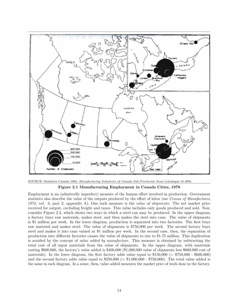
SOURCE: Statistics Canada 1982, Manufacturing Industries of Canada Sub-Provincial Areas (catalogue 31-209).

Figure 2.1 Manufacturing Employment in Canada Cities, 1978

Employment is an (admittedly imperfect) measure of the human effort involved in production. Governmentstatistics also describe the value of the outputs produced by the effort of labor (see Census of Manufactures,1972, vol. 3, part 2, appendix A). One such measure is the value of shipments: The net market pricereceived for output, excluding freight and taxes. This value includes only goods produced and sold. Now,consider Figure 2.2, which shows two ways in which a steel can may be produced. In the upper diagram,a factory buys raw materials, makes steel, and then makes the steel into cans. The value of shipmentsis $1 million per week. In the lower diagram, production is separated into two factories. The first buysraw material and makes steel: The value of shipments is $750,000 per week. The second factory buyssteel and makes it into cans valued at $1 million per week. In the second case, then, the separation ofproduction into different factories causes the value of shipments to rise to $1.75 million. This duplicationis avoided by the concept of value added by manufacture. This measure is obtained by subtracting thetotal cost of all input materials from the value of shipments. In the upper diagram, with materialscosting $600,000, the factory’s value added is $400,000 ($1,000,000 value of shipments less $600,000 cost ofmaterials). In the lower diagram, the first factory adds value equal to $150,000 (= $750,000 - $600,000)and the second factory adds value equal to $250,000 (= $1,000,000 - $750,000). The total value added isthe same in each diagram. In a sense, then, value added measures the market price of work done in the factory.

14

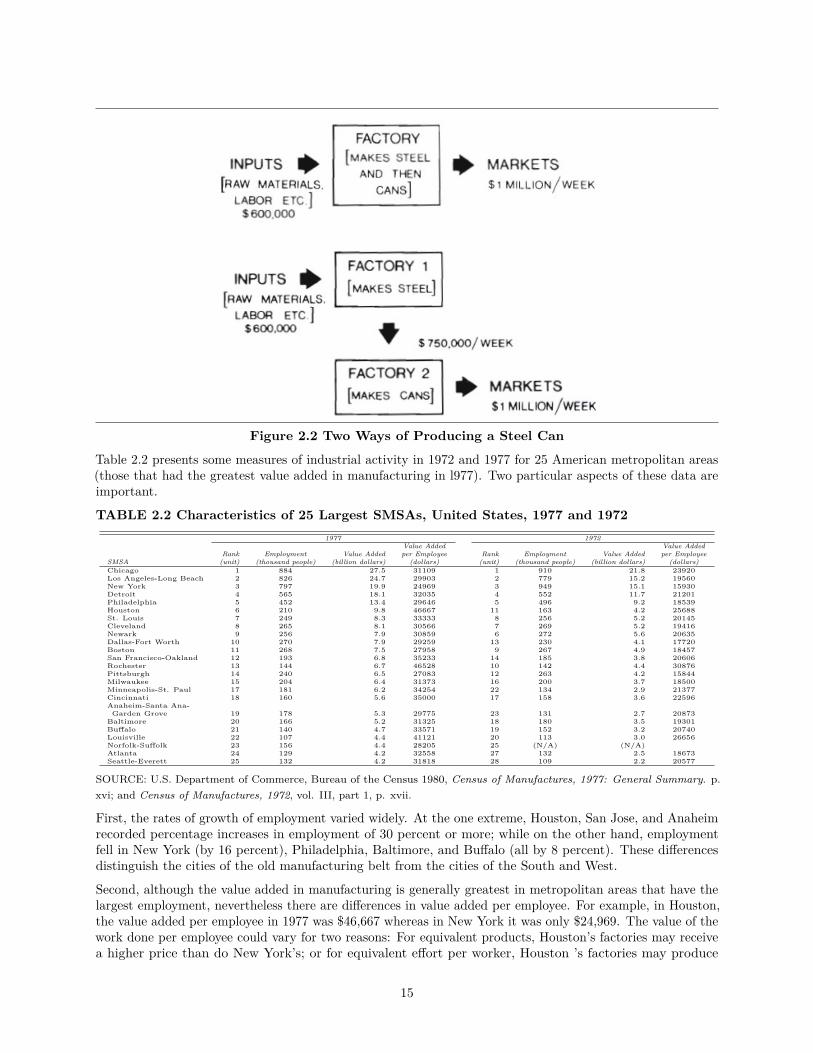
Figure 2.2 Two Ways of Producing a Steel Can

Table 2.2 presents some measures of industrial activity in 1972 and 1977 for 25 American metropolitan areas(those that had the greatest value added in manufacturing in l977). Two particular aspects of these data areimportant.

TABLE 2.2 Characteristics of 25 Largest SMSAs, United States, 1977 and 19721977 1972

Value Added Value AddedRank Employment Value Added per Employee Rank Employment Value Added per Employee

SMSA (unit) (thousand people) (billion dollars) (dollars) (unit) (thousand people) (billion dollars) (dollars)Chicago 1 884 27.5 31109 1 910 21.8 23920Los Angeles-Long Beach 2 826 24.7 29903 2 779 15.2 19560New York 3 797 19.9 24969 3 949 15.1 15930Detroit 4 565 18.1 32035 4 552 11.7 21201Philadelphia 5 452 13.4 29646 5 496 9.2 18539Houston 6 210 9.8 46667 11 163 4.2 25688St. Louis 7 249 8.3 33333 8 256 5.2 20145Cleveland 8 265 8.1 30566 7 269 5.2 19416Newark 9 256 7.9 30859 6 272 5.6 20635Dallas-Fort Worth 10 270 7.9 29259 13 230 4.1 17720Boston 11 268 7.5 27958 9 267 4.9 18457San Francisco-Oakland 12 193 6.8 35233 14 185 3.8 20606Rochester 13 144 6.7 46528 10 142 4.4 30876Pittsburgh 14 240 6.5 27083 12 263 4.2 15844Milwaukee 15 204 6.4 31373 16 200 3.7 18500Minneapolis-St. Paul 17 181 6.2 34254 22 134 2.9 21377Cincinnati 18 160 5.6 35000 17 158 3.6 22596Anaheim-Santa Ana-Garden Grove 19 178 5.3 29775 23 131 2.7 20873

Baltimore 20 166 5.2 31325 18 180 3.5 19301Buffalo 21 140 4.7 33571 19 152 3.2 20740Louisville 22 107 4.4 41121 20 113 3.0 26656Norfolk-Suffolk 23 156 4.4 28205 25 (N/A) (N/A)Atlanta 24 129 4.2 32558 27 132 2.5 18673Seattle-Everett 25 132 4.2 31818 28 109 2.2 20577

SOURCE: U.S. Department of Commerce, Bureau of the Census 1980, Census of Manufactures, 1977: General Summary. p.xvi; and Census of Manufactures, 1972, vol. III, part 1, p. xvii.

First, the rates of growth of employment varied widely. At the one extreme, Houston, San Jose, and Anaheimrecorded percentage increases in employment of 30 percent or more; while on the other hand, employmentfell in New York (by 16 percent), Philadelphia, Baltimore, and Buffalo (all by 8 percent). These differencesdistinguish the cities of the old manufacturing belt from the cities of the South and West.

Second, although the value added in manufacturing is generally greatest in metropolitan areas that have thelargest employment, nevertheless there are differences in value added per employee. For example, in Houston,the value added per employee in 1977 was $46,667 whereas in New York it was only $24,969. The value of thework done per employee could vary for two reasons: For equivalent products, Houston’s factories may receivea higher price than do New York’s; or for equivalent effort per worker, Houston ’s factories may produce

15

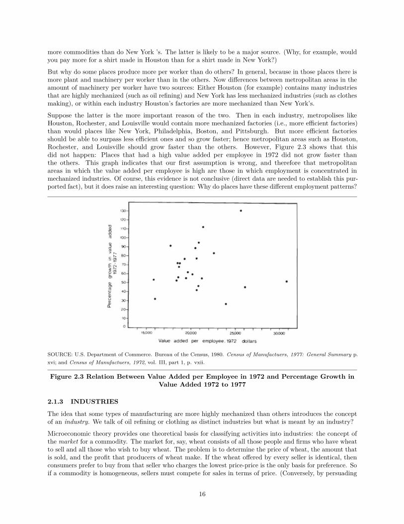
more commodities than do New York ’s. The latter is likely to be a major source. (Why, for example, wouldyou pay more for a shirt made in Houston than for a shirt made in New York?)

But why do some places produce more per worker than do others? In general, because in those places there ismore plant and machinery per worker than in the others. Now differences between metropolitan areas in theamount of machinery per worker have two sources: Either Houston (for example) contains many industriesthat are highly mechanized (such as oil refining) and New York has less mechanized industries (such as clothesmaking), or within each industry Houston’s factories are more mechanized than New York’s.

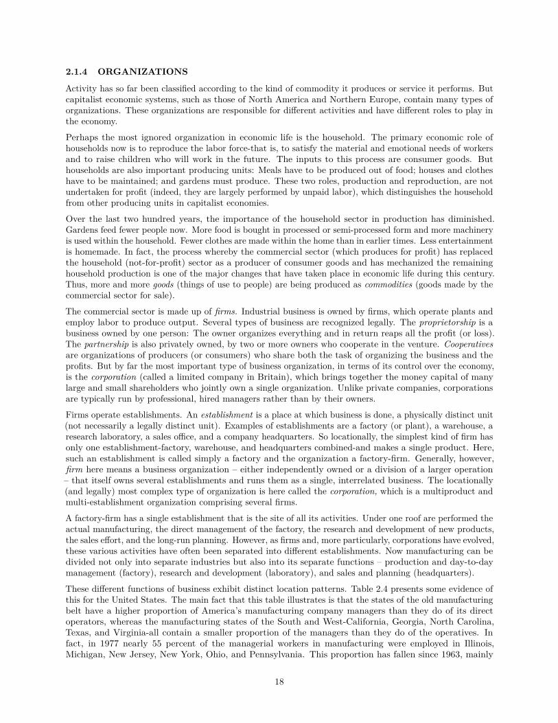
Suppose the latter is the more important reason of the two. Then in each industry, metropolises likeHouston, Rochester, and Louisville would contain more mechanized factories (i.e., more efficient factories)than would places like New York, Philadelphia, Boston, and Pittsburgh. But more efficient factoriesshould be able to surpass less efficient ones and so grow faster; hence metropolitan areas such as Houston,Rochester, and Louisville should grow faster than the others. However, Figure 2.3 shows that thisdid not happen: Places that had a high value added per employee in 1972 did not grow faster thanthe others. This graph indicates that our first assumption is wrong, and therefore that metropolitanareas in which the value added per employee is high are those in which employment is concentrated inmechanized industries. Of course, this evidence is not conclusive (direct data are needed to establish this pur-ported fact), but it does raise an interesting question: Why do places have these different employment patterns?

SOURCE: U.S. Department of Commerce. Bureau of the Census, 1980. Census of Manufactuers, 1977: General Summary p.xvi; and Census of Manufactuers, 1972, vol. III, part 1, p. vxii.

Figure 2.3 Relation Between Value Added per Employee in 1972 and Percentage Growth inValue Added 1972 to 1977

2.1.3 INDUSTRIES

The idea that some types of manufacturing are more highly mechanized than others introduces the conceptof an industry. We talk of oil refining or clothing as distinct industries but what is meant by an industry?

Microeconomic theory provides one theoretical basis for classifying activities into industries: the concept ofthe market for a commodity. The market for, say, wheat consists of all those people and firms who have wheatto sell and all those who wish to buy wheat. The problem is to determine the price of wheat, the amount thatis sold, and the profit that producers of wheat make. If the wheat offered by every seller is identical, thenconsumers prefer to buy from that seller who charges the lowest price-price is the only basis for preference. Soif a commodity is homogeneous, sellers must compete for sales in terms of price. (Conversely, by persuading

16

consumers that their commodities are not homogeneous, sellers can try to avoid price competition.) Inmicroeconomic theory, then, a commodity is a homogeneous product, and different sellers are distinguishedonly by price. Provided that there are enough sellers, no consumer will buy from a seller who tries to sell ata price above the others: All sellers of the commodity therefore offer the same price. Thus, arises the idea ofa competitive market: Many independent sellers of a homogeneous commodity, all selling at the same price.Such a group of sellers is a theoretical industry.

In practice, however, this notion of an industry is far too limited. Some commodities are virtually homogeneous:A pharmaceutical drug, for example, is made according to a precise formula. But most commodities arelike automobiles, dishwashers, and cookies in that there are many different kinds of them. Other industriesare defined not by the commodity they make but by the type of buyer to whom they sell: The agriculturalmachinery industry sells a variety of machines to farmers. Some industries are defined by the materialthey process: Petrochemical industries make many products from oil. Furthermore, a single market may besupplied by two or more industries: The dairy industry and the vegetable oil industry compete to sell spreadsfor bread.

Whatever the theoretical issues, in practice industries are defined by government statisticians who haveproduced a Standard Industrial Classification. The principles of the U.S. classification are discussed inthe “Introduction” to each Census of Manufactures; for Canada, see Statistics Canada, Standard IndustrialClassification Manual. The United States and Canada both define twenty major groups, such as food andbeverage industries or paper and allied industries. Each major group is divided into three-digit industries:143 in the United States and 112 in Canada. The United States also has four-digit classifications comprising451 industries. Table 2.3 illustrates the way in which this classification system works.

Table 2.3 Structure Of U.S. Standard Industrial Classification

SOURCES: U.S. Deparment of Commerce, Bureau of the Census, 1976. Census of Manufactures, 1972, vol. 3 part 2, appendix.For Canada, see Statistics Canada, 1971. Standard Industrial Manual, Revised 1970 (catalogue 12-501).

In the Standard Industrial Classification most industries are defined in terms of specific groups of products,usually made by similar materials and processes. But some industries are defined by the process used(aluminum foundries) and some by the material used (wood office furniture). However, no matter how carefulor detailed the classification, the factories grouped in an industry do not account for all the production of thatindustry, and those factories also produce commodities belonging to other industries. Both these problems arecaused by the fact that factories generally produce a variety of commodities. Therefore, aluminum foundriesin New York do not necessarily produce the same products as aluminum foundries in Texas. Industries arenot as homogeneous as we commonly think (or as we consider them for empirical research).

17

2.1.4 ORGANIZATIONS

Activity has so far been classified according to the kind of commodity it produces or service it performs. Butcapitalist economic systems, such as those of North America and Northern Europe, contain many types oforganizations. These organizations are responsible for different activities and have different roles to play inthe economy.

Perhaps the most ignored organization in economic life is the household. The primary economic role ofhouseholds now is to reproduce the labor force-that is, to satisfy the material and emotional needs of workersand to raise children who will work in the future. The inputs to this process are consumer goods. Buthouseholds are also important producing units: Meals have to be produced out of food; houses and clotheshave to be maintained; and gardens must produce. These two roles, production and reproduction, are notundertaken for profit (indeed, they are largely performed by unpaid labor), which distinguishes the householdfrom other producing units in capitalist economies.

Over the last two hundred years, the importance of the household sector in production has diminished.Gardens feed fewer people now. More food is bought in processed or semi-processed form and more machineryis used within the household. Fewer clothes are made within the home than in earlier times. Less entertainmentis homemade. In fact, the process whereby the commercial sector (which produces for profit) has replacedthe household (not-for-profit) sector as a producer of consumer goods and has mechanized the remaininghousehold production is one of the major changes that have taken place in economic life during this century.Thus, more and more goods (things of use to people) are being produced as commodities (goods made by thecommercial sector for sale).

The commercial sector is made up of firms. Industrial business is owned by firms, which operate plants andemploy labor to produce output. Several types of business are recognized legally. The proprietorship is abusiness owned by one person: The owner organizes everything and in return reaps all the profit (or loss).The partnership is also privately owned, by two or more owners who cooperate in the venture. Cooperativesare organizations of producers (or consumers) who share both the task of organizing the business and theprofits. But by far the most important type of business organization, in terms of its control over the economy,is the corporation (called a limited company in Britain), which brings together the money capital of manylarge and small shareholders who jointly own a single organization. Unlike private companies, corporationsare typically run by professional, hired managers rather than by their owners.

Firms operate establishments. An establishment is a place at which business is done, a physically distinct unit(not necessarily a legally distinct unit). Examples of establishments are a factory (or plant), a warehouse, aresearch laboratory, a sales office, and a company headquarters. So locationally, the simplest kind of firm hasonly one establishment-factory, warehouse, and headquarters combined-and makes a single product. Here,such an establishment is called simply a factory and the organization a factory-firm. Generally, however,firm here means a business organization – either independently owned or a division of a larger operation– that itself owns several establishments and runs them as a single, interrelated business. The locationally(and legally) most complex type of organization is here called the corporation, which is a multiproduct andmulti-establishment organization comprising several firms.

A factory-firm has a single establishment that is the site of all its activities. Under one roof are performed theactual manufacturing, the direct management of the factory, the research and development of new products,the sales effort, and the long-run planning. However, as firms and, more particularly, corporations have evolved,these various activities have often been separated into different establishments. Now manufacturing can bedivided not only into separate industries but also into its separate functions – production and day-to-daymanagement (factory), research and development (laboratory), and sales and planning (headquarters).

These different functions of business exhibit distinct location patterns. Table 2.4 presents some evidence ofthis for the United States. The main fact that this table illustrates is that the states of the old manufacturingbelt have a higher proportion of America’s manufacturing company managers than they do of its directoperators, whereas the manufacturing states of the South and West-California, Georgia, North Carolina,Texas, and Virginia-all contain a smaller proportion of the managers than they do of the operatives. Infact, in 1977 nearly 55 percent of the managerial workers in manufacturing were employed in Illinois,Michigan, New Jersey, New York, Ohio, and Pennsylvania. This proportion has fallen since 1963, mainly

18

because of the precipitous decline of New York state as an employer of manufacturing managers and operatives.

TABLE 2.4 Percentage Distribution of Operatives and of Managerial Workers, Selected U.S.States, 1963 and 1977

Ratio, 1977, ofManagerial

Percentage of U.S. Percentage: Percentage:Managers in State Operatives in State Operative

State 1963 1977 1963 1977 PercentageCallifornia 6.5 5.5 8.3 9.1 0.60Connecticut 2.1 3.2 2.5 2.0 1.60Delaware 2.4 2.3 0.3 0.2 11.50Georgia 0.6 1.4 2.2 2.5 0.56Illinois 8.3 8.9 7.1 6.4 1.39Indiana 1.4 1.6 3.7 3.7 0.43Massachusetts 3.8 3.1 4.0 3.1 1.00Michigan 11.4 9.8 5.4 5.5 1.78Minnesota 2.1 2.8 1.4 1.6 1.75Missouri 2.6 2.7 2.3 2.2 1.22New Jersey 7.1 8.1 4.8 3.7 2.19New York 20.0 11.7 10.5 7.5 1.56North Carolina 1.7 2.4 3.2 4.0 0.60Ohio 7.5 7.5 7.3 6.8 1.10Pennsylvania 9.5 8.1 8.2 6.7 1.21Tennessee 0.6 0.8 2.0 2.6 0.31Texas 2.1 4.1 3.1 4.5 0.91Virginia 1.0 1.0 1.8 2.1 0.48Wisconsin 1.9 2.1 2.8 2.8 0.75

SOURCE: U.S. Department of Commerce, Bureau of the Census 1980. Census of Manufactures, 1977: GeneralSummary, pp. 1-12 to 1-14.NOTE: States are only included if they contained 2% of U.S. operatives or managers in 1977. Observe the effectsof state taxation provisions for incorporation on the managerial/operatives ratio for Delaware.

2.2 Evolution of ManufacturingIndustries and the organizations that run them have changed dramatically during the last two centuries.These changes have caused the location of industry to change too, for the location of industry reflects thebroader structure of society. This section describes two aspects of the evolution of manufacturing since themid-nineteenth century: changes in the organizationof production and changes in the types of production. Itis important to study the manner in which manufacturing has evolved, first because the present containsrelict features of the past (New England mill towns, the industrial northeast, inner industrial districts ofthe old manufacturing cities), and second because the relative importance of the various factors that affectlocation has changed over time.

In the mid-nineteenth century, firms and plants were small. Table 2.5 shows some of the relevant data for theUnited States. In 1869, the average manufacturing establishment employed eight people and used only 1.14horsepower of machinery per worker. Most firms were unincorporated, either proprietorships or partnerships.Also in the nineteenth century, wage labor was much less prevalent than it is today (Table 2.6): In 1870 lessthan half of the population was in the labor force; even by the turn of the century, wages and salaries ofemployees accounted for only 55 percent of national income. Conversely, there were many manufacturingestablishments-one for every 111 people in 1870.

19

TABLE 2.5 Selected Aspects of U.S. Manufacturing Industry, 1870-1980

Number of Number of Employees HorsepowerEstablishments Production Other Value Added per Worker

Year (thousands) (thousands) (thousands) (billions of dollars) (unit)1977 360 13700 5900 585 –1967 311 13955 4537 262 –1954 287 12372 3272 117 9.581947 241 11900 2400 81 –1929 207 8370 1290 31 4.911899a 205 4502 348 4.65 2.181899b 509 5098 380 5.48 –1869b 252 2054 1.40 1.14

SOURCE: U.S. Department of Commerce, Bureau of the Census, 1975. Historical Statistics of the United States,Colonial Times to 1970, pp. 666 and 681; and Statistical Abstract of the United States, 1981, p. 780a. Factories excluding hand and industries.b. Factories including hand and industries.

TABLE 2.6: U.S. Labor Force and National Income Characteristics, 1900-1980

Labor Force as Percentage of Population Percentage of National Income Accruing to:Nonagricultural,

Year All Civilian, Employed Employees Businessa Rentb Profitc Interestd1977 62.8 54.9 – – – – –1967 60.6 52.9 71.1 10.0 3.3 12.4 3.21954 57.6 46.5 – – – – –1947 56.8 45.7 65.5 15.6 3.8 14.1 0.91929 56.2 42.2 63.0 15.8 6.6 6.4 8.11900 53.7 – 55.0 23.6 9.1 6.8 5.5

SOURCES: U.S. Department of Commerce, Bureau of teh Census. 1975. Historical Statistics of the United States, ColonialTimes to 1970, pp. 127 and 236NOTE: Where data are missing, they are unavailablea. Income of unincorporated businessb. Rental income of persons.c. Corporate profits before tax.d. Net interest.

The manufacturing sector was a capitalist sector. It was organized by owners to produce commodities forsale using wage labor, with the goal of making profits. Many activities are not organized in this way: Thehousehold and family business do not use wage labor, nor do legal and medical services. Agriculture, whenrun by family farms, produces some commodities not for sale and uses little wage labor. In Table 2.6, thesum of employee compensation and corporate profits shows that at the turn of the century some 62 percentof the U.S. national income arose in capitalist organizations (remember that the national income does omitnot-for-sale production).

Within manufacturing, firms seek profits. There are three main avenues whereby profits can be made. First,a firm can seek to enlarge its profits by producing its commodities more efficiently than do rival firms, thusmaking a greater profit per unit of output or, if it reduces its prices, enlarging its share of the market.This is the route of technical change in the production of existing commodities. Second, a firm can seek to

20

produce new commodities-televisions as well as radios, cars as well as bicycles, or microcomputers as well asscientific measuring devices. This is the route of new product development. Associated with this route isthe third method of raising profit: enlarging the sphere of capitalist commodity production by taking overactivities previously performed by noncapitalist organizations. In particular, this method has taken overmuch household production: food preparation, house maintenance, and clothing production have all beenincreasingly performed outside the household and mechanized. All three routes to profit have affected thescope, type, and organization of production.

Table 2.6 contains some indexes of the effect of enlarging the sphere of capitalist commodity production. Thenonagricultural civilian labor force has more than doubled as a proportion of the population, and the laborforce is now 60 percent of the population: There has been a decline in the number of people left at home towork in the household. Wages or salaries and profits account for over 80 percent of the U.S. national income(compared to 62 percent in 1900), so property and private business income now comprise only one-eighthof the total of all income. Thus, an increasing proportion of the population works outside the home (musttravel to work) and works for pay in profit-seeking firms.

New product development and increasing participation of the household sector together imply that the rangeof commodities produced by manufacturers is now significantly larger than it was before. One obvious effectof this process has been the creation of entirely new industries: the chemical, instruments, and electrical andelectronic machinery industries were all insignificant in the nineteenth century. Manufacturing now meansa wider set of processes than it used to. Two other aspects of this process deserve further comment: theproduct cycle, and research and development.

It has been claimed that new products are introduced into the market in a characteristic pattern. When aninnovation is produced and a new commodity is first made, firms are uncertain about the design, productionmethod, and market for the commodity. The market is small and uncertain, so firms are small (or small partsof corporations) and labor intensive. As the market for the commodity is enlarged by advertising and by itsacceptance as a part of daily life, and as firms acquire appropriate production techniques, profitability rises.These profits encourage firms to seek larger market shares by standardizing the commodity and mechanizingits production. Prices now fall and output rises until everyone is using the commodity; as this expansion phaseends, the only sales are those due to the replacement of obsolete items and the increase in consumption perhead. This history, with its phases of initial production, high profits, standardization, and market saturation,is called the product cycle hypothesis. It claims that at different phases, manufacturing establishments differand so may have different locational needs.

Table 2.7 illustrates one aspect of the product cycle hypothesis-the rates of growth of U.S. industrygroups at different times. Some industries were well developed during the nineteenth century andhave never grown faster than has manufacturing as a whole since 1900: textile mill products (SIC 22),apparel (23), lumber and wood products (24), and leather industries (31, apart from the aberration of1919). These industries were in the saturated phase before 1900. Another group reached their peakgrowth rates before 1919 – tobacco (21), printing and publishing (27), petroleum and coal products (29),and primary metals (33). The third group comprises industries that grew fastest since World War II:chemicals (28) and instruments (38) in the 1950s; paper and paper products (26) and machinery (35,36) in the 1960s; furniture (25), rubber and plastics (30), and stone, clay, and glass products (32) inthe 1970s. The transport industry (37) has two peaks – one in the period between 1899 and 1919 andone in the 1950s. Such product cycles are even more clearly seen in the data for three- and four-digit industries.

21

TABLE 2.7 Index Numbers of U.S. Manufacturing Production by Industry 1900-1980

SOURCES: U.S. Department of Commerce, Bureau of the Census, 1975. Historical Statistics of the United States.Colonial Times to 1970, pp.667-8; and Statistical Abstract of the United States, 1981, p.778NOTE: The index numbers combine three not strictly comparable series - for the 1899 to 1947 and 1947 to 1970from Historical Statistics, and for 1970 to 1980 from Statistical Abstract.a. Short names only; full names are in Table 2.3.b. 1967 = 100

The path to greater profits via new products has spawned an entire twentieth century industry: researchand development. However, it is the first route to profits-technical change-that has had the main effect onthe organization of production. Cost-reducing technical changes within factories have taken the form of newequipment, standardized production methods, and economies in the use of raw materials. Now each workerhas ten times the horsepower available to nineteenth-century workers (Table 2.5), and indexes of output perhour of work show the same rise. By 1977, each establishment had 54 employees, and over one-quarter of themanufacturing workers were employed in plants where over one thousand people worked. The sheer increasein the size of factories and in the amount of machinery per worker are the major changes to have affectedmanufacturing work.

Increases in plant size have been accompanied by the concentration of output and capital in a few corporationsin each industry. The production of many industries is now dominated by a few firms. Whereas in 1899,

22

unincorporated businesses still accounted for 35 percent of the value added in manufacturing, this proportionhad fallen to less than 5 percent by the 1960s. By this time, too, one-quarter of all the value added inmanufacturing was produced by the 50 largest companies. The price of this corporate market power has beenan enlargement in the proportion of nonproduction employees, from 7 percent in 1899 to over 30 percent now(see Table 2.5).

These three routes to greater profit (technical change, new commodities, and enlargement of the sphere ofcommodity production) and their effects upon the economy have been set within the context of a system inwhich the state plays a larger role now than it did formerly. (The state is the set of all government institutions,local and national.) The state provides major markets for manufacturers, particularly the armaments andspace industries: By the 1960s, U.S. government purchases accounted for almost one-quarter of the output ofthe transport equipment and ordnance industries and one-sixth of the electrical equipment produced (U.S.Department of Commerce, Historical Statistics, p. 272). The state has also supported ailing industries byrunning them directly (as in the United Kingdom and Canada), by guaranteeing loans, and by reducing taxeson corporate profits (in the United States from 45 percent in 1960 to 36-37 percent in 1979 and 1980; U.S.Department of Commerce, Statistical Abstract, p. 777). There is some claim that local variations in taxesaffect industrial location, but this will be examined in Chapter 4. Particularly in the United Kingdom andCanada, the state has involved itself in regional planning (ostensibly intended to direct manufacturing plantsto locations where unemployment rates are high, but it is likely that these policies have had limited effects onthe location of industry).

These changes in the organization and type of production have altered the lives of all of us. They affect usboth as consumers and as workers. Part of this effect occurs by changes in the location of industry, and thetask of industrial location theory is to understand that link between social and locational change. To developthat understanding, we must now begin the task of theorizing location. In Chapter 6, we return to this linkby applying the location principles to actual societies.

2.3 Further ReadingSome aspects of work and employment are discussed by E. B. Philips and R. T. LeGates in City Lights(1981, pp. 449-472). A more prosaic introduction to the notion of industrial systems and the components ofthose systems is contained in F. E. I. Hamilton and G. J. R. Linge (eds.), Spatial Analysis, Industry and theIndustrial Environment: 1, Industrial Systems (1979, pp. 1-23).

23

3 PROFITS AND LOCATIONThe previous chapters have claimed as a guiding principle that the task of location theory is to link thechanges that are taking place in society (the type and organization of production) to the spatial distributionof industry. We have now reviewed the nature of the units that operate in society and have described someimportant changes that have occurred over the last one hundred years. The link between these changes andlocation is location theory. That theory has two parts: first, an understanding of the way the economy works,and then an application of that understanding to the historical context to analyze industrial location patterns.This chapter attempts the first part: to understand the way in which the economy works.

Assume what has been taken for granted – that the economies of Western Europe and North America (andparticularly their manufacturing sectors) are capitalist. Production is organized by the owners of firms; theowners’ goal is to sell the firm’s output in order to make profits. Firms use capital to buy raw materials,semi-finished goods, the plant and machinery, and to hire labor in order to produce commodities for sale.The coordination of all this activity (aggregate output and price) is achieved by the market rather than by aplanner.

But what are the rules of the operation of such an economy? This question can be answered in two ways.One is to make claims about the overall goals of the economic system, such as asserting that the economy isorganized to achieve maximum rates of economic growth. The other way is followed here: to analyze theeconomy at the level of the individual firm and to explain location patterns by referring to the decisions madeby firms. This chapter explains the basis for these decisions, by examining location decisions theoretically.

3.1 Location in TheoryThere are three kinds of location decisions. The first is the decision to build or buy a new establishment.The firm is starting in business or relocating its business or building additional capacity. Location theory hastraditionally concentrated on this type of decision, as Chapter 4 will reveal. Second, the firm can reorganizeproduction, by altering the products produced at its various establishments or by closing some factories andconcentrating production at others. The problem then is not to add capacity but to rearrange it or even toreduce it. The third decision is the decision to close down an establishment-to reduce capacity. Often, butnot always, this decision is involuntary, being forced by bankruptcy.

In each of these cases, the firm is making a decision to invest or to disinvest. This decision depends on theexistence of perceived opportunities to sell (or the lack of opportunities) and on the firm’s perceived ability tofind the investment. Unforced location decisions are thus investment decisions, and the choice of a locationdepends on the perception of an opportunity.

Once established, a business must either grow or stagnate. There are business people who are happy tocontrol small, old-fashioned firms, but they account for very little manufacturing output. Successful firms arethose that survive their initial growth pains and then are able to increase their capital and scale of operations.The recent history of the high-technology computer industry of “Silicon Valley” (around San Jose, California)illustrates this process.

A firm can increase its scale of production only by capital investment. There are two sources of this capital.One is the investment of the firm ’s own profits; in 1980, firms retained over 60 percent of their after-taxprofits (U.S. Department of Commerce, Statistical Abstract, p. 777) and these retained earnings comprisedover 80 percent of gross investment in equipment and buildings (p. 781). Second, capital may be obtainedfrom investors or borrowed from financial institutions. People and institutions invest and lend in order toobtain a return on their investment, and the surest evidence about that return is a past level of profits. Themore profit a firm makes, then, the more it can grow. (However, for the economy as a whole, more profitdoes not equal more growth because profits can be invested abroad.) In traditional economic theory, thisthesis is summarized in the principle that firms seek to maximize profits – in particular, seek locations thatmaximize profits.

Maximizing profits means that the firm chooses the most profitable location or set of locations in view. Thisprinciple is not meant in the precise sense. Some decisions are highly constrained by the firm’s circumstances

24

so that there are only a few alternatives: For example, there may be only two or three blocks of land for salein a given city to which the roads are good enough for heavy trucks, for which waste disposal provisions havebeen made, and utilities have been connected. For other decisions, the firm has greater freedom to choose.The theoretical claim is simple: Decisions are best understood as the decisions of profit-maximizing firms.

There have been two main objections to this principle. The first claims that people do not know enoughto be able to choose optimum locations. The second objection states that corporations are not now run byowners but by managers, who have no personal stake in corporate profits. Let’s consider the second objectionfirst, for it is the less serious.

3.1.1 MANAGERIALISM

The idea of the maximum profit criterion was first popularized by Adam Smith, an eighteenth-century Britisheconomist who claimed that capitalism works by appealing to people ’s self-interest. It is in each person’sinterest to increase his or her wealth. At the dawn of industrial capitalism in the early nineteenth century,most manufacturing businesses were unincorporated firms owned by one or a few individuals (who typicallyalso managed the business). Owners had a direct, personal incentive to maximize the profit of firms.

Virtually all manufacturing output is now produced by large corporations. These corporations are owned bystockholders, pension funds, insurance companies, and banks; but they are run by professional managers. Thewealth of managers is not directly related to the profitability of a corporation; therefore, managers have lessincentive than do owner-operators to make profit-maximizing decisions. Alternative decision criteria includesecurity or size; that is, decisions are made in order to guarantee the future of the firm or to maximize itssales. This claim is made by those who advance behavioral theories of the firm (see, for example, Cyert andMarsh 1963, and Baumol 1959) and it is bolstered by interviews with business people who have sometimeschosen a location for what they say are personal reasons.

Despite its popularity, the behavioral argument fails. The flaw of the behavioral approach is that it personalizesthe profit motive. Smith claimed that firms seek profits to satisfy the personal greed of their owners; andundoubtedly, many people do want to become rich, just as many owners obtain psychic rewards from operatingtheir own businesses. Still the large corporations that dominate manufacturing maximize profits – not becauseof the personal whim of their managers, but because they have no alternative. If a firm does not keep up inthe race for profits, it stagnates and in the long run, dies. Low profits imply both reduced dividends andlower retained earnings that reduce stockholders’ incomes and the capital appreciation of the stock, bothof which drive away investors. As the retained earnings fall, so reinvestment and product development arecurtailed, which drive profits even lower when techniques and product lines become obsolete. The goal ofmaximum profits is not a personal whim but a structural necessity.

3.1.2 UNCERTAINTY

The second argument against the claim that firms make decisions to maximize profits is far more serious thanthe first. It is the argument that firms simply do not have the information they require to maximize profits.

Firms are uncertain: They clearly do not possess enough information to guarantee that a decision is aprofit-maximizing one. A firm faces three main sources of uncertainty: Some data may be too expensive toobtain; the future can never be predicted with perfect accuracy; and other firms may make later decisions (tolocate, to develop new products, or to market products) that affect the anticipated benefits. For all thesereasons, the actual decision may not tum out to be as good as the firm had expected.

The problem of uncertainty is particularly acute for new location decisions. The impact of uncertaintydepends on the amount of capital committed by the decision and the ease with which the decision can berevoked. The decision to hire a particular worker, Jones, commits little capital (Jones’s wage) and is easilychanged (Jones can be fired). The decision to produce at a particular output level for the next month is bothcostlier and less easily changed. Automobile manufacturers invest even more in producing a new style of car:After years of design and testing (capital investment), the choice of a design is not easily changed in lessthan several years. (Of course, advertising reduces the risk of failure in this case.) The location decision ismore expensive still: It involves setting up or relocating the entire plant, equipment, and work force of an

25

establishment. This expense is greater for larger establishments but involves a smaller proportion of the totalassets of multiplant corporations than those of factory firms. Also, the location decision is not easily undone –establishments cannot simply be picked up and moved elsewhere. So, a poor locational choice has long-termeffects on profitability.Uncertainty affects location decisions because they are both costly and fixed. While these characteristicsencourage firms to seek actively for maximum profit locations, nevertheless, there will always be someuncertainty. Therefore, the expected outcome of a decision must be distinguished from the actual outcome.Technically, this distinction is between ex ante and expost evaluations.Location decisions are made in this manner: For each of the feasible sites, find out how much can be sold, howmuch it costs to produce that output, and the expected prices. After obtaining these data for each site, thelocations can be compared (this is the ex ante evaluation) and the most profitable one selected (this locationis the ex ante optimum). When the establishment is built and running, the firm discovers the actual costsand sales at each place: This is the ex post optimum. Clearly, a firm can only seek the ex ante optimum.This idea has been taken one step further. Investment information has two characteristics: First, it is notfree, so that managers have to pay for the data on which to base decisions; and second, people have only alimited capacity to process information (although this capacity has increased as computers have become morewidely used). These characteristics have prompted the claims that maximum profit locations (even ex anteoptimum) are fundamentally unobtainable, and thus managers should choose some levels of profits that wouldsatisfy them and then make decisions so as to obtain that satisfactory profit. Such decision making is calledsatisficing (attaining a satisfactory profit) as opposed to optimizing (obtaining the highest level of profit).Now, a remarkable fact has been discovered that relates satisfactory and optimal decisions. Suppose that youhave to choose a location for an investment. You evaluate sites one by one and compute the profit you canmake at each. After each calculation you decide to choose that site or to examine the next. Any rejectionyou make must be final. There is a cost to evaluate each site; although this cost fluctuates, you neverthelessexpect it to be constant on average. Now, what rule do you use to choose a location? It turns out that theoptimal rule is to satisfice. That is, if you want to choose the location which yields you the most profit net ofthe cost searching, you must first decide upon a satisfactory level of profit and then choose the first locationyou find that yields at least that level. Satisficing is optimal!Apparently, the simple rule that decisions are made to maximize profits needs to be clarified. Firms can onlyfind ex ante optima, not ex post optima (except by chance); and the selection of a best site must recognizethe costs of searching. It follows that even though firms are optimizing, the economy need not be located in aprofit-maximizing pattern: After the event, better locations could be found than the places actually chosen.Thus, we can imagine a location pattern that comprises many establishments located by firms seeking optimal(i.e., satisficing) ex ante locations, yet this location pattern could be rearranged to give every firm higherprofits.But this idea must not be overemphasized. The pattern of location in a society results not merely from firms’decisions, but also from society’s evaluation of those decisions. If at a given location a firm cannot makethe normal (i.e., satisfactory) rate of profit, then it cannot attract investors nor create the capital needed torenovate and expand: It will fall even further behind its peers in the industry. The attainment of a normalrate of profit is a socially imposed goal-and a firm ’s ex ante optimum may not be good enough to attain it.Factory closures are a constant reminder of this fact.The process whereby society imposes its profitability criterion upon the decisions of individuals can be seennot only in plant closings but also in settlement patterns. Figure 3.1 illustrates the process. During theprocess of European settlement of America, many towns and villages were set up at apparently advantageoussites. There were far too many for the needs of the economy, so only the locationally fittest places survived(This argument is extended by Alchian 1950.)These are some of the arguments that surround the claim that firms maximize profits. This claim is a soundbasis for location theory despite the contrary arguments. Location decisions are ex ante optima when searchcosts are considered; thus, a firm that has perfect information may be able to find a better site. However, theactual location pattern is a consequence not only of firms’ decisions but also of the weeding out of inefficientfirms by competition: The end result looks as if firms did find the profit maximum.

26

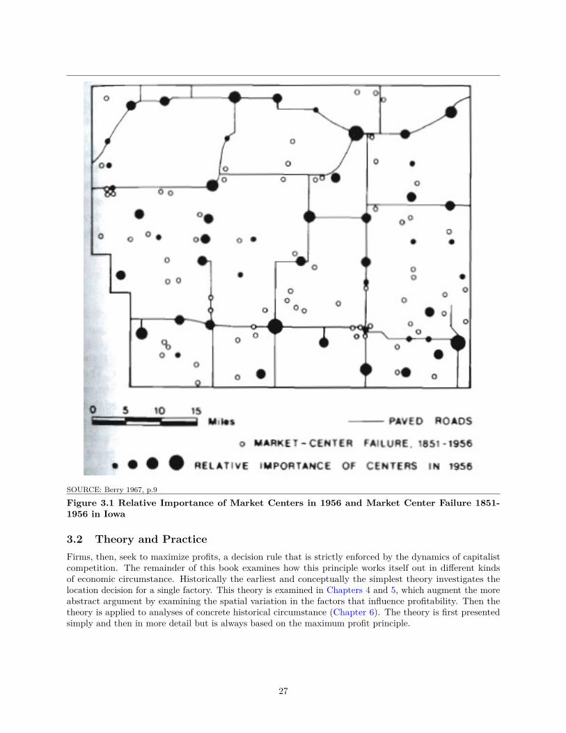
SOURCE: Berry 1967, p.9

Figure 3.1 Relative Importance of Market Centers in 1956 and Market Center Failure 1851-1956 in Iowa

3.2 Theory and PracticeFirms, then, seek to maximize profits, a decision rule that is strictly enforced by the dynamics of capitalistcompetition. The remainder of this book examines how this principle works itself out in different kindsof economic circumstance. Historically the earliest and conceptually the simplest theory investigates thelocation decision for a single factory. This theory is examined in Chapters 4 and 5, which augment the moreabstract argument by examining the spatial variation in the factors that influence profitability. Then thetheory is applied to analyses of concrete historical circumstance (Chapter 6). The theory is first presentedsimply and then in more detail but is always based on the maximum profit principle.

27

3.3 Further ReadingAn introduction to the ideas of theory and model is provided by P. E. Lloyd and P. Dicken in Locationin Space (1977, pp. 8-17). Some general criticisms of industrial location theory – and suggestions for itsimprovement – are found in the papers by David Smith and Doreen Massey in F. E. I. Hamilton and G. J. R.Linge (eds.) Spatial Analysis, Industry and the Industrial Environment: 1, Industrial Systems, (1979, pp.37-55, 57-72).

28

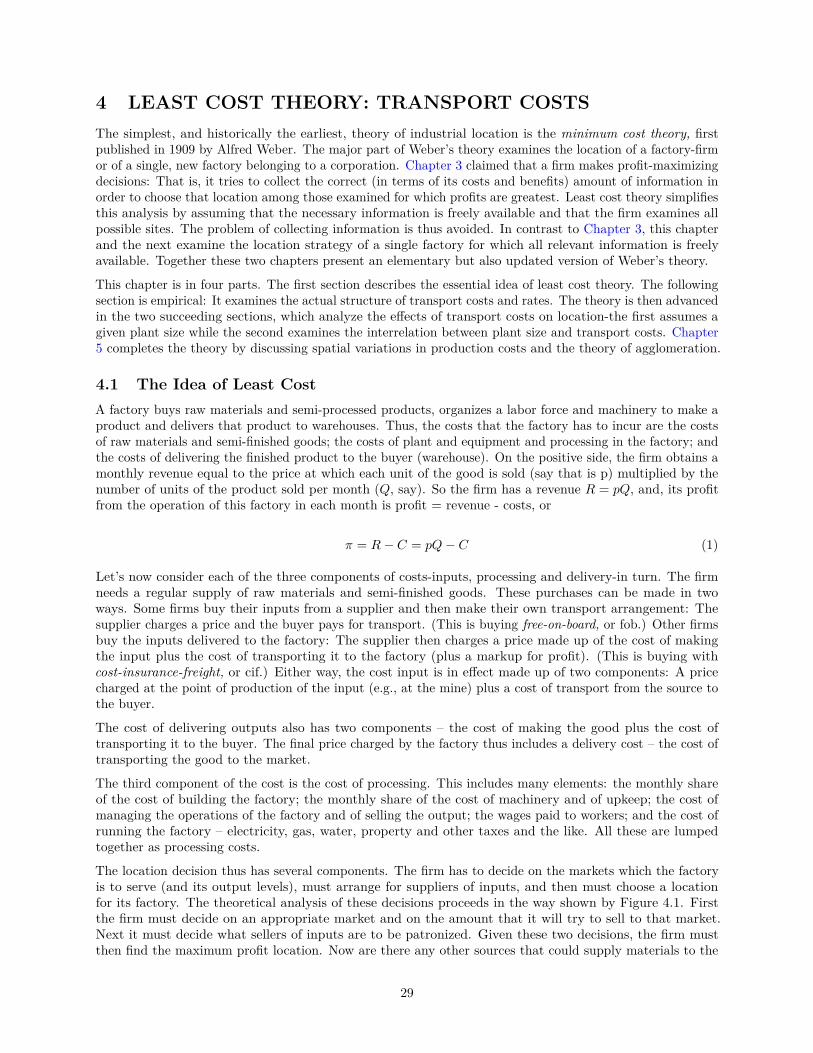
4 LEAST COST THEORY: TRANSPORT COSTSThe simplest, and historically the earliest, theory of industrial location is the minimum cost theory, firstpublished in 1909 by Alfred Weber. The major part of Weber’s theory examines the location of a factory-firmor of a single, new factory belonging to a corporation. Chapter 3 claimed that a firm makes profit-maximizingdecisions: That is, it tries to collect the correct (in terms of its costs and benefits) amount of information inorder to choose that location among those examined for which profits are greatest. Least cost theory simplifiesthis analysis by assuming that the necessary information is freely available and that the firm examines allpossible sites. The problem of collecting information is thus avoided. In contrast to Chapter 3, this chapterand the next examine the location strategy of a single factory for which all relevant information is freelyavailable. Together these two chapters present an elementary but also updated version of Weber’s theory.

This chapter is in four parts. The first section describes the essential idea of least cost theory. The followingsection is empirical: It examines the actual structure of transport costs and rates. The theory is then advancedin the two succeeding sections, which analyze the effects of transport costs on location-the first assumes agiven plant size while the second examines the interrelation between plant size and transport costs. Chapter5 completes the theory by discussing spatial variations in production costs and the theory of agglomeration.

4.1 The Idea of Least CostA factory buys raw materials and semi-processed products, organizes a labor force and machinery to make aproduct and delivers that product to warehouses. Thus, the costs that the factory has to incur are the costsof raw materials and semi-finished goods; the costs of plant and equipment and processing in the factory; andthe costs of delivering the finished product to the buyer (warehouse). On the positive side, the firm obtains amonthly revenue equal to the price at which each unit of the good is sold (say that is p) multiplied by thenumber of units of the product sold per month (Q, say). So the firm has a revenue R = pQ, and, its profitfrom the operation of this factory in each month is profit = revenue - costs, or

π = R− C = pQ− C (1)

Let’s now consider each of the three components of costs-inputs, processing and delivery-in turn. The firmneeds a regular supply of raw materials and semi-finished goods. These purchases can be made in twoways. Some firms buy their inputs from a supplier and then make their own transport arrangement: Thesupplier charges a price and the buyer pays for transport. (This is buying free-on-board, or fob.) Other firmsbuy the inputs delivered to the factory: The supplier then charges a price made up of the cost of makingthe input plus the cost of transporting it to the factory (plus a markup for profit). (This is buying withcost-insurance-freight, or cif.) Either way, the cost input is in effect made up of two components: A pricecharged at the point of production of the input (e.g., at the mine) plus a cost of transport from the source tothe buyer.

The cost of delivering outputs also has two components – the cost of making the good plus the cost oftransporting it to the buyer. The final price charged by the factory thus includes a delivery cost – the cost oftransporting the good to the market.

The third component of the cost is the cost of processing. This includes many elements: the monthly shareof the cost of building the factory; the monthly share of the cost of machinery and of upkeep; the cost ofmanaging the operations of the factory and of selling the output; the wages paid to workers; and the cost ofrunning the factory – electricity, gas, water, property and other taxes and the like. All these are lumpedtogether as processing costs.

The location decision thus has several components. The firm has to decide on the markets which the factoryis to serve (and its output levels), must arrange for suppliers of inputs, and then must choose a locationfor its factory. The theoretical analysis of these decisions proceeds in the way shown by Figure 4.1. Firstthe firm must decide on an appropriate market and on the amount that it will try to sell to that market.Next it must decide what sellers of inputs are to be patronized. Given these two decisions, the firm mustthen find the maximum profit location. Now are there any other sources that could supply materials to the

29

factory? If so, suppose that one of these other sources is patronized, and reconsider the maximum profitlocation. Continue to search for alternative sources of supply and reevaluate the location until all othersuppliers have been considered. Could the factory supply any additional or different markets? If so, chooseone of these markets and return to step 2. Continue iterating 5, 2, 3, and 4 until all alternative markets havebeen evaluated. This procedure will provide the firm with a maximum profit combination of markets (andoutputs), suppliers, and location.

Figure 4.1 Flow Chart of a Firm’s Location Decision for a Factory

Suppose that step 1 has been accomplished and that a given market has been chosen. Then p and Q areknown. There remains a pair of decisions – suppliers and location. Equation 1 shows that for a given pair pand Q, the choice of suppliers and of location maximizes profits if and only if it minimizes costs. That is, forgiven market and price decisions, the firm’s choice of suppliers and locations must be a minimum cost one.The first stage in the theory of industrial location must then be to find minimum cost locations and suppliersto serve a given market – hence the name least cost theory.

So the first problem is, given a certain market, find that set of suppliers and that location that minimize thecost of serving that market (the market may comprise one city, several cities or the nation). For example,suppose that a firm wants to sell 600 chairs a month to the federal government in Washington, D.C. Each

30

chair weighs an average of 13 pounds. The firm needs 6,000 pounds of wood per month, available fromsuppliers X1, X2, or X3; it needs 4,000 pounds of steel tube, from Y1 or Y2; and it needs 1,000 pounds ofmiscellaneous fittings available from Z. It has six combinations of suppliers: X1 for wood and Y1 for tube; orX1 for wood and Y2 for tube; X2 and Y1; X2 and Y2; X3 and Y1; or X3 and Y2. For each combination ofsuppliers, a least cost location has to be found, and then the least cost combination of suppliers.

Thus the problem has become even simpler: For a given set of markets and suppliers, find the locationthat minimizes costs. Figure 4.2 is a map showing the location of the various suppliers and the singlemarket, M . The figure also shows the costs of transporting the supplies and chairs as well as the possiblesites of production S1, S2, S3, and S4, which are all near places where there is available labor and power.Table 4.1 lays out the calculations of costs if fittings came from Z, tube from Y2, and wood from X2.You can see that the least cost site is S4. The table also lays out the costs of locating at S3 for theother five combinations of suppliers. You should now complete these calculations for sites S2, S3 andS4. The result is that you can find the least cost combination of suppliers and location to serve themarket at M ; namely, use X1, Y2, Z, and locate at S1 (the market). It is a straightforward matter to dothe same calculations for other market and so to find the maximum profit market, set of suppliers, and location.

TABLE 4.1 Calculation of Minimum Cost Location for Data in Figure 4.2

S1 S2 S3 S4( 1) Costs of production (in dollars) 12000 12000 12000 13000( 2) Transport costs on fittings 400 350 300 250( 3) Transport costs on wood from X1 2000 0 2000 3000( 4) Transport cost on tube from Y2 1100 700 500 600( 5) Transport costs on chairs on M 2500 3800 4000

Total costs (1+2+3+4+5) 15500 16550 19600 20850

( 6) Transport costs on wood from X1 2000 0 2000 3000( 7) Transport costs on tube from Y1 1200 800 600 200

Total costs (1+2+5+6+7) 15600 16650 19700 20450

( 8) Transport costs on wood from X2 5000 2800 2000 500( 9) Transport costs on tube from Y2 1100 700 500 600

Total costs (1+2+5+8+9) 18500 18730 18600 18350

(10) Transport costs on wood from X2 5000 2800 2000 500(11) Transport costs on tube from Y1 1200 800 600 800

Total costs (1+2+5+10+11) 18600 18850 18700 17950

(12) Transport costs on wood from X3 7000 5000 4200 3100(13) Transport costs on tube from Y2 1100 700 500 600

Total costs (1+2+5+12+13) 20500 21500 23800 20950

(14) Transport costs on wood from X3 7000 5000 4200 3100(15) Transport costs on tube from Y1 1200 800 600 200

Total costs (1+2+5+14+15) 20600 21650 23900 20550

31

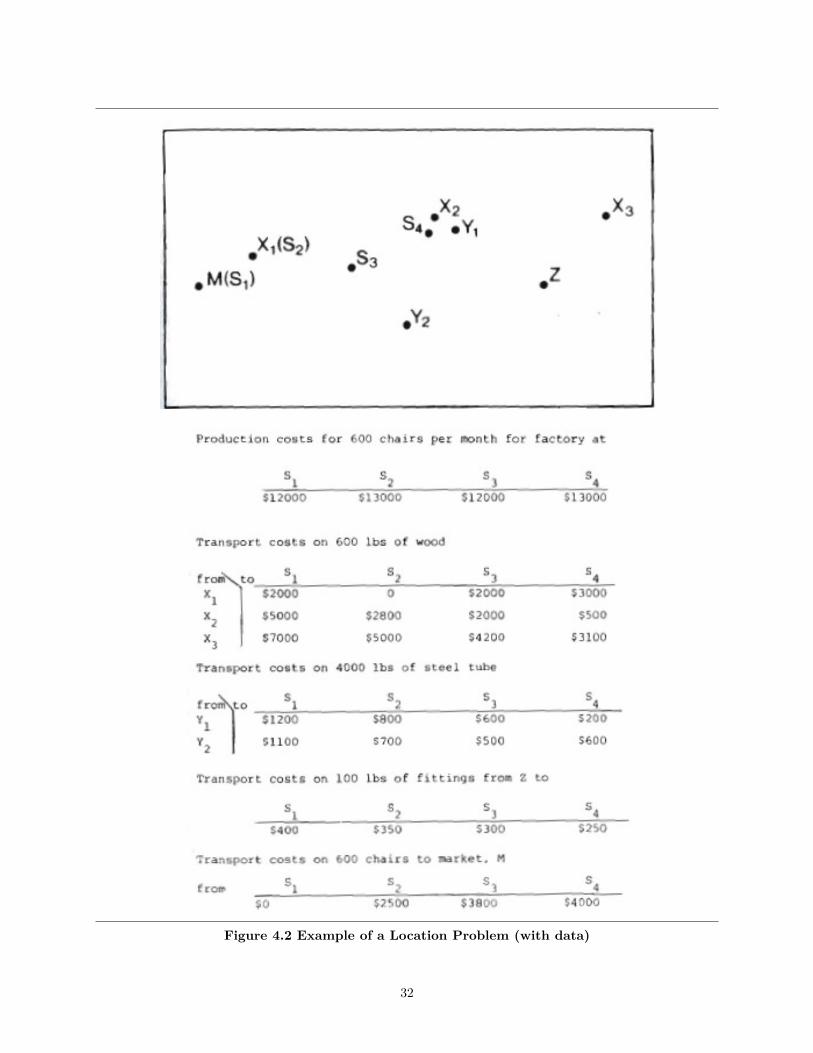
Figure 4.2 Example of a Location Problem (with data)

32

Evidently this sort of calculation can be made for any problem, and in practice this is what firms do ifthey have some freedom of choice in locating a factory. But location theory must do more than this: Itmust also state some general rules that allow us to interpret the economic landscape. The first part of theconstruction of these general rules is attempted in the following sections by ignoring production costs entirelyand examining only the influence of transport costs on location. To do this, the nature of transport costs inreality must be described.

4.2 Transport RatesLocation decisions imply a particular spatial pattern of trade in commodities. Once a location decision hasbeen made, then patterns of purchases and of market supplies are fixed. Thus, location decisions are theeconomic logic underlying spatial interaction (for an introduction to this field, see Haynes and Fotheringham1984). Conversely, the location decision is itself influenced by the costs of transporting commodities overspace. The next section examines the nature of those costs: first, by presenting some theory of transportrates, and second by providing evidence about the actual costs of transport.

4.2.1 THEORY

The structure of transport rates is extremely complex. This structure is now examined by considering thenature of a transport company and its costs (rates being set as costs plus a markup for profits). Suppose,then, that you buy a quantity of input and you ship it to your factory. What costs of the transport companydo you have to pay for?

First, you have to pay a share of the office, sales, and organization costs of the transport company. Secretaries,warehouses, managers, traffic organizers, and the office must be paid for. These costs are proportional to thenumber of separate journeys that have to be organized, so there is a particular fixed cost to organize yourshipment. If you are a regular user of the transport company – say you make the same shipment once a weekthen the company can schedule your shipment regularly and so can discount the fixed cost for your regularbusiness.

The fixed cost of organizing your shipment also depends on the size of your shipment in relation to thesize of transporter the company uses. If your commodity fills a truck, the company simply has to organizethat truck. But if you have only a small quantity, the company has to organize several shipments to usethe one truck fully. In trucking, the fixed cost of organization is therefore lower for truckload lots thanfor Jess-than-truckload lots. By contrast, rail freight is almost always of less-than-trainload lots, so a railcompany has to organize many shipments to put a train of freight together.

The second item you have to pay for is the loading of the truck or rail car. The truck must go to your supplier,or the rail car to a siding, and must load up. Now, the fixed cost of organization is independent on both theamount you want shipped (apart from the economy of truckload lots) and the distance of the journey; on theother hand, the terminal cost of loading depends partly on the amount you ship but is independent of thelength of the journey. The terminal cost also depends on the fragility of the goods: A front-end loader canquickly and cheaply load ten tons of ore, but furniture must be packaged by hand and loaded more carefully.

Then you must pay for the journey itself. This cost has two components. The first is your share of the costof the vehicle’s upkeep and its right of way – maintenance, costs of insurance, road taxes in the case of atruck, and in addition rail companies must pay to operate and to maintain their track. These costs dependlargely on the length of the journey and on the proportion of the total load that is yours (i.e., the volume ofyour load). Second, there are out-of-pocket costs attributable to the journey – the wages, fuel, and road tolls.Wages are proportional to the time taken – that is, distance. Considering that a driver and brakeman canoperate a freight train of several hundred cars, the cost of wages per ton is far lower on trains than on trucks.Fuel and tolls depend on the distance of the shipment, but also increase as the weight of the load rises.

The final cost that you have to pay is unloading. This is a terminal cost, similar in structure to that at theoutset of the journey.

In addition to these costs, the transport company charges you a sum to cover its profits. In practice, thisprofit is a standard percentage markup over costs. Thus, the total charge you must pay to the transport

33

company is total costs plus, say, 20 percent of those costs.

These arguments about the nature of transport costs are summarized in Figures 4.3 and 4.4. We have arguedthat rail freight is subject to greater terminal charges but lower line haul costs than is truck freight, andFigure 4.4 reflects this, indicating that railways should be favored for long hauls and trucks for shorter.(There is some evidence that this is the case.) One other aspect of this diagram is interesting. ConsiderTable 4.2 which classifies the possible ways in which the terminal and line haul costs of rail and truck couldbe compared. If trucks had higher terminal charges and higher line haul costs, then railways would becheaper for all distances; why would anyone use a truck? Equally, if railways had the higher terminal chargesand higher line haul costs, trucks would always be cheaper, and no one would use railways. Hence the factthat both railways and trucks exist in competition with each other means that the mode having the higherterminal cost also has the lower line haul cost.

Figure 4.3 Costs of Transport in Relation to Distance and Weight

Figure 4.4 Comparison of Costs of Transport by Rail and Truck

TABLE 4.2 Possible Structures of Terminal and Line Haul Costs for Truck and Rail Freight

Line Haul Costs Termianl Coststruck > rail truck > railtruck > rail truck < railtruck < rail truck > railtruck < rail truck < rail

34

Before examining the structure of actual freight rates, some complicating factors must be introduced intothis simple picture. The complications are return journeys, dead time, and practical freight rate setting.

Each outward journey must be balanced in some way by a return journey. (If not, the origin would eventuallyrun out of vehicles and the destination would be overrun with empty trucks or cars.) If the transport companycan readily find a load for the return journey, then that load can pay to return the vehicle to its origin. Butif no return load exists (nor even a load for a roundabout return), then you are liable to be charged forthe return journey of the vehicle as well as the outward one. In practice, this means that transporting acommodity over a route in which the volume of shipments is largely one way is more expensive than shippinga commodity over a route in which the shipments in each direction largely balance.

The out-of-pocket costs of a journey, directly attributable to you, include the wage of the driver and otherworkers while the vehicle is moving. But the transport company must pay the workers for a whole day, sayfor eight hours. So if your journey involves one hour of loading, five hours of driving , and then another hourof unloading, the terminal costs must include the two hours during which the driver waited for the truck tobe loaded, and the five hours of driving must also be charged at such a rate as to pay for the eighth hour ofthe driver’s day, when he or she can do nothing useful. Transport rates for journeys that do not take exactlya whole number of days must be calculated to pay for this dead time. (Vehicle dead time must also be paid.)

In principle, when you ask the transport company to ship your materials, an accountant should calculatethe direct and indirect costs of the order. In practice the company has previously computed the direct andindirect costs of various kinds of shipment, depending on whether it is regular or not, a carload or not, itsease of loading and cartage, its weight or volume, and the distance it must be transported. But this costwill not increase linearly with each mile as shown in Figure 4.3, for practical rates are quoted in zones. Forexample, the following rates may be quoted: $0.40 per thousand pounds per mile for destinations within 50miles, $0.35 per thousand pounds per mile for destinations between 50 and 120 miles and $0.30 per thousandpounds per mile for all destinations beyond that to which the transport company travels. This method ofcomputing and quoting freight rates economizes on the accounting effort of the transport firm.

4.2.2 TRANSPORT COSTS IN PRACTICE

Several economic geography texts contain data on the cost of transport. One example is Lowe and Moryadas(1975, pp. 31-39). But by far the most detailed published calculation is that of Harris and Hopkins (1972),which is based on 1965 data published by the Interstate Commerce Commission of the United States. Thesedata show the out-of-pocket costs of transporting paper containers by rail and by truck for various regions ofthe United States. Here the rates for the Mid-Atlantic region are presented.

The data are contained in Figure 4.5. All the curves reflect out-of-pocket expenses only and so do not includemarkups for profits and overheads. The rail freight costs include terminal costs ($85.09 per car plus $0.039per ton) and line haul costs. The line haul costs are broken at 32 miles, reflecting the hypothetical situationin which the load is picked up and carried for its first 32 miles by a local train (“way train”) and then sent onby a “through train.” Line haul costs are $0.289 per car plus $0.004 per ton for each mile by way train and$0.211 per car plus $0.002 per ton for each mile by through train. An allowance of $0.076 per ton is addedfor loss and damage. Rail freight rates, then, are essentially linear in distance. Truck rates are computedfrom common carrier costs. The overhead charges include pickup and delivery, platform handling, and billingand collecting; they are $3.68 per ton for greater than ten ton lots and $7.37 per ton for five ton lots. Linehaul rates depend on both the distance travelled and the weight of the shipment; for 9 miles or less, the costis $0.077 per ton per mile for five ton lots and $0.0616 per ton per mile for greater than ten ton lots. Incontrast to rail freight charges, truck rates decline with distance. The net effect of these different costs isthat trucks are cheaper than rail freight over short distances and particularly for small lots: For ten-ton lots,rail becomes cheaper over truck for distances over 500 miles whereas for five-ton lots, truck is cheaper thanrail over all distances examined.

35

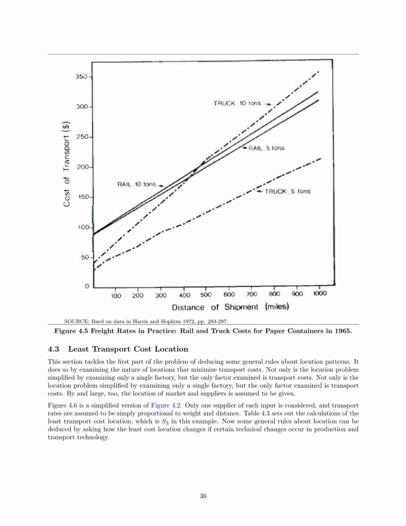
SOURCE: Baed on data in Harris and Hopkins 1972, pp. 283-297.

Figure 4.5 Freight Rates in Practice: Rail and Truck Costs for Paper Containers in 1965.

4.3 Least Transport Cost LocationThis section tackles the first part of the problem of deducing some general rules about location patterns. Itdoes so by examining the nature of locations that minimize transport costs. Not only is the location problemsimplified by examining only a single factory, but the only factor examined is transport costs. Not only is thelocation problem simplified by examining only a single factory, but the only factor examined is transportcosts. By and large, too, the location of market and suppliers is assumed to be given.

Figure 4.6 is a simplified version of Figure 4.2. Only one supplier of each input is considered, and transportrates are assumed to be simply proportional to weight and distance. Table 4.3 sets out the calculations of theleast transport cost location, which is S3 in this example. Now some general rules about location can bededuced by asking how the least cost location changes if certain technical changes occur in production andtransport technology.

36

Figure 4.6 Simplified Location Problem

TABLE 4.3 Calculations of Transport Costs for Problems of Figure 4.6

Site of Transport Costs to Site from Source Transport Total Cost ofProduction X Y Z Costs to M Transport

S1 6000 3600 1200 0 10800S2 3600 3200 900 3120 10820S3 2100 1600 500 5460 9660S4 0 3000 600 7800 10860S5 4500 0 400 7020 11920S6 3600 1200 700 4680 10180

4.3.1 EFFICIENCY IN USING ONE MATERIAL

What happens if the weight of one of the inputs falls compared to the weight of other materials? Suppose,for example, that the old technology used 1,900 pounds of wood to produce 600 chairs. You may computethe least transport cost location for this old technology to check that it is S4. In the old technology, whenwood was inefficiently used, the factory was located at the source of that material; but the new technology,which economizes on the use of wood, allows the firm to locate nearer to the other inputs or the market. Thisconclusion is relevant to two practical issues.

Consider, first, the process of making steel slabs out of iron ore. This process is in practice divided intoseveral stages. First, iron ore is mined. This ore may be 5 percent iron, say, so that 20 tons of ore are neededto produce l ton of iron. So, the ore is treated in a beneficiation plant that makes pellets having an iron orecontent of perhaps 70 percent. Thus, 1 ton of pellets needs 14 tons of ore. In new technologies, these pelletsare used directly to make steel: Ignoring other components, 1 ton of steel needs 1.4 tons of pellets. In thefirst process, 14 tons of inputs are needed to make 1 ton of output and so beneficiation plants are located ator near iron ore mines. In the second process, 1.4 tons of input are needed to make l ton of output and sosteel plants are located near other inputs or the market.

Also, the production processes of many industries have been altered over time so as to economize on the useof a major input material If the economy is sufficiently great, the pattern of location of the industries maychange as factories are less attracted to those inputs than in the past.

37

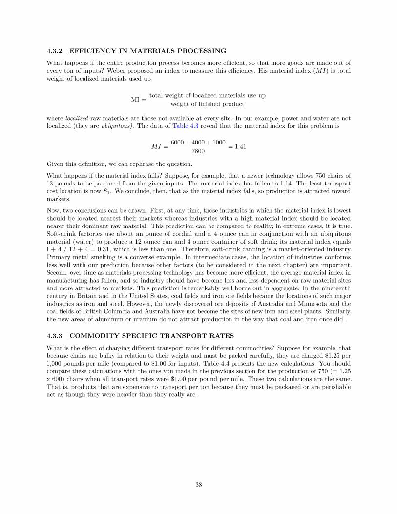
4.3.2 EFFICIENCY IN MATERIALS PROCESSING

What happens if the entire production process becomes more efficient, so that more goods are made out ofevery ton of inputs? Weber proposed an index to measure this efficiency. His material index (MI) is totalweight of localized materials used up

MI = total weight of localized materials use upweight of finished product

where localized raw materials are those not available at every site. In our example, power and water are notlocalized (they are ubiquitous). The data of Table 4.3 reveal that the material index for this problem is

MI = 6000 + 4000 + 10007800 = 1.41

Given this definition, we can rephrase the question.

What happens if the material index falls? Suppose, for example, that a newer technology allows 750 chairs of13 pounds to be produced from the given inputs. The material index has fallen to 1.14. The least transportcost location is now S1. We conclude, then, that as the material index falls, so production is attracted towardmarkets.

Now, two conclusions can be drawn. First, at any time, those industries in which the material index is lowestshould be located nearest their markets whereas industries with a high material index should be locatednearer their dominant raw material. This prediction can be compared to reality; in extreme cases, it is true.Soft-drink factories use about an ounce of cordial and a 4 ounce can in conjunction with an ubiquitousmaterial (water) to produce a 12 ounce can and 4 ounce container of soft drink; its material index equalsl + 4 / 12 + 4 = 0.31, which is less than one. Therefore, soft-drink canning is a market-oriented industry.Primary metal smelting is a converse example. In intermediate cases, the location of industries conformsless well with our prediction because other factors (to be considered in the next chapter) are important.Second, over time as materials-processing technology has become more efficient, the average material index inmanufacturing has fallen, and so industry should have become less and less dependent on raw material sitesand more attracted to markets. This prediction is remarkably well borne out in aggregate. In the nineteenthcentury in Britain and in the United States, coal fields and iron ore fields became the locations of such majorindustries as iron and steel. However, the newly discovered ore deposits of Australia and Minnesota and thecoal fields of British Columbia and Australia have not become the sites of new iron and steel plants. Similarly,the new areas of aluminum or uranium do not attract production in the way that coal and iron once did.

4.3.3 COMMODITY SPECIFIC TRANSPORT RATES

What is the effect of charging different transport rates for different commodities? Suppose for example, thatbecause chairs are bulky in relation to their weight and must be packed carefully, they are charged $1.25 per1,000 pounds per mile (compared to $1.00 for inputs). Table 4.4 presents the new calculations. You shouldcompare these calculations with the ones you made in the previous section for the production of 750 (= 1.25x 600) chairs when all transport rates were $1.00 per pound per mile. These two calculations are the same.That is, products that are expensive to transport per ton because they must be packaged or are perishableact as though they were heavier than they really are.

38

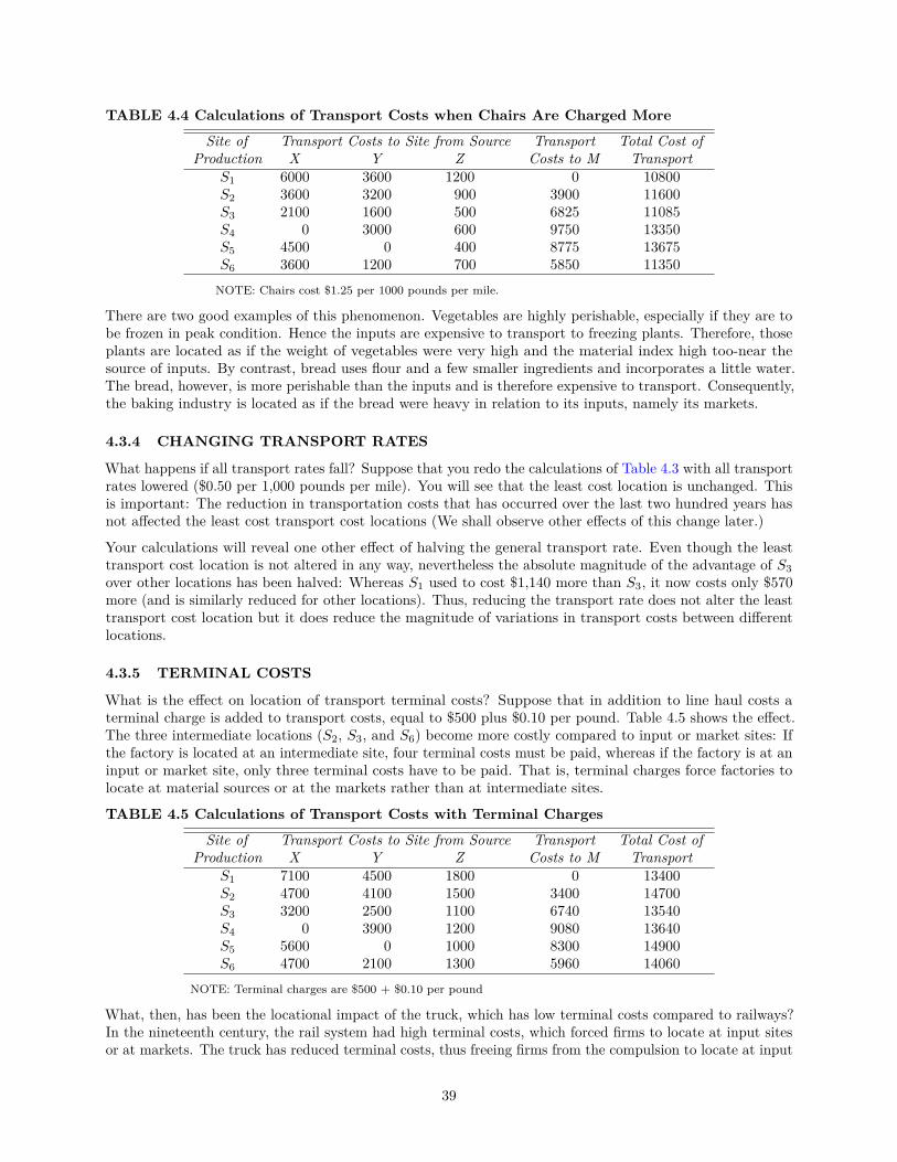
TABLE 4.4 Calculations of Transport Costs when Chairs Are Charged More

Site of Transport Costs to Site from Source Transport Total Cost ofProduction X Y Z Costs to M Transport

S1 6000 3600 1200 0 10800S2 3600 3200 900 3900 11600S3 2100 1600 500 6825 11085S4 0 3000 600 9750 13350S5 4500 0 400 8775 13675S6 3600 1200 700 5850 11350NOTE: Chairs cost $1.25 per 1000 pounds per mile.

There are two good examples of this phenomenon. Vegetables are highly perishable, especially if they are tobe frozen in peak condition. Hence the inputs are expensive to transport to freezing plants. Therefore, thoseplants are located as if the weight of vegetables were very high and the material index high too-near thesource of inputs. By contrast, bread uses flour and a few smaller ingredients and incorporates a little water.The bread, however, is more perishable than the inputs and is therefore expensive to transport. Consequently,the baking industry is located as if the bread were heavy in relation to its inputs, namely its markets.

4.3.4 CHANGING TRANSPORT RATES

What happens if all transport rates fall? Suppose that you redo the calculations of Table 4.3 with all transportrates lowered ($0.50 per 1,000 pounds per mile). You will see that the least cost location is unchanged. Thisis important: The reduction in transportation costs that has occurred over the last two hundred years hasnot affected the least cost transport cost locations (We shall observe other effects of this change later.)

Your calculations will reveal one other effect of halving the general transport rate. Even though the leasttransport cost location is not altered in any way, nevertheless the absolute magnitude of the advantage of S3over other locations has been halved: Whereas S1 used to cost $1,140 more than S3, it now costs only $570more (and is similarly reduced for other locations). Thus, reducing the transport rate does not alter the leasttransport cost location but it does reduce the magnitude of variations in transport costs between differentlocations.

4.3.5 TERMINAL COSTS

What is the effect on location of transport terminal costs? Suppose that in addition to line haul costs aterminal charge is added to transport costs, equal to $500 plus $0.10 per pound. Table 4.5 shows the effect.The three intermediate locations (S2, S3, and S6) become more costly compared to input or market sites: Ifthe factory is located at an intermediate site, four terminal costs must be paid, whereas if the factory is at aninput or market site, only three terminal costs have to be paid. That is, terminal charges force factories tolocate at material sources or at the markets rather than at intermediate sites.

TABLE 4.5 Calculations of Transport Costs with Terminal Charges

Site of Transport Costs to Site from Source Transport Total Cost ofProduction X Y Z Costs to M Transport

S1 7100 4500 1800 0 13400S2 4700 4100 1500 3400 14700S3 3200 2500 1100 6740 13540S4 0 3900 1200 9080 13640S5 5600 0 1000 8300 14900S6 4700 2100 1300 5960 14060

NOTE: Terminal charges are $500 + $0.10 per pound

What, then, has been the locational impact of the truck, which has low terminal costs compared to railways?In the nineteenth century, the rail system had high terminal costs, which forced firms to locate at input sitesor at markets. The truck has reduced terminal costs, thus freeing firms from the compulsion to locate at input

39

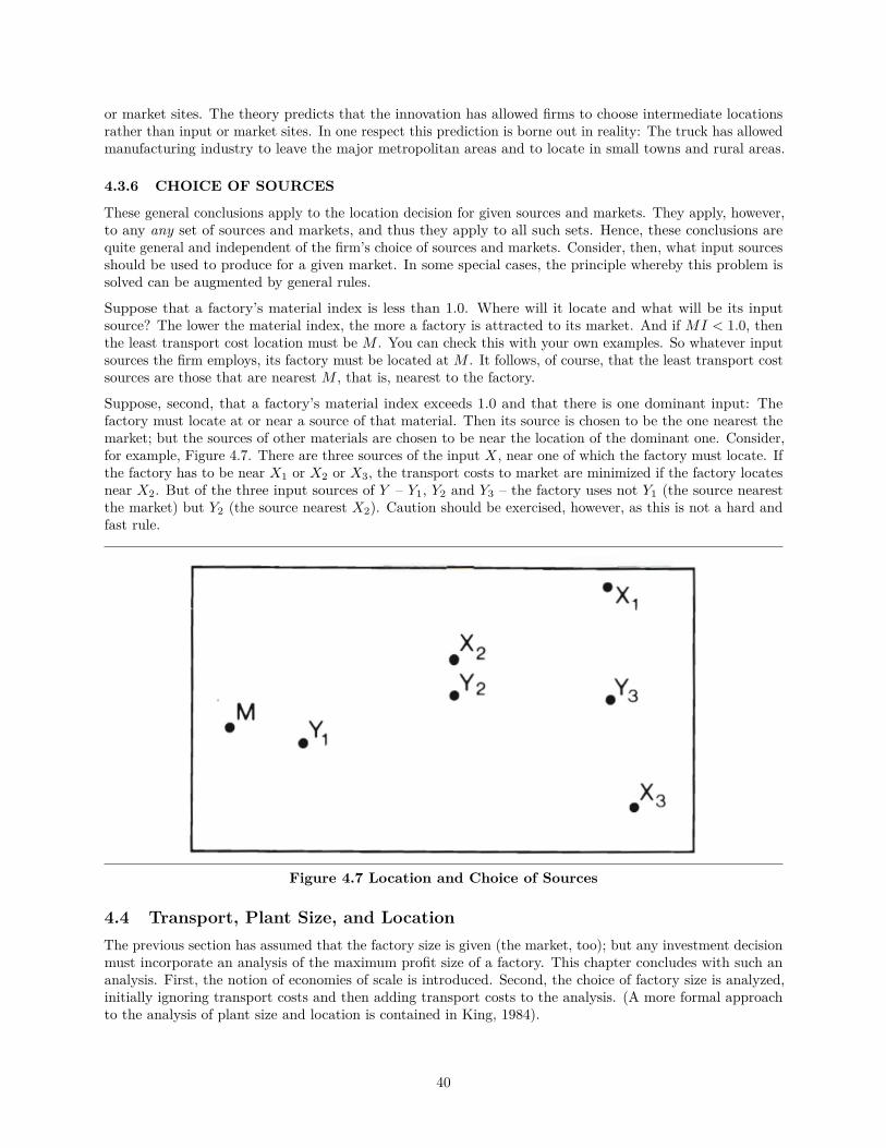
or market sites. The theory predicts that the innovation has allowed firms to choose intermediate locationsrather than input or market sites. In one respect this prediction is borne out in reality: The truck has allowedmanufacturing industry to leave the major metropolitan areas and to locate in small towns and rural areas.

4.3.6 CHOICE OF SOURCES

These general conclusions apply to the location decision for given sources and markets. They apply, however,to any any set of sources and markets, and thus they apply to all such sets. Hence, these conclusions arequite general and independent of the firm’s choice of sources and markets. Consider, then, what input sourcesshould be used to produce for a given market. In some special cases, the principle whereby this problem issolved can be augmented by general rules.

Suppose that a factory’s material index is less than 1.0. Where will it locate and what will be its inputsource? The lower the material index, the more a factory is attracted to its market. And if MI < 1.0, thenthe least transport cost location must be M . You can check this with your own examples. So whatever inputsources the firm employs, its factory must be located at M . It follows, of course, that the least transport costsources are those that are nearest M , that is, nearest to the factory.

Suppose, second, that a factory’s material index exceeds 1.0 and that there is one dominant input: Thefactory must locate at or near a source of that material. Then its source is chosen to be the one nearest themarket; but the sources of other materials are chosen to be near the location of the dominant one. Consider,for example, Figure 4.7. There are three sources of the input X, near one of which the factory must locate. Ifthe factory has to be near X1 or X2 or X3, the transport costs to market are minimized if the factory locatesnear X2. But of the three input sources of Y – Y1, Y2 and Y3 – the factory uses not Y1 (the source nearestthe market) but Y2 (the source nearest X2). Caution should be exercised, however, as this is not a hard andfast rule.

Figure 4.7 Location and Choice of Sources

4.4 Transport, Plant Size, and LocationThe previous section has assumed that the factory size is given (the market, too); but any investment decisionmust incorporate an analysis of the maximum profit size of a factory. This chapter concludes with such ananalysis. First, the notion of economies of scale is introduced. Second, the choice of factory size is analyzed,initially ignoring transport costs and then adding transport costs to the analysis. (A more formal approachto the analysis of plant size and location is contained in King, 1984).

40

4.4.1 ECONOMIES OF SCALE

The phrase economies of scale means the savings in production costs as operations are enlarged. There aretwo kinds of economies of scale. The first are the economies of large firms over small, some aspects of whichwere examined in Chapter 2. The second kind of scale economy is that of large factories; it is this economyth.at is analyzed in this section. In theory there are several reasons why large factories are more efficient(produce at less cost) than small ones.

The first reason is the division of labor within a factory. A small factory that employs only one person toperform all the operations needed to produce a commodity is using unspecialized labor. The person spends,say, 30 minutes on task 1, 2 1/2 hours on task 2, 2 hours on task 3, 3 hours on task 4. Suppose, however, thatthe factory hires 97 people: 60 for task 1, 12 for task 2, 15 for task 3, and 10 for task 4. Then each workercould learn one operation thoroughly, no labor time would be lost in passing from one operation to the next,each operation could be mechanized more easily, and each more specialized laborer would be less skilled inaggregate and therefore paid less. In this example, 97 is the least number of employees in a factory whereeach laborer was specialized in this way. The division of labor was one of the bases for factory organizationin the nineteenth century, before mechanization.

Now that factories are generally mechanized, a second economy has become important: the economy of largemachines. Equipment that stores materials and machines (the power of which depends on their volume) aresubject to a geometric economy: The volume of a cube increases as the cube of its linear dimension, but thearea of its faces increases as six times the square of that length. Thus, ships, storage tanks, and factories areall subject. to this economy, the only limitation on which is provided by the strength of materials.

The third main economy is the economy of massed reserves. Factories maintain inventories of spare parts formachines and reserve stocks of materials to guard against breakdown or emergencies. Now the size of thesereserves must increase as the level of production increases; but for a given risk, the level of reserves risesmore slowly than the level of output. Hence the cost of the reserve per unit of output is less for large levelsthan for small.

These three economies are of differing significance. The economy of reserves is real but probably quite small.The economy of large machines is most important for factories in which storage is important but is subject tothe limits of material strength. The main economy of large scale is that which arises from the division of laborand the need to link processes and machines in a continuous process. However, there exist no convincingmeasurements that demonstrate the real existence of scale economies, at least beyond a minimum size. (SeeLloyd and Dicken 1977, pp. 273-280, for further discussion of this issue.)

4.4.2 FACTORY SIZE

Suppose that a factory is going to be built to produce a commodity that will be sold in a city. Severalfactories already exist in the city, but the entrepreneur believes that there is room for another. Initially,assume that the costs of transport do not vary with the level of output. How large should the factory be?

Figure 4.8 illustrates the method of analyzing this question. The solid line on this diagram shows how costsvary in relation to scale: The hypothesis is that there are some economies of scale, but for output levelsgreater than 1,000 units per month scale economies are insignificant. (You can perform the same analysiswith different hypotheses about scale economies.)

The dashed line of Figure 4.8 reflects the entrepreneur’s beliefs about how much can be sold at each givenprice. If the price is too high, few people will buy; as the price is reduced, more will buy, until at a very lowprice, the factory can capture the entire market in the city.

41

Figure 4.8 Choice of Factory Size

The firm’s strategy is to try to maximize its profit per unit of output that is, to choose a level of output suchthat the difference between the price received and the cost paid is greatest. On Figure 4.8 this occurs at anoutput of 750 units per month, which is below the minimum efficient size of the plant.

Now let us introduce costs of transport. If the factory is to sell to one city, transport costs are small. As itincreases the scale of its operations, however, it must sell to people who live further and further away. Hencethe larger the output of the firm, the greater the costs of transport it must pay to deliver its output to theconsumers. The firm can now increase its output by selling more to its local market (by lowering its price) orby increasing the spatial extent of the market it serves.

Figure 4 .9 shows how to analyze this problem. The solid lines show the costs of production and transport tomarket for market areas of varying extent: The larger the market, the greater these costs. The dashed lineshows how much the firm can sell for a given price in each of the market areas. Hence for each market area,an optimum level of output can be determined to maximize the price-cost difference. In this case you can seethat the firm makes more profit if it sells to a market with a radius of 20 miles than if it sells over a 10-mileradius.

Figure 4.9 Factory Size in Spatial Market

42

Now the figure also allows you to analyze the effects of changes in transport rates on the size of factories.Suppose that transport rates fall. The quantity/price relationship is not affected, but the costs of servinglarger markets fall. Hence the effects of transport costs on the cost curves fall, and the higher curves diminishtoward the costs (no transport) line. It follows that the benefit of selling to larger markets is increased, andso plant size rises as transport costs fall.

4.5 ConclusionThis chapter has analyzed the structure of transport rates and examined the relations between transportcosts and location. By and large, transport rates have fallen over the last two hundred years, and the leastcost theory predicts that this change has affected location patterns in several ways. These effects include theincreasing size of markets served by one factory, the greater freedom of factories to locate at intermediatesites (neither at material sources nor at markets), and the decreasing attraction of industry to raw materials.

In an immediate sense, then, changes in the structure of transport costs cause these locational adjustments.Yet you should beware of a mechanical or technological interpretation of locational change as due to changingtransport cost structures and materials processing technology: The new technologies have the observedlocational effects only in the context of the specific social system (e.g., in the context of profit maximizingfirms); and the new technologies do not appear out of nowhere – they have to be produced as a result ofinvestment decisions by entrepreneurs – and thus the causes of the technical changes and their specific formneed to be investigated.

4.6 Further ReadingOne of the best discussions of transport costs and location that could be used to follow up this chapter iscontained in Location in Space by P. E. Lloyd and P. Dicken, (1977, pp. 157-195). P. Haggett, A. D. Cliff,and A. Frey discuss transport networks in Locational Models (1977, pp. 64-96).

43

5 LEAST COST THEORY: PRODUCTION COSTS AND AG-GLOMERATION

In addition to transport costs, least cost theory examines the influence on location of two other factors: spatialvariations in production costs and economies of agglomeration. This chapter completes the presentationof the theory by examining these two factors. The discussion is divided into five parts. The followingsection presents the basic theory about the effects of production cost variations on location. This theoreticaldiscussion is succeeded by three more empirical sections that examine nonwage costs, labor costs, and theissue of amenities and business climate. This chapter concludes by reverting to a theoretical mode andexamining the effects of agglomeration on location.

The last chapter ended by warning against technological determinism, for transport rate changes have tobe produced by society. This idea, that spatial variations in production costs are themselves produced bysociety, is more emphasized in this chapter. The central claim of the chapter is that labor costs are becomingthe most significant factor affecting location but that the spatial variations in these costs are themselves theoutcome of earlier development decisions. In this sense, labor is a produced factor of production.

5.1 Production CostsNot only do transport costs vary over space, but so do production costs. For any given market and suppliers,the choice of location must therefore reflect spatial variations in production costs as well as in transportcosts. In practice, this amounts to (1) discovering the production costs at each possible location; (2) addingproduction and transport costs at each location; and (3) choosing that location at which these combinedcosts are least. This is quite straightforward-but can we discover some general principles about the effects ofproduction costs on location?

One important principle can be deduced if we return to Figure 4.7 and Table 4.3. Suppose we add to thatproblem the data on production costs for 600 chairs at each site (see Table 5.1). The least cost location issite S3, for its combined transport and production costs are less than those for all other sites. Now supposethat the transport cost is halved. Then the site-to-site variation in transport costs is halved too, and spatialvariations in production costs take on greater significance. As Table 5.1 shows, the new least cost location isS2. (Observe that S2 is not, however, the site with the least production costs.) The principle is this: Astransport rates fall in relation to costs of production, so production cost variations rise in significance as alocational factor compared to transport costs. We can apply this principle in two ways.

TABLE 5.1 Effects of Production Costs on LocationTransport Costs

Production Total Cost of Transport Production After Rate Is Transport plus ProductionSite from Table 4.3 Costs Halved Before Rate is Changed After Rate is HalvedS1 10800 2150 5400 12950 7550S2 10820 2000 5410 12820 7410S3 9660 2600 4830 12220 7430S4 10860 2000 5430 12860 7430S5 11920 1640 5960 13570 7600S6 10180 2510 5090 12690 7600

First, we know that transport rates have fallen over time in relation to other costs. We shall also see in thefollowing sections that there remain large spatial variations in costs of production – especially wages. Hence,we anticipate that this relative fall in transport rates has permitted firms a greater freedom than they usedto have to seek out least production cost locations. In particular, this means that firms can now more readilyescape the regions in which labor costs are high.

Second, costs of transport vary for different industries. Some industries sell a light product of high value, forwhich transport costs are small compared to production costs: fashion clothing for example. Other industriesuse bulky materials and produce bulky output and so are dominated by transport costs: iron and steel, forexample. Our principle tells us that different industries locate with respect to different factors: Productioncosts dominate for fashion clothing; transport costs dominate for iron and steel.

44

5.2 Nonlabor CostsThere are many other costs of doing business besides transport costs and labor costs: Plant and equipmenthave to be acquired; land has to be bought or rented; and taxes must be paid. Other costs, like the cost ofthe sales effort, are presumed not to vary with the location of the factory. This section examines the spatialvariability in the cost and availability of these factors.

5.2.1 PLANT AND EQUIPMENT

Some factories must be located in the middle of nowhere – for example plants that pelletize iron ore, orprocess lumber. Such factories are built far from existing road or rail links. Hence the plant, equipment, andthe transport link itself are all expensive to build. Most factories, however, are not built in such isolatedplaces – because there are no workers and plants would be expensive. Being input-output operations, factoriesgenerally must be near existing transport links. For such factories, spatial variations in the costs of plant andequipment are insignificant.

Consider the following data (for 1978, from U.S. Department of Commerce Statistical Abstract of the UnitedStates 1981, p. 777). In that year, U S. manufacturing plants spent $55.2 billion on new capital expenditures.Suppose that these capital items were in such out-of-the-way spots that an extra 10 percent had to be spenton transport: $5.52 billion. Now, the yearly interest at 12 percent on these transport costs is $0.66 billion,which is merely 0.1 percent of the value added by manufacture and only 0.54 percent of the total profit earnedby manufacturers in 1978. Thus, spatial variations in the price of plant and equipment can have little effecton aggregate locational choices within advanced economies (although they may have greater effect withinparticular industries).

However, the effective cost of plant and equipment could vary spatially if there are spatial differences in thecost of the capital that has to be borrowed to buy the plant and the machinery. This cost varies spatiallyonly if there are barriers to mobility – that is, if a lender in New York, say, is more willing to lend to a NewYork firm than to an Atlanta firm. There are two such barriers. The first is a difference in information.When travel was costly and slow, economic conditions and investment potential in borrowing regions werenot widely appreciated in lending regions-hence, lenders were less willing than they ought to have been tolend outside their home region. The second barrier is the cost of the loan made between separate places. Inthe nineteenth century, New York banks made loans to Westerners via intermediaries, who charged a fee: SoWestern loans cost more to administer than loans to North Easterners. Nowadays, the major cost of loans isthe risk of lending capital across national boundaries. Within the United States, a creditor is subject to lawand nonrepayment brings legal penalties. But American firms that invest abroad have no such legal backup,for foreign firms cannot be required by U.S. law to honor a debt.

Hence, the cost and availability of capital do vary spatially (Lloyd and Dicken 1977, pp. 230-231), presentsome evidence, too). Of course, anyone would find it hard to borrow in order to build a steel mill in southernFlorida: this, however, is hardly an effective restriction. The effective locational restrictions that arise fromcapital are caused by lack of information and the costs of distance. Within advanced economies, theserestrictions are now of little importance, but they do deter cross-boundary flows.

5.2.2 LAND AND TAXES

There are enormous variations in the price of land between the center of a metropolitan area and its periphery.Land at the center can be thousands of times as costly as peripheral land. These variations are a strongincentive for firms to locate in suburbs rather than in metropolitan areas if they are able to. But the variationin prices between land in the suburbs and land in small towns is much less.

How significant are these variations? In the United States in 1978, the average factory had a net value of$10,993 per worker in structures, of which, say, one-third is land – about $3665 per worker. If the firm paidinterest on this investment at 12 percent per annum, the cost of land is $440 per worker, less than 1 percentof the value added per worker and only 0.4 percent of the value of shipments per worker. Thus, while thedifference between central city and suburban land prices is important (and this is one of the reasons why

45

manufacturing plants have been decentralizing to the suburbs since World War II), the difference betweenthe prices of land in different cities or between different areas is not great enough to affect profitability much.

The same is true of taxes and business incentives. We frequently learn that tax levels are too high or businessincentives too low for a firm to locate a factory in this place or that – so we are led to believe that suchgovernment behavior can affect location. Yet we should be leery of such claims; firms have an incentive toclaim that taxes or incentives are more influential than they really are in order to obtain a better deal forthemselves. So we must consider the level of taxes and incentives more carefully.

Governments in most Western European and North American countries offer incentives if firms locate theirfactories in particular places, such as depressed areas. Such incentives typically take several forms: reducedbusiness tax obligations; low cost business loans; overhead projects (such as business parks); and freedomfrom legal restrictions on such business practices as labor relations. Business people strongly favor suchincentives, and popular impressions suggest that location incentives are important influences on locationchoice. Yet the evidence is uniformly negative: Firms make their plans, find out about the incentives availableat the planned location, and then apply for the incentives (Harrison and Kanter 1978); econometric modelsfind no statistically significant relationship between growth in manufacturing employment in the U.S. statesand the level of state and local taxes (Bloom 1955; Thompson and Mattila 1959; Treysz et al. 1976). Thus,you should remain skeptical about the role of incentives. While businesses obviously benefit from them, theincentives cannot be large enough nor continue long enough to affect firms’ locations in the long run.

5.2.3 CONCLUSIONS

The most important point emphasized in this section is that nonlabor costs do not vary greatly over space-certainly not sufficiently to affect profitability noticeably. The prices of plant, equipment, land, and taxesall vary spatially. However, the cost of the assets to the firm is not their price but the costs of the interestneeded to pay for the loan to buy them, and generally this cost is only a small proportion of sales or even ofvalue added. Apart from the costs of transport, then, the only remaining factor of location is labor costs.

5.3 Wage RatesLabor is the essential factor in manufacturing. The cost of labor is high and the evidence from politicaladvocates of wage controls and the seriousness of wage bargaining suggests that business people regard thiscost as significant. Equally, it has been argued that unionization and high wage rates in the northeasternUnited States have contributed to the industrial decline of that region. So now we examine data on thespatial variability of the costs of labor.

5.3.1 WAGE RATE VARIATIONS

Despite mechanization, automation, and computer processing, labor costs remain high. In 1977, payrollsaccounted for 45.1 percent of the U.S. value added (U.S. Department of Commerce, Statistical Abstract, 1981,p. 777). In some industries, the payroll is a small proportion of value added: only one-sixth in tobaccoproducts (SIC 21) and petroleum and coal products (SIC 29), about 25 percent in chemicals (SIC 28), and33 percent in food industries (SIC 20). In other major SIC groups, the payroll exceeds 40 percent of valueadded, reaching 50 percent in furniture (SIC 25), leather (SIC 31), and primary metal industries (SIC 33). InU.S. manufacturing as a whole, a 20 percent increase in payroll would absorb 9 percent of the value added.Unlike the costs examined in the previous section, the costs of labor are a high proportion of the costs ofmanufacturing.

The costs of the payroll understate the labor costs that firms must pay. In addition to wages and salaries,U.S. firms make contributions to employees’ and other social security programs. In 1977, these contributionsadded $50 billion to the payroll bill, equivalent to 8.5 percent of total value added (U.S. Department ofCommerce, Census of Manufactures 1977, General Summary, p. 1-46). Thus, even now, labor accounts forover half of U.S. value added in manufacturing.

The payroll itself can be divided into two parts. One is the payment to production workers (wages) and theother is the payment to administrative, sales, research, and other nonproduction workers. Production workers

46

earned in 1977 about 60 percent of the payroll, a fall from 68 percent in 1954 and 75 percent in 1947 (U.S.Department of Commerce, Statistical Abstract 1981, p. 777).

Not only are labor costs high, they also vary over space. Figure 5.1 is a map of the payroll per employee ineach state of the United States as a proportion of the U.S. average in 1972. The wage rates in the areas withhighest earnings (Delaware, Michigan, and Washington) are all more than 50 percent greater than in thestates with lowest wages (North Carolina, Mississippi, Arkansas, New Mexico). In general, wages are belowthe U.S. average in New England and throughout the South except for in Connecticut, Delaware, Maryland,and Washington, D. C.; wages are above the U.S. average in the Mid-Atlantic, East North Central, andPacific regions, except for Pennsylvania. These large spatial variations conform to the popular perception.

SOURCE: U.S. Department of Commerce, Bureau of the Census 1975, Census of Manufactures, 1972, GeneralSummary Volume. pp 46-67.

Figure 5.1 Average Wage per Hour of Manufacturing Employees

But these variations in wages are not the ones that most concern a firm. The wage rates shown on Figure 5.1may vary for two reasons: Either Michigan’s firms pay higher wages in each industry than do Arkansas’sfirms, or Michigan’s employees work in higher wage industries than do Arkansas’s employees. Tables 5.2and 5.3 provide some evidence about these alternatives for two industry groups-textiles (SIC 22) and paperindustries (SIC 26). Even within the three-digit industries, there remain substantial interregional variationsin hourly wages. Within the textile industries, the Pacific, Mid-Atlantic, and East North Central states payabove the U.S. average, and the South pays below. In the paper industries, the pattern of wage variations isless consistent: The North East generally pays below and the West pays above the U.S. average, but theNorth Central and Southern states sometimes pay more and sometimes less than the U.S. average. Evenwithin one industry, then, there are large variations between states in the average wage paid per worker.

5.3.2 CAUSES OF WAGE RATE VARIATIONS

A complete theory of industrial location cannot simply accept the evidence of Figure 5.1 and Tables 5.2and 5.3 but must inquire about the origin of spatial differences in wages. Wage levels are not simply given

47

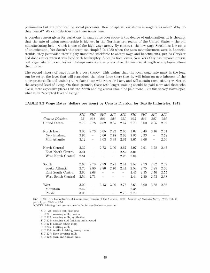
phenomena but are produced by social processes. How do spatial variations in wage rates arise? Why dothey persist? We can only touch on these issues here.

A popular reason given for variations in wage rates over space is the degree of unionization. It is thoughtthat the rate of union membership is highest in the Northeastern region of the United States – the oldmanufacturing belt – which is one of the high wage areas. By contrast, the low wage South has low ratesof unionization. Yet doesn’t this seem too simple? In 1982 when the auto manufacturers were in financialtrouble, they persuaded their highly unionized workforce to accept wage and benefits cuts, just as Chryslerhad done earlier when it was faced with bankruptcy. Since its fiscal crisis, New York City has imposed drasticreal wage cuts on its employees. Perhaps unions are as powerful as the financial strength of employers allowsthem to be.

The second theory of wage rates is a cost theory. This claims that the local wage rate must in the longrun be set at the level that will reproduce the labor force there-that is, will bring on new laborers of theappropriate skills and training to replace those who retire or leave, and will sustain each existing worker atthe accepted level of living. On these grounds, those with longer training should be paid more and those wholive in more expensive places (like the North and big cities) should be paid more. But this theory leaves openwhat is an “accepted level of living.”

TABLE 5.2 Wage Rates (dollars per hour) by Census Division for Textile Industries, 1972

SIC SIC SIC SIC SIC SIC SIC SIC SICCensus Division 22 221 222 223 224 225 226 227 228United States 2.79 2.78 2.82 2.85 2.57 2.70 3.00 2.95 2.59

North East 3.06 2.73 3.05 2.92 2.65 3.02 3.48 3.46 2.61New England 2.94 – 3.06 2.78 2.63 2.86 3.23 – 2.58Mid-Atlantic 3.12 – 3.03 3.39 2.67 3.05 3.66 – 2.66

North Central 3.32 – 2.73 3.00 2.67 2.97 2.91 3.28 2.47East North Central 3.41 – – – 2.82 3.01 – – –West North Central 2.81 – – – 2.25 2.84 – – –

South 2.68 2.78 2.79 2.71 2.44 2.52 2.73 2.82 2.59South Atlantic 2.70 2.80 2.80 2.70 2.44 2.54 2.75 2.85 2.60East South Central 2.60 2.68 – – – 2.46 2.55 2.70 2.55West South Central 2.54 2.71 – – – 2.44 2.50 2.53 2.38

West 3.02 – 3.13 3.00 2.75 2.63 3.00 3.58 2.56Mountain 2.42 – – – – 2.38 – – –Pacific 3.08 – – – 2.75 2.70 – – –

SOURCE: U.S. Department of Commerce, Bureau of the Census. 1975. Census of Manufactures, 1972, vol. 2,part 1, pp. 22-3 to 22-7.NOTES: Missing data are not available for nondisclosure reasons.

SIC 22: textile mill productsSIC 221: weaving mills, cottonSIC 222: weaving mills, syntheticsSIC 223: weaving and finishing mills, woodSIC 224: narrow fabric millsSIC 225: knitting millsSIC 226: textile finishing, except woolSIC 227: floor covering millsSIC 228: yarn and thread mills

48

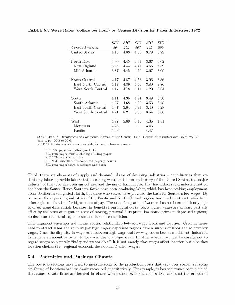
TABLE 5.3 Wage Rates (dollars per hour) by Census Division for Paper Industries, 1972

SIC SIC SIC SIC SICCensus Division 26 262 263 264 265United States 4.15 4.83 4.86 3.79 3.72

North East 3.90 4.45 4.31 3.67 3.62New England 3.95 4.44 4.41 3.66 3.39Mid-Atlantic 3.87 4.45 4.26 3.67 3.69

North Central 4.17 4.87 4.58 3.96 3.86East North Central 4.17 4.89 4.56 3.89 3.86West North Central 4.17 4.78 5.11 4.20 3.84

South 4.11 4.95 4.94 3.49 3.38South Atlantic 4.07 4.68 4.90 3.53 3.48East South Central 4.07 5.04 4.93 3.40 3.28West South Central 4.21 5.21 5.06 3.54 3.36

West 4.97 5.89 5.46 4.36 4.51Mountain 4.23 – – 3.43 –Pacific 5.03 – – 4.47 –

SOURCE: U.S. Department of Commerce, Bureau of the Census. 1975. Census of Manufactures, 1972, vol. 2,part 1, pp. 26-3 to 26-6.NOTES: Missing data are not available for nondisclosure reasons.

SIC 26: paper and allied productsSIC 262: paper mills excluding building paperSIC 263: paperboard millsSIC 264: miscellaneous converted paper productsSIC 265: paperboard containers and boxes

Third, there are elements of supply and demand. Areas of declining industries – or industries that areshedding labor – provide labor that is seeking work. In the recent history of the United States, the majorindustry of this type has been agriculture, and the major farming area that has lacked rapid industrializationhas been the South. Hence Southern farms have been producing labor, which has been seeking employment.Some Southerners migrated North, but those who stayed have provided the basis for Southern low wages. Bycontrast, the expanding industries of the Pacific and North Central regions have had to attract labor fromother regions – that is, offer higher rates of pay. The rate of migration of workers has not been sufficiently highto offset wage differentials because the benefits from migration (a job, a higher wage) are at least partiallyoffset by the costs of migration (cost of moving, personal disruption, low house prices in depressed regions).So declining industrial regions continue to offer cheap labor.

This argument envisages a dynamic spatial relationship between wage levels and location. Growing areasneed to attract labor and so must pay high wages; depressed regions have a surplus of labor and so offer lowwages. Once the disparity in wage costs between high wage and low wage areas becomes sufficient, industrialfirms have an incentive to try to locate in the low wage areas. In other words, we must be careful not toregard wages as a purely “independent variable.” It is not merely that wages affect location but also thatlocation choices (i.e., regional economic development) affect wages.

5.4 Amenities and Business ClimateThe previous sections have tried to measure some of the production costs that vary over space. Yet someattributes of locations are less easily measured quantitatively. For example, it has sometimes been claimedthat some private firms are located in places where their owners prefer to live, and that the growth of

49

the South and Southwest is partly attributable to its climate. Can this argument be assessed? Similarly,businesspeople do assess places in terms of their receptivity to the ideals of business, and some people claimthat some places have a more favorable business climate than do others. What is meant by business climate,and is it important? This section addresses these two questions.

5.4.1 AMENITIES

In some respects, the South is a cheaper place to live and to do business in than is the Northeast. Heatingcosts less, property taxes are often lower, and wages and statutory labor practices cost less in the South thanin the Northeast. But these factors have already been considered in the list of location variables. The questionof amenities, then, is this: Are there any pure (nonmonetary) effects of climate, landscape, intellectual life,or other amenities that attract firms? Put in this way, the question has only one answer: Such attractionscan only affect a firm’s choice between two otherwise equally profitable locations. Thus, the pure effect ofamenities must be small.

In practice, then, it seems that amenities can influence location decisions only through their effect on othercosts. The presence of intellectual resources may make it easy for a laboratory to attract scientists. To theextent that sun and warmth reduce heating costs they diminish production costs. If workers do really prefersun to snow, then it may be easy to attract labor to warmer spots. But these hardly seem to be majorconsiderations in locating multimillion dollar factories.

5.4.2 BUSINESS CLIMATE

The concept of business climate refers to the willingness of the population of a place to subscribe to the idealsof business. In practice, this means giving the firm freedom to run its business with minimum interferencefrom the state or from workers’ organizations.

The state can interfere with business in several ways. It can raise property taxes or, conversely, can offerlocational incentives. The state can also regulate industry by imposing legal limits to pollution, by imposingemployment standards, and by requiring certain forms of health and retirement insurance. Workers’ unionsmay affect wage levels, employment standards, and the freedom of the firm to lay off, transfer, or dischargeworkers.

In the first instance, at least, business climate probably varies inversely with wages – being most favorableto business where wages are relatively low, or workers least unionized. However, business climate is not anindependent locational variable; like wages, it is produced by the existing industrial structure. That is to say,where the demand for labor is high in relation to its supply, workers have more power than where there arefew jobs available. Hence, labor in high demand regions can more easily force union recognition, employmentand health standards, and pollution controls. Thus, we can hardly claim that business climate affects locationwithout explaining how business climate arises in response to existing levels of manufacturing development.

5.5 AgglomerationAn agglomeration is a point on the earth’s surface at which economic activity is particularly dense. Ametropolitan area is a spatial concentration of industry. Economies of agglomeration are those savings inproduction costs that occur when factories locate near one another. Suppose for example, that there aretwo possible sites, S1 and S2, and two factories, F1 and F2. Table 5.4 gives the production costs per unit ofoutput for each factory depending on its location. Considered alone, F1 should locate at S1 and F2 at S2.But if F1 and F2 both locate at S2, they each save some production costs: This saving is the economy ofagglomeration. What are the sources of agglomeration economies?

50

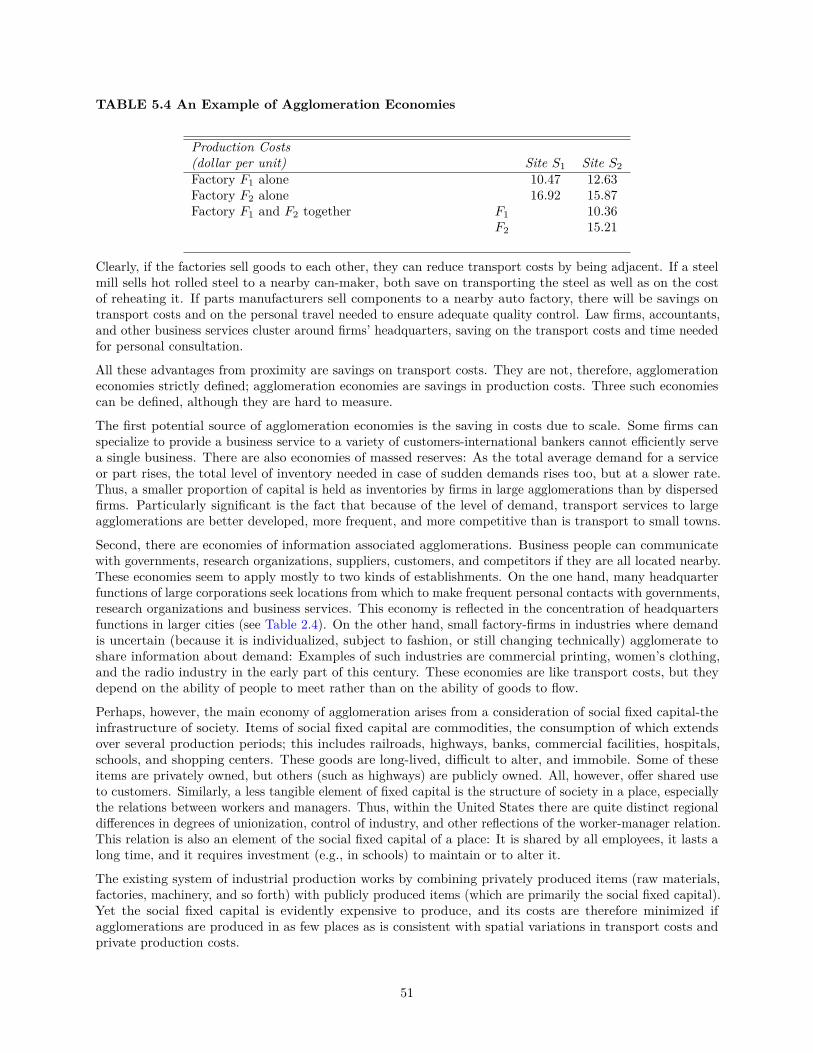
TABLE 5.4 An Example of Agglomeration Economies

Production Costs(dollar per unit) Site S1 Site S2Factory F1 alone 10.47 12.63Factory F2 alone 16.92 15.87Factory F1 and F2 together F1 10.36

F2 15.21

Clearly, if the factories sell goods to each other, they can reduce transport costs by being adjacent. If a steelmill sells hot rolled steel to a nearby can-maker, both save on transporting the steel as well as on the costof reheating it. If parts manufacturers sell components to a nearby auto factory, there will be savings ontransport costs and on the personal travel needed to ensure adequate quality control. Law firms, accountants,and other business services cluster around firms’ headquarters, saving on the transport costs and time neededfor personal consultation.

All these advantages from proximity are savings on transport costs. They are not, therefore, agglomerationeconomies strictly defined; agglomeration economies are savings in production costs. Three such economiescan be defined, although they are hard to measure.

The first potential source of agglomeration economies is the saving in costs due to scale. Some firms canspecialize to provide a business service to a variety of customers-international bankers cannot efficiently servea single business. There are also economies of massed reserves: As the total average demand for a serviceor part rises, the total level of inventory needed in case of sudden demands rises too, but at a slower rate.Thus, a smaller proportion of capital is held as inventories by firms in large agglomerations than by dispersedfirms. Particularly significant is the fact that because of the level of demand, transport services to largeagglomerations are better developed, more frequent, and more competitive than is transport to small towns.

Second, there are economies of information associated agglomerations. Business people can communicatewith governments, research organizations, suppliers, customers, and competitors if they are all located nearby.These economies seem to apply mostly to two kinds of establishments. On the one hand, many headquarterfunctions of large corporations seek locations from which to make frequent personal contacts with governments,research organizations and business services. This economy is reflected in the concentration of headquartersfunctions in larger cities (see Table 2.4). On the other hand, small factory-firms in industries where demandis uncertain (because it is individualized, subject to fashion, or still changing technically) agglomerate toshare information about demand: Examples of such industries are commercial printing, women’s clothing,and the radio industry in the early part of this century. These economies are like transport costs, but theydepend on the ability of people to meet rather than on the ability of goods to flow.

Perhaps, however, the main economy of agglomeration arises from a consideration of social fixed capital-theinfrastructure of society. Items of social fixed capital are commodities, the consumption of which extendsover several production periods; this includes railroads, highways, banks, commercial facilities, hospitals,schools, and shopping centers. These goods are long-lived, difficult to alter, and immobile. Some of theseitems are privately owned, but others (such as highways) are publicly owned. All, however, offer shared useto customers. Similarly, a less tangible element of fixed capital is the structure of society in a place, especiallythe relations between workers and managers. Thus, within the United States there are quite distinct regionaldifferences in degrees of unionization, control of industry, and other reflections of the worker-manager relation.This relation is also an element of the social fixed capital of a place: It is shared by all employees, it lasts along time, and it requires investment (e.g., in schools) to maintain or to alter it.

The existing system of industrial production works by combining privately produced items (raw materials,factories, machinery, and so forth) with publicly produced items (which are primarily the social fixed capital).Yet the social fixed capital is evidently expensive to produce, and its costs are therefore minimized ifagglomerations are produced in as few places as is consistent with spatial variations in transport costs andprivate production costs.

51

This view of agglomeration establishes the process as part of the system of industrial production. As anagglomeration is regarded as a conglomeration of social fixed capital (and its users), it is natural to envisagethat capital becoming outdated. Just as private fixed capital – a machine or factory – can become obsolete,so can an agglomeration in the sense that other arrangements of social fixed capital can deliver their servicesto users more cheaply. The City of New York is an example. It offered the following as social fixed capital:free university system; unparalleled port facilities; a variety of business services; many small rentable factories;few freeways; a large skilled but highly unionized and well-paid labor force. These things are not needed bymodern industry, which uses instead automated, horizontally laid-out factories employing cheap, unskilledlabor and often based on truck transport. As an agglomeration of social fixed capital, New York is nowobsolete and so, like an obsolete machine, is being abandoned by manufacturing firms.

One additional aspect of agglomeration theory is important: the location of several establishments belongingto a single firm. Suppose for example, that a firm wishes to set up one factory producing good X, anotherproducing good Y , a research laboratory, and a headquarters facility. Should these all be in separate placesor all in one place?

The firms’s decision can be analyzed as follows. First, examine the transport and production costs of eachfacility in turn. We have already shown how to do this and discussed the structure of costs for each type ofestablishment. Second, the firm must decide what savings could be achieved if the facilities were combined.Do the two factories share services or transfer products? Would the research laboratory save by beingadjacent to a factory (easy testing of ideas) or the headquarters (access to decision making and promotion ofinnovations)? Would the headquarters save by being near the laboratory or factory (cheaper day-to-daycontrol and communication, but less focus on long range rather than immediate problems)? Figure 5.2 showsthe savings that the firm thinks could be achieved by the headquarters, factories, and laboratory in onefacility. Now, around the least cost sites of each single establishment are drawn contour lines of productionand transport costs, showing how these costs rise from the least cost site. Thus, at the $1 million isolinearound X, transport and production would cost $1 million more than at X. Such contour lines are drawnaround each site. The dark shaded area thus represents all those places at which the total additional costsof perating each facility away from its optimal location are less than the firm’s anticipated savings fromagglomeration. They are therefore all places at which the firm could profitably combine its facilities. (If therewere no place at which the total additional costs of operation were less than the savings, than all facilitieswould disperse.) In Figure 5.2, the facilities should agglomerate.

Figure 5.2 Analysis of Agglomeration of Production Facilities of a Firm

52

5.6 ConclusionWhereas the previous chapter focused on the effect of transport costs on location, this one has examinedproduction costs and agglomeration economies. The most important spatially varying production cost isthe cost of labor for industry as a whole (although particular industries may exhibit particular locationalneeds). These are supplemented by economies of agglomeration, notably produced and shared items of socialfixed capital. We must reiterate the warnings given at the end of the previous chapter-these items (laborcosts and social fixed capital) are themselves produced by the effect of earlier location decisions on the socialenvironment. It remains to apply these ideas in practice, that is, to combine the theory of Chapters 3, 4,and 5 with the ideas on social organization in Chapter 2, in order to understand changes in actual locationpatterns.

5.7 Further ReadingPeter Lloyd and Peter Dicken’s Location in Space (1977, pp. 197-299) contains a mass of data on productioncosts and agglomeration economies in Canada, the United Kingdom, and the United States. It is by far thebest general source of data; on more specific issues, you should follow up the references given in the text ofthe chapter.

53

6 INDUSTRIAL LOCATION IN PRACTICELocation theory is one of the principal bases of geography. Agricultural location and land use theory is one ofthe principal supports of agricultural geography. Central place theory is crucial to urban geography; andindustrial location theory underlies both urban geography and regional development as well as forming onesource for spatial interaction theory.

This book has so far presented an introduction to the theory of industrial location. It has emphasized thatlocation must be studied in the context of a given social and economic system. At present, in North Americalocation can be interpreted as the interplay of two forces within the framework of least cost theory: Oneis the attempt to minimize transport costs, a factor of diminishing significance; the other is the effort tominimize labor costs. An important argument is that labor costs, like agglomeration economies, are notsimply given but are themselves produced by the operation of the economic system in the past.

Now it is time to apply some of these ideas in practice-to see how the task of understanding some real-worldlocation patterns and changes forces us to introduce additional elements to our theory. The following sectionsof this chapter contain examples of the location of the aircraft parts industry in New England, the spatialcomponent of British industrial decline, and the distribution of industry within metropolitan areas.

6.1 Aircraft Parts Industry in New EnglandNew England is one of the regions of the northeastern United States that shows most clearly the patternof relative growth and relative decline that characterizes regional economies. The aircraft parts industryexemplifies this pattern; it shows also how the perceived locational attributes of the region for the industryhave changed over time. Studies of the industry have been made by Estall (1966, pp. 157-170) and Bluestoneet al. (1981); this section draws from these studies.

The pattern of location of the aircraft industry was established soon after World War I provided a securemarket for aircraft, and the broad outlines of this pattern have changed little since then (except duringperiods of very rapid expansion, such as World War II). By 1972, nearly 95 percent of the value of completecommercial aircraft was produced on the West Coast (Washington and California), although military aircraftproduction was more dispersed (40 percent being in the South). Aircraft engines, however, were producedoverwhelmingly in the Northeast and North Central states: Connecticut and Massachusetts alone produced 45percent of all engine parts and accessories. The main producers in New England now are Pratt and Whitney,General Electric (both making large jet turbines), Sikorsky (helicopters), Hamilton-Standard (propellersand parts), and Avco-Lycoming (small jet turbines). Supplying these producers are a variety of small andmedium-sized subcontractors.

The production of airframes on the West Coast is resource-oriented – oriented, that is, toward locationswhere large factories do not have to be heated and where, for a high proportion of the time, the weather isgood enough for flying. Good weather is vital for airplanes flown by visual rules. Once located, however, thehuge investments in factories and production facilities effectively prevented the firms from relocating exceptunder intense government pressure.

Just as airframe production became concentrated on the West Coast, so propeller and engine production wasattracted to the Northeast. In this case, the important factors were the metalworking facilities and skilledwork force of the Northeast. Few other areas could offer so many laborers skilled in metalworking or suchmetalworking facilities, particularly for products that had to be made accurately. Now, the large supplyof engineers and scientists produced in New England helps keep engine production there. Indeed, some ofthe important aircraft engine producers evolved from other metalworking concerns: The Pratt and Whitneyengine plant took over the facilities and skilled labor force of the earlier Pratt and Whitney Tool Company ofHartford, Connecticut. Hamilton-Standard, however, shifted to Hartford from Pittsburgh in 1931, after beingbought by the same conglomerate (United Aircraft) that owned Pratt and Whitney – a move that centralizedproduction and management in one area. Essentially, then, this interpretation of the engine and propellersegment of the aircraft industry concerns both labor (but in terms of availability and skill rather than wage)and agglomeration economies. These characteristics of New England were themselves produced by its earlier

54

metalworking tradition. It is evident in the location of both aspects of the aircraft industry that transportcosts have little effect.

Superficially, at least, the importance of New England in the aircraft industry has been increasing over recentyears. For the aircraft industry as a whole, New England’s share of the U.S. value of shipments was 13.0percent in 1976 (a 25 percent rise since 1964) and its share of U.S. value added was 11.0 percent (up 8.4percent since 1964). Hence the ratio of value added to value of shipments has fallen: Less of the final value ofshipments is being manufactured in New England while a growing proportion is being made elsewhere andshipped to the region for final assembly. The region’s aircraft industry is now less healthy than it appears atfirst sight: The advantages of New England as a location seem to have diminished over time. Two changesunderlie this trend. On the one hand, the major producers – Pratt and Whitney and General Electric, forexample – buy more parts from subcontractors than they make in-house: Over 50 percent of engine partsare bought from subcontractors. On the other hand, more and more of this subcontracting occurs outsidethe region than within it. There is little evidence that labor costs, transport or energy charges, or taxes arehigher in New England than elsewhere in the United States, so why have these changes occurred?

One background factor must be mentioned first. In the theoretical discussion of least cost models, it waspointed out that as transport costs fell, so the attraction of cheap production cost sites became more significant.Undoubtedly, the dispersal of parts production from New England would have been more costly had it notbeen for the postwar reductions in long distance transport and communications costs.

But why do aircraft engine producers buy from subcontractors rather than produce in-house? Theorysuggests that if a subcontractor could supply many firms, it could gain economies of scale in the productionof components that were needed infrequently by any individual firm. But this does not apply in this case,for there are only two large jet engine producers in the United States and most subcontractors sell only toone firm. Two reasons are more important. First, large firms use subcontractors to guarantee supply of aninput. Secondary sources of inputs and parallel production by several subcontractors are used to reduce anydisruption caused by work stoppages or other failures. Such backup facilities are especially important in theaircraft industry, where delays can mean the loss of most of a market (as, for example, the DC-10 dominatesthe L-1011 and the 707 dominated the slightly late DC-8). Second, subcontractors can be used to reduce theeffect of sales fluctuations upon large firms. The demand for both military and commercial aircraft fluctuateswidely, which implies that the use of the industry’s labor and productive facilities should vary too, causingprofit rates to fluctuate. Suppose that an industry employs 1000 people, 800 of whom make parts and 200assemble these parts. If there is one firm and no subcontracting, a 50 percent fall in demand translates intoa fall of 50 percent in that firm’s sales. But suppose that there is one large firm, employing 400 producersof parts and 200 assemblers, and a set of subcontractors who together employ another 400 workers. Now a50 percent fall in demand can be handled by the big firm cutting its work force to 300 producers and 100assemblers (67 percent of the original work force) while buying in parts from 100 producers (to keep some ofthe subcontractor in the business). By subcontracting and varying its purchases from these subcontractors,the prime firms can partially isolate themselves from the effects of market fluctuations.

Finally, then, why does this rising level of subcontracting and pooled production translate into locationalchanges in the industry? Falling transport costs allow, but do not demand, dispersal of these plants fromNew England. Parallel production facilities have been set up by the two large engine producers in Quebec,West Virginia, and Vermont, which in contrast to their main facilities are nonunionized. Such plants provideproduction capacity during labor disputes and thus weaken workers’ ability to strike. To do this, of course,the new plants must be geographically separated from the old ones. Subcontractors have been subject to adifferent set of pressures: The big firms employ geographically more dispersed subcontractors than before,partly to spread the risk of stoppages, and partly to avoid the problems created by recent shortages of supplyof skilled labor in New England. It is also claimed that subcontractors in New England find it more difficultto borrow investment capital than do subcontractors elsewhere, but it is not clear why this is so.

This examination of the aircraft parts industry in New England hascon firmed some aspects of the leastcost theory in Chapters 4 and 5. The relative importance of labor and agglomeration economies has beenemphasized in the context of an industry to which transport costs are of little significance. But the examplehas also introduced some novel features, especially the issues raised by the relations between big firms and

55

their subcontractors. A more complex theory of location must evidently treat the questions of parallelproduction and multiple sources of inputs.

6.2 Industrial Decline in the United KingdomThe recent decline of the manufacturing industries in the United Kingdom is well known. Between 1966and 1981, the number of people employed in manufacturing in the United Kingdom fell from 8.6 million to6.0 million (Massey and Meegan 1982, p.5). The decline has not affected all industries and regions in thesame ways; this section draws on the work of Massey and Meegan to examine the spatial implications of thedecline. The most important theoretical point to be made by the example is that the geographic distributionof industrial employment must be understood in terms of the performance of the economy as a whole: Inparticular, the geography of job loss can be understood only by studying the causes of that job loss – thegeography of employment decline cannot be understood simply in terms of the characteristics of differentareas of the country. The example also shows the extent to which location theory can be used to analyzedecisions other than the location of a single new plant.

Massey and Meegan studied 31 different industries, ranging from iron and steel through jute manufacture,from grain milling through scientific instruments. They concentrated on the period 1968-1973. Within theseindustries, three specific forms of the reorganization of industrial production were identified: (l) intensification,(2) investment and technical change, and (3) rationalization. Each has different implications for locationpatterns.

One form of production reorganization that causes employment reorganization is intensification. This meansthe reorganization of a production process to increase productivity without closing plants or making majorinvestment in new forms of production. In practice, then, intensification means fragmenting tasks, speedingup conveyor belts, new mechanization, or greater incentives. Intensification, then, is cheap, and so a favoredway of raising productivity when profits are low (for instance during a depression). Then, if sales are stagnant,intensification implies job loss. Of the 31 industries, 6 followed this route: In the case of bicycle manufacture,for example, sales rose by 6.2 percent and productivity by 16 percent, but employment fell by 9 percent over1968-1973.

In 16 of the 31 industries, employment decline was accompanied by heavy net capital investment, usually in amajor reorganization of the production process that resulted in much less labor per unit of output. Thisis investment and technical change. The physical changes included mechanization, increases in scale, andalteration of the commodity. One example is the production of aluminum: A 25 percent increase in outputwas accompanied by a 40 percent increase in productivity, causing an 11 percent decline in employment.(Thus, large-scale capital investment and sales growth need not be associated with employment growth.)Generally, this investment occurred in a period of slow growth or decline, and so it was not embodied in new,extra capacity but in replacement capacity.

The third and final form of production reorganization is rationalization. Unlike the other strategies, thisproduces job loss by direct disinvestment: complete or partial plant closure, scrapping of capital equipment,and cutbacks in the labor force. There is no major reinvestment in plants or machinery, the only alterationbeing one of scale. Generally, this strategy is caused by lack of profitability: If an industry is unprofitable,capital is withdrawn to be reinvested in sectors with higher rates of profit. (This does not necessarily meanthat the closed plant is unprofitable; only that it is less profitable than others.) Nine industries suffered joblosses because of rationalization. In iron castings, for example, output fell 4 percent, productivity rose 19percent, and employment fell 18 percent. (Presumably productivity rose as the least productive plants wereclosed.)

Each strategy has a different effect on employment patterns. Intensification reduces employment at existingplants, involving neither plant closure nor new investment. Its effect is confined to the existing plant sites.Unequal regional effects are produced not by job transfer or job creation, but by the differential distribution ofjob loss. Rationalization also involves no new locations, so changes in employment all occur within the existinggeographic distribution. It may, however, mean employment growth at some sites (e.g., large, centralizedfactories if smaller outlying plants are closed down). Some regions may gain a small number of jobs at theexpense of other regions’ loss of many jobs. Rationalization may imply the complete closure of some plants.

56

By contrast to the first two strategies, technical change always involves net investment, so there is alwayssome decision to be made about the location of that investment. In periods of stable or falling sales, this newinvestment is accompanied by plant closures elsewhere.

This argument may be summarized as follows:

Intensification: employment losses at the site;Rationalization: employment losses at the site, plant closures, plus possibly some

small local gains as capacity is centralized;Technical change: employment cuts at the site, or new locations and closures.

An example of rationalization has been chosen for more detailed analysis: the iron castings (foundry) industry.Rationalization is the reverse of the location decision, concerning which factories or parts of factories to close.Our theoretical criterion is that the least profitable capacity is scrapped first. Least cost theory identifiesattributes of location that affect profitability especially, in this example, labor costs (and militancy) andaccessibility to growing markets. To the analysis of this theory, however, must be added the characteristics ofthe plants themselves: labor productivity and economies of scale, for example. Clearly locational factorswill have geographical effects (some regions have more jobs than others); but it does not follow that regionalvariations in rates of job loss must be due to the locational factors, for productivity and plant size maythemselves vary regionally.

Nearly 16,000 jobs were lost in the iron castings industry between 1968 and 1973. Figure 6.1 shows thegeographic distribution of these losses, which varied from 11 percent in the Midlands to 35 percent in Wales.Variations in the losses are attributable to two factors. First is the degree of out output change in each regionas a consequence of specialization in supplying different industries. Output rose in the South, and was moreor less stable in Yorkshire, the Midlands, and Wales; the other regions, in which output fell, all lost over 20percent of their employment in this industry. This, then, is a geographic location factor – namely, accessto growing markets. The second factor concerns plant characteristics. There was a far higher closure rateamong small foundries than among large, and an associated tendency for productivity increases to occurmore quickly in some regions than others.

Two lessons should be drawn from this example. The first is Massey and Meegan’s insistence that locationalanalysis must begin with an understanding of the effects of national and international economic conditionsupon the industry, and in particular upon the nature of the production decisions that are being made. Second,in the context of plant closures, this example demonstrates that locational analysis must include not onlythe factors discussed in least cost theory but also factors internal to the plant (such as its age, scale, andproductivity). Another extension to the theory must be made.

6.3 Location of Manufacturing in CitiesWhereas the first example analyzed the performance of one industry in a region and the second examinedthe regional performances of several industries, this section uses location theory to understand the evolutionof patterns of industrial location within U.S. and Canadian cities. The example demonstrates how thegeneral principles of least cost location theory must be applied within the context of changing characteristicsof production in order to understand how location patterns change: Location depends on productioncharacteristics. The section draws on the work of Scott (1982) and Webber (1983).

We begin by considering manufacturing location within nineteenth-century cities. Several characteristics ofthese cities were important. (1) Near the central core were located the intercity transport terminals (ocean,river, canal, or rail) and the surrounding labor force, living at high density. (2) Intercity freight movementwas far cheaper than intercity transport. (3) Within cities, people could be moved more cheaply than couldfreight. Also, (4) raw material processing was inefficient, so that much weight was lost during manufacture.

57

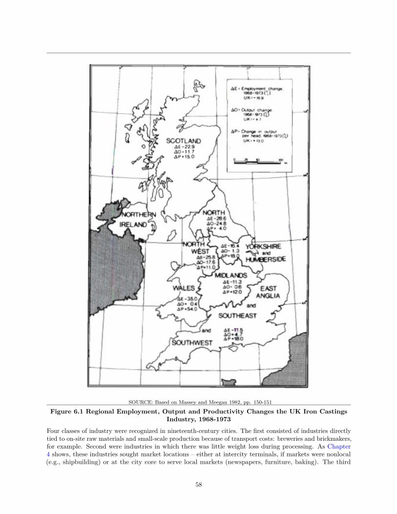
SOURCE: Based on Massey and Meegan 1982, pp. 150-151

Figure 6.1 Regional Employment, Output and Productivity Changes the UK Iron CastingsIndustry, 1968-1973

Four classes of industry were recognized in nineteenth-century cities. The first consisted of industries directlytied to on-site raw materials and small-scale production because of transport costs: breweries and brickmakers,for example. Second were industries in which there was little weight loss during processing. As Chapter4 shows, these industries sought market locations – either at intercity terminals, if markets were nonlocal(e.g., shipbuilding) or at the city core to serve local markets (newspapers, furniture, baking). The third

58

group of industries suffered large weight losses during processing and so had to be located near the sourceof raw materials – that is, the transport terminals. The waterfronts of Toronto and Montreal still exhibitsome relics of these industries – sugar-refining and flour-milling mainly. Fourth were the industries thatneed little materials but much labor: Being small scale and labor intensive, such industries as clothing,printing, and precision manufacturing located near the source of labor, the city core. Thus, we understandwhy, with labor, intercity and local markets, and raw materials all located near the city cores, manufacturingin nineteenth-century cities was so highly centralized.

During the twentieth century, however, the concentrated, high density nineteenth-century manufacturing cityhas exploded over the surrounding countryside. Throughout North America, the inner cities have been losingmanufacturing jobs whereas the outer areas-of metropolitan regions have been gaining. The problem, then, isto determine how these locational changes are related to the evolution of the economy.

Several processes have been occurring (see also Chapter 2). One is competition between firms, which leadsthem to try to reduce work by mechanization and increasing plant size. Accompanying this technical changehas been a search for new markets. As industrial markets become saturated (remember the product cyclehypothesis), new products and new markets must be found. Both processes reflect an ever-increasing emphasisupon innovation and have been accompanied by a significant lowering of transport rates (at least untilrecently, when world oil price rises have affected transport costs). These processes have had three importantmanifestations. (1) Increases in plant size have been accompanied by increasing concentration of marketpower in a few firms in each industry (although some industries are still characterized by small firms). This,in turn, has had several consequences. Plants are now less likely than they were to serve a single city, andso the attraction of the CBD as the point of easiest access to the city market has diminished. In addition,conglomerate ownership of several plants appears to have made locational change easier and faster (Masseyand Meegan, 1982, discuss this issue). As plants have grown larger, transport costs have fallen, so access toterminals and to labor has become less significant than spatial variations in production costs- especially thecost of land. (2) New commodities have been continuously introduced by firms to replace goods and servicespreviously produced by the domestic economy, so now there are many more industries than there were. (3)The state has provided several new markets for firms to exploit. In the United States, the arms and spaceindustry is one of them. But more important has been the state’s attempt to increase (and stabilize) demandby establishing high levels of investment in housing, urban freeways, transit systems, and automobiles.

The locational effect of these processes upon industry in cities has been dramatic. (Still, the small-scale,labor-intensive, and the site-oriented industries have been less affected than the others. Typically, theseindustries remain downtown. But because of product innovation, these industries are of declining importance.)Intraurban freight rates have fallen and materials processing has become more efficient. Technical changeshave replaced labor by machinery and land. The work force has been suburbanized. Also, the CBD hasbecome highly congested. Thus, as the materials-intensive industries (the second and third types) were freedfrom their ties to central terminals and as the labor force and local markets dispersed to the suburbs, soneeds for space and CBD congestion pushed them away from central locations too.

This example demonstrates, then, how the changing balance of transport and production costs at differentlocations has altered the geography of manufacturing industry within cities. In tum, however, changes inproduction and transport costs must themselves be understood as a result of mechanization, scale changes,new products, and state provision of markets. Again, then, we see how economic changes lead to locationalchanges.

6.4 ConclusionThis book has provided only an introduction to the theory of industrial location. Nevertheless, I have tried topresent a modern view of location theory, one that introduces you at least to some current research problems.Thus, the “introductoriness” arises from simplification of issues, evasion of some problems with the argument,avoidance of formal (and often, mathematical) treatments of location theory and a failure to treat adequatelysuch issues as industry structure and the internationalization of production. Yet the main arguments arenot “introductory” ones: The notion of maximum profit and least cost location is central to location theory;around this idea must be stated several issues of method – the importance of historical context, the need

59

to understand production decisions as a prelude to location decisions, the falling significance of transportcosts, the prominence of labor costs and agglomeration economies among production costs, and the factthat labor characteristics and the agglomeration economies at places are both produced characteristics. Theexamples have shown how these themes must be elaborated within a more complete theory of location; thisbook should be considered a first, not the last, word on location theory.

You will learn much more about industrial location if you read four additional books. The first is Lloyd andDicken’s Location in Space. This is a traditional but very good treatment of both theoretical and empiricalaspects of location. Second, consult the two studies upon which the first two sections of this chapter arebased: Bluestone et al.’s examination of the aircraft industry in New England, and Massey and Meegan’sAnatomy of Job Loss. These will take you far into ideas of context, labor costs, and industrial structure.Finally, Rees, Hewings, and Stafford have published a collection of papers, Industrial Location and RegionalSystems, which will give you an idea of the scope of modern industrial geography.

60

REFERENCESAlchian, A. A. 1950. Uncertainty, evolution and economic theory. Journal of Political Economy 58: 211-221.

Baumol, W. J. 1959. Business behavior, value and growth. New York: Macmillan.

Berry, B.J.L. 1967. Geography of market centres and retail distribution. Englewood Cliffs, NJ: Prentice-Hall.

Bloom, C. C. 1955. State and local tax differentials. Iowa City: State University of Iowa.

Bluestone, B., Jordon, P., and Sullivan, M. 1981. Aircraft industry dynamics. Boston: Auburn House.

Cyert, R. M., and Marsh, J. G. 1963. A behavioral theory of the firm. Englewood Cliffs, NJ: Prentice-Hall.

Estall, R. C. 1966. New England: A study of industrial adjustment. London: Bell.

Estall, R. C., and Buchanan, R. 0. 1973. Industrial activity and economic geography. 3rd ed. London:Hutchinson.

Haggett, P., Cliff, A. D., and Frey, A. 1977. Location models. London: Arnold.

Hamilton, F.E.I., and Linge, G.J.R. 1979. Spatial analysis, industry and the industrial environment:1,lndustrial systems. New York: John Wiley.

Harris, C. C., and Hopkins, F. E. 1972. Locational analysis. Lexington, MA: Lexington Books.

Harrison, B., and Kanter, S. 1978. The political economy of states’ job-creation business incentives. Journalof the American Institute of Planners 44: 424-435.

Haynes, K., and Fotheringham, A. S. 1984. Gravity and spatial interaction models. Beverly Hills, CA: Sage.

King, L. J. 1984. Central place theory. Beverly Hills, CA: Sage.

Lloyd, P. E., and Dicken, P. 1977. Location in space. 2nd ed. New York: Harper & Row.

Lowe, J.C., and Moryadas, S. 1975. The geography of movement. Boston: Houghton Mifflin.

Massey, D. 1979. A critical evaluation of industrial-location theory. In Spatial analysis, industry and theindustrial environment: 1, Industrial systems, eds. F.E.I. Hamilton and G.J.R. Linge, pp. 57-72. New York:John Wiley.

--- and Meegan, R. 1982. The anatomy of job loss. London:Methuen.

Phillips, E. B., and LeGates, R. T. 1981. City lights. New York:Oxford University Press.

Rees, J., Hewings, G.J.D. and Stafford, H. A. 1981. Industrial locations and regional systems. New York:Bergin.

Scott, A. J. 1982. Location patterns and dynamics of industrial activity in the modern metropolis. UrbanStudies. 19: 111-142.

Smith, D. M. 1979. Modelling industrial location: Towards a broader view of the space economy. In Spatialanalysis, industry and the industrial environment: I, Industrial systems, eds. F.E.I. Hamilton and G.J.R.Longe, pp. 57-72. New York: John Wiley.

Statistics Canada. Various years. Census of population. Ottawa: Author

---Annual. Manufacturing industries of Canada: national and provincial areas (catalogue 31-203). Ottawa:Author.

---Annual. Manufacturing industries of Canada: subprovincial areas (catalogue 31-209). Ottawa: Author.

--- 1972. Standard industrial classification manual (revised 1970). Onawa: Author.

Thompson, W. R., and Mattila, J. 1959. State industrial development. Detroit: Wayne State UniversityPress.

61

Treysz, G., Friedlaender, A., and Tresch. R. 1976. An overview of a quarterly econometric model ofMassachusetts and its fiscal structure. New England Journal of Business and Economics 1: 57-72.

U.S. Department of Commerce, Bureau of the Census. Series. Census of manufactures. Washington, DC:U.S. Government Printing Office.

---. County business patterns. Washington, DC: U.S. Government Printing Office.

---. Historical statistics of the United States, colonial times to 1970. Washington, DC: U.S. GovernmentPrinting Office.

---. 1981. Statistical abstract of the United States. Washington, DC: U.S. Government Printing Office.

Webber, M. J. 1983. Location of manufacturing activity in cities. Urban Geography 3: 203-221.

Weber, A. 1909. Theory of the location of industries. Chicago: University of Chicago Press.

Yeates, M. 1975. Main street. New York: Macmillan.

62

ABOUT THE AUTHORMICHAEL J. WEBBER is Professor of Geography at McMaster University in Hamilton, Ontario. He receivedhis Ph.D. from the Australian National University in 1967. Professor Webber is the editor of Papers, RegionalScience Association and on the editorial boards of Geographical Analysis and Journal of Regional Science.He has published several books on location theory-Impact of Uncertainty on Location and (coauthored)Christaller Central Place Structures-and on operational urban models-Information Theory and Urban SpatialStructure and Explanation, Prediction and Planning. His papers have appeared in a variety of geographicaljournals. Professor Webber’s research interests now include both industrial location theory and regionaleconomic development, particularly in relation to technical change and economic cycles.

63

SCIENTIFIC GEOGRAPHY SERIESThis series presents the contributions of scientific geography in small books or modules. Introductory modulesare designed to reduce learning barriers; successive volumes gradually increase in complexity, preparing thereader for contemporary developments in this exciting field. Emphasizing practical utility and real -worldexamples, this series of modules is intended for use as classroom texts and as reference books for researchersand professionals.

Volume 1CENTRAL PLACE THEORY by Leslie J King

Volume 2GRAVITY AND SPATIAL INTERACTION MODELS by Kingsley E. Haynes & A. Stewart Fother-ingham

Volume 3INDUSTRIAL LOCATION by Michael J Webber

Volume 4REGIONAL POPULATION PROJECTION MODELS by Andrei Rogers

Volume 5SPATIAL TRANSPORTATION MOD ELING by Christian Werner

Volume 6REGIONAL INPUT-OUTPUT ANALYSIS by Geoffrey J. D. Hewings

Volume 7HUMAN MIGRATION by W.A.V. Clark

Volume 8POINT PATTERN ANALYSIS by Barry N. Boots & Arthur Getis

Volume 9SPATIAL AUTOCORRELATION by John Odland

Volume 10SPATIAL DIFFUSION by Richard Morrill. Gary L. Gaile & Grant Ian Thrall

SAGE PUBLICATIONSThe Publishers of Professional Social ScienceNewbury Park Beverly Hills London New Delhi

64