Improving Performance inMetal Oxide Field-effectTransistorsVom Fachbereich Material- und Geowissenschaftenzur Erlangung des akademischen Grades Doktor-Ingenieur (Dr.-Ing.)genehmigte Dissertation von Mr. Daniel E. Walker, MPhys, MPhilgeboren am 3. Mai 1983 in Truro, GroßbritannienDarmstadt 2013 — D 17

Improving Performance in Metal Oxide Field-effect Transistors

Genehmigte Dissertation von Mr. Daniel E. Walker, MPhys, MPhilgeboren am 3. Mai 1983 in Truro, Großbritannien

1. Gutachten: Prof. Dr. Heinz von Seggern2. Gutachten: Prof. Dr. Wolfgang Donner

Tag der Einreichung: 19.04.2013Tag der Prüfung: 21.06.2013

Darmstadt — D 17

Contents

1 Introduction 3

2 Background 72.1 The Metal Oxide Field-effect Transistor . . . . . . . . . . . . . . . . . . . . . . . . . . . 7

2.2 Oxide Materials in the Literature . . . . . . . . . . . . . . . . . . . . . . . . . . . . . . . 19

2.3 Scanning Probe Methods . . . . . . . . . . . . . . . . . . . . . . . . . . . . . . . . . . . 23

3 Experimental Techniques and Transistor Characterization 313.1 Precursor Materials . . . . . . . . . . . . . . . . . . . . . . . . . . . . . . . . . . . . . . . 31

3.2 Fabrication of Transistors . . . . . . . . . . . . . . . . . . . . . . . . . . . . . . . . . . . 31

3.3 Scanning Probe Microscopy . . . . . . . . . . . . . . . . . . . . . . . . . . . . . . . . . . 35

3.4 Further Techniques . . . . . . . . . . . . . . . . . . . . . . . . . . . . . . . . . . . . . . . 38

3.5 Characterizing Transistors . . . . . . . . . . . . . . . . . . . . . . . . . . . . . . . . . . . 40

3.6 Models for Mobility and Threshold Voltage Extraction . . . . . . . . . . . . . . . . . . 41

4 Device Optimization 474.1 Formulation Optimization . . . . . . . . . . . . . . . . . . . . . . . . . . . . . . . . . . . 47

4.2 Process Optimization . . . . . . . . . . . . . . . . . . . . . . . . . . . . . . . . . . . . . . 52

4.3 Origins of Gate-current in Spin-coated Devices . . . . . . . . . . . . . . . . . . . . . . 58

4.4 Summary of Device Optimization Processes . . . . . . . . . . . . . . . . . . . . . . . . 60

5 The Influence of layer morphology on TFT Performance 615.1 Investigating Single Layers . . . . . . . . . . . . . . . . . . . . . . . . . . . . . . . . . . 61

5.2 Using Multiple Layers . . . . . . . . . . . . . . . . . . . . . . . . . . . . . . . . . . . . . 67

5.3 Qualitative Model of Layer Formation . . . . . . . . . . . . . . . . . . . . . . . . . . . . 74

5.4 Reducing the Required Number of Layers for High Performance . . . . . . . . . . . 76

5.5 Explanation of the Relationship between Morphology and Performance . . . . . . . 77

5.6 Summary of the Influence of Layer Morphology on Transistor Performance . . . . . 78

6 The Influence of Environment on TFT Performance 816.1 Experimental Determination of the Band Structures of ZnO and IZO . . . . . . . . . 81

6.2 The Effect of Oxygen . . . . . . . . . . . . . . . . . . . . . . . . . . . . . . . . . . . . . . 86

6.3 The Effect of Oxygen on the Contacts . . . . . . . . . . . . . . . . . . . . . . . . . . . . 88

6.4 Stress Induced Threshold Shift . . . . . . . . . . . . . . . . . . . . . . . . . . . . . . . . 89

1

6.5 The Effect of Light . . . . . . . . . . . . . . . . . . . . . . . . . . . . . . . . . . . . . . . 92

6.6 The Effect of Temperature . . . . . . . . . . . . . . . . . . . . . . . . . . . . . . . . . . . 94

6.7 Summary of the Environmental Effects . . . . . . . . . . . . . . . . . . . . . . . . . . . 99

7 Conclusions 1017.1 Future Work . . . . . . . . . . . . . . . . . . . . . . . . . . . . . . . . . . . . . . . . . . . 102

Appendices 105

Bibliography 111

Nomenclature 121

Curriculum Vitae 124

List of Publications 125

Acknowledgements 126

Authors Declaration 127

2 Contents

1 Introduction

In 1907, inventor Lee de Forest modified a Fleming diode (developed in 1904 by John Ambrose

Fleming) into a device called an Audion which used a third ’grid’ electrode to modulate the

current flowing between two other electrodes. This was the world’s first electronic amplifier

and kick-started an electronic revolution. Over the course of the next decade the Audion was

developed into triode tubes, then in 1915, Irving Langmuir invented the first vacuum tube. These

vacuum tubes became a key component in electronic products throughout the mid twentieth

century and are still used today in high power (>10kW) RF applications or high end audio

equipment.

There are, however, some issues with vacuum tubes limiting the suitability for application. The

manufacturing process is complex, therefore relatively expensive, the power consumed is high

and miniaturization is impossible. This led physicist Julius Edgar Lilienfield to patent the idea

for a solid state replacement to the vacuum tube in 1926, which was granted in 1930 [1]. Even

though he patented the idea he never published the details of any working prototype. This was

left until 1947 when, whilst working in AT&T’s Bell Labs, John Bardeen and Walter Brattain

performed an experiment with two gold electrodes on a germanium crystal mounted on a metal

base and noted an amplification in the output current depending on the potentials between the

gold electrodes. This was the first working solid state amplification device and was an example

of a point contact transistor [2, 3]. The potential of this device was not lost on group leader

William Shockley. The Bell Labs team were influential in developing the first silicon transistor,

whose inventor Gordon Teal, although at Texas Instruments in 1954, had previously worked for

Bell Labs. The Bell Labs team (specifically Dawon Kahng and Martin Atalla) went on to develop

the first, metal-oxide-semiconductor field effect transistor (MOSFET) in 1960 [4]. This device

formed the basis for modern electronics, where today billions of transistors are included on

devices the size of a finger nail, forming computer processors.

A MOSFET is crystalline silicon based and not suitable for every application. In the past

decade the market for large flat panel displays has increased ten-fold [5]. For this application the

transistors must be efficiently fabricated over large areas. Until recently this has been realized by

using plasma-enhanced chemical vapour deposition (PECVD) to form an amorphous-silicon (a-Si)

layer, which is subsequently patterned to create the transistors, enabling the switching operation

of the display. As of 2012, the vast majority of displays were fabricated using a-Si technology and

this is a fact that looks set to remain true in the coming years [6]. However, for an increasing

percentage of displays a-Si is not the technology of choice as its mobility is constrained to around

1 cm2/Vs due to large numbers of trap states [7, 8]. This limited mobility is a problem as there is

3

demand for a new generation of displays with high refresh rates, larger areas, 3D technology,

higher contrasts or all of the above. Each of these features require a higher mobility transistor for

use in the driving electronics. One possible replacement is to use polycrystalline-silicon (p-Si).

The advantage of p-Si is that the performance is proven to be adequate and that many of the a-Si

production processes still apply. The disadvantage is that p-Si contains grain boundaries, leading

to poor transistor uniformity and low yield, whilst requiring high cost, low pressure fabrication

techniques [9].

Figure 1.1: The potential of solution processed inorganic semiconductors. a) Chart showing theevolution of flat panel display backplane manufacturing volume for different materials: amorphoussilicon (a-Si), low temperature polycrystalline silicon (LTPS) and indium-gallium-zinc oxide (IGZO).Data from the Display Search third quarter 2009 report [10]. b) Progress of potential solutionprocessable materials for use in display back-plane and the relation to competing technologies.Information taken from references: [11, 12].

This led to the seeking of alternatives. Zinc oxide (ZnO) had been known to be a semiconductor

for many years from the work of Hahn in 1951 [13]. It was largely ignored for transistor appli-

cation until around the year 2000 when it was determined that it may be a useful replacement

for a-Si due to its ability to form transistors fabricated by low temperature processing routes

or to be deposited from solution [14]. As can be seen from figure 1.1, the a-Si market remains

enormous and there exists a credible business opportunity to offering an alternative, especially if

that method promises low temperature fabrication. Then, not only would it be a replacement

for a-Si, but would open up whole new markets in flexible display technologies based on plastic

substrates.

Like p-Si, ZnO is a polycrystalline material, however, the crystallites in ZnO are of the order of

a few nm in diameter, leading to a very large number of grain boundaries across the transistor

channel. These grain boundaries limit the performance of ZnO to a maximum mobility of a

few cm2/Vs particularly when solution processed, meaning ZnO is hardly an option for p-Si

replacement. In 2004 Nomura et. al. published work that showed by adding indium to the

4 1 Introduction

zinc to create indium-zinc oxide (IZO) the grain boundaries were eliminated, the material was

amorphous and had the potential to reach much higher mobilities [7]. Since then amorphous

oxide semiconductors have been shown to reach mobilities of up to 50 cm2/Vs from solution

indicating ample potential for p-Si replacement[15].

Since the work presented in this thesis began in 2009, the potential of amorphous oxide

semiconductors is starting to be realized. Notice in figure 1.1a the thin yellow section of the bar

which represents low temperature polycrystalline silicon (LTPS). LTPS is present in 1.1a from

2007, indicating its use in devices. However, the market share has not grown significantly in the

intervening years. Contrast this with the magenta line representing indium-gallium-zinc oxide

(IGZO), which has rapidly grown from non-existent in 2009, to a larger market share than p-Si

in 2012. IGZO has already found application in commercial products from Sharp, Apple and 8th

generation display demonstrators from LG Electronics [16–18].

These displays and demonstrators have all used conventional vacuum deposition methods

to fabricate the transistors within. As previously mentioned it would be advantageous to use

solution processing for these large area displays and for opening up potential new markets. This

is where the work contained in this project is focused.

The initial aim was to make solution processed ZnO devices. This was the starting point as the

ZnO material system was relatively well understood and had an established process behind it.

The theoretical background describing the operation of a field-effect transistor and the standard

accepted methods of quantifying the performance, which is critical throughout the thesis, are

described in chapter 2. In section 2.2 of chapter 2 the controversial question of the electronic

structure, and where the free charge in oxide semiconductor materials originates is introduced.

Chapter 2 finishes with an introduction to some of the salient theoretical background of the

scanning probe microscopy techniques used throughout the thesis.

Chapter 3 introduces the experimental techniques used to fabricate and measure devices and

includes a discussion on the validity of the standard methods used to quantify performance, using

example measured data to check the accuracy.

The beginning of the experimental work is described in chapter 4. This chapter focuses on

the first of the project goals which was designing the best possible, off-the-shelf formulation, for

use in solution processed semiconductor device manufacture. It begins with ZnO and modifying

the formulation to achieve the best results for two possible deposition methods, spin-coating

and ink-jet printing. The chapter progresses to optimizing the fabrication processes and finally

introducing indium to achieve a significant gain in device performance.

Chapter 5 examines the layers of deposited semi-conductors in detail and introduces a novel

technique of coating multiple layers in response to the observations derived from studying single

5

layers. The layer deposition process and resultant films are understood to a very high level

of detail and this understanding resulted in achieving the project goal of creating a solution

processable device with a performance of 20 cm2/Vs.

All the devices constructed throughout the project exhibited strong environment instability and

this led to a study presented in chapter 6, involving both ZnO and IZO devices. The response to

various environments and stimuli, focusing on the role of oxygen is examined. By studying both

materials, the extent of which the wealth of knowledge already obtained for ZnO is applicable to

the relatively new solution processed IZO devices could be determined.

Finally, chapter 7 summarizes the results and conclusions and provides thoughts on possible

directions for further research of these materials.

6 1 Introduction

2 Background

The concepts important for understanding the results presented throughout this thesis are

discussed in this chapter. The chapter begins with an introduction to the operating principle

of a generic thin-film transistor and its description with energy band diagrams. It continues by

introducing the concept of charge-carrier mobility and the standard method of extracting the

mobility value from experimental data, using the Shockley equations. Following this, the origins

of doping in metal oxide materials, and the semiconducting performance that can be expected

from examination of similar materials presented in the literature is discussed. Finally a brief

introduction on the theory of the various scanning probe methods used throughout the thesis is

compiled.

2.1 The Metal Oxide Field-effect Transistor

The field-effect transistor is just one class of many different types of transistor, the physics of

which have been described in great detail in the books ’The Physics of Semiconductor Devices’ by

S. M. Sze and Kwok K. Ng and ’Semiconductor Physics and Devices’ edited by J. Neamen [19, 20].

The following section will describe the principle of the field-effect transistor (FET) in some detail,

as not only are they the most widely used variation finding application in computer processors

and memory, all the devices fabricated in this thesis operate according to this principle. Field-

effect devices control the current flowing from one electrode, the source, to another electrode,

the drain, by modulating the charge concentration in a semiconducting material. This is achieved

by applying a potential to a third electrode, the gate, which is separated from the semiconductor

by a dielectric material.

Figure 2.1 shows the operating principle of a field-effect transistor. To visualize the operation

of a FET, one can start with a parallel plate capacitor as shown in figure 2.1a. The capacitor

is comprised of two metal plates separated by a dielectric material. When the plates are short

circuited (no electric potential difference exists between them), then no field exists across the

dielectric and there is no net charge on either plate. As a potential difference is applied an

electric field develops across the dielectric causing an equal and opposite charge build up on

the plates. This charge q is proportional to the magnitude of the potential difference applied

V , with the constant of proportionality giving the capacitance C according to q = CV . The

capacitance, measured in Farads, is determined solely by the physical parameters of the device

and is described by: C = ε0εrAd; where ε0 is the absolute permittivity of a vacuum, εr is the

7

Figure 2.1: Diagrams describing, a) the operating principle of a capacitor and b) the operatingprinciple of a field-effect transistor. S, D, and G refer to the source, drain, and gate electrodesrespectively.

relative permittivity of the dielectric, A is the area of one of the plates, and d is the distance

between the plates.

The transistor, shown in figure 2.1b is similar to the capacitor, except now one of the plates

has been split into two electrodes, the source and the drain (by convention the source is held at

ground, although it need not be) and the gap between them, known as the channel, filled with a

semiconductor. As with the capacitor a potential is applied to one electrode, the gate electrode,

relative to the source causing an electric field to build up across the dielectric. The semiconductor

then reacts to this field in a number of ways depending on its properties. When the semiconductor

is n-type, as all the materials used in this thesis, then it is the electrons that are the majority

charge-carriers. When there is no potential on the gate electrode, the semiconducting material is

not conductive and the transistor is known as an accumulation mode device. The application of

a positive gate-voltage causes electrons to accumulate at the semiconductor-dielectric interface

increasing the charge density, creating the conductive channel. If the opposite is true and

there exist sufficient charge-carriers in the channel that the device is conductive at zero applied

gate-voltage, then the application of a negative gate-voltage pushes all the charges away from

the channel region, depleting the semiconductor of charges and stopping the possibility of any

current flow between source and drain. This is known as a depletion mode device. In this way

the conductivity of the channel is controlled by the voltage applied to the gate electrode. When

another voltage difference between the source and drain electrodes, independent of the potential

of the gate, is applied, then a lateral electric field exists driving a current between them. Exactly

the same principle applies for p-type semiconductors, where a hole (the absence of an electron in

the valence band) is the majority carrier, except with the voltages reversed.

The mode of operation is not a fundamental property of a semiconductor and one semicon-

ducting material may exhibit both modes of operation depending on its doping level or the

quantity of trap states. For the applications of interest to this project, e.g. display backplane,

8 2 Background

an accumulation mode transistor is typically preferred as it is naturally off, i.e. no gate-voltage

needs to be applied to hold the transistor in the off state, which is usually more efficient, due to

minimized current leakage.

2.1.1 Energy Band Diagrams

A more detailed and quantitative method of understanding the principles described in section

2.1 is to consider energy band diagrams of the operating transistor. These diagrams are useful as

a vehicle to introduce and discuss a number of concepts, including accumulation and depletion,

semiconductor-metal contacts, and can be extended to explain the saturation and linear regimes

of operation, all of which will be discussed in this section and the section that follows.

Consider the diagram in figure 2.1a. This diagram shows a capacitor with two metal plates.

Replace the top metal plate with a semiconductor, rotate clockwise by 90° and this is the device for

which the band diagram is shown in figure 2.2. This is known as an metal-insulator-semiconductor

(MIS) structure and is a useful precursor to a FET.

Figure 2.2: The band diagram for an MIS structure under, a) flat band conditions, b) accumulationconditions and c) depletion conditions, for an n-type semiconductor.

Figure 2.2a shows the energy levels of the metal gate, labelled G, the insulator, I, and an n-type

semiconductor, SC, under flat-band conditions. As the semiconductor is n-type, the Fermi level,

EF is higher in energy than the midpoint in the band-gap, given by half the value between the

2.1 The Metal Oxide Field-effect Transistor 9

valence band maximum, EV and the conduction band minimum, EC . This diagram does not

consider any trapped charges, assumes a perfect dielectric and that the work-function of the

semiconductor is equal to that of the gate metal (φm = φSC). When there is no voltage applied

between the metal and the semiconductor, there is no electric field across the dielectric and no

bending of the conduction band and valence band. In reality it is unlikely that the work-functions

of the gate metal and the semiconductor are equal, meaning that the flat-band condition is only

reached when some voltage exists between the gate and the semiconductor.

Figure 2.2b shows the device with a positive voltage applied to the gate metal. In this case

there is a constant electric field across the dielectric which falls to zero inside the semiconductor.

As this is an ideal capacitor no current flows and the Fermi level in the semiconductor remains

constant. In the case of an n-type semiconductor and a positive gate-voltage, the bands are bent

downwards at the interface by an amount, called the surface potential, given by ΨS equal to

V −ΨD, where ΨD is the potential drop across the insulator. This has two effects. The conduction

band at the interface is at a lower energy than it is away from the interface, therefore it is

energetically favourable for any charge-carriers in the conduction band to accumulate at the

interface. Furthermore, due to this band bending the conduction band comes closer to the Fermi

level, and since the amount of charge-carriers in the conduction band depends exponentially

on the energy gap between the Fermi level and the conduction band, more charge-carriers are

excited into the conduction band at this interface. This is shown by the arrow in figure 2.2b.

Figure 2.2c shows the depletion case. Opposite to the accumulation condition the bands are

bent to higher energies at the interface, moving the conduction band away from the Fermi level,

resulting in an area at the interface depleted of mobile charge-carriers.

As with figure 2.1 previously, now consider the effect of adding a source and a drain electrode

into the semiconducting material. To achieve this with band diagrams, the energy levels can

be considered laterally across the device as shown in figure 2.3. Initially the electrodes and

semiconductor are separated as shown in 2.3a. The bands are flat, but unlike the previous case,

where for simplicity the work-functions of the metal and the semiconductor were assumed to

be the same, here the more realistic scenario for an n-type semiconductor is depicted with a

different work-function for the semiconductor than for the metal. When these materials are

externally connected, e.g. via a wire, charge will flow from one material to the other, such to

establish thermal equilibrium. The Fermi levels of the two materials will then be aligned. As the

materials are brought to close proximity of one another, an increasing amount of negative charge

accumulates at the metal surface due to the electric field in the gap between them, caused by the

contact potential (potential difference in work-functions). The system must remain charge neutral

overall, however, charge does not have to be locally homogeneous, therefore, this charge at the

metal surface may be compensated by the creation of a depleted region in the semiconductor,

known as the space-charge region. In the limiting case of the metal and semiconductor being

10 2 Background

Figure 2.3: a) The band diagram laterally from source to drain when the metal electrodes areseparated from the semiconductor by a distance, d. b) The semiconductor and electrodes in contactwith one another. If the work-function of the metal and semiconductor are different then this causesa band bending as shown. c) The application of a gate-voltage pulls the bands down in energyallowing accumulation as described in figure 2.2b.

in contact, shown in figure 2.3b, the charges reach a steady state and the bands are bent by an

amount, called the diffusion voltage, equal to the difference in work-functions of the materials.

The barrier at the interface φb is equal to the difference in the work-function of the metal and

the electron affinity of the semiconductor φb = φm − χSC . Away from the contact the electric

field inside the semiconductor decreases linearly until it reaches zero at the point the charge

build up at the metal surface is fully compensated. Any semiconducting material further from

the contact is unaffected and is said to be in the field-free region.

It should be noted that there may also be additional electronic states which exist inside the

semiconductor at the metal-semiconductor interface. These states will be largely transparent to

charge-carriers, being atomically thin, however, they may support a potential drop over them

further altering the band alignment.

The band bending at the semiconductor-electrode interface creates a barrier between the

electrode and the semiconductor, φb, which any charge-carriers must overcome to be injected

into the semiconductor. This barrier height depends mainly on the following: The intrinsic barrier

height, φb0; any electric field present in the semiconductor,ψE; and the potential a charge-carrier

experiences close to a metal surface due to the image charge effect [19]. The combination of

these electrical potentials results in a lowering of the barrier, as shown in figure 2.4 which depicts

a close look at the metal-semiconductor contact region. Furthermore, the magnitude of this

barrier is strongly dependent on any applied external electric field, being reduced as the electric

field is increased, shown by ψE2.

2.1 The Metal Oxide Field-effect Transistor 11

The contact potential barrier is critical to device performance as any charge-carrier must

overcome the barrier in order to contribute to a current. There are four distinct mechanisms

written in the literature through which this injection process may happen: Thermionic emission

where charges have enough thermal energy to overcome the barrier [21]; via a tunnelling

mechanism, also known as field-emission, through the barrier [22]; recombination in the space

charge region [23]; and via minority carrier injection to the field-free region [24]. The processes

involving minority carriers can be ruled out, as they are extremely unlikely to be efficient injection

mechanisms as the transport of minority carriers in the materials considered in this thesis is highly

inefficient. Pure thermionic emission is also unlikely as the barrier height will typically be much

larger than kB T , therefore, it would be expected that charge-carrier injection via a combination of

thermionic excitation and tunnelling through the barrier is the dominant mechanism of injection.

This mechanism is shown by the arrow in figure 2.4.

Figure 2.4: A close look at the band align-ment of the metal-semiconductor contact re-gion showing the Schottky effect for a metal-semiconductor contact. The diagram showsthe energy level of the conduction band inthe space charge region, the form of which isdue to different material work-functions,ψE ,and the influence of an applied source-drainvoltages shown in grey, ψE2.

Combining the lateral picture shown in 2.3b and the vertical picture shown in 2.1b, the effect

of applying a gate-voltage to the energy bands across the channel may be drawn. As previously

discussed the gate-voltage can result in accumulation of charges at the interface. The Fermi level

remains constant throughout, resulting in an accumulated charge in the conduction band. It is

this charge that forms the channel.

Figure 2.4 shows the effects on the contacts of applying a lateral electric field between the

source and the drain. This electric field, together with the gate potential defines the mode of

operation of the field-effect transistor as shown in figure 2.5. Figure 2.5a shows the different

12 2 Background

possible regimes of operation. With the source-drain potential difference substantially less than

the gate potential the transistor can be said to be operating in a linear regime. This means that

the density of mobile charge across the channel, due to accumulation, is approximately constant.

This is shown by the light grey area in the channel for the band diagram and by the white area in

the schematic of the transistor in figure 2.5b. As the source-drain potential difference is increased

at some point the drain potential becomes equal to that on the gate electrode. At this point there

is no accumulation due to the field-effect at the drain electrode interface. This is referred to a

the pinch-off point, labelled P.O. in figure 2.5a. Increasing the drain voltage further pushes this

pinch-off point back into the channel, as shown in figure 2.5c, effectively shortening the channel

length, although this is ignored in the long channel approximation as the shortening is small in

relation to the total channel length. This long channel approximation is assumed to be true for

all devices used in this thesis. After the pinch-off point is reached, increasing the drain voltage

further does not increase the amount of current flowing as the potential is then dropped over the

pinch-off region and the lateral electric field in the accumulation region remains constant. This

means the current flowing remains constant or, saturates, hence the name saturation region.

Figure 2.5: a) The potentials on the electrodes at various modes of operation on a field-effecttransistor. b) Band diagram showing accumulation in the linear regime and schematic of a transistordetailing the shape of the conductive channel region (white) with the dielectric polarization shownby the arrows. c) The same diagrams as b) for saturation mode. The band diagrams show theconduction band only.

2.1.2 Electronic Characteristics

As the electrodes of a field-effect transistor have potentials applied in differing configurations,

the current flowing between the source and the drain, hereafter referred to as drain-current, is

modulated. As was briefly mentioned in reference to figure 2.1, the electronic characteristics

2.1 The Metal Oxide Field-effect Transistor 13

of the transistor are typically measured with two sets of measurements sweeping the potential

on either the drain or gate electrode, whilst retaining the other at a constant potential relative

to the source. When the source-gate is swept and the source-drain voltage kept constant, the

resultant measured drain-current is referred to as a transfer characteristic. When the source-drain

voltage is swept and the source-gate voltage kept constant the resulting measured drain-current

is refereed to as the output characteristic.

Figure 2.6: a) An example of a typical output characteristic showing the drain-current response dueto varying the source-drain voltage at different gate-voltages. The solid lines are hand-drawn tomark the boundaries between the various regions of operation. b) A typical transfer characteristicshowing the drain-current plotted versus the gate-voltage in the linear and saturation regimes. Inboth plots the leakage current (gate-current) is shown in grey.

The plots in figure 2.6 show a typical output and transfer characteristic with the drain-current

plotted in black and the measured current at the gate electrode in grey. The magnitude of the gate-

current is essential as it reveals whether the device is functioning correctly, with an electrically

dense dielectric, and in some cases can give information regarding the bulk conductivity of the

semiconductor and the origin of any measured off-current (see section 4.3). Typically, for the

methods used to extract the mobility to be considered accurate, the magnitude of the gate-current

must be less than 0.01 of the drain-current. In the output characteristic the different regimes of

operation are shown. In the low drain-voltage region, marked linear region, the drain-current

responds linearly to drain-voltage. As the drain-voltage increases it starts to become comparable

to the gate-voltage, and as this happens the current enters a non-linear region, where it is no

longer linearly dependent on drain voltage, but also not saturated. In this region the channel has

not yet reached the pinch-off point, but is also significantly distorted by the electric field due

to the drain electrode. By increasing the drain-voltage further the pinch-off point is reached at

Vd = Vg , after which the current saturates as shown. The output characteristic can reveal other

useful information. In the very low drain-voltage region, typically Vd < 1 V, the characteristic

can be closely examined. If the injection properties of the electrode metal-semiconductor contact

14 2 Background

are non-ohmic then there exists a non-linear region centred on 0 V where the contact itself is

current limiting. In most cases, as for the data shown, the effect of the contact is so small it

is not observed in the output curve, indicating that no large potential barriers are inhibiting

charge-carrier injection.

Although the quantitative values describing the performance of the transistor may be extracted

from the output curve, usually it is the transfer curve that is used. Throughout this thesis it is

the transfer curve that is used to calculate mobility, threshold voltage and on-off ratio. In this

figure the transfer curve is plotted as the log of the drain-current versus the gate-voltage. It

may also be plotted with the drain current represented linearly, as in figure 2.7a. Both methods

of plotting are useful under different circumstances, but typically, for reasons discussed in the

following section, for the devices characterized throughout this project a log-plot is more useful.

The log-plot affords a rapid visual check of the validity of the extracted values, particularly the

threshold voltage which can be misleading when calculated according to the standard Shockley

equations. Furthermore, the log-plot affords the rapid identification of subtle shifts in the turn-on

voltage, marked Von in figure 2.6b1 and visual identification of the on-off ratio which is simply

the ratio of the marked values I-on divided by I-off. The mobility and threshold voltage must be

calculated.

2.1.3 Calculation of Mobility and Threshold Voltage

The mobility, µ, of a field-effect transistor is the proportionality constant describing how rapidly

the charge-carriers are transported through a solid under an applied electric field according to

v = µE, where v is the velocity and E is the driving electric field between the source and drain

electrodes in a transistor. This is a critical parameter of a transistor and is used for comparison

between devices [19]. Care must be taken in the application of mobility as there is often

confusion between the mobility of the material, an intrinsic property of the semiconductor, and

the mobility extracted from a transfer curve. A mobility extracted from the transfer curve is

not an intrinsic property of the semiconducting material, rather a property of the device and as

calculated by the generally excepted Shockley equations, does not take into account the effects

of the contacts, and assumes that the mobility remains constant regardless of the potentials of

the electrodes. This assumption is demonstratively false and discussed in greater detail later in

this section. Nevertheless, for comparison of devices constructed in this project to devices in the

literature the Shockley equations are used.1 Von is a turn-on voltage based on current flow due to the presence of an accumulation region inside the

semiconductor. It is typically defined as the point the current is above some lower limit and is determined asthe value at which the free charge-carrier density is above a certain value. Vth is a value calculated by linearextraction from the high gate-bias region and does not describe the current of the transistor at low gate biaseswhich may turn on at values significantly different from Vth. For further discussion on the differences andapplicability of either value see reference [25].

2.1 The Metal Oxide Field-effect Transistor 15

First derived by William Shockley in 1952 to describe the current behaviour of a field-effect

transistor the following equations allow the drain-current to be predicted from the electrode

voltages depending on the device geometry, the mobility and the threshold voltage of the device

[26]. For a more detailed derivation including many effects ignored here, such as the shortening

of the channel in the saturation region one can refer to references [19, 27]. What follows is

a derivation of the equations describing the behaviour of the drain-current in the linear and

saturation regimes.

For a transistor, the drain-current can be generally described by the amount of charge in the

accumulation layer divided by the amount of time each charge-carrier takes to travel from source

to drain. This is given by: Id(y) =W Q(y) v (y), where, W is the electrode width, Q is the areal

charge density and v is the charge-carrier velocity. The current must be constant throughout the

channel so this equation can be integrated from the source at y-position, 0, to the drain at L

giving:

Id =W

L

∫ L

0

Q(y) v (y) d y (2.1)

For the transistors examined in this thesis, the gradual channel approximation holds. This states

that the electric field from source to drain, E(y), is small compared to the electric field due to

the gate, E(z). This leads to the assumption that the velocity of a charge-carrier is constant

across the channel and therefore the mobility is constant. For the case of short channels or high

lateral electric fields, additional effects such as velocity saturation may occur. For a discussion

on these see reference [19]. Using the gradual channel approximation the relation v = µE,

where E is given by the lateral electric field, so v = VdL

, can be inserted into equation 2.1. At the

same time, as discussed in section 2.1, the charge present in the accumulation layer is given by

Q = C(Vg − Vth), where C is the areal capacitance of the device and Vg is the gate-voltage and

Vth is the threshold voltage. This results in:

Id =Wµ

L

∫ L

0

Q(y) E(y) d y, which evaluates to Id =W C

Lµ

Vg − Vth

Vd −Vd

2

2(2.2)

Notice that if Vg is much greater than Vd the final term in this equation may be ignored resulting

in the equation derived for a transistor operating in the linear regime:

Id =W C

Lµ

Vg − Vth

Vd , for

Vd

Vg − Vth

(2.3)

As Vd approaches Vg , theV 2

d2

term may not be ignored resulting in a decreased slope of the

current-voltage relation, shown in figure 2.6a as the non-linear region. Finally as Vd is greater

16 2 Background

than Vg this equation predicts a decrease in current. In reality this does not happen, but the

current maintains its peak value, i.e. it saturates at the point, where Vd = Vg − Vth and this may

be substituted back into equation 2.2, reducing it to:

Id =W Cµ

L

Vg − Vth

2

2for Vd ≥

Vg − Vth

(2.4)

The rearrangement of equations 2.3 and 2.4 enables the mobility and the threshold voltage in

the linear and saturation regimes to be extracted.

Figure 2.7: Mobility and threshold voltage extracted using the example experimental data from thedevice presented in 2.6 for, a) the linear regime and b) the saturation regime.

Figure 2.7 shows the extraction method performed on experimental data. The drain-current as

measured in the linear regime is plotted as a function of gate-voltage. The slope is then fitted,

giving the mobility multiplied by the device constants, W CL

. Extrapolating the fit back to zero

current gives a value for the threshold voltage. The technique is identical for the saturation

regime except in this case the square root of the drain-current must be plotted.

Notice that in both cases the experimental data deviates from the model at low gate-voltages,

where a more gradual turn on is observed before producing the linear relation that the model

predicts. This hints at some deviation from the standard Shockley equations for the devices

employed here, which is discussed in more detail in section 3.6. It also means that the threshold

voltage, which can be said to physically represent the gate-voltage value at which an accumulation

layer has formed, is consistently overestimated. This overestimation is clear when comparing

the log-plot, shown in figure 2.6b, with the linear-plot, shown in figure 2.7. This means for

these devices the Vth lacks the physical meaning but is, nevertheless, useful for device-device

comparison. The physical interpretation of the onset of accumulation is assigned to a different

quantity Von, as shown in figure 2.6b.

2.1 The Metal Oxide Field-effect Transistor 17

Many other methods for extracting the threshold voltage exist [28], however, the one that most

consistently represents the data does not rely on a physical derivation, rather looks at the point

on the drain-current curve that the rate of change of the gradient of the current is the largest.

This is known as the second differential of the transconductance method and mathematically is

the point where ∂ 2(Id )∂ Vg

2 is at maximum [29]. An example of such an extraction is shown in figure

2.8. The sharp peak is clearly visible defining the turn-on voltage, Von, and is consistent with the

onset of mobility also plotted in figure 2.8. As this method relies on the second differential it is

very prone to noise in the drain-current and must be checked against the value obtained from

Shockley extraction for rationality. It has one further advantage in that it does not depend on the

slope at high gate-voltages which can significantly deviate from linearity causing large errors in

threshold voltage extraction.

The extractions of mobility result in one value and ignore additional effects such as devices

becoming contact limited at high gate-voltages, reducing the rate of increase of the drain-current.

Further insight may be gained by extracting the mobility at each gate-voltage. This technique is

known as the transconductance method and is widely used in the field of semiconducting oxide

materials [9, 30], with some authors defining different features in this transconductance curve

to different physical phenomena [12].

The transconductance technique derives from the differentiation of equation 2.3 with respect

to gate-voltage and assumes that the mobility is only very slowly varying with gate-voltage, as

originally proposed by Horowitz [31]. This results in the equation for transconductance, gm,

given by:

gm =∂ Id

∂ Vg=

W C

LµVd (2.5)

This technique has some considerable advantages. Notice that the threshold voltage is no

longer required to calculate the mobility. Figure 2.8 shows a typical mobility extraction for

a high performance device. At low gate-voltages there is an onset of mobility as the current

rises. Fortunato et. al. attribute this to the Fermi level being very close to the conduction band

minimum (CBM), therefore even at small gate-voltages the mobility can rapidly increase [12].

This explanation may well be correct, however, it is difficult to say if the equation used to derive

the curve is revealing anything at low gate-voltages as it derives from the linear regime and at low

gate-voltages the transistor is not operating in the linear regime. The mobility curve then peaks

and starts to reduce. This reduction comes about from the slope of the drain-current decreasing

at high gate-voltages. There are two explanations put forward for this. The first and most

reasonable, is that at high currents the devices start to become contact limited. The high gate-

voltages mean that the channel becomes so conductive that even modest contact resistances can

become comparable to the channel resistance, meaning the gate-voltage has less of an influence

18 2 Background

Figure 2.8: The extraction of field-effect mobility from the transconductance and the thresholdvoltage via the second differential of drain-current method.

on the current flow. Another explanation is that at high gate-voltages the charge-carriers are

pulled closer to the interface, therefore the charge-carrier density increases, increasing scattering

effects [12]. The peak value of the mobility curve is used to define the mobility of the device,

as shown in figure 2.8. This is the method that has been employed throughout this thesis. In

most cases there is little difference in the extracted values of mobility from any of the methods

mentioned in this chapter. The difference becomes most pronounced for very high performing

transistors, where the saturation and linear mobilities may be underestimated when calculating

from the linear fit methods, due to the lower than expected current in the critical high gate-

voltage area. Figure 7.1 in the appendix provides a comparison for all of the mobility extraction

techniques.

2.2 Oxide Materials in the Literature

Zinc based oxide materials have been known for thousands of years appearing in ancient Indian

medical texts dating from 500BC [32]. Scientific study and documentation begins in the last

150 years. A simple search using the Thomson-Reuters Web-of-Knowledge database,2 reveals

more then 109,000 articles for ’zinc oxide’, the first of which was written in 1841 [33]. Research

into the electrical properties, in particular semiconducting properties, didn’t begin until a little

over 100 years later, when in 1949 a flurry or research activity began to look into some of the

2 www.webofknowledge.com

2.2 Oxide Materials in the Literature 19

topics studied in this thesis, for example, electrical properties, photo-conductivity and the role of

oxygen in determining the physical properties [13, 34, 35].

2.2.1 Electronic Structure of Zinc Oxide

Zinc oxide is a wide, direct band-gap semiconductor with an energy between the valence band

maximum (VBM) and conduction band minimum (CBM) of around 3.1 to 3.4 eV [36, 37]. Vast

amounts of literature can be found detailing the crystal and electronic structure and what follows

is merely a small summary of the points salient to this thesis [37–40].

Zinc oxide (ZnO) has a wurzite crystal structure under ambient conditions, where four cations

surround an anion in a tetrahedral arrangement. This is typical for sp3 covalently bonded solids,

however, ZnO also exhibits significant ionic character of around 55%, as calculated from the

equation developed by Linus Pauling to describe the nature of bonding in materials from the

electronegativity of the component atoms [41]. The zinc-oxygen bonding forms two electron

energy bands, one with a maximum in energy between -7 and -8 eV, the valence band, comprised

of Zn 3d electrons and the second at a higher energy, the conduction band, comprised of O 2p

and Zn 4s orbitals [42, 43].

Both the ZnO and the indium-zinc oxide (IZO) studied in this thesis are highly doped n-

type semiconductors with the Fermi level close to the CBM. The exact source of this doping

is controversial, but the debate centres around oxygen vacancies. Groups studying density

functional theory (DFT) calculations have calculated the formation energies of all the likely

defects (interstitial zinc, zinc vacancies and oxygen vacancies) [44] and have shown that

interstitial zinc would be a shallow donor but has a high energy of formation and so is unlikely

to be stable. Zinc vacancies have a low energy of formation but would occur as deep acceptor

states, not contributing to n-doping except as compensating defect sites. The oxygen vacancy site

is also calculated to lie within the band gap with a +2/0 transition approximately 1 eV below the

CBM. This would mean that the oxygen vacancy would be a neutral defect in an n-type material

and would therefore also be unable to contribute to n-doping in ZnO. The result of this is that,

theoretically at least, point defects cannot explain n-type conductivity observed in ZnO. There are

other possible mechanisms, with Al, Ga, In and H dopants all suggested to act as donors in zinc

oxide [45–48]. In fact for ZnO the only one of these that makes sense is hydrogen as it is very

hard to imagine how any of the other elements might appear in the films, unless deliberately

introduced. In fact, hydrogen has been known to be active in affecting the properties of ZnO

since 1956 [48]. The mechanism by which hydrogen is a shallow donor (Edonor < kBT) has been

convincingly explained by Janotti et. al. in reference [49] and is shown in figure 2.9a. In [49] it

is explained how hydrogen incorporated into an oxygen vacancy results in n-type doping. The 1s

hydrogen orbital interacts with the four Zn 4s dangling bonds in the vacancy to create an energy

20 2 Background

state located deep in the valence band and an anti-bonding state in the conduction band. Two

of the Zn 4s electrons form a doubly occupied state in the band-gap. Two of the other three

electrons (two from Zn 4s and one from H 1s) occupy the state in the valence band, whilst the

remaining electron would occupy the anti-bonding orbital, which is higher in energy than the

CBM and therefore the electron occupies the state at the CBM.

Figure 2.9: a) Schematic to explain the theory presented in reference [49], attributing the n-typedoping observed in ZnO to hydrogen adsorbed into an oxygen vacancy. Removing the oxygen atomfrom the lattice leaves two electrons in a mid-gap energy level. A hydrogen incorporated into theoxygen vacancy site interacts with these electrons to create two energy levels, one in the valence bandand one in the conduction band. One electron occupies the state in the conduction band and decaysthermally to the CBM. b) Diagram explaining how oxygen may deplete the surface of ZnO grains ofcharge-carriers. The dark areas around the edge of the grains represent depleted areas due to thesurface adsorbed oxygen trapping charge.

It is very difficult to experimentally test whether hydrogen is really the cause of n-type doping

as it is ubiquitous. It is present in water, every organo-metallic precursor, the forming gas used in

glove-boxes and is the dominant remaining element in UHV conditions. Therefore making and

measuring a film in the absence of hydrogen is close to impossible.

If an electron is deposited directly into the conduction band then the material should have

some intrinsic conductivity outside of any gating effects. In fact, the conductivity of the granular

ZnO films is observed to be very low. It is possible that the ZnO grains may themselves have a

high conductivity, with the semiconducting behaviour dominated by trapping at the interfaces

between the grains, pushing the conduction band at the interface to a higher energy level [46, 50].

It is physisorbed and chemisorbed oxygen (oxygen adsorbed onto the surface of the grain by

capturing an electron from the bulk) which is most often considered to be responsible for this via

2.2 Oxide Materials in the Literature 21

the mechanism shown in figure 2.9b. Furthermore, oxygen is active in these materials in other

ways. It may be fully adsorbed into the crystal structure where oxygen is incorporated into the

lattice of the film itself in an oxygen vacancy site. In this instance it would lower the doping in

the films by replacing hydrogen or eliminating the oxygen vacancy [51]. This can happen as the

oxygen vacancy itself is not static in the material but free to diffuse, albeit slowly. In tin oxide

the diffusion coefficient is measured at 10−13 cm2/s [52]. Even though the diffusion coefficient

is low, oxygen vacancies may appear near the surface allowing surface adsorbed oxygen to be

incorporated in the film.

It can also be that the surface oxygen permeates through the granular film causing depletion

throughout the film. If a void free film could be made then the oxygen would be constrained to

the surface and thickness could be varied. In this case it should be observed that as the thickness

is increased, at some point the whole film is no longer depleted and becomes metallic. This has

been studied and observed for both ZnO and IZO [53–56].

2.2.2 Progress of Device Performance

In 2004 Nomura et. al. highlighted the potential of semiconducting oxide materials by

preparing amorphous IGZO films by pulsed laser deposition and achieving device mobilities of up

to 9 cm2/Vs [7]. This created significant excitement as this was substantially higher than organic

materials and amorphous silicon. Since then many groups have attempted to make devices with

many different derivatives of doped indium or zinc based oxide materials and comprehensive

tables of the device performances can be found in references [9] and /citeFortunato2012. The

following table 2.1 includes some of the more exceptional and relevant entries found therein.

Group and Reference Material Deposition Mobility cm2/Vs Temperature °CMeyers [57] ZnO IJP & SC 1.8 150

Li [58] ZnO SC 5.26 500Adamopoulos [59] Li-ZnO SP 54 400

Han S-Y, AMFPD ’09 IGZO IJP 25.6 600Kim [15] ZITO SC 40 - 100 400

Banger [30] IZO SC 16 450

Table 2.1: Table including some of the state of the art results for solution processed oxide basedtransistors. The temperature is that at which the devices are annealed to form the oxide layer.Abbreviations: Inkjet Print (IJP), Spin Coated (SC), Spray Pyrolysis (SP) lithium doped zinc oxide(Li-ZnO), zinc indium tin oxide (ZITO), indium gallium zinc oxide (IGZO) and zinc oxide (ZnO).

The first thing to note from these tables is that the mobility is strongly dependent on the

processing temperature. Most ZnO devices published have mobilities in the region between 0.1

22 2 Background

and 1 cm2/Vs, with some notable exceptions. Meyers et. al achieved mobilites of 1.8 cm2/Vs

with a processing temperature of 150 °C using an aluminum oxide phosphate (AlPO) dielectric.

They also achieved mobilities of 3 cm2/Vs on silicon dioxide, however, requiring an anneal step at

300 °C. Nevertheless this is good achievement for ZnO at relatively low processing temperatures.

Li et. al. published the highest spin coated result to date achieving 5.26 cm2/Vs when processed

at 500 °C. Significantly higher results have been achieved by employing lithium doping and spray

pyrolysis with mobilities in excess of 50 cm2/Vs at processing temperatures of 400 °C. Kim et.

al. achieved the highest solution processed semiconductor result with mobilities reported at

over 100 cm2/Vs using tin-doping. However, when highly tin doped, the off-current suffers and

the threshold is shifted to negative values making the devices less useful for application. The

highest mobilities were also achieved by employing an ultra-thin self-assembled nano-dielectric

(SAND) and it is questionable that the results from this are truly comparable to conventional

silicon oxide dielectrics, due to the very low measurement voltages leading to ill defined regimes

of operation. That said, this group also achieved mobilities of 40 cm2/Vs using silicon dioxide

processed at 400 °C. Finally, the highly influential paper of Banger et. al. was published in Nature

Materials in 2011, using IZO, where mobilities as high as 16 cm2/Vs when annealed 450 °C or

8 cm2/Vs when annealed at 230 °C, with spin coated solution processed materials were achieved.

This remains the state of the art to this date and the devices that were fabricated to achieve this

closely resemble the devices fabricated in this thesis.

2.3 Scanning Probe Methods

A large portion of the analysis in this project was completed using scanning probe methods.

These afford topographic imaging with nanometre lateral resolution and sub-nanometre z-

resolution. The very high resolution is critical as the performance of semiconducting oxide layers

can be determined by extremely small scale morphological features within the films, as shown

in chapter 5. Scanning probe methods proved very adept at resolving these nanometre scale

features where other visualization techniques, such as SEM, lacked sufficient resolution to enable

clear conclusions to be drawn.

2.3.1 Atomic Force Microscopy

The atomic force microscope (AFM) was invented in 1986 and was a development of the

scanning tunnelling microscope (STM) invented earlier that decade [60, 61]. AFM functions by

bringing a sharp tip, mounted on a deformable cantilever, close to the surface and employing a

feedback mechanism to maintain the tip to sample distance in a constant force mode, or by using

no feedback and recording the feedback signal in a constant height mode. The first AFM used an

2.3 Scanning Probe Methods 23

STM to record the deflection of the cantilever and provide feedback. More modern systems use a

laser, where the beam deflection is measured by a 4-quadrant photo-diode. Figure 2.10 shows

the principle of the AFM.

Figure 2.10: a) Shows the basic principle of Atomic Force Microscopy. b) Depicts the form of the forceon the tip as a function of the distance from the surface. The curve is in the form of a Lennard-Jonespotential. c) Describes the modes of operation, amplitude or frequency modulation and d) shows thebehaviour of a cantilever as it approaches and retracts from a surface.

There are three potential modes of operation. Contact mode, where the tip-sample interaction

is repulsive, intermittent contact mode, often referred to as tapping mode, (or non-contact mode

in air), and ’true’ non-contact mode where the tip-sample interaction is attractive. The force on

the tip and distance from the surface in the various regimes of operation is well described by a

force curve in the form of a Lennard-Jones potential, as shown in figure 2.10b. In contact mode

the beam deflection is recorded and used to govern the piezoelectric extension controlling the tip

height allowing the tip to follow the surface.

All of the images presented in this thesis are taken in non-contact mode. Non-contact mode may

be operated utilizing two feedback mechanisms, amplitude modulation or frequency modulation.

The more common amplitude modulation, also used for tapping mode in air, see below, exploits

24 2 Background

the change in amplitude of a tip driven by an alternating current signal applied to a piezoelectric

actuator. To close approximation this can be described by a force gradient model [62]. As

the cantilever approaches the surface it undergoes a shift in its resonant frequency according

to: fe f f = f0

1−F ′(z)k0

12 where fe f f is the new resonant frequency of the cantilever, with spring

constant k0, according the force gradient F ′(z), due to the sample. If the cantilever is driven at a

frequency slightly above its natural resonant frequency f0, then as it approaches the surface the

shift in the frequency spectrum to a lower frequency results in drop in amplitude at the driven

frequency, see figure 2.10c. The operator chooses a set-point amplitude that is lower than the

amplitude of the cantilever when it is far from the sample. The AFM moves the tip closer until

the set-point amplitude is reached. The tip-sample distance may be controlled by altering the

set-point amplitude, the lower it is compared to the amplitude at f0 the closer the tip will be to

the surface. The Alsylum Research MFP-3D AFM is typically operated in amplitude modulation

mode.

The maximum sensitivity of amplitude modulation is at the point on the resonance curve where

the slope is greatest allowing the minimum change in F ′ to be detected according to:

F ′min =1

δrms

27kbTβ

ω0Q

12

(2.6)

where, δrms is the RMS amplitude of the cantilever, ω0 is the resonant frequency in radians, Q is

the quality of the resonance defined by ω0δω

(δω is the range of frequency where the amplitude

varies by half the amplitude at resonance), and β is the measurement bandwidth [62]. This

is ultimately governed by thermal noise as it has temperature dependence, T . From the above

equation it may appear that the Q-factor should be made as high as possible to get maximum

sensitivity, for example, by reducing damping by measurement in vacuum, or using a very stiff

cantilever. However, if F ′ changes during a measurement the cantilever takes some time to

respond which according to the usual bandwidth convention is given by: τ = 2Qω0

. In the case

of a vacuum system damping is very limited, therefore Q is very high and the bandwidth very

narrow not allowing sufficient range for practical imaging. Therefore, slope detection (amplitude

modulation) is not particularly suitable for vacuum measurements. The solution is to employ

frequency modulation. Frequency can be measured extremely accurately allowing the use of very

stiff (high Q) cantilevers, providing high stability close to the sample surface. Changes in F ′ cause

instantaneous changes in the frequency. The tip is kept at resonant frequency via a feedback loop

allowing the reconstruction of the sample topography. In frequency modulation mode, Q and

β are independent, β now depends not on the resonance peak width but on the characteristics

of the frequency demodulator, allowing the use of very high Q cantilevers without sacrificing

bandwidth. In the case of small amplitude oscillations, where the oscillation is less then the

2.3 Scanning Probe Methods 25

tip-sample interaction distance the frequency depends on the force gradient, F ′(z), according to:∆ωω0=− F ′(z)

2k0where ω0 is the resonant frequency far from the sample and ∆ω is the change in

frequency.

Non-contact mode AFM can be done in both vacuum and air, however, samples in air typically

have a water meniscus layer adsorbed across the surface. In this case it is very hard to keep the

tip close enough to the surface without it sticking to, or imaging the water layer. When this is

the case tapping mode can be employed. This operates in a very similar manner to amplitude

feedback in non-contact mode. The tip is driven to resonance by an ac signal to the piezoelectric

actuator, but in this case with an amplitude of oscillation high enough that the tip enters the

repulsive regime, see figure 2.10. As in non-contact mode the frequency is damped, however,

the approximation employed in the force-gradient model is no longer valid, as the amplitude of

oscillation is not small compared to the tip sample distance. The result of this is the amplitude is

also damped. Practically this means driving the tip at a frequency slightly below the resonant

frequency, rather than above as in non-contact mode. A mathematical description of dynamic

mode AFM can be found in reference [63].

2.3.2 Kelvin Probe Force Microscopy

Kelvin Probe Force Microscopy (KPFM) is a technique to measure the local contact potential

difference between a metallized AFM tip and the sample, first described by Nonnenmacher

in 1991 [64]. It functions in a similar way to a standard macroscopic Kelvin probe where a

metallized plate is brought close to the sample, forming a capacitor via an external connection. A

voltage difference exists between the plates caused by the work function difference between them

and the additional effects of surface adsorbates [65]. This can be described by the simple model:

VC PD =1e

Φ2−Φ1

, where Φ2 and Φ1 are the work functions of the two plates including the

contribution of any adsorbates, and VC PD is the contact potential difference [64]. The distance

between the plates is then varied periodically at an angular frequency, ω, resulting in a time

varying current given by:

i (t) = VC PDω∆C cos (ωt) (2.7)

where ∆C is the changing capacitance between the plates. For measurement of VC PD a backing

voltage is applied such that the current i(t) falls to zero. This principle is shown in figure

2.11a. The three cases describe the interaction between two surfaces as they are brought into

contact. In the first diagram the surfaces are separated by a distance, d, such that they are not

electrically connected. The second diagram shows the case where the surfaces are electrically

connected, either externally or when they are close enough that electrons may tunnel between

them. Equilibrium dictates that charge must flow resulting in equalization of the Fermi levels,

26 2 Background

shown by, I , on the diagram, which has the effect of charging the surfaces causing a potential

difference VC PD. The charged surfaces result in a force between them which can be removed by a

backing voltage Vdc =−VC PD.

The principle of the Kelvin probe is applied to the AFM tip and the sample, except that the

KPFM measures the response of the tip due to the force acting on it induced by VC PD to nullify

the charging, rather than the periodic current flow. This electrostatic force on the tip is described

by:

Fes (z) =−1

2∆V 2∂ C (z)

∂ z(2.8)

where ∆V is the voltage difference between the applied backing voltage and VC PD, ∂ C(z)∂ z

is the

change in capacitance caused by varying z [66]. When a voltage is applied to the tip of the form

Vac sin (ωt)+Vdc then the voltage difference V , assuming Vdc is applied to the tip, not the sample

is given by:

∆V =

Vdc − VC PD

+ Vac sin (ωt) (2.9)

as described in reference [67]. Substituting this equation into 2.8 gives the electrostatic force on

the tip:

Fes (z, t) =−1

2

∂ C (z)∂ z

Vdc − VC PD

+ Vac sin (ωt)2 (2.10)

This equation may be split into three parts: Fdc, the deflection of the tip due to the dc voltage;

F2ω, which may be used for capacitative measurements according to the technique detailed in

reference [68]; and Fω, used for measurement of VC PD:

Fω =−∂ C (z)∂ z

Vdc − VC PD

.Vac sin (ωt) (2.11)

When the electrostatic forces are applied to the tip from Vac this causes additional oscillations

of frequency ω. These are detected by a lock-in amplifier, which provides an output directly

proportional to the difference between VC PD and Vdc. Vdc is then applied such that the lock-in

output signal is zero giving −VC PD. This is done point by point across the surface building up a

local potential map. The principle described above as implemented by the Omicron VT AFM is

shown in figures 2.11a and b.

As with AFM the tip oscillation is measured by a laser reflected from the back surface of the

cantilever in resonance by a quadrant photo-diode. The frequency of oscillation is shifted due to

the forces acting on the tip. The forces can be altered by applying an external voltage to the tip

(Vex t). A small ac voltage is added to the signal allowing the lock-in amplifier to measure the

2.3 Scanning Probe Methods 27

Figure 2.11: a) Shows the energy band diagrams describing the operating principle of a Kelvin probeas two materials are brought together. b) A diagram detailing the operation of the Kelvin Probe ForceMicroscope.

slope of ∆F (Vgap), marked in figure 2.11b as Xsi g . This slope is minimized, at which point ∂ F∂ z

is

minimized and the electrical forces are compensated and Vex t is equal to the Kelvin potential, Vk

as shown in figure 2.11b.

2.3.3 Scanning Tunnelling Microscopy

Scanning Tunnelling Microscopy (STM) is performed on the same apparatus as AFM. A very

sharp tip is brought close to, but not allowed to contact, the surface of a sample such that

electrons can tunnel from the tip to the sample or vice versa, with a probability of finding an

electron that has tunnelled through the barrier given by:

Ptunnel ∝ exp

−2

r

2m (U − E)

ħh2 w

(2.12)

28 2 Background

where U is the height of the barrier, w the width, and E the energy of the electron. Particle

tunnelling is a well known consequence of wave-particle duality and an in-depth description can

be found in reference [69]. The key point is that the probability of tunnelling has an exponential

dependence on the width of the barrier. The measured current depends linearly on the probability

of tunnelling and the width of the barrier is governed by the tip to sample distance, therefore

the tunnelling current depends exponentially on the tip to sample distance. This has some

useful implications. Practically, a current set-point is chosen and the tip lowered towards the

sample surface with an applied potential difference until this current is reached. The exponential

dependence on the tip-sample distance allows the tip to be held very accurately at a set distance

from the surface governed by the set-point current and applied bias. Another consequence of

the exponential dependence is that only the very lowest point of the tip influences the feedback.

For example, assuming a tip composed of a pyramid of atoms, 90% of the current flows through

the single atom closest to the sample, allowing surfaces to be routinely imaged with atomic

resolution, not only in height but also laterally [70–72].

2.3 Scanning Probe Methods 29

3 Experimental Techniques and Transistor Characterization

The details of the experimental techniques employed in fabricating the devices used throughout

this thesis and an introduction the methods used for characterization, are described in this

chapter. The chapter begins by introducing the precursor materials and describing the established

methods for fabricating transistors or two terminal devices, including substrate preparation,

layer deposition techniques and electrode fabrication. The chapter continues by describing

the techniques used throughout the thesis to determine the layer properties and finishes by

introducing the methods employed to electrically characterize the devices and a discussion on

the accuracy of the electrical parameter extraction.

3.1 Precursor Materials

The precursor materials used in this project have been synthesized by Dr. R. Hoffmann as part

of the MerckLabs project in conjunction with the working group of Prof. Dr. Schneider in the

Chemistry department of the TU-Darmstadt. Principally two precursors were used throughout

the project, zinc oximate and indium oximate, the structures of which are detailed in figure 3.1.

Full details of the synthesis of these materials may be found in the work of Schneider et. al. and

Pashchanka et. al. respectively [73, 74]. The oximate materials are not on general sale and are

covered by patent belonging to Merck Patent GmbH [75].

Both materials are single source precursors, which means no further external chemical input

is required to result in the desired decomposition products. The zinc oximate has a density of

5.606 g/cm3, a molar mass of 333.6 g/mol and begins to decompose via the route shown in figure

3.1 at around 180 °C, with decomposition completed by 220 °C regardless of the atmospheric

gas [73]. The indium oximate has a density of 7.179 g/cm3, a molar mass of 463.1 g/mol and

also starts to decompose at around 180 °C. Unlike the zinc oxide the TGMS spectra presented in

reference [74], show an extended tail in the decomposition extending out to 400 °C. The authors

note that the decomposition route is different for the indium and zinc oximates and suggest the

routes shown in figure 3.1.

3.2 Fabrication of Transistors

In most cases and unless specifically mentioned, transistors have been prepared on highly

n-doped (n ∼ 3 × 1017 cm−3) silicon substrates with a 90 nm thermally grown oxide layer, a

31

Figure 3.1: The zinc-oximate and indium-oximate precursors used throughout this project and thedecomposition pathways. Diagrams of the zinc and indium precursors reproduced with permission,from references [73] and [74] respectively.

schematic of which is shown in figure 3.2. The substrates come pre-patterned with 30 nm gold

source and drain electrodes on a 10 nm ITO anchor layer. They are supplied coated in a polymer

protection layer which must first be removed. This is achieved by two steps of ultrasonication

in acetone for ten minutes per step. Then a cleaning procedure of ultrasonication in deionized

water, acetone and finally isopropanol, for ten minutes per step is employed to leave a clean,

residue free surface. Before the substrates are used they are either dried with dry nitrogen or left

to dry naturally in a flow box. Immediately before coating the substrates are plasma treated in

a home-built plasma chamber with an air plasma at 10 mbar. The excitation for the plasma is

supplied by a PFG300RF radio-frequency generator. The effects of the plasma treatment should

be persistent (see chapter 4), nevertheless, the active layer is deposited as quickly as possible

afterwards, typically within five minutes. The deposition method varies as described later in this

section.

32 3 Experimental Techniques and Transistor Characterization

It is also the case that for some of the devices used the ITO/Au source-drain electrodes or

the gate electrode are not required, e.g. samples for XRR measurements or 2-terminal device

structures. In these case it is possible to use substrates from the edge of the wafer which have

no source or drain electrodes. The cleaning procedure, plasma treatment and subsequent layer

deposition remain the same. In the instances where different electrode metals are required they

have been deposited by thermal evaporation through a shadow-mask from an HHV Auto 306 or

a Balzers BAK600 deposition system onto the blank substrates. The masks used were purchased

with a single cut metal strip. This allowed 5 µm fibres to be glued perpendicularly across the

strip to split it into source and drain electrodes, creating the channel area. For the two terminal

devices where there should be no gate electrode the same procedure may be employed with a

glass substrate as shown in figure 3.2.

Figure 3.2: Diagram detailing the bottom-gate bottom-contact TFT design most often employedthroughout the project (left-hand diagram) and the two-terminal device structure (right-handdiagram).

Once the substrate is prepared, the formulation is deposited according to the required tech-

nique. (The development of the formulation is described in detail in chapter 4). In most cases

experiments were run with spin coated devices as this method affords the most reproducibility,

however, in some cases, typically where patterning was required, ink-jet printed devices were

used.

3.2.1 Spin-Coating

The spin-coating method typically consists of dropping 50 µL of formulation onto the centre of

the substrate by micro-pipette. This is then spun for 30 s at 2000 rpm with a Pi-Kem DipMaster

200 spin-coater placed in a flow box. Immediately after the spin-casting the precursor must

be broken down to allow the metal oxide layer to be formed. Two methods have been used

throughout this project. For zinc-oximate precursors UV light from a Dr. Hoenle UV Cube 2000

was used by placing the samples 6 cm from the top of the chamber and exposing for the required

time, typically 5 min. Indium-oximate and zinc-oximate mixtures used to form IZO films were

3.2 Fabrication of Transistors 33

always decomposed using a hotplate treatment at 450 °C for around 10 min. This time varied

considerably and there are reports in the literature which suggest a longer time is required

[30]. However, this was examined for the oximate precursors used in this project, see chapter

4, and found not to be the case. Furthermore, it is interesting that when the zinc-oximate

precursor is used as a single precursor, UV light is the best method to break it down to form

the oxide layer. However, when mixed with indium-oximate in a binary precursor solution heat

treatment becomes preferable. ZnO layers can be formed well with heat treatment, however

IZO layers are not formed well with UV treatment. One explanation, consistent with TG curves

of precursor decomposition shown in references [73, 74] is that the indium precursor does not

completely decompose until higher temperatures which are not reached in the UV cube (this gets

to temperatures of around 250-300 °C) leading to poor quality layers.

3.2.2 Ink-Jet Printing

Ink-jet printing was employed principally as a method of producing patterned active-layer

films. It was performed with a commercially available Dimatix DMP2831 ink-jet printer. This

printer uses disposable cartridges allowing printing with small quantities, approximately 1 mL,

of ink. The cartridges have 16 nozzles and fire a drop volume of 10 pL per drop. A pattern

may be defined in the pattern editor and this is then printed according to the best method as

decided by the software. No direct control over the printing route is possible. Figure 3.3 shows

the Dimatix printer, a schematic of the pattern printed onto the standard Fraunhofer substrates

used throughout this project, and a typical result of the printing process. Specifically the pattern

is composed of a set of nested arrays. The overall pattern, as shown, is composed of a single 4

by 4 array. Each element of this array is composed of 51 by 51 individual drops with a 20 µm

spacing. As the diameter of the deposited drop is larger than 20 µm, each of the small squares

shown in the pattern in figure 3.3 comprises 2601 overlapping drops. This pattern is printed

with the waveform shown in the appendix, figure 7.2, at a firing frequency of 1kHz, with a firing

voltage optimized to give the same drop velocity, typically around 15 V. The firing frequency is

a critical parameter and must be kept at 1kHz as higher frequencies lead to serious anomalies

in drop spacing and jetting quality of the relatively un-optimized inks. Figure 3.3b shows an

example of the jetting performance from a zinc-oximate formulation. There is very limited nozzle

plate wetting and relatively small ligands, however, the formation of satellite drops can be seen

ongoing in this image. This is typical for the low viscosity, low surface tension formulations used

and deemed to be uncritical for the pattern printed where all the drops are designed to merge

into a single pattern.

The specific inks used are developed and discussed in chapter 4. In the example shown in

figure 3.3 the final deposited pattern is clearly a circular shape as opposed to the square shape of

34 3 Experimental Techniques and Transistor Characterization

Figure 3.3: a) The Dimatix DMP2831 inkjet printer and of the result of printing the active layeraccording to the pattern detailed in the diagrams on the bottom row. The Dimatix makes five passesto print each row of the pattern, printing on the forward pass only. b) A view from the Dimatixfiducial camera, looking up at the nozzle plate on the underside of the ink cartridge. The imageshows a zinc-oximate solution jetting. The nozzles can be seen as the line of round holes in the centrewith individual drops exiting downwards as detailed in the inset schematic. The appearance of dropsabove the nozzles is due to the drops reflection in the nozzle plate.

the original pattern. This is because of the coffee staining effect that has been engineered into the

process to give extremely thin active layers over the source and drain electrodes. Coffee staining

is the result of surface line pinning and the drying process where material is transported to the

edges of the pattern, as described in reference [76]. It is often an undesirable feature and can be

controlled via the Marangoni effect [77] or by simply increasing the viscosity of the formulation,

reducing the overall fluid mobility. Initially the inks were engineered to faithfully reproduce the

intended pattern and minimize coffee staining, however, it was discovered that devices made

from these inks underperformed when compared with inks that were allowed coffee stain.

3.3 Scanning Probe Microscopy

Data shown in this thesis has been taken with a commercial Omicron VT-AFM scanning probe

microscopy system, which has been modified with electrical feed-throughs, to allow transistor

samples to be connected inside the AFM itself. This is an ultra high vacuum (UHV) system

operating at pressures < 2 × 10 −10 mbar. In the cases where the samples must be measured

in air an Asylum Research MFP-3D system was used. For a detailed description of the Omicron

VT-AFM, its operation, sample mounting and data extraction refer to the PhD thesis of Dr.

Christopher Siol [78].

All scanning probe images taken over the course of this project were analysed with the open

source Gwyddion software [79]. Typically images were processed by levelling after which data

could be extracted via the various tools provided, often including line profile and area analysis

tools giving the height profiles and surface roughness characteristics respectively. All surface

3.3 Scanning Probe Microscopy 35

roughness values quoted are arithmetic average of data-points, Ra, determined from a specified

area according to the following equation:

Ra =1

N

N∑

j=1

r j

(3.1)

Following the data extraction, the histogram tool may be used to crop the pixels to a suitable

height scale for presentation.

3.3.1 Experimental Measurement with Kelvin Probe Force Microscopy

A brief discussion of the salient points of the theoretical description of KPFM has already been

given in section 2.3.2 and full details of the experimental aspects of the technique may be found

in [78]. This section explains what the KPFM actually measures, particularly in reference to band

bending caused by Fermi level alignment. These ideas are critical to understanding some of the

results presented in chapter 6.

Figure 3.4: a) Band diagram of an oxide semiconductor in contact with a gold electrode. Thedouble headed arrows show the work-function at distances from the gold given in the diagram of abottom-gate, bottom-contact TFT. b) The experimental result of scanning laterally across a channelwith all electrodes grounded.

Figure 3.4 shows the band bending present when an n-type semiconductor is contacted with a

gold electrode. Charge flows to thermal equilibrium resulting in the Fermi levels of the materials

36 3 Experimental Techniques and Transistor Characterization

aligning, as described in detail in section 2.1.1. As the work-function of the materials do not

change the energy of the vacuum level is also altered in the same way as the band energies. The

Kelvin probe is sensitive to the work-function difference between the tip and the sample and

returns a Kelvin voltage proportional to this difference, ΦTip−ΦSample. In an idealized case where

ΦTip = ΦAu and no semiconductor exists on the contact, then the measurement over the gold

electrode would be 0 V. As the tip transitions into the channel, away from the metal electrode

the Kelvin potential returns the work-function difference between the tip and the semiconductor,

Φt ip −ΦSC . This can be used to infer the amount of band banding that has occurred due to the

charge flow between semiconductor and metal, given as ∆Φ in figures 3.4a and b. The voltage

difference measured is dependent on the direction of the band bending. If the band is bent

downwards as in the figure, the Kelvin voltage returned must be positive as the work-function of

the semiconductor is lower than that of the metal.

The situation is complicated further as the devices measured in this thesis are in bottom-gate,

bottom-contact (BGBC) configuration and therefore a layer of semiconductor exists over the

contacts. If this layer was thicker than the range of band bending then there would be no step in

Kelvin potential observed between the area over the electrodes and the channel. In the cases

of the samples measured this is unlikely as the layers are typically very thin, with single layers

having a thickness of just a few nm and as such would require a very high doping concentration

to give such short range bending. Figure 3.4a marks examples of distances involved with the

layer thickness, d, assumed to be lower than the band bending range. When measuring a large

distance away from the electrode, for example in the channel, then the correct value of the

work-function difference from semiconductor to tip is measured. However, when inside the

space-charge region the measurement is of some value depending on d. This dependence may

not be so large as should be expected as the measurement of the Kelvin probe has been shown

to follow the dashed line, meaning that if the layer thickness is lower than the band bending

range the tip effectively measures a value very close to that of the electrode metal [80]. In reality

the work-function of the tip need not be that of the gold and this is shown in figure 3.4b where

there is a recorded value of 0.18 V when the tip is over the metal. There is a step in the Kelvin

potential as expected between the electrode and channel area.

3.3.2 In-situ Sharpening of STM tips

Much of the high resolution imaging done on this project was on samples with poor conductivity

or samples with an absence of conducting material over extremely short scales. This led to

frequent STM tip crashes as the feedback loop could not maintain a tunnelling current and moved

the tip closer to the surface until it contacted. An ideal STM tip uses one peak of atoms on the tip

to perform the imaging and this is easily destroyed, resulting in artefacts in the image or very

3.3 Scanning Probe Microscopy 37

poor image resolution as shown in the lower portion of the image in figure 3.5. It is much too

costly and time-consuming to change the tip each and every time this happens. Therefore, a

technique was developed to modify the tip in-situ without the need to remove the tip or sample.

The STM is typically operated with a feedback current of 1 nA and a tip to sample voltage of

1 V. In the VT-AFM it is always the tip which is biased in relation to the sample which is grounded.

The technique is simple and involves applying a tip to sample voltage of 10 V and imaging for a

short period. In the example given the high voltage imaging was performed over several lines,

however, in theory only a short, <1 s pulse is required as the feedback loop quickly responds by

pulling the tip away from the sample. This means the high electric field at the tip is maintained

for a very short time and instead of damaging the tip, alters the geometry in a favourable way

resulting in improved imaging. In practice allowing a slightly longer period for the tip to settle

before returning to the original imaging height, was noted to have a higher success rate than

simply applying a pulse. The change in imaging resolution is clearly seen in figure 3.5, where

before the high applied voltage lines, the resolution is poor in contrast to after the 10 V was

applied where the resolution is much improved.

Figure 3.5: An STM image of an IZO surface. The image shows the effect of the in-situ STM tipsharpening procedure. The poor quality of the image in the bottom half is dramatically improvedafter a short application of a high tip voltage.

3.4 Further Techniques

The other analysis techniques which have been used in a limited manner throughout the

project are described briefly in this section. The following techniques have been used but are so

ubiquitous or used so rarely that they are not described in detail: Scanning Electron Microscopy

[81], Optical Microscopy, Surface profiling with Sloan Dektak.

38 3 Experimental Techniques and Transistor Characterization

3.4.1 Specular X-Ray Reflectivity

Specular X-ray Reflectivity (XRR) measurements were carried out to determine the electron

density as a function of depth in the films. All measurements were performed by Dr. Marton Major

and Prof. Dr. W. Donner of the Strukturforschung Group at the Department of Materials Science

at the TU-Darmstadt. These measurements, used in conjunction with the other techniques enable

firm conclusions to be drawn regarding the structures of the layers. A detailed description of XRR

may be found in the original paper describing the technique by Parratt [82]. All measurements

were performed using a Rigaku Smartlab diffractometer using Cu-Kα radiation. The sample is

illuminated by a beam of x-rays at a small angle. If the surface is perfectly smooth and flat then

the beam will be reflected at this same small angle in accordance with the Fresnel reflectivity law.

If there are deviations in the surface it will result in a spreading of this angle to give an intensity

as a function of angle of the detector. This data can then be fitted by the Parratt recursion

algorithm to return the electron density of the sample as a function of depth [82].

3.4.2 Secondary Ion Mass Spectroscopy

Secondary Ion Mass Spectroscopy (SIMS) was performed in collaboration with Dr. Stefan

Flege from the Materials Analysis group of Prof. Dr. W. Ensinger, based in the Materials Science

department of the TU-Darmstadt.

SIMS was developed by Herzog and Viehboeck in the 1940’s [83]. The first SIMS instruments

appeared in the 1960’s independently developed by Liebel and Herzog [84] in America and

Castaing in France [85]. Under high vacuum conditions the sample to be analysed is bombarded

with primary ions, ejecting ionized sample material from the surface, which can then be collected

and analysed. The measurements in this thesis are from a Cameca ims5f secondary ion mass

spectrometer, where the primary ions used were positive caesium ions accelerated by a 3.3kV

accelerating voltage. The secondary ions were collected by accelerating them away from the

sample by a 3.5kV accelerating voltage. These secondary ions are sent through a sector field

mass spectrometer. The rate of arrival of secondary ions of a given species, measured in counts

per second (cps), can be plotted against sputter time to give depth dependent analysis of the

layer. SIMS is a relatively large area technique with the highly focussed ion beam raster scanned

over a 0.25 mm 2 area. Ideally, the number of secondary ions of any given element expected at

the detector is governed by equation I = IpY cp f . In this equation Ip is the primary ion current

governing the number of primary ions, Y is sputter yield of elements, c is the atom fraction of the

element (the concentration), p is the ionization probability and f is the instrument transmission

efficiency. For the SIMS results in this thesis the interesting point is a variation in ion count

3.4 Further Techniques 39

for each elemental signal as a function of depth into the layer. According to the equation, the

only factor that can cause this is a variation in the sputter yield, Y . In turn the only thing that

should cause a variation in Y is if the sample is not homogeneously dense throughout. Practically

speaking, however, the SIMS is etching through a porous film. This film, whether it is formed

from a single layer or multiple layers has interfaces where the morphology may be substantially

different from the bulk, giving rise to a change in Y , making it hard to determine conclusively that

the observed variations in the secondary ion signal is due to a change in density throughout the

film. With this in mind, for the films studied in this project, the SIMS data is used in conjunction

with data from other techniques to draw conclusions on depth dependent density of the films.

3.5 Characterizing Transistors

Transistors are characterized using a probe station which consists of a metal chuck, on a

translation stage, in a glove-box, that may be warmed or cooled. The sample lies on this chuck

which becomes the gate electrode. Two further probes are connected manually, with the aid

of a microscope, to the source and drain electrodes. These are then connected to an Agilent

4155C or Agilent B1500 parameter analyser in one of a number of ways. It can be that each

probe is connected to a separate source-measure unit (SMU) of the parameter analyser, in which

case each may be biased independently of each other and have the current flowing directly

measured. In fact this is not required to characterize a transistor and the source electrode may

simply be grounded. In this configuration the ability to directly measure the current at the source

is lost, however, this is not usually required and can also be inferred from Kirchhoff’s law by

summing the gate-current and drain-current. Transistors characterized in the Omicron VT-AFM

are a special case in that the gate electrode must be grounded. In this case the source and drain

are biased with respect to the gate and the gate-current inferred from the difference between

the measured source and drain-currents. As previously introduced in chapter 2 the output and

transfer characteristics are measured by biasing the electrodes as depicted in figure 3.6.

The output characteristic is performed by biasing the gate at a positive voltage with respect to

the source and sweeping the drain-voltage whilst recording the drain and gate-currents. Typical

values are a drain-voltage sweep from -10 V to 30 V with the gate-voltage at 0, 10, 20 and 30 V.

The transfer characteristic is performed by holding the drain-voltage constant with respect to the

source and sweeping the gate-voltage whilst measuring the drain and gate-currents. A typical

sweep would be from -10 V to 30 V with the drain-current at 5 V and 30 V, providing data for the

linear and saturation regimes respectively. The gate-voltage range of the transfer characteristic is

relatively flexible and depends strongly on the device. For example, a device which operates in

40 3 Experimental Techniques and Transistor Characterization

Figure 3.6: Figures detailing typical voltages applied to the electrodes when performing a) outputand b) transfer characteristics.

depletion mode may require a gate-voltage sweep from -30 to +30 V to accurately determine the

off-current, due to a strong negative threshold shift.1

In addition to temperature control the samples may also be exposed to incident light. For

experiments in this thesis, this has been achieved by two different techniques. The first is by

using a 100 W Oriel xenon-mercury arc discharge lamp and passing the light through a diffraction

grating and filters. This results in light of a very narrow wavelength distribution, which is then

fed through an optical fibre into the glove-box, however, the resulting intensity can be very low

at the sample surface. The second method used LED’s of different colours, shining light directly

into a fibre feed-through into the glove-box. The resultant intensity was much higher at the

expense of accuracy of the wavelength. The emission peaks of the LED’s were measured, with the

broadest having a FWHM of 38.5 nm. The LEDs spectra are shown in the appendix, figure 7.3.

3.6 Models for Mobility and Threshold Voltage Extraction

Once the transistor is electrically characterized, values may be extracted to quantify the

performance. It should be noted at this point that for every device in this thesis this is performed

via the standard and accepted transconductance technique, based on the Shockley equations

introduced in chapter 2. The reason for this is that the values may then be used for comparison

to other devices in the literature and used to provide data to other companies, where this

technique is commonly used. However, the technique of applying the Shockley model to these

1 A gate-voltage of -30 V is around the lower limit for the 90 nm SiO2 dielectric used. At this gate-voltage thevoltage between the gate and the drain electrode would be 60 V. To get to lower gate-voltages the drain-voltagewould also have to be lowered.

3.6 Models for Mobility and Threshold Voltage Extraction 41

devices is demonstratively wrong and the transconductance method can lead to a significant

over-estimation in field-effect mobility as shown in figure 3.7.

Figure 3.7: a) Fitting curves to experimental data using the Shockley equations and the Vissenbergand Matters variable range hopping model. b) Extracting the mobility as a function of gate-voltagefor the standard transconductance method, the Vissenberg and Matters variable range hopping modeland the transconductance method taking into account the gate-voltage dependence on the mobility.

Figure 3.7a shows the consequence of applying different models for fitting curves to the

experimental data for a ZnO FET in the saturation regime, using the forward sweep only and

therefore ignoring hysteresis. The red curve represents a fit according to the Shockley equation,

shown in equation 2.2. There are two parameters to this equation, the mobility and the threshold

voltage. If the data is fitted as shown in the figure, with the gradient at high gate-voltage

correct, then the threshold voltage must be set to too high a value to achieve the correct current

values at low gate-voltages. As such, the curve will never fit across the entire range of gate-

voltages, pointing to a significant deviation from the constant mobility assumed when deriving

the equations. Improved fits may be achieved using a number of different models based either on

the variable range hopping model of Vissenberg and Matters [86–88], or a model describing the

transport of electrons from grain to grain by modulation of a grain boundary potential barrier

[50]. For examples of using these models to fit experiential data and an extension to the grain

boundary model see reference [89]. The variable range hopping model will be discussed below.

At first glance it may appear to lack physical basis for use within oxide systems, based as it is

on the slow rate of transport of charge-carriers between organic molecules. However, there is

evidence that the oxide systems are comprised of nano-scale grains, so one could imagine a

charge-carrier is constrained on a grain in the same way the charge-carriers in organic small

molecules are constrained on the molecule, with the rate limiting step being hopping from grain

42 3 Experimental Techniques and Transistor Characterization

to grain. The blue curve in figure 3.7 is a fit to the data according to the equation presented in

[87] based on the variable range hopping model:

Id =−W C

L

f0

β

β − 1

h

−Vg + Vth

β−

Vd − Vg + Vth

βi

(3.2)

where the prefactor f0 which has units cm2/V2T0T−1 s, is a scaled mobility and β is the term 2T0

T

from the original model. In this model T0 is a measure of the width of an exponential density of

states and T is the temperature. By tweaking these values a much improved fit to the data can

be achieved. The threshold voltage is still slightly overestimated in this case but by not so great

an extent as in the Shockley method.

This model can also be used to extract the mobility as a function of gate-voltage according

to, µ(Vg) = f0Vgβ−2. Again, the classical Shockley mobility should be returned as the factor

f0 when β equals 2, however, when this is attempted no good curve fit may be obtained. The

best fit result is established with a threshold voltage of 5 V, f0 of 1×10−5 and β equal to 2.7,

which results in the mobility as a function of gate-voltage dependency shown in figure 3.7b.

Note that these values are reasonable with β being remarkably similar to that found for various

organic small molecules [90, 91]. Figure 3.7b shows the extracted gate-voltage dependent

mobility is lower across the range of gate-voltages than that extracted from the transconductance

method. This difference is important as it calls into question the values of mobility extracted by

the transconductance method. The question becomes, can the transconductance extraction be

reconciled with the variable range hopping model?

The error in the transconductance method stems from the derivation of the equation itself,

equation 2.5, from the differentiation of the Shockley equation describing the linear regime,

equation 2.3. Here, the differentiation is done with respect to gate-voltage, however, the mobility

is assumed constant with gate-voltage. This approximation may well be valid for mobilities which

change very slowly with gate-voltage as originally proposed by Horowitz when introducing the

method [31]. It is, however, certain that with the high performing oxide materials, where the

mobility can be shown to increase with charge density, this approximation is less valid [9, 92].

To correct this, the transistor equations should be re-derived from the charge-sheet model,

but allowing the mobility to be dependent on gate-voltage. However, to first approximation,

the mobility term in the Shockley equations can be allowed to vary with gate-voltage. The

transconductance can then be recalculated by differentiating equation 2.3 with mobility as a

3.6 Models for Mobility and Threshold Voltage Extraction 43

function of gate-voltage. This has been done and published by Reese et. al. [25, 93] and results

in the following equation for mobility:

µ+

Vg − Vth

−Vd

2

∂ µ

∂ Vg=

L

W CVd

∂ Id

∂ Vg(3.3)

It can be seen from this equation if the mobility is constant with gate-voltage it reverts to

equation 2.5, as should be expected. By the same process employed for the transconductance

method, extracting mobility as a function of gate-voltage can be performed and this results

in the red curve in figure 3.7. There is now good agreement with the variable range hopping

model. Notice also that the form of the curve has altered from the original transconductance

curve. There is a general reduction in the increase in mobility with gate-voltage, but it does not

peak and decrease within the gate-voltage values available like the transconductance method.

This alternate behaviour casts some doubt to the proposed physical origins of the form of the

transconductance curve (e.g. contact resistance limiting the current, resulting in a reduced µF ET )

put forward by some reports [12].

Figure 3.8: a) Fitting the experimental data with equation 3.3. b) Plot highlighting the over-estimation of drain-current when the gate-voltage dependence of the mobility is not taken intoaccount.

Equation 3.3 now faithfully reproduces the data as shown in figure 3.8a. However, the mobility

is no longer strictly valid as the Shockley current-voltage relation is not valid for a mobility that is

allowed to depend on gate-voltage. Finally, in a slightly circular way which is nevertheless useful

for clarity, the accuracy of the extractions from the transconductance both with and without

a gate-voltage dependent mobility may be checked by using the extracted values to simulate

the transfer curve. This is shown in figure 3.8b. It is clear that the standard transconductance

44 3 Experimental Techniques and Transistor Characterization

method over estimates the current for every gate-voltage value and, of course, the method with

the gate-voltage dependent mobility returns, the correct result.

Finally it should be considered why this corrected transconductance method is not used more

widely. The paper detailing it has, of the time of writing just three citations despite publication in

a prestigious journal [25]. In fact, the differences between the extractions are relatively small at

less than a factor of two. Combine this with the requirement to extract a result that is comparable

to mobility values others have presented means there is little advantage to considering the error

produced by a gate-voltage independent mobility.

3.6 Models for Mobility and Threshold Voltage Extraction 45

4 Device Optimization

Every experimental chapter in this thesis is concerned in some way with improving the

performance of field-effect transistors. In the later chapters this knowledge will be advanced by

gaining in depth understanding into layer formation processes and the effect of the environment

on the active layers. However, the simplest place to begin optimizing a solution processed thin

film device is by studying the solution itself and the deposition methods used to fabricate the

device. This is where the project started and this is the subject of this chapter.

4.1 Formulation Optimization

Formulation optimization is an iterative process of varying the components of a formulation

to increase the final performance of a device or remove unwanted solvents. For example, 2-

methoxyethanol1 is the standard solvent used to dissolve these precursors, however, it is toxic and

as such this solvent is often not acceptable for supply to industry. This optimization is not often

performed in academia where the absolute performance of a device is not so critical, however,

it is an area in industry where a lot of effort is spent, with some ink-jet inks containing ten or

more components representing over a decade of development [94]. The process is not limited to

ink jet printing and improvements in spin-coating solutions can be made by varying the primary

solvent and by the addition of co-solvents.

The process begins by defining a primary solvent. This is done by testing a variety of solvents

which lie at different places on a ternary plot of the Hansen solubility parameters (Hansen space)

as shown in figure 4.1. The Hansen solubility parameters are based on the premise that similar

solvents will dissolve similar materials. Each solvent is assigned three parameters according to

the energy, measured in MPa0.5, of the intermolecular forces due to dispersion also known as

London forces (δ d), dipole interaction (δ p) and hydrogen bonding (δ h).

The material to be dissolved, in this case zinc oximate precursor, is then tested for solubility in

different solvents in this space defining an area in Hansen space inside which it can be reasonably

expected that all solvents will dissolve the precursor. All the solvents in this area are checked

for safety, removing any which are described as toxic, carcinogenic, corrosive, teratogenic or

lachrymatory agents. Solvents with very low boiling points (< 40 °C) may also be removed,

leaving a list of, in the case of zinc oximate, sixty four potentially useful solvents. Many more of1 2-methoxyethanol is toxic and teratogenic with a NFPA 704 health rating of 3, meaning short exposure can

cause serious injury or residual effects.

47

Figure 4.1: Many common solvents plotted in Hansen space according to their Hansen solubilityparameters. The axis are the intermolecular forces due to dispersion also known as London forces(δd), dipole interaction (δp) and hydrogen bonding (δh). The plot shows the tested solvents andwhether the zinc oximate precursor was soluble (stars) or insoluble (crossed). The grey shaded areaidentifies the solvents likely to be useful for dissolving zinc oximate precursor and consequently usefulfor developing formulations.

these can be removed as unsuitable for the role of primary solvent for being, for example too

viscous, solid at room temperature or simply unavailable. These unsuitable solvents should not be

completely disregarded as they may be potentially very useful later on in the optimization process

as co-solvents or viscosity enhancers for ink-jet inks. From the remaining list various solvents

are then selected across a range of boiling points and vapour pressures but with moderate

viscosity, i.e. greater than 2 but less than 10 cP. It is unacceptable for the boiling point or

vapour pressure to be too low as the solvent will evaporate at a significant rate altering the

formulation concentration in time. Table 4.1 summarizes the performance of transistors made

from solutions of different primary solvents at a concentration of 50 mg/g where possible. The

precursor concentration has a significant influence on resulting performance and this will be

discussed later in the chapter (see figure 4.2). It is immediately clear that not all formulations at

a given precursor concentration exhibit the same electrical performance, with mobility varying

48 4 Device Optimization

between practically zero and 0.4 cm2/Vs. However, even with such a variation in mobility the

only solvents that can be truly eliminated as not useful for the primary solvent are those that are

incompatible with the substrate, leading to poor wetting, as the second development step is the

addition of a co-solvent.

4.1.1 Effect of Co-Solvents

Co-solvents are added in small amounts, typically less than 50 mg/g and have a large effect

on the resultant layers created from the formulation [95, 96]. The model proposed for organic

materials is relatively simple. A solvent mixture containing solvents A and B, in amounts A » B

and boiling point B > A, is deposited onto a substrate. Solvent A evaporates rapidly leaving a

thin film of either solvent B or an azeotrope of solvents A and B. This thin film evaporates slowly

or remains until an anneal step and the solute forms a more homogeneous or crystalline film

than if the film was allowed to form from a formulation containing only solvent A or B.

There are some questions of the applicability of this reasoning to precursor formulations as the

precursors themselves are typically less soluble than their organic counterparts and also need

not crystallize, as is the case for organic small molecules. As such it is harder to imagine how a

co-solvent system would benefit a precursor deposition process.

Solvents Concentration \ mg/g Average Mobility \ cm2/Vs2-butanol 50 0.171-butanol 50 0.30

1-pentanol 25 0.242-ME 50 0.25

DGME 50 0.36DMSO 100 No Wetting

NMP 50 0.381-butanol + DGME 50 + 20 0.23

1-butanol + NMP 50 + 20 0.26

Table 4.1: Table detailing the electrical performance of devices produced from ZnO formulationscomposed using different primary solvents and different concentrations. Abbreviations used refer to:2-methoxyethanol (2-ME), Dimethyl-sulfoxide (DMSO), diethylene glycol methyl ether (DGME) andn-methyl pyrrolidinone (NMP). For the co-solvent systems the concentration describes that of theprecursor + the co-solvent.

The evaporation of the solvents should proceed in the same way as for the organics, however,

the layer formation is likely to be a little different [97–99]. As solvent A evaporates during the

coating procedure the concentration of the precursor in the remaining formulation increases.

Since, for typical formulations, the precursor concentration is close to the maximum it is possible

4.1 Formulation Optimization 49

to dissolve, the precursor must then precipitate out of the formulation forming the layer which,

when annealed, will become the oxide active layer. This is very similar to a typical sol-gel

technique [100], where a suspension of nano-particles or polymers in solution (sol) is allowed to

sediment and the remaining solvent removed leaving behind a network of particles and solvent

(gel). The difference in a precursor formulation is that there are no discrete particles but only

small precursor molecules. Whether these really form a gel or simply come out of solution owing

to the increasing concentration and sediment to the substrate is not definitively answered.

Table 4.1 also shows that devices from formulations containing a single solvent have the

best performance at the given concentration. Furthering the optimization now requires an

examination of precursor concentration with solvent:co-solvent systems.

4.1.2 Performance of a Single Layer made from Different Precursor Concentrations

Figure 4.2 shows the relation of final device performance (averaged over at least four devices)

to initial precursor concentration for different formulations. There is one feature common to all

formulations and that the presence of an optimum precursor concentration. The performance

does not keep increasing or saturate but significantly decreases for higher initial concentrations.

The appearance of a peak in performance, dependant on precursor concentration, is the case

not only for all different solvents tested but also for other precursor mixtures. For example, the

IZO curve shown in figure 4.2 is a 3:2 molar ratio of indium and zinc precursors respectively

and also shows this very clear maximum behaviour. Note that the indium-zinc oxide devices

are significantly better performing than the pure zinc oxide devices and the IZO curve has been

scaled for clarity by dividing the mobility values by three. The reason behind this performance to

precursor concentration relationship is discussed in detail in chapter 5.

It is also evident that the peak performance for the single solvent formulations is at a similar

value, regardless of the solvent, of around 0.4 cm2/Vs albeit at different optimum precursor

concentrations. The peak performance reached for the optimized solvent, co-solvent system

is 0.5 cm2/Vs. Note also that 1-pentanol is plotted, which was initially a promising candidate,

however, the precursor was not soluble in high enough concentrations for the performance to

peak.

At this point in the optimization procedure the formulation is optimized for spin coating, the

final formulation being:

30 mg zinc oximate dissolved in (0.97g 1-butanol + 0.03g DGME).

The process could now be restarted by varying the primary solvent but retaining the optimum

concentrations, however, the return on effort of further optimization is low and the goal of

50 4 Device Optimization

Figure 4.2: The dependence of precursor concentration on performance for different solvents. TheIZO data has been rescaled (divided by three) for clarity. The lines are to guide the eye.

creating a formulation with optimized performance containing no toxic solvents has been

achieved for spin coated devices. Ink-jet printing is a slightly different case and requires a more

viscous solution for good jetting behaviour.

4.1.3 Enhancing Viscosity with Cyclohexanol

Cyclohexanol is a solvent of particular interest as a viscosity enhancer due to its very high

viscosity of 57.5 cP at room temperature, relatively low boiling point of 157 °C and relatively

(compared to other solvents being considered here) high vapour pressure of 130 Pa. In practice

this means the solvent, at room temperature, is a waxy solid that will readily dissolve into

a primary solvent. This significantly increases the viscosity of the resulting solution without

significant adverse effects on the final layer electrical properties when combined with a lower

vapour pressure co-solvent such as DGME.2

Increasing the viscosity of the formulation has significant consequences for ink-jet printing as

the coffee-stain effect, described in chapter 3, which has strong influence on the final material

distribution is dependent on formulation viscosity. Figure 4.3 shows the results of increasing the

quantity of cyclohexanol in the formulation for the same printed pattern and processing steps.

In the image the thicker areas of material show up as lighter in colour. It is evident that for the

patterns printed with no, or with a low concentration of cyclohexanol the material is preferentially2 DGME has a vapour pressure of 40 Pa

4.1 Formulation Optimization 51

Figure 4.3: Images showing the effects on the resulting material distribution from adding differentquantities of cyclohexanol as a viscosity enhancer. All samples were printed from a Dimatix DMPink-jet printer, using the same pattern and print settings. Areas with higher thickness appear lighterin colour.

deposited towards the edge of the pattern by the coffee-staining mechanism. As the concentration

increases, the viscosity increases from approximately 2 cP of the primary solvent (2-butanol in

this case) to over 10 cP with 200 mg/g cyclohexanol included. This amount prohibits flow in

the deposited fluid to such an extent that the material is preferentially deposited in the middle

of the pattern via the negative Marangoni mechanism. At some intermediate amount between

50 and 100 mg/g of cyclohexanol in the case of the standard optimized formulation developed

previously, the layer appears more uniform in thickness across the pattern and this should result

in more reproducible results and greater pattern placement tolerance. In fact it was discovered

that the devices with layers optimized for even thickness underperformed when compared to

devices that were allowed to coffee-stain. This is similar to the concentration increase in the

spin-coated devices resulting in poorer performance and the work in chapter 5 examines this

in detail. Further optimization of ink-jet formulation may be done by reducing the precursor

concentration so the layer is even in thickness, but remains thin.

4.2 Process Optimization

Once the optimized formulation is settled, the device and deposition process can be optimized.

This includes the source-drain contacts, substrate pretreatment, layer deposition and annealing

steps.

4.2.1 The Source and Drain Contacts

Intuitively the standard gold-ITO source drain contacts are not a particularly wise choice for

zinc oxide or indium-zinc oxide as the Fermi level of these contacts at around 5 eV [101] should

52 4 Device Optimization

not match well with the conduction band minimum of zinc oxide reported to lie at around 4.1 eV

[37, 40, 102, 103], leading to a significant injection barrier between the electrode and the active

material. A metal with a lower work-function of around 4 eV might give a device with increased

performance as the bands of a highly doped material would now be bent downwards at the

source and drain contacts creating a charge reservoir at the contact.

Figure 4.4: a) Shows the performance of different source-drain electrode metals. Abbreviations:Top-contact (TC) where the source and drain electrodes are deposited on top of the semiconductor.Bottom-contact (BC) where the semiconductor is deposited onto the source and drain electrodes. b)Shows transfer characteristics for silver, aluminium and gold source-drain electrodes.

The bar chart in figure 4.4 shows the performance averaged over more than ten devices from

three different experiments for gold (Φ = 5.1 eV), silver (Φ = 4.26 eV) and aluminium (Φ =

4.28 eV) source-drain electrodes, in both top and bottom contact configuration [101]. The source

drain metals in this experiment were thermally evaporated in-house, so the gold here is not

necessarily comparable to the gold electrodes of the standard Fraunhofer substrate which is

patterned via a lift off technique and has an ITO anchor layer. The extracted mobility shows that

aluminium top contact devices give the best performance and are better than the aluminium

bottom contact. This is expected as the active layer is deposited in air so it is reasonable to

expect the native oxide layer from the aluminium to inhibit charge-carrier injection. Gold has a

similar performance to the aluminium bottom contact devices but does not show a significant

difference between the geometries. Silver devices showed poor reproducibility and performance

in both configurations. Calcium was also tried but with a very low work-function of 2.9 eV was

not expected to perform well. In reality no working calcium devices were realized despite being

careful not to expose to oxygen during the manufacturing. It is still possible that the electrodes

oxidized due to oxygen present in the precursor or oxide semiconductor films and this was

enough to eliminate any reasonable charge-carrier injection or read-out. Finally ITO electrodes

were tested. They were fabricated by using potassium iodide solution to etch the gold away from

4.2 Process Optimization 53

the standard Fraunhofer substrates. The ITO produced good transistors although the mobility

was a lot lower than that achieved with the gold electrodes.

The mobility alone does not offer a complete picture of the device performance, as a good

transistor must also switch on close to zero volts and switch off with a low off-current. Figure 4.4b

shows the transfer curves for gold, silver and aluminium electrodes. Aluminium indeed passes

the most current, leading to its high mobility figure although it is plagued by large hysteresis

and shallow sub-threshold slope. Aluminium also suffered from a much worse device to device

reproducibility with device variations of ± 0.2 cm2/Vs, a problem much less pronounced for gold

electrodes which were only observed to show variations of ± 0.075 cm2/Vs.

So the initial intuition was partially correct and a lower work-function metal leads to higher

currents. That said the trade off in poorer transistor characteristics is not worth the increased

current. Also as can be easily seen the standard gold-ITO substrates provide the best performance.

This could be simply an effect of having more defined electrode edges, or it could be that the ITO

gold is an effective combination for injection into the oxide active layers. It should also be noted

that the result of this experiment fits with that observed by other groups for oxide materials,

where improvement in TFT performance by varying the electrode metals is gained only by mixing

metals in bilayers, for example aluminium-platinum or gold-titanium layers [104–106].

4.2.2 Examining the Contact Resistance

Producing the multicomponent source and drain electrodes is non trivial, so the scale of any

contact resistance can be examined via the transmission line method or by direct imaging using

the KPFM. The transmission line method detailed in reference [107] is performed by taking the

inverse of the slope of the output curve in the linear region at positive drain-voltage, as it is

assumed that whilst the device is operating in the linear regime the total resistance is the channel

resistance plus any parasitic resistance. Plotting this slope multiplied by the width against the

channel length results in a width normalized on-state resistance as shown in figure 4.5a. On this

plot the y-intercept is the parasitic resistance due to contact effects. The device used in this plot is

a moderately performing IZO device with an mobility extracted via the Shockley equations in the

saturation regime of 1.28 cm2/Vs. In this case the technique works well allowing one to extract

gate-voltage dependent parasitic resistances of 2.6, 5.6 and 18.9Ωcm for gate-voltages of 30, 20

and 10 V respectively. In real terms this means that for IZO devices, the 20 µm channel lengths

used for optimization throughout the thesis, the contact resistance is less than 10% of the total

device resistance even at the highest gate-voltages (lowest channel resistances). Furthermore, the

reciprocal of the slope of the width normalized on-state resistance can be plotted as a function of

gate-voltage allowing one to extract the linear mobility and the threshold voltage. For this device,

as shown in figure 4.6a, the mobility is extracted as 1.27 cm2/Vs, which is in excellent agreement

54 4 Device Optimization

with the saturated mobility calculated from the longest channel length, where channel resistance

is completely dominant. This allows the conclusion that, for this device, the contacts are not

significantly affecting the devices electrical characteristics and the device may be considered a

long channel device.

Figure 4.5: a) shows the transmission line method applied to an IZO transistor with a widthnormalized on-state resistance plotted as a function of channel length. b) shows Kelvin potential dataas a function of position in the channel for a ZnO FET at various gate biases, 7.5 V,12.5 V, 17.5 Vand 22.5 V as labelled. The contact resistance is most pronounced in the linear regime (the 22.5 Vcurve). The source side contact of the 22.5 V curve (boxed area) is expanded in the inset showing a0.34 V potential drop at the contact.

This technique has also been performed for ZnO devices and it was noted that the contact

resistance plays an even smaller role than for the IZO devices, presumably due to the significantly

poorer performance of ZnO active layer. This can be confirmed by measuring the Kelvin potential

across the channel at different gate-voltages, as shown in figure 4.5b. By examining the Kelvin

potential data at the source to drain interface, an insignificant potential drop of 0.34 V can

be observed in the linear region, where contact resistance is most pronounced. Furthermore,

when the measured work function difference between that measured over the contacts and that

measured in the channel is accounted for (see figure 3.4) this potential step is lowered further.

From this we can conclude that the contact resistance is absolutely insignificant for the ZnO

devices used and bilayer metal contacts are not necessary.

For high mobility IZO devices, with short channel lengths this line of reasoning breaks down.

When attempting to perform the transmission line technique for extracting contact resistance

one runs into significant problems due to a non linear response of the transistor with channel

length, resulting in no meaningful width normalized resistance vs length plot. One could assume

the contact resistance remains identical to the poorer performing devices and only the channel

4.2 Process Optimization 55

resistance changes. However, assuming this and then calculating the influence of the contacts

does not take into account that the transistors with improved performance have significantly

different morphology (see chapter 5) and therefore the effective width over which injection occurs

has changed (increased) which would lead to higher currents regardless of channel resistivity. The

effect of the contact resistance can be indirectly observed from current-voltage measurements

where a decrease in the slope of the drain-current at high gate-voltages is observed.3 This

decrease has been attributed to contact resistance playing a significant role in the operation of

the device [12, 108]. The result of the effect of contact resistance is shown in figure 4.6b. This

figure shows the peak mobility, as extracted via the transconductance method, as a function of

channel length averaged over four devices for each channel length. It also plots the relative

gate-voltage, accounting for threshold voltage, where the peak mobility is observed. Notice that

for short channel lengths the extracted mobility is significantly reduced. This is directly due to

the effect of larger relative contact resistance. The difference in extracted mobility between the

10 and 20 µm channel lengths is low, suggesting that the contacts play a limited role at these

lengths. The gate-voltage position of the peak mobility indicates the gate-voltage at which the

contact resistance starts to play a role in determining the extracted mobility. The fact that for the

20 µm device this is at maximum gate-voltage (i.e. it hasn’t yet peaked) also confirms that the

contacts have not yet become an issue. This is not the case for the shorter channel lengths where

the peak is observable.

Figure 4.6: a) Shows the extraction of threshold voltage and mobility from the transmission linemethod. b) Demonstrates visually the effect of decreasing transistor channel length for a highperformance device. The peak mobility refers to the maximum of mobility extracted via the transcon-ductance technique.

For the devices in this thesis the contact resistance is only observed to play a significant role

for the very best performing devices at high gate-voltages suggesting that further performance

optimization should seriously consider examining the effects of source and drain electrode metals.3 this is shown for a high performance device with a 20 µm channel in figure 7.4 in the appendix.

56 4 Device Optimization

The performance could then be quantified by KPFM in air4 or alternative gate-voltage dependent

mobility transmission line measurements, as suggested by Reese and Bao [25, 93].

4.2.3 Further Process Variables

This subsection briefly documents knowledge gained on the other process variables that

were not-specifically investigated or found to have binary outcomes with regards to device

function. These include spin coating speed, the substrate plasma pretreatment and the annealing

temperature and time.

All the formulations developed require the substrate to be plasma treated before the formulation

is coated. Different plasmas were tried but there is no discernible difference between oxygen,

nitrogen, air or argon plasmas. They all result in an extremely hydrophilic surface, where the

contact angle change of water is from 40° before the plasma treatment to ∼ 0° after treatment.

This leads to extremely good wetting properties of the formulation with the solvents that are used.

The reason for this was not specifically investigated, however, the result is consistent with the

observations of others, where it is explained that the plasma treatment creates a highly disordered

surface with an increased density of -OH groups, leading to better wetting for hydrophilic solvents

[109].

The spin coating speed was found to have a marginal effect on the outcome of the device

performance as shown in figure 5.6. The performances of two 30 mg/g devices are shown having

been fabricated with different spin speeds. For all devices the spin coating speed and time was

found to have very limited potential for significant performance increases, so long as the speed

was sufficient and the time long enough to create a uniform layer. Modifying the formulation or

precursor concentrations had a far more dramatic effect on the final outcome.

Reports exist in the literature suggesting the anneal process that initially forms the active layer

from the deposited precursors is a hydrolysis based process and that it requires up to twenty

minutes to complete. The devices reported are also annealed for a further two hours after the

hydrolysis, presumably to ensure that the process is indeed completed [30]. This process is not

to be confused with any subsequent annealing used to alter the state of surface adsorbed oxygen,

a process which takes just seconds and is discussed in detail in chapter 6. The experience built

up over the course of the project agrees with the reported time-scales and although only limited

trials have been done directly as part of this thesis, the experience and data within the working

group as a whole is extensive. Specifically this data suggests that an initial 30 s anneal time is

4 IZO becomes a conductor, or has an extremely negative threshold shift in vacuum meaning the device wouldalways be in a super-linear mode of operation exaggerating the effects of the contacts compared to normaloperation.

4.2 Process Optimization 57

insufficient: However, functioning devices have been made with anneal times of around 1 min.

Experiments performed for this thesis suggest that anneal times of 10 min can offer improvements

over shorter times, however, annealing times longer than this offer little advantage. It has also

been found that carefully controlling the temperature ramping conditions is detrimental over

simply placing the device onto an already hot hot-plate and subsequently quench cooling.

The hotplate temperature is a much more significant factor, with higher temperatures resulting

in increased performance up to 450 °C. The temperature must be over 250 °C as annealing below

this does not produce functioning devices. This is possibly due to two reasons, the first being that

the precursor does not breakdown completely leading to poor quality layers and the second being

that the state of the surface adsorbed oxygen can be shown to be affected on these time-scales at

temperatures above 200 °C. These effects have been covered in detail in the PhD Thesis of H. P.

Keil [89].

4.3 Origins of Gate-current in Spin-coated Devices

A high gate-current, often called gate leakage, is undesirable in a field-effect transistor as it

determines the off-current and considerably increases the power drain of any circuit in which it is

a component. Some of the devices presented in this thesis exhibit a high gate-current. The origin

is understood and it is not a fundamental problem with the silicon dioxide dielectric, which has a

very low leakage. As shown in 4.7b the dielectric remains isolating up until 67 V at which point

breakthrough occurs. For the 90 nm of dielectric used this corresponds to an electric field of

7.4×108 V/m, which is a reasonable value. In fact a close examination reveals that the dielectric

ceases to behave perfectly at around 55 V and for that reason the devices used throughout the

project were not stressed above a gate-voltage of 50 V (typically not above 30 V) below which

the SiO2 exhibits very low leakage.

Figure 4.7a shows transfer curves for similarly performing spin coated and ink-jet printed

devices. The on-current for each is shown in black and the gate-leakage shown in red. Notice the

gate leakage of the ink-jet printed device is far lower than that for the spin coated device and

remains in the pico-ampere range, around the lower level of current detection for the analyser,

for most of the measurement. The spin coated device shows a leakage that is modulated by the

gate-voltage and is far higher than that of the ink-jet printed device, reaching values approaching

1% of the drain-current. Notice the off-current of the spin coated device is 100 times higher

than that of the printed device in this example. Practically speaking, even this relatively high

leakage makes little or no difference to the results calculated for mobility or threshold voltage as

these values are determined from on-current data where the leakage is less than 1% of the total

drain-current. The high off-current can lead to a significant underestimation for the on-off ratio,

due to the increased off-current, and a careful examination of the data must be performed to

58 4 Device Optimization

Figure 4.7: a) Transfer curves for spin coated and ink-jet printed devices showing significantlylower leakage for the patterned ink-jet devices. b) Measurement of breakdown over the 90 nm SiO2dielectric used for devices. Inset: Diagram explaining the origin of high gate-current observed insome devices. The left-hand side of the diagram represents a spin-coated device and the right side apatterned device. The red shaded area represents an accumulation or depletion region depending onthe gate electrode bias.

check this. Furthermore, the leakage dependent off-current can be shown to depend on sample

thickness, with thicker samples having a higher off-current. All these effects are completely

understood via the idea detailed in the inset graphic in figure 4.7b.

This image shows a reflected half of a transistor structure the right side of which is patterned,

like the ink-jet printed sample, and the left side of which represents a spin coated device with no

patterning. The red area depicts the accumulation/depletion region and the arrows represent

possible leakage paths. Regardless of patterning there is some leakage through the dielectric,

however, as previously described this is very small. Leakage through the dielectric is the only

possible leakage path for the patterned device. This is not the case for the spin coated device,

where critically the semiconducting layer extends all the way to the edge of the substrate and

doubtless forms a connection to the gate electrode over the very thin, 90 nm, dielectric layer. The

largest leakage occurs in the on regime, represented by the largest arrow, where there is electron

accumulation across the entire semiconductor-dielectric interface. This accumulation creates a

conducting path directly to the gate electrode. The distance from the source and drain electrodes

to the gate is much larger than the distance between the source and drain so the current flowing

is much lower, meaning the device still functions. In the critical off regime the red area represents

a depletion region. If the semiconductor layer thickness is lower than the depletion zone width

then there is no possible path to the gate electrode and the off-current will be as low as a

patterned sample. If, however, the semiconductor layer is thicker than the depletion zone width

then, outside of this zone, the material will still have some intrinsic conductivity which can show

4.3 Origins of Gate-current in Spin-coated Devices 59

up as a leakage current. The amount of this current depends on the charge-carrier density of

the material, i.e. if it is an accumulation mode device the leakage via this path should be small,

however, if the device has a negative turn on voltage then this leakage may be high.

4.4 Summary of Device Optimization Processes

In this chapter the formulation has been optimized by changing the primary carrier solvent

and introducing a co-solvent. Choosing a primary solvent was achieved by selecting all likely

candidate solvents from the Hansen solubility parameters and eliminating those with undesirable

properties. After a set of good primary solvents were chosen secondary solvents were added to

influence the layer formation. The precursor concentration in the formulation was varied, with

the result that there is an optimum concentration for peak performance. The final formulation

had overall improved performance and reproducibility when compared to single solvent systems.

Once a standard optimized formulation had been developed viscosity enhancers were added for

improved pattern reproduction in ink-jet printers.

After the formulation optimization the devices were studied for areas in the process that could

be modified to increase final performance. The source and drain electrode metals were altered

and the contact resistance examined. It was found that the ITO-Au electrodes afforded the best

performance. Other steps in the process, such as the plasma treatment, spin coating speed, and

annealing temperature were briefly discussed. Finally the chapter ends with an explanation for

the relatively high gate-currents observed for spin coated devices, showing that the leakage is

not a problem with the dielectric material, rather a consequence of the device geometry and

spin-coating procedure. Patterning the materials is shown to eliminate the high gate-currents.

60 4 Device Optimization

5 The Influence of layer morphology on TFT Performance

At the end of the previous chapter it was demonstrated that the performance of a transistor

is strongly correlated to the concentration of precursor in solution. It was shown that the

performance does not continue to increase or even saturate as may be expected for increasing

precursor concentrations, but in fact peaks and then deteriorates for higher concentrations. This

chapter will begin with an examination of the layer morphology and attempt to explain the

underlying physical process that gives rise to this phenomenon. The chapter then continues by

showing that coating multiple layers of active material is advantageous for device performance

and demonstrates why this is the case, with a detailed analysis of the resulting layers. The chapter

concentrates on indium-zinc oxide devices for the important reason that when in a vacuum they

become conductive enough (see chapter 6) to allow Scanning Tunnelling Microscopy (STM) to

be performed, affording much higher resolution images of the layer. The applicability of these

results to zinc oxide will be briefly discussed in chapter 6. Large portions of the work presented

in this chapter are published in reference [110].

5.1 Investigating Single Layers

In figure 4.2 it is clear that the performance of a device is affected by the concentration of

precursor in the formulation used to deposit the layer. In this section the resultant layers are

investigated by scanning probe techniques and supported by SEM images.

It has been shown in section 4.1 that there is a sharp rise in performance as the precursor

concentration is increased from 10 mg/g to 30 mg/g. The reason behind this initial increase

is obvious; there can be no performance with no active material. The progressive increase of

performance and electrical characteristics reveals important information to initial layer growth.

Figure 5.1 shows the transfer characteristics of devices with different channel lengths, for an

active layer formed from solution with a precursor concentration of 5 mg/g. It shows a good

field-effect for a channel with a length of 2.5 µm, but only very poor performance in any channel

longer than this. It should be expected to observe a larger drain-current from a shorter channel

length, however, the increase should scale linearly with channel length (see equations 2.3 and

equation 2.4) and it is apparent in figure 5.1 that the increase is dramatic. From this it can

be concluded that the initial layer formation is not epitaxial in nature but rather via an island

growth mechanism, where charge transport occurs via percolation from source to drain. In this

case the behaviour observed in figure 5.1 is understandable as the longer the channel length the

less likely it is that there exists a percolation pathway.

61

Figure 5.1: Plot of transfer characteristics showing the effect of channel length on performance for alayer deposited from a formulation with a low concentration (5 mg/g) of precursor in solution.

The initial growth phase of the layer was examined by non-contact AFM by using an ultra-sharp

tip (Rc < 1 nm) as described in the experimental chapter and displayed in figure 5.2. The first

of the three AFM images in this figure shows the blank SiO2 substrate and as expected this is

relatively featureless and has a very low surface roughness of 0.14 nm. Even so, the surface is

not completely uniform and close examination does reveal small, non-discrete, features which

are almost granular in appearance. Coating a substrate with a layer from very low concentration

formulation results in limited apparent difference, see figure 5.2b although there is a modest

increase in surface roughness to 0.15 nm. It could also be tenuously argued that the surface

appears more discretely granular. However, care should be taken here as this could also be

accounted for by a different tip geometry, although considering the tip used with its fine c.a. 1 nm

radius tungsten spike, this is unlikely as any loss of this spike would result in a dramatic decrease

in resolution. A further indication that additional material lies on the silicon dioxide surface

comes from the line scans shown in figure 5.2d. The presence of individual peaks between 0.5

and 1 nm in height, and approximately 7 nm in width can be seen. These peaks are similar in

appearance to the peaks that represent the granules more clearly present in the film formed form

the higher concentration 5 mg/g solution, shown in figure 5.2c. At this concentration, the point

at which the resultant layer begins to exhibit some electrical performance, the layer structure is

visibly different. It is apparent from figure 5.2c that a granular film has formed and that this film

is relatively dense. The extracted surface roughness has increased significantly to 0.50 nm and

the form of the line scan is very different to that of a bare SiO2 substrate.

62 5 The Influence of layer morphology on TFT Performance

Figure 5.2: Non-Contact AFM images with dimension 400 nm along a side of a) blank SiO2 substrateb) 1 mg/g layer and c) 5 mg/g layer. d) shows line scans of representative areas of each sample withthe minimum point set to zero on the y-axis.

Increasing the precursor concentration further to the electrically optimal single layer concen-

tration of 30 mg/g, the grain size starts to increase. This is visible by comparison of figures 5.2c

and 5.3a. The line profiles in figure 5.3d more clearly show the difference between 5 mg/g and

30 mg/g layers in the black and green lines respectively. Quantitatively extracting a grain size has

problems as the image seen at these scales is principally governed by the geometry of the AFM

tip, both laterally and vertically. For the 5 mg/g film the vertical data is perhaps more accurate

as there is evidence from figure 5.2d that similar sized grains form at very low concentrations.

These grains are measured vertically at around 1 nm and laterally from a FWHM extraction at

around 7 nm. It is very possible that the lateral estimation is an overestimate by twice the AFM

tip width. Estimation from AFM images of the 30 mg/g is harder still, as it can no longer be

determined whether or not the tip really probes to the bottom of the layer (see figure 5.3d).

Nevertheless the grain size of this film can be estimated as 12 nm laterally and 3 nm vertically.

Similarly to the 5< mg/g film, this 12 nm is overestimated by twice the AFM tip width and

the vertical slightly underestimated. It could be simply concluded that the grain has grown by

5.1 Investigating Single Layers 63

around 5 nm. Interestingly, the surface roughness does not increase as much as may be expected

after 5 mg/g, but rather levels off as shown in figure 5.3e. However, one should be aware that

significant care should be taken in interpreting surface roughness results. Although, by definition,

surface roughness depends only on deviation of height from a mean value, see equation 3.1,

the result is strongly effected by lateral resolution and particularly at this length scale, the tip

geometry. Nevertheless, the initial sharp rise in surface roughness up until a concentration of

5 mg/g and subsequent levelling off suggests that the IZO film is formed by 5 mg/g, after which

it is a changing grain size that accounts for changing surface roughness.

The overall result from the AFM analysis showing that the film is formed by 5 mg/g fits well

with the electrical measurements presented in figure 5.1, which also suggest the layer is very

close to being completely formed at 5 mg/g.

Figure 5.3: a) Non-Contact AFM image of an IZO layer formed from the optimal concentrationprecursor for a single layer of 30 mg/g. b) STM image of the same layer c) STM image of the samelayer at a smaller length scale. d) shows AFM line scans of the 5 mg/g layer and the 30 mg/g layerwith the lowest data point of the image set to zero on the y-axis. It also shows a STM line profilefrom the same 30 mg/g sample. e) shows the surface roughness of the resultant layer as a functionof precursor concentration in the solution used to make the layer. The line is a guide for the eye.

Improved resolution can be gained by STM imaging for conducting layers. This is possible

for 30 mg/g layers but not for lower concentrations as suggested by figure 5.1, which are not

sufficiently conducting. Figures 5.3a and 5.3b show a comparison of an AFM and an STM image

of the same film at the same number of points per line and with the same dimensions. The STM

64 5 The Influence of layer morphology on TFT Performance

image shows higher resolution and whilst the film still appears granular these grains start to

show deviation from homogeneity that is not apparent in the AFM image. Figures 5.3b and 5.3c

show STM images of a 30 mg/g layer with 500 and 100 nm along each side respectively. As the

length scale is decreased it becomes clear that the grains are relatively inhomogeneous, with

neighbouring grains apparently fused in some places, and with significant gaps between them in

others. As shown by the STM profile (the red line in figure 5.3d), these gaps can reach through

the full thickness of the film to the substrate. This is further hinted at in the STM images by the

many evident horizontal scarring features. These are caused when the tip is directly over an area

of the sample that has no conducting material. The STM tip can then collide with the surface

and take some time to recover correct interaction.

5.1.1 Thicker Layers

So far the reasons for the increase of electrical performance up to the optimal single layer

concentration of 30 mg/g have been discussed. SPM techniques become less useful for examining

layers formed from higher concentrations as the layers become thicker and SPM techniques only

record the surface. For these thicker films important effects leading to a reduction in performance

occur within the layer and not so much on the surface. To study these SEM, SIMS and XRR

measurements can be utilized.

Figure 5.4 shows edge-on SEM images of increasingly thicker layers formed by mechanically

cleaving the transistors perpendicular to the channel width direction. The images are taken

with the samples titled by 75° from face on. Figure 5.4a shows a film created from a precursor

solution with a concentration of 30 mg/g and is comparable with those films imaged by SPM

methods shown in figure 5.3. Details in this image are difficult to discern, however, the active

film itself is visible and it is clear that it is flat and uniform over larger length scales. As in all

the SEM images in this figure, one of the 40 nm thick source-drain electrodes can be seen on

the left-hand half of the image. The IZO film covers both the electrode and the channel area.

Also visible in all the images is the 90 nm of SiO2 gate dielectric below which is the onset of

the highly doped silicon substrate used as the gate electrode. Small scale details of the film,

which are evident in SPM techniques are not clearly visible although some small scale variation

can be seen. Figures 5.4b and 5.4c show thicker films with 5.4b being a film formed from a

60 mg/g solution and 5.4c from 150 mg/g. Figure 5.4b shows additional IZO material over the

electrode deviating from the otherwise smooth surface observed in the channel area. The origin

of this morphology is unknown and not always present. Devices with these features do not show

adverse or improved electrical behaviour, so this was deemed not to affect the morphology or

performance of the material in the channel area or at the critical semiconductor-electrode or

semiconductor-dielectric interfaces. Figure 5.4b further shows the first indication that the film

5.1 Investigating Single Layers 65

is not solid and has an internal porous structure although this is not conclusive. Likewise in

5.4c the porous structure is apparent in the image including larger voids in the middle of the

layer. In all cases one must be aware that these samples have been cleaved and therefore it

cannot be conclusively stated that the appearance of the layers in these images is the same as

that of an undisturbed layer. Finally, these SEM images can be very useful for estimating the

thickness of thicker layers. For the layers presented here a thickness of 5.4, 21.0 and 60.0 nm

was measured for the films shown in figures 5.4a to 5.4c, respectively. These results contribute to

the determination of layer thickness and are shown in relation to thicknesses determined through

other techniques in table 7.2 in the appendix.

Figure 5.4: a) - c) Edge-on SEM images of IZO layers formed from precursor formulations of30, 60 and 150 mg/g respectively. d) Two possibilities of electron density in a 30 mg/g film asextracted by XRR measurements. e) Electron density through a 100 mg/g film as extracted by XRRmeasurement. XRR measurements courtesy of Dr. M. Major from the Strukturforschungstecknik(Structural Research) group of Prof. Dr. W. Donner. The solid vertical line at 0 nm in figures d) ande) shows the location of the semiconductor-dielectric interface.

To investigate the internals of the layers further XRR and SIMS have been performed. The

SIMS data presented in the appendix 7.5 shows an interesting dip in the secondary ion count

with a minimum close to the centre of the layer. In these cases the layers are still very thin and

the SIMS lacks depth resolution to be truly useful for the single layers. This is not true of the

XRR measurements presented in figures 5.4d and 5.4e which have exceptionally high depth

66 5 The Influence of layer morphology on TFT Performance

resolution down to 0.1 nm. Both these figures are extracted plots of electron density as a function

of thickness through the sample. Figure 5.4d shows two possible profiles for a 30 mg/g layer

both of which result from good fits to the reflection data making it impossible to determine

which profile is accurate from the XRR data alone. Taking into account the SPM data, where

the mound shaped granular features can be directly seen, only the dashed curve in figure 5.4d

is intuitive. Additionally the shallower slope from the peak of density to the top surface of the

dashed curve indicates a higher surface roughness, which is in better agreement with the surface

roughness measured by SPM techniques. This is still inconclusive as it is also possible that the

grains themselves may contain internal voids that are preferentially formed at the interface,

rendering the dotted curve the more accurate extraction. The peak density in both cases is 80 -

90 % of the accepted value of the density of bulk IZO, which is intuitively reasonable, and the

thickness extracted as 7 nm in good agreement with that extracted by other techniques (see table

7.2 in the appendix). Figure 5.4e shows the electron density for a thicker 100 mg/g layer. Again

a number of fits to the reflection data were possible, however, in this case all fits showed similar

profiles with a distinct increase in electron density at the dielectric interface and top surface. The

electron density throughout the film can be estimated from this extraction to be approximately

55 % that of bulk IZO. At the surface the density approaches 100 % of the value of bulk IZO,

whereas the density at the dielectric interface shows a more modest increase to around 75 % that

of bulk IZO. This electron density extraction is reconcilable with the SEM images presented in

the same figure and the SIMS data, which also hint at the less dense structure of the film in the

middle of the layer.

These results neatly explain the increased performance of a 30 mg/g film when compared to

the 100 mg/g film. It should be that the transistor device characteristics are dominated by the

properties of the film within the distance the gate charge is compensated from the semiconductor-

dielectric interface. Under accumulation conditions, with high numbers of charge-carriers present,

this distance is just a few nanometres. Within these critical nanometres the density of the film

made from 30 mg/g precursor solution is higher than that of the film made from 100 mg/g. The

surface of the 100 mg/g film is measured to reach almost that of the bulk density of IZO. However,

this dense region is outside of the electronic transport region at the semiconductor-dielectric

interface and plays no role in charge transport from accumulation although may play a role in

increasing the off-current in spin coated devices due to its intrinsic conductivity. This is shown

and discussed in greater detail in section 5.2.2.

5.2 Using Multiple Layers

Having examined the single layers and found full layer thickness variations in the layers made

from formulations with the optimal concentration of precursor, the obvious experiment to attempt

5.2 Using Multiple Layers 67

was to simply coat a second layer to try and fill in the voids and gain performance. This was

done and proved extremely successful, eventually resulting in over a 4-fold increase in mobility

as the results below demonstrate.

5.2.1 Performance Increase After Coating Additional Layers

Initially the optimum single layer concentration of 30 mg/g was chosen and coated a second

time. A dramatic increase in mobility is seen improving from around 3.5 to 7.5 cm2/Vs. A third,

fourth and fifth layer can then be coated. Whilst there is a modest further improvement after the

third layer and a small increase after four layers, additional layers do not improve the device

further. This can be seen in the transfer curves from a device shown in figure 5.5a where it is

evident that the increase in drain-current in the on-state, for a given gate-voltage, is greatest

after the second layer. The increasing off-current is determined by gate-leakage as the intrinsic

conductivity of the layer allows more charge to be transported over the edge of the spin coated

substrate as explained in section 4.3. It is not additional leakage through the dielectric layer.

This is shown very clearly in section 4.3, where patterning the layers removes any significant

gate-leakage. A more general result is shown in figure 5.5b, where the average mobilities of all

four 20 µm devices are shown with the error bars describing the device variation, centred on the

average. From this graph it is again clear that the largest improvement is after the second layer

is coated. It is also evident that there is a small increase in average performance of the device as

more layers are coated.

This rise in performance is interesting as it is contrary to the effect on performance that coating

thicker layers has. A device with five layers made from 30 mg/g solution has been measured by

SEM to be approximately 35 nm thick which is thicker than a single layer of 100 mg/g, yet for the

multilayer device the performance is increased, whereas, for thicker single layers the performance

decreases. This shows that the performance is not related strictly to the layer thickness but to

some other quality of the layer, which will be discussed in detail below. It is still appropriate

to mention here that this small rise in performance for many layers remains unexpected in the

framework of layer formation discussed and poorly understood. However, one may speculate at

its origins. After the second layer is coated it is not thought that the performance increase is due

to enhanced conductivity of the channel area, as the gate charge should be compensated within

the first few nanometres and this region should be inaccessible to fresh material, as shown later

in the section. It could be that there is an increasing bulk conductivity in the layer contributing

to the drain-current. This is certainly true as the rise in off-current shows, however, it is too

small to account for the observed performance increase. Much more likely is that it is simply

an improvement in the device as it is exposed to light during transfer and hotplate treatment.

As shown in chapters 4 and 6, the devices are sensitive to annealing time and very sensitive to

68 5 The Influence of layer morphology on TFT Performance

Figure 5.5: a) Transfer curves showing the effect of coating multiple layers on a device in operating inthe linear regime. Filled symbols represent the drain-current and open symbols show the gate-current.b) Graph showing the effect of coating multiple layers on the mobility and threshold voltage of adevice.

light. It should be stressed that extra anneal time or normal laboratory lighting conditions are

not enough in themselves to account for the rise in performance from the first to second layer as

is clear from results in chapters 4 and 6.

The extracted threshold voltage is also plotted in figure 5.5b. There is a dramatic decrease in

threshold voltage from about 7.0 to 2.8 V after the second layer and a subsequent minor decrease

to 2.0 V after the third, after which it is stable. This is perhaps a better indicator of a performance

change related to the channel itself and it can be seen that whilst the extracted mobility has

a minor increase as more layers are deposited, the threshold voltage remains constant. This

suggests the morphology of the layer at the semiconductor-dielectric interface is not changing

after the third layer.

As in the case for single layers it can reasonably be expected that the concentration of the

precursor solution used to form the layer is also critical in determining the performance of

multiple layer devices. This was tested and the results presented in figure 5.6.

Figure 5.6 includes the effect of spin coating speed on the device performance. There are

two curves in this figure (solid lines, furthest left with square and triangle data points) showing

the performance of a 30 mg/g layer. One was coated at 2000 rpm and the other at 3500 rpm.

It can be seen that the spin speed only weakly affects the ultimate performance of the layer,

although the faster spin speed does appear to reach this performance after less layers. The

other concentrations were coated at different spin speeds and the overall trend in the figure

5.2 Using Multiple Layers 69

Figure 5.6: The effect on device mobility of varying the concentration of precursor in the formulationused to make the layers, and coating many layers. This image also shows the effect of spin speed(30 mg/g films) and coating via inkjet printing (dashed black line). All layers were formed at 450 °Cwith anneal times of 5 min per layer.

remains, so it can be concluded that the spin speed is a relatively unimportant parameter for

coating these layers. The figure shows a strong trend for increased performance inverse to

the concentration of precursor solution used, also revealing that a higher number of layers is

required to reach this performance for the lower concentrations (see grey dotted guide line).

This line marks the boundary, performance outside of which cannot be reached for devices made

by spin coating, with the annealing temperatures and times used. The apparent relation between

the formulation precursor concentration and attainable mobility breaks down for high and low

concentrations. For 100 mg/g devices (not shown) there is no improvement in performance

when coating multiple layers. Similarly, for very low concentrations of 3 mg/g (also not shown)

the performance improvement is not so dramatic as should be expected. This can be understood

for the high concentration layers, from the previous single layer analysis. The layers are thick

and have a dense surface so when coating a second layer the precursor does not reach the

semiconductor-dielectric interface, hence there is no gain in transistor performance. For very

70 5 The Influence of layer morphology on TFT Performance

thin layers, clearly the performance increase observed cannot continue ad. infinitum, and indeed

it is observed to saturate, with the 3 mg/g layers reaching a maximum saturated mobility of

19.65 cm2/Vs. It should be mentioned that thinner layers were attempted and a 1 mg/g device

reaches approximately this same mobility but simply requires three times more layers, as should

be expected if the layers formed are dense and defect free.

5.2.2 Multiple Layer Analysis

The multiple layer films can be analysed in a similar way to the single layered films by

employing SPM, XRR and SEM techniques to build an accurate picture of what is happening to

the deposited material. The electrical performance of the different layers discussed in this section

is tabulated in the appendices in table 7.1. Figure 5.7 shows STM and SEM images of different

multiple layer samples. Figure 5.7a shows the same single layer 30 mg/g image as figure 5.3b

for reference. Figure 5.7b shows STM and SEM images of a two layer sample made from the

identical solution as the single layer shown in 5.7a. Figure 5.7c shows a STM image of five thin

5 mg/g layers and an SEM image of a 10 × 6 mg/g film, as the 5 layer film is too thin to be

properly imaged with the SEM. The morphology of this film fits well with that observed by STM

for the five layer film. Figure 5.7d shows arbitrary line scans from these images, including a line

scan from a 30 mg/g layer which has subsequently been coated with a thin 5 mg/g layer.

It is immediately clear from these images that the surface roughness decreases when multiple

layers are coated. In fact the surface roughness is measured to decrease from 0.72 nm for the

single layer to 0.52 nm for the two layer sample and decreases still further to 0.43 nm for the

five layer 5 mg/g sample. This decrease in surface roughness shows that the thickness variation

present in the single layer is reduced or absent in the multilayer films. This view is supported

by the surface profiles in figure 5.7d. The multilayer films show no large variation in height

even though they are of similar or greater thickness. The 30 + 5 mg/g film does still show

large variations although over the whole image the surface roughness is reduced to 0.65 nm.

Interestingly, the increase in performance of this sample is almost as dramatic as coating a second

30 mg/g layer. This means that coating a second layer, which by itself would offer no electrical

performance, does increase the performance when it is coated over an existing layer. This is also

strong evidence that the additional layers are not discrete and the extra material improves the

initial layer, otherwise no performance increase could be expected from coating a second layer

from a solution such a low concentration of precursor material. This is partially corroborated

from SIMS measurements where an indium-gallium-zinc (IGZO) oxide layer was sandwiched

between two IZO layers. The result is shown in the appendix, figure 7.5. Here an asymmetry

can be seen between the top IZO layer, where no gallium is measured, and the bottom IZO layer

where the gallium signal does not decay so abruptly as the onset, hinting at some intermixing of

the IGZO layer with the IZO layer onto which it is deposited.

5.2 Using Multiple Layers 71

Figure 5.7: a) STM image of a IZO single layer made from 30 mg/g solution. b) STM and SEMimage of an IZO two layer sample made from the same solution as a). c) STM image of the verysmooth 5 × 5 mg/g layer and SEM image of a 10 × 6 mg/g film. d) Arbitrary line profiles froma), b) and c) showing the multilayer samples are less rough than the single layer. This image alsoincludes a line profile of the 30 + 5 mg/g sample discussed in the text. Note that the images a) to c)are all 250 nm wide and have been levelled using Gwyddion software and the z-scale chosen to beidentical with the lowest data point set to 0 nm. The actual data was not altered or scaled in anyway.

72 5 The Influence of layer morphology on TFT Performance

As previously with the single layers the samples were measured with XRR equipment by Dr. M.

Major from the Strukturforschungstecknik (Structural Research) group of Prof. Dr. W. Donner.

The resulting data, fits and electron density extractions are shown in figure 5.8.

Figure 5.8: a) XRR data (points) and fitting (lines) of various IZO layers. Curves have been offsetfor clarity. b) Electron density profiles extracted from the data and fits in a). c) Different possibleelectron density profiles for 30 mg/g and 30 + 5 mg/g films showing the bottom denser and the topdenser models. In b) and c) the x-axis zero denotes the substrate, IZO film interface and 1.0 on they-axis denotes the calculated density of bulk IZO in the 7:3 In:Zn molar ratio used. Data and fittingcourtesy of Dr. M. Major from the Strukturforschungstecknik (Structural Research) group of Prof. Dr.W. Donner.

Figure 5.8a shows the data points and fits to that data for three different films, the 30 mg/g

and 100 mg/g single layer films and the 2 × 30 mg/g film. Figure 5.8b shows the extracted

electron densities for all the different films analysed and figure 5.8c shows the different electron

density extractions for the two possible fits of the 30 and 30 + 5 mg/g films.

The fits shown in figure 5.8a are the results of a least square curve fitting procedure, where

initially the layer was assumed to be a single homogeneous layer and the thickness and density

5.2 Using Multiple Layers 73

were taken as free fit parameters. Additional layers were added as required to get a good fit

to the data and adjustments to the free fit parameters were made such that they are consistent

with data from other techniques (SEM, SIMS). Once fitted, the thickness was compared to

that measured via other methods (SEM, WLI), see table 7.2 in the appendix, and the electron

density could be extracted. It is this electron density as a function of depth into the film that

is of primary interest here. The single layers were discussed earlier in section 5.1. Figure 5.8c

shows the resulting electron densities of layers where second layer has been coated using a low

concentration solution. The density of the layer is shown to increase slightly throughout the

depth of the layer regardless of the model used. The layer thickness increases very slightly, but

not of the order of around 20 % as might be expected from the initial precursor concentrations, if

the 5 mg/g film simply coated over the initial 30 mg/g layer. This small increase in density of the

layer is seemingly responsible for the electronic performance increase observed. The same is true

for the 2 layer 30 mg/g film when compared to the single layer at the same concentration. Both

these films have a peak density at around 5 nm from the interface of around 80 % that of bulk

IZO. The two layer film, however, has a relatively large increase in electron density between the

substrate surface and it is this peak that is thought to be the origin of increased performance.

The fact that the density at the interface does not approach the value of bulk IZO indicates that

not all voids are filled (some are inside the grains). Also, the fact that the single and multilayer

films share the same electron density exactly at the surface (the surface is shown by a dotted line

at 0 nm) suggests that any voids are not completely filled by the second layer but small voids

remain at the semiconductor-dielectric interface. Contrast this to the case for the 5 × 5 mg/g

film where the electron density rapidly increases to very close to that of the calculated bulk IZO

density and remains constant throughout the film thickness.

The results presented in this section explain why the lower concentrations result in significantly

higher mobilities and why one can no longer improve performance using ever lower concentra-

tions. By the time a film is constructed from 5 mg/g layers it comes very close to the calculated

bulk IZO density, hence no improvement can be made morphologically and as long as it is thick

enough that the gate charge can be fully compensated the electrical performance can no longer

be improved upon.

5.3 Qualitative Model of Layer Formation

The combination of the measurements presented so far in this chapter affords the development

of a qualitative picture of the mechanism behind the significant increase in mobility observed for

multilayer devices.

The first layer starts to grow via an island growth mechanism. At concentrations of less than

5 mg/g precursor, the islands are not sufficiently large to form a continuous percolation pathway

74 5 The Influence of layer morphology on TFT Performance

across a 20 µm channel and therefore the corresponding thin film transistors do not function (see

5.1). Devices with shorter channel lengths exhibit ever better function with a 2.5 µm channel

working well at this concentration, with an extracted mobility of 1.3×10−3 cm2/Vs. This channel

length dependence supports the island growth, percolation pathway mechanism.

As shown in section 5.1, for a single layer film there remain areas of full film thickness variation,

where there is no IZO material and consequently no electron propagation, which in case of a

field-effect transistor, reduces the measured mobility. Coating a second thin film bridges these

areas, increasing the measured mobility, however, the XRR shows that the second film does

not coat all the way to the SiO2 surface, hence small voids in the film remain at the dielectric

interface. An attempt was made to improve this situation by coating multiple layers at different

spin speeds and precursor concentrations. All films show a peak in the measured mobility after

a certain number of deposited layers, as shown in figure 5.6, although the absolute value of

that peak can vary significantly. Altering the spin speed for a given concentration has a small

effect, with higher spin speeds (thinner layers) achieving a slightly higher mobility. Varying

the concentration of precursor has a dramatic effect on the maximum mobility, with lower

concentrations reaching higher mobilities, however, requiring a higher number of layers to do so.

Figure 5.9: Image representing the model put forward to describe the layer formation process. Thetop row of figures describe single layers and the bottom row, multiple layers.

A consistent picture of layer formation in precursor-derived IZO films is shown in figure 5.9.

The first row of diagrams show a schematic of the single layer formation process for three

concentrations: Too low to form a continuous path; the optimum single layer concentration and

high concentrations which exhibit reduced charge-carrier mobilities. The second row of figures

shows what is believed to happen upon the application of further layers up until the point where

additional layers make no further improvement. The optimum formulation concentration for

single layer films is not the optimum for multilayer films and this is attributed to the presence of

5.3 Qualitative Model of Layer Formation 75

voids at the dielectric interface, shown experimentally by the XRR. The multiple layers of low

concentration films have been shown to be absent of voids and result in the highest mobilities.

5.4 Reducing the Required Number of Layers for High Performance

Understanding and increasing the mobility up to the point where layer morphology no longer

dictates the ultimate mobility is a useful result in and of itself, however, coating so many layers is

not a practical solution for real world applications. As such it would be highly desirable to be

able to achieve the peak device performance without such a process intensive method.

Figure 5.10: Graph showing the effect on mobility, on-off ratio and threshold voltage of coatingmultiple layers for both ink-jet printed (black data) and spin coated devices (red data). All layerscoated from a 30 mg/g formulation.

Figure 5.10 shows the result of spin coating and ink-jet printing the first few layers of a 30 mg/g

film. As previously discussed the spin coated sample does not show much improvement after the

second layer, however, the ink-jet print sample shows a very dramatic improvement peaking at

an average mobility of 15 cm2/Vs with individual devices reaching as high as 18 cm2/Vs. This

is very nearly as high as the best spin coated layers, except it is achieved after just four layers

as opposed to the fifteen layers required by spin coating. The major issue with ink-jet printing,

however, is the variability of the devices. The error bars show the variation for the devices on

the same substrate, centred on the average. For the spin coated devices the error bars show that

device to device variation is small and all devices have a mobility within 1 cm2/Vs of each other

and this variation does not change dramatically with the number of coated layers. This is not

the case for ink-jet printed devices where the device to device variation is considerable, with

76 5 The Influence of layer morphology on TFT Performance

some devices exhibiting just half of the peak performance. The reason for this huge variability

is that the printed pattern size can only be a little larger than the source-drain structure itself

to prevent neighbouring patterns from overlapping, and from material reaching the edge of the

substrate. The substrate is prepared so that the solution wets extremely well and as such, the

coffee staining of the deposited solution is large. This results in a considerable thickness variation

across the pattern, which likely effects the morphology of the film at the dielectric interface,

critically affecting the performance. It can also be seen that the on-off ratio remains high for

ink-jet printed devices. This is due to the off-current remaining low as the active layer does not

connect to the gate electrode as in a spin-coated device. Meanwhile, the threshold voltage starts

high for both layers after which it remains constant and similar to each other. Only after the fifth

layer on the ink-jet printed device does the threshold voltage shift below zero, which is consistent

with that observed for spin coated devices when many layers are coated.

5.5 Explanation of the Relationship between Morphology and Performance

To further consider why the absence of voids results in extracting a higher mobility one can

examine the Shockley equations, equations 2.3 and 2.4, which are used to calculate the mobility

from the experimental data. In both cases the equations are composed of two parts; a geometric

pre-factor determined by the physical geometry of the device and the current-voltage relation.

Since in all cases the voltages applied were identical, and it is not thought that the charge-carrier

mobility in the material itself changes, it must be one or more components in the geometric

pre-factor that change, affording the higher currents.

Figure 5.11: Diagram detailing the effect of morphology on charge transport through the layer. Thered areas represent accumulation and the blue shows the paths of the charge carriers within the layer.a) shows the case when there are defects present in the layer, leading to a reduced width available forcharge carrier injection and an increased path length the charge carriers must travel. b) shows howthe coating of a second layer reduces the effects of the defects.

5.5 Explanation of the Relationship between Morphology and Performance 77

In fact the presence of voids can conceivably impact all of these components in such a way

that the extracted mobility is lowered, as shown in figure 5.11a. The width available for charge

injection is reduced by voids, the length the charges must travel through the available percolation

pathways is increased and the area available to accumulate charge is reduced. Therefore, the

effective width is lower and the effective length higher than assumed, resulting in a deflated

value of the extracted mobility. This mobility, it should be stressed, is an extracted mobility for the

device according to the Shockley equations, not the actual mobility of the charge-carriers in the

material itself which, as stated, probably does not alter. Furthermore, when there are many full

thickness variations and defects of larger physical size, as in the single 30 mg/g films, the charges

will have to overcome many more rate limiting barriers as they overcome these defects. Finally, if

the defects cannot be overcome or are severely rate limiting, charge could build up under the

influence of the source-drain electric field. This trapped charge is compensating some of the gate

charge but not contributing to current flow, reducing the performance. By simply filling in voids

or full film thickness defects, the available width and area able to accumulate charge and form

a channel is increased and the length the charges must travel decreases, bringing the physical

values closer to the theoretical values assumed when calculating the mobility. These effects are

detailed in figure 5.11b. The small additional inset graphic in figure 5.11b shows an expanded

area of the defect once an additional layer has been coated. This example is representative of

a 30 mg/g, two later film. The second layer does not coat all the way to the semicondcutor-

dielectric interface, but does coat sufficiently deep into the defect to allow accumulation in the

second layer. It is this additional material across the void, inside the accumulation zone width,

that results in the increased performance after the second layer is coated. This figure also allows

one to visualize why coating many thin layers is even more beneficial to performance, as the

defects are completely absent in such a film.

5.6 Summary of the Influence of Layer Morphology on Transistor Performance

The work in this chapter has examined the coating of IZO active layers and specifically the

reasons why precursor concentration and coating multiple layers have such a strong impact

on resultant device performance. The finding in chapter 4 that, for single layers, electrical

performance rises and then peaks and falls at a certain precursor concentration is explained,

highlighting that the film morphology is critical in determining the performance of the device. The

understanding that in single films morphological defects limit performance, led to an examination

of coating multiple layers as a method of reducing the impact of these defects. It was found that

coating additional layers results in a strong improvement to device performance. Furthermore, it

was discovered that the optimum single layer concentration is sub-optimal for multiple layers

where, for spin coating, many layers of very low concentrations result in the best performance.

The reason for this is again morphological in nature and it has been demonstrated that only

78 5 The Influence of layer morphology on TFT Performance

these low concentration films are free of morphological defects and that the mobility saturates

at a high level no longer governed by precursor concentration. Finally this is all summarised in

a qualitative model of layer formation describing, for any precursor concentrations, the layer

formation process for single and multiple layers.

5.6 Summary of the Influence of Layer Morphology on Transistor Performance 79

6 The Influence of Environment on TFT Performance

Over the course of the project it became clear that the active materials used are very sensitive

to the environment in which they are operated, particularly when exposed to oxygen or light.

These effects are well studied in literature [111–118], however, since this is critical for potential

application, the response of devices made with oximate precursors has been studied. The chapter

begins with an experimental check on the band structures of the materials. It then goes on to

examine the effect on electrical performance of oxygen, light, temperature and electrical stress.

6.1 Experimental Determination of the Band Structures of ZnO and IZO

Determining the exact band position relative to the vacuum level is a non-trivial task due to

the relatively large errors present in the measurement techniques in relation to the positions of

the energy levels. In this section x-ray photo-electron spectroscopy (XPS) and illumination with

narrow bandwidth light is used to determine the position of the valence band maximum (VBM),

relative to the Fermi level and the electronic band gap. From there some assumptions may be

made about the position of the Fermi level, relative to the conduction band minimum (CBM) and

the Fermi level in metals to determine the absolute positions of the bands.

Figure 6.1 shows the determination of the VBM level by XPS. XPS functions by illuminating

the sample with x-rays of a known wavelength, which in turn cause electrons to be ejected

from the sample. By measuring the energy of the ejected electrons their binding energy may

be determined according to: Eb = Ephot −

EKE +φ

, where Ephot is the energy of the incident

photons, EKE is the kinetic energy and φ is the work-function of the spectrometer, as determined

by instrument calibration [119, 120]. Figure 6.1a shows the accepted method of correcting

a scan due to sample charging [121, 122]. The solid vertical line is at the literature value of

binding energy of the C1s peak of 284.8 ± 0.2 eV [123, 124]. It should be noted that the C1s

charge compensation technique is not entirely without issues, depending slightly on the exact

nature of the hydrocarbon contamination and the substrate [125]. It is clear from this plot that

the IZO sample has not undergone charging, with the C1s peak measured within experimental

error to the same value as the C1s peak literature value. The ZnO sample has exhibited charging

characteristics with a positive shift of the C1s peak of 1.3 eV, meaning that other peaks measured

on the ZnO sample should be shifted by -1.3 eV to compensate for the sample charging.

Figure 6.1b shows the area of the VBM in the XPS spectra after correction for charging. The

inset of this plot shows an expanded area of the VBM, with a linear extraction to zero intensity

81

Figure 6.1: a) XPS spectra of the C1s peak for ZnO and IZO, allowing an estimation of the magnitudeof peak shifts due to sample charging. Carbon is present in the films from adsorbed gas and precursorremnants. b) XPS spectra showing the band edge for ZnO and IZO after correction for charging. TheZn3d peak which should be located at 9.7 eV shows a significant shift in the IZO sample. The insetshows an expanded region of the VBM with linear extraction showing the energy gap between theFermi level and the VBM.

marking the value of the VBM for the IZO and ZnO samples. This is potentially interesting as the

ZnO is measured to have a smaller distance between the Fermi level and the VBM than the IZO

sample. The peak at around 10 eV is present in both samples and can be reasonably assumed to

be the Zn3d peak, which has a literature value of 9.7 eV [124]. In the IZO sample, this peak has

shifted by 1.0 eV. This would not be expected to be a charging effect as IZO is highly conductive

in UHV environments and shows no evidence in the shift of the C1s peak. Therefore, it is likely

that the Zn3d peak is shifted due to a difference in the chemical environment such as the presence

of indium, as the IZO sample is in a molar ratio of 5 to 3 of indium to zinc. Nevertheless, the

sample charging in the ZnO sample and the not completely explained Zn3d peak shift in the IZO

sample, mean that the errors on the XPS determined values for the VBM must be considered to be

relatively large, around the order of ± 1.0 eV. The values determined are intuitively acceptable

lying as they do at a value lower than the literature value for the band-gap of the material. In

fact for IZO, which is conductive in UHV environment the Fermi level should be at the conduction

band minimum CBM, meaning XPS extracts a value of the band gap for IZO of 3.0 eV. This is in

close agreement to the literature values (exact comparative values are impossible to check, as

the band gap depends on exact chemical composition), which typically describes intermediate

mixtures of IZO with a band gap around 3.0 eV [126–128].

The band gap value for IZO can be accurately cross checked, as band gap values can be

ascertained by recording the transfer characteristics whilst illuminating the sample with light

of discrete energy around the band gap. By increasing the photon energy, a dramatic change

82 6 The Influence of Environment on TFT Performance

in the characteristics is observed, at which point the photons have sufficient energy to promote

electrons directly from the valence band to the conduction band, revealing the band gap of the

material. Experimentally this was achieved outside the glove-box with a bright white light source

and a diffraction grating monochromator and filters. Inside the glove-box illumination was

achieved with LEDs. IZO samples could be measured outside the glove-box as they are relatively

stable whilst stressed in air, but ZnO devices had to be measured under an inert atmosphere.

Figure 6.2: a) The shift in threshold voltage and off-current in an IZO TFT under illumination withlight of specific wavelengths. b) The Kelvin potentials for an accumulated ZnO channel at differentelectrode voltages. The dashed line is the Kelvin potential across the channel when all electrodes aregrounded.

Figure 6.2a shows the effect of light on the threshold voltage and off-current of an IZO TFT

as the energy of the incident photons is gradually increased. It is apparent that above a certain

photon energy the threshold voltage starts to decrease at an increasing rate. The initial decrease

with photon energy below the indicated 2.5 eV is due to the stressing of the TFT in air, where

small negative threshold shifts are observed, as will be shown in section 6.2. At photon energies

higher than 2.5 eV the negative threshold shift becomes pronounced. At this same point the

previously constant off-current starts to dramatically increase. This off-current is a good, if

accidental, indicator of semiconductor bulk conductivity due to the device geometry, where the

spin coated formulation coats to the edge of the substrate, as described in section 4.3. The large

increase in off-current indicates a strong increase in the bulk conductivity of the active layer and

combined with the negative threshold shift, suggests that charge-carriers are being promoted to

the conduction band by the light.1 The energy of light required to raise the conductivity gives a

value for the band-gap, which for IZO is 2.5 eV. In practice this may be underestimated as the

band edge is not discrete, and charge-carrier promotion from VB tail states contribute to the

conductivity. This result of IZO seems to agree with the values obtained from XPS. Whilst the

1 This assumes there is no dramatic increase in intensity of the light source at 2.5 eV. The spectra of the Oriel arclamp used to illuminate the sample does not show any such change in intensity, see figure 7.3b.

6.1 Experimental Determination of the Band Structures of ZnO and IZO 83

VBM level extraction from XPS gives a slightly higher result, the tail states are not considered

in the extraction of the VBM. If one looks closely at the inset of figure 6.1b a decaying signal is

measured at energies below the 3.05 eV extracted value, extending down to 2.6 eV. As the device

would be electronically sensitive to charge-carriers promoted from these states the results do

correlate.

Illuminating ZnO in an identical way to the experiment as performed for IZO, presents diffi-

culties, due to the necessity of feeding the light through to the glove-box. Nevertheless, it was

attempted by routing the light via an optical fibre. No changes in device characteristics were

observed up to the maximum photon energies available for transmission through the fibre of

2.75 eV ( 450 nm). The solution was to use a specially designed system shining light from narrow

band LEDs through an alternate fibre capable of transmitting higher energy photons. Whilst this

does not give an exact value for the optical band-gap it does narrow it down to a range. The

results of this experiment are shown in figure 6.7b, later in this chapter, in a section specifically

on the effects of light on the devices. It shows that the blue LED at 2.63 eV has a minimal effect

on the device, whereas the violet LED at 3.06 eV (with photon energy distribution FWHM =

0.1 eV) has a strong effect, resulting in a dramatic negative shift of the threshold voltage. From

this result it can be implied that the band gap is around 3.0 eV. As is the case for IZO, this may be

an underestimation of the electronic band-gap for the same reasons. Additionally, although the

LEDs used have a narrow wavelength distribution they are not monochromatic, with distributions

ranging from a 0.1 eV FWHM for the high energy LEDs to 0.3 eV for the lower energies. The

spectra for these LEDs can be seen in the appendix, figure 7.3. This result is harder to compare

with XPS as the assumption that the Fermi level is close to, or at the CBM, is less likely to be valid

for the more lightly doped ZnO.

Once the band structure has been estimated, the absolute value relative to the vacuum level

can be inferred from a Kelvin probe measurement, from the contact formation, as shown in figure

6.2b. In this figure an accumulated ZnO channel is measured against gold electrodes at different

electric potentials. If either the work-function of the gold electrode, or that of the tip used to

measure, is known it allows the conduction band level in the semiconductor to be estimated.

In an accumulated channel the Fermi level must be at, or within kbT of the CBM and is equal

to that of the Fermi level of the metal electrode. What is measured is an approximation of the

amount of band bending due to Fermi level alignment as detailed in figure 2.3, allowing one to

infer the level of the CBM. As can be seen in the figure the difference in measured potentials

between the case when the tip is over the gold and over the semiconductor is 0.29 V. The bands

have been bent by 0.29 V, hence the natural position for the conduction band in ZnO is 0.29 eV

higher in energy than the work-function of gold. The work-function for gold in a vacuum can be

found in literature and is seen to vary between 4.68 and around 5.5 eV depending on the exact

experiment [101, 129]. These differences, it should be noted, are higher than the difference in

84 6 The Influence of Environment on TFT Performance

band bending of the ZnO. However, here a value of between 5.0 and 5.5 eV must be taken as this

is then consistent with a reasonable value of the work-function of the Ti/Pt tip used.2

Figure 6.3: Diagram showing the band energies of ZnO and IZO in relation to a gold referenceelectrode. The width of the gold energy is an estimate of the error in the work-function of gold. Thearrows show measured values.

Figure 6.3 visualizes the measurements presented in this section. The width of the gold

reference shows the range where the work-function of the electrode has been determined to

lie from literature, keeping the values consistent with the KPFM tip work-function. Since the

absolute values of the semiconductor energies are determined from this level, the errors are

approximately this amount, with the experimental errors relatively small in comparison. For

the diagram the work-function of the gold has been taken as 5.0 eV. The levels determined by

experiment agree well with literature values for ZnO, where the Fermi level, electron affinity and

ionization potential are all found to be within 0.5 eV of the values determined [102, 130, 131].

The depth of the Fermi level for IZO (0.065 eV) is determined in section 6.6 by heating the

sample. This technique does not apply to ZnO where the Fermi level is too far below the CBM to

allow electrons to be thermally promoted to the conduction band. The relative accuracy of the

determined energy levels in IZO is harder to comment on due to the composition dependence,

however, the values are reasonable [9, 132]. The existence of tail-states for the valence band

may be inferred from the difference in band-gaps extracted from XPS and optical excitation as

the optical excitation does take into account these states and with the extraction method used

here, XPS does not. The conduction band states below the mobility edge would be impossible to

see for ZnO as they lie above the Fermi level and are therefore not occupied. Some occupancy

2 The work-function of this tip should be that of the lowest energy work-function of the Ti or the Pt (it is not analloy of Ti and Pt, rather two separately deposited layers) which is Pt at between 4.8 and 5.65 eV [64, 101].

6.1 Experimental Determination of the Band Structures of ZnO and IZO 85

could be expected for IZO, however, the states are not conclusively seen in the data. A very low

increase in the XPS signal is observed at 0.3 eV below the Fermi level, but this is hardly above the

background signal, and more work with a high-resolution XPS would be required to confirm the

presence of these states [133, 134].

6.2 The Effect of Oxygen

Oxygen or more specifically oxygen vacancies, are likely to be the cause of n-type doping

in semiconducting oxide materials as discussed in chapter 2. Regardless of the validity of this

statement it can be shown that oxygen plays a vital role in the properties of any device containing

a ZnO or IZO active layer and the performance of a device is very strongly affected by oxygen.

For each experiment done in this section it could be argued that it was some other active

species, e.g. water, causing the observed phenomena. For our materials at least, this is not the

case, as shown in the PhD thesis of H. P. Keil [89]. In this work, the characteristics of a device

were measured under UHV conditions and the electronic characteristics recorded as water vapour

and then oxygen were leaked into the vacuum chamber. The threshold voltage showed no change

as water vapour is added but a significant positive shift as oxygen is added, indicating a reduction

in the number of free charge-carriers.

Figure 6.4: Plots showing the effects of exposing ZnO and IZO to different environments. The devicesinitial conditions were according to the standard fabrication procedure for each, ZnO annealed ininert atmosphere and IZO annealed in air. a) Shows the transfer curves before exposure (squares)and after 45 min (circles) exposure to air for both ZnO (dashed line) and IZO (solid line). The datawas recorded in an inert atmosphere. b) Shows the transfer curves for different lengths of time underUHV conditions, for both ZnO dashed line and IZO solid line.

Figure 6.4a shows the effect of exposing a ZnO or IZO transistor to air for different time periods.

Note that all measurements in this experiment have been performed in an argon atmosphere.

86 6 The Influence of Environment on TFT Performance

The difference is pronounced. IZO is stable, exhibiting a very small negative threshold shift and a

slight performance increase. This is not thought to be related to the air exposure and more likely

a result of electrically stressing the device as discussed in section 6.4. ZnO on the other hand

exhibits a very large positive threshold shift when exposed to air. If a ZnO device were to be left

in the air for long enough, or if it is measured in air, the threshold shift is more positive than

the voltage range available to measure and it ceases to exhibit a field-effect inside the available

voltage window. At the same time the off-current falls due to a decreasing bulk conductivity.

Figure 6.4b shows the effect of storing and measuring the transistors in a UHV environment over

a relatively long time period. Contrary to the air case, the ZnO is relatively stable whereas the IZO

undergoes a dramatic negative shift in threshold voltage. In fact the curve has already negatively

shifted, compared to an as prepared IZO TFT, by the time of the first measurement, indicating

that even small time periods under UHV conditions have a considerable effect. Similarly to ZnO

in air, IZO exhibits a strong change in off-current, in this case and increase due to increasing bulk

conductivity. After two months in the UHV environment the device shows a reduced field-effect

response in the on-current region, with the current remaining constant after a gate-voltage of

-20 V. A similar response is observed when storing devices in the glove-box. ZnO devices are

stable when stored under inert atmospheres and IZO devices exhibit a negative threshold voltage

shift, although the rate of this shift is much lower than that observed in the UHV environment.

Finally, when these devices are stored correctly (ZnO devices in a glove-box and IZO devices in

air, both in the dark) they are stable for many months. Example transfer curves are shown in the

appendix in figure 7.6a.

With this knowledge of device performance in different atmospheres a working picture of how

oxygen behaves on the devices may be constructed. The free charge in the semiconductor comes

from oxygen vacancies, filled with donor hydrogen [49]. If oxygen is present in the atmosphere

it physisorbs to the surface, weakly bonded via the van-der Waals forces. Once on the surface

it creates a trap state deep in the band gap into which any free electron may fall. The oxygen

becomes chemisorbed, now bound ionically to the surface with the electron and becoming an O−2ion or 2 O− ions [118]. This chemisorbed oxygen is stable, stabilized by the relative depth below

the CBM of the trap state. The oxygen may also be incorporated into the ZnO lattice as an oxygen

vacancy site migrates to the surface. The electron could recombine with the proton allowing

the oxygen to incorporate into the oxygen site, permanently eliminating the vacancy [51, 135],

although, the rate of this must be low compared with the rate of transfer from physisorbed to

chemisorbed oxygen.

This basic mechanism applies equally to ZnO and IZO, the difference between the behaviours

coming from the amount of free charge-carriers available. This is far higher in IZO which has

the Fermi level inside the conduction band when it has no surface adsorbed oxygen, meaning

it behaves as a conductor, or requires a very high negative gate-voltage to push the conduction

6.2 The Effect of Oxygen 87

band higher than the Fermi level at the dielectric interface, allowing depletion to occur. The

addition of oxygen to the surface creates many trap states which are filled by the electrons from

the conduction band lowering the Fermi level below the CBM. With the ZnO which already has

the Fermi level below the CBM in the oxygen free state, the addition of many deep electron

traps lowers this level still further meaning that a higher gate-voltage is required to pull the

CBM within kB T of the Fermi level at the dielectric interface, allowing accumulation to occur.

Whether this effect occurs throughout the film or simply at the grain boundaries is debatable and

dependent on the size of the grains and the amount of free charge in the first place. It should be

noted that the film itself is probably porous, so the very high surface area and very small grain

size mean that it is likely to be fully depleted, rather than just the particle surfaces being depleted.

This view is consistent with calculations by Bao et. al. where 100 nm is suggested as the critical

length scale, under which ZnO is fully depleted by adsorbed oxygen [136]. Whether the film is

fully depleted or not, the end effect would be the same, with the conductivity of the film fully

governed by the amount of adsorbed oxygen. This very simple oxygen adsorption model not only

explains the relative behaviours of the ZnO/IZO films in different atmospheres but also explains

the temperature dependence and the behaviour of the films under illumination, both of which

will be discussed in the following sections.

6.3 The Effect of Oxygen on the Contacts

For further insight into the effect of oxygen on ZnO devices, KPFM was used to examine the

locations of potential drops across the channel. It has been already shown that the presence of

oxygen significantly impedes current flow and results in a strong positive threshold shift. This

is again demonstrated in figure 6.5a for the specific device measured in this experiment. The

same device is measured without any exposure to air and then again after being exposed to

ambient conditions for one hour. Both before and after this exposure the potential profile across

the channel was examined for all points on the output curve shown in figure 6.5a. The potential

profiles for the points marked with the arrow are shown in figure 6.5b along with the height data.

Within the lateral resolution of the Kelvin probe (ca. 40 nm) the oxygen exposed sample exhibits

a much larger potential drop of 1.5 V at the source electrode than that of the non-exposed sample,

which shows less than 0.2 V.3

If it is the case that the presence of oxygen affects the potential barriers at the contacts as

suggested, this has profound implications for the film as a whole. Particularly for ZnO which

is composed of nano-scale grains it should be expected that there is some potential barrier for

charge-carriers to pass from grain to grain. Unfortunately, these length scales are far below the

3 This 0.2 V potential drop is due to the work-function difference between the gold and the ZnO, similarly to thatshown in figure 6.2b.

88 6 The Influence of Environment on TFT Performance

lateral resolution of the KPFM and cannot be directly observed, however, the overall transport

properties of the film can. Figure 6.5a suggests the transport properties of the film itself are

effected by oxygen. When the potential drop at the source electrode is accounted for, the potential

dropped across the channel of the sample before and after exposure is 2.5 V and 1 V, respectively.

As the devices are operating in the linear regime, this should result in a factor of 2.5 difference in

current. The output curves show a difference of 2.75 in the current between the non-exposed and

exposed samples, indicating a change in the transport properties of the film. Detailed discussion

of the microscopic effects of oxygen on the film itself has been previously described in the PhD

thesis of H. P. Keil [89].

Figure 6.5: a) Shows the output and transfer curves (inset) with gate-voltage or drain-voltage of10 V respectively of a ZnO device before and after 1 hour air exposure. The arrow indicates thedrain-voltage at which the Kelvin potential data shown in b) has been measured. b) The topographyand Kelvin potential across the channel of the device before and after exposure to air.

The currents in the output curves are much lower than the equivalent points at a gate-voltage

of 10 V in the transfer curves. This is due to the transfer curves being measured rapidly with no

delay on each measurement point whereas the output curves, taken with the Kelvin data, have a

14 s delay on each point to allow the KPFM time to scan the channel. The effect of introducing a

delay is relatively large and is discussed in detail in the following section.

6.4 Stress Induced Threshold Shift

After the transistors have been stressed with high source-drain voltage, a negative shift in the

turn on voltage may be observed in the sub-threshold region of the transfer curve, as shown

in figure 6.6. This shift, although relatively small and not proportionately affecting the on-

current, has significant implications for application as it raises the off-current at zero gate-voltage

considerably from 10−11 A to as high as 10−6 A, which is not acceptable. The experiments in this

6.4 Stress Induced Threshold Shift 89

section are performed on ZnO devices. IZO transistors can show similar sub-threshold behaviour.

An example of this is given in the appendix, figure 7.6b.

All transfer curves in figure 6.6 have been measured with a 5 s delay time between each

point.4 This is done to exaggerate the shift in turn-on voltage as it is dependent on the time

the device spends with high source-drain voltages applied. Furthermore, the devices exhibit a

relatively strong hysteresis depending on the length of time spent in accumulation. Under normal

measurement conditions, with a device spending around 30 s in accumulation the hysteresis is

negligible, however, with the measurement taking around 8 min the hysteresis is approximately

6 V.

Figure 6.6: Graphs detailing the evolution of the transfer characteristic during stressing for ZnOdevices, a) under high source-drain voltage conditions and b) low source-drain voltage conditions.The transfer curves presented here are recorded with a 5 s delay time on each data-point and thetime between each measurement given in the legend.

Both the hysteresis and the negative shift in turn-on voltage hint at the mechanisms that may

be acting in the channel of these devices. There are many mechanisms that could potentially

cause hysteresis, briefly outlined below and described in detail in [137]. The hysteresis in the

devices measured over the course of this project is always such that the back-sweep current is

lower than the forward-sweep. The lower back-sweep current rules out any ionic or polarization

effects associated with the dielectric and additional charge injection from the gate electrode, all

of which would cause a higher back-sweep current. The mechanism most commonly related to

hysteresis, the trapping of majority or minority carriers, can also be ruled out. If minority carriers

were being trapped in the off-state, then the forward-sweep current would be increased relative

to the back-sweep and the threshold shift should be prevalent on the forward-sweep side and the

back-sweep should remain the same independently of sweep rate. This is not observed, as the

forward sweep of the 4 V and first 30 V measurement have a turn-on voltage around zero volts as4 A delay time of 0.1 s is usually used.

90 6 The Influence of Environment on TFT Performance

is usual for these devices, but the back-sweep has shifted. Furthermore, the faster the sweep rate,

the greater the number of filled traps, meaning the hysteresis should be larger for fast sweeps,

also contrary to observation. Finally, a Kelvin probe may be used to study traps and minority

carrier injection [138]. This experiment, as described in reference [138], was performed and

no minority carrier injection was observed over the voltage ranges available for operating these

transistors, which is not surprising considering the huge barriers for injection into the valence

band that exist for these wide band-gap materials. Majority charge-carrier trapping is more

plausible as silicon dioxide is well known to be an electron trapping material [139]. However,

this can also be discounted as similarly to the minority carrier trapping scenario, the release rate

of traps during the back-sweep should be slower than the scan rate, therefore a faster scan would

result in increased hysteresis.

Thus, the observed increasing hysteresis with slower scan rates is difficult to explain. One

mechanism suggested is bipolaron formation in the semiconductor, however, this is controversial

[140, 141]. Another mechanism is the presence of ionic impurities in the semiconductor. Whether

they are charged equal or opposite to the majority carriers, the expected outcome is a lower

back-sweep current (via the same mechanism as minority or majority charge trapping), but as

the mobility of the ions in the semiconductor is likely to be very low a larger hysteresis for slower

scan rates is expected [142].

Whilst ionic impurities can explain the origins and properties of the hysteresis, it could also

be extended to explain the origin of the shift of the turn-on voltage observed, shown in figure

6.6a. Notice that initially, when the source-drain voltage is small (Vsd = 4V) there is no shift

in the forward-sweep turn on voltage. Likewise, for the forward-sweep of the first Vsd = 30V

measurement there is also no shift in the turn-on voltage. However, on the back-sweep of this

measurement the threshold shift starts to be observable and increases on subsequent Vsd = 30V

curves up to a threshold shift of around -5 V from the original turn-on voltage, after which any

further increase is very small. Returning the source-drain voltage to Vsd = 5V results in the

shift in turn-on voltage decaying back to the original value over a time-scale of tens of minutes

as shown in figure 6.6b. The following proposed mechanism is similar to that described in

references [143, 144]. The positively charged species collect under the source electrode due to

the source-drain electric field and lower the potential barrier for injection. Since the injection

rate is exponentially dependent on the height or width of this barrier a small lowering can cause

a relatively large increase in current. This idea is supported by a measurement made on the zinc

oximate precursor by Merck KGaA Elementanalytikzentrum, where a HP 4500-ICP-MS (Hewlett

Packard 4500 inductively coupled plasma mass spectroscopy) system was used to examine ionic

impurities. The measurement found significant quantities of sodium and calcium ions present

(up to 140 and 14 ppm respectively) as well as smaller amounts of heavier ions. The sodium and

calcium are interesting as the small size should lead to some mobility inside the semiconductor. It

6.4 Stress Induced Threshold Shift 91

is also possible that positively charged species could be generated by light, however, as is shown

in the following section the effect light has on the devices is far more dramatic and rapid.

6.5 The Effect of Light

It has already been shown that, as expected, light with Ephot > Eg causes a noticeable rise in

conductivity. For transistors it causes a strong negative threshold shift and rise in off-current, for

both the ZnO and the IZO devices. Examples of the transfer curves for devices exposed to light

are shown in the appendix, in figure 7.7a.

Persistent photo-conductivity is well documented for these classes of materials [118, 145, 146].

Figure 6.7a shows the presence of persistent photo-conductivity, in the form of increased current

flow when illuminated, for both the IZO and ZnO as measured with a simple two terminal device

on a glass substrate in an inert atmosphere.

Figure 6.7: a) Shows the current flowing between two electrodes on a glass substrate coated withboth ZnO and IZO active layers exposed to 3.22 eV photons. The light is switched on after 40 s andswitched off as marked on the plot. The measurements are made in inert atmosphere. b) Shows theeffect of various photon energies on the threshold voltage of a ZnO transistor.

There is significant difference between the materials. The ZnO device does return to the

original current value previous to light exposure over a time-scale of around 1000 s. Exactly

the same effect is shown for a transistor in figure 6.7b where the threshold for a ZnO transistor

returns to the pre-exposed level over time. Both the two-terminal device used here and the

transistor show approximate agreement with the recovery time constants, extracted from an

exponential fit, of around 142 and 128 s respectively.

The IZO does not decay to the original pre-exposure current, rather, exhibits some decay back

to, in this case, around two-thirds the pre-exposure current. This experiment can be extended to

92 6 The Influence of Environment on TFT Performance

show that further exposing the IZO to light can result in further conductivity increase and that

the rate of increase is not only dependent on the wavelength of the light but also on the voltage

applied between the electrodes. This result can be seen in the appendix, figure 7.7b.

Similarly to the shift in threshold voltage due to the atmosphere, these results can also be

understood by invoking the presence of, and considering the state of oxygen adsorbed onto

the surface. The ZnO device is prepared with an annealing step in the glove-box eliminating

oxygen from the surface. With this in mind, the mechanism behind the changing conductivity

when exposed to light is simply the creation of electron and hole pairs, with the electrons

promoted to the conduction band and leaving holes in the valence band. The amount by which

the conductivity is raised is dependent on the number of extra electrons in the conduction band,

which is, in turn governed by the intensity of the incident light. When the light is switched off

the electron-hole pair generation ends and conduction band electrons slowly recombine with the

immobile valence band holes, returning the conductivity to pre-exposure values.

The underlying mechanism is identical for IZO, however, the IZO is prepared in air and

therefore the surface is saturated with chemisorbed oxygen. The light creates holes in the valence

band which can combine with the electrons trapped due to the oxygen reducing the chemisorbed

oxygen to its physisorbed state. This is then only weakly bound and may disperse into the

otherwise oxygen free atmosphere. Not all the oxygen does this and the remaining physisorbed

oxygen can then recapture a conduction band electron, reducing the free charge-carrier density

and accounting for the drop in current after the light has been switched off. This mechanism

also accounts for the observed voltage dependence, as shown in the appendix, figure 7.7b, as it

requires holes to move to the oxygen trap sites and the rate of this will depend on the applied

voltage. The only way to recover the initial pre-exposure conductivity is to expose the devices to

oxygen. These results are in good agreement to the observations of others [118, 136].

There are some further details in figure 6.7b that are worth mentioning. Prior to the experiment

the transistor had been stored in the glove-box for an extended period, resulting in a slight

positive threshold shift, as described in section 6.2. This shift is thought to be due to oxygen as

the glove-box is not entirely oxygen free. Under exposure of green, then blue light the device is

returned to the virgin state with a rate depending on the energy of the photons. Light with Ephot <

Eg cannot excite electron-hole pairs where the electrons are promoted directly to the conduction

band, but it may be able to excite electrons from the oxygen trap state to the conduction band,

reducing the oxygen to the physisorbed state. Notice after the full experiment the threshold

voltage returns to the same value of around 2.5 V that is reached after this initial exposure to

sub-band gap energy photons. Any further application of the sub-band gap energy light has no

effect on the threshold voltage, as would be expected.

There are a number of other plausible explanations for this slight positive threshold shift with

time when stored in a oxygen-free environment, most of which centre on the oxygen vacancy.

6.5 The Effect of Light 93

Green light has been observed in photo-emission experiments and is attributed to the excitation of

the oxygen vacancy [147], or the change in charge of the oxygen vacancy between neutral, singly

charged, or doubly charged states [148]. Further explanations attribute this positive threshold

shift to the surface states due to adsorbates at the gold/semiconductor contacts and the changing

of the potential barrier [149]. This last explanation seems less likely as it would still rely on an

oxygen source to cause the drift in threshold voltage, meaning the more accepted effect of charge

trapping in the material causing the threshold shift remains plausible. The explanation involving

the charge states of the oxygen vacancy may well be valid, but examining this experimentally is

non-trivial.

Finally, this return to virgin state after long periods of storage provides the chance to ’reset’ the

devices simply by illumination with sub-band gap light and this is a potentially useful feature

when included in real-world application, where any threshold drift with time is undesirable. It

should be noted that IZO devices stored in air are stable, as shown in the appendix in figure 7.6.

6.6 The Effect of Temperature

This section examines the effect of measuring the transistors at different temperatures. For the

influence of annealing temperature on device performance, see chapter 4.

The experiments have been performed using two different methods, one for heating and

one for cooling. The cooling experiments were performed in a thermal scanning calorimeter

set-up, which allows the contacting of the two electrodes and cooling of the sample to liquid

nitrogen temperatures under a helium atmosphere. The heating experiments were performed in

a glove-box with an argon atmosphere. The heat source was the measurement chuck itself which

could be heated to 400 °C and also cooled to around -100 °C. Clearly the surface temperature

of the substrate is not the same as that of the chuck. The largest discrepancy is at the highest

temperatures where, for example, the surface temperature of the substrate is around 200 °C

when the chuck temperature set-point is set to 300 °C. The full calibration curve can be seen in

the appendix, figure 7.8. Figure 6.8 shows the effect on the electrical performance of changing

the temperature for both ZnO and IZO devcies.

Figure 6.8a presents the results for the IZO device. Cooling to -100 °C and heating to tem-

peratures as high as 150 °C has only a limited effect on the device performance. In fact it is

remarkably stable throughout this relatively large temperature range (compared to everyday

operating temperatures), exhibiting only a slight threshold shift of less than 5 V and a change

in on-current of around a factor of two. The directions of both changes are as expected, with

the lower temperatures resulting in slightly lower on-currents and slightly more positive thresh-

old, although a careful examination reveals the turn-on voltage does not change, merely the

94 6 The Influence of Environment on TFT Performance

Figure 6.8: The effect of chuck temperature on device performance in an argon atmosphere. a) IZO,b) ZnO

off-current is lower and the sub-threshold slope slightly less, resulting in lower currents for any

given gate-voltage and increasing the extracted threshold voltage. This behaviour is expected

for semiconductors where many of the processes have strong thermal dependence. The thermal

activation of charge into the conduction band, the overcoming of the potential barrier at the

source and drain electrodes and the overcoming of potential barriers due to the morphology of

the material during grain to grain transport, all have strong temperature dependence. In fact

the relatively small temperature dependence exhibited by the IZO TFT in this range, indicates

that these potential barriers play only a limited role in determining the transistor characteristics.

At 175 °C the first significant deviation from the room temperature characteristic occurs. This

is evident in an increase in current in the sub-threshold region. At higher temperatures the

turn-on voltage is shifted strongly to negative values and the on-current increases until, by 225 °C,

there is no longer a discernible transistor characteristic. Reducing the temperature back to room

temperature shows that this is not reversible. The non-reversible change in the device shows

remarkable parallels to the effect of storing an IZO device in the vacuum, where over time the

threshold drifts to negative values and the currents at any given point rise, pointing to a similar

mechanism underlying the observations in both experiments. This mechanism is most likely

oxygen desorption.

The most consistent explanation for the observed behaviour is that the charge trapped due

to the oxygen exists at a relatively shallow energy and can be thermally activated into the

conduction band at 200 °C ( 60 meV). This means the oxygen is no longer chemisorbed to the

surface and reverts to being physisorbed. At this high temperature it can easily overcome the

weak van-der Waals forces and simply drift away, eliminating the potential for an oxygen trap.

Then, since there is a very low oxygen content in the glove-box atmosphere it cannot be replaced.

6.6 The Effect of Temperature 95

This picture of a relatively shallow oxygen trap is also supported by the fact that these similar

effects can be observed at room temperature, albeit at vastly reduced rates. If the oxygen were

strongly bound, creating a deep trap then there should be very little or no change at room

temperatures regardless of the atmosphere. However, oxygen traps due to chemisorption are

usually reported as being deeper than 60 meV [51, 150]. Furthermore, if it were only an oxygen

desorption process it should be governed by a temperature dependent rate equation of the

sort given in reference [35] meaning that a more gradual shift might be expected, although it

should be noted that the rate equations are exponential in temperature so a sharp change is not

completely unreasonable.

There are other effects that may have a significant impact on the device performance, docu-

mented to occur at around this temperature. 61 meV is the reported energy for a second donor

level of hydrogen in ZnO [47]. Also at 177 °C it has been reported that oxygen adsorbs as an O−

ion rather than O−2 [151]. Finally, other groups have observed electronically relevant effects at

this energy level so further study in the surface effects of oxygen could be particularly interesting

[152].

Figure 6.8b shows a similar experiment for ZnO. The big difference between the IZO and the

ZnO is that the ZnO device never loses its ability to have the conductivity modulated via the

gate-voltage. Although the form of the modulation does change as the temperature is increased,

it is reversible when the sample is subsequently returned to room temperature. As the sample

is heated there is a gradual change in the electrical characteristics. Note the high temperature

characteristics exhibit a much steeper sub-threshold slope. This is likely to be caused by the

transport properties becoming less dominated by potential barriers, where the transmission rate

is exponential with temperature, meaning as soon as there is an accumulation layer the device

transitions rapidly to the on-state. The current also falls at high gate-voltages. This is well

explained by increased charge-carrier scattering expected at the high temperatures, compounded

by the high gate-voltages, increasing the charge density at the interface. Unlike the IZO the

change in behaviour is reversible as seen by comparing the initial 19 °C curve with the final

100 °C curve measured after the heating cycle. This is expected for a ZnO device where a hotplate

treatment in an inert atmosphere is required for the device to function. In this case no oxygen is

adsorbed or desorbed as the surface has already undergone a heat cycle under inert atmosphere

during the anneal step, and therefore the surface oxygen concentration is already extremely low.

The experiment does show a number of other interesting features. Similarly to the stress-based

experiments in section 6.4 the measurement points are taken with a 5 s delay, exaggerating any

hysteresis. For most curves, only the forward sweep is shown to keep the figure legible, however,

for the first three curves of the heating cycle, the back-sweep is also plotted. Notice that the

hysteresis increases as the temperature is increased from room temperature up to 100 °C. This

supports the postulation in section 6.4 that it is mobile ions that cause the hysteresis. Under

96 6 The Influence of Environment on TFT Performance

large gate-voltages these ions may collect at the interface interfering with charge transport.

At higher temperatures the ions become more mobile allowing increased numbers to collect

causing higher hysteresis. One final hint in the data supporting the mobile ion postulation is

the slight negative shift in the turn-on voltage between the 19 °C and 100 °C measurement. In

the first 19 °C measurement the ionic impurities can be assumed to be homogeneously spread

throughout the semiconductor. As the voltages are applied the ions have time to move to the

source electrode lowering the injection barrier, shifting the threshold to the negative as observed

in the stress-based experiments.5

Finally, note the hysteresis for the 100 °C experiments is lower on the cooling cycle than the

heating. After the heating, any ions would have had the time to become closer to a steady state,

at least in the lateral source to drain direction, where the electrostatic repulsion between the

ions will limit the extent to which the ions will collect due to the source-drain electric field. Any

ions are still affected by the varying gate field ensuring that the hysteresis is not completely

eliminated.

Cooling the sample can be achieved more accurately by mounting it into thermal scanning

calorimetry (TSC) equipment, which provides an inert atmosphere at the set temperature,

affording a certainty of the semiconductor temperature. Figure 6.9 shows the dependence of the

on-current for both ZnO and IZO devices.6 The on-current at a set voltage above the threshold

voltage is a useful parameter to study because it is related to the conductivity of the sample.

Starting with ZnO, the transfer curves show a reduction in on-current as the temperature is

decreased. There is a small positive threshold shift and a decrease in hysteresis down to 150 K,

after which the hysteresis becomes dramatically larger, until the device no longer functions as

a transistor by 90 K. The threshold of this device is very positive, even at room temperature.

This is because it was necessarily exposed to air during the mounting process, albeit for a short

time, however, as previously discussed this leads to a strong positive threshold shift for a ZnO

device. Most of the features of this experiment can be understood by the same mechanisms as

already introduced in the previous sections. The strong decrease in on-current with temperature

could be attributed to charge-carrier transmission across potential barriers and the decrease

in hysteresis with temperature supports a mobile ion mechanism. At the lowest temperatures,

additional effects become evident. First, there is a complete loss of gate-voltage dependent

current modulation, which occurs from 110 to 90 K. Just before this the curves start to show large

hysteresis from between 130 and 110 K. This is of particular interest as contrary to the hysteresis

at high temperatures it is determined by an increased back-sweep current, whilst the forward

sweep retains the expected threshold. This effect is not well described in the literature for ZnO5 Note it could also be negative ions being pushed away from the source electrode, the effect on the injection

barrier would be the same.6 For the complete series of transfer curves see figure 7.9 in the appendix.

6.6 The Effect of Temperature 97

based devices, but does appear similar in nature to some effects observed in silicon relating to

impurity or donor freeze-out [153]. This is sensible as at 90 K the device no longer functions

implying that donor freeze-out has occurred, which in turn would suggest that the energy level

of the donor in this material is around 14 meV below the Fermi level. This is somewhat less

than typically suggested for the hydrogen shallow donor at 30 meV [47]. The observation of

freeze-out also implies that the system is not degenerate as if the donor band overlapped the

conduction band then there would be free charge-carriers regardless of temperature.

Figure 6.9: The effects of cooling a sample. Measurements made under an inert atmosphere. a) ZnO.Inset shows the temperature axis as T−0.25 b) IZO.

The on-current, taken at V = Von+ 20V , dependence on temperature can be fitted as shown

in the inset to figure 6.9a. Here the temperature is plotted along the x-axis raised to the power

of -0.25 and the resulting straight line clearly shows the T14 dependence. This dependence is

commonly observed and attributed to phonon-assisted hopping according to the Mott theory

[154–156]. It seems unlikely that this model is directly applicable to ZnO devices, however, the

transport does seem to be dominated by a mechanism which is well described by hopping models.

Instead of molecule to molecule hopping the charge-carriers are likely localized on ZnO grains

and the transport is dominated by the grain to grain transmission, which could also be described

as grain to grain hopping.

This is not the case for IZO which has a much lower temperature dependence. Also complete

freeze-out is not observed down to 90 K with the device still showing gate-voltage dependent

drain-current modulation. However, between 190 and 150 K a similar increase in back-sweep

current is observed in the same way as the ZnO device, after which the on-current is dramatically

reduced hinting at some partial freeze-out occurring at 20 meV. Attempting to fit the on-current

dependence on temperature shows that unlike ZnO a power law dependence does not result

in a good description of the measured data. The best power law fit is produced with a T 2.5

98 6 The Influence of Environment on TFT Performance

dependence, however, an improved fit is given using σ(T ) = σ0+ηTp2 +λT

12 , as derived from

quantum correction theory [157, 158]. Here, the two temperature dependent terms arise from

the localization effect, (p is an index depending on the scattering mechanism), and the Coulomb

interaction of charge-carriers. For the IZO case, the coefficient λ extracted from the fit is much

larger than η suggesting the temperature dependence is dominated by the Coulomb interaction

and that charge-carrier scattering is relatively unimportant, further hinting that the concentration

of impurities is low and that a potential barrier at the grain boundaries or source-drain contacts

may play a critical role.

Overall the effects of temperature, especially low temperatures, are not well represented in the

literature. The properties of the materials at low temperatures could afford useful insight into

the donor levels and mechanisms and may prove to be a fruitful area of further research.

6.7 Summary of the Environmental Effects

The work in this chapter has shown that the environment, be it temperature, light or gaseous

composition is critical to the performance of the devices. Nearly all aspects of the performance

are defined by the surface adsorption of oxygen and altering any aspect of the environment

affects this delicate balance, dramatically changing the device properties.

Figure 6.10: Summary of the effects of environment on oxide TFTs. I+ represents positively chargedionic species.

Figure 6.10 summarizes the features noted in this chapter. Positively charged species are

shown collecting at the source electrode, lowering the barrier for injection which leads to the

observed negative sub-threshold shift of the drain-current in both the stress experiments and

6.7 Summary of the Environmental Effects 99

when the samples were operated exposed to incident light. More critically, the figure shows the

mechanism of oxygen adsorption and desorption. A chemisorbed oxygen molecule is shown with

its associated bound electron trapped deep in the band gap. This electron may recombine with

a photo-generated hole or be excited to the conduction band by photons with energy less than

the band-gap, leaving behind a physisorbed oxygen molecule which may then disperse from the

surface. The process can operate in reverse where an oxygen molecule is attracted to the surface

creating the trap state. This chapter has shown that it is this oxygen adsorption and desorption

process which is the important mechanism for determining the device function. Critically, for

both ZnO and IZO devices the underlying mechanism is demonstrated to be the same, meaning

knowledge gained from the one system is in principle applicable to the other.

There remains a lot of work that could be done on examining the effects of the environment

on these devices. Carefully controlling the amount of oxygen in the environment should be

particularly fruitful as will further examinations at decreased temperatures.

100 6 The Influence of Environment on TFT Performance

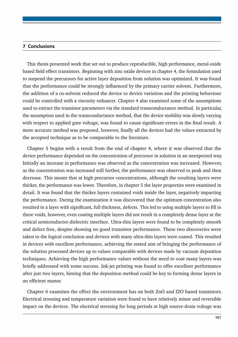
7 Conclusions

This thesis presented work that set out to produce reproducible, high performance, metal-oxide

based field effect transistors. Beginning with zinc oxide devices in chapter 4, the formulation used

to suspend the precursors for active layer deposition from solution was optimized. It was found

that the performance could be strongly influenced by the primary carrier solvent. Furthermore,

the addition of a co-solvent reduced the device to device variation and the printing behaviour

could be controlled with a viscosity enhancer. Chapter 4 also examined some of the assumptions

used to extract the transistor parameters via the standard transconductance method. In particular,

the assumption used in the transconductance method, that the device mobility was slowly varying

with respect to applied gate voltage, was found to cause significant errors in the final result. A

more accurate method was proposed, however, finally all the devices had the values extracted by

the accepted technique as to be comparable to the literature.

Chapter 5 begins with a result from the end of chapter 4, where it was observed that the

device performance depended on the concentration of precursor in solution in an unexpected way.

Initially an increase in performance was observed as the concentration was increased. However,

as the concentration was increased still further, the performance was observed to peak and then

decrease. This meant that at high precursor concentrations, although the resulting layers were

thicker, the performance was lower. Therefore, in chapter 5 the layer properties were examined in

detail. It was found that the thicker layers contained voids inside the layer, negatively impacting

the performance. During the examination it was discovered that the optimum concentration also

resulted in a layer with significant, full thickness, defects. This led to using multiple layers to fill in

these voids, however, even coating multiple layers did not result in a completely dense layer at the

critical semiconductor-dielectric interface. Ultra-thin layers were found to be completely smooth

and defect free, despite showing no good transistor performance. These two discoveries were

taken to the logical conclusion and devices with many ultra-thin layers were coated. This resulted

in devices with excellent performance, achieving the stated aim of bringing the performance of

the solution processed devices up to values comparable with devices made by vacuum deposition

techniques. Achieving the high performance values without the need to coat many layers was

briefly addressed with some success. Ink-jet printing was found to offer excellent performance

after just two layers, hinting that the deposition method could be key to forming dense layers in

an efficient manor.

Chapter 6 examines the effect the environment has on both ZnO and IZO based transistors.

Electrical stressing and temperature variation were found to have relatively minor and reversible

impact on the devices. The electrical stressing for long periods at high source-drain voltage was

101

found to have some impact in the sub-threshold region, producing a negative threshold shift and

a characteristic double turn-on. This was reversible when the source-drain voltage was removed,

but over relatively long time-scales of tens of minutes. This effect was attributed to mobile ions

in the semiconductor. The decrease of temperature did not result in threshold shifts, but did

decrease the mobility as might be expected. Heating in the absence of oxygen did have dramatic

effects but only at temperatures over 200 °C, well outside day to day operating temperatures. The

effects were persistent in devices which were initially oxygen saturated, i.e. IZO devices prepared

in air, but reversible in oxygen poor devices, i.e. ZnO devices annealed under inert atmosphere.

Light was found to induce a persistent, non-reversible photo-conductivity in oxygen rich devices,

but a reversible increase in oxygen poor devices. Again this is attributed to the oxygen desorption

from the surface as the oxygen-trapped electrons combine with the photo-generated holes. This

increased the free charge-carrier density and as there is almost no oxygen in the glove-box to

adsorb to the surface and re-trap the charge, the change is permanent.

7.1 Future Work

There are three main areas of work that should be considered for future investigations. First,

as device performance increases, the contacts play an ever more critical role. In the very highest

performing transistors the current was limited at high gate voltages by the contacts. For further

gains in performance the contact metals should be examined and carefully tuned to reduce the

contact resistance as far as is possible.

Secondly, whilst devices with excellent performance were achieved, they required the coating of

many ultra-thin layers. This is clearly unacceptable for commercial use. Ink-jet printing provided

a tantalizing hint that the deposition method was critical to achieving higher performances with

lower numbers of layers. The reason behind this remains poorly understood, but it is likely that

the ink-jet process allows a higher concentration to be used without the subsequent degradation

of layer quality. This ink-jet printing process should be tuned to give the best possible results and

more reproducible methods which allow control over the layer formation should be examined

such as spray pyrolysis.

Thirdly, although oxygen was determined to be critical to device performance, much more

could be achieved with a dedicated environment chamber, allowing the temperature to varied

along with precise control of atmospheric conditions. The devices presented in this thesis are

very sensitive to environmental factors. It is likely that further doping, e.g. with gallium, allowing

control of charge-carrier density with the composition of the active material, instead of the

external oxygen content, will be critical to reducing the sensitivity of the materials.

This work will no doubt be challenging and require many man hours of iterative optimization

and increasing understanding. However, it should be worthwhile as the oxide semiconductors

102 7 Conclusions

are currently the only semiconductors that appear capable of replacing p-Si in display backplane

construction. In the few years since the discovery of high performance oxide semiconductors

there are already commercial applications. Furthermore, if these materials can be processed

from solution and the processing temperature reduced, without compromise to performance, it

will open whole new markets in cost effective, flexible electronic circuitry. This is likely to be a

precursor dependent parameter, therefore, there is no fundamental reason why this should not

happen. Finally, regardless of specific precursor, the knowledge presented in this thesis should

remain applicable and hopefully be put to good use as people continue to develop this important

material class.

7.1 Future Work 103

Appendices

These appendices represent figures supporting data presented in the main text. The full

descriptions of the experiments to which they refer can be found in the main text, nevertheless, a

short explanation is provided in the captions along with a reference to the sections in the main

text to which the images refer.

Figure 7.1: Comparison of the different extraction methods for a very high performance transistor.It can be seen here that the extraction in the linear and saturation regimes can differ at highgate voltages. This is because, in very high performing transistors, the channel resistance becomescomparable to the resistance due to the contact injection barriers and therefore the less current isobserved to flow than would ordinarily be expected when ignoring these barriers. This is only anissue for the very highest performing devices (µ > 10 cm2/Vs) and can safely be ignored for mostof the devices in this thesis. It also suggests that for continuation of the work on improving thetransistor mobility, the source and drain contact metals should become an important area of study.The mobility extraction methods are discussed in detail in sections 2.1 and 3.6.

105

Device Mobility \ cm2/Vs Vth \V Io f f \A On-Off Ratio10 0.1 15 10−10 105

30 2.5 0.7 10−10 108

30 + 10 7.7 -2.2 10−6 104

100 0.6 4.6 10−10 108

10 + 1 0.4 7.6 10−10 106

10 + 10 4.5 2.3 10−11 108

10 + 30 3 0.5 10−10 107

10 + 50 1.5 0.9 10−10 107

10 + 100 0.8 9.9 10−11 108

ZnO - IZO 0.4 -5 10−8 105

IZO - ZnO 1.5 -0.8 10−8 106

ZnO - InO 0.5 0.4 10−7 104

InO - ZnO 6 0.7 10−4 102

InO - IZO 4 -2.3 10−4 106

Table 7.1: The electrical performance of different films mentioned throughout the thesis. The numbersin the device column refer to the concentrations of the solutions used to deposit the layers. Theseresults are referred to in the discussion on formulation optimization in section 4.1 and in the coatingof multiple layers to increase transistor performance in section 5.2.

Film \ mg/g Thickness (XRR) \ nm Thickness (WLI) \ nm Thickness (SEM) \ nm5 x 5 4.3 Too Thin Too Thin

30 7.0 8.5 9.0100 30.0 25.0 25.5

2 × 30 13.0 11.0 16.0

Table 7.2: Film thickness of IZO films measured by XRR, WLI and SEM techniques as referred tothroughout chapter 5.

106 Appendices

Figure 7.2: a) the firing and b) non-firing waveforms applied to the nozzles of the Dimatix ink-jetprinter for the patterns printed in section 3.2.2.

Figure 7.3: a) Emission peaks of LEDs used to illuminate samples. The LEDs are referred to inchapter 3, in section 3.5 and in chapter 6, in section 6.5. b) The spectra of the Oriel arc lamp usedto illuminate IZO samples in section 6.1

107

Figure 7.4: Transfer curve of a very high performance transistor, measured in the linear regime,showing a lower than expected drain current at high gate voltages. This device had a channel lengthof 20 µm and an extracted mobility of 17.01 cm2/Vs.

Figure 7.5: a) SIMS measurement of a 4 layer IZO device. The secondary ion count of all speciesvaries through the layers. b) A SIMS measurement of a sample with a gallium doped middle layer.These results are discussed in section 5.1.1.

108 Appendices

Figure 7.6: a) Plot showing the stability of an IZO device stored in air, in the dark over a 6 monthtime-frame. b) Transfer curve showing the double turn-on effect and negative shift in Von at highdrain voltages for an IZO TFT.

Figure 7.7: a. Transfer curves for ZnO whilst exposed to different lighting conditions. b. Effect ofapplied voltage on rate of change of conductivity of an IZO two terminal device. These results arepresented and discussed in section 6.5.

109

Figure 7.8: Calibrating the actual chuck temperature to the nominally applied temperature used forthe experiments presented in section 6.6.

Figure 7.9: The complete set of transfer curves for a) ZnO and b) IZO during cooling for theexperiments discussed in section 6.6.

110 Appendices

Bibliography

[1] J. S. E. Lilienfeld. Method and Apparatus for Controlling Electric Currents, Patent Number:

1745175, 1930.

[2] J. Bardeen and W. H. Brattain. Physical Review, 74(2), 230–231, 1948.

[3] J. Bardeen and W. H. Brattain. Physical Review, 75(8), 1208–1225, 1949.

[4] e. E. F. Krimmel. Silicon: evolution and future of a technology. Springer, 2004.

[5] Display Search. DisplaySearch, 2009.

[6] Society for Information Display. S.I.D. 2012 Show Issue, 28, 2012.

[7] K. Nomura, H. Ohta, A. Takagi, T. Kamiya, M. Hirano, and H. Hosono. Nature, 432(7016),

488–492, 2004.

[8] R. A. Street. Hydrogenated amorphous silicon. Cambridge University Press, 1991.

[9] T. Kamiya, K. Nomura, and H. Hosono. Science and Technology of Advanced Materials,

11(4), 044305, 2010.

[10] Display Search. DisplaySearch, 2009.

[11] T. N. M. Kimura. Nikkei Electronics Asia, Cover Story: From Printable to Printed [Part1] ,

First Appearances in E-Books, Lighting. 2010.

[12] E. Fortunato, P. Barquinha, and R. Martins. Advanced Materials, 24(22), 2945–2986, 2012.

[13] E. E. Hahn. Journal of Applied Physics, 22(7), 855–863, 1951.

[14] Y. Natsume and H. Sakata. Thin Solid Films, 372(1-2), 30–36, 2000.

[15] M. G. Kim, H. S. Kim, Y. G. Ha, J. Q. He, M. G. Kanatzidis, A. Facchetti, and T. J. Marks.

Journal of the American Chemical Society, 132(30), 10352–10364, 2010.

[16] I. Helderman. Sharp Press Release - Fascinating brilliance due to new displays. Tech. rep.,

Sharp and Semiconductor Energy Laboratory, 2012.

[17] J. Song. 2H12 Outlook Report - Semicondcutor Industry Report. Tech. rep., Daewoo

Securities Co., Ltd, 2012.

[18] Society for Information Display. Display Week 2012 Review: OLEDs. Tech. rep., SID, 2012.

111

[19] S. M. Sze. The Physics of Semiconductor Devices. John-Wiley and Sons, 2007.

[20] D. A. Neamen. Semiconductor Physics and Devices: Basic Principles. McGraw Hill, 2003.

[21] C. Herring and M. H. Nichols. Reviews of Modern Physics, 21(2), 185–270, 1949.

[22] M. Lenzling and E. H. Snow. Journal of Applied Physics, 40(1), 278, 1969.

[23] S. C. Choo. Solid-state Electronics, 11(11), 1069, 1968.

[24] D. Scharfet. Solid-state Electronics, 8(3), 299, 1965.

[25] C. Reese and Z. Bao. Journal of Applied Physics, 105(2), 024506, 2009.

[26] W. Shockley. Proceedings of the Institute of Radio Engineers, 40(11), 1365–1376, 1952.

[27] B. V. Zeghbroeck. Principles of Semicondcutor Devices. 2011.

[28] K. Terada, K. Nishiyama, and K. Hatanaka. Solid-state Electronics, 45(1), 35–40, 2001.

[29] H. S. Wong, M. H. White, T. J. Krutsick, and R. V. Booth. Solid-state Electronics, 30(9),

953–968, 1987.

[30] K. K. Banger, Y. Yamashita, K. Mori, R. L. Peterson, T. Leedham, J. Rickard, and H. Sirring-

haus. Nature Materials, 10(1), 45–50, 2011.

[31] G. Horowitz, R. Hajlaoui, D. Fichou, and A. El Kassmi. Journal of Applied Physics, 85(6),

3202–3206, 1999.

[32] Charaka, Sushruta, and Vagbhata. Charaka Samhita. N/A, 500BC.

[33] J. Waters. Provincial medical and surgical journal, 2(33), 125–127, 1841.

[34] E. E. Hahn, B. R. Russell, and P. H. Miller. Physical Review, 75(10), 1631–1631, 1949.

[35] D. A. Melnick. Physical Review, 94(5), 1438–1438, 1954.

[36] V. Srikant and D. R. Clarke. Journal of Applied Physics, 83(10), 5447–5451, 1998.

[37] A. Janotti and C. G. Van de Walle. Reports On Progress In Physics, 72(12), 126501, 2009.

[38] J. Robertson and B. Falabretti. Handbook of Transparent Conductors. Springer Science and

Business Media, 2010.

[39] H. Morkoc and U. Ozgur. Zinc Oxide - Fundementals, Materials and Device Technology.

Wiley-VCH, 2009.

[40] U. Ozgur, Y. Alivov, C. Liu, A. Teke, M. Reshchikov, S. Dogan, V. Avrutin, S. Cho, and

H. Morkoc. Journal of Applied Physics, 98(4), 2005.

112 Bibliography

[41] L. Pauling. The Nature of the Chemical Bond and the Structure of Molecules and Crystals: An

Introduction to Modern Structural Chemistry. Cornell University Press, 1960.

[42] W. Ranke. Solid State Communications, 19(7), 685–688, 1976.

[43] P. Erhart, K. Albe, and A. Klein. Physical Review B, 73(20), 205203, 2006.

[44] A. F. Kohan, G. Ceder, D. Morgan, and C. G. Van de Walle. Physical Review B, 61(22),

15019–15027, 2000.

[45] W. Tang and D. C. Cameron. Thin Solid Films, 238(1), 83–87, 1994.

[46] C.-F. Yu, S.-H. Chen, S.-J. Sun, and H. Chou. Applied Surface Science, 257(15), 2011.

[47] D. M. Hofmann, A. Hofstaetter, F. Leiter, H. J. Zhou, F. Henecker, B. K. Meyer, S. B. Orlinskii,

J. Schmidt, and P. G. Baranov. Physical Review Letters, 88(4), 045504, 2002.

[48] D. G. Thomas and J. J. Lander. Journal of Chemical Physics, 25(6), 1136–1142, 1956.

[49] A. Janotti and C. G. Van de Walle. Nature Materials, 6(1), 44–47, 2007.

[50] F. M. Hossain, J. Nishii, S. Takagi, A. Ohtomo, T. Fukumura, H. Fujioka, H. Ohno,

H. Koinuma, and M. Kawasaki. Journal of Applied Physics, 94(12), 7768–7777, 2003.

[51] H. C. G. J. Lagowski, E. S. Sproles Jr. Journal Of Applied Physics, 48, 3566, 1977.

[52] G. N. Advani, P. Klugeweiss, R. L. Longini, and A. G. Jordan. International Journal of

Electronics, 48(5), 403–411, 1980.

[53] P. Barquinha, A. Pimentel, A. Marques, L. Pereira, R. Martins, and E. Fortunato. Journal of

Non-crystalline Solids, 352(9-20), 1749–1752, 2006.

[54] B. Y. Oh, M. Jeong, H. M. H., and M. J. M. Semicond. Sci. Technol, 22, 608–612, 2007.

[55] C. S. Hwang, S. H. K. Park, W. S. Cheong, J. Shin, S. Yang, C. Byun, M. K. Ryu, D. H. Cho,

S. M. Yoon, S. M. Chung, H. Y. Chu, and K. I. Cho. SID 09 DIGEST, page 1107, 2009.

[56] J. H. Chung, J. Y. Lee, K. H.S., H. W. Jang, and J. H. Kim. Thin Solid Films, 516, 5597–5601,

2009.

[57] S. T. Meyers, J. T. Anderson, C. M. Hung, J. Thompson, J. F. Wager, and D. A. Keszler.

Journal of the American Chemical Society, 130(51), 17603–17609, 2008.

[58] C. Li, Y. Li, Y. Wu, B. Ong, and R. O. Loutfy. Journal of Materials Chemistry, 19(11),

1626–1634, 2009.

Bibliography 113

[59] G. Adamopoulos, A. Bashir, S. Thomas, W. P. Gillin, S. Georgakopoulos, M. Shkunov, M. A.

Baklar, N. Stingelin, R. C. Maher, L. F. Cohen, D. D. C. Bradley, and T. D. Anthopoulos.

Advanced Materials, 22(42), 4764, 2010.

[60] G. Binnig and H. Rohrer. Helvetica Physica Acta, 55(6), 726–735, 1982.

[61] G. Binnig, C. F. Quate, and C. Gerber. Physical Review Letters, 56(9), 930–933, 1986.

[62] Y. Martin, C. C. Williams, and H. K. Wickramasinghe. Journal of Applied Physics, 61(10),

4723–4729, 1987.

[63] R. Garcia and R. Perez. Surface Science Reports, 47(6-8), 2002.

[64] M. Nonnenmacher, M. P. Oboyle, and H. K. Wickramasinghe. Applied Physics Letters,

58(25), 2921–2923, 1991.

[65] A. J. Bennett and C. B. Duke. Physical Review, 160(3), 541, 1967.

[66] W. Melitz, J. Shen, A. C. Kummel, and S. Lee. Surface Science Reports, 66(1), 1–27, 2011.

[67] R. Shikler, T. Meoded, N. Fried, B. Mishori, and Y. Rosenwaks. Journal of Applied Physics,

86(1), 107–113, 1999.

[68] Y. Martin, D. W. Abraham, and H. K. Wickramasinghe. Applied Physics Letters, 52(13),

1103–1105, 1988.

[69] A. I. M. Rae. Quantum Mechanics. Institute of Physics, fourth edition edn., 2002.

ISBN:0750308397.

[70] U. Diebold. Surface Science Reports, 48(5-8), 2003.

[71] X. P. Gao, A. Hamelin, and M. J. Weaver. Physical Review Letters, 67(5), 618–621, 1991.

[72] O. M. Magnussen, J. Hotlos, G. Bettel, D. M. Kolb, and R. J. Behm. Journal of Vacuum

Science & Technology B, 9(2), 1991.

[73] J. J. Schneider, R. C. Hoffmann, J. Engstler, S. Dilfer, A. Klyszcz, E. Erdem, P. Jakes, and

R. A. Eichel. Journal Of Materials Chemistry, 19(10), 1449–1457, 2009.

[74] M. Pashchanka, R. C. Hoffmann, A. Gurlo, and J. J. Schneider. Journal of Materials

Chemistry, 20(38), 8311–8319, 2010.

[75] R. Kuegler, J. Schneider, and R. Hoffmann. Organometallic Zinc Compound for Preparing

Zinc Oxide Films, Patent Number: WO/2009/010142, 2009.

[76] R. D. Deegan, O. Bakajin, T. F. Dupont, G. Huber, S. R. Nagel, and T. A. Witten. Nature,

389(6653), 827–829, 1997.

114 Bibliography

[77] H. Hu and R. G. Larson. Journal of Physical Chemistry B, 110(14), 7090–7094, 2006.

[78] C. Siol. Quasistatische und transiente Oberflächenpotentialverteilungen organischer Feldef-

fekttransistoren. Ph.D. thesis, Fachgebiet Elektronische Materialeigenschaften, Fachbereich

Materialwissenschaften, Technische Universität Darmstadt, 2012.

[79] http://gwyddion.net/.

[80] O. M. Ottinger, C. Melzer, and H. von Seggern. Journal of Applied Physics, 106, 023704,

2009.

[81] M. Knoll. Zeitschrift für Technische Physik, 16, 467–475, 1935.

[82] L. G. Parratt. Physical Review, 95(2), 359–369, 1954.

[83] R. F. K. Herzog and F. P. Viehbock. Physical Review, 76(6), 855–856, 1949.

[84] H. Liebl. Journal of Applied Physics, 38(13), 5277, 1967.

[85] R. Castaing. Journal of Metals, 16(4), 331, 1964.

[86] M. C. J. M. Vissenberg and M. Matters. Physical Review B, 57(20), 12964–12967, 1998.

[87] E. C. P. Smits, S. G. J. Mathijssen, M. Colle, A. J. G. Mank, P. A. Bobbert, P. W. M. Blom,

B. de Boer, and D. M. de Leeuw. Physical Review B, 76(12), 125202, 2007.

[88] F. Torricelli, J. R. Meijboom, E. Smits, A. K. Tripathi, M. Ferroni, S. Federici, G. H. Gelinck,

L. Colalongo, Z. M. Kovacs-Vajna, D. de Leeuw, and E. Cantatore. Ieee Transactions On

Electron Devices, 58(8), 2610–2619, 2011.

[89] H. P. Keil. Modellierung gedruckter anorganisher Zink-Oxid Dünnfilmtransistoren. Ph.D.

thesis, TU - Darmstadt, Fachgebiet Integrierte Elektronische Systeme, 2012.

[90] E. J. Meijer, C. Tanase, P. W. M. Blom, E. van Veenendaal, B. H. Huisman, D. M. de Leeuw,

and T. M. Klapwijk. Applied Physics Letters, 80(20), 3838–3840, 2002.

[91] C. Tanase, E. J. Meijer, P. W. M. Blom, and D. M. de Leeuw. Organic Electronics, 4(1),

33–37, 2003.

[92] K. Jeon, C. Kim, I. Song, J. Park, S. Kim, S. Kim, Y. Park, J. H. Park, S. Lee, D. M. Kim, and

D. H. Kim. Applied Physics Letters, 93(18), 2008.

[93] C. Reese and Z. Bao. Advanced Functional Materials, 19(5), 763–771, 2009.

[94] Stephenson and Associates Inc. The Basics of Water-Based Inkjet Inks. Published Online

at http://stephenson-associates-inc.com/Water-Based%20Inkjet%20Inks.pdf.

Bibliography 115

[95] F. L. Zhang, K. G. Jespersen, C. Bjorstrom, M. Svensson, M. R. Andersson, V. Sundstrom,

K. Magnusson, E. Moons, A. Yartsev, and O. Inganas. Advanced Functional Materials, 16(5),

667–674, 2006.

[96] M. T. Dang, G. Wantz, H. Bejbouji, M. Urien, O. J. Dautel, L. Vignau, and L. Hirsch. Solar

Energy Materials and Solar Cells, 95(12), 3408–3418, 2011.

[97] C. J. BRINKER, G. C. FRYE, A. J. HURD, and C. S. ASHLEY. Thin Solid Films, 201(1),

97–108, 1991.

[98] S. M. Attia, J. Wang, G. M. Wu, J. Shen, and J. H. Ma. Journal of Materials Science &

Technology, 18(3), 211–218, 2002.

[99] M. Epifani, S. Capone, R. Rella, P. Siciliano, L. Vasanelli, G. Faglia, P. Nelli, and G. Sberveg-

lieri. Journal of Sol-gel Science and Technology, 26(1-3), 741–744, 2003.

[100] L. L. Hench and J. K. West. Chemical Reviews, 90(1), 33–72, 1990.

[101] H. B. Michaelson. Journal Of Applied Physics, 48, 4729, 1977.

[102] G. D. Sharma, R. Kumar, S. K. Sharma, and M. S. Roy. Solar Energy Materials and Solar

Cells, 90(7-8), 933–943, 2006.

[103] R. A. Powell, W. E. Spicer, and J. C. McMenami. Physical Review B, 6(8), 3056, 1972.

[104] H. K. Kim, K. K. Kim, S. J. Park, T. Y. Seong, and I. Adesida. Journal of Applied Physics, 94,

4225–4227, 2003.

[105] H. K. Kim, S. H. Han, T. Y. Seong, and W. K. Choi. Applied Physics Letters, 77(11), 1647,

2000.

[106] K. Ip, Y. W. Heo, K. H. Baik, D. P. Norton, S. J. Pearton, and F. Ren. Applied Physics Letters,

84(4), 544–546, 2004.

[107] S. W. Luan and G. W. Neudeck. Journal of Applied Physics, 72(2), 766–772, 1992.

[108] N. L. Dehuff, E. S. Kettenring, D. Hong, H. Q. Chiang, J. F. Wager, R. L. Hoffman, C. H.

Park, and D. A. Keszler. Journal of Applied Physics, 97(6), 064505, 2005.

[109] T. Suni, K. Henttinen, I. Suni, and J. Makinen. Journal of the Electrochemical Society,

149(6), G348–G351, 2002.

[110] D. E. Walker, M. Major, M. Baghaie Yazdi, A. Klyszcz, M. Haeming, K. Bonrad, C. Melzer,

W. Donner, and H. von Seggern. ACS applied materials & interfaces, 4(12), 6835–41, 2012.

[111] M. . W. Ahn, K. . S. Park, J. . H. Heo, J. . G. Park, D. . W. Kim, K. J. Choi, J. . H. Lee, and

S. . H. Hong. Applied Physics Letters, 93(26), 263103, 2008.

116 Bibliography

[112] A. F. AKTARUZZAMAN, G. L. SHARMA, and L. K. MALHOTRA. Thin Solid Films, 198(1-2),

67–74, 1991.

[113] P. R. Bueno, E. R. Leite, M. M. Oliveira, M. O. Orlandi, and E. Longo. Applied Physics

Letters, 79(1), 48–50, 2001.

[114] J. K. Jeong, H. W. Yang, J. H. Jeong, Y.-G. Mo, and H. D. Kim. Applied Physics Letters,

93(12), 123508, 2008.

[115] S. A. Studenikin and M. Cocivera. Journal of Applied Physics, 91(8), 5060–5065, 2002.

[116] K. S. Weissenrieder and J. Muller. Thin Solid Films, 300(1-2), 30–41, 1997.

[117] Q. H. Li, T. Gao, Y. G. Wang, and T. H. Wang. Applied Physics Letters, 86(12), 123117,

2005.

[118] Y. Takahashi, M. Kanmori, A. Kondoh, H. Minoura, and Y. Ohya. Japanese Journal of

Applied Physics, 33(12A), 6611–6615, 1994.

[119] K. Siegbahn and K. Edvarson. Nuclear Physics, 1(3), 137, 1956.

[120] D. R. Penn. Journal of Electron Spectroscopy and Related Phenomena, 9(1), 29–40, 1976.

[121] C. D. Wagner, W. M. Riggs, L. E. Davis, J. F. Moulder, and G. E. Mullenberg. Handbook of

X-ray Photoelectron Spectroscopy. Eden Prairie, MN. Perkin-Elmer, 1979.

[122] C. R. Werrett, A. K. Bhattacharya, and D. R. Pyke. Applied Surface Science, 103(4), 403–407,

1996.

[123] G. Schon. Journal of Electron Spectroscopy and Related Phenomena, 1(4), 377–387, 1973.

[124] XPS International. Binding Energy Lookup Table for Signals from Elements and Common

Chemical Species. 1999.

[125] P. Swift. Surface and Interface Analysis, 4(2), 47–51, 1982.

[126] C. G. Choi, S. J. Seo, and B. S. Bae. Electrochemical and Solid State Letters, 11(1), H7–H9,

2008.

[127] P. D. C. King, T. D. Veal, F. Fuchs, C. Y. Wang, D. J. Payne, A. Bourlange, H. Zhang, G. R.

Bell, V. Cimalla, O. Ambacher, R. G. Egdell, F. Bechstedt, and C. F. McConville. Physical

Review B, 79(20), 205211, 2009.

[128] J. A. McLeod, R. G. Wilks, N. A. Skorikov, L. D. Finkelstein, M. Abu-Samak, E. Z. Kurmaev,

and A. Moewes. Physical Review B, 81(24), 2010.

[129] W. M. Sachtler, G. J. H. Dorgelo, and A. A. Holscher. Surface Science, 5(2), 221, 1966.

Bibliography 117

[130] K. Jacobi, G. Zwicker, and A. Gutmann. Surface Science, 141(1), 109–125, 1984.

[131] K. B. Sundaram and A. Khan. Journal Of Vacuum Science & Technology A-Vacuum Surfaces

And Films, 15(2), 428–430, 1997.

[132] K. Ramamoorthy, K. Kumar, R. Chandramohan, and K. Sankaranarayanan. Materials

Science and Engineering B-solid State Materials For Advanced Technology, 126(1), 1–15,

2006.

[133] K. Nomura, T. Kamiya, H. Yanagi, E. Ikenaga, K. Yang, K. Kobayashi, M. Hirano, and

H. Hosono. Applied Physics Letters, 92(20), 202117, 2008.

[134] K. Nomura, T. Kamiya, E. Ikenaga, H. Yanagi, K. Kobayashi, and H. Hosono. Journal of

Applied Physics, 109(7), 073726, 2011.

[135] W. Gopel, G. Rocker, and R. Feierabend. Physical Review B, 28(6), 3427–3438, 1983.

[136] J. Bao, I. Shalish, Z. Su, R. Gurwitz, F. Capasso, X. Wang, and Z. Ren. Nanoscale Research

Letters, 6, 404, 2011.

[137] M. Egginger, M. Irimia-Vladu, R. Schwodiauer, A. Tanda, I. Frischauf, S. Bauer, and N. S.

Sariciftci. Advanced Materials, 20(5), 1018, 2008.

[138] C. Siol, C. Melzer, and H. von Seggern. Applied Physics Letters, 93(13), 2008.

[139] D. J. Dimaria. Applied Physics Letters, 51(9), 655–657, 1987.

[140] A. Salleo and R. A. Street. Physical Review B, 70, 2004.

[141] G. Paasch, S. Scheinert, A. Herasimovich, I. Horselmann, and T. Lindner. Physica Status

Solidi A-applications and Materials Science, 205(3), 534–548, 2008.

[142] K. Bradley, J. Cumings, A. Star, J. C. P. Gabriel, and G. Gruner. Nano Letters, 3(5), 639–641,

2003.

[143] Y. Kamada, S. Fujita, T. Hiramatsu, T. Matsuda, M. Furuta, and T. Hirao. Solid-State

Electronics, pages 1392–1397, 2010.

[144] Y. Kamada, S. Fujita, T. Hiramatsu, T. Matsuda, H. Nitta, M. Furuta, and T. Hirao. Japanese

Journal of Applied Physics, 49(3), 2010.

[145] B. Claflin, D. C. Look, S. J. Park, and G. Cantwell. Journal of Crystal Growth, 287(1),

16–22, 2006.

[146] R. Laiho, Y. P. Stepanov, M. P. Vlasenko, and L. S. Vlasenko. Physica B-condensed Matter,

404(23-24), 4787–4790, 2009.

118 Bibliography

[147] F. H. Leiter, H. R. Alves, A. Hofstaetter, D. M. Hofmann, and B. K. Meyer. Physica Status

Solidi B-basic Research, 226(1), R4–R5, 2001.

[148] A. Janotti and C. G. Van de Walle. Applied Physics Letters, 87(12), 122102, 2005.

[149] H. L. Mosbacker, Y. M. Strzhemechny, B. D. White, P. E. Smith, D. C. Look, D. C. Reynolds,

C. W. Litton, and L. J. Brillson. Applied Physics Letters, 87(1), 012102, 2005.

[150] Y. G. W. Q. H. Li, T. Gao and T. H. Wanga. Applied Physics Letters, 86, 2005.

[151] H. Chon and J. Pajares. Journal of Catalysis, 14(3), 257, 1969.

[152] F. D. Auret, W. E. Meyer, P. J. J. van Rensburg, M. Hayes, J. M. Nel, H. von Wenckstern,

H. Hochmuth, G. Biehne, M. Lorenz, and M. Grundmann. Journal of Physics: Conference

Series, 100(4), 042038, 2008.

[153] F. H. Gaensslen and R. C. Jaeger. Solid-state Electronics, 22(4), 423–430, 1979.

[154] D. Adler. Critical Reviews in Solid State Sciences, 2(3), 317, 1971.

[155] D. Adler, L. P. Flora, and S. D. Senturia. Solid State Communications, 12(1), 9–12, 1973.

[156] N. F. Mott. Philosophical Magazine, 19(160), 835, 1969.

[157] G. M. Minkov, O. E. Rut, A. V. Germanenko, A. A. Sherstobitov, V. I. Shashkin, O. I. Khrykin,

and V. M. Daniltsev. Physical Review B, 64(23), 235327, 2001.

[158] X. D. Liu, E. Y. Jiang, and Z. Q. Li. Journal of Applied Physics, 102(7), 073708, 2007.

Bibliography 119

120

Nomenclature

Symbol or Abbreviation Meaning

β measurement bandwidth / Hz

β term 2T/T0 in Vissenberg-Matters model

δd ,δh,δp Hansen solubility parameters / M Pa0.5

δrms RMS amplitude of oscillation of a cantilever / m

ε0 permittivity of free space / Fm−1

εr relative permittivity / nounits

µ mobility / cm2/Vs

σ conductivity / S

φ work-function / eV

Φ energy in a band diagram or work-function / eV

χ electron affinity / eV

ω0 resonant angular frequency / rads−1

h reduced Planck’s constant / Js

A area / m2

C capacitance / F

c atom fraction or concentration / m−3

d and D dielectric thickness or distance / m

E electric field / V m−1

E energy / J or eV

e charge of an electron / C

EC energy level of conduction band minimum / eV

EF Fermi level / eV

EV energy level of valence band maximum / eV

F force / N

f frequency / Hz

f SIMS instrument transmission efficiency

gm transconductance / S

I dc current / A

i imaginary unit or ac current / A

Id Ig Is drain, gate, source current / A

Ip primary ion current / A

k0 spring constant / Nm−1

L transistor channel length / m

m mass / kg

kb Boltzmann’s constant / m2kgs−2K−1

121

Symbol or Abbreviation Meaning

P or p probability / no units

Q charge / C or quality factor / dimensionless

q charge / C

T temperature / C or K

t time / s

U height of a potential barrier / V

V voltage or potential difference / V

Vth threshold voltage / V

v velocity / ms−2

Vd Vg Vs drain, gate, source voltage / V

W transistor channel width / m

Y yield / secondary particles per primary particle

z vertical displacement / m

2-ME 2-methoxyethanol

a-Si amorphous silicon

AC alternating current

AFM atomic force microscopy

AIPO amorphous aluminum oxide phosphate

BGBC Bottom-gate bottom-contact

CBM conduction band minimum

DC direct current

DFT density functional theory

DGME diethylene glycol methyl ether

DMSO dimethyl-sulfoxide

FET field-effect transistor

I-on, I-off on and off currents

IGZO indium-gallium-zinc oxide

IJP ink-jet print(er)

ITO indium-tin oxide

IZO indium-zinc oxide

KPFM Kelvin probe force microscopy

LED light emitting diode

LTPS low temperature polycrystalline silicon

MOSFET metal oxide semiconductor field-effect transistor

NFPA national fire protection association

NMP n-methyl pyrrolidinone

122 Nomenclature

Symbol or Abbreviation Meaning

p-Si polycrystalline silicon

PECVD plasma enhanced chemical vapour deposition

SAND self-assembled nano-dielectric

SEM scanning electron microscopy

SIMS secondary ion mass spectroscopy

SiO2 silicon dioxide

SMU source-measure unit

SPM scanning probe microscopy

STM scanning tunnelling microscopy

TFT thin-film transistor

TG or TGMS thermo-gravimetric mass spectroscopy

TSC thermal scanning calorimetery

UHV ultra-high vacuum (pressure < 10−9 mbar

VBM valence band maximum

WLI white light interferometer

XPS x-ray photo-electron spectroscopy

XRR x-ray reflectivity

ZITO zinc-indium-tin oxide

ZnO zinc oxide

123

Curriculum Vitae

Personal Details

Name Daniel Edward Walker

Birth Date 03.05.83

Birth Place Truro, U.K.

Schooling

1987 - 1994 Mount Charles C.P.

1994 - 1999 Penrice Language College

1999 - 2001 St. Austell College

University Education

Oct 2001 - Jun 2005 Undergraduate Masters, MPhys, Physics with Astronomy, Uni-

versity of Southampton.

Oct 2005 - Dec 2006 Masters Degree, MPhil, Physics, Thesis title : ’Studies of

the low frequency dielectric constants and conductance of

two molecular systems; carbon nanotubes and polyaromatic

molecular wires.’, University of Southampton.

Jun 2009 - Feb 2013 Doctorate Degree, PhD, Thesis title : ’Improving Performance

in Metal Oxide Field-effect Transistors’, Technische Univer-

sität Darmstadt.

Employment

Jan 2007 - May 2009 Merck Chemicals U.K. Ltd.

124

List of Publications

Walker D. E., Siol C., Melzer C. and von Seggern H.

Charge Transport Across Zinc Oxide Field Effect Transistors, DS 29.27, DPG Spring Meeting 2010,

Regensburg.

Walker D. E., Melzer C. and von Seggern H.

The Influence of Oxygen on the Potential Distribution of Operating Zinc Oxide FETs, DS 42.107,

DPG Spring Meeting 2011, Dresden.

Walker D. E., Häming M., Issanin A., Klyszcz A, Kaloumenos M., Hoffmann R., Bonrad K., Melzer

C., von Seggern H.

The Dependence of Field Effect Mobility on Layer Thickness in Ultra-Thin Film, Solution Processed,

Indium Zinc Oxide TFTs, DS 20.5, DPG Spring Meeting 2012, Berlin.

Walker D. E., Häming M., Issanin A., Klyszcz A., Kaloumenos M., Hoffmann R., Bonrad K., Melzer

C., von Seggern H.

The Dependence of Field Effect Mobility on Layer Thickness in Ultra-Thin Film, Solution Processed,

Indium Zinc Oxide TFTs, SYMP H 2.7, e-MRS Spring Meeting 2012, Strasbourg.

Kehrer L. A., Feldmeier E. J., Siol C., Walker D. E., Melzer C., von Seggern H

A new method to realize kelvin probe investigations of a shielded channel in poly(3-

hexylthiophene)-based top-gate field-effect transistors, Applied Physics A, Nov. 2012.

Walker D. E., Major M., Baghaie Yazdi M., Klyszcz A., Häming M., Bonrad K., Melzer C., Donner

W., von Seggern H.

High mobility indium zinc oxide thin film field-effect transistors by semiconductor layer engi-

neering, ACS Applied Materials and Interfaces, Nov 2012.

125

Acknowledgements

I am, of course, extremely thankful to Prof. von Seggern for his openness, willingness to

discuss, and guidance without which this thesis would not have been possible. Similarly, I am

indebted to Christian Melzer for his huge depth of knowledge in materials science and ready

disposition to discuss ideas and direct experiments.

I have been fortunate to have a wonderful set of office colleagues, with who I have had a lot

of fun socially, and for whom I have utmost respect professionally. So, in no particular order,

special thanks to Andrea Gassmann, Lorenz Kehrer, Oliver Ottinger and latterly Emanuelle Reis

Simas. I must also extend my appreciation to Christopher Siol for introducing me to much of

the specialist equipment I used throughout the thesis. I had a great time working in Germany

on this project and that is mostly due to the fantastic people of the e-mat group: Gabi K, Bernd,

Helga, Sabine and Gabi A; the post-docs, Christian, Yogi, Graham, Sergei, Manu and Corinna;

the repeat visitors (most people want to come back it seems!), Lucas, Ivan, Greg, Vladislav and

Sergei F ("I check"); Fellow PhD students, Jörg, Eva, Katja, Martin, Tobi, Paul, Riitta and last, but

far from least Oili!

I am also heavily indebted to my colleagues at the MerckLabs. So, I extend particular thanks

to Sabine Renker for initiating the project and Klaus Bonrad for continued support. I further

thank those I worked closely with within the Merck-Labs framework, especially Andreas Klyszcz,

Marc Haeming, Alexander Issanin, Rudolph Hoffmann, Stefan Dilfer, Hans-Peter Keil, Mareiki

Kaloumenos and Paul Mundt.

Furthermore, I should once again mention those who helped scientifically in specific areas

of this thesis. Thank-you Prof. Donner and Marton Major for the X-ray refraction work and

contribution to the resulting combined paper. Thanks to Lucas Fugikawa Santos for help with

understanding the shortfalls of the mobility calculations. Finally thanks to my family, for

supporting me in my decision to come and live in Germany to undertake this project, and friends

both in the U.K. and Germany.

126

Authors Declaration

I hereby declare that this thesis is my own work and effort and that it has not been previously

submitted for any award. Where other sources of information have been used they have been

acknowledged. In the case collaborative efforts the collaborators have been acknowledged.

Signed

D. E. Walker

Feb. 2013, Darmstadt.

127