A

btbdt©

K

1

b[bansNsdap

(dEa

F

0d

Available online at www.sciencedirect.com

Electric Power Systems Research 78 (2008) 337–345

Improving large-disturbance stability through optimalbifurcation control and time domain simulations

Wei Gu a,∗, Federico Milano b, Ping Jiang a, Jianyong Zheng a

a SouthEast University, School of Electrical Engineering, NanJing, Chinab University of Castilla-La Mancha, Department of Electrical Engineering, Ciudad Real 13071, Spain

Received 20 July 2006; received in revised form 17 January 2007; accepted 2 March 2007Available online 11 April 2007

bstract

This paper presents an approach for improving, through practical assumptions, the stability of power systems subjected to large distur-ances. The proposed method is composed of two steps, solved iteratively. The first step solves an optimal bifurcation control problemhat guarantees the small-signal stability of the equilibrium point. The proposed optimal bifurcation control addresses saddle-node and Hopf

ifurcations. The second step is an N − 1 contingency analysis computed through time domain simulations. The second step guarantees the large-isturbance stability of the equilibrium point. The WSCC 9-bus and New England 39-bus systems are used to illustrate and test the proposedechnique.

2007 Elsevier B.V. All rights reserved.

isturb

tObaatspwE[jp

tr

eywords: Optimal bifurcation control; Small-signal stability analysis; Large d

. Introduction

Transient stability, or more in general, large-disturbance sta-ility has always been a key topic of power system analysis1–6]. However, there are still several issues, ranging from sta-ility analysis methods to control schemes, that need to beddressed. Nowadays research studies face mainly two bottle-ecks. (i) A huge amount of calculations, especially time domainimulations, is needed for large-disturbance stability studies.ew generation computers and parallel processing can help in

peeding up calculations. (ii) It is mathematically challenging toetermine the stability region of a set of non-linear differentiallgebraic equations such as the power system model [3]. Thisaper addresses the latter point.

Time domain simulation (TDS) and energy functionEF) methods are the traditional approaches to study large-

isturbance stability [3,4]. Some new results about TDS andF methods can be found in Refs. [7,8], respectively. The TDSpproach can be applied to any level of detail of power sys-

∗ Corresponding authors. Tel.: +86 13814005169E-mail addresses: WGu@seu.edu.cn (W. Gu),

ederico.Milano@uclm.es (F. Milano).

ppslb

si

378-7796/$ – see front matter © 2007 Elsevier B.V. All rights reserved.oi:10.1016/j.epsr.2007.03.002

ance; N − 1 contingency analysis; Saddle-node bifurcation; Hopf bifurcation

em models and gives a visual information about state variables.ne of the main disadvantages of the TDS approach, except foreing time-consuming, is that it does not provide informationbout the stability margin of the system. Therefore, the TDSpproach is not effective for stability control. On the contrary,he EF approach is able to provide an index that measures theystem stability. However, EF methods can be applied only toower system for which the energy function is known and onlyork for first-swing stability analysis. Due to these limitations,F methods are typically used in conjunction with TDS methods

9,10]. In this vein, in this paper, the TDS analysis is used in con-unction with a small-signal stability constrained optimizationroblem.

Small-signal stability analysis techniques, based on bifurca-ion theory, has been proposed in Refs. [11–13]. The “feasibilityegion” or, in other words, the small-signal stability region, wasresented in Ref. [12] to identify the stability region in thearameter space. This paper uses this concept of small-signaltability region for the formulation of an optimization prob-em. In particular, this paper addresses saddle-node and Hopf

ifurcations.

The proposed optimization problem is based on a variety oftability constrained OPF problems that have been presentedn the literature, such as the maximization of the distance to

3 stems

vlumCacts

piRtisIut

pag

taetc[saoaod

(

(

oataNstt

2

2

e

x

wewR

tvat

p[

wfcsge

�

dmap

daf

P

wa

da

(

(

(

38 W. Gu et al. / Electric Power Sy

oltage collapse [14–17]. The computation of the maximumoading condition is only a part of the information that can besed for avoiding instability. One can be interested in deter-ining how control variables affect the loading margin [18].learly this is useful both to determine the most critical vari-bles and to design an effective corrective action to avoid theollapse [19]. This paper proposes an optimization problemhat allows finding the critical stability condition of a powerystem.

It has to be noted the relevance of the variations of controlarameters and their sensitivities with respect to the stabil-ty margin in several practical applications. For example, inefs. [17,20,21], the stability region for the most critical con-

ingency is determined through a sensitivity analysis, whilen Refs. [22,23] parameter sensitivities are used to properlyet up primary and secondary voltage regulation, respectively.n Ref. [24], voltage and transmission line thermal limits aresed to determine the feasibility region of inter area powerransfers.

Based on these results, this paper proposes an optimizationroblem to find the optimal control variable profile that ensuresn adequate stability region with inclusion of an N − 1 contin-ency criterion.

The optimization problem proposed in this paper is ableo optimize system control parameters in order to ensure andequate stability margin of the optimal equilibrium point. How-ver, large-disturbance stability cannot be taken into account byhe optimization problem. It is well known that dynamic bifur-ations can be triggered by large-disturbances [25,26]. In Refs.27,28], N − 1 contingency analysis is obtained through exten-ive time domain simulations. In this vein, this paper proposesn iterative technique that combines the stability constrainedptimization problem and simulation-based N − 1 contingencynalysis. The proposed iterative method leads to the definitionf a control parameter set that guarantee both small and large-isturbance stability.

In summary the novel contribution of the paper are as follows:

1) Proposal of a stability constrained OPF for optimizing con-trol parameters. The solution of this OPF problem ensuresthe small-signal stability of the system. Stability constraintstake into account saddle-node and Hopf bifurcations.

2) Proposal of an iterative method that computes repeatedlythe OPF problem and time domain simulations followingcontingencies. The result of this procedure is an equilibriumpoint that is stable for both small-signal stability and large-disturbance stability.

The paper is organized as follows. Section 2 provides outlinesf differential-algebraic equations of power systems, bifurcationnalysis and the definition of small-signal stability region. Sec-ion 3 presents the proposed optimal bifurcation control modelnd Section 4 presents the approach for taking into account

− 1 contingency analysis and improving large-disturbances

tability. In Section 5, the proposed technique is illustrated andested through the WSCC 9-bus and the New England 39-busest systems. Finally, in Section 6, conclusions are duly drawn.

2

e

Research 78 (2008) 337–345

. Outlines of power system stability analysis

.1. Differential algebraic equations

Power electric systems can be represented as a set of differ-ntial algebraic equations (DAE) [29]:

˙ = f (x, y, μ, p), 0 = g(x, y, μ, p) (1)

here (f : Rn × Rm × Rk × Rl → Rn) is the vector of differ-

ntial equations; x ∈Rn the vector of state variables associatedith generators, loads and system controllers; (g : Rn × Rm ×k → R

m) the vector of algebraic equations; y ∈Rm the vec-or of algebraic variables; μ ∈Rk the vector of uncontrollableariables; and p ∈Rl is the vector of control variables. It isssumed that algebraic variables can vary instantaneously, i.e.heir transients are assumed to be “infinitely” fast.

Eq. (1) can be linearized at an equilibrium point (x0, y0, μ0,0), as follows:

�x

0

]=

[fx fy

gx gy

] [�x

�y

]= Atot

[�x

�y

](2)

here Atot is the full system Jacobian matrix, and fx = ∂f/∂x|0,y = ∂f/∂y|0, gx = ∂g/∂x|0 and gy = ∂g/∂y|0 are the Jacobian matri-es of the differential and algebraic equations with respect to thetate and algebraic variables, respectively. If it is assumed thaty is non-singular, the vector of algebraic variables �y can beliminated from Eq. (2), as follows:

x = (fx − fyg−1y gx)�x = Asys�x (3)

Thus the DAE can be implicitly reduced to a set of ordinaryifferential equations (ODE). Observe that if gy is singular, theodel of the system has to be revised as the dynamics of some

lgebraic equations cannot be neglected [30]. Thus it is alwaysossible to formulate a set of DAE for which gy is not singular.

In order to give a rigorous definition of the bifurcationsiscussed in this paper, let us assume that the uncontrollable vari-bles are scalar, i.e. μ ∈R. In our formulation, μ is the loadingactor that multiplies load powers as follows:μL = μP0

L, QμL = μQ0

L (4)

here P0L and Q0

L are the base case or initial load profile (μ = 1t the base case).

The loading factor is commonly used in stability studies toetermine the maximum loading condition that can be eitherssociated with Refs. [25,26,30]:

1) voltage stability limit (collapse point) corresponding to asystem singularity (saddle-node bifurcation);

2) system controller limits such as generator reactive powerlimits (limit-induced bifurcation);

3) frequency stability (Hopf bifurcation).

.2. Bifurcations analysis

In this paper, bifurcation points are identified through theigenvalue loci of the state matrix Asys.

stems

F

x

iva

A

sA

bb

2

mp(c

(

((

2

mz

(

(

i“i

drp

2

aaA

A

t[

w

u

wi

Fne

a

••

cgmd

2

ctsroniwB

W. Gu et al. / Electric Power Sy

For the sake of definition, let us define the vector of functionsas follows:

˙ = F (x, μ) = f (x, y(x, μ), μ) (5)

.e. F is the set of differential equations where the algebraicariables y have been substituted for their explicit function of xnd μ. Thus, one has:

sys = ∂F

∂x|0 (6)

Observe that, from the practical point of view, it is not neces-ary to know explicitly the function y(x, μ) since the state matrixsys can be computed from Eq. (3).

The bifurcations discussed in this paper are the saddle-nodeifurcation and the Hopf bifurcation. The definitions of theseifurcations are as follows [11].

.2.1. Saddle-node bifurcation (SNB)A SNB point is an equilibrium point (x0, μ0) at which the state

atrix presents one zero eigenvalue. SNB are associated with aair of equilibrium points, one stable (s.e.p.) and one unstableu.e.p.) that coalesce and disappear. The following transversalityonditions hold:

1) the state matrix Asys has a simple and unique eigenvaluewith right and left eigenvectors v and w such that Asysv =AT

sysw = 0;

2) wT∂F/∂μ|0 = 0;3) wT[∂2F/∂x2]v �= 0.

.2.2. Hopf bifurcation (HB)A HB point is an equilibrium point (x0, μ0) at which the state

atrix presents a complex conjugate pair of eigenvalues withero real part. The following transversality conditions hold:

1) the state matrix Asys has a simple pair of purely imaginaryeigenvalues λ(μ0) = ±jβ and no other eigenvalues with zeroreal part;

2) dR{λ(μ)/dμ|0} �= 0.

The HB gives a birth to a zero-amplitude limit cycle withnitial period T0 = 2π/β. If the limit cycle is stable the HB issupercritical”; if the limit cycle is unstable the HB is “subcrit-cal”.

Observe that limit-induced bifurcations (LIBs) [30] are notiscussed since, control limits of AVRs and of other systemegulators are implicitly taken into account in the optimizationroblem that is proposed in Section 3.

.3. Direct method for bifurcation analysis

The following direct method can be used to identify both SNBnd HB [26]. Let us define λ = α + jβ and u as one eigenvalue

x

nd its associated right eigenvector, respectively, of the matrixsys. Then:

sysux = λux (7)

u

sp

Research 78 (2008) 337–345 339

Let us also define u = [ uTx uT

y ]T

, where uy = −g−1y gxux,

hus Eq. (7) can be rewritten as:

fx fy

gx gy

] [ux

uy

]= (α + jβ)

[ux

0

](8)

here

x = uxR + juxI, uy = uyR + juyI (9)

here uxR, uxI ∈Rn and uyR, uyI ∈Rm. By substituting Eq. (9)n Eq. (8), one has:

0 = fxuxR + fyuyR − αuxR + βuxI,

0 = fxuxI + fyuyI − αuxI − βuxR, 0 = gxuxR + gyuyR,

0 = gxuxI + gyuyI (10)

inally, considering the system DAE, Eq. (10) and imposing aon-trivial for the eigenvectors, one obtains the following set ofquations:

0 = f (x, y, μ, p), 0 = g(x, y, μ, p),

0 = fxuxR + fyuyR − αuxR + βuxI,

0 = fxuxI + fyuyI − αuxI − βuxR, 0 = gxuxR + gyuyR,

0 = gxuxI + gyuyI, 1 = uTxRuxR − uT

xIuxI,

0 = uTxRuxI − uT

xIuxR (11)

Observe that Eq. (11) is valid for both SNB and HB points,s follows:

at SNB points, uxR = ux, uyR = uy, uxI = uyI = 0, and α = β = 0;at HB points, α = 0 and β �= 0.

Observe also that Eq. (11) is seldom used for computing bifur-ation points because obtaining a solution highly depends on aood initial guess of the eigenvectors [30]. However this for-ulation is useful if used within an optimization problem, as

iscussed in Section 3.

.4. Stability manifold

A definition of “small signal stability region”, sayΩSSSR, alsoalled “feasibility region”, was given in Refs. [12,13]. Accordingo that definition, ΩSSSR is “the stability region in the variablepace, which is composed of all equilibrium points that can beeached quasi-statically from the current operating point with-ut loss of local stability”. If singularity-induced bifurcations areot a concern (i.e. gy is non-singular), the small-signal stabil-ty region can be rewritten as ΩSSSR = {BSNB ∪ BHB ∪ BLIB},here BSNB is the unstable region identified by SNB points,HB the unstable region identified by HB points, and BLIB is the

nstable region identified by LIB points.

Observe that there is no general technique to obtain the entiretability region of a set of DAE, except for solving several com-utationally expensive time domain simulations with negative

3 stems

toa

3

oiao

o

wcw

C

wwta

tci

stii

ptemot

tc

iicp

t

4

rcn

tc

(

(

(

dsiμ

ts

cμ

gsti

aTi

40 W. Gu et al. / Electric Power Sy

ime [11]. Furthermore, time domain techniques are effectivenly for a reduced number of state variables x and control vari-bles p.

. Optimal bifurcation control

The optimal bifurcation control (OBC) can be defined as theptimal configuration of control variables p so that the solutions within the small-signal stability region ΩSSSR. In the OBCnalysis, one has to minimize a control “cost” that is a functionf control variables.

The OBC approach proposed in this paper is a non-linearptimization problem, as follows:

Min. C(p)

s.t. 0 = f (x, y, μ, p)

0 = g(x, y, μ, p)

0 = fxuxR + fyuyR + βuxI

0 = fxuxI + fyuyI − βuxR

0 = gxuxR + gyuyR

0 = gxuxI + gyuyI

1 = uTxRuxR − uT

xIuxI

0 = uTxRuxI − uT

xIuxR

μ ≥ μmin

h(x, y, μ, p) ≤ 0

(12)

here C(p) is the objective function that represents the “cost” ofhanging control variables p. In this paper the following structureill be used:

(p) =∑

i

ci(pi − p0i )

2(13)

here p0i and ci are the standard or default value and the

eight, respectively, of the control variable pi. The inequali-ies h(h ∈R) represent physical and security constraints suchs voltage limits, regulators limits, etc.

The loading factor constraint μ ≥ μmin imposes that the solu-ion has to present a minimum loading level. If μ > 1, the systeman be overloaded with respect to the base case. Observe thatncreasingμmin typically leads to increase the objective function.

For a given minimum value of the loading factor μmin, theolution of Eq. (12) provides the bifurcation point that minimizeshe control variable variation. Observe that the proposed models able to find both SNB and HB points. LIB points are also takenmplicitly into account through inequalities h.

Observe that changing regulator gains and/or other controllerarameters p can highly impact the overall system stability. Athis aim, Eq. (12) takes into account the differential-algebraicquations f and g of the system. Differential equations f includeachine models and regulator control loops. Thus the solution

f Eq. (12) ensures the local stability of the dynamic system at

he optimal equilibrium point.

Observe also that Eq. (12) guarantees the best set of con-rol parameters p only for local stability. This is because theontingency analysis is not directly included in Eq. (12). There

(

Research 78 (2008) 337–345

s currently no well-assessed and efficient method that allowsncluding large-disturbance stability constraints (which basi-ally implies the use of time domain simulations) in an OPFroblem.

In this paper the inclusion of contingencies is obtainedhrough an iterative method that is described in Section 4.

. N − 1 contingency analysis

The solution of Eq. (12) is within the small-signal stabilityegion as defined in Ref. [12]. However, it is possible that aontingency (e.g. a line outage) triggers a bifurcation. It is thusecessary to take into account an N − 1 contingency analysis.

We make the following practical assumptions to guaranteehe large-disturbance stability and, in turn, to include the N − 1ontingency analysis in the optimal bifurcation control:

1) The post-contingency large-disturbance stability region inthe variable space is a subset of the small-signal stabilityregion under the same contingency. This is a conservativeassumption.

2) The lower the loading margin, the higher the stability marginof the system. Thus it is always possible to find a post-disturbance stable condition. This assumption can be easilyproved since a system with no load and with no generation(μ = 0) is certainly stable.

3) The sensitivity of the loading factor with respect to a con-trol variable, say dμ/dp, at a solution point maintains its signafter the occurrence of a large perturbation. This assumptionis not true in general, however it holds for a variety of typicalcontrol variables and can thus be used to approximate thelarge-disturbance stability based on the small-signal stabil-ity region.

In our approach, the uncontrollable variable μ is used toefine the frontier of the stability region ΩSSSR, as follows. If theystem shows a bifurcation point for a given value of the load-ng factor μ = μcrit, then all the equilibrium points are stable for

< μcrit. We assume that if μcrit is sufficiently high, and thushe small-signal stability region ΩSSSR sufficiently big, then theystem is also stable for large disturbances.

Problem (12) is then used to find the optimal profile of theontrol variables p that leads to the desired stability margin (i.e.≥ μmin) for a given contingency. However, since Eq. (12) only

uarantees a local stability, one has to check that the system istable for a large perturbation (e.g. line outages) by means ofime domain simulations. If the system is not stable, one has toncrease the stability margin μmin, thus increasing ΩSSSR.

It is relevant to note that the use of time domain simulationslso allows excluding the occurrence of transient instabilities.hus the proposed technique is also suitable for transient stabil-

ty control.

This approach can be summarized as follows:

1) Initialization of the stability margin μmin0 = 1. This step

imposes that the base case solution is feasible and stable.

stems

(

(

(

(

(

l

o

Fp

ntdata

ttAdgtt

osabt

5

W. Gu et al. / Electric Power Sy

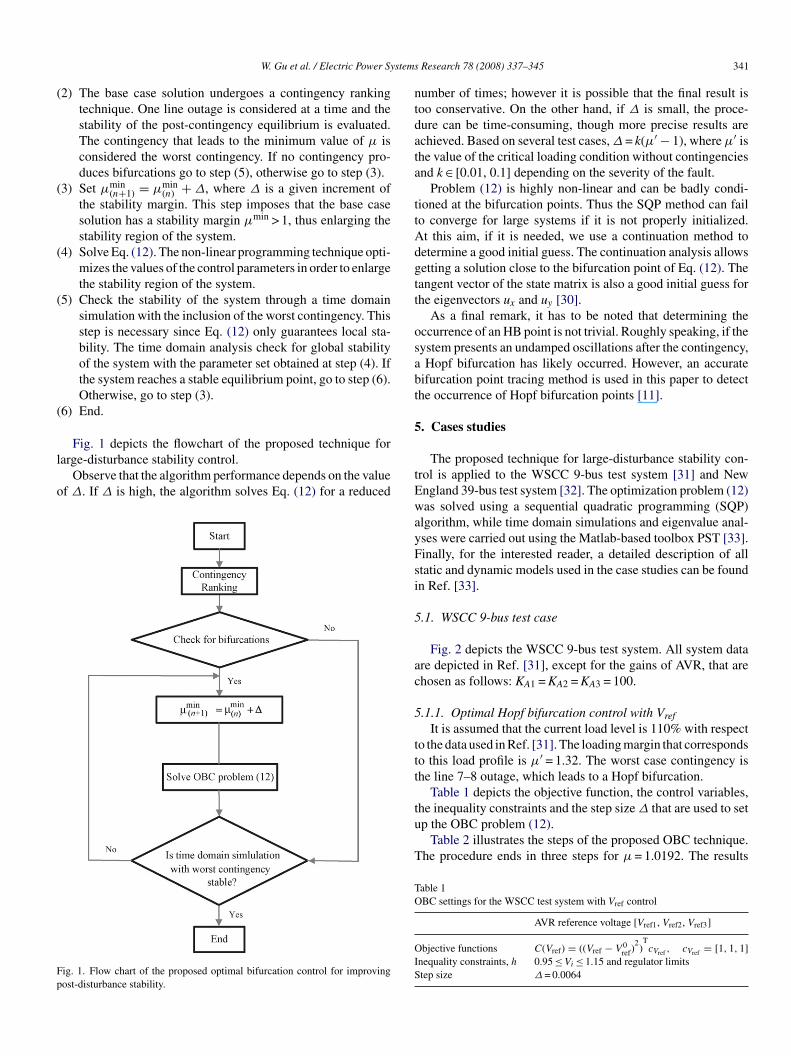
2) The base case solution undergoes a contingency rankingtechnique. One line outage is considered at a time and thestability of the post-contingency equilibrium is evaluated.The contingency that leads to the minimum value of μ isconsidered the worst contingency. If no contingency pro-duces bifurcations go to step (5), otherwise go to step (3).

3) Set μmin(n+1) = μmin

(n) + Δ, where Δ is a given increment ofthe stability margin. This step imposes that the base casesolution has a stability margin μmin > 1, thus enlarging thestability region of the system.

4) Solve Eq. (12). The non-linear programming technique opti-mizes the values of the control parameters in order to enlargethe stability region of the system.

5) Check the stability of the system through a time domainsimulation with the inclusion of the worst contingency. Thisstep is necessary since Eq. (12) only guarantees local sta-bility. The time domain analysis check for global stabilityof the system with the parameter set obtained at step (4). Ifthe system reaches a stable equilibrium point, go to step (6).Otherwise, go to step (3).

6) End.

Fig. 1 depicts the flowchart of the proposed technique forarge-disturbance stability control.

Observe that the algorithm performance depends on the valuef Δ. If Δ is high, the algorithm solves Eq. (12) for a reduced

ig. 1. Flow chart of the proposed optimal bifurcation control for improvingost-disturbance stability.

tEwayFsi

5

ac

5

ttt

tu

T

TO

OIS

Research 78 (2008) 337–345 341

umber of times; however it is possible that the final result isoo conservative. On the other hand, if Δ is small, the proce-ure can be time-consuming, though more precise results arechieved. Based on several test cases, Δ = k(μ′ − 1), where μ′ ishe value of the critical loading condition without contingenciesnd k ∈ [0.01, 0.1] depending on the severity of the fault.

Problem (12) is highly non-linear and can be badly condi-ioned at the bifurcation points. Thus the SQP method can failo converge for large systems if it is not properly initialized.t this aim, if it is needed, we use a continuation method toetermine a good initial guess. The continuation analysis allowsetting a solution close to the bifurcation point of Eq. (12). Theangent vector of the state matrix is also a good initial guess forhe eigenvectors ux and uy [30].

As a final remark, it has to be noted that determining theccurrence of an HB point is not trivial. Roughly speaking, if theystem presents an undamped oscillations after the contingency,Hopf bifurcation has likely occurred. However, an accurate

ifurcation point tracing method is used in this paper to detecthe occurrence of Hopf bifurcation points [11].

. Cases studies

The proposed technique for large-disturbance stability con-rol is applied to the WSCC 9-bus test system [31] and Newngland 39-bus test system [32]. The optimization problem (12)as solved using a sequential quadratic programming (SQP)

lgorithm, while time domain simulations and eigenvalue anal-ses were carried out using the Matlab-based toolbox PST [33].inally, for the interested reader, a detailed description of alltatic and dynamic models used in the case studies can be foundn Ref. [33].

.1. WSCC 9-bus test case

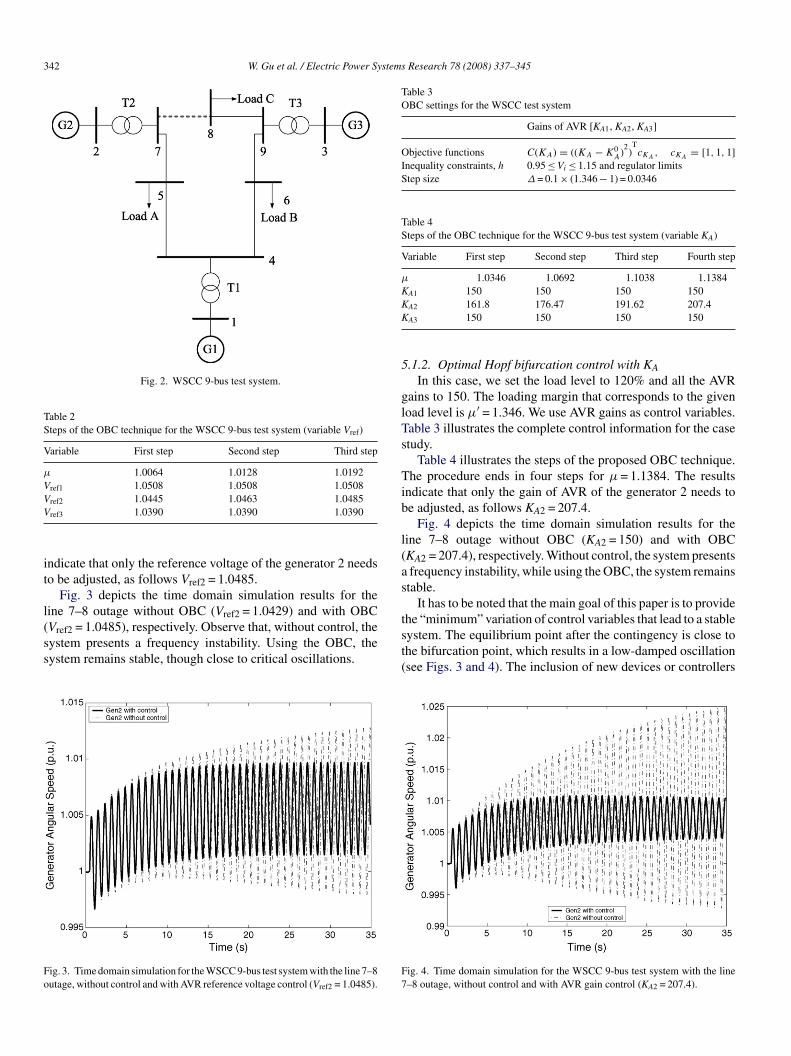
Fig. 2 depicts the WSCC 9-bus test system. All system datare depicted in Ref. [31], except for the gains of AVR, that arehosen as follows: KA1 = KA2 = KA3 = 100.

.1.1. Optimal Hopf bifurcation control with VrefIt is assumed that the current load level is 110% with respect

o the data used in Ref. [31]. The loading margin that correspondso this load profile is μ′ = 1.32. The worst case contingency ishe line 7–8 outage, which leads to a Hopf bifurcation.

Table 1 depicts the objective function, the control variables,

he inequality constraints and the step size Δ that are used to setp the OBC problem (12).

Table 2 illustrates the steps of the proposed OBC technique.he procedure ends in three steps for μ = 1.0192. The results

able 1BC settings for the WSCC test system with Vref control

AVR reference voltage [Vref1, Vref2, Vref3]

bjective functions C(Vref) = ((Vref − V 0ref)

2)TcVref , cVref = [1, 1, 1]

nequality constraints, h 0.95 ≤ Vi ≤ 1.15 and regulator limitstep size Δ = 0.0064

342 W. Gu et al. / Electric Power Systems Research 78 (2008) 337–345

Fig. 2. WSCC 9-bus test system.

Table 2Steps of the OBC technique for the WSCC 9-bus test system (variable Vref)

Variable First step Second step Third step

μ 1.0064 1.0128 1.0192Vref1 1.0508 1.0508 1.0508VV

it

l(ss

Fo

Table 3OBC settings for the WSCC test system

Gains of AVR [KA1, KA2, KA3]

Objective functions C(KA) = ((KA − K0A

)2)TcKA

, cKA= [1, 1, 1]

Inequality constraints, h 0.95 ≤ Vi ≤ 1.15 and regulator limitsStep size Δ = 0.1 × (1.346 − 1) = 0.0346

Table 4Steps of the OBC technique for the WSCC 9-bus test system (variable KA)

Variable First step Second step Third step Fourth step

μ 1.0346 1.0692 1.1038 1.1384KA1 150 150 150 150KK

5

glTs

Tib

l(as

t

ref2 1.0445 1.0463 1.0485

ref3 1.0390 1.0390 1.0390

ndicate that only the reference voltage of the generator 2 needso be adjusted, as follows Vref2 = 1.0485.

Fig. 3 depicts the time domain simulation results for theine 7–8 outage without OBC (Vref2 = 1.0429) and with OBC

Vref2 = 1.0485), respectively. Observe that, without control, theystem presents a frequency instability. Using the OBC, theystem remains stable, though close to critical oscillations.

ig. 3. Time domain simulation for the WSCC 9-bus test system with the line 7–8utage, without control and with AVR reference voltage control (Vref2 = 1.0485).

st(

F7

A2 161.8 176.47 191.62 207.4

A3 150 150 150 150

.1.2. Optimal Hopf bifurcation control with KA

In this case, we set the load level to 120% and all the AVRains to 150. The loading margin that corresponds to the givenoad level is μ′ = 1.346. We use AVR gains as control variables.able 3 illustrates the complete control information for the casetudy.

Table 4 illustrates the steps of the proposed OBC technique.he procedure ends in four steps for μ = 1.1384. The results

ndicate that only the gain of AVR of the generator 2 needs toe adjusted, as follows KA2 = 207.4.

Fig. 4 depicts the time domain simulation results for theine 7–8 outage without OBC (KA2 = 150) and with OBCKA2 = 207.4), respectively. Without control, the system presentsfrequency instability, while using the OBC, the system remainstable.

It has to be noted that the main goal of this paper is to providehe “minimum” variation of control variables that lead to a stable

ystem. The equilibrium point after the contingency is close tohe bifurcation point, which results in a low-damped oscillationsee Figs. 3 and 4). The inclusion of new devices or controllers

ig. 4. Time domain simulation for the WSCC 9-bus test system with the line–8 outage, without control and with AVR gain control (KA2 = 207.4).

W. Gu et al. / Electric Power Systems Research 78 (2008) 337–345 343

sto

cdc

5

d

5

toTs

twe

taw

1toKbp

F1

e(

usu

Ttt

1O

5

c1itipo

the inequality constraints and the step size Δ that are used toset up the OBC problem (12). In this case, defining a good ini-tial guess is not an issue, since the size of Eq. (12) in the caseof saddle-node bifurcation control is the half the size of Hopf

Table 5Steps of the OBC technique for the New England test system (HB control)

Variable First step Second step Third step

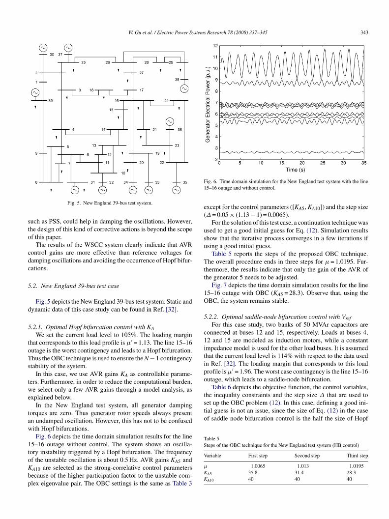
Fig. 5. New England 39-bus test system.

uch as PSS, could help in damping the oscillations. However,he design of this kind of corrective actions is beyond the scopef this paper.

The results of the WSCC system clearly indicate that AVRontrol gains are more effective than reference voltages foramping oscillations and avoiding the occurrence of Hopf bifur-ations.

.2. New England 39-bus test case

Fig. 5 depicts the New England 39-bus test system. Static andynamic data of this case study can be found in Ref. [32].

.2.1. Optimal Hopf bifurcation control with KA

We set the current load level to 105%. The loading marginhat corresponds to this load profile is μ′ = 1.13. The line 15–16utage is the worst contingency and leads to a Hopf bifurcation.hus the OBC technique is used to ensure the N − 1 contingencytability of the system.

In this case, we use AVR gains KA as controllable parame-ers. Furthermore, in order to reduce the computational burden,e select only a few AVR gains through a model analysis, as

xplained below.In the New England test system, all generator damping

orques are zero. Thus generator rotor speeds always presentn undamped oscillation. However, this has not to be confusedith Hopf bifurcations.Fig. 6 depicts the time domain simulation results for the line

5–16 outage without control. The system shows an oscilla-ory instability triggered by a Hopf bifurcation. The frequency

f the unstable oscillation is about 0.5 Hz. AVR gains KA5 andA10 are selected as the strong-correlative control parametersecause of the higher participation factor to the unstable com-lex eigenvalue pair. The OBC settings is the same as Table 3

μ

KK

ig. 6. Time domain simulation for the New England test system with the line5–16 outage and without control.

xcept for the control parameters ([KA5, KA10]) and the step sizeΔ = 0.05 × (1.13 − 1) = 0.0065).

For the solution of this test case, a continuation technique wassed to get a good initial guess for Eq. (12). Simulation resultshow that the iterative process converges in a few iterations ifsing a good initial guess.

Table 5 reports the steps of the proposed OBC technique.he overall procedure ends in three steps for μ = 1.0195. Fur-

hermore, the results indicate that only the gain of the AVR ofhe generator 5 needs to be adjusted.

Fig. 7 depicts the time domain simulation results for the line5–16 outage with OBC (KA5 = 28.3). Observe that, using theBC, the system remains stable.

.2.2. Optimal saddle-node bifurcation control with VrefFor this case study, two banks of 50 MVAr capacitors are

onnected at buses 12 and 15, respectively. Loads at buses 4,2 and 15 are modeled as induction motors, while a constantmpedance model is used for the other load buses. It is assumedhat the current load level is 114% with respect to the data usedn Ref. [32]. The loading margin that corresponds to this loadrofile is μ′ = 1.96. The worst case contingency is the line 15–16utage, which leads to a saddle-node bifurcation.

Table 6 depicts the objective function, the control variables,

1.0065 1.013 1.0195

A5 35.8 31.4 28.3

A10 40 40 40

344 W. Gu et al. / Electric Power Systems Research 78 (2008) 337–345

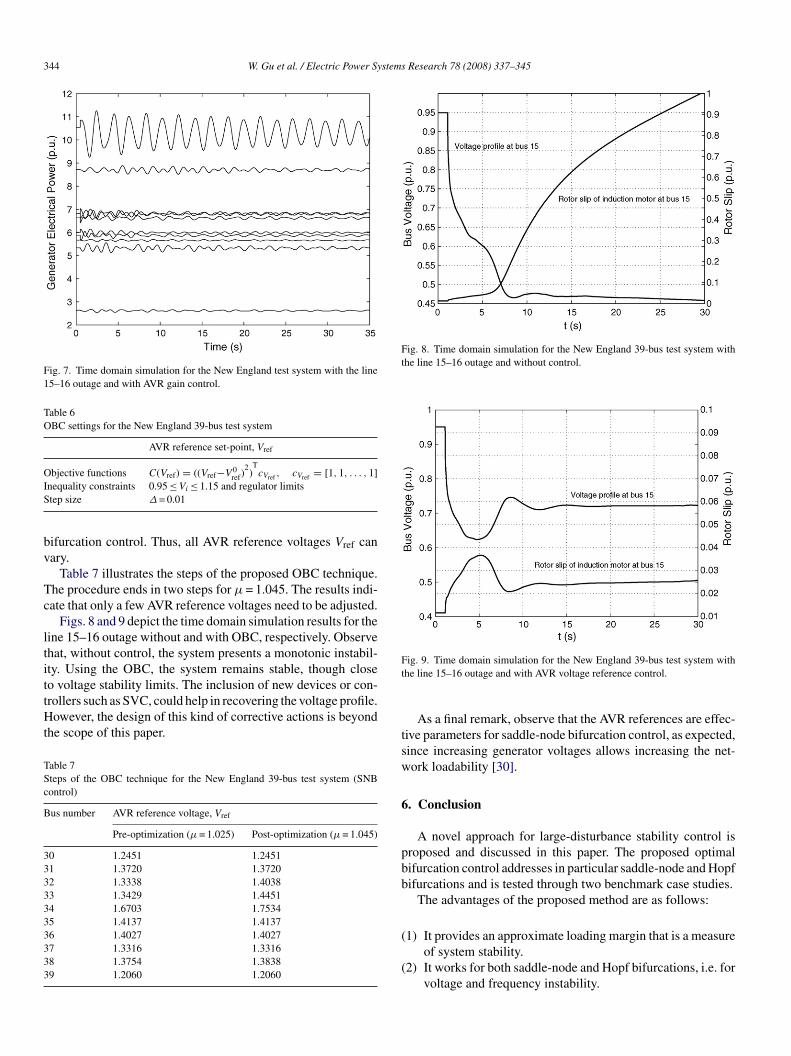
Fig. 7. Time domain simulation for the New England test system with the line15–16 outage and with AVR gain control.

Table 6OBC settings for the New England 39-bus test system

AVR reference set-point, Vref

Objective functions C(V ) = ((V −V 0 )2)Tc , c = [1, 1, . . . , 1]

IS

bv

Tc

ltittHt

TSc

B

3333333333

Fig. 8. Time domain simulation for the New England 39-bus test system withthe line 15–16 outage and without control.

Ft

ref ref ref Vref Vref

nequality constraints 0.95 ≤ Vi ≤ 1.15 and regulator limitstep size Δ = 0.01

ifurcation control. Thus, all AVR reference voltages Vref canary.

Table 7 illustrates the steps of the proposed OBC technique.he procedure ends in two steps for μ = 1.045. The results indi-ate that only a few AVR reference voltages need to be adjusted.

Figs. 8 and 9 depict the time domain simulation results for theine 15–16 outage without and with OBC, respectively. Observehat, without control, the system presents a monotonic instabil-ty. Using the OBC, the system remains stable, though close

o voltage stability limits. The inclusion of new devices or con-rollers such as SVC, could help in recovering the voltage profile.owever, the design of this kind of corrective actions is beyond

he scope of this paper.

able 7teps of the OBC technique for the New England 39-bus test system (SNBontrol)

us number AVR reference voltage, Vref

Pre-optimization (μ = 1.025) Post-optimization (μ = 1.045)

0 1.2451 1.24511 1.3720 1.37202 1.3338 1.40383 1.3429 1.44514 1.6703 1.75345 1.4137 1.41376 1.4027 1.40277 1.3316 1.33168 1.3754 1.38389 1.2060 1.2060

tsw

6

pbb

(

(

ig. 9. Time domain simulation for the New England 39-bus test system withhe line 15–16 outage and with AVR voltage reference control.

As a final remark, observe that the AVR references are effec-ive parameters for saddle-node bifurcation control, as expected,ince increasing generator voltages allows increasing the net-ork loadability [30].

. Conclusion

A novel approach for large-disturbance stability control isroposed and discussed in this paper. The proposed optimalifurcation control addresses in particular saddle-node and Hopfifurcations and is tested through two benchmark case studies.

The advantages of the proposed method are as follows:

1) It provides an approximate loading margin that is a measureof system stability.

2) It works for both saddle-node and Hopf bifurcations, i.e. forvoltage and frequency instability.

stems

(

fiit

A

S2M

R

[

[

[

[

[

[

[

[

[

[

[

[

[

[

[

[

[

[

[

[

[

[

W. Gu et al. / Electric Power Sy

3) The use of time domain simulations also allows excludingthe occurrence of transient instabilities and avoid bifurca-tions triggered by contingencies.

Future works will concentrate on finding a simple criterion tond adequate values for the step increment Δ, whose evaluation

s currently based on off-line analyses. The authors are currentlyesting the proposed method on large-scale case studies.

cknowledgments

Federico Milano is partly supported by the Ministry ofcience and Education of Spain through CICYT Project DPI-003-01362 and by Junta de Comunidades de Castilla-Laancha through project PBI-05-053.

eferences

[1] M.A. Pai, Energy Function Analysis for Power System Stability, KluwerAcademic Publishers, Norwell, 1989.

[2] Y. Ni, S. Chen, B. Zhang, Theory and Analysis of Dynamic Power Systems,Tsinghua University Press, Beijing, 2002.

[3] H.-D. Chiang, C.-C. Chu, G. Cauley, Direct stability analysis of electricpower systems using energy functions: theory, applications, and perspec-tive, Proc. IEEE 83 (11) (1995) 1497–1529.

[4] V. Vittal, Consequence and impact of electric utility industry restructuringon transient stability and small-signal stability analysis, Proc. IEEE 88 (2)(2000) 196–207.

[5] Y. Xue, Extended equal area criterion revised, IEEE Trans. Power Syst. 7(1992) 1012–1022.

[6] M. Ilic, J. Zaborszky, Dynamic Control of Large Electric Power Systems,Wiley-Interscience Publication, New York, 2000.

[7] T. Van Cutsem, M.E. Grenier, D. Lefebvre, Combined detailed and quasisteady-state time simulations for large-disturbance analysis, Int. J. Elect.Power Energy Syst. 28 (9) (2006) 634–642.

[8] C.D. Vournas, N.G. Sakellaridis, Region of attraction in a power sys-tem with discrete LTCs, IEEE Trans. Power Syst. 53 (7) (2006) 1610–1618.

[9] D. Ruiz-Vega, M. Pavella, A comprehensive approach to transient stabilitycontrol. I. Near optimal preventive control, IEEE Trans. Power Syst. 18 (4)(2003) 1446–1453.

10] D. Ruiz-Vega, M. Pavella, A comprehensive approach to transient stabilitycontrol. II. Open loop emergency control, IEEE Trans. Power Syst. 18 (4)(2003) 1446–1453.

11] R. Seydel, Practical Bifurcation and Stability Analysis: from Equilibriumto Chaos, 2nd ed., Springer-Verlag, New York, 1994.

12] V. Venkatasubramanian, H. Schattler, J. Zaborszky, Dynamics of large con-

strained nonlinear systems—a taxonomy theory, Proc. IEEE 83 (11) (1995)1530–1561.

13] V. Venkatasubramanian, H. Schattler, J. Zaborszky, Local bifurcations andfeasibility regions in differential-algebraic systems, IEEE Trans. Automat.Control 40 (12) (1995) 1992–2013.

[

[

Research 78 (2008) 337–345 345

14] W. Rosehart, C.A. Cannizares, V.H. Quintana, Optimal power flow incorpo-rating voltage collapse constraints, in: Proceedings of the 1999 IEEE-PESSummer Meeting, Edmonton, Alberta, 1999, pp. 820–825.

15] C.A. Canizares, W. Rosehart, A. Berizzi, C. Bovo, Comparison of voltagesecurity constrained optimal power flow techniques, in: Proceedings ofthe 2001 IEEE-PES Summer Meeting, Vancouver, BC, Canada, 2001, pp.1680–1685.

16] W.D. Rosehart, C.A. Canizares, V. Quintana, Multi-objective optimalpower flows to evaluate voltage security costs in power networks, IEEETrans. Power Syst. 18 (2) (2003) 578–587.

17] F. Milano, C.A. Canizares, M. Invernizzi, Voltage stability constrained OPFmarket models considering N − 1 contingency criteria, Elect. Power Syst.Res. 74 (1) (2005) 27–36.

18] C.A. Canizares, Calculating optimal system parameters to maximize thedistance to saddle-node bifurcations, IEEE Trans. Circuits Syst.-I. Fundam.Theory Appl. 45 (3) (1998) 225–237.

19] M.M. Begovic, G. Phadke, Control of voltage stability using sensitivityanalysis, IEEE Trans. Power Syst. 7 (1) (1992) 114–120.

20] S. Greene, I. Dobson, F.L. Alvarado, Contingency ranking for voltage col-lapse via sensitivities from single nose curve, IEEE Trans. Power Syst. 14(1) (1999) 232–240.

21] F. Capitanescu, T. Van Cutsem, Unified sensitivity analysis of unstable orlow voltages caused by load increases or contingencys, IEEE Trans. PowerSyst. 20 (1) (2005) 321–329.

22] S. Greene, I. Dobson, F.L. Alvarado, Sensitivity of transfer capability mar-gins with a fast formula, IEEE Trans. Power Syst. 17 (1) (2002) 34–40.

23] C.A. Canizares, C. Cavallo, M. Pozzi, S. Corsi, Comparing secondary volt-age regulation and shunt compensation for improving voltage stability andtransfer capability in the Italian power system, Elect. Power Syst. Res. 73(1) (2005) 67–76.

24] S. Wunderlich, T. Wu, R. Fischl, R. O’Connell, An inter-area transmissionand voltage limitation (TVLIM) program, IEEE Trans. Power Syst. 10 (3)(1995) 1257–1263.

25] N. Mithulananthan, C.A. Canizares, J. Reeve, J.J. Rogers, Comparison ofPSS, SVC, and STATCOM controllers for damping power system oscilla-tions, IEEE Trans. Power Syst. 18 (2) (2003) 786–792.

26] C.A. Canizares, N. Mithulananthan, F. Milano, J. Reeve, Linear perfor-mance indices to predict oscillatory stability problems in power systems,IEEE Trans. Power Syst. 19 (2) (2004) 1104–1114.

27] T. Van Cutsem, An approach to corrective control of voltage instabilityusing simulation and sensitivity, IEEE Trans. Power Syst. 10 (2) (1995)616–622.

28] T. Van Cutsem, C. Vournas, Voltage stability analysis in transient and mid-term time scales, IEEE Trans. Power Syst. 11 (1) (1996) 146–154.

29] P. Kundur, Power System Stability and Control, McGraw Hill, New York,1994.

30] C.A. Canizares, Voltage stability assessment: concepts, practices and tools,Tech. rep., IEEE/PES Power System Stability Subcommittee, Final Docu-ment, August 2002.

31] P.W. Sauer, M.A. Pai, Power System Dynamics and Stability, Prentice Hall,

Upper Saddle River, NJ, 1998.

32] W. Gu, Optimal bifurcation control in power systems, PhD Thesis, South-east University, China, May 2006.

33] Cherry Tree Scientific Software, Power System Toolbox Ver. 2.0: DynamicTutorial and Functions, 1999.