Introduction to Magnetohydrodynamic

Simulations

Seiji ZENITANIDivision of Theoretical Astronomy

SOKENDAI 2014/2015

Outline

• Day 1 - Magnetohydrodynamics (MHD)

• Introduction & MHD gallery

• Basic equations, fundamental notions

• MHD waves

• Day 2

• MHD Theory (cont.) - Conservation form, shocks

• Simulations - Riemann solver, HLL, TVD

• Simulations - Recent topics (Higher-order schemes, div B)

• Assignments - 1D simulation

What is MagnetoHydrodDynamics (MHD)? 磁気流体力学／電磁流体力学、磁流体力学（中文）

•A fluid framework for macroscopic plasma motion

• “Plasma” consists of...

• Charged particles (ionized gas)

• Magnetic fields

electron

Atomic nucleus

Atom

magnetic field line

ion

electron

Plasma B

Magneto fluid

MHD motion

MHD gallery

MHD gallery - solar corona

Kusano et al. 2012 ApJ NASA / TRACE satellite

•Highly filamented structure

•Triggering of flares (magnetic eruption)

MHD process - Magnetic reconnection

Zenitani & Miyoshi 2011 Phys. Plasmas

Jet

Jet

•Underlying mechanism of solar flares

Turbulent reconnection

MHD gallery - Heliosphere

•Global simulations ofHeliosphere & planetary magnetosphere

Shiota et al. 2014 Space Weather Matsumoto et al. 2010 IEEE trans.

MHD process - Kelvin-Helmholtz instability

Weathernews.jp 2015

Matsumoto & Hoshino 2004 GRL

MHD gallery - Pulsar M’shpere

•Magnetically-dominated environments

•Exotic variants of MHD - Force-free / Relativistic MHD

Tchekovskoy et al. 2013 MNRASSpitkovsky 2011 ASSP

MHD gallery - Black hole system

•Black hole accretion disks + jet launching

Machida et al. 2003 ApJ Kato et al. 2004 ApJ

MHD equations

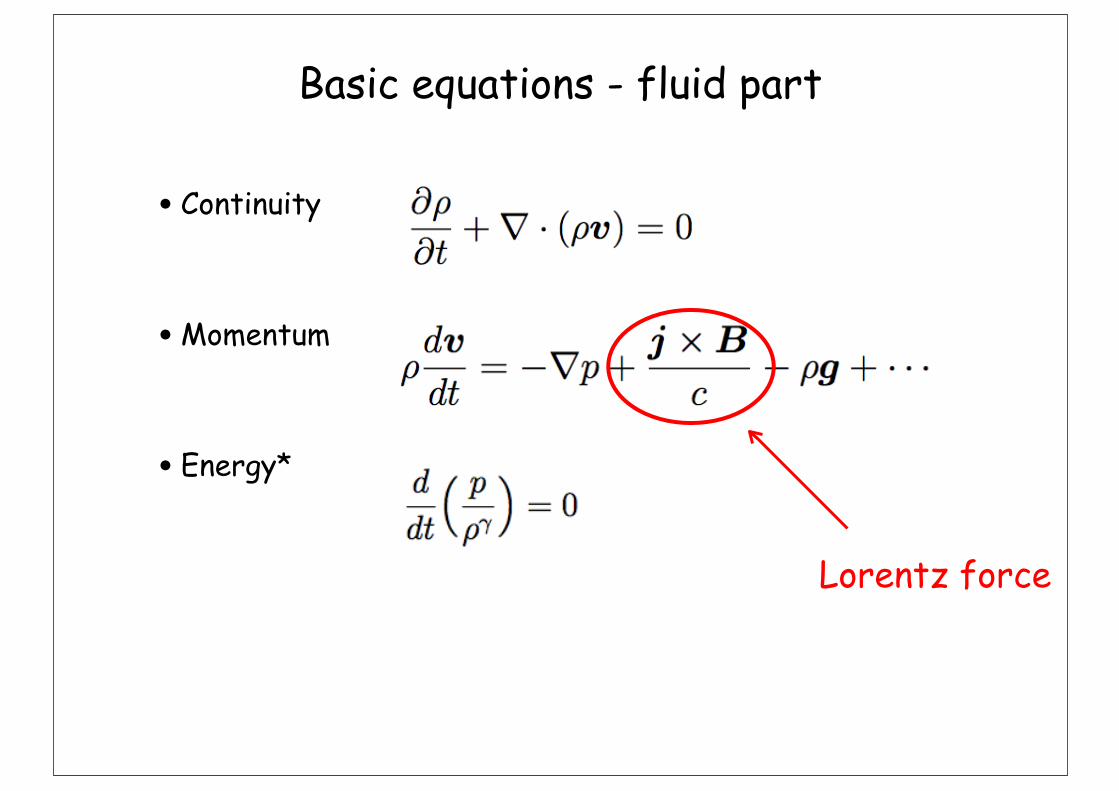
Basic equations - fluid part

•Continuity

•Momentum

•Energy*

Lorentz force

Lorentz force = magnetic pressure + magnetic tension

•Examples:

•B = (0,x,0) B = (y,1,0)“magnetic tension”“magnetic pressure”

How magnetic tension works ...

• It tends to be straight

Basic equations - EM part

•Faraday’s law

•Ampere’s law

•Of course it follows the constraints in Maxwell eqs.

~O(V2/c2)

•Continuity

•Momentum

•Energy*

•Magnetic field

•Constraint

MHD equations ...?

We have 8 equations, but 11 unknowns...

•Ideal condition

•No electric field in the moving frame at v

•Particle motion in the perpendicular plane

Closure - ideal condition

E

e-

p+

vE�B =cE �B

B2

•Continuity

•Momentum

•Energy*

•Magnetic field

• Ideal condition

• Constraint

Ideal MHD equations

Plasma

•Time: Length:

Scales of MHD

Log T

Log L

Kineticmodel

MHD

Alfvén speed

magnetic field line

ion

electron

B

�ci =eB

mic

dirL,e

��1ci

⌦�1ce

!�1pe

•Magnetic flux in a comoving surface is conserved

•Similar to Kelvin’s circulation theorem in hydrodynamics

•Magnetic field is “frozen-in” to the flow field V

Flux frozen-in

B

dlv

Stern 1966 SSR

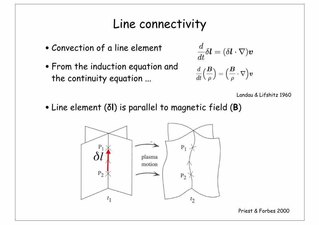
Line connectivity

•Convection of a line element

•From the induction equation andthe continuity equation ...

• Line element (δl) is parallel to magnetic field (B)

Priest & Forbes 2000

δl

Landau & Lifshitz 1960

Field line motion in ideal MHD

•All in all, it is convenient to consider that plasmas and “magnetic field lines” move together at the same speed

B

E

e-

p+

Resistivity

•We sometimes consider the resistivity in the MHD frame

•Plasma version of Ohm’s law, or simply “Ohm’s law”

•This modifies the induction equation in the following way

•Energy equation needs to be modified accordingly, because it brings Ohmic heating.

Diffusion termConvection term

•Ohm’s law

•Ideal condition

•Frozen-in condition

• Line connection

•Topology condition ...

• In nonideal case of R≠0, it is not always possible to define the field line velocity.

•Don’t worry, eventually, magnetic field lines are virtual lines.

General discussion...

MHD waves

•Linearization

•Hydrodynamics

•Sound (compressional) wave

Waves in hydrodynamics

1: small oscillation0: average value

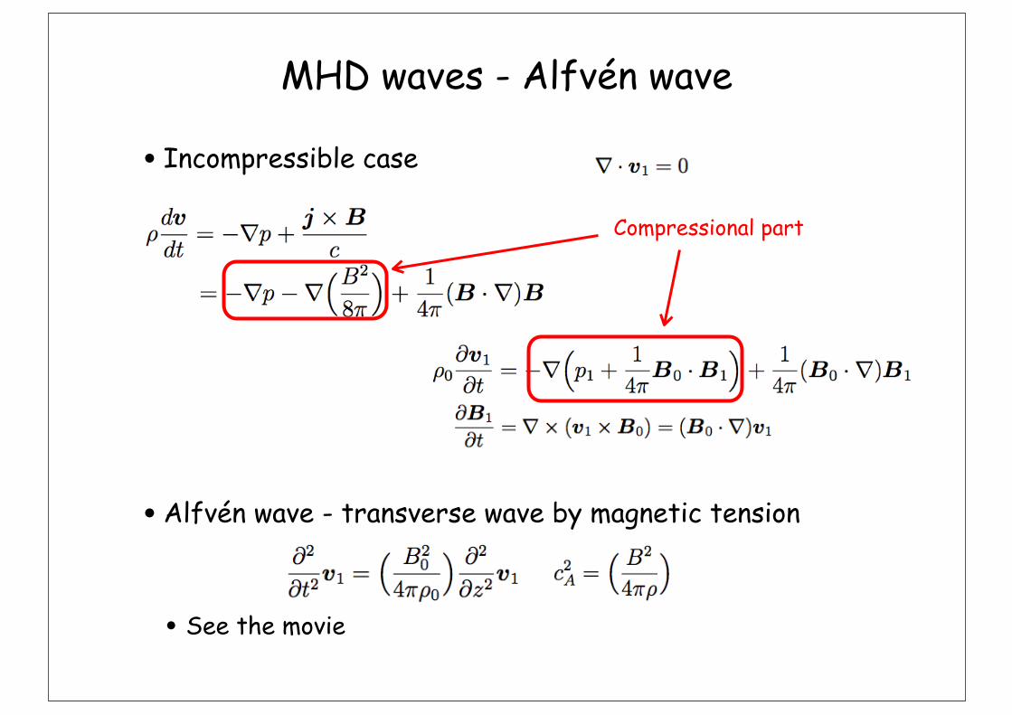
•Incompressible case

•Alfvén wave - transverse wave by magnetic tension

• See the movie

MHD waves - Alfvén wave

Compressional part

Alfvén wave paper (1942)

Hannes Alfvén (1908-1995)

• 1970 Novel Prize in PhysicsAlfvén 1942 Nature

Alfvén wave - observation

•Solar photosphere, observed by Hinode satellite

Okamoto et al. 2007 Sciencehttp://hinode.nao.ac.jp/gallery/

•Small oscillation

•MHD equations

•After SOME algebra

MHD waves - magnetosonic waves

MHD waves - magnetosonic waves

•Again, linearized MHD equations

•Dispersion relation:

• Fast/slow magnetosonic waves

• Compressional waves due to fluid and magnetic* pressures

z

x

y

B

kθ

Alfvén wave(Parallel propagation)

Sound wave(Spherical propagation)

Compressional* wave by magnetic pressure

MHD waves - magnetosonic waves

•Alfvén wave

•Fast and slowmagnetosonic waves

•Friedrichs diagram (phase-speed)

• cs > cA

B B

•cs < cA

cAcosθ

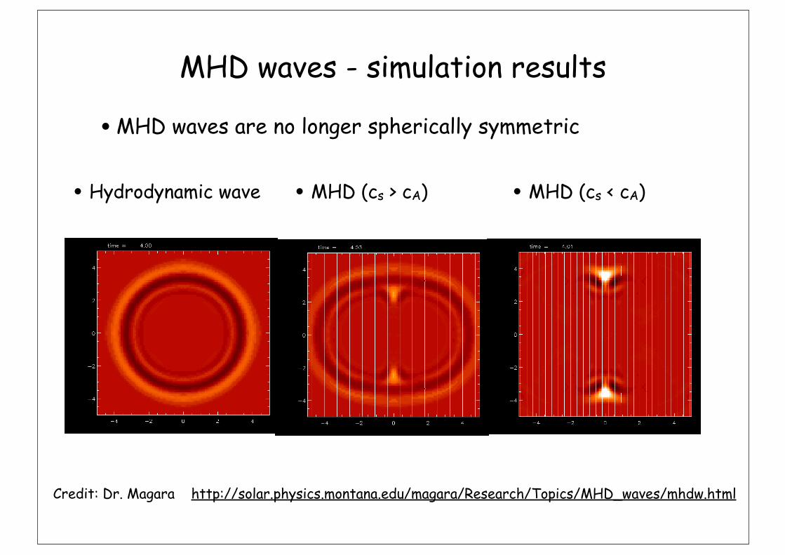
•MHD waves are no longer spherically symmetric

MHD waves - simulation results

• Hydrodynamic wave • MHD (cs < cA) • MHD (cs > cA)

Credit: Dr. Magara http://solar.physics.montana.edu/magara/Research/Topics/MHD_waves/mhdw.html

Summary

•MHD = Magnetohydrodynamics

• Plasmas and magnetic field lines move together

•MHD physics highly depends on the direction of B

•Magnetic pressure vs magnetic tension

•Alfvén wave

•Magnetosonic waves

Further reading

•宇宙流体力学、坂下＆池内 (1996)

•Plasma Physics for Astrophysics, R. M. Kulsrud (2004)

•Magnetohydrodynamics of the Sun, E. R. Priest (2014)

•シリーズ現代の天文学 12. 天体物理学の基礎 II, ２章

•シリーズ現代の天文学 14. シミュレーション天文学

•W. A. Newcomb, Ann. Phys. (1958)

set polarunset keya=1; s=1.2plot a*abs(cos(t)) lw 3, \sqrt(0.5*(a**2+s**2+sqrt((a**2+s**2)**2-(2*a*s*cos(t))**2))) lw 3, \sqrt(0.5*(a**2+s**2-sqrt((a**2+s**2)**2-(2*a*s*cos(t))**2))) lw 3

• gnuplot code for Friedrichs diagram

Outline

• Day 1 - Magnetohydrodynamics (MHD)

• Introduction & MHD gallery

• Basic equations, fundamental notions

• MHD waves

• Day 2

• MHD Theory (cont.) - Conservation form, shocks

• Simulations techniques - Riemann solver, HLL, MUSCL

• Simulations techniques - div B

• Assignments - 1D simulation

•Continuity

•Momentum

•Energy*

•Magnetic field

• Ideal condition

• Constraint

Review - ideal MHD equations

Review - MHD waves

•Alfvén wave

•Fast and slowmagnetosonic waves

•Friedrichs diagram (phase-speed)

• cs > cA

B B

•cs < cA

cAcosθ

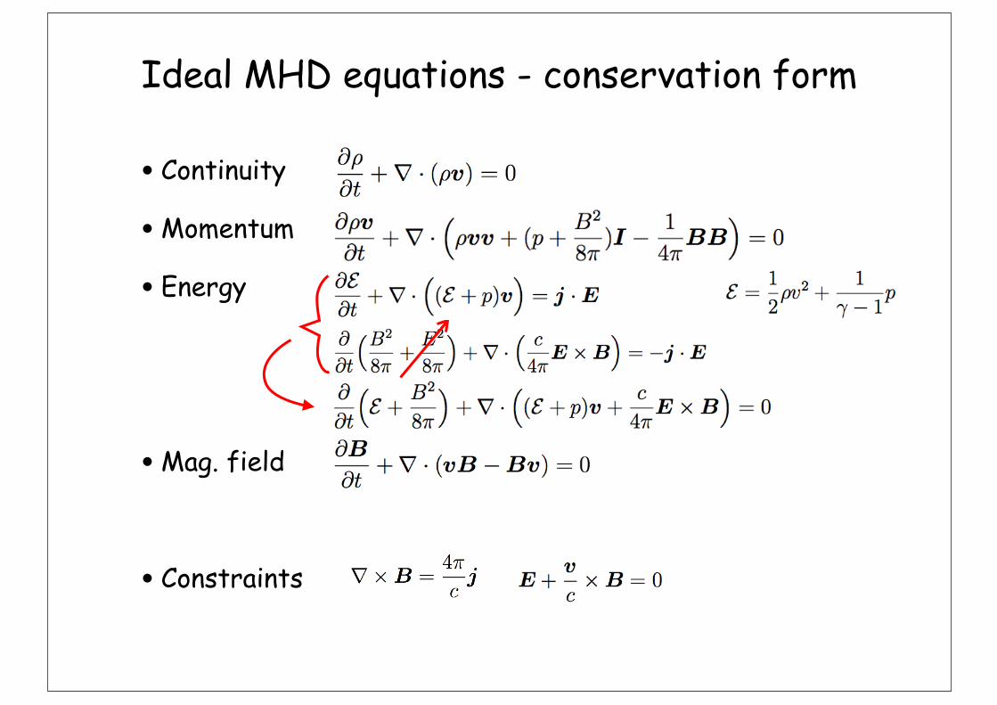
•Continuity

•Momentum

•Energy

•Mag. field

•Constraints

Ideal MHD equations - conservation form

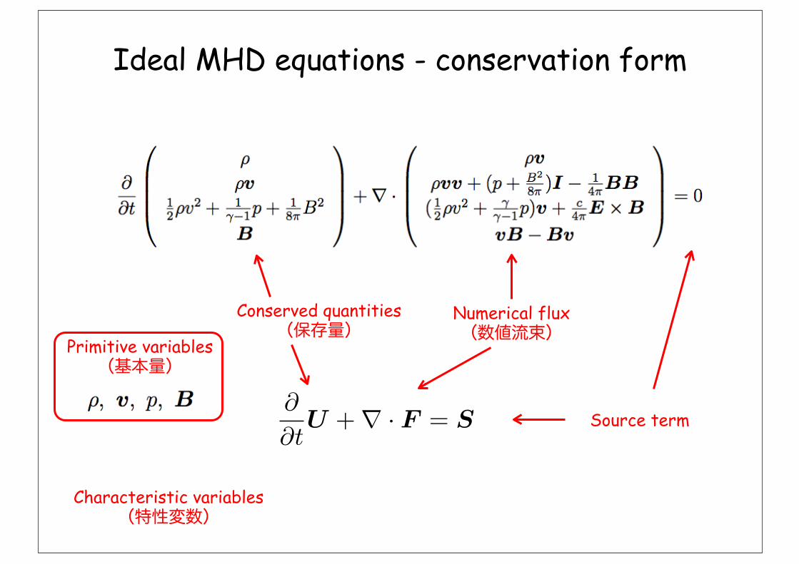
Ideal MHD equations - conservation form

Source term

Numerical flux（数値流束）

Conserved quantities（保存量）

Primitive variables（基本量）

Characteristic variables（特性変数）

•Conservation form is friendly with finite volume method

•One can deal with shocks (“Shock-capturing” code)

Finite volume method

Shocks in the Universe

Mach 1887

Jokipii 2008

NASA/CXC/Rutgers/J.Hughes et al. 2005

•Sudden jump in physical quantities

• Nonlinear wave steepens into a shock

• Supersonic flow slows down to a subsonic speed

• Fast explosion propagates into a medium...

• Shock is a big enemy to numerical simulations!

Shocks

MHD shocks & discontinuities

Fast shock (FS) Slow shock (SS)

Rotational discontinuity Contact discontinuity

Tangential discontinuity

Intermediate shock*

Upwind scheme

•We use numerical flux on the “upwind” side

•Time-evolution by the 1st-order Euler method

Generic form

c

Diffusion term

Monotonicity（単調性）

Riemann solver (1/2)

•Riemann problem

• Time evolution from two flat states

• Nonlinear problem in HD

•Riemann solver

• Solve Riemann problem at each cell interface

U

x

U

U

Riemann solver (2/2)

U

U

x

t

x

t•Switches to an Upwind scheme

MHD Riemann problem

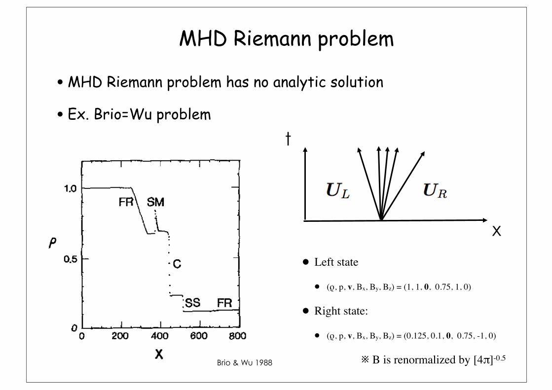
Brio & Wu 1988　

•MHD Riemann problem has no analytic solution

•Ex. Brio=Wu problem

x

t

• Left state

• (ρ, p, v, Bx, By, Bz) = (1, 1, 0, 0.75, 1, 0)

• Right state:

• (ρ, p, v, Bx, By, Bz) = (0.125, 0.1, 0, 0.75, -1, 0)

※ B is renormalized by [4π]-0.5

Approximate Riemann solver - HLL solver (1/2)

x

t U

U

x

t

•Harten–Lan–van Leer (1983)

Approximate Riemann solver - HLL solver (2/2)

Fastest signal = fast wave

x

t

Jump conditionsfor the λ-moving discontinuity

F hll �= F (Uhll)Note that

•HLLD solver (Miyoshi & Kusano 2005)

•Relativistic HLLD solver (Mignone et al. 2009)

•Exact solver (Takahashi & Yamada 2014)

Better Riemann solvers

•Time-marching - Higher-order Runge-Kutta method

•Spatial profile - MUSCL interpolation (linear version)

• ex. minmod limiter

Higher accuracy

RLR

i i+1i+1/2i-1/2

• We should interpolate characteristic variables for higher (≧3rd) order.

• We often interpolate primitive/conservative variables for 2nd order

MUSCL interpolation

r

B B=2r B=r

2

1

0

RL

0 ≦ x ≦ 1

limiter function (≧0)

•Fractional step

• Compute x for Δt/2 (Lx) --> Compute y for Δt/2 (Ly) --> ...

• U(t+Δt) = Lx(Δt/2) Ly(Δt/2) Lz(Δt) Ly(Δt/2) Lx(Δt/2) U(t)

•All at once

Multi-dimensional problem

•MHD scientists worry about the “solenoidal condition”

•Non-zero error:

• The magnetic topology is distorted

• Theorists are just unhappy

• Unphysical force grows in the system

Multi-dimensional problem

Unphysical force

• 1. Projection scheme (Brackbill & Barnes 1983, Tóth 2000)

• Solve Poisson equation every timestep

•2. Constraint-Transport (Evans & Hawley 1988)

• Set up the staggered grid for B

Divergence cleaning methods (1/2)

•3. Hyperbolic divergence cleaning method (Dedner et al. 2002)

• A new virtual potential

• Telegraph equation of div B

• 4. Artificial diffusivity for finite difference code (Kawai 2013)

•And many others

Divergence cleaning methods (2/2)

•Use an MHD code or write your own code

• Athena - https://trac.princeton.edu/Athena/

• CANS+ - http://www.astro.phys.s.chiba-u.ac.jp/cans/doc/

• PLUTO - http://plutocode.ph.unito.it/

• OpenMHD - http://th.nao.ac.jp/MEMBER/zenitani/openmhd-j.html

• In these codes, the factor 4π is often set to 1.

• Try EITHER of the following problems, plot something, and explain the figure in a paragraph by 12 Feb 2015.

• 1. Brio-Wu problem

• 2. MHD fast shock problem

[Option] Assignment

•Consider a Riemann problem of interpenetrating flows

• We will see shocks when the flow speed exceeds the fast speed,

MHD fast-shock problem

x

t

x

t

By=B0

-V+V

Shock propagation

•流体力学の数値計算法、藤井孝藏（1994）

•岩波講座地球惑星科学６ 地球連続体力学、寺澤敏夫（1996）

•A multi-state HLL approximate Riemann solver for ideal magnetohydrodynamics, Miyoshi & Kusano, J. Comput. Phys. (2005)

•The div B = 0 Constraint in Shock-Capturing Magnetohydrodynamics Codes, Toth, J. Comput. Phys. (2000)

•数値シミュレーションは div B=0 を守れるか?、三好隆博、物理学会誌（2014年７月号）

Further reading