Oxidation of Copper and Electronic Transport in Copper Oxides
Upload
khangminh22Category
view
3download
0
Atomistic Simulations of Iron Oxides
DANIEL MEILAK
DOCTOR OF PHILOSOPHY
The University of YorkPHYSICS
APRIL 2021
ABSTRACT
Iron oxides such as magnetite, maghemite and cobalt ferrite are of huge impor-
tance to biomedical applications where they are used in cancer treatments and
drug delivery. The ability to fine tune their magnetic properties for these applica-
tions has seen great interest in recent years. While they have been studied for
centuries in bulk form, their properties at the nanoscale have only seen a surface
level of understanding. In this thesis, I present a state-of-the-art investigation
into the strength and scaling of these materials using an atomistic model to
simulate them on a scale comparable to realistic applications. By forming an
accurate model of the materials, outlining their structure, exchange interactions
and anisotropy, each material is simulated with unprecedented detail, showing
the changes in the overall system as the individual atomic spins move. This study
shows how finite size effects lower the magnetic properties, such as the Curie
temperature and magnetisation scaling of the system depending on the size and
shape of the particle. As they are modelled at the atomic scale, the sublattices
of each material have been investigated, showing that the overall properties
are a symptom of multiple interacting components which can behave differently
to each other and scale differently with temperature. In addition to simulating
each material on its own, core-shell particles consisting of combinations of each
material have also been investigated to better understand the behaviour of each
system when the relative sizes of the core and shell are changed, as well as the
overall properties of the particle which can be fine tuned for different applications.
i
ACKNOWLEDGMENTS
I would like to thank my supervisor, Richard Evans, for steering me throughout
the PhD. Without your help, knowledge and enthusiasm, as well as the many
conversations and similar interests we shared, I would not have been able to do
this work. The computational magnetism group was a wonderful environment to
be in. I’ll never forget the outings and hiking adventures, as well as the many
lunches we enjoyed together. Thank you, Roy, Mara, Sergiu, Andrea, Sarah, Luke,
Andrew, Tim and everyone else I met in the group, it would not have been half as
fun without you.
I must extend a huge thanks to my parents, who have pushed me along the
whole way, offering help and guidance at every step. A ’thank you’ in a hundred
languages would not be nearly enough to start with.
Finally, I owe both my sanity and happiness to the many friends I made at my
time in university. Noodles and Scot, I treasure every minute I’ve been around
you, sorry for riling you both so much! Charlie, Patrick, Joshua, Drezzak, Kieran,
Nolly, Ciaran, Chris, Shane, Mitty, Jay, Fluro, Conor, Dhillan, Simon, Ben, Jacob,
Tommy, Toby, Ali and everyone else I haven’t named here, you are all the best and
I love you all dearly.
ii
AUTHOR’S DECLARATION
I declare that the work in this thesis was carried out in accordance
with the requirements of the University’s Regulations and Code of
Practice for Research Degree Programmes and that it has not been
submitted for any other academic award. Except where indicated by
specific reference in the text, the work is the candidate’s own work.
Work done in collaboration with, or with the assistance of, others, is
indicated as such. Any views expressed in the thesis are those of the
author.
SIGNED: ............................................. DATE: ................................
iii
LIST OF PUBLICATIONS
1. SD Oberdick, A Abdelgawad, C Moya, S Mesbahi-Vasey, D Kepaptsoglou,
VK Lazarov, RFL Evans, D Meilak, E Skoropata, J van Lierop, et al. Spin
canting across core/shell Fe3O4/MnxFe3− xO4 nanoparticles. Scientific re-ports, 8(1):1–12, 2018
2. D Meilak, S Jenkins, R Pond, and RFL Evans. Massively parallel atomistic
simulation of ultrafast thermal spin dynamics of a permalloy vortex. arXivpreprint arXiv:1908.08885, 2019
3. R Moreno, S Poyser, D Meilak, A Meo, S Jenkins, VK Lazarov, G Vallejo-
Fernandez, S Majetich, and RFL Evans. The role of faceting and elongation
on the magnetic anisotropy of magnetite Fe3O4 nanocrystals. Scientificreports, 10(1):1–14, 2020
iv
CONTENTS
Page
Abstract i
Acknowledgments ii
Author’s declaration iii
List of Publications iv
List of Tables vii
List of Figures viii
1 Introduction 11.1 Origins of Magnetism . . . . . . . . . . . . . . . . . . . . . . . . . . . . 1
1.1.1 Types of Magnetism . . . . . . . . . . . . . . . . . . . . . . . . 2
1.2 Motivation for Research . . . . . . . . . . . . . . . . . . . . . . . . . . 3
1.3 Thesis Outline . . . . . . . . . . . . . . . . . . . . . . . . . . . . . . . . 6
2 Modelling Methods 82.1 Introduction . . . . . . . . . . . . . . . . . . . . . . . . . . . . . . . . . 8
2.2 Heisenberg Hamiltonian . . . . . . . . . . . . . . . . . . . . . . . . . . 9
2.2.1 Exchange Interaction . . . . . . . . . . . . . . . . . . . . . . . 10
2.2.2 Magnetocrystalline Anisotropy . . . . . . . . . . . . . . . . . . 13
2.3 Integration Methods . . . . . . . . . . . . . . . . . . . . . . . . . . . . . 14
2.3.1 Spin Dynamics . . . . . . . . . . . . . . . . . . . . . . . . . . . 14
2.3.2 Langevin dynamics . . . . . . . . . . . . . . . . . . . . . . . . . 16
2.3.3 Time Integration of the LLG . . . . . . . . . . . . . . . . . . . 16
2.3.4 Monte Carlo Methods . . . . . . . . . . . . . . . . . . . . . . . 18
2.4 Temperature Rescaling . . . . . . . . . . . . . . . . . . . . . . . . . . . 20
2.5 VAMPIRE Software Package . . . . . . . . . . . . . . . . . . . . . . . . 22
2.6 Visualisation . . . . . . . . . . . . . . . . . . . . . . . . . . . . . . . . . 23
v
2.7 Conclusion . . . . . . . . . . . . . . . . . . . . . . . . . . . . . . . . . . 27
3 Magnetite 283.1 Introduction . . . . . . . . . . . . . . . . . . . . . . . . . . . . . . . . . 28
3.2 Modelling Magnetite . . . . . . . . . . . . . . . . . . . . . . . . . . . . 31
3.2.1 Structure . . . . . . . . . . . . . . . . . . . . . . . . . . . . . . . 31
3.2.2 Cation Occupancy . . . . . . . . . . . . . . . . . . . . . . . . . . 34
3.2.3 Phase Changes . . . . . . . . . . . . . . . . . . . . . . . . . . . 35
3.2.4 Anisotropy . . . . . . . . . . . . . . . . . . . . . . . . . . . . . . 37
3.2.5 Exchange . . . . . . . . . . . . . . . . . . . . . . . . . . . . . . . 41
3.3 Simulating Magnetite . . . . . . . . . . . . . . . . . . . . . . . . . . . . 43
3.3.1 First Simulation . . . . . . . . . . . . . . . . . . . . . . . . . . 43
3.4 Magnetisation Curves . . . . . . . . . . . . . . . . . . . . . . . . . . . . 48
3.4.1 Spin visualisation . . . . . . . . . . . . . . . . . . . . . . . . . . 52
3.4.2 Sublattice Magnetisation . . . . . . . . . . . . . . . . . . . . . 53
3.5 Calculating the Curie Temperature . . . . . . . . . . . . . . . . . . . 55
3.5.1 Fitting Sublattice Magnetisation . . . . . . . . . . . . . . . . . 58
3.6 Specific Heat . . . . . . . . . . . . . . . . . . . . . . . . . . . . . . . . . 59
3.7 Susceptibility . . . . . . . . . . . . . . . . . . . . . . . . . . . . . . . . . 64
3.8 Rescaling . . . . . . . . . . . . . . . . . . . . . . . . . . . . . . . . . . . 68
3.9 Anisotropy . . . . . . . . . . . . . . . . . . . . . . . . . . . . . . . . . . 77
3.10 Conclusion . . . . . . . . . . . . . . . . . . . . . . . . . . . . . . . . . . 79
4 Finite Size Scaling and Particle Elongation 814.1 Introduction . . . . . . . . . . . . . . . . . . . . . . . . . . . . . . . . . 81
4.1.1 Spherical Nanoparticles . . . . . . . . . . . . . . . . . . . . . . 82
4.1.2 Faceted Nanoparticles . . . . . . . . . . . . . . . . . . . . . . . 88
4.1.3 Periodic Systems . . . . . . . . . . . . . . . . . . . . . . . . . . 91
4.2 Particle Elongation . . . . . . . . . . . . . . . . . . . . . . . . . . . . . 94
4.3 Conclusion . . . . . . . . . . . . . . . . . . . . . . . . . . . . . . . . . . 98
5 Maghemite 1005.1 Introduction . . . . . . . . . . . . . . . . . . . . . . . . . . . . . . . . . 100
5.2 Structure . . . . . . . . . . . . . . . . . . . . . . . . . . . . . . . . . . . 101
5.3 Parameters . . . . . . . . . . . . . . . . . . . . . . . . . . . . . . . . . . 105
5.3.1 Anisotropy . . . . . . . . . . . . . . . . . . . . . . . . . . . . . . 108
5.3.2 Exchange . . . . . . . . . . . . . . . . . . . . . . . . . . . . . . . 108
5.4 Simulating Maghemite . . . . . . . . . . . . . . . . . . . . . . . . . . . 110
5.4.1 Rescaling Parameter . . . . . . . . . . . . . . . . . . . . . . . . 113
vi
5.5 FSS Properties of Maghemite . . . . . . . . . . . . . . . . . . . . . . . 117
5.5.1 Periodic Boundary Conditions . . . . . . . . . . . . . . . . . . 117
5.5.2 Nanoparticles . . . . . . . . . . . . . . . . . . . . . . . . . . . . 118
5.6 Beta Scaling . . . . . . . . . . . . . . . . . . . . . . . . . . . . . . . . . 119
5.7 Conclusion . . . . . . . . . . . . . . . . . . . . . . . . . . . . . . . . . . 122
6 Cobalt Ferrite 1246.1 Introduction . . . . . . . . . . . . . . . . . . . . . . . . . . . . . . . . . 124
6.2 Structure . . . . . . . . . . . . . . . . . . . . . . . . . . . . . . . . . . . 125
6.3 Parameters . . . . . . . . . . . . . . . . . . . . . . . . . . . . . . . . . . 128
6.3.1 Anisotropy . . . . . . . . . . . . . . . . . . . . . . . . . . . . . . 129
6.3.2 Exchange . . . . . . . . . . . . . . . . . . . . . . . . . . . . . . . 131
6.4 Simulating Cobalt Ferrite . . . . . . . . . . . . . . . . . . . . . . . . . 133
6.4.1 Anisotropy . . . . . . . . . . . . . . . . . . . . . . . . . . . . . . 136
6.4.2 Particle Elongation . . . . . . . . . . . . . . . . . . . . . . . . . 138
6.4.3 Rescaling Parameter . . . . . . . . . . . . . . . . . . . . . . . . 140
6.5 FSS Properties of Cobalt Ferrite . . . . . . . . . . . . . . . . . . . . . 141
6.6 Conclusion . . . . . . . . . . . . . . . . . . . . . . . . . . . . . . . . . . 144
7 Core-Shell Nanoparticles 1467.1 Introduction . . . . . . . . . . . . . . . . . . . . . . . . . . . . . . . . . 146
7.2 Structure . . . . . . . . . . . . . . . . . . . . . . . . . . . . . . . . . . . 147
7.3 Magnetite-Maghemite . . . . . . . . . . . . . . . . . . . . . . . . . . . 149
7.4 Magnetite-Cobalt Ferrite . . . . . . . . . . . . . . . . . . . . . . . . . . 155
7.5 Conclusion . . . . . . . . . . . . . . . . . . . . . . . . . . . . . . . . . . 158
8 Conclusions 1608.1 Further Work . . . . . . . . . . . . . . . . . . . . . . . . . . . . . . . . . 163
Bibliography 165
LIST OF TABLES
TABLE Page
3.1 Spin-only moments of ions of first transition series . . . . . . . . . . . . 30
vii
3.2 Wyckoff positions for Fd-3m crystal structures . . . . . . . . . . . . . . . 31
3.3 Ionic radii of ionic species in spinels . . . . . . . . . . . . . . . . . . . . . 33
3.4 Sets of exchange constants for magnetite . . . . . . . . . . . . . . . . . . 42
3.5 Fitting α and β for Fe3O4 . . . . . . . . . . . . . . . . . . . . . . . . . . . . 72
3.6 Fit β for elemental ferromagnets . . . . . . . . . . . . . . . . . . . . . . . 73
4.1 β and TC for spherical magnetite nanoparticles . . . . . . . . . . . . . . 86
5.1 Maghemite vacancy coordinates . . . . . . . . . . . . . . . . . . . . . . . . 103
5.2 Proposed exchange constants for maghemite . . . . . . . . . . . . . . . . 109
6.1 Cobalt ion to magnetite surface binding energies . . . . . . . . . . . . . 126
6.2 CoFe2O4 structures and lattice parameters . . . . . . . . . . . . . . . . . 127
6.3 Exchange values for cobalt ferrite . . . . . . . . . . . . . . . . . . . . . . . 132
6.4 Exchange values for CFA and CFB . . . . . . . . . . . . . . . . . . . . . . 134
6.5 β exponents for cobalt ferrite . . . . . . . . . . . . . . . . . . . . . . . . . 138
LIST OF FIGURES
FIGURE Page
1.1 Types of magnetism . . . . . . . . . . . . . . . . . . . . . . . . . . . . . . . 2
1.2 Iron oxides in the global system . . . . . . . . . . . . . . . . . . . . . . . . 4
2.1 Monte Carlo trial moves . . . . . . . . . . . . . . . . . . . . . . . . . . . . 19
2.2 Monte Carlo sampling . . . . . . . . . . . . . . . . . . . . . . . . . . . . . . 19
2.3 Rescaling applied to cobalt and iron . . . . . . . . . . . . . . . . . . . . . 23
2.4 Colour map comparison . . . . . . . . . . . . . . . . . . . . . . . . . . . . . 25
2.5 Cyclic colour map comparison . . . . . . . . . . . . . . . . . . . . . . . . . 26
3.1 MvsT of typical ferrimagnets . . . . . . . . . . . . . . . . . . . . . . . . . 29
3.2 Crystal lattices of ferrites . . . . . . . . . . . . . . . . . . . . . . . . . . . 29
3.3 Crystal structure of cubic ferrites . . . . . . . . . . . . . . . . . . . . . . . 32
3.4 Unit cell of magnetite . . . . . . . . . . . . . . . . . . . . . . . . . . . . . . 34
3.5 Electron energy levels of Feoct ions . . . . . . . . . . . . . . . . . . . . . . 36
3.6 Principal anisotropy directions . . . . . . . . . . . . . . . . . . . . . . . . 38
viii
LIST OF FIGURES
3.7 MvsH curves for different anisotropy directions . . . . . . . . . . . . . . 39
3.8 Anisotropy constants of magnetite . . . . . . . . . . . . . . . . . . . . . . 40
3.9 Oxygen mediated superexchange . . . . . . . . . . . . . . . . . . . . . . . 41
3.10 Unit vector magnetisation . . . . . . . . . . . . . . . . . . . . . . . . . . . 44
3.11 Fe3O4 spin orientation vs temperature . . . . . . . . . . . . . . . . . . . . 45
3.12 Fe3O4 magnetisation at 300K . . . . . . . . . . . . . . . . . . . . . . . . . 46
3.13 Fe3O4 magnetisation at 10 and 850K . . . . . . . . . . . . . . . . . . . . . 47
3.14 Fe3O4 PBCs 6 nm MvsT . . . . . . . . . . . . . . . . . . . . . . . . . . . . 49
3.15 TC and Tp points . . . . . . . . . . . . . . . . . . . . . . . . . . . . . . . . . 50
3.16 Monte Carlo and LLG comparison with Fe3O4 . . . . . . . . . . . . . . . 51
3.17 Spin visualisation with varying temperature . . . . . . . . . . . . . . . . 52
3.18 Fe3O4 sublattice magnetisation . . . . . . . . . . . . . . . . . . . . . . . . 54
3.19 Fitting MvsT using Curie-Bloch and Kuz’min . . . . . . . . . . . . . . . 57
3.20 Fitting sublattice magnetisation . . . . . . . . . . . . . . . . . . . . . . . 59
3.21 Temperature enthaply relationship of 1 mol of water . . . . . . . . . . . 60
3.22 Convergence of specific heat . . . . . . . . . . . . . . . . . . . . . . . . . . 62
3.23 Specific heat of 6 nm PBC magnetite . . . . . . . . . . . . . . . . . . . . . 63
3.24 Susceptibility of 6 nm PBC magnetite . . . . . . . . . . . . . . . . . . . . 66
3.25 Sublattice susceptibility for 6 nm PBC magnetite . . . . . . . . . . . . . 67
3.26 Intra and inter-sublattice modes . . . . . . . . . . . . . . . . . . . . . . . 68
3.27 Comparison of calculated and experimental MvsT of Fe3O4 . . . . . . . 69
3.28 Experimental saturation magnetisation scaling of Fe3O4 . . . . . . . . . 70
3.29 Fitting experimental MvsT of Fe3O4 . . . . . . . . . . . . . . . . . . . . . 71
3.30 Fitting sublattice magnetisation for PBC 16 nm Fe3O4 . . . . . . . . . . 74
3.31 Comparison of simulated magnetisation to experiment . . . . . . . . . . 75
3.32 Rescaled specific heat of 6 nm magnetite with PBC . . . . . . . . . . . . 76
3.33 Fe3O4 restoring torque against angle from z-axis . . . . . . . . . . . . . 77
3.34 Fe3O4 temperature scaling of restoring torque . . . . . . . . . . . . . . . 78
3.35 Anisotropy scaling with magnetisation . . . . . . . . . . . . . . . . . . . . 79
4.1 Spherical and faceted nanoparticles . . . . . . . . . . . . . . . . . . . . . 83
4.2 FSS analysis of spherical Fe3O4 nanoparticles . . . . . . . . . . . . . . . 84
4.3 2 nm spherical nanoparticle . . . . . . . . . . . . . . . . . . . . . . . . . . 85
4.4 Magnetite spherical rescaled magnetisation FSS . . . . . . . . . . . . . 86
4.5 Magnetite spherical rescaled susceptibility FSS . . . . . . . . . . . . . . 87
4.6 β and TC for spherical magnetite nanoparticles . . . . . . . . . . . . . . 88
4.7 Surface of faceted nanoparticle . . . . . . . . . . . . . . . . . . . . . . . . 89
4.8 Construction of faceted nanoparticles . . . . . . . . . . . . . . . . . . . . 89
4.9 Non-normalised MvsT of faceted Fe3O4 . . . . . . . . . . . . . . . . . . . 90
ix
LIST OF FIGURES
4.10 Normalised MvsT of faceted Fe3O4 . . . . . . . . . . . . . . . . . . . . . . 91
4.11 FSS MvsT for PBC Fe3O4 . . . . . . . . . . . . . . . . . . . . . . . . . . . 92
4.12 TC and β scaling of PBC magnetite . . . . . . . . . . . . . . . . . . . . . . 93
4.13 Anisotropy energy surface of elongated nanoparticles . . . . . . . . . . . 96
4.14 Magnetisation components of elongated magnetite nanoparticles . . . . 97
5.1 Maghemite unit cell vacancies . . . . . . . . . . . . . . . . . . . . . . . . . 102
5.2 Maghemite unit cell with determined vacancies . . . . . . . . . . . . . . 104
5.3 Experimental saturation magnetisation of maghemite . . . . . . . . . . 107
5.4 Convergence of magnetic properties for maghemite . . . . . . . . . . . . 112
5.5 Susceptibility scaling of 6 nm PBC maghemite . . . . . . . . . . . . . . . 113
5.6 Magnetisation scaling of 6 nm PBC maghemite . . . . . . . . . . . . . . 114
5.7 Experimental MvsT scaling of maghemite . . . . . . . . . . . . . . . . . . 115
5.8 Fitting exponents for maghemite . . . . . . . . . . . . . . . . . . . . . . . 116
5.9 MvsT for maghemite . . . . . . . . . . . . . . . . . . . . . . . . . . . . . . 118
5.10 Magnetisation and susceptibility scaling of maghemite sublattices . . . 119
5.11 Magnetisation scaling of spherical maghemite nanoparticles . . . . . . 120
5.12 TC scaling for maghemite particles . . . . . . . . . . . . . . . . . . . . . . 121
5.13 β scaling for PBC maghemite . . . . . . . . . . . . . . . . . . . . . . . . . 122
6.1 Cobalt ferrite properties and applications . . . . . . . . . . . . . . . . . . 125
6.2 Cobalt integration into magnetite surface . . . . . . . . . . . . . . . . . . 126
6.3 Saturation magnetisation of bulk and nanoparticle CoFe2O4 . . . . . . 128
6.4 Temperature scaling of cobalt ferrite anisotropy . . . . . . . . . . . . . . 129
6.5 CoFe2O4 anisotropy scaling comparison . . . . . . . . . . . . . . . . . . . 130
6.6 Convergence test for CoFe2O4 . . . . . . . . . . . . . . . . . . . . . . . . . 134
6.7 Susceptibility of CoFe2O4 using CFA and CFB . . . . . . . . . . . . . . . 136
6.8 Magnetisation of CoFe2O4 using CFA and CFB . . . . . . . . . . . . . . 137
6.9 CoFe2O4 restoring torque and anisotropy scaling . . . . . . . . . . . . . 138
6.10 Magnetisation components of elongated CoFe2O4 nanoparticles . . . . 139
6.11 Experimental saturation magnetisation of CoFe2O4 . . . . . . . . . . . . 140
6.12 Magnetisation scaling of cobalt ferrite . . . . . . . . . . . . . . . . . . . . 141
6.13 MvsT of cobalt ferrite sublattices . . . . . . . . . . . . . . . . . . . . . . . 142
6.14 Rescaled MvsT of CFA . . . . . . . . . . . . . . . . . . . . . . . . . . . . . 143
6.15 β scaling of CFA nanoparticles . . . . . . . . . . . . . . . . . . . . . . . . 144
6.16 β and TC scaling of CFA and CFB . . . . . . . . . . . . . . . . . . . . . . 145
7.1 Core-shell nanoparticle . . . . . . . . . . . . . . . . . . . . . . . . . . . . . 148
7.2 MvsT of magnetite-maghemite particles . . . . . . . . . . . . . . . . . . . 150
x
LIST OF FIGURES
7.3 Sublattice MvsT of magnetite-maghemite particles . . . . . . . . . . . . 151
7.4 β scaling of magnetite-maghemite particles . . . . . . . . . . . . . . . . . 152
7.5 Susceptibility scaling of magnetite-maghemite particles . . . . . . . . . 153
7.6 Curie temperature of magnetite-maghemite particles . . . . . . . . . . . 154
7.7 MvsT of magnetite-cobalt ferrite particles . . . . . . . . . . . . . . . . . . 155
7.8 Susceptibility scaling of magnetite-cobalt ferrite particles . . . . . . . . 157
7.9 β scaling of magnetite-cobalt ferrite particles . . . . . . . . . . . . . . . . 158
xi
CH
AP
TE
R
1INTRODUCTION
1.1 Origins of Magnetism
While in modern times magnets play an important role in almost all parts of our
life, being integral to electronics of all forms, their history stretches to the first
great scientists and mathematicians who studied the world around them. The
first magnetic materials were found across the globe in iron rich areas, where
lodestones affected by the strong fields in lighting became weakly attracted to the
Earth’s magnetic field. Centuries would pass before these magnetised rocks would
be studied closely to better understand their origins and properties, with one
of the first truly scientific studies being done by William Gilbert who published
"De Magnete" in 1600 [4]. Moving ahead several centuries further, magnets of all
forms are being used in electronics for data storage, with a rapid need for faster,
and more dense media fuelling further research into the properties of magnetic
materials.
The origin of magnetism within these materials is from the electrons bound to
every atom in the system. The electrons possess both orbital and spin magnetic
moments, the former relating to the movement of the electronic charge about
the nucleus, while the latter comes from an intrinsic property of the elementary
particle, its spin. The orbital moment of electrons is typically small due to the
strong electrostatic interaction with the crystal field however the spin moment of
the electrons can be a significant contribution depending on the atomic species.
Typically, the moments of each electron bound by an atom align such that they
form pairs of opposite magnetic moments, with parallel orientations of the same
1
1. INTRODUCTION
energy state disallowed by the Pauli exclusion principle. This is the case for most
materials which exhibit diamagnetism. In the presence of a magnetic field, a
purely diamagnetic material opposes the field.
Other forms of magnetism are possible due to unpaired electrons, which
leave the atoms with a net angular momentum. This results in several different
behaviours depending on how the magnetic moments align.
1.1.1 Types of Magnetism
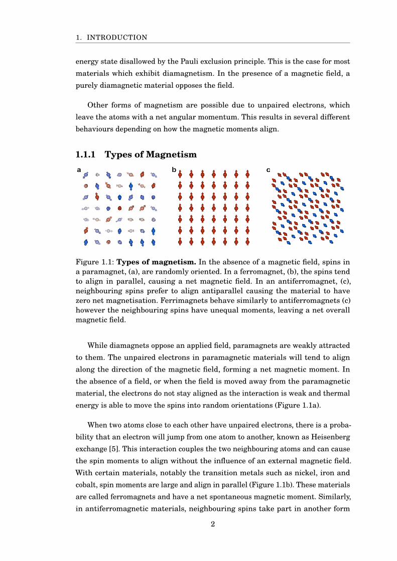
Figure 1.1: Types of magnetism. In the absence of a magnetic field, spins ina paramagnet, (a), are randomly oriented. In a ferromagnet, (b), the spins tendto align in parallel, causing a net magnetic field. In an antiferromagnet, (c),neighbouring spins prefer to align antiparallel causing the material to havezero net magnetisation. Ferrimagnets behave similarly to antiferromagnets (c)however the neighbouring spins have unequal moments, leaving a net overallmagnetic field.
While diamagnets oppose an applied field, paramagnets are weakly attracted
to them. The unpaired electrons in paramagnetic materials will tend to align
along the direction of the magnetic field, forming a net magnetic moment. In
the absence of a field, or when the field is moved away from the paramagnetic
material, the electrons do not stay aligned as the interaction is weak and thermal
energy is able to move the spins into random orientations (Figure 1.1a).
When two atoms close to each other have unpaired electrons, there is a proba-
bility that an electron will jump from one atom to another, known as Heisenberg
exchange [5]. This interaction couples the two neighbouring atoms and can cause
the spin moments to align without the influence of an external magnetic field.
With certain materials, notably the transition metals such as nickel, iron and
cobalt, spin moments are large and align in parallel (Figure 1.1b). These materials
are called ferromagnets and have a net spontaneous magnetic moment. Similarly,
in antiferromagnetic materials, neighbouring spins take part in another form
2
1. INTRODUCTION
of coupling where the spins are aligned antiparallel to each other. The material
is made up of two competing sublattices with equal moments which cause the
overall material to have a zero net magnetic moment and therefore no field.
One further state of ordered magnetism is called ferrimagnetism, which shares
some of the properties of ferro and antiferromagnets. In a ferrimagnet, two
competing sublattices exist where neighbouring spins align antiparallel, however
the moments on the electrons in each sublattice are unequal leading to a dominant
spin orientation in the material. Due to the dominant orientation, the material
exhibits a net magnetic moment. Ferrimagnetism was one of the last forms of
magnetic ordering to be discovered after research by Louis Néel in 1948[6]. From
this research we now know that the first magnetic material found in lodestones,
an iron oxide called magnetite, was a ferrimagnet.
1.2 Motivation for Research
The magnetic properties of small particles have become hugely important in
the last 50 years due to their intrinsic properties that make them ideal for
various applications. Nanoparticles can be made to relatively specific sizes, close
to the sizes of cells, proteins and genes, allowing them to interact with every
level of cellular biology. Depending on the material, these nanoparticles can be
biocompatible, such as magnetite which is readily detected in the brain [7], or in
the case of cobalt ferrite, where studies are still being performed to determine the
level of cytotoxicity [8], these nanoparticles can also be coated in biocompatible
non-magnetic materials.
Due to their magnetic properties, these particles can be manipulated by an
external magnetic field opening up a host of biomedical applications. Drug delivery
is a promising field due to the current problems caused by the usage of non-specific
chemicals which are administered in high dosages, causing significant side effects
[10–12]. The aim of magnetic carriers is to target specific sites and reduce the
amount of systemic distribution of the cytotoxic drug, reducing side effects. This
also leads to a reduction in dosage which further reduces adverse effects.
Varying magnetic fields can also be used, transferring energy from the exciting
field to the nanoparticle. Due to Néel relaxation, the particles then output energy
in the form of heat, which affects the surrounding area. The field of hyperthermia,
a form of cancer treatment, has seen groups around the world studying different
materials to find an ideal method of delivering toxic amounts of thermal energy
3
1. INTRODUCTION
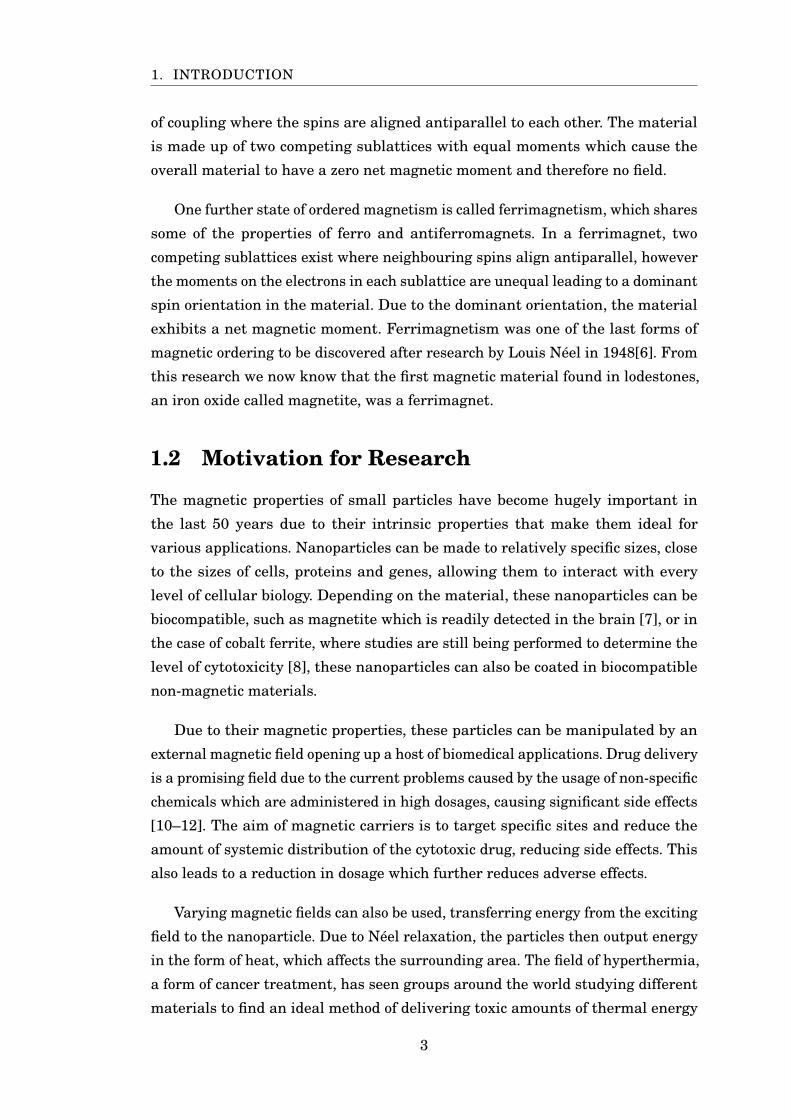
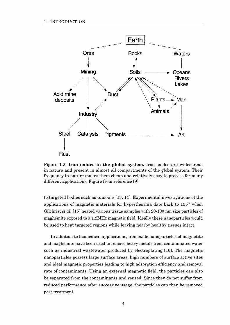
Figure 1.2: Iron oxides in the global system. Iron oxides are widespreadin nature and present in almost all compartments of the global system. Theirfrequency in nature makes them cheap and relatively easy to process for manydifferent applications. Figure from reference [9].
to targeted bodies such as tumours [13, 14]. Experimental investigations of the
applications of magnetic materials for hyperthermia date back to 1957 when
Gilchrist et al. [15] heated various tissue samples with 20-100 nm size particles of
maghemite exposed to a 1.2MHz magnetic field. Ideally these nanoparticles would
be used to heat targeted regions while leaving nearby healthy tissues intact.
In addition to biomedical applications, iron oxide nanoparticles of magnetite
and maghemite have been used to remove heavy metals from contaminated water
such as industrial wastewater produced by electroplating [16]. The magnetic
nanoparticles possess large surface areas, high numbers of surface active sites
and ideal magnetic properties leading to high adsorption efficiency and removal
rate of contaminants. Using an external magnetic field, the particles can also
be separated from the contaminants and reused. Since they do not suffer from
reduced performance after successive usage, the particles can then be removed
post treatment.
4
1. INTRODUCTION
Iron oxide nanoparticles have hugely benefited from recent research, and it is
now possible to consistently reproduce particles with a desired surface structure
[17]. Their surfaces frequently reconstruct, and the resulting surfaces can exhibit
markedly different electronic and magnetic structures to the bulk compound.
Interface engineering offers an interesting opportunity to improve performance
and apply the particles to newer fields of research such as spintronics where
studies into magnetite had recently stagnated due to the presence of a magnetic
dead layer at the interface [18]. It may now be possible to reconstruct the surface
of iron oxide nanoparticles to avoid this issue [17].
While years of research have gone into studying the formation of nanoparticles,
their surfaces and structure, far fewer studies have laid out an in-depth analysis
of the magnetic properties of the particles specific to their size and mineral
content. Surface effects drastically alter the properties of the particles away from
that of bulk, leading to more research being required to fully understand the
materials. Here, an opportunity for different methods of study arises. Most of
the applications mentioned here make use of iron oxide nanoparticles less than
30 nm in diameter, particularly in biomedical applications as above this size
particles will quickly be endocytosed by macrophages and removed from the body
[19]. At this scale it becomes more difficult to synthesise consistent nanoparticle
shapes and sizes however a different approach, such as theoretical modelling and
simulation, allows for studying these materials with relative ease and can help to
study more complex materials made up of different elements.
Micromagnetic modelling is a commonly used technique which helps to study
large uniform magnetic systems by treating continuous regions of similar spins
as single units and simulating the system by evaluating the magnetic properties
at each unit. For nanoparticles around 30 nm in size, a more detailed approach is
possible and, in many cases, necessary. In nanoparticles of this size, the number of
atoms is typically around 100 thousand to 1 million, making fine grain atomistic
simulations, which treat each atomic moment individually, possible on modest
hardware. This can lead to more detailed analysis of the systems under question,
revealing the properties of the system as well as any sublattices which exist in
more complex materials. In many systems, the spin configuration is also complex,
and cannot be grouped well into similar domains, leading to atomistic modelling
being the easiest way to accurately represent their structure.
This general approach to studying iron oxides is not new [20, 21], however it
is still nascent, with the current state of research requiring large scale approx-
5
1. INTRODUCTION
imations to modelling and the current output being low in resolution, dealing
with only the smallest scale nanoparticles around 6 nm in size, and few other
published data sets for particle shapes and sizes. In addition, not all materials
currently have the information available to be modelled accurately. In studies
which use the popular 3D Heisenberg model to simulate iron oxides, the largest
contribution to the magnetic properties of the system comes from the exchange
interaction of the neighbouring spins. These interactions can be defined by a set
of constants which are unique to each material. While for the most well studied
materials, such as magnetite, these values have been well studied, most other
iron oxides are simulated using borrowed sets of exchange from differing materi-
als, or use exchange values calculated from mean field models with significant
approximations, which have not been tested appropriately in multiple works and
show some disagreement with past studies.
This work attempts to bridge together the current available information on
three materials, the well-studied magnetite and its close neighbours maghemite
and cobalt ferrite. This is done by creating a complete set of atomistic models,
which agree well with current experimental data. In particular we study their
temperature scaling properties, as well as the finite size effects which affect
all systems at the nanometre scale. The VAMPIRE software package has been
used to create high quality data for these magnetic properties, as well as other
areas of interest such as spin switching, and core-shell nanoparticles made up of
combinations of these materials.
1.3 Thesis Outline
To start we shall cover the various methods used throughout the thesis in Chapter
2, with an in depth look at the 3D Heisenberg Hamiltonian and the methods
used to solve it as well as visualisation methods to better understand our results.
Chapter 3 then introduces the core elements of this thesis concerning magnetite,
its history, current state of understanding and finally simulations of the material
in bulk form, with Chapter 4 focusing on nanoparticles of magnetite and their
finite size effects. Chapters 5 and 6 cover similar materials in maghemite and
cobalt ferrite respectively, going over the differences of these materials and mag-
netite and performing similar simulations and analysis. Chapter 7 puts together
some of the information from previous chapters to look at mixed iron oxide core-
shell nanoparticles and how they behave depending on their constitution. Finally,
Chapter 8 concludes this thesis, covering the main points of the thesis as well as
6

1. INTRODUCTION
outlining future work.
7
CH
AP
TE
R
2MODELLING METHODS
2.1 Introduction
Modelling of magnetic materials has become a necessity for assessing and predict-
ing the usability of different materials for specific purposes. Without it, it would
be difficult for magnet based appliances to reach their current level of speed,
reliability and efficiency. Early models, such as that developed by Ernst Ising
[22], were used to understand phase changes in magnetic materials by modelling
the system as a lattice of spin-up or spin-down magnetic dipole moments. This
simplified system would be affected by heat but tend to equilibrium over time,
creating magnetic phases.
Most modern day magnetic materials modelling is done using micromagnetics
[23, 24] which predicts the behaviour of systems of sub-micrometer length scales.
While this approach is more complex that the Ising model it must still make
significant approximations; rather than account for every atomic spin, dipoles are
grouped forming a continuous vector field. Here it is assumed that due to exchange
interactions, the atomic dipoles within a small volume are mostly aligned and
their averaged behaviour is a good approximation to that of individual spins. One
of the downsides of this method is that it struggles to correctly model systems
where short range spin fluctuations are large or can deviate from nearby spins
quickly. In addition, non-uniform systems made up of multiple materials pose a
significant hurdle to micromagnetics as complex crystal structures often involve
short range interactions between divergent spins. To remedy this a different
approach is required, which gives up some of the benefits of micromagnetics in
8
2. MODELLING METHODS
being able to model very large uniform systems but instead allows for a much
higher resolution and detailed understanding of nanometre scale magnetism.
Atomistic modelling is now one of the most promising tools available in under-
standing magnetic materials. Atomistic spin models are based on the principle
that each atom possesses a local magnetic moment located on the lattice site. This
assumes that all the electrons are localised around the atom which could be at
odds with metals containing 3D outer electrons such as iron where the electrons
are loosely bound, however ab-initio calculations of the electron density show that
even in 3D ferromagnetic materials the spin polarisation is well localised to the
lattice site [25]. These localised moments are known as magnetic moments and
their magnitudes depend on the atomic species.
2.2 Heisenberg Hamiltonian
The Heisenberg spin model encapsulates the essential physical components of a
magnetic material at the atomic level. Its aim is to describe the interactions of
each atomic spin moment, µs, and its neighbouring moments within the system
and possible external magnetic field. The energy contributions of each interaction
are summed together to make up the overall energy of the system. Thus, the spin
Hamiltonian, H , can be written in the following form:
H =Hexchange +Hanisotropy +Happlied (2.1)
This describes the energy contributions of the exchange interaction, the
magnetic anisotropy and any externally applied magnetic field. The exchange
and anisotropy energies are intrinsic to the material however the applied field,
Happlied, is usually the result of an external system, such as a nearby magnetic
material or an effective field from an electric current. The energy of the applied
field is given by:
Happlied =−∑iµsSiBapplied (2.2)
where µs is the spin magnetic moment and Si the spin vector at site i. The lowest
energy configuration corresponds to the spins aligning along the applied field, B.
9
2. MODELLING METHODS
2.2.1 Exchange Interaction
The dominant contribution of the spin Hamiltonian in ferromagnetic materials is
the exchange field, which arises due to the symmetry of the electron wavefunc-
tion and the Pauli exclusion principle which affects the orientation of spins in
overlapping electron orbitals [26]. To understand how this interaction arises, we
can examine the simple case of the helium atom. Consider an electron in a state
ψa(r1) at r1 and another at state ψb(r2) at r2, the combined wavefunction of the
system, Ψ(r1,r2), can be defined as a linear combination of the individual election
wavefunctions which must be a solution to the Schrödinger equation:
Ψ(r1,r2)=ψa(r1)ψb(r2) (2.3)
[− ~2
2m∇2
1 −~2
2m∇2
2 −2e2
r1− 2e2
r2+ e2
r12
]Ψ(r1,r2)= EΨ(r1,r2) (2.4)
Here E is the energy of the system and is equal to Ea +Eb, the energy of
electrons a and b. r12 is the separation between the two electrons and corresponds
to the interaction between them. The electrons are indistinguishable therefore
ψa(r2)ψb(r1) is also a solution to the Schrödinger equation, hence the following
must be true:
|Ψ(r1,r2)|2 dr1dr2 = |Ψ(r2,r1)|2 dr1dr2 (2.5)
There are two possibilities from this equation: Ψsym, the wavefunction is
symmetric as Ψ(r1,r2) =Ψ(r2,r1) or the wavefunction is anti-symmetric, Ψanti,
as −Ψ(r1,r2)=Ψ(r2,r1). We can form a general solution to the wavefunction using
either state:
Ψsym(r1,r2)= 1p2
[ψa(r1)ψb(r2)+ψa(r2)ψb(r1)
](2.6)
Ψanti(r1,r2)= 1p2
[ψa(r1)ψb(r2)−ψa(r2)ψb(r1)
](2.7)
As electrons are bound by the Pauli exclusion principle, and two identical
electrons cannot occupy the same quantum state, the overall wavefunction must
10
2. MODELLING METHODS
be anti-symmetric. So far we have not included the spin component of the wave-
function, with α = spin up, β = spin down, which also come in symmetric and
anti-symmetric forms. There are eight possible configurations of the two electron
spin states [26]:
ψa(r1)αaψb(r2)αb ψb(r1)αaψa(r2)αb
ψa(r1)αaψb(r2)βb ψb(r1)βaψa(r2)αb
ψa(r1)βaψb(r2)αb ψb(r1)αaψa(r2)βb
ψa(r1)βaψb(r2)βb ψb(r1)βaψa(r2)βb
(2.8)
The anti-symmetric wavefunctions for the system can be constructed by taking
appropriate linear combinations of the products in 2.8. If the total wavefunction
is to be anti-symmetric, either the spin-dependent part must be anti-symmetric
and the spatial part symmetric, or vice versa. Doing this we end up with four
functions:
Ψ(r1,r2)= 1p2
[ψa(r1)ψb(r2)−ψa(r2)ψb(r1)
]αaαb
Ψ(r1,r2)= 1p2
[ψa(r1)ψb(r2)−ψa(r2)ψb(r1)
]βaβb
Ψ(r1,r2)= 1p2
[ψa(r1)ψb(r2)−ψa(r2)ψb(r1)
] 1p2
[αaβb +αbβa
]Ψ(r1,r2)= 1p
2
[ψa(r1)ψb(r2)+ψa(r2)ψb(r1)
] 1p2
[αaβb −αbβa
](2.9)
The spin components are eigenfunctions of the operators representing the
total spin, S, of the two particles and of their total z-component. In the first
three states the electron spins are aligned in parallel, while in the fourth they
are antiparallel. The first three functions have their total spin quantum number
S = 1, and the quantum numbers associated with the z-component equal to 1,
-1 and 0 respectively. Collectively, these states are known as a triplet ΨT , with
energy ET . The fourth function has zero spin, S = 0, and is know as a singlet
ΨS with energy ES. Hence we can condense the four states into two possible
wavefunctions:
ΨT = 1p2
[ψa(r1)ψb(r2)−ψa(r2)ψb(r1)
]χT
ΨS = 1p2
[ψa(r1)ψb(r2)+ψa(r2)ψb(r1)
]χS
(2.10)
11
2. MODELLING METHODS
with energies:
ET =∫ ∫
Ψ∗TH ΨT dr1dr2
ES =∫ ∫
Ψ∗SH ΨSdr1dr2
(2.11)
with the assumption that the spin parts of the wave function χT and χS are
normalised, the difference between the two energies is:
ES −ET = 2∫ ∫
ψ∗a(r1)ψ∗
b(r2)H ψa(r2)ψb(r1)dr1dr2 (2.12)
If we consider two spin half particles coupled by an exchange interaction, the
joint operator Stot = S1 ·S2, so S2tot = S2
1 +S22 +2S1 ·S2. Therefore, the difference
between single and triplet states can be parameterized by AS1 ·S2. Combining
these two particles results in a joint entity with spin quantum number S = 0
(singlet) or S = 1 (triplet) depending on the relative orientation of the two spins.
The eigenvalues of S2tot are S(S+1) so for the singlet case S1 ·S2 =−3/4 whereas
for the triplet case S1 ·S2 = 1/4 [27].
Hence the Hamiltonian can be written in the form:
H = 14
(ES +3ET)− (ES −ET)S1 ·S2 (2.13)
This Hamiltonian can be split into two terms, a radial component Hrad and
a spin component Hspin = (ES −ET)S1 ·S2. From this we define an exchange
constant, Jex:
Jex = 12
(ES −ET) (2.14)
or more simply the spin Hamiltonian is:
Hspin =−2JexS1 ·S2 (2.15)
When Jex is negative, an anti-ferromagnetic arrangement is more favourable
(ES < ET ), while if Jex is positive, a ferromagnetic arrangement is more favourable
12
2. MODELLING METHODS
(ET < ES). This is a simple example for the interactions of two identical electrons
however it forms the basis for more complex systems with higher numbers of
electrons. In the extended Heisenberg model, an approximation to the exchange
treats all spins in the systems as pairs of electrons leading to the overall exchange
Hamiltonian:
Hexchange =−∑i< j
Ji jSi ·S j (2.16)
where Si and S j are spins of atoms i and j. The form of Ji j depends on the form of
the interaction. In the simple case this interaction is isotropic, depending on the
relative orientation of the spins not their particular directions. In more complex
materials it forms a tensor with components:
J i j =
Jxx Jxy Jxz
Jyx Jyy Jyz
Jzx Jzy Jzz
(2.17)
In practice, the values of Ji j can be calculated (typically approximated) us-
ing ab-initio methods or by fitting experimental results [28, 29]. The energies of
exchange are around 1-2eV which is usually much larger than the next largest con-
tribution and gives rise to magnetic ordering temperatures around 300-1300K[30].
While equation 2.16 takes into account all spins in the system, the exchange
energy is dependent on the distance between each spin. The energy contributions
from spins further than second or third nearest neighbours is often small, hence
it is often approximated to be only nearest neighbour exchange.
2.2.2 Magnetocrystalline Anisotropy
While the exchange energy affects the interatomic spin interactions, the anisotropy
energy determines the preferred directions of the atomic moments. Anisotropy
can be caused by several different mechanisms, such as overall system structure
in the case of elongated particles, which causes an overall shape anisotropy as
the demagnetising field will not be equal for all directions causing spins to align
along the axis of elongation. The most common form of anisotropy is magnetocrys-
talline anisotropy which is a result of the crystal symmetries interacting with
the spin-orbit coupling of the electron. Magnetocrystalline anisotropy can form in
different flavours, the simplest being uniaxial anisotropy, where the spins prefer
to align along a single axis, called the easy axis. This form of anisotropy usually
13
2. MODELLING METHODS
exists when there is a distortion along a single axis of the material, such as in
hexagonal systems. The uniaxial single-ion anisotropy single energy is given by
the expression:
Huniaxial =−ku∑
i(Si ·e)2 (2.18)
where ku is the uniaxial anisotropy energy per atom and e is the easy axis
vector. In cubic systems a different form of magnetocrystalline anisotropy usually
occurs: cubic anisotropy. Materials such as iron and nickel have multiple preferred
anisotropy directions which are separated in energy level leading to one direction
being preferred. This type of anisotropy is usually much weaker than uniaxial
anisotropy. The axes are typically called the easy, medium and hard axes, in order
of increasing energy. Cubic anisotropy can be described by the following equation:
Hcubic =+kc
2
∑i
(S4x +S4
y +S4z) (2.19)
where kc is the cubic anisotropy energy per atom and Sx, Sy and Sz are the
components of the spin moment S.
2.3 Integration Methods
The Heisenberg Hamiltonian provides a robust method of finding the energy of the
system however methods for calculating time evolution or thermal fluctuations is
still required. In addition, it is important to show the temperature dependence of
the system as well as its ground state, therefore methods for relaxing the system
are also needed. There are several possible models that can find the ground state
of the system. Some require a time-dependent simulation of the system while
others are time-independent and relax to the ground state. Two such methods are
presented here: the stochastic Landau-Lifshitz-Gilbert equation for calculating
spin dynamics, and the Monte Carlo method for calculating static properties.
2.3.1 Spin Dynamics
Landau and Lifshitz [31] first described the time-dependent behaviour of a mag-
netic materials (specifically ferromagnets) by using equation 2.20, named after
its authors, created from looking at magnetic resonance experiments.
14
2. MODELLING METHODS
∂m∂t
=−γ[m×B+αm× (m×B)] (2.20)
Here, m is a unit vector describing the direction of the sample magnetisation,
B is the effective field acting on the system, γ called the gyromagnetic ratio is the
ratio of its magnetic moment to its angular momentum, and α, a phenomenological
damping constant which is dependent on the material. The physical origin of the
Landau-Lifshitz equation can be explained by splitting equation 2.20 into two
terms. The first refers to the quantum mechanical precession of spins around an
applied field. The second term containing the damping constant α accounts for
energy dissipation from the system. Energy transfer occurs due to the coupling
of the atomic moments to a heat bath. The strength of the coupling is linked to
the value of the damping constant, which determines how quickly the atomic
moments align to the applied field.
Gilbert would later show that this method yields incorrect dynamics for ma-
terials with high damping [32] and adjusted the damping parameter to have
a maximum value, called critical damping, when α = 1. The altered equation
is known as the Landau-Lifshitz-Gilbert equation, or LLG, and was originally
used to describe macroscopic magnetisation of a sample, however in principle the
equation applies equally well to micromagnetics and is often used in this field
[33].
The LLG can be formulated for atomistic simulations by excluding extrinsic
spin interactions, such as from demagnetising fields or surface defects. Here,
only intrinsic damping contributions from the spin-lattice and spin-electron in-
teractions are considered. To distinguish the macroscopic damping parameter α,
which includes all damping contributions, from the microscopic, we use a different
parameter, λ. The LLG equation can be described by:
∂Si
∂t=− γ
(1+λ2)[Si ×Bi
eff +λSi × (Si ×Bieff)] (2.21)
where Si is a unit vector representing the direction of the magnetic spin moment of
site i and Bieff is the net magnetic field on each spin. The atomistic LLG describes
the interaction of an atomic spin moment with an effective magnetic field. The
effective field at the site i can be calculated as:
Bieff =− 1
µs
∂H
∂Si(2.22)
15
2. MODELLING METHODS
where µs is the local spin moment.
2.3.2 Langevin dynamics
So far we have described the time-dependent behaviour of a system using the LLG
however equations 2.21 and 2.22 are independent of temperature and only apply
at zero Kelvin. At high temperatures, the magnetic properties of the system can
change completely as the energy of the temperature fluctuations becomes higher
than that of the exchange and the system transitions to a paramagnetic state.
To take this behaviour into account, Brown developed a new approach by using
Langevin Dynamics [34]. The thermal effects are modelled as a Gaussian white
noise term affecting each atomic site where increasing the temperature increases
the width of the Gaussian distribution. This in turn represents stronger thermal
fluctuations. The Gaussian distribution is three dimensional with a mean of zero
and the instantaneous thermal field on each spin is given by:
Bithermal =Γ(t)
√2λkBTγµs∆t
(2.23)
where kB = 1.38064852×10⁻²³ J is the Boltzmann constant, T the simulation
temperature, λ the Gilbert damping parameter, γ the gyromagnetic ratio, µs the
magnitude of the magnetic moment and ∆t the integration time step. Hence
combining equations 2.22 and 2.23 the modified effective field at site i is:
Bieff =− 1
µs
∂H
∂Si+Bi
thermal (2.24)
2.3.3 Time Integration of the LLG
An integration scheme is required to solve the LLG to determine the time evo-
lution of a system of spins. Due to the physical nature of the problem, there are
limitations on the solvers we can use. The principal requirement for a solver [35]
is that the magnitudes of the spins are conserved. The most simple but robust
solver that satisfies this requirement is the Euler method which assumes a linear
change in spin direction in a single time step. Nowadays the Euler method is
seldom used due to the popularity of improved Euler methods [36] such as the
Runge-Kutta family of methods, which are more stable and reduce the number of
steps required to calculate the next spin position.
16

2. MODELLING METHODS
A popular second order, two stage, Runge-Kutta method is known as the Heun
method [37] which employs a predictor-corrector algorithm allowing for larger
time steps and a possible large speed up in calculation time. The Heun scheme
does not conserve energy and must be continually renormalized to predict correct
dynamics. Despite other schemes existing which would intrinsically preserve
energy, there is often a computational cost incurred in their usage that outweighs
the possible benefits. Hence the simplicity and ease of application of the Heun
method makes it a popular choice in magnetics simulations[30, 37].
The predictor-corrector algorithm functions as follows: first the predictor step
calculates a spin direction S′i by performing one Euler integration step:
S′i =Si +∆S∆t (2.25)
where
∆S=− γ
(1+λ2)[Si ×Bi
eff +λSi × (Si ×Bieff)] (2.26)
The effective field is then recalculated with the predicted spin positions and
this step is repeated for every spin in the system. The corrector step then performs
another Euler integration step and uses the predicted spin positions and revised
field to calculate the final configuration by averaging the results. The completed
integration step is given by:
St+∆ti =Si + 1
2[∆S+∆S′]∆t (2.27)
where
∆S′ =− γ
(1+λ2)[S′
i ×Bi′eff +λS′
i × (S′i ×Bi′
eff)] (2.28)
The corrector step is also performed for every spin in the system and the overall
process is repeated many times to determine the time-dependent properties.
The speed of the algorithm is dependant on the size of the time step, ∆t.Ideally one would like to use the largest time step possible to simulate systems
quickly or for a long time. In micromagnetics, the minimum time step is a well
17
2. MODELLING METHODS
defined quantity since the largest field (typically the exchange term) defines the
precession frequency. For atomistic simulations using Langevin dynamics, the
effective field becomes temperature dependant. Hence for atomistic models, the
most difficult region to integrate is in the immediate vicinity of the Curie point.
This leads to a straight forward method for testing the parameter: a time step
size is chosen appropriately if the mean magnetisation varies smoothly around
the Curie temperature of the system. If the chosen time step is low enough, the
Heun scheme and LLG will be able to simulate realistic time-dependent dynamics
for magnetic systems.
2.3.4 Monte Carlo Methods
By using the LLG, an investigation of the time-dependent dynamics will reveal
realistic physical dynamics from the starting point of the simulation through to
the equilibrium point where the system is fully relaxed. In some cases, these
dynamics are not required and only the eventual equilibrium point is needed.
The Monte Carlo Metropolis algorithm is a simple but robust method that offers
a more optimal method to determine equilibrium properties when intermediate
dynamics are not necessary [38].
Applied to a classical spin system, the Monte Carlo Metropolis algorithm
works by choosing a random spin i, and changing its direction, Si, to a new trial
position S′i. The difference in energy ∆E = E(S′
i)−E(Si) between the initial and
final position is calculated and the trial move is accepted or rejected according to
a probability, P, such that:
P = exp(− ∆E
kBT
)(2.29)
If ∆E is negative, the final state is lower in energy and the trial move is
accepted (P > 1). If the probability is less than 1, and ∆E is positive, the value
is compared to a random number between 0-1 and the move is accepted if the
probability value is higher, allowing for thermal fluctuations to cause a small
increase in energy trial move. This process is repeated for every spin in the system
and after each move is accepted or rejected, the result is a single Monte Carlo
step.
The typical requirements for a Monte Carlo algorithm are ergodicity and
reversibility, i.e. all spin movements must be possible and the probability of a
move from position Si to S′i must be the same as the probability of a move from S′
i
18
2. MODELLING METHODS
to Si. The latter follows from equation 2.29 as the probability is only dependent
on the initial and final energies. The former, ergodicity, is also true as any spin
trial move is possible however their probabilities can be drastically different. At
high temperatures, most moves are roughly equally probable, however at low
temperatures, large spin deviations are very unlikely, leading to most trial moves
being rejected. For an efficient algorithm, an acceptance rate of around 50% is
desired.
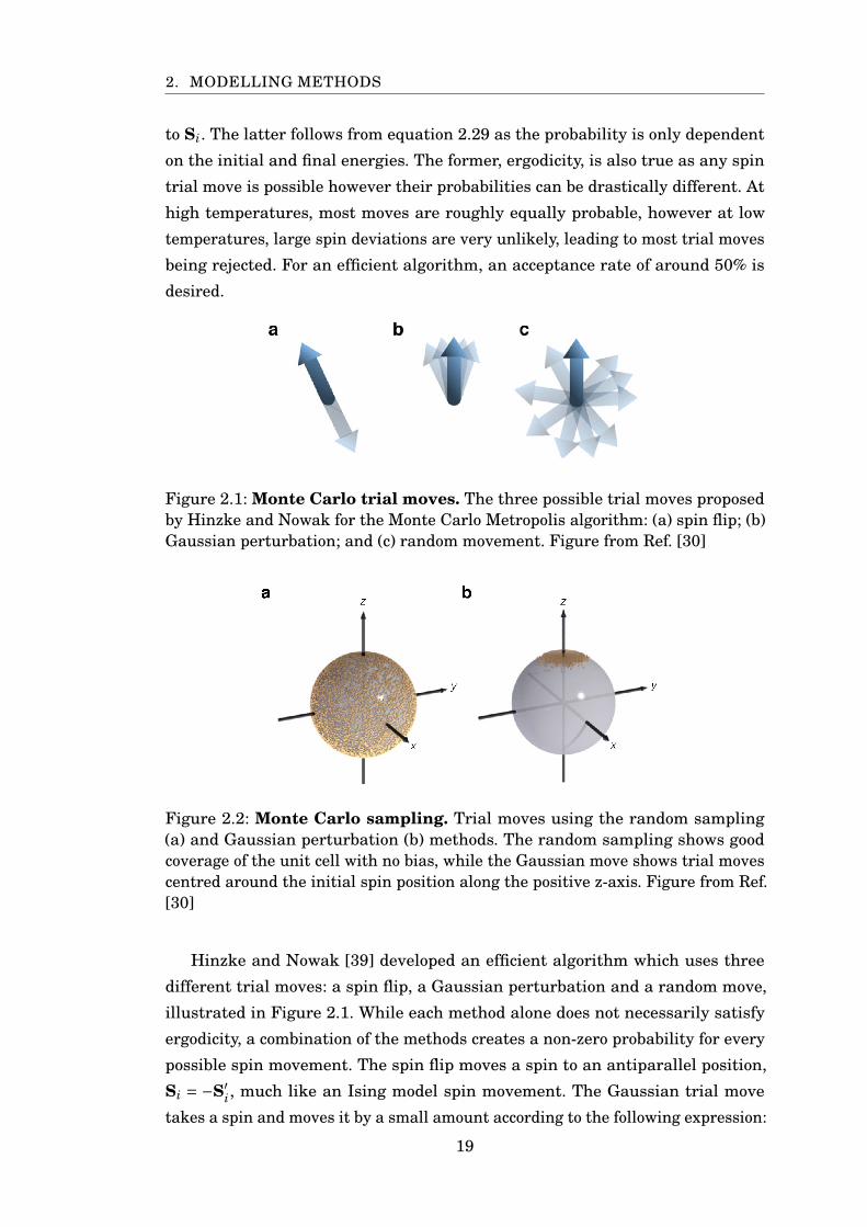
Figure 2.1: Monte Carlo trial moves. The three possible trial moves proposedby Hinzke and Nowak for the Monte Carlo Metropolis algorithm: (a) spin flip; (b)Gaussian perturbation; and (c) random movement. Figure from Ref. [30]
Figure 2.2: Monte Carlo sampling. Trial moves using the random sampling(a) and Gaussian perturbation (b) methods. The random sampling shows goodcoverage of the unit cell with no bias, while the Gaussian move shows trial movescentred around the initial spin position along the positive z-axis. Figure from Ref.[30]
Hinzke and Nowak [39] developed an efficient algorithm which uses three
different trial moves: a spin flip, a Gaussian perturbation and a random move,
illustrated in Figure 2.1. While each method alone does not necessarily satisfy
ergodicity, a combination of the methods creates a non-zero probability for every
possible spin movement. The spin flip moves a spin to an antiparallel position,
Si = −S′i, much like an Ising model spin movement. The Gaussian trial move
takes a spin and moves it by a small amount according to the following expression:
19
2. MODELLING METHODS
S′i =
Si +σgΓ
|Si +σgΓ|(2.30)
where σg is the width of a cone around the initial spin and Γ is a Gaussian
distributed random number. The size of the cone depends on temperature and is
usually of the form
σg = 225
(kBTµB
)1/5(2.31)
At low to medium temperatures, small spin movements are more likely, and
the Gaussian trial move is favoured. Finally, the random spin movement chooses
a position on the unit sphere according to
S′i =
Γ
|Γ| (2.32)
ensuring ergodicity for the complete algorithm. The three possible move are
performed one at a time, chosen randomly, for each spin in the system per Monte
Carlo step.
2.4 Temperature Rescaling
The Heisenberg model we have introduced can be used to effectively model mag-
netic materials of all forms, using ab initio or experimental input parameters to
produce well defined output. On comparison with experimental results however,
many properties such as temperature scaling behaviour of magnetisation or spe-
cific heat have been shown to depart from those expected from experiment. The
major contributing factor to this effect is the classical nature of the model, where
spins are defined as localised classical atomic spins si =µSi on the surface of the
unit sphere, |si| = 1. At the lowest level, magnetic materials, and in particular
spins, behave according to quantum mechanical effects and are constrained to
particular eigenvalues. While at the macroscopic level, a quantum mechanical
system and a classical one is able to take on all possible values of overall spin
direction due to an averaging out of individual spins, this does not yield the same
thermodynamic effects.
To remedy the disparity between quantum and classical models, a tempera-
ture rescaling mechanism has been developed by Evans et al. [40]. To derive an
20
2. MODELLING METHODS
appropriate scaling method, we compare the magnetisation and temperature rela-
tionship for each approach. First we consider the total magnetisation M(T)= ⟨S⟩and the normalised magnetisation m(T)= M(T)/M(0K). In the low temperature
limit, m can be calculated as:
m = 1− 1N
∑k
nk (2.33)
where N is the number of spins and the sum is over the spin-wave occupation
number of wave vector k. Classically, the occupation number of a spin wave of
energy εk corresponds to the high-temperature limit of the Boltzmann law in
reciprocal space:
nk = kBT/εk (2.34)
however quantum mechanically they are bosonic modes of the spin lattice and
therefore follow the Bose-Einstein distribution:
nk = 1/[exp(εk/kBT)−1] (2.35)
The spin wave energy should be the same irrespective of the model used, hence
the difference in the magnetisation predicted by quantum and classical models
is due to their different statistical behaviours. We now examine the behaviour of
both models in a low and high temperature phase. At low temperatures equation
2.33 has a well-known result [41]:
mclassical(T)≈ 1− 13
TTC
(2.36)
where TC is the Curie temperature which has the same value for both classical
and quantum systems. Similarly in the quantum Heisenberg case:
mquantum(T)≈ 1− 13
s(
TTC
)3/2(2.37)
we obtain the Bloch law [26]. Here s is a slope factor which is a function of the
spin quantum number, the Watson integral and the Riemann ζ function. Equating
equations 2.36 and 2.37 we find:
21
2. MODELLING METHODS
Tclassical
TC= s
(Tquantum
TC
)3/2(2.38)
which relates the low temperature quantum magnetisation to a rescaled classical
magnetisation. In the high temperature phase close to TC, the spin-wave energy
is high and ε/kBT → 0. Hence 1/[exp(εk/kBT)−1] ≈ εk/kBT. Spin quantisation
is therefore not a factor in the high temperature phase. At high temperatures
the magnetisation should scale according to a power law, m(τ)= (1−τ)β, where
τ= T/TC and β is a critical exponent often cited as 1/3 for the Heisenberg model
[42].
The low temperature behaviour of classical and quantum systems can be
related using a relatively simple equation and the high temperature behaviour for
both cases tends to equality. Evans [40] suggests that a good relation between both
regimes for all temperatures can be modelled using the Curie-Bloch equation:
M(τ)= (1−τα)β (2.39)
This equation is a direct extrapolation of low temperature behaviour according
to Bloch’s law and high temperature behaviour near the critical exponent. α is
the only fitting parameter required to relate the classical and quantum scaling at
all temperatures. With the assumption that β is the same for both classical and
quantum systems, we can fit experimental data using equation 2.39 to find the
appropriate value of α for our system. We are then able to rescale the temperatures
of simulated results according to:
Tsim
TC=
(Texp
TC
)α(2.40)
which should yield results much closer to experiment with a better qualitative
magnetisation scaling. This technique has already been applied to elemental
ferromagnets and shows very good agreement with the experimentally measured
magnetisations for all studied materials [40].
2.5 VAMPIRE Software Package
The modelling methods explained in this chapter have been implemented into
VAMPIRE, an open-source atomistic spin dynamics software package developed
22
2. MODELLING METHODS
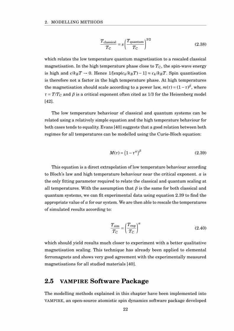
Figure 2.3: Rescaling applied to Fe and Co. Blue points show the simulateddata points using a Monte Carlo approach. These are fit using the Curie-Blochequation and shown with blue curves. The gold curves show the experimentallymeasured temperature-dependent magnetisation, Ref. [43] for cobalt, (a), and Ref.[44] for iron, (b). The gold points are the simulated data points, rescaled usingequation 2.40. Both sets of data show excellent agreement with experimentalresults. Insets are plots of relative error of the rescaled magnetisation comparedto the experimental data. Figure from Ref. [40].
at the University of York [30]. This package is authored by Richard Evans and
the computational magnetism group at the University of York and is available
for personal research according to the rules of the GNU General Public License
or GPL. The code base is written in C++ and can run on most hardware, in
either serial, parallel or GPU modes. Most results in this thesis are calculated
using the VAMPIRE software package which handles simulation as well as data
output. In addition, this work made extensive use of the Viking Cluster, a high
performance compute facility provided by the University of York, which was used
to run VAMPIRE.
2.6 Visualisation
The VAMPIRE software package outputs data such as temperature or magnetisa-
tion values in plain text. Most of the plots using the data presented in the thesis
are made using Gnuplot [45], a portable command-line driven graphing utility.
In addition to raw data, VAMPIRE is able to output spin coordinate data such as
positions and spin directions for output using external programs. Atomic positions
can be displayed using chemical structure visualisation software such as Jmol
[46] or Rasmol [47].
A component of the work done for this thesis was rewriting the spin’s direction
visualisation output in VAMPIRE. Alongside common simulation output such as
23
2. MODELLING METHODS
magnetisation or field strength which are easily accessible from the data output,
system visualisation forms a crucial component of data analysis as it provides a
more easily readable form of visual output, as well as allowing for much easier
system set up and testing. As ferro, ferri and anti-ferromagnetic systems have
significantly different spin structures, spin visualisation is a relatively quick and
easy method for parameter verification before starting simulations. Visualisation
of the initial system state can save hours of wasted simulation time by catching
simple errors in system set-up. In addition, spin visualisation can complement
plots of output data as together they form a more complete picture of the magnetic
properties being investigated. To render this data, external programs such as
POV-Ray [48] are used.
The reliability of spin visualisation is therefore of crucial importance both to
the user and to any desired recipients of the final data. A significant issue with
spin visualisation is the type of colour map and its parent colour space used to
colour individual elements. A colour map can be thought of as a line or curve
drawn through a three dimensional colour space, or an organisation of colours
collected arbitrarily or by using mathematical rigour (for example Adobe RGB
or sRGB [49]). An effective colour map presents a list of colours which can be
structured and allows the communication of metric information. The latter has
become a common issue in widely used vendor colour maps due to a few different
factors separate to those related to the representation when displayed digitally
due to viewing angle or display calibration. Colours can be represented as a
tuple of values between 0-255(RGB) or 0-1(HSL) and while it is possible to create
a colour map consisting of equally spaced positions between these values, the
relationship between the distance of the colours from each other is non-linear with
human perception of colour difference. It is therefore common for colour maps to
contain perceptually uniform or flat regions of colour which may vary significantly
in RGB value but be very difficult to distinguish using only human perception.
Put differently, human perception can cause distinct groups of colours to become
essentially indistinguishable from each other leading to a loss or corruption in
conveyed information. While not directly related, colour maps used to address
colour blindness can also be adjusted. In addition to colour, lightness can pose
another barrier due to high brightness or saturation causing perceived colour
blending [50]. Most studies looking at colour perception in scientific data analysis
have been restricted to cartographic applications [51, 52] however inspired by the
work done by Peter Kovesi [53] this theory has been applied to the visualisation
output of VAMPIRE.
24
2. MODELLING METHODS
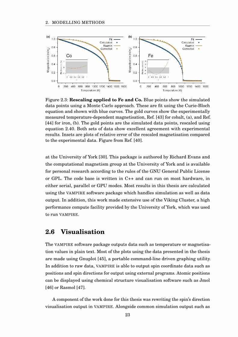
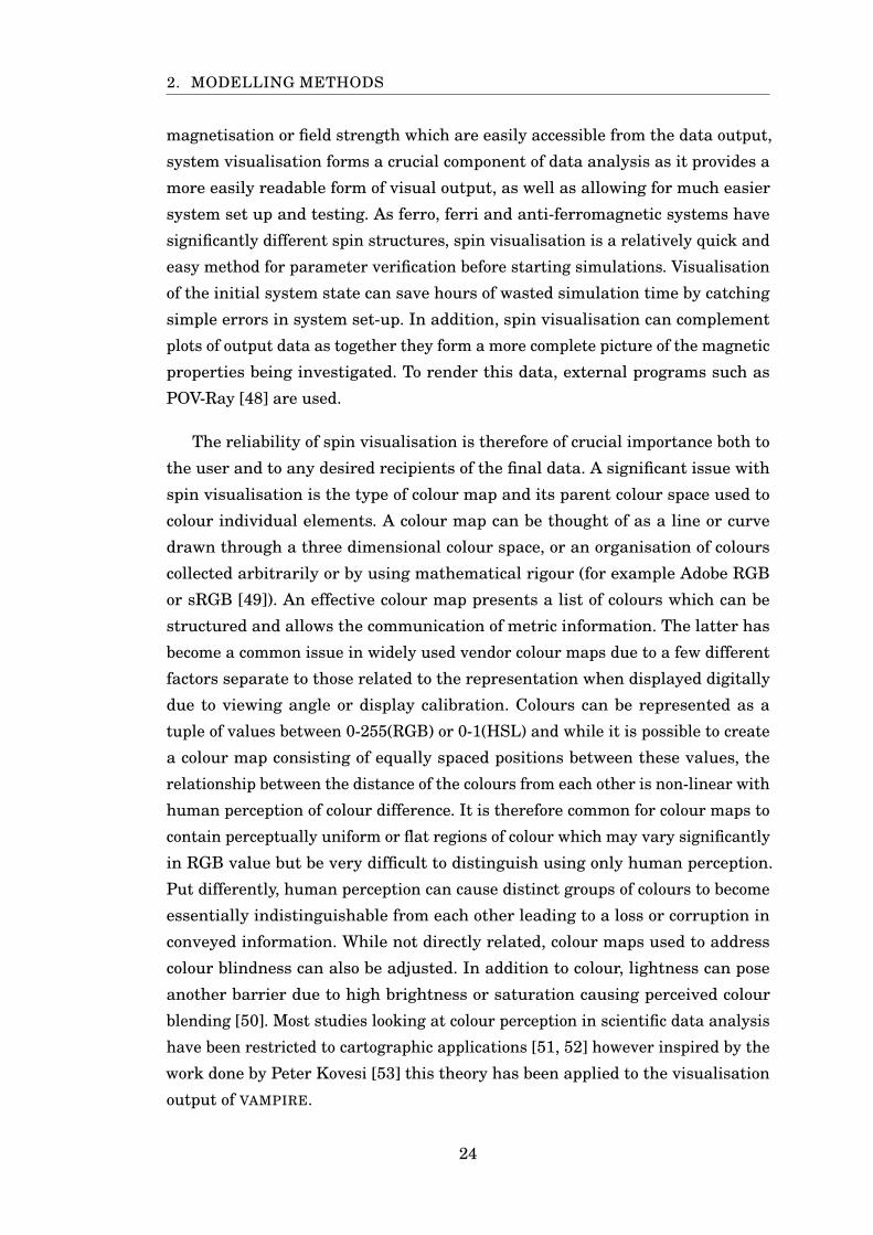
Figure 2.4: Comparison of commonly used colour maps and perceptuallyuniform colour maps designed by Kovesi [53]. To show their differences theyare shown on top of a sine wave gradient superimposed on a ramp function whichprovides a set of constant magnitude features presented at different offsets. Highsaturation regions such as red or green are blurred in the base colour maps butcan be adjusted to have reduced intensity and higher perceptual uniformity inthe modified maps. Image from Ref. [54]
This change is particularly relevant to spin direction visualisation as the data
varies over a continuous range, leading to high likelihoods of similarly oriented
groups of spins positioned closely to each other. As an example, consider a system
in a low temperature regime being modelled using the Monte Carlo method
explained earlier. Due to the low temperature, the most likely Monte Carlo trial
move is the Gaussian move as spin flips and random movements occur when the
system is higher in energy and are more likely to be rejected. This would lead to
small spin deviations centred around the initial positions of the spins. Depending
on the colour map used, deviations from the initial spin direction by as much as
10% can appear as the same colour as the initial direction leading to a simple
misunderstanding of the generated results. Vortex configuration systems, such as
permalloy [55], pose a significant issue as they are usually represented by a colour
wheel which uses a high saturation continuous colour spectrum, susceptible to
reduced colour perception.
To remedy this issue, where possible, any spin visualisation shown in this
thesis is made using a perceptually uniform colour map which makes as clear
as possible the difference in similar value spin orientations while making little
25
2. MODELLING METHODS
sacrifice in colour fidelity and visual appeal. A comparison of colour maps used in
this work and common maps supplied by different vendors is shown in Figures
2.4 and 2.5.
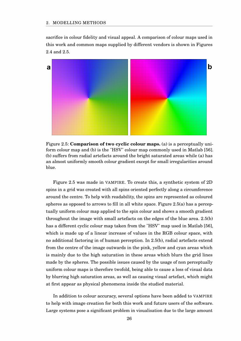
Figure 2.5: Comparison of two cyclic colour maps. (a) is a perceptually uni-form colour map and (b) is the "HSV" colour map commonly used in Matlab [56].(b) suffers from radial artefacts around the bright saturated areas while (a) hasan almost uniformly smooth colour gradient except for small irregularities aroundblue.
Figure 2.5 was made in VAMPIRE. To create this, a synthetic system of 2D
spins in a grid was created with all spins oriented perfectly along a circumference
around the centre. To help with readability, the spins are represented as coloured
spheres as opposed to arrows to fill in all white space. Figure 2.5(a) has a percep-
tually uniform colour map applied to the spin colour and shows a smooth gradient
throughout the image with small artefacts on the edges of the blue area. 2.5(b)
has a different cyclic colour map taken from the "HSV" map used in Matlab [56],
which is made up of a linear increase of values in the RGB colour space, with
no additional factoring in of human perception. In 2.5(b), radial artefacts extend
from the centre of the image outwards in the pink, yellow and cyan areas which
is mainly due to the high saturation in these areas which blurs the grid lines
made by the spheres. The possible issues caused by the usage of non perceptually
uniform colour maps is therefore twofold, being able to cause a loss of visual data
by blurring high saturation areas, as well as causing visual artefact, which might
at first appear as physical phenomena inside the studied material.
In addition to colour accuracy, several options have been added to VAMPIRE
to help with image creation for both this work and future users of the software.
Large systems pose a significant problem in visualisation due to the large amount
26
2. MODELLING METHODS
of memory and rendering time required for hundreds of millions of spins. To help
with this, it is possible to ignore spins behind the outer layer of atoms, which
are required for the simulation but can be effectively removed for visualisation
purposes. In addition, sometimes it is only the spins on a cross section or within the
block of simulated material that is of particular interest. With the latest changes,
it is possible to cut a cross section of the system to reveal a plane of spins across
any axis. Finally, the last option added to VAMPIRE POV-Ray visualisation is suited
to ferri or antiferromagnetic materials as it can flip the colour of antiparallel
spins. In antiferromagnetic materials, two competing sublattices show up in
visualisation as antiparallel arrows in different colours. Due to the change in
colour, the overall image exhibits a blurry quality as the two opposite colours
are on adjacent spins. To remedy this, the usual arrow shape of the spins are
conserved, making it obvious that the material is still antiferromagnetic, however
the colours of one sublattice are swapped to match those opposing. This makes
the overall direction of the spins more obvious, hence domains of spins oriented in
slightly different directions can be more easily identified.
Almost all these additions have been used in creating visualisation for this
thesis and are now implemented in the latest available versions of the VAMPIRE
software package.
2.7 Conclusion
In this chapter we have discussed the fundamentals of atomistic spin models,
simulation methods for finding both time-dependant and time-independent states
of magnetic systems, and visualisation methods for better understanding our
results. In the next chapter we shall apply these methods to magnetite, a well-
known magnetic material, to better understand its magnetic properties in both
bulk and nanoparticle form.
27

CH
AP
TE
R
3MAGNETITE
3.1 Introduction
Magnetite is the oldest known magnetic substance, found in lodestones, it was
the first major discovery of magnetism by ancient peoples. It is also the most
magnetic of all the naturally occurring minerals on Earth. On its own, it does
not ordinarily retain a permanent magnetisation, however with the inclusion of
minerals such as ions of titanium and manganese, its coercivity rises enough to
be a permanent magnet [57]. Pieces of magnetite were used in China as early as
300BC as compasses, and references to lodestones can be found in Greek texts
such as "Theogony" by Hesiod, where the Titan Cronus was given a lump of
magnetite instead of his son Zeus. In addition, the mineral was also broken down
as a source for iron, which gave the first glimpse into the crystal structure of the
material.
Magnetite is an iron oxide known as a ferrite, initially thought to be ferro-
magnetic such as plain iron. In a paper published in 1948, L. Néel showed that
this was not the case and that there existed several distinct forms of magnetism,
magnetite itself being ferrimagnetic [6]. Ferrimagnets were found to behave some-
what similarly to ferromagnets, both carrying a spontaneous magnetisation which
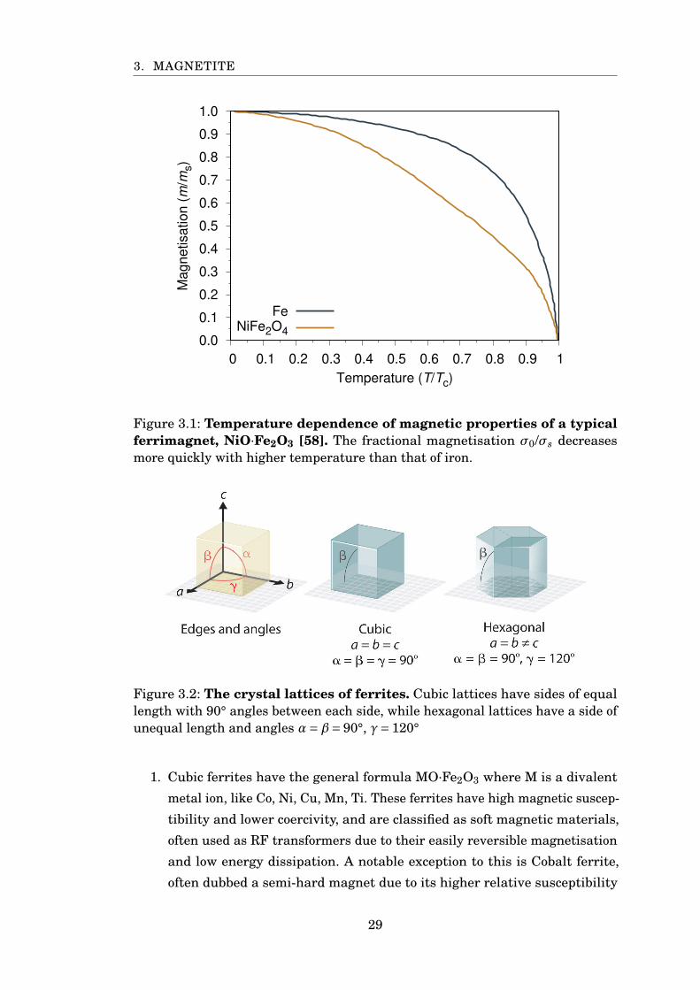
disappears above a critical point, Figure 3.1. The magnetic properties of ferrites
are a result of their complex crystal structures.
Ferrites can be divided into two major groups, also shown in Figure 3.2:
28
3. MAGNETITE
0.0
0.1
0.2
0.3
0.4
0.5
0.6
0.7
0.8
0.9
1.0
0 0.1 0.2 0.3 0.4 0.5 0.6 0.7 0.8 0.9 1
Magnetisation (
m/m
s)
Temperature (T/Tc)
FeNiFe2O4
Figure 3.1: Temperature dependence of magnetic properties of a typicalferrimagnet, NiO·Fe2O3 [58]. The fractional magnetisation σ0/σs decreasesmore quickly with higher temperature than that of iron.
Figure 3.2: The crystal lattices of ferrites. Cubic lattices have sides of equallength with 90° angles between each side, while hexagonal lattices have a side ofunequal length and angles α=β= 90°, γ= 120°
1. Cubic ferrites have the general formula MO·Fe2O3 where M is a divalent
metal ion, like Co, Ni, Cu, Mn, Ti. These ferrites have high magnetic suscep-
tibility and lower coercivity, and are classified as soft magnetic materials,
often used as RF transformers due to their easily reversible magnetisation
and low energy dissipation. A notable exception to this is Cobalt ferrite,
often dubbed a semi-hard magnet due to its higher relative susceptibility
29
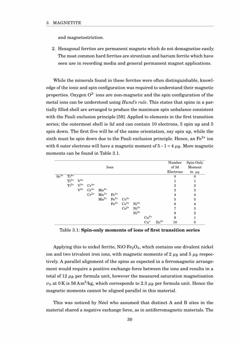
3. MAGNETITE
and magnetostriction.
2. Hexagonal ferrites are permanent magnets which do not demagnetise easily.
The most common hard ferrites are strontium and barium ferrite which have
seen use in recording media and general permanent magnet applications.
While the minerals found in these ferrites were often distinguishable, knowl-
edge of the ionic and spin configuration was required to understand their magnetic
properties. Oxygen O2- ions are non-magnetic and the spin configuration of the
metal ions can be understood using Hund’s rule. This states that spins in a par-
tially filled shell are arranged to produce the maximum spin unbalance consistent
with the Pauli exclusion principle [59]. Applied to elements in the first transition
series; the outermost shell is 3d and can contain 10 electrons, 5 spin up and 5
spin down. The first five will be of the same orientation, say spin up, while the
sixth must be spin down due to the Pauli exclusion principle. Hence, an Fe2+ ion
with 6 outer electrons will have a magnetic moment of 5−1= 4 µB. More magnetic
moments can be found in Table 3.1.
IonsNumber
of 3dElectrons
Spin-OnlyMoment
in µBSc3+ Ti4+ 0 0
Ti3+ V4+ 1 1Ti2+ V3+ Cr4+ 2 2
V2+ Cr3+ Mn4+ 3 3Cr2+ Mn3+ Fe4+ 4 4
Mn2+ Fe3+ Co4+ 5 5Fe2+ Co3+ Ni4+ 6 4
Co2+ Ni3+ 7 3Ni2+ 8 2
Cu2+ 9 1Cu+ Zn2+ 10 0
Table 3.1: Spin-only moments of ions of first transition series
Applying this to nickel ferrite, NiO·Fe2O3, which contains one divalent nickel
ion and two trivalent iron ions, with magnetic moments of 2 µB and 5 µB respec-
tively. A parallel alignment of the spins as expected in a ferromagnetic arrange-
ment would require a positive exchange force between the ions and results in a
total of 12 µB per formula unit, however the measured saturation magnetisation
σ0 at 0 K is 56 Am2/kg, which corresponds to 2.3 µB per formula unit. Hence the
magnetic moments cannot be aligned parallel in this material.
This was noticed by Néel who assumed that distinct A and B sites in the
material shared a negative exchange force, as in antiferromagnetic materials. The
30
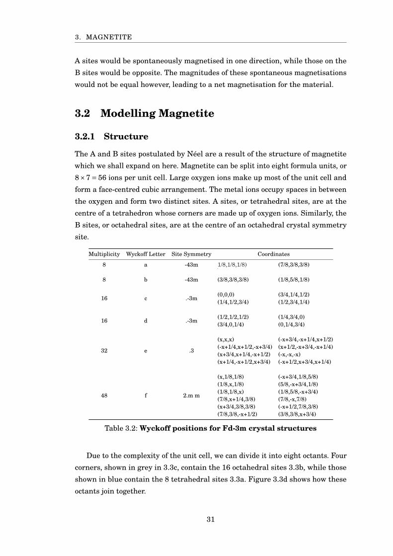
3. MAGNETITE
A sites would be spontaneously magnetised in one direction, while those on the
B sites would be opposite. The magnitudes of these spontaneous magnetisations
would not be equal however, leading to a net magnetisation for the material.
3.2 Modelling Magnetite
3.2.1 Structure
The A and B sites postulated by Néel are a result of the structure of magnetite
which we shall expand on here. Magnetite can be split into eight formula units, or
8×7= 56 ions per unit cell. Large oxygen ions make up most of the unit cell and
form a face-centred cubic arrangement. The metal ions occupy spaces in between
the oxygen and form two distinct sites. A sites, or tetrahedral sites, are at the
centre of a tetrahedron whose corners are made up of oxygen ions. Similarly, the
B sites, or octahedral sites, are at the centre of an octahedral crystal symmetry
site.
Multiplicity Wyckoff Letter Site Symmetry Coordinates
8 a -43m 1/8,1/8,1/8) (7/8,3/8,3/8)
8 b -43m (3/8,3/8,3/8) (1/8,5/8,1/8)
(0,0,0) (3/4,1/4,1/2)16 c .-3m
(1/4,1/2,3/4) (1/2,3/4,1/4)
(1/2,1/2,1/2) (1/4,3/4,0)16 d .-3m
(3/4,0,1/4) (0,1/4,3/4)
(x,x,x) (-x+3/4,-x+1/4,x+1/2)(-x+1/4,x+1/2,-x+3/4) (x+1/2,-x+3/4,-x+1/4)(x+3/4,x+1/4,-x+1/2) (-x,-x,-x)
32 e .3
(x+1/4,-x+1/2,x+3/4) (-x+1/2,x+3/4,x+1/4)
(x,1/8,1/8) (-x+3/4,1/8,5/8)(1/8,x,1/8) (5/8,-x+3/4,1/8)(1/8,1/8,x) (1/8,5/8,-x+3/4)(7/8,x+1/4,3/8) (7/8,-x,7/8)(x+3/4,3/8,3/8) (-x+1/2,7/8,3/8)
48 f 2.m m
(7/8,3/8,-x+1/2) (3/8,3/8,x+3/4)
Table 3.2: Wyckoff positions for Fd-3m crystal structures
Due to the complexity of the unit cell, we can divide it into eight octants. Four
corners, shown in grey in 3.3c, contain the 16 octahedral sites 3.3b, while those
shown in blue contain the 8 tetrahedral sites 3.3a. Figure 3.3d shows how these
octants join together.
31
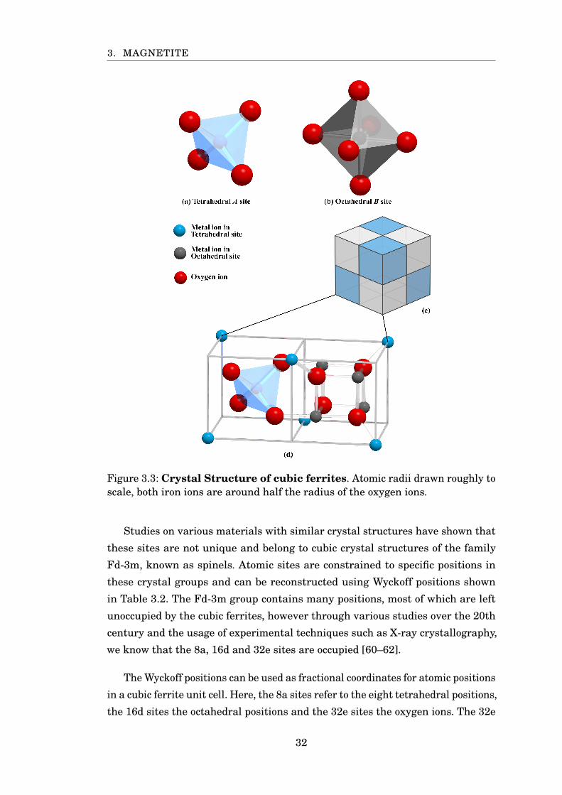
3. MAGNETITE
Figure 3.3: Crystal Structure of cubic ferrites. Atomic radii drawn roughly toscale, both iron ions are around half the radius of the oxygen ions.
Studies on various materials with similar crystal structures have shown that
these sites are not unique and belong to cubic crystal structures of the family
Fd-3m, known as spinels. Atomic sites are constrained to specific positions in
these crystal groups and can be reconstructed using Wyckoff positions shown
in Table 3.2. The Fd-3m group contains many positions, most of which are left
unoccupied by the cubic ferrites, however through various studies over the 20th
century and the usage of experimental techniques such as X-ray crystallography,
we know that the 8a, 16d and 32e sites are occupied [60–62].
The Wyckoff positions can be used as fractional coordinates for atomic positions
in a cubic ferrite unit cell. Here, the 8a sites refer to the eight tetrahedral positions,
the 16d sites the octahedral positions and the 32e sites the oxygen ions. The 32e
32
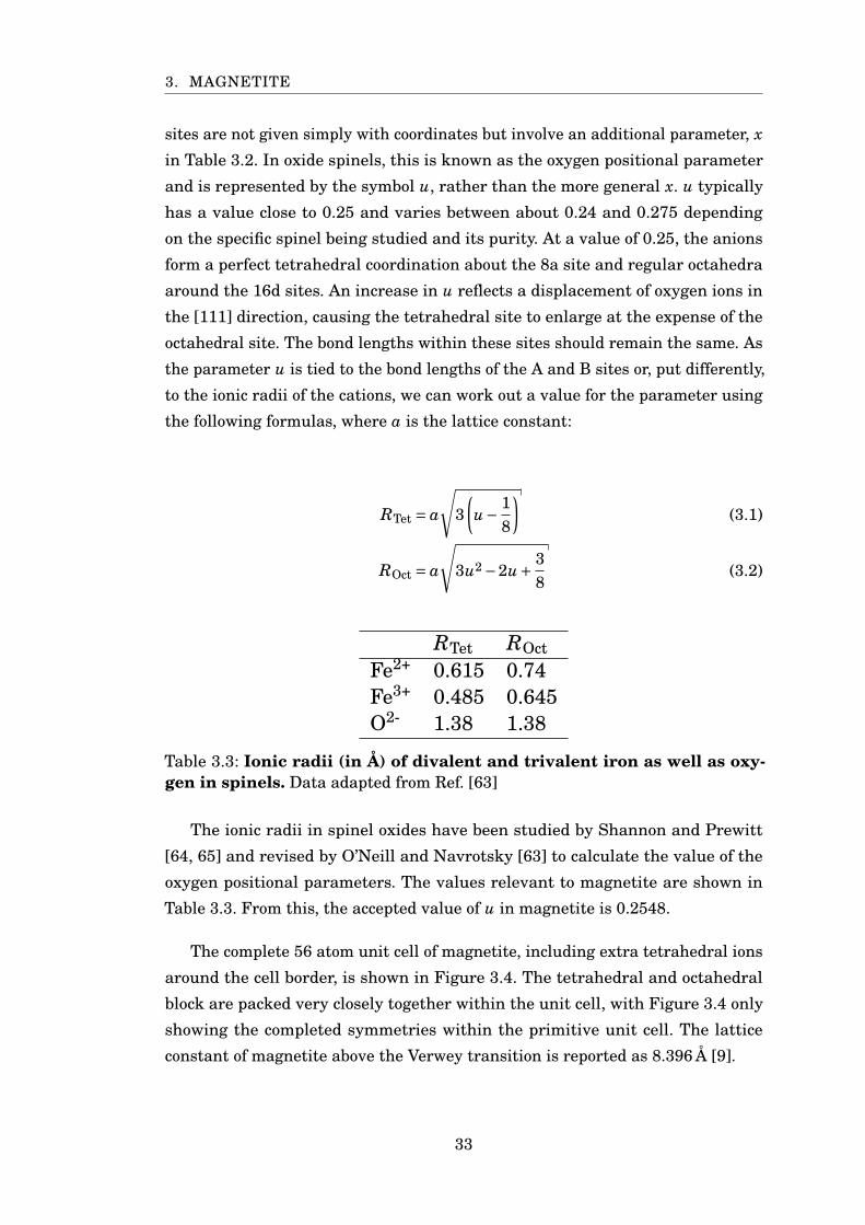
3. MAGNETITE
sites are not given simply with coordinates but involve an additional parameter, xin Table 3.2. In oxide spinels, this is known as the oxygen positional parameter
and is represented by the symbol u, rather than the more general x. u typically
has a value close to 0.25 and varies between about 0.24 and 0.275 depending
on the specific spinel being studied and its purity. At a value of 0.25, the anions
form a perfect tetrahedral coordination about the 8a site and regular octahedra
around the 16d sites. An increase in u reflects a displacement of oxygen ions in
the [111] direction, causing the tetrahedral site to enlarge at the expense of the
octahedral site. The bond lengths within these sites should remain the same. As
the parameter u is tied to the bond lengths of the A and B sites or, put differently,
to the ionic radii of the cations, we can work out a value for the parameter using
the following formulas, where a is the lattice constant:
RTet = a
√3
(u− 1
8
)(3.1)
ROct = a
√3u2 −2u+ 3
8(3.2)
RTet ROctFe2+ 0.615 0.74Fe3+ 0.485 0.645O2- 1.38 1.38
Table 3.3: Ionic radii (in Å) of divalent and trivalent iron as well as oxy-gen in spinels. Data adapted from Ref. [63]
The ionic radii in spinel oxides have been studied by Shannon and Prewitt
[64, 65] and revised by O’Neill and Navrotsky [63] to calculate the value of the
oxygen positional parameters. The values relevant to magnetite are shown in
Table 3.3. From this, the accepted value of u in magnetite is 0.2548.
The complete 56 atom unit cell of magnetite, including extra tetrahedral ions
around the cell border, is shown in Figure 3.4. The tetrahedral and octahedral
block are packed very closely together within the unit cell, with Figure 3.4 only
showing the completed symmetries within the primitive unit cell. The lattice
constant of magnetite above the Verwey transition is reported as 8.396 Å [9].
33
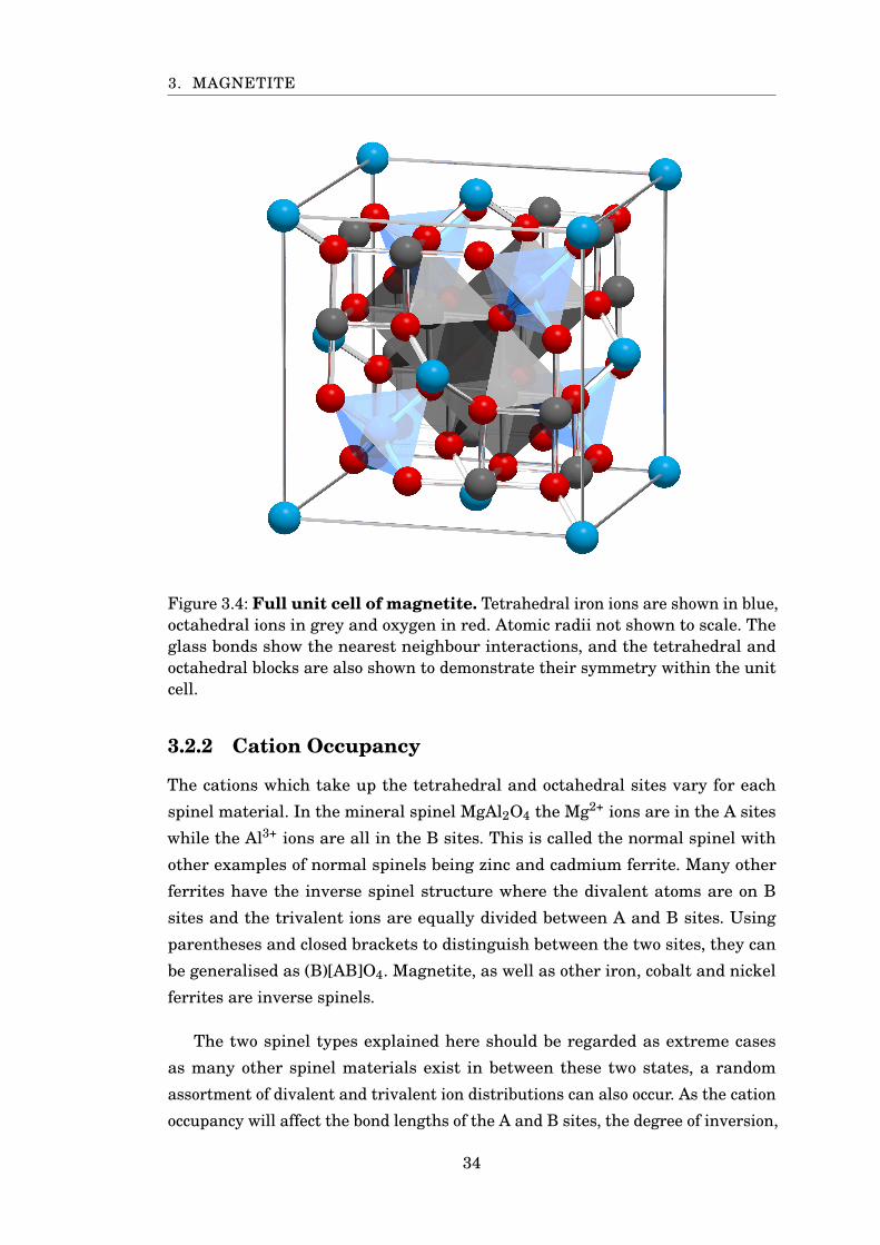
3. MAGNETITE
Figure 3.4: Full unit cell of magnetite. Tetrahedral iron ions are shown in blue,octahedral ions in grey and oxygen in red. Atomic radii not shown to scale. Theglass bonds show the nearest neighbour interactions, and the tetrahedral andoctahedral blocks are also shown to demonstrate their symmetry within the unitcell.
3.2.2 Cation Occupancy
The cations which take up the tetrahedral and octahedral sites vary for each
spinel material. In the mineral spinel MgAl2O4 the Mg2+ ions are in the A sites
while the Al3+ ions are all in the B sites. This is called the normal spinel with
other examples of normal spinels being zinc and cadmium ferrite. Many other
ferrites have the inverse spinel structure where the divalent atoms are on B
sites and the trivalent ions are equally divided between A and B sites. Using
parentheses and closed brackets to distinguish between the two sites, they can
be generalised as (B)[AB]O4. Magnetite, as well as other iron, cobalt and nickel
ferrites are inverse spinels.
The two spinel types explained here should be regarded as extreme cases
as many other spinel materials exist in between these two states, a random
assortment of divalent and trivalent ion distributions can also occur. As the cation
occupancy will affect the bond lengths of the A and B sites, the degree of inversion,
34
3. MAGNETITE
or the fraction of tetrahedral sites which are occupied by trivalent atoms also has
a large effect on the oxygen positional parameter mentioned previously.
3.2.3 Phase Changes
Néel’s paper [6] on ferrites prompted further studies into the magnetic properties
of these materials however years earlier it was a paper written by Evert Verwey
which began a still ongoing study into the electronic structure of magnetite [66].
In it he started with some of the assumptions we have so far covered concerning
the mixed B site occupation of Fe2+ and Fe3+ ions;
“Fe3O4 has a very remarkable crystal structure involving a probably statistical
distribution of both Fe2+ and Fe3+ ions at equivalent lattice points.”
In this paper, Verwey examined a transition in the properties of magnetite
around 120 K. He cited changes in the magnetic properties, specific heat and
lattice constant of the material. This anomaly would come to be recognised as a
first-order phase transition later named after Verwey. At 124 Kelvin, magnetite
undergoes a structural change becoming monoclinic, the lattice parameters a, b, care no longer equal and the angles are no longer all 90°. The exact causes for this
transition are still heavily debated today [67], however they are related to the B
site iron atoms. Initially, a purely ionic picture was assumed, postulating that
conductivity occurred via the hopping of electrons on the octahedral sublattice
(Fe2+− e− Fe3+). Below the Verwey transition, this electron exchange would be
frozen out and with a long-range charge order established between the cations.
For the next 40-50 years since Verwey’s paper, many studies were done on
the transition to find whether it occurred over a single or multiple stages, as
this was suggested by the existence of multiple peaks in the specific heat and
could be a possible reason for the large changes in conductivity before and after
the transition. Some of these issues would be resolved after a meeting in 1979
arranged by Sir Nevill Mott in Cambridge focusing on the transition. Studies done
on magnetite after the meeting benefited hugely from some of the insight it gave
on sample preparation. Researchers learned that only by carefully preparing high-
quality single crystals could these questions be addressed. The Verwey transition
is highly dependent on the quality of the system being studied and defects such
as oxygen vacancies, or the existence of small quantities of maghemite, hematite
or other impurities, as well as system shape and size, can affect the temperature
or even existence of the transition. An excellent paper on the history of studies on
the Verwey transition as well as developments up to 2002 was written by Walz
35
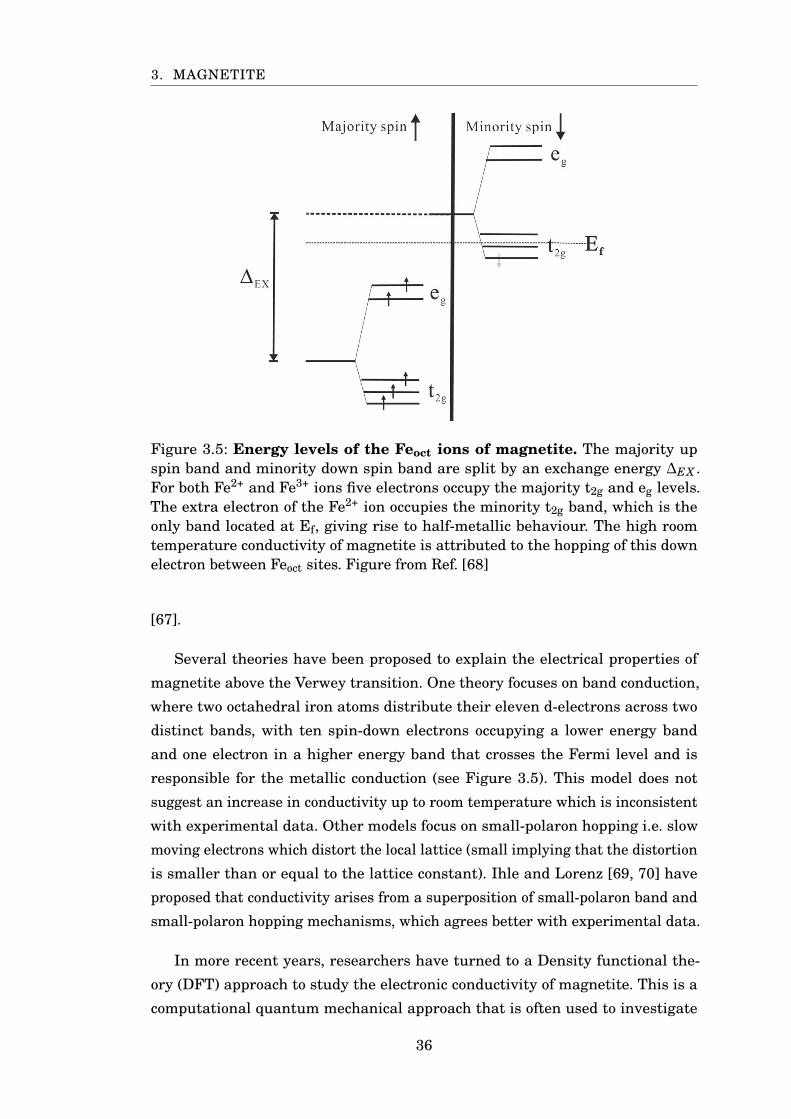
3. MAGNETITE
Figure 3.5: Energy levels of the Feoct ions of magnetite. The majority upspin band and minority down spin band are split by an exchange energy ∆EX .For both Fe2+ and Fe3+ ions five electrons occupy the majority t2g and eg levels.The extra electron of the Fe2+ ion occupies the minority t2g band, which is theonly band located at Ef, giving rise to half-metallic behaviour. The high roomtemperature conductivity of magnetite is attributed to the hopping of this downelectron between Feoct sites. Figure from Ref. [68]
[67].
Several theories have been proposed to explain the electrical properties of
magnetite above the Verwey transition. One theory focuses on band conduction,
where two octahedral iron atoms distribute their eleven d-electrons across two
distinct bands, with ten spin-down electrons occupying a lower energy band
and one electron in a higher energy band that crosses the Fermi level and is
responsible for the metallic conduction (see Figure 3.5). This model does not
suggest an increase in conductivity up to room temperature which is inconsistent
with experimental data. Other models focus on small-polaron hopping i.e. slow
moving electrons which distort the local lattice (small implying that the distortion
is smaller than or equal to the lattice constant). Ihle and Lorenz [69, 70] have
proposed that conductivity arises from a superposition of small-polaron band and
small-polaron hopping mechanisms, which agrees better with experimental data.
In more recent years, researchers have turned to a Density functional the-
ory (DFT) approach to study the electronic conductivity of magnetite. This is a
computational quantum mechanical approach that is often used to investigate
36
3. MAGNETITE
the ground state of materials by taking advantage of the periodicity of the unit
cell to simulate bulk properties. The computational cost of simulating a system of
many interacting electrons is reduced by simulating an energetically equivalent
system of non-interacting electrons in an external effective potential, such as
the local-density approximation (LDA), which is based upon the exchange and
correlation energy density in a uniform gas. Computational cost can be further
reduced by dividing the total number of electrons, with which computational time
scales, into inner electrons and valence electrons. Inner core electrons are strongly
bound and do not play a significant role in chemical binding of atoms. Particularly
in metals and semiconductors, these inner electrons screen the nucleus from the
valence electrons and can therefore be approximated by using a pseudopotential
which replaces the potential felt by the valence electrons.
Early DFT calculations, performed as early as 1984 [71], were used to cal-
culate the band structure of magnetite however these calculations were not yet
completely reliable due to the relative crudeness of approximations which had
to be used at the time due to the lack of computational power [72]. The LDA
is another problem for materials such as magnetite which have more strongly
correlated electrons and is often remedied with the usage of a Hubbard-like term
(which helps to approximate interacting particles). This approach is known as
DFT+U. A summary of this method and its usage on magnetite is provided in Ref.
[73].
The exact distinction between divalent and trivalent iron ions in the octahedral
lattice remains a contentious issue however it is generally agreed that the high
temperature phase of magnetite does not distinguish between them [74]. The
oxidation states below the Verwey transition are often reported to vary between
2.4+ and 2.9+ [75].
3.2.4 Anisotropy
So far we have a clear understanding of the structure of magnetite, its unit cell
atom positions and their occupation at various temperatures. Next, we shall
cover the main forces which affect its magnetic properties. The anisotropy, here
referring to the magnetocrystalline anisotropy, is intrinsic to the crystal and
describes the magnetic properties of a material according to the direction its spins
are aligned. In cubic crystals, there are three principal directions along which the
spins can align, shown in Figure 3.6: the ⟨100⟩, ⟨110⟩ and ⟨111⟩ directions.
Different materials can be aligned along any of these directions however the
37
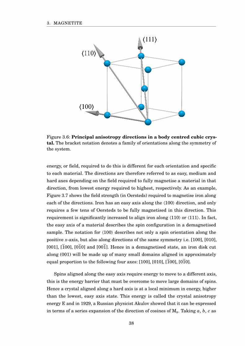
3. MAGNETITE
Figure 3.6: Principal anisotropy directions in a body centred cubic crys-tal. The bracket notation denotes a family of orientations along the symmetry ofthe system.
energy, or field, required to do this is different for each orientation and specific
to each material. The directions are therefore referred to as easy, medium and
hard axes depending on the field required to fully magnetise a material in that
direction, from lowest energy required to highest, respectively. As an example,
Figure 3.7 shows the field strength (in Oersteds) required to magnetise iron along
each of the directions. Iron has an easy axis along the ⟨100⟩ direction, and only
requires a few tens of Oersteds to be fully magnetised in this direction. This
requirement is significantly increased to align iron along ⟨110⟩ or ⟨111⟩. In fact,
the easy axis of a material describes the spin configuration in a demagnetised
sample. The notation for ⟨100⟩ describes not only a spin orientation along the
positive x-axis, but also along directions of the same symmetry i.e. [100], [010],
[001], [100], [010] and [001]. Hence in a demagnetised state, an iron disk cut
along (001) will be made up of many small domains aligned in approximately
equal proportion to the following four axes: [100], [010], [100], [010].
Spins aligned along the easy axis require energy to move to a different axis,
this is the energy barrier that must be overcome to move large domains of spins.
Hence a crystal aligned along a hard axis is at a local minimum in energy, higher
than the lowest, easy axis state. This energy is called the crystal anisotropy
energy E and in 1929, a Russian physicist Akulov showed that it can be expressed
in terms of a series expansion of the direction of cosines of Ms. Taking a, b, c as
38
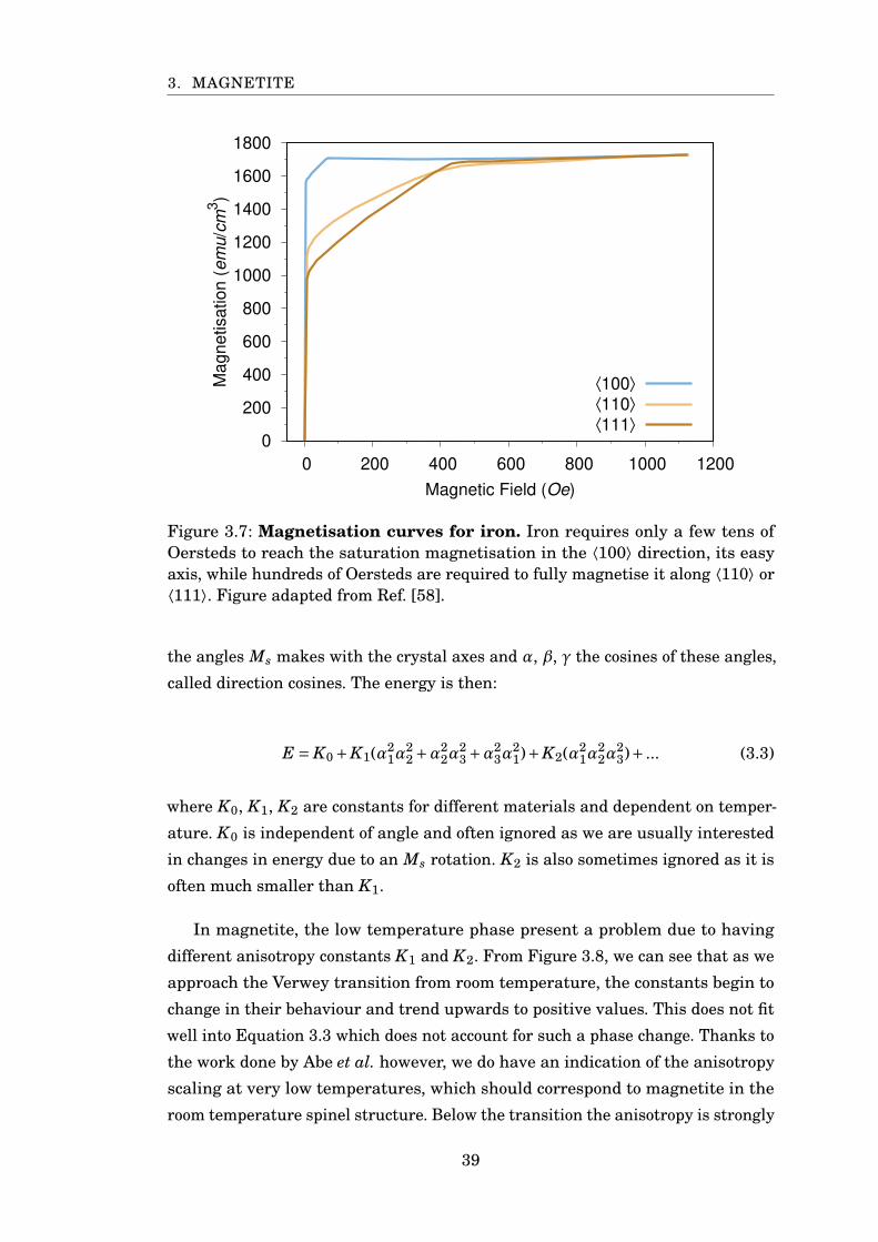
3. MAGNETITE
0
200
400
600
800
1000
1200
1400
1600
1800
0 200 400 600 800 1000 1200
Magnetisation (
em
u/c
m3)
Magnetic Field (Oe)
⟨100⟩
⟨110⟩
⟨111⟩
Figure 3.7: Magnetisation curves for iron. Iron requires only a few tens ofOersteds to reach the saturation magnetisation in the ⟨100⟩ direction, its easyaxis, while hundreds of Oersteds are required to fully magnetise it along ⟨110⟩ or⟨111⟩. Figure adapted from Ref. [58].
the angles Ms makes with the crystal axes and α, β, γ the cosines of these angles,
called direction cosines. The energy is then:
E = K0 +K1(α21α
22 +α2
2α23 +α2
3α21)+K2(α2
1α22α
23)+ ... (3.3)
where K0, K1, K2 are constants for different materials and dependent on temper-
ature. K0 is independent of angle and often ignored as we are usually interested
in changes in energy due to an Ms rotation. K2 is also sometimes ignored as it is
often much smaller than K1.
In magnetite, the low temperature phase present a problem due to having
different anisotropy constants K1 and K2. From Figure 3.8, we can see that as we
approach the Verwey transition from room temperature, the constants begin to
change in their behaviour and trend upwards to positive values. This does not fit
well into Equation 3.3 which does not account for such a phase change. Thanks to
the work done by Abe et al. however, we do have an indication of the anisotropy
scaling at very low temperatures, which should correspond to magnetite in the
room temperature spinel structure. Below the transition the anisotropy is strongly
39
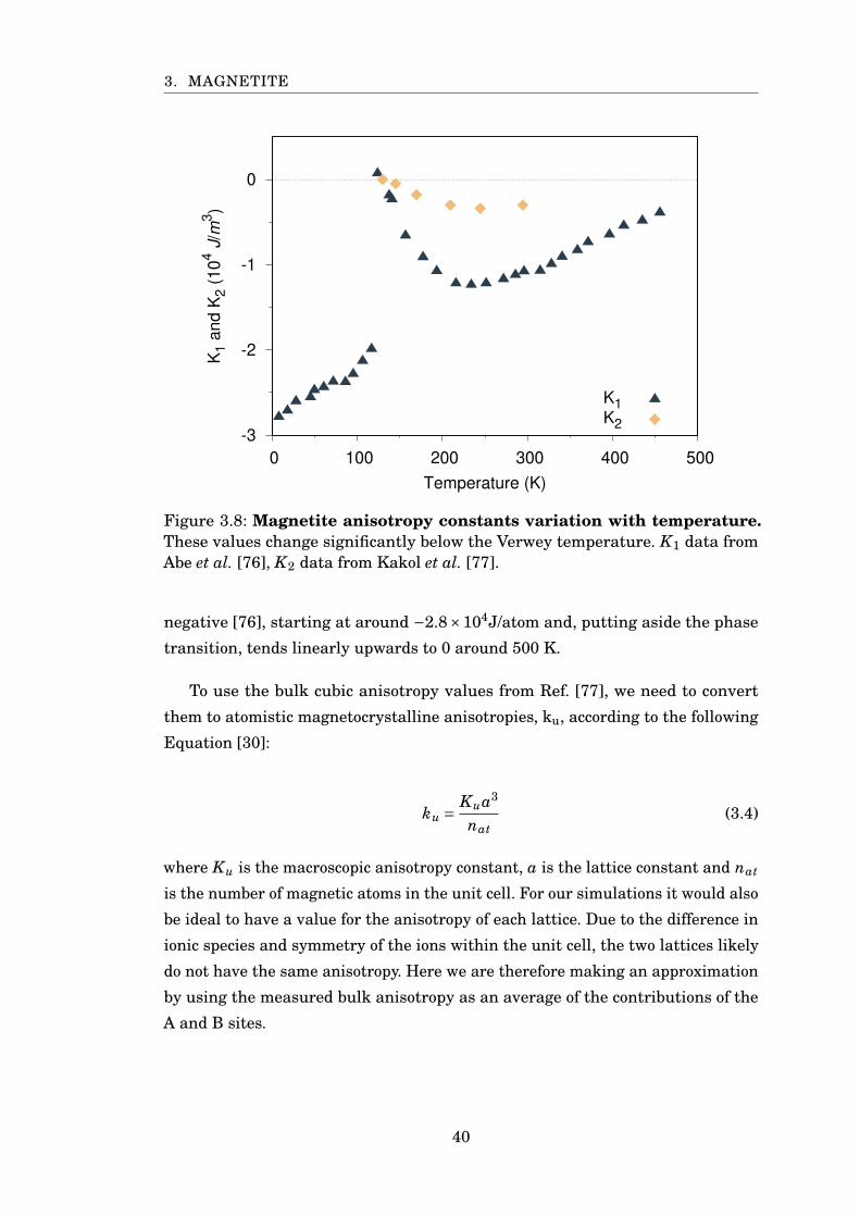
3. MAGNETITE
-3
-2
-1
0
0 100 200 300 400 500
K1 a
nd K
2 (
10
4 J
/m3)
Temperature (K)
K1K2
Figure 3.8: Magnetite anisotropy constants variation with temperature.These values change significantly below the Verwey temperature. K1 data fromAbe et al. [76], K2 data from Kakol et al. [77].
negative [76], starting at around −2.8×10⁴J/atom and, putting aside the phase
transition, tends linearly upwards to 0 around 500 K.
To use the bulk cubic anisotropy values from Ref. [77], we need to convert
them to atomistic magnetocrystalline anisotropies, ku, according to the following
Equation [30]:
ku = Kua3
nat(3.4)
where Ku is the macroscopic anisotropy constant, a is the lattice constant and nat
is the number of magnetic atoms in the unit cell. For our simulations it would also
be ideal to have a value for the anisotropy of each lattice. Due to the difference in
ionic species and symmetry of the ions within the unit cell, the two lattices likely
do not have the same anisotropy. Here we are therefore making an approximation
by using the measured bulk anisotropy as an average of the contributions of the
A and B sites.
40
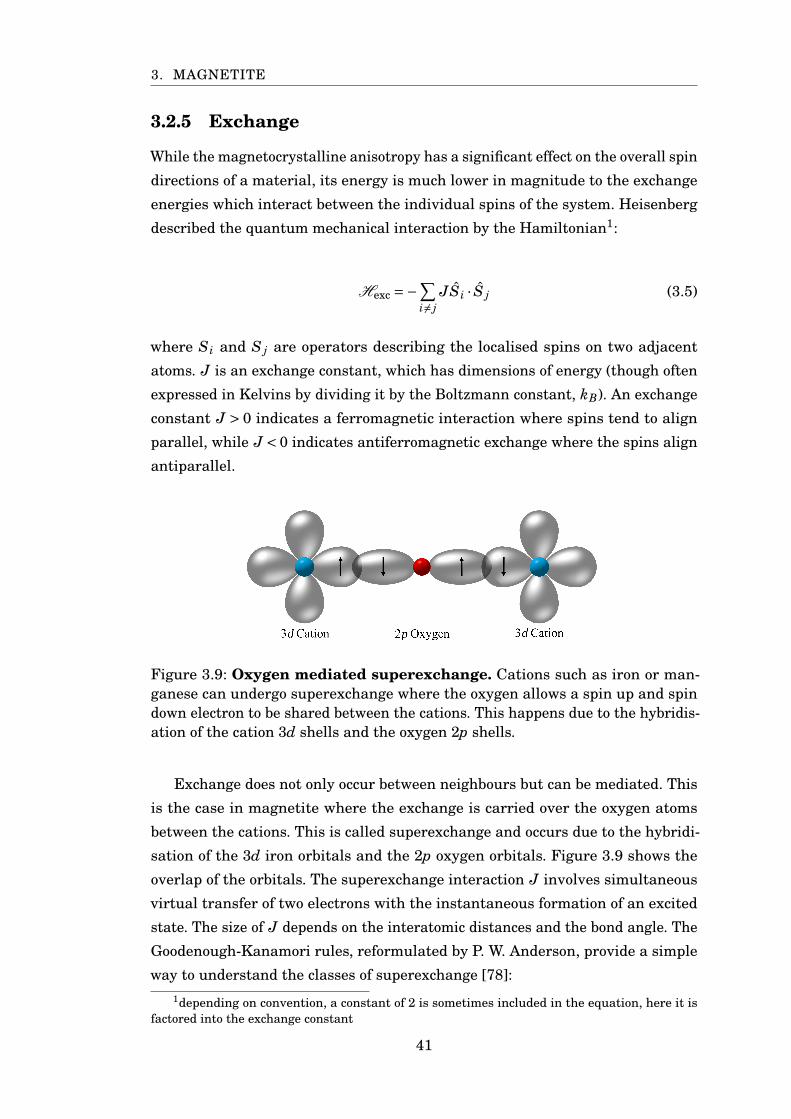
3. MAGNETITE
3.2.5 Exchange
While the magnetocrystalline anisotropy has a significant effect on the overall spin
directions of a material, its energy is much lower in magnitude to the exchange
energies which interact between the individual spins of the system. Heisenberg
described the quantum mechanical interaction by the Hamiltonian1:
Hexc =−∑i 6= j
JSi · S j (3.5)
where Si and S j are operators describing the localised spins on two adjacent
atoms. J is an exchange constant, which has dimensions of energy (though often
expressed in Kelvins by dividing it by the Boltzmann constant, kB). An exchange
constant J > 0 indicates a ferromagnetic interaction where spins tend to align
parallel, while J < 0 indicates antiferromagnetic exchange where the spins align
antiparallel.
Figure 3.9: Oxygen mediated superexchange. Cations such as iron or man-ganese can undergo superexchange where the oxygen allows a spin up and spindown electron to be shared between the cations. This happens due to the hybridis-ation of the cation 3d shells and the oxygen 2p shells.
Exchange does not only occur between neighbours but can be mediated. This
is the case in magnetite where the exchange is carried over the oxygen atoms
between the cations. This is called superexchange and occurs due to the hybridi-
sation of the 3d iron orbitals and the 2p oxygen orbitals. Figure 3.9 shows the
overlap of the orbitals. The superexchange interaction J involves simultaneous
virtual transfer of two electrons with the instantaneous formation of an excited
state. The size of J depends on the interatomic distances and the bond angle. The
Goodenough-Kanamori rules, reformulated by P. W. Anderson, provide a simple
way to understand the classes of superexchange [78]:1depending on convention, a constant of 2 is sometimes included in the equation, here it is
factored into the exchange constant
41
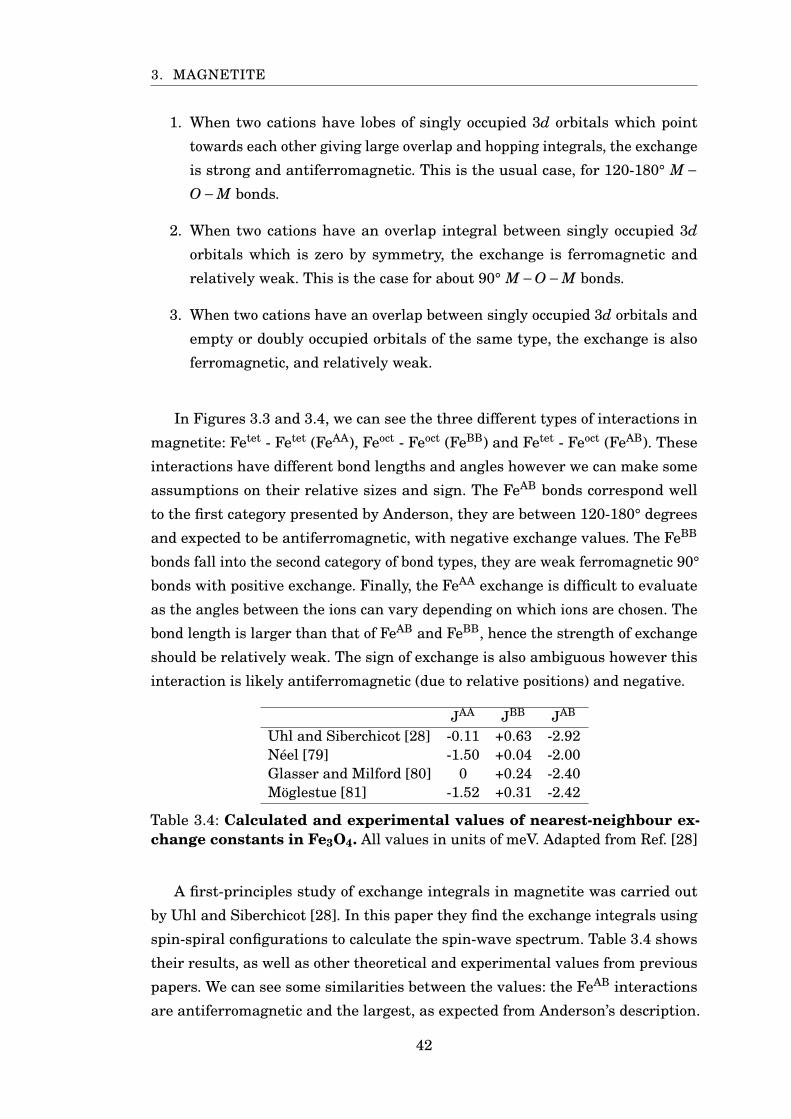
3. MAGNETITE
1. When two cations have lobes of singly occupied 3d orbitals which point
towards each other giving large overlap and hopping integrals, the exchange
is strong and antiferromagnetic. This is the usual case, for 120-180° M −O−M bonds.
2. When two cations have an overlap integral between singly occupied 3dorbitals which is zero by symmetry, the exchange is ferromagnetic and
relatively weak. This is the case for about 90° M−O−M bonds.
3. When two cations have an overlap between singly occupied 3d orbitals and
empty or doubly occupied orbitals of the same type, the exchange is also
ferromagnetic, and relatively weak.
In Figures 3.3 and 3.4, we can see the three different types of interactions in
magnetite: Fetet - Fetet (FeAA), Feoct - Feoct (FeBB) and Fetet - Feoct (FeAB). These
interactions have different bond lengths and angles however we can make some
assumptions on their relative sizes and sign. The FeAB bonds correspond well
to the first category presented by Anderson, they are between 120-180° degrees
and expected to be antiferromagnetic, with negative exchange values. The FeBB
bonds fall into the second category of bond types, they are weak ferromagnetic 90°
bonds with positive exchange. Finally, the FeAA exchange is difficult to evaluate
as the angles between the ions can vary depending on which ions are chosen. The
bond length is larger than that of FeAB and FeBB, hence the strength of exchange
should be relatively weak. The sign of exchange is also ambiguous however this
interaction is likely antiferromagnetic (due to relative positions) and negative.
JAA JBB JAB
Uhl and Siberchicot [28] -0.11 +0.63 -2.92Néel [79] -1.50 +0.04 -2.00Glasser and Milford [80] 0 +0.24 -2.40Möglestue [81] -1.52 +0.31 -2.42
Table 3.4: Calculated and experimental values of nearest-neighbour ex-change constants in Fe3O4. All values in units of meV. Adapted from Ref. [28]
A first-principles study of exchange integrals in magnetite was carried out
by Uhl and Siberchicot [28]. In this paper they find the exchange integrals using
spin-spiral configurations to calculate the spin-wave spectrum. Table 3.4 shows
their results, as well as other theoretical and experimental values from previous
papers. We can see some similarities between the values: the FeAB interactions
are antiferromagnetic and the largest, as expected from Anderson’s description.
42
3. MAGNETITE
The FeBB interactions are much smaller, with most values given being an order of
magnitude lower than the FeAB interactions. The FeAA interactions present the
largest variance as the results of Néel and Möglestue suggest they are close to
the FeAB interactions in magnitude. The results presented by Uhl and Siberchicot
are most commonly found in the literature and generally regarded as accurate,
hence we shall be using these values as a starting point for our calculations.
3.3 Simulating Magnetite
Magnetite is the first material we consider in this thesis. The aim is to understand
the data produced, keeping in mind our initial assumptions and the properties
discussed in the previous chapter. As this work is being done using the VAMPIRE
simulation package, we have unprecedented access to single spin level data which
is still rare to see in current research papers. At the same time, we shall still be
able to compare micromagnetic level behaviour to similar theoretical works which
studied this material [20, 21, 82] as well as the experimental data for the overall
system properties such as the Curie temperature.
3.3.1 First Simulation
We can simulate a small system with periodic boundary conditions (PBCs) to
approach bulk properties. To recap some of the system parameters we have
discussed in this chapter:
• The system is cubic with a lattice constant of a = 8.397Å
• There are three unique materials:
– Tetrahedral site iron 3+ ions with spin moment 5 µB
– Octahedral iron ions in a mixed 2.5+ state with spin moment 4.5 µB
– Non-magnetic oxygen 2- ions
• The anisotropy direction is ⟨111⟩, with a negative anisotropy constant.
• The exchange interaction values (in meV) are JAA =−0.11, JBB = 0.63 and
JAB =−2.92.
As a first simulation we can find the equilibrated magnetisation of a PBC
particle. To keep simulation time low, we shall use a system of around 8 nm width
43
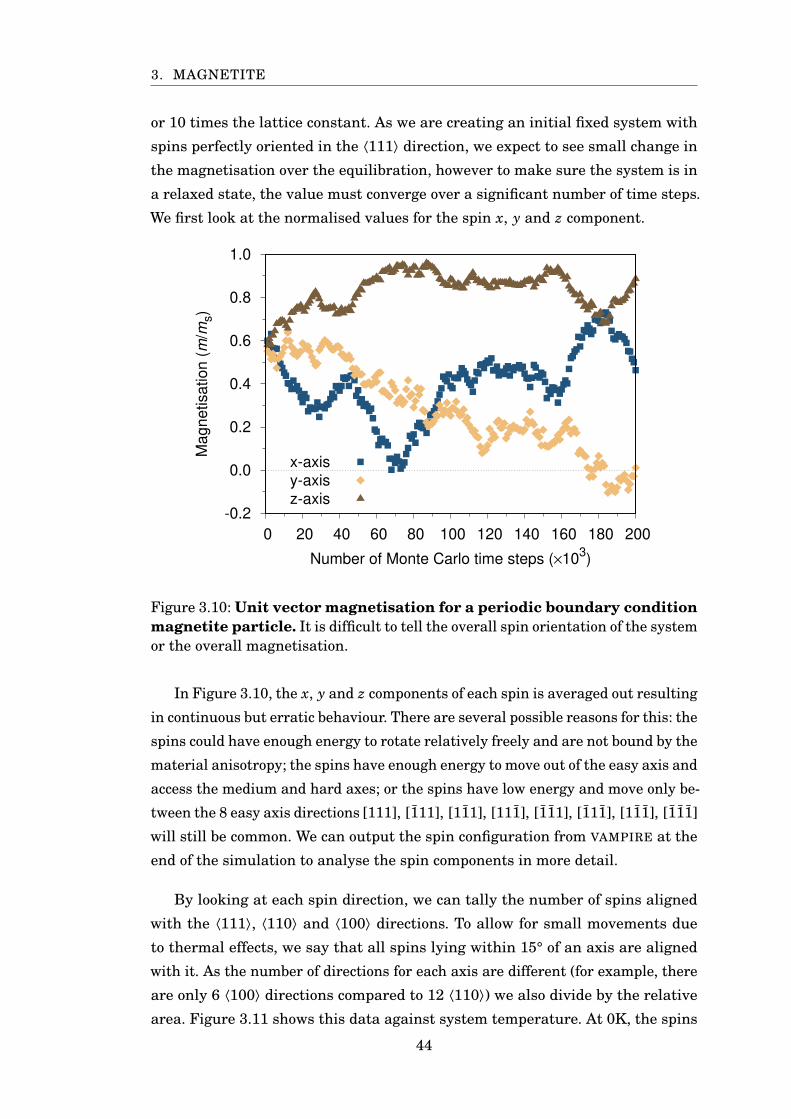
3. MAGNETITE
or 10 times the lattice constant. As we are creating an initial fixed system with
spins perfectly oriented in the ⟨111⟩ direction, we expect to see small change in
the magnetisation over the equilibration, however to make sure the system is in
a relaxed state, the value must converge over a significant number of time steps.
We first look at the normalised values for the spin x, y and z component.
-0.2
0.0
0.2
0.4
0.6
0.8
1.0
0 20 40 60 80 100 120 140 160 180 200
Magnetisation (
m/m
s)
Number of Monte Carlo time steps (×103)
x-axis
y-axis
z-axis
Figure 3.10: Unit vector magnetisation for a periodic boundary conditionmagnetite particle. It is difficult to tell the overall spin orientation of the systemor the overall magnetisation.
In Figure 3.10, the x, y and z components of each spin is averaged out resulting
in continuous but erratic behaviour. There are several possible reasons for this: the
spins could have enough energy to rotate relatively freely and are not bound by the
material anisotropy; the spins have enough energy to move out of the easy axis and
access the medium and hard axes; or the spins have low energy and move only be-
tween the 8 easy axis directions [111], [111], [111], [111], [111], [111], [111], [111]
will still be common. We can output the spin configuration from VAMPIRE at the
end of the simulation to analyse the spin components in more detail.
By looking at each spin direction, we can tally the number of spins aligned
with the ⟨111⟩, ⟨110⟩ and ⟨100⟩ directions. To allow for small movements due
to thermal effects, we say that all spins lying within 15° of an axis are aligned
with it. As the number of directions for each axis are different (for example, there
are only 6 ⟨100⟩ directions compared to 12 ⟨110⟩) we also divide by the relative
area. Figure 3.11 shows this data against system temperature. At 0K, the spins
44
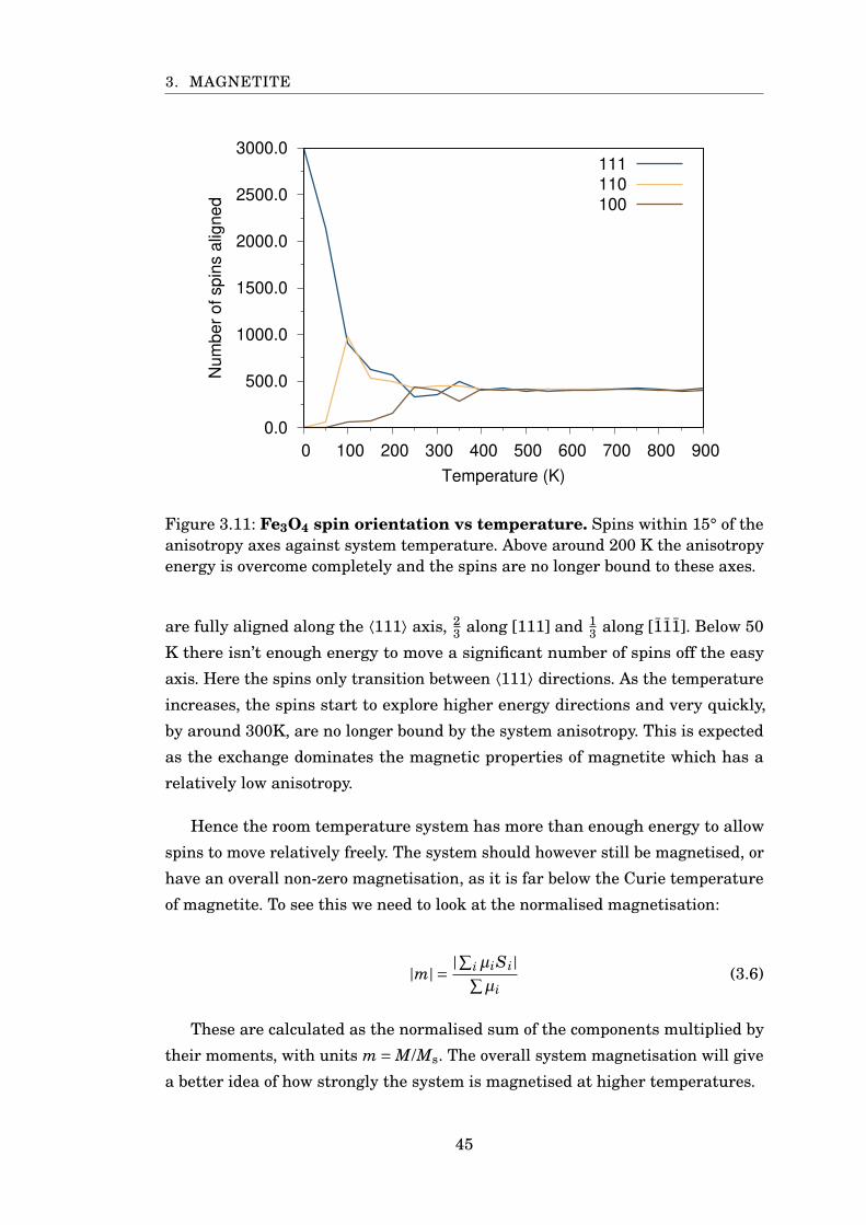
3. MAGNETITE
0.0
500.0
1000.0
1500.0
2000.0
2500.0
3000.0
0 100 200 300 400 500 600 700 800 900
Num
ber
of spin
s a
ligned
Temperature (K)
111
110
100
Figure 3.11: Fe3O4 spin orientation vs temperature. Spins within 15° of theanisotropy axes against system temperature. Above around 200 K the anisotropyenergy is overcome completely and the spins are no longer bound to these axes.
are fully aligned along the ⟨111⟩ axis, 23 along [111] and 1
3 along [111]. Below 50
K there isn’t enough energy to move a significant number of spins off the easy
axis. Here the spins only transition between ⟨111⟩ directions. As the temperature
increases, the spins start to explore higher energy directions and very quickly,
by around 300K, are no longer bound by the system anisotropy. This is expected
as the exchange dominates the magnetic properties of magnetite which has a
relatively low anisotropy.
Hence the room temperature system has more than enough energy to allow
spins to move relatively freely. The system should however still be magnetised, or
have an overall non-zero magnetisation, as it is far below the Curie temperature
of magnetite. To see this we need to look at the normalised magnetisation:
|m| = |∑iµiSi|∑µi
(3.6)
These are calculated as the normalised sum of the components multiplied by
their moments, with units m = M/Ms. The overall system magnetisation will give
a better idea of how strongly the system is magnetised at higher temperatures.
45
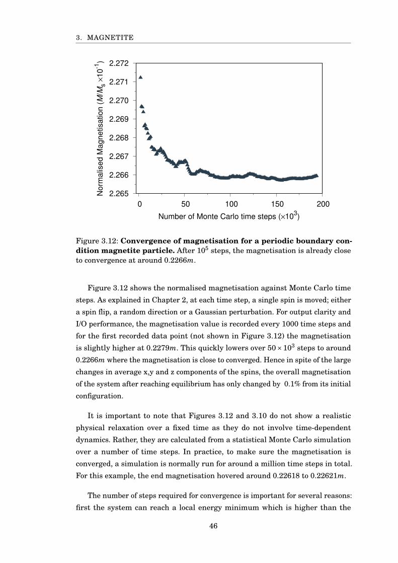
3. MAGNETITE
2.265
2.266
2.267
2.268
2.269
2.270
2.271
2.272
0 50 100 150 200
Norm
alis
ed M
agnetisation (
M/M
s ×
10
-1)
Number of Monte Carlo time steps (×103)
Figure 3.12: Convergence of magnetisation for a periodic boundary con-dition magnetite particle. After 105 steps, the magnetisation is already closeto convergence at around 0.2266m.
Figure 3.12 shows the normalised magnetisation against Monte Carlo time
steps. As explained in Chapter 2, at each time step, a single spin is moved; either
a spin flip, a random direction or a Gaussian perturbation. For output clarity and
I/O performance, the magnetisation value is recorded every 1000 time steps and
for the first recorded data point (not shown in Figure 3.12) the magnetisation
is slightly higher at 0.2279m. This quickly lowers over 50×103 steps to around
0.2266m where the magnetisation is close to converged. Hence in spite of the large
changes in average x,y and z components of the spins, the overall magnetisation
of the system after reaching equilibrium has only changed by 0.1% from its initial
configuration.
It is important to note that Figures 3.12 and 3.10 do not show a realistic
physical relaxation over a fixed time as they do not involve time-dependent
dynamics. Rather, they are calculated from a statistical Monte Carlo simulation
over a number of time steps. In practice, to make sure the magnetisation is
converged, a simulation is normally run for around a million time steps in total.
For this example, the end magnetisation hovered around 0.22618 to 0.22621m.
The number of steps required for convergence is important for several reasons:
first the system can reach a local energy minimum which is higher than the
46
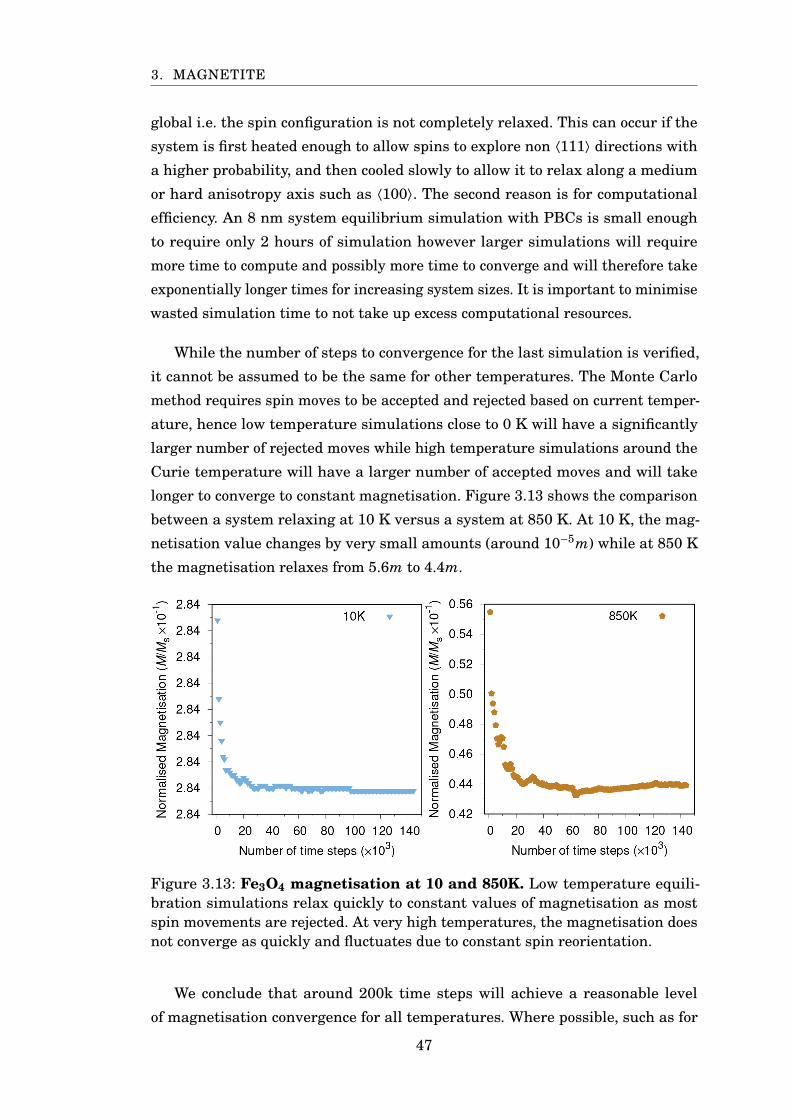
3. MAGNETITE
global i.e. the spin configuration is not completely relaxed. This can occur if the
system is first heated enough to allow spins to explore non ⟨111⟩ directions with
a higher probability, and then cooled slowly to allow it to relax along a medium
or hard anisotropy axis such as ⟨100⟩. The second reason is for computational
efficiency. An 8 nm system equilibrium simulation with PBCs is small enough
to require only 2 hours of simulation however larger simulations will require
more time to compute and possibly more time to converge and will therefore take
exponentially longer times for increasing system sizes. It is important to minimise
wasted simulation time to not take up excess computational resources.
While the number of steps to convergence for the last simulation is verified,
it cannot be assumed to be the same for other temperatures. The Monte Carlo
method requires spin moves to be accepted and rejected based on current temper-
ature, hence low temperature simulations close to 0 K will have a significantly
larger number of rejected moves while high temperature simulations around the
Curie temperature will have a larger number of accepted moves and will take
longer to converge to constant magnetisation. Figure 3.13 shows the comparison
between a system relaxing at 10 K versus a system at 850 K. At 10 K, the mag-
netisation value changes by very small amounts (around 10−5m) while at 850 K
the magnetisation relaxes from 5.6m to 4.4m.
Figure 3.13: Fe3O4 magnetisation at 10 and 850K. Low temperature equili-bration simulations relax quickly to constant values of magnetisation as mostspin movements are rejected. At very high temperatures, the magnetisation doesnot converge as quickly and fluctuates due to constant spin reorientation.
We conclude that around 200k time steps will achieve a reasonable level
of magnetisation convergence for all temperatures. Where possible, such as for
47
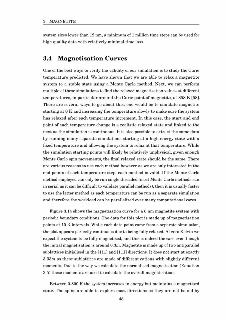
3. MAGNETITE
system sizes lower than 12 nm, a minimum of 1 million time steps can be used for
high quality data with relatively minimal time loss.
3.4 Magnetisation Curves
One of the best ways to verify the validity of our simulation is to study the Curie
temperature predicted. We have shown that we are able to relax a magnetite
system to a stable state using a Monte Carlo method. Next, we can perform
multiple of these simulations to find the relaxed magnetisation values at different
temperatures, in particular around the Curie point of magnetite, at 858 K [58].
There are several ways to go about this; one would be to simulate magnetite
starting at 0 K and increasing the temperature slowly to make sure the system
has relaxed after each temperature increment. In this case, the start and end
point of each temperature change is a realistic relaxed state and linked to the
next as the simulation is continuous. It is also possible to extract the same data
by running many separate simulations starting at a high energy state with a
fixed temperature and allowing the system to relax at that temperature. While
the simulation starting points will likely be relatively unphysical, given enough
Monte Carlo spin movements, the final relaxed state should be the same. There
are various reasons to use each method however as we are only interested in the
end points of each temperature step, each method is valid. If the Monte Carlo
method employed can only be run single threaded (most Monte Carlo methods run
in serial as it can be difficult to validate parallel methods), then it is usually faster
to use the latter method as each temperature can be run as a separate simulation
and therefore the workload can be parallelized over many computational cores.
Figure 3.14 shows the magnetisation curve for a 6 nm magnetite system with
periodic boundary conditions. The data for this plot is made up of magnetisation
points at 10 K intervals. While each data point came from a separate simulation,
the plot appears perfectly continuous due to being fully relaxed. At zero Kelvin we
expect the system to be fully magnetised, and this is indeed the case even though
the initial magnetisation is around 0.3m. Magnetite is made up of two antiparallel
sublattices initialised in the [111] and [111] directions. It does not start at exactly
3.33m as these sublattices are made of different cations with slightly different
moments. Due to the way we calculate the normalised magnetisation (Equation
3.5) these moments are used to calculate the overall magnetisation.
Between 0-800 K the system increases in energy but maintains a magnetised
state. The spins are able to explore most directions as they are not bound by
48
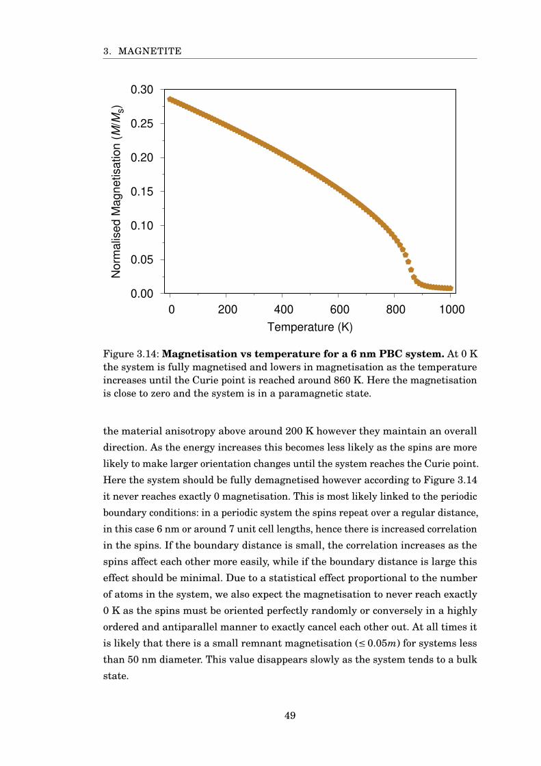
3. MAGNETITE
0.00
0.05
0.10
0.15
0.20
0.25
0.30
0 200 400 600 800 1000
Norm
alis
ed M
agnetisation (
M/M
s)
Temperature (K)
Figure 3.14: Magnetisation vs temperature for a 6 nm PBC system. At 0 Kthe system is fully magnetised and lowers in magnetisation as the temperatureincreases until the Curie point is reached around 860 K. Here the magnetisationis close to zero and the system is in a paramagnetic state.
the material anisotropy above around 200 K however they maintain an overall
direction. As the energy increases this becomes less likely as the spins are more
likely to make larger orientation changes until the system reaches the Curie point.
Here the system should be fully demagnetised however according to Figure 3.14
it never reaches exactly 0 magnetisation. This is most likely linked to the periodic
boundary conditions: in a periodic system the spins repeat over a regular distance,
in this case 6 nm or around 7 unit cell lengths, hence there is increased correlation
in the spins. If the boundary distance is small, the correlation increases as the
spins affect each other more easily, while if the boundary distance is large this
effect should be minimal. Due to a statistical effect proportional to the number
of atoms in the system, we also expect the magnetisation to never reach exactly
0 K as the spins must be oriented perfectly randomly or conversely in a highly
ordered and antiparallel manner to exactly cancel each other out. At all times it
is likely that there is a small remnant magnetisation (≤ 0.05m) for systems less
than 50 nm diameter. This value disappears slowly as the system tends to a bulk
state.
49
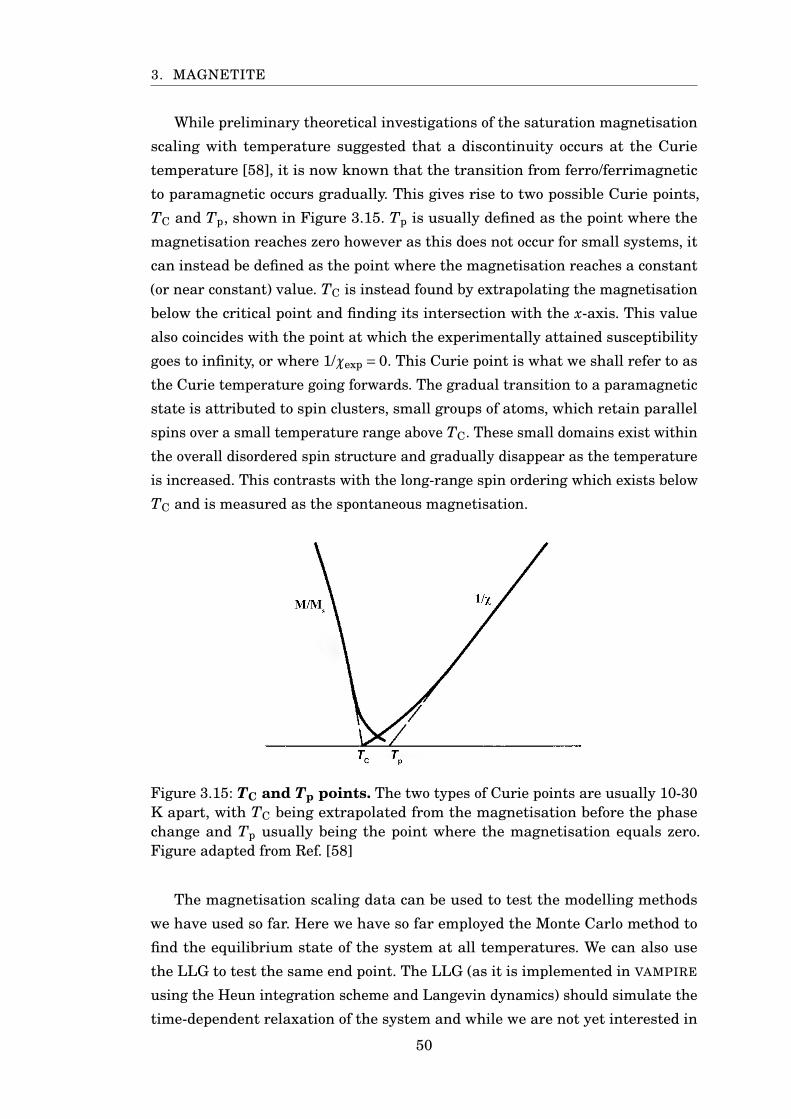
3. MAGNETITE
While preliminary theoretical investigations of the saturation magnetisation
scaling with temperature suggested that a discontinuity occurs at the Curie
temperature [58], it is now known that the transition from ferro/ferrimagnetic
to paramagnetic occurs gradually. This gives rise to two possible Curie points,
TC and Tp, shown in Figure 3.15. Tp is usually defined as the point where the
magnetisation reaches zero however as this does not occur for small systems, it
can instead be defined as the point where the magnetisation reaches a constant
(or near constant) value. TC is instead found by extrapolating the magnetisation
below the critical point and finding its intersection with the x-axis. This value
also coincides with the point at which the experimentally attained susceptibility
goes to infinity, or where 1/χexp = 0. This Curie point is what we shall refer to as
the Curie temperature going forwards. The gradual transition to a paramagnetic
state is attributed to spin clusters, small groups of atoms, which retain parallel
spins over a small temperature range above TC. These small domains exist within
the overall disordered spin structure and gradually disappear as the temperature
is increased. This contrasts with the long-range spin ordering which exists below
TC and is measured as the spontaneous magnetisation.
Figure 3.15: TC and Tp points. The two types of Curie points are usually 10-30K apart, with TC being extrapolated from the magnetisation before the phasechange and Tp usually being the point where the magnetisation equals zero.Figure adapted from Ref. [58]
The magnetisation scaling data can be used to test the modelling methods
we have used so far. Here we have so far employed the Monte Carlo method to
find the equilibrium state of the system at all temperatures. We can also use
the LLG to test the same end point. The LLG (as it is implemented in VAMPIRE
using the Heun integration scheme and Langevin dynamics) should simulate the
time-dependent relaxation of the system and while we are not yet interested in
50
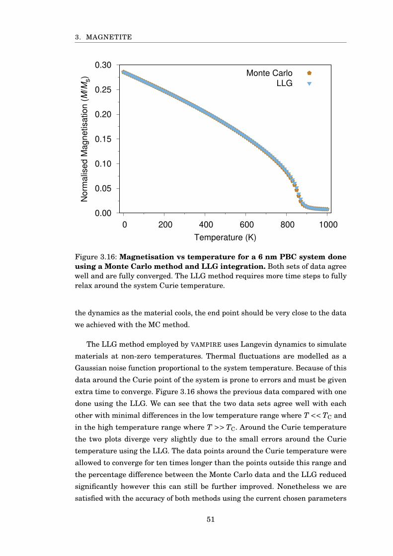
3. MAGNETITE
0.00
0.05
0.10
0.15
0.20
0.25
0.30
0 200 400 600 800 1000
Norm
alis
ed M
agnetisation (
M/M
s)
Temperature (K)
Monte Carlo
LLG
Figure 3.16: Magnetisation vs temperature for a 6 nm PBC system doneusing a Monte Carlo method and LLG integration. Both sets of data agreewell and are fully converged. The LLG method requires more time steps to fullyrelax around the system Curie temperature.
the dynamics as the material cools, the end point should be very close to the data
we achieved with the MC method.
The LLG method employed by VAMPIRE uses Langevin dynamics to simulate
materials at non-zero temperatures. Thermal fluctuations are modelled as a
Gaussian noise function proportional to the system temperature. Because of this
data around the Curie point of the system is prone to errors and must be given
extra time to converge. Figure 3.16 shows the previous data compared with one
done using the LLG. We can see that the two data sets agree well with each
other with minimal differences in the low temperature range where T <<TC and
in the high temperature range where T >> TC. Around the Curie temperature
the two plots diverge very slightly due to the small errors around the Curie
temperature using the LLG. The data points around the Curie temperature were
allowed to converge for ten times longer than the points outside this range and
the percentage difference between the Monte Carlo data and the LLG reduced
significantly however this can still be further improved. Nonetheless we are
satisfied with the accuracy of both methods using the current chosen parameters
51
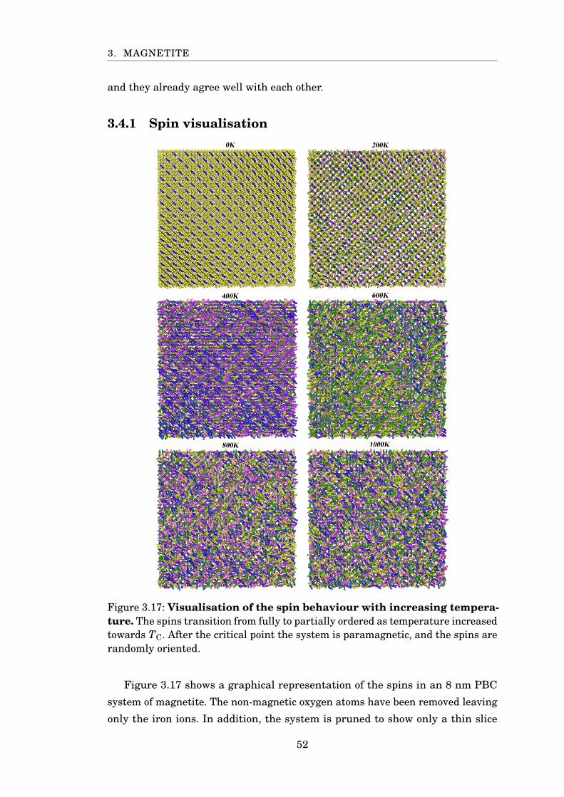
3. MAGNETITE
and they already agree well with each other.
3.4.1 Spin visualisation
Figure 3.17: Visualisation of the spin behaviour with increasing tempera-ture. The spins transition from fully to partially ordered as temperature increasedtowards TC. After the critical point the system is paramagnetic, and the spins arerandomly oriented.
Figure 3.17 shows a graphical representation of the spins in an 8 nm PBC
system of magnetite. The non-magnetic oxygen atoms have been removed leaving
only the iron ions. In addition, the system is pruned to show only a thin slice
52
3. MAGNETITE
of the fully simulated material for visual clarity. These images were the result
of Monte Carlo simulations used to find the equilibrated state of magnetite at
various temperatures.
Starting at 0K, the system starts fully magnetised with each sublattice ori-
ented along the easy axis. Here, yellow spins point along the positive axis, while
blue spins are negative. The bright green and magenta coloured spins are oriented
perpendicular to these and transitional colours are used in between.
Due to the lack of thermal energy, spins are essentially locked into the easy
axis orientation for temperatures close to 0 K. With a significant increase to
thermal energy, at 200 K, the spins start to move out of their initial orientation,
which can be seen from the new spin colours which deviate from the 0 K yellow
and blue.
In spite of the new spin orientations in the system, a long-range ordering
occurs over the whole system as it is still magnetised below its Curie temperature.
The 400 and 600 K images show that many spins reorient into the ⟨100⟩ axis and
there is still a clear distinction between spins on the tetrahedral and octahedral
axes which remain mostly antiparallel. At 600 K this is slightly less clear as small,
localised, clusters of spins become oriented randomly.
At 800 K it is difficult to visually discern a long range ordering of the spins.
The system is only 50 K below the Curie temperature and the transition to a
paramagnetic state has begun. Somewhat opposite to the 400 K image, it is
possible to spot clusters of aligned spins indicating that the system remains
slightly magnetised. Finally at 1000 K the system has passed TC and is fully
demagnetised. The distribution of colours in the visualisation is roughly equal as
there is no overall spin direction and any spin orientation is allowed.
3.4.2 Sublattice Magnetisation
Earlier in the chapter we looked at the spin direction values of the system on a
single spin level. Another method we can use to more closely examine the physical
properties of our system is to look at the individual sublattices of magnetite.
VAMPIRE is able to output material based properties of the system, such as
the material magnetisation, and since these materials are distinct, not just in
number but also spin moment and exchange, it is worth looking at differences
in their magnetic properties. The overall magnetic properties of the system are
a symptom of these smaller scale properties and while most experimental data
53
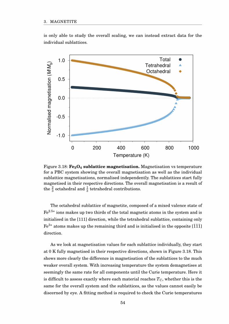
3. MAGNETITE
is only able to study the overall scaling, we can instead extract data for the
individual sublattices.
-1.0
-0.5
0.0
0.5
1.0
0 200 400 600 800 1000
Norm
alis
ed m
agnetisation (
M/M
s)
Temperature (K)
Total
Tetrahedral
Octahedral
Figure 3.18: Fe3O4 sublattice magnetisation. Magnetisation vs temperaturefor a PBC system showing the overall magnetisation as well as the individualsublattice magnetisations, normalised independently. The sublattices start fullymagnetised in their respective directions. The overall magnetisation is a result ofthe 2
3 octahedral and 13 tetrahedral contributions.
The octahedral sublattice of magnetite, composed of a mixed valence state of
Fe2.5+ ions makes up two thirds of the total magnetic atoms in the system and is
initialised in the [111] direction, while the tetrahedral sublattice, containing only
Fe3+ atoms makes up the remaining third and is initialised in the opposite [111]
direction.
As we look at magnetisation values for each sublattice individually, they start
at 0 K fully magnetised in their respective directions, shown in Figure 3.18. This
shows more clearly the difference in magnetisation of the sublattices to the much
weaker overall system. With increasing temperature the system demagnetises at
seemingly the same rate for all components until the Curie temperature. Here it
is difficult to assess exactly where each material reaches TC, whether this is the
same for the overall system and the sublattices, as the values cannot easily be
discerned by eye. A fitting method is required to check the Curie temperatures
54
3. MAGNETITE
of the various components as it is a non-trivial question whether the TC point
should be the same.
3.5 Calculating the Curie Temperature
The Curie point of magnetite has already been mentioned several times as the
temperature region around 850 K. Figure 3.18 clearly shows the system tending
to a demagnetised state in this region and we have already suggested a reason for
the magnetisation never reaching exactly 0 K. The value of TC is mainly dictated
by the exchange interaction values of magnetite however it can deviate from the
bulk value for various reasons including material imperfections, surface defects
and system shape. In ideal conditions bulk magnetite has a Curie temperature
of 858 K [58] however our current model employs PBC and will not necessarily
produce the same value. We need to find an appropriate method for extracting the
Curie temperature of our system to better understand how parameter changes
such as system size and shape will affect the system.
The temperature dependence of magnetisation at low temperatures can be
approximated using Bloch’s law [83]:
M(T)= M(0)(1−τ 3
2
)(3.7)
Here M(0) is the spontaneous magnetisation at 0 K and τ= T/TC. Alone this
equation does not approximate well the magnetisation around the critical point
[84] where:
M(T)∝ (TC −T)β (3.8)
Hence we use an interpolation of equations 3.7 and 3.8 to form the Curie-Bloch
equation:
M(τ)= (1−τα)β (3.9)
where α is an empirical constant, here equal to 1 as we are modelling classical
physics. The parameter β is a critical exponent related to the Curie temperature
of the system [85] and often linked to a universality class which suggests that
the value of the exponent changes only with the model used (such as Heisenberg
55
3. MAGNETITE
or Ising) [42, 86] and macroscopic parameters such as system dimensions. While
this fitting method is very commonly used for the temperature dependence of
the magnetisation, other fitting models are also used such as one developed by
Kuz’min [87]:
M(τ)=(1− sτ
32 − (1− s)τp
)β(3.10)
Here s and p are used as fitting parameters, p > 3/2 and s > 0. Notice that if
the system is treated as a pure Bloch ferromagnet, i.e. s = 1, p = 3/2 and α= p,
equations 2.39 and 3.10 are identical, demonstrating the same physical origin
of these equations. We now can fit the overall magnetisation of the 6 nm PBC
system we have simulated however it is necessary to make small adjustments to
both equations to resolve the initial and final values of the plots. Both equations
expect a ferromagnetic MvsT, starting at 1m at 0 K and finishing at 0m at the
Curie point. To resolve this we use two parameters, A and B, which are set to the
initial and final (in temperature) magnetisation values of our simulation.
A = M(0)
B = M(1000)
M(τ)= A(1−τα)β+B (3.11)
M(τ)= A(1− sτ
32 − (1− s)τp
)β+B (3.12)
Using this modification, both fitting equations can handle ferrimagnetic sys-
tems which do not reach a magnetisation value of 0m at high temperature. Figure
3.19 shows the fitting, done using Gnuplot [45], which employs the nonlinear
least-squares (NLLS) Marquardt-Levenberg algorithm. Using both methods, the
Curie temperature was calculated to be 878.4 K with a standard error < 0.5 K
while β was calculated to be 0.563 (±0.0023) using the Curie-Bloch equation and
0.0565 (±0.0074) using the Kuz’min equation. This shows excellent agreement
using both fitting methods, however the s and p parameters used in Equation
3.10 showed a high sensitivity to change and relatively higher standard error. Due
to the relative simplicity of the Curie-Bloch equation, we shall use it by default
when fitting magnetisation plots in the future.
56
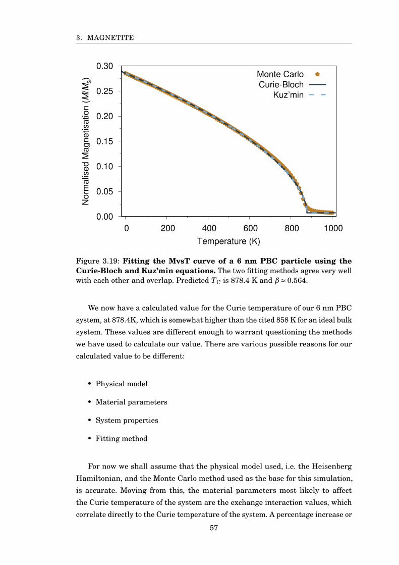
3. MAGNETITE
0.00
0.05
0.10
0.15
0.20
0.25
0.30
0 200 400 600 800 1000
Norm
alis
ed M
agnetisation (
M/M
s)
Temperature (K)
Monte Carlo
Curie-Bloch
Kuz’min
Figure 3.19: Fitting the MvsT curve of a 6 nm PBC particle using theCurie-Bloch and Kuz’min equations. The two fitting methods agree very wellwith each other and overlap. Predicted TC is 878.4 K and β≈ 0.564.
We now have a calculated value for the Curie temperature of our 6 nm PBC
system, at 878.4K, which is somewhat higher than the cited 858 K for an ideal bulk
system. These values are different enough to warrant questioning the methods
we have used to calculate our value. There are various possible reasons for our
calculated value to be different:
• Physical model
• Material parameters
• System properties
• Fitting method
For now we shall assume that the physical model used, i.e. the Heisenberg
Hamiltonian, and the Monte Carlo method used as the base for this simulation,
is accurate. Moving from this, the material parameters most likely to affect
the Curie temperature of the system are the exchange interaction values, which
correlate directly to the Curie temperature of the system. A percentage increase or
57
3. MAGNETITE
reduction of the exchange interaction magnitudes will cause a similar percentage
increase or reduction in the Curie temperature, hence the values currently used
may be slightly higher than required. Next, the system properties could also be
affecting the Curie temperature. For example, we have chosen a block particle as
a base with periodic boundary conditions. The periodic nature of our system could
easily increase the overall spin correlation if it is in effect over a short enough
distance. With an overall system size of only 6 nm, less than 10 times the lattice
constant, it is very likely this is having a non-negligible effect. Finally, the fitting
method may also be at fault. While the equations suggested seem physically
sound, there are enough degrees of freedom to allow for statistical errors. If we
take a closer look at the fitting and evaluate it by eye, the low temperature region
shows much better fitting than the area around the critical point. Due to the
asymptotic decrease in magnetisation around TC, both models struggle to follow
the data points well.
It is very likely that each of these factors is affecting the calculated Curie
temperature. An easy fix to this issue would be to change the exchange parameters
by a factor, to achieve the same calculated TC as the ideal, however this would
be a very lazy approach and would not reflect on the accuracy of our model or
methods used. The physical properties of the system, its shape, size and surface
properties will be explored in later chapters as, while they may be having lesser
effects here, changes will be much more apparent when we are no longer trying
to approximate bulk conditions. To improve our fitting methods, we can look to
reduce the degrees of freedom used in our equations, either by constraining β or
TC, or attempt to calculate the system Curie temperature from other data.
3.5.1 Fitting Sublattice Magnetisation
In addition to fitting the overall material magnetisation, we can also use the
Curie-Bloch equation to fit the sublattice magnetisation which will not necessarily
predict the same Curie temperature or β values. Each sublattice experiences
different values for the exchange and can therefore have a subtly different critical
point. We use the Curie-Bloch equation to fit the sublattice magnetisation in
Figure 3.20.
While the sublattice appear to have very similar shapes, we can first compare
the fitted values of β: 0.297 and 0.399 for the tetrahedral and octahedral sub-
lattices respectively, with an asymptotic standard error less than 1.6%. These
values are very distinct from each other and the overall system which had a fitted
58
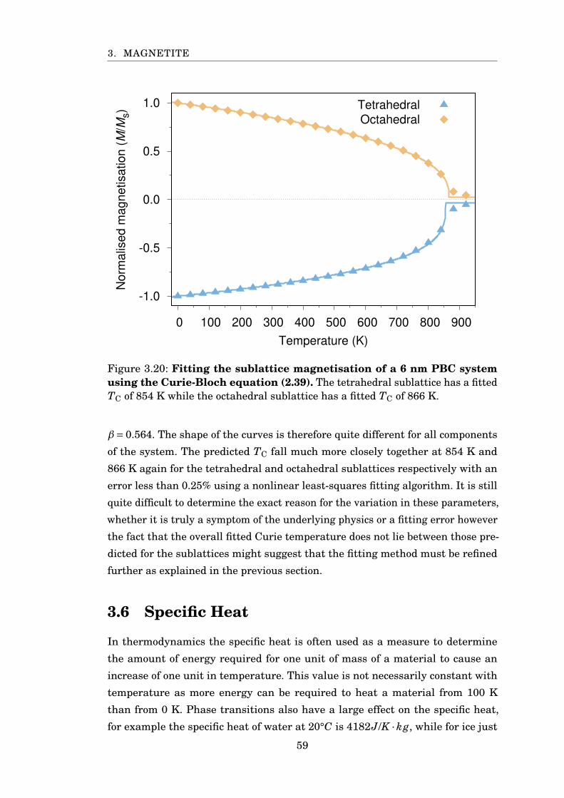
3. MAGNETITE
-1.0
-0.5
0.0
0.5
1.0
0 100 200 300 400 500 600 700 800 900
Norm
alis
ed m
agnetisation (
M/M
s)
Temperature (K)
Tetrahedral
Octahedral
Figure 3.20: Fitting the sublattice magnetisation of a 6 nm PBC systemusing the Curie-Bloch equation (2.39). The tetrahedral sublattice has a fittedTC of 854 K while the octahedral sublattice has a fitted TC of 866 K.
β= 0.564. The shape of the curves is therefore quite different for all components
of the system. The predicted TC fall much more closely together at 854 K and
866 K again for the tetrahedral and octahedral sublattices respectively with an
error less than 0.25% using a nonlinear least-squares fitting algorithm. It is still
quite difficult to determine the exact reason for the variation in these parameters,
whether it is truly a symptom of the underlying physics or a fitting error however
the fact that the overall fitted Curie temperature does not lie between those pre-
dicted for the sublattices might suggest that the fitting method must be refined
further as explained in the previous section.
3.6 Specific Heat
In thermodynamics the specific heat is often used as a measure to determine
the amount of energy required for one unit of mass of a material to cause an
increase of one unit in temperature. This value is not necessarily constant with
temperature as more energy can be required to heat a material from 100 K
than from 0 K. Phase transitions also have a large effect on the specific heat,
for example the specific heat of water at 20°C is 4182J/K ·kg, while for ice just
59
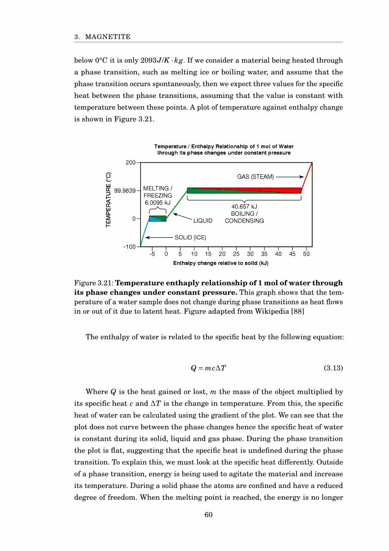
3. MAGNETITE
below 0°C it is only 2093J/K ·kg. If we consider a material being heated through
a phase transition, such as melting ice or boiling water, and assume that the
phase transition occurs spontaneously, then we expect three values for the specific
heat between the phase transitions, assuming that the value is constant with
temperature between these points. A plot of temperature against enthalpy change
is shown in Figure 3.21.
Figure 3.21: Temperature enthaply relationship of 1 mol of water throughits phase changes under constant pressure. This graph shows that the tem-perature of a water sample does not change during phase transitions as heat flowsin or out of it due to latent heat. Figure adapted from Wikipedia [88]
The enthalpy of water is related to the specific heat by the following equation:
Q = mc∆T (3.13)
Where Q is the heat gained or lost, m the mass of the object multiplied by
its specific heat c and ∆T is the change in temperature. From this, the specific
heat of water can be calculated using the gradient of the plot. We can see that the
plot does not curve between the phase changes hence the specific heat of water
is constant during its solid, liquid and gas phase. During the phase transition
the plot is flat, suggesting that the specific heat is undefined during the phase
transition. To explain this, we must look at the specific heat differently. Outside
of a phase transition, energy is being used to agitate the material and increase
its temperature. During a solid phase the atoms are confined and have a reduced
degree of freedom. When the melting point is reached, the energy is no longer
60
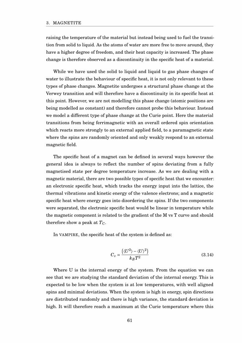
3. MAGNETITE
raising the temperature of the material but instead being used to fuel the transi-
tion from solid to liquid. As the atoms of water are more free to move around, they
have a higher degree of freedom, and their heat capacity is increased. The phase
change is therefore observed as a discontinuity in the specific heat of a material.
While we have used the solid to liquid and liquid to gas phase changes of
water to illustrate the behaviour of specific heat, it is not only relevant to these
types of phase changes. Magnetite undergoes a structural phase change at the
Verwey transition and will therefore have a discontinuity in its specific heat at
this point. However, we are not modelling this phase change (atomic positions are
being modelled as constant) and therefore cannot probe this behaviour. Instead
we model a different type of phase change at the Curie point. Here the material
transitions from being ferrimagnetic with an overall ordered spin orientation
which reacts more strongly to an external applied field, to a paramagnetic state
where the spins are randomly oriented and only weakly respond to an external
magnetic field.
The specific heat of a magnet can be defined in several ways however the
general idea is always to reflect the number of spins deviating from a fully
magnetised state per degree temperature increase. As we are dealing with a
magnetic material, there are two possible types of specific heat that we encounter:
an electronic specific heat, which tracks the energy input into the lattice, the
thermal vibrations and kinetic energy of the valence electrons; and a magnetic
specific heat where energy goes into disordering the spins. If the two components
were separated, the electronic specific heat would be linear in temperature while
the magnetic component is related to the gradient of the M vs T curve and should
therefore show a peak at TC.
In VAMPIRE, the specific heat of the system is defined as:
Cv =(⟨U2⟩−⟨U⟩2)
kBT2 (3.14)
Where U is the internal energy of the system. From the equation we can
see that we are studying the standard deviation of the internal energy. This is
expected to be low when the system is at low temperatures, with well aligned
spins and minimal deviations. When the system is high in energy, spin directions
are distributed randomly and there is high variance, the standard deviation is
high. It will therefore reach a maximum at the Curie temperature where this
61
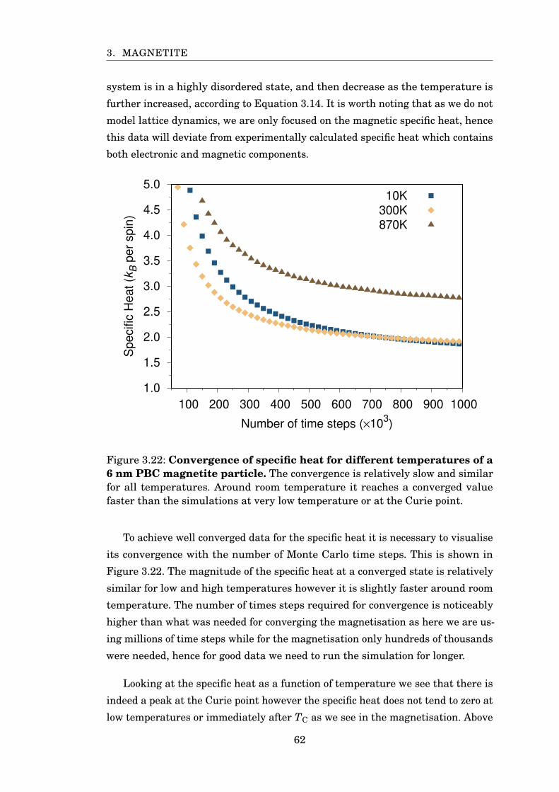
3. MAGNETITE
system is in a highly disordered state, and then decrease as the temperature is
further increased, according to Equation 3.14. It is worth noting that as we do not
model lattice dynamics, we are only focused on the magnetic specific heat, hence
this data will deviate from experimentally calculated specific heat which contains
both electronic and magnetic components.
1.0
1.5
2.0
2.5
3.0
3.5
4.0
4.5
5.0
100 200 300 400 500 600 700 800 900 1000
Specific
Heat (k
B p
er
spin
)
Number of time steps (×103)
10K
300K
870K
Figure 3.22: Convergence of specific heat for different temperatures of a6 nm PBC magnetite particle. The convergence is relatively slow and similarfor all temperatures. Around room temperature it reaches a converged valuefaster than the simulations at very low temperature or at the Curie point.
To achieve well converged data for the specific heat it is necessary to visualise
its convergence with the number of Monte Carlo time steps. This is shown in
Figure 3.22. The magnitude of the specific heat at a converged state is relatively
similar for low and high temperatures however it is slightly faster around room
temperature. The number of times steps required for convergence is noticeably
higher than what was needed for converging the magnetisation as here we are us-
ing millions of time steps while for the magnetisation only hundreds of thousands
were needed, hence for good data we need to run the simulation for longer.
Looking at the specific heat as a function of temperature we see that there is
indeed a peak at the Curie point however the specific heat does not tend to zero at
low temperatures or immediately after TC as we see in the magnetisation. Above
62
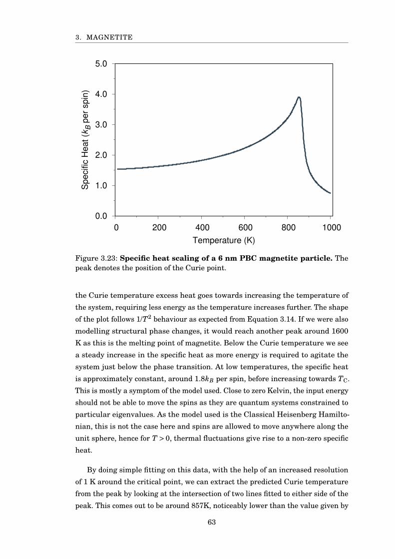
3. MAGNETITE
0.0
1.0
2.0
3.0
4.0
5.0
0 200 400 600 800 1000
Specific
Heat (k
B p
er
spin
)
Temperature (K)
Figure 3.23: Specific heat scaling of a 6 nm PBC magnetite particle. Thepeak denotes the position of the Curie point.
the Curie temperature excess heat goes towards increasing the temperature of
the system, requiring less energy as the temperature increases further. The shape
of the plot follows 1/T2 behaviour as expected from Equation 3.14. If we were also
modelling structural phase changes, it would reach another peak around 1600
K as this is the melting point of magnetite. Below the Curie temperature we see
a steady increase in the specific heat as more energy is required to agitate the
system just below the phase transition. At low temperatures, the specific heat
is approximately constant, around 1.8kB per spin, before increasing towards TC.
This is mostly a symptom of the model used. Close to zero Kelvin, the input energy
should not be able to move the spins as they are quantum systems constrained to
particular eigenvalues. As the model used is the Classical Heisenberg Hamilto-
nian, this is not the case here and spins are allowed to move anywhere along the
unit sphere, hence for T > 0, thermal fluctuations give rise to a non-zero specific
heat.
By doing simple fitting on this data, with the help of an increased resolution
of 1 K around the critical point, we can extract the predicted Curie temperature
from the peak by looking at the intersection of two lines fitted to either side of the
peak. This comes out to be around 857K, noticeably lower than the value given by
63
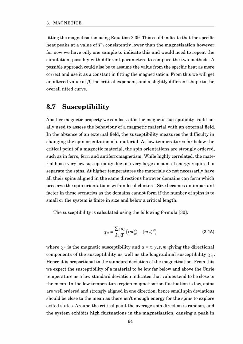
3. MAGNETITE
fitting the magnetisation using Equation 2.39. This could indicate that the specific
heat peaks at a value of TC consistently lower than the magnetisation however
for now we have only one sample to indicate this and would need to repeat the
simulation, possibly with different parameters to compare the two methods. A
possible approach could also be to assume the value from the specific heat as more
correct and use it as a constant in fitting the magnetisation. From this we will get
an altered value of β, the critical exponent, and a slightly different shape to the
overall fitted curve.
3.7 Susceptibility
Another magnetic property we can look at is the magnetic susceptibility tradition-
ally used to assess the behaviour of a magnetic material with an external field.
In the absence of an external field, the susceptibility measures the difficulty in
changing the spin orientation of a material. At low temperatures far below the
critical point of a magnetic material, the spin orientations are strongly ordered,
such as in ferro, ferri and antiferromagnetism. While highly correlated, the mate-
rial has a very low susceptibility due to a very large amount of energy required to
separate the spins. At higher temperatures the materials do not necessarily have
all their spins aligned in the same directions however domains can form which
preserve the spin orientations within local clusters. Size becomes an important
factor in these scenarios as the domains cannot form if the number of spins is to
small or the system is finite in size and below a critical length.
The susceptibility is calculated using the following formula [30]:
χα =∑
iµi
kBT(⟨m2
α⟩−⟨mα⟩2) (3.15)
where χα is the magnetic susceptibility and α= x, y, z,m giving the directional
components of the susceptibility as well as the longitudinal susceptibility χm.
Hence it is proportional to the standard deviation of the magnetisation. From this
we expect the susceptibility of a material to be low far below and above the Curie
temperature as a low standard deviation indicates that values tend to be close to
the mean. In the low temperature region magnetisation fluctuation is low, spins
are well ordered and strongly aligned in one direction, hence small spin deviations
should be close to the mean as there isn’t enough energy for the spins to explore
exited states. Around the critical point the average spin direction is random, and
the system exhibits high fluctuations in the magnetisation, causing a peak in
64
3. MAGNETITE
the susceptibility. Above TC, all spin directions are treated similarly and the
susceptibility decreases as T is increased. This formulation of the susceptibility
is quite different to the experimentally measured values of χ or 1/χ, which are
less commonly used when discussing nanoparticles as its measurement becomes
difficult and artificial. As such the formulation of susceptibility in Equation 3.15
is best used for investigating the Curie temperature of the system.
To achieve well converged data for the susceptibility, many millions of Monte
Carlo time steps must be used. Compared to the magnetisation, at least ten times
the number of steps is used to have a relatively smoothly varying susceptibility
versus temperature plot. The convergence also scales with temperature as values
for susceptibility around the critical point take noticeably longer to converge
than data points further away. Even for relatively small systems around 10 nm
diameter, susceptibility data is the most time consuming to calculate however
it should give a very good indication of the Curie temperature as this should
be indicated by a simple peak. It is difficult to fit the susceptibility due to its
discontinuity at TC and therefore the sample rate around this point is increased.
While the susceptibility behaviour is smooth away from the critical point, we
perform one equilibration simulation per 10 K temperature step however around
TC, this is increased to one simulation per 1 K temperature step to fully capture
the peak of the susceptibility as well as any sharp increases or decreases in its
value. For a PBC system of around 6 nm size, each simulation can take around
twelve hours to complete on a single core of a modern Intel Xeon processor
(released around 2017).
The susceptibility for a 6 nm PBC particle is shown in Fig. 3.24. At low
temperatures the spins are aligned close together and there isn’t enough energy
for the spins to diverge from each other significantly. As the temperature increases
the standard deviation increases as it is more likely for spins to follow random
directions, as seen in Figure 3.11. At the Curie point, the system transitions to a
disordered state as it is now paramagnetic and the susceptibility peaks. As the
system is heated further, the average spin orientation is random and the standard
deviation lowers again due to the overall properties becoming uniform.
To extract a value for TC, we can fit two curves on each side of the susceptibility
and find their intersection. This shows that the predicted Curie temperature for
this system is around 862 K which lies somewhere in between the values predicted
by the magnetisation and the specific heat. Before making a comparison of these
values, we can also study the sublattice susceptibility of the system to check
65
3. MAGNETITE
0.0
0.5
1.0
1.5
2.0
2.5
3.0
3.5
0 200 400 600 800 1000
Mean S
usceptibili
ty (
T -
1 ×
10
-3)
Temperature (K)
Figure 3.24: Susceptibility vs temperature curve of a 6 nm PBC magnetiteparticle. The susceptibility is very low below the Curie temperature as theaverage spin directions are still ordered and the standard deviation of the spinsis small. At the Curie temperature there is a sharp discontinuity as the spinstransition from an ordered to disordered (paramagnetic) state.
whether these are predicted to be different, as shown with the magnetisation, or
if they lie closer together.
Figure 3.25 compares the sublattice susceptibilities to the overall susceptibil-
ity of the system which is an order of magnitude lower in size. To understand why
this is the case we must consider the sublattices individually as on their own they
are mostly made up of spins oriented in similar directions, as least during the low
temperature phase, which are still strongly correlated to each other. When we add
up the contributions of both sublattices, we are now comparing spins which have
much larger difference in their directions as the two sublattices are antiparallel at
low temperatures. This creates a distinction between the intra-sublattice suscep-
tibility, that of the sublattices individually, and the inter-sublattice susceptibility
which is the result of the overall contributions and represented by the "Total" line
on Figure 3.25. An illustration of these two modes is shown in Figure 3.26.
The overall behaviour for the plots remains the same irrespective of the
magnitudes of the components. We can now extract the Curie temperatures
66
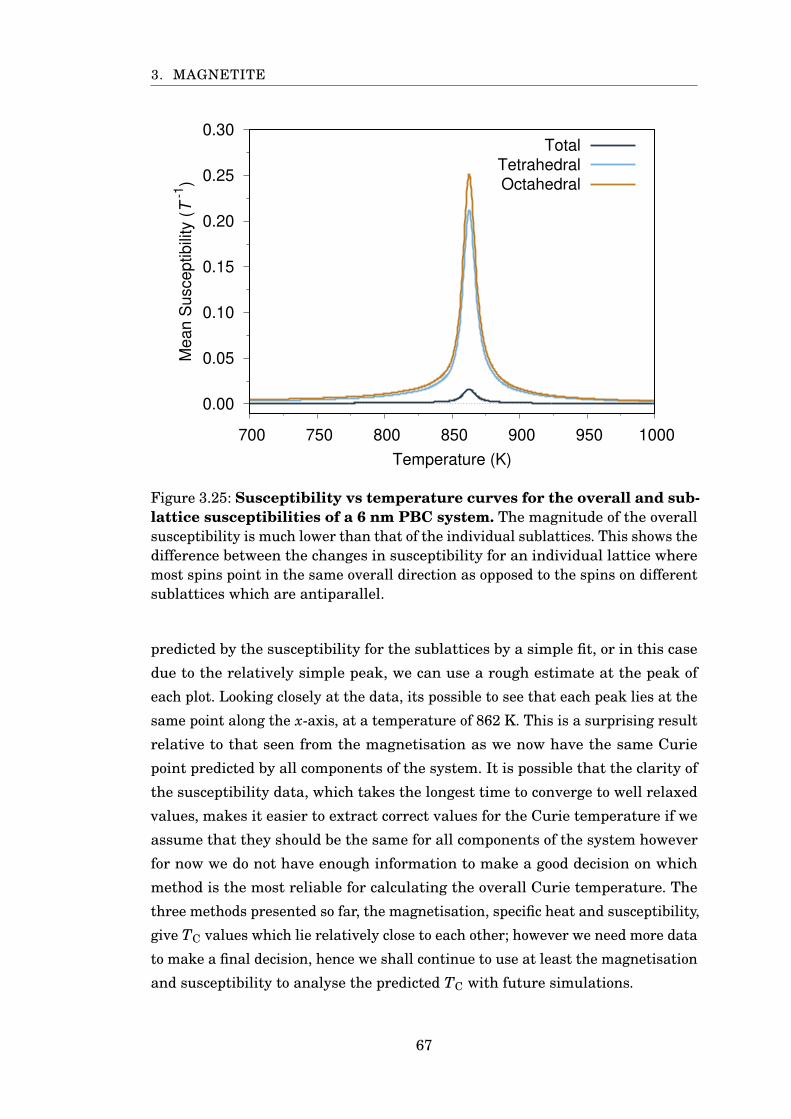
3. MAGNETITE
0.00
0.05
0.10
0.15
0.20
0.25
0.30
700 750 800 850 900 950 1000
Mean S
usceptibili
ty (
T -
1)
Temperature (K)
Total
Tetrahedral
Octahedral
Figure 3.25: Susceptibility vs temperature curves for the overall and sub-lattice susceptibilities of a 6 nm PBC system. The magnitude of the overallsusceptibility is much lower than that of the individual sublattices. This shows thedifference between the changes in susceptibility for an individual lattice wheremost spins point in the same overall direction as opposed to the spins on differentsublattices which are antiparallel.
predicted by the susceptibility for the sublattices by a simple fit, or in this case
due to the relatively simple peak, we can use a rough estimate at the peak of
each plot. Looking closely at the data, its possible to see that each peak lies at the
same point along the x-axis, at a temperature of 862 K. This is a surprising result
relative to that seen from the magnetisation as we now have the same Curie
point predicted by all components of the system. It is possible that the clarity of
the susceptibility data, which takes the longest time to converge to well relaxed
values, makes it easier to extract correct values for the Curie temperature if we
assume that they should be the same for all components of the system however
for now we do not have enough information to make a good decision on which
method is the most reliable for calculating the overall Curie temperature. The
three methods presented so far, the magnetisation, specific heat and susceptibility,
give TC values which lie relatively close to each other; however we need more data
to make a final decision, hence we shall continue to use at least the magnetisation
and susceptibility to analyse the predicted TC with future simulations.
67
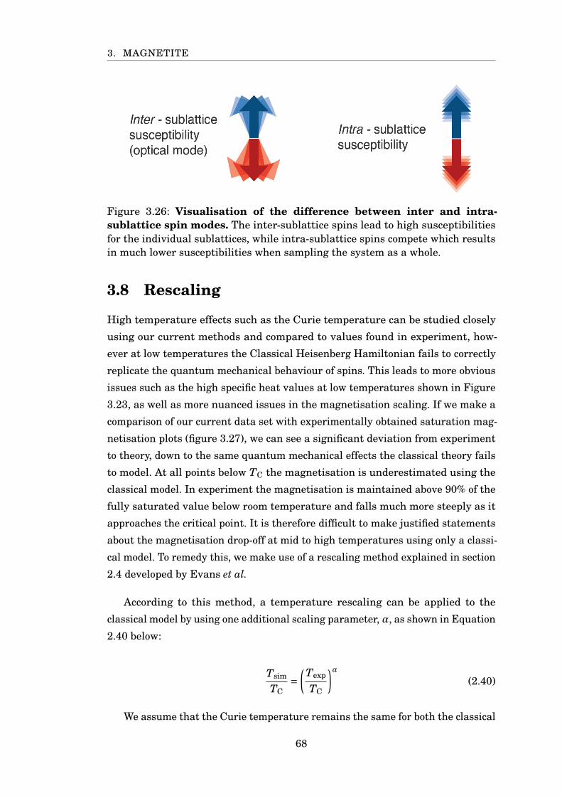
3. MAGNETITE
Figure 3.26: Visualisation of the difference between inter and intra-sublattice spin modes. The inter-sublattice spins lead to high susceptibilitiesfor the individual sublattices, while intra-sublattice spins compete which resultsin much lower susceptibilities when sampling the system as a whole.
3.8 Rescaling
High temperature effects such as the Curie temperature can be studied closely
using our current methods and compared to values found in experiment, how-
ever at low temperatures the Classical Heisenberg Hamiltonian fails to correctly
replicate the quantum mechanical behaviour of spins. This leads to more obvious
issues such as the high specific heat values at low temperatures shown in Figure
3.23, as well as more nuanced issues in the magnetisation scaling. If we make a
comparison of our current data set with experimentally obtained saturation mag-
netisation plots (figure 3.27), we can see a significant deviation from experiment
to theory, down to the same quantum mechanical effects the classical theory fails
to model. At all points below TC the magnetisation is underestimated using the
classical model. In experiment the magnetisation is maintained above 90% of the
fully saturated value below room temperature and falls much more steeply as it
approaches the critical point. It is therefore difficult to make justified statements
about the magnetisation drop-off at mid to high temperatures using only a classi-
cal model. To remedy this, we make use of a rescaling method explained in section
2.4 developed by Evans et al.
According to this method, a temperature rescaling can be applied to the
classical model by using one additional scaling parameter, α, as shown in Equation
2.40 below:
Tsim
TC=
(Texp
TC
)α(2.40)
We assume that the Curie temperature remains the same for both the classical
68
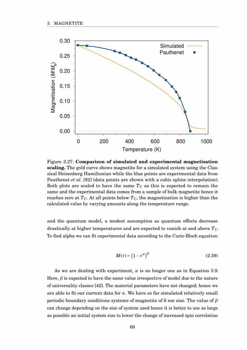
3. MAGNETITE
0.00
0.05
0.10
0.15
0.20
0.25
0.30
0 200 400 600 800 1000
Magnetisation (
M/M
s)
Temperature (K)
Simulated
Pauthenet
Figure 3.27: Comparison of simulated and experimental magnetisationscaling. The gold curve shows magnetite for a simulated system using the Clas-sical Heisenberg Hamiltonian while the blue points are experimental data fromPauthenet et al. [82] (data points are shown with a cubic spline interpolation).Both plots are scaled to have the same TC as this is expected to remain thesame and the experimental data comes from a sample of bulk magnetite hence itreaches zero at TC. At all points below TC, the magnetisation is higher than thecalculated value by varying amounts along the temperature range.
and the quantum model, a modest assumption as quantum effects decrease
drastically at higher temperatures and are expected to vanish at and above TC.
To find alpha we can fit experimental data according to the Curie-Bloch equation:
M(τ)= (1−τα)β (2.39)
As we are dealing with experiment, α is no longer one as in Equation 3.9.
Here, β is expected to have the same value irrespective of model due to the nature
of universality classes [42]. The material parameters have not changed; hence we
are able to fit our current data for α. We have so far simulated relatively small
periodic boundary conditions systems of magnetite of 6 nm size. The value of β
can change depending on the size of system used hence it is better to use as large
as possible an initial system size to lower the change of increased spin correlation
69
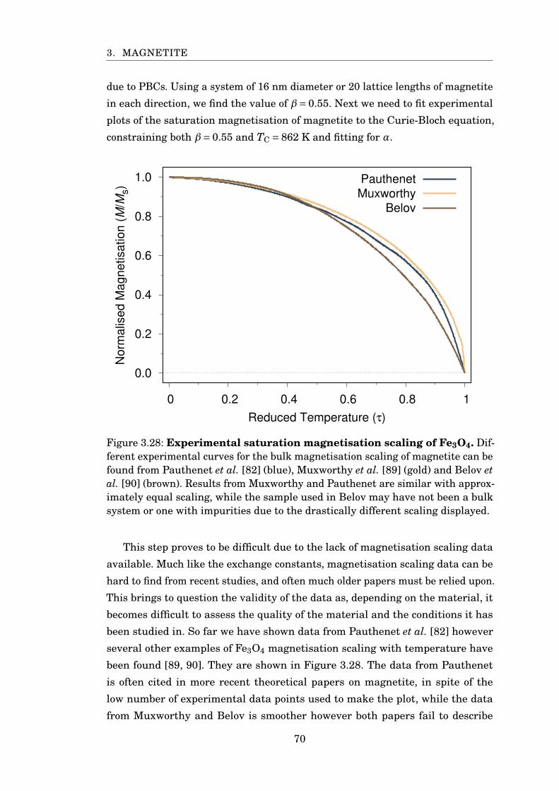
3. MAGNETITE
due to PBCs. Using a system of 16 nm diameter or 20 lattice lengths of magnetite
in each direction, we find the value of β= 0.55. Next we need to fit experimental
plots of the saturation magnetisation of magnetite to the Curie-Bloch equation,
constraining both β= 0.55 and TC = 862 K and fitting for α.
0.0
0.2
0.4
0.6
0.8
1.0
0 0.2 0.4 0.6 0.8 1
Norm
alis
ed M
agnetisation (
M/M
s)
Reduced Temperature (τ)
Pauthenet
Muxworthy
Belov
Figure 3.28: Experimental saturation magnetisation scaling of Fe3O4. Dif-ferent experimental curves for the bulk magnetisation scaling of magnetite can befound from Pauthenet et al. [82] (blue), Muxworthy et al. [89] (gold) and Belov etal. [90] (brown). Results from Muxworthy and Pauthenet are similar with approx-imately equal scaling, while the sample used in Belov may have not been a bulksystem or one with impurities due to the drastically different scaling displayed.
This step proves to be difficult due to the lack of magnetisation scaling data
available. Much like the exchange constants, magnetisation scaling data can be
hard to find from recent studies, and often much older papers must be relied upon.
This brings to question the validity of the data as, depending on the material, it
becomes difficult to assess the quality of the material and the conditions it has
been studied in. So far we have shown data from Pauthenet et al. [82] however
several other examples of Fe3O4 magnetisation scaling with temperature have
been found [89, 90]. They are shown in Figure 3.28. The data from Pauthenet
is often cited in more recent theoretical papers on magnetite, in spite of the
low number of experimental data points used to make the plot, while the data
from Muxworthy and Belov is smoother however both papers fail to describe
70
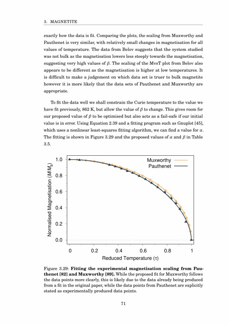
3. MAGNETITE
exactly how the data is fit. Comparing the plots, the scaling from Muxworthy and
Pauthenet is very similar, with relatively small changes in magnetisation for all
values of temperature. The data from Belov suggests that the system studied
was not bulk as the magnetisation lowers less steeply towards the magnetisation,
suggesting very high values of β. The scaling of the MvsT plot from Belov also
appears to be different as the magnetisation is higher at low temperatures. It
is difficult to make a judgement on which data set is truer to bulk magnetite
however it is more likely that the data sets of Pauthenet and Muxworthy are
appropriate.
To fit the data well we shall constrain the Curie temperature to the value we
have fit previously, 862 K, but allow the value of β to change. This gives room for
our proposed value of β to be optimised but also acts as a fail-safe if our initial
value is in error. Using Equation 2.39 and a fitting program such as Gnuplot [45],
which uses a nonlinear least-squares fitting algorithm, we can find a value for α.
The fitting is shown in Figure 3.29 and the proposed values of α and β in Table
3.5.
0.0
0.2
0.4
0.6
0.8
1.0
0 0.2 0.4 0.6 0.8 1
Norm
alis
ed M
agnetisation (
M/M
s)
Reduced Temperature (τ)
Muxworthy
Pauthenet
Figure 3.29: Fitting the experimental magnetisation scaling from Pau-thenet [82] and Muxworthy [89]. While the proposed fit for Muxworthy followsthe data points more clearly, this is likely due to the data already being producedfrom a fit in the original paper, while the data points from Pauthenet are explicitlystated as experimentally produced data points.
71
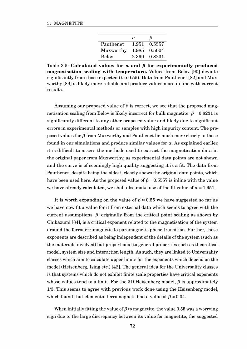
3. MAGNETITE
α β
Pauthenet 1.951 0.5557Muxworthy 1.985 0.5004Belov 2.399 0.8231
Table 3.5: Calculated values for α and β for experimentally producedmagnetisation scaling with temperature. Values from Belov [90] deviatesignificantly from those expected (β≈ 0.55). Data from Pauthenet [82] and Mux-worthy [89] is likely more reliable and produce values more in line with currentresults.
Assuming our proposed value of β is correct, we see that the proposed mag-
netisation scaling from Belov is likely incorrect for bulk magnetite. β= 0.8231 is
significantly different to any other proposed value and likely due to significant
errors in experimental methods or samples with high impurity content. The pro-
posed values for β from Muxworthy and Pauthenet lie much more closely to those
found in our simulations and produce similar values for α. As explained earlier,
it is difficult to assess the methods used to extract the magnetisation data in
the original paper from Muxworthy, as experimental data points are not shown
and the curve is of seemingly high quality suggesting it is a fit. The data from
Pauthenet, despite being the oldest, clearly shows the original data points, which
have been used here. As the proposed value of β= 0.5557 is inline with the value
we have already calculated, we shall also make use of the fit value of α= 1.951.
It is worth expanding on the value of β ≈ 0.55 we have suggested so far as
we have now fit a value for it from external data which seems to agree with the
current assumptions. β, originally from the critical point scaling as shown by
Chikazumi [84], is a critical exponent related to the magnetisation of the system
around the ferro/ferrimagnetic to paramagnetic phase transition. Further, these
exponents are described as being independent of the details of the system (such as
the materials involved) but proportional to general properties such as theoretical
model, system size and interaction length. As such, they are linked to Universality
classes which aim to calculate upper limits for the exponents which depend on the
model (Heisenberg, Ising etc.) [42]. The general idea for the Universality classes
is that systems which do not exhibit finite scale properties have critical exponents
whose values tend to a limit. For the 3D Heisenberg model, β is approximately
1/3. This seems to agree with previous work done using the Heisenberg model,
which found that elemental ferromagnets had a value of β≈ 0.34.
When initially fitting the value of β to magnetite, the value 0.55 was a worrying
sign due to the large discrepancy between its value for magnetite, the suggested
72
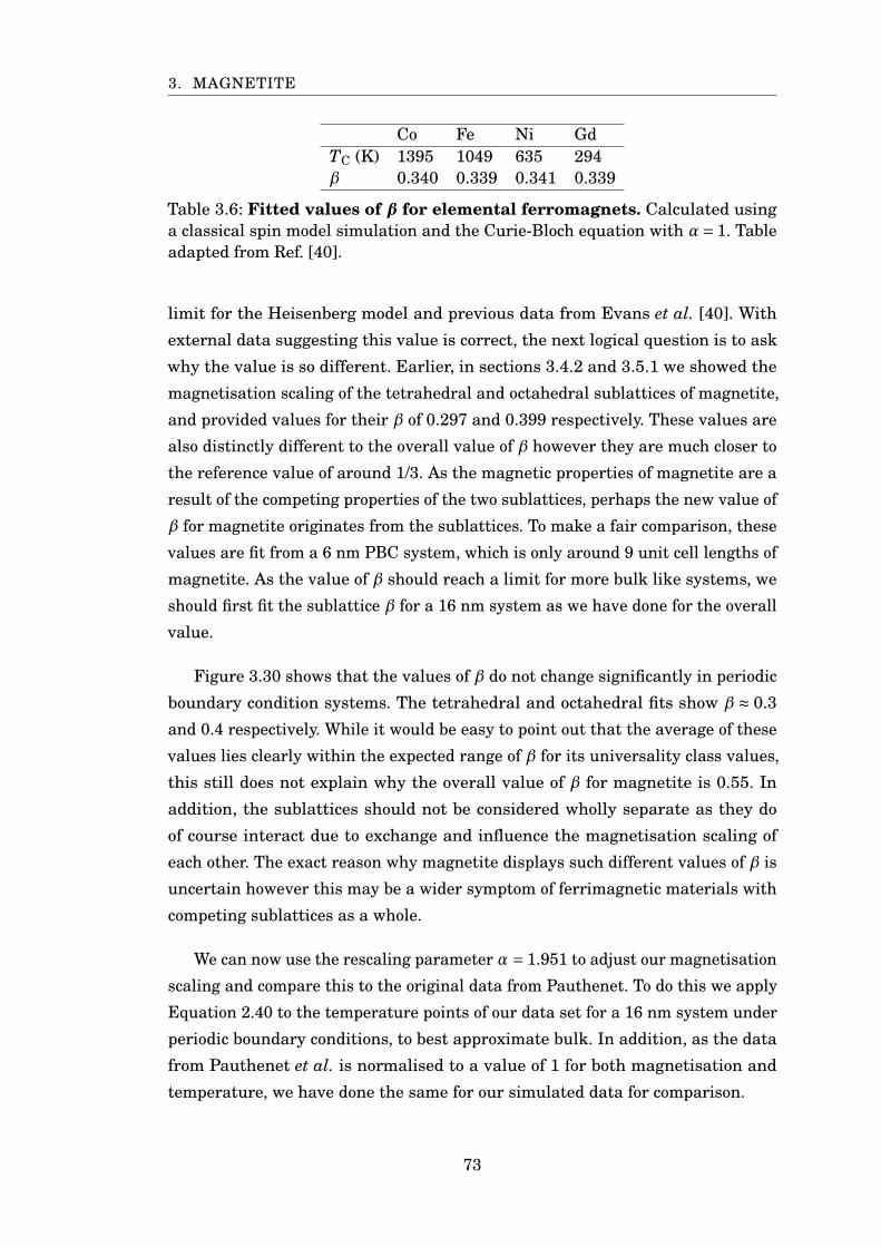
3. MAGNETITE
Co Fe Ni GdTC (K) 1395 1049 635 294β 0.340 0.339 0.341 0.339
Table 3.6: Fitted values of β for elemental ferromagnets. Calculated usinga classical spin model simulation and the Curie-Bloch equation with α= 1. Tableadapted from Ref. [40].
limit for the Heisenberg model and previous data from Evans et al. [40]. With
external data suggesting this value is correct, the next logical question is to ask
why the value is so different. Earlier, in sections 3.4.2 and 3.5.1 we showed the
magnetisation scaling of the tetrahedral and octahedral sublattices of magnetite,
and provided values for their β of 0.297 and 0.399 respectively. These values are
also distinctly different to the overall value of β however they are much closer to
the reference value of around 1/3. As the magnetic properties of magnetite are a
result of the competing properties of the two sublattices, perhaps the new value of
β for magnetite originates from the sublattices. To make a fair comparison, these
values are fit from a 6 nm PBC system, which is only around 9 unit cell lengths of
magnetite. As the value of β should reach a limit for more bulk like systems, we
should first fit the sublattice β for a 16 nm system as we have done for the overall
value.
Figure 3.30 shows that the values of β do not change significantly in periodic
boundary condition systems. The tetrahedral and octahedral fits show β ≈ 0.3
and 0.4 respectively. While it would be easy to point out that the average of these
values lies clearly within the expected range of β for its universality class values,
this still does not explain why the overall value of β for magnetite is 0.55. In
addition, the sublattices should not be considered wholly separate as they do
of course interact due to exchange and influence the magnetisation scaling of
each other. The exact reason why magnetite displays such different values of β is
uncertain however this may be a wider symptom of ferrimagnetic materials with
competing sublattices as a whole.
We can now use the rescaling parameter α = 1.951 to adjust our magnetisation
scaling and compare this to the original data from Pauthenet. To do this we apply
Equation 2.40 to the temperature points of our data set for a 16 nm system under
periodic boundary conditions, to best approximate bulk. In addition, as the data
from Pauthenet et al. is normalised to a value of 1 for both magnetisation and
temperature, we have done the same for our simulated data for comparison.
73
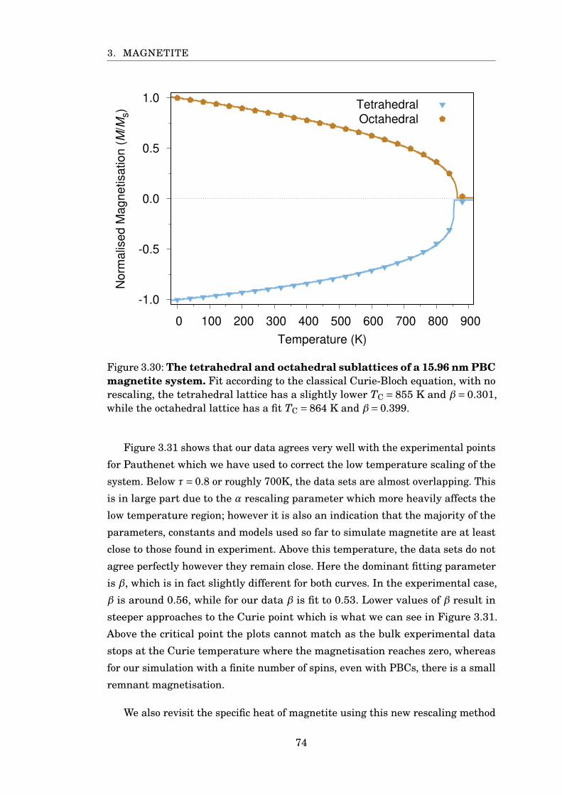
3. MAGNETITE
-1.0
-0.5
0.0
0.5
1.0
0 100 200 300 400 500 600 700 800 900
Norm
alis
ed M
agnetisation (
M/M
s)
Temperature (K)
Tetrahedral
Octahedral
Figure 3.30: The tetrahedral and octahedral sublattices of a 15.96 nm PBCmagnetite system. Fit according to the classical Curie-Bloch equation, with norescaling, the tetrahedral lattice has a slightly lower TC = 855 K and β= 0.301,while the octahedral lattice has a fit TC = 864 K and β= 0.399.
Figure 3.31 shows that our data agrees very well with the experimental points
for Pauthenet which we have used to correct the low temperature scaling of the
system. Below τ= 0.8 or roughly 700K, the data sets are almost overlapping. This
is in large part due to the α rescaling parameter which more heavily affects the
low temperature region; however it is also an indication that the majority of the
parameters, constants and models used so far to simulate magnetite are at least
close to those found in experiment. Above this temperature, the data sets do not
agree perfectly however they remain close. Here the dominant fitting parameter
is β, which is in fact slightly different for both curves. In the experimental case,
β is around 0.56, while for our data β is fit to 0.53. Lower values of β result in
steeper approaches to the Curie point which is what we can see in Figure 3.31.
Above the critical point the plots cannot match as the bulk experimental data
stops at the Curie temperature where the magnetisation reaches zero, whereas
for our simulation with a finite number of spins, even with PBCs, there is a small
remnant magnetisation.
We also revisit the specific heat of magnetite using this new rescaling method
74
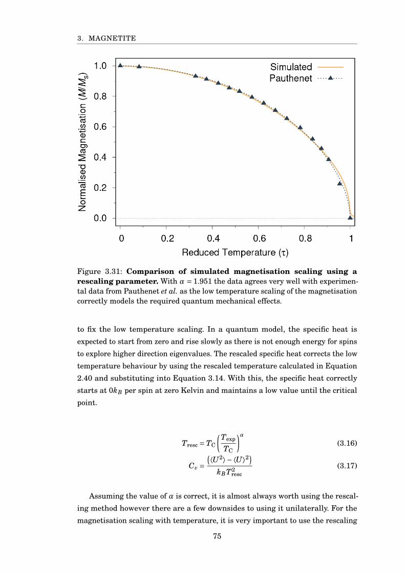
3. MAGNETITE
Figure 3.31: Comparison of simulated magnetisation scaling using arescaling parameter. With α = 1.951 the data agrees very well with experimen-tal data from Pauthenet et al. as the low temperature scaling of the magnetisationcorrectly models the required quantum mechanical effects.
to fix the low temperature scaling. In a quantum model, the specific heat is
expected to start from zero and rise slowly as there is not enough energy for spins
to explore higher direction eigenvalues. The rescaled specific heat corrects the low
temperature behaviour by using the rescaled temperature calculated in Equation
2.40 and substituting into Equation 3.14. With this, the specific heat correctly
starts at 0kB per spin at zero Kelvin and maintains a low value until the critical
point.
Tresc =TC
(Texp
TC
)α(3.16)
Cv =(⟨U2⟩−⟨U⟩2)
kBT2resc
(3.17)
Assuming the value of α is correct, it is almost always worth using the rescal-
ing method however there are a few downsides to using it unilaterally. For the
magnetisation scaling with temperature, it is very important to use the rescaling
75
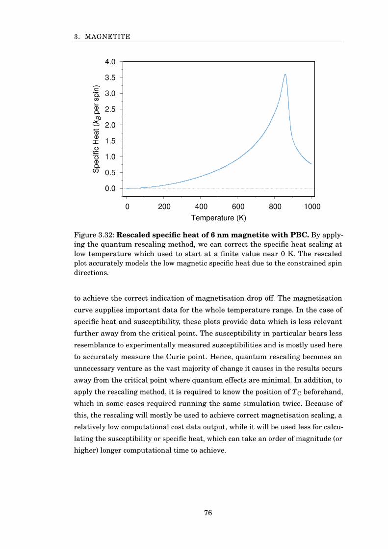
3. MAGNETITE
0.0
0.5
1.0
1.5
2.0
2.5
3.0
3.5
4.0
0 200 400 600 800 1000
Specific
Heat (k
B p
er
spin
)
Temperature (K)
Figure 3.32: Rescaled specific heat of 6 nm magnetite with PBC. By apply-ing the quantum rescaling method, we can correct the specific heat scaling atlow temperature which used to start at a finite value near 0 K. The rescaledplot accurately models the low magnetic specific heat due to the constrained spindirections.
to achieve the correct indication of magnetisation drop off. The magnetisation
curve supplies important data for the whole temperature range. In the case of
specific heat and susceptibility, these plots provide data which is less relevant
further away from the critical point. The susceptibility in particular bears less
resemblance to experimentally measured susceptibilities and is mostly used here
to accurately measure the Curie point. Hence, quantum rescaling becomes an
unnecessary venture as the vast majority of change it causes in the results occurs
away from the critical point where quantum effects are minimal. In addition, to
apply the rescaling method, it is required to know the position of TC beforehand,
which in some cases required running the same simulation twice. Because of
this, the rescaling will mostly be used to achieve correct magnetisation scaling, a
relatively low computational cost data output, while it will be used less for calcu-
lating the susceptibility or specific heat, which can take an order of magnitude (or
higher) longer computational time to achieve.
76
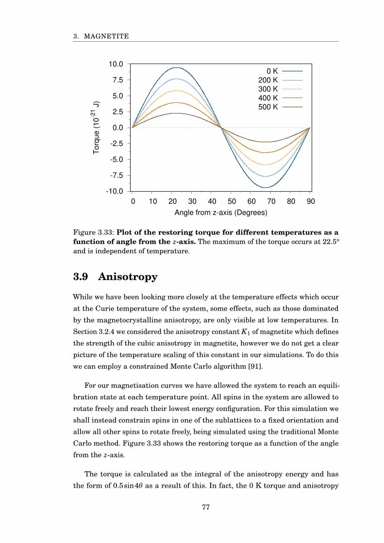
3. MAGNETITE
-10.0
-7.5
-5.0
-2.5
0.0
2.5
5.0
7.5
10.0
0 10 20 30 40 50 60 70 80 90
Torq
ue (
10
-21 J
)
Angle from z-axis (Degrees)
0 K
200 K
300 K
400 K
500 K
Figure 3.33: Plot of the restoring torque for different temperatures as afunction of angle from the z-axis. The maximum of the torque occurs at 22.5°and is independent of temperature.
3.9 Anisotropy
While we have been looking more closely at the temperature effects which occur
at the Curie temperature of the system, some effects, such as those dominated
by the magnetocrystalline anisotropy, are only visible at low temperatures. In
Section 3.2.4 we considered the anisotropy constant K1 of magnetite which defines
the strength of the cubic anisotropy in magnetite, however we do not get a clear
picture of the temperature scaling of this constant in our simulations. To do this
we can employ a constrained Monte Carlo algorithm [91].
For our magnetisation curves we have allowed the system to reach an equili-
bration state at each temperature point. All spins in the system are allowed to
rotate freely and reach their lowest energy configuration. For this simulation we
shall instead constrain spins in one of the sublattices to a fixed orientation and
allow all other spins to rotate freely, being simulated using the traditional Monte
Carlo method. Figure 3.33 shows the restoring torque as a function of the angle
from the z-axis.
The torque is calculated as the integral of the anisotropy energy and has
the form of 0.5sin4θ as a result of this. In fact, the 0 K torque and anisotropy
77
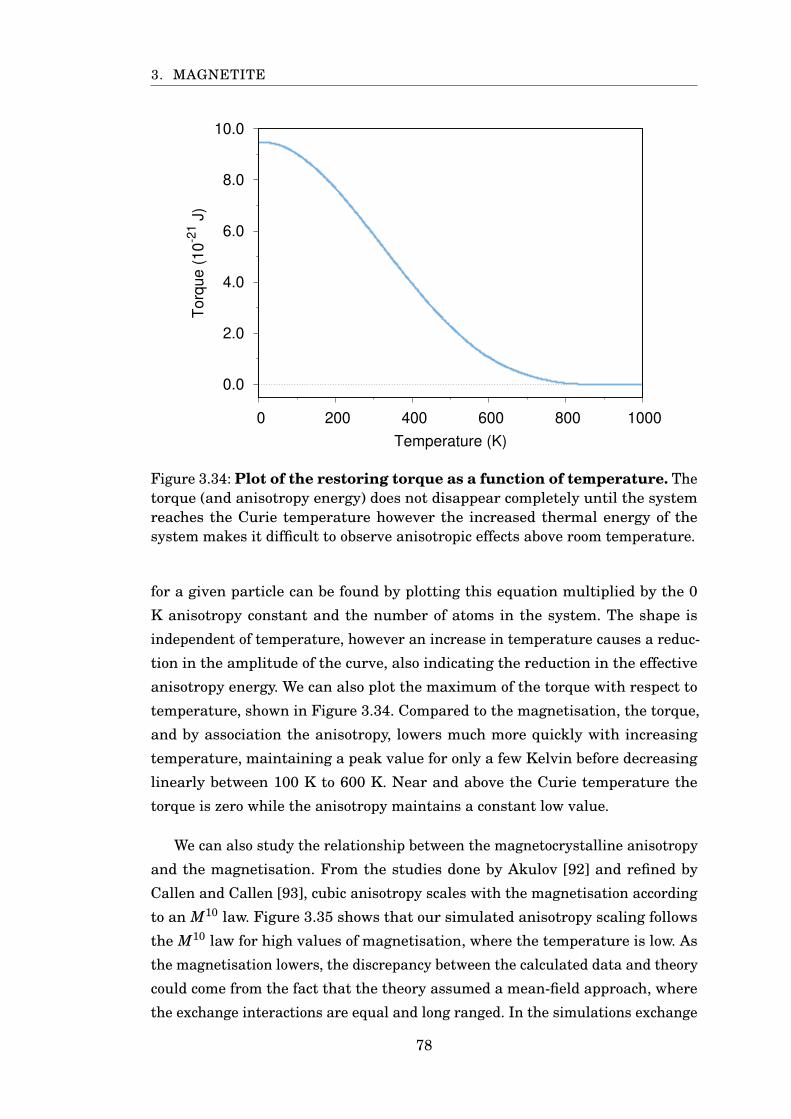
3. MAGNETITE
0.0
2.0
4.0
6.0
8.0
10.0
0 200 400 600 800 1000
Torq
ue (
10
-21 J
)
Temperature (K)
Figure 3.34: Plot of the restoring torque as a function of temperature. Thetorque (and anisotropy energy) does not disappear completely until the systemreaches the Curie temperature however the increased thermal energy of thesystem makes it difficult to observe anisotropic effects above room temperature.
for a given particle can be found by plotting this equation multiplied by the 0
K anisotropy constant and the number of atoms in the system. The shape is
independent of temperature, however an increase in temperature causes a reduc-
tion in the amplitude of the curve, also indicating the reduction in the effective
anisotropy energy. We can also plot the maximum of the torque with respect to
temperature, shown in Figure 3.34. Compared to the magnetisation, the torque,
and by association the anisotropy, lowers much more quickly with increasing
temperature, maintaining a peak value for only a few Kelvin before decreasing
linearly between 100 K to 600 K. Near and above the Curie temperature the
torque is zero while the anisotropy maintains a constant low value.
We can also study the relationship between the magnetocrystalline anisotropy
and the magnetisation. From the studies done by Akulov [92] and refined by
Callen and Callen [93], cubic anisotropy scales with the magnetisation according
to an M10 law. Figure 3.35 shows that our simulated anisotropy scaling follows
the M10 law for high values of magnetisation, where the temperature is low. As
the magnetisation lowers, the discrepancy between the calculated data and theory
could come from the fact that the theory assumed a mean-field approach, where
the exchange interactions are equal and long ranged. In the simulations exchange
78
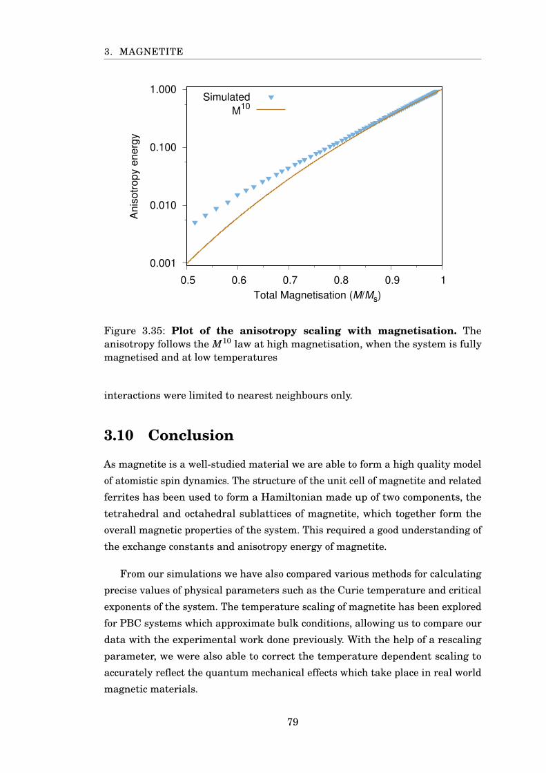
3. MAGNETITE
0.001
0.010
0.100
1.000
0.5 0.6 0.7 0.8 0.9 1
Anis
otr
opy e
nerg
y
Total Magnetisation (M/Ms)
Simulated
M10
Figure 3.35: Plot of the anisotropy scaling with magnetisation. Theanisotropy follows the M10 law at high magnetisation, when the system is fullymagnetised and at low temperatures
interactions were limited to nearest neighbours only.
3.10 Conclusion
As magnetite is a well-studied material we are able to form a high quality model
of atomistic spin dynamics. The structure of the unit cell of magnetite and related
ferrites has been used to form a Hamiltonian made up of two components, the
tetrahedral and octahedral sublattices of magnetite, which together form the
overall magnetic properties of the system. This required a good understanding of
the exchange constants and anisotropy energy of magnetite.
From our simulations we have also compared various methods for calculating
precise values of physical parameters such as the Curie temperature and critical
exponents of the system. The temperature scaling of magnetite has been explored
for PBC systems which approximate bulk conditions, allowing us to compare our
data with the experimental work done previously. With the help of a rescaling
parameter, we were also able to correct the temperature dependent scaling to
accurately reflect the quantum mechanical effects which take place in real world
magnetic materials.
79

3. MAGNETITE
Next we shall explore how the properties of magnetite vary when it is in
nanoparticle form and subject to topological effects.
80

CH
AP
TE
R
4FINITE SIZE SCALING AND PARTICLE ELONGATION
4.1 Introduction
At small sizes where the number of atoms in a magnetic particle are in the order of
103 to 105, statistical effects occur due to the finite number of spins. These effects
are described as finite size effects, with early studies into magnetic applications
by D. P. Landau and K. Binder [94, 95] who used Ising models and Monte Carlo
methods to predict how this affects more simple systems. This area of study
has remained popular with other groups focusing on specific materials such as
the recent work done by Jun Wang [96] looking at barium hexaferrite platelets.
The finite size scaling (FSS) occurs irrespective of the dimensionality of the
system, either in 3D nanoparticles, or 2D thin films [20, 97]. While this analysis
has already been applied to magnetite [20, 98] using both experimental and
computational approaches, much of the studies performed relied on simplifications
such as particularly small systems sizes with low sampling at these scales, or
model approximations such as the Ising model which fails to accurately model
magnetite due to its constrained spin directions. This makes it difficult to model
the intra and inter sublattice effects shown in chapter 3.4.2. Experimental studies
have additional complexity due to the possibility of imperfect samples, particularly
when dealing with less stable materials. It can also be very difficult to study
nanoparticles with constrained sizes and more often a range of particle sizes
is observed. The purity of the samples is also not easy to control as magnetite
nanoparticles can exhibit rust, the formation of maghemite or hematite as well
as other impurities depending on the materials and methods used to create the
81
4. FINITE SIZE SCALING AND PARTICLE ELONGATION
sample.
Here, we try to model finite size systems using the 3D Heisenberg model and
study both the overall magnetic properties, as well as any differences that occur
at the sublattice level, to form a complete data set of finite size scaling from small
particles of the order of one unit cell, to a system which approaches, at least
asymptotically, a bulk magnetite system.
So far we have covered various magnetic properties we can use to assess the
system. Periodic boundary condition systems give a good benchmark for bulk
system properties, and we can now compare this with finite size systems which
have broken exchange interactions at the surface. There are various types of
finite size systems that we can explore, which highlight different properties. Here
these shall be divided into spherical and faceted systems. Spherical nanoparticles
can be formed, depending on experimental methods used, for various iron oxide
nanoparticles [17] however these are often less stable. For this work, they have
the benefit of maintaining the ratio of each sublattice despite their size. As the
surface is terminated at the same radius over the whole particle, no sublattice
or surface termination is preferred or dominant over another. Faceted particles
suffer from exactly this issue. Many different types of faceted iron oxide particles
have been seen in experiment [9, 99], their structures depending on the surface
orientation and termination. In addition to finite size effects, these particles
are usually dominated by the sublattice which terminates their composition. Of
course, the separation between these types of particles is not always obvious as
a highly faceted particle may be approximately spherical however we shall only
deal with perfectly spherical nanoparticles and faceted particles with only two or
three different surface orientations.
4.1.1 Spherical Nanoparticles
First we can look at spherical particles as they simplify two aspects of the finite
size scaling that we will examine: the shape and surface. Roughly spherical parti-
cles can be formed in experiment and are often coated in silicon, for biomedical
applications [100]. Their surfaces are usually not perfectly spherical however for
now we shall approximate this and assume an ideal sphere.
To start we can look at the finite size scaling properties of spherical particles
of diameters ranging between 2 and 16 nm diameter, or up to 20 unit cell widths.
At this size range, we are dealing with fine nanoparticles containing up to roughly
100,000 magnetic atoms. Figure 4.2 shows the finite size scaling of these nanopar-
82
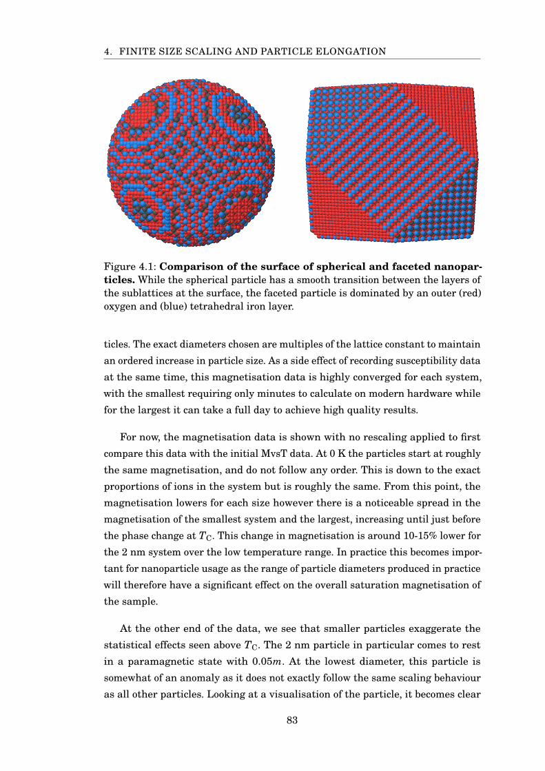
4. FINITE SIZE SCALING AND PARTICLE ELONGATION
Figure 4.1: Comparison of the surface of spherical and faceted nanopar-ticles. While the spherical particle has a smooth transition between the layers ofthe sublattices at the surface, the faceted particle is dominated by an outer (red)oxygen and (blue) tetrahedral iron layer.
ticles. The exact diameters chosen are multiples of the lattice constant to maintain
an ordered increase in particle size. As a side effect of recording susceptibility data
at the same time, this magnetisation data is highly converged for each system,
with the smallest requiring only minutes to calculate on modern hardware while
for the largest it can take a full day to achieve high quality results.
For now, the magnetisation data is shown with no rescaling applied to first
compare this data with the initial MvsT data. At 0 K the particles start at roughly
the same magnetisation, and do not follow any order. This is down to the exact
proportions of ions in the system but is roughly the same. From this point, the
magnetisation lowers for each size however there is a noticeable spread in the
magnetisation of the smallest system and the largest, increasing until just before
the phase change at TC. This change in magnetisation is around 10-15% lower for
the 2 nm system over the low temperature range. In practice this becomes impor-
tant for nanoparticle usage as the range of particle diameters produced in practice
will therefore have a significant effect on the overall saturation magnetisation of
the sample.
At the other end of the data, we see that smaller particles exaggerate the
statistical effects seen above TC. The 2 nm particle in particular comes to rest
in a paramagnetic state with 0.05m. At the lowest diameter, this particle is
somewhat of an anomaly as it does not exactly follow the same scaling behaviour
as all other particles. Looking at a visualisation of the particle, it becomes clear
83
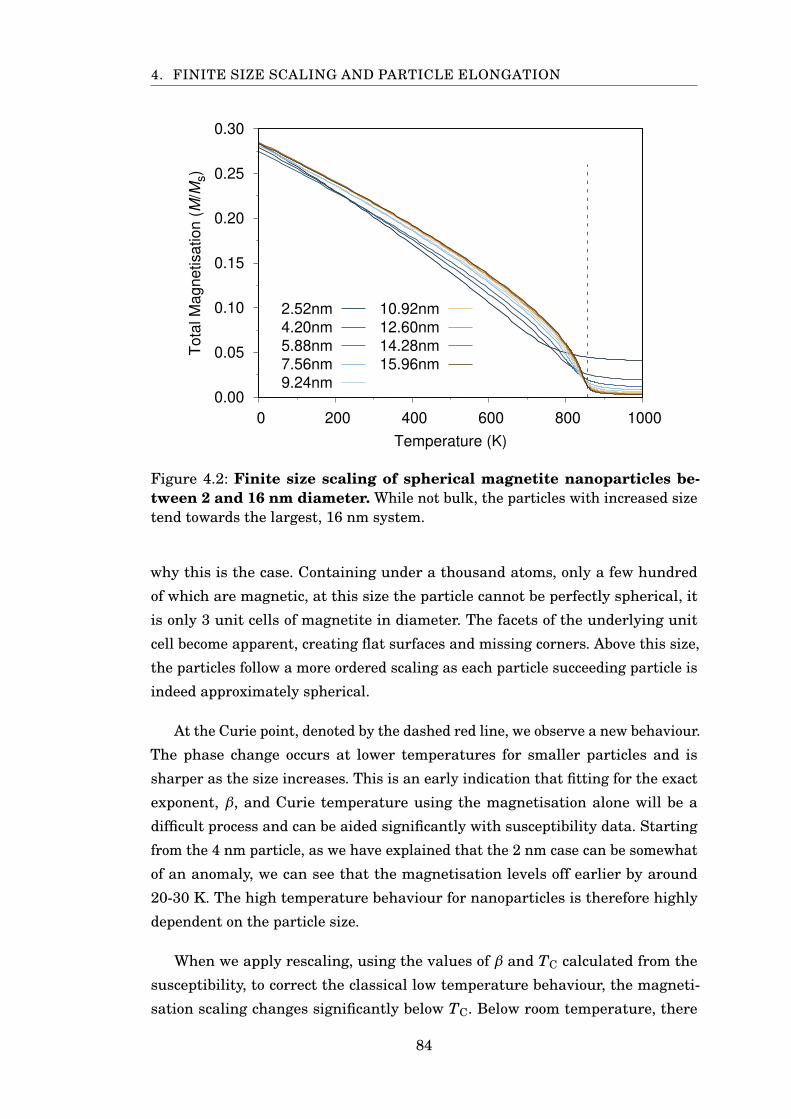
4. FINITE SIZE SCALING AND PARTICLE ELONGATION
0.00
0.05
0.10
0.15
0.20
0.25
0.30
0 200 400 600 800 1000
Tota
l M
agnetisation (
M/M
s)
Temperature (K)
2.52nm
4.20nm
5.88nm
7.56nm
9.24nm
10.92nm
12.60nm
14.28nm
15.96nm
Figure 4.2: Finite size scaling of spherical magnetite nanoparticles be-tween 2 and 16 nm diameter. While not bulk, the particles with increased sizetend towards the largest, 16 nm system.
why this is the case. Containing under a thousand atoms, only a few hundred
of which are magnetic, at this size the particle cannot be perfectly spherical, it
is only 3 unit cells of magnetite in diameter. The facets of the underlying unit
cell become apparent, creating flat surfaces and missing corners. Above this size,
the particles follow a more ordered scaling as each particle succeeding particle is
indeed approximately spherical.
At the Curie point, denoted by the dashed red line, we observe a new behaviour.
The phase change occurs at lower temperatures for smaller particles and is
sharper as the size increases. This is an early indication that fitting for the exact
exponent, β, and Curie temperature using the magnetisation alone will be a
difficult process and can be aided significantly with susceptibility data. Starting
from the 4 nm particle, as we have explained that the 2 nm case can be somewhat
of an anomaly, we can see that the magnetisation levels off earlier by around
20-30 K. The high temperature behaviour for nanoparticles is therefore highly
dependent on the particle size.
When we apply rescaling, using the values of β and TC calculated from the
susceptibility, to correct the classical low temperature behaviour, the magneti-
sation scaling changes significantly below TC. Below room temperature, there
84
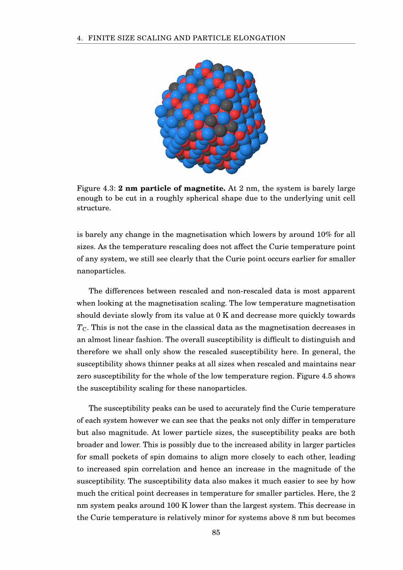
4. FINITE SIZE SCALING AND PARTICLE ELONGATION
Figure 4.3: 2 nm particle of magnetite. At 2 nm, the system is barely largeenough to be cut in a roughly spherical shape due to the underlying unit cellstructure.
is barely any change in the magnetisation which lowers by around 10% for all
sizes. As the temperature rescaling does not affect the Curie temperature point
of any system, we still see clearly that the Curie point occurs earlier for smaller
nanoparticles.
The differences between rescaled and non-rescaled data is most apparent
when looking at the magnetisation scaling. The low temperature magnetisation
should deviate slowly from its value at 0 K and decrease more quickly towards
TC. This is not the case in the classical data as the magnetisation decreases in
an almost linear fashion. The overall susceptibility is difficult to distinguish and
therefore we shall only show the rescaled susceptibility here. In general, the
susceptibility shows thinner peaks at all sizes when rescaled and maintains near
zero susceptibility for the whole of the low temperature region. Figure 4.5 shows
the susceptibility scaling for these nanoparticles.
The susceptibility peaks can be used to accurately find the Curie temperature
of each system however we can see that the peaks not only differ in temperature
but also magnitude. At lower particle sizes, the susceptibility peaks are both
broader and lower. This is possibly due to the increased ability in larger particles
for small pockets of spin domains to align more closely to each other, leading
to increased spin correlation and hence an increase in the magnitude of the
susceptibility. The susceptibility data also makes it much easier to see by how
much the critical point decreases in temperature for smaller particles. Here, the 2
nm system peaks around 100 K lower than the largest system. This decrease in
the Curie temperature is relatively minor for systems above 8 nm but becomes
85
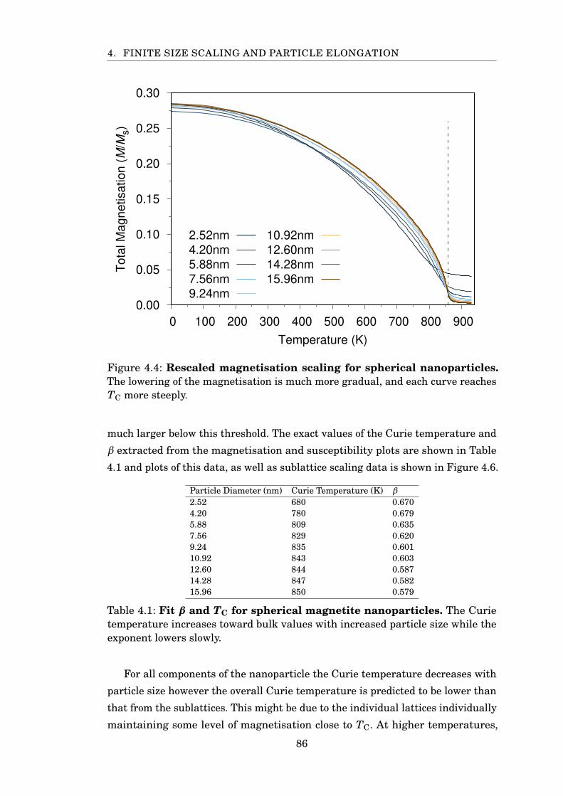
4. FINITE SIZE SCALING AND PARTICLE ELONGATION
0.00
0.05
0.10
0.15
0.20
0.25
0.30
0 100 200 300 400 500 600 700 800 900
Tota
l M
agnetisation (
M/M
s)
Temperature (K)
2.52nm
4.20nm
5.88nm
7.56nm
9.24nm
10.92nm
12.60nm
14.28nm
15.96nm
Figure 4.4: Rescaled magnetisation scaling for spherical nanoparticles.The lowering of the magnetisation is much more gradual, and each curve reachesTC more steeply.
much larger below this threshold. The exact values of the Curie temperature and
β extracted from the magnetisation and susceptibility plots are shown in Table
4.1 and plots of this data, as well as sublattice scaling data is shown in Figure 4.6.
Particle Diameter (nm) Curie Temperature (K) β
2.52 680 0.6704.20 780 0.6795.88 809 0.6357.56 829 0.6209.24 835 0.60110.92 843 0.60312.60 844 0.58714.28 847 0.58215.96 850 0.579
Table 4.1: Fit β and TC for spherical magnetite nanoparticles. The Curietemperature increases toward bulk values with increased particle size while theexponent lowers slowly.
For all components of the nanoparticle the Curie temperature decreases with
particle size however the overall Curie temperature is predicted to be lower than
that from the sublattices. This might be due to the individual lattices individually
maintaining some level of magnetisation close to TC. At higher temperatures,
86
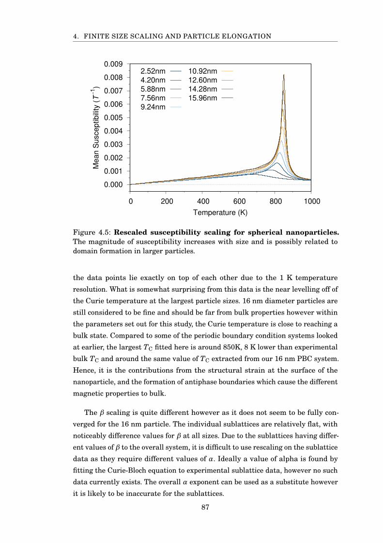
4. FINITE SIZE SCALING AND PARTICLE ELONGATION
0.000
0.001
0.002
0.003
0.004
0.005
0.006
0.007
0.008
0.009
0 200 400 600 800 1000
Mean S
usceptibili
ty (
T -
1)
Temperature (K)
2.52nm
4.20nm
5.88nm
7.56nm
9.24nm
10.92nm
12.60nm
14.28nm
15.96nm
Figure 4.5: Rescaled susceptibility scaling for spherical nanoparticles.The magnitude of susceptibility increases with size and is possibly related todomain formation in larger particles.
the data points lie exactly on top of each other due to the 1 K temperature
resolution. What is somewhat surprising from this data is the near levelling off of
the Curie temperature at the largest particle sizes. 16 nm diameter particles are
still considered to be fine and should be far from bulk properties however within
the parameters set out for this study, the Curie temperature is close to reaching a
bulk state. Compared to some of the periodic boundary condition systems looked
at earlier, the largest TC fitted here is around 850K, 8 K lower than experimental
bulk TC and around the same value of TC extracted from our 16 nm PBC system.
Hence, it is the contributions from the structural strain at the surface of the
nanoparticle, and the formation of antiphase boundaries which cause the different
magnetic properties to bulk.
The β scaling is quite different however as it does not seem to be fully con-
verged for the 16 nm particle. The individual sublattices are relatively flat, with
noticeably difference values for β at all sizes. Due to the sublattices having differ-
ent values of β to the overall system, it is difficult to use rescaling on the sublattice
data as they require different values of α. Ideally a value of alpha is found by
fitting the Curie-Bloch equation to experimental sublattice data, however no such
data currently exists. The overall α exponent can be used as a substitute however
it is likely to be inaccurate for the sublattices.
87
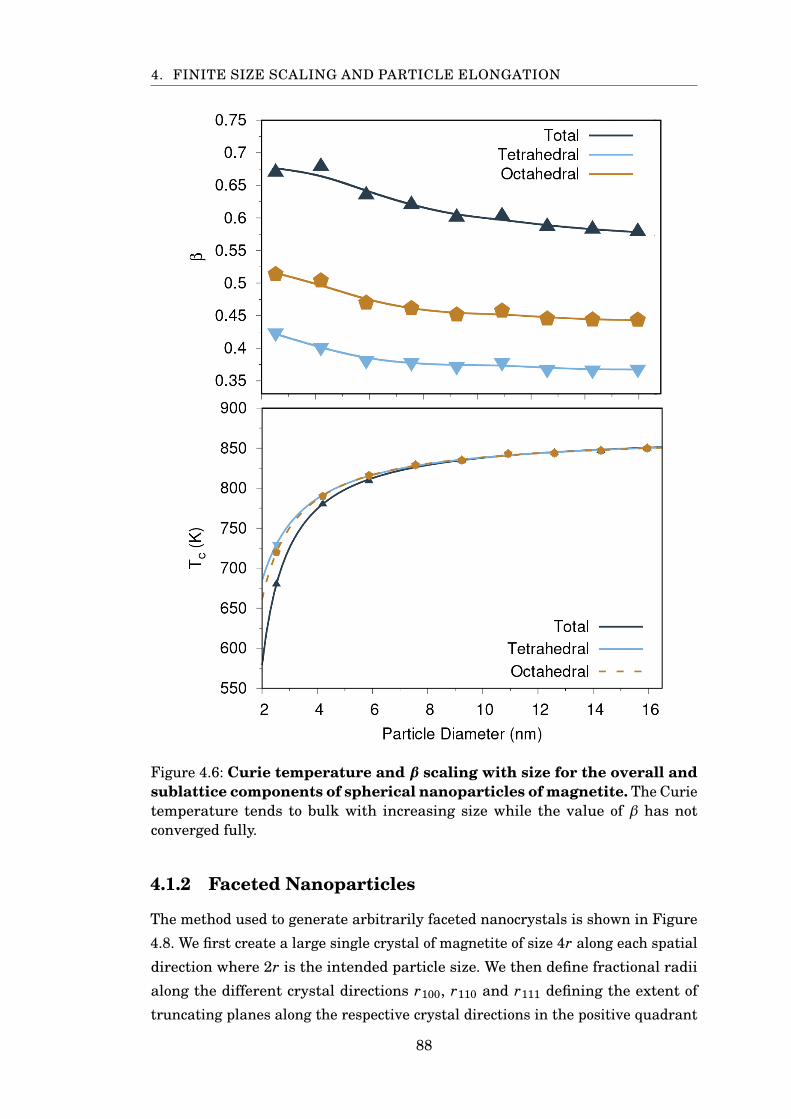
4. FINITE SIZE SCALING AND PARTICLE ELONGATION
Figure 4.6: Curie temperature and β scaling with size for the overall andsublattice components of spherical nanoparticles of magnetite. The Curietemperature tends to bulk with increasing size while the value of β has notconverged fully.
4.1.2 Faceted Nanoparticles
The method used to generate arbitrarily faceted nanocrystals is shown in Figure
4.8. We first create a large single crystal of magnetite of size 4r along each spatial
direction where 2r is the intended particle size. We then define fractional radii
along the different crystal directions r100, r110 and r111 defining the extent of
truncating planes along the respective crystal directions in the positive quadrant
88
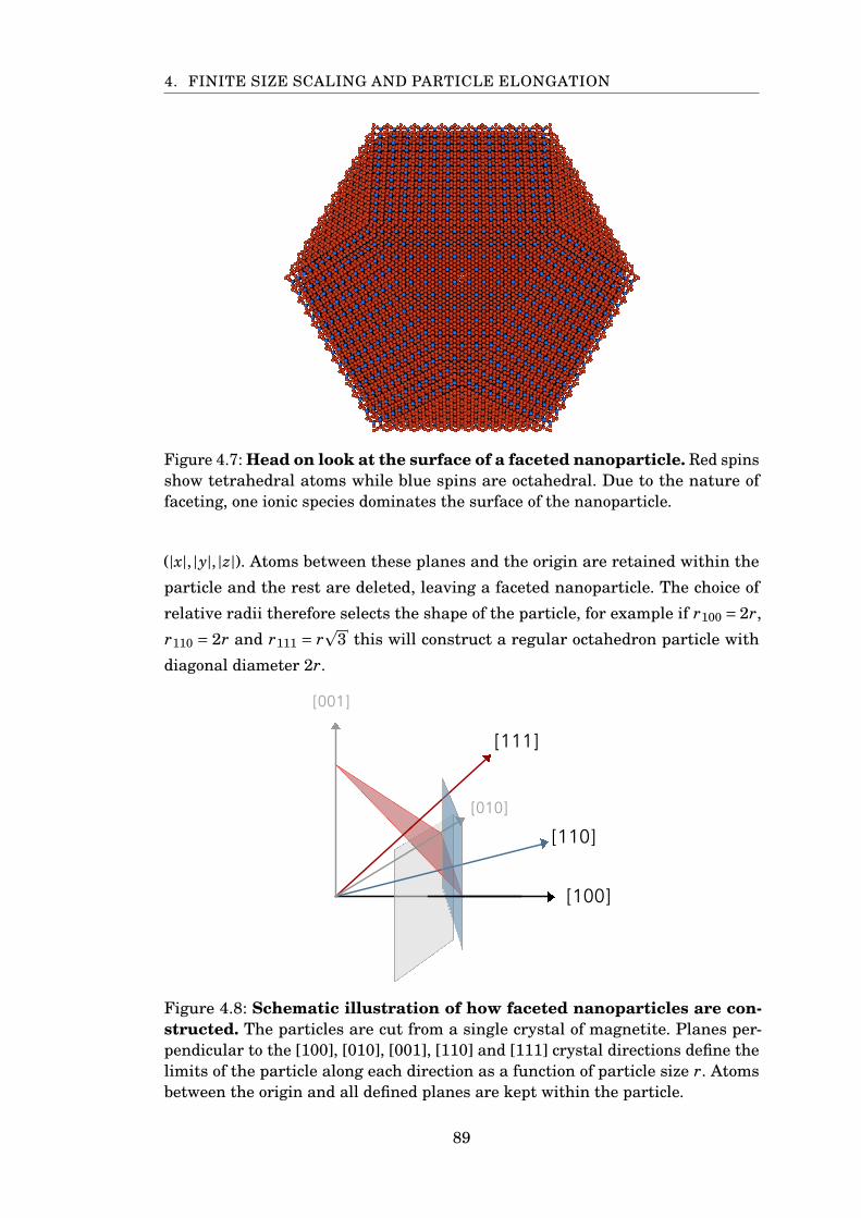
4. FINITE SIZE SCALING AND PARTICLE ELONGATION
Figure 4.7: Head on look at the surface of a faceted nanoparticle. Red spinsshow tetrahedral atoms while blue spins are octahedral. Due to the nature offaceting, one ionic species dominates the surface of the nanoparticle.
(|x|, |y|, |z|). Atoms between these planes and the origin are retained within the
particle and the rest are deleted, leaving a faceted nanoparticle. The choice of
relative radii therefore selects the shape of the particle, for example if r100 = 2r,
r110 = 2r and r111 = rp
3 this will construct a regular octahedron particle with
diagonal diameter 2r.
[001]
[100]
[010]
[111]
[110]
Figure 4.8: Schematic illustration of how faceted nanoparticles are con-structed. The particles are cut from a single crystal of magnetite. Planes per-pendicular to the [100], [010], [001], [110] and [111] crystal directions define thelimits of the particle along each direction as a function of particle size r. Atomsbetween the origin and all defined planes are kept within the particle.
89
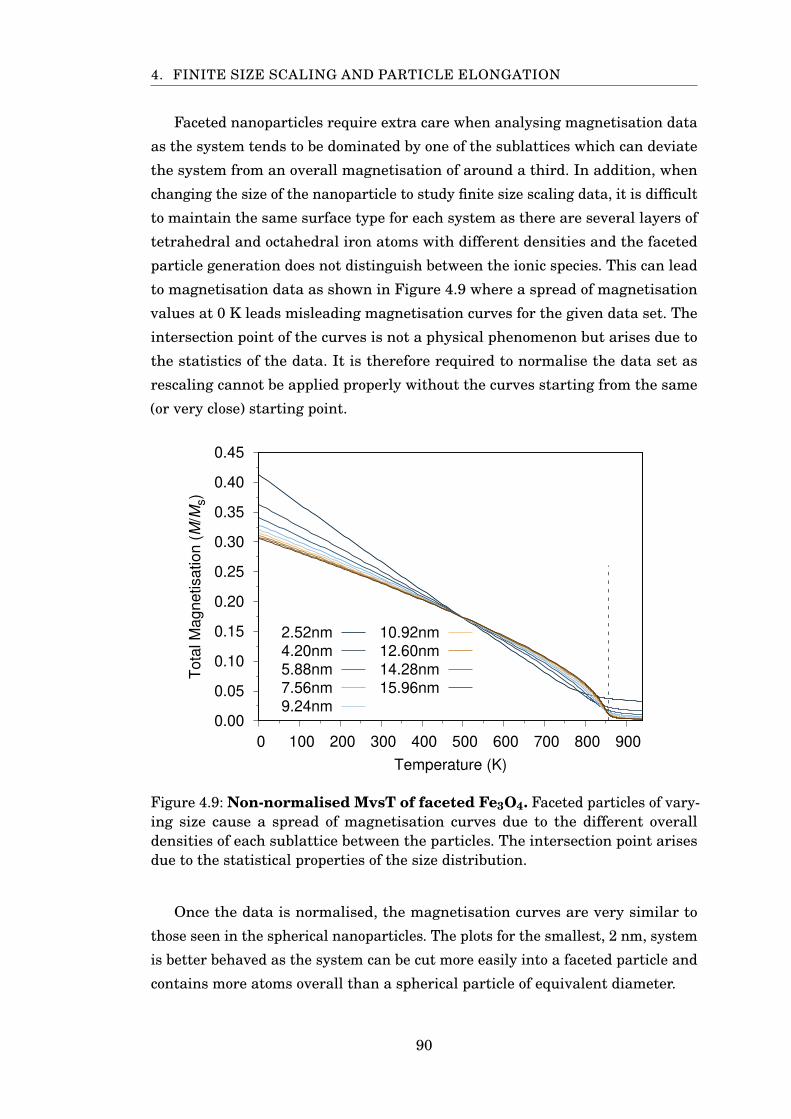
4. FINITE SIZE SCALING AND PARTICLE ELONGATION
Faceted nanoparticles require extra care when analysing magnetisation data
as the system tends to be dominated by one of the sublattices which can deviate
the system from an overall magnetisation of around a third. In addition, when
changing the size of the nanoparticle to study finite size scaling data, it is difficult
to maintain the same surface type for each system as there are several layers of
tetrahedral and octahedral iron atoms with different densities and the faceted
particle generation does not distinguish between the ionic species. This can lead
to magnetisation data as shown in Figure 4.9 where a spread of magnetisation
values at 0 K leads misleading magnetisation curves for the given data set. The
intersection point of the curves is not a physical phenomenon but arises due to
the statistics of the data. It is therefore required to normalise the data set as
rescaling cannot be applied properly without the curves starting from the same
(or very close) starting point.
0.00
0.05
0.10
0.15
0.20
0.25
0.30
0.35
0.40
0.45
0 100 200 300 400 500 600 700 800 900
Tota
l M
agnetisation (
M/M
s)
Temperature (K)
2.52nm
4.20nm
5.88nm
7.56nm
9.24nm
10.92nm
12.60nm
14.28nm
15.96nm
Figure 4.9: Non-normalised MvsT of faceted Fe3O4. Faceted particles of vary-ing size cause a spread of magnetisation curves due to the different overalldensities of each sublattice between the particles. The intersection point arisesdue to the statistical properties of the size distribution.
Once the data is normalised, the magnetisation curves are very similar to
those seen in the spherical nanoparticles. The plots for the smallest, 2 nm, system
is better behaved as the system can be cut more easily into a faceted particle and
contains more atoms overall than a spherical particle of equivalent diameter.
90
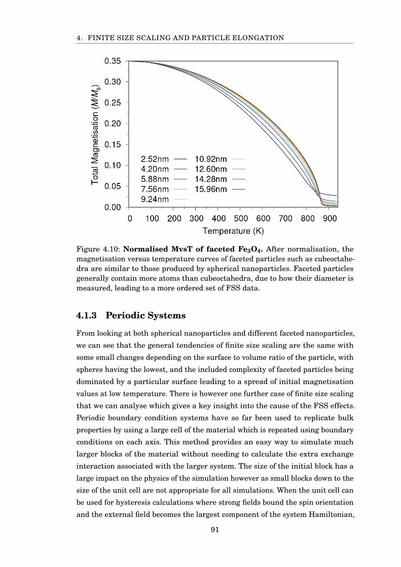
4. FINITE SIZE SCALING AND PARTICLE ELONGATION
Figure 4.10: Normalised MvsT of faceted Fe3O4. After normalisation, themagnetisation versus temperature curves of faceted particles such as cubeoctahe-dra are similar to those produced by spherical nanoparticles. Faceted particlesgenerally contain more atoms than cubeoctahedra, due to how their diameter ismeasured, leading to a more ordered set of FSS data.
4.1.3 Periodic Systems
From looking at both spherical nanoparticles and different faceted nanoparticles,
we can see that the general tendencies of finite size scaling are the same with
some small changes depending on the surface to volume ratio of the particle, with
spheres having the lowest, and the included complexity of faceted particles being
dominated by a particular surface leading to a spread of initial magnetisation
values at low temperature. There is however one further case of finite size scaling
that we can analyse which gives a key insight into the cause of the FSS effects.
Periodic boundary condition systems have so far been used to replicate bulk
properties by using a large cell of the material which is repeated using boundary
conditions on each axis. This method provides an easy way to simulate much
larger blocks of the material without needing to calculate the extra exchange
interaction associated with the larger system. The size of the initial block has a
large impact on the physics of the simulation however as small blocks down to the
size of the unit cell are not appropriate for all simulations. When the unit cell can
be used for hysteresis calculations where strong fields bound the spin orientation
and the external field becomes the largest component of the system Hamiltonian,
91
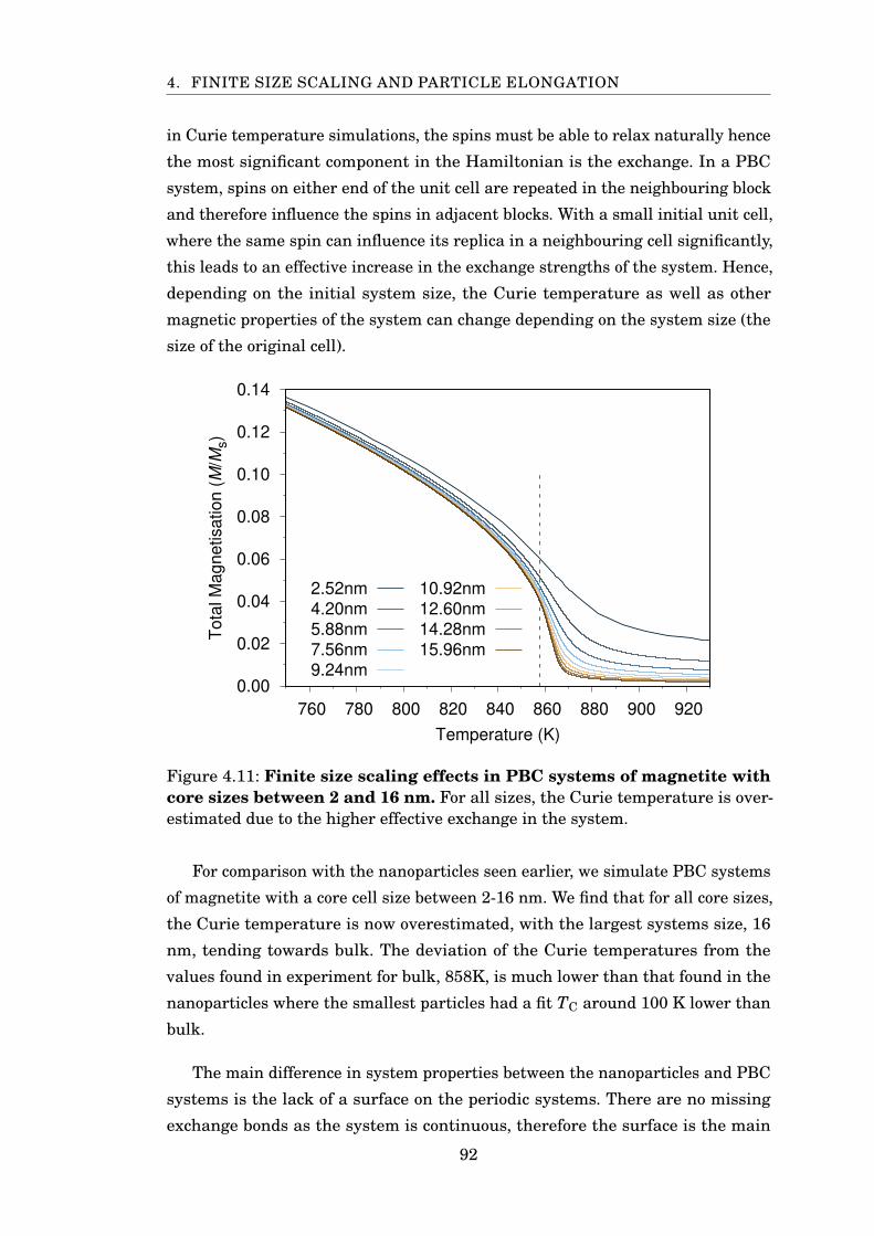
4. FINITE SIZE SCALING AND PARTICLE ELONGATION
in Curie temperature simulations, the spins must be able to relax naturally hence
the most significant component in the Hamiltonian is the exchange. In a PBC
system, spins on either end of the unit cell are repeated in the neighbouring block
and therefore influence the spins in adjacent blocks. With a small initial unit cell,
where the same spin can influence its replica in a neighbouring cell significantly,
this leads to an effective increase in the exchange strengths of the system. Hence,
depending on the initial system size, the Curie temperature as well as other
magnetic properties of the system can change depending on the system size (the
size of the original cell).
0.00
0.02
0.04
0.06
0.08
0.10
0.12
0.14
760 780 800 820 840 860 880 900 920
Tota
l M
agnetisation (
M/M
s)
Temperature (K)
2.52nm
4.20nm
5.88nm
7.56nm
9.24nm
10.92nm
12.60nm
14.28nm
15.96nm
Figure 4.11: Finite size scaling effects in PBC systems of magnetite withcore sizes between 2 and 16 nm. For all sizes, the Curie temperature is over-estimated due to the higher effective exchange in the system.
For comparison with the nanoparticles seen earlier, we simulate PBC systems
of magnetite with a core cell size between 2-16 nm. We find that for all core sizes,
the Curie temperature is now overestimated, with the largest systems size, 16
nm, tending towards bulk. The deviation of the Curie temperatures from the
values found in experiment for bulk, 858K, is much lower than that found in the
nanoparticles where the smallest particles had a fit TC around 100 K lower than
bulk.
The main difference in system properties between the nanoparticles and PBC
systems is the lack of a surface on the periodic systems. There are no missing
exchange bonds as the system is continuous, therefore the surface is the main
92
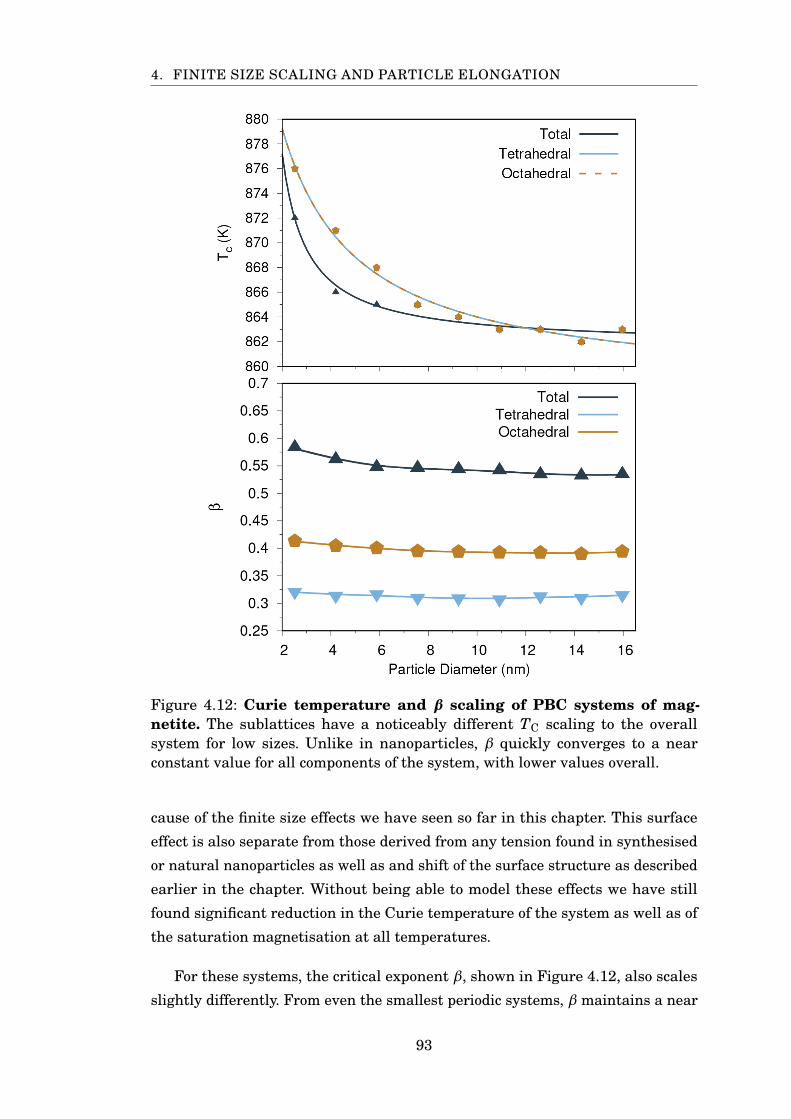
4. FINITE SIZE SCALING AND PARTICLE ELONGATION
Figure 4.12: Curie temperature and β scaling of PBC systems of mag-netite. The sublattices have a noticeably different TC scaling to the overallsystem for low sizes. Unlike in nanoparticles, β quickly converges to a nearconstant value for all components of the system, with lower values overall.
cause of the finite size effects we have seen so far in this chapter. This surface
effect is also separate from those derived from any tension found in synthesised
or natural nanoparticles as well as and shift of the surface structure as described
earlier in the chapter. Without being able to model these effects we have still
found significant reduction in the Curie temperature of the system as well as of
the saturation magnetisation at all temperatures.
For these systems, the critical exponent β, shown in Figure 4.12, also scales
slightly differently. From even the smallest periodic systems, β maintains a near
93
4. FINITE SIZE SCALING AND PARTICLE ELONGATION
constant value for all components of the system, unlike the nanoparticles where
the values for the overall system had not fully converged. The values for β are
still lowered across the board with the tetrahedral and octahedral sublattices at
0.313 and 0.392 respectively and the overall system at 0.541.
4.2 Particle Elongation
Particle size effects are not constrained to uniform size changes, some effects are
only observed when a single axis of the particle is increased. The magnetocrys-
talline anisotropy can be affected by particle elongation, changing the magnetic
properties of the system from superparamagnetic to a blocked ferrimagnetic
state. So far, we have covered intrinsic contributions to the anisotropy such as
uniaxial or cubic. Magnetite itself is subject to cubic anisotropy [101] however
this is not necessarily the largest contribution to the effective anisotropy, Keff.
Cubic anisotropy itself is much smaller than would be expected from the usual
anisotropy constants K1 and K2 due to the nature of the energy surface. The
effective anisotropy is Keff = K1/4 for ⟨100⟩ easy and Keff = K1/12 for ⟨111⟩ easy
axis systems, the latter being the case for most ferrites including magnetite.
Surface anisotropy can also have significant effects on the structural [102] and
magnetic properties [103], and is difficult to model due to its dependence on the
surface termination of the nanoparticles. While some surfaces such as the [100]
termination are found to have a large surface anisotropy contribution [104], these
surfaces are also likely to be unstable due to their polar nature at the interface.
As we cannot model structural changes at the surface of nanoparticles, and the
strength of the surface anisotropy is highly variable, we cannot correctly factor
it into our low temperature calculations. Shape anisotropy, or the anisotropy
contributions due to changes in the elongation of the system, are more easily
modelled and may also dominate the effective anisotropy [105].
Shape anisotropy is related to the demagnetising field, which opposes and is
caused by the magnetisation of the particle. The energy of the field is given by
Hdemag =12µ0M · ( ¯NM) (4.1)
where µ0 = 4π×10−7 is the permeability of free space, M is the vector magneti-
sation and ¯N is the demagnetisation tensor, which depends on the shape and
geometry of the system. For simple elongated systems which we shall use here,
94
4. FINITE SIZE SCALING AND PARTICLE ELONGATION
the off-diagonal components of the demagnetisation tensor are small and ¯N can
be approximated by a diagonal matrix:
¯N ≈
Nxx 0 0
0 Nyy 0
0 0 Nzz
(4.2)
Hence Equation 4.1 expands to:
Hdemag =µ0
2
(Mx My Mz
)Nxx 0 0
0 Nyy 0
0 0 Nzz
Mx
My
Mz
(4.3)
Hdemag =µ0
2(NxxM2
x +NyyM2y +NzzM2
z ) (4.4)
For a uniformly magnetised particle elongated along the z-axis the perpen-
dicular components of the demagnetising energy are the same. Considering the
change in energy for a rotation of the magnetisation in the x-z plane the z and
x components of the magnetisation are related by M2x = (1−M2
z ). Applying the
substitution Mz = mzMs, where Ms is the saturation magnetisation, yields an
effective shape anisotropy of
Hshape =µ0M2
s
2(Nxx −Nzz)m2
z (4.5)
Combining the shape and cubic anisotropy contributions, we get
Heff(m)=+Kc
2(m4
x +m4y +m4
z)+ µ0M2s
2(Nxx −Nzz)m2
z (4.6)
where m is a unit vector with components mx, my, mz describing the magnetisa-
tion of the particle and Kc is the effective cubic anisotropy.
Nanoparticle elongation is not uncommon in experimental samples, with dif-
ferent elongation lengths in the range 0-20% [106]. While larger elongations will
have a stronger effect on the anisotropy, it is worth simulating the effect of elon-
gations within this range as they are more likely to occur. Figure 4.13 shows the
orientation dependence in spherical polar coordinates of the effective anisotropy
95
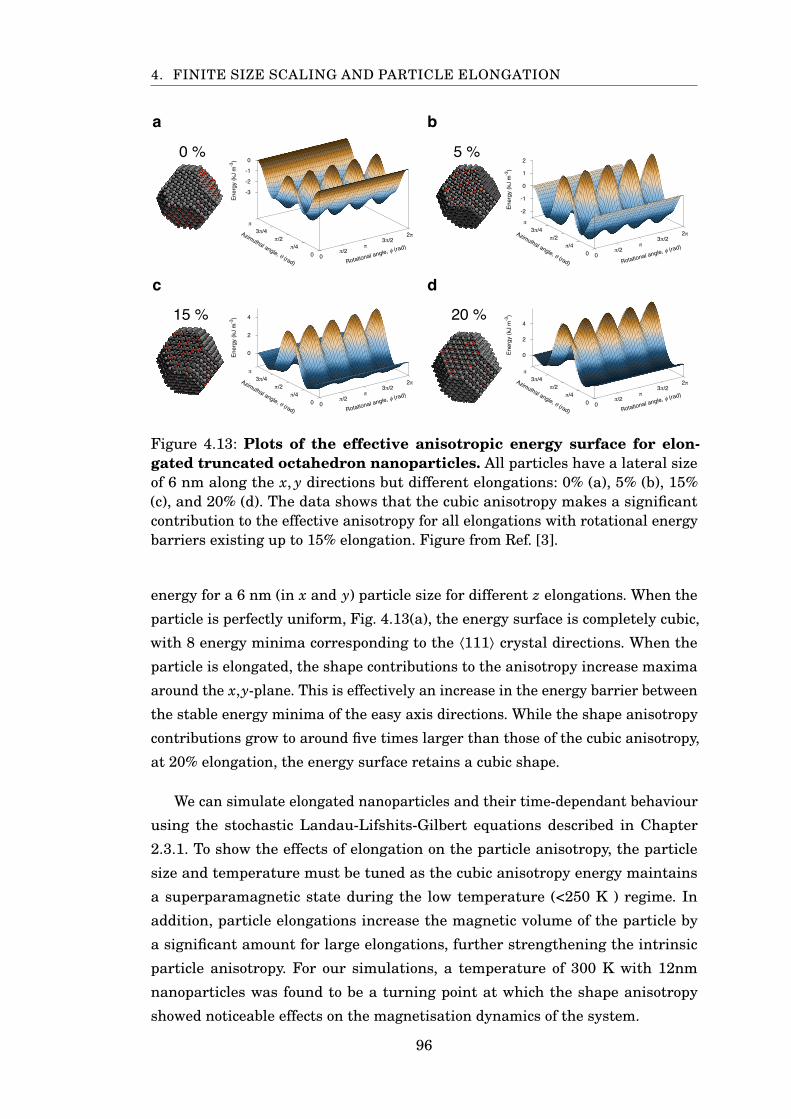
4. FINITE SIZE SCALING AND PARTICLE ELONGATION
Rotational angle, φ (rad)
Azimuthal angle, θ (rad)0
π/2π
3π/22π
0π/4
π/23π/4
π
-3
-2
-1
0
Ener
gy (k
J m
-3)
Rotational angle, φ (rad)
Azimuthal angle, θ (rad)0
π/2π
3π/22π
0π/4
π/23π/4
π
0
2
4
Ener
gy (k
J m
-3)
Rotational angle, φ (rad)
Azimuthal angle, θ (rad)0
π/2π
3π/22π
0π/4
π/23π/4
π
0
2
4
Ener
gy (k
J m
-3)
Rotational angle, φ (rad)
Azimuthal angle, θ (rad)0
π/2π
3π/22π
0π/4
π/23π/4
π
-2
-1
0
1
2
Ener
gy (k
J m
-3)
15 %
0 % 5 %
20 %
a b
c d
Figure 4.13: Plots of the effective anisotropic energy surface for elon-gated truncated octahedron nanoparticles. All particles have a lateral sizeof 6 nm along the x, y directions but different elongations: 0% (a), 5% (b), 15%(c), and 20% (d). The data shows that the cubic anisotropy makes a significantcontribution to the effective anisotropy for all elongations with rotational energybarriers existing up to 15% elongation. Figure from Ref. [3].
energy for a 6 nm (in x and y) particle size for different z elongations. When the
particle is perfectly uniform, Fig. 4.13(a), the energy surface is completely cubic,
with 8 energy minima corresponding to the ⟨111⟩ crystal directions. When the
particle is elongated, the shape contributions to the anisotropy increase maxima
around the x,y-plane. This is effectively an increase in the energy barrier between
the stable energy minima of the easy axis directions. While the shape anisotropy
contributions grow to around five times larger than those of the cubic anisotropy,
at 20% elongation, the energy surface retains a cubic shape.
We can simulate elongated nanoparticles and their time-dependant behaviour
using the stochastic Landau-Lifshits-Gilbert equations described in Chapter
2.3.1. To show the effects of elongation on the particle anisotropy, the particle
size and temperature must be tuned as the cubic anisotropy energy maintains
a superparamagnetic state during the low temperature (<250 K ) regime. In
addition, particle elongations increase the magnetic volume of the particle by
a significant amount for large elongations, further strengthening the intrinsic
particle anisotropy. For our simulations, a temperature of 300 K with 12nm
nanoparticles was found to be a turning point at which the shape anisotropy
showed noticeable effects on the magnetisation dynamics of the system.
96
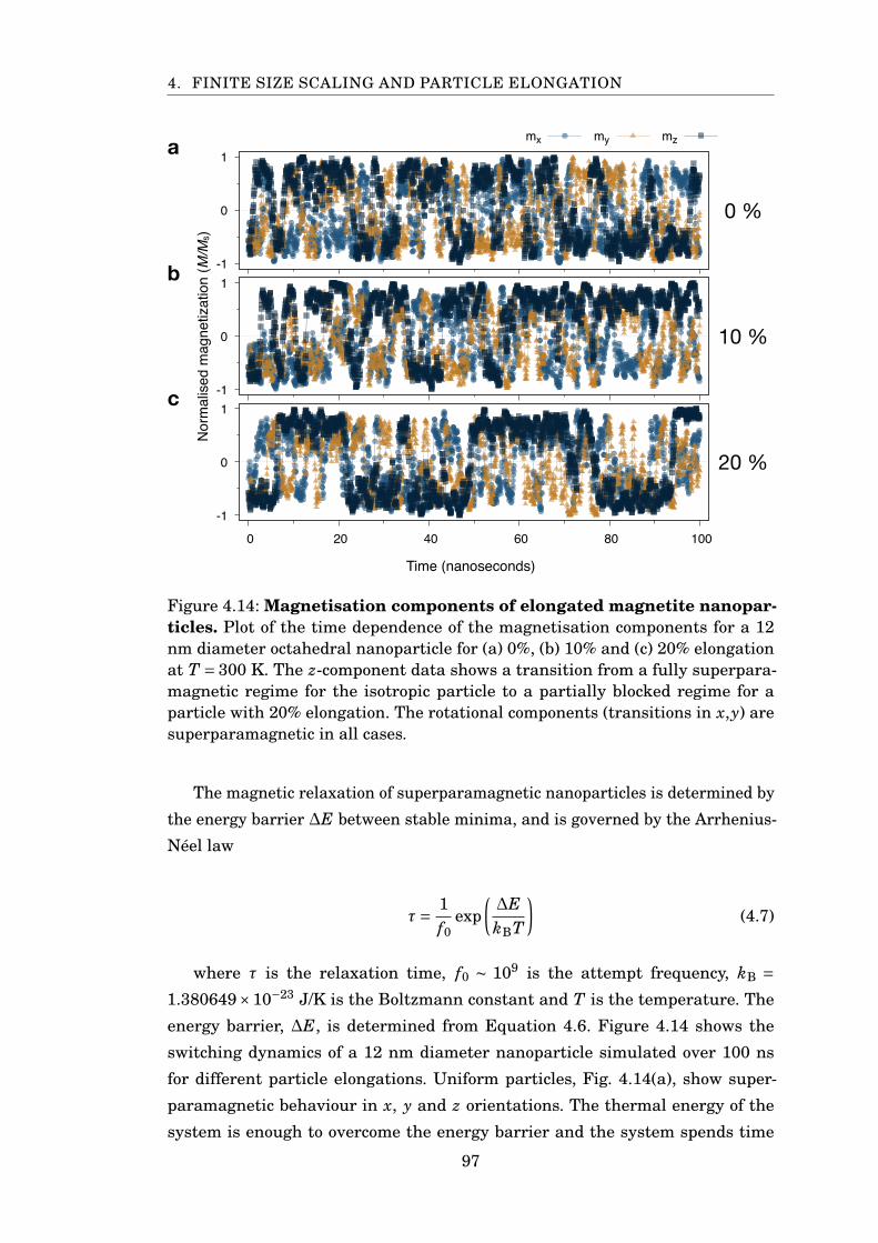
4. FINITE SIZE SCALING AND PARTICLE ELONGATION
-1
0
1
0 20 40 60 80 100
a mx my mz
-1
0
1
0 20 40 60 80 100
c mx my mz-1
0
1
0 20 40 60 80 100
b mx my mz
Nor
mal
ised
mag
netiz
atio
n (M/M
s)0 %
10 %
20 %
a
b
c
Time (nanoseconds)
Figure 4.14: Magnetisation components of elongated magnetite nanopar-ticles. Plot of the time dependence of the magnetisation components for a 12nm diameter octahedral nanoparticle for (a) 0%, (b) 10% and (c) 20% elongationat T = 300 K. The z-component data shows a transition from a fully superpara-magnetic regime for the isotropic particle to a partially blocked regime for aparticle with 20% elongation. The rotational components (transitions in x,y) aresuperparamagnetic in all cases.
The magnetic relaxation of superparamagnetic nanoparticles is determined by
the energy barrier ∆E between stable minima, and is governed by the Arrhenius-
Néel law
τ= 1f0
exp(∆EkBT
)(4.7)
where τ is the relaxation time, f0 ∼ 109 is the attempt frequency, kB =1.380649×10⁻²³ J/K is the Boltzmann constant and T is the temperature. The
energy barrier, ∆E, is determined from Equation 4.6. Figure 4.14 shows the
switching dynamics of a 12 nm diameter nanoparticle simulated over 100 ns
for different particle elongations. Uniform particles, Fig. 4.14(a), show super-
paramagnetic behaviour in x, y and z orientations. The thermal energy of the
system is enough to overcome the energy barrier and the system spends time
97
4. FINITE SIZE SCALING AND PARTICLE ELONGATION
equally in the 8 easy axis directions. A large time scale is required to see the
effects of particle elongation as even at 0% elongation, the system is metastable
along the different orientations, spending around 2-5 ns in each before switching.
At 10% elongation, Fig. 4.14(b), the spin switching has slowed and there are
fewer transitions along the ±z-axis due to the increased shape anisotropy. This
effect is not drastic however and despite the significant change in particle shape,
the increased number of magnetic volumes simultaneously increases the cubic
anisotropy which maintains a similar regime. At 20% elongation, Fig. 4.14(c),
the shape anisotropy and increased energy barrier has stopped more transitions
occurring. The system now spends around τ≈ 15 ns in each orientation. This is
still much shorter than the blocking times found in experimental measurements
of individual nanoparticles which are in the microsecond timescale [107], likely
indicating that surface anisotropy, which we are unable to show here, has a more
significant effect on small particles with elongations around 20%.
4.3 Conclusion
The temperature scaling properties of magnetite are heavily affected by finite
size effects. The magnetisation of nanoparticles can be reduced by more than 10%
at room temperature which is significant for applications which require a fine
understanding of the overall magnetic properties of a sample. In addition, the
shape of the nanoparticles may have more nuanced effects on the temperature
scaling due to the dominance of a sublattice at the surface of the particle. When
comparing PBC systems to nanoparticles, we find that most of these effects are
dependent on the surface to volume ratio of particle, with larger ratios causing
exponentially higher deviations of the magnetic properties from bulk. By using
methods from the previous chapter, we were able to accurately model the changes
to the Curie temperature and β parameter of the system when nanoparticles were
small, leading to longer phase transitions and difficult to fit magnetisation curves.
We have also modelled non-uniform changes to the particle size, which can
change the low temperature magnetic properties of the particle from a fully su-
perparamagnetic state to a partially blocked state, depending on the elongation
of the system along a particular axis. While this does not fully capture the ex-
perimental anisotropy of the nanoparticles, which are found to be fully blocked
for a longer time scale, we have developed a more sophisticated model of the
anisotropy which is important for the future development of magnetic hyperther-
mia where nanoparticle properties should have reproducible heating properties
98

4. FINITE SIZE SCALING AND PARTICLE ELONGATION
with a narrow distribution of size and magnetic properties.
Next, we shall look at a closely related material, maghemite, which shares
many traits with magnetite but is less stable and, because of this, less well
reviewed in the literature.
99

CH
AP
TE
R
5MAGHEMITE
5.1 Introduction
Maghemite, not to be confused with magnetite, is another well-known magnetic
iron oxide that has been studied for more than a century. In nature it occurs
near iron oxyhydroxide rich minerals as a brown or yellow pigment in terrestrial
sediments and soils. Synthesis of impure maghemite has been documented since
the 19th century, according to the 1837 textbook of Schubarth [108]. The alchemist
Kunckel had already synthesised maghemite by heating metallic iron in air until
red-hot. Initially, likely due to impurities, the samples of maghemite were thought
to be paramagnetic and its use was restricted to pigments or as an abrasive
material. Through oxidation of magnetite, a method still used today, Baudisch
and Welo [109] explored the magnetic properties of maghemite but were not able
to distinguish these properties as being intrinsic to maghemite rather than a
remnant from magnetite or other iron oxide impurities.
Maghemite and its structure was characterised in the early 20th century,
noting the distinction between hematite, another iron oxide with a closely re-
lated chemical structure, and magnetite, which is structurally the closest. While
hematite, an antiferromagnetic material then thought of as paramagnetic (this
was before Néel developed the concept of antiferromagnetism [6]), was noted
to be stable, maghemite was found to be unstable even at room temperature
[110], with an inverse spinel defect structure. Much like magnetite, it was not
immediately realised that maghemite was not ferromagnetic, as in elemental iron,
100
5. MAGHEMITE
but ferrimagnetic due to its more complicated structure.
One of the first uses of maghemite had to do with one of the early technological
advances in the 1930-40s, the magnetic tape. Initially made using carbonyl iron,
these were later improved through the usage of magnetite and then maghemite
with the development of acicular (needle shaped) magnetic particles [111]. More
recently, they have been used along with other iron oxides for biomedical applica-
tions due to their biocompatibility and relative ease of synthesis. Paired with a
surface coating of various possible materials such as silica, PVA or dextran, it has
seen use as a magnetic drug carrier, able to carry cytotoxic drugs, or target anti-
bodies [112]. Another important field of study is magnetic hyperthermia involving
the catabolism of tumours by magnetic heating of the nanoparticles. These studies
date back to 1957 when Glichrist et al. heated various tissue samples with 20-100
nm size particles of maghemite exposed to a 1.2MHz magnetic field [15]. Finally,
maghemite nanoparticles are a promising material for adsorption of heavy metals
from industrial wastewater due to their adsorption efficiency and reusability and
recoverability, making them distinct from similar iron based materials which are
more difficult to recover and become a secondary waste product [16, 113].
5.2 Structure
The simple chemical formula of maghemite is Fe2O3 however there are several
other minerals that share the same formula. In the 1987 edition of his book,
Wells mentions four different Fe2O3 phases [114] which had been studied: the
thermodynamically stable, almost non-magnetic, hematite phase α-Fe2O3 which
has a trigonal corundum structure [115]; two less stable phases known as β-Fe2O3,
a body-centred cubic oxide which converts to hematite at high temperatures, and
ε-Fe2O3, a rhombic phase which is difficult to prepare without impurities [116];
and a probably cubic phase which would be known as γ-Fe2O3, due to a proposal
of Haber as γ-Fe2O3 can be made from dehydrating needle-shaped γ-FeOOH
crystals.
The exact structure of maghemite was uncovered through the oxidation of
magnetite. When Fe3O4 is oxidised directly, Fe2+ is converted to Fe3+ within
the spinel structure and compensating iron vacancies appear in the octahedral
sublattice. The defective spinel structure is remarkably robust and can accommo-
date the full range of stoichiometry between Fe3O4 and Fe2O3. In the extreme
case, all Fe is oxidised to Fe3+, and maghemite is formed. γ-Fe2O3 is metastable
against transformation to α-Fe2O3 but exists partly because the conversion from
101
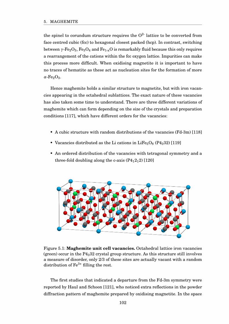
5. MAGHEMITE
the spinel to corundum structure requires the O2- lattice to be converted from
face centred cubic (fcc) to hexagonal closest packed (hcp). In contrast, switching
between γ-Fe2O3, Fe3O4 and Fe1-xO is remarkably fluid because this only requires
a rearrangement of the cations within the fcc oxygen lattice. Impurities can make
this process more difficult. When oxidising magnetite it is important to have
no traces of hematite as these act as nucleation sites for the formation of more
α-Fe2O3.
Hence maghemite holds a similar structure to magnetite, but with iron vacan-
cies appearing in the octahedral sublattices. The exact nature of these vacancies
has also taken some time to understand. There are three different variations of
maghemite which can form depending on the size of the crystals and preparation
conditions [117], which have different orders for the vacancies:
• A cubic structure with random distributions of the vacancies (Fd-3m) [118]
• Vacancies distributed as the Li cations in LiFe5O8 (P4332) [119]
• An ordered distribution of the vacancies with tetragonal symmetry and a
three-fold doubling along the c-axis (P41212) [120]
Figure 5.1: Maghemite unit cell vacancies. Octahedral lattice iron vacancies(green) occur in the P4332 crystal group structure. As this structure still involvesa measure of disorder, only 2/3 of these sites are actually vacant with a randomdistribution of Fe3+ filling the rest.
The first studies that indicated a departure from the Fd-3m symmetry were
reported by Haul and Schoon [121], who noticed extra reflections in the powder
diffraction pattern of maghemite prepared by oxidising magnetite. In the space
102
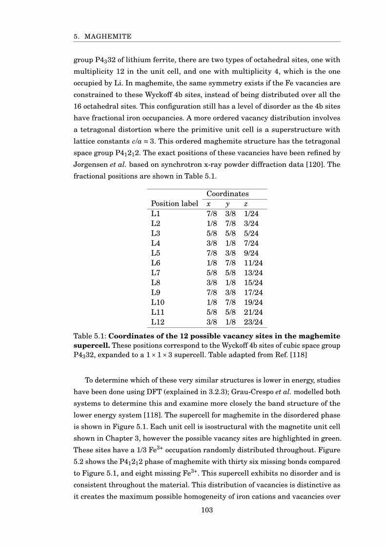
5. MAGHEMITE
group P4332 of lithium ferrite, there are two types of octahedral sites, one with
multiplicity 12 in the unit cell, and one with multiplicity 4, which is the one
occupied by Li. In maghemite, the same symmetry exists if the Fe vacancies are
constrained to these Wyckoff 4b sites, instead of being distributed over all the
16 octahedral sites. This configuration still has a level of disorder as the 4b sites
have fractional iron occupancies. A more ordered vacancy distribution involves
a tetragonal distortion where the primitive unit cell is a superstructure with
lattice constants c/a ≈ 3. This ordered maghemite structure has the tetragonal
space group P41212. The exact positions of these vacancies have been refined by
Jorgensen et al. based on synchrotron x-ray powder diffraction data [120]. The
fractional positions are shown in Table 5.1.
CoordinatesPosition label x y zL1 7/8 3/8 1/24L2 1/8 7/8 3/24L3 5/8 5/8 5/24L4 3/8 1/8 7/24L5 7/8 3/8 9/24L6 1/8 7/8 11/24L7 5/8 5/8 13/24L8 3/8 1/8 15/24L9 7/8 3/8 17/24L10 1/8 7/8 19/24L11 5/8 5/8 21/24L12 3/8 1/8 23/24
Table 5.1: Coordinates of the 12 possible vacancy sites in the maghemitesupercell. These positions correspond to the Wyckoff 4b sites of cubic space groupP4332, expanded to a 1×1×3 supercell. Table adapted from Ref. [118]
To determine which of these very similar structures is lower in energy, studies
have been done using DFT (explained in 3.2.3); Grau-Crespo et al. modelled both
systems to determine this and examine more closely the band structure of the
lower energy system [118]. The supercell for maghemite in the disordered phase
is shown in Figure 5.1. Each unit cell is isostructural with the magnetite unit cell
shown in Chapter 3, however the possible vacancy sites are highlighted in green.
These sites have a 1/3 Fe3+ occupation randomly distributed throughout. Figure
5.2 shows the P41212 phase of maghemite with thirty six missing bonds compared
to Figure 5.1, and eight missing Fe3+. This supercell exhibits no disorder and is
consistent throughout the material. This distribution of vacancies is distinctive as
it creates the maximum possible homogeneity of iron cations and vacancies over
103
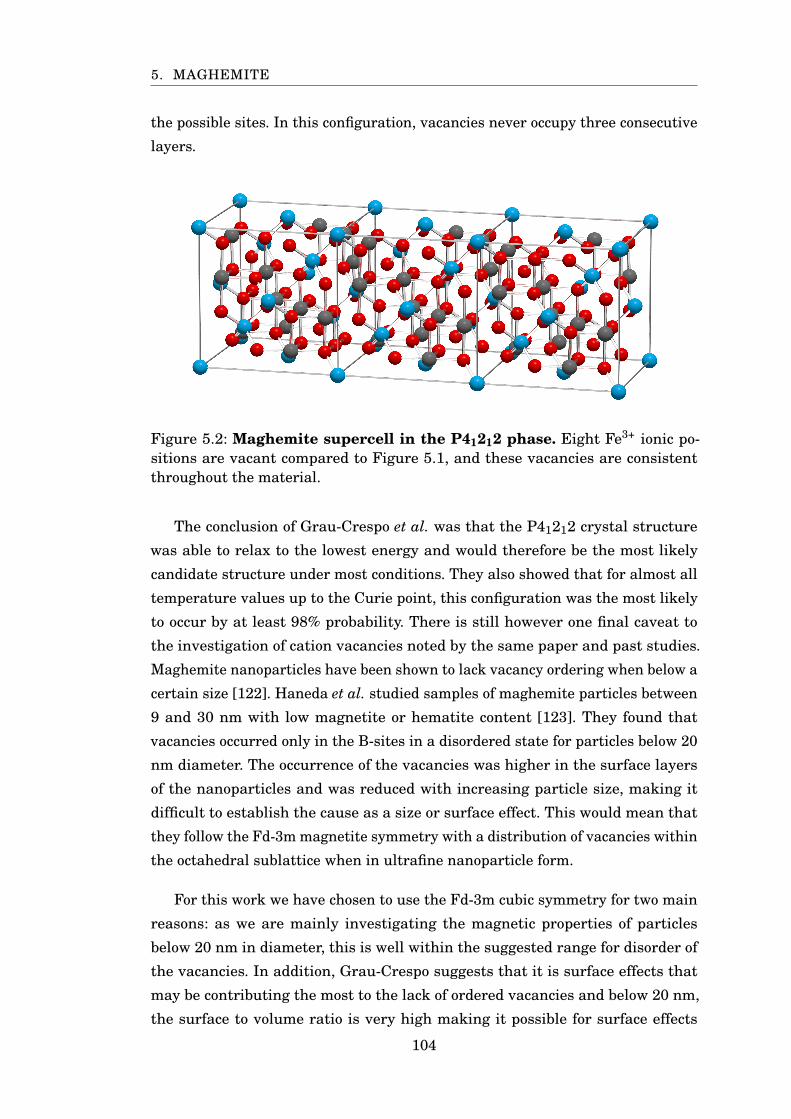
5. MAGHEMITE
the possible sites. In this configuration, vacancies never occupy three consecutive
layers.
Figure 5.2: Maghemite supercell in the P41212 phase. Eight Fe3+ ionic po-sitions are vacant compared to Figure 5.1, and these vacancies are consistentthroughout the material.
The conclusion of Grau-Crespo et al. was that the P41212 crystal structure
was able to relax to the lowest energy and would therefore be the most likely
candidate structure under most conditions. They also showed that for almost all
temperature values up to the Curie point, this configuration was the most likely
to occur by at least 98% probability. There is still however one final caveat to
the investigation of cation vacancies noted by the same paper and past studies.
Maghemite nanoparticles have been shown to lack vacancy ordering when below a
certain size [122]. Haneda et al. studied samples of maghemite particles between
9 and 30 nm with low magnetite or hematite content [123]. They found that
vacancies occurred only in the B-sites in a disordered state for particles below 20
nm diameter. The occurrence of the vacancies was higher in the surface layers
of the nanoparticles and was reduced with increasing particle size, making it
difficult to establish the cause as a size or surface effect. This would mean that
they follow the Fd-3m magnetite symmetry with a distribution of vacancies within
the octahedral sublattice when in ultrafine nanoparticle form.
For this work we have chosen to use the Fd-3m cubic symmetry for two main
reasons: as we are mainly investigating the magnetic properties of particles
below 20 nm in diameter, this is well within the suggested range for disorder of
the vacancies. In addition, Grau-Crespo suggests that it is surface effects that
may be contributing the most to the lack of ordered vacancies and below 20 nm,
the surface to volume ratio is very high making it possible for surface effects
104
5. MAGHEMITE
to dominate. For the second reason, as we shall see in later chapters, we shall
be investigating core-shell particles with magnetite cores and maghemite shells
where it is very likely that, in practice, the unit cell structure for both materials
will relax to accommodate both materials and therefore maghemite will be bound
more strongly to an Fd-3m crystal symmetry.
5.3 Parameters
Due to the uncertainty in the structure of maghemite due to its different phases as
well as possibilities of mixing with similar ferrites, it is often difficult to find con-
sistently used parameters for the material. The lattice constant of maghemite is
sometimes reported to be around 8.347 Å[17] however this value changes slightly
from paper to paper. In some experiments where maghemite was prepared by
oxidation of magnetite particles, lattice parameters between 8.347Å and 8.397Å
have been shown, suggesting a mixing of structures between maghemite and
magnetite [124]. In a DFT study, which determined the regular vacancy distribu-
tion in bulk maghemite, a relaxed lattice constant of 8.359Å was suggested [118],
however this is specific to the tetragonal structure of maghemite. For this study,
we shall use the most commonly reported value of 8.347Å, which seems to be used
in conjunction with cubic symmetry maghemite.
Another important parameter for maghemite is its Curie temperature which
has been used to identify the material, in particular due to its chemical compo-
sition being very similar to magnetite and hematite. There is much debate on
the exact value of this parameter for several reasons. Similar to the determina-
tion of the lattice parameter, it can be difficult to test the purity of the sample
being studied leading to averaged out values of Curie temperature somewhere
between magnetite and maghemite. Also, due to the metastability of maghemite,
it is difficult to study the temperature dependent properties of the material if it
is decomposing during the process. The actual temperature of conversion from
maghemite to hematite is also disputed with some papers suggesting very low
values close to room temperatures [125], while others record much higher tem-
peratures around 900 K [126]. This is likely due to sample contamination where
small hematite impurities act as nucleation sites, causing the material to decom-
pose more quickly. Initially it was assumed to be impossible to determine the
Curie temperature of maghemite for this reason. While some natural samples of
maghemite would convert completely to hematite before reaching TC, this is not
true for all geological variations of maghemite as others have reported thermal
105
5. MAGHEMITE
stability of around 870 K [127, 128], with a possible reason being the inclusion of
metallic impurities which help to stabilise the system. More recently, theoretical
studies of maghemite which can remove the possibility of metallic or other iron
oxide impurities have been done to determine the exact value of TC.
A recent study by Liu et al. in 2010 [125] looked at the magnetisation versus
temperature properties of various grain sizes of maghemite to determine their
Curie point. What they found was a strong dependence of the critical point on
the shape of the grains, in particular their spin orientation being in either a
multi-domain (MD) state with multiple different spin orientation regions, or a
single-domain (SD) state where most of the spins where magnetised in the same
direction. Larger particles can form multi-domain structures more easily as they
are heated as different spin domains are able to grow naturally when they are
far away enough from surface boundaries which would constrain spin direction
and domain growth. In small particles this is much more difficult as the spins do
not have enough space to form multi-domain structures and are influenced more
heavily by their nearby spin neighbours. At the same time, both particle types
were subject to the same rapid heating process to convert them from magnetite to
maghemite and after analysis of the particles by Mössbauer spectroscopy, only
the small single-domain particles were fully converted, while the larger particles
still showed high levels of magnetite.
The saturation magnetisation curves from Liu et al. [125] are shown in Figure
5.3, which has two plots, one for the MD particles, and one for the SD particles. We
can see without fitting the plots that the Curie temperature is lower for the MD
particles. The exact method for extracting the Curie temperature is not specified
however the Curie temperatures for the MD particles is around 850 K and for
the SD particles 910K, suggesting that the Curie temperature of maghemite is
higher than that of magnetite. This difference is important when we apply it to
the nanoparticles we are simulating as they are always within the small particle
single-domain phase, hence we expect a Curie temperature above 900 K. Aside
from the Curie temperature we note that the scaling behaviour of the magnetisa-
tion for these particles is also very different. The multi-domain particles maintain
a higher magnetisation, and therefore spin correlation, for higher temperatures,
while the single-domain particles see a steady decrease to the Curie point. At room
temperature there is a 20% difference in the magnetisation of the particles which
would need to be considered when using them for biomedical heating applications.
This temperature scaling demonstrates some of the differences between magnetite
and maghemite particles and is a strong reason for their usage in individual appli-
106
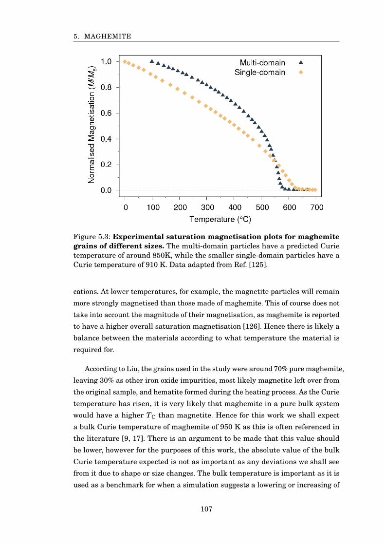
5. MAGHEMITE
Figure 5.3: Experimental saturation magnetisation plots for maghemitegrains of different sizes. The multi-domain particles have a predicted Curietemperature of around 850K, while the smaller single-domain particles have aCurie temperature of 910 K. Data adapted from Ref. [125].
cations. At lower temperatures, for example, the magnetite particles will remain
more strongly magnetised than those made of maghemite. This of course does not
take into account the magnitude of their magnetisation, as maghemite is reported
to have a higher overall saturation magnetisation [126]. Hence there is likely a
balance between the materials according to what temperature the material is
required for.
According to Liu, the grains used in the study were around 70% pure maghemite,
leaving 30% as other iron oxide impurities, most likely magnetite left over from
the original sample, and hematite formed during the heating process. As the Curie
temperature has risen, it is very likely that maghemite in a pure bulk system
would have a higher TC than magnetite. Hence for this work we shall expect
a bulk Curie temperature of maghemite of 950 K as this is often referenced in
the literature [9, 17]. There is an argument to be made that this value should
be lower, however for the purposes of this work, the absolute value of the bulk
Curie temperature expected is not as important as any deviations we shall see
from it due to shape or size changes. The bulk temperature is important as it is
used as a benchmark for when a simulation suggests a lowering or increasing of
107

5. MAGHEMITE
the critical point. The values of exchange used in our simulations are the largest
contributors to the system Curie temperature however if we change all exchange
values by the same factor, the system Curie point will change by a similar amount.
Hence, if in reality the Curie temperature of maghemite is 800K, we can divide all
exchange values by a constant to simulate a lower TC while preserving the ratio
of the exchanges which is much more important. These ratios, such as the ratio of
FeA-FeA (tetrahedral to tetrahedral exchange) compared to FeB-FeB (octahedral
to octahedral exchange) help to evaluate the overall magnetic properties of the
system as they define the temperature scaling.
5.3.1 Anisotropy
Following on from the uncertainty in macroscopic properties of maghemite, we
find that current research is no clearer on theoretical modelling parameters
such as the magnetocrystalline cubic anisotropy constant K , or the exchange
interaction values. The nature of the anisotropy in maghemite is cubic, with an
easy axis direction of [111] and is likely to be very weak, lower than the anisotropy
of magnetite which is well known for having a relatively low bulk anisotropy. In
the literature it is possible to find a value of 4.7×10⁴erg/cm3, cited from Krupicka
et al. [129], however we do not have an idea of the temperature scaling of the
anisotropy, nor do we have any higher order anisotropy values. In addition, the
original source is no longer available and therefore further research into the
origin of this value is impossible. In spite of this, several theoretical modelling
papers [130, 131] use the same value and therefore it is currently the best choice
available. Using equation 3.3, the bulk cubic anisotropy can be converted to an
atomistic anisotropy, ku =−5.12×10⁻²⁶J/atom.
5.3.2 Exchange
The exchange interaction values for magnetite we use are from Uhl and Siber-
chicot [28] who calculated them from first principles. This type of analysis does
not exist for maghemite, and the exchange values found in the literature come
from different sources. Two sets of exchange parameters for maghemite are listed
in Table 5.2, which come from proposed exchange values of different materials.
They are shown in units of Kelvin, as in the original paper where these values are
expressed as temperatures, and in units of energy (meV) which is more commonly
used today. These values are related by the simple equation E = kBT.
The first set of values should look familiar as they are from the same paper by
108
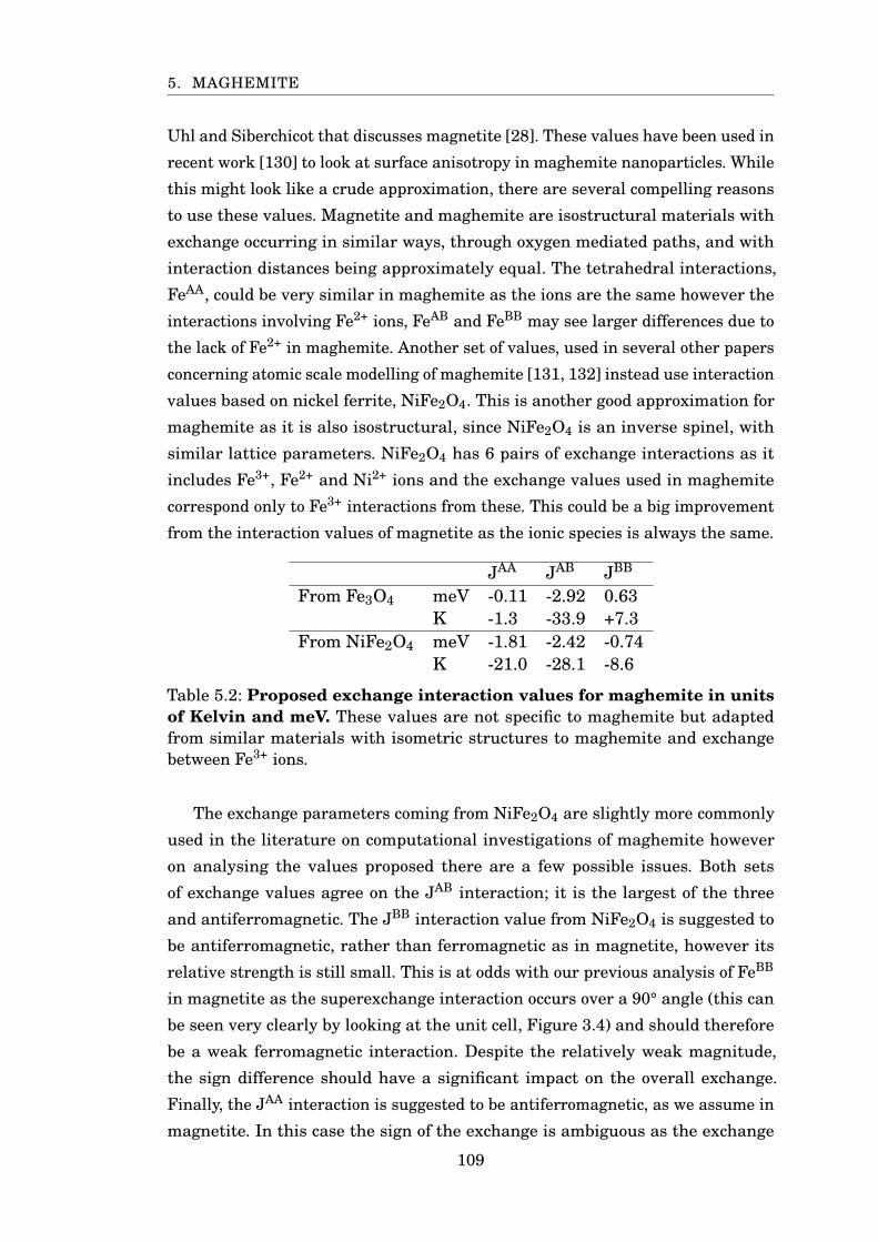
5. MAGHEMITE
Uhl and Siberchicot that discusses magnetite [28]. These values have been used in
recent work [130] to look at surface anisotropy in maghemite nanoparticles. While
this might look like a crude approximation, there are several compelling reasons
to use these values. Magnetite and maghemite are isostructural materials with
exchange occurring in similar ways, through oxygen mediated paths, and with
interaction distances being approximately equal. The tetrahedral interactions,
FeAA, could be very similar in maghemite as the ions are the same however the
interactions involving Fe2+ ions, FeAB and FeBB may see larger differences due to
the lack of Fe2+ in maghemite. Another set of values, used in several other papers
concerning atomic scale modelling of maghemite [131, 132] instead use interaction
values based on nickel ferrite, NiFe2O4. This is another good approximation for
maghemite as it is also isostructural, since NiFe2O4 is an inverse spinel, with
similar lattice parameters. NiFe2O4 has 6 pairs of exchange interactions as it
includes Fe3+, Fe2+ and Ni2+ ions and the exchange values used in maghemite
correspond only to Fe3+ interactions from these. This could be a big improvement
from the interaction values of magnetite as the ionic species is always the same.
JAA JAB JBB
From Fe3O4 meV -0.11 -2.92 0.63K -1.3 -33.9 +7.3
From NiFe2O4 meV -1.81 -2.42 -0.74K -21.0 -28.1 -8.6
Table 5.2: Proposed exchange interaction values for maghemite in unitsof Kelvin and meV. These values are not specific to maghemite but adaptedfrom similar materials with isometric structures to maghemite and exchangebetween Fe3+ ions.
The exchange parameters coming from NiFe2O4 are slightly more commonly
used in the literature on computational investigations of maghemite however
on analysing the values proposed there are a few possible issues. Both sets
of exchange values agree on the JAB interaction; it is the largest of the three
and antiferromagnetic. The JBB interaction value from NiFe2O4 is suggested to
be antiferromagnetic, rather than ferromagnetic as in magnetite, however its
relative strength is still small. This is at odds with our previous analysis of FeBB
in magnetite as the superexchange interaction occurs over a 90° angle (this can
be seen very clearly by looking at the unit cell, Figure 3.4) and should therefore
be a weak ferromagnetic interaction. Despite the relatively weak magnitude,
the sign difference should have a significant impact on the overall exchange.
Finally, the JAA interaction is suggested to be antiferromagnetic, as we assume in
magnetite. In this case the sign of the exchange is ambiguous as the exchange
109
5. MAGHEMITE
occurs infrequently in the unit cell and over large distances. It is because of this
that the relatively high magnitude of the JAA interaction taken from NiFe2O4
does not apply well to maghemite. The strength of an Fe3+-O2--Fe3+ interaction is
likely related to the number of such interactions within the unit cell and their
interaction ranges [133]. Here this interaction is both infrequent and over a
long range therefore it is much more likely to be the smallest interaction as in
magnetite. It is also worth pointing out that this interaction occurs in exactly
the same way, and between exactly the same species in magnetite, and should
therefore be the most transferable value between systems.
In Chapter 3.3, we have shown that the original exchange interaction values
suggested by Uhl and Siberchicot replicate the magnetic properties of magnetite
well, the predicted Curie temperature and magnetisation scaling (using quantum
rescaling) agree very well with experiment. As we lack the same quality of ex-
change interaction values for maghemite, it seems that the best starting values
are those of isostructural magnetite. This is of course an approximation; however
it is necessary due to the current lack of well-founded values available. As such,
we will have to adjust these starting values to replicate the Curie temperature of
maghemite, 950K, by multiplying each exchange value by a constant factor. By
doing this, we preserve the relative values of each exchange, and therefore the
scaling of magnetic properties and exponents, but maintain the Curie temperature
expected.
5.4 Simulating Maghemite
As we have now compiled a suitable set of parameters for modelling maghemite,
we can now investigate its temperature scaling properties. As with magnetite, we
begin with a small periodic boundary conditions system to approximate the bulk
properties of the system. To recap the parameters:
• The system is cubic with a lattice constant of a = 8.347Å
• There are three unique materials:
– Tetrahedral site iron 3+ ions with spin moment 5µB
– Octahedral site iron 3+ ions with spin moment 5µB
– Non-magnetic oxygen 2- ions
• Iron vacancies (11%) occur in the octahedral sublattice
110
5. MAGHEMITE
• The anisotropy direction is ⟨111⟩
• The exchange interaction values (in meV) are JAA =−0.12, JBB = 0.68 and
JAB =−3.15. These values correspond to the values in Table 5.2 multiplied
by approximately 1.08.
As with magnetite, the simulations are checked to ensure all final data points
are converged. The magnetisation reaches convergence very quickly as it equi-
librates after only 50k Monte Carlo time steps. The susceptibility and specific
heat values take longer to converge, relaxing over the first 100k time steps and
reaching equilibrium almost asymptotically. To ensure convergence for all temper-
atures and properties, most simulations are run until at least 1 million time steps.
The convergence for a 6 nm system around room temperature is shown in Figure
5.4. While the magnetisation looks like it is still erratic, this is simply a symptom
of scaling all data sets between 0-1 as the magnitudes of the magnetisation, sus-
ceptibility and specific heat are at different scales. The initial max value of the
magnetisation is 0.2288m and the lowest is 0.2291m therefore the magnetisation
is essentially a flat line and immediately converged. The susceptibility and specific
heat take much longer to converge properly and therefore require more time steps.
Rather than plotting the magnetisation, it is worth using the raw susceptibility
to find the value of TC for this system. For these initial simulations, we cannot
use any rescaling parameters as magnetisation scaling and the β parameter is
required first, however the susceptibility will be mostly unaffected by the classical
model as the most relevant data points occur around TC where quantum effects
no longer persist. With a precise point for TC we can fit the magnetisation curve
more easily for the exponent, β. According to Figure 5.5 the Curie temperature
occurs around 960K, with PBC finite size effects increasing the Curie temperature
moderately due to increased spin correlation through the periodic boundaries.
The sublattices also peak around 960 K (±0.5K), with the width of the peak of
each plot spanning around 100K, indicating the Curie temperature occurs in the
middle of a more gradual transition from ferrimagnetic to paramagnetic. As it is
a ferrimagnet, we also see the difference in magnitudes of the sublattice suscep-
tibilities and the overall susceptibility indicating the intra and inter-sublattice
modes (Figure 3.26). We now use this to more accurately fit the magnetisation
scaling versus temperature, still using only the classical model.
Using Gnuplot [45], we fit the magnetisation according to the classical Curie-
Bloch equation (3.9) and constrain the Curie temperature to 960K, from the
111
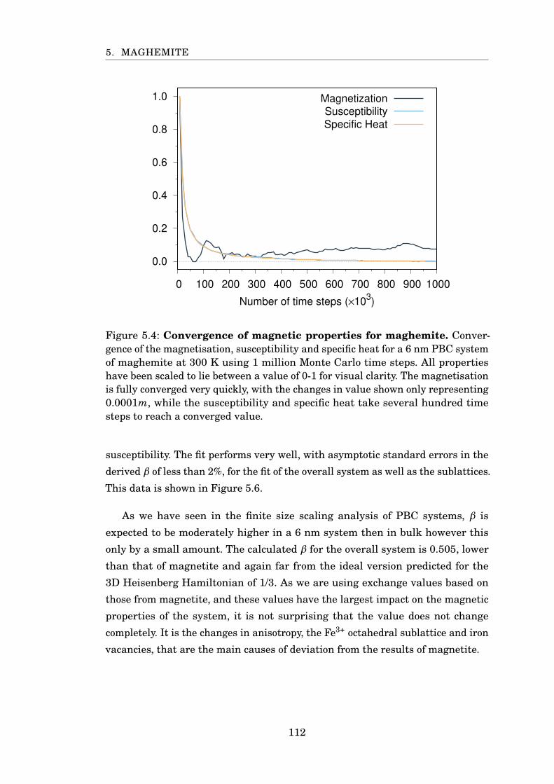
5. MAGHEMITE
0.0
0.2
0.4
0.6
0.8
1.0
0 100 200 300 400 500 600 700 800 900 1000
Number of time steps (×103)
Magnetization
Susceptibility
Specific Heat
Figure 5.4: Convergence of magnetic properties for maghemite. Conver-gence of the magnetisation, susceptibility and specific heat for a 6 nm PBC systemof maghemite at 300 K using 1 million Monte Carlo time steps. All propertieshave been scaled to lie between a value of 0-1 for visual clarity. The magnetisationis fully converged very quickly, with the changes in value shown only representing0.0001m, while the susceptibility and specific heat take several hundred timesteps to reach a converged value.
susceptibility. The fit performs very well, with asymptotic standard errors in the
derived β of less than 2%, for the fit of the overall system as well as the sublattices.
This data is shown in Figure 5.6.
As we have seen in the finite size scaling analysis of PBC systems, β is
expected to be moderately higher in a 6 nm system then in bulk however this
only by a small amount. The calculated β for the overall system is 0.505, lower
than that of magnetite and again far from the ideal version predicted for the
3D Heisenberg Hamiltonian of 1/3. As we are using exchange values based on
those from magnetite, and these values have the largest impact on the magnetic
properties of the system, it is not surprising that the value does not change
completely. It is the changes in anisotropy, the Fe3+ octahedral sublattice and iron
vacancies, that are the main causes of deviation from the results of magnetite.
112
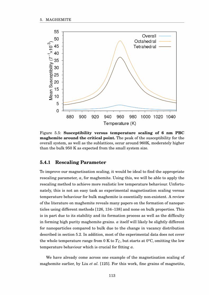
5. MAGHEMITE
Figure 5.5: Susceptibility versus temperature scaling of 6 nm PBCmaghemite around the critical point. The peak of the susceptibility for theoverall system, as well as the sublattices, occur around 960K, moderately higherthan the bulk 950 K as expected from the small system size.
5.4.1 Rescaling Parameter
To improve our magnetisation scaling, it would be ideal to find the appropriate
rescaling parameter, α, for maghemite. Using this, we will be able to apply the
rescaling method to achieve more realistic low temperature behaviour. Unfortu-
nately, this is not an easy task as experimental magnetisation scaling versus
temperature behaviour for bulk maghemite is essentially non-existent. A review
of the literature on maghemite reveals many papers on the formation of nanopar-
ticles using different methods [126, 134–138] and none on bulk properties. This
is in part due to its stability and its formation process as well as the difficulty
in forming high purity maghemite grains. α itself will likely be slightly different
for nanoparticles compared to bulk due to the change in vacancy distribution
described in section 5.2. In addition, most of the experimental data does not cover
the whole temperature range from 0 K to TC, but starts at 0°C, omitting the low
temperature behaviour which is crucial for fitting α.
We have already come across one example of the magnetisation scaling of
maghemite earlier, by Liu et al. [125]. For this work, fine grains of magnetite,
113
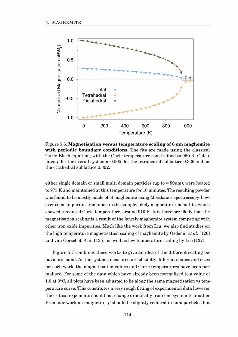
5. MAGHEMITE
-1.0
-0.5
0.0
0.5
1.0
0 200 400 600 800 1000
Norm
alis
ed M
agnetisation (
M/M
s)
Temperature (K)
Total
Tetrahedral
Octahedral
Figure 5.6: Magnetisation versus temperature scaling of 6 nm maghemitewith periodic boundary conditions. The fits are made using the classicalCurie-Bloch equation, with the Curie temperature constrained to 960 K. Calcu-lated β for the overall system is 0.505, for the tetrahedral sublattice 0.326 and forthe octahedral sublattice 0.392.
either single domain or small multi domain particles (up to ≈ 50µm), were heated
to 975 K and maintained at this temperature for 10 minutes. The resulting powder
was found to be mostly made of of maghemite using Mössbauer spectroscopy, how-
ever some impurities remained in the sample, likely magnetite or hematite, which
showed a reduced Curie temperature, around 910 K. It is therefore likely that the
magnetisation scaling is a result of the largely maghemite system competing with
other iron oxide impurities. Much like the work from Liu, we also find studies on
the high temperature magnetisation scaling of maghemite by Özdemir et al. [126]
and van Oorschot et al. [135], as well as low temperature scaling by Lee [137].
Figure 5.7 combines these works to give an idea of the different scaling be-
haviours found. As the systems measured are of subtly different shapes and sizes
for each work, the magnetisation values and Curie temperatures have been nor-
malised. For some of the data which have already been normalised to a value of
1.0 at 0°C, all plots have been adjusted to lie along the same magnetisation vs tem-
perature curve. This constitutes a very rough fitting of experimental data however
the critical exponents should not change drastically from one system to another.
From our work on magnetite, β should be slightly reduced in nanoparticles but
114
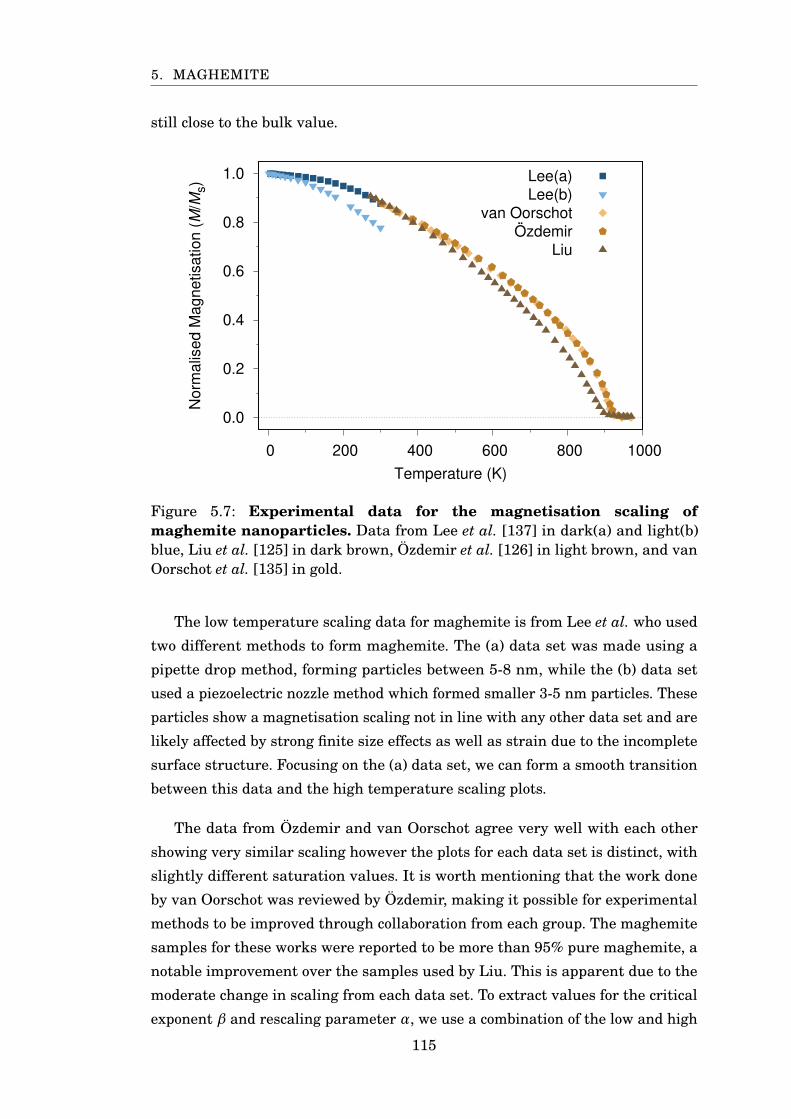
5. MAGHEMITE
still close to the bulk value.
0.0
0.2
0.4
0.6
0.8
1.0
0 200 400 600 800 1000
Nor
mal
ised
Mag
netis
atio
n (M
/Ms)
Temperature (K)
Lee(a)Lee(b)
van OorschotÖzdemir
Liu
Figure 5.7: Experimental data for the magnetisation scaling ofmaghemite nanoparticles. Data from Lee et al. [137] in dark(a) and light(b)blue, Liu et al. [125] in dark brown, Özdemir et al. [126] in light brown, and vanOorschot et al. [135] in gold.
The low temperature scaling data for maghemite is from Lee et al. who used
two different methods to form maghemite. The (a) data set was made using a
pipette drop method, forming particles between 5-8 nm, while the (b) data set
used a piezoelectric nozzle method which formed smaller 3-5 nm particles. These
particles show a magnetisation scaling not in line with any other data set and are
likely affected by strong finite size effects as well as strain due to the incomplete
surface structure. Focusing on the (a) data set, we can form a smooth transition
between this data and the high temperature scaling plots.
The data from Özdemir and van Oorschot agree very well with each other
showing very similar scaling however the plots for each data set is distinct, with
slightly different saturation values. It is worth mentioning that the work done
by van Oorschot was reviewed by Özdemir, making it possible for experimental
methods to be improved through collaboration from each group. The maghemite
samples for these works were reported to be more than 95% pure maghemite, a
notable improvement over the samples used by Liu. This is apparent due to the
moderate change in scaling from each data set. To extract values for the critical
exponent β and rescaling parameter α, we use a combination of the low and high
115
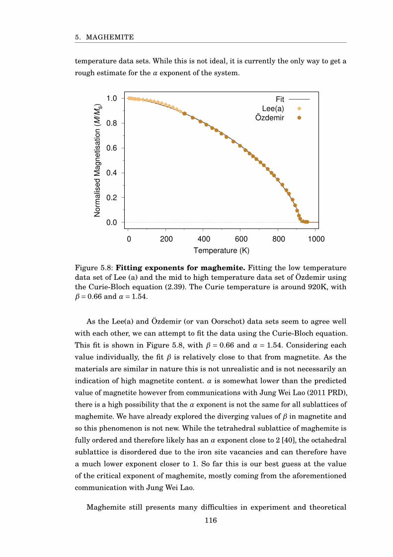
5. MAGHEMITE
temperature data sets. While this is not ideal, it is currently the only way to get a
rough estimate for the α exponent of the system.
0.0
0.2
0.4
0.6
0.8
1.0
0 200 400 600 800 1000
Nor
mal
ised
Mag
netis
atio
n (M
/Ms)
Temperature (K)
FitLee(a)
Özdemir
Figure 5.8: Fitting exponents for maghemite. Fitting the low temperaturedata set of Lee (a) and the mid to high temperature data set of Özdemir usingthe Curie-Bloch equation (2.39). The Curie temperature is around 920K, withβ= 0.66 and α= 1.54.
As the Lee(a) and Özdemir (or van Oorschot) data sets seem to agree well
with each other, we can attempt to fit the data using the Curie-Bloch equation.
This fit is shown in Figure 5.8, with β = 0.66 and α = 1.54. Considering each
value individually, the fit β is relatively close to that from magnetite. As the
materials are similar in nature this is not unrealistic and is not necessarily an
indication of high magnetite content. α is somewhat lower than the predicted
value of magnetite however from communications with Jung Wei Lao (2011 PRD),
there is a high possibility that the α exponent is not the same for all sublattices of
maghemite. We have already explored the diverging values of β in magnetite and
so this phenomenon is not new. While the tetrahedral sublattice of maghemite is
fully ordered and therefore likely has an α exponent close to 2 [40], the octahedral
sublattice is disordered due to the iron site vacancies and can therefore have
a much lower exponent closer to 1. So far this is our best guess at the value
of the critical exponent of maghemite, mostly coming from the aforementioned
communication with Jung Wei Lao.
Maghemite still presents many difficulties in experiment and theoretical
116
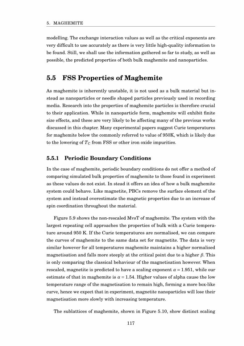
5. MAGHEMITE
modelling. The exchange interaction values as well as the critical exponents are
very difficult to use accurately as there is very little high-quality information to
be found. Still, we shall use the information gathered so far to study, as well as
possible, the predicted properties of both bulk maghemite and nanoparticles.
5.5 FSS Properties of Maghemite
As maghemite is inherently unstable, it is not used as a bulk material but in-
stead as nanoparticles or needle shaped particles previously used in recording
media. Research into the properties of maghemite particles is therefore crucial
to their application. While in nanoparticle form, maghemite will exhibit finite
size effects, and these are very likely to be affecting many of the previous works
discussed in this chapter. Many experimental papers suggest Curie temperatures
for maghemite below the commonly referred to value of 950K, which is likely due
to the lowering of TC from FSS or other iron oxide impurities.
5.5.1 Periodic Boundary Conditions
In the case of maghemite, periodic boundary conditions do not offer a method of
comparing simulated bulk properties of maghemite to those found in experiment
as these values do not exist. In stead it offers an idea of how a bulk maghemite
system could behave. Like magnetite, PBCs remove the surface element of the
system and instead overestimate the magnetic properties due to an increase of
spin coordination throughout the material.
Figure 5.9 shows the non-rescaled MvsT of maghemite. The system with the
largest repeating cell approaches the properties of bulk with a Curie tempera-
ture around 950 K. If the Curie temperatures are normalised, we can compare
the curves of maghemite to the same data set for magnetite. The data is very
similar however for all temperatures maghemite maintains a higher normalised
magnetisation and falls more steeply at the critical point due to a higher β. This
is only comparing the classical behaviour of the magnetisation however. When
rescaled, magnetite is predicted to have a scaling exponent α= 1.951, while our
estimate of that in maghemite is α= 1.54. Higher values of alpha cause the low
temperature range of the magnetisation to remain high, forming a more box-like
curve, hence we expect that in experiment, magnetite nanoparticles will lose their
magnetisation more slowly with increasing temperature.
The sublattices of maghemite, shown in Figure 5.10, show distinct scaling
117
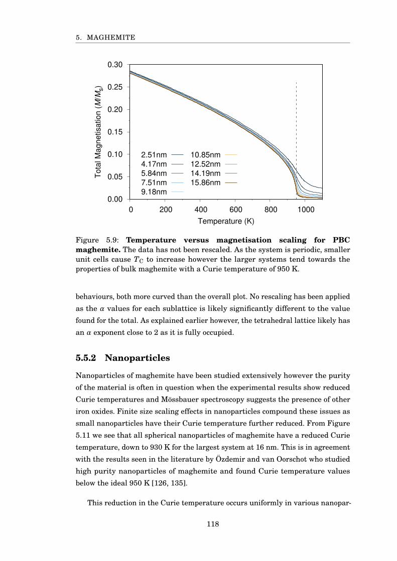
5. MAGHEMITE
0.00
0.05
0.10
0.15
0.20
0.25
0.30
0 200 400 600 800 1000
Tota
l M
agnetisation (
M/M
s)
Temperature (K)
2.51nm
4.17nm
5.84nm
7.51nm
9.18nm
10.85nm
12.52nm
14.19nm
15.86nm
Figure 5.9: Temperature versus magnetisation scaling for PBCmaghemite. The data has not been rescaled. As the system is periodic, smallerunit cells cause TC to increase however the larger systems tend towards theproperties of bulk maghemite with a Curie temperature of 950 K.
behaviours, both more curved than the overall plot. No rescaling has been applied
as the α values for each sublattice is likely significantly different to the value
found for the total. As explained earlier however, the tetrahedral lattice likely has
an α exponent close to 2 as it is fully occupied.
5.5.2 Nanoparticles
Nanoparticles of maghemite have been studied extensively however the purity
of the material is often in question when the experimental results show reduced
Curie temperatures and Mössbauer spectroscopy suggests the presence of other
iron oxides. Finite size scaling effects in nanoparticles compound these issues as
small nanoparticles have their Curie temperature further reduced. From Figure
5.11 we see that all spherical nanoparticles of maghemite have a reduced Curie
temperature, down to 930 K for the largest system at 16 nm. This is in agreement
with the results seen in the literature by Özdemir and van Oorschot who studied
high purity nanoparticles of maghemite and found Curie temperature values
below the ideal 950 K [126, 135].
This reduction in the Curie temperature occurs uniformly in various nanopar-
118
5. MAGHEMITE
Figure 5.10: Magnetisation and susceptibility scaling of the sublattices ofmaghemite. The sublattices behave differently to each other, with the octahedralmagnetisation lowering more quickly, and will therefore have differing β expo-nents. Despite this, the susceptibility plots show that each lattice has a closelyaligned TC.
ticle shapes including spherical and faceted systems. The scaling is also roughly
proportional to the number of atoms in the system (for symmetric particles),
causing spherical systems to exhibit the lowest overall Curie temperature due to
having the lowest surface area to volume ratio.
5.6 Beta Scaling
So far we have only used the β parameter to describe and compare the mag-
netisation scaling of finite size systems for both magnetite and maghemite. The
parameter itself is not set in any way but is a result of the interactions of the
particular system. For bulk systems, the value of β is often used as a constant
and defined as a critical exponent however this carries several implications on
the value of the parameter.
In general, critical exponents describe the behaviour of a material around a
continuous phase transition. It is dependent on the size of the system, the interac-
tion range and the spin dimension (such as a 2D Ising model or 3D Heisenberg).
119
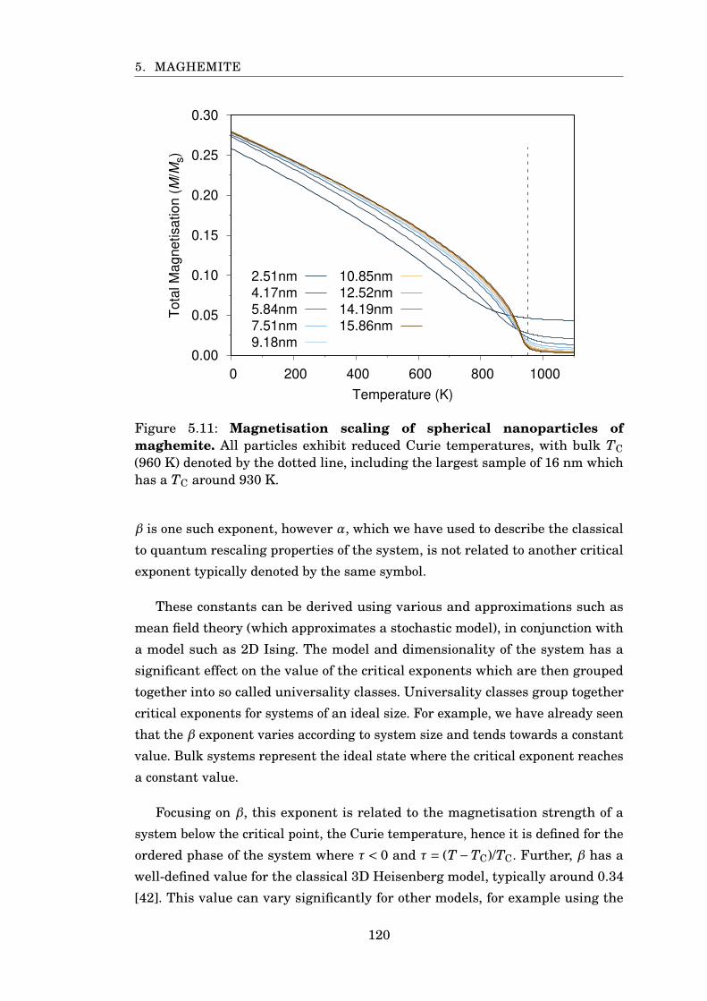
5. MAGHEMITE
0.00
0.05
0.10
0.15
0.20
0.25
0.30
0 200 400 600 800 1000
Tota
l M
agnetisation (
M/M
s)
Temperature (K)
2.51nm
4.17nm
5.84nm
7.51nm
9.18nm
10.85nm
12.52nm
14.19nm
15.86nm
Figure 5.11: Magnetisation scaling of spherical nanoparticles ofmaghemite. All particles exhibit reduced Curie temperatures, with bulk TC(960 K) denoted by the dotted line, including the largest sample of 16 nm whichhas a TC around 930 K.
β is one such exponent, however α, which we have used to describe the classical
to quantum rescaling properties of the system, is not related to another critical
exponent typically denoted by the same symbol.
These constants can be derived using various and approximations such as
mean field theory (which approximates a stochastic model), in conjunction with
a model such as 2D Ising. The model and dimensionality of the system has a
significant effect on the value of the critical exponents which are then grouped
together into so called universality classes. Universality classes group together
critical exponents for systems of an ideal size. For example, we have already seen
that the β exponent varies according to system size and tends towards a constant
value. Bulk systems represent the ideal state where the critical exponent reaches
a constant value.
Focusing on β, this exponent is related to the magnetisation strength of a
system below the critical point, the Curie temperature, hence it is defined for the
ordered phase of the system where τ < 0 and τ = (T −TC)/TC. Further, β has a
well-defined value for the classical 3D Heisenberg model, typically around 0.34
[42]. This value can vary significantly for other models, for example using the
120
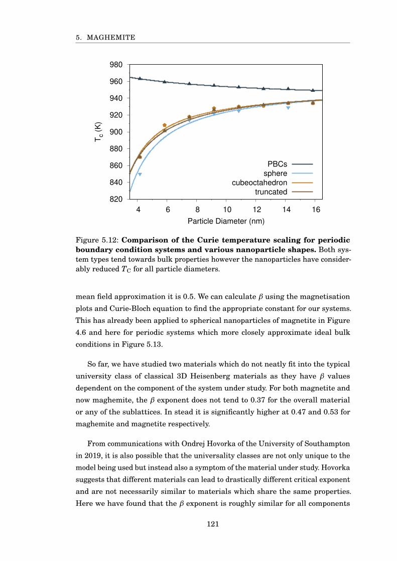
5. MAGHEMITE
820
840
860
880
900
920
940
960
980
4 6 8 10 12 14 16
Tc (
K)
Particle Diameter (nm)
PBCs
sphere
cubeoctahedron
truncated
Figure 5.12: Comparison of the Curie temperature scaling for periodicboundary condition systems and various nanoparticle shapes. Both sys-tem types tend towards bulk properties however the nanoparticles have consider-ably reduced TC for all particle diameters.
mean field approximation it is 0.5. We can calculate β using the magnetisation
plots and Curie-Bloch equation to find the appropriate constant for our systems.
This has already been applied to spherical nanoparticles of magnetite in Figure
4.6 and here for periodic systems which more closely approximate ideal bulk
conditions in Figure 5.13.
So far, we have studied two materials which do not neatly fit into the typical
university class of classical 3D Heisenberg materials as they have β values
dependent on the component of the system under study. For both magnetite and
now maghemite, the β exponent does not tend to 0.37 for the overall material
or any of the sublattices. In stead it is significantly higher at 0.47 and 0.53 for
maghemite and magnetite respectively.
From communications with Ondrej Hovorka of the University of Southampton
in 2019, it is also possible that the universality classes are not only unique to the
model being used but instead also a symptom of the material under study. Hovorka
suggests that different materials can lead to drastically different critical exponent
and are not necessarily similar to materials which share the same properties.
Here we have found that the β exponent is roughly similar for all components
121
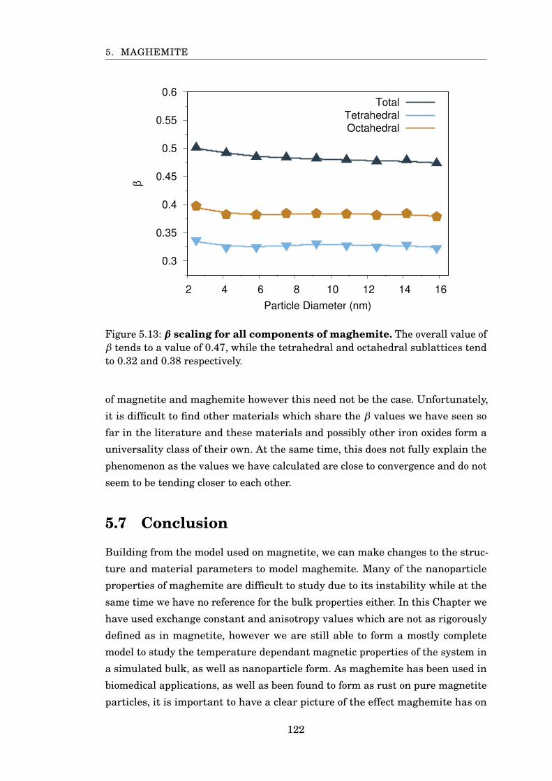
5. MAGHEMITE
0.3
0.35
0.4
0.45
0.5
0.55
0.6
2 4 6 8 10 12 14 16
β
Particle Diameter (nm)
Total
Tetrahedral
Octahedral
Figure 5.13: β scaling for all components of maghemite. The overall value ofβ tends to a value of 0.47, while the tetrahedral and octahedral sublattices tendto 0.32 and 0.38 respectively.
of magnetite and maghemite however this need not be the case. Unfortunately,
it is difficult to find other materials which share the β values we have seen so
far in the literature and these materials and possibly other iron oxides form a
universality class of their own. At the same time, this does not fully explain the
phenomenon as the values we have calculated are close to convergence and do not
seem to be tending closer to each other.
5.7 Conclusion
Building from the model used on magnetite, we can make changes to the struc-
ture and material parameters to model maghemite. Many of the nanoparticle
properties of maghemite are difficult to study due to its instability while at the
same time we have no reference for the bulk properties either. In this Chapter we
have used exchange constant and anisotropy values which are not as rigorously
defined as in magnetite, however we are still able to form a mostly complete
model to study the temperature dependant magnetic properties of the system in
a simulated bulk, as well as nanoparticle form. As maghemite has been used in
biomedical applications, as well as been found to form as rust on pure magnetite
particles, it is important to have a clear picture of the effect maghemite has on
122
5. MAGHEMITE
the magnetic properties of nanoparticles at the nanometer scale.
Maghemite has also shown consistency in our results compared to those of
magnetite. The critical exponent β of maghemite shows values close to those
found in magnetite for all components, the overall system and sublattices. This
is a curious result as it is in stark contrast to most of the literature on the 3DHeisenberg predicted value. This is possibly due to the materials belonging to
a separate universality class of their own, as suggested by Hovorka, or due to
separate parameters from size or shape which may be affecting the converged
value of the exponent.
123
CH
AP
TE
R
6COBALT FERRITE
6.1 Introduction
The surface of iron oxides such as magnetite is widely studied due to its complexity
and variation. In addition to understanding the nature of surface structure, much
work has gone into understanding the adsorption properties of the material.
Adsorption, specifically adsorption on solid surfaces, is the adhesion of atoms, ions
or molecules due to surface energy differences between the original material, and
the compound. Iron oxides are able to integrate a significant number of materials
into their surfaces: hydrogen [139], water [140] and organic compounds [141, 142]
are of interest due to the catalytic reactions iron oxides take part in. The water-gas
shift reaction for example uses an iron-oxide based catalyst to convert water and
carbon monoxide to hydrogen gas and carbon dioxide [143].
Metal adsorption on Fe3O4 has also been intensely studied due to the use of
iron oxides as a support material in catalysis, however this interaction can go a
step further as some metals integrate themselves into the sub-layers or bulk of
the iron oxide, forming new materials. This does not occur for all metals, and the
process can be divided into two groups: non-ferrite-forming metals, such as Au,
Ag, Pd and Pt [144–146], and ferrite-forming metals such as Co, Ni, Cu, Mn, Ti
and more [147–149]. For this chapter we shall focus on one such metal ferrite,
formed by doping magnetite with cobalt.
Cobalt ferrite, in particular nanoparticles of cobalt ferrite, have seen interest
due to their many uses such as for permanent magnets [151], as high-performance
124
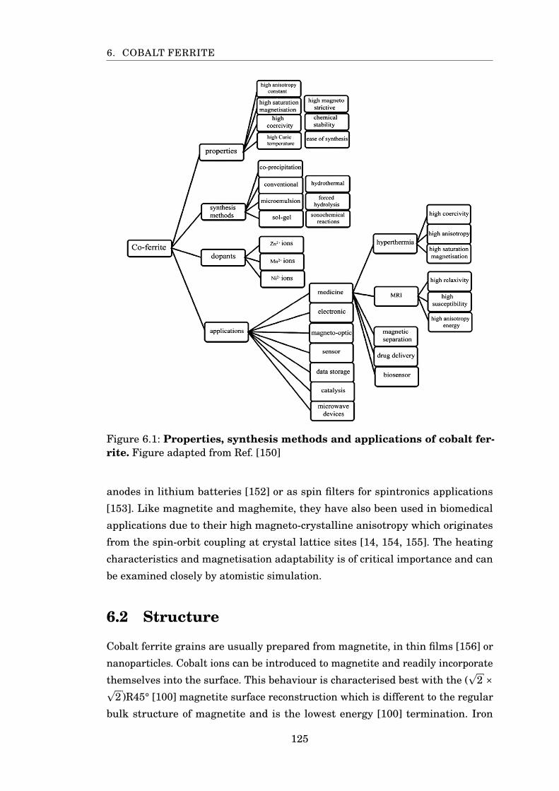
6. COBALT FERRITE
Figure 6.1: Properties, synthesis methods and applications of cobalt fer-rite. Figure adapted from Ref. [150]
anodes in lithium batteries [152] or as spin filters for spintronics applications
[153]. Like magnetite and maghemite, they have also been used in biomedical
applications due to their high magneto-crystalline anisotropy which originates
from the spin-orbit coupling at crystal lattice sites [14, 154, 155]. The heating
characteristics and magnetisation adaptability is of critical importance and can
be examined closely by atomistic simulation.
6.2 Structure
Cobalt ferrite grains are usually prepared from magnetite, in thin films [156] or
nanoparticles. Cobalt ions can be introduced to magnetite and readily incorporate
themselves into the surface. This behaviour is characterised best with the (p
2 ×p2 )R45° [100] magnetite surface reconstruction which is different to the regular
bulk structure of magnetite and is the lowest energy [100] termination. Iron
125
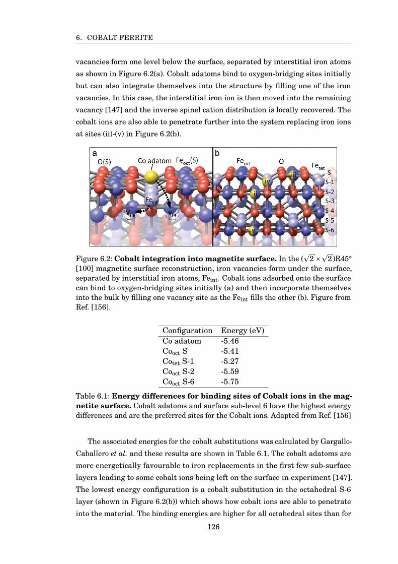
6. COBALT FERRITE
vacancies form one level below the surface, separated by interstitial iron atoms
as shown in Figure 6.2(a). Cobalt adatoms bind to oxygen-bridging sites initially
but can also integrate themselves into the structure by filling one of the iron
vacancies. In this case, the interstitial iron ion is then moved into the remaining
vacancy [147] and the inverse spinel cation distribution is locally recovered. The
cobalt ions are also able to penetrate further into the system replacing iron ions
at sites (ii)-(v) in Figure 6.2(b).
Figure 6.2: Cobalt integration into magnetite surface. In the (p
2 ×p2 )R45°
[100] magnetite surface reconstruction, iron vacancies form under the surface,separated by interstitial iron atoms, Feint. Cobalt ions adsorbed onto the surfacecan bind to oxygen-bridging sites initially (a) and then incorporate themselvesinto the bulk by filling one vacancy site as the Feint fills the other (b). Figure fromRef. [156].
Configuration Energy (eV)Co adatom -5.46Cooct S -5.41Cotet S-1 -5.27Cooct S-2 -5.59Cooct S-6 -5.75
Table 6.1: Energy differences for binding sites of Cobalt ions in the mag-netite surface. Cobalt adatoms and surface sub-level 6 have the highest energydifferences and are the preferred sites for the Cobalt ions. Adapted from Ref. [156]
The associated energies for the cobalt substitutions was calculated by Gargallo-
Caballero et al. and these results are shown in Table 6.1. The cobalt adatoms are
more energetically favourable to iron replacements in the first few sub-surface
layers leading to some cobalt ions being left on the surface in experiment [147].
The lowest energy configuration is a cobalt substitution in the octahedral S-6
layer (shown in Figure 6.2(b)) which shows how cobalt ions are able to penetrate
into the material. The binding energies are higher for all octahedral sites than for
126
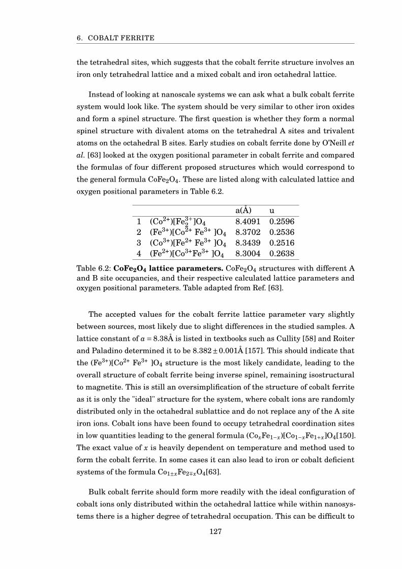
6. COBALT FERRITE
the tetrahedral sites, which suggests that the cobalt ferrite structure involves an
iron only tetrahedral lattice and a mixed cobalt and iron octahedral lattice.
Instead of looking at nanoscale systems we can ask what a bulk cobalt ferrite
system would look like. The system should be very similar to other iron oxides
and form a spinel structure. The first question is whether they form a normal
spinel structure with divalent atoms on the tetrahedral A sites and trivalent
atoms on the octahedral B sites. Early studies on cobalt ferrite done by O’Neill etal. [63] looked at the oxygen positional parameter in cobalt ferrite and compared
the formulas of four different proposed structures which would correspond to
the general formula CoFe2O4. These are listed along with calculated lattice and
oxygen positional parameters in Table 6.2.
a(Å) u1 (Co2+)[Fe3+
2 ]O4 8.4091 0.25962 (Fe3+)[Co2+ Fe3+ ]O4 8.3702 0.25363 (Co3+)[Fe2+ Fe3+ ]O4 8.3439 0.25164 (Fe2+)[Co3+Fe3+ ]O4 8.3004 0.2638
Table 6.2: CoFe2O4 lattice parameters. CoFe2O4 structures with different Aand B site occupancies, and their respective calculated lattice parameters andoxygen positional parameters. Table adapted from Ref. [63].
The accepted values for the cobalt ferrite lattice parameter vary slightly
between sources, most likely due to slight differences in the studied samples. A
lattice constant of a = 8.38Å is listed in textbooks such as Cullity [58] and Roiter
and Paladino determined it to be 8.382±0.001Å [157]. This should indicate that
the (Fe3+)[Co2+ Fe3+ ]O4 structure is the most likely candidate, leading to the
overall structure of cobalt ferrite being inverse spinel, remaining isostructural
to magnetite. This is still an oversimplification of the structure of cobalt ferrite
as it is only the "ideal" structure for the system, where cobalt ions are randomly
distributed only in the octahedral sublattice and do not replace any of the A site
iron ions. Cobalt ions have been found to occupy tetrahedral coordination sites
in low quantities leading to the general formula (CoxFe1−x)[Co1−xFe1+x]O4[150].
The exact value of x is heavily dependent on temperature and method used to
form the cobalt ferrite. In some cases it can also lead to iron or cobalt deficient
systems of the formula Co1±xFe2∓xO4[63].
Bulk cobalt ferrite should form more readily with the ideal configuration of
cobalt ions only distributed within the octahedral lattice while within nanosys-
tems there is a higher degree of tetrahedral occupation. This can be difficult to
127
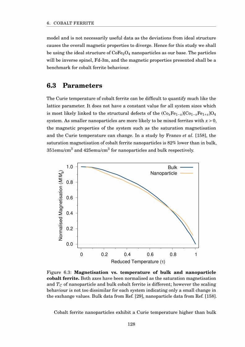
6. COBALT FERRITE
model and is not necessarily useful data as the deviations from ideal structure
causes the overall magnetic properties to diverge. Hence for this study we shall
be using the ideal structure of CoFe2O4 nanoparticles as our base. The particles
will be inverse spinel, Fd-3m, and the magnetic properties presented shall be a
benchmark for cobalt ferrite behaviour.
6.3 Parameters
The Curie temperature of cobalt ferrite can be difficult to quantify much like the
lattice parameter. It does not have a constant value for all system sizes which
is most likely linked to the structural defects of the (CoxFe1−x)[Co1−xFe1+x]O4
system. As smaller nanoparticles are more likely to be mixed ferrites with x > 0,
the magnetic properties of the system such as the saturation magnetisation
and the Curie temperature can change. In a study by Franco et al. [158], the
saturation magnetisation of cobalt ferrite nanoparticles is 82% lower than in bulk,
351emu/cm3 and 425emu/cm3 for nanoparticles and bulk respectively.
0.0
0.2
0.4
0.6
0.8
1.0
0 0.2 0.4 0.6 0.8 1
Norm
alis
ed M
agnetisation (
M/M
s)
Reduced Temperature (τ)
Bulk
Nanoparticle
Figure 6.3: Magnetisation vs. temperature of bulk and nanoparticlecobalt ferrite. Both axes have been normalised as the saturation magnetisationand TC of nanoparticle and bulk cobalt ferrite is different; however the scalingbehaviour is not too dissimilar for each system indicating only a small change inthe exchange values. Bulk data from Ref. [29], nanoparticle data from Ref. [158].
Cobalt ferrite nanoparticles exhibit a Curie temperature higher than bulk
128
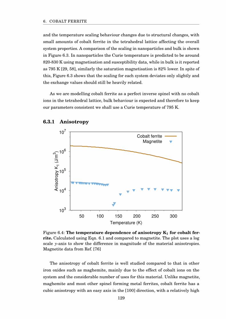
6. COBALT FERRITE
and the temperature scaling behaviour changes due to structural changes, with
small amounts of cobalt ferrite in the tetrahedral lattice affecting the overall
system properties. A comparison of the scaling in nanoparticles and bulk is shown
in Figure 6.3. In nanoparticles the Curie temperature is predicted to be around
820-830 K using magnetisation and susceptibility data, while in bulk is it reported
as 795 K [29, 58], similarly the saturation magnetisation is 82% lower. In spite of
this, Figure 6.3 shows that the scaling for each system deviates only slightly and
the exchange values should still be heavily related.
As we are modelling cobalt ferrite as a perfect inverse spinel with no cobalt
ions in the tetrahedral lattice, bulk behaviour is expected and therefore to keep
our parameters consistent we shall use a Curie temperature of 795 K.
6.3.1 Anisotropy
103
104
105
106
107
50 100 150 200 250 300
Anis
otr
opy K
1 (
J/m
3)
Temperature (K)
Cobalt ferrite
Magnetite
Figure 6.4: The temperature dependence of anisotropy K1 for cobalt fer-rite. Calculated using Eqn. 6.1 and compared to magnetite. The plot uses a logscale y-axis to show the difference in magnitude of the material anisotropies.Magnetite data from Ref. [76]
The anisotropy of cobalt ferrite is well studied compared to that in other
iron oxides such as maghemite, mainly due to the effect of cobalt ions on the
system and the considerable number of uses for this material. Unlike magnetite,
maghemite and most other spinel forming metal ferrites, cobalt ferrite has a
cubic anisotropy with an easy axis in the [100] direction, with a relatively high
129
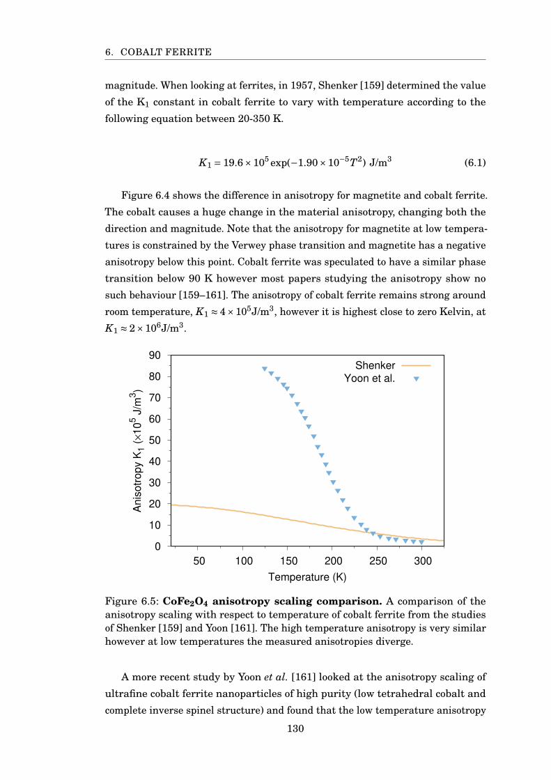
6. COBALT FERRITE
magnitude. When looking at ferrites, in 1957, Shenker [159] determined the value
of the K1 constant in cobalt ferrite to vary with temperature according to the
following equation between 20-350 K.
K1 = 19.6×10⁵ exp(−1.90×10⁻⁵T2) J/m3 (6.1)
Figure 6.4 shows the difference in anisotropy for magnetite and cobalt ferrite.
The cobalt causes a huge change in the material anisotropy, changing both the
direction and magnitude. Note that the anisotropy for magnetite at low tempera-
tures is constrained by the Verwey phase transition and magnetite has a negative
anisotropy below this point. Cobalt ferrite was speculated to have a similar phase
transition below 90 K however most papers studying the anisotropy show no
such behaviour [159–161]. The anisotropy of cobalt ferrite remains strong around
room temperature, K1 ≈ 4×10⁵J/m3, however it is highest close to zero Kelvin, at
K1 ≈ 2×10⁶J/m3.
0
10
20
30
40
50
60
70
80
90
50 100 150 200 250 300
Anis
otr
opy K
1 (
×10
5 J
/m3)
Temperature (K)
Shenker
Yoon et al.
Figure 6.5: CoFe2O4 anisotropy scaling comparison. A comparison of theanisotropy scaling with respect to temperature of cobalt ferrite from the studiesof Shenker [159] and Yoon [161]. The high temperature anisotropy is very similarhowever at low temperatures the measured anisotropies diverge.
A more recent study by Yoon et al. [161] looked at the anisotropy scaling of
ultrafine cobalt ferrite nanoparticles of high purity (low tetrahedral cobalt and
complete inverse spinel structure) and found that the low temperature anisotropy
130
6. COBALT FERRITE
was several times higher than previously reported, reaching 8×10⁶J/m3. Both
studies are shown in Figure 6.5. The anisotropy is very high close to zero Kelvin in
the case of Yoon, and lowers greatly towards room temperature. Surface anisotropy
is likely the largest factor causing the discrepancy between the two data sets,
and is often several times larger in magnitude to the intrinsic magnetocrystalline
anisotropy of the material [162].
This discrepancy makes choosing an appropriate value for the anisotropy
constant of cobalt ferrite very difficult as it will affect low temperature magnetic
properties more heavily. For most scaling behaviour where the magnetic properties
around the Curie temperature are in focus, the room temperature value can be
used as the anisotropy will have little effect. When studying the low temperature
magnetic properties, the higher anisotropy strength will also be considered due to
the effects on spin-switching.
6.3.2 Exchange
The exchange interaction values for cobalt ferrite are less well reviewed in the
literature. Some papers list exchange interaction values for cobalt ferrite in a
2-lattice model [163] however this is a less than ideal approach to understanding
cobalt ferrite. In the 2-lattice model, the spinels are assumed to have the over-
all formula AB2O, with two lattices each containing a divalent species, A, and
trivalent species B. Following this there are three possible exchange values, JAA,
JAB and JBB. Maghemite is a good example for this model as although both A
and B species are Fe3+, the superexchange distances between tetrahedral and
octahedral iron ions are different and therefore the two can be treated differently.
The exchange interactions for the system can therefore be fully explained using
three parameters. This is the same system that was initially applied to magnetite
by Néel [6] who understood that two different ionic species existed in the octahe-
dral lattice but hoped that it could be approximated by one exchange value. This
assumption would turn out to be fruitful as (omitting more recent explanations
covered in Chapter 3) the Fe2+ and Fe3+ ions in magnetite form a mixed valence
state of Fe2.5+ above the Verwey transition and are mostly indistinguishable
[74, 164]. This allows the 2-lattice model to work well for magnetite.
In cobalt ferrite there are three distinct ionic species: tetrahedral Fe3+, octa-
hedral Fe3+ and octahedral Co2+, which in equal amounts make up all magnetic
atoms in the unit cell. In CoFe2O4 the octahedral ions do not form a mixed state
and are therefore represented as (A)[BB’]O. Hence there are six total interactions:
131
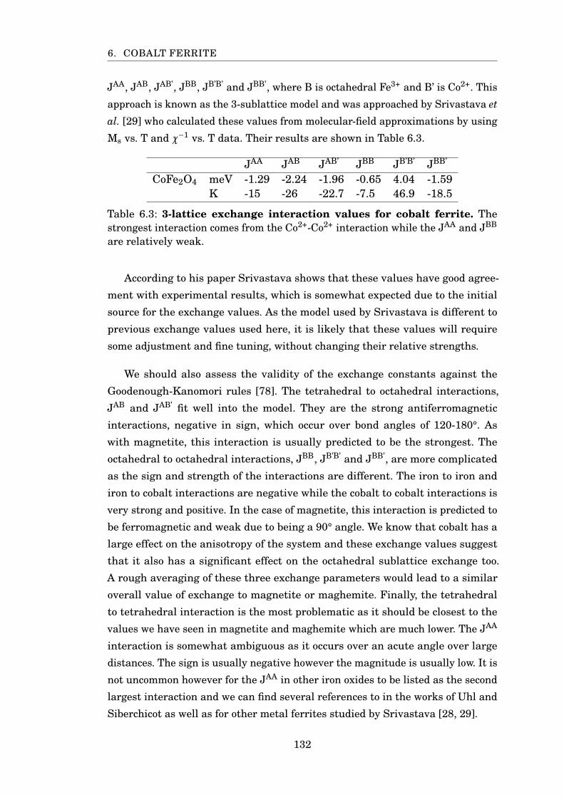
6. COBALT FERRITE
JAA, JAB, JAB’, JBB, JB’B’ and JBB’, where B is octahedral Fe3+ and B’ is Co2+. This
approach is known as the 3-sublattice model and was approached by Srivastava etal. [29] who calculated these values from molecular-field approximations by using
Ms vs. T and χ−1 vs. T data. Their results are shown in Table 6.3.
JAA JAB JAB’ JBB JB’B’ JBB’
CoFe2O4 meV -1.29 -2.24 -1.96 -0.65 4.04 -1.59K -15 -26 -22.7 -7.5 46.9 -18.5
Table 6.3: 3-lattice exchange interaction values for cobalt ferrite. Thestrongest interaction comes from the Co2+-Co2+ interaction while the JAA and JBB
are relatively weak.
According to his paper Srivastava shows that these values have good agree-
ment with experimental results, which is somewhat expected due to the initial
source for the exchange values. As the model used by Srivastava is different to
previous exchange values used here, it is likely that these values will require
some adjustment and fine tuning, without changing their relative strengths.
We should also assess the validity of the exchange constants against the
Goodenough-Kanomori rules [78]. The tetrahedral to octahedral interactions,
JAB and JAB’ fit well into the model. They are the strong antiferromagnetic
interactions, negative in sign, which occur over bond angles of 120-180°. As
with magnetite, this interaction is usually predicted to be the strongest. The
octahedral to octahedral interactions, JBB, JB’B’ and JBB’, are more complicated
as the sign and strength of the interactions are different. The iron to iron and
iron to cobalt interactions are negative while the cobalt to cobalt interactions is
very strong and positive. In the case of magnetite, this interaction is predicted to
be ferromagnetic and weak due to being a 90° angle. We know that cobalt has a
large effect on the anisotropy of the system and these exchange values suggest
that it also has a significant effect on the octahedral sublattice exchange too.
A rough averaging of these three exchange parameters would lead to a similar
overall value of exchange to magnetite or maghemite. Finally, the tetrahedral
to tetrahedral interaction is the most problematic as it should be closest to the
values we have seen in magnetite and maghemite which are much lower. The JAA
interaction is somewhat ambiguous as it occurs over an acute angle over large
distances. The sign is usually negative however the magnitude is usually low. It is
not uncommon however for the JAA in other iron oxides to be listed as the second
largest interaction and we can find several references to in the works of Uhl and
Siberchicot as well as for other metal ferrites studied by Srivastava [28, 29].
132
6. COBALT FERRITE
As a comparison, we have also made an educated guess at the exchange con-
stants for cobalt ferrite starting again from the values used in magnetite. This has
the unfortunate side effect that the cobalt and iron contributions to the exchange
in the octahedral lattice are averaged out however we preserve a separation in
these lattices to correctly model the strong spin moment on cobalt ions as well
as their contribution to the overall system anisotropy. While cobalt ferrite is a
widely studied material and without the instability drawbacks of maghemite, it
has been difficult to find a suitable set of exchange parameters that is clearly a
good representation of experiment, as we have found with magnetite. The extra
set of exchange constants is another way to try out different initial parameters,
specifically those with the highest contribution to the system Hamiltonian.
6.4 Simulating Cobalt Ferrite
With the current set of parameters we have compiled for cobalt ferrite, we can
start to simulate the material using the same methods used in magnetite and
maghemite. Due to the uncertainty in the exchange parameters however, we shall
be using two sets of data, referred to as CFA, using the exchange parameters of
Srivastava et al., and CFB which uses exchange parameters based on magnetite.
To recap the parameters:
• The system is cubic with a lattice constant of a = 8.382Å
• There are four unique materials:
– Tetrahedral site iron 3+ ions with spin moment 5µB
– Octahedral site iron 3+ ions with spin moment 5µB
– Octahedral site cobalt 2+ ions with spin moment 4.6µB
– Non-magnetic oxygen 2- ions
• The anisotropy direction is ⟨100⟩
• Two sets of exchange parameters, CFA and CFB, with 6 constants each,
shown below in Table 6.4.
As with previous materials we first plot for the convergence of each data set.
The susceptibility and specific heat require a large amount of Monte Carlo time
steps to fully relax. Figure 6.6 shows the convergence, with each plot normalised
between 0 and 1 as each set varies significantly in magnitude. We are modelling
133
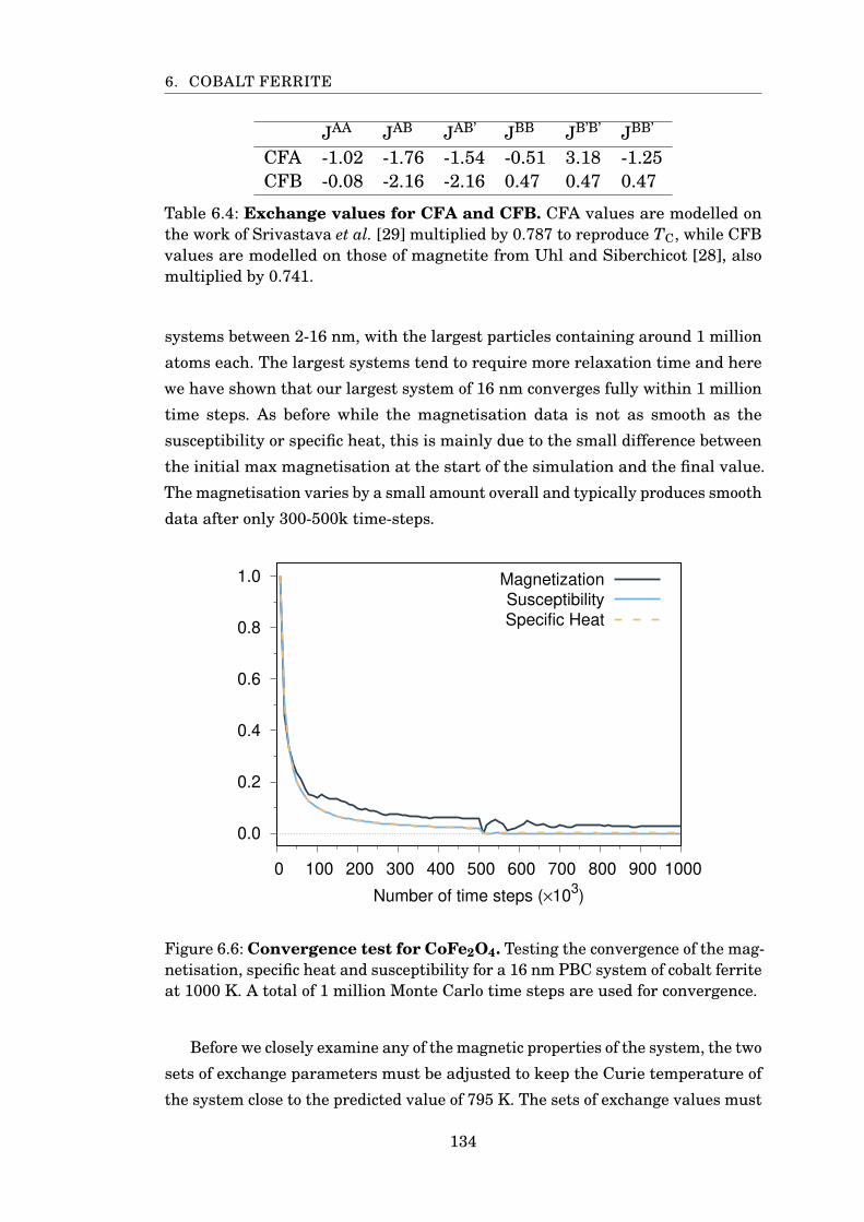
6. COBALT FERRITE
JAA JAB JAB’ JBB JB’B’ JBB’
CFA -1.02 -1.76 -1.54 -0.51 3.18 -1.25CFB -0.08 -2.16 -2.16 0.47 0.47 0.47
Table 6.4: Exchange values for CFA and CFB. CFA values are modelled onthe work of Srivastava et al. [29] multiplied by 0.787 to reproduce TC, while CFBvalues are modelled on those of magnetite from Uhl and Siberchicot [28], alsomultiplied by 0.741.
systems between 2-16 nm, with the largest particles containing around 1 million
atoms each. The largest systems tend to require more relaxation time and here
we have shown that our largest system of 16 nm converges fully within 1 million
time steps. As before while the magnetisation data is not as smooth as the
susceptibility or specific heat, this is mainly due to the small difference between
the initial max magnetisation at the start of the simulation and the final value.
The magnetisation varies by a small amount overall and typically produces smooth
data after only 300-500k time-steps.
0.0
0.2
0.4
0.6
0.8
1.0
0 100 200 300 400 500 600 700 800 900 1000
Number of time steps (×103)
Magnetization
Susceptibility
Specific Heat
Figure 6.6: Convergence test for CoFe2O4. Testing the convergence of the mag-netisation, specific heat and susceptibility for a 16 nm PBC system of cobalt ferriteat 1000 K. A total of 1 million Monte Carlo time steps are used for convergence.
Before we closely examine any of the magnetic properties of the system, the two
sets of exchange parameters must be adjusted to keep the Curie temperature of
the system close to the predicted value of 795 K. The sets of exchange values must
134
6. COBALT FERRITE
be multiplied by a constant to have the phase transition occur at the right position
in our simulations. The exchange constants used in CFA must be increased
significantly, by about 20%. This can be due to several factors, however the
differences in the models used is likely a contributing factor. Meanwhile, the
exchange parameters for CFB would end up with a Curie point around 850K, as
in magnetite, however they must be lowered by around 7% to correctly reflect the
lower critical point of cobalt ferrite.
The data sets do not agree perfectly, there is an approximately 5 K difference
in the peaks, with the exchange values of CFA being slightly too high, however
they both peak around 800 K, close to ideal value of 795 K. We can already see
some of the difference between the sets of exchange here as in the set derived
from magnetite the octahedral sublattices, including cobalt, behave very similarly,
both sharing the same exchange values and lying roughly between the cobalt
and octahedral plots from (a). The overall and tetrahedral components to the
susceptibility agree well with each other which is promising as these are a result
of completely separate exchange values.
Using the Curie temperature point predicted by the susceptibility we can
fit the magnetisation scaling according to the Curie-Bloch equation. This will
improve the fitting for small nanoparticles where finite size effects cause the
phase transition to occur more gradually and obscure the Curie temperature. In
Figure 6.8 we can compare the magnetisation scaling with temperature for both
sets of exchange, as well as the fit β values.
The magnetisation curves demonstrate similar properties to the susceptibility,
CFB behaves as if it is a 2-lattice model, with the cobalt and octahedral lattice
behaving exactly the same and having the same β exponent. Meanwhile Figure
6.8a shows varying β exponents for the octahedral sublattices. In addition, both
sets have varying β exponents for each component of the system. These are listed
for comparison in Table 6.5.
The β exponents for the tetrahedral sublattice agree well with each other.
Referring back the exchange constants, the JAA interactions are quite different
in each set, with the values from Ref [29] being the same in sign but an order of
magnitude larger, making the similarity in the scaling of the tetrahedral lattice
surprising. The overall β exponents are different due to the large difference in the
octahedral sublattice for each system. β= 0.45 is relatively high for an octahedral
β exponent compared to the values we have seen from magnetite and maghemite.
135
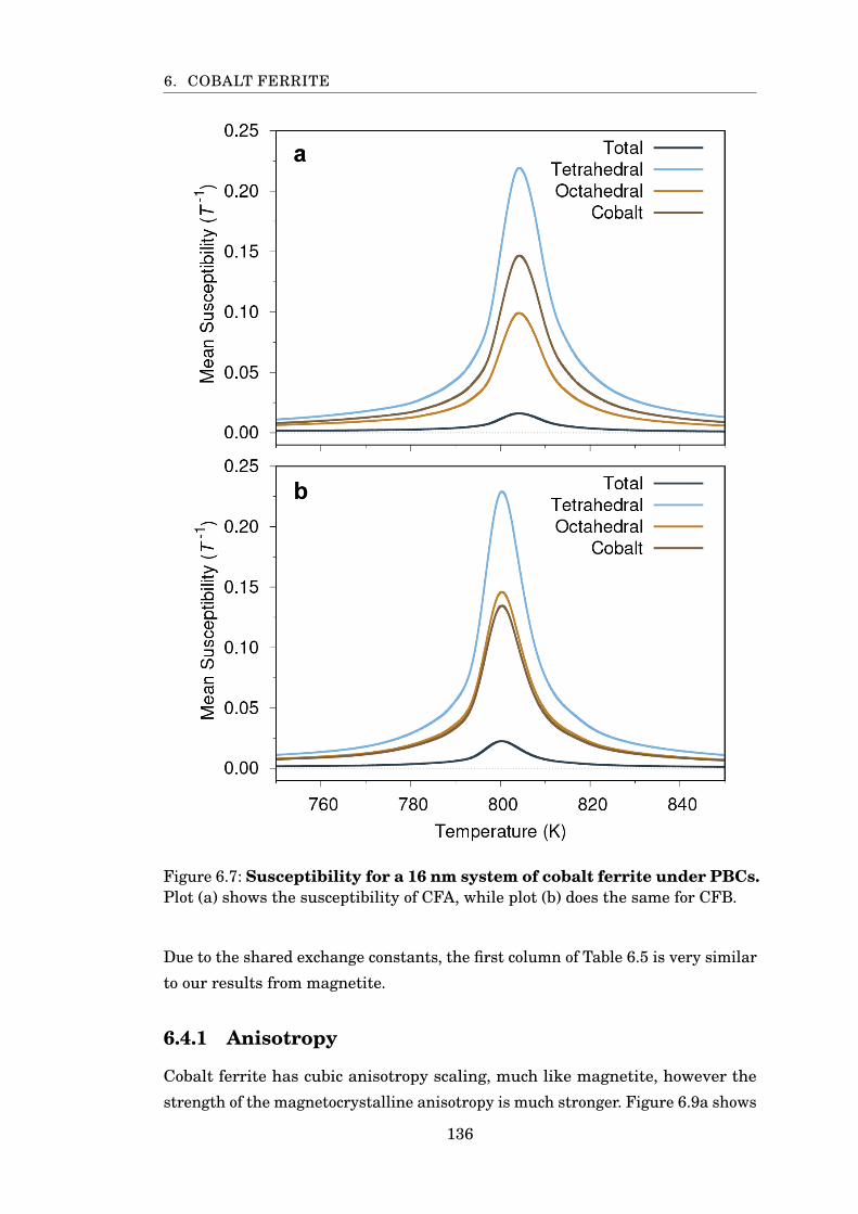
6. COBALT FERRITE
Figure 6.7: Susceptibility for a 16 nm system of cobalt ferrite under PBCs.Plot (a) shows the susceptibility of CFA, while plot (b) does the same for CFB.
Due to the shared exchange constants, the first column of Table 6.5 is very similar
to our results from magnetite.
6.4.1 Anisotropy
Cobalt ferrite has cubic anisotropy scaling, much like magnetite, however the
strength of the magnetocrystalline anisotropy is much stronger. Figure 6.9a shows
136
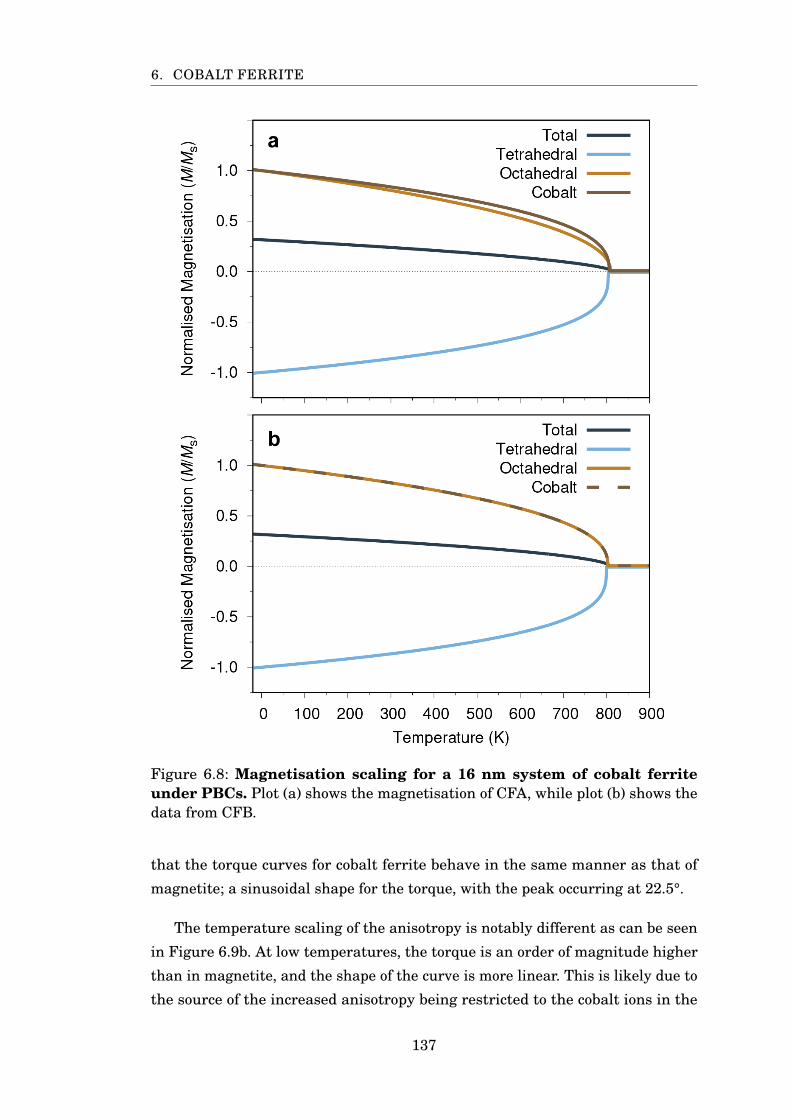
6. COBALT FERRITE
Figure 6.8: Magnetisation scaling for a 16 nm system of cobalt ferriteunder PBCs. Plot (a) shows the magnetisation of CFA, while plot (b) shows thedata from CFB.
that the torque curves for cobalt ferrite behave in the same manner as that of
magnetite; a sinusoidal shape for the torque, with the peak occurring at 22.5°.
The temperature scaling of the anisotropy is notably different as can be seen
in Figure 6.9b. At low temperatures, the torque is an order of magnitude higher
than in magnetite, and the shape of the curve is more linear. This is likely due to
the source of the increased anisotropy being restricted to the cobalt ions in the
137
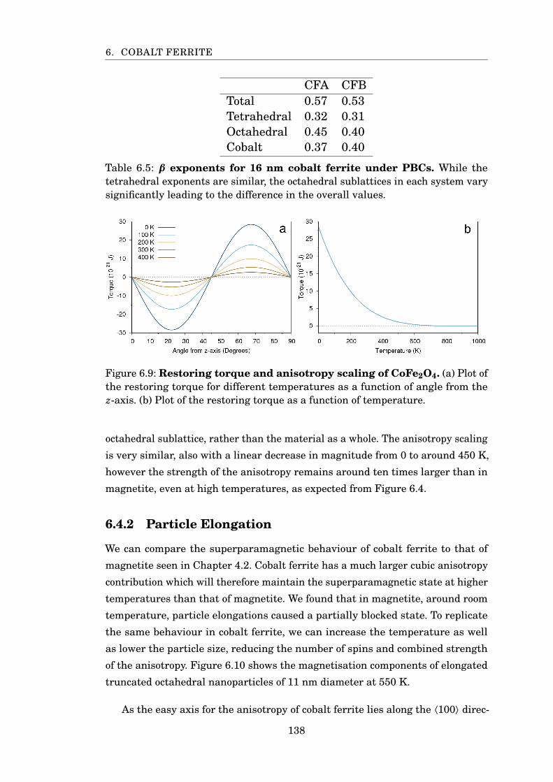
6. COBALT FERRITE
CFA CFBTotal 0.57 0.53Tetrahedral 0.32 0.31Octahedral 0.45 0.40Cobalt 0.37 0.40
Table 6.5: β exponents for 16 nm cobalt ferrite under PBCs. While thetetrahedral exponents are similar, the octahedral sublattices in each system varysignificantly leading to the difference in the overall values.
Figure 6.9: Restoring torque and anisotropy scaling of CoFe2O4. (a) Plot ofthe restoring torque for different temperatures as a function of angle from thez-axis. (b) Plot of the restoring torque as a function of temperature.
octahedral sublattice, rather than the material as a whole. The anisotropy scaling
is very similar, also with a linear decrease in magnitude from 0 to around 450 K,
however the strength of the anisotropy remains around ten times larger than in
magnetite, even at high temperatures, as expected from Figure 6.4.
6.4.2 Particle Elongation
We can compare the superparamagnetic behaviour of cobalt ferrite to that of
magnetite seen in Chapter 4.2. Cobalt ferrite has a much larger cubic anisotropy
contribution which will therefore maintain the superparamagnetic state at higher
temperatures than that of magnetite. We found that in magnetite, around room
temperature, particle elongations caused a partially blocked state. To replicate
the same behaviour in cobalt ferrite, we can increase the temperature as well
as lower the particle size, reducing the number of spins and combined strength
of the anisotropy. Figure 6.10 shows the magnetisation components of elongated
truncated octahedral nanoparticles of 11 nm diameter at 550 K.
As the easy axis for the anisotropy of cobalt ferrite lies along the ⟨100⟩ direc-
138
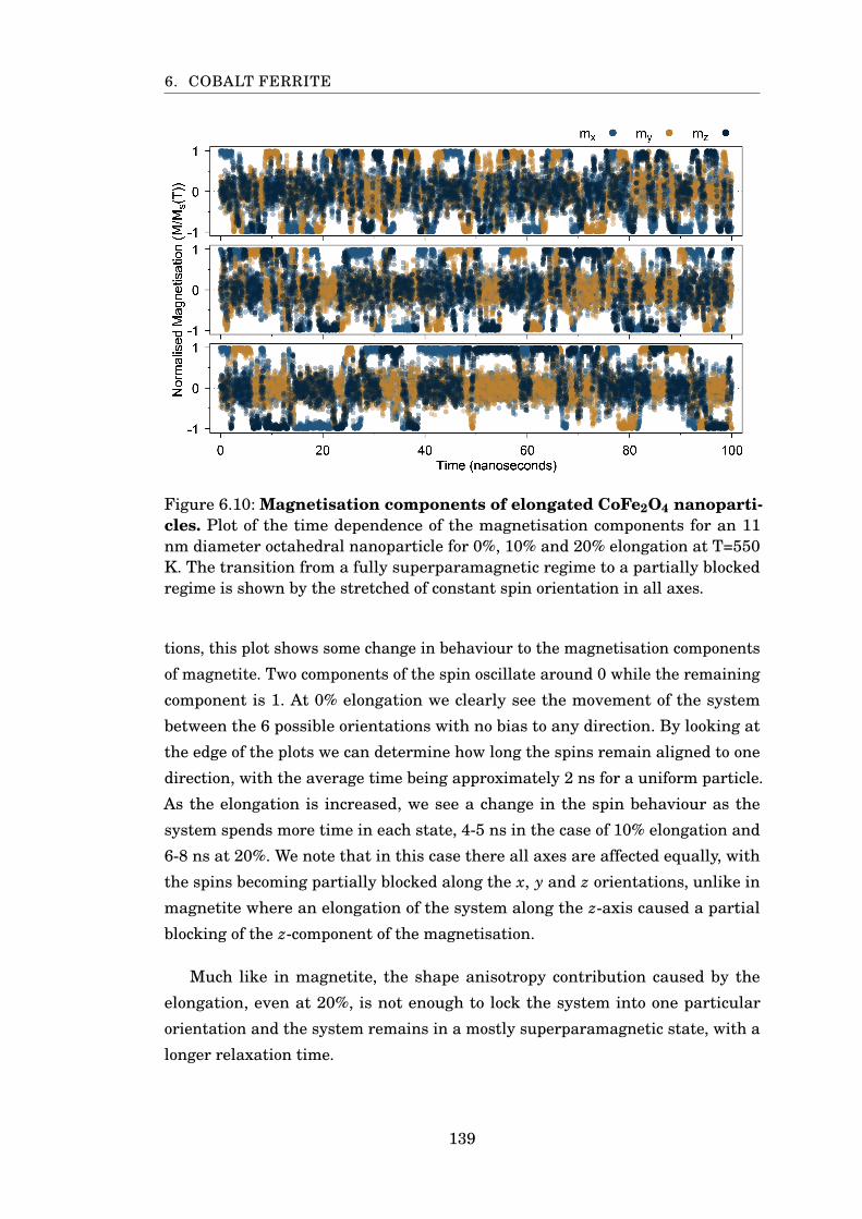
6. COBALT FERRITE
Figure 6.10: Magnetisation components of elongated CoFe2O4 nanoparti-cles. Plot of the time dependence of the magnetisation components for an 11nm diameter octahedral nanoparticle for 0%, 10% and 20% elongation at T=550K. The transition from a fully superparamagnetic regime to a partially blockedregime is shown by the stretched of constant spin orientation in all axes.
tions, this plot shows some change in behaviour to the magnetisation components
of magnetite. Two components of the spin oscillate around 0 while the remaining
component is 1. At 0% elongation we clearly see the movement of the system
between the 6 possible orientations with no bias to any direction. By looking at
the edge of the plots we can determine how long the spins remain aligned to one
direction, with the average time being approximately 2 ns for a uniform particle.
As the elongation is increased, we see a change in the spin behaviour as the
system spends more time in each state, 4-5 ns in the case of 10% elongation and
6-8 ns at 20%. We note that in this case there all axes are affected equally, with
the spins becoming partially blocked along the x, y and z orientations, unlike in
magnetite where an elongation of the system along the z-axis caused a partial
blocking of the z-component of the magnetisation.
Much like in magnetite, the shape anisotropy contribution caused by the
elongation, even at 20%, is not enough to lock the system into one particular
orientation and the system remains in a mostly superparamagnetic state, with a
longer relaxation time.
139
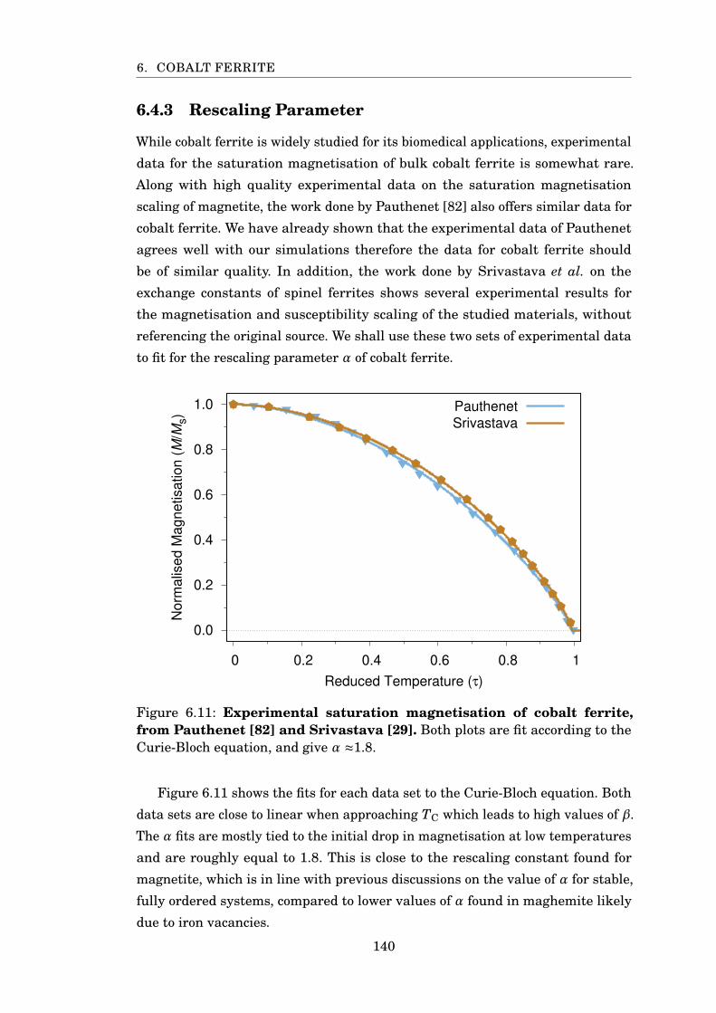
6. COBALT FERRITE
6.4.3 Rescaling Parameter
While cobalt ferrite is widely studied for its biomedical applications, experimental
data for the saturation magnetisation of bulk cobalt ferrite is somewhat rare.
Along with high quality experimental data on the saturation magnetisation
scaling of magnetite, the work done by Pauthenet [82] also offers similar data for
cobalt ferrite. We have already shown that the experimental data of Pauthenet
agrees well with our simulations therefore the data for cobalt ferrite should
be of similar quality. In addition, the work done by Srivastava et al. on the
exchange constants of spinel ferrites shows several experimental results for
the magnetisation and susceptibility scaling of the studied materials, without
referencing the original source. We shall use these two sets of experimental data
to fit for the rescaling parameter α of cobalt ferrite.
0.0
0.2
0.4
0.6
0.8
1.0
0 0.2 0.4 0.6 0.8 1
Norm
alis
ed M
agnetisation (
M/M
s)
Reduced Temperature (τ)
Pauthenet
Srivastava
Figure 6.11: Experimental saturation magnetisation of cobalt ferrite,from Pauthenet [82] and Srivastava [29]. Both plots are fit according to theCurie-Bloch equation, and give α ≈1.8.
Figure 6.11 shows the fits for each data set to the Curie-Bloch equation. Both
data sets are close to linear when approaching TC which leads to high values of β.
The α fits are mostly tied to the initial drop in magnetisation at low temperatures
and are roughly equal to 1.8. This is close to the rescaling constant found for
magnetite, which is in line with previous discussions on the value of α for stable,
fully ordered systems, compared to lower values of α found in maghemite likely
due to iron vacancies.
140
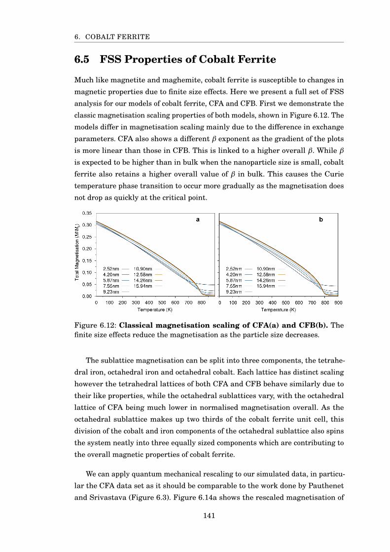
6. COBALT FERRITE
6.5 FSS Properties of Cobalt Ferrite
Much like magnetite and maghemite, cobalt ferrite is susceptible to changes in
magnetic properties due to finite size effects. Here we present a full set of FSS
analysis for our models of cobalt ferrite, CFA and CFB. First we demonstrate the
classic magnetisation scaling properties of both models, shown in Figure 6.12. The
models differ in magnetisation scaling mainly due to the difference in exchange
parameters. CFA also shows a different β exponent as the gradient of the plots
is more linear than those in CFB. This is linked to a higher overall β. While β
is expected to be higher than in bulk when the nanoparticle size is small, cobalt
ferrite also retains a higher overall value of β in bulk. This causes the Curie
temperature phase transition to occur more gradually as the magnetisation does
not drop as quickly at the critical point.
Figure 6.12: Classical magnetisation scaling of CFA(a) and CFB(b). Thefinite size effects reduce the magnetisation as the particle size decreases.
The sublattice magnetisation can be split into three components, the tetrahe-
dral iron, octahedral iron and octahedral cobalt. Each lattice has distinct scaling
however the tetrahedral lattices of both CFA and CFB behave similarly due to
their like properties, while the octahedral sublattices vary, with the octahedral
lattice of CFA being much lower in normalised magnetisation overall. As the
octahedral sublattice makes up two thirds of the cobalt ferrite unit cell, this
division of the cobalt and iron components of the octahedral sublattice also spins
the system neatly into three equally sized components which are contributing to
the overall magnetic properties of cobalt ferrite.
We can apply quantum mechanical rescaling to our simulated data, in particu-
lar the CFA data set as it should be comparable to the work done by Pauthenet
and Srivastava (Figure 6.3). Figure 6.14a shows the rescaled magnetisation of
141
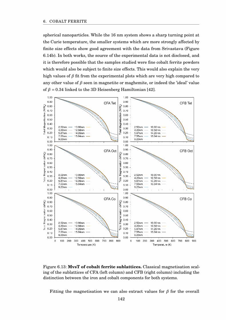
6. COBALT FERRITE
spherical nanoparticles. While the 16 nm system shows a sharp turning point at
the Curie temperature, the smaller systems which are more strongly affected by
finite size effects show good agreement with the data from Srivastava (Figure
6.14b). In both works, the source of the experimental data is not disclosed, and
it is therefore possible that the samples studied were fine cobalt ferrite powders
which would also be subject to finite size effects. This would also explain the very
high values of β fit from the experimental plots which are very high compared to
any other value of β seen in magnetite or maghemite, or indeed the ’ideal’ value
of β = 0.34 linked to the 3D Heisenberg Hamiltonian [42].
Figure 6.13: MvsT of cobalt ferrite sublattices. Classical magnetisation scal-ing of the sublattices of CFA (left column) and CFB (right column) including thedistinction between the iron and cobalt components for both systems.
Fitting the magnetisation we can also extract values for β for the overall
142
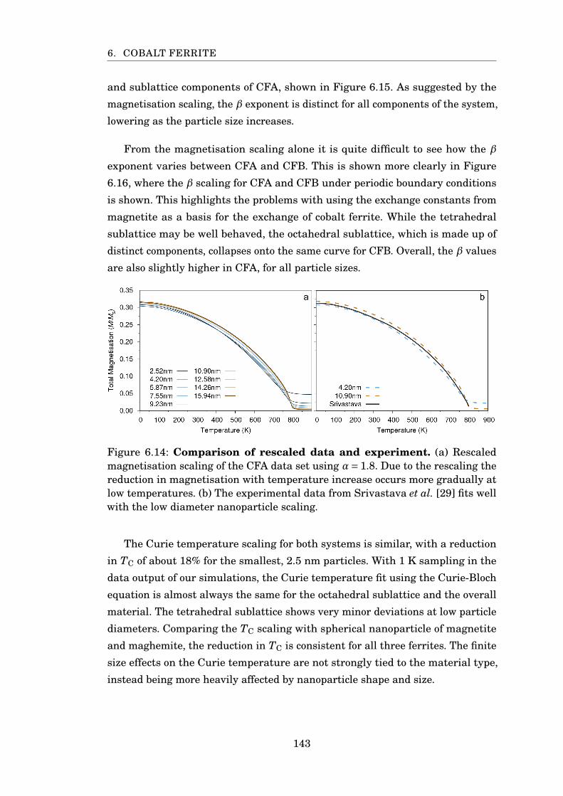
6. COBALT FERRITE
and sublattice components of CFA, shown in Figure 6.15. As suggested by the
magnetisation scaling, the β exponent is distinct for all components of the system,
lowering as the particle size increases.
From the magnetisation scaling alone it is quite difficult to see how the β
exponent varies between CFA and CFB. This is shown more clearly in Figure
6.16, where the β scaling for CFA and CFB under periodic boundary conditions
is shown. This highlights the problems with using the exchange constants from
magnetite as a basis for the exchange of cobalt ferrite. While the tetrahedral
sublattice may be well behaved, the octahedral sublattice, which is made up of
distinct components, collapses onto the same curve for CFB. Overall, the β values
are also slightly higher in CFA, for all particle sizes.
Figure 6.14: Comparison of rescaled data and experiment. (a) Rescaledmagnetisation scaling of the CFA data set using α= 1.8. Due to the rescaling thereduction in magnetisation with temperature increase occurs more gradually atlow temperatures. (b) The experimental data from Srivastava et al. [29] fits wellwith the low diameter nanoparticle scaling.
The Curie temperature scaling for both systems is similar, with a reduction
in TC of about 18% for the smallest, 2.5 nm particles. With 1 K sampling in the
data output of our simulations, the Curie temperature fit using the Curie-Bloch
equation is almost always the same for the octahedral sublattice and the overall
material. The tetrahedral sublattice shows very minor deviations at low particle
diameters. Comparing the TC scaling with spherical nanoparticle of magnetite
and maghemite, the reduction in TC is consistent for all three ferrites. The finite
size effects on the Curie temperature are not strongly tied to the material type,
instead being more heavily affected by nanoparticle shape and size.
143
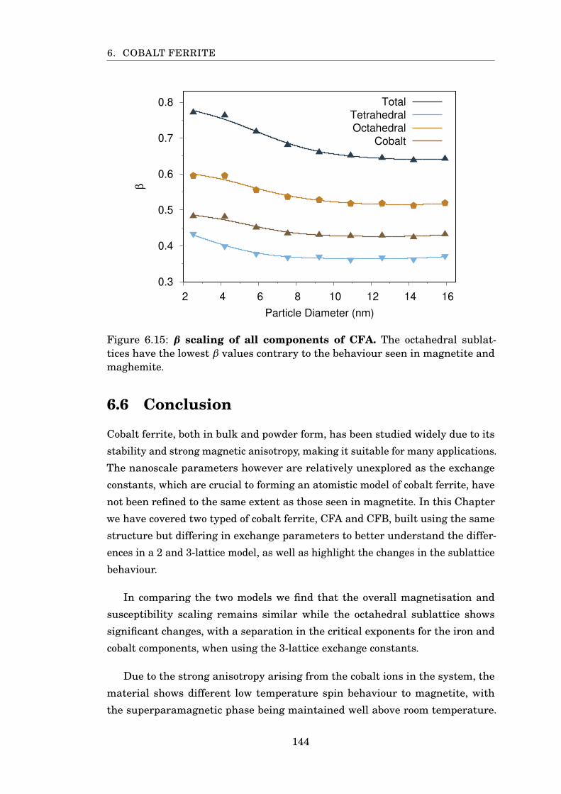
6. COBALT FERRITE
0.3
0.4
0.5
0.6
0.7
0.8
2 4 6 8 10 12 14 16
β
Particle Diameter (nm)
Total
Tetrahedral
Octahedral
Cobalt
Figure 6.15: β scaling of all components of CFA. The octahedral sublat-tices have the lowest β values contrary to the behaviour seen in magnetite andmaghemite.
6.6 Conclusion
Cobalt ferrite, both in bulk and powder form, has been studied widely due to its
stability and strong magnetic anisotropy, making it suitable for many applications.
The nanoscale parameters however are relatively unexplored as the exchange
constants, which are crucial to forming an atomistic model of cobalt ferrite, have
not been refined to the same extent as those seen in magnetite. In this Chapter
we have covered two typed of cobalt ferrite, CFA and CFB, built using the same
structure but differing in exchange parameters to better understand the differ-
ences in a 2 and 3-lattice model, as well as highlight the changes in the sublattice
behaviour.
In comparing the two models we find that the overall magnetisation and
susceptibility scaling remains similar while the octahedral sublattice shows
significant changes, with a separation in the critical exponents for the iron and
cobalt components, when using the 3-lattice exchange constants.
Due to the strong anisotropy arising from the cobalt ions in the system, the
material shows different low temperature spin behaviour to magnetite, with
the superparamagnetic phase being maintained well above room temperature.
144
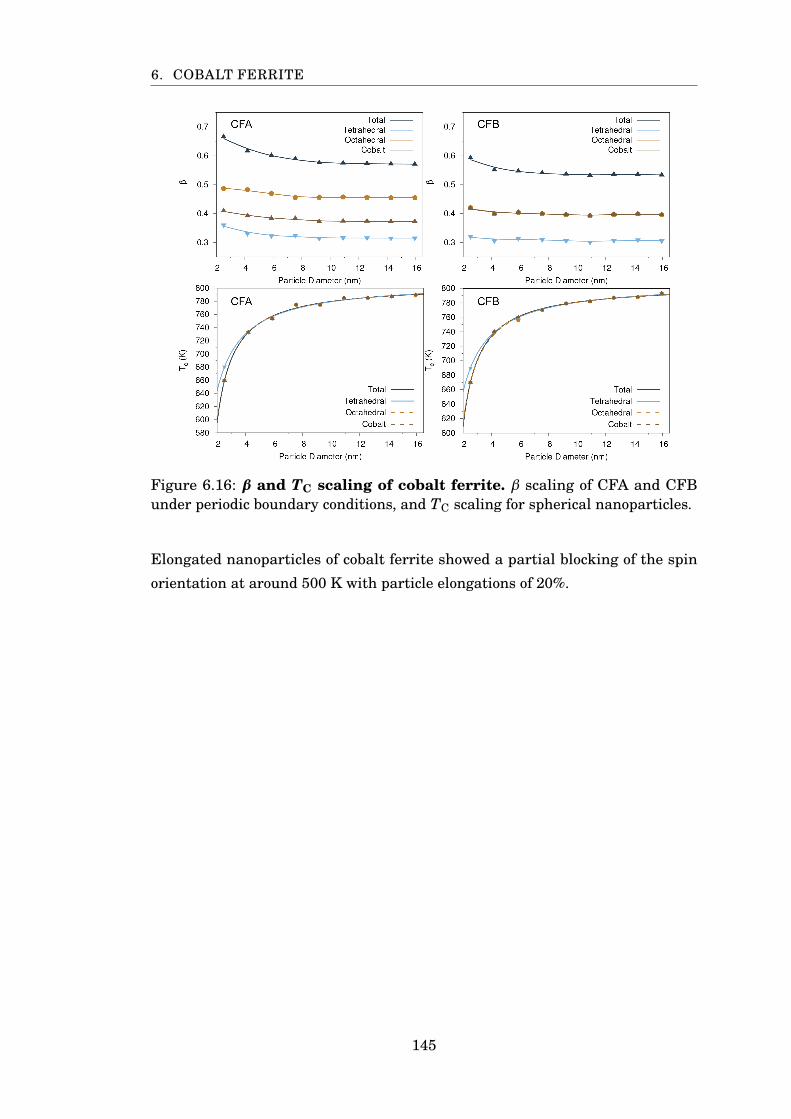
6. COBALT FERRITE
Figure 6.16: β and TC scaling of cobalt ferrite. β scaling of CFA and CFBunder periodic boundary conditions, and TC scaling for spherical nanoparticles.
Elongated nanoparticles of cobalt ferrite showed a partial blocking of the spin
orientation at around 500 K with particle elongations of 20%.
145
CH
AP
TE
R
7CORE-SHELL NANOPARTICLES
7.1 Introduction
In hyperthermia, the heat output of the nanoparticles roughly scales with the
saturation magnetisation of the magnetic material. While iron oxide nanoparticles
tend to be favoured for their biocompatibility and biodegradability, most materials
suffer from lower magnetocrystalline anisotropies leading to lower heat outputs.
Cobalt ferrite helps to alleviate this issue as it exhibits a very high saturation
magnetisation, with the cobalt ions lending a much higher anisotropy to the
system. While nanoparticle properties are typically defined by the size, shape,
surface and material content, one further way in which it is possible to gain
further control over the magnetic properties of a sample is to form core-shell
nanoparticles made up of different materials.
A core-shell nanoparticle is typically composed of two or more materials, one
forming the core at the centre of the nanoparticle, and further materials forming
shells on top of the core. The materials used to form core-shell nanoparticles can
be substantially different in type and use case. In many biomedical applications,
nanoparticles can be coated in organic or silicon based materials either to shield
the magnetic particle from the surrounding environment or to perform additional
functions by attaching hydrophilic/phobic molecules to the particle surface [100,
165].
In addition to shielding, core-shell particles can be used to combine the proper-
ties of similar materials, achieving an intermediate effect between the properties
146
7. CORE-SHELL NANOPARTICLES
of either system. The core diameter then acts as an additional parameter in fine
tuning the relative strengths of the magnetic properties of each material [19].
This applies to the materials we have studied so far. As magnetite, maghemite
and cobalt ferrite share similar structures, all Fd-3m materials with a tetrahedral-
octahedral sublattice composition and similar lattice parameters, these materials
can be mixed to form core-shell nanoparticles with overall properties defined by
the relative amount of materials in each particle.
In addition, maghemite is of particular interest and the shell component of a
core-shell nanoparticle as this material forms naturally over time as a product
of oxidation in small magnetite nanoparticles typically used for their superpara-
magnetic behaviour in hyperthermia applications [166]. When around 10 nm in
diameter, magnetite nanoparticles tend to form thin layers of maghemite which
are typically referred to as magnetic dead layers, heavily reducing the effec-
tiveness of the nanoparticles by decreasing their saturation magnetisation and
anisotropy, as well as slightly modifying the effective size of the nanoparticles
[167, 168]. Due to the similarity in material composition for these particles, it is
also more difficult to identify the core-shell diameters in experiment.
Here we study two different core-shell systems: magnetite-maghemite and
magnetite-cobalt ferrite, to get a better understanding of the change in magnetic
properties of the particles, in particular the magnetisation scaling and the change
to the Curie temperature as a result of the mixing of the materials.
7.2 Structure
The generation of core-shell nanoparticles is done natively in VAMPIRE by specify-
ing the core-shell diameters of the contained materials. While core-shell particles
can be created in various different forms, we shall be simulating the most basic
system with an inner core at the centre of the particle composed of one mate-
rial, surrounded by a continuous shell of the second. Figure 7.1 shows a typical
spherical core-shell nanoparticle with a core diameter roughly half that of the
whole particle. As we are dealing with spherical systems, the diameter of the core
and shell is not related linearly to the amount of each material contained in the
system. A core with a diameter of half the particle makes up less than 15% of the
material content of the system. As such, particles shall be created based on the
percentage content of each of the materials.
To form epitaxial particles with a single crystal approximation, the lattice
147
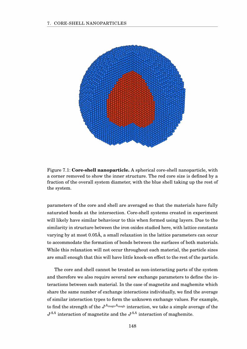
7. CORE-SHELL NANOPARTICLES
Figure 7.1: Core-shell nanoparticle. A spherical core-shell nanoparticle, witha corner removed to show the inner structure. The red core size is defined by afraction of the overall system diameter, with the blue shell taking up the rest ofthe system.
parameters of the core and shell are averaged so that the materials have fully
saturated bonds at the intersection. Core-shell systems created in experiment
will likely have similar behaviour to this when formed using layers. Due to the
similarity in structure between the iron oxides studied here, with lattice constants
varying by at most 0.05Å, a small relaxation in the lattice parameters can occur
to accommodate the formation of bonds between the surfaces of both materials.
While this relaxation will not occur throughout each material, the particle sizes
are small enough that this will have little knock-on effect to the rest of the particle.
The core and shell cannot be treated as non-interacting parts of the system
and therefore we also require several new exchange parameters to define the in-
teractions between each material. In the case of magnetite and maghemite which
share the same number of exchange interactions individually, we find the average
of similar interaction types to form the unknown exchange values. For example,
to find the strength of the JAmagn Amagh interaction, we take a simple average of the
JAA interaction of magnetite and the JAA interaction of maghemite.
148
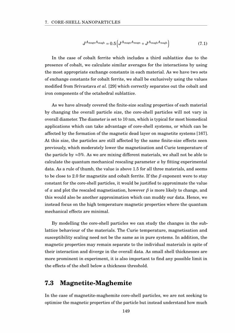
7. CORE-SHELL NANOPARTICLES
JAmagn Amagh = 0.5(JAmagn Amagn + JAmagh Amagh
)(7.1)
In the case of cobalt ferrite which includes a third sublattice due to the
presence of cobalt, we calculate similar averages for the interactions by using
the most appropriate exchange constants in each material. As we have two sets
of exchange constants for cobalt ferrite, we shall be exclusively using the values
modified from Srivastava et al. [29] which correctly separates out the cobalt and
iron components of the octahedral sublattice.
As we have already covered the finite-size scaling properties of each material
by changing the overall particle size, the core-shell particles will not vary in
overall diameter. The diameter is set to 10 nm, which is typical for most biomedical
applications which can take advantage of core-shell systems, or which can be
affected by the formation of the magnetic dead layer on magnetite systems [167].
At this size, the particles are still affected by the same finite-size effects seen
previously, which moderately lower the magnetisation and Curie temperature of
the particle by ≈5%. As we are mixing different materials, we shall not be able to
calculate the quantum mechanical rescaling parameter α by fitting experimental
data. As a rule of thumb, the value is above 1.5 for all three materials, and seems
to be close to 2.0 for magnetite and cobalt ferrite. If the β exponent were to stay
constant for the core-shell particles, it would be justified to approximate the value
of α and plot the rescaled magnetisation, however β is more likely to change, and
this would also be another approximation which can muddy our data. Hence, we
instead focus on the high temperature magnetic properties where the quantum
mechanical effects are minimal.
By modelling the core-shell particles we can study the changes in the sub-
lattice behaviour of the materials. The Curie temperature, magnetisation and
susceptibility scaling need not be the same as in pure systems. In addition, the
magnetic properties may remain separate to the individual materials in spite of
their interaction and diverge in the overall data. As small shell thicknesses are
more prominent in experiment, it is also important to find any possible limit in
the effects of the shell below a thickness threshold.
7.3 Magnetite-Maghemite
In the case of magnetite-maghemite core-shell particles, we are not seeking to
optimise the magnetic properties of the particle but instead understand how much
149
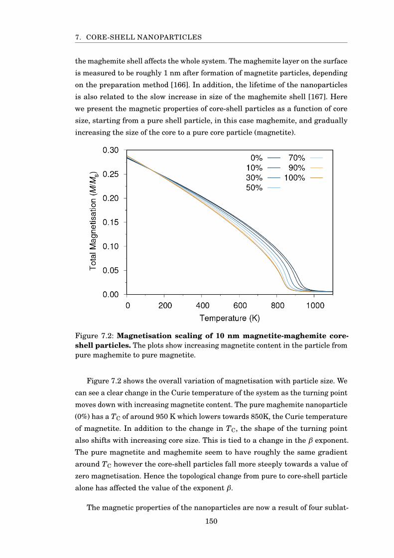
7. CORE-SHELL NANOPARTICLES
the maghemite shell affects the whole system. The maghemite layer on the surface
is measured to be roughly 1 nm after formation of magnetite particles, depending
on the preparation method [166]. In addition, the lifetime of the nanoparticles
is also related to the slow increase in size of the maghemite shell [167]. Here
we present the magnetic properties of core-shell particles as a function of core
size, starting from a pure shell particle, in this case maghemite, and gradually
increasing the size of the core to a pure core particle (magnetite).
Figure 7.2: Magnetisation scaling of 10 nm magnetite-maghemite core-shell particles. The plots show increasing magnetite content in the particle frompure maghemite to pure magnetite.
Figure 7.2 shows the overall variation of magnetisation with particle size. We
can see a clear change in the Curie temperature of the system as the turning point
moves down with increasing magnetite content. The pure maghemite nanoparticle
(0%) has a TC of around 950 K which lowers towards 850K, the Curie temperature
of magnetite. In addition to the change in TC, the shape of the turning point
also shifts with increasing core size. This is tied to a change in the β exponent.
The pure magnetite and maghemite seem to have roughly the same gradient
around TC however the core-shell particles fall more steeply towards a value of
zero magnetisation. Hence the topological change from pure to core-shell particle
alone has affected the value of the exponent β.
The magnetic properties of the nanoparticles are now a result of four sublat-
150
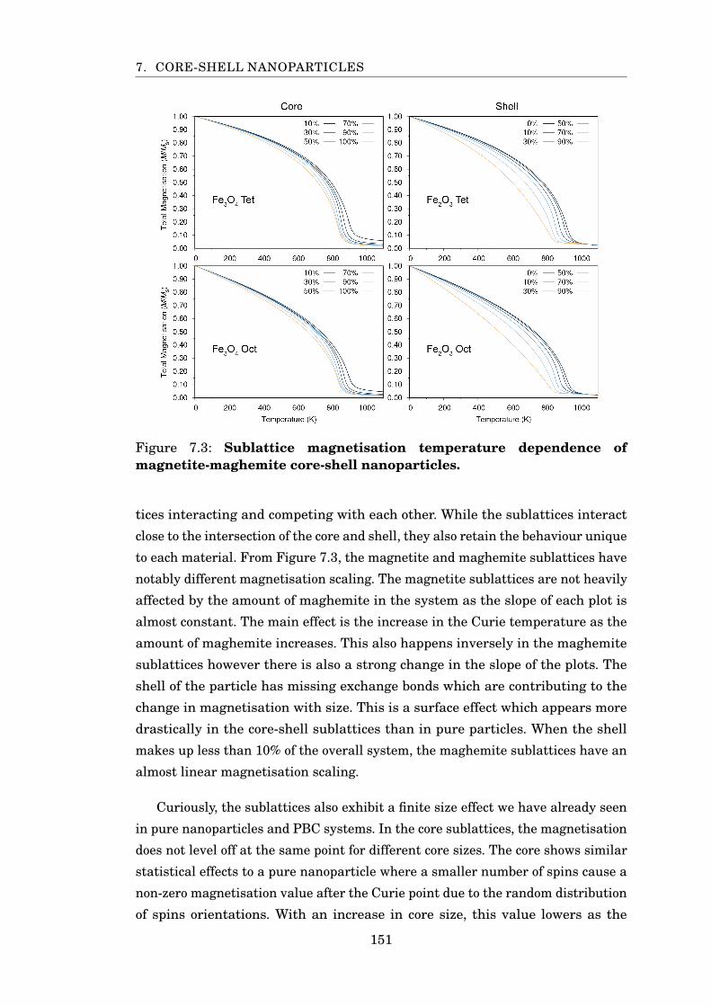
7. CORE-SHELL NANOPARTICLES
Figure 7.3: Sublattice magnetisation temperature dependence ofmagnetite-maghemite core-shell nanoparticles.
tices interacting and competing with each other. While the sublattices interact
close to the intersection of the core and shell, they also retain the behaviour unique
to each material. From Figure 7.3, the magnetite and maghemite sublattices have
notably different magnetisation scaling. The magnetite sublattices are not heavily
affected by the amount of maghemite in the system as the slope of each plot is
almost constant. The main effect is the increase in the Curie temperature as the
amount of maghemite increases. This also happens inversely in the maghemite
sublattices however there is also a strong change in the slope of the plots. The
shell of the particle has missing exchange bonds which are contributing to the
change in magnetisation with size. This is a surface effect which appears more
drastically in the core-shell sublattices than in pure particles. When the shell
makes up less than 10% of the overall system, the maghemite sublattices have an
almost linear magnetisation scaling.
Curiously, the sublattices also exhibit a finite size effect we have already seen
in pure nanoparticles and PBC systems. In the core sublattices, the magnetisation
does not level off at the same point for different core sizes. The core shows similar
statistical effects to a pure nanoparticle where a smaller number of spins cause a
non-zero magnetisation value after the Curie point due to the random distribution
of spins orientations. With an increase in core size, this value lowers as the
151
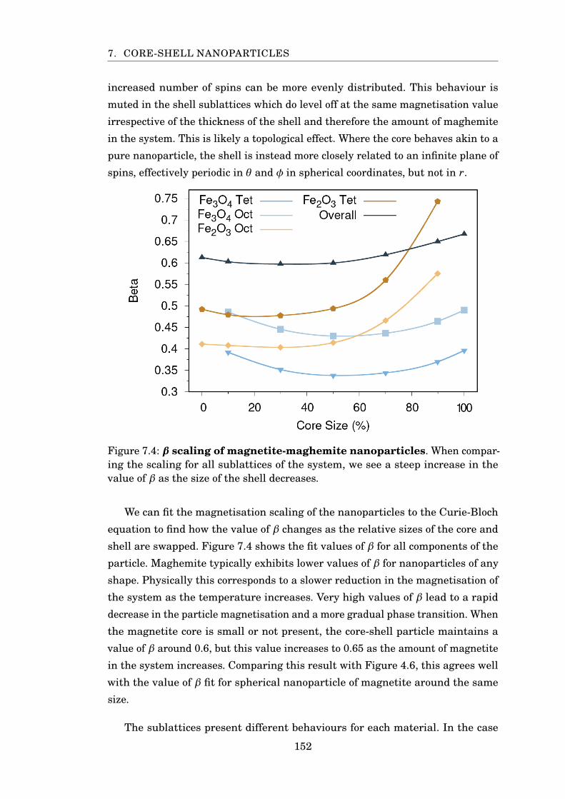
7. CORE-SHELL NANOPARTICLES
increased number of spins can be more evenly distributed. This behaviour is
muted in the shell sublattices which do level off at the same magnetisation value
irrespective of the thickness of the shell and therefore the amount of maghemite
in the system. This is likely a topological effect. Where the core behaves akin to a
pure nanoparticle, the shell is instead more closely related to an infinite plane of
spins, effectively periodic in θ and φ in spherical coordinates, but not in r.
Figure 7.4: β scaling of magnetite-maghemite nanoparticles. When compar-ing the scaling for all sublattices of the system, we see a steep increase in thevalue of β as the size of the shell decreases.
We can fit the magnetisation scaling of the nanoparticles to the Curie-Bloch
equation to find how the value of β changes as the relative sizes of the core and
shell are swapped. Figure 7.4 shows the fit values of β for all components of the
particle. Maghemite typically exhibits lower values of β for nanoparticles of any
shape. Physically this corresponds to a slower reduction in the magnetisation of
the system as the temperature increases. Very high values of β lead to a rapid
decrease in the particle magnetisation and a more gradual phase transition. When
the magnetite core is small or not present, the core-shell particle maintains a
value of β around 0.6, but this value increases to 0.65 as the amount of magnetite
in the system increases. Comparing this result with Figure 4.6, this agrees well
with the value of β fit for spherical nanoparticle of magnetite around the same
size.
The sublattices present different behaviours for each material. In the case
152
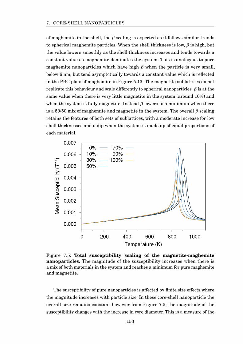
7. CORE-SHELL NANOPARTICLES
of maghemite in the shell, the β scaling is expected as it follows similar trends
to spherical maghemite particles. When the shell thickness is low, β is high, but
the value lowers smoothly as the shell thickness increases and tends towards a
constant value as maghemite dominates the system. This is analogous to pure
maghemite nanoparticles which have high β when the particle is very small,
below 6 nm, but tend asymptotically towards a constant value which is reflected
in the PBC plots of maghemite in Figure 5.13. The magnetite sublattices do not
replicate this behaviour and scale differently to spherical nanoparticles. β is at the
same value when there is very little magnetite in the system (around 10%) and
when the system is fully magnetite. Instead β lowers to a minimum when there
is a 50/50 mix of maghemite and magnetite in the system. The overall β scaling
retains the features of both sets of sublattices, with a moderate increase for low
shell thicknesses and a dip when the system is made up of equal proportions of
each material.
Figure 7.5: Total susceptibility scaling of the magnetite-maghemitenanoparticles. The magnitude of the susceptibility increases when there isa mix of both materials in the system and reaches a minimum for pure maghemiteand magnetite.
The susceptibility of pure nanoparticles is affected by finite size effects where
the magnitude increases with particle size. In these core-shell nanoparticle the
overall size remains constant however from Figure 7.5, the magnitude of the
susceptibility changes with the increase in core diameter. This is a measure of the
153
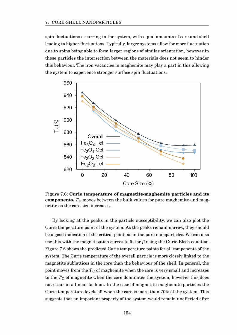
7. CORE-SHELL NANOPARTICLES
spin fluctuations occurring in the system, with equal amounts of core and shell
leading to higher fluctuations. Typically, larger systems allow for more fluctuation
due to spins being able to form larger regions of similar orientation, however in
these particles the intersection between the materials does not seem to hinder
this behaviour. The iron vacancies in maghemite may play a part in this allowing
the system to experience stronger surface spin fluctuations.
Figure 7.6: Curie temperature of magnetite-maghemite particles and itscomponents. TC moves between the bulk values for pure maghemite and mag-netite as the core size increases.
By looking at the peaks in the particle susceptibility, we can also plot the
Curie temperature point of the system. As the peaks remain narrow, they should
be a good indication of the critical point, as in the pure nanoparticles. We can also
use this with the magnetisation curves to fit for β using the Curie-Bloch equation.
Figure 7.6 shows the predicted Curie temperature points for all components of the
system. The Curie temperature of the overall particle is more closely linked to the
magnetite sublattices in the core than the behaviour of the shell. In general, the
point moves from the TC of maghemite when the core is very small and increases
to the TC of magnetite when the core dominates the system, however this does
not occur in a linear fashion. In the case of magnetite-maghemite particles the
Curie temperature levels off when the core is more than 70% of the system. This
suggests that an important property of the system would remain unaffected after
154
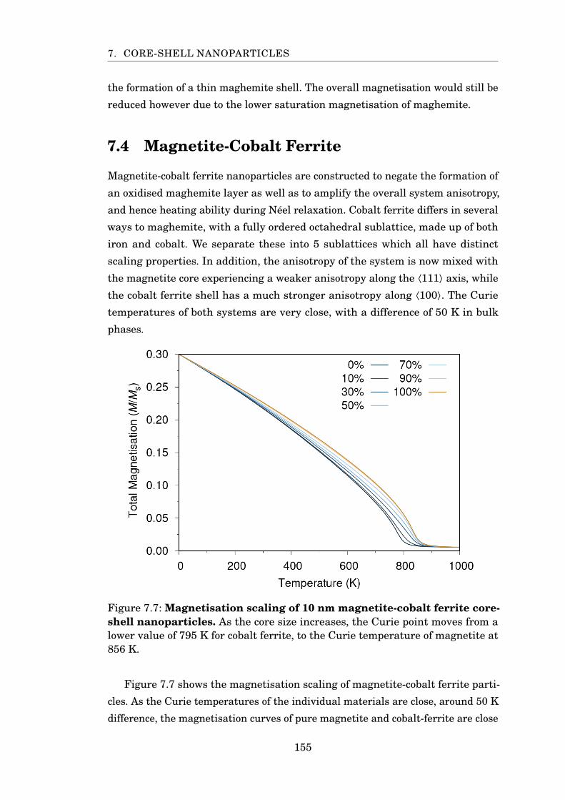
7. CORE-SHELL NANOPARTICLES
the formation of a thin maghemite shell. The overall magnetisation would still be
reduced however due to the lower saturation magnetisation of maghemite.
7.4 Magnetite-Cobalt Ferrite
Magnetite-cobalt ferrite nanoparticles are constructed to negate the formation of
an oxidised maghemite layer as well as to amplify the overall system anisotropy,
and hence heating ability during Néel relaxation. Cobalt ferrite differs in several
ways to maghemite, with a fully ordered octahedral sublattice, made up of both
iron and cobalt. We separate these into 5 sublattices which all have distinct
scaling properties. In addition, the anisotropy of the system is now mixed with
the magnetite core experiencing a weaker anisotropy along the ⟨111⟩ axis, while
the cobalt ferrite shell has a much stronger anisotropy along ⟨100⟩. The Curie
temperatures of both systems are very close, with a difference of 50 K in bulk
phases.
Figure 7.7: Magnetisation scaling of 10 nm magnetite-cobalt ferrite core-shell nanoparticles. As the core size increases, the Curie point moves from alower value of 795 K for cobalt ferrite, to the Curie temperature of magnetite at856 K.
Figure 7.7 shows the magnetisation scaling of magnetite-cobalt ferrite parti-
cles. As the Curie temperatures of the individual materials are close, around 50 K
difference, the magnetisation curves of pure magnetite and cobalt-ferrite are close
155
7. CORE-SHELL NANOPARTICLES
together. To emphasise the change in the shape of the plots, the curves have been
adjusted to start at a magnetisation of 0.3 at 0 K, similar to the magnetisation
curves of bulk magnetite. The raw data is spread out at 0K due to the difference
in structure and magnetic moments between the two materials, making it difficult
to compare the plots. This resembles Figure 4.9, where the magnetisation plots
are spread due to the change in surface composition of the faceted magnetite
nanoparticles. We see that the core-shell particles, which lie in between the pure
cobalt-ferrite and pure magnetite plots, approach the critical point more directly,
making the transition broader. This is linked with an increase in the β scaling for
these systems, which is the opposite behaviour to what was seen in the magnetite-
maghemite particles where all mixed systems had an overall lower value of β and
approached the Curie point more steeply.
The sublattice magnetisation scaling follows similar trends, with the mag-
netite sublattices showing very small deviations from pure magnetite for all core
sizes, while the cobalt ferrite sublattices are more strongly affected by the increas-
ing core. In these sublattices the magnetisation lowers by as much as 10% at room
temperature and up to 20% at higher temperatures when the amount of cobalt
ferrite in the system is decreased and it only forms a thin shell at the surface.
The susceptibility scaling of these nanoparticles (Figure 7.8) shows inverse
behaviour to that in the magnetite-maghemite particles. Here the magnitude of
the susceptibility is lowest when there is an equal proportion of both materials in
the system. Individually, the sublattices have the highest magnitude when their
material content in the particle is highest, which explains the minimum in the
overall plot. Due to the very low values of susceptibility, particularly in the cobalt
ferrite sublattices, it is very difficult to find a value for the Curie temperature
point, as the peak is not easy to isolate. Despite this we can observe general
trends in the scaling of the Curie temperature. From the overall susceptibility,
the Curie temperature moves from around 800K, TC of cobalt-ferrite, to 850K,
TC of magnetite. The Curie temperature is very close to 850 K when there is
more than 70% magnetite in the particle. This follows the same behaviour as the
magnetite-maghemite particles where there was also very little change in TC at
large core sizes. When the core size is small (0-30% particle content), the Curie
temperature changes significantly. It is therefore likely that when using other
magnetic materials, Curie temperature scaling in core-shell nanoparticles follows
the same path regardless of the specific materials. The magnetite sublattices are
not heavily affected by the amount of cobalt ferrite in the system as they do not
peak below 825 K. Conversely the cobalt ferrite is heavily affected by the core as
156
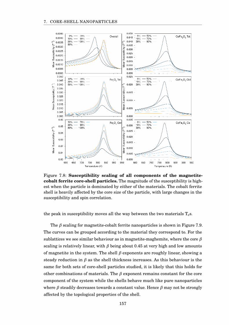
7. CORE-SHELL NANOPARTICLES
Figure 7.8: Susceptibility scaling of all components of the magnetite-cobalt ferrite core-shell particles. The magnitude of the susceptibility is high-est when the particle is dominated by either of the materials. The cobalt ferriteshell is heavily affected by the core size of the particle, with large changes in thesusceptibility and spin correlation.
the peak in susceptibility moves all the way between the two materials Tcs.
The β scaling for magnetite-cobalt ferrite nanoparticles is shown in Figure 7.9.
The curves can be grouped according to the material they correspond to. For the
sublattices we see similar behaviour as in magnetite-maghemite, where the core β
scaling is relatively linear, with β being about 0.45 at very high and low amounts
of magnetite in the system. The shell β exponents are roughly linear, showing a
steady reduction in β as the shell thickness increases. As this behaviour is the
same for both sets of core-shell particles studied, it is likely that this holds for
other combinations of materials. The β exponent remains constant for the core
component of the system while the shells behave much like pure nanoparticles
where β steadily decreases towards a constant value. Hence β may not be strongly
affected by the topological properties of the shell.
157
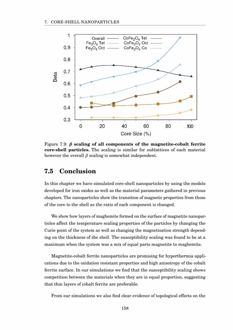
7. CORE-SHELL NANOPARTICLES
Figure 7.9: β scaling of all components of the magnetite-cobalt ferritecore-shell particles. The scaling is similar for sublattices of each materialhowever the overall β scaling is somewhat independent.
7.5 Conclusion
In this chapter we have simulated core-shell nanoparticles by using the models
developed for iron oxides as well as the material parameters gathered in previous
chapters. The nanoparticles show the transition of magnetic properties from those
of the core to the shell as the ratio of each component is changed.
We show how layers of maghemite formed on the surface of magnetite nanopar-
ticles affect the temperature scaling properties of the particles by changing the
Curie point of the system as well as changing the magnetisation strength depend-
ing on the thickness of the shell. The susceptibility scaling was found to be at a
maximum when the system was a mix of equal parts magnetite to maghemite.
Magnetite-cobalt ferrite nanoparticles are promising for hyperthermia appli-
cations due to the oxidation resistant properties and high anisotropy of the cobalt
ferrite surface. In our simulations we find that the susceptibility scaling shows
competition between the materials when they are in equal proportion, suggesting
that thin layers of cobalt ferrite are preferable.
From our simulations we also find clear evidence of topological effects on the
158

7. CORE-SHELL NANOPARTICLES
temperature scaling of the magnetic properties of the nanoparticles. The strength
of the magnetic properties of the core were roughly equal at 70% material content
to 100% leaving room for optimisation in the structure of core-shell systems.
159
CH
AP
TE
R
8CONCLUSIONS
The magnetic properties of iron oxides are affected by topology and scale and
require a better understanding to be used optimally in biomedical and industrial
applications. While these materials share similar traits, small changes in compo-
sition as well as shape and size can be useful in designing nanoparticles fit for
individual uses. In this chapter we summarise the key points of this work which
has explored three such materials: magnetite, maghemite and cobalt ferrite.
In Chapter 3 the foundation for this work is made. A 3D Heisenberg Hamilto-
nian was formulated for spinel iron oxides such as magnetite, which is made up
of the interactions of the tetrahedral and octahedral sublattice interactions of a
ferrimagnetic material. Due to the body of research into the magnetic properties
of magnetite, we can form a precise atomistic model for the material by using sev-
eral parameters including the oxygen positional parameter, cubic anisotropy and
exchange constants. By analysing the data produced by our simulations, we have
devised different methods to extract the critical exponents of the system which are
difficult to fit solely from the magnetisation, but much more clearly shown in the
susceptibility. To remedy the discrepancy between our classical spin model and
the real quantum mechanical effects of spin, we have also used a correcting factor
to rescale our simulations and reintroduce these quantum mechanical effects
into our final data. We find that the temperature dependent magnetisation of
our simulations agrees very well with experiment. In our simulations we find
that the sublattices of magnetite show a noticeable deviation in their fitted mag-
netic properties such as β and TC from that of the overall material. While TC
remains close, β and hence the magnetisation scaling, is markedly different for
160
8. CONCLUSIONS
all components of the system. With increasing temperature, these components
lose their magnetisation at different rates. We distinguish the modes over which
the sublattices interact, with the interaction between closely aligned spins within
their own sublattices, as well as the competition between antiparallel spins in
different sublattices, which shows up in the comparison between the sublattice
susceptibilities compared to those of the overall system.
Chapter 4 shows how the magnetic properties change when a material is in
bulk and nanoparticle form. While we cannot correctly model the strains and
full effects of the surface of nanoparticles, we show that finite size effects in
nanoparticles around 8 nm can lower the system magnetisation by as much
as 15% at room temperature, which is crucial for biomedical applications such
as hyperthermia which require a consistent amount of energy output from the
particles. Ideally, samples of magnetite intended for medicinal use should be
about 10 nm in diameter, as this significantly reduces the finite size effects. As
there is often a spread of radii produced in experimental samples, this suggests
that the average diameter should be closer to 15 nm, to minimise the number
of smaller particles. The Curie temperature of nanoparticles tends toward the
value of bulk as the system size is increased, starting at a much lower value,
reduced by more than 100K, when the particle is less than 4 nm. The strength
of these effects is also tied to the surface to volume ratio of the particle which is
determined by shape. Faceted nanoparticles are hence more susceptible to these
effects for the same number of atoms than spherical particles. As the type of
faceting, the particle shape and surface termination, is strongly dependant on the
experimental methods used to form the particle, this is also crucial in tuning the
properties of the system. At room temperature, elongated particles can also cause
deviation in the expected superparamagnetic behaviour of the system due to an
increased overall anisotropy of the system. The elongation of the particle causes a
shape anisotropy which, while not as strong as surface anisotropy, can cause the
system to become partially blocked for particles with a elongation of 20%.
We then apply the model and methods used to analyse magnetite on the less
well understood maghemite in Chapter 5. With a closely related structure, the
details of the exact structure of maghemite are dependent on several factors and
their study is made more difficult due to the unstable nature of the material
and the ease of contamination with other iron oxides. Due to these gaps in
understanding, some of the parameters for this material are disputed. The nature
of the iron vacancies is found to be regular when it is in nanoparticle form,
leading to a pure Fd-3m spinel structure. To model the exchange between the
161
8. CONCLUSIONS
iron ions in maghemite, we must use exchange constants derived from magnetite
as these have not been derived from first principles for maghemite, partially
due to the uncertainty in the exact structure of the system. We show that it
is very likely that many experimental measurements taken for maghemite are
heavily affected by finite size effects which reduces the magnetisation scaling of
the system, with some samples showing markedly different behaviour possibly
due to sample contamination. The critical exponent β shows much similarity with
that of magnetite, which is expected due to the similarity in structure of these
materials, however in comparison to the ideal value proposed for β in a general
3D Heisenberg model, there is significant deviation. Ferromagnets modelled using
the Heisenberg Hamiltonian are expected to have a β scaling of around 0.34
however our materials show much higher values, at 0.55 and 0.47 for magnetite
and maghemite respectively suggesting that these materials may belong to a
different universality class or that commonly assumed ideal value does not hold
for all materials.
In Chapter 6 we study another related material, cobalt ferrite, which shares
the same structure to magnetite but is often used for its much higher material
anisotropy caused by the cobalt ions in the system. Cobalt ferrite can be difficult to
study due to the variation in magnetic properties dependant on the exact amount
of cobalt in the system. In fact, the structure of cobalt ferrite is dependant also
on its location within each sublattice. The room temperature properties of cobalt
ferrite are well understood with many studies covering the change in anisotropy
strength with temperature. For our modelling however, some components are
less well understood. The strength of interaction between the sublattices of the
material which now contains an additional component due to the inclusion of
cobalt is still being refined. We therefore model two similar systems, one using a
simple 2-lattice model, which approximates the octahedral lattice by combining
the effects of the iron and cobalt contributions, as well as a 3-lattice model which
uses relatively untested exchange constants found in the literature. We find
that the 2-lattice model cannot correctly replicate the magnetic behaviour of the
octahedral sublattices which have significantly different scaling. In comparing
the magnetisation scaling of our simulations with those of experiment we also
find that the experimental data likely does not come from bulk like cobalt ferrite
as it more closely matches the magnetisation scaling of nanoparticles under finite
size effects.
The materials studied so far have been used together in different applications,
sometimes without intent. Magnetite nanoparticles can suffer from the formation
162
8. CONCLUSIONS
of a maghemite surface which creates a magnetic dead layer and changes the
overall magnetic properties, lowering the overall magnetisation. In Chapter 7
we study core-shell nanoparticles, combinations of magnetite-maghemite and
magnetite-cobalt ferrite to understand how the relative sizes of the core and shell
as well as contained materials affects the overall properties of the system. We find
the topological effects create differences in the magnetisation of the core and shell,
with the magnetisation strength of the cores reaching a maximum at around 70%
core size. Depending on the combination of materials, the susceptibility is at a
maximum for a mixing of the materials, in the case of magnetite-maghemite, but
at a minimum at the same point in maghemite-cobalt ferrite, showing a change
in the spin behaviour of each particle.
In conclusion, this is the first comprehensive atomistic investigation into
several iron oxides, simulated with details which are not possible using micro-
magnetic or current ab-initio approaches. The model gives results which match
experimental measurements, and from this more complex structures such as finite
size systems and different core-shell combinations can be studied.
8.1 Further Work
The materials covered in this work have been studied extensively for many years,
however gaps in the current knowledge of their structure and properties at the
nanoscale remain. We have created models using the most up to date information
for each material, in many cases choosing the parameters which best suited our
use cases, however in the case of maghemite and cobalt ferrite, many of the
atomistic parameters have not yet been fully refined. Much of the experimental
data shows symptoms of finite size scaling effects and sample impurities, which
leads to uncertainty in the reference bulk parameters such as the predicted Curie
temperature and exchange parameters.
The exchange parameters in particular are the most important component of
our simulations, forming the majority of the energy contributions to the system.
While we find that the suggested exchange values for magnetite are promising,
work is required to find a more suitable set of parameters for maghemite and
cobalt ferrite, depending on their exact compositions. Density functional theory, or
DFT, is a promising avenue for calculating these parameters however due to the
ab initio nature of the simulations, many more details must be fleshed out to form
a competent model. In addition, DFT does not necessarily lend itself immediately
to magnetic materials and additional approximations and computation is needed
163
8. CONCLUSIONS
to model ferrimagnetic materials which do not have a simple spin structure.
The properties of nanoparticles are strongly tied to the effects of the particle
surface, both in spherical and faceted particles, however we have been unable to
model changes in the surface structure or to choose specific surface configurations
for our study. This is another vast area of study, particularly in the case of
magnetite, which presents several possible surface configurations depending on
the orientation of the surface. An important continuation of this work would be to
study various low energy configurations to better understand their effects. This is
also strongly tied to the magnetocrystalline anisotropy which should also have a
significant contribution from the surface. The superparamagnetic properties of
low temperature iron oxides are strongly bound by the surface anisotropy which
we have been unable to model here.
With the constant improvements to computer hardware, the possible system
sizes which can be studied continues to increase. While today systems of 100 nm
are feasible using the highest end super computers available, many magnetic
phenomena such as spin vortices are only observed at or above this scale [2]
and will become easier to study in the coming years. The detail and accuracy of
atomistic models will be crucial to understanding the complex spin behaviours
occurring in these systems.
164
BIBLIOGRAPHY
[1] SD Oberdick, A Abdelgawad, C Moya, S Mesbahi-Vasey, D Kepaptsoglou,
VK Lazarov, RFL Evans, D Meilak, E Skoropata, J van Lierop, et al. Spin
canting across core/shell Fe3O4/MnxFe3− xO4 nanoparticles. Scientific re-ports, 8(1):1–12, 2018.
[2] D Meilak, S Jenkins, R Pond, and RFL Evans. Massively parallel atomistic
simulation of ultrafast thermal spin dynamics of a permalloy vortex. arXivpreprint arXiv:1908.08885, 2019.
[3] R Moreno, S Poyser, D Meilak, A Meo, S Jenkins, VK Lazarov, G Vallejo-
Fernandez, S Majetich, and RFL Evans. The role of faceting and elongation
on the magnetic anisotropy of magnetite Fe3O4 nanocrystals. Scientificreports, 10(1):1–14, 2020.
[4] W Gilbert. De magnete. Courier Corporation, 1958.
[5] W Heisenberg. Zur theorie des ferromagnetismus. Z. Phys, 49:619, 1928.
[6] L Néel. Propriétés magnétiques des ferrites; ferrimagnétisme et antiferro-
magnétisme. In Annales de physique, volume 12, pages 137–198, 1948.
[7] JL Kirschvink, A Kobayashi-Kirschvink, and BJ Woodford. Magnetite
biomineralization in the human brain. Proceedings of the National Academyof Sciences, 89(16):7683–7687, 1992.
[8] F Ahmad and Y Zhou. Pitfalls and challenges in nanotoxicology: a case of
cobalt ferrite nanocomposites. Chemical research in toxicology, 30(2):492–
507, 2017.
[9] RM Cornell and U Schwertmann. The iron oxides: structure, properties,reactions, occurrences and uses. John Wiley & Sons, 2003.
[10] S Guo, D Li, L Zhang, J Li, and E Wang. Monodisperse mesoporous su-
perparamagnetic single-crystal magnetite nanoparticles for drug delivery.
Biomaterials, 30(10):1881–1889, 2009.
165
BIBLIOGRAPHY
[11] S Chandra, S Mehta, S Nigam, and D Bahadur. Dendritic magnetite
nanocarriers for drug delivery applications. New Journal of Chemistry,
34(4):648–655, 2010.
[12] B Perlstein, Z Ram, D Daniels, A Ocherashvilli, Y Roth, S Margel, and
Y Mardor. Convection-enhanced delivery of maghemite nanoparticles: in-
creased efficacy and MRI monitoring. Neuro-oncology, 10(2):153–161, 2008.
[13] EM Múzquiz-Ramos, V Guerrero-Chávez, BI Macías-Martínez, CM López-
Badillo, and LA García-Cerda. Synthesis and characterization of maghemite
nanoparticles for hyperthermia applications. Ceramics International,41(1):397–402, 2015.
[14] SW Lee, S Bae, Y Takemura, IB Shim, TM Kim, J Kim, HJ Lee, S Zurn,
and CS Kim. Self-heating characteristics of cobalt ferrite nanoparticles for
hyperthermia application. Journal of Magnetism and Magnetic Materials,
310(2):2868–2870, 2007.
[15] RK Gilchrist, R Medal, WD Shorey, RC Hanselman, JC Parrott, and
CB Taylor. Selective inductive heating of lymph nodes. Annals of surgery,
146(4):596, 1957.
[16] J Hu, G Chen, and IMC Lo. Selective removal of heavy metals from indus-
trial wastewater using maghemite nanoparticle: performance and mecha-
nisms. Journal of environmental engineering, 132(7):709–715, 2006.
[17] GS Parkinson. Iron oxide surfaces. Surface Science Reports, 71(1):272–365,
2016.
[18] AV Ramos, JB Moussy, MJ Guittet, AM Bataille, M Gautier-Soyer, M Viret,
C Gatel, P Bayle-Guillemaud, and E Snoeck. Magnetotransport proper-
ties of Fe3O4 epitaxial thin films: thickness effects driven by antiphase
boundaries. Journal of applied physics, 100(10):103902, 2006.
[19] AH Habib, CL Ondeck, P Chaudhary, MR Bockstaller, and ME McHenry.
Evaluation of iron-cobalt/ferrite core-shell nanoparticles for cancer ther-
motherapy. Journal of Applied Physics, 103(7):07A307, 2008.
[20] J Mazo-Zuluaga and J Restrepo. Magnetite thin films: A simulational
approach. Physica B: Condensed Matter, 384(1-2):224–226, 2006.
[21] J Mazo-Zuluaga, J Restrepo, and J Mejía-López. Influence of non-
stoichiometry on the magnetic properties of magnetite nanoparticles. Jour-nal of Physics: Condensed Matter, 20(19):195213, 2008.
166
BIBLIOGRAPHY
[22] E Ising. Beitrag zur theorie des ferromagnetismus. Zeitschrift für Physik,
31(1):253–258, 1925.
[23] MJ Donahue, DG Porter, J Lau, RD McMichael, and MJ Donahue. Intera-
gency report NISTIR 6376. national institute of standards and technology,
gaithersburg. NIST Journal of Research, 114:57–67, 1999.
[24] W Scholz, J Fidler, T Schrefl, D Suess, H Forster, V Tsiantos, et al. Scalable
parallel micromagnetic solvers for magnetic nanostructures. ComputationalMaterials Science, 28(2):366–383, 2003.
[25] D Jiles. Introduction to magnetism and magnetic materials. CRC press,
2015.
[26] NW Ashcroft, ND Mermin, et al. Solid state physics. New York: Holt,
Rinehart and Winston„ 1976.
[27] D Thouless. Magnetism in condensed matter. American Journal of Physics,
71(1):94–94, 2003.
[28] M Uhl and B Siberchicot. A first-principles study of exchange integrals in
magnetite. Journal of Physics: Condensed Matter, 7(22):4227, 1995.
[29] CM Srivastava, G Srinivasan, and NG Nanadikar. Exchange constants in
spinel ferrites. Physical Review B, 19(1):499, 1979.
[30] RFL Evans, WJ Fan, P Chureemart, TA Ostler, MOA Ellis, and
RW Chantrell. Atomistic spin model simulations of magnetic nanoma-
terials. Journal of Physics: Condensed Matter, 26(10):103202, 2014.
[31] LD Landau and EM Lifshitz. To the theory of magnetic permeability
dispersion in ferromagnetic solids. Sov. Phys, 8:153–166, 1935.
[32] TL Gilbert. A lagrangian formulation of the gyromagnetic equation of the
magnetization field. Phys. Rev., 100:1243, 1955.
[33] MOA Ellis, RFL Evans, TA Ostler, J Barker, U Atxitia, O Chubykalo-
Fesenko, and RW Chantrell. The Landau–Lifshitz equation in atomistic
models. Low Temperature Physics, 41(9):705–712, 2015.
[34] W Brown. Thermal fluctuation of fine ferromagnetic particles. IEEETransactions on Magnetics, 15(5):1196–1208, 1979.
167
BIBLIOGRAPHY
[35] DV Berkov and NL Gorn. Thermally activated processes in magnetic
systems consisting of rigid dipoles: equivalence of the Ito and Stratonovich
stochastic calculus. Journal of Physics: Condensed Matter, 14(13):L281,
2002.
[36] E Süli and DF Mayers. An introduction to numerical analysis. Cambridge
university press, 2003.
[37] JL García-Palacios and FJ Lázaro. Langevin-dynamics study of the dynam-
ical properties of small magnetic particles. Physical Review B, 58(22):14937,
1998.
[38] N Metropolis, AW Rosenbluth, MN Rosenbluth, AH Teller, and E Teller.
Equation of state calculations by fast computing machines. The journal ofchemical physics, 21(6):1087–1092, 1953.
[39] D Hinzke and U Nowak. Monte Carlo simulation of magnetization switching
in a Heisenberg model for small ferromagnetic particles. Computer physicscommunications, 121:334–337, 1999.
[40] RFL Evans, U Atxitia, and RW Chantrell. Quantitative simulation of
temperature-dependent magnetization dynamics and equilibrium proper-
ties of elemental ferromagnets. Physical Review B, 91(14):144425, 2015.
[41] RM White. Quantum theory of magnetism, volume 1. Springer, 1983.
[42] M Campostrini, M Hasenbusch, A Pelissetto, P Rossi, and E Vicari. Criti-
cal exponents and equation of state of the three-dimensional Heisenberg
universality class. Physical Review B, 65(14):144520, 2002.
[43] J Crangle. Lix. the magnetic moments of cobalt-copper alloys. The London,Edinburgh, and Dublin Philosophical Magazine and Journal of Science,
46(376):499–513, 1955.
[44] J Crangle and GM Goodman. The magnetization of pure iron and nickel.
Proceedings of the Royal Society of London. A. Mathematical and PhysicalSciences, 321(1547):477–491, 1971.
[45] T Williams, C Kelley, et al. Gnuplot 4.6: an interactive plotting program.
http://gnuplot.sourceforge.net/, April 2013.
[46] A Herraez. Biomolecules in the computer: Jmol to the rescue. Biochemistryand Molecular Biology Education, 34(4):255–261, 2006.
168
BIBLIOGRAPHY
[47] RA Sayle and EJ Milner-White. RASMOL: biomolecular graphics for all.
Trends in biochemical sciences, 20(9):374–376, 1995.
[48] T Plachetka. POV Ray: persistence of vision parallel raytracer. In Proc.of Spring Conf. on Computer Graphics, Budmerice, Slovakia, volume 123,
1998.
[49] S Süsstrunk, R Buckley, and S Swen. Standard RGB color spaces. In Colorand Imaging Conference, pages 127–134. Society for Imaging Science and
Technology, 1999.
[50] P Lennie and M D’Zmura. Mechanisms of color vision. Critical reviews inneurobiology, 3(4):333–400, 1988.
[51] CA Brewer. Color use guidelines for mapping. Visualization in moderncartography, 1994:123–148, 1994.
[52] CA Brewer. Spectral schemes: Controversial color use on maps. Cartographyand Geographic Information Systems, 24(4):203–220, 1997.
[53] P Kovesi. Good colour maps: How to design them. arXiv preprintarXiv:1509.03700, 2015.
[54] P Kovesi. Perceptually uniform colourmaps, 2015.
[55] T Shinjo, T Okuno, R Hassdorf, K Shigeto, and T Ono. Magnetic vortex core
observation in circular dots of permalloy. Science, 289(5481):930–932, 2000.
[56] MATLAB. version 7.10.0 (R2010a). The MathWorks Inc., Natick, Mas-
sachusetts, 2010.
[57] JF Keithley. The story of electrical and magnetic measurements: from 500BC to the 1940s. John Wiley & Sons, 1999.
[58] BD Cullity and CD Graham. Introduction to magnetic materials. John
Wiley & Sons, 2011.
[59] J Katriel and R Pauncz. Theoretical interpretation of Hund’s rule. Advancesin Quantum Chemistry, 10:143–185, 1977.
[60] WH Bragg. The structure of magnetite and the spinels. Nature,
95(2386):561–561, 1915.
[61] EJW Verwey and JH de Boer. Cation arrangement in a few oxides with
crystal structures of the spinel type. Recueil des Travaux Chimiques desPays-Bas, 55(6):531–540, 1936.
169
BIBLIOGRAPHY
[62] ME Fleet. The structure of magnetite. Acta Crystallographica Section B:Structural Crystallography and Crystal Chemistry, 37(4):917–920, 1981.
[63] HSC O’Neill and A Navrotsky. Simple spinels; crystallographic parameters,
cation radii, lattice energies, and cation distribution. American Mineralo-gist, 68(1-2):181–194, 1983.
[64] RD Shannon and CT Prewitt. Effective ionic radii in oxides and fluorides.
Acta Crystallographica Section B: Structural Crystallography and CrystalChemistry, 25(5):925–946, 1969.
[65] RD Shannon. Revised effective ionic radii and systematic studies of in-
teratomic distances in halides and chalcogenides. Acta crystallographicasection A: crystal physics, diffraction, theoretical and general crystallogra-phy, 32(5):751–767, 1976.
[66] EJW Verwey. Electronic conduction of magnetite (Fe3O4) and its transition
point at low temperatures. Nature, 144(3642):327–328, 1939.
[67] F Walz. The Verwey transition-a topical review. Journal of Physics: Con-densed Matter, 14(12):R285, 2002.
[68] K Jordan, A Cazacu, G Manai, SF Ceballos, S Murphy, and IV Shvets.
Scanning tunneling spectroscopy study of the electronic structure of Fe3O4
surfaces. Physical Review B, 74(8):085416, 2006.
[69] D Ihle and B Lorenz. Small-polaron band versus hopping conduction in
Fe3O4. Journal of Physics C: Solid State Physics, 18(21):L647, 1985.
[70] D Ihle and B Lorenz. Small-polaron conduction and short-range order in
Fe3O4. Journal of Physics C: Solid State Physics, 19(26):5239, 1986.
[71] A Yanase and K Siratori. Band structure in the high temperature phase of
Fe3O4. Journal of the Physical Society of Japan, 53(1):312–317, 1984.
[72] A Yanase and N Hamada. Electronic structure in high temperature phase
of Fe3O4. Journal of the Physical Society of Japan, 68(5):1607–1613, 1999.
[73] HT Jeng, GY Guo, and DJ Huang. Charge-orbital ordering in low-
temperature structures of magnetite: GGA+U investigations. PhysicalReview B, 74(19):195115, 2006.
[74] J García and G Subías. The Verwey transition-a new perspective. Journalof Physics: Condensed Matter, 16(7):R145, 2004.
170
BIBLIOGRAPHY
[75] MS Senn, I Loa, JP Wright, and JP Attfield. Electronic orders in the Verwey
structure of magnetite. Physical Review B, 85(12):125119, 2012.
[76] K Abe, Y Miyamoto, and S Chikazumi. Magnetocrystalline anisotropy of
low temperature phase of magnetite. Journal of the Physical Society ofJapan, 41(6):1894–1902, 1976.
[77] Z Kakol and JM Honig. Influence of deviations from ideal stoichiometry
on the anisotropy parameters of magnetite Fe3(1- δ)O4. Physical Review B,
40(13):9090, 1989.
[78] JB Goodenough. Goodenough-kanamori rule. Scholarpedia, 3(10):7382,
2008.
[79] L Néel. Magnetism and local molecular field. Science, 174(4013):985–992,
1971.
[80] ML Glasser and FJ Milford. Spin wave spectra of magnetite. PhysicalReview, 130(5):1783, 1963.
[81] KT Moglestue. Exchange integrals in magnetite. Neutron inelastic scatter-ing, 2:117–122, 1968.
[82] R Pauthenet and L Bochirol. Aimantation spontanée des ferrites. Journalde Physique et le Radium, 12(3):249–251, 1951.
[83] F Bloch. Zur theorie des ferromagnetismus. Zeitschrift für Physik, 61(3-
4):206–219, 1930.
[84] S Chikazumi and CD Graham. Physics of Ferromagnetism 2e. Oxford
University Press on Demand, 2009.
[85] RM Suter and C Hohenemser. Review of measurements of critical exponent
beta in simple magnetic systems. Journal of Applied Physics, 50(B3):1814–
1816, 1979.
[86] AW Sandvik. Critical temperature and the transition from quantum to
classical order parameter fluctuations in the three-dimensional Heisenberg
antiferromagnet. Physical review letters, 80(23):5196, 1998.
[87] MD Kuz’min. Shape of temperature dependence of spontaneous magne-
tization of ferromagnets: quantitative analysis. Physical review letters,
94(10):107204, 2005.
171
BIBLIOGRAPHY
[88] L Greg. Temperature enthaply relationship of 1 mol of water through its
phase changes under constant pressure, 2006.
[89] AR Muxworthy and E McClelland. Review of the low-temperature magnetic
properties of magnetite from a rock magnetic perspective. GeophysicalJournal International, 140(1):101–114, 2000.
[90] KP Belov. Ferrimagnets with a weak magnetic sublattice. Physics-Uspekhi,39(6):623, 1996.
[91] P Asselin, RFL Evans, J Barker, RW Chantrell, R Yanes, O Chubykalo-
Fesenko, D Hinzke, and U Nowak. Constrained monte carlo method and
calculation of the temperature dependence of magnetic anisotropy. PhysicalReview B, 82(5):054415, 2010.
[92] N Akulov. Zur quantentheorie der temperaturabhängigkeit der mag-
netisierungskurve. Zeitschrift für Physik, 100(3-4):197–202, 1936.
[93] HB Callen and E Callen. The present status of the temperature dependence
of magnetocrystalline anisotropy, and the l (l+ 1) 2 power law. Journal ofPhysics and Chemistry of Solids, 27(8):1271–1285, 1966.
[94] DP Landau, HH Lee, and W Kao. Critical behavior of a 3D ising model in a
random field. Journal of Applied Physics, 49(3):1356–1358, 1978.
[95] K Binder. Applications of monte Carlo methods to statistical physics. Re-ports on Progress in Physics, 60(5):487, 1997.
[96] J Wang, F Zhao, W Wu, and G Zhao. Finite-size scaling relation of the curie
temperature in barium hexaferrite platelets. Journal of Applied Physics,
110(12):123909, 2011.
[97] O Hovorka, S Devos, Q Coopman, WJ Fan, CJ Aas, RFL Evans, Xi Chen,
G Ju, and RW Chantrell. The Curie temperature distribution of FePt
granular magnetic recording media. Applied Physics Letters, 101(5):052406,
2012.
[98] J Wang, W Wu, F Zhao, and G Zhao. Curie temperature reduction in
SiO2-coated ultrafine Fe3O4 nanoparticles: quantitative agreement with a
finite-size scaling law. Applied physics letters, 98(8):083107, 2011.
[99] L Zhao, H Zhang, Y Xing, S Song, S Yu, W Shi, X Guo, J Yang, Y Lei, and
F Cao. Morphology-controlled synthesis of magnetites with nanoporous
172
BIBLIOGRAPHY
structures and excellent magnetic properties. Chemistry of Materials,
20(1):198–204, 2008.
[100] QA Pankhurst, J Connolly, SK Jones, and J Dobson. Applications of mag-
netic nanoparticles in biomedicine. Journal of physics D: Applied physics,
36(13):R167, 2003.
[101] R Reznícek, V Chlan, H Štepánková, P Novák, and M Maryško. Magne-
tocrystalline anisotropy of magnetite. Journal of Physics: Condensed Matter,
24(5):055501, 2012.
[102] DA Garanin and H Kachkachi. Surface contribution to the anisotropy of
magnetic nanoparticles. Physical review letters, 90(6):065504, 2003.
[103] P Allia, G Barrera, P Tiberto, T Nardi, Y Leterrier, and M Sangermano.
Fe3O4 nanoparticles and nanocomposites with potential application in
biomedicine and in communication technologies: Nanoparticle aggregation,
interaction, and effective magnetic anisotropy. Journal of Applied Physics,
116(11):113903, 2014.
[104] JMD Coey, IV Shvets, R Wiesendanger, and HJ Güntherodt. Charge freezing
and surface anisotropy on magnetite (100). Journal of applied physics,
73(10):6742–6744, 1993.
[105] G Vallejo-Fernandez and K O’Grady. Effect of the distribution of anisotropy
constants on hysteresis losses for magnetic hyperthermia applications.
Applied Physics Letters, 103(14):142417, 2013.
[106] AG Roca, L Gutiérrez, H Gavilán, MEF Brollo, S Veintemillas-Verdaguer,
and M del Puerto Morales. Design strategies for shape-controlled magnetic
iron oxide nanoparticles. Advanced drug delivery reviews, 138:68–104,
2019.
[107] SK Piotrowski, MF Matty, and SA Majetich. Magnetic fluctuations in
individual superparamagnetic particles. IEEE Transactions on Magnetics,
50(11):1–4, 2014.
[108] EL Schubarth. Lehrbuch der theoretischen Chemie, volume 1. Springer,
1837.
[109] O Baudisch and LA Welo. Hysteresis-messungen als werkzeug zur er-
mittlung der feinstruktur ferromagnetischer verbindungen. Naturwis-senschaften, 14(46):1005–1011, 1926.
173
BIBLIOGRAPHY
[110] H Sachse and R Haase. Die magnetischen umwandlungen des regulären
ferrioxyds. Z. physik. Chem., Abt. A, 148:401–412, 1930.
[111] C Marvin. Magnetic impulse record member, magnetic material, and
method of making magnetic material, 1947. US Patent 2694656A.
[112] S Mornet, F Grasset, J Portier, and E Duguet. Maghemite silica nanoparti-
cles for biological applications, 2002.
[113] M Hua, S Zhang, B Pan, W Zhang, L Lv, and Q Zhang. Heavy metal removal
from water/wastewater by nanosized metal oxides: a review. Journal ofhazardous materials, 211:317–331, 2012.
[114] AF Wells. Structural inorganic chemistry. Oxford university press, 2012.
[115] L Pauling and SB Hendricks. The crystal structures of hematite and
corundum. Journal of the American Chemical Society, 47(3):781–790, 1925.
[116] C Dejoie, P Sciau, W Li, L Noé, A Mehta, K Chen, H Luo, M Kunz, N Tamura,
and Z Liu. Learning from the past: Rare ε-Fe2O3 in the ancient black-glazed
Jian (Tenmoku) wares. Scientific Reports, 4:4941, 2014.
[117] TJ Bastow, A Trinchi, MR Hill, R Harris, and TH Muster. Vacancy ordering
in γ-Fe2O3 nanocrystals observed by 57Fe NMR. Journal of Magnetismand Magnetic Materials, 321(17):2677–2681, 2009.
[118] R Grau-Crespo, AY Al-Baitai, I Saadoune, and NH De Leeuw. Vacancy
ordering and electronic structure of γ-Fe2O3 (maghemite): a theoretical
investigation. Journal of Physics: Condensed Matter, 22(25):255401, 2010.
[119] PB Braun. A superstructure in spinels. Nature, 170(4339):1123–1123,
1952.
[120] JE Jørgensen, L Mosegaard, LE Thomsen, TR Jensen, and JC Hanson.
Formation of γ-Fe2O3 nanoparticles and vacancy ordering: An in situ X-ray
powder diffraction study. Journal of Solid State Chemistry, 180(1):180–185,
2007.
[121] R Haul and T Schoon. Zur struktur des ferromagnetischen eisen (III)-oxyds
γ-Fe2O3. Zeitschrift für physikalische Chemie, 44(1):216–226, 1939.
[122] H Takei and S Chiba. Vacancy ordering in epitaxially-grown single crystals
of γ-Fe2O3. Journal of the Physical Society of Japan, 21(7):1255–1263, 1966.
174
BIBLIOGRAPHY
[123] K Haneda and AH Morrish. Vacancy ordering in γ-Fe2O3 small particles.
Solid State Communications, 22(12):779–782, 1977.
[124] AU Gehring, H Fischer, M Louvel, K Kunze, and PG Weidler. High temper-
ature stability of natural maghemite: a magnetic and spectroscopic study.
Geophysical Journal International, 179(3):1361–1371, 2009.
[125] XM Liu, J Shaw, JZ Jiang, J Bloemendal, P Hesse, T Rolph, and XG Mao.
Analysis on variety and characteristics of maghemite. Science China EarthSciences, 53(8):1153–1162, 2010.
[126] Ö Özdemir. High-temperature hysteresis and thermoremanence of single-
domain maghemite. Physics of the Earth and planetary interiors, 65(1-
2):125–136, 1990.
[127] J Gee and M Nakanishi. Magnetic petrology and magnetic properties of
western pacific guyots: implications for seamount paleopoles. In Proceedingsof the Ocean Drilling Program. Scientific results, volume 144, pages 615–
630, 1995.
[128] V Chevrier, PE Mathé, P Rochette, and HP Gunnlaugsson. Magnetic
study of an antarctic weathering profile on basalt: Implications for recent
weathering on mars. Earth and Planetary Science Letters, 244(3-4):501–514,
2006.
[129] S Krupicka and K Zaveta. Anisotropy, induced anisotropy and related
phenomena, edited by DJ Craik. Magnetic Oxides, pages 235–287, 1975.
[130] J Restrepo, Y Labaye, and JM Greneche. Surface anisotropy in maghemite
nanoparticles. Physica B: Condensed Matter, 384(1-2):221–223, 2006.
[131] H Kachkachi, A Ezzir, M Nogues, and E Tronc. Surface effects in nanopar-
ticles: application to maghemite γ-Fe2O3. The European Physical JournalB, 14(4):681–689, 2000.
[132] RH Kodama, AE Berkowitz, EJ McNiff Jr, and S Foner. Surface spin
disorder in NiFe2O4 nanoparticles. Physical Review Letters, 77(2):394,
1996.
[133] MA Gilleo. Superexchange interaction energy for Fe3+-O2--Fe3+ linkages.
Physical Review, 109(3):777, 1958.
175
BIBLIOGRAPHY
[134] W Wu, XH Xiao, SF Zhang, TC Peng, J Zhou, F Ren, and CZ Jiang. Syn-
thesis and magnetic properties of maghemite (γ-Fe2O3) short-nanotubes.
Nanoscale research letters, 5(9):1474–1479, 2010.
[135] IHM Van Oorschot and MJ Dekkers. Dissolution behaviour of fine-grained
magnetite and maghemite in the citrate–bicarbonate–dithionite extraction
method. Earth and Planetary Science Letters, 167(3-4):283–295, 1999.
[136] S Mo, F Bo, PV Hendriksen, S Linderoth, et al. Spin-glass-like ordering
of the magnetic moments of interacting nanosized maghemite particles.
Physical Review B, 52(1):287, 1995.
[137] SJ Lee, JR Jeong, SC Shin, JC Kim, and JD Kim. Synthesis and char-
acterization of superparamagnetic maghemite nanoparticles prepared by
coprecipitation technique. Journal of Magnetism and Magnetic Materials,
282:147–150, 2004.
[138] VN Nikiforov, AE Goldt, EA Gudilin, VG Sredin, and V Yu Irhin. Magnetic
properties of maghemite nanoparticles. Bulletin of the Russian Academy ofSciences: Physics, 78(10):1075–1080, 2014.
[139] N Mulakaluri and R Pentcheva. Hydrogen adsorption and site-selective
reduction of the Fe3O4 (001) surface: Insights from first principles. TheJournal of Physical Chemistry C, 116(31):16447–16453, 2012.
[140] CHF Peden, GS Herman, IZ Ismagilov, BD Kay, MA Henderson, YJ Kim,
and SA Chambers. Model catalyst studies with single crystals and epitaxial
thin oxide films. Catalysis today, 51(3-4):513–519, 1999.
[141] O Gamba, H Noei, J Pavelec, R Bliem, M Schmid, U Diebold, A Stierle, and
GS Parkinson. Adsorption of formic acid on the Fe3O4 (001) surface. TheJournal of Physical Chemistry C, 119(35):20459–20465, 2015.
[142] Z Li, DV Potapenko, KT Rim, M Flytzani-Stephanopoulos, GW Flynn,
RM Osgood, XD Wen, and ER Batista. Reactions of deuterated methanol
(cd3od) on Fe3O4 (111). The Journal of Physical Chemistry C, 119(2):1113–
1120, 2015.
[143] C Ratnasamy and JP Wagner. Water gas shift catalysis. Catalysis Reviews,
51(3):325–440, 2009.
[144] R Bliem, J van der Hoeven, A Zavodny, O Gamba, J Pavelec, PE de Jongh,
M Schmid, U Diebold, and GS Parkinson. An atomic-scale view of CO
176
BIBLIOGRAPHY
and H2 oxidation on a Pt/Fe3O4 model catalyst. Angewandte Chemie,
127(47):14205–14208, 2015.
[145] GS Parkinson, Z Novotny, G Argentero, M Schmid, J Pavelec, R Kosak,
P Blaha, and U Diebold. Carbon monoxide-induced adatom sintering in a
Pd–Fe3O4 model catalyst. Nature materials, 12(8):724–728, 2013.
[146] DH Zhang, HB Li, GD Li, and JS Chen. Magnetically recyclable ag-ferrite
catalysts: general synthesis and support effects in the epoxidation of styrene.
Dalton Transactions, pages 10527–10533, 2009.
[147] R Bliem, J Pavelec, O Gamba, E McDermott, Z Wang, S Gerhold, M Wagner,
J Osiecki, K Schulte, M Schmid, et al. Adsorption and incorporation of
transition metals at the magnetite Fe3O4 (001) surface. Physical Review B,
92(7):075440, 2015.
[148] P Xue, Z Fu, and Z Yang. The density functional theory studies on the
promoting effect of the Cu-modified Fe3O4 catalysts. Physics Letters A,
379(6):607–612, 2015.
[149] CC Winterbourn. Toxicity of iron and hydrogen peroxide: the Fenton reac-
tion. Toxicology letters, 82:969–974, 1995.
[150] S Amiri and H Shokrollahi. The role of cobalt ferrite magnetic nanoparticles
in medical science. Materials Science and Engineering: C, 33(1):1–8, 2013.
[151] A López-Ortega, E Lottini, CJ Fernandez, and C Sangregorio. Exploring the
magnetic properties of cobalt-ferrite nanoparticles for the development of a
rare-earth-free permanent magnet. Chemistry of Materials, 27(11):4048–
4056, 2015.
[152] P Lavela, GF Ortiz, JL Tirado, E Zhecheva, R Stoyanova, and Sv Ivanova.
High-performance transition metal mixed oxides in conversion electrodes: a
combined spectroscopic and electrochemical study. The Journal of PhysicalChemistry C, 111(38):14238–14246, 2007.
[153] F Rigato, S Piano, M Foerster, F Giubileo, AM Cucolo, and J Fontcuberta.
Andreev reflection in ferrimagnetic CoFe2O4 spin filters. Physical ReviewB, 81(17):174415, 2010.
[154] DH Kim, DE Nikles, DT Johnson, and CS Brazel. Heat generation of aque-
ously dispersed CoFe2O4 nanoparticles as heating agents for magnetically
activated drug delivery and hyperthermia. Journal of Magnetism andMagnetic Materials, 320(19):2390–2396, 2008.
177
BIBLIOGRAPHY
[155] M Pita, JM Abad, C Vaz-Dominguez, C Briones, E Mateo-Martí, JA Martín-
Gago, M del Puerto Morales, and VM Fernández. Synthesis of cobalt ferrite
core/metallic shell nanoparticles for the development of a specific PNA/DNA
biosensor. Journal of colloid and interface science, 321(2):484–492, 2008.
[156] R Gargallo-Caballero, L Martín-García, A Quesada, C Granados-Miralles,
M Foerster, L Aballe, R Bliem, GS Parkinson, P Blaha, JF Marco, et al. Co
on Fe3O4 (001): Towards precise control of surface properties. The Journalof Chemical Physics, 144(9):094704, 2016.
[157] BD Roiter and AE Paladino. Phase equilibria in the ferrite region of the
system FeCoO. Journal of the American Ceramic Society, 45(3):128–133,
1962.
[158] A Franco Jr and FC e Silva. High temperature magnetic properties of cobalt
ferrite nanoparticles. Applied Physics Letters, 96(17):172505, 2010.
[159] H Shenker. Magnetic anisotropy of cobalt ferrite (Co1.01Fe2.00O3.62) and
nickel cobalt ferrite (Ni0.72Fe0.20Co0.08Fe2O4). Physical Review, 107(5):1246,
1957.
[160] M Tachiki. Origin of the magnetic anisotropy energy of cobalt ferrite.
Progress of Theoretical Physics, 23(6):1055–1072, 1960.
[161] S Yoon. Temperature dependence of magnetic anisotropy constant in
CoFe2O4 nanoparticles examined by Mössbauer spectroscopy. HyperfineInteractions, 231(1-3):21–28, 2015.
[162] D Peddis, F Orru, A Ardu, C Cannas, A Musinu, and G Piccaluga. Interpar-
ticle interactions and magnetic anisotropy in cobalt ferrite nanoparticles:
influence of molecular coating. Chemistry of Materials, 24(6):1062–1071,
2012.
[163] SJ Kim, SW Lee, and CS Kim. Mössbauer studies on exchange interactions
in CoFe2O4. Japanese Journal of Applied Physics, 40(8R):4897, 2001.
[164] R Bliem, E McDermott, P Ferstl, M Setvin, O Gamba, J Pavelec, MA Schnei-
der, M Schmid, U Diebold, P Blaha, et al. Subsurface cation vacancy
stabilization of the magnetite (001) surface. Science, 346(6214):1215–1218,
2014.
[165] R Ghosh Chaudhuri and S Paria. Core/shell nanoparticles: classes, proper-
ties, synthesis mechanisms, characterization, and applications. Chemicalreviews, 112(4):2373–2433, 2012.
178
BIBLIOGRAPHY
[166] R Frison, G Cernuto, A Cervellino, O Zaharko, GM Colonna, A Guagliardi,
and N Masciocchi. Magnetite–maghemite nanoparticles in the 5–15 nm
range: Correlating the core–shell composition and the surface structure to
the magnetic properties. a total scattering study. Chemistry of Materials,
25(23):4820–4827, 2013.
[167] SJ Iyengar, M Joy, CK Ghosh, S Dey, RK Kotnala, and S Ghosh. Magnetic, X-
ray and Mössbauer studies on magnetite/maghemite core–shell nanostruc-
tures fabricated through an aqueous route. RSC advances, 4(110):64919–
64929, 2014.
[168] L Signorini, L Pasquini, L Savini, R Carboni, F Boscherini, E Bonetti,
A Giglia, M Pedio, N Mahne, and S Nannarone. Size-dependent oxidation in
iron/iron oxide core-shell nanoparticles. Physical Review B, 68(19):195423,
2003.
179
Copyright © 2022 FDOKUMEN