Channel bifurcation in braided rivers: equilibrium configurations and stability
13
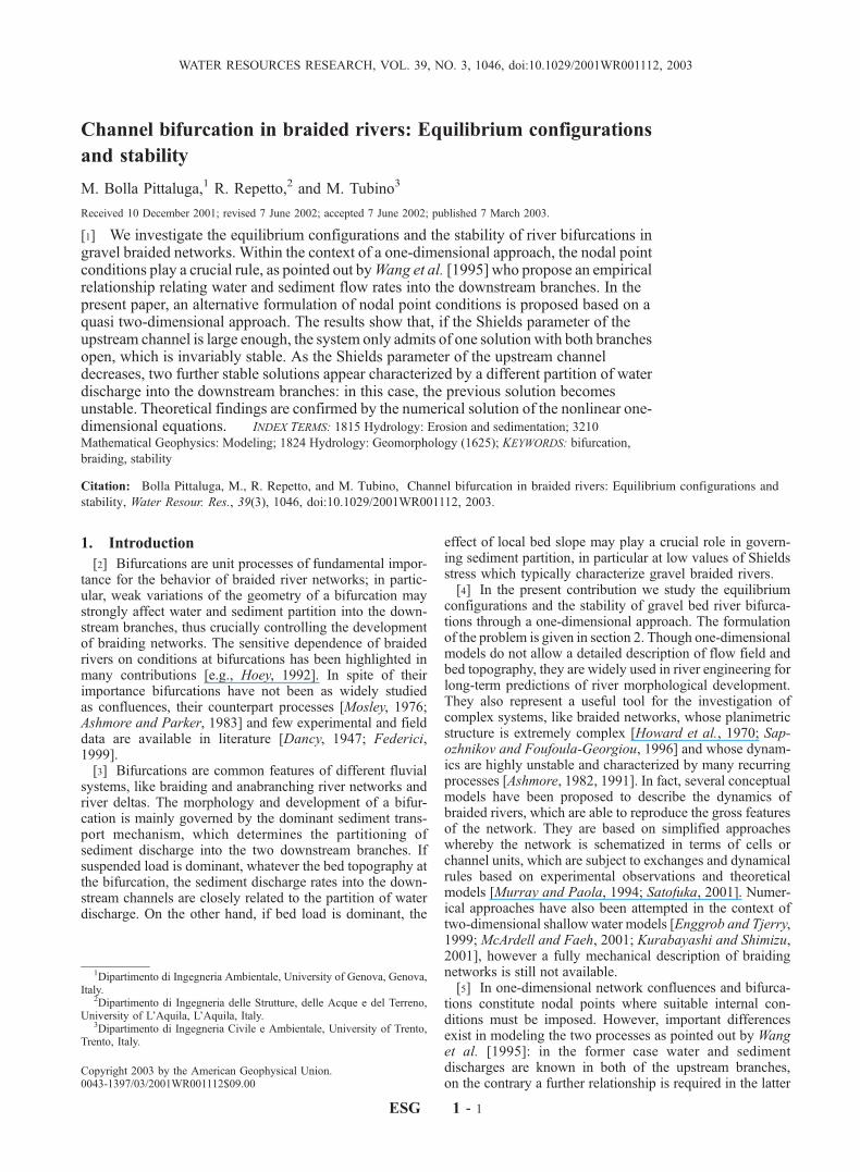
Channel bifurcation in braided rivers: Equilibrium configurations and stability M. Bolla Pittaluga, 1 R. Repetto, 2 and M. Tubino 3 Received 10 December 2001; revised 7 June 2002; accepted 7 June 2002; published 7 March 2003. [1] We investigate the equilibrium configurations and the stability of river bifurcations in gravel braided networks. Within the context of a one-dimensional approach, the nodal point conditions play a crucial rule, as pointed out by Wang et al. [1995] who propose an empirical relationship relating water and sediment flow rates into the downstream branches. In the present paper, an alternative formulation of nodal point conditions is proposed based on a quasi two-dimensional approach. The results show that, if the Shields parameter of the upstream channel is large enough, the system only admits of one solution with both branches open, which is invariably stable. As the Shields parameter of the upstream channel decreases, two further stable solutions appear characterized by a different partition of water discharge into the downstream branches: in this case, the previous solution becomes unstable. Theoretical findings are confirmed by the numerical solution of the nonlinear one- dimensional equations. INDEX TERMS: 1815 Hydrology: Erosion and sedimentation; 3210 Mathematical Geophysics: Modeling; 1824 Hydrology: Geomorphology (1625); KEYWORDS: bifurcation, braiding, stability Citation: Bolla Pittaluga, M., R. Repetto, and M. Tubino, Channel bifurcation in braided rivers: Equilibrium configurations and stability, Water Resour. Res., 39(3), 1046, doi:10.1029/2001WR001112, 2003. 1. Introduction [2] Bifurcations are unit processes of fundamental impor- tance for the behavior of braided river networks; in partic- ular, weak variations of the geometry of a bifurcation may strongly affect water and sediment partition into the down- stream branches, thus crucially controlling the development of braiding networks. The sensitive dependence of braided rivers on conditions at bifurcations has been highlighted in many contributions [e.g., Hoey , 1992]. In spite of their importance bifurcations have not been as widely studied as confluences, their counterpart processes [Mosley , 1976; Ashmore and Parker, 1983] and few experimental and field data are available in literature [Dancy , 1947; Federici, 1999]. [3] Bifurcations are common features of different fluvial systems, like braiding and anabranching river networks and river deltas. The morphology and development of a bifur- cation is mainly governed by the dominant sediment trans- port mechanism, which determines the partitioning of sediment discharge into the two downstream branches. If suspended load is dominant, whatever the bed topography at the bifurcation, the sediment discharge rates into the down- stream channels are closely related to the partition of water discharge. On the other hand, if bed load is dominant, the effect of local bed slope may play a crucial role in govern- ing sediment partition, in particular at low values of Shields stress which typically characterize gravel braided rivers. [4] In the present contribution we study the equilibrium configurations and the stability of gravel bed river bifurca- tions through a one-dimensional approach. The formulation of the problem is given in section 2. Though one-dimensional models do not allow a detailed description of flow field and bed topography, they are widely used in river engineering for long-term predictions of river morphological development. They also represent a useful tool for the investigation of complex systems, like braided networks, whose planimetric structure is extremely complex [Howard et al., 1970; Sap- ozhnikov and Foufoula-Georgiou, 1996] and whose dynam- ics are highly unstable and characterized by many recurring processes [Ashmore, 1982, 1991]. In fact, several conceptual models have been proposed to describe the dynamics of braided rivers, which are able to reproduce the gross features of the network. They are based on simplified approaches whereby the network is schematized in terms of cells or channel units, which are subject to exchanges and dynamical rules based on experimental observations and theoretical models [Murray and Paola, 1994; Satofuka, 2001]. Numer- ical approaches have also been attempted in the context of two-dimensional shallow water models [Enggrob and Tjerry , 1999; McArdell and Faeh, 2001; Kurabayashi and Shimizu, 2001], however a fully mechanical description of braiding networks is still not available. [5] In one-dimensional network confluences and bifurca- tions constitute nodal points where suitable internal con- ditions must be imposed. However, important differences exist in modeling the two processes as pointed out by Wang et al. [1995]: in the former case water and sediment discharges are known in both of the upstream branches, on the contrary a further relationship is required in the latter 1 Dipartimento di Ingegneria Ambientale, University of Genova, Genova, Italy. 2 Dipartimento di Ingegneria delle Strutture, delle Acque e del Terreno, University of L’Aquila, L’Aquila, Italy. 3 Dipartimento di Ingegneria Civile e Ambientale, University of Trento, Trento, Italy. Copyright 2003 by the American Geophysical Union. 0043-1397/03/2001WR001112$09.00 ESG 1 - 1 WATER RESOURCES RESEARCH, VOL. 39, NO. 3, 1046, doi:10.1029/2001WR001112, 2003
-
Upload
independent -
Category
Documents
-
view
1 -
download
0
Transcript of Channel bifurcation in braided rivers: equilibrium configurations and stability
Channel bifurcation in braided rivers: Equilibrium configurations
and stability
M. Bolla Pittaluga,1 R. Repetto,2 and M. Tubino3
Received 10 December 2001; revised 7 June 2002; accepted 7 June 2002; published 7 March 2003.
[1] We investigate the equilibrium configurations and the stability of river bifurcations ingravel braided networks. Within the context of a one-dimensional approach, the nodal pointconditions play a crucial rule, as pointed out byWang et al. [1995] who propose an empiricalrelationship relating water and sediment flow rates into the downstream branches. In thepresent paper, an alternative formulation of nodal point conditions is proposed based on aquasi two-dimensional approach. The results show that, if the Shields parameter of theupstream channel is large enough, the system only admits of one solution with both branchesopen, which is invariably stable. As the Shields parameter of the upstream channeldecreases, two further stable solutions appear characterized by a different partition of waterdischarge into the downstream branches: in this case, the previous solution becomesunstable. Theoretical findings are confirmed by the numerical solution of the nonlinear one-dimensional equations. INDEX TERMS: 1815 Hydrology: Erosion and sedimentation; 3210
Mathematical Geophysics: Modeling; 1824 Hydrology: Geomorphology (1625); KEYWORDS: bifurcation,
braiding, stability
Citation: Bolla Pittaluga, M., R. Repetto, and M. Tubino, Channel bifurcation in braided rivers: Equilibrium configurations and
stability, Water Resour. Res., 39(3), 1046, doi:10.1029/2001WR001112, 2003.
1. Introduction
[2] Bifurcations are unit processes of fundamental impor-tance for the behavior of braided river networks; in partic-ular, weak variations of the geometry of a bifurcation maystrongly affect water and sediment partition into the down-stream branches, thus crucially controlling the developmentof braiding networks. The sensitive dependence of braidedrivers on conditions at bifurcations has been highlighted inmany contributions [e.g., Hoey, 1992]. In spite of theirimportance bifurcations have not been as widely studiedas confluences, their counterpart processes [Mosley, 1976;Ashmore and Parker, 1983] and few experimental and fielddata are available in literature [Dancy, 1947; Federici,1999].[3] Bifurcations are common features of different fluvial
systems, like braiding and anabranching river networks andriver deltas. The morphology and development of a bifur-cation is mainly governed by the dominant sediment trans-port mechanism, which determines the partitioning ofsediment discharge into the two downstream branches. Ifsuspended load is dominant, whatever the bed topography atthe bifurcation, the sediment discharge rates into the down-stream channels are closely related to the partition of waterdischarge. On the other hand, if bed load is dominant, the
effect of local bed slope may play a crucial role in govern-ing sediment partition, in particular at low values of Shieldsstress which typically characterize gravel braided rivers.[4] In the present contribution we study the equilibrium
configurations and the stability of gravel bed river bifurca-tions through a one-dimensional approach. The formulationof the problem is given in section 2. Though one-dimensionalmodels do not allow a detailed description of flow field andbed topography, they are widely used in river engineering forlong-term predictions of river morphological development.They also represent a useful tool for the investigation ofcomplex systems, like braided networks, whose planimetricstructure is extremely complex [Howard et al., 1970; Sap-ozhnikov and Foufoula-Georgiou, 1996] and whose dynam-ics are highly unstable and characterized by many recurringprocesses [Ashmore, 1982, 1991]. In fact, several conceptualmodels have been proposed to describe the dynamics ofbraided rivers, which are able to reproduce the gross featuresof the network. They are based on simplified approacheswhereby the network is schematized in terms of cells orchannel units, which are subject to exchanges and dynamicalrules based on experimental observations and theoreticalmodels [Murray and Paola, 1994; Satofuka, 2001]. Numer-ical approaches have also been attempted in the context oftwo-dimensional shallow water models [Enggrob and Tjerry,1999; McArdell and Faeh, 2001; Kurabayashi and Shimizu,2001], however a fully mechanical description of braidingnetworks is still not available.[5] In one-dimensional network confluences and bifurca-
tions constitute nodal points where suitable internal con-ditions must be imposed. However, important differencesexist in modeling the two processes as pointed out by Wanget al. [1995]: in the former case water and sedimentdischarges are known in both of the upstream branches,on the contrary a further relationship is required in the latter
1Dipartimento di Ingegneria Ambientale, University of Genova, Genova,Italy.
2Dipartimento di Ingegneria delle Strutture, delle Acque e del Terreno,University of L’Aquila, L’Aquila, Italy.
3Dipartimento di Ingegneria Civile e Ambientale, University of Trento,Trento, Italy.
Copyright 2003 by the American Geophysical Union.0043-1397/03/2001WR001112$09.00
ESG 1 - 1
WATER RESOURCES RESEARCH, VOL. 39, NO. 3, 1046, doi:10.1029/2001WR001112, 2003

case, which governs water and sediment distribution in thetwo downstream channels.[6] A first attempt to describe river bifurcations with
movable bed through a one-dimensional model is due toWang et al. [1995] who devoted particular attention to thecase of river deltas; a brief overview of their work isreported in section 3. A further contribution, in the caseof dominant suspended load, is due to Slingerland andSmith [1998] who investigated the conditions leading toavulsion of a meandering river.[7] Wang et al. [1995] introduce an empirical nodal point
condition which relates water and sediment discharges intothe downstream branches. Their analysis suggests that sucha condition plays a crucial role on the long-term evolutionof the system. However, the nodal point condition dependson an empirical parameter which may vary significantlyaccording to the estimates provided by the Authors; hence,the above approach can hardly be applied to predict theevolution of a real bifurcation.[8] In order to overcome this difficulty an alternative
formulation for the nodal point conditions, based on a quasitwo-dimensional approach, is proposed in section 4 of thepresent paper. The equilibrium configurations of a simplechannel loop are theoretically investigated in section 5.Section 6 is devoted to the linear stability analysis of theabove solutions. Moreover theoretical results are comparedwith the full numerical solution of one-dimensional equa-tions in section 7. Finally, section 8 is devoted to someconcluding remarks.
2. Formulation of the Problem
[9] The one-dimensional model is formulated in terms ofthe dependent variables D, H, and Q, namely water depth,free surface level and flow discharge, respectively. In thefollowing we assume a wide rectangular cross section withfixed banks. The above hypothesis may turn out to be notcompletely adequate when applied to self-formed channelswhere channel width may adjust to water discharge. Theflow equations are written in the form
bD;t þ Q;x ¼ 0; ð1aÞ
Q;t þQ2
�
� �;x
þ g�H;x þ g�j ¼ 0; ð1bÞ
where b is channel width, � is the cross-sectional area, g thegravitational acceleration and j = t/(rgD), with t bottomshear stress and r water density. Finally t is time and x thelongitudinal coordinate. Equations (1a) and (1b) are coupledwith the sediment continuity equation which reads
1� pð Þbh;t þ ðbqÞ;x ¼ 0; ð2Þ
with q sediment discharge per unit width, p sedimentporosity and h = H � D bottom elevation. In order tocomplete the mathematical formulation of the problem,closure relationships for j and q are introduced as follows
j ¼ Q2
gC2�2D; q ¼ � J;Jcrð Þ
ffiffiffiffiffiffiffiffiffiffiffiffiffiffiffiffiffiffiffiffirs � rr
gd3s
r; ð3Þ
where � is the dimensionless sediment transport formula,expressed in terms of the local value of Shields parameter
J ¼ rgDjrs � rð Þgds
¼ rQ2
rs � rð ÞgdsC2b2D2; ð4Þ
and of its threshold value for sediment mobilization Jcr.Furthermore, ds and rs represent the mean diameter anddensity of the sediment and C is the Chezy coefficient. Inthe following we evaluate the bed load function � throughthe formula proposed by Meyer-Peter and Muller [1948]which reads
� ¼ 8 J� Jcrð Þ3=2; Jcr ¼ 0:047; ð5Þ
while the friction coefficient C is evaluated in terms of thelocal depth through a standard logarithmic law.[10] The system (1a), (1b), and (2) can be readily written
in the form
bD;t þ Q;x ¼ 0; ð6aÞ
Q;t þ2Q
�Q;x þ g� H;x þ j
� �� Q2
�2bD;x þ Db;x� �
¼ 0; ð6bÞ
1� pð ÞbH;t þ 1� pð ÞQ;x þ bq;J JDD;x þ JQQ;x
� �þ qb;x ¼ 0;
ð6cÞ
where
JQ ¼ @J@Q
����D
; JD ¼ @J@D
����Q
: ð7Þ
The system (6a)–(6c) is hyperbolic and admits of threecharacteristic curves: two of them describe downstreampropagation of information (positive celerity) while the thirdone describes upstream propagation (negative celerity).Hence, in order to determine the solution in each branch it isnecessary to impose, in addition to the initial condition, twoboundary conditions at the channel inlet andone at the channeloutlet. As a consequence five relationships are required at thebifurcation both in the case of subcritical and supercriticalflow, namely one for the outlet of the upstream channel andtwo for the inlet of each of the downstream branches.
3. An Overview of the Model byWang et al. [1995]
[11] In this section we give a brief overview of the workof Wang et al. [1995]. The Authors consider the simplegeometry sketched in Figure 1: channel a bifurcates intotwo symmetrical branches (b and c) which flow into a lake,which imposes a constant water level. All branches haveconstant width and bed slope is constant throughout thenetwork. At the inlet section of channel a water andsediment discharges are prescribed. Wang et al. [1995]propose the following nodal point conditions at thebifurcation:1. water discharge balance
Qa ¼ Qb þ Qc; ð8Þ
ESG 1 - 2 BOLLA PITTALUGA ET AL.: CHANNEL BIFURCATION IN BRAIDED RIVERS

2. sediment discharge balance
Qsa ¼ baqa ¼ bbqb þ bcqc; ð9Þ
3, 4. constancy of water level
Ha ¼ Hb ð10aÞ
Ha ¼ Hc ð10bÞ
where subscripts denote the branch as shown in Figure 1.
5. In addition, the Authors introduce a nodal pointrelationship governing water and sediment partitioning inchannels b and c in the form
bbqb
bcqc¼ Qb
Qc
� �kbb
bc
� �1�k
; k > 0ð Þ: ð11Þ
The reader should note that relationship (11) is empiricaland requires the knowledge of the exponent k. Theempirical estimates provided by the authors, which arebased on measurements in a real bifurcation and in alaboratory flume, are largely different, being equal to 2.2and 6, respectively.[12] The first problem tackled by Wang et al. [1995] is
that of finding the equilibrium configurations of the system.Their analysis shows that the following equilibria arepossible:1. both branches are open;2, 3. one of the two branches is closed and all water and
sediment flow into the other branch.Notice that in the case of a symmetrical bifurcation (constantslope throughout the network and bb = bc) the solution 1implies the same flow conditions in the two branches. Wanget al. [1995] then perform a linear stability analysis of theconfiguration 1 under the hypothesis of uniform flow in the
whole network. Water and sediment discharges areevaluated through the following relationships:
Qi ¼ biCiD3=2i S
1=2i g1=2; ð12aÞ
qi ¼ MQi
biDi
� �n
; ð12bÞ
where Si represents the slope of channel i (b or c) and M is aconstant.[13] The configuration with both branches open is found
to be stable provided k > n/3, with k the exponent of thenodal point relationship (11) and n the exponent appearingin the sediment transport formula (12b). On the other hand,for values of k < n/3, the bifurcation is unstable; this impliesthat the system should develop toward one of the otherequilibrium configurations. It is noted that Wang et al.[1995] use the sediment transport formula proposed byEngelund and Hansen [1967]; hence in their work n is equalto 5. With a different bed load formula the threshold valueof k may be strongly dependent on Shields parameter J, inparticular at relatively small values of J as typically occursin braided rivers.
4. A Physically Based Nodal Point Relationship
[14] The approach by Wang et al. [1995] can hardly beapplied to predict the evolution of a real bifurcation: theparameter k, which is found to govern the systemdevelopment, is unknown and it is neither related to thelocal hydraulic conditions at the nodal point nor to thegeometry of the bifurcation.[15] To overcome the above difficulties an alternative
formulation for the nodal point conditions is proposed herein.At first we note that, in the context of a two-dimensionalmodel, specific nodal point conditions for water and sedimentdischarges division would no longer be required: referring tothe sketch reported in Figure 2a, whatever the computational
Figure 1. Sketch of the geometry considered by Wang et al. [1995].
BOLLA PITTALUGA ET AL.: CHANNEL BIFURCATION IN BRAIDED RIVERS ESG 1 - 3

mesh, the solution is obtained solving the flow equations andsediment continuity equation in each cell with suitableboundary conditions at the channel banks. Also notice thattwo-dimensional effects are mainly felt close to the bifurca-tion where strong deviations from the one-dimensional flowconfiguration and significant transverse bottom gradients arelikely to occur. This suggests that a simplified approach canbe adopted whereby a quasi two-dimensional scheme isintroduced close to the bifurcation (Figure 2b). More pre-cisely we assume that the effect of the bifurcation is feltwithin the final reach of the upstream channel, with lengthequal to aba, which is considered as virtually divided intotwo adjacent cells. Sediment continuity is applied separatelyto each cell. The incoming sediment discharge is assumed tobe uniformly distributed along the upstream section of thereach, i. e. channel a feeds each cell (say cell i) with afraction of the total sediment discharge equal to bi/(bb + bc).Furthermore, the transverse exchange of sediment betweenthe two adjacent cells is taken into account. The soliddischarges leaving both cells feed the two downstreambranches of the network.[16] The longitudinal length aba of the final reach of the
upstream channel, where two-dimensional effects areincluded, should have the same order of magnitude of theupward distance from the nodal point required for the effectsof the bifurcation on bed topography to decay. To determinethe order of magnitude of the parameter a, experiments havebeen carried out in a flume, with a length of 18 m and a widthof 60 cm, in the Laboratory of the Department ofEnvironmental Engineering of Genova University. Thedownstream part of the flume was divided into two partsof equal width, through a longitudinal Plexiglas panel, thussimulating a bifurcation. In Figure 3 the measured bedtopography close to the bifurcation is reported: the localamplitude A1 of the leading transverse mode of the Fourierrepresentation of bed elevation, scaled with its amplitude atthe bifurcation, is plotted versus the upward distance fromthe nodal point s. It appears that the upstream influence ofthe bifurcation almost vanishes at a distance of few channelwidths, say 2–3 times ba, which suggests that a is an order 1parameter. Notice that a further contribution to transversebed deformation in the upstream channel was also due to thepresence of migrating alternate bars. Also notice that onlythe results of experiments in which a significant difference
between bed elevations at the inlets of the two branches wasobserved are reported in Figure 3.[17] In the present model the transverse exchange of
sediments just upstream of the bifurcation is evaluated onthe basis of a well established procedure which has beenwidely adopted to describe two-dimensional bed load trans-port over an inclined bed [Ikeda et al., 1981]. The bed loadvector can be expressed through the relationship
qx; qy� �
¼ �
ffiffiffiffiffiffiffiffiffiffiffiffiffiffiffiffiffiffiffiffirs � rr
gd3s
rcos d; sin dð Þ; ð13Þ
where x and y represent the longitudinal and transversecoordinates, respectively. In the case of mild bed slope andquasi unidirectional flow cos d � 1 and the followingexpression is obtained
qy ¼ qx V U2 þ V 2� ��1=2� rffiffiffi
Jp @h
@y
� ; ð14Þ
where U and V are longitudinal and transverse velocitycomponents, respectively, and the last term accounts for theeffect of gravity related to transverse bed slope @h/@y,which makes particle trajectories deviate with respect tobottom stress direction. The constant r in (14) has beenexperimentally determined and it ranges between 0.3 and 1[e.g., Ikeda et al., 1981; Talmon et al., 1995].[18] According to (13) and (14) the transverse sediment
exchange between the two adjacent cells of the final reachof channel a (see Figure 2) is estimated in our modelthrough the bulk relationship
qy ¼ qaQyDa
QaaDabc
� rffiffiffiffiffiJa
p @h@y
� : ð15Þ
The transverse velocity V has been evaluated as the ratio Qy/(abaDabc), where the transverse flow discharge Qy iscomputed through a mass balance applied to each of thetwo cells
Qy ¼1
2Qb � Qc � Qa
bb � bc
bb þ bc
� �; ð16Þ
Figure 2. Scheme of the nodal point relationship.
ESG 1 - 4 BOLLA PITTALUGA ET AL.: CHANNEL BIFURCATION IN BRAIDED RIVERS

and Dabc is the average depth
Dabc ¼1
2
Db þ Dc
2þ Da
� �: ð17Þ
Furthermore (U2 + V2)�1/2 is estimated as the bulk velocityof the incoming flow and the transverse bed slope @h/@y iscalculated in terms of the difference between bed elevationsat the inlet of channels b and c.[19] In summary, the proposed nodal point conditions at
the bifurcation are the following:1. water discharge balance (8);2, 3. water level constancy (10a) and (10b);4, 5. Exner equation applied to both cells of the final
reach of channel a
1
21� pð Þ dhb
dtþqb � qa
bbbbþbc
�aba
� qy
bb¼ 0; ð18aÞ
1
21� pð Þ dhc
dtþqc � qa
bcbbþbc
�aba
þ qy
bc¼ 0: ð18bÞ
Notice that the resulting scour or deposition dhi/dt isassigned to the inlet section of the downstream branch i.[20] The adoption of (18a) and (18b) implies that sedi-
ment transport balance (9) at the nodal point is no longersatisfied: therefore a discontinuity may be originated in bedelevation at the inlets of channels b and c. This result seemssensible when applied to braided rivers in which strongvariations of bed profile are often encountered close tochannel bifurcations.
[21] It is worth noticing that, in spite of its approximatecharacter, the above formulation seems able to reproducethe main effects on flow and sediment transport induced bya bifurcation. However, several important local effects areneglected, which may be associated with the angle ofbifurcation, the planimetrical development of the branches,the strong three-dimensionality of the flow and the occur-rence of large-scale bar forms in the channel. An example ofan experimental run in which alternate bars formed inchannel a is given in Figure 4. The partition of flow
Figure 3. The amplitude of the first transverse mode of the Fourier representation of measured bedprofile, scaled with its value at the nodal point, is plotted versus the dimensionless upward distance fromthe nodal point s/ba (ba = 0.6 m, ds = 1.2 mm; run 1: Qa = 15.0 l/s, Sa = 0.002; run 2: Qa = 24.9 l/s, Sa =0.002; run 3: Qa = 15.0 l/s, Sa = 0.002). The transverse structure of the first Fourier mode is sketched inthe lower left-hand part of the figure.
Figure 4. The water discharges measured in the twobranches of the experimental flume are plotted versus time.Alternate bars were migrating along channel a.
BOLLA PITTALUGA ET AL.: CHANNEL BIFURCATION IN BRAIDED RIVERS ESG 1 - 5

discharge into the downstream branches displays anoscillating behavior as the result of the local periodicchange of transverse bed slope close to the nodal pointinduced by the migration of alternate bar fronts along theupstream channel.
5. A Simple Channel Loop: EquilibriumConfigurations
[22] In this section we apply the nodal point relationshipsproposed above to study the equilibrium configurations ofthe simple channel loop sketched in Figure 5. At theconfluence point the surface level is assumed to be constant;hence, the geometry considered herein is equivalent to thatanalyzed by Wang et al. [1995] and depicted in Figure 1.[23] We assume given values of water and sediment
discharges (Qa, baqa) in the upstream channel; furthermorethe geometrical characteristics of the network, i. e. channellengths Lb and Lc and channel widths ba, bb, and bc arefixed. As mentioned in section 2, in the present model theadjustment of channel width to discharge is not considered;as a consequence the width of each branch may bearbitrarily given. For the sake of simplicity, most of theresults presented in the following are obtained with bb = bc= ba/2; a different choice will be explicitly specified.[24] In a single channel, uniform flow over a flat bed is
the steady equilibrium solution of the one-dimensionalequations (6a)–(6c), provided the channel has constantwidth and it is transporting sediment. Hence, to find thepossible equilibrium configurations of the loop we assumeuniform flow conditions in channels b and c. Furtherrelationships are given by the nodal point conditions (8),(10a), (10b), (18a), and (18b) where, at the equilibrium, weimpose dhi/dt = 0 (i = b, c). Notice that in the steady caseconsidered herein (18a) and (18b) impose the constancy ofsediment discharge throughout the nodal point, as expressedby (9). In conclusion, we need to solve a nonlinear systemof seven algebraic equations for the unknowns Qb, Qc, Db,Dc, Ha, Hb, and Hc. The solution is found numerically usingthe Newton–Raphson method.[25] Results are discussed in terms of the relevant dimen-
sionless parameters of the uniform flow in the upstreamchannel, for given flow discharge, sediment discharge,channels width and grain size, namely the Shields stressJa, the aspect ratio ba, defined as the half-width to depth
ratio, and the Chezy coefficient Ca. We note that the aboveparameters completely determine in dimensionless form theflow in the upstream channel.[26] At first we note that for all possible geometrical
configurations of the loop and flow conditions in channel a,the system admits of at least two trivial solutions in whicheither channel b or channel c is closed and all water andsediment flow into the other channel.[27] The equilibrium configurations of the single channel
loop sketched in Figure 5 are found to be crucially dependenton the value of Shields stress of the upstream channel Ja.[28] For relatively high values of Shields parameter Ja of
channel a the system only admits of one solution with bothchannels b and c open. In Figure 6 the ratio Qb/Qc betweenthe water discharges in channels b and c, at equilibrium, isplotted versus the ratio between channel lengths Lb/Lc. Inthe same figure the ratio Db/Dc between the water depths isalso reported. Notice that, since the water level at theconfluence point is constant, increasing Lb/Lc is equivalentto decreasing the ratio between the channel slopes Sb/Sc.Figure 6 shows that at equilibrium the ratio Qb/Qc (as wellas Db/Dc) is equal to 1 when the lengths of channels b and care equal (Lb = Lc), which implies that the solution is
Figure 5. Sketch of the channel loop.
Figure 6. The ratios Qb/Qc and Db/Dc between equili-brium values of water discharges and water depths inchannels b and c are plotted versus the ratio betweenchannel lengths Lb/Lc (Ja = 0.3, ba = 8, Ca = 12.5).
ESG 1 - 6 BOLLA PITTALUGA ET AL.: CHANNEL BIFURCATION IN BRAIDED RIVERS
symmetrical: flow conditions are exactly the same in the twobranches of the loop. Increasing Lb/Lc, the ratio Qb/Qc (andconsequently Db/Dc) progressively decreases, such that thewater discharge is lower in channel b where the slope ismilder with respect to channel c.[29] At low values of the Shields parameter Ja, for a
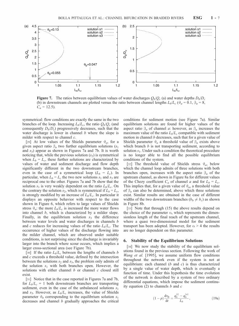
given aspect ratio ba two further equilibrium solutions (s1and s3) appear as shown in Figures 7a and 7b. It is worthnoticing that, while the previous solution (s2) is symmetricalwhen Lb = Lc, these further solutions are characterized byvalues of water and sediment discharge and flow depthsignificantly different in the two downstream branches,even in the case of a symmetrical loop (Lb = Lc). Inparticular, when Lb = Lc the two new solutions s1 and s3 arereciprocal one to the other. Figures 7a and 7b show that thesolution s1 is very weakly dependent on the ratio Lb/Lc. Onthe contrary the solution s2, which is symmetrical if Lb = Lc,is strongly modified by an increase of Lb/Lc. In particular itdisplays an opposite behavior with respect to the caseshown in Figure 6, which refers to large values of Shieldsstress Ja: the more Lb/Lc is increased the more water flowsinto channel b, which is characterized by a milder slope.Finally, in the equilibrium solution s3 the differencebetween water levels and water discharges in channels band c reduces for increasing values of the ratio Lb/Lc. Theoccurrence of higher values of the discharge flowing intothe milder channel, which are observed under suitableconditions, is not surprising since the discharge is invariablylarger into the branch where scour occurs, which implies alarger cross-sectional area (see Figure 7b).[30] If the ratio Lb/Lc between the lengths of channels b
and c exceeds a threshold value, defined by the intersectionbetween the solutions s2 and s3, the problem only admits ofthe solution s1 with both branches open. However, thesolutions with either channel b or channel c closed stillexist.[31] Notice that in the case reported in Figures 7a and 7b,
for Lb/Lc = 1 both downstream branches are transportingsediment, even in the case of the unbalanced solutions s1and s3. However, as Lb/Lc increases, the value of Shieldsparameter Jb corresponding to the equilibrium solution s1decreases and channel b gradually approaches the critical
conditions for sediment motion (see Figure 7a). Similarequilibrium solutions are found for higher values of theaspect ratio ba of channel a: however, as ba increases themaximum value of the ratio Lb/Lc compatible with sedimentmotion in channel b decreases, such that for a given value ofShields parameter Ja a threshold value of ba exists abovewhich branch b is not transporting sediment, according tosolution s1. Under such a condition the theoretical procedureis no longer able to find all the possible equilibriumconditions of the system.[32] The threshold value of Shields stress Ja, below
which the channel loop admits of three solutions with bothbranches open, increases with the aspect ratio ba of theupstream channel, as shown in Figure 8a for different valuesof the Chezy coefficient Ca of channel a and for Lb = Lc.This implies that, for a given value of Ja, a threshold valueof ba can also be determined, above which three solutionsexist. Similar results are obtained in the case of differentwidths of the two downstream branches (bb 6¼ bc) as shownin Figure 8b.[33] Note that through (15) the above results depend on
the choice of the parameter a, which represents the dimen-sionless length of the final reach of the upstream channel,where a quasi two-dimensional model for the sedimenttransport has been adopted. However, for a > 4 the resultsare no longer dependent on this parameter.
6. Stability of the Equilibrium Solutions
[34] We now study the stability of the equilibrium sol-utions found in the previous section. Following the work ofWang et al. [1995], we assume uniform flow conditionsthroughout the network even if the system is not atequilibrium: each channel (b and c) is thus characterizedby a single value of water depth, which is eventually afunction of time. Under this hypothesis the time evolutionof the network is described by a system of two ordinarydifferential equations, which impose the sediment continu-ity equation (2) to channels b and c
1� pð Þ dhbdt
¼q
ið Þb � q
oð Þb
Lb; ð19aÞ
Figure 7. The ratios between equilibrium values of water discharges Qb/Qc (a) and water depths Db/Dc
(b) in downstream channels are plotted versus the ratio between channel lengths Lb/Lc (Ja = 0.1, ba = 8,Ca = 12.5).
BOLLA PITTALUGA ET AL.: CHANNEL BIFURCATION IN BRAIDED RIVERS ESG 1 - 7

1� pð Þ dhcdt
¼ q ið Þc � q oð Þ
c
Lc; ð19bÞ
where qj(i) and qj
(o) represent sediment discharge per unitwidth entering (i) and leaving (o) channel j, respectively.Notice that in the present analysis water level variations intime at the nodal point are accounted for; hence, thederivative dhj/dt appears in (19a) and (19b), instead of dDj/dtas it was proposed by Wang et al. [1995]. The sedimentdischarge leaving each channel is set equal to the transportcapacity of the flow (5) while the incoming solid discharge isdetermined through the nodal point conditions (18a) and(18b). Using (12a) and (5) and the nodal point conditions (8),(10a), (10b), (18a), and (18b), the system (19a) and (19b)can be written in the following form
dDb
dt¼ F 1 Db;Dcð Þ; ð20aÞ
dDc
dt¼ F 2ðDb;DcÞ; ð20bÞ
where the time derivative of the water depth in each branch isa function of the water depths in both channels; atequilibrium we have F 1= F 2 = 0. The eigenvalues of theJacobian associated to system (20a) and (20b) govern thestability of the solution: if both the eigenvalues are negativethe equilibrium configuration is stable; if one of the twoeigenvalues is positive the equilibrium is unstable and thesystem evolves toward another equilibrium solution.[35] We now consider the stability of the equilibrium
solutions of the channel loop sketched in Figure 5, in thecase in which channels b and c have the same width andlength; hence, we assume bb = bc = ba/2 and Lb = Lc.[36] In the previous section we have shown that, provided
the Shields stress Ja in the upstream channel is greater thana threshold value, which depends on the aspect ratio ba andon the Chezy coefficient Ca, the loop only admits of onesolution with both branches open. This solution issymmetrical, i. e. both branches have the same hydraulicconditions: Db = Dc and Qb = Qc. The linear stability
analysis suggests that this solution is invariably stable sinceboth the eigenvalues of the Jacobian are negative. Hence,the loop keeps both branches open in time.[37] At relatively small values of Shields parameter Ja
two further solutions appear (s1 and s3), which arecharacterized by greatly different values of water dischargein the two branches of the loop. Under such conditions thesymmetrical solution (s2) is linearly unstable (one of theeigenvalues of the Jacobian is positive); hence, the thresholdcurve reported in Figure 8 can be thought of as the neutralstability curve for the symmetrical equilibrium configura-tion s2. If the Shields stress Ja falls above the curve thesolution s2 is stable; on the other hand, if Ja falls below themarginal curve the solution s2 is unstable and the systemeither develops toward another equilibrium solution (s1 ors3) or it tends to close one of the two branches of the loop.[38] Furthermore, the theory shows that the unbalanced
equilibrium solutions s1 and s3 are invariably stable.However, it is worth noticing that though mathematicallystable the solutions s1 and s3 may be physically unstable. Infact, as we discussed in the previous section, at relativelylarge values of the aspect ratio ba, sediment transportvanishes either in channel b or in channel c at equilibrium(solutions s1 and s3). Under this condition a smallperturbation of channel geometry at the bifurcation mayeasily cause the system to abandon one of the two branchesleading to its complete closure. Notice, furthermore, that thesolutions with one of the two branches closed are alwaysstable.[39] The above results do not change qualitatively when a
nonsymmetrical loop is considered (Lb 6¼ Lc).[40] The results presented above are summarized in
Figures 9a and 9b. In Figure 9a the ratio Qb/Qc atequilibrium is plotted versus the Shields stress Ja of theupstream channel, for given values of the aspect ratio ba andof Chezy coefficient Ca. Stable and unstable solutions areindicated with continuous and dotted lines, respectively. Atrelatively high values of Ja a single solution is found;decreasing the Shields stress of the upstream channel abifurcation occurs which leads to the generation of two newsolutions (s1 and s3). The figure also shows that theunbalance of water discharges into the downstream
Figure 8. The threshold value of Ja above which the channel loop only admits of one solution withboth branches open and below which three solutions are found is plotted in the plane (ba, Ja) for differentvalues of the Chezy coefficient Ca (a) and for different widths in channels b and c (b) (Ca = 12.5).
ESG 1 - 8 BOLLA PITTALUGA ET AL.: CHANNEL BIFURCATION IN BRAIDED RIVERS

branches associated to the latter solutions occurs graduallyfor decreasing values of Ja, and it grows until the Shieldsstress in one branch reaches the critical value and sedimenttransport vanishes. The figure also shows that when onlyone equilibrium solution exists, such a solution is invariablystable; on the other hand once two further solutions occurthey are invariably stable while the previous solutionbecomes unstable. The bifurcation diagram associated withthe mathematical system (20a) and (20b) is also reported inFigure 9 in terms of the aspect ratio ba of the upstreamchannel.[41] The existence of stable equilibrium solutions charac-
terized by unbalanced values of flow discharge in thedownstream branches is mainly related to the effect oftransverse sediment transport qy, which is accounted forthrough the nodal point conditions (18a) and (18b). In factthe solutions s1 and s3 are characterized by differenttransport capacities in the downstream branches. Equili-brium is achieved when the transverse sediment fluxinduced by transverse bed slope and by flow exchange atthe bifurcation is such to lead each branch to be fed with therequired sediment supply. As a consequence qy plays astabilizing role. In fact if we neglect this contribution andset qy = 0 in (18a) and (18b), the one-dimensional modelinvariably predicts instability of the symmetrical solution s2,for any value of the Shields stress Ja of the upstreamchannel. Furthermore, the unbalanced equilibrium solutionsno longer exist.[42] The linear stability analysis suggests that at low
values of the Shields parameter Ja the symmetrical solutionof the simple loop sketched in Figure 5 is unstable. Thisfinding is, at least qualitatively, confirmed by the experi-mental observations of Federici [1999] who studied thebehavior of simple symmetrical bifurcation shaped into acohesionless bed made of a well sorted sediment with meandiameter equal to 0.5 mm. The geometry of the experi-mental bifurcations was not fixed, contrary to the assump-tion made in our theory, except for the position of the inletand the outlet sections; in particular channel widths werearbitrarily chosen by the system. The bifurcation wasdefined stable if both branches remained open in time and it
was defined unstable when one of the two channels tended tobe closed. The experimental results, summarized in Table 1(J, b, and C represent the Shields stress, the width ratio andthe Chezy parameter at the inlet section, respectively) displaythe same tendency as the theoretical predictions: at highvalues of the Shields stress in the upstream channel thebifurcation always keeps both branches open while, at lowvalues of the Shields parameter, the bifurcation is unstable.
7. The Numerical Model
[43] In this section the theoretical findings discussed insections 5 and 6 are compared with the results of a fullynumerical model. The network is solved following thetechnique introduced by Schaffranek et al. [1981]: at eachtime step the boundary values of the unknown variables,including the internal nodal points, are preliminarycomputed for all the branches of the network; then (6a)–(6c) are solved along each branch, with the given boundaryconditions, using the ‘‘box scheme,’’ originally proposed byPreissmann [1961], whereby time and space derivatives arecomputed as weighted average of finite differences,evaluated in adjacent points along the perimeter of eachcomputational cell.[44] The stability of the equilibrium solutions of the
simple loop sketched in Figure 5 is investigated numericallyby perturbing the initial equilibrium condition with theintroduction of an arbitrarily small sediment bump in oneof the two downstream branches and following the behaviorof the system in time.
Figure 9. Stability diagrams of system (20a) and (20b): the ratio Qb/Qc between water discharges inchannels b and c at equilibrium is plotted versus the Shields stress Ja (a) and the aspect ratio ba (b) ofthe upstream channel. Continuous lines indicate stable solutions; dotted lines indicate unstable solutions.(a) ba = 8, Ca = 12.5; (b) Ja = 0.1, Ca = 12.5.
Table 1. Summary of the Experimental Results of Federici [1999]
J b C
0.06 9.4 10.40 unstable0.07 30.1 9.23 unstable0.09 9.4 10.40 unstable0.09 10.7 10.0 unstable0.12 10.7 10.07 stable0.18 12.5 9.68 stable0.27 30.0 7.95 stable
BOLLA PITTALUGA ET AL.: CHANNEL BIFURCATION IN BRAIDED RIVERS ESG 1 - 9

[45] At first we consider the case of a symmetrical net-work, so that bb = bc = ba/2 and Lb = Lc. The initialcondition is the symmetrical configuration with Qb = Qc andDb = Dc. In Figures 10 and 11 the bottom profile throughoutthe network is plotted at different times, for two differentvalues of the Shields parameter Ja in the upstream channel.The geometrical and hydraulic conditions of channel a arethe same as those adopted to compute the equilibriumconfigurations reported in Figures 6 and 7 (for Lb/Lc = 1).[46] In agreement with the theoretical findings, the
numerical solution predicts the stability of the loop forJa = 0.3, as reported in Figure 10: the sediment bump,introduced in channel c, is progressively damped, hence, aftersome time, deposition occurs along the whole channel c,whose depth slowly decreases in time until the unperturbedinitial configuration is reestablished in the system. Channel bis almost unaffected by the presence of the perturbationinduced in channel c except for a weak erosion process whichcharacterizes the initial stage of the numerical run.[47] In the case of Ja = 0.1 the numerical model predicts
instability of the symmetrical equilibrium configuration inagreement with the theoretical results. The networkdevelopment is shown in Figure 11: the initial transientdoes not differ significantly from the previous stable case;however, deposition in branch c grows in time and
consequently branch b undergoes an erosion process. InFigure 12 the ratio Qb/Qc between the discharges at themiddle point of channels b and c is plotted versus time. Itappears that the loop evolves from the initial symmetricalconfiguration (Qb/Qc = 1) to the unbalanced equilibriumcondition referred to as solution s3 in Figure 7, which is thusstable as predicted by the linear theory. Notice that the loopevolves alternatively toward the solution s1 or s3 dependingon the channel (b or c) in which the perturbation isintroduced.[48] We now finally consider the case of a nonsymmet-
rical loop, with branches characterized by different lengthsand we still assume for simplicity bb = bc = ba/2. Anonsymmetrical loop is equivalent to a system with twobranches with the same length (Lb = Lc) and different waterlevels imposed at the outlet of each channel. The latterprocedure is more efficient numerically since it allows us tofollow the behavior of the system under different geome-trical configurations simply changing the water level at theend of one branch.[49] In Figure 13 examples of numerical runs are
reported: the ratio between the water discharges in channelsb and c is plotted versus time. At the beginning of thesimulations, water level is kept constant at the outlet sectionof each downstream channel; furthermore, the initial
Figure 10. Longitudinal profile of bed elevation under stable conditions (the initial bed slope has beenfiltered out from the results): Da = 1.87 m, Qa = 365 m3/s, ba = 30 m, ds = 0.056 m. The correspondingvalues of the dimensionless parameters of the upstream channel are Ja = 0.3, ba = 8, Ca = 12.5.
ESG 1 - 10 BOLLA PITTALUGA ET AL.: CHANNEL BIFURCATION IN BRAIDED RIVERS

condition is given by the equilibrium configuration s3reported in Figure 7 for Lb/Lc = 1. At a certain time waterlevel is raised in channel b to a prescribed value such thatthe system is equivalent to the case in which the ratio Lb/Lcis equal to 1.05 (continuous line). It appears that the ratiobetween the water discharges Qb/Qc decreases until thenew equilibrium solution is reached (see solution s3 inFigure 7).[50] The dotted line in Figure 13 represents the case in
which water level in channel b is raised to a value whichcorresponds to Lb/Lc = 1.08. According to Figure 7, undersuch a condition, the equilibrium solution s3 does not existanymore: the only possible equilibrium configuration of theloop is given by the solution s1. In agreement withtheoretical results the loop rapidly evolves toward the s1solution, moving from an initial configuration in whichchannel b is fed with more water than channel c to anopposite configuration whereby larger water dischargeoccurs in channel c.
8. Conclusions
[51] The present model, without the claim to describe indetail the flow field and bed topography in channel bifur-cations, is proposed as a useful tool to predict the long-term
evolution of a channel network through a simple one-dimensional approach.[52] The model is based on a nodal point condition,
which allows for the inclusion of two-dimensional effects
Figure 11. Longitudinal profile of bed elevation under unstable conditions (the initial bed slope hasbeen filtered out from the results): Da = 1.87 m, Qa = 211 m3/s, ba = 30 m, ds = 0.056 m. Thecorresponding values of the dimensionless parameters of the upstream channel are Ja = 0.1, ba = 8, Ca =12.5.
Figure 12. The ratio Qb/Qc between water discharges inchannels b and c is plotted versus time (Ja = 0.1, ba = 8,Ca = 12.5).
BOLLA PITTALUGA ET AL.: CHANNEL BIFURCATION IN BRAIDED RIVERS ESG 1 - 11

close to the bifurcation. In the case of a simple channel loopthe model predicts the existence of a threshold value of theShields parameter in the upstream channel above which theloop only admits of one equilibrium solution with bothbranches open; this solution is found to be invariably stable.For values of the Shields parameter below the above thresh-old two further equilibrium configurations appear, which arecharacterized by different values of water discharge flowinginto the two downstream branches. Under these conditionsthe two new solutions are stable while the previous solutionbecomes unstable.[53] Notice that braided gravel rivers are typically char-
acterized by low values of Shields stress, even at highstages. Furthermore, stable, symmetrical bifurcations areseldom observed. Hence, the present model seems toprovide a sound interpretation for one of the leadingmechanisms, which are responsible for the highly unstablecharacter of braided networks.[54] The model also provides useful information on the
physical mechanism that governs the development of abifurcation in gravel braided rivers, in which sedimenttransport mainly occurs as bed load. In particular it isshown that the transverse exchange of sediment, inducedby topographical effects close to the channel division, playsa crucial role on the stability of the bifurcation and allowsthe system to admit of equilibrium configurations charac-terized by different values of flow and sediment dischargesinto the downstream branches. Also notice that the rela-tively small length of each branch in a braided network, dueto the continuous interplay of channels, might suggest thatnonuniform downstream boundary conditions significantlyaffect the development of the network. However, providedthe length of the upstream channel is sufficient to preventchanges of boundary conditions at the inlet, the presentwork suggests that the behavior of a bifurcation is mainlyrelated to the actual hydraulic conditions and geometry atthe nodal point. Under such conditions backwater effectsmay strongly affect the equilibrium configurations but donot influence their stability.[55] Finally, it is worth recalling that several important
local effects have been neglected in the present approach,
such as the planimetrical geometry of the bifurcation, thestrong three-dimensionality of the flow and the occurrenceof large-scale bar forms. In this respect the present modelhas to be considered as a suitable starting point for morerefined analyses, adequately supported by experimental andfield observations.
Notation
b channel widthC Chezy coefficientD water depthds sediment diameterg gravitational accelerationH free surface elevationj t/(rgD)k coefficient of the nodal point relationship by
Wang et al. [1995]L channel lengthn power of the sediment transport law by Wang
et al. [1995]p sediment porosityQ water dischargeQs sediment dischargeQy transverse water dischargeq sediment discharge per unit widthqy transverse sediment discharge per unit widthq(i) sediment discharge per unit width entering the
channelq(o) sediment discharge per unit width leaving the
channelr empirical constant for transverse slope effectS channel slope
U = (U,V ) depth averaged velocity vectort timex longitudinal coordinatey transverse coordinatea dimensionless length of the final reach of
channel ab aspect ratiod deviation between sediment transport and
bottom stress� bed load functionh bed elevation� cross-section areaJ Shields parameter
Jcr critical value of Shields parameter for sedimentmovement
r water densityrs sediment densityt bottom shear stress
[56] Acknowledgments. This work has been developed within theframework of the ‘‘Centro di Eccellenza Universitario per la DifesaIdrogeologica dell’Ambiente Montano-CUDAM’’ and of the project ‘‘Mor-fodinamica delle reti fluviali-COFIN2001’’ cofunded by the Italian Ministryof University and Scientific Research and the University of Trento. Apreliminary version of the present work has been presented at RCEM 2001[Bolla Pittaluga et al., 2001]. The authors thank the anonymous referees fortheir constructive criticism, which contributed to the improvement of themanuscript.
ReferencesAshmore, P. E., Laboratory modeling of gravel bed stream morphology,Earth Surf. Processes Landforms, 7, 201–225, 1982.
Figure 13. The ratio Qb/Qc between water discharges inchannels b and c is plotted versus time. Water level at theoutlet of channel b has been raised to simulate brancheswith different lengths (Ja = 0.1, ba = 8, Ca = 12.5).
ESG 1 - 12 BOLLA PITTALUGA ET AL.: CHANNEL BIFURCATION IN BRAIDED RIVERS

Ashmore, P. E., How do gravel-bed rivers braid?, Can. J. Earth Sci., 28,326–341, 1991.
Ashmore, P. E., and G. Parker, Confluence scour in coarse braided streams,Water Resour. Res., 19, 392–402, 1983.
Bolla Pittaluga, M., R. Repetto, and M. Tubino, Channel bifurcation in one-dimensional models: A physically based nodal point condition, paperpresented at IAHR-RCEM Symposium, Int. Assoc. for Hydraul. Res.,Obihiro, Japan, 2001.
Dancy, A. G., Stream sedimentation in divided channel, M.S. thesis, IowaState Coll., Ames, Iowa, 1947.
Engelund, F., and E. Hansen, A Monograph on Sediment Transport inAlluvial Streams, Danish Tech. Press, Copenhagen, 1967.
Enggrob, H. G., and S. Tjerry, Simulation of morphological characteristicsof a braided river, in IAHR-RCEM Symposium, Genova, Italy, pp. 585–594, 1999.
Federici, B., Osservazioni sperimentali su biforcazioni negli alvei intrecciati(Experimental observations on bifurcations in braided rivers), Masterthesis, Univ. of Genova, Italy (in Italian), 1999.
Hoey, T., Temporal variations in bedload transport rates and sediment sto-rage in gravel-bed rivers, Prog. Phys. Geogr., 16(3), 319–338, 1992.
Howard, A. D., M. E. Keetch, and C. L. Vincent, Topological and geome-trical properties of braided streams, Water Resour. Res., 6, 1674–1688,1970.
Ikeda, S., G. Parker, and K. Sawai, Bend theory of river meanders, part 1,Linear development, J. Fluid Mech., 112, 363–377, 1981.
Kurabayashi, H., and Y. Shimizy, Calculation and visualization of bedconfiguration in braided rivers, in 6th Symposium on Visualization,Corea, Pusan, 2001.
McArdell, B., and R. Faeh, A computational investigation of river braiding,in Gravel Bed Rivers V, edited by M. P. Mosley, pp. 73–94, Hydrol. Soc.,Inc., Wellington, New Zealand, 2001.
Meyer-Peter, E., and R. Muller, Formulas for bedload transport, in III Conf.of Int. Assoc. of Hydraul. Res., Stockholm, Sweden, 1948.
Mosley, M. P., An experimental study of channel confluences, J. Geol.,84(5), 535–562, 1976.
Murray, A. B., and C. Paola, A cellular model of braided rivers, Nature,371, 54–57, 1994.
Preissmann, A., 1st Congres de l’Association Francaise de Calcul, Greno-ble, 1961.
Sapozhnikov, V., and E. Foufoula-Georgiou, Self-affinity in braided rivers,Water Resour. Res., 32, 1429–1439, 1996.
Satofuka, Y., Prediction and mitigation of channel variation in a mountai-nous river, Ph.D. dissertation, Kyoto Univ., Japan (in Japanese), 2001.
Schaffranek, R. W., D. E. Golberg, and R. A. Baltzer, U.S. Geol. Surv. Tech.Water Resour. Invest. Rep., 7(3), 1981.
Slingerland, R., and N. D. Smith, Necessary condition for a meandering-river avulsion, Geology, 26(5), 435–438, 1998.
Talmon, A., M. C. L. M. van Mierlo, and N. Struiksma, Laboratory mea-surements of direction of sediment transport on transverse alluvial-bedslopes, J. Hydraul. Res., 33(4), 519–534, 1995.
Wang, Z. B., R. J. Fokkink, and M. De Vries, Stability of river bifurcationsin 1D morphodynamics models, J. Hydraul. Res., 33(6), 739–750,1995.
����������������������������M. Bolla Pittaluga, Dipartimento di Ingegneria Ambientale, University
of Genova, Genova, Italy.R. Repetto, Dipartimento di Ingegneria delle Strutture, delle Acque e del
Terreno, University of L’Aquila, L’Aquila, Italy. ([email protected])M. Tubino, Dipartimento di Ingegneria Civile e Ambientale, University
of Trento, Trento, Italy.
BOLLA PITTALUGA ET AL.: CHANNEL BIFURCATION IN BRAIDED RIVERS ESG 1 - 13