1

Draft Final

Impact of Reforms in Agricultural Input Markets

on Crop Sector Profitability in Bangladesh

Sajjad Zohir Senior Research Fellow

Bangladesh Institute of Development Studies sajjad@sdnbd.org

January 2001

This research has been sponsored by SAPRI-Bangladesh. The author acknowledges assistance received from Muhammad Yunus, Research Fellow, BIDS

2

Table of Content

Chapter 1 Introduction 1 Chapter 2 Review of Policy Reforms 3 Policy Perspectives in 1982 3 Facts on Government Intervention till 1982 5

Policy Reforms since 1982 7 Chapter 3 Issues and Methods 10 Chapter 4 Changes in Crop Sector Profitability 13

Introduction 13 Changes in the Fertilizer Market 13 Market for Irrigation 17

Relative Prices vs Relative Availability 21 Land Allocation by Crops 23 Intensity in Input Use 24 Crop Sector Profitability – an estimate on changes 26 Impact of Policy Reforms: a quantitative exercise 30 Chapter 5 Beyond Structural Adjustment: policies to address emerging concerns 33 Appendix A Spatial Integration of Farm-level Fertilizer Prices after the SAP (1995-99) 38 Appendix B Statistical Tables 44 Appendix C A Note on the Aggregate Profitability of the Crop Sector 68 Appendix D Equations and Variables for SUR Estimation in Ahmed (2000) 73 References 74

3

Impact of Policy Reforms on Crop Sector Profitability in Bangladesh

Chapter 1

Introduction

After the Independence, most of the organized activities in Bangladesh economy

were owned and operated by the public sector through various public agencies.

Such a state of ownership was partly rooted in the past policy regimes and was

partly a de facto outcome due to absence of the previous entrepreneurs and

institutions. Since the late 1970’s, reforms in the food and agriculture sector were

initiated to gradually limit the space of the public sector. These reforms remained

at sectoral level, until being packaged under the Structural Adjustment Policies

(SAP) during the second half of the 1980’s. While policy reforms continued into

the 1990’s, some of the major reforms in the agricultural input markets came

about in the 1980’s. Two important elements of these reforms were perceived to

include, reduction of subsidy, and increasing the participation of private sector in

the procurement and distribution of inputs. From such perspective, effects of

reforms on the crop sector profitability in general, and farm-level profitability in

particular, were expected to be mixed. Reduction of subsidy was expected to

reduce farmers’ profit (net income) and adversely affect crop sector growth. On

the contrary, increased competition in the input market due to private sector

participation was expected to lower input prices and raise farm-level profitability.

With these a priors, the present study reviews the policy reforms pertaining to the

(chemical) fertilizer and irrigation markets, and provides estimates on changes in

crop sector profitability over the reform period. Strictly speaking, methodological

problems restrict us from establishing causality and from rigorous estimation of

the effect of reforms. Thus, attempts have been made to conjecture on the

effects through association of events and outcomes.

4

The study is based on secondary sources, and therefore, limited by the

availability of data. The Government of Bangladesh (GOB) and the World Bank

(WB) document and research materials have been consulted for reviewing the

policy reforms undertaken during the 1980’s. Published and unpublished data

from (International Fertilizer Development Center - IFDC), as well as published

data from other studies, have been analyzed and used for the present study.

Some of the technical aspects and more rigorous statistical analyses have been

relegated to appendix.

Policy reforms are reviewed in the following chapter, while chapter 3 outlines the

methods and issues dealt with in chapter 4. The latter describes the changes in

the input markets, presents findings on input prices, crop choice and crop sector

profitability. The concluding chapter discusses some of the emerging issues that

may be rooted in the dynamics unleashed by policy reforms.

5

Chapter 2

Review of Policy Reforms

Tracing policy changes with a view to assess their impacts on a sub-sector of an

economy is always difficult. One obvious difficulty is in defining the scope, that is,

in identifying the relevant policy areas. Additional difficulty arises in identifying the

policy instruments, whose changes need to be traced. In assessing changes in

profitability of the crop sector, we conveniently group policies in terms of the area

they are expected to impact upon. The latter may be broadly categorized into

three: domestic output market, input market and trade & exchange rate policies.

Conventional policy types, such as, pricing, fiscal, monetary and institutional

reforms may each have bearings on both output and input markets. While the

present chapter briefly touches upon various policy reforms that had implications

for the input and output markets pertaining to the crop sector in Bangladesh, the

primary focus will be on those addressing the chemical fertilizer and mechanized

irrigation markets. In reviewing the policy reforms, we draw upon various

government and World Bank documents to highlight on how these reforms came

about.

Policy Perspectives in 1982

While policy changes is a continual process, and it is often difficult to draw a

time-line for pre-post comparison, we pick on the 1982 World Bank document

(Bangladesh: Foodgrain Self-Sufficiency and Crop Diversification) to represent

the set of ideas prior to the onset of numerous policy changes during the 1980’s,

in both input and output markets.1 The WB document notes that “Bangladesh’s

agricultural strategy clearly must continue to place strong emphasis on raising

foodgrain production” (p. 2). It also notes that the central thrust of the medium

term food production plan (MTFPP) should be on “the provision of additional

1 Another document consulted in later part of this report is the “Bangladesh Minor Irrigation: A Joint Revie w by Government and the World Bank”, published in December 1992 (GoB 1992).

6

irrigation, drainage and flood control facilities” (p. 4) and “the complementary use

of other modern inputs, such as fertilizers and HYV seeds, must continue to be

increased simultaneously if the full potential of improved water management is to

be realized” (p. 4).

As far back in 1982, there is recognition that GOB had “initiated a policy shift

towards greater reliance on private financial and managerial resources” (p. 5).

The WB document recommends vigorous pursuit of such policy, “particularly in

the areas if minor irrigation and of recurrent input supply and distribution” (p. 5).

More specifically, it mentions of “handing over responsibility for the procurement,

marketing, servicing and management of minor irrigation equipment to the private

sector, direct sale of pumps and tubewells to farmers and cooperatives, phasing

out of seasonal equipment rentals, movement towards full-cost pricing for

agricultural production assets and inputs, and vigorous extension training to

improve farmer ability to extract the full potential from modern inputs” (p. 5). As a

matter of fact, by 1982, the GOB had already taken measures to switch from the

rental programs for minor irrigation equipment to a sales program, and had

decided to subsequently move towards full-cost sales pricing (for STWs and

LLPs).

While continued effort towards reduction of subsidy on fertilizer is noted, the

document had a narrow focus on its distribution. The reason lies in the fact that

by the end of 1982, fertilizer marketing was predominantly in the private sector at

the retail level, and was being “reorganized from a BADC monopoly to extensive

private involvement in wholesale distribution at the thana level” (pp. 28-29). The

report was critical of the practice of officially fixing both wholesale and retail

prices for private dealers, and recommended an interim strategy “to fix the

wholesale price, to ensure adequate supply at the wholesale level, and to allow

market forces and dealer competition to take care of the rest” (p. 29).

7

Two other important inputs in the crop sector production are seeds and

pesticides. Subsidies on pesticides were eliminated in 1980 with the transfer of

responsibility for the import and distribution of this input from the Ministry of

Agriculture to the private sector. Subsidy on seeds continued, and the WB

document of 1982 mentions of a GOB decision to eliminate this subsidy over a

period of three years (from 1982).

Government interventions in the output market, in the forms of procurement and

offtakes at given prices, were generally considered to be in line with what the WB

thought to be appropriate during that period. This is partly reflected in the

following statement made in the report: “In recent years, grain procurement

prices have been set primarily in accordance with considerations of maintaining

producer incentives in the face of rising input costs. The available evidence

suggests that this has been successfully accomplished … . In the medium run,

the present procurement prices should be roughly maintained in real terms

through periodic adjustments necessitated by both domestic inflation and

exchange rate movements.” (pp. 9-10) The WB document is however more

emphatic in the area of public food distribution. It reiterates previous

recommendations to reduce subsidy element in the ration system, direct a

greater proportion of the ration distribution to the poor, and to make use of open

market sales (of government stock) to reduce seasonal and annual market price

fluctuations.

Some Facts on Government Intervention in Input and Output Market till 1982

Input subsidies on fertilizer and irrigation amounted to about 15 percent of GOB’s

tax revenue in FY1981. Subsidy on fertilizer amounted to Tk. 1.2 billion in

FY1981, even though subsidy in unit terms was reduced from 50 percent of

BADC’s cost in FY1979, to 42 percent in FY1980, 32 percent in FY1981, and an

8

estimated 21 percent in FY1982 (WB:1982; 47).2 A rough estimate suggested

that subsidy on minor irrigation (accounting for amortization of equipments)

amounted to Tk. 600 million in FY1982. The major portion of this subsidy was

due to rental of LLP and DTW by the BADC and BWDB at concessional terms.

As of 1982, substantial subsidies continued to be provided for the use of major

irrigation – i.e., of large-scale gravity and canal irrigation schemes. Water

charges assessed for the large-scale irrigation schemes were fairly modest; and

yet, one estimate suggests that only 5.7 percent of these were actually realized

during 1984-91 period.3

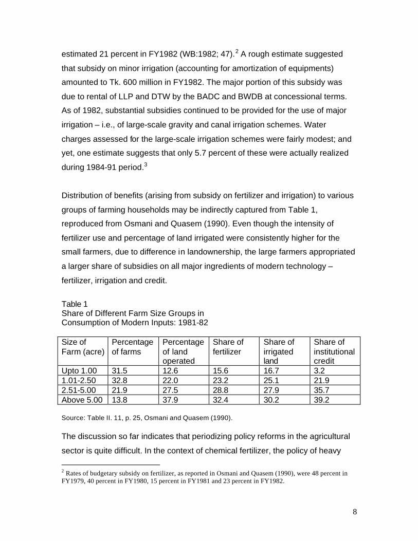
Distribution of benefits (arising from subsidy on fertilizer and irrigation) to various

groups of farming households may be indirectly captured from Table 1,

reproduced from Osmani and Quasem (1990). Even though the intensity of

fertilizer use and percentage of land irrigated were consistently higher for the

small farmers, due to difference in landownership, the large farmers appropriated

a larger share of subsidies on all major ingredients of modern technology –

fertilizer, irrigation and credit.

Table 1 Share of Different Farm Size Groups in Consumption of Modern Inputs: 1981-82 Size of Farm (acre)

Percentage of farms

Percentage of land operated

Share of fertilizer

Share of irrigated land

Share of institutional credit

Upto 1.00 31.5 12.6 15.6 16.7 3.2 1.01-2.50 32.8 22.0 23.2 25.1 21.9 2.51-5.00 21.9 27.5 28.8 27.9 35.7 Above 5.00 13.8 37.9 32.4 30.2 39.2 Source: Table II. 11, p. 25, Osmani and Quasem (1990).

The discussion so far indicates that periodizing policy reforms in the agricultural

sector is quite difficult. In the context of chemical fertilizer, the policy of heavy

2 Rates of budgetary subsidy on fertilizer, as reported in Osmani and Quasem (1990), were 48 percent in FY1979, 40 percent in FY1980, 15 percent in FY1981 and 23 percent in FY1982.

9

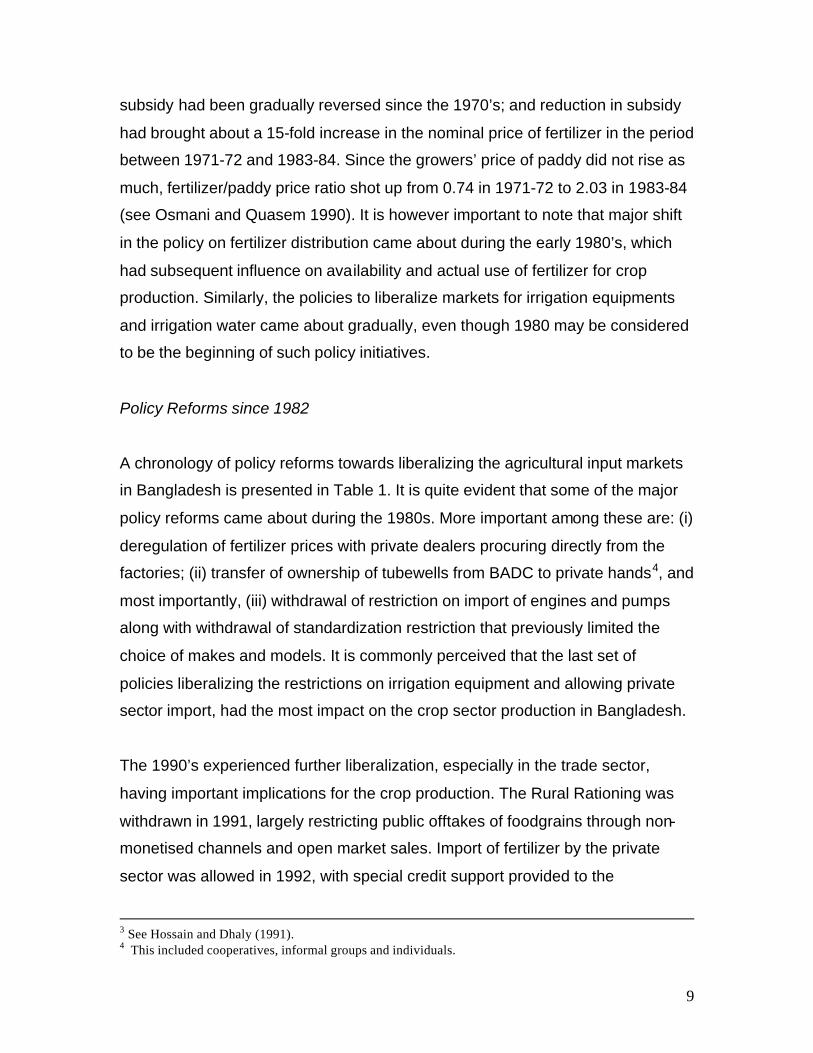
subsidy had been gradually reversed since the 1970’s; and reduction in subsidy

had brought about a 15-fold increase in the nominal price of fertilizer in the period

between 1971-72 and 1983-84. Since the growers’ price of paddy did not rise as

much, fertilizer/paddy price ratio shot up from 0.74 in 1971-72 to 2.03 in 1983-84

(see Osmani and Quasem 1990). It is however important to note that major shift

in the policy on fertilizer distribution came about during the early 1980’s, which

had subsequent influence on availability and actual use of fertilizer for crop

production. Similarly, the policies to liberalize markets for irrigation equipments

and irrigation water came about gradually, even though 1980 may be considered

to be the beginning of such policy initiatives.

Policy Reforms since 1982

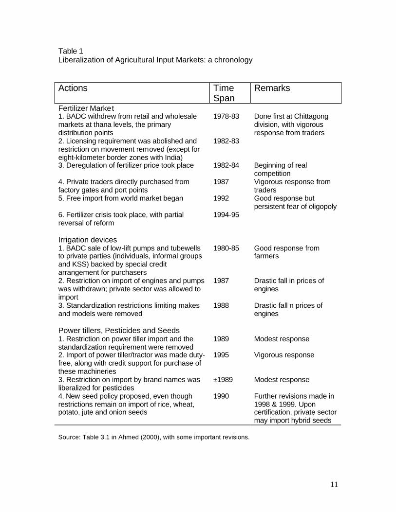
A chronology of policy reforms towards liberalizing the agricultural input markets

in Bangladesh is presented in Table 1. It is quite evident that some of the major

policy reforms came about during the 1980s. More important among these are: (i)

deregulation of fertilizer prices with private dealers procuring directly from the

factories; (ii) transfer of ownership of tubewells from BADC to private hands4, and

most importantly, (iii) withdrawal of restriction on import of engines and pumps

along with withdrawal of standardization restriction that previously limited the

choice of makes and models. It is commonly perceived that the last set of

policies liberalizing the restrictions on irrigation equipment and allowing private

sector import, had the most impact on the crop sector production in Bangladesh.

The 1990’s experienced further liberalization, especially in the trade sector,

having important implications for the crop production. The Rural Rationing was

withdrawn in 1991, largely restricting public offtakes of foodgrains through non-

monetised channels and open market sales. Import of fertilizer by the private

sector was allowed in 1992, with special credit support provided to the

3 See Hossain and Dhaly (1991). 4 This included cooperatives, informal groups and individuals.

10

importers.5 During the same time, private sector participation in import of

foodgrains was also opened up. The latter is believed to have reduced budgetary

burden of the GOB and helped in stabilizing prices during shortfalls in domestic

production. The 1990’s is also marked by significant increase in mechanization of

crop production, largely facilitated by the liberal policy towards importation of

farm machinery and farm credit to support it.

5 Private sector was also allowed to import urea during 1994, which was discontinued after the crisis in fertilizer market during 1995.

11

Table 1 Liberalization of Agricultural Input Markets: a chronology Actions Time

Span Remarks

Fertilizer Market 1. BADC withdrew from retail and wholesale markets at thana levels, the primary distribution points

1978-83 Done first at Chittagong division, with vigorous response from traders

2. Licensing requirement was abolished and restriction on movement removed (except for eight-kilometer border zones with India)

1982-83

3. Deregulation of fertilizer price took place 1982-84 Beginning of real competition

4. Private traders directly purchased from factory gates and port points

1987 Vigorous response from traders

5. Free import from world market began 1992 Good response but persistent fear of oligopoly

6. Fertilizer crisis took place, with partial reversal of reform

1994-95

Irrigation devices 1. BADC sale of low-lift pumps and tubewells to private parties (individuals, informal groups and KSS) backed by special credit arrangement for purchasers

1980-85 Good response from farmers

2. Restriction on import of engines and pumps was withdrawn; private sector was allowed to import

1987 Drastic fall in prices of engines

3. Standardization restrictions limiting makes and models were removed

1988 Drastic fall n prices of engines

Power tillers, Pesticides and Seeds 1. Restriction on power tiller import and the standardization requirement were removed

1989 Modest response

2. Import of power tiller/tractor was made duty-free, along with credit support for purchase of these machineries

1995 Vigorous response

3. Restriction on import by brand names was liberalized for pesticides

±1989 Modest response

4. New seed policy proposed, even though restrictions remain on import of rice, wheat, potato, jute and onion seeds

1990 Further revisions made in 1998 & 1999. Upon certification, private sector may import hybrid seeds

Source: Table 3.1 in Ahmed (2000), with some important revisions.

12

Chapter 3

Issues and Methods

The primary objective of the study is to assess the changes in profitability in crop

production at the farm level as a consequence of the policy reform in the

agricultural input markets in Bangladesh. Two markets under consideration are

chemical fertilizer and mechanized irrigation. There are two different sets of

issues: identification of the timing of the reforms so that time series data on the

real economy may be mapped on it for empirical assessment of the impact; and

the second set of issues relate to linking individual policy reforms with final

outcomes affecting crop sector profitability. We discuss these issues briefly and

outline the methods adopted.

As noted in the previous chapter, reforms in food and agricultural sectors

commenced since the 1970’s; and the process had been quite gradual. Even

though government intervention in the foodgrain market continues, it had gone

through phases of rationalizing procurement prices, reduction of subsidy on

ration distribution with subsequent phasing out of urban and (later) rural

rationing. In the area of input markets, there are two important dimensions in

policy packaging. The first involves the amount/extent of subsidy provided, and

the other relates to transfer of ownership/activities to private sector (from public

agencies).6 It has already been noted that subsidy reduction on inputs had been

a gradual process, and one is unable to identify a single year to demarcate

between pre- and post-policy periods. However, with regards to deregulation and

privatization of procurement/import and distribution of inputs, one is able to

identify certain time-specific policies. Deregulation in fertilizer prices took place

during 1982-84, with private traders subsequently allowed to procure from factory

gates and port since 1987. Similarly, ownership of public-owned irrigation

equipments was transferred to private hands during 1980-85 (which continued

beyond this period); while the private sector was allowed to import makes and

6 Note that an activity may be transferred to private sector and yet subsidy may continue.

13

brands of own choice since 1987. This was followed by the policy on removal of

siting restriction following the 1987-88 flood. Under the circumstance, one may

consider the whole of 1980’s as the decade of policy changes; and compare

performance of the economy (discounting for the autonomous changes) during

the beginning and the end of the decade. This is what we have done in the

following section, being fully aware about the limitation that such comparisons do

not allow us to associate changes with any individual policy reform.

On an a priori basis, it is however possible to identify a number of policies along

with expected effects of these policies. Following Ahmed (2000), these are

summarized in Table 2 below.

Table 2 Policy-Outcome Linkages Policy Meso-level effects Effects on input use

and crop choice Direction of profit

Reduction of subsidy on fertilizer

Increase in fertilizer prices

Reduced fertilizer consumption

Decrease

Lowering of retail prices due to increased competition

Increase in fertilizer consumption

Increase Privatization of fertilizer distribution

Increase in price instability due to alleged oligopoly at dealers’ level

Sub-optimal choice of crops

Decrease

Reduction of subsidy on irrigation

Increase in the price of irrigation water

Shift away from irrigated crop

Decrease

Wider choice of crops, especially HYV rice

Increase Withdrawal of restriction on private sector import, and on brands/makes

Wider choice and increased competition, leading to increased investment in irrigation and decrease in price of irrigation water

Expansion in irrigated area, leading to wider choice of cropping pattern

Increase

Note: If one accounts for the complementarities in use of inputs, increase in irrigated area is expected to facilitate crop production, which subsequently leads to increased consumption of chemical fertilizer.

The above description in Table 2 suggests that impacts of policy reforms need to

be traced through changes in meso-level variables (i.e., prices), with subsequent

impacts on crop and inputs choice, which subsequently influenced crop-sector

14

profitability. While the major part of chapter 4 deals with these issues, we also

critically examine the findings presented in Ahmed (2000), based on SUR

(Seemingly Unrelated Regression) estimates of a system of equations.

15

Chapter 4

Changes in Crop Sector Profitability

Introduction

This chapter compares state of market prices, choice of crops and crop-sector

profitability at two different periods; average of 1978-79 to 1980-81 and average

of 1990-91 to 1991-92. The last period precedes the policy on import

liberalization, which included private imports of fertilizer and foodgrains. On

occasions, we will inform the readers on more recent data to highlight on

subsequent changes. The last part of the chapter makes an attempt to

summarize the impacts of policy reforms, where the findings in Ahmed (2000) are

also highlighted.

Changes in the Fertilizer Market

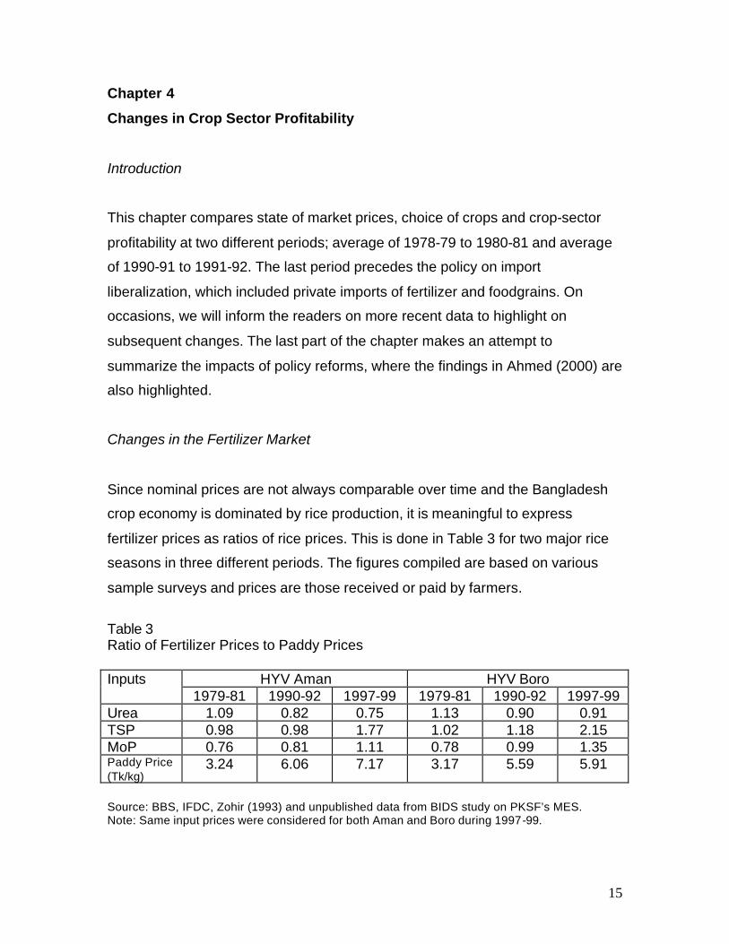
Since nominal prices are not always comparable over time and the Bangladesh

crop economy is dominated by rice production, it is meaningful to express

fertilizer prices as ratios of rice prices. This is done in Table 3 for two major rice

seasons in three different periods. The figures compiled are based on various

sample surveys and prices are those received or paid by farmers.

Table 3 Ratio of Fertilizer Prices to Paddy Prices

HYV Aman HYV Boro Inputs 1979-81 1990-92 1997-99 1979-81 1990-92 1997-99

Urea 1.09 0.82 0.75 1.13 0.90 0.91 TSP 0.98 0.98 1.77 1.02 1.18 2.15 MoP 0.76 0.81 1.11 0.78 0.99 1.35 Paddy Price (Tk/kg)

3.24 6.06 7.17 3.17 5.59 5.91

Source: BBS, IFDC, Zohir (1993) and unpublished data from BIDS study on PKSF’s MES. Note: Same input prices were considered for both Aman and Boro during 1997-99.

16

Since subsidy on BADC-imported TSP and MoP continued till the end of 1991,

and there was allegedly implicit subsidy on urea through administered factory-

gate urea prices, real price of fertilizer had effectively declined in real terms over

the decade of policy reforms under consideration. While administered factory-

gate urea prices continued into the 1990’s, subsidies on TSP and MoP were

eliminated; and the latter prices kept par with international prices. Thus, fertilizer-

paddy price ratios with respect to these two chemical fertilizers increased

dramatically during the 1990’s (see Table 3).

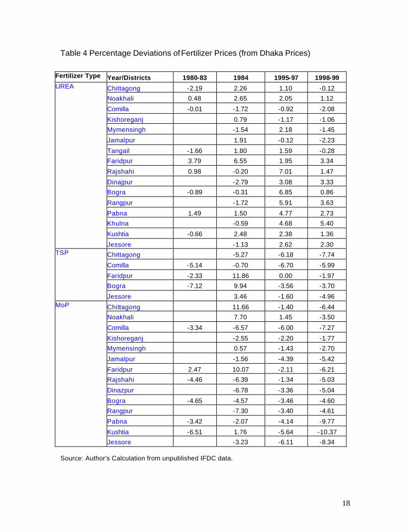
There are three other sets of price summaries, all based on data collected by the

IFDC at different stages of their involvement in Bangladesh. Analysis on spatial

price integration of the fertilizer market was only feasible for 1995-99 period due

to data limitation, details of which are presented in Appendix A. The analysis

suggests that the market is competitive and the retail prices in different regions of

the country are well integrated. Since the data on fertilizer prices was incomplete,

a second set of analysis compares price deviations in a number of districts (from

Dhaka prices) during the early 1980’s and during the 1990’s. Summary of the

findings is presented in Table 4 below. The findings suggest that spatial price

differences have increased in the case of urea for a number of districts,

particularly in the north-west region. In contrast, price differences in MoP have

declined for most districts during the 1990’s, when compared with early 1980’s.7

It needs mentioning that the figures on 1990’s capture the effects of trade

liberalization on fertilizer imports and private sector participation in such imports.

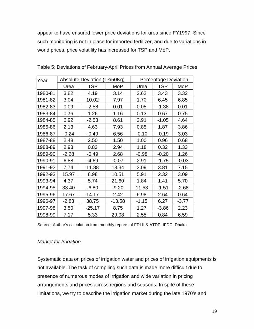
The final set of price statistics are based on monthly price data (national

averages) and try to capture the price volatility at the farm level arising due to

non-availability of fertilizer during the peak periods. We assume February, March

and April to constitute the period of peak demand for fertilizer. Thus, average

price for these three months is expressed as percentage of average price in a

fiscal year in Table 5. Price deviations during the peak period are found to have

7 No clear trend is observed for price differences in TSP.

17

declined after the initial introduction of private dealership at the retail level; and

the deviations remained quite low until the introduction of private import of

fertilizer. Since then price volatility had increased, allegedly due to presence of

oligopoly. However, strict monitoring to regulate the operations of the dealers

18

Table 4 Percentage Deviations of Fertilizer Prices (from Dhaka Prices)

Fertilizer Type Year/Districts 1980-83 1984 1995-97 1998-99

Chittagong -2.19 2.26 1.10 -0.12

Noakhali 0.48 2.65 2.05 1.12

Comilla -0.01 -1.72 -0.92 -2.08

Kishoreganj 0.79 -1.17 -1.06

Mymensingh -1.54 2.18 -1.45

Jamalpur 1.91 -0.12 -2.23

Tangail -1.66 1.80 1.59 -0.28

Faridpur 3.79 6.55 1.95 3.34

Rajshahi 0.98 -0.20 7.01 1.47

Dinajpur -2.79 3.08 3.33

Bogra -0.89 -0.31 6.85 0.86

Rangpur -1.72 5.91 3.63

Pabna 1.49 1.50 4.77 2.73

Khulna -0.59 4.68 5.40

Kushtia -0.66 2.48 2.38 1.36

UREA

Jessore -1.13 2.62 2.30

Chittagong -5.27 -6.18 -7.74

Comilla -5.14 -0.70 -6.70 -5.99

Faridpur -2.33 11.86 0.00 -1.97

Bogra -7.12 9.94 -3.56 -3.70

TSP

Jessore 3.46 -1.60 -4.96

Chittagong 11.66 -1.40 -6.44

Noakhali 7.70 1.45 -3.50

Comilla -3.34 -6.57 -6.00 -7.27

Kishoreganj -2.55 -2.20 -1.77

Mymensingh 0.57 -1.43 -2.70

Jamalpur -1.56 -4.39 -5.42

Faridpur 2.47 10.07 -2.11 -6.21

Rajshahi -4.46 -6.39 -1.34 -5.03

Dinazpur -6.78 -3.36 -5.04

Bogra -4.65 -4.57 -3.46 -4.60

Rangpur -7.30 -3.40 -4.61

Pabna -3.42 -2.07 -4.14 -9.77

Kushtia -6.51 1.76 -5.64 -10.37

MoP

Jessore -3.23 -6.11 -8.34 Source: Author's Calculation from unpublished IFDC data.

19

appear to have ensured lower price deviations for urea since FY1997. Since

such monitoring is not in place for imported fertilizer, and due to variations in

world prices, price volatility has increased for TSP and MoP.

Table 5: Deviations of February-April Prices from Annual Average Prices

Absolute Deviation (Tk/50Kg) Percentage Deviation Year Urea TSP MoP Urea TSP MoP 1980-81 3.82 4.19 3.14 2.62 3.43 3.32 1981-82 3.04 10.02 7.97 1.70 6.45 6.85 1982-83 0.09 -2.58 0.01 0.05 -1.38 0.01 1983-84 0.26 1.26 1.16 0.13 0.67 0.75 1984-85 6.92 -2.53 8.61 2.91 -1.05 4.64 1985-86 2.13 4.63 7.93 0.85 1.87 3.86 1986-87 -0.24 -0.49 6.56 -0.10 -0.19 3.03 1987-88 2.48 2.50 1.50 1.00 0.96 0.68 1988-89 2.93 0.83 2.94 1.18 0.32 1.33 1989-90 -2.28 -0.49 2.68 -0.98 -0.20 1.26 1990-91 6.88 -4.69 -0.07 2.91 -1.75 -0.03 1991-92 7.74 11.88 18.34 3.09 3.81 7.15 1992-93 15.97 8.98 10.51 5.91 2.32 3.09 1993-94 4.37 5.74 21.60 1.84 1.41 5.70 1994-95 33.40 -6.80 -9.20 11.53 -1.51 -2.68 1995-96 17.67 14.17 2.42 6.98 2.64 0.64 1996-97 -2.83 38.75 -13.58 -1.15 6.27 -3.77 1997-98 3.50 -25.17 8.75 1.27 -3.86 2.23 1998-99 7.17 5.33 29.08 2.55 0.84 6.59 Source: Author's calculation from monthly reports of FDI-II & ATDP, IFDC, Dhaka Market for Irrigation

Systematic data on prices of irrigation water and prices of irrigation equipments is

not available. The task of compiling such data is made more difficult due to

presence of numerous modes of irrigation and wide variation in pricing

arrangements and prices across regions and seasons. In spite of these

limitations, we try to describe the irrigation market during the late 1970’s and

20

early 1980’s, and present information pertaining to irrigation prices, compiled

from secondary sources.

By 1980, three modern minor irrigation technologies – Low Lift Pumps (LLP),

Deep Tubewells (DTW) and Shallow Tubewells (STW) – were available through

BADC. During the early 1980’s, these were either purchased or rented from

BADC; and were managed either by KSS groups, informal pump groups related

directly to BADC, private owners who may be individuals or groups, or landless

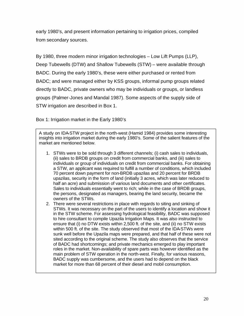
groups (Palmer-Jones and Mandal 1987). Some aspects of the supply side of

STW irrigation are described in Box 1.

Box 1: Irrigation market in the Early 1980’s

A study on IDA-STW project in the north-west (Hamid 1984) provides some interesting insights into irrigation market during the early 1980’s. Some of the salient features of the market are mentioned below.

1. STWs were to be sold through 3 different channels; (i) cash sales to individuals, (ii) sales to BRDB groups on credit from commercial banks, and (iii) sales to individuals or group of individuals on credit from commercial banks. For obtaining a STW, an applicant was required to fulfill a number of conditions, which included 70 percent down payment for non-BRDB upazilas and 20 percent for BRDB upazilas, security in the form of land (initially 3 acres, which was later reduced to half an acre) and submission of various land documents and other certificates. Sales to individuals essentially went to rich; while in the case of BRDB groups, the persons, designated as managers, bearing the land security, became the owners of the STWs.

2. There were several restrictions in place with regards to siting and sinking of STWs. It was necessary on the part of the users to identify a location and show it in the STW scheme. For assessing hydrological feasibility, BADC was supposed to hire consultant to compile Upazila Irrigation Maps. It was also instructed to ensure that (i) no DTW exists within 2,500 ft. of the site, and (ii) no STW exists within 500 ft. of the site. The study observed that most of the IDA-STWs were sunk well before the Upazila maps were prepared, and that half of these were not sited according to the original scheme. The study also observes that the service of BADC had shortcomings; and private mechanics emerged to play important roles in the market. Non-availability of spare parts was however identified as the main problem of STW operation in the north-west. Finally, for various reasons, BADC supply was cumbersome, and the users had to depend on the black market for more than 68 percent of their diesel and mobil consumption.

21

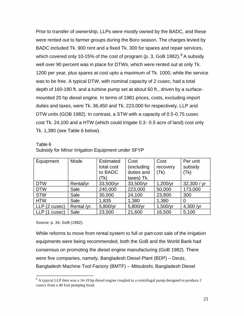
Prior to transfer of ownership, LLPs were mostly owned by the BADC, and these

were rented out to farmer groups during the Boro season. The charges levied by

BADC included Tk. 900 rent and a fixed Tk. 300 for spares and repair services,

which covered only 10-15% of the cost of program (p. 3, GoB 1982).8 A subsidy

well over 90 percent was in place for DTWs, which were rented out at only Tk.

1200 per year, plus spares at cost upto a maximum of Tk. 1000, while the service

was to be free. A typical DTW, with nominal capacity of 2 cusec, had a total

depth of 160-180 ft. and a turbine pump set at about 60 ft., driven by a surface-

mounted 20 hp diesel engine. In terms of 1981 prices, costs, excluding import

duties and taxes, were Tk. 36,450 and Tk. 223,000 for respectively, LLP and

DTW units (GOB 1982). In contrast, a STW with a capacity of 0.5-0.75 cusec

cost Tk. 24,100 and a HTW (which could irrigate 0.3 - 0.5 acre of land) cost only

Tk. 1,380 (see Table 6 below).

Table 6 Subsidy for Minor Irrigation Equipment under SFYP Equipment Mode Estimated

total cost to BADC (Tk)

Cost (excluding duties and taxes) Tk.

Cost recovery (Tk)

Per unit subsidy (Tk)

DTW Rental/yr 33,500/yr 33,500/yr 1,200/yr 32,300 / yr DTW Sale 240,000 223,000 50,000 173,000 STW Sale 30,000 24,100 23,800 300 HTW Sale 1,835 1,380 1,380 0 LLP (2 cusec) Rental /yr. 5,800/yr 5,800/yr 1,500/yr 4,300 /yr LLP (1 cusec) Sale 23,500 21,600 16,500 5,100 Source: p. 34, GoB (1982). While reforms to move from rental system to full or part-cost sale of the irrigation

equipments were being recommended, both the GoB and the World Bank had

consensus on promoting the diesel engine manufacturing (GoB 1982). There

were five companies, namely, Bangladesh Diesel Plant (BDP) – Deutz,

Bangladesh Machine Tool Factory (BMTF) – Mitsubishi, Bangladesh Diesel

8 A typical LLP then was a 16-18 hp diesel engine coupled to a centrifugal pump designed to produce 2 cusecs from a 40 foot pumping head.

22

Engine Co. (BDEC) – Yanmar, Bangladesh Diesel Ltd (BDL) – Lister, and

Bangladesh Milnars Engineering Complex (MEC) – Kiloskar;9 had already

government approval to manufacture diesel engines. Protection was given to this

industry with the hope that there would be positive linkage effects and external

economies (p. 23, GoB 1982).

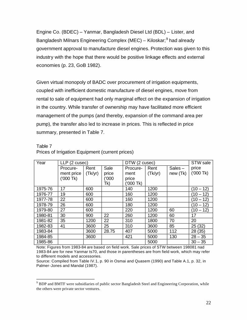
Given virtual monopoly of BADC over procurement of irrigation equipments,

coupled with inefficient domestic manufacture of diesel engines, move from

rental to sale of equipment had only marginal effect on the expansion of irrigation

in the country. While transfer of ownership may have facilitated more efficient

management of the pumps (and thereby, expansion of the command area per

pump), the transfer also led to increase in prices. This is reflected in price

summary, presented in Table 7.

Table 7 Prices of Irrigation Equipment (current prices)

LLP (2 cusec) DTW (2 cusec) Year Procure- ment price (‘000 Tk)

Rent (Tk/yr)

Sale price (‘000 Tk)

Procure-ment price (‘000 Tk)

Rent (Tk/yr)

Sales – new (Tk)

STW sale price (‘000 Tk)

1975-76 17 600 140 1200 (10 – 12) 1976-77 19 600 160 1200 (10 – 12) 1977-78 22 600 160 1200 (10 – 12) 1978-79 26 600 180 1200 (10 – 12) 1979-80 27 600 220 1200 60 (10 – 12) 1980-81 30 900 22 260 1200 60 17 1981-82 35 1200 22 310 1800 70 20 1982-83 41 3600 25 310 3600 85 25 (32) 1983-84 3600 28.75 407 5000 112 28 (35) 1984-85 3600 421 5000 130 28 – 35 1985-86 5000 30 – 35 Note: Figures from 1983-84 are based on field work. Sale prices of STW between 198081 nad 1983-84 are for new Yanmar ts70, and those in parentheses are from field work, which may refer to different models and accessories. Source: Compiled from Table IV.1, p. 90 in Osmai and Quasem (1990) and Table A.1, p. 32, in Palmer-Jones and Mandal (1987).

9 BDP and BMTF were subsidiaries of public sector Bangladesh Steel and Engineering Corporation, while the others were private sector ventures.

23

For obvious reason, the price of irrigation paid at farm level had increased during

the 1980’s. While per acre irrigation costs was only Tk. 210 and Tk. 400

respectively for rented DTW and STW, the cost increased to more than Tk. 800

and Tk. 1800 for the two modes respectively by 1984 (Osmani and Quasem

1990 and Palmer-Jones and Mandal 1987). There were wide variations in pricing

across managements and modes of payments. Normally, farmers had to pay

higher prices under individually owned equipment, and if the payment had to be

made in kind (paddy).10 Moreover, the water prices were substantially lower

under electricity-run engines compared to those under diesel-run engines. Other

than the introduction of electricity-run engines, the most significant change

occurred in the irrigation market when restriction on brands was withdrawn and

private sector was allowed to import during 1987. This provided a wider choice of

irrigation equipment at cheaper prices, and thereby, promoted investment in the

minor irrigation sector. The jump in sale of STW units through private dealers,

most of which were imported by the private sector, is quite evident in the

summary statistics presented in Table B.1, in Appendix B. Trends in area under

irrigation, by modes and regions are summarized in Tables B.15 to B.24 in the

same Appendix.

Relative Prices vs Relative Availability

Traditional economic analysis is often bogged down with changes in relative

prices of inputs leading to changes in choice variables. Following such a

perspective, one may hypothesize that policy reforms in the agricultural input

markets led to lowering of prices of fertilizer and irrigation, which subsequently

led to increase in their use, and thereby to increase in output and profitability. It is

true that the price of urea as a ratio of rice price had declined over the years due

to continuation of implicit subsidy on urea produced by public sector industry. In

case of the other two major varieties of chemical fertilizer, their prices had

10 In the case of payment in kind, one would expect the price to be higher than under cash payment since there was risk sharing involved and payment is made after harvest under the former arrangement.

24

evidently increased relative to rice prices, though only after 1992. It is generally

agreed that timely availability of fertilizer has been more important in influencing

its use than variation in its prices at the margin. It is also commonly understood

that of the two inputs under study, irrigation had acted as the lead input in

promoting crop sector growth in Bangladesh.11 Here also, availability of irrigation

facility rather than changes in its relative prices had been instrumental in

promoting growth. It is true that increase in the irrigation price paid by the farmers

(who had already adopted the technology) adversely affected profitability.

However, decline in price of irrigation equipment, coupled with a wider choice set

through unrestricted private import, promoted investment on minor irrigation.

Such investment enabled farmers in new areas to choose crops that would raise

profit. Thus, one may conjecture that early adopters of modern technology had

reaped higher benefits during the initial years, which declined with policy reforms

during the 1980’s; and the policy reforms helped expansion of modern

technology to new areas (due to reduced investment cost) where the farmers

derived positive benefits. Such a conjecture is supported by evidence provided in

Mahmud et al (1994), where it is shown that rice production in Tangail, Noakhali

and Chittagong had recorded high growth rates during 1967-68 to 1977-78

period (respectively, 10.56, 5.12 and 4.12 percents per year), while these

districts performed poorly during 1979-80 to 1989-90 period (with annual growth

rates of –1.12, 2.47 and 0.51 respectively).12

The present study does not pursue the above analysis. In stead, we look into the

implications for crop choice and consequent changes in aggregate profitability of

the crop sector in Bangladesh. Crop-sector profitability may increase for one or

more of the following four reasons: (i) general increase in the relative price of

output to those of inputs, (ii) favorable shift in relative prices of inputs, (iii) land

improvements making it feasible to shift land allocation towards producing more

11 See Ahmed (2000). 12 See Table 2.10 in p. 23, Mahmud et al (1994). One may also look into the recent work by Raisuddin Ahmed. It is important to note that within a dynamic setting, additional income accrued by the early

25

profitable crops, and (iv) optimal use of inputs under individual crops (moving

towards the boundary of production frontier from within). We have already noted

that other than in the case of urea, relative price of the main crop sector produce

(rice) did not increase vis-à-vis other inputs during the decade under scrutiny

(1980’s). It is also beyond the scope of the present study to comprehensively

address the relative contribution of individual inputs to growth and then map

evidence on changes in relative prices of these inputs on such contributions, in

order to address point (ii) above.13 In the rest of the chapter, therefore, we look

into changes in land allocation and in intensity of input use before presenting

summary statistics on changes in aggregate profitability of the crop sector.

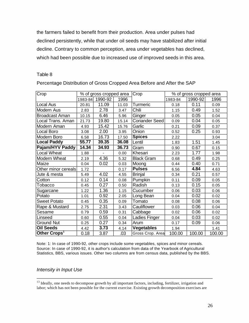
Land Allocation by Crops

Expansion of area under modern irrigation had primarily facilitated HYV Boro rice

cultivation during the dry season. Provision of supplementary irrigation, along

with flood protection measures, had also facilitated cultivation of HYV Aman rice

during the wet season. Over the reform period (whole of 1980’s), for obvious

reasons of emphasizing on cereal production, share of cereals in gross cropped

area increased, while most other crop groups recorded marginal declines in their

shares. However, the major shift was within rice, and the share of HYV/Pajam

paddy increased from 14.3 percent of gross cropped area to about 35 percent

over a decade. This is equivalent to about 47 percent of total rice area, which

had later increased to more than 50 percent in 1996. The growth in total output

due to switching from local to modern variety has however died down during the

1990’s. It is important to note that quite a large number of non-rice minor crops

(especially, spices and vegetables) exhibited large profit in static analyses

(Mahmud et al 1994). Yet, due to market uncertainty and problems with micro-

management of minor irrigation to accommodate their production within rice area,

adopters of technology may find ways into new line of economic activities, which has rarely been probed in the context of Bangladesh.

26

the farmers failed to benefit from their production. Area under pulses had

declined persistently, while that under oil seeds may have stabilized after initial

decline. Contrary to common perception, area under vegetables has declined,

which had been possible due to increased use of improved seeds in this area.

Table 8

Percentage Distribution of Gross Cropped Area Before and After the SAP

% of gross cropped area % of gross cropped area Crop 1983-84 1990-92 1996

Crop 1983-84 1990-92 1996

Local Aus 20.81 11.09 11.03 Turmeric 0.18 0.11 0.09 Modern Aus 2.83 2.78 3.47 Chili 1.15 0.49 1.52 Broadcast Aman 10.15 6.46 5.96 Ginger 0.05 0.05 0.04 Local Trans. Aman 21.73 19.80 15.14 Coriander Seed 0.09 0.04 0.05 Modern Aman 4.93 15.42 15.76 Garlic 0.21 0.09 0.37 Local Boro 3.08 2.00 3.95 Onion 0.52 0.25 0.93 Modern Boro 6.58 16.73 17.50 Spices 2.22 3.04 Local Paddy 55.77 39.35 36.08 Lentil 1.83 1.51 1.45 Pajam/HYV Paddy 14.34 34.93 36.73 Gram 0.90 0.67 0.15 Local Wheat 1.88 - 0.00 Khesari 2.23 1.77 1.98 Modern Wheat 2.19 4.36 5.32 Black Gram 0.68 0.49 0.25 Maize 0.04 0.02 0.03 Moong 0.44 0.40 0.71 Other minor cereals 1.72 0.17 Pulses 6.56 4.84 4.63 Jute & mesta 5.49 4.02 4.55 Brinjal 0.34 0.21 0.57 Cotton 0.12 0.14 0.08 Pumpkin 0.11 0.09 0.05 Tobacco 0.45 0.27 0.50 Radish 0.13 0.15 0.05 Sugarcane 1.22 1.36 1.15 Cucumber 0.06 0.03 0.06 Potato 1.01 0.92 2.05 Long Bean 0.04 0.02 0.02 Sweet Potato 0.45 0.35 0.09 Tomato 0.08 0.08 0.06 Rape & Mustard 2.75 2.31 3.43 Cauliflower 0.03 0.06 0.04 Sesame 0.79 0.59 0.31 Cabbage 0.02 0.06 0.02 Linseed 0.60 0.55 0.04 Ladies Finger 0.04 0.03 0.02 Ground Nut 0.25 0.27 0.34 Arum 0.17 0.09 0.06 Oil Seeds 4.42 3.73 4.14 Vegetables 1.94 1.41 Other Crops1 0.18 3.87 .03 Gross Crop. Area 100.00 100.00 100.00 Note: 1: In case of 1990-92, other crops include some vegetables, spices and minor cereals. Source: In case of 1990-92, it is author's calculation from data of the Yearbook of Agricultural Statistics, BBS, various issues. Other two columns are from census data, published by the BBS. Intensity in Input Use

13 Ideally, one needs to decompose growth by all important factors, including, fertilizer, irrigation and labor; which has not been possible for the current exercise. Existing growth decomposition exercises are

27

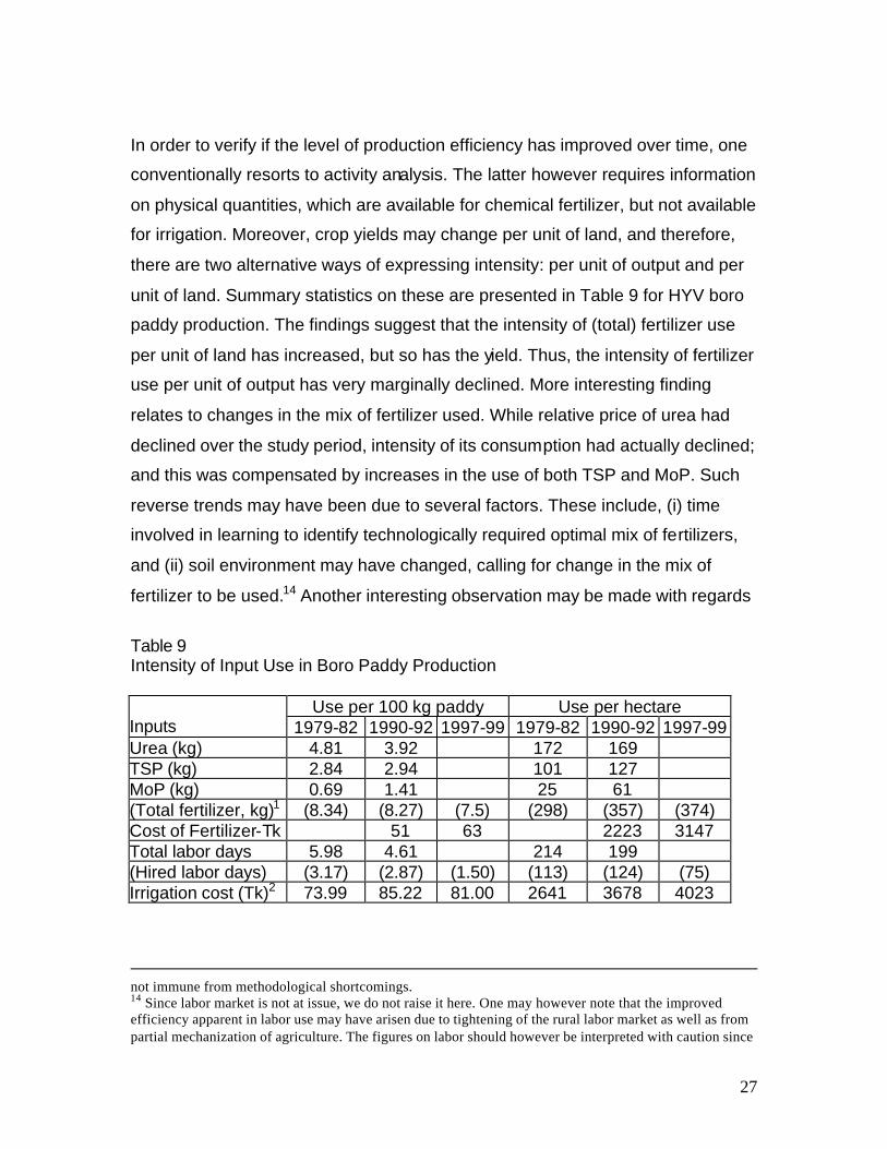
In order to verify if the level of production efficiency has improved over time, one

conventionally resorts to activity analysis. The latter however requires information

on physical quantities, which are available for chemical fertilizer, but not available

for irrigation. Moreover, crop yields may change per unit of land, and therefore,

there are two alternative ways of expressing intensity: per unit of output and per

unit of land. Summary statistics on these are presented in Table 9 for HYV boro

paddy production. The findings suggest that the intensity of (total) fertilizer use

per unit of land has increased, but so has the yield. Thus, the intensity of fertilizer

use per unit of output has very marginally declined. More interesting finding

relates to changes in the mix of fertilizer used. While relative price of urea had

declined over the study period, intensity of its consumption had actually declined;

and this was compensated by increases in the use of both TSP and MoP. Such

reverse trends may have been due to several factors. These include, (i) time

involved in learning to identify technologically required optimal mix of fertilizers,

and (ii) soil environment may have changed, calling for change in the mix of

fertilizer to be used.14 Another interesting observation may be made with regards

Table 9 Intensity of Input Use in Boro Paddy Production

Use per 100 kg paddy Use per hectare Inputs 1979-82 1990-92 1997-99 1979-82 1990-92 1997-99 Urea (kg) 4.81 3.92 172 169 TSP (kg) 2.84 2.94 101 127 MoP (kg) 0.69 1.41 25 61 (Total fertilizer, kg)1 (8.34) (8.27) (7.5) (298) (357) (374) Cost of Fertilizer-Tk 51 63 2223 3147 Total labor days 5.98 4.61 214 199 (Hired labor days) (3.17) (2.87) (1.50) (113) (124) (75) Irrigation cost (Tk)2 73.99 85.22 81.00 2641 3678 4023

not immune from methodological shortcomings. 14 Since labor market is not at issue, we do not raise it here. One may however note that the improved efficiency apparent in labor use may have arisen due to tightening of the rural labor market as well as from partial mechanization of agriculture. The figures on labor should however be interpreted with caution since

28

Note 1: Cost of fertilizer was available for 1997-99. Assuming the mix to be same as 1990-92, total quantity of fertilizer use was estimated. If the shares of TSP and MoP are assumed to have increased, estimate on use of fertilizer would be lower. Note 2: Monetary values for the first two periods are in 1990-91 prices. Source: Appendix tables; and unpublished data from BIDS Study on PKSF-MES (Zohir et al 2000). to more recent trends: both fertilizer and irrigation costs per unit of land have

increased; but they have declined per unit of output.

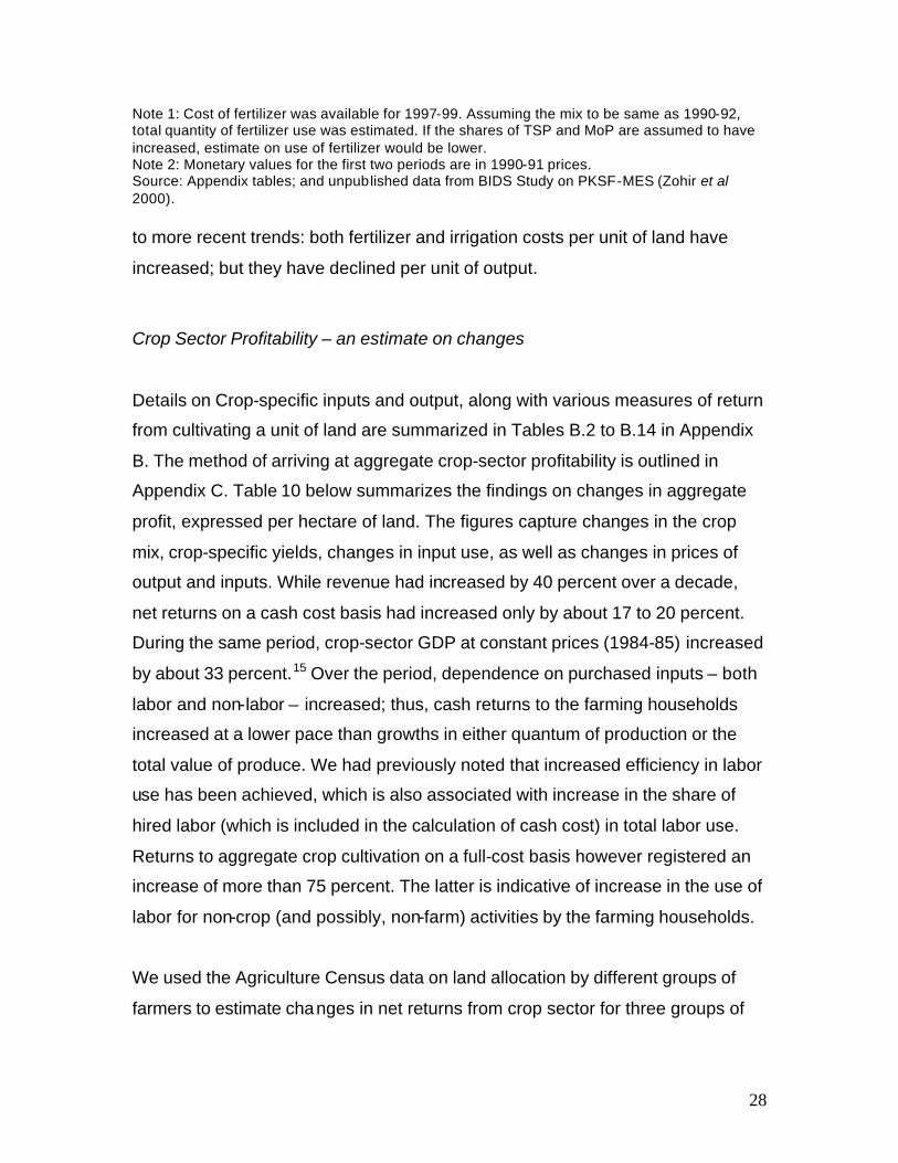
Crop Sector Profitability – an estimate on changes

Details on Crop-specific inputs and output, along with various measures of return

from cultivating a unit of land are summarized in Tables B.2 to B.14 in Appendix

B. The method of arriving at aggregate crop-sector profitability is outlined in

Appendix C. Table 10 below summarizes the findings on changes in aggregate

profit, expressed per hectare of land. The figures capture changes in the crop

mix, crop-specific yields, changes in input use, as well as changes in prices of

output and inputs. While revenue had increased by 40 percent over a decade,

net returns on a cash cost basis had increased only by about 17 to 20 percent.

During the same period, crop-sector GDP at constant prices (1984-85) increased

by about 33 percent.15 Over the period, dependence on purchased inputs – both

labor and non-labor – increased; thus, cash returns to the farming households

increased at a lower pace than growths in either quantum of production or the

total value of produce. We had previously noted that increased efficiency in labor

use has been achieved, which is also associated with increase in the share of

hired labor (which is included in the calculation of cash cost) in total labor use.

Returns to aggregate crop cultivation on a full-cost basis however registered an

increase of more than 75 percent. The latter is indicative of increase in the use of

labor for non-crop (and possibly, non-farm) activities by the farming households.

We used the Agriculture Census data on land allocation by different groups of

farmers to estimate changes in net returns from crop sector for three groups of

29

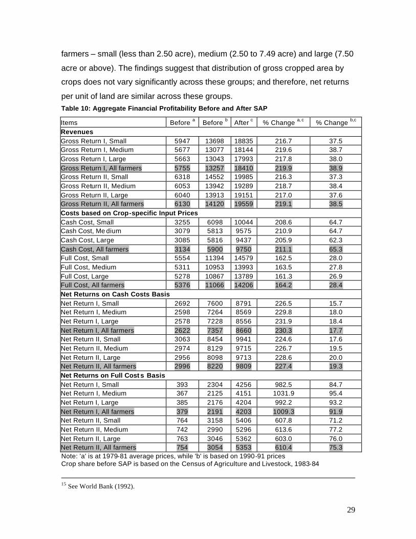
farmers – small (less than 2.50 acre), medium (2.50 to 7.49 acre) and large (7.50

acre or above). The findings suggest that distribution of gross cropped area by

crops does not vary significantly across these groups; and therefore, net returns

per unit of land are similar across these groups. Table 10: Aggregate Financial Profitability Before and After SAP

Items Before a Before b After c % Change a, c % Change b,c Revenues Gross Return I, Small 5947 13698 18835 216.7 37.5 Gross Return I, Medium 5677 13077 18144 219.6 38.7 Gross Return I, Large 5663 13043 17993 217.8 38.0 Gross Return I, All farmers 5755 13257 18410 219.9 38.9 Gross Return II, Small 6318 14552 19985 216.3 37.3 Gross Return II, Medium 6053 13942 19289 218.7 38.4 Gross Return II, Large 6040 13913 19151 217.0 37.6 Gross Return II, All farmers 6130 14120 19559 219.1 38.5 Costs based on Crop-specific Input Prices Cash Cost, Small 3255 6098 10044 208.6 64.7 Cash Cost, Me dium 3079 5813 9575 210.9 64.7 Cash Cost, Large 3085 5816 9437 205.9 62.3 Cash Cost, All farmers 3134 5900 9750 211.1 65.3 Full Cost, Small 5554 11394 14579 162.5 28.0 Full Cost, Medium 5311 10953 13993 163.5 27.8 Full Cost, Large 5278 10867 13789 161.3 26.9 Full Cost, All farmers 5376 11066 14206 164.2 28.4 Net Returns on Cash Costs Basis Net Return I, Small 2692 7600 8791 226.5 15.7 Net Return I, Medium 2598 7264 8569 229.8 18.0 Net Return I, Large 2578 7228 8556 231.9 18.4 Net Return I, All farmers 2622 7357 8660 230.3 17.7 Net Return II, Small 3063 8454 9941 224.6 17.6 Net Return II, Medium 2974 8129 9715 226.7 19.5 Net Return II, Large 2956 8098 9713 228.6 20.0 Net Return II, All farmers 2996 8220 9809 227.4 19.3 Net Returns on Full Cost s Basis Net Return I, Small 393 2304 4256 982.5 84.7 Net Return I, Medium 367 2125 4151 1031.9 95.4 Net Return I, Large 385 2176 4204 992.2 93.2 Net Return I, All farmers 379 2191 4203 1009.3 91.9 Net Return II, Small 764 3158 5406 607.8 71.2 Net Return II, Medium 742 2990 5296 613.6 77.2 Net Return II, Large 763 3046 5362 603.0 76.0 Net Return II, All farmers 754 3054 5353 610.4 75.3 Note: 'a' is at 1979-81 average prices, while 'b' is based on 1990-91 prices Crop share before SAP is based on the Census of Agriculture and Livestock, 1983-84

15 See World Bank (1992).

30

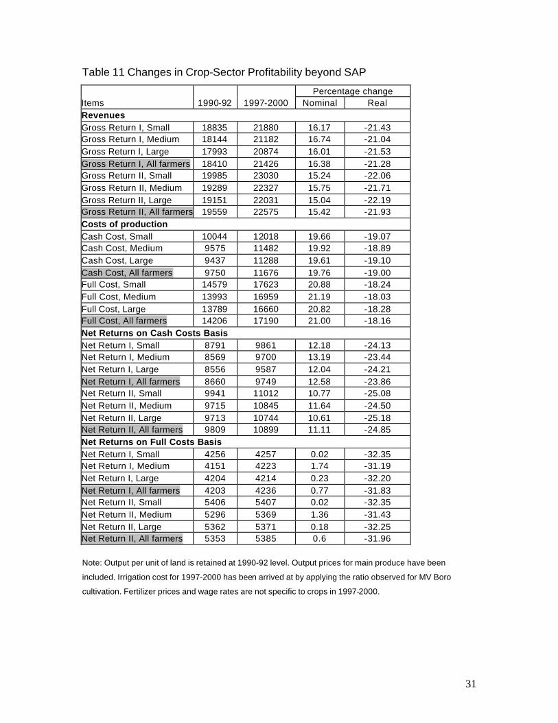
Crop share after SAP is based on the Census of Agriculture, 1996 The relevant figures in 'a' were calculated from Tables B.2 & B.5 weighted by the share of the crop in the total cropped area. The relevant figures in 'b' were calculated from Tables B.2 & B.6 weighted by the share of the crop in the total cropped area. The relevant figures in 'c' were calculated from Tables B.3 & B.6 weighted by the share of the crop in the total cropped area. Source: Author's Calculation Increase in crop-sector profitability has however dampened during the 1990’s. A

comparison with 1997-2000, upon changing a limited set of variables (on which

information was available), shows net returns on per unit of land, in nominal

terms, to have increased at the most by less than 1 percent on full-cost basis

(Table 11). This is primarily because the wage rates have increased by more

than 25 percent over the period; fertilizer costs have increased by more than 50

percent and irrigation costs have increased by about 10 percent. In contrast, the

prices of most crop-sector produce have only marginally increased. In real terms,

returns on land declined by more than 25 percent, which largely reflects the

persistent decline in terms of trade against crop sector in Bangladesh. Note that

our estimate on changes in profitability over the recent past is only suggestive

and does not capture the changes in land productivity. However, given that

physical quantity of output produced per unit of land did not increase significantly

over the years, the finding on decline in real profitability of the crop sector during

the 1990’s remains valid.

In the absence of counter-factual scenario, it is hard to suggest if the growth in

aggregate crop-sector profit is high or low, nor is possible to associate the

changes with reforms in the markets of agricultural inputs. The following section

attempts to address this, following the recent work in Ahmed (2000).

31

Table 11 Changes in Crop-Sector Profitability beyond SAP

Percentage change Items 1990-92 1997-2000 Nominal Real Revenues Gross Return I, Small 18835 21880 16.17 -21.43 Gross Return I, Medium 18144 21182 16.74 -21.04 Gross Return I, Large 17993 20874 16.01 -21.53 Gross Return I, All farmers 18410 21426 16.38 -21.28 Gross Return II, Small 19985 23030 15.24 -22.06 Gross Return II, Medium 19289 22327 15.75 -21.71 Gross Return II, Large 19151 22031 15.04 -22.19 Gross Return II, All farmers 19559 22575 15.42 -21.93 Costs of production Cash Cost, Small 10044 12018 19.66 -19.07 Cash Cost, Medium 9575 11482 19.92 -18.89 Cash Cost, Large 9437 11288 19.61 -19.10 Cash Cost, All farmers 9750 11676 19.76 -19.00 Full Cost, Small 14579 17623 20.88 -18.24 Full Cost, Medium 13993 16959 21.19 -18.03 Full Cost, Large 13789 16660 20.82 -18.28 Full Cost, All farmers 14206 17190 21.00 -18.16 Net Returns on Cash Costs Basis Net Return I, Small 8791 9861 12.18 -24.13 Net Return I, Medium 8569 9700 13.19 -23.44 Net Return I, Large 8556 9587 12.04 -24.21 Net Return I, All farmers 8660 9749 12.58 -23.86 Net Return II, Small 9941 11012 10.77 -25.08 Net Return II, Medium 9715 10845 11.64 -24.50 Net Return II, Large 9713 10744 10.61 -25.18 Net Return II, All farmers 9809 10899 11.11 -24.85 Net Returns on Full Costs Basis Net Return I, Small 4256 4257 0.02 -32.35 Net Return I, Medium 4151 4223 1.74 -31.19 Net Return I, Large 4204 4214 0.23 -32.20 Net Return I, All farmers 4203 4236 0.77 -31.83 Net Return II, Small 5406 5407 0.02 -32.35 Net Return II, Medium 5296 5369 1.36 -31.43 Net Return II, Large 5362 5371 0.18 -32.25 Net Return II, All farmers 5353 5385 0.6 -31.96

Note: Output per unit of land is retained at 1990-92 level. Output prices for main produce have been

included. Irrigation cost for 1997-2000 has been arrived at by applying the ratio observed for MV Boro

cultivation. Fertilizer prices and wage rates are not specific to crops in 1997-2000.

32

Impact of Policy Reforms: a quantitative exercise

In a recent publication (Ahmed 2000), Ahmed estimates a system with five

equations by Zellner’s Seemingly Unrelated Regression (SUR) method, and

shows that reforms in the market for irrigation equipment had significant impact in

increasing the area under irrigation, which had played central role in promoting

the crop-sector production (captured in terms of rice production). The equations

estimated and the description of variables, are summarized in Appendix D. Since

the data was provided in Ahmed (2000), we were able to re-estimate the

equations by the same SUR method with RATS (Regression Analysis of Time

Series) program. Ahmed’s estimates (of model 1 reported in Ahmed 2000) and

our estimates of the same sets of equations are presented in the first two

columns in Table 12. There are variations in the estimated coefficients, even

though the estimated t-statistics are comparable. More importantly, Ahmed

considers 1988-89 as the first year of the post-reform period, and accordingly

chooses the dummy variable. Our discussion in the text suggests that 1987-88

should be considered in stead. We have therefore defined the dummy variable

differently, and the estimates are reported in the third column in Table 11. Since

private sector import of fertilizer was allowed since 1992 and a number of other

important reforms in the foodgrain market came about around that time, we

include an additional dummy for 1992-93 onward, and estimate the set of

equations, whose results are summarized in the fourth column in Table 11. In the

following, we summarize the differences in our estimates with those in Ahmed

(2000).

1. The perverse negative relation between short-term credit and fertilizer

consumption remains, but is statistically insignificant.

2. Irrigated area is found to have dominant influence on fertilizer

consumption and the sign of relative price of fertilizer is negative, but

insignificant. However, unlike Ahmed’s estimate, fertilizer consumption

had increased during post-1988 period.

33

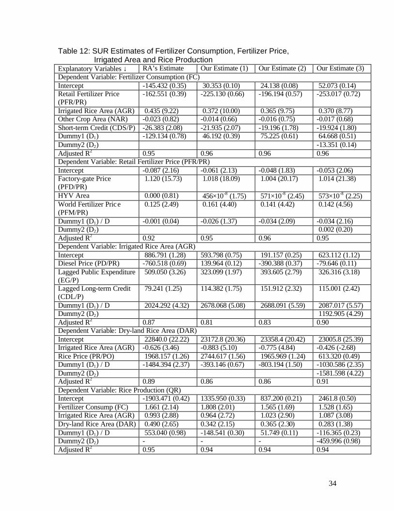
3. Retail fertilizer price is found to be significantly related with factory-gate

price, but a unit increase in the latter is found to increase the retail price by

only 1.01 (and not 1.2 as found by Ahmed). This suggests of greater price

transmission than that evident from Ahmed’s estimates. More importantly,

Ahmed found the period dummy to be insignificant, where as, we find the

fertilizer price to have significantly declined during post-1987-88 period

(with marginal increase after import liberalization). This is important to

note since lower fertilizer prices may have facilitated adoption of HYV rice,

which is difficult to be captured with the specification of equations

estimated in Ahmed (2000).

4. The equation on irrigated rice area has right signs for diesel price and

lagged public expenditures on water development measures. However,

unlike Ahmed (2000), estimated coefficient for long-term credit in our

exercise is statistically significant, which is expected.

5. It is true that irrigated area under rice increased significantly during post-

1992 period, which remains to be adequately explained. However, it had

also increased significantly during 1987-92 period, following the policy

reforms.

6. Relationship between dry land rice area and irrigated rice area has

changed substantially during the 1990’s compared to the earlier period.

The size of dry land rice area has clearly declined more during the post-

1992 period than the decline during 1987-92.

7. Finally, when two dummies are included, irrigated area emerges as the

single variable that significantly effects production of rice.

In spite of the differences, both the exercises suggest that policy reforms in the market for irrigation equipment, undertaken during 1987 and 1988, had been central in promoting crop-sector growth in Bangladesh.

34

Table 12: SUR Estimates of Fertilizer Consumption, Fertilizer Price, Irrigated Area and Rice Production

Explanatory Variables ↓ RA’s Estimate Our Estimate (1) Our Estimate (2) Our Estimate (3) Dependent Variable: Fertilizer Consumption (FC) Intercept -145.432 (0.35) 30.353 (0.10) 24.138 (0.08) 52.073 (0.14) Retail Fertilizer Price (PFR/PR)

-162.551 (0.39) -225.130 (0.66) -196.194 (0.57) -253.017 (0.72)

Irrigated Rice Area (AGR) 0.435 (9.22) 0.372 (10.00) 0.365 (9.75) 0.370 (8.77) Other Crop Area (NAR) -0.023 (0.82) -0.014 (0.66) -0.016 (0.75) -0.017 (0.68) Short-term Credit (CDS/P) -26.383 (2.08) -21.935 (2.07) -19.196 (1.78) -19.924 (1.80) Dummy1 (D1) -129.134 (0.78) 46.192 (0.39) 75.225 (0.61) 64.668 (0.51) Dummy2 (D2) -13.351 (0.14) Adjusted R2 0.95 0.96 0.96 0.96 Dependent Variable: Retail Fertilizer Price (PFR/PR) Intercept -0.087 (2.16) -0.061 (2.13) -0.048 (1.83) -0.053 (2.06) Factory-gate Price (PFD/PR)

1.120 (15.73) 1.018 (18.09) 1.004 (20.17) 1.014 (21.38)

HYV Area 0.000 (0.81) 456×10-8 (1.75) 571×10-8 (2.45) 573×10-8 (2.25) World Fertilizer Price (PFM/PR)

0.125 (2.49) 0.161 (4.40) 0.141 (4.42) 0.142 (4.56)

Dummy1 (D1) / D -0.001 (0.04) -0.026 (1.37) -0.034 (2.09) -0.034 (2.16) Dummy2 (D2) 0.002 (0.20) Adjusted R2 0.92 0.95 0.96 0.95 Dependent Variable: Irrigated Rice Area (AGR) Intercept 886.791 (1.28) 593.798 (0.75) 191.157 (0.25) 623.112 (1.12) Diesel Price (PD/PR) -760.518 (0.69) 139.964 (0.12) -390.388 (0.37) -79.646 (0.11) Lagged Public Expenditure (EG/P)

509.050 (3.26) 323.099 (1.97) 393.605 (2.79) 326.316 (3.18)

Lagged Long-term Credit (CDL/P)

79.241 (1.25) 114.382 (1.75) 151.912 (2.32) 115.001 (2.42)

Dummy1 (D1) / D 2024.292 (4.32) 2678.068 (5.08) 2688.091 (5.59) 2087.017 (5.57) Dummy2 (D2) 1192.905 (4.29) Adjusted R2 0.87 0.81 0.83 0.90 Dependent Variable: Dry-land Rice Area (DAR) Intercept 22840.0 (22.22) 23172.8 (20.36) 23358.4 (20.42) 23005.8 (25.39) Irrigated Rice Area (AGR) -0.626 (3.46) -0.883 (5.10) -0.775 (4.84) -0.426 (-2.68) Rice Price (PR/PO) 1968.157 (1.26) 2744.617 (1.56) 1965.969 (1.24) 613.320 (0.49) Dummy1 (D1) / D -1484.394 (2.37) -393.146 (0.67) -803.194 (1.50) -1030.586 (2.35) Dummy2 (D2) -1581.598 (4.22) Adjusted R2 0.89 0.86 0.86 0.91 Dependent Variable: Rice Production (QR) Intercept -1903.471 (0.42) 1335.950 (0.33) 837.200 (0.21) 2461.8 (0.50) Fertilizer Consump (FC) 1.661 (2.14) 1.808 (2.01) 1.565 (1.69) 1.528 (1.65) Irrigated Rice Area (AGR) 0.993 (2.88) 0.964 (2.72) 1.023 (2.90) 1.087 (3.08) Dry-land Rice Area (DAR) 0.490 (2.65) 0.342 (2.15) 0.365 (2.30) 0.283 (1.38) Dummy1 (D1) / D 553.040 (0.98) -148.541 (0.30) 51.749 (0.11) -116.365 (0.23) Dummy2 (D2) - - - -459.996 (0.98) Adjusted R2 0.95 0.94 0.94 0.94

35

Chapter 5

Beyond Structural Adjustment: policies to address emerging concerns

Introduction

The present study raised the problem in periodization in order to adequately

assess the impacts of structural adjustment policies on the crop sector

profitability in Bangladesh. We had compared 1990-92 (post-SAP) with 1979-81

(pre-SAP) and found the fa rmer-level net returns from crop production to have

increased in real terms. The econometric exercise had shown that liberalization

with regards to the irrigation market (procurement of equipments as well as siting

of wells) had the most significant impact on the adoption of modern variety of

rice, which raised land productivity and increased farm-level profit. Moreover,

gradual privatization of fertilizer distribution had generally ensured timely supply

of fertilizer to the farmers; and the fertilizer market is found to be spatially well-

integrated. Thus, short-term impacts of SAP in these two areas are found to be

positive. Policies, however, open up new opportunities, and the short-term gains

may not be sustained in the long term. Moreover, behavior of agents under a

new policy regime raise new set of issues, all of which may not be conducive to

healthy growth in the agricultural sector. Even though a limited set of information

have been provided on recent changes in the crop sector, they suggest of

stagnation in the crop sector, with possible decline in returns from crop

production in real terms. It is therefore important that the second generation

problems be raised so that the economy may be revitalized out of current

stagnation and future policies may designed upon lessons drawn from past

experience. We discuss a number of such issues, which are directly related to

policy changes that were initiated during the 1980’s and early 1990’s.

36

Observations on the Irrigation Sector

There are several lessons to be learnt from the policy experiences during the

1980’s; these are summarized below.

1. The move towards import substitution with establishment of plants to

manufacture pumps and diesel engines during the early 1980’s proved to

be a wastage of scarce capital for the country. These plants turned out to

be inefficient when the standardization was withdrawn and private import

of irrigation equipment was allowed during 1987.

2. In retrospect, it now appears that continuation of subsidy on fertilizer

during the late 1980’s was not a fair policy to maintain, especially since

such subsidy was later withdrawn during 1992. Since there are

complementarities in usage of the two inputs (irrigation water and

chemical fertilizer), stability in relative prices and availability of these

inputs is crucial in ensuring healthy investment. It is quite possible that low

fertilizer prices had induced excessive investment on minor irrigation, a

part of which turned out to be less economic under later policy regime

(with no fertilizer subsidy). This, however, remains a conjecture, and

cannot be verified due to absence of adequate data.

3. Increase in investment on irrigation with the withdrawal of standardization

does suggest that size of investment is an important factor, which should

be duly considered in future policy formulation.

4. While withdrawal of standardization did promote investment in irrigation, in

the absence of complete knowledge on makes, farmers had often incurred

losses due to inappropriate choices. Adequate information, independent of

the promotional activities of the commercial firms, could have reduced

such losses.

Increase investment in irrigation opened up several new concerns, which needs

to be adequately addressed in the future. They include,

37

1. Current practice of irrigation through flooding of land promotes rice

cultivation, and in the absence of appropriate design of field channels,

cultivation of minor crops in association with rice within the same

command area has not been in vogue. Thus, increased dependence on

minor irrigation has led to increase in the extent of monoculture practice in

the crop sector. We have also observed that revenue from rice production

has declined in real terms; and it is necessary to promote other crops in

order to reverse the trend.

2. Excessive extraction of ground water is believed to have led to drying out

of aquifers during the dry season. In parts of the country, this has led to

digging the well deeper, and often switching from shallow to deep

tubewells. Such technological switch necessitates significant institutional

rearrangements. Moreover, irrigation with deep tubewell at the latter’s

economic price, is yet to prove financially viable. These two aspects

remain to be resolved in the future.

3. Extraction of ground water, in excess of the natural recharging capacity of

the aquifers, is also believed to have led to the arsenic problem, which is

considered to be a major health disaster during the recent past. It is

therefore important to bring in balance between the alternative uses of

water and between alternative sources of water.

Observations on the Fertilizer Sector

Policy changes had been more gradual in the field of chemical fertilizer. Gradual

phasing out of the monopoly role, once played by the BADC, is considered to

have benefited the farmers. There are however several aspects to take note of

for future policy making. These are briefly highlighted below.

1. On withdrawal of subsidy, the experience shows that there had always

been two opposite views, upheld by the World Bank and the GoB, without

any party ever engaging in any major confrontation. GoB was able to

continue its subsidies on imported fertilizer until 1992; and is alleged to

38

continue with implicit subsidy on urea through administration of mill-gate

prices. Unfortunately, the debate was never based on meaningful

reference prices. In the specific context of Bangladesh, where urea is

locally produced and MoP and part of TSP are imported, it is necessary to

define the objectives of a price policy (including tax and subsidy) more

explicitly. Simplistic reference to the world price is no less dubious than an

ad hoc continuation of subsidy on fertilizer on political ground. In future, it

is therefore important to resolve this issue, not only within the context of

the crop sector, but also upon taking cognizance of the externalities that

fertilizer use cause for other sub-sectors of the economy.

2. Private sector participation in procurement and distribution of fertilizer

gave rise to several vices of the market forces. Two noteworthy ones are,

(i) since the content of any particular fertilizer is not visible, it has been

easy for profit-seeking firm to fool the customers and sale poor quality

fertilizer (say, TSP) at a price normally associated with higher quality

fertilizer; and (ii) due to differences in demand for fertilizer across seasons

and across space, market segmentation (across time and space) and

oligopolistic pricing has often been observed.16 Effort by the current

Minister for Agriculture in regulating the market forces through persuasion

and threat (to cancel dealership) is generally perceived to have been

effective. In future, it is important to institutionalize regular monitoring of

the market forces and regulate market forces, which deviate from fair play.

3. The policy focus on fertilizer had largely dealt with three major types of

fertilizer – urea, TSP and MoP. The concern with environmental

degradation due to fertilizer use and due to more intensive cultivation of

land requires future policies to address use of micro-nutrients as well.

16 An extreme consequence of which was observed during the fertilizer crisis of 1994-95.

39

Concluding Observation

The present study had a narrow focus on two major input markets and policy

changes affecting these markets to explain how crop-sector profitability had

changed due to structural adjustment policies. It abstracted from the changes in

the output market, which determines one important component of profit (i.e.,

prices influencing revenue). Various exercises presented in this paper shows that

crop sector profit had increased during the 1980’s in real terms, and that such

increase is largely attributable to increase in output due to switch to modern

variety of rice, facilitated by change in policy towards the irrigation sector. It is

however important to acknowledge the fact that output prices (especially, that of

rice) had also increased; and is alleged to have been artificially maintained at a

high level till the market crush in 1992. The trends during the recent past clearly

show how the stagnation in output prices may reduce the real return from crop

cultivation. These are outcomes of broad macroeconomic policies pursued; and

have not been probed into in this study.

The review of policies suggest that both the Government of Bangladesh and the

World Bank had identical objective of raising crop sector output, primarily through

increasing food production. There had also been consensus on how to realize

this objective. The only difference possibly lay in the pace of bringing about the

required changes. Given that the oversights have been commonly erred and the

short-term decisions have been commonly upheld, it may be worth looking into,

in future, how the appearances are so similar. On the whole, policies of the

1980’s had helped farmers in Bangladesh to reap additional benefits in real

terms. This could not however be sustained during the 1990’s, both due to

stagnation in crop-specific yield and deteriorating terms of trade for the crop

sector. The report does not discuss the technologies in the pipeline. Within the

current set, it is suggested that there should be regular monitoring of the input

markets and regulatory mechanisms may be institutionalized to make the market

function in a healthy way.

40

Appendix A

Spatial Integration of Farm-level Fertilizer Prices after the SAP (1995-99)

With the onset of the Structural Adjustment Program (SAP) the fertilizer market in

Bangladesh underwent significant changes. The past system of selling fertilizers

through Bangladesh Agricultural Development Corporation appointed dealers

was gradually phased out; instead the private sector dealers were allowed to

operate in the fertilizer market. As a result of increased competition on the part of

the dealers, availability of this input to farmers is expected to be better assured.

However, it still remains to be examined whether the private sector involvement

of the fertilizer distribution has brought any fruit to the farmers in terms of

competitive price across the spatial markets. Because under competitive

environment, prices of fertilizers in terminal markets equal prices in the source

market plus the transportation costs inclusive of normal profit. When this

condition is fulfilled, price changes in the source market, in the presence of

competition, will lead to price changes in the terminal markets. Such a relation

among several spatially separated markets represents an extreme case when

the two markets are integrated. This relationship may be examined by applying

the cointegration technique on the price series of different types of fertilizers

across the markets.

Monthly price data for March ’95 to August ’99 were obtained from the ATDP of

the IFDC, Dhaka, which collects such data for more than 400 markets and on

various types of fertilizers. These dissaggregated price series were used to

construct the aggregate price series for the 19 old districts. Due to some missing

cases, observations on 17 markets of urea prices, 6 markets of TSP prices, and

15 markets of MoP prices were used in the exercise. Before applying the

cointegration technique, the order of integration of the variables was examined

by ADF and KPSS tests17. These unit root tests, considered as a whole, are

17 For details see Fuller (1976), Dickey and Fuller (1979, 1981), and Kwiatkowski et al. (1992).

41

expected to give more accurate pictures of the order of integration of the price

series. The lag length of the ADF test was chosen on the basis of its significance:

initially maximum number of lags (12 lags in the present case) was included in

the regression and the last lag was retained if it was found significant at 5% error

probability level. In the estimation of the long-run variance of residuals, the lag

truncation parameter was set at l = 8 on the basis of the Kwiatkowski et al (1992)

criterion of choosing the value of l at which the test statistic settles down. The

order of integration was assumed as I(1) when ‘unequivocal decision’ could not

be arrived at – favoring the order of integration when one of the two tests

supports it.

The unit root results reported in Tables A.1 & A.2 indicate that all of the market

specific series are I(1) except the prices of urea fertilizers in Comilla,

Mymensingh, Jamalpur, Rajshahi, and Pabna. As these five price series seem to

be I(2), no cointegration exercise was conducted involving these series. Although

two series of different orders of integration cannot be cointegrated, this apparent

mixture of different order series is still possible when three (or more) series are

involved18.

Since the present cointegration analysis involves more than two variables the

Engle-Granger (1987) two-step method is inappropriate, due to its small sample

bias, which produces results that are not invariant to the direction of

normalization, i.e., the choice of dependent variable. Consequently, the

Johansen multivariate method (1988) was applied to test the spatial market

integration. Following Johansen, the lag lengths of the VAR were selected. The

deterministic components of cointegrating VARs included an unrestricted

constant in view of transportation costs involved in realizing the ‘commodity

arbitrage’ opportunity, if any. The numbers of cointegrating vector were

18 See Granger (1986) in support of this contention. See also Johansen (1992) for a discussion of how to implement multivariate cointegration tests when the set of variables under consideration consists of both I(1) and I(2) variables.

42

determined on the basis of trace and λ-max statistics. The hypothesis of at most

one cointegrating vector cannot be rejected in many cases.

The exercise was carried in two steps for fertilizer prices in most of the

administrative divisions: in the first step, the spatial market integration in an

administrative division was examined. Once cointegration was found in all

divisions, a representative market from each administrative division was selected

and cointegration across these ‘representative markets’ was examined. As the

Johansen statistics in Table A.3 shows, the highest number of cointegrating

vectors was found for the urea prices of Dhaka administrative division. In all

other markets, at least one cointegrating vector could be found.

The above analysis implies that spatial markets usually maintain a long run

relationship with a neutral band due to transportation costs between markets. As

fertilizer dealers always try to make profit out of any spatial rice differential

through arbitrage, fertilizer prices, even at the retail level appear to have become

highly competitive. As a result, farmers are able to purchase fertilizers at the

competitive prices across the districts of the country round the year.

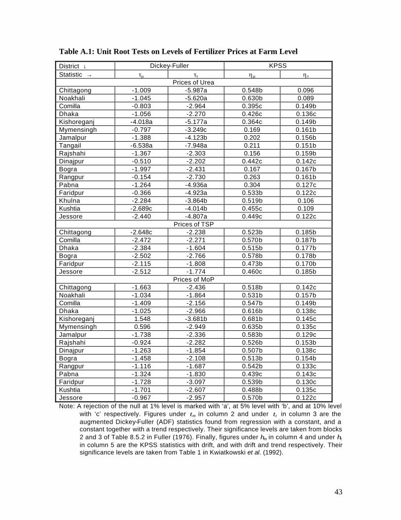
43

Table A.1: Unit Root Tests on Levels of Fertilizer Prices at Farm Level

District ↓ Dickey-Fuller KPSS Statistic → τµ ττ ηµ ητ

Prices of Urea Chittagong -1.009 -5.987a 0.548b 0.096 Noakhali -1.045 -5.620a 0.630b 0.089 Comilla -0.803 -2.964 0.395c 0.149b Dhaka -1.056 -2.270 0.426c 0.136c Kishoreganj -4.018a -5.177a 0.364c 0.149b Mymensingh -0.797 -3.249c 0.169 0.161b Jamalpur -1.388 -4.123b 0.202 0.156b Tangail -6.538a -7.948a 0.211 0.151b Rajshahi -1.367 -2.303 0.156 0.159b Dinajpur -0.510 -2.202 0.442c 0.142c Bogra -1.997 -2.431 0.167 0.167b Rangpur -0.154 -2.730 0.263 0.161b Pabna -1.264 -4.936a 0.304 0.127c Faridpur -0.366 -4.923a 0.533b 0.122c Khulna -2.284 -3.864b 0.519b 0.106 Kushtia -2.689c -4.014b 0.455c 0.109 Jessore -2.440 -4.807a 0.449c 0.122c

Prices of TSP Chittagong -2.648c -2.238 0.523b 0.185b Comilla -2.472 -2.271 0.570b 0.187b Dhaka -2.384 -1.604 0.515b 0.177b Bogra -2.502 -2.766 0.578b 0.178b Faridpur -2.115 -1.808 0.473b 0.170b Jessore -2.512 -1.774 0.460c 0.185b

Prices of MoP Chittagong -1.663 -2.436 0.518b 0.142c Noakhali -1.034 -1.864 0.531b 0.157b Comilla -1.409 -2.156 0.547b 0.149b Dhaka -1.025 -2.966 0.616b 0.138c Kishoreganj 1.548 -3.681b 0.681b 0.145c Mymensingh 0.596 -2.949 0.635b 0.135c Jamalpur -1.738 -2.336 0.583b 0.129c Rajshahi -0.924 -2.282 0.526b 0.153b Dinajpur -1.263 -1.854 0.507b 0.138c Bogra -1.458 -2.108 0.513b 0.154b Rangpur -1.116 -1.687 0.542b 0.133c Pabna -1.324 -1.830 0.439c 0.143c Faridpur -1.728 -3.097 0.539b 0.130c Kushtia -1.701 -2.607 0.488b 0.135c Jessore -0.967 -2.957 0.570b 0.122c Note: A rejection of the null at 1% level is marked with ‘a’, at 5% level with ‘b’, and at 10% level

with ‘c’ respectively. Figures under τµ in column 2 and under ττ in column 3 are the augmented Dickey-Fuller (ADF) statistics found from regression with a constant, and a constant together with a trend respectively. Their significance levels are taken from blocks 2 and 3 of Table 8.5.2 in Fuller (1976). Finally, figures under ηµ in column 4 and under ητ in column 5 are the KPSS statistics with drift, and with drift and trend respectively. Their significance levels are taken from Table 1 in Kwiatkowski et al. (1992).

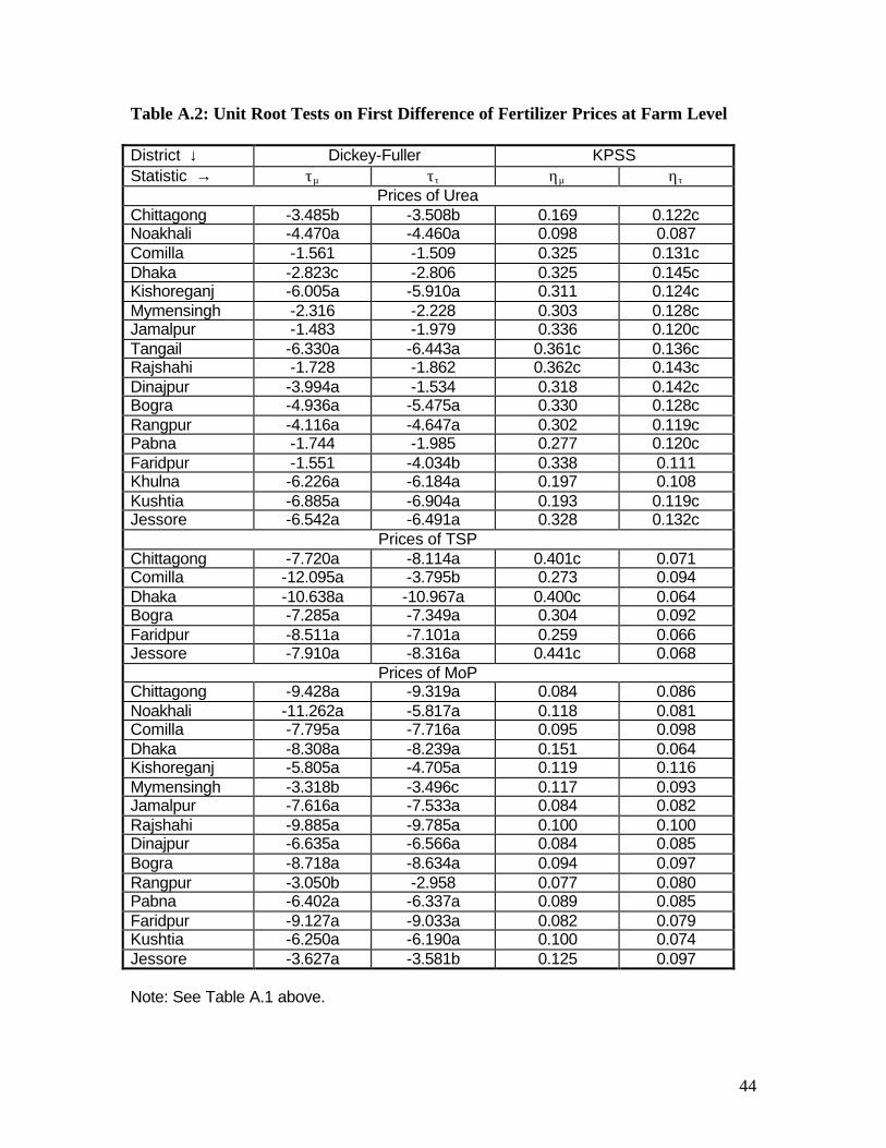
44

Table A.2: Unit Root Tests on First Difference of Fertilizer Prices at Farm Level District ↓ Dickey-Fuller KPSS Statistic → τµ ττ ηµ ητ

Prices of Urea Chittagong -3.485b -3.508b 0.169 0.122c Noakhali -4.470a -4.460a 0.098 0.087 Comilla -1.561 -1.509 0.325 0.131c Dhaka -2.823c -2.806 0.325 0.145c Kishoreganj -6.005a -5.910a 0.311 0.124c Mymensingh -2.316 -2.228 0.303 0.128c Jamalpur -1.483 -1.979 0.336 0.120c Tangail -6.330a -6.443a 0.361c 0.136c Rajshahi -1.728 -1.862 0.362c 0.143c Dinajpur -3.994a -1.534 0.318 0.142c Bogra -4.936a -5.475a 0.330 0.128c Rangpur -4.116a -4.647a 0.302 0.119c Pabna -1.744 -1.985 0.277 0.120c Faridpur -1.551 -4.034b 0.338 0.111 Khulna -6.226a -6.184a 0.197 0.108 Kushtia -6.885a -6.904a 0.193 0.119c Jessore -6.542a -6.491a 0.328 0.132c

Prices of TSP Chittagong -7.720a -8.114a 0.401c 0.071 Comilla -12.095a -3.795b 0.273 0.094 Dhaka -10.638a -10.967a 0.400c 0.064 Bogra -7.285a -7.349a 0.304 0.092 Faridpur -8.511a -7.101a 0.259 0.066 Jessore -7.910a -8.316a 0.441c 0.068

Prices of MoP Chittagong -9.428a -9.319a 0.084 0.086 Noakhali -11.262a -5.817a 0.118 0.081 Comilla -7.795a -7.716a 0.095 0.098 Dhaka -8.308a -8.239a 0.151 0.064 Kishoreganj -5.805a -4.705a 0.119 0.116 Mymensingh -3.318b -3.496c 0.117 0.093 Jamalpur -7.616a -7.533a 0.084 0.082 Rajshahi -9.885a -9.785a 0.100 0.100 Dinajpur -6.635a -6.566a 0.084 0.085 Bogra -8.718a -8.634a 0.094 0.097 Rangpur -3.050b -2.958 0.077 0.080 Pabna -6.402a -6.337a 0.089 0.085 Faridpur -9.127a -9.033a 0.082 0.079 Kushtia -6.250a -6.190a 0.100 0.074 Jessore -3.627a -3.581b 0.125 0.097 Note: See Table A.1 above.

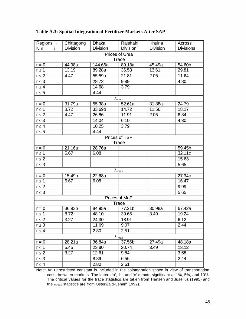
45

Table A.3: Spatial Integration of Fertilizer Markets After SAP Regions → Null ↓

Chittagong Division

Dhaka Division

Rajshahi Division

Khulna Division

Across Divisions

Prices of Urea Trace

r = 0 44.98a 144.66a 89.13a 45.49a 54.60b r ≤ 1 13.19 89.28a 36.53 13.61 29.81 r ≤ 2 4.47 55.59a 21.81 2.05 11.64 r ≤ 3 28.72 9.89 4.80 r ≤ 4 14.68 3.79 r ≤ 5 4.44

λ-max r = 0 31.79a 55.38a 52.61a 31.88a 24.79 r ≤ 1 8.72 33.69b 14.72 11.56 18.17 r ≤ 2 4.47 26.86 11.91 2.05 6.84 r ≤ 3 14.04 6.10 4.80 r ≤ 4 10.25 3.79 r ≤ 5 4.44

Prices of TSP Trace

r = 0 21.16a 28.76a 59.45b r ≤ 1 5.67 6.08 32.11c r ≤ 2 15.63 r ≤ 3 5.65

λ-max r = 0 15.49b 22.68a 27.34c r ≤ 1 5.67 6.08 16.47 r ≤ 2 9.99 r ≤ 3 5.65

Prices of MoP Trace

r = 0 36.93b 84.95a 77.21b 30.98a 67.42a r ≤ 1 8.72 48.10 39.65 3.49 19.24 r ≤ 2 3.27 24.30 18.91 6.12 r ≤ 3 11.69 9.07 2.44 r ≤ 4 2.80 2.51

λ-max r = 0 28.21a 36.84a 37.56b 27.49a 48.18a r ≤ 1 5.45 23.80 20.74 3.49 13.12 r ≤ 2 3.27 12.61 9.84 3.68 r ≤ 3 8.89 6.56 2.44 r ≤ 4 2.80 2.51 Note: An unrestricted constant is included in the cointegration space in view of transportation

costs between markets. The letters ‘a’, ‘b’, and ‘c’ denote significant at 1%, 5%, and 10%. The critical values for the trace statistics are taken from Hansen and Juselius (1995) and the λ-max statistics are from Osterwald-Lenum(1992).

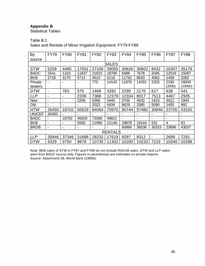
46

Appendix B Statistical Tables Table B.1 Sales and Rentals of Minor Irrigation Equipment, FY79-FY88 By source

FY79 FY80 FY81 FY82 FY83 FY84 FY85 FY86 FY87 FY88

SALES STW 5259 4485 17551 27100 39055 30626 30602 8432 16307 35179 BADC 2541 1315 11837 21815 18796 6988 7678 2045 12519 15097 BKB 2718 3170 5714 4510 6116 11762 8633 4062 1458 2082 Private dealers

- - - 775 14143 11876 14291 2325 2330 (2000)

18000 (10000)

DTW - 763 575 1468 3282 2290 2170 617 638 541 LLP - - 2206 7388 12379 12334 8017 7513 4467 2935 New - - 2206 5366 5445 3705 4632 2423 3012 1943 Old - - - 2022 6934 8629 3385 5090 1455 992 HTW 26450 18702 50529 84064 70970 90744 57480 30846 23700 43100 UNICEF 26450 - - - - - - - - - BADC - 18702 45029 72068 49821 - - - - - BKB - - 5500 11996 21149 29878 19144 531 4 63 BRDB - - - - - 60866 38336 30315 23696 43037

RENTALS LLP 35846 37346 31688 28232 17619 9297 8312 - 2699 7291 DTW 9329 9750 9878 10735 11302 10200 10233 7219 10240 10288 Note: BKB sales of STW in FY87 and FY88 do not include RAKUB sales. DTW and LLP sales were from BADC source only. Figures in parentheses are estimates on private imports. Source: Attachment 38, World Bank (1990b).

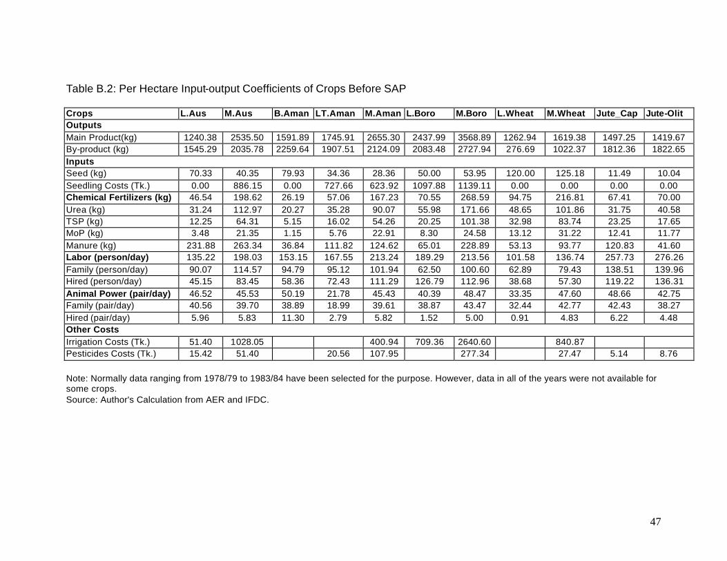
47

Table B.2: Per Hectare Input-output Coefficients of Crops Before SAP Crops L.Aus M.Aus B.Aman LT.Aman M.Aman L.Boro M.Boro L.Wheat M.Wheat Jute_Cap Jute-Olit Outputs Main Product(kg) 1240.38 2535.50 1591.89 1745.91 2655.30 2437.99 3568.89 1262.94 1619.38 1497.25 1419.67 By-product (kg) 1545.29 2035.78 2259.64 1907.51 2124.09 2083.48 2727.94 276.69 1022.37 1812.36 1822.65 Inputs Seed (kg) 70.33 40.35 79.93 34.36 28.36 50.00 53.95 120.00 125.18 11.49 10.04 Seedling Costs (Tk.) 0.00 886.15 0.00 727.66 623.92 1097.88 1139.11 0.00 0.00 0.00 0.00 Chemical Fertilizers (kg) 46.54 198.62 26.19 57.06 167.23 70.55 268.59 94.75 216.81 67.41 70.00 Urea (kg) 31.24 112.97 20.27 35.28 90.07 55.98 171.66 48.65 101.86 31.75 40.58 TSP (kg) 12.25 64.31 5.15 16.02 54.26 20.25 101.38 32.98 83.74 23.25 17.65 MoP (kg) 3.48 21.35 1.15 5.76 22.91 8.30 24.58 13.12 31.22 12.41 11.77 Manure (kg) 231.88 263.34 36.84 111.82 124.62 65.01 228.89 53.13 93.77 120.83 41.60 Labor (person/day) 135.22 198.03 153.15 167.55 213.24 189.29 213.56 101.58 136.74 257.73 276.26 Family (person/day) 90.07 114.57 94.79 95.12 101.94 62.50 100.60 62.89 79.43 138.51 139.96 Hired (person/day) 45.15 83.45 58.36 72.43 111.29 126.79 112.96 38.68 57.30 119.22 136.31 Animal Power (pair/day) 46.52 45.53 50.19 21.78 45.43 40.39 48.47 33.35 47.60 48.66 42.75 Family (pair/day) 40.56 39.70 38.89 18.99 39.61 38.87 43.47 32.44 42.77 42.43 38.27 Hired (pair/day) 5.96 5.83 11.30 2.79 5.82 1.52 5.00 0.91 4.83 6.22 4.48 Other Costs Irrigation Costs (Tk.) 51.40 1028.05 400.94 709.36 2640.60 840.87 Pesticides Costs (Tk.) 15.42 51.40 20.56 107.95 277.34 27.47 5.14 8.76

Note: Normally data ranging from 1978/79 to 1983/84 have been selected for the purpose. However, data in all of the years were not available for some crops. Source: Author's Calculation from AER and IFDC.

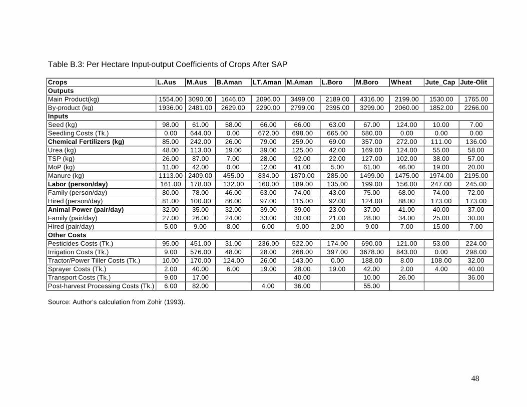
48

Table B.3: Per Hectare Input-output Coefficients of Crops After SAP Crops L.Aus M.Aus B.Aman LT.Aman M.Aman L.Boro M.Boro Wheat Jute_Cap Jute-Olit Outputs Main Product(kg) 1554.00 3090.00 1646.00 2096.00 3499.00 2189.00 4316.00 2199.00 1530.00 1765.00 By-product (kg) 1936.00 2481.00 2629.00 2290.00 2799.00 2395.00 3299.00 2060.00 1852.00 2266.00 Inputs Seed (kg) 98.00 61.00 58.00 66.00 66.00 63.00 67.00 124.00 10.00 7.00 Seedling Costs (Tk.) 0.00 644.00 0.00 672.00 698.00 665.00 680.00 0.00 0.00 0.00 Chemical Fertilizers (kg) 85.00 242.00 26.00 79.00 259.00 69.00 357.00 272.00 111.00 136.00 Urea (kg) 48.00 113.00 19.00 39.00 125.00 42.00 169.00 124.00 55.00 58.00 TSP (kg) 26.00 87.00 7.00 28.00 92.00 22.00 127.00 102.00 38.00 57.00 MoP (kg) 11.00 42.00 0.00 12.00 41.00 5.00 61.00 46.00 19.00 20.00 Manure (kg) 1113.00 2409.00 455.00 834.00 1870.00 285.00 1499.00 1475.00 1974.00 2195.00 Labor (person/day) 161.00 178.00 132.00 160.00 189.00 135.00 199.00 156.00 247.00 245.00 Family (person/day) 80.00 78.00 46.00 63.00 74.00 43.00 75.00 68.00 74.00 72.00 Hired (person/day) 81.00 100.00 86.00 97.00 115.00 92.00 124.00 88.00 173.00 173.00 Animal Power (pair/day) 32.00 35.00 32.00 39.00 39.00 23.00 37.00 41.00 40.00 37.00 Family (pair/day) 27.00 26.00 24.00 33.00 30.00 21.00 28.00 34.00 25.00 30.00 Hired (pair/day) 5.00 9.00 8.00 6.00 9.00 2.00 9.00 7.00 15.00 7.00 Other Costs Pesticides Costs (Tk.) 95.00 451.00 31.00 236.00 522.00 174.00 690.00 121.00 53.00 224.00 Irrigation Costs (Tk.) 9.00 576.00 48.00 28.00 268.00 397.00 3678.00 843.00 0.00 298.00 Tractor/Power Tiller Costs (Tk.) 10.00 170.00 124.00 26.00 143.00 0.00 188.00 8.00 108.00 32.00 Sprayer Costs (Tk.) 2.00 40.00 6.00 19.00 28.00 19.00 42.00 2.00 4.00 40.00 Transport Costs (Tk.) 9.00 17.00 40.00 10.00 26.00 36.00 Post-harvest Processing Costs (Tk.) 6.00 82.00 4.00 36.00 55.00 Source: Author's calculation from Zohir (1993).

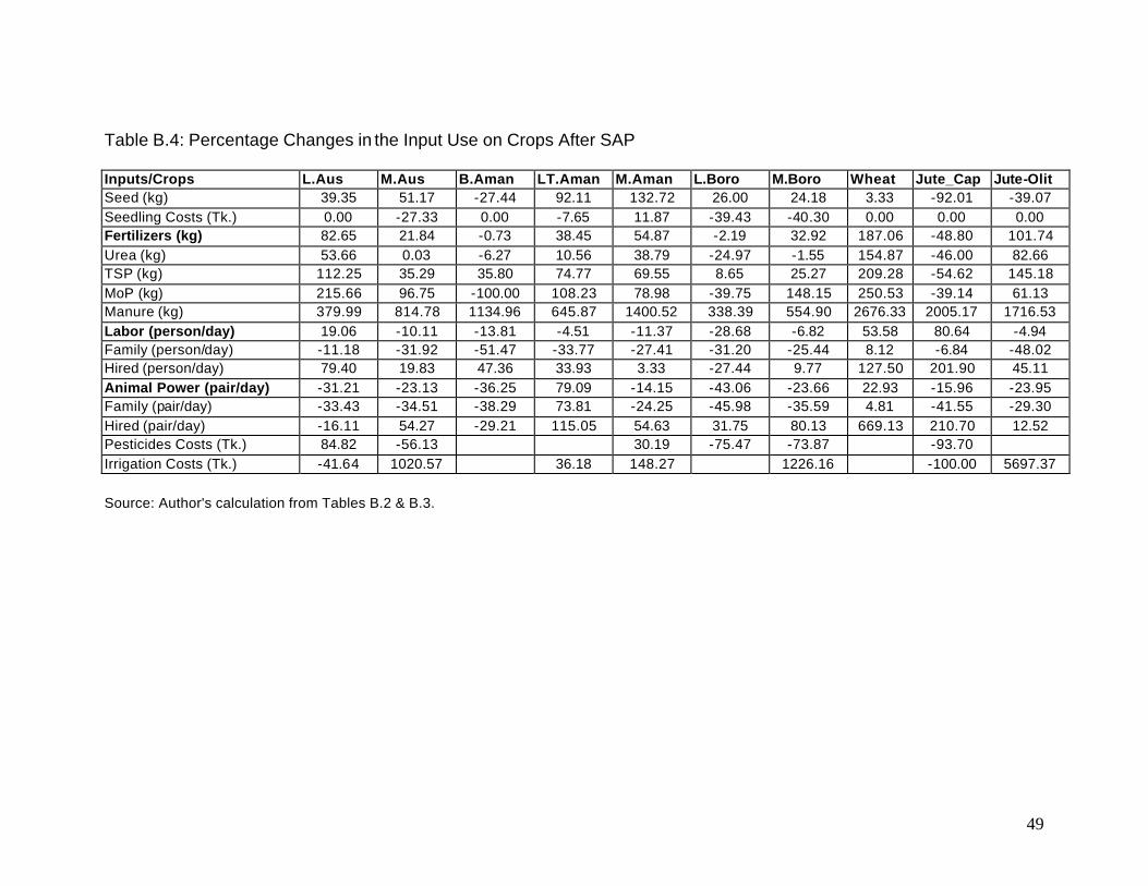
49

Table B.4: Percentage Changes in the Input Use on Crops After SAP Inputs/Crops L.Aus M.Aus B.Aman LT.Aman M.Aman L.Boro M.Boro Wheat Jute_Cap Jute-Olit Seed (kg) 39.35 51.17 -27.44 92.11 132.72 26.00 24.18 3.33 -92.01 -39.07 Seedling Costs (Tk.) 0.00 -27.33 0.00 -7.65 11.87 -39.43 -40.30 0.00 0.00 0.00 Fertilizers (kg) 82.65 21.84 -0.73 38.45 54.87 -2.19 32.92 187.06 -48.80 101.74 Urea (kg) 53.66 0.03 -6.27 10.56 38.79 -24.97 -1.55 154.87 -46.00 82.66 TSP (kg) 112.25 35.29 35.80 74.77 69.55 8.65 25.27 209.28 -54.62 145.18 MoP (kg) 215.66 96.75 -100.00 108.23 78.98 -39.75 148.15 250.53 -39.14 61.13 Manure (kg) 379.99 814.78 1134.96 645.87 1400.52 338.39 554.90 2676.33 2005.17 1716.53 Labor (person/day) 19.06 -10.11 -13.81 -4.51 -11.37 -28.68 -6.82 53.58 80.64 -4.94 Family (person/day) -11.18 -31.92 -51.47 -33.77 -27.41 -31.20 -25.44 8.12 -6.84 -48.02 Hired (person/day) 79.40 19.83 47.36 33.93 3.33 -27.44 9.77 127.50 201.90 45.11 Animal Power (pair/day) -31.21 -23.13 -36.25 79.09 -14.15 -43.06 -23.66 22.93 -15.96 -23.95 Family (pair/day) -33.43 -34.51 -38.29 73.81 -24.25 -45.98 -35.59 4.81 -41.55 -29.30 Hired (pair/day) -16.11 54.27 -29.21 115.05 54.63 31.75 80.13 669.13 210.70 12.52 Pesticides Costs (Tk.) 84.82 -56.13 30.19 -75.47 -73.87 -93.70 Irrigation Costs (Tk.) -41.64 1020.57 36.18 148.27 1226.16 -100.00 5697.37

Source: Author's calculation from Tables B.2 & B.3.

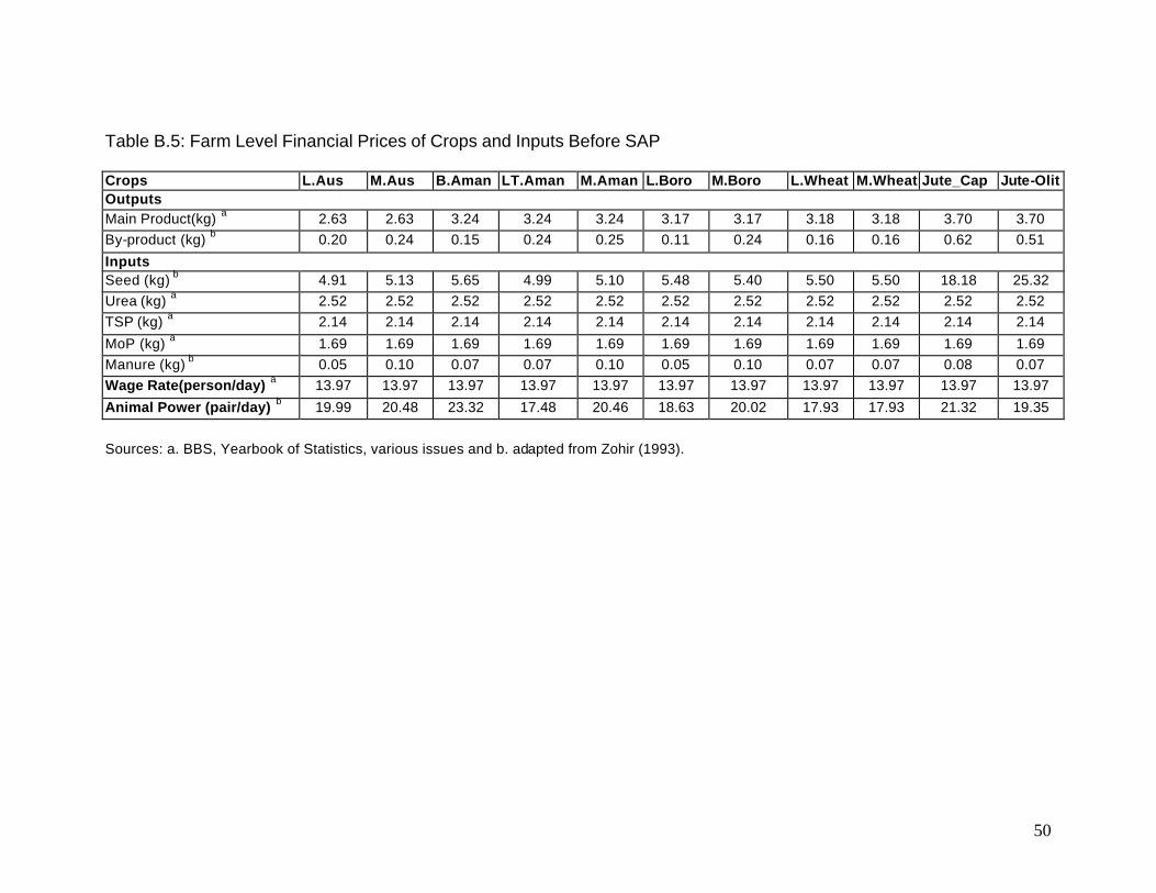
50

Table B.5: Farm Level Financial Prices of Crops and Inputs Before SAP Crops L.Aus M.Aus B.Aman LT.Aman M.Aman L.Boro M.Boro L.Wheat M.Wheat Jute_Cap Jute-Olit Outputs Main Product(kg) a 2.63 2.63 3.24 3.24 3.24 3.17 3.17 3.18 3.18 3.70 3.70

By-product (kg) b 0.20 0.24 0.15 0.24 0.25 0.11 0.24 0.16 0.16 0.62 0.51

Inputs Seed (kg) b 4.91 5.13 5.65 4.99 5.10 5.48 5.40 5.50 5.50 18.18 25.32

Urea (kg) a 2.52 2.52 2.52 2.52 2.52 2.52 2.52 2.52 2.52 2.52 2.52

TSP (kg) a 2.14 2.14 2.14 2.14 2.14 2.14 2.14 2.14 2.14 2.14 2.14

MoP (kg) a 1.69 1.69 1.69 1.69 1.69 1.69 1.69 1.69 1.69 1.69 1.69

Manure (kg) b 0.05 0.10 0.07 0.07 0.10 0.05 0.10 0.07 0.07 0.08 0.07

Wage Rate(person/day) a 13.97 13.97 13.97 13.97 13.97 13.97 13.97 13.97 13.97 13.97 13.97

Animal Power (pair/day) b 19.99 20.48 23.32 17.48 20.46 18.63 20.02 17.93 17.93 21.32 19.35

Sources: a. BBS, Yearbook of Statistics, various issues and b. adapted from Zohir (1993).

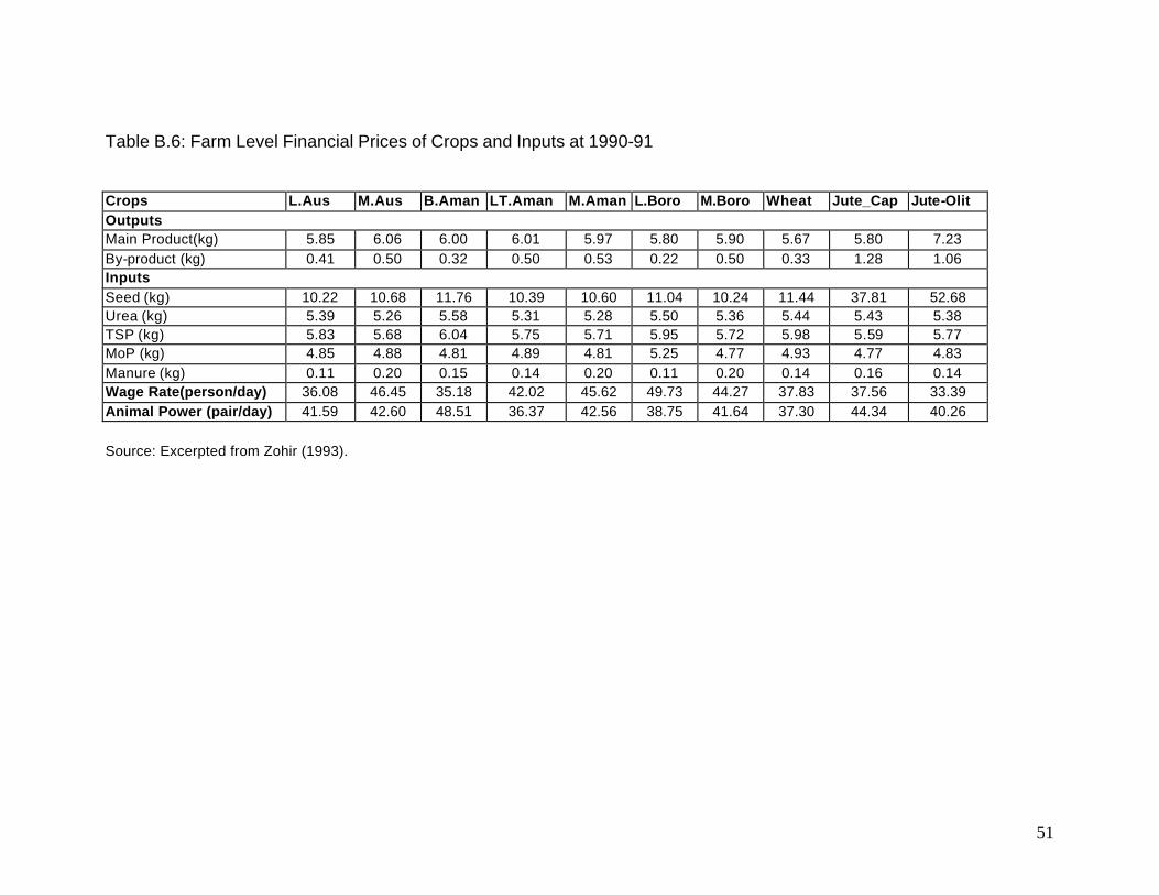
51

Table B.6: Farm Level Financial Prices of Crops and Inputs at 1990-91 Crops L.Aus M.Aus B.Aman LT.Aman M.Aman L.Boro M.Boro Wheat Jute_Cap Jute-Olit Outputs Main Product(kg) 5.85 6.06 6.00 6.01 5.97 5.80 5.90 5.67 5.80 7.23 By-product (kg) 0.41 0.50 0.32 0.50 0.53 0.22 0.50 0.33 1.28 1.06 Inputs Seed (kg) 10.22 10.68 11.76 10.39 10.60 11.04 10.24 11.44 37.81 52.68 Urea (kg) 5.39 5.26 5.58 5.31 5.28 5.50 5.36 5.44 5.43 5.38 TSP (kg) 5.83 5.68 6.04 5.75 5.71 5.95 5.72 5.98 5.59 5.77 MoP (kg) 4.85 4.88 4.81 4.89 4.81 5.25 4.77 4.93 4.77 4.83 Manure (kg) 0.11 0.20 0.15 0.14 0.20 0.11 0.20 0.14 0.16 0.14 Wage Rate(person/day) 36.08 46.45 35.18 42.02 45.62 49.73 44.27 37.83 37.56 33.39 Animal Power (pair/day) 41.59 42.60 48.51 36.37 42.56 38.75 41.64 37.30 44.34 40.26

Source: Excerpted from Zohir (1993).

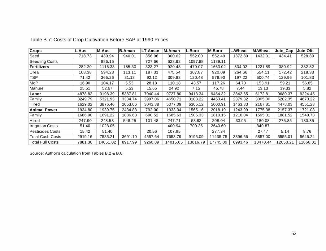
52

Table B.7: Costs of Crop Cultivation Before SAP at 1990 Prices Crops L.Aus M.Aus B.Aman LT.Aman M.Aman L.Boro M.Boro L.Wheat M.Wheat Jute_Cap Jute-Olit Seed 718.73 430.94 940.01 356.96 300.62 552.00 552.49 1372.80 1432.01 434.41 528.89 Seedling Costs 886.15 727.66 623.92 1097.88 1139.11 Fertilizers 282.20 1116.33 155.30 323.27 920.48 479.07 1663.02 534.02 1221.89 380.92 382.82 Urea 168.38 594.23 113.11 187.31 475.54 307.87 920.09 264.66 554.11 172.42 218.33 TSP 71.42 365.26 31.13 92.12 309.83 120.48 579.90 197.22 500.74 129.96 101.83 MoP 16.90 104.17 5.53 28.18 110.18 43.57 117.26 64.70 153.91 59.21 56.85 Manure 25.51 52.67 5.53 15.65 24.92 7.15 45.78 7.44 13.13 19.33 5.82 Labor 4878.82 9198.39 5387.81 7040.44 9727.80 9413.34 9454.32 3842.65 5172.81 9680.37 9224.45 Family 3249.79 5321.93 3334.74 3997.06 4650.71 3108.22 4453.41 2379.32 3005.00 5202.35 4673.22 Hired 1629.02 3876.46 2053.06 3043.38 5077.09 6305.12 5000.91 1463.33 2167.81 4478.03 4551.23 Animal Power 1934.80 1939.75 2434.88 792.00 1933.34 1565.16 2018.19 1243.99 1775.38 2157.37 1721.08 Family 1686.90 1691.22 1886.63 690.52 1685.63 1506.33 1810.15 1210.04 1595.31 1881.52 1540.73 Hired 247.90 248.53 548.25 101.48 247.71 58.82 208.04 33.95 180.08 275.85 180.35 Irrigation Costs 51.40 1028.05 400.94 709.36 2640.60 840.87 Pesticides Costs 15.42 51.40 20.56 107.95 277.34 27.47 5.14 8.76 Total Cash Costs 2919.16 7585.21 3691.10 4557.64 7653.79 9195.09 11435.75 3396.66 5857.00 5555.01 5646.24 Total Full Costs 7881.36 14651.02 8917.99 9260.89 14015.05 13816.79 17745.09 6993.46 10470.44 12658.21 11866.01

Source: Author's calculation from Tables B.2 & B.6.

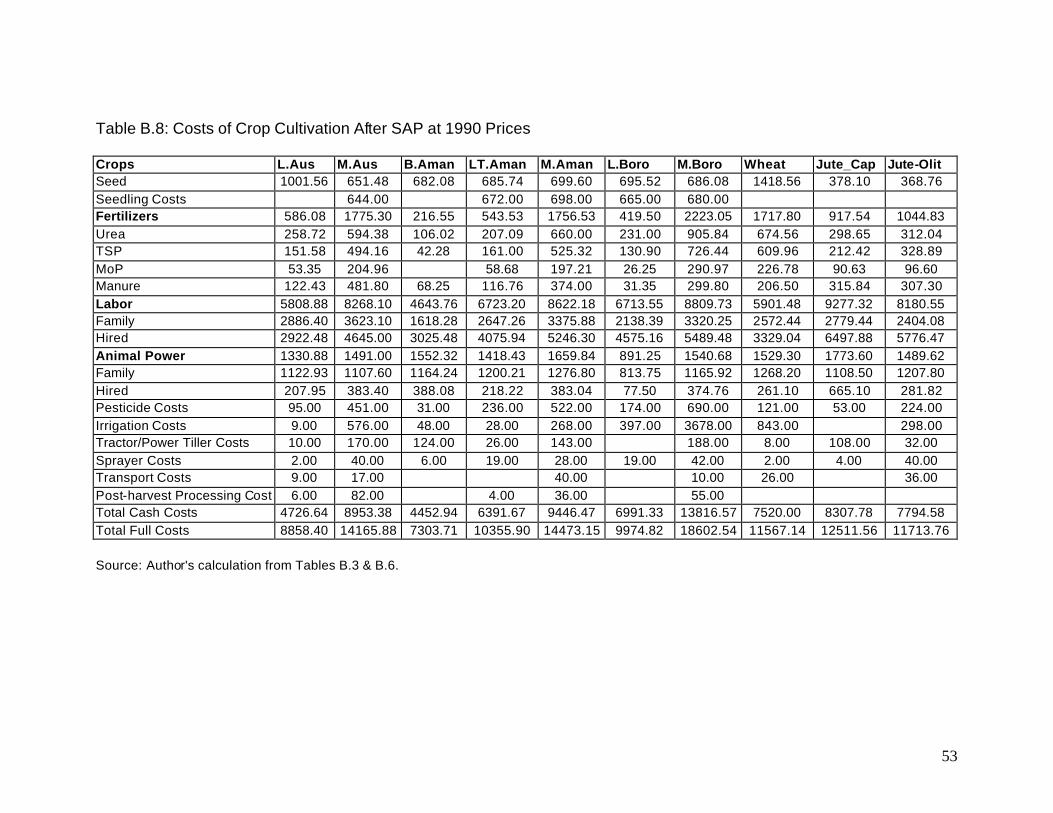
53

Table B.8: Costs of Crop Cultivation After SAP at 1990 Prices Crops L.Aus M.Aus B.Aman LT.Aman M.Aman L.Boro M.Boro Wheat Jute_Cap Jute-Olit Seed 1001.56 651.48 682.08 685.74 699.60 695.52 686.08 1418.56 378.10 368.76 Seedling Costs 644.00 672.00 698.00 665.00 680.00 Fertilizers 586.08 1775.30 216.55 543.53 1756.53 419.50 2223.05 1717.80 917.54 1044.83 Urea 258.72 594.38 106.02 207.09 660.00 231.00 905.84 674.56 298.65 312.04 TSP 151.58 494.16 42.28 161.00 525.32 130.90 726.44 609.96 212.42 328.89 MoP 53.35 204.96 58.68 197.21 26.25 290.97 226.78 90.63 96.60 Manure 122.43 481.80 68.25 116.76 374.00 31.35 299.80 206.50 315.84 307.30 Labor 5808.88 8268.10 4643.76 6723.20 8622.18 6713.55 8809.73 5901.48 9277.32 8180.55 Family 2886.40 3623.10 1618.28 2647.26 3375.88 2138.39 3320.25 2572.44 2779.44 2404.08 Hired 2922.48 4645.00 3025.48 4075.94 5246.30 4575.16 5489.48 3329.04 6497.88 5776.47 Animal Power 1330.88 1491.00 1552.32 1418.43 1659.84 891.25 1540.68 1529.30 1773.60 1489.62 Family 1122.93 1107.60 1164.24 1200.21 1276.80 813.75 1165.92 1268.20 1108.50 1207.80 Hired 207.95 383.40 388.08 218.22 383.04 77.50 374.76 261.10 665.10 281.82 Pesticide Costs 95.00 451.00 31.00 236.00 522.00 174.00 690.00 121.00 53.00 224.00 Irrigation Costs 9.00 576.00 48.00 28.00 268.00 397.00 3678.00 843.00 298.00 Tractor/Power Tiller Costs 10.00 170.00 124.00 26.00 143.00 188.00 8.00 108.00 32.00 Sprayer Costs 2.00 40.00 6.00 19.00 28.00 19.00 42.00 2.00 4.00 40.00 Transport Costs 9.00 17.00 40.00 10.00 26.00 36.00 Post-harvest Processing Cost 6.00 82.00 4.00 36.00 55.00 Total Cash Costs 4726.64 8953.38 4452.94 6391.67 9446.47 6991.33 13816.57 7520.00 8307.78 7794.58 Total Full Costs 8858.40 14165.88 7303.71 10355.90 14473.15 9974.82 18602.54 11567.14 12511.56 11713.76

Source: Author's calculation from Tables B.3 & B.6.

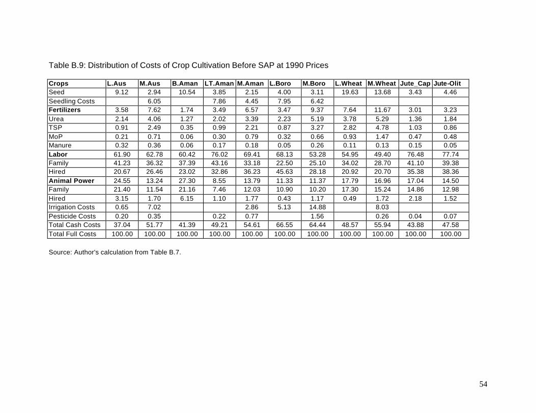
54

Table B.9: Distribution of Costs of Crop Cultivation Before SAP at 1990 Prices Crops L.Aus M.Aus B.Aman LT.Aman M.Aman L.Boro M.Boro L.Wheat M.Wheat Jute_Cap Jute-Olit Seed 9.12 2.94 10.54 3.85 2.15 4.00 3.11 19.63 13.68 3.43 4.46 Seedling Costs 6.05 7.86 4.45 7.95 6.42 Fertilizers 3.58 7.62 1.74 3.49 6.57 3.47 9.37 7.64 11.67 3.01 3.23 Urea 2.14 4.06 1.27 2.02 3.39 2.23 5.19 3.78 5.29 1.36 1.84 TSP 0.91 2.49 0.35 0.99 2.21 0.87 3.27 2.82 4.78 1.03 0.86 MoP 0.21 0.71 0.06 0.30 0.79 0.32 0.66 0.93 1.47 0.47 0.48 Manure 0.32 0.36 0.06 0.17 0.18 0.05 0.26 0.11 0.13 0.15 0.05 Labor 61.90 62.78 60.42 76.02 69.41 68.13 53.28 54.95 49.40 76.48 77.74 Family 41.23 36.32 37.39 43.16 33.18 22.50 25.10 34.02 28.70 41.10 39.38 Hired 20.67 26.46 23.02 32.86 36.23 45.63 28.18 20.92 20.70 35.38 38.36 Animal Power 24.55 13.24 27.30 8.55 13.79 11.33 11.37 17.79 16.96 17.04 14.50 Family 21.40 11.54 21.16 7.46 12.03 10.90 10.20 17.30 15.24 14.86 12.98 Hired 3.15 1.70 6.15 1.10 1.77 0.43 1.17 0.49 1.72 2.18 1.52 Irrigation Costs 0.65 7.02 2.86 5.13 14.88 8.03 Pesticide Costs 0.20 0.35 0.22 0.77 1.56 0.26 0.04 0.07 Total Cash Costs 37.04 51.77 41.39 49.21 54.61 66.55 64.44 48.57 55.94 43.88 47.58 Total Full Costs 100.00 100.00 100.00 100.00 100.00 100.00 100.00 100.00 100.00 100.00 100.00

Source: Author's calculation from Table B.7.

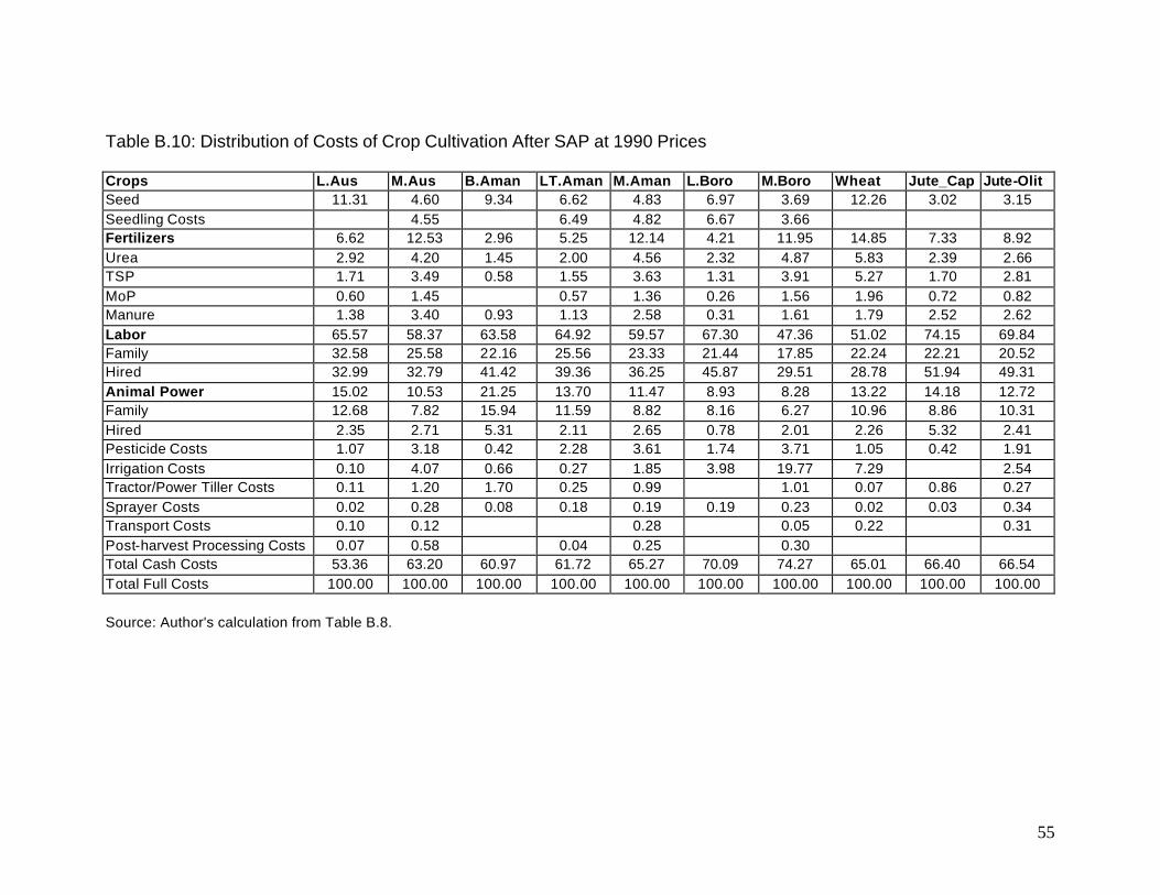
55

Table B.10: Distribution of Costs of Crop Cultivation After SAP at 1990 Prices Crops L.Aus M.Aus B.Aman LT.Aman M.Aman L.Boro M.Boro Wheat Jute_Cap Jute-Olit Seed 11.31 4.60 9.34 6.62 4.83 6.97 3.69 12.26 3.02 3.15 Seedling Costs 4.55 6.49 4.82 6.67 3.66 Fertilizers 6.62 12.53 2.96 5.25 12.14 4.21 11.95 14.85 7.33 8.92 Urea 2.92 4.20 1.45 2.00 4.56 2.32 4.87 5.83 2.39 2.66 TSP 1.71 3.49 0.58 1.55 3.63 1.31 3.91 5.27 1.70 2.81 MoP 0.60 1.45 0.57 1.36 0.26 1.56 1.96 0.72 0.82 Manure 1.38 3.40 0.93 1.13 2.58 0.31 1.61 1.79 2.52 2.62 Labor 65.57 58.37 63.58 64.92 59.57 67.30 47.36 51.02 74.15 69.84 Family 32.58 25.58 22.16 25.56 23.33 21.44 17.85 22.24 22.21 20.52 Hired 32.99 32.79 41.42 39.36 36.25 45.87 29.51 28.78 51.94 49.31 Animal Power 15.02 10.53 21.25 13.70 11.47 8.93 8.28 13.22 14.18 12.72 Family 12.68 7.82 15.94 11.59 8.82 8.16 6.27 10.96 8.86 10.31 Hired 2.35 2.71 5.31 2.11 2.65 0.78 2.01 2.26 5.32 2.41 Pesticide Costs 1.07 3.18 0.42 2.28 3.61 1.74 3.71 1.05 0.42 1.91 Irrigation Costs 0.10 4.07 0.66 0.27 1.85 3.98 19.77 7.29 2.54 Tractor/Power Tiller Costs 0.11 1.20 1.70 0.25 0.99 1.01 0.07 0.86 0.27 Sprayer Costs 0.02 0.28 0.08 0.18 0.19 0.19 0.23 0.02 0.03 0.34 Transport Costs 0.10 0.12 0.28 0.05 0.22 0.31 Post-harvest Processing Costs 0.07 0.58 0.04 0.25 0.30 Total Cash Costs 53.36 63.20 60.97 61.72 65.27 70.09 74.27 65.01 66.40 66.54 Total Full Costs 100.00 100.00 100.00 100.00 100.00 100.00 100.00 100.00 100.00 100.00

Source: Author's calculation from Table B.8.

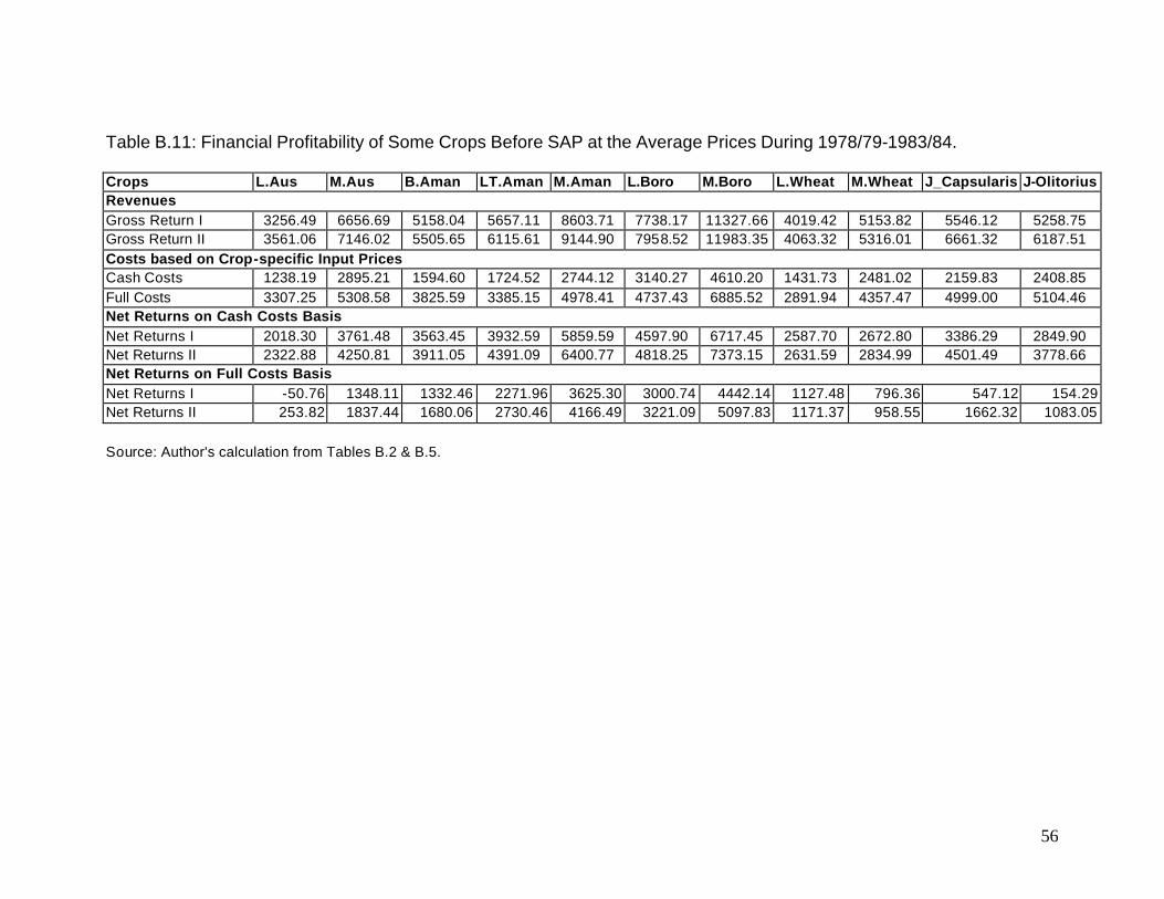
56

Table B.11: Financial Profitability of Some Crops Before SAP at the Average Prices During 1978/79-1983/84. Crops L.Aus M.Aus B.Aman LT.Aman M.Aman L.Boro M.Boro L.Wheat M.Wheat J_Capsularis J-Olitorius Revenues Gross Return I 3256.49 6656.69 5158.04 5657.11 8603.71 7738.17 11327.66 4019.42 5153.82 5546.12 5258.75 Gross Return II 3561.06 7146.02 5505.65 6115.61 9144.90 7958.52 11983.35 4063.32 5316.01 6661.32 6187.51 Costs based on Crop-specific Input Prices Cash Costs 1238.19 2895.21 1594.60 1724.52 2744.12 3140.27 4610.20 1431.73 2481.02 2159.83 2408.85 Full Costs 3307.25 5308.58 3825.59 3385.15 4978.41 4737.43 6885.52 2891.94 4357.47 4999.00 5104.46 Net Returns on Cash Costs Basis Net Returns I 2018.30 3761.48 3563.45 3932.59 5859.59 4597.90 6717.45 2587.70 2672.80 3386.29 2849.90 Net Returns II 2322.88 4250.81 3911.05 4391.09 6400.77 4818.25 7373.15 2631.59 2834.99 4501.49 3778.66 Net Returns on Full Costs Basis Net Returns I -50.76 1348.11 1332.46 2271.96 3625.30 3000.74 4442.14 1127.48 796.36 547.12 154.29 Net Returns II 253.82 1837.44 1680.06 2730.46 4166.49 3221.09 5097.83 1171.37 958.55 1662.32 1083.05

Source: Author's calculation from Tables B.2 & B.5.

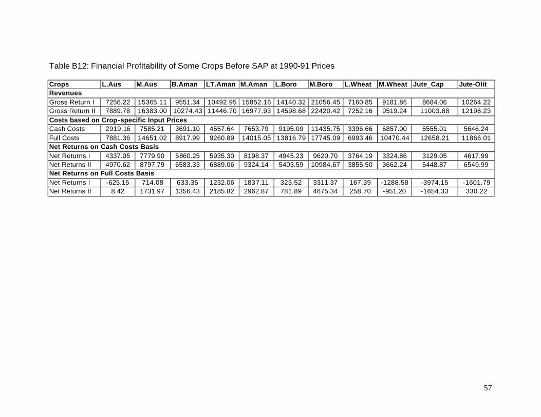
57

Table B12: Financial Profitability of Some Crops Before SAP at 1990-91 Prices Crops L.Aus M.Aus B.Aman LT.Aman M.Aman L.Boro M.Boro L.Wheat M.Wheat Jute_Cap Jute-Olit Revenues Gross Return I 7256.22 15365.11 9551.34 10492.95 15852.16 14140.32 21056.45 7160.85 9181.86 8684.06 10264.22 Gross Return II 7889.78 16383.00 10274.43 11446.70 16977.93 14598.68 22420.42 7252.16 9519.24 11003.88 12196.23 Costs based on Crop-specific Input Prices Cash Costs 2919.16 7585.21 3691.10 4557.64 7653.79 9195.09 11435.75 3396.66 5857.00 5555.01 5646.24 Full Costs 7881.36 14651.02 8917.99 9260.89 14015.05 13816.79 17745.09 6993.46 10470.44 12658.21 11866.01 Net Returns on Cash Costs Basis Net Returns I 4337.05 7779.90 5860.25 5935.30 8198.37 4945.23 9620.70 3764.19 3324.86 3129.05 4617.99 Net Returns II 4970.62 8797.79 6583.33 6889.06 9324.14 5403.59 10984.67 3855.50 3662.24 5448.87 6549.99 Net Returns on Full Costs Basis Net Returns I -625.15 714.08 633.35 1232.06 1837.11 323.52 3311.37 167.39 -1288.58 -3974.15 -1601.79 Net Returns II 8.42 1731.97 1356.43 2185.82 2962.87 781.89 4675.34 258.70 -951.20 -1654.33 330.22

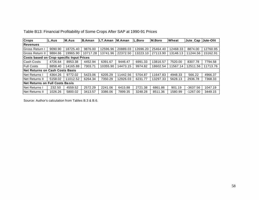
58

Table B13: Financial Profitability of Some Crops After SAP at 1990-91 Prices Crops L.Aus M.Aus B.Aman LT.Aman M.Aman L.Boro M.Boro Wheat Jute_Cap Jute-Olit Revenues Gross Return I 9090.90 18725.40 9876.00 12596.96 20889.03 12696.20 25464.40 12468.33 8874.00 12760.95 Gross Return II 9884.66 19965.90 10717.28 13741.96 22372.50 13223.10 27113.90 13148.13 11244.56 15162.91 Costs based on Crop-specific Input Prices Cash Costs 4726.64 8953.38 4452.94 6391.67 9446.47 6991.33 13816.57 7520.00 8307.78 7794.58 Full Costs 8858.40 14165.88 7303.71 10355.90 14473.15 9974.82 18602.54 11567.14 12511.56 11713.76 Net Returns on Cash Costs Basis Net Returns I 4364.26 9772.02 5423.06 6205.29 11442.56 5704.87 11647.83 4948.33 566.22 4966.37 Net Returns II 5158.02 11012.52 6264.34 7350.29 12926.03 6231.77 13297.33 5628.13 2936.78 7368.33 Net Returns on Full Costs Ba sis Net Returns I 232.50 4559.52 2572.29 2241.06 6415.88 2721.38 6861.86 901.19 -3637.56 1047.19 Net Returns II 1026.26 5800.02 3413.57 3386.06 7899.35 3248.28 8511.36 1580.99 -1267.00 3449.15

Source: Author's calculation from Tables B.3 & B.6.

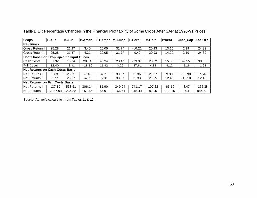
59

Table B.14: Percentage Changes in the Financial Profitability of Some Crops After SAP at 1990-91 Prices Crops L.Aus M.Aus B.Aman LT.Aman M.Aman L.Boro M.Boro Wheat Jute_Cap Jute-Olit Revenues Gross Return I 25.28 21.87 3.40 20.05 31.77 -10.21 20.93 13.15 2.19 24.32 Gross Return II 25.28 21.87 4.31 20.05 31.77 -9.42 20.93 14.20 2.19 24.32 Costs based on Crop-specific Input Prices Cash Costs 61.92 18.04 20.64 40.24 23.42 -23.97 20.82 15.63 49.55 38.05 Full Costs 12.40 -3.31 -18.10 11.82 3.27 -27.81 4.83 8.12 -1.16 -1.28 Net Returns on Cash Costs Basis Net Returns I 0.63 25.61 -7.46 4.55 39.57 15.36 21.07 9.90 -81.90 7.54 Net Returns II 3.77 25.17 -4.85 6.70 38.63 15.33 21.05 12.43 -46.10 12.49 Net Returns on Full Costs Basis Net Returns I -137.19 538.51 306.14 81.90 249.24 741.17 107.22 -65.19 -8.47 -165.38 Net Returns II 12087.94 234.88 151.66 54.91 166.61 315.44 82.05 -139.15 -23.41 944.50

Source: Author's calculation from Tables 11 & 12.

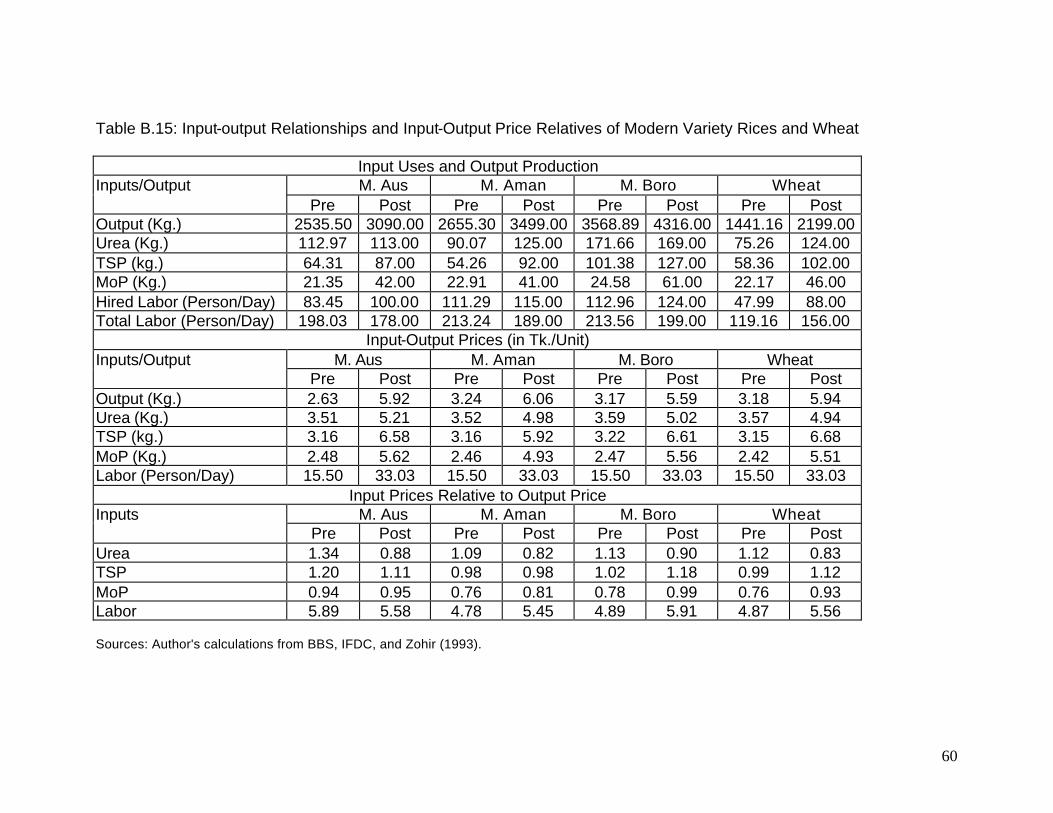
60

Table B.15: Input-output Relationships and Input-Output Price Relatives of Modern Variety Rices and Wheat

Input Uses and Output Production M. Aus M. Aman M. Boro Wheat Inputs/Output

Pre Post Pre Post Pre Post Pre Post Output (Kg.) 2535.50 3090.00 2655.30 3499.00 3568.89 4316.00 1441.16 2199.00 Urea (Kg.) 112.97 113.00 90.07 125.00 171.66 169.00 75.26 124.00 TSP (kg.) 64.31 87.00 54.26 92.00 101.38 127.00 58.36 102.00 MoP (Kg.) 21.35 42.00 22.91 41.00 24.58 61.00 22.17 46.00 Hired Labor (Person/Day) 83.45 100.00 111.29 115.00 112.96 124.00 47.99 88.00 Total Labor (Person/Day) 198.03 178.00 213.24 189.00 213.56 199.00 119.16 156.00

Input-Output Prices (in Tk./Unit) M. Aus M. Aman M. Boro Wheat Inputs/Output

Pre Post Pre Post Pre Post Pre Post Output (Kg.) 2.63 5.92 3.24 6.06 3.17 5.59 3.18 5.94 Urea (Kg.) 3.51 5.21 3.52 4.98 3.59 5.02 3.57 4.94 TSP (kg.) 3.16 6.58 3.16 5.92 3.22 6.61 3.15 6.68 MoP (Kg.) 2.48 5.62 2.46 4.93 2.47 5.56 2.42 5.51 Labor (Person/Day) 15.50 33.03 15.50 33.03 15.50 33.03 15.50 33.03

Input Prices Relative to Output Price M. Aus M. Aman M. Boro Wheat Inputs

Pre Post Pre Post Pre Post Pre Post Urea 1.34 0.88 1.09 0.82 1.13 0.90 1.12 0.83 TSP 1.20 1.11 0.98 0.98 1.02 1.18 0.99 1.12 MoP 0.94 0.95 0.76 0.81 0.78 0.99 0.76 0.93 Labor 5.89 5.58 4.78 5.45 4.89 5.91 4.87 5.56 Sources: Author's calculations from BBS, IFDC, and Zohir (1993).

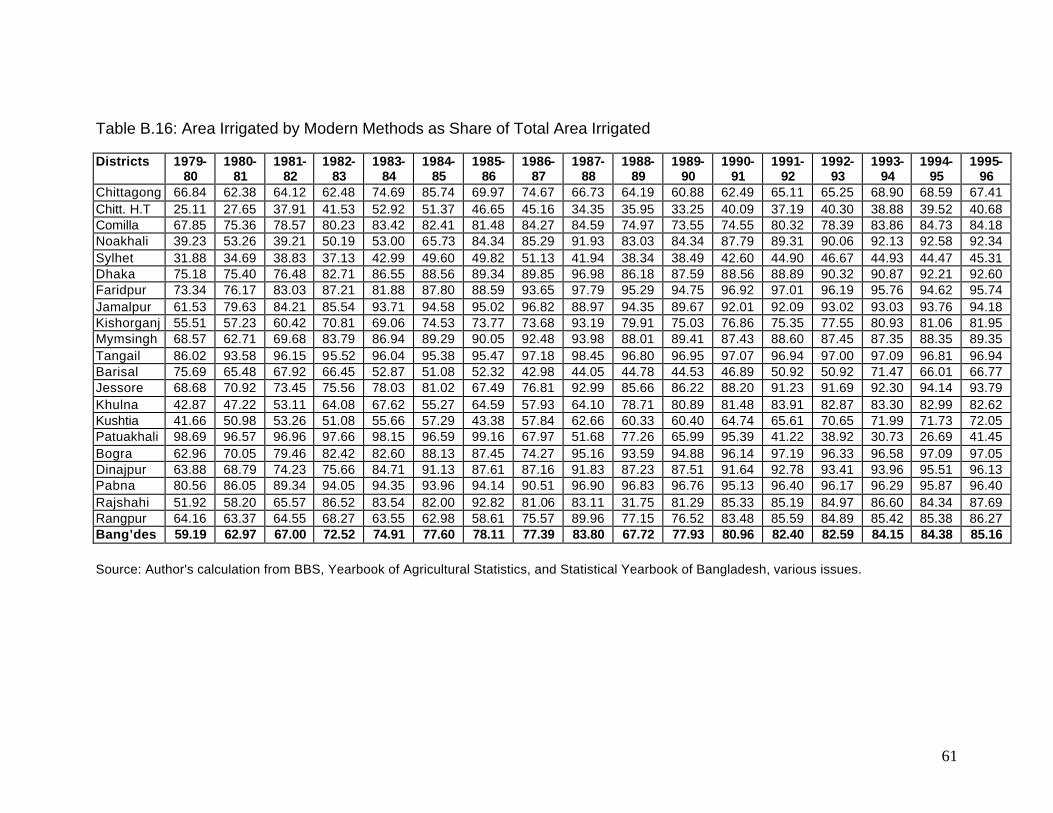
61

Table B.16: Area Irrigated by Modern Methods as Share of Total Area Irrigated Districts 1979-

80 1980-

81 1981-

82 1982-

83 1983-

84 1984-

85 1985-

86 1986-

87 1987-

88 1988-

89 1989-

90 1990-

91 1991-

92 1992-

93 1993-

94 1994-

95 1995-

96 Chittagong 66.84 62.38 64.12 62.48 74.69 85.74 69.97 74.67 66.73 64.19 60.88 62.49 65.11 65.25 68.90 68.59 67.41 Chitt. H.T 25.11 27.65 37.91 41.53 52.92 51.37 46.65 45.16 34.35 35.95 33.25 40.09 37.19 40.30 38.88 39.52 40.68 Comilla 67.85 75.36 78.57 80.23 83.42 82.41 81.48 84.27 84.59 74.97 73.55 74.55 80.32 78.39 83.86 84.73 84.18 Noakhali 39.23 53.26 39.21 50.19 53.00 65.73 84.34 85.29 91.93 83.03 84.34 87.79 89.31 90.06 92.13 92.58 92.34 Sylhet 31.88 34.69 38.83 37.13 42.99 49.60 49.82 51.13 41.94 38.34 38.49 42.60 44.90 46.67 44.93 44.47 45.31 Dhaka 75.18 75.40 76.48 82.71 86.55 88.56 89.34 89.85 96.98 86.18 87.59 88.56 88.89 90.32 90.87 92.21 92.60 Faridpur 73.34 76.17 83.03 87.21 81.88 87.80 88.59 93.65 97.79 95.29 94.75 96.92 97.01 96.19 95.76 94.62 95.74 Jamalpur 61.53 79.63 84.21 85.54 93.71 94.58 95.02 96.82 88.97 94.35 89.67 92.01 92.09 93.02 93.03 93.76 94.18 Kishorganj 55.51 57.23 60.42 70.81 69.06 74.53 73.77 73.68 93.19 79.91 75.03 76.86 75.35 77.55 80.93 81.06 81.95 Mymsingh 68.57 62.71 69.68 83.79 86.94 89.29 90.05 92.48 93.98 88.01 89.41 87.43 88.60 87.45 87.35 88.35 89.35 Tangail 86.02 93.58 96.15 95.52 96.04 95.38 95.47 97.18 98.45 96.80 96.95 97.07 96.94 97.00 97.09 96.81 96.94 Barisal 75.69 65.48 67.92 66.45 52.87 51.08 52.32 42.98 44.05 44.78 44.53 46.89 50.92 50.92 71.47 66.01 66.77 Jessore 68.68 70.92 73.45 75.56 78.03 81.02 67.49 76.81 92.99 85.66 86.22 88.20 91.23 91.69 92.30 94.14 93.79 Khulna 42.87 47.22 53.11 64.08 67.62 55.27 64.59 57.93 64.10 78.71 80.89 81.48 83.91 82.87 83.30 82.99 82.62 Kushtia 41.66 50.98 53.26 51.08 55.66 57.29 43.38 57.84 62.66 60.33 60.40 64.74 65.61 70.65 71.99 71.73 72.05 Patuakhali 98.69 96.57 96.96 97.66 98.15 96.59 99.16 67.97 51.68 77.26 65.99 95.39 41.22 38.92 30.73 26.69 41.45 Bogra 62.96 70.05 79.46 82.42 82.60 88.13 87.45 74.27 95.16 93.59 94.88 96.14 97.19 96.33 96.58 97.09 97.05 Dinajpur 63.88 68.79 74.23 75.66 84.71 91.13 87.61 87.16 91.83 87.23 87.51 91.64 92.78 93.41 93.96 95.51 96.13 Pabna 80.56 86.05 89.34 94.05 94.35 93.96 94.14 90.51 96.90 96.83 96.76 95.13 96.40 96.17 96.29 95.87 96.40 Rajshahi 51.92 58.20 65.57 86.52 83.54 82.00 92.82 81.06 83.11 31.75 81.29 85.33 85.19 84.97 86.60 84.34 87.69 Rangpur 64.16 63.37 64.55 68.27 63.55 62.98 58.61 75.57 89.96 77.15 76.52 83.48 85.59 84.89 85.42 85.38 86.27 Bang’des 59.19 62.97 67.00 72.52 74.91 77.60 78.11 77.39 83.80 67.72 77.93 80.96 82.40 82.59 84.15 84.38 85.16

Source: Author's calculation from BBS, Yearbook of Agricultural Statistics, and Statistical Yearbook of Bangladesh, various issues.

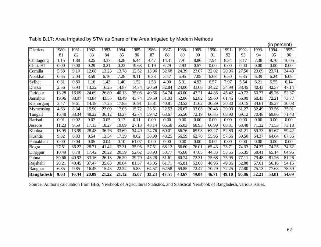
62

Table B.17: Area Irrigated by STW as Share of the Area Irrigated by Modern Methods (in percent)

Districts 1980-81

1981-82

1982-83

1983-84

1984-85

1985-86

1986-87

1987-88

1988-89

1989-90

1990-91

1991-92

1992-93

1993-94

1994-95

1995-96

Chittagong 1.15 1.88 3.25 3.37 3.28 6.44 4.47 14.31 7.91 8.86 7.94 8.34 8.17 7.38 9.70 10.05 Chitt. HT 0.00 0.00 0.29 0.21 0.22 19.63 0.19 6.29 2.93 0.57 0.00 0.00 0.00 0.00 0.00 0.00 Comilla 5.68 9.10 12.08 13.23 13.78 12.52 13.96 32.68 24.39 23.07 22.02 20.96 27.50 23.69 23.71 24.48 Noakhali 0.65 2.04 3.59 6.16 7.28 9.11 6.33 5.47 6.95 7.05 6.68 6.50 6.35 6.39 6.24 6.09 Sylhet 0.31 0.80 1.16 1.43 1.40 1.52 1.58 4.00 5.31 4.93 6.57 7.97 5.54 6.21 6.55 6.14 Dhaka 2.56 6.93 13.32 16.25 14.87 14.74 20.69 32.84 24.00 33.06 34.22 34.99 38.45 40.43 42.57 47.14 Faridpur 13.28 16.69 24.69 26.89 40.13 35.08 40.66 54.74 43.00 47.71 44.86 45.42 49.72 50.77 49.76 52.37 Jamalpur 19.96 38.97 43.84 43.55 43.49 43.74 39.59 51.03 52.06 62.82 59.60 61.45 66.99 68.43 72.21 73.77 Kishorganj 3.47 9.61 14.18 17.25 17.85 16.91 15.81 40.81 23.53 31.62 30.39 30.30 30.15 34.61 35.27 36.08 Mymensing 4.63 8.34 15.90 22.09 17.03 15.72 23.51 22.53 26.67 33.08 30.43 29.90 31.27 32.49 33.56 35.01 Tangail 16.48 33.34 48.22 36.12 43.27 42.74 59.42 63.67 65.50 72.19 66.85 68.90 69.12 70.48 69.86 71.48 Barisal 0.01 0.02 0.02 0.05 0.17 0.11 0.00 0.00 0.00 0.00 0.00 0.00 0.00 0.00 0.00 0.00 Jessore 11.23 9.59 17.13 18.27 19.89 27.13 48.14 66.58 65.03 68.93 60.99 68.31 68.48 71.32 71.53 73.18 Khulna 16.95 13.99 28.48 36.76 33.69 34.40 24.76 60.01 56.76 65.98 63.27 52.89 61.21 59.33 61.67 59.42 Kushtia 9.32 8.83 9.54 13.54 17.39 0.02 38.99 48.25 56.59 62.78 55.96 57.56 59.50 64.37 64.64 67.36 Patuakhali 0.00 0.04 0.05 0.04 0.10 61.07 0.00 0.00 0.00 0.00 0.00 0.00 0.00 0.00 0.00 0.00 Bogra 27.51 36.22 28.71 41.42 37.31 35.95 57.51 68.12 66.60 76.01 65.43 73.71 74.33 74.27 74.25 74.32 Dinajpur 10.49 8.78 17.42 20.22 20.59 52.62 38.93 50.77 45.68 47.85 44.33 53.55 55.35 58.41 65.14 64.96 Pabna 39.66 40.92 33.16 26.13 26.29 29.79 43.28 51.61 60.74 72.31 75.68 75.95 77.11 79.48 81.26 81.26 Rajshahi 20.21 40.45 37.47 35.63 30.04 81.57 43.05 61.71 45.81 52.08 48.96 49.36 52.88 57.61 56.16 54.16 Rangpur 6.35 9.85 16.45 15.45 22.22 5.85 64.57 62.58 69.85 72.47 70.29 72.25 72.80 75.13 77.63 78.59 Bangladesh 9.63 16.44 20.09 21.22 21.12 35.07 33.23 47.51 43.67 49.04 46.71 49.10 50.86 52.21 53.81 54.69 Source: Author's calculation from BBS, Yearbook of Agricultural Statistics, and Statistical Yearbook of Bangladesh, various issues.

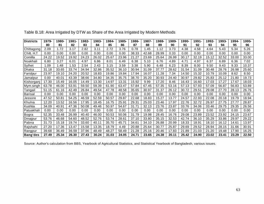
63

Table B.18: Area Irrigated by DTW as Share of the Area Irrigated by Modern Methods Districts 1979-

80 1980-

81 1981-

82 1982-

83 1983-

84 1984-

85 1985-

86 1986-

87 1987-

88 1988-

89 1989-

90 1990-

91 1991-

92 1992-

93 1993-

94 1994-

95 1995-

96 Chittagong 2.09 1.72 3.17 2.82 3.11 2.72 3.76 0.78 1.45 1.12 3.73 4.38 4.58 4.64 5.43 5.34 5.26 Chitt. H.T 0.00 0.00 0.00 0.00 0.00 0.00 0.00 38.33 42.68 28.99 0.33 0.00 0.00 0.00 0.00 0.00 0.00 Comilla 24.22 19.52 19.92 24.23 26.02 25.67 23.96 21.27 23.69 25.64 26.99 30.17 32.19 15.12 32.52 33.00 33.00 Noakhali 6.80 3.27 6.01 4.97 6.86 8.01 6.49 6.38 5.10 6.76 4.89 4.71 4.97 6.37 6.89 6.36 7.02 Sylhet 1.09 1.48 1.53 2.54 2.43 3.15 3.59 3.38 5.90 6.48 6.23 8.39 8.00 9.50 9.43 9.33 10.37 Dhaka 31.18 33.65 33.74 34.94 32.86 35.52 36.10 30.94 31.09 37.77 28.62 31.54 31.09 30.48 28.76 26.98 25.60 Faridpur 23.97 19.10 24.20 20.52 18.83 19.86 19.84 17.94 16.07 11.28 7.34 14.50 15.32 10.79 10.09 8.62 8.50 Jamalpur 0.00 40.01 43.39 38.66 34.80 34.35 35.75 38.70 35.20 30.93 24.40 30.97 29.82 25.83 25.12 21.80 19.73 Kishorganj 17.30 15.49 16.05 14.49 13.30 14.97 13.31 15.92 9.99 17.20 8.46 16.43 16.60 17.03 17.27 17.67 18.03 Mym.singh 63.78 46.00 53.91 59.50 59.39 61.90 63.47 57.84 67.45 57.35 53.16 57.13 57.93 57.09 56.87 56.83 53.89 Tangail 51.15 61.16 42.49 26.84 49.54 47.78 48.58 35.65 30.97 31.37 26.12 30.72 29.51 29.08 27.70 28.13 26.76 Barisal 0.00 0.00 0.00 0.00 0.00 0.00 0.00 0.00 0.00 0.00 0.00 0.00 0.00 0.00 0.00 0.00 0.00 Jessore 47.52 50.81 54.25 46.59 52.59 50.57 29.87 22.68 18.83 15.27 13.77 24.57 22.93 22.08 20.18 19.79 18.94 Khulna 12.20 13.52 16.56 17.95 18.45 16.75 25.91 29.31 25.03 23.46 17.97 22.76 32.72 26.97 27.75 27.77 28.87 Kushtia 34.09 40.91 47.36 50.08 49.46 50.97 54.67 31.71 32.13 23.76 23.87 33.76 34.06 33.46 29.75 29.35 26.56 Patuakhali 0.00 0.00 0.00 0.00 0.00 0.00 0.00 0.00 0.00 0.00 0.00 0.00 0.00 0.00 0.00 0.00 0.00 Bogra 52.35 33.48 26.99 40.40 46.00 50.53 50.06 31.79 19.98 28.45 16.76 29.08 23.89 23.52 23.92 24.15 23.67 Dinajpur 53.76 46.68 54.60 48.52 52.76 53.74 28.61 37.10 33.80 35.15 32.53 42.74 36.10 35.29 33.86 29.97 29.22 Pabna 31.73 15.18 19.74 33.60 40.11 35.70 45.71 34.61 34.10 26.88 20.99 18.33 18.91 18.10 16.12 14.61 13.97 Rajshahi 27.20 17.36 13.47 15.58 13.35 18.79 4.49 20.88 25.64 30.77 25.87 29.69 29.52 28.94 28.15 31.66 30.91 Rangpur 39.68 36.49 36.59 37.96 48.49 48.27 58.49 21.28 25.16 20.46 17.83 21.89 21.03 21.20 19.48 17.90 16.25 Bang’des 27.49 25.34 26.30 27.43 30.24 31.03 24.05 24.71 23.65 24.38 20.11 25.42 24.90 23.02 23.41 23.29 22.50

Source: Author's calculation from BBS, Yearbook of Agricultural Statistics, and Statistical Yearbook of Bangladesh, various issues.

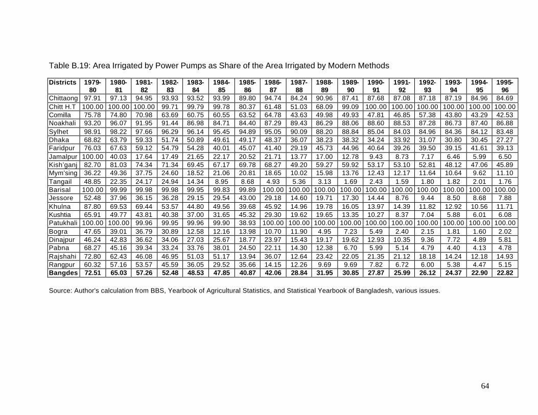
64

Table B.19: Area Irrigated by Power Pumps as Share of the Area Irrigated by Modern Methods Districts 1979-

80 1980-

81 1981-

82 1982-

83 1983-

84 1984-

85 1985-

86 1986-

87 1987-

88 1988-

89 1989-

90 1990-

91 1991-

92 1992-

93 1993-

94 1994-

95 1995-

96 Chittaong 97.91 97.13 94.95 93.93 93.52 93.99 89.80 94.74 84.24 90.96 87.41 87.68 87.08 87.18 87.19 84.96 84.69 Chitt H.T 100.00 100.00 100.00 99.71 99.79 99.78 80.37 61.48 51.03 68.09 99.09 100.00 100.00 100.00 100.00 100.00 100.00 Comilla 75.78 74.80 70.98 63.69 60.75 60.55 63.52 64.78 43.63 49.98 49.93 47.81 46.85 57.38 43.80 43.29 42.53 Noakhali 93.20 96.07 91.95 91.44 86.98 84.71 84.40 87.29 89.43 86.29 88.06 88.60 88.53 87.28 86.73 87.40 86.88 Sylhet 98.91 98.22 97.66 96.29 96.14 95.45 94.89 95.05 90.09 88.20 88.84 85.04 84.03 84.96 84.36 84.12 83.48 Dhaka 68.82 63.79 59.33 51.74 50.89 49.61 49.17 48.37 36.07 38.23 38.32 34.24 33.92 31.07 30.80 30.45 27.27 Faridpur 76.03 67.63 59.12 54.79 54.28 40.01 45.07 41.40 29.19 45.73 44.96 40.64 39.26 39.50 39.15 41.61 39.13 Jamalpur 100.00 40.03 17.64 17.49 21.65 22.17 20.52 21.71 13.77 17.00 12.78 9.43 8.73 7.17 6.46 5.99 6.50 Kish’ganj 82.70 81.03 74.34 71.34 69.45 67.17 69.78 68.27 49.20 59.27 59.92 53.17 53.10 52.81 48.12 47.06 45.89 Mym’sing 36.22 49.36 37.75 24.60 18.52 21.06 20.81 18.65 10.02 15.98 13.76 12.43 12.17 11.64 10.64 9.62 11.10 Tangail 48.85 22.35 24.17 24.94 14.34 8.95 8.68 4.93 5.36 3.13 1.69 2.43 1.59 1.80 1.82 2.01 1.76 Barisal 100.00 99.99 99.98 99.98 99.95 99.83 99.89 100.00 100.00 100.00 100.00 100.00 100.00 100.00 100.00 100.00 100.00 Jessore 52.48 37.96 36.15 36.28 29.15 29.54 43.00 29.18 14.60 19.71 17.30 14.44 8.76 9.44 8.50 8.68 7.88 Khulna 87.80 69.53 69.44 53.57 44.80 49.56 39.68 45.92 14.96 19.78 16.05 13.97 14.39 11.82 12.92 10.56 11.71 Kushtia 65.91 49.77 43.81 40.38 37.00 31.65 45.32 29.30 19.62 19.65 13.35 10.27 8.37 7.04 5.88 6.01 6.08 Patukhali 100.00 100.00 99.96 99.95 99.96 99.90 38.93 100.00 100.00 100.00 100.00 100.00 100.00 100.00 100.00 100.00 100.00 Bogra 47.65 39.01 36.79 30.89 12.58 12.16 13.98 10.70 11.90 4.95 7.23 5.49 2.40 2.15 1.81 1.60 2.02 Dinajpur 46.24 42.83 36.62 34.06 27.03 25.67 18.77 23.97 15.43 19.17 19.62 12.93 10.35 9.36 7.72 4.89 5.81 Pabna 68.27 45.16 39.34 33.24 33.76 38.01 24.50 22.11 14.30 12.38 6.70 5.99 5.14 4.79 4.40 4.13 4.78 Rajshahi 72.80 62.43 46.08 46.95 51.03 51.17 13.94 36.07 12.64 23.42 22.05 21.35 21.12 18.18 14.24 12.18 14.93 Rangpur 60.32 57.16 53.57 45.59 36.05 29.52 35.66 14.15 12.26 9.69 9.69 7.82 6.72 6.00 5.38 4.47 5.15 Bangdes 72.51 65.03 57.26 52.48 48.53 47.85 40.87 42.06 28.84 31.95 30.85 27.87 25.99 26.12 24.37 22.90 22.82

Source: Author's calculation from BBS, Yearbook of Agricultural Statistics, and Statistical Yearbook of Bangladesh, various issues.

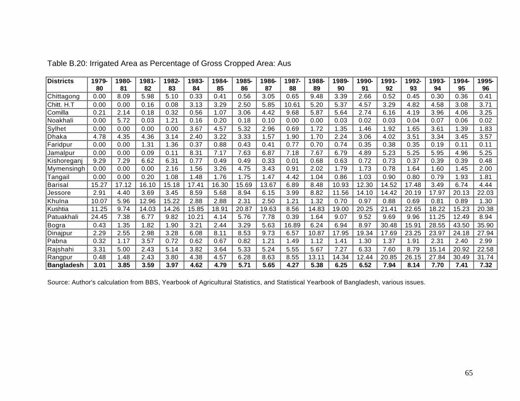
65

Table B.20: Irrigated Area as Percentage of Gross Cropped Area: Aus Districts 1979-

80 1980-

81 1981-

82 1982-

83 1983-

84 1984-

85 1985-

86 1986-

87 1987-

88 1988-

89 1989-

90 1990-

91 1991-

92 1992-

93 1993-

94 1994-

95 1995-

96 Chittagong 0.00 8.09 5.98 5.10 0.33 0.41 0.56 3.05 0.65 9.48 3.39 2.66 0.52 0.45 0.30 0.36 0.41 Chitt. H.T 0.00 0.00 0.16 0.08 3.13 3.29 2.50 5.85 10.61 5.20 5.37 4.57 3.29 4.82 4.58 3.08 3.71 Comilla 0.21 2.14 0.18 0.32 0.56 1.07 3.06 4.42 9.68 5.87 5.64 2.74 6.16 4.19 3.96 4.06 3.25 Noakhali 0.00 5.72 0.03 1.21 0.16 0.20 0.18 0.10 0.00 0.00 0.03 0.02 0.03 0.04 0.07 0.06 0.02 Sylhet 0.00 0.00 0.00 0.00 3.67 4.57 5.32 2.96 0.69 1.72 1.35 1.46 1.92 1.65 3.61 1.39 1.83 Dhaka 4.78 4.35 4.36 3.14 2.40 3.22 3.33 1.57 1.90 1.70 2.24 3.06 4.02 3.51 3.34 3.45 3.57 Faridpur 0.00 0.00 1.31 1.36 0.37 0.88 0.43 0.41 0.77 0.70 0.74 0.35 0.38 0.35 0.19 0.11 0.11 Jamalpur 0.00 0.00 0.09 0.11 8.31 7.17 7.63 6.87 7.18 7.67 6.79 4.89 5.23 5.25 5.95 4.96 5.25 Kishoreganj 9.29 7.29 6.62 6.31 0.77 0.49 0.49 0.33 0.01 0.68 0.63 0.72 0.73 0.37 0.39 0.39 0.48 Mymensingh 0.00 0.00 0.00 2.16 1.56 3.26 4.75 3.43 0.91 2.02 1.79 1.73 0.78 1.64 1.60 1.45 2.00 Tangail 0.00 0.00 0.20 1.08 1.48 1.76 1.75 1.47 4.42 1.04 0.86 1.03 0.90 0.80 0.79 1.93 1.81 Barisal 15.27 17.12 16.10 15.18 17.41 16.30 15.69 13.67 6.89 8.48 10.93 12.30 14.52 17.48 3.49 6.74 4.44 Jessore 2.91 4.40 3.69 3.45 8.59 5.68 8.94 6.15 3.99 8.82 11.56 14.10 14.42 20.19 17.97 20.13 22.03 Khulna 10.07 5.96 12.96 15.22 2.88 2.88 2.31 2.50 1.21 1.32 0.70 0.97 0.88 0.69 0.81 0.89 1.30 Kushtia 11.25 9.74 14.03 14.26 15.85 18.91 20.87 19.63 8.56 14.83 19.00 20.25 21.41 22.65 18.22 15.23 20.38 Patuakhali 24.45 7.38 6.77 9.82 10.21 4.14 5.76 7.78 0.39 1.64 9.07 9.52 9.69 9.96 11.25 12.49 8.94 Bogra 0.43 1.35 1.82 1.90 3.21 2.44 3.29 5.63 16.89 6.24 6.94 8.97 30.48 15.91 28.55 43.50 35.90 Dinajpur 2.29 2.55 2.98 3.28 6.08 8.11 8.53 9.73 6.57 10.87 17.95 19.34 17.69 23.25 23.97 24.18 27.94 Pabna 0.32 1.17 3.57 0.72 0.62 0.67 0.82 1.21 1.49 1.12 1.41 1.30 1.37 1.91 2.31 2.40 2.99 Rajshahi 3.31 5.00 2.43 5.14 3.82 3.64 5.33 5.24 5.55 5.67 7.27 6.33 7.60 8.79 15.14 20.92 22.58 Rangpur 0.48 1.48 2.43 3.80 4.38 4.57 6.28 8.63 8.55 13.11 14.34 12.44 20.85 26.15 27.84 30.49 31.74 Bangladesh 3.01 3.85 3.59 3.97 4.62 4.79 5.71 5.65 4.27 5.38 6.25 6.52 7.94 8.14 7.70 7.41 7.32

Source: Author's calculation from BBS, Yearbook of Agricultural Statistics, and Statistical Yearbook of Bangladesh, various issues.

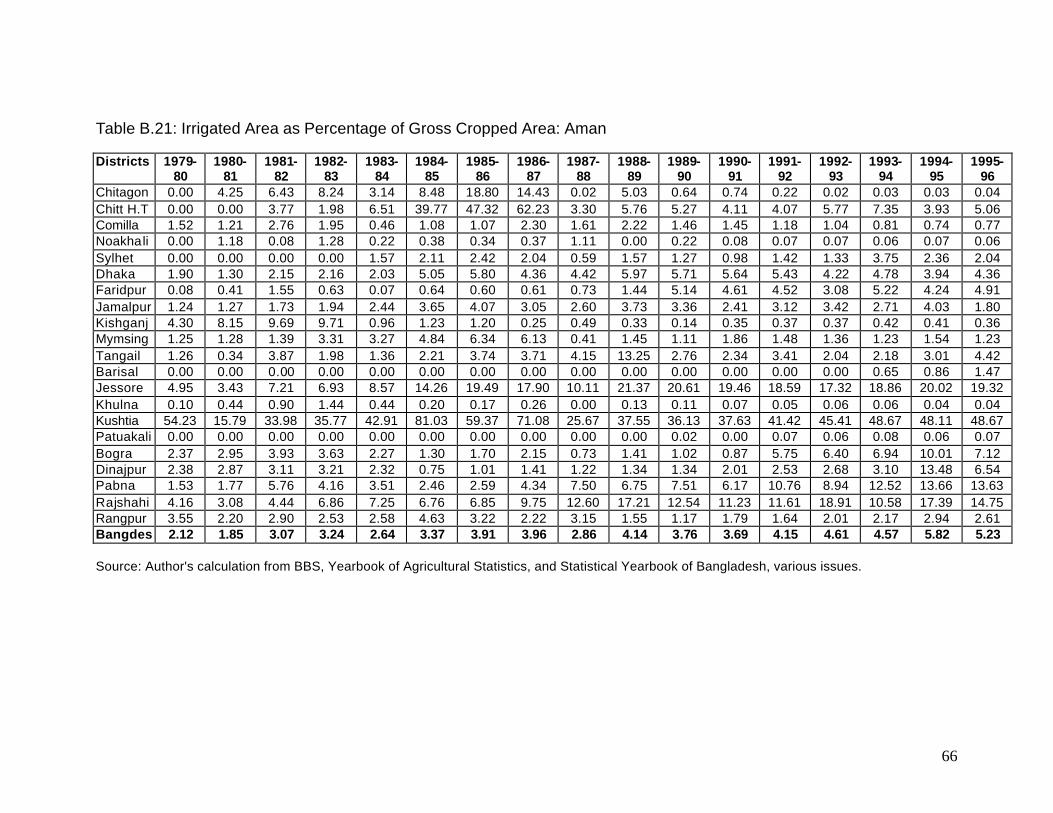
66

Table B.21: Irrigated Area as Percentage of Gross Cropped Area: Aman Districts 1979-

80 1980-

81 1981-

82 1982-

83 1983-

84 1984-

85 1985-

86 1986-

87 1987-

88 1988-

89 1989-

90 1990-

91 1991-

92 1992-

93 1993-

94 1994-

95 1995-

96 Chitagon 0.00 4.25 6.43 8.24 3.14 8.48 18.80 14.43 0.02 5.03 0.64 0.74 0.22 0.02 0.03 0.03 0.04 Chitt H.T 0.00 0.00 3.77 1.98 6.51 39.77 47.32 62.23 3.30 5.76 5.27 4.11 4.07 5.77 7.35 3.93 5.06 Comilla 1.52 1.21 2.76 1.95 0.46 1.08 1.07 2.30 1.61 2.22 1.46 1.45 1.18 1.04 0.81 0.74 0.77 Noakhali 0.00 1.18 0.08 1.28 0.22 0.38 0.34 0.37 1.11 0.00 0.22 0.08 0.07 0.07 0.06 0.07 0.06 Sylhet 0.00 0.00 0.00 0.00 1.57 2.11 2.42 2.04 0.59 1.57 1.27 0.98 1.42 1.33 3.75 2.36 2.04 Dhaka 1.90 1.30 2.15 2.16 2.03 5.05 5.80 4.36 4.42 5.97 5.71 5.64 5.43 4.22 4.78 3.94 4.36 Faridpur 0.08 0.41 1.55 0.63 0.07 0.64 0.60 0.61 0.73 1.44 5.14 4.61 4.52 3.08 5.22 4.24 4.91 Jamalpur 1.24 1.27 1.73 1.94 2.44 3.65 4.07 3.05 2.60 3.73 3.36 2.41 3.12 3.42 2.71 4.03 1.80 Kishganj 4.30 8.15 9.69 9.71 0.96 1.23 1.20 0.25 0.49 0.33 0.14 0.35 0.37 0.37 0.42 0.41 0.36 Mymsing 1.25 1.28 1.39 3.31 3.27 4.84 6.34 6.13 0.41 1.45 1.11 1.86 1.48 1.36 1.23 1.54 1.23 Tangail 1.26 0.34 3.87 1.98 1.36 2.21 3.74 3.71 4.15 13.25 2.76 2.34 3.41 2.04 2.18 3.01 4.42 Barisal 0.00 0.00 0.00 0.00 0.00 0.00 0.00 0.00 0.00 0.00 0.00 0.00 0.00 0.00 0.65 0.86 1.47 Jessore 4.95 3.43 7.21 6.93 8.57 14.26 19.49 17.90 10.11 21.37 20.61 19.46 18.59 17.32 18.86 20.02 19.32 Khulna 0.10 0.44 0.90 1.44 0.44 0.20 0.17 0.26 0.00 0.13 0.11 0.07 0.05 0.06 0.06 0.04 0.04 Kushtia 54.23 15.79 33.98 35.77 42.91 81.03 59.37 71.08 25.67 37.55 36.13 37.63 41.42 45.41 48.67 48.11 48.67 Patuakali 0.00 0.00 0.00 0.00 0.00 0.00 0.00 0.00 0.00 0.00 0.02 0.00 0.07 0.06 0.08 0.06 0.07 Bogra 2.37 2.95 3.93 3.63 2.27 1.30 1.70 2.15 0.73 1.41 1.02 0.87 5.75 6.40 6.94 10.01 7.12 Dinajpur 2.38 2.87 3.11 3.21 2.32 0.75 1.01 1.41 1.22 1.34 1.34 2.01 2.53 2.68 3.10 13.48 6.54 Pabna 1.53 1.77 5.76 4.16 3.51 2.46 2.59 4.34 7.50 6.75 7.51 6.17 10.76 8.94 12.52 13.66 13.63 Rajshahi 4.16 3.08 4.44 6.86 7.25 6.76 6.85 9.75 12.60 17.21 12.54 11.23 11.61 18.91 10.58 17.39 14.75 Rangpur 3.55 2.20 2.90 2.53 2.58 4.63 3.22 2.22 3.15 1.55 1.17 1.79 1.64 2.01 2.17 2.94 2.61 Bangdes 2.12 1.85 3.07 3.24 2.64 3.37 3.91 3.96 2.86 4.14 3.76 3.69 4.15 4.61 4.57 5.82 5.23 Source: Author's calculation from BBS, Yearbook of Agricultural Statistics, and Statistical Yearbook of Bangladesh, various issues.

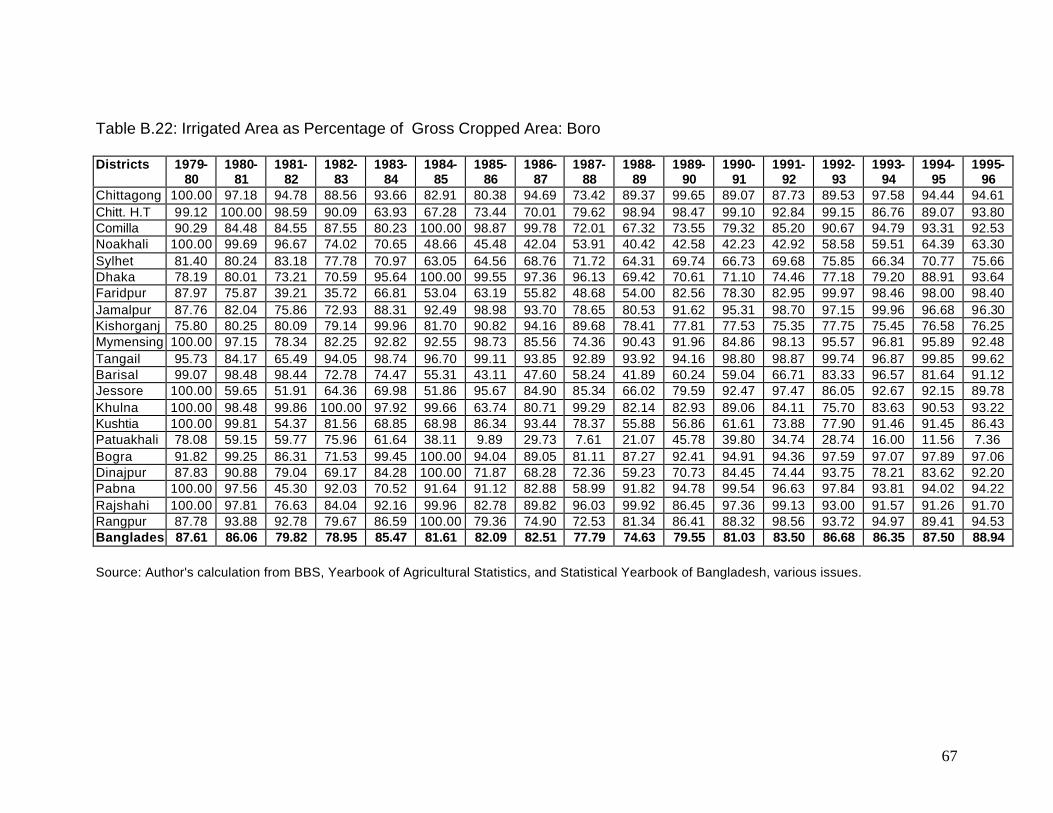
67

Table B.22: Irrigated Area as Percentage of Gross Cropped Area: Boro Districts 1979-

80 1980-

81 1981-

82 1982-

83 1983-

84 1984-

85 1985-

86 1986-

87 1987-

88 1988-

89 1989-

90 1990-

91 1991-

92 1992-

93 1993-

94 1994-

95 1995-

96 Chittagong 100.00 97.18 94.78 88.56 93.66 82.91 80.38 94.69 73.42 89.37 99.65 89.07 87.73 89.53 97.58 94.44 94.61 Chitt. H.T 99.12 100.00 98.59 90.09 63.93 67.28 73.44 70.01 79.62 98.94 98.47 99.10 92.84 99.15 86.76 89.07 93.80 Comilla 90.29 84.48 84.55 87.55 80.23 100.00 98.87 99.78 72.01 67.32 73.55 79.32 85.20 90.67 94.79 93.31 92.53 Noakhali 100.00 99.69 96.67 74.02 70.65 48.66 45.48 42.04 53.91 40.42 42.58 42.23 42.92 58.58 59.51 64.39 63.30 Sylhet 81.40 80.24 83.18 77.78 70.97 63.05 64.56 68.76 71.72 64.31 69.74 66.73 69.68 75.85 66.34 70.77 75.66 Dhaka 78.19 80.01 73.21 70.59 95.64 100.00 99.55 97.36 96.13 69.42 70.61 71.10 74.46 77.18 79.20 88.91 93.64 Faridpur 87.97 75.87 39.21 35.72 66.81 53.04 63.19 55.82 48.68 54.00 82.56 78.30 82.95 99.97 98.46 98.00 98.40 Jamalpur 87.76 82.04 75.86 72.93 88.31 92.49 98.98 93.70 78.65 80.53 91.62 95.31 98.70 97.15 99.96 96.68 96.30 Kishorganj 75.80 80.25 80.09 79.14 99.96 81.70 90.82 94.16 89.68 78.41 77.81 77.53 75.35 77.75 75.45 76.58 76.25 Mymensing 100.00 97.15 78.34 82.25 92.82 92.55 98.73 85.56 74.36 90.43 91.96 84.86 98.13 95.57 96.81 95.89 92.48 Tangail 95.73 84.17 65.49 94.05 98.74 96.70 99.11 93.85 92.89 93.92 94.16 98.80 98.87 99.74 96.87 99.85 99.62 Barisal 99.07 98.48 98.44 72.78 74.47 55.31 43.11 47.60 58.24 41.89 60.24 59.04 66.71 83.33 96.57 81.64 91.12 Jessore 100.00 59.65 51.91 64.36 69.98 51.86 95.67 84.90 85.34 66.02 79.59 92.47 97.47 86.05 92.67 92.15 89.78 Khulna 100.00 98.48 99.86 100.00 97.92 99.66 63.74 80.71 99.29 82.14 82.93 89.06 84.11 75.70 83.63 90.53 93.22 Kushtia 100.00 99.81 54.37 81.56 68.85 68.98 86.34 93.44 78.37 55.88 56.86 61.61 73.88 77.90 91.46 91.45 86.43 Patuakhali 78.08 59.15 59.77 75.96 61.64 38.11 9.89 29.73 7.61 21.07 45.78 39.80 34.74 28.74 16.00 11.56 7.36 Bogra 91.82 99.25 86.31 71.53 99.45 100.00 94.04 89.05 81.11 87.27 92.41 94.91 94.36 97.59 97.07 97.89 97.06 Dinajpur 87.83 90.88 79.04 69.17 84.28 100.00 71.87 68.28 72.36 59.23 70.73 84.45 74.44 93.75 78.21 83.62 92.20 Pabna 100.00 97.56 45.30 92.03 70.52 91.64 91.12 82.88 58.99 91.82 94.78 99.54 96.63 97.84 93.81 94.02 94.22 Rajshahi 100.00 97.81 76.63 84.04 92.16 99.96 82.78 89.82 96.03 99.92 86.45 97.36 99.13 93.00 91.57 91.26 91.70 Rangpur 87.78 93.88 92.78 79.67 86.59 100.00 79.36 74.90 72.53 81.34 86.41 88.32 98.56 93.72 94.97 89.41 94.53 Banglades 87.61 86.06 79.82 78.95 85.47 81.61 82.09 82.51 77.79 74.63 79.55 81.03 83.50 86.68 86.35 87.50 88.94

Source: Author's calculation from BBS, Yearbook of Agricultural Statistics, and Statistical Yearbook of Bangladesh, various issues.

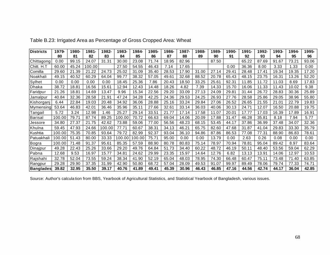
68

Table B.23: Irrigated Area as Percentage of Gross Cropped Area: Wheat Districts 1979-

80 1980-

81 1981-

82 1982-

83 1983-

84 1984-

85 1985-

86 1986-

87 1987-

88 1988-

89 1989-

90 1990-

91 1991-

92 1992-

93 1993-

94 1994-

95 1995-

96 Chittagong 0.00 99.15 24.07 31.31 30.00 23.08 71.74 18.95 82.96 87.50 65.22 87.69 91.67 73.21 93.06 Chitt. H.T 60.00 45.24 100.00 27.50 54.55 46.43 7.14 17.65 0.00 36.36 8.00 3.33 1.33 0.00 Comilla 29.60 21.39 21.22 24.73 25.02 31.09 35.40 28.53 17.90 31.00 27.14 29.41 28.48 17.41 19.34 19.35 17.20 Noakhali 49.15 40.52 60.29 64.04 99.77 38.32 57.05 49.61 32.68 88.52 20.78 65.43 48.15 23.75 16.31 13.26 52.20 Sylhet 0.00 0.00 0.00 0.00 18.45 25.36 7.86 20.43 18.50 33.25 25.61 92.31 11.85 11.72 11.03 8.69 17.83 Dhaka 38.72 18.81 16.56 15.61 12.94 12.43 14.48 18.26 4.82 7.39 14.33 15.70 16.06 11.33 11.43 10.02 9.38 Faridpur 21.26 18.81 14.69 13.47 9.96 15.34 22.56 29.20 33.09 27.13 24.09 29.81 31.44 26.72 28.83 30.36 25.89 Jamalpur 40.84 32.36 28.58 21.91 47.24 34.28 42.25 24.36 29.53 24.25 26.93 27.76 28.58 25.86 29.05 38.96 55.80 Kishorganj 6.44 22.84 19.03 20.48 34.92 36.06 28.88 25.16 33.24 29.84 27.06 26.52 26.65 21.55 21.01 22.79 19.83 Mymensing 53.64 46.83 42.01 36.46 35.96 35.11 27.66 32.61 33.14 36.03 40.06 30.13 24.71 12.07 16.50 20.88 19.75 Tangail 5.72 3.24 12.98 1.46 25.27 29.14 33.51 21.77 17.14 17.58 11.07 20.01 17.77 17.03 16.39 17.89 16.91 Barisal 100.00 79.71 87.74 89.25 100.00 70.72 66.63 69.04 14.06 20.09 17.88 31.47 46.28 35.81 8.18 7.94 5.77 Jessore 34.80 27.37 21.75 42.62 73.88 59.06 77.00 56.56 48.23 68.15 53.45 44.17 37.86 36.99 37.48 34.07 32.36 Khulna 59.45 47.93 24.66 100.00 77.71 60.67 38.31 34.13 46.21 65.75 82.60 47.68 31.87 41.04 29.83 33.30 35.79 Kushtia 100.00 75.35 70.85 93.64 79.72 82.99 92.37 93.04 36.10 94.86 87.86 86.53 77.08 77.31 88.90 86.83 78.61 Patuakhali 100.00 51.43 80.00 33.33 100.00 100.00 75.71 95.00 0.00 0.00 13.79 0.00 2.63 0.26 0.08 0.00 0.00 Bogra 100.00 71.48 91.37 95.61 85.35 57.59 88.90 80.78 80.83 75.14 78.97 70.94 78.81 95.04 89.42 8.97 83.64 Dinajpur 49.28 22.43 25.26 33.66 29.20 49.76 64.84 51.73 34.40 60.22 48.72 46.19 50.11 48.40 53.56 59.04 62.29 Pabna 12.68 9.53 16.97 15.77 34.81 24.62 29.99 23.35 15.97 14.64 12.76 6.82 13.13 13.91 14.06 12.97 10.53 Rajshahi 32.78 52.04 73.55 59.24 38.34 41.90 52.19 65.04 48.03 78.95 74.30 66.48 60.47 75.11 73.48 71.40 63.85 Rangpur 29.28 29.90 37.35 31.99 42.90 50.80 68.72 57.04 28.09 49.53 91.07 99.97 89.49 78.06 79.74 77.33 74.71 Banglades 39.82 32.95 35.50 39.17 40.76 41.89 49.41 45.39 30.96 46.43 46.85 47.16 44.56 42.74 44.17 36.04 42.85 Source: Author's calcula tion from BBS, Yearbook of Agricultural Statistics, and Statistical Yearbook of Bangladesh, various issues.

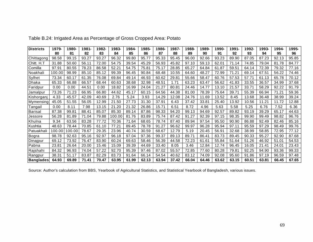
69

Table B.24: Irrigated Area as Percentage of Gross Cropped Area: Potato Districts 1979-

80 1980-

81 1981-

82 1982-

83 1983-

84 1984-

85 1985-

86 1986-

87 1987-

88 1988-

89 1989-

90 1990-

91 1991-

92 1992-

93 1993-

94 1994-

95 1995-

96 Chittagong 98.58 99.15 93.27 93.27 96.32 99.80 95.77 95.33 95.45 96.00 92.66 93.23 89.90 87.05 87.23 92.13 95.85 Chitt. H.T 31.88 50.60 56.11 72.00 54.75 39.54 45.29 56.93 45.82 97.10 59.13 62.01 71.14 74.85 79.04 81.78 84.77 Comilla 97.91 80.55 78.23 86.58 52.21 54.75 75.81 75.17 28.85 65.27 64.84 61.87 59.51 64.14 72.39 79.32 77.16 Noakhali 100.00 98.99 85.10 85.12 99.39 96.45 90.84 68.48 10.55 64.60 48.27 72.99 71.21 69.14 67.51 56.22 74.46 Sylhet 73.34 60.17 61.35 76.08 69.84 49.14 46.93 60.62 29.81 55.66 58.47 60.76 57.53 57.71 61.13 65.78 70.12 Dhaka 65.33 66.88 66.57 68.44 60.63 38.68 32.98 48.51 1.71 63.23 63.47 56.62 41.83 33.55 36.57 34.99 37.68 Faridpur 0.00 0.00 44.51 0.00 18.82 16.99 24.04 21.27 80.81 24.46 14.77 13.10 21.57 33.71 58.29 92.22 91.79 Jamalpur 73.26 71.23 66.95 66.80 44.62 45.17 60.15 64.56 44.38 81.00 78.39 75.64 39.71 55.39 66.94 71.21 59.36 Kishorganj 4.33 45.57 42.09 40.69 2.76 5.24 3.93 14.29 12.08 24.76 11.69 13.52 8.45 13.68 36.48 38.99 39.24 Mymensing 45.05 51.55 56.05 12.99 21.50 27.73 31.30 37.91 6.43 37.42 33.81 25.40 13.92 10.56 11.21 11.72 12.88 Tangail 0.00 8.11 7.98 13.15 21.20 21.32 26.86 15.71 6.51 8.72 4.96 5.63 5.58 5.25 6.76 7.52 6.36 Barisal 87.38 99.81 88.41 85.07 85.30 89.14 87.86 98.33 94.20 99.13 94.69 92.57 89.82 93.19 39.29 65.17 44.63 Jessore 56.28 81.89 71.04 79.88 100.00 81.76 83.89 75.74 87.42 91.27 92.39 97.15 98.35 99.90 99.49 98.82 96.76 Khulna 9.34 63.56 83.28 77.72 70.36 71.64 68.65 78.74 87.40 89.94 97.54 95.50 90.90 86.88 92.49 82.46 85.16 Kushtia 48.63 78.44 70.85 61.10 77.21 89.45 78.78 91.27 96.62 99.97 96.28 95.94 97.11 95.59 97.29 98.49 99.76 Patuakhali 100.00 100.00 78.67 29.35 23.96 40.74 30.59 68.67 12.79 5.19 20.45 56.91 32.68 38.99 58.85 72.95 77.12 Bogra 98.78 92.63 95.16 92.97 96.18 97.04 97.36 99.37 89.13 89.71 86.41 83.73 89.45 90.33 95.27 92.90 87.68 Dinajpur 69.12 73.92 76.47 83.90 60.24 69.63 58.46 56.39 44.58 72.23 61.61 55.84 51.64 51.26 46.92 51.01 54.53 Pabna 23.81 26.64 20.00 15.46 15.09 39.39 44.69 33.40 8.05 3.46 12.84 12.74 96.45 16.05 21.41 24.01 23.43 Rajshahi 84.32 96.93 74.04 57.22 92.70 95.39 97.46 87.02 55.57 72.85 77.60 80.28 79.81 92.25 94.90 93.36 99.33 Rangpur 38.31 51.17 83.87 82.29 83.73 91.64 66.14 54.54 40.62 83.12 74.09 92.08 95.60 91.86 97.19 96.59 97.48 Banglades 64.93 69.89 71.41 70.47 63.95 61.99 62.13 63.94 37.42 66.04 64.46 63.62 63.15 60.51 63.81 66.45 67.65

Source: Author's calculation from BBS, Yearbook of Agricultural Statistics, and Statistical Yearbook of Bangladesh, various issues.

70

Appendix C

A Note on the Aggregate Profitability of the Crop Sector

An understanding of the incentive structure for sustained growth of agriculture is

required for policy formulation. The profitability of individual crop reveals

comparative dynamics within the crop sector only; it does not provide

comparative advantage of the agriculture sector over the other sectors of the

economy. The aggregate financial profitability of the crop sector as a whole is

required to assess the latter comparative dynamics.

It would have been ideal if all the crops produced in the country could be

considered in the profitability analysis. This was not possible due to lack of

relevant information. We considered around three dozens of crops for estimating

aggregate financial profitability of the crop sector during pre- and post-SAP

periods. These crops, however, account for more than 96 per cent of the gross

cropped area in Bangladesh.

Information on all crops was not available for both the periods. While Zohir

(1993) provided information on the physical input-output structures of most crops

for 1990-91, they were not readily available for the pre-SAP period. Various

studies by the Agro-Economic Research Unit of the Ministry of Agriculture and

the International Fertilizer Development Center, Dhaka, provided information on

some of the major crops for the latter period (see Table A1).

It was relatively easy to estimate aggregate profitability of the crop sector for the

post-SAP period. Since we wanted to include all the crops in order to ensure

some degree of robustness of the aggregate profitability estimate, it was

assumed that the input-output structures for the minor crops remained

unchanged – that is, the pre-SAP input-output structure was same as that

observed during the post-SAP period. It may be noted that changes in

technology and market environment during the 1980s affected primarily the major

crops. This was particularly so due to the fact that most of these (minor) crops

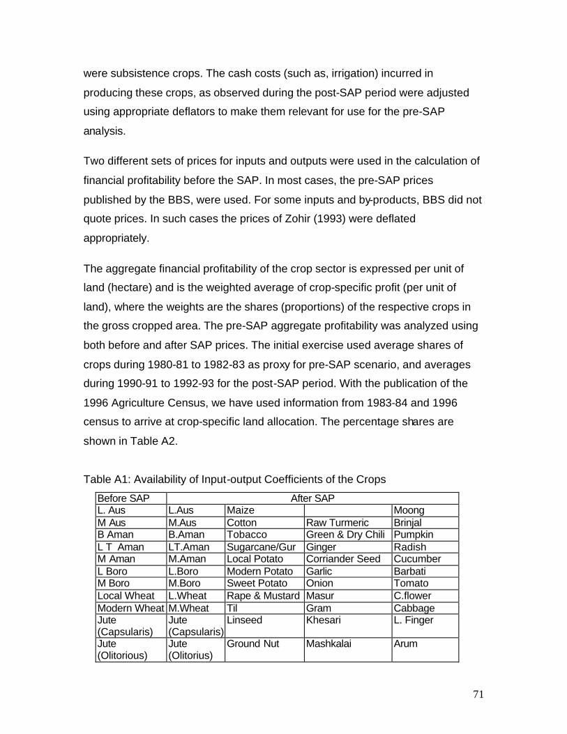
71

were subsistence crops. The cash costs (such as, irrigation) incurred in

producing these crops, as observed during the post-SAP period were adjusted

using appropriate deflators to make them relevant for use for the pre-SAP

analysis.

Two different sets of prices for inputs and outputs were used in the calculation of

financial profitability before the SAP. In most cases, the pre-SAP prices

published by the BBS, were used. For some inputs and by-products, BBS did not

quote prices. In such cases the prices of Zohir (1993) were deflated

appropriately.

The aggregate financial profitability of the crop sector is expressed per unit of

land (hectare) and is the weighted average of crop-specific profit (per unit of

land), where the weights are the shares (proportions) of the respective crops in

the gross cropped area. The pre-SAP aggregate profitability was analyzed using

both before and after SAP prices. The initial exercise used average shares of

crops during 1980-81 to 1982-83 as proxy for pre-SAP scenario, and averages

during 1990-91 to 1992-93 for the post-SAP period. With the publication of the

1996 Agriculture Census, we have used information from 1983-84 and 1996

census to arrive at crop-specific land allocation. The percentage shares are

shown in Table A2.

Table A1: Availability of Input-output Coefficients of the Crops

Before SAP After SAP L. Aus L.Aus Maize Moong M Aus M.Aus Cotton Raw Turmeric Brinjal B Aman B.Aman Tobacco Green & Dry Chili Pumpkin L T Aman LT.Aman Sugarcane/Gur Ginger Radish M Aman M.Aman Local Potato Corriander Seed Cucumber L Boro L.Boro Modern Potato Garlic Barbati M Boro M.Boro Sweet Potato Onion Tomato Local Wheat L.Wheat Rape & Mustard Masur C.flower Modern Wheat M.Wheat Til Gram Cabbage Jute (Capsularis)

Jute (Capsularis)

Linseed Khesari L. Finger

Jute (Olitorious)

Jute (Olitorius)

Ground Nut Mashkalai Arum

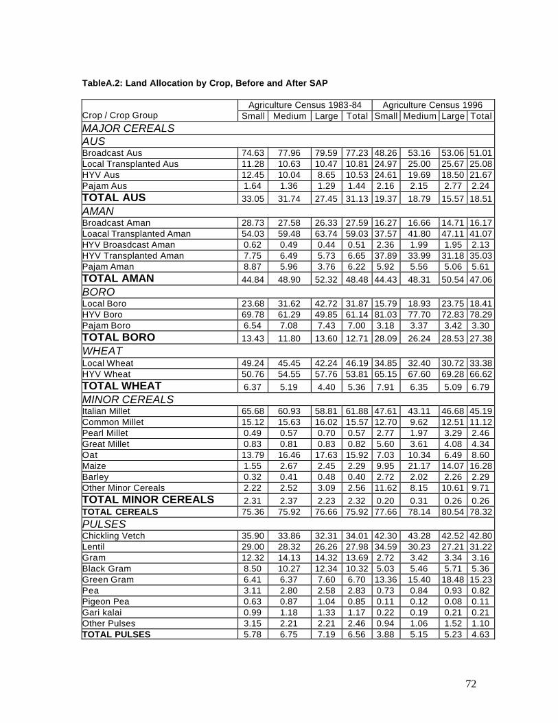
72

TableA.2: Land Allocation by Crop, Before and After SAP

Agriculture Census 1983-84 Agriculture Census 1996 Crop / Crop Group Small Medium Large Total Small Medium Large Total

MAJOR CEREALS AUS Broadcast Aus 74.63 77.96 79.59 77.23 48.26 53.16 53.06 51.01 Local Transplanted Aus 11.28 10.63 10.47 10.81 24.97 25.00 25.67 25.08 HYV Aus 12.45 10.04 8.65 10.53 24.61 19.69 18.50 21.67 Pajam Aus 1.64 1.36 1.29 1.44 2.16 2.15 2.77 2.24 TOTAL AUS 33.05 31.74 27.45 31.13 19.37 18.79 15.57 18.51

AMAN Broadcast Aman 28.73 27.58 26.33 27.59 16.27 16.66 14.71 16.17 Loacal Transplanted Aman 54.03 59.48 63.74 59.03 37.57 41.80 47.11 41.07 HYV Broasdcast Aman 0.62 0.49 0.44 0.51 2.36 1.99 1.95 2.13 HYV Transplanted Aman 7.75 6.49 5.73 6.65 37.89 33.99 31.18 35.03 Pajam Aman 8.87 5.96 3.76 6.22 5.92 5.56 5.06 5.61 TOTAL AMAN 44.84 48.90 52.32 48.48 44.43 48.31 50.54 47.06

BORO Local Boro 23.68 31.62 42.72 31.87 15.79 18.93 23.75 18.41 HYV Boro 69.78 61.29 49.85 61.14 81.03 77.70 72.83 78.29 Pajam Boro 6.54 7.08 7.43 7.00 3.18 3.37 3.42 3.30 TOTAL BORO 13.43 11.80 13.60 12.71 28.09 26.24 28.53 27.38

WHEAT Local Wheat 49.24 45.45 42.24 46.19 34.85 32.40 30.72 33.38 HYV Wheat 50.76 54.55 57.76 53.81 65.15 67.60 69.28 66.62 TOTAL WHEAT 6.37 5.19 4.40 5.36 7.91 6.35 5.09 6.79

MINOR CEREALS Italian Millet 65.68 60.93 58.81 61.88 47.61 43.11 46.68 45.19 Common Millet 15.12 15.63 16.02 15.57 12.70 9.62 12.51 11.12 Pearl Millet 0.49 0.57 0.70 0.57 2.77 1.97 3.29 2.46 Great Millet 0.83 0.81 0.83 0.82 5.60 3.61 4.08 4.34 Oat 13.79 16.46 17.63 15.92 7.03 10.34 6.49 8.60 Maize 1.55 2.67 2.45 2.29 9.95 21.17 14.07 16.28 Barley 0.32 0.41 0.48 0.40 2.72 2.02 2.26 2.29 Other Minor Cereals 2.22 2.52 3.09 2.56 11.62 8.15 10.61 9.71 TOTAL MINOR CEREALS 2.31 2.37 2.23 2.32 0.20 0.31 0.26 0.26 TOTAL CEREALS 75.36 75.92 76.66 75.92 77.66 78.14 80.54 78.32

PULSES Chickling Vetch 35.90 33.86 32.31 34.01 42.30 43.28 42.52 42.80 Lentil 29.00 28.32 26.26 27.98 34.59 30.23 27.21 31.22 Gram 12.32 14.13 14.32 13.69 2.72 3.42 3.34 3.16 Black Gram 8.50 10.27 12.34 10.32 5.03 5.46 5.71 5.36 Green Gram 6.41 6.37 7.60 6.70 13.36 15.40 18.48 15.23 Pea 3.11 2.80 2.58 2.83 0.73 0.84 0.93 0.82 Pigeon Pea 0.63 0.87 1.04 0.85 0.11 0.12 0.08 0.11 Gari kalai 0.99 1.18 1.33 1.17 0.22 0.19 0.21 0.21 Other Pulses 3.15 2.21 2.21 2.46 0.94 1.06 1.52 1.10 TOTAL PULSES 5.78 6.75 7.19 6.56 3.88 5.15 5.23 4.63

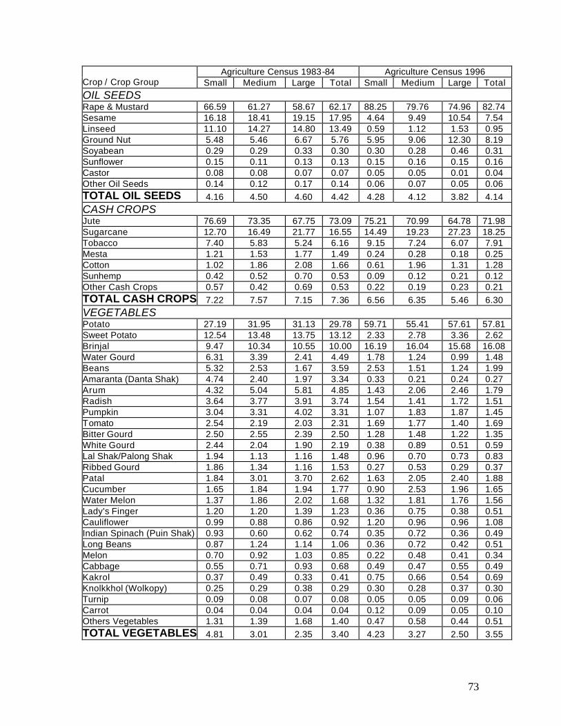
73

Agriculture Census 1983-84 Agriculture Census 1996 Crop / Crop Group Small Medium Large Total Small Medium Large Total

OIL SEEDS Rape & Mustard 66.59 61.27 58.67 62.17 88.25 79.76 74.96 82.74 Sesame 16.18 18.41 19.15 17.95 4.64 9.49 10.54 7.54 Linseed 11.10 14.27 14.80 13.49 0.59 1.12 1.53 0.95 Ground Nut 5.48 5.46 6.67 5.76 5.95 9.06 12.30 8.19 Soyabean 0.29 0.29 0.33 0.30 0.30 0.28 0.46 0.31 Sunflower 0.15 0.11 0.13 0.13 0.15 0.16 0.15 0.16 Castor 0.08 0.08 0.07 0.07 0.05 0.05 0.01 0.04 Other Oil Seeds 0.14 0.12 0.17 0.14 0.06 0.07 0.05 0.06 TOTAL OIL SEEDS 4.16 4.50 4.60 4.42 4.28 4.12 3.82 4.14

CASH CROPS Jute 76.69 73.35 67.75 73.09 75.21 70.99 64.78 71.98 Sugarcane 12.70 16.49 21.77 16.55 14.49 19.23 27.23 18.25 Tobacco 7.40 5.83 5.24 6.16 9.15 7.24 6.07 7.91 Mesta 1.21 1.53 1.77 1.49 0.24 0.28 0.18 0.25 Cotton 1.02 1.86 2.08 1.66 0.61 1.96 1.31 1.28 Sunhemp 0.42 0.52 0.70 0.53 0.09 0.12 0.21 0.12 Other Cash Crops 0.57 0.42 0.69 0.53 0.22 0.19 0.23 0.21 TOTAL CASH CROPS 7.22 7.57 7.15 7.36 6.56 6.35 5.46 6.30

VEGETABLES Potato 27.19 31.95 31.13 29.78 59.71 55.41 57.61 57.81 Sweet Potato 12.54 13.48 13.75 13.12 2.33 2.78 3.36 2.62 Brinjal 9.47 10.34 10.55 10.00 16.19 16.04 15.68 16.08 Water Gourd 6.31 3.39 2.41 4.49 1.78 1.24 0.99 1.48 Beans 5.32 2.53 1.67 3.59 2.53 1.51 1.24 1.99 Amaranta (Danta Shak) 4.74 2.40 1.97 3.34 0.33 0.21 0.24 0.27 Arum 4.32 5.04 5.81 4.85 1.43 2.06 2.46 1.79 Radish 3.64 3.77 3.91 3.74 1.54 1.41 1.72 1.51 Pumpkin 3.04 3.31 4.02 3.31 1.07 1.83 1.87 1.45 Tomato 2.54 2.19 2.03 2.31 1.69 1.77 1.40 1.69 Bitter Gourd 2.50 2.55 2.39 2.50 1.28 1.48 1.22 1.35 White Gourd 2.44 2.04 1.90 2.19 0.38 0.89 0.51 0.59 Lal Shak/Palong Shak 1.94 1.13 1.16 1.48 0.96 0.70 0.73 0.83 Ribbed Gourd 1.86 1.34 1.16 1.53 0.27 0.53 0.29 0.37 Patal 1.84 3.01 3.70 2.62 1.63 2.05 2.40 1.88 Cucumber 1.65 1.84 1.94 1.77 0.90 2.53 1.96 1.65 Water Melon 1.37 1.86 2.02 1.68 1.32 1.81 1.76 1.56 Lady's Finger 1.20 1.20 1.39 1.23 0.36 0.75 0.38 0.51 Cauliflower 0.99 0.88 0.86 0.92 1.20 0.96 0.96 1.08 Indian Spinach (Puin Shak) 0.93 0.60 0.62 0.74 0.35 0.72 0.36 0.49 Long Beans 0.87 1.24 1.14 1.06 0.36 0.72 0.42 0.51 Melon 0.70 0.92 1.03 0.85 0.22 0.48 0.41 0.34 Cabbage 0.55 0.71 0.93 0.68 0.49 0.47 0.55 0.49 Kakrol 0.37 0.49 0.33 0.41 0.75 0.66 0.54 0.69 Knolkkhol (Wolkopy) 0.25 0.29 0.38 0.29 0.30 0.28 0.37 0.30 Turnip 0.09 0.08 0.07 0.08 0.05 0.05 0.09 0.06 Carrot 0.04 0.04 0.04 0.04 0.12 0.09 0.05 0.10 Others Vegetables 1.31 1.39 1.68 1.40 0.47 0.58 0.44 0.51 TOTAL VEGETABLES 4.81 3.01 2.35 3.40 4.23 3.27 2.50 3.55

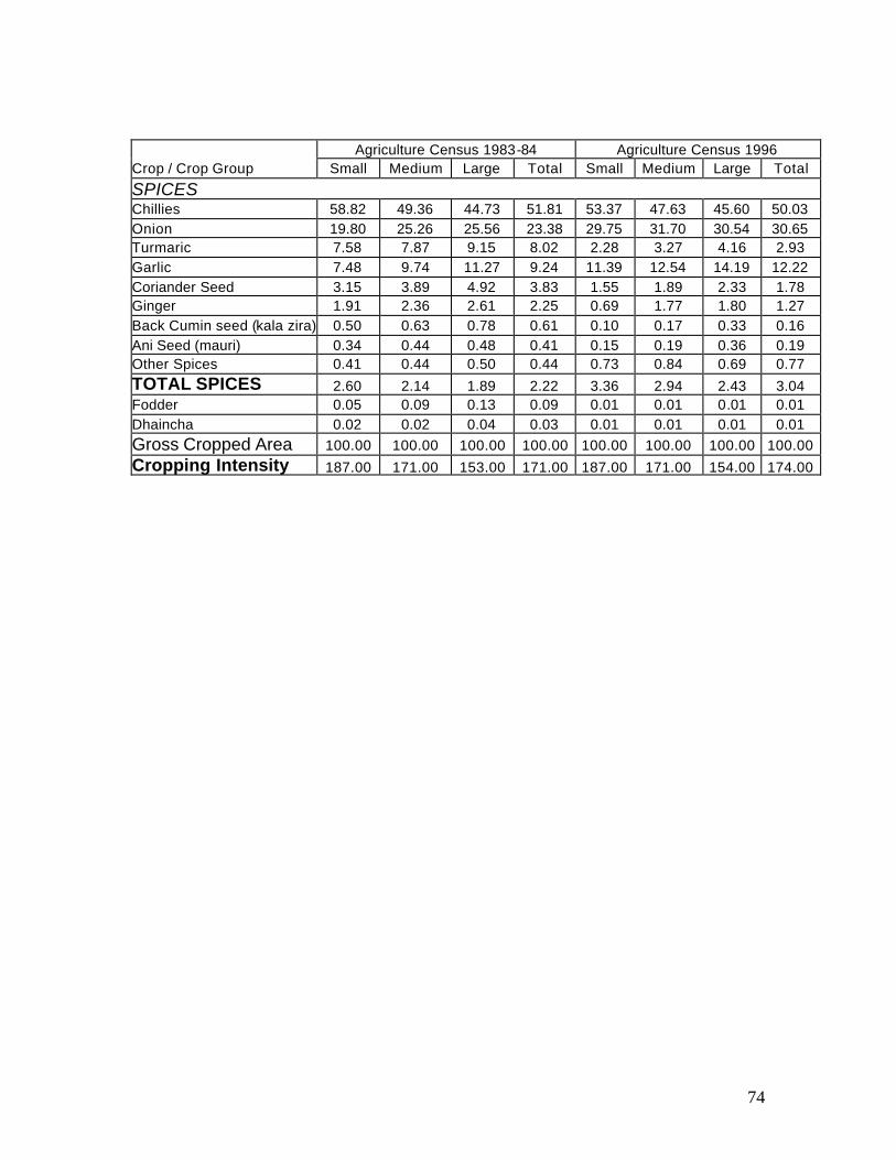
74

Agriculture Census 1983-84 Agriculture Census 1996 Crop / Crop Group Small Medium Large Total Small Medium Large Total

SPICES Chillies 58.82 49.36 44.73 51.81 53.37 47.63 45.60 50.03 Onion 19.80 25.26 25.56 23.38 29.75 31.70 30.54 30.65 Turmaric 7.58 7.87 9.15 8.02 2.28 3.27 4.16 2.93 Garlic 7.48 9.74 11.27 9.24 11.39 12.54 14.19 12.22 Coriander Seed 3.15 3.89 4.92 3.83 1.55 1.89 2.33 1.78 Ginger 1.91 2.36 2.61 2.25 0.69 1.77 1.80 1.27 Back Cumin seed (kala zira) 0.50 0.63 0.78 0.61 0.10 0.17 0.33 0.16 Ani Seed (mauri) 0.34 0.44 0.48 0.41 0.15 0.19 0.36 0.19 Other Spices 0.41 0.44 0.50 0.44 0.73 0.84 0.69 0.77

TOTAL SPICES 2.60 2.14 1.89 2.22 3.36 2.94 2.43 3.04 Fodder 0.05 0.09 0.13 0.09 0.01 0.01 0.01 0.01 Dhaincha 0.02 0.02 0.04 0.03 0.01 0.01 0.01 0.01

Gross Cropped Area 100.00 100.00 100.00 100.00 100.00 100.00 100.00 100.00

Cropping Intensity 187.00 171.00 153.00 171.00 187.00 171.00 154.00 174.00

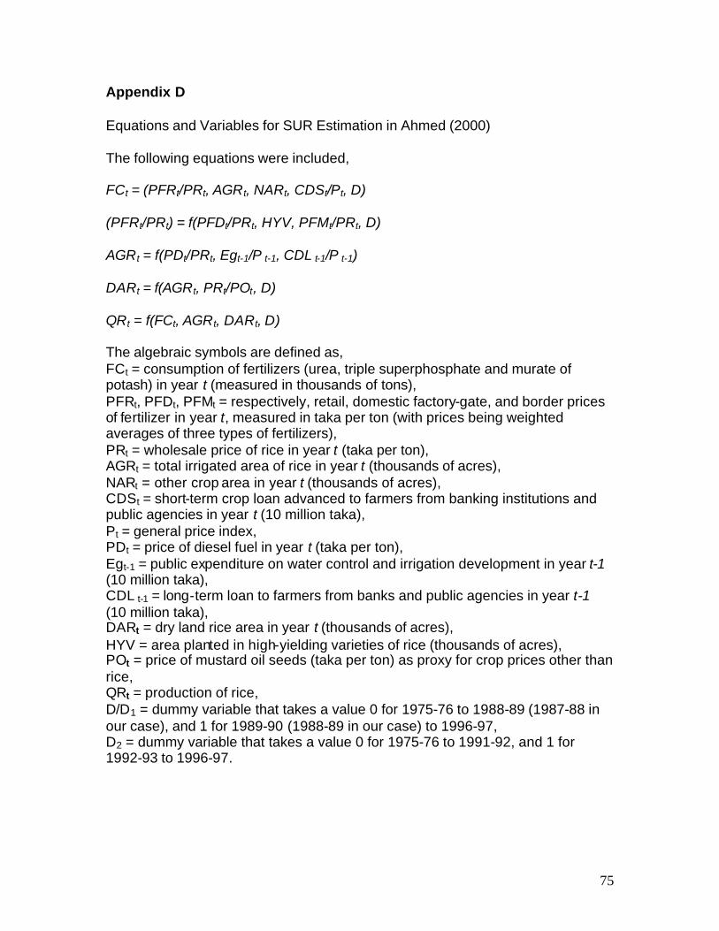
75

Appendix D Equations and Variables for SUR Estimation in Ahmed (2000) The following equations were included, FCt = (PFRt/PRt, AGRt, NARt, CDSt/Pt, D) (PFRt/PRt) = f(PFDt/PRt, HYV, PFMt/PRt, D) AGRt = f(PDt/PRt, Egt-1/P t-1, CDL t-1/P t-1) DARt = f(AGRt, PRt/POt, D) QRt = f(FCt, AGRt, DARt, D) The algebraic symbols are defined as, FCt = consumption of fertilizers (urea, triple superphosphate and murate of potash) in year t (measured in thousands of tons), PFRt, PFDt, PFMt = respectively, retail, domestic factory-gate, and border prices of fertilizer in year t, measured in taka per ton (with prices being weighted averages of three types of fertilizers), PRt = wholesale price of rice in year t (taka per ton), AGRt = total irrigated area of rice in year t (thousands of acres), NARt = other crop area in year t (thousands of acres), CDSt = short-term crop loan advanced to farmers from banking institutions and public agencies in year t (10 million taka), Pt = general price index, PDt = price of diesel fuel in year t (taka per ton), Egt-1 = public expenditure on water control and irrigation development in year t-1 (10 million taka), CDL t-1 = long-term loan to farmers from banks and public agencies in year t-1 (10 million taka), DARt = dry land rice area in year t (thousands of acres), HYV = area planted in high-yielding varieties of rice (thousands of acres), POt = price of mustard oil seeds (taka per ton) as proxy for crop prices other than rice, QRt = production of rice, D/D1 = dummy variable that takes a value 0 for 1975-76 to 1988-89 (1987-88 in our case), and 1 for 1989-90 (1988-89 in our case) to 1996-97, D2 = dummy variable that takes a value 0 for 1975-76 to 1991-92, and 1 for 1992-93 to 1996-97.

76

References AER (1978/79): “Costs and Returns: Survey for Bangladesh, 1978/79”, Agro-Economic Research, Ministry of Agriculture and Forests, Dhaka, Vol. I (Aus Paddy), Vol. II (Broadcast Aman Paddy), Vol. III (Transplanted Aman Paddy), Vol. V (Boro Paddy), Vol. VI (Wheat), Vol. VII (Jute). AER (1979/80): “Costs and Returns: Survey for Bangladesh, 1979/80”, Agro-Economic Research, Ministry of Agriculture and Forests, Dhaka, Vol. I (Broadcast Aman Paddy), Vol. II (Aus Paddy), Vol. III (Jute). AER (1981-82): “Costs and Returns: Survey for Bangladesh, 1981-82”, Agro-Economic Research, Ministry of Agriculture, Dhaka, Vol. I (Aus Paddy), Vol. II (Wheat). AER (1982-83): “Costs and Returns: Survey for Bangladesh, 1982-83”, Agro-Economic Research, Ministry of Agriculture, Dhaka, Vol. I (Aus Paddy), Vol. II (Jute), Vol. III (Transplanted Aman Paddy), Vol. IV (Broadcast Aman Paddy), Vol. V (Wheat), Vol. VI (Boro Paddy). Ahmed, R. (2000). “Liberalization of Agricultural Input Markets in Bangladesh”, pp. 49-72, in Out of the Shadow of Famine: Evolving Food Markets and Food Policy in Bangladesh, edited by Raisuddin Ahmed, Steven Haggblade and Tawfiq-e-Elahi Chowdhury, The Johns Hopkins University Press, Baltimore. BBS: Statistical Yearbook of Bangladesh, Bangladesh Bureau of Statistics, various issues. BBS: Yearbook of Agricultural Statistics, Bangladesh Bureau of Statistics, various issues. Dickey, D. A., and W. A. Fuller (1979): “Distribution of the Estimators for Autoregressive Time Series with a Unit Root”, Journal of the American Statistical Association, vol. 74, 427-31. Dickey, D. A., and W. A. Fuller (1981): “Likelihood Ratio Statistics for Autoregressive Time Series with a Unit Root”, Econometrica, vol. 49, pp. 1057-1072. Engle, R. F., and C. W. J. Granger (1987): “Cointegration and Error Correction: Representation, Estimation and Testing”, Econometrica, vol. 55, pp. 251-276. Fuller, W. A. (1976): Introduction to Statistical Time Series, New York, John Wiley and Sons.

77

GoB. (1982). Bangladesh Minor Irrigation Sector: A Joint Review by Government and the World Bank, December, Dhaka. Granger, C. W. “Developments in the Study of Cointegrated Economic Variables”, Oxford Bulletin of Economics and Statistics, vol. 48, pp. 213-228. Hamid, M.A. (1984). “Institutional and Organizational Development: Some Experiences of Shallow Tubewell Irrigation in North West Bangladesh”, pp. 1-16, The Bangladesh Journal of Agricultural Economics, Vol. VII, No. 1, June. Hansen, H. and K. Juselius (1995): CATS in RATS: Cointegration Analysis of Time Series, Illinois, Estima. Hossain, M. and M.R. Dhaly (1991). Tracer Study on Recent Agricultural Policies in Bangladesh, mimeo., BIDS, Dhaka. IFDC: Monthly Farm Level Survey Data on Fertilizer Prices from October, 1980 to December, 1984 published by the International Fertilizer Development Center, Dhaka. IFDC: Monthly Farm Level Survey Data on Fertilizer Prices from March 1995 to August 1999 unpublished. Jaim, W.M.H. and M.M. Rahman (1978). “Relative Profitability of HYV Boro under Different Systems of Tubewell Irrigation in an Area of Bangladesh”, pp. 56-92, The Bangladesh Journal of Agricultural Economics, Vol. 1, No. 1, June. Johansen, S. (1988): “Statistical Analysis of Cointegration Vectors”, Journal of Economic Dynamics and Control, vol. 12, pp. 231-254. (1992): “Testing Weak Exogeneity and the Order of Cointegration in UK Money Demand Data”, Journal of Policy Modeling, vol. 14, pp. 313-334. Kwiatkowski et al. (1992): “Testing the Null Hypothesis of Stationarity Against the Alternative of a Unit Root: How Sure Are We That Economic Time Series Have a Unit Root”, Journal of Econometrics, vol. 54, pp. 159-178. Mahmud, W., S.H. Rahman and S. Zohir. (1994). Agricultural Growth through Crop Diversification, Working Paper No. 7, Food Policy in Bangladesh, International Food Policy Research Institute, Washington, D.C., July. Osmani, S.R. and M.A. Quasem (1990). Pricing and Subsidy Policies for Bangladesh Agriculture, Research Monograph no. 11, Bangladesh Institute of Development Studies, Dhaka.

78

Osterwald-Lenum, M. (1992): “A Note with Quintiles of the Asymptotic Distribution of the ML Cointegration Rank Test Statistics”, Oxford Bulletin of Economics and Statistics, vol. 54, pp. 461-472. Palmer-Jones, R.W. and M.A.S. Mandal (1987). Irrigation Groups in Bangladesh, ODI-IIMI Irrigation Management Network 87/2c, Overseas Development Institute, London, August. Sidhu, S. S., C. A. Baanante and E. Ahsan (1982): “Agricultural Production, Fertilizer Use and Equity Considerations: Results and Analysis of Farm Survey Data, 1979/80, Bangladesh” Dhaka, International Fertilizer Development Center. Sidhu, S. S., C. A. Baanante and E. Ahsan (1984): “Agricultural Production, Fertilizer Use and Equity Considerations: Results and Analysis of Farm Survey Data, 1980-82, Bangladesh” Dhaka, International Fertilizer Development Center. World Bank (1982). Bangladesh: Foodgrain Self-Sufficiency and Crop Diversification, report no. 3953-BD, August 3. World Bank (1990a). Program Performance Audit Report – Bangladesh – Import Program Credits IX-XIII (Credits 1071, 1194, 1300, 1471 and 1655-BD) and Overview of Policy Reforms in the 1980s, Operations Evaluation Department, April 16. World Bank (1990b). Program Performance Audit Report – Bangladesh – Import Program Credits IX-XIII (Credits 1071, 1194, 1300, 1471 and 1655-BD) and Overview of Institutional and Policy Reforms in the 1980s – outstanding issues (attachments), Operations Evaluation Department. World Bank (1992). Bangladesh: Selected Issues in External Competitiveness and Economic Efficiency, Report No. 10265-BD, March 16. Zohir, S. (1993): “Input-output Coefficients in Crop Production Activities in Bangladesh with Results on Relative Financial Profitability at Farm Level” WP 1, IFPRI-BIDS Agricultural Diversification Project, Dhaka, Bangladesh Institute of Development Studies. Zohir, S., S. Mahmud and B. Sen (2000). “Impact of Microfinance on Rural Households in Bangladesh: findings from BIDS surveys”, mimeo., BIDS, December.