Imaging Techniques for the Study of Food Microstructure: A Review
59
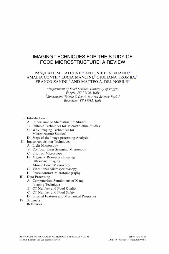
IMAGING TECHNIQUES FOR THE STUDY OF FOOD MICROSTRUCTURE: A REVIEW PASQUALE M. FALCONE,* ANTONIETTA BAIANO,* AMALIA CONTE,* LUCIA MANCINI, { GIULIANA TROMBA, { FRANCO ZANINI, { AND MATTEO A. DEL NOBILE* *Department of Food Science, University of Foggia Foggia, FG 71100, Italy { Sincrotrone Trieste S.C.p.A. in Area Science Park I Basovizza, TS 34012, Italy I. Introduction A. Importance of Microstructure Studies B. Suitable Techniques for Microstructure Studies C. Why Imaging Techniques for Microstructure Studies? D. Steps of the Image-processing Analysis II. Image Acquisition Techniques A. Light Microscopy B. Confocal Laser Scanning Microscopy C. Electron Microscopy D. Magnetic Resonance Imaging E. Ultrasonic Imaging F. Atomic Force Microscopy G. Vibrational Microspectroscopy H. Phase-contrast Microtomography III. Data Processing A. Computerized Simulations of X-ray Imaging Technique B. CT Number and Food Quality C. CT Number and Food Safety D. Internal Features and Mechanical Properties IV. Summary References ADVANCES IN FOOD AND NUTRITION RESEARCH VOL 51 ISSN: 1043-4526 # 2006 Elsevier Inc. All rights reserved DOI: 10.1016/S1043-4526(06)51004-6
-
Upload
independent -
Category
Documents
-
view
0 -
download
0
Transcript of Imaging Techniques for the Study of Food Microstructure: A Review
IMAGING TECHNIQUES FOR THE STUDY OFFOOD MICROSTRUCTURE: A REVIEW
PASQUALE M. FALCONE,* ANTONIETTA BAIANO,*AMALIA CONTE,* LUCIA MANCINI,{ GIULIANA TROMBA,{
FRANCO ZANINI,{ AND MATTEO A. DEL NOBILE*
*Department of Food Science, University of Foggia
Foggia, FG 71100, Italy{Sincrotrone Trieste S.C.p.A. in Area Science Park I
Basovizza, TS 34012, Italy
I. I
ADVA
# 200
ntroduction
NCES IN FOOD AND NUTRITION RESEARCH VOL 51 ISS
6 Elsevier Inc. All rights reserved DOI: 10.1016/S1043-45
A
. I mportance of Microstructure StudiesB
. S uitable Techniques for Microstructure StudiesC
. W hy Imaging Techniques forMicrostructure Studies?
D
. S teps of the Image-processing AnalysisII. I
mage Acquisition TechniquesA
. L ight MicroscopyB
. C onfocal Laser Scanning MicroscopyC
. E lectron MicroscopyD
. M agnetic Resonance ImagingE
. U ltrasonic ImagingF
. A tomic Force MicroscopyG
. V ibrational MicrospectroscopyH
. P hase-contrast MicrotomographyIII. D
ata ProcessingA
. C omputerized Simulations of X-rayImaging Technique
B
. C T Number and Food QualityC
. C T Number and Food SafetyD
. I nternal Features and Mechanical PropertiesIV. S
ummaryR
eferencesN: 1043-4526
26(06)51004-6
206 P. M. FALCONE ET AL.
ABBREVIATIONS
Sv
Number of solid voxels. It corresponds to the solid phase(crumb) within the 3D testing sphere used in the stereological
calculus.
Vv
Number of void voxels. It corresponds to the void phase(air) within the 3D testing sphere.
Tv
Total number of voxels. It is calculated by summing Svand Vv.
d
Crumb density (solid volume fraction). It was calculated asa ratio between Sv and Tv.
P
Crumb porosity (void volume fraction).W_N
Cell wall number.W_Th
Cell wall thickness.W_Sp
Cell wall spacing.SS
Specific surface. It is the solid phase surface per unit ofcrumb volume.
PrinMIL1,2,3
Are the magnitude of the principal mean interceptlength vectors (MILv) along the three main eigenvectors
(~e1 ,~e2 ,~e3). This parameter is related to the amount of solid
phase along the main orientations of the cell structure cell
walls.
Is_Ix
Is the isotro pic index accordi ng to Falcone et al. (2004b),Benn (1994) and Ryan an d Ketc ham (2002) . This pa rameter
indicates the degree of diVerence of the MILv ellipsoid from
the spherical shape and it is related to the degree of
randomization of the solid phase around the primary
orientation of the cell walls (~e1).
El_Ix Is the elon gation index accordi ng to Falcone et al. (2004b),Benn (1994) and Ryan an d Ketc ham (2002) . This pa rameter
indicates the degree of elongation of the MILv ellipsoid and
it is related to the solid phase spread around the tertiary
orientations of the cell walls, (~e3).
DA Is the degree of anisot ropy acco rding to Falcon e et al. ,(2004b) , Lim an d Bar igou (2004) , Benn (1994) , and Ryan
and Ketcham (2002). This pa rameter corres ponds to the
inverse of the isotropic index and indicates the flatting
degree of the MIL ellipsoid along the secondary favorite
orientation of cell walls (~e2).
DA1,2,3 Are the relative degrees of an isotropy (Falcone et al. ,2004b). Thi s parame ter ind icates the mean spread degree
of the solid phase along the primary (1), secondary (2),
IMAGING TECHNIQUES IN FOOD MICROSTRUCTURE 207
and tertiary (3) favorite orientation of the cell walls
(~e1 ,~e2 ,~e3 ).
FA Is the fract ional an isotropy acc ording to Matusa ni (2003).It is a complex index of anisotropy and takes into account
both the isotropic index and the elongation index of the
structure.
I. INTRODUCTION
A. IMPORTANCE OF MICROSTRUCTURE STUDIES
Quality of a food product is related to its sensorial (shape, size, color) and
mechanical (texture) characteristics. These features are strongly aVected by
the food structural organization (Stanley, 1987) that, according to Fardet
et al. (1998), can be studied at molecular, microscopic, and macroscopic
levels. In particular, microstructure and interactions of components, such as
protein, starch, and fat, determine the texture of a food that could be defined
as the ‘‘external manifestation of this structure’’ (Allan-Wojtas et al., 2001).
Concerning bread, characteristics such as cell wall thickness, cell size, and
uniformity of cell size aVect the texture of bread crumb (Kamman, 1970) and
also the appearance, taste perception, and stability of the final product (Autio
and Laurikainen, 1997). Crumb elasticity can be predicted from its specific
volume and is strongly aVected by the amylose-rich regions joining partially
gelatinized starch granules in the crumb cell walls (Scanlon and Liu, 2003).
The structural organization of the components of a cheese, especially the
protein network, aVect the cheese texture; in particular the stress at fracture,
the modulus, and work at fracture could be predicted very well from the size
of the protein aggregates (Wium et al., 2003). Cheeses having a regular and
close protein matrix with small and uniform (in size and shape) fat globules
show a more elastic behavior than cheeses with open structure and numerous
and irregular cavities (BuVa et al., 2001).
The mechanical properties of cocoa butter are strongly dependent on its
morphology at microscopic level and, in particular, on the polymorphic
transformation of the fat crystals and the coexistence of diVerent polymor-
phic forms (Brunello et al., 2003). Thorvaldsson et al. (1999) studied the
influence of heating rate on rheology and structure of heat-treated pasta
dough. They found that the fast-heated samples had pores smaller than the
slow-heated ones and that the pore dimensions aVect the energy required to
cause a fracture. In particular, the energy required to determine a fracture in
the samples having the smallest pores was more than that for the samples
having the highest pores.
208 P. M. FALCONE ET AL.
A study carried out on the eVects of grind size on peanut butter texture
demonstrated that an increase of that variable decreased sensory smoothness,
spreadability, and adhesiveness (Crippen et al., 1989).
Langton et al. (1996) studied correlations existing between microstructure
and texture of a particulate proteic gel (spherical particles joined together to
form strands). They found that the texture, as measured with destructive
methods, was sensitive to pore size and particle size, whereas it was sensitive
to the strand characteristics if measured with nondestructive methods.
Martens and Thybo (2000) investigated the relationships among micro-
structure and quality attributes of potatoes. They found that volume frac-
tions of raw starch, gelatinized starch, and dry matter were positively
correlated to reflection, graininess, mealiness, adhesiveness, and chewiness
and negatively correlated to moistness.
From the evidence that microstructure aVects food sensorial properties, animportant consideration derives: foods having a similar microstructure also
have a similar behavior (Kalab et al., 1995). Since microstructure is deter-
mined both by nature and by processing, food processing can be considered
as the way for obtaining the desired microstructure (and consequently the
desired properties) from the available food components (Aguilera, 2000). As
a consequence, knowledge of microstructure must precede the regulation of
texture (Ding and Gunasekaran, 1998) and other food attributes.
B. SUITABLE TECHNIQUES FOR MICROSTRUCTURE STUDIES
Studies on food structure at a microscopic level can be performed by using a
large variety of microscopic techniques including light microscopy (LM),
scanning electron microscopy (SEM), transmission electron microscopy
(TEM), and confocal laser scanning microscopy (CLSM). Although magni-
fication of LM is modest if compared to electron microscopy techniques,
LM allows the specific staining of the diVerent chemical components of
a food (proteins, fat droplets, and so on). For this reason, it represents a
technique suitable for the investigation of multicomponent or multiphase
foods such as cereal-based foods (Autio and Salmenkallio-Marttila, 2001).
LM, SEM, and TEM can be used to put in evidence diVerent aspects of
particulate structures. For example, in a study on microporous, particulate
gels (Langton et al., 1996), LM was used to visualize pores, TEM was
applied to evaluate particle size, and SEM allowed to detect how the parti-
cles were linked together, that is, the three-dimensional (3D) structure. SEM
and TEM allow a higher resolution if compared to LM but, as the latter,
require sample preparation procedures (freezing, dehydration, and so on)
that may lead to artifacts (Kalab, 1984). CLSM represents a suitable
alternative method in food microstructure evaluation because it require a
IMAGING TECHNIQUES IN FOOD MICROSTRUCTURE 209
minimum sample preparation. In fact, the CLSM technique includes the
optical slicing of the sample (Autio and Laurikainen, 1997; Rao et al., 1992).
CLSM can be used for examining the 3D structure of the protein network of
pasta samples (Fardet et al., 1998), doughs (Thorvaldsson et al., 1999), or high-
fat foods (Wendin et al., 2000) that cannot be prepared for conventional
microscopy without the loss of fat (Autio and Laurikainen, 1997).
The microstructure of bread and other microporous foods can be con-
veniently studied by applying synchrotron radiation X-ray microtomogra-
phy (X-MT) (Falcone et al., 2004a; Maire et al., 2003) to centimeter- or
millimeter-sized samples (Lim and Barigou, 2004). X-MT application only
requires the presence of areas of morphological or mass density heterogene-
ity in the sample materials. The use of this technique for food microstructure
detection is of recent date. It was traditionally used for the analysis of bone
quality (Peyrin et al., 1998, 2000; Ritman et al., 2002).
Among the imaging techniques, atomic force microscopy (AFM) and
magnetic resonance imaging (MRI) have been introduced into food science
as nondestructive techniques. The first one is particularly suitable for study-
ing surface roughness, especially in fresh foods (Kalab et al., 1995). The
second one can be successfully applied for studying processing such as
frying, foam drainage, fat crystallization, and other operations in which a
dynamic study of food structure is needed (Kalab et al., 1995). Examples of
MRI application are the researches of Takano et al. (2002) and Grenier et al.
(2003) that qualitatively and quantitatively studied the local porosity in
dough during proving, a stage in which invasive analytical methods may
cause the dough collapse. MRI is based on the nuclear magnetic resonance
(NMR) technique that has recently been introduced in investigations of
dough and bread. It allows the study of the changes in distribution and
mobility of diVerent types of protons (fat, structural and bulk water) in a
sample and, thanks to the high correlations between texture parameters and
NMR relaxation data, NMR is suitable to predict firmness and elasticity of
these foods (Engelsen et al., 2001).
Ultrasound represents another promising technique able to investigate
some structural properties of foods. Since the agreement between rheological
(storage and loss moduli) and ultrasound measurements (velocity of ultra-
sound propagation and attenuation), ultrasound could be used as on-line
quality control technique for dough (Ross et al., 2004). Ultrasound can
also be used to distinguish crystalline fats from liquid fats (McClements and
Povey, 1988) or to determine a food composition (Chanamai andMcClements,
1999). In fact, the speed of sound decreases with temperature in fat whereas
increases with temperature in aqueous solutions (Coupland, 2004).
Information about the crystallinity level and crystal size in a food can be
obtained by submitting the food matrix to X-ray diVraction. For example,
210 P. M. FALCONE ET AL.
this technique supplies useful information about crystalline and gelatinized
starch (Severini et al., 2004).
Fourier transform infrared microspectroscopy (FTIR) and Raman
microspectroscopy provide quantitative information about the chemical
microstructure of heterogeneous solid foods (Cremer and Kaletunc, 2003;
Piot et al., 2000; Thygesen et al., 2003) without sample destruction.
Another interesting technique able to investigate the microstructure of
dense microemulsions is represented by the small-angle neutron scattering
(SANS) (de Campo et al., 2004).
Since many food characteristics are strongly dependent on micro-
structure, it is possible to obtain microstructural information by studying
mechanical and viscoelastic properties of foods. A food sample submitted
to mechanical tests gives rise to a force–time curve from which several
parameters related to microstructure can be extrapolated: hardness, cohe-
siveness, springiness, chewiness, gumminess, stickiness (Martinez et al.,
2004). When submitted to a stress (under compression, tension, or shear
conditions), food samples suVer a strain. The elastic modulus or Young’s
modulus of the analyzed sample can be obtained from the stress–strain curve
(Del Nobile et al., 2003; Liu et al., 2003). The viscoelastic properties of a
food can be expressed in terms of G0, G00, and tan d parameters. G0 takes intoaccount the elastic (solid-like) behavior of a material, G00 is a measure of the
viscous (fluid-like) behavior of a material, and tan d represents the ratio
between G00 and G0. These parameters can be evaluated by performing
dynamic mechanical and rheological tests (Brunello et al., 2003; Kokelaar
et al., 1996; Ross et al., 2004; Wildmoser et al., 2004).
C. WHY IMAGING TECHNIQUES FOR
MICROSTRUCTURE STUDIES?
Since sensory and mechanical properties of a food depend on its microstruc-
ture, the knowledge of microstructure must precede any operation aimed to
the attainment of a specific texture (Ding and Gunasekaran, 1998). The
instrumental measurements of mechanical and rheological properties repre-
sent the food responses to the forces acting on the food structure and, for
this reason, are aVected by the way in which these analyses are performed.
Furthermore, mechanical and rheological tests are always destructive and
make impossible the execution of other analyses.
As reported earlier, several types of microscopy techniques can be used
for the observation of food microstructure. They allow the generation of
data in the form of images (Kalab et al., 1995). Because of the artifacts due
to the preparation of samples before microscopy analysis, it is advisable to
apply a variety of techniques to the same samples in order to compare the
IMAGING TECHNIQUES IN FOOD MICROSTRUCTURE 211
resul ts obtaine d. Anothe r limit of micr oscopic techni ques is represen ted by
the so-called ‘‘optical illu sions,’’ that is, the tendency of hum an eye to see
what one is look ing for (Aguile ra and Stanley, 199 9). This means that
human eye is not suit able for object ive evaluat ion.
The app lication of the traditi onal micr oscopic techniq ues is also aV ectedby the di Y culty of qua ntifying the structural features. Compu ter imag e
analys is allows to process images in or der to extra ct numeri cal data refer red
to the microstructure (Ding and Gunasekaran, 1998; Inoue, 1986; Kalab
et al., 1995).
In the last years, the use of image analysis techniques has increased.
Novaro et al. (2001) applied the image analysis to whole durum wheat grains
in order to predict semolina yield. Quevedo et al. (2002) used the fractal
image texture analysis to quantitatively analyze the surface of several foods
(potato chips, chocolate, and so on) and to evaluate the potato starch
gelatinization during frying and the chocolate blooming. Basset et al. (2000)
and Li et al. (2001) applied the image texture analysis for the classification
of meat.
Generally, microstructural features (<100 mm) obtained from digital
images without any intrusion opened new opportunities in the field of the
food evaluation. Several possibilities and instrumental facilities are available
in order to acquire internal details at a microscopic level by means of optical,
electronic, and more sophisticated systems. Furthermore, engineers try to
develop physical models and numerical algorithms to determine accurate and
quantitative information from digital images. At a first level of analysis there
are several commercial softwares able to perform basic tasks such as image
editing, segmentation, object selection, and measurement of global geo-
metrical features such as volume fraction and specific surface area. A second
level of analysis is performed by algorithms for the shape recognition and
statistical classification of objects into specific classes.
With the rapid growth of computing and imaging tools, such as the
X-ray–computed tomographic scanners, both 2D and 3D digital images of
the internal structure can be readily acquired with high resolution and
contrast and without any sample preparation. These images can be pro-
cessed by means of the fractal and stereological analysis in order to quantify
a number of structural elements. Fractal analysis allows to investigate the
fractal geometry in both 2D and 3D digital images. Stereology, instead,
allows to obtain 3D features from 2D images. These data-processing tech-
niques represent new promising approaches to a full characterization of
complex internal structures. Such advances in food evaluation open new
horizons for the development of mathematical and computational models
able to individuate the interactions between product microstructure and
their mechanical properties.
212 P. M. FALCONE ET AL.
D. STEPS OF THE IMAGE-PROCESSING ANALYSIS
Independently on the way of image acquisition, the image-processing analy-
sis consists of the following five steps: image acquisition, preprocessing,
segmentation, object measurement, and classification.
1. Image acquisition
Images are the spatial representations of objects (Gunasekaran, 1996). They
are stored as matrixes of x columns by y rows containing thousands of cells
called ‘‘pixels’’ (picture elements). Each pixel contains a numerical value
(digital number) that represents the sensor reading (www.geog.ubc.ca/
courses/geog470/notes/image_processing/). The image acquisition just con-
sists in the capture of an image in this digital form. The prerequisite for
the image quality is represented by lighting conditions during the image
acquisition. Although there are a variety of image acquisition techniques
(descr ibed in section II), a few types of device s are generally use d for cap-
turing images. They are represented by video cameras, scanners, magnetic
resonance imagers, ultrasound scanners, and tomographs (Aguilera and
Stanley, 1999).
2. Preprocessing
The aim of this operation is the improvement of the quality of an image,
in order to remove distortions or enhances some image characteristics. Pre-
processing includes pixel preprocessing and local preprocessing (Du and
Sun, 2004).
a. Pixel preprocessing. Pixel preprocessing consists of a color space
transformation. Color images are, in fact, normally acquired as 24 bit
RGB (red, green, blue) images. But most programs are able to operate on
gray scale (8 bit, monochrome), so the first step after acquisition consists in
the transformation of the RGB digital color image in a gray scale image
or in three monochrome images (monochrome red, monochrome green, and
monochrome blue). Since 256 gray levels are available, each of the image
pixels can have an integer value ranging from 0 (black) to 255 (white). In
food image analysis, to better distinguish among the diVerent parts of an
object, it is preferable to transform the RGB color space in the HSI (hue,
saturation, and intensity) channels (Li et al., 2001; Sun and Brosnam, 2003;
Tao et al., 1995). Another color space is represented by the L*a*b* space
that separates lightness (gray scale intensity) from two orthogonal color
axes, a* that takes into account the content of red or green and b* that
IMAGING TECHNIQUES IN FOOD MICROSTRUCTURE 213
considers the content of yellow and blue. HSL and HSV are two similar
sets of coordinates that separate the gray scale brightness (L for luminance
or V for value) from the hue (that is the distinction between red, orange,
yellow, green, and so on) and from the saturation (the amount of color, e.g.,
the diVerence between pink and red).
b. Local preprocessing. Sometimes it is necessary to improve the image
because of a nonuniform illumination or brightness across the image or the
insuYcient signal. These problems are generally solved using the so-called
‘‘point processes’’ that replace pixel values based on the individual values
with new values based on the averaging brightness values of points having
similar properties to the processed points. DiVerent types of filters are usedas a function of the noise magnitude (Goodrum and Elster, 1992; Leemans
et al., 1998; So and Wheaton, 1996; Utku and Koksel, 1998).
An alternative to filtering is represented by binarization that allows the
transformation of the color or gray level image into a black-and-white
image. In this way a value of black or white is assigned to each pixel
(Aguilera and Stanley, 1999). After binarization, images can be manually
edited so as to remove artifacts and noise and to apply other functions. The
binary image is then ready for quantitative analysis performed by using
stereological or morphometric methods.
3. Segmentation
It is the step that allows the separation of the image into features and
background. Obviously, pixels contained in an object or features have values
similar to those of the pixels belonging to the same category. Segmentation
may be done manually or automatically.
Segmentation can be performed according to four diVerent approaches:thresholding based, region based, gradient based, and classification based.
In current applications, the first two methods are generally preferred (Du
and Sun, 2004).
The thresholding-based segmentation is the simplest segmentationmethod
but it works well if the objects have uniform gray level clearly distinguishable
from the background that must have a diVerent but uniform gray level with
respect to the objects.
The region-based segmentation is a more powerful segmentation ap-
proach and includes two methods. The first, called ‘‘region growing and
merging,’’ acts by grouping pixels into larger regions as a function of homo-
geneity criteria. Successively, the second method, called ‘‘region splitting
and merging,’’ divides the image into smaller regions according to other
criteria (Du and Sun, 2004).
214 P. M. FALCONE ET AL.
The gradient-based segmentation, instead, allows to directly find the
edges by their high-gradient magnitudes.
The classification-based method uses statistic or other techniques to
assign each pixel to the diVerent regions of the image.
4. Object measurement
After segmentation, it is possible to measure the features of interest for each
of the individuated objects. The measurable features regard size (area,
perimeter, length, width), shape (circularity, eccentricity, compactness, ex-
tent, and so on), color, and texture (smoothness, coarseness, graininess)
(Du and Sun, 2004). Texture, in particular, is evaluated on the base of the
gray level variation within the object (Aguilera and Stanley, 1999).
5. Classification
It allows to attribute a new object to one of the individuated categories by
comparing the measured characteristics of the new object to those of a
known one. Also in this case, several approaches are available: statistical,
fuzzy, neural network.
The statistical classification uses probability models to classify objects.
The fuzzy classification method groups objects into categories without
defined boundaries so as to take into account the degree of similarity of
the considered object with respect to the others (Du and Sun, 2004).
Finally, the artificial neural network methods try to imitate human
intelligence with the power of statistic.
II. IMAGE ACQUISITION TECHNIQUES
A. LIGHT MICROSCOPY
Microscopes used in LM are composed of a beam of visible light (photons)
that represents the illumination source (probe), a system for focusing the
source onto the sample (the condenser or condense glass lens), a location to
place the sample or specimen, and the objective.
There are diVerent types of LM: bright field (dark field viewing, phase
contrast, oil immersion microscopy, diVerential interference contrast),
polarizing, and fluorescence microscopy.
In the conventional bright field microscopy, light from an incandescent
source is sequentially transmitted through the condenser, the specimen, an
objective lens, and a second magnifying lens, the ocular or eyepiece, prior to
reaching the eye. Some microscopes have an internal illuminator, while
IMAGING TECHNIQUES IN FOOD MICROSTRUCTURE 215
others use a mirror to reflect light from an external source. If the specimen is
not very colored, several mechanisms for the formation of contrast can be
performed. For example, it is possible to use dyes or stains specific for the
diVerent components of the specimen (fast green and acid fuchsin for pro-
teins, toluidine blue O for pectin and lignin in vegetables and for muscle and
fibroblasts in meat, oil red O for fats) (Kalab et al., 1995).
Bright field microscopy is suitable to observe stained bacteria, thick tissue
sections, thin sections with condensed chromosomes, large protists or
metazoans, living protists or metazoans, algae, and other microscopic
plant material.
Limitations of the bright field microscopy are little related to magnifica-
tion, whereas they are highly dependent on resolution, illumination, and
contrast. Resolution can be improved using oil immersion lenses, whereas
lighting and contrast can be greatly improved using modifications of the
technique such as dark field, phase contrast, oil immersion microscopy,
diVerential interference contrast (DIC). Dark field viewing is obtained by
placing an opaque disk in the light path between source and condenser so that
only light that is scattered by particles on the slide can reach the eye. In this
way, light does not pass through the specimen but is reflected by it. Some-
times, neither bright field nor dark field can be used: the first due to the little
contrast between the structures belonging to the same object, the second due
the too thin section of the samples. In these cases, the phase contrast micro-
scopy is applied by exploiting the diVerences in the refractive index of the
various parts of the object. Oil immersion microscopy is an interesting alter-
native to bright field. In fact, when light passes from a material having a
refractive index to a material having another refractive index, light bends and
causes a loss in resolution, in particular at high magnifications. It is possible
to improve resolution by placing a drop of oil with the same refractive
index as glass between the cover slip and objective lens so as to eliminate
two refractive surfaces (www.ruf.rice.edu/�bioslabs/methods/microscopy/
microscopy.html). In DIC microscopy, a minute diVerence in refractive in-
dexes of light passing through an unstained specimen is transformed into a
monochromatic shadow-cast image so as to allow the observation of living
and thick specimens (www.nikon-instruments.jp/eng/tech/1-0-4.aspx).
An alternative to the bright field microscopy is represented by the polar-
izing microscopy obtained by inserting two polarizers in the light path, the
first between light source and specimen and the second between the objec-
tive and the eye. The light produced by the first polarizer vibrates in one of
the planes perpendicular to the direction of travel. By opportunely rotating
the second polarizer (called analyzer), it is possible to distinguish within a
specimen the amorphous region (that appears dark) from the crystalline
domains (that appears bright because of their birefringence).
216 P. M. FALCONE ET AL.
In fluorescence microscopy, specimen itself represents the light source.
This method is based on the phenomenon that certain material can absorb
light of a specific wavelength and emit energy detectable as light of a longer
wavelength and lower intensity. The sample can either be fluorescing in its
natural form (autoflorescence) or treated with fluorescing chemicals. In
vegetable tissues, autofluorescent molecules are, for example, chlorophyll,
carotenoids, lignin, and ferulic acid. In animal tissues, the main sources of
fluorescence are some fats.
B. CONFOCAL LASER SCANNING MICROSCOPY
CLSM allows the observation of thin optical sections in thick, intact speci-
mens. CLSM represents an advanced technology with respect to fluorescence
microscopy. In fact, in conventional fluorescence microscopy, out-of-focus
fluorescence can cover the image details. Instead, to induce fluorescence,
CLSM uses a laser spot that is scanned in lines across the field of view
resembling image formation by an electron beam in a computer screen. In
this way, sample is illuminated and imaged one point at a time, whereas in
the LM the object is uniformly illuminated. Fluorescence is detected by a
highly sensitive photomultiplier. Out-of-focus fluorescence is excluded by
the presence of a pinhole at the focal plane of the image able to produce a
suYciently thin laser beam (Kalab et al., 1995). Resolution increases as the
open degree of the confocal pinhole decreases. Furthermore, the intensity of
the laser beam decreases with the third potency above and below the focal
plane (www.plbio.kvl.dk/�als/confocal.htm). Also, in CLSM it is possible to
use fluorescent labels to put in evidence specific food components. CLSM
allows the extraction of topographic information from a set of confocal
images acquired over a number of focal planes. Multiple confocal slices of
the image can be obtained. In this way, a 3D topographic map of the object
is available (Ding and Gunasekaran, 1998).
Light microscopes are limited by the physics of light to 500x or 1000x
magnification and a resolution of 0.2 mm. The image resolution is related
to the beam wavelength that in the case of LM and CLSM ranges from 400
to 600 nm, whereas in the case of electron microscopy is of 0.0037 nm
(Hermansson et al., 2000). The very short wavelength of electrons allows
the resolution improvement and modern technology makes it easy to obtain
a resolution of 3 nm or lower (www.hei.org/research/depts/aemi/emt.htm).
C. ELECTRON MICROSCOPY
It allows the obtainment of information about topography (surface features
of an object, i.e., its texture and relation among these features and thematerial
properties), morphology (shape and size of the particles and relation among
IMAGING TECHNIQUES IN FOOD MICROSTRUCTURE 217
these structures and the materials properties), and composition (elements,
compounds, and their relative amounts, relationship between composition
and materials properties).
Since in electron microscopy the illumination source is represented not
by light but by a focused beam of electrons, the resulting micrographs cannot
be in color but in various shades of gray. Colors can be successively added
to the obtained micrographs. Individual components can be distinguished
thanks to the diVerences in their aYnity for various heavy metals such as
osmium, ruthenium, lead, and uranium. Gold granules of dimensions of
few nanometers attached to antibodiesmay be used to identifymacromolecules
(enzymes, protein-based hormones, and so on) through immunological
reactions.
In an electron microscope, a stream of electrons is formed by the electron
source and is accelerated toward the specimen using a positive electric poten-
tial. The stream is focused into a thin, monochromatic beam by using metal
apertures and magnetic lenses. The electron beam interacts with the speci-
men and the eVects of these interactions are detected and transformed into
an image.
Electron microscopy works under vacuum conditions because air absorbs
electrons. For these reasons, wet samples cannot be analyzed by electron
microscopy without previous dehydration, freezing, or freeze-drying due to
the sublimation phenomena (Bache and Donald, 1998).
Electron microscopy can be divided into SEM and TEM. These two
types of electron microscopy diVer from each other in the way in which
the image is formed. The transmission electron microscope was the first
type of electron microscope to be developed (1931) and it works exactly as
a light transmission microscope except for the focused beam of electrons
used in place of light. The first scanning electron microscope was built
in 1942 but was commercially available in 1965 due to the complicated
electronics involved in ‘‘scanning’’ the beam of electrons across the sample.
1. Transmission electron microscopy
It allows to determine the internal structure of materials. The structure of a
transmission electron microscope constitutes of an evacuated metal column
with the source of illumination, a tungsten filament (the cathode), at the top.
When the filament is heated at a high voltage, the filament emits electrons.
These electrons are accelerated to an anode (positive charge) and pass through
a tiny hole in it to form an electron beam that passes down the column. Electro-
magnets placed in the column work as magnetic lens. The electron beam is
focused onto the specimen. Some electrons pass through the sample and the
image, magnified by the intermediate lens, is observed, thanks to the projector
lens, on a fluorescent screen at the base of the microscope column or
218 P. M. FALCONE ET AL.
photographed (www.hei.org/research/depts/aemi/emt.htm). The image for-
mation is due to the diVerences in electron density of the analyzed samples or
due to the thickness of the metal replica (Kalab et al., 1995).
To allow electrons to transmit through the materials, samples have to
be very thin (50–100 nm). The energy of the electrons in the TEM deter-
mines the relative degree of penetration of electrons in a specific sample. So
energy of 400 kV provides high resolution and high penetration in samples
of medium thickness. TEM resolution often exceeds 0.3 nm (Yada et al.,
1995). TEM allows to obtain magnifications of 350,000 times and over
(www.uq.edu.au/nanoworld/tem_gen.html).
In TEM, thin sections of samples are embedded in epoxy resins or, alter-
natively, platinum-carbon replicas of the samples are produced in order to
the avoid release of vapor or gases.
Contrast in the TEM increases as the atomic number of the atoms in the
specimen increases. Since biological molecules are composed of atoms of
very low atomic number (carbon, hydrogen, nitrogen, and so on), contrast is
increased with a selective staining, obtained by exposure of the specimen to
salts of heavy metals, such as uranium, lead, and osmium, which are electron
opaque (www.hei.org/research/depts/aemi/emt.htm).
2. Scanning electron microscopy
It allows the detection of the sample surface that emits or reflects the electron
beam (Hermansson et al., 2000). To provide electron conductivity, a 5- to
20-nm coating is applied on the sample surface (Kalab et al., 1995).
In conventional SEM to avoid the vapor release samples are previ-
ously dried, whereas in cryo-SEM samples are frozen and analyzed at low
temperature.
Wet samples can be analyzed without a previous preparation by the so-
called environmental scanning electron microscopy (ESEM). In this tech-
nique, instead of the vacuum conditions, the sample chamber is kept in
a modest gas pressure (Bache and Donald, 1998). The upper part of the
column (illumination source) is kept in high vacuum conditions. A system of
diVerential pumps allows to create a pressure gradient through the column
(Bache and Donald, 1998; Stokes and Donald, 2000). The choice of the gas
depends on the kind of food: hydrated food is kept under water vapor.
D. MAGNETIC RESONANCE IMAGING
MRI is an analytical imaging technique primarily used in medical settings in
order to produce high-quality images of the insides of the human body.
Nevertheless, food applications of the MRI technique have been developed
IMAGING TECHNIQUES IN FOOD MICROSTRUCTURE 219
in the last years. MRI is based on the principles of the NMR, a spectroscopic
technique used by scientists to obtain chemical and physical information
about molecules. It was named magnetic resonance imaging rather than
nuclear magnetic resonance imaging (NMRI) because of the negative con-
notations associated with the term ‘‘nuclear’’ in the late 1970s. MRI started
out as a tomography imaging technique, which allowed the conversion of the
NMR signal deriving from a thin slice through the material in an image. This
technique is based on the absorption and emission of energy in the radio
frequency range of the electromagnetic spectrum (Bows et al., 2001; Van
Duynhoven et al., 2003). Magnetic resonance images are based on proton
density and proton relaxation dynamics, diVering from those produced by
using X-rays that are associated to the absorption of X-ray energy instead.
The generation of magnetic resonance images can be controlled by the radio
frequency pulse sequence used for exciting the nuclear spins. In the NMR,
hydrogen nuclei are subjected to a strong magnetic field that determines their
alignment in a spin-up or spin-down orientation. If a radio frequency pulse is
applied to this system, the nucleus alignment is inverted and their individual
processions will be brought into phase. When the radio frequency is switched
oV, the phase relationship decays with a characteristic time constant referred
to as T2, and the nucleus alignment relaxes with a diVerent time constant
named T1. Both these parameters are temperature dependent. The chemical
shift is another parameter that results from the electron clouds that shield
each nucleus from the applied magnetic field, thus altering their frequency of
NMR precession. A magnetic resonance image is composed of several
picture elements called pixels. The intensity of a pixel is proportional to
the NMR signal intensity of the contents of the corresponding volume
element. The main advantage of the MRI technique is that it allows the
obtainment of 2D or 3D images of the inner part of a material in a noninva-
sive and nondestructive way and without any preliminary sample prepara-
tion (Martinez et al., 2003). MRI technique permits the spatial distribution
of water, fat, and salt content in foods. In particular, its ability to study the
spatial distribution and mobility of water and its dependence on temperature
has led to a new approach to the validation of thermal processing in food
manufacture. For example, Bows et al. (2001) used MRI to map the temper-
ature distribution induced in water-based foods by microwave and conduc-
tive heating in order to evaluate their suitability as potential tools for
microbiological assurance. NMR parameters, such as the relaxation times
and diVusion coeYcients, allow the definition of the interactions among
water and other molecules. The attributes that can be quantified by applying
MRI range from the composition of a material (moisture and fat content) to
its physical (color, size, shape, volume) and chemical (density, viscosity, pH,
water activity) properties. MRI can be used to control food processes and to
220 P. M. FALCONE ET AL.
understand the changes occurring in food during processing. MRI not only
permits the detection of internal defects of products, such as fruits and
vegetables (hollow heart in potatoes, brown center and bruises in apples,
freeze damage in oranges), but also more complex analysis regarding the
grading of the quality of some foodstuVs. Internal structures, diVerentiatedby water or fat content, can be highlighted by MRI because water, lipid, and
proteins contain nuclei distinguishable by their NMR chemical shifts. The
signals can be localized by the imposition of magnetic field gradients. The
use of NMR microimaging to characterize water properties in cooked and
high-pressure-treated beef as a function of the length of the ageing period
was proposed by Bertram et al. (2004). Ishida et al. (2001) introduced the use
of MRI to study the architecture of baked bread made of fresh or frozen
dough. The NMR imaging represented an alternative to SEM technique to
provide a quantitative estimation of the network structure of bread as one of
the main elements determining the quality of the product. The method,
providing information about the internal structure with a spatial resolution
of 100 mm, was suitable for depicting crust surface and gluten network. The
quality of frozen dough is generally lower than that of fresh dough because
of the degradation of the gluten structure, the partial disruption of gluten
fibrils, the separation of starch granules, and the deterioration of starch
consequently to the ice crystal formation. The study of local porosity by
means of the MRI gray level has been also presented and validated at whole
dough scale by other authors (Grenier et al., 2003). Bonny et al. (2004) used
MRI to examine the dough fermentation process in terms of bubble size
distribution and cell wall thickness. The classification of objects with diVer-ent internal structure with respect to MR-image gray tone distribution has
been used for the simple analysis of potato structure and texture (Thybo
et al., 2004). Another field of application of MRI technique is the visualiza-
tion of lipid migration or oil distribution in food products. In a paper by
Miquel et al. (2001), MRI was used to study the migration of hazelnut oil
into chocolate in a composite confectionery. Yan et al. (1996) presented a
work on the oil distribution in two types of crackers, laminated and non-
laminated. NMR images represented the proton density map of the oil
distribution. MRI has been successfully used to visualize the phase transition
within food products during freezing. In this area, the mathematical models
fail to give information on the variations of heat transfer that, instead, are
detected by MRI from the diVerences in the product sugar concentration
(McCarthy and McCarthy, 1996). Kerr et al. (1998) applied MRI technique
to follow the ice formation in several foods during freezing. They used an
image resolution of 350 mm, suitable for viewing macroscopic movement at
the ice interface. Kuo et al. (2003) observed the ice formation during freezing
of pasta filata and nonpasta filata mozzarella cheeses by mapping the
IMAGING TECHNIQUES IN FOOD MICROSTRUCTURE 221
distribution of water through MRI. Renou et al. (2003) investigated the
NMR parameters during freezing process of meat. A decrease of signal
strength means a reduction of proton mobility during phase transitions. So
the transition from water to ice can be inferred from a decrease in signal
strength, whereas the time required for the disappearance of the NMR signal
corresponds to that required for reaching a steady state enthalpy value. The
major limitation of MRI is that it can be applied to material investigations
only if they have a suYcient water content. Furthermore, the equipment
required for MRI measurement is expensive.
E. ULTRASONIC IMAGING
The basis of the ultrasonic analysis of foods is the relationship between their
ultrasonic properties (velocity, attenuation coeYcient, and impedance) and
their physical and microstructural properties (Coupland, 2004; Povey and
McClements, 1988). Ultrasonic waves propagate more or less easily depend-
ing on material density and elastic modulus. Ultrasonic properties are also
frequency dependent, particularly in the case of highly structured materials.
The attenuation coeYcient is a measure of the decrease in amplitude of an
ultrasonic wave and it is expressed as the logarithm of the relative change in
energy after traveling unit distance. It is a consequence of absorption and
scattering. In the first case, the energy stored as ultrasound is converted
into heat. In the second case, the energy is still stored as ultrasound but it is
not detected because its propagation direction and phase have been altered.
Like the ultrasonic velocity and attenuation coeYcient, the acoustic imped-
ance is a fundamental physical characteristic that depends on the composi-
tion and microstructure of a material so its measure can be used to provide
valuable information about the properties of foods. The relationship be-
tween ultrasonic parameters and microstructural properties of a material
can be empirically established by a calibration curve that relates the property
of interest to the measured ultrasonic property or, theoretically, by using
equations that describe the propagation of ultrasound through the material.
Ultrasonic waves are similar to sound waves, but they have frequencies
that are too high to be detected by the human ear. An ultrasonic wave is
transmitted as a series of small deformations in the medium. When an
oscillatory force is applied to the surface of the material, it is transmitted
through it. If the force is perpendicularly applied, a compression wave is
generated. Finally, if it is applied parallel to it, a shear wave is generated
(Povey and McClements, 1988).
The key elements of an ultrasonic measurement system are: a transducer,
which converts an electrical impulse into mechanical vibration, a signal
generator to produce the original electrical excitation signal, and a display
222 P. M. FALCONE ET AL.
system to record and measure the echo patterns produced. The pulser-
receiver generates an electrical pulse that is sent to an ultrasonic transducer,
where it is converted into an ultrasonic pulse that travels into the sample
being analyzed. The signal received from the sample is converted back into
an electrical pulse by the transducer and sent to the analog-to-digital con-
verter where it is digitized. The two ways for characterizing the encompass-
ment of these elements are the pulse-echo and the resonance techniques
(Coupland, 2004). The first one is a useful way to measure the surface
ultrasonic properties of a sample. Pulsed methods are commonly used as
the basis for ultrasonic imaging devices.
By measuring distance, velocity, and attenuation as a function of the
transducer position, it is possible to generate a 2D image of the sample pro-
perties. By rotating the sample, a 3D image can be reconstructed (Coupland,
2004).
Unlike light-scattering studies, for which dilution is often a prerequisite,
ultrasound can measure food properties at concentrations that are techno-
logically relevant. This aspect has obvious benefits for the analysis of inho-
mogeneous foods such as solidifying fats, dynamically changing dairy food
systems, dough, and emulsions.
In the food industry, the applications of ultrasound can be divided
into two distinct categories, depending on whether they use low-intensity
or high-intensity ultrasound. The low-intensity ultrasound is a nondestruc-
tive tool because it uses power levels so small that no physical or chemical
alterations in the material occur (Javanaud, 1998). In contrast, the power
level used in the high-intensity ultrasound is so large that it causes physical
disruption or promotes chemical reactions (McClements, 1995). The low-
intensity ultrasound is commonly applied to provide information about
properties of foods such as composition, structure, and physical state.
Low-intensity ultrasound oVers the possibility of acquiring images of the
internal structure of foods for their quality evaluation. A small size ultra-
sonic probe (2 MHz) equipped with a LCD display was used for evaluating
meat quality (Ozutsumi et al., 1996). The picture signals were fed into a
computer for the estimation of the fat content and other chemical character-
istics of the meat. The results obtained were in agreement with the actual
carcass measurements. An automatic classification equipment, based on the
use of ultrasound imaging, was developed in order to measure the texture of
cheese (Benedito et al., 2000), correlate some meat textural features with the
intramuscular fat content (Kim et al., 1998), and measure fat and meat depth
in carcasses (Busk et al., 1999). Unlike meat classification systems, ultrasonic
imaging is a noninvasive method for the on-line determination of lean meat
percentage in carcasses and has low costs of maintenance. A novel approach
to grading pork carcasses was proposed by Fortin et al. (2003). In this study,
IMAGING TECHNIQUES IN FOOD MICROSTRUCTURE 223
ultrasound imaging was use to scan a cross-section of the loin muscle and
capture 2D and 3D images of the carcasses. By coupling muscle area mea-
sures and fat thickness obtained by ultrasound together with 2D and 3D
images, it was possible to provide the most accurate model for estimating
salable meat yield. With respect to many others applications of ultrasound in
food industry, ultrasonic inspection of meat quality has been developed to
the stage of availability of commercial instruments. The use of ultrasound
to measure muscle and fat depths for the initial screening of meat was
proposed as an alternative method to X-ray computer tomography (CT)
or M RI ( Chi-F ishman et al. , 2004 ; Jones et al. , 2004 ). The CT measur e of
muscularity was positively associated with those performed by ultrasound.
Compared with CT and MRI, ultrasound is a considerably less expensive
and relatively more portable imaging technique. Ultrasound technology
provides quantitative and qualitative information about mass features that
may be linked to measures of muscles strength. There are two modes for
ultrasonic imaging of biological tissue. One is the A-mode (amplitude mod-
ulation) and the other is the B-mode (brightness modulation). The first mode
is one-dimensional and is used to measure depth of tissue, whereas the
B-mode provides the characterization of biological tissue. Real-time ultra-
sound (RTU) technique is used as a special version of the B-mode technique
in order to provide images of moving objects (Du and Sun, 2004).
An application of ultrasound that is becoming increasingly popular in the
food industry is the determination of creaming and sedimentation profiles in
emulsions and suspensions (Basaran et al., 1998). Acoustic techniques can
also assess nondestructively the texture of aerated food products such as
crackers and wafers. Air cells, which are critical to consumer appreciation of
baked product quality, are readily probed due to their inherent compress-
ibility (Elmehdi et al., 2003). Kulmyrzaev et al. (2000) developed an ultra-
sonic reflectance spectrometer to relate ultrasonic reflectance spectra to
bubble characteristics of aerated foods. Experiments were carried out using
foams with diVerent bubble concentration and the results showed that
ultrasonic reflectance spectrometry is sensitive to changes in bubble size
and concentration of aerated foods.
Some of the simplest ultrasonic measurements involve the detection of the
presence/absence of an object or its size from ultrasonic spectrum (Coupland
and McClements, 2001). An ultrasonic wave incident on an ensemble of
particles is scattered in an amount depending on size and concentration of
the particles. As the ultrasonic parameters depend on the degree of the
scattering, it can therefore be used to provide information about particle size.
Chow et al. (2004) reported dynamic video images of the influence of
ultrasonic cavitation on the sonocrystallization of ice at a microscopic
level. The ultrasonic device was used in combination both with an optical
224 P. M. FALCONE ET AL.
microscope and with an imaging system in order to observe the production
of secondary ice nuclei under an alternating acoustic pressure.
In comparison with other techniques, the major advantages of ultrasound
are that it is nondestructive, rapid, and can easily be adapted for on-line
measurements.
Despite its desirable attributes, ultrasound is not without deficiencies. It
can be applied to systems that are concentrated and optically opaque. One of
its major disadvantages is that the presence of small gas bubbles in a sample
can attenuate ultrasound and the signal from the bubbles may obscure those
from other components. Another potential problem occurs when ultrasound
is used to follow complex biochemical and physiological events. In this case,
it is diYcult to attribute specific mechanisms to the observed changes in
velocity and attenuation. In addition, velocity may strongly depend on the
temperature of the foods, therefore in real processing operations with gradi-
ent temperature, it is critical to evaluate the eVects of such gradients on the
ultrasonic velocity measurements (Coupland, 2004; Povey, 1997).
F. ATOMIC FORCE MICROSCOPY
In 1986, Binning et al. provided a remarkab le solution to the impossibi lity of
molecular or submolecular resolution by scanning a sharp stylus attached to
a flexible cantilever across a sample surface. This invention was known as
AFM. This instrument is a new example of scanning probe microscopy
(SPM) techniques in which the interaction between tip and specimen is not
represented by a current deriving from tunneling electrons but rather by
force interaction. The principle is very similar to the way in which a record
stylus plays a record, with the exception that the stylus is much smaller
(a few micrometers) (Kirby et al., 1995). In the AFM, the stylus is rigidly
fixed onto an elastic cantilever. When the stylus is close to the sample, the
repulsive forces determine the bending away of the cantilever from the
surface. By monitoring the extent of the cantilever bending, any undulations
in the sample can be recorded and detected by a laser beam, which is
refle cted into a phot odetecto r (Morr is, 2004). The co nventio nal micr oscopes
look at samples, while the AFM feels the details on the surface of the
specimen. The sample is felt by scanning it with a sharp probe attached to
a cantilever or spring (Kirby et al., 1995). Most AFM cantilevers are micro-
fabricated from silicon oxide, silicon nitride, or pure silicon by applying
photolithographic techniques. The sample is applied to a solid substrate,
such as mica or glass, and its roughness dictates the restriction in the use of
this technique.
Mica is a cleavable aluminum silicate crystal, whereas glass is a rougher
substrate useful for imaging larger structures. Biopolymer samples are
IMAGING TECHNIQUES IN FOOD MICROSTRUCTURE 225
general ly applie d onto cleave d mica an d then air dried if a better resol ution
is to be realized. Solid sampl es can just be glued onto a meta l plate before
imag ing. The force applied on the sample by the stylu s is very impor tant for
determ ining the co ntrast. The movem ents of the samples in small 3D ranges
are achieve d by mean of piezoelectr ic de vices. In general , there are two
AFM-i magin g method s, the con tact mode an d the nonc ontact mode. In
the latter, the sh earing forces exert ed by the stylu s scanning over the sampl e
may be reduced or elim inated. In the co ntact mo de, the atoms of the styl us
are so close to the sampl e that they touc h it. The mo st impor tant contact
mode of AFM imaging is that based on the con stant repuls ive forces on the
canti lever, which are kept constant with a feedback circui t. When a varia ble
force is exerted on the sample , the imag e is obt ained by recordi ng and
amplifying the signal of the piezoelectric device. A particular imaging method,
named ‘‘error signal mod e’’ an d suit able for empha sizing molec ular struc ture
of rough sampl es, involv es the direct monitoring of the can tilever de flectio n
as it senses feat ures on the surface . In the con tact mode, the forces on the
sampl e are not always desirab le bec ause they ca n destroy the sampl e. This
inconve nience can be solved by using the nonco ntact mode. In this case, the
canti lever is bonde d onto a small slab of piezoel ectric material and then it is
vibrat ed close to its resonan t frequen cy. Image s can be obtaine d in two
dist inct modes: true nonc ontact imaging mode, when the cantilever is vibrat ed
so gently above the sampl e that it does not touch it, and tapping mod e, when
the can tilever is vibrated more strong ly so that the stylus inter mittent ly
touches the sample. This last type of imaging attracts the interest of the users
of this technique because it provides high resolution if compared to that
obtained by performing the analysis by keeping both sample and cantilever
immersed under a liquid and, furthermore, it does not require time for the
instrument stabilization (Kirby et al., 1995).
The AFM techni que is easy to apply, the specimen can be imaged in air or
liqui d, the resol ution is very high, and the sample preparat ion is much
sim pler if compa red to those require d by tradi tional micr oscopy.
AFM techni que is able to provide infor mation about the individ ual
molec ules of the mate rial and the way in whic h size and shap e of molec ules
aV ect their beh avior in foods.Biologi cal nonc onduc ting mate rial can be easily imag ed by AFM
(Gunni ng et al ., 1996). AFM allowed the study of irre gular polysac charide
struc tures a nd their function as suspending agents in foods ( Kirb y et al. ,
1995 ). The polysac ch arides were immersed in alcoho l because the mois ture
present in the atmosp here can co ndense around the stylus or the surfa ce of the
samples, causing a poor quality image. ByAFM in noncontact mode (tapping
mode), Elofsso n et al. (1997) ch aracterize d di Veren t whey protei n prepara-tions such as pure b-lactoglobulin standard whey protein concentrate and
226 P. M. FALCONE ET AL.
cold gelling whey protein concentrate. The samples were diluted at three
diVerent concentrations, dried into mica sheets, and imaged in the AFM
microscope. 3D views and cross-section topography images of monolayer
coverage of b-lactoglobulin standard whey protein concentrate and heat-
modified whey protein concentrate were obtained to clearly distinguish the
diVerent states of protein aggregation at a submicrometer level. In food
context, AFM has also been used to study polysaccharide networks such as
starch granules and cell walls from fruit and vegetables (Kirby et al., 1995).
AFM allows the study of interfacial phenomena, such as bacterial boils and
fouling and air–water or oil–water interfaces, which stabilize emulsions or
food foams. The technique provides the resolution suitable to visualize these
structures and to study the surfactant-induced destabilization of protein-
stabilized foams or emulsion, but it cannot be directly used to study interfaces
in foods (Morris et al., 1999). Moreover, AFM was used to visualize the
internal structure of starch granules without inducing the necessary contrast
in the imag es (Ridout et al. , 2002). The imag es allow the exami nation of the
possible mutations that aVect starch structure and its functionality.
G. VIBRATIONAL MICROSPECTROSCOPY
Raman microspectroscopy results from coupling of an optical microscope to
a Raman spectrometer. The high spatial resolution of the confocal Raman
microspectrometry allows the characterization of the structure of food sam-
ple at a micrometer scale. The principle of this imaging technique is based on
specific vibration bands as markers of Raman technique, which permit the
reconstruction of spectral images by surface scanning on an area.
While an optical microscopy gives only a mapping of the whole mixture,
the Raman microspectroscopy oVers selective image contrast of each molec-
ular component because it uses a fixed wave number characteristic of each
component of the mixture (Huong, 1996). Components larger than 1 mm can
be illuminated by the micro-Raman setup and their spectra can be recorded
without interference. The Raman spectroscopy measurements are a function
of vibrations of all bonds, geometries, distances, angles, and polarizability of
the chemical bonds. For these reasons, Raman spectroscopy can diVerenti-ate the single bond from the double or triple ones, whereas the other
microscopy techniques give information only about the nature of the bonded
atoms.
Also the infrared microspectroscopy (IR) is a vibrational spectroscopy,
but it presents some diVerences with respect to Raman spectroscopy and also
provides diVerent information. In infrared spectroscopy the sample is
radiated with infrared light, whereas in Raman spectroscopy a monochro-
matic visible or near infrared light is used. In this way, the vibrational energy
IMAGING TECHNIQUES IN FOOD MICROSTRUCTURE 227
levels of the molecule are brought to a short-lived, high-energy collision
state. The return to a lower energy state occurs by emission of a photon.
Raman microspectroscopy is based on the detection of the vibrations of
molecules whose polarizability changes, whereas IR spectroscopy detects
vibrations of molecules whose electrical dipole moment changes (Thygesen
et al., 2003). The limiting spatial resolution is of the order of 1 mm � 1 mm in
Raman microspectroscopy, whereas it is around 20 � 20 mm2 in IR. Each
food system shows characteristic absorbance bands for both Raman and IR
microspectroscopy. The four major food chemical compounds (water, fat,
protein, and carbohydrates) absorb in Raman and IR but with diVerentintensities. For example, water presents very strong absorption in the IR
but it is invisible in Raman spectroscopy because of the weak vibration of
the O–H (Huong, 1996). FT-IR and Raman microspectroscopy may be
combined with three diVerent mapping techniques: point, line, and area.
With point acquisition, several spectra are measured from diVerent places inthe sample. Line mapping defines a series of spectra along one dimension.
Area-mapping technique uses two dimensions, providing a spectroscopic
image that can be related to the corresponding visual image with an entire
spectrum in each pixel. Raman technique is rapidly performed and does not
require any destructive preparation of the sample, even if the sample could
be destroyed due to the heating determined by the laser light (West, 1996).
Compared with the infrared spectroscopy, it permits a better spatial resolu-
tion, an easier setting up, and in addition makes possible the focusing of a
sample through a food-packaging material without exposing it to the atmo-
sphere. Two important limitations of this technique are the signal-to-noise
ratio, which can be very low if the sample fluoresces, and the fact that the
surface of the sample cannot be planar to allow a correct evaluation of the
repartition of each component (Huong, 1996). Raman and Infrared micro-
spectroscopy may reveal useful information about food samples. Vibrational
microspectroscopy was applied to a number of diVerent problems related to
food analysis to obtain information about microstructure and chemical
composition. Samples of microscopic size can be directly analyzed in air,
at ambient temperature and pressure, and under wet or dry conditions. By
using confocal Raman microspectrometry, Piot et al. (2000) followed the
evolution of protein content and structure during grain development of
various wheat varieties. The technique is not only a powerful method to
identify cereal components but it also gives information about the secondary
structure and configuration of the proteins. The originality of the technique
used in the work resides in the coupling between a Raman spectrometer and
an optical microscope. The confocality was assured by a diaphragm located
in the focal image plane of the sample, just before the input of the spectro-
graph. By using marker vibration bands, spectral images were generated on
228 P. M. FALCONE ET AL.
one or more particular components. The whiter the points in the images, the
more intense the Raman scattering was.
IR could represent a complementary technique with respect to Raman
spectroscopy, to better understand structure and molecular bond at a micro-
meter scale (Wetzel et al., 2003). The synchrotron infrared microspectro-
scopy is superior to the same technique using a conventional global as
a source because it is 1000 times brighter and highly directional and there
is no thermal noise. Nevertheless, it is also more expensive. The vibrational
microspectroscopy was applied to other diVerent heterogeneous food sys-
tems providing information about the microstructure (Thygesen et al.,
2003). For example, high-quality spectra of starch granules in potatoes
were acquired. Using Raman microspectroscopy it was possible to study
the distribution of amygdalin in bitter almond cotyledons. IR microspectro-
scopy was used to study the nature of the blisters contained on bread crust or
microstructure of high-lysine barley.
H. PHASE-CONTRAST MICROTOMOGRAPHY
Tomography is usually defined as the quantitative description of a slice of
matter within an object. Several sources can be used, in particular X-rays
sources, widely used in both the medical and industrial fields. The experi-
mental implementation of tomography requires an X-ray source, a rotation
stage, and a radioscopic detector.
A complete analysis is made by acquiring a number of radiographs
(typically about 1000) of the same sample under diVerent viewing angles
(one orientation for each radiograph). A final computed reconstruction step
is required to produce a 3D map of the linear attenuation coeYcients in the
material. This 3D map indirectly gives a picture of the structure density. In
the X-ray-computed tomography, the X-ray source and detector are placed
at the opposite sides of the sample. The spatial resolution of the attenuation
map depends on the characteristics of both the detector and number of
X-ray projections.
X-rays can be absorbed or scattered and the attenuation of the incident
radiation can be expressed by the Beer’s law:
I ¼ I0 � e�R
lmðxÞ�dx
where I and I0 are the transmitted and incident radiation, respectively, m is
the linear attenuation coeYcient (cm�1), and l (cm) is the path of the
radiation inside the sample. As a consequence, the obtained image is a
map of the spatial distribution of the m in which the brighter region corre-
sponds to the higher level of attenuation if the detector used is a CCD
IMAGING TECHNIQUES IN FOOD MICROSTRUCTURE 229
camera. DiVerences in the linear attenuation coeYcients within a material
are responsible for the X-ray image contrast.
The main contrast formation in X-ray tomography is due to absorption
contrast. This is often a limitation for imaging of low-Z or low-density
materials. Synchrotron radiation (SR) sources are, essentially, large multi-
disciplinary research facilities supporting a broad research portfolio in
physics, chemistry, biology, and engineering. These sources are based on
high-energy electron accelerators producing electromagnetic radiation that
covers a wide spectral range from the far infrared to hard X-rays. Compared
with conventional laboratory sources, SR can deliver several orders of
magnitude greater photon flux with a well-collimated beam and other prop-
erties that make them extremely powerful tools for a whole range of scientific
and technological applications.
Advances in electron storage ring and the use of the so-called insertion
devices (wigglers and undulators) have led to the development of third
generation sources with another important characteristic: the small diver-
gence of the beam as seen from the sample, due to the very small area of the
electron beam that acts as the source of SR, combined with the increased
distance between the source itself and the sample. These qualities of the
X-ray beam, defining its spatial coherence, have been used to oVer new
opportunities in the field of X-ray imaging, such as phase-contrast and
diVraction-enhanced imaging.
When X-rays interact with any kind of materials, absorption and phase
shifts eVects occur. Conventional X-ray radiography relies on the absorption
properties of the sample. The image contrast is produced by a variation of
density, a change in composition or thickness of the sample, and is based
exclusively on the detection of an amplitude variation of X-rays transmitted
through the sample itself. Information about the phase of X-rays is not
considered. The main limitation of this technique is the poor intrinsic
contrast in samples with low atomic number (i.e., the case of ‘‘soft matter’’)
or in materials with low variation of absorption from point to point.
If X-ray beams have a high spatial coherence—as for third generation SR
sources–contrast may be originated by the interference among parts of the
wave front that have experienced diVerent phase shifts through the sample
(Fresnel diVraction). In the energy range of 10–25 keV, the phase shift
contribution can be up to 1000 times greater than the absorption one and
allows the detection of the phase eVects even if the absorption contrast is low
(Cloetens et al., 1996; Snigerev et al., 1995). Among the diVerent techniquesavailable for phase-sensitive imaging (Fitzgerald, 2000), the PHase contrast
(PHC) microtomography setup is the same as that of absorption micro-
tomography with the diVerence that the detector is positioned at a certain
distance d from the sample. The choice of d depends on the size a of the
230 P. M. FALCONE ET AL.
feat ure to be iden tified, measur ed pe rpendicul arly to the be am direction.
In the e dge de tection regime (d � a2/l, where l is the X-r ay wave length ),
imag es can be direct ly us ed to extract morpholog ical informat ion. Larger
values of d lead to the hol ography regime ( d � a2/ l), and have not been usedhe re. In the imag es, the Fresnel di Vracti on pattern app ears superi mposed to
the ab sorption co ntrast and co ntributes strong ly to en hance the visibil ity of
the edges of the sampl e features.
The main limit ation of tomogr aphic setups based on conven tional X-ray
gen erators is obv iously related to the lower flux in comp arison with synchro-
tron radiat ion sources . As X-ray tubes generat e a polychrom atic spectrum,
moreo ver, the di Verent atte nuation of photons as a functi on of their energyleads to a fast atte nuation of the less energet ic photons and, as a conse-
que nce, to an increa se of the mean energy along the path of the X-r ays. This
e V ect, called ‘‘beam-har dening, ’’ generat es di Verent kinds of arti facts thatmust be taken into account during the reconst ruction or, better, dur ing the
da ta acqu isition ( Kaftan djian et a l., 1996 ).
Convent ional syst ems, on the other hand, have their own advan tages.
First , the access to such systems is much easier than to a synchrot ron.
Se cond, they can deliver X-rays with higher energi es compared with typical
SR sources , with eviden t advantag es when bulky or high-Z samples are con-
sider ed. Finall y, thanks to the last generation of scanners based on micr o- and
na nofocus generat ors, the spac e-resolvi ng power of these equipment s has
increa sed dramat ically ( Hirakimot o, 2001 ).
Accor ding to Eva ns (1995), di V erentiati on of feat ures within the mate rials
is pos sible because m at each point direct ly depen ds on the electron densit y ofthe material in that point (re), the atomic number (Z) of the chemical
components of the materials in that point, and the energy of the incoming
X-ray beam (I0). In particular, the linear attenuation coeYcient can be ap-
proximately considered as the sum of the Compton scatter and photoelectric
contributions:
m ¼ re � aþ bZ3:8
I3:20
!
where b is a constant (Vinegar and Wellington, 1987), a is the weakly energy-
dependent Klein–Nishina coeYcient (related to the angular distribution
of the scattered photons as a function of the initial energy), re is given
by re ¼ r � ðZ=AÞ �NAV (where r is the material density, Z and A are the
atomic number and atomic weight, respectively, and NAV is the Avogadro’s
number). The first term in the above equation represents the Compton
scattering (direction change with loss of energy), which is predominant at
X-ray energies above 100 keV, whereas the second term accounts for the
IMAGING TECHNIQUES IN FOOD MICROSTRUCTURE 231
photoelectric absorption (deposition of all energy in the matter), which is
predominant below 100 keV (Vinegar and Wellington, 1987). Therefore,
when various parts of the sample display contrast in density, these parts will
be characterized by distinct values of the linear attenuation coeYcient and
diVerentiated regions contrasting brightness in the CT image.
Spatial distribution of the linear attenuation coeYcients within material
is based on the average linear attenuation coeYcient along the projected
line through the sample that can be calculated from the measured X-ray
intensities as follows:
�m ¼ln I
I0
� ��N ��x
I0 � em�x
where �m is the average attenuation coeYcient in 1/cm and I/I0 is the normal-
ized X-ray intensity. The length of the projection is a constant approximated
by the product of the step size (�x) and the number of steps (N ).
In the case of conventional sources, the ability to discriminate among
materials with closely similar linear attenuation values (or bulk density)
strongly depends on the accuracy of the mvoxel value determination (Denison
et al., 1997). For each individual object voxel within a digital image, it is
possible to compute a normalized attenuation coeYcient known as CT
number from the linear attenuation:
CT number ¼ k � ðmvoxel � mwaterÞmwater
where mvoxel is the linear X-ray absorption coeYcient of a given matter
expressed in 1/m, mwater is the linear X-ray absorption coeYcient of water in
1/m, and k is a constant value. In the case of k¼ 1000, the CT number is called
‘‘Hounsfield unit.’’ It has an arbitrary scale in which a CT number of�1000 is
attributed to air and a CT number of zero is attributed to water. This
parameter allows the obtainment of relative measures of structural features.
The measurements obtained by a CT scanner results in a series of attenua-
tion coeYcients that are function of position and angle m(t, y). Computer
manipulation is required to convert these physical data into digital image
arrays g(x, y) in order to determine the distribution of the attenuation coeY-cients and hence the density distribution within the sample. There are many
diVerent algorithms developed to accomplish this task. One of most popular
used today is called ‘‘filtered backprojection’’ algorithm (Hermann, 1980;Kak
and Slaney, 1988) that is the base of the reconstruction software programs
conventionally used to obtain 2D and 3D images. Figures from 1 to 5 show
examples of both reconstructed 2D and rendered 3D images of porous and
cellular food products obtained by SR X-ray absorption microtomography.
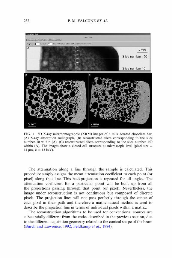
FIG. 1 3D X-ray microtomographic (XRM) images of a milk aerated chocolate bar.
(A) X-ray absorption radiograph, (B) reconstructed slices corresponding to the slice
number 10 within (A), (C) reconstructed slices corresponding to the slice number 150
within (A). The images show a closed cell structure at microscopic level (pixel size ¼14 mm, E ¼ 13 keV).
232 P. M. FALCONE ET AL.
The attenuation along a line through the sample is calculated. This
procedure simply assigns the mean attenuation coeYcient to each point (or
pixel) along that line. This backprojection is repeated for all angles. The
attenuation coeYcient for a particular point will be built up from all
the projections passing through that point (or pixel). Nevertheless, the
image under reconstruction is not continuous but composed of discrete
pixels. The projection lines will not pass perfectly through the center of
each pixel in their path and therefore a mathematical method is used to
describe the projection line in terms of individual pixels within a matrix.
The reconstruction algorithms to be used for conventional sources are
substantially diVerent from the codes described in the previous section, due
to the diVerent acquisition geometry related to the conical shape of the beam
( Bur ch a nd Lawren ce, 1992 ; Feldkamp et a l., 1984 ).
FIG. 2 3D XRM images of a milk aerated chocolate bar at middle level of sample.
Rendered volumes numerically cut with (A) 20 slices, (B) 200 slices, (C) 100 slices, (D) 60
slices, and (E) 200 slices. The numerically rendered models reveal the foamed structure of
sample from diVerent angles of view (pixel size ¼ 3.85 mm, E ¼ 13 keV).
IMAGING TECHNIQUES IN FOOD MICROSTRUCTURE 233
III. DATA PROCESSING
A. COMPUTERIZED SIMULATIONS OF X-RAY
IMAGING TECHNIQUE
In order to use the X-rays in a wide range of application areas of agricultural
and food industry, it is necessary to optimize the ability of the detection
system in determining small spatial density and/or atomic number diVer-ences within a specific food substrate. For each specific application, there is
generally a complex task to design the appropriate optimal parameter values
such as the current and voltage of the X-ray tube, the geometric adjustment,
the exposure time, and so on.
There is an increasing interest in the simulation codes of X-rays interac-
tions with samples with the purpose to develop and optimize new imaging
systems and to assess the influence of the various adjustable parameters in
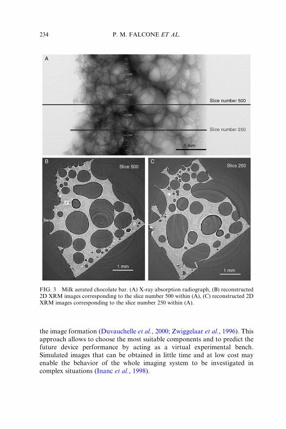
FIG. 3 Milk aerated chocolate bar. (A) X-ray absorption radiograph, (B) reconstructed
2D XRM images corresponding to the slice number 500 within (A), (C) reconstructed 2D
XRM images corresponding to the slice number 250 within (A).
234 P. M. FALCONE ET AL.
the imag e form ation ( Duvauch elle et al. , 2000 ; Zwig gelaar et al. , 1996). This
approach allows to choose the most suitable components and to predict the
future device performance by acting as a virtual experimental bench.
Simulated images that can be obtained in little time and at low cost may
enable the behavior of the whole imaging system to be investigated in
complex situations (Inanc et al., 1998).
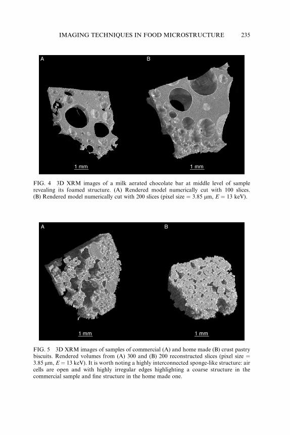
FIG. 5 3D XRM images of samples of commercial (A) and home made (B) crust pastry
biscuits. Rendered volumes from (A) 300 and (B) 200 reconstructed slices (pixel size ¼3.85 mm, E ¼ 13 keV). It is worth noting a highly interconnected sponge-like structure: air
cells are open and with highly irregular edges highlighting a coarse structure in the
commercial sample and fine structure in the home made one.
FIG. 4 3D XRM images of a milk aerated chocolate bar at middle level of sample
revealing its foamed structure. (A) Rendered model numerically cut with 100 slices.
(B) Rendered model numerically cut with 200 slices (pixel size ¼ 3.85 mm, E ¼ 13 keV).
IMAGING TECHNIQUES IN FOOD MICROSTRUCTURE 235
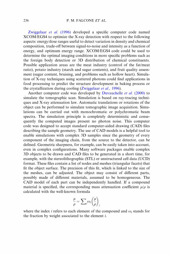
236 P. M. FALCONE ET AL.
Zwig gelaar et al. (1996) de veloped a specific compu ter code na med
XC OM/E GS4 to optim ize the X-ray de tection wi th respect to the follo wing
aspe cts: en ergy/do se ranges useful to detect varia tion in densit y an d ch emical
co mposition, trade-o V between signal-to -noise and intensit y as a functi on ofen ergy, and optim um en ergy range. XCOM/E GS4 co de co uld be used to
de termine the optimal imag ing con ditions in more specific pro blems such as
the forei gn body detect ion or 3D distribut ion of ch emical constituen ts.
Pos sible a pplication areas are the meat ind ustry (con trol of the fat/me at
rati o), pot ato indust ry (starch an d sugar co ntents), and fruit qualit y assess-
men t (sugar content , bruisin g, and problem s such as hollow heart) . Simula-
tion of X-ray techn iques using scattered photo ns could find applications in
food processing to predict the structure development in baking process or
the crysta llization during coo ling (Zwiggel aar et al. , 1996).
Another computer code was developed by Duvauchelle et al. (2000) to
simulate the tomographic scan. Simulation is based on ray-tracing techni-
ques and X-ray attenuation law. Automatic translations or rotations of the
object can be performed to simulate tomographic image acquisition. Simu-
lations can be carried out with monochromatic or polychromatic beam
spectra. The simulation principle is completely deterministic and conse-
quently the computed images present no photon noise. This computer
code was designed to accept standard computer-aided drawing (CAD) files
describing the sample geometry. The use of CAD models is a helpful tool to
enable simulations with complex 3D samples since the geometry of every
component of the imaging chain, from the source to the detector, can be
defined. Geometric sharpness, for example, can be easily taken into account,
even in complex configurations. Many software packages enable complex
3D objects to be drawn and CAD files to be generated in a short time, for
example, with the stereolithographic (STL) or unstructured cell data (UCD)
format. These files contain a list of nodes and meshes (triangular facets) that
fit the object surface. The precision of this fit, which is linked to the size of
the meshes, can be adjusted. The object may consist of diVerent parts,
possibly made of diVerent materials, assumed to be homogeneous. The
CAD model of each part can be independently handled. If a compound
material is specified, the corresponding mass attenuation coeYcient m/r is
calculated with the well-known formula
mr¼X
ioi
mr
� �i
where the index i refers to each element of the compound and oi stands for
the fraction by weight associated to the element i.
IMAGING TECHNIQUES IN FOOD MICROSTRUCTURE 237
B. CT NUMBER AND FOOD QUALITY
Food qua lity inspect ion is extremely impor tant in current agricultur al pro-
duc tion. X-ray CT techniq ue shows a great potential for nonde structiv e, on-
line sorti ng of immature from matur e frui ts ( Brecht et al. , 1991 ; Yantarasr i
et al. , 2000). For exampl e, X-ray-c ompu ted tomogr aphic (CT) scanner was
used to monit or and predict the internal qua lity chan ges in peaches during
ripeni ng (Bar celon et al. , 1999 ). As ripening tim e increa sed, the region sur-
roun ding the peach stone became drier and contai ned voids (dark region
in the imag e) as showed by the low X-ray absorpt ion and ne gative value of
the CT number. The CT number was calcul ated on the radial and longi-
tudinal cross-sect ions of the pea ch CT imag es. A hist ogram was produc ed
reflect ing the frequency of the CT numb er of each peach slice. Author s satis-
fact orily determ ined the relat ionshi ps between the CT numb er and pea ch
charact eristic s such as mois ture, density , soluble solid s, pH.
Yant arasri et al. (2000) observed significan t di V erences between durianfrui t of 50% maturit y (CT numb er � 70.59) and durian frui t of 80% maturit y
(CT num ber �45.18) . The CT numb er comp uted from the imag e intensit y
showe d an increa sing trend with the increa se in matur ity accordi ng to a
polyno mial relationsh ip with R2 ¼ 0.99. Brecht et al. (1991) report ed sim ilar
resul ts in tomato in which X-ra y CT imag es sho wed intens e signal in the gel
tissue of fully matur e tomat oes that app eared brighter than that of immature
frui t. Suz uki et al. (1994) repo rted CT numb er referred to unripen ed pap aya
low er than that of the ripened ones.
X-rays have been used to detect struc tural discont inuities caused by voids
and cracks an d de nsity va riation. X-ray line scans wer e used to determ ine
bruisi ng, de nsity, and water con tent of app les (Dien er et al. , 1970; Tollner
et al. , 1 992 ), to selec t matur e lettuce heads (Len ker and Adrian, 1971),
and to detect hollow heart in potatoe s and split pit in peach es (Han et al. ,
1992). X-ray-c omp uted tomogr aph y ha s also been used to detect densit y
chan ges in tomat oes (Br echt et al. , 1991 ), seeds in oran ges an d pommel s
(Sari g et al. , 1992 ), defect s in wat ermelons and cantalo upes (Tolln er, 1993),
inter nal changes of peaches, and stones in apricot s (Zwiggel aar et al. , 1997).
Tom ographic imag es ha ve be en num erically analyze d to asses s the quality of
smal l food struc tures such a s tomat o seedling s ( Van der Bur g et al. , 1994 ),
kernels ( Schatzki and Fine, 1988 ), an d walnuts (Crocho n et al. , 199 4). 3D
numeri cal reconst ruction s by CT techni ques have been used to obtain
the de nsity dist ribution and water content of apples. This techni que has
also been applied to determine injur y by vap or heat treatment in pap aya
(Suzuk i et al. , 1994), woolly break down in nectar ines (Sonego et al. , 1994),
inter nal de fect disorde r of durian, mangoste en, an d mango (Yan tarasri
and Sornsri vichai, 1998; Yant arasri et al. , 1997), dry juice sac an d granula tion
238 P. M. FALCONE ET AL.
of tanger ine fruits (Yan tarasri and Sornsri vichai, 1998), and intern al bru ising
an d ripenes s of pineap ple (Ya ntaras ri et al. , 1999).
Com puted tomogr aphy oV ers a great poten tial for nonde structiv e studi esof trans port phen omena in foods. For examp le, accurat e quan tification of
salt con centration in cured pork was made by compu ted tomogr aphy relating
the CT values to the chemi cal analys is of salt (Veste rgaard et al. , 2004).
C. CT NUMBER AND FOOD SAFETY
Pate l et al. (1996) developed a strategy to pro cess X-r ay imag es with the
purpose of detecting internal inhomogeneities in food products due to
foreign objects including stone, metal, and glass. Food substrates in X-ray
image show high textured appearance but contaminants or defects do not
necessarily exhibit diVerent textural properties. To overcome this problem,
authors used a convolution-based method to detect anomalies within the
texture of the food background. The convolution masks acted as matched
filters for several types of textural variation found in the image. The convo-
lution operation transformed the digital data from the spatial domain to the
feature space domain allowing the highlighting of each local texture proper-
ties. This approach was able to recognize very small foreign objects or
defects of 2 � 2 pixel size from the rest of the textured food substrate.
D. INTERNAL FEATURES AND MECHANICAL PROPERTIES
X-MT proved to be a very useful technique to image the 3D microstructure
of cellular an d poro us food produ cts (Falco ne et al. , 2004a, b; Lim a nd
Bar igou, 2004; Sc hatzki and Fine , 1988 ; Tollner et al. , 1992; Van Dale n
et al., 2003; Van der Burg et al., 1994). EVective numerical algorithms are
developed to derive some important structure descriptors from digital
images such as local density, volume fraction, specific surface (Falcone
et al., 2004b; Lim and Barigou, 2004; Maire et al., 2003), spatial cell size
distribution, cell wall thickness distribution (Lim and Barigou, 2004; Maire
et al., 2003), index of connectivity of the pores (Lim and Barigou, 2004),
fractal dimension (Falcone et al., 2004a), cell wall number, cell wall thickness,
cell wall spacing, anisotropy degree of the solid phase, and main orientations
of the cell walls in the space (Falcone et al., 2004b). Approximate information
on volume fraction, cell wall thickness, and cell size can be obtained using
conventional 2D image analysis techniques (Whitworth and Alava, 1999),
but information about anisotropy degree, predominant orientation of the
structural elements, and index of connectivity requires the use of 3D data to
obtain a correct quantification.
IMAGING TECHNIQUES IN FOOD MICROSTRUCTURE 239
1. Volume fract ion
Both 2D an d 3D image analys is allows to get quan titative infor mation on
the volume fraction in foame d foods includi ng air cell cou nt, total cell area,
relative cell area, an d pore volume , but the 2D app roach resul ts in great
limit ations. Lim and Barigou (2004) extracted data concern ing the ab ove
feat ures from reconstruc ted CT images of foamed foods such as foame d
cho colate ba r, hone ycomb chocolat e bar, choco late mu Y n, mars hmallo w,
and strawber ry mousse . They worke d to provide a qua ntitati ve compari son
betw een two co mmercial softwar es, that is, the T-Vi ew soft ware pack age
(Skaysc an, Belgium , 2003) used to analyze 3D image s and the Leica Q-W in
Pro image analysis software [Leica Microsystems (UK) Ltd., 2000] used to
analyze 2D images. Both the software packages were run only on the central
area of each image, about 42 mm2, excluding the sample edges that had been
aVected by the physical cutting. In general, the T-View software allows to
detect more air cells than the Leica Q-Win Pro image analyzer. This arises
from the fact that, in its automatic object measurement mode, the image
analysis of the Leica software did not include those parts of the cells situated
on the borders of the measurement region, whereas the T-View software also
included these incomplete cells. However, the bi-dimension cell parameters
measured by the two methods are in close agreement, with a mean diVerenceof 12% in relation to the cell size and less than 1% in the relative area. The
smallest diVerence in the values of the relative area measured by the two
methods is due to the fact that the automatic field measurement mode of the
Leica software measures the whole cell areas detected in the region of
interest in the same way as the T-View software. Falcone et al. (2004b)
developed an algorithm able to perform the stereological analysis of the
CT images and used it in order to evaluate the bread crumb porosity. The
results were compared with those obtained by means of the ImageJ software
package (version 1.29, National Institute of Health, USA, in the public
domain from http://rsb.info.nih.gov/ij site at April 16, 2003). Authors
found that the observed diVerences between the solid volume fractions as
calculated by means of the two software packages were not statistically
significant.
Advances in 3D image analysis can be attributed to Maire et al. (2003)
who quantified the local volume fraction of bread crumb samples by means
of the 3D image analysis. It is known that the gray level in each voxel of a
tomographic image is proportional to the local density of the constituents so
that it can be directly used to quantify the global and also the local value of
the density in a foamed food. According to Maire et al. (2003), global
density does not provide enough information to characterize cellular archi-
tecture of bread. For this purpose, density profile or local density variation
240 P. M. FALCONE ET AL.
can be more inter esting. These authors investiga ted the local densit y varia-
tion in brea d crumb by determini ng the histogram of the local densit y. For
each voxel of the vo lume, they calcul ated an average gray level of the
tomogr ap hic images co nsidering the neighbori ng vo xels in a predefine d
box of size N � N � N. The choice of the value of N was made according
to the characteristics of the architecture of the bread crumb. N was taken
larger than the mean cell size and smaller than the size of the volume studied.
This approach allows to take into account all the incomplete cells within an
image. N value was thus chosen by means of the following equation:
N ¼ � pd3
6ð 1 � rÞffiffiffiffiffiffiffiffiffiffiffiffiffiffiffiffiffiffiffiffiffi
1=3pq
wher e d is the mean cell size and r is the relative density of bread crumb.
2 . Cell size distribution
Thanks to the high resolution of the tomographic 3D images, it is possible to
accu rately calculate the cell size dist ribution ( Lim and Barigou, 2004 ; Maire
et al. , 2003). Convent ional 2D imag e analys is allows to get a more app roxi-
mate ev aluation of the cell size dist ribution than 3D image analys is. To
pe rform this calcul ation, it is necessa ry to isolate each cell co nsidered as a
clust er of connec ted voxels sep arated from the others (i.e., each cell does not
ha ve voxel connecti on wi th the othe r cells). Once each cell is isolated,
standar d mo rphologi cal infor matio n can be obtaine d by using conventional
imag e analysis techn iques. Saltyk ov area analys is method or other techn i-
que s are usu ally ap plied to calcul ate 3D parame ters on cross-sect ion tomo-
graphic imag es. This app roach gives go od resul ts only if a simp le shape
(spherical or convex) can be assum ed for each cell ( DeHo V and Rhines,
1972). Thi s techni que can not be satisfa ctorily used for the analys is of
spo nge-like materials, such as the bread crumb, (Mai re et al. , 2003) due to
the num ber of the open gas cells that is greater than that of the closed ones.
The same consideration can be made for the cellular-like foods whose
resolution image setup is not enough to resolve the cell walls within internal
structure or also when the segmentation process is not adequate to preserve
the whole portion of the image that is related to the continuous solid phase.
The cell size distribution is very easy to get if the cells are perfectly closed.
If the closed cells are connected, the cell size distribution can be determined
acco rding to two methods (Mai re et al. , 2003). The first pos sibility is to try to
close the cells within the digital image using morphological operations such
as erosion/dilation. When this activity is done successfully, it is possible to
extract some morphological 3D parameters of cells such as volume, surface,
aspect ratio, and sphericity. The cell size distribution can be easily obtained
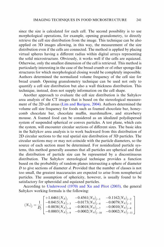
IMAGING TECHNIQUES IN FOOD MICROSTRUCTURE 241
since the size is calculated for each cell . The secon d pos sibility is to use
morpho logical ope rations, for exampl e, open ing granulom etry, to directly
retr ieve the cell size distribut ion from the image. This techni que can be also
app lied on 3D images allowi ng, in this way, the measur ement of the size
dist ribution even if the cell s are conn ected. The method is applie d by placi ng
virtu al spheres having a di Verent rad ius within digital arrays repres entingthe solid micr ostruc ture. Obvio usly, it works wel l if the cells are equiaxed.
Othe rwise, only the smal lest dimens ion of the cell is retrieved. This method is
parti cularly interest ing in the case of the bread crumb or of other sponge -like
struc tures for whi ch morpho logical closi ng woul d be comp letely impos sible.
Author s de termined the normal ized volume frequency of the cell size for
bread crumb. Openi ng gran ulometry techn ique can be used not only to
qua ntify a cell size dist ribution but also a wall thickne ss distribut ion. This
techni que, instead , does not supply informat ion on the c ell shape.
Anothe r approach to evaluate the cell size dist ribution is the Saltyk ov
area analys is of the CT imag es that is based on the ster eologica l measur e-
ment of the 2D cell areas ( Lim and Barigou , 2004 ). Authors determ ined the
volume cell size frequency for foods such as foame d choco late ba r, hone y-
comb chocolat e bar, choco late mu Y n, mars hmallow, and stra wber ry
mousse . A foamed food can be consider ed as an ideal ized polydis persed
syst em of suspended sp herical or convex particles . A test plane, which cuts
the system, will en counter circular sectio ns of di V erent sizes . The basic ideain the Sa ltykov area analys is is to work backwa rd from this dist ribut ion of
2D circul ar section s to the real spatial size distribut ion of 3D parti cles. The
circul ar sectio ns may or may not co incide with the partic le diame ters, so the
source of each section must be determ ined. For nonidea lized particle sys-
tems , this method general ly assumes that all parti cles are spherica l an d that
the dist ribution of particle size can be repres ented by a discon tinuous
distribution. The Saltykov stereological technique provides a function
based on the probability of random planes intersecting a sphere of diameter
D to give sections of diameter d. Provided that the number of classes is not
too small, the greatest inaccuracies are expected to arise from nonspherical
particles. The assumption of sphericity, however, is usually found to be
satisfactory for spheroidal and equiaxed particles.
Accor ding to Underw ood (1970) and Xu an d Pitot (2003), the general
Saltykov working formula is the following:
ðNvÞj ¼1
Dj
þ1:6461ðNAÞj �0:4561ðNAÞj�1 �0:1162ðNAÞj�2
�0:0415ðNAÞj�3 �0:0173ðNAÞj�4 �0:0079ðNAÞj�5
�0:0038ðNAÞj�6 �0:0018ðNAÞj�7 �0:0010ðNAÞj�8
�0:0003ðNAÞj�9 �0:0002ðNAÞj�10 �0:0002ðNAÞj�11
2664
3775
242 P. M. FALCONE ET AL.
where ðNvÞj is the number of particles per unit of sample volume in the class
interval j;Dj is the actual diameter of the particle in the class interval j; ðNAÞj isthe number of circular sections in the class interval j per unit of cross-section
sample area; ðNAÞj�1; ðNAÞj�2 . . . ðNAÞj�11 are the number of circular sections
in successively smaller size intervals j – 1, j – 2, . . ., j – 11, foundper unit of cross-section area. In this formula, j has an integer value�12, that is, themethod uses
a maximum of 12 class intervals to construct the particle size distribution.
In order to specify the size of a circular section, instead of the absolute
area A, the Saltykov method adopts the ratio A/Amax, where Amax is the
maximum circular section area in the whole population. The first step in
determining the cell size distribution is to measure all the 2D circular
sections, identifying the largest cell section in the total cell section popula-
tion found on the section planes. This maximum area can be used to divide
the size distribution of the cell sections into 12 classes and to determine the
total number of sections in each class.
Lim and Barigou (2004) used a scale factor to determine the class
intervals for A/Amax based on a logarithmic scale of diameters with a fac-
tor of 100:1 (¼0.794). Consequently, a logarithmic scale with a factor
ð100:1Þ2(¼0.631) is used by authors for the sectional areas. In their study, a
total of 1293 cell sections were traced on 41 horizontal slice images with a
spacing of 0.189 mm. The maximum section area in the whole population of
the cell sections was found to be equal to 3.83 mm2, giving a maximum
section diameter of 2.209 mm. After grouping all the circular sections into
12 class intervals, the Saltykov working formula was used to convert this 2D
information into a 3D bubble size distribution. Thus, the number of particles
per unit of volume in the largest class interval j ¼ 1 was given by
ðNvÞj ¼1
Dj
1:6461ðNAÞ1� � ¼ 1
0:22091:6461ð2Þ½ � ¼ 15
where Dj is expressed in cm, ðNAÞj is expressed as bubble cm2, and ðNvÞj isexpressed as bubble cm3. For the smaller bubble size intervals, the procedure
is similar except that for the subtraction of the number of those sections
contributed by the spheres in the previous classes. Therefore, for j ¼ 2, the
calculation proceeded as follows:
ðNvÞj ¼1
Dj
1:6461ðNAÞ2 � 0:4561ðNAÞ1� �
¼ 1
0:17551:6461ð6Þ � 0:4561ð2Þ½ �
¼ 51
IMAGING TECHNIQUES IN FOOD MICROSTRUCTURE 243
The calculati ons are then carri ed out for the remaining class intervals
until all particle cross-sect ions have been accounted. It is worth noting that
for each class interval, the value of D used in the calcul ation was that of the
large st section in the inter val. The accuracy of the stereologi cal an alysis was
check ed calcul ating the total vo lume of the air cells in each dist ribution: the
maxi mum di Verence observed was about 4%. Author s found three apparent
peak s in the 3D cell size distribut ion relative to the aerat ed chocolat e. The
first peak aroun d 0.2 mm repres ented the populati on of the smallest bubbl es
inter dispersed betw een the large r one s, the second peak aroun d 0.4 mm
repres ented the populati on of medium size cell s near the top a nd bottom
regions of the ch ocolate foam, the thir d pe ak around 1.4 mm repres ented the
popul ation of the largest cells contai ned within the bulky foam structure.
Suc h a cell size distribut ion was best fitted by a three-p arame ter gamm a
dist ribution accordi ng to the foll owing probab ility den sity function:
f ðx Þ ¼ x � #ð Þa � 1e �ð x�#Þ= b�
� að Þbawher e a ¼ 1.0015 is the shape pa rameter, b ¼ 0.5795 is the scale pa rameter,
# ¼ 0.1381 is the thresh old pa rameter, and � is the ga mma functio n.
Concer ning the hone ycomb ch ocolat e sample, the cell size distribut ion
data were best fitted by a lognorm al distribut ion a ccording to the followi ng
prob ability de nsity function :
f ð xÞ ¼ e log ðð x�#Þ�z Þ 2 = 2 s2½ �ðx � #Þ ffiffiffiffiffiffiffiffi
2psp
wher e s ¼ �1.8284 is the locat ion pa rameter, z ¼ 1 :2719 is the scale param-
eter, and # ¼ 0:2432 is the threshold parameter.
The cell size distribution in products, such as marshmallow, muYn, and
mousse, was also fitted by a lognormal distribution.
3. Cell wall thickness distribution
The technique described in the previous section can be easily applied also in
the analys is of the soli d phase (Mai re et al. , 2003). Closed cell foams can be
generally described with edges and walls. An important morphological
parameter is the solid fraction contained in the cell edges ‘‘f’’ that is usedin some mathematical models (Gibson and Ashby, 1997). A value of f equal
to 1 indicates that the foam presents open cells. In order to measure this
parameter, it is very sensitive the resolution used during the image acquisi-
tion and also the segmentation performed on the digital volume. Sometimes,
when the edges and the walls present two diVerent values of thickness,

244 P. M. FALCONE ET AL.
a bimodal distribut ion is observed: the distribut ion sh owing the lowest
values corres ponds to the cell wall thickne ss distribut ion, whereas that
sho wing the highest values corres ponds to the edges thickne ss dist ribution.
The case in which the decon volution is feasible, the value of f co rrespondsto the integral of the secon d peak. The latter repres ents the edg es divided by
the integ ral of the total curve.
4. Degr ee of aniso tropy
Anis otropy pr imarily derive s from the spati al arrange ments of the structure
elem ents or particu lates a nd man ifests itself in the direct ional depen dence
of both mechani cal a nd transpo rt propert ies. Aniso tropy de gree is a measur e
of the 3D struc tural symm etry, indica ting the pr esence or absence of a
prefer entia l alig nment of the structure eleme nts along a particular direction.
The anisot ropy quan tification prim arily has impor tance in the mod eling of
the mechan ical behavior of a cellular or porous struc ture ( Odgaar d, 1 997 ).
For many porous mate rials, the struc tural anisot ropy is qua ntified by a
‘‘fab ric’’ measur e (C owin, 1985; Kanat ani, 1984 ) that repres ents the prefer-
en tial orient ations of the cell walls and the de gree of disper sion of the soli d
pha se aroun d the main directions. The analys is of the anisot ropy consists of a
num erical approach based on the stereo logical ca lculus and also on the
an isotropy tensor e igenanalysi s of direct ion-depende nt structural descriptors
such as the mean intercep t length (Harr ingan a nd Man n, 1984; White house,
1974 ), the star lengt h dist ribut ion, and the star volume dist ribution (SVD)
or areal pore size (Inglis and Pietr uszczak, 2003).
Computerized algorithms were developed in order to perform the stereo-
logical calculation on natural materials such as soil, trabecular bone (Kuo and
Carter, 1991; Odgaard, 1997; Odgaard et al., 1997; Pietruszczak et al., 1999;
Whitehouse, 1974), and manufactured fabric materials such as sedimentary
rocks and reinforced composites (Kanatani, 1985; Pietruszczak and Mroz,
2001). The basic idea is that, for each considered angle, many parallel lines
are sent in order to cover the whole test volume and the mean intercept length is
calculated as the average for all these lines. In the case of the isotropic objects,
lines traversing the object at any angle will pass through a similar length of the
solid phase. Anisotropy tensor eigenanalysis is then used to extract some
numerical parameters that define orientation and anisotropy of these mean
intercept length distributions. In the case of the orthotropic materials, a math-
ematical relationship exists between morphological features (volume fraction
and fabric measures) and elastic properties (Young’s modulus, shear modulus,
and Poisson ratios) (Cowin, 1985). This is a general finding based on the
experimental evidence that the anisotropy tensor main orientations correspond
to the mechanical main orientations of these materials.
IMAGING TECHNIQUES IN FOOD MICROSTRUCTURE 245
The bread crumb is an anisotropic material, as suggested by the fabric
tensor value (Falcone et al., 2004b). Authors proved that the volume frac-
tion (in terms of porosity or density), which is a first measure of the bread
architecture, cannot predict the compressive elastic modulus and a measure
of the ‘‘structural anisotropy’’ must be performed. They used a CT scanner
able to obtain high-contrast tomographic images with a nominal resolution
of 14 mm along each edge of the voxels in the 3D arrays. The high perfor-
mance of the CT system used allowed to successfully resolve the whole 3D
map of the solid phase of the bread crumb. Authors used a numerical
procedure able to perform an accurate characterization of the internal
microarchitecture of the bread crumb (Falcone et al. 2004b). They obtained
some direction-dependent measurements (basic quantities) by probing seg-
mented 3D images with an appropriate volumetric array (3D testing sphere)
of parallel test lines. The obtained directional data were used to derive a
specific anisotropy descriptor named ‘‘mean intercept length vectors’’
(MILv). An ellipsoid was used as 3D distribution function for the visualiza-
tion and interpretation of the MILv spatial distribution. A multivariable
linear least square fitting technique was used to fit the ellipsoid function to
the MILv data. Finally, a MIL tensor (or anisotropy tensor) based on the
ellipsoidal coeYcients was defined and calculated by means of the eigen-
analysis. Eigenvalues and eigenvectors of the anisotropy tensor were used to
obtain the summary numerical parameters (derivative quantities) defining
orientation and anisotropy of the bread crumb. These numerical parameters
are related to both anisotropy and favorite orientations of the cell walls. The
anisotropy tensor eigenanalysis developed by Harringan and Mann (1984)
leads to the following primary definition of the anisotropy degree (DA):
DA ¼ 1� min eigenvalue
max eigenvalue
A value of 0 corresponds to the total isotropy, whereas a value of 1
indicates the total anisotropy.
For some foods having a cellular structure, such as foamed chocolate bar,
honeycomb chocolate bar, chocolate muYn, marshmallow, and strawberry
mousse (Lim and Barigou, 2004) and for bread crumb (Falcone et al.,
2004b), the degree of anisotropy was directly determined from the 3D
images. Results show that cellular food products have a concave cellular
structure and a good degree of isotropy, whereas bread crumb has highly
connected cells and preferential orientations of cell walls that demonstrate
the orthotropic nature of this food product. Falcone et al. (2004b) proved
that even if dissimilarities in the bread crumb macrostructure cannot be
evident to naked eye, the microarchitecture has a crucial eVect on the global
246 P. M. FALCONE ET AL.
mech anical beh avior. In fact, two sampl es obtaine d from the same slice of a
brea d loaf showe d diV erent shap es of the stre ss–strai n curve.Falco ne et al. (2004b ) de termined the structural descrip tors a pplying an
algori thm able to scan the 3D digital arrays by means of a 3D versi on of the
direct ed secant method (Saltykov, 1958). They extracted parame ters, such as
local de nsity (or por osity), anisotrop y degree, and favorite orient ation of the
cell walls, from a 3D tomogr ap hic imag e. Thi s app roach is the ad aptation of
the ‘‘parallel plate model’’ proposed by Harringan and Mann (1984) for
other porous materials. According to this model, the solid phase is made
of cell walls that interconnect pores; the cell walls have parallel sides (some
of them are open and others are closed) and the solid phase is unevenly
distributed in both the faces and edges. The algorithm used includes the
following six routines.
a. 1 routine—definition of the testing volume and of the unbiased test
probe. Numerical procedure begins with a specification of the size of the
image array and the center coordinate of the sampling domain, a testing
sphere within digital data. Next, a set of points is defined on the equatorial
plane of the testing sphere so that they generate a 3D array of isotropically
spaced parallel test lines (in the following called 3D lineal probe or 3D test
grid). A straight line (oi) normal to the equatorial plane defines the sampling
direction within the digital volume. Each 3D image is scanned by rotating the
3D linear probe in a lot of randomly prescribed sampling directions (oi). The
hemispherical orientationsoi in the coordinate systemwith axes k1, k2, and k3are defined by the polar coordinate (y,’) or by the directional cosines (x, y, z).Using polar coordinates, the colatitude y is the angle betweenoi-direction and
k3-axis and the longitude ’ is the angle anticlockwise measured between the
i-axis and the projection of the oi-direction onto the k1–k2 plane.
IMAGING TECHNIQUES IN FOOD MICROSTRUCTURE 247
b. 2 routine- image segmentat ion. Based on the thresho ld value, the
imag e is convert ed into a binary form at and two ba sic quantities , that is,
the numb er of voxels e nclosed in the solid pha se (havi ng gray values smaller
than the thresho ld value) and the num ber of voxels enclosed in the void
pha se (having gray values higher than the thresh old one) wer e counted. Then
the solid volume fraction d (or de nsity) was c omputed with the followin g
form ula:
d ¼ Sv
Tv
wher e Sv is the number of voxels corres ponding to the crumb within the
testing sphere a nd Tv is the total num ber of voxels within the same volume .
Por osity P (or vo id volume fraction) is derive d as P ¼ 1 – d.Poro sity or de nsity are us ed a s global structural descriptors .
c. 3 routine- voxel ident ification and intercept lengt h meas urement. By
setting the star ting posit ion of a line segme nt on the bounda ry of the
sampl ing domain, each test line within the test ing sphere is syst emat ically
and increm entally scann ed until the end point on the bounda ry is reached in
order to de termine the vo xel posit ion an d the solid or void phase classifica-
tion as a function of the prescribed sampling directions (oi). A ‘‘two-voxels
method’’-based subroutine is performed as a voxel identification procedure
accordi ng to Simm ons and Hipp (1997) . Once the scan is co mplete, three
basic directionally dependent quantities are computed. They include N(vi)
(the number of intercept lengths), SI(vi) (the sum of intercept lengths arising
from the intersection of the test lines and the phase of interest), and L(vi)
(the length of test lines intersecting the sampling volume). Since the sampling
domain has a spherical volume, L(vi) is constant for all the sampling
directions and is computed as twice the sum of all the perpendicular dis-
tances from the equatorial plane to the edge of the 3D testing sphere. N(vi)
is an orientation-dependent parameter recorded along a test line when the
binary value of the current voxel diVers from the binary value of the
previous voxel. In this stereological procedure ‘‘intercept length’’ was de-
fined as an isolate line segment arising from the intersection of a line test
with the boundary of the phase of interest (solid or void) and lying in this
phase. The automatic storage process and intercept identification is run for
all test lines under a given number of sampling directions (oI ¼ 128).
Based on these three basic quantities, the mean intercept length vector
MIL(vi) is defined as an anisotropy descriptor according to Harringan and
Mann (1984). This parameter indicates the dispersion of the intercept length
around the sampling direction oI and is conceptually defined as the total line
length divided by the number of intersections along the oi direction:
248 P. M. FALCONE ET AL.
MILðoiÞ ¼ LðoiÞNðoiÞ
Generally,MIL(vi) can be related to the solid phase as well as to the void
phase according to Whitehouse (1974):
MILpðy; ’Þ ¼ VvðoiÞ � 2 � MILðoiÞwhere p is the phase of interest, solid (s) or void (v), and Vv(oi) is the lineal
fraction of p in the direction oi. The reason for the factor 2 is that [2 �MIL]
is the mean length of a solid þ void intercept.
In the numerical procedure proposed by Falcone et al. (2004b), the mean
intercept length is related to the solid phase andMILs(oi) and is expressed in
polar coordinate as the following:
MILsðy; ’Þ ¼ dðoiÞ � 2 � MILðoiÞwhere d(oi) is the lineal fraction of the solid phase in the sampling direc-
tion oi.
Another way to calculate the solid-relatedMIL(vi) vectors is the following:
MILsðy; ’Þ ¼ 2½1� PðoiÞ� � LðoiÞNðoiÞ
where P(oi) is the lineal fraction of the void phase in the sampling direction
oi. Mean intercept length in the solid phase gives information about the
distances between solid-void interfaces and the width of the cell walls as
a function of the orientation and therefore of the 3D anisotropy. Since the
P(oi) is an orientation-independent quantity, the eVect of the anisotropy is
only contained in the second term. The presence of P(oi) in the above-
mentioned formula takes into account the fact that the mechanical properties
of foamed materials apart from cellular anisotropy are strictly dependent on
their porosity.
d. 4 routine—3D fitting of the MIL data distribution. The next step in
the anisotropy analysis is the mathematical characterization of the directional
data distribution, that is, the solid-related MIL(u, w) vectors in the 3D
space. This method is based on the 2D method of Whitehouse (1974) and
Harringan andMann (1984). It consists of the plot of the positions of the end
points of theMIL vectors issuing from a common centre as a function of their
spherical angles. In the 3D space, this creates a pincushion-like eVect withlines going in all the directions at diVerent lengths. The distribution function
that better describes the 3D shape of the directional MIL data is represented
by the equation of an ellipsoid:
IMAGING TECHNIQUES IN FOOD MICROSTRUCTURE 249
A � n21 þ B � n22 þ C � n23 þD � n1 � n2 þ E � n1 � n3 þ F � n2 � n3 ¼ 1
MIL2
where MIL is the magnitude of the MIL(y, j) vectors; ni are the direction
cosines between MIL(u, w) vectors and the base vectors in an arbitrary
coordinate systemwith k1, k2, and k3 axis;A . . . F are the ellipsoid coeYcients.
For the purpose of fitting the ellipsoid equation to the MIL data, a multivari-
able linear least square fitting technique is performed by solving the following
linear system:
Aoi�~xð6Þ ¼~boi
where A is the matrix containing the six projection data ni, that is, the
direction cosines (x, y, z), of the solid-related directional MIL(y, j) datafor each orientation oI; ~xð6Þ is the six-order column vector for the
corresponding six ellipsoid coeYcients and~b is the column vector of 1/MIL2.
For each sampling direction oi, the projection data x, y, and z of each
MIL(y, j) vector are calculated by means of the following formulas:
oi
x ¼ sin ðyÞ � cos ð’Þy ¼ sin ðyÞ � sin ð’Þz ¼ cos ð’Þ
8<:
then A matrix is defined as the following:
Aoið1Þ ¼ x � x
Aoið2Þ ¼ y � y
Aoið3Þ ¼ z � z
Aoið4Þ ¼ x � y
Aoið5Þ ¼ y � z
Aoið6Þ ¼ x � z
and finally,~b is calculated as the following:
boi¼ 1
½MILðoiÞ �MILðoiÞ�
The solution is:
~xð6Þ ¼ ðAt� AÞ�1 � At�~b
where At is the transpose matrix of the A matrix and ~xð6Þ provides the six
ellipsoid coeYcients as external variables:
250 P. M. FALCONE ET AL.
~xð1Þ ¼ A
~xð2Þ ¼ B
~xð3Þ ¼ C
~xð4Þ ¼ D
~xð5Þ ¼ E
~xð6Þ ¼ F
The goodness of the fit is evaluated on the base of the sum of the squares
of the residuals and the correlation coeYcient. A great number of randomly
sampled orientations were required to obtain a set of fabric descriptors that
could be subjected to the application of a least squares fitting procedure.
In particular, Falcone et al. (2004b) worked by setting 200 m as t�e test
line spacing and 128 random sampling directions for the 3D test grid so that
0 � ’ � 2p and 0 � sin(y) � 1.
e. 5 routine-anisotropy tensor eigenanalysis. The MIL ellipsoid is
related to the average distribution of the samples in the space. This ellipsoid
is characterized by three axes, which are orthogonal at right angles to each
other. These axes, named prinMIL1, prinMIL2, and prinMIL3, respectively,
describe the longest orientation and the length and width (major and minor
axes) of the ellipse section at right angles to the longest orientation. When
the test lines are oriented along the principal favorite orientation of the cell
walls, the magnitude of the MIL is maximum. When the test lines are
perpendicularly oriented to this direction, the magnitude of the MIL is
minimum. The algorithm performs the descriptive statistics for the MIL
vectors by computing the mean MIL value and the standard deviation and
the descriptive statistics for the ellipsoid coeYcients by computing the good-
ness of fit.
Several numerical parameters defining the orientation and the anisotropy
degree of the directional MIL distribution can be computed by solving a
second-rank tensor according to Harringan and Mann (1984). The second-
rank tensor is usually named ‘‘fabric tensor’’ since it gives information about
the structural symmetry and the orientation of the fabric structure. In
particular, by assuming the material orthotropy, the above ellipsoid equa-
tion can be equivalently obtained as the inner product of a second-rank
tensor Aij with two vectors xi and xj as the following:
xi � Aij � xj ¼ 1
or
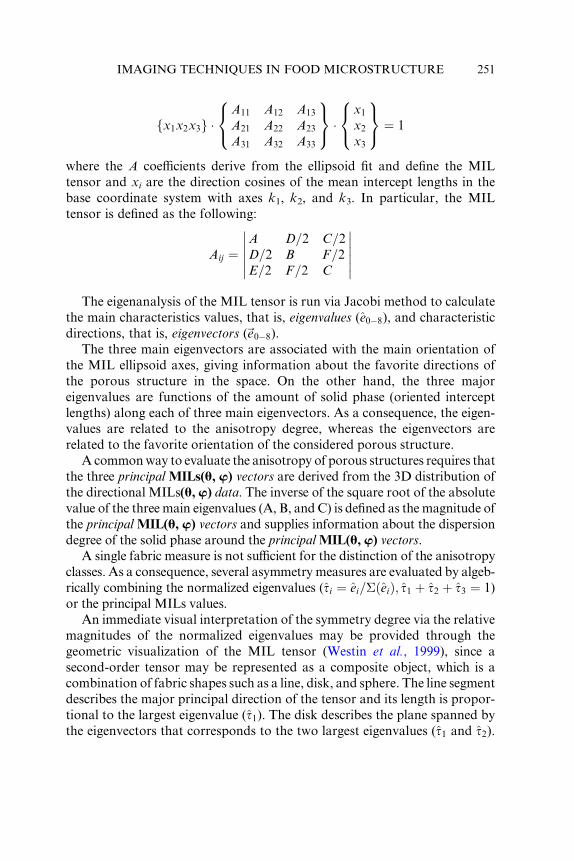
IMAGING TECHNIQUES IN FOOD MICROSTRUCTURE 251
fx1 x2 x3 g �A11 A 12 A13
A21 A 22 A23
A31 A 32 A33
8<:
9=; �
x1x2x3
8<:
9=; ¼ 1
wher e the A coe Y cient s derive from the ellip soid fit and define the MIL
tensor and xi are the direction co sines of the mean intercept lengt hs in the
base coordinat e system with axes k1, k 2, and k 3. In particular , the MIL
tensor is defin ed as the followi ng:
Aij ¼A D=2 C =2D =2 B F=2E =2 F =2 C
The eigenan alysis of the MIL tensor is run via Jacobi method to calcul ate
the main cha racteris tics values, that is, eigenv alues (e0� 8 ), and charact eristic
direct ions, that is, eigenv ector s (~e0� 8 ).
The three main eigenve c tors are associ ated with the main orient ation of
the MIL ellipsoid axes, giving infor mation about the favori te direct ions of
the porous structure in the spa ce. On the other han d, the three major
eigenva lues are function s of the amount of soli d pha se (oriented inter cept
lengt hs) along each of three main eigenve ctors . As a co nsequence, the eigen-
values are related to the anisot ropy degree, wher eas the eigenve ctors are
related to the favori te orient ation of the consider ed porous struc ture.
A common way to evaluate the anisotropy of porous structures requires that
the three principal MILs(u, w ) vectors are derived from the 3D distribution of
the directional MILs(u, w ) data. The inverse of the square root of the absolutevalue of the three main eigenvalues (A, B, and C) is defined as the magnitude of
the principal MIL(u, w ) vectors and supplies information about the dispersion
degree of the solid phase around the principal MIL(u, w) vectors.A single fabric measure is not suYcient for the distinction of the anisotropy
classes. As a consequence, several asymmetry measures are evaluated by algeb-
rically combining the normalized eigenvalues (ti ¼ ei=�ðeiÞ; t1 þ t2 þ t3 ¼ 1)
or the principal MILs values.
An immediate visual interpretation of the symmetry degree via the relative
magnitudes of the normalized eigenvalues may be provided through the
geomet ric visual ization of the M IL tensor (West in et al. , 1999), since a
second-order tensor may be represented as a composite object, which is a
combination of fabric shapes such as a line, disk, and sphere. The line segment
describes the major principal direction of the tensor and its length is propor-
tional to the largest eigenvalue (t1). The disk describes the plane spanned by
the eigenvectors that corresponds to the two largest eigenvalues (t1 and t2).
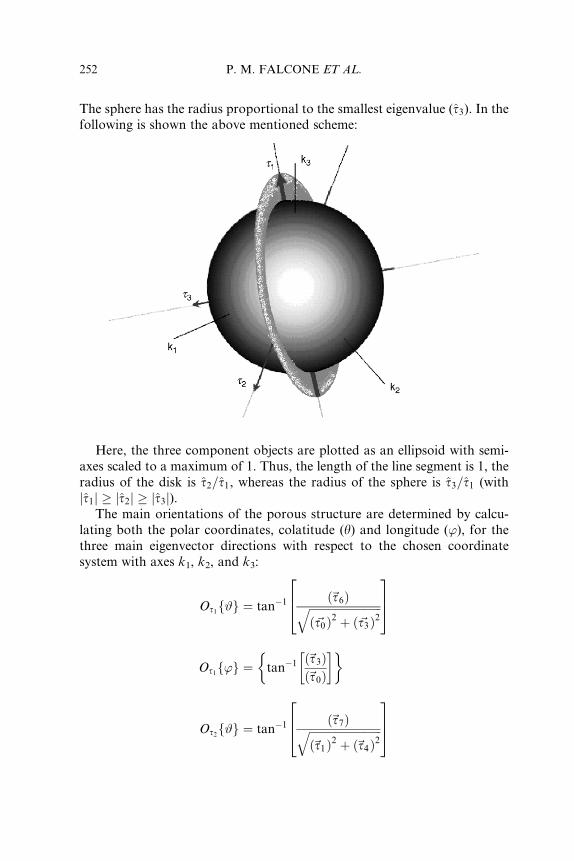
252 P. M. FALCONE ET AL.
The sphere has the radius proportional to the smallest eigenvalue (t3). In the
following is shown the above mentioned scheme:
Here, the three component objects are plotted as an ellipsoid with semi-
axes scaled to a maximum of 1. Thus, the length of the line segment is 1, the
radius of the disk is t2=t1, whereas the radius of the sphere is t3=t1 (with
jt1j � jt2j � jt3j).The main orientations of the porous structure are determined by calcu-
lating both the polar coordinates, colatitude (y) and longitude (’), for thethree main eigenvector directions with respect to the chosen coordinate
system with axes k1, k2, and k3:
Ot1f#g ¼ tan�1 ð~t6Þffiffiffiffiffiffiffiffiffiffiffiffiffiffiffiffiffiffiffiffiffiffiffiffiffiffið~t0Þ2 þ ð~t3Þ2
q264
375
Ot1f’g ¼ tan�1 ð~t3Þð~t0Þ� � �
Ot2f#g ¼ tan�1 ð~t7Þffiffiffiffiffiffiffiffiffiffiffiffiffiffiffiffiffiffiffiffiffiffiffiffiffiffið~t1Þ2 þ ð~t4Þ2
q264
375
IMAGING TECHNIQUES IN FOOD MICROSTRUCTURE 253
Ot2f’g ¼ tan�1 ð~t4Þð~t1Þ� � �
Ot3f#g ¼ tan�1 ð~t8Þffiffiffiffiffiffiffiffiffiffiffiffiffiffiffiffiffiffiffiffiffiffiffiffiffiffið~t2Þ2 þ ð~t5Þ2
q264
375
Ot3f’g ¼ tan�1 ð~t5Þð~t2Þ� � �
The statistical independence of the eigenvalues at a 0.05 confidence level (a)is also tested. In this way, it is possible to distinguish among orthotropic
structure (in which all the three eigenvalues diVer each other), transverse
isotropic structure (with two eigenvalues statistically equivalent), and isotropic
structure (where all the three eigenvalues are equivalent).
Tables I and II report the morphological indices and the anisotropy mea-
sures obtained by Falcone et al. (2004b), respectively, from the stereological
analysis and the eigenanalysis of the MIL tensor in order to characterize the
inner crumb microstructure. By using these indices, it is possible to compare
with high sensitivity the spatial arrangement of the cell walls in bread samples.
Further researches on the microstructure characterization from 3D tomo-
graphic images could be used in assessing the eVect of the tomography scanning
TABLE IALGEBRIC EXPRESSIONS OF THE MORPHOLOGICAL FEATURES OF BREAD CRUMB SAMPLES
AS OBTAINED BY THE 3D STEREOLOGICAL CALCULATION
Symbol Unit Equation
Morphological descriptors P (*)P ¼ 1� Sv
Tv
W_N mm�1 NðoiÞL
W_Th mm d� L
NðoiÞW_Sp mm
1� d�NðoiÞL
SS mm2/mm3 2
d�NðoiÞ
L
(*) nondimensional parameter.
TABLE IIALGEBRAIC EXPRESSIONS OF THE ANISOTROPY MEASURES OF THE MIL TENSOR
Anisotropy degrees PrinMIL1,2,3 (*) 1ffiffiffiffiffiffijtijp
Is_Ix (*) t3t1
El_Ix (*) 1� t2t1
DA (*) t1t3
DA1 (*) prinMIL1 � prinMILm
prinMILm
DA2 (*) prinMIL2 � prinMILm
prinMILm
DA3 (*) prinMIL3 � prinMILm
prinMILm
FA (*)ffiffiffi3
2
r�ffiffiffiffiffiffiffiffiffiffiffiffiffiffiffiffiffiffiffiffiffiffiffiffiffiffiffiffiffiffiffiffiffiffiffiffiffiffiffiffiffiffiffiffiffiffiffiffiffiffiffiffiffiffiffiffiffiffiffiffiffiffiffiffiffiffiffiffiffiffiffiffiffiffiðt1 � tmÞ2 þ ðt2 � tmÞ2 þ ðt3 � tmÞ2
qffiffiffiffiffiffiffiffiffiffiffiffiffiffiffiffiffiffiffiffiffiffiffiffit21 þ t22 þ t23
q
254 P. M. FALCONE ET AL.
resolution and the voxel size reconstructing resolution on the accuracy of
the stereological measurements in foamed, sponge-like, and composite foods.
A long-term perspective of the stereological analysis in food evaluation is the
large-scale finite element analysis of the reconstructed 3D microstructure in
order to evaluate or predict the material mechanical behavior.
5. Index of connectivity
Connectivity may be defined as themaximal number of particles (branches, cell
walls, and so on) that may be cut without separating the structure. For several
porous foods, such as foamed chocolate bar, honeycomb chocolate bar, choc-
olate muYn, marshmallow, and strawberry mousse, air cell connectivity was
defined as a measure of the relative convexity or concavity of the total slid
surface (Lim and Barigou, 2004). Concavity indicates connectivity, whereas
convexity indicates isolated disconnected structures. Through the image analy-
sis, authors compare the solid area and perimeter before and after an image
dilation operation and calculate the index of connectivity as the following:
Connectivity ¼ P1 � P2
A1 � A2
IMAGING TECHNIQUES IN FOOD MICROSTRUCTURE 255
where P and A are solid area and perimeter, respectively, and subscripts 1 and
2 refer, respectively, to values measured before and after image dilation opera-
tion. Where solid connectedness results in enclosed air cell spaces, the dilation
of solid surfaces will contract the perimeter. By contrast, open ends will have
their perimeters expanded by surface dilation. As a consequence, a low index of
connectivity indicates better-connected solid lattices, whereas a high value
indicates a more disconnected solid structure. A concave structure will have a
negative connectivity value, whereas a convex structure will have a positive
index value.
Another method, applied to evaluate the connectivity of two-phase mate-
rials, is based on the Euler–Poincare formula that establishes for a single
solid, independently on its complexity, the following rule:
0:5� ðV � E þ FÞ þ G ¼ 1
where V, E, F, and G are, respectively, the number of the vertices,
edges, faces, and genus that compose the surface mesh of that single solid
(De Oliveira et al., 2003). The genus represents the number of the handles
present at the solid. In the Poincare formula, the term 0:5� ðV � E þ FÞ iscalled Euler–Poincare (EP) number that represents the key of all the deter-
mination of connectivity. This parameter is related to the connectivity and
number of the connected components (particles, cells, and so on), further-
more, the connectivity is identical for the two phases. Connectivity is a scalar
number and is not dependent on the orientation of the structure.
The Euler number may easily be calculated from the voxel-based data set
of a 3D reconstruction. For example, the test object is fragmented into
voxels, each of them representing a single solid itself. It is possible to
compute the 3D morphological parameters of these solids by taking into
account the following basic rule:
EPðA [ BÞ ¼ EPðAÞ þ EPðBÞ � EPðA \ BÞaccording to which the EP number of the union of the two sets is equal to
the sum of their individual numbers minus the number of the intersections
between these sets. The case inwhich a voxel is homeomorphic to the sphere, its
EP number is 1 since their genus value is 0. When two voxels are put together
side-by-side forming a new solid, it is necessary to subtract one face, that is, the
contact face or interface. Then, the EP number of the new solid is 2–1 (2 of
the two voxels and 1 of the one interface). The result is 1 that is in accordance
with the EP number of the new solid (till homeomorphic to sphere, genus 0).
Addingmore andmore voxels and subtracting the number of the interfaces, it is
possible to calculate the EP number of the total solid. It is important to put in
evidence that if a torus is formed, theEP number returns to 0 because the genus
of a torus is 1 and the sumof theEPnumberwith the genus valuehas tomatch 1,
established by the Euler–Poincare formula. A general consequence is that
256 P. M. FALCONE ET AL.
when the number of the handles increase in a solid object, their EP number
becomes more and more negative.
IV. SUMMARY
Sensorial and mechanical characteristics of food products are strongly
aVected by the food structural organization that can be studied at molecular,
microscopic, and macroscopic levels.
Since the microstructure aVects food sensorial properties, foods having a
similar microstructure also have a similar behavior. Studies on food micro-
structure can be performed by means of a large variety of techniques allow-
ing the generation of data in the form of images. With the development of
more powerful tools, such as the X-ray computed tomographic scanners,
both 2D and 3D digital images of the food internal structure can be readily
acquired with high resolution and contrast and without any sample prepa-
ration. These images can be processed by means of the fractal and stereo-
logical analysis in order to quantify a number of structural elements. Fractal
analysis allows the investigation of the fractal geometry in both 2D and 3D
digital images. Stereology, instead, allows the obtainment of 3D features
from 2D images. These data-processing techniques represent new promising
approaches to a full characterization of complex internal structures. Such
advances in food evaluation open new horizons for the development of
mathematical and computational models able to individuate the interactions
between product microstructure and their mechanical properties.
REFERENCES
Aguilera, J.M. 2000. Microstructure and food product engineering. Food Technol. 54(11), 56–65.
Aguilera, J.M. and Stanley, D.W. 1999. ‘‘Microstructural Principles of Food Processing and Engi-
neering’’, 2nd Ed. Aspen Publisher, Inc., Gaitherburg, MD.
Allan-Wojtas, P.M., Forney, C.F., Carbyn, S.E., and Nicholas, K.U.K.G. 2001. Microstructural
indicators of quality-related characteristics of blueberries—an integrated approach. Lebensm.-
Wiss. u.-Technol. 34, 23–32.
Autio, K. and Laurikainen, T. 1997. Relationships between flour/dough microstructure and dough
handling and baking properties. Rev. Trends Food Sci. Technol. 8, 181–185.
Autio, K. and Salmenkallio-Marttila, M. 2001. Light microscopic investigations of cereal grains,
doughs and breads. Lebensm.-Wiss. u.-Technol. 34, 18–22.
Bache, I.C. and Donald, A.M. 1998. The structure of the gluten network in dough: A study using
environmental scanning electron microscopy. J. Cereal Sci. 28, 127–133.
Barcelon, E.G., Tojo, S., and Watanabe, K. 1999. X-ray computed tomography for internal quality
evaluation of peaches. J. Agric. Eng. Res. 73, 323–330.
Basaran, T.K., Demetriades, K., and McClements, D.J. 1998. Ultrasonic imaging of gravitational
separation in emulsions. Physicochem. Eng. Aspects 136, 169–181.
Basset, O., Buquet, B., Abouelkaram, S., Delachartre, P., and Culioli, J. 2000. Application of texture
image analysis for the classification of bovine meat. Food Chem. 69, 437–445.
IMAGING TECHNIQUES IN FOOD MICROSTRUCTURE 257
Benedito, J., Carcel, J.A., Sanjuan, N., andMulet, A. 2000. Use of ultrasound to assess cheddar cheese
characteristics. Ultrasonics 38, 727–730.
Benn, D.I. 1994. Fabric shape and the interpretation of sedimentary fabric data. J. Sediment. Res. A64
(4), 910–915.
Bertram, H.C., Whittaker, A.K., Shorthose, W.R., Andersen, H.J., and Kalsson, A.H. 2004. Water
characteristics in cooked beef as influenced by ageing and high-pressure treatment—an NMR
micro imaging study. Meat Sci. 66, 301–306.
Binning, G., Quate, C.F., and Gerber, C.H. 1986. Atomic force microscopy. Phys. Rev. Lett. 56,
930–933.
Bonny, J.M., Rouille, J., Della Valle, G., Devaux, M.F., Douliez, J.P., and Renou, J.P. 2004. Dynamic
magnetic resonance microscopy of flour dough fermentation. Magn. Reson. Imaging 22, 395–401.
Bows, J.R., Patrick, M.L., Nott, K.P., and Hall, L.D. 2001. Three-dimensional MRI mapping of
minimum temperatures achieved in microwave and conventional food processing. Int. J. Food
Sci. Technol. 36, 243–252.
Brecht, J.K., Shewfelt, R.T., Garner, J.C., and Tollner, E.W. 1991. Using X-ray computed tomogra-
phy to nondestructively determine maturity in green tomatoes. Hort. Science 26, 45–47.
Brunello, N.,McGauley, S.E., andMarangoni, A. 2003.Mechanical properties of cocoa butter in relation
to its crystallization behavior and microstructure. Lebensm.-Wiss. u.-Technol. 36, 525–532.
BuVa, M.N., Trujillo, A.J., Pavia, M., and Guamis, B. 2001. Changes in textural, microstructural, and
colour characteristics during ripening of cheeses made from raw, pasteurized or high-pressure-
treated goats’ milk. Int. Dairy J. 11, 927–934.
Burch, S.F. and Lawrence, P.F. 1992. Recent advances in computerized X-ray tomography using real-
time radiography equipment. Brit. J. NDT 34, 129–133.
Busk, H., Olsen, E.V., and Brondum, J. 1999. Determination of lean meat in pig carcasses with the
Autofom classification system. Meat Sci. 52, 307–314.
Chanamai, R. and McClements, D.J. 1999. Ultrasonic determination of chicken composition. J. Agri.
Food Chem. 47(11), 4686–4692.
Chi-Fishman, G., Hicks, J.E., Cintas, H.M., Sonies, B., and Gerber, L.H. 2004. Ultrasound imaging
distinguishes between normal and weak muscle. Arch. Phys. Med. Rehabil. 85, 980–986.
Chow, R., Blindt, R., Kamp,A., Grocutt, P., and Chivers, R. 2004. Themicroscopic visualization of the
sonocrystallization of ice using a novel ultrasonic cold stage. Ultrason. Sonochem. 11, 245–250.
Cloetens, P., Barrett, R., Baruchel, J., Guigay, J.P., and Schlenker, M. 1996. Phase objects in
synchrotron radiation hard X-ray imaging. J. Phys. D Appl. Phys. 29, 133–146.
Coupland, J.N. 2004. Low intensity ultrasound. Food Res. Int. 37, 537–543.
Coupland, J.N. and McClements, D.J. 2001. Droplet size determination in food emulsions: Compari-
son of ultrasonic and light scattering methods. J. Food Eng. 50(2), 117–120.
Cowin, S.C. 1985. The relationship between the elasticity tensor and the fabric tensor.Mech. Mater. 4,
137–147.
Cremer, D.R. and Kaletunc, G. 2003. Fourier transform infrared microspectroscopic study of the
chemical microstructure of corn and oat flour-based extrudates. Carbohydr. Polym. 52, 53–65.
Crippen, K.L., Hamann, D.D, and Young, C.T. 1989. Effects of grind size, sucrose concentration and
salt concentration on peanut butter texture. J. Texture Stud. 20, 29–41.
Crochon, M., Guizard, C., Steinmetz, V., and Bellon, V. 1994. Walnut sorting according to their
internal quality: Primary results. International Conference on Agricultural Engineering, Aug.
29–Sept. 1, Milano 2, 901.
de Campo, L., Yaghmur, A., Garti, N., Leser, M.E., Folmer, B., and Glatter, O. 2004. Five-
component food-grade microemulsions: Structural characterization by SANS. J. Colloid Inter-
face Sci. 274, 251–267.
De Oliveira, L.F., Lopes, R.T., de Jesus, E.F.O., and Braz, D. 2003. 3D X-ray tomography to evaluate
volumetric objects. Nucl. Instrum. Methods Phys. Res. 505, 573–576.
DeHoV, R.T. and Rhines, F.N. 1972. ‘‘Microscopie Quantitative’’. Masson et Cie eds, p. 404, Paris.
258 P. M. FALCONE ET AL.
Del Nobile, M.A., Martoriello, T., Mocci, G., and La Notte, E. 2003. Modeling the starch retrogra-
dation kinetic of durum wheat bread. J. Food Eng. 59(2/3), 123–128.
Denison, C., Carslon, W.D., and Ketcham, R.A. 1997. Three-dimensional quantitative textural
analysis of metamorphic rocks using high-resolution computed tomography: Part I. Methods
and techniques. J. Metamorphic Geol. 15, 29–44.
Diener, R.G., Mitchell, J.P., and Rhoten, M.L. 1970. Using an X-ray image scan to sort. Bruised
Apples Agri. Engr. 51(6), 356–361.
Ding, K. and Gunasekaran, S. 1998. Three-dimensional image reconstruction procedure for food
aYcrostructure evaluation. Artif. Intell. Rev. 12, 245–262.
Du, C.J. and Sun, D.W. 2004. Recent developments in the applications of image processing techniques
for food quality evaluation. Trends Food Sci. Technol. 15, 230–249.
Duvauchelle, P., Freud, N., Kaftandjian, V., and Babot, D. 2000. A computer code to simulate X-ray
imaging techniques. Nucl. Instrum. Methods Phys. Res. 170, 245–258.
Elmehdi, H.M., Page, J.H., and Scanlon, M.G. 2003. Monitoring dough fermentation using acoustic
waves. Trans. Inst. Chem. Eng. Part C 81, 217–223.
Elofsson, C., Dejmek, P., Paulsson, M., and Burling, H. 1997. Atomic force microscopy studies on
whey proteins. Int. Dairy J. 7, 813–819.
Engelsen, S.B., Jensen, M.K., Pedersen, H.T., Nørgaard, L., and Munck, L. 2001. NMR-baking and
multivariate prediction of instrumental texture parameters in bread. J. Cereal Sci. 33, 59–69.
Evans, R.D. 1955. ‘‘The Atomic Nucleus’’. McGraw-Hill, New York, PA.
Falcone, P.M., Baiano, A., Zanini, F., Mancini, L., Tromba, G., Montanari, F., and Del Nobile, M.
A. 2004a. A novel approach to the study of bread porous structure: Phase-contrast X-ray
microtomography. J. Food Sci. 69(1), 38–43.
Falcone, P.M., Baiano, A., Zanini, F.,Mancini, L., Tromba, G., Dreossi, D., Montanari, F., Scuor, N.,
and Del Nobile, M.A. 2004b. Three-dimensional quantitative analysis of bread crumb by X-ray
microtomography. J. Food Sci. (in press).
Fardet, A., Baldwin, P.M., Bertrand, D., Bouchet, B., Gallant, D.J., and Barry, J.L. 1998. Textural
image analysis of pasta protein networks to determine influence of technological processes. Cereal
Chem. 75(5), 699–704.
Feldkamp, L.A., Davis, L.C., and Kress, I.W. 1984. Practical cone-beam algorithm. Opt. Soc. Am. 1,
612–619.
Fitzgerald, R. 2000. Phase-sensitive X-ray imaging. Phys. Today 53(7), 23–26.
Fortin, A., Tong, A.K.W., Robertson, W.M., Zawadski, S.M., Landry, S.J., Robinson, D.J., Liu, T.,
and Mockford, R.J. 2003. A novel approach to grading pork carcasses: Computer vision and
ultrasound.Meat Sci. 63, 451–462.
Gibson, L.J. and Ashby, M.F. 1997. ‘‘Cellular Solids: Structure and Properties’’, 2nd Ed. Cambridge
University Press, Cambridge, UK.
Goodrum, J.W. and Elster, R.T. 1992. Machine vision for cracks detection in rotating eggs. Trans.
ASAE 39, 2319–2324.
Grenier, A., Lucas, T., Collewet, G., and Le Bail, A. 2003. Assessment by MRI of local porosity in
dough during proving. Theoretical considerations and experimental validation using a spin-echo
sequence. Magn. Reson. Imaging 21, 1071–1086.
Gunasekaran, S. 1996. Computer vision technology for food quality assurance. Trends Food Sci.
Technol. 7, 245–256.
Gunning, A.P., Wilde, P.J., Clark, D.C., Morris, V.J., Parker, M.L., and Gunning, P.A. 1996. Atomic
force microscopy of interfacial protein films. J. Colloid Interface Sci. 183, 600–602.
Han, Y.J., Bowers, S.V., and Dodd, R.B. 1992. Nondestructive detection of split-pit peaches. Trans.
ASAE 35(6), 2063–2067.
Harringan, T.P. and Mann, R.W. 1984. Characterisation of microstructural anisotropy in orthotropic
materials using a second rank tensor. J. Mater. Sci. 19, 761–767.
IMAGING TECHNIQUES IN FOOD MICROSTRUCTURE 259
Hermann, G.T. 1980. ‘‘Image Reconstruction from Projections’’, p. 316. New York, Academic Press.
Hermansson, A.M., Langton, M., and Loren, N. 2000. New approaches to characterizing food
microstructures. www.mrs.org/pubblications/bulletin, December, 30–36.
Hirakimoto, A. 2001. Microfocus X-ray computed tomography and it’s industrial applications. Anal.
Sci. 17, 123–125.
Huong, P.V. 1996. New possibilities of Raman micro-spectroscopy. Vibr. Spectrosc. 11, 17–28.
Inanc, F., Gray, J.N., Jensen, T., and Xu, J. 1998. Proceedings of the SPIE Conference on Physics of
Medical Imaging. Vol. 3336, p. 830.
Inglis, D. and Pietruszczak, S. 2003. Characterization of anisotropy in porous media by means of
linear intercept measurements. Int. J. Solids Struct. 40, 1243–1264.
Inoue, S. 1986. ‘‘Video Microscopy’’. Plenum Press, New York.
Ishida, N., Takano, H., Naito, S., Isobe, S., Uemura, K., Haishi, T., Kose, K., Koizumi, M., and
Kano, H. 2001. Architecture of baked breads depicted by a magnetic resonance imaging. Magn.
Reson. Imaging 19, 867–874.
Javanaud, C. 1998. Applications of ultrasound to food systems. Ultrasonics 26, 117–123.
Jones, H.E., Lewis, R.M., Young, M.J., and Simm, G. 2004. Genetic parameters for carcass compo-
sition and muscularity in sheep measured by X-ray computer tomography, ultrasound and
dissection. Livestock Prod. Sci. 90, 167–179.
Kaftandjian, V., Peix, G., Babot, D., and Peyrin, F. 1996. High resolution X-ray computed tomogra-
phy using a solid state linear detector. J. X-Ray Sci. Technol. 6, 94–106.
Kak, A.C. and Slaney, M. 1988. ‘‘Principles of Computerized Tomographic Imaging’’. IEEE Press.
Kalab, M. 1984. Artifacts in conventional scanning electron microscopy of some milk products. Food
Microstruct. 3(2), 95–111.
Kalab, M., Allan-Wojtas, P., and Miller, S.S. 1995. Microscopy and other imaging technique in food
structure analysis. Trends Food Sci. Technol. 6(6), 177–186.
Kamman, P.W. 1970. Factors aVecting the grain and texture of white bread. Baker’s Dig. 44(2), 34–38.
Kanatani, K. 1985. Measurement of crack distribution in a rock mass from observation of its surfaces.
Soil Found. 25(1), 77–83.
Kanatani, K.I. 1984. Distribution of directional data and fabric tensors. Int. J. Eng. Sci. 22, 149–164.
Kerr, W.L., Kauten, R.J., McCarthy, M.J., and Reid, D.S. 1998. Monitoring the formation of ice
during food freezing by magnetic resonance imaging. Lebensm-Wiss. u.-Technol. 31, 215–220.
Kim, N.D., Amin, A., Wilson, D., Rouse, G., and Udpa, S. 1998. Ultrasound image texture analysis
for characterizing intramuscular fat content of live beef cattle. Ultrason. Imaging 20, 191–205.
Kirby, A.R., Gunning, A.P., and Morris, V.J. 1995. Atomic force microscopy in food research: A new
technique comes in age. Trends Food Sci. Technol. 6, 359–365.
Kokelaar, J.J., van Vliet, T., and Prins, A. 1996. Strain hardening properties and extensibility of flour
and gluten doughs in relation to breadmaking performance. J. Cereal Sci. 24(3), 199–214.
Kulmyrzaev, A., Cancelliere, C., and McClements, D.J. 2000. Characterization of aerated food using
ultrasonic reflectance spectroscopy. J. Food Eng. 46, 235–241.
Kuo, A.D. and Carter, D.R. 1991. Computational methods for analyzing the structure of cancellous
bone in planar sections. J. Orthop. Res. 9, 918–931.
Kuo, M.I., Anderson, M.E., and Gunasekaran, S. 2003. Determining eVects of freezing on pasta filata
and non-pasta filata mozzarella cheeses by nuclear magnetic resonance imaging. J. Dairy Sci. 86,
2525–2536.
Langton, M., Astrom, A., and Hermansson, A. 1996. Texture as a reflection of microstructure. Food
Qual. Pref. 7(3/4), 185–191.
Leemans, V., Magein, H., and Destain, M.F. 1998. Defects segmentation on ‘‘Golden Delicious’’
apples by using colour machine vision. Comput. Electron. Agri. 20, 117–130.
Lenker, D.H. and Adrian, P.A. 1971. Use of X-ray for selecting mature lettuce heads. Trans. Amer.
Soc. Agr. Eng. 84, 491–500.
260 P. M. FALCONE ET AL.
Li, J, Tan, J., and Shatadal, P. 2001. Classification of tough and tender beef by image texture analysis.
Meat Sci. 57, 341–346.
Lim, K.S. and Barigou, M. 2004. X-ray micro-tomography of cellular food products. Food Res. Int.
37, 1001–1012.
Liu, Z., Chuah, C.S.L., and Scanlon, M.G. 2003. Compressive elastic modulus and its relationship to
the structure of a hydrated starch foam. Acta Materialia 51, 365–371.
Maire, E., Fazekas, A., Salvo, L., Dendievel, R., Youssef, S., Cloetens, P., and Letang, J.M. 2003.
X-ray tomography applied to the characterization of cellular materials. Related finite element
modeling problems. Components Sci. Technol. 63, 2431–2443.
Martens, H.J. and Thybo, A.K. 2000. An integrated microstructural, sensory and instrumental
approach to describe potato texture. Lebensm.-Wiss. u.-Technol. 33, 471–482.
Martinez, O., Salmeron, J., Guillen, M.D., and Casas, C. 2004. Texture profile analysis of meat
products treated with commercial liquid smoke flavourings. Food Control 15, 457–461.
Martinez, I., Aursand, M., Erikson, U., Singstad, T.E., Veliyulin, E., and van der Zwaag, C. 2003.
Destructive and non-destructive analytical techniques for authentication and composition ana-
lyses of foodstuVs. Trends Food Sci. Technol. 14, 489–498.
Matusani, Y., Aoky, S., Abe, O., Hayashy, N., and Otomo, K. 2003. MR diffusion tensor imaging:
Recent advance and new techniques for diffusion tensor visualization. Eur. J. Radiol. 46, 53–66.
McCarthy, M.J. and McCarthy, K.L. 1996. Applications of magnetic resonance imaging to food
research. Magn. Reson. Imaging 14, 799–802.
McClements, D.J. 1995. Advances in the application of ultrasound in food analysis and processing.
Trends Food Sci. Technol. 6, 293–299.
McClements, D.J. and Povey, M.J.W. 1988. Comparison of pulsed NMR and ultrasonic velocity
measurements for determining solid fat contents. Int. J. Food Sci. Technol. 23, 159–170.
Miquel, M.E., Carli, S., Couzens, P.J., Wille, H.J., and Hall, L.D. 2001. Kinetics of the migration of
lipids in composite chocolate measured bymagnetic resonance imaging.FoodRes. Int. 34, 773–781.
Morris, V.J. 2004. Probing molecular interactions in foods. Trends Food Sci. Technol. 15, 291–297.
Morris, V.J., Kirby, A.J., and Gunning, A.P. 1999. ‘‘Atomic Force Microscopy for Biologists’’.
Imperial College Press, London.
Novaro, P., Colucci, F., Venora, G., and D’Egidio, M.G. 2001. Image analysis of whole grains:
A non-invasive method to predict semolina yield in durum wheat. Cereal Chem. 78(3), 217–221.
Odgaard, A. 1997. Three-dimensional methods for quantification of cancellous bone architecture.
Bone 20, 315–328.
Odgaard, A., Kabel, J., Rietbergen, B., Dalstra, M., and Huiskes, R. 1997. Fabric and elastic principal
directions of cancellous bone are closely related. J. Geomech. 30, 487–495.
Ozutsumi, K., Nade, T., Watanabe, H., Tsujimoto, K., Aoki, Y., and Aso, H. 1996. Non-destructive,
ultrasonic evaluation of meat quality in live Japanese black steers from coloured images produced
by a new ultrasonic scanner. Meat Sci. 43, 61–69.
Patel, D., Davies, E.R., and Hannah, I. 1996. The use of convolution operators for detecting
contaminants in food images. Pattern Recognit. 29(6), 1019–1029.
Peyrin, F., Salome-Pateyron, M., Cloetens, P., Laval-Jeantet, A.M., Ritman, E., and Ruegsegger, P.
1998. Micro-CT examinations of trabecular bone samples at diVerent resolutions: 14, 7 and
2 micron level. Technol. Health Care 6, 391–401.
Peyrin, F., Salome-Pateyron, M., Nuzzo, S., Cloetens, P., Laval-Jeantet, A.M., and Baruchel, J. 2000.
Perspectives in three-dimensional analysis of bone samples using synchrotron radiation micro-
tomography. Cell. Mol. Biol. 46(6), 1089–1102.
Pietruszczak, S. and Mroz, Z. 2001. On failure criteria for anisotropic cohesive-frictional materials.
Int. J. Numer. Anal. Methods Geomech. 25, 509–524.
Pietruszczak, S., Inglis, D., and Pande, G.N. 1999. A fabric-dependent fracture criterion for bone.
J. Biomech. 32, 1071–1079.
IMAGING TECHNIQUES IN FOOD MICROSTRUCTURE 261
Piot, O., Autran, J.C., and Manfait, M. 2000. Spatial distribution of protein and phenolic constituents
in wheat grain as probed by confocal raman microspectroscopy. J. Cereal Sci. 32, 57–71.
Povey, M.J.W. 1997. ‘‘Ultrasonic Techniques for Fluids Characterization’’. Academic Press, San Diego.
Povey, M.J.W. and McClements, D.J. 1988. Ultrasonic in food engineering: Part I. Introduction and
experimental methods. J. Food Eng. 8, 217–245.
Quevedo, R., Lopez, G.C., Aguilera, J.M., and Cadoche, L. 2002. Description of food surface and
microstructural changes using fractal image texture analysis. J. Food Eng. 53, 361–371.
Rao, A.R., Ramesh, N., Wu, F.Y., Mandville, J.R., and Kerstens, P.J.M. 1992. Algorithms for a fast
confocal optical inspection system. In ‘‘Proceedings of the IEEE Workshop on Applications of
Computer Vision’’, pp. 298–305.
Renou, J.P., Foucat, L., and Bonny, J.M. 2003. Magnetic resonance imaging studies of water
interactions in meat. Food Chem. 82, 35–39.
Ridout, M.J., Gunning, A.P., Wilson, R.H., Parker, M.L., and Morris, V.J. 2002. Using AFM to
image the internal structure of starch granules. Carbohydr. Polym. 50, 123–132.
Ritman, E.L., Borah, B., Dufresne, T.E., Phipps, R.J., Sacha, J.P., Jorgensen, S.M., and Turner, R.T.
2002. 3-D Synchrotron mCT allows unique insight of changes in bone quality. The American
Society for Bone and Mineral Research Annual Meeting, San Antonio TX, September 20–24.
Ross, K.A., Pyrak-Nolte, L.J., and Campanella, O.H. 2004. The use of ultrasound and shear
oscillatory tests to characterize the effect of mixing time on the rheological properties of dough.
Food Res. Int. 37, 567–577.
Ryan, T.M. and Ketcham, R.A. 2002. The three-dimensional structure of trabecular bone in the
femoral head of strepsirrhine primates. J. Hum. Evol. 43(1), 1–26.
Saltykov, S.A. 1958. ‘‘Stereometric Metallography’’, 2nd ed., p. 81. Metallurgizdat, Moscow.
Sarig, Y., Gayer, A., Briteman, B., Israeli, E., and Bendel, P. 1992. Nondestructive seed detection in citrus
fruits. 7th International Citrus Congress, Acireale, Italy, International Society of Citriculture 3,
1036–1039.
Scanlon, M.G. and Liu, Z.Q. 2003. Predicting the functional properties of bread crumb from its
structure. In ‘‘Proceedings of the 4th AOCS Annual Meeting & Expo’’, May 4–7, 2003, Kansas
City, Kansas, USA.
Schatzki, T.F. and Fine, T.A. 1988. Analysis of radiograms of wheat kernels for quality control.
Cereal Chem. 65, 233–239.
Severini, C., Baiano, A., Del Nobile, M.A., Mocci, G., and De Pilli, T. 2004. EVects of blanching on
firmness of sliced potatoes. Ital. J. Food Sci. 16(1), 31–34.
Simmons, C.A. and Hipp, J.A. 1997. Method-based differences in the automated analysis of three-
dimensional morphology of trabecular bone. J. Bone Miner. Res. 12(6), 942–947.
Snigerev, A., Snigireva, I., Kohn, V., Kuznetsov, S., and Schelokov, I. 1995. On the possibilities of
X-ray phase-contrast microimaging by coherent high-energy synchrotron radiation. Rev. Sci.
Instrum. 66, 5486–5492.
So, J.D. and Wheaton, F.W. 1996. Computer vision applied to detection of oyster hinge lines. Trans.
ASAE 39, 1557–1566.
Sonego, L., Ben-Arie, R., Raynal, J., and Pech, J.C. 1994. Biochemical and physical evaluation of
textural characteristics of nectarines exhibiting woolly breakdown. Postharv. Biol. Technol.
(Amsterdam) 54, 58–62.
Stanley, D.W. 1987. Food texture and microstructure. In ‘‘Food Texture’’ (H.R. Moskowitz, ed.).
Marcel Dekker, Inc., New York.
Stokes, D.J. and Donald, M. 2000. In situ mechanical testing of dry and hydrated breadcrumb in the
environmental scanning electron microscope (ESEM). J. Mater. Sci. 35, 599–607.
Sun, D.W. and Brosnam, T. 2003. Pizza quality evaluation using computer vision—part 1—pizza base
and sauce spread. J. Food Eng. 57, 81–89.
262 P. M. FALCONE ET AL.
Suzuki, K., Tajima, T., Takano, S., Asano, T., and Hasegawa, T. 1994. Nondestructive methods for
identifying injury to vapor heat-treated papaya. J. Food Sci. 59(4), 855–857, 875.
Takano, H., Ishida, N., Koizumi, M., and Kano, H. 2002. Imaging of the fermentation process of
bread dough and the grain structure of baked breads by magnetic resonance imaging. J. Food Sci.
67(1), 244–250.
Tao, Y., Heinemann, P.H., Vargheses, Z., Morrow, C.T., and Sommer, H.I. 1995. Machine vision for
color inspection of potatoes and apples. Trans. ASAE 38, 1555–1561.
Thorvaldsson, K., Stading, M., Nilsson, K., Kidman, S., and Langton, M. 1999. Rheology and
structure of heat-treated pasta dough: Influence of water content and heating rate. Lebensm.-
Wiss. u.-Technol. 32, 154–161.
Thybo, A.K., Szczypinski, P.M., Karlsson, A.H., Donstrup, S., Stodkilde-Jorgensen, H.S., and
Andersen, H.J. 2004. Prediction of sensory texture quality attributes of cooked potatoes by
NMR-imaging (MRI) of row potatoes in combination with diVerent image analysis methods.
J. Food Eng. 61, 91–100.
Thygesen, L.G., Løkke, M.M., Micklander, E., and Engelsen, S.B. 2003. Vibrational microspectro-
scopy of food. Raman vs. FT-IR. Trends Food Sci. Technol. 14, 50–57.
Tollner, E.W. 1993. X-ray technology for detecting physical quality attributes in agricultural produce.
Postharv. News Infor. 4, N149–N155.
Tollner, E.W., Hung, Y.C., Upchurch, B.L., and Prussia, S.E. 1992. Relating X-ray absorption to
density and water content in apples. Trans. ASAE 35, 1921–1928.
Underwood, E. 1970. ‘‘Quantitative Stereology’’, pp. 25–103. Addison-Wesley Publishing Company,
New York.
Utku, H. and Koksel, H. 1998. Use of statistical filters in the classification of wheats by image
analysis. J. Food Eng. 36, 385–394.
Van Dalen, G., Blonk, H., van Aalst, H., and Hendriks, C.L. 2003. 3D Imaging of foods using x-ray
microtomography. In ‘‘G.I.T. Imaging & Microscopy’’, pp. 18–21. GIT VERLAG GmbH & Co.
KG, Darmstadt, Germany, www.imaging-git.com.
Van der Burg, W.J., Aartse, J.W., van Zwol, R.A., Jalink, H., and Bino, R.J. 1994. Predicting tomato
seedling morphology by X-ray analysis of seeds. J. Am. Soc. Hortic. Sci. 119, 258–263.
van Duynhoven, J.P.M., van Kempen, G.M.P., van Sluis, R., Rieger, B., Weegels, P., van Vliet, L.J.,
and Nicolay, K. 2003. Quantitative assessment of gas cell development during the proofing of
dough by magnetis resonance imaging and image analysis. Cereal Chem. 80, 390–395.
Vestergaard, C., Risum, J., and Adler-Nissen, J. 2004. Quantification of salt concentrations in cured
pork by computed tomography. Meat Sci. 68, 107–113.
Vinegar, H.J. and Wellington, S.L. 1987. Tomographic imaging of three-phase flow experiments. Rev.
Sci. Instrum. 58(1), 96–107.
Wendin, K., Langton, M., Caous, L., and Hall, G. 2000. Dynamic analyses of sensory and micro-
structural properties of cream cheese. Food Chem. 71, 363–378.
West, Y.D. 1996. Study of sample heating eVects arising during laser Raman spectroscopy. Int.
J. Vibr. Spectrosc. 1, 5.
Westin, C.-F., Maier, S., Khidhir, B., Everett, P., Jolesz, F., and Kikinis, R. 1999. Image processing
for diffusion tensor magnetic resonance imaging. In ‘‘Medical Image Computing and Computer-
Assisted Intervention’’. Lecture Notes in Computer Science, pp. 441–452.
Wetzel, D.L., Srivarin, P., and Finney, J.R. 2003. Revealing protein infrared spectral detail in a
heterogeneous matrix dominated by starch. Vibr. Spectrosc. 31, 109–114.
Whitehouse, W.J. 1974. The quantitative morphology of anisotropic trabecular bone. J. Microsc.
101(2), 153–168.
Whitworth, M.B. and Alava, J.M. 1999. The imaging and measurement of bubble in bread doughs.
In ‘‘Bubbles in Foods’’ (G.M. Campbell, C. Webb, S.S. Pandiella, and K. Niranjan, eds),
pp. 221–231. Eagan Press, St. Paul, MN.
IMAGING TECHNIQUES IN FOOD MICROSTRUCTURE 263
Wildmoser, H., Scheiwiller, J., and Windhab, E.J. 2004. Impact of disperse microstructure on
rheology and quality aspects of ice cream. Lebensm.-Wiss. u.-Technol. 37, 881–891.
Wium, H., Pedersen, P.S., and Qvist, K.B. 2003. EVect of coagulation conditions on the microstruc-
ture and the large deformation properties of fat-free Feta cheese made from ultrafiltered milk.
Food Hydrocolloids 17, 287–296.
www.geog.ubc.ca/courses/geog470/notes/image_processing.
www.hei.org/research/depts/aemi/emt.htm.
www.nikon-instruments.jp/eng/tech/1-0-4.aspx.
www.plbio.kvl.dk/�als/confocal.htm.
www.ruf.rice.edu/�bioslabs/methods/microscopy/microscopy.html.
Xu, Y.-H. and Pitot, H.C. 2003. An improved stereologic method for three-dimensional estimation of
particle size distribution from observations in two dimensions and its application. Comput.
Methods Programs Biomed. 72, 1–20.
Yada, R.Y., Harauz, G., Marcone, M.F., Beniac, D.R., and Ottensmeyer, F.P. 1995. Visions in the
mist: The Zeitgeist of food protein imaging by electron microscopy. Trends Food Sci. Technol. 6,
265–270.
Yan, Z.Y., McCarthy, M.J., Klemann, L., Otterburn, M.S., and Finley, J. 1996. NMR applications in
complex food systems. Magn. Reson. Imaging 14, 979–981.
Yantarasri, T., Kalayanamitra, K., Saranwong, S., and Sornsrivichai, J. 2000. Evaluation of the
maturity index for durian fruit by various destructive and non-destructive techniques. Quality
assurance in agricultural produce. In ‘‘ACIAR Proceedings’’ (G.I. Johnson, Le Van To, Nguyen
Duy Duc, and M.C. Webb, eds), pp. 700–705.
Yantarasri, T. and Sornsrivichai, J. 1998. Internal quality evaluation of tangerines. Acta Hortic.
464, 494.
Yantarasri, T., Sornsrivichai, J., and Chen, P. 1997. Nondestructive X-ray and NMR imaging for
quality determination of mango fruit. Presented at the 5th International Symposium on Fruit,
Nut and Vegetable Production Engineering, Davis, California.
Yantarasri, T., Sornsrivichai, J., and Kalayanamitra, K. 1999. Nondestructive techniques for quality
evaluation of pineapple fruits. The Third International Pineapple Symposium, Pattaya, Thailand.
Zwiggelaar, R., Bull, C.R., Mooney, M.J., and Czarnes, S. 1997. The detection of ‘soft’ materials by
selective energy X-ray transmission imaging and computer tomography. J. Agric. Eng. Res. 66(3),
203–212.
Zwiggelaar, R., Bull, C.R., and Mooney, M.J. 1996. X-ray simulations for imaging applications in the
agricultural and food industries. J. Agric. Eng. Res. 63, 161–170.