Heuristics for the flow line problem with setup costs

European Journal of Operational Research 110 (1998) 76-98

EUROPEAN JOURNAL

OF OPERATIONAL RESEARCH

Theory and Methodology

Heuristics for the flow line problem with setup costs

Roger Z. Rios-Mercado ‘, Jonathan F. Bard * University of Texas at Austin, Austin, TX 78712-1063, USA

Received 1 August 1996; accepted 1 May 1997

Abstract

This paper presents two new heuristics for the flowshop scheduling problem with sequence-dependent setup times (SDSTs) and makespan minimization objective. The first is an extension of a procedure that has been very successful for the general flowshop scheduling problem. The other is a greedy randomized adaptive search procedure (GRASP) which is a technique that has achieved good results on a variety of combinatorial optimization problems. Both heuristics are compared to a previously proposed algorithm based on the traveling salesman problem (TSP). In addition, local search procedures are developed and adapted to each of the heuristics. A two-phase lower bounding scheme is presented as well. The first phase finds a lower bound based on the assignment relaxation for the asymmetric TSP. In phase two, attempts are made to improve the bound by inserting idle time. All procedures are compared for two different classes of randomly generated instances. In the first case where setup times are an order of magnitude smaller than the processing times, the new approaches prove superior to the TSP-based heuristic; for the case where both processing and setup times are identically distributed, the TSP-based heuristic outperforms the proposed procedures. 0 1998 Elsevier Science B.V. All rights reserved.

Keywords: Heuristics; Flowshop scheduling; Setup times; Makespan

1. Introduction

In this paper, we address the problem of finding a permutation schedule of n jobs in an m-machine flowshop environment that minimizes the maxi- mum completion time C,,,,, of all jobs, also known as the makespan. The jobs are available at time zero and have sequence-dependent setup times (SDSTs) on each machine. All problem para-

* Corresponding author. E-mail: [email protected]. ’ E-mail: [email protected].

meters, such as processing times and setup times, are assumed to be known with certainty. This problem is regarded in the scheduling literature as the SDST flowshop. Another way to represent scheduling problems is by using the standard clifilv notation [l]. In this regard, our problem is written as FISijk, PrmUICnl,7., where the first field describes the machine environment (F stands for an m-machine flowshop), the second field provides details of processing characteristics and constraints (sijk stands for SDSTs and prmu means that the order or permutation in which the jobs go through the first machine is maintained throughout the system;

0377-2217/98/$19.00 0 1998 Elsevier Science B.V. All rights reserved. Z’ZZSO377-2217(97)00213-O

R. Z. Rios-Mercado, J. F. Bard I European Journal of Operational Research 110 (1997) 7698 77

i.e., the queues in front of each machine operate according to the FIFO discipline), and the third field contains the objective to be minimized. The SDST flowshop is .,V.“P-hard. We can see this by noting that the one machine version of the problem with zero processing times corresponds to an instance of the well-known asymmetric traveling salesman problem (ATSP).

The SDST flowshop is encountered in many manufacturing environments such as those arising in the chemical and pharmaceutical industries. For example, the use of a single system to produce different chemical compounds may require some cleansing between process runs, while the time to set up a facility for the next task may be strongly dependent on its immediate predecessor. Thus it is not always acceptable to assume that the time required to perform any task is independent of its position in the sequence.

Sequence-dependent properties are relevant in other fields as well. For example, the scheduling of aircraft approaching or leaving a terminal area can be modeled as a single-machine scheduling problem. Because the time separations between successive aircraft belonging to different fleets vary according to their respective position, sequence- dependent processing times must be allowed for a more realistic description of the problem.

Our work includes the development of two new heuristics and a local search phase. One of the proposed heuristics is based on an idea due to Nawaz et al. [2] that has been very successful for the general flowshop scheduling problem with no setup times. We extend their approach to handle this fea- ture. The other algorithm we develop is called a greedy randomized adaptive search procedure (GRASP), which is a heuristic approach to combinatorial optimization problems that combines greedy heuristics, randomization, and local search techniques. GRASP has been applied successfully to set covering problems [3], airline flight scheduling and maintenance base planning [4], scheduling on parallel machines [S], and vehicle routing problems with time windows [6]. The proposed procedures are compared to a previously developed algorithm due to Simons [7]. His algorithm attempts to exploit the strong relationship between the SDST flowshop and the ATSP.

Another contribution of this work is the development of a lower bounding scheme for the SDST flowshop. The proposed scheme consists of two phases: in phase one, a lower bound based on the assignment (AP) relaxation of the ATSP is computed. In phase two, we attempt to improve this bound by inserting idle time. All the procedures are evaluated for two different classes of randomly generated instances. For the case where the setup times are an order of magnitude smaller than that of the processing times, the proposed algorithms prove superior to Simons’ heuristic (SETUP ( I). For the case where both processing and setup times are identically distributed, SETUP( ) outperforms the proposed heuristics. We also found that the latter type of instances were more “difficult” to solve in the sense that the relative gap between the heuristic solution and the lower bound is significantly larger than the gap found for the former type of instances. In many of these cases near-optimal solutions were obtained.

The rest of the paper is organized as follows. A brief literature review is presented in Section 2. In Section 3 we formally describe and formulate the problem as a mixed-integer program. Heuristics and local search procedures are described in Sec- tions 4 and 5, respectively. The lower bounding scheme is presented in Section 6. We then highlight our computational experience in Section 7 and conclude with a discussion of the results.

2. Related work

For an excellent review of flowshop scheduling in general, including computational complexity results, see [S]. For a more general overview on complexity results and optimization and approximation algorithms involving single-machine, parallel machines, open shops, job shops, and flowshop scheduling problems, the reader is referred to Lawler et al. [9].

2.1. Minimizing makespan on regular ~flowshops

The flowshop scheduling problem (with no setups) has been an intense subject of study over the past 25 years. Several exact optimization schemes,

78 R. 2. Rim-Mercado, J. F. Bard I European Journal of Operational Research 110 (1997) 76-98

mostly based on branch-and-bound, have been proposed for F]]C,,,,, including those of Potts [lo] and Carlier and Rebai [I I].

Heuristic approaches for F] 1 C,,, can be divided into (a) quick procedures [2,12] and (b) extensive search procedures [ 13,141 (including techniques such as tabu search). Several studies have shown (e.g. [15]) that the most effective, quick procedure is the heuristic due to Nawaz et al. [2]. In our work, we attempt to take advantage of this result and extend their algorithm to the case where setup times are included. Our implementation, NEHT-RB ( > , is further described in Section 4.2.

2.2. Sequence-dependent setup times

2.2.1. Heuristics The most relevant work on heuristics for

~l~ijk,P~+nax is due to Simons [7]. He describes four heuristics and compares them with three benchmarks that represent generally practiced approaches to scheduling in this environment. Experi- mental results for problems with up to 15 machines and 15 jobs are presented. His findings indicate that two of the proposed heuristics (SETUPS > and TOTAL ( 1) produce substantially better results than the other methods tested. This is the procedure we use as a benchmark to test our algorithms.

2.2.2. Exact optimization To the best of our knowledge, no exact methods

have been proposed for the SDST flowshop. How- ever, Gupta [16] presents a branch-and-bound algorithm for the case where the objective is to minimize the total machine setup time. No computational results are reported. All other work is restricted to the l- and 2-machine case.

2.2.3. 2-machine case Work on F2lsi.ik, prmu]C,,,,, includes that by

Corwin and Esogbue [17], who consider a subclass of this problem that arises when one of the machines has no setup times. After establishing the optimality of permutation schedules, they develop an efficient dynamic programming formulation which they show is comparable, from a computational standpoint, to the corresponding formulation of the TSP. No algorithm is developed.

Gupta and Darrow [ 181 establish the .,h’Y- hardness of the problem and show that permutation schedules do not always minimize makespan. They derive sufficient conditions for a permutation schedule to be optimal, and propose and evaluate empirically four heuristics. They observe that the procedures perform quite well for problems where setup times are an order of magnitude smaller than the processing times. However, when the magnitude of the setup times was in the same range as the processing times, the performance of the first two proposed algorithms decreased sharply.

Szwarc and Gupta [ 191 develop a polynomially bounded approximate method for the special case where the SDSTs are additive. Their computational experiments show optimal results for the 2-machine case. Work on the l-machine case is re- viewed in [8].

3. Mathematical formulation

In the flowshop environment, a set of n jobs must be scheduled through a set of m machines, where each job has the same routing. Therefore, without loss of generality, we assume that the machines are ordered according to how they are vis- ited by each job. Although for a general flowshop the job sequence may not be the same for every machine, here we assume a permutation schedule; i.e., a subset of the feasible schedules that requires the same job sequence on every machine. We suppose that each job is available at time zero and has no due date (i.e., for job j ready time yj = 0 and due date dj = co). We also assume that there is a setup time which is sequence dependent so that for every machine i there is a setup time that must precede the start of a given task that de- pends on both the job to be processed (k) and the job that immediately precedes it (‘J. The setup time on machine i is denoted by sijk and is assumed to be asymmetric; i.e., sijk # slkj. After the 1aSt job has been processed on a given machine, the machine is brought back to an acceptable “ending” state. We assume that this last operation takes zero time because we are interested in job completion time rather than machine completion time. Our objective is to minimize the time at which the last

R. Z. Rios-Mercudo, J.F. Bard I European Journal qf Operational Research 110 (I 997) 76 98 7’)

job in the sequence finishes processing on the last j,kjobindices;jEJ={1,2,...,n} machine, also known as makespan. As pointed JO J U (0) extended set of jobs, including a out in Section 1, this problem is denoted by dummy job denoted by 0 F[Sijk, prmu/C,,, or SDST flowshop. ?? Input data

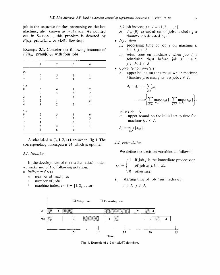
Example 3.1. Consider the following instance of F2Js;jk. prmuIC,,, with four jobs.

pij processing time of job j on machine i;

iEI,jEJ

I z 3 4

PI/ I 6 3 2 1 2 2 2 4 2

Sl,,: 0 3 4 I 7 I 5 3 2 2 5 3 I 3 2 I 5 4 3 2 5 _

sz,p 0 2 3 I 6 1 I 3 5 2 4 3 1 3 3 4 I 4 7 8 4

A schedule S = (3,1,2,4) is shown in Fig. 1. The corresponding makespan is 24, which is optimal.

Sijk setup time on machine i when job j is scheduled right before job k: i E I. j E Jo,k E J

?? Computed parameters Ai upper bound on the time at which machine

i finishes processing its last job: i E I.

A, = Ai- + CP<, jtJ

where A0 = 0 B; upper bound on the initial setup time for

machine i; i t I,

3.2. Formulation

3.1. Notation

In the development of the mathematical model, we make use of the following notation. ?? Indices and sets

m number of machines n number of jobs i machineindex; iEZ={1,2,....m}

We define the decision variables as follows:

Xjk =

1

1 if job j is the immediate predecessor

of job k: j, k E JO>

0 otherwise,

y,; = starting time of job j on machine i.

i E I, j E J.

0 Setup time 0 Processing time

Ml

M2

5 IO Time

> 15 20 25

Fig. 1. Example of a 2 x 4 SDST flowshop.

80 R.Z. Rios-Mercado. J.F. Burd I European Journal of Operational Research 110 (1997) 76-98

C - completion times of all jobs (makespan). max -

In the definition of xjk, notice that XOj = 1

(XjO = 1) implies that job j is the first (last) job in the sequence for j E J. Also notice that s,ak denotes the initial setup time on machine i when job k has no predecessor; i.e., when job k is scheduled first, for all k E J. This variable definition yields what we call a TSP-based formulation.

(IS) minimize C,,, subject to (1)

c xjk = 1, k E Jo, (4 kEJo /#k

c xJk = l, j E JO (3) kEJ,, k#j

Y<i + pij + Sijk d Yik

+Ai(l -xjk), iE I,j,

k E J, _i # k, (4)

SiOk < Yik+Bi(l -XOk)r

i E I, k E J, (5)

ymj+Pmj d Cm,,, j E J, (6)

Yij + Pij d Yi+lj>

i E I \ {m}, j E J, (7)

xjk E {O,l>,

j,k E Jo, .i # k, (8)

Yij 2 O, i E I, j E J. (9)

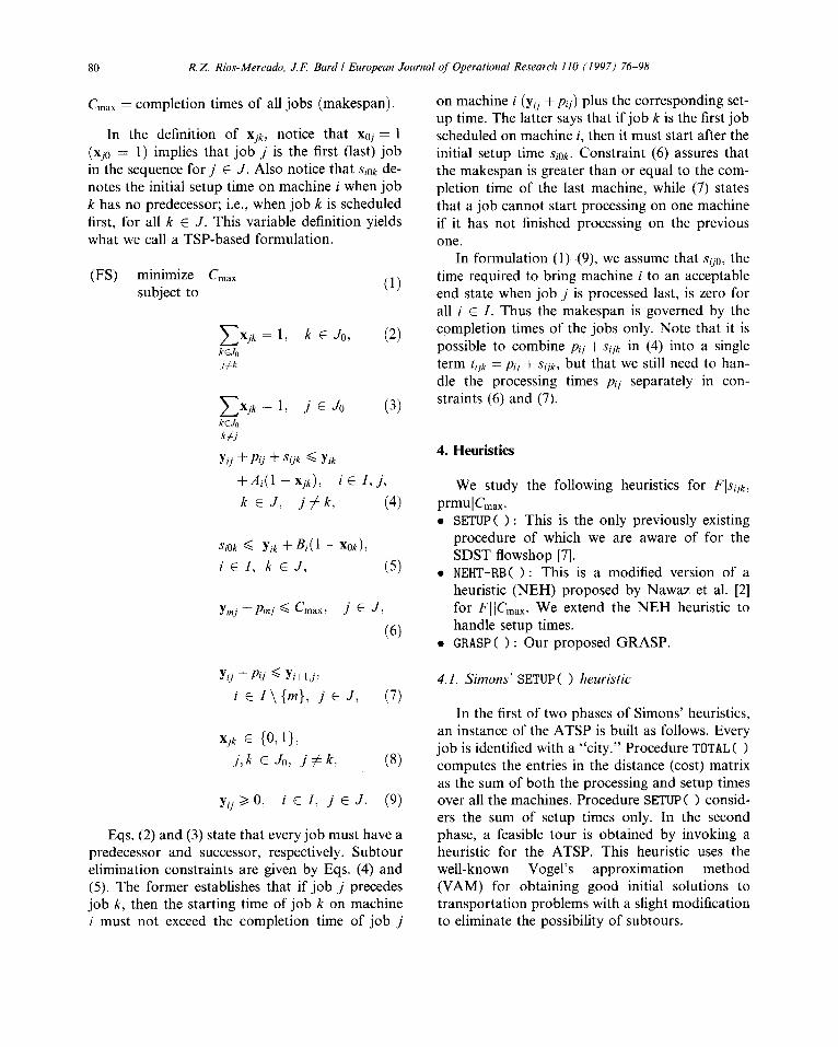
Eqs. (2) and (3) state that every job must have a predecessor and successor, respectively. Subtour elimination constraints are given by Eqs. (4) and (5). The former establishes that if job j precedes job k, then the starting time of job k on machine i must not exceed the completion time of job j

on machine i ( yij + pij) plus the corresponding setup time. The latter says that if job k is the first job scheduled on machine i, then it must start after the initial setup time SjOk. Constraint (6) assures that the makespan is greater than or equal to the completion time of the last machine, while (7) states that a job cannot start processing on one machine if it has not finished processing on the previous one.

In formulation (l)-(9), we assume that sijo, the time required to bring machine i to an acceptable end state when job j is processed last, is zero for all i E I. Thus the makespan is governed by the completion times of the jobs only. Note that it is possible to combine pij + sijk in (4) into a single term ti/k = pij + sijk, but that we still need to handle the processing times pij separately in constraints (6) and (7).

4. Heuristics

We study the following heuristics for FISijk,

prmuIG,,.

SETUPS > : This is the only previously existing procedure of which we are aware of for the SDST flowshop [7]. NEHT-RB( ) : This is a modified version of a heuristic (NEH) proposed by Nawaz et al. [2] for FI I%,,. We extend the NEH heuristic to handle setup times. GRASP ( > : Our proposed GRASP.

4.1. Simons’ SETUP ( > heuristic

In the first of two phases of Simons’ heuristics, an instance of the ATSP is built as follows. Every job is identified with a “city.” Procedure TOTALC > computes the entries in the distance (cost) matrix as the sum of both the processing and setup times over all the machines. Procedure SETUPS > consid- ers the sum of setup times only. In the second phase, a feasible tour is obtained by invoking a heuristic for the ATSP. This heuristic uses the well-known Vogel’s approximation method (VAM) for obtaining good initial solutions to transportation problems with a slight modification to eliminate the possibility of subtours.

R. Z. Rios-Mercado, J.F. Bard I European Journal of Operrrtional Research 1 IO (1997) 76 98 XI

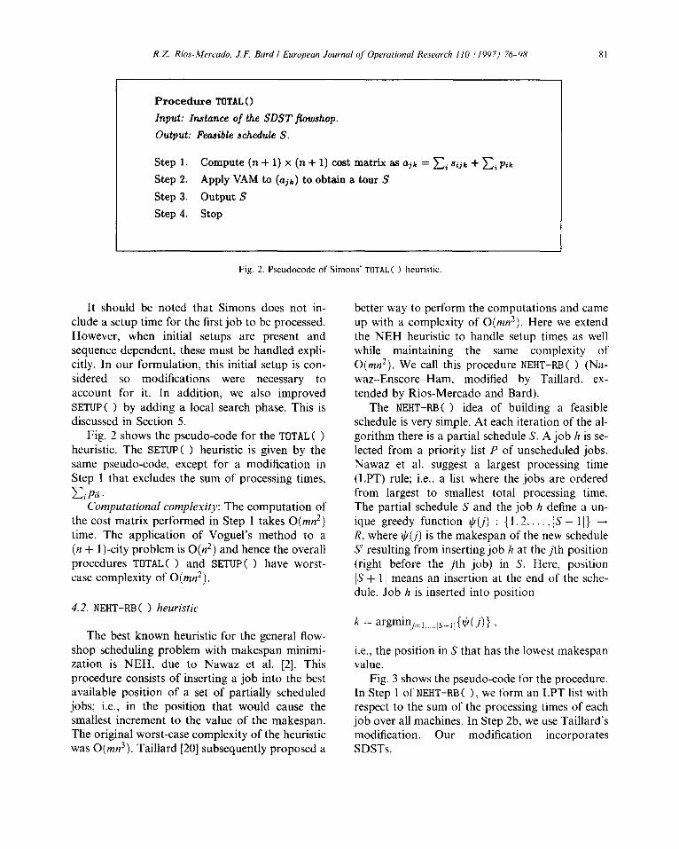
Procedure TOTAL ( )

Input: Instance of the SDST jlowshop.

output:

Step 1.

Step 2.

Step 3.

Step 4.

Feasible schedule S.

Compute (n+ 1) X (n + 1) CO& matrix aS ajk = ci sijk + ci Pik

Apply VAM to (ajk) to obtain a tour S

output s

stop

Fig. 2. Pseudocode of Simons’ TOTALC ) heuristic.

It should be noted that Simons does not include a setup time for the first job to be processed. However, when initial setups are present and sequence dependent, these must be handled expli- citly. In our formulation, this initial setup is considered so modifications were necessary to account for it. In addition, we also improved SETUPS > by adding a local search phase. This is discussed in Section 5.

Fig. 2 shows the pseudo-code for the TOTALC > heuristic. The SETUPS 1 heuristic is given by the same pseudo-code, except for a modification in Step I that excludes the sum of processing times, CiPik.

Computational complexity: The computation of the cost matrix performed in Step 1 takes O(mn*) time. The application of Voguel’s method to a (n + I)-city problem is O(n*) and hence the overall procedures TOTALC ) and SETUP ( > have worst- case complexity of O(mn*).

4.2. NEHT-RB( > heuristic

The best known heuristic for the general flowshop scheduling problem with makespan minimization is NEH, due to Nawaz et al. [2]. This procedure consists of inserting a job into the best available position of a set of partially scheduled jobs; i.e., in the position that would cause the smallest increment to the value of the makespan. The original worst-case complexity of the heuristic was 0(mn3). Taillard [20] subsequently proposed a

better way to perform the computations and came up with a complexity of O(mn?). Here we extend the NEH heuristic to handle setup times as well while maintaining the same complexity of O(mn*). We call this procedure NEHT-RB( 1 (Na- waz-Enscore-Ham, modified by Taillard, extended by Rios-Mercado and Bard).

The NEHT-RB( > idea of building a feasible schedule is very simple. At each iteration of the algorithm there is a partial schedule S. A job h is selected from a priority list P of unscheduled jobs. Nawaz et al. suggest a largest processing time (LPT) rule; i.e., a list where the jobs are ordered from largest to smallest total processing time. The partial schedule S and the job h define a unique greedy function $b) : { 1.2.. , jS + 1 I} + R, where $0’) is the makespan of the new schedule S’ resulting from inserting job h at the jth position (right before the jth job) in S. Here, position /S + l/ means an insertion at the end of the schedule. Job h is inserted into position

k = argmini=l.....,,+@(j)) 1

i.e., the position in S that has the lowest makespan value.

Fig. 3 shows the pseudo-code for the procedure. In Step 1 of NEHT-RB ( 1, we form an LPT list with respect to the sum of the processing times of each job over all machines. In Step 2b, we use Taillard’s modification. Our modification incorporates SDSTs.

82 R. 2. Rios-Mercado, J.F. Bard I European Journal of Operational Research 110 (1997) 76-98

I

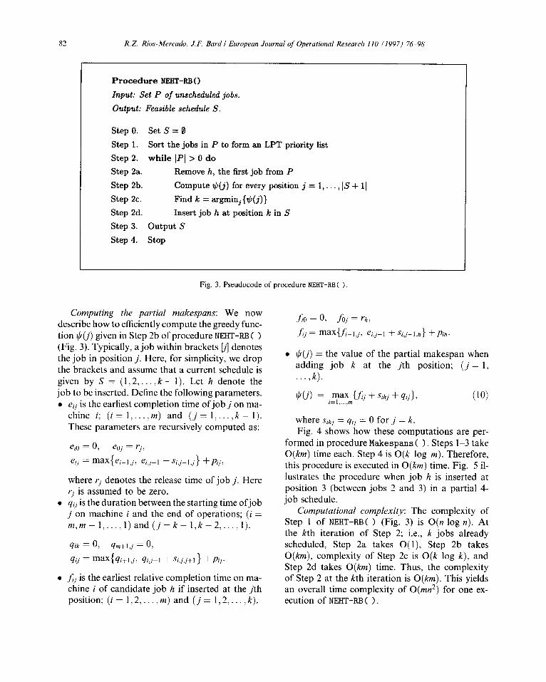
Procedure NEHT-FLB 0

Input: Set P of unscheduled jobs.

Output: Feasible schedule S.

Step 0. Set S = 0 Step 1. Sort the jobs in P to form an LPT priority list

Step 2. while IPI > 0 do

Step 2a. Remove h, the first job from P

Step 2b. Compute g(j) for every position j = 1, .

Step 2~. Find k = argminj{$(j)}

Step 2d. Insert job h at position k in S

Step 3. Output S

Step 4. Stop

‘., IS + 11

Fig. 3. Pseudocode of procedure NEHT-RB( )

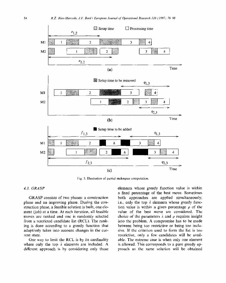
Computing the partial makespans: We now describe how to efficiently compute the greedy function $0’) given in Step 2b of procedure NEHT-RB ( > (Fig. 3). Typically, a job within brackets b] denotes the job in position j. Here, for simplicity, we drop the brackets and assume that a current schedule is given by S = (1,2,... , k - 1). Let h denote the job to be inserted. Define the following parameters.

eij is the earliest completion time of job j on machine i; (i = 1, . . , m) and ( j = 1, . . . , k - 1). These parameters are recursively computed as:

e;o = 0, eoi = 'J,

eiJ = max{ei-lj, ei,,j-1 + si,j-l.,j} +pij,

where rj denotes the release time of job j. Here ci is assumed to be zero. qij is the duration between the starting time ofjob j on machine i and the end of operations; (i = m,m- l,... ,l)and(j=k-l,k-2 ,..., 1).

qik = 0, 4m+l.j = 0,

9ij = max qi+l,j) qij+l + Si,jj+l 1 > +PiJ.

f;j is theearl ies re a t 1 t ive completion time on machine i of candidate job h if inserted at the jth position; (i = 1,2, . . . ,m) and (j= 1,2 ,..., k).

hO=O, foj=rh,

fq= max{f;:~~.j~ ei,J-l +si,j-l,h} fpih.

?? $0’) = the value of the partial makespan when adding job k at the jth position; (j = 1, ..., k).

(10)

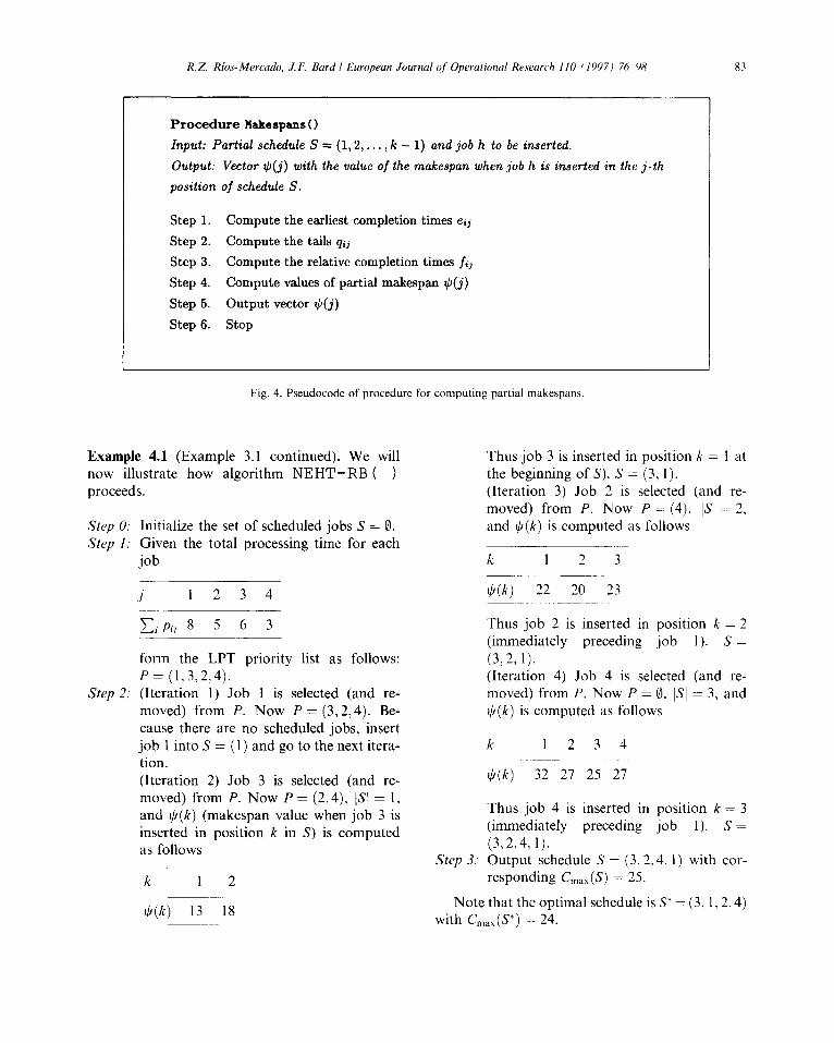
where sihj = qij = 0 for j = k. Fig. 4 shows how these computations are per-

formed in procedure Makespans ( 1. Steps l-3 take O(km) time each. Step 4 is O(k log m). Therefore, this procedure is executed in O(km) time. Fig. 5 il- lustrates the procedure when job h is inserted at position 3 (between jobs 2 and 3) in a partial 4- job schedule.

Computational complexity: The complexity of Step 1 of NEHT-RB( > (Fig. 3) is O(n log n). At the kth iteration of Step 2; i.e., k jobs already scheduled, Step 2a takes O(l), Step 2b takes O(km), complexity of Step 2c is O(k log k), and Step 2d takes O(km) time. Thus, the complexity of Step 2 at the kth iteration is O(km). This yields an overall time complexity of 0(mn2) for one execution of NEHT-RB ( 1.

R. Z. Rios-Mercado, J.F. Bard I European Journal of Operutional Research 110 (19971 76 98 83

Procedure Makespans 0

Input: Partial schedule S = (1,2,. . . , k - 1) and job h to be inserted.

Output: Vector $(j) with the value of the makespan when job h is inserted in the j-th

position of schedule S.

Step 1. Compute the earliest completion times eij

Step 2. Compute the tails qij

Step 3. Compute the relative completion times fij

Step 4. Compute values of partial malcespan $(j)

Step 5. Output vector $(j)

Step 6. Stop

Fig. 4. Pseudocode of procedure for computing partial makespans

Example 4.1 (Example 3.1 continued). We will now illustrate how algorithm NEHT-RB ( ) proceeds.

Stl?p 0: Step I:

Step 2:

Initialize the set of scheduled jobs S = 0. Given the total processing time for each job

i 1 2 3 4

Cip;i 8 5 6 3

form the LPT priority list as follows: P = (1,3,2,4). (Iteration 1) Job 1 is selected (and removed) from P. Now P = (3,2,4). Be- cause there are no scheduled jobs, insert job 1 into S = (1) and go to the next iteration. (Iteration 2) Job 3 is selected (and removed) from P. Now P = (2,4), ISI = 1, and $(k) (makespan value when job 3 is inserted in position k in S) is computed as follows

k 1 2

I&) 13 18

Thus job 3 is inserted in position k = 1 at the beginning of S). S = (3, 1). (Iteration 3) Job 2 is selected (and removed) from P. Now P = (4), IS/ = 2, and $(k) is computed as follows

k 1 2 3

$(k) 22 20 23

Thus job 2 is inserted in position k = 2 (immediately preceding job I). S = (3.2. 1). (Iteration 4) Job 4 is selected (and removed) from P. Now P = 0. ISI = 3, and $(k) is computed as follows

k 1 2 3 4

$(k) 32 27 25 27

Thus job 4 is inserted in position k = 3 (immediately preceding job I). S = (3,2.4, 1).

Step 3: Output schedule S = (3,2,4, 1) with corresponding C,,,,X(S) = 25.

Note that the optima1 schedule is S* = (3, 1.2.4) with C,,,(S*) = 24.

84 R. 2. Rios-Mercado, J. F. Bard I European Journal of Operational Research 110 (1997) 76-98

Ml

M2

Ml

M2

Ml

M2

4.3. GRASP

•i Processing time

Setup time to be removed

(b)

q2,3 > Time

Setup time to be added

(c)

Fig. 5. Illustration of partial makespan computation.

Time

GRASP consists of two phases: a construction phase and an improving phase. During the construction phase, a feasible solution is built, one element uob) at a time. At each iteration, all feasible moves are ranked and one is randomly selected from a restricted candidate list (RCL). The rank- ing is done according to a greedy function that adaptively takes into account changes in the current state.

One way to limit the RCL is by its cardinality where only the top I elements are included. A different approach is by considering only those

elements whose greedy function value is within a fixed percentage of the best move. Sometimes both approaches are applied simultaneously; i.e., only the top i elements whose greedy function value is within a given percentage p of the value of the best move are considered. The choice of the parameters /z and p requires insight into the problem. A compromise has to be made between being too restrictive or being too inclu- sive. If the criterion used to form the list is too restrictive, only a few candidates will be available. The extreme case is when only one element is allowed. This corresponds to a pure greedy approach so the same solution will be obtained

R. Z. Rim-Mercado, J.F. Bard I European Journal oj‘ Operational Research 110 (I 997) 76 9X 85

lnitidization

L = EMF’TY (list of schedules in workbtg subset)

i = 0 (phase I counter)

Tbesc = EMPTY (best schedule)

Malrespan~)=m

c r T

r- Append S(i) to L

L + L + S(i) Phase 2: Apply local search lo

best schedule in L to

\ , obtain schedule T

\

No Ye.5 I

Fig. 6. Flow chart of complete GRASP algorithm.

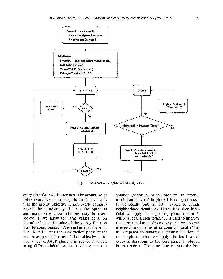
every time GRASP is executed. The advantage of being restrictive in forming the candidate list is that the greedy objective is not overly compromised; the disadvantage is that the optimum and many very good solutions may be over- looked. If we allow for large values of A, on the other hand, the value of the greedy function may be compromised. This implies that the solutions found during the construction phase might not be as good in terms of their objective function value. GRASP phase 1 is applied N times, using different initial seed values to generate a

solution (schedule) to the problem. In general, a solution delivered in phase 1 is not guaranteed to be locally optimal with respect to simple neighborhood definitions. Hence it is often bene- ficial to apply an improving phase (phase 2) where a local search technique is used to improve the current solution. Since doing the local search is expensive (in terms of its computational effort) as compared to building a feasible solution, in our implementation we apply the local search every K iterations to the best phase 1 solution in that subset. The procedure outputs the best

86 R.Z. Rios-Mercudo, J.F. Bard I European Journal of Operational Research 110 (1997) 76-98

of the N/K local optimal solutions. Fig. 6 shows a flow chart of our implementation.

The fundamental difference between GRASP and other meta-heuristics such as tabu search and simulated annealing is that GRASP relies on high quality phase 1 solutions (due to the inherent worst-case complexity of the local search) whereas the other methods do not require good feasible solutions. They spend practically all of their time improving the incumbent solution and attempting to overcome local optimality. For a GRASP tutorial, the reader is referred to [21].

Below we present a GRASP for FIs;~~, prmu I Cm,, based on job insertion. This approach was found to be significantly more successful than a GRASP based on appending jobs to the partial schedule.

GRASP for the SDST Flowshop: The GRASP construction phase follows the same insertion idea as algorithm NEHT-RB( > discussed in Section 4.2. The difference between them is the selection strategy for inserting the next unscheduled job into the partial schedule. Recall that NEHT-RB( > always inserts the job in the best available position.

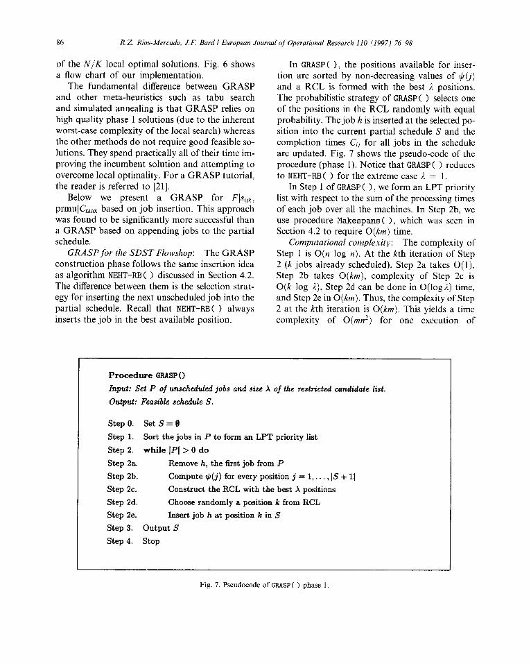
In GRASP( >, the positions available for insertion are sorted by non-decreasing values of $G) and a RCL is formed with the best J. positions. The probabilistic strategy of GRASPS > selects one of the positions in the RCL randomly with equal probability. The job h is inserted at the selected position into the current partial schedule S and the completion times Co for all jobs in the schedule are updated. Fig. 7 shows the pseudo-code of the procedure (phase 1). Notice that GRASPS > reduces to NEHT-RB( ) for the extreme case 1 = 1.

In Step 1 of GRASP ( 1, we form an LPT priority list with respect to the sum of the processing times of each job over all the machines. In Step 2b, we use procedure Makespans ( >, which was seen in Section 4.2 to require O(km) time.

Computational complexity: The complexity of Step 1 is O(n log n). At the kth iteration of Step 2 (k jobs already scheduled), Step 2a takes O(l), Step 2b takes O(km), complexity of Step 2c is O(k log n), Step 2d can be done in O(logE,) time, and Step 2e in O(km). Thus, the complexity of Step 2 at the kth iteration is O(km). This yields a time complexity of O(mn2) for one execution of

Procedure GRASP (>

Input: Set P of unscheduled jobs and size X of the restricted candidate list.

output: Feasible schedule S.

Step 0.

Step 1.

Step 2.

Step 2a.

Step 2b.

Step 2c.

Step 2d.

Step 2e.

Step 3.

Step 4.

Set S = 0

Sort the jobs in P to form an LPT priority list

while lPl > 0 do

Remove h, the first job from P

Compute $(j) for every position j = 1,. . . , IS + 11

Construct the RCL with the best X positions

Choose randomly a position k from RCL

Insert job h at position k in S

output s

stop

Fig. 7. Pseudocode of CRASPC ) phase 1.

R.Z. Rios-Mercado. J.F. Bard I European Journal of’ Operational Research I10 (19971 76 98 87

GRASP( > phase 1. Therefore, the overall phase 1 time complexity is O(Nmn2).

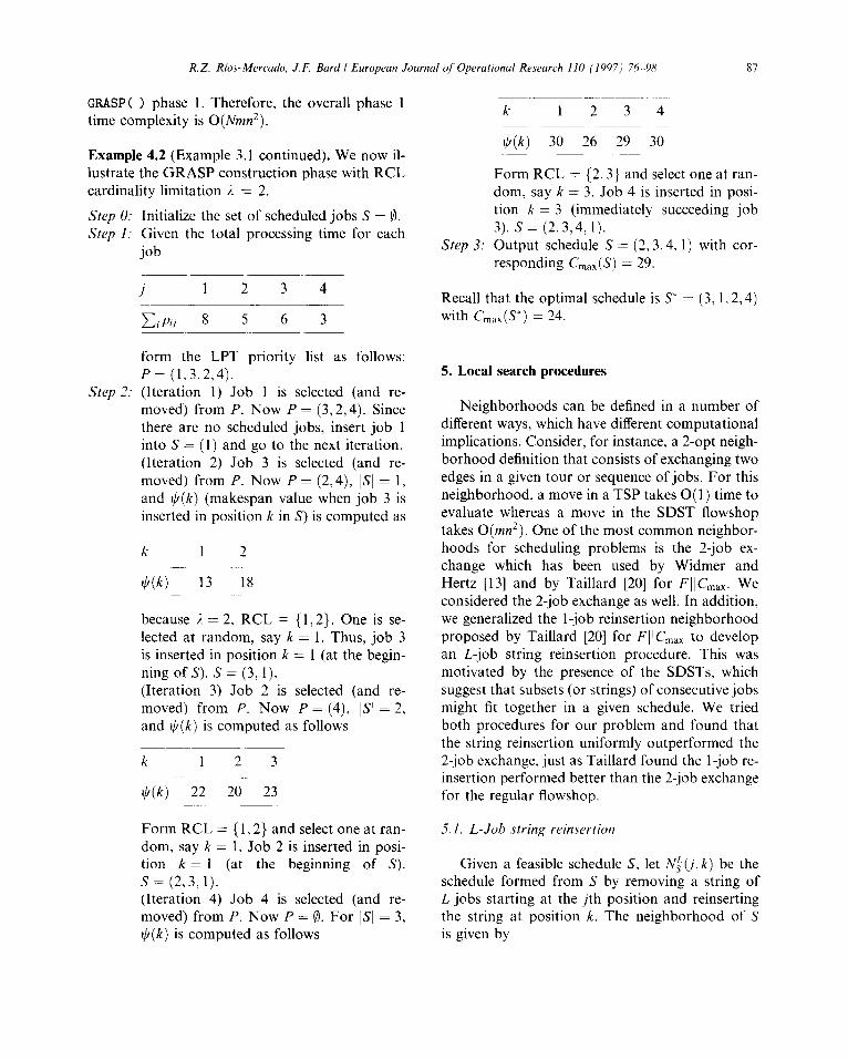
Example 4.2 (Example 3.1 continued). We now illustrate the GRASP construction phase with RCL cardinality limitation i = 2.

Step 0: Step 1.

Step 2:

Initialize the set of scheduled jobs S = 0. Given the total processing time for each job ~~___

.i 1 2 3 4

Cipij 8 5 6 3

form the LPT priority list as follows: P= (1,3,2,4). (Iteration 1) Job 1 is selected (and removed) from P. Now P = (3,2,4). Since there are no scheduled jobs, insert job 1 into S = (1) and go to the next iteration. (Iteration 2) Job 3 is selected (and removed) from P. Now P = (2,4), ISI = 1. and $(k) (makespan value when job 3 is inserted in position k in S) is computed as

k 1 2

$(k) 13 18

because 3. = 2, RCL = { 1,2}. One is selected at random, say k = 1. Thus, job 3 is inserted in position k = 1 (at the beginning of S). S = (3,l). (Iteration 3) Job 2 is selected (and removed) from P. Now P = (4), IS( = 2, and $(k) is computed as follows

k 1 2 3

t+h(k) 22 20 23

Form RCL = { 1,2} and select one at random, say k = 1. Job 2 is inserted in position k = 1 (at the beginning of S). S= (2,3,1). (Iteration 4) Job 4 is selected (and removed) from P. Now P = 0. For ISI = 3, $(k) is computed as follows

Step 3:

~~.~ k 1 2 3 4

i//(k) 30 26 29 30

Form RCL = {2,3} and select one at random, say k = 3. Job 4 is inserted in position k = 3 (immediately succeeding job 3). s = (2,3,4,1). Output schedule S = (2.3.4. 1) with corresponding Cmax(S) = 29.

Recall that the optimal schedule is S* = (3. 1.2.4) with C,,,,,(S*) = 24.

5. Local search procedures

Neighborhoods can be defined in a number of different ways, which have different computational implications. Consider, for instance, a 2-opt neighborhood definition that consists of exchanging two edges in a given tour or sequence of jobs. For this neighborhood, a move in a TSP takes 0( 1) time to evaluate whereas a move in the SDST flowshop takes 0(mn2). One of the most common neighborhoods for scheduling problems is the 2-job exchange which has been used by Widmer and Hertz [13] and by Taillard [20] for FI I&,,. We considered the 2-job exchange as well. In addition, we generalized the l-job reinsertion neighborhood proposed by Taillard [20] for FI (C,,, to develop an L-job string reinsertion procedure. This was motivated by the presence of the SDSTs, which suggest that subsets (or strings) of consecutive jobs might fit together in a given schedule. We tried both procedures for our problem and found that the string reinsertion uniformly outperformed the 2-job exchange, just as Taillard found the l-job reinsertion performed better than the 2-job exchange for the regular flowshop.

5.1. L-Job string reinsertion

Given a feasible schedule S, let Nicj, k) be the schedule formed from S by removing a string of L jobs starting at the jth position and reinserting the string at position k. The neighborhood of S is given by

88 R. 2. Rios-Mercado, J. F. Bard I European Journal of Operational Research I10 (I 997) 76-98

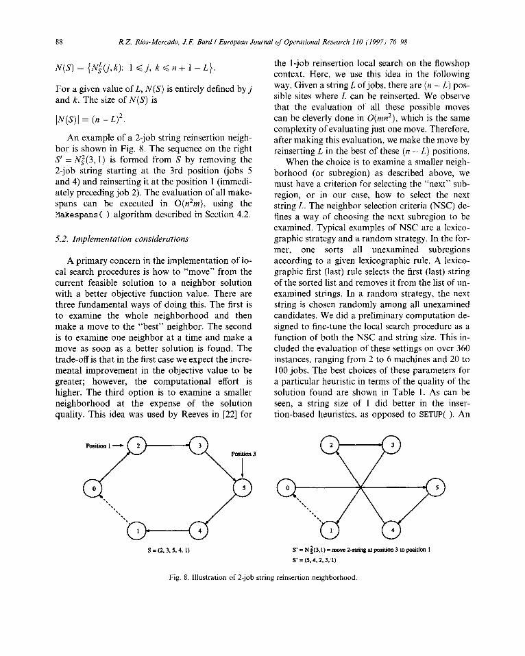
N(S) = {A&$ k): 1 d j, k < 12 + 1 - L}. the l-job reinsertion local search on the flowshop context. Here, we use this idea in the following way. Given a string L of jobs, there are (n - L) possible sites where L can be reinserted. We observe that the evaluation of all these possible moves can be cleverly done in O(mn2), which is the same complexity of evaluating just one move. Therefore, after making this evaluation, we make the move by reinserting L in the best of these (n - L) positions.

For a given value of L, N(S) is entirely defined by j and k. The size of N(S) is

pv(S)I = (n - q2,

An example of a 2-job string reinsertion neighbor is shown in Fig. 8. The sequence on the right S’ = N,2(3,1) is formed from S by removing the 2-job string starting at the 3rd position (jobs 5 and 4) and reinserting it at the position 1 (immediately preceding job 2). The evaluation of all makespans can be executed in 0(n2m), using the Makespans( > algorithm described in Section 4.2.

5.2. Implementation considerations

A primary concern in the implementation of local search procedures is how to “move” from the current feasible solution to a neighbor solution with a better objective function value. There are three fundamental ways of doing this. The first is to examine the whole neighborhood and then make a move to the “best” neighbor. The second is to examine one neighbor at a time and make a move as soon as a better solution is found. The trade-off is that in the first case we expect the incre- mental improvement in the objective value to be greater; however, the computational effort is higher. The third option is to examine a smaller neighborhood at the expense of the solution quality. This idea was used by Reeves in [22] for

When the choice is to examine a smaller neighborhood (or subregion) as described above, we must have a criterion for selecting the “next” subregion, or in our case, how to select the next string L. The neighbor selection criteria (NSC) de- fines a way of choosing the next subregion to be examined. Typical examples of NSC are a lexicographic strategy and a random strategy. In the former, one sorts all unexamined subregions according to a given lexicographic rule. A lexicographic first (last) rule selects the first (last) string of the sorted list and removes it from the list of unexamined strings. In a random strategy, the next string is chosen randomly among all unexamined candidates. We did a preliminary computation de- signed to fine-tune the local search procedure as a function of both the NSC and string size. This included the evaluation of these settings on over 360 instances, ranging from 2 to 6 machines and 20 to 100 jobs. The best choices of these parameters for a particular heuristic in terms of the quality of the solution found are shown in Table 1. As can be seen, a string size of 1 did better in the insertion-based heuristics, as opposed to SETUP( ). An

S’=Na(3,1)=movc2_wingatposition3topositionl

S’ = (5.4.2.3.‘1)

Fig. 8. Illustration of 2-job string reinsertion neighborhood.

R. Z. Rios- Mercado. J. I? Bard I European Journal of’ Operational Research 110 (I 997) 76 98

Table I Parameter selection for string reinsertion procedure

Heuristic String size NSC

SETUP ( ) 3 Lexicographic (last) NEHT-RB ( ) I Lexicographic (last) GRASP ( ) I Lexicographic (first)

explanation of this is that both NEHT-RB( > and GRASP ( > are heuristics that find a feasible solution by inserting one job at a time. This produces a feasible schedule where the interrelationship among strings of jobs may not be as strong a feasible solution delivered by SETUP ( > which is a TSP-based heuristic. Thus, SETUPS > benefits better from a 3- job string reinsertion.

6. Lower bounds

Recall the MIP formulation (l)-(9) presented in Section 3. Constraint (7) implies that

y,j + Pii 2 Yi.-I,, +PiLI.j, iEZ\{rn},jEJ.

Therefore, the makespan constraint (6) can also be written as

Y,j+p,jdCmd,, iEI. jEJ.

By relaxing the machine link constraints (7) the starting time for a job j on a given machine i is no longer linked to the finishing time on the previous machine. We call this new problem separable flow shop (SFS), with optimal objective function value u(SFS). It is clear that u(SFS) d #(KY), where c(FS) is the optimal value of problem FS.

Let SFS(i) be the SFS problem where all the subtour elimination and makespan constraints not related to machine i are removed. Let S = ( 1, , PI) be a feasible schedule for SFS(i). Here we assume for simplicity that the jobs in S are sequenced in order so the makespan of S is given by

G,X(~) = SiOl + PiI + Sil2 + pi2 + . .

+ Si.n- I .n + /An + Sin0

= PPij + 2 sij.j+lXj.j+l 1 +I j=o

where index n + 1 corresponds to index 0 Sin0 = 0. Thus SFS(i) can be expressed as

(SFS(i)) minimize Cpij + x xs,jkXjk

itJo ;C.IC, ii.,,, kff

89

and

(11)

subject to c x,k = 1, k E Jo> iEi(J IFFX-

(l-2)

c X.jk = 1 , .I’ E Jo. ~~‘0 k#i

(13)

Yij- Yik + PI, + Sljk

< A!( 1 - xjk).

,j, k E J. .j # k.

(14)

-Y&S. SiOk d Bi( 1 - XOk)3 kEJ. (15)

x,k E (0, 1). j.k E Jo.

.i # k (16)

yji 3 O. .i E J (17)

for all i E I.

6.1. A lower bounding scheme .fbv the SDSTjIowshop

For a fixed machine i, Cjpij in (11) is constant so problem SFS(i) reduces to an instance of the ATSP, where JO is the set of vertices and sijk the distance between vertices j and k. Eqs. (12) and (13) corre- spond to the assignment constraints. Time-based subtour elimination constraints are given by (14) and (15). From the imposed relaxations we have

i(SFS(i)) < tl(SFS) < a(FS)

for all i E I. Because any valid lower bound for SFS(i), call it L,, is a valid lower bound for FS, we then proceed to compute a lower bound for

90 R.Z. Rim-Mercado, J.F. Bard I European Journal of Operational Research 110 (1997) 76-98

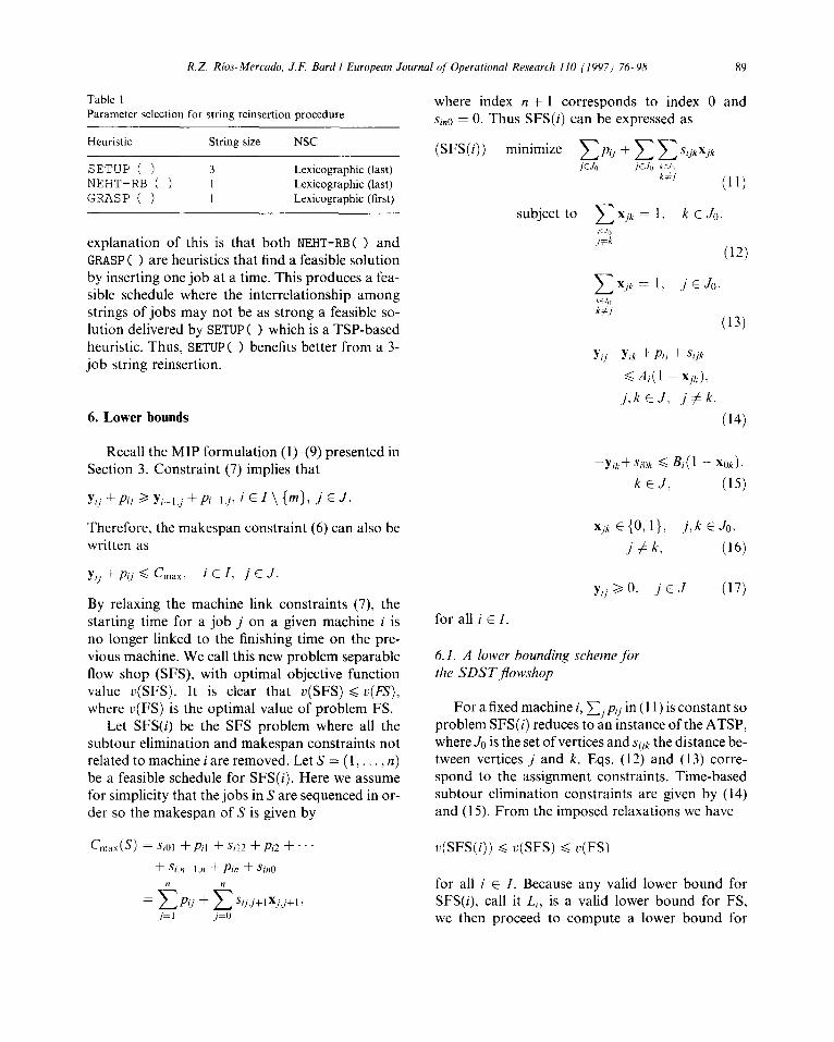
Procedure lower_bound_FS 0 (Phase 1) Input: An instance of the SDSTflowshop with corresponding setup time matrix (sijk)

and processing time matrix (pii).

Output: Lower bound Cfi;B, for the value of the makespan &a~.

Step 1. for i = 1 to m do

Step la. Let Pi = Cjpij

Step lb. Let cjk = Sijk be the input cost matrix for the ATSP SFS(d)

Step lc. L; = Pi + lower_bounddTSP (cjk )

Step 2. OUtpUt C/$g = maXi

Step 3. Stop

Fig. 9. Pseudocode of lower bounding procedure for SDST Bowshop (phase I)

every subproblem SFS(1’) and obtain a lower bound on v(FS) by CkfX = maxi,,{&}.

The suggested lower bounding procedure for FS is outlined in Fig. 9, where procedure lower_ bound_ATSP (cjk) in Step lc is any valid lower bound for SFS(I’) (ATSP with cost matrix (cjk)).

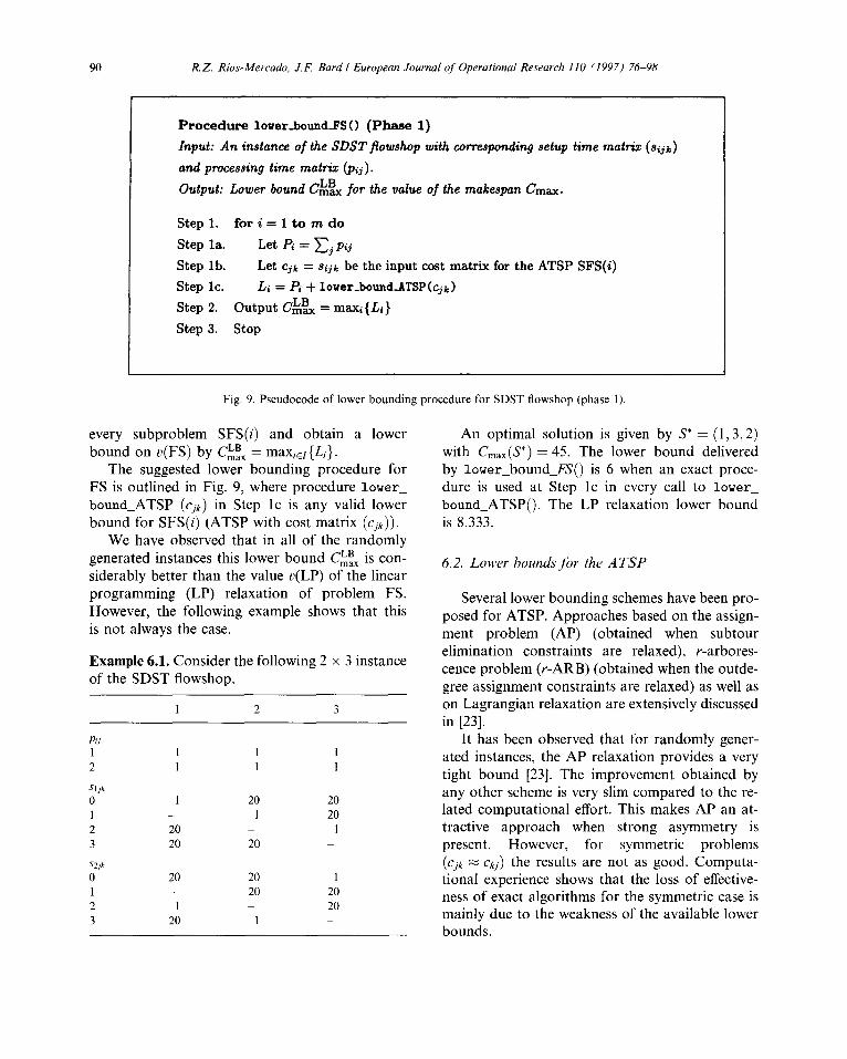
We have observed that in all of the randomly generated instances this lower bound C’i& is considerably better than the value u(LP) of the linear programming (LP) relaxation of problem FS. However, the following example shows that this is not always the case.

Example 6.1. Consider the following 2 x 3 instance of the SDST flowshop.

1 2 3

Pij 1 2

Sl/k

0 1 2 3

S2jk

0 1 2 3

1 1 1 I I I

1 20 20 _ 1 20 20 I 20 20

20 20 1 20 20

1 20 20 1

An optimal solution is given by S* = (1,3,2) with C ,,,(S*) = 45. The lower bound delivered by lower_bound_FS() is 6 when an exact procedure is used at Step lc in every call to lower_ bound_ATSP(). The LP relaxation lower bound is 8.333.

6.2. Lower bounds jbr the ATSP

Several lower bounding schemes have been proposed for ATSP. Approaches based on the assignment problem (AP) (obtained when subtour elimination constraints are relaxed), r-arbores- cence problem (r-ARB) (obtained when the outde- gree assignment constraints are relaxed) as well as on Lagrangian relaxation are extensively discussed in [23].

It has been observed that for randomly generated instances, the AP relaxation provides a very tight bound [23]. The improvement obtained by any other scheme is very slim compared to the related computational effort. This makes AP an at- tractive approach when strong asymmetry is present. However, for symmetric problems (cj++ M ck,) the results are not as good. Computa- tional experience shows that the loss of effective- ness of exact algorithms for the symmetric case is mainly due to the weakness of the available lower bounds.

R.Z. Rios-Mercudo, J.F. Bard I European Journal of Operational Research I10 (1997) 7698 91

To deal with harder cases, schemes based on additive approaches have been developed. Balas and Christofides [24] proposed an additive approach based on Lagrangian relaxation. Most re- cently, Fischetti and Toth [25] have implemented an additive scheme that outperformed the restricted Lagrangian approach of Balas and Chris- tofides. Their procedure yields a sequence of increasing lower bounds within a general frame- work that exploits several substructures of the ATSP including AP and r-ARB. We compared two lower bounding schemes for the SDST flowshop. One is based on the AP relaxation and the other on the additive approach of Fischetti and Toth. In our experiments, we observed that the improvement obtained by the latter was very small. This is attributed to the fact that for the instances having setup times that are completely asymmetric, the AP bound is very tight. This phenom- enon was also observed by Fischetti and Toth for the ATSP. As the problem becomes less asymmetric the results yielded by the additive approach improve considerably. Since the data sets we are working with are assumed to have asymmetric setup times, we use the lower bounding approach based on the AP relaxation.

6.3. Improving the lower hound for SDSTjlowshop

Let Cij be the completion time of job j on machine i. In particular, let K be the completion of time of the last job on machine i; i.e., T, is the time at which machine i finishes processing. Then we have the following relation:

C;, = max{C,-I.,, Ci.-I +Si\i-1.j) +Pij.

In particular, if n represents the last job in the sequence, then we have

Gin = max{Ci-I,,,, ci.n-l + S,,,-l.n} +Pin.

Because 7; = Ci, we have that T - pin >, z-1. This is valid for job n, and certainly it is also valid for pyin = minjeJ(Pij}; i E I. This suggests the following recursive improvement for a set {Li}, where Li is a valid lower bound on the completion time on machine i; i E 1. If A = Li-t - (Li -pp’“) > 0,

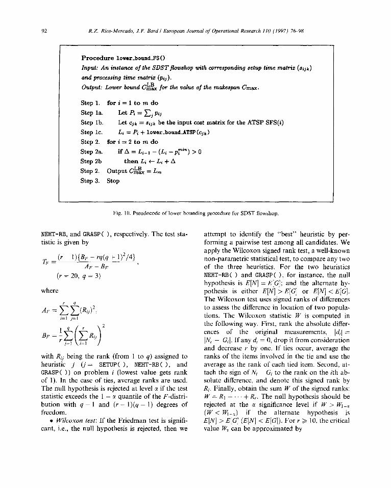
then Li can be improved by A; that is, Li + Li + A. Hence C,!$, = L, is a valid lower bound for C,,,.

We have observed that this improvement step has achieved up to a 5% reduction on the relative gap for most of the instances examined. The modified procedure is shown in Fig. 10.

7. Experimental work

All procedures were coded in C + + and compiled with the Sun C + + compiler CC version 2.0.1 and optimization flag set to -0. CPU times were obtained by calling the clock( 1 function on a SPARCStation 10. To evaluate the various schemes, 20 instances of the SDST flowshop were randomly generated for every combination m x n E { (2,4,6) x (20.50, 100)). for two different classes of data sets (available from authors). ?? Data set A: pQ E [1,99] and .yijA- E [l, lo]. ?? Data set B: pi, E [l. 991 and s;jh E [ 1.991. It has been reported that many real-world instances match data set A (e.g. [18]). Data set B is included to allow us to investigate the effect on the algorithms when the setup times assume a wider range.

For each set of instances we performed several comparisons.

?? Summary statistics: To identify dominating characteristics we compiled the following objective function value statistics. ~ Number of times heuristic is best or tied for

best. - Average percentage above lower bound

and the following time related statistics. ~ Average CPU time. - Worst CPU time.

??Friedman test: This is a non-parametric test, analogous to the classical ANOVA test of homo- geneity, which we apply to the null hypothesis:

Ho : E[S] = E[N] = E[G].

under the assumption of normal distributions with a common variance, where S: N, and G are random variables corresponding to percentages above the lower bound generated by heuristics SETUPS >,

92 R. Z. Rios-Mercado, J. F. Bard I European Journal of Operational Research 110 (1997) 76-98

Procedure lover_bound_FS 0

Input: An instance of the SDSTfiowshop with corresponding setup time matrix (sijk)

and processing time matrix (pii).

Output: Lower bound CkBa for the value of the makespan Cm=.


Step la. Let Pi = Cj pij

Step lb. Let Cjb = 8ijk be the input cost matrix for the ATSP SFS(i)

Step lc. Li = Pi + loWer_bo~d_ATSP (cjk >


Step 2a. ifA=Li_l-(Li-ppn)>O

Step 2b thenLitLi+A

Step 2. Output Cfi;B, = L,

Step 3. Stop

Fig. 10. Pseudocode of lower bounding procedure for SDST flowshop.

NEHT-RB, and GRASP ( 1, respectively. The test statistic is given by

TF = (r - l){BF - rq(q + 1)2/4} AF -BF

3

(?” = 20, q = 3)

where

AF = 2 k(Rij)2, i=l j=l

2

with Rij being the rank (from 1 to q) assigned to heuristic j (j = SETUPS 1, NEHT-FtB ( 1, and GRASPS 1) on problem i (lowest value gets rank of 1). In the case of ties, average ranks are used. The null hypothesis is rejected at level c( if the test statistic exceeds the 1 - CI quantile of the F-distribution with q - 1 and (Y - l)(q - 1) degrees of freedom.

?? Wilcoxon test: If the Friedman test is significant, i.e., the null hypothesis is rejected, then we

attempt to identify the “best” heuristic by per- forming a pairwise test among all candidates. We apply the Wilcoxon signed rank test, a well-known non-parametric statistical test, to compare any two of the three heuristics. For the two heuristics NEHT-RB( > and GRASPS >, for instance, the null hypothesis is E[N] = E[G]; and the alternate hypothesis is either E[N] > E[G] or E[N] < E[G]. The Wilcoxon test uses signed ranks of differences to assess the difference in location of two popula- tions. The Wilcoxon statistic W is computed in the following way. First, rank the absolute differences of the original measurements, MI = INi - Gil. If any d; = 0, drop it from consideration and decrease Y by one. If ties occur, average the ranks of the items involved in the tie and use the average as the rank of each tied item. Second, at- tach the sign of Ni - Gi to the rank on the ith absolute difference, and denote this signed rank by Ri. Finally, obtain the sum W of the signed ranks: W = RI + + R,. The null hypothesis should be rejected at the c1 significance level if W > WI-, (W < WI_,) if the alternate hypothesis is E[N] > E[G] (E[N] < E[G]). For r 3 10, the critical value W, can be approximated by

R. Z. Rios- Mereado. J.F. Bard I European Journal of’ Oprrarional Research I10 (1997) 76 98 93

W, = Z(cc)&(r + 1)(2r + 1)/6,

where Z(g) is the standard normal fractile such that the proportion x of the area is to the left of

Z(z). ?? Expected utility: This approach for compar-

ing two or more heuristics is based on the notion that we seek a heuristic that performs well on the average and that very rarely performs poorly; i.e., it is concerned with downside risk as well as expected accuracy. The procedure incorporates this attitude towards risk in a risk-averse utility function. As suggested by Golden and Stewart, we calculate the expected utility for each heuristic as c( - p( 1 - it)-;. where 6 = s’/X.? = (x/.s)~ are estimated parameters of a gamma distribution; ‘2 = 600, /j = 100 are arbitrarily chosen parameters and t = 0.05 gives a measure of risk aversion for the utility function. It should be pointed out that t must be less than l/g for each heuristic.

These settings were used to conduct the experiments; i.e., we applied the construction phase N = 100 times and then we did the local search once every K = 10 iterations on the most promis- ing solution in that subset (see Section 4.3). To evaluate the quality of the heuristics we compared the results with those obtained from our AP-based two-phase lower bounding procedure discussed in Section 6.

7.1. Experiment 1: Datu set A

The application of the Friedman test, Wilcoxon test, and the expected utility approach to evaluate heuristics is proposed by Golden and Stewart [26] for the TSP.

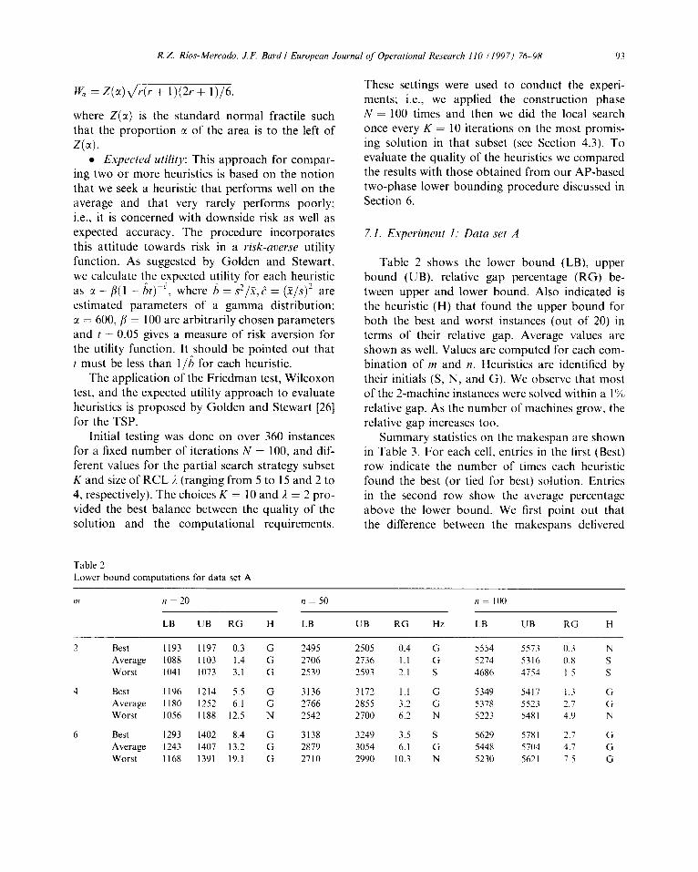
Table 2 shows the lower bound (LB), upper bound (UB), relative gap percentage (RG) between upper and lower bound. Also indicated is the heuristic (H) that found the upper bound for both the best and worst instances (out of 20) in terms of their relative gap. Average values are shown as well. Values are computed for each combination of m and n. Heuristics are identified by their initials (S, N, and G). We observe that most of the 2-machine instances were solved within a 1% relative gap. As the number of machines grow, the relative gap increases too.

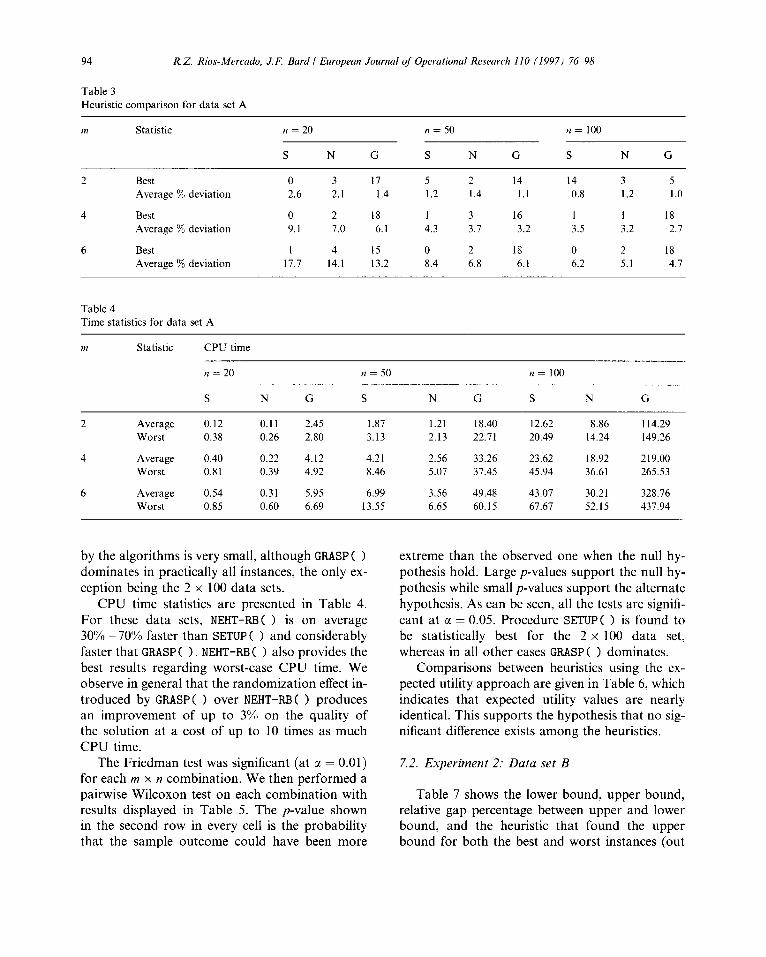
Initial testing was done on over 360 instances Summary statistics on the makespan are shown for a fixed number of iterations N = 100, and dif- in Table 3. For each cell, entries in the first (Best) ferent values for the partial search strategy subset row indicate the number of times each heuristic K and size of RCL 1. (ranging from 5 to 15 and 2 to found the best (or tied for best) solution. Entries 4, respectively). The choices K = 10 and 1, = 2 pro- in the second row show the average percentage vided the best balance between the quality of the above the lower bound. We first point out that solution and the computational requirements. the difference between the makespans delivered

Table 2 Lower bound computations for data set A

WI n = 20 n = 50 n = 100

LB UB RG H LB UB RG Hz LB LJB RG H

2 Best Average Worst



1193 1197 0.3 G 2495 1088 1103 1.4 G 2706 1041 1073 3.1 G 2539

1196 1214 5.5 G 3136 1180 1252 6.1 G 2166 1056 1188 12.5 N 2542

1293 1402 8.4 G 3138 1243 1407 13.2 G 2879 1168 1391 19.1 G 2710

2505 2136 2593

3172 2855 2700

3249 3054

0.4 G I.1 G 2.1 s

I.1 G 3.2 G 6.2 N

3.5 s 6.1 G

10.3 N

5554 5274 4686

5349 5378 5223

5629 544% 5230

5573 0.3 N 5316 0.8 S 4754 I.5 S

5417 1.3 G 5523 2.1 G 548 I 4.9 N

578 I 2.7 G 5704 4.7 G 5621 7.5 G

94 R. Z. Rios-Mercado, J.F. Bard I European Journal of Operational Research 110 (1997) 76-98

Table 3 Heuristic comparison for data set A

tn Statistic n = 20 n = 50 n= 100

S N G S N G s N G

2 Best 0 3 17 5 2 14 14 3 5 Average % deviation 2.6 2.1 1.4 1.2 1.4 1.1 0.8 1.2 1.0



Table 4 Time statistics for data set A

Statistic

Average Worst

Average worst

Average Worst

CPU time

n = 20 n = 50 n= 100

S N G S N G S N G

0.12 0.11 2.45 1.87 1.21 18.40 12.62 8.86 114.29 0.38 0.26 2.80 3.13 2.13 22.71 20.49 14.24 149.26

0.40 0.22 4.12 4.21 2.56 33.26 23.62 18.92 219.00 0.81 0.39 4.92 8.46 5.07 37.45 45.94 36.61 265.53

0.54 0.31 5.95 6.99 3.56 49.48 43.07 30.21 328.76 0.85 0.60 6.69 13.55 6.65 60.15 67.67 52.15 437.94

by the algorithms is very small, although GRASP ( > dominates in practically all instances, the only ex- ception being the 2 x 100 data sets.

CPU time statistics are presented in Table 4. For these data sets, NEHT-RB( 1 is on average 30% - 70% faster than SETUP ( > and considerably faster that GRASP ( 1. NEHT-RB ( 1 also provides the best results regarding worst-case CPU time. We observe in general that the randomization effect in- troduced by GRASPS > over NEHT-RB ( > produces an improvement of up to 3% on the quality of the solution at a cost of up to 10 times as much CPU time.

The Friedman test was significant (at CI = 0.01) for each m x n combination. We then performed a pairwise Wilcoxon test on each combination with results displayed in Table 5. The p-value shown in the second row in every cell is the probability that the sample outcome could have been more

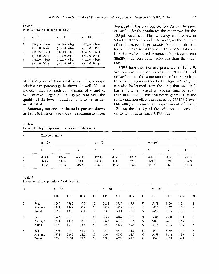
extreme than the observed one when the null hypothesis hold. Large p-values support the null hypothesis while small p-values support the alternate hypothesis. As can be seen, all the tests are significant at CI = 0.05. Procedure SETUPS > is found to be statistically best for the 2 x 100 data set, whereas in all other cases GRASPS > dominates.

Comparisons between heuristics using the expected utility approach are given in Table 6, which indicates that expected utility values are nearly identical. This supports the hypothesis that no significant difference exists among the heuristics.

7.2. Experiment 2: Data set B

Table 7 shows the lower bound, upper bound, relative gap percentage between upper and lower bound, and the heuristic that found the upper bound for both the best and worst instances (out

XPES 8SSS 6L9S

SEZS 88bS 9OLS

Z6Lb 98ES 8SbS

9 Z'Z9 GLEP f) L'IS LSSP f) 8'Ib bl9b

S P‘LP L81b S S'SE 6LOb S L'6Z 601b

S O‘EZ l8Zf S E'LI 8ZfE S 6'11 6ZSf

OOLZ POOE PSZt

Ob8Z Sb6Z L9lE

9 9'L9 PllZ ?I S'ZS 5602 N L'IP ZEIZ

S f'ES 2581 c) L'8E EZ81 5) L'SZ El91

S I'OE SLEI t> 6'02 89P1 t) L'6 Z6EI

I9ZI PLEI SOS1

8021 blfl f8Zl

LSOI PIZI 6951

1SJOM

a%waAv lsaa 9

lSlO,n a8s.tahv

wa b

NOM a8elahv

wa Z

a las elep .IOJ suogelndwo3 punoq lamoi

L ai9eL

S'L8b f‘98b E’EOP E.fPP E'l8b b'9Lb S'O9b Z'LSP 9'Ebb 9 6'Z6b 8'16b L'O6b S‘I6b Z'O6b 9'88b l'E8b 9'08b 6'ELb b S'L6b O'L6b 1'86b Z'L6b S'96b 8'96b p'96b 9'b6b P'E6b Z

9 N S 9 N S 9 N S

001 = 1' OS =u oz =u

icvlgn pamdxx IU

JO ISO~ TV II? uognlos ayl JO d$gtmb ay$ uo ~JI 01 dn JO luautaho_tdur! UR sampo.td ( )~-,LH~N .ta~o ( )dsvzr:, Lq pampow! IDaNa uo~~ez~u~opum ayl Ir?yl IwauaEi u! aA.tasqo aM . ( ) gtl-~m~ urq~ .toyeqaq auy asm-wow p+t!duta _tallaq E sr?y ( )dnkzs vql aiqv ayl ur0.g pauJea1 aq 0slR uc3 $1 . ( )dsvxl myI .tawg Qqmaprsuo3 Qaq utayl ~0 yloq ‘auy Jo wnourr! awes ayl aysl ( )dnms

pm ( )im-dmN ‘a&tam uo ‘~eyl aA.tasqo aM ‘fj ajqt?L u! pavtasa.td a.te s3gsyw atg nd3

‘OMJ

.qw ayl my1 suoyyos .taliaq s.taAgap ( )dsvw

(slas elvp qo&) sammu! paz!s ~sa~p3_us ayl _IO+J 2as wt?p 0s x 9 ayl u! paA_tasqo aq um y3!q~ ‘ital -jaq op 01 spual ( )dsvx~ ‘a%reI sla8 sauymut JO .taqmnu ayl sB ‘.talzaMoH ‘IlaM SE samejsu! qo[-0s u! pamasqo si Lxtapual sy~ .slas EIE~ qo[-001 ayl .I~J 0~4 .taylo ayi sam~!utop ICIleaj3 ( )dfms ‘UaaS aq m3 sv xog3as sno!Aa.td aqi u! paqysap

asoy] sv 8ugaut autes ayi amy sagug ‘8 a1qEL u! u~oys am uvdsayeut ayl uo m!ls!lels hXt.tUtnS

.tayuty aq 01 sureuta.t punoq .taMol ayl JO Llgsnb ayl ‘JaAaMoy tsde%! ay1ya.t .ta?!_wI aA.tasqo am x pw zu JO uogtmquto~ yxa .to~ palnduxos a.te satyEA ‘IlaM se UMO~S s! a%luaxad ds8 ahge1a.t a%_taAE ayL .dt&l aAgala_t .t!ay! JO stmal u! (0~ JO

(bOOO'0 > d) (1l00~0 > d 1 (sooo~o > d) iw ( )dSvm mq ( )dSVW isaq ( )dSVEI 9

(9000’0 > d 1 (lroo~o > d) (1100'0~~) tw ( )dSV?Kl lsaq ( )dSVKl lsaq ( )dSVKl b (6blO'O > d) (bbbO.0 > d, (POOO'O > d)

w-l ( kxms mq ( )dSV’tI3 vaq ( )dSV?XI 5

001 =u 0s = 1, ()z = I, IU

v las elep Jo3 sllnsaJ Isal uoxosl!fi s al9E.L

96 R.Z. Rios-Mercado, J.F. Bard I European Journal of Operutional Research 110 (1997) 76-98

Table 8 Heuristic comparison for data set B

,?I Statistic n = 20 n = 50 n= 100

S N G S N G s N G


4 Best 2 0 18 15 I 4 20 0 0 Average % deviation 43.7 43.4 38.7 38.5 43.0 40.2 35.4 44.1 42.2


Table 9 Time statistics for data set B

Statistic

Average Worst

Average worst

Average Worst

CPU time (set)

n = 20

S N

0.11 0.12 0.17 0.21

0.23 0.20 0.37 0.46

0.28 0.27 0.50 0.78

n = 50 n = 100

G S N G S N G

2.50 1.19 1.53 19.95 6.75 9.58 130.79 2.76 1.80 3.60 23.70 9.56 14.91 146.75

3.96 1.85 2.12 29.52 10.43 13.71 178.83 4.34 2.95 4.99 33.44 18.16 30.24 205.56

5.20 2.57 2.44 37.42 15.92 16.86 219.23 5.90 4.31 4.42 46.78 24.28 38.83 259.28

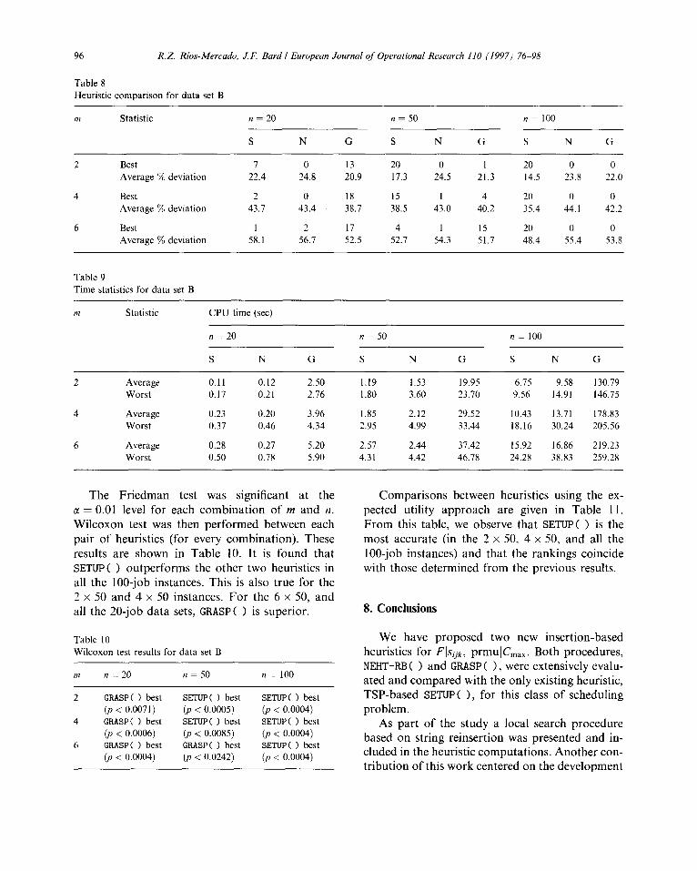
The Friedman test was significant at the M = 0.01 level for each combination of m and n. Wilcoxon test was then performed between each pair of heuristics (for every combination). These results are shown in Table 10. It is found that SETUPS > outperforms the other two heuristics in all the loo-job instances. This is also true for the 2 x 50 and 4 x 50 instances. For the 6 x 50, and all the 20-job data sets, GRASPS > is superior.

Table 10 Wilcoxon test results for data set B

m n = 20 n = 50 n = 100

2 GMSP( ) best SETUF’( ) best SETUPS ) best (p < 0.0071) (p < 0.0005) (p < 0.0004)

4 GRASPS ) best SETUP< ) best SETUPS ) best (p < 0.0006) (p < 0.0085) (p < 0.0004)

6 GFlASP( ) best GRASP( ) best SETUF( ) best (JI < 0.0004) (p < 0.0242) @ < 0.0004)

Comparisons between heuristics using the expected utility approach are given in Table 11. From this table, we observe that SETUPS > is the most accurate (in the 2 x 50, 4 x 50, and all the loo-job instances) and that the rankings coincide with those determined from the previous results.

8. Conclusions

We have proposed two new insertion-based heuristics for FISijk, prmuIC,,,. Both procedures, NEHT-RE3 ( > and GRASP ( 1, were extensively evaluated and compared with the only existing heuristic, TSP-based SETUPS 1, for this class of scheduling problem.

As part of the study a local search procedure based on string reinsertion was presented and included in the heuristic computations. Another contribution of this work centered on the development

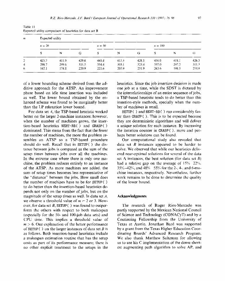
Table 11

R.Z. Rios-Mercado, J.F. Bard I European Jounlal qf Operational Researcll 110 (19971 76. 98 97

Expected utility comparison of heuristics for data set B

Expected utility

II = 20 n = 50 n = 100

S N G S N G S N G

2 423.1 411.9 429.6 445.4 413.5 428.5 456.0 418.1 426.3 4 298.7 299.6 331.5 334.4 303. I 323.4 357.0 297.’ 311.3 6 162.1 174.8 220.9 221.6 205.9 231.9 263.6 198.5 214.9

of a lower bounding scheme derived from the ad- heuristics. Since the job insertion decision is made ditive approach for the ATSP. An improvement one job at a time, while the SDST is dictated by phase based on idle time insertion was included the interrelationships of an entire sequence of jobs, as well. The lower bound obtained by the en- a TSP-based heuristic tends to do better than this hanced scheme was found to be marginally better insertion-style methods, specially when the num- than the LP relaxation lower bound. ber of machines is small.

For data set A, the TSP-based heuristic worked better on the larger 2-machine instances; however, when the number of machines grows, the insertion-based heuristics NEHT-RB( > and GRASPS > dominated. This stems from the fact that the fewer the number of machines, the more the problem re- sembles an ATSP so a TSP-based procedure should do well. Recall that in SETUPS > the distance between jobs is computed as the sum of the setup times between jobs over all the machines. In the extreme case where there is only one machine, the problem reduces entirely to an instance of the ATSP. As more machines are added, the sum of setup times becomes less representative of the “distance” between the jobs. How small does the number of machines have to be for SETUPS 1 to do better than the insertion-based heuristics de- pends not only on the number of jobs, but on the magnitude of the setup times as well. In data set A, we observe a threshold value of m = 2 or 3. How- ever, for data set B, SETUPS > was found to outper- form the others with respect to both makespan (especially for the 50- and loo-job data sets) and CPU time. This implies a threshold value of m > 6. One explanation of the better performance of SETUP ( > on the larger instances of data set B is as follows. Both insertion-based heuristics include a makespan estimation routine that has the setup costs as part of its performance measure; there is no other explicit treatment to the setups in the

SETUP ( 1 and NEHT-RB ( > run considerably faster than GRASP ( 1. This is to be expected because they are deterministic algorithms and will deliver a unique solution for each instance. By increasing the iteration counter in GRASPS 1, more and per- haps better solutions can be found.

Our computational study also revealed that data set B instances appeared to be harder to solve. We observed that while our heuristics delivered near-optimal solutions for several of the data set A instances, the best solution (for data set B) had a relative gap on the average of 15% ~~22’%, 35% 42%, and 48% ~ 55% for the 2-, 4-, and 6-machine instances, respectively. Nevertheless. further work remains to be done to determine the quality of the lower bound.

Acknowledgments

The research of Roger Rios-Mercado was partly supported by the Mexican National Council of Science and Technology (CONACyT) and by a Continuing Fellowship from the University of Texas at Austin. Jonathan Bard was supported by a grant from the Texas Higher Education Coor- dinating Boards’ Advanced Research Program. We also thank Matthew Saltzman for allowing us to use his C implementation of the dense short- est augmenting path algorithm to solve AP, and

98 R. Z. Rios-Mercado, J.F. Bard I European Journal of Operational Research 1 I0 (1997) 76-98

Mateo Fischetti and Paolo Toth for providing their FORTRAN code to solve r-SAP.

We also thank an anonymous referee whose suggestions helped improve the presentation of this paper.

References

[II

VI

[31

[41

[51

PI

[71

PI

191

M. Pinedo inedo, Scheduling: Theory, Algorithms, and Systems, Prentice-Hall, Englewood Cliffs, New Jersey, 1995. M. Nawaz, E.E. Enscore Jr., I. Ham, A heuristic algorithm for the m-machine, n-job flow-shop sequencing problem, OMEGA The International Journal of Management Science 11 (1) (1983) 91-95. T.A. Feo, M.G.C. Resende, A probabilistic heuristic for a computationally difficult set covering problem, Operations Research Letters 8 (2) (1989) 67-71. T.A. Feo, J.F. Bard, Flight scheduling and maintenance base planning, Management Science 35 (12) (1989) 1415- 1432. M. Laguna, J.L. Gonzalez-Velarde, A search heuristic for just-in-time scheduling in parallel machines, Journal of Intelligent Manufacturing 2 (1991) 253-260. G. Kontoravdis, J.F. Bard, A randomized adaptive search procedure for the vehicle routing problem with time windows, ORSA Journal on Computing 7 (1) (1995) 10-23. J.V. Simons Jr., Heuristics in flow shop scheduling with sequence dependent setup times, OMEGA The Interna- tional Journal of Management Science 20 (2) (1992) 215- 225. R.Z. Rios-Mercado, Optimization of the flow shop scheduling problem with setup times, Ph.D. thesis, Uni- versity of Texas at Austin, Austin, TX, 1997. E.L. Lawler, J.K. Lenstra, A.H.G. Rinnooy Kan, D. Shmoys, Sequencing and scheduling: Algorithms and complexity, in: S.S. Graves, A.H.G. Rinnooy Kan, P. Zip- kin (Eds.), Handbook in Operations Research and Management Science, vol. 4, Logistics of Production and Inventory, North-Holland, New York, 1993, pp. 4455522.

[IO] C.N. Potts, An adaptive branching rule for the permutation flow-shop problem, European Journal of Operational Research 5 (1) (1980) 19-25.

[l l] J. Carlier, I. Rebai, Two branch and bound algorithms for the permutation flow shop problem, European Journal of Operational Research 90 (2) (1996) 2388251.

[12] S. Sarin, M. Lefoka, Scheduling heuristics for the n-job M- machine flow shop, OMEGA The International Journal of Management Science 21 (2) (1993) 229-234.

1131 M. Widmer, A. Hertz, A new heuristic method for the flow shop sequencing problem, European Journal of Opera- tional Research 41 (2) (1989) 1866193.

[14] E. Nowicki, C. Smutnicki, A fast tabu search algorithm for the flow shop problem, Report 8/94, Institute of Engineer- ing Cybernetics, Technical University of Wrocaw, 1994.

[15] S. Turner, D. Booth, Comparison of heuristics for flow shop sequencing, OMEGA The International Journal of Management Science 15 (1) (1987) 75-85.

[16] S.K. Gupta, n jobs and m machines job-shop problems with sequence-dependent set-up times, International Jour- nal of Production Research 20 (5) (1982) 6433656.

[17] B.D. Corwin, A.O. Esogbue, Two machine flow shop scheduling problems with sequence dependent setup times: A dynamic programming approach, Naval Research Logistics Quarterly 21 (3) (1974) 5 15-524.

[18] J.N.D. Gupta, W.P. Darrow, The two-machine sequence dependent flowshop scheduling problem, European Jour- nal of Operational Research 24 (3) (1986) 4399446.

[19] W. Szwarc, J.N.D. Gupta, A flow-shop with sequence- dependent additive setup times. Naval Research Logistics Quarterly 34 (5) (1987) 619-627.

1201 E. Taillard, Some efficient heuristic methods for the flow shop sequencing problem, European Journal of Opera- tional Research 47 (1) (1990) 65574.

[21] T.A. Feo. M.G.C. Resende, Greedy randomized adaptive search procedures, Journal of Global Optimization 6 (1995) 1099133.

[22] C.R. Reeves, Improving the efficiency of tabu search for machine sequencing problems, Journal of the Operational Research Society 44 (4) (1993) 375-382.

[23] E. Balas, P. Toth, Branch and bound methods, in: E.L. Lawler. J.K. Lenstra, A.H.G. Rinnoy Kan, D.B. Shmoys (Eds.), The Traveling Salesman Problem: A Guided Tour of Combinatorial Optimization, John Wiley and Sons, Chichester, 1990, 361401.

[24] E. Balas, N. Christofides, A restricted Lagrangean approach to the traveling salesman problem. Mathematical Programming 21 (1) (1981) 1946.

[25] M. Fischetti, P. Toth, An additive bounding procedure for the asymmetric traveling salesman problem, Mathematical Programming 53 (2) (1992) 173-197.

[26] B.L. Golden, W.R. Stewart, Empirical analysis of heuristics, in: E.L. Lawler, J.K. Lenstra, A.H.G. Rinnoy Kan, D.B. Shmoys (Eds.), The Traveling Salesman Problem, John Wiley and Sons, New York, 1990, pp. 2077249.

Heuristics for the flow line problem with setup costs

Documents

Transcript of Heuristics for the flow line problem with setup costs