ClickHere

for

FullArticle

Heat and salt balances over the New England continental shelf,August 1996 to June 1997

S. J. Lentz,1 R. K. Shearman,2 and A. J. Plueddemann1

Received 21 December 2009; revised 20 March 2010; accepted 1 April 2010; published 29 July 2010.

[1] Heat and salt balances over the New England shelf are examined using 10 month timeseries of currents, temperature, and salinity from a four element moored array and surfaceheat and freshwater fluxes from a meteorological buoy. A principal result is closure ofthe heat budget to 10 W m−2. The seasonal variation in depth‐average temperature, from14°C in September to 5°C in March, was primarily due to the seasonal variation in surfaceheat flux and a heat loss in winter caused by along‐shelf advection of colder water from thenortheast. Conductivity sensor drifts precluded closing the salt balance on time scales ofmonths or longer. For time scales of days to weeks, depth‐average temperature and salinityvariability were primarily due to advection. Advective heat and salt flux divergences werestrongest and most complex in winter, when there were large cross‐shelf temperatureand salinity gradients at the site due to the shelf‐slope front that separates cooler, fresher shelfwater from warmer, saltier slope water. Onshore flow of warm, salty slope water nearthe bottom and offshore flow of cooler, fresher shelf water due to persistent eastward(upwelling‐favorable) winds caused a temperature increase of nearly 3°C and a salinityincrease of 0.8 in winter. Along‐shelf barotropic tidal currents caused a temperature decreaseof 1.5°C and a salinity decrease of 0.7. Wave‐driven Stokes drift caused a temperatureincrease of 0.5°C and a salinity increase of 0.4 from mid December to January when therewere large waves and large near‐surface cross‐shelf temperature and salinity gradients.

Citation: Lentz, S. J., R. K. Shearman, and A. J. Plueddemann (2010), Heat and salt balances over the New England continentalshelf, August 1996 to June 1997, J. Geophys. Res., 115, C07017, doi:10.1029/2009JC006073.

1. Introduction

[2] The objective of this study is to determine the processescontributing to temperature and salinity variability over timescales of days to a year on the New England shelf. Of par-ticular interest is the relative importance of advection and thespecific advective processes that cause substantial variationsin the depth‐average temperature and salinity. Temperatureand salinity are important to shelf dynamics because theydetermine the density distribution which is a key element ofshelf dynamics. Additionally, understanding processes con-trolling temperature and salinity variability provide insightinto important advective pathways that are likely to influencedistributions of other constituents, such as nutrients.[3] Water temperatures on the New England shelf undergo

a large seasonal variation, with depth‐averaged temperaturesat mid‐shelf ranging from a maximum of about 12°C in latesummer to a minimum of about 5°C in late winter [Bigelow,1933;Mayer et al., 1979; Beardsley et al., 1985; Lentz et al.,2003a]. This seasonal variation is qualitatively consistentwith the seasonal variation in surface heat flux, i.e., surface

warming in spring and summer and surface cooling in falland winter [Beardsley and Boicourt, 1981; Joyce, 1987;Mountain et al., 1996; Beardsley et al., 2003]. However, therelative importance of advection to the seasonal variationin temperature, and to temperature variability in general,remains unclear because few observational studies haveprovided accurate estimates of the horizontal temperaturegradients.[4] There have been only a few quantitative studies of the

heat balance over the Middle Atlantic Bight (MAB) conti-nental shelf. Lentz et al. [2003b] used a 6‐month mooredarray deployment to examine the heat balance at mid‐shelf onthe southern flank of Georges Bank, to the northeast of theNew England shelf. They found that the seasonal increase intemperature from February to August 1995 was primarily dueto surface heating while advective heat fluxes dominated thetemperature variability over time scales of days to weeks.There have been several direct estimates of the cross‐shelfeddy heat flux at the shelf‐slope front which indicate that theonshore heat flux at the front is small relative to the surfaceheat flux [Houghton et al., 1988, 1994; Garvine et al., 1989;Gawarkiewicz et al., 2004]. Bignami and Hopkins [2003]inferred from surface heat fluxes and temperature changesthat advective heat fluxes at the southern end of the MiddleAtlantic Bight, near Cape Hatteras, must be large. Recently,Lentz [2010] used historical data to show that surface heatfluxes and along‐shelf advection could account for the

1Department of Physical Oceanography, Woods Hole OceanographicInstitution, Woods Hole, Massachusetts, USA.

2College of Oceanic and Atmospheric Sciences, Oregon StateUniversity, Corvallis, Oregon, USA.

Copyright 2010 by the American Geophysical Union.0148‐0227/10/2009JC006073

JOURNAL OF GEOPHYSICAL RESEARCH, VOL. 115, C07017, doi:10.1029/2009JC006073, 2010

C07017 1 of 12

observed along‐isobath temperature increase from northeastto southwest in the MAB. However, this result was sensitiveto the uncertainty in the surface heat flux climatologies.Several studies of the heat balance over the MAB inner shelfindicate that cross‐shelf advection (upwelling) tends to bal-ance surface heating over the inner‐shelf in summer whenthermal stratification is strong, but that cooling and possiblyalong‐shelf advection dominate the inner‐shelf heat balancein winter when thermal stratification is weak [Austin andLentz, 1999; Wilkin, 2006; Fewings, 2007]. Only the Geor-ges Bank measurements were sufficient to directly estimatethe terms in the local heat balance at mid shelf and that studyonly spanned half the annual cycle.[5] In contrast to temperature, the seasonal variation in

salinity on the New England shelf is small compared toeither shorter time scale variations or inter‐annual variations[Manning, 1991]. There is a slight freshening of the NewEngland shelf water in spring, presumably associated withincreased freshwater runoff in the Gulf of Maine and farthernorth [Bigelow and Sears, 1935; Manning, 1991], and pos-sibly to local runoff from the southern coast of New England,notably the Connecticut River [Lentz et al., 2003a]. Salinityvariations on the shelf are assumed to be primarily due toadvection, since evaporation minus precipitation is small[Beardsley and Boicourt, 1981; Joyce, 1987]. Potentiallyimportant contributions to salinity variability on the NewEngland shelf include along‐shelf advection of freshwaterrunoff and cross‐shelf displacements of the shelf‐slope front

that separates the relatively fresh shelf water from saltierslope water [e.g., Bigelow and Sears, 1935; Manning, 1991;Linder and Gawarkiewicz, 1998; Lentz et al., 2003a].[6] There have been a number of estimates of the volume

salt budget for the MAB aimed at determining the cross‐shelfflux of salt at the shelfbreak [Wright, 1976; Fairbanks, 1982;Brink, 1998; Bignami and Hopkins, 2003], as well as, a fewdirect estimates of the cross‐shelf salt flux at the shelf break[Garvine et al., 1989; Gawarkiewicz et al., 2004]. Thesestudies suggest there is an onshore flux of salt at the shelfbreak but the magnitude is poorly constrained. However,there has been only one study that provided direct estimationof the terms in the local salt balance in the region, the study onthe southern flank of Georges Bank [Lentz et al., 2003b].They found that salinity variations were dominated byadvection, notably movement of saltier slope water onto thesouthern flank of Georges Bank.[7] In this study, the depth‐averaged heat and salt balances

over the New England shelf are examined using observationsfrom a moored array deployed at mid‐shelf that spans almosta full year (August 1996 to June 1997) as part of the CoastalMixing and Optics program (CMO). The moored arrayobservations included a suite of meteorological measure-ments that provide direct estimates of the surface heat andfreshwater fluxes, as well as, temperature, salinity (fromconductivity and temperature), and current observations thatallow estimation of the horizontal advective fluxes and thechanges in temperature and salinity. Surface gravity wavemeasurements also allow estimation of the heat and salt fluxdue to the wave‐driven Stokes drift [Fewings, 2007].[8] Lentz et al. [2003a] found that water temperatures

during CMO were similar to monthly means based on his-torical hydrographic data except near the bottom wheretemperatures were colder than historical means in fall andwarmer than historical means in winter. This suggests theprocesses contributing to the heat balance during CMO areprobably typical for this region. The CMO salinities weresubstantially fresher (0.5–1, practical salinity scale) thannormal. Similar anomalies were also observed during 1996–1997 north of the New England shelf suggesting the anom-alously low salinities were a large‐scale phenomenon[Benway and Jossi, 1998; Smith et al., 2001]. This suggeststhe processes contributing to the salt balance during CMOmay not be typical for this region, at least for time scales ofmonths or longer.

2. Observations and Analysis

2.1. Moored Array and Data Processing

[9] The CMO moored array consisted of four sites locatedon the outer half of the New England continental shelf southof Cape Cod, Massachusetts [Lentz et al., 2003b; Shearmanand Lentz, 2003]. A heavily instrumented central site onthe 70‐m isobath was surrounded by three more lightlyinstrumented sites, an inshore site 11 km onshore of thecentral site in 64 m of water, an offshore site 12.5 km off-shore of the central site in 86 m of water, and an along-shore site 14.5 km east of the central site in 69 m of water(Figure 1).[10] Temperature, conductivity, and current observations

spanning the water column were obtained from instrumentsdeployed on surface/subsurface mooring pairs at each site.

Figure 1. Map showing locations of the inshore (i), central(c), offshore (o), and alongshore (a) sites on the New Englandshelf south of Cape Cod and the orientation of the x, y coor-dinate frame, x is positive toward the east. The along‐shelfsite is located 8° clockwise from the x axis and the inshoreand offshore sites are 20° and 15° clockwise from the y axis.The 50‐m, 70‐m, and 100‐m isobaths are also shown.

LENTZ ET AL.: HEAT AND SALT BALANCES NEW ENGLAND SHELF C07017C07017

2 of 12

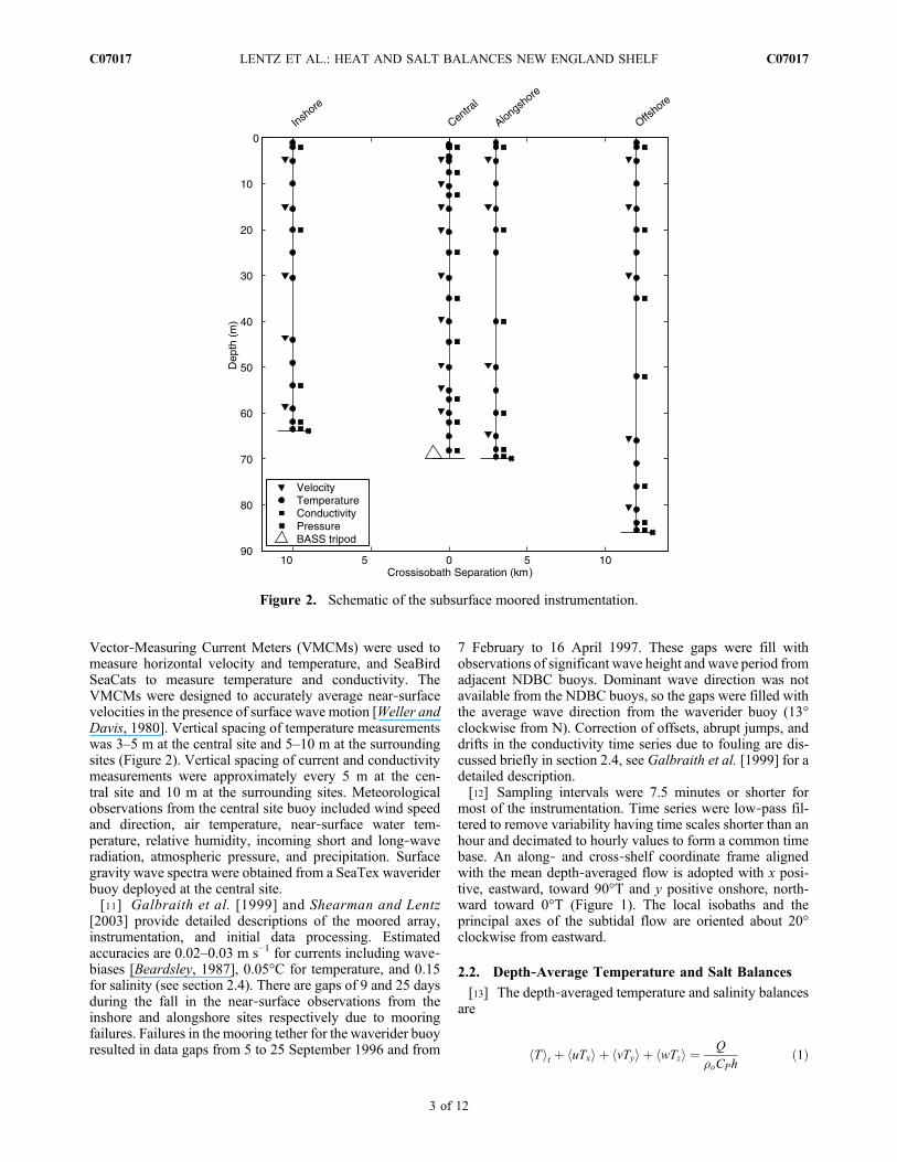
Vector‐Measuring Current Meters (VMCMs) were used tomeasure horizontal velocity and temperature, and SeaBirdSeaCats to measure temperature and conductivity. TheVMCMs were designed to accurately average near‐surfacevelocities in the presence of surface wave motion [Weller andDavis, 1980]. Vertical spacing of temperature measurementswas 3–5 m at the central site and 5–10 m at the surroundingsites (Figure 2). Vertical spacing of current and conductivitymeasurements were approximately every 5 m at the cen-tral site and 10 m at the surrounding sites. Meteorologicalobservations from the central site buoy included wind speedand direction, air temperature, near‐surface water tem-perature, relative humidity, incoming short and long‐waveradiation, atmospheric pressure, and precipitation. Surfacegravity wave spectra were obtained from a SeaTex waveriderbuoy deployed at the central site.[11] Galbraith et al. [1999] and Shearman and Lentz

[2003] provide detailed descriptions of the moored array,instrumentation, and initial data processing. Estimatedaccuracies are 0.02–0.03 m s−1 for currents including wave‐biases [Beardsley, 1987], 0.05°C for temperature, and 0.15for salinity (see section 2.4). There are gaps of 9 and 25 daysduring the fall in the near‐surface observations from theinshore and alongshore sites respectively due to mooringfailures. Failures in the mooring tether for the waverider buoyresulted in data gaps from 5 to 25 September 1996 and from

7 February to 16 April 1997. These gaps were fill withobservations of significant wave height and wave period fromadjacent NDBC buoys. Dominant wave direction was notavailable from the NDBC buoys, so the gaps were filled withthe average wave direction from the waverider buoy (13°clockwise from N). Correction of offsets, abrupt jumps, anddrifts in the conductivity time series due to fouling are dis-cussed briefly in section 2.4, see Galbraith et al. [1999] for adetailed description.[12] Sampling intervals were 7.5 minutes or shorter for

most of the instrumentation. Time series were low‐pass fil-tered to remove variability having time scales shorter than anhour and decimated to hourly values to form a common timebase. An along‐ and cross‐shelf coordinate frame alignedwith the mean depth‐averaged flow is adopted with x posi-tive, eastward, toward 90°T and y positive onshore, north-ward toward 0°T (Figure 1). The local isobaths and theprincipal axes of the subtidal flow are oriented about 20°clockwise from eastward.

2.2. Depth‐Average Temperature and Salt Balances

[13] The depth‐averaged temperature and salinity balancesare

hTit þ huTxi þ hvTyi þ hwTzi ¼ Q

�oCPhð1Þ

Figure 2. Schematic of the subsurface moored instrumentation.

LENTZ ET AL.: HEAT AND SALT BALANCES NEW ENGLAND SHELF C07017C07017

3 of 12

and

hSit þ huSxi þ hvSyi þ hwSzi ¼ � ðP � EÞSrefh

; ð2Þ

where T is temperature, S is salinity, t is time, u, v, andw are the along‐shelf, cross‐shelf and vertical components ofvelocity, hi indicates the depth‐average from the surface tothe bottom, t, x, y, and z subscripts imply differentiation, Q isthe surface heat flux, ro = 1025 kg m−3 is a reference density,CP = 4190 W kg−1°C−1 is the heat capacity of sea water, Pis the precipitation rate and E is the evaporation rate (both inm s−1), Sref = 32 is a reference salinity (approximately themean salinity), and h is the water depth (70 m at the centralsite). Fluxes of heat and salt through the sea floor are assumedto be negligible. All of the terms in (1) and (2) can be esti-mated using the available observations (as described below)except the vertical advective flux terms hwTzi and hwSzi.Rough estimates assuming w ≈ uhx suggest these terms aregenerally small, but they could be significant during periodswhen vertical temperature and salinity gradients are large.The vertical advective fluxes are not considered in the sub-sequent analysis.[14] To focus on the observed temperature and salinity

variability and to emphasize longer time scales, (1) and (2) areintegrated in time from the start of the time series (t = 0) toget

hTi ¼ To þ Qcum � FT ð3Þ

and

hSi ¼ So þ PEcum � FS; ð4Þ

where To = hT(t = 0)i, So = hS(t = 0)i,

Qcum ¼Z t

0

Q

�oCPhdt; and PEcum ¼ �

Z t

0

ðP � EÞSrefh

dt

are the cumulative surface heat and freshwater fluxes, and

FT ¼Z t

0ðhuTxi þ hvTyiÞdt

and

FS ¼Z t

0ðhuSxi þ hvSyiÞdt

are the cumulative horizontal advective heat and salt fluxes.[15] It will be shown in section 3.4 that tidal variability and

surface gravity waves make significant contributions to thesubtidal advective heat and salt fluxes. To separate the con-tributions of subtidal and tidal (and other high frequency)variability to the advective fluxes, the current, temperaturegradient and salinity gradient time series are decomposed intolow‐frequency (periods longer than 38 hours) and high‐frequency (periods between 38 and 2 hours) components,e.g., u = ulf + uhf. The hourly time series of each variable werelow‐pass filtered using PL64 [Beardsley et al., 1985], whichhas a half‐power point of 38 hours, to estimate the low‐frequency time‐series. The high‐frequency time series werethen calculated by subtracting the low‐frequency time seriesfrom the original hourly time series, e.g., uhf = u − ulf. The

cumulative advective heat flux contributions from the low‐frequency and high‐frequency variability are

FTlf ¼Z t

0hulf T lf

x i þ hvlf T lfy idt

and

FThf ¼Z t

0huhf Thf

x i þ hvhf Thfy idt:

The cross‐term contributions, e.g., ulfTxhf, though not identi-

cally zero because of the finite record length and imperfectfilter, are negligible, less than 0.3% of the variance of FTlf orFThf.[16] The current, temperature, and conductivity sensors

did not sample fast enough to resolve surface gravity waves.However, the temperature and salt flux due to covariance ofsurface gravity wave current and temperature (or salinity)variability can be estimated from the associated Stokes driftvelocity (ust, vst) and the observed temperature or salinitygradients as ustTx + vstTy [Fewings, 2007]. The Stokesvelocities were estimated from the significant wave heightHsig, the wave period Tp and the wave direction �w as

ðust; vstÞ ¼ H2sig!k

16

coshð2k½zþ h�Þsinh2ðkhÞ ðcosð�wÞ; sinð�wÞÞ; ð5Þ

where w is the frequency corresponding to the dominant waveperiod, and k is the magnitude of the wave number deter-mined from the dispersion relation for linear surface gravitywaves. Thus, the cumulative advective heat flux due to sur-face gravity waves is

FTst ¼Z t

0hustTxi þ hvstTyidt:

The resulting cumulative heat balance is

hTi ¼ To þ Qcum � FTlf � FThf � FTst ð6Þ

and the corresponding cumulative salt balance is

hSi ¼ So þ PEcum � FSlf � FShf � FSst: ð7Þ

2.3. Estimation of Terms in the Temperatureand Salt Balances

[17] Estimates of the terms in the temperature and saltbalances are centered on the central site (h = 70 m). Depth‐averages are estimated using a trapezoidal rule, extrapolatingto the surface or bottom by assuming variables are verticallyuniform near the boundaries. Current measurements weretypically within 5 m of the surface and bottom and temper-ature and conductivity measurements were within 1–2 m(Figure 2). Time derivatives are estimated as centered, finitedifferences over two‐hour intervals.[18] Surface heat flux, evaporation, and wind stress were

estimated from the meteorological measurements using bulkformulas [Fairall et al., 1996]. Horizontal advective fluxesare estimated using the velocity at the central site and esti-mating horizontal temperature and salinity gradients usingobservations from all four mooring sites. The temperatures

LENTZ ET AL.: HEAT AND SALT BALANCES NEW ENGLAND SHELF C07017C07017

4 of 12

and salinities at each site were interpolated to the depths of thecurrent observations at the central site. The mooring siteswere not exactly aligned with the x, y coordinate axes, thealong‐shelf site was 8° clockwise from the x axis and theinshore and offshore sites are 20° and 15° clockwise fromthe y axis (Figure 1). Therefore, horizontal temperature andsalinity gradients were estimated by fitting a plane to thevertically interpolated temperatures or salinities at each depthfor each hour and then estimating the horizontal gradientsalong the x and y axes. Use of a quadratic fit in the cross‐shelfdirection, since there are three moorings, does not substan-tially improve the closure of the heat and salt balances.

2.4. Salinity Offsets

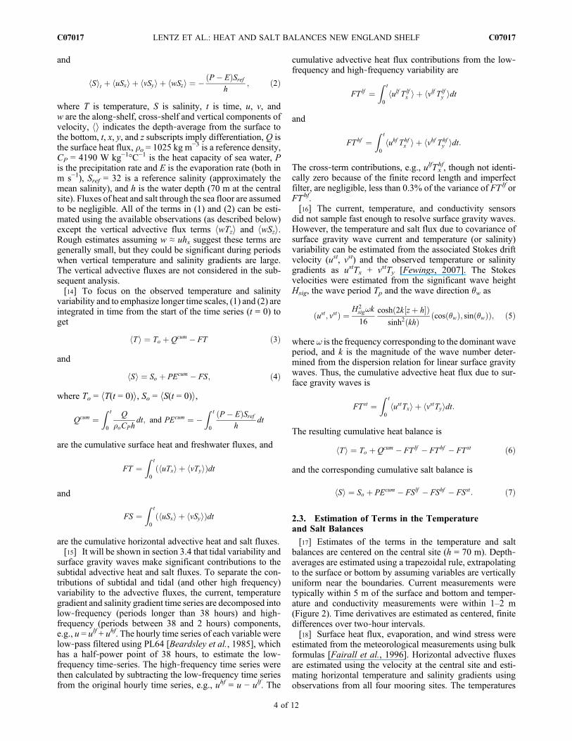
[19] The conductivity time series exhibited offsets, abruptjumps, and drifts due to fouling that were identified andcorrected (to the extent possible) by comparisons with adja-cent instruments on the same mooring and shipboard CTDcasts near the moorings [Galbraith et al., 1999]. The offsetsand drifts are more severe near the bottom and are likely dueto suspended sediment fouling the conductivity cell ratherthan bio‐fouling. Inaccuracies in our initial correction of theconductivity time series are almost certainly the cause of largedrifts in the cumulative advective salt flux FS (Figure 3a,dashed line) that are inconsistent with other terms in thecumulative salt balance (discussed in section 3.3.3). Theseoffsets are small relative to the salinity variability, but the

resulting inaccuracies in the salinity gradient estimates resultin large drifts in the cumulative advective salt flux.[20] Ad hoc time‐dependent, depth‐independent salinity

offsets of 0.15 or less, chosen to minimize the discrepancy inthe cumulative salt balance, were applied to the salinity timeseries from the offshore and alongshore sites (Figure 3b).These small offsets (Figure 3b) are sufficient to remove thelarge drifts in the advective salt flux (Figure 3a, solid line) andare applied in the subsequent analyzes to facilitate examina-tion of the salt balance. Application of these ad hoc offsetsmeans that salt balance results for time scales longer thanweeks are only qualitative, but does not change the vari-ability, or affect the interpretation of results, on time scalesof days to weeks.

3. Results

3.1. Wind Stress, Surface Gravity Waves,and Currents

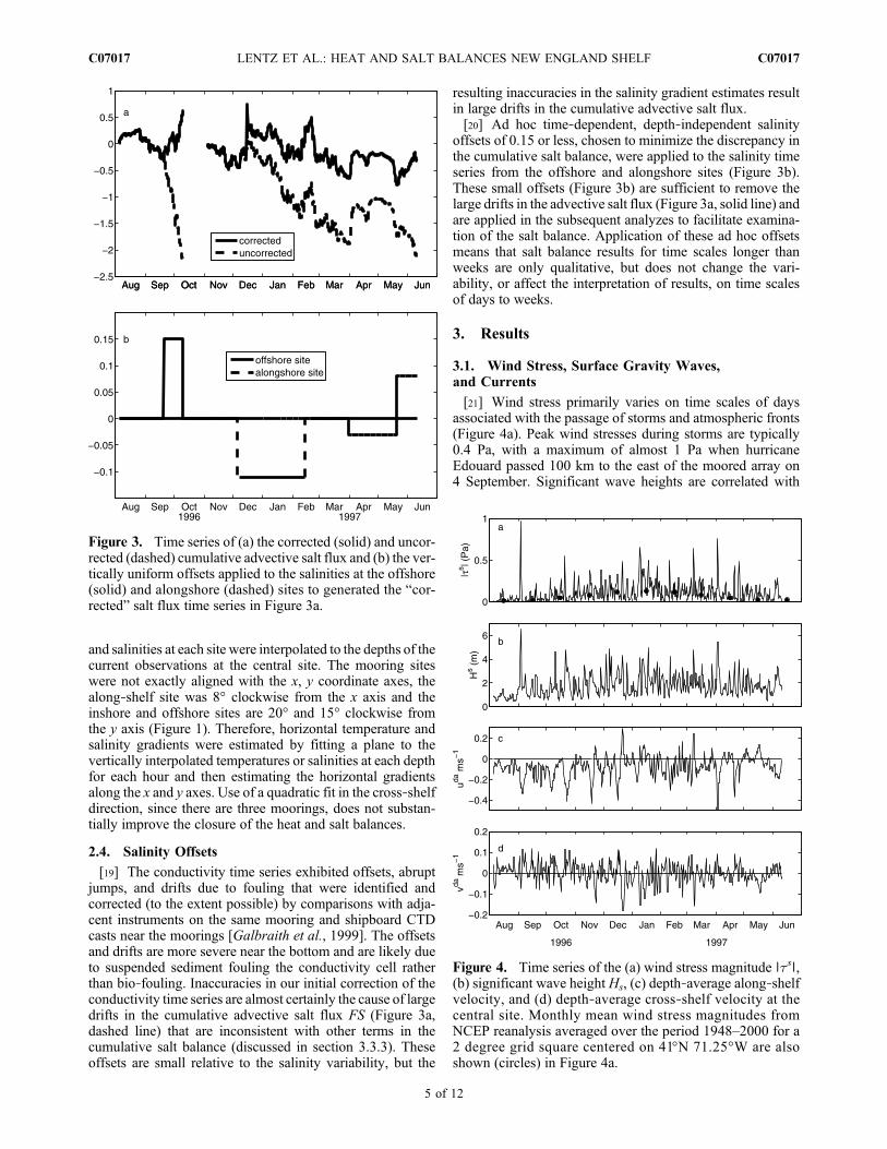
[21] Wind stress primarily varies on time scales of daysassociated with the passage of storms and atmospheric fronts(Figure 4a). Peak wind stresses during storms are typically0.4 Pa, with a maximum of almost 1 Pa when hurricaneEdouard passed 100 km to the east of the moored array on4 September. Significant wave heights are correlated with

Figure 3. Time series of (a) the corrected (solid) and uncor-rected (dashed) cumulative advective salt flux and (b) the ver-tically uniform offsets applied to the salinities at the offshore(solid) and alongshore (dashed) sites to generated the “cor-rected” salt flux time series in Figure 3a.

Figure 4. Time series of the (a) wind stress magnitude ∣ts∣,(b) significant wave height Hs, (c) depth‐average along‐shelfvelocity, and (d) depth‐average cross‐shelf velocity at thecentral site. Monthly mean wind stress magnitudes fromNCEP reanalysis averaged over the period 1948–2000 for a2 degree grid square centered on 41°N 71.25°W are alsoshown (circles) in Figure 4a.

LENTZ ET AL.: HEAT AND SALT BALANCES NEW ENGLAND SHELF C07017C07017

5 of 12

wind stress magnitude, with peak values of 3–5 m duringstorms (Figure 4b). The dominant wave direction tends to beonshore and peak wave periods are typically 6–12 s. Windstresses and waves are larger in fall and winter and smallerin summer and spring.[22] Subtidal currents are polarized along‐shelf, with

depth‐average along‐shelf currents ranging from −0.5 to0.3 m s−1 and depth‐average cross‐shelf currents generallyless than 0.1 m s−1 in magnitude (Figures 4c and 4d)[Beardsley et al., 1985; Shearman and Lentz, 2003]. Depth‐average along‐shelf currents consist of events lasting days toweeks that are typically westward, with only a few notableeastward current events in winter (Figure 4c). The mean,depth‐average cross‐shelf current is zero because along‐shelf is defined as aligned with the mean depth‐averagedcurrent. Tidal currents are predominantly semi‐diurnal withan amplitude of about 0.1 m s−1 [Shearman and Lentz, 2004]and episodic near‐inertial currents with rms velocities up to0.1 m s−1 occur during stratified periods [Shearman, 2005].

3.2. Temperature

3.2.1. Water Temperature Temporal Variabilityand Structure[23] Water temperatures at the central site during the CMO

deployment exhibit a large annual variation that is consis-tent with the typical annual cycle over the New England shelf[Beardsley and Boicourt, 1981; Lentz et al., 2003a]. Thedepth‐average temperature at the central site rises from

10°C in early August to a maximum of about 14°C in midSeptember, decreases through the fall and winter to a mini-mum of 5°C inmidMarch, and then, beginning in early April,rises again to 8°C in late May (Figure 5a, black line). Asimilar annual variation was observed at all four sites.[24] There is a large vertical variation in temperature in

August (seasonal thermocline), with warm water (>18°C) inthe upper 20 m and cooler water (<10°C) in the lower 50 mseparated by a sharp thermocline (Figure 5a, red and bluelines). The vertical temperature difference decreases toapproximately zero by November in response to severalstorms [Lentz et al., 2003a]. Water temperatures continue todecrease through winter. Near the bottom there is a fairlypersistent temperature inversion (near‐bottom water warmerthan near‐surface water) from mid December to March. Thiswarmer near‐bottom water is associated with the onshoremovement of the foot of the shelf‐slope front that separatescooler, fresher shelf water from warmer, saltier slope water[Linder and Gawarkiewicz, 1998]. The seasonal thermoclineredevelops in spring as near‐surface waters warm.[25] The depth‐average along‐shelf and cross‐shelf tem-

perature gradients hTxi, hTyi are variable on time scales ofdays to months (standard deviations of 2.5 × 10−5 and 4 ×10−5 °C m−1) (Figures 5b and 5c). The mean along‐shelf andcross‐shelf temperature gradients (−0.5 × 10−5 °C m−1 and−0.6 × 10−5 °C m−1 respectively), are both small relative tothe variability, with warmer water to the west and offshore.However, hTyi exhibits a substantial seasonal variation with apositive gradient (≈5 × 10−5 °C m−1, warmer water onshore)from August to November and a negative gradient (≈−5 ×10−5 °C m−1) from December to March, and a near‐zerocross‐shelf gradient during April and May (Figure 5c). Thisseasonal variation in hTyi is qualitatively consistent with thetendency for surface heating in summer to increase tem-peratures in shallow water more than in deep water and sur-face cooling in winter to decrease water temperatures inshallow water more than in deep water [Shearman and Lentz,2003].3.2.2. Surface Heat Flux[26] The net surface heat flux exhibits a large seasonal

variation (Figure 6a). In the summer and spring (August toSeptember and April to June), there is a positive (into theocean) surface heat flux of 100–200 W m−2 due to incomingsolar radiation (Figure 6b) and small latent and sensible heatlosses (Figure 6c). In fall, the net surface heat flux decreases,as solar radiation decreases and cooling due to latent andsensible heat loss increases. In winter (November–January),solar heating is relatively small (≈50 W m−2) and latent andsensible heat losses are large (up to 200Wm−2 for each). Thelarge (<−100 W m−2) latent and sensible heat loss events inwinter are typically associated with south‐eastward windsthat bring cold, dry air from the continent over the shelf.There is a relatively constant heat loss of about −50 W m−2

due to the net long‐wave radiation (Figure 6b). The monthlymeans from the NCEP Reanalysis indicate that the seasonalvariation in surface heat flux during the CMO deploymentperiod was fairly typical.3.2.3. Heat Balance[27] The cumulative heat balance is examined by compar-

ing the right‐hand and left‐hand sides of (6). The sum of thecumulative surface and advective heat fluxes (Figure 7a, redline) matches both the seasonal variation and most of the

Figure 5. Time series of (a) the near‐surface (red), near‐bot-tom (blue), and depth‐average (black) temperature and thedepth‐average (b) along‐shelf (hTxi) and (c) cross‐shelf (hTyi)temperature gradients at the central site.

LENTZ ET AL.: HEAT AND SALT BALANCES NEW ENGLAND SHELF C07017C07017

6 of 12

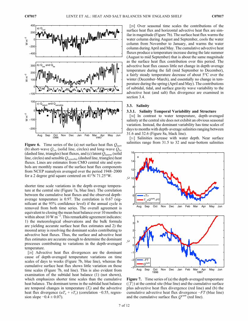
shorter time scale variations in the depth‐average tempera-ture at the central site (Figure 7a, blue line). The correlationbetween the cumulative heat fluxes and the observed depth‐average temperature is 0.97. The correlation is 0.67 (sig-nificant at the 95% confidence level) if the annual cycle isremoved from both time series. The overall agreement isequivalent to closing the mean heat balance over 10months towithin about 10Wm−2. This remarkable agreement indicates:1) the meteorological observations and the bulk formulaare yielding accurate surface heat flux estimates and 2) themoored array is resolving the dominant scales contributing toadvective heat fluxes. Thus, the surface and advective heatflux estimates are accurate enough to determine the dominantprocesses contributing to variations in the depth‐averagedtemperature.[28] Advective heat flux divergences are the dominant

cause of depth‐averaged temperature variations on timescales of days to weeks (Figure 7b, blue line), whereas thecumulative surface heat flux shows little variation on thosetime scales (Figure 7b, red line). This is also evident fromexamination of the subtidal heat balance (1) (not shown),which emphasizes shorter time scales than the cumulativeheat balance. The dominant terms in the subtidal heat balanceare temporal changes in temperature (Tt) and the advectiveheat flux divergence (uTx + vTy) (correlation −0.55, regres-sion slope −0.4 ± 0.07).

[29] Over seasonal time scales the contributions of thesurface heat flux and horizontal advective heat flux are sim-ilar in magnitude (Figure 7b). The surface heat flux warms thewater column during August and September, cools the watercolumn from November to January, and warms the watercolumn during April andMay. The cumulative advective heatfluxes produce a temperature increase during the late summer(August to mid September) that is about the same magnitudeas the surface heat flux contribution over this period. Theadvective heat flux causes little net change in depth‐averagetemperature during the fall (mid September to December),a fairly steady temperature decrease of about 5°C over thewinter (December–March), and essentially no change in tem-perature during the spring (April andMay). The contributionsof subtidal, tidal, and surface gravity wave variability to theadvective heat (and salt) flux divergence are examined insection 3.4.

3.3. Salinity

3.3.1. Salinity Temporal Variability and Structure[30] In contrast to water temperature, depth‐averaged

salinity at the central site does not exhibit an obvious seasonalvariation. Instead, the dominant variability has time scales ofdays tomonths with depth‐average salinities ranging between31.6 and 32.6 (Figure 8a, black line).[31] Salinities increase with water depth. Near surface

salinities range from 31.5 to 32 and near‐bottom salinitiesFigure 6. Time series of the (a) net surface heat flux Qnet,(b) short‐wave Qsw (solid line, circles) and long‐wave Qlw

(dashed line, triangles) heat fluxes, and (c) latentQlatent (solidline, circles) and sensibleQsensible (dashed line, triangles) heatfluxes. Lines are estimates from CMO central site and sym-bols are monthly means of the surface heat flux componentsfrom NCEP reanalysis averaged over the period 1948–2000for a 2 degree grid square centered on 41°N 71.25°W.

Figure 7. Time series of (a) the depth‐averaged temperature(hTi) at the central site (blue line) and the cumulative surfaceplus advective heat flux divergence (red line) and (b) thecumulative advective heat flux divergence −FT (blue line)and the cumulative surface flux Qcum (red line).

LENTZ ET AL.: HEAT AND SALT BALANCES NEW ENGLAND SHELF C07017C07017

7 of 12

range from 32 to 34 (Figure 8a). Large increases in near‐bottom salinity in fall and winter are associated with theonshore movement of the foot of the shelf‐slope front(salinities >32.5) [e.g., Linder and Gawarkiewicz, 1998].During fall and winter, there is a tendency for near‐surfacesalinities to decrease when near‐bottom salinities increase,suggesting an offshoremovement of near‐surface water whenthere is an onshore movement of near‐bottom water. The footof the shelf‐slope front is present at the central site most of thetime between mid December and early March due to anom-alously strong and persistent eastward (upwelling‐favorable)winds. In spring, there are intervals when salinities are ver-tically well mixed due to storms (early and late April) andnear‐surface low‐salinity events in mid April and late Maydue to fresher Connecticut River plumewater carried offshoreand eastward by eastward winds [Lentz et al., 2003a].[32] The mean depth‐average along‐shelf salinity gradient

(hSxi, −0.1 × 10−5 m−1) is small relative to the subtidalvariability (standard deviation 0.7 × 10−5 m−1; Figure 8b). Incontrast, there is a negative (fresher water onshore) depth‐averaged cross‐shelf salinity gradient (hSyi) during most ofthe deployment, with a few exceptions, notably in August1996 and late April to early May 1997 when hSyi is approx-imately zero (Figure 8c). The mean cross‐shelf salinitygradient is −1.2 × 10−5 m−1. The standard deviation (1.0 ×10−5 m−1) of the subtidal variations in hSyi is about the samemagnitude as the mean. Maximum magnitudes of hSyi are

typically about −3.0 × 10−5 m−1 and often occur when the footof the shelf‐slope front is near the central site.[33] There are occasional spikes in the salinity and tem-

perature gradients associated with features that are notresolved by the coarse moored array spacing (Figures 8b, 8c,5b, and 5c). One example is a warm salty intrusion of slopewater that passed through the array in late August [see Lentz,2003, Figure 1], resulting in spikes most notably in hTyi andhSyi. The intrusion was about 40 m thick, centered at a depthof about 40 m, and had an along‐shelf extent of about 10 kmbased on the measure along‐shelf currents and the duration ofthe event at the central and offshore mooring sites. A secondexample is a near‐bottom intrusion of slope water in midDecember that was observed at the central mooring site butnot at the along‐shelf mooring site resulting in large spikes inhTxi and hSxi. These unresolved features result in “jumps” inthe cumulative advective heat and salt fluxes (see for examplethe mid December jump in advective heat flux divergence inFigure 7b).3.3.2. Evaporation and Precipitation[34] Evaporation is relatively large (≈0.5 cm day−1) in

fall and winter and nearly zero in late summer and spring,consistent with historical monthly means from the NCEPReanalysis (Figure 9a). The evaporation events in fall andwinter are due to offshore movement of cold dry air fromthe continent. During the CMO deployment, precipitationexceeds evaporation in the fall (August to October) due

Figure 8. Time series of the (a) near‐surface (red), near‐bot-tom (blue), and depth‐average (black) salinity, and the depth‐average (b) along‐shelf (hSxi) and (c) cross‐shelf (hSyi) salin-ity gradients at the central site.

Figure 9. Time series of the daily averaged (a) evaporation(E) and (b) precipitation (P) rates at the central site. Monthlymeans of E (circles) and ‐P (triangles) from NCEP reanalysisaveraged over the period 1948–2000 for a 2 degree grid squarecentered on 41°N 71.25°W are both shown in Figure 9a.

LENTZ ET AL.: HEAT AND SALT BALANCES NEW ENGLAND SHELF C07017C07017

8 of 12

primarily to six large precipitation events (3–6 cm day−1;Figure 9b). During the rest of the deployment precipitation issimilar in magnitude to evaporation when averaged over timescales of weeks to months and the net freshwater surface fluxis relatively small. Monthly means from the NCEP reanalysisalso indicate a general tendency for evaporation and precip-itation to balance so that the net surface freshwater flux issmall (Figure 9a).3.3.3. Salt Balance[35] The estimated terms in the cumulative salt budget do

not balance on time scales of months or longer unless thead hoc salinity bias corrections are applied (Figure 3a). Afterapplying the salinity bias corrections shown in Figure 3b,there is reasonable agreement between the observed salinityat the central site and the cumulative salt flux divergence(Figure 10a). The agreement in variations with time scales ofdays to weeks is not affected by the salinity bias corrections.The correlation between the depth‐average salinity at thecentral site and the cumulative surface and advective fluxdivergence shown in Figure 10a is 0.73 (significant at the95% confidence level).[36] Advective salt flux convergences and divergences are

the dominant cause of the observed depth‐average salinityvariability at the central site (Figure 10b). The dominant termsin the subtidal salt balance (2) (not shown), which emphasizesshorter time scales than the cumulative salt balance, are

temporal changes in salinity driven by the advective saltflux divergence (correlation −0.58, regression slope −0.81 ±0.13). Note the subtidal salt balance results are the samewhether or not the salinity bias corrections are appliedbecause only the cumulative salt balance is sensitive to thesmall bias errors. Evaporation and precipitation tend to bal-ance and hence generally make a negligible contribution tothe depth‐average salinity variability, except in September1996 when several large precipitation events (Figure 9b)reduce the depth‐average salinity by about 0.2.

3.4. Processes Contributing to Advective Heatand Salt Flux Divergences

[37] The cumulative advective heat and salt flux diver-gences (Figures 7b and 10b) include substantial contributionsfrom subtidal variability (periods of 38 hours or longer), tidalvariability (periods 12–24 h), and the Stokes drift veloc-ity associated with surface gravity waves (periods 6–12 s;Figure 11). Each of these contributions is discussed below forboth heat and salt.3.4.1. Subtidal Variability[38] The largest contributions to the cumulative advective

heat and salt flux divergence come from the subtidal vari-ability (FTlf and FSlf) (Figure 11, thick lines). Two processesaccount for most of the subtidal heat and salt flux divergence:1) along‐shelf advection of colder water from the northeasttoward the southwest by the depth‐average flow, and 2)

Figure 10. Time series of (a) the depth‐averaged salinity(hSi) at the central site (blue line) and the cumulative surfaceand advective flux divergence (red line) and (b) the cumula-tive advective salt flux divergence (blue line) and cumulativesurface freshwater flux (evaporation minus precipitation; redline).

Figure 11. Advective (a) heat and (b) salt flux divergencedue to the subtidal variability (Flf; thick lines), tidal variabil-ity (Fhf; dashed lines) and surface gravity wave Stokes drift(Fst; thin lines).

LENTZ ET AL.: HEAT AND SALT BALANCES NEW ENGLAND SHELF C07017C07017

9 of 12

wind‐driven cross‐shelf advection (coastal upwelling) thattransports warmer, saltier slope water onshore near thebottom and cooler, fresher shelf offshore near the surface.To separate these two contributions, the subtidal variabilityis further decomposed into depth‐averaged (e.g., ulfda) anddepth‐dependent (e.g., ulfdd) components. For example,ulf = ulfda + ulfdd, where ulfda = hulfi, ulfdd = ulf − ulfda, and

FTlf ¼ FTlfda þ FTlfdd :

[39] Most of the variability in the advective heat and saltflux divergence on time scales of days to weeks is due tothe subtidal depth‐averaged flow (compare solid lines inFigure 12 with thick lines in Figure 11). There is also a longertime scale 6°C temperature decrease in winter (Figure 12a)due to the depth‐averagewestward along‐shelf flow (Figure 4c)acting on the weak along‐shelf temperature gradient (colderwater toward the northeast; Figure 5b). The correspondingsalinity decrease in winter due to the depth‐averaged flow(Figure 12b) is less certain because of the uncertainty associatedwith the bias errors (section 2.3), but it is reasonable since shelfwaters also tend to be fresher toward the northeast in winter(Figure 8b) [Linder et al., 2006].[40] The heat and salt flux divergence driven by the depth‐

dependent exchange flow is generally negligible except forthe period from mid December to mid February when theshelf‐slope front is located at the CMO array site (Figure 12,dashed lines). During this period, a cross‐isobath exchange

flow drives an onshore transport of warm, salty slope waternear the bottom and an offshore transport of cooler, freshershelf water near the surface. The net result is an increase in thedepth‐averaged temperature and salinity of 3°C and 0.7,respectively. This increase in temperature and salinity par-tially offsets the substantial decreases in temperature andsalinity from mid December to the end of March due to thedepth‐average flow (Figure 12, solid lines). Lentz et al.[2003a] show that the onshore movement of the foot of theshelf‐slope front is due to anomalously strong and persistentupwelling favorable winds in the winter of 1996–1997.3.4.2. Tidal‐Band Variability[41] The advective flux divergence due to the high‐

frequency (tidal) variability (periods between 2 and 38 hours)causes a 1.5°C temperature decrease and a 0.7 salinitydecrease between mid December and the end of January(Figure 11, dashed lines). The high‐frequency variability alsocauses a 1.5°C temperature increase in August. In both casesthe cumulative flux divergence is due almost entirely to thedepth‐average tidal currents acting on the depth‐averagetemperature and salinity gradients suggesting that baroclinicprocesses are not the cause of the high‐frequency fluxes.[42] Barotropic tides are the dominant source of high‐

frequency current variability on the New England shelf[Shearman and Lentz, 2004]. To determine whether the high‐frequency contributions to the heat and salt flux divergenceare due to the barotropic tides, a harmonic tidal analysis of thecurrents, temperature gradients, and salinity gradients wascarried out [Pawlowicz et al., 2002].[43] Six tidal constituents (O1, P1, K1, M2, S2, N2) account

for 92% of the high‐frequency depth‐average current vari-ance, but less than 1% of the high‐frequency depth‐averagedtemperature gradient variance and less than 3% of thehigh‐frequency depth‐averaged salinity gradient variance.Consequently, using the results of the harmonic analysis tocompute the product of current and temperature gradientvariability or current and salinity gradient variability resultsin a negligible contribution to the observed heat and salt fluxdivergences. In contrast, the product of tidal currents and thebroad‐band high‐frequency temperature or salinity gradienttime series (i.e., decomposing currents, but not temperatureor salinity gradients into tidal constituents) accounts for theobserved flux divergence due to the high‐frequency vari-ability. The flux divergences occur during periods whenthe high‐frequency variability in the temperature or salinitygradients happens to be coherent with the barotropic tidalcurrents. It is unclear whether the coherence is random or aconsequence of some process. It is also unclear whether thisis a local phenomenon associated with along‐shelf variationsin the tidal response around Nantucket Shoals [Wilkin, 2006]or a larger scale phenomenon.3.4.3. Surface Gravity Wave Variability[44] Surface gravity waves are primarily directed onshore

at the CMO site, and thus the cumulative advective heat andsalt fluxes are dominated by the contribution of the onshoreStokes drift velocity ust to the cross‐shelf flux componentsustTx and ustSx. The onshore Stokes drift velocity has littleimpact on the heat and salt balances, except in February 1997when the cumulative advective heat and salt flux divergencescause a temperature increase of about 0.7°C and a salinityincrease of 0.4 at the central site (Figure 11, thin lines). Whilethe Stokes drift velocity contribution to the heat balance

Figure 12. Advective (a) heat and (b) salt flux divergencedue to the subtidal depth‐average flow (solid lines) and thesubtidal depth‐dependent exchange flow (dashed lines).

LENTZ ET AL.: HEAT AND SALT BALANCES NEW ENGLAND SHELF C07017C07017

10 of 12

is smaller than the subtidal and tidal flux divergences(Figure 11a), the contribution to the salt balance is similar insize to the subtidal and tidal flux divergences (Figure 11b).The heat and salt flux due to the Stokes drift in February is atfirst puzzling since the waves were not particularly largeduring this period relative to rest of the fall and winter(Figure 4b). The wave‐driven advective flux divergence islarge in February because the Stokes drift velocity is alwaysconcentrated near the surface and the near‐surface cross‐shelftemperature and salinity gradients, which the Stokes drift actson, are largest in February (Figure 13).[45] The potential role of surface gravity waves in forcing

cross‐shelf fluxes of heat and salt have not been considereduntil recently [Fewings, 2007]. The results presented heresuggest that even over the mid to outer‐shelf surface gravitywaves may result in significant onshore fluxes of both heatand salt in winter in regions of strong near‐surface cross‐shelfgradients such as the shelf‐slope front. In particular, thecumulative heat budget for CMO (Figure 7) closes less well ifthe surface gravity wave contribution is neglected.[46] The net onshore heat and salt flux due to waves (in the

absence of any other forcing) is the sum of the wave‐drivenflux (estimated using the Stokes velocity) and any flux due tothe “mean” (time scales long compared to the wave period)flow driven by surface gravity waves. The flux due to thewave‐driven mean flow is presumably resolved by ourmeasurements and hence included in our estimates of theadvective heat and salt flux.[47] However, we can not determine the net onshore flux

due to surface gravity waves because we are not able to isolatethat portion of the observed “mean” currents due to surfacegravity wave forcing. The wave‐driven mean flow may beequal and opposite to the Stokes velocity as found by Lentzet al. [2008] over the inner shelf, resulting in no net wave‐driven heat or salt flux. Clearly, a better understanding of“mean” flows driven by surface gravity waves is essential tounderstanding the potential role of surface gravity waves intransporting heat, salt, and other constituents. The resultspresented here suggest studies using fixed instruments that donot sample fast enough (1 Hz) or close enough to the surface(above the wave trough) to directly measure the wave‐driven

fluxes need to consider estimating the wave‐driven flux usingthe Stokes drift velocity (as done here using equation (5)).

4. Summary

[48] The dominant terms in the depth‐averaged heat andsalt balances over time scales of days to months on the mid toouter New England continental shelf are determined usingcurrent, temperature, and salinity time series from a four‐element moored array and meteorological observations froma surface buoy deployed between August 1996 and June1997. Close agreement between the observed depth‐averagetemperature and the time integral of the surface and advectiveheat fluxes indicates that the moored array observationsprovide accurate estimates of the dominant terms in the heatbalance (Figure 7a). There is also close agreement betweenthe observed depth‐average salinity and the time integral ofthe surface and advective salt flux on time scales of days toweeks (Figure 10a), but not at longer time scales unless adhoc salinity corrections are applied (Figure 3).[49] Depth‐average temperature variability was dominated

by the annual cycle ranging from 14°C in August to 5°C inMarch. A large part of the annual variation was due to thesurface heat flux (Figure 7b), whichwarmed the shelf water inspring and summer due primarily to solar radiation andcooled the shelf water in late fall and winter due to latent andsensible heat loss (Figure 6). Horizontal advection resulted ina steady cooling during the winter and a briefer warming inlate summer (Figure 7b). Temperature variability on timescales of days to weeks was dominated by advective heatfluxes.[50] Depth‐average salinity variability was primarily at

time scales of days to weeks and did not exhibit an obviousseasonal variation (Figure 10a). Salinity variations werealmost entirely due to advection (Figure 10b). Precipitationand evaporation tended to balance so the net freshwater fluxwas small.[51] Advective heat and salt flux divergences included

substantial contributions from subtidal variability (periodslonger than 38 hours), tidal‐band variability (periods 12–24 hours), and surface gravity wave variability (periods of 6–12 s; Figure 11). The largest contribution was from thepersistent depth‐averaged westward along‐shelf flow ad-vecting cooler and fresher water from the northeast toward thesouthwest resulting in a 6°C temperature decrease and a 1.4salinity decrease during the winter (Figure 11, thick lines).This temperature and salinity decrease was partially com-pensated by a wind‐driven cross‐shelf upwelling circulationin winter that advected warm, salty slope water onshore nearthe bottom and cooler, fresher shelf water offshore near thesurface (Figure 11, thin lines). Correlations between baro-tropic along‐shelf tidal currents and tidal‐band variability inthe along‐shelf temperature and salinity gradients causeddecreases in temperature of 1.5°C and salinity of 0.7 frommidDecember to January (Figure 11, dashed lines), when the footof the shelf‐slope front was located at the moored array site. Itis unclear why the along‐shelf temperature and salinity gra-dient tidal‐band variations are coherent with the barotropictidal currents during this period. Stokes drift associated withsurface gravity waves resulted in a temperature increase of0.7°C and a salinity increase of 0.4 in February (Figure 11,thin lines). These fluxes were large in February because the

Figure 13. Near‐surface cross‐shelf (a) temperature and(b) salinity gradients.

LENTZ ET AL.: HEAT AND SALT BALANCES NEW ENGLAND SHELF C07017C07017

11 of 12

wave‐driven Stokes velocities are concentrated near thesurface and this was the period when near‐surface cross‐shelftemperature and salinity gradients were largest at the CMOmoored array site. The relatively large magnitude of thefluxes due to surface gravity waves and the accurate closureof the 10 month heat balance with Stokes drift contribu-tions included suggest that wave‐driven Stokes transportsneed to be considered in estimates of cross‐shelf heat andsalt transport.

[52] Acknowledgments. The design, deployment, and recovery of themoored array, the preparation of the instruments, and processing of the datawere done by N. Galbraith, W. Ostrom, R. Payne, Trask, G. Tupper, J. Ware,and B. Way of the Upper Ocean Processes Group with assistance fromM. Baumgartner, C. Marquette, M. Martin, N. McPhee, E. Terray, and S.Worrilow. The moorings were fabricated by the WHOI Rigging Shop underthe direction of D. Simoneau. The success of the field program was a directresult of the exceptional efforts of all those involved and that effort is greatlyappreciated. The field program was funded by the Office of Naval Research,Code 322, under grant N00014‐95‐1‐0339. Analysis was also partially sup-ported by the National Science Foundation Physical Oceanography programunder grants OCE‐0647050 and OCE‐0548961.

ReferencesAustin, J. A., and S. J. Lentz (1999), The relationship between synopticweather systems and meteorological forcing on the North Carolina innershelf, J. Geophys. Res., 104(C8), 18,159–18,186.

Beardsley, R. C. (1987), A comparison of the vector‐averaging currentmeter and newEdgerton, Germeshausen, andGrier, Inc., vector‐measuringcurrent meter on a surface mooring in CODE 1, J. Geophys. Res., 92(C2),1845–1860.

Beardsley, R. C., and W. C. Boicourt (1981), On estuarine and continental‐shelf circulation in the Middle Atlantic Bight, in Evolution of PhysicalOceanography: Scientific Surveys in Honor of Henry Stommel, editedby B. A. Warren and C. Wunsch, pp. 198–233, MIT Press, Cambridge,Mass.

Beardsley, R. C., R. Limeburner, and L. K. Rosenfeld (1985), Introduction toCODE‐2 moored array and large‐scale data report, in CODE‐2 MooredArray and Large Scale Data Report, Tech. Rep. 85–35, edited byR. Limeburner, pp. 1–22, Woods Hole Oceanogr. Inst., Woods Hole, Mass.

Beardsley, R. C., S. J. Lentz, R. A. Weller, R. Limeburner, J. D. Irish, andJ. B. Edson (2003), Surface forcing on the southern flank of GeorgesBank, February–August 1995, J. Geophys. Res., 108(C11), 8007,doi:10.1029/2002JC001359.

Benway, R. L., and J. W. Jossi (1998), Departures of 1996 temperaturesand salinities in the Middle Atlantic Bight and Gulf of Maine from his-torical means, J. Northwest Atl. Fish. Sci., 24, 61–86.

Bigelow, H. B. (1933), Studies of the waters on the continental shelf, CapeCod to Chesapeake Bay, part I, The cycle of temperature, Pap. Phys.Oceanogr. Meteorol., 2(4), 1–135.

Bigelow, H. B., and M. Sears (1935), Studies of the waters on the continen-tal shelf, Cape Cod to Chesapeake Bay, part II, Salinity, Pap. Phys.Oceanogr. Meteorol., 4(1), 1–94.

Bignami, F., and T. S. Hopkins (2003), Salt and heat trends in the shelfwaters of the southern Middle‐Atlantic Bight, Cont. Shelf Res., 23(6),647–667.

Brink, K. H. (1998), Deep‐sea forcing and exchange processes, in TheGlobal Coastal Ocean Processes and Methods, The Sea, vol. 10, editedby K. H. Brink and A. R. Robinson, pp. 151–167, John Wiley, New York.

Fairall, C. W., E. F. Bradley, D. P. Rogers, J. B. Edson, and G. S. Young(1996), Bulk parameterization of air‐sea fluxes for Tropical Ocean‐Global Atmosphere Coupled‐Ocean Atmosphere Response Experiment,J. Geophys. Res., 101(C2), 3747–3764.

Fairbanks, R. G. (1982), The origin of continental shelf and slope water inthe New York Bight and Gulf of Maine: Evidence from H2

18O/H216O ratio

measurements, J. Geophys. Res., 87(C8), 5796–5808.Fewings, M. R. (2007), Cross‐shelf circulation and momentum and heatbalances over the inner continental shelf near Martha’s Vineyard, Massa-chusetts, Ph.D. thesis, 267 pp., Woods Hole Oceanogr. Inst. and Mass.Inst. of Technol. Jt. Program in Oceanogr./Appl. Ocean Sci. and Eng.,Woods Hole, Mass.

Galbraith, N., A. Plueddemann, S. Lentz, S. Anderson, M. Baumgartner,and J. Edson (1999), Coastal Mixing and Optics Experiment mooredarray data report, Tech. Rep. WHOI‐99‐15, 156 pp., Woods Hole Ocea-nogr. Inst., Woods Hole, Mass.

Garvine, R. W., K.‐C. Wong, and G. G. Gawarkiewicz (1989), Quanti-tative properties of shelfbreak eddies, J. Geophys. Res., 94(C10),14,475–14,483.

Gawarkiewicz, G., K. H. Brink, F. Bahr, R. C. Beardsley, M. Caruso, J. F.Lynch, and C.‐S. Chiu (2004), A large‐amplitude meander of the shelf-break front during summer south of New England: Observations from theShelfbreak PRIMER experiment, J. Geophys. Res., 109, C03006,doi:10.1029/2002JC001468.

Houghton, R. W., F. Aikman III, and H. W. Ou (1988), Shelf‐slope frontalstructure and cross‐shelf exchange at the New England shelf‐break,Cont. Shelf Res., 8(5–7), 687–710.

Houghton, R. W., C. N. Flagg, and L. J. Pietrafesa (1994), Shelf‐slopewater frontal structure, motion and eddy heat flux in the southern MiddleAtlantic Bight, Deep Sea Res., 41(2–3), 273–306.

Joyce, T. M. (1987), Meteorology and air‐sea interactions, in The MarineEnvironment of the U.S. Atlantic Continental Slope and Rise, edited byJ. D. Milliman and W. R. Wright, pp. 5–26, Jones and Bartlett, Boston.

Lentz, S. J. (2003), A climatology of salty intrusions over the continentalshelf from Georges Bank to Cape Hatteras, J. Geophys. Res., 108(C10),3326, doi:10.1029/2003JC001859.

Lentz, S. J. (2010), The mean along‐isobath heat and salt balances overthe Middle Atlantic Bight continental shelf, J. Phys. Oceanogr., 40,934–948.

Lentz, S. J., K. Shearman, S. Anderson, A. Plueddemann, and J. Edson(2003a), The evolution of stratification over the New England shelfduring the Coastal Mixing and Optics study, August 1996–June 1997,J. Geophys. Res., 108(C1), 3008, doi:10.1029/2001JC001121.

Lentz, S. J., R. C. Beardsley, J. D. Irish, J. Manning, P. C. Smith, andR. A. Weller (2003b), Temperature and salt balances on Georges BankFebruary–August 1995, J. Geophys. Res., 108(C11), 8006, doi:10.1029/2001JC001220.

Lentz, S. J., M. Fewings, P. Howd, J. Fredericks, and K. Hathaway (2008),Observations and a model of undertow over the inner continental shelf,J. Phys. Oceanogr., 38, 2341–2357.

Linder, C. A., and G. Gawarkiewicz (1998), A climatology of the shelf-break front in the Middle Atlantic Bight, J. Geophys. Res., 103(C9),18,405–18,423.

Linder, C. A., G. G. Gawarkiewicz, and M. Taylor (2006), Climatologicalestimation of environmental uncertainty over the Middle Atlantic Bightshelf and slope, IEEE J. Oceanic Eng., 31(2), 308–324.

Manning, J. (1991), Middle Atlantic Bight salinity: Interannual variability,Cont. Shelf Res., 11(2), 123–137.

Mayer, D. A., D. V. Hansen, and D. A. Ortman (1979), Long‐term currentand temperature observation on the Middle Atlantic shelf, J. Geophys.Res., 84(C4), 1776–1792.

Mountain, D. G., G. A. Strout, and R. C. Beardsley (1996), Surface heatflux in the Gulf of Maine, Deep Sea Res., 43(7–8), 1533–1546.

Pawlowicz, R., R. Beardsley, and S. J. Lentz (2002), Classical tidalharmonic analysis with errors in MATLAB using T_TIDE, Comput.Geosci., 28(8), 929–937.

Shearman, R. K. (2005), Observations of near‐inertial current variability onthe New England shelf, J. Geophys. Res., 110, C02012, doi:10.1029/2004JC002341.

Shearman, R. K., and S. J. Lentz (2003), Dynamics of mean and subtidalflow on the New England shelf, J. Geophys. Res., 108(C8), 3281,doi:10.1029/2002JC001417.

Shearman, R. K., and S. J. Lentz (2004), Observations of tidal variability onthe New England shelf, J. Geophys. Res., 109, C06010, doi:10.1029/2003JC001972.

Smith, P. C., R. W. Houghton, R. G. Fairbanks, and D. G. Mountain(2001), Interannual variability of boundary fluxes and water mass prop-erties in the Gulf of Maine and on Georges Bank: 1993–1997, Deep SeaRes., 48(1–3), 37–70.

Weller, R. A., and R. E. Davis (1980), A vector‐measuring current meter,Deep Sea Res., 27(7), 575–582.

Wilkin, J. L. (2006), The summertime heat budget and circulation of south-east New England shelf waters, J. Phys. Oceanogr., 36, 1997–2011.

Wright, W. R. (1976), The limits of shelf water south of Cape Cod, 1941 to1972, J. Mar. Res., 34(1), 1–14.

S. J. Lentz, Department of Physical Oceanography, Woods HoleOceanographic Institution, Mail Stop 21, Woods Hole, MA 02543, USA.(slentz@whoi.edu)A. J. Plueddemann, Department of Physical Oceanography, Woods Hole

Oceanographic Institution, Mail Stop 29, Woods Hole, MA 02543, USA.(aplueddemann@whoi.edu)R. K. Shearman, College of Oceanic and Atmospheric Sciences, Oregon

State University, 104 COAS Administration Building, Corvallis, OR97331, USA. (shearman@coas.oregonstate.edu)

LENTZ ET AL.: HEAT AND SALT BALANCES NEW ENGLAND SHELF C07017C07017

12 of 12