Acoustic characterization of seafloor habitats on the western continental shelf of India Bishwajit Chakraborty, Vasudev Mahale, Gajanan Navelkar, B. Ramalingeswara Rao, R. G. Prabhudesai, Baban Ingole, and G. Janakiraman

Chakraborty, B., Mahale, V., Navelkar, G., Rao, B. R.,. Prabhudesai, R. G., Ingole, B., and Janakirinam, G. 2007. Acoustic characterization of seafloor habitats on the western continental shelf of India. – ICES Journal of Marine Science, 64(3): 551-558.

This is a study of the interaction effects of the dual frequency (210 and 33 kHz) backscatter signal

with seafloor sediment and benthic biota along a transect in water 27–83 m deep offshore of the Goa

region of India’s central west coast. Estimation of the power law exponent using seafloor topographic

data provided equivalent values even when using dual high-frequency systems for different grain-size

sediments. Backscatter signals corrected from system-related gain, etc., reveal better correlations with

sedimentary and benthic parameters than the estimated coherence parameters (using echo peaks).

Statistically, correlations are significant for the 210 kHz backscatter signal with sand and calcium

carbonate (CaCO3) sediment content. Also, correlations are higher for macrobenthic biomass (wet

weight) and population density with a 210 kHz backscatter strength, emphasizing the dominant

seawater-seafloor interface scattering process. For 33 kHz backscatter strength, the absence of such

correlations indicates a different scattering processes, i.e. dominant sediment volume scattering

attributable to the comparatively lower signal attenuation. Additionally, to validate the results, the

backscatter signal from other locations in the vicinity of this transect were considered.

Keywords: backscatter strength, benthic habitats, echo peaks, seafloor classifications, sediment grain size. B.Chakraborty, V. Mahale, G. Navelkar, B. R. Rao, R. G. Prabhudesai, and B. Ingole: National Institute of Oceanography, Dona Paula, Goa: 403 004, India. G. Janakiraman, National Institute of Ocean Technology, Velachery, Tambaram Road, Chennai: 601 302, India. Correspondence to B. Chakraborty: tel: +91 832 2450 450, fax: +91 832 2450 602/603: e-mail bishwajt@nio.org.

ICES J. Mar. Sci.: 64(3); 2007; 551-558

2

Introduction

Understanding sound-signal characteristics from the seafloor is very complicated because of

variations in the physical parameters at different scales. For seafloor characterization, the vertical

incidence beam of an echosounding system has long been recognized as a useful profiling tool (Pace,

1983). Parameters such as sediment grain size, surface relief at the water–sediment interface, and

variations within the sediment matrix generally control the sound-signal scattering. Studies using

multi-parameter-based scattering models have been employed for seafloor classification and

characterization, using the echo-peak probability density function (Rice PDF). Rice PDF-based

studies provide mixed results for coarser seafloor sediments (sand and silty sand), but for finer

seafloor sediments (clayey silt and clays), classification is difficult (Chakraborty and Pathak, 1999).

However, currently developed temporal models (Pouliquen and Lurton, 1982) utilizing echo

envelopes are successful for certain specific data sets, although these models may not produce reliable

results for dominant biogenic or anisotropic seafloor sediments, which may require further stringent

approximations (Sternlicht and de Moustier, 2003). In order to develop the most general quantitative

model, a rigorous understanding of the physical relationship among processes (environmental) and

properties (acoustic, electrical and mechanical) being developed at the high frequency ranges of the

acoustic signals (Thorsos and Richardson, 2002) is required. Specifically, such a quantitative model

must include such processes as sediment–habitat interactions (Richardson and Bryant, 1996) and the

effect of seafloor calcium carbonate contents on backscatter signals (Davis et al., 1996) for remote

sediment characterizations. This means that regional seafloor backscatter and sediment data

acquisition in several areas is needed for effective model development.

Earlier work involving Rice PDF studies from three locations of the western Indian continental

shelf between Mangalore and Kochi provided information on seafloor microtopographic roughness at

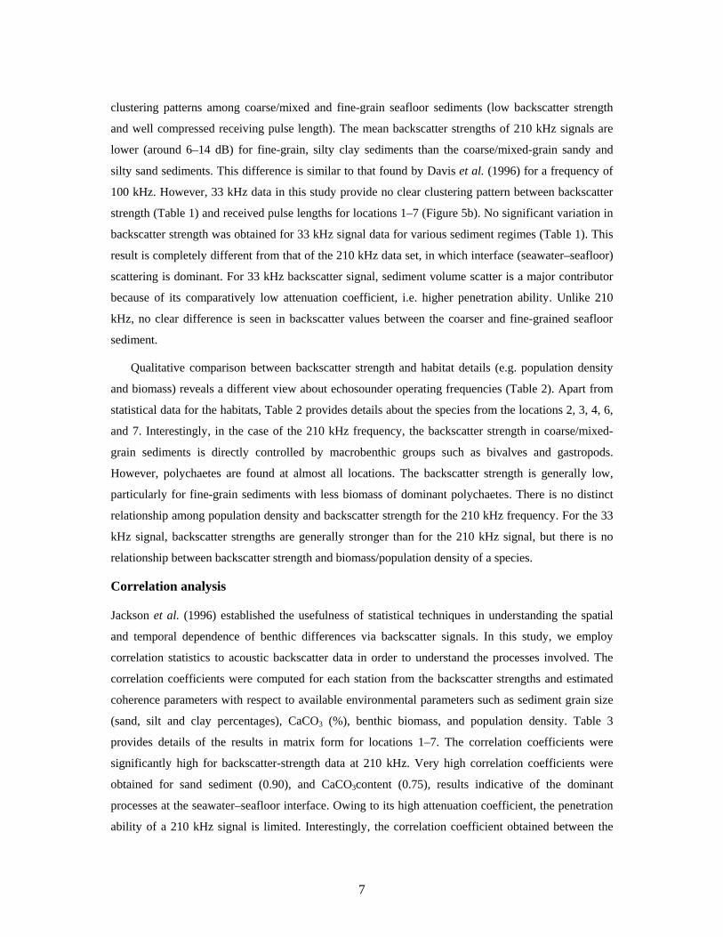
12 kHz (Chakraborty et al., 2001). This work extends the detailed data acquisition activity of January

2005 (Anon., 2005) in the shelf region off Marmugao (Figure 1) with a dual-frequency (210 and 33

kHz) vertical beam echo-sounding envelope exercise with surface sediment sample collection at seven

locations (1–7), covering finer clays and coarser sands. The importance of benthic production is

known in this part of the study area (Parulekar, 1976; Parulekar et al., 1982; Ingole et al., 2002), and

it allowed us to check the effect on the dual acoustic-signal frequencies attributable to benthic

habitats. Further, estimation of the quantitative biomass and population density of benthic habitats at

these seven locations was carried out using sediment samples. We wish to present the statistical

relationship between the acoustic signal backscatter parameters and certain environmental parameters

of geological and biological importance on this central western Indian continental shelf. In addition,

we acquired dual-frequency backscatter signals and sediment samples from seven other locations (8–

3

14) in the vicinity (Figure 1). This was done to validate the results obtained from the seven locations

along the main transect. Echo data sets for the present study were acquired from flat topography;

within the shelf area considered for this study the slope is less than 0.5° (Rao and Wagle, 1997). The

ship’s speed was very slow (~1 knot) during data acquisition.

Material and methods

Data acquisition and the survey area

A Reson Navitronic NS–420 dual-frequency, single-beam echosounder was utilized for this exercise.

The raw analogue output on the receiver circuit board was tapped and connected to a PCL–1712L 12-

bit A/D card installed on a personal computer (PC) with a sampling rate of 1 MHz. The echo data

from locations 1–14 (Figure 1) were acquired at frequencies of 210 and 33 kHz, with 1000 sounding

pings each. As the receiving window is considered to be 40 ms, each snapshot received consisted of

40 000 sample data points from the normal-incidence beam echoes. The echo-waveform data acquired

through an A/D card are binary in nature, and are converted to ASCII format within the range –5 to

+5 V. We employed a two-step data-cleaning method: first, removal of the saturated or clipped

waveforms, and second, removal of the waveforms showing inconsistent echo-energy values within

the particular location data. The second step was carried out after employing a Hilbert transform to

obtain the echo envelope, which is again suitably down-sampled to 200 points within the range 0–5 V.

Our data processing is detailed by Navelkar et al. (2005). Examples of the dual-frequency echo

envelopes are shown in Figure 2. However, few pings were acquired from location 7 using the 33 kHz

signal, so that location is not utilized in the analysis. Detail of the data-acquisition methods are also

given in Chakraborty et al. (2005). Sound-signal penetration and attenuation into the seabed is

different between the 210 and the 33 kHz frequencies. The received echo length for 33 kHz is 3–4

times more than for 210 kHz in this data set.

The survey area is located off Marmugao (15°10`N 73°10`E to 15°40`N 73°55`E), and the survey

was conducted aboard the coastal research vessel (CRV) “Sagar Purvi” along the track shown in

Figure 1. The single-beam 33 kHz bathymetry data along the transect and at seven stations was logged

by GPS onto the PC through a serial port, using a hyper-terminal. Simultaneously, Reson 8101 (240

kHz) multi-beam, echosounder data were acquired for mapping the seafloor. The raw bathymetry data

files after manual cleaning were put into grids using spline-interpolation (grid cell size 10 m), in order

to plot contour maps and to extract depth profiles using Geographical Mapping Tools (GMT) (Douds,

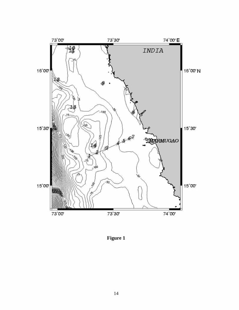
1998). This evenly spaced depth profile was then used to estimate the Power Spectral Density (PSD)

of the grid’s bathymetric data. Also, PSD estimation was carried out over the depth profile obtained

from the hyper-terminal-logged data (33 kHz) (Figure 3a). Applying the power law expression for

4

curve fitting over the PSD provides the spectral slopes. Non-significantly different power law

exponent parameters for two frequencies were 1.89 and 1.92, respectively, for the 240 and 33 kHz

depth profiles, which indicate an even seafloor along the transect with different sediment grain size

(Figure 3b, c).

During the cruise, ground-truth samples were collected by grab at all locations where echo data

acquisitions were made. The surface-sediment samples were analysed by pipette methods (Folk,

1968) for grain-size information in terms of sand, silt, and clay percentages, and the calcium

carbonate content was determined using a Karbonate bomb (Table 1). Analyses of benthic habitats

were carried out based on Holme and McIntyre (1984). Sediment samples from locations 1–7 for

benthic studies were acquired during the CRV “Sagar Sukti” cruise of February 2005. Table 1 lists the

results by station for macrobenthos also. However, the population density data in silty sand sediments

showed extremely high values for bivalves, 1194.4 per m2, out of a total value of 2189.44 m2 at

location 2. The estimated biomass at location 2 was of the order of 7.96 g m–2. The biomass at

location 3 with silty sand sediments was similar, but population density was very low. Low values of

population density and biomass were found comparatively fine-grained silty clay sediments at

locations 4, 6, and 7 (Table 2). No direct relationship among biota and sediment grain size could be

drawn when comparing with the backscatter echo data of the two frequencies (Tables 1, 2). Therefore,

statistical analysis was required to determine the extent of the relationships with acoustic-signal

backscatter and benthic habitat.

Coherence parameter estimation

We estimated the coherence parameter (γ) of the echo peak of the acquired waveform data. The term γ

is defined as a ratio between the coherently reflected and the incoherently scattered echo energy. The

Rice PDF of the echo peak amplitude e from the seabed is described (Stanton, 1984) as

P(e) = [2e(1 + γ)/<e2>] * exp{–[(1 + γ)e2 + γ<e2>] / <e2> } I0(q) . (1)

The term q in the modified Bessel function I0 (q) can be expressed as

q = 2e [γ(1 + γ)]0.5 / ( < e2> )0.5. (2)

The expected value of the echo-peak squared is denoted by <e2>, and γ is the measure of the relative

roughness or smoothness of the seafloor, i.e. the coherence parameter. The Rice PDF is expressed

5

with respect to γ, which is used to fit the histograms of the echo peaks. The echo-peak data so

obtained from the envelope data are used to draw the histograms for each location.

In order to determine γ for the different areas, a moment method based upon Talukdar and Lawing

(1991) is applied. We define a new variable y′ = e/√<e2> and use it in Equation (1). The first moment

(μ) of the Rice PDF is expressed in terms of γ and y′ as

μ = < y′ > = {Γ( 3/2)/(1 + γ)0.5} * exp(–γ/2) [(1 + γ) I0 (γ/2) + γI1(γ/2)] . (3)

In Equation (3), μ varies between √π/2 (Rayleigh PDF, γ = 0) and 1 (Gaussian PDF). The mean value

of the peak data set is normalized with the second moment of the echo-peak data, and is compared

with the theoretical mean (μ), using Equation (2) to estimate γ. Using the estimated γ value in

Equation (1), well-matched PDF curves can be plotted (Figure 4).

Backscatter data processing

In order to compute backscatter strength from the raw backscatter signal of the dual- beam

echosounder, we followed Urick (1967), as referenced in Greenlaw et al. (2004) and Sternlicht and de

Moustier (2003):

< 10 * log10S > = < 20 * log10 UA > – Vtot – Gup – SL + < 40 * log10 (R) > + 2*α b * R – 10 * log10 A, (4)

where S is backscatter strength, UA the raw backscatter signal obtained from particular locations, and

Vtot is system gain and operator gain utilized in the echosounder. For the source level (SL) and

receiving sensitivity (Gup), two different sets of values were used for two frequencies, i.e. 210 and 33

kHz. Similarly, for the attenuation coefficient (αb), two values corresponding to 210 and 33 kHz were

used. Here, R is the vertical depth in metres and A is the beam-insonified area. For a circular beam

towards the normal incidence direction with a longer pulse period, A = πr2. Here, r is the radius of the

footprint, which is a function of beam width and vertical distance. The computed values of backscatter

strength (dB) are presented with respect to echo length. However, although echo data were acquired

for an echo length of 0.04 s, we employed an adaptive method to determine the actual window length

and computed backscatter strength for the two operating frequencies. We selected 10% of the highest

peak value as a threshold level to identify the initial and final endpoints of the data window for the

receiving envelope waveform. When analysing the data, we used the echo-waveform envelopes with

6

numerous distinct peaks: we did not employ an averaging technique to smooth the data, as other

workers have done.

Results and discussion

Coherence parameter results using peak PDF

The data points in Figure 4 represent the experimental echo-peak PDFs, and the curves describe the

theoretical PDFs for the 210 and 33 kHz frequencies, respectively. We know that the scattering

phenomenon is dependent on the sound-signal operating frequency, which is relatively dominant for

210 kHz rather than for the 33 kHz signal. In 210 kHz signal data from location 1, which has coarser

sediments and very high CaCO3 content, and locations 5 and 6, with fine grain sediments, the γ values

are comparatively low, whereas for mixed type sediment at locations 2 and 3, the γ values are high

(Table 1). Stanton and Clay (1986) show that for the same seafloor, if the γ values at a particular

operating frequency are known, then we can predict γ values for any other frequency. Accordingly, at

the 33 kHz operating frequency, the γ value is expected to have higher values than the corresponding

210 kHz frequency for the same seafloor, and we observe this in our estimated γ values (except at

location 3). However, we found irregular γ values for the 33 kHz operating frequency owing to its

higher penetration ability. Therefore, γ values cannot be predicted correctly, especially when there is a

complex seafloor system where surface and immediately subsurface sediments are dominant with

varying grain size, CaCO3 content, and benthic habitats. The results of the model study using echo-

peak PDF data show some interesting seafloor roughness parameters, when employing Rice PDF-

based models. However, there was no significant correlation among the estimated coherence

parameters for two operating frequencies for different seafloor locations (Tables 1 and 3).

Backscatter

For the 210 kHz frequency there is clear distinction between the first three locations in their coarser

sand and silty sand sediments and their relatively clayey sediment in terms of backscatter strength and

received pulse length (Figure 5a). However, the backscatter strength and pulse lengths are higher at

locations 1 and 2, which contain sand and silty sand with CaCO3 content of 91% and 75.3%,

respectively. The relatively higher backscatter strength and low pulse length at location 3 may be

attributed to the reduced CaCO3 content of sediments (41.6%) there. Backscatter strengths were

higher and the spread of received pulse lengths relatively wide for the three coarse/mixed-grain

sediments. This indicates a dominant but fluctuating scattering phenomenon in the coarse/mixed-grain

sediment locations, especially those with high CaCO3 content. Moreover, there were distinct

7

clustering patterns among coarse/mixed and fine-grain seafloor sediments (low backscatter strength

and well compressed receiving pulse length). The mean backscatter strengths of 210 kHz signals are

lower (around 6–14 dB) for fine-grain, silty clay sediments than the coarse/mixed-grain sandy and

silty sand sediments. This difference is similar to that found by Davis et al. (1996) for a frequency of

100 kHz. However, 33 kHz data in this study provide no clear clustering pattern between backscatter

strength (Table 1) and received pulse lengths for locations 1–7 (Figure 5b). No significant variation in

backscatter strength was obtained for 33 kHz signal data for various sediment regimes (Table 1). This

result is completely different from that of the 210 kHz data set, in which interface (seawater–seafloor)

scattering is dominant. For 33 kHz backscatter signal, sediment volume scatter is a major contributor

because of its comparatively low attenuation coefficient, i.e. higher penetration ability. Unlike 210

kHz, no clear difference is seen in backscatter values between the coarser and fine-grained seafloor

sediment.

Qualitative comparison between backscatter strength and habitat details (e.g. population density

and biomass) reveals a different view about echosounder operating frequencies (Table 2). Apart from

statistical data for the habitats, Table 2 provides details about the species from the locations 2, 3, 4, 6,

and 7. Interestingly, in the case of the 210 kHz frequency, the backscatter strength in coarse/mixed-

grain sediments is directly controlled by macrobenthic groups such as bivalves and gastropods.

However, polychaetes are found at almost all locations. The backscatter strength is generally low,

particularly for fine-grain sediments with less biomass of dominant polychaetes. There is no distinct

relationship among population density and backscatter strength for the 210 kHz frequency. For the 33

kHz signal, backscatter strengths are generally stronger than for the 210 kHz signal, but there is no

relationship between backscatter strength and biomass/population density of a species.

Correlation analysis

Jackson et al. (1996) established the usefulness of statistical techniques in understanding the spatial

and temporal dependence of benthic differences via backscatter signals. In this study, we employ

correlation statistics to acoustic backscatter data in order to understand the processes involved. The

correlation coefficients were computed for each station from the backscatter strengths and estimated

coherence parameters with respect to available environmental parameters such as sediment grain size

(sand, silt and clay percentages), CaCO3 (%), benthic biomass, and population density. Table 3

provides details of the results in matrix form for locations 1–7. The correlation coefficients were

significantly high for backscatter-strength data at 210 kHz. Very high correlation coefficients were

obtained for sand sediment (0.90), and CaCO3content (0.75), results indicative of the dominant

processes at the seawater–seafloor interface. Owing to its high attenuation coefficient, the penetration

ability of a 210 kHz signal is limited. Interestingly, the correlation coefficient obtained between the

8

210 kHz signal backscatter strength and CaCO3 content are similar to the results presented by Davis et

al. (1996) for 100 kHz, i.e. their 0.67 vs. our 0.75. Moreover, good correlation between backscatter

signal and benthic biomass (0.91) and population density (0.58) indicate significant correlation

between surficial benthic habitats and the related 210 kHz backscatter strength, especially at sandy

and silty-sand sediment locations. Correlation coefficients for the coherence parameter (γ) and other

environmental parameters for the 210 kHz signal are average. As already mentioned, coherence

parameters are computed using only the echo peaks of the signals and compared with backscatter

strength for which the entire echo envelope is used. Correlation results for average backscatter

strength (entire envelope) would be expected to be better than when echo-peak levels are used for

estimation.

For the 33 kHz signal, there were good correlations only for sediments having high silt (0.68) and

clay (0.75) content, and correlations were poor for benthic population density (0.09) and negative for

biomass. The lower correlation values obtained with 33 kHz are indicative of different scattering

phenomena than when 210 kHz signal data are applied. As already mentioned, the 33 kHz signal has

the higher volume scattering effect because of its greater penetration ability than 210 kHz. At 210 kHz

signal levels, moderate to high correlations for benthic population density and biomass indicate the

existence of appreciable sizes of benthic habitats at the seawater–seafloor interface.

Earlier, we presented data along the transect of seven locations (Figure 1, Table 1). However, in

order to validate these results we also include the results from seven other locations (8–14) in the

vicinity of the transect (see Figure 1). However, the coherence parameters of these data sets were not

computed because of their insignificant correlations with sediment and benthic parameters. Owing to

the non-availability of benthic data from locations 8–14, we do not have population density and

biomass parameters for correlation studies. To investigate the interrelationships among estimated

backscatter strength and sediment grain-size distribution, we present correlation coefficients in Table

3. Those correlation coefficients relate to the operational frequency applied. Correlations were good

for 210 kHz backscatter signals for parameters such as sand (0.83) and CaCO3 content (0.74), but

coefficients are negative for silt and clay. For the 33 kHz backscatter signal, the estimated correlation

coefficients were negative for coarser sand and CaCO3 content at locations 1–7. However, correlation

was poor for silty and clay (0.28) sediments. Generally, the 33 kHz backscatter signal had better

penetration ability, so may be encountering different subsurface sediment layer compositions at

locations 1–7, although the surface sediments are the same. The sediment grain-size information

provided for this study is based on the top sediment surface acquired by a grab, so cannot be used for

subsurface layers of sediment.

9

Table 3 also summarizes the correlation coefficients between backscatter strength and sediment

grain size and CaCO3 content at all 14 locations. Correlation coefficients are high for CaCO3 (0.64)

and sand (0.76) content for the 210 kHz signal, whereas for silt and clay sediments correlations were

negative. For the 33 kHz backscatter signal, there are weak correlations only for silt (0.09) and clay

(0.36) content. In general, the correlation results presented in Table 3 are similar for the 210 kHz

signal and all sediment types, but the 33 kHz signal encountered different sediment environments

because of its better signal-penetration capability.

Overview

We have attempted to identify interrelationships between various seafloor parameters in terms of

backscatter-echo signal data acquired using a dual-frequency, single vertical-beam echosounder on the

continental shelf of the Arabian Sea off western India (near Marmugao). Similar power-law exponent

parameters are obtained using seafloor topographic data for two frequencies (33 kHz and 210 kHz).

Tapped dual frequency (210 kHz and 33 kHz) echosounder peak data were used for Rice PDF-based

studies to estimate the coherence parameter from a transect. They do not show any regular variations

with respect to the seafloor sediment or habitat parameters. However, in order to incorporate a

correction into backscatter strength, system-related gain parameters were utilized. Presentation in

Figure 5 of the computed backscatter strengths within the reverberation window (allowing a threshold

of 10%) provides two distinct patterns between coarse and fine-grain sediments for the 210 kHz

backscatter signal. Such patterns were not observed for the 33 kHz backscatter signal, differences that

can be attributed to the greater signal penetration capability of the 33 kHz signal and the dominance of

the volume scattering from the sediment. For the 210 kHz signal, the seawater–seafloor interface

scattering was dominant. Using two operating frequencies for a similar area of seafloor, the

dominance of two different scattering processes was clear. Statistical relationships among signal

parameters (backscatter strengths and coherence parameters using echo peaks), along with sediment

grain size and benthic habitats (population density and biomass), indicate obvious relationships

among sediment grain size and benthic habitat through correlations between backscatter strength and

estimated coherence, using echo peaks. Correlation percentages were very high between the 210 kHz

backscatter signal and the CaCO3 and sand sediment content. There was also a clear correlation

between the 210 kHz backscatter signal and benthic biomass and population density. These positive

correlation values for the 210 kHz backscatter signal with sediment and macrobenthos affirm the

dominance of seawater–seafloor interface scattering. For the 33 kHz backscatter signal, there were no

regular relationships between backscatter and sediment or macrobenthos. This is due to the existence

of top-layer sediment characteristics such as sand and CaCO3 for coarse/mixed-grain sediment. A

similar existence of surficial, i.e. interface between seawater and seafloor, benthic biomass and

10

population density indicates poor correlation with the 33 kHz backscatter signal, which indirectly

reflects the dominance of the volume-scattering process. Attempts to validate the correlation results

between backscatter signal and sediment parameters during the transect by use of other backscatter

data sets acquired from adjacent locations at the same time strongly support the statistical relationship

we found.

Acknowledgements We thank S. R. Shetye, Director of the NIO, for his encouragement and permission to publish this

work, the Director, NIOT, Chennai, for vessel support, and Shri Padmanathan for assistance.

Financial support (GAP 1493) was obtained from the Department of Information Technology (DIT),

New Delhi, India. Finally, we thank Van Holliday of BAE Systems for his encouragement, and an

anonymous reviewer for useful suggestions on our draft manuscript, which is NIO contribution 4212.

References

Anon. 2005. “Sagar Purvi” cruise report, 03/05. NIOT, Chennai. 12 pp.

Chakraborty, B., and Pathak, D. 1999. Seabottom backscatter studies in the western continental shelf of India. Journal of Sound and Vibration, 219: 51–62.

Chakraborty, B., Kaustubha, R., Hegde, A., and Pereira, A. 2001. Acoustic seafloor sediment classification using self organizing feature maps. IEEE Transactions on Geoscience Remote Sensing. 38: 2722–2725.

Chakraborty, B., Navelkar, G., Prabhudesai, R. G., Janakiraman, G., Mahale, V., Fernandez, W., and Rao, N. 2005. Echo-waveform classification using model and model-free techniques: experimental study results from central western continental shelf of India. In Proceedings of the IEEE MTS. Washington DC.

Davis, K. S., Slowey, N. C., Stender, I. H., Fiedler, H., Bryant, W. R., and Fechner, G. 1996. Acoustic backscatter and sediment textural properties of inner shelf sands, northeastern Gulf of Mexico. Geo-Marine Letters, 16: 273–278.

Douds, A. S. B. 1998. Fractal analysis of topography and structure across the Appalachian foreland of West Virginia. MS thesis, University of West Virginia. 115 pp.

Folk, R. L. 1968. Petrology of Sediment Rocks. Hemphills, Austin, Texas. 177 pp.

Greenlaw, C., Holliday, D. V., and McGehee, D. E. 2004. High-frequency scattering from saturated sand sediments. Journal of the Acoustical Society of America, 115: 2818–2813.

Ingole, B. S., Rodrigues, N., and Ansari, Z. A. 2002. Macrobenthic communities of the coastal waters of Dhabol, west coast of India. Indian Journal of Marine Science. 31: 93–99.

Jackson, D. R., Williams, K. L., and Briggs, K. B. 1996. High-frequency acoustic observations of benthic– spatial and temporal variability. Geo-Marine Letters. 16: 212–218.

11

Navelkar, G., Prabhudesai, R. G., and Chakraborty, B. 2005. Dual-frequency, echo-data acquisition system for seafloor classification. In Proceedings of the National Symposium on Ocean Electronics. pp. 42–48. Allied Publishing. New Delhi. 309 pp.

Pace, N. G. 1983. Acoustic classification of seabed. In CRC Handbook of Geophysical Exploration at Sea, pp. 211–218. Ed. by R. A. Geyer. CRC Press, Boca Raton, Florida.

Parulekar, A. H. 1976. Benthos of the Arabian Sea. Journal of the Indian Fisheries Association. 6: 1–10.

Parulekar, A. H., Harkantra, S. N., and Ansari, Z. A. 1982. Benthic production and assessment of demersal fishery resources of the Indian Seas. Indian Journal of Marine Science. 11: 107–114.

Pouliquen, E., and Lurton, X. 1992. Sea-bed identification using echosounder signals. In Proceedings of the 1st European Conference on Underwater Acoustics, pp. 535–538. Ed. by M. Weydert. Elsevier, London. 764 pp.

Rao, V. P., and Wagle, B. G. 1997. Geomorphology and surficial geology of the western continental shelf of India: a review. Current Science, 73: 330–349.

Richardson, M. D., and Bryant, W. R. 1996. Benthic boundary-layer processes in coastal environments: an introduction. Geo-Marine Letters, 16: 133–139.

Stanton, T. K. 1984. Sonar estimates of seafloor micro-roughness. Journal of the Acoustical Society of America, 77: 809–818.

Stanton, T. K., and Clay, C. S. 1986. Sonar echo-statistics as a remote sensing tool: volume and seafloor. IEEE Journal of Oceanic Engineering, 11: 79–96.

Sternlicht, D., and de Moustier, C. 2003. Time-dependent, seafloor acoustic backscatter (10–100 kHz). Journal of the Acoustical Society of America, 114: 2709–2725.

Talukdar, K. K., and Lawing, W. D. 1991. Estimation of the parameters of the Rice distribution. Journal of the Acoustical Society of America, 89: 1093–1107.

Thorsos, E. I., and Richardson, M. D. 2002. Guest Editorial. IEEE Journal of Oceanic Engineering, 27: 341–344.

Figure legends Figure: 1. Survey area and data-acquisition locations. Figure 2. Echo-envelope data for (a) and (b) the 33kHz signal, and (c) and (d) the 210 kHz signal for sandy and clay sediments, respectively. Figure 3. (a) Depth profiles from the 33 kHz single-beam echosounder, and 240 kHz multi-beam grid data and sampling locations (y-axis exaggeration, 500 ×). Power Spectral Density (PSD) plotted against wave number for the (b) the 210 kHz and (c) the 33 kHz profile. Figure 4. (a) 210 kHz and (b) 33 kHz echo-peak Probability Density Function (PDF) and Rice PDFs (dashed line and asterisks, PDF data; solid line and + signs, Rice PDF). Figure 5. Backscatter Strength (dB) plotted against receiving echo-window length for seven locations for (a) the 210 kHz signal and (b) the 33 kHz signal (red, green, blue, light blue, magenta, yellow, and black indicate locations 1–7, respectively).

12

Table 1. Dual-frequency backscatter strength and coherence parameters, sediment grain size, and benthic habitat at the study locations.

Backscatter

strength (dB) Coherence

parameter (γ) Sediment content (%) Benthic habitat Location Depth

(m) 33 kHz

210 kHz

33 kHz

210 kHz

Sand

Silt

Clay

CaCO3 Density (no. m–2)

Biomass (g m–3)

1 83.52 –31.72 –32.60 10 09 94.0 00.0 06.0 91.00 - - 2 75.56 –28.17 –32.13 31 15 68.7 17.5 13.7 75.30 2189 7.96 3 66.73 –30.92 –30.46 09 20 77.0 15.0 08.0 41.66 597.0 7.49 4 52.39 –27.85 –44.47 21 16 02.2 45.0 52.8 17.30 199.9 1.59 5 42.00 –26.31 –38.74 11 08 02.7 40.0 57.3 10.00 - - 6 32.65 –27.52 –38.78 27 08 00.7 15.0 84.3 10.00 577.7 3.87 7 27.48 –28.72 –40.51 - 09 01.2 40.0 58.8 10.00 796.1 0.062

8* 24.00 –24.43 –34.18 - - 02.5 25.0 72.5 05.0 - - 9* 34.62 –27.75 –34.99 - - 01.4 45.0 53.6 05.0 - - 10* 56.04 –26.01 –36.74 - - 01.5 45.0 53.5 08.0 - - 11* 62.28 –33.62 –34.47 - - 01.1 50.0 48.9 10.0 - - 12* 85.41 –38.63 –34.28 - - 74.0 17.5 08.5 81.3 - - 13* 78.33 –31.59 –30.75 - - 93.0 02.5 04.5 64.0 - - 14* 76.95 –21.97 –29.40 - - 93.3 05.0 01.7 88.0 - -

* Location data used for validating the results

13

Table 2. Species groups analysed, and statistical parameters by location.

Species group Location

Nemertenia Bivalvia Gastopoda Polychaeta Crustacea Amphipoda

Density (number)

Biomass(g m–2)

2 0.0 1 194.4 199.04 796.16 0.0 0.0 2 189.44 7.962 3 0.0 199.04 99.04 99.04 0.0 0.0 597.12 7.492 4 0.0 22.22 0.0 155.54 22.22 0.0 199.98 1.593 6 88.88 0.0 0.0 488.86 0.0 0.0 577.72 3.875 7 0.0 0.0 0.0 796.16 0.0 0.0 796.16 0.062

Table 3. Correlation coefficients obtained between backscatter strength at the two frequencies and sediment and benthic parameters for subsets of locations and for all locations.

Variable CaCO3 (%) Sand (%) Silt (%) Clay (%) Density (no. m–2)

Biomass (g m–3)

Locations 1–7 only Backscatter strength at 33 kHz –0.68 –0.81 0.68 0.75 0.09 –0.41

Backscatter strength at 210 kHz 0.75 0.90 –0.80 –0.80 0.58 0.91

γ at 33 kHz –0.06 –0.29 0.07 0.35 0.57 –0.09 γ at 210 kHz 0.21 0.41 –0.02 –0.55 0.03 0.58 Locations 8–14 only Backscatter strength at 33 kHz –0.21 –0.15 –0.05 0.28 – –

Backscatter strength at 210 kHz 0.74 0.83 –0.84 –0.74 – –

All locations (1–14) Backscatter strength at 33 kHz –0.29 –0.28 0.09 0.36 – –

Backscatter strength at 210 kHz 0.64 0.76 –0.66 –0.72 – –

14

Figure 1

15

Figure 2

16

Figure 3

17

Figure 4

18

Figure 5