JOURNAL OF GEOPHYSICAL RESEARCH, VOL. 96, NO. B10, PAGES 16,151-16,160, SEPTEMBER 10, 1991

Seafloor Compliance Observed by Long-Period Pressure and Displacement Measurements

WAYNE C. CRAWFORD, $PAHR C. WEBB, AND JOHN A. HILDEBRAND

Scripps Institution of Oceanography, University of California, San Diego

La Jolla

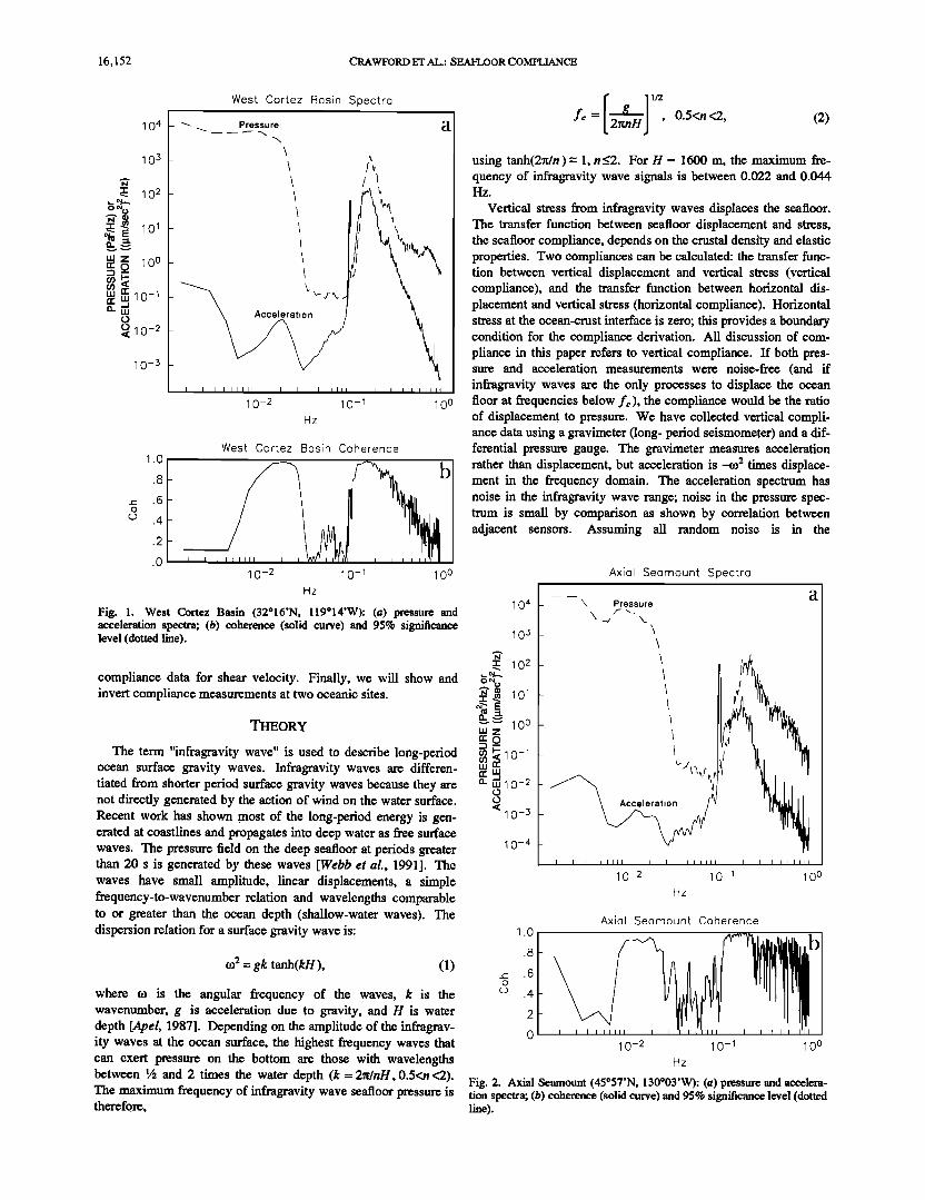
Ocean surface waves with periods longer than 30 s create periodic, horizontally propagating pressure fields at the deep seafloor. Seafloor displacements resulting from these pressure fields depend on the density and elastic parameters of the oceanic crust. The displacement to pressure transfer function, the seafloor compliance, pro- vides information about ocean crustal density and elasticity, and we outline a linearized inversion method to determine ocean crustal shear velocity from the compliance. By computing compliance partial differences with respect to changes in ocean crust shear velocity, we provide estimates of inversion stability and of the compli- ance sensitivity to crustal properties. Seafloor compliance, measured from pressure and acceleration spectra, is presented for two different sites: Axial Seamount on the Juan de Fuca Ridge and the West Cortez Basin in the California continental borderlands. The compliances and inverted structure for these two sites show significant differences; in particular, a zone of low shear strength is observed at depth within Axial Seamount, suggesting the presence of at least 3% partial melt Within the upper 2500 meters of the ediface. These results suggest that the method provides a useful new geophysical prospecting tool.

INTRODUCTION compliant at high frequencies corresponding to shallow levels. Axial Seamount, an active volcano, has relatively high compli-

Knowledge of oceanic crustal structure provides important ance at low frequencies corresponding to deep levels, suggesting insights into crustal formation and hydrothermal circulation. reduced shear strength at depth within the volcano. Seismic methods are a practical approach to determining crustal Coherence between seafloor pressure and vertical acceleration structure; however, compressional and shear properties must be is also high in the microseism band, above 0.1 Hz. Energy in the measured to provide a complete seismic picture of the oceanic microseism band is primarily associated with propagating elastic crust. Shear velocities are particularly difficult to measure with waves along the seabed and in the water. The compliance func- conventional seismic techniques and are essential to determining tion in this band depends on phase velocities of the many modes oceanic crustal porosity [Fryer et al., 1991]. Crustal porosity con- of the oceanic waveguide. Bradner [1963] and others have sug- strains hydrothermal circulation and seafloor acoustic reflectance, gested that ratios of vertical displacement to pressure associated as well as providing information about oceanic crustal formation. with microseisms could be used to determine crustal structure, but A geophysical prospecting method sensitive to shear velocity in practice the various modes interfere to provide an ambiguous structure could sense crustal magma chambers, which have low result. shear velocity. Relating oceanic crustal structure to compliance has roots in

We present a method for profiling ocean crustal elastic parame- work on Earth tides. Beaumont and Lambert [1972] determined ters using the ocean bottom pressure field as the driving source. that Earth tide measurements were contaminated by ocean tidal This method is a development of a technique pioneere d in shallow loading dependent on the structure of the Earth's upper layers. water by Yamamoto and others [Yamarnoto and Torii, 1986; Tre- Measurements of ocean tidal loading from stations on land have vorrow et al., 1988; Yamamoto et al., 1989]. A low-frequency proven useless for studying the elastic structure of the Earth pressure field is created on the ocean bottom by ocean surface because of the complicated tidal structure in coastal regions and gravity waves. The horizontal scale of the pressure field is set by the large wavelength of the effect. Measurements at the deep the wavelength of the surface gravity waves. This pressure field seafloor at tidal frequencies may be of more use for determining causes deformation of the seafloor, resulting in seafloor pressure deep elastic structure. Recently, Yamamoto and others and vertical acceleration which show significant coherence below [Yamarnoto and Torii, 1986; Trevorrow et al., 1988; Yamamoto et 0.03 Hz (Figures 1 and 2). The amplitude of seafloor deformation al., 1989] found the compliance of sediments forced by gravity below 0.03 Hz depends on oceanic crustal elastic parameters, water waves in shallow water (10-50 m) could be inverted to especially shear properties; low crustal rigidity leads to large determine the shear modulus in the sediment. We invert compli- seafloor displacements. Seafloor compliance is the transfer func- ance data for Earth structure using a technique applicable to hard tion between seafloor deformation and seafloor pressure as a func- rock as well as sediments. The inversion cons•ns shear veloci- tion of frequency. We present measurements of seafloor compli- ties at sites where compressional velocities are constrained by ance from two sites: Axial Seamount on the Juan de Fuca Ridge other techniques, such as seismic refraction. and the West Cortez Basin in the California continental border- This paper differs from previous work in three areas: instru- lands. Seafloor compliance is significantly different at the two mentation, forward modeling of compliance, and inversion sites. West Cortez Basin has a thick sediment layer and is more methods. The differences in instrumentation and forward model-

ing are necessary because our measurements are made at lower Copyright 1991 by theAmericanGeophysicalUnion. frequencies corresponding to the long wavelengths of ocean

penetrating water waves in the deep ocean (more than 1000 m Paper number 91JB1577. deep). We will briefly outline the theory of infragravity waves 0148-0227/91/91JB-01577505.00 and seafloor compliance, then explain the method we use to invert

16,151

16,152 CRAWFORD ET AL.: SEAFLOOR COMPLIANCE

West Cortez Basin Spectra

10 4

10 3

•--. 10 2 o%

•_. -- 10 •

n' • 10 ̧

LU • 10-•

•10-2 10-3

- • Pressure

_

1 0 -2 1 O-• 10 ø Hz

West Cortez Basin Coherence 1.0

.8- b _c: .6 o

¸ .4

.2

o0 I I I I 10-2 10-1 10 0

Hz

Fig. 1. West Cortez Basin (32ø16'N, 119ø14'W): (a) pressure and acceleration spectra; (b) coherence (solid curve) and 95% significance level (dotted line).

compliance data for shear velocity. Finally, we will show and invert compliance measurements at two oceanic sites.

THEORY

The term "infragravity wave" is used to describe long-period ocean surface gravity waves. Infragravity waves are differen- tiated from shorter period surface gravity waves because they are not directly generated by the action of wind on the water surface. Recent work has shown most of the long-period energy is gen- erated at coastlines and propagates into deep water as free surface waves. The pressure field on the deep seafloor at periods greater than 20 s is generated by these waves [Webb et al., 1991]. The waves have small amplitude, linear displacements, a simple frequency-to-wavenumber relation and wavelengths comparable to or greater than the ocean depth (shallow-water waves). The dispersion relation for a surface gravity wave is:

to2 = gk tanh(kH ), (1)

where to is the angular frequency of the waves, k is the wavenumber, g is acceleration due to gravity, and H is water depth [Apel, 1987]. Depending on the amplitude of the infragrav- ity waves at the ocean surface, the highest frequency waves that can exert pressure on the bottom are those with wavelengths between « and 2 times the water depth (k = 2•/nH, 0.5<n <2). The maximum frequency of infragravity wave seafloor pressure is therefore,

I 1112 g

f ½ = 2•ntt , 0.5<n<2, (2)

using tanh(2•/n )= 1, n_<2. For H = 1600 m, the maximum fre- quency of infragravity wave signals is between 0.022 and 0.044 Hz.

Vertical stress from infragravity waves displaces the seafloor. The transfer function between seafloor displacement and stress, the seafloor compliance, depends on the crustal density and elastic properties. Two compliances can be calculated: the transfer func- tion between vertical displacement and vertical stress (vertical compliance), and the transfer function between horizontal dis- placement and vertical stress (horizontal compliance). Horizontal stress at the ocean-crust interface is zero; this provides a boundary condition for the compliance derivation. All discussion of com- pliance in this paper refers to vertical compliance. If both pres- sure and acceleration measurements were noise-free (and if infragravity waves are the only processes to displace the ocean floor at frequencies below f½), the compliance would be the ratio of displacement to pressure. We have collected vertical compli- ance data using a gravimeter (long- period seismometer) and a dif- ferential pressure gauge. The gravimeter measures acceleration rather than displacement, but acceleration is _to2 times displace- ment in the frequency domain. The acceleration spectrum has noise in the infragravity wave range; noise in the pressure spec- trum is small by comparison as shown by correlation between adjacent sensors. Assuming all random noise is in the

Axial Seamaunt Spectra

10 4

10 3

N

E 10 2

--..- ,oo

g?• 0 -1

13_• 0-2 o o

10-3

10-4

- X Pressure

_

_

_

_

_

10-2 10 -• 10 0 Hz

lO

8

= 6 o

co 4

2

0

Axial Seamaunt Coherence

ii 1 i 10-2 0-1 10 0

Hz

Fig. 2. Axial Seamount (45ø57'N, 130ø03'W): (a) pressure and accelera- tion spectra; (b) coherence (solid curve) and 95% significance level (dotted line).

CRAWFORD ET AL.: SEAFLOOR COMPLIANCE 16,153

acceleration/displacement spectrum, the square of the vertical compliance (•) is obtained from the vertical displacement spec- trum (•qa), the pressure spectrum (•qv), and the coherence between the two (Tea) using the following equation:

I•(co)l (3)

•l•l }x 2 - (8A) 33. 2k g,2(ix+)•) 2'

• I•1 = _ 2•x2+2• xz+3.2 (8B) 3[[ 2k p,2(g+3.) 2 '

Since p, 3., and g are always positive, all of the partial derivatives are negative; an increase in either of the Lam6 parameters will

Multiplying the ratio of displacement to pressure by the coherence result in a decrease in the magnitude of vertical compliance. The squared accounts for both random noise in the displacement spec- partial derivatives of I•l with respect to seismic velocities c• and trum and the possibility that the low-frequency displacements have sources other than infragravity waves. An estimate of the compliance uncertainty is given by

I•(to) I, (4)

[• are also negative. This agrees with intuition that the less rigid or more compressible a material is, the farther it will be displaced by a given force. Assuming that different frequencies are tuned to structure at different depths in the crust, we speculate that a decrease in shear velocity at some depth will result in an increase of compliance at the corresponding frequency. From the equa- tions (8A and 8B), 31(I/3•x must be at least twice the magnitude of 3 I•l/3•. and typically is more than 5 times as great, meaning

with na the number of data windows used to calculate the spectra that vertical compliance is more sensitive to changes in rigidity g and coherences [Bendat and Piersol, 1980]. than to changes in 3.. Similarly, compliance is typically twice as

The equation of motion in an elastic medium is:

•2t/i P-b7- = (X + axax,

•2U i

+ (5) /4 i is the displacement of a particle in the xi direction, p is the den- sity of the material, g is a Lam6 parameter known as the rigidity or the shear modulus, and 3. is the second Lam4 parameter. We solve for the vertical compliance:

•(co)- u• u• (6) ?= •(u,•.x+U• x) + 21u, u• '

where uid =3ui/3xj. Compressional velocity c• and shear velocity [3 are related to the Lamd parameters 3. and !x by pc• 2 = (3.+2g) and

sensitive to changes in shear velocity [• than to changes in compressional velocity c•. Equation (7) shows that compliance of a uniform half-space is less sensitive to changes in density p than to changes in compressional velocity c•.

The problem of determining compliance for a laterally homo- genous Earth with P and SV waves can be solved numerically. One of the most common numerical solutions is the propagator matrix method [Aki and Richards, 1980, pp. 273-283] combined with the method of minor vectors [Woodhouse, 1980]. For calcu- lation of compliance of a known layered Earth model, we use an implementation of the minor vector propagator written by Gorn- berg and Masters [1988]. Two boundary conditions are (1) hor- izontal stress (*zJ) vanishes at the seafloor; and (2) a uniform half-space of material underlies the layered model.

To understand the effect of crustal structure on the compliance function, we constructed five oceanic crustal models and com-

p[•2= g,. Plane waves forcing the seafloor excite compressional puted their compliance, assuming a water depth of 1600 m. We (P) and vertical shear (SV) evanescent waves in the Earth. Equa- tion (6) has not been solved analytically, but we can use a compu- tational propagator matrix method to determine seafloor compli-

Oceanic Crust Models Compliance of Oceanic Crust Models

ance, where the oceanic crust is modeled as a finite number of ø •.•;11 discrete flat layers overlying an infinite uniform half-space. -5oo To relate the crustal elastic parameters and the compliance, we - -

first modeltheEarthasauniformhalf-space. Sorrels and Goforth -•oool i • ,

[1973] derived the compliance of a uniform half-space when _•500i '- .................. forced by a plane pressure wave traveling on the free surface at a •0-9

muh woity thn V SV in the Earth. This situation is called quasi-static because the inertial •,•

terms are small' and applies tø øur study because infragravity c• -3øøø• waves have velocities less than 200 m s -• in water up to 4000 m 0,01 ,,"' - deep, while P and SV waves in the Earth typically travel at veloci- -3500

ties greater than 2000ms -•. Under the quasi-static assumption, -4000[ •-• (7) -sooo

1

which leads to:

1

_•[ 2[[([[ + •)

0 2 4 0 0.01 0.02 0.03 0.04 0.05

Shear velocity (km/s) Frequency (Hz)

Fig. 3. Earth models and resulting compliances, H - uniform half-space, S • ideal sediment-covered model, M - ideal magma chamber model, A - ideal asthenosphere model, N - normal [Spudich and Orcutt, 1980] model: (a) shear velocities of the models: each assumes density - 2.5 glcm 3, compressional velocity - 7 km/s; (b) compliances calculated from the models, assuming water depth - 1600 m, normalized by dividing by the wavenumber k (c0) of infragravity water waves.

16,154 CRAWFORD Err AL.: SEAFLOOR COMPLIANCE

calculate normalized compliance, the compliance after the filter- velocity •x--7 km/s, and density p--2.5 g]cm 3. Figure 3b shows ing effect of the ocean is removed, by multiplying compliance by that low-velocity zones correspond to regions of high compliance, the wavenumber k (to) of the water waves. The normalized com- in agreement with the partial derivatives of equation (8). Further- pliance of a uniform half-space is constant (see equation (7)). more, it appears that shallow structure is sensed at higher frequen- Figure 3 shows the models and compliances of (1) a uniform cies than deep structure, in agreement with the intuitive argument half-space (model H); (2) a sedimentary basin model (model S); that longer wavelength water waves penetrate deeper into the (3) a magma chamber model (model M); (4) a shallow astheno- crust. sphere model (model A); (5) normal oceanic crust [Spudich and To test the properties of the compliance function inferred from Orcutt, 1980] (model N). All of the models have compressional Figure 3, we computed the partial differences of the compliance

0.5

_

Compliance Partials- Shear Vel: 1600m: Half-Space i i ! i i i

,,?/ ,,,,, %,,,,-',,,

t t I i l

0.005 0.01 0.015 0.02 0.025 0.03

al

0.035

Frequency (Hz)

0.4

0.2

-0.2

-0.4

-0.6

-0.8

Compliance Partials: Shear Vel' 1600m: Nom•al

b

,__, "',, .... I I I I I 1

0.005 0.01 0.015 0.02 0.025 0.03 0 0.035

Frequency (Hz)

Fig. 4. Compliance sensitivity to changes in shear velocity of one layer of models H and N of figure 3. (a) half-space model (H) with depth of modified layer indicated, (b) normal oceanic crust model (N) with depth of modified layer indicated.

CRAWFORD ET AL.: SEAFLOOR COMPLIANCE 16,155

function for changes in shear velocity. We used the uniform result in a model with more structure than is necessary to explain half-space (model H) and the normal seafloor (model N) of Figure the data. We construct a model with many more layers than there 3 to calculate these partial differences. To calculate each curve in are data points so that we will not introduce unnecessary structure Figure 4a, we increased the shear velocity of one layer of model into the model. Furthermore, the data are never exact. As a H by 5% and calculated the compliance, then decreased the shear result, there exist an infinite number of possible G -g and an velocity of the same layer to 5ø70 below its original value and cal- infinite number of m *•t that will fit the data equally well. To culated the compliance. We subtracted the second compliance select one G -g , we must have some preconception of what a good from the first, and normalized the resulting vector by dividing by a model looks like. To force the model toward this preconception, positive constant so that the maximum absolute value of the vec- we choose a model norm for minimization. The construction of tor was 1. The curves of Figure 4b were calculated using the G -g in order to minimize the chosen norm is discussed by Parker same procedure, starting with the normal seafloor (model N). [1977] and Menke [1984]. The most common construction Normalization over emphasizes curves whose peaks are outside methods for G -g are to minimize the L2 norm of the first differ- the frequency band of Figure 4 (the layers down to 400 m in Fig- ence or the second difference of the model (hereafter referred to ure 4a; the layers down to 200 m in Figure 4b). It is apparent that as C•L2 and C2L2 inversions). These constraints are used because different frequencies "tune" to structure at different depths, and they attempt to make the model as featureless as possible by that the tuning frequencies decrease with increasing depth. Figure 4b, the partials of the oceanic crust model, shows a shift of partial difference peaks to lower frequencies compared to Figure 4a. The low rigidity zone near the oceanic crust model surface amplifies the contribution of the shallow layers, masking the higher fre- quency contribution of changes in the deeper layers. If the com- pliance function were linear, Figures 4a and 4b would look the same. The danger of the nonlinearity is that it may allow more than one domain of attraction for the linearized compliance func- tion. If there is more than one domain of attraction, the inversion result will not be unique. Unlike the partials calculated in equa- tions (7) and (8), the partials of Figure 4 are not all negative. An increase in shear velocity [I requires •. to decrease for the compressional velocity a to remain fixed. Therefore the effect of an increase in !x is countered by the effect of a decrease in •..

minimizing the slope (C1L2) or the curvature (C2L2) of the model. With the C2L2 constraint, structure in m *•t is due to structure in the true model and not an artifact of the inversion process. Another method of construction of G -g is the "singular value decomposition" ($VD) technique [Menke, 1984], which minim- izes the L2 norm of the model with the empirical property that the second difference of the model is also decreased. Yamamoto and

Torii [ 1986] have successfully used the $VD method on shallow- water compliance data. We do not use the SVD method because it does not explicitly minimize the second difference of the model and therefore allows extraneous structure. Discussion and illus-

tration of the very different models that can be obtained by dif- ferent methods of inversion of discrete, inexact data are found in Constable et al., [ 1987] and Smith and Booker [ 1988].

Linear inverse theory has developed to the point where its Since 3 I gl/31x is typically greater magnitude than 31•1/3X, the application is straightforward. Unfortunately, the compliance partial differences of compliance with respect to shear velocity are problem is nonlinear. We must write G(.) as a function of m, and usually negative; however, 31•l/311(z) is positive at some fie- the linear algebra techniques of linear inverse theory are no longer quencies and depths. Calculations of compliance function partial applicable. A common method for solving nonlinear inverse differences with respect to a and p suggest that compliance is typ- problems is to treat them as linear inverse problems locally and to ically twice as sensitive to changes in shear velocity [3 than to iterate to obtain a solution. This approach has the pitfall that there changes in compressional velocity a, and over 10 times as sensi- may be more than one "basin of attraction" for the function. The tive to changes in [I than to changes in density p. answer may not be unique, since G(.) is dependent upon the start-

ing model. When the problem is only weakly nonlinear (more specifically, when the functional to be minimized is convex) the

INVERSION linearization approach will be successful. Yamamoto and Torii's The goal of inverse theory is to calculate a model (in our case, [1986] use of linear techniques is justified because their functional

is only weakly nonlinear. We have not been able to prove that our shear velocity of the oceanic crust) from some data (in our case, seafloor compliance), when we know how to calculate the data as functional is convex, so we must be more cautious in linearization a function of the model. For discrete data, a discrete model, and a of the inversion and use of techniques developed for linear inverse linear relation between the model and the data, we calculate the theory to characterize inversion quality.

We use Occam's inversion [Constable et al., 1987] to obtain data vector d from the model vector m by multiplying the model by a matrix of representors G: shear velocity structure from compliance data, using either C•L2

or C2L2 inversion. Forward problem solutions are calculated

Gm= d. (9) using the implementation of the minor vector propagator men- tioned earlier. Models of compressional velocity (a(z)) and den-

Our goal is to find G -g such that sity (p(z)) of the oceanic crust at the study site are assumed, and we invert compliance data for shear velocity. We use ct(z) esti- mates from refraction and reflection seismology studies and esti-

G -g d = m •t, (10) mate p(z) based on the compressional velocities and facies ana- lyses. Inversion accuracy is not as dependent on at(z) and p(z)

and models as might be suspected, because of the much greater sensi- tivity of the compliance function to shear velocity than to these

Gm *•t = GG -g d = d + T, (11) parameters. A model with a thin layer of very low shear velocity results in a

where T represents uncertainty in the data. If the dimension of compliance function with a narrow, high compliance, peak. m *•t equals the dimension of d and d is exact, then G -g =G -•. Relating the location of this peak to the depth of the low-velocity We don't know the number and thickness of layers in the earth, layer provides an estimate of the depth sensitivity of the compli- however, so this calculation is unreasonable, as it will usually ance function. We calculated compliance of 28 models, each a

16,156 CRAWFORD ET AL.: SEAFLOOR COMPI_ZANCE

4.5

3.5

3

2.5

2

1.5

0.5

Best fit: depth- 0.164*wavelength ...-"' ß

ß

ß

•" I I I i 0 5 10 15 20 25

Water wavelength (km)

Fig. 5. Wavelength-depth relationship of a half-space with one thin layer of low shear velocityß

copy of model H with a 1 m thick low shear velocity layer The model inversions (Figure 6) show structure where their inserted at a depth between 100 and 4200 m below the seafloor. generating models had structure and, more importantly, no We plot compliance peaks against water wavelength because the extraneous structure. Inversion of the half-space model (H) depth of penetration of water waves should depend on their resulted in a half-space model. There is a slight error in shear wavelength. Equation (1) gives the relation between frequency velocity of the inverted half-space that is due to the 5% random and water wavelength. Figure 5 shows that the wavelength-depth noise we added to the compliances. We could easily calculate relationship is linear for the uniform half-space model containing error bars for the inverted model, but only because we know that one, thin, low shear velocity layer. The water wavelengths are the starting model was also a half-space. Inversion of the normal clustered at discrete values because they were derived from oceanic crest model (N) resulted in a model very similar to model discrete frequencies. Figure 5 suggests that for the half-space N. The negative slope below 2500 m of the N model inversion model H, structural features are observed down to a depth approx- reflects a decrease in shear velocity that we put in model N at imately 1/6 the wavelength of the longest water wave coherent 2500 m depth. Inverted shear velocity does not increase at greater with seafloor acceleration. Because the surface waves excited in depths, suggesting that compliance in the frequency band of our the seafloor decay exponentially with depth, the effect of seafloor experimental data cannot sense structure below approximately structure on the compliance function decays exponentially with 2500 m depth. Inversion of the magma chamber model (M) gen- depth. We account for this by increasing layer thickness emtes a model with a low shear velocity zone, but the zone is at a exponentially with depth, so that each layer has approximately greater depth than the model M magma chamber. The partial equal effect on the compliance data. For the inversions in this difference curves of Figure 4b suggest that a region of low shear paper we created a 50-m-thick top layer, then made every succes- velocity dominates the compliance function at lower than typical sive layer 1.1 times as thick as the layer above. The minor vector frequencies, which could be modeled as a region of slightly higher propagator program treats the bottom layer as an infinite half- shear velocity at greater depths. The inverted model of the space. asthenosphere model (A) compliance data has much less structure

A standard test of linear inversion quality is calculation of a than the original model, although it does show increasing shear resolution matrix R=G -g G [Menke, 1984]. For nonlinear inver- velocity with depth. The inverted model's lack of structure is sion a linearized approximation of the resolution matrix is some- probably due to decreasing resolution with increasing depth, and times calculated from the G and G -g of the last iteration of the because the structure in the asthenosphere model is near the inversion. The resulting resolution matrix often has very little to empirical depth limit (2500 m) of the compliance frequency band. do with the actual resolution of the inversion because of the inade- Inversion of the sediment-filled basin model (S) results in a model quacy of linearization [Parker, 1984]. We do notcalculate resolu- with more gradual velocity change than the sharp sediment- tion matrices in this paper. Instead, we computed C2L2 inversions basement interface of model S. C2L2 inversion smooths the stmc- of the models of Figure 3. We restricted compliance frequencies ture of model S over 2500 m of the inverted model. We speculate to the range obtained from our deep-ocean experimental sites. that the low shear velocity of the sediments dominate the compli- The thickness of the estimated model layers are independent of ance function, so that the effect of the basement rocks is not those used to generate the model, since we assumed no previous sensed until very low frequencies. We do not expect these knowledge about the model. We added 5ø2'0 noise to the compli- methods will be able to discern much structure in rocks beneath a ances (from Figure 3b) before inverting. thick layer of sediments.

CRAWFORD ET AL.: SEAFLOOR COMPLIANCE 16,157

-lOOO

-1500

-2000

-2500

-3000

Oceanic Crust Model Inversions

Inverted shear velocity (krn/s)

Fig. 6. Shear velocity C2L2 inversions of Figure 3B compliances plus 5% noiseß H - uniform half-space, S - ideal sediment-covered model, M • ideal magma chamber model, A • ideal asthenosphere model, N • normal [Spudich and Orcutt, 1980] modelß

Inversion quality depends on the amount of noise in the data. Figure 7 shows inverted models of normal oceanic crust (Figure 3a, model N) with different noise levels added to the model's compliance. It appears that 10% noise is the most that we can accept and expect to obtain well-constrained inversions. When noise levels are high, there may be temptation to overfit the data in the model inversion. Even the slightest amount of overfitting, however, results in unwarranted and often extreme structure in the

model [Constable et al., 1987; Smith and Booker, 1988]. None of the inversions in this paper include error bars on the

inverted models. When the model is an exact function of the data, it is reasonable to map uncertainty from the data onto the model.

-1500

-E -2000

-2500

-3000

-3500

Inversions of normal oceanic crust model compliance

%_-.1._7... •, ; ' ] ;:---,-..•, •riginal model :-:-•- •.-,

- : , i : - _ , ..... •. : ' : ,

ß ß

* , .. ', ß

,

ß

- •0% '- - -, : '"', i ß

ß ß

: :•o% _ , ,

ß ,

! .... :,....: i : : to% ß

Inversio: • start i . i %' m{ del : . . ß i i ' I ß -4000

0 1 2 3 4 5

Inverted shear velocity (km/s)

Fig. 7. Shear velocity C2L 2 inversions of normal (model N) oceanic crust compliance plus different noise levels. Each curve is labeled with the amount of noise added to the compliance values as a percentage of the ini- um •umpumlc• values. Model N and 'the inversion starting model are displayed for comparison.

INSTRUMF2qTATION

We use a LaCoste-Romberg underwater gravimeter to measure seafloor acceleration [Lacoste, 1967; Hildebrand et al., 1990]. This sensor is used as a long-period seismometer on land [Agnew and Berger, 1978] and its useful frequency range is two decades lower than typical ocean bottom seismometers. LaCoste- Romberg underwater gravimeters are similar to conventional land gravimeters, except that the operation of underwater gravimeters is actuated by motors for leveling and for adjustment of the meas- urement micrometer. The sensor consists of a zero-length spring and a 0.1-kg mass. The position of the mass is sensed by capaci- tive plates. An analog feedback system is used to stabilize the mass position by applying a voltage to the capacitive plates. Tests of coherence between two of the land seismometers on the same

pier suggest the instrument noise is flat at frequencies above 0.003 Hz, and may be as low as -181 dB relative to 1 m 2 s -3 [Agnew and Berger, 1978]. The underwater gravimeter uses different elec- tronics than these devices, however, and was limited by noise in the PdD converter at frequencies below 0.01 Hz. The gravimeter has recently been modified to reduce electronic noise; these modifications may extend the frequency range of coherence meas-

We use inverse theory because there exist an infinite number of urements and increase coherence in the infragravity wave band. models that fit the data equally wellß The locus of these model The pressure signal associated with the infragravity waves is solutions is impossible to determine, and uncertainty estimates measured using a differential gauge [Cox et al., 1984]. The prin- derived from this locus would be very pessimisti c estimates of the ciple behind a differential gauge is to measure the difference of quality of our inversion, since the value of each model element is pressure between the ocean and a fluid within a rigid reference not explicitly constrained by C2L2 inversion. We do not ask the chamber. At short time scales the differences reflect pressure reader to trust the values of the model elements; instead, we state that the Earth's crust has more structure than the inverted models

(compare, for example, Figures 3a and 5). Any structure in the inverted model reflects at least as much structure in the oceanic

crust. The inference of inversion quality drawn from Figure 7 is the best quantitative error estimate we can make, and this applies only for oceanic crust models similar to model N.

fluctuations in the ocean; at long time scales (greater than 1000 s) a capillary leak allows the reference chamber to equilibrate with ocean pressures. The differential mode permits the use of a very sensitive strain gauge to measure ocean pressure fluctuations while withstanding the enormous pressures of the deep ocean. Over-pressure relief valves protect the strain gauge during deploy- ment and recovery. The gauge outperforms standard low-

16,158 CRAWFORD ET AL.: SEAFLOOR COMPLIANCE

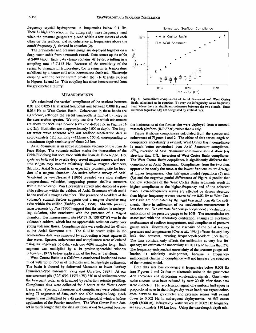
frequency crystal hydrophones at frequencies below 0.1 Hz. There is high coherence in the infragravity wave frequency band when the pressure gauges are placed within a few meters of each other on the seafloor, and no coherence at frequencies above the cutoff frequency f½ derived in equation (2).

The gravimeter and pressure gauge are deployed together on a deep-ocean cable from a research vessel. Data comes up the cable at 2400 baud. Each data clump contains 42 bytes, resulting in a sampling rate of 7.143 Hz. Because of the sensitivity of the spring to changes in temperature, the grav'maeter is temperature stabilized by a heater coil with thermostatic feedback. Electronic coupling with the heater current created the 0.1-Hz spike evident in Figures la and 2a. This coupling has since been removed from the gravimeter circuitry.

MEASUREMENTS

We calculated the vertical compliance of the seafloor between 0.01 and 0.025 Hz at Axial Seamount and between 0.008 Hz and

0.034 Hz at West Cortez Basin. Coherences in these bands are

significant, although the useful bandwidth is limited by noise in the acceleration spectra. We only use data for which coherences

Normolized Seofloor Complionce

10-9

-10

ß = W Cortez Bosin _

_

- []= Axiol Seamount _

_

- z

i

.010 .020 .030

Frequency (Hz)

Fig. 8. Normalized compliances of Axial Seamount and West Cortez Basin calculated as in equation (3) over the infragravity wave frequency band where there is significant coherence between the two signals. Error estimates (equation (4)) are designated by vertical bars.

are above the 95% significance level (the dotted line in Figures lb the instruments at the former site were deployed from a moored and 2b). Both sites are at approximately 1600 m depth. The long- research platform (R/P FLIP) rather than a ship. est water wave coherent with our seafloor acceleration data is Figure 8 shows compliances calculated from the spectra and approximately 12.5 km long (--125m/s x 100 s), corresponding to coherences of Figures 1 and 2. The effect of data series length on a maximum depth sensitivity of about 2.5 km. compliance uncertainty is evident; West Cortez Basin compriance

Axial Seamount is an active submarine volcano on the Juan de is much better constrained than Axial Seamount compliance. Fuca Ridge. The volcanic edifice marks the intersection of the C2L2 inversion of Axial Seamount compliance should allow less Cobb-Eikleberg hot spot trace with the Juan de Fuca Ridge. Hot structure than C2L2 inversion of West Cortez Basin compliance. s, pots are believed to overlie deep-seated magma sources, and oce- The West Cortez Basin compriance is significantly different than anic ridges may contain relatively shallow magma chambers, therefore Axial Seamount is an especially promising site for loca- tion of a magma chamber. An active seismic survey of Axial Seamount by van Heeswijk [1986] revealed very slow shallow compressional velocities, suggesting porous shallow structure within the volcano. Van Heeswijk's survey also disclosed a pos- sible reflector within the caldera of Axial Seamount Which could

be the roof of a magma chamber. The presence of a caldera at the

compliance at Axial Seamount. Compliances from the two sites appear to be nearly the same at the lowest frequencies but diverge at higher frequencies. Our half-space model (equations (7) and (8)) and the negative partial differences of Figure 4 predict that the low velocities of the West Cortez Basin sed'maents result in

higher compliance at the higher-frequency end of the coherent band. Lower-frequency waves are affected by deeper structure than higher-frequency waves; waves below 0.02 Hz at West Cor-

volcano's summit further suggests that a magma chamber may tez Basin are dominated by the rigid basement beneath the sedi- exist within the edifice [Embley et al., 1990]. Absolute pressure ments. Error in calibration of the acceleration measurements is measurements by Fox [1990] suggest that the caldera is undergo- less than 1%. We estimate frequency-independent uncertainties in ing deflation, also consistent with the presence of a magma calibration of the pressure gauge to be 10%. The uncertainties are chamber. Our measurement site (45ø57'N, 130ø03'W)was in the associated with the laboratory calibration, changes in dectronic volcano's caldera, which has no appreciable sediment cover over performance at seafloor temperatures, and compliance of pressure young volcanic flows. Compriance data were collected for 45 min gauge seals. Uncertainty in the viscosity of the oil at seafloor at the Axial Seamount site. The 0.1-Hz heater spike in the pressures and temperatures [Cox et al., 1984] affects the capillary acceleration data was removed by subtracting a least squares fit leak time constant, creating frequency-dependent uncertainty. sine wave. Spectra, coherences and compliances were calculated The time constant only affects the calibration at very low fre- using six segments of data, each one 4096 samples long. Each quency; we estimate the uncertainty at 0.01 Hz to be less then 3%. segment was multipried by a 4x prolate-spheroidal window [Thomson, 1977] before application of the Fourier transform.

West Cortez Basin is a California continental borderland basin

filled with up to 750 m of turbidites and hemipelagic sediments. The basin is floored by deformed Mesozoic to lower Tertiary Franciscan-type basement [Teng and Gorsline, 1989]. At our

The frequency-independent uncertainty of the pressure gauge cali- bration is relatively unimportant, because a frequency- independent change in compliance will not increase the structure of the inverted model.

Both data sets lose coherence at frequencies below 0.008 Hz (see Figures 1 and 2) due to electronic noise in the gravimeter

measurement site (32ø16'N, 119ø14'W) 350 m of sediments cover A/D converter and decreasing acceleration signals. Crravimeter the basement rock, as determined by reflection seismic profiring. noise sources have been reduced by over 20 dB after these data Compliance data were collected for 8 hours at the West Cortez were collected. The acceleration signal of a uniform half-space is Basin site. Spectra, coherences and compliances were calculated proportional to to in the infragravity wave band; we expect coher- using 71 segments of data, each one 4096 samples long. Each ence between the gravimeter and pressure sensor will extend segment was multiplied by a 4x prolate-spheroidal window before down to 0.002 Hz in subsequent deployments. At full ocean application of the Fourier transform. The West Cortez Basin data depth (5000 m), infragravity water waves at 0.002 Hz frequency set is much longer than the data set from Axial Seamount because are approximately 110 km long. Using the wavelength-depth rela-

CRAWFORD ET AL.: SEAFLOOR COMPLIANCE 16,159

Axial Volcano Starting Model

0 0 i 0

-1000 -1000 -1500

-2500 -2000 -2000

-3000 -2500 P -2500 $ -3500

-4000 -3000 -3000 0 0 2 4 ; 8 0 2 4 6 8

W Cortez Basin Starting Model Inverted Shear Velocities

•'•,_•:xial

Velocity (krn/s) OR Density (g/cc) Velocity (kin/s) OR Density (g/cc)

-,

.010 .020 .030

Shear velocity (kin/s) Freq ue ncy (H z)

b

Fig. 9. Starting models for inversion of experimental data, $ - shear velo- city, P = compressional velocity, D = density: (a) Axial Seamount starting model, and (b) West Cortez Basin starting model.

Fig. 10. Inversion of Axial Seamount and West Cortez Basin data: a) inverted shear velocities (WC1 • West Cortez Basin, C1L2 inversion; WC2 - West Cortez Basin, C2L2 inversion), and b) comparison of com- pliances of inverted models to data.

tion of Figure 5, compliance values taken in water of 5000 m out of the range of temperature effects on solids and suggest par- depth may be sensitive to structure to a depth of 18 km below the tial melt. Applying relations for [3(partial melt)/13(solid) from an seafloor. Compliance inversion is useful at ridge crests because of experimental study of peridotitc under 10+ kBar pressure [Murase a lack of masking effects from sediments and because changes in shear velocity are probably more distinct near ridge crests. A typ- ical ocean depth over a ridge crest is 2000 m; 0.002-Hz water waves have wavelengths of 70 km, and may be able to sense to 11 km depth. Deep structure is determined with lower resolution than shallow structure. Inversion of the magma chamber model (M) in Figure 6 suggests that a zone of low shear velocity shifts the effect of structure at depth to lower frequencies; a conserva- tive prediction for inversion penetration is 6-7 km at a ridge crest.

Figure 9 shows the starting models for inversions at Axial Seamount and West Cortez Basin data. Our models of density (p(z)) and compressional velocity (c•(z)) at Axial Seamount (Figure 9a) are based on seismic refraction and reflection studies by van Heeswijk [1986]. The West Cortez Basin p(z) and c•(z) models (Figure 9b) are based on seismic reflection data (Scripps Institution of Oceanography, Geological Data Center, also Calvin Lee, personal communication, 1991), California continental bord- erland studies by Teng and Gorsline [1989], and sediment elastic parameter derivations by Hamilton [1980]. Figure 10 shows the results of the inversions. The West Cortez Basin data are well

constrained, but inversion reveals no compelling structure. We first used C2L2 inversion to generate a West Cortez Basin model, (WC2 in Figure 10a) but because the inverted model had a low second difference we also generated a C 1L 2 inversion of the data (WC1 in Figure 10a). This inversion is similar to the WC2 inver- sion and provides confidence in the quality of the inversion. It appears that structure above 2500 m is well constrained for the West Cortez basin data. The inverted Axial Seamount model

and Fukuyama, 1980] and numerical models of rock independent of pressure [Schtneling, 1985], a region of at least 3% partial melt is required between 1500 and 2500 m depth within the edifice. This result •s consistent w•th other suggestions o[•a, •agma chamber beneath Axial Seamount based on petrolog.ic'•[Rh•ødes et al., 1990], magnetic [Tivey and Johnson, 1990], gravim•c [Hil- debrand et al., 1990], hydrothermal [Etnbley et al., 1990] and deformational [Fox, 1990] studies.

CONCLUSIONS

We have described an approach to profiling Earth structure, using pressure and displacement spectra to measure vertical com- pliance of the oceanic crust. Displacement information is meas- ured using a low-frequency seismometer different from those found in conventional OBSs. We measured compliance at two sites, Axial Seamount and West Cortez Basin, and the compliance data agree with our knowledge of these sites. In particular, the difference between compliance of rocks and of thick sediments is apparent. The compliance data were inverted for a model of shear velocities. The data provide evidence for a region of partial melt beneath 1500 m depth below the caldera of Axial Seamount. The inversion accuracy is presently limited by the hardware- constrained coherence bandwidth between pressure and. accelera- tion spectra. We believe that by decreasing electronic noise in the acceleration measurements we will improve the compliance meas-

(Figure 10a) shows shear velocity that decreases with depth at urements, providing good coherences to frequencies as low as depths greater than 1500 m beneath the seafloor. The decrease in 0.002 Hz. shear velocity increases the L2 norm of the second difference of There are many unanswered questions about the oceanic crust the model. C2L2 inversion minimizes this value to the greatest which could be better constrained through compliance inversions. degree allowed by the data; the region of low shear velocity is With the ability to sense shear velocity structure to 6-7 km required to fit the data. At 2200 m depth, shear velocity has beneath a 2000-m-deep seabed, compliance inversion should con- decreased by 8% from its maximum value. Assuming that the strain shear velocities to the bottom of young oceanic crust. The decrease in shear velocity is due to temperature effects, we calcu- compressional information obtained from active seismic soume late [3(observed)/•(normal) < 0.92. Studies of temperature effects experiments is complemented by shear information from the rela- on peridotites [Sato et al., 1989] reveal this velocity variation is tively simple process of compliance inversion.

16,160 CRAWFORD ET AL.: SEAFLOOR COMPLIANCE

Acknowledgments. We are indebted to V. Pavlicek, T. Deaton, and P. Hammer for development, construction and maintenance of the underwater gravimeter and differential pressure gauge. R. Parker and T. Yamamoto provided critical and insightful review of the paper. We thank S. Con- stable for the use of the Occam's inversion subroutines, and C. Lee for providing seismic reflection data and stacking velocities from West Cortez Basin. C. Fox and the NOAA Vents program supplied valuable ship time and encouragement. Research support was provided by the ONR Marine Geology and Geophysics program and the ONR MPL/ARL Program; we thank J. Kravitz and R. Jacobson for their encouragement and support.

REFERENCES

Agnew, D.C. and J. Berger, Vertical seismic noise at very low frequen- cies, J. Geophys. Res., 83, 5420-5424, 1978.

Aki, K., A. Christofferson, and E. S. Husebye, Determination of the three- dimensional seismic structure of the lithosphere, J. Geophys. Res., 82, 277-296, 1977.

Aki, K. and P. G. Richards, Quantitative Seismology: Theory and Methods, vol. I and II,W. H. Freeman, New York, 1980.

Apel, J. R., Principles of Ocean Physics, Academic, San Diego, Califor- nia, 1987.

Beaumont, C. and A. Lambert, Crustal structure from surface load tilts using a finite element model, Geophys. J., 39, 203-226, 1972.

Bendat, J. S. and A. G. Piersol, Engineering Applications of Correlation and Spectral Analysis, John Wiley, New York, 1980.

Bradner, H., Probing sea-bottom sediments with microseismic noise, J. Geophys. Res., 68, 1788-1791, 1963.

Constable, S.C., R. L. Parker, and C. G. Constable, Occam's inversion: A practical algorithm for generating smooth models from electromagnetic sounding data, Geophysics, 52, 289-300, 1987.

Cox, C. S., T. Deaton, and S.C. Webb, A deep sea differential pressure gauge, J. Atmos. Oceanic Technol., 1,237-246, 1984.

Embley, R. W., K. M. Murphy, and C. G. Fox, High-resolution studies of the summit of axial volcano, J. Geophys. Res., 95, 12785-12872, 1990.

Fox, C. G., Evidence of active ground deformation on the mid-ocean ridge: Axial Seamount, Juan de Fuca Ridge, April-June 1988, J. Geo- phys. Res., 95, 12813-12822, 1990.

Fryer, G. J., D. J. Miller, and P. A. Miller, Seismic anisotropy and age- dependent structure of the upper oceanic crust, in The Evolution of Mid-Oceanic Ridges, edited by J. M. Sinton, pp. 1-8, AGU, Washing- ton, D.C., 1991.

Gomberg, J. S. and T. G. Masters, Waveform modeling using locked- mode synthetic and differential seismograms: application to determina- tion of the structure of Mexico, Geophys. J., 94, 193-218, 1988.

Hamilton, E. L., Geoacoustic modeling of the sea floor, J. Acoust. Soc. Am., 68, 1313-1340, 1980.

Hildebrand, J. A., J. M. Stevenson, P. T. C. Hammer, M. A. Zumberge, R. L. Parker, C. G. Fox, and P. J. Meis, A seafloor and sea surface gravity survey of Axial Volcano, J. Geophys. Res., 95, 12751-12763, 1990.

Lacoste, L. J. B., Measurement of grav'ty at sea and in the air, Rev. Geo- phys., 5, 477-526, 1967.

Menke, W., Geophysical Data Analysis: Discrete Inverse Theory, Academic, San Diego, California, 1984.

Murase, T. and H. Fukuyama, Structure and properties of liquids and glasses, Year Book, Carnegie Inst. Wash., 79, 307-310, 1980.

Parker, R. L., Understanding inverse theory, Ann. Rev. Earth Planet. Sci., 5, 35-64, 1977.

Parker, R. L., The inverse problem of resistivity sounding, Geophysics, 49, 2!43-2158, 1984.

Rhodes, J. M., C. Morgan, and R. A. Liias, Geochemistry of Axial Seamount lavas: Magmafie relation between the Cobb hotspot and the Juan de Fuca Ridge, J. Geophys. Res., 95, 12713-12733, 1990.

Sato, H., I. S. Sacks, and T. Murase, The use of laboratory velocity data for estimating temperature and partial melt fraction in the low-velocity zone: Comparison with heat flow and electrical conductivity studies, J. Geophys. Res., 94, 5689-5704, 1989.

Schmeling, H., Numerical models on the influence of partial melt on elas- tic, anelastic, and electric properties of rocks. Part I: elasticity and anelasticity, Phys. Earth. Planet. Inter., 41, 34-57, 1985.

Smith, J. T. and J. R. Booker, Magnetotelluric inversion for minimum structure, Geophysics, 53, 1565-1576, 1988.

Sorrels, G. G. and T. T. Goforth, Low frequency Earth motion generated by slowly propagating, partially organized pressure fields, Bull. Seismol. Soc. Am., 63, 1583-1601, 1973.

Spudich, P. and J. Orcutt, A new look at the seismic velocity structure of the oceaniccrust, Rev. Geophys., 18, 627-645, 1980.

Teng, L. S. and D. S. Gorsline, Late Cenozoic sedimentation in California continental borderland basins as revealed by seismic facies analysis, Geol. Soc. Am. Bull•, 101, 27-41, 1989.

Thomson, D. J., Spectrum estimation techniques for characterization and development of WT4 waveguide I, Bell Syst. Tech. J., 56, 1769-1813, 1977.

Tivey, M. and H. P. Johnson, The magnetic structure of Axial Seamount, Juan de Fuca Ridge, J. Geophys. Res., 95, 12735-12750, 1990.

van Heeswijk, M., Shallow crustal structure of the caldera of Axial Seamount, Juan de Fuca Ridge, M.Sc. thesis, Oregon State Univ., 1986.

Webb, S.C., X. Zhang, and W. C. Crawford, Infragravity waves in the deep ocean, J. Geophys. Res., 96, 2723-2736, 1991.

Woodhouse, J. H., Efficient and stable methods for performing seismic calculations in stratified media, Proc. Int. Sch. Phys. Enrico Fermi, 78, 127-151, 1980.

Yamamoto, T. and T. Torii, Seabed shear modulus profile inversions using surface gravity (water) wave-induced bottom waves, Geophys. J. R. Astron. Soc., 85, 413-431, 1986.

Yamamoto, T., M. V. Trevorrow, M. Badicy, and A. Turgut, Determina- tion of the seabed porosity and shear modulus profiles using a gravity wave inversion, Geophys. J. Int., 98, 173-182, 1989.

W.C. Crawford, J.A. Hildebrand and S.C. Webb, Scripps Institution of Oceanography, 0205, University of California, San Diego, La Jolla, CA 92093-0205.

(Received October 10, 1990; revised April 25, 1991;

accepted Jtme 12, 1991.)