Calibration of a seafloor micro-topography laser high definition profiler

-- LASERS

VIDEOCAMERA

SEAFLOOR

Calibration of a seafloor micro-topography laser high definition

profiler

Nicholas P. Chotiros, Kathryn R. Loeffler, Thien-An N. Nguyen

Applied Research Laboratories, The University of Texas at Austin, Texas 78713-8029

ABSTRACT

A two-part method for calibrating a laser high definition profiler is presented. The profiler consists of laser line sources

and a video camera, and it is designed to be deployed on a remotely operated vehicle (ROV). In the first part, distortions

in the digital image were measured using images of a test grid, and corrected by an interpolation method based on a

virtual pinhole camera model. In the second part, the equations of the laser planes were determined according to their

intersections with a target of known geometry, whose position and orientation were obtained by a registration process.

Keywords: calibration, laser profiling, image correction, registration

1. INTRODUCTION

Microtopography of the seafloor, of scales between a millimeter and a meter, are of particular interest in the field of

high-frequency acoustic scattering. There are few instruments available to make the measurements. Multibeam sonars

are generally designed to measure larger features. Medical ultrasound devices have the required resolution but do not

have the range. A device, called In-situ Measurement of Porosity IMP[1], using a conductivity probe at the end of a

robot arm on a rail has been used to profile along a line over distances up to 5 m. Using stereophotogrammetry Briggs

[2] has successfully obtained wavenumber roughness spectra from a variety of sediment types. There are a couple of

limitations, one of which is the requirement for good visibility because the stereo processing method requires very high

image resolution. Typically measurements are made over an area of about one square meter. Another limitation is that it

requires a stable platform, usually a structure sitting on the seafloor, such as rail or quadrupod [3]. The laser light sheet,

in which a laser beam is spread into a fan by a cylindrical lens, is another approach. By observing perturbations of the

illuminated plane, it has been used in a stationary configuration to visualize sediment transport [4]. In the approach used

here, which will be called laser profiling, one or more laser fans intersect the seafloor to produce illuminated profiles

which may be captured on a video camera, and the 3D profile of each stripe is computed from the image. The concept is

illustrated in Fig. 1, and an implementation is shown in Fig. 2. This paper concerns the calibration of a laser profiler.

Figure 1. Laser profiling concept. One or more laser fans are projected on the seafloor. The illuminated profiles

are imaged by a camera at an oblique angle.

Laser Radar Technology and Applications XV, edited by Monte D. Turner, Gary W. Kamerman,Proc. of SPIE Vol. 7684, 768416 · © 2010 SPIE · CCC code: 0277-786X/10/$18 · doi: 10.1117/12.849054

Proc. of SPIE Vol. 7684 768416-1

Downloaded From: http://proceedings.spiedigitallibrary.org/ on 08/11/2015 Terms of Use: http://spiedigitallibrary.org/ss/TermsOfUse.aspx

6 x 5mW 635nm diodelaser modules + linegenerating opticsI

Modified PhatomHD-2 ROV

camcorder inwater-tighthousing

Figure 2. An implementation of the laser profiler.

2. METHODS

The calibration for the laser profiling system was a two-part process. In the first part image distortions were corrected

and an undistorted virtual camera that followed the pinhole camera model was constructed [5]. In the second part, the

laser plane equations were determined using a calibration target of known geometry. The methods are designed to allow

on-site calibration with the minimum of hardware. The test targets are simple to deploy, inexpensive and expendable.

2.1 Image distortion corrections

The virtual camera was constructed as follows. The origin of a (x,y) coordinate system was placed at the center of the

image. Comparing the image of a test grid with the original, x and y error maps were calculated and used as the basis for

an interpolation-based image-warping transform. Then, the optical center and focal distance of a virtual camera,

representing the entire camera/housing/water arrangement, were calculated.

The actual camera is a commercial camcorder housed in a waterproof case with a plexiglass window. Light rays that

travel from an object must cross the water/window interface, the window/air interface, then pass through the camera lens

before reaching the camera’s sensor plane. The multiple refractions, combined with misalignments that may occur

within the camera or within the camera enclosure, cause the digital image to be distorted in an irregular pattern. Due to

its irregularity, a technique was developed to directly map from a distorted to a corrected image. While most camera

calibration techniques strive to find a specific function to fit the radial and tangential lens distortion [6,7] of a given

camera and calculate the camera’s internal parameters using non-linear optimization methods[8], the chosen method here

is to model the distortions created by the camera/housing/water arrangement as a black box process where the input and

output are the only important parameters. The key assumption made to validate this treatment of the problem is that the

distortion created by the image capture arrangement is repeatable. This assumption is reasonable since the position of the

camera within its housing is fixed and because light speed in water is negligibly affected by water conditions in most

natural environments. This treatment of the distortion correction problem is ideal for the circumstances of this calibration

as it affords a calibration process that is flexible, robust, and realizable with a commercially available camera for which

strict standards of accuracy are not guaranteed. The distortion correction algorithm described here is logistically easy to

implement, as it does not require precise equipment that would be difficult to use underwater.

To correct for image distortions, the distortion pattern first needed to be identified. This was accomplished through the

use of a test target to generate a distorted/ideal image pair from which x and y error maps could be created. The target

was a 0.61 m by1.22 m (2’x4’) planar stainless steel rectangle onto which a regular grid of 6.35 mm (1/4”) diameter

black dots had been placed at 2.54 cm (1”) horizontal and vertical intervals. In a test tank, an underwater experimental

image of the test grid was captured. For this image, the camera/housing arrangement was positioned so that the image

plane of the camera was approximately parallel to the grid plane to eliminate external rotational distortion. The x- and y-

image coordinates of the grid points were extracted from the test image. Using the grid points in the center of the image



"tttU

JJ.W

IIIItt

t*S

%lll

Ildt*

¼flI

MM

iJ "

IIJ...

Ill

..Itw

flnu

nwJ:

u1u

v.-,

.-nn

I,nn

rnn-

.v:r

::,

- -w

'..

ITV

flfl

S."

,.,IIw

IlII7

1

as a rough positional reference, a grid of the ideal point positions was computed. For every measured grid point, the x-

and y- error relative to the corresponding ideal grid was measured and indexed to its pixel position in a two-dimensional

array. Polynomial curves were fit horizontally and vertically along these initial points in the error arrays and used to

interpolate a specific error value for each pixel in the test image. Fig. 3 is a graphical representation of the x and y pixel

errors.

Figure 3. Images of x- (left) and y- (right) errors represented as grayscale. The darkest regions of the image

correspond to the most negative error and vice-versa. The gray band around each image is a buffer.

Two virtual grids with densely packed points evenly distributed across the image space were generated—one of which

was subsequently distorted according to the calculated x- and y- pixel errors, as shown in Fig. 4. These virtual grids were

passed as reference points to an image warping algorithm to correct image distortions. An example of the results is

shown in Fig. 5.

Figure 4. Warp grids: original (red) and corrected (blue) positions.



(a)

0 J 0000C.0.0G 00 000 0-0000t00000QQQQQ0Q0CU0.00.0-000DO0000000 0J4D.0.00Q Q Q c c p0.0.0.0.00.00000000222pppoqq0009 9p pppp0.0,0.0.c0.0.0.0.009999000000000006000000000000 00000oOO60000ooOO000ciooc100000oO0Oo000oroci00000jcrciccrcictctaoo00000000®eeec00000.o.o000000 000.0.000 000 0. 0CA0G00.0000 0000 00 00 0 000 0D.0.0.00.Q0.0.O.Q0000 0 00 00 0000.00000 0 002 000000 00 0000oQQ000000o.00.QQQQQQpppp,00000c'ccooQ99c9oppppo.qqcc9o2o0000c,c7o000000000000000000000boocicroc,000.ooOOOôOOböbbodd06O0O00000000coo.o

(b)

000 0000 00000 000 00 @00

000 00 0000 00000 00 @0 00 00 000 000 00 00 00 00 0 0 @00000000 00000000000 000 0000000000000 00 @®®®@ 00000000 @000000 0 @00 00 0 0000 0 10000 100 00 1010 1010 0010 01001010 1001010 010 10 (0 101010

00 0 1010) 00 00 00 00 10) 10100 000 1010 @10010 0010 10 100 10(1010) 0 10000 00 0110 00 00 10010 00000 @0 1010 @010 10 1010 101000 000000101000010000010010 001010100100000100000000100 00100100010l000)1010000 01000100000000000 00000000000000000 010001000 0101000 00 00 0(10 1010 00) @010 1010 0) ®)) 0010 10 00)

Figure 5. Uncorrected (a) and corrected (b) grid images (white dots) compared to their ideal coordinates (red circles).

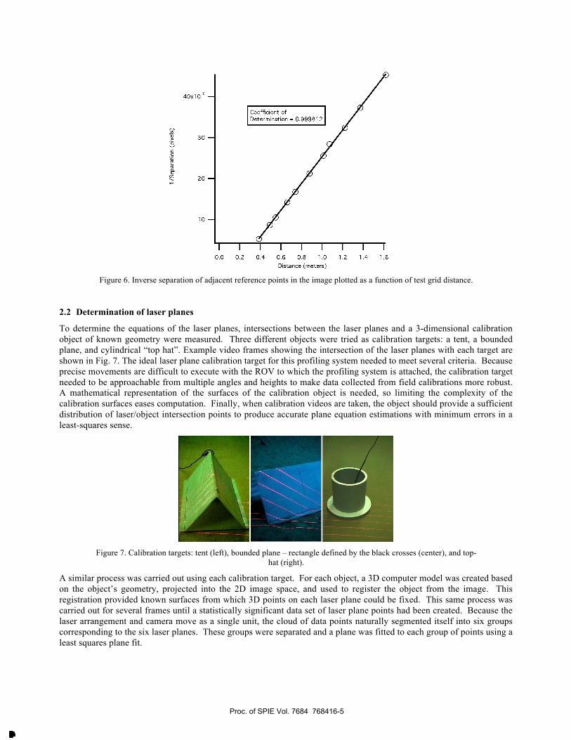
To find the focal length of the virtual camera, images of the same grid target were captured at several distances from an

arbitrary origin. The images were corrected using the warping process described above, and the average separation

between adjacent grid points (white dots) in each image was measured. Based on the pinhole camera model, the

separation between the points should tend to infinity as the distance from the object to the optical center tends to zero.

Using this relationship, the offset of the measured target distances was determined by plotting the inverse target point

separation against the measured distance, as shown in Fig. 6. The intercept of the best-fit straight line with the distance

axis indicated the difference between the measured and the correct distance. The linearity of the inverse separation vs.

distance plot was important as it both validated the assumption that the distortion of the camera arrangement was

repeatable, and thus correctable via the warping process, and it indicated how well the virtual camera fit the pinhole

camera model. For a perfect fit the points would be precisely linear. In this experiment, a coefficient of determination

of 0.999812 for the linear regression of the eleven data points was obtained.

The focal length of the virtual camera was determined according to the simple trigonometric relationship,

f =aX

A (1)

where f is the focal distance, a the pixel separation in the image, X the corrected distance, and A the actual point

separation, i.e. 2.54 cm. The focal distance for each measurement range was calculated and the results were averaged to

determine the best estimate.

Using a Cartesian world coordinate system with its origin at the optical center of the virtual camera and the x-axis

extending along the camera’s forward axis, the 3-dimensional world coordinates map to 2-dimensional image

coordinates using the following formulae:

xim =ywxw

f +Cimx (2)

yim =zwxw

f +Cimx (3)

where (xim, yim) are image coordinates, (xw, yw, zw) world coordinates, f the focal distance of the virtual camera in pixels,

and (Cimx, Cimy) the pixel coordinates of the center of the image.



40x103 -

30 -

20 -

10

Coefficient ofDetermination = 0.999812

I I I I I I

0.0 0.2 0.4 0.6 0.8 1.0 1.2 1.4 1.6

Distance (meters)

Figure 6. Inverse separation of adjacent reference points in the image plotted as a function of test grid distance.

2.2 Determination of laser planes

To determine the equations of the laser planes, intersections between the laser planes and a 3-dimensional calibration

object of known geometry were measured. Three different objects were tried as calibration targets: a tent, a bounded

plane, and cylindrical “top hat”. Example video frames showing the intersection of the laser planes with each target are

shown in Fig. 7. The ideal laser plane calibration target for this profiling system needed to meet several criteria. Because

precise movements are difficult to execute with the ROV to which the profiling system is attached, the calibration target

needed to be approachable from multiple angles and heights to make data collected from field calibrations more robust.

A mathematical representation of the surfaces of the calibration object is needed, so limiting the complexity of the

calibration surfaces eases computation. Finally, when calibration videos are taken, the object should provide a sufficient

distribution of laser/object intersection points to produce accurate plane equation estimations with minimum errors in a

least-squares sense.

Figure 7. Calibration targets: tent (left), bounded plane – rectangle defined by the black crosses (center), and top-

hat (right).

A similar process was carried out using each calibration target. For each object, a 3D computer model was created based

on the object’s geometry, projected into the 2D image space, and used to register the object from the image. This

registration provided known surfaces from which 3D points on each laser plane could be fixed. This same process was

carried out for several frames until a statistically significant data set of laser plane points had been created. Because the

laser arrangement and camera move as a single unit, the cloud of data points naturally segmented itself into six groups

corresponding to the six laser planes. These groups were separated and a plane was fitted to each group of points using a

least squares plane fit.



The major differences between the calibration targets concerned object registration. The plane and tent were registered

by minimizing the sum of the squared differences between reference points, typically corners, in the projected computer

model and corresponding points in the corrected digital image. This method proved to be less accurate than desired. For

the tent, reference points from the digital image were difficult to locate precisely because of poor contrast in the image.

For the plane, frames in which the plane object was nearly parallel to the image plane could not be accurately registered

because the pixel coordinates of the reference points were relatively insensitive to small rotations. For both objects, the

pixel coordinates of the reference points in each image had to be manually identified, which introduced human error and

was time consuming.

The top-hat object was designed to correct the problems with the bounded plane and tent models. The top-hat was

painted to specifically highlight the planar surfaces used to locate the 3D laser plane intersection points. The painting

also made it possible to isolate the object from the image by thresholding, which allowed us to largely automate the

registration process. Registering the top-hat was done by a simulated annealing maximization algorithm in which the

parameter to be maximized was the cross-correlation peak between the object in the image and an image mask made

from the computer model of the object. To prepare the target image for registration, a Laplacian of the Gaussian edge

detector was used to locate the object in the image. Then an image mask of the 3D model was created with points along

the circular edges of the object. Parameters to adjust the rotation and translation of the 3D model were then passed to a

simulated annealing function and the best-fit position and orientation of the object in the image was found. An example

of the registration result is shown in the left panel of Fig. 8. After registration, the equations of the planar faces of the

top-hat were calculated from the model in the world coordinates.

Figure 8. Left: Identified object edges (white) and the registered position of the computer model (red dots); (a)

distortions in the processed image due to shadows and (b) light colored debris in the background. Right: Identified

laser/object intersection points (red).

The laser/object intersection points were extracted from the image using color and adaptive thresholding techniques, an

example of which is shown in the right panel of Fig. 5. Laser points from the image were transformed into 3D

coordinates at the intersection of the pixel rays and the top-hat planes, according to the following formulae. From the

plane equation,

x = a + by + cz (4)

where a, b, and c are the computed coefficients for a top-hat plane. The world coordinates of each laser/object

intersection point on that plane are given by,

xw =a

(1 b tan( y ) c tan( z )) (5)

yw = xw tan( y ) (6)

zw = xw tan( z ) (7)



N

-0.1 -

0.0 -

0.1

0.2 -

0.3 -

£1

C

C

C

C

4.

1.2 1.4 1.5

where, tan( y ) =(xim Cimx )

f (8)

tan( z ) =(yim Cimy )

f (9)

Figure 9. Coordinates of laser points projected on to the x-z plane. Clouds of points are separable and color-coded by laser plane.

Cloud width due in part to laser planes not perfectly perpendicular to x-z plane.

By processing multiple frames in this manner, a 3D cloud of laser points was generated. In the x-z plane, the natural

segmentation of the points into groups was apparent, as illustrated in Fig. 6. For each laser, two sub-groups are

identifiable, one for each of the two target planes. A least squares plane fit was computed for each laser point group to

find the plane coefficients for each laser.

3. RESULTS AND REMARKS

The estimated plane coefficients for the six laser planes using the top-hat target and the registration process described

above are shown in Table I. These values were calculated from laser/object intersection points collected from eleven

video frames. The a values indicate where each laser plane intersects the x-axis and the b and c values relate to rotations

about the y- and z-axes respectively. These plane coefficients are in agreement with the geometry of the profiling system

setup and indicate nearly parallel laser planes with a slight negative rotation about the y-axis and an approximate 40° tilt

relative to the camera’s forward x-axis.

Table I. Laser plane coefficients

Laser 1 Laser 2 Laser 3 Laser 4 Laser 5 Laser 6

a 0.996 1.083 1.171 1.256 1.3409 1.416

b -0.061 -0.060 -0.072 -0.068 -0.083 -0.076

c 0.873 0.874 0.858 0.846 0.852 0.835

The calibration process described has several application specific advantages. First, using calibration targets and a

virtual camera model minimized external measurements that are difficult to make accurately when the device is being

calibrated in the field. The virtual camera model both corrects for distortions and allows for conversion between 2D



image and 3D world coordinates without precise knowledge of the physical camera’s internal arrangement. Finally, with

information about the geometry of the calibration targets, the calibration can be largely automated.

From previous calibrations of similar profiling systems, it is apparent that error in the laser plane coefficients is caused

by both physical distortions in the laser arrangement and random error. Of the three calibration targets used, the top-hat

target had the lowest standard deviation about the rotational plane parameters b and c, indicating the least amount of

random error. The standard deviations of both the b and c values, in Table I, correspond to a standard deviation in angle

of 0.5 degrees. Since each pair of sub-groups in Fig. 6 has a separation of approximately 0.3 m, the error in angle

corresponds to a standard deviation in position of around 3 mm. Assuming the errors are zero-mean random processes,

the final calibration error may be reduced by increasing the number of samples. The above results were obtained with a

DVD quality camcorder. Since then, a HD quality camcorder has been put into service. The higher resolution allows the

same accuracy to be achieved over a larger field of view. An image of the top-hat target is shown in Fig. 10.

Figure 10. Top-hat calibration target image from a HD camcorder using green lasers.

ACKNOWLEDGMENTS

Video footage of the tent and top-hat targets were made in the test tank of the Applied Research Laboratories, The

University of Texas at Austin (ARL:UT). Video footage of the bounded-plane target was from the Measurement and

Analysis of the Relationship between the Environment and Sonar or Synthetic Aperture Sonar performance (MARES)

joint experiment between the NATO Undersea Research Centre (NURC) and ARL:UT. The authors wish to

acknowledge the ARL:UT team, projector leader Marcia Isakson and ROV pilot James Piper, and the outstanding

cooperation by NURC, Mario Zampolli, chief scientist, Captain Andrea Iacono and the crew of the RV Leonardo,

Gaetano Canepa and the Engineering Coordinator Per Arne Sletner for assistance in many areas..

REFERENCES

[1] Tang, D., "Fine-Scale Measurements of Sediment Roughness and Subbottom Variability", IEEE J. Oceanic Eng.,

29, 929-939 (2004).

[2] Briggs, K. B., "Microtopographical Roughness of Shallow-Water Continental Shelves", IEEE J. Oceanic Eng., 14,

360-367 (1989).



[3] Lyons, A. P., Fox, W. L. J., Hasiotis, T., and Pouliquen, E., "Characterization of the Two-Dimensional Roughness

of Wave-Rippled Sea Floors Using Digital Photogrammetry", IEEE J. Oceanic Eng., 27, 515-524 (2002).

[4] Crawford, A. M., and Hay, A., "A Simple System for Laser-Illuminated Video Imaging of Sediment Suspension and

Bed Topography", IEEE J. Oceanic Eng., 23, 12-19 (1989).

[5] Cumani, A., and Guiducci, A., "Geometric Camera Calibration: The Virtual Camera Approach", IEEE Trans.

Consumer Electronics, 8, 375-384 (1995).

[6] Yu, W., "An Embedded Camera Lens Distortion Correction Method for Mobile Computing Applications", IEEE

Trans. Consumer Electronics, 49, 894-901 (2003).

[7] Tsai, R. Y., "A Versatile Camera Calibration Technique for High-Accuracy 3d Machine Vision Metrology Using

Off-the-Shelf TV Cameras and Lenses", IEEE Transactions on Robotics and Automation, RA-3, 323-344 (1987).

[8] Weng, J., Cohen, P., and Herniou, M., "Camera Calibration with Distortion Models and Accuracy Evaluation",

IEEE Transactions On Pattern Analysis And Machine Intelligence, 14, 965-980 (1992).



Calibration of a seafloor micro-topography laser high definition profiler

Documents

Transcript of Calibration of a seafloor micro-topography laser high definition profiler