British Columbian continental shelf as a source of dissolved iron to the subarctic northeast Pacific...

British Columbian continental shelf as a source of dissolved iron

to the subarctic northeast Pacific Ocean

Jay T. Cullen,1 Marina Chong,1 and Debby Ianson1,2

Received 8 August 2008; revised 12 May 2009; accepted 7 July 2009; published 24 October 2009.

[1] The distribution of dissolved (<0.4 mm) iron (Fe) across the continental shelf andslope of Queen Charlotte Sound on the west coast of Canada was examined to estimatethe potential of these waters as a source of Fe to the Fe-limited waters of the subarcticnortheast Pacific. Iron profiles obtained in shelf, slope, and offshore waters demonstratedecreasing concentrations of Fe with distance from the continent. Within 50 m of the shelfsediments dissolved Fe concentrations were 5.3 ± 0.3 nM. This signal was detected,although attenuated by 80%, along the isopycnal surface at offshore stations 40–50 kmseaward of the shelf break, strongly suggesting cross-shelf transport of an Fe-rich plumeoriginating in low dissolved oxygen (<3 ml L�1, <130 mmol kg�1) waters in subsurfacewater over the continental shelf. Several physical mechanisms that may cause theseFe-enriched waters to advect offshore in this region (i.e., tidal currents and Ekmantransport in the bottom boundary layer, coastal downwelling/relaxation from upwelling,and the formation of anticyclonic, westward-propagating, coastal eddies) are discussed.We suggest that strong tidal currents over broad continental shelves may play a key role inFe supply to ocean basins.

Citation: Cullen, J. T., M. Chong, and D. Ianson (2009), British Columbian continental shelf as a source of dissolved iron to the

subarctic northeast Pacific Ocean, Global Biogeochem. Cycles, 23, GB4012, doi:10.1029/2008GB003326.

1. Introduction

[2] Iron (Fe) is an essential micronutrient for marinemicrobes owing largely to the importance of Fe and Fe-sulfur proteins in photosynthetic and respiratory electrontransfer reactions [Kustka et al., 2003; Raven et al., 1999].In oxygenated seawater Fe is only sparingly soluble [Liuand Millero, 2002; Millero, 1998] and its low concentrationin surface waters of remote, high nutrient–low chlorophyll(HNLC) regions limits photosynthetic carbon fixation andnutrient utilization by resident phytoplankton [Boyd et al.,2007; Coale et al., 1996; de Baar et al., 2005] and thecarbon use efficiencies of heterotrophic marine bacteria[Tortell et al., 1999, 1996]. As a consequence of itsregulatory role on primary productivity in the open ocean,the marine cycling of Fe is closely linked to that of carbonand nitrogen [Falkowski, 1997]. Motivation to understandthe dominant sources and sinks of biologically utilizableFe to and from the sea is understandably high [Hendersonet al., 2007].[3] The vertical and horizontal distribution of Fe in

seawater is regulated by the balance between input andremoval processes and underlying biological, chemical andphysical transformations of Fe species in the ocean’s interior

[Johnson et al., 1997; Moffett, 2001]. There exists apronounced onshore-offshore gradient in surface water dis-solved Fe concentrations driven primarily by the proximityof coastal waters to terrestrial, fluvial and sedimentary Fesources. Studies in the productive, seasonal upwelling zonesin the California Current system off the west coast of NorthAmerica and the Peruvian Upwelling system indicate thatthis gradient is enhanced in regions where Fe-rich deepwaters that come in contact with wide reducing shelf sedi-ments are brought to the surface [Bruland, 2005; Chase etal., 2007; Johnson et al., 2001, 1999; Lohan and Bruland,2008]. The elevated Fe levels are observed to have aregulatory effect on phytoplankton community structurewith diatoms dominating in the Fe-rich upwelling watersand picoplankton dominating in low-Fe waters furtheroffshore [Hare et al., 2005; Hutchins and Bruland, 1998;Hutchins et al., 2002]. Thus Fe can play an important role incontrolling productivity and species composition of themicrobial communities even in dynamic, terrestrially prox-imate coastal upwelling environments.[4] The pronounced onshore-offshore gradient in dis-

solved and suspended particulate Fe concentrations at thecontinental margins represent a potential source of Fe to thepredominantly oligotrophic open ocean basins. Iron belowthe surface mixed layer is less likely to be scavenged orused by the biota than in the surface layer, thus its residencetime may be longer and appreciable physical transport morefeasible. However, fluxes of Fe from the coastal ocean to theinterior are poorly constrained at present [Henderson et al.,2007]. A recently discovered transport mechanism that

GLOBAL BIOGEOCHEMICAL CYCLES, VOL. 23, GB4012, doi:10.1029/2008GB003326, 2009

1School of Earth and Ocean Sciences, University of Victoria, Victoria,British Columbia, Canada.

2Fisheries and Oceans Canada, Institute of Ocean Sciences, Sidney,British Columbia, Canada.

Copyright 2009 by the American Geophysical Union.0886-6236/09/2008GB003326

GB4012 1 of 12

significantly impacts the Fe budget of the northeast Pacificis the formation of westward moving, anticyclonic, meso-scale coastal eddies [Ladd et al., 2005; Tabata, 1982; Milleret al., 2005]. Called Haida eddies in our study area, theyform off the southern tip of the Queen Charlotte Islands inlate winter and track westward into the subarctic northeastPacific [Crawford et al., 2002]. Haida eddies can beobserved using satellite altimetry as areas of elevated seasurface height and recent work has found that these eddiestransport from 3000 to 6000 km3 of water up to 1000 kmwest into the Gulf of Alaska, where Fe limitation ofprimary productivity occurs [Whitney and Robert, 2002].In the first detailed study of the biogeochemistry of theseeddies, a Haida eddy that formed in the winter of 2000 wasfollowed for 20 months and sampled repeatedly for nutrientdynamics [Peterson et al., 2005]. Total dissolved Fe con-centrations (0.2 mm filtered, stored at pH 1.5 > 7 monthsand microwaved before analysis) in a forming eddy were ashigh as 5 nmol L�1 in the upper 200 m of the water column[Johnson et al., 2005]. The labile and total Fe concentra-tions in the observed eddy decreased quickly over the firstyear but still contained 1.5 to twofold more Fe thansurrounding waters 16 months later. According to estimatesby Johnson et al. [2005], 5–50% of the dissolved Fe in thesoutheastern Gulf of Alaska reaches this region through heformation and passage of Haida eddies, indicating that theseeddies may represent the dominant mechanism where Fefrom the margin is transported to the HNLC subarcticnortheast Pacific.

[5] Indeed, there is tantalizing evidence that Fe from thecontinental margin can be transported great distances andmay represent a significant source of biologically availableFe to open oligotrophic and high nutrient–low chlorophyll(HNLC) areas of the ocean [Lam and Bishop, 2008; Lam etal., 2006]. Extended X-ray absorption fine structure analysis(EXAFS) of micron-sized Fe-rich particles collected in theupper 200 m at Ocean Station Papa (50�N, 145�W) indicatedthat the chemical composition was best fit by a mixture offerrihydrite (Fe5O3(OH)9) and goethite (FeO(OH)). Thismineral composition and depth distribution combined witha tracer study using a general ocean circulation modelsuggested that the particles likely originated on the conti-nental margins and were transported horizontally (�900 km)into the basin at depths 0–300 m [Lam et al., 2006]. Indeed,continental shelf sources of Fe and lateral transport processesmay represent a heretofore underappreciated long-rangecontributor to the biologically labile pool of Fe in remoteocean ecosystems.[6] In this study we investigate the distribution of dis-

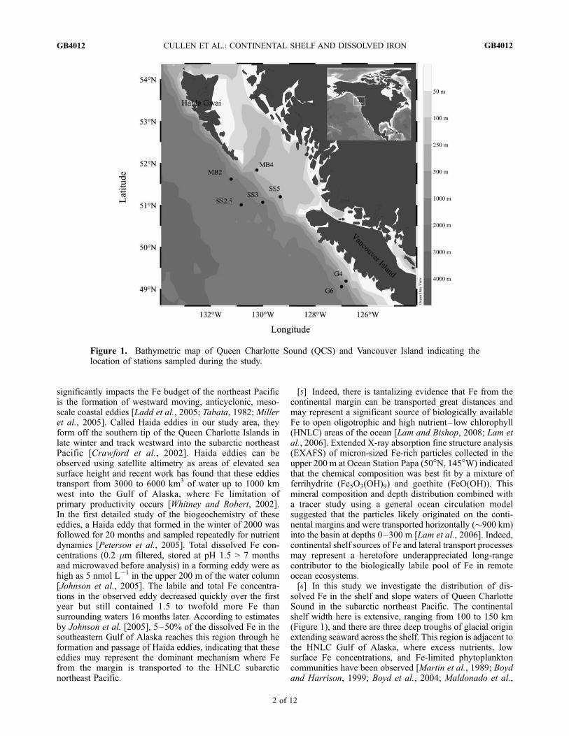
solved Fe in the shelf and slope waters of Queen CharlotteSound in the subarctic northeast Pacific. The continentalshelf width here is extensive, ranging from 100 to 150 km(Figure 1), and there are three deep troughs of glacial originextending seaward across the shelf. This region is adjacent tothe HNLC Gulf of Alaska, where excess nutrients, lowsurface Fe concentrations, and Fe-limited phytoplanktoncommunities have been observed [Martin et al., 1989; Boydand Harrison, 1999; Boyd et al., 2004; Maldonado et al.,

Figure 1. Bathymetric map of Queen Charlotte Sound (QCS) and Vancouver Island indicating thelocation of stations sampled during the study.

GB4012 CULLEN ET AL.: CONTINENTAL SHELF AND DISSOLVED IRON

2 of 12

GB4012

1999]. Horizontal Fe gradients are therefore likely to be largeand fluxes from the continental shelf potentially important tothe biological community for the periodic relaxation of Felimiting conditions experienced by large diatoms in theHNLC gyre [Boyd et al., 1998]. We present a set of dissolvedFe profiles from Queen Charlotte Sound, with stationsrepresentative of the continental shelf, the shelf slope, andthe region seaward of the shelf slope break. Potentialphysical mechanisms facilitating offshore transport of Ferich shelf waters into the northeast subarctic Pacific arediscussed and the importance of this transport is examined.

2. Materials and Methods

2.1. Study Site

[7] Three onshore-offshore transects were sampled duringAugust 2004 from the CCGS John P. Tully. The first twowithin Queen Charlotte Sound (MB and SS) crossed theshelf break. The third (G) on the west coast of VancouverIsland (Figure 1) ended at the shelf break. The MB linecrossed the Moresby Trough, a steep submarine canyon ofglacial origin transecting the continental shelf. The SS linefollowed the Goose Island Trough, a similar canyon, to thesouth of the MB line. Water column profiles were collectedat each station.

2.2. Sampling Protocol

[8] Seawater was collected for trace metal analysis usingTeflon

1

coated 10 or 12 L GO-Flo bottles (General Oceanics)deployed on a Kevlar line and tripped at depth with Teflon

1

messengers [Bruland et al., 1979]. On board, in the ship’s wetlab, the bottles were overpressured with high-purity nitrogengas. Acid-washed Teflon

1

tubing connected the GO-Flobottles to in-line acid-cleaned acrylic filtration units(Geofilter

1

) that were contained in a Class 100 (HEPA)laminar flow bench. The seawater samples were filteredthrough acid-washed 142 mm diameter 0.4 mm polycar-bonate membranes (Isopore) into 500 mL acid-cleaned low-density polyethylene bottles. The sample bottles weredouble-bagged, kept in the cooler through the durationof the cruise, and then acidified to pH 2 with 12 N HCl(SeastarTM) upon return to the laboratory. In additionseawater samples were drawn from a 24-place rosettemounted with 10 L PVC Niskin bottles and were analyzedfor dissolved nutrients and oxygen. Conductivity, temper-ature and depth (CTD) profiles were taken using a SeaBirdSBE 911Plus CTD and sigmaT was calculated fromtemperature (T) and salinity (S) using the equations of[Millero and Poisson, 1981]. Transmission of light at 660 nmwas measured with a 25 cm path length Sea Tech instrumentinterfaced with the SBE 911Plus.

2.3. Reagents

[9] SeastarTMBaseline (SEASTARChemicals Inc., Sidney,British Columbia) trace metal pure hydrochloric acid (HCl33% w/w) and ammonia (NH3 20% w/w) were used toacidify seawater samples and subsequently to raise the pHback to 8.0 before analysis. Milli-Q water (>18 Mohm cm)was used for all rinsing and sample preparation. The Fe-binding ligand, 2,3-dihydroxynaphthalene (DHN) (AcrosOrganics) was dissolved in Milli-Q water by heating inthe microwave for 10 s at a time until fully dissolved.

Ammonia was added (final concentration of 1%) and thenthe solution was purified by shaking with 5 mL of chloro-form for 3 min. The solution was allowed to settle andseparate and the DHN in the aqueous phase was extractedwith a pipette into another container and cleaned withchloroform a second time. The DHN was then pipetted intoa 30 mL Teflon1 PFA bottle and diluted 10–15 fold(depending on concentration) with distilled methanol. Theanalytical sensitivity of the DHN was found to remainconstant upon repeated measurements of low-Fe seawaterwith different batches of the purified ligand, indicating thatany error associated with the DHN concentration has anegligible effect on the sensitivity.[10] A combined catalytic oxidant and buffer solution was

prepared and purified (C. van den Berg, personal commu-nication, 2005) as follows: the catalytic oxidant bromatewas prepared using potassium bromate (Fluka) dissolved inMilli-Q water (0.45 M). To remove any trace metals in thereagent, 100 mM of MnO2 was added and the solution wasstirred a minimum of 2 h. The buffer, piperazine-1,4-bis(2-hydroxypropanesulfonic acid) (POPSO), was made up to1 M in a 1 M ammonia solution (pH 8). The POPSO wascleaned with MnO2 as well. The purified bromate was thenfiltered through an acid rinsed 0.2 mm sterile filter (Sarstedt)and an appropriate volume of POPSO was filtered and addedto the solution. A final cleaning with MnO2 was performedbefore the bromate/POPSO solution was used for analysis.[11] MnO2 was prepared by mixing 0.02 M KMnO4 with

0.03 MnCl2 and stirred while adding 0.1 M NaOH until thepH reached 7–8.5 (C. van den Berg, personal communica-tion, 2005). The solution was centrifuged, the supernatantdiscarded, and the process was repeated 3 times. The finalprecipitate was suspended in Milli-Q water at a finalconcentration of 0.05 M.

2.4. Experimental Methods

[12] Standard trace metal clean techniques were applied inperforming Fe analysis by adsorptive cathodic strippingvoltammetry (CSV). Total dissolved Fe concentrations weredetermined following a method developed by [Obata andvan den Berg, 2001] using a Metrohm 663 VA standhanging mercury drop electrode connected to a mAutolabIII potentiostat. For each analysis, 10 mL of acidifiedseawater was pipetted into the voltammetric cell cup andammonia was added to the sample until the pH reached 8.Then 0.2 M of the catalytic oxidant, KBrO3, 0.01 M POPSOto buffer the solution to pH 8, and 20 mM of the Fe-bindingligand, DHN, were added to the cell cup and the solutionwas purged while stirring for 3 min with 0.2 mm filteredhigh-purity nitrogen gas. After degassing, a new mercurydrop was extruded and the deposition potential was held at�0.1 V while stirring for 15 to 180s depending on theconcentration of Fe in the sample to concentrate the Fe-DHNcomplex at the working electrode. The stirrer was thenturned off and the potential was scanned from �0.1 to�0.9 V at a scan rate of 24 mV/s using the sampled dcmode. The concentration of Fe in each sample was deter-mined by standard additions of 0.5 to 2 nM of Fe (III). Theblank was measured to be 50 pM and the detection limit,calculated as 3 times the standard deviation of the concen-tration in low-Fe seawater, was 25 pM based on a 60 s


3 of 12

GB4012

deposition. Accuracy of the method was determined bymultiple analyses of the SAFE D2 Fe standard (n = 10,[Fe]T = 1.01 ± 0.1 nM; consensus value 0.91 ± 0.17 nM)[Johnson et al., 2007].[13] Nitrate (nitrite plus nitrate) samples were analyzed

onboard with a TechniconTM Autoanalyser II [Wood et al.,1967]. Oxygen samples were also measured on board. Theywere titrated to a colorimetric endpoint using an automatedWinkler titration.

3. Results

[14] Vertical profiles of temperature (T), salinity (S),nitrate (NO3

�), dissolved oxygen (O2), and dissolved Fe atStation MB4 and MB2 are presented in Figure 2. Theprofiles of T and S along the line were similar withindications of fresher (by about 0.4 PSU) in the upper80 m inshore at the shelf break. The temperature in that depthrange decreased rapidly from the surface and was about thesame at each station. Cooler water (� 0.5�C) was observedinshore at MB4 in the depth range 120–200 m relative toMB2. However, there was no significant difference indensity with depth and so no evidence of upwelling ordownwelling at the time of our study. Dissolved nitrateconcentrations were depleted in surface waters at bothstations with minimum values of 0.54 mM (10 m) and

0.18 mM (10 m) at MB4 and MB2, respectively. Below100 m nitrate concentrations were higher with depth atMB4 than the offshore station reaching maximum concen-trations of 44.1 mM at a depth of 195 m (Figure 2c).Dissolved O2 concentrations decreased with depth at bothstations (Figure 2d). At MB4 surface (10 m) concentra-tions were 6.07 mL L�1 (265 mmol kg�1) and decreased toa minimum of 1.95 mL L�1 (84.6 mmol kg�1) at 195 mjust above the bottom. Dissolved O2 concentrations were6.56 mL L�1 (286 mmol kg�1) at 10 m depth offshore atMB2 and dropped to a minimum value of 0.28 mL L�1

(12.2 mmol kg�1) at a depth of 500 m. At MB4 dissolvedFe concentrations were lowest in surface waters with aminimum value of 0.36 ± 0.06 nM at 20 m and increasedto a maximum value of 3.5 ± 0.6 nM in the 195 m deepsample (Figure 2e). The dissolved Fe profile demonstratedless vertical structure at MB2 with a minimum value of0.33 ± 0.03 nM at 10 m depth and a maximum value of1.62 ± 0.12 nM at 700 m. The subsurface dissolved Fepeak at MB4 was accompanied by a minor reduction inbeam transmission (Figure 2f).[15] Similar to the MB line there is little across-shore

variability in T and S profiles along the SS line (Figures 3aand 3b). SS runs along a trough. Dissolved nitrate concen-trations in surface waters (10 m) were higher inshore (SS5,5.53 mM) and decreased offshore (SS3, 0.39 mM; SS2.5,

Figure 2. Vertical profiles at stations MB2 and MB4 of (a) temperature, (b) salinity, (c) nitrate,(d) oxygen, (e) dissolved Fe, and (f) beam attenuation as % transmission. Error bars in Figure 2e representthe standard error of replicate analyses of each sample. Bottom depth at MB4 is indicated by hatcheddouble bar in Figure 2f (200 m). Bottom depth for MB2 was 2200 m.


4 of 12

GB4012

0.18 mM) (Figure 3c). Nitrate concentrations increased withincreasing depth at all stations reaching maximum values of37.9 mM, 45.4 mM, and 45.2 mM for depths of 250, 900 and900 m at stations SS5, SS3 and SS2.5, 232, respectively.Similar to the MB Line dissolved O2 concentrations werehighest in the upper 50 m of the water column at all stations(Figure 3d). Inshore at SS5, dissolved O2 had a maximumof 6.20 mL L�1 (271 mmol kg�1) at the surface withconcentrations generally decreasing with depth to a mini-mum value of 1.68 mL L�1 (73 mmol kg�1). Surface waterconcentrations were similar at SS3 with a range of 5.11–6.06 mL L�1 (223–265 mmol kg�1) in the upper 50 m.Below 50 m concentrations at SS3 decreased with depthreaching a minimum of 0.32 mL L�1 (13.9 mmol kg�1) at1000 m. Dissolved O2 concentrations were > 5.08 mL L�1

(221 mmol kg�1) in the upper 50 m of the water column at theoffshore station SS2.5 and decreased rapidly to a minimum of0.22 mL L�1 (9.56 mmol kg�1) at 900 m. Vertical profiles ofdissolved Fe concentrations along the SS Line are presentedin Figure 3e. Concentrations at the inshore station SS5 werelowest at 10 m depth (0.48 ± 0.1 nM) and increased tomaximum concentrations of 5.31 ± 0.28 nM near to the shelfsediments. The vertical profile at the shelf slope station SS3was typified by a broad subsurface concentration maximumbetween 100 and 500 m. Concentrations in this maximumwere highest at 200 m (5.07 ± 0.74 nM) with a range of

1.45–5.07 nM). In the upper 75 m concentrations were< 0.31 nM. Below the subsurface maximum dissolvedFe concentrations dropped to a minimum of 0.71 ± 0.06 nMbefore increasing to 1.27 ± 0.003 nM at 900 m. Offshoreat SS2.5 Fe concentrations were below 0.37 nM in theupper 50 m and rose to a subsurface peak of 0.92 ± 0.09 nMat 300 m with a maximum concentration at the deepest depthsampled (900 m) of 1.20 ± 0.10 nM (Figure 3e). Thesubsurface maxima in dissolved Fe at SS5 and SS3 corre-sponded with identifiable subsurface reductions in lighttransmission (Figure 3f).[16] Figures 4a–4c summarize hydrographic data and

dissolved nitrate, oxygen and Fe concentrations at twostations G4 and G6. The T and S data show that the coastalcirculation south of Queen Charlotte Sound was significantlydifferent. There was a pronounced difference between theoffshore and shelf break station. In general over the shelf onthe G line the water was colder and saltier than offshore at thesame depths, indicative of recent upwelling (Figures 4a–4b).In addition surface salinities off the west coast of VancouverIsland [Nemcek et al., 2008, Figure 1b] were higher thanstations in the Sound. Surface temperature was highestoffshore at G6 (17.48�C at 5 m). Inshore at G4 surfacetemperatures were �3�C lower (T = 14.41�C at 5 m).Dissolved nitrate tended to be higher and oxygen concen-trations lower for a given depth inshore at G4 compared to the

Figure 3. Vertical profiles at stations SS2.5, SS3, and SS5 of (a) temperature, (b) salinity, (c) nitrate,(d) oxygen, (e) dissolved Fe, and (f) beam attenuation as % transmission. Error bars in Figure 3e representthe standard error of replicate analyses of each sample. Bottom depth at SS5 is indicated by hatched doublebar in Figure 3f (280 m). Bottom depths for SS3 and SS2.5 are 1400 m and 2200 m, respectively.


5 of 12

GB4012

offshore station G6 (Figures 4c and 4d) as anticipated withupwelled waters over the shelf. Dissolved nitrate concen-trations were 0.3 mM at 2 m depth and increased to amaximum of 34.3 mM at 126 m depth at G4. Surfaceconcentrations at G6 were 0.29 mM at 10 m and increasedto 46.5 mM at 800 m. Two dissolved Fe measurements weremade at G4 with 0.34 nM detected at 25 m and 1.32 nM at75 m (Figure 4e). Dissolved Fe concentrations were lowerin surface waters offshore at G6 (0.13 nM at 10 m) with asubsurface maximum at 400 m of 2.54 nM. Light wasstrongly attenuated close to bottom depth at G4 while, insubsurface waters at G6 there was little change in %transmission with increasing depth (Figure 4f).

4. Discussion

4.1. Continental Shelves as Sources of Fe

[17] Along continental margins, waters are typically Fereplete relative to the Fe requirements of eukaryotic phyto-plankton (but seeHutchins and Bruland [1998] andHutchinset al. [2002]) fueling high in situ rates of primary production.Concentrations of dissolved and particulate Fe in coastalwaters are higher largely owing to their proximity to terres-trial inputs from rivers [Buck et al., 2007; Wetz et al., 2006]and the atmosphere [Gao et al., 2003], resuspension ofbottom sediments [Nedelec et al., 2007], flux of reduced

Fe from sediments during diagenesis [Elrod et al., 2004;Johnson et al., 1999; Ussher et al., 2007; Lohan andBruland, 2008] and in productive eastern boundary systemsby seasonal, wind-driven upwelling events that bring higherFe waters to the surface [Bruland et al., 2001; Chase et al.,2005a, 2002].[18] Previous studies of the Fe cycle in coastal waters

have highlighted the importance of shelf width on the fluxof Fe from reducing sediments as well as the on-shelftransport of Fe enriched subsurface waters during winddriven upwelling events [Bruland, 2005; Bruland et al.,2001, 2005; Chase et al., 2007]. For example, the conti-nental shelf of central Peru can extend for 150 km offshoreand total dissolved Fe concentrations approach values of118 nM in these suboxic shelf waters [Bruland et al., 2005].In southern Peru however, the shelf is only about 10 kmwide and here near bottom dissolved Fe concentrations liebetween 1.4 to 4.6 nM. The effect of shelf width on Feconcentrations was also investigated off central Californiaand the Oregon coast of western North America [Bruland etal., 2001; Chase et al., 2005a, 2007]. In both cases, totaldissolved Fe in surface waters over wider shelves wassignificantly higher than Fe in waters south of where theshelf is only a few kilometers wide. In our study, the regionof the continental shelf where the MB and SS lines aresituated is broader than the shelf areas off California and

Figure 4. Vertical profiles at stations G4 and G6 of (a) temperature, (b) salinity, (c) nitrate, (d) oxygen,(e) dissolved Fe, and (f) beam attenuation as % transmission. Error bars in Figure 4e represent thestandard error of replicate analyses of each sample. Bottom depths at G4 (200 m) and G6 (900) areindicated by hatched double bars in Figure 4f.


6 of 12

GB4012

Oregon, and more similar to Peru at a width of approxi-mately 150 km. In comparison, the shelf off the west coastof Vancouver Island where the G line lies is about 40 kmwide, still wider than Oregon and California. Station G6possesses a middepth dissolved Fe concentration (2.54 ±0.12 nM, Figure 4e) that is approximately half of what isobserved at station SS3 (5.07 ± 0.74 nM, Figure 3e). At ourshallow water stations (MB4, SS5 and G4) the presence ofelevated concentrations of dissolved Fe in waters in closecontact with the sea bottom agrees with previous findingsthat point to reducing sediments as major sources of Fe tooverlying waters [Elrod et al., 2004; Johnson et al., 1999;Ussher et al., 2007]. Thus the variation we observe in thevertical distribution of dissolved Fe in our study may reflectthe much broader shelf width in Queen Charlotte Soundrelative to the G line off of Vancouver Island, allowingbenthic waters to be in contact with a larger area of Fe-richsediments.[19] An onshore-offshore dissolved Fe gradient is evident

in the middepth and near bottom waters of stations fromboth the MB and SS lines (Figures 2e and 3e). This decreasein dissolved Fe across the shelf slope probably reflects asimilar gradient in total (dissolved and particulate) Fe, atrend that has been reported in studies off the California[Johnson et al., 2001], and Oregon shelf [Chase et al.,2005b, 2002]. Higher concentrations of dissolved Fe foundat the coastal stations compared to offshore sites is consis-tent with the idea that continental margins are a significantsource of Fe to slope waters and potentially the oceaninterior. Indeed, recent work in the eastern and westernsubarctic Pacific demonstrates that lateral advection ofsediments from continental shelves are the most likelysource for stocks of particulate Fe detected in the upper500 m of these remote HNLC regions [Lam and Bishop,2008; Lam et al., 2006]. Calculations assuming that sedi-ments from coastal shelves may be more labile thanatmospheric dust and that higher dissolved Fe is observedto accompany the subsurface particulate plume suggest thatsubsurface Fe delivery from the shelf is of similar impor-

tance to atmospheric dust in supplementing biological Fedemand in HNLC surface waters [Lam and Bishop, 2008;Lam et al., 2006]. Our results indicate that dissolved Feconcentrations are significantly elevated in waters influ-enced by the continental shelf in Queen Charlotte Sound.Consistent with the studies of [Lam and Bishop, 2008; Lamet al., 2006] we hypothesize that advection of this bottomlayer across the shelf at intermediate depths is a criticalprocess with respect to open ocean Fe budgets that results inthe transport of Fe-rich shelf waters across the shelf slopebreak. Unlike source terms for Fe in surface waters, sub-surface transport of the Fe enriched shelf water will limitlosses of Fe to both biological uptake and particle surfacescavenging, processes that are heightened in productivesurface waters.[20] To track the movement of waters within the benthic

layer, the dissolved Fe concentrations are plotted against sTand presented in Figure 5. The most striking featureemerging from the density plots shown in Figure 5 is thepresence of a layer of elevated Fe at sT values between 26and 27, surfaces that represent waters in contact withreducing shelf sediments. Less dense waters show relativelylow Fe concentrations with little variation across the shelfbut in the most dense shelf waters, the increase in dissolvedFe is dramatic. In the northern end of the sound along theMB line, this layer is observed between 75 and 150 m depthboth over the shelf and offshore. South of this transect, asimilar feature is visible along the SS line where dissolvedFe is high below 250 m over the shelf, shoals slightly to200 m over the shelf slope break and then sinks to 300 moffshore. Limited data collected along the G Line suggestthe process is taking place along the west coast of VancouverIsland given the similarity between the G6 and SS3 dissolvedFe profiles.[21] The trend in dissolved Fe distribution across the

continental shelf is highly suggestive of some means ofcross-shelf transport of high-Fe waters (Figure 5). By thetime the water originating from the shelf reaches theoffshore stations, however, only 50 to 80% of the dissolved

Figure 5. The concentration of dissolved Fe versus sigma-T for the (a) MB, (b) SS, and (c) G stations.Error bars represent the standard error of replicate analyses of samples.


7 of 12

GB4012

Fe present on the shelf remains in the waters beyond theshelf break as would be expected from dilution as the Fetravels from its shelf source and gradually mixes withsurrounding lower dissolved Fe waters. An additionalmechanism for the loss of dissolved Fe is through increasedFe oxide formation and chemical scavenging as the shelfwaters mix with more oxygenated waters, effectively re-moving dissolved Fe from the water column and providinga source for the oxidized labile particulate Fe in thesubsurface observed by others in similar ocean regimes[Lam and Bishop, 2008; Lam et al., 2006; Nedelec et al.,2007]. For example, along the MB line, the oxygen con-centrations in the Fe-rich water mass found between depthsof 100–150 m is 1.8–3.2 mL L�1 inshore at MB4 andincreases to 3–3.8 mL L�1 at the offshore station MB2(Figures 2d and 5a). Increased oxygen concentrations andpH in these Fe rich isopycnal surfaces will increase oxida-tion and scavenging rates and partition more dissolved Feinto particulate and colloidal pools as one moves offshore.At some stations the high dissolved Fe features werecoincident with decreased light transmission (e.g., SS5 andSS3, Figure 3f) suggesting the presence of suspended sedi-ments while other dissolved Fe subsurface peaks occurredindependent of increased light attenuation. Light attenuationat 660 nm is most sensitive to particles 1–100 mm in size[Sullivan et al., 2005] and can indicate the presence ofresuspended shelf sediments or fresh precipitates in the watercolumn. However, beam transmission may not detect thepresence of colloidal material that could contribute signifi-cantly to our observed dissolved (<0.4 mm) Fe concentra-tions. The lack of size-fractionated particulate Fe dataprecludes us from determining directly whether our highdissolved Fe plumes contain significant quantities of partic-ulate Fe and/or colloidal Fe. Nonetheless, subsurface plumesenriched in particulate Fe are detected 102–103 km offshoreand likely contribute significantly to open ocean Fe budgets[Lam and Bishop, 2008; Lam et al., 2006]. Below we discussseveral physical processes that may aid in transporting theseFe-enriched margin waters of the Queen Charlotte Soundacross the shelf break.

4.2. Physical Transport of Subsurface Water Off theContinental Shelf

[22] Exchange between the coastal and open oceanremains understudied. Often fronts that prohibit exchangeare formed off the shelf break. There are also episodic jets,filaments and eddies that carry coastal water offshore in theupper layer, especially in Eastern Boundary Currents(EBCs) [e.g., Strub et al., 1991]. With the exception ofeddies this transport occurs primarily in the upper layer[e.g., Brink et al., 1991]. Onshore flow of water occurs inthe lower layer during upwelling events, characteristic ofEBCs, and offshore flow may occur during relaxationperiods between upwelling events or during active downw-elling [Lentz, 1992; Smith, 1994]. Again these exchangesare episodic. Subsurface cross-shelf exchange may occurwhere alongshore currents experience bottom friction (i.e.,Ekman transport) [Brink, 1998; Lentz and Trowbridge,1991]. Although time scales are not particularly welldefined [Brink, 1998] this exchange has the potential tobe more continuous. Coastal upwelling, and sometimes

downwelling, circulation is a feature of ECBs in general[Smith, 1994]. Episodes of either up or downwelling arelikely to affect direction of bottom flow.[23] Downwelling generally pushes subsurface water off-

shore, as the surface flow is onshore, and so is likely toprovide periodic seaward transport. In addition, it has beenhypothesized that even a time of relaxation between up-welling events on the coast may produce a strong pulse ofoffshore flow in the bottom boundary layer [Hales et al.,2006]. Our CTD data suggest that upwelling occurs on theG line, but not in the Sound. Although few data exist, it isgenerally thought that the northern tip of Vancouver Islandis the boundary between summer upwelling and summerrelaxation in the North American west coast ECB. It hasbeen hypothesized that there may be some deep onshoreflow through the canyons in the Sound [Whitney et al.,2005] but otherwise there appears to be little upwelling.Downwelling winds are strong along the entire BC coastduring winter, but downwelling events occur only occasion-ally during summer [e.g., Ianson et al., 2003]. Our CTDdata show no evidence of downwelling at the time of ourstudy. However, during the winter season downwelling islikely to provide strong pulses of Fe from the Sound tooffshore waters.[24] Anticylonic, mesoscale eddies in the Gulf of Alaska

can affect cross-shelf transport by entraining shelf waterinto their core and then propagating away from the coast[Ladd et al., 2005], introducing Fe-rich coastal waters intothis HNLC region. These eddies are generated off the tip ofCape St. James, where warmer, fresher water from HecateStrait flows over the colder, more saline waters of QueenCharlotte Sound [Di Lorenzo et al., 2005]. The resultantbuoyant flow forms plumes which spin off as small anticy-clonic eddies and when the flow is strong, these smalleddies merge to become Haida eddies [Di Lorenzo et al.,2005]. Haida Eddies are observed to convey water,nutrients, and biota characteristic of the Hecate Strait,Queen Charlotte Sound, and West Coast Queen Charlottesarea, westward into the Gulf of Alaska as far out as StationP [Mackas and Galbraith, 2002; Whitney and Robert,2002]. In the winter when these eddies are produced,primary productivity is minimal and surface concentrationsof dissolved Fe and nutrients are presumably much highercompared to the values detected during our samplingperiod. Calculations based on observations of the especiallylarge 1998 Haida eddy show that these eddies can transportup to 5000–6000 km3 of Fe- and nutrient-replete coastalwater every year [Whitney and Robert, 2002].[25] Johnson et al. [2005], also provide an estimate of

the amount of iron transported offshore by Haida eddies.Using a volume of 3100 km3 for a typical newly formededdy, the Haida-2001 eddy was calculated to contain about4.8 � 107 mol of total (particulate and dissolved) Fe.Since at least two eddies are formed annually, the yearlyexport of Fe to offshore waters is then double this amount.In comparison, on the basis of an atmospheric depositionrate of 0.08–0.16 mmol m�1 d�1 [Duce, 1986], Johnson etal. [2005] calculate that over the oceanic area that isaffected by Haida eddies, the annual atmospheric flux ofFe is 2.5–5.0 � 107 mol, the same order of magnitude as


8 of 12

GB4012

Fe transport by one eddy. Thus, Haida eddies are asimportant as atmospheric deposition, a mode that hastraditionally been thought to be the principal source of Feto this remote region.[26] In the summer, during our study, the circulation in

Queen Charlotte Sound is dominated by strong tidal cur-rents. These currents are especially powerful over theextensive shallow (60–120 m deep) banks (Figure 1) andextend to the bottom of the water column [Cummins andOey, 1997; Foreman et al., 1993]. Such currents have beenestablished to have a strong influence on water columnturbulence over shelf areas [Bowers et al., 2005; Xing andDavies, 2002], serving as an important source of energy formixing within the benthic boundary layer. The BC coast isrocky with many fjords and steep bathymetry. As a result,tidal currents near headlands and fjord and channel entran-ces are exceptionally energetic throughout the water columnand at some locations generate shelf waves that allow thehigh energy from these regions to spread along the coastand also into Queen Charlotte Sound [e.g., Foreman andThomson, 1997]. The banks in the Sound have a layer ofclean beach sand (0.5–1 m thick; J. V. Barrie, personalcommunication, 2009) on the top with finer dark sand thathas exceptionally high concentrations of heavy minerals onthe slopes of the banks (roughly 110–140 m depth) [Barrie,1991]. These sands are rich in Fe and are easily suspendedby winter storm waves and local tidal currents [Barrie et al.,1988]. During suspension pore waters will also be liberated.[27] This near bottom Fe-rich water may be transported

from the shelf offshore via Ekman transport. As in thesurface, this transport is a consequence of friction. Mass fluxoccurs perpendicular to the surface friction (in the bottomlayer the ‘‘surface’’ is the sediment-water interface) and to theright in the northern hemisphere [Cushman-Roisin, 1994].Thus, subsurface offshore transport from Queen CharlotteSound requires northwest flow that interacts with the bottom.[28] Current measurements were not made in this study,

however we know that the tidal currents are strong andreach the bottom on the banks [Foreman et al., 1993]. Thesecurrents are semidiurnal and so cause flow toward thenorthwest twice daily. In addition there is a polewardflowing undercurrent (the California undercurrent), as is acommon feature of EBCs [Lentz and Trowbridge, 1991]. Atleast at times, this current still persists along the shelf breakbelow 100 m as far north as Queen Charlotte Sound (R. E.Thomson and M. V. Krassovski, The California Undercur-rent: Transporting nutrient rich water from Baja Californiato the Aleutian Islands, manuscript in preparation, 2009),although it appears to be weaker than it is further south.Both the undercurrent and tidal streams could cause nearbottom water to flow off the shelf and slope and provide arelatively consistent source of iron to the adjacent offshorewaters at middepths.[29] To make a rough estimate of how much Fe may be

exported via Ekman transport we first consider the case of asteady current, which has been well studied, and thenexpand the problem to include the fluctuating nature oftidal currents. We assume that fluid transported from thebanks during a tidal cycle becomes mixed so that theprocess is not reversible.

[30] These estimations require the use of physical termsthat are not well known thus we have used more than onemethod (including classical Ekman theory and a popularempirical approach) to allow comparison. First the thicknessof the Ekman layer, DE, is calculated and then the nettransport.[31] Given the latitude (50� N; so f, the coriolis parameter,

is 1.1e�4 s�1) and assuming a range in Kv, eddy viscosity, of0.001–0.01 m2 s�1 (Kv is poorly known but often assumedto be 0.01 m2 s�1 in the upper layer of the ocean and itgenerally decreases with depth), DE is 4–10 m in the Sound.This estimate assumes homogeneous flow and a flat bottom,the classical Ekman approximation; DE = (2 Kv/f )

1/2)[Cushman-Roisin, 1994]. Using a common empiricalapproximation that accounts for nonidealized flow (DE

�0.4u*/f, where u* is the turbulent friction velocity definedbelow [Cushman-Roisin, 1994]), the same range of Kv anda typical lower-layer current (v) of 0.1 m s�1 (an averagetidal current [Foreman et al., 1993] and also the expectedvelocity of the CUC (Thomson and Krassovski, manu-script in preparation, 2009)) yields a thicker DE of 10–30 m. Note that u* = v Kv/DE so that DE = (0.16 v Kv/f

2)2/3.The combination of these estimates ranges over an orderof magnitude, and is similar to an in depth analysis ofmore than one measure of DE from field data collected inAugust over the Oregon shelf [see Perlin et al., 2007,Figure 7].[32] The classical net transport, U, can be approximated

as v DE/2 [Cushman-Roisin, 488 1994]. Using the classicalDE estimated above (3–10 m) and a conservative v of0.1 m s�1 (note that maximum tidal currents near thebottom are about 0.3 m s�1) [Foreman et al., 1993], U is0.2–0.5 m2 s�1. U may also be estimated as t/r f, where r isthe density of the fluid (for our purposes 1000 kg m�3) andt is the stress in the v direction (�CD v2). In this case thepoorly known quantity is the drag coefficient, CD, ratherthan the eddy viscosity Kv. Thus U is 0.2 m2 s�1 using aCD of 10�3 [Perlin et al., 2007] and v of 0.1 m s�1, asabove. It is satisfying that both estimates agree and are ofthe same order.[33] We now consider the fact that the tidal currents

fluctuate in time. In Queen Charlotte Sound the tidal periodis 12.42 h. The relationship for U above (t/r f ) becomesmodified so that U = ft/[r ( f 2 � W2)]) where W is the tidalfrequency (K. Brink, personal communication, 2009). Thetransport U increases above the steady state case by about40%. The length scale associated with this transport isU/(DE W) and is about 200–500 m using a midrange DE

of 10 m. Therefore tidal Ekman transport may move Fe richwater hundreds of meters off the shelf during each tidalcycle and our assumption that these waters become mixedand do not simply slosh back appears reasonable. Inaddition the process whereby Ekman transport is con-strained or ‘‘shut off’’ over a stratified slope [Lentz andTrowbridge, 1991] after a certain amount of time [Garrett etal., 1993] is unlikely to occur over such short (semidiurnal)tidal periods (K. H. Brink and S. J. Lentz, manuscript inpreparation, 2009) so this potential iron source over theslope sediments appears to be relatively robust as well asover the banks.


9 of 12

GB4012

[34] Given an average Fe concentration near the bottom atMB4 and SS5 (4 ± 1 nM), a rough estimate of the alongshoreextent of the banks in the Sound (150 km) and scalingU (using the conservative estimate of 0.2–0.5 m2 s�1)down by a factor of 3 (so that only the northwest compo-nent of the tidal currents is included over time scalesexceeding many days), the resulting bottom Ekman trans-port of Fe out of Queen Charlotte Sound is 1–4 � 106 molFe yr�1. This flux is an order of magnitude lower than theestimated annual supply of Fe via atmospheric deposition tothe subarctic Northeast Pacific of 2.5–5.0 � 107 mol Feyr�1 [Duce, 1986] and transport estimated for a singleHaida eddy of 4.8 � 107 mol eddy�1 [Johnson et al.,2005]. However, our estimate considers tidal currents in theSound alone and does not include the other shelf areasbordering the Gyre. Nor does it include potential transportdue to the California Undercurrent or pulses from winterdownwelling. Furthermore, the estimate is conservative andwould be as much as ninefold larger if we used theempirical formulation of Ekman depth and a larger tidalcurrent. The only assumption that would cause us tooverestimate this Fe contribution is that the tidal transportis well mixed with surrounding waters and that a portion ofthe Fe does not slosh back on to the shelf in during the nexttidal cycle; however, we have also chosen a smaller rangein KV relative to subsurface values from other tidally activebanks (e.g., George’s Bank KV = 0.02–0.06 512 m2 s�1)[Chen and Beardsley, 1998, and references therein]. Inaddition, while the absolute transport may be of a lowerorder, the Fe may be more labile [Lam and Bishop, 2008]than eolian forms and it is delivered subsurface so that itsresidence time will be considerably longer.[35] We hypothesize that while a combination of the

above mechanisms (and perhaps others) contributes to thetransport of continental shelf Fe offshore, at the time of ourstudy, tidal currents likely played an important role in theseaward transport of Fe that we observed. Thus, we suggestthat the combination of strong and dominant tidal flow andextensive shallow banks provide an ever-present source ofsubsurface Fe-rich water to the Alaskan Gyre in our studyregion and note that during the winter months it is likelythat this flux of Fe is enhanced. Previous work in theAlaskan Gyre has linked eolian supply of Fe to episodicevents where phytoplankton biomass was enhanced relativeto average background levels [Boyd et al., 1998; Bishop etal., 2002]. Given existing uncertainties in aerosol solubilityand the time scale on which eolian Fe signals are processedin open ocean surface waters it remains difficult to unequiv-ocally relate dust deposition events to distinct biogeochem-ical responses [Boyd et al., 2009]. Therefore, it is possiblethat lateral transport processes like mesoscale eddies[Johnson et al., 2005], and the subsurface transport of Fefrom continental shelves outlined here and detected in theinterior of the northwest and northeast Pacific [Lam et al.,2006; Lam and Bishop, 2008] may also be responsible forFe induced phytoplankton blooms in the HNLC waters.Subsurface Fe could be introduced to the photic zone by netupwelling (�3 m/yr) in the gyre generated by basin-scalewind stress curl [Gargett, 1991], or by deep mixing events

which may help to explain high chlorophyll a events knownto occur in winter [see Boyd et al., 1998].

5. Conclusions

[36] Dissolved Fe concentrations in waters over the con-tinental shelf of Queen Charlotte Sound are elevated relativeto near surface and slope waters, especially within thebottom 20–50 m of the water column. As nutrients insurface waters show depletion at all stations, this regionappears to be Fe replete and highly productive. At depth,dissolved Fe concentrations decrease significantly acrossthe shelf slope and plots of Fe versus density suggest thatthis exceptionally Fe-rich bottom layer in shelf waters flowsoffshore across the slope following isopycnal surfaces. Thebroad continental shelf in this area has an important role asthe primary source of iron to overlying waters through theresuspension of sediments and benthic fluxes. There arefour possible mechanisms that may contribute to the off-shore, downslope advection of this Fe-replete layer: tidalcurrents, Ekman transport within the bottom boundary layer,upwelling/downwelling along the shelf break, and theformation of Haida eddies. Our estimates suggest that tidalcurrent induced Ekman transport of Fe across the shelfbreak may represent a source of Fe to the ocean interior thatis within an order of magnitude of eolian and mesoscaleeddy fluxes determined by others. Future work quantifyingthe effect of these physical processes on Fe distribution isneeded in order to gain a more empirical understanding oftheir potential of supplying Fe-rich, coastal waters to theocean interior and more generally the importance of conti-nental shelf derived Fe in open ocean Fe biogeochemicalbudgets.

[37] Acknowledgments. We thank the captain and crew of the CCGSJohn P. Tully for their assistance on this research expedition. We are gratefulto M. Robert, D. Anderson, and D. Tuele for technical support at sea;M. Hennekes for the nutrient analysis; and K. Brown for trace elementsampling. We thank G. Gatien for data formatting and archiving. We aregrateful to J. V. Barrie for his input concerning the character of sedimentsin the sound and to K. Brink, J. Klymak, and W. Williamson for manyhelpful conversations concerning the bottom boundary layer. Funding forthis work was provided by NSERC grants to J.T.C. and financial supportfrom Fisheries and Oceans Canada to D.I.

ReferencesBarrie, J. V. (1991), Contemporary and relict titaniferous sand facies on thewestern Canadian contintental shelf, Cont. Shelf Res., 11, 67 – 79,doi:10.1016/0278-4343(91)90035-5.

Barrie, J. V., M. Emory-Moore, J. L. Luternauer, and B. D. Bornhold(1988), Origin of modern heavy mineral deposits, northern BritishColumbia continental shelf, Mar. Geol., 84, 43 – 51, doi:10.1016/0025-3227(88)90124-7.

Bishop, J. K. B., R. E. Davis, and J. T. Sherman (2002), Robotic observa-tions of dust storm enhancement of carbon biomass in the north Pacific,Science, 298, 817–821, doi:10.1126/science.1074961.

Bowers, D. G., K. M. Ellis, and S. E. Jones (2005), Isolated turbiditymaxima in shelf seas, Cont. Shelf Res., 25, 1071–1080, doi:10.1016/j.csr.2004.12.010.

Boyd, P. W., C. S. Wong, J. Merrill, F. Whitney, J. Snow, P. J. Harrison, andJ. Gower (1998), Atmospheric iron supply and enhanced vertical carbonflux in the NE subarctic Pacific: Is there a connection?, Global Biogeo-chem. Cycles, 12, 429–441.

Boyd, P. W., and P. J. Harrison (1999), Phytoplankton dynamics in the NEsubarctic Pacific, Deep Sea Res., Part II, 46, 2405–2432, doi:10.1016/S0967-0645(99)00069-7.


10 of 12

GB4012

Boyd, P. W., et al. (2004), The decline and fate of an iron-induced subarcticphytoplankton bloom, Nature, 428, 549–553, doi:10.1038/nature02437.

Boyd, P. W., et al. (2007), Mesoscale iron enrichment experiments1993–2005: Synthesis and future directions, Science, 315, 612–617,doi:10.1126/science.1131669.

Boyd, P. W., D. S. Mackie, and K. A. Hunter (2009), Aerosol iron deposi-tion to the surface ocean: Modes of iron supply and biological responses,Mar. Chem., doi:10.1016/j.marchem.2009.01.008, in press.

Brink, K. H. (1998), Coastal physical processes overview, in The Sea,vol. 13, edited by A. R. Robinson and K. H. Brink, pp. 37–59,Harvard Univ. Press, Cambridge, Mass.

Brink, K. H., R. C. Beardsley, P. P. Niiler, M. Abbott, A. Huyer, S. Ramp,T. Stanton, and D. Stuart (1991), Statistical properties of near-surfaceflow in the California coastal transition zone, J. Geophys. Res., 96,14,693–14,706, doi:10.1029/91JC01072.

Bruland, K. W. (2005), The role of iron as a micronutrient influencingphytoplankton in coastal upwelling regimes, Geochim. Cosmochim.Acta, 69(10), 1–3, doi:10.1016/j.gca.2005.03.022.

Bruland, K. W., R. P. Franks, G. A. Knauer, and J. H. Martin (1979),Sampling and analytical methods for the determination of copper,cadmium, zinc, and nickel at nanogram per liter level in seawater,Anal. Chim. Acta, 105, 233–245, doi:10.1016/S0003-2670(01)83754-5.

Bruland, K. W., E. L. Rue, and G. J. Smith (2001), Iron and macronutrientsin California coastal upwelling regimes: Implications for diatom blooms,Limnol. Oceanogr., 46(7), 1661–1674.

Bruland, K. W., E. L. Rue, G. J. Smith, and G. R. DiTullio (2005), Iron,macronutrients and diatom blooms in the Peru upwelling regime: Brownand blue waters of Peru,Mar. Chem., 93, 81–103, doi:10.1016/j.marchem.2004.06.011.

Buck, K. N., M. C. Lohan, C. J. M. Berger, and K. W. Bruland (2007),Dissolved iron speciation in two distinct river plumes and an estu-ary: Implications for riverine iron supply, Limnol. Oceanogr., 52(2),843–855.

Chase, Z., A. van Geen, P. M. Kosro, J. Marra, and P. A. Wheeler (2002),Iron, nutrient, and phytoplankton distributions in Oregon coastal waters,J. Geophys. Res., 107(C10), 3174, doi:10.1029/2001JC000987.

Chase, Z., B. Hales, T. Cowles, R. Schwartz, and A. van Geen (2005a),Distribution and variability of iron input to Oregon coastal waters duringthe upwelling season, J. Geophys. Res., 110, C10S12, doi:10.1029/2004JC002590.

Chase, Z., K. S. Johnson, V. A. Elrod, J. N. Plant, S. E. Fitzwater,L. Pickell, and C. M. Sakamoto (2005b), Manganese and iron distribu-tions off central California influenced by upwelling and shelf width,Mar. Chem., 95, 235–254, doi:10.1016/j.marchem.2004.09.006.

Chase, Z., P. G. Strutton, and B. Hales (2007), Iron links river runoffand shelf width to phytoplankton biomass along the U.S. West Coast,Geophys. Res. Lett., 34, L04607, doi:10.1029/2006GL028069.

Chen, C., and R. C. Beardsley (1998), Tidal mixing and cross-frontalexchange over a finite amplitude asymmetric bank: A model study withapplication to George’s Bank, J. Mar. Res., 56(6), 1163 – 1201,doi:10.1357/002224098765093607.

Coale, K. H., et al. (1996), A massive phytoplankton bloom induced by anecosystem-scale iron fertilization experiment in the equatorial PacificOcean, Nature, 383, 495–501, doi:10.1038/383495a0.

Crawford, W. R., J. Y. Cherniawsky, G. G. Foreman, and J. F. R. Fower(2002), Formation of the Haida-1998 oceanic eddy, J. Geophys. Res.,107(C7), 3069, doi:10.1029/2001JC000876.

Cummins, P. F., and L. Y. Oey (1997), Simulation of barotropic andbaroclinic tides off northern British Columbia, J. Phys. Oceanogr., 27,762–781, doi:10.1175/1520-0485(1997)027<0762:SOBABT>2.0.CO;2.

Cushman-Roisin, B. (1994), Introduction to Geophysical Fluid Dynamics,Prentice Hall, Englewood Cliffs, N. J.

de Baar, H. J. W., et al. (2005), Synthesis of iron fertilization experiments:From the Iron Age in the Age of Enlightenment, J. Geophys. Res., 110,C09S16, doi:10.1029/2004JC002601.

Di Lorenzo, E., M. G. G. Foreman, and W. R. Crawford (2005), Modellingthe generation of Haida Eddies, Deep Sea Res., Part II, 52, 853–873,doi:10.1016/j.dsr2.2005.02.007.

Duce, R. A. (1986), The impact of atmospheric nitrogen, phosphorus, andiron species on marine biological productivity, in The Role of Air-SeaExchange in Geochemical Cycling, edited by P. Buat-Menard, pp. 497–529, D. Reidel, Dordrecht.

Elrod, V. A., W. M. Berelson, K. H. Coale, and K. S. Johnson (2004), Theflux of iron from continental shelf sediments: A missing source for globalbudgets, Geophys. Res. Lett., 31, L12307, doi:10.1029/2004GL020216.

Falkowski, P. G. (1997), Evolution of the nitrogen cycle and its influenceon the biological sequestration of CO2 in the ocean, Nature, 387,272–275, doi:10.1038/387272a0.

Foreman, M. G. G., and R. E. Thomson (1997), Three-dimensional modelsimulations of tides and buoyancy currents along the west coast ofVancouver Island, J. Phys. Oceanogr., 27, 1300–1325, doi:10.1175/1520-0485(1997)027<1300:TDMSOT>2.0.CO;2.

Foreman, M. G. G., R. F. Henry, R. A. Walters, V. A. Ballantyne, andA. Finite-Element (1993), Model for tides and resonance along thenorth coast of British Columbia, J. Geophys. Res., 98, 2509–2531,doi:10.1029/92JC02470.

Gao, Y., S. M. Fan, and J. L. Sarmiento (2003), Aeolian iron input to theocean through precipitation scavenging: A modeling perspective and itsimplication for natural iron fertilization in the ocean, J. Geophys. Res.,108(D7), 4221, doi:10.1029/2002JD002420.

Gargett, A. E. (1991), Physical processes and the maintenance of nutrient-rich euphotic zones, Limnol. Oceanogr., 36(8), 1527–1545.

Garrett, C., P. MacCready, and P. B. Rhines (1993), Boundary mixing andarrested Ekman layers: Rotation stratified flow near a sloping bottom,Annu. Rev. Fluid Mech., 25, 291 – 324, doi:10.1146/annurev.fl.25.010193.001451.

Hales, B., L. Karp-Boss, A. Perlin, and P. A. Wheeler (2006), Oxygenproduction and carbon sequestration in an upwelling coastal margin,Global Biogeochem. Cycles, 20, GB3001, doi:10.1029/2005GB002517.

Hare, C. E., G. R. DiTullio, C. G. Trick, S. W. Wilhelm, K. W. Bruland,E. L. Rue, and D. A. Hutchins (2005), Phytoplankton community struc-ture changes following simulated upwelled iron inputs in the Peruupwelling region, Aquat. Microb. Ecol., 38(3), 269–282, doi:10.3354/ame038269.

Henderson, G. M., et al. (2007), GEOTRACES: An international study ofthe global marine biogeochemical cycles of trace elements and theirisotopes, Chem. Erde Geochem., 67(2), 85–131, doi:10.1016/j.chemer.2007.02.001.

Hutchins, D. A., and K. W. Bruland (1998), Iron-limited diatom growth andSi:N uptake ratios in a coastal upwelling regime, Nature, 393, 561–564,doi:10.1038/31203.

Hutchins, D. A., et al. (2002), Phytoplankton iron limitation in the Hum-boldt Current and Peru Upwelling, Limnol. Oceanogr., 47(4), 997–1011.

Ianson, D., S. E. Allen, S. L. Harris, K. J. Orians, D. E. Varela, and C. S.Wong (2003), The inorganic carbon system in the coastal upwellingregion west of Vancouver Island, Canada, Deep Sea Res., Part I, 50(8),1023–1042, doi:10.1016/S0967-0637(03)00114-6.

Johnson, K. S., R. M. Gordon, and K. H. Coale (1997), What controlsdissolved iron concentrations in the world ocean?, Mar. Chem., 57,137–161, doi:10.1016/S0304-4203(97)00043-1.

Johnson, K. S., F. P. Chavez, and G. E. Friederich (1999), Continental-shelfsediment as a primary source of iron for coastal phytoplankton, Nature,398, 697–700, doi:10.1038/19511.

Johnson, K. S., F. P. Chavez, V. A. Elrod, S. E. Fitzwater, J. T. Pennington,K. R. Buck, and P. M. Walz (2001), The annual cycle of iron and thebiological response in central California coastal waters, Geophys. Res.Lett., 28, 1247–1250, doi:10.1029/2000GL012433.

Johnson, K. S., et al. (2007), Developing standards for dissolved ironin seawater, Eos Trans. AGU, 88(11), 131 – 132, doi:10.1029/2007EO110003.

Johnson, W. K., L. A. Miller, N. E. Sutherland, and C. S. Wong (2005), Irontransport by mesoscale Haida eddies in the Gulf of Alaska, Deep SeaRes., Part II, 52, 933–953, doi:10.1016/j.dsr2.2004.08.017.

Kustka, A., S. Sanudo-Wilhelmy, E. J. Carpenter, D. G. Capone, andJ. A. Raven (2003), A revised estimate of the iron use efficiency ofnitrogen fixation, with special reference to the marine cyanobacteriumTrichodesmium spp. (Cyanophyta), J. Phycol. , 39(1), 12 – 25,doi:10.1046/j.1529-8817.2003.01156.x.

Ladd, C., P. Stabeno, and E. D. Cokelet (2005), A note on cross-shelfexchange in the northern Gulf of Alaska, Deep Sea Res., Part II, 52,667–679, doi:10.1016/j.dsr2.2004.12.022.

Lam, P. J., and J. K. B. Bishop (2008), The continental margin is a keysource of iron to the HNLC North Pacific Ocean, Geophys. Res. Lett., 35,L07608, doi:10.1029/2008GL033294.

Lam, P. J., J. K. B. Bishop, C. C. Henning, M. A. Marcus, G. A. Waychunas,and I. Y. Fung (2006), Wintertime phytoplankton bloom in the subarcticPacific supported by continental margin iron,Global Biogeochem. Cycles,20, GB1006, doi:10.1029/2005GB002557.

Lentz, S. J. (1992), The surface boundary-layer in coastal upwellingregions, J. Phys. Oceanogr., 22, 1517 – 1539, doi:10.1175/1520-0485(1992)022<1517:TSBLIC>2.0.CO;2.

Lentz, S. J., and J. H. Trowbridge (1991), The bottom boundary-layer overthe northern California shelf, J. Phys. Oceanogr., 21, 1186–1201,doi:10.1175/1520-0485(1991)021<1186:TBBLOT>2.0.CO;2.

Liu, X., and F. J. Millero (2002), The solubility of iron in seawater, Mar.Chem., 77, 43–54, doi:10.1016/S0304-4203(01)00074-3.


11 of 12

GB4012

Lohan, M. C., and K. W. Bruland (2008), Elevated Fe(II) and dissolved Fein hypoxic shelf waters off Oregon and Washington: An enhanced sourceof iron to coastal upwelling regimes, Environ. Sci. Technol., 42(17),6462–6468, doi:10.1021/es800144j.

Mackas, D., and M. Galbraith (2002), Zooplankton distribution anddynamics in a North Pacific eddy of coastal origin: I. Transport andloss of continental margin species, J. Oceanogr., 58, 725 – 738,doi:10.1023/A:1022802625242.

Maldonado, M. T., P. W. Boyd, P. J. Harrison, and N. M. Price (1999),Co-limitation of phytoplankton growth by light and Fe during winter inthe NE subarctic Pacific Ocean, Deep Sea Res., Part II, 46, 2475–2485,doi:10.1016/S0967-0645(99)00072-7.

Martin, J. H., R. M. Gordon, S. Fitzwater, and W. W. Broenkow(1989), VERTEX: Phytoplankton/iron studies in the Gulf of Alaska,Deep Sea Res., Part A, 36(5), 649 – 680, doi:10.1016/0198-0149(89)90144-1.

Miller, L. A., M. Robert, and W. R. Crawford (2005), The large, westward-propagating Haida eddies of the Pacific eastern boundary, Deep Sea Res.,Part II, 52, 845–851, doi:10.1016/j.dsr2.2005.02.002.

Millero, F. J. (1998), Solubility of Fe(III) in seawater, Earth Planet. Sci.Lett., 154, 323–329, doi:10.1016/S0012-821X(97)00179-9.

Millero, F. J., and A. Poisson (1981), International one-atmosphere equa-tion of state of seawater, Deep Sea Res., Part A, 28(6), 625–629.

Moffett, J. W. (2001), Transformations among different forms of iron in theocean, in The Biogeochemistry of Iron in Seawater, edited by D. R.Turner and K. A. Hunter, pp. 343–373, John Wiley, New York.

Nedelec, F., P. J. Statham, and M. Mowlem (2007), Processes influencingdissolved iron distributions below the surface at the Atlantic Ocean-CelticSea shelf edge, Mar. Chem., 104, 156–170, doi:10.1016/j.marchem.2006.10.011.

Nemcek, N., D. Ianson, and P. D. Tortell (2008), A high-resolution surveyof DMS, CO2, and O2/Ar distributions in productive coastal waters,Global Biogeochem. Cycles, 22, GB2009, doi:10.1029/2006GB002879.

Obata, H., and C. M. G. van den Berg (2001), Determination of picomolarlevels of iron in seawater using catalytic cathodic stripping voltammetry,Anal. Chem., 73, 2522–2528, doi:10.1021/ac001495d.

Perlin, A., J. J. Moun, J. M. Klymak, M. D. Leine, T. Boyd, and P. M.Korso (2007), Organization of stratification, turbulence, and veering inthe bottom Ekman layers, J. Geophys. Res., 112, C05S90, doi:10.1029/2004JC002641.

Peterson, T. D., F. A. Whitney, and P. J. Harrison (2005), Macronutrientdynamics in an anticyclonic mesoscale eddy in the Gulf of Alaska, DeepSea Res., Part II, 52, 909–932, doi:10.1016/j.dsr2.2005.02.004.

Raven, J. A., M. Evans, and R. E. Korb (1999), The role of trace metals inphotosynthetic electron transport in O2-evolving organisms, Photosynth.Res., 60, 111–149, doi:10.1023/A:1006282714942.

Smith, R. L. (1994), The physical processes of coastal upwelling systems,in Upwelling in the Ocean: Modern processes and Ancient Records,edited by C. P. Summerhayes, pp. 39–64, John Wiley, New York.

Strub, P. T., P. M. Kosro, and A. Huyer (1991), The nature of the coldfilaments in the California current system, J. Geophys. Res., 96,14,743–14,768, doi:10.1029/91JC01024.

Sullivan, J. M., M. S. Twardowski, P. L. Donaghay, and S. A. Freeman(2005), Use of optical scattering to discriminate particle types in coastalwaters, Appl. Opt., 44(9), 1667–1680, doi:10.1364/AO.44.001667.

Tabata, S. (1982), The anticyclonic, baroclinic eddy off Sitka, Alaska, in thenortheast Pacific Ocean, J. Phys. Oceanogr., 12, 1260 – 1282,doi:10.1175/1520-0485(1982)012<1260:TABEOS>2.0.CO;2.

Tortell, P. D., M. T. Maldonado, and N. M. Price (1996), The role ofheterotrophic bacteria in iron-limited ocean ecosystems, Nature, 383,330–332, doi:10.1038/383330a0.

Tortell, P. D., M. T. Maldonado, J. Granger, and N. M. Price (1999), Marinebacteria and biogeochemical cycling of iron in the oceans, FEMS Micro-biol. Ecol., 29, 1–11, doi:10.1111/j.1574-6941.1999.tb00593.x.

Ussher, S. J., P. J. Worsfold, E. P. Achterberg, A. Laes, S. Blain,P. Laan, and H. J. W. de Baar (2007), Distribution and redox speciationof dissolved iron on the European continental margin, Limnol. Ocea-nogr., 52(6), 2530–2539.

Wetz, M. S., B. Hales, Z. Chase, P. A. Wheeler, and M. M. Whitney (2006),Riverine input of macronutrients, iron, and organic matter to the coastalocean off Oregon, USA, during the winter, Limnol. Oceanogr., 51(5),2221–2231.

Whitney, F., and M. Robert (2002), Structure of Haida eddies and theirtransport of nutrient from coastal margins into the NE Pacific Ocean,J. Oceanogr., 58, 715–723, doi:10.1023/A:1022850508403.

Whitney, F., K. Conway, R. Thomson, V. Barrie, M. Krautter, andG. Mungov (2005), Oceanographic habitat of sponge reefs on thewestern Canadian continental shelf, Cont. Shelf Res., 25, 211–226,doi:10.1016/j.csr.2004.09.003.

Wood, E. D., F. A. J. Armstrong, and F. A. Richards (1967), Determinationof nitrate in sea water by cadmium-copper reduction to nitrite, J. Mar.Biol. Assoc. U. K., 47(1), 23–31.

Xing, J. X., and A. M. Davies (2002), Influence of wind direction, windwaves, and density stratification upon sediment transport in shelf edgeregions: The Iberian shelf, J. Geophys. Res., 107(C8), 3101, doi:10.1029/2001JC000961.

��M. Chong, J. T. Cullen, and D. Ianson, School of Earth and Ocean

Sciences, University of Victoria, P.O. Box 3055 STN CSC, Victoria, BCV8W 3P6, Canada. ([email protected])


12 of 12

GB4012

British Columbian continental shelf as a source of dissolved iron to the subarctic northeast Pacific...

Documents

Transcript of British Columbian continental shelf as a source of dissolved iron to the subarctic northeast Pacific...