dissolved sediment delivery by the samaru stream into the

i

DISSOLVED SEDIMENT DELIVERY BY THE SAMARU STREAM INTO THE

AHMADU BELLO UNIVERSITY RESERVIOR, ZARIA, NIGERIA

BY

Jonah SHEHU

MSc/Scie/11812/2011-2012

(MSc Environmental Management)

A DISSERTATION SUBMITTED TO THE POSTGRADUATE SCHOOL, AHMADU

BELLO UNIVERSITY, ZARIA, IN PARTIAL FULFILLMENT OF THE

REQUIREMENTS FOR THE AWARD OF THE DEGREE OF MASTER OF SCIENCE

IN ENVIRONMENTAL MANAGEMENT

AUGUST, 2015

ii

DECLARATION

I, Shehu Jonah hereby declare that this thesis has been written by me with the effort of my

supervisor and that it is the product of my research work. It has not been presented in any

previous application for a higher degree. All materials, ideas, quotations and views from other

sources are indicated and the sources of the information used in the review or in support of the

arguments are duly acknowledged in the references.

………………………………. ................................................

Jonah SHEHU Date

iii

CERTIFICATION

This dissertation entitled ―DISSOLVED SEDIMENT DELIVERY BY THE SAMARU

STREAM INTO THE AHMADU BELLO UNIVERSITY RESERVIOR, ZARIA,

NIGERIA‖, by Shehu Jonah meets the regulations governing the award of the degree of Master

of Science of Ahmadu Bello University, Zaria and is approved for its contribution to the body of

knowledge.

…………………………… …………………………….

Dr. Yusuf Yakubu Obadaki Date

Chairman, Supervisory Committee

……………………………... ……………………………..

Dr. Patricia Adamma Ekwumemgbo Date

Member, Supervisory Committee

……………………………….. ………………………………

Dr. Ibrahim Jaro Musa Date

Head of Department

……………………………….. ……………………………….

Prof. Kabir Bala Date

Dean, Postgraduate School

iv

DEDICATION

I am dedicating this project to my parents Mal. Shehu Tula Yiri and Mallama Halima Shehu Tula

who supported me all through the course of this research.

v

ACKNOWLDEMENT

I will begin by thanking and expressing my profound gratitude to my Creator, Most Merciful,

Most Beneficent and Most Compassionate for giving me the strength and energy to undertake

and complete this research work successfully.

First in my list of appreciation is my supervisor, Dr. Yusuf Yakubu Obadaki for his patience,

kindness, warmness and above all, his meticulousness in intellectual disposition. Thank you so

much for allowing me to tap from your brilliance. Also, I am greatly indebted to my second

supervisor, Dr. Patricia Ekwumengbo for her understanding and input into this research.

Words cannot express my heartfelt gratitude to my parents whom I have dedicated this project.

Whatever success I have achieved, or will achieve, I owe to you.

To the rest of my family and friends to numerous to mention individually here who have

encouraged and supported me in the course of carrying out this research either directly or

indirectly, verbally or in letters. I am saying thank you very much.

However, this two persons I must mention and thank individually because of their constructive

inputs into this research. Mal. Umoru of Geography Physical Laboratory and Mal. Mohammed

Tukur of the Centre for Energy Research and Training (CERT) A.B.U Zaria.

Lastly, I want to thank the entire staff of Geography Department A.B.U Zaria, but most

importantly, the Head of Department; Dr. Ibrahim Jaro Musa the Post Graduate Coordinator; Dr.

R.O. Yusuf, and the Post Graduate Seminar Co-ordinator; Dr. Y.Y. Obadaki for sanitizing the

Geography Post Graduate programme.

vi

ABSTRACT

This study assessed the dissolved sediment delivery by the Samaru stream into the Kubanni

reservoir by monitoring the stream for seven months. The study assessed the dissolved sediment

concentration, stream discharges using the USDH 48 sampler to collect sediment sample, an

estimate of the dissolved sediment yield and the dissolved mineral component of the sediment by

the use of an XRF analysis.The AV method was employed for the discharge measurement of the

Stream which gave a mean value of 0.2528m3/s and an annual total discharge value of

4,850,232m3/yr. The lowest discharge of 0.057m

3/s was recorded in April and the highest

discharge of 4.133m3/s was recorded in August. Regressing rainfall on discharges shows that

there is a strong direct relationship between the two at 0.05 significant levels. The relationship is

strong because both r (0.913) and r2 (0.834) values are significantly high. Dissolved sediment

concentration (Cd1) values obtained vary from a minimum value of 20mg/l to a maximum value

of 120mg/l with a mean value of 58.87mg/l and total sum of 4180mg/l.The rating equation

relationship shows that there is a weakbut direct relationship between Cd1 and Q at 0.05

significant level because both values of r (0.122) and r2 (0.015) are low. Derived dissolved

sediment discharge (Qd) obtained vary from a minimum value of 1.14mg/s to a maximum value

of 325.44mg/s with a, mean value of 44.52mg/s and a total value of 3162mg/s. Relating Qd with

Cd1 shows that there is direct relationship between the two with the values of r (0.545) and r2

(0.296) and also, Qd and Q were related and the rating curve gives a very strong relationship

with a straight line starting from the origin and both values of r (0.866) and r2

(0.749) are high. A

totalvalue of 174,000 kg/yr was produced as the dissolved sediment yield of the stream with a

Channel Sediment Yield (CSY) of 174 tons/yr.

vii

The XRF analysis identified a total of 17 mineral compounds and elements with varying degree

of concentrations ranging from as low as 0.001mg/l for Re2O7andV2O5 to 8.88mg/l for CaO in

the compounds and as low as 0.0 for Re to 9.50mg/l for Ca in the elements. 11 of the compounds

and elements identified are of heavy metals with nickel (Ni) as the most toxic with a mean

concentration value of 0.08mg/l while the WHO (2011) and NSDQW recommended standards

for drinking and domestic use are 0.02mg/l and 0.07mg/l respectively and the limits to

discharges into a stream is below 1mg/l which is therefore, relatively above the recommended

standard for drinking and domestic use but below the standard for discharges into the stream.

Other elements identified to be above the recommended standard are Iron (Fe) with a mean value

of 1.25mg/l and the permissible limits for drinking and domestic use as 0.3mg/l. Also, aluminum

(Al) has concentration value of 0.38mg/l while its permissible limit for drinking purpose is

0.2mg/l. Comparing the result of the XRF analysis with WHO (2011) and NSDQW(2007)

recommended standards, it was observed that most of the heavy metals identified arebelow the

permissible limits for drinking purpose, domestic use and discharges into a stream which implies

that the Samaru stream is not very polluted and finally, an F-ratio test (ANOVA) between the

compounds of heavy metals and the compounds of non-heavy metalswas conducted and the

result gives a significance value of 0.036 to imply that there is a significant difference between

the two at 0.05 level of significance. This indicates that there is a difference in the effects of the

factors that contributes in dissolve sediments yield to the composition and distribution of the

compounds in the sediments of Samaru stream.

viii

TABLE OF CONTENTS

Title Page - - - - - - - - - - - i

Declaration - - - - - - - - - - - ii

Certification - - - - - - - - - - -iii

Dedication - - - - - - - - - - -iv

Acknowledgment - - - - - - - - - -v

Abstract - - - - - - - - - - -vi

Table of Contents - - - - - - - - - -vii

List of Tables - - - - - - - - - - -viii

List of Figures - - - - - - - - - - -ix

List of Plates - - - - - - - - - - -x

CHAPTER ONE: INTRODUCTION

1.1 Background to the Study - - - - - - - -1

1.2 The Research Problem - - - - - - - -6

1.3 Aim and Objectives - - - - - - - - -10

1.4 Hypotheses - - - - - - - - - -11

1.5 Scope of Study - - - - - - - - -11

1.6 Justification of study - - - - - - - - -12

1.7 Organization of the Study - - - - - - - -12

ix

CHAPTER TWO: LITERATURE REVIEW

2.1 Concept of Dissolved Sediment - - - - - - - -13

2.2 Factors that Govern the Percent Dissolved Sediment - - - - -17

2.2.1 Climate: Temperature and Precipitation - - - - - -17

2.2.2 Vegetation - - - - - - - - - -19

2.2.3 Human Activities - - - - - - - - -22

2.2.3.1 Man`s Direct Channel Manipulation - - - - - - -23

2.2.3.2 Urbanization - - - - - - - - - -25

2.2.4 Rock Solubility - - - - - - - - - -27

2.2.5 Erodibilty of Materials in the Drainage Basin - - - - - -32

2.2.5.1 Texture - - - - - - - - - -36

2.2.5.2 Structure - - - - - - - - - -36

2.2.5.3 Soil OrganicMatter - - - - - - - - -37

2.2.5.4 Permeability - - - - - - - - - -37

2.2.6 Relief and Slope - - - - - - - - - -38

2.3Water Quality - - - - - - - - - -39

2.3.1 Microbial Aspect - - - - - - - - -41

2.3.2 Chemical Aspect - - - - - - - - -42

2.3.3 Radiological Aspect - - - - - - - - -43

x

2.3.4 Acceptability Aspect: Taste, Odour and Appearance - - - - -44

2.4 The Concept of Water Pollution - - - - - - - -44

2.4.1 Point Source - - - - - - - - - -45

2.4.2 Non-Point Source - - - - - - - - -45

2.4.3 Man made Pollution - - - - - - - - -45

2.4.4 Natural pollution - - - - - - - - -46

2.4.5 Water pollutants - - - - - - - - - -47

2.4.5.1Toxicity - - - - - - - - - -48

2.4.5.2 Symptoms - - - - - - - - - -49

2.4.5.3 Detrimental effects - - - - - - - - -50

2.4.5.4 Remediation - - - - - - - - - -52

2.4.5.5 Benefits - - - - - - - - - -53

2.5 Related Previous Studies - - - - - - - - -53

CHAPTER THREE: THE STUDY AREA AND METHODOLOGY

3.1 Study area - - - - - - - - - - -57

3.1.1 Location - - - - - - - - - - -57

3.1.2 Climate - - - - - - - - - - -59

xi

3.1.3 Geology - - - - - - - - - - -60

3.1.4 Soil - - - - - - - - - - -63

3.1.5 Vegetation - - - - - - - - - -65

3.1.6Landforms - - - - - - - - - -66

3.1.7 Land Use - - - - - - - - - -66

3.1.7 Drainage Characteristics - - - - - - - -67

3.2 Methodology - - - - - - - - - -69

3.2.1 Reconnaissance Survey - - - - - - - - -69

3.2.2Types and Sources of Data - - - - - - - -69

3.2.3Techniques of Data Collection - - - - - - - -70

3.2.3.1 Collection, Preservation and Storage of the Samples - - - - -70

3.2.3.2 Stream Discharge - - - - - - - - -70

3.2.4 Dissolved Sediment Concentration - - - - - - -72

3.2.5 Mineral Composition and Heavy Metal Test - - - - - -73

3.2.6 Data Analysis - - - - - - - - - -76

3.2.6.1 Rainfall-Discharge Relationship - - - - - - -76

3.2.6.2 Estimation of Dissolved Sediment Yield - - - - - -77

xii

3.2.6.3 Dissolved Sediment Concentration-Discharge Relationship - - - -78

3.2.6.4 Dissolved Sediment Discharge-Discharge Relationship - - - -78

3.2.6.5 Dissolved Sediment Concentration-Dissolved Sediment Discharge Relationship -78

3.2.6.6 Conversion of % Residue Sample to Mg/l - - - - - -79

3.2.6.7 Statistical Analysis - - - - - - - - -79

CHAPTER FOUR: RESULTS AND DISCUSSION

4.1 Stream Discharge - - - - - - - - - -81

4.1.2 Rainfall-Discharge Relationship - - - - - - -89

4.2 Dissolved Sediment Concentration - - - - - - -96

4.3 Dissolved Sediment Concentration, Dissolved Sediment Discharge and Discharge

Relationships - - - - - - - - - -103

4.3.1 Dissolved Sediment Concentration-Discharge Relationship - - - -103

4.3.2 Dissolved Sediment Discharge-Discharge Relation - - - - -107

4.3.3 Dissolved Sediment Concentration-Dissolved Sediment Discharge Relation - -110

4.3 Estimation of Dissolved Sediment Concentration Yield - - - - -112

4.4 Mineral Composition and Heavy Metals - - - - - - -119

4.5 Comparison of Analysis with NSDQW and WHO standard - - - -127

4.5.1 Aluminum - - - - - - - - - -130

xiii

4.5.2 Manganese - - - - - - - - - -131

4.5.3 Iron - - - - - - - - - - -131

4.5.4 Nickel - - - - - - - - - - -132

4.5.5 Zinc - - - - - - - - - - -133

4.5.6 Titanium - - - - - - - - - - -134

4.5.7 Results of Major Findings - - - - - - - -136

CHAPTER FIVE: SUMMARY, CONCLUSION AND RECOMMENDATIONS

5.1 Summary - - - - - - - - - - -137

5.2 Conclusion - - - - - - - - - -139

5.3 Recommendations - - - - - - - - - -141

REFERENCES - - - - - - - - - -142

APPENDICES - - - - - - - - - -161

xiv

LIST OF TABLES

Table Page

2.1 Stability of Common Minerals under Weathering - - - - -32

2.2 Guideline Values for Drinking-Water - - - - - - -43

2.3Elements and their Detrimental Effects - - - - - - -51

4.1a Mean Instantaneous Discharge Values of Samaru Stream for 2014 (m3/s) - -83

4.1b: Summary Statistics of Table 4.1a - - - - - - -84

4.1c: Daily Discharge Values of Samaru Stream for 2014 (m3/s) - - - -85

4.1d: Summary Statistics of Table 4.1c - - - - - - -86

4.1e: Daily Discharge Values of Samaru Stream for 2014 (m3/day) - - - -87

4.1f: Discharge Regime Diagram Table for 4.1e (m3/day) - - - - -88

4.1.1a: Mean Daily Rainfall Values in mm for 2014 - - - - - -91

4.1.1b: Regime Diagram of Rainfall (mm) in Table 4.1.1a - - - - -92

4.1.1c: Coefficient of R-Q Relation - - - - - - - -95

4.1.1d: Model Summary for Cd-Q Relation - - - - - - -95

4.2a: Dissolved Sediment Concentration Values of Samaru Stream (mg/l) - - -98

4.2b: Summary Statistics of Table 4.2a - - - - - - -101

xv

4.2c: DerivedDissolved Sediment Discharge Values of Samaru Stream (mg/s) - -102

4.2d: Summary Statistics of Table 4.2c - - - - - - -105

4.3a: Coefficient of Cd1-Q Relation - - - - - - - -105

4.3b: Model Summary for Cd1-Q Relation - - - - - - -108

4.3c: Coefficient of Qd-Q Relation - - - - - - - -108

4.3d: Model Summary for Qd-Q Relation - - - - - - -111

4.3e: Coefficient of Cd1-Qd Relation - - - - - - - -111

4.3f: Model Summary for Cd1-Qd Relation - - - - - - -114

4.3.4a: Dissolved Sediment Discharge Values of Samaru Stream (mg/s) - - -114

4.3.4b: Dissolved Sediment Discharge Values kg/day for 2014 - - - -115

4.3.4c: Summary Statistics of Table 4.3.4b - - - - - - -116

4.3.4d:Regime Diagram Table for Dissolved Sediment Discharge (kg/day) - - -117

4.4a: Concentration of Compounds from XRF Analysis of Residue Sample- - -120

4.4b: Concentration of Elements from XRF Analysis of Residue Sample - - -121

4.4c: Mean of Compounds from Residue Sample - - - - -124

4.4d: Mean of Elements from Residue Sample - - - - - -125

4.4e: Compounds of Heavy Metal and compounds Non-Heavy Metals (Mg/l) - -127

4.5a: Heavy Metals Present and Their Acceptable Limits for Drinking Water - -128

4.5b: Heavy Metals Present and Their Acceptable Limits for Discharge into Streams -129

4.5c:One- WayANOVA Statistics Test for table 5.4i above (F-ratio) - - -135

xvi

LIST OF FIGURES

Figure Page

2.1: Schematic Diagram of Transport Rate - - - - - - -15

2.2: Solubility of Silica - - - - - - - - -28

2.3: Minerals Surface Leaching - - - - - - - -30

2.4: Hjulström‘s Diagram - - - - - - - - -34

3.1: Geological Map of Study Area - - - - - - - -62

3.2: Drainage Map of the Study Area on the Kubanni River Basin - - - -68

4.1a: Discharge Regime Graph for 4.1e (m3/day) - - - - - -88

4.1.1a: Rainfall Regime Graph - - - - - - - -92

4.1.1b: Graph of Relationship between Rainfall- Discharges - - - - -96

4.3a: Graph of Relationship between Dissolved Sediment Concentration-Discharge -106

4.3b: Graph of Relationship between Dissolved Sediment Discharge-Discharge - -109

4.3c: Graph of Dissolved Sediment Concentration-Dissolved Sediment Discharge - -112

4.3.4a: Regime Graph of Dissolved Sediment Concentration (kg/month) - - -118

4.4a: Mean Regime Graph of Compounds from Residue - - - - -124

4.4b: Mean Regime Graph of Elements from Residue - - - - -125

xvii

LIST OF PLATES

Plate Page

I: Samaru Stream - - - - - - - - - -58

II: Samaru Stream during an Overflow - - - - - - -58

III: In-sited Meter-ruler For Discharge measurement - - - - - -72

IV: Set of Filtration Equipment - - - - - - - -73

V: Residue of Dissolved Sediment - - - - - - - -74

xviii

LIST OF APPENDICES

1: Dissolved Sediment Concentration Laboratory Result - - - - -161

2: Mean Daily Rainfall Values of Samaru (mm) for 2014 - - - - -163

3: Summary Statistics of Rainfall from 2008-2014 - - - - - -164

4: Sediment Calculation and Conversion from Residue to Actual Concentration - -165

10: XRF Result of Sediments - - - - - - - - -166

xix

ACRONYMS AND ABBREVIATIONS USED IN TEXT

AAS- Atomic Absorption Spectrometer

Al2O3-Aluminium Oxides

AV- Area Velocity

BAL- British Anti-Lewitise

BaO- Barium Oxide

BOD- Biological Oxygen Demand

CaNa2-Calcium Disodium

Cd1- Dissolved Sediment Concentration

Cd- Cadmium

CaO- Calcium Oxide

CEC- Cation Exchange Capacity

CIA- Central Intelligence Agency

Cl-Chlorine

COD- Chemical Oxygen Demand

CSY- Channel Sediment Yield

CTS- Tropical Continental Air-Mass

DAC- Division of Agricultural Colleges

DICON- Defense Industries Cooperation of Nigeria

DMSA- Dimercaptopropanesifunate

Ds- Dissolved Sediment discharge

EDTA- Ethylenediaminetetraacetate

Eh- Activity of Electrons

xx

EU- European Union

Eu2O3– Europtium Oxides

FAO- Food and Agriculture Organization

Fe2O3– Iron II Oxides

FEPA- Federal Environmental Protection Agency

GIS- Geographic Information System

INAA- Instrumental Nitrogen Activation Analysis

ITD- Inter-Tropical Discontinuity

K2O-Potassium Oxide

MDG`s-Millienium Development Goals

MgO- Magnesium Oxide

MnO- Manganese Oxide

MTS- Maritime Southeasterly Air-Mass

Na2O- Sodium Oxide

NESREA- National Environmental Standard Regulatory and Enforcement Agency

NiO- Nickel Oxide

NPC- National Population Commission

NSDQW- Nigerian Standard for Drinking Water Quality

Pb- Lead

P2O5-Phosphorous Oxide

PVC- Polyvinyl Chloride

Q- Discharge

QD- Dissolved Sediment Discharge

xxi

Re2O7- Rhenium Oxides

RMM- Relative Molecular Mass

SiO2-Silicon Oxides

SO3- Sulphur Oxides

SON- Standard Organization of Nigeria

TiO3- Titanium Oxides

UN- United Nations

UNICEF- United Nations International Children Emergency Fund

V2O5-Vanadium Oxides

WHO- World Health Organization

XRD- X-Ray Diffraction

XRF- X-Ray Fluorescence

Y2O3- Yitterium Oxides

Yb2O3- Yitterbium

ZnO- Zinc Oxide

1

CHAPTER ONE: INTRODUCTION

1.1 BACKGROUND OF THE STUDY

The importance of water, sanitation and hygiene for health and development has been reflected

globally in series of International Policy forum. One of such conferences was the World Water

conference held in mar del Plata, Argentina in 1977 and the International Conference on Primary

Health Care, held in Alama-Ata, Kazakhstan in 1978, which launched the water supply and

sanitation campaigns of the 1981-1990, as well as the Millennium Development Goals adopted

by the General Assembly of the United Nations (UN) in 2000 and also, the outcome of the

Johannesburg World Summit for Sustainable Development in 2002. In addition, the UN General

Assembly developed the period from 2005 to 2015 as the International decade for Action,‘‘

Water for Life‘‘. Most recently, the UN General Assembly declared safety and clean drinking

water and sanitation a human right essential to the full enjoyment of life and all other human

rights (WHO, 2011) however, despite the numerous calls by the International community on the

importance of water to life. Water still remains a scarce commodity in the developing world.

Water is a natural substance which covers 71% of the earth's surface (Central Intelligence

Agency Report [CIA], 2013) and it is vital for all known forms of life on earth. 96.5% of the

planet's water is found in seas and oceans, 1.7% in groundwater, 1.7% in glaciers and the ice

caps of Antarctica and Greenland, a small fraction in other large water bodies, and 0.001% in the

air as vapor, clouds (formed of solid and liquid water particles suspended in air) and

precipitation. Only 2.5% of the earth's water is freshwater, and 98.8% of that water is in ice and

groundwater. Less than 0.3% of all freshwater is in rivers, lakes, and the atmosphere, and an

2

even smaller amount of the earth's freshwater (0.003%) is contained within biological bodies and

manufactured products (Gleick,1993).

It was estimated in Nigeria that more than half of the population have no access to clean water,

and many women and children walk hours a day to fetch water. Although, the water sector

budgetery allocation by the federal governments between 1999 to 2007 is over 357.86 Billion

naira to provide safe drinking water, yet there appears to be no solution in sight (Environment

and Health, 2010). Millions of Nigerians depend on dirty and contaminated water for domestic

use. Hundreds, die every year from water borne diseases (Garba and Egbe, 2007). According to

the joint monitoring programme of the WHO and UNICEF, 53% of household in Nigeria are

without adequate clean water (Anonymous, 2008).

Sediment is a naturally occurring material that has been broken down by the processes of

weathering and erosion, and is subsequently transported by the action of wind, water, or ice, and

/or by the force of gravity acting on the particle itself. Sediments are most often transported by

water (fluvial processes), wind (aeolian) and glaciers. The total amount of sediments that are

generated within the catchment area of a river and moved to a drainage basin to be deposited into

flood plains, storage reservoirs, or carried to the seas is referred to as sediment yield, which is a

function of many variables including nature of the geology and soil, relief characteristics,

vegetation cover, drainage characteristic, climate, time, and land use pattern within the drainage

basin (Prothero, Donald, Schwab and Fred, 1996). The greater part of sediment yield obtained

for the Malmo stream is made up of suspended sediment load (Yusuf, 2009).

There are three kinds of sediments which include bed load; this is the portion of sediment load

that is transported along the bed by sliding, rolling or hopping. Bed-load moves at velocities

3

slower than the flow and spends most of its time on or near the stream bed in traction (rolling

and sliding) and saltation (hopping) and then suspended load; this is the particulate sediment that

is carried in the body of the flow. Suspended load moves at the same velocity as the flow. A

small particle (e.g. clay and fine silt), with a large relative surface area, is held in suspension

more easily because of the electrostatic attraction between the unsatisfied charges on grain's

surface and the water molecules. This force, tending to keep the particle in the flow, is large

compared to the weight of the particle and lastly is dissolved load which comprises materials that

are chemically carried in the water or solution by a river and capable of passing through a 0.45-

µm filter membrane (Trimble, 2008).

There are a number of factors that govern the percentage bedload, dissolved and suspended load

of a water body such factors are the climatic condition which comprises mainly of temperature

and precipitation and amount of vegetation cover type of the catchment area play significant role

in the amount of load present in a water body. Others are human activities such as mining,

construction, agriculture etc and rock solubility which arechemical process involving hard water

in carbonate terrain and also erodibility of material in the drainage basin. Relief and slope also

affect the Potential Energy (PE) of flow (Steven and Daniel, 1997).

Natural and anthropogenic processes are the two main sources of sediment loads. Natural

processes of sediment loads occur without any major human interference while the

anthropogenic processes involve mainly the activities of humans upon the environment. The

major anthropogenic sources of sediment to streams are agriculture (especially row-crop

cultivation in floodplains and livestock grazing in riparian zones), forestry (with logging roads

contributing far more sediment than other practices, including clear-cutting), mining, and urban

development (construction and intensive use of unpaved, sandy roads, especially where such

4

roads intersected streams). Of these, agriculture is by far the most significant source of anthro-

pogenically derived sediment. It has been estimated that agriculture contributes about 50% of all

sediment pollution in the United States while the natural sources of sediments to streams are

volcanic eruption (lava flow), earthquakes, landslides etc. Where such natural phenomenon

occurs, they add substantial amount of sediment loads to water bodies lying within the proximity

of the occurrence of such disasters. Natural sources of sediments like the ones mentioned are

usually difficult to control unlike the anthropogenic sources (Steven and Daniel, 1997).

Deposition of sediment load into a water body can have a number of effects on the environment

which includes, upsetting the dynamic balance in the biota and ecology of water body; disrupting

the aquatic chemistry or natural buffer balance (cationic, anionic, acidic and alkalinity) of a

water body; continuous deposition of sediments resulting to siltation into a water body leads to

decrease of the depth or bank of a water; and lastly, the form and structure of a water channel

(i.e. channel morphology) can change greatly as a result of sediment deposition. A study

conducted on four streams at North Carolina near Fayetteville U.S.A on the effect of sediments

on channel morphology and stream bottom characteristics between upstream and downstream

sites proves this effect.

Another factor that can affect the environment as a result of sediment load is pollution. This is

the contamination of a substance or a body that makes it unfit for desire or intended uses.

Sediments carry a lot of debris containing harmful materials into water bodies which pollutes the

water and makes it unfit for the intended use. Inputs of sediment into water channels may often

be associated with dangerous agricultural chemicals from fertilizers such as nitrogen and

phosphorus, and also herbicides and pesticides which are washed down into water bodies by

sediments (Steven and Daniel, 1997).

5

All natural substances are linked to one or several of the over 4,660 known minerals identified

and approved by International Mineralogical Association (IMA). A mineral is an element or

chemical compounds that is normally crystalline and formed as a result of geological processes

(Nickel, 1995). The diversity and abundance of mineral species is controlled by the earth`s

chemistry. For example, silicate and oxygen constitute about 75% of the earth`s crust, which

translate directly into the predominance of Silicate minerals with a base unit of (SiO4)4 -

silicate

tetrahedral (Dyar and Guntar, 2008). Since, these minerals are found free in nature, they are

usually being absorbed through the food chain and/or water cycle by humans subsequently

affecting them positively or negatively.

Heavy metals on the other hand are among the most dangerous natural substances that man has

concentrated in its immediate environment. This is because they can neither be degraded nor

metabolized, which means they persist in the environment for a very long period (Dupler, 2001).

Metals enter into the environment or living organism either as inorganic salt or organic metallic

derivatives. The metals are classified as ―heavy metals‖ when their specific gravity is more than

5g/cm3. There are known 66 heavy metals. They get accumulated in time, in soil, water, and

plants which could have negative influence on the physiological activities of their host. For

example, in plants, they influence photosynthesis, gaseous exchange, nutrient absorption, and in

determining the reduction in plant growth, dry matter accumulation and yield. In small

concentration, the traces of heavy metals in plants, or animals are not toxic however in excess

amount they are detrimental to health. Lead (Pb), Cadmium (Cd), Mercury (Hg), and Arsenic

(As) are an exception, because they are toxic even in very low concentration (Ferner, 2001).

Monitoring the endangerment of soil with heavy metals is of interest due to their influence on

6

groundwater and surface water and also on plants, animals and humans (Clemente, Dickson, and

Lepp, 2008).

1.2 STATEMENT OF THE RESEARCH PROBLEM

Prior to 1973, Ahmadu Bello University (ABU) water demand had always been met, though

inadequate and irregularly, by the Zaria water treatment plant, located some 25 km south-east of

the institution. The desire to achieve equilibrium between water supply and demand led the ABU

authority, in 1973, to start the construction of a small earth dam across River Kubanni in order to

retain water that would meet the community‘s present and future needs. At the completion of the

dam, in 1974, it had a storage capacity of 2.6 x 106 m

3 with depth of about 8.5m, a catchment

area of 57km2, and a lake surface area of 83.4 ha and supply capacity of 13.64 million litres per

day to cater for about 50,000 people (Committee on Water Resources and Supply, 2004). There

is a hollow spill way in the dam, constructed to release excess water out of the dam. The

utilization of the dam is however being threatened by pollution and siltation (Yusuf, 2006).

Therefore, siltation occurs because most dams are sediment traps and the ABU reservoir is one

of them. The dams are usually constructed in such a way that materials such as eroded earth,

weathered rocks, sand from erosional processes and other debris from flooding activities are

emptied into the dam as sediments and with little or no means of flowing out. These sediments

are trapped in the body of the dam andaccumulate over time to reduce the depth of the dam and

as well as the volume of water the dam can retain thereby affecting the quantity of water

production of the reservoir.A study by Iguisi (1997) on the effect of sedimentation in the

ABUreservoir, recorded a reservoir depth of 5.2m as against the initial 8.5m which indicate a

loss of about 3.3m that is, about 30% loss in storage capacity which occurred in 23 years and an

average annual loss of about 14.3cm. This problem have been shown to be as a result of

7

sediments transported and deposited into the reservoir from eroded materials of the catchment

areas.

A report by the ABU Committee on the protection of the ABU reservoir stated in 2008 that, from

the year 2023, a process of rationing water to its consumers will begin; first from the dry season,

and later both seasons. Furthermore, the Committee declared that from the year 2039, there will

be no more water in the reservoir during dry season, and finally by the year 2059, the reservoir

will completely silt up. Which means it will disappear from the map completely.

In conformity with the present problem of sedimentation of the dam, Ologe (1973) remarked

before the construction of the dam that there is high sediment generation within the Kubanni

basin and therefore likely to silted up like the Daudawa dam in Katsina state, where dredging has

been carried out in an attempt to restore the storage capacity of the dam. It also confirms the

statement of Ogunrombi (1979) that high rates of sediment supply to the reservoir by sheet

erosion and from gullies, which are widespread in the river catchment, should normally be

expected.

Yusuf (2006) assessed the magnitude of suspended sediment produced by the northernmost

(Malmo) tributary of the Kubanni River. A Channel Sediment Yield (CSY) value of 482 tons/yr

was derived for the catchment area of the tributary. Again, Yusuf (2009) attempted a

comparative analysis of the suspended and dissolved sediment yields of the same tributary using

the suspended sediment yield acquired in his previous study in 2006. From the samples of the

filtered river water (i.e. aliquot) from which the dissolved concentration (i.e. total dissolved

solids) was derived and the discharge records which have been carefully kept, the dissolved

sediment loads provide the basis for estimating the dissolved sediment yield. The results showed

8

that the dissolved sediment yield is higher than the suspended sediment yield of the tributary.

Although there is no statistically significant difference between them, the result is not quite

representative of the geology of the study area that is predominantly basement complex; where it

is expected that the suspended sediment yield will be higher than the dissolved sediment yield. In

a recent study by Yusuf (2012) to assess the sediment delivery into the Kubanni reservoir for the

four tributaries (i.e, Malmo, Goruba, Tukurwa and Maigamo), a direct relationship between

suspended/dissolved sediment load and discharge was also established with the suspended load

being higher than the dissolved load in all cases.

Further studies carried out by Yusuf and Igbinigie (2010) then Yusuf and Iguisi (2012) on the

tributaries of the Kubanni reservoir observed that, rainfall plays a significant role in the

discharge of water into the streams, and subsequently, influencing the suspended and dissolved

sediment loads discharges. These were attributed to human activities such as land cultivation,

grazing etc which summed up to aggravate the rate of discharge of suspended/dissolved sediment

into the Kubanni reservoir.

It is equally important to note that, while siltation of the Kubanni dam is posing a great risk to

the continuous existence of the ABU reservoir as presented by Iguisi (1997), Yusuf (2006 and

2009), Yusuf and Igbinigie (2010), Yusuf and Iguisi (2012), as well as Yusuf (2012)

respectively. Pollution which can mainly be examined by looking at the dissolved sediment may

be posing an even greater risk to the survival of all forms of life in the dam and those who

consume the water directly or indirectly because with the exception of physical pollutant where

the polluting parameters are easily identified by the eyes, chemical, bacteriological and

radioactive pollutants are not quite easily identified by the naked eyes, making them to be more

hazardous and dangerous.

9

In a recent study of the update on water quality of the Samaru stream by Garba, Yusuf, Arabi,

Musa, and Schoeneich (2014), domestic and agricultural wastes were identified as the two main

types of pollutants affecting the water quality of the reservoir. The domestic wastes were

attributed to badly constructed or leaked latrines from houses, mechanics workshops and battery

charging shops from Samaru town which are washed down through Samaru stream during

raining season into the Kubanni reservoir while the agricultural pollutants includes organic or

inorganic wastes from pesticides and fertilizers applied in farms and washed down into the

Kubanni Reservoir during raining season as well and they are mostly from the other tributaries of

the dam which therefore affects the quality of the water.

Previous studies on the water quality of the reservoir have somewhat shown the dam to be in a

polluted state, works by Udoh, Singh and Omenesa (1986),Yusuf (1992), Jeb (1996), Obamuwe

(1998), Udoh (1999), Garba and Schoeneich (2004) have demonstrated this.

Although, a large number of the studies attributed the pollution sources to be from agricultural

activities particularly in the area of fertilizer and pesticides application such studies includes

Iguisi, Funtua and Obamawe (2001), Garba and Schoeneich(2003),Ewa, Ewa and

Ikpokonte(2004),Uzairu, Harrison, Balareba and Nnaji (2008) and Butu and Iguisi (2012).

However, Yusuf and Shuaibu (2009) viewed it differently. In a study conducted by them, on the

effect of waste discharges into Samaru Stream, it was observed that solid and liquid waste

materials from refuse dumping, domestic waste, market garbages, soak-away pits and open

gutters generated in Samaru town are washed down to the major drainage system along Zaria-

Sokoto road during raining season into the stream, finding its way into the A.B.U reservoir, thus

posing a great danger to aquatic life, irrigated farms, cattles using the water for grazing and some

10

neighboring villages who use the water for domestic purposes such as molding of bricks,

washing clothes and some cases even for drinking purposes. The result obtained from the study

infers that the Samaru Stream is, still well oxygenated and can be said to be safe. However, the

safety of this stream is being threatened by the continuous deposition of waste into it from

Samaru town. It is therefore of doubtful water quality and needs improvement especially as

previous research on the stream have found the water to be in a polluted state and of low

aesthetic quality.

This research therefore, sets out to investigate the dissolved sediment component of Samaru

Stream, a minor tributary contributing into the Kubanni reservoir, A.B.U Zaria, in a view to

inform the relevant stakeholders on the pollution state of the water to ensure the good quality of

treated water for public consumption.

The research questions therefore include;

1. What is the concentration of the dissolved load of Samaru stream?

2. What is the discharge of the Samaru stream?

3. What is the total dissolved sediment generated by the Samaru stream?

4. What is the chemical composition of the dissolved sediment of Samaru stream?

5. What is the relationship of heavy metals in the dissolved sediment of Samaru stream with

the recommended standards?

1.3 AIM AND OBJECTIVES

The aim of the study is assessing the dissolved sediment delivery by the Samaru Stream into the

Ahmadu Bello University reservoir Zaria, Nigeria. This aim will be achieved through the

following sets of objectives, to;

i. determine the dissolved sediment concentration of Samaru Stream.

11

ii. determine the discharge of the Samaru Stream.

iii. estimate the dissolved sediment yield of the Samaru Stream.

iv. analyze the mineral composition and heavy metals in the dissolved sediment loads of

Samaru Stream.

v. compare result of analysis with NSDQW (2007) and WHO (2011) recommended

standards

1.4 RESEARCH HYPOTHESES

Based on the aim and objectives of the study, the following hypotheses are to be tested:

I. There is no significant relationship between stream discharge and rainfall.

II. There is no significant relationship between dissolved sediment concentration load and

stream discharge of the Samaru stream.

III. There is no significant relationship between dissolved sediment discharge and stream

discharge.

IV. There is no significant relationship between dissolved sediment concentration load and

dissolved sediment discharge.

V. There is no significant difference in the mineral composition between the compounds of

heavy metals and compounds of non heavy metals in the dissolved sediment load of

Samaru stream and the NESREA and WHO recommended standards.

1.5 SCOPE OF THE STUDY

Much emphasis in the recent past has been laid on the suspended load of Samaru stream. This

research study however, is limited only to the dissolved sediment delivery of the Samaru stream,

a minor tributary of the Kubanni River, with specific interest on its dissolved sediment

12

concentration, dissolved sediment yield, mineral composition and heavy metals content in order

to examine the water quality. The study will cover a monitoring flow period of the Samaru

stream, from May to November, 2014.

1.6 JUSTIFICATION OF THE STUDY

The justification of the research project is to assessthe pollution state of the Samaru stream

through the dissolved sediment load, which previous studies have shown to be a high contributor

of pollutants into the Kubanni reservior (Garba et al, 2014) which is the main source of treated

water for the ABU community, as well as other communities surrounding the reservior, who still

despite the banning and strict warning by the university authority to discontinue activities such as

irigation farming, fishing and grazing, still, engage in such practises. Understanding the

dissolved sediment load of the Samaru stream will therefore, go a long way in providing useful

information to the management of the University in employing measures of hindering or

minimizing the rate of sediment load pollution from the Samaru stream in reaching the reservior.

Also, it will ensure adequacy of water treatment measures for the University consumption and

safer water for other activities being engaged in the Kubanni Basin will be ensured.

1.7 ORGANIZATION OF THE STUDY

The study is divided into five chapters. Chapter one intoduces the study and presents the research

problem, aim and objectives, hypotheses and the research justification while chapter two deals

with the theoretical framework and review of relevent literatures. Chapter three gives the

description of the study area andmethodology for data collection while the result and discussion

is presented in chapter four. Chapter five presents the summary, conclusion and recommendation

of the study.

13

CHAPTER TWO: LITERATURE REVIEW

2.1 THE CONCEPT OF SEDIMENT LOAD

The complexity and subjectivity of the concept of water pollution has been a topic of discussion

and debate globally as a result of man`s continuous impact upon the bodies of water (Mrowka,

1974).These polluting materials are carried into the rivers or streams as sediment load. It is

possible to divide sediment load into these three kinds of sediment.They are:

Suspended load; this is the particulate sediment that is carried in the body of the flow. It consist

of organic and inorganic particulate matter in suspension on a moving water. Suspended load

moves at the same velocity as the flow as a small particle (e.g. clay and fine silt), with a large

relative surface area, is held in suspension more easily because of the electrostatic attraction

between the unsatisfied charges on grain's surface and the water molecules. This force, tending to

keep the particle in the flow is large compare to the weight of the particle. The quantity and

quality of the load is defined in terms of; competence and capacity. Competence is the large size

clast that a stream can carry. It is a function of velocity and slope, whereas capacity is the

volume of sediment a stream can carry. It is function of velocity and discharge.

Bedload on the other hand consist of coarse materials such as gravels, boulders and stones that

move along the bottom of the channel. They move by skipping, rolling and sliding or saltation.

Bedload moves at velocities slower than the flow and spends most of its time on or near the

stream bed. The mechanism of grain motion involves the following. Traction(rolling and

sliding). The important factors in traction are: frictional drag and lift forces exerted by the flow

and slope and Saltation(hopping). Which is the grain temporarily suspended by fluid vortices or

14

by ballistic impact and then released. Grain movement may be continuous or intermittent

depending on the flowregime that is the strength of flow and lastly.

Dissolved load; this is the material that is chemically carried in the water or a solution by a river;

capable of passing through a 0.45-µm membrane filter.It consist of the organic and inorganic

particulate matter in solution by a mobile matrix such as water (Ward, 1975; Painter, 1976;

Smith and Stopp, 1978; Trimble, 2008).

Due to turbulent mixing, there is no much distinction between suspended and bedload. The

turbulent mixing of waters usually lead to the interchange of materials between the two mode of

transport. Therefore, in regards to catchment denudation, the suspended and dissolved load are

the important component. However, from geomorphological point of view, bedload is the

principal component because it affects river channel adjustment (Knighton, 1998). However

Ayoade, (1988) further states that dissolved load is the most important sediment in the

assessment of water quality and pollution of which this research is focused.

Sediment containing embedded dissolved load are generally transported based on the strength of

the flow that carries it and its own size, volume, density, and shape. Stronger flows will increase

the lift and drag on the particle, causing it to rise, while larger or denser particles will be more

likely to fall through the flow in fluvial processes such as: rivers, streams, and overland flow.

Fluvial sediment transport can result in the formation of ripples and dunes, in fractal-shaped

patterns of erosion, in complex patterns of natural river systems, and in the development of

floodplains (McPherson, 1975).

15

Figure 2.1 presents a schematic diagram of the transport rate from where the different types of

sediment load are carried in the flow of a waterbody.Dissolved load is captured as composed of

disassociated ions moving along with the flow. It may, however, constitute a significant

proportion (often several percent, but occasionally not greater than half) of the total amount of

material being transported by the stream (McPherson, 1975).

Figure. 2.1:Adopted from Fernandez-Luque and van Beek, 1976

Rivers and streams carry sediment in their flows. This sediment can be in a variety of locations

within the flow, depending on the balance between the upwards velocity on the particle (drag and

lift forces), and the settling velocity of the particle. These relationships are given in the Rouse

number, which is a ratio of sediment fall velocity to upwards velocity (Reading, 1978).

If the upwards velocity approximately equals the settling velocity, sediment will be transported

downstream entirely as suspended load. If the upwards velocity is much less than the settling

velocity, but still high enough for the sediment to move, it will move along the bed as bed

load by rolling, sliding, and saltating (jumping up into the flow, being transported a short

https://en.wikipedia.org/wiki/File:Stream_Load.gif

16

distance then settling again). If the upwards velocity is higher than the settling velocity, the

sediment will be transported high in the flow as wash load (Siever, 1988).

Sedimentsare also classified based on their grain size and/or its composition. Sediment size is

measured on a log base 2 scale, called the "Phi" scale, which classifies particles by size from

"colloid" to "boulder" (Nichols, 1999)

On the other hand the composition of dissolved sediment can be measured in terms of the parent

rock lithology, mineral composition and its chemical make-up which means the mineral content

of the soil is determined by the parent material, thus a soil derived from a single rock type can

often be deficient in one or more minerals while a soil weatherd from a mixed rock will have

several minerals present in it (Hall, 1999; Gore, 2011)

Dissolved matter is invisible and is transported in the form of chemical ions into waterbodies.

All streams carry some type of dissolved load from mineral alteration of parent rock, chemical

erosion, or may even be the result of groundwater seepage into the stream. Minerals comprising

the dissolved load have the smallest particle size of the three types of sediment (Strahler and

Strahler, 2006).

Common ions from earth material that are dissolved and carried in solution are calcium,

bicarbonate, patassium, sulfate, and chloride. These ions may react to form new minerals if

proper chemical conditons are encountered during flow. Minerals may also precipitate in trapped

pools through evaporation (Aristides and Panos, 2006).

Leached ions or minerals from weathered earth materials (rocks) and erosion processes constitute

to form the dissolved load of water sediment. Dissolved sediments are therefore, formed when

17

rocks are exposed to the sun and rain for a long peroid of time, which makes them to change

overtime from cracking, peeling, rusting, fading and ultimately they fall apart. When they fall

apart, they become what geologist call regolith. If left alone, regolith becomes soil with their

constituent minerals and ions, which when blown or washed away to waterbodies becomes

dissolved sediment(Aristides and Panos, 2006).

2.2 FACTORS AFFECTING DISSOLVED SEDIMENT YIELD

Dissolved sediment production and transportation is dependent on the magnitude of various

active and passive forces operating within the catchment area. Climate is a major determinant of

dissolved sediment of whichever form both at the continental or sub-continental level (Fournier,

1960), other less determinant but equally important factors include; vegetation as controlled by

climate (Douglas, 1967), human activities (Milliman and Syvitski, 1992), rock solubility

(Khasawneh and Dolls, 1978), erodibility of materials (Yang, Lianyou, Ping and Tong, 2005)

and relief and slope (Painter, 1976; Joshua, Perron and James, 2007).

2.2.1 Climate: Temperature and Precipitation.

Weather refers to short-term manifestations of atmospheric activities such as wind, precipitation,

and storms. Weather is experienced as wet or dry, warm or cold, windy or calm. While climate is

the overall pattern of weather conditions in a place, and includes both predictable seasonal

changes in each year, and extreme weather conditions and events over a longer time frame. A

region's climate and weather both derive from its latitude and elevation, its topography and

landforms, and the movement of heat and moisture in the earth's atmosphere (Strahler, 1960;

Monkhouse, 1978). Surface processes for example that sculpt landscapes and geological

processes that cause tectonic uplift which in turns produces sediment from denudation of these

high uplift are greatly mediated by climate (Roeet al,2008).

18

The two most important elements of climate are precipitation and temperature. Patterns of

precipitation involve the timing, amount, and form. The range of temperatures characteristic of a

region affect the growth of vegetation, the development of soils, changes in landforms, animal

life, and the availability of water. These in turn affect the way humans interact with the

environment for shelter, food, clothing, and water.

Precipitation as an element of climate therefore, plays a significant role in sediment generation.

For example, in areas where there is a high and heavy precipitation events particularly, in

temperate regions where humidity is another major factor of temperature influencing

precipitation, erosion is more prone to occur than the tropical regions, where the amount and

intensity of rainfall recorded annually is less as well as the humidity. The temperate regions

therefore will facilitate and aggravate the activities of gully and stream or channel erosion more

which will further promote and enhance the leaching of earth minerals from the soil into water

bodies as dissolved sediment (Strahler, 1960; Monkhouse, 1978).

Studies conducted by Corbel (1964) on four temperature zones using rainfall and two relief

classes found that erosion rates varies with temperature, with the tropics recording the lowest

than the temperate while Fournier (1960) show the effect of climate on erosion to be declining

steadily from the tropical regions through the equatorial regions to the temperate and cold

regions. It was observed by Yusuf (2006) that the divergence of opinion must be due the lack of

adequate data with which to resolve the complex variations of erosion control.

Furthermore, rainfalland temperatureare the most important aspects of climate, and both

influence the aquatic environment. The amount and timing of rainfall are strongly linked to

hydrological patterns within drainage basins, so seasonally varying precipitation produces

19

seasonal differences in river discharge and patterns of flooding and thus seasonal differences in

the physical and chemical characteristics of the river (Tison, Pope and Boyelen, 1980).

River discharge has important effects on water quality, including the dilution of dissolved

substances at high flows and the suspension of sediment particles eroded from the river banks or

substrate by high flows. Rainfall as already stated is responsible for erosion processes. It causes

erosion within the drainage basin, and elevated surface flows can carry eroded sediment to the

river. Flooding on the other hand can result in the exchange of nutrients between flooded river

banks and the river itself. Temperature influences the rate of chemical reactions as well as

physical processes such as evaporation and the melting of ice and snow (Tison, Pope and

Boyelen, 1980).

2.2.2 Vegetation

Vegetation type, amount or density influences greatly the volume of water runoff and sediment

that is being generated and dischaged within a catchement area. These however, is dependent on

the geology, soil and as well climate of the region (Schumm, 1977).Vegetation represents a

healthy plant life and the amount of ground soil that the plants and animals within the vegetative

area can provide. Vegetation has no particular taxa, life forms, structure, spatial extend, or any

other specific botanical or good characteristics. It is broader than flora which refer exclusive to

species and their composition. Plant community is perhaps seen to be the closet synonym than

flora, but vegetation can, and often does, refer to a wider range of spatial scales than that term

does, including scales as large as the global (Schumm, 1977).

Vegetation goes hand in hand with precipitation because with increasing precipitation, there will

be increasing vegetation cover. It was further observed by Schumm (1977) that the annual

20

rainfall of 250-350mm in the United States, shows erosion to be at a maximum and below the

250-350mm concentration of sediment is higher due to the fact that areas of low rainfall may

have high storm intensity as well as decreased total sediment generation. However, vegetal cover

will increase with lower erosion and sediment generation at rainfall measurement above 250-

350mm but, once vegetation cover is completed it was observed that increase in precipitation

may give higher sediment generation as was seen in many upland peat areas in the United

Kingdom (Breckle, 2002). The soil is highly protected from raindrops impact in a dense

vegetated region than in less dense vegetated region thereby reducing water surface runoff rate,

increases transpiration rate, improve soil structure and hold the soil in place.

Furthermore, the effective rainfall energy of raindrops is reduced by interception of leaves and

tree branches that are not in contact directly with the soil surface but they affect the velocity of

runoff in a prolonged rainfall period. Again, raindrops from tree leaves canopy may regain some

appreciable amount of velocity on their way down to the soil surface although, less than the

initial velocities of the free falling raindrops thereby increasing surface runoff velocity and

transport. However, if the distance between the trees leaves canopy and the ground surface is

close, raindrops cannot regain any appreciable amount of falling velocity thereby obstructing

runoff by reducing its velocity and transport (Wischmeier and Smith, 1978).

The total rainfall energy expended at the soil surface increases or reduces depending on the

height and density of the tree leaves canopy from which the raindrop falls. Erosion may be very

effective under tree shaded surfaces of a vegetated region because the soil aggregates may be

quite unstable.

21

The vegetated region therefore characterizes by abundant grasses and humus from decayed

leaves allows more infiltration of surface water than a bare surface. This can be evidence in

humid tropics characterize by dense and thick vegetation cover will have minimal infiltration

rate than the drier tropical savannas with tufted grasses growing as separate clumps, wide

expense of bare surfaces especially during dry season. Thus, sediment generation varies from 60-

100tons/km2/yr on lowlands and rises to 200tons/km

2/yr on highlands. Grasslands are therefore

liable to severe rain splash and wash erosion particularly at the beginning of the raining

period.Fournier (1960), shows in a study of the Sahel vegetation regions of West Africa that it is

characterize with thorn scrubs, constitutes one of the most severe water erosion regions of the

world, with a denudation rate of 1000 and 2000 tons/km2/yr.

The above studies therefore highlighted the modification of vegetation types in the humid

tropics, tropics and the Sahel regions upon sedimentation specifically the suspended load. This

modification also influences the dissolved load since the temporal and spatial dynamic nature of

the vegetation greatly modifies the vegetated region with regards to the dissolved sediment. One

of such forces operating in the vegetation region which plays a significant role in bringing

modification is called dynamics. Dynamism in vegetation is defined primarily as changes in

species composition and/or vegetation structure (Davies et al, 2012).

These changes can be abrupt or gradual (ubiquitous). Abrupt changes are generally referred to as

disturbances which include wildfires, high winds, landslides, floods, avalanches and the like.

Such events can change the structure and composition of vegetation very quickly which in-turn

will interact with the soil, topography, climate etc of a region from which the dissolved

constituent of its sediment is also being modifed.

22

Finally, it is expected that regions such as the humid tropics or temperate regions with thick

evergreen leaves cover, abundant decaying leaves as well as tall trees will have dissolved

sediment rich in plant associated minerals than regions such as the sahel, characterized by shrubs

and sparsely distributed tress. This is vice verse to the Sahel and other vegetation regions

Fournier (1960). Therefore, the concentration of dissolved load is expected to be more in the

humid tropics than in the sahel region.

2.2.3 Human Activities

The character and quality of a stream at all locations both upstream and downstream can be

affected greatlyeither by man`s alteration or other natural processes. However, man`s alteration

seems the most profound which when occurred results to changes in the natural vegetation.

Naturally, there is a dynamic balance that exists between the particle size and amount of

sediment transported by a stream, and the discharge and slope of the stream. However, a variety

of human activities such as agriculture, construction, mining etc, can distabilise and disrupt this

balance which leads to the generation of high rates of sediment input into water column (i.e.,

increased turbidity) and increased deposition of sediment on the stream bottom resulting to the

decrease of stream depth. Sediment deposition also causes the upsetting of the balance between

the biota and ecology of a water body, disruption of the acquatic chemistry of a water bodyand

also pollutes the water. These human factors discussed can have adverse effect on the

composition of sediment in a stream particularly the dissolved load(Steven and Daniel, 1997).

The major anthropogenic sources of sediment to streams are agriculture (especially row-crop

cultivation in floodplains and livestock grazing in riparian zones), forestry (with logging roads

contributing far more sediment than other practices, including clear-cutting), mining, and urban

23

development. Of these, agriculture is by far the most significant source of anthro-pogenically

derived sediment. It has been estimated that agriculture contributes about 50% of all sediment

pollution in the United States (Steven and Daniel, 1997).

Domestic and municipal wastes from human activities can affect the quality of water because

they can be absorbed into water bodies as dissolved sediment. When household wastes generated

from sewages, soak-aways and gutters are not adequately maintainedthey are release into the

environment and are subsequently absorbed and carried into water bodies by water run off from

precipitation. Continues deposition and absorbption of these waste into water bodies willin turn

affects the quality of the water.Thomas (1956) presented a more comprehensive analysis of

man`s impact to water quality.These human activities which are of direct impact to water quality

influences and alter sediment in water. It can be grouped under the following four major

headings:

2.2.3.1 Man`s direct channel manipulation

This is perhaps the most obvious, direct and visible physical human activity that influences a

waterbody which involves dam and reservoir construction, channelization and river-bank

treatment, irrigation diversion effects and modification of watershed characteristics.

The first recorded dam was constructed approximately 5000 years ago in Egypt (Biswas, 1970).

Since that time, dams have been built throughout the world for various purposes which includes

hydro electricity generation, irrigation, purification and cooling of nuclear reactors etc. Rutter

and Engstrom (1964) recognized two distinct purposes of reservoir regulations: (1) storage of

excess water, and (2) release of store water for beneficial uses.

24

In addition to regulating streamflow, dams and the reservoir behind them exercise an important

degree of control over the river quality both upstream and downstream .From the structure of

primary importance is the functioning of a reservoir as a sediment trap. Although, a major

disadvantage of this process is that, it causes siltation (decrease in depth) of the dam over time.

Todd (1970) highlighted the effectiveness of reservoirs within the United State as sediment traps.

Also, the release of relatively sediment- free water below a reservoir causes adjustments to take

place within the channel system to achieve a new equilibrium, not only in river morphology and

river metamorphosis, but also the aquatic ecosystem (Leopold, Wolman and Miller

1964;Wolman, 1967; de Vries and Klavers, 1994; Schumm, 1969; Komura and Simons, 1967).

Channelization simply means straightening and shortening of a natural water channel. The

primary effect of this process is to increase gradient and reduce the time of transmission of

discharge through the channelized reach, thus steeping the rising segment of the flood

hydrograph. Normally, large quantities of water are stored in river banks and on flood plain as

the river stage rises and overflows its banks. The water is later released as the stream/river stage

falls. However, if the stream/river has been lined with concrete or if the higher stages have been

confined to the channel by means of artificial levees or dikes, banks or flood plain storage is not

possible and therefore the effect will be to increase the flood peak downstream(Spieker, 1970;

Gilbert, 1971).

The impact of channelization on the dissolved sediement of a stream or river can be catastrophic

to aquatic community. A major effect of channelization is the reduction of nutrient input from

rich leached mineralsdue to destruction of overhanging bank vegetation from which the

dissolved component of sediment derived most of its constituent which either makes a stream

fertile or poor in nutrient composition.

25

Iirrigation has being in practice for many years. At least six millennia in the Tigris-Euphrates

valleys, five millennia in the Nile valley of Egypt, two and a half millennia in the Hwang and

Yangtze valleys and two millennia in the Indus Valley, present day India which spread

throughout the world into the humid as well as arid regions, to an estimated of more than 500

million acres during the 1970`s (Beckinsale, 1969). The most prominent effect of irrigation on

sedimentation particularly on the dissolved sediment is in the area of fertilizer and pesticide

application. Chemicals as pesticide when applied returned to the channel from seepage or

peculation and when the water becomes incapable of purifying itself either from aerobic or

inaerobic reaction, the chemicals becomes pollutant which are being absorbed as dissolved

sediment.

Destruction of native vegetation of watersheds is possibly the most geographically significant

modification upon the stream or river that affects sediment generation as well as dissolved

sediment composition in a water body. The alteration of catchment vegetation by means of fire

may have the earliest, most constant, and universally applied impact upon streams and rivers

(Stewart, 1956).During a forest fire, chemical changes that require years of microbial activity can

occur within a matter of seconds (Debano et al, 1998) and during rainfall, products of these

reactions are washed down into water bodies as dissolved sediment.

2.2.3.2 Urbanization

Urbanization is the physical growth of urban areas as a result of rural migration and even

suburban concentration in cities. Studies conducted by scholars such as Thomas (1956), Savini

and Kammer (1961) have shown urbanization to have a serious effect upon the various

component of the hydrologic system. Urbanization affects sediment generation as well as the

26

quality ofstream waters in a number of ways which includes the roofing of watershed surface

which reduces infiltration of precipitation thus increasing the peak run-off and shortening the lag

time between precipitation and peak run-off. It also causes the reduction in groundwater recharge

in response to the decreased infiltration of precipitation reduces the amount of base flow or low

water flow in the stream channel,the initial construction accompanying urbanization produces

increased sediment loads for the stream channels and lastly there would be channel erosion,

enlargement and sedimentation owing to construction activities.

Again, modification of drainage network through the construction of storm drains, thus

influencing lag time (shortening real time) between precipitation and peak discharge,

channelization, concrete lining of channels, reduction of bed bank, and floodplain storage are

human activities that affects sediment generation which will in turn alters the dissolved sediment

composition of the water body (Mrowka, 1974).

Apart from agricultural and construction activities, mining is another human activity that

contribute enormous amount of dissolved sediment into water bodies. Mining is an activity that

involves digging down into the earth crust, in some cases up to several kilometres for the

exploration of minerals that are used as raw materials in chemical and petrochemical industries

or other manufacturing industries such as the jewelry, steel etc. In the course of mining, tons of

earth material are removed from the bottom of the ground and heaped on the surface which is

further washed down by precipitation to water bodies as sediment. Also, during mining processes

the earth is depleted thereby causing other minerals either toxic or non to be release into the

environment. The toxic minerals which are hazardous to human health will eventually find their

way to water bodies through any of the sediment transportation means.

27

Domestic and municipal wastes are other forms of human activities that can affect the quality of

water through its dissolved sediment. Sewage, soak-aways and gutters that are not adequately

maintained can be drained by precipitation into water bodies which will ultimately upset the

quality of the water.

2.2.4 Rock Solubility

This is mostly attained through chemical weathering however, in mechanical process of

weathering, frost heaving rocks absorb water, get swelled up and contract in cool weather,

breaking down to release lots of minerals in respond. Therefore, minerals that are abundantly

found in a weathered rock will form most of the dissolved sediment that will be carried to the

nearest water body. For instance, when a rock contains abundant calcium oxide (CaO) minerals,

and it undergoes weathering, mineral in the weathered rock will in turn become soluble and go

into solution, to be transported as dissolved sediment rich in calcium carbonate. This is the

reason why, different streams and rivers have different types and amount of minerals(Khasawneh

and Doll. 1978).

Solubility of minerals may be affected by temperature, activity of hydrogen ions (pH) and the

activity of electrons (Eh) and the concentrations of other species in the solution except for

carbonates, most minerals become more soluble at highertemperatures. The solubility of most

minerals in pure water is very low compared to their solubility in weathering procesess (e.g.

silicates, oxides, sulfides). Halides, sulfates, and carbonates are generally much more soluble in

pure water than in rocks. The relative solubility of halides and sulfates can be inferred from their

sequence of precipitation from evaporating seawater (Khasawneh and Doll. 1978).

28

An illustration of solubility in mineral quartz with a chemical formular SiO2 is shown in fig 2.3

via a reaction with water. The graph gives the effect of temperature and pH on the dissolution of

quartz.

(a) (b)

Figure.2.2:Solubility of silica as a function of temperature andpH:

(a) Solubility as a function of temperature less than 7. After Siever 1962.

(b) Solubility as a function of pH at 25oC. After Garrels and Mackenzie (1971, 149).

The degree of completion of these reactions is also affected by pH. This pH further influences

the form that Al will take: Al3+, Al (OH)3, Al(OH)

4- Water flow through rock or sediment is also

a factor as it can remove the soluble products. Water in general is highly important in silicate

weathering.

Dissolution rates for silicates are limited by the kinetics of the various processes involved. The

two possible limitations are the same as those for crystallization.

29

• Transport limitation; limited by the kinetics of diffusion through the leached layer (Diffusion in

the adjacent aqueous solution is sufficiently rapid to be ignored here. For other materials this

may be different)

• Reaction limitation; -limited by the kinetics of surface reactions (breaking of bonds and

formation of new minerals - e.g. hydrolysis) Silicate weathering tends to be reaction-limited.

Note also that reaction rates (and the equilibrium conditions) are affected by both temperature

and pH. Biological processes are also important for enhancing silicate weathering through the

production of acids, for example; in the formation of clay.

In the formation of clays from weathering process an example of a product commonly obtained

are the silicate rocks, particularly those containing feldspars.Of course, in its mineralogical

definition clay minerals have sheet structures (broadly similar to micas), and are typically

identified using X-Ray Diffraction (XRD) (Chenet al, 2013).

Minerals after undergoing dissolution which involves some basic chemical reactions are leached

out from rocks or other earth surfaces to be transported mostly in dissolved form into streams

and rivers. An experiment to illustrate surface leaching is presented below. It is a simplified

representation of leached layer formation on an albite surface in an experimental dissolution

process. An example of a mineral leaching is presented in Fig. 2.3 below.

30

Figure. 2.3: Minerals Surface leaching: Adopted from (Hellman, 1997).

Initially, sodium and aluminum are preferentially leached with respect to silica because Na-O

and Al-O bonds are broken more rapidly than Si-O bond. The thickness of the leached layer

which is porous and open structure increases during this initial period. Eventually, a steady state

is reached with detachment reactions occurring at equal stoichiometric rates for all three bond

types. The dissolution rate is surface reaction controlled (reaction at the solid-liquid interface

controlled the rate) rather than diffusion controlled (diffusion of reaction product through the

leached layered, control the rate). Experimental result shows that the thickness of the leached

layered are a function of pH. The data suggest that dissolution occur non-uniformly with greater

leaching at the dislocations, microcracks and other defects at the albite crystal (Chen et al, 2013).

Oxidation-reduction reaction is the common reaction type that occurs during dissolution and

leaching of weathered minerals from the rock or any other earth surfaces. It involves the addition

of oxygen atom to a compound or the subtraction of hydrogen atom to a compound (Hogan,

2010).

Biological processes play an important role, especially during photosynthesis. It produces both

free oxygen (an oxidizing agent) and organic matter (a strong reducing agent during respiration

and decomposition). C, O, N, S, Fe, and Mn are key elements involved in oxidation-reduction

31

reactions under near-surface conditions. All have more than reduction near one oxidation state,

and all four are sufficiently abundant to be important. Cr, V, As, and Ce also undergo redox

reactions, but these are generally present at trace abundances. Elements that react strongly with

the above can also be affected by redox conditions. For example, Cu and Ni abundances in

solution drop dramatically at low Eh since reduced S combines with Cu and Ni to form solid

sulfides (Zambell, Adams, Gorring, and Schwartman, 2012).

Oxidation-reduction reactions are common at/near the Earth‘s surface as it is the interface

between the atmosphere (which contains free oxygen) and the Earth‘s interior (where free

oxygen is absent). Thus, there is a transition from more oxidizing to more reducing conditions

with depth. As igneous and metamorphic rocks largely form under more reducing conditions,

rock weathering often includes significant oxidation (Chen et al, 2013). Table 2.1 presents an

example of the stability of some common minerals under weathering condition.

32

Table 2.1 Stability of common minerals under weathering

Stability of

Minerals

Rate of

Weathering

Stability of Minerals Rate of

Weathering

Most Stable

Iron oxide

(heamatite)

Aluminium

hydroxide

(gibbsite)

Quartz

Clay Minerals

Muscovite

Potassium

feldspar

(orthoclase)

Biotite

Sodium rich Feldspar

(albite)

Amphiboles

Pyroxene

Calcium- rich

Feldspar (anorthite)

Olivine

Calcite

Halite

Least Stable

Sources: Historial Geology/Chemical Weathering. En.wikibooks.org

2.2.5 Erodibilty of Material

Erodibilty is the colapse, detachment or removal of earth materials as a result of anthropogenic

(construction, mining, agriculture etc) and natural processes such as weathering. It is also,

defined by its resistance to two energy sources: the impact of raindrops on the soil surface, and

33

the shearing action of runoff between clods in grooves or rills. Erosion which is considered and

identified as the principal process that causes erodibility of soil occurs as a result of several

factors including rainfall intensity, steepness of slope, length of slope, vegetative cover, and

management practise. Besides all this, the inherent properties of a soil play a major role in the

ability of water to detach and transport its soil particles. This intrinsic property of soil is the soil

erodibility (O`Green, Elkins and Lewis, 2012).

An example of a study that gave the relationship between soil erodibility, transportation and

deposition of sediment into a drainage basin was conducted by Filip Hjulstrom and called the

Hjulstrom curve in canals (Gretener, 1935). The curve presented in figure 2.6 shows the critical

erosion velocity in cm/s as a function of particle size in mm, while the lower curve shows the

deposition velocity as a function of particle size. The graph further shows the three sectors,

depending on water velocity and the diameter of soil particles. Analysis of the erosion sector

shows that the diameter of the particles of the most fragile matter is about 100 microns, i.e. fine

sand. With finer matter, cohesion develops simply as the surfaces of the clays rub together, while

coarser clumps become increasingly heavy and therefore harder to transport. This kind of trial is

concerned with resistance to the erosive force of river or runoff in a wet environment.

34

Figure. 2.4: Hjulström’s diagram (Hjulstrom, 1935)

The information provided by the diagram indicates that the material most easily dislodged by

runoff has a texture close to that of fine (100 macrons) sand. The coarser material has heavy

particles which can only be moved at higher fluid speed. Also, as long as the flow is slow (25

cm/sec), it cannot erode. Measures will therefore have to be taken to spread and slow down the

flow, in order to prevent linear erosion. This is the basis of the theory of dissipation of runoff

energy. Again, fine clay and loam particles are easily transported, even at low speeds, but in the

case of anything coarser than fine sand, it is a short distance from erosion site to sedimentation

35

site. This explains why ditches to channel runoff water either erode if they are too narrow or

steep, or silt up with coarse material which cannot be moved. This is one of the reasons why

diversion ditches are unpopular in developing countries, for such ditches and channel terraces

have to be regularly cleared and maintained.

Soil erodiblity is an important index to evaluate the soil sensitivity to erosion and it helps in

understanding the mechanisim of soil erosion. It is usually evaluated by measuring the soil

physiochemical properties, scouring effect, simulated rainfall experiment and wind tunnel

experiment (Yang, Lianyou, Ping and Tong, 2005).

Furthermore, soil scientists have long realized that soils react at varying speeds to raindrop attack

and structural degradation. A whole series of laboratory and field tests has been set up to try to

define structural stability with respect to water - for example, Ellison's capsules (1944) where

sifted aggregates are exposed to raindrop energy, Hénin's structural stability test where

aggregates are submerged and sifted under water, the waterdrop test where graded clods (30 gr)

are exposed to drops of water falling from a specific height and Middleton's dispersion test

(1930) which seeks to compare the content of particles naturally dispersed in water with and

without dispersant (FAO, 2013).

Soil erosion is a three step process. It begins with particle detachment (erodibility), followed by

particle transport and finally deposition of transported particles in a new location. The first two

steps are influenced to a large extent by the nature and properties of the soil. Four major

properties that governed erodibility are texture (particle size distribution), structure, organic

matter content, and permeability (FAO, 2013).

36

2.2.5.1`Soil Texture

Soil texture is determined by the percentage weight of sand, silt, and clay particles in a soil

sample. The size of a soil particle determines whether it is sand, silt, or clay. Sand particles have

a diameter of 0.05 to 2mm; silt particles can range from 0.002 to 0.05mm. Clay particles are

smaller than 0.002mm in diameter. Soil texture is an important property contributing to soil`s

erodibility. Soil with high content of silt, very fine sand (0.05 to 0.10mm in diameter) or

expanding clay materials tend to have high erodibily. Erodibility is low for clay-rich soils with

low shrink-swell capacity because these clay particles mass together into larger aggregate that

resist detachment and transport (FAO, 2013; Mepas, 2013).

Sandy soils with large amount of fine, medium, or coarse sand particles (0.01 to 2.0mm in

diameter) also have low erodiblity. Again sandy particles lack the ability to aggregate together,

but because most sandy soils are highly permeable, water runoff is low therefore, erosion is often

slight. Medium textured soils (loamy soils) tend to be most erodible due to their high amount of

silt and very find sand because these soils tend to have moderate to low permeability and low

resistance to particle detachment(FAO, 2013; Mepas, 2013).

2.2.5.2`Soil Structure

Soil structure is the aggregation of individual soil particles into larger aggregates of identifiable

shape. Well developed soil structure promotes a network of cracks and large pores that

accommodate infiltrating water, resulting in reduced erosion due to decreased runoff. Good

aggregation therefore holds particles together enabling the soil to resist the detachment forces of

water and raindrop impact(FAO, 2013; Mepas, 2013).

37

2.2.5.3`Soil Organic Matter

Soil Organic Matter (SOM) is an aggregate agent that binds mineral particles together to develop

structure in the soil. Un-decomposed organic residue present at the soil surface protects the soil

against raindrop impact. Highly decomposed organic matter in the soil called humus act as a glue

to bind soil particles together into aggregate. Soils that are higher in organic matter are more

resistant to erosion and therefore, less deposition of sediments (dissolved) into water

bodies(FAO, 2013; Mepas, 2013).

2.2.5.4`Permeability

Permeability is a measure of the rate at which water percolates through a soil. It is a function of

texture, structure, and soil bulk density. Water rapidly enters highly permeable soils reducing

runoff and therefore, soil erosion. The terms permeability and infiltration are not synonymous.

Infiltration describes the entry of water into soils whereas, permeability describes the ease with

which water or other materials move through soils (FAO, 2013; Mepas, 2013).

In erodibility of soil, the K-factor is an important component. It is a measure of the soils particles

susceptibility to detachment and be transported as a result of raindrop impact, runoff and other

erosional processes.

Permeability of the soil profile affects K because it affects runoff rates, detachment and

infiltration rates. Mineralogy which associated with permeability has a significant effect on K as

well for some soils, including subsoils. For example, soils dominated by kaolinite normally have

greater permeability than those dominated by montmorillonite. Sodic soils seal quickly, causing

decreasing permeability.

38

2.2.5.5`Relief and Slope

Relief is the difference in the height and lowest elevation of a region. It is measure in units of

length (e.g meters). Relief controls the erosional rate of an area. It can be described for example,

as saying the distance from the top of a mountain to the bottom of the valley is 500meters

(wiki.answer). Slope on the other hand is the spatial variability of an elevation or, a measure in

the change in elevation. It is measure in units of length per length (e.g cm/km). Slope controls

the local stability of landscapes and therefore, sediment transport (England and Molnar, 1990;

Montgomery, 1994; Bonnet and Crave, 2006).

Slope and relief influence surface runoffs which in turn combine to influence weathering, erosion

and sediment transport processes. This was investigated in a study by Harden (2006) to examine

the sediment generation rates and its response to control variables (runoff and relief ratio) in the

principal Rivers of Colombia and the Pacific coasts in the Andres. This is an important river on a

worldwide basis due to their contribution of sediment fluxes for the global budget (Milliman and

Meade, 1983; Milliman and Syvitski 1992; Restrepo, Kjerfe and Hermelin, 2002).

The Andres is a tectonically active region characterized by active volcanism, ongoing uplift,

earthquake and high magnitude mass movement (Harden, 2006). The Andrean rivers of the

Colombia was found to exhibit the highest sediment yields of all medium-large rivers of South

America due to the interplay of (1) high rates runoff (1,750-7,300mm yr-1) (2)Steep relief within

the catchments (3)Low values of discharge variability (Qmax-Qmin) and, (4) Episodic sediment

delivery due to either geologic events or climate anomalies.

Milliman and Syvitski (1992) observed that topography and basin area exert the major influence

on sediment generation of most rivers, while climate, geology, and land use being the second. A

robust correlation between sediment generation and maximum elevation was demonstrated for

39

mountainous rivers in North and South America, Asia and Oceania, and showed that

mountainous rivers have greater loads (dissolved) and yield than do upland rivers, which in turn

have higher loads (dissolved) and yield than lowland rivers.Another study to stimulate sediment

load to coastal ocean by Moulder and Syvitski (1996) Syvitski and Milliman (2007) have shown

that sediment fluxes is condition by geomorphic and tectonic influence, which includes area and

relief.

Furthermore, hillslope erosion processes was found to be controlled in part by topographic

variables such as mean model elevation, maximum elevation, relief ratio and slope angle of the

riverbed. The relief ratio and slope angle of the river are possibly more relevant to fluvial

transport of sediment (Hovius, 1998).Similar observation for catchment area of Colorado USA

by Schumn(1977) and Summerfield and Hullton(1994) attribute relief to represent the potential

energy available for erosion to influence deposition of sediment loads into basin and finally to

water bodies. Again, Summerfield and Hulton (1994) noted the strong role of relief and runoff in

influencing denudation rates for major basins worldwide. Also, their data showed that relief and

climate account for a remarkably high amount of explained variance from the main Colorado

Rivers. These studies have therefore, demonstrated that a high relief ratio and slope angle

corresponds to a more pronounced topography and thus a higher erosion and sediment deposition

analysis (Harden, 2006).

2.3 WATER QUALITY

Water quality is an important component in water treatment because it is used to asses the

pollution state of a water.And as earlier stated that the dissolved sediment is the most important

component in the assesement of water quality (Ayoade, 1988). It is therefore important to

40

highlight some concept on the quality of water because it can be perceived by the investigator

and his particular value system which is subject to change with time (Mrowka, 1974). However,

Wolman (1971) demonstrated water quality as embodying both the character of the fluid in

transit and physical attributes of the channel. Therefore, water quality can be defined as the

totality of all the physical and chemical characteristic of the fluid and the physical channel at any

given cross section along the length of the water course.

Furthermore, results on debates and discussions on the various subjectivity and complex issues in

relation to water quality have produced a more better and acceptable approaches to the studying

and understanding of the quality of water. These can be seen from the standards guidelines for

water quality which is being accepted to be used globally for measuring the quality of water for

domestic use and industrial discharges into waterways because diseases related to contamination

of drinking-water constitute a major burden on human health. Interventions to improve the

quality of drinking-water provide significant benefits to health. Guideline values are derived for

many chemical constituents of drinking-water. Guideline values normally represent the

concentration of a constituent that does not result in any significant risk to health over a lifetime

of consumption. A number of provisional guideline values have been established based on the

practical level of treatment performance or analytical achievability (WHO, 2011).

The nature and form of drinking-water guideline may vary among countries and regions.

Approaches that may work in one country or region will not necessarily transfer to other

countries or regions. Therefore, each country usually reviews its needs and capacities in

developing a regulatory framework. This approach entails systematic assessment of risks

throughout a drinking-water supply—from the catchment and its source through to the consumer.

41

Example of bodies involved in providing guidelines in regulating and ensuring the quality of

water are the World Health Organization (WHO), European Union (EU), US Environmenatal

Protection Agency, and Federal Environmatal Protection Agency (FEPA) in Nigeria water

guidelines etc. The guidelines provides a holistic framework for safe drinking-water which

includes supporting information on microbial aspects, chemical aspects, radiological aspects

acceptability aspects, and aspects which provides an overview of the interrelationships amongthe

individual aspects of the guidelines in ensuring drinking-water safety (WHO, 2011).

2.3.1 Microbial Aspects

The primary emphasis of microbial aspect is on prevention or reduction of the entry of pathogens

into water sources and reducing reliance on treatment processes for removal of pathogens. The

greatest microbial risks are associated with ingestion of water that is contaminated with faeces

from humans or animals (including birds).Faeces can be a source of pathogenic bacteria, viruses,

protozoa and helminths. Faecally derived pathogens are the principal concerns in setting health-

based targets for microbial safety. Microbial water quality often varies rapidly and over a wide

range. Short-term peaks in pathogen concentration may increase disease risks considerably and

may trigger outbreaks of waterborne disease which are particularly to be avoided because of their

capacity to result in the simultaneous infection of a large number of persons and potentially a

high proportion of the community (WHO, 2011).

Microbial water quality is therefore based on the analysis of faecal indicator microorganisms,

with the organism of choice being Escherichia coli or, alternatively, thermotolerant coliforms

etc. Microbial infection through unsafe drinking-water contaminated with soil or faeces could act

as a carrier of other infectious parasites, such as Balantidium coli (balantidiasis) and certain

helminths (species of Fasciola, Fasciolopsis, Echinococcus, Spirometra, Ascaris, Trichuris,

42

Toxocara, Necator, Ancylostoma, Strongyloides and Taenia solium. Some commonly

encountered microbial tests in water quality are Chemical Oxygen Demand (COD), coliforms

and Biological Oxygen Demand (BOD) (WHO, 2011).

2.3.2 Chemical Aspects

The health concerns associated with chemical constituents of drinking-water in which this study

is based differ from those associated with microbial contamination and they arise primarily from

the ability of chemical constituents to cause adverse health effects after prolonged periods of

exposure.Changes in water quality occur progressively, except for those substances that are

discharged or leached intermittently to flowing surface waters or groundwater supplies from, for

example, contaminated landfill sites etc.

Chemical water quality therefore involves the assessment of the adequacy of the chemical

quality of drinking-water with comparison of the results of water quality analysis with guideline

values. Table 2.2 below gives example of chemicals that are of concern to water quality and their

recommended valuess.The following are some techniques that are used to ascertain or investigate

the toxic chemical quality of water. They are; X-Ray Floursenece (XRF) analysis, Atomic

Absorption Spectrometry (AAS) analysis etc.Example of some hazardeous chemicals that are

found in water arefluoride, arsenic, lead, cadmium, mercury, nickel etc (WHO, 2011)

43

Table 2.2 Guideline values for naturally occurring chemicals that are of health significance

In drinking-water.

Guideline Value

Chemical μg/l mg/l Remarks

Inorganic

Arsenic 10 (A, T) 0.01 (A,T)

Barium 700 0.7

Boron 2400 2.4

Chromium 50 (P) 0.05 (P) For total chromium

Fluoride 1500 1.5 Volume of water consumed and intake from

other sources should be considered when

setting

national

standards

Selenium 40 (P) 0.04 (P)

Uranium

Addressed

30 (P)

0.03 (P)

Only chemical aspects of uranium

Organic

Microcystin-LR

1 (P)

0.001 (P)

For total microcystin-LR (free plus cell- bound)

A, provisional guideline value because calculated guideline value is below the achievable

quantification level; P, provisional guideline value because of uncertainties in the health

database; T, provisional guideline value because calculated guideline value is below the

level that can be achieved through practical treatment methods, source protection, etc

2.3.3 Radiological Aspects

This involves the health risks associated with the presence of naturally occurring radionuclides in

drinking-water, although the contribution of drinking-water to total exposure to radionuclides is

very small under normal circumstances. The guideline values were still set but not for individual

radionuclides in drinkingwater which was based on screening drinking-water for gross alpha and

gross beta radiation activity (WHO, 2011).

44

2.3.4 Acceptability Aspects: Taste, Odour and Appearance

Water should be free of tastes and odours that would be objectionable. In assessing the quality of

drinking-water, it is principallyrelied upon the senses. Microbial, chemical and physical

constituents of water may affect the appearance, odour or taste of the water,which quality and

accepatability can easily be evaluate on the basis of these criteria. Although these constituents

mayhave no direct health effects, water that is highly turbid, is highly coloured or has an

objectionable taste or odour may be regarded as unsafe and rejected (WHO, 2011).

2.4 THE CONCEPT OF WATERPOLLUTION

Pollution is the introduction of contaminants into the natural environment that causes adverse

change. Pollution can take the form of chemical substances or energy, such as noise, heat or

light. Pollutants, the components of pollution, can be either foreign substances/energies or

naturally occurring contaminants. Pollution is often classed as point source or nonpoint source

(Merriam-Webster, 2013). There are three major forms of pollution. They are air, land and water.

Water pollution is however, the focused of this study.

Water pollution is therefore, the discharge of wastewater directly or indirectly from commercial

and industrial waste (intentionally or through spills), or discharges of untreated domestic sewage,

and chemical contaminants such as chlorine, from treated sewage into water bodies without

adequate treatment to remove the harmful compound. Also, it is the release of waste and

contaminants into surface runoff flowing to surface waters (including urban runoff and

agricultural runoff, which may contain chemical fertilizer and pesticides). There are two main

sources of water pollution which are based on their origin. They are;

45

2.4.1 Point Source

Direct (Point source) water pollution refers to contaminants that enter a waterway from a single,

identifiable source, such as a pipe or ditch. For example, discharges from a sewage treatment

plant, a factory, or a city storm drain. Others are: municipal storm sewer systems and industrial

storm water, such as from construction sites (Hogan, 2010).

2.4.2 Non-Point Source

Indirect (Non-source Point) Non–point source pollution refers to diffuse contamination that does

not originate from a single discrete source and similarly not directly from human activities.

Rather Non-Point Source pollution is often the cumulative effect of small amounts of

contaminants gathered from a large area (Hogan, 2010).

Furthermore, based on Wolman (1971) definition of water quality to consist of at least two broad

spectra of attributes; thus associated with the fluid transported through a stream channel and

those associated with the physical channel itself. Water pollution therefore, owing to their

different spatial distributions may be divided into natural and man-made categories.

46

2.4.3 Man made Pollution

Whatever we put down into our homes or communities eventually ends up in our water sources.

It may be home cleaning products, prescription drugs, food garbages from the markets, office

waste or whatever which eventually causes water pollution. Example is sediments.

Again, manufacturing has always been a great tool for the economy of any country but slack

regulations have allowed companies to severely pollute our air and water, and the output makes a

lot of difference to the environment. In general practice, almost all the manufacturing unit dump

waste directly into rivers and lakes, polluting the water. As a result of which the water source for

millions of people has been found to be contaminated with hundreds of toxic chemicals from

industrial waste.

In recent years, chemicals have been used extensively in the agricultural sector which causes

large quantities of pesticides and herbicides to be released or drained into the main sources of

water therebypollutingthe water. An example is fertilizers(Mrowka, 1974).

Another form of pollution by man is thermal pollution. Thermal pollution may be as the result of

direct or indirect human action. Man may directly increase the temperature of a stream by

injecting cooling water from an industrial plant back into the stream or remove the riparian

vegetation shading the channel, thus increasing the incidence of solar radiation received by the

channel and therefore increasing the temperature of the stream indirectly (Pluhowski, 1970).

2.4.4 Natural pollution

Natural phenomenon such as run-off lava from volcanic eruption can increase the temperature as

well as introducetoxic chemicals into a water body which may have adverse affect on the quality

47

of the water. Algabloom is another natural phenomenon that occurs on the surface of the water.

This happens when there is an abnormal growth of algae plant species on the entire surface of a

water body that prevent adequate transfer of sunlight and air into the water affecting aerobic

reaction in the water, therefore disrupting the natural buffer balance in the water. During

earthquakes and tsunamis the earth crust splits open into several depths below the earth surface.

Debris, sand and broken rock materials are subsequently transported as sediments into water

bodies. Harmful, toxic, hazardous and contaminated substances are also transported during these

processes (Enviropedia, 2014)

2.4.5 Water Pollutants

Out of all pollutants of water, heavy metals such as lead, cadmium, and mercury, and toxic

organic chemicals such as pesticides, polychlorinated biphenyls (PCBs), dioxins, polycyclic

aromatic hydrocarbons (PAHs), petrochemicals and phenolic compounds pose the greatest threat

to man and the environment because they are not easily removed from water in conventional

treatment processes, with resultant adverse effects upon exposure to them (Enviropedia, 2014).

The term heavy metal was used as far back in 1817 when Gmelin (1849) divided the elements

into nonmetal, light metal and heavy metal. Although, there is no widely agreed definition of

heavy metal however some basic criteria is being used to define heavy metals which includes;

density, atomic weight, atomic number or position in the periodic table (Duffus, 2002). Density

ranges from above 3g/cm3 to above 7g/cm

3, atomic weight starts from greater than 40, atomic

number are usually given as greater than 20 and ends at 92 (Uranium) (Habashi, 2009,). Heavy

metals can therefore be defined as chemical elements with specific gravity that is atleast 5 times

the specific gravity of water. The specific gravity of a substance is the ratio of the density of the

48

substance to the density of water at 4oC (39

oF). Simply stated, specific gravity is a measure of

density of a given amount of a solid substance when it is compared to an equal amount of water.

Some well known toxic metallic elements with specific gravity that is 5 times or more times that

of water are arsenic, 5.7; cadmium, 8.65; iron, 7.9; lead, 11.34; mercury, 13.546 etc (Lide, 1992).

A metal is also called heavy metal if, in its standard state it has a specific gravity of more than

5g/cm3. Hawkes (1997) went further to define heavy metal as all metals in group 3 to 16 and

period 4 and greater in the periodic table.

Every 1000kg of normal soil contains 200g chromium, 80g nickel, 16g, lead, 0.5g mercury and

0.2g cadmium (Caobisco, 1996). There are sixty known heavy metals but 35 of these metals are

of concern to us because of their occupational or residential exposure. However, 23 of these

heavy metals which includes; antimony, arsenic, bismuth, cadmium, cerium, chromium, cobalt,

copper, gallium, gold, iron, lead, manganese, mercury, nickel, platinum, silver, tellurium,

thallium, tin, uranium, vanadium, and zinc are of more significant concern because they persist

for longer period without degrading and metabolizing in the environment (Glanze, 1996).

Heavy metals are present naturally in all components of the environment: atmosphere, land and

water bodies and become concentrated as a result of human caused activities. Common sources

of these human activities are mining, industrial waste, vehicle emissions, lead-acid batteries,

fertilizers, paints and treated wood (Di Maio, 2001). Heavy metal effect upon the water body is

perhaps the most pronounced. This is because a significant amount of these heavy metals present

in the soil are leaches and eroded out during erosion and weathering to be deposited into

waterbodies. Also, the atmospheric components of heavy metals enter the waterbodies through

precipitation while the heavy metals on the land are equally washed down to water bodies by

run-off during storm events. Therefore, it is evident that the water bodies are the final sink of

49

large concentration heavy metals.Although, small amount of heavy elements are common in our

environment, diet and they are even necessary for good health, but large amount of any of them

can cause acute and chronic toxicity (poisoning).

2.4.5.1 Toxicity

Heavy metals become toxic when they accumulate in the soft tissue and are not metabolized by

the body. They enter the body through food, water, air and or through absorption through the

skin when they come in contact with humans in activities such as agriculture, manufacturing

industries (mining, textile, pharmaceutical, petrochemicals, agrochemicals, cosmetics etc) and

residential settings. Industrial exposure accounts for the common route of exposure for adults

while ingestion is the common route of exposure in children (Roberts, 1999). Children may

develop toxic levels from the normal hand-to-mouth activity of children who come in contact

with contaminated soil or by actually eating objects that are not food (dirt, paint chips etc). Other

common routes of exposure are during radiological procedures in hospitals from inappropriate

dosing or monitoring during intravenous (parental) nutrition/breast feeding, from chemotherapy

of cancer patients and radioactive operations in nuclear reactors (Dupler, 2001; Smith and Stopp,

1997; Lupton, Kao, Johnson, Graham and Helwig, 1985).

Acute poisoning is more likely to result from inhalation or skin contact of dust, fumes or vapors,

or materials in the workplace as well as from agricultural practices where plants absorb heavy

metals from the soil, as well as from fertilizer application etc, (example, is Ita-Itai poisoning

from indigestion of rice irrigated with water containing the toxic metal cadmium)

50

2.4.5.2 Symptoms

Indicative of acute toxicity is not difficult to recognize because the symptoms are usually severe,

rapid in onset (Ferner, 2001). Acute poisoning is often associated with cramping, nausea,

vomiting, pain, sweating, headaches, difficulty breathing, convulsion, impaired cognitive, motor,

and language skill etc. The symptoms of toxicity resulting from chronic exposure such as

impaired cognitive, motor, and language skills, leaning difficulties, nervousness and emotional

instability, insomnia, nausea, lethargy, and feeling ill are also easily recognized however, they

much more difficult to associate with their causes. Symptoms of chronic exposure are very

similar to symptoms of other health conditions and they often develop slowly over the months or

even years. Sometimes the symptoms of chronic exposure actually abate from time to time,

leading the person to postpone seeking treatment, thinking the symptoms are related to

something else.

2.4.5.3 Detrimental Effects

Heavy metals can bind to vital cellular components, such as structural proteins, enzymes,

and nucleic acids, and interfere with their functioning (Landis, Sofield and Yu, 2000). Effects

and symptoms of heavy metal poisoning can vary according to the metal or metal compound and

the dose involved. Broadly, long-term exposure to heavy metal can result to various health

implications (Nielen and Marvin, 2008).

In general, heavy metals toxicity can result in damage or reduced mental and central nervous

function, lower energy levels, and damage to blood composition, lungs, kidney, liver and other

vital organs. Long-term exposure may result in slowly progressing physical, muscular and

neurological degenerative process that mimic Alzheimer`s disease, Parkinson`s disease,

51

muscular dystrophy, and multiple sclerosis. Allergies are not uncommon and repeated long-term

contact with some metals or their compounds are carcinogenic and affect the circulation of blood

(Amirah, Afiza, Faizal, Nurliyana and Laili, 2013) Beryllium and aluminum although light

metals are sometimes considered as heavy metals in view of their toxicity (Volesky, 1990).

Beryllium exposure can result to lung and heart disorder. Aluminum on the other hand is a major

inhibitor of crop growth (Saxena and Misra, 2010). Table 2.3 presents some toxic elements with

their detrimental effects.

Table 2.3 Elements and their Detrimental Effects

Element Acute exposure Chronic exposure Main article

Cadmium Pneumonitis (lung

inflammation)

Lung cancer

Osteomalacia (softening of bones)

Proteinuria (excess protein in urine;

possible kidney damage)

Cadmium

poisoning

Mercury

Diarrhea

Fever

Vomiting

Stomatitis (inflammation of gums and

mouth)

Nausea

Nephrotic syndrome (nonspecific kidney

disorder)

Neurasthenia (neurotic disorder)

Parageusia (metallic taste)

Pink Disease (pain and pink discoloration

of hands and feet)

Tremor

Mercury

poisoning

Lead Encephalopathy (brain

dysfunction)

Nausea

Anemia

Encephalopathy

Foot drop/wrist drop (palsy)

Lead

poisoning

http://en.wikipedia.org/wiki/Toxicity#Factors_influencing_toxicity

http://en.wikipedia.org/wiki/Toxicity#Factors_influencing_toxicity

http://en.wikipedia.org/wiki/Pneumonitis

http://en.wikipedia.org/wiki/Lung_cancer

http://en.wikipedia.org/wiki/Osteomalacia

http://en.wikipedia.org/wiki/Proteinuria

http://en.wikipedia.org/wiki/Cadmium_poisoning

http://en.wikipedia.org/wiki/Cadmium_poisoning

http://en.wikipedia.org/wiki/Diarrhea

http://en.wikipedia.org/wiki/Fever

http://en.wikipedia.org/wiki/Vomiting

http://en.wikipedia.org/wiki/Stomatitis

http://en.wikipedia.org/wiki/Nausea

http://en.wikipedia.org/wiki/Nephrotic_syndrome

http://en.wikipedia.org/wiki/Neurasthenia

http://en.wikipedia.org/wiki/Parageusia

http://en.wikipedia.org/wiki/Mercury_poisoning#Infantile_acrodynia

http://en.wikipedia.org/wiki/Tremor

http://en.wikipedia.org/wiki/Mercury_poisoning

http://en.wikipedia.org/wiki/Mercury_poisoning

http://en.wikipedia.org/wiki/Encephalopathy

http://en.wikipedia.org/wiki/Anemia

http://en.wikipedia.org/wiki/Foot_drop

http://en.wikipedia.org/wiki/Wrist_drop

http://en.wikipedia.org/wiki/Lead_poisoning

http://en.wikipedia.org/wiki/Lead_poisoning

52

Vomiting Nephropathy (kidney disease)

Chromium

Gastrointestinal

hemorrhage(bleeding)

Hemolysis (red blood cell

destruction)

Acute renal failure

Pulmonary fibrosis (lung scarring)

Lung cancer

Chromium

toxicity

Arsenic

Nausea

Vomiting

Diarrhea

Encephalopathy

Multi-organ effects

Arrhythmia

Painful neuropathy

Diabetes

Hypopigmentation/Hyperkeratosis

Cancer

Arsenic

poisoning

2.4.3.4 Remediation

In humans, heavy metal poisoning is generally treated by the administration of chelating agents

(Blannn and Ahmed, 2014). These are chemical compounds, such as CaNa2 EDTA (calcium

disodium ethylenediaminetetraacetate) that convert heavy metals to chemically inert forms that

can be excreted without further interaction with the body. Chelates are not without side effects

and can also remove beneficial metals from the body. Vitamin and mineral supplements are

sometimes co-administered for this reason (American Cancer Society, 2008). Other chelating

agents frequently used in therapy are dimercaprol (also known as BAL or British Anti-Lewitise).

Oral chelating agents used as alternative to BAL are 2, 3- demercaptosuccinic acid (DMSA),

dimercaptopropanesifunate (DMPS), and D-penicillamine. Another agent, deferoxamine is often

used to chelate iron (Wentz, 2000).

Soils contaminated by heavy metals can be remediated by one or more of the following

technologies: isolation; immobilization; toxicity reduction; physical separation; or

http://en.wikipedia.org/wiki/Gastrointestinal_hemorrhage

http://en.wikipedia.org/wiki/Gastrointestinal_hemorrhage

http://en.wikipedia.org/wiki/Hemolysis

http://en.wikipedia.org/wiki/Acute_renal_failure

http://en.wikipedia.org/wiki/Pulmonary_fibrosis

http://en.wikipedia.org/wiki/Lung_cancer

http://en.wikipedia.org/wiki/Chromium_toxicity

http://en.wikipedia.org/wiki/Chromium_toxicity

http://en.wikipedia.org/wiki/Arrhythmia

http://en.wikipedia.org/wiki/Neuropathy

http://en.wikipedia.org/wiki/Hypopigmentation

http://en.wikipedia.org/wiki/Hyperkeratosis

http://en.wikipedia.org/wiki/Cancer

http://en.wikipedia.org/wiki/Arsenic_poisoning

http://en.wikipedia.org/wiki/Arsenic_poisoning

53

extraction.Isolation involves the use of caps, membranes or below-ground barriers in an attempt

to quarantine the contaminated soil. Immobilization aims to alter the properties of the soil so as

to hinder the mobility of the heavy contaminants. Toxicity reduction attempts to oxidise or

reduce the heavy metal ions, via chemical or biological means into less toxic or mobile

forms. Physical separation involves the removal of the contaminated soil and the separation of

the metal contaminants by mechanical means. Extraction is an on or off-site process that uses

chemicals, high-temperature volatization, or electrolysis to extract contaminants from soils. The

process or processes used will vary according to contaminant and the characteristics of the site

(Evanko and Dzombak, 1997).

2.4.3.5 Benefits

Heavy metals despite their toxic nature are essential in small quantities, for human health. These

elements include vanadium, manganese, iron, copper, cobalt, zinc, selenium, strontium, and

molybdenum (Banfalvi, 2011). A deficiency of these essential elements may increase

susceptibility of heavy metal poisoning (Chowdhury and Chandra, 1997).

2.5 Related Previous Studies

In large amount, heavy metals are dangerous to health asalready highlighted and when they are

washed into waterbodies they become absorbed as dissolved sediment load. An example was the

―Minamata‖ Bay disaster, at Japan in the 60s caused by mercury poisoning of consumers of fish

harvested from the Minamata Bay Japan, which had received untreated effluent from a plastic

factory.

Also, was the case of ―ita-itai‖ poisoning from ingestion of rice irrigated with effluent containing

the toxic metal cadmium leading to the lost of several life‘s (FEPA, 1988). Heavy metals are

54

also, known to be carcinogenic and fatal because of their bio-accumulation in nature (Gower,

1980). Nigeria also has been a victim of this illegal act, when in 1988 about 3,880tons of toxic

and hazardous waste were dumped in Koko, the then Benue state and now Edo by an Italian

company (FEPA, 1988).

Man‘s activities have also increased in the loading of contaminants to the Kubanni River, a

major drainage basin in Zaria town. It was observed by Hankouraou (1998) that the increased

loading of the river channel bed with wastes could result in increased concentration of many

metal contaminants in the water, consequently affecting the survival of aquatic organism and

human beings that use such waters for domestic purposes.

Studies on the water quality of Samaru stream as well as the Kubanni reservoir where it empties

have being conducted by several researchers with the use of different techniques and

methodologies.Such researchers includes; Udoh, Singh and Omenesa (1986), Yusuf (1992), Jeb

(1996), Obamuwe (1998), Udoh (1999), Garba (2000), Iguisi, Funtua and Obamawe (2001),

Ewa, Ewa and Ikpokonte (2004), Butu and Iguisi (2012),and Garba et al (2014).

Udoh et al (1986) analysed heavy metals in the Kubanni reservoir and found the concentration of

lead (Pb) to be 500ppb. Yusuf (1992) analysed nine samples of the raw Kubanni reservoir

sediment sample and found the concentration of lead to be in the range of 243 to 409 ppb, with

average of 279 ppb.Jeb (1996) sampled and analysed the head waters of the Kubanni reservoir

and found a lead concentration of between 1and 5ppb. Furthermore, Obamuwe (1998) used the

XRF technique to analysed the raw water of Kubanni reservoir and found the concentration of

lead to be in the range of 17 and 97 ppb. Also, Udoh (1999) analysed treated and untreated water

of Kubanni reservoir and found an insignificant difference in the two groups, with lead

55

concentration values ranging between 0 and 37 ppb. Again, a study by Garba and Schoeneich

(2004) on the actual lead (Pb) content of Kubanni reservoir and areas within its drainage basin

considered by the researchers as non-polluted regions indicated a lead concentration value in the

range of<0.024 ppm to ˃0.01 ppm for the reservoir, and from < 0.014 ppm to ˃0.008 ppm lead

(Pb) for the areas considered as non-polluted. This shows a concentration in the non-polluted

water of Kubanni drainage basin to be less than 14 ppb (0.014ppm) and not more than 24ppb

(0.024ppm) for the reservoir. While these studies on heavy metals in the Kubanni reservoirshows

the concentration value of toxic metals such as lead (Pb), cadmium (Cd) and mercury (Hg) to be

above the WHO recommended standards,Uzairu, Harrision, Balarabe and Nnaji (2008) shows

their concentration to be within the recommended standards on a study on the Kubanni reservoir.

Similarly, Garba (2000) and Garba and Schoeneich (2003) using two different methodologies to

analysed the raw water of Kubanni reservoir found a lead value ranging between 14 and 8 ppb

while Iguisi, Funtua and Obamawe (2001) analysed the surface waters of Kubanni reservoir

using X-Ray Fluorescene (XRF) technique and found a total number of 18 metals in various

level of concentration. Ewa, Ewa and Ikpokonte (2004) on the other hand analysed the sediments

from the entire course of the River Kubanni using X-Ray Fluorescene (XRF) technique and

determined 11 metals of interest in various concentration. Butu and Iguisi (2012) analysed 29

metals in the sediments of the Kubanni river using the most sophisticated and highly accurate

method; the instrumental Nitrogen Activation Analysis (INAA) because of its capability of

detecting all the metal pollutants that are present in the river sediments in a more accurate

manner.

An important stream to the Kubanni reservoir is the Samaru stream. Usman (1998) analysed for

lead in Samaru stream, a tributary of Kubanni reservoir and found a concentration level of lead

56

to be 2160 ppb while an updated study by Garba et al (2014) on the update of water quality of

Samaru stream using a multi analyte photometer found an average concentration value of lead to

be 0.95mg/l from ten sampling points while the WHO (2011) recommended standard for lead is

0.01mg/l.

It was observed from these studies carried out on Kubanni reservoir from 1986-2014 that there is

a gradual decrease in concentration level of metal pollutants such as lead. The decrease in the

concentrationof lead in the Kubanni reservoir and as well as the Samaru stream can be attributed

to the decreasingwaste discharges, washing of debris and effluents containing lead from the

catchment areas into the river.

Lastly, a most recent study that attempted to investigate the dissolved load (Cd1) also, known and

referred to as total dissolved solid (TDS) of Samaru stream was carried out by Yusuf and

Igbinigie (2010) where they examined the relationship amongst discharge (Q), suspended

sediment discharge (Cs) and dissolved sediment discharge (Qd) of Samaru stream in which the

dissolved sediment discharges was derived from the dissolved sediment concentration. Result

from the rating equation shows that there is a direct relationship between dissolved sediment

concentration (Cd1) and discharge (Q) while the rating curve produced a straight line scatter

curve which however did not start from the origin, indicating a weak relationship.

57

CHAPTER THREE: THE STUDY AREA& METHODOLOGY

3.1 STUDY AREA

3.1.1 Location

The study area is in Samaru Zaria, Kaduna State, Nigeria. The study site is a 1st order minor

tributary of the Kubanni River located within the Kubanni drainage basin, lying about 11008'32"-

11009'38"N and 7

038'36"- 7

038'48"E.It has a stream length of 1.05km, a basin area of 2.28km

2, a

drainage density of 0.4605m/km2, a relative relief of 30.48m (Yusuf and Igbinige, 2010);

maximum depth of 3.01m and a maximum width of 10.8m The Kubanni River have its source

from the Kampagi Hill, in Biye, near Zaria. It flows in southeast direction of Samaru through

Ahmadu Bello University. The Kubanni River which forms one of the main drainage systems in

Zaria carries water almost throughout the year.

The drainage systems of Zaria focus mainly on River Galma which originates from the Jos

plateau in the South Western area of the Shetu hills, some 350km away from Zaria (Abdulrafiu,

1977). Except for Galma River, all streams in the area are seasonal, flowing only during and

after rains, although the larger ones have surface water along stretches for much of the year.

The study area is at an altitude of 550-700 meters. It is about 13km from Zaria-city on the

Sokoto road, 8km to Shika and 7km from Basawa. Samaru evolved from a small colonial

farming settlement to become a large community, a melting-pot, often referred to as "the

University village". It is cosmopolitan in nature, drawing and fusing people of divergent national

and international backgrounds. A picture depicting the study area is shown in Plate 3.1 and Plate

3.2.

58

Plate 3.1:Samaru Stream at Location 11o08'38"N-007

o38'47"E

Plate 3.2: Samaru Stream during an Overflow at Location 11o08'32"N-007

o38'48"E

59

3.1.2 Climate

The study area belongs to the tropical continental type of climate corresponding to Koppen‘s

tropical savannah or tropical wet and dry climate zone (Aw), characterized by strong seasonality

in rainfall and temperature distributions. The rainy season starts around May and ends early mid-

October, while the dry season starts in November and ends in April. The season coincide with

the southward and northward movement of the surface transition between the hot, moist tropical

maritime southeasterly air-mass (MTS) of the sourthen hermisphere of the Atlantic ocean origin

and the cold, drier tropical continental air-mass (CTS) which is blown by the northeast trade

winds from the sahara desert known as the Inter-tropical Discontinuity (ITD) (Oladipo, 1985).

The area has a relatively high humidity in the rainy season (90%) and low during the dry months,

reaching as low as 30% during harmatten period. Evaporation rate as high as 2940.7mm/a, has

been recorded (Kaduna State Water Board, 1987)

The number of rainy days varies considerably from year to year, but appears to have a long term

average of about 92 days (Hocking and Thomas 1979). However, in the recent years the number

of rainy days has appeared to have reduced considerably. This was observed from the calculation

of the annual record data of rainfall days of Samaru town, covering a peroid of 7yrs that is 2008

to 2014, which shows a diminshing average rainfall of 74days (Authors Computation, 2015)

instead of the 92 days recorded by Hocking and Thomas (1979) ( appendice 2).

60

The movement of the Intertropical Discontinuity (ITD) has lead to seasonal changes. Zaria is

located north of the ITD. The ITD moves to south of Zaria around the middle of November

causing the replacement of the dry continental north easterly by the moist south westerly air

which is on the surface. The ITD oscillates forward and backward before finally moving south of

Zaria. This movement of the ITD north and south of Zaria is usually associated with the varying

attendant temperature changes therefore, the region experiences cold and hot weather. Mean

daily temperature shows a peak of 390C in October while the mean minimum temperature rises

from its lowest values of 70C to 8

0C in December and January respectively with the highest in

July having 110C and August 11.3

0C. The onset of harmattan is normally marked by sudden drop

of both relative humidity and vapour presuure (Ojo, 1982; Ati, 1990).

3.1.3 Geology

The geological features are characterized as follows; the basement gneiss, porphyritic granite and

medium grained granite (Fig.3.2).The last two were intruded into the basement gneiss during the

Pan African. The greater part ofthe area is covered with thick regolith mainly derived from in-

situ weathering of the basementrocks, which in some areas on the watershed is up to 30 metres

thick (Garba, 2000).

The region is also characterized with superficial and alluvium deposits. The superficial deposits

comprises of the young and old laterites, as well as the young and old alluvium. In the some

places the laterites formed duricrust (hard iron pan). Superficial deposits are noticeable along the

down cuts of river valleys. Furthermore, thick lateritic regolith soil has developed in the region

from chemical weathering. Massive and hardened laterites from older (vermicular and vesicular

types) occur at high levels on the upland close to the interfuves as measas and buttes. During

erosion the older laterites are destroyed and the rubbles from the erosion process are transferred

61

to a gentler sloping surface at lower levels where it undergoes some geological processes to form

the younger laterites (Wright and McCurry, 1970; Ologe 1972; Bello, 1973; Yusuf, 2006)

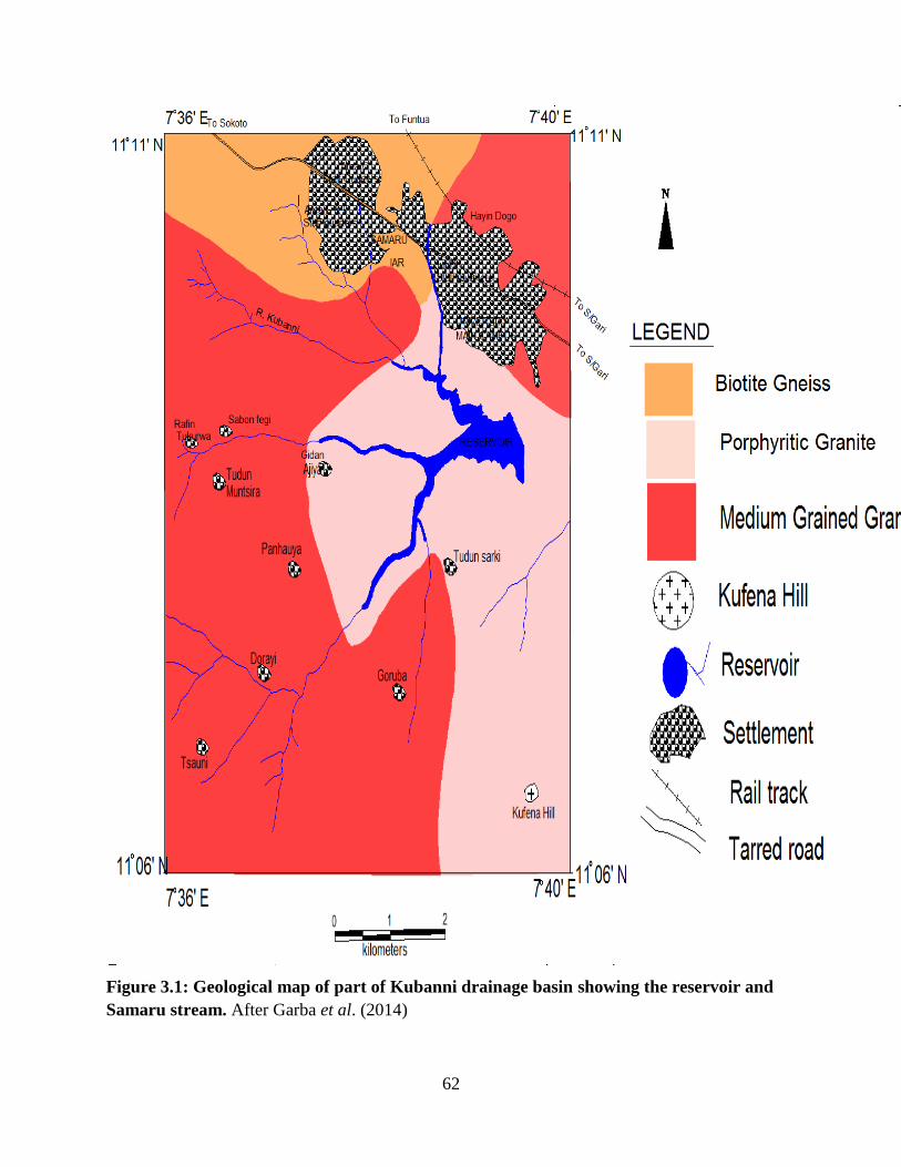
62

Figure 3.1: Geological map of part of Kubanni drainage basin showing the reservoir and

Samaru stream. After Garba et al. (2014)

63

The alluvial deposits in the study area on the other hand are exogenic terrigenous materials that

are transported from a river and deposited by flooding water over the banks of a river. The

alluvium deposits are quite extensively wide open consisting of brown to brownish red sands,

silts and clay. Thorp (1970) described these sites of the older alluvium deposits within the study

area as where gullies erosion is incised into them. The shallowness of the streams around the

region enables the formation of extensive flood plains along the rivers which often floods during

the rainy seasons (Nassef and Olugboye, 1979).

Furthermore, Ololobou (1982) observed a site along the Zaria by-pass, 0.5km from the bridge

within the Kubanni basin where the presence of younger laterites with recent alluvial deposits

along the Kubanni River was prominent.

3.1.4 Soils

The soil type is highly leached ferruginous tropical soils, developed on weathered regolith

overlain by a thin deposit of windblown silt from the Sahara desert during many decades of the

propagation of the tropical Continental air mass into the area (Wright and McCurry, 1970). The

soil occurs as loess, covering pre-Cambrian rocks (mainly crystalline acid rocks). These

ferruginous soils exhibits a marked differentiation of the horizon and are characterized by the

separation of free iron oxides (Fe2) which may hinder the infiltration of rain water from the

formation mottles and concretion in the soil thereby enhancing surface run-off.

The soil texture in the study area is sandy clay loam with clay dominating as kaolinite with the

presence of mica and feldspar, having an average pH of 7.1 and fairly neutral in reaction and an

organic matter content that is low (Harpstead, 1973). This has implication on soil structure

stability, organic nutrient and soil retention capacity.

64

Klinkenberg (1970) described the soil pattern of Zaria according to the geological units

identified by Wright and McCurry (1970). They are; (a) Fadama soils: in a valley system, an

extensive wide fadama soils are usually developed. These are dark grey clays with a poor

drainage formed from alluvial materials. They are widespread within the Galma, Shika and

Kubanni Basins. Ipinmidum (1972) classified them as hydromorphic; (b) Soils developed on

Metasediments (Schists and Quartzites): soils, west of Zaria are shallow and stony in the

interfluves crests as a result of the widespread elongated quartzite ridges. Although, at the middle

and lower slope the soil profile are deeper, with signs of clay accumulation, reddish-grey in color

and concretions of iron (laterites) are found and lastly; (c) Soils developed on Granites: these are

soils that are close to the granitic outcrops which appears deep and consisting mainly of

weathered material which does not show a distinct profile development. Fragments of

unweathered quartz and feldspar are found while deep clayer soils further away the granite hills

are also found. Mottled soils with grayish color are found in the lower sloping and poorly

drained areas (Yusuf, 2006).

The major developmental processes occurring in the soil major profile involve the leaching of

clay minerals and ions. The soil profile is occasion with marked horizon differentiation with iron

oxides deposits in the clay-rich B-horizon, underlying the A-horizon, in form of mottles,

concretion or as ferruginous hard pans called duricrusts. Due to alleviation of the fines of the A-

horizon, the topsoil is coarse (Nyagba, 1986).

It was observed by Kowal and Kassam (1978) and Jaiyeoba (1986) that human activities such as

bush burning, overgrazing, continuous cultivation and rapid oxidation decomposition of

humified organic matter of the soil have reduced by about (1-2%) the organic matter and

65

nitrogen content of the soil. There is low activity of the clay particles which resulted in the

lowing of the cation exchange capacity (CEC) of the soil and exchangeable bases.

3.1.5 Vegetation

Natural vegetation of the study area is the Northern Guinea Savannah. Unfortunately this

characteristic vegetation cover is hardly preserved due to urbanization and poor management

practices, like fuelwood harvesting, annual bush burning, cultivation and intensive grazing

(Ologe, 1971). The Northern Guinea Savannah zone is the largest natural vegetation zone in

Nigeria and is boardered on the north by the Sudan Savannah and to the south by the derived

savannah. It is characterized by scenty deciduous trees, herbs, shrubs and grasses (Olowu, 1986;

Ogunjobi, 1993).The herbs and grasses grow very tall in some places particularly around the

basins where water retention and moisture is high. There is presence of evergreen trees along the

Perennial river and streams, mangoes tress are the common tress seen dotting the region. This is

due to the seasonal character of rainfall which favors the growth of the tree species. These

mangoes trees are planted by locals for their fruits and shades.

The vegetation of the region is usually green in color during the rainy season and yellowish or

brownish in dry season.Isoberlina doka with an average height of 0.5m is the dominant shrub in

the region. Other shrub species are the Butryspermum spp, Pilliostigma spp,Terminalia

avicenniodes and Vitea spp. Some other tree plants found includeMangniferaindica,

Parkiaclappertononia and several others which are found to be useful by man. It is a common

feature to see these trees left standing during cultivation.A common grass community is the

Andropogon spp (Kwabe, 1987) which dried up during the dry season and reappears when the

wet season returns. Grazing for livestock and grass cutting for local mud house construction are

the common human activities that contribute to the absence of the grass.

66

3.1.7 Landforms

The study area is within the Galma basin situated on an extensive peneplain developed on

crystalline metamorphic rocks of the basement complex which extends uninterrupted from

Sokoto to Lake Chad and northwards from Southern Kaduna to Tigueddi Scarp near Agadas in

Niger Republic.It is located at Zaria plain, a dissected part of the Zaria – Kano Portions and

believed to be overlain by wind, drift sediments(Wright and McCurry, 1970). The peneplain is a

gently undulating erosional surface that was capped by the development of an extensive laterites

cover, identified as possibily of the Pliocene age, according to Du Preez (1952). It varies in

altitude, from 550m to 740m above sea level, dotted with outcrops of rocky inselbergs and

lateritic iron stone, with the Kufena hill attaining a height of 820m and a flat top lateritic

ironstone capped residuals. Iguisi (1996) identified the study area to be close to the Kampagi Hill

which is about 708m above sea level. The laterite cover has been reduced to scattered layers,

separated by a thin but highly variable succession of wind and water sediments.The shape of the

valley side slopes shows a convex-concave form with some rectilinear elements.

3.1.8 Land Use

Prior to the year 2000, agriculture (both upland fields and fadama or irrigation farming), grazing

and fishing are the predominant human activities within the basin of the study area. These

activities were however stopped, in an effort to reduce the rate of siltation of the A.B.U dam or

reservoir which researchers such Iguisi (1997) and Yusuf (2006) have shown to be responsible

for the silting of the reservoir from sediment generated from the catchment areas and deposited

into the basin. The university authority adhered to the recommendation on the research carried

out on the Kubanni reservoir and then banned all forms of human activities such as agriculture,

67

grazing etc that were taking place in the area. This was done in order to protect the reservoir

from silting completely like the Daudawa dam in Katsina state. The measure taken to tackle the

problem was by embarking on an intensive conservation campaign. Tree plantations have since

taken over the basin in order to reduce erosion rate from water run-off which influences soil

erodibility and sediment generation which is ultimately being transported and deposited into the

basin.

In the absence of agriculture and grazing activities therefore, the most obvious human activities

that are of concern to the Kubanni reservoir are those that take place in Samaru, a satellite town

bordering the northern tributary of the Kubanni reservoir. Human activities such as wastes

generation from market garbage‘s (rotten and decaying vegetables, fruits etc), domestic wastes

(gutters, soak-aways, and latrines), plastics wastes (polythene bags etc) as well as wastes from

such activities like carpentry, mechanic workshop discharges are all washed down during the

raining season into the Kubanni dam through Samaru stream.

3.1.8 Drainage Characteristics

The Samaru stream linking at the northernmost tributary of the Kubanni river is a 1st order

stream with a total stream length of 1.05km, a basin area of 2.28km2, drainage density of

0.4605m/km2 and a relative relief of about 30.48m

2 (Yusuf and Igbinigie, 2010). The Samaru

stream flows into the Malmo River and finally, all drain into the A.B.U reservoir. The Samaru

stream is seasonal that is, it flows only during wet season and seize during the dry season,

although groundwater is usually found at or near surface in some cases throughout the year.

Water draining into the Samaru stream from part of the A.B.U University (Danfodio hostel,

68

ICSA Ramat hostel, Block of 9 flats, Area 2 Quarters andCommunity Market), helps in

sustaining the flowing water during the dry seasons.

Evidence of poor conservation and landuse practices from faming activities and overgrazing in

the past has resulted into the development of gullies and steep slope in the basin which makes

transportation of soil and rainwater disposal into the stream especially, the valley sides

encourage a high velocity runoff down the slope, thereby increasing mass movement or high rate

of soil wash (Ologe, 1971; 1972; Bello 1973; Ogunrombi, 1979; Iguisi, 1997). Recurrent

undermining and collapse of gullyside walls headscarp recession due to energy increase of

concentrated runoff leads to gully growth which results to the development of micropediments,

mounds and hillocks (Bello, 1973).A map showing the drainage location of the study area is

presented in Figure 3.2.

69

Fig. 3.2: Location of the Study Area on the Kubanni River Basin

Source: Zaria SHEET 102 South-West.

70

3.2 METHODOLOGY

This section will discuss the various methods that was employed in generating and analysing

data for the study, in order to achieve the aim of this study, a reconnaissance survey was carried

out in order to be well acquainted with the study area. These provided useful information in the

mapping and identifying the location for the gauging station where daily stream data and sample

collection would be carried out.

3.2.1 RECONNAISSANCE SURVEY

After the reconnaissance survey a stream depth and width was found to vary almost throughout

the stream. This was attributed to uneven uniform spread of streambed. Therefore, stream depth

measurement was taken between 180-200m upstream from the intersection of the Samaru stream

and the Malmo River. The stream depth measured at the gauging station during the period of

lowest water flow was 0.80m while 2.5m was recorded during the constant water flowing in the

month of August and 3.01m depth during overflow. Furthermore, a stream width of 10.8m was

recorded.

It is equally important to note that despite the banning of all human activities at the Kubanni

basin by the ABU committee on the protection of the Kubanni reservoir, there is still illegal

grazing from migrating herdsman‘s as well as cattle‘s from staff that stray into the basin. Also,

small scale fishing activities are seen taking place around the basin.

3.2.2 TYPES AND SOURCES OF DATA:

(i) Primary data:This includes data on stream discharge, mineral composition, heavy metal and

sediment concentration that was acquired from the field and the laboratory.

71

(ii) Secondary Data: The secondary data on rainfall and water quality parameters were obtained

from Institute of Agricultural Research (IAR), ABU, Zaria, Division of Agricultural Colleges

(DAC) and the World Health Organisation (WHO, 2011) and National Environmental Standards

and Regulatory Enforcement Agency (NSDQW, 2007) standards for water pollutants.

3.2.3 TECHNIQUES OF DATA COLLECTION

3.2.3.1Collection, Preservation and Storage of the Samples

These involved going to the gauging station at the site of the study area to collect daily data on

stream discharges. This was done at 7am and 6pm of every day respectively. However, if

between the stipulated time, rainfall was experienced, an additional stream discharge reading was

recorded, and the average reading taken, as well as collecting a representative sediment sample

of water from the Samaru stream using a USDH sediment sampler. The depth-integrated sample

was collected at a velocity similar to the stream flow velocity. The sediment sample was taken

after each rainfall, for the entire raining season. Sample collected from the sediment sampler

was transfered into a 500ml plastic container, labelled and taken into the physical laboratory in

Geography department, A.B.U to be prepared and runned. The choice of sample volume

collected is to ensure having a substantial amount of dissolved sediment residue of atleast 0.2g

that is sufficient in carrying out the analysis in the lab. Sample collected were preserved in the

refrigerator when analysis wasnot conducted immediately (Water Pollution Control Federation,

1986).

3.2.3.2Stream Discharge (Q)

This is the volume of water passing through a given cross-section of a river during a given period

of time. Units used are those of volume/time, and values are usually reported in cubic meters per

72

second (m3/s) or in litres per second (1/s).The measurement of stream discharge usually involves

consideration of both stage and velocity. There are a number of ways in which river discharge

can be measured. These include velocity-area technique, dilution gauging, volumetric gauging,

the slope area technique, weirs and flumes (control structure method) and the rated section. The

velocity-area technique used by Yusuf and Iguisi (2012) was adopted. This is based on the fact

that discharge, Q, is a function of average stream velocity, V, and the cross-sectional area of the

channel, A, at the point of measurement.

Stream discharge measurements were observed after rainfall events and twice a day; in the

morning (around 7.00am) and in the evening (around 6.00pm) everyday, which represent

instantaneous and regular interval monitoring (Ogunkoya, 2000). Subsequently, the daily

average readings were calculated in order to obtain the stream discharge. The velocity-area

technique is represented as;

Q=AV………………………………………………………………………..................3.1

where,

Q= Stream discharge

A= cross-sectional area; is the product of the stream width and stream depth.And,

V= average stream velocity; is the product of the time taken fora polyvinyl chloride (PVC)

material to flow unobstructed for a stipulated length within the stream. The PVC is a weightless

piece of object that can float effortlessly on water. This provided the choice of using it to take the

stream velocity. Plate 3.1 shows a staff guagefor stream discharge measurement at the gauging

station for stream depth measurement.

73

3.2.4 Dissolved Sediment Concentration (Cd1)

(i) Laboratory Analyses

The dissolved sediment concentration was obtained by filtering the sample collected from the

field by an automated filtering pump using a Whatman cellulose nitrate membrane 0.45µm filter

paper to dissociate the suspended sediment from the dissolved sediment. The filtered dissolved

sediment was poured into a beaker to be evaporatedto dryness in the oven. The weight of the

beaker that was used in drying the sample was taken, before and after the drying process. The

difference in weight of the beaker/crucible will give the concentration of the dissolved sediment,

following the procedure of Smith and Stopp (1978). The data obtained in (g/ml) is converted to

(mg/l) by multiplying each value by 4 and 100. Plate 3.2 shows a set of filtration equipment at

the Physical Geography lab.

Plate 3.1:InstalledStaff Guage at Location 11o08'38"N-007

o38'47"E

74

Plate 3.2: Set of Filtration Equipment

3.2.5 Mineral Composition and Heavy Metal Test

(i) Preparation of Sample

Samples were collected from the field and filtered at the Geography department laboratory by an

automated filtering pump using the Whatman cellulose nitrate membrane 0.45µm filter paper and

evaporated to dryness. The dry residue samplewas carefully scrapped out of the crucible and

taken to Defence Industries Kaduna (DICON) where it was runned by an X- Ray Fluorescence

(XRF) machine for mineral compositon as well as the heavy metals in the sediment. Plate 3.3

shows a residue sediment sample shortly before the XRF analysis.

75

Plate 3.3: Residue of Dissolved sediment ready for Analysis

(ii) Laboratory Analyses:

Samples collected, for the mineral composition and heavy metals test was analyzed by the use of

an XRF machine at DICON in Kakuri, Kaduna. The XRF technique operates in an

electromagnetic wave frequency such as the visible light ray, but the key difference is its

extremely short wavelength, measuring from 100A to 0.1A. Compared to normal

electromagnetic waves, X-ray easily passes through material and it becomes stronger as the

material's atomic number decreases. X-ray Fluorescence analysis is a method that uses the

Characteristic X-ray (fluorescent X-ray) that is generated when X-ray is irradiated on a

substance. The fluorescence X-ray is the excess energy irradiated as electromagnetic field, which

is generated when the irradiated X-ray forces the constituent atom's inner-shell electrons to the

outer shell and the vacant space (acceptor) falls on the outer-shell electrons. These rays possess

energy characteristic to each element and qualitative analysis using Mosley's Equation and

quantitative analysis using the energy's X-ray intensity (number of photons) are possible. It

captures minerals in a sample (Seiko,2013). Examples, of minerals thatcan be identified by an

XRF are; Na2O, MgO, Al2O3, SiO2, P2O5, K2O, SO3, CaO, TiO2, Cr2O3, Mn2O3, Fe2O3, ZnO,

76

SrO and Cl. Furthermore, the XRF technique also have the capability of producing result of

analysis in elemental form.

(iii)Sample Size to be Analysed

Systematic sampling procedure was employed to achieve an appreciable analytical sampling

size in the study in order to get a good resultof analysis of data within the designed and stipulated

time frame of the research work. Furthermore, because of the variability of analytical and

sampling procedures (population variability), a single sample,is insufficient to reach any

reasonable desired level of confidence. Therefore, the required number of samples for a mobile

matrix such as water was estimated as follows (Keith, Patton, and Edward, 1996; Sigma, 2012).

N≥ Za/2

x S2.....................................................................................................3.2

U

Where:

N= number of samples.

Z a/2

= Student-z statistic for a given confidence level.

S= overall standard deviation, and

U= acceptable level of uncertainty of margin of error .

A 95% degree of confidence correspond to a=0.05. From the normal curve of the Z-distrubution.

Each of the shaded tails has an area of a/2=0.025.The region to the left of Z a/2

and to the right of

Z=0 is 0.5-0.025, or 0.475. In the table of the standard normal(Z) distribution, an area of 0.475

corresponds to a Z value of 1.96.

77

Therefore, if U is ±2, and Z a/2

= 95% confidence level as desired, which correspond to 1.96 and

S= 4.12, calculated from the annual record data of rainfall days of Samaru town, covering a

period of 5yrs that is 2008 to 2012 with an average rainfall of 77days. Applying the above

formula will give approximately 33 samples.

Furthermore, the 33 samples obtained from the procedure of Keith, Patton and Edward (1996)

werereduced systematically into 3 samples by grouping the entire 33 samples into 3 groups, of

11 samples each. One sample was taken from eachof the 3 groups to give 3 samples.

Therefore, 3 samples were collected for the XRF mineral compounds and heavy Metals analysis.

These 3 samples were spread through the raining season from the month of April to October

according to this order. That is, the 1st rain of April was collected, the second sample was

collected on 18th

July and the third and last sample was collected on the 10th

of October.

3.2.6 Data Analysis

3.2.5.1 Rainfall-Discharge Relationship

A precise form of rating curve as proposed by Bauer and Tille (1996) was used to regress rainfall

on stream discharge, by using their log exponents (log) as shown below.

Log Q= log a + b log R…………………………………………………………………..3.3

Where Q = Stream Discharge in m3/s

R = Rainfall in mm

a + b = Constants representing the intercept and slope of the rating plot respectively.

Furthermore, rainfall records for analysis were obtained from two meteorological stations for

comparison. The two stations are the Soil Science Department and Divisional of Agricultural

78

College (DAC), both in A.B.U Zaria (see appendix). However, the rainfall data of DAC was

used for these analyses because it was found to pick the lowest measurement of rainfall 0.20mm

as aginst the 0.04mm of the soil science records while a total of 71days of rainfall were

recoreded for the DAC measurment against the 70days for Soil Science.

3.2.5.2 Estimation of Dissolved Sediment Yield

As dissolved sediment measurements are rarely continuous, temporal extrapolation is often

required to enable a reasonable estimate of dissolved sediment yield to be made. This is the total

amount of dissolved sediment load that was generated within the catchment area of the Samaru

stream. It involved all data on dissolved sediment concentration and dissolved sediment

discharge; a product of dissolved sediment concentration and discharge to stream discharge on

the basis of a limited number of sediment measurements (Yusuf, 2006).

A precise form of rating curve as proposed by Bauer and Tille (1969) was used to regressed

stream discharge on the dissolved sediment discharge, by using their log exponents (log) as

shown below:

Log Qd= log a + b log Q ……………………………………………………………..3.4

Where Qd = Dissolved Sediment discharge in mg/s

Q = Stream Discharge in m3/s


The dissolved sediment discharge (Qd) in mg/s, a product of discharge and concentration would

be then converted to kg/day thus:

Qd = QCd * 60 * 60 * 24………………………………………………………………3.5

1000

Where Qd = Dissolved Sediment Discharge in kg/day

79

Q = Stream Discharge in m3/s

Cd = Dissolved Sediment Concentration in mg3/l

Therefore, a continuous record of dissolved sediment discharges provided an estimate of the

dissolved sediment yield throughout the year (Ferguson, 1987).

3.2.5.3 Dissolved Sediment Concentration-Discharge Relationship

Log Cd= log a + b log Q………………………………………………………………..3.6

Where Cd = Dissolved Sediment Concentration in mg/l

Q = Discharge in m3/s


3.2.5.4Dissolved Sediment Discharge-Discharge Relationship

Log Qd= log a + b log Q……………………………………………………………….3.7

Where Qd = Dissolved Sediment Discharge in mg/s

Q = Dissolved Sediment Discharge in m3/s


3.2.5.5Dissolved Sediment Concentration-Dissolved Sediment Discharge Relationship

A precise form of rating curve as proposed by Bauer and Tille (1996) was used to regressed

dissolved sediment discharge on dissolved sediment concentration, by using their log exponents

(log) as shown below.

Log Cd= log a + b log Qd……………………………………………………………..3.8

Where Cd = Dissolved Sediment Concentration in mg/l

Qd = Dissolved Sediment Discharge in mg/s

80


3.2.5.5 Conversion of % Residue Sample to Mg/l

In order to get the basis for comparision of result with the recommended standards, the

equivalent concentration of the XRF analysis obtained in % was converted to mg/l. This was

obtainedfrom the initial volume of sediment samples used in generating the residue by the

filtration and evaporation procedures. The volumes of sediment used for the XRF analysis to

generate 1g of residue sample from each of the three rainfalls collected are 3.5 litres, 5 litres and

7.5 litres in this order because as rainfall progresses the dissolved sediment values as deposits in

the samples were also decreasing. The calculation and conversion work is presented in appendix

4, and was done for each compound and element obtained from the XRF analysis.

3.2.5.6Statistical Analysis

Result of the samples analysed in the laboratory was interpretated using both descriptive and

inferential statistical test and compared with the WHO and NSDQW standards for metal

pollutants. The inferential statistical test used is the regression analysis, t-test, f-ratio and the z-

test (sample size) and Analysis of Variance (ANOVA). The ANOVAtest is a statistical tool for

measuring the significant difference between two unequal groups of data with normal and

independent distribution. It was used in measuring the significant difference between the mineral

composition and inorganic heavy metals pollutant of the dissolved sediment load of the Samaru

stream. The z-test was employed in determination of sample size while the correlation and

regression analysis on the other hand was used to see if, there is any significant relationship

between the stream discharge and dissolved sediment load of the Samaru stream. All analyses

were carried out by the use of Excel and the SPSS statistical package. The confidence level used

81

in accepting or rejecting the hypotheses is 95% corresponding to an alpha value of 0.05. For

instance;

i. In determining the dissolved sediment concentration of the stream. The statistical tool

used in the analysis was descriptive (mean, standard deviation etc) analysis.

ii. In determining the discharge of the stream. The statistical tool used in the analysis

was descriptive (mean, standard deviation etc) analysis.

iii. In estimation of the dissolved sediment yield of the stream. The statistical tool used in

the analysis was descriptive (mean, standard, deviation etc) and regression analysis.

iv. In analyzing the mineral composition and heavy metals in the dissolved sediment of

stream. The statistical tool used in the analysis was descriptive (mean) analysis.

v. In establishing the hypotheses. The statistical tool used was the t-test, f-ratio and

regression analysis.

82

CHAPTER FOUR: RESULTS AND DISCUSSION

4.1 Stream Discharge

Stream discharge measurement and observation of Samaru stream started on the 1st of April,

2014 and ended on the 31st ofOctober, 2014 covering a period of 7 months and total of 214 days

which corresponded to the raining season duration of the study area. The velocity-cross-sectional

area (AV) method was employed in obtaining and recording the stream discharge which involves

the used of a meter rule and a lighted weight Polyvinyl Chloride (PVC) material that could easily

float on water surface. This object was allowed to float freely on the water surface; to cover a

given distance, in this case 8 meters was chosen to be the distance to be covered. The time taken

to cover the distance is taken. Time taken recorded in seconds (s) provided the variable that was

used to calculate the stream velocity, a function of distance (m) and time (s).

Data on daily mean instantaneous discharge in m3/s is presented in table 4.1a and the summary

statistic is presented in Table 4.1bwhile the daily stream discharge also in m3/s is presented in

table 4.1c and the summary statistic is in Table 4.1d. Also, the daily discharge values were

converted to m3/day and the result is shown in Table 4.1e with the regime table in 4.1f and fig.

4.1a.

Therefore, a total of 52.078m3/s daily mean instantaneous recording was obtained for 71 rainfall

days varying with the lowest value of 0.057m3/s recorded in April and the highest of 4.133m

3/s

recorded in August which gives a mean value of 0.7335m3/s, a std. error of mean value of

0.9210, a standard deviation of 0.7761 and a variance of 0.602 while the daily mean

instanstaneous discharge values available for 44 days with a missing values of 142 was recorded

for the same stream by Yusuf and Igbinige (2010) showing a varying value starting from as low

83

as 0.01m3/s to 0.42m

3/s with a mean value of 0.165m

3/s, a standard error of mean 0.014, a

standard deviation of 0.092 and a variance of 0.008. Also, the daily discharge values obtained for

214 days gave a total of 54.107m3/s with the lowest value of 0.010m

3/s recorded in October and

the highest value of 4.133m3/s recorded in August with a mean value of 0.2528 m

3/s, a std. error

of mean value of 0.0383, a std. deviation of 0.5597 and a variance of 0.313.

Furthermore, converting the daily mean instantaneous values from m3/s to m

3/day as seen in

Table 4.1e and the regime graph in Fig.4.1a gave a total stream discharge value of

4,805,232m3/yr for the year 2014 with October having the lowest percentage discharge of 1%

and August with the highest percentage discharge of 38% as shown in the discharge regime

diagram in Fig. 4.1f.There are days which the measurement is impossible because the water flow

is too low and therefore difficult to observe.

84

Table 4.1a Instantaneous Daily Discharge Values of Samaru Stream for 2014 (m3/s)

DATE JAN FEB MAR APRIL MAY JUNE JULY AUG SEPT OCT NOV DEC

1 1.557 0.137 0.143

2 0.245 0.078 4.133 1.112

3 1.072 1.378 0.667

4 0.128 0.057

5 1.292 1.292 4.068 1.553

6 0.375

7 0.057 0.130

8 0.500 1.173 0.917

9 0.282 0.157 1.112

10 0.305

11 0.258 1.288 0.655

12 0.950 0.187 0.138

13 0.315 0.147

14 1.353 0.592

15 1.095 0.663

16 0.838 0.167 0.752

17 0.700 0.612 0.362

18 0.762 0.862

19 0.142 0.195

20 0.707 0.147

21 0.120 2.590

22 0.112 0.430

23 0.108

24

25 1.097

26 0.922

27 1.388 0.138

28 0.637 0.488 0.685 1.012

29 0.535 0.433

30 0.125 0.123 0.890

31 0.288 0.172 1.978

TOTAL 4.043 5.698 5.511 6.367 20.777 9.177 0.505

85

Table 4.1b: Summary Statistics of Table 4.1a

STATISTICS

VALUE

N VALID

MISSING

71

143

Mean

.7335

Std. Error of Mean

.9210

Std. Deviation

.77605

Variance

.602

Range

4.08

Minimum

.06

Maximum

4.13

Sum

52.078

86

Table 4.1c Daily Discharge Values of Samaru Stream for 2014 (m3/s).


1 0.020 0.020 0.016 1.557 0.137 0.143

2 0.245 0.078 0.014 4.133 1.112 0.030

3 1.072 0.010 1.378 0.667 0.030 0.025

4 0.020 0.008 0.020 0.030 0.128 0.057

5 1.292 1.292 0.018 4.068 1.553 0.020

6 0.020 0.020 0.375 0.030 0.030 0.018

7 0.057 0.018 0.015 0.020 0.025 0.130 0.016

8 0.500 0.016 0.013 1.173 0.020 0.917 0.014

9 0.020 0.282 0.010 0.020 0.157 1.112 0.012

10 0.018 0.020 0.008 0.018 0.020 0.030 0.305

11 0.016 0.018 0.006 0.258 1.288 0.655 0.014

12 0.014 0.014 0.004 0.950 0.187 0.138 0.012

13 0.012 0.012 0.315 0.020 0.147 0.030 0.010

14 0.010 0.010 1.353 0.018 0.592 0.025 0.008

15 1.095 0.008 0.020 0.016 0.030 0.663 0.006

16 0.022 0.006 0.838 0.167 0.025 0.752 0.004

17 0.018 0.004 0.700 0.018 0.612 0.362 0.004

18 0.016 0.002 0.020 0.762 0.862 0.195 0.003

19 0.014 0.002 0.018 0.020 0.142 0.030 0.003

20 0.707 0.002 0.016 0.018 0.147 0.025 0.003

21 0.020 0.000 0.014 0.120 2.590 0.023 0.002

22 0.018 0.000 0.112 0.018 0.430 0.020 0.002

23 0.016 0.108 0.014 0.016 0.030 0.018 0.002

24 0.014 0.020 0.012 0.014 0.025 0.016 0.002

25 0.012 0.018 0.010 0.012 1.097 0.014 0.002

26 0.922 0.016 0.008 0.010 0.025 0.012

27 0.020 1.388 0.138 0.008 0.020 0.010

28 0.637 0.488 0.685 1.012 0.018 0.008

29 0.020 0.535 0.020 0.020 0.016 0.433

30 0.125 0.020 0.018 0.018 0.123 0.890

31 0.288 0.172 1.978

TOTAL 4.323 5.964 5.795 6.719 21.091 9.498 0.717

87

Table 4.1d: Summary Statistics of Table 4.1c (m3/s)

STATISTICS

VALUE

N VALID

MISSING

214

149

Mean .2528

Std. Error of Mean .03826

Std. Deviation .55966

Variance .313

Range 4.13

Minimum 0.00

Maximum 4.13

Sum 54.107

88

Table 4.1e: Daily Discharge values of Samaru Stream for 2014 (m3/day)

DATE JN FB MR APRIL MAY JUNE JULY AUG SEPT OCT NV DC

1 0.000 1728 1728 1382.4 134524.8 11836.8 12355.2

2 0.000 21168 6739.2 1209.6 357091.2 96076.8 2592

3 0.000 92620.8 864 119059.2 57628.8 2592 2160

4 0.000 1728 691.2 1728 2592 11059.2 4924.8

5 0.000 111628.8 111628.8 1555.2 351475.2 134179.2 1728

6 0.000 1728 1728 32400 2592 2592 1555.2

7 4924.8 1555.2 1296 1728 2160 11232 1382.4

8 43200 1382.4 1123.2 101347.2 1728 79228.8 1209.6

9 1728 24364.8 864 1728 13564.8 96076.8 1036.8

10 1555.2 1728 691.2 1555.2 1728 2592 26352

11 1382.4 1555.2 518.4 22291.2 111283.2 56592 1209.6

12 1209.6 1209.6 345.6 82080 16156.8 11923.2 1036.8

13 1036.8 1036.8 27216 1728 12700.8 2592 864

14 864 864 116899.2 1555.2 51148.8 2160 691.2

15 94608 691.2 1728 1382.4 2592 57283.2 518.4

16 1900.8 518.4 72403.2 144288 2160 64972.8 345.6

17 1728 345.6 60480 1555.2 52876.8 31276.8 345.6

18 1555.2 172.8 1728 65836.8 74476.8 16848 259.2

19 1382.4 172.8 1555.2 1728 12268.8 2592 259.2

20 61084.8 172.8 1382.4 1555.2 12700.8 2160 259.2

21 1728 0.000 1209.6 10368 223776 1987.2 172.8

22 1555.2 0.000 9676.8 1555.2 37152 1728 172.8

23 1382.4 9331.2 1209.6 1382.4 2592 1555.2 172.8

24 1209.6 1728 1036.8 1209.6 2160 1382.4 172.8

25 1036.8 1555.2 864 1036.8 94790.8 1209.6 172.8

26 79660.8 1382.4 691.2 864 2160 1036.8 0.000

27 1728 119923.2 11923.2 691.2 1728 864 0.000

28 55036.8 42163.2 59184 87436.8 1555.2 691.2 0.000

29 1728 46224 1728 1728 1382.4 37411.2 0.000

30 10800 1728 1555.2 1555.2 10627.2 76896 0.000

31 24883.2 14860.8 170899.2 0.000

TOTAL 374025.6 515289.6 500688 710380.8 1822272.4 820627.2 61948.8

Sum Total=4,805,232.2m3/yr

89

Table 4.1f: Discharge Regime Table for table 4.1e (m3/month)

NO: MONTHS DISCHARGE

(m3/months)

FRACTION OF

TOTAL

DISCHARGE

PERCENT OF

TOTAL

DISCHARGE

(%)

1 JAN -- -- --

2 FEB -- -- --

3 MARCH -- -- --

4 APRIL 374025.6 0.08 8

5 MAY 515289.6 0.11 11

6 JUNE 500688 0.10 10

7 JULY 710380.8 0.15 15

8 AUG 1822272.4 0.38 38

9 SEPT 820627.2 0.17 17

10 OCT 61948.8 0.01 1

11 NOV -- -- --

12 DEC -- -- --

TOTAL 4,805,232.2 1 100

Sum Total=4,805,232 m3/yr

Fig. 4.1a: Discharge Regime Graph for Table 4.1e (m3/day)

0

200000

400000

600000

800000

1000000

1200000

1400000

1600000

1800000

2000000

DIS

CH

AR

GE

(m

3/d

ay

)

MONTHS

90

It is worth noting that the annual total discharge of 4,805,232 m3/yr obtained using the AV

method is higher in relation to the total annual discharge of 1,204,200 m3/yr obtained by Yusuf

(2006) in a study of the Samaru stream using both the weir and AV method in the year 2006. The

difference can be attributed to the difference in the position of the gauging station with

increasing volume of water passing down the stream.

4.1.1: Rainfall –Discharge Relationship

Rainfall data from Division of Agricultural Colleges (DAC), ABU Zaria provides the rainfall

measurement in (mm) that was used in the study for sample collection which began on the 7April

and ended on 10October as presented in Table 4.1.1a,regime diagram Table 4.1.1b and

Fig.4.1.1a. A total of 1017mm rainfall was recorded for 71days in 2014, showing August with

the highest rate of rainfalls for the year with 397.5mm and October the least with 9.4mm.The

rain varies from as low as 0.20mm observed in 27June, 2014 to as high as 97.60mm observed on

2August, 2014.

Furthermore, regime diagram Table 4.1.1b shows a peak rainfall of 39% recorded in August,

followed by September with 18%. The two months alone contribute 57% of the total annual

rainfall in 2014 while the lowest recorded was in October with 1%.Also, the highest peak rainfall

per day of 97.60 mm was recorded in August while the lowest is 0.2mm recorded in June as

demonstrated in Fig.4.1.1a.

Therefore, Table 4.1.1a and Table 4.1.1bwithFig.4.1.1a shows that Samaru stream is indeed a

seasonal stream which flows in relation to the amount and duration of rainfall pattern of the

season. August has total rainfall record of 396.7mm with a stream discharge of

1822272.2m3/month representing 38% of the annually discharge which contributes more than a

91

quarter of volume of discharge into the stream. September followed by a rainfall record of

186.3mm with a discharge value of 820627.2m3/month and 18% contribution of discharge into

the stream. The least is October with a total rainfall of 10.4mm, a discharge value of

61948.8m3/month and contributing just 1% of discharge into the stream. The two months of

August and September alone contribute about 60% of the stream discharges for the year 2014

while the remaining months contribute 30% of the stream discharges.

92

Table 4.1.1a: Mean Daily Rainfall Values in mm for 2014

DAYS JN FB MAR APRIL MAY JUNE JULY AUG SEPT OCT NV DC

1 32.7 3.5 3.6

2 4.4 3.7 97.6 22.9

3 24.0 30.2 11.9

4 3.3 0.6

5 27.7 23.6 56.0 34.2

6 7.6

7 1.6 0.8

8 11.7 23.2 17.4

9 6.3 2.7 24.3

10 6.2

11 5.1 26.2 10.5

12 7.0 4.8 2.0

13 TR 6.4 0.4

14 17.9 12.0

15 20.1 13.6

16 15.8 4.4 14.5

17 4.1 13.3 9.1

18 TR 14.7 17.7

19 0.5 4.2

20 13.6 2.1

21 4.7 51.0

22 9.4 TR 6.2

23 2.3 TR

24

25 20.2

26 17.4

27 29.0 0.2

28 14.5 9.6 16.8 22.7

29 10.7 7.9

30 2.5 1.6 18.1

31 5.2 5.0 40.5

TOTAL 81.4 119.2 97.9 124.6 397.4 186.3 10.4

Total= 1017mm; 71rain days.

Adopted from Division of Agricultural Colleges Metrological Station (DAC), A.B.U Zaria

93

Table 4.1.1b: Regime Diagram of Rainfall (mm) in Table 4.1.1a

NO: MONTHS RAINFALL

(MM)

FRACTION OF

TOTAL

RAINFALL

PERCENT OF

TOTAL

RAINFALL

(%)

1 JAN -- -- --

2 FEB -- -- --

3 MARCH -- -- --

4 APRIL 81.4 0.08 8

5 MAY 119.2 0.12 12

6 JUNE 97.9 0.10 10

7 JULY 124.6 0.12 12

8 AUG 397.4 0.39 39

9 SEPT 186.3 0.18 18

10 OCT 10.4 0.01 1

11 NOV -- -- --

12 DEC -- -- --

TOTAL 1017 1 100

Sum Total=1017mm

Fig. 4.1b: Rainfall Regime Diagram for 2014

0

50

100

150

200

250

300

350

400

MONTHS

RA

INF

AL

L (

mm

)

94

Lastly, another reason observed for the difference in stream discharge was that a total of 58 days

of rainfall was recorded in 2006 with the highest rain of 45.30mm while a total of 71 days and

the highest rainfall of 97.60mm (Table 4.1.1a) rainfall were recorded in 2014. This gives a

rainfall difference of 13days, representing days without instantenous stream discharge

measurement records for 2006 against 2014. Therefore, duration and intensity of rainfall

occurance plays a significant role in the flow of water in a stream.

Furthermore, a log-log relationship of a rating curve relating the daily mean instantaneous

rainfall values to stream discharge is shown in fig.4.1c.

The rating equation derived from the relationship, using their log exponents, as shown in table

4.1.1c is of the form:

LogQ=100.552

R0.036

(i.e Q= 3.5645 R0.036

)………………………………………………….4.1a

While the regression equation is of the form:

Log Q= 0.552+0.036 log R…...…………………………………………………………….4.2b

Therefore, the regression coefficient of correlation (r) value of 0.913 and coefficient of

determination (r2) of 0.834 as shown in Table 4.1.1d

The equations 4.1 and 4.2 illustrated that there is a direct relationship between stream discharge

and rainfall which can be verified by checking the significance of the regression coefficient, the

t-ratio test was conducted for a and b (intercept and slope) and it was found in both cases that ta

andtb were statistically significant at the 0.05 level of significance as presented in Table 4.1c.

Therefore, we concluded that there is strong relationship between the regression coefficients in

both cases.

95

Furthermore, the coefficient of correlation (r) and the coefficient of determination (r2) both

measure the strength of the linear correlation between the two variables. Both of the values of (r)

and (r2) are high suggesting thestrenght of rainfall in determination of the stream discharge. Also,

plot of rainfall (mm) against discharge (m3/s) of the stream in Fig.4.1.1b gave a lower peak

discharge of 0.001m3/s and a higher peak discharge of 4.150m

3/s while the log-log relationship

between rainfall and discharge shows that there is a direct relationship between discharges and

rainfall at 0.05 level of significance.

Table 4.1.1c: Coefficient of R-Q Relation

Factor

Coefficients Std. Error T Sig.

(Constant)

0.552

0.047

11.755

0.000

LOGR

0.036

0.003

11.846

0 .000

a. Dependent Variable: Discharge

Table 4.1.1d: Model Summary for R-Q Relation

R r2 Std. Error of

The Estimate

F Sig

0.913

0.834

0.13510

140.334

.000

a. Predictors: (Constant), Rainfall

b. Dependent Variable: Discharge

96

Fig. 4.1.1b: Relationship between Rainfall- Discharges

Comparing the rainfall-discharge relationship obtained by Yusuf (2006) shows that both

relationship are strong except for the fact that the values of (r) 0.295 and (r2) 0.087 are lower for

Yusuf (2006) against the coefficient of correlation (r) 0.913 and coefficient of determination (r2)

0.834 in this study which produces a straight line graph starting from the origin while the former

gave a straight line graph which however did not start from the origin, indicating the higher

values of (r) and (r2).

4.2 Dissolved Sediment Concentration (Cd1)

Data collected on dissolved sediment concentration began on the 7 April, 2014 and ended on 10

October, 2014. These values were the difference in weight of filtered sediment before and after

0

0.5

1

1.5

2

2.5

0 5 10 15 20 25 30 35 40

DIS

CH

AR

GE

(m

3/s

)

RAINFALL (mm)

97

evaporation in an oven (i.e. filtrate + crucible). The data in (mg/l) is presented in table 4.2a with

the summary statistics in table 4.2b.

The result obtained from the summary statistics shows that the range is 100mg/l, a mean value of

58.87mg/l, with a standard error of mean of 3.47, a standard deviation of 292550, a variance

of855.855 and a minimum and maximum values of 20mg/l and 120mg/l respectively. These

minimum and maximum dissolved sediment concentration values were spread across the year

with April marking the commencement of the rainfall season having more of 120mg/l dissolved

sediment concentration values while October has values of 20mg/l.

The variation in distributioan of the dissolved sediment values can be explained to the fact that

before the commencement of rainfall in April, more mineral compounds or constituents as

dissolved materials are being concentrated in the soil surfaces and as the rain commences in

April, the mineral matters concentrates are being washed down into the stream as dissolved

sediments loads. Another observation is that the rate of dilution of minerals increases as rainfall

progresess.

98

Table 4.2a: Dissolved Sediment Concentration Values of Samaru Stream (mg/l)


1 40 40 20

2 80 40 40 80

3 80 40 40

4 40 20

5 80 40 80 40

6 40

7 120 40

8 120 80 40

9 40 80 40

10 40

11 40 80 20

12 40 40 20

13 80 40

14 80 40

15 120 40

16 80 40 40 40

17 80 40 40

18 120 40 20

19

20 120 40

21 80 40 40

22 40

23 80

24

25 40

26 120

27 80 120

28 120 80 80 80

29 40 40

30 80 40 40

31 80 40 40

TOTAL 800 640 680 560 840 580 80

Sum Total= 4180mg/l

99

Table 4.2b: Summary Statistics of Table 4.2a

STATISTICS VALUE

N VALID

MISSING

71

143

Mean 58.8732

Std. Error of Mean 3.47193

Std. Deviation 292550

Variance 855.855

Range 100.00

Minimum 20.00

Maximum 120.00

Sum 4180.00

100

Furthermore, values of derived dissolved sediment discharge, a product of dissolved sediment

concentration and discharge is presented in table 4.2c and the summary statistics in table 4.2d.

The summary statistics illustrates that derived dissolved sediment discharges varied from as low

as 1.14mg/s on 4th

of October 2014 to 325.44mg/s on the 5th

of August 2014 giving a range of

324.30mg/s, a mean value 44.52mg/s, a standard error of mean of 6.07, a standard deviation of

51.132, a variance of 2615 and a minimum and maximum values of 1.14mg/l and 325.44mg/l

respevtively.

Therefore, from the result of the derived dissolved sediment discharge in Table 4.2c, August has

the highest value of 1051.6mg/s, followed by April with 480.16mg/s and May with 423.16mg/s.

The least monthly dissolved sediment discharge of 16.2mg/s was recorded in October while a

total dissolved sediment discharge value of 3161.9mg/s was obtained.

101

Table 4.2c: Derived Dissolved Sediment Discharge Values of Samaru Stream (mg/s)


1 62.28 5.48 2.86

2 19.6 3.12 165.32 88.96

3 85.76 55.12 26.68

4 5.12 1.14

5 103.36 51.68 325.44 62.12

6 15

7 6.84 5.2

8 60 93.84 36.68

9 11.28 12.56 44.48

10 12.2

11 10.32 103.04 13.1

12 38 7.48 2.76

13 25.2 5.88

14 108.24 23.68

15 131.4 26.52

16 67.04 6.68 30.08

17 56 24.48 14.48

18 91.44 34.48 7.24

19 5.68

20 84.84 5.88

21 4.8 103.6

22 8.96 17.2

23 8.64

24

25 43.88

26 110.64

27 111.04 16.56

28 76.44 39.04 54.8 80.96

29 21.4 17.32

30 10 4.92 35.6

31 23.04 6.88 79.12

TOTAL 480.16 423.16 391.6 403.04 1051.6 395.14 16.2

102

Table 4.2d: Summary Statistics of Table 4.2c

STATISTICS VALUE

N VALID

MISSING

71

143

Mean 44.5197


Std. Deviation 51.132

Variance 2615

Range 324.30

Minimum 1.14

Maximum 325.44

Sum 3161.9

103

4.3 Dissolved Sediment Concentration, Dissolved Sediment Discharge and Discharge

Relationships

4.3.1 Dissolved Sediment Concentration (Cd1)-Discharge (Q) Relation

A log-log relationship of a rating curve relating the daily mean instantaneous stream discharge

values to dissolved sediment concentration is shown in Figure4.3a.

The rating equation derived from the relationship, using their log exponents, as shown in Table

4.3a is of the form:

LogCd1=101.737

Q0.059

(i.e Cd1= 54.5758 Q0.059

)............................................................4.3a


Log Cd1= Log 1.737+0.059log Q…………………………………………………………..4.3b


determination (r2) of 0.015 as shown in Table 4.3b.

The equations 4.3a and 4.3b illustrated that there is a direct relationship between dissolved

sediment concentration and stream discharge which can be verify by checking the significance of

the regression coefficient, the t-ratio test was conducted for a and b (intercept and slope). It was

found in both cases that ta 55.260 and tb 1.024 were statistically significant at the 0.05 level of

significance as presented in Table 4.3a. Therefore, we concluded that there is poor relationship

between the regression coefficients in both cases.

As indicated earlier, the coefficient of correlation (r) and coefficient of determination (r2)

measure the strength of the linear correlation between the two variables and the ratio of

104

explained variation to the total variation. And, both of the values of (r) and (r2) are low,

suggesting that discharge wasnota strong determinant of dissolved sediment concentration (Cs)

as seen in Table 4.3b.

The low value of r(0.122) and r2(0.015) observed which according to a study of sediment yield

by Walling (1971), Gregory and Walling (1973) is being attributed as one of the several

problems being encountered in studying of sediments.The low r and r2

may however be linked to

the poor relationship between discharge and dissolved sediment concentration values which

decreasesas the rain progresses into the year. Furthermore, the graph of relationship between

dissolved sediment concentration and discharge in Fig.4.3a gave a low peak dissolved sediment

concentration scatter of 20mg/l and a high peak scatter of 120mg/l.

105

Table 4.3a: Coefficient of Cd1-Q Relation

Factor

Coefficients Std. Error t Sig.

(Constant)

1.737

0.031

55.260

0.000

LOGQ

0.059

0.058

1.024

0.309

a. Dependent Variable: LOGCd1

Table 4.3b: Model Summary for Cd1-Q Relation

R

r2

Std. Error of

the Estimate

F

Sig.

0.122

0.015

0.21083

1.049

0.309

a. Predictors: (Constant),LOGQ

b. Dependent Variable:LOGCd1

106

Fig.4.3a: Graph of Relationship Between Dissolved Sediment Concentration (Cd1) and

Discharge (Q)

Comparing the relationship between dissolved sediment concentration (Cd1) and discharge (Q) of

Samaru stream with a study by Yusuf and Igbinigie (2010) where they found that there is a direct

relationship between dissolved sediment concentration and discharge with (r) 0.042 and (r2) 0.002

against the (r) 0.122 and (r2) 0.015 of this study. Both values were however low which indicates

that the relationship is a weak one.

0

20

40

60

80

100

120

140

0 0.5 1 1.5 2 2.5

DIS

SIO

LV

ED

SE

DIM

EN

T C

ON

C

(mg/l

)

DISCHARGE (m3/s)

107

4.3.2 Dissolved Sediment Discharge (Qd) - Discharge (Q) Relation

A log-log relationship of a rating curve relating the daily mean instantaneous discharge values to

dissolved sediment discharge is shown in Fig. 4.3b.

The rating equation derived from the relationship, using their log exponents, as shown in Table

4.3c is of the form:

Log Qd=102.068

Q57.576

(i.e Qd= 52.845 Q57.576

……………………………………………….4.3c


Log Qd= Log 2.068+ 57.576 log Q………………………………………………………….4.3d


determination (r2) of 0.749 as shown in Table 4.3c.

The equations 4.3c and 4.3d illustrated that there is a direct relationship between dissolved

sediment discharge and discharge which can be verify by checking the significance of the

regression coefficient, the t-ratio test was conducted for a and b (intercept and slope). It was found

in both cases that ta 43.689 and tb 14.361 were statically significant at the 0.05 level of significance

as presented in Table 4.3c. Therefore, we concluded that there is strong relationship between the

regression coefficients in both cases. Furthermore, the graph of relationship between dissolved

sediment discharge and discharge in Fig. 4.3b gave a low peak dissolved sediment discharge

scatter of 0.1mg/s and a high peak scatter of 325mg/s.

108

Table 4.3c: Coefficient of Qd-Q Relation

Factor

Coefficients Std.

Error

T Sig.

(Constant)

2.068

0.060

23.631

0.000

LOGQ

57.576

0.073

14.361

0.000

a. Dependent Variable: Qd

Table 4.3d: Model Summary for Qd-Q Relation

R

r2

Std. Error of

the Estimate

F

Sig.

0.866

0.749

0.26446

206.248

0.000

a. Predictors: (Constant), LOGQ

b. Dependent Variable: LOGQd

109

Figure 4.3b: Graph of Relationship between Dissolved Sediment Discharge (Qd) and

Discharge (Q)

Comparing this relationship with a study by Yusuf and Igbinigie (2010) where they examined the

relationship between dissolved sediment discharges (Qd) and discharge (Q) of Samaru stream

and found that there is a direct relationship between Qd and Q with (r) 0.901 and (r2) 0.812

values which corresponded to a (r) 0.866 and (r2) 0.749 values obatined in this study. Both

relationships ofQd and Q are however strong. The 2014 study was therefore found to be in

agreement with the 2010 study of Yusuf and Igbinigie.

0

20

40

60

80

100

120

140

0 0.5 1 1.5 2 2.5

DIS

SIO

LV

ED

SE

DIM

EN

T C

ON

C

(mg/l

)

DISCHARGE (m3/s)

110

4.3.3 Dissolved Sediment Concentration (Cd1)- Dissolved Sediment Discharge (Qd) Relation

A log-log relationship of a rating curve relating the daily mean instantaneous dissolved sediment

discharge values to dissolved sediment concentration is shown in Figure 4.3c.

The rating equation derived from the relationship, using their log exponents, as shown in Table 4.3e

is of the form:

Log Cd1=101.415

Qd0.219

(i.e Cd1= 26.002 Qd0.020

………………………………………………4.3e


Log Cd1= Log 1.4150+ 0.020 log Qd…………………………………………………………4.3f

Therefore, the regression coefficient of correlation (r) value of 0.545 and coefficient of determination

(r2) of 0.296 as shown in table 4.3f.

The equations 4.3e and 4.3f illustrated that there is a direct relationship between dissolved sediment

concentration and dissolved sediment discharge which can be verified by checking the significance

of the regression coefficient, the t-ratio test was conducted for a and b (intercept and slope). Both

values of r (0.545) and r2 (0.296) were not very high as seen from the straight line graph in Figure

4.3c which did not start from the origin. Also, it was found that ta 23.631 and tb 5.393 were statically

significant at the 0.05 level of significance as presented in Table 4.3e. Therefore, we concluded that

there is weak relationship between the regression coefficients in both cases. Furthermore, the graph

of relationship between dissolved sediment concentration and dissolved sediment discharge in Figure

4.3c, gave a low peak dissolved sediment concentration scatter of 20mg/l and a high peak scatter of

111

120 mg/l which corresponded to 0.1mg/s low peak scatter and 325mg/s high peak scatter of dissolved

sediment discharges.

Table 4.3e: Coefficient of Cd1- Qd Relation.

Factor

Coefficients Std. Error t Sig.

(Constant)

1.415

0.060

23.631

0.000

LOGQd

0.219

0.041

5.393

0.000

a. Dependent Variable: LOQCd1

Table 4.3f: Model Summary for Cd1- Qd Relation

R

r2

Std. Error of

the Estimate

F

Sig.

0.545

0.296

0.17817

29.080

0.000

a. Predictors: (Constant), LOGQd

b. Dependent Variable: LOGCd1

112

Fig. 4.3c: Graph of Relationship between Dissolved Sediment Concentration (Cd) and

Dissolved Sediment Discharge (Qd)

4.3.4 Estimation of Dissolved Sediment Yield

In order to find the dissolved sediment yield for the period of study, equation 4.3d, was used in

estimatingthe dissolved sediment discharges in mg/s which gave a total of 3085.1mg/s as

presented in the Table 4.3.4a while using equation 3.5, dissolved sediment discharges in mg/s is

converted to kg/day as displayed in Table 4.3.4b and the summary statistics in Table 4.3.4c

which gives a total dissolved sediment discharge (Qd) of 174,000kg/yr varying from as low as

27.65kg/day on the 21st and 22

nd of May, 2014 to 20,600kg/day on the 2

nd of August, 2014 which

gives a range of 20,600kg/day with a mean daily value of 861.13kg/day, a standard deviation of

2432, a variance of 5915000.

0

20

40

60

80

100

120

140

0 20 40 60 80 100 120 140 160

DIS

SO

LV

ED

SE

DIM

EN

T C

ON

C

(mg/l

)

DISSOLVED SEDIMENT DISCHARGE (mg/s)

113

Table 4.3.4d gives the derived monthly distribution of dissolved sediment discharge while the

regime graph is illustrated in Figure 4.3.4a. It was observed that high dissolved sediment

discharges were experienced in August with peak dissolved sediment discharges of 52% then

followed by September with 28 % and April with 7 % while the lowest dissolved sediment

discharges was experienced in the month of May and October with just 3% contributaion

respectively of dissolved sediment discharges. Figure 4.3.4a further shows the graphical

representation of the percent dissolved sediment discharge values of the months in the year.

114

Table 4.3.4a: Dissolved Sediment Discharge Values of Samaru Stream (mg/s)


1 1.47 1.47 1.24 89.96 8.20 8.55

2 14.42 4.81 1.12 238.28 64.34 2.04

3 62.04 0.89 79.66 38.72 2.04 1.75

4 1.47 0.78 1.47 2.04 7.69 3.60

5 74.70 74.70 1.35 234.53 89.73 1.47

6 1.47 1.47 21.91 2.043 2.04 1.35

7 3.60 1.35 1.18 1.47 1.75 7.80 1.24

8 29.10 1.24 1.06 67.85 1.47 53.11 1.12

9 1.47 16.55 0.89 1.47 9.35 64.34 1.01

10 1.35 1.47 0.78 1.35 1.47 2.04 17.88

11 1.24 1.35 0.66 15.17 74.47 38.03 1.47

12 1.12 1.12 0.55 55.01 11.08 8.26 1.47

13 1.01 1.01 18.45 1.47 8.78 2.04 1.47

14 0.89 0.89 78.22 1.35 34.40 1.75 1.47

15 63.36 0.78 1.47 1.24 2.04 38.49 1.47

16 1.58 0.66 48.56 9.93 1.75 43.61 0.89

17 1.35 0.55 40.62 1.35 35.55 21.16 0.89

18 1.24 0.43 1.46 44.19 49.95 11.54 0.89

19 1.12 0.43 1.35 1.47 8.49 2.04 0.89

20 41.02 0.43 1.24 1.35 8.78 1.75 0.89

21 1.47 0.32 1.12 7.22 49.44 1.64 0.89

22 1.35 0.32 6.76 1.35 25.07 1.47 0.89

23 1.24 6.54 1.12 1.24 2.04 1.35 0.89

24 1.12 1.47 1.01 1.12 1.75 1.23 0.89

25 1.01 1.35 0.89 1.01 63.48 1.12 0.89

26 53.40 1.24 0.78 0.89 1.75 1.01

27 1.47 80.23 8.26 0.77 1.47 0.89

28 36.99 28.41 39.76 58.58 1.35 0.78

29 1.47 31.12 1.47 1.47 1.24 25.25

30 7.51 1.47 1.35 1.35 7.40 51.56

31 16.90 10.22 114.20

TOTAL 256.48 352.20 343.13 396.64 1124.09 556.30 56.26

Sum Total= 3085.1mg/s

115

Table 4.3.4b: Dissolved Sediment Discharge Values kg/day for 2014


1 127.01 127.01 107.14 777.25 708.48 738.72

2 124.59 415.58 96.77 20587.39 5472.58 176.26

3 536.03 76.90 688.26 3345.41 176.27 151.20

4 127.01 67.39 127.01 176.26 664.42 311.04

5 745.41 645.41 116.64 20263.39 7752.67 127.01

6 127.01 127.01 189.30 176.26 176.26 116.64

7 311.04 116.64 101.95 127.01 151.20 673.92 107.14

8 2514.24 107.14 91.59 586.22 127.01 4588.70 96.77

9 127.01 142.99 76.90 127.01 807.84 5558.98 87.26

10 116.64 127.01 67.39 116.40 127.01 176.26 1544.83

11 107.14 116.64 57.02 131.07 6434.21 3285.80 127.01

12 96.77 96.77 47.52 475.29 957.31 713.66 127.01

13 87.26 87.26 159.41 127.01 758.59 176.26 127.01

14 76.90 74.30 675.21 116.64 2972.16 151.20 127.01

15 5474.30 67.39 127.01 107.14 1762.56 3325.54 127.01

16 136.51 57.02 419.56 85.80 151.20 3767.90 76.90

17 116.64 47.52 350.96 116.64 3071.52 1828.22 76.90

18 107.14 37.15 126.14 381.80 4315.68 997.06 76.90

19 96.77 37.15 116.64 127.01 733.54 176.26 76.90

20 354.41 37.15 107.14 116.64 758.59 151.20 76.90

21 127.01 27.65 96.77 623.81 4271.62 141.70 76.90

22 116.64 27.65 584.06 116.64 2166.05 127.01 76.90

23 107.14 56.51 96.77 107.14 176.26 116.64 76.90

24 96.77 127.01 87.26 103.68 151.20 106.27 76.90

25 87.26 107.14 76.90 87.26 5484.67 96.77 76.90

26 461.38 107.14 67.39 76.90 151.20 87.26

27 127.01 693.19 713.66 66.53 127.01 76.90

28 319.60 245.46 343.53 506.13 116.64 67.39

29 127.01 268.88 127.01 127.01 107.14 2181.60

30 64.89 127.01 116.64 107.14 639.36 4454.78

31 146.01 883.01 9866.88

TOTAL 11357.48 4872.84 6293.73 6872.05 91712.41 47977.96 4860.92

Sum Total= 174, 000 kg/yr

116

Table 4.3.4c: Summary Statistics of Table 4.2f

STATISTICS VALUE

N VALID

MISSING

202

12

Mean 861.13


Std. Deviation 2432

Variance 5915000

Range 20600

Minimum 27.65

Maximum 20600

Sum 174000

117

Table 4.3.4d: Regime Diagram Table for Dissolved Sediment Dicharge (kg/day)

NO: MONTHS DISSOLVED

SEDIMENT

DISCHARGE

(g/month)

FRACTION OF

TOTAL

DISSOLVED

DISCHARGE

(g/month)

PERCENT OF

TOTAL

DISSOLVED

DISCHARGE (%)

1 JAN -- -- --

2 FEB -- -- --

3 MARCH -- -- --

4 APRIL 11357.48 0.07 7

5 MAY 4872.84 0.03 3

6 JUNE 6293.73 0.04 4

7 JULY 6872.05 0.04 4

8 AUG 91712.41 0.52 52

9 SEPT 47977.96 0.28 28

10 OCT 4860.92 0.03 3

11 NOV -- -- --

12 DEC -- -- --

TOTAL 174 000 1.0 100

Sum Total= 174,000 kg/yr

Lastly, in order to estimate the dissolved sediment yield produced, the annual total dissolved

sediment yield of 174,000kg/yr derived from equation 3.5 and presented in Table 4.3.4b is

divided by 1000 which gives a Channel Sediment Yield (CYS) value of 174tons/km2/yr. The

amount is high and can be attributed to the anthropogenic activities taking place upstream.

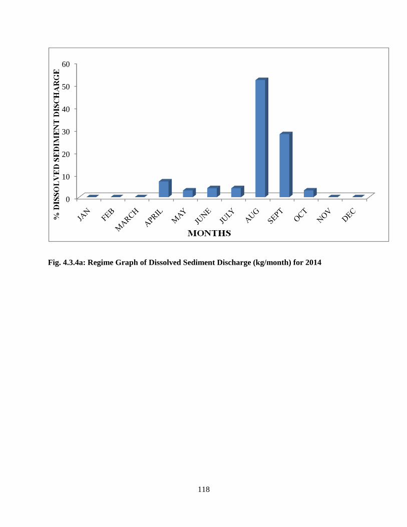
118

Fig. 4.3.4a: Regime Graph of Dissolved Sediment Discharge (kg/month) for 2014

0

10

20

30

40

50

60

119

4.4: Mineral Composition and Heavy Metals.

Based on the sample size for a mobile matrix by Keith, Patton and Edward (1996) of 33 samples

calculated and applying systematic random sampling gave a total of 3 samples that were

analysed throughout the year. The sediment samples therefore, analyzed by the XRF

includessample collected on the first day of rainfall on the 7th

of April, 2014, the middle day of

rainfall on the 18th

ofJuly, 2014 and the last day of rainfall collected on 10th

of October,

2014which were prepared into residual form in the Geography department physical laboratory

before taking to Defense Industries Cooperation of Nigeria (DICON).

After the analysis, 14 compounds were found in sediment one; with 8 heavy metals while 15

mineral compounds were found in sediment two; with also 8 heavy metals present and lastly,16

mineral compounds were found in sediment three which contains 10 heavy metals. The results of

the analyses are presented in Table 4.4a and 4.4b for the compounds and elements obtained

while their mean values is presented in Table 4.4c and 4.4d respectively. Altogether, a total of 17

mineral compounds were identified for the three samples. They are; Al2O3, SiO2, SO3, Cl, K2O,

CaO, TiO2, V2O5, MnO, Fe2O3, NiO, ZnO, Y2O3, BaO, Eu2O3, Yb2O3 and Re2O7. Out of the 16

compounds identified, 11 are heavy metals derivatives. They include; Al2O3, TiO2, V2O5, MnO,

Fe2O3, NiO, ZnO, Y2O3, Eu2O3, Yb2O3 and Re2O7. Aluminum and titanium although, light

metals are sometimes referred to as heavy metals in view of their toxicity to health. They are

heavy metals because at low concentration they are regarded toxic and hazardous to health. The

remaining 5 compounds such as chlorine (Cl), sulphur oxides (SO3), silicon oxide (SiO) are

classified as non-metallic oxides.

120

Table 4.4a: Concentration of Compounds From XRF Analysis of Residue Sample

Sediment 1 Sediment 2 Sediment 3

% Mg/l % Mg/l % Mg/l

SiO2 10.5 3 Al2O3 1.9 0.38 SiO2 9.62 1.28

SO3 11.9 3.4 SiO2 6.74 1.35 SO3 13.0 1.73

Cl 25.3 7.23 SO3 9.61 1.92 Cl 24.6 3.28

K2O 8.09 2.3 Cl 22.0 4.4 K2O 9.36 1.25

CaO 42.49 12.14 K2O 13.4 2.68 CaO 41.95 5.59

TiO2 0.10 0.03 CaO 44.61 8.92 TiO2 0.11 0.015

V2O5 0.004 0.001 TiO2 0.071 0.014 V2O5 0.004 0.0005

MnO 0.063 0.018 MnO 0.03 0.006 MnO 0.029 0.004

Fe2O3 0.522 0.15 Fe2O3 0.560 0.112 Fe2O3 0.512 0.07

NiO 0.341 0.10 NiO 0.349 0.07 NiO 0.15 0.02

ZnO 0.040 0.01 ZnO 0.02 0.004 ZnO 0.038 0.005

Y2O3 0.45 0.13 Y2O3 0.29 0.06 Y2O3 0.3 0.04

BaO 0.12 0.03 BaO 0.14 0.03 BaO 0.13 0.017

Re2O7 0.08 0.02 Eu2O3 0.11 0.02 Eu2O3 0.11 0.015

Re2O7 0.15 0.03 Yb2O3 0.01 0.001

Re2O7 0.15 0.02

Total 100 28.559 99.98 19.996 100.073 13.338

121

Table 4.4b: Concentration of Elements From XRF Analysis of Residue Sample

Sediment 1 Sediment 2 Sediment 3

% Mg/l % Mg/l % Mg/l

Si 4.74 1.35 Al 0.81 0.16 Si 4.22 0.56

S 5.41 1.55 Si 2.92 0.58 S 6.03 0.84

Cl 33.1 9.46 S 4.32 0.86 Cl 31.1 4.15

K 9.57 2.73 Cl 27.00 5.4 K 11.1 1.48

Ca 45.24 12.93 K 15.5 3.1 Ca 45.73 6.10

Ti 0.10 0.03 Ca 47.31 9.46 Ti 0.097 0.013

V 0.007 0.002 Ti 0.069 0.014 V 0.0 0.0

Mn 0.071 0.02 Mn 0.03 0.006 Mn 0.03 0.004

Fe 0.561 0.16 Fe 0.670 0.134 Fe 0.614 0.08

Ni 0.417 0.12 Ni 0.457 0.09 Ni 0.20 0.03

Zn 0.033 0.009 Zn 0.04 0.008 Zn 0.061 0.008

Y 0.41 0.12 Y 0.25 0.05 Y 0.2 0.03

Ba 0.17 0.05 Ba 0.21 0.042 Ba 0.21 0.03

Re 0.16 0.05 Eu 0.21 0.042 Eu 0.17 0.02

Re 0.2 0.04 Yb 0.0 0.0

Re 0.2 0.03

Total 99.989 28.581 99.996 19.986 99.96 13.375

122

The variation in the number of compounds indentified for each sediment sample can be

attributed to the factors that influence dissolved sediment load and the volume and intensity of

rainfall experienced because it was observed that the sample taken at the first rainfall of the year

contains 14 compounds, the middle rain contains 15 compounds while the third rain contians 16

compounds in that order. These suggest that as the rain progresses there are more particles that

are being eroded from the earth as dissolved sediment to become mineral compounds in the

stream.

Table 4.4a gives the total concentration values obtained in the residue sediment samples in their

compoundform which shows that sediment one has calcium oxide (CaO) as the most abundant

mineral with 42.49% and vanadium oxide (V2O5) is the least abundant with 0.004% and a total

percent concentration of 99.989%.

Sediment two again has calcium oxide (CaO) as the most abundant mineral with 44.61% while

manganese oxide (MnO) is the least abundant mineral with 0.03% and a total percent

concentration of 99.996%.

Lastly, the third and final sediment three also has calcium oxide (CaO) as the most abundant

mineral compound with 41.95% and vanadium oxide (V2O5) is the least in abundance with

0.004% and a total percent concentration of 99.96%.

123

Also, Table 4.4c and Table 4.4d gives the three combined sediments in summed and the average

taken. This was done in order to get a good representation of each element in the three sediments

analysed.

Therefore, Table 4.4c and Figure 4.4a showsCaO as the most abundant mineral compound found

with a mean concentration value of 8.8mg/l while the least are V2O5 and Re2O7 with mean value

of 0.001mg/l. A total mean concentration value of 25.621mg/l was calculated for all compounds

identified from the XRF analysis of the residue sample.

Table 4.4d and Figure 4.4b on the other hand identified Ca as the most abundant element found

with a mean concentration value of 9.50mg/l and the least is V with 0.002mg/l while a total

mean concentration value of 21.839mg/l was calculated for all the elements identified from the

XRF analysis of the residue sample. The mean concentration value of Ca when compare with a

recent study of the stream by Garba et al. (2014) using a V2000 multi analyte photometer gave a

mean concentration value of Ca as 10.02mg/l indicating a close similarities in abundance and

that the concentration of Ca have reduced with about 0.52mg/l.

124

Table 4.4c: Mean of Compounds from Residue Sample

NO COMPOUNDS MEAN (mg/l)

1 Al2O3 0.38

2 SiO2 1.88

3 SO3 2.35

4 Cl 4.97

5 K2O 5.40

6 CaO 8.88

7 TiO2 0.02

8 V2O5 0.001

9 MnO 0.025

10 Fe2O3 1.29

11 NiO 0.06

12 ZnO 0.006

13 Y2O3 0.20

14 BaO 0.07

15 Eu2O3 0.028

16 Re2O7 0.001

17 Yb2O3 0.06

TOTAL 25.621

Figure. 4.4a: Mean Regime Graph of Compounds from Residue

0123456789

(mg/l

)

COMPOUNDS

125

Table 4.4d: Mean of Elements from Residue Sample

NO ELEMENTS MEAN (mg/l)

1 Al 0.16

2 Si 0.83

3 S 1.02

4 Cl 6.34

5 K 2.44

6 Ca 9.50

7 Ti 0.019

8 V 0.002

9 Mn 0.01

10 Fe 1.25

11 Ni 0.08

12 Zn 0.008

13 Y 0.07

14 Ba 0.04

15 Eu 0.03

16 Re 0.0

17 Yb 0.04

TOTAL 21.839

Figure.4.4b: Mean Regime Graph of Elements from Residue

0123456789

10

Al Si Si Cl K Ca Ti V Mn Fe Ni Zn Y Ba Eu Yb Re

(mg/l

)

ELEMENTS

126

Oxides are binary components of oxygen (O2) with another element to form compounds of

oxygen (e.g. CO2, ZnO and SO2) which occurs under various reaction processes such as; direct

heating with O2 (e.g.bush burning: 2Mg + O22MgO), reaction of O2 with compounds at higher

temperature (2PbS + 3O22PbO + 2SO2) etc.Compounds of O2 can be form from metals and non-

metals as acidic, basic, amphoteric, neutral and or compound oxides depending on their reaction

with water (H2O) to give an acid, base, salt and water or a mixture of salts (Emsley, 1971;

Greenwood and Earnshaw, 2002; Zumbahl, 2014; Helmenstine, 2014).

As earlier discussed under ―Water Pollutants‖ in Page 48 of this study that the criteria used in

defining heavy metals are; density ranging from 3g/cm3 to 7g/cm

3, atomic weight starts from

greater than 40, atomic number greater than 20 and ends at 90 (Harbashi, 2009) and specific

gravity that is atleast 5 times the specific gravity of water (Lide, 1992) while Hawkes (1997)

defined all metalsin group 3 to 16 and period 4 and greater in the periodic table as heavy metals.

Based on these classification Ca, Ba and K although, alkali metals are not considered and

reffered to as heavy metals. Therefore, the following; CaO, BaO and K2O are classified as non-

heavy metal compounds. Al on the other hand, an alkaline earth metal in group 3 and period 2 of

the periodic table, atomic number of 13 and specific gravity of 2.56 is being referred to as an

heavy metal because it is injurious in excess amount to human health and does not metabolise

and degrade fast in the environment.Therefore, Al2O3 is classified as a heavy metal and assigned

a NESREA and WHO standard.

Table 4.4e therefore, presents the classification of the sediments identified from the XRF

analysis of the residue sample into compounds of heavy metals and compounds of non-heavy

metals in (mg/l) in order to provide information on the nature of mineral composition and

distribution in the sediments in regards to toxicity.

127

Table 4.4e: Compounds of Heavy Metals and compounds of Non-Heavy Metalsfrom

Residue of Sediment Sample (Mg/l)

NO: HEAVY-METAL

COMPOUNDS

Mg/L

NON-HEAVY

METAL

COMPOUNDS

Mg/L

1 Al2O3 0.38 SiO2 1.88

2 TiO2 0.02 SO3 2.35

3 V2O5 0.0013 Cl 4.97

4 MnO 0.25 K2O 5.40

5 Fe2O3 1.25 CaO 8.88

6 NiO 0.06 BaO 0.07

7 ZnO 0.006 ---- 0

8 Y2O3 0.20 ---- 0

9 Eu2O3 0.28 ---- 0

10 Yb2O3 0.001 ---- 0

11 Re2O7 0.06 ---- 0

TOTAL 2.5803 14.67

4.5 Comparison of Analysis with NSDQW and WHO standard

In order to achieve an adequate environmental protection measure with consideration to

countries socio-economic and climatic differences, standards are therefore set based on

nationally environmental baseline data (WHO, 2011). For this study, the(WHO, 2011) and

(NSDQW, 2007)standards were adopted for water quality which comprises recommended

standards for drinking water, domestic use and discharges into the stream.

The result of the analysis as shown in Table 4.5a, level of concentration of Al, Mn, Fe,and Ni are

above the (WHO, 2011) and (NSDQW, 2007) recommended standards for both drinking and

discharges into stream except for Zn and Ti which were found to be below limits while the

remaining metals V, Y, Eu, Yb and Re are however not specified for (WHO, 2011) and

(NSDQW, 2007) comparison. The heavy metals therefore identified and their corresponding

128

accepatable limits for drinking purposes or discharges into stream are; Al, Mn, Fe, Ni, Zn and Ti

(FEPA, 1988; NSDQW, 2007; WHO, 2011).

Table 4.5a: Heavy Metals Present and Their Acceptable Limits for Drinking Water

NO:

HEAV

METAL

PPM PPB Mg/l NSDQW

STANDARD

(mg/l)

WHO

STANDARD

(mg/l)

1 Al 0.38 380 0.16 Below 0.2 Below 0.2

2 Ti 0.02 20 0.02 Not specified Not specified

3 V 0.0013 1.3 0.002 Not specified Not specified

4 Mn 0.25 250 0.01 Below 0.2 Below 0.1

5 Fe 1.25 1250 1.25 Below 0.3 Below 0.3

6 Ni 0.08 80 0.08 Below 0.02 Below 0.07

7 Zn 0.06 60 0.008 Below 3 Below 3

8 Y 0.20 200 0.07 Not specified Not specified

9 Eu 0.028 28 0.03 Not specified Not specified

10 Re 0.06 60 0.0 Not specified Not specified

Adopted from World Health Organization (WHO) and Nigerian Standard for Drinking

Water Quality (NSDQW) water quality guidelines

Table 4.5a givesthe average values of heavy metals identified in the three sediments for the XRF

analysis and their recommended limits fordrinking purposes into the stream by (WHO, 2011) and

(NSDQW, 2007).The table shows that most of the elements with the exception of those not

specified are above the threshold limits. Nickel (Ni) which has been identified as one of the most

toxic heavy metal was found to contain a value of 0.08mg/l while its acceptable limit is 0.02 and

0.07 by (WHO, 2011) and (NSDQW, 2007) respectively. Others are iron (Fe) with a value of

1.25mg/l and a recommended limits of 0.3mg/l. However, Zinc (Zn) which has a value of

0.09mg/l and a recommended limit of 3mg/l was found to be within the limits recommended.

129

Table 4.5b on the other hand presents the average values of heavy metals identified in the three

sediments from the XRF analysis and their recommended limits for discharges into the stream by

(WHO, 2011) and (NSDQW, 2007).

Table 4.5b: Heavy Metals Present and Their Acceptable Limits for Discharge into

Streams

NO:

HEAVY

METAL

PPM PPB Mg/l NSDQW

STANDARD

(mg/l)

WHO

STANDARD

(mg/l)

1 Al 0.38 380 0.38 Not Specified Not specified

2 Ti 0.02 20 0.02 Below 10 Not specified

3 V 0.0013 1.3 0.0013 Not specified Not specified

4 Mn 0.25 250 0.25 Below 5 Not specified

5 Fe 1.25 1250 1.25 Below 20 Not specified

6 Ni 0.08 80 0.08 Below 1 Not specified

7 Zn 0.06 60 0.06 Below 1 Not specified

8 Y 0.20 200 0.20 Not specified Not specified

9 Eu 0.028 28 0.028 Not specified Not specified

10 Re 0.06 60 0.06 Not specified Not specified

Not specified Not specified

Adopted from World Health Organization (WHO) and Nigerian Standard for Drinking

Water Quality (NSDQW) water quality guidelines

The Table therefore shows that all the heavy metals identified and their recommended limits

being specified by (WHO, 2011) and (NSDQW, 2007) are below the recommended limits.

Titanium (Ti) has a value of 0.19mg/l and the recommended limits is below 10mg/l, manganese

(Mn) has a value of 0.10mg/l and the recommended limits is below 5mg/l, Iron (Fe) has a value

of 1.25mg/l and the recommended limits is below 20mg/l, Nickel (Ni) has a value of 0.70mg/l

and the recommended limits is below 1mg/l and lastly, Zinc (Zn) with a value of 0.08mg/l has a

recommended limts of below 1mg/l.

130

It is important to note that there are some heavy metals in the table whose acceptable limits have

not being specified; this is because they are categorized as elements with no practical

significance to sanitation or health. For instance the US Environmental Protection Agency

(USEPA, 2011) report says Vanadium cause no hazard of significance in water.

Comparing the result of analysis with that of Garba et al (2014) for Samaru stream shows that

there is a decreasing concentration of metal pollutants particularly Zn and Fe which they

analysed using a V2000 multi analyte photometer to be 0.31mg/l and 1.51mg/l respectively

against the 0.08mg/l and 1.25mg/l analysed using the XRF analysis. Other heavy metals

identified by Garba et al (2014) include, lead (Pb), Cadmium (Cd) and Mercury (Hg) which were

however, not identified using the XRF analysis because they are below the detection limits.

4.5.1 Aluminium (Al)

From the XRF result of sediment analysis of Samaru stream. Al was detected with a mean value

of 0.38mg/l while the NESREA and WHO reccomemded standards is 0.2mg/l while a study by

Butu and Iguisi (2012) on the increasing levels of metal pollutants in River Kubanni using the

INAA technique shows Al to have a concentration level of 40000mg/l while another study by

Butu and Ati (2013) on the sources and levels of concentration of metal pollutants in the

Kubanni dam from sediment samples still using the INAA shows Alto have a mean

concentration value of 32025mg/l and lastly a study by Butu (2013) on the spatial variation in

the levels of contaminat in River Kubanni from sediment samples using the INAA method found

Al to have a concentration level of 34900mg/l. In accidental intake of a large amount of

aluminium, chelation is employed to detoxify it from the body by deferoxamine mesylate (Igor,

2012). Comparing the XRF result of the Samaru stream therefore shows that Samaru stream

131

contributesan insignificant amount of Al into the Kubanni dam out of the five main tributaries of

the dam.

4.5.2 Manganese (Mn)

A mean value of 0.25mg/l of Mn was obtained from the XRF analysis of the sediment samples of

Samaru stream which was found to be above the recommended standards by both NESREA and

WHO of 0.2mg/l and 0.1mg/l respectively.

In the same study by Butu and Iguisi (2012) on the increasing levels of metal pollutants in River

Kubanni using the INAA technique shows Mn to have a concentration level of 247.75mg/l while

a study by Butu (2013) on the spatial variation in the levels of contaminat in River Kubanni from

sediment samples using the INAA method found a concentration value of Mn to be 293.25mg/l.

Again a study by Butu and Ati (2013) on the sources and levels of concentration of metal

pollutants in the Kubanni dam from sediment samples still using the INAA shows Mn to have a

mean concentration value of 2200mg/l.Although, values obtained are all above the recommended

standards by NESREA and WHO. The concentration of Mn on the Kubanni basin can generally

be said to be increasing from 2012 to 2014 however, Samaru stream can still be said to be

contributing an insignificant amount into the reservoir.

4.5.3 Iron (Fe)

Iron is by mass the most common element on the Earth, forming much of Earth's

outer and innercore (Demazeau, Buffat, Pouchard and Hagenmuller, 1982). Humans experience

iron toxicity above 0.2 mg/l of iron for every kilogram of mass, and 0.6 mg/l per kilogram is

considered a lethal dose(Cheney, Gumbiner, Benson and Tenenbein, 1995). The Dietary

132

Reference Intake (DRI) lists the Tolerable Upper Intake Level (UL) for adults as 45 mg/day. For

children under fourteen years old the UL is 40 mg/day.

The Fe value obtained from the XRF analysis of the sediment samples of Samaru stream was

1.25mg/l which is above the recommended standards by both NESREA and WHO of 0.3mg/l

respectively while a study by Butu and Iguisi (2013) to assessd the level of heavy metals in the

sediment samples of River Kubanni by the use of an INAA technique shows that Fe has a mean

value of 16500mg/l. Also, a study by Butu and Ati (2013) on the sources and levels of

concentration of metal pollutants in the Kubanni dam from sediment samples still using the

INAA shows Fe to have a mean concentration value of 15562.50mg/l. The two studies of Butu

and Iguisi (2013) and Butu and Ati (2013) shows a slight decrease in the concentration of Fe in

the Kubanni dam and all the values obtained are also far above the recommended standards. The

result of the XRF analysis of Samaru stream therefore shows that the stream contributes an

insignificant amount of Fe into the Kubanni dam.

Furthermore, a recent study on Samaru stream by Garba et al (2014) found Fe to have a

concentration value of 1.37mg/l. This suggests that the concentration of Fe in the stream is

gradually reducing. The medical management of iron toxicity is complicated, and can include

use of a specific chelating agent called deferoxamine to bind and expel excess iron from the body

(Tenenbein, 1996)

4.5.4 Nickel (Ni)

Nickel is commonly found in association with iron ore limonite, which often contains 1-2%

nickel. Nickel is believed carcinogenic and therefore a toxic metal. In the US, the minimal risk

level of nickel and its compounds is set to 0.2 µg/m3 for inhalation during 15–364 days while the

133

Tolerable Upper Limit of dietary nickel is 1000 µg/day, and the estimated average ingestion is

69-162 µg/day (Trumbo, Yates, Schlicker and Poos, 2001).

The sediment analysis of Samaru stream using the XRF technique gave a mean concentration

value of Ni at 0.08mg/l against the 0.02mg/l and 0.07mg/l recommendard standards byNESREA

and WHO which indicates that it is above the limits while a study by Iguisi and Funtua (2001) on

the concentration level of heavy metals on the sediment samples of kubanni dam shows a

concentration value for Ni as 0.02mg/l. Another study by Abolude, Davies and Chia (2009) on

the distribution and concentration of trace elements in Kubanni reservoir using the Atomic

Absorption Spectrophotometer (AAS) technique shows nickel to have a concentration value of

1.80mg/l. From the following results of analysis it shows that Ni is above the recommended

standards by both NESREA and WHO.However, comparing the result of the analysis from 2001-

2014 shows a that the concentration of Ni in the Kubanni basin especially the Samaru stream a

minor tributary of the dam have relatively increased although, below the Abolude, Davies and

Chia (2009) result.

4.5.5 Zinc (Zn)

Soil contains 5–770 mg/l of zinc with an average of 64 mg/l. seawater has only 30 mg/l zinc and

the atmosphere contains 0.1–4 µg/m3. Zinc deficiency is associated with many diseases. In

children it causes growth retardation, delayed sexual maturation, infection susceptibility,

and diarrhea. Consumption of excess zinc can cause ataxia, lethargy and copper deficiency

(Hambidge and Krebs, 2007).

Concentrations of zinc as low as 2 mg/l can adversely affects the amount of oxygen that fish can

carry in their blood while levels of zinc in excess of 500 ppm in soil interfere with the ability of

134

plants to absorb other essential metals, such as iron and manganese (Heath, 1995).The

Recommended dietary Allowance (RDA) intake in the US is 8 mg/day for women and

11 mg/day for men while the U.S. National Research Council set a Tolerable Upper Intake of

40 mg/day (Connie and Christine, 2009).

The result of XRF analysis of the sediment samples of Samaru stream was0.06mg/l for mean

concentration of Zn while the NESREA and WHO recommendard standard is 3mg/l. This

indicates that the concentration of Zn in the sediment of Samaru stream is above the

recommendard standards.Furthermore, Abolude, Davies and Chia (2009) on a study of the the

distribution and concentration of trace elements in Kubanni reservoir found a concentration level

of Zn to be 0.51mg/l by using the Atomic Absorption Spectrophotometer (AAS) technique and a

study by Butu and Ati (2013) on the sources and levels of concentration of metal pollutants in

the Kubanni reservoir from sediment samples using the INAA method shows Zn to have a mean

concentration value of 35.40mg/l. Butu and Iguisi (2013) analysed the concentration of heavy

metals in sediment of river Kubanni and found Zn to have a mean concentration of 103.7mg/l

while Garba et al (2014) found the concentration of Zn in the Samaru stream to be

0.56mg/lComparing these resultsshows that there is a decrease in the concentration of Zn in the

Kubanni basin particularly Samaru stream.

4.5.6 Titanium (Ti)

Titanium (Ti) is not a toxic metal and therefore not rejected by the body however, it has a

tendency to bio-accumulate in tissues that contain silica with a possible connection to yellow nail

syndrome (yellow to yellow-green discoloration of the nails) (Berglund and Bjorn, 2011).

Ti is the only metal that was assigned limits by NESREA for discharges into a stream. Result of

the XRF analysis of Samaru stream sediment was a mean concentration value of Ti to be

135

0.02mg/l while the recommended standard is 10mg/l. The value obtained is therefore below the

recommended limit.

Furthermore, a study by Iguisi and Butu (2012) on the increasing levels of metal pollutants in

Kubanni reservoir using the INAA technique shows Ti to have mean concentration of 2900mg/l

and in another study by Butu and Iguisi (2013)analysed the concentration of heavy metals in

sediment of river Kubanni and found a mean value is 3000 mg/l while Butu and Ati (2013) also

analysed the concentration of heavy metals in sediment of river Kubanni and found Ti to have a

mean concentration of 2737.50mg/l.Comparising the result obtained with previous analysis of

the sediments of Kubanni dam and basins indicates that there is a decrease in the concentration

of Ti.

Lastly, the F-ratio (ANOVA) test to find the significance difference between the compounds of

heavy metals and the compounds of non- heavy metals in all sediments was conducted and the

result is presented in Table 4.5c.

Table 4.5c: OneWay Anova on Heavy Metal and Non-Heavy Metal

Sum of Squares Df Mean Square F Sig.

Between Groups 20.278 1 20.278 5.044 .036

Within Groups 80.401 20 4.020

Total 100.679 21

With asignificance value 0.036 which is less than 0.05,there isa significant difference between

the compoundsof heavy metals and those of non-heavy metals in the sedimentat 0.05

136

significance level. In order words the null hypothesis wasaccepted and the alternative hypothesis

rejected.Therefore, this shows that the distributions of compounds are independent of the factors

that contribute to dissolved sediment formation and composition in the sediment.

4.5.7 Results of Major Findings

1. Dissolved sediment concentration (Cd) obtained vary from a minimum value of 20mg/l to

a maximum. value of 120mg/l with a mean value of 58.87mg/l, and total sum of

4180mg/l. Derived dissolved sediment discharge (Qd) using the rating curve varied from

a minimum value of 1.14mg/s to a maximum value of 325.44mg/s, and a total value of

3162mg/s.

2. The AV method was employed for the discharge measurement of the stream which gave

a mean value of 0.2528m3/s, and an annual total discharge value of 4,850,232m

3/yr. The

lowest discharge of 0.057m3/s was recorded in April and the highest discharge of

4.133m3/s was recorded in August.

3. A total value of 174,000 kg/yr was estimated as the dissolved sediment yield of the

stream with a Channel Sediment Yield (CSY) of 174 tons/yr. The amount is high and can

be attributed to the anthropogenic activities upstream.

4. A total of 17 elements with varying degree of concentrations ranging from as low as 0.0 for Re to

9.50mg/l for Ca was detected by the XRF analysis.

5. 11out of 17 elements identified were heavy metals with nickel (Ni) as the most toxic with a mean

concentration value of 0.08mg/l while the WHO (2011) and NSDQW recommended standards for

drinking and domestic use are 0.02mg/l and 0.07mg/l respectively and the limits to discharges

into a stream is below 1mg/l

137

CHAPTER FIVE: SUMMARY, CONCLUSION AND RECOMMENDATIONS

5.1 SUMMARY

This study was aimed investigating the dissolved sediment delivery by the Samaru stream into

the Kubanni reservoir, ABU Zaria andalso to measure the stream discharge by the AV method

which was achieved by monitoring the stream for a 7 months periods which corresponds to the

raining season of the study area.The total annually discharge of 4,805,232m3/yr was obtained

with August having the total mean discharges of 58783m3/yr and discharge regime of 38% while

October is the least with a mean value of 27354m3/yr and a discharge regime of 1%. Relating

stream discharges and rainfall by a rating curve gave a lower peak discharge of 0.001m3/s and a

higher peak discharge of 4.150m3/s while the log-log equation shows that there is a strong and

direct relationship between discharges and rainfall at 0.05 significant levels. Furthermore, the

dissolved sediment concentration values were obtained which gave a total value of 4180mg/l

with the highest value of 120mg/l and the lowest of 20mg/l. Also, the dissolved sediment

concentration values were converted to dissolved sediment discharge by multiplying dissolved

sediment concentration with discharge values which gave a total dissolved sediment discharge of

3161.9mg/s with August having the highest value of 1051.6mg/s and October the least with

16.2mg/s.

Relating dissolved sediment concentration with discharges by a rating curve gave a lower peak

value of 20mg/l and a higer peak value of 120mg/l while the log-log equation shows that there is

a weak but direct relationship between dissolved sediment concentration and discharges at 0.05

significant levels while relating dissolved sediment concentration and dissolved sediment

discharge and also relating dissolved sediment discharge with discharges all produced a straight

line scatter graph indicating a strong relationship in each case. The annually total dissolved

138

sediment discharge of 174, 000kg/yr was produced as an estimate of the total dissolved sediment

yield of the stream which gives a channel sediment yield of 174tons/yr.

XRF analysis was conducted to find the constituent nature of the dissolved sediment

concentration of Samaru stream. This was achieved by preparing the dissolved sediment into

residual form that was used for the XRF analysis. A total of 17 compounds were found with

calcium oxide (CaO) found to be the most abundant mineral with a mean concentration value of

8.88mg/l while the least abundant compound was vanadiumoxides (V2O5) and rhenium oxides

(Re2O7) with a mean concentration value of 0.001mg/lrespectively.Next to CaO as the most

abundant compound identified is potassium oxide (K2O) which has a mean concentration value

of 5.40mg/l.

Furthermore, from the element of residue identified from the sediment samples, calcium (Ca) is

found to be the most abundant with a mean concentration value of 9.50mg/l while the least is

rhenium (Re) with a mean concentration value of 0.0mg/l. Next to Ca as the most abundant

element found is chlorine (Cl) although, a non-metal it has a mean concentration value of

6.34mg/l. Nickel (Ni) is considered as the most toxic element identified because in small amount

it is hazardeous to humans and animals.It was found to have amean concentration value

of0.08mg/l.while its acceptable limit by NESREA, FEPA and SON is 0.02mg/l while the WHO

limit is 0.07mg/l.

Lastly, anF-ratio test (ANOVA)was conducted to find if there is a significant difference between

the concentration of the compounds of heavy metals identified and the concentration of the

compounds of non-heavy metalsidentified in the XRF analysis, and the result shows that there is

a significant difference between the two at 0.05 significant levels.

139

It is however important to note that some of the most toxic metals like Arsenic (Ar), Lead (Pb),

Cadmium (Cd2) and Mercury (Hg) which were previously being detected in the basin were not

identified by the XRF analysis and the most probable explanation is that they are below detection

limits. This implies that there is a decrease in concentration of these dangerous metal pollutants

in the Samaru stream, suggesting that the stream isnot very polluted.

5.2 CONCLUSION

The research conducted was on the dissolved sediment of Samaru streamwhere the mineral

composition, concentration of metals and estimated yield were investigated. The discharge

measurement of the Samaru stream was observed beginning in 7 April, 2014 and ended on the 10

October, 2014. The stream was found to produced a total of 4,805,232m3/yr of discharges by

using the AV method with a peak discharge of 4.133m3/s in August and a low peak discharge of

0.057m3/s recorded in October. This implies an increased of stream discharge over the years

when compareto a total discharge of 1,204,200 obatined by Yusuf (2006) for the Malmo stream

where the Samaru stream flows before finally emptying into the ABU reservoir.

Also, the stream discharge and rainfall relationship were looked at which shows that there is a

direct relationship between rainfall and discharge. Again, the following relationships were

established they are; relationship between dissolved sediment concentration and discharge,

dissolved sediment concentration and dissolved sediment discharge and lastly, the relationship

between dissolved sediment discharge and discharge which all shows that there is a direct

relationship in each case therefore,establishing the fact that the rating curve is of great advantage

to the basin in providing useful information on the relationship between dissolved sediment

concentration, dissolved sediment discharge and discharges. However, over the years the

140

strength of the relationship is steadily increasing as observed from the r and r2 values to suggest

that despite the intervention effort by the ABU authority to protect the reservoir from siltation

and pollution other human activities taken place upstream especially from Samaru town is

affecting sediment generation, transportation and deposition into the basin.

A Channel Sediment Yield (CSY) of 174tons/yr was calculated from the 174,000kg/yr of

dissolved sediment estimated for the period of study. Thedissolved sediment discharges (Qd) in

kg/yr produced vary from as low as 27.65kg/dayin May to 20,600kg/day in August. It was

observed that April has the highest peakdissolved sediment discharge from the regime Table

with 52%while the least is May and October with 3% dissolved sediment discharge peak value.

The XRF analysis provided an insight on the types and nature of minerals presents in the

dissolved sediment. The minerals identified were in their oxides form with the exception of

Chlorine (Cl) which was found in uncombined states. Calciumoxide (CaO) was found to be the

most abundant minerals with an average residual % weight of 43.02which correspond

to8.88mg/l. However, the minerals identified by the XRF were not free from heavy metals

oxides. A heavy metal of concern found was nickel with a mean concentration value of 0.08mg/l.

It is of concern because in small quantities nickel is essential, but when the uptake is too high it

can be a danger to human health. The recommended daily intake of nickel is less than 1mg but

an uptake of too large quantities of nickel has the following consequences: higher chances of

development of lung cancer, nose cancer, larynx cancer and prostate cancer, sickness and

dizziness after exposure to nickel gas, lung embolism, respiratory failure, birth defects, asthma

and chronic bronchitis, allergic reactions such as skin rashes, mainly from jewelry and heart

disorders (Lenntech, 2014).

141

Also, in order to establish if there is a significant difference between the heavy metals and the

non-heavy metals found in the sediment from the XRF analysis, anF-ratio (ANOVA) test was

conducted which results show that there is a significant difference between the two sets of

elements. This therefore, implies that the composition and distributaion of compounds and

elements both heavy metals and non heavy metals are independent of the factors that influences

sediment generation and deposition.

5.3 RECOMMENDATION

The information gathered from the study of the dissolved sediment delivery by the Samaru

stream especially from the identification of nickel in the dissolved constituent nature of the

stream has confirmed earlier studies on the soil type of the study area which Wright and

McCurry (1970); Kowal and Omolokun (1971) and Tokarski (1972) classified as highly leached

ferruginous tropical soils which developed on weathered regolith overlain by a thin deposit of

windblown silt from the Sahara desert. This suggested thepresent of a significant amount of iron

(Fe) in the soil as seen also from the result of the XRF analysis where iron has a value of

1.25mg/l and was identified in all the three sediments analyzed.

Heavy metals are derived naturally or anthropogenically. In its natural form, nickel which is the

heavy metal of concern identified by the XRF analysis is usually found in association with Iron.

About 20% of nickel is found in this association while the remaining is believe to be derived by

human activities, mostly from their released into the atmosphere by power plants and trash

incinerators which then settle to the ground or fall down after reactions with raindrop while the

larger part of all nickel compounds released to the environment are then been adsorbed by

sediment and soil particles and become immobile as a result, but are washed down to

142

waterbodies during precipitation. In acidic ground however, nickel is bound to become more

mobile and often rinse out to the groundwater (Lenntech, 2014)

The human factor that may be responsible for the identification of nickel in Samaru stream can

be associated to the growing number of small scale animal feeds production industries along

Samaru-Sokoto road where the main drainage that carries water into Kubannireservoir from

Samaru stream passes. These industries operate on huge powered generators and incinerators to

release smoke and dusts generated during production.Based on the findings of this research the

following recommendations are made.

That the operations of these industries be monitored because the Kubanni resevoir where

the Samaru stream empties is the primary means of water supply to the ABU community,

checking the operation of these industries will therefore, ease the treatment of the

waterinthe ABU reservoir for human consumption.

Effort to restore the stream embarkment from erosion in areas where it has developed

over the years should commence in order to reduce erodiblity, leaching and solubility of

earth materials that contributes immensely to dissolved sediment generation in the

stream.

The ABU authority should construct a sewage treatment plant and rehabilitate existing

sewage channels in the campus that have collapsed and deterioted because it was

observed that most of the sewages especially from Danfodio hostel, ICSA Ramat hostel,

Block of 9 flats, Area 2 Quarters and Community market find their way into the stream

thereby further polluting the water.

143

REFERENCES

Abdulrafiu, B.G. (1977) Land use changes Association with the New Galma Dam in Zaria.

Unpublished B.Sc. Dissertation, Geography Department, Ahmadu Bello University,

Zaria, Nigeria.

Abolude, D.S., Davies, O.A and Chia, A.M (2009)Distribution and Concentration of Trace

Elements in Kubanni Reservoir in Northern Nigeria. Research Journal of Environmental

and Earth science, Vol.1(2). Pp:29-44

Adanu, E.A. (1987) Some hydrological characteristics of the shallow basement aquifer in the

Zaria-Kaduna area. In:Matheis and Schandelmeir, Belkama, Rotterdam. (ed).,Current

Research in African Earth Sciences, Pp.451-454.

Akintola, J.O. (1986) Rainfall Distribution in Nigeria (1982-1988). Impact Publishers, Ibadan.

Allen, M.R. (2003) Liability for Climate Change. Nature, 421, pp: 691-892.

Ameh, P.I. (1996) Slope Analysis of Kubanni River Drainage Basin. Unpublished B.A.

Dissertation, Department of Geography, A.B.U Zaria

American Cancer Society.(2008) Chelation Theraphy. Retrieved: 28 June, 2014

Amirah, M.N., Afiza, A.S., Faizal, W.I.W., Nurliyana, M.H and Laila, S. (2013) Human Health

Risk Assesment of Metal Contamination through Consumption of Fish. Journal of

Environment Pollution and Human Health.Vol.1 (1). Pp: 1-5.

Anonymous. (2008) Nigeria; Kaduna State Government Earmark 30 Billion Naire to resolve

water crisis in the state.Daily Trust, Sept. 27.

Aristides, D. and PanosMacheras. (2006) "A century of dissolution research: From Noyes and

Whitney to the Biopharmaceutics Classification System", International Journal of

Pharmaceutics. Vol. 321. Pp: 1–11.

Arsenic (2007) ―Arsenic in Drinking Water seen as Threat.‖Predicting the Global Distribution of

Arsenic Pollution in Groundwater.Paper Presented at ―Arsenic- The Geography of

aGlobal Problem. Royal Geographic Society Arsenic Conference held at: Royal

Geographic Society, London, England. This conference is part of The Cambridge

Arsenic Project.

Ati, O.F. (1990) ―Normalization of Rainfall Series in Nigeria.Unpublished B.A Dissertation,

Department of Geography, A.B.U Zaria.

ATSDR (2013) Priority List of Hazardous Substances. Division of Toxicology and Human

Health Sciences 1600 Clifton Road NE, Mailstop F-57 Atlanta, USA.

144

Ayoade, J.O. (1988) Tropical Hydrology and Water Resources. Macmillan Publishers Ltd.,

London. Pp: 275

Bánfalvi.G.(2011) Heavy Metals, Trace Elements and their Cellular Effects: In Bánfalvi.G.

Edition, Cellular Effects of Heavy Metals, Springer, Dordrecht, pp. 3–28, ISBN 9789-

4007-0427-5.

Bauer, L., and Tille, W. (1969) Regional Differentiation of the Suspended Sediment Transport in

Thuringia and their Relation to Soil Erosion: In Gregory, K.J. and Walling, D.E.

(1973) Drainage Basin Forms and Processes: A Geomorphological Approach.Edward

Arnold Publishers Ltd., London, pp. 204-205.

Beckinsale, R.P. (1969) River Regimes. In R.J. Choley (ed.), Water, Earth and Man. London:

Methuen. pp. 445-447.

Bello, A.L. (1973) The Morphology of an Erosional Scarp, South of the Ahmadu Bello

University Zaria.Unpublised B.A Dissertation,Department of Geology, A.B.U Zaria.

Berglund, F and Bjorn, C. (2011). Titanium Sinusitis and Yellow Nail Syndrome. Biological

Trace Element Research 143 (1): 1–7.

Biswas, A.K.(1970) History of Hydrology. Amsterdam; North-Holland Publishing Co.

Blake. J.(1884)On the Connection between Physiological Action and Chemical Constitution. The

Journal of Physiology.Vol.5 (1). Pp: 36-44

Blannn.A., and Ahmed. N.(2014) Blood Science: Principles and Pathology, John Wiley & Sons,

Chichester, West Sussex,ISBN 9781-1183-5146-8

Bonnet, S., and Crave, A. (2006) Macroscale dynamics of experimental landscapes. In: Analogue

and Numerical Modelling of Crustal-Scale Processes (S. J. H. Buiter & G. Schreurs

eds.). Journal of the Geological Society of London, Special Publications.Vol.253. Pp:

327-339.

Breckle, J.W. (2002) Walter`s Vegetation of the Earth. Nordic Journal of Botany.Vol.22(6). Pp:

712.

Brookes, R.E. (1974) Suspended Sediment and Solute Transport for Rivers Entering the Severn

Estuary. Unpublished PhD thesis, University of Bristol, UK.

Butu, A.W and Iguisi, E.O. (2012) Increasing levels of Metal Pollutants in River Kubanni Zaria,

Nigeria. Research Journal of Environmental and Earth Sciences, 4(12). Pp: 1085-1089.

Butu, A.W and Iguisi, E.O. (2013) Concentration of Heavy Metals in Sediment of River

Kubanni, Zaria, Nigeria. Journal of Environment and Earth Sciences, 2(1). Pp: 10-17.

145

Butu, A.W and Ati, O.F. (2013) Sources and Levels of Concentration of Metal Pollutants in

Kubanni Dam, Zaria, Nigeria.International Journal of Development and Sustainability,

Vol. 2(2). Pp: 814-824.

Caobisco (1996) Heavy metals and Contaminants.www.caobisco.com/doc. Retrived: 25-04-

2014.

Calvaruso, C., Turpault., M-P., and Frey-Klett, P. (2006) Root-Associated Bacteria Contribute to

Minearal Weathering and to Mineral Nutrition in Trees: A Budgeting Analysis. Applied

and Environmental Microbiology 72(2): 1258-66

Carling, P.A. (1983) Particulate Dynamics, Dissolved and Total Load in Two Small Basins, in

Northern Pennines.Hydrological Journal. (28). Pp: 355-375

Carling, P.A., and Reader, N.A. (1982) Structure, composition and bulk properties of upland

stream gravels.Earth Surf. Processes &Landforms 7, 349-365.

Chapman, S.B., Hibble, J., and Rafarel, C.R. (1975) Litter accumulation under Calluna Vulgaris

on a lowland heathland in Britain. J.Ecol. 63, 259-272.

Chen, G., Liat, H., Chen, Z., Tom, T.D., and Jiwchar, G. (2013) A New Approach for Measuring

Dissolution Rates of Silicate Minerals by Using Siliconj Isotopes. Geochemica et

Cosmochimica Acta. Volume 104. Pp:261-280.

Cheney, K.. Gumbiner, C., Benson, B., Tenenbein, M. (1995) "Survival after a severe iron

poisoning treated with intermittent infusions of deferoxamine". J Toxicol Clin

Toxicol 33 (1): 61–6.Doi:10.3109/15563659509020217.PMID 7837315.

Choley, R.J. (1968) Water, Earth, and Man (ed) London: Methuen.

Chowdhury, B.A., and Chandra, R.K.(1987) 'Biological and Health Implications of Toxic Heavy

Metal and Essential Trace Element Interactions', Progress in Food & Nutrition

Science, vol. 11, no. 1, pp. 55–113

Clemente, R., Dickson, N.M., and Lepp, N.W. (2008) Mobility of metals and metalloids in

multi-element contaminated soil 20 years after cessation of pollution source activity.

Environmental Pollution,155(2):254-61

Clifton, J.C. (2007). "Mercury exposure and public health".Journal of Pediatric Clinic North

America 54 (2): 237–69.

Committee on the Protection of Kubanni Dam (2008) ―Preliminary Report on the Remaining

Storage of Kubanni Impounding Reservoir‖. Unpublished Report prepared for the Vice

Chancellor, Ahmadu Bello University, and Zaria.

http://www.caobisco.com/doc

146

Committee on Water Resources and Supply (2004) ―Report of the Committee on

WaterResources and Supply in Ahmadu Bello University, Samaru Campus, Zaria‖.

Unpublished Report prepared for the Vice Chancellor, Ahmadu Bello University, Zaria.

Connie, W. B and Christine, S. R.(2009) Handbook of Clinical Nutrition and

Aging.Springer.pp. 151–. ISBN 978-1-60327-384-8.

Corbel, J. (1964) L`Erosion Terrestre, Etude Qunatitative, Anneles De Geographie, Vol. Pp: 395-

412.

Crisp, D.T. (1966) Input and Output of Minerals for an Area of Pennine Moorland: the

Importance of Precipitation, Drainage, Peat Erosion and Animals. Journal of

Appied.Ecology.3, 327-348.

Dam.Savanna, 18(1), pp. 17-28.

Dart, R.C.(2004). Medical toxicology. Philadelphia: Williams & Wilkins. pp. 1393–1401.

Davies, G.M., Bakker, J.D., Dettweiler-Robinsion, E., Dunwiddle, P.W., Hall, S., Downs, J and

Evans, J. (2012) Trajectories of Change in Sagebrush-Steppe Vegetation Communitiesw

in Relation to Multiple Wildfires.Journal of Ecological Application.Vol. 22. Pp: 1562-

1577.

De Vries, A., and Klavers, H.C. (1994) Riverine Fluxes of Pollutants: Monitoring Strategy First,

Calculation Methods Second, Eur. Journal of Water Pollution Control, 4(2),

Demazeau, G., Buffat, B., Pouchard, M and Hagenmuller, P. (1982). "Recent Developments in

the Field of High Oxidation States of Transition Elements in Oxides Stabilization of Six-

Coordinated Iron(V)". Zeitschrift für anorganische und allgemeine Chemie 491: 60. Doi:

10.1002/zaac.19824910109.

Dewan.S.(2009) 'Metal Levels Found High in Tributary After Spill',New York Time. Retrived:

18 May 2014

Di Maio, V.J.M. (2001) Forensic Pathology, 2nd ed., CRC Press, Boca Raton, FL, ISBN 0849-

3007-2

Douglas, I. (1967) Man, Vegetation and The Sediment Yield of Rivers, Nature, 215, pp.925-8.

Du preez, J.W. (1952) The Regional Technical College Site-Zaria Water Supply.Unpublished

Geological Survey Report.

Duffus, J.H.(2002) Heavy Metals—A Meaningless Term? Pure and Applied Chemistry, vol. 74,

no. 5, pp. 793–807.

147

Dupler, D. (2001) Heavy metal poisoning. Gale encyclopedia of Alternative medicine.

Farmington Hills, Ml: Gale Group.

Dyar, M.D. and Gunter, M.E. (2008)Mineralogy and Optical Mineralogy. Chantilly, Virginia:

Mineralogical Society of America. ISBN 978-0-939950-81-2.

Eaton, J.S., Likens, G.E., and Bormmann, F.H. (1969) Use of membrane filters in gravimetric

analysis of particulate matter in natural water.Water Resources Research. 5 (5), 1151-

1156.E-mail:[email protected],dngmas@hotmail.

Emsley, J. (1971) The Inorganic Chemistry of the Non-Metals. Methuen Educational, London.

England, P., and Molnar, P. (1990) Surface uplift, uplift of rocks, and exhumation of rocks.

Journal of Geology.Vol.18. Pp: 1173-1177.

Environment and Health. (2010)Scarcity of Clean Water in Nigeria,

www.environmentandhealth.worldpress/2010/12/28/scarcity-of-clean-water-in-nigeria/

Retrieved 24-01-2013.

Enviropedia (2014) Natural Sources of Pollution. www.enviropedia.org.uk. Retrieved: 02-04-

2014.

Evanko, C.A. and Dzombak, D.A.(1997) Remediation of Metals-Contaminated Soils and

Groundwater, Technology Evaluation Report, TE 97-0-1, Ground-water Remediation

Technologies Center, Pittsburgh, PA.

Ewa, L.A., Ewa. I.O.B., and Ikpokonte A.E. (2004) Uranium-Thorium Level in the Sediments

of the Kubanni River. In:Nigeria Hydrological Application Radiant Isotopes, 52(200):

1009-1015.

FAO.(2013) Soil Erodibility.Corporate Document Repository.Food and

Agriculture.www.fao.org. Retrieved: 13-07-2014.

FEPA.(1988) Federal Environmental Protection Agency.Standards-Water Quality.Second

Schedule.Regulation 3. Pp: 25-26.

Ferguson, R.I., (1987) Hydraulic and sedimentary controls of channel pattern. In: Richard,

K.S.(ed).,River Channels; Environment and Process. Blackwell, Oxford, pp: 129-58. 6.

Ferner, D.J. (2001) Toxicity, heavy metals.eMedication Journal. May 25; 2(5): 1

Fernandez-Luque, R. and van Beek, R. (1976)Erosion and transport of bedload

sediment.Journal.Hyd. Research14 (2).

Fournier, F. (1960) Climat et Erosion Entre L` Erosion Du So I Par L` Ean At Less Precipitaions

Atmosphere Paris: Presses Univeristaires De France. In: Syvitski, J.P.M, (1978)

Sediment Fluxes and rates of Sedimentation. Encyclopedia of Earth Science. Pp: 980-

992.

mailto:[email protected],dngmas@hotmail

http://www.enviropedia.org.uk/

http://www.fao.org/

148

Garba, M.L. (2000) Lead (pd) Concentration in the Water of Kubanni Dam, Zaria. Unpublished

M.Sc. Thesis, Submitted to the department of Geology, Ahmadu Bello University,

Zaria.

Garba, M.L. and Schoenech, K. (2003) A preliminary Report on the Hydrogeology of Kubanni

Dam. The Nigerian Journal of Scientific Research, 4(1), pp: 75-80.

Garba, M.L. and Schoenech, K. (2004) Actual Lead (Pd) Content of Kubanni Dam, Samaru

Zaria. Department of Geology, Ahmadu Bello University Zaria.Academy Journal of

Science and Engineering. 3(1), pp: 118-123.

Garba, M.L. and Egbe,A. (2007) Analysis of Nigerian Abundant Water Resources and its

Industrial Applications. Water Strategic and Sustainalbe Management Journals of

Engineering and Resources Development Vol.3,No.1.

Garba, M.L., Yusuf, Y.O., Arabi, A.S., Musa, S.K. and Schoeneich, K. (2014) An Update on the

Quality of Water in Samaru Stream, Zaria, Nigeria. Zaria Geographer, Vol 21(1),

pp:75-84

Garrels, R.M. and Mackenzie, F.T. (1970) Evolution of Sedimentary Rocks. W.W Norton and

Co. New York Publication.

Gilbert, G.K (1971) Hydraulic Mining Debris in the Sierra Nevada, U.S. Geological Survey

Professional Paper. 19: pp: 483-518.

Glanze, W.D. (1996) Migration of Heavy Metals in Water. Mosby Medical Encyclopedia,

revised edition. St. Loius, Mo: C.V. Mosby.

Gmelin .L.(1849) Hand-Book of Chemistry, vol. III, Metals, translated from the German by H

Watts, Cavendish Society, London.

Gore, A.J.P. (1968) The supply of six elements by rain to an upland peat area. Journal of

Ecology. 56, 483-495.

Gore, P. J.W. (2011) Weathering.Georgia Perimeter College.

Gorham, E. (1961) Factors Influencing Supply of Major Ions to Inland Waters, with Special

Reference to the Atmosphere. Geol. Soc. Am. Bull. 72, 795-840.

Gorham.E. (1956) On the Chemical Composition of Some Waters from the Moor House Nature

Reserve.Journal of Applied Ecology. 44, 375-382.

Gower, A.M. (1980) Processes and Dimension. In: Gower, A.m. (Ed.), Water Quality in

Catchment Ecosystem. John Wiley and Sons, London.

Gretener, B. (1935) The River Fyrisan, Transportation and Deposition of Suspended

Sediment.Dept. of Physical Geography, Uppsala University. Pp: 139.

149

Greenwood, N.N and Earnshaw, A. (2002) Chemistry of the Elements, 2nd

Edition. Butterworth-

Heinemann.

Guha Mazumder, B.N. (2000) Arsenic ToxicityInstitute of Post Graduate Medical Education and

Research, 244, Acharya J.C. Bose Road, Calcutta India – 700 020. Fax.: 91-033-

4751799

Guha Mazumder ,B.N., Das Gupta, J., Santra.A., Pal. A., Ghosh A., and Sarmar. S. (1998)

Chronic Arsenic Toxicity in West Bengal – The Worst Calamity in theWorld.Journal of

Indian Medical Association. Vol. 96, no. 1, pp4-7 & 18

Guha Mazumder, D.N., Das Gupta, J., Chakraborty, A.K., Chatterjee, A., Das, D., and

Chakraborty, D. (1992).Environmental Pollution and Chronic Arsenicosis in South

Calcutta.Bull.World Health Org. 70(4): 481-485.

Guha Mazumder, D.N., Das Gupta.J., Santra.A., Pal.A., Ghose.A., Sarkar. S., Chattopadhaya, N.

and Chakraborti.D.(1997) Non-Cancer Effects of Chronic Arsenicosis with Special

Reference to Liver Damage. Pp. 112-123 in Arsenic:Exposure and Health Effects, C.O.

Abernathy, R.L. Calderon, and W.R. Chappell, Editions.London: Chapman & Hall.

GuhaMazumder, D.N., Chakraborty, A.K., and Ghose.A.(1988) Chronic Arsenic Toxicity from

Drinking Tubewell Water in Rural West Bengal.Bull. World Health Org.66: 499-506.

Gunnerson, C.G. (1967) Streamflow and Quality in the Columbia River basin. J. Sanit. Engng

Div. ASCE 93, 1-16.

Habashi.F.(2009) Gmelin and Handbuch. Bulletin for the History of Chemistry, vol. 34, no. 1,

pp. 30–1

Hall, F.R. (1970) Dissolved Solids-Discharge Relationships. Mixing Models.Wat. Resour. Res. 6

(3), 845-850.

Hall, K. (1999) The Role of Thermal Stress Fatigue in the Breakdown of Rock in Cold Regions:

Geomorphology.

Hambidge, K. M and Krebs, N. F. (2007) "Zinc Deficiency: A Special Challenge". J.

Nutr. 137 (4): 1101–5.PMID17374687.

Hankouraou, J.C. (1998) Determination of Traceable Elements in the Kubanni River Sediments

Using Energy Dispersive X-Ray Flourescene technique.Unpublised M.Sc. Thesis,

Department of Physics, Ahmadu Bello University Zaria.

Harden, C.P (2006) Latin America Journal of Sedimentologyand Basin Analysis.Version on-

line.ISSN 1851-4979. Volume 16(2): 2009

Harden, C.P., and Grable, J.L. (2006) Geomorphic response of an Appalachian Valley and Ridge

stream To ubanization, Earth Surf. Process.Landforms.,31, 1707-1720.

150

Harpstead, M.I. (1973) The Classification of Some Nigerian Soils, Soil Science, Vol. 116, 437-

443.

Hawkes, S.J. (1997) What is a "Heavy Metal? Journal of Chemical Education, Vol. 74(11),

p. 1374.

Heath, A.G. (1995) Water Pollution and Fish Physiology. Boca Raton, Florida: CRC Press.

p. 57. ISBN 0-87371-632-9.

Hellman, R. (1997) The Albite-Water System: Part IV. Diffusion Modelling of Leached and

Hydrogen Enriched Layers. Journal of Geochimica et Cosmochimica Acta. Vol. 61 (6).

Pp: 1595-1611.

Helmenstine, A.M. (2014) What are the Difference between Metals and Non-Metals. About

Education.www.chemistry.about.com. Retrieved: 04-07-2015.

Hem, J.D. (1959) Study and interpretation of the chemical characteristics of natural water.United

State Geological Survey Water. Supply Paper 1473.

Henin, S and Monnier, G. (1956) Evaluation of the Stability of the Soil Structure. In: VI Congr.

Sci. of Soil, Paris, pp. 49-52.

Hjulstrom, J. (1935) Changing Processes. www.coolgeography.co.uk. Retrived: 13-07-2014

Hocking, J.A and Thomas, N.R. (1979) Land and Water Resources of West Africa.Moray House

College of Education, Edinburgh

Hogan, C.M. (2010) Calcium.In Jorgenson, A and Cleveland, C. (eds.) Encyclopedia of Earth,

National Council for Science and the Environment, Washington DC.

Hovius, N. (1998) Controls on sediment supply by large rivers. In: Shanley, K.W., McCabe, P.J.

(Eds.), Relative Role of Eustasy, Climate and Tectonism in Continental Rocks. Soc.

Econ. Paleontol.Mineral. Spec. Publication., vol. 59, pp. 3 –16.

Igor, P. (2012) Aluminum Toxicity. New York University.Lagone Medical Center.

Iguisi, E. O. (1997) An Assessment of the Current Level of Sedimentation of the Kubanni Dam.

Savanna, 18 (1), pp. 17-28.

Iguisi, E.O. (1996) Variations of Soil Loss in two Sub-basins near Zaria, Nigeria.Unpublished

Ph.D.Thesis, Department of Geography, A.B.U., Zaria.

http://www.coolgeography.co.uk/

151

Iguisi, E.O. and Abubakar, S.M. (1998) The Effect of Landuse on Dam Siltation. Paper

Presented at The Annual Conference of Nigerian Geographical Association, University

of Uyo.

Iguisi, E.O., Funtua,I.I., and Obamawe.O.O. (2001) A Preliminary Study of the Heavy Metals

Concentration in the Surface Water of Kubanni Reserviour Zaria. Nigeria. Journal of

Earth Sci., 1(2): 26-34

Ipinmidun, I.A. (1972) A Preliminary Survey of the Agricultural Potential of Some Valleys

Around Zaria, Nigeria, Nigerian Agricultural Journal, 8(1), p.85

ISBN 0-7817-2845-2.

Jaiyeoba, I.A. (1995) Change in Soil Properties Relation to Different Land Use in Part of Semi-

Arid Savannah of Nigeria. Soil Use and Management. 11, pp: 84-89

Jaiyeoba, I.A. (1986) ―Analysis of the Reationship Between Soil Properties and Soil Forming

factors in the Nigerian Savanna.‖ Unpublished Ph.D Thesis, Department of Geography,

A.B.U, Zaria.

Jeb, N.D. (1996) Analysis of Concentration of Some Metals in Stream Water of the Upper

Kubanni Drainage Basin, Samaru, Zaria. Unpublised M.Sc. Thesis Submitted to the

Department of Geography, Ahmadu Bello University, and Zaria.

Johnson, G.A.C and Dunham, K.C. (1963) The Geology of Moor House.Monograph of the

Nature Conservancy, HMSO, London

.

Joshua, J.R., Perron, J.T., and James, W.K. (2007) Fuctional Relationship Between Denudation

and Hillslope Form and Relief. Journal of Earth and Planetary Science Letters 264

(2007). Pp: 245-258.

Kastens, K. (2010) ―The Second Law of Thermodynamics as a Unifying Theme of

Geosciences.‖Earth and Mind. Www.Serc.carleton.edu. Retrieved: 11-07-2014

Keith, L.H., Patton, D.L., and Edward, P.G (1996) Determining numbers and kind of

Analytical Samples. Chapter 1 in principles of Environmental Sampling, 2nd

ed. ACS

Professiona Reference Book, American Chemical SOC., Washington, D.C.

Khasawneh, F.E and Dolls, E.C. (1978) The Use of Phosphate Rock For Direct Application to

Soils. Journal of Advance Agronomy.Vol. 30. Pp: 159-206

Kingston R.L., Hall.S., and Sioris .L. (1993)."Clinical observations and medical outcome in 149

cases of arsenate ant killer ingestion".J. Toxicol. Clin.Toxicol.31 (4): 581–91.

Klinkenberg, K. (1970) Soils, In: Mortimore, M.J. (eds), Zaria and its Region, Occasional Paper,

4, Department of geography, A.B.U., Zaria, pp.55-60

Knighton, D. (1998) Fluvial Forms and Processes: A New Perspective. Arnold, London..

152

Komura, S., and Simons, D.B. (1967) River bed Degradation Below. Dams. Journal of

Hydrology: 9(3). Pp: 1-14.

Koppen, W., 1928. Klimakarte de Erde. Justus perthes, Gotha.

Kowal, J.M., and Adeoye, K.B. (1973) An assessment of aridity and severity of the 1972 drought

in Northern Nigeria and Neighboring counties, Savanna, 2(2), pp.145-58.

Kowal, J.M., and Kassam, A.H. (1973) An Appraisal of Drought in Savanna Areas of Nigeria,

Savanna , 2(2), pp.152-64.

Kowal, J.M., and Kassam, A.H. (1978) Agricultural Ecology of Savanna: A study of West

Africa. Oxford University Press, London.

Kowal, J.M., and Knabe, D.T. (1972) An Agroclimatological Atlas of The Northern State of

Nigeria. Nigerian Agricultural Journal.7(1), pp.27-40.

Kwabe, S.A. (1987) ―Soil Wash in Two Forest Reserves near Zaria, Northern

Nigeria.‖Unpublished M.Sc. Thesis, Department of Geography.

Landis, W.G., Sofield, R.M., and Yu M-H.(2000) Introduction to Environmental Toxicology:

Molecular Substructures to Ecological Landscapes, 4th ed., CRC Press, Boca Raton,

Florida, ISBN 9781-4398-0410-0

Langbein, W.B., and Dawdy, D.R. (1964) Occurrence of Dissolved Solids in Surface Waters of

the United States. USGS Prof. Pap. 501-D, D115-D117

Langbein, W.B., and Schumm, S.A. (1958) Yield of Sediment in Relation to Mean Annual

Precipitation.Transaction of the American Geophysical Union, 39, pp. 1076-84.

Lenntech.(2014) Water Treatment Solution.www. lenntech.com. Retrieved: 17-12-2014)

Leopold, L.B., Wolman, M.G., and Miller, J.P (1964) Fluvial Processes in Geomorphology.San

Francisco, W.H. Freeman and Co Publication.

Lide, D. (1992) CRC Handbook of Chemistry and Physics, 73rd

Edition. Boca Raton, FL: CRC

Press

Lowenstam, H.A. (1981). "Minerals formed by organisms". Science 211 (4487): 1126–1131.

Lupton, G.P., Kao, G.F., Johnson, F.B., Graham, J.H., and Helwig, E.B. (1985) Cutaneous

Mercury Granuloma. A Clinicopathologic study and Review of the Literature Journal of

American Academy Dermatol.Feb 5th;

12(2, Pt.1): 296-303

Mcpherson, H.J.(1975) Sediment Yield from Intermediate Sized Basins in Southern Alberta.

Journal of Hydrology, 25: 243-257.

153

MDG`s Report (2008) Water Analytical Brief, United Nations. www.un.org/mdg-report-2012.

Retrieved: 20-1-2013.

Mepas.(2013) Soil Erodiblity Factor.www.mepas.nnpl.gov. Retrieved: 13-07-1014

Mercury Poisoning (2006) The Karen Wetterhahn Story. University of Bristol web page

documenting her death: retrieved June 28, 2014.

Merriam-Webster (2013) Merriam-Webster Online Dictionary. Pollution. www.merriam-

webster.com. Retrieved: 16-12-2014.

Merrill, G. P. (1897) Rocks, rock-weathering and soils. New York: MacMillan Company. Pp:

411.

Middleton, H.E. (1930) Properties of Soil Which Influence Soil Erosion. Journal of U.S.

Department of Agriculture Tech. Bull.Vol. 178. Pp: 16.

Milliman, J.D., and Meade, R.H. (1983) World-Wide delivery of River Sediment to the

Ocean.The Journal of Geology. Vol 91(1) Pp: 1-21

Milliman, J.D., and Syvitski, P.M. J. (1992) Geomorphic/Tectonic Control of Sediment

Discharge to the Ocean: The Importance of Small Mountainous Rivers. The Journal of

Geology.Vol 100(5). Pp: 525-544

Milliman, J.D., and Syvitski, P.M. J. (2007) Sediment Flux and the Anthropocene.Philosophical

Transaction of the Royal Society.Vol. 369.No. 1938. Pp: 937-975.

Mills, D.A.C., and Hull, J.H. (1976) Geology of the Country around Barnard Castle. HMSO,

London

Monk, E.J., Nelson, D.W., Bensley, D.B., and Bottcher, A.B. (1981) Sediment and Nutrient

Movement from the Black Creek Watershed.Trans.Am.Soc. Agric. Engrs 24, 391-395 +

400.

Monkhouse, F.J. (1978) A Dictionary of Geography. London: Edward Arnold Publishers Ltd.

Montgomery, D. R. (1994) Valley incision and the uplift of mountain peaks. Journal of

Geophysical Research.Vol.99. Pp: 13,913-13,921.

Mortimore, M.J., and Wilson, J. (1965) Land and People in Kano Closed Settled Zone.

Occasional Paper, Department of Geography, A.B.U., Zaria, pp.120.

Moulder, T., and Syvitski, J.P.M. (1996) Climatic and Morphologic Relationships of Rivers:

Implications of Sea-Level Fluctuations on River Loads. Journal of Geology. 106, 509–

523

Mozaffarian .Dand Rimm, E.B. (2006) ―Fish Intake, Contaminat, and Human Health:

Evaluating the Risk and Benefits.‖JAMA296 (15): 1885–99

http://www.un.org/mdg-report-2012

http://www.mepas.nnpl.gov/

http://www.merriam-webster.com/

http://www.merriam-webster.com/

154

Mrowka, J.H. (1974) Man`s Impact on Stream regime and Quality. International Association of

Scientific Hydrology Publication 48, pp:30-39.

Nassef, M.O. and Olugboye, M.O. (1979).The Hydrology and Hydrogeology of Galma

Basin.Unpublished, File Report, Federal Department of Water Resources,

Nigeria.

Nerbonne, B.A., and Vondracek, B. (2001) Effects of Land use on Benthic Macroinvertebrates

and Fish in the Whitewater River, Minnesota, USA.Journal of Environment

Management.28(1). Pp: 87-99.

Nichols, G. (1999) Sedimentology and Stratigraphy:Terrigenous Clastic Sediments. Malden,

MA: Blackwell Science Ltd. pp 18-20.

Nickel, E.H. (1995) The definition of a mineral. The Canadian Mineralogist 33(3): pp. 689-690

Nielen, M.W.F., and Marvin, H.J.P (2008) Challenges in Chemical Food Contaminants and

Residue Analysis, in Y Picó Edition, Food Contaminants and Residue

Analysis, Comprehensive Analytical Chemistry, vol. 51, Elsevier, Amsterdam, pp. 1–

28,ISBN 0080-9319-28

NSDQW.(2007) Nigerian Standard for Drinking Water Quality. Nigerian Industrial Standard,

ICS 13.060.20

Nyagba, L. (1986) Solis, Climate and Vegetation. Institute of Education Press, A.B.U Zaria.

Obamuwe, O.O. (1998) Heavy Metals Concentration in A.B.U Dam. Unpublised B.Sc. Project,

Submitted to the Department of Geography, Ahmadu Bello University, Zaria.

O`Green, A.T.,Elkins. R., and Lewis,D. (2012) Erodibility of Agricultural Soils, with Examples

in Lake and Mendocino Countries‖. University of Califonia. Division of Agricultural

and Natural Resources Publication 8194.

Ogunrombi, J.A. (1979) The Water Qualit5y of Kubanni Reservior, Zaria. Savanna, 8 (2), pp.

95-99.

Ogunjabi, M.b. (1983) Hydrogeology of Part of Galma Basin: Unpublished M.Sc Thesis,

Department of Geology, Ahamdu Bello University, Zaria.

Ogunkoya, O.O. (2000) Discrepancies in discharge records derived using the staff Guage-Crest

Stage Indicator and Water Level Recorder in S.W Nigeria. The Nigerian Geographical

Journal, New Series, 3 and 4, pp. 169-182.

Ogunrombi, J.A. (1979) The water quality of Kubanni reservoir, Zaria, Savanna, 8(2), pp. 95-98

Ojo, O. (1982) The Climate of West Africa. HEB, London, pp. 63-64.

155

Oladipo, E.O. (1985) Characteristics of Thunderstorms in Zaria, Nigeria.Weather. 40. Pp: 316.

Ologe, K.O. (1971) Gully Development in the Zaria Area, Northern Nigeria (with particular

Reference to Kubanni Basin).Unpublised Ph.D Thesis, University of Liverpool.

Ologe, K.O. (1972) ― Some Aspect of the Problem of Modern Gully Erosion in Northern State of

Nigeria‖ Paper Presented at the Hydrological Technical Committee Symposium on

Hydrology in Water Resources development, Nigeria, Ahmadu Bello University, Zaria.

Ologe, K.O. (1973) Kubanni dam, Savanna, 2(1), pp. 68-74.

Ololobu, Y.P.S. (1982) ―Some Aspect of River Channel Morphology in the Zaria Area of

Northern Nigeria.Unpublished Ph.D Thesis, Department of Geography, A.B.U Zaria.

Olowu, J. (1986) Preliminary Investigation of Groundwater Condition in Zaria Sheet. 102 SW.

Unpublished Report G.S.N, No 1539.

Owonubi, J.J., and Olorunju, S.A.S. (1985) The Relationship of the First Rain and Beginning of

the Growing Season to Annual Rainfall at Samarau, Nigeria.Samaru Journal of

Agricultural Research, 3(1 and 2), pp.3-8.

Oyebande, B.L., and Martins, O. (1978) Effects of Erosion on Water Quality and Sedimentation

in Predicting Rainfall Erosion Losses: A Guide to Conservation Planning, U.S.D.A.

Agricultural Handbook. No.S37, Pg. 230.

Painter, R.B. (1976) Sediment, In Rodda, J. C. (ed.) 1976:Facets in Hydrology. John Wiley &

Sons, London. pp. 163-198.

Perry. J. and Vanderklein, E.L (1996) Water Quality: Management of a Natural

Resource, Blackwell Science, Cambridge, ISBN 0865-4246-91

Pidwirny, M. (2013) ―Soil.‖Encyclopedia of Earth.www.eoearth.org. Retrieved: 11-07-2014

Pluhowski, E.J. (1970) ‖Urbanization and its effect on the Temperature of the Stream on Long

Island, New York‖ Proffesional Paper 627-D, Washington, D.C.: U.S. Geological

Survey.

Prothero, S., Donald, F., Schwab, M., and Fred, D. (1996) Sedimentary Geology: An

Introduction toSedimentary Rocks and Stratigraphy. New York:W. H. Freeman.

Qu. C., Ma.Z., Yang. J., Lie.Y., Bi.J., and Huang. L.(2014) 'Human Exposure Pathways of

Heavy Metal in a Lead-Zinc Mining Area', in E Asrari Edition, Heavy Metal

Contamination of Water and Soil: Analysis, assessment, and remediation

strategies, Apple Academic Press, Oakville, Ontario, pp. 129–156, ISBN 9781-7718-

8004-6.

http://www.eoearth.org/

156

Reading, H. G. (1978) Sedimentary Environments: Processes, Facies and Stratigraphy,

Cambridge, MA: Blackwell Scientific Publication.

Restrepo, J., Kjerfe, B., and Hermelin, M. (2006) Factors controlling sediment yield in a major

South American Drainage Basin: the Magdalena River, Colombia, Journal of

Hydrology, 316, pp, 213-232.

Richards, K.S. (1993) Sediment Delivery and the Drainage Network, In Beven, K. and Kirkby.

M.J. (eds), Channel Network Hydrology, Wiley, Chichester, pp. 221-54

Ritter, M.E. (2006) The Physical Environment: An Introduction to Physical Geography.

http://www.onlinebooks.library.upenn.edu/webbin/book/lookupid: Retrieved: 12/6/2013

Roberts, J.R. (1999) Metal Toxicity in Children. In: Emeryville, CA. Training Manual on

Pediatric Environmemtal Health. Children`s Environmental Health Network.

Roe, G.H., Whipple, K.X., Fletcher, J.K. (2008) Feedbacks Among Climate, Erosion, and

Tectonics in a Critical Wedge Orogen.American Journal of Science308 (7): 815–842.

Rutter, E.J., and L.R. Engstrom.(1964) ‗’Hydrology of Flood Control Part III Reservoir

regulation’’ Section 25 in Ven Te Chow (ed.), Handbook of Applied Hydrology. New

York: McGraw-Hill, pp. 60-97.

Savini, J. and Kammer, J.C.(1961)‖ Urban Growth and Water Regime.‖Water –Supply Paper

1591-A, Washington, D.C.: U.S. geological Survey.

Saxena .P.and Misra.N.(2010) Remediation of Heavy Metal Contaminated Tropical Land. In:

Sherameti and Varma, A. Soil Heavy Metals, Springer-Verlag, Berlin, pp. 431–78,

ISBN 9783-6420-2435-1

Schumm, S.A. (1969) River Metamorphosis Process.American Society of Civil

Engineers.Journal of Hydrology Division. Vol. 95, pp: 255-273

Schumm, S.A. (1977) The Fluvial System. Wiley Interscience, new York and John Wiley and

Sons, London.

Schumm, S.A. (2005) River Variability and Complexity. Cambridge University Press:

Cambridge, UK; pp, 220.

Seiko Instruments GmbH Nanotechnology (2013) X-ray Fluorescence Principle.www.x-

rayfluorescene/principle: Retrieved: 5-6-2013

Siever, R. (1988), Sand, New York: Scientific American Library.

Sigma (2012) How to Determine Sample Size..http://www.isixsigma.com: Retrieved: 12/6/2013.

157

Smith, D.I., and Stopp, P. (1978) The River Basin:An Introduction to the Study of Hydrology.

Cambridge University Press, Cambridge, pp: 85-98

Smith, S.J., Skinner, M.A., and Jaffe, D.M. (1997) Case Report of Metallic Mercury Injury.

Pediatric Emergency Care. 13:114-116

SON.(2007) Standard Organisation of Nigeria.Nigerian Standard for Drinking Water Quality.

Pp: 7-8

Spieker, A.M. (1970) Natural and Consequences of Channelization. Bill Academic Publishers,

Leiden, Boston, Koln. 18, 5-23

Steven L.K., and Daniel A. S. (1997) Center for Aquatic Ecology.Illinois Natural History Survey

(INHS) Reports.

Stewart, J.R. (1956) Characterization of Non-Point Source Microbial Contamination in an

Urbanized Watershed Serving as a Municipal Water Supply.Water research

Publication. 109(6) pp: 1946-1956

Strahler, A., and Strahler, A. (2006) Introducing Physical Geography, John Wiley and Sons, Inc.

USA, pp: 548-551.

Strahler, A.N. (1960) Physical Geography. New York: John Wiley and Sons. Second Edition,

p.185

Stumm.W., and Morgan, J.J. (1981) Aquatic Chemistry (2nd edn). Wiley Interscience, New

York.

Summerfield, M.A., and Hulton, N.J. (1994) Natural Control of Fluvial Denudation Rates in

Major World Drainage Basins. Journal of Geophysical Research.Vol.99(B7). Pp:

13,871-13,883.

Takai, K. (2010). "Limits of Life and the Biosphere: Lessons from the Detection of

Microorganisms in the Deep Sea and Deep Subsurface of the Earth.". In Gargaud, M.,

Lopez-Garcia, P., Martin, H. Origins and Evolution of Life: An Astrobiological

Perspective. Cambridge, UK: Cambridge University Press. pp. 469–486.

Tenenbein, M (1996). "Benefits of Parenteral Deferoxamine for Acute Iron Poisoning". J Toxicol

Clin Toxicol 34 (5): 485–489.Doi:10.3109/15563659609028005.PMID8800185.

Terrence .J. (2002) Soil Erosion Processes, Prediction, Measurement, and Control. John Wiley

and Sons.pp: 60-61

Thomas, H.E. (1956) ‗’Changers in Quantities and Qualities of Ground and Surface Waters,‘‘ in

W.L. Thomas, Jr. (ed.). Man`s Role in Changing the Face of the Earth. Chicago:

University of Chicago Press, pp.542-563

158

Thorp, M.B. (1970) Landforms of Zaria, In: Mortimore, M.J. (ed.) Zaria and its Region.

Occasional Paper 4, Department of Geography, A.B.U Zaria.

Tison, D.L.,Pope, D.H and Boyelen, C.W. (1980) Influence of Seasonal Temperature on the

Temperature Optima of Bacteria in Sediments of Lake George, New York. Journal of

Applied Environmental Microbiology. 39(3): 675-677

Todd, D.k. (1970)The Water Encyclopedia, Port Washington, New York: Water Information

Center.

Tokarshi, A (1972) Heterogeous Terrace Arrangement, West of Ahmadu Bello University, Zaria.

Occasional paper 4.Department of Geography, A.B.U, Zaria.

Trimble, S. W. (1997) Contribution of Stream Channel Erosion to Sediment Yield from an

Urbanized Watershed. Science.Vol. 278. Pp: 1442-1444.

Trimble.S.W. (2008) Encyclopedia of Water Science. Boca Raton: CRC Press.

Trombe.F. (1952) Traite de Spéléologie.Payot, Paris.

Trumbo, P., Yates, A.A., Schlicker, S., Poos, M. (March 2001). "Dietary Reference Intakes:

Vitamin A, Vitamin K, Arsenic, Boron, Chromium, Copper, Iodine, Iron, Manganese,

Molybdenum, Nickel, Nilicon, Vanadium, and Zinc". J Am Diet Assoc101 (3): 294–301.

Udoh, A.P., Singh, K. and Omenesa, H.Z. (1986) Determination of Some Water Quality

Parameters for Drinking Water in Zaria, Nigeria. Journal of Scientific Research, 11, pp:

53-56

Udoh, C. (1999) Hydrogeochemistry of A.B.U Dam. Unpublised Geol 403 Seminar Paper,

Presented to the Department of Geology, Ahmadu Bello University, Zaria.

UNESCO. (2006) Water a Shared Responsibility. The United Nations World Water

Development Report 2.www.en.wikipedia.org/wiki/water. Retrieved: 20-1-2013.

United Nations.(2000) Water.Un.org. 2005-03-22. Retrieved 2010-07-25

USEPA. (2011) Channel Processes: Streambank Erosion. Retrived: 27 June, 2014.

USEPA.(2011) Parameters of Water Quality.Interpretation and Standard.Pp; 118.

Uzairu,A., Harrision, G.F.S., Balarabe,M.L.,and Nnaji J.C. (2008) Trace Metal Assessment of

River Kubanni, Northen Nigeria. Brazilian Journal of Aquatic Science and Technology- BJAST.

159

VenTe Chow. (1964)Handbook of Applied Hydrology: A Compendium of Water-Resources

Technology. Publishedby New York, McGraw-Hill.

Volesky .B.(1990) 'Removal and Recovery of Heavy Metals by Biosorption', in B Voleseky

Edition, Biosorption of Heavy Metals,CRC Press, Boca Raton, FL, pp. 7–44, ISBN

0849-3491-76

Walling, D.E., and Kane, P. (1982) Temporal Variation of Suspended Sediment properties. In:

Recent Developments in the Explanation and Prediction of Erosion and Sediment Yield

(Proc.Exeter Symp), 409-419. IAHS Publ. no. 137.

Walling, D.E., and Webb, B.W. (1981) Water quality. Chapter 5 in: British Rivers (ed. by

J.Lewin), 126-169. George Allen & Unwin, London.

Walling, D.E., and Webb, B.W. (1992) Water quality: Physical characteristics. In: Calow, P. and

Petts, G.E. (eds.) The River’s Handbook: Hydrological and EcologicalPrinciples.

Blackwell, Oxford, pp. 48-72.

Wang, B., Wu, R., and Li, T. (2003) Interaction and its Impact on Asian-Austrilian Monsoon

Variation. Journal Climate, 16, pp: 1196-1211.

Wanklyn, J.A., and Chapman, E.T. (1868) Water Analysis: A Practical Treatise on the

Examination of Potable Water, Trübner & Co., London

Ward, R. C. (1975) Principles of Hydrology. McGraw-Hill, London.Pg.2.

Ward, R.C. (1967)Principles of Hydrology, London: Mcgraw-Hill.

Water Pollution Control Federation. (1986) Removal of Hazadeous Wastes in Wastewater

Facilities-Halogenated Organics.Manual of Practices FD-11, Water Pollution Control

Fed., Alex-andria, Va.

Wentz, P.W. (2000) Chelation Theraphy: Conventional Treatment in Advance

Magazines/Adminstrators of the Laboratory. labCorp, Burlington . King of Prussia, PA:

Merion.

White, D.E., Hem, J.D., and Waring, G.A. (1963) Data of Geochemistry (6th edn).Chapter F.

Chemical composition of subsurfacewaters.USGS Prof. Pap.440-F.

WHO (2008)WHO Safe Water and Global Health. www.who.Int. 2008-06-25, Retrieved: 20-1-

2013.

WHO (2013) Stop Lead Poisoning in children. Retrived: 28 June, 2014.

160

WHO (2013) Towards an Assessment of The Socioeconomic impact of Arsenic Poisoning in

Bangladesh: Health Effects of Arsenic in Drinking Water. ―Drinking Water Quality.”

Wishmeier, W.H., and Smith, D.D. (1978) Predicting Rainfall Erosion Losses- A Guide to

Conservation Planning. U.S Department of Agricultural handbook, 537, Washington,

DC.

Wolman, M.G. (1967) A cycle of Sedimentation and Erosion in Urban river Channel.Blackwell

Publishing. Pp: 385-395

Wolman, M.G. (1971) ‗‘The Nation`s Rivers, Science Vol. 174, pp. 905-918.

World Health Organization, (2011) Guidelines for Drinking Water Quality- 4th

Edition. Pp: 311-

399. ISBN: 978 924 154 8151.

World Health Organization. (2008) How does Safe Water Impact Global Health. www.who.int.

retrieved: 2014-07-25.

Worsztynowicz. A. and Mill .W.(1995) 'Potential Ecological Risk due to Acidification of Heavy

Industrialized Areas - The Upper Silesia Case,' in JW Erisman & GJ Hey Edition, Acid

Rain Research: Do We Have Enough Answers?, Elsevier, Amsterdam, pp. 353–66,

ISBN 0444-8203-88

Wright, J.B. and McCurry.P.(1970) Geology of Zaria. In: Mortimore, M.J. (ed), Zaria and its

Regions.Occasional Paper 4, Department of Geography, A.B.U., Zaria.

Wright.D.A. and Welbourn. P. (2002) Environmental Toxicology,Cambridge University Press,

Cambridge, ISBN 0521-5815-16

Yang, S., Lianyou, L., Ping, Y., and Tong, C.(2005)A review of soil erodibility in water and

wind erosion research. Journal of Geographical Science. Volume 15(2). Pp: 167-176

Yusuf, A.A. (1992) A Chemical Analysis of Some Heavy Metals in the Kubannin Dam.

Unpublised Bachelor of Science Project, Submitted to the Department of Geography,

Ahmadu Bello University, Zaria.

Yusuf, Y.O. (2006) An Analysis of the Magnitude of Suspended Sediment Production by the

Northern Most Tributary of the Kubanni River, Zaria, Kaduna State. Department of

Geography, Ahmadu Bello University, Zaria. Unpublished M.Sc. Thesis.

Yusuf, Y.O. (2009) Assessment of the Magnitude of sediment produced by the Northern

Tributary of the Kubanni River. The Nigerian Geographical Journal, 5(2): pp 86-105

Yusuf, Y.O. (2009) A Comparative Analysis of the Suspended and Dissolved SedimentYield of

a tributary of the Kubanni River and their Implication on the ABU Dam.Journal of

Applied Sciences Research, 5(11). pp. 1853-1859.

http://www.who.int/

161

Yusuf, Y.O. (2009) Examination of Rainfall, Discharge, and Suspended Sediment Discharge of a

Tributary of the Kubanni River,Zaria,Kaduna State, Nigeria.Nigerian Journal of

Scientific Research (NSSR), 8: pp 77-97

Yusuf, Y.O. (2012) Sediment Delivery into the Kubanni Reservoir, Ahmadu Bello University,

Zaria, Nigeria. An Unpublished P.hD Dissertation.Department of Geography.A.B.U

Zaria.

Yusuf, Y.O. and Iguisi, E.O. (2012) ―Analysis of Changes in Suspended and Dissolved Sediment

Yields of the Malmo Stream, Zaria, Nigeria‘‘. Book of Abstract on Sustainable

Development of the Nigerian Environment, 54th

Annual Conference of the Association

of Nigerian Geographers (ANG) held at Department of Geography. Kano University of

Science and Technology, Wudil. 19th

to 23rd

November, 2012. pp: 102

Yusuf.Y.O., and Igbinigie. V.O. (2010) Examination of the Relationship Amongst Discharges,

Suspended and Dissolved Sediment Discharges of Samaru stream, Zaria, Kaduna

State.The Nigerian Geographical Journal, 6(1): pp 56-60.

Yusuf, Y.O., and Shuaibu, M.I. (2009) The Effect of Wastes Discharges on the Quality of

Samaru Stream, Zaria, Nigeria. Ecological Water Quality, Water Treatment and

Reuse.Edited by Kostas Voudoauis and Dimitra Voutsa.Pp :377.

Zambell, C.B., Adams, J.M.., Gorring, M.L., and Schwartzman, D.W. (2012) ― Effect of Lichen

Colonization on Chemical Weathering of Hornblende Granite as estimated by Aqueous

Elemental Flux,‖ Chemical Geology. 2(91). Pp: 166.

Zeman, L.Y. and Slaymaker.O.(1975) Hydrochemical Analysis to Discriminate Variable

Runoffsource areas in Alpine basins.Arct.Alp. Res. 7, 341-351.

Zumbahl, S.S. (2014) Oxide. Chemical Compounds. www.britanica.com/science/oxides.

162

Appendices

1. Table of Dissolved Sediment Concentration Result Obtained in the Lab.

SAMPLE

NUMBER.

DATE (W1)=WEIGHT

OF EMPTY

CRUCIBLE (g)

(W2)=WEIGHT

OF CRUCIBLE

+ DISSOLVED

SEDIMENT (g)

W3

(W2-

W1)

(g/ml)

g/ml to mg/l

MULTIPLYING

BY 4 and 100

1 07/04/2014 200 200.3 0.3 120

2 08/04/2014 293.6 293.9 0.3 120

3 15/04/2014 189.3 189.6 0.3 120

4 20/04/2014 176.1 176.4 0.3 120

5 26/04/2014 175.8 176.1 0.3 120

6 28/04/2014 190.3 190.0 0.3 120

7 30/04/2014 195.3 195.1 0.2 80

8 02/05/2014 204.1 204.3 0.2 80

9 03/05/2014 174.6 174.8 0.2 80

10 05/05/2014 188.5 188.3 0.2 80

11 09/05/2014 180.9 181 0.1 40

12 23/05/2014 192.7 192.5 0.2 80

13 27/05/2014 179.8 180 0.2 80

14 28/05/2014 184.5 184.7 0.2 80

15 29/05/2014 191 191.2 0.2 80

16 31/05/2014 201 201.2 0.2 80

17 03/06/2014 173.8 173.9 0.1 40

18 05/06/2014 161.7 161.8 0.1 40

19 14/06/2014 195.6 195.8 0.2 80

20 16/06/2014 195.4 195.6 0.2 80

21 18/06/2014 189.6 189.8 0.2 80

22 22/06/2014 182.8 184 0.3 120

23 28/06/2014 185.4 185.7 0.2 80

24 29/06/2014 182.9 183.1 0.2 80

25 30/06/2014 178.6 178.7 0.1 40

26 03/07/2014 174.2 174.3 0.1 40

27 06/07/2014 178.3 178.4 0.1 40

28 08/07/2014 198.7 198.9 0.2 80

29 11/07/2014 172.9 173.1 0.1 40

30 12/07/2014 175.3 175.4 0.1 40

31 16/07/2014 190.1 190.2 0.1 40

32 18/07/2014 293.7 294 0.3 120

163

33 21/07/2014 175.2 175.3 0.1 40

34 28/07/2014 175.7 175.9 0.2 80

35 31/07/2014 189.5 189.6 0.1 40

36 01/08/2014 180.8 180.9 0.1 40

37 02/08/2014 174.2 174.3 0.1 40

38 03/08/2014 182.9 183. 0.1 40

39 05/08/2014 200.1 200.3 0.2 80

40 09/08/2014 204.2 204.5 0.2 80

41 11/08/2014 189.6 189.8 0.2 80

42 12/08/2014 191.1 191.2 0.1 40

43 13/08/2014 179.9 180 0.1 40

44 14/08/2014 161.5 161.6 0.1 40

45 16/08/2014 176.2 176.3 0.1 40

46 17/08/2014 174.6 174.7 0.1 40

47 18/08/2014 201 201.1 0.1 40

48 20/08/2014 190.1 190.2 0.1 40

49 21/08/2014 185.4 185.5 0.1 40

50 22/08/2014 211 211.1 0.1 40

51 25/08/2014 186.5 186.6 0.1 40

52 29/08/2014 193.3 193.4 0.1 40

53 31/08/2014 177.3 177.4 0.1 40

54 01/09/2014 178.3 178.4 0.1 40

55 02/09/2014 187.4 187.6 0.2 80

56 04/09/2014 184.7 184.8 0.1 40

57 05/09/2014 173.2 173.3 0.1 40

58 08/09/2014 178.7 178.8 0.1 40

59 09/09/2014 195.5 195.6 0.1 40

60 11/09/2014 291.6 291.65 0.05 20

61 12/09/2014 187.3 187.35 0.05 20

62 15/09/2014 197.5 197.6 0.1 40

63 16/09/2014 199.6 199.7 0.1 40

64 17/09/2014 185.5 185.6 0.1 40

65 19/09/2014 203.4 203.45 0.05 20

66 25/09/2014 200.2 200.3 0.1 40

67 29/09/2014 185.8 185.9 0.1 40

68 30/09/2014 199.3 199.4 0.1 40

69 01/10/2014 195.9 195.95 0.05 20

70 04/10/2014 188.8 188.85 0.05 20

71 10/10/2014 199.9 200 0.1 40

164

2: Mean Daily Rainfall Values of Samaru (mm) for 2014.

DAYS JAN FEB MAR APRIL MAY JUNE JULY AUG SEPT OCT NOV DEC

1 34.0 0.7 2.0

2 TR 9.8 2.9 94.9 22.5

3 51.5 21.4 6.3

4 TR 0.7

5 26.7 30.0 97.8 31.0

6 9.0

7 1.3 TR

8 12.8 17.0 1.0

9 6.3 TR 32.4

10 5.3

11 4.8 11.8

12 4.2 TR

13 TR 4.3 4.4

14 28.7

15 28.0 13.8 13.8

16 16.1 10.3 11.9

17 3.1 1.3

18 TR 12.3 10.0

19 8.4 15.4 9.1

20 0.4 1.2

21 3.3 2.3 3.2

22 9.4 TR 46.2

23 3.3 2.3 TR 6.6

24

25 22.0

26 4.1 7.6

27 9.9 TR 18.8

28 8.7 3.3 20.4

29 6.3 16.4 16.6

30 0.4 5.4 4.9 1.0 16.1

31 3.9 13.0 28.7

TOTAL 0.4 81.2 127.2 119.1 115.7 374.3 186.5 8.0

Total=1016mm; 70 rain days

Adopted from Soil Science Department Meteorological Station, A.B.U Zaria

165

3: Summary Statistics of Rainfall from 2008-2014

NO: YEAR DAYS RAINFALL (mm)

1 2014 70 1044.2

2 2913 65 1059.1

3 2012 78 1358.1

4 2011 72 916.2

5 2010 84 1128.5

6 2009 76 1278.0

7 2008 74 1171.1

TOTAL …… 519 7955.2

MEAN ……. 74 1136.5

166

4: Sediment Calculation and Conversion from Residue to Actual Concentration

Vol. of H2O used to generate 1gram residue sample are: Sediment 1= 3.5 litres; Sediment

2= 5 litres; Sediment 3= 7.5 litres

Wt of Residue generated from sediment = 1g

Example

Sediment 1

Ni concentration in residue of Sediment 1 = 0.417%

Wt of Ni = 0.417% x1g = 0.00417g

100

Therefore, Concentration of Ni in H2O = 0.00417g x 3.5 litres = 0.0011914g/l

3.5 litres x 3.5 litres

Concentration of Ni in mg/l = 0.0011914g/l x 100 = 0.12mg/l

Sediment 2

Wt of Ni = 0.457% x 1g = 0.00457g

100

Concentration of Ni in H2O = 0.00457g x 5 litres = 0.000914g/l

5 litres x 5 litres


Sediment 3

Wt of Ni = 0.20% x 1g = 0.002g

100

Concentration of Ni in H2O = 0.002g x 7.5 litres = 0.0002667g/l

7.5 litres x 7.5 litres


Average concentration of Ni = 0.12+0.09+0.03= 0.08mg/l

dissolved sediment delivery by the samaru stream into the

Documents

Transcript of dissolved sediment delivery by the samaru stream into the