UPPER KLAMATH LAKE DRAINAGE STREAM ...
268
ATTACHMENT 1 UPPER KLAMTH LAKE DRAINAGE TMDL UPPER KLAMATH LAKE DRAINAGE STREAM TEMPERATURE ANALYSIS VEGETATION, HYDROLOGY AND MORPHOLOGY THIS DOCUMENT WILL BE USED IN THE UPPER KLAMATH BASIN TEMPERATURE TMDL PREPARED BY OREGON DEQ MAY, 2002
-
Upload
khangminh22 -
Category
Documents
-
view
0 -
download
0
Transcript of UPPER KLAMATH LAKE DRAINAGE STREAM ...

ATTACHMENT 1UPPER KLAMTH LAKE DRAINAGE TMDL
UPPER KLAMATH LAKE DRAINAGESTREAM TEMPERATURE ANALYSIS
VEGETATION, HYDROLOGY AND MORPHOLOGY
THIS DOCUMENT WILL BE USED IN THE UPPER KLAMATH BASINTEMPERATURE TMDL
PREPARED BY OREGON DEQMAY, 2002


This document was written by the Oregon Department of Environmental Quality.
Primary authors are Matthew Boyd and Brian Kasper
May, 2002
For more information contact:
Dick Pedersen, Manager of Watershed Management SectionDepartment of Environmental Quality811 Southwest 6th AvenuePortland, Oregon [email protected]


Oregon DEQMay, 2002
Page i
UPPER KLAMATH LAKE DRAINAGE STREAM TEMPERATURE ANALYSIS
VEGETATION, HYDROLOGY AND MORPHOLOGY
Table of Contents
CHAPTER 1. INTRODUCTION .......................................................................... 31.1 Scale 51.2 Scope 51.3 Overview of Stream Heating Processes 6
1.3.1 Heat Transfer Processes 71.3.2 Mass Transfer Processes 91.3.3 Human Sources of Stream Warming 111.3.4 Natural Sources and Stream Warming 141.3.5 Cumulative Effects 14
1.4 Implementation of Oregon DEQ's Stream Temperature Standard 15Summary of Temperature TMDL Development and Approach 161.4.1 Summary of Stream Temperature Standard 161.4.2 Summary of Stream Temperature TMDL Approach 171.4.3 Limitations of Stream Temperature TMDL Approach 18
CHAPTER 2. AVAILABLE DATA .................................................................... 192.1 Ground Level Data 21
2.1.1Continuous Temperature Data 222.1.2Flow Volume - Gage Data and Instream Measurements 312.1.3 Stream Surveys 33
2.2 GIS and Remotely Sensed Data 402.2.1 Overview – GIS and Remotely Sensed Data 402.2.2 10-Meter Digital Elevation Model (DEM) 412.2.3 Aerial Imagery - Digital Orthophoto Quads and Rectified Aerial Photos 412.2.4 WRIS and POD Data - Water Withdrawal Mapping 422.2.5 FLIR Temperature Data 432.2.6 Point Source Type/Location Data 115
CHAPTER 3. DERIVED DATA AND SAMPLED PARAMETERS................... 1173.1 Sampled Parameters 1213.2 Resolution - Map Scale & Horizontal Accuracy 1213.3 Stream Mapping and Segment Data Nodes 1223.4 Channel Morphology 123
3.4.1 Overview 1233.4.2 Assessment Methodology 1233.4.3 Stream Gradient, Sinuosity, and Meander Width Ratio 1273.4.4 Channel Width Assessment 1353.4.5 Bankfull Width Estimates (Current and Potential Conditions) 149
3.5 Near Stream Land Cover 1543.5.1 Near Stream Land Cover - Overview 1543.5.2 Near Stream Land Cover - Mapping, Classification and Sampling 1583.5.3 Near Stream Land Cover - Potential Condition Development 1653.5.4 Results - 2-Deminsional Near Stream Land Cover Height 168

Oregon DEQMay, 2002
Page ii
UPPER KLAMATH LAKE DRAINAGE STREAM TEMPERATURE ANALYSIS
VEGETATION, HYDROLOGY AND MORPHOLOGY
Table of Contents
CHAPTER 3. DERIVED DATA AND SAMPLED PARAMETERS (CONTINUED)3.6 Hydrology 180
3.6.1 Methodology Used for Mass Balance Development 1803.6.2 Results - Mass Balances 183
3.7 Topographic Shade Angle 185
CHAPTER 4. SIMULATIONS .......................................................................... 1874.1 Overview of Modeling Purpose, Valid Applications & Limitations 189
4.1.1 Channel Morphology Analysis 1894.1.2 Near Stream Land Cover Analysis 1904.1.3 Hydrology Analysis 1914.1.4 Effective Shade Analysis 1924.1.5 Stream Temperature Analysis 193
4.2 Effective Shade 1994.2.1 Overview - Description of Shading Processes 1994.2.2 Effective Shade Simulation Methodology 2014.2.3 Effective Shade and Solar Heat Flux Simulations 2054.2.4 Total Daily Solar Heat Load Analysis 2104.2.5 Effective Shade Curve Development 214
4.3 Stream Temperature Simulations 2204.3.1 Stream Temperature Simulation Methodology 2204.3.2 Stream Temperature Simulation Scenarios 2314.3.3 Stream Temperature Simulations Sensitivity Analysis 252
4.4 Discussion - Stream Temperature Distributions 254
ACRONYM LIST.............................................................................................. 257
LITERATURE CITED....................................................................................... 259

Attachment 1 - Upper Klamath Lake Drainage Stream Temperature Analysis
Chapter 1 - IntroductionOregon DEQ - May, 2002
Chapter 1 - Page 3
CHAPTER 1. INTRODUCTION
Wi l li am
s on R.
Syca
n R.
Woo
d R
.
Sprague R. N.F.
Fishhole Cr.
S.F.
KlamathMarsh
AgencyLake
UpperKlamath
Lake
CraterLake
Portland
Eugene
WilliamsonSubbasin
SpragueSubbasin
UpperKlamath
LakeSubbasin
Figure 1-1. The Upper Klamath Lake drainage includes three 4th field hydrologic units:Williamson, Sprague and Upper Klamath Lake Subbasins.

Attachment 1 - Upper Klamath Lake Drainage Stream Temperature Analysis
Chapter 1 - IntroductionOregon DEQ - May, 2002
Chapter 1 - Page 4
Terms Used in this Chapter
Advection - The rate of transportation of suspended/dissolved substances and heat caused byflow velocity in the water column is called advection. It is a function of stream gradient, channeldimensions and channel roughness.
Anthropogenic – Caused by or originating from humans
Background – All non-anthropogenic sources of pollutants. In cases the Department is unableto distinguish background and anthropogenic sources of pollutants, the pollutants are consideredas background in the analysis.
Dispersion - Diffusion in flowing open channels occurs at a high rate due to turbulent mixing.Water flows are turbulent because cross-sectional flow velocities are variable, with slowervelocities near the channel boundaries caused by friction. Dispersion refers to turbulent diffusionand is often much greater than molecular diffusion.
Heat - Energy associated with the random motion of molecules.
Heat Flux – Rate of heat transfer per unit surface area.
Heat Transfer - Processes that change the heat of a body. Can occur through direct contact,radiation, evaporation and other related processes.
Hydrologic Unit - A USGS classification of drainage areas: watershed (5th Field), subbasin (4th
Field) and basin (3th Field).
Hyporheic Zone - The saturated sediments and interstitial spaces beneath streams, receivingwater from both above and below ground.
Load Allocation – The portion of pollutants allowed in a total maximum daily load foranthropogenic and background nonpoint sources.
Mass Transfer - Processes that change the mass of a body. In open channel systems it canoccur through advection, dispersion and mixing with surface and subsurface waters.
Nonpoint Sources – Pollutants that originates from dispersed locations such as, but not limitedto, agricultural land uses, forestry and background sources.
Point Sources – Pollution that originates from a fixed location such as industrial waste.
Pollutant – Solid waste, chemical wastes, biological materials, radioactive materials, heat,wrecked or discarded equipment, and industrial, municipal, and agricultural waste discharge intowater.
Pollution – Alteration of physical, chemical or biological properties of any waters of the statewhich tends to, either by itself or in connection with any other substance, create a public nuisanceor which will or tends to render such waters harmful, detrimental or injurious to beneficial uses.
Solar Zenith - For any given day, the angle at which the sun is at the highest position in the sky.
Source – Any process, practice or activity that causes pollution or induces pollutants into awaterbody.
Thermodynamic - The physics that relate to the processes of heat transfer and mechanicalprocesses associated with heat.
Total Maximum Daily Load – A plan developed under the Clean Water Act that is designed toreduce pollution to levels that meet water quality standards.
Unit Volume - A standardized volume measurement.
Waste Load Allocation - The portion of pollutants allowed in a total maximum daily load for pointsource

Attachment 1 - Upper Klamath Lake Drainage Stream Temperature Analysis
Chapter 1 - IntroductionOregon DEQ - May, 2002
Chapter 1 - Page 5
1.1 ScaleThe lands that drain to Upper Klamath Lake occupy 3,774 square miles (2,415,046 acres) insouth-central Oregon, east of the Cascade Mountain Range divide. This drainage includes three4th field hydrologic unit subbasins: Upper Klamath Lake (18010203), Williamson (18010201) andSprague (18010202). While the stream temperature TMDL considers all surface waters withinthe Upper Klamath Lake Drainage, this analysis largely focuses on the largest water bodies andthose that are most thermally impaired, namely: Williamson River, Sprague River, North ForkSprague River, South Fork Sprague River, Fishhole Creek and Sycan River.
1.2 ScopeParameters that affect stream temperature can be grouped as near stream land cover, channelmorphology and hydrology. Many of these stream parameters are interrelated (i.e., the conditionof one may impact one or more of the other parameters). These parameters affect stream heattransfer processes and stream mass transfer processes to varying degrees. The analyticaltechniques employed to develop the Upper Klamath Lake Drainage Temperature TMDL aredesigned to include all of the parameters that affect stream temperature provided that availabledata and methodologies allow accurate quantification.
Stream temperature dynamics are complicated when these three parameters (i.e. near streamland cover, channel morphology and hydrology) are evaluated on a watershed or subbasin scale.Many parameters exhibit considerable spatial variability. For example, channel widthmeasurements can vary greatly over small stream lengths. Some parameters can have a diurnaland seasonal temporal component as well as spatial variability. The current analyticalapproaches developed for stream temperature assessment consider all of these parameters andrely on ground level and remotely sensed spatial data. To understand temperature on alandscape scale is a difficult and often resource intensive task. General analytical techniquesemployed in this effort are statistical and deterministic modeling of hydrologic and thermalprocesses.

Attachment 1 - Upper Klamath Lake Drainage Stream Temperature Analysis
Chapter 1 - IntroductionOregon DEQ - May, 2002
Chapter 1 - Page 6
Stated Purpose:The overriding intent of this analytical effort is to improve the understanding of the Upper KlamathLake drainage stream temperature dynamics in both spatial and temporal scales.
Acknowledged Limitations:It should be acknowledged that there are limitations to this effort:
• The scale of this effort is large with obvious challenges in capturing spatial variability in streamand landscape data. Available spatial data sets for land cover and channel morphology arecoarse, while derived data sets are limited to aerial photo resolution, rectification limitations andhuman error.
• Data are insufficient to describe high-resolution instream flow conditions making validation ofderived mass balances difficult.
• The water quality issues are complex and interrelated. The state of the science is still evolvingin the context of comprehensive landscape scaled water quality analysis. For example,quantification techniques for microclimates that occur in near stream areas are not developedand available to this effort. Regardless, recent studies indicate that forested microclimates playan important, yet variable, role in moderating air temperature, humidity fluctuations and windspeeds.
• Quantification techniques for estimating potential subsurface inflows/returns and behaviorwithin substrate are not employed in this analysis. While analytical techniques exist fordescribing subsurface/stream interactions, it is beyond the scope of this effort with regard todata availability, technical rigor and resource allocations.
• Land use patterns vary through the drainage from heavily impacted areas to areas with littlehuman impacts. However, it is extremely difficult to find large areas without some level of eithercurrent or past human impacts. The development of potential conditions that estimate streamconditions when human influences are minimized is statistically derived and based on statedassumptions within this document. Limitations to stated assumptions are presented whereappropriate. It should be acknowledged that as better information is developed theseassumptions will be refined.
While these assumptions outline potential areas of weakness in the methodology used in thestream temperature analysis, the Oregon Department of Environmental Quality has undertaken acomprehensive approach. All of the important stream parameters that can be accuratelyquantified are included in this analysis. In the context of understanding of stream temperaturedynamics in the Upper Klamath Lake drainage, these areas of limitations should be the focus forfuture study. ODEQ acknowledges the limitations stated above in accordance with thescientific method and it also recognizes that this analytical effort provides a rigorous,complete, statistically valid and advanced treatment of stream temperature dynamics.
1.3 Overview of Stream Heating ProcessesStream temperature dynamics are complex. Changes in rates of heat transfer can varyconsiderably across relatively small spatial and temporal scales. In quantifying andunderstanding stream heat and mass transfer processes, the challenge is not represented intheoretical conceptions of thermodynamics and relations to flowing water. Thermodynamics is awell-established academic discipline that offers a scientifically tested methodology forunderstanding stream temperature. In fact, the methodology used to evaluate streamtemperature is quite simple when compared to other thermodynamic applications that havebecome common technological necessities to the American way of life (i.e. a car radiators,cooling towers, solar thermal panels, insulation, etc.). Instead, the true challenge in

Attachment 1 - Upper Klamath Lake Drainage Stream Temperature Analysis
Chapter 1 - IntroductionOregon DEQ - May, 2002
Chapter 1 - Page 7
understanding stream temperature materializes with the recognition that thermally significant heatand mass transfer processes occur in very fine spatial and temporal scales. Tremendous spatialvariability occurs across a watershed, and is compounded by adding a temporal component. Atany stream reach, thermal processes constantly change throughout the day, month and year.Stream temperatures are a result of a multitude of heat transfer and mass transfer process. Theconceptual and analytical challenge is to develop a framework that captures these forms ofvariability to the best possible extent.
Water temperature change (∆Tw) is a function of the heat transfer in a discrete volume and maybe described in terms of changes in heat per unit volume. It is then possible to discuss streamtemperature change as a function of two variables: heat and mass transfer.
Water Temperature Change as a Function of Heat Exchange per Unit Volume,
VolumeHeatTw
∆∝∆
1. Heat transfer relates to processes that change heat in a defined water volume. There areseveral thermodynamic pathways that can introduce or remove heat from a stream. For anygiven stream reach heat exchange is closely related to the season, time of day and thesurrounding environment and the stream characteristics. Heat transfer processes can bedynamic and change over relatively small distances and time periods. Several heat transferprocesses can be affected by human activities. These pathways are discussed below inSection 1.3.1 Heat Transfer Processes.
2. Mass transfer relates to transport of flow volume downstream, instream mixing and theintroduction or removal of water from a stream. For instance, flow from a tributary will causea temperature change if the temperature is different from the receiving water. Mass transferoccurs commonly in stream systems as a result of advection, dispersion, groundwaterexchange, hyporheic flows, surface water exchange and other human related activities thatalter stream flow volume. Mass transfer processes are discussed in Section 1.3.2 MassTransfer Processes.
1.3.1 Heat Transfer ProcessesStream heating processes follow two cycles: a seasonal cycle and a diurnal cycle. In the PacificNorthwest, the seasonal stream heating cycle experiences a maximum positive flux duringsummer months (July and August) while the minimum seasonal stream heating periods occur inthe winter months (December and January). The diurnal net heating cycle experiences a dailymaximum at or near midday. This maximum usually corresponds to the solar zenith. The dailyminimum rate of stream heating usually occurs during the late night or the early morning. Itshould be noted, however, that meteorological conditions are variable. Cloud cover andprecipitation, humidity and wind seriously alter the heat transfer pathways between the streamand its environment.

Attachment 1 - Upper Klamath Lake Drainage Stream Temperature Analysis
Chapter 1 - IntroductionOregon DEQ - May, 2002
Chapter 1 - Page 8
Stream CrossSection
BedConduction
Heat Transfer Processes
Evaporation ConvectionSolar
(Diffuse)Solar
(Direct)Longwave
The heat transfer processes that control stream temperature include solar radiation, longwaveradiation, convection, evaporation, and bed conduction. All other processes are capable of bothintroducing and removing heat from a stream, with the exception of solar radiation, which onlydelivers heat energy. These thermal processes occur simultaneously and result in an overall rateof heat exchange with a stream.
When a stream surface is exposed to midday solar radiation, large quantities of heat will bedelivered to the stream system (Brown 1969, Beschta et al. 1987). Low levels of stream shadeallows solar radiation to become a dominant stream heating transfer process. This holds trueeven when accounting for surface reflection and the absorption properties of water outside thevisible spectrum. As would be expected maximum heat transfer rates occur when a stream isexposed to midday solar radiation.
Longwave radiation, also referred to as thermal radiation, is a source of both heating and cooling.Longwave radiation heat is derived from the atmosphere and vegetation along stream banks andis a source of heat when received by the stream surface. Water readily absorbs the thermalspectral wavelength. Longwave radiation is also emitted from the stream surface, and thus, hasa cooling influence. Thermal radiation emitted from the stream is called back radiation and canbe accurately measured from aerial remote sensing equipment. The net transfer of heat vialongwave radiation usually balances so that the amount of heat entering is similar to the rate ofheat leaving the stream (Beschta and Weatherred, 1984; Boyd, 1996). The overall net heattransfer rate from longwave radiation (i.e. the sum from the atmosphere, surrounding land coverand back radiation from the stream) is small relative to other thermal processes.
Evaporation occurs in response to internal energy of the stream (molecular motion) that randomlyexpels water molecules into the overlying air mass. Evaporation is the most effective method ofdissipating heat from water. This is the preferred cooling mechanism employed by the humanbody via perspiration. As stream temperatures increase, so does the rate of evaporation. Airmovement (wind) and low vapor pressures and relative humidity increase the rate of evaporationand accelerate stream cooling. Evaporation is the primary mechanism for stream cooling.
Condensation is the opposite of evaporation. When the air temperature reaches the dew point,the air mass at the stream surface interface becomes saturated and triggers a phase change ofwater vapor into liquid. Condensation represents a heating process, but occurs during limitedportions of the day if at all (usually during early morning periods when nighttime temperatures arecool). Condensation is a minor component relative to other the heat transfer processes.
Convection transfers heat between the stream and the air via molecular and turbulent conduction.Heat is transferred in the direction of warmer to cooler. Air can have a warming influence on thestream when the stream is cooler. The opposite is also true. The amount of convective heat

Attachment 1 - Upper Klamath Lake Drainage Stream Temperature Analysis
Chapter 1 - IntroductionOregon DEQ - May, 2002
Chapter 1 - Page 9
transfer between the stream and air is low. Air has a low conductance relative to water andsimply cannot conduct heat efficiently. An easy way to conceptualize the conductance betweenwater and air is to compare the body's perception of temperature when both water and air are atthe same temperature. Human exposure to air at 60oF is possible for long periods, whileexposure to 60oF water is fatal in a matter of two hours. Air is a poor conductor of heat.Nevertheless, this should not be interpreted to mean that air temperatures do not affect streamtemperature. Air temperatures play a complex role in stream heating processes affecting vaporpressure gradients, relative humidity and atmospheric thermal radiation levels. However, airtemperatures can only impart heat to a stream very slowly via conduction.
Depending on streambed composition, solar radiation may warm the streambed. Largersubstrate dominated streambeds and/or shallow streams may allow the bed to differentially heatand then conduct heat to the stream as long as the bed is warmer than the stream. Bedconduction of heat to the water column may cause maximum stream temperatures to occur laterin the day, possibly into the evening hours.
Heat associated with physical processes such as friction and compression is a negligible sourceand is not included in this analysis.
1.3.2 Mass Transfer ProcessesMass transfer processes refer to the downstream transport and mixing of water throughout astream system. The downstream transport of dissolved/suspended substances and heatassociated with flowing water is called advection. Dispersion results from turbulent diffusion thatmixes the water column. Due to dispersion, flowing water is usually well mixed vertically. Streamwater mixing with inflows from surface tributaries and subsurface groundwater sources alsoredistributes heat within the stream system. These processes (advection, dispersion and mixingof surface and subsurface waters) redistribute the heat of a stream system via mass transfer.
Water Surface
AdvectionDownstream transport
associated with flowing water
DispersionTurbulent mixing associated with
flowing waterTributariesMixing with
other surface waters
GroundwaterMixing with subsurface
waters
Channel Bottom
+ + +
Naturally Occurring Mass Transfer ProcessesAssociated with Stream Networks
Heat that is transported by river flow is referred to as advected heat. It follows that advection canonly occur in the downstream direction. No heat energy is lost or gained by the system duringadvection, assuming the heat from mechanical processes such as friction and compression isnegligible. Advection is simply the rate at which water and heat is transferred downstream.
Dispersion refers to the mixing caused by turbulent diffusion. In natural stream systems flows areoften vertically mixed due to turbulent diffusion of water molecules. Turbulent flows result from avariable flow velocity profile, with lower velocities occurring near the boundaries of the channel(i.e. channel bottom and stream banks). Higher velocities occur farthest away from channelboundaries, commonly at the top of the water column. The velocity profile results from the frictionbetween the flowing water and the rough surfaces of the channel. Since water is flowing atdifferent rates through the channel cross-section, turbulence is created, and vertical mixingresults. Dispersion mixes water molecules at a much higher rate than molecular diffusion.Turbulent diffusion can be calculated as a function of stream dimensions, channel roughness andaverage flow velocity. Dispersion occurs in both the upstream and downstream directions.

Attachment 1 - Upper Klamath Lake Drainage Stream Temperature Analysis
Chapter 1 - IntroductionOregon DEQ - May, 2002
Chapter 1 - Page 10
Dispersion refers to mixing fromturbulent flow.
Dispersion results from a verticalvelocity profile. Velocity varies as afunction of channel depth. Slower
velocities occur at the bottom of thewater column. Faster velocities occurat the top of the water column. The
vertical gradient in flow velocity causesa tumbling motion of water.
Channel Bottom
Stream Surface
Flow
Tributaries and groundwater mixing change the heat of a stream segment when the streamtemperature is different from the receiving water. Mixing simply changes the heat as a function ofstream and inflow volumes and temperatures. Remote sensing using forward looking infraredradiometry can easily identify areas where heat change occurs due to mixing with surface andsubsurface waters.
52
54
56
58
60
62
64
66
68
0 1 2 3 4 5 6 7 8 9 10
Tributary Flow (cfs)
Res
ultin
g St
ream
Tem
pera
rue
(*F)
Tributary Temp = 70*F
Tributary Temp = 65*F
Tributary Temp = 60*F
Tributary Temp = 55*F
Tributary Temp = 50*F
Example of Resulting Stream Temperatures After Stream Mixing With Variable Tributary Flows and Temperatures
Stream Flow = 5 cfsStream Temperature = 60oF

Attachment 1 - Upper Klamath Lake Drainage Stream Temperature Analysis
Chapter 1 - IntroductionOregon DEQ - May, 2002
Chapter 1 - Page 11
1.3.3 Human Sources of Stream WarmingThe overriding intent of the Oregon stream temperature standard is to minimize human relatedstream warming. Brown (1969) identified temperature change as a function of heat and streamvolume. Using this simple relationship, it becomes apparent that stream temperature change is afunction of the heat transfer processes and mass transfer processes. To isolate the humaninfluence on this expression, it is important to associate the human influence on the heat transferprocesses and/or mass transfer processes.
Solar Radiation and Effective Shade
The solar radiation heat process considered in the stream thermal budget is often the mostsignificant heat transfer process and can be highly influenced by human related activity.Decreased levels of stream shade increase solar radiation loading to a stream. The primaryfactors that determine of stream surface shade are near stream vegetation physicalcharacteristics and channel width. Near stream vegetation height controls the shadow lengthcast across the stream surface and the timing of the shadow. Channel width determines theshadow length necessary to shade the stream surface. Near stream vegetation and channelwidth are sometimes interrelated in that stream bank erosion rates can be a function of nearstream vegetation condition. Human activities that change the type or condition of nearstream land cover and/or alter stream channels by widening beyond appropriate channelequilibrium dimensions to levels that result in decreased stream surface shading will likehave a warming effect on stream temperature.

Attachment 1 - Upper Klamath Lake Drainage Stream Temperature Analysis
Chapter 1 - IntroductionOregon DEQ - May, 2002
Chapter 1 - Page 12
Trout Cr.
South Fork Sprague R.
Upper Sycan R.
Near stream vegetation and channelmorphology conditions are highlyinterrelated, since each affects the
condition of the other.
Stream surface shade is the primary control over the daytime rate of stream heatingfrom direct beam solar radiation. Simply put, shade is a dominant control over the rate
of stream heating.
Near Stream vegetation controlsshadow length, and therefore, thetiming of stream surface shade.
Channel morphology determinesthe shadow length necessary toshade stream. In effect, channel
morphology controls the size of thestream surface area.
Channel morphology condition andnear stream vegetation combine tocontrol the amount of stream surface
shade shade that occurs on anygiven stream segment.
Blue Cr.

Attachment 1 - Upper Klamath Lake Drainage Stream Temperature Analysis
Chapter 1 - IntroductionOregon DEQ - May, 2002
Chapter 1 - Page 13
Two Recent Studies Relating Shade and Water Temperatures
The Effect of Shade on Water: A Tub StudyJ. Moore, J. Miner and R. Bower
Department of Bioresource EngineeringOregon State University - 1999
Two tanks with equal volumes of water and similar initial temperatures were insolated on thesides and bottom. One was exposed to August solar radiation, while the other was completely
shaded. Results are presented in the graph below.
Tank Study - Seneca, Oregon
Two tanks with equal volume and as similar as possible with the exception that one is shaded and the other is not.
5556575859606162636465666768
1:00
PM
3:00
PM
5:00
PM
7:00
PM
9:00
PM
11:0
0 P
M
1:00
AM
3:00
AM
5:00
AM
7:00
AM
9:00
AM
11:0
0 A
M
Time
Wat
er T
empe
ratu
re (
o F)
Shaded Tank Non-Shaded Tank
The Impact of Shade on the Temperature of Running WaterB. Petersen, T. Stringham and W. Krueger
Department of Rangeland ResourcesOregon State University - 1999
Results"Shade from tarps provided a significant amount of protection from additional heating of the waterat all shade levels tested… affirms the importance of even small amounts of shade in moderatingstream heating."
Conclusion"At the scale of this study, air temperature appears to have a minor impact on the temperature ofwater. The dominant factor seemed to be solar radiation."

Attachment 1 - Upper Klamath Lake Drainage Stream Temperature Analysis
Chapter 1 - IntroductionOregon DEQ - May, 2002
Chapter 1 - Page 14
Stream Flow Modifications
Recall the simple relationship presented by Brown (1969):
VolumeHeatTw
∆∝∆ .
It follows that large volume streams are less responsive to temperature change, and conversely,low flow streams will exhibit greater temperature sensitivity. Specifically, stream flow volume willaffect the wetted channel dimensions (width and depth), flow velocity (and travel time) and thestream assimilative capacity. Human related reductions in flow volume can have asignificant influence of stream temperature dynamics, most likely increasing diurnalvariability in stream temperature.
Beyond the simple conception of reduced flow and corresponding reduced assimilative capacity,flow modifications can be highly complex in nature. Diversions can reroute surface watersthrough irrigation systems of various efficiencies. Often a portion of it irrigated water returns tothe stream system at some lower gradient location. In the case of the Upper Klamath Lakedrainage this is common. Diversions route water for long distances in canals and irrigationsystems causing an immediate decrease in Instream flow volume. A secondary effect, capturedin remotely sensed stream temperature data, is that the portion of irrigation flows returned to thestream system is often very warm, further increasing Instream temperatures.
1.3.4 Natural Sources and Stream WarmingNatural sources that may elevate stream temperature include drought, fires, insect damage tonear stream land cover, diseased near stream land cover and windthrow and blowdown inriparian areas. The processes in which natural sources affect stream temperatures includeincreased stream surface exposure to solar radiation and decreased summertime flows. Legacyconditions (increased width to depth ratios and decreased levels of stream surface shading) thatcurrently exist are, in part, due to natural disturbances. The extent of natural disturbances onnear stream vegetation, channel morphology and hydrology in not well documented.
1.3.5 Cumulative Effects
"Cumulative effects are those effects on the environment that result from the incremental effect ofthe action when added to past, present and reasonably foreseeable future actions... Cumulativeeffects can result from individually minor but collectively significant actions taking place over a
period of time". (Forest Ecosystem Management: An Ecological, Economic and SocialAssessment. Report of the Forest Ecosystem Management Assessment Team)

Attachment 1 - Upper Klamath Lake Drainage Stream Temperature Analysis
Chapter 1 - IntroductionOregon DEQ - May, 2002
Chapter 1 - Page 15
Stream temperature changes result from upstream and local conditions. Incremental increasescan combine to create relatively warm stream temperatures. Water has a relatively high heatcapacity (cp = 103 cal kg-1 K-1) (Satterlund and Adams 1992). Conceptually, water is a heat sink.Heat energy that is gained by the stream is retained and only slowly released back to thesurrounding environment. Any given measurement of stream temperature is the result of amultitude of processes occurring upstream, as well as those processes acting at the site ofmeasurement. For this reason it is important to consider stream temperature at a stream networkscale.
1.4 Implementation of Oregon DEQ's Stream TemperatureStandard
Beneficial Uses for the Upper Klamath Lake Drainage Waters of the State(OAR 340-41-962 Table 19)
Public Domestic Water Supply1
Private Domestic Water Supply1
Industrial Water Supply Irrigation Livestock Watering Salmonid Fish Rearing2, 3
Salmonid Fish Spawning2, 3
Resident Fish and Aquatic Life Wildlife and Hunting Fishing Boating Water Contact Recreation Aesthetic Quality
Klamath Basin Temperature StandardOAR 340-41-0962(2)(b)(A)
No measurable surface water temperature increase resulting from anthropogenic activities isallowed:
(i) In a basin for which salmonid fish rearing is a designated beneficial use, and in whichsurface water temperatures exceed 64oF (17.8oC);
(ii) In waters and periods of the year determined by the Department to support nativesalmonid spawning, egg incubation and fry emergence from the egg and from thegravels in a basin which exceeds 55oF (12.8oC);
(iii) In waters determined by the Department to support or to be necessary to maintain theviability of native Oregon bull trout when surface waters exceed 50oF (10.0oC);
(iv) In waters determined by the Department to be ecologically significant cold-waterrefugia4;
(v) In stream segments containing federally listed Threatened and Endangered species ifthe increase will impair the biological integrity of the Threatened and Endangeredpopulation.
(vi) In Oregon waters when the dissolved oxygen (DO) levels are within 0.5 mg/l or 10%saturation of the water column or intergravel DO criterion for a given stream reach orsubbasin;
(vii) In natural lakes.
1 While adequate pretreatment (filtration and disinfection) and natural quality to meet water quality standards.2 Where natural conditions are suitable for salmonid fish use.3 Salmonid fish rearing and spawning are the most sensitive beneficial use to be protected by the temperature waterquality standard.4 Ecologically Significant Cold-Water Refugia exists when all or a portion of a water body supports stenotype cold-waterspecies (flora or fauna) not otherwise supported in the sub-basin, and either: (a) maintains cold water temperatures(below numeric criterion) throughout the year relative to other stream segments throughout the sub-basin, or (b) suppliescold water to a receiving stream or downstream reach that supports cold water biota.

Attachment 1 - Upper Klamath Lake Drainage Stream Temperature Analysis
Chapter 1 - IntroductionOregon DEQ - May, 2002
Chapter 1 - Page 16
Summary of Temperature TMDL Development and ApproachOregon DEQ Temperature Standard, 303(d) Listing and TMDL Development Process
TMDL - Allocations and Surrogate MeasuresTargets for Meeting the Temperature Standard
TMDL - Source Assessment• TMDL scaled to sub-basin due to cumulative thermal processes.• Identify human related sources of stream warming• Increased solar radiation loading is the primary nonpoint source pollutant• Near stream vegetation removal/disturbance is the mechanism for
decreased stream surface shade and increased solar radiation loading• Develop system potential as the condition that allows no pollutant loading
from anthropogenic activities - establish background condition• Potential near stream vegetation is that which can reproduce at a site
given elevation, soil types, hydrology, and plant biology. Vegetationtype/condition is developed and quantified and then used to estimatenonpoint source pollutant loading
• Quantify nonpoint source heat• Quantify point source heat
• Nonpoint sources are allocated zero pollutant loading thus meeting the“no measurable surface water temperature increase resulting fromanthropogenic activities…” specified in the standard.
• Point sources are allowed heat that produces 0.25oF increase overbackground temperatures within the zone of dilution.
• Effective shade surrogate measures are used to help translate thenonpoint source heat loading allocation.
• Meeting the effective shade surrogate measures ensures attainment ofnonpoint source heat loading allocations.
Temperature Standard“no measurable surface water temperature increase
resulting from anthropogenic activities…”
303(d) ListingNumeric and qualitative triggers invoke the temperature standard.
A TMDL is then developed.
Com
pletion of Temperature TM
DL
1.4.1 Summary of Stream Temperature StandardHuman activities and aquatic species that are to be protected by water quality standards
are deemed beneficial uses. Water quality standards are developed to protect the most sensitivebeneficial use within a water body of the State. The stream temperature standard is designedto protect cold water fish (salmonids) rearing and spawning as the most sensitivebeneficial use.

Attachment 1 - Upper Klamath Lake Drainage Stream Temperature Analysis
Chapter 1 - IntroductionOregon DEQ - May, 2002
Chapter 1 - Page 17
Several numeric and qualitative trigger conditions invoke the temperature standard.Numeric triggers are based on temperatures that protect various salmonid life stages. Qualitativetriggers specify conditions that deserve special attention, such as the presence of threatened andendangered cold water species, dissolved oxygen violations and/or discharge into natural lakesystems. The occurrence of one or more of the stream temperature trigger will invoke thetemperature standard.
Once invoked, a water body is designated water quality limited. For such water qualitylimited water bodies, the temperature standard specifically states that “no measurable surfacewater temperature increase resulting from anthropogenic activities is allowed” (OAR 340-41-0962(2)(b)(A)). Thermally impaired water bodies in the Upper Klamath Lake drainage aresubject to the temperature standard that mandates a condition of no allowable anthropogenicrelated temperature increases.
1.4.2 Summary of Stream Temperature TMDL ApproachStream temperature TMDLs are generally scaled to a subbasin or basin and include all
perennial surface waters with salmonid presence or that contribute to areas with salmonidpresence. Since stream temperature results from cumulative interactions between upstream andlocal sources, the TMDL considers all surface waters that affect the temperatures of 303(d) listedwater bodies. For example, the Williamson River is water quality limited for temperature. Toaddress this listing in the TMDL, the Williamson River and all major tributaries are included in theTMDL analysis and TMDL targets apply throughout the entire stream network. This broadapproach is necessary to address the cumulative nature of stream temperature dynamics.
The temperature standard specifies that "no measurable surface water temperatureincrease resulting from anthropogenic activities is allowed”. An important step in the TMDLis to examine the anthropogenic contributions to stream heating. The pollutant is heat. TheTMDL establishes that that the anthropogenic contributions of nonpoint source solar radiationheat loading results from varying levels of decreased stream surface shade throughout the sub-basin. Decreased levels of stream shade are caused by near stream land coverdisturbance/removal and channel morphology changes. Other anthropogenic sources of streamwarming include stream flow reductions and warm surface water return flows.
System potential as defined in the TMDL as the combination of potential near streamland cover condition and potential channel morphology conditions. Potential near stream landcover is that which can grow and reproduce on a site, given: climate, elevation, soil properties,plant biology and hydrologic processes. Potential channel morphology is developed using anestimate of width to depth ratios appropriate for the Rosgen channel type regressed from regionalcurves. System potential does not consider management or land use as limiting factors. Inessence, system potential is the design condition used for TMDL analysis that meets thetemperature standard by minimizing human related warming.
• System potential is an estimate of the condition where anthropogenic activities that causestream warming are minimized.
• System potential is not an estimate of pre-settlement conditions. Although it is helpful toconsider historic land cover patterns, channel conditions and hydrology, many areas havebeen altered to the point that the historic condition is no longer attainable given drasticchanges in stream location and hydrology (channel armoring, wetland draining, urbanization,etc.).
All stream temperature TMDLs allocate heat loading. Nonpoint sources are expected toeliminate the anthropogenic portion of solar radiation heat loading. Point sources are allowedheating that results in less than 0.25oF increase in a defined mixing zone. Allocated conditionsare expressed as heat per unit time (kcal per day). The nonpoint source heat allocation istranslated to effective shade surrogate measures that linearly translates the nonpoint source solar

Attachment 1 - Upper Klamath Lake Drainage Stream Temperature Analysis
Chapter 1 - IntroductionOregon DEQ - May, 2002
Chapter 1 - Page 18
radiation allocation. Effective shade surrogate measures provide site-specific targets for landmanagers. And, attainment of the surrogate measures ensures compliance with the nonpointsource allocations.
1.4.3 Limitations of Stream Temperature TMDL ApproachIt is important to acknowledge limitations to analytical outputs to indicate where future
scientific advancements are needed and to provide some context for how results should be usedin regulatory processes, outreach and education and academic studies. The past decade hasbrought remarkable progress in stream temperature monitoring and analysis. Undoubtedly therewill be continued advancements in the science related to stream temperature.
While the stream temperature data and analytical methods presented in TMDLs arecomprehensive, there are limitations to the applicability of the results. Like any scientificinvestigation, research completed in a TMDL is limited to the current scientific understanding ofthe water quality parameter and data availability for other parameters that affect the water qualityparameter. Physical, thermodynamic and biological relationships are well understood at finitespatial and temporal scales. However, at a large scale, such as a subbasin or basin, there arelimits to the current analytical capabilities.
The state of scientific understanding of stream temperature is evolving, however, thereare still areas of analytical uncertainty that introduce errors into the analysis. Three majorlimitations should be recognized:
• Current analysis is focused on a defined critical condition. This usually occurs in late July orearly August when stream flows are low, radiant heating rates are high and ambientconditions are warm. However, there are several other important time periods where dataand analysis is less explicit. For example, spawning periods have not received such a robustconsideration.
• Current analytical methods fail to capture some upland, atmospheric and hydrologicprocesses. At a landscape scale can these exclusions can lead to errors in analyticaloutputs. For example, methods do not currently exist to simulate riparian microclimates at alandscape scale.
• In some cases, there is not scientific consensus related to riparian, channel morphology andhydrologic potential conditions. This is especially true when confronted with highly disturbedsites, meadows and marshes, potential hyporheic/subsurface flows, and sites that have beenaltered to a state where potential conditions produce an environment that is not beneficial tostream thermal conditions (such as a dike).

Attachment 1 - Upper Klamath Lake Drainage Stream Temperature Analysis
Chapter 2 - Available DataOregon DEQ - May, 2002
Chapter 2 - Page 19
CHAPTER 2. AVAILABLE DATA
USFS Staff Conducting Stream Surveys in the Upper Klamath Lake Drainage

Attachment 1 - Upper Klamath Lake Drainage Stream Temperature Analysis
Chapter 2 - Available DataOregon DEQ - May, 2002
Chapter 2 - Page 20
Terms Used in this Chapter
Canopy Cover/Density – The percentage of the area vegetation canopy/cover relative to aspecific area. Commonly measured on the ground with a densiometer or with aerial photos inplan view.
Channel Morphology – The structure, form and evolution of stream channels.
Continuous Data - Data that is collected at consistent intervals over a specified time period.
Emissivity –The ratio of the actual emitted radiance to that of an ideal blackbody. Emissivityranges from 0 to 1 (where 1 would be a blackbody) and is a term in the Steffan-Boltzmann Lawfor black body thermal radiation.
Effective Shade – The percentage of direct beam solar radiation attenuated and scattered beforereaching the ground or stream surface. Commonly measured with a Solar Pathfinder.
Forward Looking Infrared Radiometry (FLIR) – The collection of radiation data used in thisanalysis to quantify the temperature of streams and the surrounding environment.
Gage Data – Flow volume information collected at a fixed location over long time periods.
Geographic Information Systems (GIS) – A computer system designed to view, sample andcreate spatial data sets.
Ground Level Data - Data collected where staff visited a site.
Hydrology - The scientific study of the water of the earth, its occurrence, circulation anddistribution, its chemical and physical properties, and its interaction with its environment, includingits relationship to living things.
Longitudinal Direction – Parallel to the stream flow direction.
NPDES – National Pollutant Discharge Elimination System established by the CWA
Near Stream Land Cover – Vegetation or other physical structures occur in the near streamarea.
Nonpoint Sources – Pollutants that originates from dispersed locations such as, but not limitedto, agricultural land uses, forestry and background sources.
Point Sources – Pollution that originates from a fixed location such as industrial waste.
Remotely Sensed Data - Data collected from an aerial or satellite based platform.
Rosgen Stream Type – Stream groupings that are based on basic channel and valleymeasurements.
Transverse Direction - Perpendicular to the stream flow direction

Attachment 1 - Upper Klamath Lake Drainage Stream Temperature Analysis
Chapter 2 - Available DataOregon DEQ - May, 2002
Chapter 2 - Page 21
2.1 Ground Level DataSeveral ground level data collection efforts have been completed for the Upper Klamath Lakedrainage. Available ground level data sources are included and are discussed in detail in thischapter. Specifically, this stream temperature analysis relied on the following data types:continuous temperature data (USFS, DEQ, LWWG5), flow volume - gage data and instreammeasurements (USGS, USFS), near stream land cover surveys (USFS), channel morphologysurveys (USFS) and effective shade measurements (USFS).
%U
%U
%U%U
%U
%U
%U
%U%U
%U
%U
%U
%U
%U%U%U
%U%U%U%U
%U %U
%U
%U
%U%U
%U%U
%U%U
%U
%U%U
%U
%U
%U
%U%U%U%U%U
%U
#S#S
#S#S
#S#S
#S#S
#S
#S#S#S#S
#S#S#S#S#S#S#S#S
#S#S#S#S#S#S
#S#S#S
#S
#S#S
#S#S
#S
#S
#S#S
#S#S
#S#S#S#S#S #S
#S#S
#S#S
#S
#S
#S#S#S
#S#S
#S#S#S
#S#S
#S#S#S
#S#S
#S#S
#S
#S#S#S#S#S#S
#S#S
#S#S
#S#S
#S#S
#S#S
#S#S#S
#S#S #S
#S #S#S
#S#S#S #S #S
#S#S
#S#S
#S#S#S#S#S#S
#S
#S
#S#S#S
#S
#S
#S#S#S#S
#S
#S#S#S
#S#S
#S #S#S
#S#S
#S
#S#S#S#S#S#S
#S#S#S
#S#S
#S#S#S
#S#S
#S
#S#S#S #S#S
#S
#S
$T
$T
$T
$T
$T
$T
$T
$T
$T
$T$T
$T
$T
$T
$T
$T
$T
$T
$T
$T
$T
$T
$T
$T
$T
$T
Wi ll ia m
son R.
Syca
n R
.
Woo
d R
.
Sprague R. N.F.
Fishhole Cr.
S.F.
KlamathMarsh
AgencyLake
UpperKlamath
Lake
CraterLake
%U Continuous Temperature#S Riparian, Channel Morphology, Effective Shade$T Flow Volume
Figure 2-1. Ground level data collection sites. Extensive ground level data has been collectedfor stream temperature, stream flow, riparian vegetation, channel morphology and effectiveshade.
5 LWWG - Lower Williamson Watershed Group

Attachment 1 - Upper Klamath Lake Drainage Stream Temperature Analysis
Chapter 2 - Available DataOregon DEQ - May, 2002
Chapter 2 - Page 22
2.1.1 Continuous Temperature Data
Continuous temperature data are used in this analysis to:• Calibrate stream emissivity for forward looking infrared radiometry,• Calculate temperature statistics and assess the temporal component of stream temperature,• Calibrate temporal temperature simulations.
Continuous temperature data is collected at one location for a specified period of time, usuallyspanning several summertime months. Measurements were collected using thermistors6 anddata from these devices are routinely checked for accuracy. Continuous temperature data werecollected in 1999 at forty-two sites. ODEQ processed all of these data sets for the seven-daymoving average maximum stream temperature (i.e., seven-day statistic). Figure 2-2 displayscontinuous temperature data monitoring locations and seven-day moving average maximum dailytemperatures. Figures 2-3 to 2-8 graph temporal data (i.e. seasonal and daily) for selectedlocations in the Williamson, Sprague and Wood River drainages. Table 2-1 lists the seven-daymoving average daily maximum stream temperatures and the monitoring location description.
Seasonal variations in stream temperature are pronounced. The warmest stream temperaturesoccurred in late July, 1999. Data from previous years indicates that the seasonally warmeststream temperatures can occur anytime in June, July and August. Between May and Octoberstream temperatures at many sites exceeded temperature numeric criterion7. Lower mainstemreaches of the Williamson, Sprague and Sycan Rivers all experience stream temperatures in themid-70oF range. Tributary temperatures were highly variable.
Calculated seven-day moving average maximum stream temperatures indicate a large extent ofthe Williamson, Sprague and Sycan River systems exceed the 64oF numeric trigger in Oregon'sstream temperature standard. The majority of stream segments experience summertime dailystream temperatures in the low to mid-70oF range for long periods of time between May andOctober.
Areas where seasonal stream temperatures remain below the 64oF numeric trigger are limited toupper headwater reaches and at localized stream segments with mass transfers of cold waterfrom subsurface sources. Spring Creek, Larkin Springs, Wickiup Spring, Williamson River Springand Kamkaun Spring are good examples of large groundwater sources that have a significantcooling effect on receiving surface waters. The Wood River system has daily maximum streamtemperatures in the low to mid 50oF range.
This stream temperature analysis is focused on the Williamson and Sprague Riversystems, where stream temperatures exceed the numeric triggers listed in Oregon'sstream temperature standard.
6 Thermistors are small electronic devices that are used to record stream temperature at one location for a specifiedperiod of time.
7 Numeric criteria in the standard apply to salmonid rearing (64oF), spawning (55oF) and bull trout presence (50 oF).

Attachment 1 - Upper Klamath Lake Drainage Stream Temperature Analysis
Chapter 2 - Available DataOregon DEQ - May, 2002
Chapter 2 - Page 23
#S
#S
#S#S
#S
#S
#S
#S#S
#S
#S
#S
#S
#S#S#S
#S#S#S#S
#S #S
#S
#S
#S#S
#S#S
#S#S
#S
#S#S
#S
#S
#S
#S#S#S#S#S
#S
Wi ll ia m
son R.
Syca
n R
.
Woo
d R
.
Sprague R. N.F.
Fishhole Cr.
S.F.
KlamathMarsh
AgencyLake
UpperKlamath
Lake
CraterLake
Continuous Temperature - 7-Day Statistic#S Less than 50*F#S 50*F to 57*F#S 57*F to 64*F#S 64*F to 71*F#S Greater than 71*F
Figure 2-2. Continuous stream temperature measurement locations - Forty-two instreamcontinuous temperature measurements were collected in 1999. Maximum seven-day movingaverage daily maximums (7-day statistic) suggest that temperatures are highly variablethroughout the Upper Klamath Lake Drainage.

Attachment 1 - Upper Klamath Lake Drainage Stream Temperature Analysis
Chapter 2 - Available DataOregon DEQ - May, 2002
Chapter 2 - Page 24
35
45
55
65
75
85
Apr
il
May
June
July
Aug
ust
Sep
tem
ber
Oct
ober
Nov
embe
r
Max
imum
Dai
ly S
tream
Tem
pera
ture
(o F)
0
4
8
12
16
20
Diurnal Stream
Temperature Change (
oF)
35
45
55
65
75
85
Diur
nal S
tream
Te
mpe
ratu
re R
ange
(o F)
Sycan R. Above Marsh (RM 46.8)Sycan R. Below Marsh (RM 39.3)Sycan R. at Teddy Powers Meadow (RM 21.1)
Figure 2-3. Sycan River continuous temperature data (ODEQ and USFS data, 1999).

Attachment 1 - Upper Klamath Lake Drainage Stream Temperature Analysis
Chapter 2 - Available DataOregon DEQ - May, 2002
Chapter 2 - Page 25
35
45
55
65
75
85
Apr
il
May
June
July
Aug
ust
Sep
tem
ber
Oct
ober
Nov
embe
r
Max
imum
Dai
ly S
tream
Tem
pera
ture
(o F)
0
4
8
12
16
20
Diurnal Stream
Temperature Change (
oF)
35
45
55
65
75
85
Diur
nal S
tream
Te
mpe
ratu
re R
ange
(o F)
Sprague R. at Godowa Sprg Rd (RM 71.7)Sprague R at Saddle Mtn. Pit Rd. (RM 33.1)Sprague R. Mouth (RM 0.5)
Figure 2-4. Sprague River continuous temperature data (ODEQ and USFS data, 1999).

Attachment 1 - Upper Klamath Lake Drainage Stream Temperature Analysis
Chapter 2 - Available DataOregon DEQ - May, 2002
Chapter 2 - Page 26
35
45
55
65
75
85
Apr
il
May
June
July
Aug
ust
Sep
tem
ber
Oct
ober
Nov
embe
r
Max
imum
Dai
ly S
tream
Tem
pera
ture
(o F)
0
4
8
12
16
20
Diurnal Stream
Temperature Change (
oF)
35
45
55
65
75
85
Diur
nal S
tream
Te
mpe
ratu
re R
ange
(o F)
S.F. Sprague R. at Brownsworth Cr. (RM 15.3)N.F. Sprague R. at Ivory Pine Rd (RM 5.7)Fishhole Creek u/s Briggs Spring (RM 17.7)
Figure 2-5. Sprague River Tributary continuous temperature data (ODEQ and USFS data,1999).

Attachment 1 - Upper Klamath Lake Drainage Stream Temperature Analysis
Chapter 2 - Available DataOregon DEQ - May, 2002
Chapter 2 - Page 27
35
45
55
65
75
85
Apr
il
May
June
July
Aug
ust
Sep
tem
ber
Oct
ober
Nov
embe
r
Max
imum
Dai
ly S
tream
Tem
pera
ture
(o F)
0
4
8
12
16
20
Diurnal Stream
Temperature Change (
oF)
35
45
55
65
75
85
Diur
nal S
tream
Te
mpe
ratu
re R
ange
(o F)
Williamson R. at Williamson CG (RM 19.8)Williamson River above Sprague River (RM 11.3)Williamson River at Modoc Road Brdg (RM 5.2)
Figure 2-6. Williamson River continuous temperature data (ODEQ and LWWG data, 1999).

Attachment 1 - Upper Klamath Lake Drainage Stream Temperature Analysis
Chapter 2 - Available DataOregon DEQ - May, 2002
Chapter 2 - Page 28
35
45
55
65
75
85
Apr
il
May
June
July
Aug
ust
Sep
tem
ber
Oct
ober
Nov
embe
r
Max
imum
Dai
ly S
tream
Tem
pera
ture
(o F)
0
4
8
12
16
20
Diurnal Stream
Temperature Change (
oF)
35
45
55
65
75
85
Diur
nal S
tream
Te
mpe
ratu
re R
ange
(o F)
Larkin Creek Mouth (RM 0.0)
Spring Creek Mouth (RM 0.0)
Figure 2-7. Williamson River tributary continuous temperature data (ODEQ and LWWG data,1999).

Attachment 1 - Upper Klamath Lake Drainage Stream Temperature Analysis
Chapter 2 - Available DataOregon DEQ - May, 2002
Chapter 2 - Page 29
35
45
55
65
75
85
Apr
il
May
June
July
Aug
ust
Sep
tem
ber
Oct
ober
Nov
embe
r
Max
imum
Dai
ly S
tream
Tem
pera
ture
(o F)
0
4
8
12
16
20
Diurnal Stream
Temperature Change (
oF)
35
45
55
65
75
85
Diur
nal S
tream
Te
mpe
ratu
re R
ange
(o F)
Sun Cr. Crater Lake NP Boundary
Sun Creek State Forestry Boundary
Figure 2-8. Sun Creek (Wood River tributary) continuous temperature data (ODEQ and USFSdata, 1999).

Attachment 1 - Upper Klamath Lake Drainage Stream Temperature Analysis
Chapter 2 - Available DataOregon DEQ - May, 2002
Chapter 2 - Page 30
Table 2-1. Continuous Temperature Data - 7-Day Statistics
Site Name
RiverMile
(OWRD)
Distancefrom
Headwaters(miles) Date
7-DayStatistic
(oF)Sycan River at Pike's Crossing 57.5 14.0 07/28/99 67.1
Sycan River at Emigrant Crossing 54.4 17.1 07/09/99 67.3Sycan River above Marsh 46.8 24.8 07/09/99 67.6Sycan River below Marsh 39.3 32.2 05/23/99 70.8
Sycan River upstream Teddy Powers Meadow 21.1 50.4 07/29/99 72.8Sycan River downstream Teddy Powers Meadow 19.5 52.0 07/29/99 77.1
Syca
n
Sycan River at Coyote Bucket 11.9 59.6 07/29/99 74.9South Fork Sprague River upstream Corral Creek 30.3 1.8 07/10/99 55.5
South Fork Sprague River near Brownsworth Creek 15.3 16.7 07/09/99 71.4S.F.
South Fork Sprague River at Picnic Area 11.0 21.0 07/28/99 72.5North Fork Sprague River at Lee Thomas Crossing 27.4 10.1 07/10/99 67.0North Fork Sprague River at Sandhill Crossing CG 24.1 13.4 07/28/99 70.1
North Fork Sprague River at Sandhill Crossing 22.5 15.0 07/08/99 62.7North Fork Sprague River at Elbow 12.5 25.0 07/10/99 60.0
N.F
.
North Fork Sprague River at Ivory Pine Road 5.7 31.8 07/28/99 72.5Fishhole Creek upstream Briggs Spring 17.7 9.1 07/29/99 75.4
Fishhole Creek near Devil's Lake 11.1 15.7 08/22/99 76.7Sprague River above Williamson River 0.1 86.5 07/09/99 76.8
Sprague River at Private Bridge in Chiloquin, OR 0.5 86.1 07/29/99 76.1Sprague River at Chiloquin Ridge Road 5.6 81.0 07/29/99 73.7
Sprague River at Saddle Mountain Pit Road 33.1 53.6 07/26/99 74.7Sprague River at Sprague River Road Brdg - River Crest Rd 50.9 35.7 07/30/99 73.7
Spra
gue
Sprague River at Godowa Spring Road North of Beattly, OR 71.7 14.9 07/29/99 71.8Larkin Creek near Mouth 07/08/99 66.1Larkin Creek (Upper Site) 06/13/99 68.3
Spring Creek 07/07/99 49.5Canyon Springs (data suspicious) 23.6 63.0 06/12/99 46.9
Williamson River upstream Modoc Road Bridge 5.2 81.4 06/14/99 67.1Williamson River at Kirk Bridge 27.1 59.5 07/30/99 74.6
Williamson River at Lonesome Duck Lodge 8.5 78.1 06/13/99 67.2Williamson River above Sprague River 11.3 75.3 06/13/99 62.0
Williamson River at Williamson Camp Ground (LWWG) 19.8 66.8 07/09/99 71.1Williamson River at Williamson River Camp Ground (DEQ) 20.1 66.6 07/13/99 68.5
Williamson River at Kirk Gage 27.1 59.5 08/20/99 74.8Williamson River at Military Crossing Road 51.2 35.5 07/29/99 76.2
Williamson River at Silver Lake Road near Wildlife Refuge 56.2 30.4 07/29/99 74.8Williamson River below Sunnybrook Creek 17.2 69.4 07/10/99 69.3
Willi
amso
n
Williamson River above Rainbow Park Bridge 13.4 73.2 06/13/99 61.7Sun Creek at Crater Lake NP Boundary 07/25/99 51.5
Sun Creek at #3 Road 08/20/99 52.6Sun Creek above Bridge 08/20/99 53.7Su
n
Sun Creek at State Forestry Boundary 08/20/99 54.8

Attachment 1 - Upper Klamath Lake Drainage Stream Temperature Analysis
Chapter 2 - Available DataOregon DEQ - May, 2002
Chapter 2 - Page 31
2.1.2 Flow Volume - Gage Data and Instream Measurements
Flow volume data is used in this analysis to:• Develop mass balances,• Derive regional curves (Bakke et al., 2000).
Flow volume data was collected at thirty sites during the critical stream temperature period inAugust, 1999 by the U.S. Forest Service, U.S. Bureau of Reclamation and Oregon DEQ. Thesegage data and instream measurements (listed in Table 2-2) were used to develop flow massbalances for the Williamson and Sprague River systems. Figure 2-9 displays measured Augustflow rates. Bakke et al. (2000) related bankfull channel dimensions to drainage area bydeveloping regional curves based on flow and channel data collected in the Upper Klamath Lakedrainage.
$T
$T
$T
$T
$T
$T
$T
$T
$T
$T$T
$T
$T
$T
$T
$T
$T
$T
$T
$T
$T
$T
$T
$T
$T
$T
Wi ll ia m
son R.
Syca
n R
.
Woo
d R
.
Sprague R. N.F.
Fishhole Cr.
S.F.
KlamathMarsh
AgencyLake
UpperKlamath
Lake
CraterLake
Flow Volume$T Less than 5 cfs$T 5 - 25 cfs$T 25 - 100 cfs$T 100 - 250 cfs$T Greater than 250 cfs
Figure 2-9. Flow measurement locations (August, 1999). USFS, USBOR and ODEQ collectedthirty measurements during this period from gages and instream measurements.

Attachment 1 - Upper Klamath Lake Drainage Stream Temperature Analysis
Chapter 2 - Available DataOregon DEQ - May, 2002
Chapter 2 - Page 32
Table 2-2. Flow Data (August Period)
Location Date8Flow(cfs)
Agency -Method9
Sycan River coyote bucket 8/18/99 17.2 USFS – ISycan River Teddy Powers mdw 8/18/99 16.9 USFS – I
Sycan River Above Marsh 8/23/99 7.3 USFS – GSycan River Below Marsh 8/23/99 6.8 USFS – G
Sycan River below Snake Creek near Beatty, OR 8/16/99 31.0 USGS – GCrazy Creek 8/20/99 1.2 USFS – I
Watson Creek 8/11/99 0.8 USFS – IParadise Creek headwaters 8/19/99 1.5 USFS – I
Syca
n
Long Creek just upstream Sycan Marsh 8/16/99 47.8 USBIA – GSouth Fork Sprague River u/s Corral Creek 8/10/99 4.2 USFS – G
S.F
Deming Creek 8/24/99 3.1 USFS – GNorth Fork Sprague River Lee Thomas Meadow 8/19/99 13.6 USFS – G
North Fork Sprague at Ivory Pine Rd, RM 5.5 8/11/99 14.7 ODEQ – INorth Fork Sprague at Power Plant near Bly, OR 8/16/99 28.0 USGS – GN
.F.
Fivemile Creek 8/25/99 22.4 USFS – GSprague River near Beatty, OR 8/12/99 180.0 USGS – G
Sprague River at Lone Pine 8/12/99 449.1 USBIA – GSprague River at Ivory Pine Road, RM 85.3 8/11/99 30.1 ODEQ – I
Sprague River near Chiloquin, OR 8/12/99 353.0 USGS – GFishhole Creek 8/24/99 1.3 USFS – GSp
ragu
e
Trout Creek 8/18/99 2.5 USFS – IWilliamson River @ Larkin Creek 8/10/99 43.5 USFS – I
Williamson River below Sheep Creek near Lenz, OR 8/4/99 60.0 USGS – GWilliamson River near Klamath Agency, OR 8/4/99 22.0 USGS – G
Williamson River below Sprague near Chiloquin, OR 8/4/99 560.0 USGS – GWilli
amso
n
Deep Creek 8/11/99 4.6 USFS – ISevenmile Creek 8/25/99 22.6 USFS – G
Sun Creek 8/9/99 18.5 USFS – GUKL
Threemile Creek 9/3/99 3.3 USFS – I
8 Date shown is either the day measured, or the day of FLIR if a gage.9 G = Instream gage, I = Instantaneous Instream Measurement

Attachment 1 - Upper Klamath Lake Drainage Stream Temperature Analysis
Chapter 2 - Available DataOregon DEQ - May, 2002
Chapter 2 - Page 33
2.1.3 Stream SurveysThe USFS has been active in performing stream surveys in the Upper Klamath Lake drainage.Vast stream lengths have been surveyed in detail offering a wide array of ground level data.Stream survey data focuses on near stream land cover classification and measurements,extensive channel morphology measurements with Rosgen assessments and stream shademeasurements.
The level of detail, quality of work and the large extent of stream surveys conducted by USFSstaff is impressive. Their foresight and dedication to data collection has produced a largedatabase of stream information that will serve as the basis to understanding and tracking complexinteractions between stream channels, near stream land cover and human land use activities.This data set was heavily used by ODEQ in the analysis presented in this document.
2.1.3.1 Near Stream Land Cover
At each stream survey reach near stream land cover species and composition was identified, aswell as, land cover height, canopy density and width estimations. The USFS followed theKovalchick (1987) classification methodology that was an extension of plant associationsdeveloped by Hall (1973), Volland (1976) and Hopkins (1979a and b).
The primary focus of the Kovalchick classification system is to:• Describe the general geographic, topographic, edaphic, functional, and floristic features of
riparian ecosystems.• Describe successional trends and predict vegetation potential on disturbed riparian
ecosystems.• Present information on resource values and management opportunities.• Contribute to the broad regional classification program of the USDA Forest Service Region 6.
Text taken directly from Kovalchick, 1987
2.1.3.2 Channel Morphology and Rosgen Stream Classifications
Channel morphology data are used in this analysis to:• Validate GIS derived channel morphology data,• Validate GIS derived Rosgen level I stream types.
Extensive channel morphology measurements were taken at stream survey reaches. Datacollection included multiple longitudinal measurements of several channel dimensions, incision,flood prone width estimates, stream gradient, stream aspect and transverse hill slope/topographicangles. Further, pebble counts were conducted to measure streambed sediments. These dataallowed Rosgen stream type classifications that assess stream channel evolution and condition.Stream channels reach equilibrium with physical parameters and processes. Often human landuse can alter these parameters and processes, and in turn, alter stream channel conditions. TheUSFS stream surveys were designed to assess stream channel morphology via Rosgenmethodology.
Physical processes shape stream channels within a given drainage basin. These physicalprocesses are the natural result of interrelated landscape and instream characteristics andinteractions. Key parameters that affect stream channel evolution are: near stream land cover,stream flow regimes and erosion/deposition patterns.
Employing Rosgen stream characterizations helps make estimates of the evolution of streamconditions. Rosgen offers the premise that stream channels reach equilibrium with physicalparameters and processes. Human land use can alter these parameters and processes, and inturn, alter stream channel conditions. Human land use can change the near stream vegetation

Attachment 1 - Upper Klamath Lake Drainage Stream Temperature Analysis
Chapter 2 - Available DataOregon DEQ - May, 2002
Chapter 2 - Page 34
type and condition. Flow augmentation and withdrawal can change stream flow patterns.Erosion and depositional processes can increase from various landscape and instream humanactivities. By establishing the natural evolution patterns of a stream channel it may becomepossible to distinguish deviations caused by human land use activities.
Level I Rosgen stream classifications group streams (letters A through G) based on valley shape,channel patterns and channel slope and cross-section. GIS and remote sensing data can beused to estimate Level I Rosgen stream types at a landscape scale. Specifically, high-resolutionGIS stream channel, gradient and sinuosity data can be derived at a stream network scale. Byapplying these GIS derived data in combination with selected ground level checkpoints, system-wide stream type estimates can be completed.
Identification of important valley morphology characteristics can also help identify streammorphology types. Rosgen states that "the interpretation of stream types as derived from ananalysis of landforms and related valley types are reliable."10 The analysis of valley typeconsiders landform at a landscape scale. GIS analysis can be used to quantify valley slope,form/morphology, soil materials/texture and erosional process estimates. Level I stream typescan be associated with specific valley types.
Rosgen Level II morphologic classifications considers all of the Level I parameters as well assubstrate particle size, entrenchment ratio, width to depth ratio and sinuosity. Level IIclassifications can provide insight as to reach-specific sediment supply, sensitivity to disturbanceand the potential for natural recovery. Generalized characteristics can be associated with each ofthe Level II Rosgen stream classes that relate channel morphology to sensitivity to disturbance,recovery potentials, sediment supply, streambank erosion potential and vegetation controllinginfluence. Rosgen (1994) presents these characteristics to provide guidance to riparian andsediment management.
In summary, level I stream types have been estimated for major streams using USFS groundlevel data and GIS data. These level I stream classifications are then used to group streamsegments in the development of regional curves for channel width.
Geomorphic Characterization ParametersChannel Patterns: Single or Multiple Channels
Stream Slope: Stream (Water Surface) GradientValley Slope: Longitudinal Valley Gradient
Sinuosity: Stream Length Divided by Valley LengthMeander Width Ratio: Belt Width Divided by Bankfull WidthEntrenchment Ratio: Floodprone Width Divided by Bankfull Width
Width to Depth Ratio: Bankfull Width Divided by Bankfull Depth
10 D. Rosgen. 1996. Applied River Morphology. Wildland Hydrology. Pasoga Springs, Colorado. p. 4-11.

Attachment 1 - Upper Klamath Lake Drainage Stream Temperature Analysis
Chapter 2 - Available DataOregon DEQ - May, 2002
Chapter 2 - Page 35
Figure 2-10. Slope Ranges, Cross-Sections and Plan Views of Level I Rosgen Stream Types(Image from Rosgen, 1996)

Atta
chm
ent 1
- U
pper
Kla
mat
h La
ke D
rain
age
Stre
am T
empe
ratu
re A
naly
sis
Cha
pter
2 -
Avai
labl
e D
ata
Ore
gon
DEQ
- M
ay, 2
002
Cha
pter
2 -
Page
36
Tabl
e 2-
3. R
osge
n St
ream
Typ
es(D
ata
from
Ros
gen,
199
6)
Cha
nnel
Bed
Slop
eSi
nuos
ityEn
tren
chm
ent
Rat
io
Mea
nder
Wid
thR
atio
W:D
Des
crip
tion
Ros
gen
Cha
nnel
Type
Hig
h(5
% -
10%
)
Low
(1.0
- 1.
2)Lo
w(<
1.4
)
Low
Ave
= 1.
5(1
- 3)
Low
(< 1
2)
Hig
h R
elie
f, Er
osio
nal/D
epos
ition
al a
ndBe
droc
k Fe
atur
es, E
ntre
nche
d an
dC
onfin
ed S
tream
s w
/ Cas
cadi
ng R
each
esTy
pe A
Mod
erat
e(2
% -
4%)
Mod
erat
e(1
.4 -
2.2)
Low
Ave
= 3.
7(2
- 8)
Mod
erat
e(>
12)
Mod
erat
e R
elie
f, M
oder
ate
Entre
nchm
ent
and
W/D
Rat
io, N
arro
w G
ently
Slo
ping
Valle
ys, R
apid
s Pr
edom
inat
e w
/ Sco
urPo
ols
Type
BM
oder
ate
(> 1
.2)
Low
(< 1
.4)
Low
Ave
= 3.
7(2
- 8)
Low
(< 1
2)
Gul
lies,
Mod
erat
e Sl
opes
, Low
W/D
Rat
io,
Nar
row
Val
leys
or D
eepl
y In
cise
d, U
nsta
ble,
Hig
h Ba
nk E
rosi
onTy
pe G
Hig
h(>
1.2
)H
igh
(> 2
.2)
Hig
hAv
e =
11.4
(4 -
20)
Mod
erat
e/H
igh
(> 1
2)
Broa
d Va
lleys
w/ T
erra
ces,
Ass
ocia
ted
w/
Floo
dpla
ins,
Allu
vial
Soi
ls S
light
lyEn
trenc
hed,
Wel
l Def
ined
Mea
nder
ing
Cha
nnel
s
Type
C
Very
Hig
h(>
1.5
)H
igh
(> 2
.2)
Very
Hig
hAv
e =
24.2
(20
- 40)
Very
Low
(< 1
2)
Broa
d Va
lley/
Mea
dow
s, A
lluvi
al M
ater
ials
w/
Floo
dpla
ins,
Hig
hly
Sens
uous
, Sta
ble
Wel
lVe
geta
ted
Bank
s, V
ery
Low
W/D
Type
E
Sing
le
Low
(< 2
%)
Mod
erat
e(>
1.2
)Lo
w(<
1.4
)
Mod
erat
eAv
e =
5.3
(2 -
10)
Mod
erat
e/H
igh
(> 1
2)
Entre
nche
d in
Hig
hly
Wea
ther
ed M
ater
ial,
Gen
tle G
radi
ents
, Hig
h W
/D, M
eand
erin
gLa
tera
lly, U
nsta
ble
w/ H
igh
Bank
Ero
sion
Rat
es
Type
F
Low
(< 4
%)
n/a
n/a
Low
Ave
= 1.
1(1
- 2)
Very
Hig
h(>
40)
Broa
d Va
lleys
w/ A
lluvi
um, S
teep
er F
ans,
Gla
cial
Deb
ris, A
ctiv
e La
tera
l Adj
ustm
ent,
Abun
dant
Sed
imen
t Sup
ply,
Agg
rada
tiona
lPr
oces
ses,
Hig
h Be
dloa
d an
d Ba
nk E
rosi
on
Type
D
Mul
tiple
Very
Low
(< 0
.5%
)Va
riabl
eH
igh
(> 2
.2)
n/a
Low
(< 4
0)
Broa
d Lo
w G
radi
ent V
alle
ys, F
ine
Allu
vium
,M
ultip
le C
hann
els,
Lat
eral
ly S
tabl
e w
/Br
oad
Wet
land
Flo
odpl
ains
, Ver
y Lo
wBe
dloa
d, H
igh
Was
h Lo
ad S
edim
ent
Type
DA

Attachment 1 - Upper Klamath Lake Drainage Stream Temperature Analysis
Chapter 2 - Available DataOregon DEQ - May, 2002
Chapter 2 - Page 37
#####################################################################################################################################################################################################################################################################################################################################################################################################################################################################################################################################################################################################################################################################################################################################################################################################################################################################################################################################################################################################################
######################################################################################################################################################################################################################################################################################################################################################################################################################
################################################################################################################################################################################################################################
###############################################################################################################################################################################################################################################################################
###############################################################################################################################################################################################################################################################
#######################################################
###############################################################################################################################################################################################################################################################################################################################################################################################################################################################################
#################################################################################################################################################################################################
########################################################################################################
####################################################################################################################
##################################################################################################################################
####################################################################################################################################################################################
#####################################################################################################################################################################################################################################
#####################################################################################################################################################################################################################################################################################################################################################################################################################################################################################################################################################################################################################################################################################################################
#########################################################################################################################################################################################################################################################################################################################################################################################################################################################################################################################################################################################################################################################################
#############################################################################################################################################################################################################################################################################################################################################################################################################################
#######################################################################################################################################################################################################################################################################################################################################################################################################################################################################################################################################################################################################################################################################################################################################################################################################################################################################################################################################################################################################################################################################################################################################################################################################################################################################
#############################################################################################################################################################################################################################################################################################################################################################################################################################################################################################################################################################################################################################################################################################################################################################################################################################################################################################################################################################################################################################################################################################################################################################################################################################################################################################################################################################################################################################################################################################################################################################################################################################################################################################################################################################################################################################################################################################################################################################################################################################################################################################################################################################################################################################################
##########################################################################################################################################################
###############################################################################################################################################################################################################################################################################################################################################################################################################################################################################################################################################################################################################################################################################################################################################################################################################################################################################################################################################################################################################################################################################################################################################################################################################################################################################################################################################################################################################################################################################################################################################################
##################################################################################################################################################################################################################################################################################################################################################################################################################################################################################################################################################################################################################################################################################################################################################################################################################################################################################################################################
#####################################################################################################################################################################################################################################################################################################################################################################################################################################################################
########################################################################################################################################################################################################################################################################################################################################################################################################################################################################################################################################################################################################################################################################################################################################################################################################################################################################
###############################################################################################################################################################################################################################################################################################################################################################################################################################################################################################################################
###################################################################################################################################################################
##############################################################################################################################################################################################################################
######################################################################################################################################################################################################################################################################################################################################################################################################################################################################################################
################################################################################################################################################################################################################################################################################################################################################################################################################################################################################################################################################################
#####################################################################################################################################################################################################################################################################################################################################################################################################################################################################################################################################################################################################################################
#################################################################
###############################################################################################################################################################################################################################################################################################################################################################################################
##########################################################################
################################################################################################################################################################################################################################################################################################################################################
############################################################################################################################################################
##############################################################################################################################################################################################################################################################
######################################################################################################################################################################################################################################################################################################################################################################################################################################################################################
##########################################################################################################################################################################################################################################################################################################
#################################################################################################################################################################################################################################################################################################
######################################################################################################################################################################################################################################################################################################################################
############################################################################################################################################################################################################################################################################################################################################################################################################################################################################################################################################################################################################################################################################################################################################################################################################################################################################################################################################################################################################################################################################################################################################################################################################################################################################################################################################################################################################################################################################################################################################################################################################################################################################################################################################################################################################################################################################################################################################################################################################################################################################################################################################################################################################################################################################################################################################################################################################################################################################################################################
#######################################################################################################################################
Klamath Falls
ChiloquinAgency
Lake
UpperKlamath
Lake
Will
iam
son
Rive
r
Sprague River
Syca
n Ri
ver
N.F.
S.F.Fishhole Creek
KlamathMarsh
Wood River
Sun Creek
#
Rosgen Level I Stream Types
ABCDEF
#####
Figure 2-11. Level I Rosgen Stream Types (USFS and DEQ Classifications)

Attachment 1 - Upper Klamath Lake Drainage Stream Temperature Analysis
Chapter 2 - Available DataOregon DEQ - May, 2002
Chapter 2 - Page 38
2.1.3.3 Effective Shade
Effective shade data are used in this analysis to:• Validate simulated effective shade data.
Effective shade is an measurement of the portion of direct beam solar radiation that is attenuatedand scattered before reaching the stream surface. A complete definition of effective shade ispresented in Section 4.2.1 Overview – Description of Shading Processes. USFS staffmeasured effective shade with a solar pathfinder. Multiple measurements were collectedlongitudinally and then average along the survey reach. Effective shade can be highly variablewhen vegetation and channel morphology conditions are variable. Therefore, it is preferable tocollect multiple measurements in along a reach and then average the values.

Attachment 1 - Upper Klamath Lake Drainage Stream Temperature Analysis
Chapter 2 - Available DataOregon DEQ - May, 2002
Chapter 2 - Page 39
#S#S
#S#S
#S#S#S#S
#S
#S#S#S#S#S#S#S#S#S#S#S#S
#S#S#S#S#S#S
#S
#S#S#S#S
#S #S
#S#S#S
#S
#S#S
#S#S#S
#S
#S#S
#S#S
#S#S#S#S#S #S#S#S#S#S
#S
#S
#S#S#S
#S#S#S#S#S
#S#S
#S
#S#S#S#S
#S#S#S
#S#S
#S#S
#S
#S#S#S#S#S#S
#S#S
#S#S
#S#S
#S#S#S#S
#S#S#S
#S#S#S
#S#S#S
#S#S#S #S#S#S#S
#S#S#S#S#S #S#S#S
#S#S
#S#S#S
#S
#S
#S#S#S#S
#S
#S#S#S
#S#S
#S #S#S#S#S
#S#S#S#S
#S#S#S#S
#S#S
#S#S
#S#S#S
#S#S
#S
#S#S#S #S#S
#S
#S
KlamathMarsh
CraterLake
AgencyLake
UpperKlamath
Lake
Sprague R. Syca
n R.
S.F.
N.F.
Will
iam
son
R.
Effective Shade (USFS data)#S 0% - 20%#S 20% - 40%#S 40% - 60%#S 60% - 80%#S 80% - 100%
Figure 2-12. Ground level effective shade measurements. These values represent reachaverages, where data were collected every 100 feet along a stream reach (USFS data).

Attachment 1 - Upper Klamath Lake Drainage Stream Temperature Analysis
Chapter 2 - Available DataOregon DEQ - May, 2002
Chapter 2 - Page 40
2.2 GIS and Remotely Sensed Data
FLIR Temperature Scale (oF)<50 50 52 54 55 57 59 61 63 64 66 68 70 72 73 75 77
Figure - 2.13. FLIR derived surface temperatures for the Williamson River. Upper imagedisplays highly sinuous channel in low gradient valley upstream from Klamath Marsh. Lowerimage displays spring and groundwater inflow and cooling influence on mainstem directly belowKlamath Marsh.
2.2.1 Overview – GIS and Remotely Sensed DataA wealth of spatial data has been developed for the Upper Klamath Lake Drainage. This reportrelies extensively on GIS and remotely sensed data. Water quality issues in the Upper Klamath

Attachment 1 - Upper Klamath Lake Drainage Stream Temperature Analysis
Chapter 2 - Available DataOregon DEQ - May, 2002
Chapter 2 - Page 41
Lake Drainage are interrelated, complex and spread over thousands of square miles within thedrainage. The TMDL analysis strives to capture these complexities using the highest resolutiondata available. Some of the GIS data used to develop this report are listed in the table belowalong with the application for which it was used.
Table 2-3. Spatial Data and Application
Spatial Data Application
10-Meter Digital Elevation Models (DEM) • Measure Valley Morphology• Measure Topographic Shade Angles
Aerial Imagery - Digital Orthophoto Quads andRectified Aerial Photos
• Map Near Stream Land Cover• Map Channel Morphology• Map Roads, Development, Structures
FLIR Temperature Data
• Measure Surface Temperatures• Develop Longitudinal Temperature Profiles• Identify Subsurface Hydrology,
Groundwater Inflow, SpringsWater Rights Information System (WRIS) and
Points of Diversion (POD) Data• Map locations and estimate quantities of
water withdrawals
2.2.2 10-Meter Digital Elevation Model (DEM)
DEM data are used in this analysis to:• Delineate drainage area,• Sample stream elevation,• Sample topographic shade.
The Digital Elevation Model (DEM) data files are representations of cartographic information in araster form. DEMs consist of a sampled array of elevations for a number of ground positions atregularly spaced intervals. The U.S. Geological Survey, as part of the National MappingProgram, produces these digital cartographic/geographic data files. DEM grid data is rounded tothe nearest meter for ten-meter pixels. DEMs are used to determine stream elevation, streamgradient, valley gradient, valley shape/landform and topographic shade angles.
2.2.3 Aerial Imagery - Digital Orthophoto Quads and Rectified Aerial Photos
Aerial imagery is used in this analysis to:• Map stream features such as stream position, channel edges and wetted channel edges,• Map near stream vegetation,• Map instream structures such as dams, weirs, unmapped diversions/withdrawals, etc.
A digital orthophoto quad (DOQ) is a digital image of an aerial photograph in which displacementscaused by the camera angle and terrain have been removed. In addition, DOQs are projected inmap coordinates combining the image characteristics of a photograph with the geometric qualitiesof a map. The standard digital orthophoto is a black-and-white with one-meter pixels covering aUSGS quarter quadrangle.
Rectified aerial photos can be produced by scanning aerial photos into a computer and adjustingfor displacements caused by terrain and/or camera angle. Rectified aerial photos can produceextremely high resolution (less than one-meter) and multi-spectral (color) imagery. DOQs andrectified aerial photographs are used to map streams, delineate near stream vegetation and toidentify unmapped features such as diversions, small dams, etc.

Attachment 1 - Upper Klamath Lake Drainage Stream Temperature Analysis
Chapter 2 - Available DataOregon DEQ - May, 2002
Chapter 2 - Page 42
2.2.4 WRIS and POD Data - Water Withdrawal Mapping
WRIS and POD Data are used in this analysis to:• Map stream instream diversions/withdrawals,• Associate an estimated flow rate to each diversion/withdrawal.
The Oregon Water Resources Department (OWRD) maintains the Water Rights InformationSystem (WRIS). WRIS is a database used to monitor information related to water rights. Aseparate database tracks points of diversions (POD). These two databases were linked byODEQ to map the locations of diversions, rates of water use and types of water use in the UpperKlamath Lake drainage (see Figure 2-14). Consumptive use was estimated using these dataand incorporated in developing mass balance flow profiles in the Williamson River and SpragueRiver subbasins.
#S#S#S #S#S
#S#S#S#S#S#S#S#S#S
#S#S#S #S#S#S#S#S#S#S#S
#S#S #S#S#S#S#S#S
#S#S#S#S
#S
#S
S#S#S#S#S #S#S#S#S#S #S#S#S#S#S #S
#S #S#S#S
#S #S#S
#S #S#S
#S
#S #S#S
#S
#S#S#S#S#S#S#S#S
#S#S #S#S#S#S
#S
#S#S#S#S#S#S #S#S
#S#S#S#S#S#S#S#S#S#S#S #S
#S#S
#S
#S#S#S
#S
#S#S#S#S #S#S#S#S#S#S#S#S#S#S#S#S#S#S#S#S #S#S#S
#S
#S
#S
#S#S
#S#S#S#S
#S#S#S#S#S#S #S#S#S#S#S #S#S#S#S#S#S#S #S#S #S #S#S#S#S#S#S#S#S#S#S#S#S#S#S#S#S
#S#S#S#S#S
#S#S#S#S#S #S#S#S#S
#S#S#S#S#S
#S#S#S#S
#S#S#S
#S
#S#S
#S#S#S #S#S#S
#S#S#S#S#S#S
#S#S
#S
#S#S #S#S#S
#S
#S#S#S#S #S
#S#S#S#S#S#S#S#S#S#S
#S#S#S#S#S#S#S#S#S#S#S#S
#S#S#S#S#S#S
#S#S#S#S
#S#S#S#S#S#S#S #S
#S
#S#S#S
#S#S#S
#S#S#S#S
#S#S#S #S#S
#S
#S#S#S#S#S#S#S
#S#S#S#S#S#S #S#S #S#S#S#S#S#S#S#S#S
#S#S#S#S#S#S #S#S#S
#S#S#S#S#S #S
#S#S#S#S#S#S#S#S#S #S #S#S
#S#S#S#S#S#S#S #S #S#S#S#S#S#S#S#S#S
#S#S#S#S
#S#S#S#S#S#S#S#S#S#S
#S #S #S#S
#S#S
#S
#S#S
#S#S#S#S#S#S
#S#S#S#S#S#S#S #S#S #S#S#S
#S #S#S#S#S#S#S #S#S #S#S
#S#S#S#S
#S#S
#S#S#S#S#S#S#S#S#S#S#S
#S
#S#S #S#S
#S#S
#S #S#S#S#S#S #S#S#S
#S#S
#S#S#S#S #S#S
#S
#S
#S#S #S#S#S#S#S #S#S#S #S#S#S#S#S #S
#S#S
#S#S#S#S#S#S#S #S#S#S#S#S#S
#S
#S #S#S#S#S
#S#S#S
#S#S#S
#S#S
#S
#S#S
#S#S
#S#S
#S
#S#S
#S#S
#S
#S
#S
#S#S
#S#S#S#S
#S#S
#S
#S#S #S
#S#S#S
#S#S
#S #S#S#S#S #S
#S#S#S
#S#S #S #S#S#S #S
#S#S#S#S
#S #S#S#S#S#S#S #S#S#S#S
#S
#S#S#S#S#S
#S#S#S#S#S#S#S#S#S#S#S #S
#S#S#S
#S
#S#S #S#S
#S#S
#S
#S#S
#S #S#S
#S#S
#S#S
#S#S#S#S#S
#S #S#S#S
#S#S
#S#S#S
#S#S#S#S
#S#S#S#S#S#S#S#S#S#S#S#S#S#S#S#S#S#S#S#S#S#S#S#S#S#S
#S#S#S#S#S#S#S#S
#S#S#S#S
#S#S#S#S#S#S#S #S#S#S#S#S
#S#S #S
#S#S
#S
#S#S#S#S#S#S#S#S#S
#S#S#S#S
#S#S#S#S
#S#S#S#S
#S#S
#S
#S
#S#S#S#S#S#S
#S#S#S
#S #S#S
#S#S#S#S#S#S
#S#S#S#S
#S#S
#S#S#S#S#S#S#S#S#S
#S#S#S#S#S#S#S#S#S #S
#S#S#S#S#S#S#S#S#S#S#S#S #S#S#S#S#S#S #S#S#S#S#S#S#S#S #S#S#S#S#S
#S#S #S
#S #S#S#S
#S#S
#S
#S#S#S#S#S#S#S#S
#S#S#S#S#S#S#S
#S#S#S
#S#S
#S#S
#S#S#S #S#S#S#S#S#S
#S#S#S
#S
#S
#S #S
#S#S #S
#S#S
#S#S#S
#S#S#S #S#S#S #S
#S#S#S
#S
#S#S
#S
#S#S#S#S#S
#S
#S
#S
#S#S #S
#S#S#S#S
#S#S #S#S#S #S#S#S
#S#S#S#S#S
#S#S #S #S
#S#S#S#S#S
#S#S #S#S #S#S#S
#S#S#S #S
#S
#S#S#S#S#S
#S#S
#S#S
#S #S#S
#S
#S#S#S
#S
#S
#S#S#S#S
#S#S
#S#S#S#S#S#S#S#S#S#S#S
#S#S#S #S#S
#S
#S#S#S#S#S
#S #S#S#S
#S #S#S#S#S#S#S #S#S
#S#S#S
#S#S #S
#S
#S#S#S
#S#S
#S #S#S
#S
#S#S
#S#S#S
#S
#S
#S#S#S
#S#S
#S #S#S#S
#S
#S#S#S#S#S
#S
#S
#S#S#S
#S
#S
#S #S#S
#S#S
#S
#S
#S#S
#S
#S#S #S#S
#S
#S#S#S
#S
#S
#S #S#S #S#S#S#S#S#S#S#S#S#S#S#S#S#S#S#S #S
#S
#S#S#S
#S#S#S#S#S #S
#S
#S
#S#S#S
#S#S#S#S#S
#S#S#S#S#S #S#S
#S
#S#S#S#S#S#S#S#S#S
#S#S
#S
#S#S
#S
#S
#S
#S#S
#S#S#S#S#S#S
#S#S
#S
#S
#S #S#S#S
#S#S#S
#S#S
#S#S
#S
#S
#S #S#S#S
#S#S#S#S
#S#S#S
#S#S
#S
#S
#S#S
#S #S#S
#S
#S#S#S
#S#S#S
#S
#S#S#S
#S#S#S#S#S #S#S
#S #S
#S#S#S#S#S #S#S #S#S
#S#S#S#S #S
#S #S#S #S#S#S#S
#S#S#S#S#S
#S#S#S#S
#S #S#S
#S
#S#S#S
#S#S
#S#S #S
#S
#S#S
#S#S
#S
#S#S
#S#S#S
#S#S#S#S
#S#S
#S#S#S#S#S#S
#S
#S
#S#S#S#S#S#S#S#S#S#S#S#S
#S#S#S#S#S#S#S#S #S
#S#S#S#S #S#S
#S#S
#S
#S#S
#S #S#S#S#S#S#S#S#S
#S
#S#S#S#S
#S#S#S#S
#S
#S#S#S#S#S#S#S
#S#S#S
#S
#S#S#S#S#S
#S
#S#S#S
#S
#S#S#S
#S#S
#S#S#S#S
#S
#S
#S
#S#S#S#S#S
#S#S
#S
#S#S
#S#S
#S#S#S
#S
#S#S#S
#S
#S#S
#S
#S#S
#S
#S#S#S#S#S#S#S#S#S#S
#S#S#S#S#S
#S
#S#S#S #S#S#S #S#S#S#S#S#S#S
#S#S#S#S#S #S#S
#S#S#S#S
#S#S #S#S#S#S#S#S#S
#S#S#S#S#S#S
#S
#S#S#S
#S #S#S#S#S#S#S#S#S#S#S#S #S#S#S#S#S#S#S
#S#S#S#S#S#S#S#S#S#S
#S
#S
#S#S
#S#S#S#S#S
#S
#S#S
#S#S #S#S#S#S#S
#S#S#S#S
#S#S#S#S
#S#S#S#S
#S#S#S#S#S#S#S#S#S#S#S
#S#S#S#S
#S #S#S#S#S #S#S #S#S
#S
#S
#S#S#S#S#S#S
#S #S #S#S#S#S #S#S#S
#S#S
#S
#S
#S
#S#S
#S#S#S#S #S#S#S
#S #S#S#S#S#S#S#S#S#S#S#S
#S#S#S#S#S#S
#S#S
#S#S #S
#S #S#S#S#S#S#S#S
#S
#S #S #S#S
#S#S#S#S#S#S#S#S#S
#S#S#S#S
#S
#S
#S#S#S#S#S
#S#S#S#S#S#S#S#S
#S
#S
#S#S
#S
#S#S
#S
#S#S
#S#S#S
#S#S#S
#S#S#S #S#S#S#S
#S #S#S
#S#S#S#S#S#S
#S#S#S#S#S#S#S #S
#S#S#S#S#S #S
#S #S#S
#S#S #S
#S
#S#S#S#S#S#S #S
#S
#S#S#S#S#S#S
#S#S#S#S#S#S#S#S#S #S#S#S#S#S#S#S
#S#S#S#S
#S#S#S#S#S#S#S
#S#S
#S#S#S#S#S
#S#S#S#S#S#S#S#S
#S
#S#S
#S#S#S#S
#S#S#S#S#S#S
#S#S #S#S#S #S#S#S#S#S#S#S#S#S#S#S
#S #S
#S #S#S #S#S#S#S#S#S#S#S
#S#S#S
#S#S#S#S
#S
#S#S #S#S
#S#S#S
#S
#S#S#S
#S#S#S#S
#S#S#S
#S
#S #S
#S#S#S#S#S#S#S#S
#S
#S
#S
#S
#S
#S
#S#S#S#S#S
#S #S#S#S#S#S
#S#S#S#S#S #S#S#S#S
#S#S
#S#S
#S#S#S#S#S#S#S
#S
#S#S #S#S#S#S#S#S#S#S
#S#S #S#S#S#S #S#S #S
#S
#S#S
#S#S
#S#S
#S#S
#S #S#S#S
#S#S#S#S
#S #S
#S
#S
#S#S #S
#S
#S#S
#S#S#S
#S #S#S#S
#S#S#S #S
#S #S
#S #S#S#S#S
#S#S
#S
#S#S#S#S#S#S #S#S#S
#S#S
#S#S
#S#S #S#S#S
#S #S#S#S#S#S#S
#S#S#S
#S
#S
#S#S#S#S
#S#S #S
#S #S#S#S#S#S
#S#S#S#S#S
#S#S#S#S#S#S#S#S#S
#S#S#S
#S#S
#S#S#S#S#S#S
#S
#S
#S#S#S
#S#S
#S#S#S#S
#S#S
#S#S#S#S
#S#S#S
#S
#S
#S
#S#S#S
#S#S#S
#S#S#S#S#S#S
#S
#S#S
#S
#S #S
#S#S#S#S#S#S#S#S #S
#S
#S
#S#S
#S#S#S
#S
#S
#S#S
#S#S#S
#S#S
#S
#S#S
#S #S#S
#S#S#S#S#S
#S#S#S#S#S#S
#S#S
#S
#S#S#S#S#S#S#S#S#S#S#S#S#S#S#S#S#S#S#S#S#S#S#S#S#S#S#S#S#S#S#S#S#S#S#S#S#S#S#S#S#S#S#S#S#S#S#S#S#S#S#S#S#S#S#S#S#S#S#S#S#S#S#S
#S #S#S
#S
#S#S
#S#S#S
#S#S#S#S#S#S#S#S#S
#S
#S#S#S
#S#S
#S#S
#S
#S
#S #S#S
#S#S#S#S#S#S#S#S
#S#S
#S#S
#S#S#S#S#S#S #S
#S#S
#S
#S #S#S#S#S
#S
#S
#S#S#S#S#S
#S#S#S
#S#S#S#S#S#S#S#S#S#S#S#S
#S #S
#S#S#S
#S#S#S#S#S#S#S #S #S#S#S#S#S #S
#S#S #S#S #S#S#S#S#S#S
#S#S#S#S #S#S#S #S#S#S#S
#S#S
#S#S
#S#S
#S#S#S#S
#S#S#S#S#S#S#S#S#S#S#S
#S #S #S#S#S
#S#S#S#S #S#S
#S#S#S#S #S#S
#S
#S#S#S#S #S
#S #S#S#S
#S#S#S#S#S#S#S#S#S#S
#S#S#S#S
#S
#S#S#S
#S#S#S#S
#S
#S
#S#S#S#S#S#S#S#S#S #S#S#S#S#S#S#S #S#S#S#S #S#S
#S#S#S #S#S
#S#S#S#S#S#S
#S
#S#S#S
#S
#S#S #S#S
#S #S
#S#S#S #S
#S
#S#S#S
#S#S
#S
#S#S#S
#S
#S#S
#S#S#S#S#S
#S#S#S
#S#S
#S#S
#S
#S
#S#S#S#S #S#S
#S#S#S#S
#S#S#S
#S#S#S#S#S#S
#S#S#S#S #S#S#S#S#S#S #S#S
#S#S
#S #S#S#S#S#S#S#S#S#S#S#S #S#S#S#S#S
#S#S#S#S#S#S#S#S#S#S#S#S #S#S#S#S#S#S#S #S#S
#S
#S#S#S#S#S
#S#S#S#S #S#S#S#S #S
#S#S #S#S#S#S#S#S#S#S#S
#S#S #S
#S
#S#S
#S #S#S #S#S#S#S#S
#S#S#S
#S#S#S
#S#S#S
#S#S
#S#S
#S#S#S #S#S
#S#S#S#S
#S#S#S #S#S#S#S
#S#S#S#S
#S#S#S#S
#S#S#S#S#S #S#S
#S#S#S
#S#S#S#S#S#S#S
#S#S #S#S#S#S
#S#S
#S#S#S#S#S #S
#S#S#S
#S #S#S
#S#S
#S#S#S#S
#S#S#S
#S #S#S
#S#S
#S#S #S
#S#S#S#S#S
#S#S#S
#S#S#S#S#S
#S#S#S#S
#S#S#S#S
#S#S#S
#S#S#S#S#S#S
#S#S#S#S
#S#S #S#S
#S
#S#S#S
#S
#S#S#S#S#S
#S #S #S#S
#S #S#S
#S
#S#S#S
#S
#S#S
#S
#S
#S
#S#SS
#S#S#S
#S #S#S#S#S#S #S#S
#S#S#S
#S
#S #S
#S#S#S#S#S#S
#S
#S#S#S#S#S#S #S#S#S#S#S#S#S#S#S
#S
#S#S#S#S#S#S#S#S#S#S#S#S #S
#S#S#S#S#S#S#S#S
#S#S
#S#S#S#S#S#S#S#S
#S#S#S#S#S#S#S#S#S#S#S#S#S#S
#S
#S
#S#S
#S #S#S#S#S
#S
#S
#SS
#S
#S
#S #S
#S
#S
#S#S#S#S#S#S#S#S
#S
#S#S
#S
Wi ll ia m
so n R.
Syca
n R.
Woo
d R
.
Sprague R. N.F.
Fishhole Cr.
S.F.
KlamathMarsh
AgencyLake
UpperKlamath
Lake
CraterLake
Upper Klamath Lake DrainagePoints of Diversion (Withdrawal) in the
Upper Klamath Lake Drainage
Figure 2-14. Mapped points of diversion in the Upper Klamath Lake Drainage derived from theWRIS and POD databases (OWRD data, ODEQ database programming and mapping).

Attachment 1 - Upper Klamath Lake Drainage Stream Temperature Analysis
Chapter 2 - Available DataOregon DEQ - May, 2002
Chapter 2 - Page 43
FLIR Equiped helicopter
2.2.5 FLIR Temperature Data
FLIR temperature data are used in this analysis to:• Develop continuous spatial temperature data sets,• Calculate longitudinal heating profile/gradients,• Visually observe complex distributions of stream temperatures at a large landscape scale,• Map/Identify significant thermal features,• Develop mass balances,• Validate simulated stream temperatures.
FLIR thermal imagery measures the temperature of the outermost portions of the bodies/objectsin the image (i.e., ground, riparian vegetation, stream). The bodies of interest are opaque tolonger wavelengths and there is little, if any, penetration of the bodies.
FLIR data is remotely sensed from a sensor mounted on a helicopter that collects digital datadirectly from the sensor to an on-board computer at a rate that insures the imagery maintains acontinuous image overlap of at least 40%.The FLIR detects emitted radiation atwavelengths from 8-12 microns (long-wave) and records the level of emittedradiation as a digital image across the full12-bit dynamic range of the sensor. Eachimage pixel contains a measured valuethat is directly converted to atemperature. Each thermal image has aspatial resolution of less than one-halfmeter/pixel. Visible video sensorcaptures the same field-of-view as theFLIR sensor. GPS time is encoded onthe recorded video as a means tocorrelate visible video images with theFLIR images during post-processing.
Data collection is timed to capture maximum daily stream temperatures, which typically occurbetween 14:00 and 18:00 hours. The helicopter is flown longitudinally over the center of thestream channel with the sensors in a vertical (or near vertical) position. In general, the flightaltitude is selected so that the stream channel occupies approximately 20-40% of the imageframe. A minimum altitude of approximately 300 meters is used both for maneuverability and forsafety reasons. If the stream splits into two channels that cannot be covered in the sensor’s fieldof view, the survey is conducted over the larger of the two channels.
In-stream temperature data loggers (Onset Stowaways or VEMCOs) are distributed in eachsubbasin prior to the survey to ground truth (i.e. verify the accuracy) the radiant temperaturesmeasured by the FLIR. FLIR data can be viewed as GIS point coverages or FLIR imagery.
Direct observation of spatial temperature patterns and thermal gradients is a powerful applicationof FLIR derived stream temperature data. Thermally significant areas can be identified in alongitudinal stream temperature profile and related directly to specific sources (i.e. waterwithdrawal, tributary confluence, land cover patterns, etc.). Areas with stream water mixing withsubsurface flows (i.e. hyporheic and inflows) are apparent, and often dramatic, in FLIR data.Thermal changes captured with FLIR data can be quantified as a specific change in streamtemperature or a stream temperature gradient that results in a temperature change over aspecified distance.

Attachment 1 - Upper Klamath Lake Drainage Stream Temperature Analysis
Chapter 2 - Available DataOregon DEQ - May, 2002
Chapter 2 - Page 44
Confluence of Sprague River (Top Left) with the Williamson River (Left Middle)
Wickiup Spring - Williamson River mile 79.8.
FLIR Temperature Scale (oF)<50 50 52 54 55 57 59 61 63 64 66 68 70 72 73 75 77
Figure 2.15. Examples of FLIR derived surface temperatures for the Williamson River andSprague Rivers.

Attachment 1 - Upper Klamath Lake Drainage Stream Temperature Analysis
Chapter 2 - Available DataOregon DEQ - May, 2002
Chapter 2 - Page 45
2.2.5.1 Williamson River FLIR Derived Longitudinal Heating and Imagery
Williamson River longitudinal temperatures were sampled using forward looking infraredradiometry (FLIR) on August 4, 1999 between 2:19 PM and 3:25 PM. Temperature data sampledfrom the FLIR imagery reveals a spatial pattern that is variable due to localized high rates ofstream heating, numerous flow withdrawals, large contributions of subsurface flow and tributarymixing. For discussion purposes, the Williamson is broken into an upper section (river miles 56.0to 86.5) above Klamath Marsh and lower section (river miles 0.0 to 42.0) below Klamath Marsh.Figure 2-16 displays a graphic of FLIR-sampled temperatures for the Williamson River. Thelongitudinal temperature profile for the Williamson River is presented in Figure 2-17. ImagesWilliamson A-1 through A-10 depict FLIR and digital video imagery for selected areas of interest.
Temperature Scale (oF)<50 50 52 54 55 57 59 61 63 64 66 68 70 72 73 75 8581 83
Figure 2-16. Williamson River Sampled FLIR Temperatures
Upper Williamson River sampled temperatures suggest variable spatial distributions (55°F to77°F), with extremely localized cooler areas associated with springs/groundwater inflow. Theupper Williamson River originates from a series of springs that frequently moderate a high streamheating longitudinal gradient (stream heating longitudinal gradients in the uppermost six rivermiles are between 6°F and 8°F per mile). These high rates of heating are the result of low levelsof stream shade, major diversions of instream flow, impoundments and channel modifications.

Attachment 1 - Upper Klamath Lake Drainage Stream Temperature Analysis
Chapter 2 - Available DataOregon DEQ - May, 2002
Chapter 2 - Page 46
Two major springs (Williamson Spring - river mile 82.3 and Wickiup Spring - river mile 80.5) coolmainstem temperatures and add stream flow volume. Downstream from Wickiup Spring, thelongitudinal gradient of stream heating is moderated (0.5oF to 1.0oF per mile). Major stream flowdiversions occur at river mile 58.1, reducing instream flows and causing a corresponding increasein the longitudinal heating gradient (3oF per mile) which continues to Klamath Marsh(approximately river mile 56.0).
The lower Williamson spatial distribution of sampled temperatures is also variable (i.e., 47°F to80°F), where the warmest temperatures occur directly below Klamath Marsh and the coolesttemperatures are associated with springs and groundwater inflow. The lower Williamson Riverspatial temperature pattern is complex and unique. Riparian/channel conditions, topographicchanges, groundwater/spring inflows, tributary mixing and major flow diversions create complexand variable spatial temperature patterns.
Surface water draining from Klamath Marsh is warm (i.e., 75°F to 80°F). Low gradient sinuouschannels characterize river miles 28.8 to 42.0, where the longitudinal heating gradient is roughly0.5°F per mile. It should be noted that temperatures sampled in this river reach are consideredvery warm and well above levels deemed acceptable for salmonids. Flow diversions and naturalbedrock outcroppings create backwater low flow velocity reaches where some streamstratification is observed.
The lower Williamson River then enters a canyon with high gradient reaches, characterized byhigh stream flow velocities, spring inflows and mixed conifer/hardwood riparian structure.Longitudinal cooling occurs throughout this reach at roughly 1.5°F per mile. Spring Creek (rivermile 15.6) significantly cools the mainstem. The Sprague River (river mile 10.5) increasesmainstem temperature by roughly 5°F. Lower Williamson River reaches flow through a highlyimpacted area with relatively simple channels and little longitudinal temperature variability.Stream warming is more pronounced downstream from a series of significant flow withdrawals inthe lower seven river miles. Stream warming gradients are roughly 1°F per mile in the lowerseven miles of the Williamson River.
Summary of Selected FLIR Imagery - Williamson River
• Williamson - Image 1. Upper Williamson River - Meander Belt with Partial CutoffDeveloping - River Miles 85.92 to 85.35. This image demonstrates floodplain hydrologicconnectivity in a highly sinuous stream channel. Between meander belts, partial overlandand subsurface flow patterns are observed with FLIR imagery. Channel migration is animportant component of low gradient and highly sinuous stream channels. This imagedepicts a natural and healthy process that serves to maintain complex channel morphology.
• Williamson - Image 2. Upper Williamson River - Confluence of Williamson River andWilliamson Springs - River Miles 82.41 to 82.18. Williamson Springs increases stream flowand dramatically cools mainstem temperatures.
• Williamson - Image 3. Upper Williamson River - Confluence of Williamson River andWickiup Springs - River Miles 80.41 - 80.65. Wickiup Springs consists of a series of pointslaterally positioned along the stream channel that contribute cold subsurface inflow. A largeplume of cool water is delivered to the stream that reduces stream temperatures by 20+oF inthe longitudinal direction.
• Williamson - Image 4. Upper Williamson River - Sinuosity and Initiation of a Meander CutOff - River Miles 66.90 to 66.39. This image shows a highly sinuous river reach with channelmigration. Additionally, instream woody debris is initiating a meander cut off.
• Williamson - Image 5. Upper Williamson River - Sinuosity and Evidence of StreamStraightening - River Miles 63.10 to 62.45. This upper Williamson River reach is highly

Attachment 1 - Upper Klamath Lake Drainage Stream Temperature Analysis
Chapter 2 - Available DataOregon DEQ - May, 2002
Chapter 2 - Page 47
sinuous. However, evidence of stream straightening is apparent when considering visibleabandoned channel meanders. Many of these meander belts have been discontented fromthe stream channel, resulting in reduced sinuosity (i.e., stream channel simplification). As astream channel straightens, stream length is reduced and stream gradients are increased. Aconsequence of stream straightening is increased stream power that translates to highershear stress along stream banks and induces stream bank erosion/retreat and/ordowncutting. Such conditions are often compounded by near stream land coverdisturbance/removal that decreases soil cohesion, decreases rooting strength, increasesstream bank sloughing and decreases floodplain roughness. While a degree of naturalmigration of stream channels of this type commonly occurs, this image suggests that streamstraightening is occurring within this river reach.
• Williamson - Image 6. Upper Williamson River - Major Irrigation Diversion and AssociatedStream Warming - River Miles 56.53 to 56.20. Decreases in stream flow associated with thisirrigation diversion induce a stream warming longitudinal gradient of 3°F per mile. Recall thatstream temperature change is inversely proportional for flow volume. As flow volumedecreases, temperature variability increases.
• Williamson - Image 7. Lower Williamson River - Unmapped Spring - River Miles 37.97 to37.46. Several unmapped springs were detected in the FLIR imagery. This relatively smallsurface contribution to the mainstem creates a localized reduction in otherwise warm streamvolume.
• Williamson - Image 8. Lower Williamson River - Unmapped Spring - River Miles 22.09 to21.57. Additional unmapped springs significantly cool the lower Williamson River. Ofparticular importance is that these springs reduce stream temperatures to levels that createhabitat for salmonids.
• Williamson - Image 9. Lower Williamson River - Confluence of Spring Creek andWilliamson River - River Miles 16.67 to15.40. Spring Creek adds a large volume of very coldwater to the lower Williamson River. The plume associated with Spring Creek extends fornearly 1.5 miles downstream before completely mixing with the mainstem Williamson River.The result is a variable transverse temperature gradient where temperatures can vary 6°F to8°F across the channel throughout the plume.
• Williamson - Image 10. Lower Williamson River - Confluence of Sprague River andWilliamson River - River Miles 11.38 to 10.41. The Sprague River warms the lowerWilliamson River and creates a plume that extends for roughly one quarter mile downstream.

Atta
chm
ent 1
- U
pper
Kla
mat
h La
ke D
rain
age
Stre
am T
empe
ratu
re A
naly
sis
Cha
pter
2 -
Avai
labl
e D
ata
Ore
gon
DEQ
- M
ay, 2
002
Cha
pter
2 -
Page
48
Figu
re 2
-17.
Willi
amso
n R
iver
FLI
R D
eriv
ed T
empe
ratu
res
- Aug
ust 4
, 199
9 (2
:19
- 3:2
5 PM
)
40455055606570758085
0
10
20
30
40
50
60
70
80
Riv
er M
ile
FLIR Derived Stream Temperature (oF)
Kla
mat
h M
arsh
Imag
e 10
- Sp
ragu
e R
. Con
fluen
ce
Imag
e 8
- Unm
appe
d Sp
rings
Imag
e 7
- Unm
appe
d Sp
rings
Imag
e 1
- Mea
nder
Bel
t
Imag
e 2
- Will
iam
son
Sprin
gs
Imag
e 3
- Wic
kiup
Spr
ingsIm
age
5 - S
inuo
sity
/Mea
nder
Imag
e 6
- Maj
or D
iver
sion
Imag
e 9
- Spr
ing
Cr.
Con
fluen
ce
Imag
e 4
- Sin
uosi
ty/M
eand
er

Atta
chm
ent 1
- U
pper
Kla
mat
h La
ke D
rain
age
Stre
am T
empe
ratu
re A
naly
sis
FLIR
Der
ived
Tem
pera
ture
(o F) -
Augu
st 4
, 199
9 (2
:19
- 3:2
5 PM
)
<50
5052
5455
5759
6163
6466
6870
7273
7585
8183
Cha
pter
2 -
Page
49
Will
iam
son
- Im
age
1. U
pper
Willi
amso
n R
iver
- M
eand
er B
elt w
ith P
artia
l Cut
off D
evel
opin
g - R
iver
Mile
s 85
.92
to 8
5.35
.

Atta
chm
ent 1
- U
pper
Kla
mat
h La
ke D
rain
age
Stre
am T
empe
ratu
re A
naly
sis
FLIR
Der
ived
Tem
pera
ture
(o F) -
Augu
st 4
, 199
9 (2
:19
- 3:2
5 PM
)
<50
5052
5455
5759
6163
6466
6870
7273
7585
8183
Cha
pter
2 -
Page
50
Will
iam
son
- Im
age
2. U
pper
Willi
amso
n R
iver
- C
onflu
ence
of W
illiam
son
Riv
er a
nd W
illiam
son
Sprin
gs -
Riv
er M
iles
82.4
1 to
82.
18

Atta
chm
ent 1
- U
pper
Kla
mat
h La
ke D
rain
age
Stre
am T
empe
ratu
re A
naly
sis
FLIR
Der
ived
Tem
pera
ture
(o F) -
Augu
st 4
, 199
9 (2
:19
- 3:2
5 PM
)
<50
5052
5455
5759
6163
6466
6870
7273
7585
8183
Cha
pter
2 -
Page
51
Will
iam
son
- Im
age
3. U
pper
Willi
amso
n R
iver
- C
onflu
ence
of W
illiam
son
Riv
er a
nd W
icki
up S
prin
gs -
Riv
er M
iles
80.6
5 to
80.
41

Atta
chm
ent 1
- U
pper
Kla
mat
h La
ke D
rain
age
Stre
am T
empe
ratu
re A
naly
sis
FLIR
Der
ived
Tem
pera
ture
(o F) -
Augu
st 4
, 199
9 (2
:19
- 3:2
5 PM
)
<50
5052
5455
5759
6163
6466
6870
7273
7585
8183
Cha
pter
2 -
Page
52
Will
iam
son
- Im
age
4. U
pper
Willi
amso
n R
iver
- S
inuo
sity
and
Initi
atio
n of
a M
eand
er C
ut O
ff - R
iver
Mile
s 66
.90
to66
.39

Atta
chm
ent 1
- U
pper
Kla
mat
h La
ke D
rain
age
Stre
am T
empe
ratu
re A
naly
sis
FLIR
Der
ived
Tem
pera
ture
(o F) -
Augu
st 4
, 199
9 (2
:19
- 3:2
5 PM
)
<50
5052
5455
5759
6163
6466
6870
7273
7585
8183
Cha
pter
2 -
Page
53
Will
iam
son
- Im
age
5. U
pper
Willi
amso
n R
iver
- S
inuo
sity
and
Evi
denc
e of
Stre
am S
traig
hten
ing
- Riv
er M
iles
63.1
0 to
62.
45

Atta
chm
ent 1
- U
pper
Kla
mat
h La
ke D
rain
age
Stre
am T
empe
ratu
re A
naly
sis
FLIR
Der
ived
Tem
pera
ture
(o F) -
Augu
st 4
, 199
9 (2
:19
- 3:2
5 PM
)
<50
5052
5455
5759
6163
6466
6870
7273
7585
8183
Cha
pter
2 -
Page
54
Will
iam
son
- Im
age
6. U
pper
Willi
amso
n R
iver
- M
ajor
Irrig
atio
n D
iver
sion
and
Ass
ocia
ted
Stre
am W
arm
ing
- Riv
er M
iles
56.5
3 to
56.
20

Atta
chm
ent 1
- U
pper
Kla
mat
h La
ke D
rain
age
Stre
am T
empe
ratu
re A
naly
sis
FLIR
Der
ived
Tem
pera
ture
(o F) -
Augu
st 4
, 199
9 (2
:19
- 3:2
5 PM
)
<50
5052
5455
5759
6163
6466
6870
7273
7585
8183
Cha
pter
2 -
Page
55
Will
iam
son
- Im
age
7. L
ower
Willi
amso
n R
iver
- U
nmap
ped
Sprin
g - R
iver
Mile
s 37
.97
to 3
7.46

Atta
chm
ent 1
- U
pper
Kla
mat
h La
ke D
rain
age
Stre
am T
empe
ratu
re A
naly
sis
FLIR
Der
ived
Tem
pera
ture
(o F) -
Augu
st 4
, 199
9 (2
:19
- 3:2
5 PM
)
<50
5052
5455
5759
6163
6466
6870
7273
7585
8183
Cha
pter
2 -
Page
56
Will
iam
son
- Im
age
8. L
ower
Willi
amso
n R
iver
- U
nmap
ped
Sprin
g - R
iver
Mile
s 22
.09
to 2
1.57
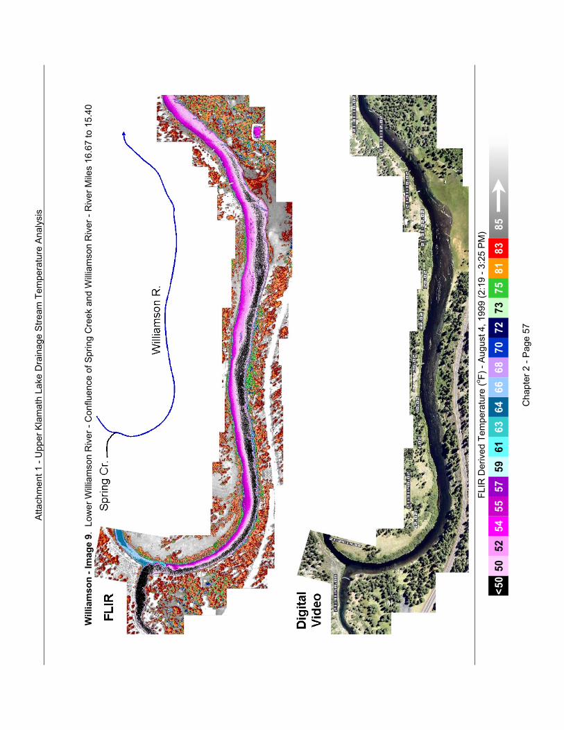
Atta
chm
ent 1
- U
pper
Kla
mat
h La
ke D
rain
age
Stre
am T
empe
ratu
re A
naly
sis
FLIR
Der
ived
Tem
pera
ture
(o F) -
Augu
st 4
, 199
9 (2
:19
- 3:2
5 PM
)
<50
5052
5455
5759
6163
6466
6870
7273
7585
8183
Cha
pter
2 -
Page
57
Will
iam
son
- Im
age
9. L
ower
Willi
amso
n R
iver
- C
onflu
ence
of S
prin
g C
reek
and
Willi
amso
n R
iver
- R
iver
Mile
s 16
.67
to 1
5.40

Atta
chm
ent 1
- U
pper
Kla
mat
h La
ke D
rain
age
Stre
am T
empe
ratu
re A
naly
sis
FLIR
Der
ived
Tem
pera
ture
(o F) -
Augu
st 4
, 199
9 (2
:19
- 3:2
5 PM
)
<50
5052
5455
5759
6163
6466
6870
7273
7585
8183
Cha
pter
2 -
Page
58
Will
iam
son
- Im
age
10.
Low
er W
illiam
son
Riv
er -
Con
fluen
ce o
f Spr
ague
Riv
er a
nd W
illiam
son
Riv
er -
Riv
er M
iles
11.3
8 to
10.
41

Attachment 1 - Upper Klamath Lake Drainage Stream Temperature Analysis
Chapter 2 - Available DataOregon DEQ, May, 2002
Chapter 2 - Page 59
2.2.5.2 Sycan River FLIR Derived Longitudinal Heating and Imagery
Sycan River longitudinal temperatures were sampled using FLIR on August 16, 1999 in twoseparate helicopter flights. The lower 58.55 river miles were sampled from 2:43 to 3:24 PM, whilethe upper 12.95 river miles were sampled from 4:53 to 5:02 PM (the helicopter had to land andrefuel). The FLIR sensor and day TV camera were turned off over the Sycan Marsh becausethere was no distinct stream channel to monitor. Figure 2-18 shows the FLIR flight path – colorcoded to represent the measured stream temperature.
Figure 2-18. Sycan River Sampled FLIR Temperatures
Headwater Sycan River temperatures in the upper 13 river miles has a longitudinal heating rate of0.6°F per mile. Through this upper area, small tributaries and some springs help moderatetemperature increases with cool mass transfers that cause sudden and temporary stream cooling.Due to the smaller flow volume of the Sycan River in this upper reach, responses to cool waterinputs are more dramatic. Likewise, the stream rapidly gains heat a short distance downstream.
The remaining portions of the Sycan River (from the mouth to river mile 58.6) has a streamtemperature profile that fluctuates between a low temperature of 60°F and a high of 72°F. Atabout river mile 54.0, the Sycan River orientation turns to a north/south direction, and the channelwidens slightly compared to upstream. This orientation exposes the river to more direct sunlight,which is likely to be one of the factors that accounts for the sharp heating observed between river

Attachment 1 - Upper Klamath Lake Drainage Stream Temperature Analysis
Chapter 2 - Available DataOregon DEQ, May, 2002
Chapter 2 - Page 60
miles 50.0 and 54.0. Beginning at approximately river mile 49.0, the Sycan River gradientlessens and the valley begins to widen. A weir at river mile 45.8 creates a marshy backwater,where the Sycan River temperature suddenly drops 6°F. A diversion canal at this weir diverts alarge volume of water. Another weir at river mile 44.0 creates more backwater. Below this weir,the Sycan River is channelized as it enters the Sycan Marsh.
Water draining the Sycan Marsh is 70°F. For the next 14 river miles, the stream temperaturefluctuates, but there is no distinct heating pattern. An unmapped spring at river 26.8 drops theriver temperature from 65°F to 60°F. Two more unmapped springs at about river mile 25.7further decrease the river temperature. For the next five river miles, temperature climbs steadilyand rapidly. Teddy Powers Meadow (river miles 17.4 to 20.2) is a stream heating area with amaximum temperature of 72°F. Temperatures decrease as the river enters a confined canyonuntil river mile 14, and downstream the temperatures rise again as the river flows in a lessconfined valley and has a steeper gradient. At about river mile 9.4, the steep gradient suddenlyflattens out as the valley opens up. The immediate decrease in gradient causes the river to bedeeper and much slower. From river mile 9.4 to the mouth, the river temperatures fluctuatebetween 66°F and 72°F.
Summary of Selected FLIR Imagery - Sycan River
• Sycan - Image 1. Sycan River – Meadow Near Headwaters – River Miles 68.26 to 68.39.Upstream of the road, the Sycan River is under 50oF. It enters the meadow shown and heatsto above 50oF in a short distance. The floodplain in this meadow is connected to the river,demonstrated by the cool ground temperatures on all sides of the stream.
• Sycan - Image 2. Sycan River - Unnamed Tributaries – River Miles 67.62 to 67.87. On theleft and bottom of the image, is land that is grazed. Notice the varying surface temperaturesof land cover within the image. Warmer land cover and ground temperatures occur in thegrazed areas where woody vegetation and shrubs are noticeably absent. There are twoseparate tributaries that flow in from the left of the image as well. The lower tributary acooling influence on the Sycan River, dropping the temperature from 59oF to 57oF.
• Sycan - Image 3. Sycan River - Meanders by Pasture – River Miles 67.42 to 66.62. Thisimage displays three distinct microclimates: the warm agricultural field surface, the cool nearstream floodplain, and the even cooler zone in the shadows of the trees (pink dotted line).Additionally, there is a stand of trees within the middle of the field that is about 70°F,compared to the above-85°F temperatures of the field. The Sycan River increases from 57°Fto 60°F in this reach.
• Sycan - Image 4. Sycan River - Meanders by Pond – River Miles 65.34 to 65.49. Thisforested stretch of the Sycan River remains rather cool. There are several areas along thebank that are 3-4°F cooler than the stream resulting from high shade levels.
• Sycan - Image 5. Sycan River – Microclimates – River Miles 64.52 to 64.64. Twomicroclimates are present in this image: the cooler north-facing hillside and the warmersouth-facing hillside. In addition, there are two cool (57°F) patches along the left bank.These cool spots are likely due to high shade levels.
• Sycan - Image 6. Sycan River – Unmapped Spring – River Miles 26.74 to 26.83. Thisunmapped spring contributes a significant volume of 49°F water to the Sycan River,decreasing the river temperatures from about 65°F to 60°F.
• Sycan - Image 7. Sycan River – Unmapped Springs – River Miles 25.58 to 25.71. There aretwo springs on the right bank, which produce cool plumes in the Sycan River and an rivertemperature decrease from 64.5°F to 61.9°F in this reach.
• Sycan - Image 8. Sycan River –Gradient Decrease – River Miles 9.18 to 9.50. This is thepoint at which the Sycan River reaches the valley bottom with a rather abrupt decrease in the

Attachment 1 - Upper Klamath Lake Drainage Stream Temperature Analysis
Chapter 2 - Available DataOregon DEQ, May, 2002
Chapter 2 - Page 61
stream gradient. Just downstream of the imagery, the Sycan River is deeper and muchslower. This lower gradient continues to the mouth. Stream temperatures fall from 71.6°F to66.2°F within 0.93 miles from the gradient drop (i.e. -5.8°F per mile).
• Sycan - Image 9. Sycan River – Irrigation Return – River Miles 4.73 to 5.04. An agriculturalirrigation surface return on the left bank (72.0°F) enters the Sycan River (66.0°F). A smalldiffuse plume results. The day video image displays a deposit of fine sediments and possibleorganic material attributed to the irrigation return.
• Sycan - Image 10. Sycan River – Brown Spring – River Miles 3.95 to 4.36. In the upper leftof the imagery is a small spring on the left bank of the river. Brown Spring enters the SycanRiver downstream of this unmapped spring on the right bank. Water from Brown spring iswarmed considerably before reaching the Sycan River. Originating one mile from the SycanRiver and traveling on the surface through ponds before reaching the Sycan River, the waterfrom Brown Spring is 69.3°F when it reaches the Sycan River.

Atta
chm
ent 1
- U
pper
Kla
mat
h La
ke D
rain
age
Stre
am T
empe
ratu
re A
naly
sis
Cha
pter
2 -
Avai
labl
e D
ata
Ore
gon
DEQ
, May
, 200
2C
hapt
er 2
- Pa
ge 6
2
Figu
re 2
-19.
Syc
an R
iver
FLI
R D
eriv
ed T
empe
ratu
res
- Aug
ust 1
6, 1
999
(2:4
3 to
3:2
4 PM
and
4:5
3 to
5:0
2 PM
)
40455055606570758085
05
1015
2025
3035
4045
5055
6065
70R
iver
Mile
FLIR Derived Stream Temperature (oF)
4:53
to 5
:02
PM2:
43 to
3:2
4 PM
Imag
e 7
- Spr
ings
Imag
e 6
- Spr
ing
Imag
e 9-
Irr
igat
ion
Ret
urn
Imag
e 5
- Mic
rocl
imat
es
Imag
e 4
- Mea
nder
s an
d Po
nd
Imag
e 3
- Mea
nder
s by
Pas
ture
Imag
e 2
- Unm
appe
d Tr
ibut
arie
s
Imag
e 1
- Mea
dow
Nea
r Hea
dwat
ers
Imag
e 10
- Br
own
Sprin
g
Imag
e 8-
G
radi
ent D
rop
Syca
n M
arsh

Atta
chm
ent 1
- U
pper
Kla
mat
h La
ke D
rain
age
Stre
am T
empe
ratu
re A
naly
sis
FLIR
Der
ived
Tem
pera
ture
(o F) -
Augu
st 1
6, 1
999
(2:4
3 to
3:2
4 PM
and
4:5
3 to
5:0
2 PM
)
<50
5052
5455
5759
6163
6466
6870
7273
7585
8183
Cha
pter
2 -
Page
63
Syca
n - I
mag
e 1.
Syc
an R
iver
– M
eado
w N
ear H
eadw
ater
s –
Riv
er M
iles
68.2
6 to
68.
39

Atta
chm
ent 1
- U
pper
Kla
mat
h La
ke D
rain
age
Stre
am T
empe
ratu
re A
naly
sis
FLIR
Der
ived
Tem
pera
ture
(o F) -
Augu
st 1
6, 1
999
(2:4
3 to
3:2
4 PM
and
4:5
3 to
5:0
2 PM
)
<50
5052
5455
5759
6163
6466
6870
7273
7585
8183
Cha
pter
2 -
Page
64
Syca
n - I
mag
e 2.
Sy
can
Riv
er -
Unn
amed
Trib
utar
ies
– R
iver
Mile
s 6
7.62
to 6
7.86

Atta
chm
ent 1
- U
pper
Kla
mat
h La
ke D
rain
age
Stre
am T
empe
ratu
re A
naly
sis
FLIR
Der
ived
Tem
pera
ture
(o F) -
Augu
st 1
6, 1
999
(2:4
3 to
3:2
4 PM
and
4:5
3 to
5:0
2 PM
)
<50
5052
5455
5759
6163
6466
6870
7273
7585
8183
Cha
pter
2 -
Page
65
Syca
n - I
mag
e 3.
Sy
can
Riv
er -
Mea
nder
s by
Pas
ture
– R
iver
Mile
s 67
.42
to 6
6.62

Atta
chm
ent 1
- U
pper
Kla
mat
h La
ke D
rain
age
Stre
am T
empe
ratu
re A
naly
sis
FLIR
Der
ived
Tem
pera
ture
(o F) -
Augu
st 1
6, 1
999
(2:4
3 to
3:2
4 PM
and
4:5
3 to
5:0
2 PM
)
<50
5052
5455
5759
6163
6466
6870
7273
7585
8183
Cha
pter
2 -
Page
66
Syca
n - I
mag
e 4.
Syc
an R
iver
- M
eand
ers
by P
ond
– R
iver
Mile
s 65
.34
to 6
5.49

Atta
chm
ent 1
- U
pper
Kla
mat
h La
ke D
rain
age
Stre
am T
empe
ratu
re A
naly
sis
FLIR
Der
ived
Tem
pera
ture
(o F) -
Augu
st 1
6, 1
999
(2:4
3 to
3:2
4 PM
and
4:5
3 to
5:0
2 PM
)
<50
5052
5455
5759
6163
6466
6870
7273
7585
8183
Cha
pter
2 -
Page
67
Syca
n - I
mag
e 5.
Sy
can
Riv
er –
Mic
rocl
imat
es –
Riv
er M
iles
64.5
2 to
64.
64

Atta
chm
ent 1
- U
pper
Kla
mat
h La
ke D
rain
age
Stre
am T
empe
ratu
re A
naly
sis
FLIR
Der
ived
Tem
pera
ture
(o F) -
Augu
st 1
6, 1
999
(2:4
3 to
3:2
4 PM
and
4:5
3 to
5:0
2 PM
)
<50
5052
5455
5759
6163
6466
6870
7273
7585
8183
Cha
pter
2 -
Page
68
Syca
n - I
mag
e 6.
Syc
an R
iver
– U
nmap
ped
Sprin
g –
Riv
er M
iles
26.7
4 to
26.
83

Atta
chm
ent 1
- U
pper
Kla
mat
h La
ke D
rain
age
Stre
am T
empe
ratu
re A
naly
sis
FLIR
Der
ived
Tem
pera
ture
(o F) -
Augu
st 1
6, 1
999
(2:4
3 to
3:2
4 PM
and
4:5
3 to
5:0
2 PM
)
<50
5052
5455
5759
6163
6466
6870
7273
7585
8183
Cha
pter
2 -
Page
69
Syca
n - I
mag
e 7.
Syc
an R
iver
– U
nmap
ped
Sprin
gs –
Riv
er M
iles
25.5
8 to
25.
71

Atta
chm
ent 1
- U
pper
Kla
mat
h La
ke D
rain
age
Stre
am T
empe
ratu
re A
naly
sis
FLIR
Der
ived
Tem
pera
ture
(o F) -
Augu
st 1
6, 1
999
(2:4
3 to
3:2
4 PM
and
4:5
3 to
5:0
2 PM
)
<50
5052
5455
5759
6163
6466
6870
7273
7585
8183
Cha
pter
2 -
Page
70
Syca
n - I
mag
e 8.
Sy
can
Riv
er –
Gra
dien
t Dro
p –
Riv
er M
iles
9.18
to 9
.50

Atta
chm
ent 1
- U
pper
Kla
mat
h La
ke D
rain
age
Stre
am T
empe
ratu
re A
naly
sis
FLIR
Der
ived
Tem
pera
ture
(o F) -
Augu
st 1
6, 1
999
(2:4
3 to
3:2
4 PM
and
4:5
3 to
5:0
2 PM
)
<50
5052
5455
5759
6163
6466
6870
7273
7585
8183
Cha
pter
2 -
Page
71
Syca
n - I
mag
e 9.
Sy
can
Riv
er –
Irrig
atio
n R
etur
n –
Riv
er M
iles
4.73
to 5
.04

Atta
chm
ent 1
- U
pper
Kla
mat
h La
ke D
rain
age
Stre
am T
empe
ratu
re A
naly
sis
FLIR
Der
ived
Tem
pera
ture
(o F) -
Augu
st 1
6, 1
999
(2:4
3 to
3:2
4 PM
and
4:5
3 to
5:0
2 PM
)
<50
5052
5455
5759
6163
6466
6870
7273
7585
8183
Cha
pter
2 -
Page
72
Syca
n - I
mag
e 10
. S
ycan
Riv
er –
Bro
wn
Sprin
g –
Riv
er M
iles
3.95
to 4
.36

Attachment 1 - Upper Klamath Lake Drainage Stream Temperature Analysis
Chapter 2 - Available DataOregon DEQ - May, 2002
Chapter 2 - Page 73
2.5.2.3 Sprague River FLIR Derived Longitudinal Heating and Imagery
Sprague River longitudinal temperatures were sampled using FLIR on August 12, 1999 from 2:16to 3:20 PM. Figure 2-20 shows the FLIR flight path, color coded to display the measured streamtemperature. At the time of FLIR sampling, the Sprague River temperatures ranged from about68°F to the 73°F. Figure 2-21 shows the FLIR derived stream temperature longitudinal profile.
Figure 2-20. Sprague River Sampled FLIR Temperatures
The temperature at the confluence of the North and South Forks (river mile 84.6) wasapproximately 70°F. Throughout the Sprague River mainstem there are many points ofdiversions and irrigation returns. As a result, the flow and thermal regime of the river fluctuates.In many river reaches there are diversion canals that re-direct large volumes of Sprague Riverwater, sometimes rejoining the mainstem a mile or two downstream. Many Sprague Riverreaches have multiple channels, characteristic of a low-gradient meandering stream and finesubstrates. Several springs enter the Sprague River and have varying degrees of cooling to theSprague River temperature. For example, Kamkaun Spring (river mile 23.5) drops the mainstemtemperature from 70°F to 66°F. Other stream segments have diffuse subsurface inflow thatoccur over a long distance (i.e. one mile). FLIR data reveal that the Sprague River is a naturallycomplex system that is highly modified by human land and water use. Stream temperaturepatterns are most affected by mass transfers to and from the river system.

Attachment 1 - Upper Klamath Lake Drainage Stream Temperature Analysis
Chapter 2 - Available DataOregon DEQ - May, 2002
Chapter 2 - Page 74
Summary of Selected FLIR Imagery - Sprague River
• Sprague - Image A-1. Sprague River – Confluence of North and South Forks - River Miles84.45 to 84.60. The North Fork Sprague River is 64°F at its mouth, while the South ForkSprague River is 72°F at its mouth. Complete mixing of the North and South Forks occursover a short distance at the first downstream bend in the Sprague River.
• Sprague - Image A-2. Sprague River – Channel Modification and Levee – River Miles 82.43to 81.88. These images display a 1.45-mile reach where the Sprague River has undergoneextensive channel modifications and a canal that diverts much of the stream along a levee.
• Sprague - Image A-3. Sprague River – Unmapped Spring – River Miles 80.74 to 81.18. A59°F spring cools the mainstem temperature from approximately 70°F to 68°F.
• Sprague - Image A-4. Sprague River – Agricultural Fields - River Miles 79.46 to 80.23. Thenear stream area is bordered by cultivated fields and remnants of woody and shrub landcover. The surface area of the cultivated fields exceeds 85°F, while the remnant areas ofwoody land cover (likely to be willows) is in the lower 70°F range.
• Sprague - Image A-5. Sprague River – Unmapped Spring - River Miles 74.26 to 74.66. Thisunmapped spring cools the mainstem temperature about 2°F.
• Sprague - Image A-6. Sprague River – Side Channel Returning - River Miles 65.57 to66.18. At the lower left corner of the imagery is a side channel returning to the SpragueRiver, 1.7 miles after branching off of the mainstem. The returning water is significantlywarmer than the mainstem and a warm plume can be observed along the right bank.
• Sprague - Image A-7. Sprague River – Kamkaun Spring - River Miles 23.29 to 23.82.Kamakaun Spring is cooling the mainstem temperature from about 70°F to 66°F. The springappears to have a significant flow contribution of 55°F water.

Atta
chm
ent 1
- U
pper
Kla
mat
h La
ke D
rain
age
Stre
am T
empe
ratu
re A
naly
sis
Cha
pter
2 -
Avai
labl
e D
ata
Ore
gon
DEQ
- M
ay, 2
002
Cha
pter
2 -
Page
75
Figu
re 2
-21.
Spr
ague
Riv
er F
LIR
Der
ived
Tem
pera
ture
s - A
ugus
t 12,
199
9 –
2:16
to 3
:20
PM
40455055606570758085
010
2030
4050
6070
80R
iver
Mile
FLIR Derived Stream Temperature (oF)
Imag
e 1
- Nor
th F
ork/
Sout
h Fo
rk C
onflu
ence
Imag
e 3
- Unm
appe
d Sp
ring
Imag
e 4
- Agr
icul
tura
l Fie
lds
Imag
e 5
- Unm
appe
d Sp
ring
Imag
e 6
- Sid
e C
hann
el R
etur
ning
Imag
e 7
- Kam
kaun
Spr
ing
Imag
e 2
- Cha
nnel
Mod
ifica
tion
and
Leve
e

Atta
chm
ent 1
- U
pper
Kla
mat
h La
ke D
rain
age
Stre
am T
empe
ratu
re A
naly
sis
FLIR
Der
ived
Tem
pera
ture
(o F) -
Augu
st 1
2, 1
999
(2:1
6 to
3:2
0 PM
)
<50
5052
5455
5759
6163
6466
6870
7273
7585
8183
Cha
pter
2 -
Page
76
Spra
gue
- Im
age
A-1
. Sp
ragu
e R
iver
– C
onflu
ence
of N
orth
and
Sou
th F
orks
- R
iver
Mile
s 84
.45
to 8
4.60

Atta
chm
ent 1
- U
pper
Kla
mat
h La
ke D
rain
age
Stre
am T
empe
ratu
re A
naly
sis
FLIR
Der
ived
Tem
pera
ture
(o F) -
Augu
st 1
2, 1
999
(2:1
6 to
3:2
0 PM
)
<50
5052
5455
5759
6163
6466
6870
7273
7585
8183
Cha
pter
2 -
Page
77
Spra
gue
- Im
age
A-2
. Sp
ragu
e R
iver
– C
hann
el M
odifi
catio
n an
d Le
vee
– R
iver
Mile
s 81
.43
to 8
2.88

Atta
chm
ent 1
- U
pper
Kla
mat
h La
ke D
rain
age
Stre
am T
empe
ratu
re A
naly
sis
FLIR
Der
ived
Tem
pera
ture
(o F) -
Augu
st 1
2, 1
999
(2:1
6 to
3:2
0 PM
)
<50
5052
5455
5759
6163
6466
6870
7273
7585
8183
Cha
pter
2 -
Page
78
Spra
gue
- Im
age
A-3
. S
prag
ue R
iver
– U
nmap
ped
Sprin
g –
Riv
er M
iles
80.7
4 to
81.
18

Atta
chm
ent 1
- U
pper
Kla
mat
h La
ke D
rain
age
Stre
am T
empe
ratu
re A
naly
sis
FLIR
Der
ived
Tem
pera
ture
(o F) -
Augu
st 1
2, 1
999
(2:1
6 to
3:2
0 PM
)
<50
5052
5455
5759
6163
6466
6870
7273
7585
8183
Cha
pter
2 -
Page
79
Spra
gue
- Im
age
A-4
. Sp
ragu
e R
iver
– A
gric
ultu
ral F
ield
s - R
iver
Mile
s 79
.46
to 8
0.23

Atta
chm
ent 1
- U
pper
Kla
mat
h La
ke D
rain
age
Stre
am T
empe
ratu
re A
naly
sis
FLIR
Der
ived
Tem
pera
ture
(o F) -
Augu
st 1
2, 1
999
(2:1
6 to
3:2
0 PM
)
<50
5052
5455
5759
6163
6466
6870
7273
7585
8183
Cha
pter
2 -
Page
80
Spra
gue
- Im
age
A-5
. Sp
ragu
e R
iver
– U
nmap
ped
Sprin
g - R
iver
Mile
s 74
.26
to 7
4.66

Atta
chm
ent 1
- U
pper
Kla
mat
h La
ke D
rain
age
Stre
am T
empe
ratu
re A
naly
sis
FLIR
Der
ived
Tem
pera
ture
(o F) -
Augu
st 1
2, 1
999
(2:1
6 to
3:2
0 PM
)
<50
5052
5455
5759
6163
6466
6870
7273
7585
8183
Cha
pter
2 -
Page
81
Spra
gue
- Im
age
A-6
. Sp
ragu
e R
iver
– S
ide
Cha
nnel
Ret
urni
ng -
Riv
er M
iles
65.5
7 to
66.
18

Atta
chm
ent 1
- U
pper
Kla
mat
h La
ke D
rain
age
Stre
am T
empe
ratu
re A
naly
sis
FLIR
Der
ived
Tem
pera
ture
(o F) -
Augu
st 1
2, 1
999
(2:1
6 to
3:2
0 PM
)
<50
5052
5455
5759
6163
6466
6870
7273
7585
8183
Cha
pter
2 -
Page
82
Spra
gue
- Im
age
A-7
. Spr
ague
Riv
er –
Kam
kaun
Spr
ing
- Riv
er M
iles
23.2
9 to
23.
82
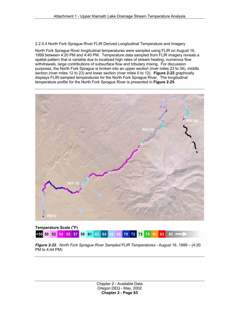
Attachment 1 - Upper Klamath Lake Drainage Stream Temperature Analysis
Chapter 2 - Available DataOregon DEQ - May, 2002
Chapter 2 - Page 83
2.2.5.4 North Fork Sprague River FLIR Derived Longitudinal Temperature and Imagery
North Fork Sprague River longitudinal temperatures were sampled using FLIR on August 16,1999 between 4:20 PM and 4:40 PM. Temperature data sampled from FLIR imagery reveals aspatial pattern that is variable due to localized high rates of stream heating, numerous flowwithdrawals, large contributions of subsurface flow and tributary mixing. For discussionpurposes, the North Fork Sprague is broken into an upper section (river miles 23 to 34), middlesection (river miles 12 to 23) and lower section (river miles 0 to 12). Figure 2-22 graphicallydisplays FLIR-sampled temperatures for the North Fork Sprague River. The longitudinaltemperature profile for the North Fork Sprague River is presented in Figure 2-25.
Temperature Scale (oF)<50 50 52 54 55 57 59 61 63 64 66 68 70 72 73 75 8581 83
Figure 2-22. North Fork Sprague River Sampled FLIR Temperatures - August 16, 1999 – (4:20PM to 4:44 PM)

Attachment 1 - Upper Klamath Lake Drainage Stream Temperature Analysis
Chapter 2 - Available DataOregon DEQ - May, 2002
Chapter 2 - Page 84
Upper North Fork Sprague River Heating Gradients - RM 23-34
FLIR sampled temperatures in the upper North Fork Sprague River show variable spatialdistributions (45oF to 65oF). Cool areas are associated with springs/groundwater inflow. Theupper North Fork Sprague River originates from a series of springs, with 55°F streamtemperatures above Lee Thomas Meadow. Stream temperatures increase dramatically as theNorth Fork Sprague River travels through Lee Thomas Meadow, with a heating gradient of 9°Fper mile (Figure 2-23). The stream temperature increases rapidly at the upper end of LeeThomas Meadow, and those high temperatures are maintained throughout downstream distanceof the meadow.
Temperature Scale (oF)<50 50 52 54 55 57 59 61 63 64 66 68 70 72 73 75 8581 83
Figure 2-23. Temperature Profile in Upper Lee Thomas Meadow (Dashed Box indicate the areahighlighted in North Fork Sprague - Image 1.) - August 16, 1999 – (4:20 PM to 4:44 PM)
Middle North Fork Sprague River Heating Gradients - RM 12-23
Temperatures become highly variable as the river travels out of Lee Thomas Meadow back into aforested area. Several major springs cool the mainstem within this reach and add flow volume.

Attachment 1 - Upper Klamath Lake Drainage Stream Temperature Analysis
Chapter 2 - Available DataOregon DEQ - May, 2002
Chapter 2 - Page 85
Water temperatures decrease downstream of a several springs around river mile 22. However,stream temperatures quickly heat in the two-mile reach downstream from these springs.
Several major springs and cold tributaries were observed between river miles 15 and 20.Temperature decreases rapidly within this reach, and are maintained at low levels of heating.The stream heating longitudinal gradients within this reach was 0.3°F per mile.
Temperature Scale (oF)<50 50 52 54 55 57 59 61 63 64 66 68 70 72 73 75 8581 83
Figure 2-24. Temperature profile in Bailey Flat (Dashed Boxes indicate areas highlighted inNorth Fork Sprague - Images 6 and 7.) - August 16, 1999 – (4:20 PM to 4:44 PM)

Attachment 1 - Upper Klamath Lake Drainage Stream Temperature Analysis
Chapter 2 - Available DataOregon DEQ - May, 2002
Chapter 2 - Page 86
Lower North Fork Sprague River Heating Gradients - RM 0-12
Sampled temperatures in the lower North Fork Sprague River had a variable spatial distribution,with temperatures increasing rapidly as the river traveled out of forested areas and into the lowermeadow system at Bailey Flat where the stream heating gradient within was 3.5°F per mile.Bailey Flat is illustrated in Figure 2-24. This high rate of heating is the result of low levels ofstream shade, flow withdrawals, the return of diverted water, and channel modifications.Elevated stream temperatures are maintained for three to four miles downstream from BaileyFlat. Water temperatures decrease slightly as the river travels downstream into the SpragueRiver Valley. Water temperatures increase once again near the mouth of the North Fork Spraguefollowing a major water diversion at River Mile 2.3.
Summary of Selected FLIR Imagery - North Fork Sprague
• North Fork Sprague - Image 1. North Fork Sprague River – Meadow Disturbance/ChannelSimplification - River Miles 29.59 to 30.24. The initial solar exposure (due to low levels ofstream shade) of the North Fork Sprague River in Lee Thomas Meadow allows streamtemperature increases rapidly. This area is a primary zone of stream heating in the NorthFork Sprague River.
• North Fork Sprague - Image 2. North Fork Sprague River – Area with Multiple Springs -River Miles 18.41 to 18.65. The discharge of multiple springs cools stream temperatures inthe North Fork Sprague River.
• North Fork Sprague - Image 3. North Fork Sprague River and Sheepy Creek Confluence -River Miles 17.46 to 17.55. A cold water tributary on mainstem temperatures in the NorthFork Sprague River cools downstream temperature to below 55°F.
• North Fork Sprague - Image 4. North Fork Sprague River – Thermal Microclimate - RiverMiles 16.54 to 16.99. Recent harvest activities are evident on the left stream bank by warmersurface temperatures. Alternatively, the intact forest stands on the right bank have coolersurface temperatures. Such differential heating is an indication of thermal microclimatetemperature increases that accompany the removal of stand structure.
• North Fork Sprague - Image 5. North Fork Sprague River – Spring Influence - River Miles14.41 to 14.47. The spring illustrated in this image is a typical spring within this reach of theriver.
• North Fork Sprague - Image 6. North Fork Sprague River - Spring Influence - River Miles13.89 to 14.03. The effect of spring flow on water temperature can be seen in this image.
• North Fork Sprague - Image 7. North Fork Sprague River – Channel Disturbance andWater Withdrawal - River Miles 10.70 to 11.36. Stream temperatures warm as the North ForkSprague River travels into Bailey Flat. A 3.5°F per mile stream heating longitudinal gradientis observed within Bailey Flat. This high rate of heating is the result of low levels of streamshade, flow withdrawals, the return of diverted water, and channel modifications.
• North Fork Sprague - Image 8. North Fork Sprague River – Warm Return Flow - RiverMiles 9.99 to 10.16. This image shows the temperature response resulting from the return ofdiverted water back into the North Fork Sprague River located at the lower end of Bailey Flat(1.2 miles downstream of Image 7). Water temperatures increase in response to the warmwater mass transfer. The return water illustrated in this image was withdrawn for the NorthFork Sprague at the top of this Bailey Flat. Water temperatures increases within this reachare likely exacerbated through other heat transfer processes in addition to mass transfer

Attachment 1 - Upper Klamath Lake Drainage Stream Temperature Analysis
Chapter 2 - Available DataOregon DEQ - May, 2002
Chapter 2 - Page 87
warming (i.e. decreased instream flow, low levels of shade and channel modifications alsocontribute to high rates of stream warming).
• North Fork Sprague - Image 9. North Fork Sprague River – Return Flow and Meryl CreekConfluence - River Miles 5.04 to 5.51. This image shows the complex nature on multiplemass transfer processes. Both a warm water return flow and the Meryl Creek confluenceaffect instream temperatures. Returns from an upstream withdrawal contribute a smallvolume of 72oF water. Meryl Creek is 63oF at the confluence and contributes a large volumeof water, with a combined effect of 1.3oF cooling to the North Fork Sprague River.
• North Fork Sprague - Image 10. North Fork Sprague River - Five Mile Creek Confluence -River Miles 2.61 to 2.72. The temperature of Five Mile Creek is slightly cooler than the NorthFork Sprague River. River hydraulics within this stretch of the river are modified (i.e.,reduced velocities, increased depths) by a diversion pushup dam located 0.3 milesdownstream of this image. Riparian vegetation is mostly absent. A small water temperaturedecrease was observed downstream of this confluence.
• North Fork Sprague - Image 11. North Fork Sprague River – Water withdrawals and returnflows - River Miles 2.30 to 2.38. This image shows a diversion push up dam. Severalagriculture warm water return flows are entering the river downstream of this dam. Watertemperatures increase downstream of this diversion, like due to the combined effect ofdecreases flow volume and warm water mass transfers associated with the agriculture returnflows.


Atta
chm
ent 1
- U
pper
Kla
mat
h La
ke D
rain
age
Stre
am T
empe
ratu
re A
naly
sis
Cha
pter
2 -
Avai
labl
e D
ata
Ore
gon
DEQ
- M
ay, 2
002
Cha
pter
2 -
Page
89
Figu
re 2
-25.
Nor
th F
ork
Spra
gue
Riv
er F
LIR
Der
ived
Tem
pera
ture
s - A
ugus
t 16,
199
9 –
(4:2
0 PM
to 4
:44
PM)
40455055606570758085
05
1015
2025
30R
iver
Mile
FLIR Derived Stream Temperature (oF)
Imag
e 1
- Ini
tial M
eado
w E
xpos
ure/
Cha
nnel
Sim
plifi
catio
n
Imag
e 2
- Mul
tiple
Spr
ings
Imag
e 3
- She
epy
Cre
ek
Imag
e 5
- Spr
ing
Imag
e 6
- Spr
ing
Imag
e 7
- Cha
nnel
Dis
turb
ance
/W
ater
With
draw
al
Imag
e 10
- Fi
ve M
ile C
reek
Imag
e 9
- Mer
yl C
reek
and
Ret
urn
Dis
char
ge
Imag
e 8
- Ret
urn
Dis
char
ge
Imag
e 11
- W
ater
With
draw
al
Imag
e 4
- Spr
ings
and
Th
erm
al M
icro
clim
ate

Atta
chm
ent 1
- U
pper
Kla
mat
h La
ke D
rain
age
Stre
am T
empe
ratu
re A
naly
sis
FLIR
Der
ived
Tem
pera
ture
(o F) -
Augu
st 1
6, 1
999
(4:2
0 PM
to 4
:44
PM)
<50
5052
5455
5759
6163
6466
6870
7273
7585
8183
Cha
pter
2 -
Page
90
Nor
th F
ork
Spra
gue
- Im
age
1. –
Nor
th F
ork
Spra
gue
Riv
er –
Mea
dow
Dis
turb
ance
/Cha
nnel
Sim
plifi
catio
n - R
iver
Mile
s 29
.59
– 30
.24.

Atta
chm
ent 1
- U
pper
Kla
mat
h La
ke D
rain
age
Stre
am T
empe
ratu
re A
naly
sis
FLIR
Der
ived
Tem
pera
ture
(o F) -
Augu
st 1
6, 1
999
(4:2
0 PM
to 4
:44
PM)
<50
5052
5455
5759
6163
6466
6870
7273
7585
8183
Cha
pter
2 -
Page
91
Nor
th F
ork
Spra
gue
- Im
age
2. N
orth
For
k Sp
ragu
e R
iver
– A
rea
with
Mul
tiple
Spr
ings
- R
iver
Mile
s 18
.41
- 18.
65

Atta
chm
ent 1
- U
pper
Kla
mat
h La
ke D
rain
age
Stre
am T
empe
ratu
re A
naly
sis
FLIR
Der
ived
Tem
pera
ture
(o F) -
Augu
st 1
6, 1
999
(4:2
0 PM
to 4
:44
PM)
<50
5052
5455
5759
6163
6466
6870
7273
7585
8183
Cha
pter
2 -
Page
92
Nor
th F
ork
Spra
gue
- Im
age
3. N
orth
For
k Sp
ragu
e R
iver
and
She
epy
Cre
ek C
onflu
ence
- R
iver
Mile
s 17
.46
– 17
.55

Atta
chm
ent 1
- U
pper
Kla
mat
h La
ke D
rain
age
Stre
am T
empe
ratu
re A
naly
sis
FLIR
Der
ived
Tem
pera
ture
(o F) -
Augu
st 1
6, 1
999
(4:2
0 PM
to 4
:44
PM)
<50
5052
5455
5759
6163
6466
6870
7273
7585
8183
Cha
pter
2 -
Page
93
Nor
th F
ork
Spra
gue
- Im
age
4. N
orth
For
k Sp
ragu
e R
iver
– T
herm
al M
icro
clim
ate
- Riv
er M
iles
16.5
4 to
16.
99

Atta
chm
ent 1
- U
pper
Kla
mat
h La
ke D
rain
age
Stre
am T
empe
ratu
re A
naly
sis
FLIR
Der
ived
Tem
pera
ture
(o F) -
Augu
st 1
6, 1
999
(4:2
0 PM
to 4
:44
PM)
<50
5052
5455
5759
6163
6466
6870
7273
7585
8183
Cha
pter
2 -
Page
94
Nor
th F
ork
Spra
gue
- Im
age
5. N
orth
For
k Sp
ragu
e R
iver
– S
prin
g In
fluen
ce -
Riv
er M
iles
14.4
1 to
14.
47

Atta
chm
ent 1
- U
pper
Kla
mat
h La
ke D
rain
age
Stre
am T
empe
ratu
re A
naly
sis
FLIR
Der
ived
Tem
pera
ture
(o F) -
Augu
st 1
6, 1
999
(4:2
0 PM
to 4
:44
PM)
<50
5052
5455
5759
6163
6466
6870
7273
7585
8183
Cha
pter
2 -
Page
95
Nor
th F
ork
Spra
gue
- Im
age
6. N
orth
For
k Sp
ragu
e R
iver
- S
prin
g In
fluen
ce -
Riv
er M
iles
13.8
9 –
14.0
3

Atta
chm
ent 1
- U
pper
Kla
mat
h La
ke D
rain
age
Stre
am T
empe
ratu
re A
naly
sis
FLIR
Der
ived
Tem
pera
ture
(o F) -
Augu
st 1
6, 1
999
(4:2
0 PM
to 4
:44
PM)
<50
5052
5455
5759
6163
6466
6870
7273
7585
8183
Cha
pter
2 -
Page
96
Nor
th F
ork
Spra
gue
- Im
age
7. N
orth
For
k Sp
ragu
e R
iver
– C
hann
el D
istu
rban
ce a
nd W
ater
With
draw
al -
Riv
er M
iles
10.7
0 –
11.3
6

Atta
chm
ent 1
- U
pper
Kla
mat
h La
ke D
rain
age
Stre
am T
empe
ratu
re A
naly
sis
FLIR
Der
ived
Tem
pera
ture
(o F) -
Augu
st 1
6, 1
999
(4:2
0 PM
to 4
:44
PM)
<50
5052
5455
5759
6163
6466
6870
7273
7585
8183
Cha
pter
2 -
Page
97
Nor
th F
ork
Spra
gue
- Im
age
8. N
orth
For
k Sp
ragu
e R
iver
– A
gric
ultu
ral R
etur
n Fl
ow -
Riv
er M
iles
9.99
– 1
0.16

Atta
chm
ent 1
- U
pper
Kla
mat
h La
ke D
rain
age
Stre
am T
empe
ratu
re A
naly
sis
FLIR
Der
ived
Tem
pera
ture
(o F) -
Augu
st 1
6, 1
999
(4:2
0 PM
to 4
:44
PM)
<50
5052
5455
5759
6163
6466
6870
7273
7585
8183
Cha
pter
2 -
Page
98
Nor
th F
ork
Spra
gue
- Im
age
9. N
orth
For
k Sp
ragu
e R
iver
– R
etur
n Fl
ow a
nd M
eryl
Cre
ek C
onflu
ence
- R
iver
Mile
s 5.
04 –
5.5
1

Atta
chm
ent 1
- U
pper
Kla
mat
h La
ke D
rain
age
Stre
am T
empe
ratu
re A
naly
sis
FLIR
Der
ived
Tem
pera
ture
(o F) -
Augu
st 1
6, 1
999
(4:2
0 PM
to 4
:44
PM)
<50
5052
5455
5759
6163
6466
6870
7273
7585
8183
Cha
pter
2 -
Page
99
Nor
th F
ork
Spra
gue
- Im
age
10.
Nor
th F
ork
Spra
gue
Riv
er -
Five
Mile
Cre
ek C
onflu
ence
- R
iver
Mile
s 2.
61 –
2.7
2

Atta
chm
ent 1
- U
pper
Kla
mat
h La
ke D
rain
age
Stre
am T
empe
ratu
re A
naly
sis
FLIR
Der
ived
Tem
pera
ture
(o F) -
Augu
st 1
6, 1
999
(4:2
0 PM
to 4
:44
PM)
<50
5052
5455
5759
6163
6466
6870
7273
7585
8183
Cha
pter
2 -
Page
100
Nor
th F
ork
Spra
gue
- Im
age
11.
Nor
th F
ork
Spra
gue
Riv
er –
Wat
er W
ithdr
awal
and
Ret
urn
Flow
s - R
iver
Mile
s 2.
30 –
2.3
8

Attachment 1 - Upper Klamath Lake Drainage Stream Temperature Analysis
Chapter 2 - Available DataOrego DEQ - May, 2002Chapter 2 - Page 101
2.2.5.5 South Fork Sprague River FLIR Derived Longitudinal Heating and Imagery
South Fork Sprague River longitudinal temperatures were sampled using FLIR on August 12,1999 from 4:04 to 4:31 PM. Figure 2-26 shows the FLIR flight path – color coded to representthe measured stream temperature. A general stream heating trend from about 50°F at theheadwaters (river mile 32) to 73°F at the mouth (river mile 0) is apparent from Figure 2-26.Examination of the longitudinal temperature profile (Figure 2-27) and actual infrared and daytelevision images reveals the smaller scale variability of the South Fork Sprague Rivertemperatures. Compared to the North Fork, the South Fork Sprague River exhibits lesslongitudinal temperature variability.
Figure 2-26. South Fork Sprague River Sampled FLIR Temperatures
The South Fork Sprague River gradually heats from 50°F to 72°F from the headwaters to rivermile 17. The river then enters a v-shaped valley and is flowing westward through an area withmoderate topographic shade, confined channels, and shade from near stream land cover.Associated longitudinal stream cooling temperature stabilization results. Starting at river mile 10a heating gradient gradually increase the stream temperatures in the longitudinal direction. Belowriver mile 10, the South Fork Sprague River flows through low gradient highly managed landswhere straightened/downcut channels, irrigation returns and diversions are common. Theselower 10 river miles continue to heat, reaching 75°F in some areas.

Attachment 1 - Upper Klamath Lake Drainage Stream Temperature Analysis
Chapter 2 - Available DataOrego DEQ - May, 2002Chapter 2 - Page 102
Summary of Selected FLIR Imagery - South Fork Sprague River
• South Fork Sprague River - Image 1. South Fork Sprague River – Buckboard CreekConfluence – River Miles 23.10 to 22.91. Midway through the reach displayed in this image,Buckboard Creek enters on the left bank of the South Fork Sprague River. Buckboard Creekenters at about 57°F, creating a visible plume of cooler water in the South Fork SpragueRiver.
• South Fork Sprague River - Image 2. South Fork Sprague River – Hyporheic Flow – RiverMiles 20.8 to 20.6. This image shows a location where some of the stream flows beneaththe surface of a gravel bar (part of a side channel) and re-surfaces cooler than it wasupstream.
• South Fork Sprague River - Image 3. South Fork Sprague River - Microclimates – RiverMiles 16.07 to 15.91. The north-facing slope in this image is much cooler than the southfacing slope of the valley. The south-facing slope has relatively little woody vegetation, butthere is a patch near the stream that is markedly cooler in temperature.
• South Fork Sprague River - Image 4. South Fork Sprague River – Brownsworth Creek andSprings – River Miles 15.35 to 15.02. Brownsworth Creek is having a significant coolingeffect on the South Fork Sprague River, dropping its temperature from 68°F to 66°F. Justdownstream of the Brownsworth Creek confluence are some unmapped springs, whichfurther cool down the South Fork Sprague River.
• South Fork Sprague River - Image 5. South Fork Sprague River – Diversion Canal – RiverMiles 10.14 to 9.78. At this location, is a major irrigation diversion. It appears as though theSouth Fork Sprague River channel has undergone anthropogenic modification in order createa pool for the diversion. This is the first of many major diversions and channel modificationscharacteristic of the South Fork Sprague River and the Sprague River mainstem.

Atta
chm
ent 1
- U
pper
Kla
mat
h La
ke D
rain
age
Stre
am T
empe
ratu
re A
naly
sis
Cha
pter
2 -
Avai
labl
e D
ata
Ore
go D
EQ -
May
, 200
2C
hapt
er 2
- Pa
ge 1
03
Figu
re 2
-27.
Sou
th F
ork
Spra
gue
Riv
er F
LIR
Der
ived
Tem
pera
ture
s - A
ugus
t 12,
199
9 - 4
:04
to 4
:31
PM
404550556065707580
05
1015
2025
30R
iver
Mile
FLIR Derived Stream Temperature (oF)
Imag
e 4
- Bro
wns
wor
th C
reek
and
Spr
ings
Imag
e 5
- Div
ersi
on in
to C
anal
Imag
e 3
- Mic
rocl
imat
es
Imag
e 2
- Hyp
orhe
ic F
low
Imag
e 1
- Buc
kboa
rd C
reek

Atta
chm
ent 1
- U
pper
Kla
mat
h La
ke D
rain
age
Stre
am T
empe
ratu
re A
naly
sis
FLIR
Der
ived
Tem
pera
ture
(o F) -
Augu
st 1
2, 1
999
(4:0
4 to
4:3
1 PM
)
<50
5052
5455
5759
6163
6466
6870
7273
7585
8183
Page
2-1
04
Sout
h Fo
rk S
prag
ue R
iver
- Im
age
1. S
outh
For
k Sp
ragu
e R
iver
– B
uckb
oard
Cre
ek C
onflu
ence
– R
iver
Mile
s 23
.10
to 2
2.91

Atta
chm
ent 1
- U
pper
Kla
mat
h La
ke D
rain
age
Stre
am T
empe
ratu
re A
naly
sis
FLIR
Der
ived
Tem
pera
ture
(o F) -
Augu
st 1
2, 1
999
(4:0
4 to
4:3
1 PM
)
<50
5052
5455
5759
6163
6466
6870
7273
7585
8183
Page
2-1
05
Sout
h Fo
rk S
prag
ue R
iver
- Im
age
2.
Sout
h Fo
rk S
prag
ue R
iver
– H
ypor
heic
Flo
w –
Riv
er M
iles
20.
8 to
20.
6

Atta
chm
ent 1
- U
pper
Kla
mat
h La
ke D
rain
age
Stre
am T
empe
ratu
re A
naly
sis
FLIR
Der
ived
Tem
pera
ture
(o F) -
Augu
st 1
2, 1
999
(4:0
4 to
4:3
1 PM
)
<50
5052
5455
5759
6163
6466
6870
7273
7585
8183
Page
2-1
06
Sout
h Fo
rk S
prag
ue R
iver
- Im
age
3.
Sout
h Fo
rk S
prag
ue R
iver
- M
icro
clim
ates
– R
iver
Mile
s 16
.07
to 1
5.91

Atta
chm
ent 1
- U
pper
Kla
mat
h La
ke D
rain
age
Stre
am T
empe
ratu
re A
naly
sis
FLIR
Der
ived
Tem
pera
ture
(o F) -
Augu
st 1
2, 1
999
(4:0
4 to
4:3
1 PM
)
<50
5052
5455
5759
6163
6466
6870
7273
7585
8183
Page
2-1
07
Sout
h Fo
rk S
prag
ue R
iver
- Im
age
4. S
outh
For
k Sp
ragu
e R
iver
– B
row
nsw
orth
Cre
ek a
nd S
prin
gs –
Riv
er M
iles
15.3
5 to
15.
02

Atta
chm
ent 1
- U
pper
Kla
mat
h La
ke D
rain
age
Stre
am T
empe
ratu
re A
naly
sis
FLIR
Der
ived
Tem
pera
ture
(o F) -
Augu
st 1
2, 1
999
(4:0
4 to
4:3
1 PM
)
<50
5052
5455
5759
6163
6466
6870
7273
7585
8183
Page
2-1
08
Sout
h Fo
rk S
prag
ue R
iver
- Im
age
5.
Sout
h Fo
rk S
prag
ue R
iver
– D
iver
sion
Can
al –
Riv
er M
iles
10.1
4 to
9.7
8

Attachment 1 - Upper Klamath Lake Drainage Stream Temperature Analysis
Chapter 2 - Available DataOregon DEQ - May, 2002
Chapter 2 - Page 109
2.2.5.6 Fishhole Creek FLIR Derived Longitudinal Heating and Imagery
Fishhole Creek longitudinal temperatures were sampled using forward looking infrared radiometry(FLIR) on August 12, 1999 from 4:42 to 4:57 PM. Figure 2-28 shows the FLIR flight path – colorcoded to display the measured stream temperature. Note that only river miles 0 through 19.0were sampled. The length of Fishhole Creek that was sampled with FLIR was over 70°F, andeven into the 80°F range. Figure 2-29 shows the longitudinal variability of the streamtemperature.
Figure 2-28. Fishhole Creek Sampled FLIR Temperatures

Attachment 1 - Upper Klamath Lake Drainage Stream Temperature Analysis
Chapter 2 - Available DataOregon DEQ - May, 2002
Chapter 2 - Page 110
At river mile 19.0, extremely warm (i.e., over 80°F) agriculture return flows are responsible for thehot temperatures seen on in this stream segment. Fishhole Creek flows through some wetlandareas and loses heat until approximately river mile 15.0. There is a wetland area at river mile17.0 where the channel splits and the stream temperature rapidly drops from 73°F to 69°F.However, temperatures throughout the sampled area are consistently warm. Streamtemperatures vary greatly in the lower 4.0 river miles due to extensive near stream and channelmodifications, points of diversion, and irrigation return flows. At river mile 3.5 a large irrigationreturn heats the stream from 69°F to 73°F.
Summary of Selected FLIR Imagery - Fishhole Creek
• Fishhole - Image 1. Fishhole Creek – Diversions Returning from Wetland Area – River Miles19.17 to 19.0. This is the upper extent of the FLIR survey. Upstream of this image (river mile19.98) there is a large diversion canal, that guides much of the Fishhole Creek flow to asaturated and/or agricultural area. The upper left corner of the imagery shows saturatedarea, with channels of warm water leading to the Fishhole Creek mainstem. It appears asthough there is a large volume in the returning channels, relative to Fishhole Creek.
• Fishhole - Image 2. Fishhole Creek – Wetland Area – River Miles 15.74 to 15.28. Thisimagery exemplifies some of the characteristic wetlands that Fishhole Creek flows through.The immediately surrounding floodplain is saturated and remains cool. Fishhole Creek coolsa few degrees as it flows a through this reach.
• Fishhole - Image 3. Fishhole Creek – Unmapped Spring – River Miles 3.60 to 3.40. In theupper left corner of the imagery is a railroad grade that guides Fishhole Creek to flownorthwestward. There is a minor channel that circumvents the railroad grade and rejoins themainstem just downstream of the railroad grade. On the left bank is what appears to be anirrigation return, which warms the stream temperature from 69°F to 73°F.

Atta
chm
ent 1
- U
pper
Kla
mat
h La
ke D
rain
age
Stre
am T
empe
ratu
re A
naly
sis
Cha
pter
2 -
Avai
labl
e D
ata
Ore
gon
DEQ
- M
ay, 2
002
Cha
pter
2 -
Page
111
Figu
re 2
-29.
Fis
hhol
e C
reek
FLI
R D
eriv
ed T
empe
ratu
res
- Aug
ust 1
2, 1
999
- 4:4
2 to
4:5
7 PM
40455055606570758085
02
46
810
1214
1618
2022
2426
Riv
er M
ile
FLIR Derived Stream Temperature (oF)
Imag
e 3
- Irr
igat
ion
Retu
rnIm
age
2 - W
etla
nd A
rea
Imag
e 1
- Div
ersi
ons
Retu
rnin
gfr
om W
etla
nd A
rea

Atta
chm
ent 1
- U
pper
Kla
mat
h La
ke D
rain
age
Stre
am T
empe
ratu
re A
naly
sis
FLIR
Der
ived
Tem
pera
ture
(o F) -
Augu
st 1
2, 1
999
(4:4
2 to
4:5
7 PM
)
<50
5052
5455
5759
6163
6466
6870
7273
7585
8183
Page
2-1
12
Fish
hole
- Im
age
1. F
ishh
ole
Cre
ek –
Div
ersi
ons
Ret
urni
ng fr
om W
etla
nd A
rea
– R
iver
Mile
s 19
.17
to 1
9.0.

Atta
chm
ent 1
- U
pper
Kla
mat
h La
ke D
rain
age
Stre
am T
empe
ratu
re A
naly
sis
FLIR
Der
ived
Tem
pera
ture
(o F) -
Augu
st 1
2, 1
999
(4:4
2 to
4:5
7 PM
)
<50
5052
5455
5759
6163
6466
6870
7273
7585
8183
Page
2-1
13
Fish
hole
- Im
age
2.
Fish
hole
Cre
ek –
Wet
land
Are
a –
Riv
er M
iles
15.7
4 to
15.
28.

Atta
chm
ent 1
- U
pper
Kla
mat
h La
ke D
rain
age
Stre
am T
empe
ratu
re A
naly
sis
FLIR
Der
ived
Tem
pera
ture
(o F) -
Augu
st 1
2, 1
999
(4:4
2 to
4:5
7 PM
)
<50
5052
5455
5759
6163
6466
6870
7273
7585
8183
Page
2-1
14
Fish
hole
- Im
age
3.
Fish
hole
Cre
ek –
Irrig
atio
n R
etur
n –
Riv
er M
iles
3.60
to 3
.40.

Attachment 1 - Upper Klamath Lake Drainage Stream Temperature Analysis
Chapter 2 - Available DataOregon DEQ - May, 2002
Chapter 2 - Page 115
2.2.6 Point Source Type/Location Data
Point Source Type/Location Data are used in this analysis to:• Map stream NPDES11 and other point sources, and develop waste load allocations.
The Oregon Department of Environmental Quality maintains a database for point sourceinformation. This data was used to place point sources within the Upper Klamath Lake drainage.Five point sources discharge to waters with in the Upper Klamath Lake drainage:
1. Crooked Creek Hatchery discharges into Crooked Creek at RM 5.62. Chiloquin Sewage Treatment Plant discharges to Williamson River at RM 11.83. Specialty Fiber Products discharges into a pond.4. Klamath Veneer dumps into Upper Klamath Lake.5. Jeld-Wen also dumps into Upper Klamath Lake.
Figure 2-30. Point sources of heat
11 National Pollutant Discharge Elimination System established by the CWA


Attachment 1 - Upper Klamath Lake Drainage Stream Temperature Analysis
Chapter 3 - Derived Data and Sampled ParametersOregon DEQ - May, 2002
Chapter 3 - Page 117
CHAPTER 3. DERIVED DATA AND SAMPLEDPARAMETERS
Figure 3-1. Rectified aerial photo with digitized stream position (blue) and near streamvegetation (red) to 300 feet from channel edge on both banks.

Attachment 1 - Upper Klamath Lake Drainage Stream Temperature Analysis
Chapter 3 - Derived Data and Sampled ParametersOregon DEQ - May, 2002
Chapter 3 - Page 118
Terms Used in this Chapter
Accuracy - the degree to which information on a map or in a digital database matches true oraccepted values. Accuracy is an issue pertaining to the quality of data and the number of errorscontained in a data set or map. In discussing a GIS database, it is possible to consider horizontaland vertical accuracy with respect to geographic position, as well as attribute, conceptual, andlogical accuracy.
Automated Sampling – Attributes of spatial data sets are sampled with ODEQ software andplaced in a database.
Bankfull Width: The channel width (perpendicular to the channel) at the bankfull height (Rosgen,1996). "Bankfull is taken to refer to the elevation of the active (i.e. frequently inundated)floodplain immediately adjacent to many stream channels, formed in the current climate regime"(Bakke et al., 2000). Where a fully developed floodplain is not present bankfull indicators can beused, such as: depositional surfaces, vegetation lines or slope breaks (Bakke et al., 2000).Bankfull channel widths generally increase in the downstream direction and may occur in a step-wise manner as a function of discharge and/or stream type changes at a major confluence.
Digital Elevation Model (DEM) – A digital file consisting of terrain elevations for ground positionsat regularly spaced horizontal intervals. Converting hypsographic and hydrographic taggedvector files produces accurate elevation models.
Digitize – Manually drawing polylines or polygons around features that are visible in rectified inaerial photography. Spatial data sets for land cover, stream position, channel width, etc. can bedeveloped by digitizing these physical attributes.
Drainage Area: The upslope area that contributes to flow accumulations above a particular pointalong a stream. This area is calculated by DEQ at various sites based on hydrography. GridBug,an automated avenue script sampling tool developed by DEQ staff, delineates drainage areausing a 30-meter pixel digital elevation model (DEM) as a base layer (Bernert, unpublished 2000).
Gradient – Refers to slope and quantified as rise divided by run.
Landsat Data – Satellite data that can be classified to identify landscape features such asvegetation, roads, buildings, etc.
Mass Balance – A longitudinal profile of flow volume derived by accounting for gains and lossesof flow.Near-Stream Disturbance Zone (NSDZ) - is defined for purposes of the TMDL as the width betweenshade-producing near-stream vegetation. This dimension was measured from rectified digitalaerial photography. Where near-stream vegetation was absent, the near-stream boundary wasused, defined as downcut stream banks or where the near-stream zone is unsuitable forvegetation growth due to external factors (i.e., roads, railways, buildings, etc.).
Terms Used in this Chapter

Attachment 1 - Upper Klamath Lake Drainage Stream Temperature Analysis
Chapter 3 - Derived Data and Sampled ParametersOregon DEQ - May, 2002
Chapter 3 - Page 119
Orthophoto – Aerial photos that have been rectified
Plan View – Looking directly down at the earth surface.
Precision - the level of measurement and exactness of description in a GIS database. Preciselocational data may measure position to a fraction of a unit. Precise attribute information mayspecify the characteristics of features in great detail. It is important to realize, however, thatprecise data--no matter how carefully measured--may be inaccurate. Surveyors may makemistakes or data may be entered into the database incorrectly.
Rectification – Adjusting for distortions caused by terrain elevation gradients and camera angleto produce map quality photo images.
Regional Curve: Leopold et al. (1964) demonstrated that bankfull channel dimensions tend toincrease with increases in drainage area. A power function is commonly used to relate channeldimensions to drainage area plotted on a log-log scale. Regional curves are generallyconstructed for hydrologic units (i.e. stratified by 5th, 4th or 3rd field HUC codes). Rosgen (1996)recommends an additional stratification by a common stream type for regional curves. "Whenstratified by stream type, plots of bankfull dimensions prove even more useful for estimatingsimilar channel dimensions for ungaged areas" (Rosgen, 1996). Level I Rosgen channel typesare used to stratify the regional curves presented below.
Resolution – Scale for which a spatial data set is accurate
Sinuosity – A quantification of the degree of meander in a stream segment.
Stream Data Node – The points created along the stream centerline at a 100-foot interval usedto sample topographic, channel and land cover parameters.
Width to Depth Ratio - Bankfull width divided by bankfull depth.


Attachment 1 - Upper Klamath Lake Drainage Stream Temperature Analysis
Chapter 3 - Derived Data and Sampled ParametersOregon DEQ - May, 2002
Chapter 3 - Page 121
3.1 Sampled ParametersSampling numeric GIS data sets for several landscape parameters and performing simplecalculations is done to derive spatial data for several stream parameters. Sampling density isuser-defined and generally matches any GIS data resolution and accuracy. The sampledparameters used in the stream temperature analysis are:
• Stream Position and Aspect,• Stream Elevation and Gradient (stream bed, valley - transverse and longitudinal),• Maximum Topographic Shade Angles (East, South, West),• Channel Width,• FLIR Temperature Data Associations, and• Near Stream Land Cover.
The following sections of this chapter detail the methodologies, results, resolution and accuracyfor each derived data type.
3.2 Resolution - Map Scale & Horizontal AccuracyDevelopment and refinement of spatial data focuses on achieving the highest resolution (i.e., lessthan 1:5,000). This includes digitizing high-resolution aerial imagery and checking against groundlevel data. In many cases land cover can be accurately mapped from existing and publiclyavailable digital orthophotos. Streams and channel edges can also be quickly and accuratelymapped to less than 1:5,000 from orthophotos, provided that channel edges are visible in planview and are several times greater than the photo resolution. In both cases ground level data areused to assess spatial data accuracy.
Ground features are accurate within the limits of the mapping accuracy. Landscape parameterscan only be reliably measured when considering the accuracy limitations. Oregon DEQrecommends GIS data mapping scales that target 1:5,000 or less, with the exception of DEMs,where 10-meter pixel data are preferred.
Map ScaleHorizontalAccuracy G
ap V
eget
atio
n
Avai
labl
e St
ream
Lay
er
DEM
Land
sat V
eget
atio
n
Rec
tifie
d Ae
rial P
hoto
Orth
opho
to
Dig
itize
d St
ream
Lay
er
Dig
itize
d Ve
geta
tion
FLIR
Imag
ery
1:250,000 ± 417.0 feet1:100,000 ± 167.0 feet1:50,000 ± 82.0 feet1:24,000 ± 40.1 feet1:20,000 ± 33.4 feet1:5,000 ± 8.4 feet1:2,000 ± 3.5 feet1:1,000 ± 1.75 feet
Recommended Map Scale &
Horizontal Accuracy Figure 3-2. Accuracy Limitations for Different Map Scales

Attachment 1 - Upper Klamath Lake Drainage Stream Temperature Analysis
Chapter 3 - Derived Data and Sampled ParametersOregon DEQ - May, 2002
Chapter 3 - Page 122
When sampling spatial data sets it is important to consider the accuracy of the GIS data beingsampled. Many data sources/types are available (Stream Layers, Digital Elevation Models,Vegetation Data, etc.); however, much of this data is coarse and may fail to capture spatiallyvariable landscape parameters. Whenever possible ODEQ samples at a high resolution.However, sampling resolution should not exceed the accuracy of the data being sampled.
Stream position is used to develop reference points for sampling. The stream polyline accuracyis a function of the map scale. For example, Figure 3-3 demonstrates that a stream polyline at1:100,000 mapping scale (red line) simplifies sinuosity and has local horizontal inaccuracies ofover 200 feet. Sampling with a 1:100,000 stream polyline will result in inaccurate samplingreference points and simplified stream sinuosity. As can be seen in Figure 3-3, a stream polylinedigitized at 1:5,000 mapping scale will properly identify stream position and will yield accuratespatial reference points for sampling of other stream parameters relative to the stream data node.
Figure 3-3. Map Scales Comparing Stream Polyline Accuracy at 1:100,000 and 1:5,000
3.3 Stream Mapping and Segment Data NodesStream position is mapped at 1:5,000 or less using rectified aerial photos and digital orthophotoquads. The centerline of the stream is estimated and digitized as a continuous stream polyline.Where the stream channel is braided, the largest stream channel is digitized. This streampolyline is then segmented into point data nodes at 100-foot intervals. Oregon DEQ has foundthat a 100-foot longitudinal sampling interval maintains data resolution without creating data setsthat overwhelm hardware limitations (i.e., computer memory and CPU time). The resultingsegmented point data nodes are used for sampling of the derived data parameters.

Attachment 1 - Upper Klamath Lake Drainage Stream Temperature Analysis
Chapter 3 - Derived Data and Sampled ParametersOregon DEQ - May, 2002
Chapter 3 - Page 123
3.4 Channel Morphology
3.4.1 OverviewChannel morphology is largely a function of high flow volume magnitude and frequency, streamgradient, sediment supply and transportation, stream bed and bank materials and stream bankstability (Rosgen 1996 and Leopold et al. 1964).
Ground level measured and GIS sampled channel morphology data reveals that some streamreaches in the Upper Klamath Lake drainage have experienced channel widening. These streamreaches were identified by developing regional curves for bankfull width estimates as a function ofdrainage area. Degraded channel morphology largely results from channelization and/or nearstream vegetation disturbance. Due to lack of data the impact of sedimentation on channelmorphology is not quantified, however, the typical response is channel widening, amongst otherchannel responses.
The predominant thermodynamic influence of channel morphology is quite simple. Widerchannels result in the combined effect of increased solar radiation loading via decreased streamsurface shade and increased stream surface area exposed to solar radiation loading. A widerstream has a larger surface exposed to surface thermal processes. Other thermal effects thatrelate to channel morphology include altered stream hydraulics caused by increased wettedperimeter and decreased stream depth. Disturbance of surface and groundwater interactionsmay also result from channel morphology modifications and have the combined effects oflowering near stream groundwater tables, reducing the groundwater inflow, removing coolsources of groundwater that serve to reduce instream temperatures and modifying hyporheicflows. Substrate changes may decrease or impair hyporheic flows (i.e. flows that occur in theinterstitial spaces in the bed substrate) that help buffer stream temperature change.
Passive restoration of channel morphology should be a primary focus of temperature relatedrestoration efforts in the Upper Klamath Lake drainage. Passive restoration efforts shouldinclude: removing sources of channel disturbance that are known to degrade and slow or preventrestoration. Near stream land cover is a primary component in shaping channel form andfunction and should be a significant emphasis in all restoration planning and activities. Activerestoration should be considered where severe channel disturbances cannot be remedied viapassive restoration techniques. Examples of areas where active restoration should beconsidered should include severe vertical down cutting, diked channels and removal of instreamstructures that prevent progress towards the desired stream channel condition. Other instreamstructures can serve as beneficial in channel restoration such as rock barbs, sedimentcatchments, etc.
3.4.2 Assessment MethodologyThe derived channel morphology data types are described in detail in this section. GIS datasampling is performed with Ttools12. Derived data sets that relate to channel morphology aredeveloped for the following streams and rivers in the Upper Klamath Lake drainage:
• Williamson River • Sprague River• North Fork Sprague River • Sycan River• South Fork Sprague River • Fishhole Creek• Trout Creek
12 Ttools is a sampling extension developed for ArcView. It is used by Oregon DEQ to create spatial data sets for streamnetworks. DEQ currently maintains the Ttools methodology and computer programming. Ttools and supportingdocumentation can be downloading from Deq at: http://waterquality.deq.state.or.us/wq/TMDLs/WQAnalTools.htm.

Attachment 1 - Upper Klamath Lake Drainage Stream Temperature Analysis
Chapter 3 - Derived Data and Sampled ParametersOregon DEQ - May, 2002
Chapter 3 - Page 124
Drainage Area
Drainage area is delineated and measured from a 30-meter digital elevation model (DEM). A sampling tooldeveloped by ODEQ delineates the contributing area ofthe watershed above specified locations along a stream.Surface area within the delineation is calculated in 30-meter pixel units. The stream data nodes are the points ofreference for sampling.
Drainage area data are used for regional curvedevelopment.
Stream Elevation
Stream elevation is measured from a 10-meter digitalelevation model (DEM). Ttools5 will auto-detect the pixelsize (either 10 meter or 30 meter) of the DEM. In order tofind the lowest pixel nearest to the stream segment node,TTools samples nine pixels: the pixel that falls directly onthe stream segment node and the eight surroundingpixels. The lowest elevation sampled is assigned to thestream segment node.
Stream elevation data are used to calculate streamgradients.
Stream Gradient
Stream gradient is calculated from the elevation of the stream node and the distance betweennodes. The DEMs have a 3.3 feet (one meter) elevation resolution. It commonly occurs that ameasurable (i.e. greater than 3.3 feet) elevation drop spans several of the stream segmentnodes. Gradients are calculated as:
Stream Gradient = Change in Stream Elevation
Stream Segment Length
Change in Stream Elevation
(# of Stream Nodes) (Segment Interval) =
Stream gradient data are used to:• Calculate stream velocity with Mannings equation• Classify Rosgen level I stream types.

Attachment 1 - Upper Klamath Lake Drainage Stream Temperature Analysis
Chapter 3 - Derived Data and Sampled ParametersOregon DEQ - May, 2002
Chapter 3 - Page 125
Stream Aspect
Stream aspect is calculated as the downstream anglebetween two stream nodes and north. Units recorded aredegrees from north, in the downstream direction.
Stream aspect data are used to:• Reference the longitudinal direction and allows the
calculation of the transverse direction at each streamdata node,
• Position the stream relative to simulated surroundingfeatures such as the sun, surrounding near streamland cover and shade producing topographic features.
Stream Aspect
21o
Stream Aspect
42o
Stream Aspect Sampling
Near Stream Disturbance Zone Width
Near stream disturbance zone width can be measuredfrom digitized channel edge polylines. At each streamsegment node, TTools measures the distance betweenthe left and right channel edge polylines in the transversedirection (i.e., perpendicular to the aspect).
Near stream disturbance zone width data are used to:• Approximate bankfull width,• Serve as inner boundaries where transverse near
stream land cover sampling starts.
Channel Width Sampling
DigitizedChannelEdges

Attachment 1 - Upper Klamath Lake Drainage Stream Temperature Analysis
Chapter 3 - Derived Data and Sampled ParametersOregon DEQ - May, 2002
Chapter 3 - Page 126
Stream Sinuosity
Stream sinuosity is the stream length to valley length ratio.Sinuosity data are calculated as:
Stream Sinuosity =Stream Length
Valley Length
Stream sinuosity data are used to:• Assess stream condition,• Develop Rosgen level I channel classifications.
Sinuosity
StreamLength
ValleyLength
Meander Width Ratio
Meander width ratio is the meander width to bankfull widthratio. Meander width is the belt width or amplitude of themeander geometry.
Meander Width Ratio = Meander Width
Bankfull Width
Meander width ratio data are used to:• Assess stream condition,• Develop Rosgen level I channel classifications
Meander Width Ratio
MeanderWidth
BankfullWidth

Attachment 1 - Upper Klamath Lake Drainage Stream Temperature Analysis
Chapter 3 - Derived Data and Sampled ParametersOregon DEQ - May, 2002
Chapter 3 - Page 127
3.4.3 Stream Gradient, Sinuosity, and Meander Width RatioGIS derived stream gradient, sinuosity and meander width ratio data are used to assess streamcondition and help classify Rosgen level I stream types. Additional data used to develop streamtypes are USFS ground level stream classifications. In some cases the Rosgen data ranges arequite broad and staff professional judgements were used to type streams. In general, Rosgenlevel I stream types can be described as follows:
Type A - High Relief, Erosional/Depositional and Bedrock Features, Entrenched and ConfinedStreams w/ Cascading Reaches
Type B - Moderate Relief, Moderate Entrenchment and W/D Ratio, Narrow Gently SlopingValleys, Rapids Predominate w/ Scour Pools
Type C - Broad Valleys w/ Terraces, Associated w/ Floodplains, Alluvial Soils SlightlyEntrenched, Well Defined Meandering Channels
Type D - Broad Valleys w/ Alluvium, Steeper Fans, Glacial Debris, Active Lateral Adjustment,Abundant Sediment Supply, Aggradational Processes, High Bedload and Bank Erosion
Type DA - Broad Low Gradient Valleys, Fine Alluvium, Multiple Channels, Laterally Stable w/Broad Wetland Floodplains, Very Low Bedload, High Wash Load Sediment
Type E - Broad Valley/Meadows, Alluvial Materials w/ Floodplains, Highly Sinuous, Stable WellVegetated Banks, Very Low W/D
Type F - Entrenched in Highly Weathered Material, Gentle Gradients, High W/D, MeanderingLaterally, Unstable w/ High Bank Erosion Rates
Type G - Gullies, Moderate Slopes, Low W/D Ratio, Narrow Valleys or Deeply Incised, Unstable,High Bank Erosion

Atta
chm
ent 1
- U
pper
Kla
mat
h La
ke D
rain
age
Stre
am T
empe
ratu
re A
naly
sis
Cha
pter
3 -
Der
ived
Dat
a an
d Sa
mpl
ed P
aram
eter
sO
rego
n D
EQ -
May
, 200
2C
hapt
er 3
- Pa
ge 1
28
Tabl
e 3-
1. C
hann
el G
radi
ent,
Sinu
osity
, Mea
nder
Wid
th R
atio
s an
d R
osge
n St
ream
Typ
es(D
ata
from
Ros
gen,
199
6)
Cha
nnel
Cha
nnel
Gra
dien
tSi
nuos
ityW
idth
to D
epth
Rat
ioM
eand
er W
idth
Rat
ioEn
tren
chm
ent R
atio
Ros
gen
Cha
nnel
Type
Hig
hAv
e =
15.7
%(5
% -
47%
)
Low
Ave
= 1.
07(1
.0 -
1.4)
Low
Ave
= 7.
9(3
- 12
)
Low
Ave
= 1.
5(1
- 3)
Low
Ave
= 1.
24(1
.0 -
1.4)
Type
A
Mod
erat
eAv
e =
3.0%
(0.2
% -
10%
)
Low
Ave
= 1.
33(1
.1 -
1.7)
Mod
erat
eAv
e =
18.6
(11
- 39)
Low
Ave
= 3.
7(2
- 8)
Low
Ave
= 1.
59(1
.2 -
2.2)
Type
B
Low
Ave
= 0.
29%
(0.0
2% -
1.3%
)
Very
Hig
hAv
e =
2.26
(1.2
- 4.
0)
Hig
hAv
e =
29.8
(10
- 90)
Hig
hAv
e =
11.4
(4 -
20)
Hig
hAv
e =
3.71
(2.3
- 32
.2)
Type
C
Mod
erat
eAv
e =
1.63
%(0
.02%
- 5.
8%)
Very
Hig
hAv
e =
2.01
(1.2
– 3
.1)
Low
Ave
= 7.
1(2
- 12
)
Very
Hig
hAv
e =
24.2
(20
- 40)
Hig
hAv
e =
41.1
3(2
.5 - ∞
)Ty
pe E
Low
Ave
= 0.
45%
(0.0
1% -
2.4%
)
Mod
erat
eAv
e =
1.56
(1.4
- 2.
0)
Hig
hAv
e =
27.6
(12
- 95)
Mod
erat
eAv
e =
5.3
(2 -
10)
Low
Ave
= 1.
15(1
.0 -
1.4)
Type
F
Sing
le
Mod
erat
eAv
e =
1.97
%(0
.03%
- 3.
9%)
Low
Ave
= 1.
36(1
.2 -
1.6)
Low
Ave
= 8.
0(3
- 11
)
Low
Ave
= 3.
7(2
- 8)
Low
Ave
= 1.
22(1
.1 -
1.4)
Type
G
Low
(< 4
%)
Varia
ble
n/a
Low
Ave
= 1.
1(1
- 2)
n/a
Type
DM
ultip
leVe
ry L
ow(<
0.5
%)
Varia
ble
n/a
n/a
n/a
Type
DA

Attachment 1 - Upper Klamath Lake Drainage Stream Temperature Analysis
Chapter 3 - Derived Data and Sampled ParametersOregon DEQ - May, 2002
Chapter 3 - Page 129
Figure 3-4. Williamson River - Stream Gradient, Sinuosity and Meander Width Ratio

Attachment 1 - Upper Klamath Lake Drainage Stream Temperature Analysis
Chapter 3 - Derived Data and Sampled ParametersOregon DEQ - May, 2002
Chapter 3 - Page 130
Figure 3-5. North Fork Sprague River - Stream Gradient, Sinuosity and Meander Width Ratio

Attachment 1 - Upper Klamath Lake Drainage Stream Temperature Analysis
Chapter 3 - Derived Data and Sampled ParametersOregon DEQ - May, 2002
Chapter 3 - Page 131
Figure 3-6. South Fork Sprague River - Stream Gradient, Sinuosity and Meander Width Ratio

Attachment 1 - Upper Klamath Lake Drainage Stream Temperature Analysis
Chapter 3 - Derived Data and Sampled ParametersOregon DEQ - May, 2002
Chapter 3 - Page 132
Figure 3-7. Sycan River - Stream Gradient, Sinuosity and Meander Width Ratio

Attachment 1 - Upper Klamath Lake Drainage Stream Temperature Analysis
Chapter 3 - Derived Data and Sampled ParametersOregon DEQ - May, 2002
Chapter 3 - Page 133
Figure 3-8. Sprague River - Stream Gradient, Sinuosity and Meander Width Ratio

Attachment 1 - Upper Klamath Lake Drainage Stream Temperature Analysis
Chapter 3 - Derived Data and Sampled ParametersOregon DEQ - May, 2002
Chapter 3 - Page 134
Figure 3-9. Fishhole Creek - Stream Gradient and Sinuosity

Attachment 1 - Upper Klamath Lake Drainage Stream Temperature Analysis
Chapter 3 - Derived Data and Sampled ParametersOregon DEQ - May, 2002
Chapter 3 - Page 135
3.4.4 Channel Width AssessmentChannel width is an important component in stream heat transfer and mass transfer processes.Effective shade, stream surface area, wetted perimeter, stream depth and stream hydraulics areall highly sensitive to channel width. Accurate measurement of channel width across the streamnetwork, coupled with other derived data, allows a comprehensive analytical methodology forassessing channel morphology. The step for channel width assessment are listed below anddisplayed in the graphics that follow.
Step 1. Stream channel edges are digitized from rectified digital aerial photography at1:5,000 or less. These channel boundaries establish the near stream disturbance zone,which is defined for purposes of the TMDL, as the width between shade-producing near-streamvegetation. Where near-stream vegetation is absent, the near-stream boundary is used,defined as downcut stream banks or where the near-stream zone is unsuitable forvegetation growth due to external factors (i.e., roads, railways, buildings, etc.).
Step 2. Sample near stream disturbance zone width at each stream data node usingTtools. The sampling algorithm measures the near stream disturbance zone width in thetransverse direction relative to the stream aspect.
Step 3. Assess the accuracy of sampled near stream disturbance zone width in estimatingground level bankfull width measurements. Establish statistical limitations for nearstream disturbance zone width values when used for estimating bankfull width.
Step 4. Relate bankfull discharge to drainage area. Bakke et al. (2000) presents regionalcurves developed for Klamath Basin and surrounding area stream systems that relatebankfull discharge to drainage area. Two relationships are developed based on drainagearea magnitude: less than 100 mi2 and greater than 100 mi2.
Step 5. Relate bankfull cross-sectional area to bankfull discharge. Bakke et al. (2000) alsopresents a regional curve relationship for bankfull channel cross-sectional area anddrainage area that is valid for drainage areas less than 100 mi2 (260 km2 ). While thisrelationship proves useful is assessing small order streams, it becomes limited since itapplies to those with small drainage areas. In attempt to extend the relationship betweenbankfull channel cross-sectional area and drainage area, DEQ has developed arelationship between bankfull channel cross-sectional area and bankfull discharge. Thisrelationship is based on the Bakke et al. (2000) relationship for bankfull discharge anddrainage area less than 100 mi2 (260 km2).
Step 6. Relate bankfull cross-sectional area to drainage area. Substituting the Bakke et al.(2000) regional curve relationships for bankfull discharge into the DEQ derivedrelationship for bankfull cross-sectional area and bankfull discharge allows bankfull cross-sectional area to be expressed as a function for all drainage areas. The two bankfulldischarge regional curve relationships presented by Bakke et al. (2000) produce tworelationships for bankfull cross-sectional area: less than (100 mi2) 260 km2 and greaterthan (193 mi2) 500 km2. The area between the two curves is simply the highest value ofthe less than 260 km2 relationship extended to the greater than 500 km2 relationship.Since the two relationships predict different values for the 260 km2 to 500 km2 region ofthe curve, the higher values are used.
Step 7. Methodology OverviewStep 8. Validate Methodology - It should be noted that validation of the DEQ derived curve for
drainage areas greater than 500 km2 is not possible due to lack of data. There is animplicit assumption that the relationship between bankfull discharge and bankfull cross-sectional area is valid throughout the range of drainage areas analyzed by this approach(0 to 10,000 km2).

Attachment 1 - Upper Klamath Lake Drainage Stream Temperature Analysis
Chapter 3 - Derived Data and Sampled ParametersOregon DEQ - May, 2002
Chapter 3 - Page 136
Step 9. Relate Bankfull Width Values to Stream Type, Width to Depth and Drainage Area.Bankfull width can be estimated as a function of width to depth ratio and cross-sectionalarea. Using this relationship for bankfull width, it is possible to relate bankfull width todrainage area and width to depth ratios. This relationship is used for a best fit tomeasured NSDZ width data. Drainage areas for all stream data nodes are calculatedfrom 30-meter digital elevation model data. Width to depth ratios are the variable usedas the basis for the best fit relationship. All derived width to depth ratios are withinpublished ranges for level I stream types (Rosgen, 1996).
Step 10. Potential bankfull width is developed as a function of stream type, drainage areaand width to depth ratios. Using the regional curve relationships for bankfull width as athreshold condition, departures from this threshold become evident. Potential bankfullwidths are assumed to be those that are at or below the regional curve threshold for theappropriate stream type.

Attachment 1 - Upper Klamath Lake Drainage Stream Temperature Analysis
Chapter 3 - Derived Data and Sampled ParametersOregon DEQ - May, 2002
Chapter 3 - Page 137
Channel Width Assessment
#
#
#
#
#
#
#
#
#
#
##
##
##
# # # # # ## # #
##
#
#
#
#
#
#
#
#
#
Step 1Digitize Channel Edge
Polylinesat 1:5,000
ODEQ refers to thesestream edge
boundaries as thenear stream
disturbance zonewidth (NSDZ).
Digitize polyline for bothvisible stream channel
edges. These boundariesdesignate the near
stream disturbance zonewidth (NSDZ).
Step 2Sample NSDZ polylines at every stream data
node (i.e. every 100 feet). The samplingalgorithm measures the distance in the
transverse direction relative to stream aspect.By measuring the distance between onemapped stream bank edge to the other
stream bank edge, an estimateof channel width is sampled
at a high resolution.
0
50
100
150
200
250
300
15.3
15.4
15.5
15.6
15.7
15.8
15.9
16.0
River Mile
Sam
pled
NS
DZ
Wid
th (f
eet)
#
#
#
#
#
#
#
#
#
#
#
#
#
#
#
#
##
##
##
##
#
#
#
#
#
#
#
#
#
#
#
#
#
#
#
#
#
#
#
#
##
##
##
##
# # # # # # # # ##
#
#
#
#
#
#
#
#
#
#
223226233223210194
200233
223
171
148
151
154
148
141
141
138
138
141
154
161
151
144128
135131
144197276249203161131
Sampled NSDZWidth Values

Attachment 1 - Upper Klamath Lake Drainage Stream Temperature Analysis
Chapter 3 - Derived Data and Sampled ParametersOregon DEQ - May, 2002
Chapter 3 - Page 138
Channel Width Assessment
In general, the NSDZ widthserves as an accurate
estimate of bankfull widths.When compared to groundlevel bank full width data,
NSDZ width samples have acorrelation coefficient of 0.94,
a standard error or 5.2 feetand an average absolute
deviation of 4.3 feet.
NSDZ width samples can beused to estimate bankfull
width provided that statisticalaccuracy limitations are
acknowledged.
Step 3Assess accuracy of ODEQ NSDZ width sampled data compared to USFS bankfull width
ground level measurements.
This methodology may overestimate bankfull widths fornarrow stream channels and
under estimate bankfullchannel width for wider stream
channels. Sources of errorinclude limited by aerial photo
resolution, plan view line ofsight to the stream channelboundaries and the clarity ofthe channel edge (i.e. there
must be a visibly definedchannel boundary). There is
an obvious bias to themethodology towards featuresvisible in plan view. Vertical
features (i.e. channelincisions, cut banks, floodplain relief, etc.) can be
difficult to distinguish for aerialphotos.
0
10
20
30
40
50
60
70
80
90
100
0 10 20 30 40 50 60 70 80 90 100BFW - USFS Ground Level
Measured Bankfull Width (feet)
NSDZ
- DE
Q G
IS S
ampl
ed N
ear S
tream
Dis
turb
ance
Zon
e W
idth
(fe
et)
1:1 Linen = 48, R2 = 0.94Se = 1.6 m (5.2 ft)|Dev| = 1.3 m (4.3 ft)F Statistic = 48Significant at 0.05
Channel Width Comparison - GIS SampledNSDZ v. Ground Level BFW Measurements
Channel Width Residuals - GIS SampledNSDZ v. Ground Level BFW Measurements
-50
-40
-30
-20
-10
0
10
20
30
40
50
0 10 20 30 40 50 60 70 80 90 100
BFW - USFS Ground Level Measured Bankfull Width (feet)
NSDZ
Res
idua
lsDE
Q G
IS S
ampl
ed N
ear S
tream
Dis
turb
ance
Zo
ne W
idth
Dev
iatio
n fr
om U
SFS
Mea
sure
d Ba
nkfu
ll W
idth
(fee
t)

Attachment 1 - Upper Klamath Lake Drainage Stream Temperature Analysis
Chapter 3 - Derived Data and Sampled ParametersOregon DEQ - May, 2002
Chapter 3 - Page 139
Channel Width Assessment
Step 4Relate bankfull discharge to drainage area
Bakke et al. (2000) presents regional curves developed for Klamath Basin and surroundingarea stream systems that relate bankfull discharge to drainage area. Two relationships aredeveloped based on drainage area magnitude: less than 100 mi2 and greater than 100 mi2.
Metric Units
Abf: Bankfull Cross-Sectional Area (m2)DA: Drainage Area (km2)Qbf: Bankfull Discharge (m3/s)
English Units
Abf: Bankfull Cross-Sectional Area (ft2)DA: Drainage Area (mi2)Qbf: Bankfull Discharge (ft3/s)
Bankfull Discharge as a Function of DrainageArea,
For all DA < 260 km2
Qbf = 0.0272.DA1.0740 (R2 = 0.91)
For all DA > 260 km2
Qbf = 0.1090.DA0.7400 (R2 > 0.99)
(Bakke et al., 2000)
Bankfull Discharge as a Function of DrainageArea,
For all DA < 100 mi2
Qbf = 2.6694.DA1.0740 (R2 = 0.91)
For all DA > 100 mi2
Qbf = 7.7843.DA0.7400 (R2 > 0.99)
(DEQ analysis)
Bankfull Discharge v. Drainage AreaRegional curves for bankfull discharge and drainage area – Klamath Basin and surround area
stream systems (data from Bakke et al., 2000).
1
10
100
1,000
10,000
1 10 100 1,000 10,000
Drainage Area - mi2(DA)
Bank
full
Flow
Rat
e - f
t3 /s(Q
bf)
For DA < 260 km2 (100 mi2)Metric Units
Qbf = 0.0272.DA1.0740
English UnitsQbf = 2.6694.DA1.0740
n = 21, R2 = 0.91Se = 0.1600 m3/s (5.65 ft3/s)
F Statistic = 213Significant at 0.05
For DA > 260 km2 (100 mi2)Metric Units
Qbf = 0.1090.DA0.7400
English UnitsQbf = 7.7843.DA0.7400
n = 5, R2 > 0.99Se = 0.0179 m3/s (0.63 ft3/s)
F Statistic = 2090Significant at 0.05

Attachment 1 - Upper Klamath Lake Drainage Stream Temperature Analysis
Chapter 3 - Derived Data and Sampled ParametersOregon DEQ - May, 2002
Chapter 3 - Page 140
Channel Width Assessment
Step 5Relate bankfull cross-sectional area to bankfull discharge
Bakke et al. (2000) also presents a regional curve relationship for bankfull channel cross-sectional area and drainage area that is valid for drainage areas less than 100 mi2 (260 km2 ).
While this relationship proves useful is assessing small order streams, it becomes limited sinceit applies to those with small drainage areas. In attempt to extend the relationship betweenbankfull channel cross-sectional area and drainage area, DEQ has developed a relationshipbetween bankfull channel cross-sectional area and bankfull discharge. This relationship isbased on the Bakke et al. (2000) relationship for bankfull discharge and drainage area less
than 100 mi2 (260 km2).
Bankfull Cross-Sectional Area v. Bankfull DischargeRelationship between bankfull cross-sectional area and bankfull discharge – Klamath Basin
and surround area stream systems (data from Bakke et al., 2000, DEQ analysis)
Metric Units
Abf: Bankfull Cross-Sectional Area (m2)DA: Drainage Area (km2)Qbf: Bankfull Discharge (m3/s)
English Units
Abf: Bankfull Cross-Sectional Area (ft2)DA: Drainage Area (mi2)Qbf: Bankfull Discharge (ft3/s)
Bankfull Cross-Sectional Area as a Function ofBankfull Discharge,
Abf = 1.5009.Qbf0.7792
(DEQ analysis)
Bankfull Cross-Sectional Area as a Function ofBankfull Discharge,
Abf = 1.0050.Qbf0.7792
(DEQ analysis)
1
10
100
1,000
1 10 100 1,000
Bankfull Flow Rate - ft3/s(Qbf)
Ban
kful
l Cro
ss-S
ectio
nal A
rea
- ft2
(Abf
)
For DA < 260 km2 (100 mi2)
Metric UnitsAbf = 1.5009.DA0.7792
English UnitsAbf = 1.0050.DA0.7792
n = 21, R2 = 0.92Se = 0.55 m2 (5.92 ft2)
F Statistic = 231Significant at 0.05
Channel Width Assessment

Attachment 1 - Upper Klamath Lake Drainage Stream Temperature Analysis
Chapter 3 - Derived Data and Sampled ParametersOregon DEQ - May, 2002
Chapter 3 - Page 141
Step 6Relate bankfull cross-sectional area to drainage area
Substituting the Bakke et al. regional curve relationships for bankfull discharge into the DEQderived relationship for bankfull cross-sectional area and bankfull discharge allows bankfull
cross-sectional area to be expressed as a function for all drainage areas.
The two bankfull discharge regional curve relationships presented by Bakke et al. areaccounted for in the figure below and produce two relationships for bankfull cross-sectional
area: less than (100 mi2) 260 km2 and greater than (193 mi2) 500 km2. The area between thetwo curves is simply the highest value of the less than 260 km2 relationship extended to the
greater than 500 km2 relationship. Since the two relationships predict different values for the260 km2 to 500 km2 region of the curve, the higher values are used.
Bankfull Cross-Sectional Area v. Drainage AreaRegional curve for bankfull cross-sectional area and drainage area – Klamath Basin and
surround area stream systems (data from Bakke et al., 2000, DEQ analysis)
1
10
100
1,000
1 10 100 1,000 10,000Drainage Area - mi2
(DA)
Bank
full
Cro
ss-S
ectio
nal A
rea
- ft2
(Abf
)
For DA < 260 km2 (100 mi2)Metric Units
Abf = 0.0905.DA0.8369
English UnitsAbf = 2.1603.DA0.8369
n = 21, R2 = 0.80Se = 0.19 m2 (2.05 ft2)
F Statistic = 80Significant at 0.05
For DA 260 km2 (100 mi2) to500 km2 (193 mi2)
Abf = 9.5 m2 (102.3 ft2)
For DA > 500 km2 (193 mi2)Metric Units
Abf = 0.2669.DA0.5766
English UnitsAbf = 4.9731.DA0.5766
Channel Width Assessment

Attachment 1 - Upper Klamath Lake Drainage Stream Temperature Analysis
Chapter 3 - Derived Data and Sampled ParametersOregon DEQ - May, 2002
Chapter 3 - Page 142
Step 7Methodology Overview
Metric Units
Abf: Bankfull Cross-Sectional Area (m2)DA: Drainage Area (km2)Qbf: Bankfull Discharge (m3/s)
English Units
Abf: Bankfull Cross-Sectional Area (ft2)DA: Drainage Area (mi2)Qbf: Bankfull Discharge (ft3/s)
Step 4
Bankfull Discharge as a Function of DrainageArea,
For all DA < 260 km2
Qbf = 0.0272.DA1.0740 (R2 = 0.91)
For all DA > 260 km2
Qbf = 0.1090.DA0.7400 (R2 > 0.99)
(Bakke et al., 2000)
Step 4
Bankfull Discharge as a Function of DrainageArea,
For all DA < 100 mi2
Qbf = 2.6694.DA1.0740 (R2 = 0.91)
For all DA > 100 mi2
Qbf = 7.7843.DA0.7400 (R2 > 0.99)
(DEQ analysis)
Step 5Bankfull Cross-Sectional Area as a Function ofBankfull Discharge,
Abf = 1.5009.Qbf0.7792
(DEQ analysis)
Step 5Bankfull Cross-Sectional Area as a Function ofBankfull Discharge,
Abf = 1.0050.Qbf0.7792
(DEQ analysis)
Step 6Bankfull Cross-Sectional Area as a Function ofDrainage Area,
For all DA < 260 km2
Abf = 1.5009.(0.0272.DA1.0740)0.7792
Which simplifies to,
Abf = 0.0905.DA0.8369 (R2 = 0.92)
DA < 260 km2 to 500 km2
Regression Equations Predict DifferingValues. Use higher range of values.
Abf = 9.5 m2
DA < 500 km2
Abf = 1.5009.(0.1090.DA0.740)0.7792
Which simplifies to,
Abf = 0.2669.DA0.5766
(DEQ analysis)
Step 6Bankfull Cross-Sectional Area as a Function ofDrainage Area,
For all DA < 100 mi2
Abf = 2.1603.DA0.8369 (R2 = 0.92)
DA < 100 mi2 to 193 mi2
Regression Equations Predict DifferingValues. Use higher range of values.
Abf = 102.3 ft2
DA < 193 mi2
Abf = 4.9731.DA0.5766
(DEQ analysis)
Channel Width Assessment

Attachment 1 - Upper Klamath Lake Drainage Stream Temperature Analysis
Chapter 3 - Derived Data and Sampled ParametersOregon DEQ - May, 2002
Chapter 3 - Page 143
Step 8Validate Methodology
The accuracy of predicting the bankfull cross-sectional area as a function of drainage area ispresented in the figure below. It should be noted that validation of the DEQ derived curve fordrainage areas greater than 500 km2 is not possible due to lack of data. There is an implicit
assumption that the relationship between bankfull discharge and bankfull cross-sectional areais valid throughout the range of drainage areas analyzed by this approach (0 to 10,000 km2).
0
10
20
30
40
50
60
70
80
90
100
0 10 20 30 40 50 60 70 80 90 100Measured Cross-Sectional Area (ft2)
Pred
icte
d Cr
oss-
Sect
iona
l Are
a (ft
2 )
For DA < 260 km2 (100 mi2)
Apredicted = 0.9353. Ameasured
n = 21, R2 = 0.92Se = 0.98 m2 (10.55 ft2)
F Statistic = 215Significant at 0.05
1:1 Line
Cross-Sectional Area ValidationPredicted v. Measured
Channel cross-sectional area - Measured vs. precited – Klamath Basin and surrounding areastream systems (data from Bakke et al., 2000, DEQ analysis).
Channel Width Assessment

Attachment 1 - Upper Klamath Lake Drainage Stream Temperature Analysis
Chapter 3 - Derived Data and Sampled ParametersOregon DEQ - May, 2002
Chapter 3 - Page 144
1
10
100
1,000
1 10 100 1,000 10,000
Drainage Area (mi2)
Bank
full
Chan
nel W
idth
(ft)
A (W:D = 7.9)
B (W:D = 18.6)
C (W:D = 29.8)
E (W:D = 7.1)
F (W:D = 27.6)
G (W:D = 8.0)
Step 9Relate Bankfull Width Values to Stream Type, Width to Depth and Drainage Area
Bankfull width can be estimated as a function of width to depth ratio and cross-sectional area.
bfAD:WBFW ⋅=
Level IStream Type
Width toDepth
A 7.9B 18.6C 29.8D N/AE 7.1F 27.6G 8.0
(Rosgen, 1996)
Using this relationship for bankfull width, it is possible torelate bankfull width to drainage area and width to depthratios. This relationship is used for a best fit to measuredNSDZ width data. Drainage areas for all stream datanodes are calculated from 30-meter digital elevation modeldata. Width to depth ratios are the variable used as thebasis for the best fit relationship. All derived width todepth ratios are within published ranges for level I streamtypes (Rosgen, 1996).
Bankfull Width as a Function of Width to Depth Ratio and Drainage Area
Channel Width Assessment

Attachment 1 - Upper Klamath Lake Drainage Stream Temperature Analysis
Chapter 3 - Derived Data and Sampled ParametersOregon DEQ - May, 2002
Chapter 3 - Page 145
Step 9 (continued)Relate Bankfull Width Values to Stream Type, Width to Depth and Drainage Area
1
10
100
1,000
10,000
1 10 100 1,000 10,000Drainage Area (mi2)
Cha
nnel
Wid
th (f
eet)
Estimated BFWB Channel NSDZ Width
B Channel RegressionAnalysis for
Average W:D = 18.6
n = 4,032, R2 = 0.60Se = 7.8 m (25.5 ft)
F Statistic = 146Significant at 0.05
1
10
100
1,000
10,000
1 10 100 1,000 10,000Drainage Area (mi2)
Cha
nnel
Wid
th (f
eet)
Estimated BFWC Channel NSDZ Width
C Channel RegressionAnalysis for
Average W:D = 29.8
n = 10,547, R2 = 0.54Se = 12.3 m (40.4 ft)
F Statistic = 581Significant at 0.05
Channel Width Assessment

Attachment 1 - Upper Klamath Lake Drainage Stream Temperature Analysis
Chapter 3 - Derived Data and Sampled ParametersOregon DEQ - May, 2002
Chapter 3 - Page 146
Step 9 (continued)Relate Bankfull Width Values to Stream Type, Width to Depth and Drainage Area
1
10
100
1,000
10,000
1 10 100 1,000 10,000Drainage Area (mi2)
Cha
nnel
Wid
th (f
eet)
Estimated BFWE Channel NSDZ Width
E Channel RegressionAnalysis for
Average W:D = 7.1
n = 56, R2 = 0.20Se = 10.0 m (32.8 ft)
F Statistic = 74Not Significant at 0.05
1
10
100
1,000
10,000
1 10 100 1,000 10,000Drainage Area (mi2)
Cha
nnel
Wid
th (f
eet)
Estimated BFWF Channel NSDZ Width
F Channel RegressionAnalysis for
Average W:D = 27.6
n = 7,373, R2 = 0.55Se = 12.3 m (40.4 ft)
F Statistic = 883Significant at 0.05

Attachment 1 - Upper Klamath Lake Drainage Stream Temperature Analysis
Chapter 3 - Derived Data and Sampled ParametersOregon DEQ - May, 2002
Chapter 3 - Page 147
Channel Width Assessment
0
500
1,000
1,500
2,000
2,500
3,000
3,500
0510152025303540455055606570758085
River Mile
Dria
nage
Are
a(m
iles2 )
Step 10Develop Potential Channel Width as a Function of Stream
Type, Width to Depth Ratios and Drainage Area
Rosgen (1996) outlines amethodology for analyzing channel
evolution. Drawing from thismethodology ODEQ estimated thepotential for change with stream
channel types. A, B, C and Estream types are considered in astable condition with little chance
for change to another stream type.D channels are braided, resulting
from natural and/or humandisturbance process. In some
cases D channels can change to Cor E stream types provided
sediment supply and streammorphology allows. All F stream
types are considered belowpotential and changed to either C
or E types, depending on thecontributing drainage area.
Using regional curve relationshipsfor bankfull width (developed inStep 9) as a threshold condition,departures above this threshold
become evident. Potentialbankfull widths are developed by
simply targeting bankfull widthvalues at or below the regional
curve threshold for the appropriatestream type. In essence the
potential stream type and width todepth ratio is targeted.
CurrentCondition
PotentialCondition
A AB BC C or ED C, D or EE EF C or E
Williamson Level I Rosgen Stream Types
Williamson River Current and PotentialBankfull Width Estimates
Williamson River Drainage Area
0
1
2
3
4
5
6
87 80 72 65 57 48 39 29 20 10
River Mile
Leve
l I R
osge
n C
hann
el T
ype
Current Condition Potential Condition
A
B
C
D
E
F
A
0
100
200
300
400
500
600
0510152025303540455055606570758085
River Mile
Estim
ated
Ban
kful
l Wid
th(fe
et)
Current Condition
Potential Condition

Attachment 1 - Upper Klamath Lake Drainage Stream Temperature Analysis
Chapter 3 - Derived Data and Sampled ParametersOregon DEQ - May, 2002
Chapter 3 - Page 148
#####################################################################################################################################################################################################################################################################################################################################################################################################################################################################################################################################################################################################################################################################################################################################################################################################################################################################################################################################################################################################################
######################################################################################################################################################################################################################################################################################################################################################################################################################
################################################################################################################################################################################################################################
###############################################################################################################################################################################################################################################################################
###############################################################################################################################################################################################################################################################
#######################################################
###############################################################################################################################################################################################################################################################################################################################################################################################################################################################################
#################################################################################################################################################################################################
########################################################################################################
####################################################################################################################
##################################################################################################################################
####################################################################################################################################################################################
#####################################################################################################################################################################################################################################
#################################################################################################################################################################################################################################################################################################################################################################################################################################################################################################################################################################################################################################################################################################################################
##########################################################################################################################################################################################################################################################################################################################################################################################################################################################################################################################################################################################################################################################################
#################################################################################################################################################################################################################################################################################################################################################################################################################################
######################################################################################################################################################################################################################################################################################################################################################################################################################################################################################################################################################################################################################################################################################################################################################################################################################################################################################################################################################################################################################################################################################################################################################################################################################################################
#############################################################################################################################################################################################################################################################################################################################################################################################################################################################################################################################################################################################################################################################################################################################################################################################################################################################################################################################################################################################################################################################################################################################################################################################################################################################################################################################################################################################################################################################################################################################################################################################################################################################################################################################################################################################################################################################################################################################################################################################################################################################################################################################################################################################################################################
##########################################################################################################################################################
###############################################################################################################################################################################################################################################################################################################################################################################################################################################################################################################################################################################################################################################################################################################################################################################################################################################################################################################################################################################################################################################################################################################################################################################################################################################################################################################################################################################################################################################################################################################################################################
##################################################################################################################################################################################################################################################################################################################################################################################################################################################################################################################################################################################################################################################################################################################################################################################################################################################################################################################################
#####################################################################################################################################################################################################################################################################################################################################################################################################################################################################
########################################################################################################################################################################################################################################################################################################################################################################################################################################################################################################################################################################################################################################################################################################################################################################################################################################################################
###############################################################################################################################################################################################################################################################################################################################################################################################################################################################################################################################
###################################################################################################################################################################
##############################################################################################################################################################################################################################
######################################################################################################################################################################################################################################################################################################################################################################################################################################################################################################
################################################################################################################################################################################################################################################################################################################################################################################################################################################################################################################################################################
#####################################################################################################################################################################################################################################################################################################################################################################################################################################################################################################################################################################################################################################
#################################################################
###############################################################################################################################################################################################################################################################################################################################################################################################
##########################################################################
################################################################################################################################################################################################################################################################################################################################################
############################################################################################################################################################
##############################################################################################################################################################################################################################################################
######################################################################################################################################################################################################################################################################################################################################################################################################################################################################################
##########################################################################################################################################################################################################################################################################################################
########################################################################################################################################################################################################################################################################################################
###############################################################################################################################################################################################################################################################################################################################
############################################################################################################################################################################################################################################################################################################################################################################################################################################################################################################################################################################################################################################################################################################################################################################################################################################################################################################################################################################################################################################################################################################################################################################################################################################################################################################################################################################################################################################################################################################################################################################################################################################################################################################################################################################################################################################################################################################################################################################################################################################################################################################################################################################################################################################################################################################################################################################################################################################################################################################################
#######################################################################################################################################
Klamath Falls
ChiloquinAgency
Lake
UpperKlamath
Lake
Will
iam
son
Rive
r
Sprague River
Syca
n Ri
ver
N.F.
S.F.Fishhole Creek
KlamathMarsh
Wood River
Sun Creek
#
Rosgen Level I Stream Types
ABCDEF
#####
Cur
rent
Con
ditio
n
#####################################################################################################################################################################################################################################################################################################################################################################################################################################################################################################################################################################################################################################################################################################################################################################################################################################################################################################################################################################################################################
######################################################################################################################################################################################################################################################################################################################################################################################################################
################################################################################################################################################################################################################################
###############################################################################################################################################################################################################################################################################
###############################################################################################################################################################################################################################################################
#######################################################
###############################################################################################################################################################################################################################################################################################################################################################################################################################################################################
#################################################################################################################################################################################################
########################################################################################################
####################################################################################################################
##################################################################################################################################
####################################################################################################################################################################################
#####################################################################################################################################################################################################################################
#####################################################################################################################################################################################################################################################################################################################################################################################################################################################################################################################################################################################################################################################################################################################
#########################################################################################################################################################################################################################################################################################################################################################################################################################################################################################################################################################################################################################################################################
#############################################################################################################################################################################################################################################################################################################################################################################################################################
#######################################################################################################################################################################################################################################################################################################################################################################################################################################################################################################################################################################################################################################################################################################################################################################################################################################################################################################################################################################################################################################################################################################################################################################################################################################################################
#############################################################################################################################################################################################################################################################################################################################################################################################################################################################################################################################################################################################################################################################################################################################################################################################################################################################################################################################################################################################################################################################################################################################################################################################################################################################################################################################################################################################################################################################################################################################################################################################################################################################################################################################################################################################################################################################################################################################################################################################################################################################################################################################################################################################################################################
##########################################################################################################################################################
###############################################################################################################################################################################################################################################################################################################################################################################################################################################################################################################################################################################################################################################################################################################################################################################################################################################################################################################################################################################################################################################################################################################################################################################################################################################################################################################################################################################################################################################################################################################################################################
##################################################################################################################################################################################################################################################################################################################################################################################################################################################################################################################################################################################################################################################################################################################################################################################################################################################################################################################################
#####################################################################################################################################################################################################################################################################################################################################################################################################################################################################
########################################################################################################################################################################################################################################################################################################################################################################################################################################################################################################################################################################################################################################################################################################################################################################################################################################################################
###############################################################################################################################################################################################################################################################################################################################################################################################################################################################################################################################
###################################################################################################################################################################
##############################################################################################################################################################################################################################
######################################################################################################################################################################################################################################################################################################################################################################################################################################################################################################
################################################################################################################################################################################################################################################################################################################################################################################################################################################################################################################################################################
#####################################################################################################################################################################################################################################################################################################################################################################################################################################################################################################################################################################################################################################
#################################################################
###############################################################################################################################################################################################################################################################################################################################################################################################
##########################################################################
################################################################################################################################################################################################################################################################################################################################################
############################################################################################################################################################
##############################################################################################################################################################################################################################################################
######################################################################################################################################################################################################################################################################################################################################################################################################################################################################################
##########################################################################################################################################################################################################################################################################################################
########################################################################################################################################################################################################################################################################################
###############################################################################################################################################################################################################################################################################################################################################
############################################################################################################################################################################################################################################################################################################################################################################################################################################################################################################################################################################################################################################################################################################################################################################################################################################################################################################################################################################################################################################################################################################################################################################################################################################################################################################################################################################################################################################################################################################################################################################################################################################################################################################################################################################################################################################################################################################################################################################################################################################################################################################################################################################################################################################################################################################################################################################################################################################################################################################################
#######################################################################################################################################
Klamath Falls
ChiloquinAgency
Lake
UpperKlamath
Lake
Will
iam
son
Rive
r
Sprague River
Syca
n Ri
ver
N.F.
S.F.Fishhole Creek
KlamathMarsh
Wood River
Sun Creek
Pote
ntia
l Con
ditio
n
Rosgen Level I stream typepotentials developed withmethodology presented in
Step 10
Figure 3.10. Rosgen stream types (level I) - current and potential conditions.

Attachment 1 - Upper Klamath Lake Drainage Stream Temperature Analysis
Chapter 3 - Derived Data and Sampled ParametersOregon DEQ - May, 2002
Chapter 3 - Page 149
3.4.5 Bankfull Width Estimates (Current and Potential Conditions)
0
500
1,000
1,500
2,000
2,500
3,000
3,500
0510152025303540455055606570758085
River Mile
Dria
nage
Are
a(m
iles2 )
Williamson River Level IRosgen Stream Types
Williamson River Current and Potential Bankfull Width Estimates
Williamson River Drainage Area
0
1
2
3
4
5
6
87 80 72 65 57 48 39 29 20 10
River Mile
Leve
l I R
osge
n C
hann
el T
ype
Current Condition Potential Condition
A
B
C
D
E
F
A
0
50
100
150
200
250
300
350
400
450
500
550
600
0510152025303540455055606570758085River Mile
Estim
ated
Ban
kful
l Wid
th (f
eet)
Current Condition Potential Condition
bfAD:WBFW ⋅= (Rosgen, 1996)
Level IStream Type
Width toDepth
A 7.9B 18.6C 29.8D N/AE 7.1F 27.6G 8.0
Where, W:D - Estimated in Step 9 XArea - Estimated in Step 6
Figure 3.11. Williamson River bankfull width estimates for current and potential conditions.

Attachment 1 - Upper Klamath Lake Drainage Stream Temperature Analysis
Chapter 3 - Derived Data and Sampled ParametersOregon DEQ - May, 2002
Chapter 3 - Page 150
South Fork Sprague RiverLevel I Rosgen Stream Types
South Fork Sprague River Current and Potential Bankfull Width Estimates
South Fork Sprague RiverDrainage Area
0
50
100
150
200
250
300
350
051015202530River Mile
Dra
inag
e A
rea
(feet
)
0
1
2
3
4
5
6
33 30 27 23 20 17 13 10 7 3River Mile
Leve
l I R
osge
n C
hann
el T
ype
Current Condition Potential Condition
A
B
C
D
E
F
AA
0
25
50
75
100
125
150
175
200
225
250
275
300
051015202530River Mile
Estim
ated
Ban
kful
l Wid
th (f
eet)
Current Condition Potential Condition
bfAD:WBFW ⋅= (Rosgen, 1996)
Level IStream Type
Width toDepth
A 7.9B 18.6C 29.8D N/AE 7.1F 27.6G 8.0
Where, W:D - Estimated in Step 9 XArea - Estimated in Step 6
Figure 3.12. South Fork Sprague River bankfull width estimates for current and potentialconditions.

Attachment 1 - Upper Klamath Lake Drainage Stream Temperature Analysis
Chapter 3 - Derived Data and Sampled ParametersOregon DEQ - May, 2002
Chapter 3 - Page 151
North Fork Sprague RiverLevel I Rosgen Stream Types
North Fork Sprague River Current and Potential Bankfull Width Estimates
North Fork Sprague RiverDrainage Area
0
50
100
150
200
250
051015202530River Mile
Dra
inag
e A
rea
(feet
)
0
1
2
3
4
5
6
34 30 28 24 21 17 15 10 7 4 0River Mile
Leve
l I R
osge
n C
hann
el T
ype
Current Condition Potential Condition
A
B
C
D
E
F
A F
0
25
50
75
100
125
150
175
200
225
250
275
300
051015202530River Mile
Estim
ated
Ban
kful
l Wid
th (f
eet)
Current Condition Potential Condition
bfAD:WBFW ⋅= (Rosgen, 1996)
Level IStream Type
Width toDepth
A 7.9B 18.6C 29.8D N/AE 7.1F 27.6G 8.0
Where, W:D - Estimated in Step 9 XArea - Estimated in Step 6
Figure 3.13. North Fork Sprague River bankfull width estimates for current and potentialconditions.

Attachment 1 - Upper Klamath Lake Drainage Stream Temperature Analysis
Chapter 3 - Derived Data and Sampled ParametersOregon DEQ - May, 2002
Chapter 3 - Page 152
Sycan River Level I RosgenStream Types
Sycan River Current and Potential Bankfull Width Estimates
Sycan River Drainage Area
0
100
200
300
400
500
600
0510152025303540455055606570River Mile
Dra
inag
e A
rea
(feet
)
0
1
2
3
4
5
6
72 66 59 51 44 36 29 22 15 7 0River Mile
Leve
l I R
osge
n C
hann
el T
ype
Current Condition Potential Condition
A
B
C
D
E
F
AA
0
38
75
113
150
188
225
263
300
338
375
413
450
0510152025303540455055606570River Mile
Estim
ated
Ban
kful
l Wid
th (f
eet)
Current Condition Potential Condition
bfAD:WBFW ⋅= (Rosgen, 1996)
Level IStream Type
Width toDepth
A 7.9B 18.6C 29.8D N/AE 7.1F 27.6G 8.0
Where, W:D - Estimated in Step 9 XArea - Estimated in Step 6
Figure 3.14. Sycan River bankfull width estimates for current and potential conditions.

Attachment 1 - Upper Klamath Lake Drainage Stream Temperature Analysis
Chapter 3 - Derived Data and Sampled ParametersOregon DEQ - May, 2002
Chapter 3 - Page 153
Sprague River Level I RosgenStream Types
Sprague River Current and Potential Bankfull Width Estimates
Sprague River Drainage Area
0
200
400
600
800
1,000
1,200
1,400
1,600
1,800
05101520253035404550556065707580River Mile
Dra
inag
e A
rea
(feet
)
0
1
2
3
4
5
6
85 77 69 60 51 43 34 26 17 8River Mile
Leve
l I R
osge
n C
hann
el T
ype
Current Condition Potential Condition
A
B
C
D
E
F
A
0
50
100
150
200
250
300
350
400
450
500
550
600
05101520253035404550556065707580River Mile
Estim
ated
Ban
kful
l Wid
th (f
eet)
Current Condition Potential Condition
bfAD:WBFW ⋅= (Rosgen, 1996)
Level IStream Type
Width toDepth
A 7.9B 18.6C 29.8D N/AE 7.1F 27.6G 8.0
Where, W:D - Estimated in Step 9 XArea - Estimated in Step 6
Figure 3.15. Sprague River bankfull width estimates for current and potential conditions.

Attachment 1 - Upper Klamath Lake Drainage Stream Temperature Analysis
Chapter 3 - Derived Data and Sampled ParametersOregon DEQ - May, 2002
Chapter 3 - Page 154
3.5 Near Stream Land Cover
3.5.1 Near Stream Land Cover - OverviewThe role of near stream land cover in maintaining a healthy stream condition and water quality iswell documented and accepted in scientific literature (Beschta et al. 1987). The list of importantimpacts that near stream land cover has upon the stream and the surrounding environment islong and warrants listing.
• Near stream land cover plays an important role in regulating radiant heat in streamthermodynamic regimes.
• Channel morphology is often highly influenced by land cover type and condition by affectingflood plain and instream roughness, contributing coarse woody debris and influencingsedimentation, stream substrate compositions and stream bank stability.
• Near stream land cover creates a thermal microclimate that generally maintains cooler airtemperatures, higher relative humidity and lower wind speeds along stream corridors.
• Riparian and instream nutrient cycles are affected by near stream land cover.
With the recognition that near stream land cover is an important parameter in influencing waterquality, ODEQ made the development of land cover data sets in the Upper Klamath Lakedrainage a high priority. Variable land cover conditions in the Upper Klamath Lake drainagerequire a higher resolution than currently available GIS data sources. To meet this need, OregonDEQ has mapped near stream land cover using rectified color aerial imagery at a 1:5,000 scale.Land cover features were mapped 300 feet in the transverse direction from each stream bank.Land cover data is developed by ODEQ in six successive steps.
Step 1. Land cover polygons and stream polylines are digitized from 1998 color aerial photos.All digitized polygons are drawn to capture visually like land cover features. All digitizedline work is completed at 1:5,000 or less.
Step 2. Basic land cover types are developed and assigned to individual polygons. The landcover types used in this effort are aggregate land cover groups, such as: conifers,hardwoods, shrubs, etc.
Step 3. Through simple assumptions regarding land cover succession and by examining landcover types adjacent to major anthropogenic disturbance areas (i.e. clearcuts, roads,cultivated fields, etc.), it is possible to develop a rule set that can be used to estimatepotential land cover conditions. For example, small conifers are assumed to have thepotential to become large conifers. A high and low range is developed in areas whereuncertainty remains about land cover succession or the potential for recovery.
Step 4. Automated sampling is conducted on classified land cover spatial data sets in 2-dimensions. Every 100 feet along the stream (i.e. in the longitudinal direction), bothstream banks are sampled every 15 feet, starting at the channel edge, out to 135 feet.This sampling rate results in 950 measurements of land cover per every mile of stream.
Step 5. Ground level land cover data is statistically summarized and sorted by land cover type.Median values for land cover height and density can then be used to describe land coverclassifications.
Step 6. Land cover physical attributes can then be described in 2-dimensions since automatedsampling occurs in both the longitudinal and transverse directions.

Attachment 1 - Upper Klamath Lake Drainage Stream Temperature Analysis
Chapter 3 - Derived Data and Sampled ParametersOregon DEQ - May, 2002
Chapter 3 - Page 155
Near Stream Land Cover Data Development
#
#
#
#
#
#
#
#
#
#
##
##
##
# # # # # # # # ##
#
#
#
#
#
#
#
#
#
#
#
#
#
#
#
#
#
#
#
#
##
##
##
# # # # # # # # ##
#
#
#
#
#
#
#
#
#
#
Pasture/Cultivated FieldRoadLarge MixSmall MixLarge HardwoodSmall HardwoodLarge ConiferSmall ConiferShrubs - UplandShrubs - WetlandGrasses - UplandGrasses - WetlandWaterDeveloped - Residential;25% Distribution of Shrubs75% Distribution of Shrubs
Step 2Classify Land
Cover
Land Cover Types
Step 1Digitize Land
CoverPolygons
and StreamPolyline at
1:5,000

Attachment 1 - Upper Klamath Lake Drainage Stream Temperature Analysis
Chapter 3 - Derived Data and Sampled ParametersOregon DEQ - May, 2002
Chapter 3 - Page 156
Near Stream Land Cover Data Development
#
#
#
#
#
#
#
#
#
#
##
##
##
# # # # # # # # ##
#
#
#
#
#
#
#
#
#
#
Potential ConditionHigh Range
Potential ConditionLow Range
Step 3Develop Potential Land Cover Condition
#
#
#
#
#
#
#
#
#
#
##
##
##
# # # # # # # # ##
#
#
#
#
#
#
#
#
#
#
#
#
#
#
#
#
#
#
#
#
##
##
##
# # # # # # # # ##
#
#
#
#
#
#
#
#
#
#
Step 4Sample Land Cover
Data Sets Red dots are stream datanodes placed at
100 foot intervals in thelongitudinal direction
Green dots representtransverse sample points for
land cover that occur atstream data nodes

Attachment 1 - Upper Klamath Lake Drainage Stream Temperature Analysis
Chapter 3 - Derived Data and Sampled ParametersOregon DEQ - May, 2002
Chapter 3 - Page 157
Near Stream Land Cover Data Development
Gram
inoid&
Forb
Wetland
Shrub
Dryland
Shrub
Conifers
Deciduous
Western
Juniper
Land
Cov
er H
eigh
t (fe
et)
Using the medianvalues for each landcover type, vegetationheight can be assigned tosampled land cover data sets.The derived data is 2-dimensional sincesampling occurs in the longitudinal and transverse directions.
34.232.3
30.529.0
27.626.1
24.322.6
20.919.0
17.215.6
14.411.7
10.28.6
7.05.4
3.51.6
120'
15'
60'
0
10
20
30
40
50
60
70
80
Step 5Assign Physical Attributes to Classifications
Step 62-Dimensional Analysis of Land Cover Attributes
Cur
rent
Con
ditio
n Ve
geta
tion
Heig
ht (f
t)
River Miles
Distan
ce fr
om
Chann
el Edg
e(ft
)
Ground level landcover data isstatistically
summarized andsorted by
vegetation type.Median valuesallow a general
description basedon site specific
data collected inthe study area.
Vegetation heightis used here as an
example.
Example - North Fork Sprague Vegetation Height
120’
120’
0’ 0’

Attachment 1 - Upper Klamath Lake Drainage Stream Temperature Analysis
Chapter 3 - Derived Data and Sampled ParametersOregon DEQ - May, 2002
Chapter 3 - Page 158
3.5.2 Near Stream Land Cover - Mapping, Classification and SamplingThe USFS collected riparian species, height, and density data at 56 sites in the Sprague Riversubbasin and the Williamson River subbasin during 1999. Data sampled at these sites resultedin 616 discrete land cover species identifications and height measurements. ODEQ grouped landcover species into land cover types, such as: graminoid/forb, shrub, other confers, westernjunipers and deciduous trees. Data were then statistically summarized by land cover type todetermine the average land cover heights and variability within the data stratification. As wouldbe expected, variability in height increased with taller growing land cover types. A possibleweakness in the data set is the relatively small samples of deciduous land cover and highvariability with this grouping. It is unclear from the data whether variability is high or simply anartifact of the small number of samples. Further, it is unclear whether the absence of deciduoussamples indicates rarity of deciduous land cover within near stream areas. Table 3-2 presentssummarized land cover height statistics derived from USFS data.
#S#S
#S#S
#S#S#S#S
#S
#S#S#S#S#S#S#S#S#S#S#S#S
#S#S#S#S#S#S
#S
#S#S#S#S
#S #S
#S#S#S
#S
#S#S
#S#S#S
#S
#S#S
#S#S
#S#S#S#S#S #S#S#S#S#S
#S
#S#S#S#S
#S#S#S#S#S
#S#S
#S
#S#S#S#S
#S#S#S
#S#S
#S#S
Klamath Falls
ChiloquinAgency
Lake
UpperKlamath
Lake
Will
iam
son
Rive
r
Sprague River
Syca
n Ri
ver
N.F.
S.F.Fishhole Creek
KlamathMarsh
Wood River
Sun Creek
USFS Data Collection Sites Land Cover Species and Physical Attribute Data
Collected in 1999
Table 3-2. Land cover Summary Statistics (USFS land cover data)
Land cover Type Samples
MedianHeight(feet)
AverageHeight(feet)
StandardDeviation
(feet)
MaximumHeight(feet)
MinimumHeight(feet)
Graminoid/Forb 362 2.0 1.8 0.9 7.0 0.3Wetland Shrub 125 4.0 6.3 5.0 38.0 1.0Dryland Shrub 22 3.0 3.4 1.7 8.0 1.0
Western Juniper 9 15.0 17.6 10.0 40.0 7.0Other Conifer 73 70.0 66.7 14.9 100.0 15.0
Deciduous 3 45.0 41.0 31.2 70.0 8.0

Attachment 1 - Upper Klamath Lake Drainage Stream Temperature Analysis
Chapter 3 - Derived Data and Sampled ParametersOregon DEQ - May, 2002
Chapter 3 - Page 159
Gram
inoid&
Forb
Wetland
Shrub
Dryland
Shrub
Conifers
Deciduous
Western
Juniper
Land
Cov
er H
eigh
t (fe
et)
Figure 3-16. Summarized land cover height data (USFS data).
Land cover and land cover classifications developed by ODEQ are presented in Table 3-3.These classifications were developed using the following criteria/assumptions:
• Average statistics developed from USFS ground level data (Table 3-2) are used to assignland cover height and density classifications.
• Several land cover classifications assumed zero height, density and overhang attributes.These include all classifications for barren, water, channel bottom, and instream structures(dam/weir/canal).
• Development classification attempts to estimate heights and density (100%) of structures(e.g. houses, buildings, etc.)
• Overhanging land cover refers to the horizontal distance that land cover occupies from thechannel edge extending over the stream channel. These values are assumed as follows:
Conifer Overhanging Distance = 10.0% land cover HeightHardwood Overhanging Distance = 15.0% land cover Height
Mixed Conifer/Hardwood Overhanging Distance = 12.5% land cover HeightNon-Woody Land cover Overhanging Distance = 50.0% land cover Height

Attachment 1 - Upper Klamath Lake Drainage Stream Temperature Analysis
Chapter 3 - Derived Data and Sampled ParametersOregon DEQ - May, 2002
Chapter 3 - Page 160
Table 3-3. ODEQ Vegetation and Land Cover Classifications for Digitized Polygons
ClassificationCode Land Cover Description
Land coverHeight(feet)
Land coverDensity
OverhangingLand cover
(feet)301 Water 0.0 0% 0.0302 Pastures/Cultivated Field/lawn 1.6 75% 1.0304 Barren - Rock 0.0 0% 0.0305 Barren - Embankment 0.0 0% 0.0308 Barren - Clearcut 0.0 0% 0.0309 Barren - Soil 0.0 0% 0.0400 Barren - Road 0.0 0% 0.0401 Barren - Forest Road 0.0 0% 0.0500 L. Mixed Conifer/Deciduous 53.8 60% 6.9501 S. Mixed Conifer/Deciduous 26.9 60% 3.3550 L. Mixed Conifer/Deciduous 53.8 30% 6.9551 S. Mixed Conifer/Deciduous 26.9 30% 3.3555 L. Mixed Conifer/Deciduous 53.8 10% 6.9600 Large Deciduous 41.0 75% 6.2601 Small Deciduous 20.3 75% 3.0650 Large Deciduous 41.0 30% 6.2651 Small Deciduous 20.3 30% 3.0655 Large Deciduous 41.0 10% 6.2700 Large Conifer 66.6 60% 6.6701 Small Conifer 33.5 60% 3.3750 Large Conifer 66.6 30% 6.6751 Small Conifer 33.5 30% 3.3755 Western Juniper 17.7 10% 1.6800 Upland shrubs 5.9 75% 1.0801 Wetland Shrubs 5.9 75% 1.0850 Dryland Shrubs 5.9 25% 1.0851 Wetland Shrubs 5.9 25% 1.0900 Wetland Grasses 1.6 75% 1.0
901/902 Dryland Grasses 1.6 75% 1.03011 Active Channel Bottom 0.0 0% 0.03248 Development – Residential 20.0 100% 0.03249 Development – Industrial 29.9 100% 0.03252 Dam/Wier 0.0 0% 0.03255 Canal 0.0 0% 0.03256 Dike 0.0 0% 0.0
1 Klamath Marsh Area 1.6 90% 1.0

Attachment 1 - Upper Klamath Lake Drainage Stream Temperature Analysis
Chapter 3 - Derived Data and Sampled ParametersOregon DEQ - May, 2002
Chapter 3 - Page 161
Table 3-4. USFS Land cover DataUSFS Site
Land coverType
Land coverName
Height(feet) USFS Site
Land coverType
Land coverName
Height(feet)
WSW018P Graminoids/Forb Agrostis 3.0 PPW325P Graminoids/Forb Canadian Goldenrod 2.0WSW019P Graminoids/Forb Agrostis 1.0 Sycan36 Graminoids/Forb Canadian Goldenrod 3.0LPN049P Graminoids/Forb Agrostis 2.0 PPM062P Graminoids/Forb Canadian Goldenrod 2.0LPM059P Graminoids/Forb Agrostis 3.0 PPW066P Graminoids/Forb Canadian Goldenrod 2.0PPM062P Graminoids/Forb Agrostis 1.5 PPM068P Graminoids/Forb Canadian Goldenrod 1.0PPM064P Graminoids/Forb Agrostis 2.0 ARW027P Graminoids/Forb Canby's Licorice Root 2.0PPW066P Graminoids/Forb Agrostis 1.5 SGW004P Graminoids/Forb Creeping Spike Rush 2.0PPM067P Graminoids/Forb Agrostis 2.0 SGW010P Graminoids/Forb Creeping Spike Rush 2.0PPN069P Graminoids/Forb Agrostis 2.5 SGW011P Graminoids/Forb Creeping Spike Rush 2.0ARW031P Graminoids/Forb Agrostis Spp 1.5 SGW013P Graminoids/Forb Creeping Spike Rush 2.0LPM053P Graminoids/Forb Agrostis Spp 1.5 WSW023P Graminoids/Forb Creeping Spike Rush 2.0WSN014P Graminoids/Forb Alder Buckthorn 7.0 WSW025P Graminoids/Forb Creeping Spike Rush 2.0WSM022P Graminoids/Forb Alpine Shooting Star 0.5 LPW051P Graminoids/Forb Creeping Spike Rush 2.5WSW017P Graminoids/Forb Alpine Timothy 1.0 LPW057P Graminoids/Forb Creeping Spike Rush 2.0LPW050P Graminoids/Forb American Brooklime 1.0 LPW058P Graminoids/Forb Creeping Spike Rush 2.0WSN400P Graminoids/Forb American Brookline 1.0 PPW325P Graminoids/Forb Creeping Spike Rush 2.5ARW027P Graminoids/Forb American Vetch 2.0 Sycan40 Graminoids/Forb Creeping Spike Rush 3.0PPM068P Graminoids/Forb American Vetch 1.0 SGW005P Graminoids/Forb Crimson Columbine 2.0PPN069P Graminoids/Forb American Vetch 2.0 SGW004P Graminoids/Forb Curly Dock 1.0PPN065P Graminoids/Forb Annual Hairgrass 1.0 SGW006P Graminoids/Forb Curly Dock 1.0SGW002P Graminoids/Forb Aquatic Sedge 4.0 LPM053P Graminoids/Forb Curly Dock 3.0SGW003P Graminoids/Forb Aquatic Sedge 2.0 PPN065P Graminoids/Forb Dewsy's Sedge 1.0SGW005P Graminoids/Forb Aquatic Sedge 1.5 ARM026P Graminoids/Forb Enchanters Night Shade 0.3SGN007P Graminoids/Forb Aquatic Sedge 1.0 ARN029P Graminoids/Forb Enchanters Night Shade 0.3SGM012P Graminoids/Forb Aquatic Sedge 1.5 SGN000P Graminoids/Forb Field Mint 1.0SGM400P Graminoids/Forb Aquatic Sedge 1.5 SGW002P Graminoids/Forb Field Mint 0.5WSN014P Graminoids/Forb Aquatic Sedge 2.0 SGW003P Graminoids/Forb Field Mint 0.5WSM015P Graminoids/Forb Aquatic Sedge 2.0 SGW004P Graminoids/Forb Field Mint 0.5WSW017P Graminoids/Forb Aquatic Sedge 1.0 SGW006P Graminoids/Forb Field Mint 0.5WSW018P Graminoids/Forb Aquatic Sedge 2.0 SGW011P Graminoids/Forb Field Mint 0.5WSN020P Graminoids/Forb Aquatic Sedge 1.5 SGW013P Graminoids/Forb Field Mint 0.5WSM022P Graminoids/Forb Aquatic Sedge 2.0 LPW057P Graminoids/Forb Field Mint 1.0WSN400P Graminoids/Forb Aquatic Sedge 3.0 LPW058P Graminoids/Forb Field Mint 0.5LPN049P Graminoids/Forb Aquatic Sedge 2.0 PPM064P Graminoids/Forb Field Mint 1.0LPW050P Graminoids/Forb Aquatic Sedge 2.0 ARM026P Graminoids/Forb Foul Mannagrass 2.0LPW052P Graminoids/Forb Aquatic Sedge 2.0 ARN028P Graminoids/Forb Foul Mannagrass 3.0LPM053P Graminoids/Forb Aquatic Sedge 1.5 ARN029P Graminoids/Forb Foul Mannagrass 2.5LPN056P Graminoids/Forb Aquatic Sedge 2.0 SGN007P Graminoids/Forb Inflated Sedge 1.0LPM061P Graminoids/Forb Aquatic Sedge 2.0 SGW010P Graminoids/Forb Inflated Sedge 2.0PPM068P Graminoids/Forb Aquatic Sedge 1.5 SGW011P Graminoids/Forb Inflated Sedge 2.0SGM012P Graminoids/Forb Argrostis Spp 1.0 SGW013P Graminoids/Forb Inflated Sedge 2.0SGW002P Graminoids/Forb Baltic Rush 1.5 WSM022P Graminoids/Forb Inflated Sedge 2.0SGM012P Graminoids/Forb Baltic Rush 1.0 LPN055P Graminoids/Forb Inflated Sedge 2.0SGW013P Graminoids/Forb Baltic Rush 1.5 LPW058P Graminoids/Forb Inflated Sedge 2.0WSN016P Graminoids/Forb Baltic Rush 2.0 PPM062P Graminoids/Forb Inflated Sedge 1.5LPW051P Graminoids/Forb Baltic Rush 2.0 SGW001P Graminoids/Forb Kentucky Bluegrass 2.0LPW050P Graminoids/Forb Baltic Rush 2.0 SGN000P Graminoids/Forb Kentucky Bluegrass 2.0PPM067P Graminoids/Forb Baltic Rush 2.0 SGW002P Graminoids/Forb Kentucky Bluegrass 2.0SGW001P Graminoids/Forb Beaked Sedge 3.0 SGW003P Graminoids/Forb Kentucky Bluegrass 2.0SGN000P Graminoids/Forb Beaked Sedge 3.0 SGW004P Graminoids/Forb Kentucky Bluegrass 2.0SGW002P Graminoids/Forb Beaked Sedge 3.0 SGW005P Graminoids/Forb Kentucky Bluegrass 2.0SGW003P Graminoids/Forb Beaked Sedge 3.0 SGW006P Graminoids/Forb Kentucky Bluegrass 2.0SGW004P Graminoids/Forb Beaked Sedge 3.0 SGM012P Graminoids/Forb Kentucky Bluegrass 1.5SGW006P Graminoids/Forb Beaked Sedge 3.0 SGM400P Graminoids/Forb Kentucky Bluegrass 1.5CAN100P Graminoids/Forb Beaked Sedge 3.0 WSN014P Graminoids/Forb Kentucky Bluegrass 2.0ARW030P Graminoids/Forb Bed Straw 2.0 WSM015P Graminoids/Forb Kentucky Bluegrass 1.5ARM401P Graminoids/Forb Big Deer Vetch 3.0 WSN020P Graminoids/Forb Kentucky Bluegrass 1.5WSW019P Graminoids/Forb Blue Wild Rye 3.0 WSM022P Graminoids/Forb Kentucky Bluegrass 2.0ARM026P Graminoids/Forb Blue Wild Rye 2.5 WSW023P Graminoids/Forb Kentucky Bluegrass 2.0ARN028P Graminoids/Forb Blue Wild Rye 2.5 ARW030P Graminoids/Forb Kentucky Bluegrass 1.5ARW027P Graminoids/Forb Blue Wild Rye 2.0 LPN049P Graminoids/Forb Kentucky Bluegrass 2.0ARN029P Graminoids/Forb Blue Wild Rye 3.0 LPW050P Graminoids/Forb Kentucky Bluegrass 2.0ARW030P Graminoids/Forb Blue Wild Rye 5.0 LPM053P Graminoids/Forb Kentucky Bluegrass 1.0ARW031P Graminoids/Forb Blue Wild Rye 2.5 LPM059P Graminoids/Forb Kentucky Bluegrass 2.0LPN055P Graminoids/Forb Blue Wild Rye 2.5 PPN065P Graminoids/Forb Kentucky Bluegrass 2.0LPN056P Graminoids/Forb Blue Wild Rye 2.5 PPM068P Graminoids/Forb Kentucky Bluegrass 2.0LPM059P Graminoids/Forb Blue Wild Rye 2.5 PPN069P Graminoids/Forb Kentucky Bluegrass 2.0LPM061P Graminoids/Forb Blue Wild Rye 3.0 WSW025P Graminoids/Forb Knot Weed 0.3PPM064P Graminoids/Forb Blue Wild Rye 2.5 ARW030P Graminoids/Forb Lance Leaved Figwort 3.0PPN065P Graminoids/Forb Blue Wild Rye 2.5 WSN020P Graminoids/Forb Large Leaved Avens 1.0PPM067P Graminoids/Forb Blue Wild Rye 3.0 WSM022P Graminoids/Forb Large Leaved Avens 1.5LPN055P Graminoids/Forb Bog Orchid 1.0 LPW050P Graminoids/Forb Large Leaved Avens 2.5LPW050P Graminoids/Forb Broad Leaf Strawberry 0.3 LPN054P Graminoids/Forb Large Leaved Avens 2.0LPM053P Graminoids/Forb Broad Leaf Strawberry 0.3 PPM063P Graminoids/Forb Large Leaved Avens 1.5LPM059P Graminoids/Forb Broad Leaf Strawberry 0.3 WSM015P Graminoids/Forb Leafy Bract Aster 1.0LPM061P Graminoids/Forb Broad Leaf Strawberry 0.3 WSW017P Graminoids/Forb Leafy Bract Aster 1.0PPM067P Graminoids/Forb Broad Leaf Strawberry 0.3 WSW018P Graminoids/Forb Leafy Bract Aster 2.0WSM015P Graminoids/Forb California Brome 2.0 WSW019P Graminoids/Forb Leafy Bract Aster 3.0ARW030P Graminoids/Forb California Brome 4.0 WSM022P Graminoids/Forb Leafy Bract Aster 1.0ARM401P Graminoids/Forb California Brome 3.5 LPN049P Graminoids/Forb Leafy Bract Aster 1.0LPN054P Graminoids/Forb California Brome 2.5 LPN056P Graminoids/Forb Leafy Bract Aster 1.0PPM062P Graminoids/Forb California Brome 2.0 PPM062P Graminoids/Forb Leafy Bract Aster 1.5ARN028P Graminoids/Forb California False Hellebore 2.5 LPM059P Graminoids/Forb Long Stalked Clover 0.5LPM059P Graminoids/Forb California False Hellebore 2.0 PPM067P Graminoids/Forb Long Stalked Clover 0.3WSW018P Graminoids/Forb Canadian Goldenrod 1.5 PPM068P Graminoids/Forb Long Stalked Clover 0.5WSW019P Graminoids/Forb Canadian Goldenrod 2.0 LPN049P Graminoids/Forb Lupine 2.0WSW023P Graminoids/Forb Canadian Goldenrod 3.0 SGW001P Graminoids/Forb Macoon's Buttercup 0.5

Attachment 1 - Upper Klamath Lake Drainage Stream Temperature Analysis
Chapter 3 - Derived Data and Sampled ParametersOregon DEQ - May, 2002
Chapter 3 - Page 162
Table 3-4continued). USFS Land cover DataUSFS Site
Land coverType
Land coverName
Height(feet) USFS Site
Land coverType
Land coverName
Height(feet)
SGW003P Graminoids/Forb Macoon's Buttercup 1.0 LPM053P Graminoids/Forb Seep Spring Monkey Flower 2.0SGW004P Graminoids/Forb Macoon's Buttercup 1.0 PPN065P Graminoids/Forb Seep Spring Monkey Flower 1.0CAN100P Graminoids/Forb Mannagrass 3.0 SGW006P Graminoids/Forb Seep Spring Monkey Flower 0.5ARN028P Graminoids/Forb Many Leaved Lupine 3.0 PPN069P Graminoids/Forb Self Heal 0.5LPN054P Graminoids/Forb Marsh Mairgold 1.0 CAN100P Graminoids/Forb Service Berry 1.0SGW005P Graminoids/Forb Marsh Marigold 1.0 LPM059P Graminoids/Forb Sheep Fescue 2.5WSW017P Graminoids/Forb Marsh Marigold 1.0 PPW325P Graminoids/Forb Sheep Fescue 1.0LPW052P Graminoids/Forb Marsh Marigold 1.0 SGN000P Graminoids/Forb Slender Cinquifoil 1.0LPN055P Graminoids/Forb Marsh Marigold 1.0 PPM067P Graminoids/Forb Slender Cinquifoil 1.0LPN056P Graminoids/Forb Marsh Marigold 1.0 LPN056P Graminoids/Forb Slender Hair Grass 2.5LPM061P Graminoids/Forb Marsh Marigold 1.0 WSW018P Graminoids/Forb Slender Hairgrass 2.5WSN400P Graminoids/Forb Mary Leaved Lupine 3.0 SGM012P Graminoids/Forb Small Bed Straw 0.3SGW010P Graminoids/Forb Meadow Arnica 1.0 WSW019P Graminoids/Forb Small Fruit Bull Rush 2.5SGW011P Graminoids/Forb Meadow Arnica 1.0 ARN028P Graminoids/Forb Small Fruit Bull Rush 2.5SGW013P Graminoids/Forb Meadow Arnica 1.5 ARN029P Graminoids/Forb Small Fruit Bull Rush 2.0WSW023P Graminoids/Forb Meadow Arnica 1.5 ARW031P Graminoids/Forb Small Fruit Bull Rush 2.0LPW051P Graminoids/Forb Meadow Arnica 1.0 ARM401P Graminoids/Forb Small Fruit Bull Rush 2.0LPW057P Graminoids/Forb Meadow Arnica 1.5 LPN054P Graminoids/Forb Small Fruit Bull Rush 2.0LPW058P Graminoids/Forb Meadow Arnica 1.0 PPM062P Graminoids/Forb Small Fruit Bull Rush 1.0LPM061P Graminoids/Forb Meadow Arnica 1.0 PPW066P Graminoids/Forb Small Fruit Bull Rush 2.5PPW325P Graminoids/Forb Meadow Arnica 1.0 CAN100P Graminoids/Forb Small Fruit Bull Rush 2.0PPN069P Graminoids/Forb Meadow Arnica 1.0 LPN049P Graminoids/Forb Smooth Fireweed 2.0WSW025P Graminoids/Forb Meadow Aster 1.0 PPW066P Graminoids/Forb Smooth Fireweed 1.5SGW001P Graminoids/Forb Meadow Barley 2.0 SGW001P Graminoids/Forb Smooth Willow Herb 1.0SGW006P Graminoids/Forb Meadow Barley 2.5 SGW003P Graminoids/Forb Smooth Willow Herb 1.0WSN016P Graminoids/Forb Meadow Barley 2.0 SGW004P Graminoids/Forb Smooth Willow Herb 1.0WSW017P Graminoids/Forb Meadow Barley 1.5 SGW006P Graminoids/Forb Smooth Willow Herb 1.0WSN020P Graminoids/Forb Meadow Barley 1.5 WSN014P Graminoids/Forb Smooth Willow Herb 1.0LPN049P Graminoids/Forb Meadow Barley 3.0 WSN016P Graminoids/Forb Smooth Willow Herb 1.0PPW325P Graminoids/Forb Meadow Barley 2.0 PPN065P Graminoids/Forb Smooth Willow Herb 1.5Sycan39 Graminoids/Forb Meadow Barley 2.0 CAN100P Graminoids/Forb Starrry Solomon's Plume 1.0
PPM064P Graminoids/Forb Meadow Barley 2.0 ARW031P Graminoids/Forb Starry Solomon's Plume 1.0SGW006P Graminoids/Forb Meadow Fontail 3.0 ARM401P Graminoids/Forb Starry Solomon's Plume 1.0SGM400P Graminoids/Forb Meadow Foxtail 2.5 LPW050P Graminoids/Forb Starry Solomon's Plume 1.0WSM015P Graminoids/Forb Meadow Foxtail 2.0 PPM063P Graminoids/Forb Starry Solomon's Plume 1.0WSN020P Graminoids/Forb Meadow Foxtail 2.5 PPM064P Graminoids/Forb Starry Solomon's Plume 1.0SGM012P Graminoids/Forb Meadow Montia 0.3 PPN065P Graminoids/Forb Starry Solomon's Plume 1.0ARN029P Graminoids/Forb Monk's Hood 4.0 PPW066P Graminoids/Forb Starry Solomon's Plume 1.0LPM059P Graminoids/Forb Mountain Sweet Sicly 2.0 ARW030P Graminoids/Forb Stinging Nettle 5.0ARM401P Graminoids/Forb Mountain Valley Violet 0.5 SGW005P Graminoids/Forb Stream Bank Butterweed 1.0SGW013P Graminoids/Forb Mugwort 2.0 WSW017P Graminoids/Forb Stream Bank Butterweed 1.5WSW019P Graminoids/Forb Mugwort 3.0 PPN065P Graminoids/Forb Stream Bank Butterweed 1.0WSW023P Graminoids/Forb Mugwort 3.0 WSM015P Graminoids/Forb Stream Bank Sencio 2.0LPW057P Graminoids/Forb Mugwort 2.0 LPW052P Graminoids/Forb Streambank Butterweed 2.0PPM062P Graminoids/Forb Mugwort 1.5 SGM400P Graminoids/Forb Streambank Buttonweed 1.0PPW066P Graminoids/Forb Mugwort 3.0 LPW052P Graminoids/Forb Swamp Onion 2.0SGN000P Graminoids/Forb Nebraska Sedge 3.0 ARN029P Graminoids/Forb Sweet Scented Bed Straw 1.0WSN016P Graminoids/Forb Nebraska Sedge 1.5 ARW031P Graminoids/Forb Sweet Scented Bed Straw 1.0PPN069P Graminoids/Forb Nebraska Sedge 2.5 SGM012P Graminoids/Forb Sweet Scented Bedstraw 0.5SGW004P Graminoids/Forb Nettle Barley 1.5 WSN014P Graminoids/Forb Sweet Scented Bedstraw 1.0SGN007P Graminoids/Forb Nevada Rush 1.0 LPN055P Graminoids/Forb Tall Managrass 2.5LPW050P Graminoids/Forb Nevada Rush 1.0 LPN054P Graminoids/Forb Tall Mannagrass 4.0LPM053P Graminoids/Forb Nevada Rush 1.0 LPN056P Graminoids/Forb Tall Mannagrass 3.0LPW057P Graminoids/Forb Northern Bed Straw 1.5 ARN029P Graminoids/Forb Triangular Leaf Sencio 3.0WSW017P Graminoids/Forb Northern Managrass 1.5 LPN056P Graminoids/Forb Triangular Leaf Sencio 2.0LPW057P Graminoids/Forb Northern Mannagrass 2.0 ARN028P Graminoids/Forb Triangular Leaved Sencio 2.0SGW011P Graminoids/Forb Oregon Checker Mallow 0.5 ARW027P Graminoids/Forb Triangular Leaved Sencio 3.0WSN016P Graminoids/Forb Oregon Checker Mallow 1.0 SGW001P Graminoids/Forb Tufted Hairgrass 2.0WSN020P Graminoids/Forb Oregon Checker Mallow 1.0 SGN000P Graminoids/Forb Tufted Hairgrass 3.0LPN054P Graminoids/Forb Oregon Checker Mallow 1.0 SGW003P Graminoids/Forb Tufted Hairgrass 2.0WSN020P Graminoids/Forb Oregon Yampah 2.0 SGW005P Graminoids/Forb Tufted Hairgrass 2.0ARW030P Graminoids/Forb Ox Eye Daisey 3.0 SGW010P Graminoids/Forb Tufted Hairgrass 2.5LPM053P Graminoids/Forb Ox Eye Daisy 2.0 SGW011P Graminoids/Forb Tufted Hairgrass 2.0SGM400P Graminoids/Forb Pagrostis 1.5 SGW013P Graminoids/Forb Tufted Hairgrass 2.0SGW002P Graminoids/Forb Pussy Toes 1.0 WSN014P Graminoids/Forb Tufted Hairgrass 2.0SGW005P Graminoids/Forb Ranger Buttons 1.5 WSN016P Graminoids/Forb Tufted Hairgrass 1.0LPW052P Graminoids/Forb Ranger Buttons 2.0 WSM022P Graminoids/Forb Tufted Hairgrass 2.0LPN055P Graminoids/Forb Ranger Buttons 3.0 ARM026P Graminoids/Forb Small Fruit Bull Rush 2.0ARM401P Graminoids/Forb Red Fescue 1.5 WSW023P Graminoids/Forb Tufted Hairgrass 2.0PPM062P Graminoids/Forb Red Fireweed 3.0 WSN400P Graminoids/Forb Tufted Hairgrass 3.0ARW031P Graminoids/Forb Richardson's Geranium 1.0 LPW051P Graminoids/Forb Tufted Hairgrass 2.5PPN069P Graminoids/Forb Rigid Hedge Nettle 2.0 LPW052P Graminoids/Forb Tufted Hairgrass 2.0CAN100P Graminoids/Forb Rigid Hedge Nettle 1.0 LPN054P Graminoids/Forb Tufted Hairgrass 2.5WSN014P Graminoids/Forb Rigid Hedgenettle 2.0 LPW057P Graminoids/Forb Tufted Hairgrass 2.0CAN100P Graminoids/Forb Rosey Twisted Stalk 2.0 LPW058P Graminoids/Forb Tufted Hairgrass 2.0ARN029P Graminoids/Forb Rusty Sedge 2.0 LPM061P Graminoids/Forb Tufted Hairgrass 2.5LPN055P Graminoids/Forb Rusty Sedge 2.0 PPM068P Graminoids/Forb Tufted Hairgrass 2.0LPM061P Graminoids/Forb Rusty Sedge 2.0 ARM026P Graminoids/Forb Twisted Stalk 2.0WSM015P Graminoids/Forb Scarlet Paintbrush 1.0 WSW025P Graminoids/Forb Water Bent Grass 4.0WSW017P Graminoids/Forb Scarlet Paintbrush 1.5 ARM026P Graminoids/Forb Water Bent Grass 2.5WSW018P Graminoids/Forb Scarlet Paintbrush 1.5 ARN028P Graminoids/Forb Water Bent Grass 3.0SGW013P Graminoids/Forb Scouring Rush 0.5 LPW051P Graminoids/Forb Water Hemlock Parsnip 3.0WSW019P Graminoids/Forb Scouring Rush 1.0 SGM012P Graminoids/Forb Watson's Willow Herb 1.5WSW023P Graminoids/Forb Scouring Rush 0.5 ARW031P Graminoids/Forb Western Buttercup 1.0PPM063P Graminoids/Forb Scouring Rush 1.0 PPM067P Graminoids/Forb Western Buttercup 1.0PPM064P Graminoids/Forb Scouring Rush 2.0 SGM400P Graminoids/Forb Western Meadow Aster 1.0SGW010P Graminoids/Forb Seep Spring Monkey Flower 1.0 SGN000P Graminoids/Forb Western Meadow Aster 1.0

Attachment 1 - Upper Klamath Lake Drainage Stream Temperature Analysis
Chapter 3 - Derived Data and Sampled ParametersOregon DEQ - May, 2002
Chapter 3 - Page 163
Table 3-4(continued). USFS Land cover DataUSFS Site
Land coverType
Land coverName
Height(feet) USFS Site
Land coverType
Land coverName
Height(feet)
SGW002P Graminoids/Forb Western Meadow Aster 1.0 LPW051P Wetland Shrub Caudata Willow 5.0SGW010P Graminoids/Forb Western Meadow Aster 1.0 PPM062P Dryland Shrub Common Choke Cherry 8.0SGW011P Graminoids/Forb Western Meadow Aster 1.0 PPW066P Dryland Shrub Common Choke Cherry 5.0WSN016P Graminoids/Forb Western Meadow Aster 1.0 PPM067P Dryland Shrub Common Choke Cherry 4.0WSN020P Graminoids/Forb Western Meadow Aster 1.0 ARW031P Wetland Shrub Common Snowberry 3.0LPW051P Graminoids/Forb Western Meadow Aster 1.0 PPM063P Wetland Shrub Common Snowberry 4.0LPW058P Graminoids/Forb Western Meadow Aster 1.0 PPM064P Wetland Shrub Common Snowberry 3.0PPW325P Graminoids/Forb Western Meadow Aster 1.5 PPN065P Wetland Shrub Common Snowberry 2.5Sycan37 Graminoids/Forb Western Meadow Aster 2.0 PPW066P Wetland Shrub Common Snowberry 3.0
PPM068P Graminoids/Forb Western Meadow Aster 1.0 CAN100P Wetland Shrub Common Snowberry 3.0ARM026P Graminoids/Forb Western Meadow Rye 3.0 ARW030P Wetland Shrub Douglas Spirea 3.0LPN049P Graminoids/Forb Western Meadow Rye 2.0 ARW027P Wetland Shrub Douglas Spirea 4.0LPN054P Graminoids/Forb Western Meadow Rye 2.0 ARW031P Wetland Shrub Douglas Spirea 4.0LPN056P Graminoids/Forb Western Meadow Rye 3.0 LPW051P Wetland Shrub Douglas Spirea 2.5LPM061P Graminoids/Forb Western Meadow Rye 2.0 LPW057P Wetland Shrub Douglas Spirea 3.0WSW025P Graminoids/Forb Western Mugwort 2.5 LPW058P Wetland Shrub Douglas Spirea 4.0PPW325P Graminoids/Forb Western Mugwort 2.5 LPM059P Wetland Shrub Douglas Spirea 2.5Sycan38 Graminoids/Forb Western Mugwort 2.0 PPW325P Wetland Shrub Douglas Spirea 4.0
PPM063P Graminoids/Forb Western Mugwort 2.0 Sycan34 Wetland Shrub Douglas Spirea 4.0PPM064P Graminoids/Forb Western Mugwort 1.0 PPM063P Wetland Shrub Douglas Spirea 5.0SGM400P Graminoids/Forb Western Polemonium 1.0 PPM064P Wetland Shrub Douglas Spirea 3.0WSM015P Graminoids/Forb Western Polemonium 1.0 PPM068P Wetland Shrub Douglas Spirea 4.0WSM022P Graminoids/Forb Western Polemonium 1.0 PPN069P Wetland Shrub Douglas Spirea 2.5ARM026P Graminoids/Forb Western Polemonium 1.0 SGW010P Wetland Shrub Douglas Spirea 2.0LPN055P Graminoids/Forb Western Polemonium 1.0 SGW011P Wetland Shrub Douglas Spirea 2.0SGW011P Graminoids/Forb Wooly Sedge 2.0 SGW013P Wetland Shrub Douglas Spirea 2.0WSW019P Graminoids/Forb Wooly Sedge 2.0 WSN014P Wetland Shrub Douglas Spirea 2.5LPW057P Graminoids/Forb Wooly Sedge 1.5 WSN016P Wetland Shrub Douglas Spirea 3.0LPW058P Graminoids/Forb Wooly Sedge 2.0 WSW023P Wetland Shrub Douglas Spirea 4.0Sycan41 Graminoids/Forb Wooly Sedge 2.0 ARM026P Wetland Shrub Douglas Spirea 3.0
PPM067P Graminoids/Forb Wooly Sedge 2.0 SGW001P Wetland Shrub Geyers Willow 4.0PPM068P Graminoids/Forb Wooly Sedge 1.5 SGW002P Wetland Shrub Geyer's Willow 5.0PPN069P Graminoids/Forb Wooly Sedge 2.0 SGW003P Wetland Shrub Geyer's Willow 3.0WSW025P Graminoids/Forb Yellow Cone 1.5 SGW005P Wetland Shrub Geyer's Willow 38.0SGW011P Graminoids/Forb Western Meadow Aster 1.0 SGN007P Wetland Shrub Geyer's Willow 2.0WSN016P Graminoids/Forb Western Meadow Aster 1.0 SGN009P Wetland Shrub Geyer's Willow 2.0WSN020P Graminoids/Forb Western Meadow Aster 1.0 SGW010P Wetland Shrub Geyer's Willow 5.0LPW051P Graminoids/Forb Western Meadow Aster 1.0 SGW011P Wetland Shrub Geyer's Willow 3.0LPW058P Graminoids/Forb Western Meadow Aster 1.0 SGM012P Wetland Shrub Geyer's Willow 6.0PPW325P Graminoids/Forb Western Meadow Aster 1.5 SGW013P Wetland Shrub Geyer's Willow 4.0Sycan37 Graminoids/Forb Western Meadow Aster 2.0 SGM400P Wetland Shrub Geyer's Willow 6.0
PPM068P Graminoids/Forb Western Meadow Aster 1.0 WSN014P Wetland Shrub Geyer's Willow 10.0ARM026P Graminoids/Forb Western Meadow Rye 3.0 WSM015P Wetland Shrub Geyer's Willow 6.0LPN049P Graminoids/Forb Western Meadow Rye 2.0 WSN016P Wetland Shrub Geyer's Willow 9.0LPN054P Graminoids/Forb Western Meadow Rye 2.0 WSW017P Wetland Shrub Geyer's Willow 12.0LPN056P Graminoids/Forb Western Meadow Rye 3.0 WSW018P Wetland Shrub Geyer's Willow 7.0LPM061P Graminoids/Forb Western Meadow Rye 2.0 WSN020P Wetland Shrub Geyer's Willow 10.0WSW025P Graminoids/Forb Western Mugwort 2.5 WSM022P Wetland Shrub Geyer's Willow 9.0PPW325P Graminoids/Forb Western Mugwort 2.5 WSN400P Wetland Shrub Geyer's Willow 13.0Sycan38 Graminoids/Forb Western Mugwort 2.0 WSW025P Wetland Shrub Geyer's Willow 15.0
PPM063P Graminoids/Forb Western Mugwort 2.0 LPW052P Wetland Shrub Geyer's Willow 1.0PPM064P Graminoids/Forb Western Mugwort 1.0 LPM053P Wetland Shrub Geyer's Willow 6.0SGM400P Graminoids/Forb Western Polemonium 1.0 LPN055P Wetland Shrub Geyer's Willow 3.0WSM015P Graminoids/Forb Western Polemonium 1.0 LPW058P Wetland Shrub Geyer's Willow 4.0WSM022P Graminoids/Forb Western Polemonium 1.0 PPM067P Wetland Shrub Geyer's Willow 6.0ARM026P Graminoids/Forb Western Polemonium 1.0 PPM068P Wetland Shrub Geyer's Willow 2.0LPN055P Graminoids/Forb Western Polemonium 1.0 ARW027P Wetland Shrub Klamath Plum 4.0SGW011P Graminoids/Forb Wooly Sedge 2.0 WSW018P Wetland Shrub Lemon's Willow 12.0WSW019P Graminoids/Forb Wooly Sedge 2.0 SGW013P Wetland Shrub Mountain Alder 2.0LPW057P Graminoids/Forb Wooly Sedge 1.5 WSN014P Wetland Shrub Mountain Alder 3.0LPW058P Graminoids/Forb Wooly Sedge 2.0 WSW018P Wetland Shrub Mountain Alder 12.0Sycan41 Graminoids/Forb Wooly Sedge 2.0 WSW019P Wetland Shrub Mountain Alder 10.0
PPM067P Graminoids/Forb Wooly Sedge 2.0 ARM026P Wetland Shrub Mountain Alder 15.0PPM068P Graminoids/Forb Wooly Sedge 1.5 ARN028P Wetland Shrub Mountain Alder 15.0PPN069P Graminoids/Forb Wooly Sedge 2.0 ARW027P Wetland Shrub Mountain Alder 16.0WSW025P Graminoids/Forb Yellow Cone 1.5 ARN029P Wetland Shrub Mountain Alder 15.0LPW057P Dryland Shrub Antelope Bitter Brush 2.0 ARW030P Wetland Shrub Mountain Alder 15.0LPW057P Dryland Shrub Antelope Bitter Brush 2.0 ARW031P Wetland Shrub Mountain Alder 17.0SGW006P Dryland Shrub Antelope Bitterbrush 3.0 ARM401P Wetland Shrub Mountain Alder 16.0SGW011P Dryland Shrub Antelope Bitterbrush 2.0 LPN056P Wetland Shrub Mountain Alder 4.0LPW058P Dryland Shrub Antelope Bitterbrush 2.0 LPM059P Wetland Shrub Mountain Alder 5.0PPN065P Dryland Shrub Antelope Bitterbrush 2.5 LPM061P Wetland Shrub Mountain Alder 4.0PPN069P Dryland Shrub Antelope Bitterbrush 2.0 PPM064P Wetland Shrub Mountain Alder 12.0SGW010P Dryland Shrub Big Sagebrush 2.0 PPN065P Wetland Shrub Mountain Alder 13.0PPN069P Dryland Shrub Big Sagebrush 2.5 SGW006P Wetland Shrub Pacific Willow 4.0LPW051P Dryland Shrub Bitterbrush 2.0 SGW013P Wetland Shrub Pacific Willow 5.0PPM068P Dryland Shrub Bitterbrush 3.0 WSM015P Wetland Shrub Pacific Willow 5.0WSM015P Wetland Shrub Bog Birch 4.0 WSW019P Wetland Shrub Pacific Willow 15.0WSN016P Wetland Shrub Bog Birch 7.0 WSN020P Wetland Shrub Pacific Willow 6.0WSN400P Wetland Shrub Douglas Water Hemlock 4.0 WSM022P Wetland Shrub Pacific Willow 6.0SGM012P Wetland Shrub Golden Currant 6.0 WSW023P Wetland Shrub Pacific Willow 7.0ARW030P Wetland Shrub Golden Currant 5.0 WSW025P Wetland Shrub Pacific Willow 15.0SGW001P Dryland Shrub Green Rabbit Brush 3.0 ARW027P Wetland Shrub Pacific Willow 6.0SGW002P Dryland Shrub Green Rabbit Brush 1.0 ARM401P Wetland Shrub Pacific Willow 20.0
LPN049P Wetland Shrub Pacific Willow 10.0LPW050P Wetland Shrub Pacific Willow 6.0
Table 3-4(continued). USFS Land cover Data

Attachment 1 - Upper Klamath Lake Drainage Stream Temperature Analysis
Chapter 3 - Derived Data and Sampled ParametersOregon DEQ - May, 2002
Chapter 3 - Page 164
USFS SiteLand cover
TypeLand cover
NameHeight(feet) USFS Site
Land coverType
Land coverName
Height(feet)
LPN054P Wetland Shrub Pacific Willow 6.0 LPM061P Tree-Conifer Lodgepole Pine 60.0LPN056P Wetland Shrub Pacific Willow 3.0 LPN049P Tree-Conifer Lodgepole Pine 60.0LPW058P Wetland Shrub Pacific Willow 4.0 LPN056P Tree-Conifer Lodgepole Pine 70.0LPM059P Wetland Shrub Pacific Willow 4.0 SGW006P Tree-Conifer Ponderosa Pine 60.0LPM061P Wetland Shrub Pacific Willow 4.0 SGW010P Tree-Conifer Ponderosa Pine 70.0Sycan32 Wetland Shrub Pacific Willow 5.0 SGW011P Tree-Conifer Ponderosa Pine 80.0
PPM062P Wetland Shrub Pacific Willow 12.0 SGM012P Tree-Conifer Ponderosa Pine 65.0PPW066P Wetland Shrub Pacific Willow 14.0 SGW013P Tree-Conifer Ponderosa Pine 70.0PPM068P Wetland Shrub Pacific Willow 6.0 WSN016P Tree-Conifer Ponderosa Pine 65.0PPN069P Wetland Shrub Pacific Willow 8.0 WSW019P Tree-Conifer Ponderosa Pine 65.0WSW023P Wetland Shrub Red Osier Dogwood 6.0 WSW023P Tree-Conifer Ponderosa Pine 100.0PPW325P Wetland Shrub Red Osier Dogwood 6.0 WSW025P Tree-Conifer Ponderosa Pine 70.0Sycan33 Wetland Shrub Red Osier Dogwood 7.0 ARW027P Tree-Conifer Ponderosa Pine 90.0
PPM062P Wetland Shrub Red Osier Dogwood 6.0 ARW030P Tree-Conifer Ponderosa Pine 80.0ARW030P Wetland Shrub Red-Osier Dogwood 13.0 ARW031P Tree-Conifer Ponderosa Pine 100.0ARW031P Wetland Shrub Red-Osier Dogwood 6.0 ARM401P Tree-Conifer Ponderosa Pine 40.0LPM059P Wetland Shrub Red-Osier Dogwood 3.0 LPN049P Tree-Conifer Ponderosa Pine 60.0PPW066P Wetland Shrub Red-Osier Dogwood 5.0 LPW051P Tree-Conifer Ponderosa Pine 80.0PPW325P Wetland Shrub River Bank Willow 4.0 LPW050P Tree-Conifer Ponderosa Pine 65.0ARM026P Wetland Shrub Swamp Current 2.0 LPM053P Tree-Conifer Ponderosa Pine 65.0ARN028P Wetland Shrub Swamp Current 2.0 LPW057P Tree-Conifer Ponderosa Pine 80.0LPM060P Wetland Shrub Swamp Current 3.0 LPW058P Tree-Conifer Ponderosa Pine 80.0CAN100P Wetland Shrub Swamp Current 3.0 Sycan31 Tree-Conifer Ponderosa pine 80.0SGW002P Wetland Shrub Wax Currant 4.0 PPM062P Tree-Conifer Ponderosa Pine 70.0SGW003P Wetland Shrub Wax Currant 3.0 PPM063P Tree-Conifer Ponderosa Pine 80.0SGW004P Wetland Shrub Wax Currant 3.0 PPM064P Tree-Conifer Ponderosa Pine 65.0SGW006P Wetland Shrub Wax Currant 4.0 PPN065P Tree-Conifer Ponderosa Pine 20.0SGW011P Wetland Shrub Wax Currant 5.0 PPW066P Tree-Conifer Ponderosa Pine 70.0LPW050P Wetland Shrub Wax Currant 5.0 PPM067P Tree-Conifer Ponderosa Pine 70.0LPM053P Wetland Shrub Wax Currant 3.0 PPM068P Tree-Conifer Ponderosa Pine 75.0SGN000P Wetland Shrub Wax Current 3.0 PPN069P Tree-Conifer Ponderosa Pine 65.0WSN016P Wetland Shrub Wax Current 4.0 PPW325P Tree-Conifer Ponderosa Pine 80.0WSW023P Dryland Shrub Western Service Berry 6.0 ARN028P Tree-Conifer White Fir 85.0ARN028P Dryland Shrub Western Service Berry 2.0 PPM067P Tree-Conifer White Fir 15.0LPM053P Dryland Shrub Western Service Berry 5.0 SGW013P Tree-Conifer Western Juniper 18.0LPW057P Dryland Shrub Western Service Berry 4.0 ARW030P Tree-Conifer Western Juniper 40.0PPM062P Dryland Shrub Western Service Berry 4.0 ARM401P Tree-Conifer Western Juniper 7.0PPM063P Dryland Shrub Western Service Berry 6.0 LPM053P Tree-Conifer Western Juniper 15.0PPM067P Dryland Shrub Western Service Berry 3.0 LPW057P Tree-Conifer Western Juniper 15.0CAN100P Wetland Shrub Willow 5.0 PPM062P Tree-Conifer Western Juniper 18.0WSW018P Wetland Shrub Woods Rose 5.0 PPM067P Tree-Conifer Western Juniper 10.0LPW057P Wetland Shrub Woods Rose 2.0 PPM068P Tree-Conifer Western Juniper 25.0PPW325P Wetland Shrub Woods Rose 4.0 PPN069P Tree-Conifer Western Juniper 10.0Sycan35 Wetland Shrub Woods Rose 3.0 PPN069P Tree-Deciduous Quaking Aspen 45.0
CAN100P Tree-Conifer Douglas Fir 70.0 PPM062P Tree-Deciduous Black Cottonwood 8.0CAN100P Tree-Conifer Incense Cedar 70.0 CAN100P Tree-Deciduous Black Cottonwood 70.0ARM401P Tree-Conifer Jeffry Pine 40.0SGW001P Tree-Conifer Lodgepole Pine 60.0SGN000P Tree-Conifer Lodgepole Pine 65.0SGW002P Tree-Conifer Lodgepole Pine 60.0SGW003P Tree-Conifer Lodgepole Pine 60.0SGW004P Tree-Conifer Lodgepole Pine 60.0SGW005P Tree-Conifer Lodgepole Pine 60.0SGW006P Tree-Conifer Lodgepole Pine 60.0SGN007P Tree-Conifer Lodgepole Pine 60.0SGN009P Tree-Conifer Lodgepole Pine 80.0SGW010P Tree-Conifer Lodgepole Pine 65.0SGW011P Tree-Conifer Lodgepole Pine 65.0SGM012P Tree-Conifer Lodgepole Pine 75.0SGW013P Tree-Conifer Lodgepole Pine 60.0SGM400P Tree-Conifer Lodgepole Pine 70.0WSN014P Tree-Conifer Lodgepole Pine 60.0WSM015P Tree-Conifer Lodgepole Pine 80.0WSN016P Tree-Conifer Lodgepole Pine 70.0WSW017P Tree-Conifer Lodgepole Pine 70.0WSW018P Tree-Conifer Lodgepole Pine 60.0WSN020P Tree-Conifer Lodgepole Pine 75.0WSM022P Tree-Conifer Lodgepole Pine 50.0WSN400P Tree-Conifer Lodgepole Pine 40.0ARM026P Tree-Conifer Lodgepole Pine 60.0ARN028P Tree-Conifer Lodgepole Pine 80.0ARW027P Tree-Conifer Lodgepole Pine 80.0ARN029P Tree-Conifer Lodgepole Pine 20.0LPW051P Tree-Conifer Lodgepole Pine 70.0LPW050P Tree-Conifer Lodgepole Pine 80.0LPW052P Tree-Conifer Lodgepole Pine 70.0LPM053P Tree-Conifer Lodgepole Pine 65.0LPN054P Tree-Conifer Lodgepole Pine 70.0LPN055P Tree-Conifer Lodgepole Pine 70.0LPW057P Tree-Conifer Lodgepole Pine 70.0LPW058P Tree-Conifer Lodgepole Pine 65.0LPM059P Tree-Conifer Lodgepole Pine 75.0LPM060P Tree-Conifer Lodgepole Pine 60.0

Attachment 1 - Upper Klamath Lake Drainage Stream Temperature Analysis
Chapter 3 - Derived Data and Sampled ParametersOregon DEQ - May, 2002
Chapter 3 - Page 165
Using classifications listed in Table 3-3, near stream land cover and land cover mapping andsampling can be completed across a large landscape scale. Summarized land cover attributes(e.g. height, density and overhang data) are used to populate the digitized land cover polygons.Automated sampling can then be conducted at user defined longitudinal and transverse intervals.Mainstem rivers and selected major tributaries are typically the focus.
The digitized/classified riparian land cover layer is sampled using Ttools. The Figure 3-17illustrates how Ttools samples riparian land cover. For every stream data node (i.e. every 100feet along the stream channel centerline), beginning at the edge of the stream channel, samplingoccurs perpendicular to the stream at eight user-defined intervals (i.e. every 15 feet). Thissampling occurs for both stream banks for every stream data node.
Land cover sampling is performed at each data node and extends in the transversedirection at a user-defined interval (the default is every 15 feet). The user also has the
option of sampling starting at the stream node or outside of the channel edge.
Figure 3-17. Automated sampling of near stream land cover data using Ttools.
3.5.3 Near Stream Land Cover - Potential Condition DevelopmentThe process of developing potential near stream land cover data should start with definitions anda discussion of the context in which it is used in the TMDL methodology. Potential near streamland cover is that which can grow and reproduce on a site given plant biology, site elevation, soilcharacteristics and local climate. Potential near stream land cover does not includeconsiderations for resource management, human use or other human disturbance. Naturaldisturbance regimes (i.e. fire, disease, wind-throw, etc.) are also not accounted for in thisdefinition. There is an assumption that despite natural disturbance, potential near stream landcover types (as defined) will survive and recover from a natural disturbance event.
The TMDL methodology is developed under the Oregon stream temperature standard where acondition of "no anthropogenic warming" is allowed. In simple terms, a condition is targetedwhere human related stream warming is minimized. Since near stream land cover is a controllingfactor in stream temperature regimes, the condition and health of land cover is considered aprimary parameter considered in the TMDL. Removal of human disturbance from near stream

Attachment 1 - Upper Klamath Lake Drainage Stream Temperature Analysis
Chapter 3 - Derived Data and Sampled ParametersOregon DEQ - May, 2002
Chapter 3 - Page 166
land cover is a pathway for compliance with Oregon's stream temperature standard. Potentialnear stream land cover, by definition, is the condition that meets Oregon's stream temperaturestandard, and is therefore, targeted in the TMDL
Developing land cover potentials can often be complex. ODEQ has attempted to simplify theprocedure for developing potential land cover data sets with simple rules based upon clearlystated assumptions. And, ODEQ acknowledges that in some areas the potential land covertype/distribution is not a well understood science. This is particularly true for low gradientmeadow systems that have been subject to the removal of woody shrubs such as willows.Literature and local expertise from the Klamath Tribes, federal and state agencies do not alwaysagree on the land cover potential of a given site. ODEQ acknowledges these uncertainties. Arange of land cover types/attributes is used in the TMDL where land cover potential is notdocumented in the literature, evident in ground level studies/data or provided by the professionaljudgment of local experts in the Upper Klamath Lake drainage and surrounding areas. TheUpper Klamath Lake drainage has numerous low gradient meadows that are largely occupied bycultivated agriculture, pastures or upland/wetland grasses. The extent that these meadows cansupport wetland and upland shrubs is not well documented. Therefore, ODEQ has developed ahigh and low probability distribution for these areas. Using a random number routine, both 75%and a 25% probability distributions were developed to simulate the range of shrub potential landcover types. The same random number routine was used to develop the graphic below.
High RangeShrub - 75% Probability Distribution
Grasses - 25% Probability Distribution
Low RangeShrub - 25% Probability Distribution
Grasses - 75% Probability Distribution
Shrub Grasses
Figure 3-18. Probability Distributions for Potential Shrub Land Cover Types

Attachment 1 - Upper Klamath Lake Drainage Stream Temperature Analysis
Chapter 3 - Derived Data and Sampled ParametersOregon DEQ - May, 2002
Chapter 3 - Page 167
Rules for Developing Potential Near Stream Land Cover1. Barren land cover types that can grow land cover (i.e. clearcut areas, embankments, forest
roads, etc.) are assigned the nearest adjacent non-developed land cover type.
2. Developed land cover types that can grow land cover are assigned the nearest adjacent non-developed land cover type.
3. Pastures, cultivated fields and lawn land cover types are assigned the nearest adjacent non-developed land cover type.
4. Instream and channel structures (i.e. dikes, canals, etc.) land cover types that can grow landcover are assigned the nearest adjacent non-developed land cover type.
5. Water and barren rock cannot grow land cover and are not changed.
6. The Klamath Marsh land cover type is not changed due to lack of information regardingpotential land cover types/attributes.
7. The Western Juniper land cover type is not changed due to lack of information regardingpotential land cover types/attributes.
8. The large conifer land cover type is considered at potential and land cover type/attributes arenot changed.
9. The large hardwood land cover type is considered at potential and land cover type/attributesare not changed.
10. The large mixed conifer/hardwood land cover type is considered at potential and land covertype/attributes are not changed.
11. The upland shrub land cover type is considered at potential and land cover type/attributes arenot changed.
12. The wetland shrub land cover type is considered at potential and land cover type/attributesare not changed.
13. The small conifer land cover type is assumed to grow to the large conifer land covertype/attributes.
14. The small hardwood land cover type is assumed to grow to the large hardwood land covertype/attributes.
15. The small mixed conifer/hardwood land cover type is assumed to grow to the large mixedconifer/hardwood land cover type/attributes.
16. In the high range, the upland grasses land cover type is assumed to grow upland shrub landcover type/attributes at a 75% probability distribution and upland grasses land covertype/attributes at a 25% probability distribution.
17. In the high range, the wetland grasses land cover type is assumed to grow wetland shrubland cover type/attributes at a 75% probability distribution and wetland grasses land covertype/attributes at a 25% probability distribution.
18. In the low range, the upland grasses land cover type is assumed to grow upland shrub landcover type/attributes at a 25% probability distribution and upland grasses land covertype/attributes at a 75% probability distribution.
19. In the low range, the wetland grasses land cover type is assumed to grow wetland shrub landcover type/attributes at a 25% probability distribution and wetland grasses land covertype/attributes at a 75% probability distribution.
20. Land cover density for each land cover type remains unchanged between current andpotential conditions.

Attachment 1 - Upper Klamath Lake Drainage Stream Temperature Analysis
Chapter 3 - Derived Data and Sampled ParametersOregon DEQ - May, 2002
Chapter 3 - Page 168
Table 3-5. ODEQ Land Cover Classifications for Digitized Polygons
Code Land Cover Description Potential Land Cover301 Water No Change302 Pastures/Cultivated Field/lawn Adjacent Non-Developed Land Cover304 Barren – Rock No Change305 Barren – Embankment Adjacent Non-Developed Land Cover308 Barren – Clearcut Adjacent Non-Developed Land Cover309 Barren - Soil Adjacent Non-Developed Land Cover400 Barren – Road Adjacent Non-Developed Land Cover401 Barren - Forest Road Adjacent Non-Developed Land Cover500 Large Mixed Conifer/Hardwood No Change501 Small Mixed Conifer/Hardwood Large Mixed Conifer/Hardwood550 Large Mixed Conifer/Hardwood No Change551 Small Mixed Conifer/Hardwood Large Mixed Conifer/Hardwood555 Large Mixed Conifer/Hardwood No Change600 Large Hardwood No Change601 Small Hardwood Large Hardwood650 Large Hardwood No Change651 Small Hardwood Large Hardwood655 Large Hardwood No Change700 Large Conifer No Change701 Small Conifer Large Conifer750 Large Conifer No Change751 Small Conifer Large Conifer755 Western Juniper No Change800 Upland shrubs No Change850 Upland Shrubs No Change801 Shrubs on wet floodplain No Change851 Shrubs on wet floodplain No Change
900 Grasses - upland High Range - 75% Distribution of Upland Shrub (800)Low Range - 25% Distribution of Upland Shrub (800)
901/902 Grasses - saturated High Range - 75% Distribution of Wetland Shrub (801)Low Range - 25% Distribution of Wetland Shrub (801)
3011 Active Channel Bottom No Change3248 Development - Residential Adjacent Non-Developed Land Cover3249 Development - Industrial Adjacent Non-Developed Land Cover3252 Dam/Weir Adjacent Non-Developed Land Cover3255 Canal Adjacent Non-Developed Land Cover3256 Dike Adjacent Non-Developed Land Cover
1 Klamath Marsh Area No Change
3.5.4 Results - 2-Deminsional Near Stream Land Cover HeightLand cover was sampled for the Williamson River, Sprague River, South and North ForksSprague River, Sycan River, Fishhole Creek and Trout Creek. The current condition anddeveloped potential near stream land cover condition (both high and low ranges) are plotted inFigures 3-19 to 3-29.

Attachment 1 - Upper Klamath Lake Drainage Stream Temperature Analysis
Chapter 3 - Derived Data and Sampled ParametersOregon DEQ - May, 2002
Chapter 3 - Page 169
Figure 3-19. Williamson River Near Stream Land cover Height - River Miles 57.7 to 86.6

Attachment 1 - Upper Klamath Lake Drainage Stream Temperature Analysis
Chapter 3 - Derived Data and Sampled ParametersOregon DEQ - May, 2002
Chapter 3 - Page 170
Figure 3-20. Williamson River Near Stream Land cover Height - River Miles 0.0 to 41.5

Attachment 1 - Upper Klamath Lake Drainage Stream Temperature Analysis
Chapter 3 - Derived Data and Sampled ParametersOregon DEQ - May, 2002
Chapter 3 - Page 171
Figure 3-21. Sycan River Near Stream Land cover Height - River Miles 36.0 to 71.5

Attachment 1 - Upper Klamath Lake Drainage Stream Temperature Analysis
Chapter 3 - Derived Data and Sampled ParametersOregon DEQ - May, 2002
Chapter 3 - Page 172
Figure 3-22. Sycan River Near Stream Land cover Height - River Miles 0.0 to 36.0

Attachment 1 - Upper Klamath Lake Drainage Stream Temperature Analysis
Chapter 3 - Derived Data and Sampled ParametersOregon DEQ - May, 2002
Chapter 3 - Page 173
Figure 3-23. North Fork Sprague River Near Stream Land cover Height - River Miles 0.0 to 34.2

Attachment 1 - Upper Klamath Lake Drainage Stream Temperature Analysis
Chapter 3 - Derived Data and Sampled ParametersOregon DEQ - May, 2002
Chapter 3 - Page 174
Figure 3-24. South Fork Sprague River Near Stream Land cover Height - River Miles 0.0 to 30.0

Attachment 1 - Upper Klamath Lake Drainage Stream Temperature Analysis
Chapter 3 - Derived Data and Sampled ParametersOregon DEQ - May, 2002
Chapter 3 - Page 175
Figure 3-25. Sprague River Near Stream Land cover Height - River Miles 56.9 to 84.6

Attachment 1 - Upper Klamath Lake Drainage Stream Temperature Analysis
Chapter 3 - Derived Data and Sampled ParametersOregon DEQ - May, 2002
Chapter 3 - Page 176
Figure 3-26. Sprague River Near Stream Land cover Height - River Miles 28.8 to 56.9

Attachment 1 - Upper Klamath Lake Drainage Stream Temperature Analysis
Chapter 3 - Derived Data and Sampled ParametersOregon DEQ - May, 2002
Chapter 3 - Page 177
Figure 3-27. Sprague River Near Stream Land cover Height - River Miles 0.0 to 28.8

Attachment 1 - Upper Klamath Lake Drainage Stream Temperature Analysis
Chapter 3 - Derived Data and Sampled ParametersOregon DEQ - May, 2002
Chapter 3 - Page 178
Figure 3-28. Fishhole Creek Near Stream Land cover Height - River Miles 0.0 to 28.0

Attachment 1 - Upper Klamath Lake Drainage Stream Temperature Analysis
Chapter 3 - Derived Data and Sampled ParametersOregon DEQ - May, 2002
Chapter 3 - Page 179
Figure 3-29. Trout Creek Near Stream Land cover Height - River Miles 0.0 to 8.0

Attachment 1 - Upper Klamath Lake Drainage Stream Temperature Analysis
Chapter 3 - Derived Data and Sampled ParametersOregon DEQ - May, 2002
Chapter 3 - Page 180
3.6 Hydrology
3.6.1 Methodology Used for Mass Balance DevelopmentFLIR sampled stream temperature data can be used to develop a mass balance for stream flowusing minimal ground level data collection points. Simply identifying mass transfer areas is animportant step in quantifying heat transfer within astream network. For example, using FLIRtemperature data, Oregon DEQ identified thirty-onemass transfer areas occurring in the North ForkSprague River. Several of the subsurface masstransfer areas were unmapped and the relativethermal and hydrologic impact to the stream systemwas not previously quantified. Further, surfacereturns from agriculture irrigation were not quantifiedin terms of flow rates or temperatures.
All stream temperature changes that result from mass transfer processes (i.e. tributaryconfluence, point source discharge, groundwater inflow, etc.) can be described mathematicallyusing the following relationship:
( ) ( )( )
( ) ( )( )inup
ininupup
mix
ininupupmix QQ
TQTQQ
TQTQT
+⋅+⋅
=⋅+⋅
=
where,Qup: Stream flow rate upstream from mass transfer processQin: Inflow volume or flow rateQmix: Resulting volume or flow rate from mass transfer process (Qup + Qin)Tup: Stream temperature directly upstream from mass transfer processTin: Temperature of inflowTmix: Resulting stream temperature from mass transfer process assuming complete mix
All water temperatures (i.e. Tup, Tin and Tmix) are apparent in the FLIR sampled streamtemperature data. Provided that at least one instream flow rate is known the other flow rates canbe calculated.
Water volume losses are often visible in FLIR imagery since diversions and water withdrawalsusually contrast with the surrounding thermal signature of landscape features. Highly managedstream flow regimes can become complicated where multiple diversions and return flows mix orwhere flow diversions and returns are unmapped and undocumented. In such cases it becomesimportant to establish the direction of flow (i.e. influent or effluent). With the precision afforded byFLIR sampled stream temperatures, effluent flows can be determined when temperatures are thesame. Temperature differences indicate that the flow is influent. This holds true even whenobserved temperature differences are very small. The rate of water loss from diversions orwithdrawals cannot be easily calculated. Oregon DEQ estimates water withdrawal flow ratesfrom the water right information maintained by Oregon Water Resources Department (OWRD).
In this fashion, a mass balance can be developed from relatively few instream measurements,FLIR stream temperature data and water rights data. Potential flow rates are easily calculatedby removing all water withdrawals and agriculture return flows.
10 tributary inflows 6 agriculture related return flows 9 subsurface inflows 6 water withdrawals
31 Mass Transfer Processes
+
N.F. Sprague River

Attachment 1 - Upper Klamath Lake Drainage Stream Temperature Analysis
Chapter 3 - Derived Data and Sampled ParametersOregon DEQ - May, 2002
Chapter 3 - Page 181
Discussion of Assumptions and Limitations for Mass Balance Methodology
1. Small mass transfer processes are not accounted. A limitation of the methodology is thatonly mass transfer processes with measured ground level flow rates or those that cause aquantifiable change in stream temperature with the receiving waters (i.e. identified by FLIRdata) can be analyzed and included in the mass balance. For example, a tributary with anunknown flow rate that cause small temperature changes (i.e. less than ±0.5oF) to thereceiving stream cannot be accurately included. This assumption can lead to an underestimate of influent mass transfer processes.
2. Limited ground level flow data limit the accuracy of derived mass balances. Errors inthe calculations of mass transfer can become cumulative and propagate in the methodologysince validation can only be performed at sites with known flow rates. These mass balanceprofiles should be considered estimates of a steady state flow condition.
3. Water withdrawals are not directly quantified. Instead, water right data is obtained fromthe POD and WRIS OWRD databases. An assumption is made that these water rights arebeing used if water availability permits. This assumption can lead to an over estimate ofwater withdrawals.
4. Water withdrawals are assumed to occur only at OWRD mapped points of diversionsites. There may have been additional diversions occurring throughout the stream network.This assumption can lead to an underestimate of water withdrawals and an under estimate ofpotential flow rates.
5. Return flows are oversimplified. An assumption is made that all return flows areagriculture related and derive from water withdrawals and irrigation practices. While in manycases this may prove accurate, there are some areas where return flows occur at or nearother natural mass transfer process (i.e. the confluence of a stream, subsurface inflows, etc.).Fishhole Creek serves as a good example for the failings of this assumption. The lowerportion of Fishhole Creek is largely diverted and modified to serve as a collection point forirrigation water diverted from the South Fork Sprague River. It is impossible to distinguishFishhole Creek potential flows, subsurface inflow rates and irrigation water withdrawn fromthe South Fork Sprague River. For simplicity, all of these flows are lumped as agriculturereturn flows. In the potential flow condition, all of these flows are removed from the SouthFork Sprague River, and thus, Sprague River system. This assumption can lead to an underestimate of potential flow rates.
6. It is not possible to determine the amount of return flows derived from ground waterwithdrawals relative to those derived from instream withdrawals. Some of the irrigatedwater comes from ground water sources. Therefore, one should assume that portions of thereturn flows are derived from ground water sources. Return flows can occur over longdistances from irrigation application and generally occur at focal points down gradient frommultiple irrigation applications. It is not possible to estimate the portion of irrigation returnflow that was pumped from ground water rights. In the potential flow condition all return flowsare removed from the mass balances. This assumption can lead to an under estimate ofpotential flow rates.
7. Return flows may deliver water that is diverted from another watershed. In some cases,irrigation canals transport diverted water to application areas in another drainage. This isespecially common in low gradient meadows, cultivated fields and drained wetlands used foragriculture production. An example is Five Mile Creek, a tributary to the North Fork SpragueRiver. Water withdrawn from Five Mile Creek is applied in lateral areas. Return flowsderived from these withdrawals occur directly to the North Fork Sprague River, instead ofreturning to Five Mile Creek. Fishhole Creek also experiences a similar change in instreamflows. The result is that accounting for a tributary flow in the potential flow condition isextremely difficult. ODEQ is unable to track return flows to withdrawal origins betweendrainage areas. When return flows are removed in the potential flow condition thisassumption can lead to an under estimate of potential tributary flow rates.
Table 3-6. Mass transfer processes and cumulative flow rates by drainage area.

Attachment 1 - Upper Klamath Lake Drainage Stream Temperature Analysis
Chapter 3 - Derived Data and Sampled ParametersOregon DEQ - May, 2002
Chapter 3 - Page 182
Number of Mass TransferProcesses
Mass Transfer ProcessFlow Rates (cfs)
Trib
utar
y In
flow
s
Agric
ultu
re R
etur
n Fl
ows
Subs
urfa
ce In
flow
s
Wat
er W
ithdr
awal
s
Tota
l
Ups
tream
Bou
ndar
y C
ondi
tion13
Trib
utar
y In
flow
s14
Agric
ultu
re R
etur
n Fl
ows15
Subs
urfa
ce In
flow
s16
Wat
er W
ithdr
awal
s17
Tota
l Flo
w p
er D
rain
age18
N.F. Sprague R. 10 6 9 6 31 15 29 9 11 -28 35
S.F. Sprague R. 6 7 4 5 22 4 24 12 7 -15 31
Sycan R. 1 2 11 11 25 5 4 13 41 -33 29
Sprague R. 6 11 23 47 87 019 116 101 358 -226 349
Williamson R. 9 12 14 47 82 1620
2321 394 55 274 -572 181
Totals 32 38 61 116 247 40 567 190 690 -874
13 The upstream boundary condition is the upper most extent for which the mass balance was completed (North Fork
Sprague River - RM 32.4, South Fork Sprague River - RM 30.0, Sycan River - RM 36.0, Sprague River - RM 84.6 andWilliamson River - RM 82.5).
14 Tributary flows are identified and quantified using FLIR data and derived mass balance flows.15 Agriculture return flows are identified and quantified using FLIR data and derived mass balance flows.16 Subsurface flows are identified and quantified using FLIR data and derived mass balance flows.17 Water withdrawals are calculated from OWRD databases for points of diversion and the water rights information
system. Data base queries and linking are performed by ODEQ staff.18 The total flow per drainage represents the flow at the mouth of each stream system.19 The Sprague River upstream boundary condition is the confluence of the South and North Fork Sprague Rivers. The
addition of these two flows as tributaries is 66.2 (South Fork Sprague River - 30.8 cfs and North Fork Sprague River -35.3 cfs).
20 Upper Williamson boundary condition downstream Williamson Spring (RM 82.5)21 Lower Williamson boundary condition downstream Upper Klamath Marsh (RM 41.6)

Attachment 1 - Upper Klamath Lake Drainage Stream Temperature Analysis
Chapter 3 - Derived Data and Sampled ParametersOregon DEQ - May, 2002
Chapter 3 - Page 183
3.6.2 Results - Mass Balances
0
10
20
30
40
50
60
051015202530River Mile
Flow
Vol
ume
(cfs
)
Current Flow Volume
Potential Flow Volume
Measured Flow
Figure 3.30. Mass balance developed for the North Fork Sprague River using instream gagedata, FLIR temperature data and water rights data.
0
5
10
15
20
25
30
35
051015202530River Mile
Flow
Vol
ume
(cfs
)
Current Flow Volume
Potential Flow Volume
Measured Flow
Figure 3.31. Mass balance developed for the South Fork Sprague River using instream gagedata, FLIR temperature data and water rights data.

Attachment 1 - Upper Klamath Lake Drainage Stream Temperature Analysis
Chapter 3 - Derived Data and Sampled ParametersOregon DEQ - May, 2002
Chapter 3 - Page 184
0
10
20
30
40
50
60
05101520253035River Mile
Flow
Vol
ume
(cfs
)
Current Flow Volume
Potential Flow Volume
Measured Flow
Figure 3.32. Mass balance developed for the Sycan River using instream gage data, FLIRtemperature data and water rights data.
0
100
200
300
400
500
600
01020304050607080River Mile
Flow
Vol
ume
(cfs
)
Current Flow Volume
Potential Flow Volume
MeasuredFlow
Figure 3.33. Mass balance developed for the Sprague River using instream gage data, FLIRtemperature data and water rights data.

Attachment 1 - Upper Klamath Lake Drainage Stream Temperature Analysis
Chapter 3 - Derived Data and Sampled ParametersOregon DEQ - May, 2002
Chapter 3 - Page 185
Figure 3.34. Mass balance developed for the Williamson River using instream gage data, FLIRtemperature data and water rights data. Downstream of Klamath Marsh the mass balance isreset to current condition flows (RM 41.6) due to geologic constraints cause by the a basalt sill.Analysis demonstrates that downstream flows become independent of flows above KlamathMarsh when marsh water table elevations drop to levels of 0.3’ or less of the basalt sill (LaMarche. 1999).
3.7 Topographic Shade AngleThe maximum topographic shade angle is calculated to the east, south and west, relative tothe stream segment node. In each direction (east, south and west) Ttools steps away fromthe stream sampling every other pixel for elevation and calculating topographic shade angle.Ttools records the value (in degrees) and the X and Y coordinates of the point that representsmaximum topographic shade angle.
Topographic Angle = tan-1 ( Elevation Above Stream
Distance from Stream )

Attachment 1 - Upper Klamath Lake Drainage Stream Temperature Analysis
Chapter 3 - Derived Data and Sampled ParametersOregon DEQ - May, 2002
Chapter 3 - Page 186
0
10
20
30
40
01020304050607080River Mile
Max
imum
Top
ogra
phic
Sha
de
Ang
le (D
egre
es)
EastSouthWest
0
10
20
30
40
0102030River Mile
Max
imum
Top
ogra
phic
Sha
de
Ang
le (D
egre
es)
EastSouthWest
0
10
20
30
40
02468101214161820222426River Mile
Max
imum
Top
ogra
phic
Sha
de
Ang
le (D
egre
es)
EastSouthWest
0
10
20
30
40
010203040506070River Mile
Max
imum
Top
ogra
phic
Sha
de
Ang
le (D
egre
es)
EastSouthWest
0
10
20
30
40
051015202530River Mile
Max
imum
Top
ogra
phic
Sha
de
Ang
le (D
egre
es)
EastSouthWest
0
10
20
30
40
01020304050607080
River Mile
Max
imum
Top
ogra
phic
Sha
de
Ang
le (D
egre
es)
EastSouthWest
Sprague River
North Fork Sprague RiverFishhole Creek
Sycan River South Fork Sprague River
Williamson River
Figure 3.35. Maximum topographic shade angles sampled from digital elevation models.

Attachment 1 - Upper Klamath Lake Drainage Stream Temperature Analysis
Chapter 4 - SimulationsOregon DEQ - May, 2002
Chapter 4 - Page 187
CHAPTER 4. SIMULATIONS
Figure 4-1. Steps used in the stream temperature simulation methodology.

Attachment 1 - Upper Klamath Lake Drainage Stream Temperature Analysis
Chapter 4 - SimulationsOregon DEQ - May, 2002
Chapter 4 - Page 188
Terms Used in this Chapter
Average Deviation – The absolute average between deviations of known x’s and known y’s.
Calibration – Simulation models are often refined by adjusting parameters and input data toincrease model performance.
Correlation Coefficient – R-Squared Value - The Pearson product moment calculated for twodata sets. The r-squared value can be interpreted as the proportion of the variance in yattributable to the variance in x.
Heat Source – A stream temperature computer model that is maintained by ODEQ.
Potential Daily Solar Load – The solar heat load that would be received without attenuation orscattering from land cover (i.e. in the absence of stream surface shade)
Sample Size (n) – The number of discrete measurements or simulated values
Shade Curve – Effective shade for a particular land cover type, latitude and time period forvarying channel width values.
Solar Altitude – The vertical angle of the sun during daytime
Solar Azimuth – The horizontal angle of the sun during daytime
Solar Heat Flux – Rate of heating per unit area from solar radiation. For the purposes of thisanalysis, the solar heat flux is the rate of heat delivery to the stream water column accounting fortopographic shading, atmospheric and land cover attenuation and scattering, surface reflection,and stream transmissivity.
Solar Heat Load – Heat derived from solar radiation per day in a given stream segment. For thepurposes of this analysis, the solar heat load is the heat delivered to the stream water column.
Total Solar Heat Load – Total daily heat delivery to the stream in the current condition.
Background Solar Heat Load – An estimate of the solar heat load under potential land coverand channel morphology conditions. This condition implies no anthropogenic warming fromnonpoint sources.
Nonpoint Source Solar Heat Load – Derived by subtracting the nonpoint source solar heat loadfrom the total solar heat load.
Simulation Scenario – Running a simulation while changing the values of one or more of theinput parameters, such as land cover or channel width.
Solar Radiation – Radiant heat derived from the sun.
Solar Zenith – The mid-day angle at which the sun is highest in the sky.
Standard Error – A measure of the amount of error in the prediction of a value for an individualknown value
System Potential – For the purposes of this analysis, potential conditions are defined for bothland cover and channel width. System potential condition occurs when both land cover andchannel width are at potential. This condition implies that a condition of no anthropogenicdisturbance.
Transmissivity – A dimensionless value measured as the fraction of incident radiation that istransmitted through the body
Ttools – A GIS sampling tool developed and maintained by ODEQ used to build input data setsfor channel morphology, land cover and FLIR.
Validation – Statistical quantification of simulation model performance.

Attachment 1 - Upper Klamath Lake Drainage Stream Temperature Analysis
Chapter 4 - SimulationsOregon DEQ - May, 2002
Chapter 4 - Page 189
4.1 Overview of Modeling Purpose, Valid Applications &Limitations
4.1.1 Channel Morphology Analysis
Modeling Purpose
• Quantify existing Rosgen stream types and morphologic parameters.• Develop a methodology to estimate a potential equilibrium condition for channel
morphology.• Establish threshold bankfull channel width conditions for the stream network, above
which channel conditions are considered to deviate from a potential equilibriumcondition.
Valid Applications
• Estimate bankfull channel cross-sectional area as a function of drainage area.• Estimate bankfull channel width as a function of drainage area and Rosgen stream
type.• Identify site-specific deviations of current condition bankfull channel width from
threshold potential conditions.
Limitations
• Methodology is based on hydrologic data such as, local gage data, GIS data andaverage width to depth ratios by Rosgen stream type. Each data source hasaccuracy considerations.
• Methodology is based on hydrologic relationships such as, rating curves for multiplechannel parameters. Each rating curve developed in this document has validationstatistics provided in Section 3.4 Channel Morphology.
• Limited gage data within the Upper Klamath Lake Drainage does not allow regionalcurve validation for drainage areas greater than 100 mi2 (260 km2).
• Many areas within the Upper Klamath Lake Drainage are not analyzed. Thisanalytical effort provides site specific bankfull channel width targets for 321.8 rivermiles of the 3008.3 river miles of the mapped stream network. Therefore, 10.7% ofthe stream network has developed site specific bankfull channel width targets.
• All applications of the channel morphology analytical methods should considervalidation statistics presented in Section 3.4 Channel Morphology.

Attachment 1 - Upper Klamath Lake Drainage Stream Temperature Analysis
Chapter 4 - SimulationsOregon DEQ - May, 2002
Chapter 4 - Page 190
4.1.2 Near Stream Land Cover Analysis
Modeling Purpose
• Quantify existing near stream land cover types and physical attributes.• Develop a methodology to estimate potential conditions for near stream land cover.• Establish threshold near stream land cover type and physical attributes for the stream
network, below which land cover conditions are considered to deviate from apotential condition.
Valid Applications
• Estimate current condition near stream land cover type and physical attributes.• Estimate potential condition near stream land cover type and physical attributes.• Identify site-specific deviations of current near stream land cover conditions from
threshold potential conditions.
Limitations
• Methodology is based on ground level and GIS data such as, vegetation surveys,and digitized polygons from air photos. Each data source has accuracyconsiderations.
• Associations used for land cover classification are assigned median values todescribe physical attributes, and in some cases, this methodology significantlyunderestimates landscape variability.
• Uncertainty regarding shrub and graminoid/forb potential distributions exists to a highdegree. Large ranges of near stream land cover type distributions are used toassess multiple potential conditions.
• Many areas within the Upper Klamath Lake Drainage are not analyzed. Thisanalytical effort provides site specific near stream land cover targets for 321.8 rivermiles of the 3008.3 river miles of the mapped stream network. Therefore, 10.7% ofthe stream network has developed site specific near stream land cover targets.

Attachment 1 - Upper Klamath Lake Drainage Stream Temperature Analysis
Chapter 4 - SimulationsOregon DEQ - May, 2002
Chapter 4 - Page 191
4.1.3 Hydrology Analysis
Modeling Purpose
• Map and quantify surface and subsurface flow inputs and withdrawal outputs.• Develop a mass balance for the stream network by quantify existing instream flow
volume• Quantify average velocity and average stream depth as a function of flow volume,
stream gradient, average channel width and channel roughness.• Develop a potential mass balance that estimates flow volumes when withdrawals and
artificial surface returns are removed.
Valid Applications
• Estimate current condition flow volume, velocity and stream depth.• Estimate potential condition flow volume, velocity and stream depth.• Identify site specific deviations of current mass balance from the threshold potential
mass balance.
Limitations
• Small mass transfer processes are not accounted.• Limited ground level flow data limit the accuracy of derived mass balances.• Water withdrawals are not directly quantified• Water withdrawals are assumed to occur only at OWRD mapped points of diversion.• Return flows are oversimplified.• It is not possible to determine the amount of return flows derived from ground water
withdrawals relative to those derived from instream withdrawals.• Return flows may deliver water that is diverted from another watershed.• Many areas within the Upper Klamath Lake Drainage are not analyzed. This
analytical effort provides site-specific mass balance values for 321.8 river miles of the3008.3 river miles of the mapped stream network. Therefore, 10.7% of the streamnetwork has developed site-specific mass balance values.
• Inter-annual variations are not simulated.• Intra-annual variations are not simulated.

Attachment 1 - Upper Klamath Lake Drainage Stream Temperature Analysis
Chapter 4 - SimulationsOregon DEQ - May, 2002
Chapter 4 - Page 192
4.1.4 Effective Shade Analysis
Modeling Purpose
• Simulate current condition effective shade levels over stream network.• Simulate potential condition effective shade levels based on channel width and land
cover types and physical attributes over stream network.• Establish threshold effective shade values for the stream network, below which
current conditions are considered to deviate from a potential condition.• Provide land cover type specific shade curves that allows target development where
site-specific targets are not completed.
Valid Applications
• Estimate current condition effective shade over the stream network.• Estimate potential condition effective shade over the stream network.• Identify site-specific deviations of current effective shade conditions from threshold
potential conditions.
Limitations
• Limitations for input parameters apply (i.e. channel morphology and near stream landcover type and physical attributes).
• A range of effective shade outputs is simulated due to the high degree of uncertaintyregarding shrub and graminoid/forb potential distributions. This range of effectiveshade outputs can be large.
• Accuracy of the methodology is limited to roughly ± 8% effective shade.• The period of simulation is valid for effective shade values that occur in late July and
early August.• Many areas within the Upper Klamath Lake Drainage are not analyzed. This
analytical effort provides site-specific effective shade targets for 321.8 river miles ofthe 3008.3 river miles of the mapped stream network. Therefore, 10.7% of thestream network has developed site-specific effective shade targets.

Attachment 1 - Upper Klamath Lake Drainage Stream Temperature Analysis
Chapter 4 - SimulationsOregon DEQ - May, 2002
Chapter 4 - Page 193
4.1.5 Stream Temperature AnalysisModeling Purpose
• Analyze critical condition stream temperature over stream network.• Analyze potential condition stream temperature based on channel width, land cover
types and physical attributes and flow volume over stream network.• Establish threshold stream temperature values for the stream network, above which
current conditions are considered to deviate from a potential condition.• Demonstrate that stream temperature regimes are significantly different in a condition
that minimizes anthropogenic warming.• Provide a reasonable assurance that beneficial uses are protected in the potential
condition to the extent possible given the natural constraints for channel morphologyand land cover type and physical attributes.
• Provide a robust methodology for stream temperature analysis, provided data andanalytical constraints.
Valid Applications
• Estimate critical condition stream temperatures over the stream network.• Estimate potential critical condition stream temperatures over the stream network.• Identify site-specific deviations of current stream temperatures from potential
conditions.• Analyze the sensitivity of single or multiple parameters on stream temperature
regimes.• Identify stream temperature distributions during critical conditions.
Limitations
• Limitations for input parameters apply (i.e. channel morphology, near stream landcover type and physical attributes and hydrology).
• A range of stream temperature outputs is simulated due to the high degree ofuncertainty regarding shrub and graminoid/forb potential distributions. This range ofstream temperature outputs can be large.
• Accuracy of the methodology is limited to roughly ± 1.2oF (± 0.7oF).• Marshes are not analyzed. Upper Klamath Lake is not analyzed.• Stream temperature results are limited to the streams for which the analysis is
completed (i.e. Williamson River, Sprague River, Sycan River, N.F. Sprague Riverand S.F. Sprague River). Application of the stream temperature output to otherstreams within or outside of the Upper Klamath Lake Drainage is not valid.
• The period of simulation is valid for stream temperature values that occur in late Julyand early August.
• Inter-annual variations are not simulated.• Intra-annual variations are not simulated.• Many areas within the Upper Klamath Lake Drainage are not analyzed. This
analytical effort provides site specific critical condition stream temperature values for266.0 river miles of the 3008.3 river miles of the mapped stream network. Therefore,8.8% of the stream network has simulated site specific critical condition streamtemperature values.

Attachment 1 - Upper Klamath Lake Drainage Stream Temperature Analysis
Chapter 4 - SimulationsOregon DEQ - May, 2002
Chapter 4 - Page 194
####################################################################################################################################################################################################################################################################################################################################################################################################################################################################################################################################################################################################################################################################################################################################################################################################################################################################################################################
#####################################################################################################################################################################################################################################################################################################################################################################################################################
##################################################################################################################################################################################################################################
################################################################################################################################################
#############################################################################################################################################################################################################################################################################################################################################################################################################################################################################
#############################################################################################################################################################################################################################################################################################################################################################################################################################################################################################################################################################################################################################
#########################################################################################################################################################################################################################################################################################################################################################################################################
######################################################################################################################################################################################################################################################################################################################################################################################################################################################################################################################################################################################################################################################################
###############################################################################################################################################################################################################################################################################################################################################################################################################################################################################################################################################################################################################################################################################################################################################################################################################################################################################################################################################################################################################################################################################################################################################################################################################################################################################################################################################################################################################################################################################################################################################################################################################################################################################################################################################################################################################################################################################################################################################################################################################################################################################################################################################################################################################################################################################################
###########################################################################################################################
#############################################################################################################################################################################################################################################################################################################################################################################################################################################################################################################################################################################################################################################################################################################################################################################################################################################################################################################################################################################################################################################################################################################################################################################################################################################################################################################################################################################################################################################################################################################
#######################################################################################################################################################################################################################################################################################################################################################################################################################################################################################################################################################################################################################################################################################################################################################################################################################################################################################################################
##################################################################################################################################################################################################################################################################################################################################################################################################################################################################################################################################################################################################################
#################################################################################################################################################################################################################################################################################################################################################################################################################################################################################################################################################################################################################################################################################################################################################################################################################################################################################################################
#########################################################################################################################################################################################################################################################################################################################################
###################################################################################################################################################################
###################################################################################################################################################################################################################################################################################################################
############################################################################################################################################################################################################################################################################################################################################################################################################################
###############################################################################################################################################################################################################################################################################################################################################################################################################################################################################################################################################################
############################################################################################################################################################################################################################################################################################################################################################################################################################################################################################################################################################################################################################################################################################
#######################################################################################################################################################################################################################################################################################################################################################################################################################################################################################################################################################################################################################################################################################################################################################################################################################################################################################################################################################################################################################################################################################################################################################################################################################################################################################################################################################################################################################################################################################################################################################################################################################################################################################################################################################################################################################################################################################################################################################################################################################################################################################################
Klamath Falls
ChiloquinAgency
Lake
UpperKlamath
Lake
Wi ll
i am
son
Rive
r
Sprague River
Syca
n Ri
ver
N.F.
S.F.Fishhole Creek
KlamathMarsh
Woo d River
Sun Creek
#
Maximum Critical Condition Daily Stream Temperature
Less than 55*F55*F - 60*F60*F - 65*F65*F - 70*F70*F - 75*FGreater than 75*F
#####
####################################################################################################################################################################################################################################################################################################################################################################################################################################################################################################################################################################################################################################################################################################################################################################################################################################################################################################################
#####################################################################################################################################################################################################################################################################################################################################################################################################################
###########################################################################################################################################################################################################################################################
#######################################################################################################################
#################################################################################################################################################################################################################################################################################################################################################################################################################################
############################################################################################################################################################################################################################################################################################################################################################################################################################################################################################################################################################################################################################################
#############################################################################################################################################################################################################################################################################################################################################################################################################################################################
###################################################################################################################################################################################################################################
###############################################################################################################################################################################################################################################################################################################################################################################################################################################################################################################################################################################################################################################################################################################################################################################################################################################################################################################################################################################################################################################################################################################################################################################################################################################################################################################################################################################################################################################################################################################################################################################################################################################################################################################################################################################################################################################################################################################################################################################################################################################################################################################################################################################################################################################################################################
#############################################################################################################################################################################################################################################################################################################################################################################################################################################################################################################################################################################################################################################################################################################################################################################################################################################################################################################################################################################################################################################################################################################################################################################################################################################################################################################################################################################################################################################################################################################################################################################################################################
########################################################################################################################################################################################################################################################################################################################################################################################################################################################################################################################################################################################################################################################################################################################################################################################################################################################################################################################################
#####################################################################################################################################################################################################################################################################################################################################################################################################################################################################################
##################################################################################################################################################################################################################################################################################################################################################################################################################################################################################################################################################################################################################################################################################################################################################################################################################################################
###############################################################################################################################################################################################################################################################################################################################################################################################################################################################################################################################
###################################################################################################################################################################
##############################################################################################################################################################################################
###################################################################################################################################################################################################################################################################################################
##############################################################################################################################################################################################################################################
#####################################################################################################################################################################################################################################################################################################################################################################################################################################################################################################################################################
################################################################################################################################################################################################################################################################################################################################################################################################################################################################################################################################################################################################################################################################################################
#######################################################################################################################################################################################################################################################################################################################################################################################################################################################################################################################################################################################################################################################################################################################################################################################################################################################################################################################################################################################################################################################################################################################################################################################################################################################################################################################################################################################################################################################################################################################################################################################################################################################################################################################################################################################################################################################################################################################################################################################################################################################################################################
Klamath Falls
ChiloquinAgency
Lake
UpperKlamath
Lake
Will
iam
son
Rive
r
Sprague River
Syca
n Ri
ver
N.F.
S.F.Fishhole Creek
KlamathMarsh
Wood Riv er
Su n Creek
Cur
rent
Con
ditio
nPo
tent
ial C
hann
elW
idth
and
Lan
d C
over
Con
ditio
ns
These simulated stream temperaturesrepresent daily maximum critical
conditions that commonly occur in Julyand August
Potential maximum streamtemperatures are simulated by using
potential channel width and land covertypes and physical attributes
(Developed in Chapter 3)
Maximum Critical ConditionDaily Stream Temperature
Figure 4-2. Simulated maximum daily stream temperatures for current conditions and potentialchannel width, land cover conditions (late July to mid-August period).

Attachment 1 - Upper Klamath Lake Drainage Stream Temperature Analysis
Chapter 4 - SimulationsOregon DEQ - May, 2002
Chapter 4 - Page 195
##################################################################################################################################################################################################################################################################################################################################################################################################################################################################################################################################################################################################################################################################################################################################################################################################################################################################################################
########################################################################################################################################################################################################################################################################################################################################################
#######################################################################################################################################################################
###############################################################################################################################################################################################################
###########################################################################
#################################################################################################################################################################################################################################################################################################################################################################################################################################
##################################################################################################################################################################################################################################################################################################################################################################################################################################################################################################################################################################################################################################################################################################################################################################################################################################################################################################################################################################################################################################################################################
######################################################################################################################################################################################################################################################################################################################################################################################################################################################################################################################################################################################################################################################################
###############################################################################################################################################################################################################################################################################################################################################################################################################################################################################################################################################################################################################################################################################################################################################################################################################################################################################################################################################################################################################################################################################################################################################################################################################################################################################################################################################################################################################################################################################################################################################################################################################################################################################################################################################################################################################################################################################################################################################################################################################################################################################################################################################################################################################################################################################################
####################################################################################################################################################################################################################################################################################################################################################################################################################################################################################################################################################################################################################################################################################################################################################################################################################################################################################################################################################################################################################################################################################################################################################################################################################################################################################################################################################################################################################################################################################################################################################################################################################
#######################################################################################################################################################################################################################################################################################################################################################################################################################################################################################################################################################################################################################################################################################################################################################################################################################################
###############################################################################################################################################################################################################################################################################################################################################################################################################################################################################################################################################################################################
#####################################################################################################################################################################################################################################################################################################################################################################################################################################################################################################################################################################################################################################################################################################################################################################################################################################
##############################################################################################################################################################################################################################################################################################################################################################################################################################################################################################################################
#################################################################################################################################################################################
#########################################################################################################################################################################################################################################################################################################################
###########################################################################################################################################################################################################################################################################################################################################################################################################
##########################################################################################################################################################################################################################################################################################################################################################################################################################################################################################################################################################
#################################################################################################################################################################################################################################################################################################################################################################################################################################################################################################################################################################################################################################################
###########################################################
#######################################################################################################################################################################################################################################################################################################################################################################################################################################################################################################################################################################################################################################################################################################################################################################################################################################################################################################################################################################################################################################################################################################################################################################################################################################################################################################################################################################################################################################################################################################################################################################################################################################################################################################################################################################################################################################################################################################################################################################################################################################################################################################
Klamath Falls
ChiloquinAgency
Lake
UpperKlamath
Lake
Wi ll
i am
son
Rive
r
Sprague River
Syca
n Ri
ver
N.F.
S.F.Fishhole Creek
KlamathMarsh
Wood River
Sun Creek
#
Maximum Critical Condition Daily Stream Temperature
Less than 55*F55*F - 60*F60*F - 65*F65*F - 70*F70*F - 75*FGreater than 75*F
#####
###########################################################################################################################################################################################################################################################################################################################################################################################################################################################################################################################################################################################################################################################################################################################################################################################################################################################################################
##############################################################################################################################################################################################################################################################################################################################################################################################################################################
###########################################################################################################################################################################################################################################################
#######################################################################################################################
#################################################################################################################################################################################################################################################################################################################################################################################################################################
############################################################################################################################################################################################################################################################################################################################################################################################################################################################################################################################################################################################################################################
#############################################################################################################################################################################################################################################################################################################################################################################################################################################################
###############################################################################################################################################################################################################################################################################################################################################################################################################################################################################################################################################################################################################################################
###############################################################################################################################################################################################################################################################################################################################################################################################################################################################################################################################################################################################################################################################################################################################################################################################################################################################################################################################################################################################################################################################################################################################################################################################################################################################################################################################################################################################################################################################################################################################################################################################################################################################################################################################################################################################################################################################################################################################################################################################################################################################################################################################################################################################################################################################################################
####################################################################################################################################################################################################################################################################################################################################################################################################################################################################################################################################################################################################################################################################################################################################################################################################################################################################################################################################################################################################################################################################################################################################################################################################################################################################################################################################################################################################################################################################################################################################################################################################################
###############################################################################################################################################################################################################################################################################################################################################################################################################################################################################################################################################################################################################################################################################################################################################################################################################################################################
###################################################################################################################################################################################################################################################################################################################################################################################################################################################################################################
###########################################################################################################################################################################################
##############################################################################################################################################################################################################################################################################################################################################################################################################################################################################################################################################################################################################################################################################################################
############################################################################################################################################################################################################################################################################################################################################################################################################################################################################################################################################
###################################################################################################################################################################
##############################################################################################################################################################################################
##########################################################################################################################################################################################################################################################################################
#######################################################################################################################################################################################################################################################
#########################################################################################################################################################################################################################################################################################################
###########################################################################################################################################################################################################################################################################################################################################################################################################################################################################################################################################################################################################################################################################################################################################################################################################################################################################
#################################################################
#######################################################################################################################################################################################################################################################################################################################################################################################################################################################################################################################################################################################################################################################################################################################################################################################################################################################################################################################################################################################################################################################################################################################################################################################################################################################################################################################################################################################################################################################################################################################################################################################################################################################################################################################################################################################################################################################################################################################################################################################################################################################################################################
Klamath Falls
ChiloquinAgencyLake
UpperKlamath
Lake
Will
iam
son
Rive
r
Sprague River
Syca
n Ri
ver
N.F.
S.F.Fishhole Creek
KlamathMarsh
Wood Riv er
Su n Creek
Cur
rent
Con
ditio
nPo
tent
ial C
hann
elW
idth
, Lan
d C
over
&Fl
ow C
ondi
tions
These simulated stream temperaturesrepresent daily maximum critical
conditions that commonly occur in Julyand August
Potential maximum streamtemperatures are simulated by usingpotential channel width, land cover
types and physical attributes and flow(Developed in Chapter 3)
Maximum Critical ConditionDaily Stream Temperature
Figure 4-3. Simulated maximum daily stream temperatures for current conditions and potentialchannel width, land cover and flow conditions (late July to mid-August period).

Attachment 1 - Upper Klamath Lake Drainage Stream Temperature Analysis
Chapter 4 - SimulationsOregon DEQ - May, 2002
Chapter 4 - Page 196
###########################################################################################################################################################################################################################################################################################################################################################################################################################################################################################################################################################################################################################################################################################################################################################################################################################################################################################
###############################################################################################################################################################################################################################################################################################################################################################################
#################################################################################################################################################################################################################
################################################################################################################################################################################################################################
########################################################################################################################################################################################################################################################################################################################################################################################################################################################################################
##########################################################################################################################################################################################################################################################################################################################################################################################################################################################################################################################################################################################################
########################################################################################################################################################################################################################################################################################################################################################################################################################################
###############################################################################################################################################################################################################################################################################################################################################################################################################################################################################################################################################################################################################################################
###############################################################################################################################################################################################################################################################################################################################################################################################################################################################################################################################################################################################################################################################################################################################################################################################################################################################################################################################################################################################################################################################################################################################################################################################################################################################################################################################################################################################################################################################################################################################################################################################################################################################################################################################################################################################################################################################################################################################################################################################################################################################################################################################################################################################################################################################################################
#############################################################################################################################################################################################################################################################################################################################################################################################################################################################################################################################################################################################################################################################################################################################################################################################################################################################################################################################################################################################################################################################################################################################################################################################################################################################################################################################################################################################################################################################################################################################################################################################################################
########################################################################################################################################################################################################################################################################################################################################################################################################################################################################################################################################################################################################################################################################################################################################################################################################################################################################################################################################
#####################################################################################################################################################################################################################################################################################################################################################################################################################################################################################
##################################################################################################################################################################################################################################################################################################################################################################################################################################################################################################################################################################################################################################################################################################################################################################################################################################################
######################################################################################################################################################################################################################################################################################################################################################################################################################################################################################################################################
###############################################################################################################################################################################################
##################################################################################################################################################################
##########################################################################################################################################################################################################################################################################################################################################################################################################################################################################################################################################
#####################################################################################################################################################################################################################################################################################################################################################################################################################################################################################################################################################
################################################################################################################################################################################################################################################################################################################################################################################################################################################################################################################################################################################################################################################################################################
#######################################################################################################################################################################################################################################################################################################################################################################################################################################################################################################################################################################################################################################################################################################################################################################################################################################################################################################################################################################################################################################################################################################################################################################################################################################################################################################################################################################################################################################################################################################################################################################################################################################################################################################################################################################################################################################################################################################################################################################################################################################################################################################
Simulated Difference in Critical ConditDaily Maximum Stream Temperature
(Potential Channel, Land Cover & Flow Condition - Current Condition)
0.0*F to +2.5*F-2.5*F to 0.0*F-5.0 *F to -2.5*F-7.5*F to -5.0*F-10.0*F to -7.5*F-15.0*F to -10.0*F
Klamath Falls
ChiloquinAgency
Lake
UpperKlamath
Lake
Will
iam
son
Rive
r
Sprague River
Syca
n Ri
ver
N.F.
S.F.Fishhole Creek
KlamathMarsh
Wood Riv er
Su n Creek
######
####################################################################################################################################################################################################################################################################################################################################################################################################################################################################################################################################################################################################################################################################################################################################################################################################################################################################################################################
######################################################################################################################################################################################################################################################################################################################################################
#################################################################################################################################################################################################################
################################################################################################################################################################################################################################
#################################################################################################################################################################################################################################################################################################################################################################################################################################
####################################################################################################################################################################################################################################################################################################################################################################################################################################################################################################################################################################################################################################################################################
##############################################################################################################################################################################################################################################################################################################################################################################################
##########################################################################################################################################################################################################################################################
#
###############################################################################################################################################################################################################################################################################################################################################################################################################################################################################################################################################################################################################################################################################################################################################################################################################################################################################################################################################################################################################################################################################################################################################################################################################################################################################################################################################################################################################################################################################################################################################################################################################################################################################################################################################################################################################################################################################################################################################################################################################################################################################################################################################################################################################################################################################################
#############################################################################################################################################################################################################################################################################################################################################################################################################################################################################################################################################################################################################################################################################################################################################################################################################################################################################################################################################################################################################################################################################################################################################################################################################################################################################################################################################################################################################################################################################################################################################################################################################################
########################################################################################################################################################################################################################################################################################################################################################################################################################################################################################################################################################################################################################################################################################################################################################################################################################################################################################################################################
#####################################################################################################################################################################################################################################################################################################################################################################################################################################################################################
##################################################################################################################################################################################################################################################################################################################################################################################################################################################################################################################################################################################################################################################################################################################################################################################################################################################
###############################################################################################################################################################################################################################################################################################################################################################################################################################################################################################################################
###################################################################################################################################################################
##############################################################################################################################################################################################
###################################################################################################################################################################################################################################################################################################
##############################################################################################################################################################################################################################################
#####################################################################################################################################################################################################################################################################################################################################################################################################################################################################################################################################################
################################################################################################################################################################################################################################################################################################################################################################################################################################################################################################################################################################################################################################################################################################
#######################################################################################################################################################################################################################################################################################################################################################################################################################################################################################################################################################################################################################################################################################################################################################################################################################################################################################################################################################################################################################################################################################################################################################################################################################################################################################################################################################################################################################################################################################################################################################################################################################################################################################################################################################################################################################################################################################################################################################################################################################################################################################################
Klamath Falls
ChiloquinAgency
Lake
UpperKlamath
Lake
Will
iam
son
Rive
r
Sprague River
Syca
n Ri
ver
N.F.
S.F.Fishhole Creek
KlamathMarsh
Wood Riv er
Su n Creek
#####
0.0*F to +2.5*F-2.5*F to 0.0*F-5.0 *F to -2.5*F-7.5*F to -5.0*F-10.0*F to -7.5*F-15.0*F to -10.0*F
Simulated Difference in Critical CondiDaily Maximum Stream Temperatur
(Potential Channel & Land Cover Condition - Current Condition)
#
Simulated Difference inCritical Condition Maximum
Stream Temperature
Sim
ulat
ed T
empe
ratu
reD
iffer
ence
Bet
wee
n Po
tent
ial
Cha
nnel
Wid
th &
Lan
d C
over
and
Cur
rent
Con
ditio
n
Sim
ulat
ed T
empe
ratu
reD
iffer
ence
Bet
wee
n Po
tent
ial
Cha
nnel
Wid
th, L
and
Cov
er &
Flow
and
Cur
rent
Con
ditio
n
Simulated TemperatureDifference is calculated as
the difference betweenpotential conditions and
current conditions
Figure 4-4. Simulated difference between maximum daily stream temperatures for currentconditions and potential conditions (late July to mid-August period).

Attachment 1 - Upper Klamath Lake Drainage Stream Temperature Analysis
Chapter 4 - SimulationsOregon DEQ - May, 2002
Chapter 4 - Page 197
#####################################################################################################################################################################################################################################################################################################################################################################################################################################################################################################################################################################################################################################################################################################################################################################################################################################################################################################################################################################################################################
######################################################################################################################################################################################################################################################################################################################################################################################################################
################################################################################################################################################################################################################################
###############################################################################################################################################################################################################################################################################
###############################################################################################################################################################################################################################################################
###############################################################################################################################################################################################################################################################################################################################################################################################################################################################################
#################################################################################################################################################################################################
########################################################################################################
####################################################################################################################
##################################################################################################################################
####################################################################################################################################################################################
#####################################################################################################################################################################################################################################
#####################################################################################################################################################################################################################################################################################################################################################################################################################################################################################################################################################################################################################################################################################################################
#########################################################################################################################################################################################################################################################################################################################################################################################################################################################################################################################################################################################################################################################################
#############################################################################################################################################################################################################################################################################################################################################################################################################################
##################################################################################################################################################################################################################################################################################################################################################################################################################################################################################################
###########################################################################################################################################################################################################################################################################################################################################################################################################################################################################################################################################################################################################################################################################################################################################################################################################################################################################################################################################################################################################################################################################################################################################################################################################################################################################################################################################################################################################################################################################################################################################################################################################################################################################################################################################################################################################################################################################################################################################################################################################################################################################################################################################################################################################################################################################################
##########################################################################################################################################################
###############################################################################################################################################################################################################################################################################################################################################################################################################################################################################################################################################################################################################################################################################################################################################################################################################################################################################################################################################################################################################################################################################################################################################################################################################################################################################################################################################################################################################################################################################################################################################################
##################################################################################################################################################################################################################################################################################################################################################################################################################################################################################################################################################################################################################################################################################################################################################################################################################################################################################################################################
#####################################################################################################################################################################################################################################################################################################################################################################################################################################################################
########################################################################################################################################################################################################################################################################################################################################################################################################################################################################################################################################################################################################################################################################################################################################################################################################################################################################
###############################################################################################################################################################################################################################################################################################################################################################################################################################################################################################################################
###################################################################################################################################################################
##############################################################################################################################################################################################################################
######################################################################################################################################################################################################################################################################################################################################################################################################################################################################################################
################################################################################################################################################################################################################################################################################################################################################################################################################################################################################################################################################################
#####################################################################################################################################################################################################################################################################################################################################################################################################################################################################################################################################################################################################################################
#################################################################
##############################################################################################################################################################################################################################################################
######################################################################################################################################################################################################################################################################################################################################################################################################################################################################################
##########################################################################################################################################################################################################################################################################################################
########################################################################################################################################################################################################################################################################################
#####################################################################################################################################################################################################################################################################
#######################################################################################################################################################################################################################################################################################################################################################################################################################################################################################################################################################################################################################################################################################################################################################################################################################################################################################################################################################################################################################################################################################################################################################################################################################################################################################################################################################################################################################################################################################################################################################################################################################################################################################################################################################################################################################################################################################################################################################################################################################################################################################################################################################################################################################################
Klamath Falls
ChiloquinAgency
Lake
UpperKlamath
Lake
Will
iam
son
Rive
r
Sprague River
Syca
n Ri
ver
N.F.
S.F.Fishhole Creek
KlamathMarsh
Wood River
Sun Creek
#####
0% - 10%10% - 20%20% - 40%40% - 60%60% - 80%80% - 100%
Effective Shade#
###############################################################################################################################################################################################################################################################################################################################################################################################################################################################################################################################################################################################################################################################################################################################################################################################################################################################################################################################################################################################################
########################################################################################################################################################################################################################################################################################################################################################
############################################################################################################################################################
###################################################################################################################################################################################################################################
######################################################################################################################################################################################################################################################################################################################################################################################################################
#############################
########################################################################################################################################################################################################################################################################################################################################################################################################################################################################################################################################################
################################################################################################################################
########################################################################################################
###########################################################################################################################
#############################################################################################################################################################################################################################################################################
###############################################################################################################################################################################################################################################################
############################################################################################################################################################################################################################################################################################################################################################################################################################################################################################################################################################################################################################################################################################################################################
################################################################################################################################################################################################################################################################################################################################################################################################################################################################################################################################################################################################################################################################################################################
########################################################################################################################################################################################################################################################################################################################################################################
#########################################################################################################################################################################################################################################################################################################################################################################################################################################################################################
###########################################################################################################################################################################################################################################################################################################################################################################################################################################################################################################################################################################################################################################################################################################################################################################################################################################################################################################################################################################################################################################################################################################################################################################################################################################################################################################################################################################################################################################################################################################################################################################################################################################################################################################################################################################################################################################################################################################################################################################################################################################################################################################################################################################################################################################################################################
############################################################################################
#############################################################################################################################################################################################################################################################################################################################################################################################################################################################################################################################################################################################################################################################################################################################################################################################################################################################################################################################################################################################################################################################################################################################################################################################################################################################################################################################################################################################################################################################################################################################################################################################################################
########################################################################################################################################################################################################################################################################################################################################################################################################################################################################################################################################################################################################################################################################################################################################################################################################################################################################################################################################
#########################################################################################################################################################################################################################################################################################################################################################################################################################################################################################################################################################################################################################################################################################################################################################################################################################################################################################################################################################################################################
##################################################################################################################################################################################################################################################################################################################################################################################################################################################################################################################################
##################################################################################################################################################################################################################################################################################################################################
#########################################################################################################################################################################################
#################################################################################################################################################################
###################################################################################################################################################################################################################################################################################
######################################################################################################################################################################################################################################
#######################################################################################################################################################################################################################################################################################################################################################################################################################################################################################################################################################################################
########################################################################################################################################################################################################################################################################################################################################################################################################################################################################################################################################################################################################################################################################################
####
##########################################################################################################################################################################################################################################################################
##########################################################################################################################################################################################################################################################################################################################################################################################################################################################################
#############################################################################################################################################################################################################################################################################################################################
##########################################################################################################################################################################################################################################################################################################################################################################################################################################################################################################################################
#######################################################################################################################################################################################################################################################################################################################################################################################################################################################################################################################################################################################################################################################################################################################################################################################################################################################################################################################################################################################################################################################################################################################################################################################################################################################################################################################################################################################################################################################################################################################################################################################################################################################################################################################################################################################################################################################################################################################################################################################################################################################################################################################################################################################################################################
Klamath Falls
ChiloquinAgency
Lake
UpperKlamath
Lake
Will
iam
son
Rive
r
Sprague River
Syca
n Ri
ver
N.F.
S.F.Fishhole Creek
KlamathMarsh
Woo d Riv er
Sun Creek
Cur
rent
Con
ditio
nPo
tent
ial C
ondi
tion
These simulated effective shadevalues represent conditions that
commonly occur in July and August
Potential effective shade values aresimulated by using channel width
and potential land cover types andphysical attributes (Developed in
Chapter 3)
Simulated Effective Shade
Figure 4-5. Simulated effective shade – current conditions and potential channel width and landcover conditions (July to August period).

Attachment 1 - Upper Klamath Lake Drainage Stream Temperature Analysis
Chapter 4 - SimulationsOregon DEQ - May, 2002
Chapter 4 - Page 198
#####################################################################################################################################################################################################################################################################################################################################################################################################################################################################################################################################################################################################################################################################################################################################################################################################################################################################################################################################################################################################################
######################################################################################################################################################################################################################################################################################################################################################################################################################
################################################################################################################################################################################################################################
###############################################################################################################################################################################################################################################################################
###############################################################################################################################################################################################################################################################
###############################################################################################################################################################################################################################################################################################################################################################################################################################################################################
#################################################################################################################################################################################################
########################################################################################################
####################################################################################################################
##################################################################################################################################
####################################################################################################################################################################################
#####################################################################################################################################################################################################################################
#####################################################################################################################################################################################################################################################################################################################################################################################################################################################################################################################################################################################################################################################################################################################
#########################################################################################################################################################################################################################################################################################################################################################################################################################################################################################################################################################################################################################################################################
#############################################################################################################################################################################################################################################################################################################################################################################################################################
##################################################################################################################################################################################################################################################################################################################################################################################################################################################################################################
###########################################################################################################################################################################################################################################################################################################################################################################################################################################################################################################################################################################################################################################################################################################################################################################################################################################################################################################################################################################################################################################################################################################################################################################################################################################################################################################################################################################################################################################################################################################################################################################################################################################################################################################################################################################################################################################################################################################################################################################################################################################################################################################################################################################################################################################################################################
##########################################################################################################################################################
###############################################################################################################################################################################################################################################################################################################################################################################################################################################################################################################################################################################################################################################################################################################################################################################################################################################################################################################################################################################################################################################################################################################################################################################################################################################################################################################################################################################################################################################################################################################################################################
##################################################################################################################################################################################################################################################################################################################################################################################################################################################################################################################################################################################################################################################################################################################################################################################################################################################################################################################################
#####################################################################################################################################################################################################################################################################################################################################################################################################################################################################
########################################################################################################################################################################################################################################################################################################################################################################################################################################################################################################################################################################################################################################################################################################################################################################################################################################################################
###############################################################################################################################################################################################################################################################################################################################################################################################################################################################################################################################
###################################################################################################################################################################
##############################################################################################################################################################################################################################
######################################################################################################################################################################################################################################################################################################################################################################################################################################################################################################
################################################################################################################################################################################################################################################################################################################################################################################################################################################################################################################################################################
#####################################################################################################################################################################################################################################################################################################################################################################################################################################################################################################################################################################################################################################
#################################################################
##############################################################################################################################################################################################################################################################
######################################################################################################################################################################################################################################################################################################################################################################################################################################################################################
##########################################################################################################################################################################################################################################################################################################
#################################################################################################################################################################################################################################################################################################
############################################################################################################################################################################################################################################################
#######################################################################################################################################################################################################################################################################################################################################################################################################################################################################################################################################################################################################################################################################################################################################################################################################################################################################################################################################################################################################################################################################################################################################################################################################################################################################################################################################################################################################################################################################################################################################################################################################################################################################################################################################################################################################################################################################################################################################################################################################################################################################################################################################################################################################################################
Klamath Falls
ChiloquinAgency
Lake
UpperKlamath
Lake
Will
iam
son
Rive
r
Sprague River
Syca
n Ri
ver
N.F.
S.F.Fishhole Creek
KlamathMarsh
Wood River
Sun Creek
#
Increase in Effective Shade(Potential Channel & Land Cover
Condition - Current Condition)0% - 5%5% - 10%10% - 15%15% - 25%25% - 50%50% - 100%
#####
Increase inEffective Shade
Incr
ease
in E
ffect
ive
Shad
e
Increase in effective shade is calculated as the differencebetween potential channel width and land cover conditions
and current conditionsFigure 4-6. Simulated increase in effective shade – the difference between potential channelwidth and land cover conditions and current conditions (July to August period).

Attachment 1 - Upper Klamath Lake Drainage Stream Temperature Analysis
Chapter 4 - SimulationsOregon DEQ - May, 2002
Chapter 4 - Page 199
4.2 Effective Shade
4.2.1 Overview - Description of Shading ProcessesStream surface shade is an important parameter that controls the stream heating derived fromsolar radiation. Recall that solar radiation has the potential to be the largest heat transfermechanism in a stream system. Human activities can degrade near stream land cover and/orchannel morphology, and in turn, decrease effective shade. It follows that human causedreductions in stream surface shade have the potential to cause significant increases in heatdelivery to a stream system. Stream shade levels can also serve as an indicator of near streamland cover and channel morphology condition. For these reasons, stream shade is a focus of thisanalytical effort.
In the Northern Hemisphere, the earth tilts on its axis toward the sun during summertime monthsallowing longer day length and higher solar altitude, both of which are functions of solardeclination (i.e., a measure of the earth’s tilt toward the sun). Geographic position (i.e., latitudeand longitude) fixes the stream to a position on the globe, while aspect provides thestream/riparian orientation. Near stream land cover height, width and density describe thephysical barriers between the stream and sun that can attenuate and scatter incoming solarradiation (i.e., produce shade). The solar position has a vertical component (i.e., solar altitude)and a horizontal component (i.e., solar azimuth) that are both functions of time/date (i.e., solardeclination) and the earth’s rotation (i.e., hour angle measured as 15o per hour). While theinteraction of these shade variables may seem complex, the mathematics that describes them isrelatively straightforward geometry. Using solar tables or mathematical simulations, the potentialdaily solar load can be quantified. The measured solar load at the stream surface can easily bemeasured with a Solar Pathfinder or estimated using mathematical shade simulation computerprograms (Boyd, 1996 and Park, 1993).
Solar2
( )1
21
SolarSolarSolarShadeEffective −
=
Where,Solar1: Potential Daily Direct Beam Solar Radiation LoadSolar2: Daily Direct Beam Solar Radiation Load Received at
the Stream Surface
Effective Shade DefinedSolar1 – Potential daily direct beam solar radiation load adjusted for
julian day, solar altitude, solar azimuth and site elevation.
Figure 4-6. Definition of effective shade

Attachment 1 - Upper Klamath Lake Drainage Stream Temperature Analysis
Chapter 4 - SimulationsOregon DEQ - May, 2002
Chapter 4 - Page 200
Geometric Relationship that Influence Shade Production
Solar Altitude and Solar Azimuth are two basic measurements of the sun'sposition. When a stream's orientation, geographic position, riparian condition
and solar position are known, shading characteristics can be simulated.
Solar Altitude measures the vertical component of the sun's positionSolar Azimuth measures the horizontal component of the sun's position
Figure 4-7. Parameters that affect shade and geometric relationships
Table 4.1. Factors that Influence Stream Surface Shade
Description
Blue – Not Influenced by Human ActivitiesRed - Influenced by Human Activities
Parameter
Season/Time Date/Time
Stream Characteristics Aspect, Channel Width
Geographic Position Latitude, Longitude
Vegetative Characteristics Near Stream Land cover Height, Width, Density
Solar Position Solar Altitude, Solar Azimuth

Attachment 1 - Upper Klamath Lake Drainage Stream Temperature Analysis
Chapter 4 - SimulationsOregon DEQ - May, 2002
Chapter 4 - Page 201
4.2.2 Effective Shade Simulation MethodologyUsing computer software developed by ODEQ22, stream surface shade can be simulated at alandscape scale. Topographic shade angle, channel morphology and land cover derived spatialdata sets serve as high resolution input data. Stream surface shade production is a function ofgeometric relationships between the sun's position and topography, near stream land cover andchannel features. For any given location, the sun's position is a function of time (i.e. season andtime of day). Provided an accurate location description (i.e. latitude and longitude), the exactposition of the sun for any given time can be easily simulated.
A vector between the sun and the stream can then be calculated. Topographic, land cover and/orstream channel features that obstruct the sun → stream vector create shade. Shade producedby topographic features and/or channel banks completely attenuates direct beam solar radiation.The shading algorithms mimic the travel direction of a photon from the sun to the stream. Thefirst potential barrier to a photon is a topographic feature. If the sun angle is greater than that oftopographic features, then the stream is not shaded from surrounding topography. The directbeam is then routed to the top of the land cover boundaries.
Land cover is broken into nineconsecutive zones, each is fifteen feet inwidth, and located in the transversedirection. The direct beam is routedthrough the vegetation zones, staring atthe outer zone 9. Each land cover heightis checked to see if it intersects the sun→ stream vector. If it does, then theattenuation of direct beam solar radiationcaused by the land cover zone occurs asa function of a light extinction coefficientand the path length through the landcover zone. Path length through the landcover zone is a function of zone width,stream aspect, solar altitude and solarazimuth. Attenuation is calculated usingBeer's Law (Oke, 1978). Direct beamradiant energy that passes through a landcover zone is then routed to the nextinner land cover zone and the process isrepeated. Once through all nine landcover zones, remaining direct beam solar radiation is routed to the stream surface. Diffuse solarradiation filters through the canopy and is attenuated as a function of canopy opening. If only theportion of the stream surface is shaded, while the remaining portion is exposed to direct beamsolar radiation, the land cover attenuated solar flux is used for the shaded portion, and anunattenuated solar flux is used for the non-shaded portion. At the stream surface, the remainingdirect beam and the received diffuse solar radiation are summed and become the solar loadreceived at the top of the stream surface (Solar2).
A portion of solar radiation is reflected off the stream surface as a function of the solar angle,while the remaining portion enters the water column. The water column solar path length is afunction of the solar angle and water depth. The portion of the received direct beam solarradiation absorbed by the water column is a function of water column path length and thetransmissivity of the water column. The remaining solar radiation is received at the stream bed,where a portion is absorbed as a function of solar angle and literature values for reflectivity 22 ODEQ has developed and maintains a computer application called Shade-a-lator that can predict stream surface shadeat a user defined spatial scales.

Attachment 1 - Upper Klamath Lake Drainage Stream Temperature Analysis
Chapter 4 - SimulationsOregon DEQ - May, 2002
Chapter 4 - Page 202
properties of quartz (Beschta and Weatherred, 1984). Heat absorbed by the streambed willcause differential heating and start conducting back to the water column. The remaining portionof solar direct beam radiation is reflected off the stream bed and travels towards the surface ofthe stream, where again there is absorption of remain solar radiation in the water column as afunction of path length and stream transmissivity.
Below are the steps used for calculating effective shade. Effective shade is a ratio of thereceived solar load to the total potential solar load. Both total potential and received solarradiation is calculated for any given day at a 10-minute time step for each stream data node.
1. Calculate solar position as a function of time and in relation to a defined location. Variablescalculated are:• solar altitude• solar zenith• solar declination• solar azimuth
2. Calculate direct beam and diffuse beam solar radiation received at the top of the land coverboundary. Variables calculated are:• air mass thickness• air mass transmissivity• topographic shade angle• solar load received at edge of atmosphere• direct beam solar radiation received at top of land cover boundary• diffuse solar radiation received at top of land cover boundary• potential solar load
3. Calculate direct beam and diffuse beam solar radiation received at the top of the streamsurface. Direct beam solar radiation is routed through all land cover zones (i.e. 9 zonesevery 15 feet starting at the furthest from the stream channel). Diffuse solar radiation isproportional to the canopy opening. Variables calculated are:• percent canopy opening• land cover transmissivity• path length through land cover• direct beam solar radiation received at top of stream• diffuse solar radiation received at top of stream• shadow extension into the stream channel• portion of the stream channel shaded (0 to 1)• total solar load received at top of stream
4. Calculate solar radiation absorbed in the water column and streambed. Variables calculatedare:• water surface reflectivity• water column transmissivity• streambed reflectivity• path length through water column• total solar load received by water column
5. Calculate effective shade. Variables calculated are:• Solar1 = daily sum of potential solar load• Solar2 = daily sum of total solar load received at top of water column• Effective Shade = (Solar1 - Solar2) / Solar1

Attachment 1 - Upper Klamath Lake Drainage Stream Temperature Analysis
Chapter 4 - SimulationsOregon DEQ - May, 2002
Chapter 4 - Page 203
4.2.2.1 Effective Shade Simulation Period and Extent
The effective shade analysis was conducted with data input sampling and a computation rateevery 100 feet along stream segments. The effective shade model is calibrated to analyze andpredict stream temperature for narrow periods of time as a function of Julian Day, however otherperiods can be simulated. Periods of simulation occurred in early to mid August and output datais reliable for the July through August period. Simulations were performed for a total of 321.8river miles in the Sprague River and Williamson River subbasins. Table 4-2 lists the spatialextent and simulation period for by river system.
Table 4-2. Effective Shade Simulation Periods and Extent
River/Stream Simulation Period Simulation ExtentWilliamson River23 Late July/Early August RM 0.0 to 41.5, 56.4 to 86.23
Sycan River24 Late July/Early August RM 0.0 to 37.8, 44.0 to 71.5North Fork Sprague River Late July/Early August RM 0.0 to 34.2South Fork Sprague River Late July/Early August RM 0.0 to 32.0
Sprague River Late July/Early August RM 0.0 to 84.6Fishhole Creek Late July/Early August RM 0.0 to 26.8
Trout Creek Late July/Early August RM 0.0 to 7.6Total Simulation Extent
321.8 river miles
4.2.2.2 Simulated Effective Shade Scenarios
Once effective shade models are calibrated, potential channel width and land cover scenarios aresimulated. The combinations of potential channel width and near stream land cover aresimulated together to maximize the benefits of potential land cover physical properties andchannel width reductions related to shade production. A range of effective shade is developed inthese scenarios because a high and low range of potential land cover was used as model input.
Shade Scenario 1: Current Condition
Shade Scenario 2: Potential Channel WidthPotential Near Stream Land Cover - High RangeAll other inputs remain unchanged
Shade Scenario 3: Potential Channel WidthPotential Near Stream Land Cover - Low RangeAll other inputs remain unchanged
4.2.2.2 Validation - Effective Shade Simulation Accuracy
Effective shade simulation validation was conducted by comparing simulated results with groundlevel measured effective shade values. Solar pathfinder data was used to collect all ground leveldata. A total of 346 discrete samples were collected in the Sprague River and Williamson Riversubbasins. Shade simulations have a standard error of 7.7% when compared to these values.The correlation coefficient between measured and simulated values is high (i.e. R2 = 0.90). Thestatistical significance of model output is roughly 8% effective shade.
23 Effective shade was not sampled in Klamath Marsh (Williamson River - river miles 41.5 to 56.4).24 Effective shade was not sampled in Sycan Marsh (Sycan River- river miles 37.8 to 44.0).

Attachment 1 - Upper Klamath Lake Drainage Stream Temperature Analysis
Chapter 4 - SimulationsOregon DEQ - May, 2002
Chapter 4 - Page 204
Figure 4-8. Simulated effective shade compared to ground level measured effective shade.

Attachment 1 - Upper Klamath Lake Drainage Stream Temperature Analysis
Chapter 4 - SimulationsOregon DEQ - May, 2002
Chapter 4 - Page 205
4.2.3 Effective Shade and Solar Heat Flux Simulations
4.2.3.1 Site Specific Effective Shade Simulations
North Fork Sprague River
South Fork Sprague River
0%
10%
20%
30%
40%
50%
60%
70%
80%
90%
100%
051015202530River Mile
Effe
ctiv
e Sh
ade
0
65
130
195
260
325
390
455
520
585
650
Sola
r Hea
t Flu
x (L
y/da
y)
Simulated Potential ConditionSimulated Current Condition
0%
10%
20%
30%
40%
50%
60%
70%
80%
90%
100%
051015202530River Mile
Effe
ctiv
e Sh
ade
0
65
130
195
260
325
390
455
520
585
650
Sola
r Hea
t Flu
x (L
y/da
y)
Simulated Potential ConditionSimulated Current Condition
Figure 4-9. Simulated effective shade data - Current condition and Potential Condition.

Attachment 1 - Upper Klamath Lake Drainage Stream Temperature Analysis
Chapter 4 - SimulationsOregon DEQ - May, 2002
Chapter 4 - Page 206
0%
10%
20%
30%
40%
50%
60%
70%
80%
90%
100%
010203040506070River Mile
Effe
ctiv
e Sh
ade
0
65
130
195
260
325
390
455
520
585
650
Sola
r Hea
t Flu
x (L
y/da
y)
Simulated Potential ConditionSimulated Current Condition
0%
10%
20%
30%
40%
50%
60%
70%
80%
90%
100%
01020304050607080River Mile
Effe
ctiv
e Sh
ade
0
65
130
195
260
325
390
455
520
585
650
Sola
r Hea
t Flu
x (L
y/da
y)
Simulated Potential Condition
Simulated Current Condition
Sycan River
Sprague River
Figure 4-9 (continued). Simulated effective shade data - Current condition and PotentialCondition.
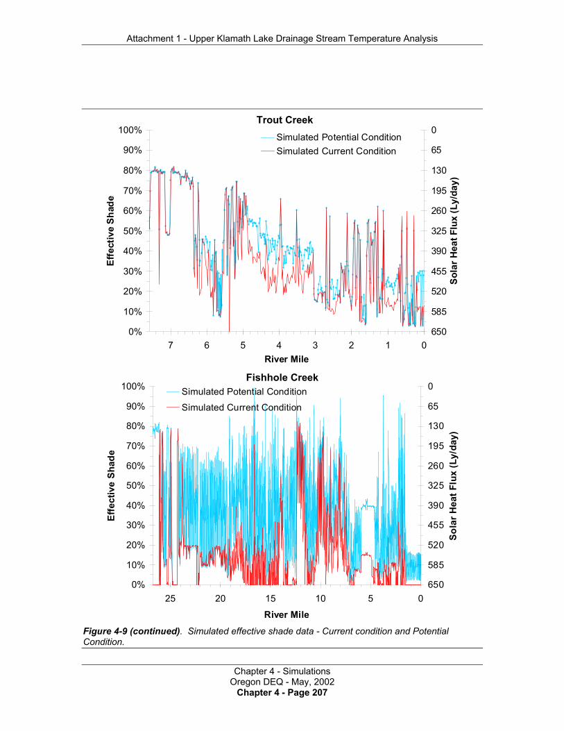
Attachment 1 - Upper Klamath Lake Drainage Stream Temperature Analysis
Chapter 4 - SimulationsOregon DEQ - May, 2002
Chapter 4 - Page 207
0%
10%
20%
30%
40%
50%
60%
70%
80%
90%
100%
0510152025
River Mile
Effe
ctiv
e Sh
ade
0
65
130
195
260
325
390
455
520
585
650
Sola
r Hea
t Flu
x (L
y/da
y)
Simulated Potential ConditionSimulated Current Condition
Fishhole Creek
Trout Creek
0%
10%
20%
30%
40%
50%
60%
70%
80%
90%
100%
01234567River Mile
Effe
ctiv
e Sh
ade
0
65
130
195
260
325
390
455
520
585
650
Sola
r Hea
t Flu
x (L
y/da
y)
Simulated Potential ConditionSimulated Current Condition
Figure 4-9 (continued). Simulated effective shade data - Current condition and PotentialCondition.

Attachment 1 - Upper Klamath Lake Drainage Stream Temperature Analysis
Chapter 4 - SimulationsOregon DEQ - May, 2002
Chapter 4 - Page 208
Williamson River
0%
10%
20%
30%
40%
50%
60%
70%
80%
90%
100%
01020304050607080River Mile
Effe
ctiv
e Sh
ade
0
65
130
195
260
325
390
455
520
585
650
Sola
r Hea
t Flu
x (L
y/da
y)
Simulated Potential ConditionSimulated Current Condition
Figure 4-9 (continued). Simulated effective shade data - Current condition and PotentialCondition.
For the sake of comparison, average effective shade values are presented in Figure 4-10.Several observations can be made from the simulations results. Effective shade levels aregenerally low in the Upper Klamath Lake drainage, in both the current and system potentialconditions. Petersen et al. (1999) points out “the importance of even small amounts of shade inmoderating stream heating.” Increases in stream shade will directly reduce solar radiation andreduce both daily maximum stream temperatures and daily fluctuation of stream temperature.This holds true when shade levels are increased from any level. So even minor increases inshade will reduce the heat transfer to the stream system.
Another observation is that lower river reaches have less shade than upper reaches. This is theresult of large channel width and the prevalence of land cover types that are shorter. Largechannels combined with shorter land cover limits the amount of shade received. The opposite isalso observed in the average shade data. Higher shade levels occur in upper reaches withnarrower channels and that generally have taller growing land cover types.
The largest disparity between the two conditions (i.e. current condition and the system potentialcondition) occurs in Fishhole Creek and the North and South Fork of the Sprague Rivers. Thisdoes not imply that these systems are the most impaired, but instead, highlights that due to therelatively small stream size, that these systems have higher shade potentials. The larger streamsystems, such as the Sycan, Sprague and Lower Williamson Rivers have a smaller differencebetween current and potential shade conditions (see Figure 4-11). It should be emphasized thateven small increases in stream shade can have a significant thermal effect (Petersen et al.,1999).

Attachment 1 - Upper Klamath Lake Drainage Stream Temperature Analysis
Chapter 4 - SimulationsOregon DEQ - May, 2002
Chapter 4 - Page 209
Figure 4-10. Average simulated effective shade data - Current condition and system potentialcondition.
Figure 4-11. The percent increase in effective shade levels from the current condition to thesystem potential condition.

Attachment 1 - Upper Klamath Lake Drainage Stream Temperature Analysis
Chapter 4 - SimulationsOregon DEQ - May, 2002
Chapter 4 - Page 210
4.2.4 Total Daily Solar Heat Load AnalysisSolar heating is established as a primary pollutant in stream heating processes. The calculationof the overall heat load received by the stream system from solar radiation yields the nonpointsources of solar heat for the total stream system as well as for each stream/river. The total dailysolar heat load is the cumulative solar heat received by a stream over one day during the criticalperiod (i.e. July/August period). For the purposes of this analytical effort, the total solar heat loadis the sum of the products of the daily solar heat flux and surface area of exposure for eachstream reach (i.e. for each stream data node every 100 ft).
( ) ( )∑∑ ⋅⋅Φ=⋅Φ=Η dxWA wettedsolarysolarsolar
Background levels of solar heat estimate the portion of the total daily solar heat load that occurswhen nonpoint sources of heat are minimized. The background condition is the system potentialtotal daily solar heat load (i.e. where anthropogenic nonpoint sources are minimized) and iscalculated by substituting the system potential daily solar flux and the potential wetted width intothe equation above. In this fashion, the total daily solar load is calculated for both the currentcondition ( solarΗ ) and the system potential condition ( Background
solarΗ ). With the background portionof the total daily solar load accounted for, the remaining portion can be attributed toanthropogenic nonpoint sources. Therefore, the anthropogenic nonpoint source total daily solarload is the difference between the total daily solar load and the background total daily solar load.Derived total daily solar loads for background sources and anthropogenic nonpoint sources arepresented in Figure 4-12.
Backgroundsolarsolar
NPSsolar Η−Η=Η
where,
yA : Stream surface area unique to each stream segment (cm2)Dx: Stream segment length and distance step in the methodology (cm)
solarΦ : Solar heat flux for unique to each stream segment (kcal cm-2 day-1)
solarΗ : Total daily solar heat load delivered to the stream (kcal day-1)NPSsolarΗ : Portion of the total daily solar heat load delivered to the stream that originates
from nonpoint sources of pollution (kcal day-1)BackgroundsolarΗ : Portion of the total daily solar heat load delivered to the stream that originates
from background sources of pollution that are not affected by human activities(kcal day-1)
Wwetted: Wetted width unique to each stream segment (cm)
Roughly one quarter of the solar loading that occurs in the Williamson and Sprague Riversystems, including major tributaries, is from anthropogenic nonpoint sources, while the remainingthree quarters of the total daily solar load originates from background sources (see Figure 4-12).
Roughly 72% of the anthropogenic nonpoint source solar heat load originates in the Williamsonand Sprague mainstem reaches. The remaining 28% of the anthropogenic nonpoint sourcessolar heat load is derived from tributary stream reaches (see Figure 4-13). It should be noted,however, that the majority of anthropogenic nonpoint solar heat sources occur in the lowergradient heavily impacted reaches of both the mainstem and tributary reaches.
The Sprague River is a major source for anthropogenic solar heat, accounting for 41.5% of thenonpoint source solar load. The Williamson River is also a major contributor of anthropogenic

Attachment 1 - Upper Klamath Lake Drainage Stream Temperature Analysis
Chapter 4 - SimulationsOregon DEQ - May, 2002
Chapter 4 - Page 211
nonpoint solar heat, accounting for 29% of the nonpoint source loading. The Sycan River andand North Fork Sprague River account for 14% and 8% of the anthropogenic nonpoint sourcesolar heat load, respectively. The South Fork, Fishhole Creek and Trout Creek contribute theleast to the anthropogenic nonpoint solar heal load accounting for 4%, 2% and <1%, respectively(see Figure 4-14).
Distribution of the Total Solar Heat Load
NonpointSource Pollution
23.9%Background
76.1%
Figure 4-12. Total daily solar heat load derived as the sum of the products of the daily solar heatflux and wetted surface area. For the purposes of this analysis the total heat load is calculatedfrom the simulated current condition. The background condition is calculated from the systempotential channel width and land cover condition simulations (Scenarios #13 and #14). Recallthat potential land cover has a high and low range. Solar heat flux output data is averaged forthese two conditions to obtain an average potential heat load. The nonpoint source load is thedifference between the current total daily solar load and the background total daily solar heatload.

Attachment 1 - Upper Klamath Lake Drainage Stream Temperature Analysis
Chapter 4 - SimulationsOregon DEQ - May, 2002
Chapter 4 - Page 212
Figure 4-13. Distribution of the total solar heat load for anthropogenic nonpoint sources andbackground sources by stream/river system.
North Fork Sprague River
8.1%
Trout Creek0.2%
Fishhole Creek1.7%South Fork
Sprague River3.7%
Sycan River14.0%
Sprague River43.8%
Williamson River28.5%
Distribution of the Total Nonpoint Source Solar Heat Load
Figure 4-14. Distribution of the total anthropogenic nonpoint source solar heat load.

Attachment 1 - Upper Klamath Lake Drainage Stream Temperature Analysis
Chapter 4 - SimulationsOregon DEQ - May, 2002
Chapter 4 - Page 213
0
1
2
3
4
5
6
7
8
27 25 23 21 19 17 15 13 11 9 7 5 3 1
River Mile
Sola
r Rad
iatio
n R
ecei
ved
by
Stre
am (1
09 cal
/day
)
Current ConditionBackground - System Potential
Sycan River Fishhole Creek
Trout Creek North Fork Sprague River
South Fork Sprague River Sprague River
Williamson River
0
3
6
9
12
15
18
72 66 61 56 50 45 40 34 29 24 18 13 8 2
River Mile
Sola
r Rad
iatio
n Re
ceiv
ed b
y St
ream
(109 c
al/d
ay)
Current ConditionBackground - System Potential
0.00.20.40.60.81.01.21.41.61.82.0
8 7 6 5 4 3 2 1 0River Mile
Sola
r Rad
iatio
n R
ecei
ved
by
Stre
am (1
09 cal
/day
)
Current ConditionBackground - System Potential
0
1
2
3
4
5
6
7
8
34 32 29 27 25 22 20 17 15 12 10 7 5 2
River Mile
Sola
r Rad
iatio
n R
ecei
ved
by
Stre
am (1
09 cal
/day
)
Current ConditionBackground - System Potential
0
1
2
3
4
5
6
7
8
32 30 27 25 23 20 18 16 13 11 9 6 4 2
River Mile
Sola
r Rad
iatio
n Re
ceiv
ed b
y St
ream
(109 c
al/d
ay)
Current ConditionBackground - System Potential
0
3
6
9
12
15
18
21
24
85 78 72 66 59 53 47 40 34 28 22 15 9 3
River Mile
Sola
r Rad
iatio
n R
ecei
ved
by
Stre
am (1
09 cal
/day
)
Current ConditionBackground - System Potential
0
3
6
9
12
15
18
21
24
87 82 77 73 68 63 57 51 35 29 22 16 10 3
River Mile
Sola
r Rad
iatio
n Re
ceiv
ed b
y St
ream
(109 c
al/d
ay)
Current ConditionBackground - System Potential
Figure 4-15. Total daily solar heat loads derived from solar heat flux and wetted surface area.

Attachment 1 - Upper Klamath Lake Drainage Stream Temperature Analysis
Chapter 4 - SimulationsOregon DEQ - May, 2002
Chapter 4 - Page 214
4.2.5 Effective Shade Curve DevelopmentEffective shade curves are designed to display effective shade levels for a specific land covertype as a function of channel width. These shade curves are intended to provide effective shadetargets where site-specific effective shade simulations have not been completed. For a list ofstream segments where effective shade simulations have been performed reference Section4.2.2.1 Effective Shade Simulation Period and Extent. Effective shade curves presented inthis document are developed for the Upper Klamath Lake drainage location (i.e. latitude andlongitude) and are accurate for the critical time period (i.e. July/August). Stream aspect is alsoconsidered in the shade curve methodology.
The land cover types used for development of the shade curves are those developed as thepotential land cover types: large conifer, large hardwood, large conifer/hardwood mix, shrub andgraminoid/forb. For more information regarding the potential land cover types reference Section3.5.3 Near Stream Land Cover - Potential Condition Development. Land cover physicaldimensions for height and density are listed on the shade curves. Determination of appropriatepotential land cover types is the responsibility of the designated management agencies andprivate citizens.
Channel width targets can be determined from regional curves developed in Section 3.4.4Channel Width Assessment. Recall that potential channel width is a function of potentialRosgen stream type, width to depth ratio and drainage area. Determination of the appropriatepotential Rosgen stream type is the responsibility of the designated management agencies andprivate citizens.
Figures 4-16 to 4-20 display shade curves for the potential land cover types. The practical use ofthese shade curves may seem complex. Indeed, it can be. However, this methodology providesland cover, channel width and effective shade targets for the remaining portions of the Williamsonand Sprague River subbasins. The shade curves also demonstrate the relationship between landcover physical properties, channel width and stream aspect.

Atta
chm
ent 1
- U
pper
Kla
mat
h La
ke D
rain
age
Stre
am T
empe
ratu
re A
naly
sis
Cha
pter
4 -
Sim
ulat
ions
Ore
gon
DEQ
- M
ay, 2
002
Cha
pter
4 -
Page
2150%10
%
20%
30%
40%
50%
60%
70%
80%
90%
100%
0
25
50
75
100
125
150
175
200
225
250
275
300
Nea
r S
trea
m D
istu
rban
ce Z
one
(met
ers)
Surrogate MeasureEffective Shade
0.0
63.0
126.
0
189.
0
252.
0
315.
0
377.
9
440.
9
503.
9
566.
9
629.
9
0.0
7.6
15.2
22.9
30.5
38.1
45.7
53.3
61.0
68.6
76.2
83.8
91.4
Nea
r S
trea
m D
istu
rban
ce Z
one
(feet
)
Solar Radiation Loading (ly/day)
0 or
180
deg
rees
from
Nor
th45
, 135
, 225
or 3
15 d
egre
es fr
om N
orth
90 o
r 270
deg
rees
from
Nor
thA
vera
ge
0%10%
20%
30%
40%
50%
60%
70%
80%
90%
100%
0
25
50
75
100
125
150
175
200
225
250
275
300
Nea
r S
trea
m D
istu
rban
ce Z
one
(met
ers)
Surrogate MeasureEffective Shade
0.0
63.0
126.
0
189.
0
252.
0
315.
0
377.
9
440.
9
503.
9
566.
9
629.
9
0.0
7.6
15.2
22.9
30.5
38.1
45.7
53.3
61.0
68.6
76.2
83.8
91.4N
ear
Str
eam
Dis
turb
ance
Zon
e (fe
et)
Solar Radiation Loading (ly/day)
0 or
180
deg
rees
from
Nor
th45
, 135
, 225
or 3
15 d
egre
es fr
om N
orth
90 o
r 270
deg
rees
from
Nor
thA
vera
ge
Shad
e C
urve
s - M
ixed
Dec
iduo
us/C
onife
r Pot
entia
l Lan
d C
over
North Fork Sprague River
Pote
ntia
l Hei
ght:
16.4
met
ers
(53.
8 fe
et)
Pote
ntia
l Den
sity
:60
%
Pote
ntia
l Ove
rhan
g:2.
1 m
eter
s (6
.9 fe
et)
Pote
ntia
l Hei
ght:
16.4
met
ers
(53.
8 fe
et)
Pote
ntia
l Den
sity
:30
%
Pote
ntia
l Ove
rhan
g:2.
1 m
eter
s (6
.9 fe
et)
Figu
re 4
-16.
Effe
ctiv
e sh
ade
curv
es fo
r the
mix
ed h
ardw
ood
and
coni
fer l
and
cove
r typ
e.

Atta
chm
ent 1
- U
pper
Kla
mat
h La
ke D
rain
age
Stre
am T
empe
ratu
re A
naly
sis
Cha
pter
4 -
Sim
ulat
ions
Ore
gon
DEQ
- M
ay, 2
002
Cha
pter
4 -
Page
216
0%10%
20%
30%
40%
50%
60%
70%
80%
90%
100%
0
25
50
75
100
125
150
175
200
225
250
275
300
Nea
r S
trea
m D
istu
rban
ce Z
one
(met
ers)
Surrogate MeasureEffective Shade
0.0
63.0
126.
0
189.
0
252.
0
315.
0
377.
9
440.
9
503.
9
566.
9
629.
9
0.0
7.6
15.2
22.9
30.5
38.1
45.7
53.3
61.0
68.6
76.2
83.8
91.4N
ear
Str
eam
Dis
turb
ance
Zon
e (fe
et)
Solar Radiation Loading (ly/day)
0 or
180
deg
rees
from
Nor
th45
, 135
, 225
or 3
15 d
egre
es fr
om N
orth
90 o
r 270
deg
rees
from
Nor
thA
vera
ge
0%10%
20%
30%
40%
50%
60%
70%
80%
90%
100%
0
25
50
75
100
125
150
175
200
225
250
275
300
Nea
r S
trea
m D
istu
rban
ce Z
one
(met
ers)
Surrogate MeasureEffective Shade
0.0
63.0
126.
0
189.
0
252.
0
315.
0
377.
9
440.
9
503.
9
566.
9
629.
9
0.0
7.6
15.2
22.9
30.5
38.1
45.7
53.3
61.0
68.6
76.2
83.8
91.4
Nea
r S
trea
m D
istu
rban
ce Z
one
(feet
)
Solar Radiation Loading (ly/day)
0 or
180
deg
rees
from
Nor
th45
, 135
, 225
or 3
15 d
egre
es fr
om N
orth
90 o
r 270
deg
rees
from
Nor
thA
vera
ge
Pote
ntia
l Hei
ght:
12.5
met
ers
(41.
0 fe
et)
Pote
ntia
l Den
sity
:75
%
Pote
ntia
l Ove
rhan
g:1.
9 m
eter
s (6
.2 fe
et)
Pote
ntia
l Hei
ght:
12.5
met
ers
(41.
0 fe
et)
Pote
ntia
l Den
sity
:30
%
Pote
ntia
l Ove
rhan
g:1.
9 m
eter
s (6
.2 fe
et)
Shad
e C
urve
- D
ecid
uous
Pot
entia
l Lan
d C
over
Trout Creek
Figu
re 4
-17.
Effe
ctiv
e sh
ade
curv
es fo
r the
dec
iduo
us/h
ardw
ood
land
cov
er ty
pe.

Atta
chm
ent 1
- U
pper
Kla
mat
h La
ke D
rain
age
Stre
am T
empe
ratu
re A
naly
sis
Cha
pter
4 -
Sim
ulat
ions
Ore
gon
DEQ
- M
ay, 2
002
Cha
pter
4 -
Page
2170%10
%
20%
30%
40%
50%
60%
70%
80%
90%
100%
0
25
50
75
100
125
150
175
200
225
250
275
300
Nea
r S
trea
m D
istu
rban
ce Z
one
(met
ers)
Surrogate MeasureEffective Shade
0.0
63.0
126.
0
189.
0
252.
0
315.
0
377.
9
440.
9
503.
9
566.
9
629.
9
0.0
7.6
15.2
22.9
30.5
38.1
45.7
53.3
61.0
68.6
76.2
83.8
91.4
Nea
r S
trea
m D
istu
rban
ce Z
one
(feet
)
Solar Radiation Loading (ly/day)
0 or
180
deg
rees
from
Nor
th45
, 135
, 225
or 3
15 d
egre
es fr
om N
orth
90 o
r 270
deg
rees
from
Nor
thA
vera
ge
0%10%
20%
30%
40%
50%
60%
70%
80%
90%
100%
0
25
50
75
100
125
150
175
200
225
250
275
300
Nea
r S
trea
m D
istu
rban
ce Z
one
(met
ers)
Surrogate MeasureEffective Shade
0.0
63.0
126.
0
189.
0
252.
0
315.
0
377.
9
440.
9
503.
9
566.
9
629.
9
0.0
7.6
15.2
22.9
30.5
38.1
45.7
53.3
61.0
68.6
76.2
83.8
91.4N
ear
Str
eam
Dis
turb
ance
Zon
e (fe
et)
Solar Radiation Loading (ly/day)
0 or
180
deg
rees
from
Nor
th45
, 135
, 225
or 3
15 d
egre
es fr
om N
orth
90 o
r 270
deg
rees
from
Nor
thA
vera
ge
Pote
ntia
l Hei
ght:
20.3
met
ers
(66.
6 fe
et)
Pote
ntia
l Den
sity
:60
%
Pote
ntia
l Ove
rhan
g:2.
0 m
eter
s (6
.6 fe
et)
Pote
ntia
l Hei
ght:
20.3
met
ers
(66.
6 fe
et)
Pote
ntia
l Den
sity
:30
%
Pote
ntia
l Ove
rhan
g:2.
0 m
eter
s (6
.6 fe
et)
Shad
e C
urve
- C
onife
r Pot
entia
l Lan
d C
over
Sycan River
Figu
re 4
-18.
Effe
ctiv
e sh
ade
curv
es fo
r the
con
ifer l
and
cove
r typ
e.

Atta
chm
ent 1
- U
pper
Kla
mat
h La
ke D
rain
age
Stre
am T
empe
ratu
re A
naly
sis
Cha
pter
4 -
Sim
ulat
ions
Ore
gon
DEQ
- M
ay, 2
002
Cha
pter
4 -
Page
218
Pote
ntia
l Hei
ght:
3.2
met
ers
(10.
5 fe
et)
Pote
ntia
l Den
sity
:90
%
Pote
ntia
l Ove
rhan
g:0.
5 m
eter
s (1
.6 fe
et)
Shad
e C
urve
- W
etla
nd S
hrub
Pot
entia
l Lan
d C
over
North Fork Sprague River
0%10%
20%
30%
40%
50%
60%
70%
80%
90%
100%
0
25
50
75
100
125
150
175
200
225
250
275
300
Nea
r S
tream
Dis
turb
ance
Zon
e (m
eter
s)
Surrogate MeasureEffective Shade
0.0
63.0
126.
0
189.
0
252.
0
315.
0
377.
9
440.
9
503.
9
566.
9
629.
9
0.0
7.6
15.2
22.9
30.5
38.1
45.7
53.3
61.0
68.6
76.2
83.8
91.4
Nea
r Str
eam
Dis
turb
ance
Zon
e (fe
et)
Solar Radiation Loading (ly/day)
0 or
180
deg
rees
from
Nor
th45
, 135
, 225
or 3
15 d
egre
es fr
om N
orth
90 o
r 270
deg
rees
from
Nor
thA
vera
ge
Figu
re 4
-19.
Effe
ctiv
e sh
ade
curv
es fo
r the
shr
ub la
nd c
over
type
.

Atta
chm
ent 1
- U
pper
Kla
mat
h La
ke D
rain
age
Stre
am T
empe
ratu
re A
naly
sis
Cha
pter
4 -
Sim
ulat
ions
Ore
gon
DEQ
- M
ay, 2
002
Cha
pter
4 -
Page
219
Pote
ntia
l Hei
ght:
0.55
met
ers
(1.8
feet
)
Pote
ntia
l Den
sity
:90
%
Pote
ntia
l Ove
rhan
g:0.
27 m
eter
s (0
.9 fe
et)
Shad
e C
urve
- G
ram
inoi
d/Fo
rb P
oten
tial L
and
Cov
er
South Fork Sprague River
0%10%
20%
30%
40%
50%
60%
70%
80%
90%
100%
0
25
50
75
100
125
150
175
200
225
250
275
300
Near
Stre
am D
istu
rban
ce Z
one
(met
ers)
Surrogate MeasureEffective Shade
0.0
63.0
126.
0
189.
0
252.
0
315.
0
377.
9
440.
9
503.
9
566.
9
629.
9
0.0
7.6
15.2
22.9
30.5
38.1
45.7
53.3
61.0
68.6
76.2
83.8
91.4
Nea
r St
ream
Dis
turb
ance
Zon
e (fe
et)
Solar Radiation Loading (ly/day)
0 or
180
deg
rees
from
Nor
th45
, 135
, 225
or 3
15 d
egre
es fr
om N
orth
90 o
r 270
deg
rees
from
Nor
thA
vera
ge
Figu
re 4
-20.
Effe
ctiv
e sh
ade
curv
es fo
r the
gra
min
oid/
forb
land
cov
er ty
pe.

Attachment 1 - Upper Klamath Lake Drainage Stream Temperature Analysis
Chapter 4 - SimulationsOregon DEQ - May, 2002
Chapter 4 - Page 220
4.3 Stream Temperature Simulations
4.3.1 Stream Temperature Simulation MethodologyWater temperature change is a function of the heat transfer in a discrete volume. Similarly, heatis a measure of stream temperature change, based on the properties of water. By excludingconstants, it can be demonstrated that temperature change is proportional to heat and inverselyproportional to river flow rates.
Calculation of Heat,( ) wwRRwRR ctQTcMT ⋅ρ⋅⋅⋅∆=⋅⋅∆=Η
Calculation of Water Temperature Change,
( ) wwRwRR ctQcM
T⋅ρ⋅⋅
Η=⋅Η=∆
Excluding constants, water temperature change is a function of heat and river flow,
RR Q
1,T Η∝∆
where,Metric units are used in all computations
RT∆ : Change in river temperature (oC)Η : Heat (cal)RQ : Flow rate (cms)RM : Mass of river volume (kg)
wc : Specific heat of water
=
kgkcal
kgcal103
wρ : Density of water
3
3
mkg10
t : Duration (sec)
All heat transfer rates can be quantified as a flux, which implies heat transfer per a unit area per aunit time. For computational purposes this methodology relies on heat flux metric units.
secly
seccmcal
TimeAreaHeatFluxHeat
2=
⋅=
⋅=
Water has a relatively high heat capacity (cw = 103 cal kg-1 K-1) (Satterlund and Adams 1992).Conceptually, water is a heat sink. Heat that is gained by the stream is retained and only slowlyreleased back to the surrounding environment. Heat released from the stream to the surroundingenvironment is represented by a negative heat flux (Φcooling). Heat delivered to the stream is apositive heat flux (Φheating). Excluding mass transfer processes, heating periods occur when thenet heat flux (Φtotal) is positive. Cooling periods occur when the net heat flux is negative.
coolingheatingtotal Φ+Φ=Φ

Attachment 1 - Upper Klamath Lake Drainage Stream Temperature Analysis
Chapter 4 - SimulationsOregon DEQ - May, 2002
Chapter 4 - Page 221
4.3.1.1 Heat Transfer Processes
In general, the net heat flux experienced by all stream/river systems follows two cycles: aseasonal cycle and a diurnal cycle. In the Pacific Northwest, the seasonal net heat cycleexperiences a maximum positive flux during summer months (July and August), while theminimum seasonal flux occurs in winter months (December and January). The diurnal net heatcycle experiences a daily maximum flux that occurs at or near the sun’s zenith angle, while thedaily minimum flux often occurs during the late night or the early morning. It should be noted,however, that meteorological conditions are variable. Cloud cover and precipitation seriouslyalter the heat relationships between the stream and its environment.
The ultimate source of heat to a stream system is solar radiation both diffuse and direct.Secondary sources of heat include longwave radiation (also referred to as thermal radiation) fromthe atmosphere and streamside vegetation, streambed conduction, and in some cases,groundwater exchange at the water-stream bed interface. Several processes dissipate heat atthe air-water interface, namely: evaporation, convection and back radiation. Heat is acquired bythe stream system when the flux of heat energy entering the stream is greater than the flux ofheat energy leaving. The net heat flux provides the rate at which energy is gained or lost per unitarea and is represented as the instantaneous summation of all heat energy components. The netheat flux (Φtotal) consists of several individual thermodynamic heat flux components, namely: solarradiation (Φsolar), long-wave radiation (Φlongwave), conduction (Φconduction), groundwater exchange(Φgroundwater) and evaporation (Φevaporation) (Wunderlich, 1972; Jobson and Keefer, 1979; Beschtaand Weatherred, 1984; Sinokrot and Stefan, 1993; Boyd, 1996). With the exception of solarradiation, which only delivers heat energy, these processes are capable of both introducing andremoving heat from a stream. The instantaneous heat transfer rate experienced by the stream isthe summation of the individual processes.
When a stream surface is exposed to midday solar radiation, large quantities of heat will bedelivered to the stream system (Brown 1969, Beschta et al. 1987). Some of the incoming solarradiation will reflect off the stream surface, depending on the elevation of the sun. All solarradiation outside the visible spectrum (0.36µ to 0.76µ) is absorbed in the first meter below thestream surface and only visible light penetrates to greater depths (Wunderlich, 1972). Sellers(1965) reported that 50% of solar energy passing through the stream surface is absorbed in thefirst 10 cm of the water column. Removal of riparian vegetation, and the shade it provides,contributes to elevated stream temperatures (Rishel et al., 1982; Brown, 1983; Beschta et al.,1987). The principal source of heat energy delivered to the water column is solar energy strikingthe stream surface directly (Brown 1970). Exposure to direct solar radiation will often cause adramatic increase in stream temperatures. The ability of riparian vegetation to shade the streamthroughout the day depends on land cover height, width, density and position relative to thestream (i.e. stream aspect). Solar Radiation (ΦSolar) is a function of the solar angle, solarazimuth, solar declination, atmospheric properties, topography, location and near stream landcover. Simulation is based on methodologies developed by Ibqal (1983), Beschta andWeatherred (1984), Chen (1996) and Boyd (1996).
Both the atmosphere and vegetation along stream banks emit longwave radiation that can heatthe stream surface. Water is nearly opaque to longwave radiation and complete absorption of allwavelengths greater than 1.2µ occurs in the first 5 cm (i.e. less than 2 inches) below the surface(Wunderlich, 1972). Longwave radiation has a cooling influence when emitted from the streamsurface. The net transfer of heat via longwave radiation usually balances so that the amount ofheat entering is similar to the rate of heat leaving the stream (Beschta and Weatherred, 1984;Boyd, 1996). Warm stream temperatures often cause the longwave radiation balance to becomenegative and the net longwave heat exchange from the atmosphere, near stream land cover andstream surface has a cooling effect (Boyd, 1996). Longwave Radiation (ΦLongwave) is derived bythe Stefan-Boltzmann Law and is a function of the emissivity of the body, the Stefan-Boltzmannconstant and the temperature of the body (Wunderlich, 1972)

Attachment 1 - Upper Klamath Lake Drainage Stream Temperature Analysis
Chapter 4 - SimulationsOregon DEQ - May, 2002
Chapter 4 - Page 222
Evaporation occurs in response to internal energy of the stream (molecular motion) that randomlyexpels water molecules from the stream surface into the overlying air mass. Evaporation is themost effective method of dissipating heat from water (Parker and Krenkel, 1969). As streamtemperatures increase, so does the rate of evaporation. Air movement (wind) and low vaporpressures increase the rate of evaporation and accelerate stream cooling (Harbeck and Meyers,1970). Evaporation (ΦEvaporation) relies on a Dalton-type equation that utilizes an exchangecoefficient, the latent heat of vaporization, wind speed, saturation vapor pressure and vaporpressure (Wunderlich, 1972).
Convection transfers heat between the stream and the air via molecular and turbulent conduction(Beschta and Weatherred, 1984). Heat is transferred in the direction of warmer to cooler. Air canhave a warming influence on the stream when the stream is cooler. The opposite is also true.The amount of convective heat transfer between the stream and air is low (Parker and Krenkel,1969; Brown, 1983, Beschta and Weatherred, 1984). Nevertheless, air temperatures play a rolein stream temperature dynamics via convection, as well as, secondary effects to other heattransfer processes affected by vapor pressure and atmospheric thermal radiation. All of theseprocesses are accounted for in the simulation methodology. Convection (ΦConvection) is a functionof the Bowen Ratio and terms include atmospheric pressure, and water and air temperatures.
Depending on streambed composition, shallow streams (less than 20 cm) may allow solarradiation to warm the streambed (Brown, 1969). Large cobble (> 25 cm diameter) dominatedstreambeds in shallow streams may store and conduct heat as long as the bed is warmer thanthe stream. Bed conduction may cause maximum stream temperatures to occur later in the day,possibly into the evening hours. Bed Conduction (ΦConduction) simulates the theoreticalrelationship ( dz/dTK bConduction ⋅=Φ ), where calculations are a function of thermal conductivityof the bed (K) and the temperature gradient of the bed (dTb/dz) (Sinokrot and Stefan, 1993). Bedconduction is solved with empirical equations developed by Beschta and Weatherred (1984).
Net Heat Flux Continuity Equation,
ΦTotal = ΦSolar + ΦLongwave + ΦEvaporation + ΦConvection + ΦConduction.
Stream CrossSection
BedConduction
Heat Transfer Processes
Evaporation ConvectionSolar
(Diffuse)Solar
(Direct)Longwave

Attachment 1 - Upper Klamath Lake Drainage Stream Temperature Analysis
Chapter 4 - SimulationsOregon DEQ - May, 2002
Chapter 4 - Page 223
Total Energy Budget Solar RadiationLongwave Radiation Air ConvectionBed Conduction Evaporation
-40
-20
0
20
40
60
80
12:00AM
3:00AM
6:00AM
9:00AM
12:00PM
3:00PM
6:00PM
9:00PM
12:00AM
Hea
t Flu
x (ly
/hr)
-40
-20
0
20
40
60
80
12:00AM
3:00AM
6:00AM
9:00AM
12:00PM
3:00PM
6:00PM
9:00PM
12:00AM
Hea
t Flu
x (ly
/hr)
North Fork Sprague RiverUpstream Lee Thomas Campground
Sprague RiverRiver Crest Road - River Mile 50.9
Figure 4-21. Examples of simulated heat transfer processes. These heat transfer outputs aregenerated at every distance node in the model methodology.
The rate change in stream temperature is driven by the heat energy flux (Φi). It is easily shownthat a defined volume of water will attain a predictable rate change in temperature, provided anaccurate prediction of the heat energy flux. The rate change in stream temperature (T) iscalculated as a function of wetted channel heat flux, wetted depth and several constants.
Rate Change in Temperature Caused by Heat Energy Thermodynamics,
⋅⋅ρΦ⋅=
∂∂
ip
ii
VcAx
tT ,
Which reduces to,
⋅⋅ρΦ=
∂∂
ip
i
DctT .
Where,Axi: cross-sectional area (m2)Cp: specific heat of water (cal kg-1·oC-1)Di: average stream depth (m)
t: time (s)T: Temperature (oC)Vi: Volume (m3)Φi: total heat energy flux (cal m-2·s-1)ρ: density of water (1000 kg/m3)

Attachment 1 - Upper Klamath Lake Drainage Stream Temperature Analysis
Chapter 4 - SimulationsOregon DEQ - May, 2002
Chapter 4 - Page 224
4.3.1.2 Mass Transfer Processes
Stream flow velocity (Ux) is calculated using Manning’s equation as a function of the channelhydraulic radius (Rh), stream gradient (So) and channel roughness estimates (n). The hydraulicradius is the ratio of the cross-sectional area (Ax) to the wetted perimeter (Pw). Channel shape isassumed to be rectangular. Under this assumption, the wetted cross-sectional area is theproduct of average depth (D) and wetted width (W). The wetted perimeter is the sum of the twowetted channel sides and the wetted width ( WD2 +⋅ ). Stream gradient data is derived fromdigital elevation model data and stream segment length information from digitized streampolylines (see Section 3.4.3). Wetted width data is sampled from digitized channel polylines fromaerial photos. Simulation inputs for channel roughness values are within the literature values forRosgen level I stream types.
32
21
32
21
32
21
WD2WDS
n1
PA
Sn1RS
n1U o
w
xohox
+⋅⋅⋅⋅=
⋅⋅=⋅⋅=
Advection redistributes heat energy in the positive longitudinal direction. No heat energy is lost orgained by the system during advection, and instead, heat energy is transferred downstream as afunction of flow velocity. In the case where flow is uniform, the rate change in temperature due toadvection is expressed in the first order partial differential equation below.
Rate Change in Temperature Caused by Advection,
xTU
tT
x ∂∂⋅−=
∂∂
Dispersion processes occur in both the upstream and downstream direction along the longitudinalaxis. Heat energy contained in the system is conserved throughout dispersion, and similar toadvection, heat energy is simply moved throughout the system. The rate change in temperaturedue to dispersion is expressed in the second order partial differential equation below.
Rate Change in Temperature Caused by Dispersion,
2
2
L xTD
tT
∂∂=
∂∂
⋅
The dispersion coefficient (DL) may be calculated by stream dimensions, roughness and flow. Instreams that exhibit high flow velocities and low longitudinal temperature gradients, it may beassumed that the system is advection dominated and the dispersion coefficient may be set tozero (Sinokrot and Stefan 1993). In the event that dispersion effects are considered significant,the appropriate value for the dispersion coefficient can be estimated with a practical approachdeveloped and employed in the QUAL 2e model (Brown and Barnwell 1987). An advantage tothis approach is that each parameter is easily measured, or in the case of Manning’s coefficient(n) and the dispersion constant (Kd), estimated.
Physical Dispersion Coefficient,
65
xdL DUnKCD ⋅⋅⋅⋅=
The simultaneous non-uniform one-dimensional transfer of heat energy is the summation of therate change in temperature due to heat energy thermodynamics, advection and dispersion.Given that the stream is subject to steady flow conditions and is well mixed, transversetemperature gradients are negligible (Sinokrot and Stefan 1993). An assumption of non-uniformflow implies that cross-sectional area and flow velocity vary with respect to longitudinal position.

Attachment 1 - Upper Klamath Lake Drainage Stream Temperature Analysis
Chapter 4 - SimulationsOregon DEQ - May, 2002
Chapter 4 - Page 225
The following second ordered parabolic partial differential equation describes the rate change intemperature for non-uniform flow.
Non-Uniform One-dimensional Heat Energy Transfer,
DcxTD
xTU
tT
p2
2
Lx ⋅ρ⋅Φ+
∂∂⋅+
∂∂⋅−=
∂∂
Steady Flow: 0t
Ux =∂∂
Non-Uniform Flow: 0x
Ux ≠∂∂
Where,
Ax: Cross-Sectional area of wetted channel (m2)C: Unit conversion
C = 3.82 for English unitsC = 1.00 for Metric units
cp: Specific heat of water (103 cal kg-1 K-1)D: Average stream depth (m)
DL: Dispersion coefficient (m2/s)Φ: Heat flux (cal m-2.s)Kd: Dispersion constantN: Manning’s coefficient
Pw: Wetted perimeter (m)Rh: Hydraulic radius (m)ρ: Density of water (103 kg m-3)
So: Stream gradientUx: Average flow velocity (m/s)W: Wetted width (m)
The solution to the one-dimensional heat energy transfer equation is essentially the summation ofthermodynamic heat energy exchange between the stream system and the surroundingenvironment and physical processes that redistribute heat energy within the stream system. It isimportant to note that all heat energy introduced into the stream is conserved, with the net heatenergy value reflected as stream temperature magnitude. Further, heat energy is transient withinthe stream system, due to longitudinal transfer of heat energy (i.e., advection and dispersion).The net heat energy flux (Φ) is calculated at every distance step and time step based on physicaland empirical formulations developed for each significant energy component. The dispersioncoefficient (DL) is assumed to equal zero.
4.3.1.3 Boundary Conditions and Initial Values
The temperatures at the upstream boundary (io) for all time steps (to ,t1,,..., tM-1, tM) are supplied bythe upstream temperature inputs. At the downstream boundary temperature at longitudinalposition in+1 is assumed to equals that of in with respect to time t. Initial values of thetemperatures at each distance node (io ,i1,,..., iN-1, iN) occurring at the starting time (to) can be inputby the model user or assumed to equal the boundary condition at time to.

Attachment 1 - Upper Klamath Lake Drainage Stream Temperature Analysis
Chapter 4 - SimulationsOregon DEQ - May, 2002
Chapter 4 - Page 226
4.3.1.4 Simulated Scenarios
Once stream temperature models are calibrated, several scenarios are simulated by changingone or more stream input parameters. The simulated scenarios focus largely on defined potentialconditions for channel width, land cover and derived mass balances. Combinations of thesepotential conditions are also simulated to investigate the cumulative thermal effect of attainingdefined conditions. These scenarios are also used for sensitivity analysis.
Scenario 1: Current ConditionScenario 2: Potential Channel Width
All other inputs remain unchangedScenario 3: Potential Flow
All other inputs remain unchangedScenario 4: Tributaries and Return Flow Temperatures Less than 64oF
All other inputs remain unchangedScenario 5: Potential Near Stream Land Cover - High Range
All other inputs remain unchangedScenario 6: Potential Near Stream Land Cover - Low Range
All other inputs remain unchangedScenario 7: Potential Channel Width
Potential Near Stream Land Cover - High RangeAll other inputs remain unchanged
Scenario 8: Potential Channel WidthPotential Near Stream Land Cover - Low RangeAll other inputs remain unchanged
Scenario 9: Potential FlowPotential Channel WidthPotential Near Stream Land Cover - High RangeAll other inputs remain unchanged
Scenario 10: Potential FlowPotential Channel WidthPotential Near Stream Land Cover - Low RangeAll other inputs remain unchanged
Scenario 11: Tributaries and Return Flow Temperatures Less than 64oFPotential FlowPotential Channel WidthPotential Near Stream Land Cover - High RangeAll other inputs remain unchanged
Scenario 12: Tributaries and Return Flow Temperatures Less than 64oFPotential FlowPotential Channel WidthPotential Near Stream Land Cover - Low RangeAll other inputs remain unchanged
Scenario 13: Tributaries and Return Flow Temperatures Less than 64oFPotential Channel WidthPotential Near Stream Land Cover - High RangeAll other inputs remain unchanged
Scenario 14: Tributaries and Return Flow Temperatures Less than 64oFPotential Channel WidthPotential Near Stream Land Cover - Low RangeAll other inputs remain unchanged
4.3.1.5 Spatial and Temporal Scale
The lengths of the defined finite difference and data input sampling rate is 100 feet. Thetemperature model is calibrated to analyze and predict stream temperature for one day, however

Attachment 1 - Upper Klamath Lake Drainage Stream Temperature Analysis
Chapter 4 - SimulationsOregon DEQ - May, 2002
Chapter 4 - Page 227
multiple days can be simulated. Prediction time steps are limited by stability considerations forthe finite difference solution method. Periods of simulation occurred in early to mid August.Simulations were performed for a total of 250.6 WRD river miles in the Sprague River andWilliamson River subbasin (actual simulation length is 266.0 river miles at 1:5,000 stream polylinescale). Table 4-3 lists the spatial extent and simulation period for by river system.
Table 4-3. Stream Temperature Simulation Periods and Extent
River/Stream Simulation Period Simulation ExtentWilliamson River25 August 4th RM 0.0 to 41.5, 56.4 to 82.5
North Fork Sprague River August 16th RM 0.0 to 32.4South Fork Sprague River August 12th RM 0.0 to 30.0
Sycan River August 16th RM 0.0 to 36.0Sprague River August 12th RM 0.0 to 84.6
Total Simulation Extent250.6 WRD river miles26
4.3.1.6 Validation - Simulation Accuracy
For the purposes of this analytical effort, validation refers to the statistical comparison ofmeasured and simulated data. Absolute average deviation and standard error statistics arecalculated for FLIR derived spatial temperature data sets, instream measured temporaltemperature data sets and combined spatial and temporal data sets. Each measurement oftemperature is discrete and is used to assess model accuracy. Simulation outputs are onlyaccurate to levels that exceed the validation statistics. A statistically significant simulated result isone that produces a temperature change greater than validation statistics listed in Table 4-4.
Stream temperatures derived from FLIR data offer an extremely robust validation data set forspatial stream temperature simulation tools (Faux et al. 2001). Since the FLIR temperature datais continuous, the number of simulated temperatures available for model validation is limited tomodel resolution. With FLIR temperature data, the spatial scalability for any given methodologyis unlimited by validation data. This represents a significant improvement over previous datasources. As an example, ODEQ simulated stream temperatures for the North Fork SpragueRiver along 57.6 km (35.7 river miles of simulation length). The selected model spatial resolutionwas 100 meters, allowing 576 discrete model output samples for calculation of validationstatistics. A similar effort that relied simply on available instream continuous monitors would haveallowed only 96 validation samples. Validation robustness of the simulation is increased by afactor of six when FLIR temperature data are used in the model methodology.
Spatial and temporal data is stratified in the validation to test for biases in the simulationmethodology. Since FLIR temperature data sets are robust spatially, there is a possibility that thesimulation could be calibrated to the specific time when FLIR data was obtained, yet performpoorly for other periods of the day. However, validation statistics demonstrate that this is not thecase. The overall simulation performance is validated using 4,735 discrete measurements andsimulations of stream temperatures during the simulation period. The absolute average deviationfrom measured data is 1.0oF and the standard error in 1.2oF. Figure 4-22 displays the validationresults for each simulated stream and river in the Williamson River and Sprague River subbasins.
25 Stream temperature was not sampled in Klamath Marsh (river miles 41.5 to 56.4).26 Actual stream simulation length is 266 miles. Stream miles have been presented in WRD River Miles for reader DEQanalysis is performed at a higher resolution that captures sinuosity resulting in more stream mileage than WRD maps.

Attachment 1 - Upper Klamath Lake Drainage Stream Temperature Analysis
Chapter 4 - SimulationsOregon DEQ - May, 2002
Chapter 4 - Page 228
Table 4-4. Stream Temperature Simulation Validation
ValidationStatistic
WilliamsonRiver
North ForkSprague
River
SouthFork
SpragueRiver
SycanRiver
SpragueRiver Total
Samples(n) 192 96 48 96 144 576
Ave.Deviation 2.1 1.6 2.1 2.0 1.4 1.8
Tem
pora
lIn
stre
amD
ata
StandardError 1.3 1.3 0.6 1.3 0.7 0.7
Samples(n) 1,220 576 506 617 1,240 4,159
Ave.Deviation 1.2 0.9 0.9 1.0 0.7 0.9
Spat
ial F
LIR
Der
ived
Tem
pera
ture
StandardError 1.6 1.1 0.8 1.2 1.1 1.2
Samples(n) 1,412 672 554 713 1,384 4,735
Ave.Deviation 1.3 1.0 1.0 1.1 0.7 1.0
Tota
l
StandardError 1.6 1.1 0.8 1.2 1.1 1.2
40
45
50
55
60
65
70
75
80
85
051015202530River Miles
Stre
am T
empe
ratu
re (o F)
Samples (n) = 576 Standard Error = 1.05oF
Average Deviation = 0.88oF
FLIR SampledTemperatures
Simulated Temperatures
4:20
PM
4:44
PM
FLIR Sample TimesAugust 16, 1999
Instream Temperature Measurements
North Fork Sprague River
Figure 4-22. Stream Temperature Simulation Compared to FLIR Derived Stream Temperatures

Attachment 1 - Upper Klamath Lake Drainage Stream Temperature Analysis
Chapter 4 - SimulationsOregon DEQ - May, 2002
Chapter 4 - Page 229
40
45
50
55
60
65
70
75
80
85
051015202530River Miles
Stre
am T
empe
ratu
re (o F)
Samples (n) = 506 Standard Error = 0.79oF
Average Deviation = 0.91oF
FLIR SampledTemperatures
Simulated Temperatures
4:04
PM
4:31
PM
FLIR Sample TimesAugust 12, 1999
Instream Temperature Measurements
South Fork Sprague River
40
45
50
55
60
65
70
75
80
85
05101520253035River Miles
Stre
am T
empe
ratu
re (o F)
Samples (n) = 617Standard Error = 1.23oF
Average Deviation = 1.00oF
FLIR Sampled Temperatures
Simulated Temperatures
2:43
PM
3:24
PM
FLIR Sample TimesAugust 16, 1999
Instream Temperature Measurements
Sycan River
Figure 4-22 (continued). Stream Temperature Simulation Compared to FLIR Derived StreamTemperatures

Attachment 1 - Upper Klamath Lake Drainage Stream Temperature Analysis
Chapter 4 - SimulationsOregon DEQ - May, 2002
Chapter 4 - Page 230
Sprague River
Williamson River
40
45
50
55
60
65
70
75
80
85
05101520253035404550556065707580River Miles
Stre
am T
empe
ratu
re (o F)
Samples (n) = 1,240 Standard Error = 1.10oF
Average Deviation = 0.65oF
FLIR SampledTemperatures
Simulated Temperatures
2:16
PM
3:20
PM
FLIR Sample TimesAugust 12, 1999
Instream Temperature Measurements
40
45
50
55
60
65
70
75
80
85
05101520253035404550556065707580River Miles
Die
l Str
eam
Tem
pera
ture
(o F)
FLIR SampledTemperature
SimulatedTemperature
Sample Size (n) = 1,314Standard Error = 1.59oF
Average Deviation = 1.21oF
InstreamTemperature
Measurements
2:50
PM
3:04
PM
3:24
PM
2:19
PM
FLIR Sample TimesAugust 4, 1999
KlamathMarsh
Figure 4-22 (continued). Stream Temperature Simulation Compared to FLIR Derived StreamTemperatures

Attachment 1 - Upper Klamath Lake Drainage Stream Temperature Analysis
Chapter 4 - SimulationsOregon DEQ - May, 2002
Chapter 4 - Page 231
4.3.2 Stream Temperature Simulation Scenarios
4.3.2.1 North Fork Sprague River Stream Temperature Simulations
Scenario #1Scenario #2
• Potential Channel Width
Scenario #3• Potential Flow Volume
Scenario #4• Tributaries/Return Flows < 64oF
Scenario #5• Potential Land Cover - High Range
Scenario #6• Potential Land Cover - Low Range
40455055606570758085
051015202530River Miles
Die
l Str
eam
Tem
pera
ture
(o F)
Current Condition
40
45
50
55
60
65
70
75
80
85
051015202530River Miles
Die
l Str
eam
Tem
pera
ture
(o F)
Current Condition
40455055606570758085
051015202530River Miles
Die
l Str
eam
Tem
pera
ture
(o F)
Current Condition
40455055606570758085
051015202530River Miles
Die
l Str
eam
Tem
pera
ture
(o F)
Current Condition
40455055606570758085
051015202530River Miles
Die
l Str
eam
Tem
pera
ture
(o F)
Current Condition
40455055606570758085
051015202530River Miles
Die
l Str
eam
Tem
pera
ture
(o F)
Current Condition
Figure 4-23. North Fork Sprague River Simulated Stream Temperature Scenarios

Attachment 1 - Upper Klamath Lake Drainage Stream Temperature Analysis
Chapter 4 - SimulationsOregon DEQ - May, 2002
Chapter 4 - Page 232
Scenario #8• Potential Channel Width• Potential Land Cover - Low Range
Scenario #9• Potential Flow Volume• Potential Channel Width• Potential Land Cover - High Range
Scenario #10• Potential Flow Volume• Potential Channel Width• Potential Land Cover - Low Range
Scenario #7• Potential Channel Width• Potential Land Cover - High Range
Scenario #11• Potential Flow Volume• Potential Channel Width• Potential Land Cover - High Range•Tributaries/Return Flows < 64oF
Scenario #12• Potential Flow Volume• Potential Channel Width• Potential Land Cover - Low Range•Tributaries/Return Flows < 64oF
40455055606570758085
051015202530River Miles
Die
l Str
eam
Tem
pera
ture
(o F)
Current Condition
40455055606570758085
051015202530River Miles
Die
l Str
eam
Tem
pera
ture
(o F)
Current Condition
40455055606570758085
051015202530River Miles
Die
l Str
eam
Tem
pera
ture
(o F)
Current Condition
40455055606570758085
051015202530River Miles
Die
l Str
eam
Tem
pera
ture
(o F)Current Condition
40455055606570758085
051015202530River Miles
Die
l Str
eam
Tem
pera
ture
(o F)
Current Condition
40455055606570758085
051015202530River Miles
Die
l Str
eam
Tem
pera
ture
(o F)
Current Condition
Figure 4-23 (continued). North Fork Sprague River Simulated Stream Temperature Scenarios

Attachment 1 - Upper Klamath Lake Drainage Stream Temperature Analysis
Chapter 4 - SimulationsOregon DEQ - May, 2002
Chapter 4 - Page 233
Scenario #13• Potential Channel Width• Potential Land Cover - High Range•Tributaries/Return Flows < 64oF
Scenario #14• Potential Channel Width• Potential Land Cover - Low Range•Tributaries/Return Flows < 64oF
40455055606570758085
051015202530River Miles
Die
l Str
eam
Tem
pera
ture
(o F)
Current Condition
40455055606570758085
051015202530River Miles
Die
l Str
eam
Tem
pera
ture
(o F)
Current Condition
Figure 4-23 (continued). North Fork Sprague River Simulated Stream Temperature Scenarios
North Fork Sprague River
45
50
55
60
65
70
75
1 2 3 4 5 6 7 8 9 10 11 12 13 14
Scenario
Deg
rees
Fah
renh
eit
Average Daily Temperature
Average Minimum Daily Temperature
Average Maximum Daily Temperature
Figure 4-24. North Fork Sprague River summary of average maximum stream temperatures foreach scenario over the entire simulation length (34.2 river miles).

Attachment 1 - Upper Klamath Lake Drainage Stream Temperature Analysis
Chapter 4 - SimulationsOregon DEQ - May, 2002
Chapter 4 - Page 234
Current Condition
Potential Channel Width and Land Cover
Potential Channel Width, Land Cover and Flow Rate
A range of maximum daily temperatures is presented due to theuncertainty regarding levels of effective shade that results from simulating
high and low ranges of targeted potential near stream land cover
Current Condition
Potential Channel Width and Land Cover
Potential Channel Width, Land Cover and Flow Rate
Maximum Daily Temperature Ranges (oF)
40
45
50
55
60
65
70
75
80
85
051015202530River Miles
Dai
ly M
axim
um T
empe
ratu
res
(o F)
Maximum Daily Stream Temperature
Maximum Daily Stream Temperature Distribution
Figure 4-25. North Fork Sprague River summary of maximum daily simulated potential streamtemperatures. Upper chart displays the longitudinal profile of maximum daily streamtemperatures. A range is provided showing the range of potential temperatures due touncertainty related to the potential land cover condition. The lower chart is a histogram thatshows the distribution of simulated maximum daily stream temperatures for the current conditioncompared to potential channel width, land cover and flow rate.

Attachment 1 - Upper Klamath Lake Drainage Stream Temperature Analysis
Chapter 4 - SimulationsOregon DEQ - May, 2002
Chapter 4 - Page 235
4.3.2.2 South Fork Sprague River Stream Temperature Simulations
Scenario #1Scenario #2
• Potential Channel Width
Scenario #3• Potential Flow Volume
Scenario #4• Tributaries/Return Flows < 64oF
Scenario #5• Potential Land Cover - High Range
Scenario #6• Potential Land Cover - Low Range
40455055606570758085
051015202530River Miles
Die
l Str
eam
Tem
pera
ture
(o F)
Current Condition
40455055606570758085
051015202530River Miles
Die
l Str
eam
Tem
pera
ture
(o F)
Current Condition
40455055606570758085
051015202530River Miles
Die
l Str
eam
Tem
pera
ture
(o F)
Current Condition
40455055606570758085
051015202530River Miles
Die
l Str
eam
Tem
pera
ture
(o F)
Current Condition
40455055606570758085
051015202530River Miles
Die
l Str
eam
Tem
pera
ture
(o F)
Current Condition
40455055606570758085
051015202530River Miles
Die
l Str
eam
Tem
pera
ture
(o F)
Current Condition
Figure 4-26. South Fork Sprague River Simulated Stream Temperature Scenarios

Attachment 1 - Upper Klamath Lake Drainage Stream Temperature Analysis
Chapter 4 - SimulationsOregon DEQ - May, 2002
Chapter 4 - Page 236
Scenario #8• Potential Channel Width• Potential Land Cover - Low Range
Scenario #9• Potential Flow Volume• Potential Channel Width• Potential Land Cover - High Range
Scenario #10• Potential Flow Volume• Potential Channel Width• Potential Land Cover - Low Range
Scenario #7• Potential Channel Width• Potential Land Cover - High Range
Scenario #11• Potential Flow Volume• Potential Channel Width• Potential Land Cover - High Range•Tributaries/Return Flows < 64oF
Scenario #12• Potential Flow Volume• Potential Channel Width• Potential Land Cover - Low Range•Tributaries/Return Flows < 64oF
40455055606570758085
051015202530River Miles
Die
l Str
eam
Tem
pera
ture
(o F)
Current Condition
40455055606570758085
051015202530River Miles
Die
l Str
eam
Tem
pera
ture
(o F)
Current Condition
40455055606570758085
051015202530River Miles
Die
l Str
eam
Tem
pera
ture
(o F)
Current Condition
40455055606570758085
051015202530River Miles
Die
l Str
eam
Tem
pera
ture
(o F)
Current Condition
40455055606570758085
051015202530River Miles
Die
l Str
eam
Tem
pera
ture
(o F)
Current Condition
40455055606570758085
051015202530River Miles
Die
l Str
eam
Tem
pera
ture
(o F)
Current Condition
Figure 4-26 (continued). South Fork Sprague River Simulated Stream Temperature Scenarios

Attachment 1 - Upper Klamath Lake Drainage Stream Temperature Analysis
Chapter 4 - SimulationsOregon DEQ - May, 2002
Chapter 4 - Page 237
Scenario #13• Potential Channel Width• Potential Land Cover - High Range•Tributaries/Return Flows < 64oF
Scenario #14• Potential Channel Width• Potential Land Cover - Low Range•Tributaries/Return Flows < 64oF
40455055606570758085
051015202530River Miles
Die
l Str
eam
Tem
pera
ture
(o F)
Current Condition
40455055606570758085
051015202530River Miles
Die
l Str
eam
Tem
pera
ture
(o F)
Current Condition
Figure 4-26 (continued). South Fork Sprague River Simulated Stream Temperature Scenarios
South Fork Sprague River
45
50
55
60
65
70
75
1 2 3 4 5 6 7 8 9 10 11 12 13 14
Scenario
Deg
rees
Fah
renh
eit
Average Daily Temperature
Average Minimum Daily Temperature
Average Maximum Daily Temperature
Figure 4-27. South Fork Sprague River Summary Average Simulated Stream TemperatureScenarios. Average values calculated for the entire simulation length (30.0 river miles).

Attachment 1 - Upper Klamath Lake Drainage Stream Temperature Analysis
Chapter 4 - SimulationsOregon DEQ - May, 2002
Chapter 4 - Page 238
40
45
50
55
60
65
70
75
80
85
051015202530River Miles
Dai
ly M
axim
um T
empe
ratu
res
(o F)
Maximum Daily Stream Temperature Distribution
Current Condition
Potential Channel Width and Land Cover
Potential Channel Width, Land Cover and Flow Rate
A range of maximum daily temperatures is presented due to theuncertainty regarding levels of effective shade that results from simulating
high and low ranges of targeted potential near stream land cover
Current Condition
Potential Channel Width and Land Cover
Potential Channel Width, Land Cover and Flow Rate
Maximum Daily Temperature Ranges (oF)
Maximum Daily Stream Temperature
Figure 4-28. South Fork Sprague River summary of maximum daily simulated potential streamtemperatures. Upper chart displays the longitudinal profile of maximum daily streamtemperatures. A range is provided showing the range of potential temperatures due touncertainty related to the potential land cover condition. The lower chart is a histogram thatshows the distribution of simulated maximum daily stream temperatures for the current conditioncompared to potential channel width, land cover and flow rate.

Attachment 1 - Upper Klamath Lake Drainage Stream Temperature Analysis
Chapter 4 - SimulationsOregon DEQ - May, 2002
Chapter 4 - Page 239
4.3.2.3 Sycan River Stream Temperature Simulations
Scenario #1Scenario #2
• Potential Channel Width
Scenario #3• Potential Flow Volume
Scenario #4• Tributaries/Return Flows < 64oF
Scenario #5• Potential Land Cover - High Range
Scenario #6• Potential Land Cover - Low Range
40455055606570758085
05101520253035River Miles
Die
l Str
eam
Tem
pera
ture
(o F)
Current Condition
40455055606570758085
05101520253035River Miles
Die
l Str
eam
Tem
pera
ture
(o F)
Current Condition
40455055606570758085
05101520253035River Miles
Die
l Str
eam
Tem
pera
ture
(o F)
Current Condition
40455055606570758085
05101520253035River Miles
Die
l Str
eam
Tem
pera
ture
(o F)
Current Condition
40455055606570758085
05101520253035River Miles
Die
l Str
eam
Tem
pera
ture
(o F)
Current Condition
40455055606570758085
05101520253035River Miles
Die
l Str
eam
Tem
pera
ture
(o F)
Current Condition
Figure 4-29. Sycan River Simulated Stream Temperature Scenarios

Attachment 1 - Upper Klamath Lake Drainage Stream Temperature Analysis
Chapter 4 - SimulationsOregon DEQ - May, 2002
Chapter 4 - Page 240
Scenario #8• Potential Channel Width• Potential Land Cover - Low Range
Scenario #9• Potential Flow Volume• Potential Channel Width• Potential Land Cover - High Range
Scenario #10• Potential Flow Volume• Potential Channel Width• Potential Land Cover - Low Range
Scenario #7• Potential Channel Width• Potential Land Cover - High Range
Scenario #11• Potential Flow Volume• Potential Channel Width• Potential Land Cover - High Range•Tributaries/Return Flows < 64oF
Scenario #12• Potential Flow Volume• Potential Channel Width• Potential Land Cover - Low Range•Tributaries/Return Flows < 64oF
40455055606570758085
05101520253035River Miles
Die
l Str
eam
Tem
pera
ture
(o F)
Current Condition
40455055606570758085
05101520253035River Miles
Die
l Str
eam
Tem
pera
ture
(o F)
Current Condition
40455055606570758085
05101520253035River Miles
Die
l Str
eam
Tem
pera
ture
(o F)
Current Condition
40455055606570758085
05101520253035River Miles
Die
l Str
eam
Tem
pera
ture
(o F)Current Condition
40455055606570758085
05101520253035River Miles
Die
l Str
eam
Tem
pera
ture
(o F)
Current Condition
40455055606570758085
05101520253035River Miles
Die
l Str
eam
Tem
pera
ture
(o F)
Current Condition
Figure 4-29 (continued). Sycan River Simulated Stream Temperature Scenarios

Attachment 1 - Upper Klamath Lake Drainage Stream Temperature Analysis
Chapter 4 - SimulationsOregon DEQ - May, 2002
Chapter 4 - Page 241
Scenario #13• Potential Channel Width• Potential Land Cover - High Range•Tributaries/Return Flows < 64oF
Scenario #14• Potential Channel Width• Potential Land Cover - Low Range•Tributaries/Return Flows < 64oF
40455055606570758085
05101520253035River Miles
Die
l Str
eam
Tem
pera
ture
(o F)
Current Condition
40455055606570758085
05101520253035River Miles
Die
l Str
eam
Tem
pera
ture
(o F)
Current Condition
Figure 4-29 (continued). Sycan River Simulated Stream Temperature Scenarios
Sycan River
45
50
55
60
65
70
75
1 2 3 4 5 6 7 8 9 10 11 12 13 14
Scenario
Deg
rees
Fah
renh
eit
Average Daily Temperature
Average Minimum Daily Temperature
Average Maximum Daily Temperature
Figure 4-30. Sycan River Summary Average Simulated Stream Temperature Scenarios.Average values calculated for the entire simulation length (36.0 river miles).

Attachment 1 - Upper Klamath Lake Drainage Stream Temperature Analysis
Chapter 4 - SimulationsOregon DEQ - May, 2002
Chapter 4 - Page 242
40
45
50
55
60
65
70
75
80
85
05101520253035River Miles
Dai
ly M
axim
um T
empe
ratu
res
(o F)
Maximum Daily Stream Temperature Distribution
Current Condition
Potential Channel Width and Land Cover
Potential Channel Width, Land Cover and Flow Rate
A range of maximum daily temperatures is presented due to theuncertainty regarding levels of effective shade that results from simulating
high and low ranges of targeted potential near stream land cover
Current Condition
Potential Channel Width and Land Cover
Potential Channel Width, Land Cover and Flow Rate
Maximum Daily Temperature Ranges (oF)
Maximum Daily Stream Temperature
Figure 4-31. Sycan River summary of maximum daily simulated potential stream temperatures.Upper chart displays the longitudinal profile of maximum daily stream temperatures. A range isprovided showing the range of potential temperatures due to uncertainty related to the potentialland cover condition. The lower chart is a histogram that shows the distribution of simulatedmaximum daily stream temperatures for the current condition compared to potential channelwidth, land cover and flow rate.

Attachment 1 - Upper Klamath Lake Drainage Stream Temperature Analysis
Chapter 4 - SimulationsOregon DEQ - May, 2002
Chapter 4 - Page 243
4.3.2.4 Sprague River Stream Temperature Simulations
Scenario #1Scenario #2
• Potential Channel Width
Scenario #3• Potential Flow Volume
Scenario #4• Tributaries/Return Flows < 64oF
Scenario #5• Potential Land Cover - High Range
Scenario #6• Potential Land Cover - Low Range
40455055606570758085
05101520253035404550556065707580
River Miles
Die
l Str
eam
Tem
pera
ture
(o F)
Current Condition
40455055606570758085
05101520253035404550556065707580
River Miles
Die
l Str
eam
Tem
pera
ture
(o F)
Current Condition
40455055606570758085
05101520253035404550556065707580
River Miles
Die
l Str
eam
Tem
pera
ture
(o F)
Current Condition
40455055606570758085
05101520253035404550556065707580
River Miles
Die
l Str
eam
Tem
pera
ture
(o F)
Current Condition
40455055606570758085
05101520253035404550556065707580
River Miles
Die
l Str
eam
Tem
pera
ture
(o F)
Current Condition
40455055606570758085
05101520253035404550556065707580
River Miles
Die
l Str
eam
Tem
pera
ture
(o F)
Current Condition
Figure 4-32. Sprague River Simulated Stream Temperature Scenarios

Attachment 1 - Upper Klamath Lake Drainage Stream Temperature Analysis
Chapter 4 - SimulationsOregon DEQ - May, 2002
Chapter 4 - Page 244
Scenario #8• Potential Channel Width• Potential Land Cover - Low Range
Scenario #9• Potential Flow Volume• Potential Channel Width• Potential Land Cover - High Range
Scenario #10• Potential Flow Volume• Potential Channel Width• Potential Land Cover - Low Range
Scenario #7• Potential Channel Width• Potential Land Cover - High Range
Scenario #11• Potential Flow Volume• Potential Channel Width• Potential Land Cover - High Range•Tributaries/Return Flows < 64oF
Scenario #12• Potential Flow Volume• Potential Channel Width• Potential Land Cover - Low Range•Tributaries/Return Flows < 64oF
40455055606570758085
05101520253035404550556065707580
River Miles
Die
l Str
eam
Tem
pera
ture
(o F)
Current Condition
40455055606570758085
05101520253035404550556065707580
River Miles
Die
l Str
eam
Tem
pera
ture
(o F)
Current Condition
40455055606570758085
05101520253035404550556065707580
River Miles
Die
l Str
eam
Tem
pera
ture
(o F)
Current Condition
40455055606570758085
05101520253035404550556065707580
River Miles
Die
l Str
eam
Tem
pera
ture
(o F)Current Condition
40455055606570758085
05101520253035404550556065707580
River Miles
Die
l Str
eam
Tem
pera
ture
(o F)
Current Condition
40455055606570758085
05101520253035404550556065707580
River Miles
Die
l Str
eam
Tem
pera
ture
(o F)
Current Condition
Figure 4-32 (continued). Sprague River Simulated Stream Temperature Scenarios

Attachment 1 - Upper Klamath Lake Drainage Stream Temperature Analysis
Chapter 4 - SimulationsOregon DEQ - May, 2002
Chapter 4 - Page 245
Scenario #13• Potential Channel Width• Potential Land Cover - High Range•Tributaries/Return Flows < 64oF
Scenario #14• Potential Channel Width• Potential Land Cover - Low Range•Tributaries/Return Flows < 64oF
40455055606570758085
05101520253035404550556065707580
River Miles
Die
l Str
eam
Tem
pera
ture
(o F)
Current Condition
40455055606570758085
05101520253035404550556065707580
River Miles
Die
l Str
eam
Tem
pera
ture
(o F)
Current Condition
Figure 4-32 (continued). Sprague River Simulated Stream Temperature Scenarios
Sprague River
45
50
55
60
65
70
75
1 2 3 4 5 6 7 8 9 10 11 12 13 14
Scenario
Deg
rees
Fah
renh
eit
Average Daily TemperatureAverage Minimum Daily Temperature
Average Maximum Daily Temperature
Figure 4-33. Sprague Summary Average Simulated Stream Temperature Scenarios. Averagevalues calculated for the entire simulation length (84.6 river miles).

Attachment 1 - Upper Klamath Lake Drainage Stream Temperature Analysis
Chapter 4 - SimulationsOregon DEQ - May, 2002
Chapter 4 - Page 246
Maximum Daily Stream Temperature Distribution
Current Condition
Potential ChannelWidth and Land Cover
Potential ChannelWidth, Land Cover andFlow Rate
A range of maximum daily temperatures is presented due to theuncertainty regarding levels of effective shade that results from simulating
high and low ranges of targeted potential near stream land cover
Current Condition
Potential Channel Width and Land Cover
Potential Channel Width, Land Cover and Flow Rate
Maximum Daily Temperature Ranges (oF)
Maximum Daily Stream Temperature
40
45
50
55
60
65
70
75
80
85
05101520253035404550556065707580River Miles
Dai
ly M
axim
um T
empe
ratu
res
(o F)
Figure 4-34. Sprague River summary of maximum daily simulated potential stream temperatures.Upper chart displays the longitudinal profile of maximum daily stream temperatures. A range isprovided showing the range of potential temperatures due to uncertainty related to the potentialland cover condition. The lower chart is a histogram that shows the distribution of simulatedmaximum daily stream temperatures for the current condition compared to potential channelwidth, land cover and flow rate.

Attachment 1 - Upper Klamath Lake Drainage Stream Temperature Analysis
Chapter 4 - SimulationsOregon DEQ - May, 2002
Chapter 4 - Page 247
4.3.2.5 Williamson River Stream Temperature Simulations
Scenario #1Scenario #2
• Potential Channel Width
Scenario #3• Potential Flow Volume
Scenario #4• Tributaries/Return Flows < 64oF
Scenario #5• Potential Land Cover - High Range
Scenario #6• Potential Land Cover - Low Range
40455055606570758085
05101520253035404550556065707580River Miles
Die
l Str
eam
Tem
pera
ture
(o F)
KlamathMarsh
CurrentCondition
40455055606570758085
05101520253035404550556065707580River Miles
Die
l Str
eam
Tem
pera
ture
(o F)
KlamathMarsh
CurrentCondition
40455055606570758085
05101520253035404550556065707580River Miles
Die
l Str
eam
Tem
pera
ture
(o F)
KlamathMarsh
CurrentCondition
40455055606570758085
05101520253035404550556065707580River Miles
Die
l Str
eam
Tem
pera
ture
(o F)
CurrentCondition Klamath
Marsh
40455055606570758085
05101520253035404550556065707580River Miles
Die
l Str
eam
Tem
pera
ture
(o F)
CurrentCondition Klamath
Marsh
40455055606570758085
05101520253035404550556065707580River Miles
Die
l Str
eam
Tem
pera
ture
(o F)
CurrentCondition
KlamathMarsh
Figure 4-35. Williamson River Simulated Stream Temperature Scenarios

Attachment 1 - Upper Klamath Lake Drainage Stream Temperature Analysis
Chapter 4 - SimulationsOregon DEQ - May, 2002
Chapter 4 - Page 248
Scenario #8• Potential Channel Width• Potential Land Cover - Low Range
Scenario #9• Potential Flow Volume• Potential Channel Width• Potential Land Cover - High Range
Scenario #10• Potential Flow Volume• Potential Channel Width• Potential Land Cover - Low Range
Scenario #7• Potential Channel Width• Potential Land Cover - High Range
Scenario #11• Potential Flow Volume• Potential Channel Width• Potential Land Cover - High Range•Tributaries/Return Flows < 64oF
Scenario #12• Potential Flow Volume• Potential Channel Width• Potential Land Cover - Low Range•Tributaries/Return Flows < 64oF
40455055606570758085
05101520253035404550556065707580River Miles
Die
l Str
eam
Tem
pera
ture
(o F)
CurrentCondition Klamath
Marsh
40455055606570758085
05101520253035404550556065707580River Miles
Die
l Str
eam
Tem
pera
ture
(o F)
CurrentCondition Klamath
Marsh
40455055606570758085
05101520253035404550556065707580River Miles
Die
l Str
eam
Tem
pera
ture
(o F)
CurrentCondition Klamath
Marsh
40455055606570758085
05101520253035404550556065707580River Miles
Die
l Str
eam
Tem
pera
ture
(o F)Current
Condition KlamathMarsh
40455055606570758085
05101520253035404550556065707580River Miles
Die
l Str
eam
Tem
pera
ture
(o F)
CurrentCondition Klamath
Marsh
40455055606570758085
05101520253035404550556065707580River Miles
Die
l Str
eam
Tem
pera
ture
(o F)
KlamathMarsh
CurrentCondition
Figure 4-35 (continued). Williamson River Simulated Stream Temperature Scenarios

Attachment 1 - Upper Klamath Lake Drainage Stream Temperature Analysis
Chapter 4 - SimulationsOregon DEQ - May, 2002
Chapter 4 - Page 249
Scenario #13• Potential Channel Width• Potential Land Cover - High Range•Tributaries/Return Flows < 64oF
Scenario #14• Potential Channel Width• Potential Land Cover - Low Range•Tributaries/Return Flows < 64oF
40455055606570758085
05101520253035404550556065707580River Miles
Die
l Str
eam
Tem
pera
ture
(o F)
CurrentCondition Klamath
Marsh
40455055606570758085
05101520253035404550556065707580River Miles
Die
l Str
eam
Tem
pera
ture
(o F)
CurrentCondition Klamath
Marsh
Figure 4-35 (continued). Williamson River Simulated Stream Temperature Scenarios

Attachment 1 - Upper Klamath Lake Drainage Stream Temperature Analysis
Chapter 4 - SimulationsOregon DEQ - May, 2002
Chapter 4 - Page 250
Williamson River below Klamath Marsh
45
50
55
60
65
70
75
1 2 3 4 5 6 7 8 9 10 11 12 13 14
Scenario
Deg
rees
Fah
renh
eit
Average Daily TemperatureAverage Minimum Daily Temperature
Average Maximum Daily Temperature
Williamson River above Klamath Marsh
45
50
55
60
65
70
75
1 2 3 4 5 6 7 8 9 10 11 12 13 14
Scenario
Deg
rees
Fah
renh
eit
Average Daily TemperatureAverage Minimum Daily Temperature
Average Maximum Daily Temperature
Figure 4-36. Williamson Summary Average Simulated Stream Temperature Scenarios. Averagevalues calculated for the entire simulation length (67.6 river miles).

Attachment 1 - Upper Klamath Lake Drainage Stream Temperature Analysis
Chapter 4 - SimulationsOregon DEQ - May, 2002
Chapter 4 - Page 251
Current Condition
Potential Channel Width and Land Cover
Potential Channel Width, Land Cover and Flow Rate
A range of maximum daily temperatures is presented due to theuncertainty regarding levels of effective shade that results from simulating
high and low ranges of targeted potential near stream land cover
Current Condition
Potential Channel Width and Land Cover
Potential Channel Width, Land Cover and Flow Rate
Maximum Daily Temperature Ranges (oF)
40
45
50
55
60
65
70
75
80
85
05101520253035404550556065707580River Mile
Dai
ly M
axim
um T
empe
ratu
re (o F) Klamath
Marsh
Maximum Daily Stream Temperature Distribution
Maximum Daily Stream Temperature
Figure 4-37. Williamson River summary of maximum daily simulated potential streamtemperatures. Upper chart displays the longitudinal profile of maximum daily streamtemperatures. A range is provided showing the range of potential temperatures due touncertainty related to the potential land cover condition. The lower chart is a histogram thatshows the distribution of simulated maximum daily stream temperatures for the current conditioncompared to potential channel width, land cover and flow rate.

Attachment 1 - Upper Klamath Lake Drainage Stream Temperature Analysis
Chapter 4 - SimulationsOregon DEQ - May, 2002
Chapter 4 - Page 252
4.3.3 Stream Temperature Simulations Sensitivity AnalysisIn general, the rivers/streams exhibited high levels of sensitivity to potential land cover andchannel width reductions and potential flow combinations. Single parameter scenarios thatsimulated one potential condition while leaving other parameters in the current condition result insmaller temperatures reductions. Largest temperature reductions occur from scenarios thatinclude potential land cover, channel width, flow rates and reduce tributary temperature to below64oF (i.e. scenarios 11 and 12).
The upper Williamson River and North Fork Sprague River have exhibited the highest sensitivityto system potential conditions. The lower Williamson River and the South Fork Sprague Riverhave a moderate sensitivity to system potential conditions, while the Sycan River and SpragueRiver have low sensitivity to system potential conditions. Figure 4-38 displays the sensitivityanalysis by evaluating the average stream temperature reduction over the analyzed streamlengths.
Simulated ScenariosScenario Scenario
1 Current Condition 8Potential Channel WidthPotential Near Stream Land Cover – Low RangeAll other inputs remain unchanged
2 Potential Channel WidthAll other inputs remain unchanged 9
Potential FlowPotential Channel WidthPotential Near Stream Land Cover – High RangeAll other inputs remain unchanged
3 Potential FlowAll other inputs remain unchanged 10
Potential FlowPotential Channel WidthPotential Near Stream Land Cover – Low RangeAll other inputs remain unchanged
4 Tributaries and Return Flow Temps < 64oFAll other inputs remain unchanged 11
Tributaries and Return Flow Temps < 64oFPotential FlowPotential Channel WidthPotential Near Stream Land Cover – High RangeAll other inputs remain unchanged
5 Potential Near Stream Land Cover – High RangeAll other inputs remain unchanged 12
Tributaries and Return Flow Temps < 64oFPotential FlowPotential Channel WidthPotential Near Stream Land Cover – Low RangeAll other inputs remain unchanged
6 Potential Near Stream Land Cover – Low RangeAll other inputs remain unchanged 13
Tributaries and Return Flow Temps < 64oFPotential Channel WidthPotential Near Stream Land Cover – High RangeAll other inputs remain unchanged
7Potential Channel WidthPotential Near Stream Land Cover – High RangeAll other inputs remain unchanged
14Tributaries and Return Flow Temps < 64oFPotential Channel WidthPotential Near Stream Land Cover – Low RangeAll other inputs remain unchanged

Atta
chm
ent 1
- U
pper
Kla
mat
h La
ke D
rain
age
Stre
am T
empe
ratu
re A
naly
sis
Cha
pter
4 -
Sim
ulat
ions
Ore
gon
DEQ
- M
ay, 2
002
Cha
pter
4 -
Page
253
2.9
0.6
0.1
2.1
1.1
5.4
4.1
6.0
4.8
6.1
4.8
5.4
4.2
0.9
0.9
0.5
1.1
0.7
2.3
1.7
3.2
2.7
3.4
2.8
2.7
2.2
012345678910
Scenario #2
Scenario #3
Scenario #4
Scenario #5
Scenario #6
Scenario #7
Scenario #8
Scenario #9
Scenario #10
Scenario #11
Scenario #12
Scenario #13
Scenario #14
Average Stream TemperatureReduction (
oF)
Nor
th F
ork
Spra
gue
Riv
erSo
uth
Fork
Spr
ague
Riv
er
0.4
1.9
1.5
1.4
0.5
1.9
1.0
3.8
3.0
6.1
5.3
3.6
2.7
1.0
1.0
1.5
0.3
0.2
1.5
1.3
2.6
2.8
3.4
3.0
3.0
2.7
012345678910
Scenario #2
Scenario #3
Scenario #4
Scenario #5
Scenario #6
Scenario #7
Scenario #8
Scenario #9
Scenario #10
Scenario #11
Scenario #12
Scenario #13
Scenario #14
Average Stream TemperatureReduction (
oF)
Upp
er W
illiam
son
- Hea
dwat
ers
to K
lam
ath
Mar
shLo
wer
Willi
amso
n - K
lam
ath
Mar
sh to
Mou
th
0.3
0.2
0.2
0.5
0.2
0.8
0.3
0.9
0.4
1.2
0.6
1.1
0.6
1.1
1.0
1.3
0.8
0.4
2.1
1.6
3.6
3.0
4.0
3.4
3.6
3.1
012345678910
Scenario #2
Scenario #3
Scenario #4
Scenario #5
Scenario #6
Scenario #7
Scenario #8
Scenario #9
Scenario #10
Scenario #11
Scenario #12
Scenario #13
Scenario #14
Average Stream TemperatureReduction (
oF)
Syca
n R
iver
Spra
gue
Riv
er
Figu
re 4
-38.
Stre
am T
empe
ratu
re S
cena
rios
- Sen
sitiv
ity A
naly
sis

Attachment 1 - Upper Klamath Lake Drainage Stream Temperature Analysis
Chapter 4 - SimulationsOregon DEQ - May, 2002
Chapter 4 - Page 254
4.4 Discussion - Stream Temperature DistributionsMaximum daily stream temperature distributions are presented in Figure 4-37. Currently 61% of thesampled stream segments (162 river miles) in the Upper Klamath Lake Drainage exceed 68oF27. Underpotential land cover and channel width, 17% of the simulated stream segments (45 river miles) exceed68oF resulting in an additional 117 river miles that remain below this temperature threshold whencompared to the current condition. When potential flow volume is added to potential land cover andchannel width, 10% of the simulated stream segments (26 river miles) exceed 68oF, resulting in anadditional 19 river miles below this threshold condition when compared to the potential land cover andchannel width. Results indicate that 83% of the stream length can achieve maximum daily streamtemperatures less than 68oF under system potential conditions. With this result comes a reality that 17%of the stream system will remain above 68oF.
An overriding emphasis of this analysis is the focus on spatial distributions of stream temperatures in theUpper Klamath Lake drainage. Comparisons of stream temperature distributions capture the variabilitythat naturally exists in stream thermodynamics. Spatial variability is observed in all of the streamsegments sampled and analyzed. With the advent of new sampling technologies and analytical tools thatinclude landscape scaled data and computational methodologies, an improved understanding of streamtemperature dynamics is emerging (Boyd, 1996, Faux et al. 2001, Torgersen et al., 1995, Torgersen etal., 1999, Torgersen et al., 2001, ODEQ 2000a, ODEQ 2001a, ODEQ2001b, ODEQ 2001c). Thisunderstanding accommodates spatial and temporal variability that includes departures from biologicallyderived temperature threshold conditions.
Further, simple conceptual models that focus on a single stream, landscape or atmospheric parameterwill fail to capture the interactions of a multitude of parameters that are interrelated. These parameterscombine to have complex thermal effects. As an example, at a network scale modeling demonstratesthat stream temperatures are relatively insensitive to potential land cover conditions. However, whencoupled with potential channel width, stream temperatures are highly sensitive to potential land cover.When flow volume is increased to potential, the temperature reductions created by potential land coverand channel width are further increased. The results of this analytical effort clearly demonstrate thata comprehensive restoration approach should be developed that focuses on the protection andrecovery of land cover and channel morphology, and increases instream flow volume.
27 The proposed EPA sub-lethal temperature limit for redband trout is 68oF (EPA 2001).

Attachment 1 - Upper Klamath Lake Drainage Stream Temperature Analysis
Chapter 4 - SimulationsOregon DEQ - May, 2002
Chapter 4 - Page 255
0%
10%
20%
30%
40%
50%
60%
70%
80%
90%
100%
<55.0*F 55.0*F-59.5*F
59.5*F-64.0*F
64.0*F-68.5*F
68.5*F-73.0*F
73.0*F-77.5*F
>77.5*F
Cum
ulat
ive
Dis
trib
utio
n of
Dai
ly M
axim
um S
trea
m
Tem
pera
ture
s O
ver S
imul
ated
Str
eam
Len
gth
0.0
26.6
53.2
79.8
106.4
133.0
159.6
186.2
212.8
239.4
266.0
Cum
ulat
ive
Sim
ulat
ed S
trea
m L
engt
h - R
iver
Mile
s
Current ConditionPotential Channel Width and Land CoverPotential Channel Width, Land Cover & Flow
Figure 4-39. Distributions of maximum daily stream temperatures in the Williamson River and SpragueRiver stream network (266 river miles) for current and potential conditions.


Upper Klamath Lake Drainage Stream Temperature Analysis
Oregon DEQ, July, 2001Acronym List - Page 257
ACRONYM LISTBLM – Bureau of Land Management
CFR - Code of Federal Regulations
cfs - cubic feet per second
CWA - Clean Water Act
DEM - Digital Elevation Model
DEQ - Department of Environmental Quality(Oregon)
DOQ - Digital Orthophoto Quad
DOQQ - Digital Orthophoto Quarter Quad
EPA - (United States) EnvironmentalProtection Agency
FLIR - Forward Looking Infrared Radiometry
HUC - Hydrologic Unit Code
LA - Load Allocation
LC - Loading Capacity
NSDZ - Near-Stream Disturbance Zone
OAR - Oregon Administrative Rules
ODA - Oregon Department of Agriculture
ODEQ - Oregon Department ofEnvironmental Quality
ODF - Oregon Department of Forestry
ODFW - Oregon Department of Fish andWildlife
OWRD - Oregon Water ResourcesDepartment
R2 – Correlation coefficient
RM - River Mile
SE - Standard Error
TMDL - Total Maximum Daily Load
USBR (US BOR) - United States Bureau ofReclamation
US COE - United States Army Corps ofEngineers
USDA - United States Department ofAgriculture
USFS - United States Forest Service
USGS - United States Geological Survey
W:D - Width to Depth (ratio)
WLA - Waste Load Allocation
WQS - Water Quality Standard
WWTP - Waste Water Treatment Plant


Upper Klamath Lake Drainage Stream Temperature Analysis
Oregon DEQ - November, 2001Literature Cited - Page 259
LITERATURE CITEDBakke P. D., W. M. Lucas, M. L. McNamara. 2000. Preliminary assessment of regional bankfullrelationships in the upper Klamath Basin, Oregon. International Conference on Riparian Ecologyand Management in Multi-Land Use Watersheds. American Water Resources Association.August, 2000. Edited by P. J. Wigington, Jr. and R. L. Beschta.
Bernert, J. (unpublished) 2000. Grid-Bug: ArcView extension for watershed delineation.
Beschta, R. L., R. E. Bilby, G. W. Brown, L. B. Holtby, and T. D. Hofstra. 1987. Streamtemperature and aquatic habitat: Fisheries and forestry interactions. Pages 191-232 in E. O. Saloand T. W. Cundy, eds. Streamside management: Forestry and fishery interactions. University ofWashington, Institute of Forest Resources, Seattle, USA.
Beschta, R.L. and J. Weatherred. 1984. A computer model for predicting streamtemperatures resulting from the management of streamside vegetation. USDA Forest Service.WSDG-AD-00009.
Bowen, I.S. 1926. The ration of heat loss by convection and evaporation from any watersurface. Physical Review. Series 2, Vol. 27:779-787.
Boyd, M.S. 1996. Heat Source: stream temperature prediction. Master’s Thesis. Departmentsof Civil and Bioresource Engineering, Oregon State University, Corvallis, Oregon.
Brown, G.W. 1983. Chapter III, Water Temperature. Forestry and Water Quality. Oregon StateUniversity Bookstore. Pp. 47-57.
Brown, G.W. 1970. Predicting the effects of clearcutting on stream temperature. Journal of Soiland Water Conservation. 25:11-13.
Brown, G.W. 1969. Predicting temperatures of small streams. Water Resour. Res. 5(1):68-75.
Brown, L.C. and T.O. Barnwell. 1987. The enhanced stream water quality models qual2e andqual2e-uncas: documentation and user manual. U.S. Environmental Protection Agency, Athens,Georgia.
Chen, D.Y. 1996. Hydrologic and water quality modeling for aquatic ecosystem protection andrestoration in forest watersheds: a case study of stream temperature in the Upper Grande RondeRiver, Oregon. Ph.D. dissertation. University, of Georgia. Athens, Georgia.
Chow, V.T. 1959. Open Channel Hydraulics. New York: McGraw-Hill Co.
Chow, V.T., Maidment, D.R., and L.W. Mays, 1988. Applied Hydrology, McGraw-Hill, New York.
Faux, R. N., P. Maus, C. Torgersen, and M. Boyd. 2001. Airborne Thermal Infrared (TIR)Remote Sensing Application to USDA USFS Stream Temperature Monitoring Programs: NewApproaches for monitoring thermal variability. USFS Remote Sensing Applications Center, SaltLake City, Utah.
Hall, F.C. 1973. Plant communities of the Blue Mountains in eastern Oregon and southeasternWashington. Area guide 3-1. Portland, OR: U.S. Department of Agriculture, Forest Service,Pacific Northwest Region 6. 62 p.
Harbeck, G.E. and J.S. Meyers. 1970. Present day evaporation measurement techniques. J.Hydraulic Division. A.S.C.E., Prceed. Paper 7388.
Hopkins, W. A. 1979a. Plant associations of the Fremont National Forest. R6-ECOL-133-1983.Portland, OR: U.S. Department of Agriculture, Forest Service, Pacific Northwest Region 6. 96 p.
Hopkins, W. A. 1979b. Plant associations of the Crooked River National Forest. R6-ECOL-79-004. Portland, OR: U.S. Department of Agriculture, Forest Service, Pacific Northwest Region 6.106 p.

Upper Klamath Lake Drainage Stream Temperature Analysis
Oregon DEQ - November, 2001Literature Cited - Page 260
Ibqal, M. 1983. An Introduction to Solar Radiation. Academic Press. New York. 213 pp.
Jobson, H.E. and T.N. Keefer. 1979. Modeling highly transient flow, mass and heat transfer inthe Chattahoochee River near Atlanta, Georgia. Geological Survey Professional Paper 1136.U.S. Gov. Printing Office, Washington D.C.
Kovalchick, B. L. 1987. Riparian zone associations: Deschutes, Ochoco, Fremont and WinemaNational Forests. R6 ECOL TP-279-87. Portland, OR: U.S. Department of Agriculture, ForestService, Pacific Northwest Region 6. 171 p.
La Marche, J.L. 1999. An assessment of the effects of Klamath Marsh on water rights aboveand below Klamath Marsh. Klamath Alternative Dispute Resolution, Hydrology SteeringCommittee.
Leopold, L. B., M. G. Wolman and J. P. Miller. 1964. Fluvial Processes in Geomorphology.Freeman, San Francisco, California. 522 pp.
Li, H.W., G.L. Lamberti, T.N. Pearsons, C.K. Tait, J.L. Li, and J.C. Buckhouse. 1994.Cumulative effects of riparian disturbance along high desert trout streams of the John Day Basin,Oregon. Am. Fish Soc. 123:627-640.
Oke, T. R. 1978. Boundary Layer Climates. Maethuen and Company, Ltd. London, England.372 pp.
Oregon Department of Environmental Quality. 2000. Upper Grande Ronde River SubbasinTotal Maximum Daily Load.
Oregon Department of Environmental Quality. 2001a. Umatilla River Subbasin TotalMaximum Daily Load.
Oregon Department of Environmental Quality. 2001b. Tualatin River Subbasin TotalMaximum Daily Load.
Oregon Department of Environmental Quality. 2001c. Tillamook Bay Drainage TotalMaximum Daily Load.
Oregon Water Resources Department. 2001. Water rights information system (WRIS) andpoints of diversion (POD) databases. http://www.wrd.state.or.us/.
Park, C. 1993. SHADOW: stream temperature management program. User's Manual v. 2.3.USDA Forest Service. Pacific Northwest Region.
Parker, F.L. and P.A. Krenkel. 1969. Thermal pollution: status of the art. Rep. 3.Department of Environmental and Resource Engineering, Vanderbilt University, Nashville, TN.
Petersen, B., T. Stringham and W. Krueger. 1999. The impact of shade on the temperature ofrunning water. Department of Rangeland Resources. Oregon State University.
Rishel, G.B., Lynch, J.A. and E.S. Corbett.. 1982. Seasonal stream temperature changesfollowing forest harvesting. J. Environ. Qual. 11:112-116.
Rosgen, D. 1996. Applied River Morphology. Wildland Hydrology. Pagosa Springs, Colorada.
Sattterland, D.R. and P.W. Adams. 1992. Wildland Watershed Managemet. 2nd edition.John Wiley and Sons, Inc., New York.
Sellers, W.D. 1965. Physical Climatology. University of Chicago Press. Chicago, IL. 272 pp.
Sinokrot, B.A. and H.G. Stefan. 1993. Stream temperature dynamics: measurement andmodeling. Water Resour. Res. 29(7):2299-2312.
Torgersen, C.E., D.M. Price, H.W. Li, and B.A. McIntosh. 1995. Thermal refugia and chinooksalmon habitat in Oregon: Applications of airborne thermal videography. Proceedings of the 15thBiennial Workshop on Color Photography and Videography in Resource Assessment, TerreHaute, Indiana. May, 1995. American Society for Photogrammetry and Remote Sensing.

Upper Klamath Lake Drainage Stream Temperature Analysis
Oregon DEQ - November, 2001Literature Cited - Page 261
Torgersen, C. E., D. M. Price, H. W. Li, and B. A. McIntosh. 1999. Multiscale thermal refugiaand stream habitat associations of chinook salmon in northeastern Oregon. EcologicalApplications 9: 301-319.
Torgersen, C.E., R. Faux, B.A. McIntosh, N. Poage, and D.J. Norton. 2001. Airborne thermalremote sensing for water temperature assessment in rivers and streams. Remote Sensing ofEnvironment 76(3): 386-398.
U.S. Environmental Protection Agency, Rgion 10. 2001. Proposed EPA Region 10 Guidancefor State and Tribal Water Quality Standards.
Volland, L.A. 1976. Plant communities of central Oregon pumice zone. USDA-PNW-R6 AreaGuide 4-2. 133 p.
Watershed Sciences, LLC. 1999. Klamath Forward Looking Infrared Radiometery (FLIR)Survey. Prepared for ODEQ.
Wunderlich, T.E. 1972. Heat and mass transfer between a water surface and the atmosphere.Water Resources Research Laboratory, Tennessee Valley Authority. Report No. 14, NorrisTennessee. Pp 4.20.


For more information contact:
Dick Pedersen, Manager of Watershed Management SectionDepartment of Environmental Quality811 Southwest 6th AvenuePortland, Oregon [email protected]