MODELLING OF URBAN STORMWATER DRAINAGE ...

MODELLING OF URBAN STORMWATER

DRAINAGE SYSTEMS USING ILSAX

BY

SUNIL THOSAINGE DAYARATNE

B.Eng. (Peradeniya), M.Eng. (Roorkee), M.Eng. (Melbourne)

CPEng., MIEAust., C.Eng., MIE (SL), MAWWA, LMIAH, LMSLAAS

THESIS SUBMITTED IN FULFILMENT OF THE REQUIREMENT FOR

THE DEGREE OF DOCTOR OF PHILOSOPHY

SCHOOL OF THE BUILT ENVIRONMENT

VICTORIA UNIVERSITY OF TECHNOLOGY, AUSTRALIA

AUGUST 2000

iii

To:

Ranjani, Kushan & MaduwanthiRanjani, Kushan & MaduwanthiRanjani, Kushan & MaduwanthiRanjani, Kushan & Maduwanthi

ii

ABSTRACT

Over the last few decades, the world has witnessed rapid urbanisation. One of the many

complex problems resulting from increased urbanisation is related to management of

stormwater from developed areas. If stormwater is not managed properly, it may lead to

flooding of urban areas, and deterioration of water quality in rivers and receiving waters.

Urban drainage systems are used to manage urban stormwater.

For design of effective and economic urban drainage systems, it is important to estimate

the design flows accurately. Many computer based mathematical models have been

developed to study catchment runoff (or flows) in urban environments. These models may

be used in different stages of the projects such as screening, planning, design and

operation. Each stage may require a different model, although some models can be used

for several of these stages.

A customer survey was conducted in May 1997 to study the current practice in Victoria

(Australia) on stormwater drainage design and analysis, as part of this thesis. The survey

was restricted to city/shire councils and consultants, who are engaged in design and

analysis of urban drainage systems. The results of the survey showed that 95% of

respondents used the Statistical Rational method. Also, it was revealed that most

respondents were reluctant to use stormwater drainage computer models, since there were

no adequate guidelines and information available to use them especially for ungauged

catchments. According to 5% of the respondents, who used models, ILSAX was the most

widely used stormwater drainage computer model in Victoria. The 1987 edition of the

Australian Rainfall-Runoff (ARR87) suggests the ILSAX model as one of the computer

models that can be used for stormwater drainage design and analysis. Due to these reasons,

the ILSAX model was used in this study in an attempt to produce further guidance to users

in development and calibration of ILSAX models of urban drainage systems.

In order to use the ILSAX model, it is necessary to estimate the model parameters for

catchments under consideration. The model parameters include loss model parameters (i.e.

iii

infiltration and depression storage parameters) and other parameters related to the

catchment (such as percent imperviousness, soil cover and conveyance system parameters).

Some of these parameters can be estimated from available maps and drawings of the

catchment. The ideal method to determine these parameters (which cannot be reliably

determined from available maps and drawings) is through calibration of these models using

observed rainfall and runoff data. However, only few urban catchments are monitored for

rainfall and runoff, and therefore calibration can be done only for these catchments. At

present, there are no clear guidelines to estimate the model parameters for ungauged

catchments where no rainfall-runoff data are available. In this PhD project, first the

ILSAX model was calibrated for some gauged urban catchments. From the results of

calibration of these catchments, regression equations were developed to estimate some

model parameters for use in gauged and ungauged urban stormwater catchments.

Before calibrating the ILSAX model for gauged catchments, a detailed study was

conducted to;

• select the most appropriate modelling option (out of many available in ILSAX) for

modelling various urban drainage processes,

• study the sensitivity of model parameters on simulated storm hydrographs, and

• study the effect of catchment subdivision on storm hydrographs.

This detailed study was conducted using two typical urban catchments (i.e. one ‘small’ and

one ‘large’) in Melbourne metropolitan area (Victoria) considering four design storms of

different average recurrence intervals (ARI). Three storms with ARI of 1, 10 and 100 years,

and one with ARI greater than 100 years were considered in the study. The results

obtained from this detailed study were subsequently used in model calibration of the study

catchments. The results showed that the runoff volume of ‘large’ storm events was more

sensitive to the antecedent moisture condition and the soil curve number (which determines

soil infiltration) and less sensitive to the pervious and impervious area depression storages.

However, for ‘small’ storm events, the runoff volume was sensitive to the impervious area

depression storage. The peak discharge was sensitive to pipe roughness, pit choke factor,

pit capacity parameters and gutter characteristics for both ‘small’ and ‘large’ storm events.

iv

The results also showed that the storm hydrograph was sensitive to the catchment

subdivision.

The accuracy of rainfall-runoff modelling can be adversely influenced by erroneous input

data. Therefore, the selection of accurate input data is crucial for development of reliable

and predictive models. In this research project, a number of data analysis techniques were

used to select good quality data for model calibration.

For calibration of model parameters, parameter optimisation was preferred to the trial and

error visual comparison of observed and modelled output responses, due to subjectivity and

time-consuming nature of the latter approach. It was also preferred in this study, since the

model parameters obtained from calibration were used in the development of regional

equations for use in gauged and ungauged catchments. Therefore, it was necessary to have

a standard method which can be repeated, and produced the same result when the method

is applied at different times for a catchment. An optimisation procedure was developed in

this thesis, to estimate the model parameters of ILSAX. The procedure was designed to

produce the ‘best’ set of model parameters that considered several storm events

simultaneously. The PEST computer software program was used for the parameter

optimisation. According to this procedure, the impervious area parameters can be obtained

from frequent ‘small’ storm events, while the pervious area parameters can be obtained

from less-frequent ‘large’ storm events.

Twenty two urban catchments in the Melbourne metropolitan area (Victoria) were

considered in the model parameter optimisation. Several ‘small’ and ‘large’ storm events

were considered for each catchment. However, it was found during the analysis that the

selected ‘large’ storm events did not produce any pervious area runoff, and therefore it was

not possible to estimate the pervious area parameters for these catchments. The Giralang

urban catchment in Canberra (Australia) was then selected to demonstrate the optimisation

procedure for estimating both impervious and pervious area parameters, since data on

‘small’ and ‘large’ storm events were available for this catchment. The calibration results

were verified using different sets of storm events, which were not used in the calibration,

for all catchments. The optimised model parameters obtained for each catchment were

able to produce hydrographs similar to the observed hydrographs, during verification. The

v

impervious area parameters obtained from optimisation agreed well with the information

obtained from other sources such as areal photographs, site visits and published literature.

Similarly, the pervious area parameters obtained for the Giralang catchment agreed well

with the values given in the published literature.

If ILSAX is to be used for ungauged drainage systems for which no storm data are

available, then the model parameters have to be estimated by some other means. One

method is to estimate them through regional equations, if available. These regional

equations generally relate the model parameters to measurable catchment properties. In

this study, analyses were conducted to develop such regional equations for use in ungauged

residential urban catchments in the Melbourne metropolitan area. The Melbourne

metropolitan area was considered as one hydrologically homogeneous group, since the

urban development is similar in the area. The equations were developed for the land-use

parameters of directly connected impervious area percentage (DCIA) and supplementary

area percentage (SA), and the directly connected impervious area depression storage (DSi).

Several influential catchment parameters such as catchment area, catchment slope, distance

from the Central Business District to the catchment and household density were considered

as independent variables in these regional equations.

A regional equation was developed for DCIA as a function of the household density. A

similar equation was also developed to determine SA as a function of household density.

DCIA was obtained from the model parameter optimisation using rainfall-runoff data (i.e.

calibration), while SA and household density were obtained from the available drawings

and field visits. These two equations showed a very good correlation with household

density and therefore, DCIA and SA can be estimated accurately using these two equations.

The city/shire councils generally have information on the household density in already-

developed urban areas and therefore, these two equations can be used to estimate DCIA

and SA for these areas. For new catchments, these equations can be used to estimate DCIA

and SA based on the proposed household density.

The directly connected impervious area depression storage (DSi) is the only ILSAX model

loss parameter that was obtained from the calibration, and this is the loss parameter that is

more sensitive for ‘small’ storm events of the urban drainage catchments. A regional

vi

equation was attempted for this parameter by relating with the catchment slope, since the

catchment slope was found to have some correlation with DSi according to past studies.

However, the results in this study did not show a correlation between these two variables.

Therefore, based on the results of this study, a range of 0 - 1 mm was recommended for

DSi. Because of the recommended range for DSi, the sensitivity of DSi against DCIA was

revisited and found that DSi was less sensitive compared to DCIA, in simulating the peak

discharge and time to peak discharge for both ‘small’ and ‘large’ storm events. However,

there is a little impact for runoff volume and hydrograph shape for ‘small’ storm events.

Therefore, defining a range for DSi is justified for modelling purposes and the user can

choose a suitable value within this range from engineering judgement.

vii

DECLARATION

This thesis contains no material which has been accepted for the award of any other degree

or diploma in any university or institution and, to the best of the author’s knowledge and

belief, contains no material previously written or published by another person except where

due reference is made in the text.

Sunil Thosainge Dayaratne

31 August 2000

viii

ACKNOWLEDGMENTS

First and foremost I would like to express my appreciation and my sincere gratitude to my

supervisor Associate Professor, Dr. Chris Perera without whose constant support and help

this thesis could not have been completed. His inspiration, enthusiasm and encouragement

have made this research successful. I am grateful to him for always been available for

discussion (especially given his extra ordinarily busy schedule) and for always managing to

re-frame periods of frustration in positive light. I would also like to thank Chris for

providing me with so many opportunities to broaden my Engineering experience, and for

creating a flexible and enthusiastic research environment.

I am thankful to Dr Andrews Takyi (Canada) for his contribution to this research in early

stages as the co-supervisor.

I am indebted to School of the Built Environment, Victoria University of Technology (VU)

for awarding me the ARC Urban Stormwater Postgraduate Research Scholarship for my

studies, and for use of their facilities. I also pay my sincere thanks to all the fellow

postgraduate students, technical staff and administrative staff of VU, especially the

research office staffs for their friendliness and willingness to help.

I would also like to thank the all city/shire council staff involved in this project for

providing necessary information.

I am deeply conscious of the importance in my family, without whose emotional support I

would not have tackled this research. I would memorise respectfully my late parents who

gave me a priceless education and a respect for learning. Special thanks also due to my

ever loving wife Ranjani, who has been a constant source of encouragement and who has

provided me with the sense of well being necessary to complete this project and also boldly

took up the challenge of grass widowhoodship for last few years. Last but not least; I thank

my two beautiful children Kushan and Maduwanthi those who missed their dad a lot and

their tolerance during this research project.

ix

TABLE OF CONTENTS

ABSTRACT........................................................................................................................ii

DECLARATION .............................................................................................................vii

ACKNOWLEDGMENTS ..............................................................................................viii

TABLE OF CONTENTS .................................................................................................ix

LIST OF FIGURES ........................................................................................................xix

LIST OF TABLES.........................................................................................................xxii

LIST OF ABBREVIATIONS ......................................................................................xxiv

LIST OF PUBLICATIONS ..........................................................................................xxv

CHAPTER 1...................................................................................................2

INTRODUCTION .........................................................................................2 1.1 URBAN HYDROLOGY........................................................................................ 2

1.2 EFFECT OF URBANISATION ON STORM RUNOFF....................................... 3

1.3 URBAN STORMWATER MANAGEMENT ....................................................... 4

1.4 SIGNIFICANCE OF THE RESEARCH................................................................ 6

1.5 AIMS OF THE PROJECT ..................................................................................... 8

1.6 OUTLINE OF THE THESIS.................................................................................. 9

CHAPTER 2.................................................................................................11

URBAN STORMWATER DRAINAGE MODELLING.........................11 2.1 INTRODUCTION ................................................................................................ 11

2.2 COMPONENTS OF URBAN DRAINAGE SYSTEM ....................................... 12

2.2.1 Property Drainage.........................................................................................13

2.2.2 Street Drainage..............................................................................................14

2.2.3 Trunk Drainage..............................................................................................15

2.2.4 Retention and Detention Basins.....................................................................15

2.2.5 Receiving Water Bodies .................................................................................15

2.3 URBAN DRAINAGE COMPUTER MODELS .................................................. 16

2.3.1 Statistical Rational Method (SRM) ................................................................17

x

2.3.2 Models Based on Statistical Rational Method...............................................19

2.3.2.1 Wallingford Procedure ............................................................................... 19

2.3.2.2 RatHGL ...................................................................................................... 20

2.3.3 Pipe Drainage Models ...................................................................................20

2.3.3.1 SWMM....................................................................................................... 20

2.3.3.2 MOUSE ...................................................................................................... 21

2.3.3.3 CIVILCAD ................................................................................................. 21

2.3.4 Other Catchment and Hydraulic Models.......................................................22

2.3.4.1 RAFTS........................................................................................................ 22

2.3.4.2 RORB ........................................................................................................ 23

2.3.4.3 WBNM ....................................................................................................... 24

2.3.4.4 AUSQUAL ................................................................................................. 24

2.3.4.5 STORM ...................................................................................................... 25

2.3.4.6 DR3M ......................................................................................................... 25

2.3.4.7 HSPF........................................................................................................... 26

2.3.4.8 HEC-RAS ................................................................................................... 26

2.4 MODELLING APPROACHES USED IN COMPUTER MODELS................... 27

2.4.1 Loss Modelling...............................................................................................27

2.4.1.1 Impervious and pervious area depression storage ...................................... 32

2.4.1.2 Pervious area infiltration loss ..................................................................... 33

2.4.1.3 Evaporation loss ......................................................................................... 38

2.4.2 Overland Flow Modelling..............................................................................38

2.4.2.1 Time-area method....................................................................................... 39

2.4.2.2 Linear and nonlinear reservoir representation ............................................ 39

2.4.2.3 Muskingum routing approach..................................................................... 40

2.4.3 Modelling of Pipe and Channel Flows ..........................................................41

2.4.3.1 Unsteady flow models ................................................................................ 41

2.4.3.2 Steady flow models..................................................................................... 42

2.4.3.3 Time-lag method......................................................................................... 42

2.4.4 Modelling of Flow through Storages .............................................................43

2.5 LEVEL OF ACCURACY IN URBAN CATCHMENT MODELS ..................... 43

2.5.1 Calibrated Studies..........................................................................................44

2.5.1.1 Kidd (1978a) study....................................................................................... 44

xi

2.5.1.2 Heeps and Mein (1973a,b) study................................................................ 48

2.5.1.3 Dayaratne (1996) study............................................................................... 50

2.5.1.4 Other studies ............................................................................................... 50

2.5.2 Non-Calibrated Studies..................................................................................52

2.5.3 Quantification of Model Accuracy.................................................................55

2.6 SUMMARY ......................................................................................................... 59

CHAPTER 3.................................................................................................61

CURRENT URBAN DRAINAGE DESIGN AND ANALYSIS

PRACTICE IN VICTORIA .......................................................................61 3.1 INTRODUCTION ................................................................................................ 61

3.2 CUSTOMER SURVEY ....................................................................................... 62

3.2.1 Design of Questionnaire ................................................................................62

3.2.2 Selected Organisations and Respondents ......................................................63

3.3 RESULTS OF THE SURVEY ............................................................................. 64

3.3.1 Methods and Computer Models .....................................................................64

3.3.2 Rainfall Information ......................................................................................65

3.3.3 Model Parameters of Statistical Rational Method ........................................66

3.3.4 Model Parameters of Computer Models........................................................68

3.3.5 Return Period.................................................................................................70

3.3.6 Other Important Issues Raised by Respondents.............................................72

3.3.7 Water Quality Considerations .......................................................................74

3.4 COMPARISON WITH PREVIOUS SIMILAR STUDIES.................................. 74

3.5 SUMMARY ......................................................................................................... 76

CHAPTER 4.................................................................................................77

THE ILSAX MODEL .................................................................................77 4.1 INTRODUCTION ................................................................................................ 77

4.2 ALTERNATIVE MODELLING OPTIONS OF HYDROLOGIC AND

HYDRAULIC PROCESSES ................................................................................. 80

4.2.1 Options for Modelling of Rainfall Excess from Pervious Areas....................82

4.2.2 Options for Modelling of Times of Entry for Overland Flow Routing ..........87

xii

4.2.2.1 User-defined times of entry ........................................................................ 88

4.2.2.2 ILLUDAS-SA method................................................................................ 88

4.2.2.3 ARR87 Method .......................................................................................... 89

4.2.3 Options for Pipe and Channel Routing..........................................................93

4.2.3.1 Time-shift method ...................................................................................... 93

4.2.3.2 Implicit hydrological method...................................................................... 93

4.2.4 Modelling of Pit Inlets ..................................................................................94

4.2.4.1 On-grade pits .............................................................................................. 96

4.2.4.2 Sag pits ....................................................................................................... 97

4.2.4.3 Choke factor ............................................................................................... 97

4.3 ILSAX MODEL PARAMETERS AND THEIR ESTIMATION ........................ 98

4.3.1 Pervious and Impervious Area Depression Storage...................................100

4.3.2 Infiltration Parameters ...............................................................................100

4.3.3 Other Parameters.........................................................................................101

4.4 DRAINS MODEL .............................................................................................. 102

CHAPTER 5...............................................................................................104

DATA COLLECTION AND ANALYSIS...............................................104 5.1 INTRODUCTION .............................................................................................. 104

5.2 STUDY CATCHMENTS................................................................................... 106

5.3 DATA REQUIREMENTS FOR ILSAX MODELLING ................................... 109

5.4 DATA COLLECTION AND PRELIMINARY ANALYSIS OF

MELBOURNE METROPOLITAN CATCHMENTS ....................................... 110

5.4.1 Rainfall/Runoff Data Collection ..................................................................110

5.4.2 Rainfall/Runoff Data Analysis .....................................................................111

5.4.3 Catchment and Drainage System Data Collection ......................................113

5.5 DATA OF GIRALANG CATCHMENT ........................................................... 113

5.6 SUMMARY ....................................................................................................... 114

CHAPTER 6...............................................................................................115

INVESTIGATION OF ILSAX MODELLING OPTIONS AND

xiii

MODEL PARAMETER SENSITIVITY ................................................115 6.1 INTRODUCTION .............................................................................................. 115

6.2 METHODOLOGY USED.................................................................................. 116

6.3 CATCHMENT SELECTION............................................................................. 118

6.4 STORM EVENT SELECTION.......................................................................... 119

6.5 ILSAX MODELLING OPTIONS ...................................................................... 121

6.5.1 Pervious Area Runoff Loss Subtraction.......................................................123

6.5.2 Overland Flow and Pipe Routing ................................................................125

6.5.2.1 Time of entry for overland flow routing .................................................... 125

6.5.2.2 Pipe routing.............................................................................................. 128

6.5.3 Pit Inlet Capacity Restrictions .....................................................................130

6.6 SENSITIVITY OF ILSAX MODEL PARAMETERS....................................... 132

6.6.1 Ranking Index ..............................................................................................133

6.6.2 Parameter Sensitivity Ranking.....................................................................136

6.6.3 Ranking of Model Parameters Based on Runoff Volume.............................139

6.6.4 Ranking of Model Parameters Based on Peak Discharge...........................142

6.7 LEVEL OF CATCHMENT SUBDIVISION ..................................................... 144

6.8 SUMMARY AND CONCLUSIONS................................................................. 148

CHAPTER 7...............................................................................................151

ESTIMATION OF ILSAX MODEL PARAMETERS FOR

STUDY CATCHMENTS..........................................................................151 7.1 INTRODUCTION .............................................................................................. 151

7.2 CATCHMENT RAINFALL/RUNOFF DATA AND ANALYSIS.................... 152

7.2.1 Study Catchments.........................................................................................152

7.2.2 Rainfall/Runoff Data and Event Selection ...................................................152

7.2.3 Use of Rainfall and Runoff Depth Plots of Significant Storm Events..........153

7.2.3.1 Theory of rainfall-runoff depth plots ........................................................ 153

7.2.3.2 Accuracy of rainfall-runoff events............................................................ 155

7.2.3.3 Estimation of directly connected impervious area parameters from

RR plots .................................................................................................... 155

7.2.4 Rainfall and Runoff Events for Calibration and Verification......................158

xiv

7.3 ADDITIONAL CONSIDERATIONS PRIOR TO MODEL CALIBRATION

USING HYDROGRAPH MODELLING.......................................................... 159

7.3.1 ILSAX Modelling Options............................................................................163

7.3.2 Pit Inlet Capacity .........................................................................................163

7.3.3 Property Time ..............................................................................................164

7.3.4 Consideration of DCIA as a Parameter ......................................................166

7.3.5 Estimation of Np ...........................................................................................168

7.3.6 Computational Time Step.............................................................................168

7.3.7 Catchment Subdivision ................................................................................168

7.4 REVIEW OF MODEL CALIBRATION USING HYDROGRAPH

MODELLING..................................................................................................... 170

7.4.1 Objective Functions Used in Optimisation ..................................................172

7.4.2 Comparison of Different Objective Functions.............................................177

7.4.3 PEST Computer Software ............................................................................178

7.5 CALIBRATION OF STUDY CATCHMENTS USING HYDROGRAPH

MODELLING.................................................................................................... 179

7.5.1 Adopted Calibration Procedure...................................................................180

7.5.2 Preparation of Data Files............................................................................183

7.5.3 Calibration of Study Catchments in Melbourne Metropolitan Area ...........185

7.5.3.1 Calibration of Catchment BA2................................................................. 186

7.5.3.2 Calibration of Catchment BA2A .............................................................. 187

7.5.3.3 Calibration of Catchment BA3................................................................. 187

7.5.3.4 Calibration of Catchment BA3A .............................................................. 187

7.5.3.5 Calibration of Catchment BA3B .............................................................. 189

7.5.3.6 Calibration of Catchment BO1A .............................................................. 189

7.5.3.7 Calibration of Catchment BO2A .............................................................. 189

7.5.3.8 Calibration of Catchment BR1 ................................................................. 189

7.5.3.9 Calibration of Catchment BR1A .............................................................. 190

7.5.3.10 Calibration of Catchment BR2.............................................................. 190

7.5.3.11 Calibration of Catchment BR2A........................................................... 190

7.5.3.12 Calibration of Catchment BR3.............................................................. 190

7.5.3.13 Calibration of Catchment H2 ................................................................ 191

7.5.3.14 Calibration of Catchment H2A ............................................................. 191

xv

7.5.3.15 Calibration of Catchment K1 ................................................................ 191

7.5.3.16 Calibration of Catchment K1A ............................................................. 191

7.5.3.17 Calibration of Catchment K1B.............................................................. 192





7.5.3.22 Calibration of Catchment K3B.............................................................. 193

7.5.3.23 Results of Calibration............................................................................ 193

7.5.3.24 Comparison of calibration results with other source of information .... 194

7.5.4 Calibration of Giralang Catchment.............................................................196

7.6 VERIFICATION OF CALIBRATION RESULTS OBTAINED FROM

HYDROGRAPH MODELLING........................................................................ 204

7.6.1 Verification of Catchment BA2 ....................................................................205

7.6.2 Verification of Catchment BA2A..................................................................205

7.6.3 Verification of Catchment BA3 ....................................................................205

7.6.4 Verification of Catchment BA3A..................................................................208

7.6.5 Verification of Catchment BA3B..................................................................208

7.6.6 Verification of Catchment BO1A .................................................................208

7.6.7 Verification of Catchment BO2A .................................................................208

7.6.8 Verification of Catchment BR1 ....................................................................208

7.6.9 Verification of Catchment BR1A..................................................................209


7.6.11 Verification of Catchment BR2A..................................................................209


7.6.13 Verification of Catchment H2 ......................................................................210

7.6.14 Verification of Catchment H2A....................................................................210

7.6.15 Verification of Catchment K1 ......................................................................210

7.6.16 Verification of Catchment K1A....................................................................210

7.6.17 Verification of Catchment K1B....................................................................211




xvi


7.6.22 Verification of Catchment K3B....................................................................212

7.6.23 Verification of Catchment GI.......................................................................212

7.6.24 Results of Verification..................................................................................212

7.7 SUMMARY ....................................................................................................... 213

CHAPTER 8...............................................................................................216

DEVELOPMENT OF REGIONAL RELATIONSHIPS FOR

ESTIMATING IMPERVIOUS AREA PARAMETERS ......................216 8.1 INTRODUCTION .............................................................................................. 216

8.2 REVIEW OF REGIONALISATION TECHNIQUES USED IN URBAN

CATCHMENT MODELLING.......................................................................... 216

8.3 CATCHMENT SELECTION FOR REGIONALISATION............................... 221

8.4 SELECTED MODEL PARAMETERS AND OTHER CANDIDATE

VARIABLES FOR REGIONALISATION ....................................................... 222

8.4.1 Estimation of Candidates Variables for Regionalisation ............................223

8.5 SELECTED CATCHMENT PROPERTIES FOR REGIONALISATION ........ 227

8.5.l Estimation of Catchment Properties ...............................................................228

8.6 IDENTIFICATION OF HOMOGENEOUS REGIONS .................................... 229

8.7 DEVELOPMENT OF REGIONAL EQUATIONS............................................ 229

8.7.1 Split Sample Procedure................................................................................234

8.7.2 Regionalisation of DCIA..............................................................................235

8.7.2.1 Identification of influential catchment characteristics.............................. 235

8.7.2.2 Development of regression equation for DCIA........................................ 238

8.7.3 Regional Equation for Supplementary Area Percentage (SA).....................241

8.7.4 Regionalisation of DSi .................................................................................243

8.7.4.1 Identification of influential catchment characteristics.............................. 243

8.7.4.2 Regionalisation equation for DSi.............................................................. 244

8.7.5 Further Sensitivity Studies of DSi and DCIA...............................................246

8.7.6 Limitation of Regional Equations ................................................................250

8.8 SUMMARY ....................................................................................................... 253

xvii

CHAPTER 9...............................................................................................255

SUMMARY OF METHODOLOGY, CONCLUSIONS AND

RECOMMENDATIONS ..........................................................................255 9.1 SUMMARY OF METHODOLOGY ................................................................. 255

9.2 CONCLUSIONS ................................................................................................ 257

9.2.1 Literature Review.........................................................................................257

9.2.2 Customer Survey ..........................................................................................257

9.2.3 Data Collection and Analysis ......................................................................258

9.2.4 Selection of Appropriate Modelling Options ...............................................259

9.2.5 Sensitivity Analysis ......................................................................................260

9.2.6 Catchment Subdivision ................................................................................261

9.2.7 Model Calibration........................................................................................262

9.2.8 Parameter Regionalisation ..........................................................................264

9.2.9 Other Issues .................................................................................................265

9.2.9.1 Catchment data ......................................................................................... 265

9.2.9.2 Subcatchment slope .................................................................................. 265

9.2.9.3 Computational time step........................................................................... 266

9.2.9.4 Property time ............................................................................................ 266

9.2.10 Transferability of Results to Other Models..................................................267

9.3 RECOMMENDATIONS FOR FUTURE RESEARCH .................................... 267

9.3.1 Equivalent Pit Capacity ...............................................................................267

9.3.2 Choke Factor ...............................................................................................268

9.3.3 Property Time ..............................................................................................268

9.3.4 Determination of AMC.................................................................................268

9.3.5 Curve Numbers ............................................................................................269

9.3.6 Effect of Scaling Factors..............................................................................269

9.3.7 Modelling Concepts and Parameter Settings ..............................................269

REFERENCES ....................................................................................... 270

APPENDICES A) Customer Survey Questionnaire

xviii

B) Catchment Plans

C) Runoff Depth Versus Rainfall Depth Plots

D) Events Selected for Calibration and Verification

E) Calibration Plots

F) Verification Plots

xix

LIST OF FIGURES

Figure 2.1: Urban Drainage System................................................................................... 13

Figure 3.1: Number of Questionnaires Sent and Responses Received .............................. 64

Figure 3.2: Number of Users of Urban Catchment Models ............................................... 65

Figure 3.3: Different Methods Used by Respondents to Estimate Model Parameters of

Computer Models ............................................................................................ 69

Figure 3.4: Results of Surveys on Methods Used in Practice ............................................ 75

Figure 4.1: ILSAX Representation of a Catchment ........................................................... 81

Figure 4.2: Basic ILSAX Modelling Element.................................................................... 81

Figure 4.3: Infiltration Curves for Soil Types Used in ILSAX.......................................... 83

Figure 4.4: Construction of Hydrograph by the Time-Area Method ................................. 86

Figure 4.5: Gutter Flow Characteristics............................................................................. 90

Figure 4.6: Bypass Flow and Overflow in a Pipe Reach ................................................... 95

Figure 4.7: ILSAX Model Representation and Its Parameters........................................... 99

Figure 5.1: Locations of Study Catchments..................................................................... 105

Figure 5.2: Time Series Plots of Measured Flow Depth and Velocity ............................ 112

Figure 5.3: Rainfall Hyetograph and Runoff Hydrograph Plots for a Storm Event......... 112

Figure 6.1: IFD Curve for Altona Meadows and Therry Street Catchments ................... 120

Figure 6.2: Hyetographs and Base Run Hydrographs for Four Design Storms ............... 122

Figure 6.3: Effect of Loss Subtraction Methods on Runoff Volume............................... 124

Figure 6.4: Effect of Time of Entry Methods for Overland Flow Routing on Peak

Discharge ....................................................................................................... 126

Figure 6.5: Effect of Pipe Routing Methods on Peak Discharge ..................................... 129

Figure 6.6: Effect of Pit Inlet Capacity on Peak Discharge ............................................. 131

Figure 6.7: SC for Total Runoff Volume......................................................................... 141

Figure 6.8: SC For Peak Discharge of Pipe Flow ............................................................ 143

Figure 6.9: Effect of Catchment Subdivision on Peak Discharge.................................... 146

Figure 6.10: Flow Path for Different Subdivisions.......................................................... 147

Figure 7.1: Rainfall-Runoff Depth Relationship from Different Catchment Surfaces .... 154

Figure 7.2: Sample RR Plot Used for Data Checking (Catchment BA2A) ..................... 156

Figure 7.3: RR Plot for Catchment BA2A after Removing Erroneous Data ................... 156

xx

Figure 7.4: Hydrographs with Different Property Times for Catchment BA2A.............. 165

Figure 7.5: Hydrographs for Different Values of DCIA.................................................. 167

Figure 7.6: The Process Diagram for Optimisation Algorithm ....................................... 182

Figure 7.7: Flow Chart Representing the Data Files for Pest-Calibration ....................... 185

Figure 7.8:Hyetograph and Hydrographs for Calibration Events of Catchment BA2A .. 188

Figure 7.9: Optimised DCIA for Study Catchments........................................................ 194

Figure 7.10: Optimised DSi for Study Catchments.......................................................... 195

Figure 7.11: DCIA from Calibration and RR Plots for Study Catchments...................... 198

Figure 7.12: DSi from Calibration and RR Plots for Study Catchments ......................... 198

Figure 7.13: Runoff Depth Versus Rainfall Depth Plot of Catchment GI....................... 199

Figure 7.14: Calibration Plots for ‘Small’ Storm Events of Giralang Catchment ........... 201

Figure 7.15: Calibration Plots for ‘Large’ Storm Events of Giralang Catchment ........... 203

Figure 7.16: Verification Plots of Catchment BA2A....................................................... 206

Figure 7.17: Verification Plots for Giralang Catchment.................................................. 207

Figure 8.1: Subcatchments and ‘Remaining’ Catchment in a Major Catchment............. 224

Figure 8.2: DCIA on Council Basis ................................................................................. 233

Figure 8.3: SA on Council Basis...................................................................................... 233

Figure 8.4: DSi on Council Basis..................................................................................... 234

Figure 8.5: DCIA Versus Total Area for Study Catchments ........................................... 236

Figure 8.6: DCIA Versus Household Density for Study Catchments.............................. 237

Figure 8.7: DCIA Versus Distance from Melbourne CBD for Study Catchments .......... 237

Figure 8.8: DCIA Versus Household Density for Calibration Catchments ..................... 239

Figure 8.9: Verification of Regional Equation of DCIA Versus Household Density...... 239

Figure 8.10: DCIA Versus Household Density for Study Catchments............................ 240

Figure 8.11: SA Versus Household Density for Calibration Catchments........................ 241

Figure 8.12: Verification of Regional Equation of SA Versus Household Density ........ 242

Figure 8.13: SA Versus hhd for Study Catchments ......................................................... 243

Figure 8.14: DSi Versus Average Catchment Slopes for Study Catchments................... 245

Figure 8.15: DSi Versus DCIA for Study Catchments..................................................... 246

Figure 8.16: Sensitivity of DSi and DCIA for Altona Meadows Catchment for 1 Year

ARI Storm Event........................................................................................... 248

Figure 8.17: Sensitivity of DSi and DCIA for Therry Street Catchment for 1 Year ARI

Storm Event ................................................................................................... 249

xxi

Figure 8.18: Sensitivity of DSi and DCIA for Altona Meadows Catchment for 100 Year

ARI Storm Event........................................................................................... 251

Figure 8.19: Sensitivity of DSi and DCIA for Therry Street Catchment for 1 Year

ARI Storm Event........................................................................................... 252

xxii

LIST OF TABLES

Table 2.1: Modelling Methods Used in Different Models................................................. 29

Table 2.2: Six Different Objective Functions Used in Kidd’s (1978a) Study ................... 44

Table 2.3: Parameters of selected loss models................................................................... 46

Table 2.5: Summary of Percentage Errors for Non-Calibrated Studies............................. 58

Table 3.1: Source of Information Estimating Runoff Coefficient ..................................... 67

Table 3.2: Return Periods Used by the Respondents for Design and Analysis ................. 70

Table 3.3: Recommended Return Period ........................................................................... 71

Table 4.1: Different Development Stages of the ILSAX Model........................................ 79

Table 4.2: Selection of Antecedent Moisture Condition ................................................... 84

Table 4.3: GUT Factor for Typical Gutter Section in Victoria........................................ 102

Table 5.1: Characteristics of Study Catchments .............................................................. 107

Table 6.1: Base Run Model Parameter Values ................................................................ 117

Table 6.2: Selected Storm Events .................................................................................... 121

Table 6.3: Effect of Different Loss Subtraction Methods................................................ 124

Table 6.4: Values for Different Time of Entry Methods ................................................. 126

Table 6.5: Values for Different Pipe Routing Methods ................................................... 128

Table 6.6: Results of Two Methods for Pit Inlet Capacity Restrictions .......................... 130

Table 6.7: Selected Parameter Values for the Sensitivity Analysis ................................. 138

Table 6.8: Peak Discharges for Three Subdivisions ........................................................ 146

Table 7.1: Directly Connected Impervious Area Parameters from RR Plots................... 157

Table 7.2: DCIA from RR Plots and Areal Photographs................................................. 158

Table 7.3: Summary of Statistics of Storm Events Selected for Modelling of

Catchment BA2A............................................................................................ 161

Table 7.4: Hydrograph Attributes for Fine and Medium Catchment Subdivision of

Catchment H2 (Event C4)............................................................................... 169

Table 7.5: Catchment Subdivision used Calibration and Verification of

Study Catchments .......................................................................................... 170

Table 7.6: DCIA and DSi Values from Different Methods for Study Catchments.......... 197

Table 7.7: Calibration Values of Giralang Catchment for ‘Small’ Storm Events ........... 200

Table 7.8:Calibration Values of Giralang Catchment for ‘Large’ Storm Events............. 202

xxiii

Table 7.9: Parameters from Calibration using Hydrograph Modelling and RR Plots ..... 204

Table 8.1: DCIA and DSi Values from Different Methods for Study Catchments.......... 226

Table 8.2: Selected Parameter Values for Regionalisation.............................................. 227

Table 8.3: Properties of Selected Residential Catchments for Regionalisation............... 231

Table 8.4: Catchment Selection for Split Sampling Procedure ....................................... 235

Table 8.5: Hydrograph Attributes for 1-year ARI Storm Event....................................... 247

Table 8.6: Hydrograph Attributes for 100-year ARI Storm Event................................... 250

Table 8.7: Limitation of Variables for Regional Equations............................................. 253

xxiv

LIST OF ABBREVIATIONS

Abbreviation Meaning ACT Australian Capital Territory

AMC Antecedent Moisture Condition

API Antecedent Precipitation Index

ARI Average Recurrence Interval

ARR Australian Rainfall & Runoff

ARR87 Australian Rainfall and Runoff 1987 Edition

CN Curve Number

DCIA Directly connected impervious area

DRM Deterministic Rational method

GIS Geographic Information System

GPT Gross Pollutant Trap

HGL Hydraulic Grade Line

hhd Household density

IFD Intensity-Frequency-Duration curves

ILSAX ILSAX urban stormwater drainage design & analysis program

MCBD Melbourne Central Business District

RFM Rational Formula method to compute peak discharge

RR Plot Rainfall-Runoff depth plots

SA Supplementary area

SCS U.S. Soil Conservation Service

SRM Statistical Rational method

SWMM Storm Water Management Model

TIA Total impervious area

USA United States of America

USAFEMA USA Federal Emergency Management Authority

VU Victoria University of Technology, Australia

xxv

LIST OF PUBLICATIONS

This thesis is the result of four years of research work since September 1996 at School of

the Built Environment, Victoria University of Technology. During this period, following

research papers related to this project were published.

Dayaratne, S.T. and Perera, B.J.C. (2000), “Estimation of Impervious Area Parameters for

Use in Urban Drainage Models”, 3rd International Hydrology and Water Resources

Symposium, Hydro2000, 20-23 November 2000, Perth, Australia, (Abstract accepted;

paper under preparation).

Dayaratne, S.T. and Perera, B.J.C. (1999), “Parameter Optimisation of Urban Stormwater

Drainage Models”, 8th International Conference on Urban Storm Drainage, Sydney,

Australia, 30 August-3 September 1999, pp 1768-1775.

Dayaratne, S.T. and Perera, B.J.C. (1999), “Towards Regionalisation of Urban Stormwater

Drainage Model Parameters”, 25th Hydrology and Water Resources Symposium and 2nd

International Conference on Water Resources and Environment Research, Queensland,

Australia, 6-8 July 1999, pp 825-830.

Maheepala, U., Dayaratne, S.T. and Perera, B.J.C. (1999), “Diagnostic Checking and

Analysis of Hydrologic Data of Urban Stormwater Drainage Systems”, 25th Hydrology and

Water Resources Symposium and 2nd International Conference on Water Resources and

Environment Research, Queensland, Australia, 6-8 July 1999, pp 813-818.

Dayaratne, S.T., Perera, B.J.C. and Takyi, A. (1998), “Sensitivity of Urban Storm Event

Hydrographs to ILSAX Model Parameters”, International Symposium on Stormwater

Management, HydraStorm’98, Adelaide, Australia, 27-30 September 1998, pp 343-348.

xxvi

Perera, B.J.C., Takyi, A.K., Nichol, E.R., Maheepala, U.K. and Dayaratne, S.T. (1998),

Urban Stormwater Monitoring Project, First Progress Report for City of Hobsons Bay,

Victoria University of Technology, Australia.

(Nine similar reports for nine other city/shire councils in Victoria were prepared)

2

CHAPTER 1

INTRODUCTION 1.1 URBAN HYDROLOGY

Urban hydrology is defined as the interdisciplinary science of water and its

interrelationships with urban people (Jones, 1971). Perhaps the most obvious definition of

urban hydrology would be the study of the hydrological processes occurring within the

urban environment. It is a relatively new science, with the bulk of its knowledge

accumulated since early 1960s. The beginning of urban hydrology can be traced to the time

shortly after the automobile became the major means of transportation in the United States.

Roads were paved to facilitate travel, allowing the growth of the suburbs where the

commuter escaped the congestion of inner-city life. The result was the rapid creation of

large impervious areas, producing significant problems such as regular flooding, inadequate

drainage facilities, erosion, sedimentation and deterioration of water quality in receiving

water bodies. Urbanisation of a rural catchment can cause a dramatic change to the

hydrology and in particular to the peak flows. The science of urban hydrology was born out

of the necessity to understand and control these problems.

Australia is a large continent of some 7,700 million square kilometers with a population of

about 18 million. However, 80-85% of this population lives in 3.3% of the nation’s land

area. The level of urbanisation in Australia is estimated to be 85% of already-developed

areas, with 63% of this is in nation’s twelve major urban cities. Each of these 12 cities has

a population of at least 100,000. The United Nations has estimated that the level of

urbanisation for developed countries is about 73% (Fleming, 1994).

Storm drainage has become a central issue in urban planning and management, particularly

in developed countries with substantial urban infrastructure in place. The magnitude of

investments required to construct, operate and maintain urban storm drainage facilities and

the potential for significant adverse social and environmental impacts mandate the use of

the best possible methods for planning, analysis and design.

3

1.2 EFFECT OF URBANISATION ON STORM RUNOFF

The increase in population density and building density exert the most obvious influence on

hydrological processes in an urban area. Modification of the land surface during

urbanisation alters the stormwater runoff characteristics. The major modification which

alters the runoff process is the impervious surfaces of the catchment such as roofs, side

walks, roadways and parking lots, which were previously pervious.

Another factor is the natural channels, which were in existence before urbanisation, are

often straightened, deepened and lined to make them hydraulically smoother. Gutters,

drains and storm drainage pipes are laid in the urbanised area to convey runoff rapidly to

stream channels. These increase flow velocities, which directly affect the timing of the

runoff hydrographs. The combined effect of all these changes is to reduce the lag time of

runoff. Since a larger volume of runoff (due to urbanisation) is discharged within a shorter

time interval, the peak discharge inevitably increase.

The amount of waterborne waste increases in response to the growth in population and

building density. The quality of stormwater runoff deteriorates as contaminants are washed

from streets, roofs and paved areas. The disposal of both solid and waterborne wastes may

also have an adverse effect on groundwater quality. The degradation of the quality of flows

in both the drainage networks serving the urban area and the underlying aquifers, gives rise

to major hydrological problems.

Urbanisation also considerably affects the climate of the area. It has been found that

precipitation, evaporation and local temperature increase due to urbanisation (Hall, 1984).

The urban atmosphere is characterised by a marked abundance of dust particles along with

sulphur dioxide and other gases. These contaminants not only reduce the clarity of the

atmosphere, thereby decreasing the amount of incoming radiation and sunshine, but also

provide an excess of condensation nuclei that may change the nature of city fogs and affect

the characteristics of precipitation. Increase of population density and impervious area

leads to higher absorption of incoming radiation. Due to urbanisation the evaporation may

reduce as transpiration (lack of vegetation) and soil moisture (loss of pervious areas)

4

reduce. Reduction of evaporation increases the sensible heat resulting a temperature

increase.

Urban catchments are rarely stationary with time (i.e. urbanisation takes place over a period

of years). This can be seen in the Melbourne metropolitan area in Australia over the last

few decades. During late seventies and early eighties, the allotment sizes remained the

same but a trend was seen for larger dwellings of average areas around 180 to 280 m2.

Increases in the number of vehicles per property and changes to outdoor living styles

caused considerable increases in paved areas in the properties in terms of garages and

driveways, amounting to about 320 to 400 m2 of impervious surfaces. These figures

equated to about 40% to 50% of the allotment being impervious (Giancarro, 1995). During

late eighties and early nineties, as a result of State and Federal Government policies,

dealing with urban consolidation, the average size of residential allotments began to

significantly reduce, increasing impervious areas because of the reduced garden size.

1.3 URBAN STORMWATER MANAGEMENT

Before 1980s, stormwater was considered as a nuisance and the main objective of

stormwater management was to dispose stormwater as quickly as possible to receiving

water bodies. This meant that no matter how large the rainfall or its duration, the drainage

system was expected to remove runoff as quickly as possible, in an attempt to restore

maximum convenience to the community in the shortest possible period of time. No

consideration was given to stormwater as a valuable resource. Furthermore, the receiving

water bodies were adversely affected due to poor quality stormwater.

In recent times, stormwater has been considered as a resource due to scarcity of water

resources. Stormwater is a significant component of the urban water cycle, and its

improved management offers potentially significant environmental, economic and social

benefits. Urban stormwater management objectives now pursue the goal of ecological

sustainable development and better environmental outcomes. This objective results in

vastly improved stormwater quality. One of these technologies is the infiltration

technology incorporating soaking wells, pervious tanks and biologically engineered soil

5

filter medium. Infiltration techniques may provide an effective solution to overcoming

stormwater contamination. One other technique is the reuse of stormwater. Reuse of

treated stormwater can be considered as a substitute for other sources of water supply for

non-potable uses.

In Australia, stormwater pollution was not considered as a serious problem until the 1980s.

Stormwater management in Australia has developed greatly over the last fifteen years. In

1995, authorities in Melbourne took a particular interest in litter and gross pollutants, and

all states introduced or tightened erosion and sedimentation controls (Robinson and

O’Loughlin, 1999). Soil erosion and sediment controls, and stormwater treatment devices

are now commonly used.

Structural and non-structural stormwater management measures often need to be combined

to manage the hydrology of urban runoff and to remove stormwater pollutants. One group

of stormwater management measures that has proved effective in removing stormwater

pollutants associated with fine particulates (such as suspended solids, nutrients and

toxicants) is constructed wetlands and ponds. Constructed wetlands also satisfy urban

design objectives, providing passive recreational and landscape value, wildlife habitat and

flood control. A gross pollutant trap is an another structural pollution control measure that

traps litter and sediment to improve water quality in receiving waters. Community

involvement in clean up programs and source controls, re-vegetation programs of disturbed

land, and minimal bare soil in urban gardens (especially those on sloping land) are some of

the non-structural measures.

The stormwater drainage network represents a large capital investment and hence due

consideration should be given to its design, management and maintenance. For example,

Cullino (1995) reported that the drainage network in Waverley, Victoria (Australia) was

significantly under capacity due to recent greater building densities, and an expenditure of

about $200 million as at 1995 was required for the existing underground drainage network

to be replaced or augmented to cope with a five year storm event. To achieve the best

practice in the design and whole-life cycle management of stormwater infrastructure

requires the adoption of appropriate design standards dealing with major and minor storms,

and the encouragement of practices to extend the retention time in the stormwater systems.

6

The Australian Rainfall and Runoff (The Institution of Engineers, 1987), referred to as

ARR87 in this thesis, provides guidelines for design of stormwater drainage systems.

These guidelines are based on the limited information and data available at the time of

preparation of ARR87. However, the ARR87 encourages the use of innovative solutions in

urban stormwater management and allows the designers to deviate from the guidelines

when additional good quality data and design information are available.

1.4 SIGNIFICANCE OF THE RESEARCH

Urban flooding is a major social and economic problem in Australia. According to a study

conducted by the Department of Primary Industries and Energy (1992), flood damage costs

Australia around $300 million per year as at 1992, with about 200,000 urban properties

across Australia prone to flooding due to a 100 year flood. For example, on 17 February

1972, an intense thunderstorm flooded many city buildings in Melbourne, causing

extensive damage. The Australian newspaper on 19 February 1972 reported that the

estimated damage due to this flood was in excess of $ 1 million as at 1972.

In addition to these massive economic costs of flood destruction, there are also major social

disruptions associated with emotional disturbance, relocation, counselling and loss of

important private and personal articles, and in some cases loss of human life. However,

flooding is one of the most manageable of natural disasters, if flood prone areas are

identified and suitable flood mitigation strategies are implemented.

The most practical way of identifying flood prone areas, and the effectiveness of flood

mitigation strategies is by the application of mathematical models, which consider complex

hydrological and hydraulic processes of these areas. The hydrologic models compute peak

flows and/or flood hydrographs, which are required to design the system components of

drainage systems to minimise flood damage. If there are errors in peak flows and/or flood

hydrographs, the drainage system will be either undersized or oversized. The former

results in flooding of the urban areas and causes inconvenience to the residents in the flood

affected area. The latter produces an uneconomical design, which is equally undesirable.

7

Thus, for the design of an efficient and economic urban drainage system, it is important to

estimate the design flows and/or flood hydrographs accurately.

When dealing with urban drainage design, in some cases the full flood hydrograph is not

required. Simple peak flow design methods in particular the Statistical Rational method

are sufficient to design inlets, pipes, gutters and channels in locations where rainfall

variability and/or storage effects can be neglected. This is often the case for small urban

catchments. In these design methods, it is assumed that the calculated peak discharge has

the same average recurrence interval (ARI) as the design rainfall. These peak flow design

methods can be considered as simple mathematical models.

In most cases, the design of urban drainage systems involves consideration of flood

storage, permanent storage, off-channel storage, inter-drainage diversions, pumping

installations and silting of drains. This requires knowledge of flood hydrographs instead of

just flood peak. The full hydrograph can be obtained from the rainfall-runoff models such

as ILSAX (O’Loughlin, 1993), RAFTS (WP Software, 1991), RORB (Laurenson and

Mein, 1990), SWMM (U.S. Environmental Protection Agency, 1992) and WBNM (Boyd et

al., 2000). To use these rainfall-runoff models, it is necessary to estimate the model

parameters and land-use parameters for the urban catchments under consideration. The

parameters include those of the loss models (mainly infiltration and depression storage

parameters) and characteristics of the catchment (such as directly connected impervious

area, supplementary area and pervious area). The ideal method to determine model

parameters is to calibrate the models using observed rainfall and runoff data. However,

only few urban catchments are monitored for rainfall and runoff. This is mainly due to

large cost associated with monitoring of these catchments. On the basis of an urban

stormwater monitoring program conducted by Victoria University of Technology (VU)

during 1996-99, it was estimated that the initial capital cost (as at 1997) was about $35,000

to gauge and monitor a typical 100 hectare urban catchment. This included one

pluviometer and three flow meters. However, this cost did not cover the cost of

installation, maintenance and downloading of data. Thus, it is expensive and impractical to

monitor every urban catchment. Therefore, it is important to develop methods to estimate

the model parameters accurately to use rainfall-runoff models for ungauged urban

catchments.

8

ILSAX (O’Loughlin, 1993) is a relatively simple mathematical model and is widely used

by the local government authorities and consultants in Australia for design and analysis of

urban drainage systems. However, there are no adequate guidelines especially for

estimating the ILSAX model parameters for ungauged urban catchments. This was

addressed in this research project, among other issues. First, the ILSAX model was

calibrated for selected gauged catchments considering appropriate catchment subdivision

and observed storm events. From the results of calibration of these catchments, the

regional equations were developed to estimate model parameters for use in ungauged urban

stormwater catchments.

The results of this research project will guide users of ILSAX to develop reliable and

accurate computer models for urban drainage systems. This will allow the users to

compute the flow hydrographs more accurately than the currently available methods, which

in turn allows the designers to analyse the flood mitigation strategies accurately. These

procedures will assist in the formulation of effective flood mitigation strategies and in the

development of suitable capital work programs to reduce flood damage and lessen social

disruptions due to urban flooding.

1.5 AIMS OF THE PROJECT

The main aim of this research project is to develop improved methodologies for design and

analysis of urban stormwater drainage systems using the ILSAX model and to provide

further guidance to users on development of these models. To achieve the main aim of the

study, the following specific tasks were undertaken.

(i) Collect and analyse data such as storm and runoff events, land-use conditions, soil

and vegetation details for the 22 study catchments in Melbourne metropolitan area in

Victoria (Australia) and one study catchment in Canberra (Australia).

(ii) Select suitable storm events of the study catchments for model parameter calibration.

(iii) Identify the most suitable ILSAX modelling options (out of several options available)

to model various hydrological and hydraulic processes, to determine the appropriate

9

catchment subdivision for calibration of models, and to determine the most sensitive

model parameters.

(iv) Calibrate the ILSAX model parameters for the study.

(v) Develop regional equations to estimate model parameters and land-use parameters

for use in hydrograph modelling of ungauged urban catchments in Melbourne

metropolitan area.

(vi) Provide guidance for estimation of the ILSAX model parameters and modelling

strategies for both gauged and ungauged urban stormwater catchments.

The scope of this research project was limited to the ILSAX model. Although the

DRAINS model (O’Loughlin and Stack, 1998) is a more recent version of the ILSAX

model, it was not used in this study, since the project was started prior to the release of

DRAINS. However, the procedures and guidelines developed for ILSAX can be extended

to DRAINS, since the hydrology and hydraulics of the two models are similar. Similarly,

other urban drainage models [e.g. SWMM (U.S. Environmental Protection Agency, 1992),

CIVILCAD (Surveying and Engineering Software, 1997) and MOUSE (Danish Hydraulic

Institute, 1988)] use similar principles to those of ILSAX in modelling various urban

drainage processes. Therefore, there is a possibility of using the results of this study with

the other urban drainage computer models.

1.6 OUTLINE OF THE THESIS

Chapter 2 reviews the literature on modelling techniques used in current urban catchment

models in simulating various urban drainage processes. They include loss modelling,

overland flow modelling, pipe and channel modelling, and modelling of runoff through

storages. The chapter also includes a discussion on possible errors in modelling these

processes.

Chapter 3 discusses the results of a survey conducted among stormwater drainage

practitioners in government and consulting offices in Victoria. The survey investigated the

current practice used in design and analysis of urban stormwater drainage systems. It also

identified the widely used urban drainage models in Victoria and the problems faced by the

practitioners in using these computer models.

10

Chapter 4 describes the ILSAX model parameters and different options available in

ILSAX to simulate various hydrological and hydraulic processes. Estimation of the

ILSAX model parameters is also reviewed in this chapter.

The collection of hydrologic and physical data required for modelling of urban stormwater

drainage systems of the study catchments is described in Chapter 5. It also discusses

diagnostic checks used to check accuracy and consistency of the rainfall-runoff data.

A detailed study was carried out to study the different modelling options available in the

ILSAX model, the sensitivity of model parameters with respect to simulated storm

hydrographs and the effect of catchment subdivision on storm hydrographs using two urban

catchments in Melbourne metropolitan area. The details of this study and the results are

discussed in Chapter 6.

Chapter 7 describes the two-stage inner/outer optimisation procedure developed to

optimise model parameters of the ILSAX model and the results of model parameters for

study catchments. Calibration results were also compared with the information obtained

from other sources and were verified using independent storm events. These details are

also given in this chapter.

Chapter 8 reviews the literature on regionalisation techniques that can be used for urban

catchment models to regionalise model parameters. Also the development of regional

equations for impervious area model parameters is presented in this chapter.

A summary of the research study and the conclusions drawn from the study are presented

in Chapter 9. Recommendations for future research work arising from the research in this

thesis are also outlined in this chapter.

11

CHAPTER 2

URBAN STORMWATER DRAINAGE MODELLING

2.1 INTRODUCTION

Combined sewers were constructed in many cities of the United States before 1900 without

recognising the need for segregation and treatment of domestic and industrial wastes from

storm runoff (Hall, 1984). Although these systems still exist in older municipalities in the

U.S., separate sewers have dominated the construction during the 20th century. Separate

systems for stormwater drainage and sewerage are almost universal in Australia.

The main purpose of urban drainage systems is to collect stormwater and convey it to

receiving waters, with minimal nuisance, danger or damage, at least in the conventional

drainage systems. However, in recent times emphasis has been shifted from disposal of

stormwater to total management of stormwater, considering stormwater as a resource

(CEPA, 1993). In addition to collection and disposal of stormwater, several other

objectives are considered in total management of stormwater. These objectives include:

limiting pollutants entering receiving waters through water quality control measures such

as wetlands; minimising other adverse impacts of urbanisation (e.g. erosion and

sedimentation); water conservation in semi-arid and arid areas; integration of large-scale

drainage works into overall town planning schemes with multipurpose land-use (such as

drainage, recreation or transportation), and reuse of stormwater.

The design methods for urban drainage systems include a wide range from rule-of-thumb

methods to computer models. The Statistical Rational method has been commonly used in

Australia for computing flows for urban drainage design. However, there is an increased

tendency in recent times to use computer models to analyse complex drainage systems.

These models generally consider the major hydrological and hydraulic processes of urban

drainage systems such as interception, infiltration (from pervious surfaces), depression

storage, overland flow, gutter flow and pipe flow. These computer models can be used for

12

both storm event modelling and continuous simulation. Storm event modelling which

considers the generation of flood hydrographs due to a storm is important in urban drainage

design. The continuous modelling, which deals with modelling of the drainage system

over a long period, is important in estimating stormwater yield, which can be reused.

Urban hydrologic models have two major components: runoff generation and runoff

routing. The runoff generation component is responsible for partitioning rainfall into

surface runoff and losses, while the runoff routing component routes the surface runoff

from the catchment to the outlet. Runoff from an urban drainage catchment consists of an

initial runoff from impervious areas (such as roofs, buildings, roads and parking lots),

which flows into the storm drainage system. There is also a delayed response

accompanying infiltration and storage, which occurs in pervious areas that are flat or gently

sloping such as gardens, parks or playgrounds. The pervious and impervious surfaces in an

urban catchment can be expected to behave quite differently, both in terms of rainfall

losses and travel lag-times. Most urban drainage models consider these pervious and

impervious areas separately.

This chapter first describes the main features of an urban drainage system, followed by a

brief description of the computer models that can be used for hydrograph modelling of

these systems. Then, a review of the techniques used by different computer models in

modelling of various components of the urban drainage rainfall-runoff process is presented.

Finally, the likely errors produced by these models are discussed in this chapter.

2.2 COMPONENTS OF URBAN DRAINAGE SYSTEM

A stormwater drainage system describing processes and components are shown in Figure

2.1. The main parts of an urban drainage system are:

• Property drainage,

• Street drainage (including both piped and surface flows),

• Trunk drainage (consisting of large conduits, usually open channels located on

lands reserved for drainage purpose), and

• Receiving water bodies.

13

Figure 2.1: Urban Drainage System

(The Institution of Engineers, 1987)

2.2.1 Property Drainage

Properties consist of two types of hydrologically important surfaces namely impervious and

pervious areas. Impervious areas consist of surfaces such as house roofs, backyard sheds,

garages, driveways, access roads, parking places, tennis courts etc. Pervious areas in urban

catchments consist of areas such as residential backyards, parks, playgrounds etc. The

stormwater from both impervious and pervious surfaces is connected to the drainage

system. The roof is the main impervious portion of a property.

The roof drainage system consists of gutters, down pipes, receiver boxes and runoff inlets.

Roof gutters have different shapes such as rectangular and trapezoidal gutters. The gutters

generally discharge freely into a receiver box, the depth of which can be selected so as to

14

match the use of a downpipe of convenient size. The receiver box is then connected by

downpipes. It should be noted that the receiver boxes are used only for large buildings

such as office buildings, schools, factories etc., and not for small houses.

2.2.2 Street Drainage

Streets are normally drained by a network of gutters, pits and pipes. The street drainage

system collects runoff from road surfaces as well as land adjoining streets, and discharged

to trunk drains. In addition, in some cases runoff from properties is also disposed to the

street drainage system.

The stormwater from the street gutter system enters the underground drainage system

through inlets located in street gutters. There are three types of inlets in use, namely kerb

inlets, gutter inlets and combined inlets. The kerb inlet has a vertical opening to catch the

gutter flow. Although the gutter may be depressed slightly in front of the kerb inlet, it

offers no obstruction to traffic. The gutter inlet is an opening covered by a horizontal grate

through which stormwater enters. The disadvantage of the gutter inlet is that debris

collecting on the grate may block the inlet (Hammer, 1977). Combined inlets, composed

of both kerb and gutter openings, are also common in urban drainage systems.

Street grade, kerb design and gutter depression define the best type of inlet for a particular

situation. Nevertheless, minimising traffic interference and reducing inlet blockage often

take precedence over hydraulic efficiency in selecting the type of inlet.

15

2.2.3 Trunk Drainage

The trunk drainage system consists of large conduits or open channels (concrete or earth)

which carry runoff from the local street drainage system to receiving waters. They are

generally located in a dedicated drainage easement. Trunk drains serve several sub-areas,

which are physically large, and therefore, the overflows are likely to cause direct damage

and prolonged inconvenience (The Institution of Engineers, 1987).

2.2.4 Retention and Detention Basins

Retention basins, often known as water quality control ponds at least in recent times, are

small lakes located in-stream or off-stream along urban waterways. They can be extremely

effective in removing pollutants, since they allow a range of physical, chemical and/or

biological processes to take place, which improve water quality. Retention basins hold

stormwater for considerable periods, which cause stormwater to be in the hydrologic cycle

via infiltration, percolation and evapotranspiration.

Detention basins are commonly known as retarding and compensating basins in Australia.

The detention basins hold runoff for short time periods to reduce peak flow rates and later

release into natural or artificial watercourses. Therefore, the volume of stormwater runoff

is relatively unchanged from the original volume. They may be sport fields of specific

sizes and shapes (e.g. football and cricket grounds). The sides of basins are usually sloping

earth embankments, suitable for spectator use if they are sport fields.

Both retention and detention basins have been used extensively throughout Australia and

overseas, to provide economical and practical solutions to a range of drainage problems.

2.2.5 Receiving Water Bodies

The major receiving water bodies that are considered in urban drainage include rivers,

lakes, bays, the sea and ground water storages.

16

2.3 URBAN DRAINAGE COMPUTER MODELS

The Statistical Rational method is still being widely used as the preferred method both in

Australia and overseas for pipe design in urban drainage systems instead of the more

advanced runoff routing procedures which produce hydrographs (Goyen et al., 1989).

Although the hydrograph methods were not well established in 1960s, even at that time the

practitioners derived hydrographs using the Rational method. They generated triangular

and trapezoidal hydrographs using the peak discharge from Rational method and time of

concentration by other methods.

As reported in Aitken (1975), there had been many attempts to use overseas computer

models directly or to modify overseas models to suit Australian urban catchments. At that

time, two problems were found in selecting overseas computer models for use in Australia.

The first problem was the existence of separate systems for urban stormwater and sewage

water collection in Australia as opposed to single systems used in these models. The

second problem was the soil types underlying the urban areas in different cities in Australia

(with high variations in infiltration characteristics), which were different to those that were

used in the development of the overseas models. However, these problems are not issues

anymore since most overseas drainage models are flexible enough to cater for the above

two problems. The examples are SWMM (U.S. Environmental Protection Agency, 1992)

and MOUSE (Danish Hydraulic Institute, 1988). In some cases, the overseas computer

programs are successfully modified to suit the Australian conditions. A good example of

this is the ILSAX (O’Loughlin, 1993) model.

Several urban drainage computer models are used in Australia and overseas. A survey

conducted as part of this thesis and described in Chapter 3 indicated that ILSAX

(O’Loughlin, 1993), RAFTS (WP Software, 1991), RatHGL (WP Software, 1992),

CIVILCAD (Surveying and Engineering Software, 1997), RORB (Laurenson and Mein,

1990), SWMM (U.S. Environmental Protection Agency, 1992), WBNM (Boyd et al.,

2000) and HEC-RAS (Hydrologic Engineering Centre, 2000) were used in Victoria as

urban drainage computer models for design and analysis. The order given above is based

on usage of these models in Victoria based on the above survey. ILSAX was widely used

followed by RAFTS etc.

17

The other widely used urban drainage models in Australia and overseas in modelling event

hydrographs are AUSQUAL (White and Cattell, 1992), STORM (U.S. Army Corps of

Engineers, 1977), MOUSE (Danish Hydraulic Institute, 1988), DR3M (Alley and Smith,

1990) and HSPF (Johanson et al., 1984). The models AUSQUAL, STORM, DR3M and

HSPF were specially developed for water quality simulation in urban drainage systems

while MOUSE was developed for both hydraulic and water quality simulation.

These models are briefly described in the following sections, except the ILSAX model.

The ILSAX model, which is used in this thesis, is described in detail in Chapter 4. In

addition to the above computer models, the Statistical Rational method is described, since

it is widely used in Australia. In the following sections, the Statistical Rational method is

described first, followed by the computer models based on Statistical Rational method.

Then the pipe drainage models are discussed. Finally, the other catchment and hydraulic

models are presented.

2.3.1 Statistical Rational Method (SRM)

The Rational Formula method (RFM) is a simple mathematical rainfall-peak runoff model.

Two forms of RFM have been used in the past, namely deterministic and statistical. Aitken

(1975) in his study found that the RFM as a deterministic model was of little value in the

urban situation. As a statistical model (SRM), it was found to have some merit. However,

considerable care has to be taken in the selection of the runoff coefficient, which is always

subjective and depends on personal judgement. The ARR87 recommends the SRM.

Several major assumptions are made in SRM. They are:

(i) The design storm is uniform in intensity over the catchment in both time and

space,

(ii) The rainfall duration is equal to the time of concentration of the catchment,

(iii) The peak runoff is a fraction of the average rainfall rather than the residual

after abstraction of losses,

18

(iv) The return period of the peak discharge is equal to that of the rainfall intensity,

and

(v) Rainfall runoff response is linear.

SRM is given in Equation 2.1.

Qpeak = 360

AICy ⋅⋅ (2.1)

where Qpeak is the peak discharge (m3/s),

Cy is the runoff coefficient corresponding to return period y,

A is the catchment area (ha), and

I is the average rainfall intensity (mm/h) of a storm with return period

y and storm duration tc.

For single land-use catchments, losses are assumed to be the same for the whole catchment.

Therefore, the runoff coefficient is a function of return period and fraction of

imperviousness. If the catchment consists with different land-uses having different losses,

then the area-weighted runoff coefficient should be computed (Argue, 1986). The time of

concentration in urban catchments can be calculated by adding of property time, gutter time

and pipe flow time.

The main shortfalls of SRM are:

• The subjectivity of the catchment runoff coefficient (although there are

guidelines given in ARR87 based on limited data),

• Uniformly distributed storms are rarely experienced over the catchment,

• Storms are not uniform in intensity,

• The return period of runoff and rainfall would rarely agree,

• The catchment time of concentration may be unknown or at best variable,

• It is applicable only to small catchments, and

• Only peak discharge can be estimated.

19

2.3.2 Models Based on Statistical Rational Method

2.3.2.1 Wallingford Procedure

Hall (1984) presented a complete description of the Wallingford procedure, which sets out

a modified version of the Rational Formula method for homogeneous areas up to 150

hectares. This method allowed for the routing effects by introducing a routing coefficient

in addition to volumetric runoff coefficient. The Wallingford Rational Formula method,

applied mostly in the UK, is presented in Equation 2.2. This equation can be applied either

actual storm or design storm.

QP = 2.78 CV CR I A (2.2)

where CV is the volumetric runoff coefficient,

CR is the routing coefficient (a value 1.3 is recommended for design),

QP is the peak discharge (l/s),

I is the average rainfall intensity (mm/h), and

A is the total catchment area (ha).

In Equation 2.2, CV = PR / 100, where PR is the percentage runoff of the catchment (as a

ratio of rainfall) and estimated from Equation 2.3.

PR = 0.829 IMP + 25.0 SOIL + 0.078 UCWI - 20.7 (2.3)

where IMP is the directly connected impervious area (%),

SOIL is the soil index (map available for U.K.), and

UCWI is an antecedent wetness index.

If the catchment consists of only impervious areas, then

CV = PR / IMP (2.4)

20

where PR is computed from Equation 2.3. This method has been used by one shire council

in Victoria at the time of the survey (i.e. May 1997) for one catchment. In this application,

the user assumed a value for SOIL index for this catchment based on U.K. soil indices, but

considering similar characteristics of the soil.

2.3.2.2 RatHGL

RatHGL model (WP Software, 1992) uses the Statistical Rational method (Rat) for

modelling hydrology and the Hydraulic Grade Line (HGL) analysis for modelling

hydraulics of the urban drainage systems. RatHGL considers all possible area/time of

concentration combinations above each node (i.e. partial area effects) and computes the

maximum flow. In estimating the HGL at each node, friction energy losses along the pipes

are estimated using the Colebrook-White or Darcy-Weisbach equations. Pit junction

energy losses in the form of empirical pit pressure change coefficients are applied to

entrance/exit flows and pit configurations.

2.3.3 Pipe Drainage Models

2.3.3.1 SWMM

SWMM (U.S. Environmental Protection Agency, 1992) is a comprehensive computer

model for simulation of urban runoff quantity and quality in storm and combined sewer

systems. SWMM stands for Storm Water Management Model. All aspects of the urban

hydrologic and quality cycles are simulated, including surface runoff, transport through the

drainage network, storage and treatment. Like most hydrologic models, SWMM

subdivides the overall catchment into subcatchments, predicting runoff from the

subcatchments on the basis of their individual properties, and combining their outflows

using a flow routing scheme. SWMM can also simulate backwater effects.

In SWMM, subcatchments are represented mathematically as spatially lumped, nonlinear

reservoirs, and their outflows are routed via the channel/pipe. Subcatchments are

subdivided into three subareas, impervious area with and without depression storage, and

21

pervious areas with depression storage. Flow from one subarea is not routed over another

subarea. Overland flow is generated from each of the three subareas by approximating

them as nonlinear reservoirs. This nonlinear reservoir is established by combining the

continuity equation with Manning's equation. Infiltration from pervious areas can be

computed by either Horton or Green-Ampt equation.

Flow routing in channel/pipes is also performed through a nonlinear reservoir by

combining the continuity equation with Manning's equation.

2.3.3.2 MOUSE

MOUSE (Danish Hydraulic Institute, 1988) stands for Modelling Of Urban SEwers and is

a hydrologic-hydraulic model applicable only for modelling of urban catchments. This

model is used extensively for sewerage design in Australia compared to the design of

stormwater drainage networks (Lindberg and Car, 1992). The hydrologic part of the model

deals with simulation of runoff using two methods: a simple method based on time-area

diagram and a complex method based on kinematic wave theory and continuity equation.

The hydraulic part of the model simulates flow routing in closed conduits or open channels.

Three options are available in MOUSE to compute depth and velocity of flow. The first is

the kinematic wave method, which is mostly applied to part full flow conditions. The

second is the diffusive wave method, which considers backwater and surcharge in the

systems. The last is the dynamic wave method, which provides a full hydrodynamic

solution. MOUSE, like SWMM, is well-suited for analysing the hydraulic performance of

complex looped sewer systems including overflows, storage basins and pumping stations.

Water quality modelling and prediction is also included in the MOUSE model.

2.3.3.3 CIVILCAD

CIVILCAD (Surveying and Engineering Software, 1997) is a multipurpose design

computer package. It was mainly a design tool for road design, although it provides

facilities for drainage design. However, this package is rarely used only for drainage

design by city/shire councils in Victoria (personal communication with R. Silva, Buloke

22

Shire Council, Victoria, 1999). The drainage module of CIVILCAD performs the

following basic functions:

• Perform hydrological calculations to calculate surface runoff, gutter flow and pipe

flow.

• Design the pipes interactively to obtain the optimum combination of diameters,

slopes and depths of pipes.

• Perform backwater analysis to ensure satisfactory hydraulic performance.

• Produce reports of calculations including tables and figures (both hydrographs and

longitudinal sections).

The CIVILCAD uses ILSAX model procedures to compute rainfall excess. The hydraulic

grade line method is used for pipe flow analysis.

2.3.4 Other Catchment and Hydraulic Models

2.3.4.1 RAFTS

The RAFTS (WP Software, 1991) model has been used in Australia since 1980s. RAFTS

stands for Runoff Analysis and Flow Training Simulation. RAFTS simulates runoff

hydrographs at defined points throughout the catchment for specific rainfall events (both

observed and design). RAFTS is suitable for modelling of catchments ranging from rural

to fully urbanised. The model is capable of analysing catchments comprising natural

waterways, formalised channels, pipes, retarding and retention basins, and any combination

of these. There are no specific limitations on the catchment size. It has been successfully

used for on-site detention and on catchments up to 20,000 km2 (WP Software, 1991).

RAFTS can be used in event or continuous mode, with appropriate rainfall inputs.

Like most rainfall-runoff models, RAFTS requires the catchment to be sub-divided into

several subcatchments. Each subcatchment is then divided into 10 subareas within RAFTS

based on lines of equal travel time or isochrones. Runoff from each subarea is routed using

the Laurenson’s (1964) runoff routing procedure to obtain the outflow hydrograph of a

23

subcatchment. RAFTS can model pervious and impervious areas separately. However, it

does not consider directly connected impervious area and supplementary area separately as

in ILSAX and SWMM. RAFTS uses initial loss-continuing loss model or Philip’s

infiltration equation to simulate the excess runoff.

Pipe flow is determined using Manning’s equation. Overflow is computed as the portion

of the total subcatchment inflow, which cannot flow through the pipe because of

inadequate capacity. Pit inlet capacity restriction is not considered in this model. For flood

routing through pipes and trunk drainage system, the Muskingum procedure is used. As an

alternative to channel routing where physical data is lacking, RAFTS allows a simple

channel lagging procedure whereby the flood hydrograph is simply lagged by an

appropriate time with zero attenuation. Lag times are calculated in RAFTS using flow

velocity computed from the Manning’s equation. Puls’ level pool routing procedure is

used in the retarding and retention basins.

2.3.4.2 RORB

RORB (Laurenson and Mein, 1990) is a general runoff and streamflow routing program

that can be used to calculate flood hydrographs from rainfall and other channel inputs. The

typical application of this model requires the subdivision of the catchment into several

subcatchments. Each subcatchment is represented by a node. Nonlinear storages (which

are called reach storages) are connected between adjacent nodes to model the flow from

one subcatchment to another. For each subcatchment, RORB computes the rainfall excess,

which is routed through the reach storage. The initial loss-continuing loss model or initial

loss-proportional loss can be used to compute the rainfall excess. Areal variability of loss

parameters from one subarea to another is provided through the fraction imperviousness

incorporated in the loss model for urban catchments.

The RORB model accommodates the effect of urbanisation by weighting reach length by a

factor. This factor is used to scale the reach length, which is assumed to be a surrogate for

the catchment and channel lag.

24

The main drawback of using RORB for urban catchments is the lumping of all impervious

areas in a subcatchment without considering directly connected and supplementary areas

separately. It does not model the pipe hydraulics.

2.3.4.3 WBNM

The WBNM (Boyd et al., 2000) model is an event based nonlinear runoff routing model,

capable of modelling runoff from small and large catchments. In WBNM, a catchment is

divided into a number of subcatchments and is represented by a separate storage element.

Each urbanised subcatchment is divided into pervious and impervious subareas, with

separate rainfall losses to compute the rainfall excess. Five alternative loss models (i.e.

initial loss-constant loss rate, initial loss-loss rates varying in steps, initial loss–runoff

proportion, Horton continually varying loss rate and Green-Ampt varying loss) are

available in WBNM to model rainfall losses. Overland flow in each subcatchment is

modelled by a nonlinear reservoir with time-lag. Three options available for channel

routing are:

a) Nonlinear routing using a “channel factor” selected to reflect the increased flow

velocities in the “improved” channel.

b) Muskingum routing, with its parameters selected based on the translation and

attenuation properties of the reach.

c) Time-lag method, in which the upstream hydrograph is delayed through the reach by

a specified time (but without attenuation) to produce the downstream hydrograph.

2.3.4.4 AUSQUAL

AUSQUAL (White and Cattell, 1992) was developed as a tool for use in water quality

management in Australia. AUS refers to Australian conditions, Q indicates that it is an

essentially a quality model while UAL states that the model is based on unit area loading of

constant concentration. The hydrological simulation in AUSQUAL is based on the

subdivision of the catchment into several subcatchments, to account for different land uses.

Each subcatchment considers three different flow path namely overland, gutter/pipe and

25

trunk drainage. AUSQUAL determines the hydrologic response of the catchment by

generating a series of triangular hydrographs for each subcatchment using the time-area

model, based on times of concentration of the three flow paths. After generation of the

individual subcatchment hydrographs, each hydrograph is routed to the catchment outlet by

applying the appropriate time lag to the hydrograph considering a representative velocity

and the flow path length.

The hydraulic component of AUSQUAL is weak and therefore, it is not basically set up to

analyse the detailed pipe networks.

2.3.4.5 STORM

The U.S. Army Corps of Engineers (1977) developed Stormwater Runoff Model

(STORM) to analyse quantity and quality of runoff from urban and nonurban catchments.

STORM was primarily developed to evaluate the stormwater storage and treatment

capacity required to reduce untreated overflows below specified values. Computations of

treatment, storage and overflow proceed in an hourly basis by simple runoff volume and

pollutant mass balance for the entire catchment. Since this model runs on hourly time step,

this model is not suitable for small catchments where time of concentration is less than one

hour.

STORM is a continuous simulation model. This model is basically a planning model and

therefore, not suitable for detailed quantity or quality modelling. Runoff can be determined

in one of three ways. They are the runoff coefficient method, the U.S. Soil Conservation

Service (SCS) curve number technique and a method which combines the above two.

2.3.4.6 DR3M

DR3M (Alley and Smith, 1990) stands for Distributed Routing Rainfall-Runoff Model.

This model simulates the quantity and quality of surface runoff from urban catchments.

The model can be operated as a lumped parameter model or as a distributed parameter

model. The DR3M model considers separate volumes of pervious and impervious area

26

rainfall excess. Infiltration losses from pervious area are computed using the Green-Ampt

infiltration equation. Two types of impervious surfaces namely directly connected and

supplementary area are considered by the model in computing impervious area rainfall

excess like in ILSAX and SWMM. The kinematic wave method is used to generate runoff

from rainfall over subcatchments and to route through drainage system. This model can

produce runoff hydrographs and quality pollutographs at any location of the drainage

system.

2.3.4.7 HSPF

HSPF (Johanson et al., 1984) stands for Hydrocomp Simulation Program in Fortran. It can

be used as an event model or continuous model. HSPF is essentially an agricultural model,

improved to handle the impervious areas. In this model, the rainfall excess computations

are based on the Stanford watershed model (Craford and Linsley, 1966). Impervious area

water balance is similar to that in the pervious areas without infiltration. It cannot model

detailed pipe networks. Therefore, this model is not suited to analyse detail drainage

systems except as a planning model. The model can be used on large catchments of area

up to several thousands square kilometers, as a planning model.

2.3.4.8 HEC-RAS

HEC-RAS (US Army Corps of Engineers, 2000) is widely used in Australia for flood

profile calculations. In urban drainage context, HEC-RAS can be used to design and

analyse of trunk drainage systems. HEC-RAS is designed to perform one-dimensional

hydraulic calculations for a full network of natural and constructed channels. The basic

computational procedure is based on the solution of the one-dimensional energy equation.

Energy losses are evaluated by Manning’s equation. The momentum equation is used in

situations where the water surface profile is rapidly varied.

27

2.4 MODELLING APPROACHES USED IN COMPUTER MODELS

Most urban catchment models use hydrologic and hydraulic computations such as loss

modelling, overland flow routing and pipe routing in simulating the runoff response.

Different methods are used in different models in computing these hydrologic and

hydraulic responses. These methods are summarised in Table 2.1 for the models described

in Section 2.3 (including ILSAX).

In Table 2.1, models are described as event or continuous models in the second column.

The continuous model uses daily rainfall and daily evaporation data to provide a

continuous accounting of soil moisture on a daily basis. In event models, model is set up

for an event such as a flood event. Evaporation losses are modelled in continuous models,

but generally not in event models. The third column defines the scheme used for

modelling pervious and impervious area. In some models, two areas are analysed

separately (Separate), while in the other models they are lumped (Lumped). The other

columns define the methods used for loss modelling, overland flow routing and pipe flow

routing.

2.4.1 Loss Modelling

Storm loss for an event is defined as the amount of precipitation that does not appear as

direct runoff. The storm loss includes moisture intercepted by vegetation (interception

loss), percolated into soil (infiltration) or retained by surface storage (depression). It can

occur from both impervious and pervious surfaces. These losses can be modelled by four

different loss components: impervious area depression storage (impervious area initial

loss), pervious area depression storage (pervious area initial loss), pervious area continuous

loss, and evaporation loss from both impervious and pervious surfaces. However, in storm

event hydrograph modelling, evaporation from pervious and impervious areas can be

neglected, as it is insignificant compared to other losses.

29

Table 2.1: Modelling Methods Used in Different Models

Model Continuous or Event Model

Impervious and Pervious Area

Lumped or Separated

Loss Model Overland Flow Routing Method

Pipe Routing Method

Can Water Quality

Parameters be Simulated?

Output

Wallingford Event Lumped Statistical Rational method

Not considered Not considered No Only peak discharge

RatHGL Event Lumped Statistical Rational method

Not considered Hydraulic grade line

No Hydrologic and hydraulic information at each node

CIVILCAD Event Separate Horton Time-area Manning’s Equation

No Hydrographs at each pit can be modelled.

ILSAX Event Separate Horton Time-area Manning’s equation

No Hydrographs at each pit can be modelled.

SWMM

• Event or • Continuous

Separate • Horton • Green-Ampt

Nonlinear reservoir

Kinematic wave Yes Hydrograph at each pit

MOUSE • Event or • Continuous

Lumped Horton • Time-area • Kinematic

wave

• Kinematic wave

• Diffusive wave • Dynamic wave

Yes Can be generated runoff hydrographs at defined points

30

Table 2.1 Continued ……..



Lumped or Separated


Pipe Routing Method

Can Water Quality


Output

RAFTS-XP • Event or • Continuous

Separate • Philip’s equation or

• ARBM model

Laurenson’s (1964) runoff routing procedure

• Muskingum method or

• Time-lag

No Can be generated runoff hydrographs at defined points

RORB Event Lumped Runoff coefficient

Nonlinear Nonlinear No Can be generated runoff hydrographs at defined points

WBNM2000 Event Separate • Initial loss-constant loss rate

• Initial loss-loss rate varying insteps

• Initial loss-runoff proportion

• Horton • Green-Ampt

Nonlinear reservoir with time lag

• Nonlinear • Time-lag • Muskingum

No Can be generated runoff hydrographs at defined points

31

Table 2.1 Continued ……..



Lumped or Separated


Pipe Routing Method

Can Water Quality


Output

AUSQUAL • Event • Continuous

• Lumped • Separate

• Runoff coefficient

• Boughton model

Time-area Time-lag Yes One hydrograph for single catchment

STORM • Event or • Continuous

Lumped • Runoff coefficient

• SCS method

Not considered Not considered Yes One hydrograph for single catchment

DR3M • Event or • Continuous

Separate Green-Ampt Kinematic wave Kinematic wave Yes Can be generated runoff hydrographs at defined points

HSPF • Event or • Continuous

Separate Stanford model Kinematic wave Kinematic wave Yes One hydrograph for single catchment

HEC-RAS Not applicable • Manning’s equation

• Gradually varied flow

No Can be generated water surface profile

32

Computer models simulating the rainfall runoff process (including urban drainage models)

have focused mainly on catchment hydraulics, in particular, overland flow, channel flow

and large storage areas. Less emphasis has been placed on losses (especially infiltration),

which can have a greater bearing on the accuracy of results than the catchment hydraulics

(Priestley et al., 1997). The paucity of infiltration on initial losses constitutes one of the

greatest weaknesses in Australian flood design (Pilgrim and Robinson, 1988). However, as

Mein and Goyen (1988) stated, the uncertainties of soil behaviour and the areal variability

of soil properties do not justify the use of anything more than the simplest loss model in

rainfall-runoff modelling. In some urban drainage computer models, storm losses from

impervious and pervious areas are modelled separately. Examples are DR3M (Alley and

Smith, 1990), SWMM (U.S. Environmental Protection Agency, 1992), ILSAX

(O’Loughlin, 1993) and CIVILCAD (Surveying and Engineering Software, 1997).

However, the models such as RORB (Laurenson and Mein, 1990), RAFTS (WP Software,

1991) and STORM (U.S. Army Corps of Engineers, 1977) lump these two areas together.

2.4.1.1 Impervious and pervious area depression storage

Depression storage is a volume that must be filled prior to the occurrence of runoff on both

pervious and impervious areas and can be considered as an initial loss. It represents a loss

caused by such phenomena as interception, surface wetting and surface ponding. The

losses from impervious areas are simple to calculate. Simply, the depression storage is

subtracted from rainfall hyetograph to compute the rainfall excess. The impervious area

depression storage is depleted only by evaporation. However, in storm event modelling,

the evaporation loss is insignificant and therefore the impervious area depression storage is

assumed to be a constant in most urban drainage models. Typical values would be 0 to 2

mm for impervious area depression storage.

The pervious area depression storage is subject to infiltration and evaporation, and

therefore it is continuously and rapidly replenished. However, it is small compared to

infiltration losses. Therefore, the pervious area depression storage is also assumed to be

constant in most urban drainage models. Typical values would be 2 to 10 mm for pervious

area depression storage (O’Loughlin, 1993).

33

2.4.1.2 Pervious area infiltration loss

Several equations have been developed for modelling the process of water entry into soil

from surface at a point. Some of them are based on fitting empirical equations to

infiltration data; others are analytical/numerical solutions to the complex equations

describing the water movement in soils, with various simplifying assumptions. The Horton

equation is one such empirical equation, while the Philip and Green-Ampt equations are

examples of theoretical equations used in urban drainage models. Ideally, the parameters

of these equations should be estimated using the results of field infiltrometer tests for at

several sites of the catchment due to several antecedent moisture conditions.

Other types of infiltration loss models are spatially lumped models, which have been

conceptualised. Some of the most frequently used methods for spatially lumped losses

include constant loss rate, initial loss-continuing loss, proportional loss, antecedent

precipitation index and SCS curve procedure (Nandakumar et al., 1994). From these

methods, initial loss-continuing loss, constant loss rate (i.e. runoff coefficient) and SCS

methods have been used in urban drainage computer models. Such conceptualised models

do not consider the spatial variability or the temporal pattern of storm losses adequately.

The model parameters of these types are estimated using the total catchment runoff.

However, the spatially lumped loss models are widely used because of their simplicity and

ability to approximate catchment runoff behaviour (Nandakumar et al., 1994). In some

computer models, a component of the loss model is represented by a point infiltration

equation. For example, the ILSAX model uses initial loss-continuing loss model with its

continuing loss model represented by the Horton equation, which considers average

conditions over the entire catchment. Point infiltration methods and spatially lumped

models used in urban drainage models are described in the following sections.

(a) Horton equation

34

Horton (1940) observed that infiltration capacity decreased with time until it reached a

constant value, and described this process by the exponential equation given in Equation

2.5.

tkccp ffff .

0 )( −−+= (2.5)

where fp is the infiltration capacity of soil (m/s),

fc is the minimum or ultimate value of fp (m/s),

f0 is the maximum or initial value of fp (m/s),

t is the time from beginning of storm (s), and

k is the decay coefficient (s-1).

Due to its simplicity, several hydrologic models such as SWMM (U.S. Environmental

Protection Agency, 1992), ILSAX (O’Loughlin, 1993) and MOUSE (Danish Hydraulic

Institute, 1988) use the Horton equation in infiltration loss modelling. The infiltration

parameters (i.e. f0, fc and k) are generally obtained from calibration considering the average

conditions over the entire catchment or from tables, which relate the parameters to soil type

(for ungauged catchments) and initial moisture content. Estimating these parameters has

never been an easy task. Literature values vary largely and cause a great deal of

uncertainty. Theoretically, the parameters depend on soil type, vegetation and soil

moisture content.

The Horton equation is generally applicable for shallow ponded conditions (i.e. infiltration

at potential rate). Therefore, the applicability of this equation during intermittent rainfall is

questionable, although the above models have neglected this effect.

(b) Green-Ampt model

The Green and Ampt (1911) infiltration model is probably the most physically-based

model used to determine the losses due to infiltration. The most significant advantage of

the Green-Ampt model over the other similar models is that the parameters have a physical

basis. The Green-Ampt model uses Darcy’s Law assuming ponded conditions, a constant

matric potential at the wetting front, and uniform moisture content and conductivity to

35

model infiltration. Mein and Larson (1971) showed that the Green-Ampt model could be

presented by a two-stage model given by Equations 2.6 and 2.7 for a constant intensity

rainfall at the surface (rather than ponded conditions).

For F < Fs: f = i and; FS IMD

ik

su

s

=−

( )

1, for i >ks (2.6)

Fs is not calculated for i ≤ ks,

For F ≥ Fs: f = fp and,

f kS IMD

Fp su= +

1

( ) (2.7)

where i is the rainfall intensity (m/s),

f is the infiltration capacity (m/s),

fp is the infiltration capacity into soil (m/s),

F is the cumulative infiltration volume (m3/m2),

Fs is the cumulative infiltration volume required to cause surface

saturation (m),

Su is the average capillary suction at the wetting form (m of water),

IMD is the initial moisture deficit for this event (m/m), and

ks is the saturated hydraulic conductivity of soil (m/s).

Infiltration is thus related to the volume of water infiltrated as well as to the moisture

conditions in the surface soil zone. Like the Horton equation, the parameters (i.e. ks, S and

IMD) can be estimated based on available field data (i.e. hydraulic conductivity of soil, soil

porosity, actual moisture content and capillary suction) or through calibration using

rainfall/runoff data. In the SWMM model, the infiltration from pervious areas may be

computed by either the Horton or Green-Ampt equations.

(c) Phillip equation

36

Philip (1957) obtained a two-term solution (i.e. ‘S t1/2’ and ‘A t’ in Equation 2.8) to the

Richards’ equation for a homogeneous soil with uniform initial moisture content and

ponded conditions at the surface. This is a physically based model having two parameters

(i.e. S and A).

F = S t1/2 + A t (2.8)

where F is the cumulative infiltrated volume,

S and A are functions of soil water diffusivity, initial water content

and ponded depth, and

t is the time from start of storm event.

The RAFTS model (WP Software, 1991) uses the Phillip equation to compute rainfall

excess. Parameters can be estimated using the measurements of soil properties or by model

calibration using rainfall/runoff data. Sorptivity (S) can be estimated from the infiltrometer

tests. The parameter A can be estimated from the measurements of saturated hydraulic

conductivity.

(d) SCS method

The Soil Conservation Service’s (SCS) runoff equation, which was in common use since

mid 1950’s in the USA, was developed for estimating direct runoff from storm rainfall.

This equation was developed based on more than 20 years of rainfall-runoff studies of

small rural catchments (U.S. Soil Conservation Service, 1985). It was originally developed

to estimate runoff volume and peak discharge for design of soil conservation works and

flood control projects, but later extended to estimate the complete hydrograph (Kumar and

Jain, 1982). This method is used in STORM (U.S. Army Corps of Engineers, 1977)

model.

The SCS method uses physical characteristics of catchment, soil group and soil wetness

conditions. This method was originally proposed for rural catchments, but after some

modifications, is now applicable on urban catchments. The SCS method uses a curvilinear

relationship between accumulated runoff and accumulated rainfall. The curve number

37

(CN) is defined in terms of soil type, antecedent moisture condition, land-use treatment and

hydrological condition of the catchment. The basic equations used in this method for a

rainfall event are:

Q = ( )P IaP Ia S

−− +

2

for P ≥ Ia (2.9)

Q = 0 for P≤ Ia (2.10)

where Q is the accumulated runoff (mm),

P is the accumulated precipitation (mm),

Ia is the initial abstraction, represents all initial losses (depression

storage, interception and infiltration during the filling of depression

storage) that occur prior to the time when runoff begins (mm), and

S is the total soil moisture capacity for storage of water (mm) and is

related to pre-storm and watershed characteristics.

To eliminate the necessity of estimating both variables, Ia and S, an empirical relationship

was derived using records of rainfall and runoff from experimental watersheds, as follows:

Ia = 0.2 S (2.11)

Also the curve number (CN) and soil moisture capacity (S) are related by the following

equation:

S = 101000 −CN

(2.12)

Therefore, substituting Equations 2.11 and 2.12 into Equation 2.9, Q can be derived as:

)8008(

)2002( 2

CNP

CNP

Q++

−+= (2.13)

38

Therefore, if CN is known for a catchment, Q can be computed for known rainfall event

(P). CN values have been published for most of the regions in the United States based on

extensive field studies. However, no such data are available for Australian catchments.

Aitken (1973) reported that the method had given poor predictions for runoff events in

Australian catchments with bias towards overestimating the runoff volume, and that the

prediction was very sensitive to the selection of CN. Pilgrim (1989) concluded that in the

absence of locally derived CN values, the method could not be recommended as a

satisfactory design method for Australian catchments.

2.4.1.3 Evaporation loss

For modelling of individual storm events, the evaporation is relatively unimportant.

However, for long-term analysis of the urban water budget (through long-term simulation

of urban catchments), the evaporation is just as important as for rural catchments (Bedient

and Huber, 1992).

2.4.2 Overland Flow Modelling

Overland flow is a major process in simulating runoff hydrographs of an urban drainage

system. Overland flow deals with both impervious and pervious areas. However, the

overland flow is not modelled in all urban drainage models. Instead, the rainfall excess and

routing are lumped together and the inflow runoff hydrograph is computed at a pit without

considering overland flow routing. Examples are the Rational formula method and the

SCS method. In the models where overland flow is modelled explicitly, the rainfall excess

is computed first and then this rainfall excess is routed over catchment surface into a pit.

Different approaches have been used to model the overland flow component in these urban

catchment models. These methods are applied for both pervious and impervious areas.

They include:

• Time-area routing with linear time-area diagram,

• Linear and nonlinear reservoir representation, and

39

• Muskingum routing approach.

2.4.2.1 Time-area method

The time-area method is used in ILSAX (O’Loughlin, 1993) and STORM (U.S. Army

Corps of Engineers, 1977) models for overland flow routing. The details of this method

are given in Section 4.2.1. Therefore, the details are not repeated here.

2.4.2.2 Linear and nonlinear reservoir representation

The overland flow component over catchment surface can be represented by linear or

nonlinear reservoirs. Nonlinear reservoir model is a two-parameter (n, K) model, based on

successive storage routing without translation among storages. The model uses storage and

continuity equations, as follows.

Storage Equation: S = K qn (2.14)

Continuity Equation: dS/dt = I - Q (2.15)

Combining Equations 2.14 and 2.15, the overland flow routing equation is obtained (i.e.

Equation 2.16).

Routing Equation: I - Q – n K Qn-1 (dQ/dt) = 0 (2.16)

where S is the storage (m3),

I is the inflow (m3/s),

Q is the outflow (m3/s),

n is the number of reservoirs,

K is the storage coefficient, and

t is time (s) from starts of runoff.

40

Single linear reservoir is a special case with n = 1 and K equals to the time lag (hours)

between hyetograph and hydrograph.

Linear or nonlinear routing is used in SWMM (U.S. Environmental Protection Agency,

1992), WALLRUS (Hydraulics Research Ltd., 1991) and RAFTS (WP Software, 1991)

models for modelling overland flow routing.

2.4.2.3 Muskingum routing approach

The Muskingum method is a different representation of a nonlinear reservoir described in

the previous section. The storage function for the catchment is used in the continuity

equation given in Equations 2.17-2.21. This method was used in RAFTS (WP Software,

1991).

(i1+i2).∆t/2 - (q1+q2).∆t/2 = S2-S1 (2.17)

where i1, i2 are inflows at beginning and end of routing period (m3/s),

∆ t is routing interval (h),

q1, q2 are outflows from the storage at beginning and end of routing period

(m3/s), and

S1, S2 are storages volume at beginning and end of routing period

(hrs.m3/s).

Substituting S2 and S1 in equations: S1 = k1 q1 and S2 = k2 q2 to Equation 2.17:

q2 = c0 .i2 + c1 i 1 + c2 q1 (2.18)

where c0 = c1 = ∆ t / (2k2+∆ t) (2.19)

c2 = (2k1-∆ t) / (2k2+∆ t) (2.20)

i1, i2 are inflows at beginning and end of routing period (m3/s),

∆ t is routing interval (h),

k1, k2 are storage delay times as a function of q defined by Equation 2.21,

q1, q2 are outflows from the storage at beginning and end of routing period

41

(m3/s), and

S1, S2 are storages volume at beginning and end of routing period

(hrs.m3/s).

An iterative solution to Equation 2.18 is required to the interrelation between co, c1, c2, k2

and q2 in RAFTS the Newton Raphson iteration is used. K1 and K2 defined via Equation

2.21.

k = B qn (2.21)

2.4.3 Modelling of Pipe and Channel Flows

Methods that have been used to model pipe and channel flow include unsteady flow

models, steady flow models, time-lag method, linear and nonlinear reservoir routing, and

applying Muskingum routing parameters derived from recorded hydrographs. The theory

of the latter two methods for pipe/channel routing is the same as for catchment overland

flow routing described in Sections 2.4.2.2 and 2.4.2.3.

2.4.3.1 Unsteady flow models This method uses different simplifications of the complete dynamic equation (i.e. Saint-

Venant equation) of flow, as shown in Equation 2.22.

∂∂

∂∂

∂∂

Qt x

QA

gA Yx

gAS gASf o+

+ + − =

2

0 (2.22)

where t is the time,

x is the longitudinal direction measured horizontally,

A is the flow cross-sectional area normal to x,

Q is the discharge through A,

Y is the depth of flow,

So is the channel slope,

42

Sf is the friction slope, and

g is the gravitational acceleration.

In Equation 2.22, the first term, known as the local acceleration term, is important, when

flow is highly unsteady. The second term, the convective acceleration term, is important

when the flow changes rapidly with respect to space (i.e. rapidly changing water surface

over the length). The third, the pressure term, is important when there is a pressure

gradient caused by changing depth of nonuniform flow. The fourth term represents the

resistance due to bed friction. The last term denotes the gravity driven force due to bed

slope. The Kinematic wave equation considers only the last two terms of Equation 2.22.

In the last few decades, researchers have extensively used the finite difference technique

(Chiang and Bedient, 1986) to solve the full dynamic Saint-Venant equation in urban

runoff models. Although this approach provides very accurate hydraulic simulations, it

requires extensive input data and involves excessive computer time to generate the results.

Kinematic or full dynamic equation can be used with SWMM (U.S. Environmental

Protection Agency, 1992), DR3M (Alley and Smith, 1990), and WALLRUS (Hydraulics

Research Ltd., 1991) models.

2.4.3.2 Steady flow models A widely used steady flow model in urban drainage computer models is the Manning’s

equation. The ILSAX (O’Loughlin, 1993) model used this method for pipe routing.

2.4.3.3 Time-lag method

In this method, the lag time is computed as time taken for the maximum discharge to travel

the pipe/channel reach from upstream to downstream. The upstream hydrograph is then

lagged by this travel time to obtain the downstream hydrograph. This method does not

consider attenuation effects due to storage in the pipe/channel and therefore, the

43

hydrograph shape and peak are the same for upstream and downstream hydrographs. The

time-lag method can be used in the ILSAX model for pipe routing, as one of the options.

2.4.4 Modelling of Flow through Storages

Most urban drainage models use modified Puls and Muskingum routing methods to model

flow through storages. These methods are based on the continuity equation and a

relationship linking outflow rates from the storage to various water levels in the storage. A

description of these methods can be found in any standard hydraulics or hydrology

textbook (e.g. Chow, 1973; Mutreja, 1990).

2.5 LEVEL OF ACCURACY IN URBAN CATCHMENT MODELS

Very little literature is available on the level of accuracy of urban drainage computer

models. Several comparative studies on these models were found, but the level of

accuracy of these models was not presented in most of these studies. The main purpose of

this section is to review studies that compare urban catchment models and to quantify the

level of accuracy associated with each model. Although the level of accuracy depends on

each individual process of the rainfall-runoff chain, only the hydrographs at the outlets

were considered in the review, since outputs in relation to each of these processes were not

available.

Two groups of comparative studies were found in the literature in relation to urban

drainage computer models. The first group (called calibrated studies in this review) covers

studies, where the models were calibrated for a catchment and then verified using

independent data sets for the same catchment. The second group (referred to as non-

calibrated studies in this review) covers studies, where the models were not calibrated and

the parameter values were assumed or taken from other sources, or calibration and

verification of models were not clearly explained in the literature.

Section 2.5.1 and 2.5.2 review the calibrated and non-calibrated studies respectively in a

qualitative manner. Section 2.5.3 presents a quantitative assessment of the level of

44

accuracy associated with urban drainage models conducted by the author using the results

of calibrated and non-calibrated studies.

2.5.1 Calibrated Studies

2.5.1.1 Kidd (1978a) study

In Kidd (1978a), alternative optimisation strategies and objective functions, different loss

models and different surface routing models were considered. Data from the Netherlands,

Sweden and UK consisting of 188 rainfall-runoff events on 18 urban catchments were

used. The catchment areas varied from 78 m2 to 20,000 m2, and the impervious fraction of

subcatchments varied from 50% to 100%.

Comparison of Objective Functions

Six different objective functions were investigated in Kidd's study. They are given in

Table 2.2. These objective functions can be used to calibrate model parameters under

different objectives. ISE and BISE deal with the overall shape of the hydrograph, while

VOL considers only the runoff volume. PISE can be used to optimise model parameters

matching observed and modelled hydrograph ordinates close to peak discharge without

considering small discharges. The other objective functions consider peak and time to

peak discharge.

Table 2.2: Six Different Objective Functions Used in Kidd’s (1978a) Study

Objective Function

Formula

Integral Square Error (ISE) ISE= { }( ) /Q Q Qo m o− ×∑ ∑2 100%

Biased Integral Square Error (BISE) BISE= { }( ) /Q Q Qo m o2 2 100%− ×∑ ∑

45

Error in Peak Estimate (PEAK) PEAK= { }( ) /P P Po m o− ×100% Error in Predicted Volume (VOL) VOL= { }( ) /V V Vo m o− ×100% Time to Peak (TTP) TTP= { }TP TPo m− Partial Integral Square Error (PISE)

PISE= { }( ) /Q Q Qo m o− ×∑ ∑2 100% For Qo> Po /2

where Qo is the observed discharge ordinate,

Qm is the modelled discharge ordinate,

Po is the observed peak discharge,

Pm is the modelled peak discharge,

Vo is the observed runoff volume,

Vm is the modelled runoff volume,

TPo is the observed time to peak, and

TPm is the modelled time to peak.

The constant proportional loss model and the Nash Cascade surface routing model were

used for three catchments (out of 18 catchments referred in the study) in this part of the

comparison. In the constant proportional loss model, the depression storage (DEPSTO) is

first subtracted, then the remaining losses distributed as a fixed proportion of the remaining

rainfall period. This is a two parameter (i.e. DEPSTO and the runoff coefficient) model.

Nash Cascade surface routing model is also a two parameter (i.e. n and K) model. In this

model, storage routing is performed using n equal linear reservoirs each with routing

constant equal to K. Kidd (1978a) discussed these models in details. Seven storm events

were considered for each of the three catchments and model parameters estimated in two

ways.

a) A single 'best' parameter set considering all events to satisfy the particular

objective function.

b) A parameter set for each event. These parameter sets were then used to produce

an average parameter set.

Thus for each catchment, eight sets of parameter values (7 sets for seven events including

the single 'best' parameter set considering all events and 1 set for average) were obtained

46

for each objective function. By using each of these eight parameter sets, the hydrographs

were simulated for different storm events which were not used in calibration (3, 4 and 4

events for the three catchments) as verification events and the values of objective (error)

functions computed for each event. Each parameter set was ranked according to the value

obtained for each error function for an event. Since the results varied from one storm to

another, the ranks for error functions were summed for each catchment in Kidd's study, and

the best objective functions were determined from these summed values.

Based on the results of verification, the PISE 'best' parameter set had given the best result a

greater number of times, with the BISE 'best' parameter set the second, the ISE 'best'

parameter set the third, and the ISE average set the fourth.

Comparison of Loss Models

Three different loss models (i.e. phi-index, constant proportional loss and variable

proportional loss) were studied in Kidd (1978a) using an arbitrarily chosen surface routing

model (i.e. nonlinear reservoir which has two parameters, n and K). These loss models

were discussed in details in Kidd (1978a). The parameters of the loss models are given in

Table 2.3.

Table 2.3: Parameters of selected loss models

(Kidd, 1978a)

Model Name Number of Parameters Parameters

Constant Proportional Loss (Kidd,

1978a)

2 DEPSTO, PC

Phi-index (Kidd, 1978a) 2 DEPSTO, PHI

47

Variable Proportional Loss (Kidd,

1978a)

3 ALPHA, Zo, ZE

where DEPSTO is the depression storage of pervious area,

PC is the runoff coefficient,

PHI is the constant rate of loss value,

Zo is the fraction of loss at start of storm,

ZE is the fraction of loss at end of storm, and

ALPHA is the constant.

Three catchments were selected for comparison of loss models. Kidd (1978a) does not say

whether these three catchments were same as in the study of ‘comparison of objective

functions’. These catchments had an only single inlet (pit). Therefore, the runoff from

these catchments represented only overland flow. The value of depression storage

(DEPSTO) was found from a previously derived regression equation. PC, PHI, ALPHA,

Zo and ZE values were estimated by equalling the volume of net rainfall and the volume of

runoff. The exponent (n) of the nonlinear reservoir routing model (S = K .Qn) was fixed at

0.67. For each catchment, the parameter K was optimised for each loss model considering

a number of storm events. The average K was then estimated for each catchment. This

value of K was used to compute the ISE objective (error) function for ten independent

events of the three catchments for different loss models.

Based on the results of the study, it was found that the Phi-index loss model was

significantly inferior to the other two loss models in terms of runoff volume. No

significant difference could be observed between constant proportional and variable

proportional loss models.

Comparison of Overland Flow Routing Models

Seven surface routing models (i.e. linear reservoir, nonlinear reservoir, nonlinear with time

lag, Nash cascade, Muskingum, time of entry and unit hydrograph) were compared in this

study. These routing models were discussed in Section 2.4.2 and the previous section of

this thesis, except the unit hydrograph models. The unit hydrograph method assumes that

48

the catchment response is linear. The hydrograph ordinates for any rainfall depth can be

computed by multiplying the unit hydrograph ordinates by rainfall depth.

Three catchments were initially used to study sensitivity of overland flow routing model

parameters. Kidd (1978a) does not say whether these three catchments were same as in the

previous two comparisons. The overland flow routing models had one to three model

parameters. The constant proportional loss model was used and the loss parameters were

derived for each storm by matching the runoff volume of modelled and observed

hydrographs. The sensitivity of overland flow routing model parameters was studied and

the most sensitive parameter was identified for each overland flow routing model.

Fourteen catchments of the eighteen catchments were selected to calibrate the above most

sensitive parameter, while the other routing parameters were set at reasonable values. As

earlier, the constant proportional loss model was used and the loss parameters were derived

for each storm by matching the runoff volume of modelled and observed hydrographs. The

most sensitive parameter of each model was then optimised for the 14 catchments. These

most sensitive parameters were then used in a regional study to correlate them with

catchment characteristics.

The remaining four catchments were then considered and the most sensitive parameters of

the overland flow routing models were determined from the above regional expressions. As

earlier, the constant proportional loss model was used and the loss parameters were derived

for each storm by matching the runoff volume of modelled and observed hydrographs. The

value of the objective (error) function was computed for each of these catchments to

compare the routing models. A general conclusion drawn from the analysis was that the

nonlinear models performed better than the linear ones.

2.5.1.2 Heeps and Mein (1973a,b) study

Three urban catchment models, the Road Research Laboratory model - RRL (Terstriep and

Stall, 1969), the University of Cincinnati Urban Runoff Model - UCUR (Papadakis and

Preul, 1972) and the Storm Water Management model - SWMM (U.S. Environmental

49

Protection Agency, 1992) were applied to an urban catchment in Australia (Heeps, 1973,

Heeps and Mein, 1973a,b). The catchment considered was Yarralumla Creek at Mawson

in Canberra. The RRL model is an early version of the ILSAX model (O’Loughlin, 1993).

The main difference between RRL and ILSAX is that RRL ignores pervious areas.

Interception, depression storage and evaporation are likewise omitted. Gutter flow is not

permitted in RRL. The UCUR model routes the flows overland, and through gutters and

pipes using continuity and Manning’s resistance equation. Infiltration is accounted for

using Horton’s equation and surface retention is related to depression storage using an

exponential equation. The drainage area is divided into subcatchments. Starting with

overland flow, the excess rainfall is routed through successive components of the drainage

system.

Initially, a qualitative comparison was made on the ability of each model to predict the

outflow hydrograph using data on several storms. The degree of subdivision of the

catchment required by each model was also examined. Three subdivisions were

considered namely, coarse subdivision (neglecting all lateral drains and considering each

subcatchment to contribute directly to the inlets of the main drain), medium subdivision

(considering first order lateral drains as well as the main drain) and fine subdivision

(considering all drains).

No data were available for infiltration and depression storage of this catchment, and

therefore the infiltration and depression storage parameters were estimated by calibrating

the models using one storm event. These values were then used with five other storm

events to compare the models. The modelled hydrographs were visually compared with the

observed hydrographs in the assessment.

The results of Heeps and Mein study showed that SWMM consistently produced the best

results. Furthermore, the RRL method was found to be inadequate. From the results of

five independent storms that were not used in the calibration, the runoff volume was

underestimated by RRL and overestimated by UCUR. SWMM also overestimated the

runoff volume except in one event. Underestimation of runoff volume in RRL may be due

to neglect of the pervious area runoff. All models gave the highest error in peak runoff

compared to runoff volume and time to peak discharge.

50

It was also found in Heeps and Mein study that the degree of subdivision of the catchment

had a significant influence on the peak discharge predicted by each of the models.

However, no recommendations were given regarding the best subdivision to be used in

design and analysis.

2.5.1.3 Dayaratne (1996) study

Dayaratne (1996) studied the accuracy of ILSAX, SWMM and Deterministic Rational

method (DRM) using different calibration and verification storm events. The Giralang

catchment in Canberra was used in the study. The calibration of the ILSAX and DRM

model parameters was done by trial and error. The SWMM model parameter calibration

was done through optimisation using the Pattern Search (Monro, 1971) technique.

The model parameters estimated from calibration yielded different results for different

storm events showing storm dependency on model parameters. The calibration also

produced different parameter values for different objective functions.

Analysis of ten observed storms events during calibration and verification, indicated that

both the ILSAX and SWMM models gave higher errors in simulating runoff volume, peak

discharge and time to peak discharge for ‘small’ rainfall events (< 1 year ARI) compared to

medium events. For medium size rainfall storm events (2-10 year ARI), both these models

were equally good in simulating peak discharge and time to peak discharge but giving

relatively high errors in simulating runoff volume. Generally, RFM model gave the highest

error in peak discharge compared to SWMM and ILSAX.

2.5.1.4 Other studies

Black and Aitken (1977) used the twenty-one parameter Australian Representative Basin

Model - ARBM (Australian Water Resources Council, 1973) and the sixteen parameter

Hydrocomp Simulation Programming - HSPF (Johanson et al., 1984) model to simulate the

behaviour of two urban catchments in Australia. The catchments considered were

51

Yarralumla Creek at Mawson (Canberra) and Vine Street (Melbourne). ARBM models

urban catchments as well as rural catchments. The pervious and impervious areas are

considered separately. Nineteen parameters are used to represent the catchment

characteristics and each of these parameters has a physical significance. The nonlinear

runoff routing method developed by Laurenson (1964) was used to route the combined

surface runoff from impervious and pervious areas. Two extra parameters are required for

this routing method. HSPF was described briefly in Section 2.3.4.7.

These two models were calibrated with observed hydrographs at the catchment outlets and

tested using independent rainfall-runoff data sets. The results of flood peak estimates of

these two models were shown as scatter diagrams for both calibration and verification

(Black and Aitken, 1977). Thirty eight and forty events from Yarralumla Creek and Vine

Street catchments respectively were selected for verification. For calibration events, the

ARBM results appeared to be slightly better than those of HSPF, which consistently over-

estimated the peak of small events. In the verification, ARBM had a tendency to under-

estimate flood peaks frequently while the HSPF continued to over-estimate peaks of small

events and under-estimate the peaks of large events (Black and Aitken, 1977). Based on

statistics on 78 storm events, the maximum errors in flood peak by ARBM and HSPF

models were -2.1% and +4.2% respectively. For the runoff volume, the maximum errors

were +26.3% and +27.4% respectively. In general, both models gave accurate flood peaks

and satisfactory runoff volumes. The number of parameters in both models was large and

therefore considerable effort had to be taken for model calibration.

Zech et al. (1994) applied the Digital Terrain Model - DTM (Grandjean and Zech, 1991)

for a partly urbanised catchment. The results of the DTM model were compared with those

of SWMM (U.S. Environmental Protection Agency, 1992) and WALLRUS (Hydraulics

Research Ltd., 1991). It allows the use of Geographic Information System (GIS) to

manipulate input data and output results, and display the data and results on catchment

maps. SWMM was discussed briefly in Section 2.3.3.1. WALLRUS is an event model.

Loss models used in WALLRUS are the runoff coefficient and SCS methods. Nonlinear

reservoir routing is used to route overland flow, while pipe routing is done by the

Muskingum method. WALLRUS can simulate the surcharging and pressurised flows. The

calibration procedure for each model was not discussed details in Zech et al. (1994).

52

Visual comparison of simulated and observed hydrographs of these models for two

verification storm events showed excellent agreement with observed hydrographs.

Naidu and Kearney (1995) applied ILSAX to a catchment in the Central Business District

of Auckland (catchment area is 170 ha with 90% impervious) to identify the most effective

drainage strategy to meet current and future development needs. Naidu and Kearney (1995)

stated that the model was calibrated, but the details were not given. Three independent

events were then considered and the results compared with observed hydrographs. The

results showed that the ILSAX model produced accurate results for peak flows within the

error of -7.3% to +9.0%. This study concluded that the ILSAX model were adequate for

modelling of steep upper catchment.

Maheepala (1999) used ILSAX and SWMM models to study the flood mitigation measures

of the Timbertop Estate catchment in City of Knox, Victoria. In this study, the rainfall and

runoff data of three storm events were used to calibrate the parameters of the two models.

The percentage impervious area of the catchment and the depression storage were

considered as calibration parameters. Parameter sets were computed for each storm event

and the average values from the three parameter sets were used as the catchment

parameters. Three additional storm events were used for testing of calibrated model

parameters. Maheepala (1999) found that both models were equally good in simulating

runoff volume and time to peak discharge. However, some differences were found for

peak discharges of two events (out of three) from both models.

2.5.2 Non-Calibrated Studies

Terstriep and Stall (1969) used the RRL model and the Chicago (Tholin and Keifer, 1960)

method on three urban catchments. The simulated and observed hydrographs at the

catchment outlet were compared for 39 storm events. Both models had simulated peak

discharge, time to peak discharge and runoff volume satisfactorily.

Papadakis and Preul (1972) tested the Chicago method, UCUR and SWMM in three case

studies. By using suitable parameter values from the available manuals, the runoff

53

hydrographs were computed. The results showed that UCUR and SWMM produced

almost the same results, but the Chicago method gave lower peak and lower recession limb

than the other two. The times to peak discharge from the three methods were the same.

Aitken (1975) applied the Deterministic Rational method (DRM), the Statistical Rational

method (SRM), RRL and the Laurenson Runoff Routing model (LRR) to several gauged

urban catchments in Sydney, Melbourne, Brisbane, Adelaide and Canberra. The models

were already discussed previously except the LRR model, which is almost similar to

RORB. From the results of this study, it was found that the DRM and RRL methods were

satisfactory to compute peak discharge for sewer systems of relatively small areas and that

the error range for peak discharge was -19% to +21%.

Aitken (1975) reviewed each model and the following conclusions were made:

a) the SRM was shown to have considerable merit when applied to data for

Melbourne, but results were inaccurate in the case of high rainfall intensity or

when applied to large catchments,

b) the RRL was found to be a very convenient and accurate design tool where

design rainfalls were of comparatively low intensities,

c) for large urban catchments where the areal variation of catchment rainfall was

significant, it was shown that the LRR model reproduced the observed

hydrographs satisfactorily, and

d) a mathematical model of the rainfall-runoff process was required for urban

catchments in Australia.

Vale et al. (1986) applied the ILSAX and SWMM models for Fishers Ghost Creek and the

Bunnerong stormwater channel gauge catchment at Morouba (Australia). The major

objective of the study was to assess the accuracy of SWMM in modelling runoff and to

determine suitability of SWMM as a general model for stormwater drainage system design

and analysis. ILSAX was taken as the benchmark. The SWMM model was applied to 13

storm events of Fishers Ghost Creek catchment, while both SWMM and ILSAX models

were applied to 12 storm events of Bunnerong stormwater channel. Both models were not

calibrated. Depression storages were taken as 1 mm for impervious areas and 5 mm for

54

pervious areas. The simpler Horton model was used to model infiltration loss, using

infiltration curves developed by Terstriep and Stall (1974) for ILLUDAS (Terstriep and

Stall, 1974). Appropriate infiltration curves were selected for the soil types of the

catchments and the antecedent moisture conditions. Antecedent moisture conditions were

estimated using the total rainfall for the 5 days preceding the storm as given in the ILSAX

manual (O’Loughlin, 1993). The Bunnerong stormwater channel results showed marked

differences between calculated and recorded runoff volumes and peak flow rates from both

models. From the comparison of hydrographs of the Bunnerong stormwater channel, it

was seen that the ILSAX results were better than those of SWMM.

The Pressurised ILLUDAS Backwater Simulator - PIBS (Chiang and Bedient, 1986) is a

modified version of the original ILLUDAS model. PIBS can model both surcharged

conditions in pipes and variable tailwater levels. A comparison was made by Chiang and

Bedient (1986) between PIBS and EXTRAN (of SWMM). A 53-piped system, which

drains the 0.77 km2 area of Texas Medical Centre, was selected for the comparison.

Simulated hydrographs from PIBS and EXTRAN showed that there was good agreement

between the simulated outflow hydrographs, which meant that the capabilities of both PIBS

and EXTRAN in term of modelling both surcharge and variable tail water conditions are

equal.

Kemp (1994) applied RAFTS (WP Software, 1991), RORB (Laurenson and Mein, 1990)

and ILSAX models to two urban catchments, namely Algate Creek and Frederick Street

catchments in Australia to examine the performance of these three models. The results

showed that all models showed marked differences between recorded and calculated runoff

volumes. This suggests that there was either an error in rainfall and/or flow

measurements, or an error in simulating the rainfall excess in models. No model was

superior to the others.

Ball (1987a) compared the predicted hydrographs from ILSAX, SWMM (EXTRAN block)

and PIPENET (Ball, 1987b) models, which use different techniques for modelling

hydraulics of free surface and pressurised flow in pipe networks. PIPENET is similar to

SWMM, but deals only with the hydraulic component of an urban drainage system. It was

developed to determine the propagation of hydrograph through an urban drainage network

55

consisting of pipes and manholes. Three hypothetical pipe networks were considered

under conditions of both pressurised and free surface flow regimes. Discharge hydrographs

predicted by each model at the downstream end of each pipe network were computed using

assumed inflow hydrographs at the upstream inlets. Results of the study showed that a

truncation of the discharge hydrograph occurred whenever ILSAX was used to route

pressurised flows. This effect was not shown in SWMM or PIPENET, as they explicitly

modelled the pressurised flow conditions. Additionally, the ILSAX model did not model

flow reversals, while the other two models were capable of simulating this effect.

2.5.3 Quantification of Model Accuracy

As a part of this review, an attempt was made by the author to quantify the model accuracy

by reviewing the comparative studies published in the literature in simulating the event

runoff hydrographs of urban catchments. For most of these studies, the plots of simulated

and observed hydrographs were given, but no quantification of model errors was done. For

these studies, model simulation errors were quantified by measuring the difference between

observed and simulated hydrographs. Results of all comparative studies were analysed

with three error functions (i.e. Equations 2.23-2.25) relating the differences between

observed and simulated hydrograph peak, volume and time to peak. These three attributes

are important in design and analysis of urban drainage systems. Peak discharge is required

in urban drainage design for sizing pipes, culvert and bridges. Runoff volume is required

for design and operation of flood control structures such as retarding basins. Time to peak

discharge is required for flood forecasting and operation of control structures during storm

events.

Error in runoff volume (VOL),

VOL ={(Vm-Vo) / Vo} x 100 (2.23)

Error in peak discharge (PEAK),

PEAK ={(Pm-Po) / Po} x 100 (2.24)

Error in time to peak discharge (TTP),

56

TTP = {(TPm-TPo) / TPo} x 100 (2.25)

where Po is the observed peak discharge,

Pm is the modelled peak discharge,

Vo is the observed runoff volume,

Vm is the modelled runoff volume,

TPo is the observed time to peak, and

TPm is the modelled time to peak.

Equations 2.23-2.25 were used to compute the model errors for both calibrated and non-

calibrated studies reviewed in Sections 2.5.1 and 2.5.2 respectively. The results are shown

in Tables 2.4 and 2.5 respectively. These tables show the catchment characteristics (i.e.

area and percent imperviousness), number of events used in calibration and verification,

and the error range arising from different events.

57

Table 2.4: Summary of Percentage Errors for Calibrated Studies

% Error

Volume Time to Peak

Model

or

Method

Cat.

Area

(ha.)

Imp.

%

No. of Eve.

Peak Discharge

Reference

ILSAX 94 24 10 1 to –143 0 to 100 -7 to 100 Dayaratne (1996)

41 37 1 19 1 19 Maheepala (1999)

9 50 1 29 1 36 Maheepala (1999)

14 47 3 26 to 57 0 to 1 4 to 73 Maheepala (1999)

RRL 502 20 5 -53 to -21 N/A -64 to +38 Heeps and Mein (1973a)

SWMM 502 20 5 -21 to +64 N/A -53 to +128 Heeps and Mein (1973a)

15 N/A 2 -20 to -16 0 to +5 -25 to -22 Zech et al. (1994)

94 24 10 6 to 99 0 to -50 1 to -108 Dayaratne (1996)

41 37 1 23 2 13 Maheepala (1999)

9 50 1 29 2 15 Maheepala (1999)

14 47 3 26 to 57 0 to 1 3 to 32 Maheepala (1999)

UCUR Model 502 20 5 +45.0 to +134 N/A -48.0 to +66 Heeps and Mein (1973a)

ARBM 502 20 78 8 to 26 N/A 0 to -2 Black and Aitken (1977)

HSP 502 20 78 4 to 27 N/A 0 to 4 Black and Aitken (1977)

94 24 10 N/A N/A 0 to -120 Dayaratne (1996)

DTM 15 N/A 3 -2 to +6 0.0 to +2.0 -2 to +2 Zech et al. (1994)

WALLRUS 15 N/A 1 -28 +10 -30 Zech et al. (1994)

Key to Acronyms for Tables 2.4 Cat. Area (ha.) Catchment area in hectares Imp. Impervious area as a percentage of total catchment area No of Eve. Number of storm events considered in study N/A Not available or not applicable

The results of the study on level of accuracy of computer models showed a large

variability, which does not permit any conclusions to be drawn. However, in general the

time to peak has been modelled better than the peak and runoff volume. The routing

parameters such as pipe roughness, gutter factors and pit capacity parameters affect the

time to peak discharge, which suggests that the routing parameters had been estimated

fairly accurately in those studies; these parameters in general have the least variability. The

accuracy of time to peak discharge depends on the computational time step used in the

analysis. If short time step is used, the accuracy will be more. The results also showed that

the runoff peak and volume had larger errors, which suggests that the rainfall excess may

58

not have been calculated correctly. The impervious and pervious area parameters such as

depression storages, antecedent moisture content and soil curve number, affect the rainfall

excess. These parameters in general have the highest variability. Therefore, the study on

level accuracy suggests that it is necessary to estimate these impervious and pervious

parameters accurately.

Table 2.5: Summary of Percentage Errors for Non-Calibrated Studies

% error Model

Method

Cat. Area

(ha.)

Imp.

%

No. of Eve.

Volume Time to peak

Discharge

Peak

Discharge

Reference

RRL 32 45 1 +18 +6 +21 Terstriep and Stall (1969)

1 100 10 N/A N/A -17 to +20 Terstriep and Stall (1969)

916 44 28 N/A N/A -27 to +17 Terstriep and Stall (1969)

5 45 2 -27 to -22 +4 to +19 -4 to +24 Papadakis and Preul (1972)

70 36 5 -51 to +103 N/A -9 to +87 Heeps and Mein (1975a)

70 36 16 N/A N/A -97 to +60 Aitken (1975)

5 No. N/A 271 N/A N/A +1 to +6 Aitken (1973)

ILSAX 57 55 12 +83 to +414 N/A +33 to +156 Vale et al. (1986)

57 55 12 61 to 320 N/A 17 to 159 Vale et al. (1986)

5 45 1 -14 +25 -11 Papadakis and Preul (1972)

960 55 3 -48 to -22 -40 to +118 -38 to 0 Papadakis and Preul (1972)

70 36 5 +2 to +149 N/A +1 to +107 Heeps and Mein (1973a)

Chicago 32 45 1 +36 -6 +21 Terstriep and Stall (1969)

Method 5 45 1 +18 -4 +4 Papadakis and Preul (1972)

UCUR 5 45 2 -27 to -11 -4 to +31 -7 to +4 Papadakis and Preul (1972)

Model 960 55 3 -32 to +1 -18 to +4 -20 to +4 Papadakis and Preul (1972)

70 36 5 +39 to +249 N/A +19 to +203 Heeps and Mein (1973a)

RFD 70 36 16 N/A N/A -131 to +56 Aitken (1975)

5 No. N/A 271 N/A N/A -21 to +19 Aitken (1975)

Key to Acronyms for Tables 2.5 Cat. No. Catchment number Cat. Area (ha.) Catchment area in hectares Imp. Impervious area as a percentage of total catchment area No of Eve. Number of storm events considered in study N/A Not available or not applicable (quantity) no. Number of catchments considered

59

The inaccuracies in runoff peak and volume are higher for ungauged catchments compared

to the gauged. Therefore, the review also highlights the necessity for guidelines or

improved methods for the application of urban drainage models for ungauged catchments

in simulating of peak discharge and runoff volume. Some studies in this review showed

that the model error depends on storm characteristics and the land use conditions of

catchments.

2.6 SUMMARY

The main parts of an urban drainage system consist of property drainage, street drainage,

trunk drainage and major water receiving bodies. In most drainage systems, retention and

detention basins are also used for flood control and water quality improvement. Several

urban drainage models have been developed to simulate the rainfall-runoff process of urban

drainage systems. The major components of these models include the modelling of rainfall

excess, overland flow routing and pipe routing. Different models use different methods to

model these components.

Most drainage models calculate rainfall excess using hydrologic methods and this rainfall

excess is then routed through the pipe system and other system components using hydraulic

methods. However, there are other models where hydrology and hydraulics of the system

are lumped together in computing flood hydrographs and/or peak discharges. The choice

between the two types of models depends on the type of the catchment to be modelled, the

availability of catchment data, the level of complexity and sophistication required in the

simulation of the catchment runoff response and time available for the analysis.

It is important to know the level of accuracy obtained from various urban drainage models,

before embarking on an urban drainage study. However, no information is available on the

level of accuracy of these models. Several individual comparative studies have been found

in the literature, but quantification of the level of accuracy of these models has not been

done in most of these studies. An attempt was made in this project to study the level of

accuracy of these models and found a large variability in model errors.

60

Due to large variability of the errors found in this study, it was difficult to draw specific

conclusions on superiority of one model over another. In general, the errors in time to peak

discharge seemed to be less compared to those of peak discharge and runoff volume, which

suggests that the routing processes have been modelled reasonably well in those studies.

The routing parameters in general have the least variability. The rainfall excess may not

have been modelled accurately and these parameters in general have the highest variability.

Some studies in this review also showed that the model error was dependent on storm

characteristics and land use conditions of catchments. The inaccuracies in runoff peak and

volume were higher for ungauged catchments compared to the gauged. Therefore, the

review also highlighted the necessity for guidelines or improved methods for application of

urban drainage models for ungauged catchments in simulating of peak discharge and runoff

volume.

61

CHAPTER 3

CURRENT URBAN DRAINAGE DESIGN AND ANALYSIS

PRACTICE IN VICTORIA

3.1 INTRODUCTION

The average annual expenditure in Australia for urban drainage works is approximately 52

million Australian dollars (Maidment, 1993) as at 1988. Design of drainage works affects

the cost and therefore, it is important to estimate the flood magnitudes accurately for use in

design. There are several methods available to determine these flood magnitudes. The

development of these methods is continuously in progress. In 200 years of European

settlement in Australia, the design methods for drainage systems have changed from rule-

of-thumb methods to standardised and sophisticated methods (including computer models)

based on experiments and research. The evolution of these design methods is as follows

(O’Loughlin and Joliffe, 1987).

Up to 1845 rule-of-thumb methods

1845-1935 empirical equations

1935-1985 the Rational method

Post 1985 computer models

As stated in Section 2.1, recent emphasis is on total management of stormwater instead of

the quick disposal method practised earlier. The total management of stormwater requires

an innovative conceptual design of the system consisting of rainwater tanks, wetlands etc.

However, the design of the drainage components requires the estimation of flows through

above methods.

The Rational method and the widely used urban drainage computer models were discussed

in Section 2.3. As stated in Section 2.3, the Rational method is still widely used as the

preferred method both in Australia and overseas for pipe system design instead of the more

62

advanced computer methods. In the last few decades, some of the important developments

in urban drainage design are (O’Loughlin and Joliffe, 1987):

• pipe and channel friction equations,

• description of hydraulic behaviour of pits, culvert and other drainage system

components, and

• modelling of flows in pipe networks by finite difference techniques.

Since there are several methods available for estimating design flows in urban drainage

design and analysis, it is important to know the current methods that are being used.

Therefore, a customer survey was conducted in May 1997 to investigate the current

practice used by Government Authorities and consultants in Victoria (Australia) for design

and analysis of urban stormwater drainage systems.

This chapter presents the details and the results of the customer survey. Then, the current

methods used for model parameter estimation, design rainfall data, return periods used in

design and analysis, and water quality issues are discussed based on the information

obtained from the survey.

3.2 CUSTOMER SURVEY

The major objective of the customer survey was to investigate the methods that were used

by practitioners (at the time of customer survey) for urban drainage design and analysis

especially in relation to estimation of flows. The other objectives were to identify the

problems faced by the practitioners in an attempt to address these problems in this thesis.

Due to time and resource constraints, the survey was limited to Victoria.

3.2.1 Design of Questionnaire

The questionnaire consisted of two parts. The first part of the questionnaire was designed

to

63

• identify the method used for estimating design flows,

• identify the methods used to obtain the model parameters and rainfall

information,

• identify the return periods used for design and analysis, and

• understand the difficulties faced by practitioners in applying computer models.

The second part was designed to get information on

• the current practice in relation to water quality aspects of urban drainage, and

• other information/problems/comments on the methods applied in design and

analysis of urban drainage systems.

A copy of the questionnaire is included in Appendix A.

3.2.2 Selected Organisations and Respondents

The questionnaire was sent to 78 city/shire councils (i.e. all city/shire councils in Victoria)

and 38 consultants, who were engaged in urban stormwater drainage design and analysis.

This group was considered to be a good cross-section of the organisations that deal with

urban drainage design and analysis. Figure 3.1 shows the number of questionnaires sent,

the number of responses received and the number of organisations engaged in urban

stormwater drainage design and analysis from the group that responded to the

questionnaire. In this survey, the replies from city/shire councils were higher (60%),

compared to the consultants (31%). The 93% of the respondents were engaged in urban

drainage design and analysis. This response is quite usual for this type of a survey in the

sense that those who are engaged in activities described in the questionnaire tend to

respond.

64

Figure 3.1: Number of Questionnaires Sent and Responses Received

3.3 RESULTS OF THE SURVEY

3.3.1 Methods and Computer Models

According to the survey results, the widely used methods and computer models used in

Victoria for stormwater drainage design and analysis are Rational Formula method, ILSAX

(O’Loughlin, 1993), RAFTS-XP (WP Software, 1991), RatHGL (WP Software, 1992),

CIVILCAD (Surveying and Engineering Software, 1997), RORB (Laurenson and Mein,

1990), WBNM (Boyd et al., 2000), Wallingford Procedure (Hall, 1984) and HEC-RAS

(Hydrologic Engineering Centre, 2000). These methods and models were discussed in

Section 2.3. The number of users of these models is shown in Figure 3.2. The Rational

Formula method was the common method used for their design. Fifty one out of 59

respondents (86%) used the Rational Formula method. The ILSAX model was the most

popular (17% of the respondents) among the respondents in relation to computer models.

RAFTS, RatHGL and RORB were the other computer models used by the respondents. It

65

should be noted, as discussed in Section 2.3, some of these models can model the pipe

drainage networks, while the others are catchment models.

51

9 86 6 5

2 1 1 10

10

20

30

40

50

60SR

M

ILSA

X

RAF

TS-X

P

Rat

HG

L

CIV

ILC

AD

RO

RB

SWM

M

WB

NM

Wal

lingf

ord

HEC

-RAS

Num

ber o

f Use

rs

Figure 3.2: Number of Users of Urban Catchment Models

3.3.2 Rainfall Information All councils and consultants responded in the survey deal with ungauged drainage systems

(where rainfall and flow are not monitored), as it is the case with most urban catchments.

They use design rainfalls as recommended in ARR87. Majority of them (78%) extracted

rainfall data from the IFD curves of the site for a given storm duration and a return period,

but consider an uniform temporal pattern. The reason for this is that they used the

Statistical Rational method for the design and the method does not require the temporal

pattern. Rest (22%) used rainfall data from the IFD curves with the temporal pattern as

recommended in ARR87. This group uses computer models.

One of the important factors, which describe the catchment response, is the temporal

pattern of the storm event. Ball (1992) carried out an investigation of the influence of the

storm temporal patterns and made the following observations.

66

• The temporal pattern of rainfall excess influences the catchment response,

• The design temporal patterns presented in ARR87 result in early peaking of the

runoff hydrograph compared to that obtained using a constant rate of rainfall

excess,

• Of the design patterns, the 25 minutes pattern consistently predicted the highest

peak flow rate and flow depth irrespective of the hydrological zone, and

• Rectangular and triangular storm patterns provide reasonable bounds to potential

hydrographs arising from alternative patterns.

The analysis of (Ball, 1992) shows the importance of temporal patterns in urban drainage

analysis, especially when computer models are used and also highlights the weakness of

the current (ARR87) temporal patterns.

3.3.3 Model Parameters of Statistical Rational Method

The runoff coefficient and the time of concentration are the parameters of the widely used

Statistical Rational method. Many relationships have been proposed relating runoff

coefficients and time of concentration to factors such as land-use, surface type, slope and

rainfall intensity (The Institution of Engineers, 1977, 1987; VicRoads, 1995; ACT

Department of Urban Services, 1996). When runoff coefficient of a catchment increases

due to urbanisation, the runoff volume increases. Furthermore, the time of concentration

reduces as a result of artificial pipes and channels, which reduces the time to peak

discharge causing an increase in peak discharge.

Three sources had been used by respondents to obtain the runoff coefficients for urban

drainage systems in Victoria. They were ARR87, ARR77 and VicRoads charts. The

ARR87 method is based on the statistical interpretation of runoff coefficients, using data

from a few urban gauged catchments (The Institution of Engineers, 1987). The method

relates the coefficient to the impervious fraction of the catchment, and to its rainfall

climate, expressed as the 10 year ARI, 1-hour intensity. An equation is given to compute

67

the 10 year ARI runoff coefficient (C10). For return periods other than the 10 year, the

runoff coefficient is computed using C10 and a frequency factor given in ARR87.

The ARR77 provides several curves to obtain the runoff coefficient for different land uses

and storm duration. VicRoads charts are graphical representation of the ARR87 method.

Table 3.1 shows the different methods used by the respondents in estimating the runoff

coefficient. The majority (80%) uses ARR87, with 11% using ARR77. The rest uses

VicRoads charts. Since VicRoads charts use the ARR87 method, almost 90% use the

ARR87 method.

Table 3.1: Source of Information Estimating Runoff Coefficient

Method % Use of Respondents

ARR87 80

ARR77 11

VicRoads charts 9

The ARR87 method does not consider the slope of the catchment in computing the runoff

coefficient. It can be considered that catchments with lesser slope will have higher losses

(or a lower runoff coefficient), since water is in contact with soil for a longer time.

Although, the ARR87 method does not allow for the slope explicitly in computing the

runoff coefficient, the slope is included implicitly through the time of concentration.

Lower slope produces higher tc, effectively reducing rainfall intensity, which produces

lesser runoff.

The Rational Formula method requires some estimate of time of travel of runoff (i.e. time

of concentration of the catchment). Flows can reach drains via roof-to-gutter conduits,

overland flow paths or along gutters. In many cases flows travel along two or three paths.

For flows from roofs and other surfaces which drain quickly through down pipes and

underground drains, a single response time (i.e. property time) can be nominated. The

ARR87 suggests 5 minutes as the property time for single dwellings. Similarly, the

ARR87 recommends the kinematic wave equation to compute the overland flow time and

Manning’s formula for flow time in channels and pipes. Gutter flow time can be estimated

68

from design aids for relationships derived from hydraulic models (e.g. VicRoads, 1995) or

field measurements. If such information is not available for the gutter cross-section being

used, the equation given in Section 4.2.2.3 can be used.

3.3.4 Model Parameters of Computer Models

Five methods were used by those respondents who used computer models, to obtain the

model parameters of urban drainage computer models that were used. These methods

were:

• use of regional parameters,

• use of default values given in user’s manual,

• model parameters by calibration, and

• use of the calibrated parameter values from nearby catchments.

Figure 3.3 shows the above methods used by respondents. Six percent of those

respondents obtained the parameter values from the regional equations. However, the

respondents did not mention the regional equations that were used. These respondents

were contacted again to find out the regional equations used. Most of those respondents

used RORB with parameters determined from regional expressions given in ARR87.

Some respondents had used Statistical Rational method with model parameters from the

regional equations given by ACT Department of Urban Services (1996). The ACT

Department of Urban Services provided few regional equations to determine time of

concentration (tc) and runoff coefficient of pervious area (Cp) of urban catchments for the

use in Statistical Rational method.

69

Default Values in User's Manual

48%

Regional Parameters6%

Model Calibration26%

Nearby Catchments20%

Figure 3.3: Different Methods used by Respondents to Estimate Model Parameters of

Computer Models

Most of those respondents who used computer models (48%) obtain the model parameter

values from the defaults given in respective user’s manuals. Generally, the user’s manuals

provide a range for the parameters and therefore, the user needs some engineering

experience to choose a suitable value. Few respondents calibrated models (i.e. ILSAX and

RORB) using observed rainfall-runoff events. However, most of them used one or two

events for calibration and the model parameters were not verified using independent data

sets. The main reason might be inadequate recorded storm events for calibration and

verification. Twenty percent of respondents from the model users stated that they

determined the model parameters from the values of nearby catchments. However, in most

cases, these catchments were not nearby and the parameter values were obtained from

studies for closest catchments found in the literature. Most of the respondents stressed that

they had not enough guidelines or regional equations to derive the model parameters for

ungauged urban catchments, where rainfall and runoff data are not available.

70

3.3.5 Return Period

The average recurrence interval (ARI) or return period is defined as the average interval in

years between the occurrence of a specified discharge or larger. This has been expressed as

a probability of exceedance in exceeding a discharge of certain magnitude (The Institution

of Engineers, 1987). This is a convenient way to describe the degree of protection offered

by the design. When selecting the average recurrence interval for a design, the following

factors should be considered:

• The consequences of flooding, such as damage to property, road and structures,

• Traffic delays or extra travel distance due to road closure during floods,

• Maintenance costs of structures, and

• The additional cost of providing for a longer average recurrence interval.

The size or scale of an urban drainage system can be expressed in terms of the return

period of the design flows, which can be carried by the system. General practice of urban

drainage design is to design the system for low ARI storm events (i.e. design) and test the

system for higher ARI storm events (i.e. analysis). The return periods used by the

respondents of the survey are given in Table 3.2 for design and analysis separately. Results

of this survey show that there is no single return period that had been used for components

of the drainage system. For example, some respondents used 5 year return period for the

design of easement, while others used 10 year return period. The location of the structure

and the structural component determine the return period to be used in the design. The

main difficulty in compiling this information was that different respondents defined the

system components differently. There is no clear definition for some drainage system

components. For example, there is no clear definition of minor and major works.

Table 3.2: Return Periods Used by the Respondents for Design and Analysis

71

Structure/Component Return Period

Design Analysis

Minor works (gutter and pipes for minor storms) 5 10

Major works (drainage routes for major storms) 50, 100 100

Road reserves 2, 5 10

Easement 5, 10 10

Private property 2, 5, 20 5, 20

Industrial 10, 20 10, 20

Street drain 5, 10, 20 20, 50, 100

Road culvert 50 100

Recommended Return Periods in Literature

The decision as to the return period to be adopted in design is essentially a problem of

balancing average annual benefits against average annual cost, with regards to the standard

of protection from flooding which the community demands. It is difficult to conduct this

sort of investigation for each system component of an urban drainage system, during the

design stage. Therefore, it is a common practice to specify the return period for these

structures by experience or through some form of guidelines.

The recommended return periods by different authorities and experts for design and

analysis of different components of urban drainage system in Australia are summarised in

Table 3.3.

Table 3.3: Recommended Return period

72

Components Return period Reference Design

(Years) Analysis (Years)

Road surface (Hydroplanning) 0.5-2 NAASRA, 1986 Major roads- Gutters Inlets Table Drains Catch drains Major roads

5-10 10-20 10-20 10-20

10-25 25-50 25-50 25-50 100

NAASRA, 1986 ARR, 1987

Minor roads- Gutters Inlets Table Drains Catch drains

5-10 5-10 10-20 10-20

10-25 10-25 25-50 25-50

NAASRA, 1986

Intensely developed business, commercial and industrial areas

20 20-50

ARR, 1958 ARR, 1987

Business, commercial and industrial areas, closely but not intensely developed

10 25-100 5-40

ARR, 1958, 1987 ARR, 1977 O'Loughlin and Avery, 1980

Intensely developed residential areas

10 10-25 5-20

ARR, 1958, 1987 ARR, 1977 O'Loughlin and Avery, 1980

Sparsely developed residential areas 5 1-10

ARR, 1958, 1987 ARR, 1977

Sparsely built-up areas 3 1-10

ARR, 1958 ARR, 1977

3.3.6 Other Important Issues Raised by Respondents

The following important points were raised by the respondents of this survey, as additional

information.

• No regional relationships available to compute the model parameters for use in

ungauged catchments, where there are no rainfall and flow data are available.

• No drainage package to work in conjunction with road design package.

• Lack of user friendly methods to enter input data into the models.

• Lack of good information on coefficient of runoff and travel time for small urban

catchments.

• Lack of information or methods to compute pit capacity parameters.

• No accurate methods to calculate pipe flows when surcharge occurred.

These issues are discussed below.

73

Most urban catchments are ungauged. As seen from comments from the respondents,

urban drainage designers are reluctant to use the computer models since suitable model

parameters are not available for ungauged catchments. Therefore, it is necessary to

develop regional equations to estimate model parameters of widely used urban drainage

models.

Some respondents highlighted the necessity of a drainage package to work in conjunction

with a road design package. CIVILCAD computer software has this functionality, although

its drainage analysis capabilities are limited.

Some respondents were concerned about the difficulty in entering data into urban drainage

models. Several attempts have been made recently on this point. For example, the ILSIN

program had been introduced to ease the data preparation procedure of the ILSAX model.

Currently, the user friendliness of ILSAX has been further increased by the introduction of

DRAINS (O’Loughlin and Stack, 1998), which runs on Windows. Similar user-friendly

data entry capabilities exist in current urban drainage models such as XP-UDD2000 (XP

Software, 2000a) and XP-SWMM (XP Software, 2000b).

Designers require relationships to determine inflow rates into pits and possible bypass

flows. However, there is some limited information or methods available to compute pit

capacities, which determine inflow rates to the pits and bypass flows. The ILSAX user’s

manual (O’Loughlin, 1993) provided the mathematical expressions to estimate pit

capacities. These expressions are discussed in detail in Chapter 4. O’Loughlin et al.

(1992a) provided parameter values for the expressions dealing with few standard pits. The

ARR87 provided a plot representing the flow rate captured against approaching inflow for

two pit inlet sizes. The ACT Department of Urban Services (1996) provided several

curves for different pit sizes and cross fall slopes. Pezzaniti et al. (1999) developed a full

scale laboratory model, which can be used to test different types of pit. However, this

document did not provide the results of the laboratory tests, but can be requested.

Therefore, it is necessary to identify the different types of pits in sites and derive pit

capacity parameters with different site conditions (e.g. cross fall slopes) and pit sizes.

74

Several urban drainage models such as SWMM, WALLRUS, MOUSE, RatHGL,

DRAINS, XP-UDD2000 etc., can model surcharge flows. However, ILSAX and RORB

models cannot handle surcharge flows.

3.3.7 Water Quality Considerations

Water quality problems in urban drainage systems are not so severe in Australia compared

in many places in North America and Europe (O’Loughlin et al., 1992b). However, there

are locations where pollutants carried in urban stormwaters have contributed to problems in

receiving waters. Therefore, control measures are very important for the total management

of stormwater. For the completeness of this survey and to get a feel on water quality

improvement methods used by practitioners, a question regarding water quality measures

was included in the questionnaire. According to respondents, the following measures have

been implemented by some councils in Victoria to improve water quality in urban drainage

networks and receiving water bodies.

• Design of wetlands for removal of nutrient, sediment, trash and oil.

• Construction of litter and silt traps.

• Street sweeping.

• Routine maintenance.

• Collection of chemical wastes separately.

• Holistic (or integrated) catchment management approach.

• Implementation of education programs to reduce litter entering receiving water

bodies.

3.4 COMPARISON WITH PREVIOUS SIMILAR STUDIES

As stated in Mein and Goyen (1988), the USA Federal Emergency Management Agency

(USA FEMA) conducted a survey on urban flood estimation methods in USA in 1986 and

75

found that more than 90% practitioners used manual methods such as Rational Formula

method and TR-55 method (US Soil Conservation Service, 1986) for stormwater drainage

design and analysis. A market analysis survey for Australian practice in urban stormwater

drainage design and analysis conducted by WP Software in 1989, found that 78% of

practitioners use manual methods (O’Loughlin and Goyen, 1990). Only 22% use computer

models. The present survey conducted in Victoria found that 79% use manual methods (in

this case the Rational Formula method) and remaining 21% use computer models.

Comparing the present study (which was restricted to Victoria) with the WP Software

study in 1989 (dealing with whole of Australia), the use of computer models in Victoria for

drainage analysis is almost same as the national figure. Details of these surveys are given in

Figure 3.4. Moreover, within the 9 years from 1989 to 1997, the percentage users of

computer models for urban drainage design and analysis have not increased. However, the

general perception is that there are more users of computer models in urban drainage

design and analysis now compared to 1989. Perhaps what this mean is that there are more

consultants and government authorities conducting urban drainage studies in 1997

compared to 1989.

Figure 3.4: Results of Surveys on Methods Used in Practice

76

3.5 SUMMARY

A Victoria wide survey was conducted in May 1997 to investigate the current practice used

by government authorities and consultants in design and analysis of urban stormwater

drainage systems. A questionnaire was prepared and sent to 78 city/shire councils and 38

consultants in Victoria. These are the organisations that deal with urban drainage system

design and analysis in Victoria.

The results of the survey showed that a large number of respondents still use manual (and

approximate) methods such as Rational Formula method (which involve many

assumptions) for urban drainage design studies. Based on the survey conducted in this

study, only 21% use computer models in Victoria for urban drainage design and analysis.

This is an agreement with the findings of a similar but national survey conducted in 1989.

The ILSAX model was the widely used computer model in Victoria.

Based on the survey results, most designers were reluctant to use computer models since

most of them were not user-friendly at the time of the survey. In addition, adequate

guidelines were not available to use of these models. Users find difficulty in selecting the

model parameters for application of these models to ungauged urban drainage systems.

77

CHAPTER 4

THE ILSAX MODEL

4.1 INTRODUCTION

As stated in Section 2.3, the ILSAX model was used in this study. The major reason for

this was that it was the widely used computer model for stormwater drainage design and

analysis in Victoria, as found from the customer survey conducted in May 1997 (Chapter

3). The name ILSAX stands for “ILLUDAS-SA with something extra (ILLUDAS-

SA+eXtra). Since its development in 1986 as an improved version of ILLUDAS-SA

(Watson, 1981), the ILSAX model has been used widely in Australia and New Zealand for

many large projects such as the analysis of the Auckland drainage system (O’Loughlin and

Stack, 1998).

The ILSAX model has a long history of development. It started as the RRL (Road

Research Laboratory) model in 1962 (Terstriep and Stall, 1969). Table 4.1 shows the

historical development of the ILSAX model and its future development. Details of

different stages of the development are given in O’Loughlin and Stack (1998).

A detailed analysis was conducted in Chapter 6 to select the appropriate modelling options

to be used in this thesis from several options available for modelling various hydrologic

and hydraulic processes. These modelling options are related to pervious area loss

subtraction, time of entry for overland flow routing, pipe routing and pit inlet capacity

restrictions. Only a description of these modelling options is presented in this chapter. For

full details of the ILSAX model, the reader is referred to O’Loughlin (1993) and

O’Loughlin and Stack (1998).

79

Table 4.1: Different Development Stages of the ILSAX Model

Model Year of

Development

Important Features, Enhancements to Previous Version

RRL (Terstriep and Stall, 1969) 1962 Included only impervious areas

ILLUDAS (Wenzel and Voorhees,

1980)

1974 Incorporated modelling of pervious areas

ILLUDAS-SA (Watson, 1981) 1981 No major changes to modelling philosophy except that additional pervious

area loss modelling options added. The other main changes were:

• The program was converted to metric units,

• The input and output facilities were improved,

• Rainfall hyetographs or patterns can be entered in four ways,

• Provision was made to carry out sensitivity analyses, and

• An arbitrary runoff hydrograph can be inserted at any point in the

design system.

ILSAX (O’Loughlin, 1993) 1986 Included more detailed methods for overland flow routing and pit entry

modelling.

DRAINS (O’Loughlin & Stack,

1998)

1998 Included improved methods for supplementary area and pipe hydraulic

(Hydraulic Grade Line) modelling. Converted to Windows.

80

4.2 ALTERNATIVE MODELLING OPTIONS OF HYDROLOGIC AND

HYDRAULIC PROCESSES

The ILSAX computer model is capable of describing the behaviour of a catchment and a

pipe system for real storm events, as well as statistically based design storms. In order to

use the ILSAX model, the catchment is divided into several subcatchments according to

land use or other physiographic conditions. It uses storm rainfall as input, subtracts

infiltration and other losses, and routes the resultant rainfall excess through the

subcatchment and the pipe system. It models dendritic or tree-like networks, but cannot

handle looped systems.

A schematic diagram is shown in Figure 4.1, which illustrates the ILSAX modelling

representation of an urban or semi-urban catchment. It also shows various components of

drainage system such as inlets, pipes and detention storage, and the flow paths. At the

upper ends of reaches, an inlet receives stormwater from its subcatchment and discharges

to the rest of the system via outlet pipe of the subcatchment. Therefore, a basic modelling

element in ILSAX can be considered as the pit with its subcatchment and the outlet pipe, as

shown in Figure 4.2. The pits other than those at the upper ends receive stormwater from

their subcatchments as well as from upstream inlet pipes.

As seen in Figures 4.1 and 4.2, each subcatchment can be divided into three significant

parts, namely directly connected impervious area, supplementary area and pervious area.

In addition, there can be a fourth catchment surface, which does not contribute to runoff

(e.g. swimming pool). This area is excluded from the catchment area in modelling. The

directly connected impervious area includes road surfaces, driveways, roofs and other

elements that are directly connected to the drainage system. The supplementary area

considers the impervious area which is not directly connected to the drainage system, but

the runoff from these areas flows over the pervious surfaces before reaching the drainage

system. The pervious area includes bare surfaces, porous pavements, lawns and other

elements that are directly connected to the drainage system.

81

Figure 4.1: ILSAX Representation of a Catchment

(O’Loughlin, 1993)

directly connected impervious area

pervious areasupplementaryarea

inletoverflow

pitpipe or channel

Figure 4.2: Basic ILSAX Modelling Element

82

Generally, the directly connected impervious area responds first to the rainfall. Then,

supplementary areas and pervious areas respond. In most cases, for ‘small’ storm events,

the runoff is generated only from the directly connected impervious area, while for ‘large’

storm events, the runoff is also generated from supplementary and previous areas.

The rainfall excess from different types of land surfaces (i.e. directly connected impervious

areas, supplementary areas and pervious areas) should be estimated first to obtain the input

hydrograph into a pit inlet. The rainfall excess is computed by subtracting evaporation,

infiltration and other losses from rainfall. In storm event modelling, the evaporation loss is

insignificant since duration of storm event is small and evaporation itself is less during a

storm event. The rainfall excess is then routed through different overland surfaces (i.e.

over property, road and gutter system). After overland flow routing, the surface runoff

enters the pipe system through pit inlets. The runoff is then routed through the conveyance

system, which includes pipes and channels, in some cases detention or retention basins.

4.2.1 Options for Modelling of Rainfall Excess from Pervious Areas

The rainfall excess corresponding to different surfaces (i.e. directly connected impervious

areas, supplementary areas and pervious areas) are modelled differently in ILSAX because

of their different processes. Since there are two methods available for modelling rainfall

excess from pervious areas, they are discussed in this section. These methods are studied

in detail in Section 6.5. The details of modelling rainfall excess for directly connected

impervious areas and supplementary area are described in O’Loughlin (1993).

The pervious area losses are modelled in the ILSAX model through an initial and

continuous loss model. The initial loss model is represented by pervious area depression

storage, which accounts for the processes of interception, depression storage and

evaporation. The continuing loss allows for infiltration and estimated from the Horton

infiltration equation. Since the ILSAX model is an event model, the conditions at the start

of the event must be established by defining a value of the antecedent moisture conditions

(AMC) for the soil underlying the pervious area. The ILSAX model defines four soil

classifications designated as A, B, C and D, as shown in Figure 4.3. These soil

83

classifications are also called the Curve Numbers (CN) in ILSAX, and given values 1, 2, 3

and 4 respectively. Other soil types can be generated by interpolation between these four

classifications. These soil types are used in conjunction with antecedent moisture

conditions (AMC’s), which fix the points on the infiltration curves at which calculations

commence (Figure 4.3).

Figure 4.3: Infiltration Curves for Soil Types Used in ILSAX


The soil type CN in ILSAX is described by the Horton infiltration equation, as follows.

ktccp effff −−+= )( 0 (4.1)

where fp is the infiltration capacity of soil (m/s),

84

fc is the minimum or ultimate value of fp (m/s),

f0 is the maximum or initial value of fp (m/s),

t is the time from beginning of storm (s), and

k is the decay coefficient (s-1).

To define the soil type of a catchment, the user can specify CN in the range 1 to 4 (non-

integer numbers are possible) according to soil type of the catchment and AMC value

considering the rainfall occurred prior to the storm event. Then the four soil curves (or

intermediate curve if CN is non-integer value) are used in conjunction with AMC which fix

the points on the infiltration curves at which calculations commence. The second option is

to define a curve with characteristics provided by the user. In this option, the user has to

enter f0, fc, k and four AMC values (altogether 7 parameters) to define the curve for

catchment soil type.

AMCs immediately prior to the storm event obviously play a very significant role in

determining the actual pervious area runoff contribution. The effect is more significant, as

the magnitude of the storm event increases because of the potential for increased pervious

area runoff. Table 4.2, which is reproduced from the ILSAX manual (O’Loghlin, 1993),

provides some guidance for selecting the AMC immediately prior to the storm event by

considering the total 5-day rainfall depths prior to the event.

As can be seen from Table 4.2, the AMC does not consider the temporal distribution of the

rainfall during the previous five days. In reality, the AMC condition of a catchment that

receives 25 mm of rainfall on the first day of the 5-day period prior to the storm event is

not the same as the catchment receiving 25 mm of rainfall on the fifth day. However,

Table 4.2 is the best information currently available to compute the initial AMC.

As stated earlier, there are two options in ILSAX to compute the rainfall excess from

pervious areas. In the first method, the losses are subtracted from rainfall, while in the

second method, losses are subtracted from supply rate (i.e. after rainfall is routed using the

time-area method). These methods are explained below.

Table 4.2: Selection of Antecedent Moisture Condition

85


AMC

condition

Description Total Rainfall in 5 days

Preceding the Storm (mm)

1 Completely dry 0

2 Rather dry 0 to 12.5

3 Rather wet 12.5 to 25.0

4 Saturated Over 25.0

Losses subtracted from rainfall

In this method, the losses (i.e. both initial and continuous) are subtracted from the rainfall

to compute rainfall excess. The rainfall excess is then routed using the time-area method.

During the hydrograph event, although rainfall stops at the end of storm, flows may still

travel across pervious surfaces to the catchment outlet, which will have extra continuing

losses. Therefore, this method does not allow for the possible continuing losses after

rainfall stops.

Losses subtracted from supply rate

In this method, the hyetograph is convolved with the time-area diagram without

considering losses to obtain the supply rate. Then, both initial and continuing losses are

subtracted from this supply rate. This method is preferred since it allows for possible

losses even after rainfall stops.

Time-Area Method

Both methods above use the time-area method to generate hydrographs for each

subcatchment area. In this method, the rainfall hyetograph (whether the original rainfall or

the rainfall excess) is combined with the time-area diagram in a similar manner to unit

hydrograph calculations. Figure 4.4 illustrates the time-area procedure. The following

paragraphs explain the basic theory of this procedure, as described in O’Loughlin (1993).

86

Figure 4.4: Construction of Hydrograph by the Time-Area Method


The rainfall hyetograph is divided into computational time steps of ∆t. ∆t is a user-defined

value and is a fraction of the time of concentration (or the time of entry) for a subcatchment

area. The time of concentration is determined from the methods described in Section 4.2.2.

87

The time-area diagram (i.e. a plot of the catchment area contributing to runoff at the inlet

pit versus time from the start of the storm) is also divided into time steps of ∆t. This

diagram can be visualised by drawing isochrones, or lines of equal time of travel to the

catchment outlet. For times greater than the time of concentration, the area contributing

equals the total area of the catchment. ILSAX assumes a linear relationship between

contributing area and time of concentration, as shown in Figure 4.4(a).

When a storm commences in a catchment which has a time of entry of 3∆t (Figure 4.4), the

initial flow Q0 is zero. After one time step ∆t, only sub-area A1 contributes to the flow at

the outlet. Any runoff from other sub-areas is still in transit to the outlet. Thus the flow

rate at the end of the first time step can be approximated using the formula of Q1 = C.A1.I1,

where C represents the conversion factor from mm/h to m3/s units (If A is in ha, C =

1/360), and I1 is the average rainfall intensity (mm/h) during the first time step.

At the end of the second time step, there are two contributions to the outlet flow, Q2, due to

the first and second blocks of rainfall. First contribution is from subarea A1 due to second

block of rainfall (=C.A1.I2) and the second contribution is from subarea A2 due to first

block of rainfall (=C.A2.I1). Therefore, Q2 = C.(A1.I2 + A2.I1). At the end of the third time

step, there are three contributions, Q3 = C.(A1.I3 + A2.I2 + A3.I1), and so on, as shown in

Figure 4.4. The hydrograph builds up to a peak and then recedes once rainfall stops and

catchment drains.

4.2.2 Options for Modelling of Times of Entry for Overland Flow Routing

Times of entry must be specified or calculated within ILSAX for modelling overland flow

from impervious and pervious areas. They are effectively the same as the times of

concentration (or times of travel) used in the Rational Formula method. They are used to

set the base lengths of the time-area diagram in computing hydrographs of subcatchments

from different surfaces.

Three options are available in ILSAX to compute the time of entry. Each option considers

the pervious and impervious area separately. The ILSAX model does not allow the

88

overland hydrograph computed from an impervious or pervious area to be routed over

another area. The three options to compute the time of entry are listed below.

• User-defined time of entry,

• ILLUDAS-SA method and

• ARR87 method.

4.2.2.1 User-defined times of entry

With this option, the times of entry for both pervious and impervious areas can be

calculated by the user beforehand and enter them directly into ILSAX. However, this

method can be time consuming if the system consists of a large number of pits and if it is

required to calculate the time of entry for each pit.

4.2.2.2 ILLUDAS-SA method

The second option for computing the time of entry is the method used in the ILLUDAS-SA

model (Watson, 1981). Under this option, the times of entry for impervious and pervious

areas are computed differently. These methods are described below.

Time of Entry for Impervious Area

For this option, the time of entry is computed as the sum of the travel time from houses to

the gutter (i.e. property time) and the gutter time. The user should specify the lengths and

slopes of the gutters to calculate the time in street gutters (i.e. gutter time). Manning’s

equation with a hydraulic radius of 60 mm and a roughness coefficient of 0.020 are

assumed in computing the gutter time and then two minutes added to allow for the property

time. It is assumed that the depth of flow is approximately 60 mm in computing the gutter

time. These assumptions are not valid for every storm event and every impervious surface.

For larger events, the flow depth may exceed 60 mm. Surface roughness varies from one

impervious area to another. The property time may not always be 2 minutes.

89

Time of Entry for Pervious area

The time of entry for pervious area is computed based on the kinematics wave equation

(O’Loughlin, 1993) for overland flow and is given by Equation 4.2.

toverland = 6.94 (L n)0.6 / i0.4 s0.3 (4.2)

where toverland is the overland flow time (min),

L is the flow path length (m),

i is the rainfall intensity (mm/h),

s is the slope of pervious area (m/m) and

n is the surface roughness or retardance coefficient (similar,

but not identical to the coefficient ‘n’ in Manning’s

formula. Typical values are given in O’Loughlin, 1993).

In ILLUDAS-SA, n is set at 0.05 and I is at 25 mm/h. Therefore, if rainfall intensity of an

event is different from 25 mm/h or retardence coefficient is different from 0.05, this

method may not produce correct pervious area time of entry.

4.2.2.3 ARR87 Method

This method is a modification of the ILLUDAS-SA method and is recommended in

Chapter 14 of ARR87 (The Institution of Engineers, 1987). The ARR87 relationship is

more complex compared to the other two methods. Flow path lengths, slopes, cross-

sectional details of gutters and surface roughness coefficients are required as input for this

method.

Time of entry for impervious areas

90

As for the ILLUDAS-SA method, the time of entry in the ARR87 method consists of gutter

and property time. The gutter time can be considered for two configurations for this

option, namely the gutter profile with vertical and sloping kerbs as shown in Figure 4.5.

For gutters with a vertical kerb, the discharge equation is obtained by applying the Izzard

equation for a triangular channel. The Izzard equation is given by:

Figure 4.5: Gutter Flow Characteristics


Q = 0.375 F (Z/n) d8/3 S01/2 (4.3)

where Q is the flow rate (m3/s),

F is the flow correction factor,

Z is the gutter cross slopes (m/m),

n is the Manning roughness coefficient,

d is the greatest gutter depths (m), and

S0 is the longitudinal slope (m/m).

91

The gutter flow for this configuration is then given by:

Q = 0.375 F [(ZG/nG) (dG8/3- dP

8/3) + (ZP/nP) dP8/3] S0

1/2

(4.4)

Cross sectional area of the gutter (A) is given by:

A= [ZG (dG2- dP

2) + ZP dP2]/2 (4.5)

where ZG is the gutter cross slopes (m/m),

ZP is the pavement cross slopes (m/m),

dG is the greatest gutter depths (m), and

dP is the greatest pavement depths (m).

From continuity equation, the average flow velocity in the gutter (V) can be expressed as:

V= Q/A = 0.375 F [(ZG/nG) (dG8/3-dP

8/3) + (ZP/nP) dP8/3] S0

1/2/A (4.6)

where Q is the flow rate (m3/s),

F is the flow correction factor,

ZG is the gutter cross slopes (m/m),

ZP is the pavement cross slope (m/m),

nG is the Manning roughness coefficient for gutter,

nP is the Manning roughness coefficient for pavement,

dG is the greatest gutter depths (m),

dP is the greatest pavement depths (m), and

S0 is the longitudinal slope (m/m).

The general equation for calculation of gutter time is:

Time = 60*

)_(V

LengthGutter (4.7)

92

where Gutter_Length is gutter length.

The travel time from roof to pit (i.e. sum of gutter time and property time) given in ILSAX

as:

Time = 60**

)_(

0SGUTLengthGutter + to (4.8)

where to is travel time allowed for roof to gutter (5 min constant time as default or a user-

defined time).

Therefore, combining these equations (i.e. Equations 4.6, 4.7 and 4.8), it can be shown that

GUT equals:

GUT= 0.75 F [(ZG/nG)(dG8/3- dP

8/3) + (ZP/nP) dP8/3] / [ZG.(dG

2- dP2) + ZP dP

2]

(4.9)

where F is the flow correction factor,

ZG is the gutter cross slopes (m/m), (Figure 4.5a)

ZP is the pavement cross slopes (m/m),

nG is the Manning roughness coefficient of gutter,

np is the Manning roughness coefficient of pavement,



As can be seen from Equation 4.9, GUT factor depends on F and geometry of the gutter. In

the absence of more precise information, ILSAX assumes F as 0.8 for vertical kerb gutters.

Where the face of a kerb is relatively steep, it can be considered to be vertical. For gutter

profile with sloping kerb (Figure 4.5b), the same method used in vertical kerb can be used

to compute GUT approximating ZG to be equal to w/dG.

93

The ILLUDAS-SA procedure assumes two minutes as the property time and is in-built into

ILSAX. Therefore, the user cannot change the property time with the ILLUDAS-SA

procedure. The ARR87 method, on the other hand, suggests five minutes as the property

time and also provides facility to use a different value, if required.

Time of Entry for Pervious area

Equation 4.2 is used to compute the time of entry for pervious area. However, this option

allows the user to enter a retardance coefficient n, and uses I as the mean intensity of the

rainfall pattern provided for the storm under consideration, as opposed to the ILLUDAS-

SA method. Therefore, the ARR87 method offers more flexibility than the ILLUDAS-SA

in computing the pervious area time of entry.

4.2.3 Options for Pipe and Channel Routing

Pipe and channel routing procedures model the passage of flows through a pipe/channel

reach. Due to the travel time and storage effects in pipes and channels, the downstream

hydrograph shape and peak discharge are different from those of the upstream hydrograph.

Two pipe/channel flow routing procedures namely time-shift and implicit hydrological

methods are available in ILSAX.

4.2.3.1 Time-shift method

The time-shift method lags the upstream hydrograph by the time of travel with respect to

peak flow to produce the downstream hydrograph. In this method, the storage effects are

neglected. Therefore, the downstream hydrograph shape and peak discharges are the same

for both upstream and downstream hydrographs.

4.2.3.2 Implicit hydrological method

The implicit hydrological method considers routing of the upstream hydrograph through

the storage occurring in the reach (pipe and channel) to produce the downstream

94

hydrograph. Therefore, the peak discharge of the downstream hydrograph is lower than

that of the upstream hydrograph. Since this method considers the storage effects in routing,

it is obviously better than the time-shift method, although the data requirements are

heavier. The reach cross section is an input for this option, and the following reach cross

sections can be modelled in ILSAX.

a) circular section,

b) closed rectangular section,

c) open trapezoidal section (including rectangular and triangular sections), and

d) irregular open or closed sections.

Pipe friction relationships are important in determining reach flow capacities. In the

ILSAX, the model users have a choice of using the Manning’s formula or the Colebrook-

White equation for all types of reach cross-sections.

4.2.4 Modelling of Pit Inlets

In piped stormwater drainage systems, pits serve several purposes. They act as inlets for

stormwater, as points where pipes can conveniently change their size, slope or direction,

and as inspection and maintenance openings. Stormwater entry into these pits depends on

their inlet capacities.

The hydraulic capacity of an inlet depends on its geometry and the characteristics of the

gutter flow. Inadequate inlet capacity or poor inlet location may cause:

• under utilisation of the underground system; and

• flooding on traffic lanes resulting in hazard to moving vehicles, or overflow into

adjacent properties.

Before discussing the pit inlets, it is important to understand the difference between bypass

flow and overflow definition in ILSAX. These two types of flows are shown in Figure 4.6.

If overland (surface) flows approaching to a pit is higher than the its inlet capacity, then

95

bypass flow at the pit occurs. Similarly, at the pit if the sum of approaching pipe flow and

inflow from the pit is higher than the reach capacity of the immediately downstream pipe,

then overflow occurs from this pit.

Approaching surface flow

Pipe inflow

Bypass flow

Surface inflow > Pit capacity

Approaching surface flow

Pipe inflow

Overflow

Pipe flow > Reach capacity (a) Bypass flow (b) Overflow

Figure 4.6: Bypass Flow and Overflow in a Pipe Reach

Two types of pits are commonly used. They are on-grade and sag pits. On-grade pits are

generally located on a slope. Bypass flows from an on-grade pits move away from the pit

and travel into the next pit. Sag pits, on the other hand, are located in a depression (or sag),

so that water cannot readily escape. If the capacity of the sag pit is not sufficient to accept

all flows arriving at the pit, stormwater ponds near the pit until it becomes high enough to

cross some barriers such as the crown of a road. Ponded water is released to the pit, when

the inlet capacity becomes available. There are several variations of these two common pit

types (NAASRA, 1986, O’Loughlin, 1993). For both on-grade and sag pits, there are three

types of inlets namely side entry (or kerb-opening), grade inlets and combine inlets. For

details of these different variations of these pits, the reader is referred to McIllawraith

(1959), NAASRA (1986), O’Loughlin et al. (1992a) and O’Loughlin (1993).

The ILSAX model has two ways of modelling the pit inlet capacity. They are:

• No inlet restriction (Infinite capacity) - In this case, unlimited inlet capacity is

assumed. However, if reach capacity is not sufficient to cater for the incoming

96

flow, then the overflows at the pit are stored at the upstream end of the reach and

released back into the reach when capacity becomes available. This option is

available for both on-grade and sag pits.

• Inlet capacity determined by relationships obtained through hydraulic model studies

(Finite capacity) - This option is also available for both on-grade and sag pits.

When modelling on-grade pits, bypass and overflows can be directed to a pit

downstream or directed out of the drainage system. With sag pits, water will pond,

up to an user-defined limit. Once water level exceeds the limit, bypass flows can be

directed out of the system or directed to a downstream pit. Generally, these

relationships have to be determined through hydraulic model studies, since there is

no comprehensive theory available to determine them. The inlet capacity can be

changed significantly by small differences in dimensions and by features such as

depressions and types of grate. For details of these pits and estimation of their

capacity parameters, the reader is referred to The Institution of Engineers (1987),

O’Loughlin et al. (1992a), O’Loughlin (1993) and Pezzaniti et al. (1999). This

method is better than the no inlet restriction method, since it is more closer to the

reality.

4.2.4.1 On-grade pits

The relationship available in the ILSAX model to describe on-grade pit inlet capacity has

the form of Equation 4.10.

CAPACITY = CAP1+ CAP2 Q + CAP3 Q CAP4 (4.10)

where CAPACITY is the inlet capacity (m3/s),

Q is the flow discharge arriving at the

Inlet (m3/s) and

CAP1, CAP2, CAP3 and CAP4 are the factors supplied by users.

The relationship given in Equation 4.10 can be used as a linear equation, polynomial or

power function, depending on the values of user-defined parameters. The main practical

97

difficulty is to get the correct values for these four parameters. The ARR87 provides a

curve for on-grade pits to estimate these parameters, for pits of 1 m and 2 m sizes.

4.2.4.2 Sag pits

For a sag pit, the following relationship is available in the ILSAX model to compute the

inlet capacity:

CAPACITY = VCAP1+ VCAP2.V VCAP3 (4.11)

where CAPACITY is the inlet capacity (m3/s),

Q is the flow rate arriving at the inlet

(m3/s),

VCAP1, VCAP2, VCAP3 are the factors supplied by users, and

V is the ponded volume (m3).

The user has to develop a relationship for ponded volume (V) and inlet flow velocity (Q)

from VCAP1, VCAP2 and VCAP3 can be estimated.

4.2.4.3 Choke factor

When the mathematical relationships are derived from hydraulic model testing, the tests are

generally conducted with water, free from debris. However, stormwater flows carry debris

loads during storm events. Because of these debris loads, the inlet capacity will be

reduced. The choke factor allows for this effect in ILSAX.

For both on-grade and sag pits, the choke factor (CF) simulates the blockage of the pit. If

CF is 0, there is no blockage at the pit and the inlet capacity is determined from either

Equation 4.10 or 4.11. If it is 1, then there will be complete blockage at the pit and

stormwater does not enter the pit at all. Typical values recommended in the ILSAX user

manual are 0.2 for an on-grade pit and 0.5 for a sag pit. However, it is understood that CF

depends on conditions of the catchment prior to the storm event. These conditions depend

98

on the cleaning frequency of road-gutter system, the season of year (i.e. more blockage

during Autumn due to fallen leaves), prior rainfall etc. The choke factor is a dynamic

parameter for a catchment like AMC. However, the ILSAX model treats this factor as a

static factor. Although, an average value of choke factor can be selected for design of

urban drainage systems, the most suitable value of the choke factor at the time of analysis

should be taken in the analysis (i.e. evaluation of adequacy of the system for different

rainfall conditions) of these systems.

4.3 ILSAX MODEL PARAMETERS AND THEIR ESTIMATION

As any other computer model, the ILSAX model has its model parameters. The ILSAX

model is conceptualised as shown in Figure 4.7 showing its model parameters. They can

be divided into two main groups. The first group deals with the parameters responsible for

the rainfall excess. The second group accounts for routing parameters of pervious and

impervious areas, and drainage pipes and channels. These two groups are loosely termed

in this thesis as hydrological and routing parameters respectively. The hydrological

parameters are the pervious area depression storage (DSp), the impervious area depression

storage (DSi), the soil curve number (CN) and the antecedent moisture condition (AMC).

The parameters CN and AMC define the infiltration process of pervious areas. The routing

parameters are the Manning’s friction coefficient of pipes (Np), the retardance coefficient

of pervious areas (Nr) and the choke factor (CF). Additionally, the gutter flow factor

(GUT) and two pit parameters (CAP3 and CAP4) for grade pit inlets were also considered.

Although the sag pits can be modelled with ILSAX, they are not shown in Figure 4.7, since

they were not present in this study catchments described in this thesis. Therefore,

altogether six ILSAX routing parameters were considered in this study.

GUT can be estimated from hydraulic data of the gutters and the pit capacity parameters

from published literature based on physical hydraulic modelling and hence, both these

parameters are dependent on the physical characteristics of gutters and pits. Therefore,

GUT and pit capacity parameters can be considered as data, but they should be carefully

selected since they affect the output response.

99

The hydrological parameters are responsible for the runoff volume of the catchment but the

routing parameters do not affect the runoff volume. Therefore, the runoff volume depends

only on the hydrological parameters, while the peak discharge depends on both

hydrological and routing parameters.

supplementary area directly connected

impervious area

pervious area

infiltration

DSp

DSi

pit

inlet

kerb and gutter

conduit

overflow

CNAMC

GUT

CFCAP3CAP4

Np

Nr

Figure 4.7: ILSAX Model Representation and Its Parameters

The hydrologic parameters define the rainfall excess and depend on specific catchment

characteristics (e.g. soil type, percent imperviousness, and depression storage) and in some

cases on rainfall characteristics. These parameters are sensitive to output responses such as

runoff volume and peak of the hydrographs. Therefore, the hydrologic parameters should

be calibrated for gauged catchments or estimated by some reliable method for ungauged

catchments. The routing parameters describe flow routing in the catchment and the

pipe/channel systems. They are often fairly constant or, at least, can be estimated or

extracted from literature with less variability. These parameters are less sensitive to output

responses compared to the hydrologic parameters. The sensitivity of both sets of

parameters was carried out and discussed in detail in Chapter 6. The estimation of the

ILSAX model parameters is discussed in Sections 4.3.1 to 4.3.3.

100

4.3.1 Pervious and Impervious Area Depression Storage

Depression storage is a volume that must be filled prior to the occurrence of runoff on both

pervious and impervious areas. It represents a loss or an initial abstraction caused by such

phenomena as surface ponding, surface wetting, interception and evaporation. Depression

storage of directly connected impervious areas may be derived from rainfall-runoff data by

plotting runoff depth versus rainfall depth for storm events (Alley and Veenhuis, 1983,

U.S. Environmental Protection Agency, 1992, and Boyd et al., 1993). This method will be

discussed in detail and used in Chapter 7 for study catchments. However, there is no such

method available to compute the pervious area depression storage and therefore, it is

necessary to treat the pervious area depression storage as a calibration parameter if

rainfall/runoff data are available for the catchment.

As will be discussed in Section 8.2, Kidd (1978a) developed a regional regression equation

to compute the directly connected impervious area depression storage using data from

European catchments. In this equation, the directly connected impervious area depression

storage is expressed as a function of the catchment slope. However, the directly connected

impervious area depression storage does not depend only on the catchment slope, but also

on land-use type, physiographic condition of surfaces, etc. Due to these reasons, the

applicability of the equation for Australian catchments is questionable. However, the U.S.

Environmental Protection Agency (1992) suggested the use of this equation to compute the

directly connected impervious area depression storage, in the absence of better information.

4.3.2 Infiltration Parameters

As explained in Section 4.2.1, the ILSAX model uses the Horton’s infiltration equation to

compute the infiltration losses from pervious areas. Although it is one of the well-known

infiltration equations available, there is little guidance to determine parameters fo, fc and k

for a particular catchment. Some guidance is available for estimating fc based on the soil

group (U.S. Environmental Protection Agency, 1992). The parameters fc and k depend on

the soil and vegetation. Ideally, these parameters should be estimated using results from

field infiltrometer tests for several sites of the catchment. They can be estimated without

any reference to a particular storm. However, the results from such infiltrometer tests are

101

not generally available for use in urban catchments. The parameter fo, on the other hand, is

storm dependent or should be known prior to the storm event. Hence, it is not practical to

determine fo through field infiltrometer tests prior to the storm event. In the absence of

such infiltrometer measurements, these parameters have to be calibrated using rainfall-

runoff data of storm events for gauged catchments. As stated in Section 4.2.1, it is possible

to estimate fo from Table 4.2 using 5-day prior rainfall depth.

As stated in Section 4.2.1, in the ILSAX model, the user can input either the Horton

infiltration parameters (fo, fc and k), and four AMC values or an infiltration curve from four

pre-defined curves (identified by integer or non-integer CN between 1-4) according to soil

type. The latter method is preferred since it involved one curve number and one AMC

value for calibration compared to four parameters in the former.

4.3.3 Other Parameters

Np and Nr can be obtained from the ILSAX user’s manual or other literature since they are

fairly standard values. Pit capacity parameters are available for few configurations of grade

pits in the literature (The Institution of Engineers, 1987; O’Loughlin et al., 1992a;

O’Loughlin, 1993, Pezzaniti et al., 1999). Pit capacity parameters for sag pits are difficult

to find from the literature except for one sag pit configuration given in the ILSAX user

manual. There is not much information about the values for CF in the literature except one

value each has been suggested for grade and sag pits in the ILSAX user manual. Therefore,

further hydraulic model studies should be conducted to define these parameters for

different common configurations of all types of pits.

GUT can be computed from geometry of kerb and surface roughness of gutter using

Equation 4.9. In ILSAX, GUT should be entered into the Pipe file as data. However, there

is no guidance given in the ILSAX user manual to choose the value for GUT. After

discussions with engineers in City/Shire councils in Victoria on typical gutters and their

dimensions, the GUT factor was calculated by the author for these typical sections. These

GUT factors are given in Table 4.3.

102

Table 4.3: GUT Factor for Typical Gutter Section in Victoria

Gutter

Section

dG (mm) ZG Zp nG np GUT

1 150 8.0 40 0.012 0.014 10

2 150 8.0 30 0.012 0.014 11

3 150 7.5 40 0.012 0.025 4

4 150 33.0 40 0.012 0.025 12

Notes:

ZG is the gutter cross slopes (m/m), (Figure 4.5a),

ZP is the pavement cross slopes (m/m), (Figure 4.5a),

nG is the Manning roughness coefficient of gutter, (Figure 4.5a),

np is the Manning roughness coefficient of pavement,



4.4 DRAINS MODEL

DRAINS (O’Loughlin and Stack, 1998) is the successor to ILSAX. It runs on PCs with

Microsoft Windows 95 and NT systems. It is a standard windows package. The DRAINS

model provides a Windows graphical interface. Users can define the drainage system

components such as subcatchments, pits, pipes and overflow routes. Right clicking on a

component will display a pop-up menu from which user can choose to enter data or view

results in various formats. The ARR87 design rainfall patterns can be entered separately.

Results such as runoff hydrographs are displayed graphically and can be pasted into other

Windows program such as spreadsheets and word processors. It produces summary graphs

and tables, and longitudinal sections of pipes.

The DRAINS model has almost all features of the ILSAX model, including the modelling

of pit bypass flows and detention storages. The major modelling differences in DRAINS

compared to ILSAX are:

103

• Modelling of depression storage in supplementary areas and

• Employing hydraulic grade line (HGL) method for modelling of pipe system

hydraulics.

The other enhancements are:

• A main window where drainage system components can be added and viewed,

• A variety of outputs providing results in formats easily transferred to reports and

drawings,

• Help and checking systems, and

• Preparation of design drawings.

According to O’Loughlin and Stack (1998) the next enhancement of this model will

include rural hydrology, full hydrodynamic modelling, sanitary sewer and property

drainage design, stormwater quality modelling and many other design and investigation

tasks enabling it to model small-scale property drainage systems, rural runoff and sanitary

sewers.

Although the DRAINS model is a more recent version of ILSAX, it was not used in this

study, since the project was started prior to the release of the DRAINS model. However,

the procedures that were used in this thesis can be extended to the DRAINS model, since

the hydrology and the most of hydraulics of the two models are similar.

104

CHAPTER 5

DATA COLLECTION AND ANALYSIS

5.1 INTRODUCTION

Good quality hydrologic and physical data are required to calibrate and test the parameters

of hydrologic models. It is understood that good quality hydrologic data are not readily

available for most urban drainage catchments. The Victoria University of Technology

(VU), in collaboration with ten widely dispersed local government city/shire councils in

Victoria, conducted a major data acquisition program for 26 major urban catchments. Up

to three major catchments were selected from each city/shire council. These 26 catchments

were selected to suit the specific needs of each collaborating city/shire council and to

ensure that different catchment characteristics and hydraulic systems were represented.

The catchments were located within the collaborating city/shire council boundaries, and

these boundaries are shown in Figure 5.1. Although 26 major catchments were monitored

for rainfall/runoff data, only the catchments in the Melbourne metropolitan area were

considered in this thesis, since one of the aims is to regionalise the ILSAX model

parameters for use in Melbourne metropolitan area. Since ‘large’ rainfall events from the

Melbourne metropolitan catchments were not recorded during the monitoring period (i.e.

1996 to 1999), the Giralang catchment from Canberra, which had rainfall/runoff data for a

long period including ‘large’ storm events, was also selected.

Catchment and hydraulic data were compiled from several sources including drainage,

contour, land use and soil maps, areal photographs, site visits, and drainage design and

asset management information. These catchments were monitored continuously for rainfall

and runoff during storm events since July 1996. The magnitude and the temporal variation

of rainfall were measured with automatic pluviometers installed close to the centroid of

each catchment.

105

Mildura

Swan Hill

Charlton

Horsham

Bendigo

Hamilton

WarrnamboolColac

Geelong

Ballart

Melbourne

Moc

Yarram

Orbost

Wodonga

Bairnsdale

Corryong Yarrawonga

Wangaratta Shepparton

Yea

Echuca

City of Warrnambool

City of Ballarat

Shire of Campaspe

City ofGreater

Shepparton

PortPhilip Bay

City of BrimbankCity of Melbourne

City of Hobsons Bay

City of Banyule

City of Boroondara

City of Knox

SeeInsert

Melbourne

30

Figure 5.1: Locations of Study Catchments

106

Stormwater runoff in each catchment was continuously monitored at the outlet of the

catchment and on average at two upstream locations, using Ultrasonic Doppler flowmeters.

The rainfall/runoff data for storm events were collected until the end of 1999.

The accuracy of the results of any modelling exercise largely depends on the accuracy of

the data used. For this reason to calibrate the rainfall-runoff models, accurate rainfall-

runoff data and catchment data are required. Therefore, the rainfall and runoff data

acquired in the data acquisition project were checked for accuracy and consistency. This

chapter describes the study catchments used in this thesis and the collection of hydrologic

(i.e. rainfall/runoff) and other data required for modelling.

5.2 STUDY CATCHMENTS

Eleven major urban drainage catchments from 5 city councils located within a 30-km

radius of Melbourne Central Business District (MCBD) were selected for this study. These

major catchments were monitored for rainfall and runoff data. The five councils were

Banyule, Borrondara, Brimbank, Hobsons Bay and Knox (Figure 5.1). Catchments from

Melbourne City council were not selected, although three catchments were monitored for

rainfall and runoff data. This is because the drainage systems of these monitored

catchments had looped pipes, which cannot be modelled by ILSAX and also the pipe

drainage system were changed during the monitoring period. These 11 major catchments

had 11 subcatchments, which were also monitored. Therefore, a total of 22 catchments

were considered as study catchments and all these catchments had rainfall data at a

representative location and flow data at the catchment outlets. In addition to these 22

Melbourne metropolitan catchments, the Giralang catchment in Canberra was also selected

as a study catchment. This is because the Giralang catchment had ‘large’storms recorded,

while the Melbourne metropolitan catchments did not have the ‘large’ events during the

monitoring period. Large storms are required to calibrate the pervious area parameters.

The key characteristics of these catchments are given in Table 5.1. These characteristics

include catchment code, catchment name, council, catchment area, land-use and other

details.

107

Table 5.1: Characteristics of Study Catchments

Catchment Code Catchment Council Catchment Area (ha) No. of

Subcatchments

Major Pipe

Sizes (mm)

Total Pipe

Length (m)

Total Gutter

Length (m)

BA2 45 24 300-1050 2131 3882

BA2A

Heidelberg

14 14 300-675 1067 2322

BA3 43 37 300-825 2776 4882

BA3A 30 22 300-750 1589 3319

BA3B

Karingal Reserve

Greenbourough

11 5 300-450 799 1787

BO1A Balwyn North 3 3 300-450 270 730

BO2A Kew

Banyule

5 3 300-450 200 550

108

Table 5.1 Continued ………

Catchment Code Catchment Council Catchment Area (ha) No. of

Subcatchments

Major Pipe

Sizes (mm)

Total Pipe Length

(m)

Total Gutter Length

(m)

BR1 8 12 375-750 610 2032

BR1A

Delahey

4 5 375-675 212 969

BR2 39 16 375-900 1597 4082

BR2A

Kealba

14 12 375-750 1037 2482

BR3 Sunshine

Brimbank

20 7 750-1200 962 2746

H2 14 28 375-2@450 1125 2225

H2A

Altona Meadows

Hobsons Bay

7 12 375-525 544 994

K1 22 18 300-750 1611 3705

K1A 10 10 300-675 472 1024

K1B

Boronia

5 4 300-450 455 988

K2 30 19 450-675 2093 3980

K2A

Ferntree Gully

16 11 450-600 1241 2730

K3 41 76 300-1050 4293 8458

K3A 9 28 300-525 1871 3829

K3B

Rowville

Knox

14 5 300-525 930 2144

GI Giralang Canberra 94 14 300-1950 2730 4380

109

The major catchment BO1 had undergone changes to land-use conditions during the

monitoring period. This was because the subcatchment BO1B of the major catchment

BO1, which was previously bare land was converted to a housing estate during the

monitoring period. BO1B had limited data on rainfall/runoff and BO1 had non-

homogeneous data. Therefore, only BO1A was considered in this study and listed in Table

5.1.

The catchment code is made of the council name (e.g. BA for Banyule, K for Knox etc.),

major catchment number (e.g. 1, 2, 3 etc) and flow meter number of the subcatchment (e.g.

A, B etc). For the major catchment, the flow meter number is not included in the

catchment code. For example, the catchment code BA3 indicates the third major

catchment in Banyule city council. The catchment tag BA3A indicates the first

subcatchment of the third major catchment in Banyule city council, while BA3B indicates

the second subcatchment.

The study catchments and their drainage layouts are shown in Appendix B. These

catchment plans show the catchment and subcatchment boundaries, flow meter and

pluviometer locations, and main and secondary drainage lines. The catchment areas of

these drainage systems were measured from the catchment plans using planimeters and

vary from 3 ha to 45 ha. The slopes of the catchments were measured from contour maps

and construction drawings. The average land slopes in the catchments vary from 0.3% to

6%. The catchment imperviousness was computed from the information in areal

photographs and land use maps and found to be 29 - 80%. The land use conditions of these

catchments are residential, industrial, commercial or a mixture of these.

5.3 DATA REQUIREMENTS FOR ILSAX MODELLING

The ILSAX model requires hydrological data, physical properties of the catchments and

stormwater drainage system details for modelling. Two data files namely, the Run and

Rain file, and the Pipe file are prepared based on above data. The Run and Rainfall file

provides information such as catchment soil type, depression storage values for different

110

surfaces of the catchment, pipe roughness, antecedent moisture conditions, and rainfall and

runoff data of storm events. The Pipe file contains the information on each reach of the

stormwater network, such as diameter, length, slope and pipe roughness of pipe (i.e. only if

it is different from the global value given in the Run and Rainfall file), pit inlet type and

associated parameters in pit entry capacity calculations, subcatchment area details (i.e. total

area of the subcatchment, and pervious, impervious and supplementary area percentages),

times of entry for pervious and impervious areas, detention basin data, etc.

5.4 DATA COLLECTION AND PRELIMINARY ANALYSIS OF MELBOURNE METROPOLITAN CATCHMENTS

5.4.1 Rainfall/Runoff Data Collection One of the major purposes of the data collection program conducted by VU was to develop

and calibrate urban drainage models for the monitored drainage systems. Therefore, it was

necessary to collect complete rainfall hyetographs and runoff hydrographs for storm events.

Therefore, the catchments were continuously monitored for rainfall and runoff storm

events. The details of the monitoring program are found in Maheepala et al. (1998),

Maheepala et al. (1999), Maheepala and Perera (1999), Maheepala (1999). Some details

are given below. The rainfall/runoff data collection program was conducted as a separate

project, not as part of this PhD project.

Automatic electronic tipping bucket type pluviometers with 0.2 mm accuracy (i.e. one tip

of the bucket is equivalent to 0.2 mm of rainfall over the catchment) were used to monitor

the temporal pattern and the magnitude of storm events. These pluviometers were installed

close to the centroid of each catchment. The rainfall data records stored in pluviometers

were downloaded into a notebook computer at two-month intervals. The magnitude and

the temporal variation of storms were then obtained from these records.

For each of the 22 catchments, the stormwater runoff was monitored at the catchment

outlet. Ultrasonic Doppler type flowmeters were installed on the inverts of drainage

conduits to measure the flow depth and velocity, continuously at two-minute intervals. The

111

measured data were stored in the flowmeters and downloaded into a computer at monthly

intervals.

5.4.2 Rainfall/Runoff Data Analysis

Raw hydrologic data (i.e. rainfall/runoff data) acquired from the data acquisition program

were carefully checked for accuracy and consistency as part of the program. Whenever

possible, the collected rainfall data were checked against independent rainfall data obtained

from other nearby measuring stations operated by Melbourne Water and Bureau of

Meteorology, for selected ‘large’ storm events. After the data were downloaded from

pluviometers and flowmeters, they were manually checked for apparent malfunctioning of

instruments, and errors and inconsistencies in the raw data.

The storm events were selected from the runoff data series by removing the data recorded

during dry periods. The rainfall data for storm events and the corresponding runoff data

were then checked for consistency in terms of temporal trends. Graphical time series plots

of recorded flow depth and velocity were used in this preliminary data checking process.

Figure 5.2 shows a time series plot showing temporal trends of velocity and depth of flow

for a selected storm event together with rainfall of the event. The flow velocity measured

at a given monitoring point should increase as the flow depth increases and vice versa, as

shown in Figure 5.2.

The quality of rainfall/runoff data can be best observed by plotting rainfall and runoff in the

same chart. When a catchment has several monitoring stations as the case in this data

acquisition program (i.e. subcatchments within the major catchment), the data obtained at

the outlet and at other upstream monitoring points can be plotted as shown in Figures 5.3,

together with the rainfall of the event. These plots can be used to detect timing errors of

rainfall/runoff data of storm events. As shown in Figure 5.3, the runoff peak should occur

some time after the rainfall peak. Furthermore, the time of concentration (i.e.

approximately estimated as the time between peak rainfall and peak runoff) of internal

subcatchments should be smaller than that of the whole catchment.

112

0

2 0

4 0

6 0

8 0

1 0 0

1 2 0

1 4 0

1 6 0

1 8 0

2 0 0

0 11 22 33 44 55 66 77 88 99 110

T ime (min )

Rai

nfal

l Int

ensi

ty (m

m/h

)

0

5 0 0

1 0 0 0

1 5 0 0

2 0 0 0

2 5 0 0

Flow

Dep

th (m

m),

Vel

ocity

(mm

/s)R a in f a ll I n t e n sit y

F lo w D e p t hF lo w Ve lo c it y

Figure 5.2: Time Series Plots of Measured Flow Depth and Velocity

0

20

40

60

80

100

120

140

160

0 6 12 18 24 30 36 42 48 54 60 66 72 78 84 90 96 102

108

Time (min)

Rai

nfal

l Int

ensi

ty (m

m/h

)

0

50100

150

200250

300

350

400450

500

Stor

mw

ater

Run

off (

l/s)

Rainfall IntensityRunoff - Catchment Outlet Runoff - Sub Catchment 1 Runoff - Sub Catchment 2

Figure 5.3: Rainfall Hyetograph and Runoff Hydrograph Plots for a Storm Event

113

These plots are good indicators of the accuracy and consistency of rainfall and runoff data.

They were prepared for all storm events of the study catchments, as part of the monitoring

program.

After each data download, the rainfall data for storm events and the corresponding runoff

data were checked for consistency in terms of rainfall and runoff volumes. For each storm

event, rainfall and stormwater runoff depths of each catchment were computed and

compared. The runoff depth should be always less than the rainfall depth.

Further data analysis was conducted under this PhD project to select the storm events for

calibration and verification of urban drainage models of the study catchments. These data

analyses are explained in Section 7.2.3.2.

5.4.3 Catchment and Drainage System Data Collection

The physical data of the catchments and their stormwater drainage systems were also

collected for modelling of study catchments. This was conducted as part of this PhD

project. These data include pipe system and land-use layout, catchment areas, percentage

impervious and pervious areas, soil type or infiltration characteristics of catchment soils,

topography of the catchments, lengths of overland flow paths, and dimensions, slopes and

roughness parameters of drainage conduits, etc. These data were compiled from several

sources such as drainage, contour, land-use and soil maps, areal photographs, drainage

design and asset management information, reports on previous studies, VicRoad road

directory and site visits.

5.5 DATA OF GIRALANG CATCHMENT

As stated in Section 5.2, the Giralang catchment was used to demonstrate the model

calibration process for ‘large’ storm events. Urbanisation of this catchment was fully

completed in 1976. The areal maps used in this study had been photographed in 1976.

Since then, there were not significant changes to the catchment (Laurenson et al., 1985).

The drainage plans used to extract data for modelling work in this study were prepared in

114

1976. Therefore, the rainfall-runoff data of the Giralang catchment after 1976 were

considered for this study. Clearly defined ‘small’ and ‘large’ storm events were selected

from the rainfall-runoff database.

5.6 SUMMARY

Good quality hydrologic data (i.e. rainfall and runoff data) should be used in developing

computer models for urban drainage systems, in order to obtain accurate results and

reliable predictions. Once the data are corrected, they should checked for their accuracy

and consistency. Several methods had been employed to check the data consistency and

accuracy of the study catchments. Therefore, good quality hydrologic data were available

for both Melbourne metropolitan and Giralang catchments. In addition to hydrologic data,

physical data of these catchments and their drainage systems were collected. These data

were compiled from several sources such as drainage, contour, land-use and soil maps,

areal photographs, drainage design and asset management information, reports on previous

studies, VicRoad road directory and site visits.

115

CHAPTER 6

INVESTIGATION OF ILSAX MODELLING OPTIONS AND

MODEL PARAMETER SENSITIVITY

6.1 INTRODUCTION

As stated in early chapters, the ILSAX model was used in this study. In modelling certain

hydrologic and hydraulic processes, the ILSAX model allows the user to select one of the

available modelling options. These options were described in detail in Section 4.2. They

were studied in this chapter with the aim of selecting one option each for each of those

processes with several modelling options. Once the preferred modelling options were

selected, they were used in Chapter 7 for estimating the model parameters of the study

catchments. In order to use the ILSAX model, like any other mathematical model, the

model parameters should be known. The model parameters are generally estimated by

calibration, if the catchments are gauged for rainfall and runoff. Otherwise, they are

estimated from the information in the published literature. To calibrate the models

effectively, it is important to know the sensitivity of model output to each model

parameter. Similarly, when a model is applied to an ungauged catchment, care should be

taken to select the “accurate” values for all sensitive model parameters. This information

can be obtained from a sensitivity analysis of the model parameters.

Sensitivity analysis of model parameters requires the investigation of changes in the model

output to the changes in model parameters. Such an analysis is required as part of an effort

to increase the understanding of a modeller’s knowledge of the processes considered in the

model. It may also be the first step of a model calibration exercise, whereby the key model

parameters are identified. This chapter also dealt with a detailed study to identify the most

sensitive model parameters of the ILSAX model. These sensitivity parameters were given

careful attention in Chapter 7 in model calibration.

116

The level of catchment subdivision is important in the analysis of urban drainage systems

using rainfall-runoff models. The level of catchment subdivision indicates the level of

information to be considered in modelling. The suitable catchment subdivisions found in

the literature were also tested in this chapter in order to select the best catchment

subdivision for use in Chapter 7.

In this chapter, the methodology used for these three investigations (i.e. modelling options,

parameter sensitivity and catchment subdivision) is described first, followed by catchment

and storm event selections for the study. Detailed studies conducted on different modelling

options, the sensitivity of model parameters and the effect of catchment subdivision on

storm hydrograph are presented then. Finally, conclusions drawn from this detailed

investigation are outlined for use in Chapter 7.

6.2 METHODOLOGY USED

The methodology used for all three investigations (i.e. ILSAX modelling options,

sensitivity of ILSAX model parameters and effect of catchment subdivision) is similar. A

base run was first defined considering a suitable option for those hydrologic and hydraulic

processes which have more than one modelling option (available in ILSAX), some suitable

base values for model parameters and a suitable catchment subdivision method. Different

ILSAX modelling options, different model parameters and different catchment

subdivisions were then carried out and their results were compared with those obtained

from the base run.

The base run was defined using the following modelling options. The selection of these

modelling options was qualitatively justified in Section 4.2.

• Loss subtraction from supply rate, for pervious area loss modelling.

• The ARR87 method for overland flow routing,

• The implicit method for pipe routing, and

• The finite capacity for inlets.

117

The base run model parameter values for CN, AMC, DSp and DSi were selected as the

middle value of the recommended range in the ILSAX manual (O’Loughlin, 1993). The

Np, Nr and CF values were selected as ‘reasonable’ best values for the catchments from the

recommended range in the ILSAX manual. A reasonable GUT value was selected as the

base value from the calculated GUT range (Section 4.3.3). CAP3 and CAP4 values were

taken from O’Loughlin et al. (1992a). These base run parameters are shown in Table 6.1.

Fine subdivision was used in the base run.

Table 6.1: Base Run Model Parameter Values

Parameter Value DSp (mm) 5.0 DSi (mm) 1.0 CN 2.5 AMC 2.5 Np 0.012 Nr 0.2 CF 0.2 GUT 10 CAP3 0.345 CAP4 0.738

One ‘small’ and one ‘large’ catchment, selected from the major Melbourne metropolitan

catchments were considered in this detailed investigation. At the time of this investigation,

‘large’ storm events producing runoff from pervious areas had not been collected in the

stormwater drainage monitoring program (Section 5.2). Therefore, four design storms of

different magnitudes were considered in this study.

At the catchment outlet, there are two hydrographs that need to be considered in this

investigation to model the total catchment runoff. First is the hydrograph representing pipe

flow (i.e. catchment outlet is considered as this pipe) and the other representing the bypass

flow from the last pit (which is just upstream of the catchment outlet). The ILSAX model

produces the complete pipe flow hydrograph, but does not give the full hydrograph for

bypass flow. For bypass flow, only the peak discharge and runoff volume corresponding to

a storm event are given. For the sensitivity analysis of the hydrological parameters, the

total catchment runoff volume (both bypass and pipe flow volume) and pipe flow

118

hydrograph were considered. However, for sensitivity analysis of the routing parameters,

only the pipe flow hydrograph was considered. In the remainder of the chapter, peak

discharge refers to peak of the pipe flow hydrograph, and runoff volume refers to both pipe

flow and bypass flow volume.

6.3 CATCHMENT SELECTION

The Altona Meadows catchment (H2) in City of Hobsons Bay and the Therry Street

catchment in City of Melbourne were selected for this detailed investigation. The Altona

Meadows catchment was also considered in Chapter 7 in model parameter optimisation and

regionalisation. However, the Therry Street catchment was not considered in Chapter 7,

due to lack of adequate good quality rainfall/runoff data. The catchment areas of the

Altona Meadows and the Therry Street catchments are 14 ha and 56 ha respectively with

80% and 91% imperviousness. The Therry Street catchment is the largest catchment of the

monitored drainage catchments (Section 5.1), while the Altona Meadows catchment is the

smallest major catchment. These two catchments represent typical ‘small’ and ‘large’

urban drainage catchments.

For both catchments, detail investigation was carried out by comparing the hydrographs at

the outlet (i.e. pipe just downstream of the last pit). For the Altona Meadows catchment,

the outlet pipe was not full due to different storm events conducted in the investigation.

Therefore, the actual pipe diameters were considered in the analysis of this catchment.

However, the initial ILSAX runs for the Therry Street catchment showed that the outlet

pipe was full for storm events with ARI (i.e. Average Recurrence Interval) greater than 2

years and produced the same peak discharge at the outlet for these storms. This restricts

the peak discharge comparisons in this study. Therefore, the underground pipe drainage

system of the Therry Street catchment was first designed for the 100 year ARI and then

used for the purpose of this study. The drainage system with new diameters produces

different hydrograph peaks for different magnitude storms up to 100 year ARI.

119

6.4 STORM EVENT SELECTION

As stated in Section 5.2, the selected two catchments were monitored for rainfall and

runoff since 1996, as part of the stormwater data acquisition program of VU. However, at

the time of this investigation, ‘large’ storm events producing runoff from pervious areas

had not been recorded during the monitoring period. Therefore, four design storms of

different magnitudes were considered in the study.

By analysing the significant storm events of the stormwater program, it was found that the

time difference between rainfall and runoff peaks at the outlet of each of these two

catchments was of the order of 25 minutes. Similarly, considering various design storms of

different durations with ARR87 temporal patterns, it was also found that the critical storm

duration for the two catchments was also 25 minutes. This critical storm duration was

computed as the storm duration that produced the highest peak discharge by comparing the

runoff peaks due to different storm durations. This is the method recommended in ARR87

to select the critical storm duration. Therefore, four design storms of 25 minutes duration

were selected for 1 year, 10 year, 100 year and very large (> 100 year ARI) return periods

for each catchment. The Intensity-Frequency-Duration (IFD) curves were developed for

the catchments using ARR87. The IFD curves are the same for the two catchments, since

they are only 10 km apart. These curves are shown in Figure 6.1.

The rainfall intensities were read from the IFD curves for ARIs of 1, 10 and 100 years, and

computed the rainfall depth. However, 70 mm of depth of storm was considered for the

very large event (> 100 year ARI) for both catchments. The storm temporal pattern of

ARR87 for 25 minutes duration was used to obtain the rainfall distribution (i.e.

hyetograph) of these design storms. The details of the selected storm events used in this

study are given in Table 6.2. The hydrographs were obtained from running the ILSAX

model.

120

Figure 6.1: IFD Curve for Altona Meadows and Therry Street Catchments

121

Table 6.2: Selected Storm Events

Storm Event No. ARI (years) Duration (min) Rainfall Depth (mm)

E1 1 25 9

E2 10 25 20

E3 100 25 35

E4 > 100 25 70

The hyetographs and hydrographs corresponding to base run parameters for four design

storms are shown in Figure 6.2. As seen in Figure 6.2, the outlet pipe of the Altona

Meadows catchment is not full for four design storms. The outlet pipe of Therry Street

catchment is also not full for first two design storms. However, the outlet pipe of the

Therry Street catchment is full for the two ‘large’ storm events, as expected.

6.5 ILSAX MODELLING OPTIONS

As stated in Section 4.2, different options are available in the ILSAX model for subtraction

of pervious area runoff losses, overland and pipe routing, and modelling of inlet pits.

However, there are no adequate guidelines to select the most appropriate option for a

particular study. Therefore, these modelling options were investigated using the selected

design storm events of the two catchments. Once the modelling options were selected, they

were used in Chapter 7 for all study catchments.

In order to investigate different ILSAX modelling options, the base run options and

parameters (Section 6.2) were considered except for the modelling option under

investigation. The results from this run were then compared with the base run results

(Figure 6.2).

122

0.0

2.0

4.0

6.0

8.0

0 2 4 6 8 10 12 14 16 18 20 22 24 26 28 30 32 34 36 38 40 42 44 46 48

Time (min)D

isch

arge

, Q (m

3 /s)

0

20

40

60

80

100

120

140

Rainfall Intensity, I (m

m/h)

I (mm/h)Q (m3/s), Craig StreetQ (m3/s), Therry Street

(a) 1 year ARI

0.0

2.0

4.0

6.0

8.0

10.0

12.0

14.0

0 2 4 6 8 10 12 14 16 18 20 22 24 26 28 30 32 34 36 38 40 42 44 46 48

Time (min)

Dis

char

ge, Q

(m3 /s

)

0

50

100

150

200

250

300


m/h)


(b) 10 year ARI

0.0

4.0

8.0

12.0

16.0

20.0

0 2 4 6 8 10 12 14 16 18 20 22 24 26 28 30 32 34 36 38 40 42 44 46 48

Time (min)

Dis

char

ge, Q

(m3 /s

)

0

50

100

150

200

250

300

350

400

450

500


m/h)


(c) 100 year ARI

0.0

4.0

8.0

12.0

16.0

20.0

0 2 4 6 8 10 12 14 16 18 20 22 24 26 28 30 32 34 36 38 40 42 44 46 48

Time (min)

Dis

char

ge, Q

(m3 /s

)

0

100

200

300

400

500

600

700

800


m/h)


(d) > 100 year ARI

Figure 6.2: Hyetographs and Base Run Hydrographs for Four Design Storms

123

6.5.1 Pervious Area Runoff Loss Subtraction

As discussed in Section 4.2, in the ILSAX model, the rainfall losses from pervious areas

can be subtracted from either the rainfall hyetograph before it is convolved with the time-

area diagram or can be subtracted from a “supply rate” determined by first convolving the

total hyetograph with the time-area diagram. These options were investigated in this study

using the selected design storms. The results in terms of runoff volume, peak discharge

and time to peak discharge for both catchments are given in Table 6.3. Figure 6.3 shows

the effect of these methods on runoff volume for both catchments, since only the runoff

volume changes with the loss subtraction option used. This figure gives the percentage

difference of runoff volume for the loss subtraction from rainfall compared to loss

subtraction from supply rate. This form of percentage difference was selected since the

base run considered the pervious area runoff loss subtraction from supply rate. There is no

difference in runoff volume produced by the two loss subtraction methods for the first two

storm events (E1 and E2) of both catchments, which suggests that there is no pervious area

runoff for these two storm events. This was confirmed by examining the pervious area

runoff produced in the model output.

For the two largest storm events (E3 and E4), the first method (losses subtracted from

rainfall) gives higher runoff volumes compared to the second method (1.7% and 1.2%

increase for the Altona Meadows catchment and 0.01% and 0.04% increase for the Therry

Street catchment respectively). Although these catchments are typical urban catchments in

the Melbourne metropolitan area in terms of their area, they have fairly small pervious

areas (20% and 9% respectively for Altona Meadows and Therry Street catchments). If

pervious areas are larger, these differences can become larger.

For each design storm, the results of the investigation showed that the peak discharge and

the time to peak discharge from the two methods were the same. The simulated runoff

discharge ordinates up to 25 min (which is the storm duration for all storms) should be the

same from both methods. Peak of the hydrograph generally occurs during the storm

duration and therefore the peak discharge and the time to peak discharge should be the

same from both methods. After 25 min, the ordinates of the hydrograph corresponding to

loss subtraction from rainfall should produce higher values than the subtraction from

124

supply rate since the latter method considers further losses. This explains the higher runoff

volumes in the former method.

Table 6.3: Effect of Different Loss Subtraction Methods

Storm Event

Number

Losses Subtraction

Method

Altona Meadows Catchment Therry Street Catchment

V (m3) P (m3/s) TTP (min) V (m3) P (m3/s) TTP (min)

E1 From rainfall 939 0.718 18 4261 5.253 18

E2 2186 1.068 18 9932 11.210 18

E3 4137 1.247 18 18408 12.495 14

E4 8762 1.443 18 38492 12.495 10

E1 From supply 939 0.718 18 4261 5.253 18

E2 rate 2186 1.068 18 9932 11.210 18

E3 4067 1.247 18 18405 12.495 14

E4 8656 1.443 18 37477 12.495 10

V= Runoff volume, P= Peak discharge, TTP= Time to peak discharge

Figure 6.3: Effect of Loss Subtraction Methods on Runoff Volume

125

The peak discharge of the Therry catchment for storms E3 and E4 were the same. This was

to be expected since the pipe was full during these storms. This was because the Therry

catchment pipe system was designed for a 100 year ARI storm event for the purpose of this

study.

Data requirements for the two methods are the same. However, in reality, stormwater

travels over the pervious surfaces even after rainfall stops, and thus gives a better

representation of the physical processes. Therefore, the method that subtracts losses from

the supply rate is recommended and was used in Chapter 7.

6.5.2 Overland Flow and Pipe Routing

There are two options (i.e. ILLUDAS-SA procedure and ARR87 method) available in the

ILSAX model to compute the time of entry to a pit for overland flow routing and two

options (i.e. time-shift and implicit methods) for pipe routing.

6.5.2.1 Time of entry for overland flow routing

The time of entry is required to set the base lengths of pervious and impervious area time-

area diagrams (O’Loughlin, 1993). The reader is referred to Section 4.2 for details of time

of entry for overland flow routing. The two modelling options for computing time of entry

for overland flow routing were studied using the above design storms (Section 6.4) on the

selected two catchments (Section 6.3). The peak discharge and time to peak discharge

obtained from the ILSAX model are given in Table 6.4. The runoff volume due to these

two methods should not be different, since the rainfall excess is the same for both methods.

Figure 6.4 shows the effect of these methods on peak discharge for both catchments, since

only the peak discharge changes with the overland flow routing method. This figure gives

the percentage difference of peak discharge of the ILLUDAS-SA method compared with

the ARR87 method. This form of percentage difference was selected since the base run

considered the ARR87 method for overland flow routing.

126

Table 6.4: Values for Different Time of Entry Methods

Storm Event

Number

Time of Entry Method

Altona Meadows Catchment

Therry Street Catchment

P (m3/s) TTP (min) P (m3/s) TTP (min)

E1 ILLUDAS-SA 0.731 16 5.404 18

E2 1.086 16 11.654 18

E3 1.258 16 12.495 12

E4 1.437 16 12.495 10

E1 ARR87 0.718 18 5.253 18

E2 1.068 18 11.210 18

E3 1.247 18 12.495 14

E4 1.443 18 12.495 10

P= Peak discharge, TTP= Time to peak discharge

Figure 6.4: Effect of Time of Entry Methods for Overland Flow Routing on Peak Discharge

127

The results of the study showed that the ILLUDAS-SA procedure produced higher peak

discharges and equal or lower times to peak discharge compared to the ARR87 method for

all storms of both catchments, except the largest storm event of the Altona Meadows

catchment. Two largest storm events of the Therry Street catchment gave the same peak

discharge because the outlet pipe was full, as described earlier (Section 6.5.1).

From the information given in the ILSAX user’s manual, the times of entry of impervious

and pervious area from these two methods can be derived from Equations 6.1-6.4.

[TEimpervious]ILLUDAS-SA = (0.002 * S-0.5 * L + 2) (6.1)

[TEpervious]ILLUDAS-SA = (0.32 * S-0.3 * L0.6) (6.2)

[TEimpervious]ARR 87 = (0.02 * L * S-0.5 * GUT-1 + to) (6.3)

[TEpervious]ARR 87 = [6.94 * (L * N)0.6 * I-0.4 * S-0.3] (6.4)

where TE is the time of entry (min),

S is the slope of flow path (m/m),

L is the length of flow path (m),

GUT is the gutter factor (Section 4.3.3),

to is the property time,

N is the surface roughness (or retardance factor), and

I is the rainfall intensity (mm/h).

Equations 6.1 and 6.3 show that the times of entry of impervious areas from the ILLUDAS-

SA and ARR87 methods produce the same results if GUT and property time in the ARR87

method are assumed at 10 and 2 min respectively. Equations 6.2 and 6.4 show that times

of entry of pervious areas from the ILLUDAS-SA method is independent of rainfall

intensity while the ARR87 method considers the rainfall intensity. Therefore, the

ILLUDAS-SA procedure should give the same time of entry for all storms, while the

ARR87 method produces the time of entry, which decreases as magnitude of the rainfall

intensity increase. This fact is not clearly seen in results of either Table 6.4 or Figure 6.4,

since the results are with respect to the outlet. The hydrograph attributes at the outlet

depend on many processes other than the time of entry. They include pipe routing, bypass

flow, overflow etc. Also, the computational time step used in modelling was 2 minutes

128

and this time step does not show the difference of the two methods on time to peak

discharge, because of rounding errors.

The data requirements of the ILLUDAS-SA method are low compared to the ARR87

method. Although, the percentage differences of peak discharge from these two methods

are small, they increase with increase in catchment size (i.e. percentage difference of peak

discharge for the Altona Meadows and Therry Street catchments for Event E1 was 1.7%

and 2.8% respectively while these values for Event E2 were 2% and 4% respectively).

Therefore, for accurate modelling of peak discharge, the ARR87 method is recommended

and was used in Chapter 7.

6.5.2.2 Pipe routing

The ILSAX model provides two options for pipe routing, namely the time-shift method and

the implicit method (Section 4.2.3). The time-shift option simply calculates the flow travel

time through a reach and lags the hydrograph by this time. Therefore, there is no change in

the hydrograph shape with time-shift routing. The implicit procedure performs a storage

routing through the reach, calculating the reach storage from the depth of flow. However,

it does not allow for dynamic effects such as pressurisation and backwater. These two

options were studied using the four design storms (Section 6.4) on the selected two

catchments (Section 6.3). The results are given in Table 6.5. Figure 6.5 shows the effect

of these methods on peak discharge of both catchments, since only the peak discharge

changes with routing options. This figure gives the percentage difference of peak

discharges for the time-shift method compared to the implicit method. This form of

percentage difference was selected, since the base run considered the implicit method for

pipe routing.

Table 6.5: Values for Different Pipe Routing Methods

129

Storm Event

Number





E1 Time-shift 0.710 18 4.930 18

E2 1.067 18 10.806 18

E3 1.247 18 12.495 16

E4 1.443 18 12.495 10

E1 Implicit 0.718 18 5.253 18

E2 1.068 18 11.210 18

E3 1.247 18 12.495 14

E4 1.443 18 12.495 10


Figure 6.5: Effect of Pipe Routing Methods on Peak Discharge

The results of the study showed that there were no significant differences between the two

methods in simulating the peak discharge and time to peak discharge for the Altona

Meadows catchment. However, there was a significant difference in peak discharge from

the two methods in the Therry Street catchment except the two largest storm events. The

130

largest two events should produce the same peak discharge as discussed in Section 6.5.1.

Time to peak discharge was almost the same from the two methods. The runoff volume

from both methods should be the same, as discussed in Section 6.5.2.1.

Data requirements for the two methods are the same. The implicit method, which

considers the storage effects, is recommended and was used in Chapter 7 for pipe routing,

since it models the physical process more realistically than the time-shift method.

6.5.3 Pit Inlet Capacity Restrictions

The ILSAX model provides two options for modelling pit inlet capacities (Section 4.2.4).

The first option considers no inlet restriction (i.e. infinite capacity). With this type of

inlets, inflow of any magnitude can enter the pipe system through the pit inlet, provided the

reach capacity of the downstream pipe is adequate. If the incoming flow is higher than the

reach capacity, overflow occurs. In ILSAX, this overflow is conceptually stored at the

upstream end of the reach and released back to the reach when capacity becomes available.

The other option is the consideration of actual pit inlet capacities (i.e. finite capacity). In

this case, if the incoming flow is higher than the inlet capacity, the excess flow travels to

the next designated pit as bypass flow.

These two modelling options were studied using the four design storms (Section 6.4) on

the selected two catchments (Section 6.3). The peak discharge and time to peak discharge

at the outlet of the two catchments are given in Table 6.6. Figure 6.6 shows the effect of

these methods on peak discharge for both catchments, since the peak discharge changes

with pit inlet capacity restriction method. This figure gives the percentage difference of

peak discharge for the infinite capacity method compared to the finite capacity method.

This form of percentage difference was selected, since the base run considered the finite

capacity method.

Table 6.6: Results of Two Methods for Pit Inlet Capacity Restrictions

131

Storm Event

Number





E1 No inlet 0.585 18 5.343 18

E2 restriction 0.859 16 11.769 18

E3 1.188 18 12.495 14

E4 1.251 14 12.495 12

E1 0.718 18 5.253 18

E2 Actual inlet 1.068 18 11.210 18

E3 capacity 1.247 18 12.495 14

E4 1.443 18 12.495 10


Figure 6.6: Effect of Pit Inlet Capacity on Peak Discharge

132

The results showed that the peak discharges were different with respect to inlet capacity

option in two catchments. The Altona Meadows catchment gave lower peak discharges for

all selected design storms for the infinite inlet capacity option. However, the Therry Street

catchment gave higher or equal peak discharge for all selected design storms for the infinite

inlet capacity option. There was no difference in the two largest storm events of the Therry

Street catchment, since the outlet pipe was full, as explained in Section 6.5.1.

Therefore, the peak discharge depends on combine effects of catchment details such as pipe

and the pit inlet capacity modelling method. Since the finite capacity method considers the

actual pit inlet capacity, it is a more realistic representation of the physical drainage system.

Therefore, this method is recommended and used in Chapter 7. However, if the modeller is

interested only on total catchment runoff volume, then the infinite capacity option can be

used, since the data requirements for this method are less.

6.6 SENSITIVITY OF ILSAX MODEL PARAMETERS

Generally, the purpose of a sensitivity analyses is to determine which input parameters

apply the most influence on model results. Therefore, the parameter sensitivity analysis

provides the information on:

• which parameters require more consideration in modelling, thereby reducing

output uncertainty,

• which parameters are insignificant and should be given less consideration in

modelling,

• which parameters are most highly correlated with the output, and

• what is the change to the output response, if the model parameters deviate

significantly from the ‘optimum’ set.

In a model, there may be several sensitive parameters. Of these, some are more sensitive

than the others. Therefore, it is important to know which parameters are the most sensitive

among the sensitive parameters. They can be identified through parameter ranking which

133

shows the amount of influence that each parameter has on the model output. Although

there are several sensitivity techniques are available, each of which would result in a

slightly different sensitivity ranking (Hamby, 1994). Since the main purpose of the

sensitivity analysis of this chapter was to obtain a broader feeling of the sensitive

parameters of ILSAX, a detailed sensitivity analysis was not conducted and therefore a

simple sensitivity analysis method (i.e. one at a time sensitivity analysis) was used.

Four hydrological parameters (i.e. DSi, DSp, CN and AMC) and six routing parameters (i.e.

Np, Nr, CF, GUT, CAP3 and CAP4) were considered in the parameter ranking. Sag pits

were not considered in the parameter sensitivity ranking, since they were not present in the

study catchments. The output responses of runoff volume and peak discharge were

considered in parameter ranking. Variation of parameter ranking with respect to storm

magnitude was also considered. This sensitivity information was used for the ILSAX

model calibration discussed in Chapter 7. Since the time to peak discharge did not change

considerably based on 2 minutes simulation time step, it was not considered in the

sensitivity analysis. The ranking of model parameters with respect to sensitivity of runoff

volume and peak discharge will be valuable to the modeller in determining most sensitive

parameters in a modelling exercise. For example, if the runoff volume is more important

than the other hydrograph attributes in a particular modelling exercise (e.g. design of

retarding basins and floodways), then the modeller can put more effort into the accurate

determination of most sensitive parameters with respect to ranking of model parameters in

terms of runoff volume. However, for design of small to medium hydraulic structures, the

flood peak is more important and therefore the most sensitive parameters with respect to

ranking based on peak discharge should be considered.

6.6.1 Ranking Index

In the past, different researchers have defined the model parameter sensitivity differently.

McCuen (1972) defined it as the rate of change of the model output with respect to the

change in the value of the parameter under consideration, while keeping the other

parameters constant. Frankel and Hansen (1968) defined the parameter sensitivity in a

general sense as the effect of parameter changes on the dynamics of a system (i.e. the time

134

response, the state, the transfer function, or any other quantity characterising system

dynamics).

A literature review was conducted to find a suitable technique to rank the model

parameters. After searching through the literature, few formulae were found that could be

applied for ranking of model parameters. However, they were not used for ranking model

parameters in those studies.

One of the simple methods of determining parameter sensitivity is to calculate the output

percentage difference from a range of output responses resulting from several values

between minimum and maximum of one input parameter (Hoffman and Gardner, 1983;

Bauer and Hamby, 1991). Hoffman and Gardner (1983) defined the sensitivity index (Sia)

in this case as:

Sia = (Dmax - Dmin) / Dmax (6.5)

where Dmin and Dmax represent the minimum and maximum output values respectively,

resulting from varying the input parameter over its entire range. By computing SIa for each

input parameter, ranking can be obtained. Although, this method is very simple to apply, it

is very subjective in obtaining the minimum and maximum value for a model parameter.

Maheshwari (1988) used the sensitivity index (SIb) to study the sensitivity of parameters of

a mathematical model used for border irrigation. SIb is defined by Equation 6.6.

SIb = ∆

−∑=

N

ici

cini

XXX

N1

)(100

(6.6)

where N is the number of points in an output,

Xci is the value of output for the ith point due to base value of the input

parameter,

Xni is the value of output for the ith point due to new value of the input

parameter, and

135

∆ is the absolute value of change in the input parameter, expressed as

a percentage of its base value.

The sensitivity index (SIb) represents the percentage change in the model output from that

of the base run resulting from a one-percent change in the value of an input parameter from

its base value. If several values are used for a parameter, then several SIb values are

computed from Equation 6.6, unlike in SIa. Therefore, it is difficult to obtain a single

ranking number for a parameter by applying this equation since it produces a number of SIb

values. Hence, this method is not suitable for parameter ranking.

In the PEST software (Watermark Numerical Computing, 1998), the parameter sensitivity

(S) for a particular outcome is calculated as the ratio of the difference between the model

outcomes due to current and base parameter set, to the difference between the values of

current and base parameter sets. If n parameters are changed from their base values in a

particular modelling exercise, then the parameter sensitivity is given by,

S = (O – Ob) / {(P1 – P1,b)2 + (P2 – P2,b)2 + ………………..+ (Pn – Pn,b)2}1/2

(6.7)

where O is the model output corresponding to the current parameter set,

Ob is the model output corresponding to the base parameter set,

Pn is the current value of the nth parameter, and

Pn,b is the base value of the nth parameter.

Thus, if only a single parameter P differs from the base set, S then becomes:

S = (O – Ob) / (P – Pb) (6.8)

S gives a dimensional quantity. McCuen (1972) also used S for sensitivity analysis. Since

the ILSAX model parameters have different types of units (i.e. DSp and DSi in mm, while

CN, AMC, Np, Nr, CAP3 and CAP4 are non-dimensional), S is not suitable for this study

to rank the model parameters.

136

Lei and Schilling (1994) and Lei (1996) carried out a parameter uncertainty propagation

analysis in the runoff block of the HYSTEM-EXTRAN (Fuchs and Verworn, 1988) model.

In their study, the parameter sensitivity was characterised by a sensitivity coefficient (SC),

which was defined as the ratio of the coefficient of variance (CV) of a model output to the

coefficient of variance of the model parameter itself. SC is a non-dimensional quantity. It

can be derived from the model output values corresponding to different values of a

parameter, keeping the other parameters constant. Although SC was not used for

parameter ranking in their study, SC can be used for the present study, since SC is non-

dimensional and also (to a certain extent) standardised. Therefore, it can be used to

compare the parameters having different units. Also, SC produces a single value for a

parameter combining the range of values of a parameter and corresponding outputs, unlike

of SIb of Maheswari (1988). SC is expressed in Equation 6.9.

SC = CVo / CVp (6.9)

where subscripts o and p refer to the model output and the model parameter under

consideration. Larger the number of points used in computing SC, the accuracy is higher.

However, the number of points used to compute SC was not mentioned in Lei and

Schilling (1994). In this study, model parameters were obtained on estimates and uniform

distribution was considered for each parameter based on recommendations of 15

international urban hydrology experts. When computing CV in the Lei and Schilling

(1994) study, the average value of parameters was taken as mean value.

If CV of output vary largely with CV of a particular input parameter, then parameter is a

highly sensitive parameter giving high value for SC. If an input parameter is not highly

sensitive, the output response will not change significantly with respect to different values

of the parameter, producing a lower CV and lower SC of the output response.

6.6.2 Parameter Sensitivity Ranking

137

As stated in Section 4.3, the runoff volume depends only on the hydrological parameters,

while the peak discharge depends on both hydrological and routing parameters. Therefore,

the sensitivity of the hydrological parameters on both runoff volume and peak discharge

was studied. Also, the sensitivity of routing parameters was considered on peak discharge.

Conceptually, the simplest method of sensitivity analysis is to repeatedly vary one

parameter at a time while holding other parameters at fixed values (Gardner et al., 1980;

Breshears, 1987; Crick et al., 1987). This method is commonly known as ‘one-at-a-time’

method and was used in this study. Therefore, for each parameter (except CAP3 and

CAP4), several values between published minimum and maximum values were considered,

as shown in Table 6.7. The CAP3 and CAP4 values between -20% to 20% of base run

value were considered since the variation of CAP3 and CAP4 with different types of grade

pits as given in O’Loughlin et al. (1992a) were within ± 20%. The CAP3 and CAP4

values were changed simultaneously to see the effect of both parameters since both

parameters increase together when pit capacity increase. The first row of Table 6.7

contains the parameter values of the base run of sensitivity analysis.

For each model run, one parameter was changed while the other parameters were kept at

their base values. Therefore, for one catchment and each design storm, 36 model runs were

considered. Since two catchments and four design storms were considered in the study, the

ILSAX model was run 288 (= 36 * 4 * 2) times. These results were used to rank the model

parameters.

138

Table 6.7: Selected Parameter Values for the Sensitivity Analysis

DSp (mm)

DSi (mm)

CN AMC Np Nr CF GUT CAP3 CAP4

4 1 2 2 0.012 0.2 0.2 10 0.345 0.738

0 1 2 2 0.012 0.2 0.2 10 0.345 0.738

2 1 2 2 0.012 0.2 0.2 10 0.345 0.738

6 1 2 2 0.012 0.2 0.2 10 0.345 0.738

8 1 2 2 0.012 0.2 0.2 10 0.345 0.738

10 1 2 2 0.012 0.2 0.2 10 0.345 0.738

4 0.0 2 2 0.012 0.2 0.2 10 0.345 0.738

4 0.5 2 2 0.012 0.2 0.2 10 0.345 0.738

4 1.5 2 2 0.012 0.2 0.2 10 0.345 0.738

4 2.0 2 2 0.012 0.2 0.2 10 0.345 0.738

4 1 1 2 0.012 0.2 0.2 10 0.345 0.738

4 1 3 2 0.012 0.2 0.2 10 0.345 0.738

4 1 4 2 0.012 0.2 0.2 10 0.345 0.738

4 1 2 1 0.012 0.2 0.2 10 0.345 0.738

4 1 2 3 0.012 0.2 0.2 10 0.345 0.738

4 1 2 4 0.012 0.2 0.2 10 0.345 0.738

4 1 2 2 0.011 0.2 0.2 10 0.345 0.738

4 1 2 2 0.013 0.2 0.2 10 0.345 0.738

4 1 2 2 0.014 0.2 0.2 10 0.345 0.738

4 1 2 2 0.015 0.2 0.2 10 0.345 0.738

4 1 2 2 0.016 0.2 0.2 10 0.345 0.738

4 1 2 2 0.012 0.1 0.2 10 0.345 0.738

4 1 2 2 0.012 0.3 0.2 10 0.345 0.738

4 1 2 2 0.012 0.4 0.2 10 0.345 0.738

4 1 2 2 0.012 0.2 0.0 10 0.345 0.738

4 1 2 2 0.012 0.2 0.4 10 0.345 0.738

4 1 2 2 0.012 0.2 0.6 10 0.345 0.738

4 1 2 2 0.012 0.2 0.8 10 0.345 0.738

4 1 2 2 0.012 0.2 0.2 4 0.345 0.738

4 1 2 2 0.012 0.2 0.2 6 0.345 0.738

4 1 2 2 0.012 0.2 0.2 8 0.345 0.738

4 1 2 2 0.012 0.2 0.2 12 0.345 0.738

4 1 2 2 0.012 0.2 0.2 10 0.276 0.590

4 1 2 2 0.012 0.2 0.2 10 0.310 0.664

4 1 2 2 0.012 0.2 0.2 10 0.380 0.812

4 1 2 2 0.012 0.2 0.2 10 0.414 0.886

139

For the sensitivity analysis, SENSAN module of PEST computer program (Watermark

Numerical Computing, 1998) was used. SENSAN is model-independent and can

communicate with a model through its own input and output files. SENSAN can conduct

the sensitivity analysis automatically by adjusting model parameter inputs, running the

model, reading the relevant outputs of interest, writing their values on a file and then

commencing the whole cycle again. This process runs for each parameter and continues

until the last set. SENSAN requires four types of input files namely the template files, the

instruction files, the parameter variation file and the SENSAN control file. In this

sensitivity analysis, two template files (i.e. for ILSAX rainfall and pipe files), one

instruction file (i.e. for ILSAX output file), one parameter variation file and a SENSAN

control file were prepared for each design storm. The details on the use of SENSAN for

sensitivity analysis of model parameters are found in Watermark Numerical Computing

(1998).

In this study, SC defined by Lei and Schilling (1994) and Lei (1996) was used to rank the

model parameters based on their sensitivity to hydrograph attributes of runoff volume and

peak discharge. Uniform distribution was assumed for ILSAX model parameters in this

study, since there are no other information available in relation to probability distributions

of these parameters. Standard theoretical equations were used to compute the mean and the

standard deviation (thus CV) of input parameters using minimum and maximum values.

CV of the output responses (i.e. runoff volume and peak discharge) was computed using

several values of the input parameters within the range defined by their minimum and

maximum values. The minimum and maximum values were obtained from O’Loughlin et

al. (1992a) and O’Loughlin (1993). SC was computed for each model parameter using the

results in 288 model runs as described above. SC was computed separately for each design

storm.

6.6.3 Ranking of Model Parameters Based on Runoff Volume

As stated in Section 4.3, the model parameters of the pervious area depression storage

(DSp), impervious area depression storage (DSi), soil curve number (CN) and antecedent

140

moisture condition (AMC) are responsible for the runoff volume of the catchment. The

other parameters (i.e. routing parameters) do not affect the runoff volume.

Figure 6.7 shows the sensitivity coefficient (SC) of runoff volume for each influencing

model parameter considering the four design storms. SC was computed from Equation 6.9

considering 6 points for DSp, 5 points for DSi and 4 points each for CN and AMC. As can

be seen from Figure 6.7, DSp, CN and AMC are sensitive only for the two largest storm

events, since pervious area runoff was not present for the smaller events. DSi is sensitive

for all four storm events.

As the storm magnitude increases, SC of DSi decreases. This is to be expected since

variation of runoff depth due to different DSi values at higher ARI storms is less compared

to that of lower ARIs, since most runoff is originated from pervious areas. For largest

storm events (i.e. 100 year ARI and > 100 year ARI), SC for parameters DSp, CN and

AMC increases slightly with the increase of storm magnitude, since the rate of pervious

area runoff contribution increases with the storm magnitude. However, SC for DSp is

smaller than those of CN and AMC. These results are similar for both catchments.

In summary, the ranking of model parameters based on total runoff volume can be

expressed in Equations 6.10 and 6.11 for ‘small’ (<= 10 year ARI) and ‘large’ (>= 100 year

ARI) storm events respectively. These results are based on the ranking index SC (i.e.

Equation 6.9), and based on study of two catchments and four design storms.

For ‘small’ storm events, only DSi (6.10)

For ‘large’ storm events, AMC = CN > DSi > DSp (6.11)

Therefore, DSi is the only sensitive parameter in simulation of ‘small’ storm events for

runoff volume and AMC and CN are for ‘larger’ events, irrespective to catchment size.

141

(a) Altona Meadows

(b) Therry Street

Figure 6.7: SC for Total Runoff Volume

142

6.6.4 Ranking of Model Parameters Based on Peak Discharge

As stated in Section 4.3, both hydrological (i.e. DSi, DSp, CN and AMC) and routing

parameters (i.e. CF, Np, Nr, GUT, CAP3 and CAP4) affect the peak discharge of a

catchment. The parameter sensitivity ranking based on the peak discharge of the pipe just

downstream of the catchment outlet (ignoring the bypass flow for which hydrograph is not

available from ILSAX) was analysed using four design storms of the two catchments

(Section 6.3).

Figure 6.8 shows the sensitivity rankings for the two catchments. For both catchments,

Figure 6.8 shows that the hydrological parameters are not important in terms of parameter

ranking on peak discharge for four design storms. Nr was also not sensitive on peak

discharge. Np showed a high SC for both catchments. Np, CAP3 and CAP4 were the most

sensitive parameters for the four design storm events of the Altona Meadows catchment.

CF and GUT were less sensitive for this catchment. Np was the most sensitive in the

Therry Street catchment. CF, GUT, CAP3 and CAP4 were less sensitive for the two

‘small’ storm events of the Therry Street catchment. The sensitivity could not be seen for

the two largest events since the outlet pipe was full, giving the same discharge for most

options. The detail rankings for both catchments are given in Equations 6.12 and 6.13.

CAP3 = CAP4 > Np > CF > GUT for four events of

the Altona Meadows catchment (6.12)

Np > CAP3 = CAP4 > CF > GUT for two ‘small’ storm events of

the Therry Street catchment (6.13)

Therefore, it can said that the pipe roughness coefficient and the inlet capacity parameters

are the most sensitive routing parameters for a catchment irrespective of the storm

magnitude, based on limited experiments conducted on sensitivity analysis in this study.

143

(a) Altona Meadows

(b) Therry Street

Figure 6.8: SC for Peak Discharge of Pipe Flow

144

6.7 LEVEL OF CATCHMENT SUBDIVISION

The level of catchment subdivision is important in the analysis of urban drainage systems

using any rainfall-runoff model. The typical questions asked by the modeller in this

respect would be: does the model require every pipe and pit to be included, or can an

acceptable result be achieved by considering only the major pipes and associated pits?

However, the catchment subdivision in urban drainage models has received little attention

in the literature.

Heeps and Mein (1973a,b) considered three categories of subdivisions in applying three

computer models to an urban catchment in Australia. The subdivisions used were coarse

(neglecting all lateral drains and considering each subcatchment to contribute directly to

the inlets of the main drain), medium (considering the first-order lateral drains as well as

the main drain) and fine (considering all drains). The results of the study were presented

qualitatively and indicated that the degree of subdivision of a catchment had a marked

influence on the simulated outflow hydrograph. However, they do not recommend the

type of subdivision required for urban drainage modelling.

Zaghloul (1981) applied the SWMM (U.S. Environmental Protection Agency, 1992)

model for several hypothetical and real urban catchments to illustrate the effect of

subdivision on the accuracy of runoff simulation and to investigate the accepted level of

subdivision. Fine and coarse subdivisions were used in the study. The definition for

subdivision used in this study seems to be similar to that of Heeps and Mein (1973a,b).

Zaghloul (1981) concluded in this study that for small catchments, conduit routing was

insignificant and therefore coarse subdivision can be used. However, Zaghloul did not

define the physical size of ‘small’ catchments. It was also emphasised that the flow

simulation by coarse subdivision could be used for planning but not for design. For design

purposes, detailed simulation using fine subdivision was recommended.

In the present study, the effect of subdivision was investigated using the three subdivision

schemes used by Heeps and Mein (1973a,b). For fine subdivision, every pit in the

drainage system was included. For medium subdivision, the pits of main and secondary

(i.e. first-order) drains, which have flow-contributing subcatchments were considered. In

145

addition, if the diameter and the slope of inlet and outlet pipes changed at pits, these pits

were also considered. For coarse subdivision, only the pits of the main drainage line of the

medium subdivision were considered. The same design storms used in Section 6.4 were

used for the subdivision analysis. The base run in Section 6.5 was considered, which

included fine subdivision for comparison purposes. The actual capacities of the pits were

used for all subdivisions. Although this may not be realistic for medium and coarse

subdivisions, there is no information to compute an equivalent pit capacity for medium

and coarse subdivisions, at this stage.

The peak discharges of the outlet pipe are shown in Figure 6.9 for the Altona Meadows

and Therry Street catchments for different subdivisions analysed. The results showed that

the peak discharge was the highest for fine subdivision, while it was the lowest for coarse

subdivision for both catchments. In the Therry Street catchment, the peak discharge at the

outlet was the same for two largest storm events, since the outlet pipe was full for these

two storm events. The absolute and percentage difference of peak discharges for the three

subdivisions are given in Table 6.8. The percentage difference was computed with respect

to fine subdivision, since fine subdivision was closer to the reality.

The time to peak discharge of each catchment was almost the same for all three

subdivisions. The total runoff volume (pipe flow and bypass flow) for all subdivisions

should be the same and it was seen from the results. As seen from Table 6.8, the

percentage difference of peak discharge of the coarse subdivision is always higher (or at

least equal) to that of the medium subdivision. Therefore, the coarse subdivision gives

more errors in peak discharge compared to the fine and medium subdivisions.

146

0

2

4

6

8

10

12

14

E1 E2 E3 E4Event No.

Peak

Dis

char

ge (m

3 /s) Fine subdivision

Medium subdivision

Coarse subdivision

Therry catchment

Altona Meadows catchment

Figure 6.9: Effect of Catchment Subdivision on Peak Discharge

Table 6.8: Peak Discharges for Three Subdivisions

Catchment Event Peak discharge (m3/s)

Fine subdivision Medium subdivision Coarse subdivision

Absolute %

difference

Absolute %

difference

Absolute %

difference

E1 0.718 N/A 0.531 26 0.505 30

Altona E2 1.068 N/A 0.845 21 0.780 27

Meadows E3 1.247 N/A 1.102 12 1.010 19

E4 1.443 N/A 1.334 8 1.326 8

E1 5.253 N/A 4.561 13 4.196 20

Therry Street E2 11.210 N/A 9.628 14 8.689 22

E3 12.495 N/A 12.495 0 12.495 0

E4 12.495 N/A 12.495 0 12.495 0

N/A Not applicable

The data requirements are less for coarse subdivision. Therefore, if only the runoff

volume is important in an analysis, then the coarse subdivision can be used. Otherwise,

the fine subdivision is recommended for the simulation of accurate peak discharge.

147

At least three factors are responsible for the differences in results due to the effect of

subdivision. They are the overland and bypass travel time, the storage effect of the

conveyance system (which affects pipe routing) and the capacity of modelled pits. For

coarse subdivision, the bypass and overland flow times are the largest, while pipe routing

is the minimum. For fine subdivision, it is the reverse. This is explained below by

considering a hypothetical drainage network shown in Figure 6.10 using fine and coarse

subdivisions.

P8

P7

P6

P5P4P3P2P1

Figure 6.10: Flow Path for Different Subdivisions

For fine subdivision, all pits are modelled. Assume that only the pits P2 and P5 are

modelled for the coarse subdivision. The overland flow paths for coarse subdivision at

pits P2 and P5 are higher than those corresponding to the fine subdivision. Additionally, if

flow at pit P2 is higher than its pit capacity, excess flow leaves the pit as bypass flow up to

pit P5 in coarse subdivision compared to in fine subdivision.

The increase in overland bypass flow length in coarse subdivision increases the travel time

compared to the fine subdivision and the base length of the hydrograph. This will give a

lower peak discharge since the runoff volume is the same for both cases. However, the

pipe routing (i.e. storage effect in pipe system) in coarse subdivision is less compared to

148

the fine subdivision (e.g. in fine subdivision subcatchment flow at Pits 3 and 4 are pipe-

routed to Pit 5, whereas these flows are treated as overland flow in coarse subdivision),

which tends to give a higher peak discharge for coarse subdivision. This effect may not be

as large as that for overland and bypass flow. There may also be a possibility that the

effects of the overland and bypass flow time and pipe routing might compensate with each

other in estimating the peak discharge. For fine subdivision, the actual capacity of each pit

is considered, while the actual capacity of the pit at the location of the modelled pit is

considered for medium and coarse subdivisions. In the medium and coarse subdivisions,

some pits are not modelled and this may reduce the pipe flow in underground pipe system,

which also tends to reduce the peak discharge for medium and coarse subdivisions.

6.8 SUMMARY AND CONCLUSIONS

The use of ILSAX modelling options, the sensitivity of ILSAX parameters on hydrograph

attributes (i.e. runoff volume, peak discharge and time to peak discharge) and the effect of

catchment subdivision were studied and discussed in this chapter. For all these studies, one

typical ‘small’ (i.e. Altona Meadows) and one ‘large’ (i.e. Therry Street) catchment were

considered with four design storms. The design storms covered the magnitudes of storms

from ARI of 1 year to greater than 100 years. For sensitivity analysis, the SENSAN of

PEST (Watermark Numerical Computing, 1998) optimisation module was used. Based on

these results, the following conclusions were drawn.

Analysis of different modelling options of ILSAX revealed that the rainfall loss subtraction

from supply rate, overland flow routing using the ARR87 procedure, pipe routing by the

implicit scheme and consideration of actual pit capacities were the most preferable options

in urban drainage studies. This recommendation was based on the accuracy of modelling

of relevant processes and the accuracy of model output response (i.e. hydrograph attributes

of runoff volume, peak discharge and time to peak discharge). The accuracy of modelling

of relevant processes was conducted by equations and the procedures and for modelling of

these processes. The accuracy of model output response was based on limited experiments

conducted in this study using two catchments and four design storms.

149

The model parameter sensitivity on runoff volume and peak discharge was analysed in

detail, again based on these two catchments and four design storms. Since time to peak

discharge was almost the same with respect to model parameters, it was not considered. As

far as sensitivity of hydrological parameters on runoff volume was concerned, DSi was the

only parameter sensitive to runoff volume for ‘small’ storm events. All hydrological

parameters, AMC, CN, DSi and DSp were sensitive (in that order of sensitivity) to runoff

volume for ‘large’ storm events. However, the sensitivity of DSi and DSp is less for larger

events compared to CN and AMC. Sensitivity of DSi decreased with increase of storm

magnitude for both catchments. Sensitivity of AMC, CN and DSp increased with increase

of storm event magnitude of larger events for both catchments. When storm magnitude

increases, the sensitivity of pervious parameters does not change after exceeds the certain

storm magnitude. The runoff volume does not depend on routing parameters.

Only the on-grade pits were considered in the sensitivity analysis dealing with routing

parameters, since sag pits were not present in those two study catchments. CAP3, CAP4,

Np, CF and GUT were the sensitive parameters for peak discharge in the order of

sensitivity for all design storm events of the Altona Meadows catchment. The sensitivity

of Np, CAP3, CAP4, CF and GUT were the sensitive parameters in the order of sensitivity

for ‘small’ storm events of the Therry Street catchment. The sensitivity of these parameters

could not be analysed for the larger storm events since the outlet pipe of the Therry Street

catchment was full for two larger events.

The results of this study also suggest that the catchment subdivision affects the peak

discharge. This is because of the dependence of peak discharge on the overland and bypass

flow behaviour, the storage effects of the drainage system and the pit capacity, which are

modelled differently for different levels of subdivision. The main difficulty in medium and

coarse subdivision is to estimate the pit capacity of the modelled pits through an equivalent

pit capacity to account for the effects of the other pits that were not modelled. Previous

studies on urban drainage analysis have not considered this effect and therefore further

research is required to compute the equivalent pit capacity. This aspect is considered to be

beyond the scope of this study. As general criteria, if only the runoff volume is important

in an analysis, then the coarse subdivision can be used. Otherwise, the fine subdivision is

recommended.

151

CHAPTER 7

ESTIMATION OF ILSAX MODEL PARAMETERS FOR

STUDY CATCHMENTS

7.1 INTRODUCTION

To use mathematical models for design and analysis of urban drainage systems, it is

necessary to estimate the model parameters relevant to these systems. The model

parameters for gauged drainage systems are generally estimated from calibration of the

models. However, this is not possible for ungauged systems due to the absence of rainfall

and runoff data. If regional equations (correlating model parameters to the drainage system

and other details) are available, they can be used to estimate the model parameters for

ungauged drainage systems. To develop such regional equations, it is also necessary to

estimate the model parameters for gauged catchments through calibration. Calibration can

be performed by visual comparison of modelled and observed hydrographs, or through

parameter optimisation.

As stated earlier, the ILSAX model was used in this study. A parameter optimisation

method was used to calibrate the model parameters using data on observed rainfall-runoff

events of the study catchments. Then, these model parameters were verified using rainfall-

runoff events, which were not used in the calibration.

First, the ILSAX model parameters are briefly discussed in this chapter, followed by a

description of the selection of rainfall/runoff events for calibration. The optimisation

process used for calibration of model parameters, known as the two-stage inner/outer

optimisation procedure is described then. This is followed by the results of the model

calibration and verification and a discussion of the results. Finally, the conclusions drawn

from the calibration study are presented.

152

Twenty two catchments from the Melbourne metropolitan area and one catchment from

Canberra were used in model parameter estimation. Because of the volume of work

involved in the analysis of all Melbourne catchments, the results of only one catchment

from the Melbourne metropolitan area are shown in this chapter, while those of the

remaining catchments are given in Appendices C-F. However, the results of the Giralang

catchment in Canberra is given in this chapter, since it is the only catchment that produced

pervious area runoff with respect to calibration and verification storm events.

7.2 CATCHMENT RAINFALL/RUNOFF DATA AND ANALYSIS

7.2.1 Study Catchments

Twenty two urban drainage catchments from five city councils located within a 30 km

radius from Melbourne Central Business District (MCBD) were selected for the study for

estimation of ILSAX model parameters. Of the 22 catchments, 11 were major catchments,

while the remaining 11 were subcatchments of these major catchments. In addition, one

catchment from Canberra (Giralang catchment) was selected for the demonstration of the

calibration procedure for ‘large’ storm events, since the observed events in Melbourne

catchments were not large enough to produce runoff from pervious areas. Details of these

catchments are given in Section 5.2.

7.2.2 Rainfall/Runoff Data and Event Selection

As discussed in Sections 5.4.1 and 5.4.2, the MCBD study catchments were continuously

monitored for rainfall/runoff during 1996-1999. The hyetograph and hydrograph were

plotted for each storm event, to investigate whether they are accurate enough for use in

model calibration. Clearly defined significant events were selected as the significant

events, which show reasonably, correct hydrograph response to rainfall hyetograph, and

used in further analysis, as described in Section 7.2.3.

153

A similar data analysis procedure was followed for the Giralang catchment (Dayaratne,

1996), except selection of events. Other data analysis in relation to this catchment is

described in Section 7.5.4.

7.2.3 Use of Rainfall and Runoff Depth Plots of Significant Storm Events

The runoff depth versus rainfall depth plots (RR plots) of an urban drainage catchment can

be used to determine the accuracy of rainfall-runoff data, to separate ‘small’ and ‘large’

storm events, and to estimate the directly connected impervious area percentage (DCIA)

and its depression storage (DSi). In these plots, the runoff depths are computed as the ratio

of runoff volume at the catchment outlet to the total area of the catchment. These plots

have been used by Kidd (1978a,b), Laurenson et al. (1985), Bufill and Boyd (1992), Boyd

et al. (1993), Dayaratne (1996) and Maheepala (1999) in their studies to determine DCIA

and DSi. The theory of RR plots is briefly discussed below, followed by the use of these

plots for data checking, separation of storm events for the calibration of ‘small’ and ‘large’

events, and estimation of catchment parameters.

7.2.3.1 Theory of rainfall-runoff depth plots

The catchment area of an urban catchment can be divided into three significant catchment

surfaces such as directly connected impervious area (Ai), supplementary area (As) and

pervious area (Ap). These surfaces are explained in Section 4.2. Even for ‘small’ rainfall

depths, the directly connected impervious area responds immediately after fitting its

depression storage. However, there could be cases where there are directly connected

impervious areas with no depression storage, thus responding almost immediately as the

rainfall commences. As rainfall depth increases, then both supplementary area and

pervious area respond again after their respective depression storages. However, it is

difficult to say which surface (from supplementary or pervious surfaces) responds first,

since it depends on the location of these surfaces with respect to the catchment outlet.

Bufill and Boyd (1992) and Boyd et al. (1993) conceptualised the RR plots, as shown in

Figure 7.1.

154

Rainfall Depth (mm)

LossesA

B

C

D

E

Runo

ff D

epth

(mm

)

45

Supplementary

areacontribution

Pervious area

contributionD

irectly connectedim

pervious areacontribution

DSi DSs DSpO

F

G

H

Ai / A

(Ai + As) / A

J K

(Ai + As + Ap) / A

Notations

DSi Directly connected impervious area depression storage

DSs Supplementary area depression storage

DSp Pervious area depression storage

A Total catchment area

Ai Directly connected impervious area

As Supplementary area

Ap Pervious area

Figure 7.1: Rainfall-Runoff Depth Relationship from Different Catchment Surfaces

In Figure 7.1, it is assumed that the directly connected impervious area responds first,

followed by the supplementary area and finally by the pervious area. However, as

explained earlier, this is not the general case. For this reason, Kidd (1978a,b), Laurenson et

al. (1985), Bufill and Boyd (1992), Boyd et al. (1993), Dayaratne (1996) and Maheepala

(1999) used RR plots only to estimate parameters related to directly connected impervious

areas.

In Figure 7.1, the segment FG represents runoff contributing from the directly connected

impervious area and the slope of FG (=Ai/A) gives the directly connected impervious area

percentage (DCIA). The depression storage (DSi) of directly connected impervious area is

given by OF. The segments GH represent runoff contribution from directly connected

impervious and supplementary areas and the segment HB represents runoff from all three

surfaces. The gradients of GH and HB give [(Ai+As)/A] and [(Ai+As+Ap)/A] respectively.

Theoretically, GH and HB should be curvilinear because of the non-linearity of runoff

response due to non-linear soil infiltration. However, in Figure 7.1, they are approximated

155

as straight lines. OJ and OK give the depression storage of supplementary and pervious

areas respectively.

Based on the above discussion, DCIA and DSi can be estimated as a lumped catchment

parameter with reasonable accuracy provided that the rainfall-runoff data are measured

accurately and the catchment area estimated correctly.

7.2.3.2 Accuracy of rainfall-runoff events

For an event, the runoff depth should be always less than the corresponding rainfall depth.

Due to the errors in measurements, there may be instances where the runoff depth is greater

than the rainfall depth for some events. If runoff depth is plotted against rainfall depth,

these events can be seen above the 450 line that passes through the origin. Therefore, all

available significant storm events were plotted on the RR plot and checked whether there

were events above the 450 line. This was done for all study catchments. If there were

events where the runoff depths were greater than the rainfall depths, those events were

removed from the data set. A sample RR plot for catchment BA2A is shown in Figure 7.2.

In this plot, events indicated by ‘triangle’ symbol were removed from the data.

7.2.3.3 Estimation of directly connected impervious area parameters from RR plots

After removing erroneous data (as in Section 7.3.3.2), the RR plots were constructed again.

These RR plots were used to estimate DCIA and DSi of each catchment. This estimation

was based on the theory presented in Section 7.2.3.1. A sample RR plot is shown in Figure

7.3 for the catchment BA2A. This plot gives DCIA and DSi values 35% and 0.38 mm (=

0.13/0.35) respectively with a correlation coefficient of 0.92. From this plot, five ‘small’

storm events and another five ‘large’ storm events were selected for model calibration

using hydrograph modelling. However, the ILSAX hydrograph modelling of these five

‘large’ storm events showed that they did not produce pervious area runoff. Therefore, of

these ten events, eight events were selected for calibration and verification (5 for

calibration and 3 for verification). These selected events are shown in Figure 7.3 as C1 to

C5 for calibration events and V1 to V3 for verification events.

156

0

5

10

15

20

25

0 5 10 15 20 25

Ranifall Depth (mm)

Run

off D

epth

(mm

) Rainfall depth = Runoff depth line

Figure 7.2: Sample RR Plot used for Data Checking (Catchment BA2A)

y = 0.35x - 0.13R2 = 0.92

0

5

10

15

20

25

0 5 10 15 20 25

Ranifall Depth (mm)

Run

off D

epth

(mm


C1

V1

C4

C3C5

C2

V3

V2

Figure 7.3: RR Plot for Catchment BA2A after Removing Erroneous Data

The RR plots were obtained for all study catchments and Giralang catchment, and DCIA

and DSi values for these catchments were estimated from these plots. DCIA and DSi

157

obtained from the RR plots and correlation coefficient (R2) are given in Table 7.1. The RR

plots for the study catchments are given in Appendix C. Except for very few catchments,

the RR plots showed very good correlation without significant scatter. Ninety one percent

of the catchments showed greater than R2 of 0.8.

Table 7.1: Directly Connected Impervious Area Parameters from RR Plots

Catchment Code DCIA (%) DSi (mm) R2

BA2 47 0.57 0.83 BA2A 35 0.37 0.92 BA3 42 0.69 0.93 BA3A 35 0.69 0.90 BA3B 32 0.59 0.89 BO1A 50 0.14 0.72 BO2A 40 0.50 0.84 BR1 53 0.19 0.96 BR1A 58 0.29 0.98 BR2 52 0.31 0.95 BR2A 54 0.22 0.96 BR3 42 0.50 0.98 H2 77 0.90 0.95 H2A 67 1.03 0.96 K1 34 0.41 0.79 K1A 44 0.34 0.83 K1B 49 1.29 0.87 K2 35 1.17 0.87 K2A 26 1.77 0.92 K3 37 0.08 0.83 K3A 52 0.38 0.96 K3B 28 0.29 0.80 GI 19 0.26 0.93

The parameter estimates obtained from the RR plots were checked against the values

obtained for the total impervious area of catchments (which includes the supplementary

area) from areal photographs. This comparison was done only for 40% of the catchments,

since areal photographs were not available for the other catchments. The DCIA values

obtained from RR plots and estimated from areal photograph (for the study catchments for

which areal photographs were available) are given in Table 7.2. The DCIA values

estimated from areal photographs were always higher than the values obtained from RR

plots, with the exception of one catchment (i.e. K1). This is to be expected, since the total

158

impervious area includes both directly connected impervious area and supplementary area.

The difference between two methods was within 10% limit except one catchment (i.e.

K3B). The catchment K3B gave 17% higher value from areal photograph compared to

value from the RR plot. However, estimating the total impervious area from areal

photograph is a very approximate method and should be used only to check total

impervious area obtained by other means.

Table 7.2: DCIA from RR Plots and Areal Photographs

Catchment Code DCIA (%) From RR plots From areal photographs

H2 77 86 H2A 67 70 K1 34 40 K1A 44 45 K1B 49 51 K2 35 40 K2A 26 35 K3 37 40 K3A 52 54 K3B 28 45

7.2.4 Rainfall and Runoff Events for Calibration and Verification

Several storm events were selected from the RR plot described in Section 7.2.3.3 for

calibration and verification of model parameters using hydrograph modelling. Although

the procedure described in Section 7.2.3.3 can be considered as a calibration procedure to

estimate the directly connected impervious area parameters (i.e. DCIA and DSi), it

considers only the runoff volume and no consideration was given to other attributes of the

hydrographs such as peak discharge and time to peak discharge, which are equally

important in urban drainage design and analysis. Therefore, the hydrograph modelling

using selected storm events can be considered as another method to estimate model

parameters of the study catchments. Since this method considers all attributes of

hydrographs (i.e. runoff volume, peak discharge, time to peak discharge and shape), this

can be considered to be a better method than the RR plots. The details of the selected eight

events (i.e. five for calibration and three for verification) of catchment BA2A are given in

159

Table 7.3. The same information of events selected from other catchments for calibration

and verification is given in Appendix D.

The total rainfall duration, the maximum intensity and the total rainfall depth of the storm

event were obtained from the event hyetograph. The stormwater runoff volume and the

maximum discharge were obtained from the event hydrograph.

The average recurrence interval (ARI) of each event was determined considering storm

bursts within an event. All bursts greater than or equal to 6 minutes were considered for

each selected storm event. The average intensity for these bursts was computed and plotted

on the IFD curve derived for each catchment to assign ARI for the event. The event may

have several such bursts which are plotted on the IFD curve. The burst which gives the

highest ARI is considered as the initial bursts and the corresponding ARI is considered as

the event ARI in Table 7.3. As indicated in Table 7.3, the ARIs are less than 1 year for

seven events and two years for one event in catchment BA2A.

7.3 ADDITIONAL CONSIDERATIONS PRIOR TO MODEL CALIBRATION

USING HYDROGRAPH MODELLING

The results of the model calibration are affected by many factors other than rainfall/runoff

and catchment data. These factors need to be considered before the model calibration of

study catchments. They are discussed below.

161

Table 7.3: Summary of Statistics of Storm Events Selected for Modelling of Catchment BA2A

Event Properties Calibration Events Verification Events

Event number C1 C2 C3 C4 C5 V1 V2 V3 Date of occurrence 14.09.97 10.11.97 16.02.98 20.04.98 19.05.98 20.05.98 25.05.98 06.06.98

Total rainfall duration (min) 426 124 370 274 286 332 344 200

Total rainfall depth (mm) 10.6 15.3 17.2 6.7 16.4 11.8 4.9 3.8

Maximum 2 min. intensity (mm/h) 18 126 12 12 42 12 4 12

ARI of storm event (years) <1 2 <1 <1 <1 <1 <1 <1

Average intensity of most severe burst (mm/h) 10.0 70.0 10.0 8.2 36.0 10.0 3.3 12.0

Stormwater runoff volume (m3) 543 509 917 346 802 843 268 267

Maximum discharge (m3/s) 0.104 0.528 0.099 0.080 0.373 0.119 0.043 0.113

163

7.3.1 ILSAX Modelling Options

Different modelling options are available in ILSAX for subtraction of rainfall losses,

routing of overland and pipe flow, and modelling of pit inlets. These options were

discussed in Section 4.2 and investigated in detail in Section 6.5 using ‘small’ and ‘large’

design storms considering two urban catchments (i.e. a typical ‘small’ and a typical

‘large’). Analysis of different modelling options of ILSAX revealed that the rainfall loss

subtraction from supply rate, overland flow routing using the ARR87 method, pipe routing

by the implicit scheme and consideration of actual pit capacities were the most preferable

options in modelling urban drainage systems using ILSAX. These modelling options

except for the pit inlet capacity option were used in this chapter. Since the collection of pit

information and defining suitable pit capacity parameters for each and every pit of a

catchment are extremely difficult with the available information, the infinite capacity

option was reassessed for the events selected for the calibration. This is described in

Section 7.3.2.

7.3.2 Pit Inlet Capacity

Inlet pit capacity separates incoming runoff to a pit into pipe flow and bypass flow. If pit

capacity is not sufficient to receive the incoming inflow fully, then part of the flow goes as

bypass flow and the remainder goes as pipe flow. On the other hand, if pit capacity is

sufficient to capture the incoming inflows fully, the total incoming flow at the pit goes as

pipe flow. Therefore, the bypass flow is a function of the pit inlet capacity. As stated in

Section 4.2.4, ILSAX has two options to model pit capacity, namely infinite capacity and

finite capacity.

Bypass flow from catchment H2 was analysed for these two inlet capacity options

considering the selected events of each catchment for calibration. First, the inflow

hydrograph at each pit was computed using the ILSAX model for a considered event. Then

peak discharge of inflow hydrograph at a pit was compared with the computed pit capacity

of the respective pit. It was observed that peak discharges for inflow hydrographs for all

164

selected events for calibration was less than the respective computed pit capacities.

Therefore, either pit capacity option (i.e. finite or infinite capacity) gives the same

simulation results for the selected events for calibration.

These results were supported by the comments from city/shire council engineers (R. Silva,

Buloke Shire, 1999 and M. Ishra, Greater Shepparton City Council, 2000). According to

these discussions, the inlet pits in Victoria are designed considering a 5 year ARI (or more)

design storm. Therefore, any storm event less than 5 year ARI can in general be captured

at the pit completely if there is no blockage at the pit. As can be seen in Table 7.3 and

tables in Appendix D, there are no rainfall/runoff events (which are used for calibration and

verification) which are greater than those corresponding to 5 year ARI. This means that no

bypass flow occurs for the events selected for calibration and therefore infinite capacity

modelling option can be used for both calibration and verification.

7.3.3 Property Time

The property time is the time for roof runoff of a property to reach the road gutter system.

The property time is included in the ILSAX model in calculating the pit entry time. This

pit entry time sets the base length of the time-area diagram of the impervious area at each

pit. If a higher property time is assumed, the time of entry of pit inflow hydrograph

increases. As a result, the base length of inlet hydrograph increases causing a reduction in

peak discharge.

The effect of property time was studied in this section using event C2 (Figure 7.3 and

Table 7.3) of catchment BA2A. Two property times, 5 min and 2 min, were considered.

The ARR87 and ILSAX manual recommend 5 min as the property time, while 2 min has

been built into ILLUDAS-SA as the property time. Stephens and Kuczera (1999) also

suggested 2 min as a property time in residential blocks. DCIA was kept constant at 35%,

which was obtained from the RR plot. The results are shown in Figure 7.4. This figure

shows the hyetograph, the corresponding observed hydrograph, computed hydrographs

using the property time at each pit inlet of 2 and 5 min. As expected, 2-min property time

165

produced a higher peak discharge and a lesser time to peak discharge compared to those of

5 min property time. In both cases, the runoff volume is the same, as it should be.

0.0

0.2

0.4

0.6

0.8

1.0

1.2

0 20 40 60 80 100 120 140

Time (min)

Q (m

3 /s)

0

50

100

150

200

250

300

I (mm

/h)

I (mm/h)Q (m3/s), ObservedQ (m3/s), Property time= 5 minQ (m3/s), Property time = 2 min

Figure 7.4: Hydrographs with Different Property Times for Catchment BA2A

For each calibration event of each catchment, the property time was initially assumed as

five minutes and corresponding simulated hydrographs were obtained considering the

values of DCIA and DSi obtained from the RR plots (Section 7.2.3.3). It should be noted

(as it is later described) that the runoff generated in calibration events was only from

impervious areas. These simulated hydrographs were then visually compared with the

observed hydrographs and investigated further whether the simulated hydrographs can be

improved by changing the property time. The results of the study catchments showed that

modelling could not be improved by changing the property time from five minutes to two

minutes for selected calibration rainfall/runoff events. The reasons are given below:

• Five calibration rainfall/runoff events from each catchment showed different

results with respect to property times. Some events even may require the larger

property times (i.e. even larger than 5 min), while the others require smaller

values, to match with the observed hydrographs.

166

• The events with multipeaks showed different characteristics. In some events,

first peak requires an increase property time, while the second peak require a

lower property time. Other multi-peak events had the opposite effect.

• In some cases, the property time may have to be increased to more than ten

minutes to match with the observed time to peak discharge.

Since there is no strong evidence found in this study to discard the property time as five

minutes, the property time of five minutes was considered in the model calibration of this

Chapter.

7.3.4 Consideration of DCIA as a Parameter

Since DCIA, DSi and Np parameters are more sensitive to ‘small’ storm events, which

occur frequently, an attempt was made to estimate these parameters accurately using

different methods. Generally, urban drainage systems are designed using frequent ‘small’

runoff events to reduce ‘nuisance’ flooding, and therefore, the accurate estimation of these

parameters is important. The directly connected impervious area (DCIA) is a very sensitive

parameter in simulation of ‘small’ storm events. Therefore, it is very important to obtain

this parameter accurately.

DCIA of a catchment is very difficult to measure physically, since it requires the

identification of individual properties, which are connected to the drainage system.

Ghafouri (1996) and Choi and Ball (1999) suggested that DCIA should be considered as a

calibration parameter in urban drainage models. In this study, DCIA was computed using

three methods as follow:

• approximate estimate using areal photographs,

• rainfall-runoff depth plots, and

• model calibration using hydrograph modelling up to five events for each catchment.

As stated earlier, the last method considers all hydrograph attributes (i.e. runoff volume,

peak discharge, time to peak discharge and shape) in estimating model parameters, it was

167

used as the preferred method to compute DCIA in this study. The other two methods were

used to check the accuracy of the estimates obtained from the third method. The effect of

DCIA on the simulated hydrograph was studied using catchment BA2A, considering a

storm event from the selected calibration events (i.e. C2). The property time was kept

constant at 5 minutes. Two values of DCIA (i.e. 31 and 46%) were considered and the

results are shown in Figure 7.5. These two DCIA values were arbitrarily selected to show

the effects of different DCIA on hydrograph response. As can be seen from Figure 7.5, as

DCIA changes, the time to peak discharge does not change, while the peak discharge and

runoff volume increase with increase in DCIA, as they should be. The reason for the same

time to peak discharge may be rounding-off errors due to the computational time step of 2

min used. Because of this time step, the difference in time to peak cannot be seen.

0.0

0.2

0.4

0.6

0.8

1.0

1.2

0 20 40 60 80 100 120 140

Time (min)

Q (m

3 /s)

0

100

200

300

400

I (mm

/h)

I (mm/h)

Q (m3/s), Observed

Q (m3/s), DCIA = 31%

Q (m3/s), DCIA = 46%

Figure 7.5: Hydrographs for Different Values of DCIA

168

7.3.5 Estimation of Np

Initial numerical experiments for the selected events of this study suggested that Np was not

sensitive. Therefore, Np was set at a constant value of 0.012.

7.3.6 Computational Time Step

Computer models that generate hydrographs can give different results for different

computational time steps used in the calculations. O’Loughlin et al. (1998) studied the

effect due to different time step using the ILSAX and DRAINS models, and found that

increasing the calculation time step decreases the peak discharge by as much as 50%.

Furthermore, they recommended the use 1 or 2 minutes time step for both these models.

ILSAX model can handle only up to 720 ordinates of the hydrographs. If one minute

interval is used, some events cannot be analysed due to this upper limit of the number of

ordinates. However, this may not be serious problem, since ILSAX can be recompiled with

a higher number of time steps. Nevertheless, a computational time step of two minutes

was used for all model runs. This was justified as the hydrographs were recorded at 2

minutes interval.

7.3.7 Catchment Subdivision

The results of the study on effect of catchment subdivision on hydrographs discussed in

Section 6.7 showed that the peak discharge was dependent on the catchment subdivision

selected. Fine-subdivision was the best modelling option, provided the required data are

available. Therefore, an attempt was made to collect catchment data for fine-subdivision

analysis of the study catchments, whenever possible. When required data were not

available for fine-subdivision, data required at least for medium-subdivision were

collected. Therefore, the study catchments were at least modelled using medium

subdivision, but in most cases with fine subdivision.

169

The effect of using medium-subdivision (as opposed to fine subdivision) were investigated

for those catchments which had data for fine subdivision modelling using the highest

rainfall event selected for calibration. However, these catchments were modelled using

fine subdivision in the calibration using hydrograph modelling in this chapter. Although

catchment BA2A was used as the sample catchment in previous sections, the catchment H2

was used in this case since BA2A did not have information for the fine-subdivision

analysis.

Table 7.4 shows the simulated and observed hydrograph attributes for fine and medium

catchment subdivisions for catchment H2 for the most intensed observed storm (C4).

Table 7.4: Hydrograph Attributes for Fine and Medium Catchment Subdivision of

Catchment H2 (Event C4)

Observed Simulated Subdivision

V (m3) P (m3/s) TTP (min) V (m3) P (m3/s) TTP (min)

Fine 2116 0.762 68 2495 0.642 68

Medium 2495 0.629 68

V- Runoff volume, P- Peak discharge, TTP- Time to peak discharge

It can be seen that runoff volume does not change with subdivision, as it should be.

However, the peak discharge changes with the subdivision. Theoretically, the time to peak

discharge changes with the subdivision. However, it cannot be seen from the results in

Table 7.4. The reason may be the difference of time to peak discharge from the two

subdivisions is less than the computational time step of 2 min.

The type of subdivisions used for the study catchments is shown in Table 7.5. In total, the

fine subdivision was used for 15 catchments and the medium subdivision was used for the

remaining eight catchments.

170

Table 7.5: Catchment Subdivision used Calibration and Verification of Study Catchments

Catchment Tag

Fine Subdivision Medium Subdivision

BO1A, BO2A BA2, BA2A, BA3, BA3A, BA3B

BR1, BR1A, BR2, BR2A, BR3 K2, K2A

H2, H2A GI

K1, K1A, K1B, K3, K3A, K3B

7.4 REVIEW OF MODEL CALIBRATION USING HYDROGRAPH MODELLING

Ideally, the mathematical models simulating the rainfall-runoff behaviour of catchments

should have model parameters, which have direct physical significance and are measurable.

Given the conceptual nature of mathematical models, the values of some of these

parameters cannot be obtained from field measurements. For example, the impervious area

depression storage (DSi) cannot be estimated through field measurements of the catchment.

Therefore, a calibration strategy is required to estimate these model parameters, which are

either impossible or difficult to measure.

The goal of the calibration is to obtain the ‘best’ parameter set which produce a good fit

between the measured and model predicted output, within a reasonable accuracy. This is

achieved by adjusting the model parameters. The accuracy is fixed by establishing a

criterion of goodness of fit of the simulated response of the model to that of the observed

catchment response. This is commonly done using the trial and error calibration approach

because of simplicity.

The trial and error method is widely being used to calibrate urban runoff models.

Examples are Vale et al. (1986), Adams (1991); O’Loughlin et al. (1991); Dayaratne

(1996) and Maheepala (1999). With this method, the simulated hydrographs corresponding

to different parameter values are visually compared with the observed hydrograph. The

parameter set, which match observed and simulated hydrographs best, are selected as the

171

calibrated parameter set. The trial and error calibration method is subjective and time

consuming.

An optimisation method was used in this study to estimate the ILSAX model parameters

instead of the usual trial and error method. The parameter optimisation methods eliminate

the subjectivity of the trial and error method and even reduce time spent on calibration in

most cases. This was necessary in the study because a large number of catchments were

used and each catchment considered several storm events in calibration. This was also

important, since one of the major aims of this project was to derive the regional prediction

equations for the ILSAX model parameters and that these model parameters (obtained from

calibration of the study catchments) which were used in deriving these equations should be

uniquely determined and free from subjective decisions as far as possible. The following

sections review literature on parameter optimisation approach used to calibrate urban

drainage models.

The parameter optimisation for rainfall/runoff models has been carried out in the past in

two different forms. The first group (Dyer et al., 1995; Dayaratne, 1996) modified the

computer code of the modelling package to include an optimisation algorithm with an

appropriate objective function. The advantage of this method is that the user can

incorporate any objective function. However, the user needs a good knowledge of the

computer programming language used in the package. The second group uses generalised

parameter optimisation packages, which can be linked to the modelling package. In this

method, the user does not have full control over the type of objective function to be used.

However, the parameter optimisation can be carried out without the knowledge of

computer programming. The examples of such generalised optimisation packages include

NLFIT (Kuczera, 1987) and PEST (Watermark Numerical Computing, Australia, 1998).

These two software programs have similar capabilities. In this study, the parameter

optimisation was carried out using PEST. The PEST computer software is described in

Section 7.4.3.

172

7.4.1 Objective Functions Used in Optimisation

Objective function is an essential component of a parameter optimisation procedure to

measure the goodness of fit of observed and modelled output responses. The model

parameter set is determined based on comparison of objective functions dealing with

different parameter sets. The parameter set, which gives the ‘best’ objective function, is

considered as the calibration result. The process does not involve visual comparison of

observed and computed hydrographs for each parameter set, eliminating the subjectivity

and time consuming nature of the trial and error method.

Available literature was reviewed to study the objective function used for calibration of

urban drainage model parameters. All objective functions that were used in the past can be

grouped into three categories. The first category considers specific features of the

hydrograph such as peak of the hydrograph or hydrograph volume. These objective

functions do not consider the overall shape of the hydrograph. The second category

considers all hydrograph ordinates in the objective function and attempts to match the

overall shape of the observed and computed hydrographs. In these two types of objective

functions, calibration is done for individual storm events. The third group of objective

functions consider several storm events together in calibrating the model parameters.

These objective functions produce a single set of parameters that are good for simulating

all those events. In some objective functions under the second and third groups, the

weightage factor was used to control different parts of the hydrograph. This type of

objective function allows the user to adopt different weightage factors according to the

importance and accuracy of hydrograph attributes or different parts of the hydrograph.

These three methods can be combined with each other to develop better objective

functions. The literature in relation to the use of the three categories of objective functions

is reviewed below.

The following notation is used for the review of objective functions. When objective

functions are listed in this section, only the function is stated. The actual objective

function was the minimisation of this function.

OF is the objective function,

173

subscript ‘o’ refers to observed,

subscript ‘m’ refers to modelled,

V is the runoff volume,

P is the peak discharge,

TP is the time to peak discharge,

Q(i)’ is the ith discharge ordinate,

Q is the average discharge,

n is the number of ordinates of hydrograph, and

N is the number of storm events.

(a) First Group of Objective Functions

The first group of objective functions deal with only one hydrograph attribute. The

obvious examples of this group are the objective functions that compare observed and

simulated peak flows such as:

OF = Po - Pm ` (7.1)

OF = Po / Pm (7.2)

These equations can also be written using peak discharge and time to peak discharge.

Similar objective functions to those of Equations 7.1 and 7.2 have been used in a number

of studies (Kidd, 1978a,b; Hossain et al. 1978; Bouvior and Desbordes, 1990; Nathan,

1990; Naidu and Kearney, 1995 and Muncaster et al., 1997). They deal with the difference

between observed and modelled runoff volumes, flow peaks and times to peak discharge.

These objective functions are given in Equations 7.3, 7.4 and 7.5. The main drawback of

these objective functions is that only one attribute of the hydrograph is considered in the

optimisation. For example, if the model is calibrated for runoff volume, then the peak

discharge may not be adequately modelled with the calibrated parameter set.

OF = { }( ) /V V Vo m o− ×100% (7.3)

OF = { }( ) /P P Po m o− ×100% (7.4)

OF = { }( ) /TP TP TPo m o− x 100% (7.5)

174

(b) Second Group of Objective Functions

The objective functions consider the hydrograph shape. A widely used objective function

of this group of objective functions is the Integral Square Error (ISE) function (Bielawski,

1984) and its nondimensional forms. Several researchers (Kidd, 1978a,b; Sefe and

Boughton, 1982; Bufill, 1989; Chiew and McMahon, 1993; and Goulburn-Murray Water,

1997) used different forms of the Integral Square Error function as given by Equations 7.6-

7.13. Although, the standard ISE objective function (Equation 7.6) is biased to high flows,

their nondimensional forms remove this biasness. Equation 7.10 optimises the flow in the

vicinity of peak discharge.

OF = ( ( ) ( ))Q i Q io mi

n

−=∑

1

2

(7.6)

OF = ( ( ) ( ))

( )

Q i Q i

Q i

o mi

n

oi

n

−=

=

∑

∑

2

1

1

(7.7)

OF = ( )( ( ) ( ))

( )

.Q i Q i

Q i

o mi

n

oi

n

−×=

=

∑

∑

2 0 5

1

1

100 (7.8)

OF = ( )Q i Q i

Q i

o mi

n

oi

n

2 2 0 5

1

1

100( ) ( )

( )

.−

×=

=

∑

∑ (7.9)

OF = ( )Q i Q i

Q i

o mi

n

oi

n

2 2 0 5

1

1

100( ) ( )

( )

.−

×=

=

∑

∑ where Qo≥ Po / 2 (7.10)

175

OF = ( )1 0 5 0 5

QQ i Q i

oo m( ) ( ). .−∑ (7.11)

OF = ( )Q i Q io m( ) ( ). .0 2 0 22

−∑ (7.12)

OF = ( )Q i Q io m( ) ( ).5 .50 02

−∑ (7.13)

Dyer et al. (1994) proposed the objective function given in Equation 7.14 to calibrate the

RORB Runoff Routing model Parameters. In this objective function, the hydrograph

ordinates have been standardised with its peak.

OF =

Q i Q iP

Q iP

m

oi

n

o

oi

n

02

1

1

( ) ( )

( )

−

=

=

∑

∑ (7.14)

Lichty et al. (1968) proposed Equation 7.15 to consider the overall shape of the

hydrograph. However, the contribution to the objective function is large for small flows

especially when the base lengths of simulated and observed hydrographs are different. If

there are zero flows either in the observed or the simulated hydrograph, then this objective

function does not work. However, this problem can be overcome by adding a small

number to all flow ordinates.

OF = 2

1

))(ln)((ln∑=

−n

imo iQiQ (7.15)

Bufill (1989) and Adams (1991) used Equation 7.16 in their studies. This objective

function can simulate high as well as low flows better than Equation 7.15, since the

differences are not squared.

176

OF = 1

1nQ i Q i

i

n

o m=∑ −ln ( ) ln ( ) (7.16)

Watermark Numerical Computing (1998) used an objective function similar to ISE but

incorporated some weighting factor (wi). This objective function can be represented by

Equation 7.17. The main advantage of this objective function is that the user can take

control of any part of the hydrograph in optimisation by giving suitable weighting factors.

The larger the weight pertaining to a particular observation the greater the contribution that

the observation makes to the objective function. In most other objective functions, all

observations carry equal weights in the parameter estimation process.

OF = ( )w Q i Q ii o m( ( ) ( ))−∑2

(7.17)

(c) Third Group of Objective Functions

The third group of objective functions consider several storm events together in calibrating

the model parameters. Under this category, the following objective functions were found

in the literature. Wenzel and Voorhees (1980) used two separate objective functions (i.e.

Equation 7.18 and 7.19) to calibrate the ILLUDAS model using several events

simultaneously. The first objective function (Equation 7.18) considers only the runoff

volume.

OF = 2

1ln∑

=

N

i o

m

VV (7.18)

The second objective function (i.e. Equation 7.19) deals with the shape of the runoff

hydrograph with more weight given to the peak discharge.

OF = ( )

−∑∑

= =

N

i

n

jjiojim

io

jim jQjQP

jQ

1 1

2,,,,

,

,, )()()(

(7.19)

177

where Qm,i,j is the modelled runoff hydrograph ordinates for event i and time interval

j,

Qo,i,j is the observed runoff hydrograph ordinates for event i and time interval

j, and

Po,i is the observed runoff hydrograph peak for storm event i.

Alley and Smith (1990) used Equation 7.18 to calibrate the D3RM model considering

several events simultaneously.

Pisaniello (1997) used the logarithmic form as in Equations 7.20 in his studies. In this

equation, only peak discharge is considered.

OF = (ln ln ) * / lnP P Po mi

n

o−=∑

1100 (7.20)

Dayaratne and Perera (1999) used Equation 7.21, which produce the best parameter value

considering the three hydrograph attributes and several storm events. In this equation,

equal weight is given to the three attributes. This objective function has been successfully

used in their study and also used in this thesis.

OF = 1/3 {(Vo-Vm)/Vo + (Po-Pm)/Po + (TPo-TPm)/TPo} (7.21)

These objective functions (Equation 7.18-7.21) produce a single set of parameters for

storms of different magnitudes. They basically assume that model parameters are

independent of the magnitude of storms. However, the objective functions of category (a)

and (b) are useful when model parameters are storm dependent and when it is necessary to

find a relationship between model parameters and storm characteristics.

7.4.2 Comparison of Different Objective Functions

Limited literature is available on the comparison of various objective functions related to

urban drainage modelling. They are reviewed in this section. As discussed in detail in

178

Section 2.5.1.1, Kidd (1978a) applied Nash cascade surface routing submodel for three

urban catchments to test the suitability of the objective functions. Four objective functions,

Integral Square Error (ISE, Equation 7.8), Biased Integral Square Error (BISE, Equation

7.9), Partial Integral Square Error (PISE, Equation 7.10) and Peak error (PEAK, Equation

7.4) were used. Optimisation was carried out to produce the ‘best’ parameter set

considering all events (which is called combined) and one parameter set for each individual

event. Average parameter values (which is called average) were computed from the

individual event parameter values. It was found that the PISE (combined) parameter set

produced the best result, followed by the BISE (combined) parameter set second. The ISE

(combined) parameter set and the ISE (average) set were ranked as third and fourth

respectively.

This study concluded that the parameters obtained from PISE (combined) should be used if

a single parameter set is to be used for modelling storms of different magnitudes.

However, if values of the best parameter(s) obtained on individual events are required (to

identify any possible relationship between parameters and storm characteristics for

example), then the ISE function should be used.

Sorroshian and Gupta (1995) stated that the selection of objective function is user defined

and can be subjective. The calibrated parameters obtained from two different objective

functions are different (Kidd, 1978a and Dayaratne, 1996). Therefore, the suitable

objective function should be decided by the user based on the objective of the study.

7.4.3 PEST Computer Software

The PEST (Parameter ESTimation) computer software was used to optimise the parameters

of the ILSAX model for study catchments. PEST can be used with most computer

simulation models without modifying the computer code of these models. PEST does not

directly access the modelling package, but implicitly does it through input and output files.

The modelling package can be written in any computer language.

179

PEST uses the Gauss-Marquardt-Levenberg method (Marquardt, 1963) for parameter

estimation. In this method, parameter estimation is an iterative process. At the beginning

of each iteration the relationship between model parameters and model-generated

observations is linearised by formulating it as a Taylor series expansion about the currently

best parameter set, hence the derivatives of all observations with respect to all parameters

must be calculated. This linearised problem is then solved for a better parameter set, and

the new parameters tested by running the model again. By comparing parameter changes

and objective function improvement achieved through the current iteration with those

achieved in previous iterations, PEST can tell whether it is worth undertaking another

optimisation iteration, and if so, the whole process is repeated. This method performs well

where model output is highly sensitive to the model parameters. In such cases, this method

normally results in fewer model runs than most other parameter estimation methods, a

definite advantage where model run-times are large (Watermark Computing, 1998).

PEST requires three types of input files. These are template files, instruction files and an

input control file. Template files should be prepared for each model input file on which

parameters are identified. Instruction file should be prepared for each model output file on

which model simulated values are identified. An input control file supplies PEST the

names of all template and instruction files, the names of the corresponding model input and

output files, the problem size, the control variables, the initial parameter values, the

observed values and weights, etc. For details of these files, the reader is referred to Section

7.5.2.

7.5 CALIBRATION OF STUDY CATCHMENTS USING HYDROGRAPH MODELLING

As stated previously, urban catchments respond differently to storm events of different

magnitudes. If urban catchment models are calibrated without considering the magnitude

180

of storm events, the calibrated model parameters may be in error. ‘Small’ events produce

the runoff only from impervious area. Therefore, only the impervious area parameters need

to be considered when the models are calibrated for ‘small’ storm events. For ‘large’ storm

events, runoff is generally produced from both pervious and impervious areas. However,

the runoff generation mechanism from impervious areas still remains the same as for

‘small’ storm events. Therefore, it can be said that the impervious area parameters can be

calibrated using ‘small’ storm events first. The pervious area parameters can then be

calibrated from ‘large’ storm events, keeping the impervious area parameters obtained from

‘small’ storm events constant.

When estimating model parameters using several storm events, the common practice (e.g.

Kidd, 1978a, Dayaratne, 1996) had been to estimate these parameters for each storm event

and then use an ‘averaging’ method to get a single parameter set. This method is generally

satisfactory when there is only one model parameter that needs to be estimated. However,

when there are several parameters that need to be calibrated, due to parameter interaction

effects generally in models, the ‘averaged’ parameter set may not be the ‘best’ parameter

set. Therefore, a different approach is employed in this study. The details of the approach

are given in Section 7.5.1.

7.5.1 Adopted Calibration Procedure

An optimisation procedure called the two-stage inner/outer optimisation was developed to

calibrate the model parameters for study catchments in this thesis. This procedure is

represented by the process diagram shown in Figure 7.6. The parameter optimisation of

each drainage catchment model was carried out in two stages. During the first stage, the

model parameters responsible for ‘small’ storm events (i.e. DCIA and DSi) were obtained.

During the second stage, the additional parameters responsible for ‘large’ storm events (i.e.

DSp and CN) were obtained. AMC value was decided from Table 4.2 of this thesis.

During the second stage, no changes were made to the parameters obtained from the first

stage.

181

During each stage, a methodology was developed to get the ‘best’ set of parameters for

each drainage catchment, considering all calibration storm events. The methodology is

explained for the first stage. However, it is the same for the second stage, except that

different model parameters are considered.

The first stage deals with the model parameters of DCIA and DSi that are responsible for

‘small’ runoff events. An optimised set of the above parameters was obtained for each

storm event by linking PEST with ILSAX model through input and output files. The

default objective function of PEST was used in this optimisation with equal weights for all

hydrograph ordinates, which minimised the sum of squared differences between modelled

and observed hydrograph ordinates. This is the inner optimisation for stage 1.

182

Figure 7.6: The Process Diagram for Optimisation Algorithm

Single optimised value set for DSi, DCIA, DSp, CN

PEST optimisation DSi, DCIA

Manual optimisation

PEST optimisation DSp, CN

Manual optimisation

‘Small’ events

PEST optimised parameter sets(DCIA, DSi) corresponding to each storm

Single optimised value set for DSi, DCIA

PEST optimised parameter sets (CN, DSp) corresponding to each storm

‘large’ events

STAGE 1

STAGE 2

183

An outer optimisation for stage 1 was then carried out with respect to all selected

calibration storm events (5 events in this study). The objective function used in the outer

optimisation considers the effect of all events and the effect of output responses of runoff

volume, peak discharge and time to peak discharge. These output responses are important

for water resources planners in urban stormwater management (Section 2.5.3). The outer

optimisation produces the ‘best’ parameter set from the individual parameter sets

corresponding to each event. Mathematically, the objective function used in the outer

optimisation can be written as:

( )[ ]∑ ∑= =

−..,1 ,,

,,,,/

nj TPPVijijijiji

ObObOMin (7.22)

where Oi, j is the modelled output response (i) of V, P or TP and storm event j,

Obi, j is the observed output response (i) of V, P or TP and storm event j,

V is the runoff volume,

P is the peak discharge,

TP is the time to peak discharge, and

N is the number of storm events.

The inner optimisation (by linking PEST with ILSAX model) was carried out automatically

using the required data files, while the outer optimisation was carried out manually. This

inner/outer optimisation procedure gives the set of model parameters, which can be

considered as the ‘best’ for all storm events analysed. Once a single set of DCIA and DSi

are estimated from the first stage optimisation, a single set of pervious area parameters of

DSp and CN are optimised from the second stage, similar to the first stage.

7.5.2 Preparation of Data Files

The inner optimisation (through PEST) requires several data files. They can be categorised

into three sets. First set is the ILSAX model data files. For each storm event (both ‘small’

and ‘large’), two data files were created, namely the pipe file and the rainfall file.

However, there were no ‘large’ storm events for Melbourne metropolitan catchments. Both

‘small’ and ‘large’ storm events were considered for the Giralang catchment. The

184

parameters DCIA and DSi obtained from the rainfall/runoff depth plot were used in pipe

file and rainfall file respectively. These estimates were necessary to initiate the

optimisation process in PEST. The parameters DSp and CN parameters were also included

in the rainfall file. Initial values of these two parameters were taken from the middle

values of the recommended range in the ILSAX user manual. AMC value was taken from

Table 4.2 of this thesis considering 5 days rainfall depth prior to the event and entered in

the rainfall file. All modelling options recommended in Section 6.8 except for pit inlet

capacity were used in the rainfall and pipe files. As justified in Section 7.3.2, the infinite

capacity option was used for modelling pit inlets for ‘small’ storm events of the Melbourne

metropolitan catchments. However, actual pit capacities were used for the Giralang

catchment, since ‘large’ storm events were analysed for this catchment. A computational

time step of two minutes was used in the rainfall file. Once the pipe and rainfall files were

prepared for each storm event, the ILSAX model was run to produce the output files,

before using PEST. The separate PEST files had to be prepared for each selected storm

event for the calibration.

The second category of data file consists of files required for running PEST. As stated in

Section 7.4.3, they are pipe template file, rainfall template file, output instruction file, and

parameter file.

Template files can be prepared by slight modifications to data files in order to indicate

where adjustable parameter values are to be written to that file. These changes are in the

form of “parameter space identifiers” character strings which both identify where a

particular parameter is found, and provide the parameter with a name.

PEST must be instructed on how to read a model output file and identify model-generated

observations. Unfortunately, observations cannot be read from model output files using the

template concept since many models cannot be relied upon to produce an output file of

identical structure on each model run. Therefore, PEST requires, then, that for each model

output file which must be opened and perused for observation values, an instruction file be

provided detailing how to find those observations. This instruction file can be prepared

using a text editor.

185

The third category is a PEST control file which “brings it all together”, supplying PEST

with the names of all template and instruction files together with the model input/output

files to which they pertain. It also provides PEST with the model name, parameter initial

estimates, field or laboratory measurements to which model outcomes must be matched,

prior parameter information, and a number of PEST variables, which control the

implementation of the Gauss-Marquardt-Lavenberg method.

These files were created for each storm event. The data file structure for PEST-calibration

of this study is summarised by the flow chart shown in Figure 7.7.

ILSAX Pipe File(P.dat)

ILSAX MODEL

ILSAX Output File(E.out)

ILSAX Rain File(R.dat)

ILSAX Pipe TemplateFile

(P tpl)

PEST

ILSAX Instruction File(E.ins)

ILSAX Template File(R.tpl)

PEST Parameter File(E.par)

Input Listing File(File.inp)

R.datP.datE.out

PEST Control File(E.pst)PEST Output File

(E.rec)

Figure 7.7: Flow Chart Representing the Data Files for PEST-Calibration

7.5.3 Calibration of Study Catchments in Melbourne Metropolitan Area

The two-stage inner/outer optimisation procedure described in the previous section was

used to obtain the ‘best’ parameter set for each catchment. The first stage produced

individual sets of model parameters (i.e. DCIA and DSi) corresponding to each of the

selected ‘small’ events, with one of them as the ‘best’ parameter set. The initial studies

performed with different seed values of DCIA and DSi showed that different optimisation

runs yielded the same set of optimised parameters, and hence giving the ‘optimum’ set of

186

parameters for the storm event under consideration. However, there were no ‘large’ events,

large enough to produce pervious area runoff. Therefore, the stage 2 of the optimisation

was not carried out for the Melbourne metropolitan catchments and the pervious area

parameters (i.e. DSp and CN) could not be estimated.

The inner optimisation (i.e. PEST optimisation) used the DCIA and DSi obtained from the

RR plots (Section 7.2.3.3) as the seed to initiate the optimisation. There is a possibility

that these initial values play a role in the optimisation process and may trap the optimum

parameter set to produce a ‘local’ optimum. The ranges for DCIA between 0 to 100%, and

for DSi between 0 - 2 mm were adopted in PEST optimisation.

The hyetograph, observed hydrograph and two hydrographs from the optimisation

procedure corresponding to five ‘small’ storm events of catchment BA2A are shown in

Figure 7.8. The two hydrographs in each plot represent the hydrographs due to the PEST-

optimised parameter set for the storm event and the 'best' parameter set considering all

storm events. As can be seen from Figure 7.8, the ‘best’ set of model parameters produces

a reasonable match between observed and modelled hydrographs for all storm events. The

calibration plots (similar to Figure 7.8) for the other catchments are given in Appendix E.

Assessment of the calibration plots for all catchments is given below under separate

headings.

7.5.3.1 Calibration of Catchment BA2

From the selected five events used for calibration, only four events provided successful

PEST calibration results. One event did not converge to the optimum solution and the

PEST optimisation stopped halfway. The results are shown in Figure E1 of Appendix E.

All these events in Figure E1 had multipeaks, and the calibration showed that the shape and

time to peak discharge were satisfactorily modelled for all these events with the ‘best’

parameter set. One event simulated the peak discharge well, while the other three events

overestimated the peak.

187

7.5.3.2 Calibration of Catchment BA2A

From the selected five events for calibration, all events provided successful PEST

calibration results. These five calibration results are shown in Figure E2 of Appendix E.

They were also shown in Figure 7.8, as a sample plot. All these events had multipeaks.

Four events simulated the shape, peak discharge, time to peak discharge and multipeaks

well, while the other event showed a time shift.

7.5.3.3 Calibration of Catchment BA3


PEST calibration results. One event did not converge to the optimum solution and PEST

optimisation stopped halfway. The results are shown in Figure E3 of Appendix E. All

these events had multipeaks, and the calibration showed that the shape, time to peak

discharge and multipeaks were modelled well for all these events.

7.5.3.4 Calibration of Catchment BA3A

From the selected five events used for calibration, all events provided successful PEST

calibration results. The results are shown in Figure E4 of Appendix E. All these events

had multipeaks, and the calibration showed that the four events simulated the shape, peak

discharge, time to peak discharge and multipeaks well while the other event did not

simulate the peak discharge correctly.

188

0.00

0.04

0.08

0.12

0.16

0.20

0 50 100 150 200 250 300 350 400 450

Time (min)

Q (m

3 /s)

0

10

20

30

40

50

I (mm

/h)

I (mm/h)

Q (m3/s), Obs

Q (m3/s), PEST

Q (m3/s), Best

0.00

0.20

0.40

0.60

0.80

1.00

0 20 40 60 80 100 120 140

Time (min)

Q (m

3 /s)

0

100

200

300

400

I (mm

/h)

I (mm/h)

Q (m3/s), Obs

Q (m3/s), PEST

Q (m3/s), Best

(a) Event C1 (b) Event C2

0.00

0.04

0.08

0.12

0.16

0.20

0 50 100 150 200 250 300 350 400

Time (min)

Q (m

3 /s)

0

5

10

15

20

25

30

I (mm

/h)I (mm/h)

Q (m3/s), Obs

Q (m3/s), PEST

Q (m3/s), Best

0.00

0.04

0.08

0.12

0 50 100 150 200 250 300

Time (min)

Q (m

3 /s)

0

10

20

30

40

I (mm

/h)

I (mm/h)

Q (m3/s), Obs

Q (m3/s), PEST

Q (m3/s), Best

(c) Event C3 (d) Event C4

0.00

0.10

0.20

0.30

0.40

0.50

0 50 100 150 200 250 300

Time (min)

Q (m

3 /s)

0

20

40

60

80

100

I (mm

/h)

I (mm/h)

Q (m3/s), Obs

Q (m3/s), PEST

Q (m3/s), Best

(e) Event C5

Figure 7.8:Hyetograph and Hydrographs for Calibration Events of Catchment BA2A

189

7.5.3.5 Calibration of Catchment BA3B



had multipeaks, and the calibration showed that the shape, peak discharge, time to peak

discharge and multipeaks modelled for all these events with reasonably accuracy.

7.5.3.6 Calibration of Catchment BO1A




All these events had multipeaks, and the calibration showed that the shape and time to peak

discharge were correctly modelled for all these events.

7.5.3.7 Calibration of Catchment BO2A


calibration results. One event did not converge to the optimum solution and the PEST

optimisation stopped halfway. The results are shown in Figure E7 of Appendix E. All

these events had multipeaks, and the calibration showed that the shape, peak discharge,

time to peak discharge and multipeaks were modelled for all these events with reasonable

accuracy.

7.5.3.8 Calibration of Catchment BR1




190

All these events had multipeaks, and the calibration showed that the shape, time to peak

discharge and multipeaks were modelled satisfactorily for all these events.

7.5.3.9 Calibration of Catchment BR1A




All these events had multipeaks, and the calibration showed that the shape, peak discharge

and time to peak discharge were modelled satisfactorily for all these events.




had multipeaks, and the calibration showed that the shape and time to peak discharge were

modelled satisfactorily for three events, while the other two events showed in time-shift in

the modelled hydrographs.

7.5.3.11 Calibration of Catchment BR2A




discharge and multipeaks were modelled for all these events with reasonable accuracy.




191



7.5.3.13 Calibration of Catchment H2





7.5.3.14 Calibration of Catchment H2A





discharge and multipeaks were modelled satisfactorily for all these events.

7.5.3.15 Calibration of Catchment K1





7.5.3.16 Calibration of Catchment K1A





192

7.5.3.17 Calibration of Catchment K1B



had multipeaks, and the calibration showed that the shape, time to peak discharge and

multipeaks discharge were satisfactorily modelled only for three events using the ‘best’

parameter set. In other two events peak discharges were significantly different.


From the selected five events used for calibration, only three events provided successful

PEST calibration results. Two events did not converge to the optimum solution and the


All these events had multipeaks, and the calibration showed that simulated the shape, time

to peak discharge and multipeaks were modelled well for two events, while one event

overestimated the peak.










All these events had multipeaks, and the calibration showed that the shape, peak discharge

193

and time to peak discharge and multipeaks were modelled for all these events with

reasonable accuracy.






7.5.3.22 Calibration of Catchment K3B





discharge and multipeaks were modelled well for all these events.

7.5.3.23 Results of Calibration

The impervious area parameters of DCIA and DSi were calibrated for 22 Melbourne

catchments and 5 events (in most cases). In general, a good match was seen between

modelled and observed hydrographs for calibration storm events. The parameter values of

DCIA and DSi obtained for these 22 Melbourne catchments are shown in Figures 7.9 and

7.10 respectively. These figures show the parameter values obtained for each storm event

used in calibration and the ‘best’ set of parameters obtained considering all events. As can

be seen from these figures, there is a fair amount of scatter in the model parameters of each

catchment, obtained from different storm events. This scatter could be due to the

deficiency in the model structure (i.e. model does not simulate all processes of the drainage

system adequately), and inaccuracies in rainfall/runoff and other data used. In addition,

when many parameters have to be calibrated simultaneously, there may be different

combinations of parameters that yield (more or less) the same output response. As can be

194

seen from these figures, based on calibration corresponding to each storm of each

catchment DCIA varies from 15% to 93% and DSi from 0 to 1.8 mm. DCIA varies from

24 to 75% (Figure 7.9) and DSi varies from 0 to 1.8 mm (Figure 7.10) when only the ‘best’

parameter set is considered. The suggested range for DSi in ILSAX model User’s Manual

(O’Loughlin, 1993) is 0-2 mm, which is supported from the results of this study.

7.5.3.24 Comparison of calibration results with other source of information

As stated in Section 7.3.4, three different methods were considered in this study to estimate

DCIA of a catchment. The first method was to estimate DCIA from the areal photographs.

The second method was to obtain DCIA from the RR plots. The third method was to

obtain DCIA from model calibration using hydrograph modelling.

0

20

40

60

80

100

BA

2

BA2A BA

3

BA3A

BA

3B

BO

1A

BO

2A

BR

1

BR

1A

BR

2

BR

2A

BR

3

H2

H2A K

1

K1A

K1B K

2

K2A K

3

K3A

K3B

Catchment Tag

DC

IA (%

)

Event 1 Event 2 Event 3 Event 4 Event 3 Best

Figure 7.9: Optimised DCIA for Study Catchments

195

0.0

0.4

0.8

1.2

1.6

2.0

BA

2

BA2A BA

3

BA3A

BA

3B

BO

1A

BO

2A

BR

1

BR

1A

BR

2

BR

2A

BR

3

H2

H2A K

1

K1A

K1B K

2

K2A K

3

K3A

K3B

Catchment Tag

DS i

(mm

)

Event 1 Event 2 Event 3 Event 5 Event 5 Best

Figure 7.10: Optimised DSi for Study Catchments

In this study, DCIA values for the study catchments were obtained from the model

calibration using hydrograph modelling and the other two methods were used to check the

accuracy of the estimates obtained from hydrograph modelling. The reasons for this are

explained in Section 7.3.4. DSi values for the study catchments were also selected from the

model calibration using hydrograph modelling and the results were compared with the

values from RR plots. DCIA and DSi values obtained from these methods for the

Melbourne metropolitan catchments are given in Table 7.6. As can be seen from Table 7.6

areal photographs were available only for few catchments. The difference of DCIA values

of 17 catchments (from total 22 catchments) was within 10% of the values obtained from

calibration and RR plots. The difference of DSi values obtained from RR plots and

calibration were within 0.25 mm for 11 catchments out of 22 study catchments.

The comparison plots of DCIA and DSi from calibration using hydrograph modelling and

RR plot are given in Figures 7.11 and 7.12. This figure suggests that DCIA values

obtained from the both methods are not much different. However, Figure 7.12 suggests

that DSi values obtained from the two methods are significantly different.

196

7.5.4 Calibration of Giralang Catchment

As mentioned in Section 7.2.1, the Giralang catchment from Canberra was selected to

demonstrate the calibration procedure to obtain pervious area parameters, since the

recorded rainfall/runoff events in Melbourne metropolitan catchments were not large

enough to calibrate these parameters. The main steps of the calibration procedure used for

the Giralang catchment are summarised below, although stage 1 calibration is exactly the

same as for Melbourne metropolitan catchments.

a) Rainfall/runoff events were selected from the database. Rainfall and runoff depths of

each selected storm event were calculated, and plotted on RR plot. If there were events

above 450 line of the RR plots, those were removed. However, no such events were

found from the selected events of this catchment. The ‘large’ storm events, which show

a large departure from the regression line (above the line), were separated. The

remaining events were again plotted on a RR plot, and DSi and DCIA values were

obtained from the plot. This RR plot is shown in Figure 7.13. This plot shows a very

good correlation among data points. Using this plot, DCIA and DSi for the Giralang

catchment were estimated as 19% and 0.26 mm respectively.

197

Table 7.6: DCIA and DSi Values from Different Methods for Study Catchments

DCIA DSi Catchment

Tag Areal Photo RR Plot Hydrograph

Modelling

RR Plot Hydrograph

Modelling

Comments

BA2 47 48 0.57 0.60 Major

BA2A 35 31 0.37 0.10 Subcatchment

BA3 42 32 0.69 0.40 Major


BA3B 32 26 0.59 0.20 Subcatchment

BO1A 50 49 0.14 0.50 Subcatchment


BR1 53 60 0.19 0.10 Major

BR1A 58 57 0.29 0.00 Subcatchment

BR2 52 43 0.31 1.80 Major


BR3 42 40 0.50 0.30 Major

H2 86 77 75 0.90 1.10 Major

H2A 70 67 50 1.03 1.00 Subcatchment

K1 40 34 30 0.41 0.20 Major

K1A 45 44 32 0.34 0.80 Subcatchment

K1B 51 49 39 1.29 0.10 Subcatchment

K2 40 35 29 1.17 0.30 Major


K3 40 37 32 0.08 0.00 Major



198

0

20

40

60

80

0 10 20 30 40 50 60 70 80

DCIA from RR Plots (%)

DC

IA fr

om C

alib

ratio

n (%

)

Figure 7.11: DCIA from Calibration and RR Plots for Study Catchments

0.0

0.5

1.0

1.5

2.0

0.0 0.5 1.0 1.5 2.0

DSi (mm) from RR Plots

DS i

(mm

) fro

m C

alib

ratio

n

Figure 7.12: DSi from Calibration and RR Plots for Study Catchments

199

y = 0.19x - 0.05R2 = 0.93

0

2

4

6

8

10

12

14

16

0 2 4 6 8 10 12 14 16

Rainfall (mm)

Run

off d

epth

(mm

)

Rainfall depth = Runoff depth line

Figure 7.13: Runoff Depth versus Rainfall Depth Plot of Catchment GI

b) Five ‘small’ and five ‘large’ well-defined storm events were separated from the data set

in (a). DCIA and DSi obtained from the RR plot were used as the seed for Stage 1

optimisation. However, numerical experiments conducted with different seeds did not

produce different optimum parameter sets for selected storms. The ranges for DCIA

between 0 to 100%, and for DSi between 0 - 2 mm were adopted in PEST optimisation.

Five sets of parameter values for DCIA and DSi values were obtained from the

calibration of five ‘small’ storm events. The PEST calibrated five sets of parameter

values for the Giralang catchment is given in Table 7.7.

From the calibrated results, the storm event CS5 showed a very high value for DSi. The

general range for DSi according to most of literature is 0-2 mm (e.g. U.S. Environmental

Protection Agency, 1992 and O’Loughlin, 1993). Therefore, the storm event CS5 was

discarded from further analysis. The best parameter set was selected by applying

Equation 7.21 as the objective function considering the remaining four events. The

parameter set corresponding to storm event CS2 (i.e. DCIA = 19 and DSi = 0) was

200

found to be the best parameter set for the Giralang catchment. The calibration plots of

the four ‘small’ storm events are shown in Figure 7.14. All four events simulated

hydrograph shape satisfactorily with the ‘best’ parameter set. However, two events

overestimated the peak discharge while one event underestimated. The remaining event

simulated the peak discharge well.

Table 7.7: Calibration Values of Giralang Catchment for ‘Small’ Storm Events

Event DCIA (%) DSi (mm)

CS1 20 0.60

CS2 19 0.00

CS3 25 2.00

CS4 21 0.00

CS5 25 4.50

c) For Stage 2 calibration, seed values for ‘large’ storm events using the fixed value for

DCIA and DSi obtained from (b). The initial values for DSp and CN were taken as the

middle value of the range given in the ILSAX manual. AMC value was taken from

Table 4.2 of this thesis, according to five days total rainfall depth prior to each storm

event. In Stage 2, DSp and CN were considered as parameters in optimisation while DSi

and DCIA were fixed as the values obtained from Stage 1 optimisation. Then the PEST

optimised parameter sets were obtained for five ‘large’ storm events. Then the PEST

optimised parameter sets were obtained for five ‘large’ storm events and they are given

in Table 7.8.

201

0.0

0.4

0.8

1.2

1.6

0 50 100 150 200 250 300

Time (min)

Q (m

3 /s)

0

20

40

60

80

100

120

140

I (mm

/h)

I (mm/h)Q (m3/s), ObsQ (m3/s), PESTQ (m3/s), Best

0.0

0.2

0.4

0.6

0.8

0 50 100 150 200 250

Time (min)

Q (m

3 /s)

0

5

10

15

20

25

I (mm

/h)


(a) Event CS1 (b) Event CS2

0.0

0.5

1.0

1.5

2.0

2.5

3.0

0 50 100 150 200 250

Time (min)

Q (m

3 /s)

0

20

40

60

80

100

120

140

I (mm

/h)


0.0

0.5

1.0

1.5

2.0

2.5

0 50 100 150 200 250 300

Time (min)

Q (m

3 /s)

0

20

40

60

80

100

I (mm

/h)

I (mm/h)

Q (m3/s), ObsQ (m3/s), PEST

Q (m3/s), Best

(c) Event CS3 (d) Event CS4

Figure 7.14: Calibration Plots for ‘Small’ Storm Events of Giralang Catchment

202

Table 7.8:Calibration Values of Giralang Catchment for ‘Large’ Storm Events

Event DSp (mm) CN

CL1 6.6 1.8

CL2 7.9 2.3

CL3 2.2 2.0

CL4 2.3 1.5

CL5 2.0 1.0

As in Stage 1 optimisation, the best parameter value set for DSp and CN were obtained

from the outer optimisation and found to be the parameter set corresponding to event CL2.

The calibration plots of the five ‘large’ storm events are shown in Figure 7.15. From the

selected five events used for calibration, all events provided successful PEST calibration

results. All these events had multipeaks, and the calibration showed that the shape and

time to peak discharge were satisfactory modelled for three events, while the other two

events showed in time-shift in the modelled hydrographs. Therefore, the best parameter

sets for the Giralang catchment is shown in Table 7.9. This table also shows DCIA and

DSi obtained from RR plots.

203

0

2

4

6

8

10

0 50 100 150 200 250 300 350 400 450

Time (min)

Q (m

3 /s)

0

5

10

15

20

25

30

35

40

I (mm

/h)

I (mm/h)

Q (m3/s), Obs

Q (m3/s), PEST

Q (m3/s), Best

0

1

2

3

4

5

6

7

8

0 50 100 150 200 250 300 350 400 450

Time (min)

Q (m

3 /s)

0

5

10

15

20

25

I (mm

/h)I (mm/h)

Q (m3/s), Obs

Q (m3/s), PEST

Q (m3/s), Best

(a) Event CL1 (b) Event CL2

0

1

2

3

4

5

6

7

8

9

10

0 50 100 150 200 250 300 350 400 450 500

Time (min)

Q (m

3 /s)

0

5

10

15

20

25

I (mm

/h)

I (mm/h)

Q (m3/s), Obs

Q (m3/s), PEST

Q (m3/s), Best

0

3

6

9

12

15

0 50 100 150 200 250 300 350 400 450 500

Time (min)

Q (m

3 /s)

0

2

4

6

8

10

I (mm

/h)

I (mm/h)

Q (m3/s), Obs

Q (m3/s), PEST

Q (m3/s), Best

(c) Event CL3 (d) Event CL4

0

2

4

6

8

0 50 100 150 200 250 300

Time (min)

Q (m

3 /s)

0

5

10

15

20

25

I (mm

/h)


(e) Event CL5

Figure 7.15: Calibration Plots for ‘Large’ Storm Events of Giralang Catchment

204

Table 7.9: Parameters from Calibration using Hydrograph Modelling and RR Plots

Parameter From Calibration From RR plots

DCIA (%) 19 19

DSi (mm) 0 0.26

DSp (mm) 2.2 -

CN 2.0 -

As can be seen from Table 7.9, the DCIA values from RR plots and calibration using

hydrograph modelling were the same. However, different values for DSi were produced by

the two methods. The calibration results of DSp and CN showed considerable variation

from one storm event to another as seen from Table 7.8.

7.6 VERIFICATION OF CALIBRATION RESULTS OBTAINED FROM HYDROGRAPH MODELLING

Model verification was done to test the performance of the calibrated model parameters on

independent storm events, which were not used in the calibration. Three storm events from

each catchment were selected to verify the results. Again, these events did not produce

pervious area runoff in Melbourne metropolitan catchments.

The ILSAX model was run for these three events, with the ‘best’ set obtained from

calibration using hydrograph modelling (Sections 7.5.3 and 7.5.4). Giralang catchment

using five-day rainfall totals prior to the events were computed and AMC were estimated

for each verification event as in calibration.

The three verification events used for catchment BA2A was shown in the RR plot of Figure

7.3. The verification results for these three events are shown in Figures 7.16 and 7.17 as a

sample for Melbourne metropolitan catchments and the Giralang catchment. The

205

verification plots of other Melbourne catchments are given in Appendix F. Assessment of

the verification plots for all catchments is given below under separate headings.

7.6.1 Verification of Catchment BA2

The verification plots for the selected three events are shown in Figure F1 of Appendix F.

All these events in Figure F1 had multipeaks, and the verification showed that the shape

peak discharge and time to peak discharge were satisfactorily modelled for two events with

the ‘best’ calibrated parameter set, while the other event overestimated the peak.

7.6.2 Verification of Catchment BA2A

The verification plots for the selected three events are shown in Figure F2 of Appendix F

(in Figure 7.16 also). All these events in Figure F2 had multipeaks, and the verification

showed that the shape peak discharge and time to peak discharge were satisfactorily

modelled for all three events with the ‘best’ calibrated parameter set.

7.6.3 Verification of Catchment BA3



peak discharge and time to peak discharge were satisfactorily modelled for all three events

with the ‘best’ calibrated parameter set.

206

0.00

0.02

0.04

0.06

0.08

0.10

0.12

0.14

0 50 100 150 200 250 300 350 400

Time (min)

Q (m

3 /s)

0

10

20

30

40

50

60

70

80

90

100

I (mm

/h)

I (mm/h)

Q (m3/s), Obs

Q (m3/s), Global

(a) Event V1

0.00

0.01

0.01

0.02

0.02

0.03

0.03

0.04

0.04

0.05

0.05

0 50 100 150 200 250 300 350

Time (min)

Q (m

3 /s)

0

2

4

6

8

10

12

14

16

18

20

I (mm

/h)

I (mm/h)

Q (m3/s), Obs

Q (m3/s), Global

(b) Event V2

0.00

0.02

0.04

0.06

0.08

0.10

0.12

0.14

0 50 100 150 200

Time (min)

Q (m

3 /s)

0

5

10

15

20

25

30

35

40

I (mm

/h)

I (mm/h)

Q (m3/s), Obs

Q (m3/s), Global

(c) Event V3

Figure 7.16: Verification Plots of Catchment BA2A

207

0

1

2

3

4

5

0 100 200 300 400 500 600

Time (min)

Q (m

3 /s)

0

2

4

6

8

10

12

14

I (mm

/h)

I (mm/h)

Q (m3/s), Obs

Q (m3/s), Best

(a) Event V1

0

1

2

3

4

0 50 100 150 200 250 300 350 400 450

Time (min)

Q (m

3 /s)

0.0

0.5

1.0

1.5

2.0

I (mm

/h)

I (mm/h)

Q (m3/s), Obs

Q (m3/s), Best

(b) Event V2

0

3

6

9

12

15

0 50 100 150 200 250 300 350 400 450 500

Time (min)

Q (m

3 /s)

0

5

10

15

20

I (mm

/h)

I (mm/h)

Q (m3/s), Obs

Q (m3/s), Best

(c) Event V3

Figure 7.17: Verification Plots for Giralang Catchment

208

7.6.4 Verification of Catchment BA3A





7.6.5 Verification of Catchment BA3B





7.6.6 Verification of Catchment BO1A





7.6.7 Verification of Catchment BO2A




the ‘best’ calibrated parameter set, while the other event underestimated the peak.

7.6.8 Verification of Catchment BR1

209





7.6.9 Verification of Catchment BR1A









the ‘best’ calibrated parameter set, while the other event overestimated the peak.

7.6.11 Verification of Catchment BR2A



peak discharge and time to peak discharge were satisfactorily modelled for one events with

the ‘best’ calibrated parameter set, while the other two events underestimated the peak.


210





7.6.13 Verification of Catchment H2





7.6.14 Verification of Catchment H2A



peak discharge and time to peak discharge were satisfactorily modelled for only one event

with the ‘best’ calibrated parameter set, while the other two events underestimated the

peak.

7.6.15 Verification of Catchment K1





7.6.16 Verification of Catchment K1A

211




the ‘best’ calibrated parameter set, while the other event were not correct.

7.6.17 Verification of Catchment K1B

The verification plots for the selected two events are shown in Figure F17 of Appendix F.


peak discharge and time to peak discharge were satisfactorily modelled for both events













212









the ‘best’ calibrated parameter set, while the other event underestimated the peak.

7.6.22 Verification of Catchment K3B





7.6.23 Verification of Catchment GI

A verification plot for the Giralang catchment is shown in Figure F23 of Appendix F (and

also in Figure 7.17). All these events in Figure F23 had multipeaks, and the verification

showed that the shape peak discharge and time to peak discharge were satisfactorily

modelled for two events with the ‘best’ calibrated parameter set, while the other event

slightly underestimated the peak.

7.6.24 Results of Verification

213

The ‘best’ calibrated parameter sets of DCIA and DSi (Sections 7.5.3 and 7.5.4) were

verified for 22 Melbourne catchments and the Giralang catchment for 3 events from each

catchment. In general, a good match was seen between modelled and observed

hydrographs for verification storm events. Fourteen catchments showed that the calibrated

parameter values were satisfactory for all three events selected for the verification. The

other seven catchments showed satisfactory results only for two verification events while

the remaining catchment showed satisfactory result for one verification event.

7.7 SUMMARY

To use mathematical models for modelling of urban drainage catchments, it is necessary to

estimate the model parameters. The ideal method to determine these parameters is to

calibrate the models using observed rainfall and runoff data, if the catchments are gauged.

If the catchments are ungauged, one way of estimating these parameters is from regional

equations, which relate the model parameters to catchment characteristics. To derive these

regional equations, it is also important to estimate the model parameters accurately for

gauged catchments with different land-uses.

The ILSAX model was used in this study and the model parameters related to pervious and

impervious areas were estimated. The impervious area parameters of DSi and DCIA were

considered, while the pervious area parameters considered were DSp and CN.

Twenty-two urban drainage catchments from five city councils located in Melbourne

metropolitan area were selected for the study. Out of the 22 catchments, 11 were major

catchments, while the remaining 11 were subcatchments of these major catchments. One

catchment from Canberra (i.e. the Giralang catchment) was also considered in this study to

demonstrate the calibration procedure to estimate pervious area model parameters, since

the observed events in Melbourne metropolitan catchments were not large enough to

produce runoff from pervious areas.

Three methods were employed to estimate the directly connected impervious area

percentage (DCIA) of the study catchments. The first method was to estimate the total

214

impervious area percentage (which consisted of both DCIA and supplementary area

percentage) from areal photographs and therefore the estimate obtained from this method

represented an upper bound for DCIA. The second method was to estimate DCIA from the

rainfall-runoff depth plots using ‘small’ storm events. The third method was to calibrate

the ILSAX model using several ‘small’ storm events through hydrograph modelling and

obtain the best parameter set.

DSi was obtained from the rainfall-runoff depth plots and calibration using ‘small’ storm

events through hydrograph modelling. These two methods produce both DCIA and DSi.

Only the runoff volume is considered in the former method, while the later method

considered all hydrograph attributes (i.e. runoff volume, peak discharge, time to peak

discharge and hydrograph shape). Therefore, the parameters produced from calibration

using hydrograph modelling can be considered more realistic compared to those from the

rainfall-runoff depth plots (and also from areal photographs for DCIA).

An optimisation approach called two-stage inner/outer optimisation was developed for the

study catchments to calibrate the model parameters using hydrograph modelling. This

method produces the ‘best’ set of model parameters considering all calibration events. The

parameter optimisation of each drainage catchment model was carried out in two stages.

During the first stage, the model parameters responsible for ‘small’ storm events (i.e. DCIA

and DSi) were obtained. During the second stage, the additional parameters responsible for

‘large’ storm events (i.e. DSp and CN) were obtained. During the second stage, no changes

were made to the parameters obtained from the first stage. Each stage consisted of two

loops (i.e. inner and outer). The inner loop uses the PEST computer software to optimise

corresponding model parameters, a set of model parameters is obtained for each storm

event. The outer loop optimises the above sets of model parameters to produce the ‘best’

set considering all calibration events and hydrograph attributes of runoff volume, peak

discharge and time to peak discharge. The outer optimisation was carried out manually.

The two-stage inner/outer optimisation was used for Melbourne metropolitan catchments to

optimise impervious area parameters using hydrograph modelling. It was used to estimate

both impervious and pervious area parameters for the Giralang catchment. Comparing

215

observed hydrographs with modelled hydrographs using the ‘best’ set of parameters

obtained from the optimisation, it was found that the method produced satisfactory results.

The ‘best’ set of model parameters obtained from hydrograph modelling was verified using

three independent events for each catchment. Generally, all the verification plots were

reasonably accurate for all study catchments. The ‘best’ set of parameters obtained from

hydrograph modelling was compared with the parameter values obtained from the other

methods (i.e. RR plots and areal photographs). However, the latter estimates were used

only as checks for the ‘best’ parameter set obtained from hydrograph modelling. By

comparing the ‘best’ set of model parameters obtained from hydrograph modelling with

those of the other methods (i.e. RR plots and areal photographs), it was found the former

set of parameter estimates for the study catchments. These parameter values were used for

the regionalisation study discussed in Chapter 8. Based on the results of verification plots

and checks with respect to other methods, it can be said that two-stage inner/outer

optimisation produced satisfactory results and therefore, it can be recommended to

calibrate any urban drainage model.

For Melbourne study catchments, areal photographs were available for ten study

catchments. DCIA obtained from hydrograph modelling using the two-stage inner/outer

optimisation procedure and rainfall-runoff depth plots were compared with those obtained

from the areal photographs, and found to be less. This is to be expected since the areal

photographs give the total impervious area which includes DCIA and supplementary area.

The difference of the values from both methods for the study catchments was within a 10%

limit except for one catchment. The eighteen catchments out of 22 catchments gave less

than 10% difference for DCIA computed from the RR plots and the optimisation methods.

The 50% of study catchments gave less than 0.25 mm different for DSi computed from the

both methods.

216

CHAPTER 8

DEVELOPMENT OF REGIONAL RELATIONSHIPS FOR

ESTIMATING IMPERVIOUS AREA PARAMETERS

8.1 INTRODUCTION

In order to use urban drainage mathematical models, the model parameters can be

estimated through regional equations, as stated in Section 7.1. These regional equations

define the model parameters as functions of measurable catchment properties and (in some

cases) storm characteristics. In this chapter, the regional equations for impervious area

parameters were developed for use in ILSAX. The process of deriving regional equations

is termed as parameter regionalisation in this thesis.

In this study, model parameter regionalisation was done using only 16 catchments from the

22 Melbourne metropolitan catchments considered in Chapter 7. These 16 catchments

belonged to the land-use category of residential, and therefore the regional relationships

were developed for use in residential urban catchments in the Melbourne metropolitan area.

The regional equations developed in the past to estimate the model parameters for urban

catchments are reviewed first in this chapter. The selected model parameters used for

regionalisation and the catchment characteristics considered are described then, followed

by a study of the homogeneous regions for the regionalisation study. Finally, the

development of the regional equation is described together with the results.

8.2 REVIEW OF REGIONALISATION TECHNIQUES USED IN URBAN

CATCHMENT MODELLING

The first step in model parameter regionalisation is to identify the homogeneous regions in

terms of hydrological similarities with respect to model parameters being considered. The

217

next step then is to develop some form of equations to estimate the model parameters using

measurable and/or easily obtainable catchment and rainfall parameters. Therefore, it is

necessary to estimate the model parameters for gauged catchments (when they can be

determined from rainfall/runoff data) within the hydrologically similar group, and then

relate these to measurable and/or easily obtainable catchment and rainfall parameters.

Successful parameter regionalisation of rainfall-runoff models (both rural and urban)

depend on:

• accurate estimation of model parameters for gauged catchments,

• selection of catchment and rainfall characteristics that affect the catchment

response to rainfall and the model parameters.

• definition of homogeneous regions,

• degree to which the model parameters are correlated with catchment and rainfall

characteristics, and

• correct specification of the regionalisation model for each hydrologically similar

region.

Although there are several techniques available for regionalising hydrologic parameters of

rural catchments, such as Andrews curves (Dyer et al., 1994), index flood method

(Rahman, 1997), and neural network approaches (Cheng and Noguchi, 1996), these

methods have not been used for urban catchments. In fact, very few studies were

conducted in the past in developing regional equations for urban catchment model

parameters. A review is presented below on the regionalisation studies.

Aitken (1975) derived a regional equation for the storage lag parameter of RAFTS (WP

Software, 1991) using 11 (Australian) catchments in Melbourne, Canberra, Sydney and

Brisbane with a mixture of rural and urban land uses. The lag parameter was expressed in

terms of catchment area, slope of the main drainage line and fraction urbanised. In this

study, these 11 catchments were considered to be in one hydrologically homogeneous

region, although these capital cities are far apart from each other with different climate and

hydrological characteristics.

218

Few studies were found in the literature in regionalising parameters related to impervious

areas. Alley and Veehuis (1983) carried out direct measurements of total and directly

connected impervious areas in nineteen urban catchments in Denver, USA. They

developed an equation for estimating the directly connected impervious area percentage

(DCIA), from the total impervious area percentage (TIA) using data from 14 catchments.

These 14 catchments were considered to be in one homogeneous region. Their equation is

given below.

DCIA = 0.15 * TIA1.41 (R2 = 0.98) (8.1)

According to this equation, DCIA increases with increase in TIA. This seems to be

reasonable, since as the impervious area of a catchment increases, most of the impervious

area is directly connected to the drainage system.

Generally, the catchment imperviousness increases with increase in population density or

housing density (USEPA, 1992). Bedient and Huber (1992) developed a regional equation

to estimate the total impervious area percentage (TIA) of large urban catchments in New

Jersey, USA as a function of population density (PD, expressed as persons per acre). This

regional equation is given in Equation 8.2.

TIA = 9.6 * PD(0.573-0.017ln PD) (R2 = 0.83) (8.2)

Equation 8.2 was based on a regression analysis of 567 catchments in New Jersey.

Equations 8.1 and 8.2 are valid for the respective cities for which these equations are

developed based on data relevant to these cities. Therefore, these equations should be used

with caution elsewhere. However, Equation 8.2 was suggested in SWMM (U.S.

Environmental Protection Agency, 1992).

Kidd (1978b) used 368 storm events from 14 catchments in U.K. to derive regional

equations for urban runoff. All catchments were considered to be in one hydrological

homogeneous region. A qualitative appraisal of the relevant hydrological processes was

made to identify four catchment variables (i.e. percentage imperviousness, soil type,

catchment slope and proportion of roofs) and five storm variables (i.e. rainfall volume,

219

duration, intensity and wetness condition). After studying various combinations of

independent variables (i.e. catchment and storm variables), the finally-adopted regression

equation was dependent on percentage imperviousness (PIMP), soil index (SOIL) and

urban catchment wetness index (UCWI). The parameter SOIL and UCWI are similar to

CN and AMC parameters of ILSAX. This regional equation was developed to compute the

runoff as a percentage of rainfall (PRO) and given in Equation 8.3.

PRO = 0.924 PIMP + 53.4 SOIL + 0.065 UCWI - 33.6 (R2 = 0.73) (8.3)

In this equation, UCWI was defined as:

UCWI = 125 + 8 API5 - SMD (8.4)

where API5 is the 5-day antecedent precipitation index, and

` SMD is the soil moisture deficit.

The impervious area depression storage (DSi) represents the initial loss of the impervious

areas of urban catchments in relation to runoff generation. Although DSi could be

significant in simulation of ‘small’ storms, its effect is negligible for ‘large’ storms. Using

the same catchment data, a regression equation was developed by Kidd (1978b) to the

estimate DSi. The parameter DSi was estimated from the rainfall-runoff depth plots

considering ‘small’ storm events as described and used in Section 7.2.3.3. This regression

equation is given in Equation 8.5.

DSi = -0.109 S + 0.738 (R2 = 0.89) (8.5)

where S is the catchment slope (%)

In Equation 8.5, the catchment slope (S) was taken along a principal representative flow

path. Where more than one principal flow path were identified, a weighted average was

calculated according to the area of which a flow-path was representative. According to this

equation, the maximum DSi value is 0.74 mm and DSi equals to zero when catchment

slope exceeds 7%.

220

Kidd (1978a) developed another regression equation for DSi as a function of catchment

slope considering nineteen catchments from four European countries. This means that all

these catchments were considered in one hydrologically homogeneous region. As in Kidd

(1978b), DSi was estimated from the rainfall-runoff plots of ‘small’ storm events. The

developed regional equation is given by Equation 8.6. The catchment slope was defined as

in Kidd (1978b). There was considerable scatter of data points around the regression line.

DSi = 0.77 S-0.49 (R2 = 0.72) (8.6)

According to Equations 8.5 and 8.6, DSi decreases with the increase of catchment slope.

This may be physically justifiable, as catchment slope increases, the retention capacity of

the catchment surface reduces. This equation is suggested in SWMM (U.S. Environmental

Protection Agency, 1992).

Various studies have reported either constant values or a range for DSi (which is

representative of the initial loss. For example, Danish Hydraulic Institute (1988)

considered the magnitude of initial loss for impervious areas of urban catchments to be in a

range from 0.5 to 1 mm. Bedient and Huber (1992) reported that DSi varied from 0.5 to

1.5 mm. ILSAX (O’Loughlin, 1993) suggested a value between 0 and 2 mm. From the

study of Chapman and Salman (1996), it was found that the average initial loss in roof

surface was 0.4 mm. These values or ranges also can be considered as regional equations.

The U.S. Soil Conservation Service (1986) presented the TR-55 simplified procedures to

calculate storm runoff volume, peak discharge and storage volume required for detention

structures. These procedures were designed to apply for ‘small’ ungauged urban

catchments. Rainfall was converted to runoff volume using a runoff curve number (CN),

which depends on soil, plant cover, amount of impervious area, interception and surface

storage. The runoff volume was then transformed into a hydrograph using the unit

hydrograph theory and routing procedures that depended on runoff travel time through

segments of the catchment. Runoff depth versus rainfall depth curves were developed for

different CN values to estimate the runoff volume. A set of curve numbers was available

for the whole of the United States, which implicitly considered the whole country as one

221

homogeneous region. However, CN depends on many factors as discussed earlier which

allows for non-homogeneity.

Two regression models were developed by Driver and Tasker (1988) for estimating storm-

runoff pollutant loads and volumes of urban catchments in the United States. In this study,

269 catchments of areas between 30 and 29,000 ha were used. The United States was

divided into three homogeneous regions on the basis of mean annual rainfall. For each

homogeneous region, two regression models were developed using physical, land-use and

climatic characteristics such as total contributing drainage area, impervious area and total

rainfall. Total rainfall and total contributing drainage area were the most significant

variables in all six regression models. From these models, the most accurate models were

those for the more arid Western United States that had less rainfall and the least accurate

models were those for the East Coast and Southern United States that had high mean

annual rainfall.

The ACT Department of Urban Services (1996) in Canberra (Australia) developed a

regional equation for pervious area runoff coefficient, which was defined as in the

Statistical Rational method. This equation is given in Equation 8.7.

Cp = 0.91 - 3.14 I-0.594 (8.7)

where Cp is the runoff coefficient for pervious grassed surfaces, and

I is the rainfall intensity (mm/h).

Equation 8.7 is applicable for pervious areas in residential developments with densities in

the range of 10-15 blocks per hectare.

8.3 CATCHMENT SELECTION FOR REGIONALISATION

In Chapter 7, the model parameters were calibrated for 22 study catchments. From these

22 study catchments, 11 were major catchments and the remaining 11 were their

222

subcatchments. However, these catchments had different land-uses such as residential,

industrial, commercial and institutional. From these 11 major catchments, three major

catchments were industrial and institutional. They were excluded from the model

parameter regionalisation study, since the study was conducted on the residential

catchments. The remaining eight major catchments were residential. However, from these

eight residential catchments, one catchment had a large reserve, a school and a retirement

village. This catchment was also excluded from the model parameter regionalisation, since

the characteristics of this catchment were entirely different from the other residential

catchments. Therefore, seven residential major catchments from the study catchments and

their subcatchments were selected for the regionalisation study.

8.4 SELECTED MODEL PARAMETERS AND OTHER CANDIDATE

VARIABLES FOR REGIONALISATION

A detailed study on the sensitivity analysis of the ILSAX model parameters described in

Section 6.6 indicated that the runoff volume and peak discharge were sensitive to DSi for

‘small’ storm events, and to AMC and CN for ‘large’ storm events. These together with

DSp are the hydrological parameters in the ILSAX model. If regional equations are

developed for these parameters, then they can be used to estimate these parameters if they

cannot be obtained from field measurements or if rainfall-runoff data are not available to

calibrate the ILSAX model.

These hydrological parameters (i.e. DSi, DSp, CN and AMC) of the ILSAX model are ideal

candidates for parameter regionalisation, since they tend to depend on catchment

characteristics and are more variable in a catchment compared to routing parameters.

However, only DSi was considered in this regionalisation study, since the pervious area

hydrological parameters could not be calibrated from the recorded storm events, as

described in Section 7.2.1. In addition to DSi, the impervious area land-use parameters of

DCIA and the supplementary area percentage (SA) were included in the regionalisation

study. DCIA is an important parameter in estimating the runoff volume and peak discharge

for both ‘small’ and ‘large’ storm events. SA plays a similar role for ‘large’ storm events.

223

8.4.1 Estimation of Candidates Variables for Regionalisation

(a) DCIA and DSi

Three different methods were considered in Chapter 7 to estimate DCIA of a catchment.

Of these three methods, DCIA and DSi of the study catchments obtained from model

calibration using hydrograph modelling were considered as the model parameters. The

results from the areal photographs and rainfall-runoff depth (RR) plots were used to check

the accuracy of the above estimates. Similarly, DSi obtained from hydrograph modelling

was considered as the model parameter, although DSi values were compared with those

obtained from the RR plots. Therefore, DCIA and DSi obtained from model calibration

using hydrograph modelling were used in the regionalisation study.

The RR plot and hydrograph modelling used flow data at the catchment outlets in

estimating DCIA and DSi. Therefore, these parameters are relevant to the whole catchment

or its subcatchment depending on the flow data used. For the catchments that included one

or two subcatchments, it is more accurate to consider DCIA and DSi for the part of the

major catchment, which excludes the subcatchments (i.e. ‘remaining’ catchment). This is

because it is likely that the subcatchments and the ‘remaining’ catchment will have

different catchment properties (DCIA and DSi), although these properties will be fairly

uniform within the subcatchments and the ‘remaining’ catchment. It should also be noted

that different subcatchments were monitored in these major catchments because of their

different land use characteristics such as household densities, catchment slope etc., which

define DCIA and DSi.

Therefore, it is necessary to develop a method to estimate DCIA and DSi for the

‘remaining’ catchment, when lumped values are obtained for the major catchment from

rainfall-runoff data. Consider the hypothetical catchment shown in Figure 8.1, which has

two subcatchments (i.e. subcatchments A and B). The ‘remaining’ catchment is

subcatchment C.

224

AA AB

AC

Subcatchment A

Subcatchment C

Subcatchment B

Figure 8.1: Subcatchments and ‘Remaining’ Catchment in a Major Catchment

If the catchment areas of the major catchment and two subcatchments are A, AA and AB

respectively, the area of the remaining part of major catchment (Ac) will be (A-AA-AB).

Consider the directly connected impervious area and its depression storage for the major

catchment as DCIA and DSi. The corresponding values for subcatchments A, B and C are

then (DCIAA, DSi, A), (DCIAB, DSi, B) and (DCIAC, DSi, C) respectively. Then, DCIAC and

DSi, C can be expressed as:

DCIAC = (DCIA. A - DCIAA . AA - DCIAB. AB) / AC (8.8)

DSi, C = (DSi . A - DSi, A . AA - DSi, B. AB) / AC (8.9)

Of the seven major catchments considered in this study, five catchments had

subcatchments. DCIA and DSi were then computed for the ‘remaining’ catchment of these

five major catchments using Equations 8.8 and 8.9, corresponding to the ‘best’ set of

parameters obtained from calibration using hydrograph modelling and from RR plots.

These estimates together with the estimates for the major catchments and their

225

subcatchments are shown in Table 8.1. Note that in Table 8.1, the major catchments BA2

and BR1 have only one subcatchment, while BA3, K1 and K3 have 2 independent

subcatchments. For these catchments, the ‘remaining’ catchment tag is defined as XXXI,

where XXX refers to the major catchment tag. The major catchment BA3 has two

subcatchments BA3A and BA3B, and BA3B is a subcatchment of BA3A. Therefore, it is

necessary to consider two ‘remaining’ catchments for this case (i.e. BA3I as the

‘remaining’ catchment of the major catchment that excludes BA3A and BA3I(2) as the

‘remaining’ catchment of BA3A that excludes BA3B). Although DCIA and DSi of

‘remaining’ catchments were calculated corresponding to both RR plots and hydrograph

modelling, the parameters corresponding to hydrograph modelling were used in the

regionalisation.

(b) SA As discussed in Section 4.2, the supplementary areas are the impervious areas that are not

directly connected to the drainage system, but runoff from these areas flows over pervious

areas before reaching the drainage system. The supplementary areas of the urban

catchments cover mainly footpaths, driveways and backyard sheds. The supplementary

areas of each study residential catchment were identified and quantified from field visits.

SA for the study catchments varied from 2% to 5%. These values are given in Table 8.2.

This table also shows DCIA and DSi values that would be used for regionalisation.

226

Table 8.1: DCIA and DSi Values from Different Methods for Study Catchments

Catchment DCIA (%) DSi (mm) Comments

Tag Areal Photo RR Plot Hydrograph

Modelling

RR Plot Hydrograph

Modelling

BA2 47 48 0.57 0.60 Major


BA2I 52 56 0.66 0.83 ‘Remaining’

BA3 42 32 0.69 0.40 Major


BA3B 32 26 0.59 0.20 Subcatchment

BA3I* 59 51 0.70 0.88 ‘Remaining’

BA3I(2)** 37 23 0.74 0.20 ‘Remaining’



BR1 53 60 0.19 0.10 Major


BR1I 48 63 0.09 0.19 ‘Remaining’

K1 40 34 30 0.41 0.20 Major



K1I 10 21 0.00 0.00 ‘Remaining’

K3 40 37 32 0.08 0.00 Major



K3I 36 19 0.00 0.00 ‘Remaining’

* BA3I = BA3 - BA3A; BA3A is a subcatchment of BA3

** BA3I(2) = BA3A - BA3B; BA3B is a subcatchment of BA3A

227

Table 8.2: Selected Parameter Values for Regionalisation

Catchment Tag DCIA

(%)

DSi

(mm)

SA (%) Comments

BA2A 31 0.10 2.7 Subcatchment

BA2I 56 0.83 4.0 ‘Remaining’

BA3A 24 0.20 2.3 Subcatchment

BA3B 26 0.20 2.4 Subcatchment

BA3I 51 0.88 3.6 ‘Remaining’

BA3I(2) 23 0.20 2.2 ‘Remaining’

BO1A 49 0.50 3.6 Subcatchment

BO2A 42 0.50 3.2 Subcatchment

BR1A 57 0.00 4.1 Subcatchment

BR1I 63 0.19 4.4 ‘Remaining’

K1A 32 0.80 2.7 Subcatchment

K1B 39 0.10 3.1 Subcatchment

K1I 21 0.00 2.2 ‘Remaining’

K3A 45 0.70 3.3 Subcatchment

K3B 42 0.50 3.2 Subcatchment

K3I 19 0.00 2.0 ‘Remaining’

8.5 SELECTED CATCHMENT PROPERTIES FOR REGIONALISATION

The effect of hydrological cycle is inherently spatially varied and depends on such factors

as the shape, size, slope, drainage network, surface cover, soil characteristics and land use

patterns of the drainage basin (Goonetilleke and Jenkins, 1997). These factors affect the

runoff response to rainfall in both urban and rural catchments, and should be considered in

regionalisation studies of the model parameters. As stated in Driver and Tasker (1988), the

commonly used physical and land-use characteristics in regional equations are total

catchment area, impervious area, land-use type (i.e. industrial, commercial, residential and

non-urban land-uses) and population density (or housing density). In addition, the climatic

228

characteristics have been used in regionalisation of pervious area parameters (Driver and

Tasker, 1988). The common climatic characteristics were total storm rainfall, duration of

storm, 24-hour precipitation intensity that has a 2-year recurrence interval and mean annual

rainfall. Since only the impervious area parameters were considered in this regionalisation

study, the climatic characteristics were not important and therefore they were not included

in this study. As stated in Section 8.3, the regionalisation study was restricted to residential

land-use catchments.

It is reasonable to assume that a suburb closer to the Central Business District (CBD) of a

city is more urbanised compared to a suburb far from the city, and hence a higher DCIA for

suburbs closer to the city. Therefore, the distance from Melbourne CBD (MCBD) was

considered as a parameter in the regionalisation study. As the urban catchments

progressively urbanise, the household density increases, which increases DCIA, and

therefore the household density was also considered as a parameter in the regionalisation

study.

The retention capacity of an urban catchment depends on land-use type and its slope. Kidd

(1978a,b) found that the impervious area depression storage (DSi) depended on catchment

slope and therefore the catchment slope was included as an independent parameter in the

regionalisation of DSi.

8.5.l Estimation of Catchment Properties

The catchment area had already been measured for modelling of the study catchments. The

household density was estimated by counting the total number of households within the

study catchments through drainage plans and verified by field visits. The average slope of

the catchments was estimated in three methods. They were the arithmetic mean, area

weighted mean and geometric mean. For each pit, the catchment slope was first computed

considering the flow path length and the ground elevation difference corresponding to the

flow path length. Then the average catchment slopes were computed using subcatchment

slopes based on above three methods. Distance to the catchment from MCBD was

measured from topographical maps. These catchment properties for the study catchments

229

used for regionalisation are given in Table 8.3. As can be seen, the average catchment

slope of a catchment estimated from the three methods are similar.

8.6 IDENTIFICATION OF HOMOGENEOUS REGIONS

Several attempts were made in defining homogeneous regions for the study catchments.

The first attempt was based on the geographical boundaries. In this case, the geographical

boundary was considered as the city council boundary. To study the homogeneous regions

based on council boundaries, DCIA, SA and DSi values of the catchments were plotted as

shown in Figures 8.2-8.4. According to these three figures, there is no pattern for DCIA,

SA and DSi. Even if homogeneous regions can be selected in this way, the regional

equations cannot be developed through regression because of the small number of data

points under each council. Therefore, the selection of the homogeneous regions based on

council boundaries was discarded from further analysis.

Then, all study catchments were considered to form one homogeneous region. This

approach is conceptually satisfactory since all catchments were within 30 km radius from

MCBD and they have similar land-use characteristics such as impervious area details.

8.7 DEVELOPMENT OF REGIONAL EQUATIONS

This section discusses the development of regional equations for DCIA, SA and DSi. First

the catchment characteristics that influence these parameters were identified. Then,

regression analyses were conducted by relating the influential catchment characteristics to

these parameters. A split sample procedure was used in developing the regional equations.

231

Table 8.3: Properties of Selected Residential Catchments for Regionalisation

Council Council Catchment Catchment Residential Distance Average Catchment Slope (%) Code Name Code Area (ha) Density

(houses/ha) From MCBD

(km) Arithmetic Weighted Geometric

BA2I 30.61 10.8 12.1 3.66 3.66 3.67 BA2A 13.92 8.3 12.5 4.62 5.46 5.23 I Banyule BA3I 12.60 12.0 18.9 5.22 4.97 4.42 BA3I (2) 19.47 7.2 18.5 3.12 4.53 2.31 BA3A 29.93 6.6 18.2 4.06 4.75 3.68 BA3B 10.46 8.4 18.7 5.00 4.97 5.05

II Borrondara BO1A 3.12 8.0 12.5 4.90 4.82 4.75 BO2A 5.38 9.1 7.5 2.93 2.81 2.93

III Brimbank BR1I 3.99 11.4 19.7 0.44 0.33 0.40 BR1A 3.73 14.7 20.2 0.50 0.55 0.50 K1I 7.20 10.2 28.9 5.63 5.45 6.59 K1A 9.93 5.4 28.7 5.16 5.79 5.02

IV Knox K1B 4.88 7.8 29.2 3.04 2.38 2.91 K3I 19.09 4.1 26.6 5.25 6.03 4.95 K3A 8.73 9.6 26.2 3.58 3.64 1.84 K3B 13.48 4.8 27.1 3.17 3.74 3.58

233

10

20

30

40

50

60

70

BA

2A

BA

2I

BA

3A

BA

3B

BA

3I

BA

3I(2

)

BO

1A

BO

2A

BR

1A

BR

1I

K1A

K1B K1I

K3A

K3B K3I

Catchment

DC

IA (%

)I IVIIIII

Figure 8.2: DCIA on Council Basis

0

1

2

3

4

5

6

7

BA

2A

BA

2I

BA

3A

BA

3B

BA

3I

BA

3I(2

)

BO

1A

BO

2A

BR

1A

BR

1I

K1A

K1B K1I

K3A

K3B K3I

Catchment

SA (%

)

I IVIIIII

Figure 8.3: SA on Council Basis

234

0.0

0.2

0.4

0.6

0.8

1.0

1.2

BA

2A

BA

2I

BA

3A

BA

3B

BA

3I

BA

3I(2

)

BO

1A

BO

2A

BR

1A

BR

1I

K1A

K1B K1I

K3A

K3B K3I

Catchment

DS i

(mm

)I IVIIIII

Figure 8.4: DSi on Council Basis

8.7.1 Split Sample Procedure

If sufficient data are available, it is desirable to use a split sample procedure. In the split

sample procedure, the available data are partitioned into two groups. The first group is

used to derive the regional equations (known as the calibration in this chapter) and then

these equations are tested for its ability to reproduce the data of the second group (known

as the verification in this chapter). If the test results lie within acceptable limits, the data

and the form of the equation are accepted, and redevelopment of the equation carried out

using all available data. If the test results lie outside acceptable limits, the basic

assumptions and data used in regional equations are thoroughly checked. Then, only the

good data are used for the development of the regional equations, but the confidence in the

results is then reduced because of the small data set and lack of verification. The split

sample procedure as described above was also suggested by Maidment (1993).

The study catchments were selected for split sample procedure as given in Table 8.4. In

general terms, one catchment (i.e. either a subcatchment or the ‘remaining’ catchment)

from each major catchment was considered for verification, and the others were used for

235

calibration. From the study catchments, 10 catchments were used to derive the regional

equations and six catchments were used to test the derived equation.

Table 8.4: Catchment Selection for Split Sampling Procedure

Calibration Catchments Verification Catchments

BA2A BA2I

BA3A, BA3I, BA3I(2) BA3B

BO1A

BO2A -

BR1A BR1I

K1A, K1I K1B

K3A, K3I K3B

8.7.2 Regionalisation of DCIA

8.7.2.1 Identification of influential catchment characteristics (a) Relationship between DCIA and total catchment area

DCIA may change with the size of catchment. In large catchments, there may be more

open space areas such as reserves, playgrounds and parks. Therefore, DCIA may be less in

larger urban catchments.

DCIA of the study residential catchments were plotted against the total catchment area, as

shown in Figure 8.5. As can be seen from this figure, a fair amount of scatters exists,

although there is a general tendency that DCIA decreases with increase in the total

catchment area. DCIA can be different for catchments of the same size, especially for

small catchments. Figure 8.5 does not clearly support the hypothesis that larger catchment

have smaller DCIA and vice versa, because of the scatter of data points. Therefore, it was

not included as a variable in deriving the regional relationships for DCIA. Furthermore,

the catchment area is already included in DCIA, since DCIA is expressed as a function of

the total catchment area.

236

0

10

20

30

40

50

60

70

0 5 10 15 20 25 30 35

Total catchm ent area (ha)

DCIA (%)

Figure 8.5: DCIA versus Total Area for Study Catchments

(b) Relationship between DCIA and household density

DCIA was plotted against the household density for the study catchments, as shown in

Figure 8.6. Although there is some scatter in the plot, there is a clear trend in the plot. The

increase of household density means that there are more impervious areas in catchment and

most of these impervious areas are connected to the drainage system. The household

density was included in deriving the regional equations for DCIA.

(c) Relationship between DCIA and distance from MCBD

DCIA of the study catchments were plotted against the distances to the centroid of the

catchment from MCBD, as shown in Figure 8.7. No trend can be seen from this figure

between DCIA and the distance from MCBD. Therefore, the distance from MCBD was

not included in deriving regional expressions for DCIA.

237

0

10

20

30

40

50

60

70

5 6 7 8 9 10 11 12 13 14 15

Household Density- hhd (houses/ha)

DC

IA (%

)

Figure 8.6: DCIA versus Household Density for Study Catchments

0

10

20

30

40

50

60

70

0 5 10 15 20 25 30 35

Distance from MCBD (km)

DC

IA (%

)

Figure 8.7: DCIA versus Distance from Melbourne CBD for Study Catchments

238

(d) Selected parameters

From the results of (a)-(c) above, only the household density is important in deriving

regional equations for DCIA. Therefore, this eliminates the need to perform multiple

regression analyses for deriving regional equations.

8.7.2.2 Development of regression equation for DCIA

The split sample procedure described in Section 8.7.1 was used to derive the regional

equation for DCIA.

(i) Calibration

Several linear and non-linear functions were considered in the regression analysis for

calibration catchments having independent and dependent variables as household density

(hhd) and DCIA respectively. For non-linear functions, the functions of logarithmic,

polynomial (of different orders), power and exponential were considered. The best fits

were obtained with respect to the polynomial equations. When the order of the polynomial

is increased beyond 2, the results did not improve significantly. The best fit is shown in

Figure 8.8 and given in Equation 8.10, where hhd is the household density.

DCIA = -1.09 hhd2 + 28.13 hhd - 123.20 (R2 = 0.95) (8.10)

(ii) Verification

DCIA was estimated for verification catchments using Equation 8.10 and compared them

with the original DCIA values of these catchments (Table 8.4). This comparison is shown

in Figure 8.9.

239

DCIA = -1.09 hhd2 + 28.13 hhd - 123.20R2 = 0.95

0

10

20

30

40

50

60

70

5 6 7 8 9 10 11 12 13 14 15


DC

IA (%

)

Figure 8.8: DCIA versus Household Density for Calibration Catchments

0

10

20

30

40

50

60

70

0 10 20 30 40 50 60 70

DCIA (%, Table 8.2)

DC

IA (%

, fro

m E

quat

ion

8.10

)

Figure 8.9: Verification of Regional Equation of DCIA versus Household Density

240

(iii) Final Regional equation

Results are reasonably accurate for the verification catchments (Figure 8.9) and therefore,

all catchments were used for fine-tuning the derived regional equation. This is shown in

Figure 8.10 and the regional equation is given by Equation 8.11. Although this equation

reduces the correlation coefficient slightly (R2 changes from 0.95 to 0.90), the validity of

this equation is more since more data points were used in this derivation compared to the

equation derived just from the calibration catchments.

DCIA = -0.85 hhd2 + 23.38 hhd - 101.19R2 = 0.90

0

10

20

30

40

50

60

70

5 6 7 8 9 10 11 12 13 14 15


DC

IA (%

)

Figure 8.10: DCIA versus Household Density for Study Catchments

Therefore, the final regional equation is:

DCIA = -0.85 hhd2 + 23.38 hhd - 101.19 (R2=0.90) (8.11)

241

8.7.3 Regional Equation for Supplementary Area Percentage (SA)

Based on the analysis conducted on DCIA with respect to independent variables, it is

reasonable to assume that SA behaves similar to DCIA and correlated only with the

household density.

(i) Calibration

SA was plotted against household density as shown in Figure 8.11 for the calibration

catchments. Data points of SA for the study catchments were fitted with different type of

linear and nonlinear functions. The best-fitted function was nonlinear and given in

Equation 8.12.

SA = -0.04 hhd2 + 1.14 hhd - 3.97R2 = 0.97

0

1

2

3

4

5

5 6 7 8 9 10 11 12 13 14 15


SA (%

)

Figure 8.11: SA versus Household Density for Calibration Catchments

SA = -0.04 hhd2 + 1.14 hhd - 3.97 (R2 = 0.97) (8.12)

(ii) Verification

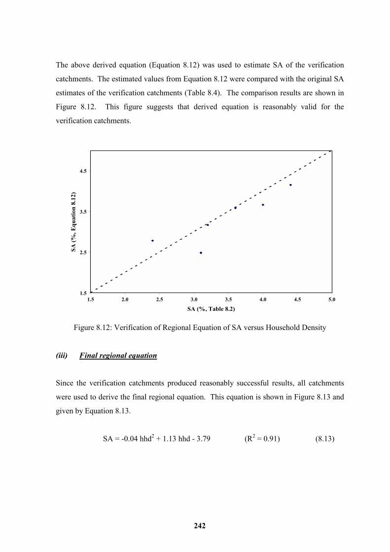
242

The above derived equation (Equation 8.12) was used to estimate SA of the verification

catchments. The estimated values from Equation 8.12 were compared with the original SA

estimates of the verification catchments (Table 8.4). The comparison results are shown in

Figure 8.12. This figure suggests that derived equation is reasonably valid for the

verification catchments.

1.5

2.5

3.5

4.5

1.5 2.0 2.5 3.0 3.5 4.0 4.5 5.0

SA (%, Table 8.2)

SA (%

, Equ

atio

n 8.

12)

Figure 8.12: Verification of Regional Equation of SA versus Household Density

(iii) Final regional equation

Since the verification catchments produced reasonably successful results, all catchments

were used to derive the final regional equation. This equation is shown in Figure 8.13 and

given by Equation 8.13.

SA = -0.04 hhd2 + 1.13 hhd - 3.79 (R2 = 0.91) (8.13)

243

SA = -0.04 hhd2 + 1.13 hhd - 3.79R2 = 0.91

0

1

2

3

4

5

5 6 7 8 9 10 11 12 13 14 15


SA (%

)

Figure 8.13: SA versus hhd for Study Catchments

8.7.4 Regionalisation of DSi

8.7.4.1 Identification of influential catchment characteristics

Based on past research such as those of Kidd (1978a,b), the regional equations of DSi had

included only the catchment slope, since the catchment slope had some effect on the

retention capacity of runoff, which is directly related to DSi. However, as stated in Section

8.2, there are other studies (Danish Hydraulic Institute, 1988; Bedient and Huber, 1992;

O’Loughlin, 1993) that recommended constant values or a range for DSi.

In this section, an attempt was made to correlate DSi with the catchment slope. In addition

to the catchment slope, DCIA was also considered.

244

(a) Relationship between DSi and catchment slope

Since the study catchments consist of a number of subcatchments draining to their own

pits, three methods (i.e. arithmetic mean, area weighted mean and geometric mean) were

used to compute the catchment slope (Section 8.5.1).

DSi versus different definitions of catchment slopes are shown in Figure 8.14. As can be

seen from this figure, there is no correlation at all between DSi and the catchment slope.

This is in contrast to the findings of Kidd (1978a,b). However, the values of DSi are

between 0 and 1 mm. This could be one of the reasons that the fixed values within a range

had been recommended by Danish Hydraulic Institute (1988), Bedient and Huber (1992)

and O’Loughlin (1993).

(b) Relationship between DSi and DCIA

Figure 8.15 shows DSi versus DCIA for study catchments. This figure suggests that there

is no correlation between these two parameters.

8.7.4.2 Regionalisation equation for DSi

Both catchment slope and DCIA did not show any correlation with DSi. However, DSi of

the study catchments were within the range of 0-1 mm. This range for DSi is comparable

with the results of previous studies (Danish Hydraulic Institute, 1988; Bedient and Huber,

1992; O’Loughlin, 1993). Therefore, it is recommended that DSi between 0 and 1 mm can

be used for the ungauged urban residential catchments in the Melbourne metropolitan area,

where there are no rainfall/runoff data available for calibrating DSi. Since a range (0 - 1

mm) was recommended for DSi, the sensitivity of DSi was revisited to see the effect on

various DSi values within the range on the hydrograph attributes (i.e. runoff volume, peak

discharge and time to peak discharge). This was also extended to DCIA. This is discussed

in Section 8.7.5.

245

0.0

0.2

0.4

0.6

0.8

1.0

0 2 4 6 8 10 12

Catchment Slope (%)

DS i

(mm

)

(i) DSi Versus Arithmetic Average Catchment Slope

0.0

0.2

0.4

0.6

0.8

1.0

0 2 4 6 8 10 12

Catchment Slope (%)

DS i

(mm

)

(ii) DSi Versus Area Weighted Average Catchment Slope

0.0

0.2

0.4

0.6

0.8

1.0

0 2 4 6 8 10 12Catchment Slope (%)

DS i

(mm

)

(iii) DSi Versus Area Geometric Average Catchment Slope

Figure 8.14: DSi versus Average Catchment Slopes for Study Catchments

246

0.0

0.2

0.4

0.6

0.8

1.0

0 10 20 30 40 50 60 70

DCIA (%)

DS i (m

m)

Figure 8.15: DSi Versus DCIA for Study Catchments

8.7.5 Further Sensitivity Studies of DSi and DCIA

The sensitivity study was conducted using two design storms (i.e. 1 and 100 year ARIs)

and two catchments used in Section 6.4. These two design storms represented a ‘small’

and ‘large’ storm event, and the two catchments represented a ‘small’ and a ‘large’ urban

catchment with typical urban densities, pits and pipes. Three values for DSi (i.e. 0.0, 0.5

and 1.0 mm) and three values for DCIA (i.e. 20%, 40% and 60%) were used.

For each DCIA value, the outlet hydrographs were computed using the ILSAX model

corresponding to three DSi values. Table 8.5 shows the details of the hydrograph attributes

for the two catchments corresponding to 1-year ARI storm event. Figures 8.16 and 8.17

show the outlet hydrographs for different values of DSi and DCIA for the 1-year ARI storm

event. From Figures 8.16 and 8.17, and Table 8.5, it can be seen that outlet hydrographs

change slightly with different DSi values for a given DCIA. The significant difference is

that as DSi increases, the starting time of the hydrograph is delayed as a result of higher

initial losses. There is also a difference in runoff volume, although peak and shape are not

that different with respect to different DSi values. However, the variation is very high with

different DCIA values.

247

Table 8.5: Hydrograph Attributes for 1-year ARI Storm Event

Attributes DSi (mm) Altona Medows Catchment Therry Street Catchment

DCIA DCIA

20% 40% 60% 20% 40% 60%

Volume (m3) 253 504 776 1035 2081 3138

Peak (m3/s) 0.213 0.385 0.503 1.089 1.997 2.510

Time to peak (min)

0.0

20 18 18 20 18 18

Volume (m3) 239 474 730 970 1949 2934

Peak (m3/s) 0.202 0.379 0.503 1.081 1.984 2.479

Time to peak (min)

0.5

20 18 18 20 20 18

Volume (m3) 226 445 695 917 1833 2755

Peak (m3/s) 0.194 0.360 0.491 1.078 1.998 2.494

Time to peak (min)

1.0

22 18 18 18 18 18

The results for the 100-year ARI are given in Table 8.6 and Figures 8.18 and 8.19 for both

catchments. The table and plots suggest that DSi does not make any significant difference

to outlet hydrographs for this event. However, DCIA makes a significant difference.

As can be seen from the results of this sensitivity study, DCIA is very sensitive for both

‘small’ and ‘large’ storm events compared to DSi. The effect of DSi on ‘large’ storm

events is insignificant, while the peak discharge is not affected by DSi for ‘small’ events.

In urban drainage studies the peak discharge is more important in most cases. Therefore,

the range between 0-1 mm can be used for DSi for ungauged catchments.

248

0.0

0.1

0.2

0.3

0.4

0.5

0.6

0 10 20 30 40 50 60

Time (min)

Q (m

3/s)

0

20

40

60

80

100

120

140

I (mm

/h)

I (mm/hr)DSi = 0.0 mmDSi = 0.5 mmDSi = 1.0 mm

(a) For DCIA = 20%

0.0

0.1

0.2

0.3

0.4

0.5

0.6

0 10 20 30 40 50 60

Time (min)

Q (m

3/s)

0

20

40

60

80

100

120

140

I (mm

/h)


(b) For DCIA = 40%

0.0

0.1

0.2

0.3

0.4

0.5

0.6

0 10 20 30 40 50 60

Time (min)

Q (m

3/s)

0

20

40

60

80

100

120

140

I (mm

/h)


(c) For DCIA = 60%

Figure 8.16: Sensitivity of DSi and DCIA for Altona Meadows Catchment for 1 year ARI

Storm Event

249

0.0

0.5

1.0

1.5

2.0

2.5

3.0

0 5 10 15 20 25 30 35 40 45 50

Time (min)

Q (m

3/s)

0

20

40

60

80

100

120

140

I (mm

/h)


(a) For DCIA = 20%

0.0

0.5

1.0

1.5

2.0

2.5

3.0

0 5 10 15 20 25 30 35 40 45 50

Time (min)

Q (m

3/s)

0

20

40

60

80

100

120

140

I (mm

/h)


(b) For DCIA = 40%

0.0

0.5

1.0

1.5

2.0

2.5

3.0

0 5 10 15 20 25 30 35 40 45 50

Time (min)

Q (m

3/s)

0

20

40

60

80

100

120

140

I (mm

/h)


(c) For DCIA = 60%

Figure 8.17: Sensitivity of DSi and DCIA for Therry Street Catchment for 1 year ARI

Storm Event

250

Table 8.6: Hydrograph Attributes for 100-year ARI Storm Event

Attributes DSi (mm) Altona Medows Catchment Therry Street Catchment

DCIA DCIA

20% 40% 60% 20% 40% 60%

Volume (m3) 1465 2346 3235 6945 10266 13593

Peak (m3/s) 0.671 0.859 1.045 2.677 2.782 2.912

Time to peak (min)

0.0

18 18 18 18 16 18

Volume (m3) 1451 2317 3183 6865 10135 13372

Peak (m3/s) 0.667 0.859 1.044 2.677 2.787 2.906

Time to peak (min)

0.5

18 18 18 18 16 18

Volume (m3) 1436 2287 3138 6817 10014 13184

Peak (m3/s) 0.665 0.859 1.044 2.677 2.790 2.909

Time to peak (min)

1.0

18 18 18 18 18 16

8.7.6 Limitation of Regional Equations

The regional equations were derived in this study only for residential catchments. The

catchment area of the study catchments used in regionalisation varied from 3 to 30 ha.

These sizes represent typical ‘small’ and ‘medium’ size urban catchments in Melbourne

metropolitan areas. Therefore, the derived regional equations are valid only for the

residential catchments whose catchment area is less than 30 ha.

There were several independent and dependent variables used in the regional equations.

The statistics (i.e. minimum, mean and maximum) of these variables are given in Table

8.7. As found by other researchers (e.g. Dyer et al., 1994, 1995), the regional equations are

valid for use with catchment variables within the range that was used in derivation of these

equations. Therefore, the validity of the regional equations outside of these ranges and

mixed land-use catchments should be tested before using them.

251

0.0

0.2

0.4

0.6

0.8

1.0

1.2

0 20 40 60 80 100 120 140 160

Time (min)

Q (m

3/s)

0

50

100

150

200

250

300

350

400

I (mm

/h)


(a) For DCIA = 20%

0.0

0.2

0.4

0.6

0.8

1.0

1.2

0 20 40 60 80 100 120 140 160

Time (min)

Q (m

3/s)

0

50

100

150

200

250

300

350

400

I (mm

/h)


(b) For DCIA = 40%

0.0

0.2

0.4

0.6

0.8

1.0

1.2

0 20 40 60 80 100 120 140 160

Time (min)

Q (m

3/s)

0

50

100

150

200

250

300

350

400

I (mm

/h)


(c) For DCIA = 60%

Figure 8.18: Sensitivity of DSi and DCIA for Altona Meadows Catchment for 100 year

ARI Storm Event

252

0.0

0.5

1.0

1.5

2.0

2.5

3.0

3.5

4.0

0 20 40 60 80 100 120 140 160

Tim e (m in)

Q (m3/s

0

50

100

150

200

250

300

350

400

I (mm/h


(a) For DCIA = 20%

0.0

0.5

1.0

1.5

2.0

2.5

3.0

3.5

4.0

0 20 40 60 80 100 120 140 160

Time (min)

Q (m

3/s)

0

50

100

150

200

250

300

350

400

I (mm

/h)


(b) For DCIA = 40%

0.0

0.5

1.0

1.5

2.0

2.5

3.0

3.5

4.0

0 20 40 60 80 100 120 140 160

Time (min)

Q (m

3/s)

0

50

100

150

200

250

300

350

400

I (mm

/h)


(c) For DCIA = 60%

Figure 8.19: Sensitivity of DSi and DCIA for Therry Street Catchment for 1 year ARI

Storm Event

253

Table 8.7: Limitation of Variables for Regional Equations

Variable Minimum Mean Maximum

Catchment area (ha) 3 12 30

Household density (houses/ha) 7 9 14

Average catchment slope (%) 0.3 4.0 6.6

DCIA (%) 19 39 63

SA (%) 2 3 5

DSi (mm) 0 0.4 0.9

8.8 SUMMARY

Sixteen urban residential catchments from the Melbourne metropolitan area were used to

develop regional equations for impervious area parameters directly connected impervious

area (DCIA), supplementary area (SA) and directly connected impervious area depression

storage (DSi). These equations were derived for use in ILSAX for ungauged Metropolitan

catchments where there are no rainfall-runoff data available to calibrate these parameters.

These 16 catchments were subcatchments of seven major residential catchments, which

were monitored for rainfall and runoff during 1996 to 1999. The pervious area parameters

were not considered in this regionalisation, since the runoffs from pervious areas were not

observed during the monitoring period. The parameter values (i.e. DCIA and DSi)

obtained from calibration using hydrograph modelling of ‘small’ storm events were used in

the regionalisation. These two parameters are related to the directly connected impervious

area. SA was obtained from the information on drainage plans and through field visits.

Two regional equations, one for DCIA and the other for SA were developed. The

independent variable considered in these equations was the household density. A split

sample procedure was used to derive the regional equations. From the study catchments,

10 catchments were initially used to derive the regional equations and these equations were

tested using the remaining six catchments. Then, all 16 catchments were used to derive the

final regional equations. The derived regional equations for DCIA and SA can be applied

for residential catchments in the Melbourne metropolitan area whose areas are less than 30

254

ha. If the household density of existing or proposed catchment is known, then DCIA and

SA of the catchment can be estimated using these equations.

DSi is the only ILSAX model parameter, which is responsible for modelling ‘small’ storm

events. Although the catchment slope was believed to represent the retention capacity (in

turn related to DSi) of the catchment, no correlation was found between DSi and the

average catchment slope of study catchments. Therefore, a range between 0 to 1 mm was

recommended in this study for DSi. Further sensitivity analysis of DSi and DCIA showed

that DSi was not significantly sensitive to the outlet hydrograph compared to DCIA for

both ‘small’ and ‘large’ storm events, especially in term of peak discharge, which is more

important in urban drainage studies in general terms.

It is important to note that the derived regional equations for DCIA and SA and the range

recommended for DSi should be used for Melbourne metropolitan residential catchments

whose properties are within the range of independent and dependent variables used in the

regionalisation study. The validity of the equations for DCIA and SA, and the range for

DSi outside the ranges used for regionalisation study should be tested before using them.

255

CHAPTER 9

SUMMARY OF METHODOLOGY, CONCLUSIONS AND

RECOMMENDATIONS

9.1 SUMMARY OF METHODOLOGY The main aim of the research study in this thesis is to develop improved methods in design

and analysis of urban stormwater drainage systems. To achieve this objective, the

following methodological aspects were considered.

1) Review of literature related to urban drainage modelling and assessment of current

urban drainage modelling practice in Victoria (Australia).

2) Study of modelling options of ILSAX, parameter sensitivity and catchment

subdivision.

3) Model parameter optimisation.

4) Development of regional equations for modelling of urban catchments.

A brief summary of the methodology under each of these aspects is given below. The

conclusions related to these aspects are given in Section 9.2.

A literature review was conducted on the physical processes of rainfall-runoff modelling of

urban catchments and how these processes are modelled by different urban drainage

models. In particular, a review was conducted on errors associated with urban drainage

models in predicting runoff peak and volume. A customer survey was then conducted in

May 1997 to identify the current practice in stormwater drainage design and analysis. Due

to resource constraints, the survey was restricted to city/shire councils and consultants in

Victoria. From the results of the survey, it was found that the ILSAX model was the

widely used stormwater drainage computer model in Victoria. Therefore, the ILSAX

model was used in this study to develop improved methods for design and analysis of

urban stormwater drainage systems.

256

The next step was to develop a consistent strategy for modelling the study catchments. A

consistent approach was necessary since the study dealt with a large number of catchments.

Therefore, a detailed study was conducted to select the appropriate modelling options (out

of many available in the ILSAX model) for modelling various urban drainage processes, to

study the sensitivity of model parameters on simulated storm hydrographs and the effect of

catchment subdivision on storm hydrographs. This was done using two urban catchments

in Melbourne considering four design storms. The two catchments represented a typical

‘small’ and a ‘large’ urban catchment in the Melbourne metropolitan area. The four design

storms ranged from storms of average recurrence interval (ARI) of 1 year to 100 year

(including one considerably above 100 year ARI). The results from this detailed study

were subsequently used in model parameter calibration.

The third step was to calibrate the ILSAX model for the study catchments using available

rainfall-runoff data. A two-stage inner/outer optimisation procedure was developed in this

study, to estimate the model parameters of ILSAX. The method was designed to provide

the ‘best’ set of model parameters that considers several storm events simultaneously.

Impervious area parameters were obtained from frequent ‘small’ storm events, while the

pervious area parameters were obtained from less-frequent ‘large’ events. The PEST

computer software was used to optimise the model parameters. Twenty-two urban

catchments in the Melbourne metropolitan area and one urban catchment in Canberra were

used as study catchments. The parameters obtained from the two-stage inner/outer

optimisation were compared with the values obtained from rainfall-runoff depth plots and

areal photographs (if available) for their validity.

The calibrated model parameters and catchment characteristics were used to develop the

regional equations for estimating impervious area parameter for use in ILSAX. These

equations can then be used for ungauged catchments, when there are no rainfall-runoff data

available to calibrate these parameters. Sixteen residential catchments in the Melbourne

metropolitan area were used to develop these regional equations. The dependent variables

considered were the directly connected impervious area percentage (DCIA), the

supplementary area percentage (SA), and directly connected impervious area depression

storage (DSi). DCIA and DSi were obtained from the two-stage inner/outer optimisation

257

(but verified with rainfall-runoff plots and areal photographs), while SA was estimated

from field visits. Pervious area parameters were not considered in the regionalisation, as

the observed runoff events did not have any pervious area runoff. The independent

variables considered in the regionalisation were catchment area, distance from Melbourne

Central Business District, household density and average catchment slope.

9.2 CONCLUSIONS

9.2.1 Literature Review

Following conclusions were drawn from the literature review conducted in this study.

• The main processes of rainfall-runoff modelling in urban catchments are related to

estimation of rainfall excess in pervious and impervious areas, and routing of this

rainfall excess through different drainage system components. Different methods are

employed by different models to compute the rainfall excess and routing through the

drainage system. These different methods in general produce different results.

• Errors related to output responses such as runoff volume, peak discharge and time to

peak discharge were quantified using published results of past modelling work. The

error analysis was conducted as applicable to both ‘calibrated and verified’ catchments

and ungauged catchments. The results of this study showed that the peak discharge

runoff volume simulated by urban drainage models had significant errors. Also, the

simulation results from ungauged catchments were less accurate compared to the results

from gauged catchments, which is the case in general.

• The literature review also showed that model error was depended on storm

characteristics and land-use type of catchments.

9.2.2 Customer Survey

258

Following important findings were extracted based on the analysis of responses of the

customer survey conducted in Victoria in May 1997.

• Majority of respondents (about 80%) used methods such as the Statistical Rational

method, which involve many assumptions, for urban drainage design and analysis. The

remaining 20% used computer models, which simulate hydrologic and hydraulic

processes related to urban drainage systems. This is a disturbing fact, since large annual

expenditures are spent on urban drainage construction works throughout Victoria and

other parts of Australia.

• Lower use of computer models was due to:

• lack of user-friendliness of the computer models,

• adequate guidelines were not available to select the model parameters (especially

for ungauged catchments), and

• adequate guidelines were not available to select the appropriate modelling options

(out of many available in these models), which can be used to model various

processes.

• The ILSAX model was the widely used urban drainage computer model in Victoria.

9.2.3 Data Collection and Analysis

The accuracy of any modelling exercise largely depends upon the accuracy of the data. For

the calibration of rainfall-runoff models, accurate catchment data and rainfall-runoff data

are required. The rainfall-runoff data can be obtained through a well maintained data

acquisition program with pluviometers and automatic flowmeters installed at strategic

locations of the stormwater drainage system. Raw hydrological data thus acquired should

be carefully checked for accuracy and consistency. Graphical time series plots of recorded

flow depth and velocity, hyetograph and hydrograph on the same chart, and rainfall-runoff

depth plots were the some techniques used in this study to check the accuracy and

consistency of rainfall-runoff data and found to be useful techniques.

259

The catchment data can be obtained from drainage plans, land-use maps, contour maps,

soil maps and areal photographs of the catchments. However, the information was

obtained from above source should be verified through field visits.

9.2.4 Selection of Appropriate Modelling Options

Most drainage models have more than one option to model various processes related to

urban drainage systems. In analysing a large number of catchments as in this study, it is

convenient to use a single modelling option in modelling a process of all study catchments.

This becomes necessary when the results are used in a regionalisation. The ILSAX model

has more than one option in modelling the following processes.

• Loss subtraction method for pervious area

• Time of entry for overland flow routing

• Pipe and channel routing

• Modelling of pit inlets

Based on analysis of modelling of various options using two urban catchments (one typical

‘small’ and one typical ‘large’) and four design storms (ARI ranging from 1-year to larger

than 100-year), the following conclusions were made. These conclusions were later used

in the calibration of the study catchments.

• For pervious area loss modelling, the ‘supply’ rate method was used, since this method

allows infiltration to occur after rainfall has stopped, which is closer to the reality. Data

requirements for both methods (i.e. losses subtracted from ‘supply’ rate and losses

subtracted from rainfall) are the same.

• For overland flow routing, the ARR87 method was used from the available two methods

(i.e. ILLUDAS-SA procedure and ARR87 method), since this method models overland

drainage components (e.g. surface, gutter flow) more realistically. However, data

requirements are more in the ARR87 method compared to the ILLUDAS-SA method.

260

• For pipe routing, the implicit method was used, since this method considered both time

lag effects and storage routing effects, which is closer to the reality. Data requirements

for both methods (i.e. time-shift and implicit methods) are the same.

• Modelling pit capacity is important since the separation of pipe flow and bypass flow is

due to pit capacity. Studies conducted with study catchments revealed that either pit

capacity option (i.e. finite or infinite capacity) could be used for modelling of pits for

‘small’ storm events whose ARI is less than 5-year. If the storm event has an ARI

greater than 5 years, the finite pit capacity option (which reflects the actual pit capacity)

should be used to model bypass flow and pipe flow accurately. However, the data

requirements for finite pit capacity option are more. The other problem with this

method is that the pit capacity parameters for all currently used pit types and sizes are

not available. These pit capacity parameters are currently obtained from physical

hydraulic model studies.

9.2.5 Sensitivity Analysis

In simulation of ‘small’ storm events, the hydrograph attributes (i.e. runoff volume, peak

discharge, time to peak discharge and hydrograph shape) were sensitive to impervious area

parameters, while they were not sensitive to pervious area parameters. This is because

there is no pervious area runoff for ‘small’ runoff events. The impervious area parameters

are also important for ‘large’ events, since runoff for these events is generated from both

impervious and pervious areas. Therefore, the accurate estimation of impervious area

parameters is very important. The only impervious parameter of the ILSAX model is DSi.

The sensitivity of DSi decreases with the increase of storm magnitude. The pervious area

parameters were sensitive only for ‘large’ storm events in simulating the runoff volume and

peak discharge. The pervious area parameters of ILSAX are antecedent soil moisture

content (AMC), soil curve number (CN) and pervious area depression storage (DSp), and

these parameters were considered in the sensitivity analysis. The sensitivity transfers from

impervious area parameters to pervious area parameters when storm magnitude increases.

These impervious and pervious parameters were called hydrologic parameters in this thesis.

261

The pit capacity parameters of on-grade pits (CAP3 and CAP4), choke factor (CF), gutter

factor (GUT) and pipe roughness (Np) were also sensitive parameters in simulating the

peak discharge in addition to hydrologic parameters. Retardance coefficient of pervious

area (Nr) was the least sensitive parameter to the peak discharge. These parameters are

called routing parameters in this thesis. They do not affect the runoff volume.

9.2.6 Catchment Subdivision

To account for areal variability of rainfall and losses, and to model different travel times of

various parts of the catchment to the outlet, the catchment should be subdivided into a

number of subcatchments. In general, three levels of subdivisions can be considered,

namely coarse subdivision (neglecting all lateral drains and considering each catchment to

contribute directly to the inlets of the main drain), a medium subdivision (considering main

drain and first order laterals) and a fine subdivision (considering all drains). The effect of

the catchment subdivision is significant for the catchments, where routing effects dominate

the rainfall-runoff process.

The results of the study suggested that the catchment subdivision was important in

modelling the peak discharge. This was because of the dependence of peak discharge on

the overland flow behaviour, the storage effects of the drainage system and the pit capacity,

which were modelled differently for different levels of subdivision. In medium and coarse

subdivisions, some pits are not modelled. For larger storm events (i.e. greater than 5 year

ARI), if finite pit capacity option is used to model bypass flow, the storage effects of pits

that were not considered in modelling should be taken into account. One way to handle

this is to define an equivalent pit capacity for the modelled pits, to allow for the capacity of

ignored pits in modelling. However, currently there is no method to compute the

equivalent pit capacity. Therefore, the equivalent capacity of the modelled pits can be

estimated based on engineering judgement considering some increase for the pit capacity

through pit capacity parameters.

262

Based on the analysis of different subdivisions, any form of subdivision can be used if only

the runoff volume is of interest. For the accurate simulation of peak discharge, the fine

subdivision should be used.

9.2.7 Model Calibration

Three methods were used to estimate the DCIA of study catchments. They are:

1) Use of areal photographs

2) Use of rainfall/runoff depth (RR) plots

3) Hydrograph modelling of storm events

Of these methods, the latter two methods also produced DSi. The RR plot gives only

DCIA and DSi, while the hydrograph modelling produces the pervious area parameters (i.e.

CN and DSp) in addition to DCIA and DSi.

The first method gives the total impervious area, which is the sum of DCIA and

supplementary area percentage. Therefore, the first method gives only an upper bound for

DCIA. The second and third methods require rainfall-runoff data and therefore the

catchments should be gauged. The RR plots consider only the runoff volume, while the

hydrograph modelling calibration considers all hydrograph attributes such as runoff

volume, peak discharge, time to peak discharge and hydrograph shape. Since the third

method considers all hydrograph attributes in estimating parameters, it is preferred but

should be verified against the other methods. The hydrograph modelling approach was

used in this thesis to calibrate the model parameters for study catchments. An optimisation

approach called two-stage inner/outer optimisation was developed in this study to calibrate

the model parameters using hydrograph modelling.

This method produces the ‘best’ set of model parameters which considering all calibration

events. The parameter optimisation of each drainage catchment model was carried out in

two stages. During the first stage, the model parameters responsible for ‘small’ storm

events (i.e. DCIA and DSi) were obtained. During the second stage, the additional

263

parameters responsible for ‘large’ storm events (i.e. DSp and CN) were obtained. During

the second stage, no changes were made to the parameters obtained from the first stage.

Each stage consisted of two loops (i.e. inner and outer). The inner loop uses PEST

computer software to optimise corresponding model parameters, a set of model parameters

is obtained for each storm event. The outer loop optimises the above sets of model

parameters to produce the ‘best’ set considering all calibration events and hydrograph

attributes of runoff volume, peak discharge and time to peak discharge. The outer

optimisation was carried out manually.

The two-stage inner/outer optimisation was used for Melbourne metropolitan catchments to

optimise impervious area parameters using hydrograph modelling. It was used to estimate

both impervious and pervious area parameters for the Giralang catchment. Comparing

observed hydrographs with modelled hydrographs using the ‘best’ set of parameters

obtained from the optimisation, it was found that the method produced satisfactory results.

The ‘best’ set of model parameters obtained from hydrograph modelling was verified using

three independent events for each catchment. Generally, all the verification plots were

reasonably accurate for all study catchments. The ‘best’ set of parameters obtained from

hydrograph modelling was compared with the parameter values obtained from the other

methods (i.e. RR plots and areal photographs). However, the latter estimates were used

only as checks for the ‘best’ parameter set obtained from hydrograph modelling. By

comparing the ‘best’ set of model parameters obtained from hydrograph modelling with

those of the other methods (i.e. RR plots and areal photographs), it was found the former

set of parameter estimates for the study catchments. These parameter values were used for

the regionalisation study. Based on the results of verification plots and checks with respect

to other methods, it can be said that two-stage inner/outer optimisation produced

satisfactory results and therefore, it can be recommended to calibrate any urban drainage

model. The calibrated parameter values for the Melbourne catchments and the Canberra

catchment were within the limit of the values given in the literature.

For Melbourne study catchments, areal photographs were available for ten study

catchments. DCIA obtained from hydrograph modelling using the two-stage inner/outer

264

optimisation procedure and rainfall-runoff depth plots were compared with those obtained

from the areal photographs, and found to be less. This is to be expected since the areal

photographs give the total impervious area which includes with DCIA and supplementary

area. The difference of the values from both methods for the study catchments was within

10% limit except one catchment. The eighteen catchments out of 22 catchments gave less

than 10% difference for DCIA computed from the RR plots and the optimisation methods.

The 50% of study catchments gave less than 0.25 mm different for DSi computed from the

both methods.

9.2.8 Parameter Regionalisation

Two equations were developed to estimate DCIA and SA from the household density.

Sixteen catchments were used in the regionalisation study. A split sample procedure was

used to derive the regional equations. From the study catchments, 10 catchments were

initially used to derive the regional equations and these equations were tested using the

remaining six catchments. Then, all 16 catchments were used to derive the final regional

equations. The derived regional equations for DCIA and SA can be applied for residential

catchments in the Melbourne metropolitan area whose areas are less than 30 ha. If the

household density of existing or proposed catchment is known, then DCIA and SA of the

catchment can be estimated using these equations.

Although the catchment slope was believed to represent the retention capacity (in turn

related to DSi) of the catchment, no correlation was found between DSi and the average

catchment slope of study catchments. Therefore, a range between 0 to 1 mm was

recommended in this study for DSi. Further sensitivity analysis of DSi and DCIA showed

that DSi was not significantly sensitive to the outlet hydrograph compared to DCIA for

both ‘small’ and ‘large’ storm events, especially in term of peak discharge, which is more

important in urban drainage studies in general terms.

The derived two equations for DCIA and SA, and the recommended range for DSi are valid

for only residential catchments in the Melbourne metropolitan area, whose catchment area

is less than 30 ha. Therefore, it is necessary to check whether the catchment under

265

investigation falls into this category and within the range of catchment parameters used to

determine these equations. Where the variables of the catchment under investigation falls

outside the range of the variables of the catchments used to define the regional equations,

the modeller should apply these equations to this catchment with caution.

9.2.9 Other Issues

Although ILSAX is widely used by the local government authorities and consultants in

Australia to design and analyse of urban drainage systems, there are no adequate guidelines

available to develop models for both gauged and ungauged urban catchments. The user

manual (O’Loughlin, 1993) provides the information on how to assemble data to construct

a model and some guidelines. However, there are many other important decisions the user

has to make before constructing a model, which have not been covered in detail in the user

manual. Some of these have already been explained in the previous conclusions. Some

other issues are briefly discussed below as further conclusions.

9.2.9.1 Catchment data

Unless catchments are fully developed, urban catchments should be treated as dynamic

systems, in which catchment properties change with time. Therefore, the ILSAX model

parameters, especially the parameter related to impervious area, changes with the

development. If rainfall-runoff data are available for a catchment for a certain time of the

year, then the other catchment data should also be collected relevant to the same period

from other sources such as areal photographs and maps.

9.2.9.2 Subcatchment slope

The times of entry (or times of concentration) are required to set the base lengths of time-

area diagrams in ILSAX for impervious and pervious areas. The user has to enter flow

266

path lengths and slopes into the model. Therefore, it is important to identify the flow

paths, and estimate their lengths and slopes correctly.

The subcatchment of a pit may consist of several household properties. In estimating the

subcatchment slope, it is assumed that water flows to the pit in the direction of the

subcatchment slope to pit. Therefore, the usual practice is to compute the slope from the

flow path determined by contour maps without considering actual flow paths. In urban

catchments, house-fencing around properties significantly changes the flow path. These

fences are usually made of colour bond steel or solid timber. Therefore, there is no free

flow between adjoining properties, and runoff from a property can then be analogues to

runoff from a rectangular tank, which is open on one side and water flows freely towards

this open end. Therefore, the length and slope of subcatchments relevant to modelled pits

should consider flow paths of individual properties instead of considering several

properties together and the flow path determined from contours.

9.2.9.3 Computational time step

The ILSAX model allows the user to specify the time step for hydrograph simulation. This

computational time step should be less than the time increment of rainfall input so that

rainfall can be adequately modelled. Therefore, a time interval less than two minutes is

recommended based on the studies of this thesis. Smaller time intervals increase the

accuracy of modelling at the expense of computer time. ILSAX has a limitation of 720

time steps in defining the simulated hydrograph, which limit the use of smaller time

intervals. This may not be a serious problem, since ILSAX can be recompiled with a larger

number of time steps.

9.2.9.4 Property time

For the Australian urban catchments, the property time is between 2-7 min according to the

published literature (e.g. The Institution of Engineers, 1987; O’Loughlin, 1993; Stephens

267

and Kuczera, 1999). The best way to handle the unknown property time of a catchment is

to assume 5-min property time in modelling the catchment and then compare the time to

peak discharge of the simulated hydrograph with that of observed hydrograph. If the time

to peak discharge is considerably different, then the property time should be changed

considering values between 2-7 min until get the best match is obtained. However, this

method can be used only for gauged catchments, where rainfall/runoff data are available.

9.2.10 Transferability of Results to Other Models

The findings regarding the computation of losses, routing methods, pit inlet modelling, and

catchment subdivision can be extended to any type of urban drainage models where these

options are available for modelling of the hydrologic and hydraulic processes. The

proposed calibration method (i.e. two-stage inner/outer optimisation) can also be used with

other urban drainage models to calibrate their parameters.

The derived regional equations for DCIA and SA can be used for any other urban

stormwater drainage model in which subcatchment surface is modelled using three types of

land parameters namely directly connected impervious area, supplementary area and

pervious area. The recommended values for DSi can also be used in any urban drainage

model, which model initial losses separately.

9.3 RECOMMENDATIONS FOR FUTURE RESEARCH

9.3.1 Equivalent Pit Capacity

The main difficulty with medium and coarse subdivision is to estimate the pit capacity of

the selected pits for modelling, to account for the effects of the other pits that were not

modelled. One way would be to define an equivalent pit capacity for the modelled pits to

account for ignored ones. Previous studies on urban drainage analysis have not considered

this effect and therefore, further research is required to compute the equivalent pit capacity.

268

9.3.2 Choke Factor

The results of this study showed that the choke factor (CF) was sensitive in simulating the

peak discharge in drainage pipes. CF is a dynamic factor for a catchment. This factor

depends on the frequency of street cleaning, dry and wet periods, and location of a pit, and

therefore, may be correlated with pollutant build-up and washoff patterns in the catchment.

Further research should be conducted to determine the appropriate value of CF for design

and evaluation of urban drainage systems based on above dependencies.

9.3.3 Property Time

The ILSAX model uses 5-min property time as default. Some other studies had suggested

that the property times between 2 to 7 min (e.g. The Institution of Engineers, 1987;

O’Loughlin, 1993; Stephens and Kuczera, 1999). Further research is required to determine

the suitable property time.

9.3.4 Determination of AMC

At present, ILSAX uses four AMC levels corresponding to total rainfall depth in five days

preceding the storm. It does not consider the distribution of the rainfall during the previous

five days. In reality, the condition that 25 mm of rainfall occurs in the first day and the

condition that 25 mm of rainfall occurs in the fifth day is not the same. Therefore, this

method has to be improved to get better results. The author suggests computing the AMC,

which relates to the antecedent precipitation index (API), by one of the two methods given

in Equations 9.1 and 9.2.

API0 = P0 + P1K + P2K2+..................+ PnKn (9.1)

or

API0 = P0 + APIi * K (9.2)

where K is a recession factor less than unity,

Pi is the 24 hour rainfall depth (mm) on ith day, and

Subscripts of 0, 1, 2 Days prior to storm event; 0 being for the current

269

day, 1 for one day prior to storm, etc.

These forms of equations have been used by Cordery (1970) and Loy et al. (1996).

9.3.5 Curve Numbers

ILSAX defines four soil classifications, designated as A, B, C and D for the soil underlying

the pervious portions of the catchment. These curves were developed by U.S. Soil

Conservation Service for U.S. catchments. Applicability of these curves to Victorian (or

Australian) urban catchments have not been tested properly. Therefore, further research is

required to identify whether these curves are suitable for Victorian (or Australian) urban

catchments. These curves can be tested using results from field infiltrometer tests with

different antecedent moisture conditions (AMCs).

9.3.6 Effect of Scaling Factors

It is expected that there would be rainfall variation within the catchment, especially for

large rainfalls. An investigation of this aspect would be worthwhile to pursue in future.

9.3.7 Modelling Concepts and Parameter Settings

Once the important parameters are identified through the sensitivity analysis and

calibration, it is worthwhile to investigate the modelling concepts and parameter settings

for calibration events of each catchment. These effects were not investigated in detail in

the thesis because of the large amount of work involved in such a study. Furthermore, such

an analysis would deviate from the main objective of the thesis. Nevertheless, it is useful

to carry out this investigation and proposed for future work.

270

REFERENCES

1. ACT Department of Urban Services, (1996), Urban Stormwater- Edition 1, ACT,

Australia.

2. Adams, A., (1991), "Application and Comparison of RORB, WBNM and RAFTS

Runoff Routing Models", International Hydrology and Water Resources Symposium,

Perth, (volume 2), pp 485-491.

3. Aitken, A.P., (1973), “Hydrologic Investigation and Design in Urban Areas”, A

Review, Australian Water Resources Council, Technical Paper No. 5, Canberra,

Australia.

4. Aitken, A.P., (1975), “Hydrologic Investigation and Design of Urban Stormwater

Drainage Systems”, Australian Water Resources Council, Technical Paper No.10,

Canberra, Australia.

5. Alley, W. M. and. Smith, P.E., (1990), “Distributed Routing Rainfall-Runoff Model

(DR3M)”, Mississippi, Water Resources Division, Gulf Coast Hydroscience Center.

6. Alley, W.M. and Veenhuis, J.E., (1983), "Effective Impervious Area in Urban

Runoff Modeling", Journal of Hydraulic Engineering Vol. 109, No. 2, pp 313-319.

7. Argue, J., (1986), “Storm Drainage Design in Small Urban Catchments”, Special

Report No. 34, Australian Road Research Board, Australia.

8. Australian Water Resources Council, (1973), Australian Representative Basin

Programme- Progress 1973, Hydrological Series No.8.

9. Ball, J.E., (1987a), “A Comparison of the Hydraulics in Three Urban Drainage

Models”, Conference on Hydraulics in Civil Engineering, Melbourne, 12-14 October

1987, pp 88-92.

10. Ball, J.E., (1987b), “Modelling of Unsteady Flows in Urban Networks Including

Some Effects of Manholes”, PhD Thesis, Department of Civil Engineering and

Surveying, University of Newcastle, Australia.

271

11. Ball, J.E., (1992), “The Influence of Temporal Patterns on Surface Runoff

Hydrographs”, International Symposium on Urban Stormwater Management, Sydney,

pp 64-69.

12. Bauer, L.R. and Hamby, D.M., (1991), “Relative Sensitivities of Existing and Novel

Model Parameters in Atmospheric Tritium Dose Estimates”, Rad. Prot. Dosimetry

37, pp 253-260.

13. Bedient, P.B. and Huber, W.C., (1992), “Urban Hydrology. Hydrology and

Floodplain Analysis”, Addison-Wesley Publishing Company, USA.

14. Bielawski, Z., (1984), “The Nash Cascade or a Single Linear Reservoir for Modelling

Urban Runoff”, Proceeding of the Third International Conference on Urban

Drainage, Sweden, pp 203-211.

15. Black, D.C. and Aitken, A.P., (1977), “Simulation of the Urban Process”, Australian

Water Resources Council, Technical Paper No. 26, Canberra, Australia.

16. Bouvior, C. and Desbordes, M., (1990), “Urban Runoff Modelling in Western

Africa”, Fifth International Conference on Urban Storm Drainage, Japan, pp 251-

256.

17. Boyd, M.J., Bufill, M.C., and Knee, R.M., (1993), “Pervious and Impervious Runoff

in Urban Catchments”, Hydrological Sciences, Journal, pp. 463-478.

18. Boyd, M.J., Rigby, T. and Drie, R.V., (2000), Watershed Bounded Network Model,

WBNM2000, Internet, http://www.uow.edu.au/eng/research/wbnm.html.

19. Breshears, D.D., (1987), Uncertainty and Sensitivity Analyses of Simulated

Concentrations of Radionuclides in Milk, M.Sc. Thesis, Fort Collins, CO: Colorado

State University,.

20. Bufill, M.C. and Boyd, M.J., (1992), “A Simple Flood Hydrograph Model for Urban

Catchments”, International Symposium on Urban Stormwater Management, Sydney,

Australia, pp 98-103.

21. Bufill, M.C., (1989), “Effect of Urbanisation on Floods”, PhD thesis, Department of

Civil and Mining Engineering, The University of Wollongong, Australia.

272

22. CEPA (Commonwealth Environment Protection Agency), (1993), “Urban

Stormwater”, Australia.

23. Chapman, T.G. and Salmon, M.A., (1996), “Roof Runoff Data Acquisition and

Analysis”, 23rd Hydrology and Water Resources Symposium, Hobart, Australia, pp

657-661.

24. Cheng, X. and Noguchi, M., (1996), “Rainfall-Runoff Modelling by Neural Network

Approach”, Proceeding of the International Conference on Water Resources and

Environmental Research (Volume II), Japan, pp 143-150.

25. Chiang, C.Y. and Bedient, P.B., (1986), “PIBS Model for Surcharge Pipe Flow”,

Proceedings of the American Society of Civil Engineers, Journal of the Hydraulic

Engineering, Vol. 112, No 3, pp. 181-192.

26. Chiew, F.H.S. and McMahon, T.A., (1993), “Data and Rainfall-Runoff Modelling in

Australia”, Hydrology and Water Resources Symposium, Newcastle, Australia, 1993,

pp 305-316.

27. Choi, K. and Ball, J.E., (1999), “Estimation of Control Parameters for Urban Runoff

Modelling by Using a Hydroinformative System”, Proceedings of 8th International

Conference on urban Storm Drainage, Sydney, pp 1776-1783.

28. Chow, V.T., (1973), “Open-Channel Hydraulics”, McGraw-Hill Book Company.

29. Cordery, I., (1970), "Initial Loss for Flood Estimation and Forecasting", Journal of

the Hydraulic Division, ASCE(HY 12), pp 2447-2465.

30. Crawford, N.H. and Linsley, R.K., (1966), “Digital Simulation in Hydrology,

Stanford Watershed Model IV”, University of Stanford, California, U.S.A., Tech.

Rep. 39.

31. Crick, M.J., Hill, M.D. and Charles, D., (1987), “The Role of Sensitivity Analysis in

Assessing Uncertainty”, Proceedings of a NEA Workshop on Uncertainty Analysis

for Performance Assessments of Radioactive Waste Disposal Systems, Paris, OECD.

273

32. Cullino, C., (1995), “Urban Stormwater Management in Search of Best Practice”,

The Second International Symposium on Urban Stormwater Management,

Melbourne, Australia, pp 49-53.

33. Danish Hydraulic Institute and Barnett Consultants Ltd, (1993), MIKE11- A

Computer Based Modelling System for Rivers and Channels (Manual, Version 3.01).

34. Danish Hydraulic Institute, (1988), “Modelling of Urban Sewer Systems on

Microcomputers”, MOUSE V3.0, Users Guide and Technical Reference, Lawson and

Treloar Pty Ltd, Australia.

35. Dayaratne, S.T. and Perera, B.J.C., (1999), “Parameter Optimisation of Urban

Stormwater Drainage Models”, Proceedings of the 8th International Conference on

Urban Storm Drainage, Sydney, Australia, pp1768-1775.

36. Dayaratne, T.S., (1996), “Assessment of Errors in Commonly Used Event

Hydrograph Urban Catchment Models”, Master Thesis, Department of Civil and

Environmental Engineering, University of Melbourne, Australia.

37. Department of Primary Industries and Energy, (1992), Floodplain Management in

Australia, Volume 1: Executive Summary. Australian Water Resources Council,

Water Management Series No. 21.

38. Driver, N.E. and Tasker, G.D., (1988), “Techniques for Estimation of Storm Runoff

Loads, Volumes and Selected Constituent Concentrations in Urban Watersheds in the

United States”, USA, U.S. Geological Survey.

39. Dyer, B. G., Nathan, R. J., McMahon, T. A. and O’Neill, I. C., (1995), “Prediction

Equations for the RORB Parameter kc Based on Catchment Characteristics”,

Australian Journal of Water Resources, Vol. 1, No. 1, pp 29-38.

40. Dyer, B.G., Nathan, R.J., McMahon, T.A. and O’Neill, I.C., (1994), “Development

of Regional Prediction Equations for the RORB Runoff Routing Model”,

Cooperative Research Centre for Catchment Hydrology, Report 94/1.

41. Fleming, N.S., (1994), An Investigation into Rainfall-Runoff Relationships,

Department of Civil and Environmental Engineering, The University of Adelaide,

Australia.

274

42. Frankel, R.J. and Hansen, W.W., (1968), “Biological and Physical Responses in a

Freshwater Dissolved Oxygen Model”, Advances in Water Quality Improvement,

Eds. Gloyna, E. and Eckenfelder, University of Texas Press, London, pp 126-140.

43. Fuchs, L. and Verworn, H.R., (1988), Microcomputer in der Stadtentwasserung,

Kannalnetzberechnung, Modellbeschreibung, Hannover.

44. Gardner, R.H., O’Neill, R.V., Mankin, J.B., Carney, J.H. and Jones, J., (1980),

“Application of Error Analysis to a Marsh Hydrology Model”, Water Resources

Research 16, pp 659-664.

45. Ghafouri, R.A., (1996), “Deterministic Analysis and Simulation of Runoff in Urban

Catchments”, PhD Thesis, Department of Civil and Mining Engineering, University

of Wollongong, Australia.

46. Giancarro, F.B., (1995), “Management of a Stormwater Drainage System within an

Established Urban Area”, The Second International Symposium on Urban

Stormwater Management, Melbourne, Australia, pp 21-25.

47. Goonetilleke, A. and Jenkins, G., (1997), “GIS as a Tool in Predicting Urban

Catchment Response”, 24th Hydrology and Water Resources Symposium

Proceedings, Auckland, New Zealand, pp 392-397.

48. Goulburn-Murray Water, (1997), “Simulation Model of Birch Creek System”, Final

Report, Victoria, Australia.

49. Goyen, A.G., Phillips, B.C. and Blaik, S., (1989), “Australian Urban Stormwater

Drainage Practice- The Technology Transfer Dilema”, Hydrology and Water

Resources Symposium, Christchurch, NZ, pp 459-463.

50. Grandjean. I. and Zech, Y., (1991), “Rainfall-Runoff Modelling of Partly Urbanized

Watersheds - Use of Digital Terrain Models”, New Technologies in Urban Drainage

(UDT 1991, Dubrovnik) Elsevier Applied Sciences, London, pp 365-372.

51. Green, W.H. and Ampt, C.A., (1911), “Studies on Soil Physics; Flow of Air and

Water Through Soils”, Journal of Agriculture Science 4, pp 1-24.

275

52. Hall, M.J., (1984), Urban Hydrology, Elsevier Applied Science Publishers, London-

New York.

53. Hamby, D.M., (1994), “A Review of Techniques for Parameter Sensitivity Analysis

of Environmental Models”, Environmental Monitoring and Assessment 32, Kluwer

Academic Publishers, Netherlands, pp 135-154.

54. Hammer, M.J., (1977), Water and Waste-Water Technology, John Wiley & Sons

Inc., New York.

55. Heeps, D.P. and Mein, R.G., (1973a), “Independent Comparison of Three Urban

Runoff Models”, Proceedings of the American Society of Civil Engineers, Journal of

the Hydraulics Division, Vol. 100, No Hy 11, pp 995-1009.

56. Heeps, D.P. and Mein, R.G., (1973b), “An Independent Evaluation of Three Urban

Stormwater Models”, Report No. 4/1973, Civil Engineering Research Reports,

Monash University, Australia.

57. Heeps, D.P., (1973), “An Evaluation of Three Urban Hydrologic Models for the

Prediction of Stormwater Runoff”, the Thesis of Master of Engineering Science,


58. Hoffman, F.O. and Gardner, R.H., (1983), “Evaluation of Uncertainties in

Environmental Radiological Assessment Models” in Till, J.E. and Meyer, H.R. (eds),

Radiological Assessments: a Textbook on Environmental Dose Assessment,

Washington, DC: U.S. Nuclear Regulatory Commission Report No. NUREG/CR-

3332.

59. Horton, R.E., (1940), "An Approach Toward a Physical Interpretation of Infiltration

Capacity”, Proceeding of Soil Science 5, pp 399-417.

60. Hossain, A., Rao, R. and Delleur, J.W., (1978), “Estimation of Direct Runoff from

Urban Watersheds”, Journal of the Hydraulics Division, Proceedings of the American

Society of Civil Engineers, Vol 104, No HY2, pp 169-188.

61. Hydraulic Research Limited, Wallingford, (1991), WALLRUS General Reference

Manual, Fourth Edition, Wallingford, U.K.

276

62. Hydrologic Engineering Centre (HEC), (2000), “HEC-RAS User’s Manual”, Internet,

http://www.wrc.hec.usace.army.mil/software-distib/hec-ras/hecrasprogram.html.

63. Johanson, R.C., Imhoff, J.C., Kittle, J.L. Jr. and Donigian, A.S. Jr., (1984),

“Hydrological Simulation Program- FORTRAN (HSPF): Users Manual for Release

8.0”, Office of Research and Development, Environmental Research Laboratory,

Athens, GA. Volumes 1 and 2.

64. Jones, D.E., Jr., (1971), “Where is Urban Hydrology Practice Today”, Proceeding of

American Society of Civil Engineering, Hydr. Div. 97 (HY 2), pp 257-264.

65. Kemp, D.J., (1994), “Calibration of the ILSAX and RAFTS Models on Two Urban

Catchments in Adelaide, South Australia”, Surface Hydrology and Water Resources

Papers, Volume 3, Water Down Under 94 Conference, Adelaide, Australia, 21-25

November 1994, pp 461-464.

66. Kidd, C.H.R, (1978a), “Rainfall-Runoff Processes Over Urban Surfaces”,

Proceedings of an International Workshop, Report No 53, Institute of Hydrology,

Wallingford, Oxon.

67. Kidd, C.H.R., (1978b), “A Calibrated Model for the Simulation of the Inlet

Hydrograph for Fully Sewered Catchments”, Urban Storm Drainage, Proceedings of

the International Conference held at the University of Southampton, U.K., pp 172 -

186.

68. Kuczera, G., (1987), Fitting and Testing Mathematical Hydrologic Models: A User

Manual for Program Suite NLFIT Version 2, Department of Civil Engineering and

Surveying, The University of Newcastle, Australia.

69. Kumar, S. and Jain, S., (1982), “Application of SCS Infiltration Model”, Water

Resource Bulletin, 18(3), pp 503-507.

70. Laurenson, E.M. and Mein, R.G., (1990), “RORB-Version 4, Runoff Routing

Program”, User Manual, Department of Civil Engineering, Monash University,

Australia.

71. Laurenson, E.M., (1964), “A Catchment Storage Model for Runoff Routing”, Journal

of Hydrology, Vol. 2, pp 141-163.

277

72. Laurenson, E.M., Codner, G.P., and Mein, R.G., (1985), “Giralang/ Gungahlin Paired

Catchment Study, A Review”, Department of Housing and Construction.

73. Lei, J.H. and Schilling, W., (1994), “Parameter Uncertainty Propagation Analysis for

Urban Rainfall Runoff Modelling”, Water Science and Technology, U.K., Vol 29, No

1-2, pp 145-154.

74. Lei, J.H., (1996), “Uncertainty Analysis of Urban Rainfall-Runoff Modelling”, PhD

Dissertation, Faculty of Civil Engineering, Norwegian University of Science and

Technology, Trondheim, Norway.

75. Lichty, R.W., Dawdy, D.R. and Bergmann, J.M., (1968), “Rainfall Runoff Model for

Small Basin Flood Hydrograph Simulation”, Proc. Symp. The Use of Analogue and

Digital Computers in Hydrology, Vol 2, Tucson, IASH/UNESCO, pp 356-367.

76. Lindberg, S. and Car, R.S., (1992), “MOUSE- Towards on On-Line Modelling

System”, International Symposium on Urban Stormwater Management, Sydney, pp

294-297.

77. Linsley, R.K., Kohler, M.A. and Paulhus, J.L.H., (1982), Hydrology for Engineers,

McGraw-Hill Inc.

78. Loy, A., Ayre, R.A. and Ruffini, J.L., (1996), “Regional Loss Model Relationships

for Catchments in South East Queensland”, 23rd Hydrology and Water Resources

Symposium, Hobart, Australia, pp 133-140.

79. Maheepala, U.K, Dayaratne, S.T. and Perera, B.J.C., (1999), “Diagnostic Checking

and Analysis of Hydrologic Data of Urban Stormwater Drainage Systems”, 25th

Hydrology and Water Resources Symposium and 2nd International Conference on

Water Resources and Environment Research, Queensland, Australia, 6-8 July 1999,

pp 813-818.

80. Maheepala, U.K. and Perera, B.J.C., (1999), “Quality Assurance Checks for a

Hydrologic Data Acquisition Program for Urban Stormwater Drainage Systems”, 8th

International Conference on Urban Stormwater Drainage, Australia, pp 2115-2122.

278

81. Maheepala, U.K., (1999), “Data Acquisition and Modelling of Urban Drainage

Catchment in the City of Knox”, Masters Thesis, Department of Civil Engineering,


82. Maheepala, U.K., Nichol, E.R., Takyi, A.K. and Perera, B.J.C., (1998),

“Occupational Health and Safety Aspects of an Data Acquisition Program”,

Proceedings of the ‘Safety in Action’ Conference, Melbourne, Australia.

83. Maheshwari, B.L., (1988), Evaluation of Border Irrigation Models for South-East

Australia, PhD Thesis, Department of Civil and Agriculture Engineering, University

of Melbourne, Australia.

84. Maidment, D.R., (1993), Hand Book of Hydrology, McGraw-Hill, USA.

85. Marquardt, D.W., (1963), “An Algorithm for Least-Squares Estimation of Nonlinear

Parameters”, Journal of Social Industrial and Applied Mathematics, 11(2), pp 431-

441.

86. McCuen, R.H., (1972), “The Role of Sensitivity Analysis in Hydrologic Modelling”,

Journal of Hydrology, Vol. 18, pp 37-53.

87. McIllawraith, J.F., (1959), “The Stormwater Drainage of Roofs, Street Gutters and

Gullies”, Metropolitan Water, Sewerage and Drainage Board, U.K.

88. Mein, R.G. and Goyen, A.G., (1988), "Urban Runoff.", Civil Engineering

Transactions, CE 30 (No. 4), pp 225-238.

89. Mein, R.G. and Larson, C.L., (1971), “Modelling Infiltration During a Steady Rain”,

Water Resources Research, Vol. 9, No. 2, pp 384-394.

90. Mein, R.G. and O’Loughlin, G.G., (1985), “Application of ILLUDAS-SA to Gauged

Catchments”, Institution of Engineers, Australia, Hydrology and Water Resources

Symposium, Sydney, Australia, pp 151-152.

91. Monro, J.C., (1971), “Direct Search Optimisation in Mathematical Modelling and a

Watershed Model Application”, National Oceanic Atmospheric Administration,

National Weather Service, U.S. Department of Commerce, Technical Memo, NWS

HYDRO 12, p 52.

279

92. Muncaster, S.H., Weinmann, P.E. and Mein, R.G., (1997), “An Application of

Continuous Hydrologic Modelling to Design Flood Estimation”, 24th Hydrology and

Water Resources Symposium Proceeding, Auckland, pp 77-82.

93. Mutreja, K.N., (1990), Applied Hydrology, Tata McGraw-Hill Publishing Company

Limited, New Delhi.

94. NAASRA (National Association of Australian State Road Authorities), (1986),

Guide to the Design of Road Surface Drainage, Sydney.

95. Naidu, C. and Kearney, M.A., (1995), “Central Business District Catchment Study”,

The Second International Symposium on Urban Stormwater Management, I.E. Aust.,

Melbourne, pp 181-187.

96. Nandakumar, N., Mein, R.G. and Siriwardena, L., (1994), “Loss Modelling for Flood

Estimation- A Review”, Cooperative Research Centre for Catchment Hydrology,

Australia, Report 94/4.

97. Nathan, R.J., (1990), “Low Flow Hydrology: Application of a Systems Approach”,

PhD Thesis, University of Melbourne.

98. O’Loughlin, G. and Goyen, A.G., (1990), “Computer Models for Urban Stormwater

Drainage in Australia”, Urban Planning and Stormwater management Proceedings,

Kular Lumper, May 28-June 1, pp 485-494.

99. O’Loughlin, G. and Stack, B., (1998), DRAINS User’s Manual, Watercom Pty Ltd,

Sydney.

100. O’Loughlin, G., (1993), “The ILSAX Program for Urban Storm Water Drainage and

Analysis”, User’s Manual for Microcomputer, Version 2.13, School of Civil

Engineering, School of Civil Engineering, University of Technology, Sydney,

Australia.

101. O’Loughlin, G., Stack, B. and Wilkinson, A, (1998), “Effects of Varying Time Steps

in Urban Rainfall-Runoff Models”, HydraStorm’98, Australia, pp 57-62.

280

102. O'Loughlin, E.M., Young, W.J. and Molloy, J.D., (1992b), Urban Stormwater:

Impacts on the Environment. Australia, CSIRO Australia, Division of Water

Resources.

103. O'Loughlin, G. and Avery, G.C., (1980), “Recurrence Intervals for Minor Urban

Drainage Works”, Hydrology and Water Resources Symposium, Adelaide, pp 39-43.

104. O'Loughlin, G., Darlington, D. and House, D., (1992a), “Mathematical Description

of Pit Entry Capacities”, International Symposium on Urban Stormwater

Management, Sydney, pp 247-249.

105. O'Loughlin, G.G. and Joliffe, I.B., (1987), “Historical Overview of Urban

Stormwater Drainage Hydraulics”, Conference on Hydraulics in Civil engineering,

Melbourne, pp 82-87.

106. O'Loughlin, G.G., Haig, R.C., Attwater, K.B. and Clare, G.R., (1991), “Calibration

of Stormwater Rainfall-Runoff Models”, International Hydrology and Water

Resources Symposium, Perth, Australia, pp 60-65.

107. Papadakis, C.N. and Preul, H.C., (1972), “University of Cincinnati Urban Runoff

Model”, Journal of the Hydraulic Division, Proceedings of the American Society of

Civil Engineering, Vol 98, No. Hy10, pp 1319-1335.

108. Pezzaniti, D., Johnston and Argue, J.R., (1999), “Road Surface Stromwater Drainage

Hydraulics: New Design Information”, 8th International Conference on Urban Storm

Drainage, Sydney, Australia, pp 754-762.

109. Philip, J.R., (1957), “The Theory of Infiltration: The Infiltration Equation and Its

Solution”, Soil Science, 77(2), pp 153-159.

110. Pilgrim, D.H. and Robinson, D.K., (1988), "Flood Estimation in Australia- Progress

to the Present, Possibilities for the Future”, Civil Engineering Transactions (CE 30),

pp 187-206.

111. Pilgrim, D.H., (1989), "Regional Methods for Estimation of Design Floods for Small

to Medium Sized Drainage Basins in Australia", International Association of

Hydrologic Science (IAHS)(181), pp 247-260.

281

112. Pisaniella, J.D., (1997), “Analysis and Modelling of private Dam Safety Assurance

Policy and Flood Capability Design/ Review Procedures, PhD Thesis, School of

Engineering, University of South Australia, Australia.

113. Priestley, S., Hollings, B.C. and Ferner Ltd, (1997), “Storage Model for Infiltration”,

24th Hydrology and Water Resources Symposium Proceedings, pp 475-480.

114. Rahman, A., (1997), “Flood Estimation for Ungauged Catchments: A Regional

Approach Using Flood and Catchment Characteristics”, PhD Thesis, Department of

Civil Engineering, Monash University, Australia.

115. Rao, A.R. and Han, J., (1981), “Optimal Parameter Estimation in urban Runoff

Models”, Second International Conference on Urban Storm Drainage, Urbana,

Illinois USA, pp 384-393.

116. Robinson, D.K. and O’Loughlin, G.G., (1999), “A Critical Review of the

Development of Stormwater Management Practice in New South Wales, Australia”,

8th International Conference on Urban Stormwater Drainage, Sydney, Australia, pp

1132-1141.

117. Sefe, F.T. and Boughton, W.C., (1982), "Variation of Model Parameter Values and

Sensitivity with Type of Objective Function", Journal of Hydrology, New Zealand

(21), pp 117-132.

118. Sorooshian, V. and Gupta, K., (1995), “Model Calibration” Computer Models of

Watershed Hydrology, ed. V. P. Singh, Water Resources Publications, Littleton,

Colo., pp 26-68.

119. Stephens, M.L. and Kuczera, G., (1999), “Testing the Time-Area Urban Runoff

Model at the Allotment Scale”, 8th International Conference on Urban Storm

Drainage, Sydney, Australia, pp 1391-1398.

120. Sueishi, T., (1963), “Runoff Estimation in Storm Sewer System Using Equivalent

Roughness”, Transaction of JSCE, No. 19, pp 41-54.

121. Sugawara, M., (1961), “On the Analysis of Runoff Structures about Several Japanese

Rivers”, Japanese Journal of Geophysics, pp 2-4.

282

122. Surveying and Engineering Software, (1997), CIVILCAD, User Manual, Volume 2,

Chapter 8.

123. Terstriep, M.L. and Stall, J.B., (1969), “Urban Runoff by Road Research Laboratory

Method”, Journal of Hydraulic Division, ASCE, Vol. 95, No. Hy 6, pp 1809-1831.

124. Terstriep, M.L. and Stall, J.B., (1974), The Illinois Urban Drainage Area Simulator

ILLUDAS, Bulletin 58, Illinois State Water Survey, Urbana.

125. The Institution of Engineers, Australia, (1958), Australian Rainfall and Runoff.



128. Tholin, A.L. and Kiefer, C.J., (1960), “The Hydrograph of Urban Runoff”,

Transactions, ASCE, Vol 125, Paper No 3061, pp 1308-1355.

129. U.S. Army Corps of Engineers, Hydrologic Engineering Centre, (1977), Storage,

Treatment, Overflow Runoff Model (STORM), User’s Manual, Davis, Canada.

130. U.S. Environmental Protection Agency (USEPA), (1992), Stormwater Management

Model, Version 4, User’s Manual, Environmental Research Laboratory, Office of

Research and Development, Athens, Georgia.

131. U.S. Soil Conservation Service, (1985), National Engineering Hand Book, Section 4,

Hydrology, U.S. Department of Agriculture, Washington, D.C.

132. U.S. Soil Conservation Service, (1986), Urban Hydrology for Small Watersheds,

Technical Release No 55, U.S. Department of Agriculture, Washington, D.C.

133. Vale, D.R., Attwater, K.B. and O’Loughlin, G.G., (1986), “Application of SWMM

to Two Urban Catchments in Sydney”, Institution of Engineers, Australia, Hydrology

and Water Resources Symposium, Brisbane, Australia, pp 268-272.

134. VicRoads, Australia, (1995), “Road Design Guidelines”, Part 7, Drainage.

135. Watermark Numerical Computing (Australia), (1998), PEST (Model Independent

Parameter Estimation), User’s Manual.

283

136. Watson, M.D., (1981), “Time-Area Method of Flood Estimation for Small

Catchments”, Report 7/81, Hydrological Research Unit, University of the

Witwatersrand, Johanesburg.

137. Wenzel, H.G. and Voorhees, M.L., (1980), “Adoption of ILLUDAS for Continuous

Simulation”, Journal of the Hydraulics Division, ASCE, Vol 106, No. HY11, pp

1795-1811.

138. White, M.J. and Cattell, F.C.R., (1992), "AUSQUAL, an Australian Water Quality

Management Model", International Symposium on Urban Storm Water Management

Sydney, pp 396-401.

139. WP Software, (1991), “RAFTS-XP (Runoff Analysis and Flow Training

Simulation)”, Version 2.7, User Manual, Australia.

140. WP Software, (1992), “RatHGL-XP”, User Manual, Australia.

141. WP Software, (1993), SWMM-XP User’s Manual, Australia.

142. WP Software, (1994), AQUALM-XP, ACT, Australia.

143. XP Software, (2000a), XP-UDD2000, Technical Description and PowerPoint

Presentation, Internet, http://www.xpsoftware.com.au/hydraulic.htm.

144. XP Software, (2000b), XP-SWMM, Technical Description and PowerPoint

Presentation, Internet, http://www.xpsoftware.com.au/hydraulic.htm.

145. Zaghloul, N.A., (1981), “SWMM Model and Level of Discretization”, Journal of the

Hydraulics Division, ASCE, Vol 107, No HY11, pp 1535-1545.

146. Zech, Y.; Sillen, X; Debources, C. and Hauwaert, A.V., (1994), “Rainfall-Runoff

Modelling of Partly Urbanised Watersheds: Comparison between a Distributed

Model using GIS and Other Models Sensitivity Analysis”, Water Science and

Technology, Vol. 29, No. 1-2, pp 163-170.

284

APPENDIX A

CUSTOMER SURVEY QUESTIONNAIRE

285

_________________________________________________________________________ QUESTIONNAIRE

Urban Stormwater Drainage Design and Analysis Practice in Victoria _________________________________________________________________________

Department of Civil and Building Engineering Victoria University of Technology

NAME OF AUTHORITY: ............................................................................................. 1. Is your authority responsible for design and/or analysis (i.e. performance of the system

under different storm conditions) of urban stormwater drainage systems? YES NO If NO, please go to question 10. 2. Which of the following method(s) has your authority used? (Tick appropriate box(es))

a) Rational formula (Runoff coefficient method)

b) ILSAX model

c) SWMM

d) RAFTS-XP

e) Any other method(s) (give a brief description, and reference if available)

_________________________________________________

_________________________________________________

_________________________________________________

_________________________________________________

_________________________________________________

_________________________________________________

_________________________________________________

__

3. Specify the reason(s) for using the selected methods above.

286

_________________________________________________

_______________________________________________________

_______________________________________________________

_______________________________________________________

_______________________________________________________

_______________________________________________________

_________________________________________

4. For methods in 2, how do you estimate model parameters?

a) Use of pre-prepared maps or charts (only for Rational formula) • ARR 87 • ARR 77

b) Use of pre-prepared maps or charts for other methods (please specify)

___________________________________________________________________

___________________________________________________________________

___________________________________________________________________

___________________________________________________________________

____

c) Model calibration

d) From a nearby catchment

e) Physical field measurement

f) Use of default values given in manuals

g) Any other method (please specify):

______________________________________________________________________________________________________________________________________________________________________________________________________________________________________________________________________________________________________________________________________________________________

287

5. How do you get rainfall information for design and analysis?

a) From ARR 87 i) IFD information ii) Temporal pattern

b) Other methods (please specify)

_________________________________________________

_________________________________________________

_________________________________________________

_________________________________________________

_________________________________________________

_______________________________

6. What return period (average recurrence interval) do you use for?

a) design b) analysis

7. Have the procedures or models adopted by you been tested using independent data sets? YES NO If YES, are the results available to us for assessment? YES NO 8. Have you encountered any difficulties in applying model/procedure and selecting

model parameters (please specify)? YES NO

_________________________________________________

_______________________________________________________

_______________________________________________________

_______________________________________________________

_______________________________________________________

_______________________________________________________

_______________________________________________________

288

_______________________________________________________

____

9. Please comment on the adequacy of the current tools (i.e. software and guidelines)

_________________________________________________

_______________________________________________________

_______________________________________________________

_______________________________________________________

_______________________________________________________

_______________________

10. Do you consider water quality control in your drainage systems (please specify)?

________________________________________________________________________________________________________________________________________________________________________________________________________________________________________________________________________________________________

11. Who should we contact for further information? (Block letters, please.) Name: ___________________________________________________________________ Position in Organisation: ___________________________________________________________________

Address: ___________________________________________________________________

___________________________________________________________________

Telephone No: __________________________________________________________________ Fax: __________________________________________________________________ E-mail: __________________________________________________________________

289

Thank you for your help. Please return this form to:

Dr Chris Perera, Senior Lecturer Department of Civil and Building Engineering Victoria University of Technology PO Box 14428 MMC Melbourne, Vic 8001 Ph: (03) 9688 4729 Fax: (03) 9688 4096

Information supplied in this survey will not be released to any individual or company. Please provide additional relevant details on a separate sheet.

290

APPENDIX B

CATCHMENT PLANS

KEY FOR CATCHMENT PLANS

Catchment boundary

Subcatchment boundary Main drainage system

Secondary drainage system

Flow meter Pluviometer

291

Figure B.1: Catchments BA2 and BA2A in Banyule City Council

292

Figure B.2: Catchments BA3, BA3A and BA3B in Banyule City Council

293

Figure B.3: Catchments BO1, BO1A and BO1B in Boroondara City Council

294

Figure B.4: Catchments BO2 and BO2A in Boroondara City Council

295

Figure B.5: Catchments BR1 and BR1A in Brimbank City Council

296

Figure B.6: Catchments BR2 and BR2A in Brimbank City Council

297

Figure B.7: Catchments BR3, BR3A and BR3B in Brimbank City Council

298

Figure B.8: Catchments H2 and H2A in Hobsons Bay City Council

299

Figure B.9: Catchments K1, K1A and K1B in Knox City Council

300

Figure B.10: Catchments K2 and K2A in Knox City Council

301

Figure B.11: Catchments K3, K3A and K3B in Knox City Council

302

Figure B.12: Giralang (GI) Catchment in Canberra

303

APPENDIX C

RUNOFF DEPTH VERSUS RAINFALL DEPTH (RR) PLOTS

304

y = 0.47x - 0.27R2 = 0.83

0

5

10

15

20

25

30

35

0 5 10 15 20 25 30 35

Ranifall Depth (mm)

Run

off D

epth

(mm

)


Figure C.1: RR Plot of Catchment BA2

y = 0.35x - 0.13R2 = 0.92

0

5

10

15

20

25

0 5 10 15 20 25

Ranifall Depth (mm)

Run

off D

epth

(mm


Figure C.2: RR Plot of Catchment BA2A

305

y = 0.42x - 0.29R2 = 0.93

0

5

10

15

20

25

30

35

40

0 5 10 15 20 25 30 35 40

Ranifall Depth (mm)

Run

off D

epth

(mm

)


Figure C.3: RR Plot of Catchment BA3

y = 0.35x - 0.24R2 = 0.90

0

5

10

15

20

25

30

0 5 10 15 20 25 30

Ranifall Depth (mm)

Run

off D

epth

(mm

)


Figure C.4: RR Plot of Catchment BA3A

306

y = 0.32x - 0.19R2 = 0.89

0

5

10

15

20

25

30

0 5 10 15 20 25 30

Ranifall Depth (mm)

Run

off D

epth

(mm

)


Figure C.5: RR Plot of Catchment BA3B

y = 0.50x - 0.07R2 = 0.72

0

5

10

15

20

25

30

35

0 5 10 15 20 25 30 35

Rainfall Depth (mm)

Run

off D

epth

(mm

)


Figure C.6: RR Plot of Catchment BO1A

307

y = 0.40x - 0.20R2 = 0.84

0

2

4

6

8

10

12

14

16

0 2 4 6 8 10 12 14 16

Rainfall Depth (mm)

Run

off D

epth

(mm

)


Figure C.7: RR Plot of Catchment BO2A

y = 0.53x - 0.10R2 = 0.96

0

2

4

6

8

10

12

14

16

18

20

0 2 4 6 8 10 12 14 16 18 20

Ranifall Depth (mm)

Run

off D

epth

(mm


Figure C.8: RR Plot of Catchment BR1

308

y = 0.58x - 0.17

R2 = 0.98

0

2

4

6

8

10

12

14

16

18

20

0 2 4 6 8 10 12 14 16 18 20

Ranifall Depth (mm)

Run

off D

epth

(mm


Figure C.9: RR Plot of Catchment BR1A

y = 0.52x - 0.16R2 = 0.95

0

5

10

15

20

0 5 10 15 20

Rainfall Depth (mm)

Run

off D

epth

(mm

)



309

y = 0.54x - 0.12R2 = 0.96

0

2

4

6

8

10

12

0 2 4 6 8 10 12

Rainfall Depth (mm)

Run

off D

epth

(mm


Figure C.11: RR Plot of Catchment BR2A

y = 0.42x - 0.21R2 = 0.98

0

5

10

15

20

25

0 5 10 15 20 25

Rainfall Depth (mm)

Run

off D

epth

(mm

)



310

y = 0.77x - 0.69R2 = 0.95

0

5

10

15

20

25

0 5 10 15 20 25

Rainfall Depth (mm)

Run

off D

epth

(mm

)


Figure C.13: RR Plot of Catchment H2

y = 0.67x - 0.68R2 = 0.96

0

5

10

15

20

25

0 5 10 15 20 25

Rainfall Depth (mm)

Run

off D

epth

(mm

)


Figure C.14: RR Plot of Catchment H2A

311

y = 0.34x - 0.14R2 = 0.79

0

5

10

15

20

25

30

35

0 5 10 15 20 25 30 35Rainfall Depth (mm)

Run

off D

epth

(mm

)


Figure C.15: RR Plot of Catchment K1

y = 0.44x - 0.15R2 = 0.83

0

5

10

15

20

25

30

0 5 10 15 20 25 30Rainfall Depth (mm)

Run

off D

epth

(mm

)


Figure C.16: RR Plot of Catchment K1A

312

y = 0.49x - 0.63R2 = 0.87

0

5

10

15

20

25

0 5 10 15 20 25Rainfall Depth (mm)

Run

off D

epth

(mm

)


Figure C.17: RR Plot of Catchment K1B

y = 0.35x - 0.41R2 = 0.87

0

5

10

15

20

25

30

35

40

45

0 5 10 15 20 25 30 35 40 45Rainfall Depth (mm)

Run

off D

epth

(mm



313

y = 0.26x - 0.46R2 = 0.92

0

5

10

15

20

25

30

35

40

45

0 5 10 15 20 25 30 35 40 45Rainfall Depth (mm)

Run

off D

epth

(mm

)



y = 0.37x - 0.03R2 = 0.83

0

5

10

15

20

25

30

35


Run

off D

epth

(mm



314

y = 0.52x - 0.20R2 = 0.96

0

5

10

15

20

25

30

0 5 10 15 20 25 30Rainfall Depth (mm)

Run

off D

epth

(mm



y = 0.28x - 0.08R2 = 0.80

0

5

10

15

20

25

30

35


Run

off D

epth

(mm

)


Figure C.22: RR lot of Catchment K3B

315

y = 0.19x - 0.05R2 = 0.93

0

2

4

6

8

10

12

14

16

0 2 4 6 8 10 12 14 16

Rainfall (mm)

Run

off d

epth

(mm


Figure C.23: RR Plot of Catchment GI

316

APPENDIX D

EVENTS SELECTED FOR CALIBRATION AND VERIFICATION

317

Table D.1: Summary of Statistics of Storm Events Selected for Modelling of Catchment BA2

Event Properties Calibration Events Verification Events

Event number C1 C2 C3 C4 V1 V2 V3 Date of occurrence 11.08.97 20.04.98 11.05.98 25.05.98 14.09.97 16.02.98 06.06.98

Total rainfall duration (min) 190 364 628 468 620 884 1002

Total rainfall depth (mm) 3.6 6.6 9.0 5.0 15.3 28.0 27.2

Maximum 2 min. intensity (mm/h) 8.0 12.0 4.0 4.0 18.0 36.0 30.0

ARI of storm event (years) <1 <1 <1 <1 <1 <1 <1

Average intensity of most severe burst (mm/h) 6.0 8.2 3.2 3.3 10.0 28.0 22.0

Stormwater runoff volume (m3) 671 1686 2271 1772 3464 4998 9436

Maximum discharge (m3/s) 0.162 0.256 0.171 0.183 0.384 0.606 0.751

318

Table D.2: Summary of Statistics of Storm Events Selected for Modelling of Catchment BA2A

Event Properties Calibration Events Verification Events Event number C1 C2 C3 C4 C5 V1 V2 V3 Date of occurrence 14.09.97 10.11.97 16.02.98 20.04.98 19.05.98 20.05.98 25.05.98 06.06.98




ARI of storm event (years) <1 2 <1 <1 <1 <1 <1 <1




319

Table D.3: Summary of Statistics of Storm Events Selected for Modelling of Catchment BA3

Event Properties Calibration Events Verification Events Event number C1 C2 C3 C4 V1 V2 V3 Date of occurrence 25.01.98 20.05.98 21.06.98 28.07.98 10.09.97 14.09.97 06.06.98



Maximum 2 min. intensity (mm/h) 20 30 24 6 21 18 48





320

Table D.4: Summary of Statistics of Storm Events Selected for Modelling of Catchment BA3A




Maximum 2 min. intensity (mm/h) 2.4 48.0 42.0 30.0 6.0 18.0 30.0 48.0

ARI of storm event (years) <1 <1 <1 <1 <1 <1 <1 <1




321

Table D.5: Summary of Statistics of Storm Events Selected for Modelling of Catchment BA3B









322

Table D.6: Summary of Statistics of Storm Events Selected for Modelling of Catchment BO1A



Total rainfall depth (mm) 10 17 5 17 24 22 13



Average intensity of most severe burst (mm/h) 9 13 5 24 11 12 12



323

Table D.7: Summary of Statistics of Storm Events Selected for Modelling of Catchment BO2A









324

Table D.8: Summary of Statistics of Storm Events Selected for Modelling of Catchment BR1









325

Table D.9: Summary of Statistics of Storm Events Selected for Modelling of Catchment BR1A





ARI of storm event (years) <1 <1 <1 <1 <1 2 <1




326






ARI of storm event (years) 2 <1 <1 <1 <1 <1 <1 <1




327

Table D.11: Summary of Statistics of Storm Events Selected for Modelling of Catchment BR2A









328










329

Table D.13: Summary of Statistics of Storm Events Selected for Modelling of Catchment H2





ARI of storm event (years) <1 <1 <1 1 <1 <1 <1 <1

Average intensity of most severe burst (mm/h) 4.5 10.2 6.0 50.0 4.0 3.0 8.0 26



330

Table D.14: Summary of Statistics of Storm Events Selected for Modelling of Catchment H2A

Event Properties Calibration Events Verification Events Event number C1 C2 C3 C4 V1 V2 V3 Date of occurrence 07.08.97 07.02.98 16.02.98 16.02.98 01.09.97 25.01.98





Average intensity of most severe burst (mm/h) 36.0 12.0 18 9.0 24.0 7.0 11.0


Maximum discharge (m3/s) 0.209 0.092 0.167 0.108 0.268 0.288 .082

331

Table D.15: Summary of Statistics of Storm Events Selected for Modelling of Catchment K1




Maximum 2 min. intensity (mm/h) 90.0 66.0 6.0 24.0 36 12 9 36

ARI of storm event (years) 2 <1 <1 <1 <1 <1 <1 <1




332

Table D.16: Summary of Statistics of Storm Events Selected for Modelling of Catchment K1A









333

Table D.17: Summary of Statistics of Storm Events Selected for Modelling of Catchment K1B

Event Properties Calibration Events Verification Events Event number C1 C2 C3 C4 C5 V1 V2 Date of occurrence 27.09.97 16.10.97 06.11.97 10.11.97 11.11.97 31.10.97 01.11.97








334


Event Properties Calibration Events Verification Events Event number C1 C2 C3 V1 V2 V3 Date of occurrence 25.12.96 31.10.97 25.01.98 22.01.97 16.02.98 20.05.98

Total rainfall duration (min) 418 386 618 352 1114 1214

Total rainfall depth (mm) 8.7 11.9 27.9 21.5 41.8 27.7

Maximum 2 min. intensity (mm/h) 11.3 15.0 24.0 15.0 30.0 15.0

ARI of storm event (years) <1 <1 <1 <1 <1 <1

Average intensity of most severe burst (mm/h) 9.3 14.1 20.0 14.1 22.0 10.1

Stormwater runoff volume (m3) 878 1416 2490 2254 3723 2467

Maximum discharge (m3/s) 0.123 0.348 0.252 0.292 0.391 0.155

335










336


Event Properties Calibration Events Verification Events Event number C1 C2 C3 C4 V1 V2 V3 Date of occurrence 29.05.97 13.06.97 01.11.97 .8.07.98 14.09.97 13.11.97 09.07.98








337










338

Table D.22: Summary of Statistics of Storm Events Selected for Modelling of Catchment K3B









339

Table D.23: Summary of Statistics of Storm Events Selected for Modelling of Catchment GI

Event Properties Calibration Events Verification Events ‘Small’ ‘Large’

Event number CS1 CS2 CS3 CS4 CL1 CL2 CL3 CL4 CL5 V1 V2 V3

Date of occurrence 15.02.77 12.09.77 12.01.78 24.11.79 06.11.89 03.01.93 05.02.81 03.03.92 25.03.84 27.01.78 12.02.81 3.392

Total rainfall duration (min)

200 35 30 15 1885 320 575 1195 695 210 250 370

Total rainfall depth (mm)

15.7 4.2 8.9 5.5 44.5 75.2 69.8 98.0 45.8 33.5 43.7 68.6

Maximum 2 min. intensity (mm/h)

52.0 12.0 50.0 38.0 144.0 97.2 60.6 136.2 94.8 19.2 39.1 120.1

ARI of storm event (years)

<1 <1 <1 <1 40 10 40 35 5 1 1 10

Average intensity of Most Severe burst (mm/h)

52.0 12.0 50.0 38.0 144.0 97.2 92.0 136.2 94.8 28.2 39.1 120.1

Stormwater runoff volume (m3)

2568 1056 1540 1728 15030 26706 28050 22961 9299 9517 12097 22961

Maximum discharge (m3/s) 1.441 0.725 1.767 2.339 8.173 7.123 9.660 10.703 6.206 4.646 2.806 10.703

340

APPENDIX E

CALIBRATION PLOTS

341

0.0

0.1

0.2

0.3

0.4

0.5

0 20 40 60 80 100 120 140 160 180 200

Time (min)

Q (m

3 /s)

0

5

10

15

20

25

I (mm

/h)


0.0

0.1

0.2

0.3

0.4

0.5

0 50 100 150 200 250 300 350 400

Time (min)

Q (m

3 /s)

0

5

10

15

20

25

I (mm

/h)

I (mm/h)

Q (m3/s), Obs

Q (m3/s), PEST

Q (m3/s), Best


0.00

0.05

0.10

0.15

0.20

0.25

0 100 200 300 400 500 600 700

Time (min)

Q (m

3 /s)

0

2

4

6

8

10

12

14

I (mm

/h)


0.00

0.05

0.10

0.15

0.20

0.25

0 100 200 300 400 500 600 700

Time (min)

Q (m

3 /s)

0

2

4

6

8

10

12

14

I (mm

/h)



Figure E1: Calibration Plots for Catchment BA2

342

0.00

0.04

0.08

0.12

0.16

0.20

0 50 100 150 200 250 300 350 400 450

Time (min)

Q (m

3 /s)

0

10

20

30

40

50

I (mm

/h)

I (mm/h)

Q (m3/s), Obs

Q (m3/s), PEST

Q (m3/s), Best

0.00

0.20

0.40

0.60

0.80

1.00

0 20 40 60 80 100 120 140

Time (min)

Q (m

3 /s)

0

100

200

300

400

I (mm

/h)

I (mm/h)

Q (m3/s), Obs

Q (m3/s), PEST

Q (m3/s), Best


0.00

0.04

0.08

0.12

0.16

0.20

0 50 100 150 200 250 300 350 400

Time (min)

Q (m

3 /s)

0

5

10

15

20

25

30

I (mm

/h)

I (mm/h)

Q (m3/s), Obs

Q (m3/s), PEST

Q (m3/s), Best

0.00

0.04

0.08

0.12

0 50 100 150 200 250 300

Time (min)

Q (m

3 /s)

0

10

20

30

40

I (mm

/h)

I (mm/h)

Q (m3/s), Obs

Q (m3/s), PEST

Q (m3/s), Best


0.00

0.10

0.20

0.30

0.40

0.50

0 50 100 150 200 250 300

Time (min)

Q (m

3 /s)

0

20

40

60

80

100

I (mm

/h)

I (mm/h)

Q (m3/s), Obs

Q (m3/s), PEST

Q (m3/s), Best

(e) Event C5

Figure E2: Calibration Plots for Catchment BA2A

343

0.00

0.10

0.20

0.30

0.40

0.50

0 50 100 150 200 250 300 350 400 450

Time (min)

Q (m

3 /s)

0

10

20

30

40

50

I (mm

/h)

I (mm/h)

Q (m3/s), Obs

Q (m3/s), PEST

Q (m3/s), Best

0.00

0.20

0.40

0.60

0.80

1.00

0 50 100 150 200 250 300 350 400 450

Time (min)

Q (m

3 /s)

0

20

40

60

I (mm

/h)

I (mm/h)

Q (m3/s), Obs

Q (m3/s), PEST

Q (m3/s), Best


0.00

0.20

0.40

0.60

0 100 200 300 400 500 600 700

Time (min)

Q (m

3 /s)

0

20

40

60

I (mm

/h)

I (mm/h)

Q (m3/s), Obs

Q (m3/s), PEST

Q (m3/s), Best

0.00

0.05

0.10

0.15

0.20

0.25

0 50 100 150 200 250 300 350 400 450

Time (min)

Q (m

3 /s)

0

4

8

12

16

20

I (mm

/h)

I (mm/h)

Q (m3/s), Obs

Q (m3/s), PEST

Q (m3/s), Best


Figure E3: Calibration Plots for Catchment BA3

344

0.00

0.01

0.02

0.03

0.04

0.05

0.06

0.07

0.08

0 100 200 300 400 500 600 700

Time (min)

Q (m

3 /s)

0

2

4

6

8

10

I (mm

/h)

I (mm/h)

Q (m3/s), Obs

Q (m3/s), PEST

Q (m3/s), Best

0.00

0.20

0.40

0.60

0.80

0 50 100 150 200 250 300

Time (min)

Q (m

3 /s)

0

20

40

60

80

100

I (mm

/h)

I (mm/h)

Q (m3/s), Obs

Q (m3/s), PEST

Q (m3/s), Best


0.00

0.10

0.20

0.30

0.40

0.50

0.60

0.70

0 50 100 150 200 250 300 350

Time (min)

Q (m

3 /s)

0

20

40

60

80

100

I (mm

/h)

I (mm/h)

Q (m3/s), Obs

Q (m3/s), PEST

Q (m3/s), Best

0.00

0.10

0.20

0.30

0.40

0.50

0 100 200 300 400 500 600 700

Time (min)

Q (m

3 /s)

0

10

20

30

40

50

60

70

I (mm

/h)

I (mm/h)

Q (m3/s), Obs

Q (m3/s), PEST

Q (m3/s), Best


0.00

0.02

0.04

0.06

0.08

0.10

0.12

0.14

0 100 200 300 400 500 600

Time (min)

Q (m

3 /s)

0

4

8

12

16

20

I (mm

/h)

I (mm/h)

Q (m3/s), Obs

Q (m3/s), PEST

Q (m3/s), Best

(e) Event C5

Figure E4: Calibration Plots for Catchment BA3A

345

0.00

0.02

0.04

0.06

0.08

0.10

0.12

0.14

0 50 100 150 200 250 300 350

Time (min)

Q (m

3 /s)

0

10

20

30

40

50

I (mm

/h)

I (mm/h)

Q (m3/s), Obs

Q (m3/s), PEST

Q (m3/s), Best

0.00

0.05

0.10

0.15

0.20

0.25

0.30

0 50 100 150 200 250

Time (min)

Q (m

3 /s)

0

20

40

60

80

100

I (mm

/h)

I (mm/h)

Q (m3/s), Obs

Q (m3/s), PEST

Q (m3/s), Best


0.00

0.04

0.08

0.12

0.16

0.20

0 20 40 60 80 100 120 140 160

Time (min)

Q (m

3 /s)

0

20

40

60

I (mm

/h)

I (mm/h)

Q (m3/s), Obs

Q (m3/s), PEST

Q (m3/s), Best

0.00

0.05

0.10

0.15

0.20

0.25

0 50 100 150 200 250

Time (min)

Q (m

3 /s)

0

20

40

60

80

100

I (mm

/h)

I (mm/h)

Q (m3/s), Obs

Q (m3/s), PEST

Q (m3/s), Best


0.00

0.01

0.02

0.03

0.04

0.05

0 50 100 150 200 250 300

Time (min)

Q (m

3 /s)

0

5

10

15

20

25

I (mm

/h)

I (mm/h)

Q (m3/s), Obs

Q (m3/s), PEST

Q (m3/s), Best

(e) Event C5

Figure E5: Calibration Plots for Catchment BA3B

346

0.00

0.01

0.02

0.03

0.04

0.05

0 50 100 150 200 250 300 350

Time (min)

Q (m

3 /s)

0

5

10

15

20

25

30

35

I (mm

/h)

I (mm/h)

Q (m3/s), Obs

Q (m3/s), PEST

Q (m3/s), Best

0.00

0.01

0.02

0.03

0.04

0.05

0.06

0.07

0 50 100 150 200 250 300 350 400

Time (min)

Q (m

3 /s)

0

10

20

30

40

50

60

70

I (mm

/h)

I (mm/h)

Q (m3/s), Obs

Q (m3/s), PEST

Q (m3/s), Best


0.000

0.005

0.010

0.015

0.020

0.025

0.030

0 50 100 150 200 250

Time (min)

Q (m

3 /s)

0

4

8

12

16

20

I (mm

/h)

I (mm/h)

Q (m3/s), Obs

Q (m3/s), PEST

Q (m3/s), Best

0.00

0.02

0.04

0.06

0.08

0.10

0.12

0.14

0 50 100 150 200 250 300

Time (min)

Q (m

3 /s)

0

10

20

30

40

50

60

70

I (mm

/h)

I (mm/h)

Q (m3/s), Obs

Q (m3/s), PEST

Q (m3/s), Best


Figure E6: Calibration Plots for Catchment BO1A

347

0.00

0.05

0.10

0.15

0.20

0.25

0 20 40 60 80 100 120 140

Time (min)

Q (m

3 /s)

0

20

40

60

80

100

I (mm

/h)

I (mm/h)

Q (m3/s), Obs

Q (m3/s), PEST

Q (m3/s), Best

0.00

0.04

0.08

0.12

0.16

0.20

0 20 40 60 80 100 120 140 160

Time (min)

Q (m

3 /s)

0

10

20

30

40

50

60

I (mm

/h)

I (mm/h)

Q (m3/s), Obs

Q (m3/s), PEST

Q (m3/s), Best


0.00

0.01

0.02

0.03

0.04

0.05

0 50 100 150 200 250

Time (min)

Q (m

3 /s)

0

5

10

15

20

25

30

I (mm

/h)I (mm/h)

Q (m3/s), Obs

Q (m3/s), PEST

Q (m3/s), Best

0.000

0.005

0.010

0.015

0.020

0.025

0.030

0 20 40 60 80 100 120 140 160

Time (min)

Q (m

3 /s)

0

2

4

6

8

10

12

14

I (mm

/h)

I (mm/h)

Q (m3/s), Obs

Q (m3/s), PEST

Q (m3/s), Best


0.00

0.01

0.02

0.03

0.04

0.05

0.06

0.07

0 50 100 150 200 250 300 350

Time (min)

Q (m

3 /s)

0

5

10

15

20

25

I (mm

/h)

I (mm/h)

Q (m3/s), Obs

Q (m3/s), PEST

Q (m3/s), Best

(e) Event C5

Figure E7: Calibration Plots for Catchment BO2A

348

0.00

0.10

0.20

0.30

0.40

0.50

0 50 100 150 200 250

Time (min)

Q (m

3 /s)

0

20

40

60

80

100

120

I (mm

/h)

I (mm/h)

Q (m3/s), Obs

Q (m3/s), PEST

Q (m3/s), Best

0.00

0.04

0.08

0.12

0.16

0.20

0 20 40 60 80 100 120 140 160 180 200

Time (min)

Q (m

3 /s)

0

10

20

30

40

50

I (mm

/h)

I (mm/h)

Q (m3/s), Obs

Q (m3/s), PEST

Q (m3/s), Best


0.00

0.02

0.04

0.06

0.08

0.10

0.12

0.14

0 20 40 60 80 100 120 140

Time (min)

Q (m

3 /s)

0

10

20

30

40

50

I (mm

/h)

I (mm/h)

Q (m3/s), Obs

Q (m3/s), PEST

Q (m3/s), Best

0.00

0.05

0.10

0.15

0.20

0.25

0 50 100 150 200 250 300 350 400

Time (min)

Q (m

3 /s)

0

20

40

60

80

I (mm

/h)

I (mm/h)

Q (m3/s), Obs

Q (m3/s), PEST

Q (m3/s), Best


Figure E8: Calibration Plots for Catchment BR1

349

0.00

0.10

0.20

0.30

0.40

0 20 40 60 80 100 120 140 160 180

Time (min)

Q (m

3 /s)

0

20

40

60

80

100

I (mm

/h)

I (mm/h)

Q (m3/s), Obs

Q (m3/s), PEST

Q (m3/s), Best

0.00

0.01

0.02

0.03

0.04

0.05

0 50 100 150 200 250

Time (min)

Q (m

3 /s)

0

10

20

30

40

I (mm

/h)

I (mm/h)

Q (m3/s), Obs

Q (m3/s), PEST

Q (m3/s), Best


0.00

0.02

0.04

0.06

0.08

0.10

0 50 100 150 200 250 300 350 400

Time (min)

Q (m

3 /s)

0

5

10

15

20

25

30

35

40

I (mm

/h)

I (mm/h)

Q (m3/s), Obs

Q (m3/s), PEST

Q (m3/s), Best

0.00

0.02

0.04

0.06

0.08

0.10

0 20 40 60 80 100 120

Time (min)

Q (m

3 /s)

0

10

20

30

40

50

60

70

80

I (mm

/h)

I (mm/h)

Q (m3/s), Obs

Q (m3/s), PEST

Q (m3/s), Best


Figure E9: Calibration Plots for Catchment BR1A

350

0.00

0.40

0.80

1.20

1.60

2.00

0 50 100 150 200 250 300 350

Time (min)

Q (m

3 /s)

0

40

80

120

160

I (mm

/h)

I (mm/h)

Q (m3/s), Obs

Q (m3/s), PEST

Q (m3/s), Best

0.00

0.20

0.40

0.60

0.80

1.00

1.20

0 20 40 60 80 100 120 140 160 180

Time (min)

Q (m

3 /s)

0

40

80

120

160

I (mm

/h)

I (mm/h)

Q (m3/s), Obs

Q (m3/s), PEST

Q (m3/s), Best


0.00

0.10

0.20

0.30

0.40

0.50

0 100 200 300 400 500 600

Time (min)

Q (m

3 /s)

0

10

20

30

40

I (mm

/h)

I (mm/h)

Q (m3/s), Obs

Q (m3/s), PEST

Q (m3/s), Best

0.00

0.10

0.20

0.30

0.40

0.50

0.60

0 100 200 300 400 500 600 700

Time (min)

Q (m

3 /s)

0

10

20

30

40

50

60

70

I (mm

/h)

I (mm/h)

Q (m3/s), Obs

Q (m3/s), PEST

Q (m3/s), Best


0.00

0.04

0.08

0.12

0.16

0.20

0 50 100 150 200 250 300 350 400 450 500

Time (min)

Q (m

3 /s)

0

5

10

15

20

25

I (mm

/h)

I (mm/h)

Q (m3/s), Obs

Q (m3/s), PEST

Q (m3/s), Best

(e) Event C5


351

0.00

0.05

0.10

0.15

0.20

0.25

0.30

0.35

0 50 100 150 200 250

Time (min)

Q (m

3 /s)

0

20

40

60

80

100

120

I (mm

/h)

I (mm/h)

Q (m3/s), Obs

Q (m3/s), PEST

Q (m3/s), Best

0.00

0.02

0.04

0.06

0.08

0 50 100 150 200 250

Time (min)

Q (m

3 /s)

0

10

20

30

40

50

60

70

I (mm

/h)

I (mm/h)

Q (m3/s), Obs

Q (m3/s), PEST

Q (m3/s), Best


0.00

0.04

0.08

0.12

0.16

0.20

0 50 100 150 200 250 300 350 400 450 500

Time (min)

Q (m

3 /s)

0

5

10

15

20

25

30

35

40

I (mm

/h)I (mm/h)

Q (m3/s), Obs

Q (m3/s), PEST

Q (m3/s), Best

0.00

0.02

0.04

0.06

0.08

0.10

0.12

0 50 100 150 200 250 300 350 400

Time (min)

Q (m

3 /s)

0

10

20

30

40

50

60

70

I (mm

/h)

I (mm/h)

Q (m3/s), Obs

Q (m3/s), PEST

Q (m3/s), Best


0.00

0.02

0.04

0.06

0.08

0.10

0.12

0 50 100 150 200 250 300 350

Time (min)

Q (m

3 /s)

0

10

20

30

40

I (mm

/h)

I (mm/h)

Q (m3/s), Obs

Q (m3/s), PEST

Q (m3/s), Best

(e) Event C5

Figure E11: Calibration Plots for Catchment BR2A

352

0.00

0.02

0.04

0.06

0.08

0.10

0.12

0 100 200 300 400 500 600 700

Time (min)

Q (m

3 /s)

0

5

10

15

20

25

I (mm

/h)

I (mm/h)

Q (m3/s), Obs

Q (m3/s), PEST

Q (m3/s), Best

0.00

0.02

0.04

0.06

0.08

0.10

0 50 100 150 200 250 300 350 400 450 500

Time (min)

Q (m

3 /s)

0

5

10

15

20

25

I (mm

/h)

I (mm/h)

Q (m3/s), Obs

Q (m3/s), PEST

Q (m3/s), Best


0.00

0.10

0.20

0.30

0.40

0.50

0 20 40 60 80 100 120 140

Time (min)

Q (m

3 /s)

0

20

40

60

80

100

120

I (mm

/h)I (mm/h)

Q (m3/s), Obs

Q (m3/s), PEST

Q (m3/s), Best

0.00

0.10

0.20

0.30

0.40

0.50

0 20 40 60 80 100 120 140 160

Time (min)

Q (m

3 /s)

0

10

20

30

40

50

60

70

80

90

100

I (mm

/h)

I (mm/h)

Q (m3/s), Obs

Q (m3/s), PEST

Q (m3/s), Best


0.00

0.02

0.04

0.06

0.08

0.10

0.12

0 50 100 150 200 250 300 350 400

Time (min)

Q (m

3 /s)

0

5

10

15

20

25

I (mm

/h)

I (mm/h)

Q (m3/s), Obs

Q (m3/s), PEST

Q (m3/s), Best

(e) Event C5


353

0.00

0.02

0.04

0.06

0.08

0.10

0 50 100 150 200 250

Time (min)

Q (m

3 /s)

0

5

10

15

20

25

I (mm

/h)

I (mm/h)

Q (m3/s), Obs

Q (m3/s), PEST

Q (m3/s), Best

0.00

0.02

0.04

0.06

0.08

0.10

0.12

0.14

0 20 40 60 80 100 120 140 160 180

Time (min)

Q (m

3 /s)

0

5

10

15

20

25

30

35

I (mm

/h)

I (mm/h)

Q (m3/s), Obs

Q (m3/s), PEST

Q (m3/s), Best


0.00

0.02

0.04

0.06

0.08

0.10

0.12

0 50 100 150 200 250 300

Time (min)

Q (m

3 /s)

0

5

10

15

20

25

I (mm

/h)

I (mm/h)

Q (m3/s), Obs

Q (m3/s), PEST

Q (m3/s), Best

0.00

0.20

0.40

0.60

0.80

1.00

0 50 100 150 200 250 300 350 400

Time (min)

Q (m

3 /s)

0

20

40

60

80

100

120

140

I (mm

/h)

I (mm/h)

Q (m3/s), Obs

Q (m3/s), PEST

Q (m3/s), Best


0.00

0.02

0.04

0.06

0.08

0 50 100 150 200 250 300 350

Time (min)

Q (m

3 /s)

0

4

8

12

16

20

I (mm

/h)

I (mm/h)

Q (m3/s), Obs

Q (m3/s), PEST

Q (m3/s), Best

(e) Event C5

Figure E13: Calibration Plots for Catchment H2

354

0.00

0.05

0.10

0.15

0.20

0.25

0 20 40 60 80 100 120 140 160

Time (min)

Q (m

3 /s)

0

20

40

60

80

100

I (mm

/h)

I (mm/h)

Q (m3/s), Obs

Q (m3/s), PEST

Q (m3/s), Best

0.00

0.02

0.04

0.06

0.08

0.10

0.12

0.14

0 50 100 150 200 250 300 350 400 450

Time (min)

Q (m

3 /s)

0

10

20

30

40

50

60

70

I (mm

/h)

I (mm/h)

Q (m3/s), Obs

Q (m3/s), PEST

Q (m3/s), Best


0.00

0.04

0.08

0.12

0.16

0.20

0 20 40 60 80 100 120 140 160

Time (min)

Q (m

3 /s)

0

10

20

30

40

50

60

I (mm

/h)

I (mm/h)

Q (m3/s), Obs

Q (m3/s), PEST

Q (m3/s), Best

0.00

0.02

0.04

0.06

0.08

0.10

0.12

0.14

0 50 100 150 200 250 300 350 400

Time (min)

Q (m

3 /s)

0

5

10

15

20

25

30

35

40

I (mm

/h)

I (mm/h)

Q (m3/s), Obs

Q (m3/s), PEST

Q (m3/s), Best


Figure E14: Calibration Plots for Catchment H2A

355

0.0

0.2

0.4

0.6

0.8

1.0

1.2

1.4

0 50 100 150 200 250 300 350 400 450 500

Time (min)

Q (m

3 /s)

0

50

100

150

200

250

I (mm

/h)

I (mm/h)

Q (m3/s), Obs

Q (m3/s), PEST

Q (m3/s), Best

0.0

0.1

0.2

0.3

0.4

0.5

0.6

0.7

0 50 100 150 200 250 300 350 400 450 500

Time (min)

Q (m

3 /s)

0

20

40

60

80

100

120

140

I (mm

/h)

I (mm/h)

Q (m3/s), Obs

Q (m3/s), PEST

Q (m3/s), Best


0.00

0.02

0.04

0.06

0.08

0.10

0.12

0 50 100 150 200 250 300 350

Time (min)

Q (m

3 /s)

0

4

8

12

16

20

I (mm

/h)I (mm/h)

Q (m3/s), Obs

Q (m3/s), PEST

Q (m3/s), Best

0.00

0.05

0.10

0.15

0.20

0.25

0.30

0.35

0 20 40 60 80 100 120 140 160 180 200

Time (min)

Q (m

3 /s)

0

10

20

30

40

50

60

70

I (mm

/h)

I (mm/h)

Q (m3/s), Obs

Q (m3/s), PEST

Q (m3/s), Best


0.0

0.1

0.2

0.3

0.4

0.5

0.6

0 50 100 150 200 250

Time (min)

Q (m

3 /s)

0

20

40

60

80

100

I (mm

/h)

I (mm/h)

Q (m3/s), Obs

Q (m3/s), PEST

Q (m3/s), Best

(e) Event C5

Figure E15: Calibration Plots for Catchment K1

356

0.00

0.02

0.04

0.06

0.08

0.10

0 20 40 60 80 100 120 140 160

Time (min)

Q (m

3 /s)

0

5

10

15

20

25

30

I (mm

/h)

I (mm/h)

Q (m3/s), Obs

Q (m3/s), PEST

Q (m3/s), Best

0.00

0.02

0.04

0.06

0.08

0.10

0 50 100 150 200 250 300 350 400 450

Time (min)

Q (m

3 /s)

0

5

10

15

20

25

30

35

40

I (mm

/h)

I (mm/h)

Q (m3/s), Obs

Q (m3/s), PEST

Q (m3/s), Best


0.00

0.04

0.08

0.12

0.16

0.20

0 20 40 60 80 100 120 140 160

Time (min)

Q (m

3 /s)

0

10

20

30

40

50

60

70

I (mm

/h)I (mm/h)

Q (m3/s), Obs

Q (m3/s), PEST

Q (m3/s), Best

0.00

0.05

0.10

0.15

0.20

0.25

0 50 100 150 200 250

Time (min)

Q (m

3 /s)

0

20

40

60

80

100

I (mm

/h)

I (mm/h)

Q (m3/s), Obs

Q (m3/s), PEST

Q (m3/s), Best


0.00

0.02

0.04

0.06

0.08

0.10

0 100 200 300 400 500 600

Time (min)

Q (m

3 /s)

0

5

10

15

20

25

30

35

I (mm

/h)

I (mm/h)

Q (m3/s), Obs

Q (m3/s), PEST

Q (m3/s), Best

(e) Event C5

Figure E16: Calibration Plots for Catchment K1A

357

0.00

0.01

0.02

0.03

0.04

0 20 40 60 80 100 120 140 160

Time (min)

Q (m

3 /s)

0

5

10

15

20

25

I (mm

/h)

I (mm/h)

Q (m3/s), Obs

Q (m3/s), PEST

Q (m3/s), Best

0.00

0.02

0.04

0.06

0.08

0 20 40 60 80 100 120 140 160 180

Time (min)

Q (m

3 /s)

0

10

20

30

40

50

60

70

I (mm

/h)

I (mm/h)

Q (m3/s), Obs

Q (m3/s), PEST

Q (m3/s), Best


0.00

0.02

0.04

0.06

0.08

0 20 40 60 80 100 120 140 160 180 200

Time (min)

Q (m

3 /s)

0

5

10

15

20

25

30

35

40

I (mm

/h)I (mm/h)

Q (m3/s), Obs

Q (m3/s), PEST

Q (m3/s), Best

0.00

0.04

0.08

0.12

0 50 100 150 200 250

Time (min)

Q (m

3 /s)

0

20

40

60

80

100

I (mm

/h)

I (mm/h)

Q (m3/s), Obs

Q (m3/s), PEST

Q (m3/s), Best


0.00

0.04

0.08

0.12

0 10 20 30 40 50 60 70 80 90

Time (min)

Q (m

3 /s)

0

20

40

60

80

100

I (mm

/h)

I (mm/h)

Q (m3/s), Obs

Q (m3/s), PEST

Q (m3/s), Best

(e) Event C5

Figure E17: Calibration Plots for Catchment K1B

358

0.00

0.04

0.08

0.12

0.16

0.20

0 50 100 150 200 250 300 350 400 450

Time (min)

Q (m

3 /s)

0

5

10

15

20

25

30

35

I (mm

/h)

I (mm/h)

Q (m3/s), Obs

Q (m3/s), PEST

Q (m3/s), Best

0.00

0.05

0.10

0.15

0.20

0.25

0.30

0.35

0.40

0 50 100 150 200 250 300 350 400 450

Time (min)

Q (m

3 /s)

0

5

10

15

20

25

30

35

40

45

50

I (mm

/h)

I (mm/h)

Q (m3/s), Obs

Q (m3/s), PEST

Q (m3/s), Best


0.0

0.1

0.2

0.3

0.4

0.5

0 100 200 300 400 500 600 700

Time (min)

Q (m

3 /s)

0

10

20

30

40

50

60

70

I (mm

/h)

I (mm/h)

Q (m3/s), Obs

Q (m3/s), PEST

Q (m3/s), Best

(c) Event C3


359

0.00

0.04

0.08

0.12

0.16

0.20

0 20 40 60 80 100 120 140 160 180

Time (min)

Q (m

3 /s)

0

10

20

30

40

50

60

70

I (mm

/h)

I (mm/h)

Q (m3/s), Obs

Q (m3/s), PEST

Q (m3/s), Best

0.00

0.10

0.20

0.30

0.40

0.50

0.60

0 20 40 60 80 100 120 140 160

Time (min)

Q (m

3 /s)

0

40

80

120

160

I (mm

/h)

I (mm/h)

Q (m3/s), Obs

Q (m3/s), PEST

Q (m3/s), Best


0.00

0.01

0.02

0.03

0.04

0.05

0.06

0.07

0 20 40 60 80 100 120 140 160 180

Time (min)

Q (m

3 /s)

0

10

20

30

40

50

60

I (mm

/h)I (mm/h)

Q (m3/s), Obs

Q (m3/s), PEST

Q (m3/s), Best

0.00

0.02

0.04

0.06

0.08

0.10

0.12

0 50 100 150 200 250

Time (min)

Q (m

3 /s)

0

10

20

30

40

50

I (mm

/h)

I (mm/h)

Q (m3/s), Obs

Q (m3/s), PEST

Q (m3/s), Best


0.00

0.04

0.08

0.12

0 100 200 300 400 500 600

Time (min)

Q (m

3 /s)

0

10

20

30

40

50

I (mm

/h)

I (mm/h)

Q (m3/s), Obs

Q (m3/s), PEST

Q (m3/s), Best

(e) Event C5


360

0.00

0.10

0.20

0.30

0.40

0 50 100 150 200 250 300 350 400 450

Time (min)

Q (m

3 /s)

0

10

20

30

40

50

I (mm

/h)

I (mm/h)

Q (m3/s), Obs

Q (m3/s), PEST

Q (m3/s), Best

0.00

0.20

0.40

0.60

0.80

0 100 200 300 400 500 600

Time (min)

Q (m

3 /s)

0

20

40

60

80

100

I (mm

/h)

I (mm/h)

Q (m3/s), Obs

Q (m3/s), PEST

Q (m3/s), Best


0.00

0.05

0.10

0.15

0.20

0.25

0.30

0 50 100 150 200 250 300 350

Time (min)

Q (m

3 /s)

0

10

20

30

40

I (mm

/h)

I (mm/h)

Q (m3/s), Obs

Q (m3/s), PEST

Q (m3/s), Best

0.0

0.1

0.2

0.3

0.4

0.5

0 50 100 150 200 250

Time (min)

Q (m

3 /s)

0

20

40

60

80

100

I (mm

/h)

I (mm/h)

Q (m3/s), Obs

Q (m3/s), PEST

Q (m3/s), Best



361

0.00

0.02

0.04

0.06

0.08

0.10

0 50 100 150 200 250 300

Time (min)

Q (m

3 /s)

0

5

10

15

20

25

I (mm

/h)

I (mm/h)

Q (m3/s), Obs

Q (m3/s), PEST

Q (m3/s), Best

0.00

0.04

0.08

0.12

0.16

0.20

0 50 100 150 200 250 300 350 400 450

Time (min)

Q (m

3 /s)

0

10

20

30

40

I (mm

/h)

I (mm/h)

Q (m3/s), Obs

Q (m3/s), PEST

Q (m3/s), Best


0.00

0.05

0.10

0.15

0.20

0.25

0 50 100 150 200 250 300 350 400 450

Time (min)

Q (m

3 /s)

0

10

20

30

40

50

60

70

I (mm

/h)I (mm/h)

Q (m3/s), Obs

Q (m3/s), PEST

Q (m3/s), Best

0.00

0.02

0.04

0.06

0.08

0.10

0.12

0 100 200 300 400 500 600

Time (min)

Q (m

3 /s)

0

5

10

15

20

25

I (mm

/h)

I (mm/h)

Q (m3/s), Obs

Q (m3/s), PEST

Q (m3/s), Best


0.0

0.1

0.2

0.3

0.4

0.5

0.6

0.7

0 50 100 150 200 250

Time (min)

Q (m

3 /s)

0

20

40

60

80

100

120

I (mm

/h)

I (mm/h)

Q (m3/s), Obs

Q (m3/s), PEST

Q (m3/s), Best

(e) Event C5


362

0.00

0.05

0.10

0.15

0.20

0.25

0 50 100 150 200 250 300 350 400 450

Time (min)

Q (m

3 /s)

0

20

40

60

80

100

I (mm

/h)

I (mm/h)

Q (m3/s), Obs

Q (m3/s), PEST

Q (m3/s), Best

0.00

0.02

0.04

0.06

0.08

0 10 20 30 40 50 60 70 80 90

Time (min)

Q (m

3 /s)

0

10

20

30

40

50

I (mm

/h)

I (mm/h)

Q (m3/s), Obs

Q (m3/s), PEST

Q (m3/s), Best


0.00

0.05

0.10

0.15

0.20

0.25

0.30

0 20 40 60 80 100 120 140

Time (min)

Q (m

3 /s)

0

20

40

60

80

100

I (mm

/h)

I (mm/h)

Q (m3/s), Obs

Q (m3/s), PEST

Q (m3/s), Best

0.00

0.04

0.08

0.12

0.16

0 50 100 150 200 250

Time (min)

Q (m

3 /s)

0

20

40

60

I (mm

/h)

I (mm/h)

Q (m3/s), Obs

Q (m3/s), PEST

Q (m3/s), Best


Figure E22: Calibration Plots for Catchment K3B

363

0.0

0.4

0.8

1.2

1.6

0 50 100 150 200 250 300

Time (min)

Q (m

3 /s)

0

20

40

60

80

100

120

140

I (mm

/h)


0.0

0.2

0.4

0.6

0.8

0 50 100 150 200 250

Time (min)

Q (m

3 /s)

0

5

10

15

20

25

I (mm

/h)


(a) Event CS1 (b) Event CS2

0.0

0.5

1.0

1.5

2.0

2.5

3.0

0 50 100 150 200 250

Time (min)

Q (m

3 /s)

0

20

40

60

80

100

120

140

I (mm

/h)I (mm/h)


Q (m3/s), Best

0.0

0.5

1.0

1.5

2.0

2.5

0 50 100 150 200 250 300

Time (min)

Q (m

3 /s)

0

20

40

60

80

100

I (mm

/h)

I (mm/h)


Q (m3/s), Best

(c) Event CS3 (d) Event CS4

Figure E23: Calibration Plots for Giralang Catchment for ‘Small’ Events

364

0

2

4

6

8

10

0 50 100 150 200 250 300 350 400 450

Time (min)

Q (m

3/s

)

0

100

200

300

400

I (mm

/h)

I (mm/h)

Q (m3/s), Obs

Q (m3/s), PEST

Q (m3/s), Best

0

2

4

6

8

0 50 100 150 200 250 300 350 400 450

Time (min)

Q (m

3 /s)

0

50

100

150

200

250

I (mm

/h)I (mm/h)

Q (m3/s), Obs

Q (m3/s), PEST

Q (m3/s), Best

(a) Event CL1 (b) Event CL2

0

2

4

6

8

10

0 50 100 150 200 250 300 350 400 450 500

Time (min)

Q (m

3 /s)

0

50

100

150

200

250

I (mm

/h)

I (mm/h)

Q (m3/s), Obs

Q (m3/s), PEST

Q (m3/s), Best

0

3

6

9

12

15

0 50 100 150 200 250 300 350 400 450 500

Time (min)

Q (m

3 /s)

0

20

40

60

80

100

I (mm

/h)

I (mm/h)

Q (m3/s), Obs

Q (m3/s), PEST

Q (m3/s), Best

(c) Event CL3 (d) Event CL4

0

2

4

6

8

0 50 100 150 200 250 300

Time (min)

Q (m

3 /s)

0

50

100

150

200

250

I (mm

/h)


(e) Event CL5

Figure E24: Calibration Plots for Giralang Catchment for ‘Large’ Events

365

APPENDIX F

VERIFICATION PLOTS

366

0.0

0.2

0.4

0.6

0.8

1.0

0 100 200 300 400 500 600 700

Time (min)

Q (m

3 /s)

0

10

20

30

40

50

I (mm

/h)

I (mm/h)

Q (m3/s), Obs

Q (m3/s), Best

(a) Event V1

0.0

0.4

0.8

1.2

1.6

2.0

0 100 200 300 400 500 600 700

Time (min)

Q (m

3 /s)

0

20

40

60

80

100

I (mm

/h)

I (mm/h)

Q (m3/s), Obs

Q (m3/s), Best

(b) Event V2

0.0

0.2

0.4

0.6

0.8

1.0

1.2

1.4

0 100 200 300 400 500 600 700

Time (min)

Q (m

3 /s)

0

20

40

60

80

100

I (mm

/h)

I (mm/h)

Q (m3/s), Obs

Q (m3/s), Best

(c) Event V3

Figure F1: Verification Plots for Catchment BA2

367

0.00

0.02

0.04

0.06

0.08

0.10

0.12

0.14

0 50 100 150 200 250 300 350 400

Time (min)

Q (m

3 /s)

0

10

20

30

40

50

60

70

80

90

100

I (mm

/h)

I (mm/h)

Q (m3/s), Obs

Q (m3/s), Best

(c) Event V1

0.00

0.01

0.02

0.03

0.04

0.05

0 50 100 150 200 250 300 350

Time (min)

Q (m

3 /s)

0

2

4

6

8

10

12

14

16

18

20

I (mm

/h)

I (mm/h)

Q (m3/s), Obs

Q (m3/s), Best

(d) Event V2

0.00

0.02

0.04

0.06

0.08

0.10

0.12

0.14

0 50 100 150 200

Time (min)

Q (m

3 /s)

0

5

10

15

20

25

30

35

40

I (mm

/h)

I (mm/h)

Q (m3/s), Obs

Q (m3/s), Best

(e) Event V3

Figure F2: Verification Plots for Catchment BA2A

368

0.00

0.20

0.40

0.60

0.80

1.00

0 50 100 150 200 250 300

Time (min)

Q (m

3 /s)

0

10

20

30

40

50

60

70

I (mm

/h)

I (mm/h)

Q (m3/s), Obs

Q (m3/s), Best

(a) Event V1

0.00

0.10

0.20

0.30

0.40

0.50

0 100 200 300 400 500 600 700 800

Time (min)

Q (m

3 /s)

0

10

20

30

40

50

60

70

I (mm

/h)

I (mm/h)

Q (m3/s), Obs

Q (m3/s), Best

(b) Event V2

0.00

0.40

0.80

1.20

1.60

2.00

0 100 200 300 400 500 600

Time (min)

Q (m

3 /s)

0

20

40

60

80

100

120

I (mm

/h)

I (mm/h)

Q (m3/s), Obs

Q (m3/s), Best

(c) Event V3

Figure F3: Verification Plots for Catchment BA3

369

0.00

0.05

0.10

0.15

0.20

0.25

0 100 200 300 400 500 600 700

Time (min)

Q (m

3 /s)

0

10

20

30

40

50

60

70

I (mm

/h)

I (mm/h)

Q (m3/s), Obs

Q (m3/s), Best

(a) Event V1

0.00

0.10

0.20

0.30

0.40

0.50

0 100 200 300 400 500 600

Time (min)

Q (m

3 /s)

0

20

40

60

80

100

120

I (mm

/h)

I (mm/h)

Q (m3/s), Obs

Q (m3/s), Best

(b) Event V2

0.00

0.20

0.40

0.60

0.80

1.00

0 100 200 300 400 500 600 700 800

Time (min)

Q (m

3 /s)

0

20

40

60

80

100

120

I (mm

/h)

I (mm/h)

Q (m3/s), Obs

Q (m3/s), Best

(c) Event V3

Figure F4: Verification Plots for Catchment BA3A

370

0.00

0.01

0.02

0.03

0.04

0.05

0.06

0.07

0 50 100 150 200 250

Time (min)

Q (m

3 /s)

0

5

10

15

20

25

I (mm

/h)

I (mm/h)

Q (m3/s), Obs

Q (m3/s), Best

(a) Event V1

0.00

0.02

0.04

0.06

0.08

0.10

0.12

0 20 40 60 80 100 120

Time (min)

Q (m

3 /s)

0

10

20

30

40

50

I (mm

/h)

I (mm/h)

Q (m3/s), Obs

Q (m3/s), Best

(b) Event V2

0.00

0.02

0.04

0.06

0.08

0.10

0 10 20 30 40 50 60 70 80 90

Time (min)

Q (m

3 /s)

0

10

20

30

40

50

I (mm

/h)

I (mm/h)

Q (m3/s), Obs

Q (m3/s), Best

(c) Event V3 Figure F5: Verification Plots for Catchment BA3B

371

0.00

0.01

0.02

0.03

0.04

0.05

0.06

0 50 100 150 200 250 300 350 400

Time (min)

Q (m

3 /s)

0

5

10

15

20

25

30

35

40

I (mm

/h)

I (mm/h)

Q (m3/s), Obs

Q (m3/s), Best

(a) Event V1

0.00

0.01

0.02

0.03

0.04

0.05

0.06

0 100 200 300 400 500

Time (min)

Q (m

3 /s)

0

10

20

30

40

50

60

70

I (mm

/h)

I (mm/h)

Q (m3/s), Obs

Q (m3/s), Best

(b) Event V2

0.00

0.01

0.02

0.03

0.04

0.05

0.06

0.07

0.08

0 20 40 60 80 100 120 140 160

Time (min)

Q (m

3 /s)

0

5

10

15

20

25

30

35

40

45

I (mm

/h)

I (mm/h)

Q (m3/s), Obs

Q (m3/s), Best

(c) Event V3 Figure F6: Verification Plots for Catchment BO1A

372

0.00

0.01

0.02

0.03

0.04

0.05

0 50 100 150 200 250 300 350

Time (min)

Q (m

3 /s)

0

5

10

15

20

25

I (mm

/h)

I (mm/h)

Q (m3/s), Obs

Q (m3/s), Best

(a) Event V1

0.00

0.05

0.10

0.15

0.20

0.25

0.30

0.35

0.40

0 10 20 30 40 50 60 70 80 90 100

Time (min)

Q (m

3 /s)

0

5

10

15

20

25

30

35

I (mm

/h)

I (mm/h)

Q (m3/s), Obs

Q (m3/s), Best

(b) Event V2

0.00

0.02

0.04

0.06

0.08

0.10

0.12

0 20 40 60 80 100 120 140

Time (min)

Q (m

3 /s)

0

5

10

15

20

25

30

I (mm

/h)

I (mm/h)

Q (m3/s), Obs

Q (m3/s), Best

(c) Event V3 Figure F7: Verification Plots for Catchment BO2A

373

0.00

0.02

0.04

0.06

0.08

0.10

0.12

0 100 200 300 400 500 600 700 800

Time (min)

Q (m

3 /s)

0

5

10

15

20

25

30

I (mm

/h)

I (mm/h)

Q (m3/s), Obs

Q (m3/s), Best

(a) Event V1

0.00

0.01

0.02

0.03

0.04

0.05

0.06

0.07

0.08

0.09

0.10

0 20 40 60 80 100 120 140 160 180

Time (min)

Q (m

3 /s)

0

5

10

15

20

25

I (mm

/h)

I (mm/h)

Q (m3/s), Obs

Q (m3/s), Best

(b) Event V2

0.00

0.01

0.02

0.03

0.04

0.05

0.06

0 50 100 150 200 250 300

Time (min)

Q (m

3 /s)

0

2

4

6

8

10

12

14

I (mm

/h)

I (mm/h)

Q (m3/s), Obs

Q (m3/s), Best

(c) Event V3

Figure F8: Verification Plots for Catchment BR1

374

0.00

0.01

0.02

0.03

0.04

0.05

0.06

0.07

0.08

0 50 100 150 200 250

Time (min)

Q (m

3 /s)

0

5

10

15

20

25

30

I (mm

/h)

I (mm/h)

Q (m3/s), Obs

Q (m3/s), Best

(a) Event V1

0.00

0.10

0.20

0.30

0.40

0.50

0 5 10 15 20 25 30 35

Time (min)

Q (m

3 /s)

0

40

80

120

160

200

I (mm

/h)

I (mm/h)

Q (m3/s), Obs

Q (m3/s), Best

(b) Event V2

0.00

0.02

0.04

0.06

0.08

0.10

0 10 20 30 40 50 60 70 80 90 100

Time (min)

Q (m

3 /s)

0

10

20

30

40

50

I (mm

/h)

I (mm/h)

Q (m3/s), Obs

Q (m3/s), Best

(c) Event V3

Figure F9: Verification Plots for Catchment BR1A

375

0.00

0.05

0.10

0.15

0.20

0.25

0.30

0 100 200 300 400 500 600 700

Time (min)

Q (m

3 /s)

0

5

10

15

20

25

I (mm

/h)

I (mm/h)

Q (m3/s), Obs

Q (m3/s), Best

(a) Event V1

0.00

0.10

0.20

0.30

0.40

0.50

0.60

0.70

0 100 200 300 400 500 600 700

Time (min)

Q (m

3 /s)

0

20

40

60

80

100

120

I (mm

/h)

I (mm/h)

Q (m3/s), Obs

Q (m3/s), Best

(b) Event V2

0.00

0.05

0.10

0.15

0.20

0.25

0.30

0.35

0.40

0 50 100 150 200 250

Time (min)

Q (m

3 /s)

0

10

20

30

40

50

I (mm

/h)

I (mm/h)

Q (m3/s), Obs

Q (m3/s), Best

(c) Event V3 Figure F10: Verification Plots for Catchment BR2

376

0.00

0.04

0.08

0.12

0.16

0.20

0 100 200 300 400 500 600 700

Time (min)

Q (m

3 /s)

0

10

20

30

40

50

I (mm

/h)

I (mm/h)

Q (m3/s), Obs

Q (m3/s), Best

(a) Event V1

0.00

0.01

0.02

0.03

0.04

0.05

0.06

0 50 100 150 200 250 300 350 400 450 500

Time (min)

Q (m

3 /s)

0

5

10

15

20

25

I (mm

/h)

I (mm/h)

Q (m3/s), Obs

Q (m3/s), Best

(b) Event V2

0.00

0.05

0.10

0.15

0.20

0.25

0.30

0.35

0 50 100 150 200 250 300 350 400

Time (min)

Q (m

3 /s)

0

10

20

30

40

50

60

70

I (mm

/h)

I (mm/h)

Q (m3/s), Obs

Q (m3/s), Best

(c) Event V3

Figure F11: Verification Plots for Catchment BR2A

377

0.00

0.02

0.04

0.06

0.08

0.10

0.12

0.14

0.16

0.18

0 100 200 300 400 500 600

Time (min)

Q (m

3 /s)

0

5

10

15

20

25

I (mm

/h)

I (mm/h)

Q (m3/s), Obs

Q (m3/s), Best

(a) Event V1

0.00

0.20

0.40

0.60

0.80

1.00

0 50 100 150 200 250

Time (min)

Q (m

3 /s)

0

20

40

60

80

100

120

140

I (mm

/h)

I (mm/h)

Q (m3/s), Obs

Q (m3/s), Best

(b) Event V2

0.00

0.05

0.10

0.15

0.20

0.25

0.30

0 20 40 60 80 100 120

Time (min)

Q (m

3 /s)

0

20

40

60

80

100

I (mm

/h)

I (mm/h)

Q (m3/s), Obs

Q (m3/s), Best

(c) Event V3

Figure F12: Verification Plots for Catchment BR3

378

0.00

0.01

0.02

0.03

0.04

0.05

0.06

0.07

0.08

0 20 40 60 80 100 120 140 160

Time (min)

Q (m

3 /s)

0

2

4

6

8

10

12

14

I (mm

/h)

I (mm/h)

Q (m3/s), Obs

Q (m3/s), Best

(a) Event V1

0.00

0.05

0.10

0.15

0.20

0.25

0 50 100 150 200 250 300 350 400 450

Time (min)

Q (m

3 /s)

0

5

10

15

20

25

30

35

I (mm

/h)

I (mm/h)

Q (m3/s), Obs

Q (m3/s), Best

(b) Event V2

0.00

0.10

0.20

0.30

0.40

0.50

0 20 40 60 80 100 120

Time (min)

Q (m

3 /s)

0

10

20

30

40

50

60

70

I (mm

/h)

I (mm/h)

Q (m3/s), Obs

Q (m3/s), Best

(c) Event V3 Figure F13: Verification Plots for Catchment H2

379

0.00

0.05

0.10

0.15

0.20

0.25

0.30

0 20 40 60 80 100 120 140 160 180 200

Time (min)

Q (m

3 /s)

0

10

20

30

40

50

60

70

I (mm

/h)

I (mm/h)

Q (m3/s), Obs

Q (m3/s), Best

(a) Event V1

0.00

0.05

0.10

0.15

0.20

0.25

0.30

0 20 40 60 80 100 120

Time (min)

Q (m

3 /s)

0

5

10

15

20

25

I (mm

/h)

I (mm/h)

Q (m3/s), Obs

Q (m3/s), Best

(b) Event V2

0.00

0.02

0.04

0.06

0.08

0.10

0 10 20 30 40 50 60 70 80 90 100

Time (min)

Q (m

3 /s)

0

5

10

15

20

25

30

I (mm

/h)

I (mm/h)

Q (m3/s), Obs

Q (m3/s), Best

(c) Event V3

Figure F14: Verification Plots for Catchment H2A

380

0.00

0.03

0.06

0.09

0.12

0.15

0.18

0 20 40 60 80 100 120 140 160

Time (min)

Q (m

3 /s)

0

5

10

15

20

25

I (mm

/h)

I (mm/h)

Q (m3/s), Obs

Q (m3/s), Best

(a) Event V1

0.00

0.02

0.04

0.06

0.08

0.10

0.12

0.14

0 20 40 60 80 100

Time (min)

Q (m

3 /s)

0

5

10

15

20

25

I (mm

/h)

I (mm/h)

Q (m3/s), Obs

Q (m3/s), Best

(b) Event V2

0.00

0.10

0.20

0.30

0.40

0.50

0.60

0 50 100 150 200

Time (min)

Q (m

3 /s)

0

10

20

30

40

50

60

70

80

90

100

I (mm

/h)

I (mm/h)

Q (m3/s), Obs

Q (m3/s), Best

(c) Event V3

Figure F15: Verification Plots for Catchment K1

381

0.00

0.01

0.02

0.03

0.04

0.05

0.06

0.07

0.08

0.09

0 100 200 300 400 500 600 700

Time (min)

Q (m

3 /s)

0

5

10

15

20

25

30

35

40

I (mm

/h)

I (mm/h)

Q (m3/s), Obs

Q (m3/s), Best

(a) Event V1

0.00

0.05

0.10

0.15

0.20

0.25

0.30

0 50 100 150 200

Time (min)

Q (m

3 /s)

0

10

20

30

40

50

60

70

80

90

100

I (mm

/h)

I (mm/h)

Q (m3/s), Obs

Q (m3/s), Best

(b) Event V2

0.00

0.02

0.04

0.06

0.08

0.10

0.12

0.14

0 20 40 60 80 100 120 140 160

Time (min)

Q (m

3 /s)

0

10

20

30

40

50

60

70

I (mm

/h)

I (mm/h)

Q (m3/s), Obs

Q (m3/s), Best

(c) Event V3

Figure F16: Verification Plots for Catchment K1A

382

0.00

0.02

0.04

0.06

0.08

0.10

0.12

0.14

0 50 100 150 200 250 300 350 400

Time (min)

Q (m

3 /s)

0

10

20

30

40

50

60

70

I (mm

/h)

I (mm/h)

Q (m3/s), Obs

Q (m3/s), Best

(a) Event V1

0.00

0.01

0.02

0.03

0.04

0.05

0 50 100 150 200 250 300

Time (min)

Q (m

3 /s)

0

5

10

15

20

25

I (mm

/h)

I (mm/h)

Q (m3/s), Obs

Q (m3/s), Best

(b) Event V2

Figure F17: Verification Plots for Catchment K1B

383

0.00

0.05

0.10

0.15

0.20

0.25

0.30

0.35

0.40

0 50 100 150 200 250 300 350

Time (min)

Q (m

3 /s)

0

5

10

15

20

25

30

35

40

45

50

I (mm

/h)

I (mm/h)

Q (m3/s), Obs

Q (m3/s), Best

(a) Event V1

0.00

0.10

0.20

0.30

0.40

0.50

0 100 200 300 400 500 600 700

Time (min)

Q (m

3 /s)

0

10

20

30

40

50

60

70

80

90

100

I (mm

/h)

I (mm/h)Q (m3/s), ObsQ (m3/s), Best

(b) Event V2

0.00

0.05

0.10

0.15

0.20

0.25

0 100 200 300 400 500 600 700

Time (min)

Q (m

3 /s)

0

10

20

30

40

50

I (mm

/h)

I (mm/h)

Q (m3/s), Obs

Q (m3/s), Best

(c) Event V3


384

0.00

0.02

0.04

0.06

0.08

0.10

0.12

0.14

0.16

0.18

0.20

0 50 100 150 200 250 300 350 400 450

Time (min)

Q (m

3 /s)

0

5

10

15

20

25

30

35

40

45

50

I (mm

/h)

I (mm/h)

Q (m3/s), Obs

Q (m3/s), Best

(a) Event V1

0.00

0.05

0.10

0.15

0.20

0.25

0.30

0 100 200 300 400 500 600

Time (min)

Q (m

3 /s)

0

10

20

30

40

50

60

70

80

90

100

I (mm

/h)

I (mm/h)

Q (m3/s), Obs

Q (m3/s), Best

(b) Event V2

0.00

0.05

0.10

0.15

0.20

0.25

0 50 100 150 200 250 300 350 400

Time (min)

Q (m

3 /s)

0

10

20

30

40

50

60

70

I (mm

/h)

I (mm/h)

Q (m3/s), Obs

Q (m3/s), Best

(c) Event V3


385

0.00

0.05

0.10

0.15

0.20

0.25

0.30

0.35

0.40

0 100 200 300 400 500 600 700

Time (min)

Q (m

3 /s)

0

5

10

15

20

25

I (mm

/h)

I (mm/h)

Q (m3/s), Obs

Q (m3/s), Best

(a) Event V1

0.00

0.02

0.04

0.06

0.08

0.10

0.12

0.14

0.16

0.18

0.20

0 100 200 300 400 500 600 700 800Time (min)

Q (m

3 /s)

0

5

10

15

20

25

I (mm

/h)

I (mm/h)Q (m3/s), ObsQ (m3/s), Best

(b) Event V2

0.00

0.05

0.10

0.15

0.20

0.25

0.30

0.35

0.40

0 50 100 150 200 250 300

Time (min)

Q (m

3 /s)

0

5

10

15

20

25

I (mm

/h)

I (mm/h)

Q (m3/s), Obs

Q (m3/s), Best

(c) Event V3


386

0.00

0.02

0.04

0.06

0.08

0.10

0.12

0.14

0.16

0.18

0.20

0 100 200 300 400 500 600 700

Time (min)

Q (m

3 /s)

0

5

10

15

20

25

30

35

I (mm

/h)

I (mm/h)

Q (m3/s), Obs

Q (m3/s), Best

(a) Event V1

0.00

0.01

0.02

0.03

0.04

0.05

0.06

0.07

0 20 40 60 80 100 120 140 160 180

Time (min)

Q (m

3 /s)

0

2

4

6

8

10

12

14

16

18

20

I (mm

/h)

I (mm/h)

Q (m3/s), Obs

Q (m3/s), Best

(b) Event V2

0.00

0.10

0.20

0.30

0.40

0.50

0.60

0.70

0 50 100 150 200 250 300 350 400

Time (min)

Q (m

3 /s)

0

10

20

30

40

50

60

70

80

90

100

I (mm

/h)

I (mm/h)

Q (m3/s), Obs

Q (m3/s), Best

(c) Event V3


387

0.00

0.02

0.04

0.06

0.08

0.10

0.12

0.14

0 20 40 60 80 100 120 140

Time (min)

Q (m

3 /s)

0

5

10

15

20

25

I (mm

/h)

I (mm/h)

Q (m3/s), Obs

Q (m3/s), Best

(a) Event V1

0.00

0.01

0.02

0.03

0.04

0.05

0.06

0.07

0 20 40 60 80 100

Time (min)

Q (m

3 /s)

0

2

4

6

8

10

12

14

16

18

20

I (mm

/h)

I (mm/h)

Q (m3/s), Obs

Q (m3/s), Best

(b) Event V2

0.00

0.02

0.04

0.06

0.08

0.10

0.12

0.14

0.16

0.18

0.20

0 100 200 300 400 500

Time (min)

Q (m

3 /s)

0

10

20

30

40

50

60

70

I (mm

/h)

I (mm/h)

Q (m3/s), Obs

Q (m3/s), Best

(c) Event V3

Figure F22: Verification Plots for Catchment K3B

388

0

1

2

3

4

5

0 100 200 300 400 500 600

Time (min)

Q (m

3 /s)

0

25

50

75

100

125

150

I (mm

/h)

I (mm/h)

Q (m3/s), Obs

Q (m3/s), Best

(a) Event V1

0

1

2

3

4

0 50 100 150 200 250 300 350 400 450

Time (min)

Q (m

3 /s)

0

5

10

15

20

I (mm

/h)

I (mm/h)

Q (m3/s), Obs

Q (m3/s), Best

(b) Event V2

0

3

6

9

12

15

0 50 100 150 200 250 300 350 400 450 500

Time (min)

Q (m

3 /s)

0

50

100

150

200

250

I (mm

/h)

I (mm/h)

Q (m3/s), Obs

Q (m3/s), Best

(c) Event V3

Figure F23: Verification Plots for Giralang Catchment

MODELLING OF URBAN STORMWATER DRAINAGE ...

Documents

Transcript of MODELLING OF URBAN STORMWATER DRAINAGE ...