
investigating the level of application/education of - OAKTrust
Upload
khangminh22Category
view
1download
0
MODEL CALIBRATION, DRAINAGE VOLUME CALCULATION
AND OPTIMIZATION IN HETEROGENEOUS FRACTURED RESERVOIRS
A Dissertation
by
SUKSANG KANG
Submitted to the Office of Graduate Studies of
Texas A&M University
in partial fulfillment of the requirements for the degree of
DOCTOR OF PHILOSOPHY
Approved by :
Chair of Committee Akhil Datta-Gupta
Committee Members John Lee
Michael King
Yalchin Efendiev
Head of Department Dan Hill
December 2012
Major Subject: Petroleum Engineering
Copyright 2012 SukSang Kang
ii
ABSTRACT
We propose a rigorous approach for well drainage volume calculations in gas
reservoirs based on the flux field derived from dual porosity finite-difference simulation
and demonstrate its application to optimize well placement. Our approach relies on a
high frequency asymptotic solution of the diffusivity equation and emulates the
propagation of a ‘pressure front’ in the reservoir along gas streamlines. The proposed
approach is a generalization of the radius of drainage concept in well test analysis (Lee
1982), which allows us not only to compute rigorously the well drainage volumes as a
function of time but also to examine the potential impact of infill wells on the drainage
volumes of existing producers. Using these results, we present a systematic approach to
optimize well placement to maximize the Estimated Ultimate Recovery.
A history matching algorithm is proposed that sequentially calibrates reservoir
parameters from the global-to-local scale considering parameter uncertainty and the
resolution of the data. Parameter updates are constrained to the prior geologic
heterogeneity and performed parsimoniously to the smallest spatial scales at which they
can be resolved by the available data. In the first step of the workflow, Genetic
Algorithm is used to assess the uncertainty in global parameters that influence field-scale
flow behavior, specifically reservoir energy. To identify the reservoir volume over which
each regional multiplier is applied, we have developed a novel approach to heterogeneity
segmentation from spectral clustering theory. The proposed clustering can capture main
feature of prior model by using second eigenvector of graph affinity matrix.
In the second stage of the workflow, we parameterize the high-resolution heterogeneity
in the spectral domain using the Grid Connectivity based Transform to severely
compress the dimension of the calibration parameter set. The GCT implicitly imposes
geological continuity and promotes minimal changes to each prior model in the
ensemble during the calibration process. The field scale utility of the workflow is then
demonstrated with the calibration of a model characterizing a structurally complex and
highly fractured reservoir.

iii
DEDICATION
This work is dedicated to my wife, JuYoun Han, who has been the support and
motivation during the good and difficult times during my four years of Ph.D. degree
period in Texas A&M University. This dissertation is not just my work. We made it
together.

iv
ACKNOWLEDGEMENTS
I would like to thank my committee chair, Dr. Akhil Datta-Gupta for all his support
during my Ph.D. studies. His guidance and insightful view have been the foundation of
my work. He also has provided economic support and an industry perspective through
the joint industry project. Also, I want to thank all my committee members, Dr. John
Lee, Dr. Michael King and Dr. Efendiev. Your comments and questions have been
invaluable to look at the problem from multiple perspectives.
Thanks, also, go to my friends, colleagues and the department faculty and staff for
making my time at Texas A&M University a great experience. Especially, I want to
acknowledge Eric, Jiang, HanYoung and JongUk for all the valuable discussions through
the different stages of my research. I want to extend my gratitude to Hopcus, Phaedra
who has supported and helped MCERI students.
I would like to thank my friends: Alvaro, Satyajit, Baljit, Yanbin, Shingo, Zheng,
Shusei, JeongMin, Jichao Yin, Jichao Han, DongJae, Song, ChangDong, Neha, Qing,
Yip, Mohan, JungTek and all the senior students of the MCERI research group.
I also want to express my gratitude to industry coworkers; JangHak (KNOC), Xian-
Huan, Zhiming, Wen (All Chevron), Andrew, Mahmut, Joaquin and Najib (All
Schlumberger) for providing us good field data and constructive discussion during
project and two summer internships.
Finally, thanks to my parents and parent-in-laws for their encouragement and support
and to my beloved daughter, EunJae and little boy, KyungHo. You have given me all
your patience and love.

v
TABLE OF CONTENTS
Page
ABSTRACT ................................................................................................................ ii
DEDICATION ............................................................................................................... iii
ACKNOWLEDGEMENTS ..............................................................................................iv
TABLE OF CONTENTS ................................................................................................... v
LIST OF FIGURES ...........................................................................................................ix
LIST OF TABLES ......................................................................................................... xiii
CHAPTER I INTRODUCTION AND OBJECTIVES ................................................. 1
1.1 Overview of Reservoir Characterization and Closed Loop Management ............... 3
1.2 Fractured Reservoirs ................................................................................................ 4
CHAPTER II DRAINAGE VOLUME CALCULATION, WELL PLACEMENT
AND HYDRAULIC FRACTURE STAGE OPTIMIZATION:
STREAMLINE APPLICATIONS TO UNCONVENTIONAL
RESERVOIRS ......................................................................................... 7
2.1 Purpose ..................................................................................................................... 7
2.2 Introduction .............................................................................................................. 9
2.3 Approach ................................................................................................................ 11
2.4 Illustration of Procedure ......................................................................................... 14
2.5 Depletion Capacity Map and Infill Targeting ......................................................... 18
2.6 Drainage Volume Calculations: Mathematical Formulation .................................. 19
2.6.1 The Pressure Wave Front ................................................................................. 22
2.6.2 Depletion Capacity Map .................................................................................. 26
2.7 Field Application of Optimal Well Placement ....................................................... 26
2.8 Field Application of Optimal Hydraulic Fracture Stages ....................................... 30
2.9 Summary and Conclusions ..................................................................................... 35
CHAPTER III A MODEL SEGMENTATION FROM SPECTRAL CLUSTERING:
NEW ZONATION ALGORITHM AND APPLICATION TO
RESERVOIR HISTORY MATCHING ................................................ 37
3.1 Purpose ................................................................................................................... 37
3.2 Introduction ............................................................................................................ 38

vi
Page
3.3 Approach ................................................................................................................ 40
3.4 Illustration of Procedure ......................................................................................... 42
3.4.1 Construction of the Affinity Laplacian Matrix and Computing the Second
Eigenvector ...................................................................................................... 43
3.4.2 Model Segmentation from Spectral Clustering ................................................ 44
3.4.3 Application to History Matching ..................................................................... 44
3.5 Mathematical Formulation ..................................................................................... 47
3.5.1 Constructing Affinity Laplacian ...................................................................... 47
3.5.2 Graphic Cut Algorithm .................................................................................... 53
3.5.3 Optimal Partitioning with Second Eigenvector ............................................... 56
3.5.4 Nature of Graph Partitioning ........................................................................... 61
3.5.5 Recursive bipartitioning and Hierarchical Approach ...................................... 62
3.5.6 Facies Edge Detect ........................................................................................... 63
3.5.7 NP hardness and Heuristic Approach .............................................................. 64
3.5.8 A Good Segmentation; Algorithm Point of View ............................................ 64
3.6 History Matching: Genetic Algorithm (GA) .......................................................... 68
3.6.1 Field Application: Brugge ................................................................................ 68
3.6.2 Field Descriptions ............................................................................................ 69
3.6.3 Spectral Decomposition (Model Segmentation) in of the Permeability Field . 70
3.6.4 History Matching Results ................................................................................ 72
3.6.5 Segmentation Experiments .............................................................................. 74
3.7 Summary and Conclusions ..................................................................................... 78
CHAPTER IV A HIERARCHAL MULTISCALE MODEL CALIBRATION WITH
SPECTRAL DOMAIN PARAMETERIZATION: APPLICATION
TO A STRUCTURALLY COMPLEX FRACTURED RESERVOIR . 80
4.1 Purpose ................................................................................................................... 80
4.2 Introduction ............................................................................................................ 81
4.3 Approach ................................................................................................................ 84
4.4 Mathematical Formulation ..................................................................................... 91
4.4.1 Genetic Algorithm ........................................................................................... 91
4.4.2 Connectivity Based Graph Laplacian .............................................................. 92
4.4.3 Spectral Domain Decomposition: Model Segmentation for Global Update ... 94
4.4.4 Reparameterization for Local Update .............................................................. 96
4.4.5 Sensitivity Calculation ..................................................................................... 98
4.4.6 Model Update in the Parameterized Domain ................................................. 100
4.5 Field Application: San Pedro Reservoir ............................................................... 100
4.5.1 Field Descriptions .......................................................................................... 101
4.5.2 Initial Fracture Network (DFN) Model .......................................................... 103
4.5.3 Global History Match: Initial Model and Parameter Sensitivity Analysis .... 108
4.5.4 Spectral Clustering: Model Segmentation ..................................................... 108

vii
Page
4.5.5 Genetic Algorithm Model Update ................................................................. 110
4.5.6 Local Parameter Calibration: Parameterization ............................................. 111
4.5.7 Identifying Water Source and Sensitivity Calculation with Streamline ........ 112
4.5.8 Local Update Results ..................................................................................... 114
4.6 Summary and Conclusions ................................................................................... 117
CHAPTER V CONCLUSION AND RECOMMENDATION ................................. 119
5.1 Drainage Volume Calculation, Well Placement and Hydraulic Fracture Stages
Optimization ........................................................................................................ 119
5.2 Model Segmentation from Spectral Clustering .................................................... 121
5.3 A Hierarchal Multiscale Model Calibration with Spectral Domain
Parameterization and its Application .................................................................. 122
5.4 Recommendation .................................................................................................. 124
NOMENCLATURE ....................................................................................................... 125
REFERENCES ............................................................................................................. 128
APPENDIX A A PETREL PLUG-IN FOR STREAMLINE TRACING,
RESERVOIR MANAGEMENT & HISTORY MATCHING ............ 139
A.1 Introduction .......................................................................................................... 139
A.2 Streamline Applications Using DESTINY .......................................................... 140
A.3 DESTINY Process and Workflow ....................................................................... 141
A.4 Installation and Getting Started ........................................................................... 144
A.5 User Interface ....................................................................................................... 145
A.5.1 Welcome ....................................................................................................... 146
A.5.2 General .......................................................................................................... 147
A.5.3 Tracing .......................................................................................................... 149
A.5.4 Diffusive TOF (Time of Flight) .................................................................... 152
A.5.5 Sensitivity ...................................................................................................... 153
A.5.6 Inversion ........................................................................................................ 155
A.5.7 Run Simulation ............................................................................................. 158
A.5.8 View Result ................................................................................................... 159
A.6 Streamline Output ................................................................................................ 162
A.7 Inversion Output .................................................................................................. 163
A.8 Test Cases ............................................................................................................ 163
A.8.1 ECLIPSE Model Tracing and History Matching .......................................... 163
A.8.2 FRONTSIM Model History Matching .......................................................... 165
A.8.3 GOR + Water cut History Matching ............................................................. 166
A.8.4 Reservoir Management Examples ................................................................ 167
A.8.5 Diffusive Time of Flight ............................................................................... 167

viii
Page
A.8.6 Flood Efficiency Map ................................................................................... 170
A.8.7 Tracing and Inversion in Coarsened Scale Model ........................................ 172
APPENDIX B A STECTRAL CLUSTERING PROGRAM WITH DESCRETE
DATA .................................................................................................. 173
B.1 Introduction .......................................................................................................... 173
B.2 Program Overview ............................................................................................... 173
B.3 The Graphic User Interface (GUI) ....................................................................... 174
B.4 Experiments ......................................................................................................... 176
B.4.1 DATA: Equally Distributed Two Groups ..................................................... 176
B.4.2 AFFINITY: Three Groups with Overlap ...................................................... 177
B.4.3 CUT: Three Groups Clustering Results ........................................................ 177
B.5 Summary .............................................................................................................. 178

ix
LIST OF FIGURES
Page
Figure 1.1. Closed Loop Reservoir Management and Control .......................................... 3
Figure 1.2. Schematics of the Different Fracture-Matrix Models ...................................... 5
Figure 2.1. Permeability of Tight Gas Section Model ..................................................... 14
Figure 2.2. DFN Distribution with Fracture Clustering and Upscaled Permeabilities .... 15
Figure 2.3. Matrix Porosity and Fracture Porosity Distribution ...................................... 15
Figure 2.4. Gas Streamlines, Well Drainage Propagation and Drained Volumes............ 16
Figure 2.5. (a) Effect of Natural Fractures on Drainage Volume for Individual Wells
and (b) on Total Drainage Volume ............................................................. 17
Figure 2.6. (a) High Fracture Density DFN (b) Effect of Fracture Density on the
Drainage Volumes ....................................................................................... 18
Figure 2.7. (a) Depletion Capacity Map based on Undrained Volumes (b) EUR Map
from Exhaustive Simulations ...................................................................... 19
Figure 2.8. Comparison between Diffusive Time of Flight Radius and Analytical
Solution ....................................................................................................... 24
Figure 2.9. Radius of Investigation and Drainage Volume Calculations in a
Heterogeneous Field. ................................................................................... 25
Figure 2.10. Field Permeability and Discrete Fracture Network (DFN) Generation ....... 27
Figure 2.11. (a) Diffusive Streamline Time of Flight and (b) Drainage Grid Blocks ...... 28
Figure 2.12. Drainage Volume in Each Well Location .................................................... 29
Figure 2.13. Depletion Capacity Map for Next Infill Well .............................................. 29
Figure 2.14. Schematic of the Two Phase Model for History Matching ......................... 30
Figure 2.15. Production Rate History Matching Results ................................................. 31
Figure 2.16. Bottom Hole Pressure History Match for Well V1 ...................................... 32
Figure 2.17. Drainage Volume (RB) based on DTOF 35 years Cut-off for Well V1
and H1 ......................................................................................................... 33
Figure 2.18. Comparison of Streamlines based on DTOF at the End of 1, 5 & 35 years
for Different Completion Options ............................................................... 34
Figure 2.19. Drainage Volume for Different Hydraulic Fracture Stages for Horizontal
Well (H1) ..................................................................................................... 35
Figure 3.1. Illustration of Spectral Image Clustering ....................................................... 39
Figure 3.2. Initial Model with Heterogeneous Permeability Field ................................... 43
Figure 3.3. Leading Eigenvalue and its Corresponding Eigenvectors; Increasing
Order ............................................................................................................ 43
Figure 3.4. Segmented Model (Ratio cut) ........................................................................ 44
x
Page
Figure 3.5. Tested History Matching Segmentations; Box Type (Left) and Proposing
(Right) ................................................................................................................... 45
Figure 3.6. Updated Field Watercut Response after Genetic Algorithm (GA) ................. 45
Figure 3.7. Compare History Matching Results ............................................................... 46
Figure 3.8. Variogram Model and Range (r) .................................................................... 50
Figure 3.9. Discrete Grid Points (3×3) ............................................................................. 51
Figure 3.10. Affinity Laplacian Matrix Construction ...................................................... 52
Figure 3.11. Second Eigenvector and Segmentation Results (Ncut) from Different
Affinity Laplacian ....................................................................................... 53
Figure 3.12. Second eigenvector and Segmentation results by Different Clustering
Algorithms (using Adjacency Based Laplacian) ........................................ 56
Figure 3.13. Fundamental Vibration Modes of Sting Problem; Leading Eigenvectors ... 58
Figure 3.14. A Hierarchal Bipartitioning ......................................................................... 62
Figure 3.15. Log-Permeability in 3 Different Facies (Left) and Second Eigenvector
of Adjacency based Construction (Right) ................................................... 63
Figure 3.16. Segmented Zone from Ratio Cut and Facies edge detection (ABL) ........... 63
Figure 3.17. Relationship between Affinity Laplacian and Geological Models .............. 64
Figure 3.18. Diminishing Behavior of Adjacency Measures ........................................... 65
Figure 3.19. Effect of Scale Factor in Eq. 5 on Second Eigenvector and Clustering ...... 65
Figure 3.20. Effect of Cut off Distance (r) in Eq. 4.6 on Second Eigenvector and
Clustering .................................................................................................... 66
Figure 3.21. Constructed Adjacency Based Laplacian (ABL) Matrix ............................. 67
Figure 3.22. Brugge Reservoir Model .............................................................................. 69
Figure 3.23. Permeability Distribution in Each Layer ..................................................... 70
Figure 3.24. Second Eigenvector (ABL) .......................................................................... 70
Figure 3.25. Segments from Normalized Cheeger Cut (NCC): 50 Zones ....................... 71
Figure 3.26. Genetic Algorithm Populations (WBHP, WWPR and WOPR); circle:
Observed, line: Initial and dot: updated ...................................................... 72
Figure 3.27. Updated Dynamic Response (WBHP, WWPR and WOPR); circle:
Observed, line: Initial and dot: updated ...................................................... 73
Figure 3.28. Updated Permeability Distribution in Each Layer ....................................... 74
Figure 3.29. Segmentation from Different Cutting Algorithms: 50 zones ....................... 76
Figure 3.30. Segmentations from Different Affinity Laplacian ....................................... 77
Figure 4.1. Global Stage Model Update ........................................................................... 87
Figure 4.2. Local Stage Model Calibration ...................................................................... 90
Figure 4.3. Construction of Connectivity Laplacian ........................................................ 93
Figure 4.4. (a) Configuration of well and faults (b) geological Model .......................... 102
xi
Page
Figure 4.5. Typical Well Section and OWC / GWC level ................................................. 102
Figure 4.6. Schematics of the Fracture-Matrix Flow Mechanism ..................................... 103
Figure 4.7. Observed Fractures from San Pedro Field ........................................................ 104
Figure 4.8. Image Logging Tool ............................................................................................ 104
Figure 4.9. Example of Steronet and Strike Rosette of all Conductive open Fractures
Interpreted on the Images (FMI) ..................................................................... 105
Figure 4.10. Example of the Fracture Interpretation in the geologic data ........................ 106
Figure 4.11. Fracture Aperture and Permeability in initial Discrete Fracture Network
(DFN) model ...................................................................................................... 107
Figure 4.12. The Second Eigen Vector ................................................................................. 109
Figure 4.13. Segmented Model (3, 20, 50 Segments from left) ........................................ 109
Figure 4.14. Results from Global Stage History Matching (Water and Gas
Production Total and Tubing Head Pressure) ............................................... 110
Figure 4.15. Field Water Production Rate (FWPR) after Global Update ........................ 111
Figure 4.16. Parameterization with Grid Connectivity ....................................................... 112
Figure 4.17. Illustration of Single Water Phase Streamline at SP1-1X Well .................. 113
Figure 4.18. 3 Phase Streamline Tracing at Aug 2006 (Left), Oct 2011 (Middle)
and Calculated Well Sensitivity (Right, SP1-2D) ........................................ 113
Figure 4.19. Well Water Production Rate (WWPR) Response ......................................... 115
Figure 4.20. Final History Matching Results in All Producers (round dot (◦):
observed, line (-): initial and star (*): updated)............................................. 115
Figure A.1. General DESITNY Process ............................................................................... 142
Figure A.2. Destiny Work Flow ............................................................................................ 143
Figure A.3. Installation Package ............................................................................................ 144
Figure A.4. DESTINY in PETREL Process......................................................................... 145
Figure A.5. DESTINY Main Module.................................................................................... 147
Figure A.6. Detail of Tracing Module .................................................................................. 149
Figure A.7. Streamline (Water Saturation) ........................................................................... 160
Figure A.8. Data Misfit (Objective Function) and Water Cut Response ......................... 160
Figure A.9. Initial / Updated / Change of Permeability Field ............................................ 161
Figure A.10. Streamline Sensitivities of Well P1 and P4 ................................................... 162
Figure A.11. Setting for FrontSim Test ................................................................................ 165
Figure A.12. Setting for GOR/WWCT Model ..................................................................... 166
Figure A.13. Results of Simulation Run and Well (P1) GOR Sensitivity ....................... 166
Figure A.14. New Reservoir Management Modules........................................................... 167
Figure A.15. Setting for Diffusive Time of Flight Calculation ......................................... 168
Figure A.16. Drainage Volume Mapping and PETREL filter ........................................... 169

xii
Page
Figure A.17. Drainage Volume Plot of Each Well and Optimal Infill Well Location ... 169
Figure A.18. Setting for Flood Efficiency Map ................................................................... 170
Figure A.19. (a) Time of Flight Distribution Map and (b) Flux Distribution Map ......... 171
Figure A.20. Setting for Coarsened Model .......................................................................... 172
Figure A.21. Inversion Process in Coarsened Mode ........................................................... 172
Figure B.1. Graphic User Interface for Clustering .............................................................. 174
Figure B.2. DATA Part ........................................................................................................... 176
Figure B.3. AFFINITY Part ................................................................................................... 177
Figure B.4. CUT Part .............................................................................................................. 178

xiii
LIST OF TABLES
Page
Table 2.1. Range of Permeability and Fracture Length from Calibrated Model (V1) ...... 32
Table 4.1. Fracture Properties ........................................................................................ 107
Table 4.2. Sensitivity Analysis ....................................................................................... 108

1
CHAPTER I
INTRODUCTION AND OBJECTIVES
Current practice of well placement in tight gas reservoirs generally involves the use of
empirical correlations based on reservoir properties and analysis of past production
histories and/or pressure maps from flow simulation. No rigorous procedure is available
to compute well drainage volumes in the presence of permeability heterogeneity
controlled by the distribution and orientation of natural fractures. The situation is
complicated by the routine use of horizontal and complex wells in unconventional gas
reservoirs and the presence of multistage hydraulic fractures. The computation of
drainage volume will be critical to our understanding of the interaction between existing
wells, potential infill locations and the estimated ultimate recovery (EUR) computations
for infill wells.
We propose a rigorous approach for well drainage volume calculations in gas
reservoirs based on the flux field derived from dual porosity finite-difference simulation
and demonstrate its application to optimize well placement and hydraulic fracture stages.
Our approach relies on a high frequency asymptotic solution of the diffusivity equation
and emulates the propagation of a ‘pressure front’ in the reservoir along gas streamlines.
The proposed approach is a generalization of the radius of drainage concept in well test
analysis (Lee 1982). The method allows us not only to compute rigorously the well
drainage volumes as a function of time but also examine the potential impact of infill
wells on the drainage volumes of existing producers. Using these results, we present a
systematic approach to optimize well placement to maximize the EUR.
We utilize the streamline-based drainage volumes to identify depleted sands and
generate a reservoir ‘depletion capacity’ map to optimize infill well placement based on
the undepleted and undrained regions. The field application clearly demonstrates a
systematic approach to optimal well placement in tight gas reservoirs. Once we get the
accurate drainage volume information, it’s applicable to wide range of optimization
target. We verified to the infill well placement and hydraulic fracture stage optimization.
2
This concept can easily be extended to optimal well spacing or completion. This
drainage volume calculation with streamline provides general but a powerful tool even
under high complex and changing well conditions.
To reduce geological uncertainty and reliable optimization plan, characterization of
reservoir is imperative before forecasting in closed-loop management workflows. We
propose a hierarchical history matching algorithm that is constrained to the prior
geologic heterogeneity and parsimoniously updates high-resolution geologic parameters
to the level that can be resolved by the available data. The hierarchical approach
calibrates, in sequence, reservoir parameters characterizing global to local regions to
account for the uncertainty in spatial scale of the parameters and the resolution of the
data. First, a probabilistic genetic algorithm (GA) is used to assess the uncertainty in
global parameters (regional permeability, pore volumes and transmissibility) that
influence field-scale flow behavior, specifically reservoir energy. Results from this
analysis are used to establish multiple prior models for the second stage of local or high-
resolution parameter calibration to well-level observation data. Next, a novel re-
parameterization method is used to considerably reduce the number of parameters for
their calibration in a low-dimensional transform domain using a grid-connectivity-based
transform (GCT) basis. The reduced model parameters implicitly impose geological
continuity and promote minimal changes to each prior model during calibration.
To get a more rigorous history matching in global scale, we develop a novel zonation
algorithm from spectral clustering scheme. The novel Spectral clustering can capture
main feature of prior model by using 2nd
eigenvector of graph affinity Laplacian. The
zoning approach from spectral clustering theory enhance speeding up global scale model
calibration, which is common in hierarchical approach and standard industry practice,
and then move to local fine scale calibration. At the same time, we can keep prior
model’s key information; facies edge, faults and channels. The proposed spectral
clustering has a clear cutting edge detection power in smoothly varying high and low
value regions. Hence, the proposed spectral clustering provides the optimal zonation
criteria for complex reservoir history matching problems.
3
The suggested systematic history matching, drainage volume calculation and
optimization procedures can be applied as a fast and rigorous closed-loop reservoir
management process, especially in highly fractured and complex geometry systems.
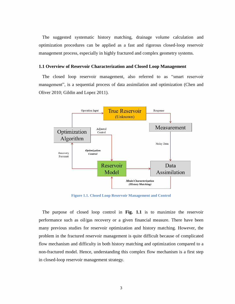
1.1 Overview of Reservoir Characterization and Closed Loop Management
The closed loop reservoir management, also referred to as “smart reservoir
management”, is a sequential process of data assimilation and optimization (Chen and
Oliver 2010; Gildin and Lopez 2011).
Figure 1.1. Closed Loop Reservoir Management and Control
The purpose of closed loop control in Fig. 1.1 is to maximize the reservoir
performance such as oil/gas recovery or a given financial measure. There have been
many previous studies for reservoir optimization and history matching. However, the
problem in the fractured reservoir management is quite difficult because of complicated
flow mechanism and difficulty in both history matching and optimization compared to a
non-fractured model. Hence, understanding this complex flow mechanism is a first step
in closed-loop reservoir management strategy.
4
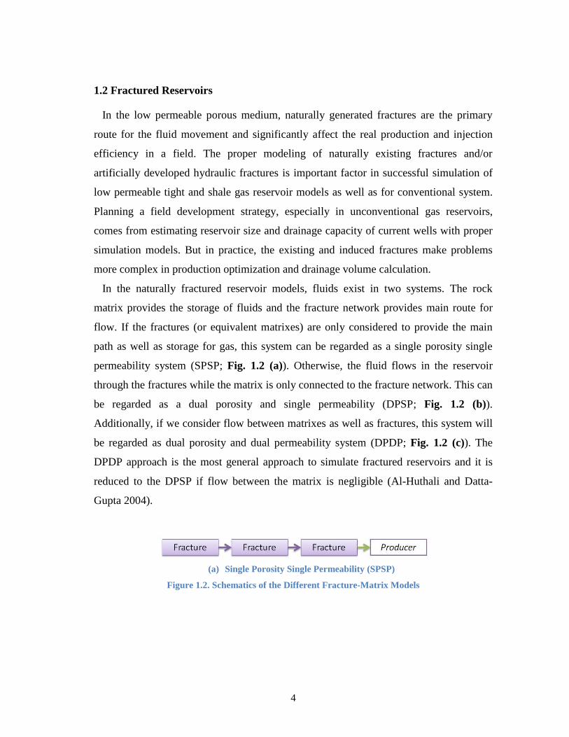
1.2 Fractured Reservoirs
In the low permeable porous medium, naturally generated fractures are the primary
route for the fluid movement and significantly affect the real production and injection
efficiency in a field. The proper modeling of naturally existing fractures and/or
artificially developed hydraulic fractures is important factor in successful simulation of
low permeable tight and shale gas reservoir models as well as for conventional system.
Planning a field development strategy, especially in unconventional gas reservoirs,
comes from estimating reservoir size and drainage capacity of current wells with proper
simulation models. But in practice, the existing and induced fractures make problems
more complex in production optimization and drainage volume calculation.
In the naturally fractured reservoir models, fluids exist in two systems. The rock
matrix provides the storage of fluids and the fracture network provides main route for
flow. If the fractures (or equivalent matrixes) are only considered to provide the main
path as well as storage for gas, this system can be regarded as a single porosity single
permeability system (SPSP; Fig. 1.2 (a)). Otherwise, the fluid flows in the reservoir
through the fractures while the matrix is only connected to the fracture network. This can
be regarded as a dual porosity and single permeability (DPSP; Fig. 1.2 (b)).
Additionally, if we consider flow between matrixes as well as fractures, this system will
be regarded as dual porosity and dual permeability system (DPDP; Fig. 1.2 (c)). The
DPDP approach is the most general approach to simulate fractured reservoirs and it is
reduced to the DPSP if flow between the matrix is negligible (Al-Huthali and Datta-
Gupta 2004).
(a) Single Porosity Single Permeability (SPSP)
Figure 1.2. Schematics of the Different Fracture-Matrix Models
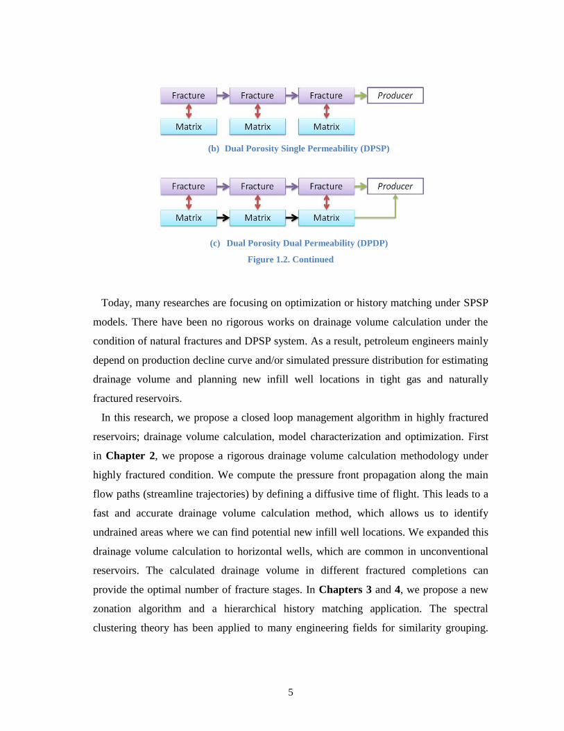
5
(b) Dual Porosity Single Permeability (DPSP)
(c) Dual Porosity Dual Permeability (DPDP)
Figure 1.2. Continued
Today, many researches are focusing on optimization or history matching under SPSP
models. There have been no rigorous works on drainage volume calculation under the
condition of natural fractures and DPSP system. As a result, petroleum engineers mainly
depend on production decline curve and/or simulated pressure distribution for estimating
drainage volume and planning new infill well locations in tight gas and naturally
fractured reservoirs.
In this research, we propose a closed loop management algorithm in highly fractured
reservoirs; drainage volume calculation, model characterization and optimization. First
in Chapter 2, we propose a rigorous drainage volume calculation methodology under
highly fractured condition. We compute the pressure front propagation along the main
flow paths (streamline trajectories) by defining a diffusive time of flight. This leads to a
fast and accurate drainage volume calculation method, which allows us to identify
undrained areas where we can find potential new infill well locations. We expanded this
drainage volume calculation to horizontal wells, which are common in unconventional
reservoirs. The calculated drainage volume in different fractured completions can
provide the optimal number of fracture stages. In Chapters 3 and 4, we propose a new
zonation algorithm and a hierarchical history matching application. The spectral
clustering theory has been applied to many engineering fields for similarity grouping.

6
The application to reservoir zonation provides promising cutting criteria for continuous
and/or fault-embedded simulation models. The systematic hierarchical approach
simplifies complex history matching problems and provides guidelines in fractured
reservoir model characterization.
7
CHAPTER II
DRAINAGE VOLUME CALCULATION, WELL PLACEMENT AND
HYDRAULIC FRACTURE STAGE OPTIMIZATION: STREAMLINE
APPLICATIONS TO UNCONVENTIONAL RESERVOIRS
2.1 Purpose
Current practice of well placement in tight gas reservoirs generally involves the use of
empirical correlations based on reservoir properties and analysis of past production
histories and/or pressure maps from flow simulation. No rigorous procedure is available
to compute well drainage volumes in the presence of permeability heterogeneity
controlled by the distribution and orientation of natural fractures. The situation is
complicated by the routine use of horizontal and complex wells in tight gas reservoirs
and the presence of multistage hydraulic fractures. The computation of drainage volume
will be critical to our understanding of the interaction between existing wells, potential
infill locations and the estimated ultimate recovery (EUR) computations for infill wells.
We propose a rigorous approach for well drainage volume calculations in tight gas
reservoirs based on the flux field derived from dual porosity finite-difference simulation
and demonstrate its application to optimize well placement. Our approach relies on a
high frequency asymptotic solution of the diffusivity equation and emulates the
propagation of a ‘pressure front’ in the reservoir along gas streamlines. The proposed
Part of this chapter is reprinted with permission from “Impact of Natural Fractures in Drainage Volume
Calculations and Optimal Well Placement in Tight Gas Reservoirs” by SukSang Kang, Akhil Datta-Gupta
and W. John Lee, 2011. Paper SPE 144338-MS presented at the 2011 SPE North American
Unconventional Gas Conference and Exhibition, The Woodlands, Texas, 14-16 June. Copyright 2011. by
the Society of Petroleum Engineers. Part of this chapter is reprinted with permission from “Optimizing Fracture Stages and Completions in
Horizontal Wells in Tight Gas Reservoirs Using Drainage Volume Calculations” by Baljit S Sehbi,
SukSang Kang, Akhil Datta-Gupta and W. John Lee, 2011. Paper SPE 144365-MS presented at the 2011
SPE North American Unconventional Gas Conference and Exhibition, The Woodlands, Texas, 14-16 June.
Copyright 2011. by the Society of Petroleum Engineers.

8
approach is a generalization of the radius of drainage concept in well test analysis (Lee
1982). The method allows us not only to compute rigorously the well drainage volumes
as a function of time but also examine the potential impact of infill wells on the drainage
volumes of existing producers. Using these results, we present a systematic approach to
optimize well placement to maximize the EUR.
We demonstrate the power and utility of our method using both synthetic and field
applications. The synthetic example is used to validate our approach by establishing
consistency between the drainage volume calculations from streamlines and the EUR
computations based on detailed finite-difference simulations. We also present
comparison of our approach with analytic drainage volume calculations for simplified
cases. The field example is from one of the tight gas fields in the Rocky Mountain
region. We utilize the streamline-based drainage volumes to identify depleted sands and
generate a reservoir ‘depletion capacity’ map to optimize infill well placement based on
the undepleted and undrained regions. The field application clearly demonstrates a
systematic approach to optimal well placement in tight gas reservoirs.
Horizontal well technology is now considered a standard completion practice in
unconventional gas reservoirs. With significant improvements in the drilling and
completion technology, many tight gas and shale gas prospects have become
economically viable. Optimizing location, distribution and the number of stages of
hydraulic fractures is an important issue in tight gas reservoir completions, particularly
for horizontal and complex wells.
A field example is shown to demonstrate the application of our approach by
optimizing well completions in a horizontal well recently drilled in the Cotton Valley
formation. We first apply the proposed drainage volume calculations in an existing
vertical well to identify its ‘region of influence’ and the potential interference from the
proposed horizontal well and the number of fracture stages in the horizontal well. The
combined drainage volumes from the vertical and horizontal well are calculated as a
function of the number of fracture stages to determine the point of diminishing return
and to optimize the number of fracture stages. The results are found to be consistent with
9
independent analysis based on rate profiles from numerical simulation and NPV
calculations.
2.2 Introduction
In low permeability gas reservoirs, natural fractures are often the primary conduit for
flow in the reservoir and can significantly impact the well performance and productivity
(Aguilera 2008). Proper modeling of the orientation, distribution and connectivity of the
natural fractures is critical to reservoir simulation and forecasting (Cipolla et al. 2009b;
Olson 2008). In particular, the understanding of the interaction between the induced
hydraulic fractures and the naturally existing fractures is an important key in the
successful development and exploitation of these reservoirs (Cipolla et al. 2011; Lee and
Hopkins 1994; Weng et al. 2011). Planning an effective field development strategy
requires estimating the drainage capacity of current wells and optimizing well placement
so as to minimize the overlapping of drainage volumes of existing wells. Production
decline curves have been widely used to compute drainage volumes and estimate EUR in
tight gas reservoirs (Blasingame and Rushing 2005; Cox et al. 2002; Fetkovich 1980;
Rushing et al. 2007). Also, pressure transient tests are commonly used in determining
the well productivity and the benefits of hydraulic fracturing in tight gas reservoirs (Lee
and Hopkins 1994). Whereas both decline curve analysis and pressure transient tests
have played a vital role in the exploitation of tight gas reservoirs, the interpretation of
such analytical tools can be considerably complicated in the presence of complex spatial
heterogeneity and natural fractures. In particular, the interactions between the hydraulic
fracture and natural fractures and their implications on the well drainage volumes cannot
be adequately accounted for by the existing analytic methods.
Our objective in this paper is to develop a systematic procedure for well placement
optimization in naturally fractured tight gas reservoirs. Towards this goal, we develop a
rigorous approach to defining well drainage volumes during numerical simulation of
naturally fractured tight gas reservoirs. Specifically, we will build on the concept of
radius of drainage as defined by (Lee 1982). Currently there is no well-defined method
10
for computing the well drainage volumes from numerical simulation in gas reservoirs. A
common practice is to use pressure contours to understand well drainage behavior with
time. The well drainage volume is defined by following the evolution of a pressure
contour level that is defined rather arbitrarily and Lee et al. (2003) define the radius of
drainage as the propagation distance of ‘maximum’ pressure disturbance resulting from
an impulse (instantaneous) source. More recently, this concept was used by Meyer et al.
(2010) to examine fracture interference in the presence of multiple hydraulic fractures in
horizontal wells. However, much of these previous developments have been limited to
homogeneous medium. We generalize the concept of drainage radius and drainage
volumes to arbitrary heterogeneous medium and completely general well conditions by
first computing the reservoir flux field from numerical simulation and then, examining
the propagation of the pressure disturbance along the gas streamlines.
Streamlines are trajectories or flow paths that are everywhere tangential to the local
flow velocity. In fact, streamlines are simply a representation of the instantaneous
velocity field. Streamlines exist whenever there is an underlying velocity field. These
include compressible and incompressible flows, steady and unsteady conditions, oil and
gas reservoirs (Datta-Gupta and King 2007). Although the visualization power of
streamlines have been widely used to examine the swept and drainage volumes in oil
reservoirs, the application of streamlines to compressible flow and particularly to gas
reservoirs has been very limited.
One of the primary challenges in the application of the streamlines to gas reservoirs is
the diffusive nature of the pressure equation. How can we define the concept of a
propagating ‘front’ when the underlying phenomenon is diffusive? Kulkarni et al. (2001)
generalized the streamline-based travel time approach to transient pressure conditions by
introducing a ‘diffusive time of flight’ and rigorously computed well drainage radius
during primary recovery and for heterogeneous permeability distributions. He et al.
(2002) showed a good agreement between streamline-derived drainage volume
calculations with decline type curve results. Kim et al. (2009) utilized the diffusive time
11
of flight to invert pressure response from interference test to characterize permeability
distribution. The power of the method was illustrated using a field application.
Britt and Smith (2009) examine horizontal well completion and stimulation
optimization for different reservoir conditions and geomechanic limitations along with
risk mitigation strategies for effective horizontal well planning. They present results of
design and optimization study followed by post appraisal study of the horizontal wells
drilled in Arkoma basin. Meyer et al. (2010) presented analytical solution for predicting
behavior of multiple transverse hydraulic fractures in a horizontal well and optimization
methodology to hydraulic fracture stages considering NPV and ROI (return on
investment). They also utilized the concept of radius of drainage (Lee 1982) to examine
the interference between multiple transverse fractures.
Our objective in this paper is to develop a procedure for computing well drainage
volumes in tight gas reservoirs. Because our approach relies on the streamlines derived
from a finite difference simulator, the method is completely general and can handle any
arbitrary heterogeneity and well conditions. The organization of the paper is as follows.
We first highlight the main features of our approach and illustrate the steps using a
synthetic example. We also validate our drainage volume calculations by comparing
with analytic solutions for homogeneous medium. Next, we discuss the mathematical
foundations behind the high frequency asymptotic solution of the diffusivity equation,
the propagation of a ‘pressure front’ in the reservoir and its relationship to the concept of
radius drainage as defined by Lee (1982). Finally, we demonstrate the power and utility
of our method using a field application.
2.3 Approach
Our goal here is to examine the evolution of drainage volume of wells in tight gas
reservoirs in the presence of natural fractures. This entails computation of well drainage
volumes in the presence of arbitrary heterogeneity, well pattern and also accounting for
well interactions. We build on the definition of radius of investigation Lee (1982) in
terms of the propagation of a pressure pulse corresponding to an impulse source/sink.
12
Specifically, we generalize the concept of a propagating pressure pulse along individual
streamlines in a gas reservoir. This allows us not only to compute and visualize the well
drainage volumes as a function of time but also provides a mechanism to quantitatively
examine the impact of well interactions on the drainage volumes and EUR. Below, we
briefly discuss the major steps in our approach followed by an illustration of the
procedure.
Fracture Generation Using a DFN Model: Proper characterization of fractures
is a key step in modeling naturally fractured reservoirs. A discrete fracture
network (DFN) model is used to represent the fracture distribution in the
reservoir. The purpose of fracture modeling is to create geological model
properties which can more closely mimic the flow behavior in the real reservoir.
We utilized tight and shale gas field data from previous studies (Bogatkov and
Babadagli 2008; Cipolla et al. 2009a; Gale and Holder 2008) to get a
representative set of fracture network model.
Dual Porosity Simulation Using Finite Difference Simulator: We have utilized
a commercial finite difference simulator (ECLIPSETM
) for modeling the gas
reservoir. A dual porosity model is used for the fluid movement along the
hydraulic and natural fractures while accounting for the matrix-fracture
interactions. All relevant physical mechanisms such as gas compressibility,
gravity effects and matrix-fracture interactions are fully accounted for in the
finite-difference simulation.
Tracing Streamline Trajectories: We utilize the flux from the finite difference
simulator to construct the streamlines in the fractures for the dual porosity model.
The fluxes can be analytically integrated on a cell-by-cell basis to trace the
streamline trajectories. The trajectory tracing is based on the method proposed by
Jimenez et al. (2008). It is computationally efficient and can be used for general
grid geometries including corner point cells. The streamlines are started at the
13
grid block centers and are traced backwards to the originating producers. Only
those grid blocks having a finite gas flux will have a streamline passing through
them. Because of high compressibility effects and the transient nature of the
flow, the streamlines are recomputed every time step based on the updated flux
field.
Computing Well Drainage Volume: The well drainage volume is a
generalization of the radius of drainage concept Lee (1982) and relies on
calculating the propagation of a pressure disturbance corresponding to an
impulse source/sink along the streamlines. Specifically, we utilize the concept of
a ‘diffusive time of flight’ based on a high frequency asymptotic solution of the
pressure equation (Datta-Gupta et al. 2001; Datta-Gupta et al. 2007; Vasco et al.
2000) as discussed later. It is shown that the pressure pulse propagates with a
velocity given by the square root of the diffusivity. We can now extend the
concept of radius of investigation to compute well drainage volumes under
completely general conditions.
Depletion Capacity Map: The well drainage volume calculations allow us to
examine the interference between existing wells and also to identify the
undrained regions for potential infill drilling. We define a ‘depletion capacity
map’ for optimal well placement based on a combination of the undrained
volumes and reservoir static and dynamic properties to maximize well
productivity.
Analysis for Various Well Completion Alternatives. A drainage volume analysis
was carried out in the Cotton Valley field example for different well completions
based on different hydraulic fracture stages being pumped in the well. The
economic analysis was performed on the projections of rate profiles from the
finite difference simulator and considering net gas and the lease operating
14
expenses. These results were compared to the drainage volumes estimated using
the proposed approach for consistency check.
2.4 Illustration of Procedure
The detailed mathematical formulation for the well drainage calculations will be
discussed in a later section. To start with, we illustrate our overall procedure using a
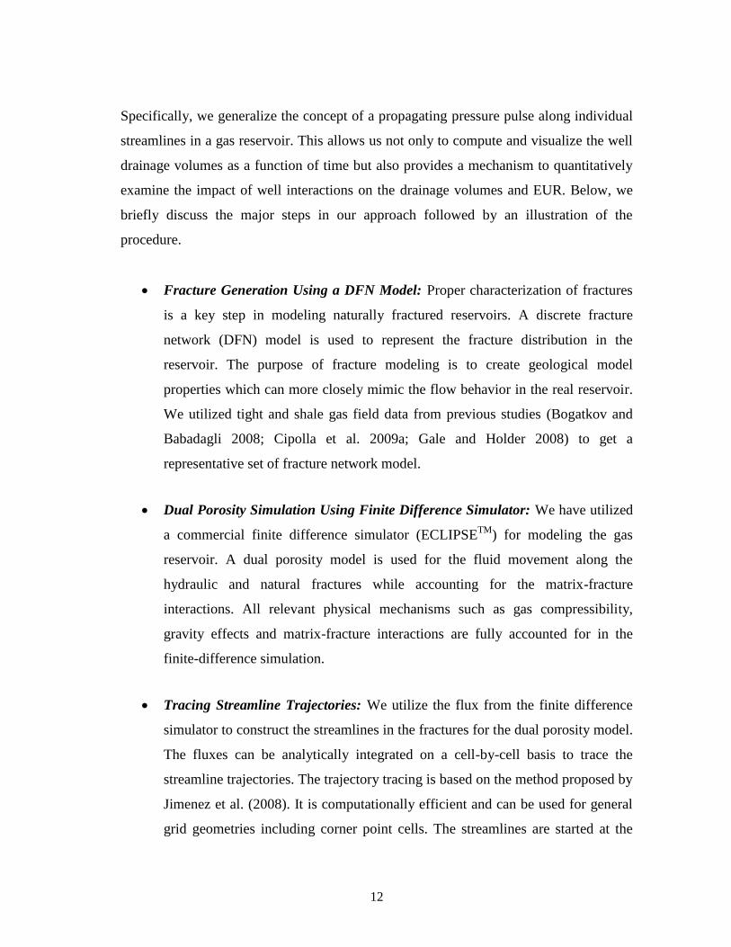
section model of a tight gas field. The 3-D reservoir model consists of water-gas phase
with 95×112×65 grid blocks. There are two producing wells, one near the center (well
147) and the other near the edge (well 148). The wells are separated by approximately
2,000 ft. The well 147 is first produced for 3 years; then well 148 starts producing. Fig.
2.1 shows the matrix permeability distribution including the well locations. The wells
are hydraulically fractured (xf : 650 ft) with a fracture conductivity of 40 md·ft.
Figure 2.1. Permeability of Tight Gas Section Model
One of our objectives here is to compute and visualize the impact of natural fractures
on the drainage volume calculations through dual-porosity simulation. For this, we
utilize a discrete fracture network (DFN) model to generate the permeability distribution
for the natural fractures. Hatzignatiou and McKoy (2000) demonstrated the use of
stochastic fracture network generation based on fracture connectivity in tight gas sands.
Olson and Taleghani (2009) suggested modeling parameters (apertures, fracture porosity
15
and effective permeability) ranges for fracture pattern generation in tight gas sands and
Gale and Holder (2008) provided an observed range of fracture properties from Barnett
Shale field. We utilize these previously suggested and observed ranges from field data
for fracture network generation. The generated aperture range is between 3×10⁻⁷
~ 3×10⁻³
(ft) with a stochastic distribution. The fracture permeability and conductivity are then
computed with cubic law from the aperture and permeability relationship (Bogatkov and
Babadagli 2008).
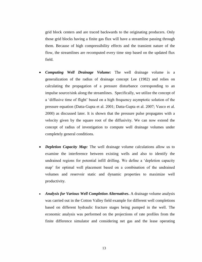
Figure 2.2. DFN Distribution with Fracture Clustering and Upscaled Permeabilities
Fig. 2.2 shows the DFN model with fracture clustering and the corresponding upscaled
fracture permeability for dual porosity flow simulation. A commercial geological
modeling package is used for this purpose (PetrelTM
). For this illustrative example, we
assume that the fracture clusters follow the trend of original matrix permeability to keep
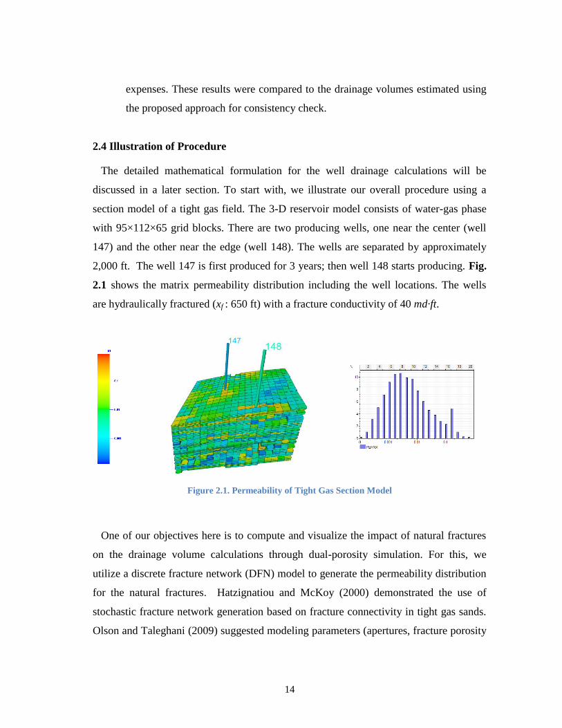
direction of heterogeneity of the original single porosity model. Fig. 2.3 shows the
distribution of porosity in the matrix and in the fracture with the fracture porosity being
much lower, as expected.
Figure 2.3. Matrix Porosity and Fracture Porosity Distribution
16
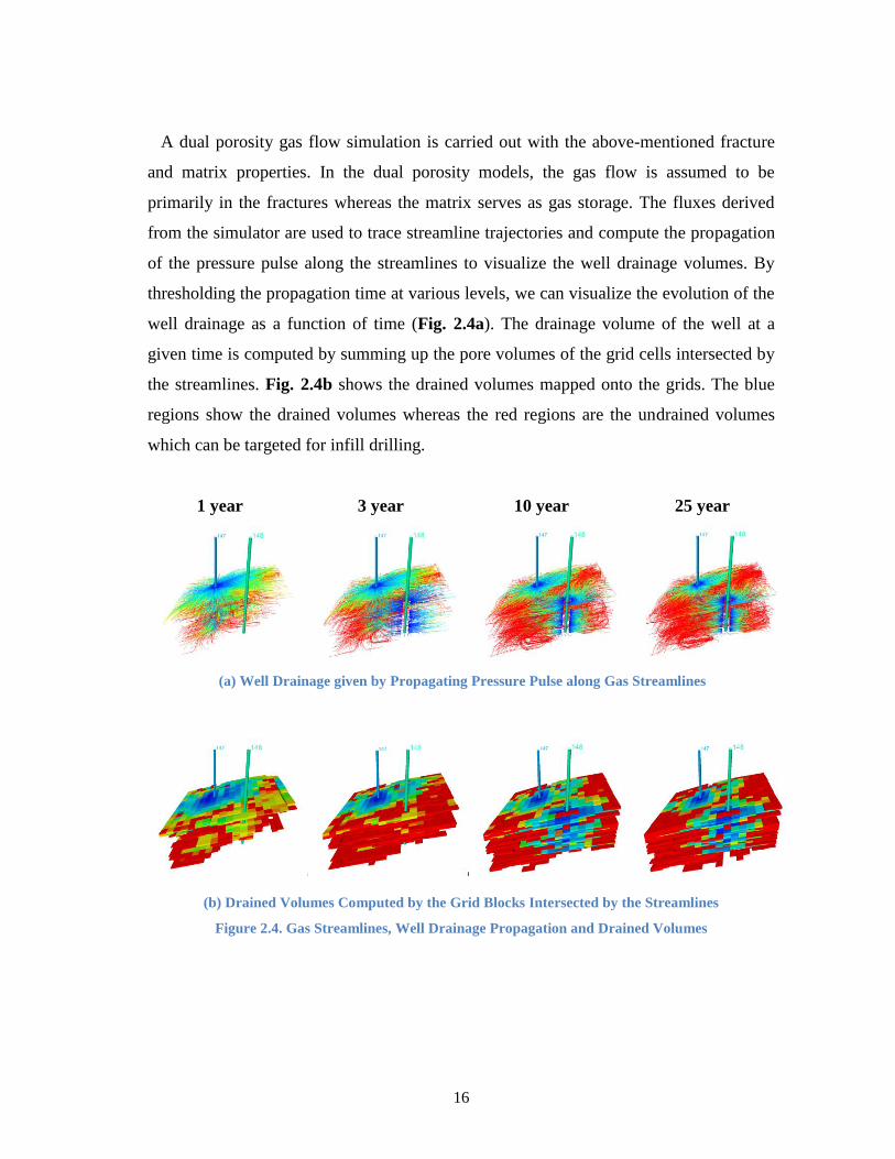
A dual porosity gas flow simulation is carried out with the above-mentioned fracture
and matrix properties. In the dual porosity models, the gas flow is assumed to be
primarily in the fractures whereas the matrix serves as gas storage. The fluxes derived
from the simulator are used to trace streamline trajectories and compute the propagation
of the pressure pulse along the streamlines to visualize the well drainage volumes. By
thresholding the propagation time at various levels, we can visualize the evolution of the
well drainage as a function of time (Fig. 2.4a). The drainage volume of the well at a
given time is computed by summing up the pore volumes of the grid cells intersected by
the streamlines. Fig. 2.4b shows the drained volumes mapped onto the grids. The blue
regions show the drained volumes whereas the red regions are the undrained volumes
which can be targeted for infill drilling.
1 year 3 year 10 year 25 year
(a) Well Drainage given by Propagating Pressure Pulse along Gas Streamlines
(b) Drained Volumes Computed by the Grid Blocks Intersected by the Streamlines
Figure 2.4. Gas Streamlines, Well Drainage Propagation and Drained Volumes

17
Fig. 2.5 shows the evolution of the drainage volumes of the two wells as a function of
time including the effects of the natural fractures (NF) as discussed above. In the same
plot we have shown the corresponding drainage volumes without the natural fractures,
that is hydraulic fracture only. The enhanced well drainage because of the interaction of
the natural fractures with the hydraulic fracture can be clearly seen in this figure. One of
the powerful features of our proposed method is that we can not only visualize the
evolution of the drainage volume with time but also quantitatively examine the
interaction of nearby wells on the drainage volume. This is also illustrated in Fig. 2.5(a).
Recall that the second well came into production after three years and the impact of the
second well on the drainage volume of the first well can be clearly seen here. In Fig.
2.5(b), we can see approximately 30% increment in the drainage volume for this
example because of the presence of the natural fractures.
Figure 2.5. (a) Effect of Natural Fractures on Drainage Volume for Individual Wells
and (b) on Total Drainage Volume
It is rather obvious that the impact of the natural fractures on the well drainage will
depend upon the specific distribution of the fractures and is likely to vary significantly
from case to case. To illustrate this, we generated a more dense fracture distribution as
shown in Fig. 2.6(a). The corresponding drainage volume evolution with time is shown
in Fig. 2.6(b). We can clearly see the acceleration effects on the drainage volume
because of the increased fracture permeability.
18
Figure 2.6. (a) High Fracture Density DFN (b) Effect of Fracture Density on the Drainage Volumes
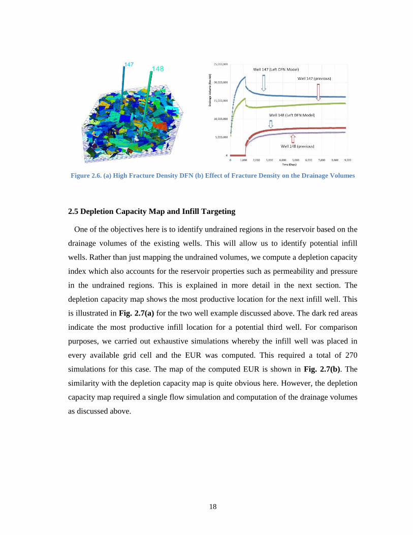
2.5 Depletion Capacity Map and Infill Targeting
One of the objectives here is to identify undrained regions in the reservoir based on the
drainage volumes of the existing wells. This will allow us to identify potential infill
wells. Rather than just mapping the undrained volumes, we compute a depletion capacity
index which also accounts for the reservoir properties such as permeability and pressure
in the undrained regions. This is explained in more detail in the next section. The
depletion capacity map shows the most productive location for the next infill well. This
is illustrated in Fig. 2.7(a) for the two well example discussed above. The dark red areas
indicate the most productive infill location for a potential third well. For comparison
purposes, we carried out exhaustive simulations whereby the infill well was placed in
every available grid cell and the EUR was computed. This required a total of 270
simulations for this case. The map of the computed EUR is shown in Fig. 2.7(b). The
similarity with the depletion capacity map is quite obvious here. However, the depletion
capacity map required a single flow simulation and computation of the drainage volumes
as discussed above.

19
Figure 2.7. (a) Depletion Capacity Map based on Undrained Volumes
(b) EUR Map from Exhaustive Simulations
2.6 Drainage Volume Calculations: Mathematical Formulation
In this section we describe the mathematical foundations for the generalization of the
radius of drainage concept (Lee 1982) using a high frequency asymptotic solution of the
diffusivity equation. For clarity of exposition, we describe our formulation in terms of
pressure although the same development can be made for gas reservoirs in terms of real
gas pseudo pressure (Al-Hussainy et al. 1966).
The transient pressure response from a heterogeneous permeable medium can be
described by the diffusivity equation
0,,
tPk
t
tPct xx
xx (2.1)
Using Fourier transform of Eq. 2.1, we obtain the following equation in the frequency
domain.
,~
,~
,~ 22
xx
xxx
x
xP
k
kPPi
k
ct
(2.2)
20
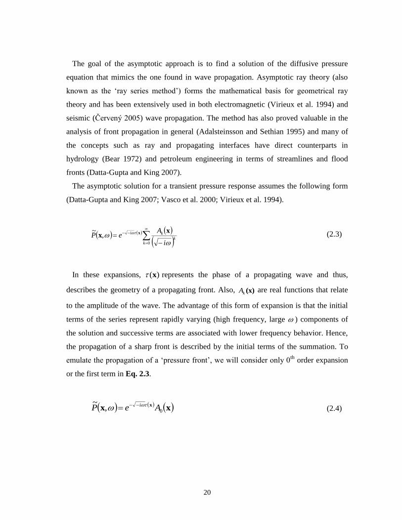
The goal of the asymptotic approach is to find a solution of the diffusive pressure
equation that mimics the one found in wave propagation. Asymptotic ray theory (also
known as the ‘ray series method’) forms the mathematical basis for geometrical ray
theory and has been extensively used in both electromagnetic (Virieux et al. 1994) and
seismic (Červený 2005) wave propagation. The method has also proved valuable in the
analysis of front propagation in general (Adalsteinsson and Sethian 1995) and many of
the concepts such as ray and propagating interfaces have direct counterparts in
hydrology (Bear 1972) and petroleum engineering in terms of streamlines and flood
fronts (Datta-Gupta and King 2007).
The asymptotic solution for a transient pressure response assumes the following form
(Datta-Gupta and King 2007; Vasco et al. 2000; Virieux et al. 1994).
0
,~
kk
ki
i
AeP
x
xx (2.3)
In these expansions, )(x represents the phase of a propagating wave and thus,
describes the geometry of a propagating front. Also, (x)kA are real functions that relate
to the amplitude of the wave. The advantage of this form of expansion is that the initial
terms of the series represent rapidly varying (high frequency, large ) components of
the solution and successive terms are associated with lower frequency behavior. Hence,
the propagation of a sharp front is described by the initial terms of the summation. To
emulate the propagation of a ‘pressure front’, we will consider only 0th
order expansion
or the first term in Eq. 2.3.
xxx
0,~
AeP i (2.4)
21
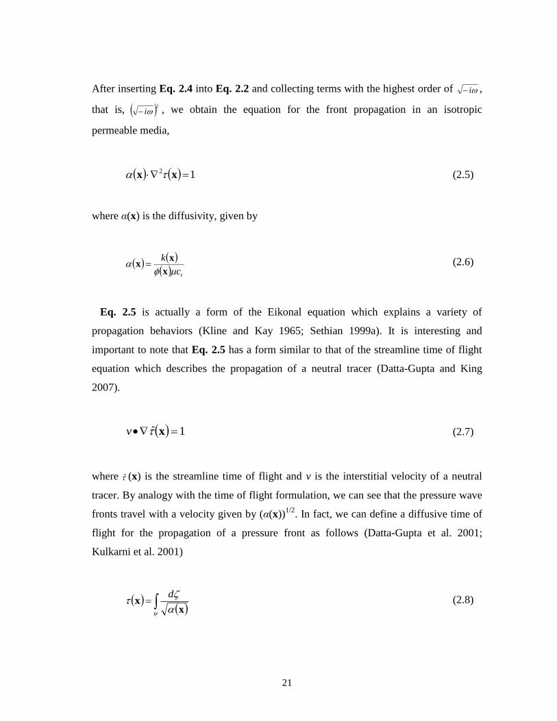
After inserting Eq. 2.4 into Eq. 2.2 and collecting terms with the highest order of i ,
that is, 2i , we obtain the equation for the front propagation in an isotropic
permeable media,
12 xx (2.5)
where α(x) is the diffusivity, given by
tc
k
x
xx (2.6)
Eq. 2.5 is actually a form of the Eikonal equation which explains a variety of
propagation behaviors (Kline and Kay 1965; Sethian 1999a). It is interesting and
important to note that Eq. 2.5 has a form similar to that of the streamline time of flight
equation which describes the propagation of a neutral tracer (Datta-Gupta and King
2007).
1ˆ xv (2.7)
where ̂ (x) is the streamline time of flight and v is the interstitial velocity of a neutral
tracer. By analogy with the time of flight formulation, we can see that the pressure wave
fronts travel with a velocity given by (α(x))1/2
. In fact, we can define a diffusive time of
flight for the propagation of a pressure front as follows (Datta-Gupta et al. 2001;
Kulkarni et al. 2001)
xx
d (2.8)
22
Note that the unit of diffusive time of flight in Eq. 2.8 is the square root of time which
is consistent with the scaling behavior of diffusive flow. However, the diffusive time of
flight is defined along the trajectories of a ‘pressure wave front’ ψ, which are given by
the ray paths of the wave equation. These trajectories are not necessarily in the
streamlines (Vasco and Finsterle 2004). Kim et al. (2009) has shown that for many
practical applications, the pressure trajectories can be approximated by the streamlines.
2.6.1 The Pressure Wave Front
Lee (1982) defines the radius of investigation at any given time as the propagation
distance of the ‘maximum’ pressure disturbance corresponding to an impulse
(instantaneous) source. In this section, we examine the physical significance of a
‘pressure front’ or a ‘diffusive’ time of flight and demonstrate its close correspondence
to the concept of the radius of investigation. The time domain solution to the 0th
order
asymptotic expansion for an impulse source is given by the inverse Fourier transform of
Eq. 2.4. For a 2-D medium, we obtain the following
ttAtP
4exp
2
2
0
xxx
(2.9)
The above equation corresponds to the propagation of a pressure response for an
impulse source in a 2-D medium. The pressure response at a fixed position, x, will be
maximized when the time derivative of Eq. 2.9 vanishes.
0
4exp
44exp
2
2
3
222
0
ttttA
t
tP xxxxx
(2.10)
This results in the following relationship between the observed time and the ‘diffusive’
time of flight for a two-dimensional medium.
23
4
2
max
xt (2.11)
Physically, the ‘diffusive’ time of flight is associated with the propagation of a front of
maximum drawdown or build up for an impulse source or sink. This concept is closely
related to the idea of a drainage radius (Lee 1982). In fact, it is interesting to note that for
a homogeneous medium with radially symmetric streamlines, Eq. 2.11 reduces to the
following.
4
2
max
rt (2.12)
where, r is the distance travelled by the pressure disturbance along streamlines and is
the diffusivity. Eq. 2.12 is exactly the same expression for the propagation time given by
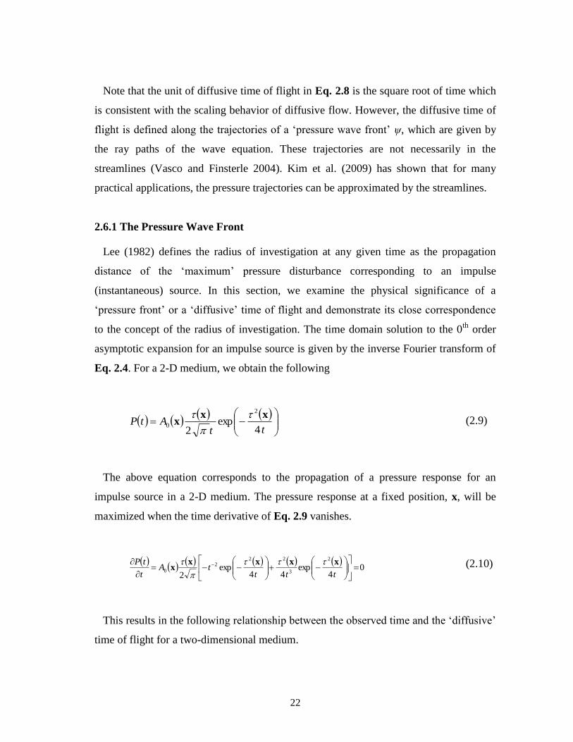
Lee (1982). To illustrate this correspondence further, we have shown in Fig. 2.8(a) the
radius of drainage at three different times computed based on the diffusive time of flight
for a single producing well in a 2-D homogeneous medium. To accomplish this, we first
trace the streamlines and compute the diffusive time of flight along the streamlines as
given by Eq. 2.8. The diffusive time of flight is then converted to physical propagation
time of the pressure pulse time using Eq. 2.11. The evolution of the drainage volume is
given by contouring the propagation time. For comparison purposes, we have also
shown in Fig. 2.8(b) the radius of drainage based on the expression given by Lee (1982).
The close correspondence between these is quite apparent from these figures.
24
(a) Drainage Radius from the Diffusive Time of Flight
Figure 2.8. Comparison between Diffusive Time of Flight Radius and Analytical Solution
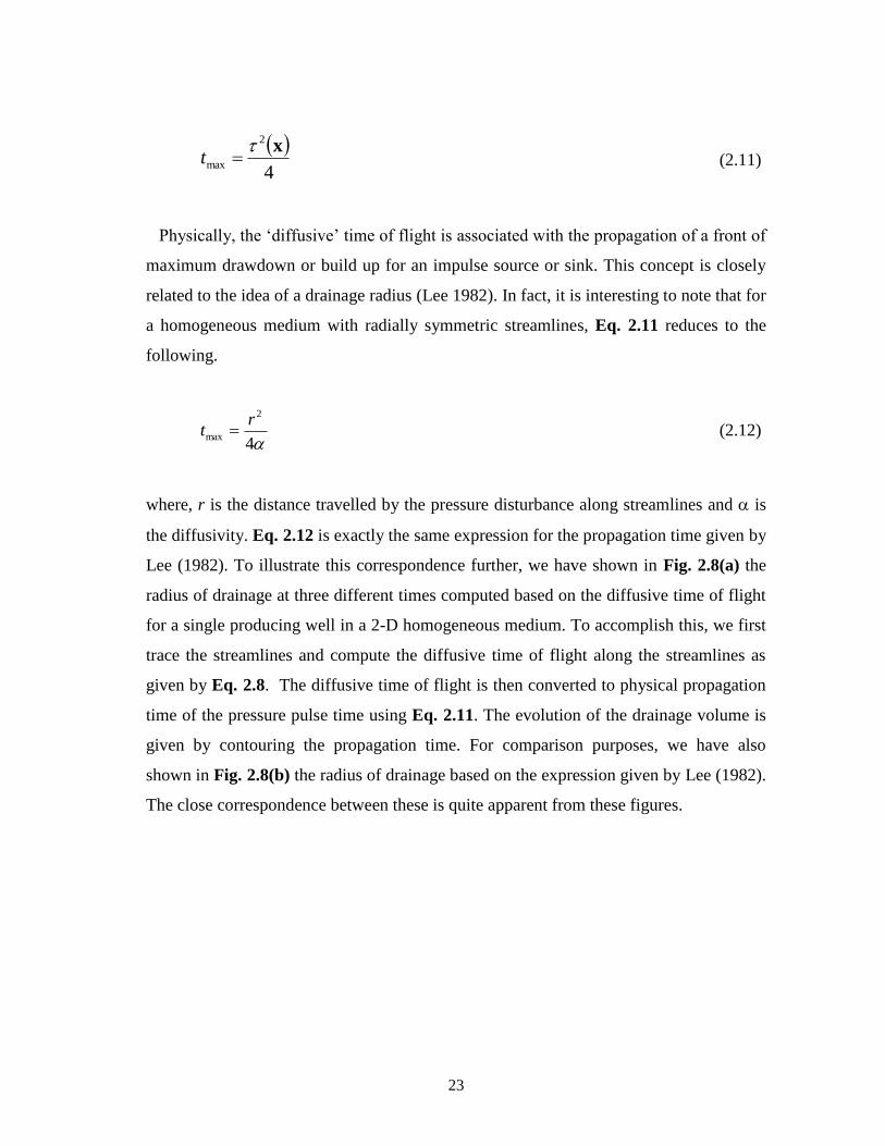
One of the major advantages of the asymptotic approach is that we can now extend the
concept of radius of investigation to any arbitrary heterogeneous medium. This is
illustrated in Fig. 2.9 It is interesting to note that although the streamlines are
recomputed based on updated flux, the streamline geometry remains remarkably similar
other than their evolution with time. The well drainage volume is computed by adding
up the volumes of the grid cells intersected by the streamlines at a given time.
0.01 day 0.05 day 0.1 day
(b) Drainage Radius Computed from Lee (1982)
-600
-400
-200
0
200
400
600
-600 -400 -200 0 200 400 600
-600
-400
-200
0
200
400
600
-600 -400 -200 0 200 400 600
-600
-400
-200
0
200
400
600
-600 -400 -200 0 200 400 600

25
Permeability Field 0.01 day 0.05 day 0.1 day
Figure 2.9. Radius of Investigation and Drainage Volume Calculations in a Heterogeneous Field.
Finally, it is worth pointing out that for a 3D medium, the time domain solution for an
impulse source will be given by the following (Kulkarni et al. 2001).
t
x
t
xxAtP
4exp
2
2
30
(2.13)
The propagation time for the pressure ‘front’ will now be related to the diffusive time
of flight through the following expression.
6
2
max
xt (2.14)
26
2.6.2 Depletion Capacity Map
One of our objectives in this paper is to optimize infill locations based on the
undrained reservoir volumes. After computing the drainage volumes associated with
existing wells, we can identify undrained region where the ‘pressure front’ has not
reached. This can be seen in Fig. 2.9 for the illustrative example with a single well in a
heterogeneous permeability field. For infill locations, instead of relying solely on the
undrained volumes, we define a ‘depletion capacity’ that includes permeability, pore
volume and reservoir ‘energy’ as indicated by the level of pressure drop at any given
time. We create a 2-D map of ‘depletion capacity’ by a vertical sum for the undrained
cells as given by the equation below:
k
kavgijporoijijij ppVkDC )(, (2.15)
The 2-D areal map of the depletion capacity can now be used as a guide to locate
potential infill locations. In the synthetic example discussed before, we have already
demonstrated the close correspondence of this depletion capacity map with exhaustive
flow simulations.
2.7 Field Application of Optimal Well Placement
In this section, we illustrate the application of our approach with a tight gas field
located at the Rocky mountain region. The section of the field under consideration has
more than 25 years of producing history and 85 production wells. The matrix
permeability is shown in Fig. 2.10(a). Because one of our objectives is to examine the
role of natural fractures, a discrete fracture network is generated along the high matrix
permeability regions. Fig. 2.10(b) also shows the generated DFN and upscale
permeability.
27
(a) Matrix Permeability Distribution
(b) Generated DFN and Upscaled Permeability Field
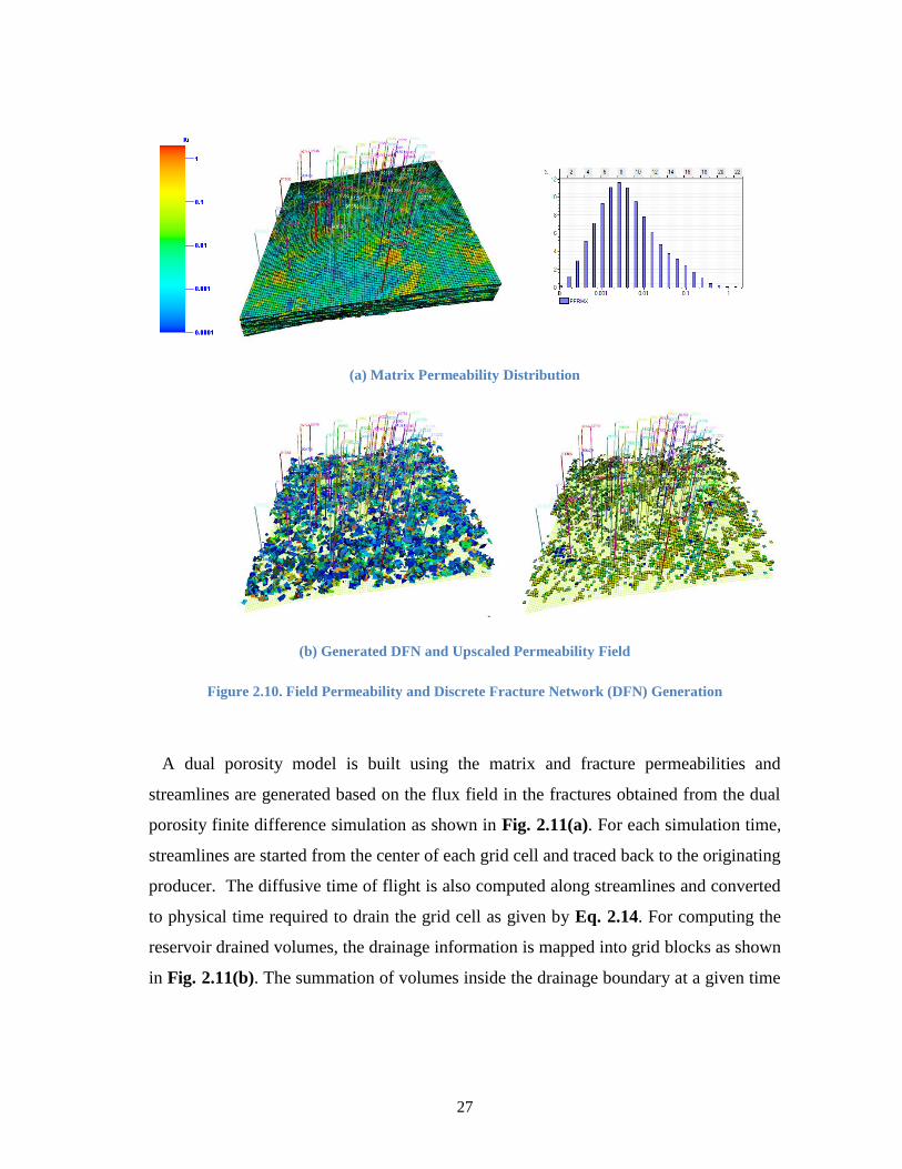
Figure 2.10. Field Permeability and Discrete Fracture Network (DFN) Generation
A dual porosity model is built using the matrix and fracture permeabilities and
streamlines are generated based on the flux field in the fractures obtained from the dual
porosity finite difference simulation as shown in Fig. 2.11(a). For each simulation time,
streamlines are started from the center of each grid cell and traced back to the originating
producer. The diffusive time of flight is also computed along streamlines and converted
to physical time required to drain the grid cell as given by Eq. 2.14. For computing the
reservoir drained volumes, the drainage information is mapped into grid blocks as shown
in Fig. 2.11(b). The summation of volumes inside the drainage boundary at a given time
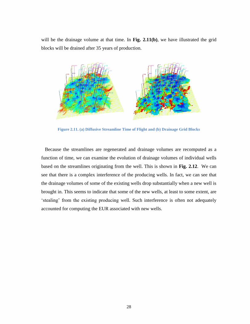
28
will be the drainage volume at that time. In Fig. 2.11(b), we have illustrated the grid
blocks will be drained after 35 years of production.
Figure 2.11. (a) Diffusive Streamline Time of Flight and (b) Drainage Grid Blocks
Because the streamlines are regenerated and drainage volumes are recomputed as a
function of time, we can examine the evolution of drainage volumes of individual wells
based on the streamlines originating from the well. This is shown in Fig. 2.12. We can
see that there is a complex interference of the producing wells. In fact, we can see that
the drainage volumes of some of the existing wells drop substantially when a new well is
brought in. This seems to indicate that some of the new wells, at least to some extent, are
‘stealing’ from the existing producing well. Such interference is often not adequately
accounted for computing the EUR associated with new wells.
29
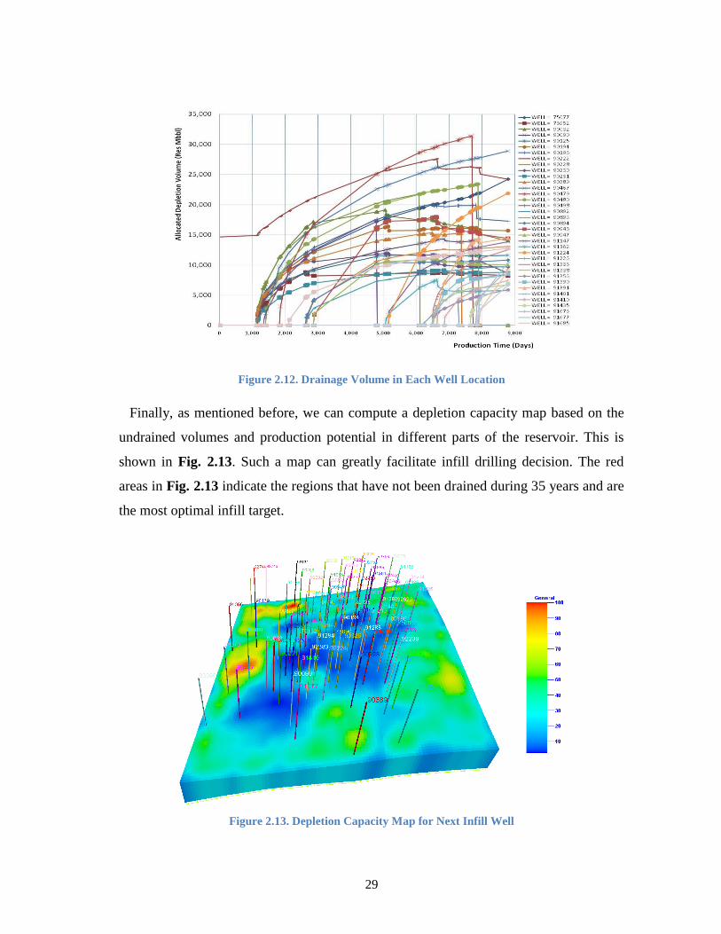
Figure 2.12. Drainage Volume in Each Well Location
Finally, as mentioned before, we can compute a depletion capacity map based on the
undrained volumes and production potential in different parts of the reservoir. This is
shown in Fig. 2.13. Such a map can greatly facilitate infill drilling decision. The red
areas in Fig. 2.13 indicate the regions that have not been drained during 35 years and are
the most optimal infill target.
Figure 2.13. Depletion Capacity Map for Next Infill Well

30
2.8 Field Application of Optimal Hydraulic Fracture Stages
In this section, we discuss the field application of the concept of the drainage volumes
to a tight gas reservoir in the Cotton Valley Formation. Specifically, we utilize the well
drainage volumes to optimize the number of hydraulic fracture stages. We also show that
the results of the drainage volume calculations to optimize the completion strategy are
similar to the conclusions arrived from calculations based on the production forecast
from finite difference simulator. The main advantage of the drainage volume approach is
that it allows to visualize evolution of the well drainage with time and also to examine
the interference between fracture stages. All these can facilitate well completion
optimization and also well placement optimization based on undrained volumes in the
reservoir (Kang et al. 2011).
The Cotton Valley group represents the first major influx of Clastic sediments into the
ancestral Gulf of Mexico (Dyman and Condon 2006). Reservoir properties and
production characteristics identified two Cotton Valley Group sandstone trends across
northern Louisiana and East Texas: a high permeability blanket sandstone trend and a
down-dip low permeability massive sandstone trend. The study well is located in low
permeability sandstone trend in Louisiana.
Figure 2.14. Schematic of the Two Phase Model for History Matching
An existing vertical well in the field had about two years of production history. This
well was history matched by building a 3D two phase reservoir model. The schematic of

31
the model is as shown in Fig. 2.14. After three years of production of the vertical well, a
horizontal well was planned. The purpose of this study is to optimize the completion
strategy of the planned horizontal well while taking into account any potential
interaction with the existing vertical well.
Layer 1 in the model in Fig. 2.14 shown above is 200 ft thick with 7.6% porosity and
45% water saturation. The second layer is 40 ft thick with 11% porosity and 98% water
saturation. The model was constrained to actual gas production. History matching was
performed to match the model BHP and water production to the observed data in Fig.
2.15.
(a) Gas Production HM (V1) (b) Water production HM (V1)
Figure 2.15. Production Rate History Matching Results
As the produced water is a combination of the formation water and fracture fluid,
Water Gas Ratio (WGR) was used as a matching parameter instead of cumulative water.
The well was treated with 685 of fluid and 1 of 20/40 white sand with
tail-in of resin coated sand. The 1-ft wide hydraulic fracture was incorporated in the
model (using local grid refinement) with an equivalent fracture conductivity of 0.1 inch
wide hydraulic fracture created in the field conditions. The existing vertical well had an
initial production of about 1.6 with a well head pressure of about 1,500 .
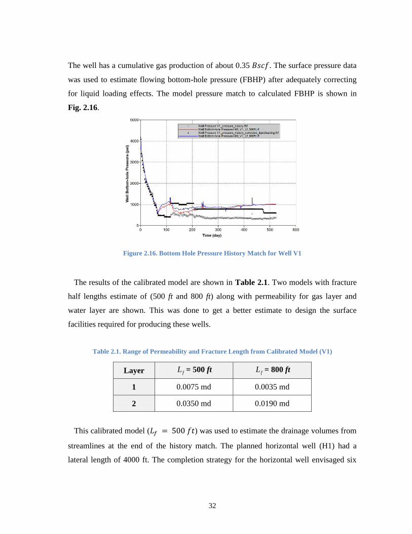
32
The well has a cumulative gas production of about 0.35 . The surface pressure data
was used to estimate flowing bottom-hole pressure (FBHP) after adequately correcting
for liquid loading effects. The model pressure match to calculated FBHP is shown in
Fig. 2.16.
Figure 2.16. Bottom Hole Pressure History Match for Well V1
The results of the calibrated model are shown in Table 2.1. Two models with fracture
half lengths estimate of (500 ft and 800 ft) along with permeability for gas layer and
water layer are shown. This was done to get a better estimate to design the surface
facilities required for producing these wells.
Table 2.1. Range of Permeability and Fracture Length from Calibrated Model (V1)
Layer fL = 500 ft fL = 800 ft
1 0.0075 md 0.0035 md
2 0.0350 md 0.0190 md
This calibrated model ( ) was used to estimate the drainage volumes from
streamlines at the end of the history match. The planned horizontal well (H1) had a
lateral length of 4000 ft. The completion strategy for the horizontal well envisaged six
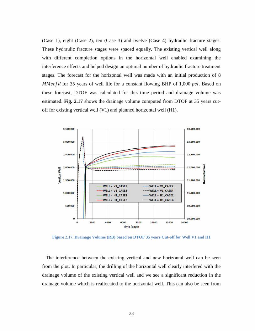
33
(Case 1), eight (Case 2), ten (Case 3) and twelve (Case 4) hydraulic fracture stages.
These hydraulic fracture stages were spaced equally. The existing vertical well along
with different completion options in the horizontal well enabled examining the
interference effects and helped design an optimal number of hydraulic fracture treatment
stages. The forecast for the horizontal well was made with an initial production of 8
for 35 years of well life for a constant flowing BHP of 1,000 . Based on
these forecast, DTOF was calculated for this time period and drainage volume was
estimated. Fig. 2.17 shows the drainage volume computed from DTOF at 35 years cut-
off for existing vertical well (V1) and planned horizontal well (H1).
Figure 2.17. Drainage Volume (RB) based on DTOF 35 years Cut-off for Well V1 and H1
The interference between the existing vertical and new horizontal well can be seen
from the plot. In particular, the drilling of the horizontal well clearly interfered with the
drainage volume of the existing vertical well and we see a significant reduction in the
drainage volume which is reallocated to the horizontal well. This can also be seen from
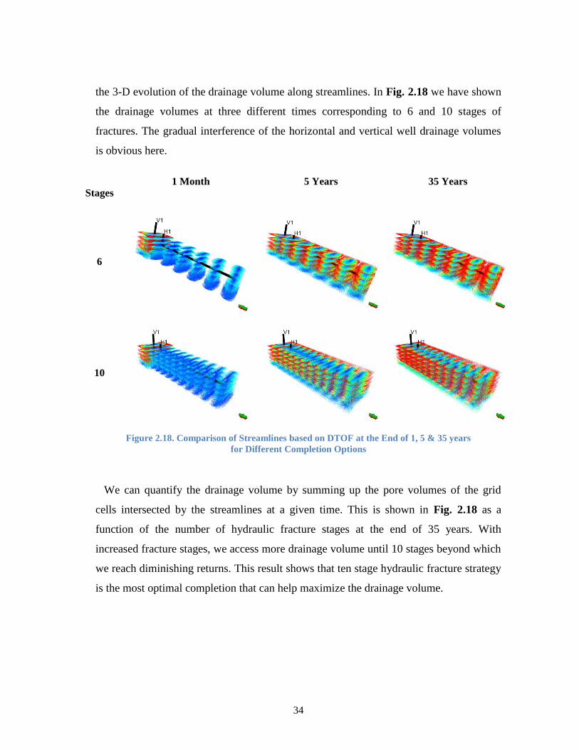
34
the 3-D evolution of the drainage volume along streamlines. In Fig. 2.18 we have shown
the drainage volumes at three different times corresponding to 6 and 10 stages of
fractures. The gradual interference of the horizontal and vertical well drainage volumes
is obvious here.
Stages 1 Month 5 Years 35 Years
6
10
Figure 2.18. Comparison of Streamlines based on DTOF at the End of 1, 5 & 35 years
for Different Completion Options
We can quantify the drainage volume by summing up the pore volumes of the grid
cells intersected by the streamlines at a given time. This is shown in Fig. 2.18 as a
function of the number of hydraulic fracture stages at the end of 35 years. With
increased fracture stages, we access more drainage volume until 10 stages beyond which
we reach diminishing returns. This result shows that ten stage hydraulic fracture strategy
is the most optimal completion that can help maximize the drainage volume.
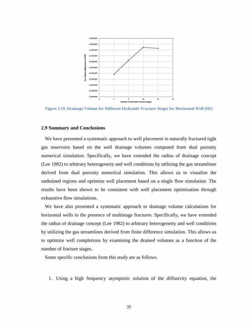
35
Figure 2.19. Drainage Volume for Different Hydraulic Fracture Stages for Horizontal Well (H1)
2.9 Summary and Conclusions
We have presented a systematic approach to well placement in naturally fractured tight
gas reservoirs based on the well drainage volumes computed from dual porosity
numerical simulation. Specifically, we have extended the radius of drainage concept
(Lee 1982) to arbitrary heterogeneity and well conditions by utilizing the gas streamlines
derived from dual porosity numerical simulation. This allows us to visualize the
undrained regions and optimize well placement based on a single flow simulation. The
results have been shown to be consistent with well placement optimization through
exhaustive flow simulations.
We have also presented a systematic approach to drainage volume calculations for
horizontal wells in the presence of multistage fractures. Specifically, we have extended
the radius of drainage concept (Lee 1982) to arbitrary heterogeneity and well conditions
by utilizing the gas streamlines derived from finite difference simulation. This allows us
to optimize well completions by examining the drained volumes as a function of the
number of fracture stages.
Some specific conclusions from this study are as follows.
1. Using a high frequency asymptotic solution of the diffusivity equation, the

36
concept of radius of drainage (Lee 1982) has been generalized to arbitrary
heterogeneous medium and general flow conditions by examining the
propagation of a ‘pressure front’ corresponding to an impulse (instantaneous)
source along gas streamlines. The gas streamlines can be traced from the flux
field of a finite-difference flow simulation.
2. Visualizing the well drainage is a physical and intuitive way of examining the
influence of existing wells and their mutual interference. By summing up the grid
cells intersected by the streamlines originating from a given well, we can
quantitatively estimate the well drainage volume, its evolution with time and
potential interference from wells in the vicinity.
3. We have used a discrete fracture network model to examine the role of natural
fractures in the well drainage volumes. As expected, the results show that the
presence of natural fractures tends to enhance the well drainage volumes and
accelerate production depending upon the distribution and orientation of
fractures.
4. Based on the undrained reservoir volumes and reservoir static and dynamic
properties, we have defined a ‘depletion capacity’ map for rapid identification
and optimization of infill locations in tight gas reservoirs. The power and utility
of the method has been demonstrated using both synthetic and field applications.
5. We have demonstrated the use of drainage volume concept in optimizing number
of fracture stages in the Cotton Valley formation. The incremental drainage
volumes with the number of fracture stages indicate that eight to ten hydraulic
fracture stages indicate the most optimal completion strategy for the horizontal
well studied from the field example.
37
CHAPTER III
A MODEL SEGMENTATION FROM SPECTRAL CLUSTERING: NEW
ZONATION ALGORITHM AND APPLICATION TO RESERVOIR HISTORY
MATCHING
3.1 Purpose
Proper characterization of reservoir is an important step for optimization and field
management. A purpose of this research is proposing a novel zonation criterion in the
history matching stage. Typically we apply a multiplier in the large scale field model and
it has been subjective to choose the parameter multiplicative region. Many industry
practices have applied a box multiplier near the well region or on the geological key
features; fault or flow barrier. Many cases applied a single multiplier over whole
reservoir field. This box multiplier approach might improve matching simulation to
observation, but it violates prior model’s important features and disengaged geologic
continuity between different region boundaries. That has been a key issue in history
matching process for geologists and reservoir engineers. It is also clear that this broken
links, between the prior and update model’s static key features, will decrease forecasting
and optimization reliability.
Our goal in the paper is minimizing static feature’s loss by proposing reasonable
zonation criteria. In other words, by using proposed zonation, we will be able to keep
main features of the prior model. At the same time, we can ensure improved history
matching quality after history matching step.
Zonation is a technique that partitions the reservoir region based on certain criteria. In
that sense, graphic partitioning provide a good decision gauge to segment regions while
keeping prior model’s main heterogeneous and/or connectivity features; such as high or
low permeable channel and barrier. For this purpose, we introduce graphical partitioning
for reservoir segmentation based on grid properties and/or connectivity. The
heterogeneity and connectivity are closely related to flow dynamics of a reservoir.
38
For history matching, we integrate genetic algorithm (GA) for calibrating reservoir
models. We demonstrated the strength and applicability of proposed zonation in
reservoir history matching problem, with both synthetic example and the Brugge field
example. This zonation approach from spectral clustering theory can enhance speed up
of global scale model calibration, which is common in hierarchal history matching
approach and in industry practice. At the same time, we can keep prior model’s main
information. Another advantage of spectral clustering is its adaptability to every grid
properties, even dynamic data at certain time.
The proposed spectral clustering has a clear edge detection power in smoothly varying
high and low valued regions. Hence, the proposed approach will provide potential
zonation criteria for reservoir history matching problems.
3.2 Introduction
The clustering or grouping algorithm is defined as “minimize the similarity between
groups and maximize the similarity within a group”. A graph partitioning from spectral
theory provides a fast way to decompose a domain for local grouping. As a matter of
fact, the spectral clustering has been used in various engineering fields; supercomputing,
machine learning, logistics, internet shopping, social network service and more. Because
of that, spectral clustering algorithm has profound theoretical background and is
comparatively easy to implement in new area.
The spectral clustering is an algorithm that partitions an affinity matrix with
eigenvectors of a graph. Pothen et al. (1990) showed that the ‘second’ smallest
eigenvalue will be positive if the graph G is connected. The corresponding second
eigenvector relates to the vertex and edge connectivity of a graph. Hagen and Kahng
(1992) applied the ratio cut partitioning and clustering for VLSI circuit design. They
adopted the spectral ‘ratio cut’ clustering to minimize the number of inter block signals.
Shi and Malik (2000) proposed a new clustering algorithm, ‘normalized cut’ and
compared with ‘ratio cut’ using some sample images. They examined the relationship
with ‘normalized cut’ and other eigenvector based partitioning algorithm. The
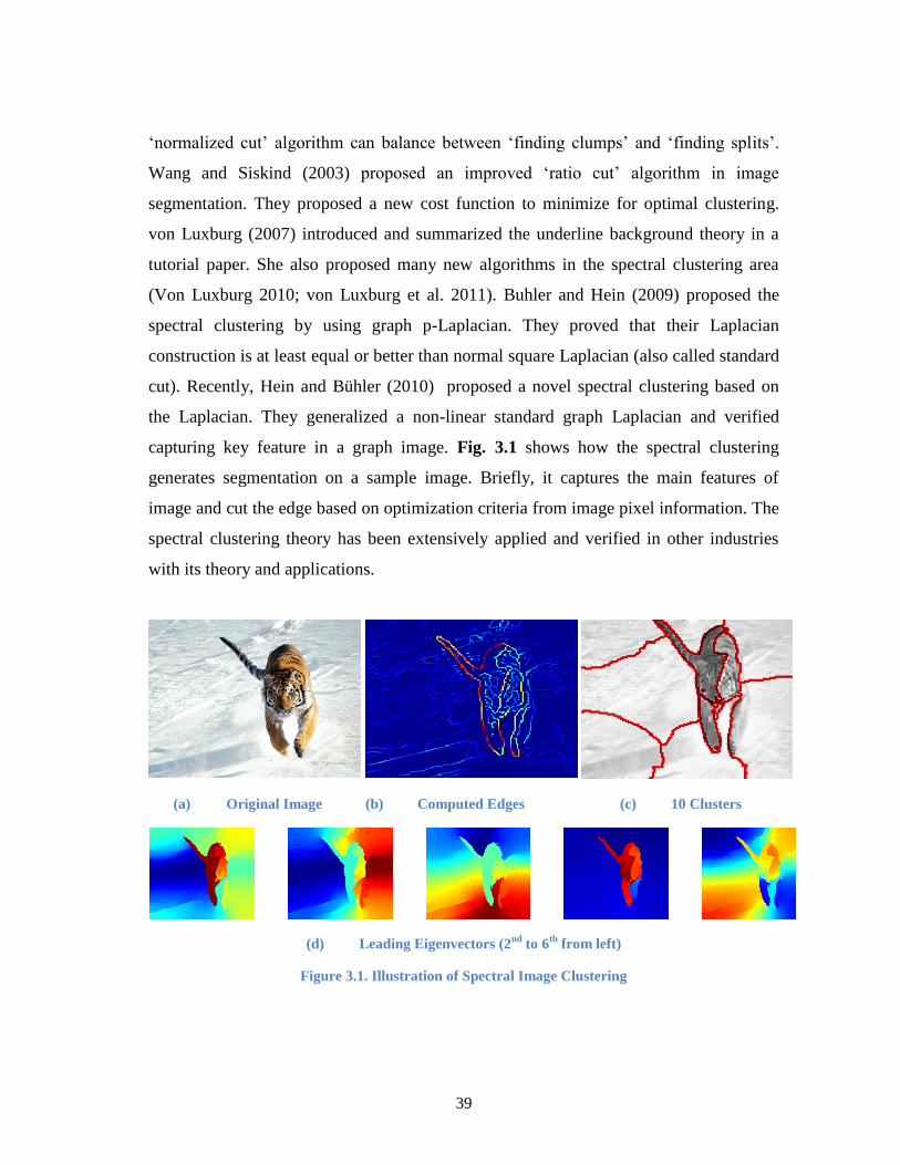
39
‘normalized cut’ algorithm can balance between ‘finding clumps’ and ‘finding splits’.
Wang and Siskind (2003) proposed an improved ‘ratio cut’ algorithm in image
segmentation. They proposed a new cost function to minimize for optimal clustering.
von Luxburg (2007) introduced and summarized the underline background theory in a
tutorial paper. She also proposed many new algorithms in the spectral clustering area
(Von Luxburg 2010; von Luxburg et al. 2011). Buhler and Hein (2009) proposed the
spectral clustering by using graph p-Laplacian. They proved that their Laplacian
construction is at least equal or better than normal square Laplacian (also called standard
cut). Recently, Hein and Bühler (2010) proposed a novel spectral clustering based on
the Laplacian. They generalized a non-linear standard graph Laplacian and verified
capturing key feature in a graph image. Fig. 3.1 shows how the spectral clustering
generates segmentation on a sample image. Briefly, it captures the main features of
image and cut the edge based on optimization criteria from image pixel information. The
spectral clustering theory has been extensively applied and verified in other industries
with its theory and applications.
(a) Original Image (b) Computed Edges (c) 10 Clusters
(d) Leading Eigenvectors (2nd
to 6th
from left)
Figure 3.1. Illustration of Spectral Image Clustering
40
In the reservoir history matching field, various zonation algorithms have been
proposed for partitioning reservoir models. Huang et al. (2001) proposed cluster analysis
for constructing fluid flow zones from seismic attributes. They used the spatially dense
set of geophysical attributes to create spatial zones. Agunwoke et al. (2004) suggested
the reservoir flow zonation based on similar geologic, physical property from well
logging data. They applied a statistical approach based on geologic litho-stratigraphic
correlation using gamma ray and resistivity logs. Brun et al. (2004) proposed the
‘Gradzone analysis’ to impose geological constraints during the gradient based history
matching process. They generated the ‘Gradzone’ based on spectral analysis of the
second derivative (Hessian) matrix from the objective function. Cominelli et al. (2007)
proposed a gradient-based multiscale parameterization method. They used the multiscale
zone as history matching parameter. D'Windt (2007) proposed a hybrid approach to
compute permeability based on Carman-Kozeny equation. His suggested an approach for
defining ‘flow zone indicators’ for identifying rock types. Most of these zonal
approaches attempt to reduce the size of model parameter or dimension of history
matching problems with certain proposed grouping or categories. Recent work of Bhark
et al. (2011a) introduced a ‘ratio cut’ for reservoir modeling application. This zonation
algorithm concept from spectral clustering can be found in their work. In this paper, we
expand this spectral zonation algorithm and verify the applicability for the reservoir
history matching problems.
3.3 Approach
Our proposed research consists of the following steps: (1) construct adjacency based
Laplacian to capture spatial variability in subsurface properties (2) use graph partitioning
techniques to create zonation and find cutting edges (3) apply the partitioning with
history matching algorithms. The graphic cut from the model geometry and/or
heterogeneity is not arbitrary and derived from optimization with graphic cutting metric.
41
Construct Affinity Laplacian We construct affinity Laplacian from the prior
connectivity and/or heterogeneity information (Bhark et al. 2011a). The
connectivity strength between grid points should be defined based on geometry
and heterogeneity. In this paper, we introduce three different ways to define the
affinity. Grid Connectivity Laplacian (GCL) is based on pure connection
between the adjacency grids. Adjacency Based Laplacian (ABL) is constructed
with model heterogeneity and Euclidean distance. These two Laplacian are
mostly used on graphic partition algorithm. A new Prior-weighted Connectivity
Laplacian (PCL) is also proposed in this paper. This Laplacian has both
connectivity and prior information, which are important key factors in reservoir
flow dynamics.
Model Segmentation from Spectral Clustering From eigenvalue decomposition
of the affinity matrix, the leading eigenvectors can be attained. The ‘second’
eigenvector, more exactly ‘eigenvector corresponding to smallest positive
eigenvalue’, will be used for spectral clustering. The reason of using ‘second’
vector is described more details in the mathematical formulation section. The
segmented zones represent the dissimilar facies or disjointed region in the
subsurface domain.
Deciding clustering algorithm and number of Segments The spectral clustering
itself is a heuristic approach. Also, there are many algorithms in the spectral
clustering area and there will return similar but different zones. Note that we use
the clustering to propose history matching zonation, not just for clustering itself.
In other words, we should decide in meaningful zones for history matching. It
requires some experiments and deciding the number of segments is a trade-off
between history matching computation time and resolution. We also illustrate
various zonation results to explain these issues.
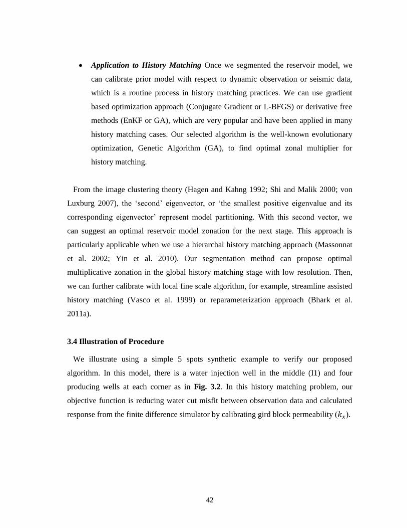
42
Application to History Matching Once we segmented the reservoir model, we
can calibrate prior model with respect to dynamic observation or seismic data,
which is a routine process in history matching practices. We can use gradient
based optimization approach (Conjugate Gradient or L-BFGS) or derivative free
methods (EnKF or GA), which are very popular and have been applied in many
history matching cases. Our selected algorithm is the well-known evolutionary
optimization, Genetic Algorithm (GA), to find optimal zonal multiplier for
history matching.
From the image clustering theory (Hagen and Kahng 1992; Shi and Malik 2000; von
Luxburg 2007), the ‘second’ eigenvector, or ‘the smallest positive eigenvalue and its
corresponding eigenvector’ represent model partitioning. With this second vector, we
can suggest an optimal reservoir model zonation for the next stage. This approach is
particularly applicable when we use a hierarchal history matching approach (Massonnat
et al. 2002; Yin et al. 2010). Our segmentation method can propose optimal
multiplicative zonation in the global history matching stage with low resolution. Then,
we can further calibrate with local fine scale algorithm, for example, streamline assisted
history matching (Vasco et al. 1999) or reparameterization approach (Bhark et al.
2011a).
3.4 Illustration of Procedure
We illustrate using a simple 5 spots synthetic example to verify our proposed
algorithm. In this model, there is a water injection well in the middle (I1) and four
producing wells at each corner as in Fig. 3.2. In this history matching problem, our
objective function is reducing water cut misfit between observation data and calculated
response from the finite difference simulator by calibrating gird block permeability ( ).
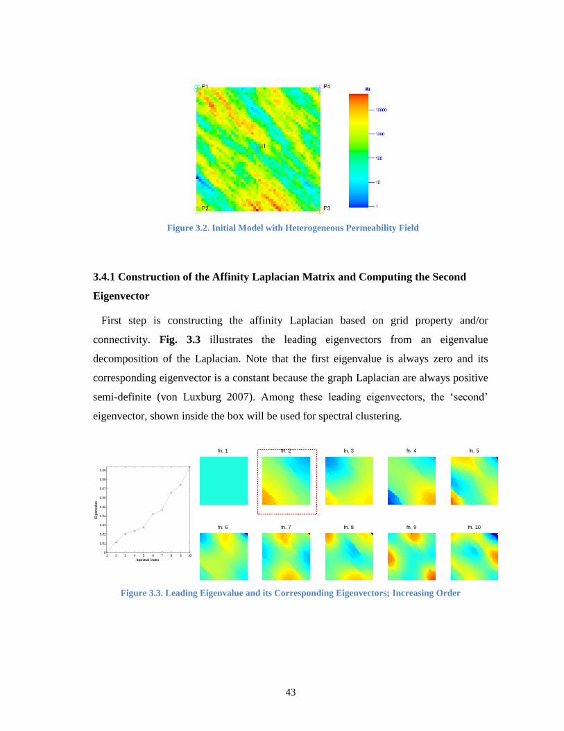
43
Figure 3.2. Initial Model with Heterogeneous Permeability Field
3.4.1 Construction of the Affinity Laplacian Matrix and Computing the Second
Eigenvector
First step is constructing the affinity Laplacian based on grid property and/or
connectivity. Fig. 3.3 illustrates the leading eigenvectors from an eigenvalue
decomposition of the Laplacian. Note that the first eigenvalue is always zero and its
corresponding eigenvector is a constant because the graph Laplacian are always positive
semi-definite (von Luxburg 2007). Among these leading eigenvectors, the ‘second’
eigenvector, shown inside the box will be used for spectral clustering.
Figure 3.3. Leading Eigenvalue and its Corresponding Eigenvectors; Increasing Order
1 2 3 4 5 6 7 8 9 100
0.01
0.02
0.03
0.04
0.05
0.06
0.07
0.08
0.09
Spectral index
Eig
en
valu
e
fn. 1 fn. 2 fn. 3 fn. 4 fn. 5
fn. 6 fn. 7 fn. 8 fn. 9 fn. 10
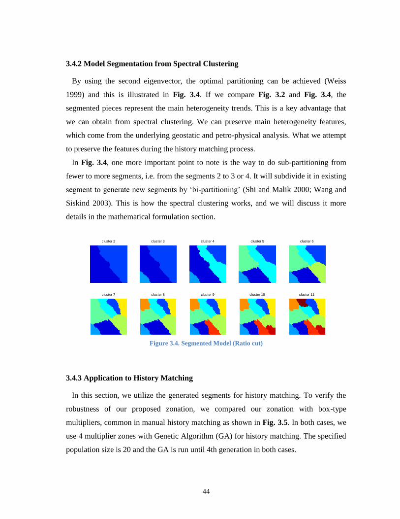
44
3.4.2 Model Segmentation from Spectral Clustering
By using the second eigenvector, the optimal partitioning can be achieved (Weiss
1999) and this is illustrated in Fig. 3.4. If we compare Fig. 3.2 and Fig. 3.4, the
segmented pieces represent the main heterogeneity trends. This is a key advantage that
we can obtain from spectral clustering. We can preserve main heterogeneity features,
which come from the underlying geostatic and petro-physical analysis. What we attempt
to preserve the features during the history matching process.
In Fig. 3.4, one more important point to note is the way to do sub-partitioning from
fewer to more segments, i.e. from the segments 2 to 3 or 4. It will subdivide it in existing
segment to generate new segments by ‘bi-partitioning’ (Shi and Malik 2000; Wang and
Siskind 2003). This is how the spectral clustering works, and we will discuss it more
details in the mathematical formulation section.
Figure 3.4. Segmented Model (Ratio cut)
3.4.3 Application to History Matching
In this section, we utilize the generated segments for history matching. To verify the
robustness of our proposed zonation, we compared our zonation with box-type
multipliers, common in manual history matching as shown in Fig. 3.5. In both cases, we
use 4 multiplier zones with Genetic Algorithm (GA) for history matching. The specified
population size is 20 and the GA is run until 4th generation in both cases.
cluster 2 cluster 3 cluster 4 cluster 5 cluster 6
cluster 7 cluster 8 cluster 9 cluster 10 cluster 11
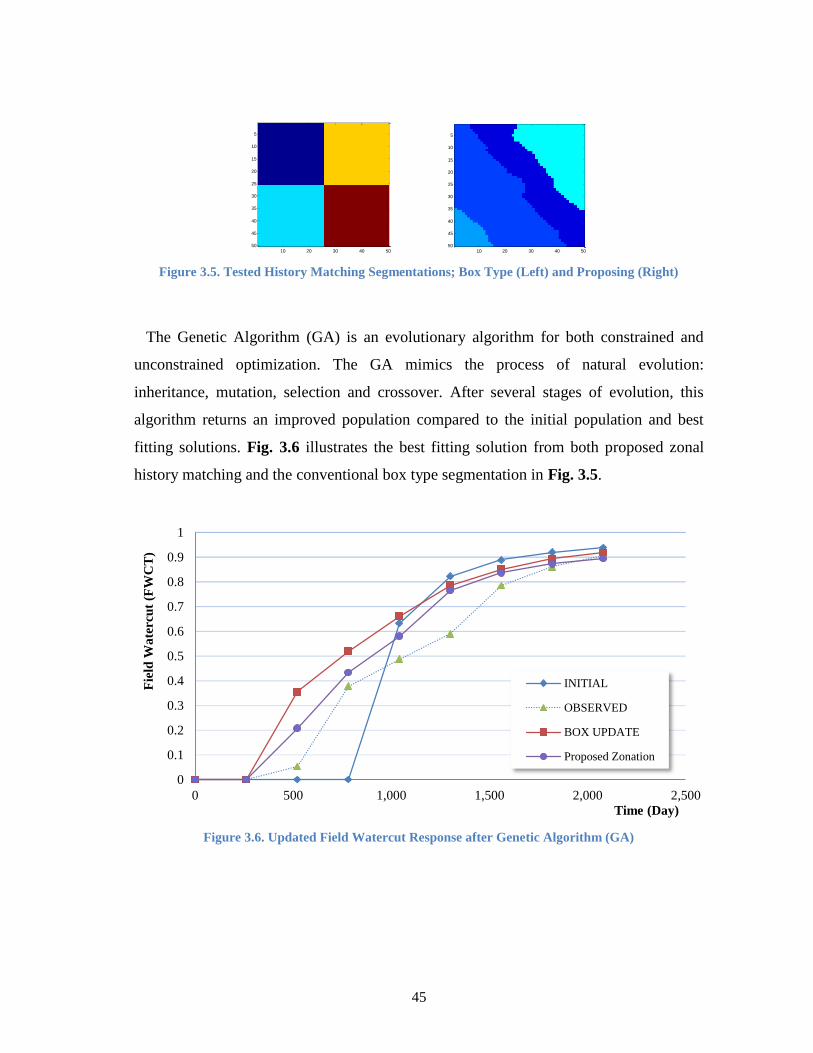
45
Figure 3.5. Tested History Matching Segmentations; Box Type (Left) and Proposing (Right)
The Genetic Algorithm (GA) is an evolutionary algorithm for both constrained and
unconstrained optimization. The GA mimics the process of natural evolution:
inheritance, mutation, selection and crossover. After several stages of evolution, this
algorithm returns an improved population compared to the initial population and best
fitting solutions. Fig. 3.6 illustrates the best fitting solution from both proposed zonal
history matching and the conventional box type segmentation in Fig. 3.5.
Figure 3.6. Updated Field Watercut Response after Genetic Algorithm (GA)
10 20 30 40 50
5
10
15
20
25
30
35
40
45
50 1
1.5
2
2.5
3
3.5
4
10 20 30 40 50
5
10
15
20
25
30
35
40
45
50 0
1
2
3
4
5
6
7
8
9
10
11
0
0.1
0.2
0.3
0.4
0.5
0.6
0.7
0.8
0.9
1
0 500 1,000 1,500 2,000 2,500
Fie
ld W
ate
rcu
t (F
WC
T)
Time (Day)
INITIAL
OBSERVED
BOX UPDATE
Proposed Zonation
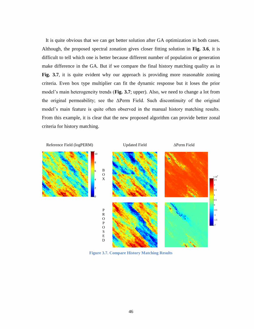
46
It is quite obvious that we can get better solution after GA optimization in both cases.
Although, the proposed spectral zonation gives closer fitting solution in Fig. 3.6, it is
difficult to tell which one is better because different number of population or generation
make difference in the GA. But if we compare the final history matching quality as in
Fig. 3.7, it is quite evident why our approach is providing more reasonable zoning
criteria. Even box type multiplier can fit the dynamic response but it loses the prior
model’s main heterogeneity trends (Fig. 3.7; upper). Also, we need to change a lot from
the original permeability; see the ΔPerm Field. Such discontinuity of the original
model’s main feature is quite often observed in the manual history matching results.
From this example, it is clear that the new proposed algorithm can provide better zonal
criteria for history matching.
Reference Field (logPERM) Updated Field ΔPerm Field
B
O
X
P
R
O
P
O
S
E
D
Figure 3.7. Compare History Matching Results
0
2
4
6
8
10
0
1
2
3
4
5
6
7
8
9
10
10 20 30 40 50
5
10
15
20
25
30
35
40
45
50 -4
-3.5
-3
-2.5
-2
-1.5
-1
-0.5
0
0.5
1x 10
4
-2
-1.5
-1
-0.5
0
0.5
1
1.5
2
2.5
x 104
0
2
4
6
8
10
-2
-1.5
-1
-0.5
0
0.5
1
1.5
2
2.5
x 104

47
3.5 Mathematical Formulation
A graph G is defined as , where V notates the vertex and E denotes the
edge, can be separated into two subgraph ̅ set by simply drawing a cutting edge on
the graph. The degree of dissimilarity of these segmented graphs can be computed as a
‘cut’ function, defined as the total weight of the edges that has been removed after the
segmented in Eq. 3.1 below.
CvCu
vuwCCcut,
),(),( (3.1)
The optimal segmentation is finding the ‘optimal cut’ of a graph G, where the
generated edge minimizes this ‘cut’ value between two clusters. The procedure is : (1)
constructing an affinity Laplacian matrix based on point connectivity (2) decomposing
the Laplacian with eigenvalue decomposition (3) segmenting domain from the second
eigenvector, known as Fiedler vector (Fiedler 1973), with graphic optimization
algorithm.
3.5.1 Constructing Affinity Laplacian
The affinity Laplacian ( ) is always symmetric and positive semidefinite, is defined as
(3.2)
In this formulation, D is the degree of affinity, L is Laplacian of system (also, called as
Kirchhoff operator) and W is the connectivity weight matrix (or conductance matrix)
between grid points, where matrix component . The degree matrix D is a
diagonal matrix, which defines the degree sum of connectivity strength ( ) between one
point (i) and others ( ) as in Eq. 3.3.
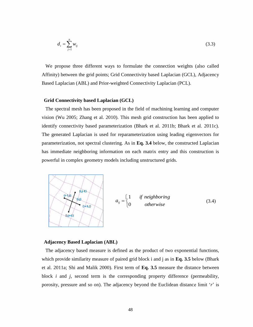
48
n
j
iji wd1
(3.3)
We propose three different ways to formulate the connection weights (also called
Affinity) between the grid points; Grid Connectivity based Laplacian (GCL), Adjacency
Based Laplacian (ABL) and Prior-weighted Connectivity Laplacian (PCL).
Grid Connectivity based Laplacian (GCL)
The spectral mesh has been proposed in the field of machining learning and computer
vision (Wu 2005; Zhang et al. 2010). This mesh grid construction has been applied to
identify connectivity based parameterization (Bhark et al. 2011b; Bhark et al. 2011c).
The generated Laplacian is used for reparameterization using leading eigenvectors for
parameterization, not spectral clustering. As in Eq. 3.4 below, the constructed Laplacian
has immediate neighboring information on each matrix entry and this construction is
powerful in complex geometry models including unstructured grids.
otherwise
gneighborinifaij
0
1 (3.4)
Adjacency Based Laplacian (ABL)
The adjacency based measure is defined as the product of two exponential functions,
which provide similarity measure of paired grid block i and j as in Eq. 3.5 below (Bhark
et al. 2011a; Shi and Malik 2000). First term of Eq. 3.5 measure the distance between
block i and j, second term is the corresponding property difference (permeability,
porosity, pressure and so on). The adjacency beyond the Euclidean distance limit ‘r’ is

49
always zero. Note that both the distance and property have value of one if two points are
located at the same coordinate or have the same property value. Also, each term
diminishes very fast if the difference is increasing due to the exponential form.
else
rxxifxx
ffa ji
I
ji
P
ji
ij
0
expexp 2
2
22
2
(3.5)
In Eq. 3.5, variables and are defined as free parameters in spectral theories
(Weiss 1999). There is no rigorous formulation but several proposals to select those two
parameters and Euclidean cut off distance r. In fact, the spectral clustering performance
is heavily dependent on the proper combination of these free parameters. Previous work
of Bhark et al. (2011a), select these three parameter indirectly. They picked parameters
such that two terms are ‘similar’ far from a point, where the parameters can be regarded
as ‘correlation thresholds for the property difference and distance between cell pairs and
both zero beyond distance r’. Fischer and Poland (2004) proposed two different selection
methods: manual using distance histogram or context-dependent similarity. Shi and
Malik (2000) recommended to set the values between 10 to 20 percent of the parameter
or distance range.
An interesting point is that if we select two free parameters as big numbers, the
calculated adjacency is approaching very fast to the GCT affinity value ( ) and
will lose heterogeneity and/or distance measure. So, a proper combination of two free
parameters as well as the cut off distance plays an important role to capture the prior
information.
Our proposed approach is using variogram to select these three parameters. First, the
Euclidean distance cut off ‘r’ is calculated from the ‘range’ of variogram analysis
(Gringarten and Deutsch 1999) as shown in Fig. 3.8.

50
Figure 3.8. Variogram Model and Range (r)
Once we decide the cut off distance, we can easily decide the distance parameter . If
we take a negligible value (ε, for example 0.001) at the boundary (r), the free parameter
for distance ( ) can be calculated as in Eq. 3.6;
ln
2rI (3.6)
The free parameter for property can be calculated initially from the range of grid
property value as in Eq. 3.7. This is an experimental formulation and comparable to
suggestion of Shi and Malik (2000).
02.0~01.0)( PipP SwherefrangeS (3.7)
In Eq. 3.5, we use different measures with norm but different order of definition is
possible, i.e. and so on with new free parameters. Basically, higher order
norms emphasize more the difference of grid property and/or connected distance.
Ideally, the optimal combination for free parameters in this ‘Gaussian kernel’ type
function is to determine variables and such that both exponential terms diminish to
similar insignificant values (ε) near the range (r).
Lag distance (h)
Range (r)
Nugget

51
Prior weighted Connectivity Laplacian (PCL)
We propose a new affinity Laplacian construction as in below Eq. 3.8. This new
formulation has both grid connectivity from GCL and prior model’s heterogeneity as in
ABL. In other words, the PCL formulation can capture faulted geometry, which is
missing in ABL and can include prior heterogeneity, which is missing in GCL. The two
free parameters in the formulation (Eq. 3.8) can be decided by the same approach as
with ABL construction even though there is no distance cut off ‘r’ term in Eq. 3.8.
else
gneighborinifxx
ffa
I
ji
P
ji
ij
0
expexp
2
22
2
(3.8)
This simple example illustrates how we construct the affinity Laplacian matrix in the
simple 9 (3×3) grid data points as in Fig. 3.9. The lines between data points show the
weighted connectivity and its strength ( ) from Eq. 3.4, 3.5 and 3.8.
Figure 3.9. Discrete Grid Points (3×3)
1 2 3
4 5 6
7 8 9
1.0 0.6
0.0 0.8
0.9 0.6
0.8
1.0
0.1
0.0
0.9
0.9

52
The constructed Laplacian in Fig. 3.10 illustrate the information captured from the
same data points in Fig. 3.9 by different definition of affinity. Note that diagonal term in
each matrix ( ) is the sum of the non-diagonal entries. PCL has the same matrix entry
points as in GCL and have same weight as in ABL matrix between adjacency points.
Only ABL takes diagonal connection in the affinity construction. Also in ABL, points
between non-diagonal (for example, 1 to 6 or 1 to 9) can have non-zero connectivity
values if Euclidean distance is inside the cut off ‘r’ and there exists a connectivity value
from Eq. 3.5.
Grid Connectivity
Laplacian (GCL)
Adjacency Based Laplacian
(ABL)
Prior-weighted
Connectivity Laplacian
(PCL)
Figure 3.10. Affinity Laplacian Matrix Construction
We illustrate how different affinity constructions affect the second eigenvector and
corresponding segmentation results from the model in Fig. 3.11 (heterogeneous 9-spot
synthetic model, Fig. 3.2); the grid connectivity Laplacian (GCL) performs cutting based
on equal weigh on each grid. Both adjacency based Laplacian (ABL) and prior-weight
connectivity Laplacian (PCL) take into account the model heterogeneity in the generated
segments. An interesting point in Fig. 3.11 is that the GCL clustering provides exactly
the same clusters as in the box zones in Fig. 3.5 (left), where we assumed that we don’t
have any prior knowledge and do a blind cutting.
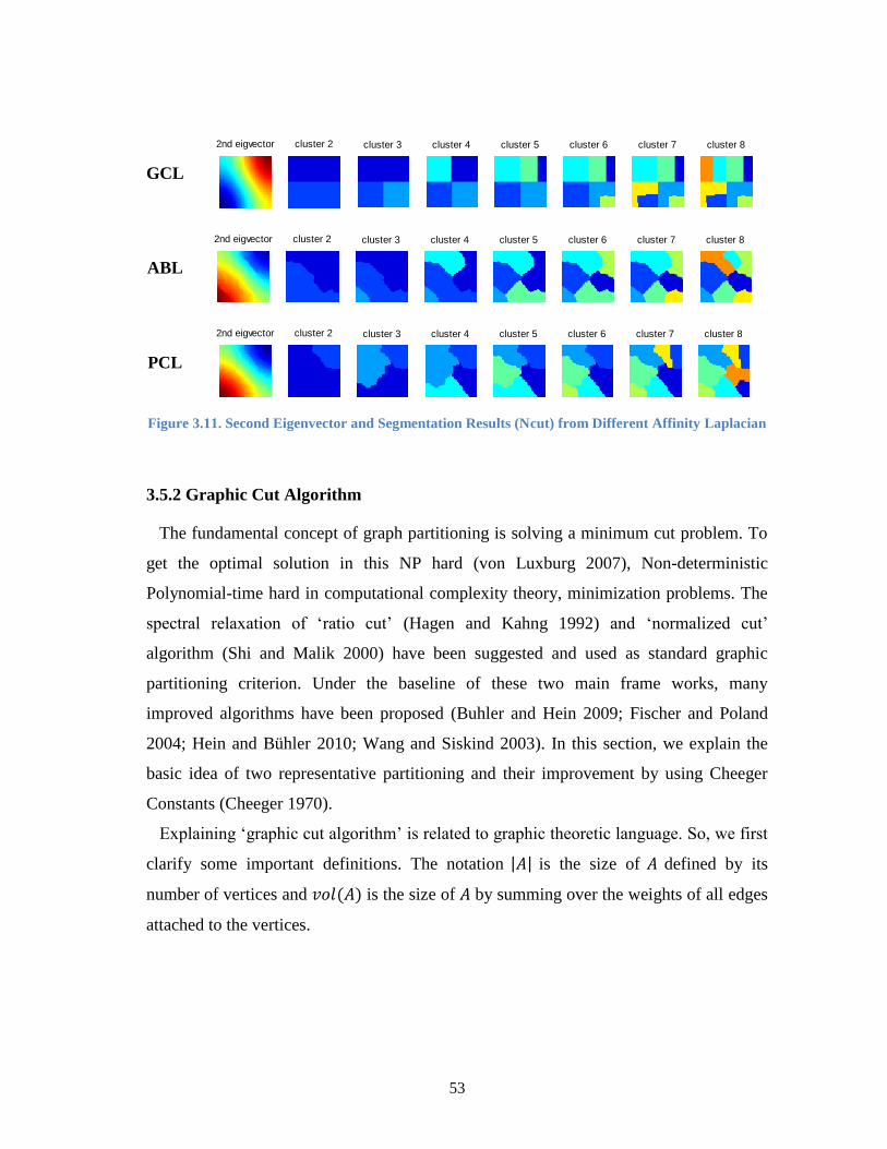
53
GCL
ABL
PCL
Figure 3.11. Second Eigenvector and Segmentation Results (Ncut) from Different Affinity Laplacian
3.5.2 Graphic Cut Algorithm
The fundamental concept of graph partitioning is solving a minimum cut problem. To
get the optimal solution in this NP hard (von Luxburg 2007), Non-deterministic
Polynomial-time hard in computational complexity theory, minimization problems. The
spectral relaxation of ‘ratio cut’ (Hagen and Kahng 1992) and ‘normalized cut’
algorithm (Shi and Malik 2000) have been suggested and used as standard graphic
partitioning criterion. Under the baseline of these two main frame works, many
improved algorithms have been proposed (Buhler and Hein 2009; Fischer and Poland
2004; Hein and Bühler 2010; Wang and Siskind 2003). In this section, we explain the
basic idea of two representative partitioning and their improvement by using Cheeger
Constants (Cheeger 1970).
Explaining ‘graphic cut algorithm’ is related to graphic theoretic language. So, we first
clarify some important definitions. The notation | | is the size of defined by its
number of vertices and is the size of by summing over the weights of all edges
attached to the vertices.
2nd eigvector cluster 2 cluster 3 cluster 4 cluster 5 cluster 6 cluster 7 cluster 8 cluster 9 cluster 10
2nd eigvector cluster 2 cluster 3 cluster 4 cluster 5 cluster 6 cluster 7 cluster 8 cluster 9 cluster 10
2nd eigvector cluster 2 cluster 3 cluster 4 cluster 5 cluster 6 cluster 7 cluster 8 cluster 9 cluster 10

54
Ratio Cut (Rcut)
The ratio cut algorithm is to find a ‘cut’, which is relaxed by the vertices between
clusters (Hagen and Kahng 1992). The size of a subset C in a graph G is measured by its
number of vertices | | ;
C
CCcut
C
CCcutCCRcut
),(),(),( (3.9)
Normalized Cut (Ncut)
The size of clustering is measured by the weights of its cutting edge (Shi and Malik
2000). The normalized cut is relaxed by the weight of edges between clusters. The main
difference between ‘ratio’ cut and ‘normalized’ cut is using un-normalized Laplacian
(ratio cut) versus the normalized one (see next section for detail).
)(
),(
)(
),(),(
Cvol
CCcut
Cvol
CCcutCCNcut (3.10)
Ratio Cheeger Cut (RCC)
The Cheeger constant is a measurement of ‘bottleneckedness’ in a graph (Cheeger
1970). The baseline of Cheeger Constant is defining isoparametric inequality in a
Riemannian geometry. Hein and Bühler (2010) proved that the Cheeger cut is at least as
good as standard spectral clustering with expensive of computation time, which is
explained with the Cheeger inequality (Amghibech 2003). They solve the nonlinear
eigen problems (Cheeger Cut) with Inverse Power Method (IPM). In the Ratio Cheeger
Cut (RCC), the balanced cut is optimized by the minimum cardinality of the clusters;
},{min
),(),(
CC
CCcutCCRCC (4.11)
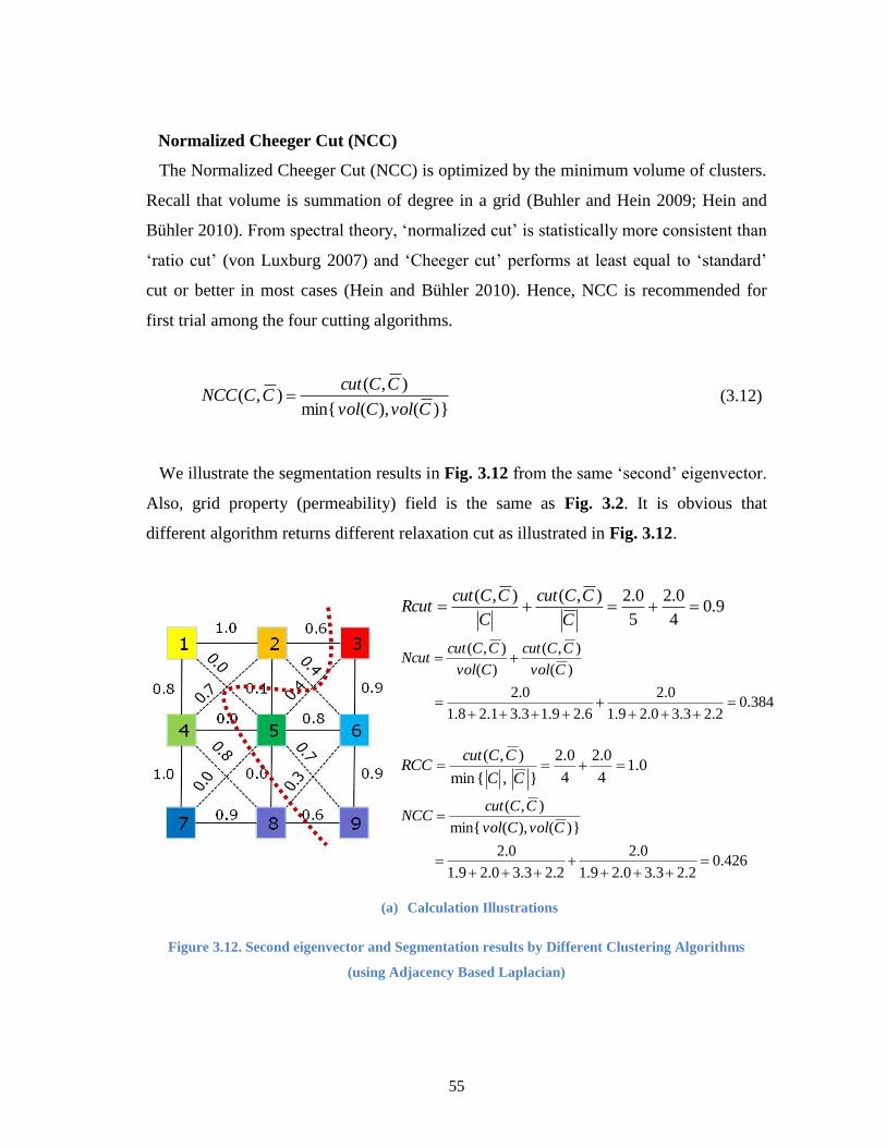
55
Normalized Cheeger Cut (NCC)
The Normalized Cheeger Cut (NCC) is optimized by the minimum volume of clusters.
Recall that volume is summation of degree in a grid (Buhler and Hein 2009; Hein and
Bühler 2010). From spectral theory, ‘normalized cut’ is statistically more consistent than
‘ratio cut’ (von Luxburg 2007) and ‘Cheeger cut’ performs at least equal to ‘standard’
cut or better in most cases (Hein and Bühler 2010). Hence, NCC is recommended for
first trial among the four cutting algorithms.
})(),(min{
),(),(
CvolCvol
CCcutCCNCC (3.12)
We illustrate the segmentation results in Fig. 3.12 from the same ‘second’ eigenvector.
Also, grid property (permeability) field is the same as Fig. 3.2. It is obvious that
different algorithm returns different relaxation cut as illustrated in Fig. 3.12.
9.04
0.2
5
0.2),(),(
C
CCcut
C
CCcutRcut
384.02.23.30.29.1
0.2
6.29.13.31.28.1
0.2
)(
),(
)(
),(
Cvol
CCcut
Cvol
CCcutNcut
0.14
0.2
4
0.2
},{min
),(
CC
CCcutRCC
426.02.23.30.29.1
0.2
2.23.30.29.1
0.2
})(),(min{
),(
CvolCvol
CCcutNCC
(a) Calculation Illustrations
Figure 3.12. Second eigenvector and Segmentation results by Different Clustering Algorithms
(using Adjacency Based Laplacian)

56
Rcut
Ncut
RCC
NCC
(b) Cutting Results from Different Algorithms
Figure 3.12. Continued
You may raise a question: “which algorithm is better one?” or “How many clusters do
we have to use for history matching?”. The selection of algorithm and number of optimal
clustering will be discussed in the ‘nature of graph partitioning’ section.
3.5.3 Optimal Partitioning with Second Eigenvector
For the graph partitioning, we use the ‘second’ eigenvector of the affinity Laplacian,
constructed from the connectivity definition. The reason why we use the ‘second’
eigenvector can be clarified with both physical and mathematical explanations (Shi and
Malik 2000; von Luxburg 2007). Note that K-means clustering, also used in many
10 20 30 40 50
5
10
15
20
25
30
35
40
45
50
-0.04
-0.03
-0.02
-0.01
0
0.01
0.02
0.03
0.04
cluster 2 cluster 3 cluster 4 cluster 5 cluster 6 cluster 7 cluster 8 cluster 9 cluster 10 cluster 11
cluster 2 cluster 3 cluster 4 cluster 5 cluster 6 cluster 7 cluster 8 cluster 9 cluster 10 cluster 11
cluster 2 cluster 3 cluster 4 cluster 5 cluster 6 cluster 7 cluster 8 cluster 9 cluster 10 cluster 11
cluster 2 cluster 3 cluster 4 cluster 5 cluster 6 cluster 7 cluster 8 cluster 9 cluster 10 cluster 11

57
clustering problems, is different from spectral clustering and it will not use ‘second’
eigenvector (Fischer and Poland 2004).
Physical Explanation
A physical analogy is provided by comparing a spring-mass system (Shi and Malik
2000) or vibration of a string as in Eq. 3.13. We can relate graphic nodes as physical
nodes and graph edges as moving part of string inside the node as in Fig. 3.12. Imagine
that if we shake this string with a strong oscillation frequency, the stationary nodes will
not move at steady state and will divide the region into subpieces as in Fig. 3.13. In the
equation, x is a location in a string, y is magnitude of vibration, t is time of a certain
moment, is linear mass and T is acting tension on each side of the string.
2
2
2
2 ),(),(
t
txy
Tx
txy
(3.13)
From general solution of this wave equation with fixed ends, where is vibration
frequency, is length of the string and is nth mode;
tfxL
nytxy n
s
mm
2cossin),(
(3.14)
The steady solution of Eq. 3.14 can be derived by plugging into Eq. 3.13;
tfxL
n
Tfytfx
L
n
L
ny k
s
mnkk
s
m
s
mk
2cossin22cossin
2
2
(3.15)
Eq. 3.16 below satisfies the steady state of string vibration with non-trivial terms of kth
harmonic mode;
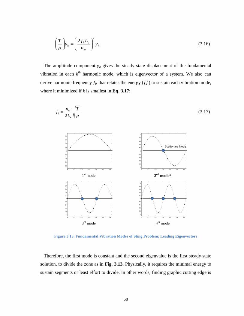
58
k
m
skk y
n
Lfy
T2
2
(3.16)
The amplitude component gives the steady state displacement of the fundamental
vibration in each kth
harmonic mode, which is eigenvector of a system. We also can
derive harmonic frequency that relates the energy ( ) to sustain each vibration mode,
where it minimized if k is smallest in Eq. 3.17;
T
L
nf
s
mk
2 (3.17)
1
st mode 2
nd mode*
3
rd mode 4
th mode
Figure 3.13. Fundamental Vibration Modes of Sting Problem; Leading Eigenvectors
Therefore, the first mode is constant and the second eigenvalue is the first steady state
solution, to divide the zone as in Fig. 3.13. Physically, it requires the minimal energy to
sustain segments or least effort to divide. In other words, finding graphic cutting edge is
0 0.1 0.2 0.3 0.4 0.5 0.6
-0.8
-0.6
-0.4
-0.2
0
0.2
0.4
0.6
0.8
0 0.1 0.2 0.3 0.4 0.5 0.6
-1
-0.8
-0.6
-0.4
-0.2
0
0.2
0.4
0.6
0.8
1
0 0.1 0.2 0.3 0.4 0.5 0.6
-1
-0.8
-0.6
-0.4
-0.2
0
0.2
0.4
0.6
0.8
1
0 0.1 0.2 0.3 0.4 0.5 0.6
-1
-0.8
-0.6
-0.4
-0.2
0
0.2
0.4
0.6
0.8
1
Stationary Node

59
a process to find “minimal effort” stationary node to divide the system. Note that
‘second’ eigenvector always divide the system into ‘two’ pieces which is called
bipartitioning. This is how the spectral clustering works in most of partitioning
algorithms.
Mathematical Explanation
In Eq. 3.1, we define the ‘cut’ function for measuring the degree of dissimilarity
between two pieces. Fiedler (1973, 1975) proved and applied the algebraic connectivity
theory from second eigenvector (called Fiedler vector) of non-directed graphs. Hagen
and Kahng (1992) provide the mathematical bipartition for ‘ratio cut’ algorithm. Shi and
Malik (2000) also prove that second eigenvector offer optimal ‘normalized cut’. It is an
important spectral property of eigenspectrum. If the graph G is connected, the second
eigenvalue ( ; also called algebraic connectivity) is positive
and first eigngenvector is a constant (Pothen et al. 1990) as already shown in Fig. 3.3.
Finding optimal clustering can be proved by solving relaxation of simple balanced
‘ratio’ cuts (von Luxburg 2007) as in Eq. 3.18;
CCwhereCCcutCC
,),(min,
(3.18)
If we choose clustering such that
Cxif
Cxiff
i
i
i
1
1 (3.19)
Here, we transformed the real value problem into discontinuous indicator vector space
(von Luxburg 2007). From Eq. 3.1, we can rearrange as;
ji jiij
CvCu
ffwLffvuwCCcut,
2
, 2
1'),(),( (3.20)

60
We have already imposed condition that | | | ̅| from Eq. 3.18, which leads to Eq.
3.21 for optimal condition;
i if 0 (3.21)
The above Eq. 3.21 indicate that
01
f 1
f (3.22)
The vector as defined in Eq. 3.19 is orthogonal to the constant identity vector ⃗ .
Also, from same definition in Eq. 3.19, norm of vector ;
nCCffn
i
i 1
22 (3.23)
The optimal clustering, which is solving minimization problem as derived in Eq. 3.20
from Eq. 3.18, can be rewritten from Eq. 3.20, 3.22 and 3.23 ( is a scale factor and
can be discarded) ;
nfandfftosubjectLff iVC 1,1'min
(3.24)
By Rayleigh Quotient (also known as Rayleigh-Ritz theorem), it can be immediately
proved that the solution of this problem is given by the second eigenvector of Laplacian
( ). Recall that ‘second’ means the smallest non-zero eigenvalue and its corresponding
eigenvector (Weiss 1960). So, we can approximate the optimal solution by the second
eigenvector in ‘ratio cut’ relaxation problems.
The optimal ‘normalized’ cut is also easily proved by same approach from the
comparable one (Eq. 3.18 with Eq. 3.25);

61
)()(,),(min,
CvolCvolwhereCCcutCC
(3.25)
We can derive the imposed conditions as ⃗ (von Luxburg
2007). Recall that D has been defined as degree of affinity in Eq. 3.2.
)('1,1'min VvolDffandfDftosubjectLff iVC
(3.26)
Now, we substitute with normalized vector in Eq. 3.26 and
;
)(1,1'min 2/1 VvolgandfDgtosubjectgLg isymVC
(3.27)
Consequently, we also arrive at the standard Rayleigh Quotient type formulation as in
Eq. 3.27. The relaxation solution is given by the second eigenvector of normalized
Laplacian ( ). Now, we can see that ‘ratio’ cut leads to un-normalized clustering as
in Eq. 3.24 while relaxing ‘normalized’ cut leads to normalized solution in Eq. 3.27.
Hence generally speaking, the ‘normalized’ cut is more statistically consistent than
‘ratio’ cut (von Luxburg 2007).
3.5.4 Nature of Graph Partitioning
We already see that different affinity construction and relaxation algorithm will lead to
different segmentation. There are also many more affinity construction and algorithms
that we cannot illustrate in this paper. Even, a small change in selecting free parameters
will induce quite different segmentations. It is almost impossible to recommend one
single method for reservoir model segmentation. Instead, we will explore the true nature
of graph partitioning and will derive ‘tentative’ answer to select cutting algorithm and
number of segments for history matching.
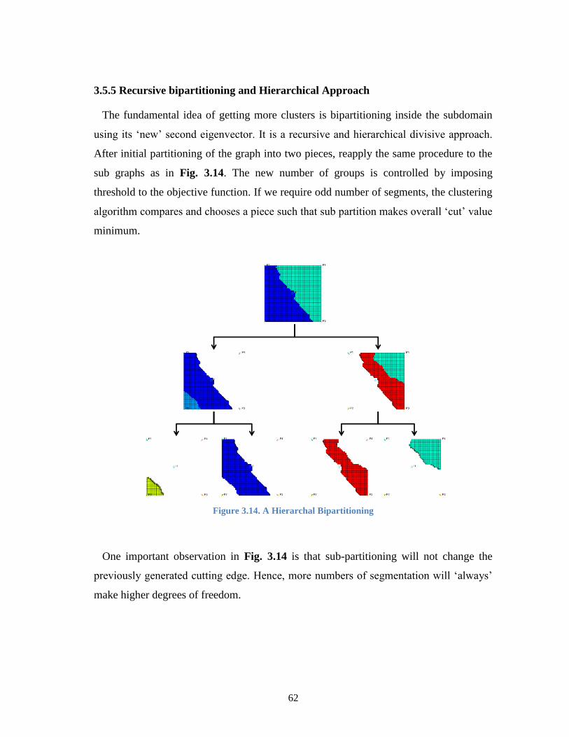
62
3.5.5 Recursive bipartitioning and Hierarchical Approach
The fundamental idea of getting more clusters is bipartitioning inside the subdomain
using its ‘new’ second eigenvector. It is a recursive and hierarchical divisive approach.
After initial partitioning of the graph into two pieces, reapply the same procedure to the
sub graphs as in Fig. 3.14. The new number of groups is controlled by imposing
threshold to the objective function. If we require odd number of segments, the clustering
algorithm compares and chooses a piece such that sub partition makes overall ‘cut’ value
minimum.
Figure 3.14. A Hierarchal Bipartitioning
One important observation in Fig. 3.14 is that sub-partitioning will not change the
previously generated cutting edge. Hence, more numbers of segmentation will ‘always’
make higher degrees of freedom.
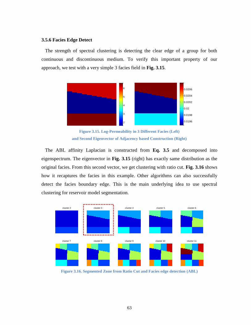
63
3.5.6 Facies Edge Detect
The strength of spectral clustering is detecting the clear edge of a group for both
continuous and discontinuous medium. To verify this important property of our
approach, we test with a very simple 3 facies field in Fig. 3.15.
Figure 3.15. Log-Permeability in 3 Different Facies (Left)
and Second Eigenvector of Adjacency based Construction (Right)
The ABL affinity Laplacian is constructed from Eq. 3.5 and decomposed into
eigenspectrum. The eigenvector in Fig. 3.15 (right) has exactly same distribution as the
original facies. From this second vector, we get clustering with ratio cut. Fig. 3.16 shows
how it recaptures the facies in this example. Other algorithms can also successfully
detect the facies boundary edge. This is the main underlying idea to use spectral
clustering for reservoir model segmentation.
Figure 3.16. Segmented Zone from Ratio Cut and Facies edge detection (ABL)
2
3
4
5
6
0.0196
0.0198
0.02
0.0202
0.0204
0.0206
cluster 2 cluster 3 cluster 4 cluster 5 cluster 6
cluster 7 cluster 8 cluster 9 cluster 10 cluster 11
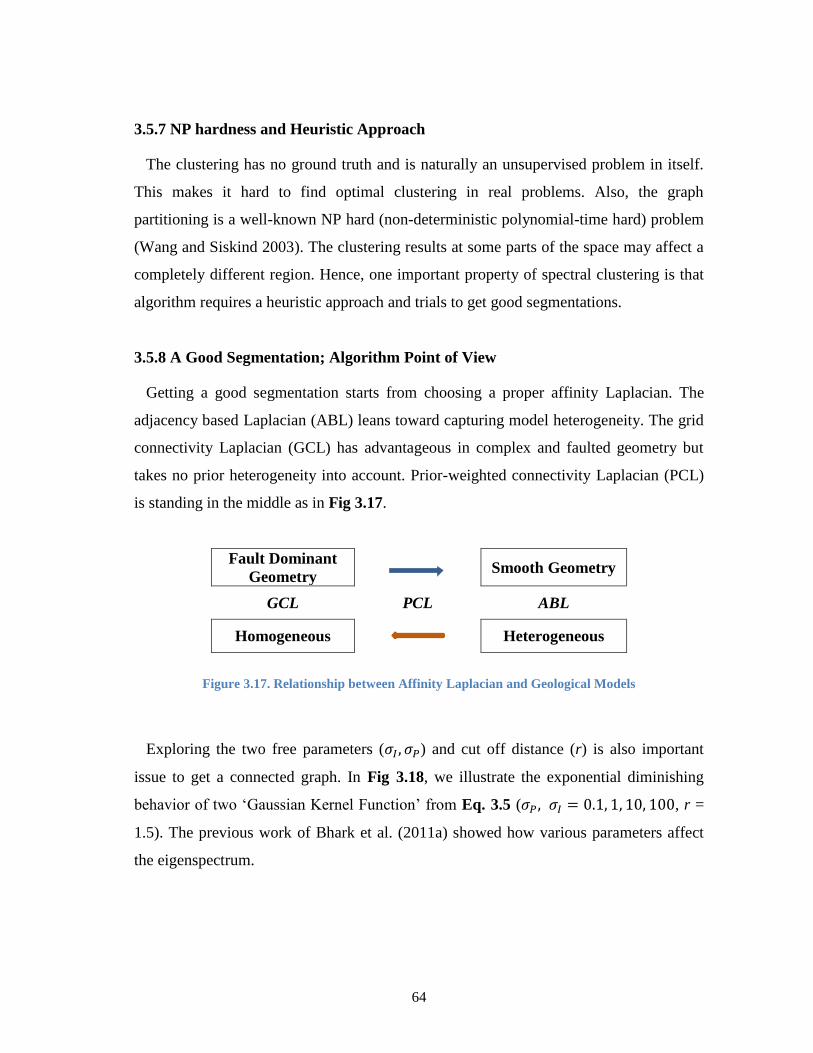
64
3.5.7 NP hardness and Heuristic Approach
The clustering has no ground truth and is naturally an unsupervised problem in itself.
This makes it hard to find optimal clustering in real problems. Also, the graph
partitioning is a well-known NP hard (non-deterministic polynomial-time hard) problem
(Wang and Siskind 2003). The clustering results at some parts of the space may affect a
completely different region. Hence, one important property of spectral clustering is that
algorithm requires a heuristic approach and trials to get good segmentations.
3.5.8 A Good Segmentation; Algorithm Point of View
Getting a good segmentation starts from choosing a proper affinity Laplacian. The
adjacency based Laplacian (ABL) leans toward capturing model heterogeneity. The grid
connectivity Laplacian (GCL) has advantageous in complex and faulted geometry but
takes no prior heterogeneity into account. Prior-weighted connectivity Laplacian (PCL)
is standing in the middle as in Fig 3.17.
Fault Dominant
Geometry Smooth Geometry
GCL PCL ABL
Homogeneous Heterogeneous
Figure 3.17. Relationship between Affinity Laplacian and Geological Models
Exploring the two free parameters ( ) and cut off distance (r) is also important
issue to get a connected graph. In Fig 3.18, we illustrate the exponential diminishing
behavior of two ‘Gaussian Kernel Function’ from Eq. 3.5 ( , r =
1.5). The previous work of Bhark et al. (2011a) showed how various parameters affect
the eigenspectrum.
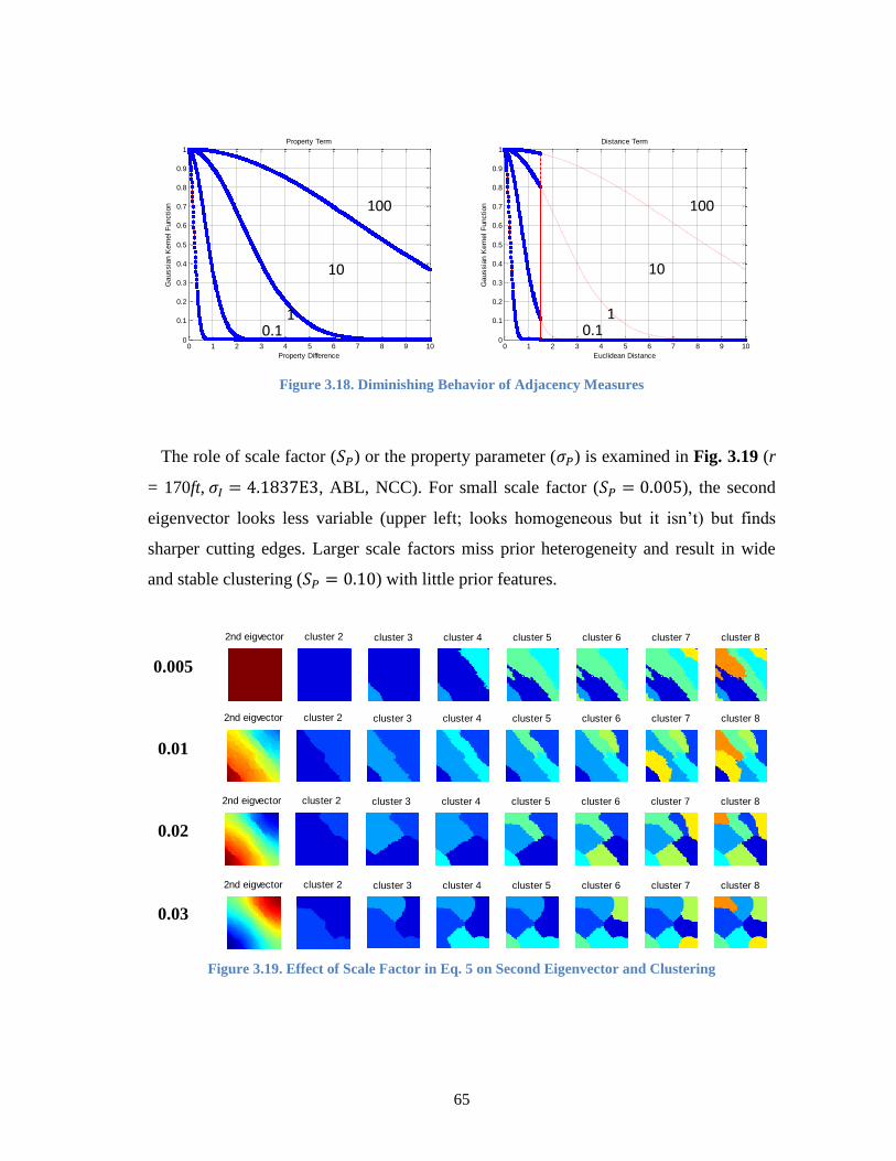
65
Figure 3.18. Diminishing Behavior of Adjacency Measures
The role of scale factor ( ) or the property parameter ( ) is examined in Fig. 3.19 (r
= 170ft, , ABL, NCC). For small scale factor ( ), the second
eigenvector looks less variable (upper left; looks homogeneous but it isn’t) but finds
sharper cutting edges. Larger scale factors miss prior heterogeneity and result in wide
and stable clustering ( ) with little prior features.
0.005
0.01
0.02
0.03
Figure 3.19. Effect of Scale Factor in Eq. 5 on Second Eigenvector and Clustering
0 1 2 3 4 5 6 7 8 9 100
0.1
0.2
0.3
0.4
0.5
0.6
0.7
0.8
0.9
1Property Term
Property Difference
Gaussia
n K
ern
el F
unction
0 1 2 3 4 5 6 7 8 9 100
0.1
0.2
0.3
0.4
0.5
0.6
0.7
0.8
0.9
1Distance Term
Euclidean Distance
Gaussia
n K
ern
el F
unction
2nd eigvector cluster 2 cluster 3 cluster 4 cluster 5 cluster 6 cluster 7 cluster 8 cluster 9 cluster 10
2nd eigvector cluster 2 cluster 3 cluster 4 cluster 5 cluster 6 cluster 7 cluster 8 cluster 9 cluster 10
2nd eigvector cluster 2 cluster 3 cluster 4 cluster 5 cluster 6 cluster 7 cluster 8 cluster 9 cluster 10
2nd eigvector cluster 2 cluster 3 cluster 4 cluster 5 cluster 6 cluster 7 cluster 8 cluster 9 cluster 10
0.1 1
10
100
0.1 1
10
100
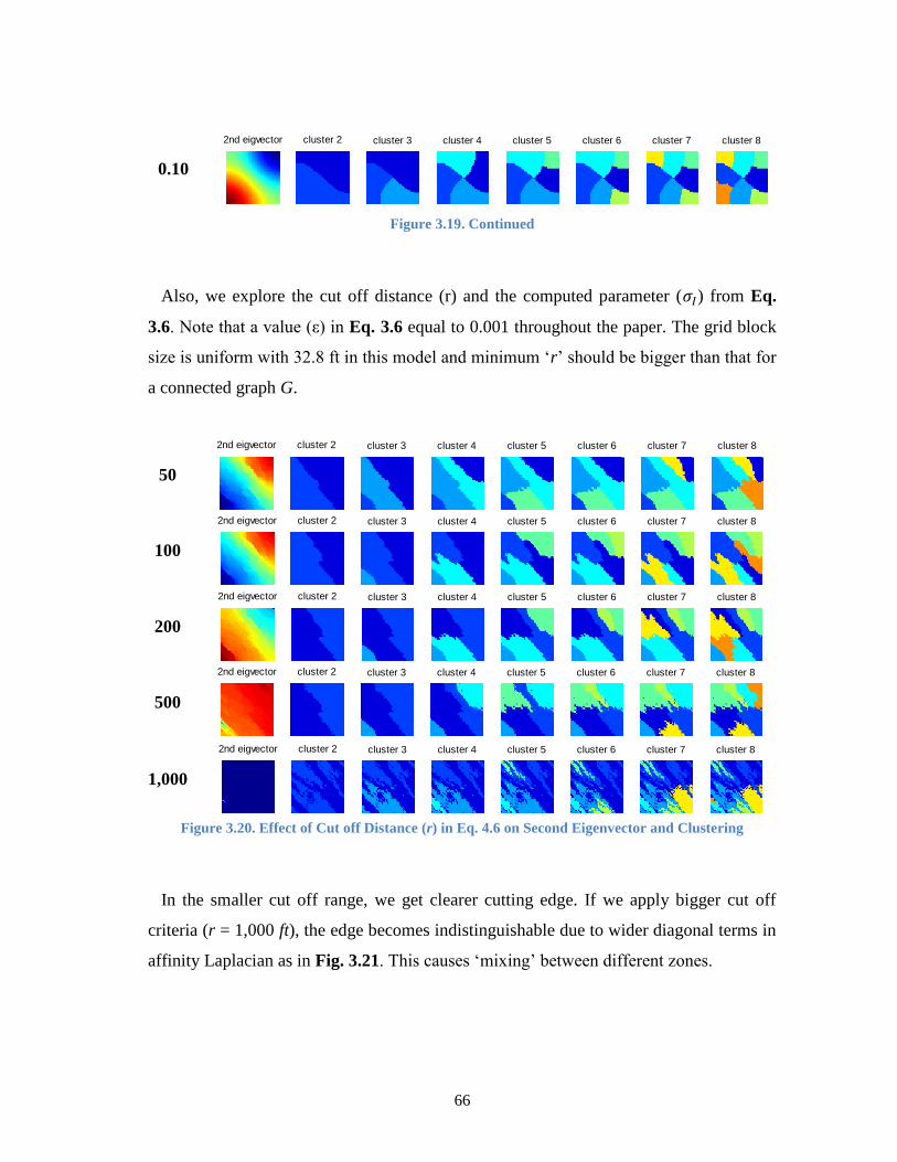
66
0.10
Figure 3.19. Continued
Also, we explore the cut off distance (r) and the computed parameter ( ) from Eq.
3.6. Note that a value (ε) in Eq. 3.6 equal to 0.001 throughout the paper. The grid block
size is uniform with 32.8 ft in this model and minimum ‘r’ should be bigger than that for
a connected graph G.
50
100
200
500
1,000
Figure 3.20. Effect of Cut off Distance (r) in Eq. 4.6 on Second Eigenvector and Clustering
In the smaller cut off range, we get clearer cutting edge. If we apply bigger cut off
criteria (r = 1,000 ft), the edge becomes indistinguishable due to wider diagonal terms in
affinity Laplacian as in Fig. 3.21. This causes ‘mixing’ between different zones.
2nd eigvector cluster 2 cluster 3 cluster 4 cluster 5 cluster 6 cluster 7 cluster 8 cluster 9 cluster 10
2nd eigvector cluster 2 cluster 3 cluster 4 cluster 5 cluster 6 cluster 7 cluster 8 cluster 9 cluster 10
2nd eigvector cluster 2 cluster 3 cluster 4 cluster 5 cluster 6 cluster 7 cluster 8 cluster 9 cluster 10
2nd eigvector cluster 2 cluster 3 cluster 4 cluster 5 cluster 6 cluster 7 cluster 8 cluster 9 cluster 10
2nd eigvector cluster 2 cluster 3 cluster 4 cluster 5 cluster 6 cluster 7 cluster 8 cluster 9 cluster 10
2nd eigvector cluster 2 cluster 3 cluster 4 cluster 5 cluster 6 cluster 7 cluster 8 cluster 9 cluster 10
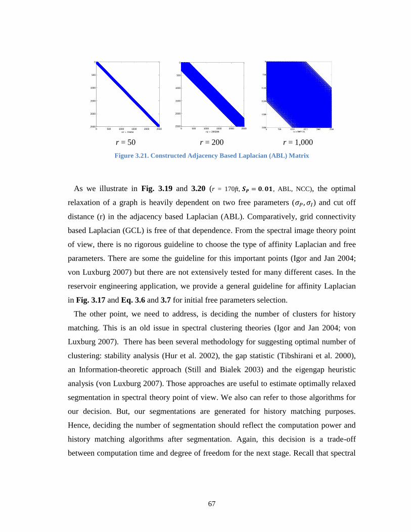
67
r = 50 r = 200 r = 1,000
Figure 3.21. Constructed Adjacency Based Laplacian (ABL) Matrix
As we illustrate in Fig. 3.19 and 3.20 (r = 170ft, , ABL, NCC), the optimal
relaxation of a graph is heavily dependent on two free parameters ( ) and cut off
distance (r) in the adjacency based Laplacian (ABL). Comparatively, grid connectivity
based Laplacian (GCL) is free of that dependence. From the spectral image theory point
of view, there is no rigorous guideline to choose the type of affinity Laplacian and free
parameters. There are some the guideline for this important points (Igor and Jan 2004;
von Luxburg 2007) but there are not extensively tested for many different cases. In the
reservoir engineering application, we provide a general guideline for affinity Laplacian
in Fig. 3.17 and Eq. 3.6 and 3.7 for initial free parameters selection.
The other point, we need to address, is deciding the number of clusters for history
matching. This is an old issue in spectral clustering theories (Igor and Jan 2004; von
Luxburg 2007). There has been several methodology for suggesting optimal number of
clustering: stability analysis (Hur et al. 2002), the gap statistic (Tibshirani et al. 2000),
an Information-theoretic approach (Still and Bialek 2003) and the eigengap heuristic
analysis (von Luxburg 2007). Those approaches are useful to estimate optimally relaxed
segmentation in spectral theory point of view. We also can refer to those algorithms for
our decision. But, our segmentations are generated for history matching purposes.
Hence, deciding the number of segmentation should reflect the computation power and
history matching algorithms after segmentation. Again, this decision is a trade-off
between computation time and degree of freedom for the next stage. Recall that spectral
0 500 1000 1500 2000 2500
0
500
1000
1500
2000
2500
nz = 19404
0 500 1000 1500 2000 2500
0
500
1000
1500
2000
2500
nz = 269288
68
clustering is a hierarchical approach and ‘always’ give higher degrees of freedom in
higher number of segmentation.
The most important key point to get good clustering is that segmented pieces should be
“meaningful” zones for history matching. This should be decided by geologic and
engineering considerations.
3.6 History Matching: Genetic Algorithm (GA)
We adapt the method genetic algorithm, one of the well-developed evolutionary
algorithms in reservoir history matching. Experimental design, genetic algorithm and
response surface are used for calibrating geological features of initial reservoir model.
The strengths of genetic algorithm are its wide flexibility in choice of parameters as well
as construction of objective function. The objective function to optimize with GA is
constructed as logarithmic summation of data misfits as in Eq. 3.28;
objective WellN
j
N
i
iiN SimObsmmmOmO1 1
21 ln),...,,()( (3.28)
3.6.1 Field Application: Brugge
In this section, we apply our model segmentation approach to a field example. We
choose the Brugge reservoir model in Fig. 3.22, a SPE benchmark case. This Brugge
reservoir model has been widely used to evaluate closed-loop reservoir management
strategy developments (Alhuthali 2009; Peters et al. 2010) and history matching
algorithm verification (Bhark et al. 2011a; Vallhs and Naevdal 2009).
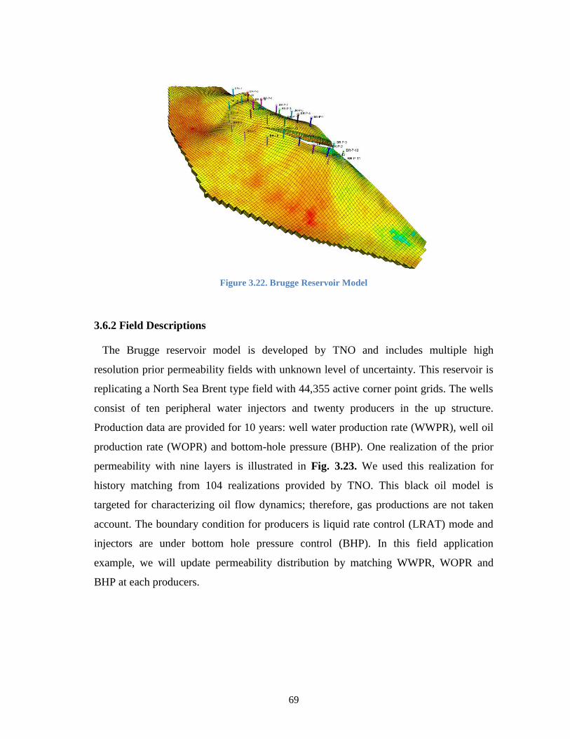
69
Figure 3.22. Brugge Reservoir Model
3.6.2 Field Descriptions
The Brugge reservoir model is developed by TNO and includes multiple high
resolution prior permeability fields with unknown level of uncertainty. This reservoir is
replicating a North Sea Brent type field with 44,355 active corner point grids. The wells
consist of ten peripheral water injectors and twenty producers in the up structure.
Production data are provided for 10 years: well water production rate (WWPR), well oil
production rate (WOPR) and bottom-hole pressure (BHP). One realization of the prior
permeability with nine layers is illustrated in Fig. 3.23. We used this realization for
history matching from 104 realizations provided by TNO. This black oil model is
targeted for characterizing oil flow dynamics; therefore, gas productions are not taken
account. The boundary condition for producers is liquid rate control (LRAT) mode and
injectors are under bottom hole pressure control (BHP). In this field application
example, we will update permeability distribution by matching WWPR, WOPR and
BHP at each producers.
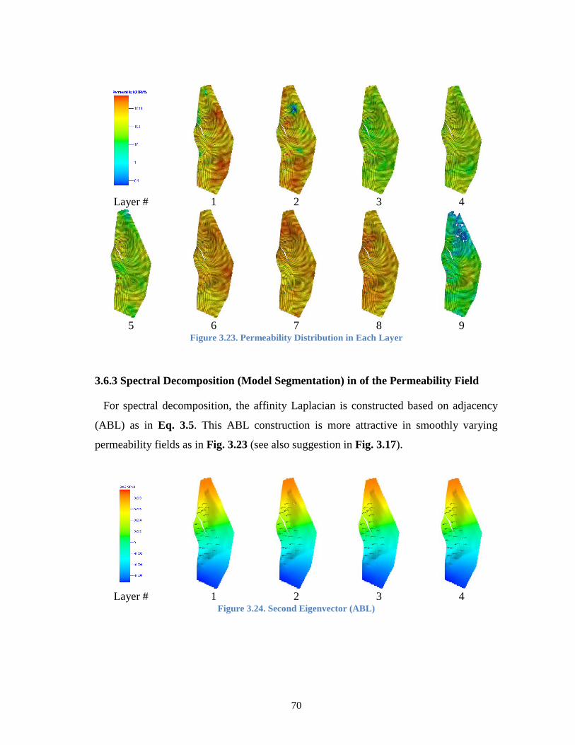
70
Layer # 1 2 3 4
5 6 7 8 9
Figure 3.23. Permeability Distribution in Each Layer
3.6.3 Spectral Decomposition (Model Segmentation) in of the Permeability Field
For spectral decomposition, the affinity Laplacian is constructed based on adjacency
(ABL) as in Eq. 3.5. This ABL construction is more attractive in smoothly varying
permeability fields as in Fig. 3.23 (see also suggestion in Fig. 3.17).
Layer # 1 2 3 4 Figure 3.24. Second Eigenvector (ABL)
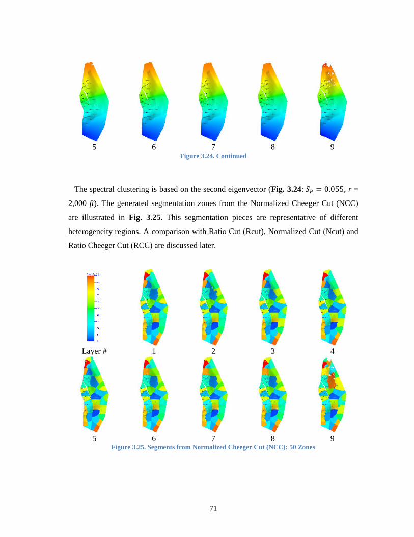
71
5 6 7 8 9
Figure 3.24. Continued
The spectral clustering is based on the second eigenvector (Fig. 3.24: , r =
2,000 ft). The generated segmentation zones from the Normalized Cheeger Cut (NCC)
are illustrated in Fig. 3.25. This segmentation pieces are representative of different
heterogeneity regions. A comparison with Ratio Cut (Rcut), Normalized Cut (Ncut) and
Ratio Cheeger Cut (RCC) are discussed later.
Layer # 1 2 3 4
5 6 7 8 9
Figure 3.25. Segments from Normalized Cheeger Cut (NCC): 50 Zones
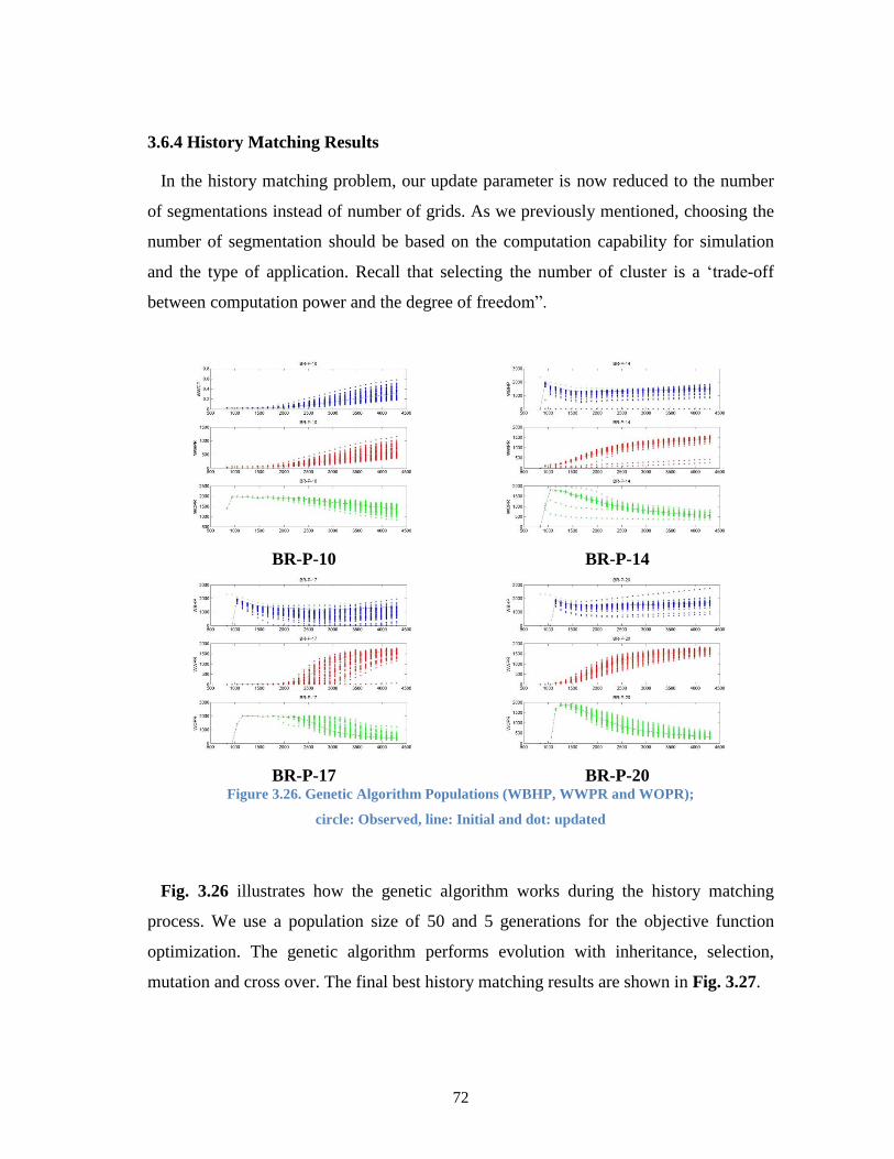
72
3.6.4 History Matching Results
In the history matching problem, our update parameter is now reduced to the number
of segmentations instead of number of grids. As we previously mentioned, choosing the
number of segmentation should be based on the computation capability for simulation
and the type of application. Recall that selecting the number of cluster is a ‘trade-off
between computation power and the degree of freedom”.
BR-P-10 BR-P-14
BR-P-17 BR-P-20
Figure 3.26. Genetic Algorithm Populations (WBHP, WWPR and WOPR);
circle: Observed, line: Initial and dot: updated
Fig. 3.26 illustrates how the genetic algorithm works during the history matching
process. We use a population size of 50 and 5 generations for the objective function
optimization. The genetic algorithm performs evolution with inheritance, selection,
mutation and cross over. The final best history matching results are shown in Fig. 3.27.
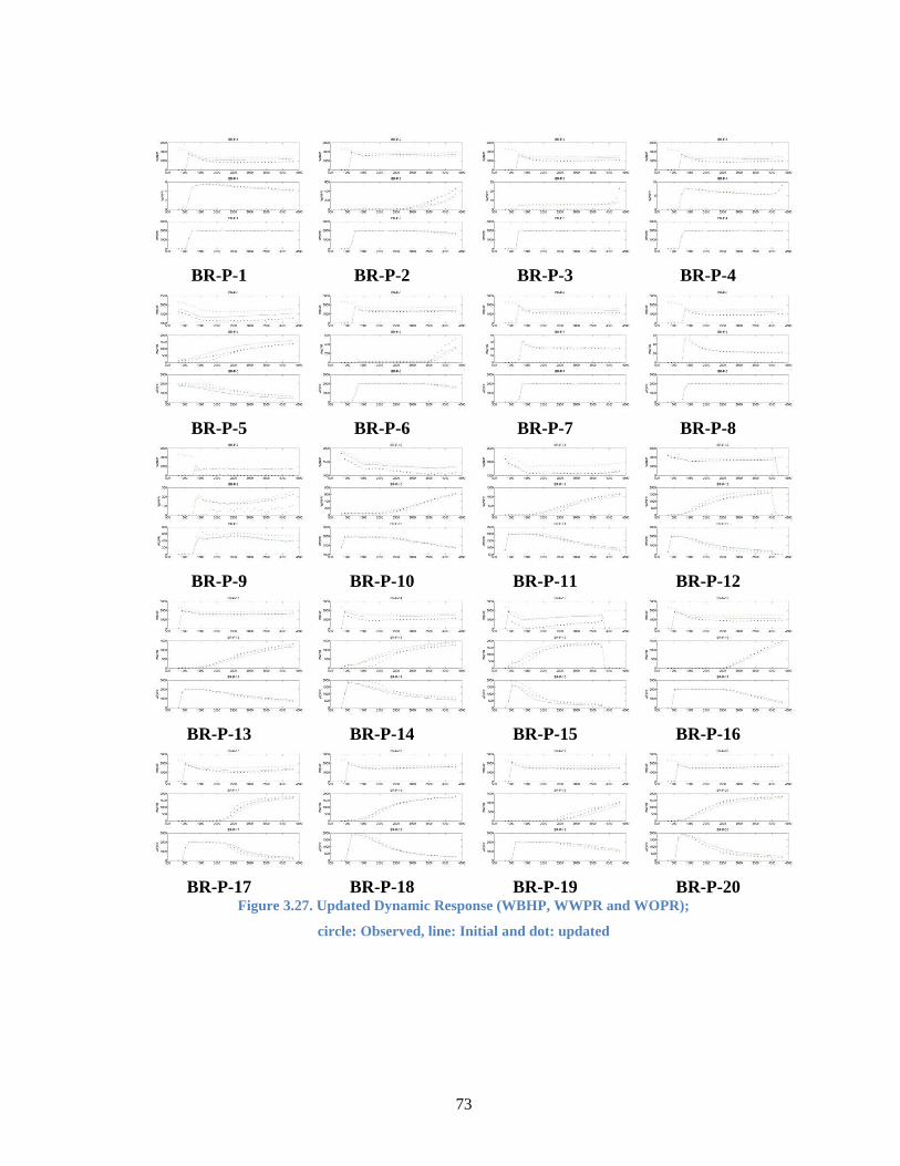
73
BR-P-1 BR-P-2 BR-P-3 BR-P-4
BR-P-5 BR-P-6 BR-P-7 BR-P-8
BR-P-9 BR-P-10 BR-P-11 BR-P-12
BR-P-13 BR-P-14 BR-P-15 BR-P-16
BR-P-17 BR-P-18 BR-P-19 BR-P-20
Figure 3.27. Updated Dynamic Response (WBHP, WWPR and WOPR);
circle: Observed, line: Initial and dot: updated
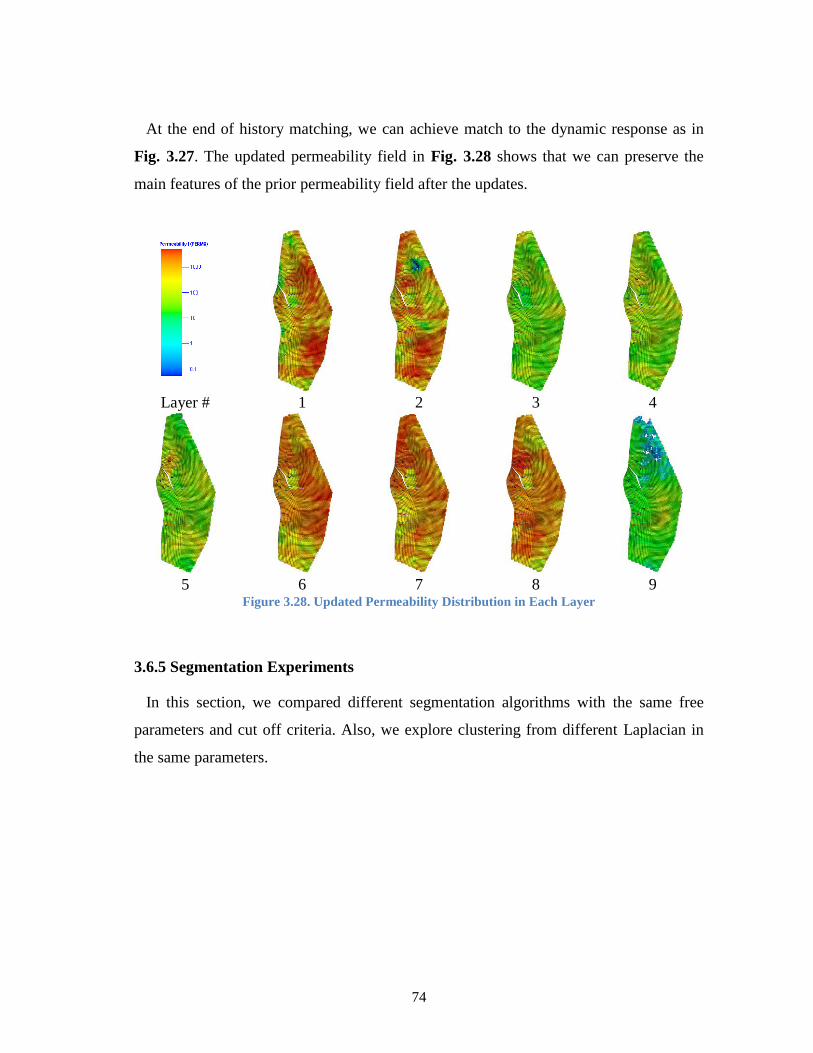
74
At the end of history matching, we can achieve match to the dynamic response as in
Fig. 3.27. The updated permeability field in Fig. 3.28 shows that we can preserve the
main features of the prior permeability field after the updates.
Layer # 1 2 3 4
5 6 7 8 9
Figure 3.28. Updated Permeability Distribution in Each Layer
3.6.5 Segmentation Experiments
In this section, we compared different segmentation algorithms with the same free
parameters and cut off criteria. Also, we explore clustering from different Laplacian in
the same parameters.
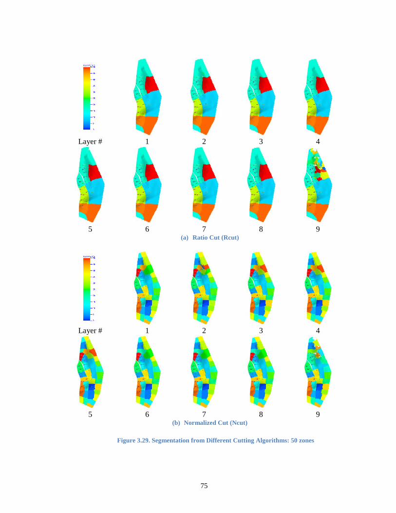
75
Layer # 1 2 3 4
5 6 7 8 9
(a) Ratio Cut (Rcut)
Layer # 1 2 3 4
5 6 7 8 9
(b) Normalized Cut (Ncut)
Figure 3.29. Segmentation from Different Cutting Algorithms: 50 zones
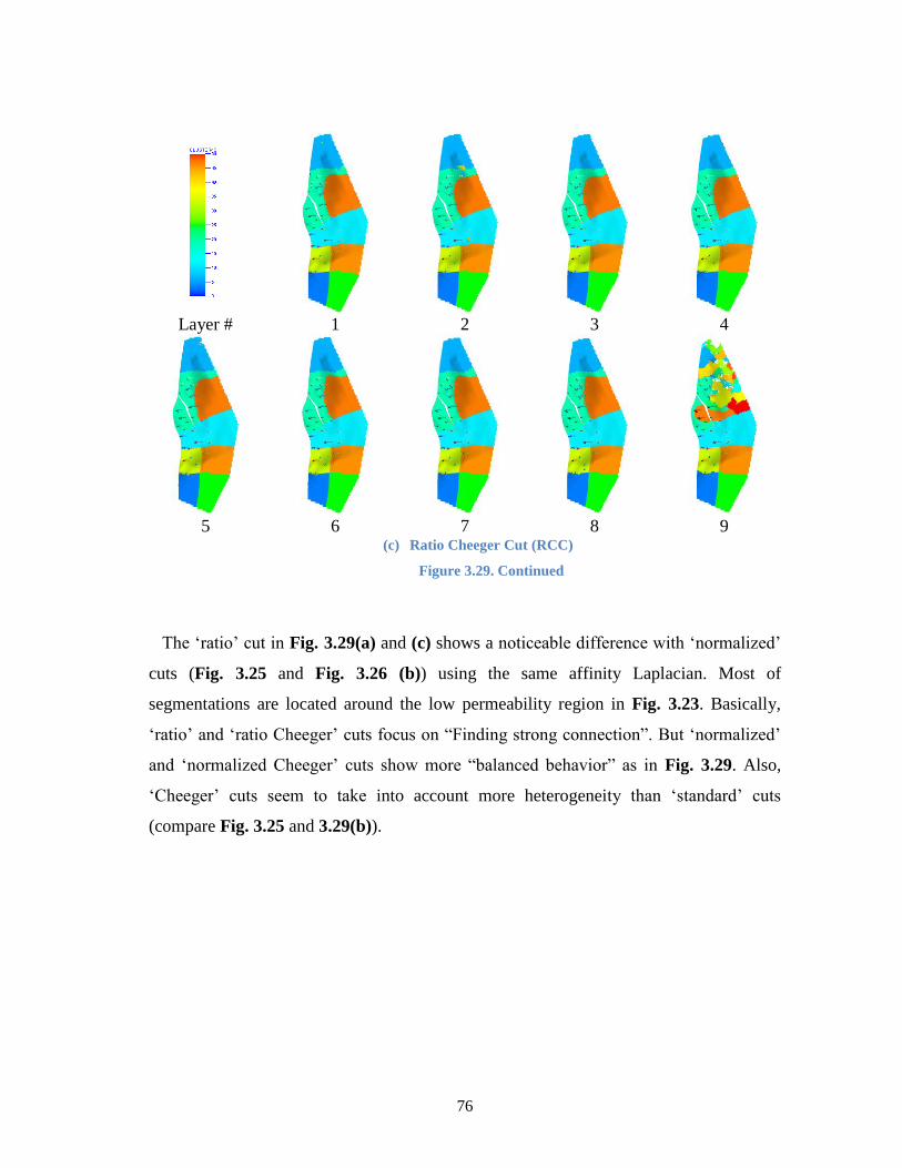
76
Layer # 1 2 3 4
5 6 7 8 9
(c) Ratio Cheeger Cut (RCC)
Figure 3.29. Continued
The ‘ratio’ cut in Fig. 3.29(a) and (c) shows a noticeable difference with ‘normalized’
cuts (Fig. 3.25 and Fig. 3.26 (b)) using the same affinity Laplacian. Most of
segmentations are located around the low permeability region in Fig. 3.23. Basically,
‘ratio’ and ‘ratio Cheeger’ cuts focus on “Finding strong connection”. But ‘normalized’
and ‘normalized Cheeger’ cuts show more “balanced behavior” as in Fig. 3.29. Also,
‘Cheeger’ cuts seem to take into account more heterogeneity than ‘standard’ cuts
(compare Fig. 3.25 and 3.29(b)).
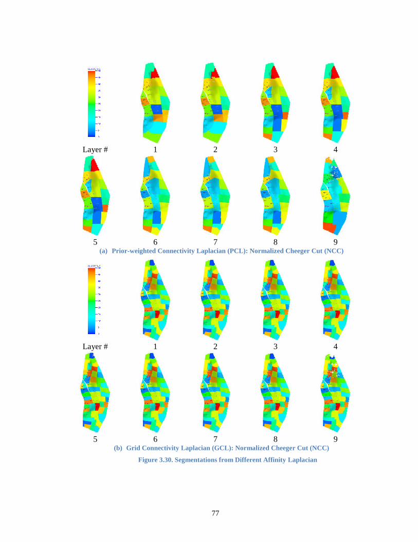
77
Layer # 1 2 3 4
5 6 7 8 9
(a) Prior-weighted Connectivity Laplacian (PCL): Normalized Cheeger Cut (NCC)
Layer # 1 2 3 4
5 6 7 8 9
(b) Grid Connectivity Laplacian (GCL): Normalized Cheeger Cut (NCC)
Figure 3.30. Segmentations from Different Affinity Laplacian
78
More interestingly in Fig. 3.30, the Prior-weight Connectivity Laplacian (PCL) is
showing features between ABL and GCL as expected (compare Fig. 3.25 and 3.30(b)).
But the Grid Connectivity Laplacian (GCL) shows less variability (almost constant) in z-
direction. Because the grid dimension of x (139) and y (48) directions are comparatively
bigger than the z direction (9), the grid connectivity is more dominant in the x-y plain.
3.7 Summary and Conclusions
We propose a new model segmentation technique from the spectral clustering theory.
The suggested approach is verified with both synthetic and the Brugge SPE benchmark
model. The new zonation algorithm provides more consistent criteria for history
matching compared to the common industry practice; box multipliers.
The procedure is to (1) construct Affinity Laplacian to capture spatial variability in
subsurface properties; (2) use graph partitioning techniques to create zonation and find
cutting edges; (3) apply partitioning with history matching algorithm. The graphic cut
from the model geometry and/or heterogeneity is not arbitrary but is satisfied by
optimization with graphic cutting metric.
1. The proposed zonation algorithm can preserve the major features of the prior
model after history matching because the generated zonation is based on the
model heterogeneity and/or connectivity information. We illustrate that spectral
clustering approach can potentially capture different facies in the reservoir.
2. We propose three different Affinity Laplacian constructions and four different
graph cutting algorithms. Basically, there is no ground truth in spectral
clustering. So, it is not possible to say which one is the best or the worst. But we
can arrive at some general conclusions from image clustering problems:
‘normalized’ cut is more statistically stable than ‘ratio’ cut. Also, ‘Cheeger’ cut
shows at least as good or better performance than ‘standard’ cut. Hence,
‘Normalized Cheeger Cut’ is a good starting point for segmentation.

79
3. The spectral clustering problem is a NP-hard and heuristic approach. As we
demonstrated, we can generate different cutting with combinations of Laplacian
and cutting algorithms. Even wider choices are available with free parameter and
cutting range. We inherited these properties in our proposed segmentation.
Hence, we require some initial experiments and experience with different
combination of cutting algorithms and Laplacian. Also, the two free parameters
and cut off range heavily impact the clustering.
4. Through human interventions and heuristics, the spectral clustering provides a
good guideline for automatic zonation criteria. This is more attractive when we
do hierarchical history matching; which is essential for history matching
problems for full-field model with decades of production history. We can adapt
this zonal concept for global stage history matching and then further calibrate
with fine scale approach.
80
CHAPTER IV
A HIERARCHAL MULTISCALE MODEL CALIBRATION WITH SPECTRAL
DOMAIN PARAMETERIZATION: APPLICATION TO A STRUCTURALLY
COMPLEX FRACTURED RESERVOIR
4.1 Purpose
A hierarchal history matching algorithm is proposed that sequentially calibrates
reservoir parameters from the global-to-local scale in consideration of parameter
uncertainty and the resolution of the data. Parameter updates are constrained to the prior
geologic heterogeneity and performed parsimoniously or only to the spatial scales at
which they can be resolved by the available data. In the first step of the workflow, a
genetic algorithm (GA) is used to assess the uncertainty in global parameters (i.e.,
regional permeability, pore volumes and aquifer strength) that influence field-scale flow
behavior, specifically reservoir energy. To identify the reservoir volume over which each
regional multiplier is applied, we have developed a novel approach to heterogeneity
segmentation from spectral clustering theory. The ensemble of model realizations
identified using GA, then reduced via cluster analysis to establish for the second stage of
local or high-resolution parameter calibration to well-level observation data. At this
stage we parameterize the high-resolution heterogeneity in the spectral domain using the
Grid Connectivity based Transform (GCT) to compress the dimension of the calibration
parameter set. At the same time, the GCT implicitly imposes geological continuity and
promotes minimal changes to each prior model in the ensemble during calibration.
We apply the proposed calibration workflow to a structurally complex and highly
fractured reservoir located offshore in Peru. The reservoir is modeled as dual porosity
and single permeability (DPSP). First, the field water and gas production are matched
using the GA with zonal multipliers for fracture porosity and shape factor (‘sigma’).
Next, well-by-well production history is matched by locally calibrating the most
uncertain fracture network property, fracture permeability distribution, which is reduced
using the GCT parameterization to improve the ill-posedness of the problem. The final
81
updated model is found to be geologically realistic and is being used for field
development strategies.
4.2 Introduction
Reservoir model calibration to field production data, commonly known as dynamic
data integration or history matching, is an essential component of successful field
development planning and optimization. The history matching of high-resolution
geological models is typically an ill-posed inverse problem because the numbers of
observed data are considerably less than the number of calibrated reservoir parameters,
which themselves are often strongly correlated. This leads to non-unique and potentially
unstable parameter solutions despite an acceptable history matching of the data.
However, if the history matching problem is structured relative to the resolution of the
data and appropriately constrained, then together with assisted history matching
algorithms a geologically consistent and close-to-optimal calibration solution can be
achieved. For this purpose, we propose a hierarchal history matching algorithm that is
constrained to the prior geologic heterogeneity and parsimoniously updates high
resolution geologic parameters to the level that they can be resolved by the available
data.
The hierarchal approach calibrates, in sequence, reservoir parameters that characterize
global-to-local regions while accounting for multiscale parameter uncertainty and the
resolution of the data. As the first component of the workflow, a history matching of the
coarse-scale genetic algorithm (GA) is applied to characterize the uncertainty in global
parameters including regional permeability, porosity and transfer function between
matrix and fracture, that influence field-scale flow behavior and reservoir energy. Rather
than using box-type or manually defined multiplier regions, we introduce a novel
method of model segmentation based on a spectral analysis of the reservoir grid
connectivity, which is an important key factor in reservoir flow dynamics. This zonal
segmentation technique assists in the definition of regional multiplier boundaries in
consideration of prior model heterogeneity and its connectivity. An eigenspectrum

82
analysis is then used to parse the ensemble of calibrated models resulting from the GA
analysis into a smaller set of prior models for the second stage of local or high resolution
parameter calibration to well observation data.
In this second workflow component, a heterogeneity parameterization technique is
used to characterize the high-resolution calibration parameters in a low-dimensional,
spectral transform domain using the Grid Connectivity-based Transform or GCT. This
compact representation of the model parameters implicitly imposes geologic continuity
and promotes minimal changes to each prior model during the calibration updates to
match well production data. The calibration of each prior model itself is performed using
an iterative least-squares method; therefore, each model is deterministically history
matched and parameter uncertainty is assessed from the ensemble of final models. To
improve the computational efficiency of this conceptual approach, the basis parameter
sensitivities at each model update steps are derived from a semi-analytical streamline
based formulation. Such that all sensitivities are computed via a single forward
simulation and streamline tracing.
The development of the proposed history matching workflow builds on the strengths
and limitations of more recent hierarchical approaches to the integration of dynamic data
into reservoir description, beginning with those based on a GA then local model
calibration. The genetic algorithm has many applications so far in reservoir history
matching. Schulze-Riegert et al. (2002) applied to complex history matching problem.
They applied genetic algorithm and arbitrary zonal multiplier for history matching.
Cheng et al. (2008) provide a robust flow chart for a structured history matching
approach listing dominant global and local parameters. They applied a GA for history
matching and determined probabilistic reservoir models using proxy models of history
match error for model filtering and optimization. Yin et al. (2010) applied a GA to
update global reservoir parameters, followed by a streamline-assisted history matching
of finer scale heterogeneity. (Bhark et al. 2011c) applied the GCT parameterization to
calibrate field-scale permeability trends (GCT) using a quasi-Newton method and then a
83
streamline-assisted calibration of local or grid-cell scale permeability at spatial scales
finer than the data could resolve using the global parameterization.
In this paper, a focus is placed on the calibration of fractured reservoirs. We
demonstrate that in addition to permeability and porosity heterogeneity, which are the
parameters typically calibrated in automatic history matching (AHM) workflows, that
the proposed methods of connectivity based segmentation and parameterization, applied
within a hierarchical approach, are applicable to fracture properties as well. The
characterization of fractured geologic properties has long been studied. Warren and Root
(1963) investigated flow behavior in naturally fractured reservoir models and defined
fracture flow with two parameters, the absolute permeability and the effective porosity.
They proved that with these two parameters, much of the fracture storage capacity and
matrix-fracture interaction could be represented. Massonnat et al. (2002) illustrated the
importance of characterizing the fracture network in a fractured carbonate reservoir.
They examined the connection from the fracture network to the flow network. Then they
conclude that fracture aperture distribution is a strong factor for assessing fracture
properties rather than fracture distribution. A more recent study by Jabbari and Zeng
(2011) suggest a third parameter description for fractured reservoirs; an elasticity
parameter similar to Poisson’s ratio and Young’s modulus should be included to account
for stress sensitive natural fracture system. They described fractured reservoir with
fracture storage capacity, matrix-fracture interaction and combined effect of both matrix
geomechanic and fracture apertures.
From these previous descriptions of fractured reservoirs, we define the fracture
parameters of interest for calibration; fracture porosity, fracture permeability and a shape
factor ( ) which characterizes matrix-fracture interface area per unit volume (Kazemi et
al. 1976). All of which are typically of large uncertainty in dual porosity finite difference
models. It should be noted that the analysis methods applied during the proposed
workflow are relevant to fractured reservoir modeling. Kang et al. (2011) investigated
the effect of natural and hydraulic fracture network for drainage volume calculation in
tight gas reservoir.
84
Previously, there have been several attempts to integrate dynamic data for fracture
characterization. Al-Huthali and Datta-Gupta (2004) presented a general dual porosity
and dual permeability formulation for streamline simulation in naturally fractured
reservoirs. They explained the domain flow mechanism in dual systems. Al-Harbi et al.
(2005) use the streamline sensitivity for fine scale Model Calibration in the fractured
reservoir. They used the streamline derived sensitivities in conjunction with a dual
porosity finite difference simulator for fine scale model update. They characterized the
fracture permeability based on streamline derived sensitivity in local grid.
In this paper, we focus on characterizing fracture properties in the complex structured
geometry with a hierarchical approach. To explain our approach, the mathematical
formulations, together with a hierarchical workflow are presented first. We then apply
the proposed calibration workflow to a highly complex and fractured reservoir field. The
field is modeled as dual porosity and single permeability (DPSP) and located offshore in
Peru. In this field example, the global dynamic data (total field water production) misfit
is successfully reduced at first along the field wise using the genetic algorithm (GA);
updating aquifer property, shape factor and fracture porosity with zonal multipliers.
Average reservoir pressures are also considered with observation data in this stage. The
well-by-well production history is then matched by calibration of the uncertain local
fracture properties; fracture permeability, which is updated using the GCT
parameterization and improved the ill-posedness of the problem.
4.3 Approach
This section explains the individual components of the proposed hierarchical workflow
from a conceptual viewpoint. The mathematical formulation behind each step is
presented in the following section. In brief summary, there are two primary hierarchical
components. The first uses a GA to calibrate the reservoir model at the global or coarse
scale using regional property multipliers, where region geometries are defined using a
novel model segmentation technique. Other global parameters, e.g., those that
characterize aquifer strength, are included in the calibration based on the outcome of a
85
parameter sensitivity analysis. These selected parameters are subsequently applied in an
experimental design for construction of a proxy model of the data misfit response
surface (Yin et al. 2010). The response proxy is required for reduction of the
computational expense of the GA-based calibration which executes inheritance,
selection, mutation and crossover of the parameters during their evolution or updating.
At termination of the GA an ensemble of globally calibrated reservoir models is defined,
so a cluster analysis is used to select a small subset that approximates the range of
variability of the complete set. In the second hierarchical component, each of the (now
prior) heterogeneity models from the first component is calibrated at the local scale. To
reduce the number of high-resolution parameters, they are compressed in a low-
dimensional transform domain in which the calibration is performed. The sensitivities of
the production data to the transform parameters, which drives a gradient-based inversion
approach, are efficiently computed using a streamline-based technique. The production
data misfit is accordingly characterized using the generalized travel time (GTT)
approach (Al-Huthali and Datta-Gupta 2004), which also exploits the efficiencies of a
streamline-base characterization of model heterogeneity as described below. The
combined approaches of spectral parameterization and GTT data misfit reduce the
dimensionality and non-linearity of the inversion, expediting data misfit reduction and
reducing the occurrence of local minimum convergence. These steps are now altogether
reviewed, referring to the field application as appropriate.
Initial Model Response and Parameter Sensitivity Analysis A proper history
matching workflow must start from a conceptual understanding of the prior
geologic model and its static and dynamic uncertainties. In the fractured field
model presented, the San Pedro field at offshore Peru, the primary uncertainties
are hydraulic continuity across the main faults, static and dynamic fracture
properties and aquifer strength. To understand the influence of these properties
on production behavior, particularly in the presence of complex flow geometries
and changing field conditions, we utilize two approaches. First, and more
86
qualitatively, we use streamline simulation to visualize and quantify fluid
movement. With individual phase streamlines, i.e., individually tracing water, oil
or gas flux trajectories as opposed to tracing the total fluid flux trajectories, the
individual phase production source and flow paths are easily identified. For
example, in the San Pedro modeling application, water phase streamlines are
used to identify the level of aquifer support, which is suspected to be strong,
from a source in the bottom layer of the reservoir model. Second, and more
quantitatively, we apply the complete set of global parameters in a sensitivity
analysis to identify the ‘heavy hitters’ that are to be applied in the first step of the
hierarchical calibration. The sensitivity analysis is efficiently computed using an
analytical proxy of the production data misfit surface, which itself is constructed
via an experimental design with a proficient Latin hypercube sampling.
Model Segmentation from Spectral Clustering To characterize static
heterogeneity related to fracture properties for the global calibration, a novel
model segmentation technique based on the theory of graph partitioning is
applied to identify regional multiplier domains over the complete grid volume.
These regions rely on the grid geometry structure to indicate a natural
partitioning rather than applying traditional box-type multiplier regions. When
the grid geometry, relative to its cell connectivity structure, is characterized in a
specific Laplacian operator or matrix, then the eigenvector corresponding to the
second smallest (non-zero) eigenvalue represents the grid grouping based on
heterogeneity and connectivity. This eigenvector, in turn, can be applied in a
spectral clustering algorithm to partition the domain (Pothen et al. 1990). We
take advantage of this property and propose an optimal model zonation for
history matching relative to a graph cut metric, which quantifies any piecewise
continuous partitioning of the grid cells. In this field application, we apply the
graphic “normalized cut” for model segmentation.
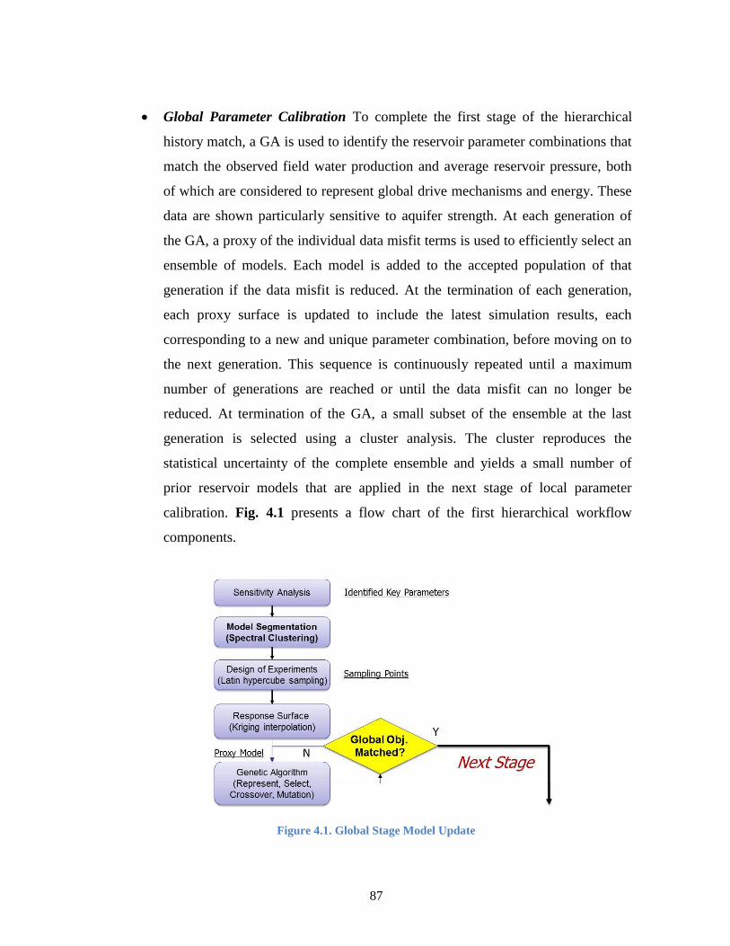
87
Global Parameter Calibration To complete the first stage of the hierarchical
history match, a GA is used to identify the reservoir parameter combinations that
match the observed field water production and average reservoir pressure, both
of which are considered to represent global drive mechanisms and energy. These
data are shown particularly sensitive to aquifer strength. At each generation of
the GA, a proxy of the individual data misfit terms is used to efficiently select an
ensemble of models. Each model is added to the accepted population of that
generation if the data misfit is reduced. At the termination of each generation,
each proxy surface is updated to include the latest simulation results, each
corresponding to a new and unique parameter combination, before moving on to
the next generation. This sequence is continuously repeated until a maximum
number of generations are reached or until the data misfit can no longer be
reduced. At termination of the GA, a small subset of the ensemble at the last
generation is selected using a cluster analysis. The cluster reproduces the
statistical uncertainty of the complete ensemble and yields a small number of
prior reservoir models that are applied in the next stage of local parameter
calibration. Fig. 4.1 presents a flow chart of the first hierarchical workflow
components.
Figure 4.1. Global Stage Model Update
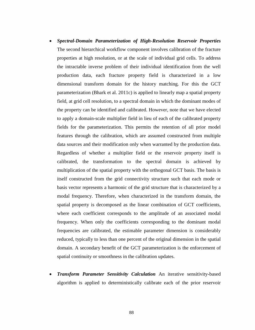
88
Spectral-Domain Parameterization of High-Resolution Reservoir Properties
The second hierarchical workflow component involves calibration of the fracture
properties at high resolution, or at the scale of individual grid cells. To address
the intractable inverse problem of their individual identification from the well
production data, each fracture property field is characterized in a low
dimensional transform domain for the history matching. For this the GCT
parameterization (Bhark et al. 2011c) is applied to linearly map a spatial property
field, at grid cell resolution, to a spectral domain in which the dominant modes of
the property can be identified and calibrated. However, note that we have elected
to apply a domain-scale multiplier field in lieu of each of the calibrated property
fields for the parameterization. This permits the retention of all prior model
features through the calibration, which are assumed constructed from multiple
data sources and their modification only when warranted by the production data.
Regardless of whether a multiplier field or the reservoir property itself is
calibrated, the transformation to the spectral domain is achieved by
multiplication of the spatial property with the orthogonal GCT basis. The basis is
itself constructed from the grid connectivity structure such that each mode or
basis vector represents a harmonic of the grid structure that is characterized by a
modal frequency. Therefore, when characterized in the transform domain, the
spatial property is decomposed as the linear combination of GCT coefficients,
where each coefficient corresponds to the amplitude of an associated modal
frequency. When only the coefficients corresponding to the dominant modal
frequencies are calibrated, the estimable parameter dimension is considerably
reduced, typically to less than one percent of the original dimension in the spatial
domain. A secondary benefit of the GCT parameterization is the enforcement of
spatial continuity or smoothness in the calibration updates.
Transform Parameter Sensitivity Calculation An iterative sensitivity-based
algorithm is applied to deterministically calibrate each of the prior reservoir
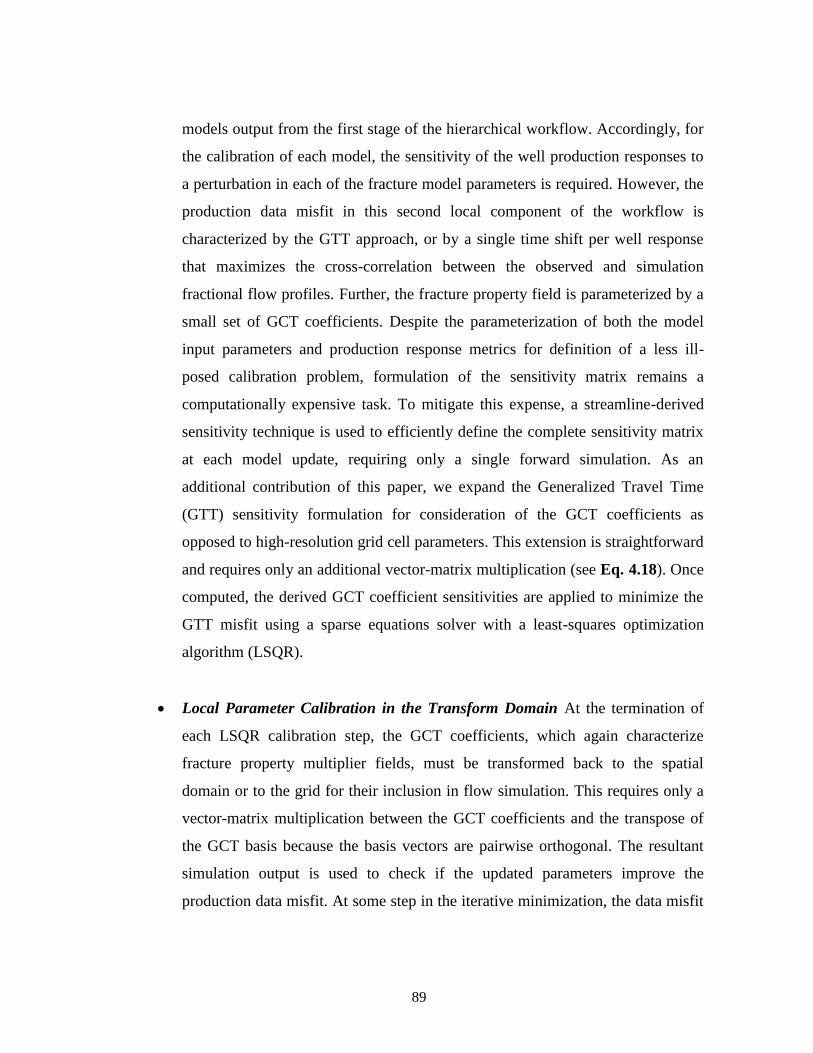
89
models output from the first stage of the hierarchical workflow. Accordingly, for
the calibration of each model, the sensitivity of the well production responses to
a perturbation in each of the fracture model parameters is required. However, the
production data misfit in this second local component of the workflow is
characterized by the GTT approach, or by a single time shift per well response
that maximizes the cross-correlation between the observed and simulation
fractional flow profiles. Further, the fracture property field is parameterized by a
small set of GCT coefficients. Despite the parameterization of both the model
input parameters and production response metrics for definition of a less ill-
posed calibration problem, formulation of the sensitivity matrix remains a
computationally expensive task. To mitigate this expense, a streamline-derived
sensitivity technique is used to efficiently define the complete sensitivity matrix
at each model update, requiring only a single forward simulation. As an
additional contribution of this paper, we expand the Generalized Travel Time
(GTT) sensitivity formulation for consideration of the GCT coefficients as
opposed to high-resolution grid cell parameters. This extension is straightforward
and requires only an additional vector-matrix multiplication (see Eq. 4.18). Once
computed, the derived GCT coefficient sensitivities are applied to minimize the
GTT misfit using a sparse equations solver with a least-squares optimization
algorithm (LSQR).
Local Parameter Calibration in the Transform Domain At the termination of
each LSQR calibration step, the GCT coefficients, which again characterize
fracture property multiplier fields, must be transformed back to the spatial
domain or to the grid for their inclusion in flow simulation. This requires only a
vector-matrix multiplication between the GCT coefficients and the transpose of
the GCT basis because the basis vectors are pairwise orthogonal. The resultant
simulation output is used to check if the updated parameters improve the
production data misfit. At some step in the iterative minimization, the data misfit
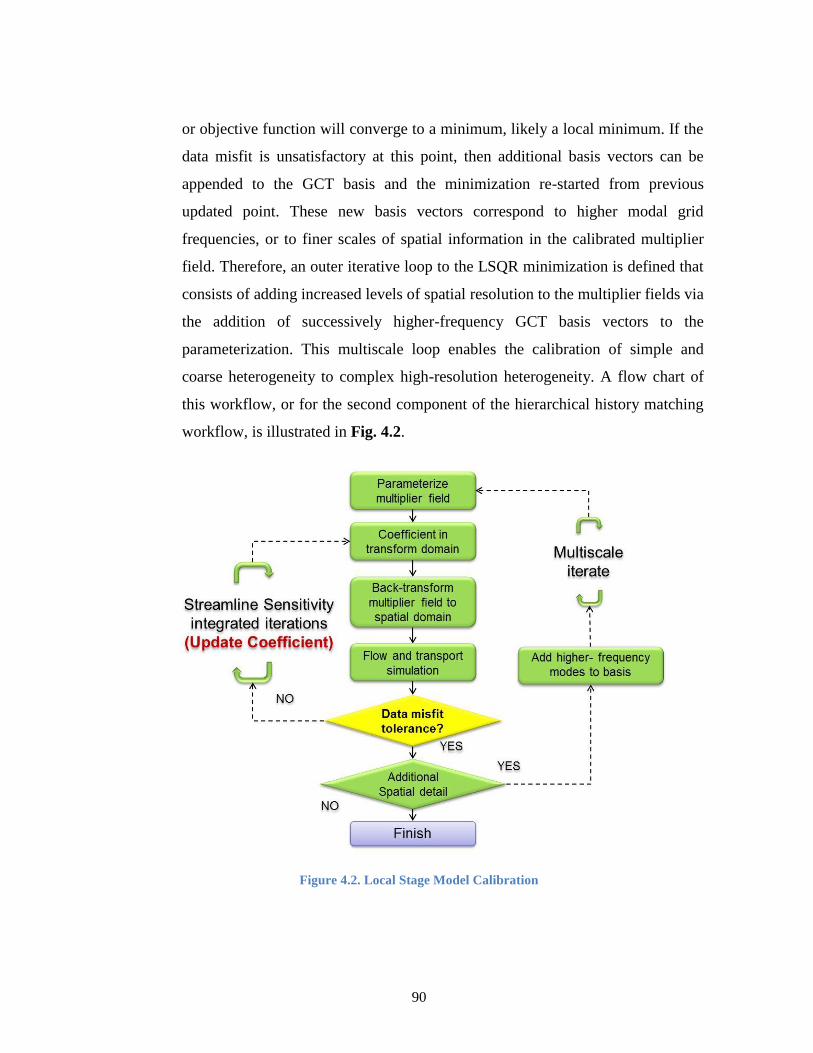
90
or objective function will converge to a minimum, likely a local minimum. If the
data misfit is unsatisfactory at this point, then additional basis vectors can be
appended to the GCT basis and the minimization re-started from previous
updated point. These new basis vectors correspond to higher modal grid
frequencies, or to finer scales of spatial information in the calibrated multiplier
field. Therefore, an outer iterative loop to the LSQR minimization is defined that
consists of adding increased levels of spatial resolution to the multiplier fields via
the addition of successively higher-frequency GCT basis vectors to the
parameterization. This multiscale loop enables the calibration of simple and
coarse heterogeneity to complex high-resolution heterogeneity. A flow chart of
this workflow, or for the second component of the hierarchical history matching
workflow, is illustrated in Fig. 4.2.
Figure 4.2. Local Stage Model Calibration
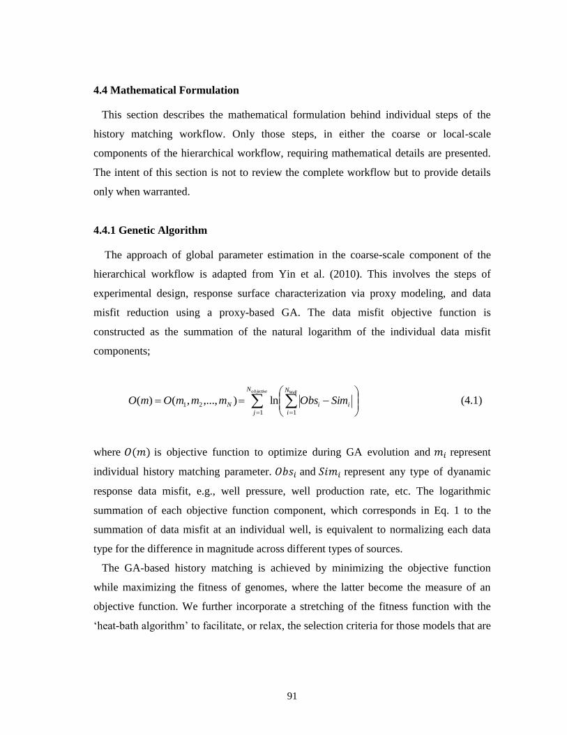
91
4.4 Mathematical Formulation
This section describes the mathematical formulation behind individual steps of the
history matching workflow. Only those steps, in either the coarse or local-scale
components of the hierarchical workflow, requiring mathematical details are presented.
The intent of this section is not to review the complete workflow but to provide details
only when warranted.
4.4.1 Genetic Algorithm
The approach of global parameter estimation in the coarse-scale component of the
hierarchical workflow is adapted from Yin et al. (2010). This involves the steps of
experimental design, response surface characterization via proxy modeling, and data
misfit reduction using a proxy-based GA. The data misfit objective function is
constructed as the summation of the natural logarithm of the individual data misfit
components;
objective WellN
j
N
i
iiN SimObsmmmOmO1 1
21 ln),...,,()( (4.1)
where is objective function to optimize during GA evolution and represent
individual history matching parameter. and represent any type of dyanamic
response data misfit, e.g., well pressure, well production rate, etc. The logarithmic
summation of each objective function component, which corresponds in Eq. 1 to the
summation of data misfit at an individual well, is equivalent to normalizing each data
type for the difference in magnitude across different types of sources.
The GA-based history matching is achieved by minimizing the objective function
while maximizing the fitness of genomes, where the latter become the measure of an
objective function. We further incorporate a stretching of the fitness function with the
‘heat-bath algorithm’ to facilitate, or relax, the selection criteria for those models that are

92
passed on to the next generation (Sen et al. 1995). The selection probability of an
individual model is given by
i
ni
nii
Tmf
TmfmP
/)(exp
)/)(exp()( (4.2)
In Eq. 4.2, is the objective function of model that is to be minimized by
maximizing fitness and is a control parameter that corresponds to
temperature in simulated annealing (SA). The heat-bath algorithm accelerates
convergence and requires fewer simulations for reduction of the objective function, both
of which properties are important to reduce the large computational expense of the GA,
particularly with field-scale models (Yin et al. 2010).
4.4.2 Connectivity Based Graph Laplacian
The spectral graph G is defined as a set of data set in a domain with
vertex and edges E, that is connectivity between and . The
graph Laplacian L is used to calculate the number and connected strength of a given
graph G. The graph Laplacian is constructed simply as , where is the
grid weighted adjacency matrix and is the degree matrix in Eq. 4.4. For an N number
of data set, is the matrix constructed as Eq. 4.3;
otherwise
gneighborinifwij
0
1 (4.3)
and the entry of degree matrix , defined as diagonal matrix, equal to the degree of each
corresponding vertex.

93
N
j
iji wd1
(4.4)
Such that each non-zero diagonal element of D is equal to the row sum of W.
Accordingly, the Laplacian is constructed only once, prior to the history matching
workflow, using grid connectivity information and is independent of the prior parameter
heterogeneity. Fig. 4.3 depicts the two-point connectivity structure, corresponding to a
5-point stencil in two dimensions, used to define Laplacian L. The graph Laplacian must
represent ‘connected’ graph G, which means all the data should have at least one
connectivity to the rest.
otherwise
ji
w
dL
ij
i
ji, (4.5)
Figure 4.3. Construction of Connectivity Laplacian
The same graph Laplacian will be used for global and local scale update; clustering for
global and reparameterization for local update. Note that the clustering in the global
stage will do spatial grouping based on ‘second eigenvector’ of Laplacian (von Luxburg
2007) and the reparameterization is to transform history matching parameters into
frequency domain with ‘leading eigenvectors’. This is important to understand that we
can use the same graph Laplacian for different stage of hierarchical history matching.
How it is possible? The leading eigenvectors of graph Laplacian, corresponding from
lowest eigenvalues, represent the dominant eigenspectrum of a system (Bhark et al.
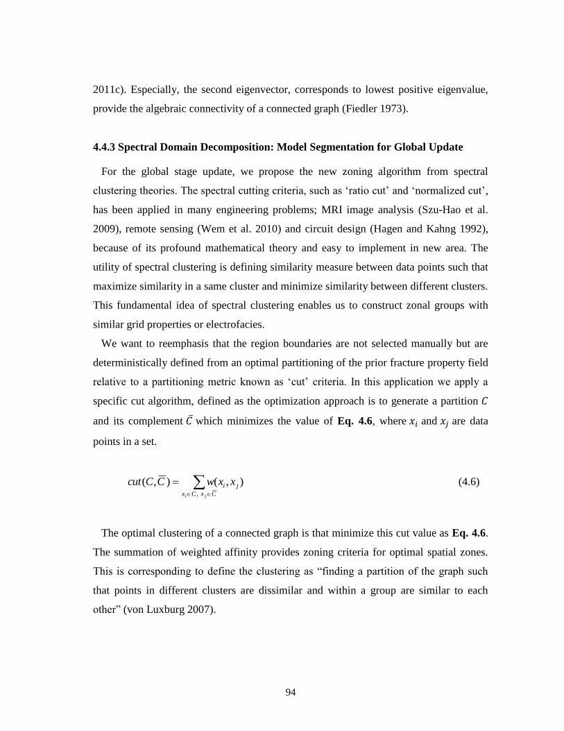
94
2011c). Especially, the second eigenvector, corresponds to lowest positive eigenvalue,
provide the algebraic connectivity of a connected graph (Fiedler 1973).
4.4.3 Spectral Domain Decomposition: Model Segmentation for Global Update
For the global stage update, we propose the new zoning algorithm from spectral
clustering theories. The spectral cutting criteria, such as ‘ratio cut’ and ‘normalized cut’,
has been applied in many engineering problems; MRI image analysis (Szu-Hao et al.
2009), remote sensing (Wem et al. 2010) and circuit design (Hagen and Kahng 1992),
because of its profound mathematical theory and easy to implement in new area. The
utility of spectral clustering is defining similarity measure between data points such that
maximize similarity in a same cluster and minimize similarity between different clusters.
This fundamental idea of spectral clustering enables us to construct zonal groups with
similar grid properties or electrofacies.
We want to reemphasis that the region boundaries are not selected manually but are
deterministically defined from an optimal partitioning of the prior fracture property field
relative to a partitioning metric known as ‘cut’ criteria. In this application we apply a
specific cut algorithm, defined as the optimization approach is to generate a partition
and its complement ̅ which minimizes the value of Eq. 4.6, where and are data
points in a set.
CxCx
ji
ji
xxwCCcut,
),(),( (4.6)
The optimal clustering of a connected graph is that minimize this cut value as Eq. 4.6.
The summation of weighted affinity provides zoning criteria for optimal spatial zones.
This is corresponding to define the clustering as “finding a partition of the graph such
that points in different clusters are dissimilar and within a group are similar to each
other” (von Luxburg 2007).

95
Now, how we find the optimal value? This is related to clustering algorithms. We
suggest a novel ‘ratio cut’ and ‘normalized cut’ partitioning for balanced clustering in
the zonation of a reservoir model. In fact, there are many clustering algorithm but most
of them are based on those two clustering idea. Before we explain algorithms, we need
to define two different ways to measure the size of a subcluster in Eq. 4.7.
CsubclusterinaffinityweightedofsumtheCvol
CsubclusterinverticesofnumbertheC
:
:
(4.7)
The minimum of Ratio Cut is shown to define the optimal partitioning of the data
characterized by the affinity matrix (Hagen and Kahng 1992). The ratio cut is clustering
based on number of vertices;
C
CCcut
C
CCcutCCRcut
),(),(),( (4.8)
In Eq. 4.8, the optimal partitioning identifies regions that have maximum similarity
within regions (numerator) balanced by the condition of equal size or number of data
(denominator) (von Luxburg 2007). In easy speaking, if we have a data set with size of
n, we can minimize (ratio cut measure) by equally dividing with n/2.
Shi and Malik (2000) proposed a new partition criteria, ‘normalized cut’, for
measuring the goodness of an image partitioning. The normalized cut is measured by the
weight of its edges. This cut measure is minimized by equal weighting. The main
difference between ‘ratio’ cut and ‘normalized’ cut is using un-normalized Laplacian for
ratio cut and normalized cut use normalized Laplacian (von Luxburg 2007).
)(
),(
)(
),(),(
Cvol
CCcut
Cvol
CCcutCCNcut (4.9)
96
The ‘normalized cut’ leads to normalized spectral clustering, which is statistically
stable, while relaxing ‘ratio cut’ leads to unnormalized spectral clustering. These two
spectral clustering algorithms provide ‘balanced’ cutting criteria even in complex
geometry, regarded as connected graph.
The approximate solution to the minimization of cut, or alternatively to the minimum
of the Rayleigh quotient (solve eigenvalue problem with iterative approximation), is
achieved by the eigen decomposition of the affinity Laplacian L. In the form of Eq. 4.5
is always positive semi-definite and, therefore, has real non-negative eigenvalues with a
smallest eigenvalue always equal to zero (von Luxburg 2007). The zero eigenvalue
corresponds to a constant eigenvector, and then the next eigenvector corresponding to
the second eigenvalue indicates an optimal partitioning of the heterogeneity information
embedded in L. If mapped onto the simulation grid, the second eigenvector depicts
spatial features, potentially including edge information, related to similar and dissimilar
regions of the prior model, where again the term ‘similar’ is defined relative to the
adjacency graph metric in Eq. 4.3.
4.4.4 Reparameterization for Local Update
The parameterization of high-resolution reservoir properties, or in this application
fracture properties defined at each grid cell, is performed using the Grid Connectivity-
based Transform or GCT (Bhark et al. 2011c) in Eq. 4.5. As described, a spatial fracture
property field is mapped to a spectral domain via the GCT basis vectors, each of which
corresponds to a modal shape of the grid structure and is associated with a modal
frequency. Several such basis vectors are shown mapped onto the grid in the application
below. The basis in its entirety is constructed as a subset of the eigenvectors of a grid
connectivity matrix, which has the form of a Laplacian operator, which characterizes
two-point grid cell connectivity over the domain that is to be parameterized.
Note that the basis functions are pairwise orthogonal to each other. This
orthogonality permits inclusion of additional fine scale variation into the multiplier field.

97
Initially, all basis coefficients except first have zero value from Eq. 4.10. So, first basis
vector contributes to calibrating field average and others to local distributions.
G
T mv (4.10)
where spatial parameter (grid properties) is the n 1 vector depicting the spatial
property at n grid cells, is the n m GCT basis where the number of basis vectors m
<< n and v is the m 1 vector of GCT coefficients that are the calibration parameters.
Because the basis vectors are pairwise orthogonal to each other, a refinement of the
parameterization by the addition of higher-frequency basis vectors (or by the addition of
finer-scale variation into the field) is achieved simply by appending the corresponding
to . After updating of the components of v during each iterate of the sensitivity-
based minimization, described next, the pairwise orthogonality of also enables an
efficient transformation of the GCT coefficient back to the spatial domain as;
vmG (4.11)
This step is required to apply the updated field in simulation. Finally, it is reiterated
that we elect not to parameterize and calibrate a fracture property field itself, but rather
to apply a parameterized multiplier field so that the prior information at its initial high-
resolution will not be degraded (Bhark et al. 2011b). Notating this prior model as ,
the parameterization is posed as;
vmm GG 0, (4.12)
where the multiplication operator )( is the entry wise product of each component. That
is, the fracture heterogeneity field applied in simulation is computed as the entry wise
product of the prior model and the calibrated multiplier field .
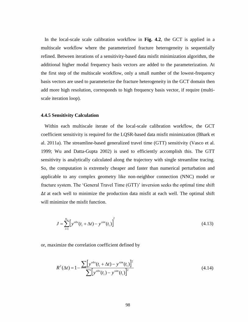
98
In the local-scale scale calibration workflow in Fig. 4.2, the GCT is applied in a
multiscale workflow where the parameterized fracture heterogeneity is sequentially
refined. Between iterations of a sensitivity-based data misfit minimization algorithm, the
additional higher modal frequency basis vectors are added to the parameterization. At
the first step of the multiscale workflow, only a small number of the lowest-frequency
basis vectors are used to parameterize the fracture heterogeneity in the GCT domain then
add more high resolution, corresponds to high frequency basis vector, if require (multi-
scale iteration loop).
4.4.5 Sensitivity Calculation
Within each multiscale iterate of the local-scale calibration workflow, the GCT
coefficient sensitivity is required for the LQSR-based data misfit minimization (Bhark et
al. 2011a). The streamline-based generalized travel time (GTT) sensitivity (Vasco et al.
1999; Wu and Datta-Gupta 2002) is used to efficiently accomplish this. The GTT
sensitivity is analytically calculated along the trajectory with single streamline tracing.
So, the computation is extremely cheaper and faster than numerical perturbation and
applicable to any complex geometry like non-neighbor connection (NNC) model or
fracture system. The ‘General Travel Time (GTT)’ inversion seeks the optimal time shift
at each well to minimize the production data misfit at each well. The optimal shift
will minimize the misfit function.
2
1
)()(
dN
i
i
sim
i
obs tyttyJ (4.13)
or, maximize the correlation coefficient defined by
2
2
2
)()(
)()(1)(
i
sim
i
obs
i
sim
i
obs
tyty
tyttytR (4.14)

99
In the dual-porosity system, the fluid flow is assumed to occur primarily through the
high permeability fracture network system and matrixes are acting as storages. So, the
streamline sensitivities are calculated by the streamline tracing along the fracture system
(Al-Harbi et al. 2005). The water cut arrival time ( ) or streamline time of flight ( )
sensitivity with respect to the fracture permeability will be calculated by
w
w
Gw
w
GG S
fdx
m
xs
S
f
mm
t/
)(/
(4.15)
Here, is ‘slowness’ which is reciprocal of interstitial velocity and integral are
evaluated along the trajectory (Vasco et al. 1999). The model parameter is linear
combination of coefficient weighted basis function and from basis orthogonality;
i
ii
G
v
v
v
m
(4.16)
or by using multiplier field from Eq. 4.12;
iG
i
G
i
G mv
vm
v
m
0,
0,
(4.17)
The calculated streamline GTT sensitivity is utilized for the basis coefficient
sensitivity from expansion;
i
Gi
G
Gi m
t
v
m
m
t
v
t
or iG
Gi
mm
t
v
t0,
(4.18)
Simply, the basis coefficient sensitive is derived from streamline general travel time
(GTT) sensitivity by multiplying basis vector as in Eq. 4.18. Also, adjoint sensitivity
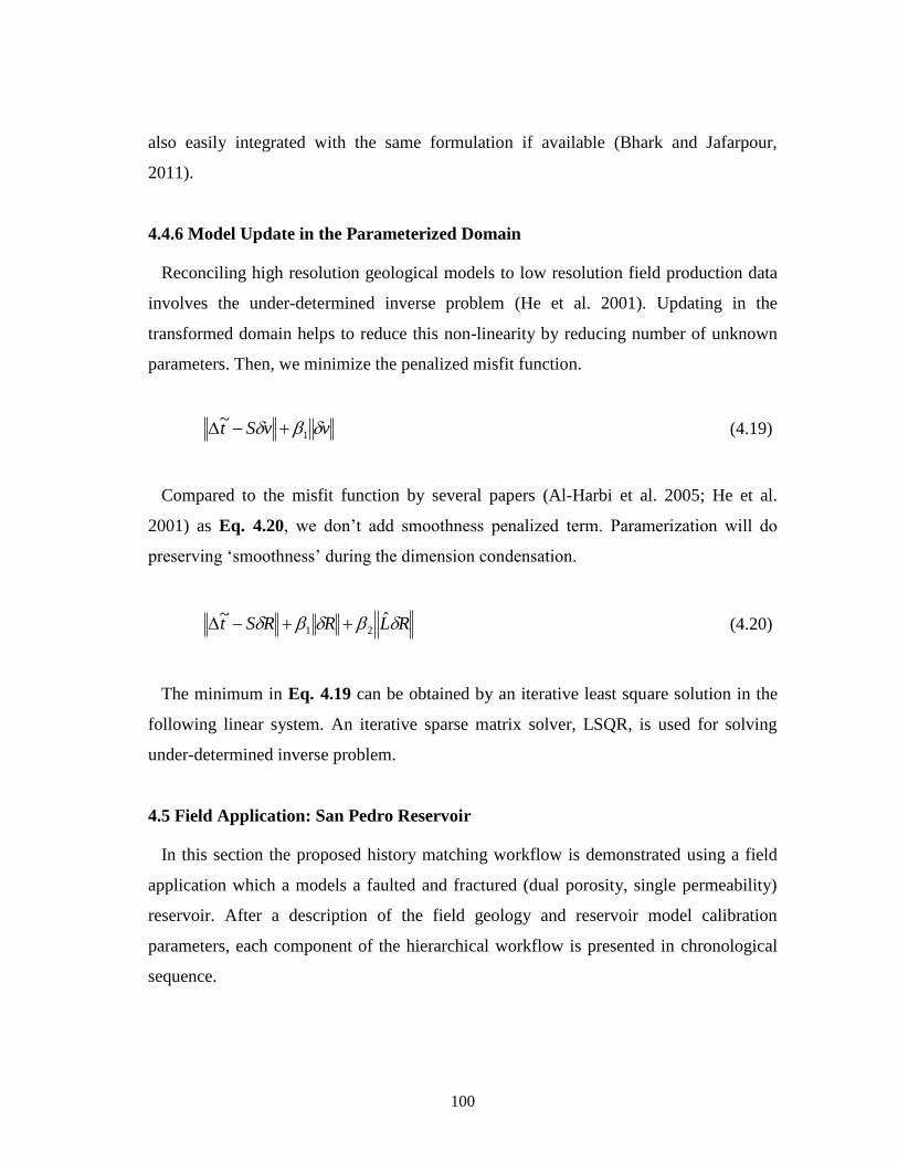
100
also easily integrated with the same formulation if available (Bhark and Jafarpour,
2011).
4.4.6 Model Update in the Parameterized Domain
Reconciling high resolution geological models to low resolution field production data
involves the under-determined inverse problem (He et al. 2001). Updating in the
transformed domain helps to reduce this non-linearity by reducing number of unknown
parameters. Then, we minimize the penalized misfit function.
vvSt 1
~ (4.19)
Compared to the misfit function by several papers (Al-Harbi et al. 2005; He et al.
2001) as Eq. 4.20, we don’t add smoothness penalized term. Paramerization will do
preserving ‘smoothness’ during the dimension condensation.
RLRRSt ˆ~21 (4.20)
The minimum in Eq. 4.19 can be obtained by an iterative least square solution in the
following linear system. An iterative sparse matrix solver, LSQR, is used for solving
under-determined inverse problem.
4.5 Field Application: San Pedro Reservoir
In this section the proposed history matching workflow is demonstrated using a field
application which a models a faulted and fractured (dual porosity, single permeability)
reservoir. After a description of the field geology and reservoir model calibration
parameters, each component of the hierarchical workflow is presented in chronological
sequence.
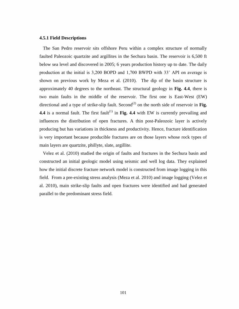
101
4.5.1 Field Descriptions
The San Pedro reservoir sits offshore Peru within a complex structure of normally
faulted Paleozoic quartzite and argillites in the Sechura basin. The reservoir is 6,500 ft
below sea level and discovered in 2005; 6 years production history up to date. The daily
production at the initial is 3,200 BOPD and 1,700 BWPD with 33˚ API on average is
shown on previous work by Meza et al. (2010). The dip of the basin structure is
approximately 40 degrees to the northeast. The structural geology in Fig. 4.4, there is
two main faults in the middle of the reservoir. The first one is East-West (EW)
directional and a type of strike-slip fault. Second(2)
on the north side of reservoir in Fig.
4.4 is a normal fault. The first fault(1)
in Fig. 4.4 with EW is currently prevailing and
influences the distribution of open fractures. A thin post-Paleozoic layer is actively
producing but has variations in thickness and productivity. Hence, fracture identification
is very important because producible fractures are on those layers whose rock types of
main layers are quartzite, phillyte, slate, argillite.
Velez et al. (2010) studied the origin of faults and fractures in the Sechura basin and
constructed an initial geologic model using seismic and well log data. They explained
how the initial discrete fracture network model is constructed from image logging in this
field. From a pre-existing stress analysis (Meza et al. 2010) and image logging (Velez et
al. 2010), main strike-slip faults and open fractures were identified and had generated
parallel to the predominant stress field.
102
Figure 4.4. (a) Configuration of well and faults (b) geological Model
From a seismic survey, the oil-water contact (OWC) is defined at 7,174 ft and the gas-
water contact (GWC) at 6,460 ft as shown in Fig. 4.5. Strong aquifer support from the
base of reservoir is inferred from pressure observations, although the size and strength of
the aquifer are highly uncertain. Initial pressure at the reservoir top level is 2,983 psi and
average pressure gradient is 0.35 psi/ft. The estimated bubble point pressure is 3,012 psi
from the PVT lab test.
Figure 4.5. Typical Well Section and OWC / GWC level
The San Pedro field has 18 production wells and 1 gas injection well are tied back to
two platforms up to date. Meza et al. (2010) determined that the well productivity
-7400
-740
0
-7300
-7200
-7000
-7100
-6900
-7200
-7100
-6800
-7300
-7000
-6700
-6900
-6900
-6600
-6700
-6800
-6800
-6500
-6600
-6400
-6300
-6700
-620
0
-610
0
-6600
-6000
-6500
-7100
-700
0
-7000
-6400
-62
00
-640
0-6
500
-6800
-6600
-6700
-680
0
-6900
-6900
-7100
-690
0
-7100
-7200
-7200
-7300
-7400 -7500
-7400
-7300
-7200
-7100
-7000 -6900 -6800
-6700
-6500
-6400 -6300
-6200-7
400
-7300
-720
0
-710
0
-7200 -7
300
-7400
-7500
-7700
-7800
-7600
-7900 -8000
-7800
-8100 -8
200
-7600
-7500
-7400
-7300-7200
-7100-7500
-7000
-6900
-6800
-6800
-6700
-6800
SP1-11D
SP1-1XSP1-1XST
SP1-2D
SP1-3CD
SP1-5X
SP1-6DSP1-7D
SP1-8DSP1-10D
SP1-4D
SP1-9DST
SP1-12DSP1A-1D
SP1A-2D
SP1A-3D
SP1A-4D
SP1A-6D
SP1A-8DBP
New SP1A-7D Proposal
SP1-9D
488400 488800 489200 489600 490000 490400 490800 491200 491600 492000 492400 492800
488400 488800 489200 489600 490000 490400 490800 491200 491600 492000 492400 492800
9380800
9381200
9381600
9382000
9382400
9382800
9383200
9383600
9384000
9380800
9381200
9381600
9382000
9382400
9382800
9383200
9383600
9384000
0 200 400 600 800 1000m
-7800
-7200
-6600
-6000
Depth
(1)
(2)
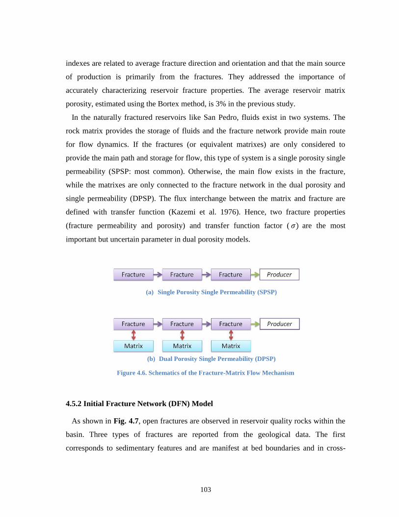
103
indexes are related to average fracture direction and orientation and that the main source
of production is primarily from the fractures. They addressed the importance of
accurately characterizing reservoir fracture properties. The average reservoir matrix
porosity, estimated using the Bortex method, is 3% in the previous study.
In the naturally fractured reservoirs like San Pedro, fluids exist in two systems. The
rock matrix provides the storage of fluids and the fracture network provide main route
for flow dynamics. If the fractures (or equivalent matrixes) are only considered to
provide the main path and storage for flow, this type of system is a single porosity single
permeability (SPSP: most common). Otherwise, the main flow exists in the fracture,
while the matrixes are only connected to the fracture network in the dual porosity and
single permeability (DPSP). The flux interchange between the matrix and fracture are
defined with transfer function (Kazemi et al. 1976). Hence, two fracture properties
(fracture permeability and porosity) and transfer function factor ( are the most
important but uncertain parameter in dual porosity models.
(a) Single Porosity Single Permeability (SPSP)
(b) Dual Porosity Single Permeability (DPSP)
Figure 4.6. Schematics of the Fracture-Matrix Flow Mechanism
4.5.2 Initial Fracture Network (DFN) Model
As shown in Fig. 4.7, open fractures are observed in reservoir quality rocks within the
basin. Three types of fractures are reported from the geological data. The first
corresponds to sedimentary features and are manifest at bed boundaries and in cross-
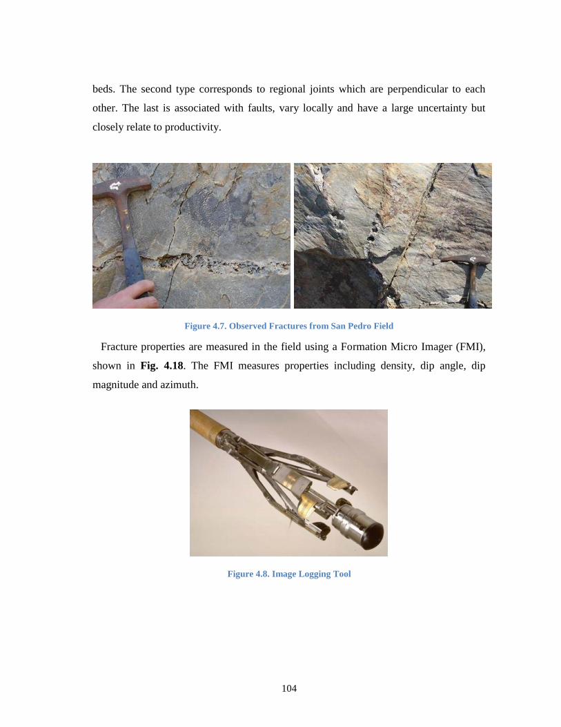
104
beds. The second type corresponds to regional joints which are perpendicular to each
other. The last is associated with faults, vary locally and have a large uncertainty but
closely relate to productivity.
Figure 4.7. Observed Fractures from San Pedro Field
Fracture properties are measured in the field using a Formation Micro Imager (FMI),
shown in Fig. 4.18. The FMI measures properties including density, dip angle, dip
magnitude and azimuth.
Figure 4.8. Image Logging Tool
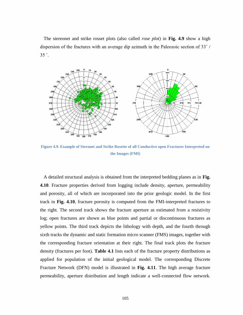
105
The stereonet and strike rosset plots (also called rose plot) in Fig. 4.9 show a high
dispersion of the fractures with an average dip azimuth in the Paleozoic section of 33˚ /
35 ˚.
Figure 4.9. Example of Steronet and Strike Rosette of all Conductive open Fractures Interpreted on
the Images (FMI)
A detailed structural analysis is obtained from the interpreted bedding planes as in Fig.
4.10. Fracture properties derived from logging include density, aperture, permeability
and porosity, all of which are incorporated into the prior geologic model. In the first
track in Fig. 4.10, fracture porosity is computed from the FMI-interpreted fractures to
the right. The second track shows the fracture aperture as estimated from a resistivity
log; open fractures are shown as blue points and partial or discontinuous fractures as
yellow points. The third track depicts the lithology with depth, and the fourth through
sixth tracks the dynamic and static formation micro scanner (FMS) images, together with
the corresponding fracture orientation at their right. The final track plots the fracture
density (fractures per foot). Table 4.1 lists each of the fracture property distributions as
applied for population of the initial geological model. The corresponding Discrete
Fracture Network (DFN) model is illustrated in Fig. 4.11. The high average fracture
permeability, aperture distribution and length indicate a well-connected flow network.
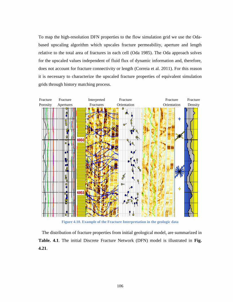
106
To map the high-resolution DFN properties to the flow simulation grid we use the Oda-
based upscaling algorithm which upscales fracture permeability, aperture and length
relative to the total area of fractures in each cell (Oda 1985). The Oda approach solves
for the upscaled values independent of fluid flux of dynamic information and, therefore,
does not account for fracture connectivity or length (Correia et al. 2011). For this reason
it is necessary to characterize the upscaled fracture properties of equivalent simulation
grids through history matching process.
Fracture
Porosity
Fracture
Apertures
Interpreted
Fractures
Fracture
Orientation
Fracture
Orientation
Fracture
Density
Figure 4.10. Example of the Fracture Interpretation in the geologic data
The distribution of fracture properties from initial geological model, are summarized in
Table. 4.1. The initial Discrete Fracture Network (DFN) model is illustrated in Fig.
4.21.

107
Table 4.1. Fracture Properties
Fracture
Properties Unit Min Max Mean
Standard
Deviation
Permeability md 33.3 1.74E+7 2.19E+6 3.5E+6
Aperture ft. 2.07E-6 1.50E-3 3.98E-4 3.5E-4
Length ft. 5.47 5.0E+2 2.21E+2 1.2E+2
Surface Area 6.01 1.25E+5 2.78E+4 2.8E+4
Dip deg 1.73 90.0 56.2 14.3
Dip azimuth deg 0 360 242 99
The high average fracture permeability, aperture distribution and its length show the
strong flow network. This fracture network is described in the geologic model then
upscaled to equivalent initial simulation model.
Figure 4.11. Fracture Aperture and Permeability in initial Discrete Fracture Network (DFN) model
For upscaling DFN properties into the simulation grid, we use Oda-based upscaling
algorithm in the geologic software package, Petrel, which upscale the fracture
permeability based on the total area of fractures in each cell (Oda 1985). This method is
fast because it solves upscaling problems without flow simulation, but it cannot account
for fracture connectivity and its length (Correia et al. 2011). Now, we have an initial
simulation grid for history matching from geologic data.
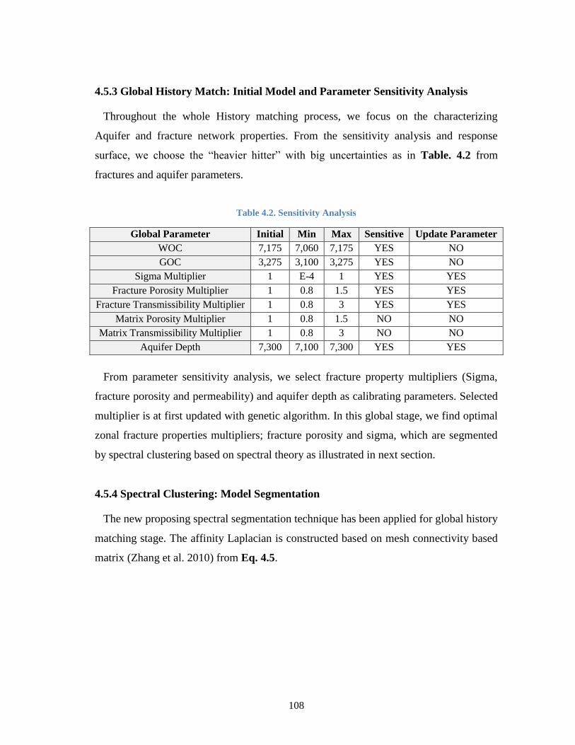
108
4.5.3 Global History Match: Initial Model and Parameter Sensitivity Analysis
Throughout the whole History matching process, we focus on the characterizing
Aquifer and fracture network properties. From the sensitivity analysis and response
surface, we choose the “heavier hitter” with big uncertainties as in Table. 4.2 from
fractures and aquifer parameters.
Table 4.2. Sensitivity Analysis
Global Parameter Initial Min Max Sensitive Update Parameter
WOC 7,175 7,060 7,175 YES NO
GOC 3,275 3,100 3,275 YES NO
Sigma Multiplier 1 E-4 1 YES YES
Fracture Porosity Multiplier 1 0.8 1.5 YES YES
Fracture Transmissibility Multiplier 1 0.8 3 YES YES
Matrix Porosity Multiplier 1 0.8 1.5 NO NO
Matrix Transmissibility Multiplier 1 0.8 3 NO NO
Aquifer Depth 7,300 7,100 7,300 YES YES
From parameter sensitivity analysis, we select fracture property multipliers (Sigma,
fracture porosity and permeability) and aquifer depth as calibrating parameters. Selected
multiplier is at first updated with genetic algorithm. In this global stage, we find optimal
zonal fracture properties multipliers; fracture porosity and sigma, which are segmented
by spectral clustering based on spectral theory as illustrated in next section.
4.5.4 Spectral Clustering: Model Segmentation
The new proposing spectral segmentation technique has been applied for global history
matching stage. The affinity Laplacian is constructed based on mesh connectivity based
matrix (Zhang et al. 2010) from Eq. 4.5.

109
Figure 4.12. The Second Eigen Vector
The second eigenvector of connectivity Laplacian, shown in Fig. 4.12, provides the
optimal spectral clustering criteria. Using this second eigenvector is the way in spectral
clustering, to optimally divide the domain into regions with minimal effort (Shi and
Malik 2000). The segmented zones are illustrated in Fig. 4.13. Selecting number of
segments in the global matching is tradeoff between computation costs and degree of
freedom. Hence, selection process is a heuristic approach and need some experience. In
this San Pedro model, we selected 20 segments for genetic algorithm calibrating
parameters (middle in Fig. 4.13). Note that using connectivity Laplacian is efficient than
weighting by prior when more than one history matching parameters with different
distribution or magnitude involve with clustering. In this stage, we update the fracture
sigma and fracture porosity, totally 40 variables plus aquifer depth for GA.
Figure 4.13. Segmented Model (3, 20, 50 Segments from left)
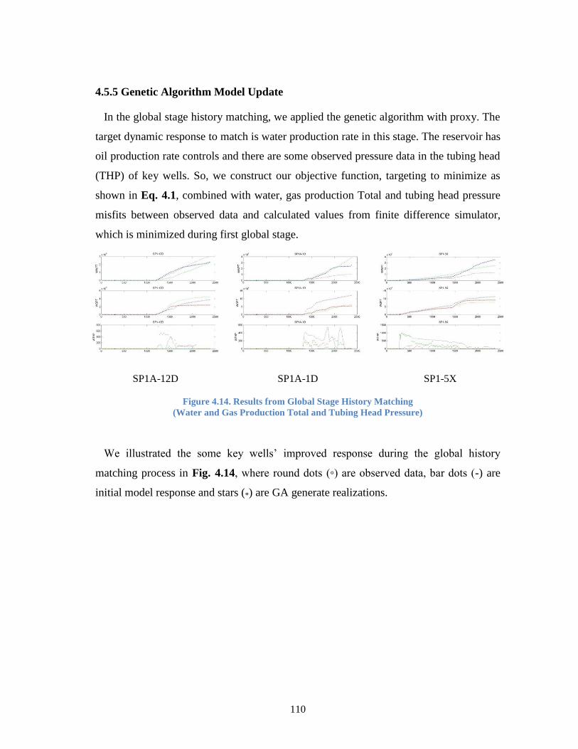
110
4.5.5 Genetic Algorithm Model Update
In the global stage history matching, we applied the genetic algorithm with proxy. The
target dynamic response to match is water production rate in this stage. The reservoir has
oil production rate controls and there are some observed pressure data in the tubing head
(THP) of key wells. So, we construct our objective function, targeting to minimize as
shown in Eq. 4.1, combined with water, gas production Total and tubing head pressure
misfits between observed data and calculated values from finite difference simulator,
which is minimized during first global stage.
SP1A-12D SP1A-1D SP1-5X
Figure 4.14. Results from Global Stage History Matching
(Water and Gas Production Total and Tubing Head Pressure)
We illustrated the some key wells’ improved response during the global history
matching process in Fig. 4.14, where round dots (◦) are observed data, bar dots (-) are
initial model response and stars (*) are GA generate realizations.
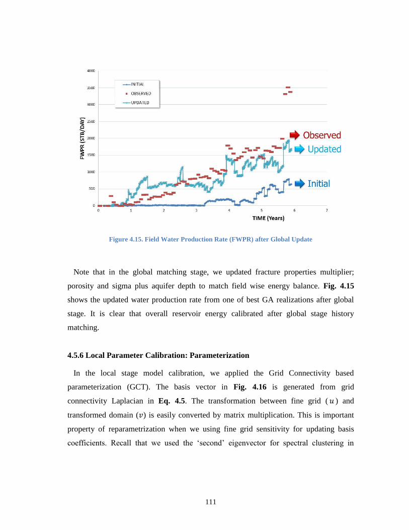
111
Figure 4.15. Field Water Production Rate (FWPR) after Global Update
Note that in the global matching stage, we updated fracture properties multiplier;
porosity and sigma plus aquifer depth to match field wise energy balance. Fig. 4.15
shows the updated water production rate from one of best GA realizations after global
stage. It is clear that overall reservoir energy calibrated after global stage history
matching.
4.5.6 Local Parameter Calibration: Parameterization
In the local stage model calibration, we applied the Grid Connectivity based
parameterization (GCT). The basis vector in Fig. 4.16 is generated from grid
connectivity Laplacian in Eq. 4.5. The transformation between fine grid ( ) and
transformed domain ( ) is easily converted by matrix multiplication. This is important
property of reparametrization when we using fine grid sensitivity for updating basis
coefficients. Recall that we used the ‘second’ eigenvector for spectral clustering in
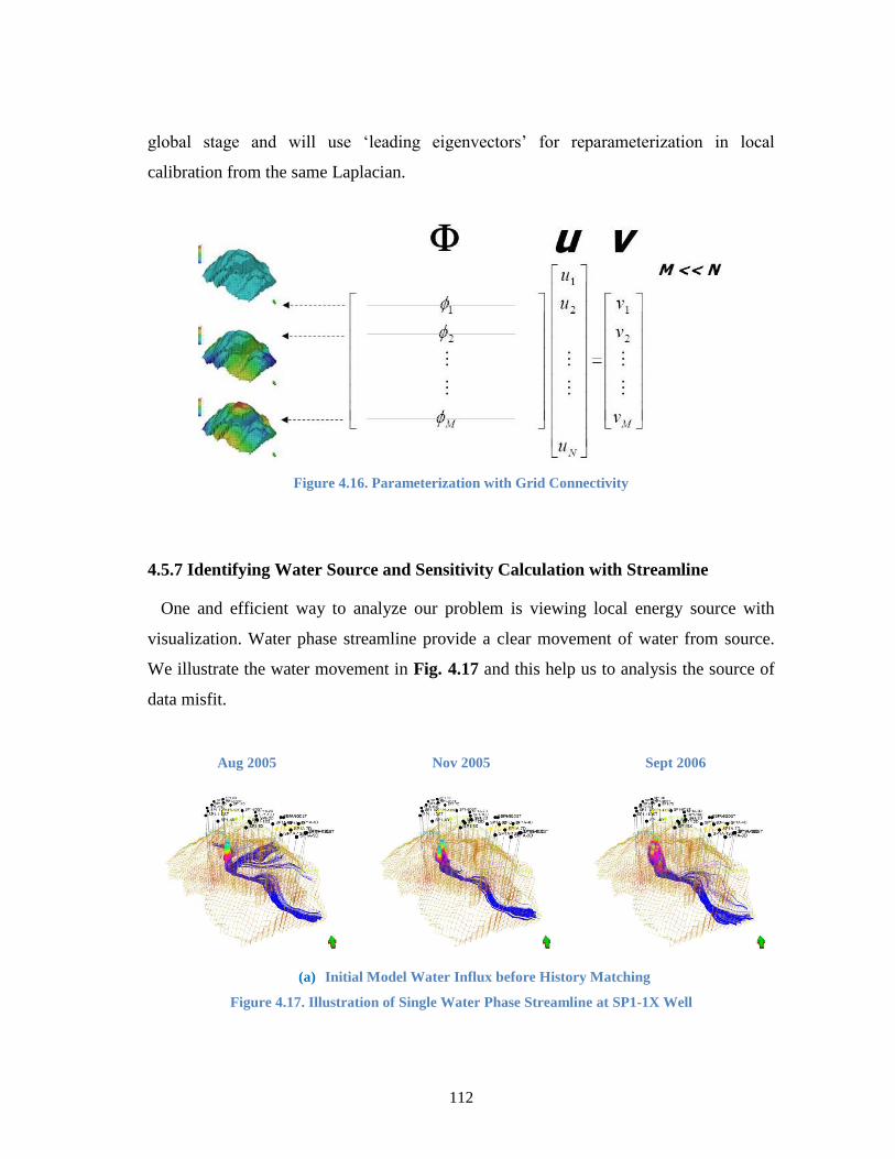
112
global stage and will use ‘leading eigenvectors’ for reparameterization in local
calibration from the same Laplacian.
Figure 4.16. Parameterization with Grid Connectivity
4.5.7 Identifying Water Source and Sensitivity Calculation with Streamline
One and efficient way to analyze our problem is viewing local energy source with
visualization. Water phase streamline provide a clear movement of water from source.
We illustrate the water movement in Fig. 4.17 and this help us to analysis the source of
data misfit.
Aug 2005 Nov 2005 Sept 2006
(a) Initial Model Water Influx before History Matching
Figure 4.17. Illustration of Single Water Phase Streamline at SP1-1X Well
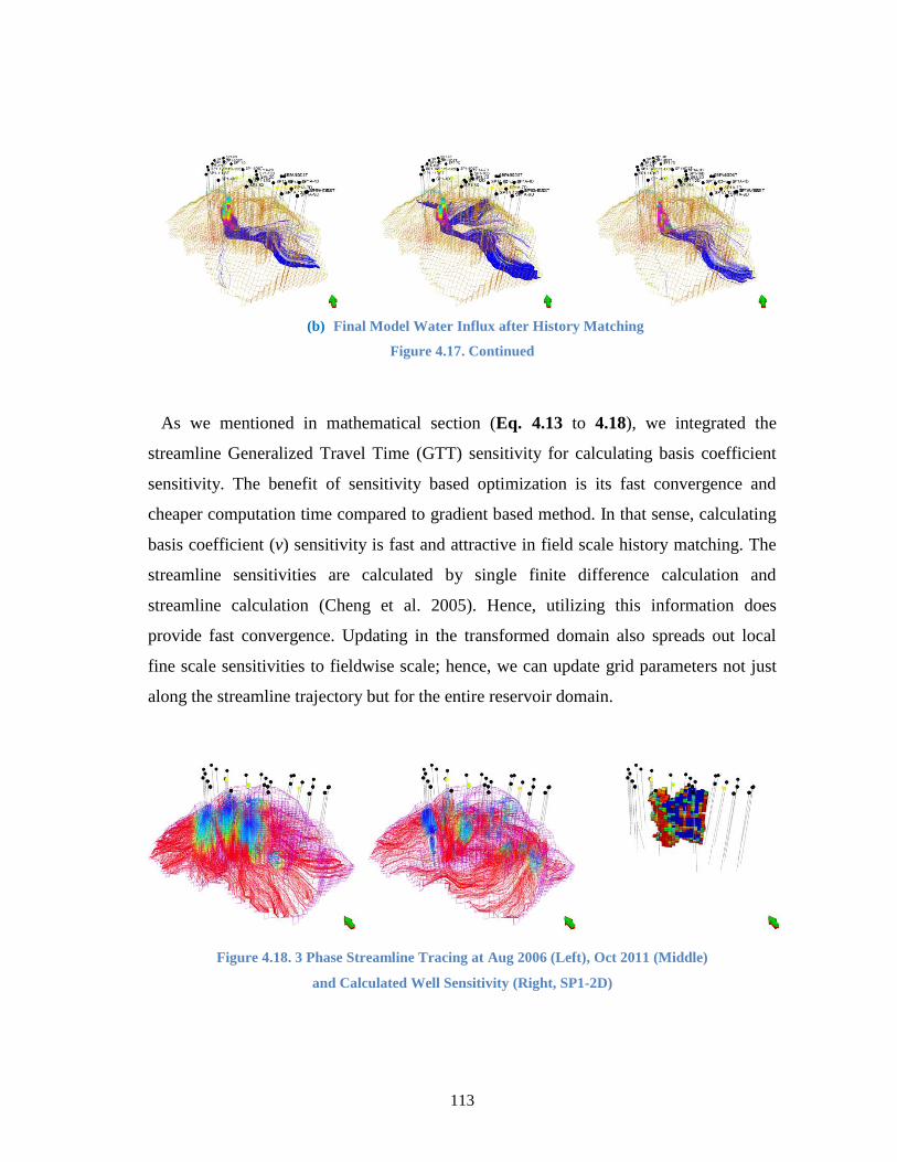
113
(b) Final Model Water Influx after History Matching
Figure 4.17. Continued
As we mentioned in mathematical section (Eq. 4.13 to 4.18), we integrated the
streamline Generalized Travel Time (GTT) sensitivity for calculating basis coefficient
sensitivity. The benefit of sensitivity based optimization is its fast convergence and
cheaper computation time compared to gradient based method. In that sense, calculating
basis coefficient (v) sensitivity is fast and attractive in field scale history matching. The
streamline sensitivities are calculated by single finite difference calculation and
streamline calculation (Cheng et al. 2005). Hence, utilizing this information does
provide fast convergence. Updating in the transformed domain also spreads out local
fine scale sensitivities to fieldwise scale; hence, we can update grid parameters not just
along the streamline trajectory but for the entire reservoir domain.
Figure 4.18. 3 Phase Streamline Tracing at Aug 2006 (Left), Oct 2011 (Middle)
and Calculated Well Sensitivity (Right, SP1-2D)
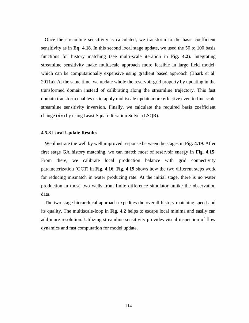
114
Once the streamline sensitivity is calculated, we transform to the basis coefficient
sensitivity as in Eq. 4.18. In this second local stage update, we used the 50 to 100 basis
functions for history matching (see multi-scale iteration in Fig. 4.2). Integrating
streamline sensitivity make multiscale approach more feasible in large field model,
which can be computationally expensive using gradient based approach (Bhark et al.
2011a). At the same time, we update whole the reservoir grid property by updating in the
transformed domain instead of calibrating along the streamline trajectory. This fast
domain transform enables us to apply multiscale update more effective even to fine scale
streamline sensitivity inversion. Finally, we calculate the required basis coefficient
change ( ) by using Least Square Iteration Solver (LSQR).
4.5.8 Local Update Results
We illustrate the well by well improved response between the stages in Fig. 4.19. After
first stage GA history matching, we can match most of reservoir energy in Fig. 4.15.
From there, we calibrate local production balance with grid connectivity
parameterization (GCT) in Fig. 4.16. Fig. 4.19 shows how the two different steps work
for reducing mismatch in water producing rate. At the initial stage, there is no water
production in those two wells from finite difference simulator unlike the observation
data.
The two stage hierarchical approach expedites the overall history matching speed and
its quality. The multiscale-loop in Fig. 4.2 helps to escape local minima and easily can
add more resolution. Utilizing streamline sensitivity provides visual inspection of flow
dynamics and fast computation for model update.
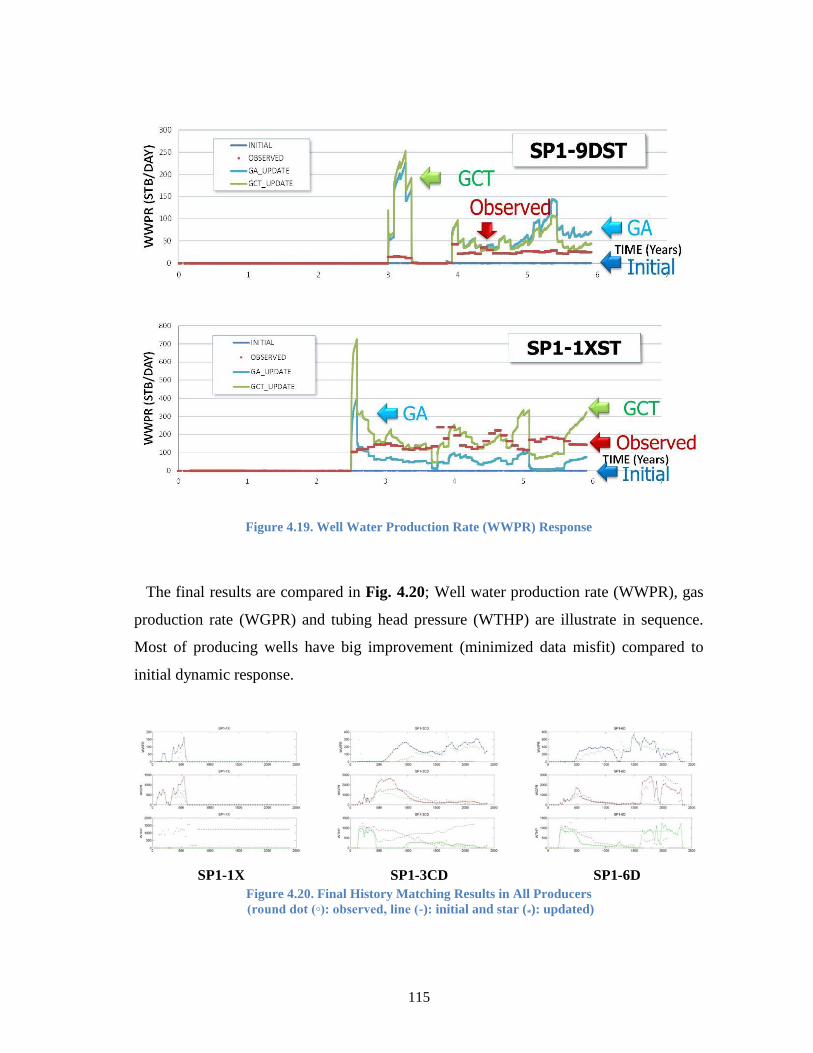
115
Figure 4.19. Well Water Production Rate (WWPR) Response
The final results are compared in Fig. 4.20; Well water production rate (WWPR), gas
production rate (WGPR) and tubing head pressure (WTHP) are illustrate in sequence.
Most of producing wells have big improvement (minimized data misfit) compared to
initial dynamic response.
SP1-1X SP1-3CD SP1-6D
Figure 4.20. Final History Matching Results in All Producers
(round dot (◦): observed, line (-): initial and star (*): updated)
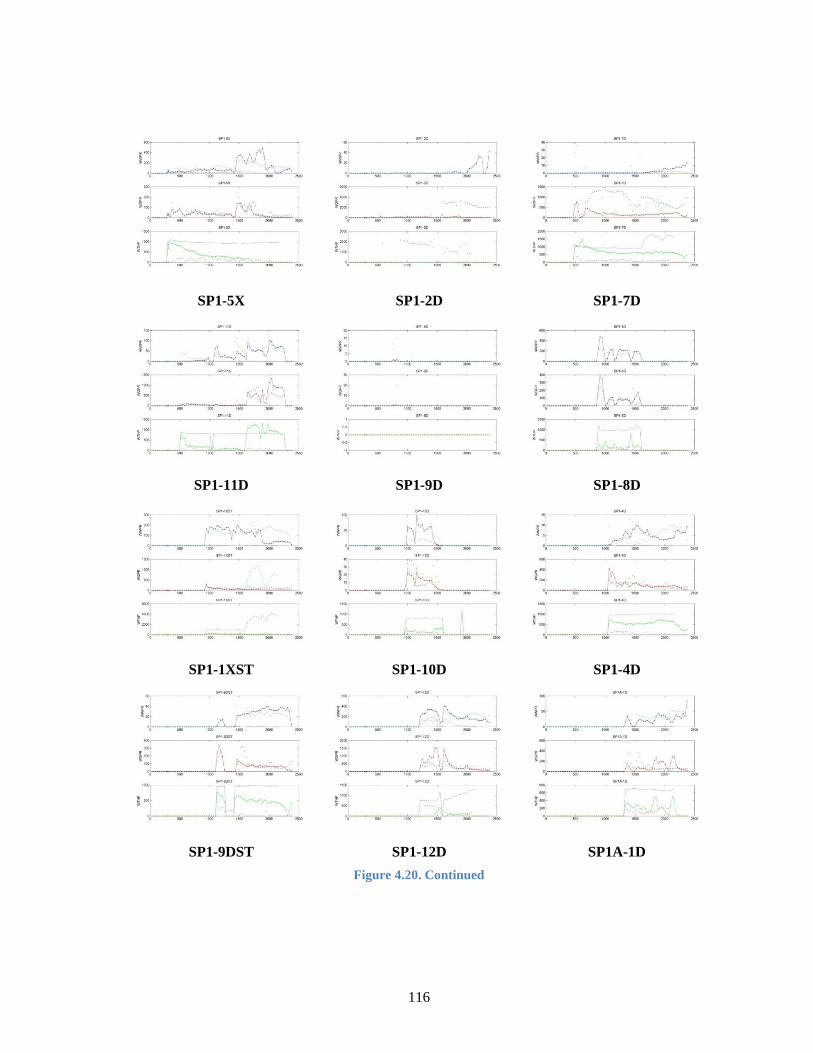
116
SP1-5X SP1-2D SP1-7D
SP1-11D SP1-9D SP1-8D
SP1-1XST SP1-10D SP1-4D
SP1-9DST SP1-12D SP1A-1D
Figure 4.20. Continued

117
4.6 Summary and Conclusions
We propose a hierarchical history matching for complex geometry and highly
fractured reservoir model. Our structured approach is successfully applied in the field
example. We characterize the most uncertain model parameters in fractured reservoirs,
fracture properties (fracture porosity, permeability and sigma) and aquifer depth. We can
summarize our results as following,
1. We have proposed a hierarchical history matching process and simplified our
problem into two stages in a highly fractured reservoir. Our approach starts from
global parameter update with zonal multiplier from spectral clustering (or
segmentation). We then calibrate local parameter with GCT parameterization.
This hierarchical or structured history match corresponds with many industry
experience but we suggest automatic history matching workflows both global
and local stage.
2. In the global scale updating, we have updated a few heavy hitters such as fracture
shape factor ( ) and fracture porosity multipliers, in addition to aquifer property.
This small size of global parameters and zonation approach can significantly
expedite field scale reservoir energy balance after minimal runs.
3. The spectral clustering using ‘Normalized cut’ from Connectivity Laplacian,
which provides a good zonation measure. This is not an arbitrary cut but based
on spectral theories. The algorithm proposes a fast and reasonable multiplicative
zones based on the flow dynamic connectivity and/or model heterogeneity.
4. Model reduction into parameterized domain with Grid Connectivity
Transformation increases the convergence speed through a significant reduction
in the parameter space. The updating in the parameter domain prevents the

118
trapping in the local minima and helps to preserve initial model heterogeneity by
introducing multiplier field.
5. Integrating streamline sensitivity or adjoint sensitivity can save expensive
computation costs compared to gradient based methods. With single reservoir
simulation and streamline tracing, we can determine basis coefficient sensitivity.
This sensitivity can be utilized for updating model with Least Square Iteration
Solver (LSQR). Model is updated not just along the streamline but at the entire
reservoir scale. The integration approach provides an easy multiscale updating
from coarse scale to finest.
6. We have validated our approach with a field example. The applicability for the
real problem has been demonstrated by a highly fractured field with complex
geometry, San Pedro in the Offshore Peru. For a complex example, initial model
analysis and a structured hierarchical history matching approach are essential in
addition to the assisted history matching algorithm.
119
CHAPTER V
CONCLUSION AND RECOMMENDATION
In this research, we focused on aspects of closed loop reservoir management,
especially for highly fractured reservoirs. The proposed new methodologies are tested in
simple synthetic and field examples. In the first part (Chapter 2), we introduce the
generalized drainage volume calculations with streamline diffusive time of flight. The
depth of investigation is calculated along the streamline trajectory from the diffusivity
equation. This approach can be applicable to unconventional tight and shale gas
reservoir under general and changing field operator conditions. The identified drainage
region can help optimize new infill well locations. We expand the drainage volume
calculations to propose optimal fracture stages in the horizontal wells. We also proposed
a novel reservoir model segmentation technique for global scale model update using
history matching and for field scale optimization in Chapter 3. Our proposed algorithm
provides decision criteria for model partitioning, multiplicative zones, in the global scale
model update.
Finally in Chapter 4, we apply a hierarchical history matching approach to a
structurally complex fractured reservoir. We suggest a systematic history matching
approach for fractured reservoirs with genetic algorithm (GA) and model segmentation
for global change and grid connectivity transformation (GCT) for local update.
5.1 Drainage Volume Calculation, Well Placement and Hydraulic Fracture Stages
Optimization
We have presented a systematic approach to well placement in naturally fractured tight
gas reservoirs based on the well drainage volumes computed from dual porosity
numerical simulation. Specifically, we have extended the radius of investigation concept
(Lee 1982) to arbitrary heterogeneity and well conditions by utilizing the gas streamlines
derived from dual porosity numerical simulation. This allows us to visualize the
undrained regions and optimize infill well placement based on a single flow simulation.

120
The results have been shown to be consistent with well placement optimization through
exhaustive flow simulations. Some specific conclusions from this study are as follows.
1. Using a high frequency asymptotic solution of the diffusivity equation, the
concept of radius of drainage (Lee 1982) has been generalized to arbitrary
heterogeneous medium and general flow conditions by examining the
propagation of a ‘pressure front’ corresponding to an impulse (instantaneous)
source along gas streamlines. The gas streamlines can be traced from the flux
field of a finite-difference flow simulation.
2. Visualizing the well drainage is a physical and intuitive way of examining the
influence of existing wells and their mutual interference. By summing up the grid
cells intersected by the streamlines originating from a producing well, we can
quantitatively estimate the well drainage volume, its evolution with time and
potential interference from wells in the vicinity.
3. We have used a discrete fracture network model to examine the role of natural
fractures in the well drainage volumes. As expected, the results show that the
presence of natural fractures tends to enhance the well drainage volumes and
accelerate production depending upon the distribution and orientation of
fractures.
4. Based on the undrained reservoir volumes and reservoir static and dynamic
properties, we have defined a ‘depletion capacity’ map for rapid identification
and optimization of infill locations in tight gas reservoirs. The power and utility
of the method has been demonstrated using both synthetic and field applications.
5. We have demonstrated the use of drainage volume concept in optimizing number
of fracture stages in the Cotton Valley formation. The incremental drainage

121
volumes with the number of fracture stages seem to reach a diminishing return.
Eight to ten hydraulic fracture stages indicate the most optimal completion
strategy for the horizontal well studied from the field example.
6. The optimization based on the drainage volume was found to be consistent with
the performance forecasting based on the rate profiles generated from the
simulator. Besides quantitative analysis, drainage volume calculations provide
the added benefits of flow visualization with no additional simulation.
5.2 Model Segmentation from Spectral Clustering
We propose a new model segmentation technique from spectral clustering theory. The
suggested zonal approach is verified with both synthetic and Brugge SPE benchmark
model. The new zonation algorithm provides rigorous criteria for history matching
compared to old industry practice of using box multiplier.
Our proposed procedure is: (1) construct adjacency based Laplacian to capture spatial
variability in subsurface properties (2) use graph partitioning techniques to create
zonation and find cutting edge (3) apply partitioning with history matching algorithm.
The graphic cut from the model geometry and/or heterogeneity is not arbitrary and is
derived from optimization with graphic cutting metric.
1. The proposed zonation algorithm can preserve the major features of the prior
model after history matching because the generated zonation is based on the
model heterogeneity and/or connectivity information. We illustrate that spectral
clustering approach can potentially capture different facies in the reservoir.
2. We propose three different Affinity Laplacian constructions and four different
graph cutting algorithms. Basically, there is no ground truth in spectral
clustering. So, it is not possible to say which one is the best or the worst. But we
can arrive at some general conclusions from image clustering problems:
122
‘normalized’ cut is more statistically stable than ‘ratio’ cut. Also, ‘Cheeger’ cut
shows at least as good or better performance than ‘standard’ cut. Hence,
‘Normalized Cheeger Cut’ is a good starting point for segmentation.
3. The spectral clustering problem is a NP-hard and heuristic approach. As we
demonstrated, we can generate different cutting with combinations of Laplacian
and cutting algorithms. Even wider choices are available with free parameter and
cutting range. We inherited these properties in our proposed segmentation.
Hence, we require some initial experiments and experience with different
combination of cutting algorithms and Laplacian. Also, the two free parameters
and cut off range heavily impact the clustering.
4. Through human interventions and heuristics, the spectral clustering provides a
good guideline for automatic zonation criteria. This is more attractive when we
do hierarchical history matching; which is essential for history matching
problems for full-field model with decades of production history. We can adapt
this zonal concept for global stage history matching and then further calibrate
with fine scale approach.
5.3 A Hierarchal Multiscale Model Calibration with Spectral Domain
Parameterization and its Application
We propose a hierarchical history matching for complex geometry and highly
fractured reservoir model. Our structured approach is successfully applied in the field
example. We characterize the most uncertain model parameters in fractured reservoirs,
fracture properties (fracture porosity, permeability and sigma) and aquifer depth. We can
summarize our results as following,
1. We have proposed a hierarchical history matching process and simplified our
problem into two stages in a highly fractured reservoir. Our approach starts from

123
global parameter update with zonal multiplier from spectral clustering (or
segmentation). We then calibrate local parameter with GCT parameterization.
This hierarchical or structured history match corresponds with many industry
experience but we suggest automatic history matching workflows both global
and local stage.
2. In the global scale updating, we have updated a few heavy hitters such as fracture
shape factor ( ) and fracture porosity multipliers, in addition to aquifer property.
This small size of global parameters and zonation approach can significantly
expedite field scale reservoir energy balance after minimal runs.
3. The spectral clustering using ‘Normalized cut’ from Connectivity Laplacian,
which provides a good zonation measure. This is not an arbitrary cut but based
on spectral theories. The algorithm proposes a fast and reasonable multiplicative
zones based on the flow dynamic connectivity and/or model heterogeneity.
4. Model reduction into parameterized domain with Grid Connectivity
Transformation increases the convergence speed through a significant reduction
in the parameter space. The updating in the parameter domain prevents the
trapping in the local minima and helps to preserve initial model heterogeneity by
introducing multiplier field.
5. Integrating streamline sensitivity or adjoint sensitivity can save expensive
computation costs compared to gradient based methods. With single reservoir
simulation and streamline tracing, we can determine basis coefficient sensitivity.
This sensitivity can be utilized for updating model with Least Square Iteration
Solver (LSQR). Model is updated not just along the streamline but at the entire
reservoir scale. The integration approach provides an easy multiscale updating
from coarse scale to finest.

124
6. We have validated our approach with a field example. The applicability for the
real problem has been demonstrated by a highly fractured field with complex
geometry, San Pedro in the Offshore Peru. For a complex example, initial model
analysis and a structured hierarchical history matching approach are essential in
addition to the assisted history matching algorithm.
5.4 Recommendation
1. Drainage Volume Calculation with Streamline Diffusive Time of Flight
1) Application to Dual Porosity and Dual Permeability (DPDP) Model.
2) Well Spacing Optimization
3) Compare with Decline Curve Analysis
4) History Matching with Pressure Transient Analysis
2. Spectral Clustering
1) Clustering with Dynamic Data
2) Include Producers and Injector Information in the Clustering
3) Co-Clustering Algorithm
4) K-Means Clustering
5) Grouping of Realizations in the Solution Space
3. Hierarchical History Matching
1) Reparameterization with Prior-weighted Connectivity Transformation
2) Fine scale Fracture Porosity and Sigma Sensitivity Calculation with
Streamline and Inversion
3) History Matching with DPDP Model

125
NOMENCLATURE
Adjacency between cell i and j
A Adjacency matrix
kA Real functions of amplitude of wave
Diffusivity
1 The strength of preserving prior model
2 The strength of change model smooth
C Cluster
C Complement of Cluster C
| | Number of Vertices
cut Objective for graph partitioning
Degree of connectivity of cell i
D Degree of connection matrix
DC
Depletion capacity
)( Entrywise product operator
R Change in the reservoir property to be made
t~
The vector of generalized travel time shift at the wells
v The vector of basis coefficient change to be made
ε A Negligible Value
Grid Property of cell i
natural vibration frequency of a system
Natural vibration frequency
Water fractional flow
ij Grid block position i, j
J Objective function for local stage
k Number of basis used for domain transform
k Permeability

126
L Grid Laplacian matrix
sL String length
L̂ A second spatial difference operator
i Eigenvalue
Vector of parameters for GA update
m Matrix
Local model parameter for local update
Linear density of string
Normalized cut
Number of observation points
n Number of connected grid points
mn Harmonic mode
Norm
Objective function
Obs
Observed data
P Probability of model
),( txp Pressure at time t
Grid property of cell i
Basis function or vector
x porosity
Streamline
r Euclidean distance cut off limit
Correlation Coefficient
Ratio cut
s(x) Slowness of streamline
S The basis coefficient sensitivity matrix
Sim Simulated response
Water saturation

127
t Time, t
maxt Time of maximum pressure change
Temperature like parameter
τ Streamline time of flight
)(x Diffusive time of flight
)(ˆ x Streamline time of flight
u Fine Grid property
Fluid viscosity
v Basis coefficient
)(xv Interstitial velocity of a neutral tracer
porvV Pore volume
Summation over the Weights of all edges attached to Vertices
Connectivity weight between grids and
W Connectivity weight Matrix
Wave frequency
w Connectivity Weight between Two Points
x Location of grid block
x Location in a String
fx Length of hydraulic fracture (one wing)
Grid centroid coordinate of cell i
Distance along the streamline
y Magnitude of Vibration

128
REFERENCES
Adalsteinsson, D. and Sethian, J. 1995. A Fast Level Set Method for Propagating
Interfaces. Journal of Computational Physics 118 (2): 269 - 277. USA
Aguilera, R. 2008. Role of Natural Fractures and Slot Porosity on Tight Gas Sands.
Paper SPE-114174-MS presented at the SPE Unconventional Reservoirs
Conference, Keystone, Colorado, USA, 02/10/2008.
Agunwoke, G.O., Egbele, E., and Onyekonwu, M. 2004. A Statistical Approach to
Reservoir Zonation. Paper SPE-88962 presented at the Nigeria Annual
International Conference and Exhibition, Abuja, Nigeria, 01/01/2004. DOI:
10.2118/88962-ms.
Al-Harbi, M.H., Cheng, H., He, Z. et al. 2005. Streamline-Based Production Data
Integration in Naturally Fractured Reservoirs. SPE Journal 10 (4): 426 - 439 DOI:
10.2118/89914-pa
Al-Hussainy, R., Jr., H.J.R., and Crawford, P.B. 1966. The Flow of Real Gases through
Porous Media, Journal of Petroleum Technology 18. DOI: 10.2118/1243-A-PA.
Al-Huthali, A.H. and Datta-Gupta, A. 2004. Streamline Simulation of Water Injection in
Naturally Fractured Reservoirs. Paper SPE-89443 presented at the SPE/DOE
Symposium on Improved Oil Recovery, Tulsa, Oklahoma, 01/01/2004. DOI:
10.2118/89443-ms.
Al-madani, H.S. and Holditch, S.A. 2011. A Methodology to Determine Both the
Technically Recoverable Resource and the Economically Recoverable Resource
in an Unconventional Gas Play. Paper SPE-141368-MS presented at the SPE
Middle East Oil and Gas Show and Conference, Manama, Bahrain, 01/01/2011.
DOI: 10.2118/141368-ms.
Alhuthali, A.H. 2009. Optimal Waterflood Management under Geologic Uncertainty
Using Rate Control: Theory and Field Applications. Paper SPE-129511-STU
presented at Annual Technical Conference and Exhibition, 10/04/2009, New
Orleans, Louisiana, USA. DOI 10.2118/129511-STU.
Amghibech, S. 2003. Eigenvalues of the Discrete P-Laplacian for Graphs. Ars
Combinatoria 67: 283-302.
Baihly, J.D., Coolidge, A.W., Dutcher, S.D. et al. 2007. Optimizing the Completion of a
Multilayer Cotton Valley Sand Using Hydraulic-Fracture Monitoring and

129
Integrated Engineering. Paper SPE-110068-MS presented at the SPE Annual
Technical Conference and Exhibition, Anaheim, California, U.S.A., 01/01/2007.
DOI: 10.2118/110068-ms.
Bear, J. 1972. Dynamics of Fluids in Porous Media. New York: American Elsevier Pub.
Co. The University of California. CA, USA.
Bhark, E.W., Datta-gupta, A., and Jafarpour, B. 2011a. History Matching with a
Multiscale Parameterization Based on Grid Connectivity and Adaptive to Prior
Information. Paper SPE-147372 presented at the SPE Annual Technical
Conference and Exhibition, Denver, Colorado, USA, 01/01/2011. DOI:
10.2118/147372-ms.
Bhark, E.W., Jafarpour, B., and Datta-Gupta, A. 2011b. A Generalized Grid
Connectivity Based Parameterization for Subsurface Flow Model Calibration.
Water Resour. Res. 47 (6): W06517. DOI: 10.1029/2010wr009982
Bhark, E.W., Rey, A., Datta-gupta, A. et al. 2011c. Multiscale Parameterization and
History Matching in Structured and Unstructured Grid Geometries. Paper SPE-
141764 presented at the SPE Reservoir Simulation Symposium, The Woodlands,
Texas, USA, 01/01/2011. DOI: 10.2118/141764-ms.
Blasingame, T.A. and Rushing, J.A. 2005. A Production-Based Method for Direct
Estimation of Gas-in-Place and Reserves. Paper SPE-98042 presented at the SPE
Eastern Regional Meeting, Morgantown, West Virginia, 09/14/. DOI.
Bogatkov, D.S. and Babadagli, T. 2008. Integrated Modeling and Statistical Analysis of
3-D Fracture Network of the Midale Field. Paper SPE-12165 presented at the
International Petroleum Technology Conference, Kuala Lumpur, Malaysia,
01/01/2008. DOI: 10.2523/12165-ms.
Britt, L.K. and Smith, M.B. 2009. Horizontal Well Completion, Stimulation
Optimization, and Risk Mitigation. Paper SPE-125526-MS presented at the SPE
Eastern Regional Meeting, Charleston, West Virginia, USA, 01/01/2009. DOI:
10.2118/125526-ms.
Brun, B., Gosselin, O., and Barker, J.W. 2004. Use of Prior Information in Gradient-
Based History Matching. SPE Journal 9 (1). DOI: 10.2118/87680-pa
Bubeck, S., Meila, M., and Von Luxburg, U. 2009. How the Initialization Affects the
Stability of the K-Means Algorithm. Arxiv preprint arXiv:0907.5494. Cornell
University Library.
130
Buhler, T. and Hein, M. 2009. Spectral Clustering Based on the Graph P-Laplacian.
Paper presented at the Proceedings of the 26th Annual International Conference
on Machine Learning, Montreal, Quebec, Canada. DOI: 10.1145/ 1553374.
1553385.
Červený, V. 2005. Seismic Ray Theory. Cambridge University Press.
Cheeger, J. 1970. A Lower Bound for the Smallest Eigenvalue of the Laplacian.
Problems Anal: 195.
Chen, Y. and Oliver, D.S. 2010. Ensemble-Based Closed-Loop Optimization Applied to
Brugge Field. SPE Reservoir Evaluation & Engineering 13 (1): 56 - 71. DOI:
10.2118/118926-pa
Cheng, H., Dehghani, K., and Billiter, T.C. 2008. A Structured Approach for
Probabilistic-Assisted History Matching Using Evolutionary Algorithms: Tengiz
Field Applications. Paper SPE-116212 presented at the SPE Annual Technical
Conference and Exhibition, Denver, Colorado, USA, 01/01/2008. DOI:
10.2118/116212-ms.
Cheng, H., Kharghoria, A., He, Z. et al. 2005. Fast History Matching of Finite-
Difference Models Using Streamline-Derived Sensitivities. SPE Reservoir
Evaluation & Engineering 10. DOI: 10.2118/89447-pa
Cipolla, C.L., Lewis, R.E., Maxwell, S.C. et al. 2011. Appraising Unconventional
Resource Plays: Separating Reservoir Quality from Completion Effectiveness.
Paper SPE-14677 presented at the International Petroleum Technology
Conference, Bangkok, Thailand, 01/01/2011. DOI: 10.2523/14677-ms.
Cipolla, C.L., Lolon, E., Erdle, J. et al. 2009a. Modeling Well Performance in Shale-Gas
Reservoirs. Paper SPE-125532 presented at the SPE/EAGE Reservoir
Characterization and Simulation Conference, Abu Dhabi, UAE, 01/01/2009. DOI:
10.2118/125532-ms.
Cipolla, C.L., Lolon, E., Mayerhofer, M.J. et al. 2009b. Fracture Design Considerations
in Horizontal Wells Drilled in Unconventional Gas Reservoirs. Paper SPE-
119366-MS presented at the SPE Hydraulic Fracturing Technology Conference,
The Woodlands, Texas, 01/19/2009.
Cipolla, C.L. and Mayerhofer, M. 1998. Understanding Fracture Performance by
Integrating Well Testing & Fracture Modeling. Paper SPE-00049044 presented
at the SPE Annual Technical Conference and Exhibition, New Orleans,
Louisiana, 01/01/1998. DOI: 10.2118/49044-ms.
131
Cominelli, A., Ferdinandi, F., Montleau, P.C.d. et al. 2007. Using Gradients to Refine
Parameterization in Field-Case History-Matching Projects. SPE Reservoir
Evaluation & Engineering 10 (3): pp. 233-240. DOI: 10.2118/93599-pa
Correia, M., Maschio, C., Schiozer, D.J. et al. 2011. Upscaling Technique Applied to
Naturally Fractured Carbonate Reservoirs. Paper SPE-143150 presented at the
Brasil Offshore Conference, Brazil, 01/01/2011. DOI: 10.2118/143150-ms.
Cox, S.A., Gilbert, J.V., Sutton, R.P. et al. 2002. Reserve Analysis for Tight Gas. Paper
SPE-78695-MS presented at the SPE Eastern Regional Meeting, Lexington,
Kentucky, 10/23/2002.
D'Windt, A. 2007. Reservoir Zonation and Permeability Estimation:A Bayesian
Approach. Paper 2007_UUU presented at the 48th Annual Logging Symposium,
Austin, Texas, 01/01/2007.
Datta-Gupta, Kulkarni, A., Yoon, K.N. et al. 2001. Streamlines, Ray Tracing and
Production Tomography: Generalization to Compressible Flow. Petroleum
Geoscience 7: 75-86.
Datta-Gupta, A. and King, M.J.M.J. 2007. Streamline Simulation :Theory and Practice.
Spe Textbook Series. Richardson, TX: Society of Petroleum Engineers.
Dhillon, I.S., Mallela, S., and Modha, D.S. 2003. Information-Theoretic Co-Clustering.
Paper presented at the Proceedings of the Ninth ACM SIGKDD International
Conference on Knowledge Discovery and Data Mining, Washington, D.C. DOI:
10.1145/956750.956764.
Dyman, T.S. and Condon, S.M. 2006. Assessment of Undiscovered Conventional Oil
and Gas Resources – Upper Jurassic – Lower Cretaceous Cotton Valley Group,
Jurassic Smackover Interior Salt Basins Total Petroleum System, in the East
Texas Basin and Louisiana – Mississippi Salt Basins Provinces. Geological
Survey Digital Data Series. USGS. http://pubs.usgs.gov/dds/dds-069/dds-069-
e/chapters.html. Downloaded 20 Aug 2011.
ElRafie, E.A. and Wattenbarger, R.A. 1997. Comprehensive Evaluation of Horizontal
Wells with Transverse Hydraulic Fractures in the Upper Bahariyia Reservoirs.
Paper SPE-00037759 presented at the Middle East Oil Show and Conference,
Bahrain, 01/01/1997. DOI: 10.2118/37759-ms.
Fetkovich, M.J. 1980. Decline Curve Analysis Using Type Curves. SPE Journal of
Petroleum Technology 32 (6): 1065-1077. DOI: 10.2118/4629-pa

132
Fiedler, M. 1973. Algebraic Connectivity of Graphs. Czechoslovak Mathematical
Journal 23: 298-305.
Fiedler, M. 1975. A Property of Eigenvectors of Nonnegative Symmetric Matrices and
Its Application to Graph Theory. Czechoslovak Mathematical Journal 25 (4):
619-633.
Fischer, I. and Poland, J. 2004. New Methods for Spectral Clustering. Technical Report
No. IDSIA-12-04. June. School of Computer Science and Engineering. Hebrew
University, Jerusalem 91904, Israel
Gale, J.F.W. and Holder, J. 2008. Natural Fractures in the Barnett Shale: Constraints on
Spatial Organization and Tensile Strength with Implications for Hydraulic
Fracture Treatment in Shale-Gas Reservoirs. Paper 08-096 presented at the 42nd
U.S. Rock Mechanics Symposium (USRMS), San Francisco, CA, 01/01/2008.
Gildin, E. and Lopez, T. 2011. Closed-Loop Reservoir Management: Do We Need
Complex Models? Paper SPE-144336-MS presented at the SPE Digital Energy
Conference and Exhibition, The Woodlands, Texas, USA, 01/01/2011. DOI:
10.2118/144336-ms.
Gringarten, E. and Deutsch, C.V. 1999. Methodology for Variogram Interpretation and
Modeling for Improved Reservoir Characterization. Paper SPE-00056654
presented at the SPE Annual Technical Conference and Exhibition, Houston,
Texas, 01/01/1999. DOI: 10.2118/56654-ms.
Hagen, L. and Kahng, A.B. 1992. New Spectral Methods for Ratio Cut Partitioning and
Clustering. Computer-Aided Design of Integrated Circuits and Systems, IEEE
Transactions on 11 (9): 1074-1085. DOI: 10.1109/43.159993
Hareland, G., Rampersad, P., Dharaphop, J. et al. 1993. Hydraulic Fracturing Design
Optimization. Paper SPE-00026950 presented at the SPE Eastern Regional
Meeting, Pittsburgh, Pennsylvania, 01/01/1993. DOI: 10.2118/26950-ms.
Hatzignatiou, D.G. and McKoy, M.L. 2000. Probabilistic Evaluation of Horizontal Wells
in Stochastic Naturally Fractured Gas Reservoirs. Paper SPE-65459 presented at
the SPE/CIM International Conference on Horizontal Well Technology, Calgary,
Alberta, Canada, 11/06/2000.
He, Z., Datta-Gupta, A., and Yoon, S. 2001. Streamline-Based Production Data
Integration under Changing Field Conditions. Paper SPE-71333 presented at the
SPE Annual Technical Conference and Exhibition, New Orleans, Louisiana,
01/01/2001. DOI: 10.2118/71333-ms.
133
He, Z., Parikh, H., Datta-Gupta, A. et al. 2002. Identifying Reservoir
Compartmentalization and Flow Barriers Using Primary Production: A
Streamline Approach. Paper SPE-77589 presented at the SPE Annual Technical
Conference and Exhibition, San Antonio, Texas, 01/01/2002. DOI:
10.2118/77589-ms.
Hein, M. and Bühler, T. 2010. An Inverse Power Method for Nonlinear Eigenproblems
with Applications in 1-Spectral Clustering and Sparse PCA. DOI: citeulike-
article-id:10384511
Holditch, S.A. and Tschirhart, N. 2005. Optimal Stimulation Treatments in Tight Gas
Sands. Paper SPE-96104-MS presented at the SPE Annual Technical Conference
and Exhibition, Dallas, Texas, 10/09/2005.
Huang, X., Bentley, L.R., and Laflamme, C. 2001. Integration of Production History and
Time-Lapse Seismic Data Guided by Seismic Attribute Zonation. Paper SPE-
68819 presented at the SPE Western Regional Meeting, Bakersfield, California,
01/01/2001. DOI: 10.2118/68819-ms.
Huffman, C.H., Harkrider, J.D., and Thompson, R.S. 1996. Fracture Stimulation
Treatment Design Optimization: What Can the Npv Vs Xf Plot Tell Us? Paper
SPE-00036575 presented at the SPE Annual Technical Conference and
Exhibition, Denver, Colorado, 01/01/1996. DOI: 10.2118/36575-ms.
Hur, A., Elisseeff, A., and Guyon, I. 2002. A Stability Based Method for Discovering
Structure in Clustered Data. In Pacific Symposium on Biocomputing: 6-17.
Igor, F. and Jan, P. 2004. New Methods for Spectral Clustering. In. Galleria 2, 6928
Manno, Switzerland: IDSIA / USI-SUPSI, Dalle Molle Institute for Artificial
Intelligence.
Jabbari, H. and Zeng, Z. 2011. A Three-Parameter Dual Porosity Model for Naturally
Fractured Reservoirs. Paper SPE-144560 presented at the SPE Western North
American Region Meeting, Anchorage, Alaska, USA, 01/01/2011. DOI:
10.2118/144560-ms.
Jimenez, E., Datta-Gupta, A., and King, M.J. 2008. Full Field Streamline Tracing in
Complex Faulted Systems with Non-Neighbor Connections. Paper SPE-113425
presented at the SPE/DOE Symposium on Improved Oil Recovery, Tulsa,
Oklahoma, USA, 01/01/2008. DOI: 10.2118/113425-ms.
Kang, S., Datta-gupta, A., and Lee, W.J.J. 2011. Impact of Natural Fractures in Drainage
Volume Calculations and Optimal Well Placement in Tight Gas Reservoirs.
Paper SPE-144338 presented at the North American Unconventional Gas

134
Conference and Exhibition, The Woodlands, Texas, USA, 01/01/2011. DOI:
10.2118/144338-ms.
Kazemi, H., Merrill Jr., L.S., Porterfield, K.L. et al. 1976. Numerical Simulation of
Water-Oil Flow in Naturally Fractured Reservoirs SPE Journal 6: 317-326. DOI:
10.2118/5719-pa
Kim, J.U., Datta-Gupta, A., Brouwer, R. et al. 2009. Calibration of High-Resolution
Reservoir Models Using Transient Pressure Data. Paper SPE-124834 presented
at the SPE Annual Technical Conference and Exhibition, New Orleans,
Louisiana, 01/01/2009. DOI: 10.2118/124834-ms.
Kline, M. and Kay, I.W. 1965. Electromagnetic Theory and Geometrical Optics. New
York: Interscience Publishers.
Kulkarni, K.N., Datta-Gupta, A., and Vasco, D.W. 2001. A Streamline Approach for
Integrating Transient Pressure Data into High-Resolution Reservoir Models. SPE
Journal 6 (3). DOI: 10.2118/74135-pa
Lee, J., Rollins, J.B., and Spivey, J.P. 2003. Pressure Transient Testing. Ed Engineers,
S.o.P. Spe Textbook Series: Richardson, Texas.
Lee, W.J. 1982. Well Testing. New York: Society of Petroleum Engineers of AIME.
Lee, W.J. and Hopkins, C.W. 1994. Characterization of Tight Reservoirs. SPE Journal
of Petroleum Technology 46 (11): 956-964. DOI: 10.2118/29091-pa
Lolon, E., Archer, R.A., Ilk, D. et al. 2008. New Semi-Analytical Solutions for
Multilayer Reservoirs. Paper SPE-114946-MS presented at the CIPC/SPE Gas
Technology Symposium 2008 Joint Conference, Calgary, Alberta, Canada,
06/16/2008.
Lolon, E.P., McVay, D.A., and Schubarth, S.K. 2003. Effect of Fracture Conductivity on
Effective Fracture Length. Paper SPE-84311-MS presented at the SPE Annual
Technical Conference and Exhibition, Denver, Colorado, 10/05/2003.
Massonnat, G., Viszkok, J., and Vrignon, M. 2002. Hierarchical Organization of Flow
Network in Fractured Carbonate Reservoirs: Identification and Characterization
of Key Parameters. Paper SPE-77488 presented at the SPE Annual Technical
Conference and Exhibition, San Antonio, Texas, 01/01/2002. DOI: 10.2118/
77488-ms.
Meyer, B.R., Bazan, L.W., Jacot, R.H. et al. 2010. Optimization of Multiple Transverse
Hydraulic Fractures in Horizontal Wellbores. Paper SPE-131732 presented at the
135
SPE Unconventional Gas Conference, Pittsburgh, Pennsylvania, USA, 01/01/
2010. DOI: 10.2118/131732-ms.
Meza, O., Gandulias, V.P., and cordova, E.n.e. 2010. Influence of Stress Field in the
Productivity of Naturally Fractured Reservoirs in Metamorphic Basement: A
Case Study of the San Pedro Field, Amotape Group. Paper SPE-138946
presented at the SPE Latin American and Caribbean Petroleum Engineering
Conference, Lima, Peru, 01/01/2010. DOI: 10.2118/138946-ms.
Oda, M. 1985. Permeability Tensor for Discontinuous Rock Masses. Géotechnique 35.
DOI 10.1680/geot.1985.35.4.483.
Olson, J.E. 2008. Multi-Fracture Propagation Modeling: Applications to Hydraulic
Fracturing in Shales and Tight Gas Sands. Paper 08-327 presented at the The
42nd U.S. Rock Mechanics Symposium (USRMS), San Francisco, CA,
01/01/2008.
Olson, J.E. and Taleghani, A.D. 2009. Modeling Simultaneous Growth of Multiple
Hydraulic Fractures and Their Interaction with Natural Fractures. Paper SPE-
119739 presented at the SPE Hydraulic Fracturing Technology Conference, The
Woodlands, Texas, 01/01/2009. DOI: 10.2118/119739-ms.
Pearson, C.M., Bond, A.J., Eck, M.E. et al. 1992. Optimal Fracture Stimulation of a
Moderate-Permeability Reservoir - Kuparuk River Unit, Alaska. SPE Production
Engineering 7 (3): 259-266. DOI: 10.2118/20707-pa
Peters, L., Arts, R., Brouwer, G. et al. 2010. Results of the Brugge Benchmark Study for
Flooding Optimization and History Matching. SPE Reservoir Evaluation &
Engineering 13 (3): 391-405. DOI: 10.2118/119094-pa
Pothen, A., Simon, H.D., and Liou, K.-P. 1990. Partitioning Sparse Matrices with
Eigenvectors of Graphs. SIAM Journal on Matrix Analysis and Applications 11
(3): 430-452.
Raghavan, R., Chen, C.C., and Agarwal, B. 1994. An Analysis of Horizontal Wells
Intercepted by Multiple Fractures. Paper PETSOC-HWC-94-39 presented at the
SPE/CIM/CANMET International Conference on Recent Advances in Horizontal
Well Applications, Calgary, Canada, 01/01/1994. DOI: 10.2118/hwc-94-39.
Richardson, M. 2000. A New and Practical Method for Fracture Design and
Optimization. Paper SPE-00059736 presented at the SPE/CERI Gas Technology
Symposium, Calgary, Alberta, Canada, 01/01/2000. DOI: 10.2118/59736-ms.
136
Rushing, J.A., Newsham, K.E., Perego, A.D. et al. 2007. Beyond Decline Curves: Life-
Cycle Reserves Appraisal Using an Integrated Work-Flow Process for Tight Gas
Sands. Paper SPE-109836-MS presented at the SPE Annual Technical
Conference and Exhibition, Anaheim, California, U.S.A., 11/11/2007. DOI.
Schulze-Riegert, R.W., Axmann, J.K., Haase, O. et al. 2002. Evolutionary Algorithms
Applied to History Matching of Complex Reservoirs. SPE Reservoir Evaluation
& Engineering 5 (2): 163-173. DOI: 10.2118/77301-pa
Sen, M.K., Datta-Gupta, A., Stoffa, P.L. et al. 1995. Stochastic Reservoir Modeling
Using Simulated Annealing and Genetic Algorithms. SPE Formation Evaluation
10 (1). DOI: 10.2118/24754-pa
Sethian, J.A. 1999a. Fast Marching Methods. SIAM Review 41: 199-235. DOI: citeulike-
article-id:3102246
Sethian, J.A. 1999b. Level Set Methods and Fast Marching Methods: Cambridge
University Press.
Shi, J. and Malik, J. 2000. Normalized Cuts and Image Segmentation. Pattern Analysis
and Machine Intelligence, IEEE Transactions on 22 (8): 888-905. DOI:
10.1109/34.868688
Still, S. and Bialek, W. 2003. How Many Clusters? An Information Theoretic
Perspective. Neural Comput. 16 (12 (December 2004)): 2483-2506. DOI:
10.1162/0899766042321751
Szu-Hao, H., Yi-Hong, C., Shang-Hong, L. et al. 2009. Learning-Based Vertebra
Detection and Iterative Normalized-Cut Segmentation for Spinal Mri. Medical
Imaging, IEEE Transactions on 28 (10): 1595-1605. DOI: 10.1109/tmi.
2009.2023362
Thompson, R.R. and Blumer, D.J. 1991. Economic Optimization of Fracture
Stimulations Using Mixed Integer-Linear Programming. Paper SPE-00021648
presented at the SPE Production Operations Symposium, Oklahoma City,
Oklahoma, 01/01/1991. DOI: 10.2118/21648-ms.
Tibshirani, R., Walther, G., and Hastie, T. 2001. Estimating the Number of Clusters in a
Dataset Via the Gap Statistic. Journal of the Royal Statistical Society: Series B
(Statistical Methodology) 63 (2): 411 - 423. London, U.K
Vallhs, B. and Naevdal, G. 2009. Revisiting Brugge Case Study Using a Hierarchical
Ensemble Kalman Filter. Paper IPTC-14074-MS presented at the International
137
Petroleum Technology Conference, Doha, Qatar, 01/01/2009. DOI: 10.2523/
14074-ms.
Vasco, D.W. and Finsterle, S. 2004. Subsurface Hydrology - W01507. Numerical
Trajectory Calculations for the Efficient Inversion of Transient Flow and Tracer
Observations (Doi 10.1029/2003wr002362). Water resources research. 40 (1):
n.p.
Vasco, D.W., Keers, H., and Karasaki, K. 2000. Estimation of Reservoir Properties
Using Transient Pressure Data: An Asymptotic Approach. Water Resour. Res. 36
(12): 3447-3465. DOI: 10.1029/2000wr900179
Vasco, D.W., Yoon, S., and Datta-Gupta, A. 1999. Integrating Dynamic Data into High-
Resolution Reservoir Models Using Streamline-Based Analytic Sensitivity
Coefficients. SPE Journal 4 (4). DOI: 10.2118/59253-pa
Velez, E.I., Vasquez, J., Frydman, M. et al. 2010. Novel Approach for Fracture
Characterization in a Metamorphic Reservoir. Paper SPE-138965 presented at
the SPE Latin American and Caribbean Petroleum Engineering Conference,
Lima, Peru, 01/01/2010. DOI: 10.2118/138965-ms.
Virieux, J., Flores-Luna, C., and Gibert, D. 1994. Asymptotic Theory for Diffusive
Electromagnetic Imaging. Geophysical Journal International 119 (3): 857-868.
DOI: 10.1111/j.1365-246X.1994.tb04022.x
von Luxburg, U. 2007. A Tutorial on Spectral Clustering. Statistics and Computing 17
(4): 395-416. DOI: citeulike-article-id:1856674
Von Luxburg, U. 2010. Clustering Stability. Foundations and Trends in Machine
Learning 2 (3) : 235 - 274. DOI: 10.1561/2200000008
von Luxburg, U., Williamson, R.C., and Guyon, I. 2011. Clustering: Science or Art?.
NIPS Workshop, December 11
Wang, S. and Siskind, J.M. 2003. Image Segmentation with Ratio Cut. Pattern Analysis
and Machine Intelligence, IEEE Transactions on 25 (6): 675-690.
Warren, J.E. and Root, P.J. 1963. The Behavior of Naturally Fractured Reservoirs. SPE
Journal 3 (3): 245-255.
Weiss, G. 1960. The Theory of Matrices. Vol. 1 and Vol. 2. F. R. Gantmacher. Chelsea
Publishing Company, New York 68, 1959. Vol. 1: X + 374 Pp. Vol. 2: X + 277
Pp. . Science 131 (3408): 1216. DOI: 10.1126/science.131.3408.1216-a
138
Weiss, Y. 1999. Segmentation Using Eigenvectors: A Unifying View. In Computer
Vision, 1999. The Proceedings of the Seventh IEEE International Conference on
972, 2:975-982.
Wem, J., Jiang, H., and Wang, Y. 2010. Normalized Cut as Basic Tool for Remote
Sensing Image. In Intelligent Computing and Integrated Systems (ICISS), 2010
International Conference on 247-249.
Weng, X., Kresse, O., Cohen, C.-E. et al. 2011. Modeling of Hydraulic-Fracture-
Network Propagation in a Naturally Fractured Formation. SPE Production &
Operations 26 (11). DOI: 10.2118/140253-pa
Wu, C.W. 2005. Algebraic Connectivity of Directed Graphs. Linear and Multilinear
Algebra 53 (3): 203-223. DOI: 10.1080/03081080500054810
Wu, Z. and Datta-Gupta, A. 2002. Rapid History Matching Using a Generalized Travel-
Time Inversion Method. SPE Journal 26 (4). DOI: 10.2118/78359-pa
Yin, J., Park, H., Datta-Gupta, A. et al. 2010. A Hierarchical Streamline-Assisted
History Matching Approach with Global and Local Parameter Updates. Paper
SPE-132642 presented at the SPE Western Regional Meeting, Anaheim,
California, USA, 01/01/2010. DOI: 10.2118/132642-ms.
Zhang, H., Van Kaick, O., and Dyer, R. 2010. Spectral Mesh Processing. Computer
Graphics Forum 29 (6): 1865-1894. DOI: 10.1111/j.1467-8659.2010.01655.x
139
APPENDIX A
A PETREL PLUG-IN FOR STREAMLINE TRACING, RESERVOIR
MANAGEMENT & HISTORY MATCHING
A.1 Introduction
Reconciling high-resolution geologic models to dynamic data such as transient
pressure, tracer and multiphase production history or time-lapse seismic data is by far
the most time-consuming aspect of the workflow for geoscientists and engineers.
Although significant advancements have been made in this area over the last decade,
current industry practice still largely involves iterative trial and error methods and
property multipliers that often result in local discontinuities and loss of geologic realism.
Manual history matching is time-consuming, manpower intensive and highly subjective.
The DESTINY plug-in is designed for fast calibration of high resolution geologic
models to dynamic data based on the research at the Texas A&M University. There are
additional functionalities in DESTINY that allow for flow visualization, reservoir
management and optimization through identification of well drainage and swept
volumes and selection of optimal well locations for infill drilling. DESTINY can be used
with both finite difference as well as streamline simulators. This extends its application
from slightly compressible flow situations (for example, waterflood about bubble point
pressure) to highly compressible flow such as gas reservoirs. DESTINY utilizes unique
information gleaned from streamlines and a novel generalized travel time inversion of
production data to update geologic models. Streamline-based sensitivities can be used to
quickly identify the discrepancies between the geologic model and reservoir dynamic
response. The sensitivities can be used in conjunction with the inversion algorithm to
make targeted changes to geologic models while preserving geologic realism. In
particular, the sensitivities can be obtained in a single forward simulation because it
utilizes an analytic approach that involves 1-D integral along streamlines. The
140
DESTINY can also be used for assisted history matching aided by the streamline-
derived sensitivities.
The DESTINY plug-in utilizes Ocean and PETREL technology extensively. It is
composed of three sequential workflows: streamline tracing, parameter sensitivity
calculation and history matching. The users can choose to turn on or off any of these
functionalities. The inversion output provides complete information on the status of the
history matching during execution. The plug-in has functions to monitor the sensitivity
of each well, the updated geological model and its production response, and the
production data misfit during the inversion process. Descriptive statistics can be
generated on a field-wide or on a facies-by-facies basis with using the PETREL
embedded functions. The synergy between PETREL and Ocean technology is fully
utilized by the plug-in.
A.2 Streamline Applications Using DESTINY
Streamlines provide several benefits for reservoir characterization and management.
The streamline trajectories and time of flight are useful for visualizing reservoir flow
dynamics. Using streamlines, we can easily identify the drainage volumes and swept
volumes associated with producers and injectors, respectively. This provides us with a
natural way to identify potential infill producer and injector locations during water
flooding. Streamlines can also be used to identify and visualize the connectivity and
communication among wells or between wells and the aquifer. This allows us to identify
the source of and also allocate fluid volumes associated with individual producers and
injectors. This information can be utilized for pattern balancing and flood optimization.
A powerful application of streamlines is in waterflood management and optimization.
The streamline time of flight provides us with a dynamic picture of the flood front
evolution. By adjusting the injection and production rates at the wells, we can manage
141
the movement of the flood front to maximize waterflood sweep efficiency. This gives us
an efficient approach to optimal waterflood management through rate control.
A commonly held misconception about the application of streamlines is that the
technology is limited to incompressible flow and requires injectors and producers. In
reality, the streamlines are simply a representation of the velocity field and streamlines
exist whenever there is an underlying velocity field. This allows us to take advantage of
the streamline technology in conjunction with finite difference simulation. For example,
we can apply streamlines to compute and visualize the drainage volumes in tight gas
reservoirs using the flux field generated from the finite difference simulation. The
drainage volumes of existing wells can then be used to optimize infill locations based on
undrained parts of the reservoir.
Streamlines are particularly useful for history matching. Streamlines can be used to
identify and target changes during history matching. In particular, streamlines can be
used to efficiently compute the sensitivity of the production response to reservoir
parameters such as porosity and permeability. These sensitivities can then be used to
facilitate manual history matching or can be used in conjunction with inversion
algorithms to suggest updates to the geologic models. Reconciling high-resolution
geologic models to production history is a very time-consuming aspect in reservoir
modeling. Current practice still involves a tedious and manual history-matching process
that is highly subjective and often employs ad-hoc property multipliers that can lead to
loss of geologic realism. Streamline can aid during history matching in terms of (i)
efficiency in workflow, (ii) obtaining geologic insight (iii) understanding reservoir
dynamics and, (iv) preserving geologic realism.
A.3 DESTINY Process and Workflow
Fig. A.1 shows the general process of DESTINY. First, it runs the forward simulator
and reads the output of the simulator. The forward simulator can be either a finite

142
difference or a streamline simulator. The current options for simulators are: ECLIPSE,
VIP and FRONTSIM. For finite difference simulators, DESTINY utilizes the flux field
to compute streamlines and time of flight. This information can then be used to visualize
swept volumes and drainage volumes of existing wells during water flooding and also
for gas reservoirs to locate potential locations for infill producers or injectors. The flux
associated with streamlines can also be used to optimize injection and production rates
of the wells to maximize flood performance. DESTINY is particularly useful for
streamline-assisted history matching. Using DESTINY, we can visualize the sensitivities
of production data with respect to reservoir properties. These sensitivities depict the
region of the geologic model impacting the production data. Guided by these
sensitivities, we can either manually update the geologic model to match the production
data or use inverse modeling techniques for suggested updates to the model.
Figure A.1. General DESITNY Process
Fig. A.2 shows the overall work flow of streamline tracing and production history
matching.
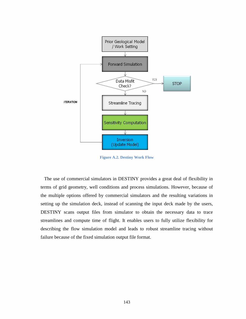
143
Figure A.2. Destiny Work Flow
The use of commercial simulators in DESTINY provides a great deal of flexibility in
terms of grid geometry, well conditions and process simulations. However, because of
the multiple options offered by commercial simulators and the resulting variations in
setting up the simulation deck, instead of scanning the input deck made by the users,
DESTINY scans output files from simulator to obtain the necessary data to trace
streamlines and compute time of flight. It enables users to fully utilize flexibility for
describing the flow simulation model and leads to robust streamline tracing without
failure because of the fixed simulation output file format.
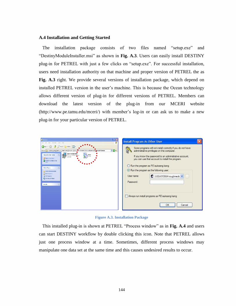
144
A.4 Installation and Getting Started
The installation package consists of two files named “setup.exe” and
“DestinyModuleInstaller.msi” as shown in Fig. A.3. Users can easily install DESTINY
plug-in for PETREL with just a few clicks on “setup.exe”. For successful installation,
users need installation authority on that machine and proper version of PETREL the as
Fig. A.3 right. We provide several versions of installation package, which depend on
installed PETREL version in the user’s machine. This is because the Ocean technology
allows different version of plug-in for different versions of PETREL. Members can
download the latest version of the plug-in from our MCERI website
(http://www.pe.tamu.edu/mceri/) with member’s log-in or can ask us to make a new
plug-in for your particular version of PETREL.
Figure A.3. Installation Package
This installed plug-in is shown at PETREL “Process window” as in Fig. A.4 and users
can start DESTINY workflow by double clicking this icon. Note that PETREL allows
just one process window at a time. Sometimes, different process windows may
manipulate one data set at the same time and this causes undesired results to occur.

145
If your model will take too long for history matching, we also provide the option to run
DESTINY as an independent process. This allows you to release the PETREL license.
This functionality enables the user to work on other jobs during DESTINY computation
as a background process.
Figure A.4. DESTINY in PETREL Process
A.5 User Interface
DESTINY module consists of 8 different tab windows. After starting DESTINY, users
can move each tab by clicking the tab name on the title or next/previous button at the
bottom right. Also in each option, DESTINY provides default values to choose for user’s
convenience. If you are not sure about those options, default values will work in many
cases.
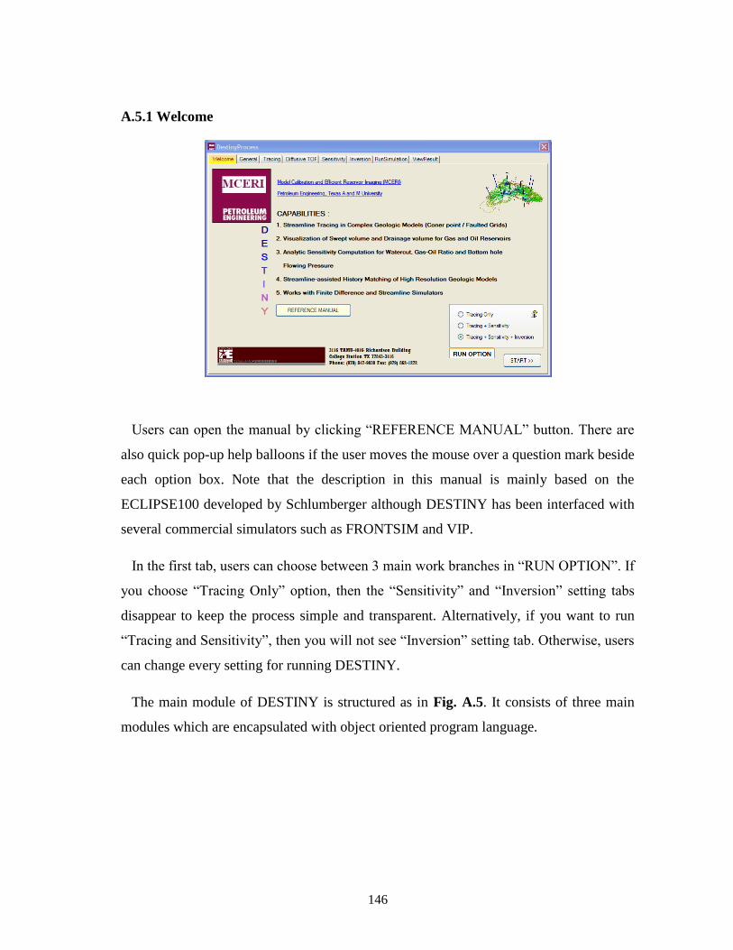
146
A.5.1 Welcome
Users can open the manual by clicking “REFERENCE MANUAL” button. There are
also quick pop-up help balloons if the user moves the mouse over a question mark beside
each option box. Note that the description in this manual is mainly based on the
ECLIPSE100 developed by Schlumberger although DESTINY has been interfaced with
several commercial simulators such as FRONTSIM and VIP.
In the first tab, users can choose between 3 main work branches in “RUN OPTION”. If
you choose “Tracing Only” option, then the “Sensitivity” and “Inversion” setting tabs
disappear to keep the process simple and transparent. Alternatively, if you want to run
“Tracing and Sensitivity”, then you will not see “Inversion” setting tab. Otherwise, users
can change every setting for running DESTINY.
The main module of DESTINY is structured as in Fig. A.5. It consists of three main
modules which are encapsulated with object oriented program language.
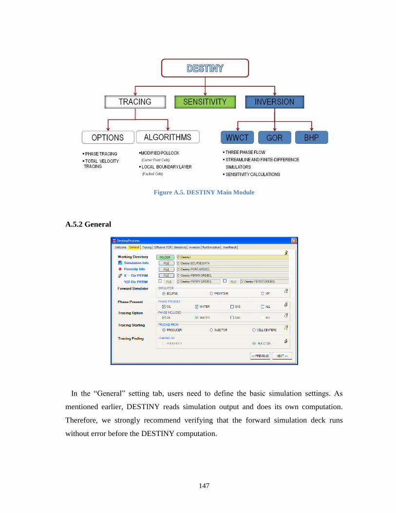
147
Figure A.5. DESTINY Main Module
A.5.2 General
In the “General” setting tab, users need to define the basic simulation settings. As
mentioned earlier, DESTINY reads simulation output and does its own computation.
Therefore, we strongly recommend verifying that the forward simulation deck runs
without error before the DESTINY computation.

148
Working Directory Defines the location of existing Forward simulation data
deck. This requires information for 3 files. “Simulation
Info: main simulation data file name”, “Porosity Info:
Porosity file name” and “PERM: Permeability file name”.
If users don’t have these porosity and permeability with
different files, users should make as separate files with
“INCLUDE” keyword for iterative model update. Users
also can consider Y and Z directional permeability to
preserve the original relationship between these directions.
It can be activated by checking the appropriate box.
Please, note that DESTINY requires a few keywords in
the simulation deck to make sure that the simulation
output contains all the information for DESTINY to
carry out its computations. These are discussed later in
the manual under ‘TEST CASES’ in Example 1.
Forward Simulator Defines which simulator will be used for tracing and
inversion calculations. Current DESTINY is interfaced to
work with ECLIPSE /FRONTSIM/VIP.
Phase Present Defines model phases for calculation. Users can check this
simulation phase from forward simulator setting.
Tracing Option Defines phases to be traced for streamline calculation.
These tracing phases should also be marked in “Phase
Present”.
Tracing Starting Defines the starting points of streamline tracing.
Streamlines can start from the injector, producer or cell
center based on the user’s visualization or computation
purpose.
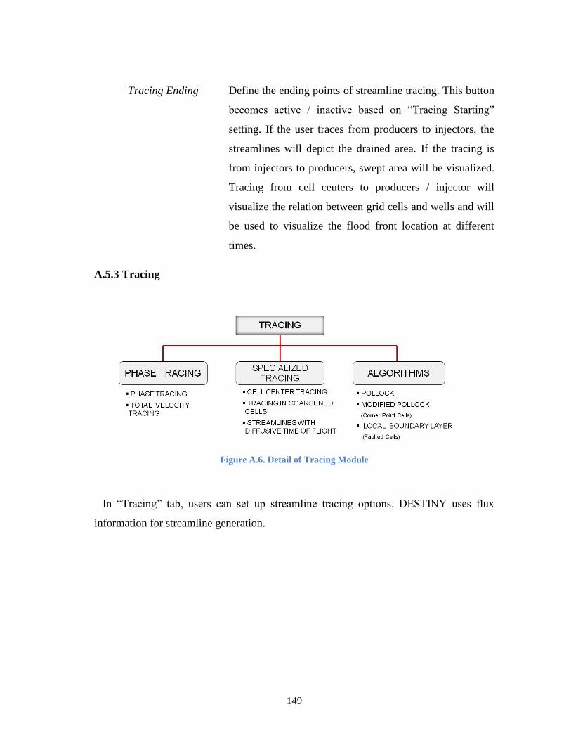
149
Tracing Ending Define the ending points of streamline tracing. This button
becomes active / inactive based on “Tracing Starting”
setting. If the user traces from producers to injectors, the
streamlines will depict the drained area. If the tracing is
from injectors to producers, swept area will be visualized.
Tracing from cell centers to producers / injector will
visualize the relation between grid cells and wells and will
be used to visualize the flood front location at different
times.
A.5.3 Tracing
Figure A.6. Detail of Tracing Module
In “Tracing” tab, users can set up streamline tracing options. DESTINY uses flux
information for streamline generation.
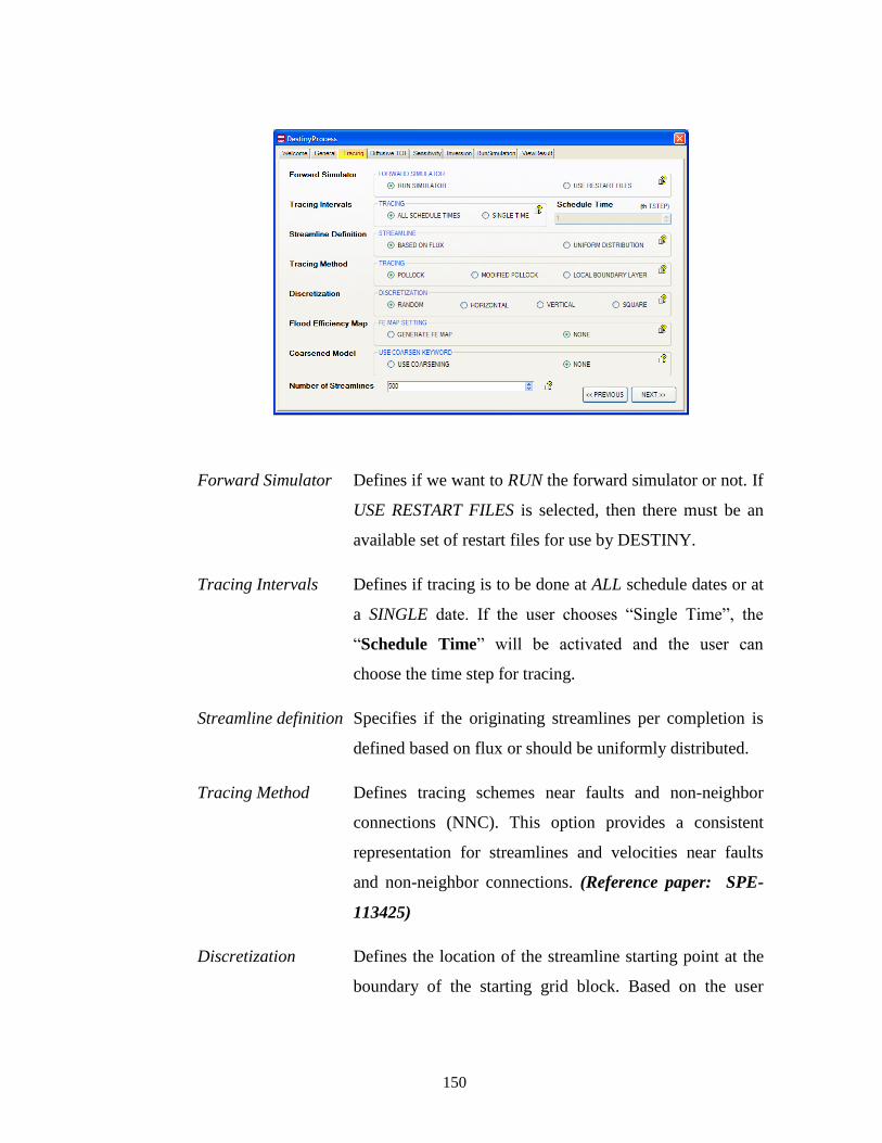
150
Forward Simulator Defines if we want to RUN the forward simulator or not. If
USE RESTART FILES is selected, then there must be an
available set of restart files for use by DESTINY.
Tracing Intervals Defines if tracing is to be done at ALL schedule dates or at
a SINGLE date. If the user chooses “Single Time”, the
“Schedule Time” will be activated and the user can
choose the time step for tracing.
Streamline definition Specifies if the originating streamlines per completion is
defined based on flux or should be uniformly distributed.
Tracing Method Defines tracing schemes near faults and non-neighbor
connections (NNC). This option provides a consistent
representation for streamlines and velocities near faults
and non-neighbor connections. (Reference paper: SPE-
113425)
Discretization Defines the location of the streamline starting point at the
boundary of the starting grid block. Based on the user
151
choice, streamlines start from those points and then tracing
continues.
Flood Efficiency Map Defines the use of Flood Efficiency MAP visualization.
Users can generate intuitive connections between injection
and production wells. DESTINY provides two methods for
MAP, based on flux and time of flight. (Reference paper:
SPE-132642)
Coarsened Model Defines the use of COARSEN keyword in Finite
Difference simulator. This option saves a lot of simulation
time for large field model and gives good approximated
result. DESTINY can trace streamline under coarsened
geometry, calculate sensitivities and calibrate model under
coarsened scale and finally update fine geological model.
Number of SLN Defines the total number of streamline for tracing. If you
choose tracing from cell centers, this option will be
ignored and try to generate from the entire grid block.

152
A.5.4 Diffusive TOF (Time of Flight)
In “Diffusive TOF” tab, ‘diffusive’ time of flight can be used to define the drainage
radius and infill well optimization in case of primary recovery or compressible flow such
as gas reservoirs.
Diffusive TOF Select if the user wants to trace using Diffusive Time of
Flight. This option is activated if the user chooses
“Tracing Only” in the “Welcome” tab. This diffusive time
of flight will trace from cell center to producer as a default.
(Reference paper: SPE-88802)
Drainage Volume Defines the well for which the user wants to calculate the
drainage volume. If the user wants to calculate for a single
well, then “Well Name” will be activated.
Calculation Time Defines if the user wants to calculate the well drainage
volume in every time step or at the last time step.
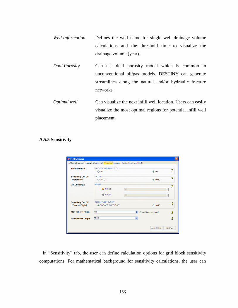
153
Well Information Defines the well name for single well drainage volume
calculations and the threshold time to visualize the
drainage volume (year).
Dual Porosity Can use dual porosity model which is common in
unconventional oil/gas models. DESTINY can generate
streamlines along the natural and/or hydraulic fracture
networks.
Optimal well Can visualize the next infill well location. Users can easily
visualize the most optimal regions for potential infill well
placement.
A.5.5 Sensitivity
In “Sensitivity” tab, the user can define calculation options for grid block sensitivity
computations. For mathematical background for sensitivity calculations, the user can

154
refer to chapter 10 of the SPE streamline textbook or papers. (Reference paper: SPE-
99465)
Normalization When checked, the sensitivities are normalized. The
normalization facilitates convergence of the inversion
algorithm when different data are involved.
Sensitivity Cut off Defines a percentile based cutoff that will be applied to
water cut sensitivities on a well-basis. It is used to reduce
unusually high and low sensitivity values.
Cut off Range Defines the upper and lower percentile for the water cut
sensitivity cut-off.
Sensitivity cut off Defines a time of flight based cut off that will be applied
to water cut sensitivities on a well-basis. This is used to
eliminate the sensitivities in stagnation regions which may
cause poor inversion performance.
Maximum TOF Defines the threshold of the time of flight for the water cut
sensitivity cut-off. This Maximum Time of Flight cut off
value is automatically calculated by multiplication of
actual producing time period with input multiplier value.
Sensitivities Output Define whether the user wants to generate sensitivity
outputs or not. This sensitivity output can be used as
reference data for manual history matching. Sensitivity
files will be found at working folder with well name and
no extension.
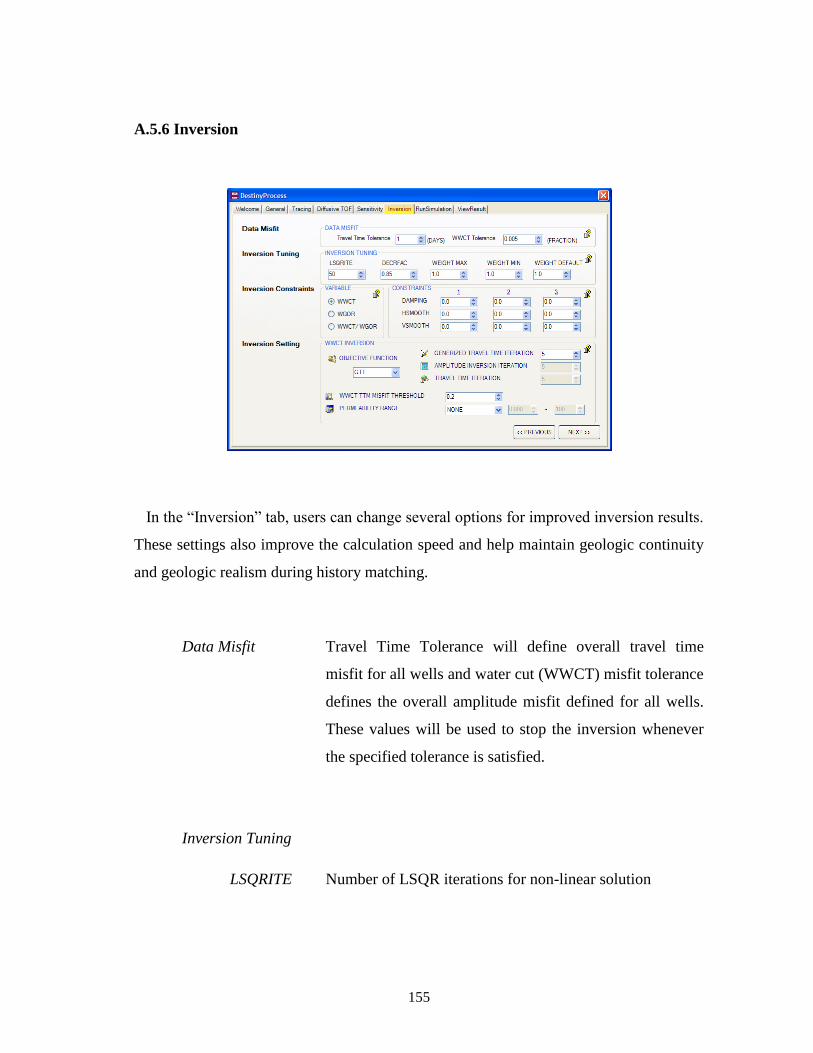
155
A.5.6 Inversion
In the “Inversion” tab, users can change several options for improved inversion results.
These settings also improve the calculation speed and help maintain geologic continuity
and geologic realism during history matching.
Data Misfit Travel Time Tolerance will define overall travel time
misfit for all wells and water cut (WWCT) misfit tolerance
defines the overall amplitude misfit defined for all wells.
These values will be used to stop the inversion whenever
the specified tolerance is satisfied.
Inversion Tuning
LSQRITE Number of LSQR iterations for non-linear solution

156
DECRFAC Decrease factor to be applied to the norm and smoothing
constraints through iterations.
Weight MAX Defines maximum weight given to permeability changes in
the each iteration.
Weight MIN Defines minimum weight given to permeability changes in
the each iteration.
Weight default Defines default weight given to permeability changes in
the each iteration.
Inversion Constraints
Variables to integrate production well water cut (WWCT) and well
gas oil ratio (WGOR). Users can also use both water-cut
and gas oil ratios.
Constraints DAMPING Norm constraint. A large value of the norm
constraint minimizes changes to the prior model. This will
lead to poor quality data match. We can then gradually
lower the norm constraint to get an acceptable compromise
between changes to the prior model and quality of the data
match.
HSMOOTH Horizontal smoothing constraint. A large
value of this parameter leads to more continuity of the
estimated property in the horizontal direction.
VSMOOTH Vertical smoothing constraint. A large
value of this parameter will lead to more continuity of the
estimated parameter in the vertical direction.

157
The inversion constraints on this version of DESTINY are
only meant to update permeability. Only the first values on
each line will be considered during the minimization of the
objective function. The other values are reserved for
further development when integrating additional reservoir
parameters.
Inversion Setting
Objective functions that are targeted for minimization. DESTINY
can utilize three options for choice of objective function (1)
“Generalized Travel Time”, (2) “Amplitude” and (3)
“Travel Time”. The travel time inversion mainly focuses
on matching the breakthrough time whereas the
generalized travel time matches both breakthrough and
amplitude response (recommended). The amplitude match
focuses on matching the production amplitude. If user
changes the objective function option, corresponding
iteration number box is activated and others are kept
inactive.
Threshold This is the water cut value selected for travel time misfit
evaluation. At every producing well, whenever the water
cut reaches this value, both simulated and observed times
will be extracted and used for misfit and sensitivity
calculations.
Permeability range enables users to set updating permeability range
during history match. By default, initial permeability field
range is used.
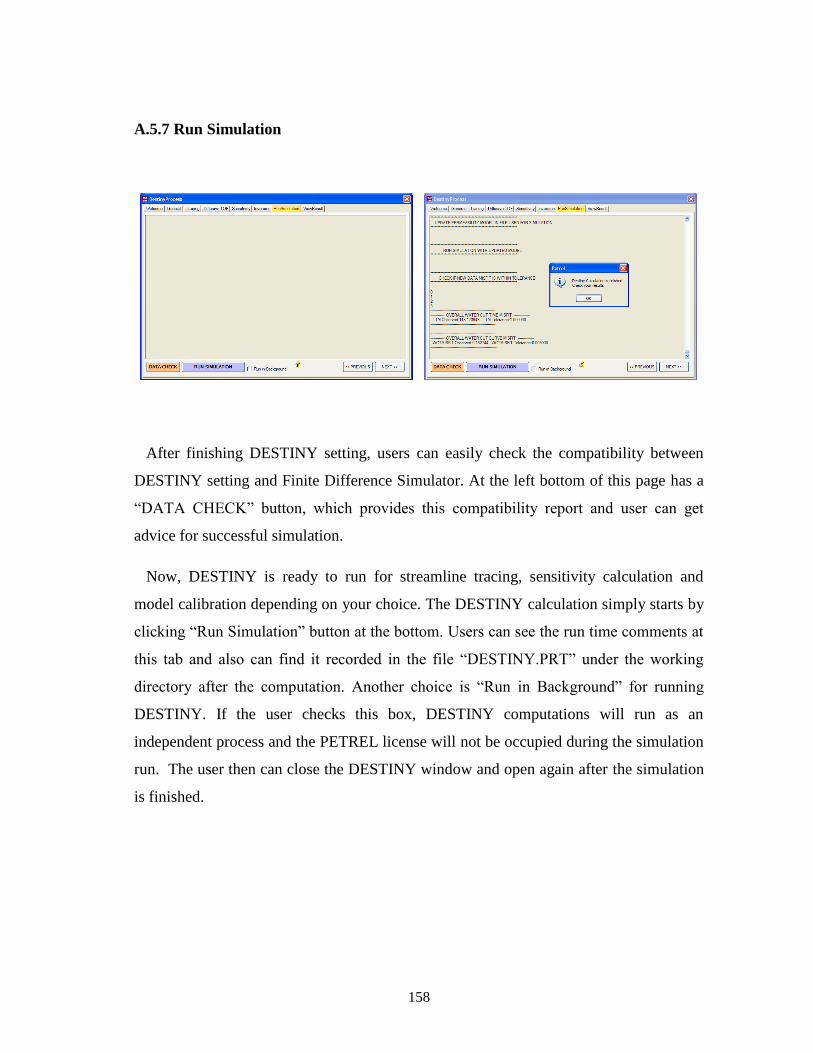
158
A.5.7 Run Simulation
After finishing DESTINY setting, users can easily check the compatibility between
DESTINY setting and Finite Difference Simulator. At the left bottom of this page has a
“DATA CHECK” button, which provides this compatibility report and user can get
advice for successful simulation.
Now, DESTINY is ready to run for streamline tracing, sensitivity calculation and
model calibration depending on your choice. The DESTINY calculation simply starts by
clicking “Run Simulation” button at the bottom. Users can see the run time comments at
this tab and also can find it recorded in the file “DESTINY.PRT” under the working
directory after the computation. Another choice is “Run in Background” for running
DESTINY. If the user checks this box, DESTINY computations will run as an
independent process and the PETREL license will not be occupied during the simulation
run. The user then can close the DESTINY window and open again after the simulation
is finished.
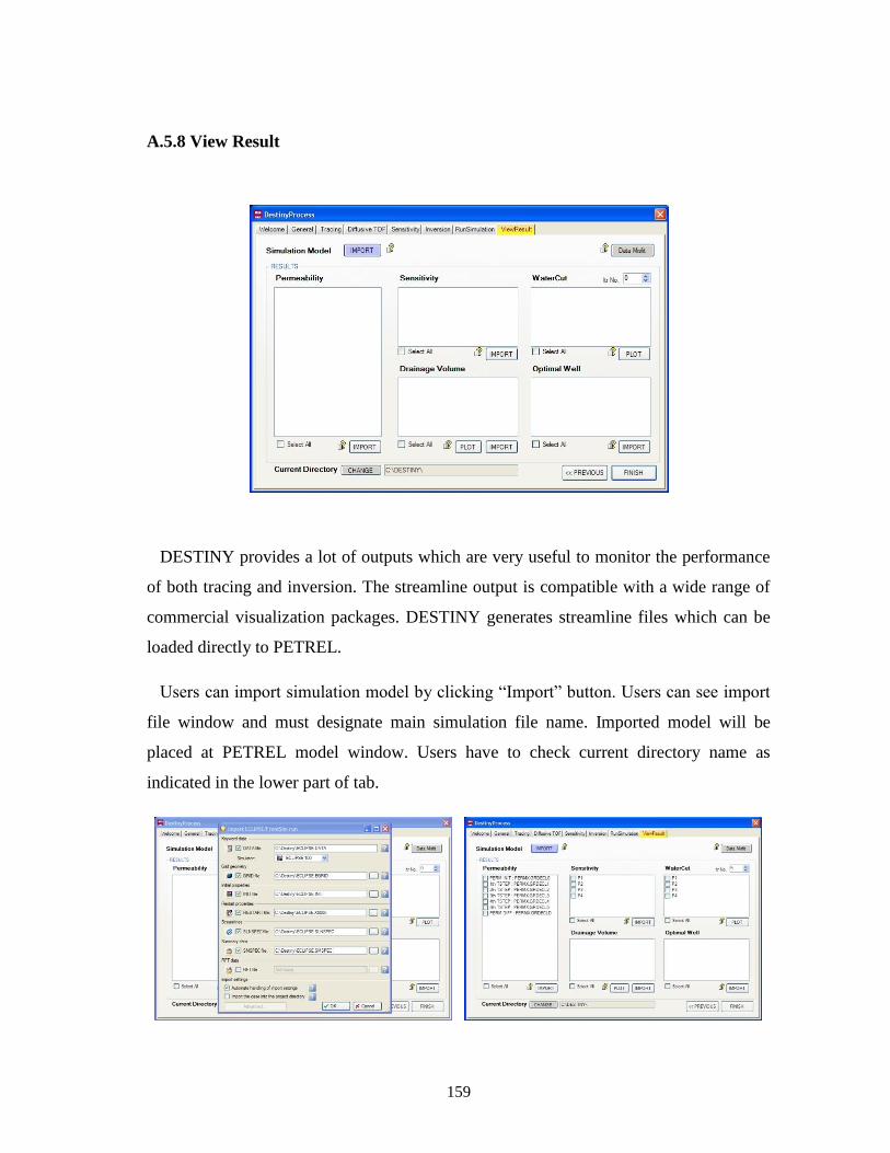
159
A.5.8 View Result
DESTINY provides a lot of outputs which are very useful to monitor the performance
of both tracing and inversion. The streamline output is compatible with a wide range of
commercial visualization packages. DESTINY generates streamline files which can be
loaded directly to PETREL.
Users can import simulation model by clicking “Import” button. Users can see import
file window and must designate main simulation file name. Imported model will be
placed at PETREL model window. Users have to check current directory name as
indicated in the lower part of tab.
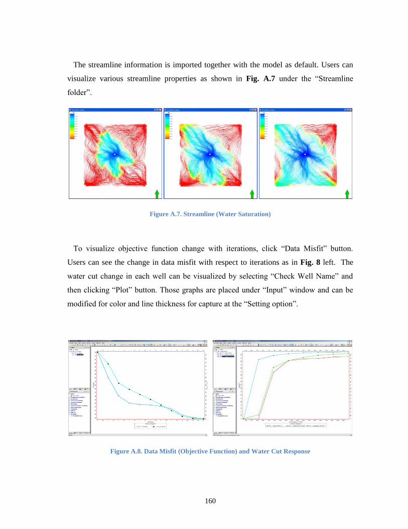
160
The streamline information is imported together with the model as default. Users can
visualize various streamline properties as shown in Fig. A.7 under the “Streamline
folder”.
Figure A.7. Streamline (Water Saturation)
To visualize objective function change with iterations, click “Data Misfit” button.
Users can see the change in data misfit with respect to iterations as in Fig. 8 left. The
water cut change in each well can be visualized by selecting “Check Well Name” and
then clicking “Plot” button. Those graphs are placed under “Input” window and can be
modified for color and line thickness for capture at the “Setting option”.
Figure A.8. Data Misfit (Objective Function) and Water Cut Response

161
To visualize the permeability field, users need to check the permeability file name and
import each permeability field. The imported data set will be placed under “Properties”.
Note that the permeability data will be in log scale as default. The user needs to turn off
this log scale and color range for visualization of permeability difference.
Figure A.9. Initial / Updated / Change of Permeability Field
To visualize the sensitivity of each well, check the well name in the “Sensitivity” list
and then import that file from working folder. Note that sensitivity is equal or less than
zero, so users also change data value range from “color table”.

162
Figure A.10. Streamline Sensitivities of Well P1 and P4
“Drainage Volume” and “Optimal Well” window will be explained at “Diffusive Time
of Flight” example.
The inversion output offers information to know the status of the history matching
performance at any iteration. DESTINY has implemented functions to monitor the
permeability changes during the inversion iterations. Descriptive statistics can be
generated to monitor the behavior of statistical moments on a field-wide or on a facie-
based basis. A brief summary of the DESTINY output files are presented for advanced
users.
A.6 Streamline Output
SLNXXX Files: When the binary output is selected, DESTINY will generate
*.sln files for every simulation time step. ECLIPSE users can use the restart files
and the *.sln files to load the entire simulation workspace to PETREL.

163
A.7 Inversion Output
Updated permeability files: After running the first inversion iteration this file
will be modified and to the end of the each iteration. The updated permeability
will be written out as initial permeability file name (the updated files will have a
suffix with the iteration number in which the permeability was updated).
resinv.obj: This file has the objective function behavior through all iterations. It
has two columns representing the travel time and amplitude misfit defined at all
producing wells included in the data integration
resInv.wwctX: It contains the simulated and observed production water cut for all
wells included in the project. At the header of each well the travel time misfit
will be written out. This file is generated at the end of the each iteration.
dynamic.bin: Binary files contain the production sensitivities. This file is used by
LSQR to perform the objective function minimization.
dynamic.ascii: An ASCII file contains the production sensitivities. This file is
provided for history matching applications where streamline-based sensitivities
are used as complementary information.
A.8 Test Cases
We provide 7 different synthetic test cases for DESTINY testing. DESTINY reads the
necessary information from the restart file of the forward simulator. Hence, it is
important to include some specific keywords in the forward simulator setting for
successful DESTINY running. We discuss these keywords in the following examples.
A.8.1 ECLIPSE Model Tracing and History Matching
(1) Eclipse Settings for Tracing

164
SECTION EECLIPSE SETTING REASON
SOLUTION
RPTSOL
'RESTART=2' /
Print output to the Restart
files
REMOVE “UNIFOUT” & “FMTOUT” Destiny use separate binary
file for each time step
SUMMARY
WOPR /
WGPR /
WWPR /
Read production rate base
on tracing phase
SCHEDULE
RPTRST
'BASIC=2' FLOWS PRESSURE
ALLPROPS/
Control restart file written
data for computation
(2) Eclipse Settings for Inversion (History Matching)
SECTION EECLIPSE SETTING REASON
GRID
INCLUDE
'PORO.GRDECL' /
INCLUDE
'PERMX.GRDECL' /
Use “INCLUDE” as
separate porosity and
permeability files for
iterative parameter update
SOLUTION RPTSOL
'RESTART=2' /
Print output to the Restart
files
SUMMARY
WOPR /
WGPR /
WWPR /
Print out production rate
base on tracing phase
WWCT /
WWCTH /
Print out water cut data and
history for water cut match
WOPT /
WWPT /
WGPT /
WOPRH /
WWPRH /
WGPRH /
Print out oil, water and gas
production rate
SCHEDULE
RPTRST
'BASIC=2' FLOWS PRESSURE
ALLPROPS /
Control restart file written
data for computation
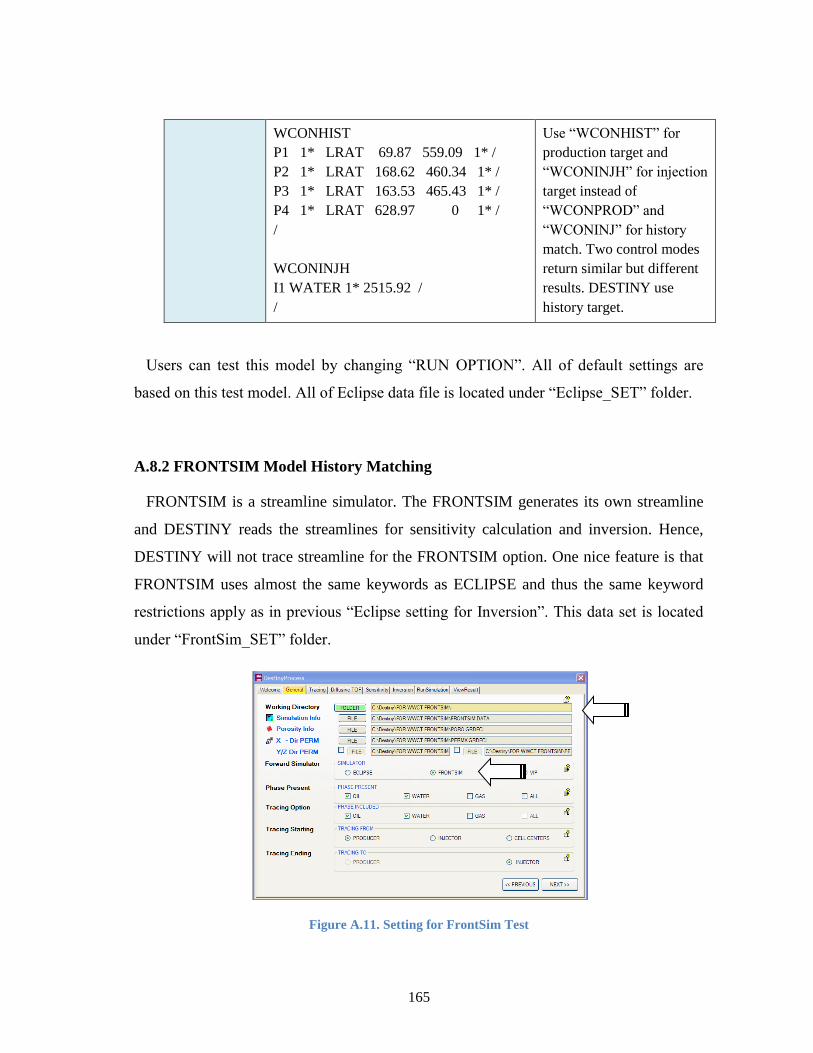
165
WCONHIST
P1 1* LRAT 69.87 559.09 1* /
P2 1* LRAT 168.62 460.34 1* /
P3 1* LRAT 163.53 465.43 1* /
P4 1* LRAT 628.97 0 1* /
/
WCONINJH
I1 WATER 1* 2515.92 /
/
Use “WCONHIST” for
production target and
“WCONINJH” for injection
target instead of
“WCONPROD” and
“WCONINJ” for history
match. Two control modes
return similar but different
results. DESTINY use
history target.
Users can test this model by changing “RUN OPTION”. All of default settings are
based on this test model. All of Eclipse data file is located under “Eclipse_SET” folder.
A.8.2 FRONTSIM Model History Matching
FRONTSIM is a streamline simulator. The FRONTSIM generates its own streamline
and DESTINY reads the streamlines for sensitivity calculation and inversion. Hence,
DESTINY will not trace streamline for the FRONTSIM option. One nice feature is that
FRONTSIM uses almost the same keywords as ECLIPSE and thus the same keyword
restrictions apply as in previous “Eclipse setting for Inversion”. This data set is located
under “FrontSim_SET” folder.
Figure A.11. Setting for FrontSim Test
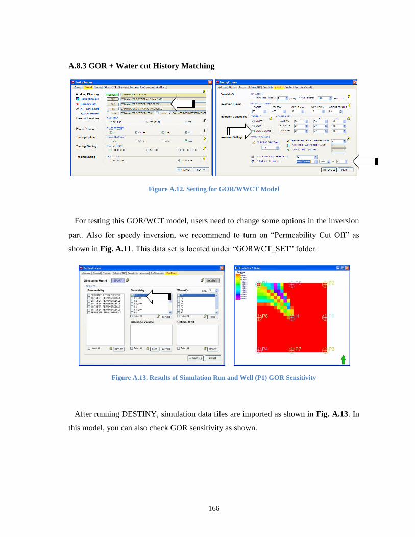
166
A.8.3 GOR + Water cut History Matching
Figure A.12. Setting for GOR/WWCT Model
For testing this GOR/WCT model, users need to change some options in the inversion
part. Also for speedy inversion, we recommend to turn on “Permeability Cut Off” as
shown in Fig. A.11. This data set is located under “GORWCT_SET” folder.
Figure A.13. Results of Simulation Run and Well (P1) GOR Sensitivity
After running DESTINY, simulation data files are imported as shown in Fig. A.13. In
this model, you can also check GOR sensitivity as shown.
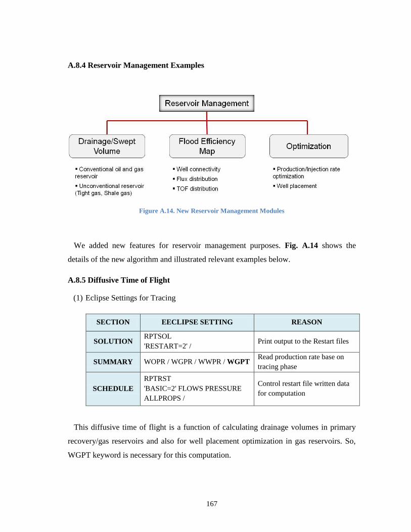
167
A.8.4 Reservoir Management Examples
Figure A.14. New Reservoir Management Modules
We added new features for reservoir management purposes. Fig. A.14 shows the
details of the new algorithm and illustrated relevant examples below.
A.8.5 Diffusive Time of Flight
(1) Eclipse Settings for Tracing
SECTION EECLIPSE SETTING REASON
SOLUTION RPTSOL
'RESTART=2' / Print output to the Restart files
SUMMARY WOPR / WGPR / WWPR / WGPT Read production rate base on
tracing phase
SCHEDULE
RPTRST
'BASIC=2' FLOWS PRESSURE
ALLPROPS /
Control restart file written data
for computation
This diffusive time of flight is a function of calculating drainage volumes in primary
recovery/gas reservoirs and also for well placement optimization in gas reservoirs. So,
WGPT keyword is necessary for this computation.

168
Figure A.15. Setting for Diffusive Time of Flight Calculation
For Diffusive time of flight test case, users need to choose “Tracing Only” at “Run
Option” and then follow the next settings as above. There is no file information here
under “Permeability”, “Sensitivity” and “WaterCut” which are related to model
inversion.
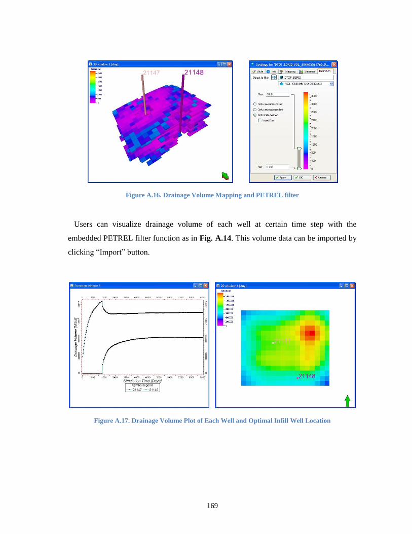
169
Figure A.16. Drainage Volume Mapping and PETREL filter
Users can visualize drainage volume of each well at certain time step with the
embedded PETREL filter function as in Fig. A.14. This volume data can be imported by
clicking “Import” button.
Figure A.17. Drainage Volume Plot of Each Well and Optimal Infill Well Location
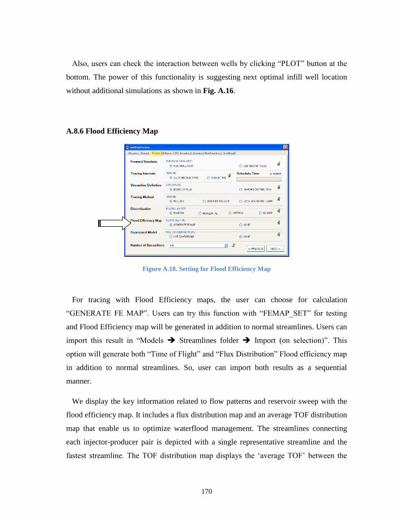
170
Also, users can check the interaction between wells by clicking “PLOT” button at the
bottom. The power of this functionality is suggesting next optimal infill well location
without additional simulations as shown in Fig. A.16.
A.8.6 Flood Efficiency Map
Figure A.18. Setting for Flood Efficiency Map
For tracing with Flood Efficiency maps, the user can choose for calculation
“GENERATE FE MAP”. Users can try this function with “FEMAP_SET” for testing
and Flood Efficiency map will be generated in addition to normal streamlines. Users can
import this result in “Models Streamlines folder Import (on selection)”. This
option will generate both “Time of Flight” and “Flux Distribution” Flood efficiency map
in addition to normal streamlines. So, user can import both results as a sequential
manner.
We display the key information related to flow patterns and reservoir sweep with the
flood efficiency map. It includes a flux distribution map and an average TOF distribution
map that enable us to optimize waterflood management. The streamlines connecting
each injector-producer pair is depicted with a single representative streamline and the
fastest streamline. The TOF distribution map displays the ‘average TOF’ between the
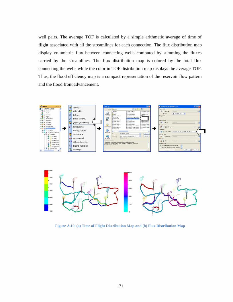
171
well pairs. The average TOF is calculated by a simple arithmetic average of time of
flight associated with all the streamlines for each connection. The flux distribution map
display volumetric flux between connecting wells computed by summing the fluxes
carried by the streamlines. The flux distribution map is colored by the total flux
connecting the wells while the color in TOF distribution map displays the average TOF.
Thus, the flood efficiency map is a compact representation of the reservoir flow pattern
and the flood front advancement.
Figure A.19. (a) Time of Flight Distribution Map and (b) Flux Distribution Map
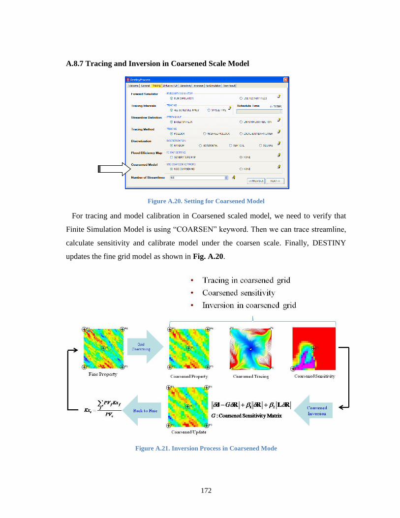
172
A.8.7 Tracing and Inversion in Coarsened Scale Model
Figure A.20. Setting for Coarsened Model
For tracing and model calibration in Coarsened scaled model, we need to verify that
Finite Simulation Model is using “COARSEN” keyword. Then we can trace streamline,
calculate sensitivity and calibrate model under the coarsen scale. Finally, DESTINY
updates the fine grid model as shown in Fig. A.20.
Figure A.21. Inversion Process in Coarsened Mode
173
APPENDIX B
A STECTRAL CLUSTERING PROGRAM WITH DESCRETE DATA
B.1 Introduction
The clustering or grouping algorithm is defined as “minimize the similarity between
groups and maximize the similarity within a group”. A graph partitioning from spectral
theory provides a fast way to decompose a domain for local spatial grouping. The
spectral clustering has been used in various engineering fields; supercomputing, machine
learning, logistics, internet shopping and social network service. Hence, the spectral
clustering algorithm has profound theoretical background and is comparatively easy to
implement in new area.
The graphic partitioning in the petroleum engineering provide a good decision gauge
to segment regions while keeping prior model’s main heterogeneous and/or connectivity
features; such as high or low permeable channel and barrier. For this purpose, we have
introduced graphical partitioning for reservoir segmentation based on grid properties
and/or connectivity on Chapter 3 and 4. The heterogeneity and connectivity are closely
related to flow dynamics of a reservoir.
To understand the Spectral Clustering features is important to get a good segmentation
results for history matching. For the purpose, we prepare a simple data clustering
program with MATLAB graphic user interface.
B.2 Program Overview
The background theories are explained more details on Chapter 3. The provided
spectral clustering demonstration program consists of the following steps: (1) Randomly
generate Gaussian distribution data clusters (2) Construct affinity Laplacian matrix
based on input free parameters and correlation distance (3) Use graph partitioning
techniques to create zonation and find groups. The graphic cut from the data location and
heterogeneity, is not arbitrary and derived from optimization with graphic cutting metric.

174
Users can easily test the correlations of initial data distribution, free parameters,
correlation distance and cutting algorithms, which are input parameters in the program.
B.3 The Graphic User Interface (GUI)
The GUI illustrated in Fig. B.1 follows this procedure as (1) generate data set (2)
construct affinity Laplacian and calculate the second eigenvector (3) apply cutting
algorithm.
Figure B.1. Graphic User Interface for Clustering
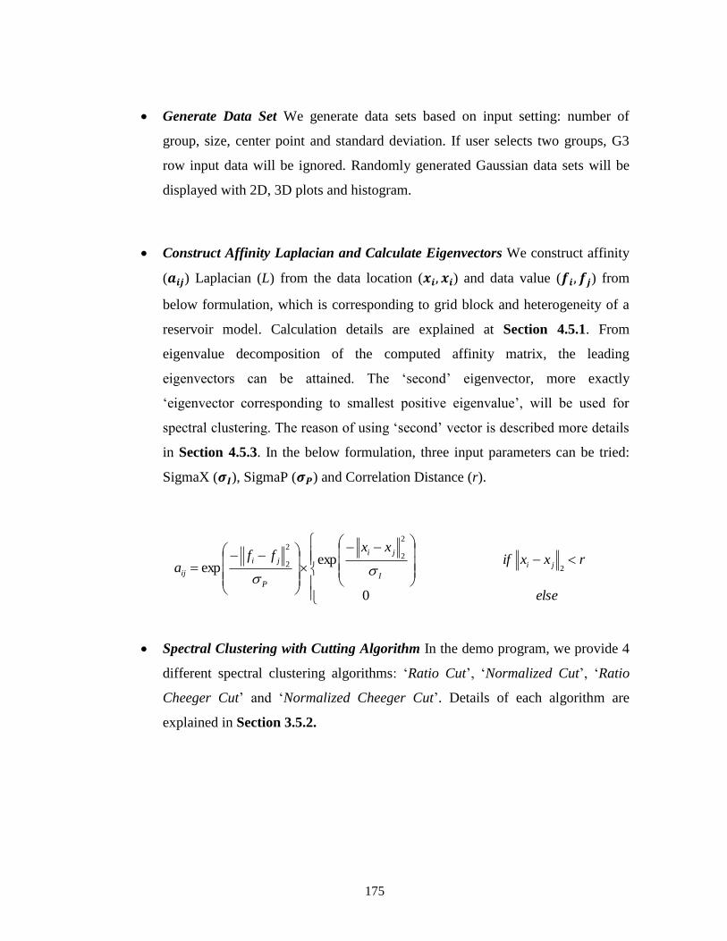
175
Generate Data Set We generate data sets based on input setting: number of
group, size, center point and standard deviation. If user selects two groups, G3
row input data will be ignored. Randomly generated Gaussian data sets will be
displayed with 2D, 3D plots and histogram.
Construct Affinity Laplacian and Calculate Eigenvectors We construct affinity
( ) Laplacian (L) from the data location ( ) and data value ( ) from
below formulation, which is corresponding to grid block and heterogeneity of a
reservoir model. Calculation details are explained at Section 4.5.1. From
eigenvalue decomposition of the computed affinity matrix, the leading
eigenvectors can be attained. The ‘second’ eigenvector, more exactly
‘eigenvector corresponding to smallest positive eigenvalue’, will be used for
spectral clustering. The reason of using ‘second’ vector is described more details
in Section 4.5.3. In the below formulation, three input parameters can be tried:
SigmaX ( ), SigmaP ( ) and Correlation Distance (r).
else
rxxifxx
ffa ji
I
ji
P
ji
ij
0
expexp 2
2
22
2
Spectral Clustering with Cutting Algorithm In the demo program, we provide 4
different spectral clustering algorithms: ‘Ratio Cut’, ‘Normalized Cut’, ‘Ratio
Cheeger Cut’ and ‘Normalized Cheeger Cut’. Details of each algorithm are
explained in Section 3.5.2.
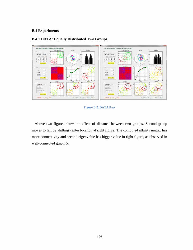
176
B.4 Experiments
B.4.1 DATA: Equally Distributed Two Groups
Figure B.2. DATA Part
Above two figures show the effect of distance between two groups. Second group
moves to left by shifting center location at right figure. The computed affinity matrix has
more connectivity and second eigenvalue has bigger value in right figure, as observed in
well-connected graph G.
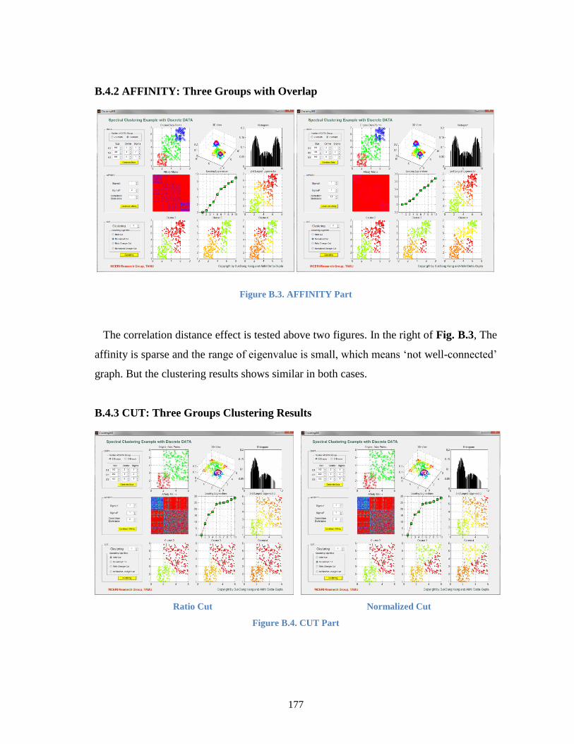
177
B.4.2 AFFINITY: Three Groups with Overlap
Figure B.3. AFFINITY Part
The correlation distance effect is tested above two figures. In the right of Fig. B.3, The
affinity is sparse and the range of eigenvalue is small, which means ‘not well-connected’
graph. But the clustering results shows similar in both cases.
B.4.3 CUT: Three Groups Clustering Results
Ratio Cut Normalized Cut
Figure B.4. CUT Part
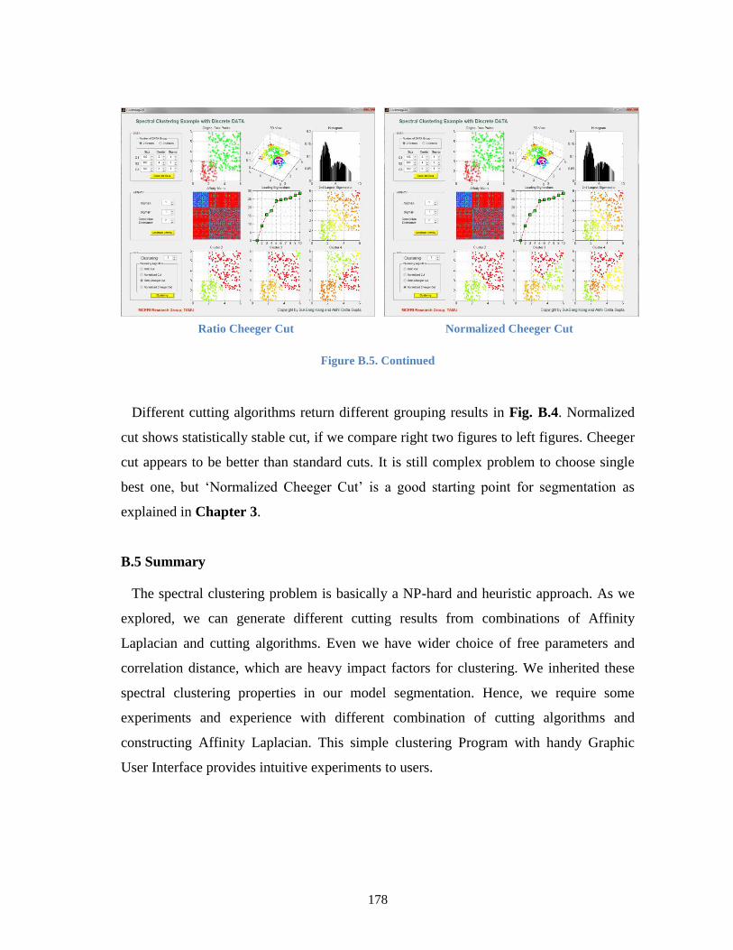
178
Ratio Cheeger Cut Normalized Cheeger Cut
Figure B.5. Continued
Different cutting algorithms return different grouping results in Fig. B.4. Normalized
cut shows statistically stable cut, if we compare right two figures to left figures. Cheeger
cut appears to be better than standard cuts. It is still complex problem to choose single
best one, but ‘Normalized Cheeger Cut’ is a good starting point for segmentation as
explained in Chapter 3.
B.5 Summary
The spectral clustering problem is basically a NP-hard and heuristic approach. As we
explored, we can generate different cutting results from combinations of Affinity
Laplacian and cutting algorithms. Even we have wider choice of free parameters and
correlation distance, which are heavy impact factors for clustering. We inherited these
spectral clustering properties in our model segmentation. Hence, we require some
experiments and experience with different combination of cutting algorithms and
constructing Affinity Laplacian. This simple clustering Program with handy Graphic
User Interface provides intuitive experiments to users.
Copyright © 2022 FDOKUMEN