MAKING BOMBS FOR PEACEFUL PURPOSES: HOW EXPLOSIVE PROCESSES

RENDER LIGNOCELLULOSIC BIOMASS MORE AMENABLE TO BIOLOGICAL

DIGESTION

A Dissertation

by

AUSTIN ELI BOND

Submitted to the Office of Graduate and Professional Studies of

Texas A&M University

in partial fulfillment of the requirements for the degree of

DOCTOR OF PHILOSOPHY

Chair of Committee, Eric Petersen

Co-chair of Committee, Mark Holtzapple

Committee Members, Hung Jue Sue

David Staack

Head of Department, Andreas Polycarpou

August 2016

Major Subject: Mechanical Engineering

Copyright 2016 Austin Bond

ii

ABSTRACT

Experiments were performed to investigate the effects of shock waves – generated by

explosive processes – on enhancing enzymatic digestibility of corn stover for conversion

into biofuels, chemicals, or animal feed. Following an alkaline chemical pretreatment

process, shock treatment was performed, which increased digestibility. Digestibility was

assessed at a standard enzyme loading of 46.7 mg protein/g glucan. Without shock, the

enzymatic conversion was 0.80 g glucan digested/g glucan fed. With shock, the enzyme

loading is reduced by ~2× while maintaining a constant conversion.

Shotgun shells and hydrogen detonation produced identical digestibility

increases; however, hydrogen detonation eliminated the need to magnetically

remove contaminants introduced from shotgun shells. Contrary to initial hypotheses,

varying vessel geometry (depth = 1–3 ft, diameter = 4–8 in) or process conditions (peak

pressure = 2.07–12.1 MPa, and solids concentration = 5–10%) had an insignificant

impact on shock treatment efficacy within the experimental domain tested. Instead, the

pressurization rate is the key parameter when scaling the shock treatment process.

Specifically, the shotgun shell blast (108,000 MPa/s) and hydrogen detonation

(4,160,000 MPa/s) generate pressure quickly enough to enhance digestibility; in contrast,

the propane deflagration (37.2 MPa/s) did not.

Therefore, process scaling is extremely simple, because a vessel that contains gas

detonations should suffice. A slurry pump enables rapid cycling of the 20-L shock tube

iii

to already function at a commercially relevant scale. The maximum benefit of shock

treatment has yet to be determined. Subsequent experiments performed with plasma

discharge and solid explosives failed to increase digestibility, at the conditions

employed; but, liquid-phase shock waves may be more effective.

iv

DEDICATION

To my parents, and the Eternal Tao.

“The world is sacred; it can’t be improved. If you tamper with it, you’ll ruin it. If you

treat it like an object, you’ll lose it.”

– Lao Tzu, Tao te Ching –

“When the Master governs, the people, are hardly aware that he exists. Next best is a

leader who is loved. Next, one who is feared. The worst is one who is despised. If you

don't trust people, you make them untrustworthy. The Master doesn't talk, he acts.

When his work is done, the people say, ‘Amazing: we did it, all by ourselves!’”.

– Lao Tzu, Tao te Ching –

“If you over esteem great men, people become powerless. If you overvalue possessions,

people begin to steal. The Master leads by emptying people’s minds and filling their

cores, by weakening their ambition and toughening their resolve. He helps people lose

everything they know, everything they desire, and creates confusion in those who think

that they know. Practice not-doing, and everything will fall into place.”

– Lao Tzu, Tao te Ching –

v

ACKNOWLEDGEMENTS

For the sake of chronological order, I would first like to first thank my many childhood

mentors, teachers, and inspirations. Fortunately, I was able to attend excellent public

schools in Richardson, Texas, which is obvious now via hindsight.

My 4th grade teacher, Mr. Chehal would read aloud Greek mythology, which was

enjoyable, entertaining, and relaxing at the time; however, learning the ancient mythos

contextualized my understanding of modern art, specifically an appreciation for the

classics and enhanced ability to recognize original work.

Thank you to Mr. Davis for teaching me the joy of performing music. As a

talented musician, you made the right choice by starting me on the French horn. I

thoroughly enjoyed playing in the symphonic band from 6th grade all the way throughout

high school. I believe studying and performing classical symphony music was very

beneficial to developing my creative and artistic talents.

Next, my middle school shop teacher Mark Means deserves recognition because

of the many intellectually stimulating and fun experiences afforded. Prototyping CO2-

powered race cars, water-powered stratoblaster rockets, and learning Computer Aided

Drafting (CAD) exemplify the playful spirit that fueled my curiosity as a fledgling

engineer. Although students risked being injured while in the machine shop, Mr. Means

vi

deserves praise for creating such a fun learning environment, especially in the presence

of an administration which likely looked to eliminate such “costly” programs.

Mary Eisenmann, my AP high school chemistry teacher, deserves praise as well.

Her class was both challenging and fun. Some of the more memorable moments were

Mrs. Eisenmann’s methane and soap bubble incineration and the marshmallow and

vacuum chamber experiment. Mrs. Eisenmann (perhaps inadvertently) helped further

my interest and passion for playing with fire. Furthermore, the tye dye lab apron looked

amazing!

Mrs. Flickinger’s physics class was certainly challenging, but various

demonstrations were exemplary of the Socratic nature of learning and teaching

pedagogy, i.e. moments in which the student is tricked into learning resulting in some

form of emotional upheaval, generally as a surprise, which further cements memories

deep into the mind. Such surprises included the prediction of directionality in

gyroscopic precession, descent rate of an oblate disk versus hoop with respect to

moment of inertia, and suspension of an oil droplet via an electric field (known as the

Millican oil drop experiment). I definitely enjoyed the engineering challenges that the

trebuchet and Rube Goldberg rollercoaster experiments provided. These experiences

furthered my interest in engineering.

vii

I am very appreciative of the opportunity to spend multiple summers working in

Carlos Hoefken’s custom machine fabrication shop, Dynametrics. Our initial meeting

was purely dumb luck. I recall that we first interacted one weekday evening awaiting

checkout at Home Depot, where I was very conspicuously purchasing components for a

potato cannon. Carlos had a genuine interest in my purchase and offered me an

internship after realizing my scientific pursuit of potato cannons. As a consequence, I

was exposed to industrial machining processes and the entire mechanical design process.

The ability to work beneath engineers as a high school student was invaluable!

Dr. Richard Jaeckle deserves mention for being one of the only medical doctors I

have ever obtained counsel from who is actually competent. His advice has definitely

helped me maximize my wellbeing, as well as completely eliminate suffering from

chronic ailments, which ironically all stemmed from improper biological digestion.

Ironically because throughout the process of studying methods to improve anaerobic

acid fermentation for biofuels, I also learned how to inhibit fermentation and maximize

the metabolic efficiency of my own intestinal tract. Personally, this was done by

absolute abstinence from egg and dairy proteins, which when incompletely digested

release soluble toxic byproducts that wreak havoc on the human immune system, in a

symptomatically insidious manner. Furthermore, learning the profound effects that pH

and pH stability have on fermentations provided the incentive for me to utilize fruits and

vegetables as a means to eat a pH balanced diet. Probiotics have also proved to be

beneficial in my own diet, which is knowledge that is complementary to biomass

viii

processing. Independent of Dr. Jaeckle, I have conducted my own research on cancer

and personally believe that a pH-balance ketogenic (low-carbohydrate) diet are effective

means to prevent and treat cancer. Nevertheless, Dr. Jaeckle’s adamant emphasis on

proper digestion, which is synonymous with immune system health, have pointed me in

the direction of pH-balance, ketogenic, dairy-free, egg-free, and a bean-free diet.

Overall, Dr. Jaeckle helped spark a curiosity in biological digestion that was far beyond

the laboratory fermenter. This curiosity has had a profound benefit on my overall

wellbeing.

Furthermore, I would like to thank Aaron Smith, Cesar Granda, Kyle Ross, and

obviously Mark Holtzapple, for their inspiration, guidance, friendship, and mentoring.

Aaron Smith and I have had and maintained a long friendship that dates all the way back

to 1000-gal fermentations at the MixAlco Process Pilot Plant (~2005). I know the

bankruptcy of Terrabon was emotionally difficult for all of us involved. My only

comment is that the bankruptcy was a Black Swan Event. I do not know if biofuels are

an economical solution to climate change, but I do believe that a carbon-neutral source

of energy will eventually be necessary for future generations. It is futile to predict the

extent and urgency of climate change far in advance, but preventing cataclysmic climate

change is not; and doing so is the ethical obligation of current world leaders.

I would also like to thank Hema Rughoonundun for mastering the enzymatic

saccharifications for the DOE project, and Shane Fullman for helping program the shock

ix

tube LabVIEW control system; it worked flawlessly! A special thanks to David

Carrabba and Gooseneck Trailer for financial and fabrication support. Thanks to Circle

H Manufacturing and BVD machines for excellent fabrication of the larger shock tube

vessels. Also, a special thanks to Randy Marek for all the help he provided in the

chemical engineering machine shop. My hope is that he is enjoying his retirement!

x

NOMENCLATURE

SLP submerged lime pretreatment

OLP oxidative lime pretreatment

PZT piezoelectric transducer

PETN pentaerythritol tetranitrate, solid explosive

C4 common plastic explosive known as composition C

Brisance the shattering capability of a high explosive

HPLC high pressure liquid chromatography

P&ID process and instrumentation diagram

MAWP maximum allowable working pressure

GUI graphical user interphase

Total Impulse the area (or antiderivative) under a force versus time curve

Rise Time the time required for a signal to reach 99% of full-scale value

Strain-rate the time rate of change of strain m/(m*s)

xi

TABLE OF CONTENTS

Page

ABSTRACT .......................................................................................................................ii

DEDICATION .................................................................................................................. iv

ACKNOWLEDGEMENTS ............................................................................................... v

NOMENCLATURE ........................................................................................................... x

TABLE OF CONTENTS .................................................................................................. xi

LIST OF FIGURES ......................................................................................................... xiv

LIST OF TABLES .......................................................................................................... xxi

CHAPTER I INTRODUCTION AND LITERATURE REVIEW .................................... 1

1.1 Front Matter .......................................................................................................... 1 1.2 Sustainability ........................................................................................................ 3 1.3 Relevant Definitions, Concepts, & Nomenclature ............................................... 6

1.4 Various Biomass Pretreatment Methods ............................................................ 19 1.5 Introduction to Shock Treatment ........................................................................ 31

1.6 Overview of DOE Project Objectives ................................................................ 41 1.7 Dissertation Scope and Objectives ..................................................................... 44

CHAPTER II 2-L SHOTGUN-SHELL-DRIVEN SHOCK TUBE ................................ 45

2.1 Brief Introduction ............................................................................................... 45

2.2 Materials and Methods ....................................................................................... 45 2.3 Results ................................................................................................................ 66

2.4 Conclusions ........................................................................................................ 91

CHAPTER III GAS EXPLOSION DRIVEN 20-L SHOCK TUBE ................................ 94

3.1 Brief Introduction ............................................................................................... 94

3.2 Materials & Methods .......................................................................................... 94 3.3 Results .............................................................................................................. 118 3.4 Conclusions ...................................................................................................... 138

CHAPTER IV SCALING UP THE SHOCK TREATMENT PROCESS ..................... 142

4.1 Materials and Methods ..................................................................................... 142

xii

4.2 Results .............................................................................................................. 145 4.3 Conclusions ...................................................................................................... 156

CHAPTER V PLASMA DISCHARGE EXPERIMENTS ............................................ 158

5.1 Brief Introduction ............................................................................................. 158

5.2 Materials and Methods ..................................................................................... 159 5.3 Results and Discussion ..................................................................................... 166 5.4 Conclusions ...................................................................................................... 171 5.5 Future Work ..................................................................................................... 173

CHAPTER VI SOLID EXPLOSIVE EXPERIMENTS ................................................ 176

6.1 Brief Introduction ............................................................................................. 176

6.2 Materials & Methods ........................................................................................ 176 6.3 Results & Discussion ........................................................................................ 183

6.4 Conclusions ...................................................................................................... 186 6.5 Future Work ..................................................................................................... 187

CHAPTER VII M&M MARS PROJECT ...................................................................... 189

7.1 Materials and Methods ..................................................................................... 189 7.2 Results and Discussion ..................................................................................... 198

7.3 Conclusions ...................................................................................................... 212 7.4 Future Work ..................................................................................................... 212

CHAPTER VIII CONCLUSIONS ................................................................................. 213

REFERENCES ............................................................................................................... 216

APPENDIX A LIME PRETREATMENT PROCEDURE ........................................... 227

APPENDIX B ENZYMATIC SACCHARIFICATION PROCEDURE ...................... 230

APPENDIX C BIOMASS DRYING PROCEDURE .................................................... 243

APPENDIX D COMPOSITIONAL ANALYSES PROCEDURES ............................. 245

LP 3.1.1 Preparation of Samples for Compositional Analysis: Air Drying .............. 245

LP 3.2.1 Determination of Extractives in Biomass .................................................... 248 LP 3.3.1 Determination of Structural Carbohydrate and Lignin in Biomass ............. 252 LP 3.4.1 Determination of Total Solids in Biomass and Process Liquids ................. 260 LP 3.5.1 Determination of Ash Content in Biomass and Process Samples ............... 262

APPENDIX E SHOTGUN SHELL SHOCK TREATMENT PROCEDURE .............. 264

xiii

APPENDIX F SHOCK PRETREATMENT PROCEDURE (GAS EXPLOSION) ..... 267

APPENDIX G LABVIEW OPERATING INSTRUCTIONS ...................................... 273

Background Information ............................................................................................ 273 DAQ Computer Information .................................................................................. 273

Relevant Files ......................................................................................................... 275 File Paths ................................................................................................................ 278

Manual Control Mode ................................................................................................ 278 Main Program Iterative Filling Mode ........................................................................ 280 Data Analysis ............................................................................................................. 289

APPENDIX H PROJECT SAFETY ANALYSIS – FILE DATED 07/12/2012 .......... 299

APPENDIX I SHOCK TREATMENT PROCEDURE – PLASMA DISCHARGE .... 322

APPENDIX J SOLID EXPLOSIVE EXPERIMENTAL PROCEDURE ..................... 324

APPENDIX K PIPE BOMB PRETREATMENT PROCEDURE ................................ 325

APPENDIX L ALKALINE PRETREATEMENT PROCEDURE (8-L REACTOR) .. 327

xiv

LIST OF FIGURES

Page

Figure 1: The “Fourth Quadrant” as defined by Nassim Taleb, ......................................... 3

Figure 2: Night-time satellite image of earth, which displays illuminated cities. [3] ........ 4

Figure 3: Macroscopic view of the MixAlco process. ....................................................... 6

Figure 4: Schlieren photograph of a muzzle blast from a 0.30-06 caliber rifle. [7] .......... 7

Figure 5: Pistol shrimp. [8] ................................................................................................ 8

Figure 6: Drawings of Mount Krakatoa before and after the volcanic eruption. [10] ...... 9

Figure 7: Shock wave lithotripsy diagram. [11] ............................................................... 10

Figure 8: Schematic diagram of explosive forming. [13] ................................................ 11

Figure 9: Blast fishing off of the Dar es Salaam coast. [16] ............................................ 12

Figure 10: Picture showing reef damage from blast fishing. [16] .................................... 13

Figure 11: Detonation wave structure. [18]...................................................................... 15

Figure 12: Transition to detonation along pipe length. structure. [18] ............................ 16

Figure 13: Effect of loading rate on the fracture toughness [21] ..................................... 18

Figure 14: Goals of pretreatment. [24] ............................................................................. 19

Figure 15: Ball milling apparatus. [25] .......................................................................... 20

Figure 16: Two-roll milling apparatus. [29] ..................................................................... 21

Figure 17: Sonication device. [32] ................................................................................... 22

Figure 18: Sonication pretreatment data. [32] .................................................................. 23

Figure 19: Hydrodynamic cavitation diagram. [32] ......................................................... 24

Figure 20: Cavitation pretreatment data. [32] .................................................................. 25

xv

Figure 21: Plasma shock pretreatment reactor used to pulverize food products. [72] ..... 33

Figure 22: Hydrodyne meat tenderization apparatus. [70] ............................................... 34

Figure 23: Xiong – shock treatment apparatus. [71] ........................................................ 35

Figure 24: Xiong – shock treatment data. [71] ................................................................. 37

Figure 25: Biomass pretreatment shock tube. .................................................................. 38

Figure 26: 2-L shock pretreatment apparatus. .................................................................. 39

Figure 27: Enzyme assay data for 2–L shock tube at 1% solids. [73] ............................. 40

Figure 28: Rumen digestibility of shock treated corn stover. [73] ................................... 41

Figure 29: Shock treatment process flow diagram. .......................................................... 42

Figure 30: Baled/modulized corn stover. ......................................................................... 43

Figure 31: 2012 harvest year corn stover stored indoors in trash bags. .......................... 43

Figure 32: Large Champion mill. ..................................................................................... 44

Figure 33: Lime pretreatment diagram. ............................................................................ 46

Figure 34: Alkaline pretreatment apparatus. .................................................................... 47

Figure 35: Foaming pretreatment broth. .......................................................................... 48

Figure 36: Manifold controlling air flow through CO2-scrubbing column. ..................... 48

Figure 37: Cross-sectional view of 2-L shock tube. ......................................................... 50

Figure 38: Spring-loaded firing mechanism. .................................................................... 53

Figure 39: Time-lapse photo of shotgun shell blast. [74] ................................................ 54

Figure 40: Piezoelectric pressure transducer operation schematic. .................................. 56

Figure 41: Mounting drawing for pressure transducers. .................................................. 57

Figure 42: Piezoelectric pressure transducers, signal conditioner, and cables. ................ 58

xvi

Figure 43: National Instruments data acquisition (DAQ) card. ....................................... 59

Figure 44: Pressure transducer locations. ......................................................................... 60

Figure 45: Shotgun shell solenoid-actuated ignition mechanism. .................................... 61

Figure 46: Solids recovery methods for shock treatment. ................................................ 63

Figure 47: 80-mesh sieve tray used for recovering shock-treated biomass. .................... 64

Figure 48: Diagram illustrating enzymatic saccharification procedure. .......................... 65

Figure 49: Saccharification tubes (horizontal) beginning incubation. ............................. 65

Figure 50: SLP mass balance. .......................................................................................... 68

Figure 51: Saccharification reproducibility (46.7 mg protein/g glucan). ......................... 71

Figure 52: Glucan content for various raw & SLP treated biomass. ................................ 73

Figure 53: Reflected wave closed petals on the shotgun shell. ........................................ 74

Figure 54: Flange damage and rust from shotgun pellets. ............................................... 75

Figure 55: Ferrous particulate from shotgun shells and combine harvesting................... 77

Figure 56: Typical pressure trace for Station T1 (unsubmerged). ................................... 78

Figure 57: Pressure trace for Station T3 (submerged). .................................................... 79

Figure 58: Isolating adapters used to minimize structure resonance noise. ..................... 80

Figure 59: Implementation of isolation adapters. ............................................................. 80

Figure 60: Subplot representation of pressure data. ......................................................... 83

Figure 62: Reloading shotguns shells. (a) = table salt on scale, (b) = table salt. ............. 85

Figure 63: Pressure traces for Station T1 (unsubmerged). ............................................... 87

Figure 64: SEM images of corn stover fiber. ................................................................... 88

Figure 65: SEM images of corn stover xylem and phloem structures. ............................ 89

xvii

Figure 66: Shock treatment “Base Case” – SLP5, 5 d, 15% solids assay. ....................... 90

Figure 67: Gas explosion system process and instrumentation diagram. ........................ 97

Figure 68: Newly fabricated and assembled gas manifold............................................... 98

Figure 69: Nylon insulator and spark plug mount for gas manifold. ............................... 99

Figure 70: Wiring board for junction box mounted within the bunker. ......................... 100

Figure 71: Junction box which houses the relay circuitry. ............................................. 101

Figure 72: Exhaust pipe and grounding wire. ................................................................ 102

Figure 73: Air compressor mounted to drive pneumatically actuated needle valves. .... 102

Figure 74: Cross-section of 8-in Schedule 160 pipe used for 20-L shock tube. ............ 103

Figure 75: Exploded view of PZT adapters for 20-L shock tube. .................................. 105

Figure 76: Machine drawing for female component of PZT adapter. ............................ 106

Figure 77: Machine drawings for nozzle. ....................................................................... 107

Figure 78: Machine drawings indicating axial transducer locations. ............................. 108

Figure 79: Drawings for the 20-L shock tube stand. ...................................................... 109

Figure 80: Cross-sectional view of the 20-L shock tube. ............................................... 110

Figure 81: Bunker during installation. ........................................................................... 112

Figure 82: Installation of additional tower section on bunker. ...................................... 113

Figure 83: Completed installation of bunker. ................................................................. 113

Figure 84: Hydrogen detectors, (a) mounted in bunker, (b) mounted in boiler shed. .... 114

Figure 85: Ventilation blower mounted to bunker wall. ................................................ 115

Figure 86: Redundant, step-down regulators mounted to bunker wall. ......................... 116

Figure 87: Relief valves mounted to fuel and oxidizer lines. ......................................... 116

xviii

Figure 88: Erection of the 3-ton gantry crane (start to finish clockwise). ..................... 117

Figure 89: (a) ASME hydrostatic pressure test. (b) Certification plate. ........................ 119

Figure 90: (a) Temporary closures used for test. (b) Detailed view of welds. ............... 120

Figure 91: Buzz-coil/relay-driven spark ignition circuit. ............................................... 121

Figure 92: Brilliant arc for dimmer switch driven ignition circuit. ................................ 122

Figure 93: Catastrophic failure of capacitor in dimmer-switch driven ignition circuit. 122

Figure 94: Gas manifold with glow plug adapter installed. ........................................... 123

Figure 95: Gas manifold with heating tape applied. ...................................................... 124

Figure 96: Glow plug adapter before and after boring out inner diameter..................... 124

Figure 97: Gas manifold before and after additional boring process. ............................ 125

Figure 98: Roughness elements/baffles used to promote hydrogen detonation. ............ 126

Figure 99: Fully installed and functioning gas explosion system. ................................. 128

Figure 100: Pressure traces for propane deflagration. .................................................... 130

Figure 101: Enzyme assay for propane deflagration. ..................................................... 131

Figure 102: 20-L shock tube manifold suspended within bunker. ................................. 132

Figure 103: 20-L shock tube after first successful inaugural test. ................................. 133

Figure 104: Pressure traces for hydrogen detonation. .................................................... 134

Figure 105: Aftermath of catastrophic gasket failure and blow-out. ............................. 135

Figure 106: Non-catastrophic failure of Teflon gasket and O-ring seal......................... 136

Figure 107: Splatter pattern comparison (a) 10% solids versus (b) 40% solids............. 136

Figure 108: Hydrogen detonation pressure trace for Station T1 (zoomed in). .............. 137

Figure 109: Hydrogen detonation pressure trace compared to propane deflagration. ... 141

xix

Figure 110: 3-ft-deep and 4-ft-deep shock tubes. .......................................................... 143

Figure 111: Enzyme assay data for various pressures and solid concentrations. ........... 150

Figure 112: Enzyme assay for propane deflagration. ..................................................... 151

Figure 113: Enzyme assay data for 2-L vs. 20-L shock tube. ........................................ 152

Figure 114: Conceptual 2–D drawings for hinged-top batch shock treatment reactor. . 153

Figure 115: 3-D drawings for hinged-top batch reactor. ................................................ 154

Figure 116: Drawing for the turbocompressor conceptual shock treatment apparatus. . 155

Figure 117: Conceptual ram-and-diverter valve shock treatment apparatus. ................. 156

Figure 118: Interior dimensions for acrylic reactor. ...................................................... 160

Figure 119: Acrylic reactor loaded with biomass slurry. ............................................... 160

Figure 120: Electrical circuit for both plasma discharge experiments. .......................... 162

Figure 121: Acrylic reactor plasma discharge. (a) isometric view, (b) top view. .......... 162

Figure 122: high-voltage capacitors used ....................................................................... 163

Figure 123: Visible particle size reduction due to extended plasma discharge pulses... 167

Figure 124: Graphical representation of data from Table 8. .......................................... 169

Figure 125: 13-µF capacitor available for Round 3.0 experiments............................... 174

Figure 126: Location of TEEX bomb range at Texas A&M Riverside Campus. .......... 176

Figure 127: Aerial view of bomb range, explosive storage shed, and pavilion. ............ 177

Figure 128: solid explosives containment method. ........................................................ 179

Figure 129: Steel oxygen tank/liner, which were destroyed during the experiment. ..... 183

Figure 130: Final sugar concentrations achieved by the end of each saccharification. . 184

Figure 131: Oven with wrist-action shaker used for pipe bomb alkaline pretreatment. 190

xx

Figure 132: Pipe bombs used for alkaline pretreatment. ................................................ 191

Figure 133: 8-L Parr reactor used for alkaline pretreatment. ......................................... 193

Figure 134: 22-L glass flask and vacuum distillation column with condenser. ............. 196

Figure 135: Entire vacuum distillation assembly. .......................................................... 196

Figure 136: Vacuum pump and condensate collection vessel used for distillation. ...... 197

Figure 137: Yields for corn stover and cassava ............................................................. 199

Figure 138: Yields for alfalfa and spent grain. ............................................................... 200

Figure 139: Master set of all corn stover sugar yields. .................................................. 202

Figure 140: Corn stover sugar yields (plotted). .............................................................. 203

Figure 141: Master set for all spent grain sugar yields. ................................................. 204

Figure 142: Spent grain sugar yields. ............................................................................. 206

Figure 143: Alfalfa sugar yield. ..................................................................................... 207

Figure 144: Master set for all cassava sugar yields. ....................................................... 208

Figure 145: Cassava sugar yields. .................................................................................. 209

Figure 146: Pouring corn stover syrup. .......................................................................... 211

xxi

LIST OF TABLES

Page

Table 1: Example conditions for oxidative lime pretreatment. [34] ................................ 28

Table 2: Various SLP yields ............................................................................................. 67

Table 3: Various enzyme activities and protein concentrations ....................................... 69

Table 4: Summary of Results for Explosive Gas Test ................................................... 127

Table 5: Enzyme assay data for various solids concentrations. ..................................... 146

Table 6: Enzyme assay data for various depths. ............................................................ 147

Table 7: Enzyme assay data for various pressures. ........................................................ 148

Table 8: Data from Round 1.0 of plasma discharge experiment. ................................... 168

Table 9: Data from Round 2.0 of plasma discharge experiment. ................................... 170

Table 10: Experimental test matrix for solid explosives experiment. ............................ 181

Table 11: Test conditions during alkaline pretreatment optimization experiments ....... 192

Table 12: Summary of process conditions and sugar yields .......................................... 201

Table 13: Summary of sugar production runs. ............................................................... 209

1

CHAPTER I

INTRODUCTION AND LITERATURE REVIEW

1.1 Front Matter

Throughout history many philosophers have made careers by attempting to predict the

future; however, except for blind luck, they are always wrong. These predictions are

always made under the postulated existence of a deterministic universe, which is utterly

wrong. The universe is stochastic in nature; thus, the future is indeterminate.

The stochastic nature of the universe is a truth that seems rational to most

individuals during a thoughtful discussion, yet this realization is intuitively neglected by

most people when considering their subsequent actions. Simply put, most people will

consciously acknowledge their inability to predict the future. Yet after the conversation

ends, they will tune the television back to the news channel for election coverage,

shuffle money between brokerage accounts, or prepare for the impending apocalypse,

with great certainty of the future outcome. This behavior indicates the discrepancy

between the ways knowledge and intuition manifest themselves in human behavior.

2

Nassim Taleb, author of The Black Swan, argues that history is dominated by low

probability events, which he refers to as Black Swan Events [1]. He has rigorously

defined a Black Swan Event as one that

1. occurs as a surprise (to the observer)

2. has major (and often catastrophic) effect

3. and is rationalized by hindsight, such that it appears obvious via a posteriori.

Some examples of historical Black Swan events follow:

9/11 terrorist attacks

2008 financial crisis

collapse of the Soviet Union

assassination of Archduke Ferdinand

advent of the internet

creation of the first microprocessor

Taleb says that the Black Swans originate from the “Fourth Quadrant” (Figure 1).

The fourth quadrant is where the unknown-unknowns lie buried beneath a random

environment and await future discovery. Neither theoretical knowledge nor intuition can

predict such Black Swan events, thus resulting in an indeterminate future.

3

Figure 1: The “Fourth Quadrant” as defined by Nassim Taleb,

1.2 Sustainability

1.2.1 Energy Consumption

Recent estimates assert that early hominin regularly (as opposed to sporadic or

opportunistically) used fire 350,000–320,000 years ago. [2] This makes fire a genuinely

primal force influencing the development of both mankind and society. The industrial

era has allowed fire to be conquered so effectively that we now refer to fire, in a more

abstract form, as energy.

Energy is both essential and pervasive to modern industrial society – so much so

that satellite images display a plethora of cities that illuminate the night sky (Figure 2).

[3] Often overlooked is that nearly all of the light emitted in the nighttime sky originates

from fire, usually from an electrical power plant burning fossil fuels. To illustrate the

4

effect of the Industrial Revolution, one simply needs to look at the luminosity, or lack

thereof, from undeveloped regions such as North Korea, Africa, and Indo-China.

Figure 2: Night-time satellite image of earth, which displays illuminated cities. [3]

Because of population growth, global energy demand is rapidly increasing. In

only 10 years (2001–2011), the world population grew from 6.1 to 6.9 billion people. [4]

It is safe to assume that the demand for energy will increase proportionately with

growing population. Nevertheless, mankind has essentially conquered planet Earth, and

hydrocarbon fuels are the primary energy source that has allowed it to happen.

The Greenhouse Gas Effect describes the accumulation of gases in the

atmosphere that cause global climate change. To a painful degree, the debate is highly

politicized. The argument that CO2 emissions drive a net increase in global temperature

is scientifically sound, yet those who counter-argue attempt to use the presence of

5

uncertainty as both a weakness and a means to invalidate such arguments. Considering

the indeterminate nature of the future, debating over the consequences of warming, or

any particular future scenarios, is a moot point. The practice of burning fossil fuels on a

global scale is simply unnatural – the magnitude of this dissonance with nature is

alarming. Instead, society should seek to harmonize itself with nature, instead of simply

conquering it.

1.2.2 Biofuels

The use of biofuels is not a new idea. In fact, in the context of harmonizing society with

nature, biofuels are an ancient concept. Prior to the proliferation of heat engines, the

domesticated horse was the primary means for transportation and farm work. Horses,

cows, and goats use mixed cultures to digest lignocellosic biomass – an abundant fuel

since the beginning of time.

1.2.3 Carboxylate Platform / MixAlco Process

The MixAlco process is a patented technology that converts any biodegradable material

into industrial fuels and chemicals. [5]. This method employs a buffered mixed-culture

fermentation to convert all non-lignin biomass components to carboxylate salts, which is

more energy efficient than thermochemical conversion. [6] The fermentation step in the

MixAlco process (Figure 3) is the heart of the process, and is inspired by ruminant

animals, such as cattle.

6

Figure 3: Macroscopic view of the MixAlco process.

1.3 Relevant Definitions, Concepts, & Nomenclature

1.3.1 Fluid Mechanics

Shock waves, a primary focus of this document, are defined as the coalescence of

pressure waves propagating through a fluid at supersonic velocities that compress and

heat the fluid via entropy generation. Using schlieren photography, shock waves can be

easily visualized. For example, Figure 4 shows the spherical blast wave and the

supersonic bullet piercing the blast. [7]

7

Figure 4: Schlieren photograph of a muzzle blast from a 0.30-06 caliber rifle. [7]

The pistol shrimp (Figure 5) is an example of an organism that has evolved a

large asymmetrical claw that generates cavitation waves as a survival mechanism. The

rapid snapping action of the claw actually ejects a high-velocity water jet — with a

speed up to 100 km/h (62 mph) — that generates a low-pressure cavitation bubble that

bursts with a loud snap [8]. This cavitation bubble burst so violently (218 dB), it is

louder than many gun shots and is strong enough to break glass. [8] Needless to say, the

cavitation waves emitted from the pistol shrimps claw are also strong enough to stun

prey, communicate with other organisms, and ward off predators.

8

Figure 5: Pistol shrimp. [8]

Every time a lightning bolt strikes, the entrained air forms an arc plasma that is

rapidly heated along the lighting channel. The heated air emits a strong shock wave that

later decays into a sound wave. Transport delays of sound are responsible for the roll of

thunder. Beyond these facts, little more is known about thunder. [9]

On August 27th 1883, Mount Krakatoa erupted and emitted a blast wave so

powerful it shook the planet and the ever-weakening soundwave remained strong enough

to be detected at weather stations as it circled the earth four times. [10] The volcanic

eruption is yet another example of shock waves that exist in nature. According to

legend, the eruption was so loud that the blast wave ruptured the eardrums of nearby

sailors in merchant marine ships. Drawings made of the volcano before and after

eruption illustrate the massive upheaval of mountainous soil and rock that was

subsequently aerosolized (Figure 6).

9

Figure 6: Drawings of Mount Krakatoa before and after the volcanic eruption. [10]

Shock wave lithotripsy is a medical procedure that was first used to help patients

remove pancreas, kidney, and gallstones. [11] Although various methods exist,

extracorporeal shock waves were first used. The shock waves were generated by

piezoelectric devices that were focused on a stone within the organ of interest. Through

subsequent treatments, the shock waves would ultimately fragment the stone into a size

that was small enough to be passed through the ureters. Given the nature of shock wave

transmission and attenuation in adipose tissue, extracorporeal shock wave lithotripsy is

less effective for obese patients. [12] Figure 7 shows a diagram for performing

extracorporeal shock wave lithotripsy.

10

Figure 7: Shock wave lithotripsy diagram. [11]

Blast forming is a process in which an explosive is suspended within water and is

subsequently detonated in an orientation so the blast wave forges a metallic sheet into

the shape of the die on which it is placed (Figure 8). Blast forming is primarily used for

low-volume parts that are prohibitively large or thick to be forged by alternate

mechanical means.

11

Figure 8: Schematic diagram of explosive forming. [13]

Explosives are used commonly in the mining industry. Their destructive power

is utilized far more effectively and economically than any previous means, such as

armies of laborers with pick axes. Without explosives, metals and fuels required for the

Industrial Revolution would never have been produced in the quantities required for

modern highway, rail, and water transport systems. [14] [15]

12

Explosive fishing still exists in modern Tanzania where it is considered a

destructive fishing practice. [16] Explosive fishing is an extraordinarily simple practice

in which explosives (often homemade) are detonated underwater. A fisher, or poacher,

needs neither expensive equipment or time to reap the bounty of the sea (Figure 9).

Figure 9: Blast fishing off of the Dar es Salaam coast. [16]

Unfortunately, explosives blast waves not only kill fish, but also permanently

damage coral reefs (Figure 10). [16] In Tanzania, this practice is both an environmental

and social problem because many fishermen are simply trying to earn a living, and many

government officials are too corrupt or apathetic to care about the environmental

damage.

13

Figure 10: Picture showing reef damage from blast fishing. [16]

In war veterans, blast waves are known to cause insidious forms of brain damage.

Soldiers return from combat seemingly unharmed, but have a wide variety of

psychological and neurological problems. Although precise neuropathological

explanations for the causes of blast-related traumatic brain injury are difficult to

conclusively identify, the causes are believed to include concussion, hemorrhage, edema,

and diffuse axonal injury. [17]

14

1.3.2 Combustion Science

Deflagrations are defined as combustion waves that propagate at subsonic velocity

relative to the unburnt gas immediately ahead of the flame. [18] Deflagrations occur

commonly and safely in many everyday scenarios, such as modern automobile

reciprocating piston engines. Deflagrations propagate relatively slowly (on the order of

cm/s) and are usually far less damaging than detonations.

On the other hand, detonations are defined as combustion waves that propagate

at a supersonic velocity relative to the unburnt gas immediately ahead of the flame. [18]

Detonations can be initiated by a shock wave emitted from a high-explosive charge, or

can be initiated by a deflagration transitioning into a detonation. Figure 11 displays the

characteristic cell structure of a detonation wave in which a shock wave compresses and

heats unburned, premixed gas, and the subsequent heat release reduces the pressure

slightly and ejects heated gas out the other side of the shock wave. The high-velocity

hot gas ejected from the back side of the shock wave further accelerates the shock wave

faster into the unburned gas. This is a positive feedback mechanism that causes

detonations to rapidly build strength and increases their damaging effects.

15

Figure 11: Detonation wave structure. [18]

For gas explosions, a detonation cannot be iniated directly; instead it appears

after the deflagration-to-detonation transition point. In the same sense that a laminar

boundary layer will likely transition to a turbulent boundary layer, under most

conditions, a deflagration wave will transition to a detonation, given the appropriate

amount of run-up distance and confinement. Run-up distance is the distance required for

a deflagration wave to travel before transitioning to a detonation wave (Figure 12). Run-

up distance is usually reported dimensionlessly in the form of pipe diameters. For

example, methane is a particularly safe gas to handle because, even when perfectly

premixed, it has an extraordinarily long run-up distance; in contrast, many precautionary

measures must be taken to prevent a hydrogen mixture from detonating.

16

Figure 12: Transition to detonation along pipe length. structure. [18]

Detonation can be promoted by inserting baffles within a tube, of specific

geometry, to promote vortex shedding and localized hot spots that increase the average

temperature and accelerate the deflagration wave. On the other hand, baffles can also

damp detonation waves by reflecting them upon each other, in a manner similar to

suppressors/silencers used to conceal muzzle blast from guns.

1.3.3 Solid Explosives

Compared to gas phase explosions, solid explosives have an extremely high energy

density. Primary (high) explosives are extraordinarily shock, heat, and pressure

sensitive. For industrial use, they are usually in dilute or stabilized form. [19]

Secondary (low) explosives, being more stable, are usually ignited solely by the

detonation from a primary explosive.

Brisance describes the destructive potential of an explosive. Brisance can be

used qualitatively, but there is a quantitative experimental sand crushing test that can be

17

used to measure brisance. [20] Generally, a faster moving detonation wave yields a

higher brisance, or greater potential to shatter the substrate of interest; however, this

phenomenon highly depends on the substrate of interest. Clearly, clay soil will respond

differently than dry sand or hard limestone.

1.3.4 Polymer Material Science

Lignocellulosic biomass is a composite material with many components that are relevant

to material science. Lignocellulose consists of three primary macroscopic constituents:

cellulose, hemicellulose, and lignin. Cellulose is a glucose polymer. Hemicellulose is a

polymer of mixed sugars, primarily xylose. Lignin is a polymer of phenylpropanoids.

Depending on the particular plant, the ratios of each component may vary. For example,

trees have a much higher lignin content than grass. Biomass has mechanical behavior

reminiscent of common industrial polymers (e.g., polyethylene) such as the strain-rate

effect.

The strain-rate effect governs the mechanical behavior of polymers.

Fundamentally, the strain-rate effect results from viscosity, which is caused by

molecular collisions. Thus, polymeric materials have a stress tensor that is both rate and

strain dependent; thus, polymers exhibit behavior of both solids and liquids.

Figure 13 displays the dramatic decrease in fracture toughness (~10×) of a

rubber-modified epoxy resin subjected to an impact test. Because polymers do not have

18

an endurance limit like metals, fatigue failures can exempt polymers from applications

requiring cyclical loading.

Figure 13: Effect of loading rate on the fracture toughness [21]

Any martial artist who has broken wooden planks knows that speed (or impact

velocity) can be just as damaging as pure strength. Bones are composites of primarily

calcium phosphate and collagen, and not purely polymeric material, but they too have

rate-dependent fracture behavior identical to lignocellosic biomass. [22]

19

1.4 Various Biomass Pretreatment Methods

Pretreatment is the first step in any lignocellulosic bioprocess. The object of

pretreatment is to render the biomass digestible, which is accomplished by removing

barriers to digestibility (Figure 14). Considerable research efforts have been devoted to

biomass pretreatment because it has been estimated to account for almost 20% of the

entire process cost, second only to the cost of biomass itself. [23] Desirable

pretreatments retain sugar integrity, prevent degradation, minimize hemicellulose

degradation, remove as much lignin as possible, decrystallize cellulose, and increase

pore size or surface area.

Figure 14: Goals of pretreatment. [24]

Lignin Lignin

Lignin

20

1.4.1 Mechanical Methods

1.4.1.1 Milling

Milling is the process of grinding the biomass to a homogenous particle size. Milling is

analogous to a cow chewing its cud, often described as a bolus. Various milling

methods include hammer milling, Wiley milling, two roll-milling, and ball milling.

Ball milling is an example of a highly effective mechanical pretreatment method

(Figure 15). Ball mills use hardened steel or alumina balls to grind the substrate into

smaller particles, thereby increasing the accessible surface area. Furthermore, the

repeated impacts decrystallize the biomass.

Figure 15: Ball milling apparatus. [25]

The primary drawbacks of ball mills are the high capital and operating costs combined

with the low capacity. The energy cost of ball milling biomass is estimated to be

21

$430/tonne of biomass at $0.05/kWh. [26] This cost is orders of magnitude greater than

can be considered for an economical biofuels process.

A two-roll mill uses two rollers with a negative contact distance, and unequal

spin rates, to physically crush the biomass under immense shear stress, thereby

disrupting the crystalline structure (Figure 16). These mills have been used successfully

for biomass pretreatment applications; however, they have many of the same drawbacks

as the ball mill, such as high capital cost, high maintenance cost, and low capacity. [27]

[28]

Figure 16: Two-roll milling apparatus. [29]

22

1.4.1.2 Sonication

Sonication uses acoustic waves to alter the microstructure of the biomass to render it

more digestible. Various patents describe the use of sonication to pretreat biomass

(Figure 17). [30] [31]

Figure 17: Sonication device. [32]

Figure 18 displays the response of sugarcane bagasse from sonication. [33] The

enzyme loading for this experiment was 5 FPU/g biomass with a substrate concentration

of 5% solids. The bagasse is rendered more digestible after approximately 75–120

23

minutes; however, the effect is small for the amount of energy used, thus sonication is

not believed to be an economical mechanical pretreatment of biomass.

Figure 18: Sonication pretreatment data. [32]

1.4.1.3 Hydrodynamic Cavitation

Hydrodynamic cavitation is another means to increase biomass digestibility. The

operating principle requires a slurry of biomass to be pumped through a convergent-

divergent shaped nozzle at a flow-rate sufficient to cause a low-pressure region that

produces cavitation bubbles (Figure 19). The biomass in the slurry is exposed to

pressure oscillations when cavitation bubbles rapidly expand and collapse.

0

100

200

300

400

500

600

700

0 15 30 45 60 75 90 105 1203-d

eq

uiv

ale

nt

glu

co

se y

ield

(m

g s

ug

ar/

g b

iom

ass)

Length of treatment (min)

Bagasse Cellulose

24

Figure 19: Hydrodynamic cavitation diagram. [32]

Experiments [33] show that the cavitation effect is indeed measurable (Figure 20);

however, the operating conditions to provide such an effect require an exorbitant amount

of energy to pump the slurry; thus, hydrodynamic cavitation is not an economical means

of biomass pretreatment.

Biomass particle

Bubble formation

Collapsing bubble

Cavitated biomass particle

25

Figure 20: Cavitation pretreatment data. [32]

1.4.2 Chemical Pretreatments

1.4.2.1 Lime Pretreatments

Lime pretreatment uses calcium hydroxide in a slurry of biomass and water. The high

pH is employed with various temperatures and pressures for a desired reaction time.

Oxidative lime treatment utilizes oxygen, or even air, to further improve performance.

[34] Lime pretreatment has proven to selectively reduce the lignin content of

lignocellulosic biomass and remove acetyl groups, while maintaining high carbohydrate

yields. [35]

Lime pretreatment is promising because it effectively removes lignin while

maintaining carbohydrate integrity. Lime is a preferred alkali because it is inexpensive,

safely handled, and environmentally friendly. [36] Lime is also compatible with

0

50

100

150

200

250

300

350

400

Bagasse Cavitationonly

Lime-treatedBagasse

Lime +Cavitation

(2h)

Cavitation(2h) + Lime

3-d

su

gar

yie

ld

(mg

su

ga

r/g

bio

ma

ss)

26

oxidants, which significantly improves lignin removal. [37] [38] [39] Also, during

pretreatment, the acetyl groups located on the xylan backbone are removed, which

results in improved cellulose access. [40] [41]

Compared to other alkaline pretreatments, lime has an additional advantage.

Most alkaline pretreatments achieve significant lignin removal and highly digestible

cellulose; however, harsher alkalis may degrade cellulose. During lime pretreatment,

carbon dioxide resulting from cellulose and hemicellulose degradation reacts with the

calcium hydroxide to form calcium carbonate, which forms protective layers over the

cellulose and prevents significant degradation [42]. In most cases, glucan recovery is

extremely high, often greater than 95%. Furthermore, hemicellulose yields are moderate

to good. [43] [44]

For a number of applications, lime pretreatment has been studied and

implemented, but this work focuses primarily on producing cellulosic biofuels. The

effectiveness of lime pretreatment has been studied for numerous feedstocks, and over a

variety of different temperatures, pressures, and reaction times. [34] [43] [45] [46] [47]

Through years of efforts, a very clear division has developed between lime

pretreatment methods, which can be classified based on reaction times. Long-term lime

pretreatments last several weeks. Generally, the pretreatment conditions are quite mild,

with maximum reaction temperatures of 75 °C. For these pretreatments, air is used as the

27

oxidizing agent, but is often not necessary for low-lignin biomass. Short-term

pretreatments use harsher reaction conditions, and are more effective with oxidative

agents (typically oxygen). Temperatures can range up to 180 °C, and reaction times

range from minutes to several hours. The Holtzapple research group has spent

considerable effort determining the recommended lime pretreatment conditions for a

variety of feedstocks (Table 1). The results show a relatively consistent trend.

Feedstocks with lower lignin contents (<22%) require less harsh temperature and

pressure, and increased pretreatment time. Those with higher lignin contents (>22%)

responded well to a shorter pretreatment time (2 h), but required more severe

temperature and oxygen pressure. Other research laboratories are also exploring lime

pretreatment. [47] [48] [49]

28

Table 1: Example conditions for oxidative lime pretreatment. [34]

Biomass Lignin

(%)

Time Temp.

(oC)

Lime loading

(g Ca(OH)2/g

biomass)

Oxygen

pressure

(bar)

Pine 34.1 2 h 140 Not reported 20.7

Poplar wood 29.3 2 h 160 0.23 13.8

Sugarcane

bagasse

23.7 2 h 130 Not reported 6.9

Sorghum 22.0 2 h 180 Not reported 6.9

Switchgrass 21.4 4 h 120 0.30 6.9

Corn stover 20.9 4 h 110 Not reported 6.9

Corn stover 20.9 4 wk 55 0.073 0.21

Another promising application of lime pretreatment is in the generation of highly

digestible lignocellulosic animal feed. Lime pretreatment is particularly suited for this

application because lime is nontoxic, inexpensive, and requires mild conditions [50].

1.4.2.2 Ammonia Fiber Expansion

Ammonia fiber expansion (AFEX) is a batch pretreatment where lignocellulosic biomass

is exposed to liquid ammonia at 70–200 °C and 6.9–27.6 bar for a desired reaction time.

[51] Upon completing the pretreatment time, the pressure is suddenly released causing

29

rapid vaporization of the ammonia, which both aids in the recycle of ammonia and

further improves digestibility. [52]

AFEX increases enzymatic digestibility of cellulose in several ways: (1) reduces

cellulose crystallinity [53] (2) deacetylates acetyl linkages [54], (3) modifies the lignin

structure [55], and (4) removes some hemicellulose. [56] This pretreatment process has

shown great promise, but the cost of ammonia and ammonia recovery must be

considered. [57]

1.4.2.3 Dilute-Acid Pretreatment

Dilute-acid pretreatment is a popular pretreatment, and has received the most

development. For years, adding dilute sulfuric acid to cellulosic materials has been used

to commercially manufacture furfural. [58] In biomass pretreatment, dilute sulfuric acid

is mixed with biomass to hydrolyze hemicellulose to xylose and other simple sugars.

Degradation of xylose can continue to produce furfural, which can be recovered by

distillation. This pretreatment is performed at 140–190 °C, and effectively removes most

hemicellulose. [59] The removal of hemicellulose increases the susceptibility of

cellulose to enzymatic digestion. [60] This pretreatment does not significantly remove

lignin, but research suggests that its structure is disrupted thereby increasing cellulose

digestibility. [39]

30

Dilute-acid pretreatment can be performed as either batch or flow-through. In

batch pretreatment, the biomass is soaked in dilute sulfuric acid for at least 4 hours at

room temperature, and then is placed in the reaction vessel, which is either heated

through the vessel walls or by steam injection. Flow-through pretreatment requires

aqueous acid to be pre-heated, and then injected through a layer of biomass. [61] [62]

The primary limitations with this pretreatment involve the corrosive nature of the

dilute acid, which mandates that all pretreatment vessels be constructed of expensive

materials. Furthermore, the low-pH pretreated solids must be neutralized before the

sugars proceed to fermentation. [24]

1.4.2.4 Liquid Hot Water Pretreatment

Another common pretreatment technology, termed hydrothermolysis, uses

pressure to maintain water in the liquid state at elevated temperature. [63] Research has

demonstrated that high-pressure water can penetrate the cell structure of biomass, and

solubilize hemicellulose. [64] [65] At temperatures of 200–230 °C and reaction times of

less than 15 min, complete removal of hemicellulose can be achieved. [66]

Furthermore, 35–60% of the lignin is also removed at these reaction conditions.

At these elevated temperatures, the pKa of pure water is significantly affected, resulting

in a pH of nearly 5.0. Also, hot water cleaves hemiacetal linkages and liberates acids in

the biomass. In response to these issues, the addition of a base is occasionally required to

31

maintain the pH between 5 and 7. This is termed “pH-controlled liquid hot water

pretreatment,” and is necessary to minimize cellulose degradation. [67]

Some benefits of liquid hot water pretreatment include the following: (1)

neutralization after pretreatment is not necessary because acid is not added, and (2) size

reduction of the incoming biomass is not needed. [68] [69]

1.5 Introduction to Shock Treatment

Overall, the concept of shock pretreating materials to improve their digestibility is

relatively new, considering the history of explosives. Very little scientific literature, or

any other documentation at that matter has been found at all. Aside from the

experiments performed within Texas A&M, only three other relevant sources have been

found. A brief timeline of the relevant shock pretreatment experiments is provided

below:

1992 – Hydrodyne first develops shock treatment as a means to tenderize meat

[70]

1998 – First report of shock treatment of lignocellulose using high explosives

and dilute acid hydrolysis (Xiong) [71]

2005 – Research begins in Holtzapple Group, Texas A&M, using enzymatic

hydrolysis [72]

2010 – Research begins in Tedeschi Group, Texas A&M, using ruminant

digestibility

32

2011 – First dissertation on shock treatment of lignocellulose

2012 – DOE first funded SBIR project for developing shock pretreatment

1.5.1 Japanese Food Processing Research

Dr. Itoh, in Japan, has prototyped a small plasma discharge shock pretreatment reactor in

which he has experimented with various food products. The published work mentions

that pineapples, apples, coffee beans, and tea leaves all have increased tenderness,

extractability, or juice yields.

The plasma discharge was initiated by a thin aluminum wire that was threaded

through the center of the reactor. Upon discharge, the wire was vaporized and a

cylindrical shock wave emanated from the center. Pressures were reported up to the GPa

range; however, the vessel walls (Figure 21) do not appear to be thick enough to take

such pressure. It may be possible that the pressure was too short to initiate a crack on

the inner surface. Regardless, the food products tested were visibly crushed by the

shock wave.

33

Figure 21: Plasma shock pretreatment reactor used to pulverize food products. [72]

1.5.2 Hydrodyne Meat Tenderizing Experiments

Hydrodyne is a company that first used solid explosives to tenderize meat. The first

experiments were performed using meat and water submersed in a plastic barrel that was

detonated in a field. The few remaining meat scraps were found to be more tender by an

ASTM tenderness method, which slices the meat.

After successful proof-of-concept experiments, the process was scaled up (Figure

22). Presumably this technology could positively impact the meat processor industry,

but patent searches have unveiled either a legal battle over technology ownership, or

delayed-onset failure during the commercialization process. Without direct contact with

the company, it is difficult to say; however, their data suggest that explosives definitely

do tenderize meat.

34

Figure 22: Hydrodyne meat tenderization apparatus. [70]

1.5.3 Explosive Biomass Pretreatment Experiments

Xiong has published results showing successful pretreatment of lignocellulosic biomass

using solid explosives. Figure 23 shows a diagram of the experimental apparatus.

35

Figure 23: Xiong – shock treatment apparatus. [71]

These experiments were performed using commercial-grade nitrogen-based solid

explosives that were suspended within a steel pressure vessel. Because the explosive

charge was hygroscopic, and would not ignite while wet, it was isolated from the

biomass using a piece of plastic tubing. The wet biomass contained approximately 40%

solids. The reason for the high solids loading is not specified; however, even at 40%

solids, enough water is held within the biomass microstructure to provide sufficient

thermal mass to keep the temperature low during the detonation process, thus avoiding

36

incinerating the solid biomass. The apparatus contained rapid-response pressure and

temperature transducers to record peak pressure and temperature.

After detonating the explosive charge within the vessel, the biomass was then unloaded

and the acid digestibility was analyzed via dilute acid hydrolysis. Few details in the

paper were provided on exactly how the maximum pressure and temperatures were

determined, as well as the methodology behind the acid hydrolysis. In Figure 24, the

data indicate that a peak blast pressure of approximately 6 MPa is sufficient to reach

80% digestibility with acid hydrolysis. [71]

The results from the explosives tests are shown in Figure 24. The data indicate

that at a peak pressure of ~ 6 MPa, dilute-acid digestibility is about 80%. Unfortunately,

little information is provided, specifically on how the pressure measurements were

obtained and how the acid hydrolysis was performed.

37

Figure 24: Xiong – shock treatment data. [71]

1.5.4 Matt Fall’s Experiments

Inspired by the first experiments performed by Hydrodyne for meat tenderization, a

shock treatment apparatus was fabricated for Texas A&M. This apparatus was driven by

a shotgun shell (Figure 25 & Figure 26).

38

1.5.4.1 Description of Shotgun Shell Driven 2-L Shock Tube

The shock tube used was a simple device in which a spring-loaded firing mechanism

was fastened to a thick-walled pipe that functioned as a barrel. The barrel was threaded

into a larger pipe that functioned as the test section. The test section was filled with a

slurry of biomass and water before being sealed and firing the shotgun shell.

Figure 25: Biomass pretreatment shock tube.

39

Figure 26: 2-L shock pretreatment apparatus.

1.5.4.2 Initial Enzyme Assay Data

Shock-treated biomass is significantly more digestible than the lime-pretreated biomass

alone; however, it is not as digestible as biomass that had been ball milled (Figure 27).

[73] These data provided the background necessary to secure funding from DOE to

determine if the shock treatment process is scalable.

40

Figure 27: Enzyme assay data for 2–L shock tube at 1% solids. [73]

1.5.4.3 Rumen Digestibility Assay

Shock-treated biomass was subsequently analyzed in a rumen digestibility assay (Figure

28), which is an assay that uses cattle rumen organisms that produce their own enzymes,

rather than supplying extracellular enzymes. [73] The results indicate that lime-

pretreated biomass that has been shocked outperformed the alfalfa standard, which

indicates that the biomass may potentially be a sustainable substitute for grain-based

animal feeds.

0

10

20

30

40

50

60

70

80

90

100

Bagasse Corn Stover Poplar Wood Sorghum Switchgrass

Ce

llulo

se d

ige

stib

ility

(%

)Time = 72 h, Enzyme Loading = 5 FPU/g raw glucan

1% solids

Untreated OLP OLP + Ball mill OLP + Shock

41

Figure 28: Rumen digestibility of shock treated corn stover. [73]

1.6 Overview of DOE Project Objectives

The DOE project was initiated starting 2012 for the purpose of determining the

scalability and commercial potential of the shock treatment technology. Prior

experiments had been completed with shotgun shells at the 2-L scale, but the project was

focused on advancing to the 20-L scale and testing whether or not a flammable gas

mixture could drive the process in lieu of the shotgun shells.

Figure 29 shows each unit operation required for the project. Optimizing and

scaling the shock pretreatment process required increasing the scale of the lime

pretreatment, which was upstream of the shock tube. Because the work was completed

42

over a two-year period, various drying steps were required after lime and shock

pretreatment in order to accumulate shelf-stable biomass prior to enzymatic hydrolysis.

Figure 29: Shock treatment process flow diagram.

Figure 30 and Figure 31 show the bales of corn stover from the 2010 harvest

year, which were kept in the field at the Texas A&M research farm. Ultimately, the

integrity of the bales came into question and the remaining corn stover was discarded.

Corn stover from the 2012 harvest year was kept indoors in a climate-controlled

building.

43

Figure 30: Baled/modulized corn stover.

Figure 31: 2012 harvest year corn stover stored indoors in trash bags.

A large Champion mill was used to mill the corn stover from its field-shredded

form into a smaller (~1 cm) uniform particle size. The Champion mill is shown in

Figure 32, but the dust collection apparatus is not shown. To operate the mill at full

capacity, a 1300 CFM dust collector was attached to the bottom side of the mill as a

means for air assistance.

44

Figure 32: Large Champion mill.

1.7 Dissertation Scope and Objectives

This dissertation characterizes the prior shotgun shell biomass shock treatment

experiments by measuring peak pressure and gathering the information necessary to

evaluate the scalability and commercially viability of a commercial viable shock

treatment process. After understanding the 2-L shotgun-shell-driven shock tube, it was

necessary to install a gas explosion system that could eliminate the shotgun shells. The

shotgun shells have many drawbacks, specifically the contaminants introduced by the

shell and the unknown effects of the pellets. Thus, the gas explosion system would

eliminate all problems caused by the shotgun shells, in addition to reaching a more

industrially relevant scale. Once the gas explosion system was installed, the 20-L shock

tube was subsequently tested. After completing experiments with the shotgun shells and

gas explosion system, plasma discharge and solid explosive experiments were also

conducted.

45

CHAPTER II

2-L SHOTGUN-SHELL-DRIVEN SHOCK TUBE

2.1 Brief Introduction

The following experiments were performed as complementary experiments to Matt

Fall’s experiments, which were tasked with the ultimate goal of investigating the

scalability of the shock treatment process. Measuring the peak pressure within the

vessel during the pretreatment is the primary object of this chapter.

2.2 Materials and Methods

2.2.1 60-L Submerged Lime Pretreatment (SLP)

Figure 33 is a schematic of the lime-pretreatment apparatus, with photographs shown in

Figure 34. The lime-pretreatment apparatus consists of a 60-L jacketed vessel that is

heated with hot water. A standard electrical water heater element (Home Depot), a

solid-state relay circuit, and a digital temperature controller maintained the water

temperature at 55oC. The vessel was filled with a slurry of water and ~4 kg of raw,

milled, corn stover at 0.10 kg dry stover/kg slurry. The corn stover was premixed with

0.15 kg Ca(OH)2/kg dry mass, which is an excess-lime condition. Daily, the vessel was

mixed by hand, and continuously via a lid-mounted impeller. To provide oxygen,

compressed air was injected through a bubbler in the bottom of the vessel. Because

compressed air contains ambient concentrations of CO2, a scrubber with a concentrated

NaOH solution was placed in series with the line to capture the CO2. The scrubber

manifold (Figure 36) facilitated gas sampling. The scrubber was effective at reducing the

46

CO2 concentration by approximately 10×, thus a maximum of ~40 ppm of CO2 entered

the lime-pretreatment vessel.

Initially, Ca(OH)2 powder was added to the CO2 scrubbing column; however,

this method was flawed because the large particulates settled to the bottom of the

column because the air flow was insufficient to maintain a fluidized bed. Thus, for

simplicity, the lime was replaced with NaOH, which is completely soluble.

Figure 33: Lime pretreatment diagram.

47

Figure 34: Alkaline pretreatment apparatus.

Several days after initiating the first pretreatment run in the pretreatment vessel,

foam was observed (Figure 35). Foam was not a major concern, but was addressed by

adding 100 mL of corn/vegetable oil weekly. This was found to be a highly effective

anti-foaming agent.

48

Figure 35: Foaming pretreatment broth.

Figure 36: Manifold controlling air flow through CO2-scrubbing column.

49

2.2.2 Operation of 2-L Shock Tube

2.2.2.1 2-L Shock Tube – Drawing

The 2-L shock tube consists of seven primary components:

1. Test section

2. Bottom blind flange

3. Top flange

4. Divergent conical nozzle

5. Mounting block

6. Barrel

7. Firing mechanism

Figure 37 shows a cross-sectional view of the fully assembled 2-L shock tube. Note that

the fill volume of the shock tube was actually 1.66 L, which was rounded to 2-L when

naming the shock tube.

50

Figure 37: Cross-sectional view of 2-L shock tube.

The test section was a 22-in-long, 4-in, Schedule 80, carbon steel pipe with 150#

class flanges attached at either end. Note that this vessel should not have had 150# class

flanges because their pressure rating is too low; nonetheless, they managed to work. The

bottom flange ultimately was replaced with a 150# class stainless steel blind flange. The

Barrel

Mounting Block

Blind Flange (top)

Conical Nozzle

Test Section

Blind Flange (bottom)

51

top flange was a 150# class, carbon steel flange, which was machined to accept the bolt

pattern on the nozzle. Additionally, it was bored out large enough for the barrel to pass

through the flange concentrically. The conical nozzle was machined from carbon steel

to meet the following specifications:

Length: 11 in

Outer diameter: 3.820 in

Inner diameter (of throat): 0.815 in

Inner diameter (of wide end): 3.549 in

Divergence angle: 7.112° from central axis

Bolt pattern: Six evenly spaced holes, 3/8-16 UNC, 2.000" deep, 1.250" from

centerline

The barrel consists of a 33-in section of 1-inch Schedule 160, thick-walled pipe.

The upper section (breech) of the barrel has straight threads, which were machined to

accept the firing mechanism (Figure 38). Straight threads at the lower section (muzzle)

accept the mounting block, a 2-in-thick section of the same rod from which the nozzle

came. It was machined to the same bolt pattern of the nozzle, except the holes were

unthreaded. The inner diameter of the mounting block is threaded completely through

with straight, female threads so that the barrel – with complementary, straight, male

threads – can be tightened against a brass gasket that rests on top of the flat upper

surface of the nozzle. The brass gasket seals the muzzle of the barrel to the top inner

surface the nozzle. A Teflon gasket provides a seal against the outer top surface of the

52

nozzle and the top flange. The brass gasket between the barrel and nozzle requires

considerable torque to seal, which was not necessary for the shotgun shells, but was

entirely necessary for the hydrogen detonation configuration.

The firing mechanism is a custom-machined assembly that houses a hard-steel

spring-loaded firing pin (Figure 38). The firing pin is located within a small cylinder

that is capped off on both ends. Each end has a small hole in the center for the pin to

retract. The pin has a protruding flange, which provides a surface for the spring to push

against. The spring coils concentrically around the pin, and is held against the top of the

cylinder. As the pin is pulled upward, energy is stored as the spring is compressed.

While the firing pin is retracted, a hitch pin is placed orthogonally through the hole in

the firing pin. The hitch pin holds the firing pin in place while the mechanism is

threaded onto the barrel. When the hitch pin is pulled out from the firing pin, the spring

energy is released, sending the firing pin downward, and hitting the primer on the

shotgun shell, thus igniting the shotgun shell.

53

Figure 38: Spring-loaded firing mechanism.

2.2.2.2 Background on Shotgun Shells

According to most shotgun shell reloaders, most of the smokeless powder in the shell is

consumed within the first 1 ft of barrel length, resulting in hot combustion gases that

consist primarily of carbon monoxide. As they expand down the barrel, the hot

combustion products rapidly cool, by the time the gas exits the barrel, it has cooled

enough to cease reacting. Shotgun shells must be loaded with a payload, which provides

the necessary confinement to burn the smokeless powder rapidly at elevated pressures.

Typically, payloads consist of steel (or lead) pellets of various sizes depending on the

target of interest. Buckshot and slugs are large-diameter pellets used for large game

54

animals, whereas small-diameter shot is used for birds. All the pellets in the payload are

cradled in a plastic component (sabot), which can be seen unfolding in Figure 39. Being

weak, the plastic sabot is usually supported by a piece of cork (wadding) that is pressed

into the back of sabot. The wadding seals and separates the combustion gases released

by the smokeless powder from the payload. Furthermore, the inertia of the payload

confines and raises the pressure in the breech, which accelerates combustion of the

smokeless powder.

Figure 39: Time-lapse photo of shotgun shell blast. [74]

Because the sabot and wadding are light, air resistance drags them backwards

relative to the pellets upon exiting the barrel, whereas the pellets proceed forward. No

shock wave is visible in Figure 39, but the shock wave likely accelerates past the pellets

upon exiting the barrel.

Pressure measurements from the 2-L shock tube indicate a quasi-isentropic

expansion through the divergent conical nozzle. The shock wave is believed to

accelerate past the pellets in the nozzle section where it proceeds to impact and reflect

55

off of the slurry prior to the impact of the pellets. The pellets then fly through the slurry

where they undoubtedly produce a wake of cavitation waves. After the pellets penetrate,

the slurry often ejects biomass in the form of a Worthington jet.

2.2.2.3 Description of Shotgun Shells and Their Selection

Throughout the project, many different shotgun shells were tested. The Winchester

XpertHV were standardized for the base-case data. The Winchester XpertHV cartridges

were a 3.5-in shell with 1-3/8 oz steel BB size shot. These shells are some of the

strongest loads commercially available.

2.2.2.4 Pressure Measurements

Pressure measurements were made with piezoelectric, rapid-response pressure

transducers (113 series manufactured by PCB Piezeotronics). Figure 40 shows the

typical layout of the piezoelectric pressure transducers. Blast pressure measurements are

difficult compared to conventional static pressure measurements, which may use a

strain-gauge and wheat-stone-bridge circuit. A quartz diaphragm is used as a

piezoelectric transducer, which converts mechanical strain into electronic charge. The

electrical charge accumulated by the quartz diaphragm is harvested through a series of

electrodes and then passes through an integrated circuit to convert the charge

accumulation into a transient voltage signal that is compatible with most DAQ systems.

Compared to their strain gauge counterparts, piezoelectric transducers have significantly

faster response times. Specifically, the 113 series transducer has a 1-µs rise-time, which

is the minimum delay between a mechanical stimulus and the full signal response.

56

Given the nature of piezoelectric transducer measurement methodology, they are

highly sensitive to wall vibrations, heat, and acoustic resonance. Thus, care is required

to avoid exciting transducer frequencies beyond their resonant frequency, which cause

resonant ringing or a completely incoherent signal. Furthermore, diaphragm heating

usually does not damage the transducer (depending on the temperature range); however,

it causes a thermally expansive strain that makes the pressure appear lower. Because of

the nature of thermal diffusion, thermal strain always takes longer to arrive in the signal

than pressure-originated strain. Thus, any application that is accompanied with heating

(e.g., blast measurements) results in a signal that is totally unreliable after more than 5

ms after the arrival of the initial shock wave. In addition to heat transfer effects, small

amounts of charge that accumulate on the quartz diaphragm eventually leak off into the

electrical capacitance of the wires; thus, within several seconds, a stable pressure

eventually is recorded as zero because of charge loss.

Figure 40: Piezoelectric pressure transducer operation schematic.

57

Figure 41 displays the transducer dimensions for mounting purposes. It is

imperative that the transducer be mounted flush with the inner wall of the pressure

vessel, which avoids contaminating the signal with turbulent noise induced by a recessed

diaphragm. Proper mounting can be quite challenging, and requires custom machining.

A small brass seal ring is used to seal the transducers. Given the small size of the seal

ring, care must be taken to avoid damaging the conjugate sealing surface by applying

excessive torque to the clamp nut. Also, the small diameter of the clamp nut lends itself

to being easily stripped.

Figure 41: Mounting drawing for pressure transducers.

To illustrate the scale, Figure 42 (left) shows the piezoelectric pressure

transducer next to a pen. Figure 42 (right) shows the constant-current DC power supply

(signal conditioner), along with a transducer and cables.

58

Figure 42: Piezoelectric pressure transducers, signal conditioner, and cables.

A National Instruments 9223, USB port mounted, Data Acquisition (DAQ) card

(Figure 43) was used to store the transient voltage signal output by the transducer. The

DAQ card was sampled at 1 MHz, which is appropriate for a transducer with a 1-µs rise

time. A LabVIEW program was used to interface with the DAQ card and store the

voltage data. The LabVIEW program performed both simultaneous analogue input and

output processes; specifically, the program would initialize and wait for the trigger

switch to be depressed by the operation. Then it would immediately start recording

pressure data, and close the switch to the relay, which released power to the firing

mechanism (Figure 45).

59

Figure 43: National Instruments data acquisition (DAQ) card.

To measure pressure, five measurement stations were retrofitted to the 2-L shock

tube (Figure 44). Station B1 was mounted on the barrel section (breech) approximately

1 inch below the petals of an opened shotgun shell. Station B2 was mounted at the

muzzle section of the barrel approximately 1 inch from the mounting block. Station T1

was mounted unsubmerged on the test section approximately 1 inch above the slurry fill

line, whereas Station T2 was mounted submerged, symmetrical with Station T1 and the

fill line. Station T3 was mounted submerged as close to the bottom flange as possible,

which was approximately 2 inches from the blind flange. A transducer was intended to

be mounted on the blind flange; however, the transducers were too expensive to be

shooting them with pellets during every run.

60

Figure 44: Pressure transducer locations.

2.2.2.5 Ignition System

Figure 45 shows the solenoid-activated firing mechanism. The electric solenoid was

added for several reasons. Primarily it was much safer to thread an already cocked firing

mechanism on the loaded barrel. In contrast, cocking the firing mechanism on the loaded

barrel, could result in an accidental slip, and release the firing pin while attempting to

insert the hitch pin through the hole in the firing pin. This could result in the shell

igniting in front of the operator’s face. In addition, the electric solenoid facilitated

remote, cordless, automated ignition by the DAQ system, rather than pulling the hitch

pin manually with a string-and-pulley assembly.

61

Figure 45: Shotgun shell solenoid-actuated ignition mechanism.

2.2.2.6 Standard Operating Procedure for the 2-L Shock Tube

For a detailed description of the standard operating procedure of the 2-L shock tube,

please refer to Appendix E.

62

2.2.3 Downstream Processing of Shocked Solids

2.2.3.1 Solids Recovery

To separate the shocked solids from the wash water or water used during shock

treatment, various methods of solid recovery were employed (Figure 46). Method A, the

primary method, used a simple 80-mesh screen filter (Figure 47). The negative to

Method A was the loss of the fine particles smaller than the pores in the 80-mesh (0.177-

µm) screen, as well as any soluble chemicals. Method B used a centrifuge to separate

the water from the solids; however, this method also lost the fine particles as well any

soluble chemicals. In addition, the centrifuge did a poor job of spinning down the coarse

solids, which made decanting the liquid difficult. Method C employed evaporation to

remove the water, which retains all soluble chemicals and fines; however, this method

also retains any residues from the smokeless powder, which inhibits enzyme activity.

63

Figure 46: Solids recovery methods for shock treatment.

Method A

Method B

Method C

64

Figure 47: 80-mesh sieve tray used for recovering shock-treated biomass.

2.2.3.2 High-Solids Enzymatic Hydrolysis

The development of a high-solids enzymatic hydrolysis was nontrivial and took several

iterations to perfect (Figure 48). In short, a test tube is first loaded with a pre-weighed

amount of biomass. Subsequently, a premixed stock solution containing the buffer,

antibiotic, water, and enzymes were added. Following the addition of the stock solution,

the test tubes were incubated for 120 h at 50oC. For the duration of the project, these

conditions were standardized. Inositol was added as an internal standard and was added

after the incubation period. Once the inositol was added, the test tubes were centrifuged

and the sugar concentration was measured via HPLC.

65

Figure 48: Diagram illustrating enzymatic saccharification procedure.

Figure 49: Saccharification tubes (horizontal) beginning incubation.

66

2.2.3.2.1 Saccharification Procedure – Summary

Please refer to the Enzymatic Saccharification Procedure in Appendix B

2.2.3.3 Biomass Compositional Analysis

To guarantee accurate enzyme loading, prior to enzymatic digestion, all shock-treated

biomass samples were analyzed for changes in composition. The compositional analysis

procedure for lignocellulosic biomass is rather long and complex. The detailed

procedure is included in the Compositional Analyses Procedure in Appendix C.

2.3 Results

2.3.1 Laboratory Measurements

2.3.1.1 Lime Pretreatment Data

Table 2 summarizes various pretreatment yields from the 60-L pretreatment vessel. The

pretreatment yield is defined as the amount dry solid recovered from the pretreatment.

Table 2 shows two different harvest years. The 2010 harvest year was initially stored in

a modular bale (Figure 30) and the 2012 harvest year stover indoors (Figure 31). In

Table 2, all pretreatment runs were conducted at identical operating conditions (10 g dry

biomass/g slurry, 15 g lime/g dry biomass, and 30 days); thus, the table represents the

typical variability in the pretreatment yield. With the exception of the more significant

variations between harvest years (i.e., module versus field stover), the pretreatment

yields are surprisingly consistent.

67

Table 2: Various SLP yields

To determine the amount of sugars solubilized during the pretreatment, a mass

balance (Figure 50) was performed around the lime pretreatment step. This case is a

typical result where ~35% of the initial solids are solubilized and removed in the liquid

stream. The remaining 65% is coarse lignocellosic fibers, which were subsequently

shock treated and hydrolyzed. The solids closure from the lime pretreatment usually

varies from 91.6–106.3%.

a (kg dry raw biomass/kg (dry biomass + water))×100

b (kg Ca(OH)

2/kg dry biomass)×100

c (kg dry biomass after SLP/kg dry raw biomass)×100

d 2012 field corn stover, unwashed, Champion Mill

68

Figure 50: SLP mass balance.

SLP Closure

100.82% total mass

98.8% glucan

98.9% xylan

133.0% arabinan

113.9% galactan

82.1% lignin

96.8% ash

Raw corn stover

0.360 kg glucan

0.222 kg xylan

0.031 kg arabinan

0.014 kg galactan

0.157 kg lignin

0.044 kg ash

0.172 kg other

1.000 kg total

SLP solids

0.346 kg glucan

0.163 kg xylan

0.017 kg arabinan

0.006 kg galactan

0.065 kg lignin

0.046 kg ash

0.142 kg other

0.786 kg total

SLP liquids

0.0097 kg glucan

0.0570 kg xylan

0.0239 kg arabinan

0.0096 kg galactan

0.0635 kg lignin

0.1718 kg ash

0.1231 kg other

0.459 kg total

Lime

0.150 kg Ca(OH) 2

Acid

0.103 kg HCl

Vegetable oil

0.052 kg

69

2.3.1.2 Enzyme Selection

Table 3 shows the details behind the activity and protein content of the enzymes tested

during the project.

Table 3: Various enzyme activities and protein concentrations

Commercial Product Activity Protein

Conc.

(mg/mL)

Filter

Paper

Activity

(FPU/mL)

Specific

Activity

(FPU/g)

Novozyme Cellic Ctec 2 cellulase 294 ± 32 225 ± 20 765

Novozyme Cellic Htec 2 hemicellulase 308 ± 34 — —

Genecor Accellerase

1000

cellulase +

hemicellulase

106 ± 10 52 ± 1 490

Spezyme CP cellulase 186 ± 10 84 ± 2 452

Protein concentration: Error band is ± 1 standard deviation. Replicates = 3 independent, with 2 measurements at each of 2 dilutions for each replicate. Filter paper performed in triplicate.

70

2.3.1.3 Reproducibility of Laboratory Measurements

To analyze the biomass, many different laboratory measurements were required. The

most important are the compositional analysis and enzymatic digestibility, which are the

performance metrics. Before making conclusions about the effect of upstream

conditions, it is important to understand the noise threshold on these measurements.

Figure 51 (top) shows the glucan digestibility with respect to various SLP

batches. For all batches, the glucan digestibility is approximately 80±2%, where the

reported variation is the standard deviation. For biochemical processes with many steps,

a standard deviation of 2% is remarkably consistent. Despite the small variability

between batches, shock treatment experiments were all performed using the same SLP

batch, as good practice. To identify any variability due to shelf-stability, Figure 51

(bottom) displays the glucan digestibility of a single SLP batch throughout the projects.

Fortunately, the tested SLP batch tested maintained a glucan digestibility of 80±1.5%,

which indicates that the biomass was indeed shelf-stable throughout the project.

71

Figure 51: Saccharification reproducibility (46.7 mg protein/g glucan).

72

Figure 52 (a) shows repeated measurements of the NIST bagasse during the

project. These data indicate that the bagasse glucan content was nominally 38.6±1.0%,

which shows that all the laboratory equipment was indeed functioning consistently

throughout the project. Figure 52 (b) shows the variations of the raw corn stover glucan

content from the 2010 and 2012 harvest year. The 2012 harvest year has ~3% lower

glucan content. The variation from 2010 and 2012 harvest year are potentially caused by

different weather patterns between years. Figure 52 (c) displays the glucan content of

the lime-pretreated biomass, which is nominally 44.0±1.0% up until SLP Batch 13.

Then, for reasons that are unknown, it dropped by ~5%. This drop could be caused by a

subtle degradation of the corn stover within the indoor storage facility (Figure 31).

Either way, variations in the composition are inevitable and are not problematic because

the composition was measured prior to enzymatic saccharification. Figure 52 (d)

displays the glucan content for various corn stover samples, which had been shock

treated after lime pretreatment.

73

(a) (b)

(c) (d)

1 2 3 4 5 6 7 8 9 10 11 12 13 14 15 16 17 18 19 20 21 22 23 24 25 26 27 280

20

40

44.3 0.8 44.0 0.8

2012 Field - Batch A2010 Module

SLP5 SLP8SLP7SLP6 SLP11 SLP13SLP12

39.4 0.7

2012 Field - Batch B

SLP14 SLP16SLP15

Glu

can

co

nte

nt

(%)

Figure 52: Glucan content for various raw & SLP treated biomass.

(a) raw bagasse, (b) raw corn stover, (c) SLP stover, (d) SLP + shock stover.

0

10

20

30

4038.6 1.0

NIST Bagasse

Glu

can

co

nten

t (%

)

74

2.3.1.4 Validation of NREL Unknowns

To verify that the laboratory equipment was indeed functioning properly, upon initiating

the DoE project, a sample of biomass with a composition unknown to anyone other than

the NREL validation team was submitted for measurement. The biomass was

subsequently analyzed using recently purchased, assembled, and installed, extractors,

rotary evaporators, HPLC, and other necessary equipment. Fortunately, all equipment

worked flawlessly, and the unknown composition was measured successfully.

2.3.2 Shock Tube Results

Figure 53 shows the petals of the shotgun shell, which were folded inwards after initially

being blown outwards against the barrel following ignition. The fact that these petals

were folded inwards confirms the hypothesis that a shock wave does indeed reflect off of

the surface of the slurry and propagates backwards up the barrel.

Figure 53: Reflected wave closed petals on the shotgun shell.

75

Figure 54 shows the damage done by the pellets from repetitive collisions with

the blind flange. Notice the orange color produced by the fresh rust generated by the

pellets scraping the paint off upon impact. This observation confirmed the hypothesis

that contaminant particles had been entering the slurry upon shock treatment, and this

explained some of the earlier failures to see a benefit from shock treatment. The carbon

steel flange was subsequently replaced with a stainless steel blind flange, which

eliminated almost all major sources of rust.

Figure 54: Flange damage and rust from shotgun pellets.

Pellets colliding with transducers eventually destroyed several transducers.

Considering the high cost (~$500/transducer), this provided strong motivation to

76

eliminate shotgun pellets from the shock tube and transition towards the cleaner, gas

detonation system.

Independent of the rust particles introduced by the blind flange, some other

metallic particles were present in the slurry of shocked biomass. These particles were

removed via a magnetic stirring rod used to mix the slurry during the washing process

following shock treatment (Figure 55). The source of all of these particles is not

completely known; however, the smokeless powder is likely to be the major source of

fine particles. The larger coarse particles most likely originated from steel shavings from

the harvester. In smokeless powder, iron particles are widely used to reduce the burn

rate by a providing thermal mass. Upon this realization, the shock tube was filled with

tap water and shocked. Afterwards, the water came out grey colored, fine ferrous

particles were removed via the same magnetic washing procedure, confirming that the

shotgun shells were the source of fine ferrous particles. Note that a control run with

unshocked water was performed, in which the tap water was removed without any

noticeable color change or suspended particles.

77

Figure 55: Ferrous particulate from shotgun shells and combine harvesting.

2.3.2.1 Pressure Traces

2.3.2.1.1 First (noisy) Pressure Traces

Figure 56 shows the raw data from a shotgun shell blast recorded from Station T1, which

is unsubmerged in the test section. Significant noise is present in the signal pipe wall

vibrations. Event A is always present in piezoelectric pressure measurements and is an

electrical artifact. The extremely short time-scale of the peak does not represent the

peak pressure generated, but rather an electronic phenomena introduced from the DAQ

card, or sampling process itself. The peak amplitude (Event B) is estimated to occur at

approximately 0.175 V. Following the arrival of the initial wave, a small reflected wave

(Event C) is apparent. Event D is most likely the arrival of strain waves, which are

transmitted upwards through the wall of the shock tube from the pellets impacting the

blind flange at the bottom of the test section.

78

Figure 56: Typical pressure trace for Station T1 (unsubmerged).

2.3.2.1.2 Totally Inaccurate Submersed Pressure Trace

Figure 57 shows the raw data recorded from Station T3, the submerged transducer in the

test section. The amplitude of the signal is clearly wrong because it corresponds to

approximately 6,000 psi, which is well above anything measured in the unsubmerged

part of the test section, which is usually around 300 psi. The amplitude appears to be

incorrect because of constructive interference between strain waves traveling through the

wall of the test section as well as pressure waves in the vessel, both of which appear to

excite the transducer near the same frequencies. Although the amplitude is incorrect, the

waveform is still useful to show that the rise time is approximately 0.24 ms, which helps

understand the characteristic time for the compression process. Notice that the

A

B

C

D

79

waveform is nearly symmetrical, indicating that the soundwave traveling through the

liquid phase is most likely isentropic, and not a shock wave.

Figure 57: Pressure trace for Station T3 (submerged).

2.3.2.1.3 Isolating Adapters

Without much success, several attempts at isolating the submerged transducers from the

vibrating walls were performed. Figure 58 shows an isolating pressure transducer

adapter, which eliminates all metal-to-metal contact between the test section walls and

the adapter. The adapter rests on a pair of rubber O-rings and is seated against a Delrin

(plastic) washer. In theory, vibrations passing through the test section walls will be

damped by the rubber and plastic materials; however, the effects were not visually

apparent in the data presented in Figure 59.

Am

plit

ud

e [

Vo

lts]

Time (s) 0.24 ms

Amplitude inaccurate

80

Figure 58: Isolating adapters used to minimize structure resonance noise.

Figure 59: Implementation of isolation adapters.

81

Compared to the pressure traces in Figure 56, the noise present in the pressure

traces of Figure 59 is dramatically lower for both the isolated and unisolated adapters.

This is caused by swapping the transducers for these with a lower pressure rating.

Specifically, the important lesson learned in capturing blast measurements is to utilize as

much of the full range of measurement possible. Specifically, the transducers were

initially installed with transducers rated for 10,000 psi; however, these transducers

received nearly 80% of their maximum voltage in the breech, a much lower pressure of

nominally 300 psi was ultimately observed in the test section. Thus, a transducer rated

for 500 psi was utilizing nearly 60% of its full-scale measurement range, whereas the

transducer rated for 10,000 psi actually had a much weaker signal. This observation

with piezoelectric measurements is counter-intuitive to conventional experimental

design. Usually the designer purchases equipment sized/rated for the maximum

conditions possible, which protects equipment from damage.

Nonetheless, the pressure traces in Figure 59 are free enough from noise to make

useful conclusions about the conditions observed in the shock treatment process.

Considering that the 2-L shock tube vessel was going to be replaced during the project,

achieving satisfactory pressure measurements was helpful, and allowed entry to the next

phase of the project.

82

2.3.2.1.4 Subplot Representations

In a side-by-side comparison, Error! Reference source not found., presents the best

case for the pressure data. Data for Stations B1 and B2 are rather clean and have many

features present in textbook-quality blast wave measurements. Specifically, the sharp

rise in pressure indicates the shock wave, and the exponential decay in pressure is the

rarefaction wave. In Station B1, the peak pressure is ~12,000 psi; however, by the time

the gas expands down to the barrel, the pressure reduces to around 1,500 psi because the

combustion gases have completely reacted and a cold gas expansion proceeds

downstream. For this particular shotgun shell loading, the test section peak pressure

(Station T1) was approximately 750 psi. Note that this high test-section pressure is

atypical because the standard Winchester shells usually generate ~300 psi. Also

noteworthy, Event B occurs after 0.191 s, which may be vibrations transmitted

backwards up the shock tube from the pellets colliding with the blind flange on the

bottom of the test section. Event A is a similar type of structural vibration waveform,

but is most likely caused by the shotgun shell igniting.

83

Figure 60: Subplot representation of pressure data.

A B

84

2.3.2.1.5 Table Salt Payload Substitution

At the initiation of the project, there were concerns that the shotgun pellets produced a

pretreatment effect on the biomass. Obviously, the best scenario would be to remove the

pellets from the shotgun shell; however, the payload must have sufficient mass to

confine the smokeless powder for rapid combustion. For pressure measurement

purposes only, table salt was chosen as a payload substitute. Anything loaded in the

payload enters the slurry. Table salt has the benefit of being soluble, and could

potentially be washed out. Any insoluble payload (e.g., sand) would enter the biomass

loaded into the enzyme assay, essentially diluting the glucan content of the biomass.

Figure 62 shows the scale used to measure both 40 grains of smokeless powder,

and the Morton table salt. Morton salt is primarily composed of sodium chloride and

potassium iodide salts. The Winchester XPertHV shells, which were standardized at the

initiation of the project, were measured to have a 40-grain loading of smokeless powder,

and 1-3/8 ounce of steel pellets. The goals were to attempt to reload a shell with

equivalent payload mass, but only 0.355 oz of table salt could fit within the shell.

85

(a) (b)

Figure 62: Reloading shotguns shells. (a) = table salt on scale, (b) = table salt.

Figure 63(a) shows the pressure traces from Station T1, which is the

unsubmerged transducer in the test section. Figure 63(a) is a fairly typical pressure trace

where the incident shock wave is nominally 300±25 psi, and the reflected wave returns

at approximately 400±100 psi. Because of noise, the magnitude of the reflected wave is

rather difficult to identify within the data. The noise is not only structural, but also

present in the flowfield itself because of the turbulent nature of the process. Notice that

the time difference between the incident and reflected waves is 0.3–0.5 ms, which

corresponds reasonably well to an incident shock wave traveling at 1200 ft/s making a 2-

inch round trip from the transducer to the slurry interface. Obviously, the exact timing

of the reflected wave is difficult to identify, but the first-order estimate helps understand

the pressure trace. Figure 63(b) has the same exact waveform and incident shock wave

pressure. The only difference is the strength of the reflected wave, which appears to

arrive 0.3–0.5 ms later at 800±100 psi.

86

With the table salt shell, it is unclear why the reflected wave is stronger. The

payload mass was significantly lighter, so it is unreasonable to expect the pressure trace

to be identical. It could be that the pellets, which may arrive shortly before the reflected

wave, also scatter the reflected wave and weaken it. Of course, the different payload

mass could be the cause as well.

(a)

Incident Shock

wave ~ =300+/-25

psi

Reflected Shock wave ~

=400+/-100 psi

0.3–0.5 ms

87

(b)

Figure 63: Pressure traces for Station T1 (unsubmerged).

(a) = Winchester shotgun shell, (b) = 40 grain smokeless powder and 0.355 oz table salt

payload.

2.3.2.2 SEM Images

Determining the causal mechanism for enhanced enzymatic digestibility from the shock

treatment process has been elusive. Prior measurements have shown that the chemical

composition of the biomass remains essentially unchanged by the shock treatment

process. Past experience has shown that the glucan content may change by several

percent, at most. This is not a mechanism for the process, but rather is a detail needed to

compare digestibility on an equivalent enzyme loading basis. This is a negligible issue

for high enzyme loadings.

Incident

Shock wave

~ =300+/-25

0.3–0.5 ms

Reflected Shock wave ~ =800+/-100 psi

88

The assumption has always been that shock treatment is a mechanical process.

Figure 64 and Figure 65 confirm this assumption by showing scanning electron

microscopy (SEM) images of changes to the microstructure of the corn stover at

different scales. Figure 64 is a scan that was photographed along the cellulose fibers,

and does not show any really remarkable differences.

Figure 64: SEM images of corn stover fiber.

Raw = raw corn stover, SLP = submerge lime pretreated stover, SLP+ST = shocked

submerge lime pretreated stover.

Figure 65 shows a more dramatic change, which occurred in the xylem and

phloem sections of the corn stover stalk. The raw corn stover has a very well organized,

repeatable structure, with long-range order. The lime-pretreated corn stover

microstructure has been disrupted, disorganized, and mangled. Unfortunately, the same

xylem and phloem structures were not found with the biomass that had been both lime

pretreated and shock pretreated. Because it is possible that rescanning the samples may

600x

5000x

Raw SLP SLP+ST

89

yield different results, this cannot be viewed as conclusive evidence that these structures

have been destroyed; however, it does indicate that the shock pretreatment likely acts on

the biomass microstructure (at a characteristic length scale of 10–100 µm).

Figure 65: SEM images of corn stover xylem and phloem structures.

2.3.2.3 Base Case Results

Figure 66 shows the result of the base-case data, which was performed with SLP Batch

#5 biomass, that was shocked at 10 g dry biomass/g slurry using Winchester XpertHV

shells, and then washed using 5 L of wash water per 100 g of dry biomass loaded. The

graph shows the digestibility at a range of different enzyme loadings. Error bars for

each enzyme loading are shown, but they are not visible because the markers are larger

than the error bars. At a constant enzyme loading, the shocked biomass is consistently

more digestible. At the standard enzyme loading of 46.7 mg protein/g glucan, there is a

Raw SLP

800x

6000x

90

slight ~5% increase in digestibility; however, if a constant conversion of 80% is

acceptable, then the enzyme loading can be reduced by ~2×. Based on these data, shock

treatment is best characterized as a means to reduce the enzyme loading at a constant

glucan conversion.

Figure 66: Shock treatment “Base Case” – SLP5, 5 d, 15% solids assay.

91

2.4 Conclusions

To produce data at industrially relevant conditions, DoE dictated a minimum conversion

of 0.7 g glucan digested/g glucan fed, and that saccharifications were performed at high

solids concentrations (0.15 g dry biomass/g slurry) to achieve targeted dewatering and

ethanol production cost. An enzyme loading of 46.7 mg protein/g glucan satisfied the

industrial relevance requirements, leaving little room for detectable improvement from

shock treatment.

Prior to saccharification, complete removal of the steel shotgun shell pellets was

an obvious prerequisite for satisfactory saccharification. Fine ferrous particles (Figure

55) accumulated on a magnetic stir rod while mixing the slurry during the post shock

treatment washing procedure. The fine ferrous particles originated from shotgun shell

smokeless powder, whereas larger steel shavings originated from harvesting. Rust

particles originated from the carbon-steel blind flange (Figure 54), which stopped the

shotgun pellets. Replacing the blind flange with its stainless steel counterpart and

thorough removal of fine ferrous particles proved to be essential in reducing

saccharification yield variability.

Successful pressure measurements required using the full-scale measurement

range of the transducer to minimize the noise introduced via structural resonance.

Drastic differences in pressure throughout the vessel were observed. Typical breech

pressure (Station B1) measurements were 8,000±500 psi, whereas test section pressures

92

(Station T1) were 300±100 psi. Satisfactory submersed pressure measurements were

never observed, most likely because of structural resonance; thus, Station T1 was

standardized as a representative process condition and recorded each run.

Attempts to significantly raise test section pressure via shotgun shell reloading

failed because the breech pressure reached the metallurgical limits of the barrel prior to

the test section. This was because the combustion gases expanded rapidly down the

nozzle after completely reacting. The peak test section pressure was virtually

independent of barrel length, whereas the peak breech pressure was highly sensitive to

the mass of smokeless powder reloaded into the shotgun shell. This method of

increasing pressure was abandoned because of safety concerns; instead, focus on

installing a gas detonation system was prioritized (which will be discussed in subsequent

chapters).

Shotgun shells loaded with table salt produced virtually identical waveforms as

shells loaded with steel shot (Figure 63), which indicates that the blast wave dominates

the pressure trace rather than the shotgun shell pellets. Furthermore, the blast wave

reflects off of the slurry, returning stronger than the incident wave. The high acoustic

impedance of the slurry prevents shock wave transmission into the liquid phase, as

indicated by the presence of a strong reflected wave indicates. This reflected wave could

indicate a loss mechanism with respect to efficiently pretreating the biomass.

93

Nevertheless, unknown effects of the pellets prevent any conclusions about the shock

wave being the dominant pretreatment mechanism.

SEM images (Figure 65) show noticeable augmentations to the microstructure,

specifically what are believed to be the xylem and phloem cells, of the biomass after

chemical pretreatment. These images indicate a characteristic length scale of 1–100 µm

associated with the pretreatment process. Structural changes in the biomass caused by

shock treatment were not visible via SEM.

Figure 66 shows the result of the base-case data. At a constant enzyme loading,

the shocked biomass is consistently more digestible than its unshocked counterpart. At

the standard enzyme loading of 46.7 mg/g, there is a slight ~5% increase in digestibility;

however, if a constant conversion of 80% is acceptable, then the enzyme loading can be

reduced by ~2×. Based on these data, shock treatment is best viewed as a means to

reduce enzyme loading to achieve a given glucan conversion.

94

CHAPTER III

GAS EXPLOSION DRIVEN 20-L SHOCK TUBE

3.1 Brief Introduction

After understanding the 2-L shotgun-shell-driven shock tube, it was necessary to install a

gas explosion system that could replace the shotgun shells. The shotgun shells have

many drawbacks, specifically the contaminants introduced by the shell and the unknown

effects of the pellets. Thus, the gas explosion system would eliminate all problems

caused by the shotgun shells, in addition to developing a technology that is more

industrially relevant.

3.2 Materials & Methods

3.2.1 Safety Concerns

The experiments for the gas explosion system require injecting a flammable – and often

explosive – gas mixture within a closed pressure vessel, and then igniting said mixture.

The primary safety concerns are for personnel operating the shock tube, because the risk

of catastrophic vessel failure is high and ejected shrapnel can be lethal. All of these

safety concerns are eliminated if the vessel is operated remotely with potentially ejected

shrapnel contained within a bunker. Thus, much of this chapter is concerned with the

safe remote operation of the shock tube within a bunker.

95

3.2.2 Process & Instrumentation Diagram

Figure 67 shows the process and instrumentation diagram (P&ID) for the gas explosion

system retrofitted to the 2-L shock tube. The operating procedure required remote

operation of the entire system, which is simple in theory, but more challenging in

practice. Based on the design, successfully filling the vessel with an explosive mixture

required actuating the needle valves on the gas manifold at the appropriate times.

Initially mass flow controllers (labeled F, A and F, M) were envisioned to fill the

vessel; however, these controllers were not suitable for a filling process where the

downstream pressure continuously increases. Instead, the final implementation of the

design bypassed the mass-flow controllers and used a high-accuracy pressure transducer

to govern the filling process. The accuracy was needed to guarantee accurate filling

because some hydrocarbon fuels have a narrow flammability concentration limits.

The valves (labeled PN, M ; PN, A ; PN, E … etc.) were high-pressure (rated for

60,000 psi) pneumatically actuated needle valves. To actuate, they required a manifold

of directional control solenoid valves (labeled ‘D, A’… etc. in black). It is important to

note that in the event of a power failure, all valves would fail closed, except for the

exhaust valve which would fail-open. Thus, a power failure would not result in a new

safety hazard. The control signals sent to the solenoid valves originated as a 10-V signal

from the DAQ system, which closed the switch in a solid-state relay (purple) and would

release 120-VAC power to the solenoid valve. The ignition circuit (in green) was hard-

96

wired into the relay lines to prevent the DAQ system from accidentally sending the

ignition signal; however, the spark ignition method ultimately failed and a simpler glow

plug circuit was implemented. The relays on the ignition circuit were meant to prevent

powering the glow plug. Ultimately, any other valves that were powered open had to be

bypassed because the additional relays provided enough of a voltage drop to prevent the

glow plug from successfully igniting gas mixtures.

Additionally, for safety, a rupture disk (3,000-psi burst pressure) was added into

the manifold. Although a rupture disk is unlikely to relieve the hot gas fast enough to

prevent a vessel failure, it may provide some benefit, so it was incorporated into the

design. Also, the high-pressure solenoid valve (5,000-psi rating) was added to the fuel

line so the gas had to pass through two solenoid valves to reach the vessel. This form of

redundancy prevents gas leaks if a vessel rupture were to compromise the needle valve

(PN, M) attached directly to the manifold.

97

Figure 67: Gas explosion system process and instrumentation diagram.

98

3.2.3 Standard Operating Procedure

A detailed description of the standard operating procedure of the 2-L shock tube is

presented in Appendix F.

3.2.4 Gas Manifold Fabrication

Figure 68 shows the completed manifold used to control the gas flow. The manifold was

machined from a solid 6-in × 6-in × 5-in billet of 304 stainless steel. Although the

valves and tubing were rated for 60,000 psi, the whole manifold weighed over 120 lb

upon completion, thus black angle iron with eye-hooks was added to support the

manifold so that it would suspend like a chandelier. Leveling was quite easy with the

chain by adjusting the number of linkages.

Figure 68: Newly fabricated and assembled gas manifold.

99

A large cavity was machined from the middle to house the spark plug adapter

and circuitry (Figure 69). The spark plug consisted of a steel rod that was bored out and

tapped with spark-plug-compatible threads. To electrically isolate the spark plug from

the rest of the vessel, a nylon rod was then machined to fit within the manifold. To

eliminate any noise introduced from the spark, electrical isolation was advised from the

piezoelectric manufacturer. In addition, it protected transducers from potential current

overload. The nylon rod was sealed against the manifold with vacuum grease and an O-

ring. Despite all of the effort with the spark plug, spark ignition ultimately failed and the

spark plug was eventually replaced with a glow plug (Figure 96).

Figure 69: Nylon insulator and spark plug mount for gas manifold.

3.2.5 Relay Control System

Figure 70 displays the circuit plate that was mounted within the bunker. Both mass flow

controllers are mounted to the plate, but they were ultimately bypassed because they

were not suitable for a filling operation with increasing downstream pressure. More

100

importantly, the directional control solenoid valves are shown mounted to their

aluminum manifold.

Figure 70: Wiring board for junction box mounted within the bunker.

Figure 71 shows the junction box that was mounted in the control room shed.

This junction box took many hours to completely wire because each solenoid valve had

to be independently wired. The 120-VAC power for the box was supplied by one of the

outlets (Figure 71); thus, all power supplied to the bunker originated from the outlet in

the control room. This allowed for the addition of a kill-switch, which could be used to

cut power to the bunker in the event of an emergency. It is important to note that in the

event of a power failure, all valves would fail closed, except for the exhaust valve which

would fail open.

101

Figure 71: Junction box which houses the relay circuitry.

Figure 72 shows an exhaust pipe that penetrates the sheet metal roof of the

bunker. Ideally, a rain cap would be used for the exhaust pipe, but a straight pipe

worked rather well, with the exception that a Tee fitting was placed on the pipe to drain

out any rain water that may have accumulated. Also in Figure 72, the grounding wire is

shown, which prevents unintentional sparks from forming that may ignite a flammable

gas mixture exiting the exhaust.

102

Figure 72: Exhaust pipe and grounding wire.

Figure 73 shows a large 60-gallon, 230-V, 11.5-CFM @ 90-psi, air compressor

that was installed to operate the pneumatically actuated high-pressure needle valves.

Because the valve actuators consume large volumes of compressed air, a compressor of

this size is the minimum allowable size for practical use.

Figure 73: Air compressor mounted to drive pneumatically actuated needle valves.

103

3.2.6 LabVIEW Control System

A detailed description of the standard operating procedure for the LabVIEW control

system is presented in Appendix G.

3.2.7 Design and Manufacturing of the Vessel

Figure 74 shows a cross-section of the 8-in Schedule 160, thick-walled pipe used to

construct the 20-L shock tube. Schedule 160 pipe is rated for nominally 3200 psi when

unheated, which represents the design pressure for the 20-L shock tube.

Figure 74: Cross-section of 8-in Schedule 160 pipe used for 20-L shock tube.

104

3.2.7.1 Machine Drawings

Figure 75–Figure 77 show the detailed machine drawings for the piezeoelctronic

pressure transducers and the nozzle. The pressure transducer adapters were mounted in

a fashion similar to the 2-L shock tube, with the exception that the wall thickness of the

20-L shock tube is considerably thicker; thus, the adapters require some additional

components to fit. Figure 75 shows an exploded view of the full assembly for the

pressure transducr adapters. Note that the component of the adapter that was welded to

the shock tube wall (labeled ‘Adapter (female)’ ) was machined to match the radius of

curvature of the inner wall of the test section pipe, which prevents turbulence from

affecting the signal. The pressure transducers were still sealed using the brass seal ring

against the inner surface of the part labeled ‘PZT adapter’; however, the PZT adapter

was sealed using a Teflon gasket and O-ring back-up combination to prevent metal-to-

metal contact between the adapter and the vibrating walls of the test section. To transmit

torque from the hex bolt through the tubing to the transducer, a thick washer was used

against the back side of the transducer. These components all required custom

machining and were extraordinarly expensive. Most of the cost was from the tight

tolerance required on the sealing face of the PZT adapter part. In total, seven adapters

and mating components were machined.

105

Figure 75: Exploded view of PZT adapters for 20-L shock tube.

106

Figure 76: Machine drawing for female component of PZT adapter.

107

Figure 77: Machine drawings for nozzle.

108

Figure 78(a) shows the length of the test section pipe needed to be cut and

machined prior to welding the weldneck flanges. Figure 78(b) shows the axial locations

of the holes bored through the pipe for the pressure transducer adapters. Note that the

bottom adapter was placed as close to the weld as possible. Also, the support pipe was

attached at the center-of-gravity, which was calculated using SolidWorks.

(a)

(b)

Figure 78: Machine drawings indicating axial transducer locations.

109

Figure 79 shows the drawings required to manufactur the stand that supports the

20-L shock tube. It is essentially an A-frame stand, with heavy-duty rolling casters on

the bottom for easy transportation. A bearing pipe was welded atop the square tubing to

harness the support pipe. Initially, a lubricated or brass bearing was envisioned to keep

the support pipe concentric with the bearing pipe, but this was unecessary. The

frictional force of the 20-L shock tube was not great enough to prevent one person from

easily rotating the shock tube upside down for cleaning.

Figure 80 shows a cross-section view of the 20-L shock tube, as drawn in

SolidWorks. The 20-L shock tube used the same pressure transducer stations as in the 2-

L shock tube. Specifically, the fill-line of the shock tube was between Stations T1 and

T2, which brought the total working/fill volume of the 20-L shock tube to 14.16 L. Thus

Figure 79: Drawings for the 20-L shock tube stand.

110

the name “20-L shock tube” is more nominal rather than an accurate description of the

fill volume used for experimentation. One difference between the 20-L shock tube and

its smaller counterpart is that the 20-L shock tube was sealed using pipe threads at the

top flange, rather than the awkward brass gasket and straight-thread combination. The

20-L shock tube was also designed to pass an ASME hydrostatic pressure test.

Figure 80: Cross-sectional view of the 20-L shock tube.

3.2.8 Bunker Fabrication and Assembly

A bunker (Figure 81) was fabricated to contain any shrapnel potentially ejected from an

accidental explosion as well as house all of the equipment for the experiments. The

walls for the bunker were constructed from 4-ft × 8-ft × 0.25-in thick steel plate. This

steel plate will to stop a direct hit from most bullets, provided the bullets are not steel

tipped, armor piercing, or high-velocity rifle rounds. Thus, considering that the shock

111

tubes have the explosive power of a shotgun shell, or even a hand grenade, the 0.25-in-

thick steel plate was considered to be an effective means to contain shrapnel.

The bunker was constructed by welding the steel plate to a rectangular frame

MIG welded from 2-in×2-in×0.125-in square tubing. The front doors were welded to

heavy-duty hinges. The door was split into upper and lower sections with the intent that

the lower section may need to be opened slightly for some experiments to facilitate

passing hoses, cables, or other ancillary equipment. These doors were secured using a

stainless steel latch purchased from McMaster-Carr industrial supply website.

To make room for the total height of the 20-L shock tube, the roof of the bunker

had to be elevated. The maroon upper section of the bunker was fabricated at

Gooseneck Trailer Manufacturing Company and subsequently delivered and installed

using the on-site 6-ton gantry crane. The maroon bunker section had eight predrilled

holes on the bottom section, as well as the top for mounting. The maroon section was

then suspended above the yellow bunker section and clamped in place. The locations of

the mounting holes were then marked on the yellow bunker section and then match

drilled, allowing the two sections to be mated. For extra reinforcement, several 2-ft×2-

in×0.125-in sections of angle iron were welded to both bunker sections straddling the

bolted seam. Because of concerns about wind, the bunker was bolted to the concrete

foundation using concrete anchors. Figure 82 shows the gantry crane supporting a

person who was installing the sheet metal roof. Although ladders with sufficient height

112

were available at the pilot plant, the gantry crane used in conjunction with a rock-

climbing harness, facilitated safely drilling the holes in the square tubing to secure the

sheet metal roof.

Figure 81: Bunker during installation.

113

Figure 82: Installation of additional tower section on bunker.

Figure 83: Completed installation of bunker.

114

3.2.9 Additional Safety Equipment Installed

Because some of the planned experiments required the use of hydrogen, several

hydrogen detectors (Figure 84) were installed at the high and low ends of the bunker.

Although the high end of the bunker is the most likely spot for a buoyant mixture of

hydrogen to accumulate, it is considered good practice to have another detector for

redundancy.

(a) (b)

Figure 84: Hydrogen detectors, (a) mounted in bunker, (b) mounted in boiler shed.

In addition to the hydrogen detectors, a small 100–500 CFM blower was

mounted to the back side of the bunker to provide make-up air as a diluent in the event

of a flammable mixture accidentally leaking or exhausting into the confined space of the

bunker (Figure 85).

115

Figure 85: Ventilation blower mounted to bunker wall.

Figure 86 shows the redundant set of regulators attached to both the fuel and

oxidizer lines. Thus, with the combination of redundant regulators and relief valves, the

risk of overfilling the vessel was mitigated. The gauges on these regulators were later

found to be ineffective at accurately controlling the line pressure; thus, they were simply

replaced with large-face dial gauges instead. Figure 87 shows the small relief valve that

was added to both the fuel and oxidizer lines to passively prevent overfilling the vessel.

116

Figure 86: Redundant, step-down regulators mounted to bunker wall.

asdf

Figure 87: Relief valves mounted to fuel and oxidizer lines.

117

3.2.10 Crane Assembly and Erection

To handle the lifting requirements of the 20-L shock tube, a higher capacity (3-ton)

rolling gantry crane was purchased. Assembling and erecting the crane was difficult

because a forklift that could operate at the pilot plant was unavailable when needed;

thus, improvisation was required. Figure 88 shows time-lapse photos throughout the

assembly and erection process. The whole process took over 12 hours with a team of six

people. The most time-consuming part was the erection, which required iterative

tensioning and repositioning of various chain-hoist. Fortunately, the black metal catwalk

and fence post provided a strong support to tilt the crane upright.

Figure 88: Erection of the 3-ton gantry crane (start to finish clockwise).

118

3.3 Results

3.3.1 ASME Hydrostatic Pressure Testing

The 20-L shock tube was designed and so that it would pass an ASME hydrostatic

pressure test. No better (or more relevant) design methodology is known to apply to blast

containment vessels. As an industry standard, the ASME Boiler & Pressure Vessel Code

is rather conservative. For example, the vessels are rated for a MAWP (maximum

allowable working pressure) that is well below the yield limit for the inner wall. Low

stresses prevent plastic deformation from occurring, which may eventually result in a

crack along the inner wall that propagates through cyclical loading. Typically, a 4:1

factor-of-safety is used for ASME vessels, which means that the burst pressure is usually

4× higher than the MAWP.

The ASME code mentions that the MAWP can be safely exceeded for brief

transient loadings, such as a blast scenario; however, little knowledge is available as to

what an acceptable margin over the MAWP may be, or what timescales are considered

brief. Nonetheless, exceeding the MAWP is poor practice.

Figure 89 shows the recently fabricated 20-L shock tube prior to the ASME

hydrostatic test along with the manufacturer’s steel plate, which has the pressure rating

stamped on it and is welded to the vessel itself. Note that the tag displays a MAWP of

2800 psig, which was slightly less than originally targeted during the design phase, but

reduction was made as an additional allowance for some of the welds.

119

(a) (b)

Figure 89: (a) ASME hydrostatic pressure test. (b) Certification plate.

The ASME code is concerned only with components that were welded together

to assemble the vessel, and excludes any parts that may be detached later. For example,

manufacturer-traceable material composition certificates had to be included for all the

pipe sections and flanges that were welded together to fabricate the vessel; however,

because the pressure transducer adapters were not welded to the vessel itself, and were

not of concern to the ASME inspector. Thus, for the hydrostatic test, the pressure

transducer ports were blinded off using a temporary closure consisting of a gasket and

steel washers (Figure 90). This alleviated any concerns about the vessel failing the test

for reasons other than faulty welding. The hydrostatic testing procedure simply required

that the vessel be pressurized up to the MAWP and hold the pressure constant, without

any detectable leaks, for a minimum of 10 min.

120

(a) (b)

Figure 90: (a) Temporary closures used for test. (b) Detailed view of welds.

3.3.2 Gas Explosion System

3.3.2.1 Ignition System Prototyping

Several different ignition methodologies were prototyped during the process of installing

the 20-L shock tube. Initially, spark ignition was envisioned but later proved to be

unsuccessful at igniting the gas mixtures tested. Figure 91 shows the first prototypical

spark ignition circuit which was formed from five major components found at the local

auto parts retailer: a 12-V battery, ignition coil, spark plug, capacitor, and a buzz coil.

The buzz coil is a special type of relay that converts 12-VDC power from the battery

into a pulsed DC current, which is used to induce a high-voltage current through the

ignition circuit. This circuit worked, but it was weak; thus, another option was pursued.

121

Figure 91: Buzz-coil/relay-driven spark ignition circuit.

The next ignition circuit prototype was identical with the exception that the buzz

coil was replaced with a household lightbulb dimmer switch. Because the dimmer

switch could operate on 120-VAC power, the 12-V battery was no longer needed.

Various capacitors were tested at different pulse frequencies until a brilliant arc (Figure

92) was produced. This arc was strong enough to justify proceeding forward with the

rest of the installation of the shock tube. One mistake – learned the hard way – was that

the dimmer switch would allow enough current through the spark plug (and capacitor)

that some time had to elapse for the capacitor to cool after operation. During one of the

tests, the capacitor became overheated and exploded catastrophically ejecting hot oil and

a polyester-like confetti (Figure 93). Fortunately, proper use of safety glasses during this

test prevented injury, and the capacitor was easily replaced.

122

Figure 92: Brilliant arc for dimmer switch driven ignition circuit.

asdfasdfasdfsdf

asdfasdfsdfasdf

Figure 93: Catastrophic failure of capacitor in dimmer-switch driven ignition circuit.

After unsuccessful attempts to achieve spark ignition with methane and air

mixtures, the spark ignition circuit was replaced with a simpler glow plug. It should be

noted that the redundant relays, which were initially wired into the spark ignition circuit

to prevent powering the circuit when any of the valves were open (green, Figure 67) –

123

had to be completely bypassed. The relays had enough resistance to prevent the glow

plug from getting hot. The installed glow plug is shown in Figure 94.

Figure 94: Gas manifold with glow plug adapter installed.

After failing to achieve ignition with the glow-plug circuit, the stainless steel

manifold was then wrapped with heating tape and heated up to 200°C in attempts to

avoid potentially quenching the flame with cold metal walls (Figure 95).

124

Figure 95: Gas manifold with heating tape applied.

Despite heating the manifold to 200°C, the stoichiometric methane and air

mixture never ignited. Thus, Figure 96 and Figure 97 show the glow plug adapter and

gas manifold before and after having the excess metal bored out to increase the distance

between the vessel walls and the glow plug. Yet, even with increased clearance between

the vessel walls, methane never ignited.

Figure 96: Glow plug adapter before and after boring out inner diameter.

125

Figure 97: Gas manifold before and after additional boring process.

Methane never ignited, regardless of whether or not the gas manifold was heated,

or if the glow plug was used in lieu of the spark plug. Propane and air mixtures were

subsequently tested. On the first try, the stoichiometric propane and air ignited, without

any special accommodations such as a heated manifold. The subsequent section will

show that the propane did not detonate, but rather only deflagrated.

To move towards a more reactive system, hydrogen and air were tested next,

which detonated with ease. Unfortunately, the detonation wave was unstable and became

very weak as it propagated down the barrel into the nozzle section. After this, a series of

roughness elements, or baffles (Figure 98) were added in the barrel section to promote

turbulence that would heat and strengthen the detonation wave. The baffles were

designed using an area ratio provided from a deflagration handbook. Note that the

baffles have a helical pattern that varies axially. Without the baffles, a detonation would

not occur. The completed gas detonation system can be seen in Figure 99

126

Despite the addition of baffles, the hydrogen and air mixture still did not produce

a strong enough detonation wave to propagate all the way into the test section.

Ultimately a stoichiometric hydrogen and oxygen mixture produced a stable detonation

wave that propagated throughout the entire ullage space of the vessel. Table 4 shows a

brief summary of the process of ignition system prototyping.

Figure 98: Roughness elements/baffles used to promote hydrogen detonation.

127

Table 4: Summary of Results for Explosive Gas Test

Vessel Fuel Oxidant Spark

plug

Glow

plug

Heating

Tape

Roughness

elements

2 L methane air Y Y N & Y N

2 L propane air N Y N N

2 L hydrogen air N Y N N

2 L hydrogen air N Y N Y

2 L hydrogen oxygen N Y N Y

20 L hydrogen oxygen N Y N Y

128

Figure 99: Fully installed and functioning gas explosion system.

Run-up tube

Igniter

2-L vessel

Manifold valves

129

3.3.2.2 Propane Deflagration Results

Figure 100 shows the pressure traces from the propane and air deflagration test (with the

transducer locations shown on the left). It is immediately apparent that the deflagration

takes ~50 ms to build up to peak pressure, and that there is no rapid pressure rise

indicative of a shock wave. The pressure traces have the same shape, implying that the

propane burnings uniformly throughout the entire ullage space. The middle two plots

record a much lower peak pressure, which it most likely caused by a negative thermal

strain in the transducers imparted from the heat release. Usually in these situations,

electrical tape is used as a thermal insulator to delay the heating of the transducer

diaphragm; however, this was not the case in these data. The bottom subplot (Figure

100), which is from the submerged transducer, clearly shows the radial resonant mode of

the wall vibration. Wall vibrations are extremely problematic because the transducer

records the vibration imparted via strain waves as part of the pressure signal, which is

not accurate. In the case of the deflagration, the noise caused by the vibrations is

manageable because the longer time-scale; however, in the case of detonations, the

vibration noise completely invalidates the magnitude of the signal.

130

Figure 100: Pressure traces for propane deflagration.

131

Figure 101 shows that propane deflagration could not increase the enzymatic

digestibility beyond the control. This implies that the strain-rate effect is a key driver for

the shock treatment process because the peak pressures are comparable to was been

generated with the shotgun shells. Notice that these data compare varied fill pressures

(45 and 100 psia), and different separation method (magnetic stirring and washing) as

well as pure evaporation. These data also provided motivation to move from a propane

fuel to hydrogen fuel.

Figure 101: Enzyme assay for propane deflagration.

3.3.2.3 Hydrogen Detonation Results

Figure 102 shows the upper nozzle section suspended within the bunker after the first

run. Note that the gas manifold (and barrel) for the 20-L shock tube is the same one

used for the 2-L shock tube; the only difference is that the barrel is threaded into an

adapter that is connected to the much larger flange and nozzle section. The gas manifold

132

weighs ~120 lb and with the blind flange, nozzle, and bolts/studs, the whole assembly

weighs over 500 lb. Thus, lowering the top flange down onto the shock tube prior to

torqueing the flange requires some finesse when using the electric hoist. Figure 103

shows the fully assembled 20-L shock tube within the bunker.

Figure 102: 20-L shock tube manifold suspended within bunker.

133

Figure 103: 20-L shock tube after first successful inaugural test.

Figure 104 shows the pressure traces recorded from hydrogen and oxygen

detonation within the 20-L shock tube. Notice that the incident shock wave propagates

past all transducers with a peak pressure of ~1750 psi and then subsequently reflects off

of the surface of the slurry, reciprocating throughout the ullage space of the vessel, at

least six times before finally getting dampened out into a more symmetrical acoustic

wave. It is important to note that the pressure most likely does not decay as rapidly as

indicated by the data, because the diaphragm is seeing significant heating over the

course of 5 ms, which causes a negative thermal strain, thereby reducing the measured

amplitude. Nevertheless, the incident shock wave is measured reliably across all

unsubmerged transducers; however, the submerged transducer does not appear to

respond to anything physically realistic. The bottom triangular waveform of the

submerged transducer is most likely responding to the acoustic resonant frequency of the

134

slurry itself, but the vertical hash marks are not easily explained. The vertical hash

marks could be caused by pin chatter, which is caused by the transducer vibrations

momentarily breaking electrical contact with the coaxial cable inserted into its back.

Unfortunately, the submerged transducers do not produce any data that is very useful.

Figure 104: Pressure traces for hydrogen detonation.

Experimenting with detonating hydrogen for the first time resulted in learning

several important lessons. Figure 105 shows the aftermath of a catastrophic gasket

failure that occurred while gradually increasing the fill pressure of the 2-L shock tube.

For several reasons, the failure occurred suddenly. The blast pressures were being

monitored in between each run to establish a coherent trend between fill pressure and

peak blast pressure. However, being legacy equipment, the 2-L shock tube, was built

with some inconsistencies in its design. Specifically, it had 150# class flanges welded

onto a 4-in Schedule 80 steel pipe. Although the pipe section could safely withstand a

steady 3,000 psi, the 150# class flanges were clearly the weakest link. Thus once the fill

135

pressure was raised to 200 psi, the flange deformed enough to allow the gasket to be

ejected; fortunately, no other damage was incurred.

Figure 105: Aftermath of catastrophic gasket failure and blow-out.

The Teflon gaskets used on the 20-L shock tube pressure transducer adapters also

suffered some minor, non-catastrophic failures. As mentioned before, Teflon gaskets

were used to seal the adapter against the vessel, and to mechanically isolate the adapter

from a vibrating wall via eliminating all metal-to-metal contact. Note that as an

additional seal, a black rubber O-ring was placed on top of the Teflon gaskets. During

initial testing, all but one of the gaskets performed flawlessly. Figure 106 shows the one

gasket and O-ring that extruded through the gap because of the high pressure within the

vessel. Insufficiently torqued cap screws were revealed to be the cause. Replacing the

damaged gasket and O-ring, and increasing the torque on the adapter eliminated future

occurrences of this problem.

136

Figure 106: Non-catastrophic failure of Teflon gasket and O-ring seal.

Figure 107 shows a very drastic difference in splatter patterns produced between

the 10% and 40% solids concentration. It is clear that the 10% solids slurry has a much

finer mist of ejecta. This may be caused by the Richtmyer–Meshkov instability

produced when the incident shock wave is transmitted into the slurry. Presumably, the

instability forms an array of small, violently rotating, turbulent, vortices that eject the

solids. In contrast, the 40% solids test ejected a solid chunk of biomass similar to a

Worthington jet as if a droplet were to splash into the slurry.

(a) (b)

Figure 107: Splatter pattern comparison (a) 10% solids versus (b) 40% solids.

137

Figure 108 shows a zoomed-in version of the pressure data collected during the

hydrogen detonation, which is remarkably clean and free of noise. Detailed examination

of the data in MatLab provides an estimate of 19 µs for the rise-time of detonation

driven shock compression process, whereas the shotgun blast wave data (Figure 56 and

Figure 57) indicate a rise-time of approximately 240 µs. Of course, much uncertainty

exists in this comparison. For one, determining the exact start and finish of the shock

wave is difficult, especially with signal noise superimposed, so an exact comparison is

not completely appropriate; nevertheless, the detonation process is orders of magnitude

faster than the shotgun shell blast wave.

Figure 108: Hydrogen detonation pressure trace for Station T1 (zoomed in).

Another means to represent the increased rate of the detonation-driven shock

compression process in terms of strain-rate, rather than characteristic time or rise-time.

138

Of course, because the data from the submerged transducers is invalid, it is difficult to

conclude that the increased speed of the detonation wave compression is beneficial to the

shock pretreatment.

3.4 Conclusions

To replicate data produced with the shotgun shell system, and then scale-up to the 20-L

shock tube, the gas explosion system was retrofitted to the 2-L shock tube. After many

months of thoughtful design and planning, the gas explosion system was successfully

installed and operated fully autonomously. Also, while simultaneously installing the gas

explosion system, the larger 20-L shock tube was also fabricated and installed, along

with other equipment necessary to operate it safely, such as adding the additional tower

section to the bunker and installation of the 3-ton crane.

For safety, autonomous operation of the shock tube was of paramount

importance. The LabVIEW program surpassed expectations in solving this problem. A

simple relay control system was devised using an NI DAQ card. The DAQ system could

simultaneously read analogue input data (e.g., pressure data) while LabVIEW would

process the data and issue commands to the relays. A kill switch, which turned bunker

power off, proved to be an essential safety feature in the event that the LabVIEW

program froze. Additional equipment was added for safety purposes, such as relief

valves and redundant regulators, which would eliminate accidental vessel overfilling,

139

also hydrogen and hydrocarbon detectors, were installed with a blower that provides

forced ventilation. Once installed, all of these features worked exquisitely.

During the installation process, several valve actuator failures occurred

sporadically, which nearly compromised the entire project schedule. Four (of the six

total) high-pressure valve actuators were defective and had a bore diameter large enough

to allow extrusion of the rubber O-ring. Fortunately, High Pressure Equipment

Company sent replacements overnight.

The 20-L shock tube was fully fabricated from high-pressure pipe and flanges,

which presented a considerable manufacturing challenge, because of the demanding

schedule required by the Department of Energy. Ideally, a full year would have been

utilized to compete the acquisition, fabrication, and installation processes; however, time

constraints required completion in ~4 months. Meeting the deadlines in this timeframe

required both a significant amount of creativity, as well as luck. Nonetheless, a

coordinated and diligent effort across all vendors, machinist, welders, and research

personnel enabled delivery of a fully functional 20-L shock tube system in time.

For the gas explosion system, a variety of different configurations were tested.

Initially, methane and air were tested, because they are the most desirable industrial fuels

available; however, this mixture would not ignite at all. Likely, the large vessel surface-

area-to-volume ratio quenched the flame. Flame quenching is also known as the

140

“engine cold start problem.” Neither combination of manifold heating (up to 200°C),

glow plug, nor spark plug were sufficient to ignite the methane. Subsequently, a mixture

of propane and air achieved glow plug ignition; however, pressure traces revealed that

the propane was deflagrating, which was later found to be inadequate at treating the

biomass. Next, hydrogen and air were successfully detonated, with the addition of

baffles/roughness elements; however, the detonation wave was unstable and did not

penetrate into the test section with any substantial overpressure. Ultimately, a shift to

hydrogen and oxygen resulted in a stable detonation wave that consumed the entire

ullage space of the vessel.

Pressure measurements were successfully harvested from the unsubmerged

transducers, with a much greater degree of clarity than provided with the shotgun shells.

The 20-L shock tube was still subject to the structural resonance issues, but the behavior

of the detonation wave was identical when compared to the pressure data from the 2-L

shock tube; specifically, the detonation wave would reflect off of the slurry and

reciprocate many times before weakening. The same relationship between fill pressure

and overpressure was observed as well.

Figure 109 compares the difference between the hydrogen detonation and the propane

deflagration. The detonation wave clearly arrives with a strong shock wave, which is

indicated by the rapid rise in pressure. In contrast, a deflagration wave slowly builds

pressure over a much longer timescale. It is important to note that after ~5 ms, the

141

amplitude/pressure is no longer accurate because the diaphragm has been heated, which

artificially lowers the signal.

Figure 109: Hydrogen detonation pressure trace compared to propane deflagration.

Overall, the installation of the gas explosion system was successful at replacing

the shotgun shells as a means to rapidly generate pressure. To safely detonate gas

mixtures, many changes were required. Hydrogen and oxygen, the most reactive

mixture tested, proved to be the most suitable for uniformly pressurizing the vessel. The

fabrication and installation of the 20-L shock tube was an extraordinarily difficult task,

but was ultimately completed on-time.

H2 detonation

Propane deflagration

142

CHAPTER IV

SCALING UP THE SHOCK TREATMENT PROCESS

4.1 Materials and Methods

A series of experiments was designed and executed to gather the data required to scale

the shock vessel volume by at least one order of magnitude. Ideally, a comprehensive

understanding of the process could be obtained to establish physical limitations that

would ultimately identify the maximum scale. Scaling data would be identified by

varying the following process operating conditions: peak overpressure, solids

concentration, and volume (which implies depth and diameter). The concern is that a

combination of weak blast wave and depth could result in unequal treatment of all the

biomass in the reactor, or possibly, that a high solids concentration could attenuate the

blast wave faster, thus inhibiting pretreatment efficacy.

4.1.1 Solids Concentration Experiments

“Dilute” solids concentrations are defined as total suspended solids less than 5%. These

experiments have already been completed by Falls et al., for which no significant

correlation was observed. [73] Solids concentration of 5–10% are of interest to the DoE

because they are considered industrially relevant with respect to the dewatering cost

downstream of fermenter. Solids concentrations higher than 10% require special pumps,

although some vendors pump biomass slurries up to 15%, depending on particle size.

Above 15% solids, lignocellosic biomass is not a pumpable slurry, and resembles a cake

or paste that require solids handling equipment (augers and conveyor belt) rather than a

143

pump. Solids handling equipment complicates both the economics, and procedures

envisioned for shock treatment process; thus, 5–10% solids was the focus for generating

industrially relevant scaling data for DoE.

4.1.2 Depth Experiments

A total of three different depths were tested, with the base-case data completed with the

2-L, or 1-ft-deep shock tube. Figure 110 shows the fully fabricated 3-ft-deep and 4-ft-

deep shock tubes, which were the deepest depths considered industrially relevant within

the scope of the DoE project.

Figure 110: 3-ft-deep and 4-ft-deep shock tubes.

4.1.3 Pressure Variation

For the scaling experiments, various pressures were tested. To start, pressures were

varied by reloading the shotgun shells. This allowed pressure to vary between 200–800

psig at Station T1, the unsubmerged transducer in the test section. Ideally, higher

pressures would have been tested with the shotgun shell system; however, reloading the

144

shotgun shells revealed that the breech pressures had increased from 8,000 to 12,000

psig, whereas the test section pressure could not exceed 800 psig.

Thus, after reaching the metallurgical limits of the barrel, further pressure

increases were achieved via the gas explosion system, which could uniformly generate

more pressure than the entire vessel could withstand. Because of gasket failures that

occurred while increasing the peak blast pressure, the full MAWP of the 20-L vessel has

never been tested. The base case for a standardized gas explosion system called for

filling the vessel with a 100-psia stochiometric mixture of hydrogen and oxygen, and

achieving a peak overpressure of 1750±100 psid.

Note that psid is defined as a differential pressure above the fill pressure; thus,

the final pressure reached 100 psia + 1750 psid = 1850 psia. Differential pressure is

reported because this is consistent with direct measurements from the piezoelectric

transducer. The charge generated from an unsteady pressure signal leaks off of the

transducer over a period of several seconds.

4.1.4 Diameter Experiments / 20-L Shock Tube Design and Installation

To gather scaling data, three different vessel diameters have been considered in the

series of experiments. The standard 2-L shock tube is fabricated from 4-in Sch 80 pipe.

Two other shock tubes fabricated out of 6-in and 8-in Sch 160 pipe were also fabricated.

145

To save time and meet the DOE milestones, the vessel fabricated from 6-in pipe was

omitted from the test matrix.

4.2 Results

4.2.1 Solids Concentration

A solids concentration of 10% is the practical upper limit for industrially relevant shock

treatment designs because of pumping requirements. Table 5 compares shock treatments

performed at 5–10% solids, which indicates that enzymatic digestibility is independent

of solids concentration within the range tested; however, lower enzyme loadings should

be tested to verify this conclusion because the 48.4 mg/g enzyme loading is high enough

to saturate the biomass, and potentially minimize the digestibility enhancement from

shock treatment. Nevertheless, solids concentration does not appear important enough to

be a meaningful design parameter. Instead the upper limit is presented as a pumping

constraint, and the lower limit is presented as a distillation cost constraint.

146

Table 5: Enzyme assay data for various solids concentrations.

Biomass

Enzyme

loadinga

Glucan Xylan Overall Pressurant

Type

SLP2+ST18

(5%

Biomass)

48.4 92.0 ±

0.004

92.5 ±

0.002

92.1 ±

0.003

Winchester

XPertHV

Shotgun

Shell

SLP2+ST19

(10%

Biomass)

48.4 91.4 ±

0.003

91.2 ±

0.01

91.3 ±

0.01

Winchester

XPertHV

Shotgun

Shell

Error = ± 1 standard deviation

4.2.2 Depth Experiments

Table 6 compares the enzymatic digestibility of the 1-ft-deep and 3-ft-deep shock tubes.

At the standard enzyme loading of 46.7 mg/g, the data indicate that the digestibility was

unaffected by varied depth. This may indeed be true; however, lower enzyme loadings

should be tested to validate this conclusion.

147

Table 6: Enzyme assay data for various depths.

Sample Depth

(ft)

Pressure

(psid*)

Biomass

Loading

(%

solids)

Enzyme

loadinga

% Hydrolysis

Glucan Xylan Overall

SLP5+ST38 1 462 ± 13 5% 46.7

82.5 ±

0.2

74.1

± 0.6

80.0 ±

0.3

SLP5+ST42 3 462 ± 18 5% 46.7

82.5 ±

0.4

72.1

± 1.1

79.3 ±

0.6

*Note: psid = differential pressure above the 100 psia fill pressure. psid is reported due

to the nature of piezoelectric blast wave measurements. Error = ± 1 standard deviation

4.2.3 Pressure Variations

To determine the effects of varied shock pressure, several shotgun shells were reloaded.

Pressure traces were reported for the peak pressure observed at Station T1, which is the

unsubmerged station in the test section. Table 7 indicates that the shock treatment effect

is virtually independent of the pressure. This effect is counterintuitive because the

hypothesis tested assumed that a higher pressure shock wave would result in enhanced

digestibility; however, the data indicate that the effect is independent of pressure (within

the domain tested).

148

Table 7: Enzyme assay data for various pressures.

Sample

Peak

Pressure

Biomass

Loading

Enzyme

loadinga

% Hydrolysis

psig

g dry

biomass

/ g

slurry

mg

protein /

g

biomass

Glucan Xylan Overall

SLP5+ST33 262 ± 41 0.05 46.7

83.2 ±

1.3

74.9 ±

1.0

80.7 ±

1.2

SLP5+ST36 285 ± 13 0.05 46.7

82.5 ±

0.2

74.5 ±

0.6

80.1 ±

0.3

SLP6+ST43 275 ± 15 0.05 46.7

85.8 ±

0.6

80.7 ±

0.1

84.3 ±

0.4

SLP5+ST39 462 ± 18 0.05 46.7

82.2 ±

1.9

72.3 ±

1.3

79.2 ±

1.7

SLP6+ST47

750 ±

250

0.05 46.7

84.5 ±

0.2

78.9 ±

1.0

82.8 ±

0.4

Error = ± 1 standard deviation

The conclusion that the digestibility enhancement is independent of pressure is

counterintuitive and incites several alternative hypotheses. The first, which was tested

exhaustively, is that the apparent shock treatment effect is caused by a procedure

149

external, or downstream, of the shock tube. Specifically, perhaps the digestibility was

enhanced by a downstream washing procedure that may remove inhibitory products.

This was readily ruled out by eliminating the washing procedure and drying the biomass

directly on the drying pan, which still showed a digestibility enhancement, therefore

nullifying the hypothesis. The more likely, and untested hypothesis, is that there is a

minimum effective pressure, and that further increases in pressure results in a saturation

effect, or diminishing returns effect. Theoretically, the minimum effective pressure

could be tested; however, the project at this timeline required advancing from the 2-L

scale, to the 20-L scale. Considering the additional equipment and procedural changes

required to partially fill an evacuated vessel fell outside the scope schedule of the funded

project.

Figure 111 summarizes all of the various depth, pressure, and solid concentration

runs tested. These data all show that shock-treated biomass is indeed slightly (nominally

3%) more digestible than its unshocked counterpart; however, there is no distinguishable

trend between depth, pressure, solids concentration with the amount of random error

present in the data. Recall that these data were all generated with the standard enzyme

loading of 46.7 mg/g, which is rather high; there may be a minimal digestibility

enhancement from shock treatment because the biomass is saturated with enzymes. A

larger effect is observable at lower enzyme loadings, but these overall digestibilities are

not within the scope of industrial relevance considered by DoE. Therefore, these data

150

represent the best that could be collected while performing scaling experiments for DoE,

rather than the best that could be collected for purely scientific endeavors.

Figure 112 shows that the propane deflagration was not able to increase the

digestibility beyond the control. This implies that the strain-rate effect is a key driver for

the shock treatment process because the peak pressures are comparable to what has been

generated with the shotgun shells. Notice that these data compare varied fill pressures

(45 and 100 psia), along with different separation methods; specifically, magnetic

stirring and washing, as well as just pure evaporation. These data also provided

motivation to replace propane with hydrogen fuel.

Figure 111: Enzyme assay data for various pressures and solid concentrations.

151

Figure 112: Enzyme assay for propane deflagration.

152

4.2.4 20-L Shock Tube Results

Figure 113 shows the enzymatic digestibility for the standard hydrogen detonation

condition (fill pressure = 100 psia, and peak overpressure = 1750 psid), which virtually

overlaps the data generated with the shotgun shell configuration; thus, the overall

treatment efficacy between the hydrogen detonation and shotgun shells appear identical.

This implies that the high pressures achieved by the hydrogen detonation system are

unnecessary, which should improve the economics by decreasing the vessel wall

thickness and reducing gas consumption

1750 psi

400 psi

Figure 113: Enzyme assay data for 2-L vs. 20-L shock tube.

153

4.2.5 Conceptual Design Commercial-scale machines

This section is included as a means to document some of the envisioned designs for

commercial-scale shock treatment machines (Figure 114 and Figure 115). It is by no

means exhaustive.

4.2.5.1 Hinged-top – Batch Reactor

Figure 114: Conceptual 2–D drawings for hinged-top batch shock treatment reactor.

154

Figure 115: 3-D drawings for hinged-top batch reactor.

4.2.5.2 Turbopump Concept

Figure 116 displays the use of a turbocompressor attached to capture waste heat. The

expander, which would expand gas exhausting from the shock tube post detonation may

be coupled with a compressor to offset the charge of compressing the hydrogen and

oxygen. Various operating conditions, or gas mixtures, may render the use of the

turbocompressor impractical. For example, hydrogen and oxygen detonate to form

water, which rapidly condense on cool metallic walls to form a vacuum shortly after

detonation; however, other gas mixture may allow effective capture of waste heat.

155

Overall, the cost of compressing gas is not likely to be significant enough to justify the

additional operational complexity and capital cost.

Figure 116: Drawing for the turbocompressor conceptual shock treatment apparatus.

4.2.5.3 Ram and Diverter Valve Concept

Figure 117 displays a valve combination which simplifies operation. The ram valve can

be pneumatically actuated, and seal effectively to contain the blast, whereas the diverter

valve can have negligible sealing requirements and facilitate filling and discharging the

vessel with slurry.

156

4.3 Conclusions

Many variables were tested during the scaling process – solids concentration (5–10%),

depth (1–3 ft), charge type (shotgun shell, gas deflagration, and gas detonation), and

pressure (250–1750 psid) – which represent the best effort to gain the information

required to reach an industrially relevant scale. Coincidentally, the strain-rate effect

proved to be the only important variable within the experimental domain; specifically,

both the hydrogen detonation and shotgun shell pretreatment were rapid enough to be

effective, but the propane deflagration was too slow to observe any enhancement in

digestibility.

Higher pressures were unnecessary to observe a benefit from shock treatment,

which indicates some kind of pressure-related saturation effect; however, this could be

due to the shock wave reflecting off of the gas-liquid interface. Submersed solid

explosives may generate a strong liquid-phase shock wave that may be a more effective.

A minimum effective pressure may exist; however, finding such a pressure fell outside

Figure 117: Conceptual ram-and-diverter valve shock treatment

apparatus.

157

of the funded work, and the experimental apparatus would require costly modifications

to measure accurately.

The combination of a large slurry pump and a rapid gas filling processing would

allow the 20-L shock tube to perform at an industrially relevant scale. Utilizing a cold-

gas shock tube with a fast-acting valve may potentially provide the same enhancement of

digestibility as the gas detonation, but a gas detonation could potentially be more

practical. Nevertheless, based on the data, a commercial-scale shock treatment device

does not need to be large, or rated for exorbitant pressures; instead, it simply needs

rapidly pressurize the biomass slurry, which at minimum, implies the presence of a gas-

phase shock wave. Further increases in digestibility may be possible by resorting to

more dangerous experiments, such as solid explosives or high-energy plasma discharge.

158

CHAPTER V

PLASMA DISCHARGE EXPERIMENTS

5.1 Brief Introduction

The following experiments were designed to duplicate data initially produced by Itoh et

al. in which various food products were shock treated using a plasma discharge. The

plasma shock treatment has the benefit of being a low-temperature mechanical

pretreatment. If effective, it could potentially be much more cost-effective than

pretreatments that require thermal processing. Not only do high-temperature processes

present difficulties with thermally unstable degradation products, the high heat capacity

of water presents a significant heating cost. Usually, this is provided by burning

hydrocarbon fuels, rather than capturing waste heat.

Historically, electricity has been avoided in chemical processes because it is

expensive; however, electricity is an organized form of energy compared to process heat,

and can have advantageous niches. For example, the reactor used by Itoh was 57.3 L in

total volume. If it were to be filled with a 10% solid slurry of biomass, it could process

5.7 kg of biomass per batch. A maximum energy input of 50 kJ would lead to a mass

specific energy input of 8.7 kJ/kg. If the electrical cost is near $0.06/kWh, then the

minimum operating cost translates to $0.145/tonne. Below (Equation 1) summarizes the

estimate described above:

Cost = 8700J

kg·

kJ

1000 J·

kW · s

kJ·

h

3600 s·

$0.06

kWh· 1000

kg

tonne=

$0.145

tonne (1)

159

This is a very attractive starting price for a potential plasma shock treatment

process, but it is important to note that Itoh’s experiments were performed using food

products, not lignocellose, which is notoriously more difficult to digest. Nonetheless,

the initial cost estimate is promising because the energy input could potentially be

increased by up to 100× before the economics would start to compete with existing

chemical pretreatment alternatives.

5.2 Materials and Methods

5.2.1 Vessel Description

The subsequent experiments were performed using a 0.55-L acrylic reactor with internal

dimensions provided in Figure 118. The reactor was not filled to the brim with the

slurry, so that a small amount of air was left in the ullage space near the lid of the

reactor. This was done primarily to facilitate loading and unloading the reactor without

spilling solids. Nevertheless, a free surface existed within the reactor, which represents

a lack of confinement by solid acrylic. As also shown in Figure 118 and Figure 119, the

electrodes – which are simply high-voltage wires – were placed near the center of the

reactor, with a gap distance of approximately 1–5 mm. The gap was adjusted to achieve

a strong spark-mode discharge, rather than a weaker corona-mode discharge. Figure 120

shows the completed acrylic reactor prior to experimentation. Note that a pressure

gauge was included on the lid of the reactor to indicate if substantial pressures were

accumulated. The acrylic reactor is very weak and can handle up to 1 atmosphere of

160

gauge pressure; however, the acrylic has the benefit of transparency, which enabled

interactive visualization during experimentation.

Figure 118: Interior dimensions for acrylic reactor.

Figure 119: Acrylic reactor loaded with biomass slurry.

161

5.2.2 Biomass Loading

In these experiments, the reactor was filled with a slurry of 5% dry raw corn stover and

water. The moisture content of the biomass was measured prior to experimentation so

that the biomass could be loaded on a dry basis, and the water internally bound in the

biomass microstructure could be accounted for. Once the internal volume of the acrylic

reactor was known, and the target solids concentration of 5% was established, the

remaining amount of water could be calculated provided that the density of the slurry is

approximately equal to that of water. Table 8 and Table 9 provide more detail on the

exact amounts of biomass loaded.

5.2.3 Electrical Circuitry Utilized

Figure 120 provides a schematic for the electrical circuit used in the experiment. It is a

simple RC circuit in which the capacitor is charged using a high-voltage DC power

supply to a predetermined voltage. The resistor was sized to adjust the charging rate and

pulse frequency of the circuit. During charging, the spark gap in the air would

eventually reach a point where the field would collapse, or break down, and transmit the

electrical current through the air gap and into the reactor on its path to ground. Two

mechanisms for adjusting the voltage were available: (1) specificy the maximum output

voltage on the power supply, and (2) set the distance between the electrodes in the spark

air gap. For higher pulse energies, the gap distance in the air had to be increased to

increase the discharge voltage.

162

Figure 120: Electrical circuit for both plasma discharge experiments.

Figure 121 shows the preliminary testing of the circuit prior to filling the reactor

with the aqueous biomass slurry. Note that these photos illustrate a beautiful blue

luminescent arc traveling through the air.

(a) (b)

Figure 121: Acrylic reactor plasma discharge. (a) isometric view, (b) top view.

163

To investigate biomass pretreatment, two different plasma discharge experiments

were performed: Round 1.0 and Round 2.0. All conditions, equipment, and circuitry

used for these experiments were identical, with the exception of the pulse energy and

number of pulses. Figure 122 shows the large, red, high-voltage 100-nF capacitor used

in both experiments.

Figure 122: high-voltage capacitors used

(Left = 100 nF).

164

5.2.4 Measuring Pulse Energy, Frequency, and Calculating Total Energy Input

In the first experiment (Round 1.0), much more information about the pulse energy is

known because a DAQ system was used to measure the voltage, current, and power

consumption of the circuit throughout the entire test. Unfortunately, during Round 2.0,

the DAQ system was unavailable for the entire experiment and could only be used

during the initial testing. For Round 1.0 experiments, the pulse energy was measured

throughout the entire experiment allowing the pulse energy to potentially be reported for

each pulse. In contrast, during Round 2.0, the pulse energy and frequency were only

measured during the first several pulses; therefore, the reported total energy input for the

Round 1.0 (Table 8) is simply the sum of all measured pulse energies; whereas, the total

energy input (Table 9) is the average measured pulse energy for five pulses multiplied

by the total number of pulses. The maximum target number of pulses was 500 pulses.

The pulse frequency was measured with the DAQ system upon initial testing and then

used to compute the amount of elapsed time required to achieve 500 pulses. Therefore,

the total energy input for Round 2.0 has more uncertainty in the value because it was

difficult to estimate when the 500th pulse occurred. Nonetheless, a stopwatch was used

for the timing, and the pulse energy and frequency were remarkably constant throughout

the entire experiment.

165

5.2.5 Standard Operating Procedure

Please refer to Appendix I for a detailed discussion of the procedure used for these

experiments.

5.2.6 Evaluating Digestibility via Enzymatic Saccharification

Any pretreatment effect from the plasma discharge pretreatment is measured via

enzymatic saccharification. The objective of the pretreatment was to render the biomass

digestible by cellulase enzymes. Because enzymes depolymerize cellulose (and

hemicellulose) into simple sugars, digestibility can easily be evaluated by analyzing the

sugar concentration in the saccharification broth at the end of the incubation period. The

sugar concentration is measured via high-pressure liquid chromatography (HPLC).

5.2.6.1 Drying Biomass for Temporary Shelf-Stable Storage

Please refer to Appendix B – Part 2 – Biomass Drying Procedure for details on how the

biomass was dried and preserved prior to saccharification.

5.2.6.2 Saccharification Procedure

Appendix B provides the procedure for the enzymatic saccharification.

166

5.3 Results and Discussion

5.3.1 Round 1.0

Four individual runs were performed during Round 1.0 of the plasma discharge

experimentation, which were labeled R0, R1, R10, and R100, where R0 was the control,

and Runs R1, R10, and R100 each had increasing amounts of energy inputs (Table 8).

During the Round 1.0 experiments, the following observations were made:

The reactor pressure increased to ~1.5 psig because of heating, consequently the

pressure was relieved several times during each run.

The final slurry temperature during R100 run was 50.4°C. Significant heat

transfer occurred during the extended time pulsing because the system was not

perfectly adiabatic.

Significant mixing occurred from the shock waves reflecting off of the walls,

which eliminated the concern about heterogeneity in the pretreatment

distribution.

Significant particle size reduction occurred across the extended pulses.

In the middle of run R100 (the last and longest run), the bottom flange on the

reactor cracked off due to fatigue; thus, it was subsequently turned upside down

to complete testing.

Initially, the significant reduction in particle size was interpreted as an indicator

of successful pretreatment; however, looks are deceiving and raw biomass is recalcitrant.

Figure 123 shows a side-by-side comparison of all the bottles tested. The R0 run on the

167

left is the control which had no exposure to plasma discharge at all. Nonetheless, a small

amount of fine particulates, which already existed in the milled corn stover, settled to the

bottom of the bottle. Runs R1, R10, and R100 have an increased amount of fine

particulate which appears to be directly proportional to the number of pulses, or energy

input. The conditions for Runs R1, R10, and R100 are listed in Table 8.

Figure 123: Visible particle size reduction due to extended plasma discharge pulses.

Table 8 summarizes the operating conditions for Round 1.0 experiments, along

with the enzyme assay performance data. Note that R1 was exposed to both the 30- and

100-nF capacitors. The 30-nF capacitor was not large enough to get an arc-mode

discharge, and resulted in only a corona-mode discharge. Thus, after several pulses, the

capacitor was switched to the 100-nF capacitor.

168

R0 R1 R10 R100

Biomass Used– corn stover corn stover corn stover corn stover

Raw vs. Pretreated– raw raw raw raw

Dry mass loadedg dry biomass 30.55 30.55 30.55 30.55

Moisture Contentg dry biomass / 100

g slurry loaded5 5 5 5

Capacitor Used nF - 30 & 100 100 100

Discharge Voltage kV 4.95 13.53 15.93

Total # of pulses – 6353 2440 12056

Total Duration [min] min 54 21 102

Average pulse rate pulse/sec 1.98 1.98 1.98

Average Pulse Energy J/pulse 1.22 9.15 12.70

Input Energy kJ 0 7.77 22.30 153.06

Sample Glucose Concentration g/L 10.60 11.14 10.91 10.70

Enzyme Blank (substrate w/o enzyme) g/L 0.27 0.34 0.30 0.49

Sample Glucose Concentration - enzyme blank g/L 10.34 10.80 10.61 10.21

Enzyme Assay

Performance

Data

Run #

Plasma

Discharge

Conditions

Biomass Loaded

Table 8: Data from Round 1.0 of plasma discharge experiment.

169

Figure 124 shows the glucose concentrations measured from the saccharification broth

upon termination of the assay.

Figure 124: Graphical representation of data from Table 8.

The reduced particle size of the biomass appeared to indicate some pretreatment

effect; however, the particle size was not reduced sufficiently to enhance the enzymatic

digestibility. Figure 124 shows a complete lack of any noticeable correlation of glucose

concentration with energy input.

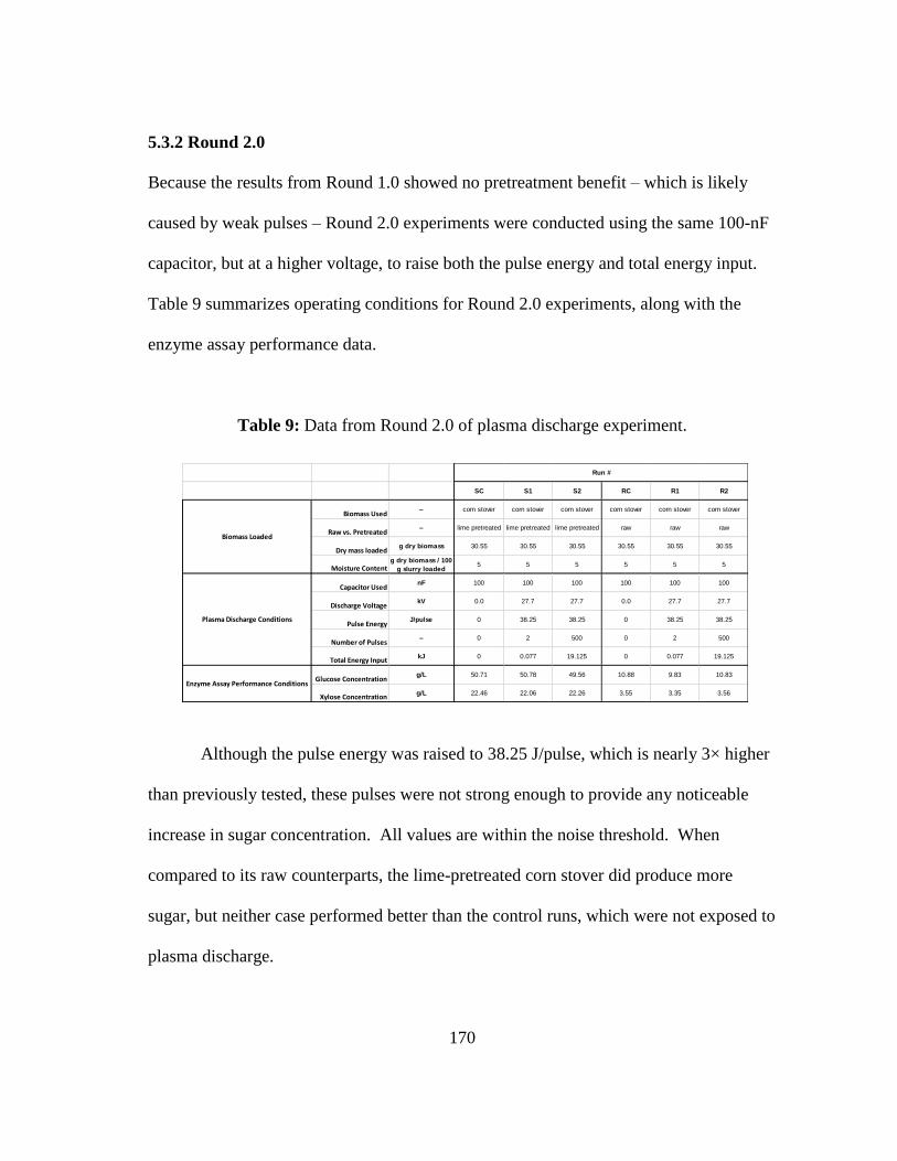
170

5.3.2 Round 2.0

Because the results from Round 1.0 showed no pretreatment benefit – which is likely

caused by weak pulses – Round 2.0 experiments were conducted using the same 100-nF

capacitor, but at a higher voltage, to raise both the pulse energy and total energy input.

Table 9 summarizes operating conditions for Round 2.0 experiments, along with the

enzyme assay performance data.

Table 9: Data from Round 2.0 of plasma discharge experiment.

Although the pulse energy was raised to 38.25 J/pulse, which is nearly 3× higher

than previously tested, these pulses were not strong enough to provide any noticeable

increase in sugar concentration. All values are within the noise threshold. When

compared to its raw counterparts, the lime-pretreated corn stover did produce more

sugar, but neither case performed better than the control runs, which were not exposed to

plasma discharge.

SC S1 S2 RC R1 R2

Biomass Used– corn stover corn stover corn stover corn stover corn stover corn stover

Raw vs. Pretreated– lime pretreated lime pretreated lime pretreated raw raw raw

Dry mass loadedg dry biomass 30.55 30.55 30.55 30.55 30.55 30.55

Moisture Contentg dry biomass / 100

g slurry loaded5 5 5 5 5 5

Capacitor UsednF 100 100 100 100 100 100

Discharge VoltagekV 0.0 27.7 27.7 0.0 27.7 27.7

Pulse EnergyJ/pulse 0 38.25 38.25 0 38.25 38.25

Number of Pulses– 0 2 500 0 2 500

Total Energy InputkJ 0 0.077 19.125 0 0.077 19.125

Glucose Concentrationg/L 50.71 50.78 49.56 10.88 9.83 10.83

Xylose Concentrationg/L 22.46 22.06 22.26 3.55 3.35 3.56

Enzyme Assay Performance Conditions

Plasma Discharge Conditions

Run #

Biomass Loaded

171

5.4 Conclusions

Overall, neither the Round 1.0 nor 2.0 experiments produced any measurable increase in

pretreatment effect. This is most likely because the pulses were too weak. Although the

pressures obtained within the reactor are unknown, it is likely that any substantial

amount of pressure (> 1 atm) would have cracked the acrylic reactor catastrophically.

Of course, the bottom flange did crack during R100 in Round 1.0. This was a fatigue

failure and not a catastrophic vessel failure. To illustrate the difference, a 100-atm gas

cylinder attached to the acrylic reactor may not be able to fill the vessel fast enough to

produce a stable shock wave during the filling process, but could easily explode the

acrylic reactor. Furthermore, plasma bubble shock waves are known to produce a highly

localized region of high temperature and pressure, which rapidly dampens and decays

when propagating outwards radially. Thus, it is reasonable to conclude that the pulse

energy is too low to produce pressures substantial enough to damage the biomass

microstructure.

Pressure measurements would be ideal for determining the efficiency at which

the electrical energy discharged into reactor is converted into high-pressure shock

waves; however, high-pressure electrical transducers were too expensive and time

consuming to install for this round of experiments. Furthermore, measuring pressure

electronically can be extraordinarily difficult when discharging plasma into a reactor

because of electromagnetic interference, which can inject enough noise to obscure the

172

pressure signal. Thus, measuring pressure may best be omitted in lieu of measuring

energy input, or pulse energy, which is both easily measured and controlled.

Several differences between the subsequent experiments and Itoh’s exist, specifically the

following:

1. The pulse energy in Itoh’s experiments is far greater (10–50 kJ/pulse) versus (1–

40 J/pulse.

2. Energy was added as one single pulse rather than repetitive pulses

3. A metallic wire was vaporized during the discharge process, rather than passing

electrical current through the liquid phase.

The food products tested by Itoh appear to have responded quite well to the

plasma discharge. Part of this may be because the pulse energy was nearly 1000× larger

than the domain tested in Rounds 1.0 and 2.0. Another possible explanation is that food

products, which are already edible to humans, need much less processing than

lignocellulosic biomass, which is notoriously difficult to digest. Either way, a large

pulse energy should correlate asymptotically with a higher pressure, which according to

Itoh provides a beneficial pretreatment effect.

Calculating the required vessel wall thickness is still a point of confusion. The

results posted by Itoh claim that observed pressures up to the 500 MPa range, which is

well above the Maximum Allowable Working Pressure for a thin-walled vessel (390-mm

173

bore size, and 20-mm wall thickness). Of course, transient pressures are known to be

less damaging than a steady pressure of equivalent magnitude. To date, very little

literature has been produced on design methodologies for blast containment vessels that

can accurately predict a relationship between maximum transient pressure, wall

thickness, and fatigue lifetime.

Thus the Round 1.0 and 2.0 experiments represent the best effort that could be

done inexpensively with existing equipment, yet it is likely that the pulse energy is still

several orders of magnitude too small to provide any measurable pretreatment effect.

Ultimately, a larger facility would be required to perform a more thorough test for a

proof-of-concept model.

5.5 Future Work

To move forward, the effects of the exploding wire technique used to create a cylindrical

shock wave developed by Itoh must be evaluated for compatibility with biological

systems. This technique may change the efficiency of converting electrical energy into a

strong shock wave, but may introduce metal into solution, which could potentially

hinder enzymatic digestion; however, the precise effects are unknown. On the other

hand, it is entirely likely that the amount of wire vaporized could be negligible.

174

5.5.1 Round 3.0 Experiments – Higher Pulse Energy

To generate an observable pretreatment effect from the plasma discharge experiments,

higher pulse energies are likely needed. A 13-µF, 100-kV capacitor is currently

available in the plasma physics laboratory (Figure 125).

Figure 125: 13-µF capacitor available for Round 3.0 experiments.

175

The pulse energy estimated by Equation 2 indicates the 13-µF capacitor charged

to 100 kV can produce pulse energies up to 65 kJ/pulse! This is well above the 50 kJ

limit of Itoh’s system in Japan, which would be closer to an equivalent comparison;

however, it should be noted that Itoh’s system produces a very high current plasma

discharge (22 kV, 200 µF, 75 kA, and 50 kJ). In contrast, the 13-µF capacitor is much

smaller and must be charged to a much higher voltage to achieve an equivalent pulse

energy

𝐸 =1

2· 𝐶 · 𝑉2 (2)

Regardless, the larger capacitor should provide a better chance of producing a

measurable pretreatment effect from plasma discharge.

176

CHAPTER VI

SOLID EXPLOSIVE EXPERIMENTS

6.1 Brief Introduction

The following experiments were conducted in an attempt to duplicate data reported by

Xiong. Because of budget constraints at the time of the experimentation, some

significant modifications were required to execute this experiment; specifically, the level

of blast confinement.

6.2 Materials & Methods

6.2.1 Facility Location and Layout

The experiments were conducted on the TEEX bomb range at Texas A&M Riverside

campus, which is located near the intersection of Highways 21 and 47. Figure 126

shows the location of the bomb range at Riverside Campus. Because Riverside campus

was originally a US Army Air Corp base prior to its acquisition by Texas A&M

University, it has several runways.

Figure 126: Location of TEEX bomb range at Texas A&M Riverside Campus.

177

The TEEX bomb range (Figure 127) is located near one of the old runways at Riverside

campus. The bomb range is primarily used for training recruits from the Department of

Homeland Security and other law enforcement agencies on proper use of high

explosives. The bomb range is complete with an explosive storage facility, as well as a

pavilion that provides shade during instructional sessions. Across the runway is the field

in which the explosive charges are detonated, which are usually partially buried

depending on the training session.

Figure 127: Aerial view of bomb range, explosive storage shed, and pavilion.

178

6.2.2 Experimental Bill of Materials

To qualitatively compare effects of both the peak blast pressure and detonation velocity,

two different types of solid explosives and loadings were used in these experiments.

Explosives with higher detonation wave velocity (e.g., pentaerythritol tetranitrate

(PETN) detonation cord) generally have a higher brisance for a loading of equivalent

size when compared to explosives with lower detonation wave velocities (e.g., C4). The

detonation velocities of C4 and PETN are both well above the acoustic velocity of water

(~1500 m/s), there is no question about the presence of a shock wave in the liquid phase.

Thus, the experiment was designed to test the hypothesis that a liquid-phase shock wave

would have the greatest chance of damaging the biomass microstructure and reveal a

beneficial pretreatment effect.

A brief list of materials used for this experiment is supplied below:

Solid Explosives

o C4/RDX

o Durasheet/PETN

o PETN detonating cord

o Blasting caps

Liner

o 5-gallon, thin-walled, scrap steel oxygen tank

o 5-gallon, plastic bucket

Milled raw corn stover

Water

Plastic tarp

179

Figure 128 describes how the materials are loaded.

Figure 128: solid explosives containment method.

Because high-pressure steel vessels were unavailable for this experiment along

with the potential for a catastrophic vessel failure, the soil at the bomb range was

envisioned to partially contain and direct the energy from the blast wave. The

experiment was designed with the hypothesis that the incident shock wave traveling

through the biomass slurry would provide sufficient energy to damage the biomass

structure, and that the stronger reflected wave would be redundant. Nonetheless,

although the blast would have been ideally contained within a vessel, this was not an

option.

The biomass slurry was premixed with water in a 5-gallon plastic bucket and

then poured into the scrap 5-gallon steel thin-walled oxygen cylinder, which had the top

removed to facilitate loading. It was envisioned as a steel liner. Because only two

180

oxygen cylinders could be obtained prior to the experiment, two 5-gallon plastic buckets

had to be used as the liner for the last two runs (Runs 2A and 2B). The liner was then

submerged so the brim was below ground level. After suspending the explosive charge

near the center of the slurry, it was covered with a plastic tarp. The plastic tarp was

envisioned as a means to capture some of the biomass that would be splattered upwards.

The soil was envisioned as a means to support the liner, provided the soil could be

packed tightly.

It is important to note that the liner was not envisioned to completely contain the

blast wave, but rather provide some means of separating the soil from the biomass. On

the day of the experiment, the soil was virtually impossible to dig using a shovel because

it was too dry. To build an improvised trench, a mechanized backhoe was used. The

soil was too hard to get a near-cylindrical hole to achieve a tight fit for the steel liner. In

fact, the contrapositive occurred: the soil was so hard the liner was essentially lying in a

rock bed. Thus, any hope that the liner could survive the blast was immediately

abandoned. Because only two steel liners were brought to the bomb range for testing,

two 5-gallon plastic buckets were also used as liners for Runs 2A and 2B.

181

6.2.3 Experimental Test Matrix

Table 10 summarizes the experimental conditions:

Table 10: Experimental test matrix for solid explosives experiment. Run

Label

Explosive

Loaded Explosive Loading Explosive Type

Biomass

Loaded Solids Concentration Liner Type

g

g explosive /

100 g dry biomass

g

g dry biomass /

100 g slurry

1A 50 g 1.79 C4 2.8 10 Steel

1B 50 g 1.79 Det Cord / PETN 2.8 10 Steel

2A 5 g 0.179 C4 2.8 10 Plastic

2B 5 g 0.179 Det Cord / PETN 2.8 10 Plastic

182

6.2.4 Standard Operating Procedure

Appendix J describes the procedure used during the solid explosive shock treatment

experiments.

6.2.4.1 Risk Assessment and Hazards Analysis Plan

Appendix H contains the Project Safety Analysis and relevant hazard discussion

6.2.5 Evaluating Digestibility via Enzymatic Saccharification

6.2.5.1 Drying Biomass for Temporary Shelf-Stable Storage

Appendix B – Part 2 – Biomass Drying Procedure provides details on how the biomass

was dried and preserved prior to saccharification

6.2.5.2 Saccharification Procedure

Appendix B provides the procedure for the enzymatic saccharification.

183

6.3 Results & Discussion

Figure 129 shows the remnants of the steel oxygen tanks envisioned as a liner for the

biomass slurry.

Figure 129: Steel oxygen tank/liner, which were destroyed during the experiment.

Needless to say, neither the scrap steel oxygen tank liner nor the 5-gallon plastic

bucket liners could contain the blast, possibly because of the rocky nature of the soil in

which the liners were placed prior to detonation. Also, the plastic tarp placed over the

bucket was destroyed and could not contain the biomass, which splattered. The blast

wave cut a ~3-inch-diameter hole through the tarp, while the rest of the tarp remained

stationary. In addition, some soil had mixed with some of the biomass because of the

rupture of the liner/bucket. Fortunately, the soil was still in hard brown chunks, which

were easily identified and removed. Because the enzymatic saccharification requires

such a small amount of biomass, finding sufficient soil-free biomass was easy.

184

After the biomass was removed from the bomb range, it was transported back to

the laboratory where it was placed on fan-driven drying racks and dried. Usually the

biomass would dry out rapidly over the course of the weekend; however, apparently the

large amount of biomass needed to be spread out over more drying racks to the keep the

layer thin, so instead the biomass took 5 days to completely dry, which is slightly longer

than usual. It is possible that microbial activity could have degraded the biomass during

the 5 days it took to dry; however, biomass is notoriously recalcitrant and difficult to

digest. In addition to this, the data do not indicate that the biomass had spoiled while on

the drying rack. There was no significant change in sugar concentration in the enzyme

assay, regardless of experimental conditions.

Figure 130: Final sugar concentrations achieved by the end of each saccharification.

Unfortunately, not only do these data in Figure 130 suggest that there was no

benefit from shock treating the biomass with solid explosive, it appears that the

0

1

2

3

4

5

6

7

8

1a 2a 1b 2b

Suga

r C

on

cen

trat

ion

g/L

Glucose Xylose

185

treatment may have actually lowered the biomass digestibility. The peak glucose

concentration for the raw corn stover was ~10 g/L, whereas the peak glucose

concentration for the shock treated biomass was only ~7 g/L.

It should be noted that several anomalies were observed throughout the

saccharification process. First, the temperature controller appears to be malfunctioning

during the 5-day incubation process. The set point was set to 50°C; however,

temperature fluctuations from 48–56°C were observed. It is possible that these

temperature fluctuations could been enough to affect the thermal stability of the enzyme;

however, because all saccharifications were performed simultaneously in the same

rolling incubator, these effects should be distributed amongst all samples. In addition to

temperature controller fluctuations, another potentially more significant anomaly was

also observed. Specifically, upon terminating the enzyme assay, the saccharification

broth was very dark colored, and nearly black, whereas the broth is usually yellow

colored. The difference in color between the raw and shocked biomass may indicate

some soluble explosive residue contaminated the biomass sample. The contaminant

could have also come from the soil; however, most of the soil was removed prior to

sampling. Thus, it is more likely that the change in color originates from some explosive

residue.

186

6.4 Conclusions

Overall, the data do not indicate that there was any benefit from shock treating biomass;

in fact, it may potentially decrease digestibility because explosive residue contaminates

the biomass during the saccharification. The results are not entirely conclusive because

the temperature controller allowed the temperature to fluctuate during the

saccharification. The effect of the soil contaminating the biomass samples because of

the ruptured plastic and steel liners is not considered to be the culprit for the decreased

digestibility of the shocked biomass. The soil was picked out by hand prior to sampling

because it was still in large, rocky chunks; therefore, it is likely that the explosive

residue caused the reduced enzymatic digestibility.

Washing the biomass over a screen extensively with water may potentially

remove the explosive residue, or at least the soluble components. It is entirely possible

that doing so would increase the digestibility of the shocked biomass up to the level of

the raw biomass; however, the case for a benefit of shock treating biomass does not

appear promising. This may result because the biomass was essentially unconfined

within the liner in the ground. The biomass may not respond to shock treatment unless it

has been impacted with a strong reflected wave confined within a steel vessel.

187

6.5 Future Work

Further experimentation could be performed to inexpensively test the effects of

confinement. Several options are available in order to test the effects of confining such a

blast. Obviously, these experiments require a significant amount of funding to complete.

One simple method for confining the blast is to fabricate a concrete blast

chamber. The chamber would consist of a cylindrical hole could be dug via an auger

and then lined with a thick layer of reinforced concrete. This concrete blast chamber

could then be covered with a large concrete block, which would need a forklift or

bulldozer to put in place. This concrete blast chamber may indeed provide the level of

confinement necessary to observe an enhanced digestibility from shock treatment with

solid explosives. Conversations with Ed Fritz, at the TEEX bomb range have indicated

that this concrete blast chamber is unlikely to contain such a blast more than once. Thus,

this option may not be viable considering the construction cost and high likelihood of

failure.

Another, potentially more viable option is to use a Total Containment Vessel to

contain the blast. These vessels are used by law enforcement bomb squads to dispose of

bombs when found. Unfortunately, it is unlikely that a bomb squad will have a spare

vessel that could be used considering their exorbitant cost and their certification for

single use only.

188

The best option for completing these experiments is to utilize the Weapons and

Complex Integration test facility at Lawerence- Livermore National Laboratory

(https://wci.llnl.gov/). Ed Brickley at TEEX Riverside Campus has stated that he trains

employees from the Lawerence-Livermore facility and they may be willing to

collaborate. Furthermore, the facility has a variety of blast chambers which can safely

contain up to 24 lbs of C4. Thus, this facility is ideal for such a test. The primary

challenge is funding.

Ed Brickley may be contacted at:

Ed.Brickley@teex.tamu.edu

979-862-1512

Riverside Building 7751

Ed Fritz may be contacted at:

Ed.Fritz@teex.tamu.edu

979-862-3410

189

CHAPTER VII

M&M MARS PROJECT

7.1 Materials and Methods

7.1.1 Alkaline Pretreatment in Pipe Bombs

Alkaline pretreatment of lignocellulose involves mixing the biomass with water and

hydroxide. Lime (Ca(OH)2) pretreatment mixes powdered lime into the slurry, whereas

sodium hydroxide (NaOH) can be added as a concentrated solution to the slurry. The

slurry is placed in a pipe bomb, sealed, and preheated in a 100°C water bath for 10–20

min prior to adding oxygen. After the oxygen is added, the pipe bombs are incubated in

a preheated oven for a specified temperature and time.

Alkaline pretreatments using sodium hydroxide (NaOH) were performed in a

small, electrically heated, laboratory convection oven (Figure 131). The oven has an

electronic temperature controller, which accepts a K-type thermocouple for a

temperature input. The oven has also been adapted with a motorized wrist action shaker,

which mixes the slurry in the pipe bombs. The shaker was set manually to the maximum

amplitude attainable while loaded with the pipe bombs.

190

Figure 131: Oven with wrist-action shaker used for pipe bomb alkaline pretreatment.

The pipe bombs are 1¼-inch-diameter 304 stainless steel pipe size nipples that

are threaded with either an elliptical or flat-bottom endcap on one side, and a pipe

coupler and reducing hex bushing on the other (Figure 132). To prevent gas leaks from

the pipe bombs, the endcaps and couplers are TIG welded, which renders them

permanently attached. The pipe coupler on the top end of the vessels also serves as

reinforcement, which prevents the pipe nipple from being crushed into an oval shape

when clamped within a vice when applying torque to the lid, or hex bushing. To prevent

leaks, a minimum of five revolutions of Teflon tape are applied

191

to the threads on the lid before torquing. This thick layer of Teflon tape also eliminates

potential metal galling, which renders the lids extremely difficult to remove. The lid of

the pipe bombs was reduced down to a diameter compatible with a ¼-in stainless steel

ball valve and quick connects. The pipe bombs also have a steel rod welded to the outer

surface of the wall to support the pipe bomb while on the shaker arm in the oven.

Figure 132: Pipe bombs used for alkaline pretreatment.

The internal volume of the pipe bombs was measured to be ~225 mL by filling

the pipe bombs with water up to the brim. This measurement method neglects the

contribution of the lid and tubing connected to the quick-connect fitting. The volume

measurement was needed to compute a reasonable fill volume for the vessel. To leave

enough volume in the ullage space of the vessel for the oxygen – a necessary reactant in

the alkaline pretreatment process – only 140 mL of the total 225 mL were filled with the

192

slurry (biomass, water, and NaOH); thus, approximately 60% of the vessels volume was

filled with slurry and the remainder was devoted to oxygen. In these studies, the solids

concentration is intentionally reduced to guarantee sufficient mixing.

7.1.1.1 Test Matrix

Table 11 shows the test matrix to design the alkaline pretreatment optimization

experiments.

Table 11: Test conditions during alkaline pretreatment optimization experiments

Feedstock Solids

Concentrations

Temperatures Times Oxygen

Pressures

Hydroxide

Concentrations

g solid biomass

/100 g slurry

°C h psig g NaOH /100 g

raw dry

biomass

Corn

Stover

5, 10 100, 120, 140 0.25,

0.5, 1

100, 300 2.5–25

Cassava 5 60, 80, 100,

120, 140, 160,

180

0.25,

0.5, 1

300 0–25

Alfalfa 5 120 1 300 2.5–10

Spent

Grain

5 100, 120, 140,

160, 180

1 300 0–25

193

7.1.1.2 Pipe Bomb Pretreatment Procedure:

Appendix K describes the pipe bomb pretreatment procedure.

7.1.2 Alkaline Pretreatment in 8-L Reactor

The same principles apply to executing alkaline pretreatment in the 8-L reactor (Figure

133), except for the following variations:

The vessel is significantly larger.

It is heated via electrical resistance heaters, rather than the water bath

preheating period and a hot air convection oven.

The vessel operates upright and is equipped with a magnetic drive that

turns an impeller within the reactor for mixing.

Oxygen was continuously supplied, thus any oxygen consumed could be

replenished during the run. (In contrast, the pipe bombs were charged

with a fixed volume of oxygen, which depletes during the run.)

Figure 133: 8-L Parr reactor used for alkaline pretreatment.

194

7.1.2.1 Alkaline Pretreatment Procedure for the 8-L Reactor:

Appendix L describes the alkaline pretreatment procedure for the 8-L reactor.

It is important to emphasize that the temperature versus time relationship in the

8-L reactor is not identical to the pipe bombs. Specifically, the temperature in the pipe

bombs rarely surpasses 85°C during the 10–20 min preheating cycle, and then

approaches the set point temperature asymptotically while in the oven. Although the

oven usually reaches the set point temperature within 10 min after closing the door, the

convective heat transfer rate in the oven is much lower than the 8-L reactor, which is

heated electrically through the walls. Thus, determining the exact start and end of the

reaction at both scales can be difficult; nonetheless, this equipment and procedure has

historically served well for characterizing biomass reactivity.

7.1.3 Enzymatic Saccharifications

Typically, enzymatic saccharification is performed batch-wise, which is simple and

versatile. In this project, batch saccharification was utilized to explore the performance

of different pretreatment methods, various types of enzymes, and enzyme loadings,

along with different antibiotics.

The optimization saccharifications (pipe bombs) utilized 2 mg/g CTec3 and 2

mg/g HTec3, with cycloheximide and tetracycline antibiotics. In contrast, the

production saccharifications employed 10 mg/g of CTec2 and 10 mg/g of HTec2, with

195

chloroform as the volatile antibiotic. (Note: CTec2 and HTec2 are approved for food

use, whereas CTec3 and HTec3 are not.)

7.1.3.1 Saccharification Procedure

Appendix B describes the enzymatic saccarifaction procedure.

7.1.4 Vacuum Distillation/Concentration of Saccharification Broth

After completing the production enzymatic saccharification, the broth was subsequently

sampled for analysis and then blended into buckets specific to each feedstock. Once the

distillation apparatus was ready, the buckets were removed from the freezer, thawed, and

contents poured into the 22-L glass boiling flask for distillation/concentration (Figure

134 to Figure 136).

The vacuum distillation system consisted of a 22-L glass boiling flask with ball-

and-socket connection on the top, which connected to a two-stage distillation column

that prevented foam and bubbles from spilling over into the condenser. The vacuum

distillation apparatus utilitized one glass condenser, as well as a larger stainless steel

condernser, both of which were glyclol-cooled shell-and-tube condensers with the tube

side employed as the condensing surface. The 22-L flask was submersed in a hot water

bath to guarantee that the process temperature never exceeds 100°C. The stainless steel

pot that housed the 22-L flask was then insulated and placed on an electric hot plate.

196

Figure 134: 22-L glass flask and vacuum distillation column with condenser.

Figure 135: Entire vacuum distillation assembly.

197

Figure 136: Vacuum pump and condensate collection vessel used for distillation.

The 22-L flask would usually require 12–18 h to remove 90% of the water in the

broth. Then, the concentrated syrup at the bottom of the flask would be diluted with

remaining saccharification broth until all the broth was concentrated and collected at the

bottom of the flask. To prevent damage to the sugars, the temperature in the 22-L flask

was maintained at 65–85°C. A vacuum pump maintained the system pressure of 26–

28.5 in Hg. Ultimately, a glass carboy captured the condensed water vapor. Once in

operation, the system would run at a rolling boil overnight without the need for

continuous monitoring.

198

7.2 Results and Discussion

7.2.1 Sugar Yield Data

7.2.1.1Process Flow Representation

Figure 137 and Figure 138 is a process flow diagram that describes the sugar yields for

all feedstocks. These diagrams show the following: the amount of biomass loaded on a

dry and wet basis, NaOH loaded, enzymes used, sugars and residual solids collected at

each step. The diagrams also show the process conditions used for both alkaline

pretreatment and enzymatic saccharification.

Table 12 summarizes the information in Figure 138. The maximum overall sugar

yields for corn stover was 48.1 g sugar/g raw dry corn stover, which indicates both a

high pretreatment and enzymatic yields.

The yields for alfalfa and spent grains were both 24.8 g sugar/g raw dry corn

stover and 24.0 g sugar/g raw dry corn stover, respectively. The spent grain had a much

lower pretreatment yield, which was compensated by a higher enzymatic yield. This

suggests that much of the spent grains were solubilized during the pretreatment and the

remaining insoluble solids, or fibers, were easily digested by the enzymes.

Cassava had the lowest overall sugar yield at 13.0 g sugar/g raw dry corn stover,

which is caused by both a low pretreatment and enzymatic yield. Nearly half of the

cassava fibers were solubilized during the alkaline pretreatment, yet the remaining fibers

199

were not easily digested by the enzymes. Although corn stover required a much higher

NaOH loading (15%), alfalfa and spent grains only required a 5% NaOH loading at the

maximum yield.

Figure 137: Yields for corn stover and cassava

200

Figure 138: Yields for alfalfa and spent grain.

201

Table 12: Summary of process conditions and sugar yields

202

7.2.1.2 Sugar Yield

7.2.1.2.1 Corn Stover

The large inventory of corn stover available for the optimization project allowed for

extensive experimentation without the concern of exhausting a limited supply. Figure

139 is the master set, or all of the data generated with corn stover at all process

conditions.

The corn stover data are well behaved. Of all variables tested (NaOH loading,

temperature, oxygen pressure, and time), sugar yield is most sensitive to NaOH loading.

Trends between higher oxygen pressures, temperatures, and times are not readily

apparent because the sugar yield data has enough noise to obscure any consistent trend.

Figure 139: Master set of all corn stover sugar yields.

203

Figure 140 presents side-by-side comparisons of all the different process

conditions that were tested with corn stover.

Figure 140: Corn stover sugar yields (plotted).

204

Coherent trends between temperature, oxygen pressure, and time are not readily

apparent because of the noise in the sugar yield data. Better statistical characterization

of the variation inherent to the experiment may benefit future work; however, it can be

noted that corn stover responds predictably to NaOH loading, which is the dominant

effect. A discussion on the variability will be included in the Conclusion section.

7.2.1.2.2 Spent Grains

Figure 141 is the master set of all spent grain sugar yield data observed during the

alkaline pretreatment optimization. Including all the data on a single plot is hard to

interpret; however, the data are presented this way for completeness.

Figure 141: Master set for all spent grain sugar yields.

205

It should be noted that the data points in Figure 141 that have error bars were

measured either in duplicate or triplicate, which characterizes the variability in the

measurement. The error bars are the standard error of the mean, or standard deviation

divided by the square root of the number of samples, which shrinks to zero as the

number of samples increases to infinity.

Figure 142 presents side-by-side comparisons of all the different process

conditions that were tested with spent grains. The spent grain data show some coherent

trends. For example, across all temperatures tested, there is usually one maximum yield

that shifts towards a lower NaOH loading as temperature increases. This result is

intuitive because at higher the temperatures, hydroxide ions are more active and can

better degrade lignin. Eventually, at higher temperatures hydroxide damages the

carbohydrates and the yield drops across all hydroxide loadings.

The maximum sugar yield occurs at 120°C, 5% NaOH, 300 psig O2, and 1 h;

thus, these conditions represent the global maximum for the spent grains.

206

Figure 142: Spent grain sugar yields.

207

7.2.1.2.3 Alfalfa

Because the inventory was limited, alfalfa was tested the least during the optimization.

The initial sugar yields were much higher than the initial test on the other feedstocks.

Figure 143 shows the maximum sugar yield for the alfalfa was just under 25%, which

was achieved with an NaOH loading of only 5%. The sugar yield appears to oscillate as

the hydroxide loading increases; however, these oscillations may very well be within the

noise.

Figure 143: Alfalfa sugar yield.

208

7.2.1.2.4 Cassava

Figure 144 shows the master set of all cassava data, which are included for

completeness. It is readily apparent that the 120°C data series stands well above the

other series. Compared to the other feedstocks, cassava has the lowest sugar yields by

far. This is caused by both low pretreatment and enzymatic yields. Cassava is much

more sensitive to temperature and time, rather than hydroxide concentration. The sugar

yields do not change very much across all hydroxide concentrations, except for the

100°C and 120°C runs. The cooler and hotter temperatures reduced yield because of too

little or too much reactivity, respectively. Figure 145 presents side-by-side comparisons

of all the different process conditions that were tested with cassava.

Figure 144: Master set for all cassava sugar yields.

209

Figure 145: Cassava sugar yields.

Table 13: Summary of sugar production runs.

Glucose Xylose

Total Sugar

Concentration

Total

Volume

Total

Sugar

(g/L) (g/L) (g/L) (L) (g)

corn stover 404 158 563 2 1125

alfalfa 309 82 391 0.5 195

cassava 125 19 144 0.5 72

spent grain 171 81 252 2 504

210

7.2.2 Sugar Production Summary

Table 13 summarizes the final sugar concentrations of the syrup from the production

runs. Initially, attempts were made to dry the sugar syrup via lyophilization (a.k.a. freeze

drying); however, the process was far too slow for the schedule, so concentrated syrup

was produced instead.

The largest quantities of sugars were created from corn stover and spent grain

feedstocks because they were the most abundant in the laboratory inventory. In contrast,

much of the cassava and alfalfa were consumed during various alkaline pretreatment and

protein extraction optimization experiments. Ultimately the entire remaining inventory

of the alfalfa and cassava were consumed for the sugar production.

Figure 146 shows corn stover syrup being poured into a glass container. This

picture is included to illustrate the high viscosity of the corn stover syrup. The container

was elevated on the scissor lift to gradually pour the syrup while unattended. The syrup

was so viscous that the pouring process took over 4 h to complete. Nonetheless, very

little residue stuck to the walls of the plastic container.

211

Figure 146: Pouring corn stover syrup.

212

7.3 Conclusions

Overall corn stover has the highest sugar yield (48.1 g sugar/g raw dry corn stover) and

was the easiest feedstock to use because it was not very sensitive to any of the process

conditions other than hydroxide loading. The spent grains and alfalfa produced the next

highest yields at 24.0 and 24.8 g sugar/g raw dry corn stover, respectively. The cassava

had the lowest yield by far (13.0 g sugar/g raw dry corn stover).

7.4 Future Work

It is clear that noise in the data obfuscates the trends between set-point temperature,

time, and oxygen pressure. Better characterization of the noise may be an option for

future studies; however, more accurate measurements of the internal process within the

reactor may eliminate such noise. For example, there were minor variations between the

exact amount of preheating time, the exact oven transient temperature profile, and the

exact incubation time. The apparent noise in the data may indeed not actually exist if

the data were plotted against the exact values versus the target/set-point values.

Interpreting data with more variables becomes increasingly more challenging. Ideally

automated data collection would resolve this issue. Ideally thermocouples and oxygen

sensors could be attached to each reactor and monitored electronically via a data

acquisition system, such as LabVIEW. One could easily measure the dissolved oxygen

content, internal temperature, and pH versus time during the reaction, which would

provide a much more accurate representation of the data, as opposed to the set-point

temperature and target incubation times.

213

CHAPTER VIII

CONCLUSIONS

The existence of a shock treatment effect was dubious upon initiating research. This was

due to instantaneously switching from dilute to high-solids enzyme assays, as per the

mandate by DOE to use industrially relevant conditions, as well as neglecting several

previously undiscovered variables; specifically, ignoring the detrimental effects of

ferrous particles introduced from the smokeless powder and steel shot, as well as the rust

(red iron oxide) accumulating on the blind flange which stopped the steel shotgun

pellets. A thorough magnetic stirring and washing procedure downstream of shock

treatment was required to remove contaminants in the slurry of biomass prior to

enzymatic hydrolysis. DOE required the use of industrially relevant enzyme assay

conditions, which prohibited dilute enzyme assays, that could have partially masked

some of the inhibitory effects of the contaminants potentially present in prior

experiments performed by Matthew Falls, et. al.

Needless to say, the shotgun shells had many drawbacks, and were promptly

replaced with an explosive gas mixture, which eliminated the contamination issues.

Methane and propane were initially tried as fuel sources; however, the methane would

not ignite, and the propane only deflagrated. More importantly, the propane deflagration

did not result in any increase in digestibility (despite comparable peak pressures), which

indicates that the shock treatment effect caused by the shotgun blast is more rate

dependent rather than pressure dependent. The hydrogen detonations produced a

214

digestibility enhancement virtually identical to the shotgun shells, which implies that the

shock treatment effect was not caused by the pellets passing through the slurry, and

potentially inducing a strong cavitation wake. Surprisingly, the shock treatment effect

was invariant with respect to the depths, volumes, and solids concentrations tested;

instead, the rapid pressurization is the most important variable, which facilitates scaling.

Pressure measurements were successful in the gas phase, which validated the

presence of a reflected shock wave which reciprocates throughout the ullage space;

however, attempts to measure pressure in the submerged phase failed, for reasons which

appear to be related to the transducer ringing response coupled with vessel resonance.

Higher pressures were unnecessary to observe a benefit from shock treatment,

which indicates some kind of pressure-related saturation effect; however, this could be

caused by the shock wave reflecting off of the gas-liquid interface. Submersed solid

explosives may generate liquid-phase shock wave that may be a more effective. A

minimum effective pressure may exist; however, finding such a pressure fell outside of

the funded work, and the experimental apparatus would require significant cost to

measure accurately.

Ultimately, a reproducible, and small (~5%), yet significant increase in

digestibility at a constant 46.7 mg/g enzyme loading, was ultimately observed; however,

the enzyme loading could be reduced by ~2× while maintaining a constant conversion of

215

0.80 g glucan digested/g glucan fed. The data indicate that shock treatment is best used

as a means to reduce enzyme loading; however, one should exercise caution when

estimating the ultimate potential of such technology. Subsequent experiments performed

with plasma discharge, and solid explosives, failed to produce any measurable increase

in digestibility, but absence of evidence for the merit of a strong liquid-phase shock

wave does not mean that a more powerful plasma discharge, or better contained blast

from solid explosives would not result in the same or better results produced with the

hydrogen detonation system. Overall, the hydrogen detonation shock treatment process

has potential to improve both the yield and economics of biomass processing, but it is

entirely likely that prior experiments have resulted in an effect that is submaximal. This

technology should definitely be pursued further to identify the maximum benefit, albeit

with bigger explosions!

216

REFERENCES

[1] N. N. Taleb, The Black Swan: the impact of the highly improbable, New York

City, New York: Rando House Trade Paperbacks, 2010.

[2] R. Shimelmitz and e. al, "‘Fire at will’: The emergence of habitual fire use 350,000

years ago," Journal of Human Evolution, vol. 77, no. 2014, pp. 196-203, 2014.

[3] C. Elvidge, M. L. Imhoff, K. E. Baugh and V. R. Hobson, "Night-time lights of the

world: 1994–1995," ISPRS Journal of Photogrammetry & Remote Sensing, vol. 56,

pp. 81-99, 2001.

[4] "World Population Summary," Bureau of the Census, Washington DC, 2011.

[5] M. T. Holtzapple, R. Davidson, M. Ross, S. Aldrett-Lee, M. Nagwani, C. M. Lee,

C. Lee, S. Adelson, W. Kaar, D. Gaskin, H. Shirage, N. S. Chang, V. Chang and

M. Loescher, "Biomass conversion to mixed alcohol fuels using the MixAlco

process," Applied Biochemistry and Biotechnology, vol. 79, no. 1, pp. 609-631,

1999.

[6] H. M and G. C, "Carboxylate Platform: The MixAlco process part 1: comparison

of three biomass conversion platforms\," Applied Biochemistry and Biotechnology

, vol. 156, no. 6, pp. 95-106, 2009.

[7] G. Settles, "The Penn State Full-scale Schlieren System," in 11th International

Symposium on Flow Visualization, Notre Dame, 2004.

217

[8] N. Ward, "Snap, Crackle and Pop – The Tale of the Pistol Shrimp," CARIBBEAN

COMPASS, p. 38, 2015.

[9] P. Graneau, "The Cause of Thunder," Journal of Physics, vol. 22, pp. 1083-1094,

1989.

[10] R. Clary and J. Wandersee, "Krakatoa Erupts," The Science Teacher, pp. 43-47,

2011.

[11] "America Pink," [Online]. Available:

http://america.pink/lithotripsy_2720474.html. [Accessed 3 3 2016].

[12] K. Hassanzadeh, Y. A. Asrbadr and M. S. G. Mirabad, "Relationship between

Success rate of Extracorporeal Shockwave Lithotripsy," Medical Journal of Tabriz

University of Medical Sciences and Health Services, vol. 37, pp. 14-19, 2015.

[13] H. Iyama and S. Itoh, "Study on Explosive Forming of Aluminum Alloy,"

International Journal of Multiphysics, vol. 4, pp. 341-349, 2010.

[14] C. L. Reese, "Twenty-Five Years Progress in Explosives," Journal of the Franklin

Institute of the State of Pennsylvania, vol. 198, pp. 745-768, 1924.

[15] S. Sydney and M. Edward, "Industrial Explosives – A Brief History of Their

Development and Use," Journal of Hazardous Materials, vol. 23, pp. 183-201,

1990.

[16] L. Slade and B. Kalangahe, "Dynamite Fishing in Tanzania," Marine Pollutin

Bulletin , vol. 101, pp. 491-496, 2015.

218

[17] K. Taber, D. Warden and R. Hurley, "Blast-Related Traumatic Brain Injury: What

Is Known?," Journal of Neuropsychiatry and Clinical Neuroscience, vol. 18, no. 2,

pp. 141-145, 2006.

[18] D. Bjerketvedt, J. R. Bakke and K. v. Wingerden, "Gas Explosion Handbook,"

Journal of Hazardous Materials, vol. 52, pp. 1-150, 1997.

[19] Funk & Wagnalls New World Encyclopedia, "Explosives," in Funk & Wagnalls

New World Encyclopedia, Chicago, World Book Inc, 2015.

[20] M. H. Keshavarz, F. Seif and H. Soury, "Prediction of the Brisance of Energetic

Materials," Propellants, Explosives, Pyrotechnics, vol. 39, pp. 284-288, 2014.

[21] M. Abadyan, V. Khademi, R. Bagheri, P. Motamedi, M. Kouchakzadeh and H.

Haddapourr, "Loading Rate-Induced Transition in Toughening Mechanism of

Rubber-Modified Epoxy," Journal of Macromolecular Science, pp. 602-614, 2010.

[22] J. Yamashita, X. Li, B. Furman, R. Rawls, X. Wang and C. M. Agrawal, "Collagen

and Bone Viscoelasticity: A Dynamic Mechanical Analysis," Journal of

Biomedical Materials Research, vol. 63, no. 1, pp. 31-36, 2001.

[23] A. Aden and T. Foust, "Technoeconomic analysis of the dilute sulfuric acid and

enzymatic hydrolysis process for the conversion of corn stover to ethanol,"

Cellulose, vol. 16, no. 4, pp. 535-545, 209.

[24] N. Mosier, C. Wyman, B. Dale, R. Elander, Y. Y. Lee, M. Holtzapple and M.

Ladish, "Features of promising technologies for pretreatment of lignocellulosic,"

Bioresource Technology, vol. 6, no. 96, pp. 673-686, 2005.

219

[25] C. Debras, Y. Liu, N. van Garderen, B. Minisini, T. Graule and F. J. Clemens,

"Development of granular materials for fluidized bed process: measuring attrition

resistance with a horizontal ball milling device and its mathematical description,"

Powder Technology, vol. 288, pp. 157-163, 2016.

[26] H. Inoue, S. Yano, T. Endo, T. Sakaki and S. Sawayama, "Combining hot-

compressed water and ball milling pretreatments to improve the efficiency of the

enzymatic hydrolysis of eucalyptus," Biotechnology for Biofuels, p. 1:2, 2008.

[27] T. Tassinari and C. Macy, "Differential Speed Two Roll Mill Pretreatment of

Cellulosic Materials for Enzymatic Hydrolysis," Biotechnology and

Bioengineering, vol. XIX, pp. 1321-1330, 1977.

[28] Y. Zheng, Z. Pan and R. Zang, "Overview of biomass pretreatment for cellulosic

ethanol production," International Journal of Agricultural & Biological

Engineering , vol. 2, no. 3, pp. 51-68, 2009.

[29] SeekPart.com, [Online]. Available: http://www.seekpart.com/equipment-

series/mixing+roll+mill.html. [Accessed 3 3 16].

[30] L. Ingram and B. Wood, "Ethanol Production from Lignocellulose". US Patent No.

6,333,181, 2001.

[31] M. Kinley and B. Krohn, "Biomass Conversion to Alcohol Using Ultrasonic

Energy". US Patent 2008/0044891, 2008.

[32] M. Jones, Effects of Physical and Chemical Pretreatments on the Crystallinity of

Bagasse, College Station: Texas A&M University , 2007.

220

[33] M. J. Madison, G. Coward-Kelly, M. Falls and M. T. Holtzapple, "Mechanical

Pretreatment of Biomass – Part 1: Acoustic and Hydrodynamic Cavitation,

manuscript".

[34] S. Kim and M. T. Holtzapple, "Lime pretreatment and enzymatic hydrolysis of

corn stover," Bioresource Technology, vol. 96, no. 18, pp. 1994-2006, 2005.

[35] R. Sierra;, C. Granda and M. T. Holtzapple, "Short-term lime pretreatment of

poplar wood," Biotechnology Progress, vol. 25, no. 2, pp. 323-332, 2009.

[36] R. R. Davidson and M. T. Holtzapple, "Methods of Biomass Pretreatment". US

Patent 5,865,898, 1999.

[37] J. Gierer, T. Reitberger, E. Yang and B. H. Yoon, "Formation and involvement in

oxygen delignification studied by the autoxidation of lignin and carbohydrate

model compounds," Journal of Wood Chemistry and Technology, vol. 21, no. 4,

pp. 313-341, 2001.

[38] H. B. Klinke , B. K. Ahring, A. S. Schmidt and A. B. Thomsen, "Characterization

of degradation products from alkaline wet oxidation of wheat straw," Bioresource

Technology, vol. 82, no. 1, pp. 15-26, 2002.

[39] B. Yang and C. E. Wyman, "Effect of xylan and lignin removal by batch and

flowthrough pretreatment on enzymatic digestibility of corn stover cellulose,"

Biotechnology and Bioengineering, vol. 86, no. 1, pp. 88-98, 2004.

221

[40] X. Pan, N. Gilkes and J. N. Saddler, "Effect of acetyl groups on enzymatic

hydrolysis of cellulosic substrates," Holzforschung, vol. 60, no. 4, pp. 398-401,

2006.

[41] X. Pan, X. Zhang, D. Gregg and J. Saddler, "Enhanced enzymatic hydrolysis of

steam-exploded douglas fir wood by alkalai-oxygen post-treatment," Aplied

Biochemistry and Biotechnology, vol. 115, no. 1, pp. 1103-1114, 2004.

[42] R. Lopez, V. Poblama, A. Licea-Claverie, M. Avalos, A. Alvarez-Castillo and V.

M. Castano, "Alkaline surface modification of sugar cane bagasse," Advanced

Composite Materials, vol. 9, no. 2, pp. 99-108, 2000.

[43] M. Fall, R. Sierra-Ramirez and M. Holtzapple, "Oxidative lime pretreatment of

Dacotah switchgrass," Applied Biochemistry and Biotechnology, p. In Press,

2011b.

[44] R. Sierra, M. T. Holtzapple and C. B. Granda, "Long-term lime pretreatment of

poplar wood," AIChE Journal, vol. 57, no. 5, pp. 1320-1328, 2010.

[45] V. Chang, M. Nagwani, C. H. Kim and M. T. Holtzapple, "Oxidative lime

pretreatment of high-lighnin biomass," Applied Biochemistry and Biotechnology,

vol. 94, no. 1, pp. 1-28, 2001.

[46] W. E. Kaar and M. T. Hotzapple, "Using lime pretreatment to facilitate the

enzymatic hydrolysis of corn stover," Biomass and Bioenergy, vol. 18, no. 3, pp.

189-199, 2000.

222

[47] J. Xu, J. J. Cheng, R. R. Sharma-Shivappa and J. C. Burns, "Lime pretreatment of

switchgrass at mild temperatures for ethanol production," Bioresource Technology,

vol. 101, no. 8, pp. 2900-2903, 2010.

[48] S. Rabelo, R. Filho and A. Costa , "Lime pretreatment of sugarcane bagasse for

bioethanol production," Applied Biochemistry and Biotechnology, vol. 153, no. 1,

pp. 139-150, 2009.

[49] B. C. Saha and M. A. Cotta, "Lime pretreatment, enzymatic saccharification and

fermentation of rice hulls to ethanol," Biomass & Bioenergy, vol. 32, no. 10, pp.

971-977, 2008.

[50] R. Sierra, Kinetic modeling and assesment of lime pretreatment of poplar wood,

PhD Dissertation, College Station, TX: Texas A&M University , 2010b.

[51] B. Bals, H. Muren, M. Allen and B. Dale, "Ammonia fiber expansion (AFEX)

treatment of eleven different forages: improvements to fiber digestibility in vitro.,"

Animal Feed Science and Technology, vol. 155, no. 2-4, pp. 147-155, 2010a.

[52] B. E. Dale and M. J. Moreira, "Freeze-explosion technique for increasing cellulose

hydrolysis," in Proceeding of Symposium on Biotechnology in Energy Production

and Conservation, Gatlinburg, TN, 1982.

[53] L. Gollapalli, B. Dale and D. Rivers, "Predicting digestibility of ammonia fiber

explosion (AFEX)-treated rice straw," Applied Biochemistry and Biotechnolgy,

Vols. 98-100, no. 1, pp. 23-35, 2002.

223

[54] D. J. Mitchell, K. Grohmann, M. E. Himmel, B. E. Dale and H. A. Schroeder,

"Effect of the degree of acetylation on the enzymatic digestion of acetylated

xylans," Journal of Wood Chemistry and Technology , vol. 10, no. 1, pp. 111-121,

1990.

[55] A. T. Martinez, A. E. Gonzalez , M. Valmaseda, B. E. Dale, M. J. Lambregts and

J. F. Haw , "Solid-state NMR studies of lignin and plant polysaccharide degraded

by fungi," Holzforschung, vol. 45, no. 1, pp. 49-54, 1991.

[56] A. Ferrer, F. Byers, B. Sulbaran-de-Ferrer, B. Dale and C. Aiello, "Optimizing

ammonia pressurization/depressurization processing conditions to enhance

enzymatic susceptibility of dwarf elephant grass," Applied Biochemistry and

Biotechnology , Vols. 84-86, no. 1, pp. 163-179, 2000.

[57] M. T. Holtzapple, J. Lundeen, R. Sturgis, J. Lewis and B. Dale, "Pretreatment of

lignocellulosic municipal solid waste by ammonia fiber explosion (AFEX),"

Applied Biochemistry and Biotechnology, vol. 5, no. 21, pp. 34-35, 1992.

[58] K. J. Zeitsch, The chemistry and technology of furfural and its many by-products,

New York: Elsevier, 2000.

[59] C. E. Wyman, B. E. Dale, R. T. Elander , M. T. Holtzapple, M. R. Ladisch and Y.

Y. Lee, "Coordinated development of leading biomass pretreatment technologies,"

Bioresource Technology, vol. 96, no. 18, pp. 1959-1966, 2005b.

[60] D. Knappert, H. Grethlein and A. Converse, "Partial acid hydrolysis of poplar

wood as a pretreatment for enzymatic hydrolysis," 1981.

224

[61] T. A. Lloyd and C. E. Wyman, "Combined sugar yields for dilute sulfuric acid

pretreatment of corn stover followe by enzymatic hydrolysis of the remaining

solids," Bioresource Technology, vol. 96, no. 18, pp. 1967-1977, 2005.

[62] D. Schell , J. Farmer, M. Newman and J. McMillan, "Dilute-sulfuric acid

pretreatment of corn stover in pilot-scale reactor," Applied Biochemistry and

Biotechnology, vol. 105, no. 1, pp. 69-85, 2003.

[63] O. Bobleter, R. Niesner and M. Rohr, "The hydrothermal degradation of cellulosic

matters to sugars and their fermentative conversion to protein," Journal of Applied

Polymer Science, vol. 20, no. 8, pp. 2083-2093, 1976.

[64] H. F. Hormeyer, W. Schwald, G. Bonn and O. Bobleter, "Hydrothermolysis of

birch wood as a pretreatment for enzymatic saccharification," Holzforschung, vol.

42, no. 2, pp. 95-98, 1988.

[65] M. Walsh, D. de la Torre Ugarte, H. Shapouri and S. Slinsky, "Bioenergy crop

production in the United States: Potential quantities, land use changes, and

economic impacts on the agricultural sector," Environmental and Resource

Economics, vol. 24, no. 4, pp. 313-333, 2003.

[66] W. S. L. Mok and M. J. Antal, "Uncatalyzed solvolysis of whole biomass

hemicellulose by hot compressed liquid water," Industrial & Engineering

Chemistry Research, vol. 31, no. 4, pp. 1157-1161, 1992.

225

[67] J. Weil, A. Sarikaya, S. L. Rau, J. Goetz, C. Ladisch, M. Brewer, R. Hendrickson

and M. Ladisch, "Pretreatment of corn fiber by pressure cooking in water," Applied

Biochemistry and Biotechnology, vol. 73, no. 1, pp. 1-17, 1998.

[68] K. L. Kohlmann, A. Sarikaya, P. J. Westgate, J. Weil, A. Velayudhan, R.

Hendrickson and M. R. Ladisch, "Enhanced enzyme activities on hydrated

lignocellulosic substrates," Enzymatic Degradation of Insoluble Carbohydrates,

vol. 618, pp. 237-255, 1996.

[69] J. Weil, A. Sarikaya, S. L. Rau, J. Goetz, C. Ladisch, M. Brewer, R. Hendrickson

and M. Ladisch, "Pretreatment of yellow poplar sawdust by pressure cooking in

water," Applied Biochemistry and Biotechnology, vol. 68, no. 1, pp. 21-40, 1997.

[70] M. Solomon and B. Berry, "Hydrodyne: Exploding Meat Tenderness,"

Agricultural Research, pp. 8-10, 1998.

[71] D. Xiong, X. Wang, R. Tian and S. Siong, "Explosive Shock Separation: A New

Approach in Pretreatment Technique of Lignocellulosic Materials," in Twenty-

Fourth Annual Conference on Explosives and Blasting Technique, New Orleans,

1998.

[72] S. Itoh, "The Industrial Application of Underwater Shock Wave," Materials

Science Forum, vol. 566, pp. 361-372, 2007.

[73] M. Falls, Development of Oxidative Lime Pretreatment and Shock Pretreatment to

Produce Highly Digestible Lignocellulose for Biofuel and Ruminant Feed

Applications, College Station, TX: Texas A&M University, 2011.

226

[74] "AEGIS Academy – Shotgun Shell Ballistics," [Online]. Available:

https://aegisacademy.com/wp-content/uploads/2015/01/aegis-academy-shotgun-

breaching-shotgun-ballistics.jpg.

227

APPENDIX A

LIME PRETREATMENT PROCEDURE

OPERATING PROCEDURE

Submerged Lime Pretreatment (SLP)

Last Updated: 2011-01-12

Approximately 4 kg air-dried, raw, corn stover was mixed with a calculated weight

calcium hydroxide (0.15 g Ca(OH)2/g dry biomass) and placed in a cylindrical jacketed

steel vessel (volume = 65.3 L). The vessel was then filled with distilled water until it

reaches a concentration ~0.1 kg dry biomass/kg water. A 6-inches free-board depth was

left to avoid spills. A heat exchanger circulated hot water through the jacket and

maintained the biomass treatment system at a constant temperature of ~55°C (Figure A-

1). CO2 in air compressed from the ambient environment was scrubbed through a

concentrated NaOH solution and then injected through a bubbler in the bottom of the

vessel.

1. Weigh the biomass and lime powder to be added and mix thoroughly to ensure a

complete contact between the lime and the biomass.

2. Fill the steel vessel with the lime/biomass mixture. Add distilled water to the vessel

until it reaches a concentration ~ 0.1 kg dry biomass/kg water

3. Fill the heat exchanger with water and start the circulation pump.

228

4. Set the temperature controller to 55 °C.

5. Adjust the air valve connected to the diffusers until the air gently bubbles up through

the mixture.

6. Add more water to the heat exchanger every day so the water does not evaporate.

7. Add more water to the vessel and keep the 6 inches free-board.

8. Check the system daily for leaks and monitor the circulation pump to ensure it retains

primed.

9. Monitor the pH of the lime slurry to ensure basic conditions are maintained (e.g.,

desired pH > 9).

10. Maintain conditions for 30 days. At the end of the time period, turn off the

temperature controller, the circulation pump and the air valve.

11. Add HCl, 5-N (~1.2 L) until achieving a pH of ~ 4–5.

12. Remove the biomass slurry from the vessel and allow to cool to room temperature.

13. Centrifuge the biomass slurry and then sample, store, or dispose of the liquid.

14. Add distilled water to the biomass to be washed and repeat Step 13 three times.

15. Spread the mixture onto aluminum drying pan and allow to air dry (5–7 days). Store

the dried biomass in a labeled container.

16. Clean the interior of the steel vessel and flush with distilled water.

229

Figure A-1: Schematic process flow diagram of pretreatment apparatus.

230

APPENDIX B

ENZYMATIC SACCHARIFICATION PROCEDURE

MixAlco ProcessTM

Laboratory Protocol 6.2

Enzymatic Saccharification of Lignocellulosic Biomass: SAC

Author(s): Hema Rughoonundun

Reviewing author(s): Tyler Mann, Melinda Wales, Kristina Golub

Date: June 30, 2011

Last Revision: February 9, 2012

Adapted from: NREL LAP 510-42629

Dependent Procedures: LP 3.4 Determination of Total Solids in Biomass; LP 7.1

Determination of Sugars by HPLC

Related Procedures: NREL 510-42629 Enzymatic Saccharification of Lignocellulosic

Biomass

I. INTRODUCTION:

i. SUMMARY: This procedure describes the enzymatic saccharification (SAC) of

cellulose from native or pretreated lignocellulosic biomass to glucose to

determine the maximum extent of digestibility under industrially relevant

231

conditions. A saturating level of commercially available cellulose and/or

xylanase and variable hydrolysis times up to one week are used.

ii. SCOPE: This method is appropriate for lignocellulosic biomass.

If the biomass may have some starch content (e.g., potato, cassava, grains),

dry weight percent cellulose calculated from total glucan must be corrected

to subtract the starch contribution to the total dry weight percent glucose.

Test specimens not suitable for analysis by this procedure include acid- and

alkaline-pretreated biomass samples that have not been washed. Unwashed

pretreated biomass samples containing free acid or alkali may change

solution pH to values outside the range of enzymatic activity; and the

unwashed glucose in the biomass may influence the final result.

Air drying of biomass samples prior to saccharification may have an impact

on the maximal conversions achieved. During air drying, irreversible pore

collapse can occur in the micro-structure of the biomass leading to decreased

enzymatic release of glucose from the cellulose.

iii. SAFETY PROCEDURES AND PRECAUTIONS

Cycloheximide, tetracycline, and sodium azide are hazardous and must be

handled with appropriate care.

Follow all applicable chemical handling and laboratory safety procedures.

232

iv. TERMINOLOGY

Biomass – Material that was or is a part of a living organism. For renewable

energy applications, the definition is limited to those materials that are plant-

derived such as agricultural residues (e.g., wheat straw, corn stover), by-

products of industrial processes (e.g., sawdust, sugar cane bagasse, pulp

residues, distillers grains), or dedicated energy crops (e.g., switchgrass,

sorghum, Miscanthus, short-rotation woody crops).

Cellulase – An enzyme preparation exhibiting all three synergistic cellulolytic

activities: endo-1,4-β-D-glucanase, exo-1,4-β-glucosidase, and β-D-

glucosidase activities, which are present to different extents in different

cellulose preparations.

Batch – Any number of samples that are analyzed and recorded together. The

maximum size of a batch will be limited by equipment constraints.

Enzymatic yield – Identifies the optimal enzyme loading that results in high

sugar yields while minimizing the use of costly enzymes, g sugar digested/g

protein loaded.

Overall yield (Yoi) – The amount of glucan or xylan enzymatically hydrolyzed

after pretreatment per unit of glucan or xylan in the raw feedstock.

Pretreated biomass – Biomass that has been chemically or thermally altered,

changing the structural composition.

233

Xylanase – An enzyme preparation that degrades the linear polysaccharide β-

1,4-xylan into xylose, thus breaking down hemicellulose, which is a major

components of plant cell walls.

II. EQUIPMENT

A suitable shaking or static incubator set at 50 ± 1 ºC, or a fixed-speed rotator

that can hold reaction vials and operate in a static incubator.

Vial rack/tray

Eppendorf tubes, 1.5 mL

pH meter

Analytical balance, accurate to 0.1 mg

200-µL and 1000-µL Eppendorf Pipetman pipet with tips

20 ×150 mm screw-top Kimax glass tubes with rubber-lined caps

Microcentrifuge

Disposable tubes, 50-mL

Syringe filters, 13-mm, nonsterile, pore size 0.22 µm

HPLC glass vials and caps; 100-µL glass inserts may be required

III. REAGENTS AND MATERIALS

Tetracycline (Tet, 10 mg/mL in 70% ethanol) and cycloheximide (Cyc,10

mg/mL in distilled water)

234

o Optional: Sodium azide (100 μL of 20 mg/mL in distilled water) can replace

tetracycline and cyclohexamide.

Do not combine sodium azide with the tetracycline/cycloheximide

combination.

o Note: this is to prevent the growth of organisms during the incubation period

of the assay.

Sodium citrate buffer (0.1 M, pH 4.8)

Inositol (60.0 g/L in distilled water)

Cellulase enzyme of known activity or protein concentration, FPU/mL or mg/mL

Optional, depending on cellulase formulation: β-glucosidase enzyme of known

activity, pNPGU/mL or CBU/mL

Optional, depending on cellulase formulation: xylanase enzyme of known protein

concentration, mg/mL

IV. PRIOR TO ANALYSIS

Perform LP 3.4 “Determination of Total Solids in Biomass” for all samples to be

digested. Moisture content should be less than or equal to 10%.

Perform LP 3.3 Determination of Structural Carbohydrate and Lignin in Biomass

For raw biomass, perform LP 3.2 “Determination of Extractives”

If biomass is to be evaluated on a g cellulose basis, the cellulose content of the

sample is initially determined as glucose, minus the contribution of any starch

present.

235

Prepare a 10 mg/mL solution of tetracycline in 70% ethanol. Store at –20 oC.

Prepare a 10 mg/mL cycloheximide solution in distilled water. Store at 4 ºC.

Prepare appropriate volume of sodium citrate buffer (0.1 M, pH 4.80)

V. PROCEDURE:

1. Weigh out the required biomass sample (B, g) on a 105 oC dry weight basis and

add to the reaction vial or tube. (Typical biomass sample size would be 1.5 g, dry

weight.)

2. For each set of replicates, make a reaction mix in an appropriate sized tube or

beaker, as follows:

a) Add 5.0 mL of 0.1 M, pH 4.8, sodium citrate buffer for each reaction tube

in the replicate set.

b) Add 80 μL (800 μg) of the tetracycline solution and 60 μL (600 μg) of the

cycloheximide solution, for each reaction tube in the replicate set.

c) Add distilled water (W, mL) to bring the total volume to 10.00 mL per

reaction tube, allowing for the amount of enzymes to be added (E1 =

cellulase, mL; E2 = cellobiase, mL; etc).

W = 5 mL – 0.06 mL – 0.08 mL – B – E1 – E2

236

NOTE: Assume that all solutions and biomass (B) have a specific gravity of

1.000 g/mL. Thus, if 1.5 g of biomass is added to the vial, it is assumed to

occupy 1.5 mL in the above equation.

3. Bring the reaction mix and the biomass to 50 oC by warming in an incubator set

at 50o ± 1 oC for 1 hour. To each reaction mix add:

a) An appropriate volume of the cellulase enzyme preparation (see Section

VI.i.)

b) Optional, depending on cellulase formulation: an appropriate volume of β-

glucosidase enzyme; typically an amount equal to 64 pNPGU/g cellulose;

c) Optional, depending on cellulase formulation: xylanase may be added at

the same time, and mix thoroughly or vortex to ensure homogeneous

distribution of enzyme.

4. Transfer the appropriate volume of reaction mix (volume = 10 mL – B, g) to each

of the replicate tubes containing the biomass.

5. Repeat Step 3 and 4 for each set of reactions, using the corresponding reaction

mixes.

6. Prepare a reaction blank for the substrate. The substrate blank contains buffer,

water, and the identical amount of substrate in 10.00 mL volume. (Add DI water

in place of enzyme.)

237

7. Prepare enzyme blanks for cellulase, β-glucosidase, and xylanase with buffer,

water, and the identical amount of the enzyme. (Add DI water in place of

substrate.)

8. Close the tubes tightly and place them in a shaking incubator at 50 oC. Incubate

with shaking or rotation sufficient to keep solids in suspension for the assay

duration, or until the release of soluble sugars from the sample(s) becomes

negligible.

a) High biomass loading makes it difficult to remove aliquots to measure the

progress of the reaction. It is recommended to prepare additional replicates

for each reaction condition that can be stopped at the appropriate time-point.

9. After the desired hydrolysis time, remove the reaction tubes from the incubator.

Pipet 0.2 mL of inositol (60 g/L) internal standard in all reaction tubes, vortex for

20 s, and place in boiling water for 20 min. This denatures the enzymes and stops

the reaction. After removing reaction tubes from boiling water, vortex for an

additional 20 s and allow to cool to room temperature. To recover liquid samples,

transfer a homogenous sample of the hydrolyzed slurry to microfuge tubes and

micro-centrifuge for 10 min. The supernatant liquid sample is filtered through a

0.22-μm filter and subjected to glucose analysis using an appropriate method,

such as LP 7.1 Determination of Sugars by HPLC.

VI. DATA ANALYSIS AND CALCULATIONS

i. Calculations

238

To calculate the amount of enzyme to be added, use the following formula:

𝐸1 = 𝐸𝐴 × B × %TS × Gx

where:

E1 = Amount of enzyme to be added, mg

EA = Enzyme concentration, mg/mL

B = Biomass, g

%TS = Total solids of the biomass, %

Gx = Glucan content of the biomass, %

To calculate glucan or xylose yield on a raw basis, use the following

formula:

Yoi = Yi × Yei

where:

i = component (glucan, G, or xylan, X)

Yoi = yield of Component i (g hydrolyzed Component i/g Component i in

raw biomass)

Yi = pretreatment yield of Component i (g residual Component i/g

Component i in raw biomass)

Yei = enzymatic yield of Component i (g hydrolyzed Component i/g

Component i in pretreated biomass).

To calculate enzymatic digestibility (g sugar digested per g sugar in

biomass in the reaction), use the following formula:

239

Digestibility = (VEH)(Cglu,eh × AHCglu + Cxyl,eh × AHCxyl)

B(1 – MC)(xglu,p + xxyl,p)(1000 mg/g)

where:

VEH = enzymatic hydrolysis total liquid volume (mL)

=0.2 mL x CIS

Cino,eh

ISC = Inositol concentration as prepared (mg/mL)

ehinoC , = HPLC-determined inositol concentration (mg/mL)

Cglu,eh = HPLC-determined glucose concentration after enzymatic

hydrolysis

(mg/mL)

Cxyl,eh = HPLC-determined xylose concentration after enzymatic hydrolysis

(mg/mL)

B = mass of biomass loaded (g)

xglu,p = mass fraction glucan in the (pretreated) sample

xxyl,p = mass fraction xylan in the (pretreated) sample

AHC = anhydrous conversion factor (0.9 for glucose, 0.88 for xylose)

Sugar yield is calculated by:

Yield = (VEH)(Cglu,eh × AHCglu + Cxyl,eh × AHCxyl)

B(1 – MC)(xglu,p YG⁄ + xxyl,p YP⁄ )(1000 mg/g)

where:

YG = pretreatment glucan yield (g glucan in pretreated/g glucan in raw)

240

YP = pretreatment xylan yield (g xylan in pretreated/g xylan in raw)

ii. Report Format: Report the percent cellulose digested in the sample to two

decimal places, on a 105 ºC dry weight basis. Report the average, standard

deviation, and relative percent difference (RPD) or percent relative standard

deviation (%RSD) of replicates.

iii. Precision and Bias: The precision of this protocol cannot be defined because it

is dependent on the enzyme source and substrate composition. Variations arise

because celluloses hydrolyze identical substrates to different extents, and also

because different pretreated biomass exhibit different amounts of homogeneity.

VII. QUALITY CONTROL

Reported significant figures or decimal places: determined by data quality

objectives. Typically, results are reported as percentages, calculated to two

decimal places. The assay conditions (e.g., % biomass in slurry, enzyme loading,

and digestion time) must be defined when reporting the results.

Sample storage: Pretreated samples stored moist or frozen should not be stored

longer than one month. Dry samples are more stable, but may cause enzymatic

hydrolytic problems due to pore collapse.

Replicates: It is recommended that the samples be run in not less than duplicate

to verify reproducibility.

Blank: Enzyme and substrate blanks are run to correct for glucose contributions

other than that produced by cellulose hydrolysis.

241

Relative percent difference criteria is not defined. It depends on the substrate

being tested. Different preparations of pretreated biomass will exhibit different

amounts of homogeneity, which will influence the extent to which they are

hydrolyzed.

Sample size: Depends on the percent dry weight cellulose composition. Typically

between 1.00 and 2.00 grams of sample will be required.

VIII. REFERENCES

Hames, B.R. 2010. Biomass Compositional Analysis for Energy Applications.

J.R. Mielenz (ed.), Biofuels, Methods in Molecular Biology, 581:145-167.

Moore, W., and D. Johnson. 1967. Procedures for the Chemical Analysis of

Wood and Wood Products. Madison, WI: U.S. Forest Products Laboratory, U.S.

Department of Agriculture

ASTM E 1757 - 01 “Standard Practice for Preparation of Biomass for

Compositional Analysis" In 2003 Annual Book of ASTM Standards, Volume

11.05. Philadelphia, PA:

American Society for Testing and Materials, International.

NREL Laboratory Analytical Procedure "Determination of Total Solids in

Biomass and Total Dissolved Solids in Liquid Process Samples"

NREL Laboratory Analytical Procedure "Determination of Ash in Biomass"

NREL laboratory Analytical Procedure “Enzymatic Saccharification of

Lignocellulosic Biomass”

242

TAPPI Test Method T264 cm-97, "Preparation of wood for chemical analysis" In

Tappi Test Methods 2002-2003. Atlanta, GA: Technical Association of the Pulp

and Paper Industry

National Forage Testing Association Methods, available on-line at

http://www.foragetesting.org/lab_procedures.php, Omaha, Nebraska, National

Forage

National Forage Testing Methods, available on-line (03-11-2011) at

http://www.uwex.edu/ces/crops/uwforage/Feeding.htm

Testing Association, Accessed April 2004 16.7 Milne, T. A.; Chum, H. L.;

Agblevor, F. A.; Johnson, D. K. (1992). “Standardized Analytical Methods”

Biomass & Bioenergy. Proceedings of International Energy Agency Bioenergy

Agreement Seminar”, 2-3 April 1992, Edinburgh, U.K. Vol. 2(1-6), 1992; pp.

341-36.

243

APPENDIX C

BIOMASS DRYING PROCEDURE

After plasma pretreatment, the biomass was returned to the laboratory and immediately

dried on fan-driven drying racks. The drying racks (Figure C-1) were installed

specifically to dry biomass samples at intermediate phases in any step of the process.

Because biological processes require water, removing the water is a reliable means to

render the biomass shelf stable, or preserved for future sampling and analyses.

Figure C-1: Fan-driven drying racks.

244

The drying racks are simple oven bun racks that were purchased at a local restaurant

supply retailer (Kesco). Box fans were then mounted to the racks using coat-hanger

wire. The cardboard box in which the fans were packaged, were used as doors for the

racks. Because the fans sucked fresh air from the lab, the doors are also sucked in while

the fans are ON. After the biomass was dried on the rack, it was then sampled for

enzymatic saccharification, and the remainder was placed in plastic bags for long-term

shelf-stable storage.

For saccharification, first biomass was added to the vessel, then buffer and DI water,

then enzyme and antibiotic solutions were pipetted. After incubation, the

saccharification vessels were then heated in boiling water to denature the enzyme. Then,

a sample of the saccharification broth was syringe filtered and injected into an HPLC to

determine the sugar concentrations.

Because these experiments were intended as an initial screening, a single enzyme

loading was used; thus, any post-saccharification increase in sugar/glucose concentration

could be easily concluded as an enhancement from the pretreatment process. Both raw

corn stover and alkaline-pretreated corn stover were used in these experiments. Because

the alkaline pretreated corn stover was already pretreated at conditions that result in near

maximum observable yields, the raw corn stover could have a more readily observable

increase in digestibility.

245

APPENDIX D

COMPOSITIONAL ANALYSES PROCEDURES

LP 3.1.1 Preparation of Samples for Compositional Analysis: Air Drying

Safety

• Milling and sieving can produce large amounts of dust. Use appropriate respiratory

protection and eye protection as needed.

• If excessive amounts of dust become airborne, a potential explosion hazard is

possible. Provide appropriate dust control measures as needed.

• Follow all applicable chemical handling and laboratory safety procedures.

Procedure

1. Biomass samples are cut into pieces with overall dimensions less than 5 × 5 × 0.6 cm

(2 × 2 × 1/4 in.).

a. Stems or twigs should not exceed 0.6 cm (1/4 in) diameter.

b. Shredded wastepaper should not exceed 1 cm (3/8 in) wide.

c. Twigs, straw and wastepaper should not exceed 20 cm (8 in) in length.

2. Spread the biomass material out on a suitable surface and allowed to air-dry.

a. Do not pile the material deeper than 15 cm.

b. Turn the material at least once per 24 h.

c. Determine the solids content using LP 3.4 “Determination of Total Solids in

Biomass and Liquid Process Samples”.

3. Continue until the material is dry. NOTE: The material is considered dry when the

moisture content is less than 10% by weight.

246

4. Feed the dried biomass into the coffee grinder, and grind until the entire sample

passes through the screen in the bottom of the mill. NOTE: Laboratory mills and

grinders can generate enough heat to damage biomass samples. Monitor the process

and allow the mill to cool to room temperature between batches.

5. Sieving:

a. Stack the sieves in the following order, starting at the bottom: solid catch pan,

80-mesh sieve, 20-mesh sieve.

b. Place the milled biomass in the 20-mesh sieve. The sample should be no more

than 7 cm deep.

c. Place the cover on the sieve stack and secure the stack in the sieve shaker. Shake

the sieves for 15 ± 1 min.

d. Treat each fraction as follows:

i. The fraction retained on the 20-mesh sieve (+20 mesh fraction) should be

reprocessed (Step 5) until no biomass remains on the 20-mesh sieve.

ii. That fraction retained on the 80-mesh sieve (–20/+80 mesh fraction) is the

prepared biomass fraction and is used for compositional analysis.

iii. The material in the solid catch pan is the fines (–80 mesh) fraction. Retain

this material for ash analysis.

e. Combine all of the –20/+80 mesh batches.

i. Weigh the combined –20/+80 mesh fraction to the nearest 0.1 g.

ii. Record the Weight of the –20/+80 mesh fraction as Wt-20/+80.

f. Combine all of –80 mesh batches.

247

i. Weigh the combined fines to the nearest 0.1 g. Record the weight of the fines

fraction as Wt-80.

NOTE: If the prepared sample is not analyzed immediately after milling/sieving, the

sample should be stored at –20°C in an airtight container or sealable polyethylene bag

until analyzed.

248

LP 3.2.1 Determination of Extractives in Biomass

Safety

1. Ethanol is flammable.

2. Follow all applicable chemical-handling procedures

Sample Preparation

1. Weigh samples for total solids determination (LP 3.4 “Determination of Total

Solids and Moisture in Biomass”) at the same time as the samples for the

extractives determination to avoid errors due to changes in humidity. The moisture

content of a biomass sample can change rapidly when exposed to air.

Extract the Sample – Soxhlet Method

2. Dry boiling flasks and other relevant glassware (bump traps and automatic

evaporator glassware) in a 105 ± 5 °C drying oven for a minimum of 12 h. Remove

the glassware and allow it to come to room temperature in a desiccator.

3. Add boiling stones or stir bars to the flasks, label clearly and record the oven dry

weight (ODW) to the nearest 1 mg. If significant foaming is expected during water

extractions, the ODW of the bump traps may also be recorded.

4. Add 2–10 g of sample to a tared extraction thimble. Record the weight to the

nearest 1 mg. The amount of samples necessary will depend on the bulk density of

the biomass. The height of the biomass in the thimble must not exceed the height

of the Soxhlet siphon tube. Label the top edge of the thimble with a pencil.

249

5. Assemble the Soxhlet apparatus. Add a 250-mL bump trap between the receiving

flask and the Soxhlet tube to control foaming, if necessary. Insert the thimble into

the Soxhlet tube.

Water Extractives

6. Add 190 ± 5 mL of HPLC grade water to the tared receiving flask. Place the

receiving flask on the Soxhlet apparatus. Adjust the heating mantles to provide a

minimum of 4–5 siphon cycles per hour.

7. Reflux for 6–24 hours. The reflux time necessary will depend on the removal rate of

components of interest, the temperature of the condensers, and the siphon rate.

8. When reflux time is complete, turn off the heating mantles and allow the glassware

to cool to room temperature.

9. If a successive ethanol extraction is to be performed, leave the thimble in the

Soxhlet extractor, removing as much residual water from the Soxhlet tube as

possible.

10. If an ethanol extraction is not necessary, remove the thimble and transfer the

extracted solids, as quantitatively as possible, onto cellulose filter paper in a

Buchner funnel. Wash the solids with approximately 100 mL of fresh HPLC grade

water. Allow the solids to dry using vacuum filtration or air dry.

11. Once the receiving flask has reached room temperature, transfer the water to a 200

mL volumetric flask. Bring to volume with HPLC grade water and mix well.

Remove a 10.00 mL aliquot of the solution.

250

12. Analyze the aliquot using HPLC (LP 3.6). Replace the remaining 190 mL of water

extract back into the water receiving flask. This removed volume must be

compensated for during calculations.

Ethanol Extractives

13. Add 190 ± 5 mL 190-proof ethyl alcohol to the tared ethanol receiving flask. Place

the receiving flask on the Soxhlet apparatus. Adjust the heating mantles to provide a

minimum of 6-10 siphon cycles per hour.

14. Reflux for 16–24 hours. The reflux time necessary will depend on the removal rate

of components of interest, the temperature of the condensers and the siphon rate.

15. When reflux time is complete, turn off the heating mantles and allow the glassware

to cool to room temperature.

16. Remove the thimble and transfer the extracted solids, as quantitatively as possible,

onto cellulose filter paper in a Buchner funnel. Wash the solids with approximately

100 mL of fresh, 190-proof ethanol. Allow the solids to dry using vacuum filtration

or air dry.

Remove Solvent from the Extractives

17. Combine any solvent from the Soxhlet tube with the solvent in the receive flask.

18. The solvent may be removed from the extract using either apparatus listed or an

equivalent device suitable for evaporating water and ethanol.

To remove the solvent using a rotary evaporator, use a rotary evaporator

equipped with a water bath set to 40 ± 5 °C and a vacuum source. Transfer the

extract into a tared round bottom boiling flask. The vacuum source should be

251

sufficient to remove solvent without extreme bumping. Continue to remove

solvent until all visible solvent is gone.

To remove solvent using a TurboVap II, transfer the extract into a tared

TurboVap tube if necessary, set the inlet pressure to 15–18 psi, and adjust the

water bath to 40 °C. Continue to remove solvent until all visible solvent is

gone.

19. Place the flask or tube in a vacuum oven at 40± 2 °C for 24 h. Cool to room

temperature in a desiccator. Weight the flask or tube and record the weight to the

nearest 0.1 mg. If necessary, this step may also be performed on the bump trap to

quantify any extract remaining in the bump trap.

252

LP 3.3.1 Determination of Structural Carbohydrate and Lignin in Biomass

Safety

1. Sulfuric acid is corrosive and should be handled with care.

2. Use caution when handling hot pressure tubes after removal from the autoclave, as

the pressurized tubes can cause an explosion hazard.

3. When placing crucibles in a furnace or removing them, use appropriate personal

protective equipment, including heat-resistant gloves.

Reagent Preparation

1. Prepare a set of sugar recovery standards (SRS) that will be taken through the

hydrolysis. SRS may include D-(+)glucose, D-(+)xylose, D-(+)galactose, -

L(+)arabinose, and D-(+)mannose.

a) Weigh out the required amount of each sugar, using a weigh boat, to the nearest

0.1 mg. Transfer to sterile 15-mL tube and add 10.0 mL deionized water. Add

348 μL of 72% sulfuric acid.

b) Transfer the SRS to an autoclave bottle and cap tightly. Label with SRS and date.

2. For each sugar monitored, prepare a series of calibration standards; use a four-point

calibration.

253

Table D-1. Suggested concentrations for calibration standards.

3. Prepare an independent calibration verification standard (CVS) for each set of

calibration standards.

Use reagents from a source or lot other than that used in preparing the calibration

standards.

Prepare the CVS at a concentration that falls in the middle of the validated range

of the calibration curve.

Component Suggested concentration

range (mg/mL)

D-cellubiose 0.1 – 4.0

D (+) glucose 0.1 – 4.0

D (+) xylose 0.1 – 4.0

D (+) galactose 0.1 – 4.0

D (+) arabinose 0.1 – 4.0

D (+) mannose 0.1 – 4.0

CVS Middle of linear range Not = calibration

point

Suggested: 2.5

254

Analyze the CVS on the HPLC after each calibration set and at regular intervals

throughout the sequence, bracketing groups of samples.

NOTE: SRS and calibration standards do not need to be prepared fresh. To prepare a

stock, weigh out each sugar and bring to volume. Filter sterilize, label appropriately and

date, and store frozen in 10-mL aliquots until use. During every use, the standards

should be observed for unusual concentration behavior. Unusual concentrations may

mean that the samples are compromised. Assuming sufficient volume, no more than 12

injections should be drawn from a single vial. In a chilled autosampler chamber, the

lifetime of the samples is approximately three to four days. To use, thaw and vortex. For

the SRS, add the appropriate amount of acid and vortex prior to transferring to an

autoclave bottle.

Sample Preparation

1. Based on the number of sample, place an appropriate number of filtering crucibles in

the muffle furnace at 575 ± 25 °C for a minimum of 4 h. Remove the crucibles from

the furnace directly into desiccators and cool for a specific period of time, 1 h is

recommended.

2. Weigh the crucibles to the nearest 0.1 mg and record this weight. [NOTE: It is

important to mark the crucibles with identifiers. Do not mark the bottom of the

filtering crucible with a porcelain marker.]

3. Repeat Steps 1–2, with one-hour re-heating, to constant weight. Constant weight is

defined as less than 0.3 mg change in weight after re-heating the crucible.

255

4. Weigh 300 ± 10 mg of the sample or QA standard into a glass test tube. Record the

weight to the nearest 0.1 mg. Label the tube with a permanent marker. [LP 3.4.1

“Determination of Total Solids in Biomass” should be performed at the same time.

The recommended batch size is four samples and a QA standard, all run in

triplicate.]

5. Add 3.00 ± 0.01 mL (or 4.92 ± 0.01 g) of 72% sulfuric acid to each tube. Use a

Teflon stir rod to mix the sample thoroughly, 1 min minimum.

6. Place the tube in a water bath set at 30 ± 3 °C and incubate the sample for 60 ± 5

minutes. Using the stir rod, stir the sample every 5–10 minutes without removing the

sample from the bath. Stirring is essential to ensure even acid to particle contact and

uniform hydrolysis.

7. Upon completion of the 60-min hydrolysis, remove the tubes from the water bath.

Dilute the acid to a 4% concentration by adding 84.00 ± 0.04 mL deionized water

using a burette.

8. Quantitatively transfer the hydrolysate to an autoclave bottle, screw the Teflon caps

on securely. Mix the sample by inverting several times to eliminate phase separation

between high and low concentration acid layers.

9. Thaw and vortex a previously prepared or frozen SRS, add the appropriate amount of

acid and vortex prior to transferring to a autoclave bottle.

10. Place the bottles in an autoclave safe rack, and place the rack in the autoclave.

Autoclave the sealed samples and SRS for one hour at 121°C, using the liquids

256

setting. After completion of the autoclave cycle, allow the hydrolysates to slowly

cool to room temperature before removing the caps.

Analyze for Acid Insoluble Lignin

11. Vacuum filter the autoclaved hydrolysis solution through one of the previously

weighed filtering crucibles. Capture the filtrate in a filtering flask.

12. Transfer an aliquot, approximately 50 mL, into a sample storage bottle. This sample

will be used to determine acid soluble lignin, as well as carbohydrates and acetyl, if

required. Acid soluble lignin determination must be done within 6 h of hydrolysis. If

the hydrolysis liquor must be stored, it can be stored at 20 oC for a maximum of two

weeks. It is important to collect the liquor aliquot before proceeding to Step 13.

13. Use deionized water to quantitatively transfer all remaining solids out of the pressure

tube into the filtering crucible. Rinse the solids with a minimum of 50 mL fresh

deionized water. [Hot deionized water may be used in place of room temperature

water to decrease the filtration time.]

14. Dry the crucible and acid insoluble residue at 105 ± 3 °C to a constant weight, usually

a minimum of 4 h.

15. Remove the samples from the oven and cool in a desiccator. Record the weight of the

crucible and dry residue to the nearest 0.1 mg.

16. Place the crucibles and residue in the muffle furnace at 575 ± 25 °C for 24 ± 6 h.

257

17. Carefully remove the crucible from the furnace directly into a desiccator and cool for

a specific amount of time, equal to the initial cool time of the crucibles, then transfer

to a desiccator and cool for 30 min.

18. Weigh the crucibles and ash to the nearest 0.1 mg and record the weight. Place the

crucibles back in the furnace and ash to a constant weight. [NOTE: The amount of

acid insoluble ash is not equal to the total amount of ash in the biomass sample. Refer

to LP 3.5.1 “Determination of Ash in Biomass” if total ash is to be determined.]

Analyze for Acid Soluble Lignin

NOTE: The analysis for acid soluble lignin must be done within six hours of hydrolysis.

19. Run a background of deionized water or 4% sulfuric acid on a UV-Visible

spectrophotometer.

20. Using the hydrolysis liquor aliquot obtained in Step 12, transfer 1 mL to a cuvette

and measure the absorbance of the sample at an appropriate wavelength.

21. Dilute the sample as necessary to bring the absorbance into the range of 0.7–1.0,

recording the dilution. Deionized water or 4% sulfuric acid may be used to dilute the

sample, but the same solvent should be used as a blank.

22. Record the absorbance to three decimal places. Reproducibility should be ± 0.05 AU.

Analyze each sample in duplicate, at minimum.

258

Analyze for Structural Carbohydrates

23. Transfer approximately 20 mL of the hydrolysis liquor obtained in Step 12 to a 50-

mL Erlenmeyer flask.

24. Use calcium carbonate to neutralize each sample; monitor pH with pH paper. After

reaching a pH of 4, add the calcium carbonate slowly, swirl the sample frequently.

After reaching pH 5–6, stop calcium carbonate addition, allow the sample to settle,

and decant off the supernatant. The pH of the liquid after settling will be

approximately 7. (Samples should never be allowed to exceed a pH of 9, as this will

result in a loss of sugars.)

25. Prepare the sample for HPLC analysis.

Pass the decanted liquid through a 0.2-μm filter into an autosampler vial.

Seal and label the vial.

Prepare each sample in duplicate, reserving one of the duplicates for analysis

later if necessary.

26. Analyze the calibration standards, CVS, and samples by HPLC using a Shodex sugar

SP0810 or Biorad Aminex HPX-87P column equipped with the appropriate guard

column. HPLC conditions:

Injection volume: 10–50 μL, dependent on concentration and detector limits.

Mobile phase: HPLC-grade water, 0.2-μm filtered and degassed.

Flow rate: 0.6 mL / minute.

Column temperature: 80–85°C.

Detector temperature: as close to column temperature as possible.

259

Detector: refractive index.

Run time: 30 minutes

NOTE: The de-ashing guard column should be placed outside of the heating unit and

kept at ambient temperature. This will help prevent artifact peaks in the

chromatogram.

27. Check test sample chromatograms for presence of cellobiose and oligomeric sugars.

Levels of cellobiose greater than 3 mg/mL indicate incomplete hydrolysis. Fresh

samples should be hydrolyzed and analyzed.

28. Check test sample chromatograms for the presence of peaks eluting before cellobiose

(retention time of 4–5 minutes using recommended conditions). These peaks may

indicate high levels of sugar degradations products in the previous sample, which is

indicative of over hydrolysis. All samples from batches showing evidence of over-

hydrolysis should have fresh samples hydrolyzed and analyzed.

260

LP 3.4.1 Determination of Total Solids in Biomass and Process Liquids

Safety

When placing crucibles in a furnace or removing them, use appropriate personal

protective equipment, including heat resistant gloves.

Prior to Analysis

The test specimen size will be dependent on the type of material and shall be

obtained in such a manner as to ensure that it is representative of the entire lot of

material being tested. The amount typically required, per replicate, is as follows:

o Solid samples: 0.5–2 g.

o Slurry samples: 2–5 g.

o Liquor samples: 10 mL (filtered through a 0.2-μm pore size filter prior to

analysis)

Procedure

1. Set convection drying oven temperature to 105 °C.

2. Using a porcelain marker, mark an appropriate number of crucibles with

identification symbols that are easy to read. Note: Marking crucibles with a

porcelain marker will permanently mark them, so a generic identifier is

recommended (e.g., 1, 2, 3, 4…).

3. Tare analytical balance.

261

4. Record identification of an empty crucible, and record weight as “crucible

weight”.

5. Thoroughly mix the sample and then weigh an appropriate amount (see Section

IV), to the nearest 0.1 mg, into a marked crucible. Record the weight of the

sample and crucible as “pre-oven weight.” Analyze each sample in duplicate, at

a minimum. NOTE: If dissolved solids are to be quantified separately, liquor

samples should be passed through a 0.2-μm filter prior to analysis.

6. Place crucibles into convection drying oven.

7. Remove crucibles from drying oven after a minimum of 24 h, and place them

directly into a desiccator.

8. Allow crucibles to cool to room temperature before weighing each in turn,

recording each weight as “post-oven weight.”

9. Return the samples to the drying oven at 105°C for 1 h.

10. Remove the container and biomass from the oven, place in a desiccator and

allow the sample to cool to room temperature.

11. Weigh each sample to the nearest 0.1 mg and record the new “post-oven weight”

if weight changes by 1% or more, relative to the initial “post-oven weight”.

12. Repeat Steps 9 through 11 until the change in the mass of the biomass is less

than 1% in 1 h.

262

LP 3.5.1 Determination of Ash Content in Biomass and Process Samples

Standard Operating Procedure

1. Sample Preparation

a. Label an appropriate number of 50-mL porcelain ashing crucibles with a

porcelain marker, and place them in a muffle furnace at 575 ± 25 °C for a

minimum of 4 h.

b. Remove the crucible from the furnace directly into a desiccator. Cool for

exactly 1 h.

c. Weigh the crucible to the nearest 0.1 mg and record the weight.

d. Determine the moisture content of each sample immediately prior to

weighing the sample.

e. Analyze each sample in duplicate, at minimum.

2. Procedure

a. Weigh 0.5 to 2.0 g, to the nearest 0.1 mg, of the sample into the tared

crucible. Record the sample weight.

b. Place the crucibles into the muffle furnace at 575 ± 25 °C for 24 ± 6 h.

When handling the crucible, protect the sample from drafts to avoid

mechanical loss of sample.

c. Carefully remove the crucible from the furnace directly into a desiccator

and cool for exactly 1 h.

d. Weigh the crucibles and ash to the nearest 0.1 mg and record the weight.

263

e. Repeat Steps V.ii.1–V.ii.4 until a constant weight (<1% variance) is

achieved.

3. Cleaning and Disposal

a. Dispose of ash in trash cans.

b. Rinse crucibles thoroughly with water to remove loose residue.

c. Dry crucibles in convection drying oven.

264

APPENDIX E

SHOTGUN SHELL SHOCK TREATMENT PROCEDURE

1. Gather all material required for the experiment. Double check that ancillary

equipment is properly functioning independently prior to assembling any

components on the apparatus. This should include:

o Firing mechanism can actuate properly

o Pressure transducers are installed and greased

o DAQ system is ready to collect data

o Electric hoist is functioning

o Impact wrench is functioning

o Bottom flange is tightened to the appropriate torque

o Gaskets for the shock tube are identified

o Biomass is weighed and moisture content is known

o Water hose has been connected

2. Measure the calculated amount of water to mix with the dried biomass and begin

to reconstitute/rehydrate the mixture.

3. Dispense biomass slurry into test section. Pour remaining water into the test

section and mix until the slurry is homogenized.

4. Measure the volume of the slurry to make sure the depth is at the fill line. If

necessary, add additional water or remove some of the slurry to guarantee the

volume is level with the fill line.

5. Place gasket on upper flange of test section and lower the barrel on top.

265

6. Use impact wrench to tighten flange.

7. Assign a filename for DAQ system to write to and put DAQ system on standby.

8. Retract firing pin on the firing mechanism, insert hitch pin.

9. Remove all non-essential personnel from area.

10. Insert shotgun shell into barrel.

11. Thread firing mechanism on to barrel.

12. Double check that bunker is closed properly and all nonessential items are

removed from bunker.

13. Retreat to control room.

14. Start collecting data.

15. Push ‘EASY’ Button trigger to remotely remove hitch pin and ignite the

cartridge

o ABORT PROCEDURE - If the shell does not ignite

Wait 10 min before approaching the shock tube

Remove starting mechanism and propellant cartridge

Dispose of cartridge as a flammable/hazardous material

Diagnose ignition problem, make appropriate modifications to

prevent misfires

16. Wait 5 s for data collection to cease.

17. Wait 2 min for plots to appear on screen and signal to be processed.

18. Approach shock tube, remove starting mechanism, verify that pressure has been

relieved and remove propellant cartridge.

266

19. Unflange shock tube.

20. Pour contents of test section into labeled Nalgene bottles to store until returning

to lab.

21. Clean up and store all equipment.

22. Upon returning to the lab pour the shock treated slurry from the Nalgene bottles

into an 80-mesh sieve screen.

23. Proceed with washing the shock treated slurry by using ~3 L of D.I. water to

rinse soluble components into the wash water.

24. Sample the wash water accordingly before discarding.

25. Spread the washed and shocked biomass on to a drying pan and turn the fan on.

26. Allow 24–48 h for the excess water to evaporate

27. Once dry, record the weight of the air dried biomass and store the biomass in a

sealed Ziploc bag.

28. Upon storage, remove samples for moisture, ash, compositional and digestibility

analyses.

29. With the mass recovered, final moisture content, and the analysis from the liquid

components, compute the solids closure required for the mass balance.

267

APPENDIX F

SHOCK PRETREATMENT PROCEDURE (GAS EXPLOSION)

LEAK TESTING PROCEDURE:

1. Prior to any testing, verify that the normally closed needle valve (PN,M) for

methane line is closed.

2. Pressurize line completely up to full cylinder pressure (nominally 2,000 psi)

3. Use ‘Snoop’ or comparable soapy water solution to coat all connections.

4. Verify that tubing has been sealed completely by inspecting to see if any bubbles

have increased in volume.

5. Tighten any connections that are leaking and repeat the above steps until all

connections have been sealed completely.

SYSTEMS CHECK:

1. Gather all material required for the experiment. Double check that ancillary

equipment is properly functioning independently prior to assembling any

components on the apparatus. This should include:

o DAQ system is sending the proper sequence of signals to valves

o Igniter can spark properly

o Pressure transducers are installed and greased

o DAQ system is ready to collect data

o Electric hoist is functioning

268

o Impact wrench is functioning

o Bottom flange is tightened to the appropriate torque

o Gaskets for the shock tube are identified

o Biomass is weighed and moisture content known.

o Water hose has been connected

2. First, verify that all relevant fuel and oxidizer cylinders are

o Safely secured inside of their respective cabinets

o Connected to the tubing that runs into the bunker without leaks

o Pressure regulators are set to a compatible pressure for flow controllers

3. Check proper functioning of all valves

o Pneumatically actuated valves (PN,M ; PN,A ; PN,N ) are functional, and

in their normally closed position, and valve (PN,E) is in its normally open

position.

4. Perform “Dry Run”

o Initialize DAQ system and matlab program for dry run

o Fill shock tube with compressed air up to 100 psi

o Monitor flow controllers output and compare with sampling pressure

transducer

o Verify that flow controller output is synchronous with pressure transducer

o Actuate spark plug

o Monitor pressure transducers to record voltage anomalies from spark plug

o Dispel air once set pressure has been reached

269

o Repeat 3× over on an automated cycle and guarantee cycles are identical

o Diagnose and eliminate any sources of variability before proceeding

LOADING TEST SECTION:

1. Measure the calculated amount of water to mix with the dried biomass and begin

to reconstitute the mixture.

2. Dispense biomass slurry into test section. Pour remaining water into the test

section

3. Mix until the slurry is homogenized.

4. Place gasket on upper flange of test section and lower the barrel on top.

5. Use impact wrench to tighten flange.

6. Remove all non-essential personnel from bunker AND gas cylinders.

INJECTING and IGNITING GAS MIXTURE:

1. Then, in the bunker, verify that injector manifold is indeed attached

2. Double check that blast doors on bunker are closed.

3. Retreat to control room.

4. Use DAQ system to fill vessel with flammable mixture.

a. Purge the air within the ullage space of the vessel with oxygen.

i. This may be done in the ‘Manual Control’ mode

ii. Fill the vessel up to 100 psia of oxygen and then discharge the

oxygen

270

iii. Repeat the oxygen injection and discharge cycle at least 3×

iv. This oxygen purge process is necessary because the LabVIEW

‘Main Program – Iterative Filling’ file assumes that the hydrogen

is injected on top of a pure oxygen atmosphere.

b. (see LabVIEW Operating instructions for more detail)

5. Verify that all flow has ceased.

ABORT PROCEDURE – if gas pressure diverges up to relief pressure

then the flow controller has malfunctioned:

Close valves (PN,M; PN,A) and open valve (PN, E) as well as the

nitrogen line (valve PN,N) to purge flammable mixture through exhaust

stack.

Close valve (PN, N)

6. Turn on power to charge the ignition coil.

7. Start collecting data.

8. Ignite gases by closing switch controlling the ignition coil (or issuing comparable

command to DAQ system).

ABORT PROCEDURE - If the gas does not ignite on first try:

o Press ignition switch again

o Double check electrical connections to ignition switch and

respective coil (outside the bunker)

o Press ignition switch again

ABORT PROCEDURE - If the gas will not ignite at all

271

o Open ‘Dump Valve’ (PN,E) to exhaust the gas to the atmosphere,

after closing valves (PN,M; PN,A)

o Waite 10 min for gas to clear before approaching bunker

CLEANING PROCEDURE:

1. Wait 5 s for data collection to cease.

2. Wait 2 min for plots to appear on screen and signal to be processed.

3. Open dump valve to exhaust the burned gases to the atmosphere through the

electrically grounded exhaust stack.

4. Next, open diluent gas (N2) purge valve (PN,N) to start purging the shock tube of

any residual gases. Purge for ~1 min with a minimum flow rate of 10 SLPM.

5. Once purging is complete, close the purge valve to stop the flow of N2.

6. Approach shock tube within bunker.

7. Unflange shock tube.

8. Pour contents of test section into labeled centrifuge bottles to store until returning

to lab.

9. Rinse test section and injector manifold with water to remove any biomass that

may have splattered.

10. Clean up and store all equipment.

272

Figure F-1: Proper lubrication of impact wrench prior to EACH use.

273

APPENDIX G

LABVIEW OPERATING INSTRUCTIONS

This section is a detailed set of instructions that describe operation of the LabVIEW

control system and gathering pressure data.

Background Information

DAQ Computer Information

LabVIEW is a software controller that has been programmed to operate the shock

treatment system fully autonomously. The LabVIEW program interfaces with the NI

DAQ card, which allows for analogue input DAQ card, as well as commands to be

issued via the analogue output DAQ card. Figure G-1 displays the wiring configuration

of the DAQ card relative to the computer. In short, the analogue output card issues a

voltage that simply closes relay switches, thereby releasing airflow to one of the

pneumatically actuated needle valves. The analogue input card accepts input data from

the piezoelectric transducers.

274

Figure G-1: Gas explosion system process and instrumentation diagram.

275

Figure G-2: DAQ computer running LabVIEW.

To log into the DAQ computer, the following credentials must be used:

User: Administrator

Password: TAMUdata

Relevant Files

Many files are used to both run the equipment, as well as process the data afterwards;

however, any new user really only needs to concern themselves with a minimum of six

different files, all of which are crucial for satisfactory operation of the equipment.

276

The two Microsoft Excel (.xlsx) files are spreadsheets that house important data

for interpreting pressure transducer data. The ‘Omega Transducer Info.xlsx’ file houses

a calibration table for the Omega pressure transducer, which is the transducer attached

directly to the gas manifold. This transducer outputs a signal that is proportional to

absolute pressure, thus it can be used to measure the process pressure even under a

partial vacuum, in addition to minor changes due to weather. The Omega transducer

governs the filling process. This file should only be altered if the transducer has been

recently recalibrated or swapped with a separate transducer. The ‘PZT Transducer Info

– 2L.xlsx’ file is needed to update the mounting and calibration information for the

piezoelectric transducers. Every time one of the piezoelectric transducers are changed,

these data must be updated. The information on this table is imported into LabVIEW

and then displayed in the ‘Echo Input’ section of the GUI as a means to double check

that the correct data has been imported.

Three different LabVIEW files are needed to operate all shock treatment

equipment. The ‘Manual Control.vi’ file is used for the dry run, which is used as a

system check to verify the integrity of each valve independently, prior to attempting to

inject a flammable gas mixture. During the dry run, the shock tube should be cyclically

charged and discharged of oxygen several times to remove the nitrogen in the ambient

atmosphere. Once the dry run has been completed the ‘Main Program Iterative

Filling.vi’ program is used to fill the shock tube with the appropriate volumes of gas and

detonate the mixture while recording the data. Afterwards the ‘Data Analysis.vi’

277

program is used for the post-processing of the pressure data to find the region of interest.

Usually about 30 s of data, sampled at 1 MHz, creates many gigabytes of data, and only

about 100 ms is really of interest. Thus, the ‘Data Analysis.vi’ program allows the user

to effectively delete the uninteresting parts of the data prior to and well beyond the

ignition event has occurred.

The ‘Data_Analysis.m’ MatLab file simply imports an Excel spreadsheet, which

is the condensed version of the LabVIEW data, and produces three plots. The first of

which is an echo input of the voltage data imported from LabVIEW. The second is a

voltage subplot, and the third is a pressure subplot.

Below is a list of all files needed to operate the shock tube:

Excel Files:

Omega Transducer Info.xlsx

PZT Transducer Info – 2L.xlsx

LabVIEW Files:

Manual Control.vi

Main Program Iterative Filling.vi

Data Analysis.vi

278

MatLab Files:

Data_Analysis.m

Below are the file paths for all the folders which contain the files needed to run the

shock tube:

File Paths

C:\Users\Administrator\Desktop\Shock Tube Files\LabView Files\Run Files

C:\Users\Administrator\Desktop\Shock Tube Files\LabView Files\Pressure Transducer

Data

C:\Users\Administrator\Desktop\Shock Tube Files\MatLab Data Analysis

Manual Control Mode

Figure G-3 contains a screenshot of the GUI for the ‘Manual Control.vi’ LabVIEW file.

This program is used to do the dry run prior to attempting to shock treat any biomass.

The Start and Stop button. Note that the kill switch must be disengaged, allowing power

to the bunker for the pressure transducer to record an accurate value. Once starting, the

program should plot the data from the Omega pressure transducer. It is not uncommom

for this pressure to be wrong until the ‘Omega Pressure Transducer’ button has been

279

toggled at least once. This is because the upstream of the transducer shuts to protect it

from the blast. This valve, being a fail-closed valve in turn traps a volume of air, which

has been known to stay at pressure for several years, until being reopened. Thus the

needle valves seal extraordinarily well.

Figure G-3: Screenshot of manual control LabVIEW program.

While performing the dry, run it is necessary to toggle each one of the switches

to learn their function. One should notice that the CH4 valve, is the fuel valve, and is

most likely going to be connected to a hydrogen cylinder. Similarly for the air valve,

280

with the exception of being connected to an oxygen cylinder. The lower exhaust valve is

optional, and historically has not been used, but can be connected to another valve if the

need arises. This valve was origninally intended to allow for a nitrogen purge line.

Optionally, for the dry run an amp-meter may be clamped around the Variac power

cable to determine the current flowing while the glow plug is powered. The Variac knob

may be adjusted in order to run the glow plug hotter or cooler; however, automotive

batteries usually output 12 V, so turning the Variac up all the way will burn out the glow

plug. Thus, the amp meter is used to verify that the glow plug is functional. Under

normal operation, the glow plug usually draw ~8 A. If an amp meter is unavailable, the

glow plug may be removed and wired external to the shock tube manifold. In this case,

it should glow rather brilliantly.

Main Program Iterative Filling Mode

The first goal in running the ‘Main Program Iterative Filling Mode.vi’ file is to

determine the appropriate input data. The ‘H2 Calcs.xlsx’ (Figure G-4) may be used to

compute the set point pressures. This spreadsheet requires the input of the Target

Pressure. At this point, the ‘Fill H2’ and ‘Fill O2’ cells will compute the set point

pressures required for the LabVIEW GUI. This calculation simply assumes that the

hydrogen is loaded on top of an initial oxygen atmosphere, and that the stoichiometric

ratio is proportional to the partial pressures.

281

Figure G-4: Screenshot of ‘H2 Calcs.xlsx’ spreadsheet used to compute set-point

pressures for filling process.

The ‘Omega Transducer Info’ file (Figure G-5) simply stores the transducer

calibration information supplied by Omega upon initial receipt of the transducer. This

spreadsheet should not be modified unless the transducer has been recalibrated or

replaced.

282

Figure G-5: Omega pressure transducer calibration table.

The ‘PZT Transducer Info – 2 L.xlsx’ spreadsheet (Figure G-6) houses all of the

important data needed to interpret the piezoelectric pressure data. The most important of

these data, with respect to LabVIEW, is voltage sensitivity, which is expressed in terms

of mV/psi. This sensitivity depends on what model of transducer is used, or

equivalently, useful measurement range, and is needed to convert the raw voltage data

into meaningful pressure data.

283

Figure G-6: Pressure transducer input table.

284

Figure G-7 displays a screenshot of the LabVIEW GUI after the filling process

has been completed. Notice that the ‘Desired Stopping Pressure Levels’ are input from

the ‘H2 Calcs.xlsx’ file. Once updating these numbers, the LabVIEW program will

prompt the user for a filename for the LabVIEW data. Afterwards, the program can be

started, and will automatically fill the vessel to the set-point pressures. None of the other

values should need to be changed. Throughout the filling and mixing process,

LabVIEW will plot the data from the Omega transducer on the graph. Notice that the

set-point pressures assume that the hydrogen is injected first, thus the ‘Fill Fuel First’

button must be pressed and illuminated prior to starting the program. The lights under

the ‘Current Operation’ box will be illuminated at different phases of the filling process.

Once the countdown timer has expired the Easy Button trigger may be depressed to

trigger the DAQ recording process, and then release power to the glow plug.

285

Figure G-7: LabVIEW screenshot after filling process has been completed.

286

Figure G-8 displays the updated ullage pressures measured from the vessel

throughout the passive mixing time. These pressures may be collected by depressing the

‘Collect data on wait for fire’ button throughout the mixing process. It is good practice

to check the pressure of the vessel throughout the mixing process to validate that the

vessel is not leaking. It is not uncommon for LabVIEW to slightly overshoot the set-

point pressure. For example, a target pressure of 100 psia, may actually be 105 psia.

Because the delay in the valve actuation is constant, the overshoot is highly

reproducible; however, if the ullage pressure drops by more than 10 psia, or 10%, a leak

is most likely present, and it should be sealed immediately. Ideally, before this point, the

leak testing has been completed, with air, oxygen, or a non-explosive mixture.

287

Figure G-8: LabVIEW screenshot displaying intermittent checks for pressure during passive mixing time.

288

Figure G-9 is the tab for the GUI needed for the shotgun shell mode. Ideally this

tab is never required because the gas explosion system has superior performance;

however, if needed, this tab may be selected, as well as the option from the dropdown

menu, to trigger the shotgun shell solenoid with timing and duration as specified with the

input values in the GUI.

Figure G-9: Input data for shotgun shell configuration.

289

Data Analysis

Figures G-10 to G-12 show the screenshots from LabVIEW to properly condense and

export the raw voltage data into MatLab where it can be plotted. The first step is to

upload the appropriate TDMS file into the dialogue box in the ‘Data Analysis.vi’ file.

Note that the TDMS files should contain 1–30 GB of data and will be found in the ‘Run

Data’ folder. Once the correct file has been selected in the LabVIEW dialogue box, then

the program may be started, after which, the number displayed in the Max Value Index’

box should start ascending as it searches the entire data. The program may be

terminated once a maximum has been identified. This value should be copied and then

updated into the ‘First Point to Start Plotting’ box. Depress the ‘Skip Finding Max (I

know where in the record I need to look)’ button and then restart the program. At which

point, the data should be plotted coherently in the ‘Waveform Graph’ window. The

index may need to be updated iteratively until all the meaningful data can be viewed in

the window. Usually, the user should decrease the index to move the maximum value

further towards the right side of the screen.

290

Figure G-10: LabVIEW screenshot upon successful identification of the ‘Max Value index’.

291

After a reasonable range of the data is fully captured by the graph in the

LabVIEW window, by iteratively updating the plotting index, the program may be

terminated. At this point, the horizontal zoom and pan options (Figure G-11) may be

used to further massage the data into an appropriate window size prior to exportation.

After a reasonable view of the data is visible, the data may be exported by right-clicking

on the graph and following the export option (Figure G-12).

292

Figure G-11: LabVIEW screenshot after adjusting the value for ‘First Point to Start Plotting’.

293

Figure G-12: Exporting LabVIEW data to Excel file.

294

Once the condensed data has been exported by LabVIEW, the ‘Data_Analysis.m’

file can be used to generate more thorough plots. The MatLab program (Figure G-13)

has the option to import either a spreadsheet or a text file. In this case, the file name

needs to be entered on Lines 11 or 12. After which, the user may press F5 to run the

program and generate the plots.

295

Figure G-13: Running Data_Analysis.m to plot data.

296

The three plots that are generated (Figure G-14) follow: (1) raw voltage data

imported from the Excel spreadsheet (as a means of echo input), (2) a raw voltage data

subplot, and (3) the pressure data. Within each plot window, the data cursor option may

be used to select individual data points and display their value. This is useful for

identifying the maximum pressure. The horizontal zoom feature is also useful for

zooming in on individual shock waves (Figure G-15). Once the data have been

analyzed, they may be saved as a MatLab figure (.fig), or an image (such as a .jpg).

Image files are useful for reports; however, a .fig file can be reopened within MatLab for

easy rescaling of the data.

297

Figure G-14: Three various plots generated from ‘Data_Analysis.m’.

298

Figure G-15: Pressure data plotted in MatLab.

299

APPENDIX H

PROJECT SAFETY ANALYSIS – FILE DATED 07/12/2012

PROJECT IDENTIFICATION SECTION

Project Name: DOE – Increasing Digestibility of Biomass via Shock Pretreatment

TEES Project Number: 32525-B5380

Project Description:

Lignocellulose composes the majority of plant material on the planet which makes it an obvious choice for

a feedstock to convert to fuels; however, nature has engineered plants to be resilient to many different

climates and atmospheres making it rather hard to decompose biologically.

Any process that renders lignocellulosic biomass more amenable to biological digestion is considered a

pretreatment process. A large variety of pretreatment methods are currently employed by processes

producing cellulosic ethanol; however, many of these processes are very energy and capital intensive, thus

increasing the cost of the end product. The most effective processes often use high-temperature and high-

pressure systems, such as steam explosion, or the consumption of relatively expensive commodity

chemicals such as dilute acid and Ammonia Fiber Expansion. As an alternative to chemical pretreatments,

many processes use enzymes, which are extremely effective at digesting cellulose; however, they are very

expensive to produce in the quantity and purity that would be required for commodity fuels.

In the context of this document, the term ‘shock tube’ refers to the prototype pretreatment apparatus.

Shock tubes are primarily used as a research instrument for combustion kinetics and typically consist of

two sections of pipe separated by a diaphragm. One section of pipe, the driver, is pressurized until the

diaphragm bursts and a shock wave of interest is later formed downstream in the driven section. The

application in this project could more accurately be described as an explosively driven shock tunnel. In

the context of this project, the ‘shock tube’ is utilized for biomass pretreatment. In short, the shock tube

consists of a barrel, nozzle, and test-section (which can be seen in Figures 1 & 2). The barrel is a segment

of thick-walled pipe in which a propellant cartridge is loaded, and the test-section is a segment of larger

diameter (~4 inch) in which a slurry of biomass is poured into prior to testing. The nozzle is simply a

machined conical divergent nozzle that joins the inner diameter of the barrel to the test section. Once the

slurry is loaded into the test-section, it is flanged up to the barrel and a propellant cartridge is inserted into

the barrel. Afterwards the starting mechanism is cocked. This mechanism consists of a spring-loaded

firing pin and a hitch pin that is inserted orthogonally through the firing pin to secure the firing pin in a

retracted position. Once the firing pin is cocked in the retracted position, a string is attached to the hitch

pin in order to enable remote actuation. With the firing mechanism secured to the top of the barrel and the

blast shields in place, the string is then pulled igniting the propellant cartridge ejecting high-pressure gases

towards the slurry of biomass.

300

Figure 1: Shock tube – drawing.

Figure 2: Shock tube prototype used for treating biomass.

301

Principal Investigator: Name: Dr. Mark Holtzapple Department/Division: Chemical Engineering

Office Location: Jack E. Brown 231

Office Phone Number: 979-845-9708 Email: m-holtzapple@tamu.edu

Researchers: Names: Austin Bond

John Dunkleman

Melinda Wales

Department/Division: Chemical Engineering

Office Location: Jack E. Brown 624 Office Phone Number: 214-558-7007

Email: austin1007i@gmail.com, john.dunkleman@chemail.tamu.edu

m-wales@tamu.edu Student Workers: Names: John Barth

Nathaniel Lane

Department/Division: Chemical Engineering (undergraduates)

Office Location: n/a

Office Phone Number: 210-313-7925 (John Barth) 512-965-7642 (Nathaniel Lane)

Email: jnb739@tamu.edu nwlane@tamu.edu

Location of Project Facilities: Building Name: University Services Building

Room No: MixAlco Pilot Plant

Project Duration (projected dates): Continually, beginning September 2011 – January 2015

302

REVIEW and AUTHORIZATION SECTION

The attached Project Safety Analysis has been reviewed by the undersigned. Any major modifications of

equipment or changes in procedures will require additional review by the Departmental Safety Committee,

and/or the Dept/Division Safety Officer, and the Dept/Division Head. In executing this work, you must

abide by the Safety Procedures of the Dept/Division, TEES and University and must inform the

Dept/Division Safety Officer of any changes in personnel or operations outside these procedures. A new

or revised PSA must be submitted to address each major significant change.

Faculty/PI: Mark Holtzapple, PhD Date

Department Head: Charles Glover, PhD Date

Dept. Safety Officer: Jerry Bradshaw/Sam Mannan Date

Manager, Engineering Safety: D. C. Breeding, PhD, RPE, CSP Date

303

STRATEGY SECTION

Purpose of Project Safety Analysis:

PSA provides the principal investigator with the opportunity to review the environmental health,

safety and security aspects of the research project to be undertaken, to identify known and potential

hazards, to assess risks, and to select and implement necessary protective controls. This will help protect

the researchers, graduate students, and staff involved with the project, reduce risk, ensure compliance, and

conserve environmental resources, and protect facilities.

Scope:

All principal investigators shall file a written report on the safety analysis of each research project

prior to the initiation of that exercise. The Project Safety Analysis (PSA) shall identify potential hazards

and assess risks by the use of system safety analysis techniques, and shall detail the engineering and

administrative controls that will be necessary to reduce risk to acceptable levels for the researchers,

graduate students, and staff as well as the occupants of the building and the environment. The PSA will

identify the costs, and the source of adequate funding, to implement necessary controls. It will identify

necessary personnel training needs. The PSA will identify a plan for ultimate disposal of leftover

equipment, materials and wastes, and the decontamination and clean up necessary to render the facility

safe to reassign and reoccupy.

Extent of Applicability:

Recognizing that no activity is without some degree of risk, and that certain routine risks are

accepted without question by the vast majority of persons (for example: machine shops that do not handle

hazardous materials, cars used for personal transportation, etc.) the applicability of this analysis has been

limited to those academic research projects that involve hazards not routinely encountered and accepted in

the course of everyday living by the vast majority of the general public.

The analysis of a project which involves only hazards of a type and magnitude routinely

encountered and accepted by the public will require justification which can be referenced to a recognized

source.

Assistance in Conducting PSA:

The Office of Engineering Safety is available to work with the Faculty/PI and research staff to

identify hazards associated with the project, assess risks, and to identify necessary protective control

measures.

304

PROCEDURE SECTION

I) Apparatus Used in the Project

A) Equipment Used in the Experiment

Equipment Required for Propellant Cartridge driven Shock Tube Quantity Description Safety Hazard

1 Shock Tube Experimental Apparatus

3 PCB Pressure Transducers None

1 DAQ System None

1 PCB Amplifier Box None

1 Propellant cartridge Fire

1 Corn Stover None

Equipment Required for Gas combustion driven Shock Tube* Quantity Description Safety Hazard

4 Electronic Solenoid Valves Electrical Shocking Hazard

1 Spark Plug Electrical Shocking Hazard

1 Automobile Ignition Coil High Voltage (~40 kV)

1 Shock Tube Experimental Apparatus

6 PCB Pressure Transducers None

1 DAQ System None

1 PCB Amplifier Box None

1 Compressed Gases (Fuel, Oxidizer, Inert) Standard Compressed Gas Safety

*please refer to the list at the end of the document for a more detailed list

B) Experiments Performed in the Project

See attached sections for more details

C) Chemicals Used in the Research Project:

Components of Propellant Cartridge: Chemical Quantity

Propellant cartridge* < 50 cartridges

*see manufacturer’s MSDS sheet for composition information

Used for Gas Combustion Driver Test Chemical Quantity

Methane 1 gas bottle

Oxygen 1 gas bottle

Compressed Air 1 gas bottle

Nitrogen (diluent gas) 1 gas bottle

Required chemical inventory current and posted? Yes {Attach a copy of the current chemical inventory for this facility}

Material Safety Data Sheets (MSDS)? Yes {Are current MSDS’s available for all chemicals?}

305

All stored chemicals segregated by Hazard Class? Yes {Stored chemicals must be segregated by Hazard Class.}

II) Analysis of Potential Hazards

A) List all Physical Hazards That May Cause:

Electrical Shock: The spark plug requires a high voltage. It must be properly grounded to

eliminate shocking hazards, as well as to protect pressure transducers.

Burns: N/A – All equipment will be operated remotely, thus no burns can occur.

Slips: N/A – All work will be conducted on the concrete slab which provides maximum traction

for boots worn.

Trips: Loose wires and hoses on the floor will either be run overhead or be properly covered to

avoid tripping hazards.

Heavy Lifting: Flanges are between 50 and 100 lbs. A chain hoist has been purchased to prevent

lifting injuries.

B) List all Chemical Hazards {Identify the name and characteristics of each chemical}

{Use the HazCom Engineering Chemical Inventory form}

Standard Attention for compressed gases; see gas list for flammables and oxidizers.

Oxidizers: Compressed O2, Compressed Air

Flammables: CH4 (methane)

Inert Compressed gas: nitrogen

C) Biological Hazards ** If Biological Hazards are present, OSHA Bloodborne Pathogen requirements and CDC Universal Precautions shall be implemented, and appropriate PPE shall be provided. **

None

D) Secure, Segregated Chemical Storage: {Chemical storage areas shall not be accessible to students/passers-by}

{All stored Chemicals and other hazardous materials shall be provided with secure storage and segregated by Hazard Class}

Locations: MixAlco Pilot Plant – Inside flammable gas cabinets

Quantities: < 4 gas cylinders

Authorized Person(s) Accessing the Chemicals: Researchers on the project

E) Hazardous Waste Disposal {All hazardous chemical waste materials must be contained, labeled, tagged, and disposed of in compliance with the TAMU Hazardous Waste Management Program}

Flammables: Propellant cartridges – will be disposed of through TAMU Hazardous Waste Program

F) Monitoring and Detection

Substance: N/A Detection method: N/A

G) List all necessary Personal Protective Equipment (PPE) {All PPE shall be ANSI/NIOSH/MSHA approved, as appropriate}

Long Pants, Long Sleeved Shirts Y (Pants)

No Shorts, No Skirts Y

306

Closed-Toed Shoes Y

Aprons/ Lab Coats N

Goggles/Face Shields Y

Gloves N

Respirators N

SCBA N

H) Personnel Training Needed for Specific Hazards {Identify the specific hazard and the individuals affected}

Standard Lab Practices, Laboratory Safety Training, Hazard Communication Training, fire extinguisher

training

Principal Investigator: Above List

Researcher/Lab Technician: Above List

Graduate Student: Above List

Student Workers: Above List

III) Potential Accidents and Responses (What if ... ?)

A) Utility Failure

Utility: Planned Response (SOP’s):

Electricity Self-Contained, No Hazard, Valves Close

Gas N/A

Air N/A

Vacuum N/A

Hot Water N/A

Cold Water N/A

Ventilation Hood N/A

Room/Lab Ventilation N/A

B) Leaks and Spills

MSDS Available: Yes

Spill Kit Available: Yes

PPE Available: Yes

Containment Procedures: Yes

Disposal Procedures: Yes

Personnel Training: Yes

TAMU rules require each lab to have capability to clean up small spills (≤ 4 liters) of each material on

hand; for large spills call 9-911 for the HazMats Emergency Response Team.

C) Equipment Failure

Equipment to Fail Shutdown Procedure

Electric Solenoid Valves None, normally closed valves return to closed position

Spark Plug Open circuit, exhaust any flammable gases

Starting Mechanism Wait 10 min, remove starting mechanism, remove propellant cartridge

Flow controller Excess gas (>150psi) is relieved through normally open valve. Methane

& Air valves close, nitrogen gas sweeps through to remove residual gas

307

D) Fire Prevention

Fire Extinguisher Locations: At entrance to plant,

maintained by Physical Plant

Building Emergency Evacuation Plan: N/A – Already outside

Evacuation Routes: N/A – Already outside

Emergency Response Procedure: Departmental Procedure

Incident Reporting and Notification Procedure: Departmental Procedure

IV) Equipment Labels

A) Utility Shut-offs labeled:

Electricity Yes

Vacuum Yes

Gas Yes

Air Yes

Hot Water Yes

Cold Water Yes

Other…

B) Identify all necessary Warning Signs:

Experiment in Progress

V) Noise

Will the project/ generate excessive noise within the bunker? Yes, Transient*

If yes, anticipated dBA is: 100~120 dBA

*NOTE: This noise will be a short pulse generated at <1 pulse/h

Will the project/ generate excessive noise outside the bunker? No

Note: The shock tube itself is a completely closed and sealed system. The bunker itself will provide

enough acoustic dampening such that the shock tube should barely be audible 20 ft away.

Type of hearing protection provided: Ear muffs will be provided; however, operating the shock tube will

only occur in the bunker remotely

VI) List all Personnel Training Needs

Laboratory Safety Training {Mandatory}

Hazard Communication Training {Mandatory}

Standard Operating Procedures (SOP)

Safe Work Practices (SWP)

Workers must be trained in operation of the shock tube and the basic physics of the process prior to

performing any experiments.

308

VII) Standard Operating Procedures (SOP) for each Planned Procedure

Safe Work Practices (SWP) Identified: Y

Safe Work Practices Standardized & Documented: Y

Affected Personnel Trained on SOP’s & SWP’s: Y (Refer to training recordkeeping requirements)

SOP – Propellant Cartridge Driver Configuration:*

*See ‘Experimental Apparatus & Configuration’ for pictures

30. Gather all material required for the experiment. Double check that ancillary equipment is

properly functioning independently prior to assembling any components on the apparatus. This

should include:

o Starting mechanism can actuate properly

o Pressure transducers are installed and greased

o DAQ system is ready to collect data

o Electric hoist is functioning

o Impact wrench is functioning

o Bottom flange is tightened to the appropriate torque

o Gaskets for the shock tube are identified

o Biomass is weighed and moisture content is known

o Water hose has been connected

31. Measure the calculated amount of water to mix with the dried biomass and begin to

reconstitute/rehydrate the mixture.

32. Dispense biomass slurry into test section. Pour remaining water into the test section and mix

until the slurry is homogenized.

33. Measure the volume of the slurry to make sure the depth is at the fill line. If necessary, add

additional water or remove some of the slurry to guarantee the volume is level with the fill line.

34. Place gasket on upper flange of test section and lower the barrel on top.

35. Use impact wrench to tighten flange.

36. Assign a filename for DAQ system to write to and put DAQ system on standby.

37. Retract firing pin on the firing mechanism, insert hitch pin, and then attach string to the hitch pin.

38. Remove all non-essential personnel from area.

39. Insert propellant cartridge into barrel.

40. Thread firing mechanism on to barrel.

41. Double check that bunker is closed properly and all nonessential items are removed from bunker.

42. Retreat to control room.

43. Start collecting data.

44. Pull string to remotely remove hitch pin and ignite the propellant cartridge

o ABORT PROCEDURE - If the shell does not ignite

Wait 5 min before approaching the shock tube

Remove starting mechanism & propellant cartridge

Dispose of cartridge as a flammable/hazardous material

Diagnose ignition problem, make appropriate modifications to prevent misfires

45. Wait 5 seconds for data collection to cease.

46. Wait 2 min for plots to appear on screen and signal to be processed.

47. Approach shock tube, remove starting mechanism, verify that pressure has been relieved and

remove propellant cartridge.

48. Unflange shock tube.

49. Pour contents of test section into labeled nalgene bottles to store until returning to lab.

50. Clean up and store all equipment.

51. Upon returning to the lab pour the shock treated slurry from the nalgene bottles into an 80 mesh

sieve screen.

309

52. Proceed with washing the shock treated slurry by using ~3 L of D.I. water to rinse soluble

components into the wash water.

53. Sample the wash water accordingly before discarding

54. Spread the washed and shocked biomass on to a drying pan and turn the fan on.

55. Allow 24-48 hrs for the excess water to evaporate

56. Once dry, record the weight of the air dried biomass and store the biomass in a sealed Ziploc bag.

57. Upon storage, remove samples for moisture, ash, compositional and digestibility analyses.

58. With the mass recovered, final moisture content, and the analysis from the liquid components,

compute the solids closure required for the mass balance.

310

SOP – Gas Combustion Driver Configuration:

1. See ‘Experimental Apparatus & Configuration’ for pictures

LEAK TESTING PROCEDURE:

6. Prior to any testing, verify that the normally closed needle valve (PN,M) for methane line is

closed.

7. Pressurize line completely up to fully cylinder’s pressure (nominally 2,000 psi)

8. Use ‘snoop’ or comparable soapy water solution to coat all connections

9. Verify that tubing has been sealed completely by inspecting to see if any bubbles have increased

in volume.

10. Tighten any connections that are leaking and repeat the above steps until all connections have

been sealed completely

SYSTEMS CHECK:

5. Gather all material required for the experiment. Double check that ancillary equipment is

properly functioning independently prior to assembling any components on the apparatus. This

should include:

o DAQ system is sending the proper sequence of signals to valves

o Igniter can spark properly

o Pressure transducers are installed and greased

o DAQ system is ready to collect data

o Electric hoist is functioning

o Impact wrench is functioning

o Bottom flange is tightened to the appropriate torque

o Gaskets for the shock tube are identified

o Biomass is weighed and moisture content known.

o Water hose has been connected

LOADING TEST SECTION:

7. Measure the calculated amount of water to mix with the dried biomass and begin to reconstitute

the mixture.

8. Dispense biomass slurry into test section. Pour remaining water into the test section

9. Mix until the slurry is homogenized.

10. Place gasket on upper flange of test section and lower the barrel on top.

11. Use impact wrench to tighten flange.

12. Remove all non-essential personnel from bunker AND gas cylinders.

INJECTING & IGNITING GAS MIXTURE:

2. First, verify that all relevant fuel and oxidizer cylinders are

o Safely secured inside of their respective cabinets

o Connected to the tubing that runs into the bunker without leaks

o Pressure regulators are set to a compatible pressure for flow controllers

o Pneumatically actuated valves (PN,M; PN,A; PN,N ) are closed and valves (PN,E &

PN,R) are open

3. Then, in the bunker, verify that injector manifold is indeed attached

4. Double check that blast doors on bunker are closed.

5. Retreat to control room.

6. Assign a filename for DAQ system to write to and put DAQ system on standby.

7. Use DAQ and mass flow controller to fill the shock tube with a combustible mixture.

8. Verify that all flow has ceased.

ABORT PROCEDURE – if gas pressure diverges up to relief pressure then the flow

controller has malfunctioned:

311

Close valves (PN,M; PN,A; & PN,R) and open nitrogen line (valve PN,N) to purge

flammable mixture through exhaust stack.

9. Turn on power to charge the ignition coil.

10. Start collecting data.

11. Ignite gases by closing switch controlling the ignition coil. (or issuing comparable command to

DAQ system)

ABORT PROCEDURE - If the gas does not ignite on first try:

o Press ignition switch again

o Double check electrical connections to ignition switch and respective coil

o Press ignition switch again

ABORT PROCEDURE - If the gas will not ignite at all

o Open ‘Dump Valve’ (PN,E) to exhaust the gas to the atmosphere, after closing

valves (PN,M; PN,A; & PN,R)

o Waite 10 min for gas to clear before approaching bunker

CLEANING PROCEDURE:

11. Wait 5 seconds for data collection to cease.

12. Wait 2 min for plots to appear on screen and signal to be processed.

13. Open dump valve to exhaust the burned gases to the atmosphere through the electrically

grounded exhaust stack

14. Next, open diluent gas (N2) purge valve (PN,N) to start purging the shock tube of any residual

gases. Purge for ~1 min with a minimum flow rate of 10 SLPM

15. Once purging is complete, close the purge valve to stop the flow of N2

16. Approach shock tube within bunker

17. Unflange shock tube.

18. Pour contents of test section into labeled centrifuge bottles to store until returning to lab.

19. Rinse test section and injector manifold with water to remove any biomass that may have

splattered.

20. Clean up and store all equipment.

312

VIII) Ultimate Disposal Plan

All materials for this project will remain at the pilot plant for future research. If the project is successful

they will become permanent and vital hardware for the operation of the plant.

IX) List & attach all necessary Emergency Planning

Emergency Response Plan Per Departmental Policy

Building Emergency Evacuation Plan Per Departmental Policy

Emergency Contact Information (ECI) Posted On Main Entrance

Spill Control Plan Per Departmental Policy

Decontamination & Clean Up Plan Per Departmental Policy

X) Internal Safety Reviews {self-inspections to be conducted by project personnel}

Procedure for Periodic Internal Safety Audit & Review:

1) Visual inspection of laboratory for normal laboratory hazards,

such as extension cords, proper storage of chemicals, etc.

2) Inspect chemical storage cabinet

Schedule for Internal Safety Review:

1) Monthly

List all mechanism(s) to ensure compliance, abatement & accountability:

1) PI will routinely work in and inspect the laboratories on a regular basis

XI) Safety Agreements

Signed By: Location of Files:

Principal Investigator

Researcher/Lab Technician

Graduate Student

Student Worker

Other…

XII) Attachment Section {List all Attachments to this document, including: }

Risk Assessment(s) & Hazard Analysis Plan (HAP)

Experimental Apparatus & Configuration

Facility Location and Layout

313

Risk Assessment and Hazards Analysis Plan

In the identification of hazards, the chief hazard on the shock tube experiment is high transient pressure

that is produced when the experiment is performed. This high pressure comes from the combustion

process occurring in the closed vessel. A secondary hazard is related to the fact that gaseous fuels,

oxidizers, and inerts are employed and could leak. The majority of the hazards and risk assessment revolve

around these two scenarios.

Built-in Hazards Accommodation

As a part of the bunker’s infrastructure, there are several built-in safety devices and standard operating

procedures that should greatly minimize the chances of personal injury to the worker. These include the

following:

1. Standard operating procedure for the experiment (see SOP, above).

2. The vessel, when running any active experiment, will always be run remotely so that no

personnel will ever be in the same room as the vessel during an experiment.

3. The bunker will have the proper infrastructure to contain any shrapnel or flames from a vessel

failure.

4. The injector manifold will automatically relieve any gases above a pressure of 150 psi during the

filling process in order to prevent igniting any gases at too high of an initial pressure.

What-if Scenarios

1. Power Failure:

o The valves controlling the flow of flammable gases will return to their normally shut

configuration if unpowered.

o Analogue gauges will allow for the vessel’s pressure to be read if the DAQ system is

unpowered.

o The valves which exhaust flammable mixtures may be remotely overridden with

compressed air only

2. Vessel Over Pressurization & Failure

o DAQ system will monitor the pressure remotely and control the ignition.

o No personnel shall be inside the bunker during an experiment.

o Remote video feed will be used to verify the area is cleared prior to starting an

experiment.

o The shock tube will be anchored to the ground to prevent:

Reflection of excessive vibrations

Rocketing of the remaining vessel due to rapidly expanding gases

Recoil of shock tube

o The bunker will be capable of containing any such explosion via:

Sufficient volume inside the bunker to allow for maximum expansion

¼” thick steel walls will contain shrapnel

No flammable gas cylinders or oxidizers will be stored inside the bunker

3. No Ignition/Abort Scenario

o If the gas mixture does not ignite then open dump valve to exhaust the pressurized

mixture of gases to the atmosphere through the electrically grounded exhaust stack.

o After the dump valve has been opened, start purging the shock tube by opening the

solenoid valve on the diluent gas (N2) inlet line. Continue purging the shock tube for

~1min with a minimum flow rate of at least 10 SLPM.

314

Experimental Apparatus & Configuration

Propellant Cartridge Driven Shock Tube:

The cartridge driven shock tube consists of the following components:

1. Starting Mechanism

2. Propellant cartridge

3. Barrel – 1-in Schedule 160 Steel Pipe

4. Divergent Nozzle/Cone

5. Test Section – 4-in Schedule 80 Steel Pipe

These components are drawn below:

Figure 1: Shock tube – drawing.

Figure 2: Shock tube used for treating biomass.

315

Figure 3: Spring-loaded starting mechanism.

The starting mechanism is “cocked” with a cotter/hitch pin inserted orthogonally through the firing pin:

Figure 4: Hitch pin used to secure the firing pin.

The shape of the hitch pin enables it to clasp the firing pin in a stable position such that the pin cannot fall

out or be easily removed. Only one person on scene may have control over the starting mechanism and

the cartridge. Strict care must be exercised that only that person has access to the shock tube during the

loading procedure. All other personnel are to retreat to the designated area during testing.

316

Gas-combustion-driven Shock Tube:

Eventually, the use of propellant cartridges as an explosive driver will need to be replaced with some form

of flammable gas mixture. Methane and air are likely choices because they are VERY difficult to detonate,

thus making them much safer to experiment with. Avoiding detonations is the primary safety concern.

The gases used in this experiment will each be controlled with an MKS Mass-Flo® M100B mass flow

controller (MFC). This MFC is capable of delivering 5 standard liters per minute of gas and controlling

the mass flow rate such that it is constant and accurate within +/- 1%. This MFC will provide accuracy

required to meter the gas in a consistent and safe action. Since the MFC interfaces with the existing DAQ

system it can easily be controlled with a single MatLab program that automates the entire filling, igniting,

and exhausting procedure.

Since the MFC’s are ~$1500 each we will only purchase the two necessary to meter the methane and air

lines. The diluent gas (nitrogen) will be controlled with an electronic solenoid valve and an analogue

regulator. Conservative operating conditions will be used to ensure that flammable mixture is completely

exhausted in the event of an aborted run.

The next page is a detailed P&ID chart which shows how every part in the whole assembly will be

connected:

317

Gas Combustion Driven Shock Tube P&ID Chart

PARTS LIST FOR GAS COMBUSTION DRIVEN SHOCK TUBE:

318

Subsytem Part # / Label Name Description/Comments Specification / Rating Methane Supply G,M Ground for methane cylinder grounded to prevent arcing n/a

Methane Supply B,M Ball valve for methane cylinder permits flow to mass flow controller >2,000 psi

Methane Supply T,M Tubing for methane supply n/a >2,000 psi

Methane Supply G,T ground for tubing grounded to prevent arcing n/a

Methane Supply H,M Flexible hose allows manifold to be removed from shock tube >2,000 psi

Injector & Exhaust Manifold F,M methane mass flow controller meters flow of methane accuracy +/- 1%

Injector & Exhaust Manifold PN,M Pneumatically actuated needle valve prevents backflow of flames into methane cylinder normally closed, >20,000 psi

Injector & Exhaust Manifold C,M check valve for methane line prevents backflow of flames into methane cylinder >20,000 psi

Injector & Exhaust Manifold S.P. Spark Plug ignites flammable mixture grouded externally

Injector & Exhaust Manifold C,A check valve for air line prevents backflow of flames into air compressor >20,000 psi

Injector & Exhaust Manifold PN,A Pneumatically actuated needle valve prevents back flow of flames into air compressor normally closed, >20,000 psi

Injector & Exhaust Manifold F,A air mass flow controller meters flow of air accuracy +/- 1%

Injector & Exhaust Manifold PN,E Pneumatically actuated needle valve closes to contain blast, opens to exhaust gases normally open, >20,000 psi

Injector & Exhaust Manifold PN,R Pneumatically actuated needle valve closes to contain blast, relieves excess gas during filling (if applicable) normally open, >20,000 psi

Injector & Exhaust Manifold B,E Ball valve for exhaust allows cleaning water to rinse off residual biomass through exhaust line n/a

Injector & Exhaust Manifold B,R Ball valve for relief line allows cleaning water to rinse off residual biomass through relief line n/a

Injector & Exhaust Manifold R Relief valve relieves excess gas during filling if flow controller fails set to ~150 psi

Injector & Exhaust Manifold G,E Ground for exhaust grounds charge created in exhaust line to prevent igniting unburned gases n/a

Nitrogen Supply B,N Ball valve for nitrogen premits flow of nitrogen gas >2,000 psi

Nitrogen Supply PN,N Pneumatically actuated needle valve prevents backflow of flames into nitrogen cylinder normally closed, >20,000 psi

Nitrogen Supply C,N check valve for nitrogen line prevents backflow of flames into nitrogen cylinder >20,000 psi

Air Supply B,A Ball valve for air compressor permits flow to mass flow controller >2,000 psi

Air Supply H,A hose for air compressor allows manifold to be removed from shock tube >2,000 psi

Air Manifold D,A directional control / spool valve for air powering valve releases flow to the compressed air line 3-way, 120 V AC powered solenoid controlled spool valve, spring return, normally closed, >150 psi

Air Manifold D,E directional control / spool valve for exhaust powering valve closes exhaust line (prior to ignition) 3-way, 120 V AC powered solenoid controlled spool valve, spring return, normally closed, >150 psi

Air Manifold D,R directional control / spool valve for relief powering valve closes relief line (prior to ignition) 3-way, 120 V AC powered solenoid controlled spool valve, spring return, normally closed, >150 psi

Air Manifold D,M directional control / spool valve for methane powering valve releases flow to the methane line 3-way, 120 V AC powered solenoid controlled spool valve, spring return, normally closed, >150 psi

Air Manifold D,N directional control / spool valve for nitrogen powering valve releases flow to nitrogen line 3-way, 120 V AC powered solenoid controlled spool valve, spring return, normally closed, >150 psi

Analogue Output R,D_A relay for air line powering relays AC power to solenoid for air line <10 V switch to close, 120 VAC on powered side

Analogue Output R,D_E relay for exhaust line powering relays AC power to solenoid for exhaust line <10 V switch to close, 120 VAC on powered side

Analogue Output R,D_R relay for relief line powering relays AC power to solenoid for releif line <10 V switch to close, 120 VAC on powered side

Analogue Output R,D_M relay for methane line powering relays AC power to solenoid for methane line <10 V switch to close, 120 VAC on powered side

Analogue Output R,D_N relay for nitrogen line powering relays AC power to solenoid for nitrogen line <10 V switch to close, 120 VAC on powered side

Spark Plug Circuit R,S_N relay for nitrogen line powering from DAQ system opens circuit to spark plug preventing accidental ignition <10 V switch to open, <10 V on powered side

Spark Plug Circuit R,S_M relay for methane line powering from DAQ system opens circuit to spark plug preventing accidental ignition <10 V switch to open, <10 V on powered side

Spark Plug Circuit R,S_A relay for air line powering from DAQ system opens circuit to spark plug preventing accidental ignition <10 V switch to open, <10 V on powered side

Spark Plug Circuit R,S_HV relay for high voltage spark plug line powering from DAQ system opens circuit to spark plug preventing accidental ignition <10 V switch to open, ~40 kV on powered side

Spark Plug Circuit G,S Ground for spark plug circuit grounds excess charge from spark plug n/a

Spark Plug Circuit Arming Switch Arming Switch Manually disengages/disconnects high voltage line to spark plug >40 kV, make-before-break

319

EXPECTED OPERATING PARAMETERS:

Many tests have been performed to determine the strength of the shock wave or magnitude of the pressure

spike with the shock tube, but the real answer still remains elusive. Many measurement problems

originate from the use of the propellant cartridges and structural resonance within the signal, thus

motivating the transition to a more precisely calibrated and controlled driving mechanism such as

flammable gases.

Now according to literature from other manufacturers and colleagues, as well as pressure measurements,

the maximum pressure observed within the shock tube’s test section appears to be ~800 psi.

Fortunately a pressure of 800 psi is not extraordinary, and according to STANJAN’s combustion

calculator, which is interfaced with ChemKin, in order to duplicate this pressure with methane and air the

shock tube must be pressurized to ~20 psig prior to ignition; however this gauge pressure will guarantee

that the equilibrium pressure hits 800 psi, which means that the real gauge pressure required to match the

non-equilibrium pressure that will get measured should be much less than 20 psig. These numbers are

very encouraging, but the experiments still need to be run.

320

Facility Location and Layout

Many iterations of bunker design have been considered in the process of preparing this

document, however after getting professional estimates, they all would cost upwards of $20,000

to construct. Since the space requirement is not exactly known we have been forced to minimize

the size of the bunker. Thus the bunker will only be able to house shock tubes of the existing

scale (2-L test section volume). Later in the project when we are tasked to build a larger shock

tube we will most likely need to build a newer and larger bunker.

This bunker is primarily designed to protect the researchers involved from shrapnel in the event

of a catastrophic vessel failure. Thus the bunker will employ 4ft x 8ft x ¼ in thick steel plate for

a protective barrier on each 4-sides of the bunker. The ¼ inch steel plate is essentially bullet

proof for our application and will function as a very conservative form of protective barrier.

Once constructed, the bunker will have a rectangular frame of 2”x2”x1/8” square tubing that will

be welded to the 4’x8’x1/4” plate. One of the plates will be welded to hinges to serve as a door.

The door will be latched shut during any test, but the top will be covered with a light gauge

corrugated sheet metal. This will capture any shrapnel that is ejected upwards and slow it to a

safe velocity as well as protect the hardware within the bunker from any rain while not in use. In

order to facilitate lifting the components of the shock tube in between runs a small electric hoist

will be welded above to support the load.

321

Sketches of the Bunker

322

APPENDIX I

SHOCK TREATMENT PROCEDURE – PLASMA DISCHARGE

1. Preliminary laboratory measurements o Measure the moisture content of the biomass by oven drying (at 105°C)

overnight

o Weigh the calculated amount of dry biomass and place into a plastic bag

for storage and transportation to the plasma lab

2. Check that reactor has

o Internal electrodes within 1–5 mm apart

o the compression fittings are sealed along the outer wall, such that they

will not leak water

3. Load the Reactor

o Dump the dry biomass into the acrylic reactor and add the calculated

amount of tap water into the reactor using a graduated cylinder

o Let the slurry soak for a minimum of 5 min to rehydrate, and stir the

slurry in order to remove any air bubbles which may be present.

o Seal the lid on the acrylic reactor

4. Wire the reactor

o Run the high voltage wires from:

the power supply, to the air gap

from the air gap to the high voltage side of the acrylic reactor

from the low voltage side of the acrylic reactor to the grounding

table

o Adjust the spark gap within the air to a reasonable starting distance (~1–

10 mm)

5. Initiate DAQ session and ancillary electronics

o Turn ON the

power supply

DAQ system

o Run the session on the DAQ software such that data for the pulse energies

will be recorded

6. Iterate to reach target pulse energy

o Supply power to the RC circuit to commence charging and discharging of

the capacitor

o Qualitatively evaluate the discharge mode to guarantee that an arc

discharge is observed, rather than the weaker corona mode discharge

o Evaluate the pulse energy and frequency and adjust the spark gap in the

air to augment the breakdown voltage to the target value.

7. Reload reactor with unshocked biomass to perform experiment at specified

conditions

o Unseal the reactor and reject the biomass loaded, because this biomass

was used only to set the operating conditions of the circuit.

323

o Reload the reactor with a fresh slurry of biomass and commence shock

treatment, at the measured pulse energy, for the specified number of

pulses.

8. Terminate experiment and cleanup work area

o Remove the biomass upon completion of the shock treatment.

Add tap water to rinse any remaining residual solids

Seal the biomass inside of a clean, plastic, Nalgene bottle for

transportation back to the lab

o Dump the biomass on to a pan, on the fan-driven drying rack, in a film

thin enough to dry the biomass within 48 h.

324

APPENDIX J

SOLID EXPLOSIVE EXPERIMENTAL PROCEDURE

1. Preparation of biomass

a. Load a calculated amount of biomass into a 5-gallon plastic bucket

b. Compute the amount of water required to reach target solids concentration

c. Fill water into the bucket with biomass

d. Mix the biomass and water until a homogenized slurry has been achieved.

2. Preparation of pit

a. Dig a hole in the dirt on the bomb range big enough to submerse the bucket

b. Insert the bucket into the dirt such that the top of the bucket is BELOW

ground level

c. Pack in extra dirt around the bucket to support the walls

d. Cover the bucket with a plastic tarp to catch the slurry that splatters upwards

3. Preparation of explosive charge (performed SOLELY by Ed Fritz, TEEX explosives

instructor)

a. Remove all nonessential personnel from testing area

b. (for more detail on the explosives handling procedure please read the Demo

procedures.pdf document, which has been provided by Ed Fritz at TEEX)

c. Perform electrical continuity test on firing wire and blasting cap

d. Measure the specified amount (5–50 g) of solid explosive (either C4 or

Durasheet PETN) and fasten accordingly to blasting cap

e. Submerse explosive charge into slurry of biomass as close to the center of the

slurry as possible

f. Check that all power to blasting machine is OFF

g. Extend wires from blasting and connect to the firing wire

h. Retreat off the bomb range back to pavilion where blasting machine is on

(~150 ft)

i. Power blasting machine

j. Detonate explosive charge by releasing power from the blasting machine

k. If charge does not detonate, follow the ABORT PROCEDURE:

i. Turn OFF the power to the blasting machine

ii. Unwire the firing wire from the blasting cap

iii. Remove explosive charge from slurry, and remove the blasting cap

iv. Dispose of explosives as hazardous material

4. Clean up procedure

a. After detonating charge, approach the pit in the ground and inspect bucket to

check for leaks

b. Remove slurry from bucket and tarp and place into an unused bucket to

transport back to the laboratory for drying and analysis

325

APPENDIX K

PIPE BOMB PRETREATMENT PROCEDURE

1. Prepare Ingredients a. pre-weigh Nalgene bottles

b. pre-weigh foil trays

c. Weigh biomass on plastic tray

d. formulate NaOH solution in Erlenmeyer flask

i. use DI water for solution

ii. weigh NaOH accurate to nearest 0.001 g

2. Load reactors i. load biomass, water, and finally NaOH solution

ii. apply Teflon tape to threaded hex bushing

iii. close/seal reactors

3. Preheat reactors & start reaction w/ O2 i. Place in hot water bath for 10–20 min

ii. Inject O2

4. Run NaOH pretreatment reaction i. Place reactors in oven

ii. Turn on shaker (at maximum amplitude)

iii. Wait specified time

iv. +10 min for oven transient

v. Thus '1 hr' = 1:10:00 (hh:mm:ss)

vi. remove reactors and place them in cool water

vii. open/unseal reactors

5. Harvest Biomass i. pre-weigh Nalgene bottles (assuming this has not already been done)

ii. empty biomass slurry into Nalgene bottle

iii. add tap water to capture residual solids

iv. repeat until ALL solids have been captured in Nalgene bottle

6. Wash Biomass a. Empty biomass from Nalgene bottle onto 80-mesh sieve tray

b. Wash biomass with tap water until water captured below in beaker has

reached the 6-L mark

c. Dump wash water down the drain

d. Continue adding wash water until another 6 L of wash water has flowed into

the beaker below

e. Dump wash water for the second time

f. Scoop biomass off of the sieve tray and place back into the Nalgene bottle for

moisture content sampling

7. Perform moisture analysis i. pre-weigh foil (assuming this has not already been done)

ii. add biomass sample to foil tray

326

b. record weight of foil tray + sample

c. record final bottle weight

i. place samples in oven

8. Freeze bottles for enzyme assay

9. Clean up

327

APPENDIX L

ALKALINE PRETREATEMENT PROCEDURE (8-L REACTOR)

1. Weight out:

a. calculated amount of biomass (as highlighted in yellow)

b. water

c. NaOH solution (100 g/L or 0.1 g/mL)

2. Fill reactor

3. Flange reactor

4. Turn on heat and mixer

5. Wait ~30 min until set-point temperature is reached

6. Pressurize reactor with oxygen once set point temperature has been reached. Leave

oxygen on throughout ENTIRE run

7. Wait the 1 h for the pretreatment reaction to occur

8. Depressurize reactor (slowly)

9. Start cooling water

10. Unflange reactor

11. Pour contents into 5-gal bucket (make sure the slurry is not TOO hot for the plastic

bucket)

12. Put bucket into refrigerator for storage until it can be washed at the pilot plant