IN-JET TRACKING EFFICIENCY ANALYSIS

FOR THE STAR TIME PROJECTION CHAMBER

IN POLARIZED PROTON-PROTON COLLISIONS AT√S = 200 GeV

A Thesis

by

LIAOYUAN HUO

Submitted to the Office of Graduate Studies ofTexas A&M University

in partial fulfillment of the requirements for the degree of

MASTER OF SCIENCE

May 2012

Major Subject: Physics

IN-JET TRACKING EFFICIENCY ANALYSIS

FOR THE STAR TIME PROJECTION CHAMBER

IN POLARIZED PROTON-PROTON COLLISIONS AT√S = 200 GeV

A Thesis

by

LIAOYUAN HUO

Submitted to the Office of Graduate Studies ofTexas A&M University

in partial fulfillment of the requirements for the degree of

MASTER OF SCIENCE

Approved by:

Chair of Committee, Carl A. GagliardiCommittee Members, Rainer J. Fries

Joseph B. NatowitzRobert E. Tribble

Head of Department, Edward S. Fry

May 2012

Major Subject: Physics

iii

ABSTRACT

In-Jet Tracking Efficiency Analysis for the STAR Time Projection Chamber

in Polarized Proton-Proton Collisions at√s = 200GeV. (May 2012)

Liaoyuan Huo, B.S., University of Science and Technology of China

Chair of Advisory Committee: Dr. Carl A. Gagliardi

As one of the major mid-rapidity tracking devices of the STAR detector at the

Relativistic Heavy-Ion Collider (RHIC), the Time Projection Chamber (TPC) plays

an important role in measuring trajectory and energy of high energy charged parti-

cles in polarized proton-proton collision experiments. TPC’s in-jet tracking efficiency

represents the largest systematic uncertainty on jet energy scale at high transverse

momentum, whose measurement contributes to the understanding of the spin struc-

ture of protons. The objective of this analysis is to get a better estimation of this

systematic uncertainty, through methods of pure Monte-Carlo simulation and real-

data embedding, in which simulated tracks are embedded into real-data events. Be-

sides, simulated tracks are also embedded into Monte-Carlo events, to make a strict

comparison for the uncertainty estimation. The result indicates that the unexplained

part of the systematic uncertainty is reduced to 3.3%, from a previous quoted value

of 5%. This analysis also suggests that future analysis, such as embedding jets into

zero-bias real data and analysis with much higher event statistics, will benefit the

understanding of the systematic uncertainty of the in-jet TPC tracking efficiency.

iv

TABLE OF CONTENTS

Page

ABSTRACT . . . . . . . . . . . . . . . . . . . . . . . . . . . . . . . . . . . . iii

LIST OF TABLES . . . . . . . . . . . . . . . . . . . . . . . . . . . . . . . . . vi

LIST OF FIGURES . . . . . . . . . . . . . . . . . . . . . . . . . . . . . . . . vii

CHAPTER

I INTRODUCTION TO JET DETECTION IN PROTON-PROTON

COLLISIONS AT RHIC . . . . . . . . . . . . . . . . . . . . . . 1

A. Proton spin and the measurement of ∆g . . . . . . . . . . 1

B. Jets and the measurement of jet asymmetry . . . . . . . . 4

C. Polarized proton-proton collisions at RHIC . . . . . . . . . 5

II BACKGROUND OF THE STAR DETECTOR AND THE

TIME PROJECTION CHAMBER . . . . . . . . . . . . . . . . 8

A. Jet detection with STAR . . . . . . . . . . . . . . . . . . . 8

1. The STAR detector and the Time Projection Chamber 8

2. Jet finding with TPC and BEMC . . . . . . . . . . . . 10

3. Jet event triggering . . . . . . . . . . . . . . . . . . . 11

4. The systematic uncertainty of TPC tracking effi-

ciency in jets . . . . . . . . . . . . . . . . . . . . . . . 12

B. Simulation tools in STAR . . . . . . . . . . . . . . . . . . 12

1. Pythia, gSTAR and Monte-Carlo simulation data

production . . . . . . . . . . . . . . . . . . . . . . . . 12

2. The TPC response simulator . . . . . . . . . . . . . . 13

III TPC TRACKING EFFICIENCY MEASUREMENT AND

SYSTEMATIC UNCERTAINTY ESTIMATION . . . . . . . . . 14

A. The embedding technique . . . . . . . . . . . . . . . . . . 16

1. Event mixing between single track simulation and

real data . . . . . . . . . . . . . . . . . . . . . . . . . 18

v

CHAPTER Page

2. Estimating systematic uncertainty of the tracking

efficiency . . . . . . . . . . . . . . . . . . . . . . . . . 19

3. Event mixing between single track simulation and

Monte-Carlo data . . . . . . . . . . . . . . . . . . . . 19

B. Issues in the embedding procedure . . . . . . . . . . . . . . 20

1. Ionization energy loss values and the “fudge factor”

in single track simulation. . . . . . . . . . . . . . . . . 20

2. TPC gas gain fluctuations. . . . . . . . . . . . . . . . 20

3. Beam luminosity dependence. . . . . . . . . . . . . . . 21

IV IMPLEMENTATIONS OF THE EMBEDDING PROCEDURE 24

A. Datasets used for analysis . . . . . . . . . . . . . . . . . . 26

1. Cuts on the embedding events . . . . . . . . . . . . . 26

2. Statistics of embedding events in real data embedding 27

3. Reweighting of the embedding events in MC embedding 28

4. Statistical uncertainty calculations with reweighting . 30

B. Kinematics of the embedded tracks . . . . . . . . . . . . . 31

1. Sampling track kinematics by jet pT of embedding jets 31

2. Local coordinate system for jets . . . . . . . . . . . . 32

C. Single track simulation, event mixing and event reconstruction 34

D. Association of tracks from reconstructed event and MC event 35

E. Applying cuts on the associated reconstructed tracks . . . 36

1. Distance of closest approach . . . . . . . . . . . . . . 37

2. Cuts on the number of fit points . . . . . . . . . . . . 38

V ANALYSIS RESULTS AND CONCLUSION . . . . . . . . . . . 39

A. Comparison of calculated tpc tracking efficiencies be-

tween real data embedding and MC embedding . . . . . . 39

B. Tracking efficiency out of jet cones . . . . . . . . . . . . . 44

C. TPC gas gain fluctuation and effects for the 6% change

of fudge factor . . . . . . . . . . . . . . . . . . . . . . . . . 46

D. Conclusion . . . . . . . . . . . . . . . . . . . . . . . . . . . 49

REFERENCES . . . . . . . . . . . . . . . . . . . . . . . . . . . . . . . . . . . 51

VITA . . . . . . . . . . . . . . . . . . . . . . . . . . . . . . . . . . . . . . . . 54

vi

LIST OF TABLES

TABLE Page

I Pure Simulation Dataset. . . . . . . . . . . . . . . . . . . . . . . 30

II Number of tracks in each jet pT bin available for sampling

embedded track kinematics. . . . . . . . . . . . . . . . . . . . . . 32

III Summary of reduced tracking efficiency due to cuts on recon-

structed tracks. . . . . . . . . . . . . . . . . . . . . . . . . . . . . 36

IV Comparison of tracking efficiencies. . . . . . . . . . . . . . . . . . 42

V Comparison of tracking efficiencies with tighter pT and η cut. . . 44

VI Comparison of tracking efficiencies out of jet cones. . . . . . . . . 46

VII Comparison of tracking efficiencies with fudge factor variations. . 48

vii

LIST OF FIGURES

FIGURE Page

1 Relative contributions from gg, qg, and qq scatterings to the

NLO polarized cross-section for jet and inclusive-π0 produc-

tion at mid pseudo-rapidities at√s = 200 GeV. . . . . . . . . . . 5

2 Detectors and relevant devices for polarized proton-proton collisions. 6

3 The STAR detector . . . . . . . . . . . . . . . . . . . . . . . . . 9

4 The structure of the TPC. . . . . . . . . . . . . . . . . . . . . . . 10

5 The structure of anode wires and read-out pads . . . . . . . . . . 11

6 Tracks from pile-up events before and after the triggering event. . 18

7 Differences in energy loss values between simulation and real

data, before and after fudge factor applied. . . . . . . . . . . . . 21

8 The TPC gas gain variation during the running period of Run 6. 22

9 BBC coincidence rate distribution. ( Events in real data used

for embedding. ) . . . . . . . . . . . . . . . . . . . . . . . . . . . 23

10 Procedures for real data and MC embedding . . . . . . . . . . . 25

11 Partonic pT distributions of embedding events in MC embed-

ding, after applying the cuts described in Sec. 1 . . . . . . . . . 29

12 Definition of Local Jet Coordinate System . . . . . . . . . . . . 33

13 Jet Patches and Corresponding TPC Sectors on the TPC Endcap. 34

14 Effects of the Cut on the Number of Common TPC Hits. . . . . 35

15 dcaD cut vs. track momentum. . . . . . . . . . . . . . . . . . . . 37

16 Cuts on the Number of Fit Points . . . . . . . . . . . . . . . . . 38

viii

FIGURE Page

17 Tracking efficiencies vs. transverse momentum (pT ) of embed-

ded tracks . . . . . . . . . . . . . . . . . . . . . . . . . . . . . . . 39

18 Tracking efficiencies vs. pseudo-rapidity (η) of embedded tracks . 40

19 Tracking efficiencies vs. azimuthal angle (φ) of embedded tracks . 41

20 Tracking efficiencies vs. pT of embedded tracks, with tighter

pT and η cuts. . . . . . . . . . . . . . . . . . . . . . . . . . . . . 42

21 Tracking efficiencies vs. η of embedded tracks, with tighter pTand η cuts. . . . . . . . . . . . . . . . . . . . . . . . . . . . . . . 43

22 Tracking efficiencies vs. φ of embedded tracks, with tighter pTand η cuts. . . . . . . . . . . . . . . . . . . . . . . . . . . . . . . 43

23 Tracking efficiencies vs. pT of embedded tracks, out of jet cones. . 45

24 Tracking efficiencies vs. η of embedded tracks, out of jet cones. . 45

25 Tracking efficiencies vs. φ of embedded tracks, out of jet cones. . 46

26 Tracking efficiencies vs. transverse pT of embedded tracks,

with various fudge factors. . . . . . . . . . . . . . . . . . . . . . . 47

27 Tracking efficiencies vs. transverse η of embedded tracks, with

various fudge factors. . . . . . . . . . . . . . . . . . . . . . . . . 47

28 Tracking efficiencies vs. transverse φ of embedded tracks, with

various fudge factors. . . . . . . . . . . . . . . . . . . . . . . . . 48

1

CHAPTER I

INTRODUCTION TO JET DETECTION IN PROTON-PROTON COLLISIONS

AT RHIC

A. Proton spin and the measurement of ∆g

Protons are fermions with a spin of 12. The proton spin was first explained by the static

constituent quark model, in which a proton consists of two up quarks and one down

quark, and constituent quark spins contribute 100% of the proton spin. Relativistic

constituent quark models, in which protons are considered as bound states of three

confined constituent quarks, bring the contribution to proton spin from quark spins

down to ∼60%. The remainder then arises from quark orbital motion. However, mea-

surements from polarized Deep Inelastic Scattering (DIS) experiments, with polarized

electrons or muons as probes, indicate that the quark contribution to the proton spin

is ∼25%[1–4], which is well below the theoretical predictions. This difference is often

cited as the “proton spin crisis”.

Most recent understanding of the proton structure indicates that a proton con-

tains three valence quarks with spin 12, gluons with spin 1 which are the force carriers

of strong interactions, and quark-anti-quark pairs (sea quarks) that are split from

gluons and then annihilate into gluons. The quarks, anti-quarks and gluons are col-

lectively referred to as partons. Spin contributions from them can be expressed as

the proton-spin sum rule[5]:

1

2=

∫ 1

0

dx[1

2

∑q

(∆q + ∆q)(x, µ2) + ∆g(x, µ2)] + Lq(µ2) + Lg(µ

2). (1.1)

This thesis follows the style of Physical Review Letters.

2

For a longitudinally polarized proton,

∆q(x, µ2) ≡ q++(x, µ2)− q−+(x, µ2),

∆g(x, µ2) ≡ g++(x, µ2)− g−+(x, µ2), (1.2)

where superscripts refer to parton helicities and subscripts refer to the parent proton

helicities, x is the Bjorken-x of the parton which specifies the fraction of the proton

momentum that is carried by the parton, and µ is the factorization scale. L stands for

the orbital angular momentum of quarks and gluons in the proton. DIS experiments

with point-like electromagnetic probes have made detailed measurements of the dis-

tribution of∑

q(∆q + ∆q)(x, µ2), but put little constraint on the gluon polarization

distribution ∆g(x, µ2)[1–4].

Polarized proton-proton collisions use quarks and gluons as probes for ∆g, through

quark-gluon and gluon-gluon hard scattering. For the production of a final state par-

ticle, e.g., the production of a pion, pp → πX, the cross-section over some generic

final state phase space dP can be expressed as

dσpp→πX

dP=∑f1,f2,f

∫dx1dx2dzf

p1 (x1, µ

2)fp2 (x2, µ2)

× dσf1f2→fX′

dP(x1p1, x2p2, pπ/z, µ)Dπ

f (z, µ2), (1.3)

where fpi is the probability density function of finding parton i in a proton with x1, Dπf

is the hadronization fragmentation function, and dσf1f2→fX′

dP is the underlying hard-

scattering cross-section. With different configurations of helicities of the colliding

1Therefore, q ≡ fpq , g ≡ fpg in Eq. 1.2.

3

protons, one can define the polarized cross-section:

d∆σpp→πX

dP≡ 1

4[dσpp→πX++

dP− dσpp→πX+−

dP− dσpp→πX−+

dP+dσpp→πX−−

dP]

=∑f1,f2,f

∫dx1dx2dz∆fp1 (x1, µ

2)∆fp2 (x2, µ2)

× d∆σf1f2→fX′

dP(x1p1, x2p2, pπ/z, µ)Dπ

f (z, µ2), (1.4)

where

d∆σf1f2→fX′

dP≡ 1

4[dσf1f2→fX

′

++

dP− dσf1f2→fX

′

+−

dP− dσf1f2→fX

′

−+

dP+dσf1f2→fX

′

−−

dP]. (1.5)

The cross-sections of the underlying hard scattering processes can be calculated by

perturbative QCD, while fpi and Dπf can be measured in other experiments. If we

can measure the polarized cross-section, we will be able to calculate the polarization

distribution functions ∆fpi .

Actually, it is more convenient to measure the longitudinal double-spin asymme-

try:

AπLL =d∆σpp→πX/dPdσpp→πX/dP

=1

P1P2

×(N ′++ +N ′−−)−R(N ′+− +N ′−+)

(N ′++ +N ′−−) +R(N ′+− +N ′−+), (1.6)

where P1, P2 are beam polarizations, N ′s are the event counts of the different spin

configurations, and

R ≡ L++ + L−−L+− + L−+

, (1.7)

which compensates the differences in beam luminosities. Therefore, once ALL is

measured, one will be able to put a constraint on ∆g, together with the (calculable)

unpolarized cross-sections and already measured distributions of ∆q.

4

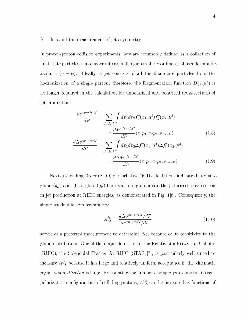
B. Jets and the measurement of jet asymmetry

In proton-proton collision experiments, jets are commonly defined as a collection of

final-state particles that cluster into a small region in the coordinates of pseudo-rapidity−

azimuth (η − φ). Ideally, a jet consists of all the final-state particles from the

hadronization of a single parton; therefore, the fragmentation function D(z, µ2) is

no longer required in the calculation for unpolarized and polarized cross-sections of

jet production:

dσpp→jetX

dP=∑f1,f2,f

∫dx1dx2f

p1 (x1, µ

2)fp2 (x2, µ2)

× dσf1f2→fX′

dP(x1p1, x2p2, pjet, µ) (1.8)

d∆σpp→jetX

dP=∑f1,f2,f

∫dx1dx2∆fp1 (x1, µ

2)∆fp2 (x2, µ2)

× d∆σf1f2→fX′

dP(x1p1, x2p2, pjet, µ) (1.9)

Next-to-Leading Order (NLO) perturbative QCD calculations indicate that quark-

gluon (qg) and gluon-gluon(gg) hard scattering dominate the polarized cross-section

in jet production at RHIC energies, as demonstrated in Fig. 1[6]. Consequently, the

single-jet double-spin asymmetry

AjetLL =d∆σpp→jetX/dPdσpp→jetX/dP

(1.10)

serves as a preferred measurement to determine ∆g, because of its sensitivity to the

gluon distribution. One of the major detectors at the Relativistic Heavy-Ion Collider

(RHIC), the Solenoidal Tracker At RHIC (STAR)[7], is particularly well suited to

measure AjetLL because it has large and relatively uniform acceptance in the kinematic

region where d∆σ/dσ is large. By counting the number of single-jet events in different

polarization configurations of colliding protons, AjetLL can be measured as functions of

5

jet kinematic variables, such as transverse momentum and pseudo-rapidity. In the

end, one can eventually constrain the gluon polarization distribution by comparing

the measured AjetLL against calculations from various theoretical models.

Fig. 1. Relative contributions from gg, qg, and qq scatterings to the NLO polarized

cross-section for jet and inclusive-π0 production at mid pseudo-rapidities at√s = 200 GeV.

C. Polarized proton-proton collisions at RHIC

Located at the Brookhaven National Laboratory, RHIC is designed to perform ex-

periments for both heavy-ion collisions with center-of-mass energy up to 200 GeV

per nucleon-nucleon pair, and polarized proton-proton collisions with center-of-mass

energy at 200 GeV and 500 GeV. Accelerated particles are carried in two separated

rings travelling in opposite directions defined as the blue beam and the yellow beam.

There are six interaction points located evenly on the RHIC rings, where the beams

6

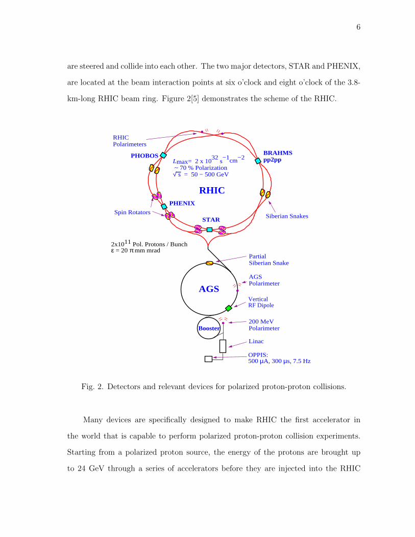
are steered and collide into each other. The two major detectors, STAR and PHENIX,

are located at the beam interaction points at six o’clock and eight o’clock of the 3.8-

km-long RHIC beam ring. Figure 2[5] demonstrates the scheme of the RHIC.

Prospects for Spin Physics at RHIC 5

•

RHIC

AGS

PartialSiberian Snake

STAR

PHENIX

RHICPolarimeters

Siberian SnakesSpin Rotators

Polarized Proton Collisions at BNL

Lmax= 2 x 1032

s−1cm−2

~ 70 % Polarization√ s = 50 − 500 GeV

Booster

2x1011 Pol. Protons / Bunchε = 20 π mm mrad

Linac

200 MeVPolarimeter

AGS Polarimeter

VerticalRF Dipole

••

BRAHMSpp2pp

•

OPPIS:500 µA, 300 µs, 7.5 Hz

PHOBOS

Figure 1: Schematic layout of the RHIC accelerator complex. Only relevant devices forpolarized pp collisions are shown.

Fig. 2. Detectors and relevant devices for polarized proton-proton collisions.

Many devices are specifically designed to make RHIC the first accelerator in

the world that is capable to perform polarized proton-proton collision experiments.

Starting from a polarized proton source, the energy of the protons are brought up

to 24 GeV through a series of accelerators before they are injected into the RHIC

7

rings[8, 9]. Protons are injected into each ring as “bunches” of protons which contain

1 ∼ 2 × 1011 protons each, with typically 110 bunches in total in each ring[10]. In

the storage ring, accelerated protons have a stable spin state which is perpendicular

to the beam direction, i.e., the transverse spin state. Each ring is equipped with

two magnets, referred as Siberian Snakes, that flip the spin state of the protons that

are passing through them, in order to prevent the beam from depolarization. There

are also four Spin Rotators located around the interaction points of both STAR and

PHENIX, which can rotate the spin of protons parallel to the beam direction when

the protons are entering the detectors, in order to perform longitudinally polarized

proton collision experiments[11], and then rotate them back to the transverse stable

state when they are leaving the interaction point. Various polarimeters are equipped

to monitor beam polarization, with proton-Carbon polarimeters for fast beam polar-

ization measurements, and a H-jet polarimeter for calibration.

The presented analysis uses the STAR data from the second longitudinal run

period of 2006, with a center-of-mass energy of 200 GeV. This run period completed

with an average polarization of 60% and an accumulated luminosity of ∼ 6pb−1.

8

CHAPTER II

BACKGROUND OF THE STAR DETECTOR AND THE TIME PROJECTION

CHAMBER

A. Jet detection with STAR

1. The STAR detector and the Time Projection Chamber

STAR, the Solenoidal Tracker At RHIC, consists of several sub-systems that cover

different rapidity ranges and functionality[7].

The Time Projection Chamber (TPC) [12], which is the innermost detector,

provides tracking for charged particles such as charged pions, electrons, protons and

etc. at mid-rapidity. The barrel side of TPC is covered by the Time of Flight

detector (ToF), which is then covered by the Barrel Electro-Magnetic Calorimeter

(BEMC), which provides energy measurement for electrons, direct gammas and short-

life neutral particles such as neutral pions.

Other detectors include forward-rapidity detectors such as Forward TPC, End-

cap Electro-Magnetic Calorimeter, Forward Pion Detector and Forward Meson Spec-

trometer, and detectors mainly used for triggering and luminosity monitoring, such

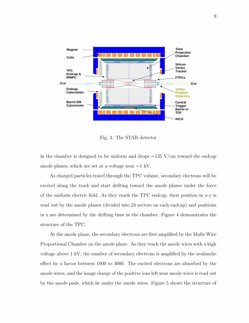
as Beam-Beam Counter (BBC) and Zero Degree Calorimeter. Figure. 3 shows the

layout of major sub-systems in the STAR detector.

Being the primary tracking device at mid-rapidity, the TPC is designed to provide

tracking and momentum measurement of charged particles at high multiplicity. The

TPC measures 4.2 meters long and 4 meters in outer diameter, which is equivalent

to -1 to 1 in pseudo-rapidity with respect to detector center, and 1 meter in inner

diameter. The chamber is filled with drift gas (P10) and divided into two chambers

by the center membrane, which is set to a high voltage of 28 kV. The electric field

9

ZCal

Barrel EM Calorimeter

EndcapCalorimeter

Magnet

Coils

TPCEndcap & MWPC

ZCal

FTPCs

VertexPositionDetectors

Central Trigger Barrel or TOF

Time Projection Chamber

Silicon Vertex Tracker

RICH

Fig. 3. The STAR detector

in the chamber is designed to be uniform and drops ∼135 V/cm toward the endcap

anode planes, which are set at a voltage near ∼1 kV.

As charged particles travel through the TPC volume, secondary electrons will be

excited along the track and start drifting toward the anode planes under the force

of the uniform electric field. As they reach the TPC endcap, their position in x-y is

read out by the anode planes (divided into 24 sectors on each endcap) and positions

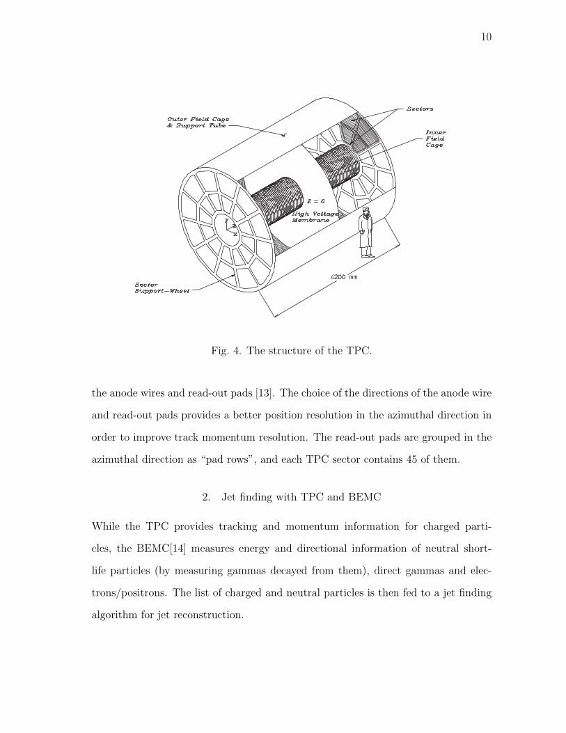
in z are determined by the drifting time in the chamber. Figure 4 demonstrates the

structure of the TPC.

At the anode plane, the secondary electrons are first amplified by the Multi-Wire

Proportional Chamber on the anode plane. As they reach the anode wires with a high

voltage above 1 kV, the number of secondary electrons is amplified by the avalanche

effect by a factor between 1000 to 3000. The excited electrons are absorbed by the

anode wires, and the image charge of the positive ions left near anode wires is read out

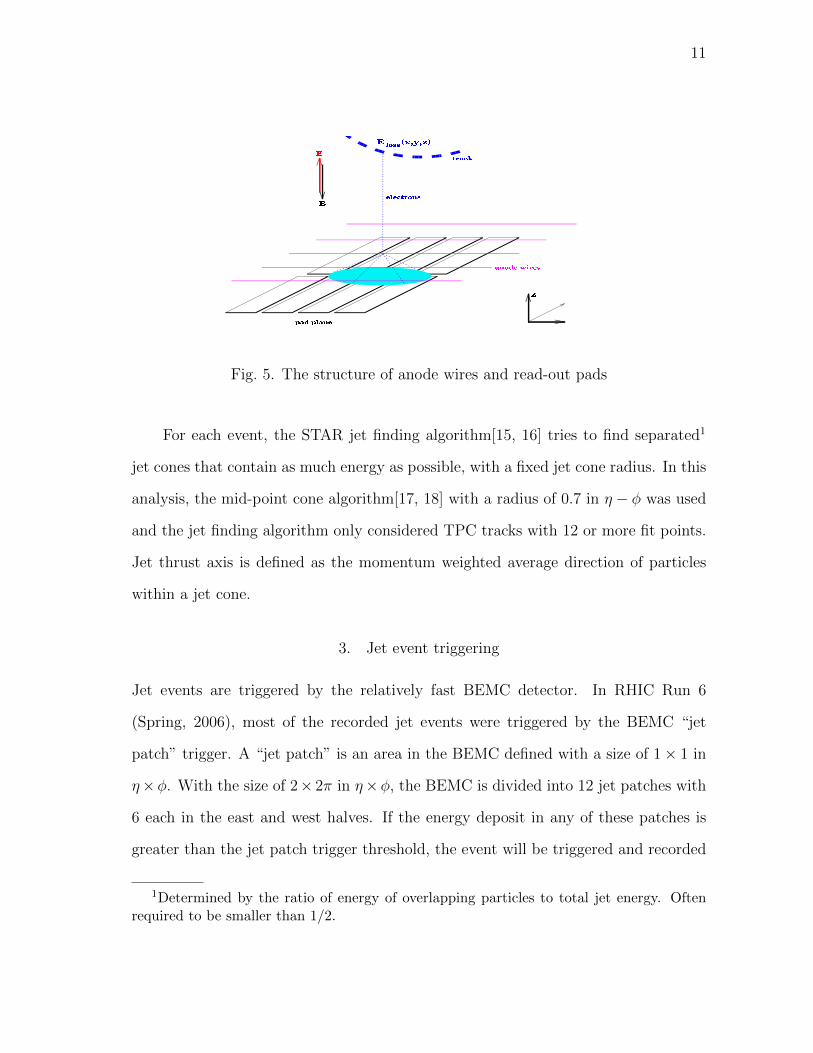
by the anode pads, which lie under the anode wires. Figure 5 shows the structure of

10

wires providing an amplification of 1000 to 3000. The positive ions created in theavalanche induce a temporary image charge on the pads which disappears as theions move away from the anode wire. The image charge is measured by a pream-plifier/shaper/waveform digitizer system. The induced charge from an avalancheis shared over several adjacent pads, so the original track position can be recon-structed to a small fraction of a pad width. There are a total of 136,608 pads in thereadout system.

The TPC is filled with P10 gas (10% methane, 90% argon) regulated at 2 mbarabove atmospheric pressure[7]. This gas has long been used in TPCs. It’s primaryattribute is a fast drift velocity which peaks at a low electric field. Operating on thepeak of the velocity curve makes the drift velocity stable and insensitive to smallvariations in temperature and pressure. Low voltage greatly simplifies the field cagedesign.

The design and specification strategy for the TPC have been guided by the limits ofthe gas and the financial limits on size. Diffusion of the drifting electrons and theirlimited number defines the position resolution. Ionization fluctuations and finitetrack length limit thedE/dx particle identification. The design specifications wereadjusted accordingly to limit cost and complexity without seriously compromisingthe potential for tracking precision and particle identification.

Fig. 1. The STAR TPC surrounds a beam-beam interaction region at RHIC. The collisionstake place near the center of the TPC.

3

Fig. 4. The structure of the TPC.

the anode wires and read-out pads [13]. The choice of the directions of the anode wire

and read-out pads provides a better position resolution in the azimuthal direction in

order to improve track momentum resolution. The read-out pads are grouped in the

azimuthal direction as “pad rows”, and each TPC sector contains 45 of them.

2. Jet finding with TPC and BEMC

While the TPC provides tracking and momentum information for charged parti-

cles, the BEMC[14] measures energy and directional information of neutral short-

life particles (by measuring gammas decayed from them), direct gammas and elec-

trons/positrons. The list of charged and neutral particles is then fed to a jet finding

algorithm for jet reconstruction.

11

radial

azimuthal

Fig. 5. The structure of anode wires and read-out pads

For each event, the STAR jet finding algorithm[15, 16] tries to find separated1

jet cones that contain as much energy as possible, with a fixed jet cone radius. In this

analysis, the mid-point cone algorithm[17, 18] with a radius of 0.7 in η − φ was used

and the jet finding algorithm only considered TPC tracks with 12 or more fit points.

Jet thrust axis is defined as the momentum weighted average direction of particles

within a jet cone.

3. Jet event triggering

Jet events are triggered by the relatively fast BEMC detector. In RHIC Run 6

(Spring, 2006), most of the recorded jet events were triggered by the BEMC “jet

patch” trigger. A “jet patch” is an area in the BEMC defined with a size of 1× 1 in

η×φ. With the size of 2× 2π in η×φ, the BEMC is divided into 12 jet patches with

6 each in the east and west halves. If the energy deposit in any of these patches is

greater than the jet patch trigger threshold, the event will be triggered and recorded

1Determined by the ratio of energy of overlapping particles to total jet energy. Oftenrequired to be smaller than 1/2.

12

as a candidate jet event.

4. The systematic uncertainty of TPC tracking efficiency in jets

In STAR, the TPC tracking efficiency within a data set is typically estimated through

embedding, in which a simulated track is mixed with other signals of an event from

real data. The mixed event is then treated as if it is from real data and reconstructed

in the same way as in real data production. Then the tracking efficiency is estimated

as the possibility of a simulated track being able to be matched with a reconstructed

track.

Standard STAR analysis assumes ∼5% uncertainty on the TPC tracking effi-

ciency, which is obtained in a study[12] which focused on identified particle measure-

ments in heavy ion collisions, instead of jets in proton+proton collisions. The present

study investigated the systematic uncertainty of the TPC tracking efficiency in jets

to see if this uncertainty could be reduced.

Both the BEMC energy resolution and the TPC tracking efficiency contribute

to the uncertainty of jet energy scale. Since BEMC resolution improves as deposited

energy increases, at high pT , TPC tracking efficiency represents the largest uncertainty

on jet energy scale. Reducing the systematic uncertainty of TPC tracking efficiency

will provide a more precise energy measurement of high pT jets.

B. Simulation tools in STAR

1. Pythia, gSTAR and Monte-Carlo simulation data production

After RHIC Run 6 finished in June, 2006, a Monte-Carlo simulation data production[19]

was made for the Run 6 detector configuration of STAR. This dataset was produced

utilizing the Pythia[20] high energy collision event generator plus the gSTAR sim-

13

ulation kit[21], which is based on GEANT3[22] and implements the STAR detector

geometry. This dataset was used in this analysis as a counterpart of the dataset of

Run 6 longitudinal data.

In addition, the gSTAR simulation kit, which can simulate the energy deposition

of primary particles in each part of the STAR detector, was used in this analysis to

generate TPC responses for the single track event used in embedding.

2. The TPC response simulator

Besides the stand alone simulation tools, part of the STAR event reconstruction code

also serves as part of the simulation process. Since gSTAR only simulates energy

deposits of primary particles, the TPC response simulator, as part of the standard

STAR code library, is used to carry on the simulation process and generate TPC ADC

values from the energy deposition.

14

CHAPTER III

TPC TRACKING EFFICIENCY MEASUREMENT AND SYSTEMATIC

UNCERTAINTY ESTIMATION

As charged primary particles travel through the TPC, they interact with the cham-

ber gas and release secondary electrons along their trajectories. Once these secondary

electrons drift through the chamber gas and reach the TPC anode planes, their po-

sition information in these planes is granularized1 with respect to the positions of

read out pads. These granularized clusters, together with their position information

along the drift direction calculated from drift time, are referred as “TPC Hits” [12].

After that, tracks are reconstructed from the detected TPC hits by a software track

fitting algorithm [23]. Then various cuts are applied to these reconstructed tracks in

jet reconstruction and further analysis.

However, some tracks from a certain proton-proton collision event may not be

reconstructed from the TPC hits, or may be excluded as “junk” tracks in the calcula-

tion of reconstructed jet energy. Listed here are some of the reasons that could cause

the inefficiencies in TPC tracking [12, 13]:

1. Limited acceptance of the detector. There exist inactive areas of read out

pads on the anode plane such as spaces used for mounting and fiducial cuts

on the edge of TPC sectors. A track that intersects these areas may have too

few detected TPC hits to be successfully reconstructed. For high momentum

tracks, this will result in an inefficiency of ∼6%.

2. Limited resolution of the positions of TPC hits. Diffusion of the secondary elec-

1Along the radial direction of the TPC anode plane; though, along the azimuthal direc-tion, positions of TPC hits are read out with multiple adjacent pads, thus acquiring a muchbetter position resolution than the width of the pads.

15

trons when they drift toward the anode wire planes, finite size of read out pads,

finite resolution of drift time measurement and noises of front end electronics

all lower the resolution of the positions of detected TPC hits. For example,

the dimension of the read out pads along the pad row is 6.20 mm for the outer

sub-sectors; though the position resolution is improved by reading out three

adjacent pads at the same time, the finite size of read out pads still introduces

∼2 mm uncertainty on the position of TPC hits along pad rows for tracks with

transverse momentum of 200 MeV.

The smeared positions of TPC hits deteriorate the quality of reconstructed

tracks. The measured properties of a reconstructed track, such as the distance

of closest approach2, will have a deviation from the true value introduced by

the uncertainty of TPC hits and fail to pass certain cuts in an analysis. Since

these cuts are only supposed to remove tracks that should not be counted in a

reconstructed event, for example, pile-up tracks and double counted split tracks,

the accidental removal of primary tracks with poor reconstruction quality should

be considered as an inefficiency of TPC tracking.

3. Merging of TPC hits. Diffusion of the drifting secondary electrons of a track

causes another problem. Though reading out adjacent pads improves the posi-

tion resolution of TPC hits, this strategy does not work in the situation when

secondary electron clusters from two different tracks overlap each other—the

distance between two clusters needs to be much larger than the resolution men-

tioned above to be successfully separated into two TPC hits. Merging of TPC

hits reduces the available TPC hits for track reconstruction and causes merging

of two adjacent tracks.

2The distance from event vertex to the reconstructed track. Will be discussed in Ch. IV.

16

These various reasons that could cause the failure of reconstructing a track make

an analytical tracking efficiency calculation infeasible. Furthermore, the high lumi-

nosity condition and the relatively slow TPC response makes this analysis even more

difficult 3. Consequently, the technique of embedding, which calculates the tracking

efficiency by Monte-Carlo simulation while utilizing real data, is used in this analysis

and discussed in this chapter.

A. The embedding technique

A detector simulator builds models of physical processes to produce reasonable and

realistic detector responses. The simulation of TPC responses is divided into two

steps. First, the gSTAR/GEANT3 simulation kit produces secondary particles that

were released by the simulated primary tracks and calculates energy depositions as

charged tracks pass through matter. Then, codes in the standard STAR analysis

chain, the StTrsMaker, simulate other processes in the TPC that could not be han-

dled by GEANT and produce raw Analog/Digital Converter (ADC) values that cor-

respond to what was recorded in real data4. The combined simulation of gSTAR plus

StTrsMaker takes care of many processes that could affect the TPC tracking, such

as multiple collisions between primary particles and detector material, diffusion of

secondary electrons during drifting, gain fluctuations of the electron avalanche near

MWPC anode wires, and responses of the TPC read out pads and signal shapers [13].

Therefore, the physical processes that could affect TPC hit reconstruction are consid-

ered in the simulation and it is applicable to the task of the TPC tracking efficiency

3The influence of the beam luminosity on TPC tracking will be discussed later in thischapter.

4In fact, only a small fraction of runs recorded the TPC ADC values to the tape; mostof the time, only real-time reconstructed TPC hits were saved while ADC information wasdropped.

17

calculation.

One possible method of estimating the TPC tracking efficiency is comparing the

tracks in the simulation data before and after the simulation and event reconstruction.

For each event, the tracking efficiency is calculated as the number of simulated tracks

that could be associated to a reconstructed track, divided by the total number of

simulated tracks. The standard Run 6 Monte-Carlo simulation data (pure simulation)

itself can serve such kind of analysis and produce valid calculations of the tracking

efficiency, as long as pure simulation provides a good approximation of true data.

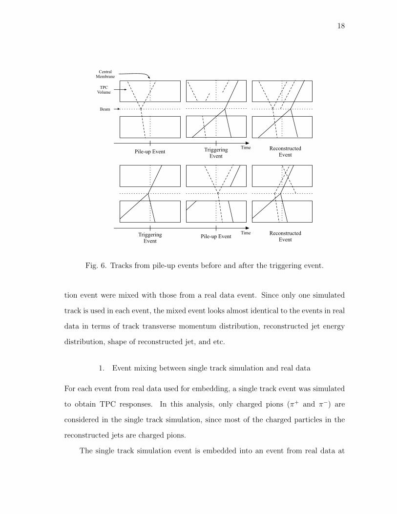
Unfortunately, however, in practice the TPC works in a much more complex

and harsher environment than the one in pure simulation. Given the facts that the

distance between the TPC central membrane and each anode wire plane is 210 cm,

and that the average gas drift velocity is 5.45 cm µs−1, the read-out time window

of the TPC is ∼40 µs, which is much longer than the RHIC beam bunch crossing

interval of ∼106 ns. At a BBC coincidence rate of 400 kHz, there are approximately

32 collisions that lie within this time window before and after the triggering event,

which are referred as “pile-up” events. Segments of tracks from pile-up events will be

read out together with tracks from the triggering event, disturbing the TPC tracking.

Since the TPC drift in the beam direction preserves the relative transverse location

of hit positions along a track, out-of-time tracks still look like tracks, but maybe with

hits lost from one end or another. On average in Run 6, there were 1.4× 102 pile-up

tracks[24] with transverse momentum greater than 0.2 GeV in each event. Figure 6

illustrates two pile-up events before and after a triggering event.

Besides the pile-up tracks, another factor that pure simulation does not con-

sider is the background from beam-gas interactions, which could also affect the TPC

tracking efficiency. In order to address these issues, the embedding technique was

used in this analysis, in which detector responses from a (single track) pure simula-

18

Time

TPC Volume

Central Membrane

Beam

Pile-up Event Reconstructed Event

Triggering Event

Pile-up EventTriggering Event

Reconstructed Event

Time

Fig. 6. Tracks from pile-up events before and after the triggering event.

tion event were mixed with those from a real data event. Since only one simulated

track is used in each event, the mixed event looks almost identical to the events in real

data in terms of track transverse momentum distribution, reconstructed jet energy

distribution, shape of reconstructed jet, and etc.

1. Event mixing between single track simulation and real data

For each event from real data used for embedding, a single track event was simulated

to obtain TPC responses. In this analysis, only charged pions (π+ and π−) are

considered in the single track simulation, since most of the charged particles in the

reconstructed jets are charged pions.

The single track simulation event is embedded into an event from real data at

19

the TPC ADC level. After a simulated track is handled by gSTAR and the TPC

response simulator, the obtained TPC ADC values are added to the ones from a real

data event. The mixed event then is fed to the event reconstruction code as a whole.

The TPC hits, the tracks and the jets are then reconstructed from the mixed TPC

ADC values step by step. The effects of the high luminosity environment on the TPC

tracking is reflected on the distorted TPC ADC values associated with the TPC hits

along the simulated track.

One major limitation on the statistical errors of this analysis is the fact that only

a small portion of the real data have the TPC ADC information4.

2. Estimating systematic uncertainty of the tracking efficiency

For a measurement of a certain value, systematic uncertainty is commonly defined as

the difference between the true value and the average of measured values when the

number of measurements approach infinity, which is the bias introduced by the inac-

curate understanding of the measurement. In this analysis of TPC tracking efficiency,

this bias could be estimated by introducing the embedding into pure simulation data

(Monte-Carlo embedding), in addition to the embedding into real data (real data

embedding). The simulation is essentially a calculation based on our understanding

of the measuring equipment, thus the difference between the calculations of MC em-

bedding and real data embedding reflects the bias on the understanding of how the

environment of the TPC volume affects the tracking efficiency.

3. Event mixing between single track simulation and Monte-Carlo data

In the embedding into Monte-Carlo data, the mixing is performed right after the

secondary electrons along the primary tracks are simulated by gSTAR, and before

the event is fed to the TPC response simulator. Despite this difference of when the

20

events are mixed, other procedures in the real data embedding and Monte-Carlo data

embedding are kept as same as possible in this analysis to prevent introducing any

other differences between these two methods instead of those that are intrinsic.

B. Issues in the embedding procedure

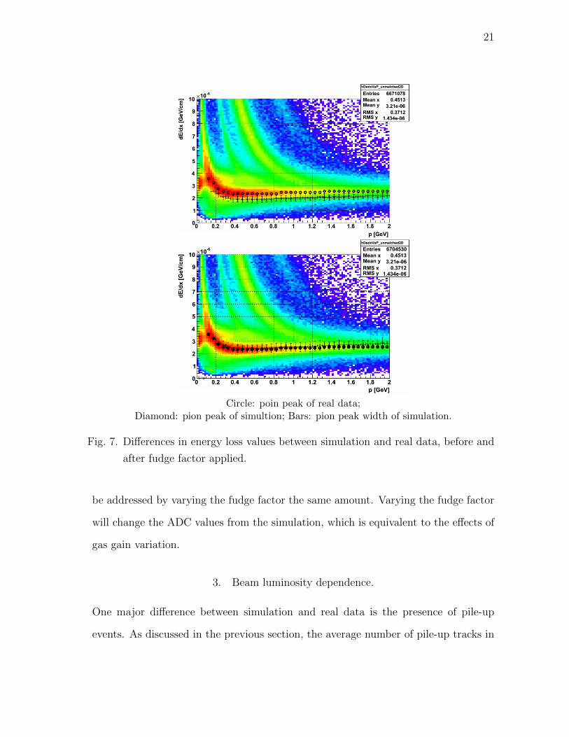
1. Ionization energy loss values and the “fudge factor” in single track simulation.

One issue in the simulation is that the value of ionization energy loss per unit distance

traveled by charged particles, dE/dx, is not consistant with real data. Figure 7 shows

the differences in dE/dx vs. track momentum. This inconsistency could be introduced

by various reasons, such as inaccurate dE/dx values, or inaccurate conversion from

dE/dx to ADC values.

To fix this issue, energy deposit values from GEANT are multiplied by a “fudge

factor” to match the values in real data. In this analysis, the fudge factor was

determined by matching the pion peaks from simulation and real data in the dE/dx

vs. track momentum plot, and the value of 1.26 was applied.

2. TPC gas gain fluctuations.

Another issue related to fudge factor in real data embedding is the fluctuations in

TPC gas gain. The TPC pressure is regulated to be 2 mbar above atmospheric

pressure [12], and fluctuates as weather conditions change; so does the TPC gas gain

which is a function of gas pressure. In the experiment, the gas gain is monitored to

calibrate TPC data to get constant dE/dx value; however, tracking efficiency is also

affected but cannot be reflected in the calibration. As shown in Figure 8 [25], gas

gain variation over the running period of Run 6 was within ±6%.

In the simulation, the effect of gas gain fluctuation on the tracking efficiency can

21

Circle: poin peak of real data;Diamond: pion peak of simultion; Bars: pion peak width of simulation.

Fig. 7. Differences in energy loss values between simulation and real data, before and

after fudge factor applied.

be addressed by varying the fudge factor the same amount. Varying the fudge factor

will change the ADC values from the simulation, which is equivalent to the effects of

gas gain variation.

3. Beam luminosity dependence.

One major difference between simulation and real data is the presence of pile-up

events. As discussed in the previous section, the average number of pile-up tracks in

22

Fig. 8. The TPC gas gain variation during the running period of Run 6.

a triggering event is proportional to the BBC coincidence rate. It is expected that

the difference between simulation and real data drops at lower BBC rates, and the

effects of pile-up tracks could be much reduced by fitting the tracking efficiency as a

function of BBC rate and using the extrapolated value at zero luminosity to compare

with simulation.

However, in this analysis, this approach did not work due to limited event-by-

event variation in BBC rate. Figure 9 demonstrates the BBC rate distribution of

the events. An attempt to fit tracking efficiency against BBC rates showed that

the correlation between tracking efficiency and BBC rate was buried in statistical

fluctuations.

23

Fig. 9. BBC coincidence rate distribution. ( Events in real data used for embedding. )

24

CHAPTER IV

IMPLEMENTATIONS OF THE EMBEDDING PROCEDURE

This chapter explains how the embedding procedure is implemented in this analysis.

In this chapter certain terms are defined as follows:

Embedding Event/Jet An event/jet into which the simulated track is embedded.

Embedded Track A single track that is simulated, mixed with embedded event,

and later reconstructed to evaluate the tracking efficiency.

Sampled Event/Jet An event/jet from which the kinematics of an embedding track

are sampled.

The implementation is done as far as possible in the same way for both real data

and MC embedding, while the largest difference is found in how the embedded tracks

and embedding events are mixed, which will be discussed in Sec. C.

The kinematics of the embedding track are sampled randomly from Run 6 200 GeV

p+p longitudinal data, for both real data and MC embedding, based on the kinematics

of the embedded jet, which are obtained from reconstructed embedding events. Ap-

plying these kinematics, a single track is simulated by GSTAR and its TPC responses

are mixed with responses from the embedding event, which are then reconstructed as

a whole event. Associations are then attempted between each primary track in the

reconstructed event and the embedded track. If no primary track can be associated

to the embedded track, then the embedded track will be considered missing due the

inefficiency of TPC tracking. Fig. 10 illustrates the procedures of both the real data

and MC embedding. Details of each step will be discussed in this chapter.

25

PART IV: GET TPC RESPONSES OF CORRESPONDING EMBEDDING EVENT

TPC ADC values from DAQ files

TPC hits from GEANT

output

PART II: SELECT EMBEDDING EVENTS

NO

PART I: PREPARE TRACKS FOR SAMPLING

Find jets in run 6 longitudinal data

Pick up tracks within jet cones,with pT > 0.2 GeV

Divide tracks into bins, by the pT of their parent jets

PART III: SAMPLE AND PREPARE KINEMATIC PARAMETERS FOR THE EMBEDDED TRACK

Pick up the jet with highest pT as the embedding jet

Randomly pick up a track in the same pT bin as the embedding jet

Get track kinematics in the local coordinates of the sampled jet

Rotate the embedded track around the embedding jet thrust axis by a random angle

Transform the kinematics into global coordinates according to the direction of the thrust axis of the embedding jet

Loop over each event in embedding

data

START

Passes Cuts?

・Primary vertex reconstructed・-120cm < vz < 120cm・Bemc-jp1-mb trigger should fire (and did fire)・At least one reconstructed jet matched to a fired jet patch・-0.9 < jet-ηdetector < 0.9・Transverse neutral energy fraction < 0.92

YES

Real data embeddingMC data embedding

Simulate TPC responsesto the embedded track in gSTAR (GEANT)

Mix TPC responses from single track MC event and embedding event

Reconstruct mixed event

MC embedded track associated to a

reconstructed track?

Passes cuts for the quality of associated reconstructed track?

YES

NO Mark embedded track as "unmatched"

Mark embedded track as "matched"YES

NO

END OF

LOOP

・Common TPC hits ≥ 6・dcaD cut・# fit points > 12・(# fit points) : (# possible fit points) > 51%

Fig. 10. Procedures for real data and MC embedding

26

A. Datasets used for analysis

Data sets both before and after reconstruction are used in this analysis. In part III

of Fig. 10, kinematics of embedding jets, which are used in sampling embedded track

kinematics, are extracted from reconstructed events, whereas the TPC responses,

which are used in event mixing, are extracted from corresponding embedding events

in datasets before reconstruction. Run 6 200 GeV p+p longitudinal data after recon-

struction are also used in sampling kinematics of embedded tracks, in both real data

and MC embedding.

1. Cuts on the embedding events

The analysis code loops over each event in the available reconstructed data sets and

selects events that pass the following cuts for embedding. These cuts separate out

events that contain at least one reconstructed jet located in the region with better

TPC performance. Furthermore, similar cuts are also commonly found in other jet

analyses[15, 16, 26] which makes this analysis more consistent with others.

(1) A primary vertex reconstructed. In this analysis, if a track cannot be associated to

the primary vertex after reconstruction, it will be considered as an inefficiency of

the TPC tracking, even though there might be a non-primary track reconstructed.

Therefore only events with a primary vertex are considered.

(2) −120 cm < vz < 120 cm, where vz is the primary vertex position with respect to

the detector center along the beam line. This cut eliminates events in which the

collision happened near the boundary of TPC.

(3) BEMC-JP1-MB trigger “should fire” in both real data and MC embedding.

BEMC-JP1-MB trigger “did fire” in real data embedding. BEMC-JP1-MB re-

27

quires a minimum energy deposit of 8.3 GeV in a single jet patch, which is defined

as a BEMC region of size 1×1 in η and φ. In the real data embedding, this trigger

contributes most of the jet events recorded in the Run 6 200 GeV p+p longitu-

dinal data and the “should fire” requirement acts as a software trigger. On the

other hand, in MC embedding, this same trigger filters the events and makes sure

that the behaviors of this trigger are also reflected in the MC data.

(4) At least one reconstructed jet matched to a fired jet patch, by requiring that the

difference between the center of the jet patch and the jet thrust axis is smaller

than 0.6 in η and φ.

(5) −0.9 < jet-ηdetector < 0.9. Given the fact that when tracks are required to have

at least 12 fit points, the TPC only has acceptable tracking efficiency approxi-

mately between −1.3 < ηdetector < 1.3, this cut ensures that most tracks in a jet

reconstructed with a cone radius of 0.7 fall in the TPC coverage.

(6) Transverse neutral energy fraction of the jet < 0.92. This value is the ratio of

the transverse energy deposited in EMC to the total transverse energy of the jet.

This cut ensures that TPC tracks contribute a significant amount of transverse

energy to the reconstructed jet, which suppresses fake jets from non-collision

backgrounds.

2. Statistics of embedding events in real data embedding

In real data embedding this analysis mainly focuses on the Run 6 200 GeV p+p

longitudinal data. In part IV of the embedding procedure illustrated in Fig. 10,

raw information of TPC responses in the form of TPC ADC values are required

to mix the embedding event with the embedded track. In the recorded data, TPC

ADC information can be found in DAQ files, which were obtained from the Data

28

AcQuisition system during the run. They were recorded for each pad as a time series

of size 512 for each of the 5692 pads on the TPC endcaps[12].

However, due to limited tape writing rate, most events recorded during the run

do not contain TPC ADC information. Instead, only online reconstructed clusters

and tracks were written to the tape. Only a subset of DAQ files from 15 runs in

the Run 6 200 GeV p+p longitudinal data contain TPC ADC information, which

totals ∼65 k. After applying the above cuts, there remains ∼9 k events available for

embedding. The limited number of events available for real data embedding is the

major contribution to the statistical uncertainty of this analysis.

3. Reweighting of the embedding events in MC embedding

Data sets from the P07ic pp 200 GeV Monte Carlo production series are used in the

MC embedding. These data sets were produced with PYTHIA v6.410 and year 2006c

geometry1 of the detector and were divided into different partonic pT bins from 3 GeV

to 65 GeV.

One difficulty in the Monte Carlo simulation arises from the steeply falling spec-

trum of the partonic pT distribution. The partonic pT spectrum of participating

partons in the collisions decays exponentially and could change several orders of

magnitude in the range of interest. On one hand, many of the interesting events have

larger partonic pT , such as events with larger jet pT and events that pass jet patch

triggers; thus good statistics are desired on these events. On the other hand, events

with smaller partonic pT cannot be ignored because of the limited detector energy

resolution and the steeply falling partonic pT spectrum. For example, even with a

minimum requirement on the reconstructed jet pT , events from a partonic pT bin that

1http://drupal.star.bnl.gov/STAR/comp/prod/monte-carlo-production-datasets

29

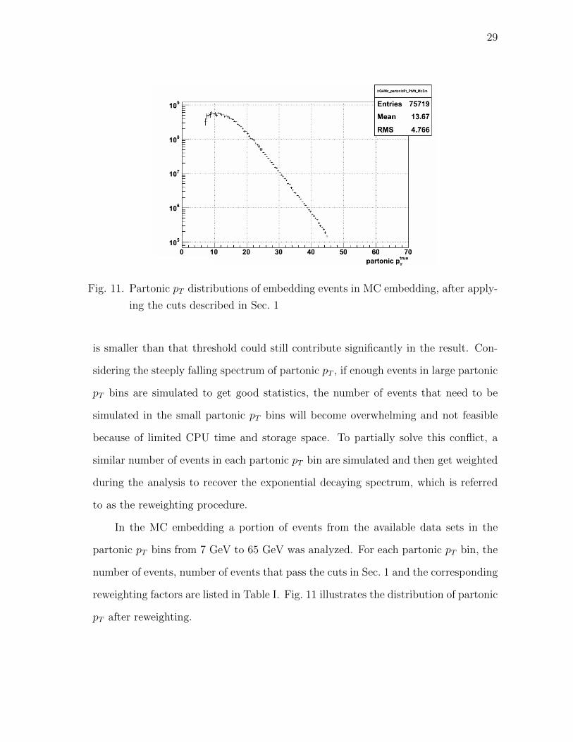
Fig. 11. Partonic pT distributions of embedding events in MC embedding, after apply-

ing the cuts described in Sec. 1

is smaller than that threshold could still contribute significantly in the result. Con-

sidering the steeply falling spectrum of partonic pT , if enough events in large partonic

pT bins are simulated to get good statistics, the number of events that need to be

simulated in the small partonic pT bins will become overwhelming and not feasible

because of limited CPU time and storage space. To partially solve this conflict, a

similar number of events in each partonic pT bin are simulated and then get weighted

during the analysis to recover the exponential decaying spectrum, which is referred

to as the reweighting procedure.

In the MC embedding a portion of events from the available data sets in the

partonic pT bins from 7 GeV to 65 GeV was analyzed. For each partonic pT bin, the

number of events, number of events that pass the cuts in Sec. 1 and the corresponding

reweighting factors are listed in Table I. Fig. 11 illustrates the distribution of partonic

pT after reweighting.

30

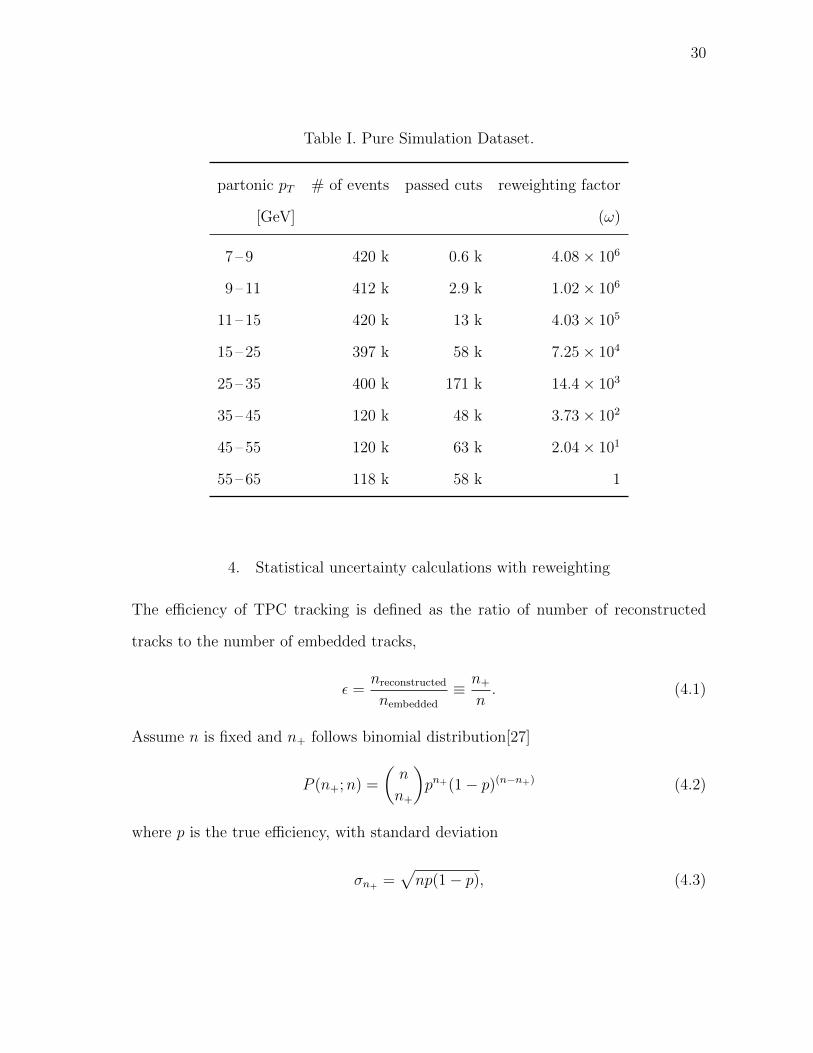
Table I. Pure Simulation Dataset.

partonic pT # of events passed cuts reweighting factor

[GeV] (ω)

7 – 9 420 k 0.6 k 4.08× 106

9 – 11 412 k 2.9 k 1.02× 106

11 – 15 420 k 13 k 4.03× 105

15 – 25 397 k 58 k 7.25× 104

25 – 35 400 k 171 k 14.4× 103

35 – 45 120 k 48 k 3.73× 102

45 – 55 120 k 63 k 2.04× 101

55 – 65 118 k 58 k 1

4. Statistical uncertainty calculations with reweighting

The efficiency of TPC tracking is defined as the ratio of number of reconstructed

tracks to the number of embedded tracks,

ε =nreconstructed

nembedded

≡ n+

n. (4.1)

Assume n is fixed and n+ follows binomial distribution[27]

P (n+;n) =

(n

n+

)pn+(1− p)(n−n+) (4.2)

where p is the true efficiency, with standard deviation

σn+ =√np(1− p), (4.3)

31

then with ε as an estimation of true efficiency p, the standard deviation of ε could be

calculated as

σε =σn+

n=

√ε(1− ε)

n. (4.4)

Notice that this formula only works fine when ε is a good estimation of p, which

requires that n, εn, and (1− ε)n are all large enough.

When reweighting is involved, the definition for the efficiency becomes

ε =

∑i ωini+∑

i ωini+ +∑

i ωini−, (4.5)

where i is the index for different partonic pT bins and∑

sum over all considered

partonic pT bins. ωi’s are the factors for reweighting and ni− is defined as

ni− ≡ n− ni+. (4.6)

Assume ni+, ni− are independent and are large enough to be considered as Poisson

distributed, with standard error propagation equation

σε =

√∑i

(∂ε

∂ni+)2σ2

ni++∑i

(∂ε

∂ni−)2σ2

ni−, (4.7)

which gives

σε =

√(∑

i ω2i ni+)(

∑i ωini−)2 + (

∑i ω

2i ni−)(

∑i ωini+)2

(∑

i ωini+ +∑

i ωini−)2(4.8)

B. Kinematics of the embedded tracks

1. Sampling track kinematics by jet pT of embedding jets

These events are picked from the same runs as the embedding events, but without

TPC ADC information and not used as an embedding event. In real data embedding,

tracks are sampled from the events in the same run as the embedding event, while in

32

MC embedding, tracks are sampled from all available events.

All the tracks found within jet cones of the reconstructed events were sampled and

divided into different bins by the transverse momentum of the sampled jet. Table

II show how many tracks are available for sampling in each jet pT bin. When an

embedding event is selected, a track is randomly selected from the bin with the

same pT of the embedding jet. In this way, the sampled kinematics reflect track

distributions related to jet pT , such as track pT and distance from the jet thrust axis.

Table II. Number of tracks in each jet pT bin available for sampling embedded track

kinematics.

jet pT range [GeV] # of tracks jet pT range [GeV] # of tracks

7.56 9.30 33914 21.3 26.2 67279

9.30 11.4 107921 26.2 32.2 23763

11.4 14.1 186008 32.2 39.6 6343

14.1 17.3 194216 39.6 48.7 1076

17.3 21.3 137005

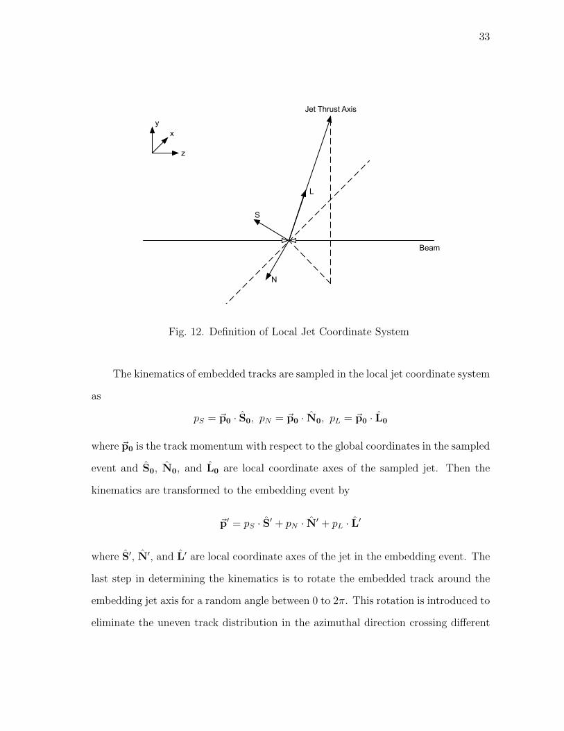
2. Local coordinate system for jets

A local jet coordinate system is defined to describe track kinematics with respect to

the jet thrust axis, which is illustrated in Fig. 12:

L Parallel to jet thrust axis.

N ≡ z×L|z×L| Perpendicular to reaction plane.

S ≡ N× L Sideways unit vector.

33

yx

z

Jet Thrust Axis

L

Beam

N

S

Fig. 12. Definition of Local Jet Coordinate System

The kinematics of embedded tracks are sampled in the local jet coordinate system

as

pS = ~p0 · S0, pN = ~p0 · N0, pL = ~p0 · L0

where ~p0 is the track momentum with respect to the global coordinates in the sampled

event and S0, N0, and L0 are local coordinate axes of the sampled jet. Then the

kinematics are transformed to the embedding event by

~p′ = pS · S′ + pN · N′ + pL · L′

where S′, N′, and L′ are local coordinate axes of the jet in the embedding event. The

last step in determining the kinematics is to rotate the embedded track around the

embedding jet axis for a random angle between 0 to 2π. This rotation is introduced to

eliminate the uneven track distribution in the azimuthal direction crossing different

34

jet patches. As illustrated in Figure 13, in the azimuthal direction, a jet patch spans

π3

and a TPC sector spans π6, with the center of each jet patch overlapping centers

of every other TPC sector, resulting a π12

distance between jet patch centers and

TPC sector boundaries. Since the jet thrust axis distribution for triggered jets is

highly weighed at the center of each jet patch, less tracks are sampled at TPC sector

boundaries where the tracking efficiency is most affected by the inactive areas of

the TPC. The randomized rotation fills the gaps near TPC sector boundaries of the

sampled track distribution and ensures that the analysis reflects the overall TPC

tracking efficiencies, instead of those within TPC sectors.

π/3

π/6

Jet Patches

TPC Sectors

Jet Thrust Axis Distribution

Fig. 13. Jet Patches and Corresponding TPC Sectors on the TPC Endcap.

C. Single track simulation, event mixing and event reconstruction

The details of single track simulation and event mixing in real data and MC em-

bedding is explained in Ch. III Sec. A. In real data embedding, the simulated TPC

ADC values of the single track event were added to those in the real data event, and

then the event was constructed as if it comes from real data. In contrast, in MC

35

embedding, the TPC responses from the single track simulation were mixed with the

event from the Monte-Carlo data as TPC hits. Then the mixed TPC hits were fed to

the TPC response simulator to get the TPC ADC values for further reconstruction.

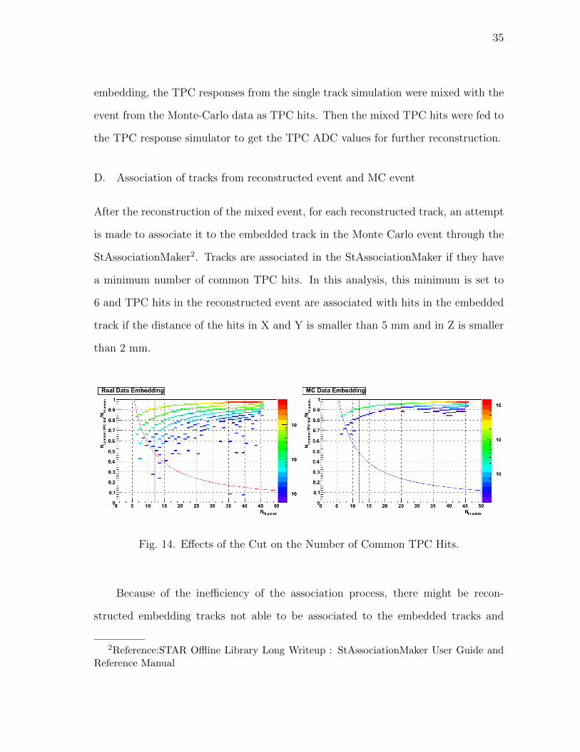
D. Association of tracks from reconstructed event and MC event

After the reconstruction of the mixed event, for each reconstructed track, an attempt

is made to associate it to the embedded track in the Monte Carlo event through the

StAssociationMaker2. Tracks are associated in the StAssociationMaker if they have

a minimum number of common TPC hits. In this analysis, this minimum is set to

6 and TPC hits in the reconstructed event are associated with hits in the embedded

track if the distance of the hits in X and Y is smaller than 5 mm and in Z is smaller

than 2 mm.

Fig. 14. Effects of the Cut on the Number of Common TPC Hits.

Because of the inefficiency of the association process, there might be recon-

structed embedding tracks not able to be associated to the embedded tracks and

2Reference:STAR Offline Library Long Writeup : StAssociationMaker User Guide andReference Manual

36

thus identified as not reconstructed. However, as illustrated in Fig. 14, for both real

data and MC embedding, only a few associated tracks were dropped3. For this reason,

it is assumed that the track association inefficiency is negligible in this analysis.

E. Applying cuts on the associated reconstructed tracks

Before an associated reconstructed track is counted as a successfully reproduced track

from the TPC, several more cuts are applied. These cuts are standard in jet finders[15,

16, 26] and are implemented to eliminate pile-up tracks and split tracks and improve

track quality. However, these cuts are imperfect and also cut off tracks that are

reconstructed from real tracks in jets and reduce the actual TPC tracking efficiency.

A summary of reduced tracking efficiency in real data and MC embedding is shown

in Table III.

Table III. Summary of reduced tracking efficiency due to cuts on reconstructed tracks.

Real Data MC Difference

Embedding Embedding

dcaD cut -3.8% -2.6% 1.2%

number of fit points > 12 -3.0% -1.8% 1.2%

number of fit pointsnumber of possible fit points

> 51% -0.5% -0.2% 0.3%

Total difference in reduction 2.7%

The cuts are applied sequentially, in the order given.

3When combined with the number of fit points > 12 cut in next section

37

1. Distance of closest approach

The Distance of Closest Approach (DCA) cut limits the distance between a track and

the primary vertex of an reconstructed event, and is implemented to remove pile-up

tracks which are irrelevant to the primary vertex. dcaD is the transverse component of

DCA. The standard cut used in Run 6 jet analysis is dependent on track momentum

dcaD <=

2 cm if pT < 0.5 GeV

(3− 2× pT/GeV)(cm) if 0.5 GeV < pT < 1 GeV

1 cm if pT > 1 GeV.

Fig. 15 illustrates the track momentum dependent dcaD cut.

The reduction of the tracking efficiency by this cut in real data embedding is 1.2%

more than that in MC embedding, which indicates that the associated reconstructed

tracks in MC embedding have better track quality.

Fig. 15. dcaD cut vs. track momentum.

38

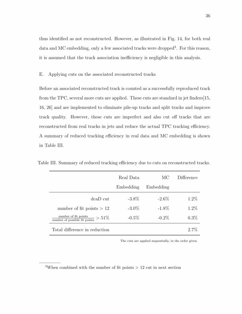
2. Cuts on the number of fit points

These cuts require that a track should at least have 12 fit points and that the number

of fit points divided by the number of “possible fit points”4 should be greater than

fifty one percent. Both of these cuts remove tracks that are likely to be reconstructed

with poor resolution. In addition, these cuts reduce the number of pile-up tracks that

typically are reconstructed using only a subset of the original hits, as well as double

counted split tracks, since the two tracks in a split track pair cannot both own more

than half of the possible fit points.

Fig. 16 illustrates the effects of these two cuts. Comparing to MC embedding,

tracking efficiency reduced about 1.5% more in real data embedding because of these

two cuts, indicating that reconstructed tracks in real data embedding have lower

quality and a larger portion of them are accidentally rejected by the cuts as pile-up

tracks and split tracks.

Fig. 16. Cuts on the Number of Fit Points

4“Possible fit points” are defined as the maximum possible number of TPC read outpads that a track could pass over, which are calculated based on track kinematics and theactive electronics channels.

39

CHAPTER V

ANALYSIS RESULTS AND CONCLUSION

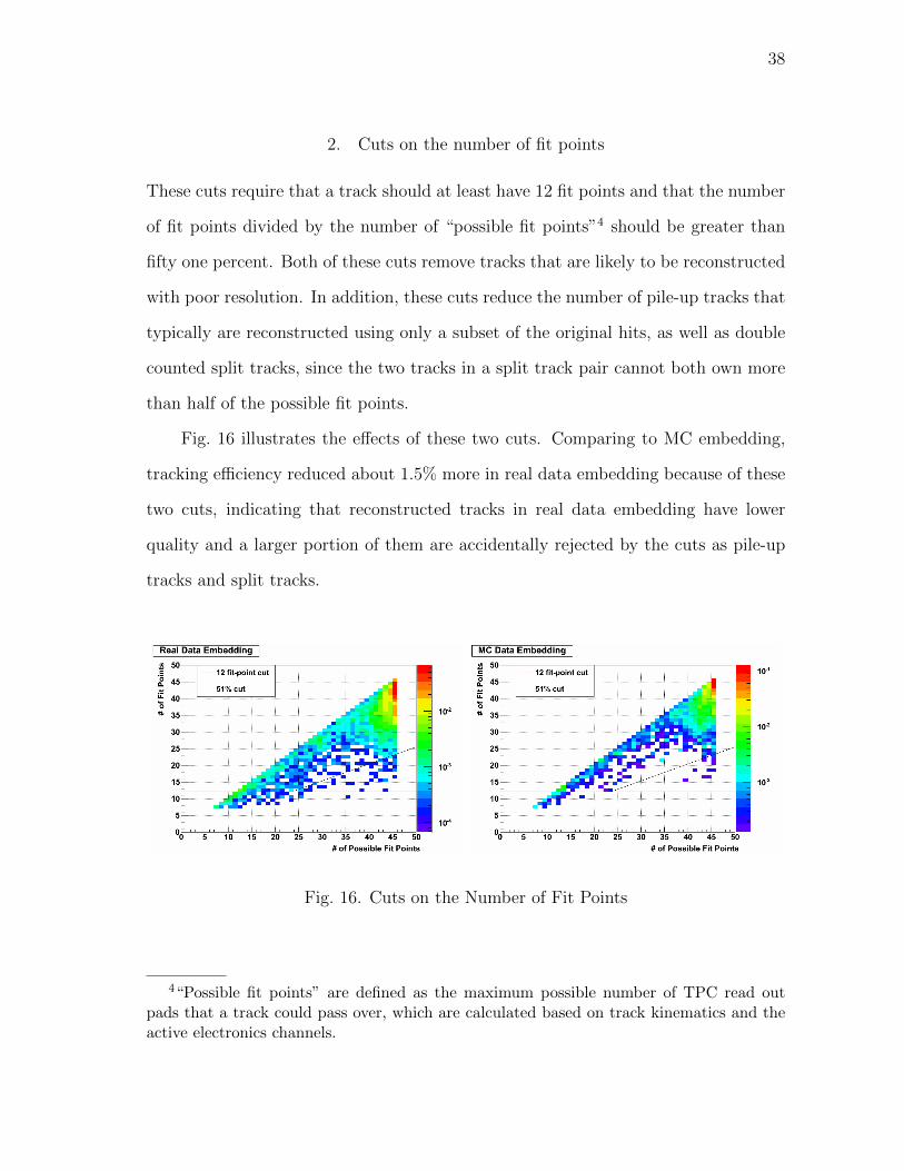
A. Comparison of calculated tpc tracking efficiencies between real data embedding

and MC embedding

This section discusses the calculation results of TPC tracking efficiencies in both real

data embedding and MC embedding, based on the datasets and analysis procedures

discussed in previous chapters, for the STAR 200 GeV proton-proton longitudinal

data during Run 6. In general, tracking efficiencies calculated in real data embedding

are systematically lower than those calculated in MC embedding.

[GeV]true

Tp

0 1 2 3 4 5 6 7 8 9 10

trackin

g e

ffic

ien

cy

0.5

0.55

0.6

0.65

0.7

0.75

0.8

0.85

0.9

0.95

1MC Data Real Data

[GeV]true

Tp

0 0.2 0.4 0.6 0.8 1 1.2 1.4 1.6 1.8 2

trackin

g e

ffic

ien

cy

0.5

0.55

0.6

0.65

0.7

0.75

0.8

0.85

0.9

0.95

1MC Data Real Data

Fig. 17. Tracking efficiencies vs. transverse momentum (pT ) of embedded tracks

Figure 17 shows tracking efficiencies vs. transverse momentum of embedded

tracks. The plot on the left is for tracks with pT between 0.2 GeV and 10 GeV,

while the right one is for low pT tracks between 0.2 GeV and 2 GeV. The result in-

40

dicates that the tracking efficiencies are relatively constant when track pT is greater

than ∼1 GeV, with only fluctuations comparable to statistical errors, in both real data

embedding and MC embedding. Tracking efficiencies start to fall drastically when pT

is lower than 0.5 GeV, as multiple scattering increases, tracks are bent by the mag-

netic field more significantly, and tracks become more unlikely to be reconstructed

properly. Though the calculated efficiency in real data embedding is consistently

lower than the one in MC data embedding, the shape of the efficiency curves matches

well with each other.

trueη

­2 ­1.5 ­1 ­0.5 0 0.5 1 1.5 2

trackin

g e

ffic

ien

cy

0

0.1

0.2

0.3

0.4

0.5

0.6

0.7

0.8

0.9

1 MC Data Real Data

Fig. 18. Tracking efficiencies vs. pseudo-rapidity (η) of embedded tracks

Figure 18 shows the dependencies of tracking efficiencies on the track pseudo-

rapidity. At mid-rapidity, tracking efficiencies are relatively independent on track

pseudo-rapidity, for both efficiencies calculated from real data embedding and MC

embedding. As track pseudo-rapidity reaches ±1, tracks start to leave the TPC vol-

ume through the TPC endcaps, resulting in shorter tracks that can be reconstructed.

As a result, tracking efficiencies start to fall rapidly beyond ±1 in pseudo-rapidity,

and the TPC loses its tracking ability when track pseudo-rapidity is larger than ∼ 1.5.

41

Similar to the tracking efficiency dependence on transverse momentum, tracking effi-

ciency calculated in real data is consistently lower than in MC embedding, although

the shapes match.

trueφ

­3 ­2 ­1 0 1 2 3

trackin

g e

ffic

ien

cy

0.7

0.75

0.8

0.85

0.9

0.95 MC Data Real Data

Fig. 19. Tracking efficiencies vs. azimuthal angle (φ) of embedded tracks

Figure 19 shows the tracking efficiencies vs. azimuthal angle of embedded tracks.

The plot is binned in φ corresponding to TPC sector boundaries, and indicates incon-

sistencies of tracking efficiency across different TPC sectors that cannot be explained

by statistical fluctuation. The solid lines indicate average tracking efficiencies calcu-

lated from dividing the number of total matched reconstructed tracks by the number

of total embedded tracks. The average tracking efficiencies are shown in Table IV.

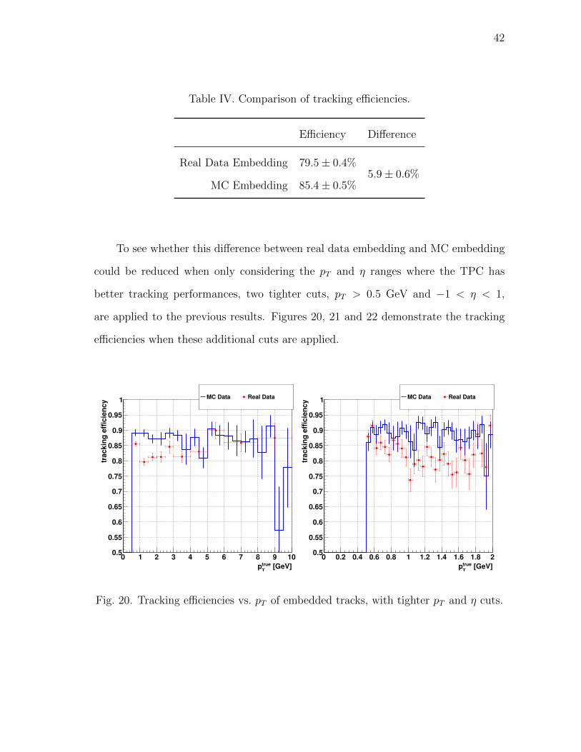
42

Table IV. Comparison of tracking efficiencies.

Efficiency Difference

Real Data Embedding 79.5± 0.4%5.9± 0.6%

MC Embedding 85.4± 0.5%

To see whether this difference between real data embedding and MC embedding

could be reduced when only considering the pT and η ranges where the TPC has

better tracking performances, two tighter cuts, pT > 0.5 GeV and −1 < η < 1,

are applied to the previous results. Figures 20, 21 and 22 demonstrate the tracking

efficiencies when these additional cuts are applied.

[GeV]true

Tp

0 1 2 3 4 5 6 7 8 9 10

trackin

g e

ffic

ien

cy

0.5

0.55

0.6

0.65

0.7

0.75

0.8

0.85

0.9

0.95

1MC Data Real Data

[GeV]true

Tp

0 0.2 0.4 0.6 0.8 1 1.2 1.4 1.6 1.8 2

trackin

g e

ffic

ien

cy

0.5

0.55

0.6

0.65

0.7

0.75

0.8

0.85

0.9

0.95

1MC Data Real Data

Fig. 20. Tracking efficiencies vs. pT of embedded tracks, with tighter pT and η cuts.

43

trueη

­2 ­1.5 ­1 ­0.5 0 0.5 1 1.5 2

trackin

g e

ffic

ien

cy

0

0.1

0.2

0.3

0.4

0.5

0.6

0.7

0.8

0.9

1 MC Data Real Data

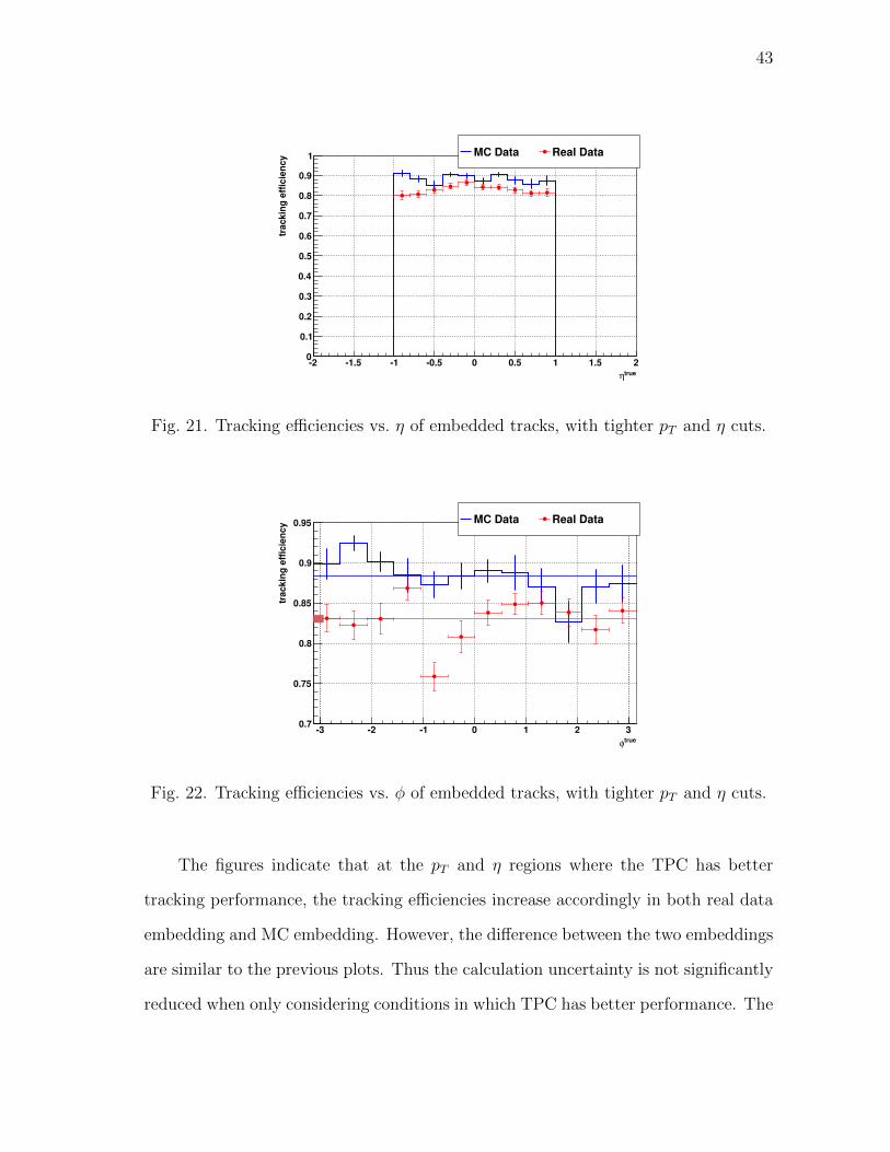
Fig. 21. Tracking efficiencies vs. η of embedded tracks, with tighter pT and η cuts.

trueφ

­3 ­2 ­1 0 1 2 3

trackin

g e

ffic

ien

cy

0.7

0.75

0.8

0.85

0.9

0.95 MC Data Real Data

Fig. 22. Tracking efficiencies vs. φ of embedded tracks, with tighter pT and η cuts.

The figures indicate that at the pT and η regions where the TPC has better

tracking performance, the tracking efficiencies increase accordingly in both real data

embedding and MC embedding. However, the difference between the two embeddings

are similar to the previous plots. Thus the calculation uncertainty is not significantly

reduced when only considering conditions in which TPC has better performance. The

44

average efficiences with the tighter cuts are summarized in Table V.

Table V. Comparison of tracking efficiencies with tighter pT and η cut.

Efficiency Difference

Real Data Embedding 83.0± 0.5%

MC Embedding 88.3± 0.6%

5.3± 0.8%

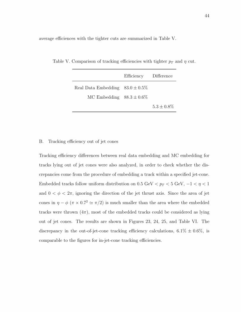
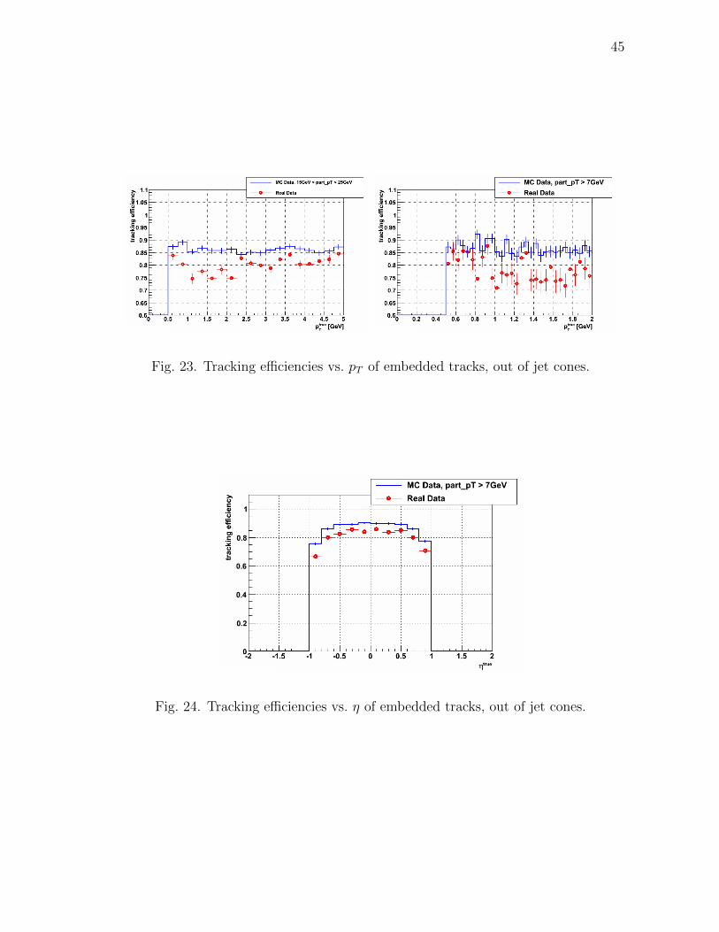
B. Tracking efficiency out of jet cones

Tracking efficiency differences between real data embedding and MC embedding for

tracks lying out of jet cones were also analyzed, in order to check whether the dis-

crepancies come from the procedure of embedding a track within a specified jet-cone.

Embedded tracks follow uniform distribution on 0.5 GeV < pT < 5 GeV, −1 < η < 1

and 0 < φ < 2π, ignoring the direction of the jet thrust axis. Since the area of jet

cones in η − φ (π × 0.72 ' π/2) is much smaller than the area where the embedded

tracks were thrown (4π), most of the embedded tracks could be considered as lying

out of jet cones. The results are shown in Figures 23, 24, 25, and Table VI. The

discrepancy in the out-of-jet-cone tracking efficiency calculations, 6.1% ± 0.6%, is

comparable to the figures for in-jet-cone tracking efficiencies.

45

Fig. 23. Tracking efficiencies vs. pT of embedded tracks, out of jet cones.

Fig. 24. Tracking efficiencies vs. η of embedded tracks, out of jet cones.

46

Fig. 25. Tracking efficiencies vs. φ of embedded tracks, out of jet cones.

Table VI. Comparison of tracking efficiencies out of jet cones.

Efficiency Difference

Real Data Embedding 80.0± 0.4%

MC Embedding 86.1± 0.5%

6.1%± 0.6%

C. TPC gas gain fluctuation and effects for the 6% change of fudge factor

As discussed in Ch. III, Sec. B.2, the effect of the TPC gas gain fluctuation on

tracking efficiency could be estimated by varying the “fudge factor” 6% in the real

data embedding. Figures 26, 27 and 28 demonstrate how the tracking efficiencies will

change when the fudge factor is varied by plus and minus 6% from the value of 1.26.

The changes on the average tracking efficiency listed in Table VII are approximately

47

0.2%, which sit within statistical uncertainties and are well below the other efficiency

differences found in this analysis.

[GeV]true

Tp

0 1 2 3 4 5 6 7 8 9 10

trackin

g e

ffic

ien

cy

0.5

0.55

0.6

0.65

0.7

0.75

0.8

0.85

0.9

0.95

1

MC Data Real Data, 1.336 (+6%)

Fudge Factor = 1.260

1.184 (­6%)

[GeV]true

Tp

0 0.2 0.4 0.6 0.8 1 1.2 1.4 1.6 1.8 2

trackin

g e

ffic

ien

cy

0.5

0.55

0.6

0.65

0.7

0.75

0.8

0.85

0.9

0.95

1

MC Data Real Data, 1.336 (+6%)

Fudge Factor = 1.260

1.184 (­6%)

Fig. 26. Tracking efficiencies vs. transverse pT of embedded tracks, with various fudge

factors.

trueη

­2 ­1.5 ­1 ­0.5 0 0.5 1 1.5 2

trackin

g e

ffic

ien

cy

0

0.1

0.2

0.3

0.4

0.5

0.6

0.7

0.8

0.9

1

MC Data Real Data, 1.336 (+6%) Fudge Factor = 1.260 1.184 (­6%)

Fig. 27. Tracking efficiencies vs. transverse η of embedded tracks, with various fudge

factors.

48

trueφ

­3 ­2 ­1 0 1 2 3

trackin

g e

ffic

ien

cy

0.7

0.75

0.8

0.85

0.9

0.95

MC Data Real Data, 1.336 (+6%)

Fudge Factor = 1.260

1.184 (­6%)

Fig. 28. Tracking efficiencies vs. transverse φ of embedded tracks, with various fudge

factors.

Table VII. Comparison of tracking efficiencies with fudge factor variations.

Fudge Factor Efficiency Difference∗

1.260 79.5± 0.4% —

Real Data Embedding 1.336 (+6%) 79.6± 0.4% 0.1± 0.6%

1.184 (−6%) 79.3± 0.4% −0.2± 0.6%

MC Embedding 85.4± 0.5% 5.9± 0.6%

* Comparing to Real Data Embedding with Fudge Factor = 1.260.

49

D. Conclusion

In the presented analysis, TPC tracking efficiencies within reconstructed jet cones

are calculated in both real data embedding and MC data embedding. Various factors

that could affect the estimation of the tracking efficiency, such as the “fudge factor”

in Monte-Carlo simulation, TPC gas gain fluctuations, and beam luminosity depen-

dence, have been explored in this analysis. Post production cuts that are commonly

used in jet analysis in proton-proton collisions were also taken into consideration.

In conclusion, the estimated tracking efficiency from embedding analysis of the

STAR Run 6 longitudinal data is 79.5%. This figure represents the overall TPC

tracking efficiency of tracks that are within reconstructed jet cones and fall into the

kinematic region of pT > 0.2 GeV and −1.6 < η < 1.6. The estimated systematic

difference between the overall tracking efficiency obtained in real data embedding and

MC data embedding is 5.9± 0.6%(statistical). The presented analysis indicates that

the difference is relatively independent on track kinematics, and is large enough to

make the uncertainty introduced by the variation of TPC gas gain negligible. The

5.9% difference is consistent with the previously quoted ∼ 5% systematic uncertainty

used in standard STAR analysis [12]; however, it has been found in this analysis

that this uncertainty could not be significantly reduced in the specific senario of jet

analysis in polarized proton-proton collisions based on the existing Monte-Carlo event

samples.

Though the origin of the discrepancy between real data embedding and MC data

embedding could not be completely explained, the presented analysis suggests that a

large portion of the difference is related to the high luminosity environment and the

pile-up tracks. In MC data embedding, because the pile-up tracks were not taken into

consideration and the resulted deterioration in track reconstruction was not reflected,

50

reconstructed embedded tracks have much better quality than those in real data

embedding. Consequently, reconstructed embedded tracks in MC data embedding

have a larger possibility to pass the cuts, which were commonly implemented in STAR

jet analysis to ensure track reconstruction quality and eliminate pile-up tracks, than

in real data embedding, as demonstrated in Figures 15 and 16. Table III indicates

that these cuts introduced ∼ 2.7% diference on tracking efficiency, which contributes

∼ 1/2 to the calculated total systematic difference.

This portion of the difference could be addressed by introducing pile-up tracks to

the MC embedding. Future analyses on simulated jets embedded into real zero-bias

data should show little difference on the behaviors of the cuts in Table III between

real data embedding and MC embedding combined with real zero-bias data. The

remaining unexplained difference, by adding up the 3.2% difference1 and 0.6% statis-

tical uncertainty in quadrature, is up to 3.3%. Since the cause of this difference could

not be identified, we adopt ±3.3% as the uncertainty on the tracking efficiency when

embedding into real data under Run 6 conditions.

To further improve the accuracy on the estimation of the TPC tracking efficiency,

more studies on the simulation tools used in this analysis are required in order to get

a better understanding on how the high multiplicity environment from real data affect

the embedded simulation track differently from the environment of pure simulation

data, or from the environment of simulation data embedded into real zero-bias events.

Also, much higher event statistics than were available from Run 6 will be required to

permit a detailed investigation of the dependence of the data–Monte-Carlo difference

on track kinematics.

1Which comes from the total difference of 5.9%, minus the 2.7% from the cuts in Table III.

51

REFERENCES

[1] J. Blumlein and H. Bottcher, Nucl. Phys. B, 841, 205 (2010).

[2] E. Leader, A. V. Sidorov, and D. B. Stamenov, Phys. Rev. D, 82, 114018 (2010).

[3] D. de Florian, R. Sassot, M. Stratmann, and W. Vogelsang, Phys. Rev. Lett.,

101, 072001 (2008).

[4] D. de Florian, R. Sassot, M. Stratmann, and W. Vogelsang, Phys. Rev. D, 80,

034030 (2009).

[5] G. Bunce, N. Saito, J. Soffer, and W. Vogelsang, Ann. Rev. Nucl. Part. Sci., 50,

525 (2000).

[6] B. Jager, M. Stratmann, and W. Vogelsang, Phys. Rev. D, 70, 034010 (2004).

[7] K. Ackermanna, N. Adamsb, C. Adlerc, Z. Ahammedd, S. Ahmadb, et al. (STAR

Collaboration), Nucl. Instr. and Meth. A, 499, 624 (2003).

[8] M. Bai, T. Roser, L. Ahrens, I. G. Alekseev, J. Alessi, et al., Phys. Rev. Lett.,

96, 174801 (2006).

[9] M. Harrison, T. Ludlam, and S. Ozaki, Nucl. Instr. and Meth. A, 499, 235

(2003).

[10] M. Bai, P. Cameron, P. Cerniglia, R. Connolly, J. Cupolo, et al., Nucl. Instr.

and Meth. A, 499, 372 (2003).

[11] I. Alekseev, C. Allgower, M. Bai, Y. Batygin, L. Bozano, et al., Nucl. Instr. and

Meth. A, 499, 392 (2003).

52

[12] M. Anderson, J. Berkovitz, W. Betts, R. Bossingham, F. Bieser, et al., Nucl.

Instr. and Meth. A, 499, 659 (2003).

[13] W. G. Gong, STAR Note, 197 (1995),

http://drupal.star.bnl.gov/STAR/starnotes?page=13&sort=number&order=

asc, STAR experiment webpage, Date Accessed April 18, 2012.

[14] M. Beddo, E. Bielick, T. Fornek, V. Guarino, D. Hill, et al., Nucl. Instr. and

Meth. A, 499, 725 (2003).

[15] B. I. Abelev, M. M. Aggarwal, Z. Ahammed, J. Amonett, B. D. Anderson, et al.

(STAR Collaboration), Phys. Rev. Lett., 97, 252001 (2006).

[16] B. I. Abelev, M. M. Aggarwal, Z. Ahammed, B. D. Anderson, D. Arkhipkin,

et al. (STAR Collaboration), Phys. Rev. Lett., 100, 232003 (2008).

[17] G. C. Blazey, J. R. Dittmann, S. D. Ellis, V. D. Elvira, K. Frame, et al., Pro-

ceedings of the Run II QCD and Weak Boson Physics Workshop (2000).

[18] T. Henry, Reconstruction and attributes of jets observed in√s = 200 GeV proton-

proton and deuteron-gold collisions at STAR, PhD dissertation, Texas A&M Uni-

versity (2006).

[19] “Monte-Carlo production datasets,”

http://drupal.star.bnl.gov/STAR/comp/prod/monte-carlo-production-datasets,

STAR experiment webpage, Date Accessed April 18, 2012.

[20] T. Sjostrand, S. Mrenna, and P. Skands, Journal of High Energy Physics, 605,

26 (2006).

53

[21] P. Jacobs and D. Irmscher, STAR Note, 235 (1996),

http://drupal.star.bnl.gov/STAR/starnotes?page=15&sort=number&order=

asc, STAR experiment webpage, Date Accessed April 18, 2012.

[22] R. Brun, F. Bruyant, M. Maire, A. McPherson, and P. Zanarini, CERN Data

Handling Division, DD/EE/84-1 (1987),

http://cdsweb.cern.ch/record/1119728/files/CERN-DD-EE-84-1.pdf, CERN

Document Server, Date Accessed April 18, 2012.

[23] J. T. Michell and I. M. Sakrejda, STAR Note, 190 (1994),

http://drupal.star.bnl.gov/STAR/starnotes?page=12&sort=number&order=

asc, STAR experiment webpage, Date Accessed April 18, 2012.

[24] M. Sarsour, Pile-up tracks or towers,

http://cyclotron.tamu.edu/star/2006Jets/sep9_2007/, Notes on 2006 jet anal-

ysis, Date Accessed April 18, 2012.

[25] Y. Fisyak,

http://www4.rcf.bnl.gov/~fisyak/star/PiD/RunVI/TpcGainVariationRunVI.png ,

Analysis Note, Date Accessed April 18, 2012.

[26] M. Sarsour (STAR Collaboration), AIP Conference Proceedings, 1149, 389

(2009).

[27] B. List, www.desy.de/~blist/notes/effic.ps.gz, Analysis Note, Date Accessed

April 18, 2012.

54

VITA

Name: Liaoyuan Huo

Address: Department of Physics and Astronomy

Texas A&M University

4242 TAMU

College Station, TX 77843-4242

Email Address: lylehuo@neo.tamu.edu

Education: B.S. Physics

University of Science and Technology of China

2007