process optimization and integration strategies for - OAKTrust
139
PROCESS OPTIMIZATION AND INTEGRATION STRATEGIES FOR MATERIAL RECLAMATION AND RECOVERY A Dissertation by HOUSSEIN A. KHEIREDDINE Submitted to the Office of Graduate Studies of Texas A&M University in partial fulfillment of the requirements for the degree of DOCTOR OF PHILOSOPHY May 2012 Major Subject: Chemical Engineering
-
Upload
khangminh22 -
Category
Documents
-
view
0 -
download
0
Transcript of process optimization and integration strategies for - OAKTrust
PROCESS OPTIMIZATION AND INTEGRATION STRATEGIES FOR
MATERIAL RECLAMATION AND RECOVERY
A Dissertation
by
HOUSSEIN A. KHEIREDDINE
Submitted to the Office of Graduate Studies of Texas A&M University
in partial fulfillment of the requirements for the degree of
DOCTOR OF PHILOSOPHY
May 2012
Major Subject: Chemical Engineering
PROCESS OPTIMIZATION AND INTEGRATION STRATEGIES FOR
MATERIAL RECLAMATION AND RECOVERY
A Dissertation
by
HOUSSEIN A. KHEIREDDINE
Submitted to the Office of Graduate Studies of Texas A&M University
in partial fulfillment of the requirements for the degree of
DOCTOR OF PHILOSOPHY
Approved by:
Co-Chairs of Committee, Mahmoud El-Halwagi Nimir Elbashir Committee Members, M. Sam Mannan Hisham Nasreldin Head of Department, Charles Glover
May 2012
Major Subject: Chemical Engineering
iii
ABSTRACT
Process Optimization and Integration Strategies for
Material Reclamation and Recovery. (May 2012)
Houssein A. Kheireddine, B.A., Texas A&M University-Kingsville
Co-Chairs of Advisory Committee: Dr. Mahmoud El-Halwagi Dr. Nimir Elbashir
Industrial facilities are characterized by the significant usage of natural resources
and the massive discharge of waste materials. An effective strategy towards the
sustainability of industrial processes is the conservation of natural resources through
waste reclamation and recycles. Because of the numerous number of design alternatives,
systematic procedures must be developed for the effective synthesis and screening of
reclamation and recycle options. The objective of this work is to develop systematic and
generally applicable procedures for the synthesis, design, and optimization of resource
conservation networks. Focus is given to two important applications: material utilities
(with water as an example) and spent products (with lube oil as an example).
Traditionally, most of the previous research efforts in the area of designing direct-
recycle water networks have considered the chemical composition as the basis for
process constraints. However, there are many design problems that are not component-
based; instead, they are property-based (e.g., pH, density, viscosity, chemical oxygen
demand (COD), basic oxygen demand (BOD), toxicity). Additionally, thermal
iv
constraints (e.g., stream temperature) may be required to identify acceptable recycles. In
this work, a novel approach is introduced to design material-utility (e.g., water) recycle
networks that allows the simultaneous consideration of mass, thermal, and property
constraints. Furthermore, the devised approach accounts for the heat of mixing and for
the interdependence of properties. An optimization formulation is developed to embed
all potential configurations of interest and to model the mass, thermal, and property
characteristics of the targeted streams and units. Solution strategies are developed to
identify stream allocation and targets for minimum fresh usage and waste discharge. A
case study on water management is solved to illustrate the concept of the proposed
approach and its computational aspects.
Next, a systematic approach is developed for the selection of solvents, solvent
blends, and system design in in extraction-based reclamation processes of spent lube oil
Property-integration tools are employed for the systematic screening of solvents and
solvent blends. The proposed approach identifies the main physical properties that
influence solvent(s) performance in extracting additives and contaminants from used
lubricating oils (i.e. solubility parameter (), viscosity (), and vapor pressure (p)). The
results of the theoretical approach are validated through comparison with experimental
data for single solvents and for solvent blends. Next, an optimization formulation is
developed and solved to identify system design and extraction solvent(s) by including
techno-economic criteria. Two case studies are solved for identification of feasible
blends and for the cost optimization of the system.
v
ACKNOWLEDGEMENTS
First of all, I would like to express my deepest thanks, regards, and appreciation
to my advisor Dr El-Halwagi. I had the honor to work under his supervision. He
supported me with any decision that helped me to become a better engineer. I want to
thank him for his countless advice toward my academic research. I very much appreciate
his effort in providing me with the ultimate working environment. Also, I want to thank
him for his assistance to work in teams and collaborate with other research groups
around the world. He has provided me with various opportunities and consistently
exposed me to different research areas in order to broaden my thinking. Through his
guidance and support, I was able to present my work and research in top national
conferences. I owe him a great deal of appreciation, and I wish him all the best.
I would also want to take the opportunity to thank my co-chair, Dr Elbashir.I
want to thank him for his valuable input and feedback toward my research. He
consistently provided me with different insights and prospective. I want to thank him for
sharing his solid experience in the re-refining of used lubricating oil. Also, I appreciate
his efforts in making himself available for discussion regardless of the distance and time
zone difference.
In addition, I would like to give special thanks to Dr. Mannan, and Dr. Nasreldin
for their precious time in reviewing my thesis and their valuable advice to produce
quality work.
vi
Particularly, I want to thank Dr Jose Maria Ponce-Ortega, Dr Denny Ng, and
Douglas Tay for their fruitful collaboration. It has been a great successful experience.
Through their help and support, I was able to make my research life more meaningful.
I would like to extend my gratitude to both the former and present members of
process optimization and integration group, Mohamed Noureldin, Kerron Gabriel, Rene’
Elms, Chun Deng, Grace Pokoo-Aikins, Bowling Ian, Buping Bao, Eman Tora, Viet
Pham, Abdullah Bin Mahfouz, Ming-Hao Chiou, Eric Pennaz for their help and
collaboration. They have truly enriched my research.
Finally, I am deeply indebted to my family. They have supported and inspired me
unconditionally throughout my entire academic career. They have been magnificent role
models. Through their love and boundless support, I was able to strive all the way
toward achieving my goals and dreams.
vii
TABLE OF CONTENTS
Page
ABSTRACT ..................................................................................................................... iii
ACKNOWLEDGEMENTS ............................................................................................... v
TABLE OF CONTENTS ................................................................................................ vii
LIST OF FIGURES ...........................................................................................................ix
LIST OF TABLES ............................................................................................................xi 1 INTRODUCTION TO PROCESS OPTIMIZATION AND INTEGRATION .......... 1
1.1 Preface and Motivation ...................................................................................... 1 1.2 Key Strategies .................................................................................................... 2 1.3 Process Integration Introduction ........................................................................ 3
1.3.1 Mass Integration .................................................................................... 3 1.3.2 Property Integration ............................................................................... 8
1.4 Optimization .................................................................................................... 12 1.5 Dissertation Goals ........................................................................................... 14
2 OBJECTIVES OF WORK ........................................................................................ 16
2.1 Objectives Overview ....................................................................................... 16 2.2 Water Conservation and Direct Recycle Network .......................................... 17 2.3 Lube Oil Reclamation and Property Integration ............................................. 18
2.3.1 Solvent Selection Systematic Approach .............................................. 18 2.3.2 Optimization formulation for Solvent Extraction in the Lube
Oil Application .................................................................................... 19
3 OPTIMIZATION OF DIRECT RECYCLE NETWORKS WITH THE SIMULTANEOUS CONSIDERATION OF PROPERTY, MASS, AND THERMAL EFFECT ................................................................................................ 20
3.1 Introduction ..................................................................................................... 20 3.2 Problem Statement ........................................................................................... 21 3.3 Approach and Mathematical Formulation ....................................................... 22
3.4 Case Study ....................................................................................................... 28 3.4.1 Data Extraction (Scenario 1) ............................................................... 30
viii
3.4.2 Data Extraction (Scenario2) ................................................................ 32 3.5 Solution and Results ........................................................................................ 34 3.6 Conclusions ..................................................................................................... 40 3.7 Nomenclatures ................................................................................................. 40
4 A PROPERTY-INTEGRATION APPROACH TO SOLVENT SCREENING AND CONCEPTUAL DESIGN OF SOLVENT-EXTRACTION SYSTEMS FOR RECYCLING USED LUBRICATING OIL .................................................... 45
4.1 Introduction and Literature Review ................................................................. 45 4.2 Problem Statement ........................................................................................... 52
4.2.1 Selection of Principal Properties and Construction of Property Clusters ................................................................................................ 52
4.2.2 Design Approach ................................................................................. 60 4.3 Case Study ....................................................................................................... 62 4.4 Conclusions ..................................................................................................... 70
5 A SYSTEMATIC TECHNO-ECONOMICAL ANALYSIS FOR THE SUPERCRITICAL SOLVENT FISCHER TROPSCH SYNTHESIS ...................... 72
5.1 Introduction ..................................................................................................... 72 5.2 Solvent Extraction Process Description and Problem Statement .................... 74 5.3 Problem Statement ........................................................................................... 76
5.3.1 Mass Balance ....................................................................................... 79 5.3.2 Component Material Balance .............................................................. 80
5.3.3 Heat Balance ........................................................................................ 81 5.3.4 Equilibrium Equations ......................................................................... 82
5.4 Optimization Formulation ............................................................................... 83 5.5 Case Study and Results. .................................................................................. 85
5.5.1 Data Collection .................................................................................... 85 5.5.2 Results and Discussions ...................................................................... 89
5.6 Conclusions ..................................................................................................... 95
6 CONCLUSIONS AND RECOMMENDATION FOR FUTURE WORK ............... 96
REFERENCES .................................................................................................................98
APPENDIX A ................................................................................................................ 105
VITA .............................................................................................................................. 128
ix
LIST OF FIGURES
Page
Figure 1.2: Sink and source composite diagram for material recycle pinch analysis (El-Halwagi, 2006) .............................................................................................. 6
Figure 1.3: Ternary diagram representation of Intra-Stream of clusters (Shelly and El-Halwagi, 2000) .......................................................................... 11
Figure 1.4: Lever arm addition for clusters (Shelly and El-Halwagi, 2000) .................... 12
Figure 3.1: Source/sink allocation with direct reuse/recycle ........................................... 23
Figure 3.2: Process flowsheet of the production of phenol from cumene ........................ 29
Figure 3.3: Optimal property-based water network with/without heat of mixing (scenario 1)......................................................................................................... 35
Figure 3.4: Optimal property-based water network with/without heat of mixing
(scenario 2)......................................................................................................... 36
Figure 3.5 The retrofitted process flow sheet based on the optimized results ................. 37
Figure 4.1: A simplified solvent extraction process. ........................................................ 49
Figure 4.2: The ternary diagram for vapor pressure, solubility parameter, and viscosity ............................................................................................................. 59
Figure 4.3: Ternary diagram that represents the three properties and identifies the feasible region for appropriate solvent extraction system ................................. 60
Figure 4.4: Schematic Diagram for our Solvent Design Approach ................................. 61
Figure 4.5: The ternary-cluster representation of the feasibility region for the three properties for solvents and blends to be employed in re-refining of used lubricating oil. .................................................................................................... 65
Figure 4.6: Single-solvent representation in the ternary diagram and their positions relative to the feasible region. ............................................................................ 67
Figure 4.7: Representation of methanol/hexane mixture on the ternary diagram. ........... 68
x
Figure 4.8: Propanol-hexane mixture representation of Case Study 3 on the ternary diagram .............................................................................................................. 70
Figure 5.1: Common Used oil disposal methods (Project Rose 1990) ............................ 72
Figure 5.2: Simplified block flow diagram for the solvent extraction process of recycling used lubricating oil. ............................................................................ 75
Figure 5.3: Process Flow Diagram for the solvent extraction process of recycling used lubricating oil. ............................................................................................ 77
Figure 5.4: Effect of solvent to oil ratio (SOR) and Temperature (T) on percent oil loss and percent sludge removal (POL/PSR) using 1- Butanol as a solvent (Katiyar 2010). ................................................................................................... 86
Figure 5.5: Effect of solvent to oil ratio (SOR) and Temperature (T) on percent oil loss and percent sludge removal (POL/PSR) using MEK as a solvent (Katiyar, 2010). .................................................................................................. 87
Figure 5.6: Butanol Fitted K value versus atmospheric column temperature ................ 125
Figure 5.7: Butanol Fitted K value versus vacuum column temperature ....................... 126
Figure 5.8: MEK Fitted K value versus atmospheric column temperature .................... 126
Figure 5.9: MEK Fitted K value versus vacuum column temperature ........................... 127
xi
LIST OF TABLES
Page
Table 3.1 Sources and fresh water (scenario 1)................................................................ 31
Table 3.2 Sink data and constraints (scenario 1) .............................................................. 32
Table 3.3 Sources and fresh water (scenario 2)................................................................ 33
Table 3.4 Sink data and constraints (scenario 2) .............................................................. 34
Table 3.5 Piping costs for the case study (32) .................................................................. 38
Table 3.6 Comparison for the optimal results with/without property constraints ............ 39 Table 4.1: List of Common additives used in lubricating oils (Kopeliovich, 2011) ....... 46
Table 4.2: Solubility parameters of base oil, additives and number of alcohol solvents .............................................................................................................. 62
Table 4.3: Experimentally reported performance of number of solvent(s) used in re-refining used oils. .......................................................................................... 66
Table 5.1: Solvents and oil costs ...................................................................................... 89
Table 5.2: SOR values at 5% and 10% solvent losses. .................................................... 90
Table 5.3: Solvent selection and extraction operating conditions at different total % sludge removed taking into account 5% of solvent is lost at each stage. ... 91
Table 5.4: Solvent selection and extraction operating conditions at different total % sludge removed taking into account 10% of solvent is lost at each stage ..... 91
Table 5.5: Result summary of the effect of base oil quality taking into account 5 % solvent loss in each stage. ........................................................................... 93
Table 5.6: Result summary of the effect of base oil quality taking into account 10% solvent loss in each stage. .......................................................................... 93
1
1 INTRODUCTION TO PROCESS OPTIMIZATION AND INTEGRATION
1.1 Preface and Motivation
Mass, heat, and property integration have been used commonly in the industry in
order to achieve core objectives of any process. Process integration has been used
mainly for resource conservation, emission reduction, and sustainability performance
improvement. These objectives have been targeted for decades now. However, they are
more important than ever before due to:
- The escalation of raw material prices: Natural Gas, crude oil, and utilities such
as fresh water and hydrogen prices keep increasing year after year. Energy is no
longer cheap. Regardless of the political influence on these prices, optimization
and integration of existing processes and invention of newer ones can help
reduce and conserve these resources.
- Depletion of natural resources: processing facilities use tremendous amount of
fresh materials. Such usage can lead to depletion of natural resources if not
recycled and managed properly.
____________
This dissertation follows the style of Education for Chemical Engineers Journal.
2
- The irresponsible usage of utilities: This applies especially to fresh water. It is a
major factor in the lack of fresh water in major parts of the world. Dumping
waste water stream irresponsibly back to the sea or into water ways has caused
major environmental issues.
- Increasing environmental regulations: Environmental Protection Agency has
been a major policy maker toward reduction of emissions and increase safety
applications. Advances in technology and science allowed scientist better
understand the effect of pollution on the environment and the human being. A lot
of work could be done in that matter in order to help create safer world.
1.2 Key Strategies
1. Recycle and reuse: Not only from economic stand point, but recycling waste
streams can have a major contribution to the conservation of these precious
resources.
2. Process Modification/alteration: Addition of extra units to the process that helps
purify toxic emissions is one way to help improve environmental performance
and conserve natural resources. Another way is to change the process as a whole
and reduce total utility usage while reaching the same output product.
3. Material substitution: Substitute toxic and unrecyclable resources by safer and
recyclable alternatives.
3
1.3 Process Integration Introduction
Process integration is a holistic approach to process design, retrofitting, and
operation whichemphasizes the unity of the process (El-Halwagi, 1997). It involves five
main activities (El-Halwagi, 2006):
1. Task Identification: It is the expression of the goal that we are aiming for, and its
description in actionable task.
2. Targeting: It is a very powerful tool that allows us to benchmark process
performance without specifying the means of achieving these targets.
3. Generation of Alternatives: It is the generation of enormous number of possible
solutions and configurations in order to achieve the goal/target.
4. Selection of Alternative(s): It is necessary to choose a feasible alternative.
However, it is more important to choose an optimum one.
5. Analysis of Selected Alternative(s): It is important to evaluate the selected
alternative. This evaluation may include economic analysis, safety analysis and
assessment, etc.
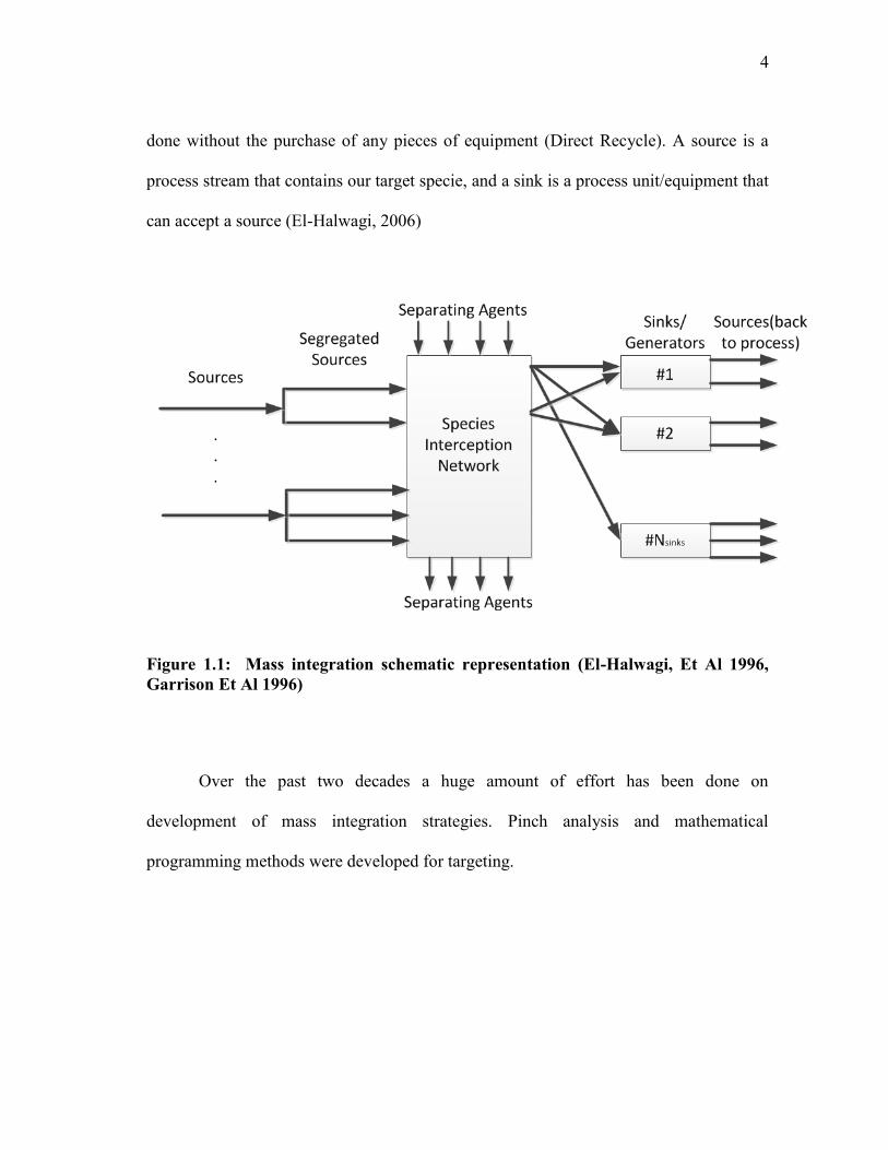
1.3.1 Mass Integration
Mass Integration is a holistic approach to the generation, separation, and routing of
species and streams throughout the process (El-Halwagi, 1997). It requires full
understanding of the mass flow within the process (Figure 1.1). This mass integration
could be done with the use of mass interceptors for purification purposes or it could be
4
done without the purchase of any pieces of equipment (Direct Recycle). A source is a
process stream that contains our target specie, and a sink is a process unit/equipment that
can accept a source (El-Halwagi, 2006)
Figure 1.1: Mass integration schematic representation (El-Halwagi, Et Al 1996, Garrison Et Al 1996)
Over the past two decades a huge amount of effort has been done on
development of mass integration strategies. Pinch analysis and mathematical
programming methods were developed for targeting.
5
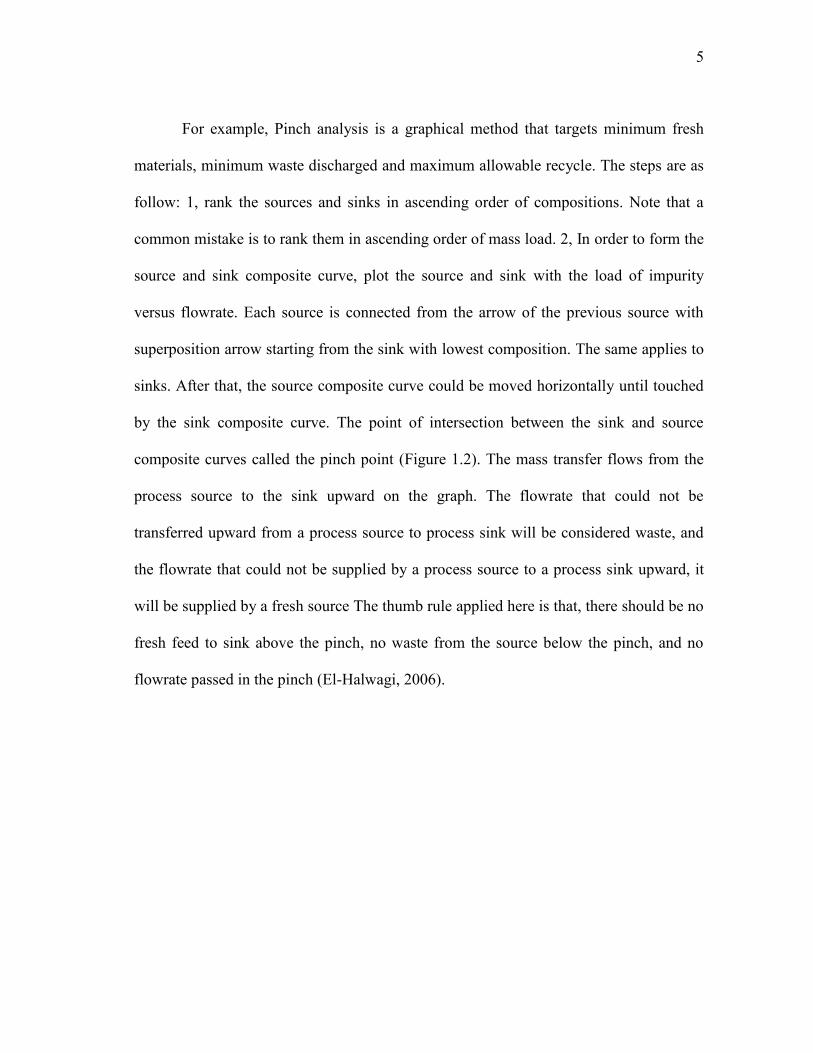
For example, Pinch analysis is a graphical method that targets minimum fresh
materials, minimum waste discharged and maximum allowable recycle. The steps are as
follow: 1, rank the sources and sinks in ascending order of compositions. Note that a
common mistake is to rank them in ascending order of mass load. 2, In order to form the
source and sink composite curve, plot the source and sink with the load of impurity
versus flowrate. Each source is connected from the arrow of the previous source with
superposition arrow starting from the sink with lowest composition. The same applies to
sinks. After that, the source composite curve could be moved horizontally until touched
by the sink composite curve. The point of intersection between the sink and source
composite curves called the pinch point (Figure 1.2). The mass transfer flows from the
process source to the sink upward on the graph. The flowrate that could not be
transferred upward from a process source to process sink will be considered waste, and
the flowrate that could not be supplied by a process source to a process sink upward, it
will be supplied by a fresh source The thumb rule applied here is that, there should be no
fresh feed to sink above the pinch, no waste from the source below the pinch, and no
flowrate passed in the pinch (El-Halwagi, 2006).
6
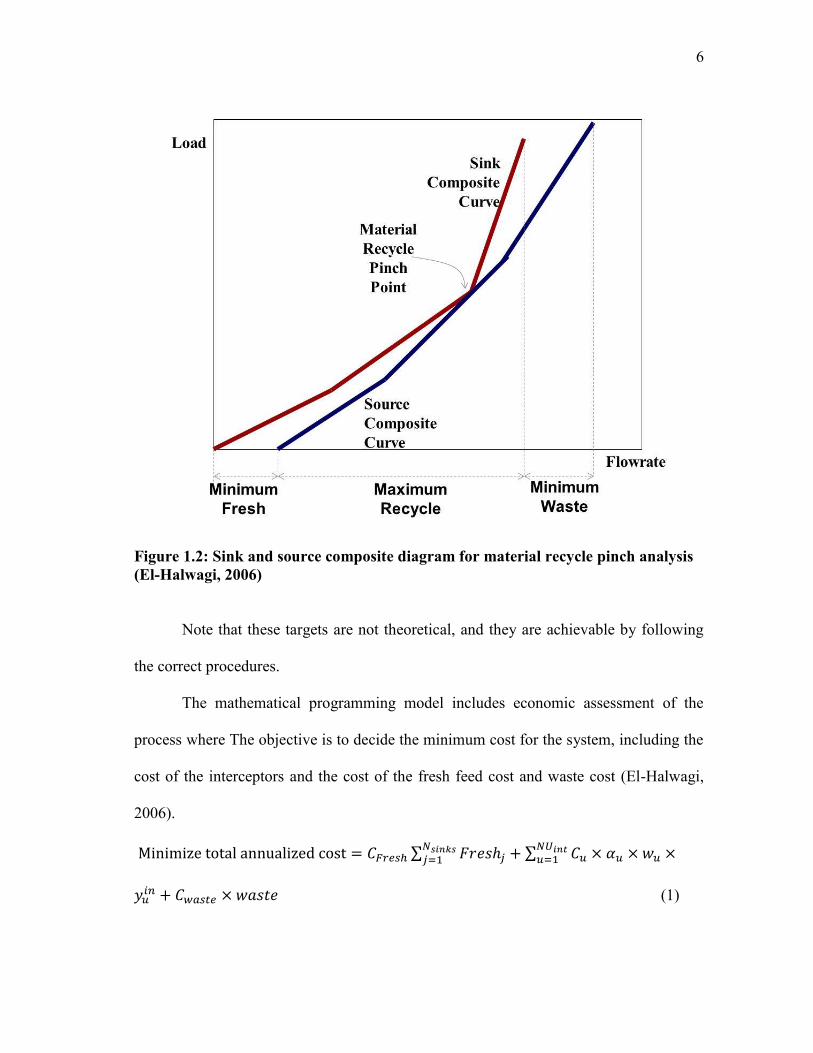
Figure 1.2: Sink and source composite diagram for material recycle pinch analysis (El-Halwagi, 2006)
Note that these targets are not theoretical, and they are achievable by following
the correct procedures.
The mathematical programming model includes economic assessment of the
process where The objective is to decide the minimum cost for the system, including the
cost of the interceptors and the cost of the fresh feed cost and waste cost (El-Halwagi,
2006).
∑ ∑
(1)
7
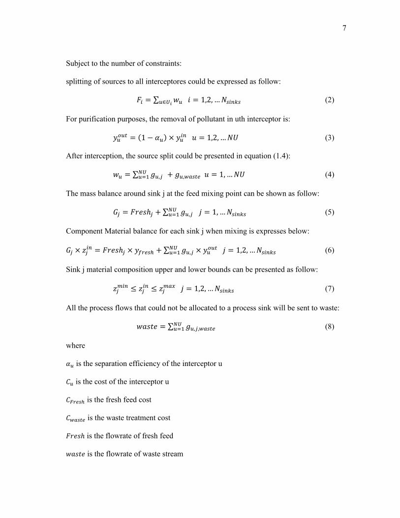
Subject to the number of constraints:
splitting of sources to all interceptores could be expressed as follow:
∑ (2)
For purification purposes, the removal of pollutant in uth interceptor is:
( )
(3)
After interception, the source split could be presented in equation (1.4):
∑ (4)
The mass balance around sink j at the feed mixing point can be shown as follow:
∑ (5)
Component Material balance for each sink j when mixing is expresses below:
∑
(6)
Sink j material composition upper and lower bounds can be presented as follow:
(7)
All the process flows that could not be allocated to a process sink will be sent to waste:
∑ (8)
where
is the separation efficiency of the interceptor u
is the cost of the interceptor u
is the fresh feed cost
is the waste treatment cost
is the flowrate of fresh feed
is the flowrate of waste stream
8
is the composition from each source to unit u
is the flowrate to each unit u
is the flowrate coming out of each unit u to different sink j
is the flowrate into each sink j
is the flowrate of each source i
is the composition of streams into each sink j
1.3.2 Property Integration
Mass integration is very powerful targeting tools. It was to batch and continuous
water networks. However, a major feature of mass integration is that it is chemo-centric.
This means that the chemical composition of a stream is the only parameter being
tracked. Because of the heavy dependence of the system design on properties, a more
important approach for optimal design is the framework of property integration which is
defined by El-Halwagi et al. (2004) as “a functionality-based holistic approach for the
allocation and manipulation of streams and processing units, which is based on
functionality tracking, adjustment and assignment throughout the process.” Several
graphical and algebraic techniques have been developed for designing and optimizing
recycle/reuse systems based on property integration (e.g., Shelley and El-Halwagi,2000;
El-Halwagi et al.,2004; Qin et al.,2004; and Ng et al.,2009).
This dependency of the system design on properties poses major property
constraints. The identification of the upper and lower property bounds values are not as
9
simple as they sound. They could be extracted from experimental results or via
simulation runs. This could be presented as following:
maxmin
iii ppp (9)
One of the major challenges of property integration is the identification of the
mixing rule expression. Different properties can have different mixing rules. Some may
be linear, and others can be non-linear. A generic mixing rule expression is shown below
(El-Halwagi, 2004):
i
iri pFPF )()( (10)
with,
P is the property of the mixture
)( iP is the property mixing operator of property r
F is the flowrate of mixture and can be expressed as follow:
i
iFF
(11)
Note that the multiplication of the flowrate by the property operator is considered
the property load. Thus, composition can be considered as a special case of property, and
the same mass integration pinch analysis that was applied to mass can be applied to any
property. This is very important when it comes to the allocation of process sources and
sinks taking into account composition and property constraints.
10
In order to normalize the property operator into a dimensionless operator , its
division by a reference value .ref
i is needed:
ref
r
irr
ir
p
)( ,
,
(12)
Then, an AUgmented Property (AUP) index for each stream i is the summation
of the dimensionless operators:
1
,
r
iriAUP
(13)
Then, the cluster for property r in stream i can be defined as follow:
i
ir
irAUP
C,
,
(14)
Now, through clustering, every stream can be presented in a ternary diagram by a
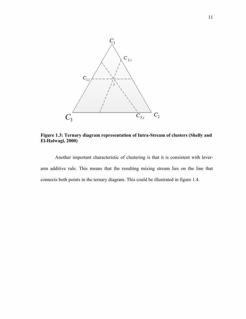
single point. This could be illustrated in figure 1.3. A very important characteristic of
clustering is that the summation of clusters is equal to 1.
11
Figure 1.3: Ternary diagram representation of Intra-Stream of clusters (Shelly and El-Halwagi, 2000)
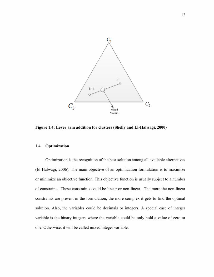
Another important characteristic of clustering is that it is consistent with lever-
arm additive rule. This means that the resulting mixing stream lies on the line that
connects both points in the ternary diagram. This could be illustrated in figure 1.4.
12
Figure 1.4: Lever arm addition for clusters (Shelly and El-Halwagi, 2000)
1.4 Optimization
Optimization is the recognition of the best solution among all available alternatives
(El-Halwagi, 2006). The main objective of an optimization formulation is to maximize
or minimize an objective function. This objective function is usually subject to a number
of constraints. These constraints could be linear or non-linear. The more the non-linear
constraints are present in the formulation, the more complex it gets to find the optimal
solution. Also, the variables could be decimals or integers. A special case of integer
variable is the binary integers where the variable could be only hold a value of zero or
one. Otherwise, it will be called mixed integer variable.
13
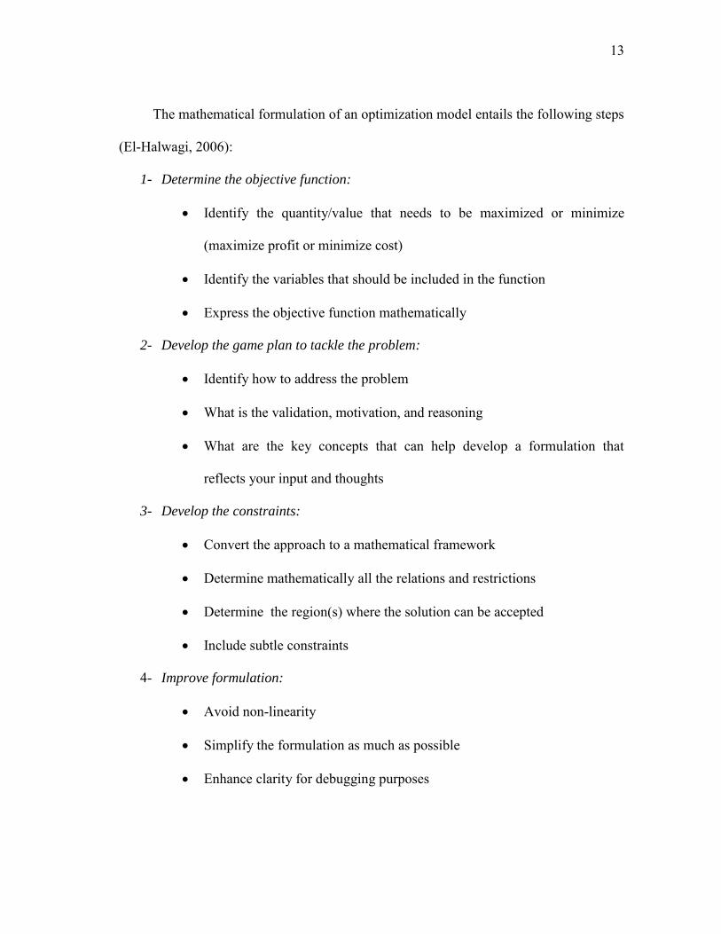
The mathematical formulation of an optimization model entails the following steps
(El-Halwagi, 2006):
1- Determine the objective function:
Identify the quantity/value that needs to be maximized or minimize
(maximize profit or minimize cost)
Identify the variables that should be included in the function
Express the objective function mathematically
2- Develop the game plan to tackle the problem:
Identify how to address the problem
What is the validation, motivation, and reasoning
What are the key concepts that can help develop a formulation that
reflects your input and thoughts
3- Develop the constraints:
Convert the approach to a mathematical framework
Determine mathematically all the relations and restrictions
Determine the region(s) where the solution can be accepted
Include subtle constraints
4- Improve formulation:
Avoid non-linearity
Simplify the formulation as much as possible
Enhance clarity for debugging purposes
14
1.5 Dissertation Goals
Water and used lubricating oil are the two waste streams that have been considered
in this work. The mishandling of these two species has led to major industrial and
environmental issues.
Process integration is an important tool that helped not only target water recycle
and lube oil reclamation for resource conservation and environmental purposes, but it
also made it economical to do so. This economical drive has posed an important task on
industry decision makers to benchmark performance and make the modifications needed
to reach those targets.
The following sections will reveal in details the objective of the proposed
approach and how it contributes to the resource conservation and reclamation (Section
2). Then, a full description of the water direct recycle network problem statement is
presented, and followed by the proposed approach. This is followed by case study in
order to illustrate the applicability of the proposed approach (Section 3). Then, problem
statement describing the need for a systematic approach for solvent selection in the re-
refining of used lubricating oil is described. Then a validation of the proposed approach
using experimental result is shown (Section 4). After forming a solvent consideration set
using the proposed approach in section 4, an optimization formulation that maximizes
profit is developed in section 5. This is done in order to obtain clear optimal results for
solvent selection based on economic assessment.

15
Finally, a case study and sensitivity analysis is presented (Section 5). Finally, section 6
will include an overall conclusion and recommendations for future work.
16
2 OBJECTIVES OF WORK
2.1 Objectives Overview
Sustainability is the satisfaction of the present generation without depriving the
future generation from the ability to meet their needs. It has social, economic, and
environmental dimensions. Therefore, in order to operate in a sustainable matter, there is
a need for efficient and responsible usage of natural resources. The intent here is to focus
on the development of systematic and generally applicable tools for the design,
integration, and optimization of resource-conservation networks that reduce the
consumption of fresh natural resources and the discharge of waste materials to the
environment. This focus is given to two important applications: water conservation and
lube-oil reclamation. For water conservation, an optimization approach will be
developed to enable the recycle of process streams while considering economic issues as
well process requirements involving mass, thermal, and property constraints. Next, lube
oil reclamation will be addressed to conserve the use of fresh base oil and to reduce the
discharge of spent oil. Two approaches will be developed. The first one is intended to
identify important bounds for the selection of solvents and solvent blends that can be
effectively used in extracting the base oil and rejecting contaminants and sludge. The
second approach involves the development of an optimization program that screens
solvents and blends and optimizes process design for lube-oil reclamation.
17
2.2 Water Conservation and Direct Recycle Network
There is a growing need to develop systematic and cost-effective design strategies
for direct recycle strategies that lead to the reduction in the consumption of fresh
materials and in the discharge of waste streams. Direct recycle network is defined as the
case when rerouting of waste streams does not require the purchase of any new pieces of
equipment (El-Halwagi, 2006). These equipments are usually mass interceptor such as
stripper, scrubber, etc. In that case, mass separating agents will be required to purify or
modify the impurity composition. Traditionally, most of the previous research efforts in
the area of designing direct-recycle networks have considered the chemical composition
as the basis for process constraints. However, there are many design problems that are
not component based, but they are property based (e.g., pH, density, viscosity, COD,
BOD, toxicity). Additionally, thermal constraints (e.g., stream temperature) may be
required to identify acceptable recycles. In this work, we introduce a novel approach to
the design of recycle networks which allows the simultaneous consideration of mass,
thermal, and property constraints. Furthermore, the devised approach also accounts for
the heat of mixing and for the interdependence of properties. An optimization
formulation is developed to embed all potential configurations of interest and to model
the mass, thermal, and property characteristics of the targeted streams and units. Solution
strategies are developed to identify stream allocation and targets for minimum fresh
usage and waste discharge. A case study is solved to illustrate the concept of the
proposed approach and its computational aspects.
18
2.3 Lube Oil Reclamation and Property Integration
2.3.1 Solvent Selection Systematic Approach
When thinking along the sustainability lines, one of the main areas that come to
mind is lube oil reclamation. It is used for many different applications (refer to section
4). It is composed of base oil and additives. Because of its stability characteristic, the
base oil molecules stay almost intact after usage. However, the man made additives wear
out. The need for sustainable re-refining technique is necessary. Also, the significant
quantities of used and discharged lubricating oils pose a major environmental problem
around the world. Recently, there has been a growing interest in the sustainable usage of
lubricating oils by adopting recovery, recycle, and reuse strategies. In this work, a
property-integration framework is used in the optimization of solvent selection for re-
refining of used lubricating oils. Property-integration tools are employed for the
systematic screening of solvents and solvent blends. The proposed approach identifies
the main physical properties that influence solvent(s) performance in extracting additives
and contaminants from used lubricating oils (i.e. solubility parameter (), viscosity (),
and vapor pressure (p)). To identify a feasibility region for an effective solvent or
solvent blends for this process, we construct a ternary diagram utilizing the property-
clustering technique. The results of the theoretical approach are validated through
comparison with experimental data for single solvents and for solvent blends.
19
2.3.2 Optimization Formulation for Solvent Extraction in the Lube Oil
Application
As discussed above, he lube oil reclamation is necessary. This could be done by
different technologies. Section 4 briefly describes the advantages and disadvantages of
each process. As shown in section 4, solvent extraction is ultimate option for many
reasons. This could be done through the use of organic solvents. This recycling should
not be done for environmental purposes only, but for economical drive as well. The
selection of solvent is not an easy task. After the application of screening method
proposed and justified in section 4, feasible solvent consideration set could be
developed. However, the selection of optimal solvent should not be valued based on
experimental performance only. Therefore, an optimization formulation based on
maximizing profit was formulated. This formulation takes into account the capital cost
as well as the operating cost associated with each solvent. A case study excluding the
capital cost was addressed to compare two major single solvents MEK and Butanol.
Experimental results and Aspen Plus Simulation were used to collect the data required.
Butanol performs better from PSR point of view. MEK performs better from POL stand
point. In most cases, MEK was favored due to its lower cost and higher ability to
preserve our valuable base oil product. Finally sensitivity analysis was performed in
order to give better insight on the results obtained.
20
3 OPTIMIZATION OF DIRECT RECYCLE NETWORKS WITH THE
SIMULTANEOUS CONSIDERATION OF PROPERTY MASS AND
THERMAL EFFECT
3.1 Introduction
The efficient use of natural resources is a key challenge to industrial facilities
seeking to operate in a sustainable manner. One of the promising means to accomplish
the sustainability objectives is material recovery and effective allocation of resources.
Over the past two decades, significant progress has been made in developing systematic
process integration techniques for conservation of mass. This effort in the field of mass
integration has emerged as an effective technique to identify performance targets for the
maximum extent of material recovery within individual processes (El-Halwagi, 1997,
1998, and 2006; Dunn et al., 2003). Direct recycle is recognized as an effective saving
tool in reducing the consumption of raw materials, generation of industrial wastes, and
cost. Much research has been performed to design cost-effective material (e.g., water,
hydrogen, solvent) recycle networks. Recent surveys can be found in literature (Foo,
2009; Faria et al., 2010; Jezowski, 2010). Three general approaches have been
developed: graphical (Wang et al., 2004; Dhole et al., 1996; Alves et al., 2002; Hallale, 2002;
El-Halwagi et al., 2003), algebraic (Feng et al., 2007; Sorin et al., 1999; Manan et al.,
2004; Foo et al., 2006), and mathematical programming (El-Halwagi et al., 1996;
Savelski et al., 2003; Hernandez-Suarez, 2004).
21
Early mass integration methodologies were based on stream compositions.
Nonetheless, there are many wastewater streams that are characterized by properties in
addition to concentrations. These problems can be effectively addressed by the property-
integration framework which is defined as “a functionality-based holistic approach for
the allocation and manipulation of streams and processing units, which is based on
functionality tracking, adjustment and assignment throughout the process”(El-Halwagi,
2004). Using the property-based approach, several methodologies have been developed
for the design of recycle/reuse networks. These include graphical (Shelly and El-
Halwagi, 2000; Kazantzi 2005), algebraic (Qin, 2004; Foo, 2006), and optimization
techniques (Ng et al., 2009; Ng et al., 2010; Ponce Ortega et al., 2009; Ponce Ortega,
2010; Nápoles-Rivera et al., 2010).
This paper expands the scope of recycle/reuse network by introducing for the first
time a systematic approach which accounts for the simultaneous consideration of mass,
property and operating temperature constraints to satisfy a set of process and
environmental regulations. The paper also addresses the dependence of properties on
composition and temperature. The problem is formulated as a nonlinear programming
NLP problem that minimizes the total annualized cost of the system while satisfying the
process and environmental constraints.
3.2 Problem Statement
The problem can be expressed as follows. Given is a set of sinks with the
constraints for the inlet flowrates and allowable compositions, properties and

22
temperatures. Also given is a set of fresh and process sources, which can be
recycle/reused in sinks. Each source has a known flowrate, composition, property and
temperature. The fresh sources have to be purchased to supplement the use of process
sources in sinks. In addition, the discharged waste has to meet the environmental
regulations. The objective is to find an optimal direct recycle/reuse network while
simultaneously considering property, mass, and thermal effects and minimizing the cost
the overall system. Furthermore, the devised approach should also account for the heat
of mixing and for the interdependence of properties.
3.3 Approach and Mathematical Formulation
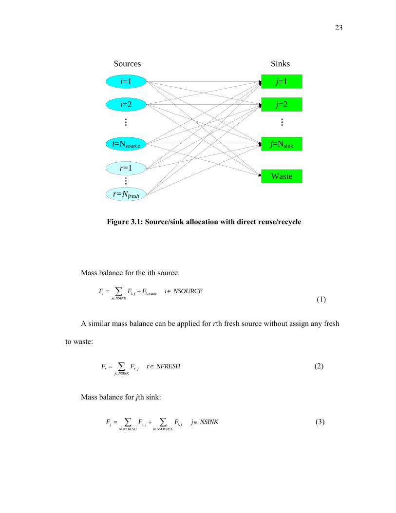
A source-sink mapping diagram is used to represent the superstructure of the
problem embedding potential configurations of interest (Figure 3.1). Each source is split
into fractions that are mixed with fractions of other streams to form the feeds to the
process sinks which must meet the process constraints expressed as bounds on
concentrations, temperature, and properties.
23
i=1 j=1
Sources Sinks
i=2 j=2
i=Nsource j=Nsink
r=1Waste
r=Nfresh
...
...
...
Figure 3.1: Source/sink allocation with direct reuse/recycle
Mass balance for the ith source:
, ,i i j i waste
j NSINK
F F F i NSOURCE
(1)
A similar mass balance can be applied for rth fresh source without assign any fresh
to waste:
,r r j
j NSINK
F F r NFRESH
(2)
Mass balance for jth sink:
, ,j r j i j
r NFRESH i NSOURCE
F F F j NSINK
(3)
24
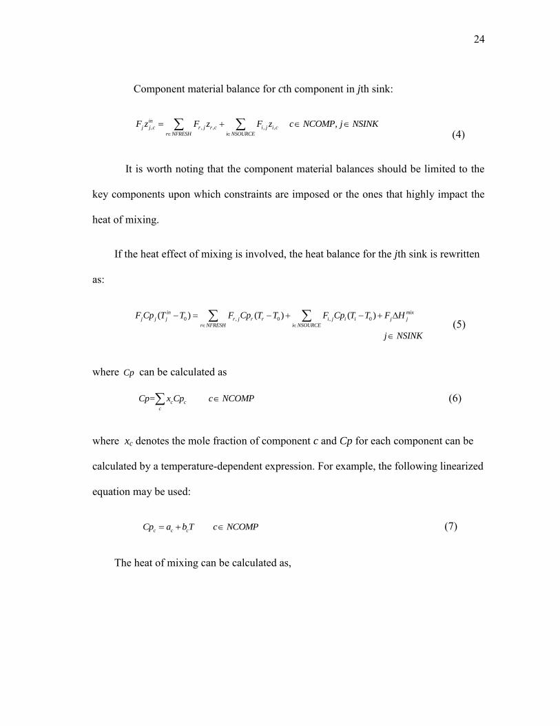
Component material balance for cth component in jth sink:
, , , , , ,in
j j c r j r c i j i c
r NFRESH i NSOURCE
F z F z F z c NCOMP j NSINK
(4)
It is worth noting that the component material balances should be limited to the
key components upon which constraints are imposed or the ones that highly impact the
heat of mixing.
If the heat effect of mixing is involved, the heat balance for the jth sink is rewritten
as:
0 , 0 , 0( ) ( ) ( )in mix
j j j r j r r i j i i j j
r NFRESH i NSOURCE
F Cp T T F Cp T T F Cp T T F H
j NSINK
(5)
where Cp can be calculated as
= c c
c
Cp x Cp c NCOMP (6)
where xc denotes the mole fraction of component c and Cp for each component can be
calculated by a temperature-dependent expression. For example, the following linearized
equation may be used:
c c cCp a b T c NCOMP (7)
The heat of mixing can be calculated as,

25
2
,
( )E
mix
P x
GRTH RT
T
(8)
For the case study, the Wilson Equation (Wilson, 1964) is selected. For the case of
binary systems:
1 1 2 12 2 2 1 21
1212 12
2121 21
ln( ) ln( )
ln
ln
EGx x x x x x
RT
ba
T
ba
T
(9a)
where x is the mole fraction, T is the absolute temperature, and is used to represent
the Wislon’s equation parameters. For multi-component systems:
(∑ ) ∑
∑ ( ) (9b)
where is the activity coefficient and Aij is given as a function of absolute temperature:
(9c)
Hence, Eq. 9 can be expressed as,
12 12 21 21
1 2
1 2 12 2 1 21
mix b bH Rx x
x x x x
(1)
Property balance for the pth property in the jth sink,
, , , , ,( ) ( ) ( ) ,in
j p j p r j p r p i j p i p
r FRESH i NSOURCE
F p F p F p p NPROP j NSINK
(2)
26
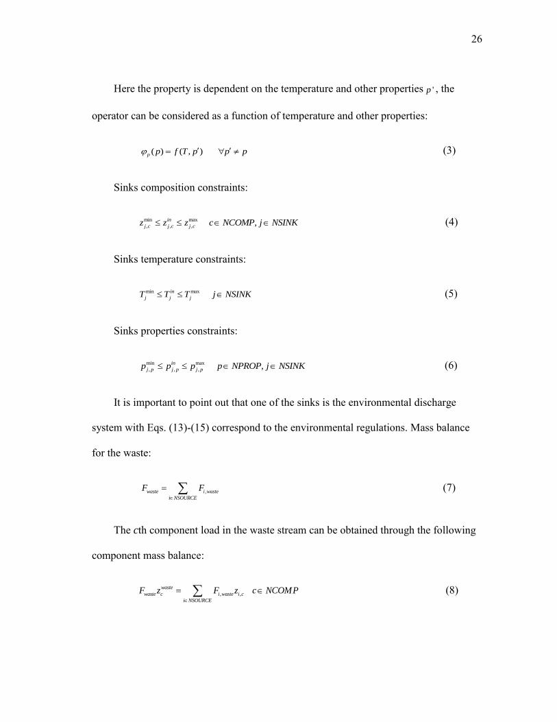
Here the property is dependent on the temperature and other properties 'p , the
operator can be considered as a function of temperature and other properties:
( ) ( , )p p f T p p p (3)
Sinks composition constraints:
min max
, , , ,in
j c j c j cz z z c NCOMP j NSINK (4)
Sinks temperature constraints:
min maxin
j j jT T T j NSINK (5)
Sinks properties constraints:
min max
, , , ,in
j p j p j pp p p p NPROP j NSINK (6)
It is important to point out that one of the sinks is the environmental discharge
system with Eqs. (13)-(15) correspond to the environmental regulations. Mass balance
for the waste:
,waste i waste
i NSOURCE
F F
(7)
The cth component load in the waste stream can be obtained through the following
component mass balance:
, ,
waste
waste c i waste i c
i NSOURCE
F z F z c NCOMP
(8)
27
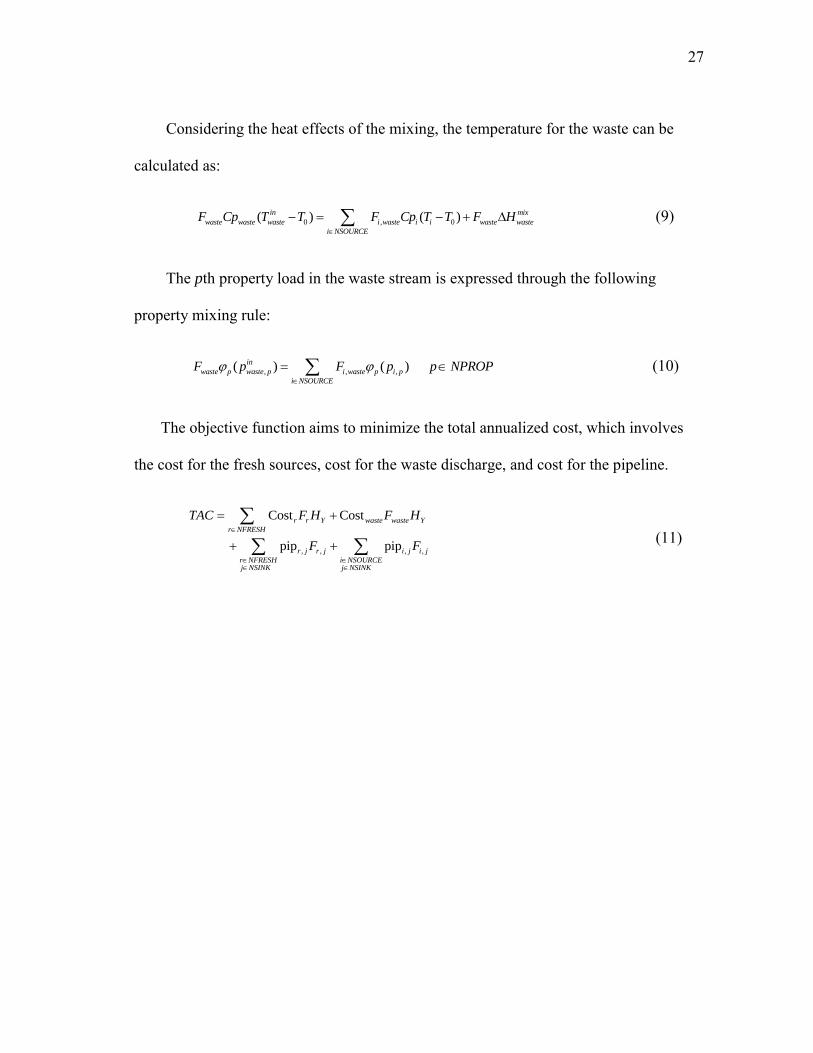
Considering the heat effects of the mixing, the temperature for the waste can be
calculated as:
0 , 0( ) ( )in mix
waste waste waste i waste i i waste waste
i NSOURCE
F Cp T T F Cp T T F H
(9)
The pth property load in the waste stream is expressed through the following
property mixing rule:
, , ,( ) ( )in
waste p waste p i waste p i p
i NSOURCE
F p F p p NPROP
(10)
The objective function aims to minimize the total annualized cost, which involves
the cost for the fresh sources, cost for the waste discharge, and cost for the pipeline.
, , , ,
Cost Cost
pip pip
r r Y waste waste Y
r NFRESH
r j r j i j i j
r NFRESH i NSOURCEj NSINK j NSINK
TAC F H F H
F F
(11)
28
3.4 Case Study
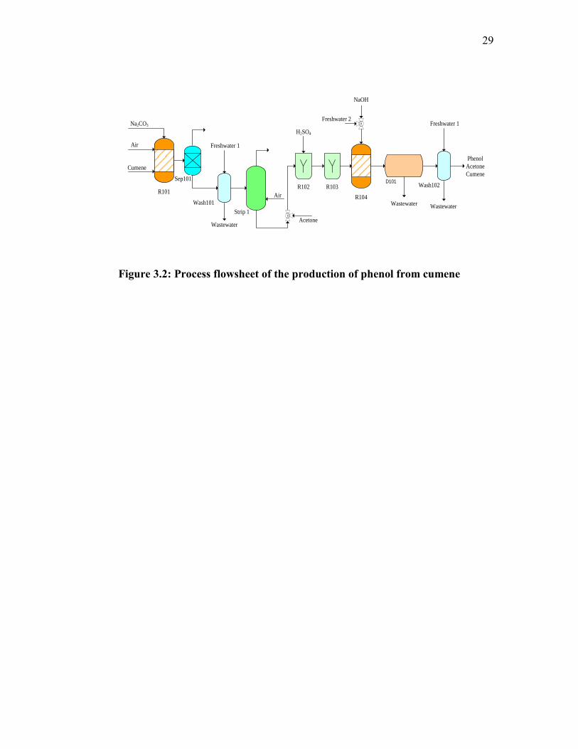
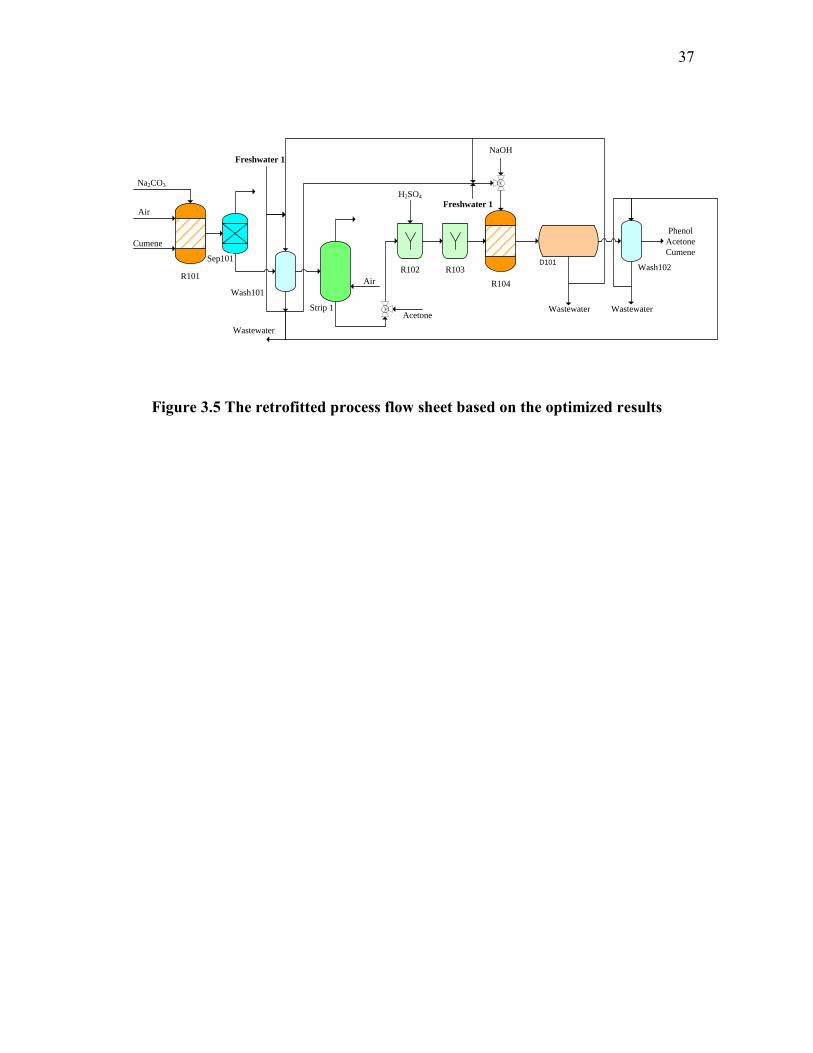
Figure 3.2 shows a schematic representation of the phenol production process
from cumene hydroperoxide (CHP). Cumene is fed into the reactor along with air and
Na2CO3 (which works as a buffer solution). In the reactor, cumene is oxidized to CHP.
The mixture of CHP and cumene is then sent to a washing operation to remove the
excess of the buffer solution and water-soluble materials.
Next, the stream leaving the washer is sent to a concentration unit in order to
increase the low concentration of CHP to 80 wt.% or higher. After that, the concentrated
CHP stream is fed to the cleavage units where the CHP is decomposed to form phenol
and acetone in the presence of sulfuric acid. The resulting cleavage stream is neutralized
with a small amount of sodium hydroxide and then it is separated into two phases
(organic and water phases). The water phase is sent to wastewater treatment and the
organic phase (which is mainly a mixture of phenol, acetone and cumene) is washed
with water to remove the excess alkali and is finally sent to distillation columns where it
is fractionated into the pure products phenol and acetone. This could be simplified in a
simple flow diagram (Figure 3.2) that summarizes visually the process described above.
29
R101
Cumene
Air
Na2CO3
Wash101
Sep101
Freshwater 1
Wastewater
Strip 1
Air
Acetone
R104
R102
H2SO4
R103
Freshwater 2
NaOH
D101
Wastewater
Wash102
Wastewater
Freshwater 1
Phenol
Acetone
Cumene
Figure 3.2: Process flowsheet of the production of phenol from cumene
30
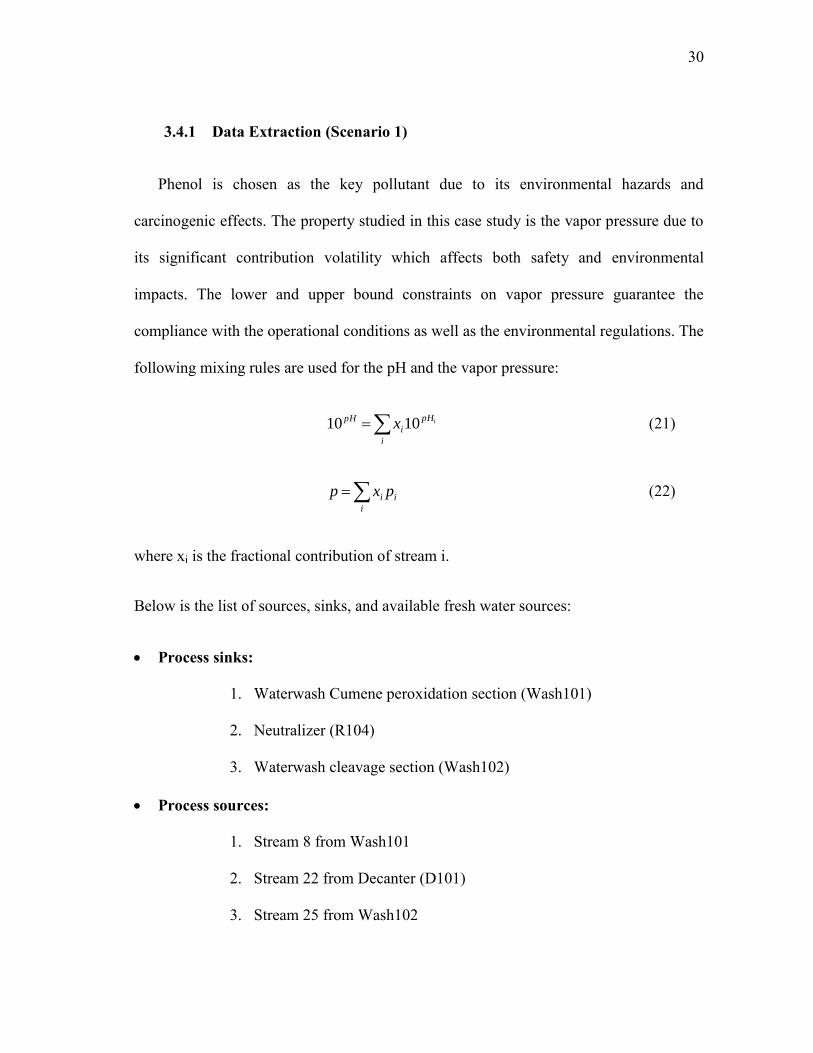
3.4.1 Data Extraction (Scenario 1)
Phenol is chosen as the key pollutant due to its environmental hazards and
carcinogenic effects. The property studied in this case study is the vapor pressure due to
its significant contribution volatility which affects both safety and environmental
impacts. The lower and upper bound constraints on vapor pressure guarantee the
compliance with the operational conditions as well as the environmental regulations. The
following mixing rules are used for the pH and the vapor pressure:
ipH
i
i
pH x 1010 (21)
i
i
i pxp (22)
where xi is the fractional contribution of stream i.
Below is the list of sources, sinks, and available fresh water sources:
Process sinks:
1. Waterwash Cumene peroxidation section (Wash101)
2. Neutralizer (R104)
3. Waterwash cleavage section (Wash102)
Process sources:
1. Stream 8 from Wash101
2. Stream 22 from Decanter (D101)
3. Stream 25 from Wash102
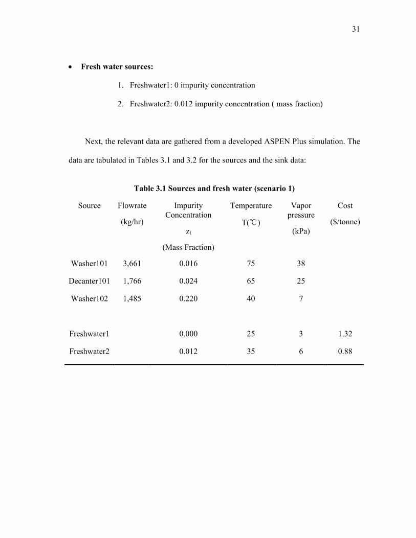
31
Fresh water sources:
1. Freshwater1: 0 impurity concentration
2. Freshwater2: 0.012 impurity concentration ( mass fraction)
Next, the relevant data are gathered from a developed ASPEN Plus simulation. The
data are tabulated in Tables 3.1 and 3.2 for the sources and the sink data:
Table 3.1 Sources and fresh water (scenario 1)
Source Flowrate
(kg/hr)
Impurity Concentration
zi
(Mass Fraction)
Temperature
T(℃)
Vapor pressure
(kPa)
Cost
($/tonne)
Washer101 3,661 0.016 75 38
Decanter101 1,766 0.024 65 25
Washer102 1,485 0.220 40 7
Freshwater1 0.000 25 3 1.32
Freshwater2 0.012 35 6 0.88
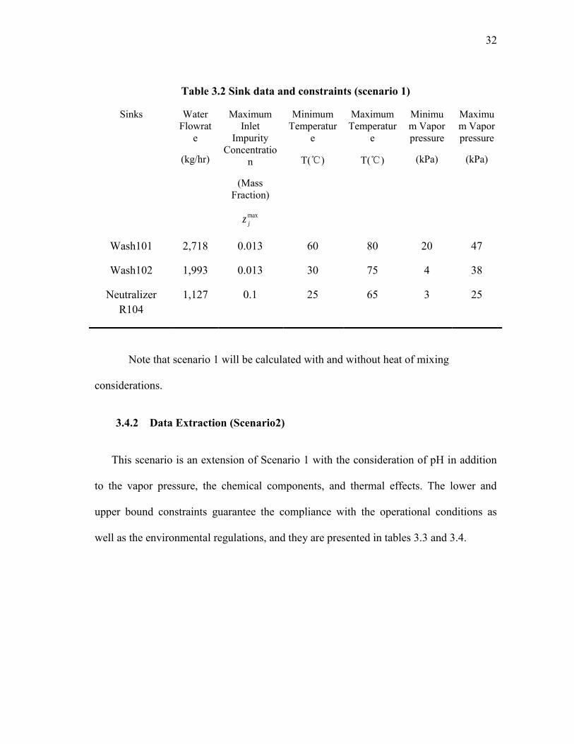
32
Table 3.2 Sink data and constraints (scenario 1)
Sinks Water Flowrat
e
(kg/hr)
Maximum Inlet
Impurity Concentratio
n
(Mass Fraction)
Minimum Temperatur
e
T(℃)
Maximum Temperatur
e
T(℃)
Minimum Vapor pressure
(kPa)
Maximum Vapor pressure
(kPa)
Wash101 2,718 0.013 60 80 20 47
Wash102 1,993 0.013 30 75 4 38
Neutralizer R104
1,127 0.1 25 65 3 25
Note that scenario 1 will be calculated with and without heat of mixing
considerations.
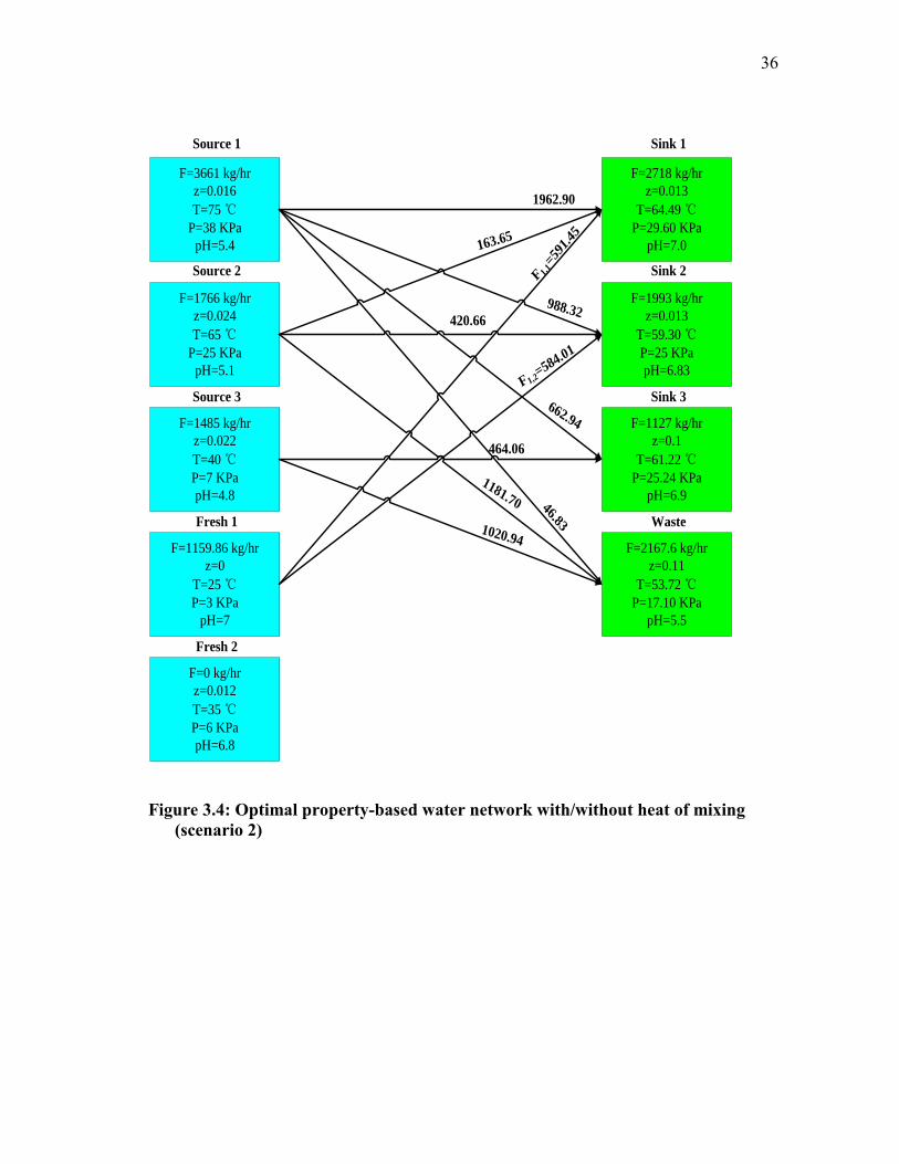
3.4.2 Data Extraction (Scenario2)
This scenario is an extension of Scenario 1 with the consideration of pH in addition
to the vapor pressure, the chemical components, and thermal effects. The lower and
upper bound constraints guarantee the compliance with the operational conditions as
well as the environmental regulations, and they are presented in tables 3.3 and 3.4.
max
jz
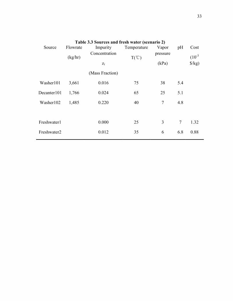
33
Table 3.3 Sources and fresh water (scenario 2)
Source Flowrate
(kg/hr)
Impurity Concentration
zi
(Mass Fraction)
Temperature
T(℃)
Vapor pressure
(kPa)
pH Cost
(10-3 $/kg)
Washer101 3,661 0.016 75 38 5.4
Decanter101 1,766 0.024 65 25 5.1
Washer102 1,485 0.220 40 7 4.8
Freshwater1 0.000 25 3 7 1.32
Freshwater2 0.012 35 6 6.8 0.88
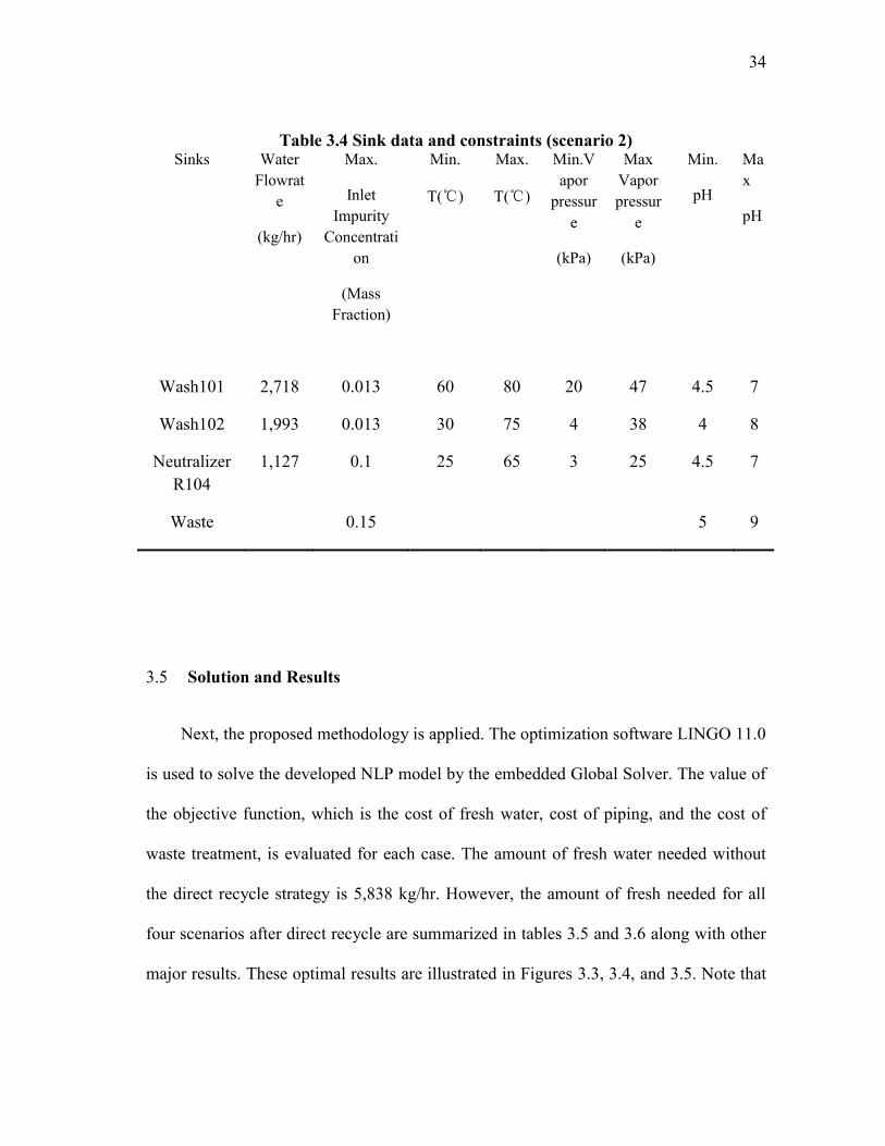
34
Table 3.4 Sink data and constraints (scenario 2) Sinks Water
Flowrate
(kg/hr)
Max.
Inlet Impurity
Concentration
(Mass Fraction)
Min.
T(℃)
Max.
T(℃)
Min.Vapor
pressure
(kPa)
Max Vapor pressur
e
(kPa)
Min.
pH
Max
pH
Wash101 2,718 0.013 60 80 20 47 4.5 7
Wash102 1,993 0.013 30 75 4 38 4 8
Neutralizer R104
1,127 0.1 25 65 3 25 4.5 7
Waste 0.15 5 9
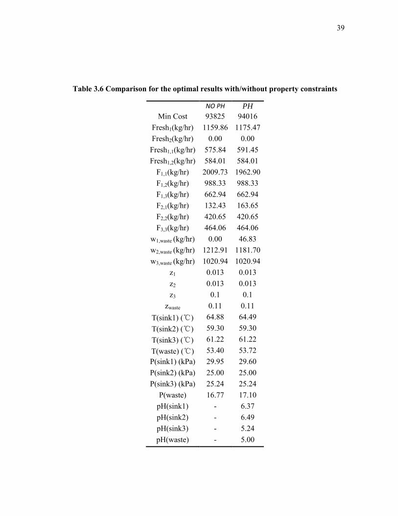
3.5 Solution and Results
Next, the proposed methodology is applied. The optimization software LINGO 11.0
is used to solve the developed NLP model by the embedded Global Solver. The value of
the objective function, which is the cost of fresh water, cost of piping, and the cost of
waste treatment, is evaluated for each case. The amount of fresh water needed without
the direct recycle strategy is 5,838 kg/hr. However, the amount of fresh needed for all
four scenarios after direct recycle are summarized in tables 3.5 and 3.6 along with other
major results. These optimal results are illustrated in Figures 3.3, 3.4, and 3.5. Note that
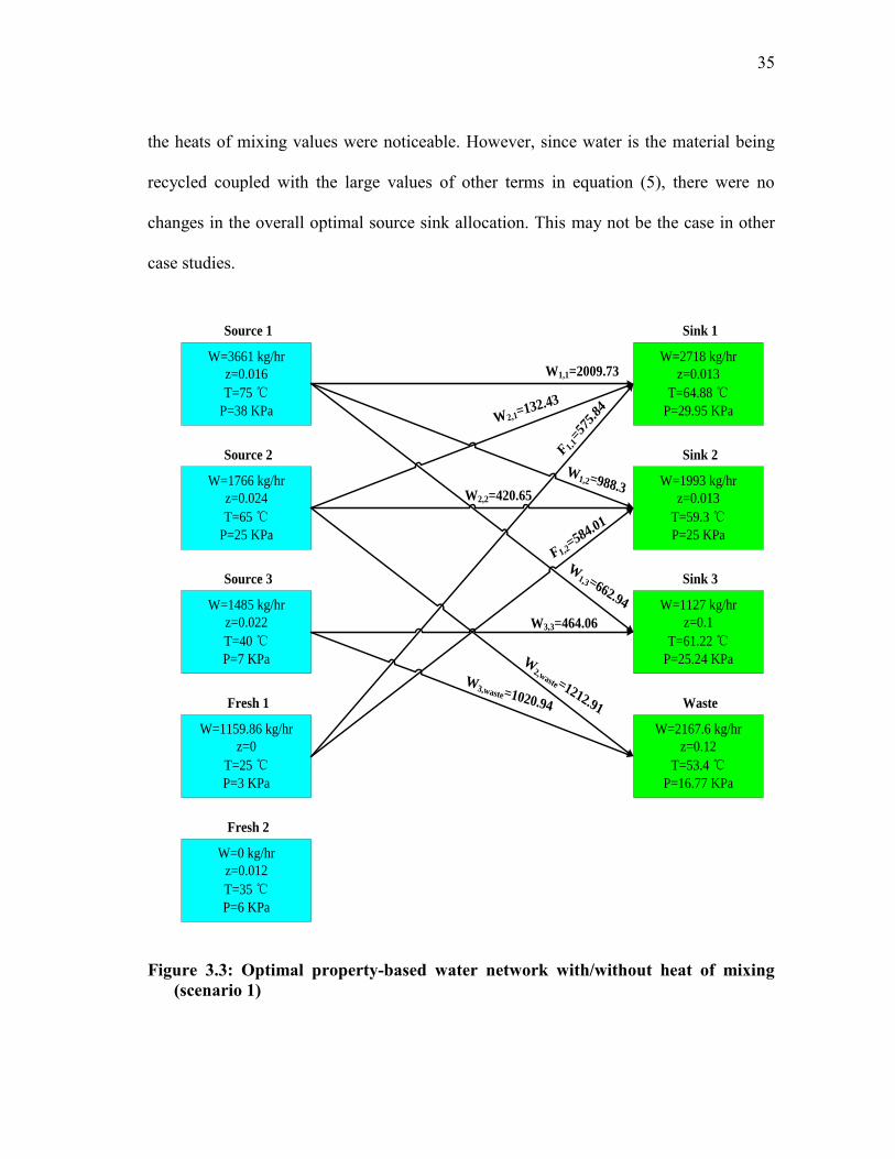
35
the heats of mixing values were noticeable. However, since water is the material being
recycled coupled with the large values of other terms in equation (5), there were no
changes in the overall optimal source sink allocation. This may not be the case in other
case studies.
W1,1=2009.73W=3661 kg/hr
z=0.016
T=75 ℃P=38 KPa
W=1766 kg/hr
z=0.024
T=65 ℃P=25 KPa
Source 1
Source 2
W=1485 kg/hr
z=0.022
T=40 ℃P=7 KPa
Source 3
W=1159.86 kg/hr
z=0
T=25 ℃P=3 KPa
Fresh 1
W=0 kg/hr
z=0.012
T=35 ℃P=6 KPa
Fresh 2
W=2718 kg/hr
z=0.013
T=64.88 ℃P=29.95 KPa
W=1993 kg/hr
z=0.013
T=59.3 ℃P=25 KPa
Sink 1
Sink 2
W=1127 kg/hr
z=0.1
T=61.22 ℃P=25.24 KPa
Sink 3
W=2167.6 kg/hr
z=0.12
T=53.4 ℃P=16.77 KPa
Waste
W1,2=988.3
W2,2=420.65
W2,waste=1212.91
W3,3=464.06
W3,waste=1020.94
F 1,1=57
5.84
F1,2=584.01
W1,3=662.94
W2,1=132.43
Figure 3.3: Optimal property-based water network with/without heat of mixing (scenario 1)
36
1962.90
F=3661 kg/hr
z=0.016
T=75 ℃P=38 KPa
pH=5.4
F=1766 kg/hr
z=0.024
T=65 ℃P=25 KPa
pH=5.1
Source 1
Source 2
F=1485 kg/hr
z=0.022
T=40 ℃P=7 KPa
pH=4.8
Source 3
F=1159.86 kg/hr
z=0
T=25 ℃P=3 KPa
pH=7
Fresh 1
F=0 kg/hr
z=0.012
T=35 ℃P=6 KPa
pH=6.8
Fresh 2
F=2718 kg/hr
z=0.013
T=64.49 ℃P=29.60 KPa
pH=7.0
F=1993 kg/hr
z=0.013
T=59.30 ℃P=25 KPa
pH=6.83
Sink 1
Sink 2
F=1127 kg/hr
z=0.1
T=61.22 ℃P=25.24 KPa
pH=6.9
Sink 3
F=2167.6 kg/hr
z=0.11
T=53.72 ℃P=17.10 KPa
pH=5.5
Waste
988.32
163.65
464.06
F 1,1=59
1.45
F1,2=584.01
662.94
420.66
1181.70
1020.94
46.83
Figure 3.4: Optimal property-based water network with/without heat of mixing (scenario 2)
37
R101
Cumene
Air
Na2CO3
Wash101
Sep101
Freshwater 1
Strip 1
Air
Acetone
R104
R102
H2SO4
R103
NaOH
D101
Wastewater
Wash102
Wastewater
Phenol
Acetone
Cumene
Freshwater 1
Wastewater
Figure 3.5 The retrofitted process flow sheet based on the optimized results
38
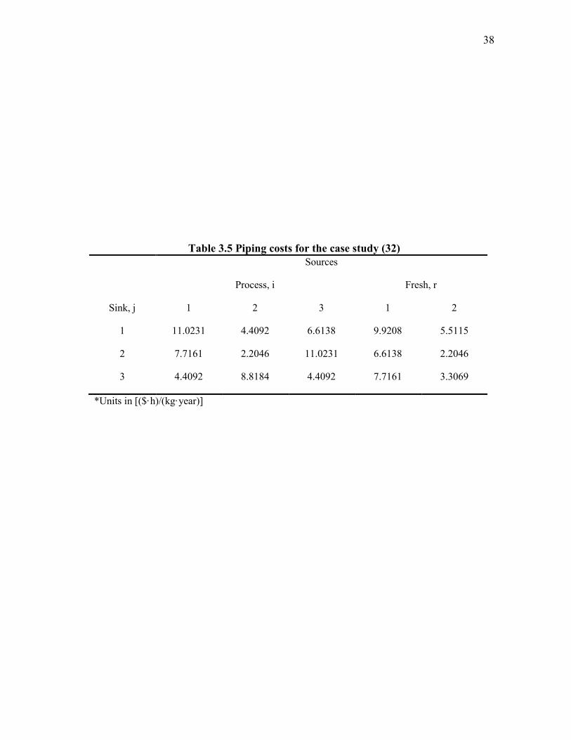
Table 3.5 Piping costs for the case study (32)
Sink, j
Sources
Process, i Fresh, r
1 2 3 1 2
1 11.0231 4.4092 6.6138 9.9208 5.5115
2 7.7161 2.2046 11.0231 6.6138 2.2046
3 4.4092 8.8184 4.4092 7.7161 3.3069
*Units in [($·h)/(kg·year)]
39
Table 3.6 Comparison for the optimal results with/without property constraints
NO PH
With pH
PH
Min Cost 93825 94016 Fresh1(kg/hr) 1159.86 1175.47 Fresh2(kg/hr) 0.00 0.00 Fresh1,1(kg/hr) 575.84 591.45 Fresh1,2(kg/hr) 584.01 584.01
F1,1(kg/hr) 2009.73 1962.90 F1,2(kg/hr) 988.33 988.33 F1,3(kg/hr) 662.94 662.94 F2,1(kg/hr) 132.43 163.65 F2,2(kg/hr) 420.65 420.65 F3,3(kg/hr) 464.06 464.06
w1,waste (kg/hr) 0.00 46.83 w2,waste (kg/hr) 1212.91 1181.70 w3,waste (kg/hr) 1020.94 1020.94
z1 0.013 0.013 z2 0.013 0.013 z3 0.1 0.1
zwaste 0.11 0.11 T(sink1) (℃) 64.88 64.49 T(sink2) (℃) 59.30 59.30 T(sink3) (℃) 61.22 61.22 T(waste) (℃) 53.40 53.72 P(sink1) (kPa) 29.95 29.60 P(sink2) (kPa) 25.00 25.00 P(sink3) (kPa) 25.24 25.24
P(waste) (kPa)
16.77 17.10 pH(sink1) - 6.37 pH(sink2) - 6.49 pH(sink3) - 5.24 pH(waste) - 5.00
40
3.6 Conclusions
This paper has introduced a systematic procedure which addresses for the first time
the simultaneous handling of concentrations, temperature, and properties to characterize
the process streams and constraints. This has been done taking into account the
interdependency of properties and their dependency on concentrations and temperature.
An optimization formulation has been developed to identify optimal allocation of
sources to sinks that will minimize the network cost while satisfying all process and
environmental constraints. Finally, a case study on water recycle in a phenol production
plant is solved.
3.7 Nomenclatures
(i) Indices:
c=index for the components,
i=index for the internal sources,
j=index for the sinks,
p=index for the properties;
r=index for the fresh sources,
waste= index for waste;
41
(ii) Sets:
NCOMP={ c | c is one of the components},
NFRESH={r | r is a fresh source},
NPROP={p | p is one of the properties};
NSINK={j | j is an internal sink},
NSOURCE={i |i is an internal source},
(iii) Parameters:
ca = Parameter in linerized temperature-dependent expression for heat capacity of
the pure component, 1.3724 J/(g·K) for water, 0.4685 J/(g·K) for phenol,
cb = Parameter in linerized temperature-dependent expression for heat capacity of
the pure component, 0.0083 J/(g·K) for water, 0.0044 J/(g·K) for phenol,
12a = Binary parameter in Wilson equation for phenol and water solution, 2.4395,
21a = Binary parameter in Wilson equation for phenol and water solution, -3.2239,
12b = Binary parameter in Wilson equation for phenol and water solution, -
2229.9297 K,
21b = Binary parameter in Wilson equation for phenol and water solution,
1046.1246 K,
cCp =heat capacity of the pure component,
42
iCp =heat capacity dependant on temperature of process source i,
rCp =heat capacity dependant on temperature of fresh source r,
Costr=unit cost of fresh source r,
Costwaste= unit cost of waste;
iF =total mass flowrate from process source i,
jF =total mass flowrate inlet process sink j,
0T = reference temperature, assumed to be 0℃,
rT =temperature of fresh source r,
iT = temperature of process source i,
min
jT =minimum temperature of process sink j,
max
jT =maximum temperature of process sink j,
,r pp =pth property of fresh source r,
,i pp =pth property of process source i,
min
,j pp =minimum property for pth property of process sink j,
max
,j pp = maximum property for pth property of process sink j,
43
R = ideal gas constant, 8.314 J/(K·mol),
,r cz = composition for cth component of fresh source r,
,i cz = composition for cth component of process source i,
min
,j cz =minimum composition for cth component of process sink j,
max
,j cz =maximum composition for cth component of process sink j,
Hy =Annual operating hours =8000 hr/year
(iv) Variables:
jCp = heat capacity dependent on temperature of process sink j,
wasteCp = heat capacity dependant on temperature of the waste,
rF =total flowrate consumed from fresh source r,
,r jF =segregated mass flowrate from fresh source r to sink j,
wasteF =total mass flowrate of the waste,
,
in
j pp = inlet property for pth property of process sink j,
,
in
waste pp =inlet property for pth property of process waste,
in
jT =inlet temperature of process sink j,
in
wasteT = inlet temperature of the waste,
44
,i jF =segregated mass flowrate from process source i to sink j,
,i wasteF =segregated mass flowrate from process source i to the waste stream,
EG = Excess Gibbs free energy, J/(K·mol),
w
cz = composition for cth component of the waste w,
,
in
j cz =inlet composition for cth component of process sink j,
mix
wasteH =enthalpy change in the mixing node before the waste,
mix
jH =enthalpy change in the mixing node before process sink j,
( )p p =property operator of pth property,
12 = Binary variable in Wilson equation for phenol and water solution,
21 = Binary variable in Wilson equation for phenol and water solution,
45
4 A PROPERTY-INTEGRATION APPROACH TO SOLVENT SCREENING
AND CONCEPTUAL DESIGN OF SOLVENT-EXTRACTION SYSTEMS
FOR RECYCLING USED LUBRICATING OIL
4.1 Introduction and Literature Review
Lubricating (lube) oils are used in significant quantities to reduce friction between
surfaces in moving parts. Lube oil primarily consists of base oil (85-90%) and additives
(10-15%). The United States Department of Energy (DOE) reported the total national
and global demand of lube oil to be 2.5 and 10.3 billion gallons per year, respectively.
Base oil is a mixture of liquid hydrocarbon molecules that contain around 20-70 carbon
atoms. Base oil may be derived from various sources with crude oil being the primary
commercial source. In order to enhance the performance of lube oil, additives are mixed
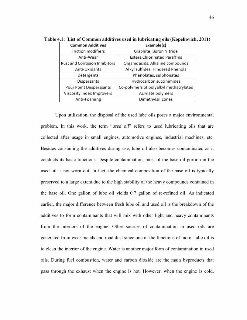
with the base oil. Table 4.1 provides a list of the most common additives used in the lube
oil application.
46
Table 4.1: List of Common additives used in lubricating oils (Kopeliovich, 2011)
Upon utilization, the disposal of the used lube oils poses a major environmental
problem. In this work, the term “used oil” refers to used lubricating oils that are
collected after usage in small engines, automotive engines, industrial machines, etc.
Besides consuming the additives during use, lube oil also becomes contaminated as it
conducts its basic functions. Despite contamination, most of the base-oil portion in the
used oil is not worn out. In fact, the chemical composition of the base oil is typically
preserved to a large extent due to the high stability of the heavy compounds contained in
the base oil. One gallon of lube oil yields 0.7 gallon of re-refined oil. As indicated
earlier, the major difference between fresh lube oil and used oil is the breakdown of the
additives to form contaminants that will mix with other light and heavy contaminants
from the interiors of the engine. Other sources of contamination in used oils are
generated from wear metals and road dust since one of the functions of motor lube oil is
to clean the interior of the engine. Water is another major form of contamination in used
oils. During fuel combustion, water and carbon dioxide are the main byproducts that
pass through the exhaust when the engine is hot. However, when the engine is cold,
Common Additives Example(s)
Friction modifiers Graphite, Boron Nitride
Anti-Wear Esters,Chlorinated Paraffins
Rust and Corrosion Inhibitors Organic acids, Alkaline compounds
Anti-Oxidants Alkyl sulfides, Hindered Phenols
Detergents Phenolates, sulphonates
Dispersants Hydrocarbon succinimides
Pour Point Desperssants Co-polymers of polyalkyl methacrylates
Viscosity Index Improvers Acrylate polymers
Anti-Foaming Dimethylsilicones
47
condensed water may reach the lube oil lines. Another source of contamination is the
oxidation of aromatics present in the base oil via the reaction with oxygen present in air.
Because of the relatively high cost of re-refining, used oils are normally disposed
of in landfills or illegally dumped in waterways making it an environmental hazard. In a
number of applications, lube oil has been successfully recycled (Laird, 1982). DOE
reported that only 17 percent of the recycled oil is being re-refined (DOE, 2006).
Examples of recycle alternatives include use as a fuel substitute in furnaces or as an
extending agent in road-paving asphalt. Re-refining is intended for recovery of base oil
for reuse for the original purpose as lube oil. Because of the rising prices of hydrocarbon
fuels as well as the depletion of natural resources coupled with the ever increasing
environmental regulations, an economically profitable and environmentally friendly re-
refining technology that recovers the valuable base oil is essential. There are three major
re-refining technologies that have been employed industrially to treat used oils. One of
the oldest technologies used to treat used oils is chemical re-refining which is based on
acid (normally sulfuric acid) followed by clay treatment. The acid-clay process involves
atmospheric distillation to remove water and light hydrocarbons. Then, the dry used oil
is treated with 5-10% by volume sulfuric acid. The sludge dissolves in the solvent
(sulfuric acid), and settles down at the bottom of the decanter. The sludge containing
sulfuric acid is removed from the bottom, and the clean oil is decanted out from the top,
where it undergoes a neutralization step with the clay. The main advantage of this
process is its capability to produce high quality base oil in an economically attractive
manner. However, the acidic sludge collected from this process is environmentally
48
hazardous, even more than the used oil itself, and, thus, requires quite expensive disposal
techniques.
The other re-refining technique is the physical re-refining which is based on
distillation processes that involve atmospheric distillation as well as vacuum distillation
and thin-film evaporation. Similar to chemical re-refining, the first step is an
atmospherics distillation process to recover the water and light hydrocarbons
contaminants. This step is followed by vacuum distillation and thin-film evaporation
(10-30 mmHg) to recover additives and other contaminants. In the last stage, the
recovered base oil goes through a hydrogenation step in a hydro reactor to completely
saturate the oxidized hydrocarbons. It is noteworthy to mention that despite the high cost
of this process, it is more environmentally friendly than the chemical re-refining.
However, this process has many challenges. For instance, the recovered oil is not of a
high quality and therefore requires additional treatment. Additionally, fouling inside the
distillation equipment normally occurs due to carbon deposition. More importantly, in
order for this approach to become economically attractive it requires a steady and large
volume input. Yet, both chemical re-refining (acid-clay process) and physical re-refining
have found their way to commercialization scale.
The third major re-refining technique for recovering used oils is the solvent
extraction re-refining process. This is a particularly attractive cleaner technology since it
is aimed at conserving natural resources and recovering (instead of destroying) the base
oil. In the solvent extraction process, the used oil and solvent are mixed in appropriate
proportions to assure miscibility of the base oil in the solvent and the rejection of
49
additives. A demulsifier is also used to coagulate the additives and dispersed particles
and enhance their aggregation and rejection as large particle (flakes) that can be
separated from the liquid by either sedimentation or centrifugation. These solvents are
referred to as extraction-flocculation solvents (Reis and Jeronimo, 1988). Figure 4.1 is a
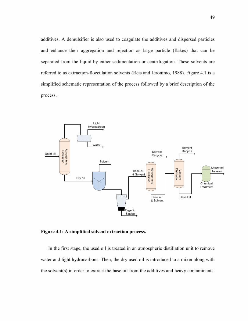
simplified schematic representation of the process followed by a brief description of the
process.
Figure 4.1: A simplified solvent extraction process.
In the first stage, the used oil is treated in an atmospheric distillation unit to remove
water and light hydrocarbons. Then, the dry used oil is introduced to a mixer along with
the solvent(s) in order to extract the base oil from the additives and heavy contaminants.
50
The mixing step is followed by a decantation unit whereby agglomeration and formation
of large flakes take place and a two-phase solution is obtained. An organic sludge
containing the worn additives and metals is decanted out the bottom of the decanter, and
the top phase contains the base oil/solvent, which is separated and sent to a series of
distillation columns for complete solvent separation for recycling purposes. Finally, base
oil undergoes chemical treatment in order to adjust its physical properties and
hydrocarbon structure to the required level. The major advantage of this technology is
that it overcomes most of the limitations encountered by the aforementioned
commercialized technologies. Compared to the acid-clay process, it produces a useful
organic sludge that may be used in the asphalt or ink industries (Reis and Jeronimo,
1982). Also, it produces high quality base oil with less likelihood of fouling compared
to the physical re-refining process. The process is also carried out at a lower overall
operating cost for similar volume input
An important experimental measurement of the effectiveness of the solvent
extraction re-refining process is normally represented by the amount of sludge removed
from the used oil. This may be expressed as the percent sludge removal (PSR), which is
the mass of sludge removed in grams per 100 g of oil (Reis and Jernimo, 1988). Another,
important parameter is the percent oil losses (POL), which is the mass of base oil lost in
the sludge phase expressed in grams per 100 g of oil (Reis and Jernimo 1988, and
Elbashir et al. 2002). These two scales are key concepts in measuring the effectiveness
of the solvent extraction process. The main operation parameters that control the
efficiency of this process are temperature, solvent-to-oil ratio, and solvent type
51
(normally referred to as the solvent extraction parameters or system). The characteristics
of the required solvent for this process have been identified by Reis and Jernimo (1988)
as follows: (1) it should be miscible in the base oil contained in the processed used oil;
(2) should have the capability to reject additives and dispersed particle from the solvent-
oil mixture; and (3) should be able to aggregate the remaining additives and
contaminants to particle sizes large enough to be separated from the base oil and solvent
mixture by either sedimentation, filtration, or centrifugation.
Despite the commercialization of numerous solvent extraction processes, there is still
a need to design a systematic approach to quickly screen alternatives to identify a set of
candidates that can be optimized. Such an approach has to; simultaneously identify
appropriate solvent or solvent blends, design an efficient recovery process for the base
oil, and establish a regeneration method for the recycle of the solvents, all while
optimizing the overall cost of the process. Because of the system’s dependence on
solvent properties, a particularly well-suited approach for optimal design is the
framework of property integration which is defined by El-Halwagi et al. (2004) as “a
functionality-based holistic approach for the allocation and manipulation of streams and
processing units, which is based on functionality tracking, adjustment and assignment
throughout the process.” Several graphical and algebraic techniques have been
developed for designing and optimizing recycle/reuse systems based on property
integration (e.g., Shelley and El-Halwagi, 2000; El-Halwagi et al.,2004; Qin et al.,2004;
and Ng et al.,2009). Optimization techniques have been used to formulate recycle
problems as property-integration tasks (e.g., Ponce-Ortega et al., 2009 and 2010, Ng et
52
al., 2009; Nápoles-Rivera, 2010). Furthermore, a proposed model was used for the
synthesis of property-based resource conservation networks in both batch and
continuous process applications. The framework takes into account direct recycle
network, interception, and waste treatment simultaneously (Chen, 2010). Combining
process and molecular design has also been accomplished through process integration
using group contributions methods (e.g., Chemmangattuvalappil et al., 2010; Solvason,
2009; Eljack et al.,2008 and 2007; and Kazantzi, 2007).
4.2 Problem Statement
Consider a solvent-extraction process for the recovery and reclamation of spent
lube oil. The selection of proper solvents and blends is on the most important decisions
for effective design and operation. It is desired to identify a systematic procedure to
provide guidelines to the designer on selecting solvents and blends with proper
properties. A combination of experimental data and simulation is to be used in defining
the feasibility ranges for the desired properties. A property integration framework is to
be utilized to generate bounds on the recommended solvents and blends.
4.2.1 Selection of Principal Properties and Construction of Property Clusters
While there are several successful experimental studies on the selection and
design of solvent extraction systems for recycle of used lube oils, there is a need to
develop systematic design approaches that guide the designer in selecting optimal
solvents or solvent blends and designing the various components of the recovery system
while accounting for the properties of the solvents, the properties of the used and
53
recovered oil, and operational criteria such as percent sludge removal and percent oil
losses (PSR and POL). The approach should also take into account the economic and
environmental aspects of the design before determining an optimum. Additionally, it
should cover every unit of the process starting from the atmospheric distillation up to the
hydro treating step (see Figure 4.1). Different units may be impacted by different
properties. For example, it is crucial to track the solubility parameter in solvent
extraction applications, as it is important to track the specific gravity and relative
volatility in decantation and distillation applications, respectively. Consequently, we
chose the solubility parameter, viscosity, and vapor pressure as the major properties of
concern for solvent selection. The following parameters are used in assessing the
performance of the solvents and solvent blends:
-Solubility parameter: The latent heat of vaporization indicates the amount of van der
Waals forces that hold liquid molecules together (Burk, 1984). For a solution to occur,
the chosen solvent must overcome these forces and find their way around and between
the base oil molecules. Solubility parameter is a good indicator of such a behavior. As it
has been stated earlier, a good solvent for re-refining used oils must be highly miscible
in the base oil and at the same time facilitate the miscibility of additives and their
subsequent coagulation through the use of a demulsifier (Reis and Jernimo, 1988). These
requirements have two indications in terms of solubility parameters of the three major
components that form the used oil (base oil, solvent, and additives + contaminants). For
dissolving the base oil and additives, the absolute value of the difference between
solubility parameter of base oil and solvent has to be as close to zero as possible to
54
facilitate the complete miscibility requirement. On the other hand, if the additives are
completely miscible, it will be difficult to coagulate them into flakes using a demulsifer
(such as KOH). Therefore, the absolute value of the difference between the solubility
parameter of the solvent and base oil and additives has to be small enough for miscibility
but not too small for coagulation and flocculation of the additives into separate flakes.
An optimum range of solubility parameters of the solvent is needed. Another important
factor is the polarity of the solvent which facilitates the rejection of the spent additives,
impurities, carbonaceous particles to flocculate and form large flakes that settle under
gravity action. Therefore, the optimum range of solubility parameters is selected for
polar solvents (e.g. alcohols, ketones).
-Viscosity: Lower viscosity solvents tend to function more favorably in solvent
extraction processes. Higher viscosity solvents typically experience a greater amount of
time for phase separation to occur. Also, the mass transfer resistance decreases as the
viscosity of the solution decreases enabling higher solvent effectiveness. From an
operational point of view, lower viscosity solutions are much easier to handle than
higher ones (specifically on pumping and tube transportation) (King, 1971).
-Vapor pressure: In order to complete the optimization loop, vapor pressure (e.g., Reid
vapor pressure “RVP”) must also be investigated. In order to obtain economical
separation, the vapor pressure difference between the solvent and the base oil must be as
great as possible so that the distillation process utilizes a minimum number of stages.
While many solvents meet this criterion, there still must be a careful balance. Having
too low of a vapor pressure causes the solvent to be very volatile whereby it is hard to
55
accomplish appropriate mass transfer during the extraction process. Also, high volatility
solvent may cause solvent losses due to atmospheric leaks causing environmentally
hazardous problem and higher operation cost.
With the appropriate property parameters identified, it is possible to formulate a
design using property-integration method. Here, we start with the concept of clustering.
The Cluster terms were introduced by Shelley and El-Halwagi (2000) for component-
less design and they have been used for the tracking of properties in the property
integration framework proposed by El-Halwagi et al. (2004). From the above analysis, it
can be concluded that there are constraints on the upper and lower bounds for each
property; this can be expressed as follows (El-Halwagi, 2006):
maxmin
iii ppp (1)
where P is the property of interest that can either be the solubility, the viscosity, or the
vapor pressure. The upper and lower bounds are determined either experimentally or via
simulation. Mixing rules are used to track properties. For instance, the viscosity mixing
rule may be expressed in the Arrhenius equation as follow:
iix lnln (2)
where,
is the composition of pure component i in the mixture
is the viscosity of pure component i in the mixture
is the viscosity of the mixture
This means that the viscosity operator )( i can be expressed as follows (Shelley
and El-Halwagi, 2000):
i
ix
56
ii ln)( (3)
From equation (3), the viscosity dimensionless operator i, can be determined
using the following equation:
ref
ii
ln
ln, (4)
where,
is the viscosity of a chosen reference solution
The Reid vapor pressure mixing rule can be expressed as follow:
(5)
where,
F is the flowrate of the mixture
P is the Reid vapor pressure of the mixture
iF is the flowrate of the pure component i in the mixture
iP is the Reid vapor pressure of pure component i in the mixture
Therefore, the Reid vapor pressure operator )( iP can be shown in equation (6).
Then, the Reid vapor pressure dimensionless operator ip, is calculated using eqn. (7):
(6)
(7)
where,
referencep is the Reid vapor pressure of a chosen reference solution.
ref
44.144.1
** ii PFPF
44.1)( ii PP
44.1
44.1
,
reference
iip
p
p
57
The solubility mixing rule is linear and can be expressed in the following equation
(Barton, 1991):
** iFF (8)
where
is the solubility parameter of the mixture
i is the solubility parameter of the pure component i in the mixture
Therefore, the solubility operator )( i can be defined as follow:
(9)
From equation (9), the solubility dimensionless operator can be calculated and expressed
in the following equation:
(10)
where
reference is the solubility parameter of a reference solution.
Then, the AUgmented Property index iAUP introduced by Shelley and El-
Halwagi (2000) is defined as the summation of the dimensionless operators as described
below:
(11)
where r represents the properties being optimized. This approach also introduces a new
parameter, which is the cluster of a property r, irC ,, that is calculated as the fraction of
the dimensionless operator divided by iAUP :
ii )(
reference
ii
,
r
iriAUP ,
58
i
ir
irAUP
C,
,
(12)
This can also be expanded to the following form to represent all properties of
concern in this study:
i
i
iAUP
C,
,
(13)
(14)
(15)
The sum of all the clusters as represented above is equal to one, i.e.:
(16)
Therefore, on a ternary diagram for the clusters of vapor pressure, solubility, and
viscosity, each solvent is represented by one point. Once the values of two clusters are
determined, the third cluster is automatically determined (because the sum of clusters is
one) as shown in Figure 4.2.
i
i
iAUP
C,
,
1, irC
i
iP
iPAUP
C,
,
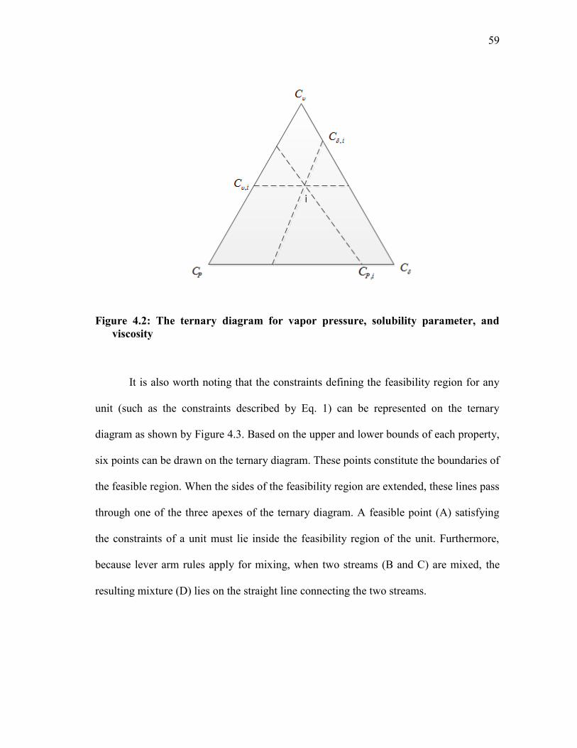
59
Figure 4.2: The ternary diagram for vapor pressure, solubility parameter, and viscosity
It is also worth noting that the constraints defining the feasibility region for any
unit (such as the constraints described by Eq. 1) can be represented on the ternary
diagram as shown by Figure 4.3. Based on the upper and lower bounds of each property,
six points can be drawn on the ternary diagram. These points constitute the boundaries of
the feasible region. When the sides of the feasibility region are extended, these lines pass
through one of the three apexes of the ternary diagram. A feasible point (A) satisfying
the constraints of a unit must lie inside the feasibility region of the unit. Furthermore,
because lever arm rules apply for mixing, when two streams (B and C) are mixed, the
resulting mixture (D) lies on the straight line connecting the two streams.
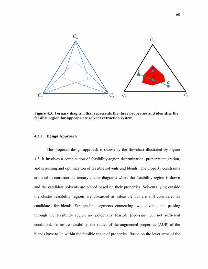
60
Figure 4.3: Ternary diagram that represents the three properties and identifies the feasible region for appropriate solvent extraction system
4.2.2 Design Approach
The proposed design approach is shown by the flowchart illustrated by Figure
4.3. It involves a combination of feasibility-region determination, property integration,
and screening and optimization of feasible solvents and blends. The property constraints
are used to construct the ternary cluster diagrams where the feasibility region is drawn
and the candidate solvents are placed based on their properties. Solvents lying outside
the cluster feasibility regions are discarded as infeasible but are still considered as
candidates for blends. Straight-line segments connecting two solvents and passing
through the feasibility region are potentially feasible (necessary but not sufficient
condition). To insure feasibility, the values of the augmented properties (AUP) of the
blends have to lie within the feasible range of properties. Based on the lever arms of the
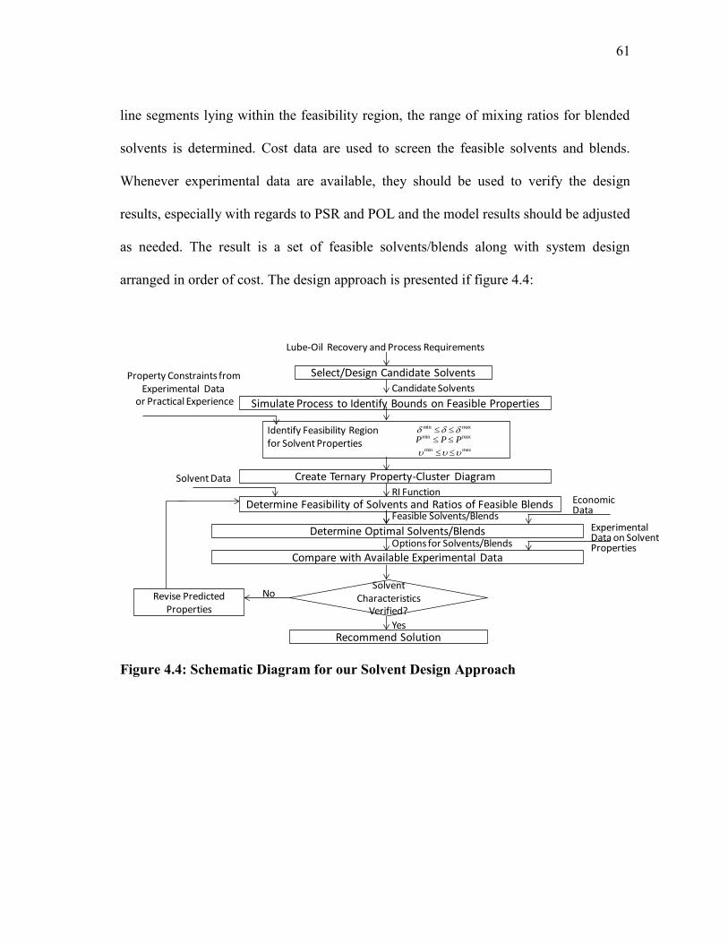
61
line segments lying within the feasibility region, the range of mixing ratios for blended
solvents is determined. Cost data are used to screen the feasible solvents and blends.
Whenever experimental data are available, they should be used to verify the design
results, especially with regards to PSR and POL and the model results should be adjusted
as needed. The result is a set of feasible solvents/blends along with system design
arranged in order of cost. The design approach is presented if figure 4.4:
Figure 4.4: Schematic Diagram for our Solvent Design Approach
Select/Design Candidate Solvents
Lube-Oil Recovery and Process Requirements
Candidate Solvents
Simulate Process to Identify Bounds on Feasible Properties
Create Ternary Property-Cluster Diagram
RI FunctionDetermine Feasibility of Solvents and Ratios of Feasible Blends
Property Constraints from Experimental Data
or Practical Experience
Solvent Data
Determine Optimal Solvents/BlendsOptions for Solvents/Blends
EconomicData
SolventCharacteristics
Verified?
Yes
Compare with Available Experimental Data
Recommend Solution
NoRevise Predicted Properties
Feasible Solvents/Blends
maxmin maxmin PPP maxmin
Identify Feasibility Regionfor Solvent Properties
ExperimentalData on SolventProperties
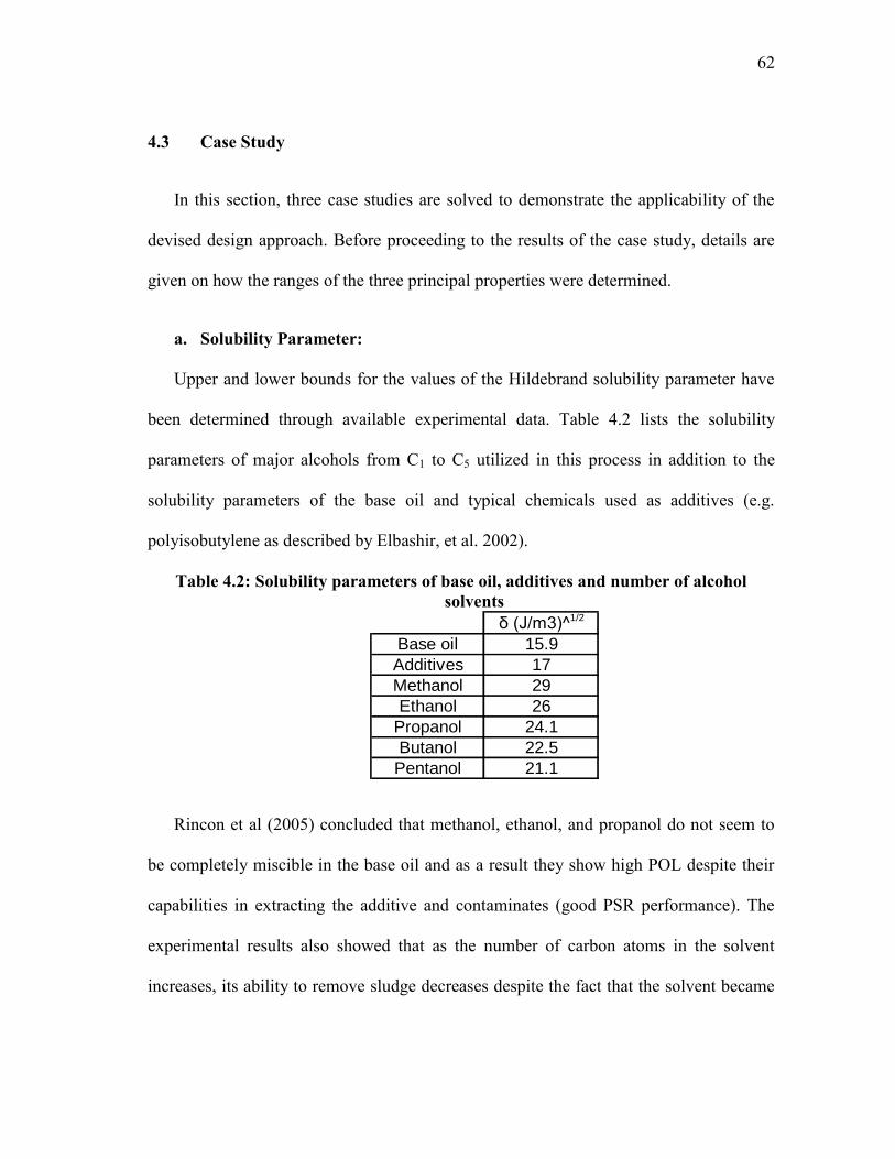
62
4.3 Case Study
In this section, three case studies are solved to demonstrate the applicability of the
devised design approach. Before proceeding to the results of the case study, details are
given on how the ranges of the three principal properties were determined.
a. Solubility Parameter:
Upper and lower bounds for the values of the Hildebrand solubility parameter have
been determined through available experimental data. Table 4.2 lists the solubility
parameters of major alcohols from C1 to C5 utilized in this process in addition to the
solubility parameters of the base oil and typical chemicals used as additives (e.g.
polyisobutylene as described by Elbashir, et al. 2002).
Table 4.2: Solubility parameters of base oil, additives and number of alcohol solvents
δ (J/m3)^1/2
Base oil 15.9
Additives 17
Methanol 29
Ethanol 26
Propanol 24.1
Butanol 22.5
Pentanol 21.1
Rincon et al (2005) concluded that methanol, ethanol, and propanol do not seem to
be completely miscible in the base oil and as a result they show high POL despite their
capabilities in extracting the additive and contaminates (good PSR performance). The
experimental results also showed that as the number of carbon atoms in the solvent
increases, its ability to remove sludge decreases despite the fact that the solvent became
63
more miscible in the oil (Reis and Jeronimo, 1988). In other words, POL as well as PSR
decreases as the number of carbons atoms increases (Reis and Jeronimo, 1988). The
experimental study suggests that butanol is a highly effective single solvent in the used
oil extraction process and that it outperforms different solvents (lcohols and ketones)
with carbon atoms ranging between 1 and 5. Considering the information summarized in
Table 4.2 in addition to the previous experimental assessments of several solvents, we
recommend that solvents with solubility parameter between 21.5 and 23.5 (J/m3)1/2
should be considered as candidates for the re-refining of used oils. Solvent(s) with
solubility parameter less than 21.5 (J/m3)1/2 are highly miscible in both the additives and
the base oil, and as a result, will make it very difficult for flocculation of contaminants
and additives (upon the addition of a demulsifier such as KOH) and the formation of the
sludge phase. On the other hand, any solvent(s), with a solubility parameter higher than
23.5 (J/m3)1/2 will be relatively immiscible in the base oil; which is an undesirable
criterion for the solvent as it leads to losses in the base oil.
b. Vapor Pressure:
Setting the vapor-pressure bounds is important for the separation process of the
solvent-recovery unit. Therefore, a set of simulation tests using the software ASPEN
Plus was used to determine these bounds. Based on the simulation results, it was found
that any solvent with a vapor pressure between 5 and 150 torr should be included in the
consideration set. When the vapor pressure is lower than 5 torr, the separation process
becomes very expensive due to the high temperature requirement. High temperature
operation does not only come with high utility cost, but it will also decrease the quality
64
of the produced re-refined base oil. Any solvent with vapor pressure higher than 150 torr
is considered too volatile, which is not desirable in this extraction process since it
reduces the liquid-liquid molecule interaction between solvent and used oil.
c. Viscosity:
Setting the viscosity bounds is crucial for the extraction unit. Therefore, the
upper bound was extracted from published experimental data (Reis and Jernimo, 1988).
Any solvent with a viscosity between 0.5 and 3.5 cp is included in the consideration of
potential solvents. A viscosity higher than 3.5 cp causes the solution to become too
viscous, which results in an increase in mass transfer resistance, and thus causes longer
extraction time and higher operating cost (stemming from a pumping system). Solvents
with typical viscosity less than 0.5 cp are normally in the gas phase, and as a result they
should be eliminated from the consideration set.
The ternary cluster representation of the aforementioned constraints is shown in
Figure 4.5 where the feasible region is plotted.
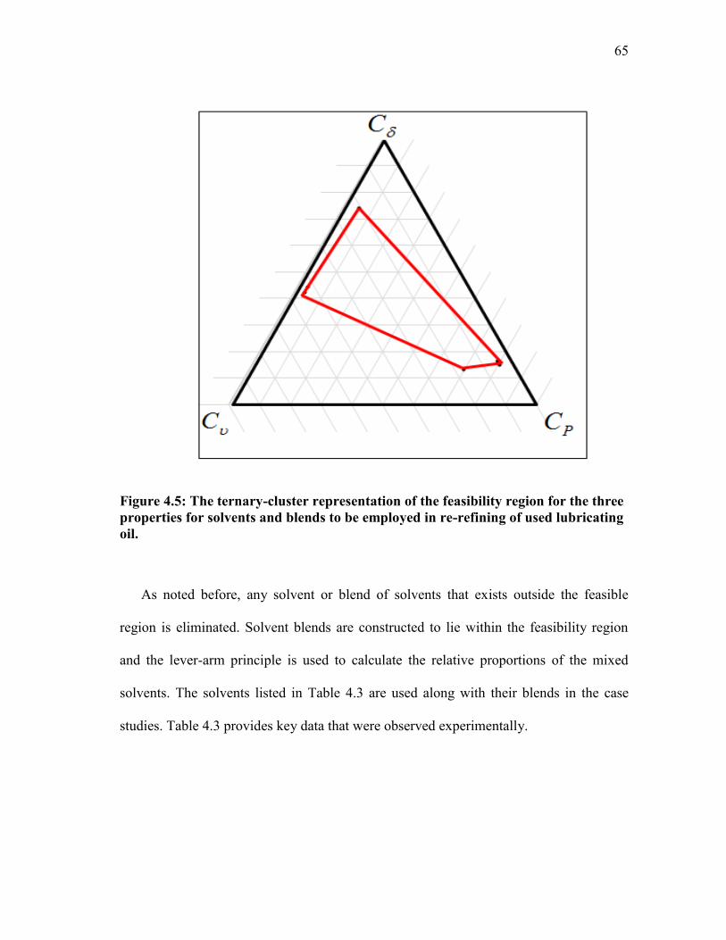
65
Figure 4.5: The ternary-cluster representation of the feasibility region for the three properties for solvents and blends to be employed in re-refining of used lubricating oil.
As noted before, any solvent or blend of solvents that exists outside the feasible
region is eliminated. Solvent blends are constructed to lie within the feasibility region
and the lever-arm principle is used to calculate the relative proportions of the mixed
solvents. The solvents listed in Table 4.3 are used along with their blends in the case
studies. Table 4.3 provides key data that were observed experimentally.
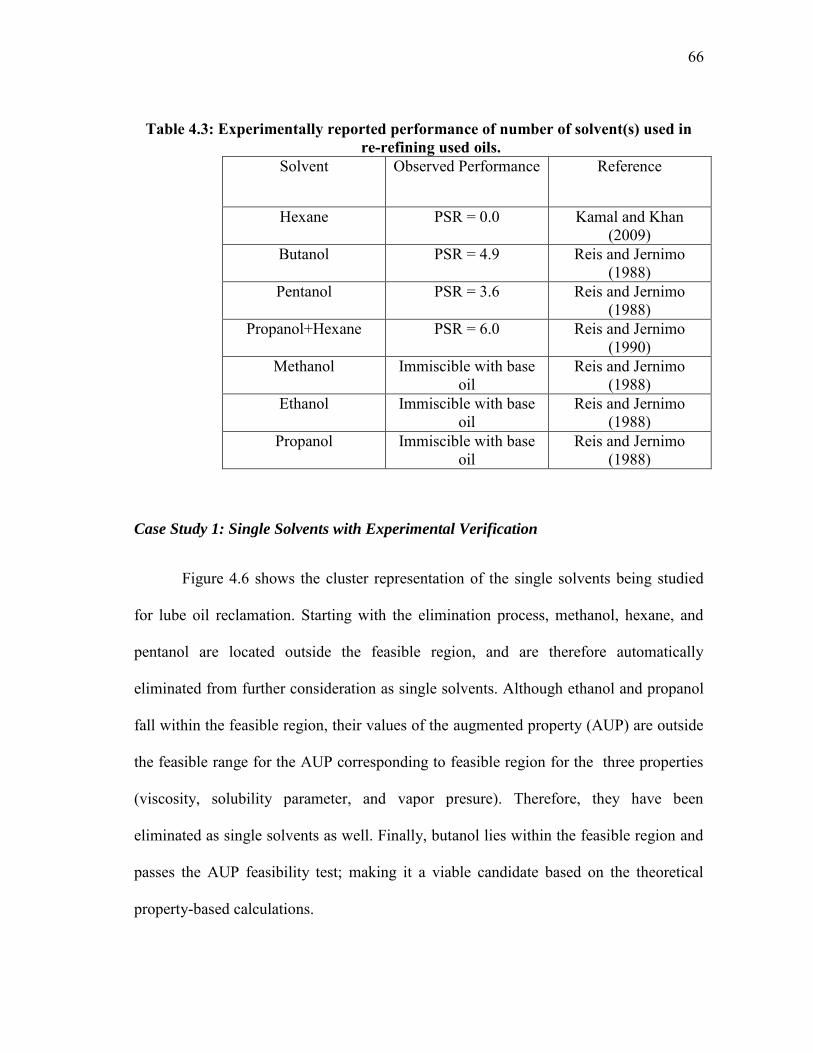
66
Table 4.3: Experimentally reported performance of number of solvent(s) used in re-refining used oils.
Solvent Observed Performance Reference
Hexane PSR = 0.0 Kamal and Khan (2009)
Butanol PSR = 4.9 Reis and Jernimo (1988)
Pentanol PSR = 3.6 Reis and Jernimo (1988)
Propanol+Hexane PSR = 6.0 Reis and Jernimo (1990)
Methanol Immiscible with base oil
Reis and Jernimo (1988)
Ethanol Immiscible with base oil
Reis and Jernimo (1988)
Propanol Immiscible with base oil
Reis and Jernimo (1988)
Case Study 1: Single Solvents with Experimental Verification
Figure 4.6 shows the cluster representation of the single solvents being studied
for lube oil reclamation. Starting with the elimination process, methanol, hexane, and
pentanol are located outside the feasible region, and are therefore automatically
eliminated from further consideration as single solvents. Although ethanol and propanol
fall within the feasible region, their values of the augmented property (AUP) are outside
the feasible range for the AUP corresponding to feasible region for the three properties
(viscosity, solubility parameter, and vapor presure). Therefore, they have been
eliminated as single solvents as well. Finally, butanol lies within the feasible region and
passes the AUP feasibility test; making it a viable candidate based on the theoretical
property-based calculations.
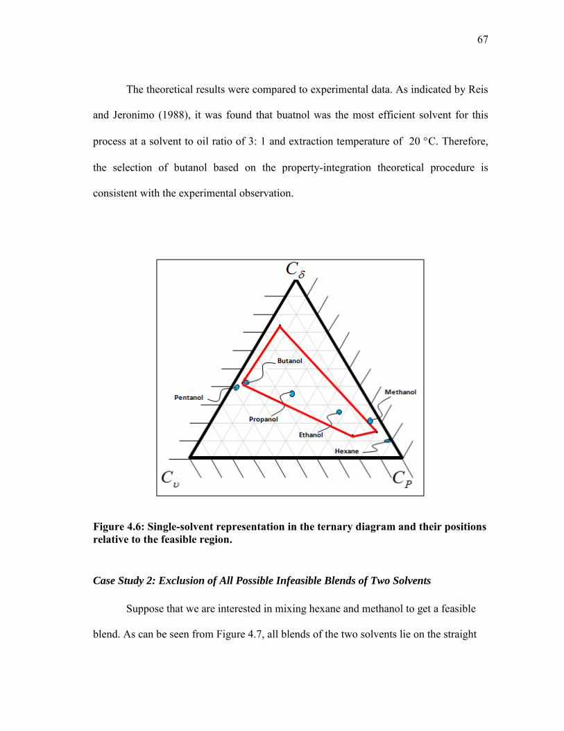
67
The theoretical results were compared to experimental data. As indicated by Reis
and Jeronimo (1988), it was found that buatnol was the most efficient solvent for this
process at a solvent to oil ratio of 3: 1 and extraction temperature of 20 C. Therefore,
the selection of butanol based on the property-integration theoretical procedure is
consistent with the experimental observation.
Figure 4.6: Single-solvent representation in the ternary diagram and their positions relative to the feasible region.
Case Study 2: Exclusion of All Possible Infeasible Blends of Two Solvents
Suppose that we are interested in mixing hexane and methanol to get a feasible
blend. As can be seen from Figure 4.7, all blends of the two solvents lie on the straight
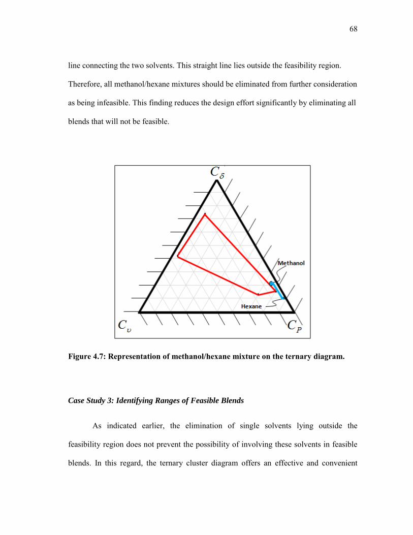
68
line connecting the two solvents. This straight line lies outside the feasibility region.
Therefore, all methanol/hexane mixtures should be eliminated from further consideration
as being infeasible. This finding reduces the design effort significantly by eliminating all
blends that will not be feasible.
Figure 4.7: Representation of methanol/hexane mixture on the ternary diagram.
Case Study 3: Identifying Ranges of Feasible Blends
As indicated earlier, the elimination of single solvents lying outside the
feasibility region does not prevent the possibility of involving these solvents in feasible
blends. In this regard, the ternary cluster diagram offers an effective and convenient
69
approach to visually determine feasible blends and the proportions of the participating
solvents. For instance, as shown in Figure 4.8, any blend of propanol and hexane is
represented by the dashed line connecting the two solvents (shown on the figure as a
dashed line). The segment lying outside the feasibility region is labeled as A, while the
segment lying inside the feasibility region is labeled as B. Based on the lever-arm rule,
section A corresponds to the mixture of hexane to propane ratio greater than 0.9. These
are infeasible mixtures. For section B, we conducted an AUP test to identify the ratios
between the two solvents and validate this performance with the experimentally reported
data. After running the AUP test on the mixture, a feasible mixture was found to exist of
all mixtures with propanol percentage between 72 and 90%. Reis and Jeronimo (1989)
experimentally measured the performance of a mixed solvent of 75% propanol and 25%
hexane and concluded that it was an effective blend. This is consistent with the range of
feasible solvents identified by our approach.
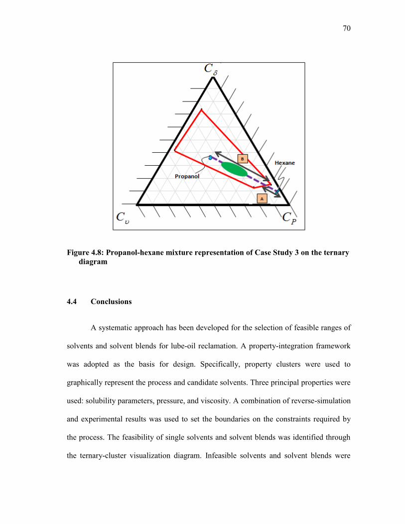
70
Figure 4.8: Propanol-hexane mixture representation of Case Study 3 on the ternary diagram
4.4 Conclusions
A systematic approach has been developed for the selection of feasible ranges of
solvents and solvent blends for lube-oil reclamation. A property-integration framework
was adopted as the basis for design. Specifically, property clusters were used to
graphically represent the process and candidate solvents. Three principal properties were
used: solubility parameters, pressure, and viscosity. A combination of reverse-simulation
and experimental results was used to set the boundaries on the constraints required by
the process. The feasibility of single solvents and solvent blends was identified through
the ternary-cluster visualization diagram. Infeasible solvents and solvent blends were

71
determined and removed from further consideration. Also, all ratios of solvent blends
leading to feasible mixtures were determined. Three case studies were solved and
compared to demonstrate the effectiveness of the devised approach. Experimental
observations were used to confirm the validity of the approach and theoretical results.
In addition to its effectiveness in selecting solvents and blends and designing
lube-oil reclamation processes, the proposed approach also serves as the basis for
guiding experimental work by identifying feasible and promising solvents and blends
and by shedding light on the insights on the design aspects.
Recommended future work includes the development of an optimization
approach to extend the applicability of the procedure to more than three key properties
and to automate the decision-making process and use it as a basis for the optimization of
solvent selection and process design.
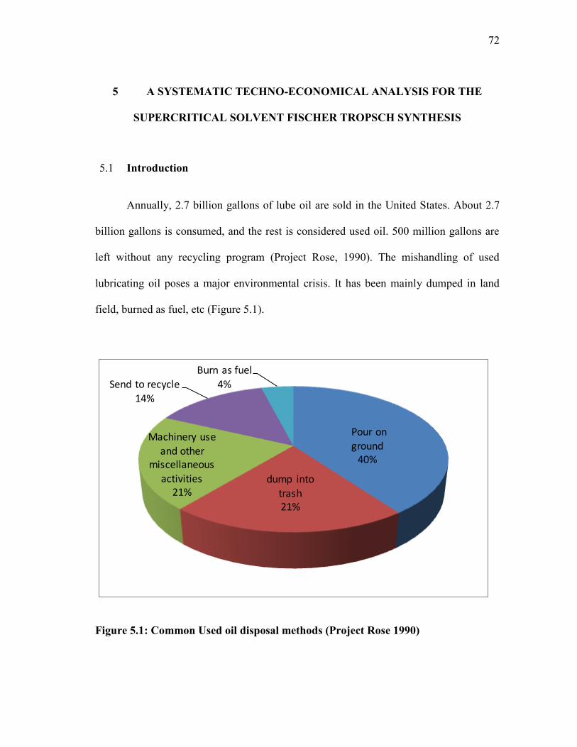
72
5 A SYSTEMATIC TECHNO-ECONOMICAL ANALYSIS FOR THE
SUPERCRITICAL SOLVENT FISCHER TROPSCH SYNTHESIS
5.1 Introduction
Annually, 2.7 billion gallons of lube oil are sold in the United States. About 2.7
billion gallons is consumed, and the rest is considered used oil. 500 million gallons are
left without any recycling program (Project Rose, 1990). The mishandling of used
lubricating oil poses a major environmental crisis. It has been mainly dumped in land
field, burned as fuel, etc (Figure 5.1).
Figure 5.1: Common Used oil disposal methods (Project Rose 1990)
Pour on ground
40%
dump into
trash21%
Machinery use
and other miscellaneous
activities21%
Send to recycle
14%
Burn as fuel4%
73
Most of these actions are harmful for the environment such as leakage into
waterways, and irresponsible toward our future generation duties such as depletion of
natural resources. The recycling of used lubricating oil is a more sustainable form of
action. It makes sense not only from the environmental point of view but economic as
well. If the used oil is fed to a boiler, a net saving of $0.65/gal could be achieved.
However, a net saving of $1.50/gal could be realized if it is recycled (Project Rose,
1990). Chemical and physical methods have been developed to recycle the used
lubricating oil. The chemical method is acid-sludge re-refining technique. It involves the
use of sulfuric acid as a solvent. The main disadvantage of such a process is the acidic
sludge produced. It is more harmful than the base oil itself. The other re-refining
technique is the physical method where the separation occurs at very high temperature
which causes the lube oil to break down. Therefore, the main disadvantages of this
technique are the low quality base oil produced, and high volume requirement for
economic purposes. Solvent extraction yields the advantages and eliminates the
disadvantages of both processes. High volume is not required; organic sludge is
produced; high quality base oil is produced.
74
The recycling of used lubricating oil not only helps in the preservation of natural
resources, but also reduces the dependency on foreign oil. This work is unique because
the developed optimization formulation not only reveals the identity of the optimal
solvent but also targets the optimal operating conditions based on profitability.
5.2 Solvent Extraction Process Description and Problem Statement
Due to the stability of the heavy base oil molecules, the base oil itself stays intact
after usage. One gallon of lube oil yields 0.7 gallon of re-refined oil (Everest, 2005). The
re-refining of used lubricating oil’s job is to completely remove the metals and worn
additives from base oil. This is not an easy task to accomplish. The solvent extraction
process could be designed in many different ways. However, there are three essentials
unites needed in order to accomplish the desired task. If further detailed design of units
is requested, simulation data will be needed in order to include all design elements in the
process. Therefore, a generic block flow diagram of the solvent extraction process could
be shown in Figure 5.2.
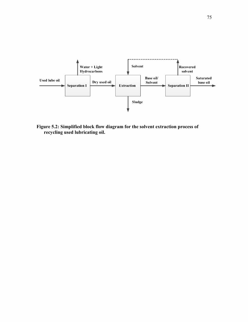
75
Figure 5.2: Simplified block flow diagram for the solvent extraction process of recycling used lubricating oil.
76
Used lubricating oil is fed to separation unit I (atmospheric distillation column)
to remove water and light hydrocarbons. Dry used oil is collected as bottom of the
column. Then, it is mixed with the organic solvent. Two phase solution is formed.
Organic sludge (bottom phase) is constituted of contaminants and lost oil/solvent
mixture. The upper phase contains the base oil and solvent mixture. The organic sludge
is easy to handle. For instance, it could be collected and sold for ink or asphalt
industries. The oil/solvent mixture is sent to separation unit II for complete regeneration
of solvent. In order to prevent the breakdown of base oil molecules at high temperature,
it is suggested to use both atmospheric and vacuum distillation columns.
5.3 Problem Statement
This section presents the model formulation for the optimization process, and
these equations are based on the representation of figure 5.3.
Note that figure 5.3 includes different equipments/units which may or may not be used
to accomplish the desired task. Therefore, it has been left to the optimization to decide
whether certain equipments are needed or not. Also, figure 5.3 shows only three units,
but the formulation includes the option of infinite number of stages. The optimization
will decide if it is worth to spend the extra capital investment for the extra unit(s) to be
purchased in order to remove the excess contaminants.
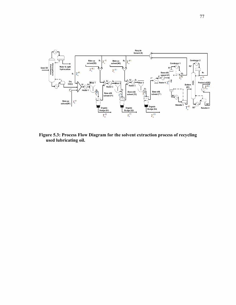
77
Figure 5.3: Process Flow Diagram for the solvent extraction process of recycling used lubricating oil.
78
There are many rooms for optimization within the process. The extraction unit
depends on three major factors. First of all, the solvent type and cost are very important
variables to be considered in the formulation. Solvent type affects the percent sludge
removal (PSR) and Percent oil Loss (POL). Note that PSR and POL are primary
parameters used for the evaluation of extraction performance. It is desired to yield the
lowest POL and the highest PSR possible. Another major factor is the operating
temperature. For instance, the higher the temperature the higher the miscibility of
solvents in oil is, but the lower the PSR is. Therefore, there is an optimal temperature at
which the chosen solvent should operate taking into account cost of heating
simultaneously. Last but not least, solvent to oil ratio (SOR) poses limitation on both
POL and PSR. In order to achieve solvent saturated mixture, high SOR is desired.
However, the higher the SOR is, the more make-up solvent and regeneration cost are
associated with such a desire. Also, it is very important to note as it has been shown
experimentally that there is an optimal SOR at which the addition of more solvent does
not cause further separation. In other words, at SOR >SORoptimal, POL and PSR remain
almost constant. This will be shown later in the case study. It is worth to note that the
limitation on the PSR affects the number of stages required in order to remove all
contaminants. This, in terms, affects the capital and operating cost of the extraction unit.
Next, the separation unit is part of the process, it has been considered in the
holistic optimization formulation. The optimal separation temperature in both the
atmospheric (SU) and vacuum distillation (VDU) has been targeted. Temperature as well
as solvent type and SOR affect the solvent recovery and operating and capital cost of
79
both columns including condensers and reboilers. Therefore, the consideration of both
units simultaneously is essential and shows the uniqueness of this work.
5.3.1 Mass Balance
This section presents the material balances in the representation of Figure 5.3.
First, the material balance around Mixer 1 is stated as follows.
111 GRUM (1)
In previous equation M1 is solvent make up fed to mixer 1, U is the mass flowrate
of dry based oil, R1 is the flowrate of regenerated/recycled solvent to extraction stage 1,
G1 is the flowrate of mixture fed to stage 1.
Material balance around mixer i with i> 1 can be stated as follows:
11 iRFMG iiii (2)
where Mi is the flowrate of solvent make-up fed to mixer i, Fi-1 is the flowrate leaving
the top of decanter i-1 before fed to the next mixer i, Ri is the flowrate of
recycled/recovered solvent to stage i, and Gi is the flowrate of mixture fed to decanter i.
The material balance around decanter i is:
IiSFG iii (3)
with i is the number of stages and it takes values of 1,2,3…istages, Fi is the flowrate of
solvent/oil mixture leaving decanter i, and Si is the flowrate of sludge leaving decanter i.
Material balance around atmospheric column (SU):
FBRa 1 (4)
80
where Ra is the flowrate of the recovered solvent leaving the top of the atmospheric
column, B1 is the bottom of the atmospheric column, F is the flowrate leaving the top of
the last decanter.
Material balance around vacuum distillation column (VDU):
21 BRB b (5)
where Rb is the flowrate of the recovered solvent leaving the top of the vacuum column,
B2 is the bottom of the vacuum column which should include the saturated base oil.
Material balance of recovered solvent:
IiRRRR ba
i
i 1
(6)
5.3.2 Component Material Balance
Similar to the mass balance, there are component balances for the base oil,
contaminants and solvent in the different sections of the diagram.
The component balance around mixer 1 is stated as follows:
NnYGYRYUYM G
n
R
na
U
n
M
na 1
1
1
1 **** (7)
In previous equation Yn is the composition by weight of component N given,
where 3,2,1N , and n=1 corresponds to the base oil, n=2 is used for the contaminants
and n=3 is for the solvent.
Component balance around mixer i and decanter i consecutively:
NnYGYRYFYM Gi
ni
Ri
ni
F
ni
Mi
nii
**** 1
1 (8)
NnYSYFYG Si
ni
Fi
ni
Gi
ni *** (9)
81
Component balance around SU and VDU consecutively:
NnYFYBYR F
n
B
n
Ra
na 11
1 *** (10)
NnYBYBYR B
n
B
n
Rb
nb 1
1
2
2 *** (11)
Component balance for the total recycled solvent is as follow:
NnYRYRYR R
n
R
n
R
n 2
2
1
1 *** (12)
5.3.3 Heat Balance
The heat balance around heat exchanger i corresponding to stage i in the
extraction unit is expressed as follow:
)(** '_
_
GiGiimix
piiHeater TTCGQ (13)
where Qheater_i is the heat load needed to increase/decrease the temperature from its value
TGi’ to an optimal extraction temperature TGi, and CPmix_i is the heat capacity of the
mixture.
Since the extraction will occur in liquid phase, it can be correlated to the pure
component values as follow:
n
p
Gi
n
imix
p nCYC *_ (14)
where Cpn is the heat capacity of pure component n and it is function of temperature.
The heat balance data around both reboilers and condensers of the distillation
columns could be extracted from ASPEN PLUS and to determine the dependence of
operating temperature.
82
5.3.4 Equilibrium Equations
The percent sludge removal (PSR) is the mass of dry sludge being removed in
grams per 100 g of used oil (Reis and Jernimo, 1988).. Therefore, the PSR from stage 1
is expressed as follow:
IiGY
SYPSR
i
Gi
i
Si
i
*)1(
*
3
2 (15)
),,( iii SORTtypesolventPSRPSR (16)
The percent oil loss is defined as the mass of base oil lost with the sludge in
grams per 100 g of used oil (Reis and Jernimo, 1988, and Elbashir et al., 2002), and it is
shown in the following equation:
IiGY
SYPOL
i
Gi
i
Si
i
*)1(
*
3
1 (17)
),,( iii SORTtypesolventPOLPOL (18)
A new variable K is defined to express the equilibrium equations in both the SU
and VDU units. Kn is the ratio of the mass fraction of component n of the bottom of the
column divided by the mass fraction of top stream. Therefore, the K relationship for the
component n in both SU and VDU is expressed consecutively as follow:
NnY
YK
Ra
n
B
nn
11 (19)
NnY
YK
Rb
n
B
nn
22 (20)
Separationseparation
n PTKK , (21)
83
5.4 Optimization Formulation
Most of the work done on the solvent extraction optimization is to find the
optimal solvent with the lowest POL and highest PSR regardless of cost. This might be a
good indication for an optimal solution, but it is not sufficient from a holistic approach.
A look at the process as a whole is necessary to find the optimal solution. As is the case
in most optimization formulations, an objective function that maximizes profit is needed,
and for this case the net profit is stated as follows:
CostSalesofitMaximize Pr (22)
sludgeSaleoilSaleSales __ (23)
wtSludgeStoilBoilSale *cos_*cos_*_ 2 (24)
where W is the hours of operation per year, Oil_cost is the cost of base oil per Kg,
Sludge_cost is the cost of sludge per Kg that could be obtained from ink or asphalt
industries.
Note that S is the combination of all the sludge leaving the extraction unit and
could be expressed as follows:
,i
i
S S i I (25)
Then, the annual cost is the summation of both annual operation cost and annual
capital cost, and it could be calculated as follow:
OperationCostCapitalCostCost __ (26)
84
The capital cost includes all major pieces of equipment in the whole process and
it is defined as:
VDUCostSUCostMixerDecanterCostHexCostCapitalCosti
i
i i
ii _____ (27)
where Cost_Hexi is the annual cost of the heat exchanger needed in stage i, which is
responsible on bringing the temperature of mixture to optimal extraction temperature,
Cost_Decanteri and Cost_Mixeri are the annual costs for the decanter and the mixer in
stage i, respectively. Cost_SU is the annual cost of the atmospheric column needed for
the separation, this includes the capital cost of the condenser and reboiler associated with
the column, and Cost_VDU is the annual capital cost of the vacuum distillation column
required, this includes the capital cost of condenser and reboiler associated with the
column.
The equations that describe the annual capital cost of these equipments are
shown below:
iiHeateriHeater
vc
iHeater
FCi ACCHeaterCost )(*_ (28)
iimixerimixer
vc
imixer
FCi VCCMixerCost )(*_ (29)
iiDecanteriDecanter
vc
iDecanter
FCi ACCDecanterCost )(*_ (30)
),,,,,(_ 1B
n
Ra
n
F
n
FF YYYPTFfSUCost (31)
),,,,1(_ 211 B
n
Rb
n
B
n
B YYYTBfVDUCost (32)
Another major cost that contributes to the total annual cost is the annual
operation cost, which depends on so many factors. It includes the cost of heating/cooling
85
needed for an optimal operating condition as well as the solvent make up cost. It is
calculated as follows:
CostupMakeboilingCostgCondenCostHeatingCostOperationCosti
i __Re_sin___ (33)
Note that Cost_Heatingi is the annual heat duty cost of stage i required to
increase the mixture temperature Ti to the optimal extraction temperature Tiopt. This cost
is obtained as the product of heat duty Qi times the heating utility cost multiplied by the
yearly hours of operation:
wHUCostQHeatingCost ii *_*_ (34)
where Cost_Condensing is the total condensing cost required by both columns and
Cost_Reboiling is the total reboiling cost required by both columns.
The Make_up_cost is expressed as follow:
i
i wSolventCostMtupMake *_*cos__ (35)
5.5 Case Study and Results
This section presents a case study to show the applicability of the proposed
optimization formulation.
5.5.1 Data Collection
To illustrate the applicability of the proposed optimization approach, a case is
presented. In this case, Methyl Ethyl Ketone (MEK) and Butanol have been chosen as
solvents of interest. As it has been proven previously (Nimir, 1997), MEK yields the
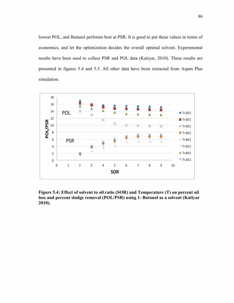
86
lowest POL, and Butanol performs best at PSR. It is good to put these values in terms of
economics, and let the optimization decides the overall optimal solvent. Experimental
results have been used to collect PSR and POL data (Katiyar, 2010). These results are
presented in figures 5.4 and 5.5. All other data have been extracted from Aspen Plus
simulation.
0
2
4
6
8
10
12
14
16
18
0 1 2 3 4 5 6 7 8 9 10
PO
L/P
SR
SOR
T=20 C
T=30 C
T=50 C
T=30 C
T=40 C
T=50 C
T=40 C
T=20 C
POL
PSR
Figure 5.4: Effect of solvent to oil ratio (SOR) and Temperature (T) on percent oil loss and percent sludge removal (POL/PSR) using 1- Butanol as a solvent (Katiyar 2010).
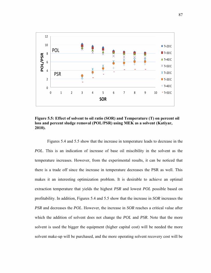
87
0
2
4
6
8
10
12
0 1 2 3 4 5 6 7 8 9 10
PO
L/P
SR
SOR
T=20 C
T=30 C
T=40 C
T=50 C
T=20 C
T=30 C
T=40 C
T=50 C
POL
PSR
Figure 5.5: Effect of solvent to oil ratio (SOR) and Temperature (T) on percent oil loss and percent sludge removal (POL/PSR) using MEK as a solvent (Katiyar, 2010).
Figures 5.4 and 5.5 show that the increase in temperature leads to decrease in the
POL. This is an indication of increase of base oil miscibility in the solvent as the
temperature increases. However, from the experimental results, it can be noticed that
there is a trade off since the increase in temperature decreases the PSR as well. This
makes it an interesting optimization problem. It is desirable to achieve an optimal
extraction temperature that yields the highest PSR and lowest POL possible based on
profitability. In addition, Figures 5.4 and 5.5 show that the increase in SOR increases the
PSR and decreases the POL. However, the increase in SOR reaches a critical value after
which the addition of solvent does not change the POL and PSR. Note that the more
solvent is used the bigger the equipment (higher capital cost) will be needed the more
solvent make-up will be purchased, and the more operating solvent recovery cost will be
88
indicated. Note that deriving equations (16) and (18) from both figures is not an easy
task to perform. Lingo optimization software has been used to derive these equations.
This was done by composing an objective function that minimizes the error between the
experimental and calculated values. A generic equation with multiple unknown
parameters and two variables (SOR and T) was assigned in order to evaluate the
calculated values. The value of the error squared was less than 4 in all cases given 32
data points for each equation. This indicated good plot fitting approach, and shows that
the generic equation provided was relatively good.
2.51851T0.15175)SOR (-0.413386.51903exp15.691 ii BUTANOL
iPOL (35)
2.313249T0.042875)SOR (-0.3865766.89802exp6.71806 ii MEK
iPOL (36)
ii T0.0555)SOR (1.669866ln 3.291565 BUTANOL
iPSR (37)
ii T0.062)SOR (1.331624ln 3.303513 MEK
iPSR (38)
Note that Ti is in degree Celsius.
To highlight the importance of operation cost, it is assumed that the process
already exists, and no need to purchase any pieces of equipment. Therefore, the capital
cost is ignored from the objective function. The distillation columns separation data have
been obtained using Aspen Plus (refer to Appendix A). Note that condensing, reboiling,
and extraction heat duties were extracted from Aspen Plus as well.
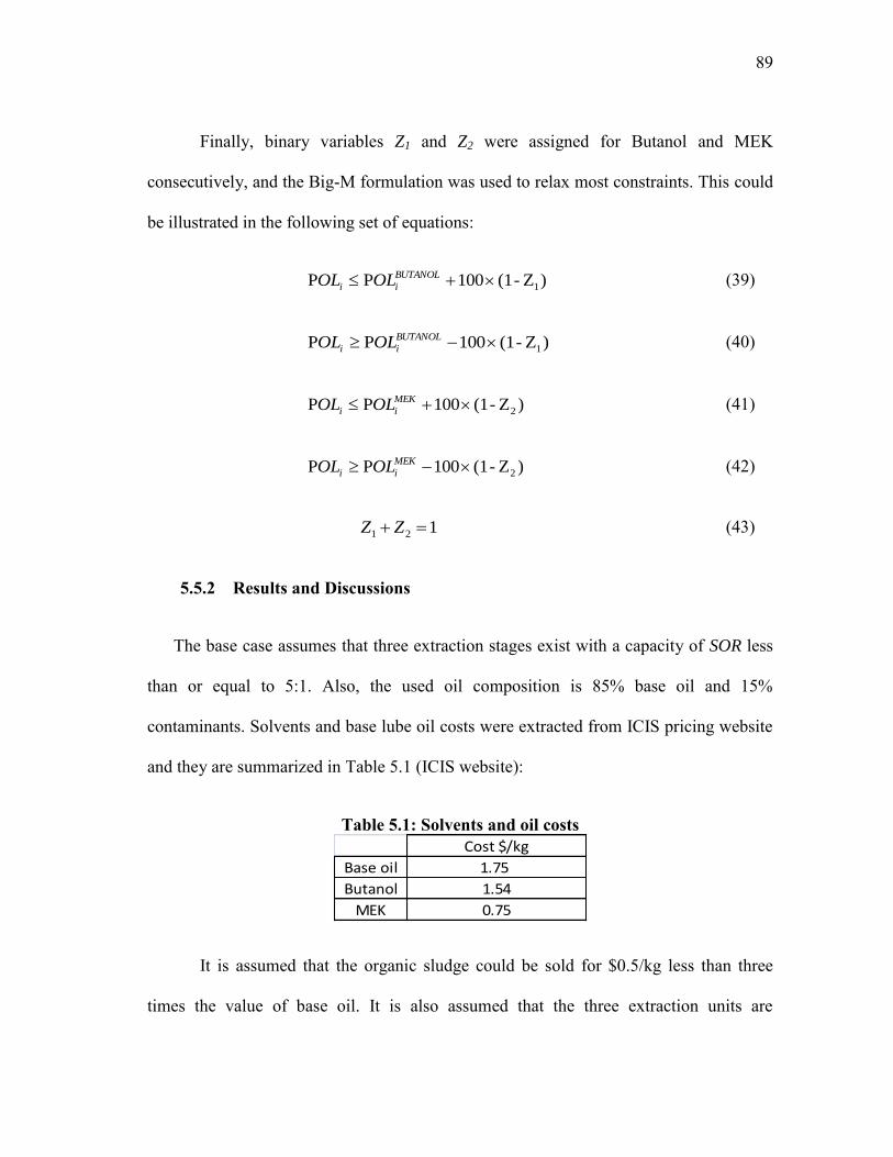
89
Finally, binary variables Z1 and Z2 were assigned for Butanol and MEK
consecutively, and the Big-M formulation was used to relax most constraints. This could
be illustrated in the following set of equations:
)Z-(1100PP 1 BUTANOL
ii OLOL (39)
)Z-(1100PP 1 BUTANOL
ii OLOL (40)
)Z-(1100PP 2 MEK
ii OLOL (41)
)Z-(1100PP 2 MEK
ii OLOL (42)
121 ZZ (43)
5.5.2 Results and Discussions
The base case assumes that three extraction stages exist with a capacity of SOR less
than or equal to 5:1. Also, the used oil composition is 85% base oil and 15%
contaminants. Solvents and base lube oil costs were extracted from ICIS pricing website
and they are summarized in Table 5.1 (ICIS website):
Table 5.1: Solvents and oil costs Cost $/kg
Base oil 1.75
Butanol 1.54
MEK 0.75
It is assumed that the organic sludge could be sold for $0.5/kg less than three
times the value of base oil. It is also assumed that the three extraction units are
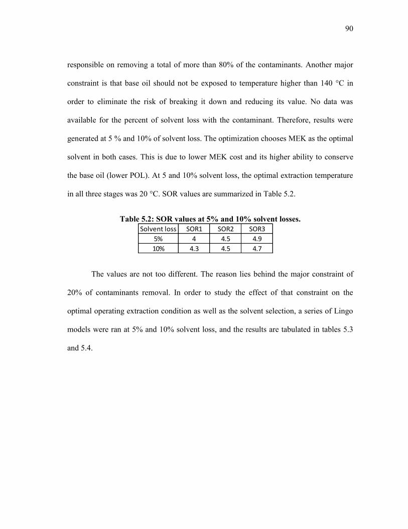
90
responsible on removing a total of more than 80% of the contaminants. Another major
constraint is that base oil should not be exposed to temperature higher than 140 °C in
order to eliminate the risk of breaking it down and reducing its value. No data was
available for the percent of solvent loss with the contaminant. Therefore, results were
generated at 5 % and 10% of solvent loss. The optimization chooses MEK as the optimal
solvent in both cases. This is due to lower MEK cost and its higher ability to conserve
the base oil (lower POL). At 5 and 10% solvent loss, the optimal extraction temperature
in all three stages was 20 °C. SOR values are summarized in Table 5.2.
Table 5.2: SOR values at 5% and 10% solvent losses.
The values are not too different. The reason lies behind the major constraint of
20% of contaminants removal. In order to study the effect of that constraint on the
optimal operating extraction condition as well as the solvent selection, a series of Lingo
models were ran at 5% and 10% solvent loss, and the results are tabulated in tables 5.3
and 5.4.
Solvent loss SOR1 SOR2 SOR3
5% 4 4.5 4.9
10% 4.3 4.5 4.7
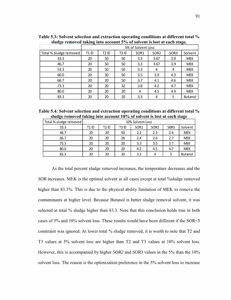
91
Table 5.3: Solvent selection and extraction operating conditions at different total % sludge removed taking into account 5% of solvent is lost at each stage.
Total % Sludge removed T1 © T2 © T3 © SOR1 SOR2 SOR3 Solvent
33.3 20 50 50 3.3 3.67 3.9 MEK
46.7 20 50 50 3.3 3.67 3.9 MEK
53.3 20 50 50 3.3 4 4 MEK
60.0 20 30 50 3.5 3.9 4.3 MEK
66.7 20 20 50 3.7 4.1 4.6 MEK
73.3 20 20 32 3.8 4.2 4.7 MEK
80.0 20 20 20 4 4.5 4.9 MEK
83.3 20 20 20 3.3 4 5 Butanol
5% of Solvent Loss
Table 5.4: Solvent selection and extraction operating conditions at different total % sludge removed taking into account 10% of solvent is lost at each stage
Total % sludge removed
33.3 T1 © T2 © T3 © SOR1 SOR2 S0R3 Solvent
46.7 20 20 50 2.2 2.3 2.4 MEK
66.7 20 20 26 2.4 2.6 2.7 MEK
73.3 20 20 20 3.3 3.5 3.7 MEK
80.0 20 20 20 4.2 4.5 4.7 MEK
83.3 20 20 20 3.3 4 5 Butanol
10% Solvent Loss
As the total percent sludge removed increases, the temperature decreases and the
SOR increases. MEK is the optimal solvent in all cases except at total %sludge removed
higher than 83.3%. This is due to the physical ability limitation of MEK to remove the
contaminants at higher level. Because Butanol is better sludge removal solvent, it was
selected at total % sludge higher than 83.3. Note that this conclusion holds true in both
cases of 5% and 10% solvent loss. These results would have been different if the SOR<5
constraint was ignored. At lower total % sludge removed, it is worth to note that T2 and
T3 values at 5% solvent loss are higher than T2 and T3 values at 10% solvent loss.
However, this is accompanied by higher SOR2 and SOR3 values in the 5% than the 10%
solvent loss. The reason is the optimization preference in the 5% solvent loss to increase
92
the temperature indicating lower oil loss and sacrificing higher SOR (higher solvent loss)
at 5% rate of solvent loss. However, in the 10% solvent loss, the optimization tendency
was to decrease the temperature indicating higher percent oil loss and decreasing SOR to
decrease the amount of solvent loss at 10% rate of solvent loss.
Another important factor to be studied is the MEK and Butanol prices variation.
If MEK price stays the same at $0.75/kg, at what price Butanol or a solvent that
performs the same as Butanol should be in order to be optimal? This solvent price value
is different in both 5% and 10% solvent loss cases. In the 5% solvent loss case, Butanol
or equivalent solvent should be at $0.35/kg or lower to become favored. In the 10%
solvent loss case, Butanol or equivalent solvent should be at $0.55/kg or lower in order
to become favored over MEK.
Now, if Butanol price stays the same at $1.54/kg, up to what price MEK or a
solvent that performs the same as MEK stays favored over Butanol? This value is
different in both 5% and 10% solvent loss cases. In the 5% solvent loss case, MEK or
equivalent solvent could be at a cost of $1.7/kg or lower to stay favored over butanol. In
the 10% solvent loss case, MEK or equivalent solvent could be at $1.54/kg or lower in
order to stay favored over Butanol.
Another sensitivity analysis is done over the quality of base oil. It is assumed that
the SOR constraint is not valid, and therefore SOR could have a value greater than 5.
This was done by the keeping the constraint on the contaminant composition leaving the
last extraction unit with base oil/solvent mixture to be less than 3% of the used oil fed to
the first extraction unit. The quality of base oil was varied by changing the composition
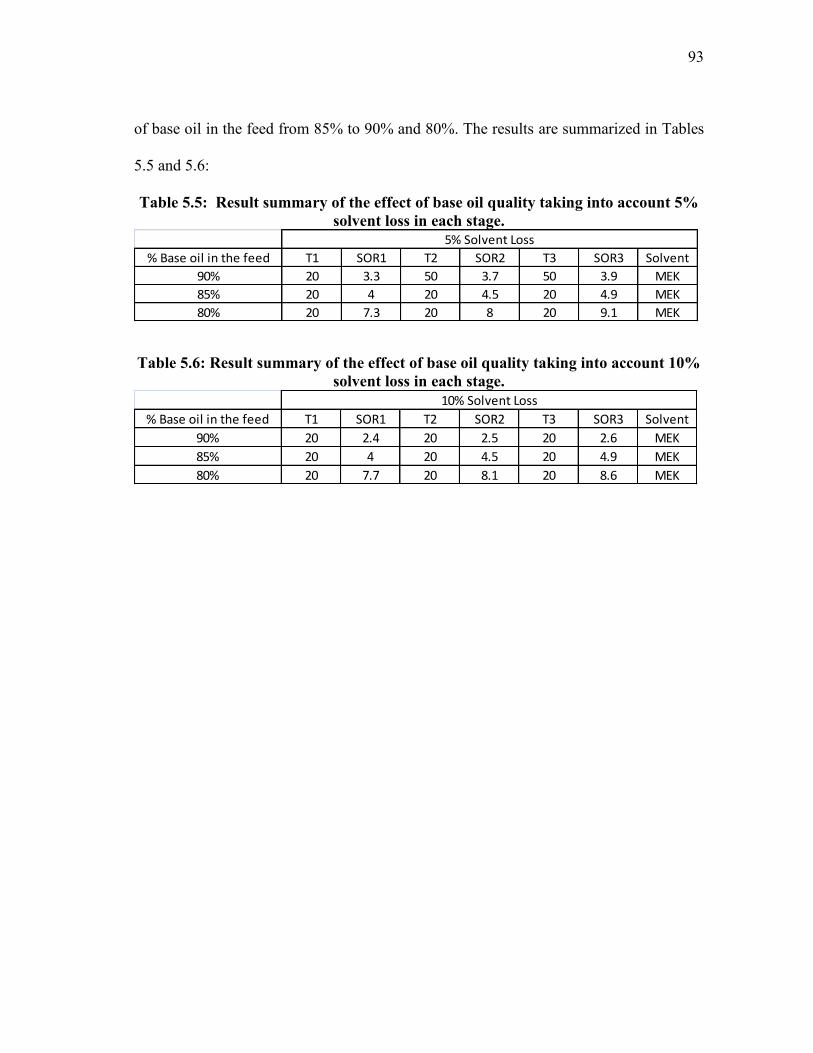
93
of base oil in the feed from 85% to 90% and 80%. The results are summarized in Tables
5.5 and 5.6:
Table 5.5: Result summary of the effect of base oil quality taking into account 5% solvent loss in each stage.
% Base oil in the feed T1 SOR1 T2 SOR2 T3 SOR3 Solvent
90% 20 3.3 50 3.7 50 3.9 MEK
85% 20 4 20 4.5 20 4.9 MEK
80% 20 7.3 20 8 20 9.1 MEK
5% Solvent Loss
Table 5.6: Result summary of the effect of base oil quality taking into account 10% solvent loss in each stage.
% Base oil in the feed T1 SOR1 T2 SOR2 T3 SOR3 Solvent
90% 20 2.4 20 2.5 20 2.6 MEK
85% 20 4 20 4.5 20 4.9 MEK
80% 20 7.7 20 8.1 20 8.6 MEK
10% Solvent Loss
94
Tables 5.5 and 5.6 show that MEK is the optimal solvent, and this is due to its
lower cost and its high ability in preserving the oil (low POL). The results in both tables
are similar in the 85% and 80% case. However the results are different in the 90% case.
This is due to the operating condition flexibility of MEK in removing lower amount of
contaminants. In the case of 10% solvent loss, lower temperature and lower SOR were
favored in order to decrease the amount of solvent loss. In the case of 5% solvent loss,
higher temperature and higher SOR were favored since the solvent loss is at lower rate.
In the 85% and 80%, MEK does not have a lot of operating condition flexibility in
removing the large amount of contaminants. The low temperature and high SOR were
necessary to satisfy the total sludge removal constraint.
Note that these results depend heavily on the assumptions made as well as the
solvents chosen for this case study. The results will be a lot different if they were to
change. Also, it would be different if this case study gave the optimization the flexibility
of deciding the number of units based on cost as shown in the generic formulation. Also,
note that this formulation could be applied not only to single solvents as shown in the
case study, but it also applies to solvent blends as well.
95
5.6 Conclusions
This paper presents an optimization formulation for the optimal production oil
from used oil through different solvents and configurations. This formulation takes into
account the capital cost as well as the operating cost associated with each solvent. The
proposed model was tested for the use of Butanol and MEK as solvent considering
experimental data and data obtained from simulation. Results show that Butanol
performs better from PSR point of view; whereas, MEK performs better from POL stand
point. In most cases, MEK was favored due to its lower cost and higher ability to
preserve our valuable base oil product.
As of future work, it would important to include safety metrics in the formulation
in order to eliminate the risk of using hazardous solvents as well as the decrease the risk
associated to the operating conditions required. In addition, it will be important to
address a case study with the inclusion of the capital cost and show its effect on the
optimal results. Finally, heat integration could be another economic incentive.
96
6 CONCLUSIONS AND RECOMMENDATION FOR FUTURE WORK
This work has introduced systematic approaches for the recycle and reclamation of
material utilities and spent products. In the area of material-utility (e.g., water) recycle; a
new process-synthesis procedure has introduced to addresses, for the first time, the
simultaneous handling of concentrations, temperature, and properties to characterize the
process streams and constraints. This has been done, taking into account the
interdependency of properties and their dependency on concentrations and temperature.
An optimization formulation has been developed to identify optimal allocation of
sources to sinks that will minimize the network cost while satisfying all process and
environmental constraints. A case study on water recycle in a phenol production plant
has been solved.
A systematic approach has also been developed for the selection of feasible ranges
of solvents and solvent blends for lube-oil reclamation. A property-integration
framework was adopted as the basis for design. Specifically, property clusters were used
to graphically represent the process and candidate solvents. Three principal properties
were used: solubility parameters, pressure, and viscosity. A combination of reverse-
simulation and experimental results was used to set the boundaries on the constraints
required by the process. The feasibility of single solvents and solvent blends was
identified through the ternary-cluster visualization diagram. Infeasible solvents and
solvent blends were determined and removed from further consideration. Also, all ratios
of solvent blends leading to feasible mixtures were determined. Next, an optimization
formulation was developed to identify the key design and operating variables of the
97
system as well as the selection of the optimal solvent(s) for extraction. Key parameters
were considered such as percent oil loss (POL), percent sludge removal (PSR), and their
dependency on temperature and solvent to oil ratio (SOR). Three case studies were
solved and compared to demonstrate the effectiveness of the devised approach.
Experimental observations were used to confirm the validity of the approach and
theoretical results.
In addition to its effectiveness in selecting solvents and blends and designing lube-
oil reclamation processes, the proposed approach also serves as the basis for guiding
experimental work by identifying feasible and promising solvents and blends and by
shedding light on the insights on the design aspects.
Recommended future work includes the following:
Inclusion of heat integration in the design of material-utility recycle networks
Incorporating additional properties (e.g., density) in the reclamation of lube oil
Comparison of extraction-based reclamation networks to other recovery and disposal
alternatives (e.g., thermal conversion)
Incorporation of safety metrics for the solvents and the process into the optimization
formulation to generate inherently safer designs
Design of flexible systems that can respond to the dynamic fluctuations in the
characteristics of wastewater streams.
Inclusion of life cycle analysis for the used materials and the designed processes.
98
REFERENCES
Alva-Argaez, A., Kokossis, A. C., Smith, R., 1998. Wastewater minimisation of
industrial systems using an integrated approach. Computers & Chemical
Engineering 22, S741-S744.
Alves, J. J., Towler, G. P., 2002. Analysis of refinery hydrogen distribution systems.
Industrial & Engineering Chemistry Research 41 (23), 5759-5769.
Arrhenius, S., 1887. The viscosity of aqueous mixtures. Z. Phys. Chem. 1, 285-298.
Barton, A.F.M., 1991. Handbook of Solubility Parameters and Other Cohesion
Parameters, CRC Press, Florida.
Chemmangattuvalappil N.G., Solvason C.C., Bommareddy S., Eden M.R., 2010
Combined property clustering and GC+ techniques for process and product
design. Computers and Chemical Engineering 34, 582-591.
Chen, C.L., Ng, D. K. S., Foo, D. C. Y., 2010. A Unified Model of Property Integration
for Batch and Continuous Processes. AIChE Journal (in press).
Dhole, V. R., Ramchandani, N., Tainsh, R. A.; Wasilewski, M.,1996. Make your process
water pay for itself. Chemical Engineering 103 (1), 100-103.
Dunn, R. F., El-Halwagi, M. M., 2003. Process integration technology review:
background and applications in the chemical process industry. Journal of
Chemical Technology and Biotechnologyc78 (9), 1011-1021.
Elbashir, N. O., Al-Zahrani, S. M., Abdul Mutalib, M. I ., Abasaeed, A. E., 2002. A
method of predicting effective solvent extraction parameters for recycling used
oils. Chemical Engineering and Processing 41(9), 765-769.
El-Halwagi, M.M., 1997. Pollution Prevention Through Process Integration, Academic
Press, San Diego.
99
El-Halwagi, M. M., 2006. Process Integration. Academic Press, San Diego.
El-Halwagi, M. M., Gabriel, F., Harell, D., 2003. Rigorous graphical targeting for
resource conservation via material recycle/reuse networks. Industrial &
Engineering Chemistry Research 42 (19), 4319-4328.
El-Halwagi, M. M., Glaswog I. M., Qin, X. , Eden, M. R., 2004. Property integration:
Componentless design techniques and visualization tools. AIChE Journal 50(8),
1854-1869.
El-Halwagi, M. M., Hamad, A. A., 1996. Synthesis of waste interception and allocation
networks. AIChE Journal 42 (11), 3087-3101.
El-Halwagi, M. M., Spriggs, H. D., 1988. Solve design puzzles with mass integration.
Chemical Engineering Progress 94(8), 25-44.
Eljack, F.T., Eden, M.R., 2008. A visual approach to molecular design using property
clusters and group contribution. Computers and Chemical Engineering 32(12),
3002-3010.
Eljack, F.T., Eden, M.R., Kazantzi, V., El-Halwagi, M.M., 2007. Simultaneous solution
of process and molecular design problems via group contribution and property
clustering techniques. AIChE Journal 53(5), 1232-1239.
Faria, D. C., Bagajewicz, M. J., 2010. On the appropriate modeling of process plant
water systems. AIChE Journal 56 (3), 668-689.
Feng, X., Bai, J., Zheng, X. S., 2007. On the use of graphical method to determine the
targets of single-contaminant regeneration recycling water systems. Chemical
Engineering Science 62 (8), 2127-2138.
Fletche, L. C, Beard, B. J, O’Blasny, R.,1982. Distilation and Solvent Extraction Process
for Rerefining Used Lubrication Oil. U.S Patent 4,360,420.
100
Foo, D. C. Y., 2009. State-of-the-art review of pinch analysis techniques for water
network synthesis. Industrial & Engineering Chemistry Research 48 (11), 5125-
5159.
Foo, D. C. Y., Kazantzi, V., El-Halwagi, M. M., Manan, Z. A., 2006. Surplus diagram
and cascade analysis technique for targeting property-based material reuse
network. Chemical Engineering Science 61 (8), 2626-2642.
Foo, D. C. Y., Manan, Z. A., 2006. Setting the minimum utility gas flowrate targets
using cascade analysis technique. Industrial & Engineering Chemistry Research
45 (17), 5986-5995.
Gabriel, F. B., El-Halwagi, M. M., 2005. Simultaneous synthesis of waste interception
and material reuse networks: Problem reformulation for global optimization.
Environmental Progress 24 (2), 171-180.
Gunaratnam, M., Alva-Argaez, A. Kokossis, A.; Kim, J. K., Smith, R., 2005. Automated
design of total water systems. Industrial & Engineering Chemistry Research 44
(3), 588-599.
Hallale, N., 2002. A new graphical targeting method for water minimisation. Advances
in Environmental Research 6 (3), 377-390.
Hernandez-Suarez, R., Castellanos-Fernandez, J., Zamora, J. M., 2004. Superstructure
decomposition and parametric optimization approach for the synthesis of
distributed wastewater treatment networks. Industrial & Engineering Chemistry
Research 43 (9), 2175-2191.
Jezowski, J., 2010. Review of water network design methods with literature annotations.
Industrial & Engineering Chemistry Research 49 (10), 4475-4516.
Kamal, A., Khan, F., 2009. Effect of extraction and adsorption on re-refining of used
lubricating oil. Oil & Gas Science and Technology-Rev.IFP 2(64), 191-197.
101
Karuppiah, R., Grossmann, I. E., 2006. Global optimization for the synthesis of
integrated water systems in chemical processes. Computers & Chemical
Engineering 30 (4), 650-673.
Katiyar, V. and Husain, S., 2010. Recycling of used lubricating oil using 1-Butanol. Int.
J. Chem. Sci. 8(3).
Kazantzi, V., El-Halwagi, M. M., 2005. Targeting material reuse via property
integration. Chemical Engineering Progress 101 (8), 28-37.
Kazantzi, V., Qin, X., El-Halwagi, M.M., Eljack, F.T., Eden, M.R. 2007. Simultaneous
process and molecular design through property clustering techniques – A
visualization tool. Industrial & Engineering Chemistry Research 46(10), 3400-
3409.
Kheireddine, H. A., Elbashir, N. O. El-Halwagi, M.M., 2012. A property-integration
approach to solvent screening and conceptual design of solvent-extraction
systems for recycling used lubricating oils. Clean Technologies and
Environmental Policy (in Press).
King, C. J., 1971. Separation Processes. McGraw-Hill, New York.
Manan, Z. A., Tan, Y. L., Foo, D. C. Y., 2004. Targeting the minimum water flow rate
using water cascade analysis technique. AIChE Journal 50 (12), 3169-3183.
Nápoles-Rivera, F., Ponce-Ortega, J. M., El-Halwagi, M. M., Jiménez-Gutiérrez, A.
2010. Global optimization of mass and property integration networks with in-
plant property interceptors. Chemical Engineering Science 65 (15), 4363-4377.
Nimir, O.M , Abdul Mutalib, M.I., Adnan, R., 1997. Recycling of used lubricating oil
by solvent extraction .University Teknologi Malaysia. Regional Symposium on
Chemical Engineering, Malaysia. B2-4.
102
Ng. D. K. S., Foo, D. C. Y., Rabie, A. and El-Halwagi, M. M., 2008. Simultaneous
synthesis of property-based water reuse/recycle and interception networks for
batch processes. AIChE Journal 54(10), 2624-2632.
Ng, D. K. S., Foo, D. C. Y.; Tan, R. R., El-Halwagi, M.M., 2009. Automated targeting
for total property-based network. Computer Aided Chemical Engineering 26,
1189-1195.
Ng, D. K. S.; Foo, D. C. Y.; Tan, R. R.; El-Halwagi, M.M., 2010. Automated targeting
technique for concentration- and property-based total resource conservation
network. Computers & Chemical Engineering 34 (5), 825-845.
Ng, D. K. S., Foo, D. C. Y., Tan, R. R., Pau, C. H. and Tan, Y. L., 2009. Automated
targeting for conventional and bilateral property-based resource conservation
network. Chemical Engineering Journal 14 (9),87-101.
Ng, D. K. S., Foo, D. C. Y., Tan, R. R.; Tan, Y. L., 2007. Ultimate flowrate targeting
with regeneration placement. Chemical Engineering Research & Design 85 (A9),
1253-1267.
Polley, G. T., Polley, H. L., 2000. Design better water networks. Chemical Engineering
Progress 96 (2), 47-52.
Ponce-Ortega, J. M., El-Halwagi, M.M., Jiménez-Gutiérrez, A., 2010. Global
optimization for the synthesis of property-based recycle and reuse networks
including environmental constraints. Comp. Chem. Eng., 34(3), 318-330.
Ponce-Ortega, J. M., Hourtua, A. C., El-Halwagi, M. M., Jiménez-Gutiérrez, A. 2009. A
property-based optimization of direct recycle networks and wastewater treatment
processes. AIChE Journal. 55 (9), 2329-2344.
Project Rose, 1990. Used Motor Oil Re-refining and Recycling. University of Alabama,
Florida Department of Environmental Regulations.
103
Qin, X., Gabriel, F., Harell, D., El-Halwagi, M.M., 2004. Algebraic techniques for
property integration via componentless design. Ind. Eng. Chem.43, 3792-3798
Reis, M.A., Jeronimo, M.S., 1982. Fabrico de Tinta de Base Para Fabrico de Tinta de
Impressao a Partir de Oleos Usados. Portuguese Patent 75, 702.
Reis, M. A.; Jeronimo, M. S., 1988. Waste lubricating oil re-refining by extraction-
flocculation. 1. A Scientific basis to design efficient solvents. Ind. Eng. Chem.
Res. 27 (7), 1222-1228.
Reis, M. A, , Jernimo S. M., 1990. Waste lubricating oil rerefining by extraction-
flocculation 2.A Method to formulate efficient composite solvents. Ind. Eng.
Chem. Res. 29, 432-436.
Rincon, J., Canizares, P., Garcia, M.T., 1989. Regeneation of used lubricant oil by polar
solvent extraction. Ind. Eng. Chem. Res. 44, 4373.
Savelski, M., Bagajewicz, M., 2003. On the necessary conditions of optimality of water
utilization systems in process plants with multiple contaminants. Chemical
Engineering Science 58 (23-24), 5349-5362.
Shelley, M. D., El-Halwagi, M.M., 2000. Component-less design of recovery and
allocation systemas: A functionality-based clustering approach. Computers and
Chemical Engineering. 24(9-10), 2081-2091.
Solvason, C.C., Chemmangattuvalappil, N.G., Eden, M.R., 2009. Decomposition
techniques for molecular synthesis and structured product design. Computer
Aided Chemical Engineering 26, 153-158.
Sorin, M., Bedard, S., 1999. The global pinch point in water reuse networks. Process
Safety and Environmental Protection 77 (B5), 305-308.
Wang, Y., Smith, R., 1994. Wastewater minimisation. Chemical Engineering Science 49
(7), 981-1006.

104
Wilson, G. M., 1964. Vapor-Liquid equilibrium. XI. A new expression for the excess
free energy of mixing. Journal of the American Chemical Society 86 (2), 127-
130.
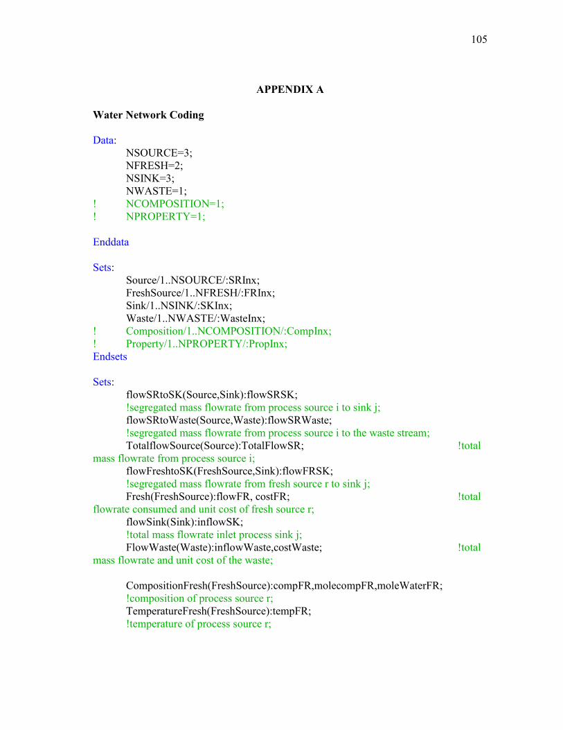
105
APPENDIX A
Water Network Coding
Data: NSOURCE=3; NFRESH=2; NSINK=3; NWASTE=1; ! NCOMPOSITION=1; ! NPROPERTY=1; Enddata Sets: Source/1..NSOURCE/:SRInx; FreshSource/1..NFRESH/:FRInx; Sink/1..NSINK/:SKInx; Waste/1..NWASTE/:WasteInx; ! Composition/1..NCOMPOSITION/:CompInx; ! Property/1..NPROPERTY/:PropInx; Endsets Sets: flowSRtoSK(Source,Sink):flowSRSK; !segregated mass flowrate from process source i to sink j; flowSRtoWaste(Source,Waste):flowSRWaste; !segregated mass flowrate from process source i to the waste stream; TotalflowSource(Source):TotalFlowSR; !total mass flowrate from process source i; flowFreshtoSK(FreshSource,Sink):flowFRSK; !segregated mass flowrate from fresh source r to sink j; Fresh(FreshSource):flowFR, costFR; !total flowrate consumed and unit cost of fresh source r; flowSink(Sink):inflowSK; !total mass flowrate inlet process sink j; FlowWaste(Waste):inflowWaste,costWaste; !total mass flowrate and unit cost of the waste; CompositionFresh(FreshSource):compFR,molecompFR,moleWaterFR; !composition of process source r; TemperatureFresh(FreshSource):tempFR; !temperature of process source r;
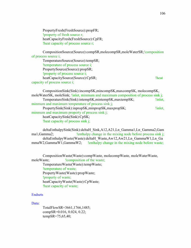
106
PropertyFresh(FreshSource):propFR; !property of fresh source r; heatCapacityFresh(FreshSource):CpFR; !heat capacity of process source r; CompositionSource(Source):compSR,molecompSR,moleWaterSR;!composition of process source i; TemperatureSource(Source):tempSR; !temperature of process source i; PropertySource(Source):propSR; !property of process source i; heatCapacitySource(Source):CpSR; !heat capacity of process source i; CompositionSink(Sink):incompSK,mincompSK,maxcompSK, molecompSK, moleWaterSK, moleSink; !inlet, minmum and maximum composition of process sink j; TemperatureSink(Sink):intempSK,mintempSK,maxtempSK; !inlet, minmum and maximum temperature of process sink j; PropertySink(Sink):inpropSK,minpropSK,maxpropSK; !inlet, minmum and maximum property of process sink j; heatCapacitySink(Sink):CpSK; !heat capacity of process sink j; deltaEnthalpySink(Sink):deltaH_Sink,A12,A21,Ln_Gamma1,Ln_Gamma2,Gamma1,Gamma2; !enthalpy change in the mixing node before process sink j; deltaEnthalpyWaste(Waste):deltaH_Waste,Aw12,Aw21,Ln_GammaW1,Ln_GammaW2,GammaW1,GammaW2; !enthalpy change in the mixing node before waste; CompositionWaste(Waste):compWaste, molecompWaste, moleWaterWaste, moleWaste; !composition of the waste; TemperatureWaste(Waste):tempWaste; !temperature of waste; PropertyWaste(Waste):propWaste; !property of waste; heatCapacityWaste(Waste):CpWaste; !heat capacity of waste; Endsets Data: TotalFlowSR=3661,1766,1485; compSR=0.016, 0.024, 0.22; tempSR=75,65,40;
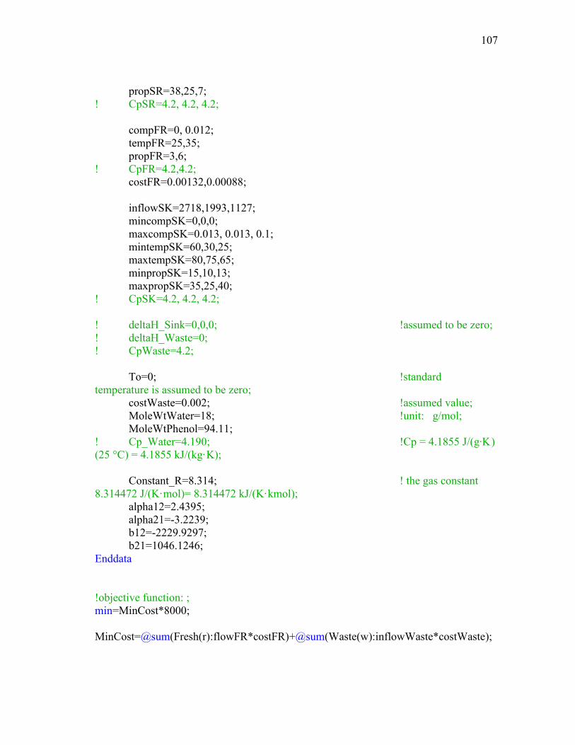
107
propSR=38,25,7; ! CpSR=4.2, 4.2, 4.2; compFR=0, 0.012; tempFR=25,35; propFR=3,6; ! CpFR=4.2,4.2; costFR=0.00132,0.00088; inflowSK=2718,1993,1127; mincompSK=0,0,0; maxcompSK=0.013, 0.013, 0.1; mintempSK=60,30,25; maxtempSK=80,75,65; minpropSK=15,10,13; maxpropSK=35,25,40; ! CpSK=4.2, 4.2, 4.2; ! deltaH_Sink=0,0,0; !assumed to be zero; ! deltaH_Waste=0; ! CpWaste=4.2; To=0; !standard temperature is assumed to be zero; costWaste=0.002; !assumed value; MoleWtWater=18; !unit: g/mol; MoleWtPhenol=94.11; ! Cp_Water=4.190; !Cp = 4.1855 J/(g·K) (25 °C) = 4.1855 kJ/(kg·K); Constant_R=8.314; ! the gas constant 8.314472 J/(K·mol)= 8.314472 kJ/(K·kmol); alpha12=2.4395; alpha21=-3.2239; b12=-2229.9297; b21=1046.1246; Enddata !objective function: ; min=MinCost*8000; MinCost=@sum(Fresh(r):flowFR*costFR)+@sum(Waste(w):inflowWaste*costWaste);
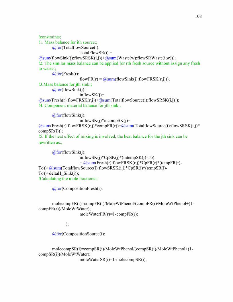
108
!constraints; !1. Mass balance for ith source:; @for(TotalflowSource(i): TotalFlowSR(i) = @sum(flowSink(j):flowSRSK(i,j))+@sum(Waste(w):flowSRWaste(i,w))); !2. The similar mass balance can be applied for rth fresh source without assign any fresh to waste:; @for(Fresh(r): flowFR(r) = @sum(flowSink(j):flowFRSK(r,j))); !3.Mass balance for jth sink:; @for(flowSink(j): inflowSK(j)= @sum(Fresh(r):flowFRSK(r,j))+@sum(TotalflowSource(i):flowSRSK(i,j))); !4. Component material balance for jth sink:;
@for(flowSink(j): inflowSK(j)*incompSK(j)= @sum(Fresh(r):flowFRSK(r,j)*compFR(r))+@sum(TotalflowSource(i):flowSRSK(i,j)*compSR(i))); !5. If the heat effect of mixing is involved, the heat balance for the jth sink can be rewritten as:;
@for(flowSink(j): inflowSK(j)*CpSK(j)*(intempSK(j)-To) = @sum(Fresh(r):flowFRSK(r,j)*CpFR(r)*(tempFR(r)-To))+@sum(TotalflowSource(i):flowSRSK(i,j)*CpSR(i)*(tempSR(i)-To))+deltaH_Sink(j)); !Calculating the mole fractions:;
@for(CompositionFresh(r):
molecompFR(r)=compFR(r)/MoleWtPhenol/(compFR(r)/MoleWtPhenol+(1-compFR(r))/MoleWtWater); moleWaterFR(r)=1-compFR(r);
);
@for(CompositionSource(i):
molecompSR(i)=compSR(i)/MoleWtPhenol/(compSR(i)/MoleWtPhenol+(1-compSR(i))/MoleWtWater); moleWaterSR(i)=1-molecompSR(i);
109
);
@for(CompositionSink(j): molecompSK(j)=incompSK(j)/MoleWtPhenol/(incompSK(j)/MoleWtPhenol+(1-incompSK(j))/MoleWtWater); moleWaterSK(j)=1-molecompSK(j); );
@for(CompositionWaste(w): molecompWaste(w)=compWaste(w)/MoleWtPhenol/(compWaste(w)/MoleWtPhenol+(1-compWaste(w))/MoleWtWater);
moleWaterWaste(w)=1-molecompWaste(w);
);
!Calculating heat capacity:;
@for(heatCapacityFresh(r):
CpFR(r)=molecompFR(r)*(0.0044*(tempFR(r)+273.15)+0.4685)+moleWaterFR(r)*(0.0083*(tempFR(r)+273.15)+1.3724);
);
@for(heatCapacitySource(i):
CpSR(i)=molecompSR(i)*(0.0044*(tempSR(i)+273.15)+0.4685)+moleWaterSR(i)*(0.0083*(tempSR(i)+273.15)+1.3724);
);
@for(heatCapacitySink(j):
CpSK(j)=molecompSK(j)*(0.0044*(intempSK(j)+273.15)+0.4685)+moleWaterSK(j)*(0.0083*(intempSK(j)+273.15)+1.3724);
);
@for(heatCapacityWaste(w):
110
CpWaste(w)=molecompWaste(w)*(0.0044*(tempWaste(w)+273.15)+0.4685)+moleWaterWaste(w)*(0.0083*(tempWaste(w)+273.15)+1.3724);
);
!Calculating heat of mixing:;
!the oringinal heat of mixing should multiply the mole flow rates of sinks or waste;
@for(deltaEnthalpySink(j):
deltaH_Sink(j)=-Constant_R*moleSink(j)*molecompSK(j)*moleWaterSK(j)*(A12(j)*b12/(molecompSK(j)+moleWaterSK(j)*A12(j))+A21(j)*b21/(moleWaterSK(j)+molecompSK(j)*A21(j)));
!Calculate the mole flow rates of sinks;
moleSink(j)=inflowSK(j)*incompSK(j)/MoleWtPhenol+inflowSK(j)*(1-incompSK(j))/MoleWtWater;
Ln_Gamma1(j)=-@log(molecompSK(j)+A12(j)*moleWaterSK(j))
+moleWaterSK(j)*(A12(j)/(molecompSK(j)+A12(j)*moleWaterSK(j))-A21(j)/(moleWaterSK(j)+A21(j)*molecompSK(j)));
Ln_Gamma2(j)=-@log(moleWaterSK(j)+A21(j)*molecompSK(j))
-molecompSK(j)*(A12(j)/(molecompSK(j)+A12(j)*moleWaterSK(j))-A21(j)/(moleWaterSK(j)+A21(j)*molecompSK(j)));
Gamma1(j)=@exp(Ln_Gamma1(j));
Gamma2(j)=@exp(Ln_Gamma2(j));
A21(j)=@exp(alpha21+b21/(intempSK(j)+273.15));
A12(j)=@exp(alpha12+b12/(intempSK(j)+273.15));
111
);
!6.Property balance in the jth sink;
@for(flowSink(j): inflowSK(j)*inpropSK(j)= @sum(Fresh(r):flowFRSK(r,j)*propFR(r))+@sum(TotalflowSource(i):flowSRSK(i,j)*propSR(i))); !7.property is dependent on the temperature and composition; ! @for(PropertySink(j): inpropSK(j)= molecompSK(j)*0.133322*2.58*@exp(0.0314*intempSK(j)) +(1-molecompSK(j))*0.133322*@exp(20.386-5132/(intempSK(j)+273.15))); !8.Sinks composition constrains:;
@for(CompositionSink(j):
incompSK(j)<=maxcompSK(j));
@for(CompositionSink(j):
incompSK(j)>=mincompSK(j)); !9.Sinks temperature constrains:;
@for(TemperatureSink(j):
intempSK(j)<=maxtempSK(j));
@for(TemperatureSink(j):
intempSK(j)>=mintempSK(j));
!10. Sinks properties constrains:;
@for(PropertySink(j):
inpropSK(j)<=maxpropSK(j));
@for(PropertySink(j):
inpropSK(j)>=minpropSK(j));
!11.Mass balance for the waste:;
112
@for(Waste(w): inflowWaste(w)= @sum(TotalflowSource(i):flowSRWaste(i,w))); !12. Component material balance for waste:;
@for(Waste(w): inflowWaste(w)*compWaste(w)= @sum(TotalflowSource(i):flowSRWaste(i,w)*compSR(i))); !13. If the heat effect of mixing is involved, the heat balance for the waste can be rewritten as:;
@for(Waste(w): inflowWaste(w)*CpWaste(w)*(tempWaste(w)-To) = @sum(TotalflowSource(i):flowSRWaste(i,w)*CpSR(i)*(tempSR(i)-To))+deltaH_Waste(w)); !Calculating heat of mixing:; @for(deltaEnthalpyWaste(w):
deltaH_Waste(w)=-Constant_R*moleWaste(w)*molecompWaste(w)*moleWaterWaste(w)*(Aw12(w)*b12/(molecompWaste(w)+moleWaterWaste(w)*Aw12(w))+Aw21(w)*b21/(moleWaterWaste(w)+molecompWaste(w)*Aw21(w)));
!!Calculate the mole flow rates of wastes;
moleWaste(w)=inflowWaste(w)*compWaste(w)/MoleWtPhenol+inflowWaste(w)*(1-compWaste(w))/MoleWtWater;
Ln_GammaW1(w)=-@log(molecompWaste(w)+Aw12(w)*moleWaterWaste(w))
+moleWaterWaste(w)*(Aw12(w)/(molecompWaste(w)+Aw12(w)*moleWaterWaste(w))-Aw21(w)/(moleWaterWaste(w)+Aw21(w)*molecompWaste(w)));
Ln_GammaW2(w)=-@log(moleWaterWaste(w)+Aw21(w)*molecompWaste(w))
-molecompWaste(w)*(Aw12(w)/(molecompWaste(w)+Aw12(w)*moleWaterWaste(w))-Aw21(w)/(moleWaterWaste(w)+Aw21(w)*molecompWaste(w)));
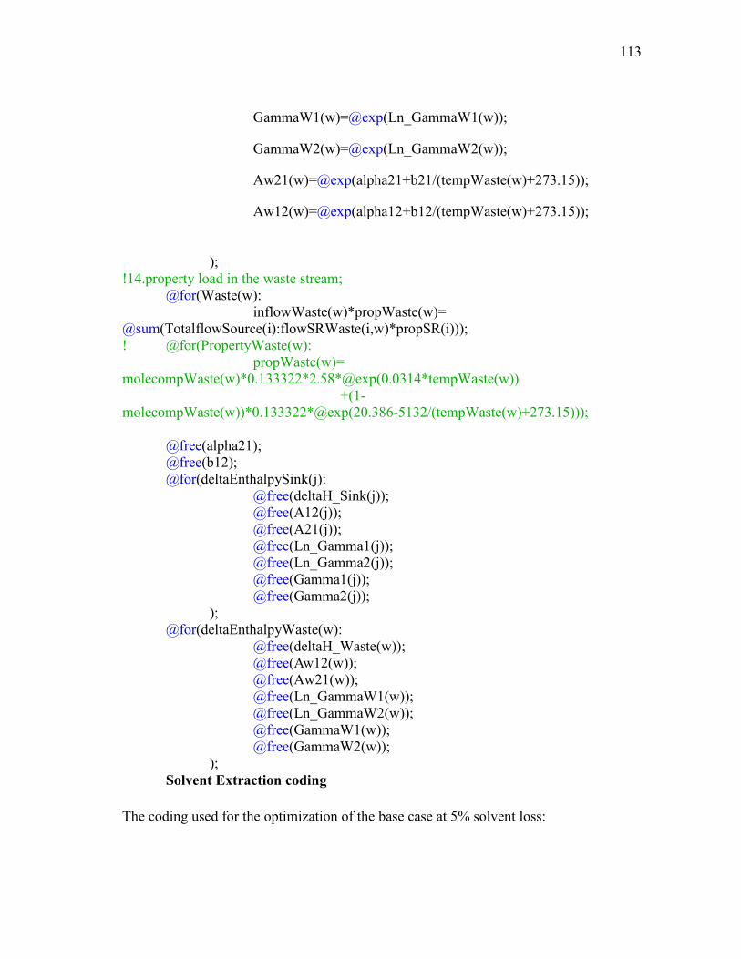
113
GammaW1(w)=@exp(Ln_GammaW1(w));
GammaW2(w)=@exp(Ln_GammaW2(w));
Aw21(w)=@exp(alpha21+b21/(tempWaste(w)+273.15));
Aw12(w)=@exp(alpha12+b12/(tempWaste(w)+273.15));
); !14.property load in the waste stream; @for(Waste(w): inflowWaste(w)*propWaste(w)= @sum(TotalflowSource(i):flowSRWaste(i,w)*propSR(i))); ! @for(PropertyWaste(w): propWaste(w)= molecompWaste(w)*0.133322*2.58*@exp(0.0314*tempWaste(w)) +(1-molecompWaste(w))*0.133322*@exp(20.386-5132/(tempWaste(w)+273.15))); @free(alpha21); @free(b12); @for(deltaEnthalpySink(j): @free(deltaH_Sink(j)); @free(A12(j)); @free(A21(j)); @free(Ln_Gamma1(j)); @free(Ln_Gamma2(j)); @free(Gamma1(j)); @free(Gamma2(j)); ); @for(deltaEnthalpyWaste(w): @free(deltaH_Waste(w)); @free(Aw12(w)); @free(Aw21(w)); @free(Ln_GammaW1(w)); @free(Ln_GammaW2(w)); @free(GammaW1(w)); @free(GammaW2(w)); ); Solvent Extraction coding
The coding used for the optimization of the base case at 5% solvent loss:
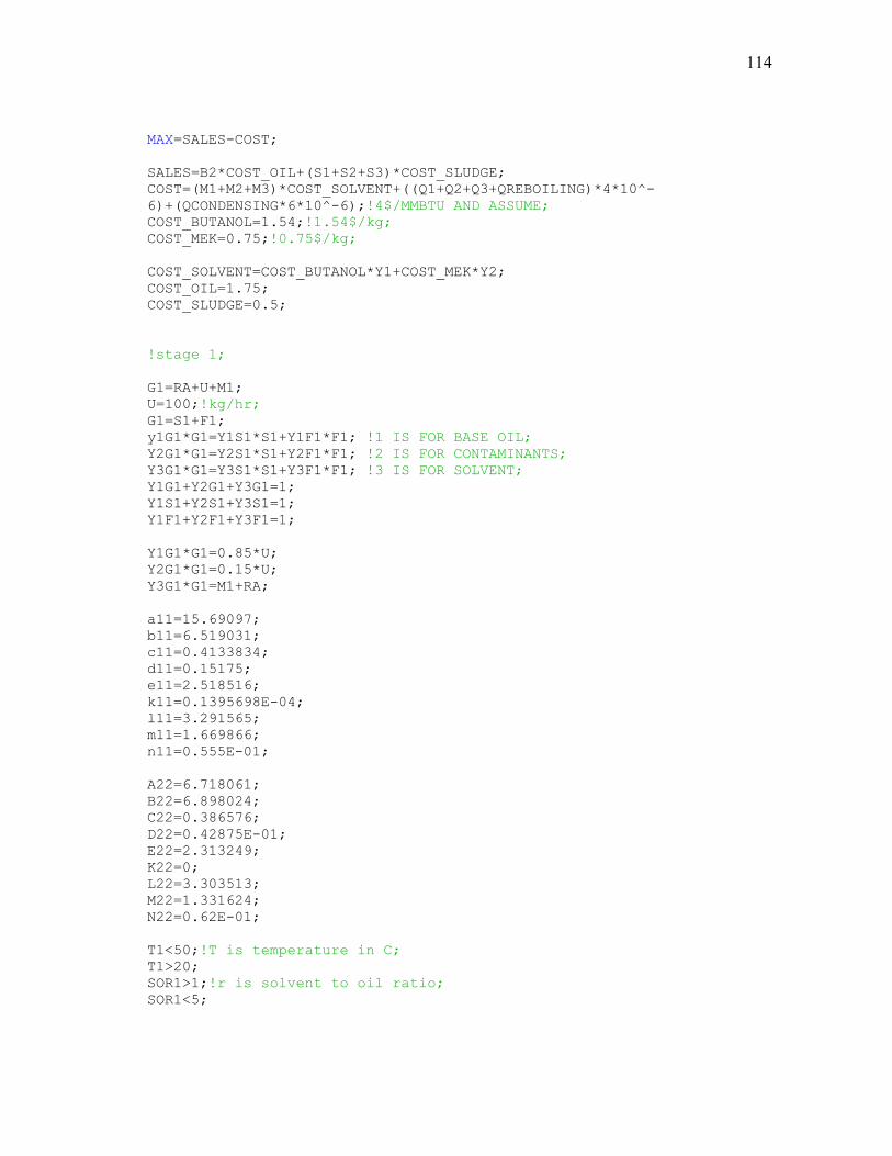
114
MAX=SALES-COST;
SALES=B2*COST_OIL+(S1+S2+S3)*COST_SLUDGE;
COST=(M1+M2+M3)*COST_SOLVENT+((Q1+Q2+Q3+QREBOILING)*4*10^-
6)+(QCONDENSING*6*10^-6);!4$/MMBTU AND ASSUME;
COST_BUTANOL=1.54;!1.54$/kg;
COST_MEK=0.75;!0.75$/kg;
COST_SOLVENT=COST_BUTANOL*Y1+COST_MEK*Y2;
COST_OIL=1.75;
COST_SLUDGE=0.5;
!stage 1;
G1=RA+U+M1;
U=100;!kg/hr;
G1=S1+F1;
y1G1*G1=Y1S1*S1+Y1F1*F1; !1 IS FOR BASE OIL;
Y2G1*G1=Y2S1*S1+Y2F1*F1; !2 IS FOR CONTAMINANTS;
Y3G1*G1=Y3S1*S1+Y3F1*F1; !3 IS FOR SOLVENT;
Y1G1+Y2G1+Y3G1=1;
Y1S1+Y2S1+Y3S1=1;
Y1F1+Y2F1+Y3F1=1;
Y1G1*G1=0.85*U;
Y2G1*G1=0.15*U;
Y3G1*G1=M1+RA;
a11=15.69097;
b11=6.519031;
c11=0.4133834;
d11=0.15175;
e11=2.518516;
k11=0.1395698E-04;
l11=3.291565;
m11=1.669866;
n11=0.555E-01;
A22=6.718061;
B22=6.898024;
C22=0.386576;
D22=0.42875E-01;
E22=2.313249;
K22=0;
L22=3.303513;
M22=1.331624;
N22=0.62E-01;
T1<50;!T is temperature in C;
T1>20;
SOR1>1;!r is solvent to oil ratio;
SOR1<5;
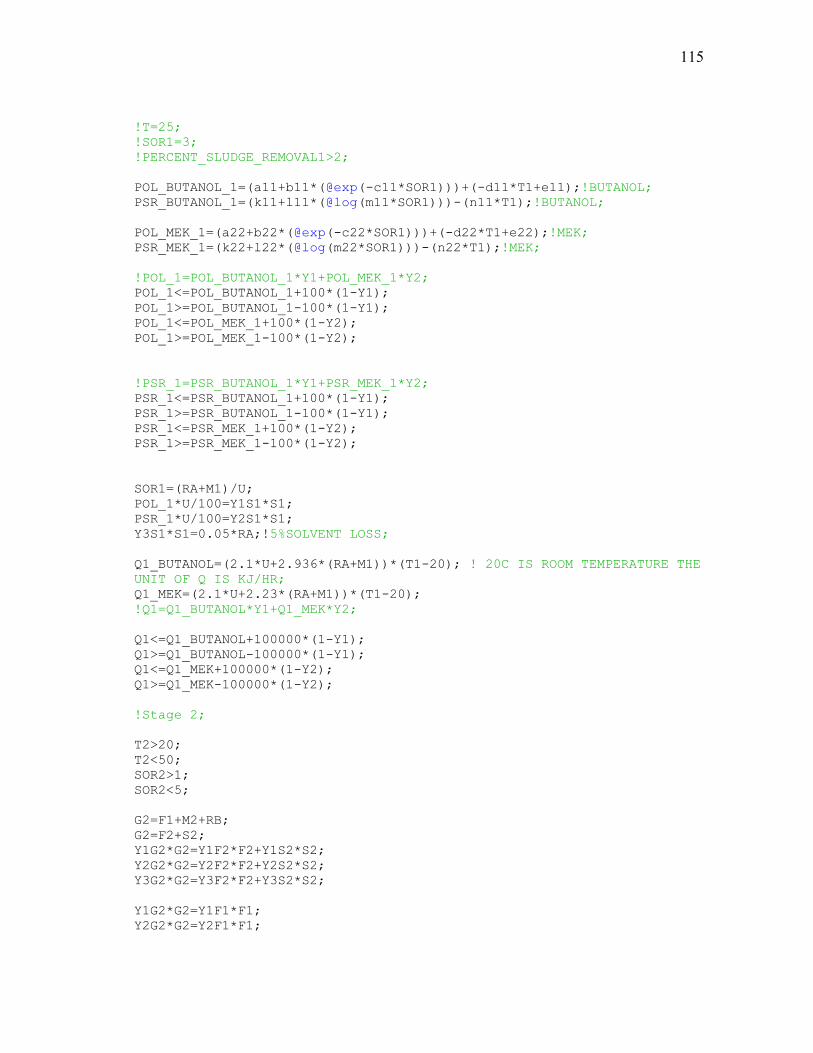
115
!T=25;
!SOR1=3;
!PERCENT_SLUDGE_REMOVAL1>2;
POL_BUTANOL_1=(a11+b11*(@exp(-c11*SOR1)))+(-d11*T1+e11);!BUTANOL;
PSR_BUTANOL_1=(k11+l11*(@log(m11*SOR1)))-(n11*T1);!BUTANOL;
POL_MEK_1=(a22+b22*(@exp(-c22*SOR1)))+(-d22*T1+e22);!MEK;
PSR_MEK_1=(k22+l22*(@log(m22*SOR1)))-(n22*T1);!MEK;
!POL_1=POL_BUTANOL_1*Y1+POL_MEK_1*Y2;
POL_1<=POL_BUTANOL_1+100*(1-Y1);
POL_1>=POL_BUTANOL_1-100*(1-Y1);
POL_1<=POL_MEK_1+100*(1-Y2);
POL_1>=POL_MEK_1-100*(1-Y2);
!PSR_1=PSR_BUTANOL_1*Y1+PSR_MEK_1*Y2;
PSR_1<=PSR_BUTANOL_1+100*(1-Y1);
PSR_1>=PSR_BUTANOL_1-100*(1-Y1);
PSR_1<=PSR_MEK_1+100*(1-Y2);
PSR_1>=PSR_MEK_1-100*(1-Y2);
SOR1=(RA+M1)/U;
POL_1*U/100=Y1S1*S1;
PSR_1*U/100=Y2S1*S1;
Y3S1*S1=0.05*RA;!5%SOLVENT LOSS;
Q1_BUTANOL=(2.1*U+2.936*(RA+M1))*(T1-20); ! 20C IS ROOM TEMPERATURE THE
UNIT OF Q IS KJ/HR;
Q1_MEK=(2.1*U+2.23*(RA+M1))*(T1-20);
!Q1=Q1_BUTANOL*Y1+Q1_MEK*Y2;
Q1<=Q1_BUTANOL+100000*(1-Y1);
Q1>=Q1_BUTANOL-100000*(1-Y1);
Q1<=Q1_MEK+100000*(1-Y2);
Q1>=Q1_MEK-100000*(1-Y2);
!Stage 2;
T2>20;
T2<50;
SOR2>1;
SOR2<5;
G2=F1+M2+RB;
G2=F2+S2;
Y1G2*G2=Y1F2*F2+Y1S2*S2;
Y2G2*G2=Y2F2*F2+Y2S2*S2;
Y3G2*G2=Y3F2*F2+Y3S2*S2;
Y1G2*G2=Y1F1*F1;
Y2G2*G2=Y2F1*F1;
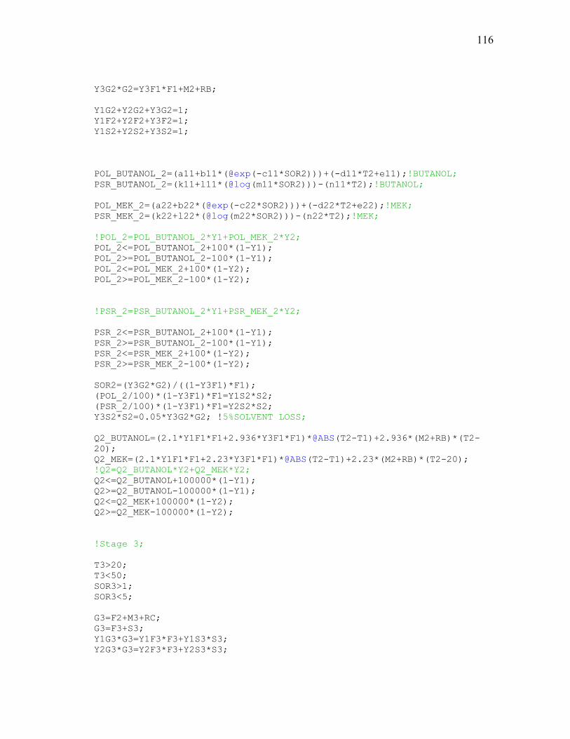
116
Y3G2*G2=Y3F1*F1+M2+RB;
Y1G2+Y2G2+Y3G2=1;
Y1F2+Y2F2+Y3F2=1;
Y1S2+Y2S2+Y3S2=1;
POL_BUTANOL_2=(a11+b11*(@exp(-c11*SOR2)))+(-d11*T2+e11);!BUTANOL;
PSR_BUTANOL_2=(k11+l11*(@log(m11*SOR2)))-(n11*T2);!BUTANOL;
POL_MEK_2=(a22+b22*(@exp(-c22*SOR2)))+(-d22*T2+e22);!MEK;
PSR_MEK_2=(k22+l22*(@log(m22*SOR2)))-(n22*T2);!MEK;
!POL_2=POL_BUTANOL_2*Y1+POL_MEK_2*Y2;
POL_2<=POL_BUTANOL_2+100*(1-Y1);
POL_2>=POL_BUTANOL_2-100*(1-Y1);
POL_2<=POL_MEK_2+100*(1-Y2);
POL_2>=POL_MEK_2-100*(1-Y2);
!PSR_2=PSR_BUTANOL_2*Y1+PSR_MEK_2*Y2;
PSR_2<=PSR_BUTANOL_2+100*(1-Y1);
PSR_2>=PSR_BUTANOL_2-100*(1-Y1);
PSR_2<=PSR_MEK_2+100*(1-Y2);
PSR_2>=PSR_MEK_2-100*(1-Y2);
SOR2=(Y3G2*G2)/((1-Y3F1)*F1);
(POL_2/100)*(1-Y3F1)*F1=Y1S2*S2;
(PSR_2/100)*(1-Y3F1)*F1=Y2S2*S2;
Y3S2*S2=0.05*Y3G2*G2; !5%SOLVENT LOSS;
Q2_BUTANOL=(2.1*Y1F1*F1+2.936*Y3F1*F1)*@ABS(T2-T1)+2.936*(M2+RB)*(T2-
20);
Q2_MEK=(2.1*Y1F1*F1+2.23*Y3F1*F1)*@ABS(T2-T1)+2.23*(M2+RB)*(T2-20);
!Q2=Q2_BUTANOL*Y2+Q2_MEK*Y2;
Q2<=Q2_BUTANOL+100000*(1-Y1);
Q2>=Q2_BUTANOL-100000*(1-Y1);
Q2<=Q2_MEK+100000*(1-Y2);
Q2>=Q2_MEK-100000*(1-Y2);
!Stage 3;
T3>20;
T3<50;
SOR3>1;
SOR3<5;
G3=F2+M3+RC;
G3=F3+S3;
Y1G3*G3=Y1F3*F3+Y1S3*S3;
Y2G3*G3=Y2F3*F3+Y2S3*S3;
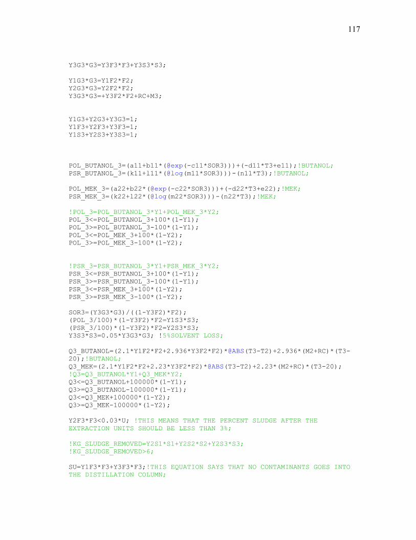
117
Y3G3*G3=Y3F3*F3+Y3S3*S3;
Y1G3*G3=Y1F2*F2;
Y2G3*G3=Y2F2*F2;
Y3G3*G3=+Y3F2*F2+RC+M3;
Y1G3+Y2G3+Y3G3=1;
Y1F3+Y2F3+Y3F3=1;
Y1S3+Y2S3+Y3S3=1;
POL_BUTANOL_3=(a11+b11*(@exp(-c11*SOR3)))+(-d11*T3+e11);!BUTANOL;
PSR_BUTANOL_3=(k11+l11*(@log(m11*SOR3)))-(n11*T3);!BUTANOL;
POL_MEK_3=(a22+b22*(@exp(-c22*SOR3)))+(-d22*T3+e22);!MEK;
PSR_MEK_3=(k22+l22*(@log(m22*SOR3)))-(n22*T3);!MEK;
!POL_3=POL_BUTANOL_3*Y1+POL_MEK_3*Y2;
POL_3<=POL_BUTANOL_3+100*(1-Y1);
POL_3>=POL_BUTANOL_3-100*(1-Y1);
POL_3<=POL_MEK_3+100*(1-Y2);
POL_3>=POL_MEK_3-100*(1-Y2);
!PSR_3=PSR_BUTANOL_3*Y1+PSR_MEK_3*Y2;
PSR_3<=PSR_BUTANOL_3+100*(1-Y1);
PSR_3>=PSR_BUTANOL_3-100*(1-Y1);
PSR_3<=PSR_MEK_3+100*(1-Y2);
PSR_3>=PSR_MEK_3-100*(1-Y2);
SOR3=(Y3G3*G3)/((1-Y3F2)*F2);
(POL_3/100)*(1-Y3F2)*F2=Y1S3*S3;
(PSR_3/100)*(1-Y3F2)*F2=Y2S3*S3;
Y3S3*S3=0.05*Y3G3*G3; !5%SOLVENT LOSS;
Q3_BUTANOL=(2.1*Y1F2*F2+2.936*Y3F2*F2)*@ABS(T3-T2)+2.936*(M2+RC)*(T3-
20);!BUTANOL;
Q3_MEK=(2.1*Y1F2*F2+2.23*Y3F2*F2)*@ABS(T3-T2)+2.23*(M2+RC)*(T3-20);
!Q3=Q3_BUTANOL*Y1+Q3_MEK*Y2;
Q3<=Q3_BUTANOL+100000*(1-Y1);
Q3>=Q3_BUTANOL-100000*(1-Y1);
Q3<=Q3_MEK+100000*(1-Y2);
Q3>=Q3_MEK-100000*(1-Y2);
Y2F3*F3<0.03*U; !THIS MEANS THAT THE PERCENT SLUDGE AFTER THE
EXTRACTION UNITS SHOULD BE LESS THAN 3%;
!KG_SLUDGE_REMOVED=Y2S1*S1+Y2S2*S2+Y2S3*S3;
!KG_SLUDGE_REMOVED>6;
SU=Y1F3*F3+Y3F3*F3;!THIS EQUATION SAYS THAT NO CONTAMINANTS GOES INTO
THE DISTILLATION COLUMN;
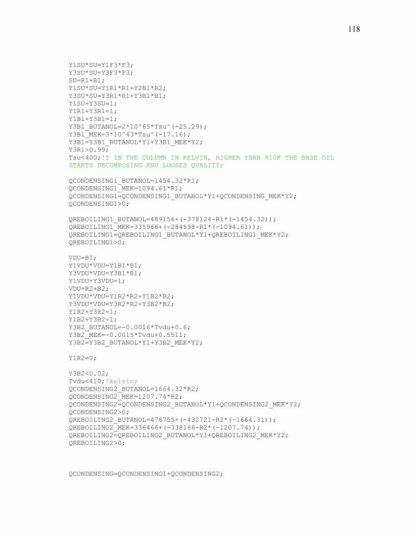
118
Y1SU*SU=Y1F3*F3;
Y3SU*SU=Y3F3*F3;
SU=R1+B1;
Y1SU*SU=Y1R1*R1+Y2B1*R2;
Y3SU*SU=Y3R1*R1+Y3B1*B1;
Y1SU+Y3SU=1;
Y1R1+Y3R1=1;
Y1B1+Y3B1=1;
Y3B1_BUTANOL=2*10^65*Tsu^(-25.29);
Y3B1_MEK=3*10^43*Tsu^(-17.16);
Y3B1=Y3B1_BUTANOL*Y1+Y3B1_MEK*Y2;
Y3R1>0.99;
Tsu<400;!T IN THE COLUMN IN KELVIN, HIGHER THAN 410K THE BASE OIL
STARTS DECOMPOSING AND LOOSES QUALITY;
QCONDENSING1_BUTANOL=1454.32*R1;
QCONDENSING1_MEK=1094.61*R1;
QCONDENSING1=QCONDENSING1_BUTANOL*Y1+QCONDENSING_MEK*Y2;
QCONDENSING1>0;
QREBOILING1_BUTANOL=489156+(-378124-R1*(-1454.32));
QREBOILING1_MEK=335966+(-284598-R1*(-1094.61));
QREBOILING1=QREBOILING1_BUTANOL*Y1+QREBOILING1_MEK*Y2;
QREBOILING1>0;
VDU=B1;
Y1VDU*VDU=Y1B1*B1;
Y3VDU*VDU=Y3B1*B1;
Y1VDU+Y3VDU=1;
VDU=R2+B2;
Y1VDU*VDU=Y1R2*R2+Y1B2*B2;
Y3VDU*VDU=Y3R2*R2+Y3B2*B2;
Y1R2+Y3R2=1;
Y1B2+Y3B2=1;
Y3B2_BUTANOL=-0.0016*Tvdu+0.6;
Y3B2_MEK=-0.0015*Tvdu+0.5511;
Y3B2=Y3B2_BUTANOL*Y1+Y3B2_MEK*Y2;
Y1R2=0;
Y3B2<0.02;
Tvdu<410;!kelvin;
QCONDENSING2_BUTANOL=1664.32*R2;
QCONDENSING2_MEK=1207.74*R2;
QCONDENSING2=QCONDENSING2_BUTANOL*Y1+QCONDENSING2_MEK*Y2;
QCONDENSING2>0;
QREBOILING2_BUTANOL=476755+(-432721-R2*(-1664.31));
QREBOILING2_MEK=336466+(-338166-R2*(-1207.74));
QREBOILING2=QREBOILING2_BUTANOL*Y1+QREBOILING2_MEK*Y2;
QREBOILING2>0;
QCONDENSING=QCONDENSING1+QCONDENSING2;
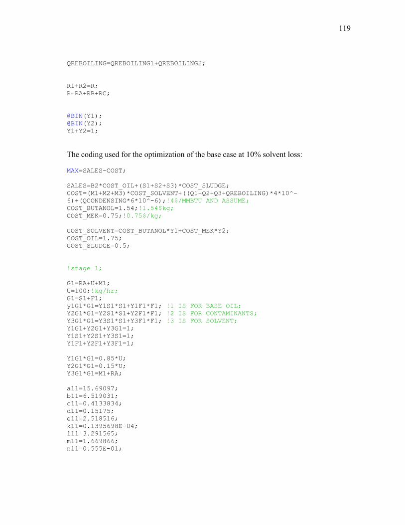
119
QREBOILING=QREBOILING1+QREBOILING2;
R1+R2=R;
R=RA+RB+RC;
@BIN(Y1);
@BIN(Y2);
Y1+Y2=1;
The coding used for the optimization of the base case at 10% solvent loss:
MAX=SALES-COST;
SALES=B2*COST_OIL+(S1+S2+S3)*COST_SLUDGE;
COST=(M1+M2+M3)*COST_SOLVENT+((Q1+Q2+Q3+QREBOILING)*4*10^-
6)+(QCONDENSING*6*10^-6);!4$/MMBTU AND ASSUME;
COST_BUTANOL=1.54;!1.54$kg;
COST_MEK=0.75;!0.75$/kg;
COST_SOLVENT=COST_BUTANOL*Y1+COST_MEK*Y2;
COST_OIL=1.75;
COST_SLUDGE=0.5;
!stage 1;
G1=RA+U+M1;
U=100;!kg/hr;
G1=S1+F1;
y1G1*G1=Y1S1*S1+Y1F1*F1; !1 IS FOR BASE OIL;
Y2G1*G1=Y2S1*S1+Y2F1*F1; !2 IS FOR CONTAMINANTS;
Y3G1*G1=Y3S1*S1+Y3F1*F1; !3 IS FOR SOLVENT;
Y1G1+Y2G1+Y3G1=1;
Y1S1+Y2S1+Y3S1=1;
Y1F1+Y2F1+Y3F1=1;
Y1G1*G1=0.85*U;
Y2G1*G1=0.15*U;
Y3G1*G1=M1+RA;
a11=15.69097;
b11=6.519031;
c11=0.4133834;
d11=0.15175;
e11=2.518516;
k11=0.1395698E-04;
l11=3.291565;
m11=1.669866;
n11=0.555E-01;
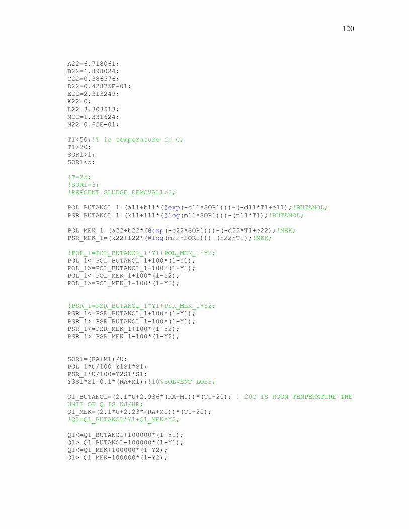
120
A22=6.718061;
B22=6.898024;
C22=0.386576;
D22=0.42875E-01;
E22=2.313249;
K22=0;
L22=3.303513;
M22=1.331624;
N22=0.62E-01;
T1<50;!T is temperature in C;
T1>20;
SOR1>1;
SOR1<5;
!T=25;
!SOR1=3;
!PERCENT_SLUDGE_REMOVAL1>2;
POL_BUTANOL_1=(a11+b11*(@exp(-c11*SOR1)))+(-d11*T1+e11);!BUTANOL;
PSR_BUTANOL_1=(k11+l11*(@log(m11*SOR1)))-(n11*T1);!BUTANOL;
POL_MEK_1=(a22+b22*(@exp(-c22*SOR1)))+(-d22*T1+e22);!MEK;
PSR_MEK_1=(k22+l22*(@log(m22*SOR1)))-(n22*T1);!MEK;
!POL_1=POL_BUTANOL_1*Y1+POL_MEK_1*Y2;
POL_1<=POL_BUTANOL_1+100*(1-Y1);
POL_1>=POL_BUTANOL_1-100*(1-Y1);
POL_1<=POL_MEK_1+100*(1-Y2);
POL_1>=POL_MEK_1-100*(1-Y2);
!PSR_1=PSR_BUTANOL_1*Y1+PSR_MEK_1*Y2;
PSR_1<=PSR_BUTANOL_1+100*(1-Y1);
PSR_1>=PSR_BUTANOL_1-100*(1-Y1);
PSR_1<=PSR_MEK_1+100*(1-Y2);
PSR_1>=PSR_MEK_1-100*(1-Y2);
SOR1=(RA+M1)/U;
POL_1*U/100=Y1S1*S1;
PSR_1*U/100=Y2S1*S1;
Y3S1*S1=0.1*(RA+M1);!10%SOLVENT LOSS;
Q1_BUTANOL=(2.1*U+2.936*(RA+M1))*(T1-20); ! 20C IS ROOM TEMPERATURE THE
UNIT OF Q IS KJ/HR;
Q1_MEK=(2.1*U+2.23*(RA+M1))*(T1-20);
!Q1=Q1_BUTANOL*Y1+Q1_MEK*Y2;
Q1<=Q1_BUTANOL+100000*(1-Y1);
Q1>=Q1_BUTANOL-100000*(1-Y1);
Q1<=Q1_MEK+100000*(1-Y2);
Q1>=Q1_MEK-100000*(1-Y2);
121
!Stage 2;
T2>20;
T2<50;
SOR2>1;
SOR2<5;
G2=F1+M2+RB;
G2=F2+S2;
Y1G2*G2=Y1F2*F2+Y1S2*S2;
Y2G2*G2=Y2F2*F2+Y2S2*S2;
Y3G2*G2=Y3F2*F2+Y3S2*S2;
Y1G2*G2=Y1F1*F1;
Y2G2*G2=Y2F1*F1;
Y3G2*G2=Y3F1*F1+M2+RB;
Y1G2+Y2G2+Y3G2=1;
Y1F2+Y2F2+Y3F2=1;
Y1S2+Y2S2+Y3S2=1;
POL_BUTANOL_2=(a11+b11*(@exp(-c11*SOR2)))+(-d11*T2+e11);!BUTANOL;
PSR_BUTANOL_2=(k11+l11*(@log(m11*SOR2)))-(n11*T2);!BUTANOL;
POL_MEK_2=(a22+b22*(@exp(-c22*SOR2)))+(-d22*T2+e22);!MEK;
PSR_MEK_2=(k22+l22*(@log(m22*SOR2)))-(n22*T2);!MEK;
!POL_2=POL_BUTANOL_2*Y1+POL_MEK_2*Y2;
POL_2<=POL_BUTANOL_2+100*(1-Y1);
POL_2>=POL_BUTANOL_2-100*(1-Y1);
POL_2<=POL_MEK_2+100*(1-Y2);
POL_2>=POL_MEK_2-100*(1-Y2);
!PSR_2=PSR_BUTANOL_2*Y1+PSR_MEK_2*Y2;
PSR_2<=PSR_BUTANOL_2+100*(1-Y1);
PSR_2>=PSR_BUTANOL_2-100*(1-Y1);
PSR_2<=PSR_MEK_2+100*(1-Y2);
PSR_2>=PSR_MEK_2-100*(1-Y2);
SOR2=(Y3G2*G2)/((1-Y3F1)*F1);
(POL_2/100)*(1-Y3F1)*F1=Y1S2*S2;
(PSR_2/100)*(1-Y3F1)*F1=Y2S2*S2;
Y3S2*S2=0.1*Y3G2*G2; !10%SOLVENT LOSS;
Q2_BUTANOL=(2.1*Y1F1*F1+2.936*Y3F1*F1)*@ABS(T2-T1)+2.936*(M2+RB)*(T2-
20);
Q2_MEK=(2.1*Y1F1*F1+2.23*Y3F1*F1)*@ABS(T2-T1)+2.23*(M2+RB)*(T2-20);
!Q2=Q2_BUTANOL*Y2+Q2_MEK*Y2;
Q2<=Q2_BUTANOL+100000*(1-Y1);
Q2>=Q2_BUTANOL-100000*(1-Y1);
122
Q2<=Q2_MEK+100000*(1-Y2);
Q2>=Q2_MEK-100000*(1-Y2);
!Stage 3;
T3>20;
T3<50;
SOR3>1;
SOR3<5;
G3=F2+M3+RC;
G3=F3+S3;
Y1G3*G3=Y1F3*F3+Y1S3*S3;
Y2G3*G3=Y2F3*F3+Y2S3*S3;
Y3G3*G3=Y3F3*F3+Y3S3*S3;
Y1G3*G3=Y1F2*F2;
Y2G3*G3=Y2F2*F2;
Y3G3*G3=+Y3F2*F2+RC+M3;
Y1G3+Y2G3+Y3G3=1;
Y1F3+Y2F3+Y3F3=1;
Y1S3+Y2S3+Y3S3=1;
POL_BUTANOL_3=(a11+b11*(@exp(-c11*SOR3)))+(-d11*T3+e11);!BUTANOL;
PSR_BUTANOL_3=(k11+l11*(@log(m11*SOR3)))-(n11*T3);!BUTANOL;
POL_MEK_3=(a22+b22*(@exp(-c22*SOR3)))+(-d22*T3+e22);!MEK;
PSR_MEK_3=(k22+l22*(@log(m22*SOR3)))-(n22*T3);!MEK;
!POL_3=POL_BUTANOL_3*Y1+POL_MEK_3*Y2;
POL_3<=POL_BUTANOL_3+100*(1-Y1);
POL_3>=POL_BUTANOL_3-100*(1-Y1);
POL_3<=POL_MEK_3+100*(1-Y2);
POL_3>=POL_MEK_3-100*(1-Y2);
!PSR_3=PSR_BUTANOL_3*Y1+PSR_MEK_3*Y2;
PSR_3<=PSR_BUTANOL_3+100*(1-Y1);
PSR_3>=PSR_BUTANOL_3-100*(1-Y1);
PSR_3<=PSR_MEK_3+100*(1-Y2);
PSR_3>=PSR_MEK_3-100*(1-Y2);
SOR3=(Y3G3*G3)/((1-Y3F2)*F2);
(POL_3/100)*(1-Y3F2)*F2=Y1S3*S3;
(PSR_3/100)*(1-Y3F2)*F2=Y2S3*S3;
Y3S3*S3=0.1*Y3G3*G3; !10%SOLVENT LOSS;
Q3_BUTANOL=(2.1*Y1F2*F2+2.936*Y3F2*F2)*@ABS(T3-T2)+2.936*(M2+RC)*(T3-
20);!BUTANOL;
123
Q3_MEK=(2.1*Y1F2*F2+2.23*Y3F2*F2)*@ABS(T3-T2)+2.23*(M2+RC)*(T3-20);
!Q3=Q3_BUTANOL*Y1+Q3_MEK*Y2;
Q3<=Q3_BUTANOL+100000*(1-Y1);
Q3>=Q3_BUTANOL-100000*(1-Y1);
Q3<=Q3_MEK+100000*(1-Y2);
Q3>=Q3_MEK-100000*(1-Y2);
Y2F3*F3<0.03*U; !THIS MEANS THAT THE PERCENT SLUDGE AFTER THE
EXTRACTION UNITS SHOULD BE LESS THAN 3%;
!KG_SLUDGE_REMOVED=Y2S1*S1+Y2S2*S2+Y2S3*S3;
!KG_SLUDGE_REMOVED>6;
SU=Y1F3*F3+Y3F3*F3;!THIS EQUATION SAYS THAT NO CONTAMINANTS GOES INTO
THE DISTILLATION COLUMN;
Y1SU*SU=Y1F3*F3;
Y3SU*SU=Y3F3*F3;
SU=R1+B1;
Y1SU*SU=Y1R1*R1+Y2B1*R2;
Y3SU*SU=Y3R1*R1+Y3B1*B1;
Y1SU+Y3SU=1;
Y1R1+Y3R1=1;
Y1B1+Y3B1=1;
Y3B1_BUTANOL=2*10^65*Tsu^(-25.29);
Y3B1_MEK=3*10^43*Tsu^(-17.16);
Y3B1=Y3B1_BUTANOL*Y1+Y3B1_MEK*Y2;
Y3R1>0.99;
Tsu<400;!T IN THE COLUMN IN KELVIN, HIGHER THAN 410K THE BASE OIL
STARTS DECOMPOSING AND LOOSES QUALITY;
QCONDENSING1_BUTANOL=1454.32*R1;
QCONDENSING1_MEK=1094.61*R1;
QCONDENSING1=QCONDENSING1_BUTANOL*Y1+QCONDENSING_MEK*Y2;
QCONDENSING1>0;
QREBOILING1_BUTANOL=489156+(-378124-R1*(-1454.32));
QREBOILING1_MEK=335966+(-284598-R1*(-1094.61));
QREBOILING1=QREBOILING1_BUTANOL*Y1+QREBOILING1_MEK*Y2;
QREBOILING1>0;
VDU=B1;
Y1VDU*VDU=Y1B1*B1;
Y3VDU*VDU=Y3B1*B1;
Y1VDU+Y3VDU=1;
VDU=R2+B2;
Y1VDU*VDU=Y1R2*R2+Y1B2*B2;
Y3VDU*VDU=Y3R2*R2+Y3B2*B2;
Y1R2+Y3R2=1;
Y1B2+Y3B2=1;
Y3B2_BUTANOL=-0.0016*Tvdu+0.6;
Y3B2_MEK=-0.0015*Tvdu+0.5511;
Y3B2=Y3B2_BUTANOL*Y1+Y3B2_MEK*Y2;
Y1R2=0;
124
Y3B2<0.02;
Tvdu<410;!kelvin;
QCONDENSING2_BUTANOL=1664.32*R2;
QCONDENSING2_MEK=1207.74*R2;
QCONDENSING2=QCONDENSING2_BUTANOL*Y1+QCONDENSING2_MEK*Y2;
QCONDENSING2>0;
QREBOILING2_BUTANOL=476755+(-432721-R2*(-1664.31));
QREBOILING2_MEK=336466+(-338166-R2*(-1207.74));
QREBOILING2=QREBOILING2_BUTANOL*Y1+QREBOILING2_MEK*Y2;
QREBOILING2>0;
QCONDENSING=QCONDENSING1+QCONDENSING2;
QREBOILING=QREBOILING1+QREBOILING2;
R1+R2=R;
R=RA+RB+RC;
@BIN(Y1);
@BIN(Y2);
Y1+Y2=1;
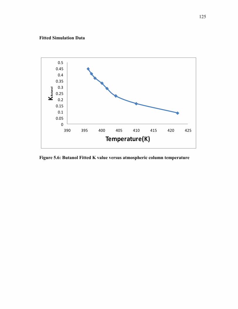
125
Fitted Simulation Data
0
0.05
0.1
0.15
0.2
0.25
0.3
0.35
0.4
0.45
0.5
390 395 400 405 410 415 420 425
KB
uta
no
l
Temperature(K)
Figure 5.6: Butanol Fitted K value versus atmospheric column temperature
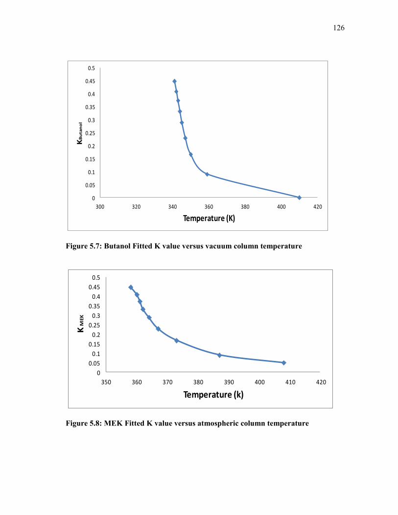
126
0
0.05
0.1
0.15
0.2
0.25
0.3
0.35
0.4
0.45
0.5
300 320 340 360 380 400 420
KB
uta
no
l
Temperature (K)
Figure 5.7: Butanol Fitted K value versus vacuum column temperature
0
0.05
0.1
0.15
0.2
0.25
0.3
0.35
0.4
0.45
0.5
350 360 370 380 390 400 410 420
K M
EK
Temperature (k)
Figure 5.8: MEK Fitted K value versus atmospheric column temperature
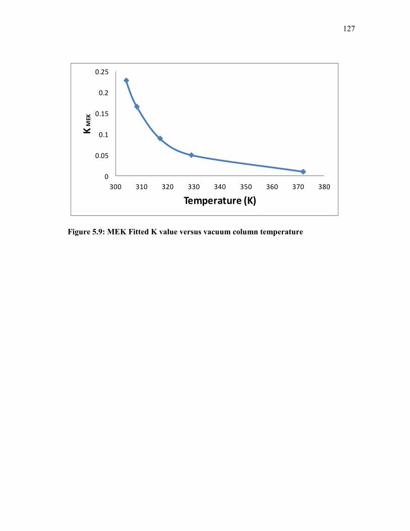
127
0
0.05
0.1
0.15
0.2
0.25
300 310 320 330 340 350 360 370 380
K M
EK
Temperature (K)
Figure 5.9: MEK Fitted K value versus vacuum column temperature
128
VITA
Name: Houssein A. Kheireddine
Address: Artie McFerrin Department of Chemical Engineering
Texas A&M University
College Station, TX 77843-3136
Email address: [email protected]
Education: B.A., Chemical Engineering, 2008
Texas A&M University-Kingsville, Kingsville, TX
Ph..D. Chemical Engineering, 2012
Texas A&M University, College Station, TX