SECURE INTEGRATED ROUTING AND LOCALIZATION IN WIRELESS

OPTICAL SENSOR NETWORKS

A Dissertation

by

UNOMA NDILI OKORAFOR

Submitted to the Office of Graduate Studies ofTexas A&M University

in partial fulfillment of the requirements for the degree of

DOCTOR OF PHILOSOPHY

August 2008

Major Subject: Electrical Engineering

SECURE INTEGRATED ROUTING AND LOCALIZATION IN WIRELESS

OPTICAL SENSOR NETWORKS

A Dissertation

by

UNOMA NDILI OKORAFOR

Submitted to the Office of Graduate Studies ofTexas A&M University

in partial fulfillment of the requirements for the degree of

DOCTOR OF PHILOSOPHY

Approved by:

Chair of Committee, Deepa KundurCommittee Members, Costas Georghiades

Srinivas ShakkottaiEun Jung Kim

Head of Department, Costas Georghiades

August 2008

Major Subject: Electrical Engineering

iii

ABSTRACT

Secure Integrated Routing and Localization in Wireless Optical Sensor Networks.

(August 2008)

Unoma Ndili Okorafor, B.Sc., University of Lagos;

M.Sc., Rice University

Chair of Advisory Committee: Dr. Deepa Kundur

Wireless ad hoc and sensor networks are envisioned to be self-organizing and

autonomous networks, that may be randomly deployed where no fixed infrastructure

is either feasible or cost-effective. The successful commercialization of such networks

depends on the feasible implementation of network services to support security-aware

applications.

Recently, free space optical (FSO) communication has emerged as a viable tech-

nology for broadband distributed wireless optical sensor network (WOSN) applica-

tions. The challenge of employing FSO include its susceptibility to adverse weather

conditions and the line of sight requirement between two communicating nodes. In

addition, it is necessary to consider security at the initial design phase of any network

and routing protocol. This dissertation addresses the feasibility of randomly deployed

WOSNs employing broad beam FSO with regard to the network layer, in which two

important problems are specifically investigated.

First, we address the parameter assignment problem which considers the rela-

tionship amongst the physical layer parameters of node density, transmission radius

and beam divergence of the FSO signal in order to yield probabilistic guarantees on

network connectivity. We analyze the node isolation property of WOSNs, and its

relation to the connectivity of the network. Theoretical analysis and experimental

investigation were conducted to assess the effects of hierarchical clustering as well

iv

as fading due to atmospheric turbulence on connectivity, thereby demonstrating the

design choices necessary to make the random deployment of the WOSN feasible.

Second, we propose a novel light-weight circuit-based, secure and integrated rout-

ing and localization paradigm within the WOSN, that leverages the resources of the

base station. Our scheme exploits the hierarchical cluster-based organization of the

network, and the directionality of links to deliver enhanced security performance in-

cluding per hop and broadcast authentication, confidentiality, integrity and freshness

of routing signals. We perform security and attack analysis and synthesis to charac-

terize the protocol’s performance, compared to existing schemes, and demonstrate its

superior performance for WOSNs.

Through the investigation of this dissertation, we demonstrate the fundamental

tradeoff between security and connectivity in WOSNs, and illustrate how the trans-

mission radius may be used as a high sensitivity tuning parameter to balance there

two metrics of network performance. We also present WOSNs as a field of study that

opens up several directions for novel research, and encompasses problems such as

connectivity analysis, secure routing and localization, intrusion detection, topology

control, secure data aggregation and novel attack scenarios.

v

To Ekpe, Chisom and Apia.

vi

ACKNOWLEDGMENTS

I want to express my deep and sincere gratitude to my academic advisor, Dr. Deepa

Kundur, for her continuous guidance and support throughout my Ph.D. work at

Texas A&M University, College Station. Her unparalleled understanding and encour-

agement have been invaluable and made my experience enjoyable.

I want to thank the members of my dissertation committee: Dr. C. Georghiades,

Dr. E. J. Kim and Dr. S. Shakkottai, for their interactions and continuously insti-

gating new ideas for me to explore. I also appreciate the time and service of Dr. N.

Reddy. I am especially indebted to Dr. Karen Butler-Purry who continues to serve

as an outstanding mentor, and has provided me with excellent advice, assistance and

comfort.

I am very thankful to all of my colleagues, and especially members of the HoLiS-

TIC research group especially Alex, Will, Nebu, Sonu and Julien. They are fun,

wonderful and interesting to work with.

I want to truly thank my husband, Ekpe, for his very strong shoulders that

supported me in every aspect during my years in graduate study. Without him, this

endeavor could not have been completed. My appreciation for my children, Chisom

and Apia, is boundless. They always give me reason to fight on. Many thanks to my

parents and parents-in-law, and my wonderful family for their continuous prayers,

love and laughter. They are the best! There are friends, too numerous to name,

whose genuine love and friendship I experienced on this journey. Thank you!

Finally, all the glory be to God almighty for whom I live, I move and I have my

being. His Son has given me life, and His Spirit comforts, guides and illuminates my

way, always.

vii

TABLE OF CONTENTS

CHAPTER Page

I INTRODUCTION . . . . . . . . . . . . . . . . . . . . . . . . . . 1

A. Overview of Wireless Optical Sensor Networks . . . . . . . 1

B. Motivation . . . . . . . . . . . . . . . . . . . . . . . . . . . 5

C. Comparison of Free Space Optical and Radio Frequency

Technologies . . . . . . . . . . . . . . . . . . . . . . . . . . 8

1. Advantages of FSO over RF Communication . . . . . 10

2. Challenges . . . . . . . . . . . . . . . . . . . . . . . . 13

D. The Wireless Optical Sensor Network Model . . . . . . . . 15

1. Graph Theoretic Framework . . . . . . . . . . . . . . 20

2. Threat Model . . . . . . . . . . . . . . . . . . . . . . . 23

3. Assumptions . . . . . . . . . . . . . . . . . . . . . . . 24

E. Dissertation Contributions . . . . . . . . . . . . . . . . . . 25

1. Organization of the Dissertation . . . . . . . . . . . . 27

II LITERATURE REVIEW . . . . . . . . . . . . . . . . . . . . . . 28

A. Background Survey on Connectivity in Wireless Sensor

Networks . . . . . . . . . . . . . . . . . . . . . . . . . . . . 28

B. Background Survey on Routing and Localization . . . . . . 35

C. Security Considerations for Routing and Localization . . . 44

III CONNECTIVITY ANALYSIS OF THE WOSN . . . . . . . . . 47

A. Relating Node Isolation and Network Connectivity . . . . . 48

B. Analysis on Node Isolation . . . . . . . . . . . . . . . . . . 51

1. Probability of No Isolated WOSN Node . . . . . . . . 51

a. Evaluating pif . . . . . . . . . . . . . . . . . . . . 52

b. Evaluating pib . . . . . . . . . . . . . . . . . . . . 53

c. Evaluating pib|f . . . . . . . . . . . . . . . . . . . 54

d. Evaluating pid . . . . . . . . . . . . . . . . . . . . 57

e. Evaluating pd . . . . . . . . . . . . . . . . . . . . 61

2. Probability of No K-isolated WOSN Node . . . . . . . 63

a. Case for K = 2 . . . . . . . . . . . . . . . . . . . 64

3. One-dimensional Case . . . . . . . . . . . . . . . . . . 69

C. Simulations and Discussion . . . . . . . . . . . . . . . . . . 72

viii

CHAPTER Page

D. Impact of Hierarchy and Clustering on Connectivity . . . . 82

E. Connectivity Analysis in a Fading Channel Model . . . . . 87

1. Fading Channel Statistical Model . . . . . . . . . . . . 89

2. Numerical Results and Observations . . . . . . . . . . 93

3. Summary of Insights . . . . . . . . . . . . . . . . . . . 94

IV SIRLOS: SECURE INTEGRATED ROUTING AND LOCAL-

IZATION SCHEME . . . . . . . . . . . . . . . . . . . . . . . . . 98

A. Introduction . . . . . . . . . . . . . . . . . . . . . . . . . . 98

B. SIRLoS: Secure Integrated Routing and Localization Scheme 100

1. Efficient Neighborhood Discovery . . . . . . . . . . . . 102

a. Off-line Key Setup . . . . . . . . . . . . . . . . . 102

b. Challenge and Respond Protocol . . . . . . . . . 103

c. Format of the CDB . . . . . . . . . . . . . . . . . 104

d. Hot Potato Node Processing of the CDB . . . . . 105

e. Determining δ . . . . . . . . . . . . . . . . . . . . 108

f. Restricted and Compounded Flooding . . . . . . 109

g. Schedule of Transmission . . . . . . . . . . . . . . 110

2. Location Estimation . . . . . . . . . . . . . . . . . . . 113

3. Secure Base Station Network Topology Reconstruction 115

4. Updating Nodes Routing Tables . . . . . . . . . . . . 116

5. Dynamic Route Setup . . . . . . . . . . . . . . . . . . 117

6. Route Maintenance . . . . . . . . . . . . . . . . . . . 118

C. Performance Evaluation . . . . . . . . . . . . . . . . . . . 119

1. Localization Error . . . . . . . . . . . . . . . . . . . . 120

2. Average Hop Count . . . . . . . . . . . . . . . . . . . 121

3. End-to-End Delay Analysis . . . . . . . . . . . . . . . 122

4. Byte Overhead . . . . . . . . . . . . . . . . . . . . . . 124

D. Security Analysis . . . . . . . . . . . . . . . . . . . . . . . 126

1. Per Hop Authentication and Routing Beacons Alteration128

a. Problem Case I . . . . . . . . . . . . . . . . . . . 129

b. Problem Case II . . . . . . . . . . . . . . . . . . . 130

2. Broadcast Authentication and Spoofed Routing Beacons 136

3. Beacon Freshness and Correlation-based Cryptanalysis 137

4. Unauthorized Alien Node Participation and Traffic

Analysis . . . . . . . . . . . . . . . . . . . . . . . . . . 138

E. Attack Analysis . . . . . . . . . . . . . . . . . . . . . . . . 138

1. BS-Circuit Collusion Attack . . . . . . . . . . . . . . . 139

ix

CHAPTER Page

2. Wormhole Attack . . . . . . . . . . . . . . . . . . . . 144

3. Other Common Routing Attacks . . . . . . . . . . . . 147

a. Type I: Sinkhole Attacks . . . . . . . . . . . . . . 147

b. Type II: Blackhole Attacks . . . . . . . . . . . . . 148

c. Type III: Other Denial of Service Attacks . . . . 149

4. Summary of Insights . . . . . . . . . . . . . . . . . . . 151

V CONCLUSION . . . . . . . . . . . . . . . . . . . . . . . . . . . 152

A. Future Work . . . . . . . . . . . . . . . . . . . . . . . . . . 153

REFERENCES . . . . . . . . . . . . . . . . . . . . . . . . . . . . . . . . . . . 154

APPENDIX A . . . . . . . . . . . . . . . . . . . . . . . . . . . . . . . . . . . 169

APPENDIX B . . . . . . . . . . . . . . . . . . . . . . . . . . . . . . . . . . . 171

APPENDIX C . . . . . . . . . . . . . . . . . . . . . . . . . . . . . . . . . . . 173

VITA . . . . . . . . . . . . . . . . . . . . . . . . . . . . . . . . . . . . . . . . 174

x

LIST OF TABLES

TABLE Page

I Attenuation effects of adverse weather conditions on a 1550

nm laser. . . . . . . . . . . . . . . . . . . . . . . . . . . . . . . . 14

II Comparison between FSO and RF communication for ad hoc

sensor networks. . . . . . . . . . . . . . . . . . . . . . . . . . . . 15

III Comparing related work on range assignment for WSNs. . . . . . 34

IV The minimum r value for corresponding network parameter

(n, α) pair values that achieve pd ≥ 0.99 in Gn(Sn, E). . . . . . . 62

V The minimum r value for corresponding network parameter

(n, α) pair values that achieve pd2 ≥ 0.99 in Gn(Sn, E). . . . . . . 70

VI Adverse Weather Parameters Affecting The FSO signal. . . . . . 90

VII Schedule of transmission algorithm SA(i). . . . . . . . . . . . . . 110

xi

LIST OF FIGURES

FIGURE Page

1 A schematic diagram of the components of a sensor node. . . . . . . 2

2 The system architecture of a typical sensor network habitat mon-itoring application. . . . . . . . . . . . . . . . . . . . . . . . . . . 3

3 The transmitter footprints of various communication models. . . . . 9

4 Various transmitter-to-receiver configurations available for FSOcommunication. . . . . . . . . . . . . . . . . . . . . . . . . . . . . 10

5 Illustrating the transmission range versus energy per bit for FSOcompared to RF. . . . . . . . . . . . . . . . . . . . . . . . . . . . 12

6 (a) Each sensor si transmits within a sector Φi defined by the 4-tuple (Υi,Θi, r, α), which are parameters of the system. (b) Nodesj only hears si if sj falls into si’s communication section, but sj

talks to si via the back channel sj → sa → sb → sc → si. . . . . . . . 16

7 A sample WOSN deployed in a unit area square region of 1 m2,with n = 200 nodes, r = 0.2m and α = 40o. The circles representnodes while associated triangular patches represent correspondingcommunication sectors. . . . . . . . . . . . . . . . . . . . . . . . . 18

8 Distinct neighborhoods of a WOSN node. . . . . . . . . . . . . . . 21

9 The BS-circuit is the concatenation of node si’s uplink and down-link paths. The entry and exit cluster head may be the same ortwo distinct nodes. Uplink path for si: si → sj → s∗a → BS.Downlink path for si: BS → s∗a → sb → sc → sd → si. . . . . . . . . 22

10 An GRG network model for a traditional RF omnidirectional sen-sor network. All links in the network are bidirectional. A nodesw is isolated if it is not within the communication range r of anyother node in the network. . . . . . . . . . . . . . . . . . . . . . . 30

xii

FIGURE Page

11 The WOSN has no isolated nodes, since every node has both anincoming and an outgoing link. However the overall network isnot (strongly) connected due to the network partition and linkdirectionality; for example, sa → sb exists, however sb sa doesnot exist. . . . . . . . . . . . . . . . . . . . . . . . . . . . . . . . 49

12 Depicting the mesh plot of the probability pd that no isolated nodeoccurs in Gn(Sn, E) with varying r and α values for different nodedensities n. The red line indicates the (r, α) pair values for whichpd = 0.99. . . . . . . . . . . . . . . . . . . . . . . . . . . . . . . . 58

13 Analytical pd (Anal) and simulation pd for Euclidean (Sim-Eucl)and Toroidal (Sim-Toro) distance metrics for K = 1, 2, with vary-ing r values, n = 500 and six preset α values. . . . . . . . . . . . . 74

14 Two examples of strong connected components (SCCs) of directedgraphs. . . . . . . . . . . . . . . . . . . . . . . . . . . . . . . . . 77

15 Comparing the probability pc that the network is connected to theprobability pd that there is no isolated network node (simulatedand analytical). . . . . . . . . . . . . . . . . . . . . . . . . . . . . 79

16 Plots of phc compared to pc for varying pCH . . . . . . . . . . . . . 85

17 An example of the region of transmission of a WOSN node in afading channel. . . . . . . . . . . . . . . . . . . . . . . . . . . . . 87

18 Geometric illustration for si → sj if d(si, sj) ≤ r and |Θi−ΨTij | ≤

α2 based on a simple monotone function. . . . . . . . . . . . . . . . 88

19 Link probability for the two weather conditions given in Table VI. . . 91

20 Comparing simulation results for pd and pc with analytical valuesfor various α and fading conditions, with Ht = 40dB. . . . . . . . . 96

21 Illustrating the format and various fields of a CDB packet. . . . . . . 104

22 Illustrating the information gathering and processing within aCDB as it traverses a BS-circuit during neighborhood discovery. . . . 107

23 Values for δ for n = 500 depend on r, α and pCH . . . . . . . . . . . 108

xiii

FIGURE Page

24 Illustrating the transmission of various packets within a sample network.112

25 The centroid of the two regions ϕ1x and ϕ2

x that comprise thecommunication sector Φx of node sx. The sector-based commu-nication provides more localized estimation of the node positionand the additional HELLO-phase provides even finer granularity. . . 113

26 A sample network with the corresponding predecessor and suc-cessor routing tables PRT(si), SRT(si) for node si. . . . . . . . . . 117

27 Simulation results for localization error versus r with pCH = 0.1. . . 119

28 Simulation results for localization error versus pCH with r = 0.1 km. 120

29 Simulation results for average hop count versus α. . . . . . . . . . . 121

30 Simulation results for average delay required for neighborhooddiscovery versus network diameter δ. . . . . . . . . . . . . . . . . . 123

31 A comparative plot of byte overhead versus number of rounds ofsimulation for SIRLoS, non-secure SIRLoS and simple-bro/simple-gather algorithm, for n = 200 nodes. . . . . . . . . . . . . . . . . . 125

32 Depicting the two scenarios in which a vulnerability exists in thesecurity of the neighborhood discovery scheme. . . . . . . . . . . . . 130

33 Illustrating the bidirectionality vulnerability problem scenario. . . . 131

34 Probability pχA(> 0) versus α for various r and pa values. . . . . 133

35 BS-circuit collusion attack. . . . . . . . . . . . . . . . . . . . . . . 139

36 Depicting the region of possibility where sx’s successor falls. . . . . . 141

37 Illustrating the vulnerability to collusion attack with pca versus α. . . 143

38 Illustrating a short range and long range wormhole attack in aWOSN, which violates geometric connectivity using the range-and-orientation constraint test. . . . . . . . . . . . . . . . . . . . . 145

xiv

FIGURE Page

B.1 Sample simulation scenario of node graph using Toroidal distancemeasure to compute the adjacency matrix. The 1s with asterisksindicates the positions affected by the Toroidal distance metricwhich would otherwise be a zero. . . . . . . . . . . . . . . . . . . . 172

1

CHAPTER I

INTRODUCTION

A. Overview of Wireless Optical Sensor Networks

The need for untethered communication and pervasive computing continues to drive

advances in mobile communications and wireless networking. To serve this purpose,

randomly deployed wireless sensor networks (WSNs) have been envisioned to consist

of groups of sensor nodes that are randomly and densely deployed to observe ambient

scalar data within a physical region of interest [1]. In many contexts, due to re-

cent technological advances, the nodes are ultra-lightweight, comprised of small-sized

wireless battery-operated nodes that are significantly resource-constrained in terms

of power, storage, computational capability and bandwidth. Each sensor node com-

prises of a sensing, processing, communication, localization, mobilizer power source

and power scavenging unit (some of which are optional, such as the mobilizer, power

scavenging and location finding units). Figure 1 depicts a schematic diagram of the

components of a typical sensor node.

Although individually, sensor nodes may be fragile and disposable, their useful-

ness comes from their easy and cost-effective deployment in large numbers to form

an unattended network. In this way, they are able to aggregate inferences about

their coverage area. For example, a WSN may contain several hundreds or thou-

sands of these sensor nodes deployed over large geographical regions. Traditionally,

the nodes form an ad-hoc network in order to communicate their sensor readings

(about objects or events in their vicinity) to a centralized sink or base station via

omni-directional radio frequency (RF). The network may be stationary or dynamic

The journal model is Proceedings of the IEEE.

2

ProcessorStorage

Power Source

SensorsADC Transceiver

PowerScavenging

LocalizationUnit Mobilizer

Fig. 1. A schematic diagram of the components of a sensor node.

with mobility-capable nodes. Their ability to be set up inexpensively, in large-scale,

and quickly makes WSNs a promising candidate for a host of applications, includ-

ing military surveillance, disaster relief, law enforcement applications, traffic control,

infrastructure security and advanced health-care monitoring. For example, a WSN

may be deployed to gather intelligence in a battle field by tracking enemy troop

movement, monitoring a secured zone, or guiding a missile target system. Other

possible applications of WSNs include monitoring environmental conditions such as

temperature/humidity, collecting pollution data, monitoring structural weaknesses in

buildings or equipment, inventory control, and detecting the presence of chemical or

biological agents, to name a few. The system architecture of a typical sensor network

habitat monitoring application is depicted in Figure 2.

Currently, through technological advances in miniaturization and micro-electro

mechanical systems (MEMS), WSNs continue to evolve towards the so-called smart

dust - dust-sized sensor nodes that can float in the atmosphere - based on the Uni-

3

2 Habitat monitoring applications

Cerpa et al.[9] describe habitat monitoring as a driver application for wireless sensor network:

habitat sensing for biocomplexity mapping. In this first cut on habitat monitoring sensor network

application, they propose a tiered architecture for such applications and a frisbee model that opti-

mizes energy effeciency when monitoring moving phenomenon.

2.1 Great Duck Island(GDI) system

In August 2002, researchers from UCB/Intel Research Laboratory deployed a mote-based tiered

sensor network on Great Duck Island, Maine, to monitor the behavior of storm petrel[21].

2.1.1 UCB Mica mote

UC Berkeley Mica mote deployed in this application use an Atmel Atmega 103 microcontroller

running at 4MHz, 916MHz radio from RF monolithics to provide bidirectional communication at

40kbps, and a pair of AA batteries to provide energy.The Mica Weather Board, stacked to the pro-

cessor board via the 51 pin extension connector, includes temperature, photoresistor, barometer,humidity and thermopile sensors. Some new designs to preserve energy on this version include an

ADC and an I2C 8x8 power switch on the sensor board,the bypassing of the DC booster etc. To

protect from the variable weather condition on GDI,the Mica mote is packaged in acrylic enclo-

sure, which will not obstruct the sensing functionality and radio communication of the motes.

2.1.2 System Architecture

32 motes were placed at area of interest(e.g., inside a burrows). Those motes, grouped into

sensor patches, transmit sensor reading to a gateway(CerfCube),which is responsible for forward-

ing the data from the sensor patch to a remote basestation through a local transmit network. The

2

Fig. 2. The system architecture of a typical sensor network habitat monitoring application.

versity of California, Berkeley’s Smart Dust project [2]. Recently, there has been

increased interest in the development of wireless optical sensor networks (WOSNs) [3–

10] as a viable contribution towards the feasible design of smart dust nodes. WOSNs

are an emerging subclass of WSNs comprised of nodes whose point-to-point commu-

nication paradigm employs directed broad-beam free space optics (FSO), a high band-

width communication technology that enables information transmission through the

atmosphere using modulated light beams. The FSO transceiver unit of WOSN nodes

achieves size reduction by a factor of up to twenty, when compared to the competing

RF antennas [2]. Furthermore, FSO continues to stand out as the leading technology

for the development of rapidly deploy-able and secure wireless sensor and surveillance

networks, with the potential for broadband communication.

Classically, WOSNs possess the following distinctive features, many of which are

shared by their RF counterparts:

4

• spatially distributed, in order to improve the performance and geographical range

of sensing functions. To ensure effective collaboration amongst network entities,

the connectivity of the network must be guaranteed;

• resource constrained, representing one of the biggest design challenges, necessi-

tates the judicious use of communication bandwidth, memory, and computation

to enhance the life span of the often portable and non-renewable power source;

• hierarchical, employing localized clustering of sensor nodes into subnetworks to

improve network scalability;

• location aware, necessitated by event-driven applications that rely on the ability

of nodes to gain knowledge of their location in order to localize, track and

communicate activities of interest within the network;

• redundant, employing densely deployed nodes to obtain more accurate and com-

plete readings of observed events;

• vulnerable to attack, due to a host of applications that deploy non-tamper re-

sistant nodes within environments that are hostile or not monitored. Security

paradigms must be considered at all network layers to guarantee privacy, con-

fidentiality, availability and authenticity of the sensor data.

The fundamental question we pose and seek to address in this dissertation is as

follows:

What are the implications of link directionality to connectivity and secure

routing for ad hoc wireless sensor networks?

The objective of this dissertation is to study the feasibility of employing FSO as the

networking paradigm in security-aware, broadband, randomly and rapidly deploy-

5

able WSNs consisting of stationary nodes. Our investigation is primarily concerned

with two main aspects of WOSNs: (1) the requirements for a probabilistic network

connectivity guarantee in the physical layer with respect to the trade off between

network parameters of node density, beam angle and communication radius; and (2)

a novel secure routing and localization scheme suited for the unique network layer

characteristics of the WOSN.

Connectivity as well as secure routing and localization under the WOSN paradigm

is challenging due in part to the directionality of links resulting from the line-of-sight

requirement for FSO communication. Because of the well known fact that incorpo-

rating security mechanisms after the design of network protocols is often non-trivial

and superficial at best [11], it is beneficial to consider security objectives in the initial

design of any protocol. Our security solution integrate routing and localization while

leveraging the natural hierarchy and link directionality in WOSNs.

B. Motivation

As with any wireless medium, FSO is susceptible to routing attacks such as data

replay, identity theft, or injection of unauthorized bits into the network. Worse, an

enemy that is able to compromise an authentic network node, may easily launch

more serious insider attacks, by extracting keying and security information from the

compromised node, and then acting as an authentic network participant [11]. Un-

fortunately, an attack in the network layer can completely cripple the WOSN and

undermine its purpose, in spite of best efforts aimed at securing other OSI layers of

the network. As noted in [12], if the routing protocol can be subverted, and messages

altered in transit, then no amount of security on the data packets can mitigate a se-

curity threat at the application layer. In addition, the vulnerability of sensor nodes to

6

physical capture and tampering, combined with the collaborative nature of multi-hop

communication, makes network layer protection mechanisms even more crucial.

The WOSN architecture is motivated by a consideration for the viable and cost-

effective choice that FSO presents for data transmission requiring enormous band-

width while achieving reduced transceiver size. FSO communication carries light

signals at extremely high frequencies, offering the highest capacity for wireless com-

munications medium. The WOSN can provide full-duplex gigabit-per-second (Gbps)

throughput for multimodal data such as multimedia, hyperspectral imagery and

multi-variate heterogeneous data. Additionally, the FSO signal can be rapidly de-

ployed because it is transmitted using unlicensed optical wavelengths that do not

require expensive government licensing, and it is unaffected by interference with ex-

isting networks. As motivating examples, we identify three cutting edge applications

of WOSNs.

Wireless Multimedia Sensor Networks comprising of sensors that collect multi-

media information such as digital images, video, and audio, requiring Gbps link

speeds [13, 14] for applications such as tactical battlefield and advanced perva-

sive health care surveillance, visual and other forms of broadband data that are

imperative for monitoring and effective decision-making. The development of

wireless multimedia sensor networks has been driven in part by recent improve-

ments in embedded devices, MEMS technology, and the advent of inexpensive

and low-resolution miniature hardware that acquire rich media content from

the environment, such as cheap CMOS video cameras and microphones. It is

widely believed that WOSNs present the most viable networking solution to the

bandwidth bottleneck that will accelerate the realization of practical wireless

multimedia sensor network systems.

7

Mission Critical Sensor Networks refers to networking for application domains

where life or livelihood may be at risk, including critical infrastructure pro-

tection, emergency and crisis intervention, and military operations. Mission

critical sensor networks aim to develop mechanisms to promote specialized net-

work protocols that are ultra-dependable, rapidly-deploy-able and secure in the

face of sudden and adverse conditions. Because the frequency spectrum used

by FSO is free/unregulated, avoids interference with existing systems, and the

signal often provides more secure communication, well designed WOSNs are a

viable solution for rapidly deploy-able mission critical networks [15].

Hybrid Sensor Networks consists of robust systems that employ a complementary

hybrid FSO-RF communication network to leverage the advantages of both

technologies [16, 17]. Hybrid sensor networks provide differentiated network

quality-of-service (QoS), motivated by an integrated heterogenous service de-

livery, such as simultaneous ultra-high bandwidth, low latency FSO channels

and ultra-reliable RF links that are resilient to packet loss. Additionally, hy-

brid FSO-RF networks can withstand a wide range of adverse environmental

conditions which either technology alone cannot provide, and are of particular

interest to several military and intelligence-gathering applications.

For several applications such as the ones cited above, it is critical that network

data be protected from intentional loss, modification, or unwanted access, necessitat-

ing the design of secure and privacy-enhancing WOSNs. In particular, it is necessary

to provide solutions for secure neighborhood discovery in ad hoc deployments, and

mechanisms to detect and recover from malicious attacks on the network. With-

out adequate security design at the network layer, WOSNs are vulnerable to attacks

including passive eavesdropping, distributed denial-of-service (DDoS) and data cor-

8

ruption [11], that can easily lead to catastrophe for critical applications.

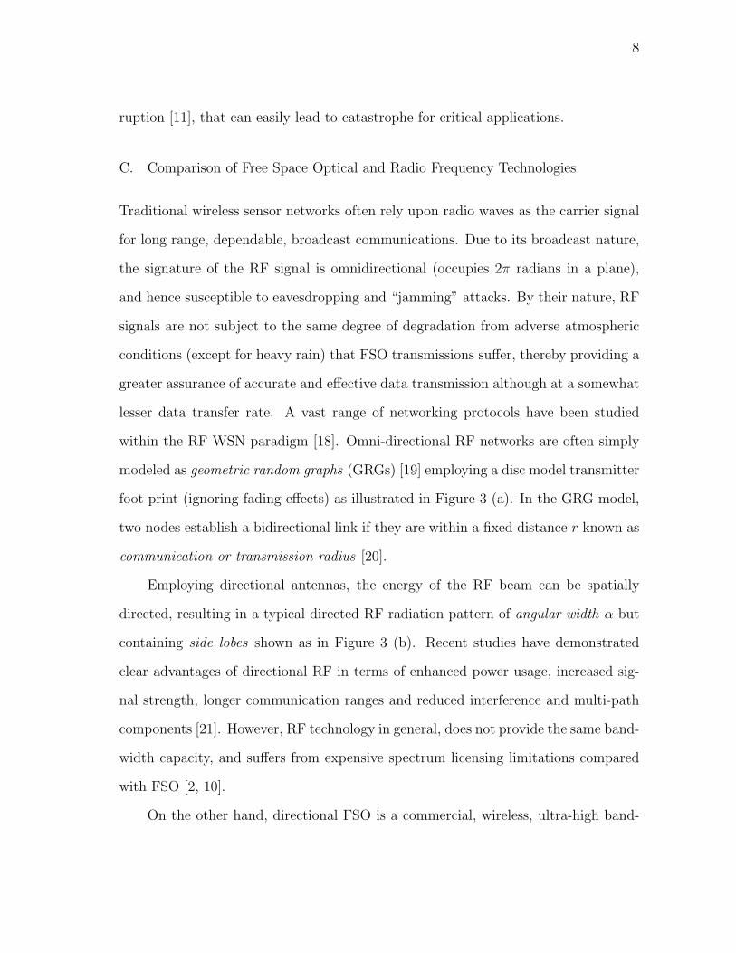
C. Comparison of Free Space Optical and Radio Frequency Technologies

Traditional wireless sensor networks often rely upon radio waves as the carrier signal

for long range, dependable, broadcast communications. Due to its broadcast nature,

the signature of the RF signal is omnidirectional (occupies 2π radians in a plane),

and hence susceptible to eavesdropping and “jamming” attacks. By their nature, RF

signals are not subject to the same degree of degradation from adverse atmospheric

conditions (except for heavy rain) that FSO transmissions suffer, thereby providing a

greater assurance of accurate and effective data transmission although at a somewhat

lesser data transfer rate. A vast range of networking protocols have been studied

within the RF WSN paradigm [18]. Omni-directional RF networks are often simply

modeled as geometric random graphs (GRGs) [19] employing a disc model transmitter

foot print (ignoring fading effects) as illustrated in Figure 3 (a). In the GRG model,

two nodes establish a bidirectional link if they are within a fixed distance r known as

communication or transmission radius [20].

Employing directional antennas, the energy of the RF beam can be spatially

directed, resulting in a typical directed RF radiation pattern of angular width α but

containing side lobes shown as in Figure 3 (b). Recent studies have demonstrated

clear advantages of directional RF in terms of enhanced power usage, increased sig-

nal strength, longer communication ranges and reduced interference and multi-path

components [21]. However, RF technology in general, does not provide the same band-

width capacity, and suffers from expensive spectrum licensing limitations compared

with FSO [2, 10].

On the other hand, directional FSO is a commercial, wireless, ultra-high band-

9

RF antenna

DirectionalRF antenna

DirectionalFSO laser

(a) Omni-directional RF (b) Directional RF (c) Free space optical

Fig. 3. The transmitter footprints of various communication models.

width line-of-sight (LOS) technology that is relatively new to the sensor network

community. By employing a directed laser (Light Amplification by the Stimulated

Emission of Radiation) or LED (Light-Emitting Diode) to transmit light beam signals,

FSO achieves very high data rates, (Gbps) over a few kilometers using unlicensed fre-

quencies in the order of hundreds of terahertz [6]. For example, current FSO systems

employing 1550nm lasers attain up to 1.25 Gbps over distances up to 6km, with an

ON-OFF keying (OOK) modulation scheme [22]. The directional broad beam FSO’s

transmitter signature is represented well, simply by a circular sector, as illustrated in

Figure 3 (c).

We note here that for the FSO transmitter, two configurations are possible; a

narrow beam highly focused energy signal with a beam diameter of a few millira-

dian (mrad), and the broad beam signal with diffused energy and significantly larger

beam diameters, greater than π/18 [17]. The FSO receiver may be employed in three

configurations: a directed, diffused or omnidirectional detectors, so that different

10

narrow beamdirectionaltransmitter

narrow beam directionalreceiver

(a)

broad beamdirectionaltransmitter

broad beam directionalreceiver

(b)

broad beamdirectionaltransmitter

Omni-directionalreceiver

(c)

Fig. 4. Various transmitter-to-receiver configurations available for FSO communication.

transmitter/receiver link configurations are possible including, a narrow beam-to-

narrow beam as depicted in Figure 4 (a), a narrow beam-to-broad beam as illus-

trated in Figure 4 (b), or a broad beam-to-omni directional configuration shown in

Figure 4 (c). For this dissertation, we adopt the broad beam-to-omnidirectional model

of Figure 4 (c) proposed for the Smart Dust [2], as it offers the most viable high band-

width networking solution in a randomly deployed ad hoc network scenario. Within

the WOSN a directed link is established from a node sa to sb if and only if sb falls

within sa’s communication sector, defined by the communication radius r and the

beam width α of the sector [9].

1. Advantages of FSO over RF Communication

WOSNs have a number of distinct advantages over RF WSNs [21], including:

Bandwidth: It is well known that FSO enables transmission bandwidths on the

order of Gbps which the current state-of-the-art RF technology struggles to pro-

11

vide [13]. For example, the IEEE 802.11x standard is limited to link throughputs

on the order of 10s of megabits per second (Mbps) [17], while current 802.15.4

compliant sensor nodes achieve nominal rates of about 250Kbps [13]. Even with

the much anticipated development and deployment of ultra-wide-band (UWB)

RF transmission techniques capable of theoretical throughput rates in excess of

675 Mbps for 1.3GHz pulse-UWB systems, the pulses are very short in space

(less than 23cm for a 1.3 GHz bandwidth pulse), and their achievable band-

width drops significantly with increased ranges (lower than 802.11a at modest

ranges of r ≥ 15m) [17]. On the other hand, FSO offers up to 1.25Gbps over

link distances over one kilometer [22] which easily satisfy the bandwidth-hungry

demands of multimodal high capacity sensor networks.

Form Factors (Size and Power per bit): Due to the simple analog circuity re-

quired for the OOK modulation scheme, the WOSN nodes can be small, and

consume less power. The size of the FSO equipment can be as small as a

laser pointer (i.e., a few millimeters), making dense integration of multiple FSO

transceivers on to a single node chip possible. Semiconductor lasers and LEDs

used for active FSO communications require very little power (a few milli-watts)

making them suitable for power limited ad-hoc sensor network scenarios. Ad-

ditionally passive FSO communication employing corner cuber retroreflectors

(CCRs) which require negligible power from the nodes may also be employed.

An illustration of the transmission range achievable versus energy per bit for

active and passive FSO compared to RF is shown in Figure 5, which illustrates

the huge power advantage of FSO over RF.

Spatial Reuse: By focusing energy in one direction, the potential for spatial reuse

is increased while interference and energy are reduced for a comparable trans-

12

Energy/bit (J/bit)

Ran

ge (m

)

x 10-7

Fig. 5. Illustrating the transmission range versus energy per bit for FSO compared to RF.

mission range. FSO also yields increased signal strength, longer communication

ranges, and reduced multi-path components compared to RF.

Security: Directed FSO communication is more secure than broadcast RF due to

the reduced spatial signature of energy from a broadcast disk model for the

GRG model, to the RSSG model, thereby reducing the chances of successful

eavesdropping. The physical difficulties in intercepting the FSO beam, its non-

susceptibility to jamming attacks, and the associated high chance of detection

with eavesdropping enhance the security property of WOSNs. This advantage is

more significant for applications deployed in unsecured or hostile environments.

Licence-free quick installation Optical wavelengths are license free, so FSO de-

ployment does not require any permissions as long as they are eye safe. Deploy-

ing WOSNs save time and money, while avoiding interference issues that plague

13

traditional broadband RF. For this reason, WOSNs can be rapidly deployed,

typically within a few hours.

2. Challenges

WOSNs face two major challenges compared to RF WSNs, including; (1) a need for

the existence of line-of-sight between communicating nodes resulting in the direction-

ality of links; and (2) the reduced transmission quality observed in adverse weather

conditions. These challenges are described in some detail below:

Requirement for Clear Line of Sight and Alignment: Clear line-of-sight re-

quirements for the reception of an FSO signal has direct implications on network

connectivity especially in an ad hoc WOSN. One proposal to alleviate the line-of-

sight limitation includes employing an accurate point-and-track beam-steering

actuator for aligning narrow beam FSO systems (i.e. the trans-receiver of a node

is a mobile unit, capable of swivel motion to align the sender’s transmitter to

the receiver) [17]. With the broad beam-to-omnidirectional transmitter/receiver

configuration employed in this dissertation, our approach to network connec-

tivity entails studying the constraints on the physical layer properties of the

network (node density, communication radius and beam width of the FSO sig-

nal) that guarantee a probabilistic measure of network connectivity [23].

Signal degradation with adverse weather: For the FSO signal, reduced bit

rates are encountered in adverse atmospheric conditions as fog, heavy snow and

rain. Table I presents the typical attenuation effects of various adverse weather

conditions on a 1550 nm laser. Additionally, light from other sources (e.g.,

direct and intense sunlight), temperature, and physical obstructions (e.g., fly-

ing birds, smoke) may temporarily interrupt or hamper the effectiveness of the

14

Table I. Attenuation effects of adverse weather conditions on a 1550 nm laser.

Condition Attenuation (dB/Km) Max range (Km)

Clear air < 1.5 > 6

Heavy rain (25mm/hr) 5 3.2

Extreme downpour (75mm/hr) 13 1.7

Heavy Snow/Light fog 20 1.25

Snowstorm/heavy fog 30 0.92

Very dense fog 60− 100 0.35 - 0.55

system. Conventionally, two approaches are taken to mitigate the effects of ad-

verse weather conditions, which include; (1) designing a hybrid FSO-RF sensor

network in which the RF serves as a backup channel during down times of the

FSO channel; and (2) considering a dense (enough) network with shortened link

distances and route redundancies which counter failed links in adverse weather

using multipath routing. In this dissertation, we are more concerned with the

latter solution by proffering connectivity analysis that incorporate models for

channel fading effects due to adverse weather and atmospheric conditions.

Safety The safety of FSO used to be an important concern since high power laser

beams (e.g., wavelengths between 400 nm to 1400 nm) can cause injury to the

eye and skin. However, lasers in the 1550 nm wavelength range have been shown

to be reasonably safe, and better able to operate in unfavorable meteorological

conditions [22].

In Table II, we summarize the significant differences between FSO and RF for

ad hoc wireless sensor networking.

15

Table II. Comparison between FSO and RF communication for ad hoc sensor net-

works.

Property FSO RF

Frequency spectrum Unregulated, free Restricted, govt. licensed, expensive

Comm. channel LOS, directional Broadcast, omni-directional

Interference Physical Obstruction, EM interference

Weather Attenuation Fog, snow, Heavy rain

Distances < 6km > 100km

Transmit Energy 10pJ/bit over 10-100m 100nJ/bit over 10-100m

Receive Energy Negligible 30− 50nJ/bit

Channel Loss ∝ 1/d2 ∝ 1/d2→7

Energy saving device CCRs 167pJ/bit pico radios 16nJ/bit

Size of Node mm3 cm3

Bandwidth up to 1.25Gbps up to 100Mbps

D. The Wireless Optical Sensor Network Model

Deployment Model: Consider a set Sn = si : i = 1, 2, · · ·n of n stationary

WOSN nodes, randomly and densely deployed in a bounded, unit area1, planar square

region A = [0, 1]2 according to a uniform distribution. Each sensor has an equal and

independent likelihood of falling at any location in A, and facing any orientation.

We emphasize that once a node falls, it is stationary, that is, incapable of altering

its location or orientation. Let vectors x = (x1, x2, · · ·xn) and y = (y1, y2, · · · yn)

represent the (x, y) position coordinates of Sn such that (xi, yi) ∼ Uniform(0, 1)2.

For ease of reference, let Υi =(

xi

yi

)be si’s point position where Υ =

(xy

). The vector

1Simple scaling can be applied to obtain other dimensions.

16

Communicationsector

Radius ofcommunication

Randomorientation

Randomposition

(a) (b)

Fig. 6. (a) Each sensor si transmits within a sector Φi defined by the 4-tuple (Υi,Θi, r, α),

which are parameters of the system. (b) Node sj only hears si if sj falls into si’s com-

munication section, but sj talks to si via the back channel sj → sa → sb → sc → si.

Θ = (Θ1, Θ2, · · ·Θn) depicts the random orientations associated with Sn such that

Θi ∼ Uniform[0, 2π) ,∀si ∈ Sn. The spatial distribution of the nodes has been well

modeled as a homogenous Poisson point process [24, 25] of density n/|A|, where |A|

is the area of A, which is one in our case making n the network density of the unit

area deployment region.

The Node: WOSN nodes employ a directed broad-beam FSO transmitter suitable

for short-range networking applications [26]. By scanning a laser beam across an

angular sector, each node si can send data within a contiguous, randomly oriented

communication sector −α/2 + Θi ≤ Φi ≤ +α/2 + Θi of radius r, and angle α ∈

[0, 2π) radians, as depicted in Figure 6(a), where Θi is the orientation of si. The

17

communication sector Φi which is completely defined by the 4-tuple (Υi, Θi, r, α) is

associated with each node si.

The node’s receiver is omnidirectional (employing several photodetectors [26])

implying that si may directly talk to sj (denoted si → sj) if and only if Υj ∈ Φi.

However, sj can only talk to si via a multi-hop back-channel or reverse route denoted

sj si, with other nodes in the network acting as routers along the reverse path

(unless of course Υi ∈ Φj). In the illustration of Figure 6(b) an example of a reverse

route for sj si : sj → sa → sb → sc → si is shown. Naturally, in discovering a

multi-hop directed reverse communication path, the notion of a circuit, first proposed

for WOSN routing in [27] results, and serves as the fundamental mechanism for

bidirectional communications in WOSNs.

The Network: The random multi-hop network cooperatively formed by Sn is

the WOSN, defined by parameters n, r and α. As previously noted, this network

architecture has recently been modeled as a random scaled sector graph (RSSG) [9],

with the case of α = 2π converging to the GRG model. The RSSG network model is

formally defined in Chapter II. Figure 7 depicts a sample simulation scenario WOSN

node graph, with A = 1 km2, n = 200 nodes, r = 0.2 m and α = 2π/9 radians. The

circles in the Figure represent nodes while the associated triangular patches represent

their communication sectors.

Cluster-Based Hierarchy: As is common, a fraction of the WOSN nodes play

the functional role of cluster heads (CHs) [2]; network gateway nodes that employ

advanced hardware such as passive cornercube retroreflectors (CCRs) [7] to establish

a bidirectional communication link with the base station. We assume that all nodes

are equipped with these CCRs, which are simple optical devices that reflect incident

18

Fig. 7. A sample WOSN deployed in a unit area square region of 1 m2, with n = 200 nodes,

r = 0.2m and α = 40o. The circles represent nodes while associated triangular

patches represent corresponding communication sectors.

light back to source, and is used by the nodes to modulate an interrogating beam from

the base station. The use of passive bidirectional communication between CHs and

the base station yields huge energy savings for the nodes compared to active laser, as

illustrated in Figure 5, and offers an attractive solution because most of the optical

energy for communication is supplied by the base station, with a negligible energy

burden used for the modulating circuitry of the CCR placed on CHs. In general,

CCRs are good for WOSNs due to their small size, ease of operation and negligible

power consumption.

After random deployment, nodes that, by virtue of their orientation, have a direct

line-of-sight communication path to the base station become CHs. This implies that

they exploit their CCRs and line-of-sight view to communication directly with the

base station [7, 10]. The set of CHs depend on individual node orientation (which is

19

uniformly random), and the base station’s location, so that cluster heads are uniformly

distributed in the network. This leads naturally to a hierarchical structure in which

nodes route data to the upwards “closest” cluster head for onward forwarding to the

base station (uplink), or receive data or broadcasts from the base station (down-link)

via another downwards “closest” cluster head. In this case, “closest” is measured in

terms of number of hops. This hierarchical architecture is tied to currently existing

FSO and CCR technology, and has also been studied, under Berkeley’s Smart Dust

Program [2, 7, 10].

CHs can send or receive data directly to or from the base station on behalf of other

nodes in their associated clusters, respectively. We denote PCH as the probability that

a node is a cluster head, and mark node sk which is a CH with an asterisk to give s∗k,

and denote the set of cluster head nodes by CH.

Medium Access Control: The medium access control data communication sub-

layer is that part of the data link layer that provides addressing and controls channel

access by dealing with issues such as channel reservation and sharing, packet collision

detection, and packet re-transmissions. In particular, for FSO used in WOSNs, a

packet switch mounted on each node enables media access control layer addressing

of data packets. In addition, the packet switch performs address-based routing of

packets received by the access device so as to route packets through the optical net-

work and detects packet collisions from devices coupled to other nodes and schedules

packet retransmissions. The well known IEEE 802.11x− 802.16 medium access con-

trol protocol interfaces for fixed broadband wireless access systems may be adapted

to the WOSN scenario [28].

20

1. Graph Theoretic Framework

We model the n-node WOSN topology simply as a directed random graph Gn(Sn, E)

consisting of a vertex node set Sn and edge set E , where every edge is an ordered pair

of distinct nodes. A random graph is one in which the vertices are randomly placed

in the plane, while a directed graph is one in which each edge has a unique direction

(i.e., edges are not bi-directed). The matrix E is represented as the n× n adjacency

matrix of Gn(Sn, E) [29] with one row and one column for every node, such that the

matrix elements are assigned values:

E(i, j)1≤i,j≤n =

(1 if Υj ∈ Φi

0 otherwise

)to indicate that there is, or there is not, an edge from si to sj respectively, and

E(i, i) = 0 ∀i disallows self loops. Directionality implies E(i, j) 6= E(j, i) necessarily,

∀i, j. An in-depth study on random graphs is provided in [19, 29], and an example of

a WOSN node graph and its associated adjacency matrix is given in the Appendix.

We further assume a virtual bidirectional grid connects all cluster heads via the base

station, so that E(k, l) = E(l, k) = 1,∀s∗k, s∗l ∈ CH. In contrast to the GRG model [19],

the adjacency matrix for WOSNs is sparser and non-symmetric.

The directional paradigm necessitates that two sets of neighbors be defined for

each WOSN node: successors and predecessors [29] illustrated in Figures 8 (a) and

(b), respectively.

Definition 1 Successors

In Gn(Sn, E), si’s successors consists of the set Si of nodes that fall within Φi such

that si can transmit data to them. Formally, we define the set Si as

Si =: sk,∀k : E(i, k) = 1,

21

(a) Node si’s successors sj, sk, sl. (b) Node si’s predecessors sf , sg, sh.

Fig. 8. Distinct neighborhoods of a WOSN node.

The cardinality of Si is denoted as δ+i , and is equivalent to si’s in degree2.

Definition 2 Predecessors

In Gn(Sn, E), si’s predecessors consists of the set Pi of nodes whose communication

sector si falls into, implying that si can receive data from such nodes. Formally, we

define the set Pi as:

Pi =: sh,∀h : E(h, i) = 1,

The cardinality of P−i is denoted as δ−i , and is equivalent to si’s out degree.3

We define a multi-hop path from node s1 to sk denoted s1 sk, as a sequence

of nodes [s1 · · · sk] such that E(i, i + 1) = 1 for all i ∈ [1 · · · k − 1]. Note that the

labeling of nodes on a path used here for illustration, is not necessarily sequential. A

2The in degree is obtained as the sum along the ith column of E.3The in degree is obtained as the sum along the ith column of E.

22

Fig. 9. The BS-circuit is the concatenation of node si’s uplink and downlink paths. The

entry and exit cluster head may be the same or two distinct nodes. Uplink path for

si: si → sj → s∗a → BS. Downlink path for si: BS → s∗a → sb → sc → sd → si.

circuit is a closed path or loop which starts and ends at the same vertex. We define a

base station-circuit (BS-circuit), illustrated in Figure 9 as a circuit which necessarily

includes the base station. The BS-circuit facilitates the definition of an uplink route

for each node si consisting of the path si BS to enable data forwarding from si

to the base station. Similarly, si’s downlink route is the path BS si for receiving

data from the base station. As shown in Figure 9, node si’s uplink paths UL(si)

and downlink paths DL(si) must necessarily include exit and entry cluster heads

respectively, which may be distinct or the same nodes. Furthermore an exit cluster

head in one BS-circuit may act as an entry cluster head for a different BS-circuit.

Every individual UL and every individual DL matches up to produce a distinct BS-

circuit.

23

2. Threat Model

The threat model enumerates the various attacks that may be launched on the WOSN,

assuming that the network is deployed in a hostile environment, and the nodes are

not tamper resistant. The routing threat model impacts the integrity and availability

of network services, by considering the proportion of vulnerable or attacker-controlled

communication channels. It has been noted [12] that the notion of confidentiality is

mute if an attacker commands majority of the data transmission paths. Following

convention, we classify the network layer threats for the WOSN as follows:

(1) Outsider routing attacks: These refer to a scenario in which the opponent

has no special access to the WOSN. In the worst case scenario, the attacker deploys

its own network of alien nodes in a distributed manner in the region, to monitor the

authentic network. We do not consider the case in which alien nodes move to block

or jam physical communication channels of nodes, since this is a physical layer attack

different from a routing or network layer attack. In general, cryptographic primitives

including encryption/decryption for privacy as well as message authentication codes

(MAC) and one way key chains for authentication, work to mitigate outsider attacks.

In this dissertation, we assume that the threat from the outsider attacker encompasses

three of the well known threats: passive eavesdropping to decipher communication

patterns or route setup; injecting false routing packets to confuse the network; and

replay attacks that disrupt routing [11].

(2) Insider routing attacks: In these attacks a motivated attacker can compro-

mise (via physical or remote exploitation) a subset of authentic nodes, gaining access

to their keys and cryptographic materials, and then launching attacks by masquerad-

ing as authentic network participants. Traditionally, the routing threat from node

compromise is measured by its impact on confidentiality data integrity, and availabil-

24

ity of network services by considering the proportion of attacker-influenced commu-

nication channels. That is, we must consider whether secret keys of un-compromised

nodes can be obtained and/or whether routing packets may be arbitrarily modified by

malicious insiders. Even though insider attacks are restricted to the limited capabili-

ties of the original nodes, their access to trusted infrastructure and network resources

makes them potentially debilitating. They are also more difficult to recognize and

stem, as cryptographic primitives do not mitigate against them.

With insider attacks, often, the best that can be done is to ensure a graceful

degradation of network performance with compromised nodes, while designing effi-

cient and robust intrusion detection and recovery mechanisms that identify malicious

nodes and isolate them from future participation in network protocols. A metric for

evaluating tolerance to insider node compromise is the proportion of network services

degraded with the fraction of nodes compromised. One of our goals in this disserta-

tion also entails constraining insider attackers to packet dropping as the only viable

attack. Routing threats from an insider attacker include all the above mentioned

outsider threats, in addition to spoofed or altered routing signals aimed at confusing

routing functions, and denial of service attacks that waste other node’s resources.

3. Assumptions

The BS is a resource-rich, powerful, location-aware and trusted entity that cannot

be compromised. In a disaster exploration situation, the BS may, for example, be

set up prior to first responder action. Nodes are homogeneous, with a fixed r and

α selected to satisfy connectivity constraints [23]. Node si is pre-deployed with a

unique individual key Ki and password PWi it shares only with the BS, and with a

network-wide key KN shared with every node, all of which are 64-bit random values.

Nodes are aware of a preset positive integer δ representing the maximum hop count,

25

and each node si ∈ CH with probability pCH .

Nodes are not tamper resistant and with probability pa may be subverted by

an attacker. Each node si is uniquely identified by its name, and is aware of its

orientation Θi by employing an inexpensive compass. Nodes are unaware of their

relative positions as the resource constraints on nodes impedes the use of global

positioning systems (GPS) or other costly localization hardware. Lightweight security

primitives employing pre-deployed symmetric keys are assumed. We denote A|B as

the concatenation of message A with message B if both messages emanate from the

same node, and A||B otherwise, while EK [M ], DK [M ] and MACKM respectively

denote the encryption, decryption and message authentication code (MAC) of message

M with key K [30], all of which use a symmetric 64-bit key. Where appropriate, the

lightweight RC5 scheme and the HMAC-MD5 algorithm (with a 128-bit authenticator

value) are utilized [31], and the XOR function ⊕ is employed to avoid byte expansion.

E. Dissertation Contributions

The research in this dissertation is focused on three important contributions.

1. Probabilistic connectivity analysis: We undertake the connectivity analysis

of WOSN systems in order to demonstrate their feasibility in random deploy-

ments. Employing probabilistic arguments, we specifically address the param-

eter assignment problem for WOSNs, stated as follows: How should physical

layer parameters of the WOSN including node density, communication radius

and transmitter beam divergence, be selected such that, with a given (high)

probability, the WOSN is connected? The tool sets we use in our analysis in-

clude random graph theory, probability theory and statistical spatial theory.

Our analysis provides a closed form expression relating the network parameters

26

to a tight upper bound on the probability that the WOSN is connected, and

therefore is of practical importance in enabling design engineers to trade off

parameter value choices for network level design of ad hoc WOSNs.

2. Secure Routing and Localization: We address secure neighborhood discov-

ery, route set up and localization of individual nodes within the WOSN. We

introduce SIRLoS, a novel lightweight secure integrated routing and localization

scheme for WOSNs. SIRLoS exploits a novel paradigm based on hierarchical

cluster-based directional circuit-based routing to offer enhanced security based

on simple symmetric cryptographic primitives that leverage the powerful base

station and an energy-saving location estimation algorithm in one step. SIRLoS

guarantees that routing and location information are protected against eaves-

dropping and unauthorized manipulation, while providing broadcast authen-

tication, data confidentiality, integrity and freshness. We demonstrate novel

insights to security benefits of link directionality within the SIRLoS framework,

and provide performance evaluations that demonstrate the potential of SIRLoS

to outperform comparable algorithms.

3. Security and Attack Analysis and Synthesis: We provide detailed security

and attack analysis and synthesis. The strengths and possible security vulnera-

bilities of SIRLoS are discussed, as well as its performance under various known

WSN routing attacks. In particular, we discuss the BS-circuit collusion attack

and wormhole attacks, and present countermeasures to thwart these attacks,

employing directionality and the connectivity of the graph. Through our anal-

ysis, we show that r is a high sensitivity parameter for network connectivity as

27

well as security, and further demonstrate the fundamental tradeoff that exists

between connectivity and security for directional sensor networks.

1. Organization of the Dissertation

The remainder of the dissertation is organized as follows: In Chapter II, we present

an overview of related literature in the areas of connectivity, routing, localization

and security in WSNs. Contribution 1 is addressed in Chapter III, which includes

the discussion of WOSN connectivity in the presence of fading channels. Chapter IV

is dedicated to addressing contributions 2 and 3. Finally we present concluding

remarks and directions for future work in Chapter V. A summary of the notations

used in this paper is presented in Appendix A. In Appendix B we present details

on computing distances in the WOSN employing the toroidal distance metric, and

present Kosaraju’s algorithm in Appendix C.

28

CHAPTER II

LITERATURE REVIEW

A. Background Survey on Connectivity in Wireless Sensor Networks

Generally, a connected network - defined as one in which a path connects every pair

of sensor nodes [19] - is desirable for the optimal functioning of the network. Network

protocols such as routing, broadcasting, clustering and medium access control, rely

heavily on the guaranteed connectivity property of the network’s physical layer. How-

ever, in designing connected WSNs, characteristics of the communication technology,

channel medium as well as considerations for energy constraints on the nodes must

also be taken into account. As the energy consumed by a node is exponentially pro-

portional to its transmitting range r, a smaller value of r not only results in reduced

energy usage, but also in reduced signal interference within the channel, and thus

increased network capacity. Therefore, in order to minimize power consumption and

maximize throughput, there is a great need to explore the minimum possible density

of nodes needed to achieve a connected wireless network [32]. A closely related prob-

lem involves determining the critical transmission range r, i.e., the minimum value

of r that guarantees connectivity.

In traditional RF WSNs in which connectivity follows a range-dependent model,

the problem of guaranteeing connectivity while minimizing some measure of energy

consumption has been termed the range-assignment problem [32]. The solution to

this problem is crucial in defining guidelines in the design of WSN [33] including

answering questions such as: how many sensor nodes should be dispersed, or which

transceiver (classified by the value of r they attain) should be used with individual

nodes in order to minimize cost? Formally, we define the range-assignment problem

29

as follows: given a set of n randomly deployed nodes, all having the same r, what is

the minimum value of r that ensures the resulting GRG network is connected?

We first identify variations of the network connectivity analysis problem for

WSNs, which we shall not address or review in this dissertation. Some definitions

of the range assignment problem encompass a more general version in which each

individual node si is assigned a unique transmission range ri ∈ (0, rmax] where rmax

denotes the maximum transmitting range possible. The solution to this version of

the problem leads to an optimal topology control protocol for the network, which has

been shown to be NP-hard (i.e., nondeterministic polynomial time hard) in deploy-

ment region dimensions higher than one [34]. For our analysis in this dissertation, we

have assume all nodes transmit using the same range r = rmax.

A number of papers have addressed the problem of assuring connectivity when

node positions are assumed to be known with certainty. In [35], for example, nodes

are carefully arranged in a grid pattern, and then fail with a specified probability, so

that the randomness arises due to node failure rather than initial node placement.

Others, for example [36, 37] have been primarily concerned with the coverage problem

in WSNs, including (1) ensuring that sensor nodes cover every point on a region of

interest, so that any event within the region may be sensed by at least one node; (2)

defining the fraction of area covered by the sensor network; and/or (3) determining

the fraction of nodes that may be removed without reducing the area coverage of the

network. Even though it has been shown that connectivity is not directly related to

coverage [35, 38], some papers [37, 39] have conjectured a connection between the

two.

Researchers have also investigated the connectivity property of dynamic ad hoc

networks with mobile nodes or agents. In [40], for example, the authors consider

the problem of controlling a network of nodes by placing differentiable constraints on

30

isolatednode

connectedsubgraph

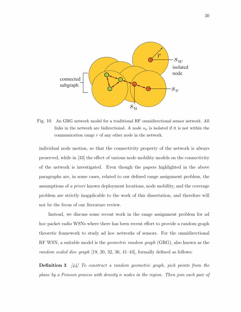
Fig. 10. An GRG network model for a traditional RF omnidirectional sensor network. All

links in the network are bidirectional. A node sw is isolated if it is not within the

communication range r of any other node in the network.

individual node motion, so that the connectivity property of the network is always

preserved, while in [33] the effect of various node mobility models on the connectivity

of the network is investigated. Even though the papers highlighted in the above

paragraphs are, in some cases, related to our defined range assignment problem, the

assumptions of a priori known deployment locations, node mobility, and the coverage

problem are strictly inapplicable to the work of this dissertation, and therefore will

not be the focus of our literature review.

Instead, we discuss some recent work in the range assignment problem for ad

hoc packet radio WSNs where there has been recent effort to provide a random graph

theoretic framework to study ad hoc networks of sensors. For the omnidirectional

RF WSN, a suitable model is the geometric random graph (GRG), also known as the

random scaled disc graph [19, 20, 32, 36, 41–43], formally defined as follows:

Definition 3 [44] To construct a random geometric graph, pick points from the

plane by a Poisson process with density n nodes in the region. Then join each pair of

31

points by a line if they are at distance less than or equal to r.

Definition 3 induces a topology in which given r, two nodes can communicate if

the distance between them is less than r. Obviously, the GRG with the r-radius model

for all nodes, relates to a simple omnidirectional network (without consideration to

channel fading) in which all links are necessarily bidirectional, so that if link sv → su

exists, then su → sv must also exist. We denote this bidirectional link as su sv.

For RF WSNs, r is a function of transmission energy, size of antenna and network

density. An isolated node in a GRG is then defined as one that falls outside the

communication range of every other node. The GRG network model illustrating a

connected subgraph and an isolated node sw is depicted in Figure 10.

One approach to the range assignment problem in GRG networks applies asymp-

totic reasoning by providing connectivity assurances as the region size or n grows to

infinity, and applies to dense networks. In one of the pioneering papers on the critical

power a node needs to transmit in order to ensure that the network is connected,

Gupta and Kumar [20] employ results from continuum percolation theory [45] and

random graphs [46], to derive the sufficient condition on r as a function of n for the

asymptotic connectivity of the GRG network. Their results show that for n nodes

uniformly deployed in a planar unit area disk, if r ≥√

[log(n) + c(n)]/πn, then the

network is asymptotically almost surely (a.a.s.) connected (as n → ∞ with prob-

ability one), only if limn→∞ c(n) = +∞, where c(n) is a constant for the n-node

network. In [33], the authors present connectivity results for real world sparse net-

works by introducing a geometric parameter that bounds the deployment area to a

finite region.

Others have analyzed asymptotic connectivity of the GRG with respect to the

minimum number of neighbors required by each node in a k-neighbor model. In [47],

32

Kleinrock and Silvester optimize an objective throughput function based on the aver-

age number of neighbors, and suggest that a fixed magic number of neighbors equal

to six is sufficient to guarantee network connectivity, regardless of the value of n.

Takagi and Kleinrock [48] later revised this magic number to eight. In [43], Xue and

Kumar show that there is no magic number, but rather that the number of neighbors

required for asymptotic connectivity grows as Θ(log n). In particular they show that

this number must be larger than 0.074 log n and less than 5.1774 log n. In [41], the

authors provide an improved lower bound for the number of neighbors required as

0.129 log n.

In [19], Penrose studied the more general problem of k-connectivity of GRG

networks deployed in d-dimensional cubes with d ≥ 2, and proved that the graph

becomes k-connected almost surely at the instant r attains the critical value at which

each node has a minimum number of k neighbors. Simply stated, this important

result implies that as n → ∞, the probability that the minimum r that achieves

k-connectivity of the network equals the minimum r that yields a minimum of k

neighbors for all nodes tends to one. Therefore, for the problem of connectivity, it

suffices to adjust r until each node has at least one neighbor, i.e., no isolated node

exists in the network. The results in [19] hold for any Lp-norm distance metric, where

1 < p < ∞.

Employing a probabilistic approach and nearest k-neighbor methods, Bettstet-

ter [42] show that for a ρ-density network, with probability at least p, no isolated node

occurs if r ≥√− ln(1− p1/n)/ρπ. He then leverages the results of [19] discussed in

the preceding paragraph to empirically demonstrate that for nodes densely deployed

in a bounded region (with n →∞), and for probability values close to one, the prob-

ability that no isolated node occurs in the network yields a tight upper bound, (and

therefore a good approximation using the same parameter values) for the probability

33

that the network is connected, if boundary conditions are compensated for. In sev-

eral of the cases cited above, a related analysis of range assignment in the presence of

fading links have also been considered. However, as with all the prior work cited here

so far, Bettstetter only focused on omnidirectional RF WSNs as modeled by GRGs.

For WOSNs, there has been relatively little research aimed at the corresponding

parameter assignment problem, stated as follows: given a set of n randomly deployed

WOSN nodes, all having the same r and α, what is the minimum value of r that

ensures the resulting network is connected? The equivalent problem of finding the

minimum n or α that ensures that the underlying network is connected has also not

been previously addressed. The parameter assignment problem for WOSNs neces-

sitates that we present a random graph model of the network (applicable also to

directional RF), termed the random scaled sector graph (RSSG), and first defined

in [9] as follows:

Definition 4 [9] For any natural n, fixed angle α and range r, let Sn = Si1≤i≤n

be a sequence of independently and uniformly distributed (i.u.d.) random coordinate

of points in [0, 1]2, and let Θ = (Θi)1≤i≤n be a sequence of i.u.d. angles in (0, 2π]

associated with Sn. Let E represent the n× n adjacency matrix such that the matrix

elements are assigned values: E(i, j)1≤i,j≤n = 1 if and only if si → sj exists. The

graph G(Sn, E) is termed the random scaled sector graph.

The RSSG is a generalization of GRGs for a network of sensors using wireless op-

tical communication, and with α set to 2π, the RSSG converges to the GRG model. To

address connectivity within the RSSG model, Diaz et al. [9], employ similar asymp-

totic connectivity arguments to show that for exactly the same constraint on r as

obtained in [20], as n →∞ the directed graph induced by the WOSN is connected as

the number of cells in the grid dissecting the deployment region goes to infinity. They

34

Table III. Comparing related work on range assignment for WSNs.Reference Comm. Analysis Deployment Other

[39] RF WSN (O) Random Geometric Coverage[50] RF WSN (O) Probabilistic Deterministic Coverage[32] RF WSN (O) Random Deterministic Coverage[35] RF WSN (O) Probabilistic Grid Coverage[42] RF WSN (O) Probabilistic Random k-connectivity[20] RF WSN (O) Asymptotic Random None[51] RF WSN (D) Probabilistic Random Coverage[52] RF WSN (D) Probabilistic Random Scheduling.[49] RF WSN (O/D) Probabilistic Stochastic None[9] WOSN Asymptotic Random None

Our Work WOSN Probabilistic Random Clustering

show that, if the ratio of r to the length of the side of the cells is kept constant, then

with probability approaching one, and as the number of cells grows there is a directed

path connecting any two nodes in the WOSN. Furthermore, they demonstrate that

with high probability, any edge in the undirected associated GRG to any WOSN may

be emulated by a path of length at most four in the directed RSSG. The authors

of [9] also provide sharp bounds on the expected maximum and minimum in and out

degree of nodes in a WOSN. However, the results for connectivity of WOSNs in [9]

are asymptotic results, which though of great theoretical interest, lack real-world ap-

plicability in sensor network scenarios involving finite area deployment regions and

number of nodes.

The work of this dissertation follows the probabilistic analysis flavor of [42] and

applies the relevance of the node isolation property to network connectivity discussed

in [19] with respect to WOSNs. The differentiating features of our research in this

regard include consideration for generalized directional sensor network models, which

encompass the omnidirectional case considered in [42]. We also consider the effects of

hierarchy and clustering on the connectivity of heterogeneous WOSNs that include a

sparse network of cluster heads placed randomly within the network. Our analytically

35

and empirical derivations are presented in Chapter III. Table III presents a limited

summary comparing some previous work that has addressed the range assignment

problem (and related versions of the problem) for WSNs in general. In the table, comm

refers to the mode of communication: omnidirectional (RF) based on GRG model or

directional; analysis refers to the methodology of connectivity analysis: asymptotic

or probabilistic; deployment refers to the deployment method: deterministic with

prior knowledge of location, (e.g., grid), random uniform distribution or stochastic

based on any distribution; and other refers to other objectives of the methodology

employed, such as coverage, energy efficiency, routing or scheduling.

B. Background Survey on Routing and Localization

A rich body of literature has considered various routing and localization techniques

specifically designed for WSNs, where energy awareness and consideration for traffic

patterns are essential design issues [18, 53–55]. Routing is defined as the process

of determining and using, in accordance with a set of rules, the route for the trans-

mission of a message from a source to a destination, while localization is the process

of determining and updating the position of nodes. Because of differences in func-

tionality, network configuration, traffic patterns and hardware constraints between

stationary WSNs and mobile ad hoc networks, many of the routing and localization

protocols designed for mobile ad hoc networks are not directly applicable to WSNs

and will not be reviewed in this dissertation. Distinguishing features which make

routing and localization in WSNs challenging include:

• Constraints in energy supply of sensor nodes necessitating innovative routing

designs that consider strict energy-awareness at all layers of the networking pro-

tocol stack in order to extend the WSN’s lifetime, while localization schemes

36

based on costly, energy-draining geographic positioning systems (GPS) are in-

feasible.

• Traffic patterns of WSNs in which the flow of data is mainly from multiple

sources to a particular destination or vice versa - i.e., nodes-to-base station and

base station-to-nodes, in contrast to the flat node-to-node or multicast traffic

patterns of ad hoc networks. This encourages a more energy efficient hierarchical

or clustering routing structure.

• Data generation pattern of sensor nodes, typically data-centric, resulting from

response to a base station query or an event rather than periodic in which subsets

of nodes periodically send their sensor readings to the base station. In data

centric WSNs, attribute-value data is requested or reported based on certain

local attributes. For example, the base station may send a [temperature > 80oF]

query to the network, and only nodes that sense temperatures greater than

80oF need report their readings. WSNs are also application specific and have a

strong requirement for location awareness in order to report data collected at

their location.

• Highly correlated data in the WSN which is typically based on a common phe-

nomena. That is, there is a high probability that data collected by several

nodes within the same region will be correlated. Such redundancy needs to be

exploited by routing protocols to improve energy and bandwidth utilization via

techniques such as data aggregation (e.g., duplicate suppression) and in-network

processing.

• The possibility of node failure which may cause frequent and unpredictable

topological changes in the network, necessitating fault tolerant designs and ef-

37

ficient route maintenance.

Due to these differences, a number of efficient and practical routing and localizations

schemes that have taken into account the inherent features of WSNs, along with the

application and architecture requirements have been proposed. We will not review

routing and localization schemes that have been proposed for mobile ad hoc or cellular

networks, even if, in some cases, they may indirectly apply to WSNs.

In general, many routing protocols for WSNs attempt to minimize energy usage

for the routing protocols while maximizing network life time. Others incorporate

various other optimization considerations including data aggregations, data dissem-

ination latency, scalability and low complexity or storage requirements. One naive

approach to routing in WSNs is flooding or gossiping, in which a node simply broad-

casts or randomly forwards its data to its local neighborhood or one neighbor, who

then recursively broadcasts or forwards this data to their own neighborhoods until

the data inadvertently reaches the base station. While nodes have no need to perform

neighborhood discovery or to maintain state (i.e., store routing tables), flooding and

gossip based routing protocols for WSNs is hugely wasteful of energy and bandwidth,

and easily result in packet implosion within the network [18].

To improve on the deficiencies of classic flooding and gossiping, Heinzelman et

al. [53] propose a family of adaptive negotiation based routing protocols called SPIN,

that employs meta-data negotiation and resource (energy) adaptation. SPIN is a

simple 3-stage protocol in which nodes send three types of messages: ADV to advertise

new data, REQ to request data and DATA which is the actual message. A node with

new data to share broadcasts an ADV containing meta-data. Nodes interested in its

data, typically the base station, then responds with a REQ message and then the

actual DATA is sent by the node to the interested party. Even though nodes are

38

also not required to maintain any per-neighbor state, the advertisement mechanism

of SPIN requires flooding, and it does not guarantee delivery of the data.

In TinyOS flooding [10], the base station sets up routing tables by periodically

broadcasting a routing packet to all the nodes in the network. All nodes that receive

the broadcast packet from the base station mark the base station as its parent and

re-broadcasts the routing packet to all its neighbors. This algorithm continues recur-

sively until all the nodes in the network have received a routing packet, and hence

know their parent node in the reversed next hop path toward the base station. Asim-

ilar protocol, the minimum cost forwarding algorithm (MCFA) [54] exploits the fact

that the direction of node-to-base station communication is always known (towards

the base station) to set up a cost field in the network.

In [55, 56], Intanagonwiwat et al. propose directed diffusion, the first data cen-

tric and application aware routing paradigm that achieves in-network consolidation

of redundant data for WSNs. In directed diffusion the sink floods interests for an

attribute-value query through the network. A query is an interest defined by an

attribute such as name of objects, interval, or geographical area, coupled with the

required value, such as “larger than a given threshold”. As the interest propagates,

they are cached at nodes, who compare any received data with requested values in

the query. Gradients are set up to forward any data satisfying the interests back to

the base station, using reverse paths. Gradients are reply links to neighbors charac-

terized by the link data rate, duration and expiration time derived from the received

query’s fields. Therefore by utilizing queries and gradients, multiple paths of varying

qualities are established between sink and sources, and one of the paths is selected

using reinforcement.

Several other data centric routing schemes that are variants of directed diffusion,

such as [57, 58] propose the use of multiple paths to send data concurrently, or

39

the use of sub-optimal paths with a given probability, to increase network lifetime.

Another approach based on directed diffusion, named rumor routing [18] employed

flooding to inject queries to the network using long lived agents. However, in contrast

to directed diffusion in which data may be routed via multiple routes, rumor routing

maintains only one route between source and destination. Another variant of directed

diffusion is gradient base routing (GBR) proposed by Shurgers et al. [59], in which

nodes measure their “height” as the minimum number of hops required to reach the

base station. Packets are then forwarded along the path with the largest gradient,

calculated as the difference between a node’s height and that of its neighbors. Directed

diffusion and its variants do not require node addressing, and there is no need to

maintain global network topology. Also data aggregation and interest caching produce

huge energy savings and improved latency. However, since they are query driven,

they prove unsuitable for applications that require continuous data delivery, such as

environmental monitoring.

Another class of routing algorithms for WSNs exploits hierarchy or clustering

to achieve data aggregation, energy efficiency and/or scalability. Hienzelnam, et

al. [53] introduce LEACH, the first hierarchical routing algorithm for WSNs. In the

setup phase of LEACH, a predetermined fraction of nodes randomly and dynamically

elect themselves as cluster heads, who aggregate data from their local clusters before

forwarding it directly via one hop to the base station. Each cluster head advertises

itself to the rest of the nodes, who then decide to which cluster they should belong

based on the signal strength of all their received cluster head advertisements. During

the steady state phase of LEACH, nodes sense and transmit data directly to cluster

heads. After a certain predetermined period, the network returns to the setup phase

again and so that a different set of cluster heads are selected, and so on.

40

In [60], PEGASIS, a chain-based enhancement over LEACH was proposed, with

the idea of only neighbor-to-neighbor communicate for optimal energy and bandwidth

utilization. The chain in PEGASIS, formed in a greedy fashion, consists of nodes that

are closest to each other forming a path to the base station, while data is aggregated

along the path. PEGASIS has been shown to increase network lifetime by about

200% over LEACH by eliminating the overhead of dynamic cluster formation and

decreasing the number of required transmission and the average transmission range.

A tree-like multi-layer hierarchical extension to PEGASIS which reduces the delay

incurred for packets from nodes distant from the base station was introduced in [61].

Unlike event driven routing such as directed diffusion, hierarchical schemes are most

appropriate for continuous data collection in WSNs.

Several other hierarchical routing protocols [18] have been proposed. For exam-

ple, TEEN [62] and its extension APTEEN [63] provide a multi-layer hierarchical

routing protocol within a data centric model designed to be responsive to sudden

changes in the sensed attributes, calibrated by a soft threshold. Other hierarchi-

cal routing protocols include a heterogenous energy-aware routing for cluster-based

sensor networks, the self organizing protocol [64], the sensor aggregates routing pro-

tocol [65], the virtual grid architecture routing [66] and the hierarchical power-aware

routing [67].

Another general class of routing protocols for WSNs are the location based algo-

rithms that employ the relative position of nodes to make routing decisions instead

of flooding. Nodes are simply assumed to know their locations. One of the earlier pa-

pers on geographic routing proposed greedy perimeter stateless routing (GPSR) [68],

a non-energy aware protocols which employs planar graphs to route data around the

perimeter of obstacles (holes). In geographic and energy aware routing, (GEAR) [69]

all routing is directed towards a particular geographical region using energy aware

41

neighbor selection to route a packet towards the sink’s general location, and recur-

sive geographic forwarding or restricted flooding to disseminate the packet inside the

destination’s vicinity. In the geographic adaptive fidelity (GAF) protocol [70], the

network is dynamically divided into fixed zones that form a hierarchical virtual grid.

Within each zone, an elected node stays awake to perform sensing and communica-

tion for a given period of time while other nodes sleep. This function is then rotated

amongst nodes in the zone. Other geographic routing algorithms for WSNs include

the greedy other adaptive face routing (GOAFR) [71], SPAN, most forward within

radius (MFR), DIR and the geographic distance routing (GEDIR) [72].

One of the main problems with location based routing algorithms is that the po-

sition of nodes are assumed to be known. In addition to geographic routing, several

WSN applications such as target tracking (requiring nodes to indicate the geographic

origin of their sensor data), rely on the ability of the nodes to gain knowledge of

their location. Location information can also help security and collaborative signal

processing algorithms in WSNs. This necessitates that light weight algorithms for

location discovery that are independent of existing infrastructure be explored as re-

source constraints of nodes preclude the use of expensive and complex localization

hardware such as GPS. These algorithms aim to enable randomly distributed, low

cost and low complexity nodes to automatically determine their position with respect

to some reference point.

Existing location discovery techniques for WSNs have been categorized into two

classes: range based and range free. Range based methods such as [73] employ abso-

lute point-to-point distance or angle estimates, and then apply trilateration or multi-

lateration techniques to find the unknown position of the node. The distance or angle

estimates may be obtained from received signal strength indicator (RSSI) measure-

ments, recursive time of arrival (TOA), time difference of arrival (TDOA), or angle

42

of arrival (AOA) of a signal. Unfortunately, these techniques do not provide enough

accuracy in WSNs or require additional hardware. Because range free solutions make

no assumptions on the availability or validity of range estimation hardware or mech-

anisms, it is being pursued as a cost effective alternative to the more expensive range

based approaches for WSNs [74].

Many range free methods depend on deducing the geometry of the network based

on interactions amongst nodes. While some explore the connectivity information of

the communication graph, others depend on the use of a small proportion of beacons

or anchors (special class of sensor nodes that are aware of their location e.g. using

GPS). Bulusu et al. [75] proposed a crude localization approximation scheme called

centroid in which nodes estimate their position as the centroid of the locations of all

beacons heard. A variant of centroid uses multiple power levels to provide a better

localization accuracy at the expense of increased communication cost. Niculescu

and Nath [76] propose DV-hop where each node determines the number of hops to

beacons, determines its distance to the beacons using average hop size estimates,

and then employs multilateration to determine their absolute location. He et al.

propose APIT, in which each node tests to determine if it is within a triangle defined

by a 3-tuple of anchors heard by the node. The location of the node is estimated

to be the center of gravity of the triangles overlapping region. A similar approach

using directional antennas for beacons is employed by Lazos and Poovendran [77].

These algorithms are fully distributed and use local broadcast for communication

with immediate neighbors, implying that they have to executed before any multihop

routing schemes such as GAF or GEAR is established.

Several of the routing and localization protocols discussed here have optimized

for the limited resources of the nodes without consideration for security, and have

also considered routing and localization as separate problems. Furthermore, the al-

43

gorithms have been designed to work in a (mostly) bidirectional network modeled by

the GRG, with a few considering link asymmetries due to the use of directional RF

antenna [78] or link fading. These schemes, including TINY OS, directed diffusion

and their variants, implicitly or explicitly assume that all (or a large proportion) of

the network links are bidirectional, and have therefore employed reverse path routing

in some form. This assumption considers that if a node is able to receive a packet

from a neighbor, with probability one, it may consider a return uplink path toward

the base station through this neighbor.

Furthermore, in many of the routing protocols for bidirectional networks, lis-

tening to periodic messages from neighbors is sufficient to determine a nodes direct

neighbors, whereas in a directed network such a mechanism only reveals predecessors,

and additional mechanisms are required to provide knowledge of successors. Some

popular ad hoc network routing schemes such as dynamic source routing [79], link

state routing [80] and distance vector routing [81] have provided modifications that

accommodate the discovery of successors in the presence of a limited fraction of di-

rectional network links, by either ignoring such links or providing a bi-directional

abstraction known as tunneling [82–86]. However, the underlying assumption of re-

verse path routing does not hold for directional WOSNs in which the vast majority

of network links are directional. Therefore, previously proposed protocols are inap-

plicable to WOSNs.

In [27], a novel protocol based on the detection of circuits for routing in purely

directional networks was first discussed. The protocol employs link advertisement

messages to gain knowledge of a local topology graph. This protocol deals only with

point-to-point links. Building upon [27] Huang et al [81] present a similar circuit-

based routing algorithm for point-to-multipoint path discovery. Based on the distance

vector routing information protocol, each node maintains a “FROM” and “TO” table

44

of all possible destination which presents a problem for scaling to large networks.

In [87], Lou and Wu extend the complexity of the algorithm by designing a multi

path routing scheme that stores one optimal circuit per successor to each destination.

While all these protocols are cheaper than flooding for directional networks, they

only work in small networks and do not scale well to the network size envisioned

for WOSNs. Also, special consideration has not been given to hierarchy, security or

efficient resource utilization that characterize routing protocols for WSNs.

Besides our work, Diaz et al. [9] are the only other researchers that have consid-

ered (separately) routing and localization for hierarchical WOSNs. For localization,

they assume cluster heads receive their coordinates from the base station while the

remaining nodes recursively employ trilateration to compute their locations based

on receiving the coordinates of three other nodes and the angle of incidence of the

incoming laser beams. They show that as the network density tends to infinity, with

probability one, all network nodes can compute their location within a limited num-

ber of iterations. They also discuss a distinct two-part route establishment protocol

for the WOSN consisting of the simple-bro protocol initiated by the base station for

down-link broadcasting from base station-to-nodes; and the node initiated simple-link

protocol for uplink communication from nodes-to-base station. This two step routing

scheme is not circuit based, and therefore does not exploit some of the redundancies

available within the double procedure. Security is also not considered in this scheme.

C. Security Considerations for Routing and Localization

Current routing protocols suffer from many security vulnerabilities ranging from sus-

ceptibility to simple attacks such as injecting malicious routing information to the

network to DDoS, and replay attacks. It is therefore crucial to consider security in

45

the design of network layer protocols [88] in order to safe guard the data and appli-

cation layers. In [11], a taxonomy of well known routing attacks for WSNs have been

highlighted including: the sybil attack [89] in which an insider attacker presents itself

using multiple identities for the purpose of underscoring fault tolerance schemes; the

sinkhole attack in which a malicious node strives to lure network traffic to itself by

several means, such as advertising itself as the base station or as having a high rate

low latency path to the base station; a laptop class form of the sinkhole attack called

the HELLO flood attack which employs a powerful device to flood advertisements to

the entire network; and the powerful wormhole attack [90] easily accomplished by an

outsider, involving a node tunneling packets through a low latency link to another

part of the network, from which it easily launches a replay attack. An attacker may

try to exploit the vulnerabilities of a routing algorithm in arbitrary ways, therefore

security must be considered at the onset of routing mechanism design. The authors

of [11] also point out the various vulnerabilities of popular WSN routing schemes to

various attacks.

Several routing protocols for WSNs that have considered security in their de-

sign can be broadly categorize into two groups, namely: those requiring asymmetric

cryptography solutions, and those that rely on symmetric cryptography. The latter

solution is widely popular for WSNs, due to the assumption that the sensor nodes

do not have the resources to support the storage and processing requirements for

public key cryptography. The most commonly utilized mechanisms that symmetric

cryptography solutions rely on to secure the routing function include hash functions,

key chains and message authentication codes. A one-way hash function is a function

that takes an input of arbitrary length and returns an output of fixed length. Hash

functions have the property of being computationally infeasible to reverse, that is, if

h = f(m), it is impossible to computer m such that f(m) = h.

46

In [31], Perrig et al. introduce “SPINS” comprised of Sensor Network En-

cryption Protocol (SNEP) for two party data authentication, privacy, integrity and

freshness, and µ-Tesla for authenticated data broadcast. µ-Tesla assumes a loosely

time-synchronized network and uses the one-way key chain with delayed key disclo-

sure to achieve broadcast authentication in a TinyOS routing scheme. Other secure

routing protocols for WSNs have specifically focused on preventing only one or two

of the known routing attacks. Secure localization algorithms have even been fewer,

with [91] as the pioneer work that discusses robust localization and counter measures

for wormhole attacks.

In this dissertation, we introduce an integrated and security-aware routing and

localization protocol for directional WOSNs. Our protocol is the first to offer the fol-

lowing distinctive features: Security consideration integrated localization and routing

scheme for WOSNs. hierarchical circuit based. The routing protocol incorporates the

three crucial components of hierarchy, data centricity and location awareness to yield

a robust design that is scalable, secure and resource aware. To the best of our knowl-

edge, this is the first integrated and security-aware routing and localization scheme

for a fully directional distributed WSN. Our algorithm is able to establish secure ad

hoc routing mechanisms to identify, track and communicate critical data such as the

presence of adversaries.

47

CHAPTER III

CONNECTIVITY ANALYSIS OF THE WOSN

The connectivity of an ad-hoc WSN is one of its essential properties, and is of particu-

lar significance in order to maintain communication among nodes. Often, connectivity

is viewed as a metric of the robustness, survivability or fault tolerance of networks,

and has been related to the network’s value [19]. Before we can adequately discuss ef-

fective medium access and network layer protocols for WOSNs, such as neighborhood

discovery, routing and localization mechanisms, it is imperative to reasonably guar-

antee the connectivity of the network at the physical layer. In this section, we employ

the traditional definition of a connected network: for every possible node pair, there

exists at least one path (sequence of nodes and edges) connecting them. Considering

edge directions, a strongly connected directed network is one in which, for every node

pair (sa, sb), ∃ sa sb and sb sa [29]. Unless confusing, we shall refer here to the

“strongly connected” property of WOSNs simply as “connected”.

This section addresses the fundamental probabilistic parameter assignment prob-

lem for WOSNs by asking the question: How can the physical layer network param-

eters of n, r and α be chosen such that, with high probability pc, the underlying

network graph G(Sn, E) of the WOSN is connected? Our analysis provides a method-

ology for, and is of practical importance in choosing parameter values for network

level design of ad hoc WOSNs, and more general models of WSNs. We make three

important contributions in this section:

1. First, we investigate the node isolation property of WOSNs, and obtain an

analytical closed form expression for the probability pd that no isolated node

occurs as a function of network parameters r, n and α.

48

2. Second, in order to study the tightness of the upper bound that pd provides

as an estimate for pc, we compare our analytical values of pd with empirical

results of pd and pc. Our results demonstrate that similar results derived [42]

for omnidirectional WSNs hold in WOSNs as α → 2π.

3. Third, we analyze the impact of hierarchy on the connectivity property of

WOSNs as a function of the fraction of nodes acting as cluster heads, and

empirically demonstrate the enhanced connectivity due to clustering.

A. Relating Node Isolation and Network Connectivity

The occurrence of isolated nodes is undesirable, as their existence undermines the goal

of achieving a highly connected network; the existence of a single isolated node implies

that the network is necessarily disconnected. However, even though guaranteeing that

no isolated nodes occur is not a sufficient condition for connectivity, it is certainly

a necessary one, and therefore an important first step towards achieving network

connectivity: a connected network implies no isolated node; however the converse is

not true [42], as a network with no isolated node does not necessarily imply that the

network is connected. Figure 11 illustrates this insufficiency condition in a WOSN

scenario. Even though there exists no isolated node, the network is not connected due

to link directionality and possible network partitions; for example, path sb sa does

not exist, even though sa → sb exists. Note that in this example, we have defined

as isolated node in the traditional graph theoretic sense for undirected graphs, that

is, each node has at least one link connecting it to another node. To consider true

network connectedness for WOSNs, in which every pair of nodes is contained in at

least one a circuit, it is imperative that we re-define the notion of a connected and an

isolated WOSN node.

49

partition

looploop

connectednetwork

no isolatednode

Fig. 11. The WOSN has no isolated nodes, since every node has both an incoming and

an outgoing link. However the overall network is not (strongly) connected due to

the network partition and link directionality; for example, sa → sb exists, however

sb sa does not exist.

An important approach to connectivity analysis in ad hoc networks relates the

conditions under which no isolated network nodes exist, to network connectivity.

Since an exact closed form analytical expression for the probability pc of network

connectivity in terms of network parameters (r, α, n/A) cannot be obtained, a highly

accurate estimate involving the probability pd that the network contains no isolated

node (easily expressed in closed form), is obtained.

Recent studies show that for dense omnidirectional WSNs, (as n → ∞), the

underlying graph is connected with high probability, at the moment (and for the r

value) at which no isolated network node occurs [19, 42]. Simply stated, this result

implies that pd provides a tight upper bound for pc as n → ∞ and for probabilities

50

close to one1, and motivates our study of parameter relationships that ensure a “no

isolated node” property for WOSNs, and its relevance to network connectivity. One

question we answer in this dissertation is; do similar results as obtained in [42] hold

for the WOSN network model?

We previously stated the necessity to define two sets of neighbors for each WOSN

node within the directed graph paradigm: successors and predecessors. The distinc-

tion between successors and predecessors is significant to the connectivity analysis of

WOSNs since a given node’s successor is necessarily not a predecessor, and as we show

later, the probability that a successor is also a predecessor is dependent on the value

of α. Before we proceed, it is necessary to define the concept of a connected and an

isolated node in Gn(Sn, E). The definition of an isolated node is somewhat different

for omni-directional networks in which node sm is isolated if the ball B(Υm, r0) of

center Υm and radius r0 is empty.

• A node si ∈ Sn is forwardK-isolated or simply fK-isolated if δ+i < K, otherwise

it is fK-connected, with bK-isolated and bK-connected similarly defined with

respect to δ−i . For example, si is f1-isolated if δ+i = 0, and f1-connected if

δ+i > 0.

• A node is K-connected if it is both fK-connected and bK-connected.

• A node is directionally-isolated (or disolated) if Si = ∅ but Pi is non-empty, or

vice versa. Similarly, it is directionally K-isolated if it is either fK-isolated or

bK-isolated.

• Node si is completely-isolated if Si = Pi = ∅.

1This holds for high probability values, which is the interesting case for WSNs.

51

• Our definition of isolated nodes in Gn(Sn, E) encompasses both completely iso-

lated and disolated nodes. In our analysis, we desire that no isolated node

occurs in order to achieve a fully connected WOSN as per our definition.

• For ease of reference, the 1-connected and directional 1-isolated properties are

simply referred to as connected and directionally-isolated, respectively. Where

there is no risk of confusion, we will refer to a directionally-isolated WOSN node

simply as an isolated node.

• There is no K-isolated WOSN node in Gn(Sn, E) if ∀si ∈ Sn, δ+i ≥ K, and

δ−i ≥ K.

• Finally, an event A is said to occur almost surely (a.s.) if the probability of

event A denoted as Pr[A] is greater than 0.99.

B. Analysis on Node Isolation

Consider the following r-assignment problem for the n-node WOSN stated as follows:

what is the minimum r, such that for a fixed α value, with high probability pd, a

node is not isolated? A similar α-assignment problem is: Given n nodes with a fixed

r, what is the minimum α such that no isolated node occurs in the WOSN with

probability pd?

1. Probability of No Isolated WOSN Node

To gain insight to these parameter assignment problems, our first step is to consider

the probability pid that a node si ∈ Sn is not isolated. Let pi

f =Pr[δ+i > 0] and

pib =Pr[δ−i > 0] denote the probabilities that si is not f1-isolated and b1-isolated,

respectively. Recall that the set of directionally isolated nodes consists of the union

52

of f1-isolated and b1-isolated nodes, and the probability that si is isolated is:

Pr[δ+i = 0 ∪ δ−i = 0],

while si is connected (i.e., not isolated) if it is both f1-connected and b1-connected

with probability pid given as:

pid = pi

f∩b = pif .p

ib|f (3.1)

where ∪ and ∩ are the union and intersection operators, respectively, and pif∩b de-

notes the probability that si is both b1-connected and f1-connected, and pib|f is the

conditional probability that si is b1-connected given it is f1-connected. Our next step

towards determining pid is to evaluate pi

f and pib|f .

a. Evaluating pif

Lemma B.1 For n →∞ and r 1, si is f1-connected with probability:

pif = Pr[δ+

i ≥ 1] = 1− e−nαr2

2 (3.2)

Proof of Lemma B.1 For this proof, we employ quadrat2 statistical methods

which is an approach taken to quantify spatial point patterns (see Chapter 8 of [25]).

Under this model, quadrats of random location and orientation are sampled, the

number of events in the quadrat are counted, and statistics derived from the counts.

It is well known [24, 25, 36, 49] that the number of points located in a quadrat of area

Aq, follows a Poisson distribution of parameter λAq, where λ is the intensity of the

Poisson process. Viewing communication sectors as quadrats, the random variable δ+i

counting the number of nodes located in si’s communication sector Φi of area αr2/2 is

2Quadrats are bounded regions of any possible shape including Φ.

53

then a Poisson point process with parameter nαr2/2, and probability density function

(pdf):

Pr[δ+i = z] =

e−nαr2

2

(nαr2

2

)z

z!(3.3)

The probability that si is f1-isolated (i.e., Φi is empty) is

Pr[δ+i = 0] = e

−nαr2

2

and the probability pif that si is f1-connected (i.e., at least one node in Φi) is:

Pr[δ+i ≥ 1] =

n−1∑z=1

e−nαr2

2 (nαr2

2)z

z!= 1− e

−nαr2

2 , (3.4)

yielding the result of Lemma B.1. The derivation of Equation 3.4 employs the series

approximation of the exponential function for large n and small αr2, given below:

ex =∞∑

z=0

xz

z!= 1 +

∞∑z=1

xz

z!.

b. Evaluating pib

Lemma B.2 For n →∞ and r 1, si is b1-connected with probability pib equal to

pif .

Proof of Lemma B.2 The b1-connectivity problem is analogous to an area

coverage problem, in which a point is “covered” if it lies within the area of the

communication sector of any other node. Obviously, si is b-connected if Υi ∈ Φj

for any j 6= i. The proof is constructed from concepts in stochastic geometry [24],

similar to the proof of area coverage derived for the general case in [36]. Consider

the WOSN with n nodes as points that are uniformly located in a unit area region.

The probability that any point Υi (which is the position of node si) does not fall

54

within an arbitrary sensor’s communication sector equals (1− αr2/2) where αr2/2 is

the area of the sector. Conditioned on the number of nodes n, the probability that

si is not covered is (1 − αr2/2)n [24]. For large n and r << 1, this Binomial is well

approximated as a Poisson so that:

Pr[si is not covered] = e−nαr2

2 ,

and the probability pib that si is b-connected (i.e., it is covered) is then obtained as:

pib = 1− e

−nαr2

2 . (3.5)

The result of Lemma B.2 follows.

c. Evaluating pib|f

Lemma B.3 For n → ∞ and αr2 1, si is b1-connected given it is f1-connected

with probability pib|f given as:

pib|f = 1− e

−nαr2

2

1− e−nαr2

2

(1− αr2

2

)n−1(

e

»nαr2(2π−α)

2π(2−αr2)

–− 1

).

Proof of Lemma B.3 Assume si is f-connected (Si 6= ∅) so that δ+i ≥ 1. We

wish to evaluate

pib|f = Pr[δ−i ≥ 1|δ+

i ≥ 1].

where δ+i ∈ Z[1, n] and δ−i ∈ Z[0, n− 1] represent the random variables counting the

number of si’s successors and predecessors, respectively, and Z is the set of integers.

Following our model with independently deployed nodes assumed, to obtain pib|f , we

consider two disjoint cases for which si can attain b-connectivity given it is already

f-connected:

Case 1 : The event that si has no bi-directional link with any of its successors, de-

55

noted [no bi], implying that of the δ+i = z nodes in Φi, none are oriented to

cover si. In this case, si may only be b-connected if it has established a link

with at least one of the n− z − 1 other nodes not in Φi, termed non-successor

nodes. This event is referred to as [no bi].

Case 2 : The event that si has at least one bi-directional link with one of its suc-

cessors. That is, at least one successor is also a predecessor, (si also falls in the

communication sector of at least one of the nodes in Φi) so that si is b-connected

by any of the z successor nodes in Φi. This event is referred to as [at least one

bi].

Due to the disjointness of case 1 and case 2, we can write:

pib|f = Pr[δ−i ≥ 1|δ+

i ≥ 1]

= 1− Pr[δ−i = 0|δ+i ≥ 1]

= 1−Pr[δ−i = 0|δ+

i ≥ 1, no bi].Pr[no bi]

−Pr[δ−i = 0|δ+

i ≥ 1, at least one bi].Pr[at least one bi]

(3.6)

Observe that Pr[δ−i = 0|δ+i ≥ 1, at least one bi] = 0, since δ−i = 0 contradicts the case

that [at least one bi] exists, so that Equation 3.6 above simplifies as:

pib|f = 1−

Pr[δ−i = 0|δ+

i ≥ 1, no bi].Pr[no bi]

= 1−n−1∑z=1

Pr[δ−i = 0|δ+i = z, δ+

i ≥ 1, no bi].Pr[no bi|δ+i = z, δ+

i ≥ 1]

× Pr[δ+i = z|δ+

i ≥ 1] (3.7)

56

Following our model of assuming uniformly random sector orientation, the prob-

ability of a bidirectional link existing between si and any of its successors sj, denoted

as Pr[sj → si|si → sj] = α/2π, so that the probability that no bidirectional link

exists between si and any of its δ+i = z successors (δ+

i ≥ 1) equals (1 − α/2π)z. For

independently deployed nodes, given that si is f-connected we have that:

Pr[no bi |δ+i = z, δ+

i ≥ 1] = (1− α

2π)z, for z = 1, 2, · · ·n− 1. (3.8)

Given our unit area deployment region, we have that:

Pr[δ−i = 0|δ+i = z, δ+

i ≥ 1, no bi] =

(1− αr2

2

)n−z−1

, (3.9)

and

Pr[δ+i = z|δ+

i ≥ 1] =Pr[(δ+

i = z) ∩ (δ+i ≥ 1)]

Pr[δ+i ≥ 1]

=(nαr2

2)ze

−nαr2

2

z!.

1

1− e−nαr2

2

(3.10)

where:

Pr[(δ+i = z) ∩ (δ+

i ≥ 1)] =

Pr[δ+i = z] for z > 0

0 for z = 0

Equation 3.10 employs the more accurate approximation for Pr(δ−i = 0|δ+i =

z, no bi) as Binomial(αr2/2) for z = 1, 2, · · ·n − 1, as the Poisson approximation is

only valid for large n and small z values (see the Appendix). Substituting Equations

57

3.8, 3.9 and 3.10 into Equation 3.7, yields:

pib|f = 1−

n−1∑z=1

(1− αr2

2

)n−z−1

.(1− α

2π)z.

(nαr2

2)ze

−nαr2

2

z!.

1

1− e−nαr2

2

= 1− e

−nαr2

2

1− e−nαr2

2

(1− αr2

2

)n−1 n−1∑z=1

(2π − α

2π.

2

2− αr2

)z

.

[(nαr2

2)z

z!

]

= 1− e−nαr2

2

1− e−nαr2

2

(1− αr2

2

)n−1 n−1∑z=1

[nαr2(2π−α)2π(2−αr2)

]zz!

(3.11)

Now, employing the series approximation of an exponential for large n and small αr2,

yields:

pib|f = 1− e

−nαr2

2

1− e−nαr2

2

(1− αr2

2

)n−1(

e

»nαr2(2π−α)

2π(2−αr2)

–− 1

), (3.12)

the result of Lemma B.3.

Observe that for the omnidirectional case with α = 2π, pib|f = 1 as expected.

That is, with the RGG communication model and all links bidirectional, if a node is

f-connected, then of course it is also b-connected. It is clear that pib|f ≥ pi

b due to the

possibility of bidirectional links.

d. Evaluating pid

Substituting Equations 3.4 and 3.12 into Equation 3.1, and simplifying yields:

pid =

[1− e

−nαr2

2

] [1− e

−nαr2

2

1− e−nαr2

2

(1− αr2

2

)n−1(

e

»nαr2(2π−α)

2π(2−αr2)

–− 1

)](3.13)

Observe that pif ≥ pi

d for large n and small αr2 with equality when α = 2π.

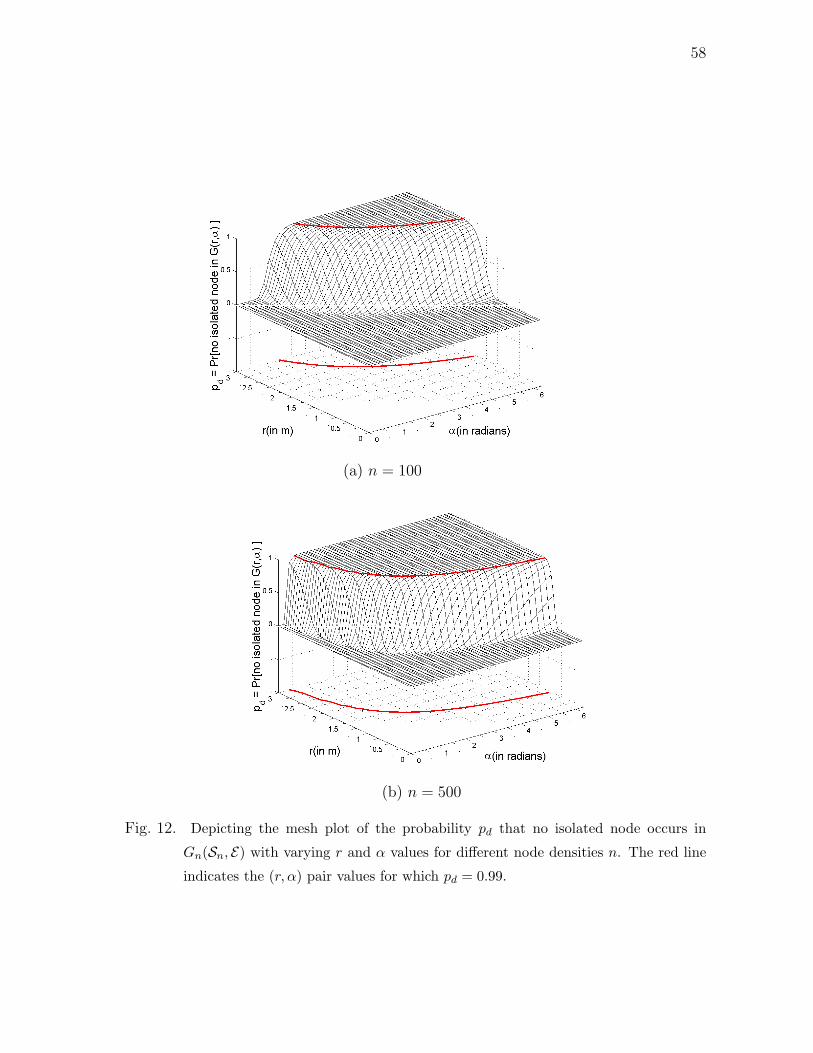
58

(a) n = 100

(b) n = 500

Fig. 12. Depicting the mesh plot of the probability pd that no isolated node occurs in

Gn(Sn, E) with varying r and α values for different node densities n. The red line

indicates the (r, α) pair values for which pd = 0.99.

59

(c) n = 1, 000

(d) n = 5, 000

Fig. 12 continued.

60

(e) n = 10, 000

(f) n = 100, 000

Fig. 12 continued.

61

e. Evaluating pd

Theorem B.4 For n → ∞ and small αr2, there is no isolated node in Gn(Sn, E)

with probability pd:

pd =[1− e

−nαr2

2

]n [1− e

−nαr2

2

1− e−nαr2

2

(1− αr2

2

)n−1(

e

»nαr2(2π−α)

2π(2−αr2)

–− 1

)]n

(3.14)

Proof of theorem B.4 Assuming statistical independence among events that

distinct nodes are isolated, Theorem B.4 follows by computing pd for n nodes as:

pd =

n

n

(pid)

n(1− pid)

0 (3.15)

where the expression for pid is given in Equation 3.13. For α = 2π we note that

pd reduces to (1 − e−nπr2)n as obtained by Bettsetter [42]. It therefore turns out

that Equation 3.14 is the expression relating network parameters n, r and α with the

probability pd that no isolated node occurs for WSNs in general.

Figure 12 illustrates pd for a range of r and α values for different n values with

the (red) line on the r−α plane of each mesh plot indicating the (r, α)-pair values for

which there is almost surely (pd = 0.99) no isolated node. We observe that as node

density n increases, network connectivity improves, and for a very dense network with

n = 100, 000, parameter value pairs as small as (r = .01, α = 6π/25) yield a network

with almost surely no isolated node.

Example 1: (Simulation Study): We perform a simulation-based study of a

WOSN to investigate the connectivity property. Employing a uniform random gener-

ator we position n WOSN nodes in a square planar region of area 1 km2, following our

deployment model. We aim to determine the minimum parameter values that achieve

a WOSN in which, with high probability (> 0.99), no node is isolated. From the an-

alytical expression of Equation 3.14, we obtain the minimum r and corresponding α

62

Table IV. The minimum r value for corresponding network parameter (n, α) pair val-

ues that achieve pd ≥ 0.99 in Gn(Sn, E).

n α = π9

α = 2π9

α = π3

α = π2

α = 3π4

α = π α = 3π2

α = 2π

100 0.755 0.527 0.426 0.345 0.281 0.243 0.198 0.172

500 0.360 0.253 0.205 0.167 0.136 0.118 0.096 0.083

1000 0.262 0.184 0.150 0.122 0.099 0.086 0.070 0.061

5000 0.125 0.088 0.072 0.058 0.048 0.041 0.034 0.029

10000 0.091 0.064 0.052 0.042 0.035 0.030 0.025 0.021

100000 0.011 0.008 0.006 0.005 0.004 0.004 0.003 0.003

required for pd ≥ 0.99 with n given, as shown in Table IV.

For example, observe that for n = 1000 and α = 2π/9, pd ≥ 0.99 is achieved with

r ≥ 0.184 km. If however the WOSN nodes are only capable of achieving r = 0.09 km

for the same α, then we need at least ∼ 5000 nodes, or at design time, we may choose

to increase α to π in order to deploy the same n = 1000 nodes and obtain the same

confidence for pd. With n = 500 nodes and α = 2π/9, α = π/2 and α = π we

obtain pd ≥ 0.99 with r ≥ 0.253 km, r ≥ 0.167 km and r ≥ 0.118 km respectively.

This compares with r ≥ 0.083 km value obtained in [42] for n = 500 nodes in the

omnidirectional network scenario.

Interestingly, we observe that for the same confidence on pd, doubling r allows us

reduce α by approximately a fourth. An interesting study beyond the scope of this

work would involve comparing the practical cost (dollar, energy) of increasing r while

reducing α (or vice versa) to determine the optimal WOSN node (r, α)-parameter

configuration based on a given cost function.

63

2. Probability of No K-isolated WOSN Node

It is necessary to consider K-connectivity in the design of robust and secure networks

in order to accommodate link and/or node failures or compromise. A K-connected

network is defined as one that remains connected after the failure of any choice

of (K − 1) nodes. To gain insight into K-connectivity for the WOSN, similar to

previous analysis we first consider the probability pdKthat no isolated node occurs

in the network, and its relationship to the network parameters n, r, α.

Obviously, a given node si is K-connected (i.e., not K-isolated) with probability:

pidK

= pifK∩bK

= pifK

.pibK |fK

, (3.16)

where pifK

is the probability that si is fK-connected, and pibK |fK

is the probability

that si is bK-connected, given it is fK-connected. The probability pdKthat no K-

isolated node occurs in the n-node network, assuming independence among events

that distinct nodes are isolated, is then pdK= (pi

dK)n. We are now left to derive pi

fK

and pibK |fK

.

By similar arguments, we easily extend the results of Lemmas B.1 and B.2 for f1-

and b1-connectedness to the fK- and bK-connected cases, respectively, and conclude

that the probability pifK

= Pr[δ+i ≥ K] that si is fK-connected is equivalent to the

probability pibK

= Pr[δ−i ≥ K] that si is bK-connected, given as:

pifK

= Pr[δ+i ≥ K] =

n−1∑m=K

e−nαr2

2 (nαr2

2)m

m!= pi

bK(3.17)

while

pibK |fK

= Pr[δ−i ≥ K|δ+i ≥ K] = 1− Pr[δ−i < K|δ+

i ≥ K] (3.18)

Equations 3.17 and 3.18 yield the basis for deriving pdKby following similar arguments

64

employed for the K = 1 case. As an illustration, we derive pdKfor K = 2 in the next

section.

a. Case for K = 2

From Equation 3.17 we readily obtain that:

pif2

= Pr[δ+i ≥ 2] =

n−1∑z=2

e−nαr2

2 (nαr2

2)z

z!= 1− e

−nαr2

2

(1 +

nαr2

2

)(3.19)

Since Pr[δ+i ≥ 2] = 1− Pr[δ+

i = 0]− Pr[δ+i = 1], where

Pr[δ+i = 0] = e

−nαr2

2 and Pr[δ+i = 1] =

nαr2

2e−nαr2

2 .

To derive pib2|f2

we employ the following:

pib2|f2

= Pr[δ−i ≥ 2|δ+i ≥ 2]

= 1− Pr[δ−i < 2|δ+i ≥ 2]

= 1− Pr[δ−i = 0|δ+i ≥ 2]− Pr[δ−i = 1|δ+

i ≥ 2]

= 1− Pr[δ−i = 0|δ+i ≥ 2, no bi].Pr[no bi]

−Pr[δ−i = 1|δ+i ≥ 2, no bi].Pr[no bi]

−Pr[δ−i = 0|δ+i ≥ 2, at least one bi].Pr[at least one bi]

−Pr[δ−i = 1|δ+i ≥ 2, exactly one bi].Pr[exactly one bi]

−Pr[δ−i = 1|δ+i ≥ 2, at least two bi].Pr[at least two bi] (3.20)

65

But Pr[δ−i = 0|δ+i ≥ 2, at least one bi] = Pr[δ−i = 1|δ+

i ≥ 2, at least two bi] = 0, so:

pib2|f2

= 1− Pr[δ−i = 0|δ+i ≥ 2, no bi].Pr[no bi]︸ ︷︷ ︸

part1

−Pr[δ−i = 1|δ+i ≥ 2, no bi].Pr[no bi]︸ ︷︷ ︸

part2

(3.21)

−Pr[δ−i = 1|δ+i ≥ 2, exactly one bi].Pr[exactly one bi]︸ ︷︷ ︸

part3

where part 1 is:

n−1∑z=2

Pr[δ−i = 0|δ+i = z, δ+

i ≥ 2, no bi].Pr[no bi|δ+i = z, δ+

i ≥ 2].Pr[δ+i = z|δ+

i ≥ 2],

part 2 is:

n−1∑z=2

Pr[δ−i = 1|δ+i = z, δ+

i ≥ 2, no bi].Pr[no bi|δ+i = z, δ+

i ≥ 2].Pr[δ+i = z|δ+

i ≥ 2],

and part 3 is:

n−1∑z=2

Pr[δ−i = 1|δ+i = z, δ+

i ≥ 2, one bi].Pr[one bi|δ+i = z, δ+

i ≥ 2].Pr[δ+i = z|δ+

i ≥ 2].

Now, we have that for z = 2, 3, · · ·n− 1:

Pr[no bi |δ+i = z, δ+

i ≥ 2] = (1− α

2π)z, (3.22)

and

Pr[one bi|δ+i = z, δ+

i ≥ 2] = zα

2π(1− α

2π)z−1, (3.23)

and

Pr[δ+i = z|δ+

i ≥ 2] =Pr[(δ+

i = z) ∩ (δ+i ≥ 2)]

Pr[δ+i ≥ 2]

=(nαr2

2)ze

−nαr2

2

z![1− e

−nαr2

2 (1 + nαr2

2)](3.24)

and

Pr[δ−i = 0|δ+i = z, δ+

i ≥ 2, no bi] =

(1− αr2

2

)n−z−1

(3.25)

66

and

Pr[δ−i = 1|δ+i = z, δ+

i ≥ 2, no bi] = (n− z − 1)

(αr2

2

)(1− αr2

2

)n−z−2

(3.26)

and

Pr[δ−i = 1|δ+i = z, δ+

i ≥ 2, exactly one bi] =

(1− αr2

2

)n−z−1

. (3.27)

where

Pr[(δ+i = z) ∩ (δ+

i ≥ 2)] =

Pr[δ+i = z] for z ≥ 2

0 for z = 0, 1

and

Pr[δ−i = k] =

(n− z − 1

k

)(αr2

2

)k (1− αr2

2

)n−z−1−k

.

Substituting Equations 3.22, 3.24 and 3.25 into part 1 of Equation 3.21, we have:

Part 1 :

n−1∑z=2

Pr[δ−i = 0|δ+i = z, δ+

i ≥ 2, no bi].Pr[no bi|δ+i = z, δ+

i ≥ 2].Pr[δ+i = z|δ+

i ≥ 2]

= Xn−1∑z=2

(1− α

2π

)z (1− αr2

2

)n−1−z (nαr2

2

)z

z!= X

(1− αr2

2

)n−1 n−1∑z=2

(nαr2(2π−α)2π(2−αr2)

)z

z!

= X

(1− αr2

2

)n−1 n−1∑z=2

Qz

z!= X

(1− αr2

2

)n−1 (eQ −Q− 1

)where

X =e−nαr2

2

1− (1 + nαr2

2)e

−nαr2

2

and Q =

[nαr2(2π − α)

2π(2− αr2)

],

and the series approximation of the exponential is employed assuming large n and

small αr2. Substituting Equations 3.22, 3.24 and 3.26 into part 2 of Equation 3.21,

we have that:

67

Part 2 :

n−1∑z=2

Pr[δ−i = 1|δ+i = z, δ+

i ≥ 2, no bi].Pr[no bi|δ+i = z, δ+

i ≥ 2].Pr[δ+i = z|δ+

i ≥ 2]

= Xαr2

2

n−1∑z=2

(n− 1− z)

(1− α

2π

)z (1− αr2

2

)n−2−z (nαr2

2

)z

z!

= Xαr2

2

(1− αr2

2

)n−2 n−1∑z=2

(n− 1)(

nαr2(2π−α)2π(2−αr2)

)z

z!−

z(

nαr2(2π−α)2π(2−αr2)

)z

z!

= Xαr2

2

(1− αr2

2

)n−2

(n− 1)(eQ −Q− 1)−Qn−1∑z=2

Qz−1

(z − 1)!

(3.28)

= Xαr2

2

(1− αr2

2

)n−2

(n− 1)(eQ −Q− 1)−Qn−2∑y=1

Qy

y!

= Xαr2

2

(1− αr2

2

)n−2 (n− 1)(eQ −Q− 1)−Q(eQ − 1)

(3.29)

Where we employed the change of variable y = z − 1 in Equation 3.28, and again,

employed the series approximation for the exponential for n large and αr2 small.

Similarly, substituting Equations 3.23, 3.24 and 3.27 into part 3 of Equation 3.21,

we obtain for large n and small αr2 that:

68

Part 3 :

n−1∑z=2

Pr[δ−i = 1|δ+i = z, δ+

i ≥ 2, one bi].Pr[one bi|δ+i = z, δ+

i ≥ 2].Pr[δ+i = z|δ+

i ≥ 2]

= Xα

2π

n−1∑z=2

z(1− α

2π

)z−1(1− αr2

2

)n−z−1 (nαr2

2

)z

z!

= Xnα2r2

4π

(1− αr2

2

)n−2 n−1∑z=2

(1− α

2π

)z−1 ( 22−αr2

)z−1(

nαr2

2

)z−1

(z − 1)!

= Xnα2r2

4π

(1− αr2

2

)n−2 n−1∑z=2

(2nαr2(2π−α)4π(2−αr2)

)z−1

(z − 1)!

= Xnα2r2

4π

(1− αr2

2

)n−2 n−2∑y=1

(nαr2(2π−α)2π(2−αr2)

)y

y!

= Xnα2r2

4π

(1− αr2

2

)n−2 (eQ − 1

)Substituting expressions for parts 1, 2 and 3 into Equation 3.21 we then obtain:

pib2|f2

= 1−X(1− αr2

2)n−1

[eQ −Q− 1

]−X

(αr2

2

)(1− αr2

2

)n−2 [(n− 1)

(eQ −Q− 1

)−Q(eQ − 1)

](3.30)

−Xnα2r2

4π

(1− αr2

2

)n−2 (eQ − 1

)(3.31)

Observe again that pib2|f2

= 1 when α = 2π, as expected. That is, for a bidirec-

tional network, for any given node si, given that δ+i ≥ 2 implies that δ−i ≥ 2 with

probability one. The probability pid2

that si is not 2-isolated is then:

pid2

= pif2

.pib2|f2

(3.32)

and the probability that no 2-isolated node occurs in the network assuming indepen-

dence is then pd2 = (pid2

)n. Expressions for pid2

and pd2 obtained by simple substi-

69

tutions, are omitted here as they appear repetitive. For α = 2π representing the

omnidirectional case we have that:

pd2 =

[1− e

−nαr2

2

(1 +

nαr2

2

)]n

.

Example 2: (Simulation study of the 2-isolation property for a directional wireless

sensor network : We consider a simulation setup similar to Example 1 with the aim

of achieving an WOSN in which a.s., no 2-isolated node occurs. Table V presents the

minimum r values corresponding to preselected α and n values for which pd2 ≥ 0.99.

We observe that for n = 5000 and α = π/2, pd2 ≥ 0.99 for r ≥ 0.064 km. However, if

the nodes are capable of r up to 0.14 km, then for the same α and pd2 confidentiality

we require only 1000 nodes. On the other hand, if our nodes are only capable of

α = 2π/9 and r = 0.07 km, then we need at least 10, 000 nodes to achieve the

same pd2 confidentiality. Our expression yields r ≥ 0.093 km for the omnidirectional

network scenario, with n = 500 as observed in [42]. Compared to the K = 1 case,

larger values for the corresponding minimum r and α are required to achieve the same

pd2 confidentiality.

3. One-dimensional Case

In this section, motivated by applications in ad hoc deployments of one-dimensional

(1-D) sensor networks [92] as well as for comparative purposes with similar work for

omnidirectional networks, we study the node isolation property in the 1-D WOSN. For

this case, we model probabilistic 1-D connectivity, incorporating the 2-D orientation

property of nodes.

Consider the set Sn of n nodes independently and uniformly distributed on an

interval [0, xmax] of the real line. Let xi ∈ [0, xmax] denote node si’s position on the

70

Table V. The minimum r value for corresponding network parameter (n, α) pair values

that achieve pd2 ≥ 0.99 in Gn(Sn, E).

n α = π9

α = 2π9

α = π3

α = π2

α = 3π4

α = π α = 3π2

α = 2π

100 0.829 0.585 0.477 0.388 0.317 0.274 0.224 0.194

500 0.395 0.279 0.228 0.186 0.152 0.132 0.108 0.093

1000 0.287 0.203 0.166 0.135 0.110 0.096 0.078 0.068

5000 0.136 0.096 0.079 0.064 0.053 0.046 0.037 0.032

10000 0.098 0.070 0.057 0.047 0.038 0.033 0.027 0.024

100000 0.012 0.008 0.007 0.006 0.005 0.004 0.004 0.003

interval [0, xmax]. Each node si ∈ Sn for (i = 1, 2, · · ·n) transmits data within an

interval Ii of length r (communication range). For large n, it is reasonable to assume

that the existence of a directed edge between any two nodes is independent of the

existence of links between the nodes and its neighbors, and that, if one node is chosen,

the other n− 1 nodes are still uniformly distributed on the line.

Let us denote the pα = α/2π as the probability that the edge si → sj exists, so

that with probability pα, the element of the adjacency matrix E1Dij = 1, if d(xi, xj) ≤ r.

That is, si → sj with probability pα if d(xi, xj) ≤ r. We define the graph G1Dn (Sn, E1D)

as the 1-D WOSN RSSG. Previous definitions for fK-connectivity, fK-isolation, bK-

connectivity and bK-isolation for the planar 2-D WOSN graphs translate in 1-D.

We consider the parameter (r, α) assignment problem for the n-node 1-D WOSN

with K = 1, and ask: What is the expression relating the parameters r, α and n

with the probability 1pd that no isolated node occurs in G1Dn (Sn, E1D)? Our goal is

to evaluate the minimum r and α values, such that 1pd ≥ 0.99, similar to the study

for the omnidirectional communication paradigm in section 4.2.1 of [42].

71

As a first step, consider for node si, the probability that any node falls within

Ii is r/xmax, and the probability that si is f-connected (to at least one node in Ii) is

then αr/2πxmax. Let 1δ+i denote the random variable counting the number of nodes

that si is f-connected to. Ignoring edge effects, the probability that (of the remaining

(n− 1) nodes) si is f-connected to k nodes in Ii is:

Pr[1δ+i = k] =

(n− 1

k

)(αr

2πxmax

)k (1− αr

2πxmax

)n−k−1

(3.33)

Employing the Poisson approximation of the Binomial for n large, r << xmax with

the ratio n/xmax kept constant [93], the probability that there are k nodes in Ii is:

Pr[1δ+i = k] =

(nαr

2πxmax

)k

k!e

−nαr2πxmax , (3.34)

and the probability that si is f-isolated (i.e., has no successors) is

Pr[1δ+i = 0] = e

−nαr2πxmax ,

so that the probability 1pif that si is f-connected is then:

Pr[1δ+i > 0] = 1− e

−nαr2πxmax (3.35)

By similar arguments given in Lemma B.2 for the 2-D case, we note that the prob-

ability 1pib that si is b-connected equals 1p

if . It is also easy to derive the probability

1pib|f that si is b-connected given it is f-connected as:

1pib|f = 1− e

−nαr2π

(1− α

2π

)n−2

− e−nαr/π(1− α

2π

)[e

“nαr2π

−nα2r4π2

”− 1

](3.36)

Simple substitutions from Equations 3.35 and 3.36 yield the probability 1pid = 1p

if .1p

ib|f

that si is not isolated. Extending this result for the n-node 1-D WOSN, the probability

1pd = (1pid)

n that no isolated node occurs in G1n(Sn, E) is then given as:

72

Corollary B.5 There is no isolated node in the 1-D network G1n(Sn, E) with proba-

bility 1pd given as:

1pd =[1− e

−nαr2π

]n [1− e

−nαr2π

(1− α

2π

)n−2

− e−nαr/π( α

2π

)(e

“nαr2π

−nα2r4π2

”− 1

)]n

(3.37)

Proof of Corollary B.5 The proof follows from the above arguments and is

similar to that of Theorem B.4. This is a generalized expression relating 1pd to n, r, α,

with the case of α = 2π yielding the omnidirectional 1-D results obtained in [42].

C. Simulations and Discussion

We employ simulations to empirically determine pd (Sim), in order to compare it with

analytical curves obtained for pd, with K set to 1 and 2. The matlab software is

used to simulate a WOSN with n = 500 nodes randomly positioned and oriented

according to a uniform distribution in a planar square region of unit area 1 km2.

We employ six representative α values (40o, 90o, 135o, 180o, 270o, 360o), and r ranging

from 0 through 0.2 km (except for α = 40o where we have used a wider range of r

values from 0 through 0.5 km in order to observe salient changes in pd). The adjacency

matrix E of the resulting WOSN is obtained using the conventional Euclidean distance

metric to determine the successors relationship of each node. Note that it is sufficient

to compute successors of each node in populating E , as predecessor relationships are

derived by reversing successor links. The computations for determining the successors

of a node is presented in the Appendix.

We study the node isolation property of Gn(Sn, E) by observing the neighbor-

hood relationships reflected in E . For each set of network parameters, our simulations

are repeated 1000 times to yield an acceptable statistical confidence of the obtained

results, and pd is measured for each random network topology. We obtain an empir-

73

ical average of pd by counting the number of directionally isolated nodes nI in each

simulation scenario, and compute pd as (1 − nI/n), averaged over the 1000 random

trials.

We conduct a second set of simulations in which E is computed using the Toroidal

distance metric to obtain pd, necessary to eliminate border effects. With the Toroidal

metric, nodes at a border of the deployment region are modeled as being adjacent to

nodes at the opposite border, creating a wrap around effect so that the flat simulation

area becomes a torus. In our plots, we refer to pd-Eucl and pd-Toro as simulation plots

obtained for pd employing the Euclidean and Toroidal distance metrics respectively.

We also conduct a third set of simulations to investigate the directional 2-isolation

property (i.e., K = 2) of WOSNs, and derive empirical curves for pd2-Eucl and pd2-

Toro to compare with analytically derived pd2 .

Figure 13 depicts plots of pd and pd2 , illustrating the simulation results qualita-

tively following the analytical plots, with pd-Toro almost exactly matching pd-Anal

as expected. We observe that pd-Eucl does not exactly match up with pd-Anal due to

adverse border effects and a finite simulation region. We note that for smaller values

of α the disparity between pd-Anal and pd-Eucl grows. This is obviously due to the

fact that border effects in this case become more severe, since nodes at the boundary

become isolated with a higher probability than for larger α values. Compensating for

this boundary effect with pd-Toro, we observe the desired result of an excellent match

with pd-Anal.

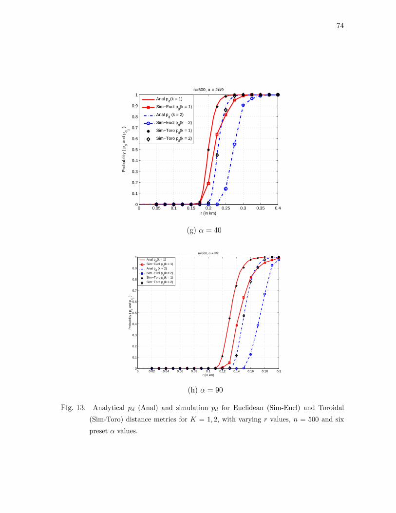
74

0 0.05 0.1 0.15 0.2 0.25 0.3 0.35 0.40

0.1

0.2

0.3

0.4

0.5

0.6

0.7

0.8

0.9

1

r (in km)

Pro

babi

lity

( p d a

nd p

d 2 )

n=500, α = 2π/9

Anal p

d(k = 1)

Sim−Eucl pd(k = 1)

Anal pd (k = 2)

Sim−Eucl pd(k = 2)

Sim−Toro pd(k = 1)

Sim−Toro pd(k = 2)

(g) α = 40

0 0.02 0.04 0.06 0.08 0.1 0.12 0.14 0.16 0.18 0.20

0.1

0.2

0.3

0.4

0.5

0.6

0.7

0.8

0.9

1n=500, α = π/2

Pro

babi

lity

( p d a

nd p

d 2 )

r (in km)

Anal pd(k = 1)

Sim−Eucl pd(k = 1)

Anal pd (k = 2)

Sim−Eucl pd(k = 2)

Sim−Toro pd(k = 1)

Sim−Toro pd(k = 2)

(h) α = 90

Fig. 13. Analytical pd (Anal) and simulation pd for Euclidean (Sim-Eucl) and Toroidal

(Sim-Toro) distance metrics for K = 1, 2, with varying r values, n = 500 and six

preset α values.

75

0 0.02 0.04 0.06 0.08 0.1 0.12 0.14 0.16 0.18 0.20

0.1

0.2

0.3

0.4

0.5

0.6

0.7

0.8

0.9

1n=500, α = 3π/4

Pro

babi

lity

( p d a

nd p

d 2 )

r (in km)

Anal pd(k = 1)

Sim−Eucl pd(k = 1)

Anal pd (k = 2)

Sim−Eucl pd(k = 2)

Sim−Toro pd(k = 1)

Sim−Toro pd(k = 2)

(c) α = 135

0 0.02 0.04 0.06 0.08 0.1 0.12 0.14 0.16 0.18 0.20

0.1

0.2

0.3

0.4

0.5

0.6

0.7

0.8

0.9

1n=500, α = π

Pro

babi

lity

( p d a

nd p

d 2 )

r (in km)

Anal pd(k = 1)

Sim−Eucl pd(k = 1)

Anal pd (k = 2)

Sim−Eucl pd(k = 2)

Sim−Toro pd(k = 1)

Sim−Toro pd(k = 2)

(d) α = 180

Fig. 13 continued.

76

0 0.05 0.1 0.15 0.20

0.1

0.2

0.3

0.4

0.5

0.6

0.7

0.8

0.9

1

r (in km)

Pro

babi

lity

( p d a

nd p

d 2 )

n=500, α = 3π/2

Anal pd(k = 1)

Sim−Eucl pd(k = 1)

Anal pd (k = 2)

Sim−Eucl pd(k = 2)

Sim−Toro pd(k = 1)

Sim−Toro pd(k = 2)

(e) α = 270

0 0.05 0.1 0.15 0.20

0.1

0.2

0.3

0.4

0.5

0.6

0.7

0.8

0.9

1

r (in km)

Pro

babi

lity

( p d a

nd p

d 2 )

n=500, α = 2π

Anal pd(k = 1)

Sim−Eucl pd(k = 1)

Anal pd (k = 2)

Sim−Eucl pd(k = 2)

Sim−Toro pd(k = 1)

Sim−Toro pd(k = 2)

(f) α = 360

Fig. 13 continued.

77

SCC of DirectedGraph A

DirectedGraph A

(a) For graph A, pc = 3/5

SCC of DirectedGraph B

DirectedGraph B

(b) For graph B, pc = 4/5

Fig. 14. Two examples of strong connected components (SCCs) of directed graphs.

We note that as n grows, (i.e., denser network), the analytical and simulation

plots will agree more closely, due to the approximations made for n → ∞ in the

derivation of the analytical equations. We also observe that the pd2 curves perform

similarly so that as α → 2π, the simulation pd more closely approach analytical pd,

more so for K = 2 than the K = 1 case. In both cases however, eliminating border

effects results in the simulations with a high degree of match to analytical predictions.

To empirically determine pc, we obtain the number of nodes nc in the largest

strongly connected component (SCC) Gcn(Sn, E) ⊂ Gn(Sn, E) as a fraction of n, where

Gcn(Sn, E) forms the largest partition of the network such that any pair of nodes in

Gcn(Sn, E) are pairwise connected. Figure 14 depicts examples of the SCC of two

78

5-node directed graphs A and B, with pc equivalent to 3/5 and 4/5 respectively.

We employ the well known Kosaraju’s algorithm [94] which efficiently implements a

depth-first-search (DFS) algorithm [95] to determine Gcn(Sn, E) in our simulations.

Kosaraju’s algorithm uses the fact that the transpose graph3 of a directed graph has

exactly the same SCC as the original graph.

Similar to the matlab simulation scenario used to study node isolation in Section

C, we generate an n-node random topology of Gn(Sn, E) over a square region of unit

area 1 km2. For n = 500, six representative α values and r varying, we repeat the

simulations 1000 times to yield an acceptable confidence of obtain results. We measure

empirical values for pc as the ratio nc/n for each trial, averaged over the 1000 random

topologies, where nc is the number of nodes in Gcn(Sn, E) obtained using Kosaraju’s

algorithm. Because Kosaraju’s algorithm is O(|E|n log n), extensive simulation time

is required to determine pc especially for large r and α values for which E is dense,

even with the use of Texas A & M’s supercomputing facilities [96].

Figure 15 compares plots of empirically derived pc (using both a Euclidean and

a Toroidal distance metric), with pd-Anal and pd-Sim, for pre-selected α values. We

observe that for large probability values, the property that pc = pd holds, when

Toroidal distance metric is used to compensate for boundary effects. This implies

that for probabilities larger than about 0.95, parameter values obtained for the curve

of pd serve as a good approximation for attaining the same pc confidence.

3The transpose graph is the same graph with the direction of every edge reversed.

79

0 0.05 0.1 0.15 0.2 0.25 0.3 0.35 0.40

0.1

0.2

0.3

0.4

0.5

0.6

0.7

0.8

0.9

1

Graph of pd and p

c for α = 40o

Pro

babi

lity

of c

onne

ctiv

ity/n

ode

isol

atio

n

r (in km)

pd − Anal

pd−Sim (Eucl)

pc − Sim (Eucl)

pc−Sim (Toro)

(a) α = 40o

0 0.02 0.04 0.06 0.08 0.1 0.12 0.14 0.16 0.18 0.20

0.1

0.2

0.3

0.4

0.5

0.6

0.7

0.8

0.9

1

Graph of pd and p

c for α= 90o

Pro

babi

lity

of c

onne

ctiv

ity/n

ode

isol

atio

n

r (in km)

pd − Anal

pd−Sim (Eucl)

pc − Sim (Eucl)

pc−Sim (Toro)

(b) α = 90o

Fig. 15. Comparing the probability pc that the network is connected to the probability pd

that there is no isolated network node (simulated and analytical).

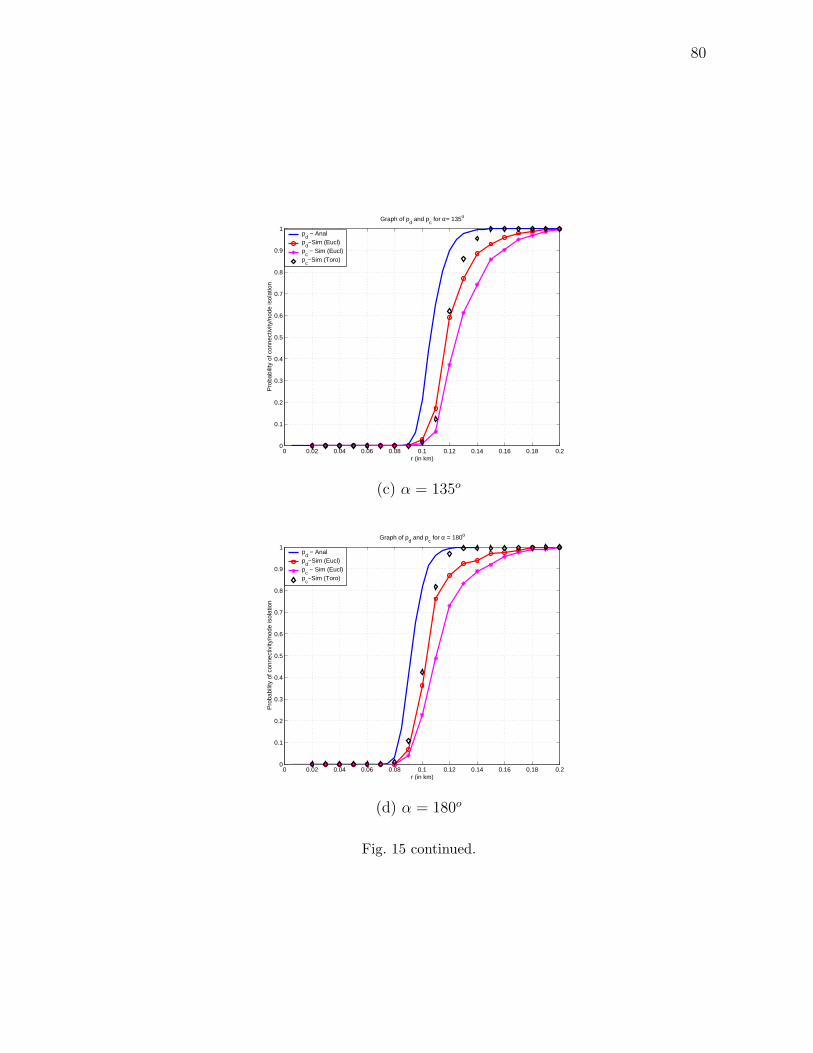
80

0 0.02 0.04 0.06 0.08 0.1 0.12 0.14 0.16 0.18 0.20

0.1

0.2

0.3

0.4

0.5

0.6

0.7

0.8

0.9

1

Graph of pd and p

c for α= 135o

Pro

babi

lity

of c

onne

ctiv

ity/n

ode

isol

atio

n

r (in km)

pd − Anal

pd−Sim (Eucl)

pc − Sim (Eucl)

pc−Sim (Toro)

(c) α = 135o

0 0.02 0.04 0.06 0.08 0.1 0.12 0.14 0.16 0.18 0.20

0.1

0.2

0.3

0.4

0.5

0.6

0.7

0.8

0.9

1

Graph of pd and p

c for α = 180o

Pro

babi

lity

of c

onne

ctiv

ity/n

ode

isol

atio

n

r (in km)

pd − Anal

pd−Sim (Eucl)

pc − Sim (Eucl)

pc−Sim (Toro)

(d) α = 180o

Fig. 15 continued.

81

0 0.02 0.04 0.06 0.08 0.1 0.12 0.14 0.16 0.18 0.20

0.1

0.2

0.3

0.4

0.5

0.6

0.7

0.8

0.9

1

Graph of pd and p

c for α= 270o

Pro

babi

lity

of c

onne

ctiv

ity/n

ode

isol

atio

n

r (in km)

pd − Anal

pd−Sim (Eucl)

pc − Sim (Eucl)

pc−Sim (Toro)

(e) α = 270o

0 0.02 0.04 0.06 0.08 0.1 0.12 0.14 0.16 0.18 0.20

0.1

0.2

0.3

0.4

0.5

0.6

0.7

0.8

0.9

1

Graph of pd and p

c for α = 360o

Pro

babi

lity

of c

onne

ctiv

ity/n

ode

isol

atio

n

r (in km)

pd − Anal

pd−Sim (Eucl)

pc − Sim (Eucl)

pc−Sim (Toro)

(f) α = 360o

Fig. 15 continued.

82

In a real world application, this would be especially true with very dense networks

and large deployment regions that minimize the boundary effects. It is noteworthy

that our results are consistent with the conclusions of [42]. That is, for directional

networks, it is also true that pd is a tight upper bound for pc for n →∞ and probabil-

ities close to one. However, we observe that this result is even more so, as α increases.

That is, as α → 2π, pc does a much better job at approaching pd, especially for large

probability values close to 1.

Another interesting phenomenon observed for pd and pc is the ‘phase transition’

property typically observed for random graphs [29], in which pc transitions rapidly

from 0 (i.e., network is disconnected with probability 1) to 1 (i.e., network is connected

with probability 1). This property gets stronger as α → 2π. For example, for

α = 40o, 180o and 360o, while pc = 0 for r = 0.20, 0.08 and 0.06 km respectively,

pc = 1 for r = 0.35, 0.18 and 0.12 km respectively. That is, for α = 40o, 180o and

360o, the ‘phase transition’ spans a distance of 0.15, 0.10 and 0.06 km respectively.

Our results lead us to state the following:

Proposition C.1 For n WOSN nodes randomly distributed and oriented on the

planar unit area square according to a uniform distribution, let rc and rd denote,

the minimum r at which the network graph Gn(Sn, E) is connected and attains no

isolated node, respectively. Then:

Pr[rc = rd] → 1 as n →∞ and α → 2π

D. Impact of Hierarchy and Clustering on Connectivity

The traffic pattern in the naturally hierarchical WOSN consisting mainly of base

station-to-nodes or nodes-to-base station traffic [97]. Consider a cluster-based WOSN

with a fraction of the nodes acting as cluster heads (CHs) that send and receive data

83

directly to and from the base station, respectively, on behalf of other nodes. In

terms of hierarchy, the base station forms the highest layer, the CHs constitute the

middle layer, while the other remaining nodes form the lowest layer of the network.

A higher class of CH nodes, perhaps equipped with more energy and communica-

tion resources may also be envisioned in a heterogenous sensor network architecture.

Clustered sensor networks have been vastly studied in the literature with regard to

improving energy [53, 97], power and topology control, scalability, load balancing,

data aggregation, fault tolerance and routing efficiency [98, 99].

Let us define the hierarchical connectivity (H-connectivity) property of the WOSN

as the connectivity of the supergraph Gsn(Sn, Es) ⊇ Gn(Sn, E) formed by adding

edges [19] between all pairs of nodes in CH. In this model, the CHs act as artic-

ulation nodes such that with high probability CH forms a cut set for the SCC of

Gsn(Sn, Es). That is, the removal of the set CH results in the likely disconnection of

Gsn(Sn, Es). H-connectivity implies that all nodes in the network can communicate

(send and receive) with the base station, conforming to the desired traffic pattern of

sensor networks.

Within this context, the question we raise is, what is the impact of pCH on the

H-connectivity property of Gn(Sn, E)? More specifically, how can we choose pCH

such that with a given probability pH , the network is H-connected. The answer to

this question is crucial in determining the fraction of ‘special’ nodes that must be

manufactured and deployed as CHs during design phase, to achieve a desired pH .

In fact, pCH is an additional tunable network parameter to enable a more flexible

network design.

We empirically evaluate the effect of clustering on H-connectivity. Similar to

previous simulations, 1000 random topologies of a 500-node network are generated

and evaluated to yield acceptable confidence on obtained empirical results. In this

84

scenario, nodes are designated as CHs with probability pCH set to three representative

values of 10%, 25%, and 40%, and the adjacency matrix of Gsn(Sn, Es) is obtained by

updating E to reflect the additional links between all CHs. We compute pH as the

ratio of the number of nodes in the SCC of Gsn(Sn, Es) to n, and obtain empirical

values for pH as the average across the 1000 trials.

Figure 16 depicts plots of pH compared to pc for the different PCH values. We

observe that for all α values clustering remarkably improves network connectivity. For

example, for α = 40o, we observe that pc = 0.33 for r = 0.25 while pH = 0.52, 0.72

and 0.85 respectively with corresponding pCH values of 10%, 25%, and 40%. Consider

for example, a WOSN deployed within a unit area (1km ×1km) planar region. If the

network owner can only afford to deploy a limited number of nodes, say 500 nodes,

each node possessing a communication radius r and angle α of 0.15m and 90o respec-

tively, he is only guaranteed a connectivity of about 20% of nodes. If however, 25%

of nodes are equipped to function as cluster heads, the connectivity of the network

improves to 60%. Further if 40% of nodes are designated as cluster heads, the net-

work connectedness of almost 80% can be guaranteed. (See Figure 16(b)). Practical

cost considerations determine the tradeoff between enhancing a node’s capability to

become a cluster head versus deploying several more of the ordinary nodes.

85

0.05 0.1 0.15 0.2 0.25 0.3 0.35 0.40

0.1

0.2

0.3

0.4

0.5

0.6

0.7

0.8

0.9

1α = 2π/9

Pro

babi

lity

of H

−co

nnec

tivity

r (in km)

pc (no clustering)

pH

(pCH

= 0.1)p

H (p

CH = 0.25)

pH

(pCH

= 0.4)

(a) α = 40o

0 0.05 0.1 0.15 0.2 0.250

0.1

0.2

0.3

0.4

0.5

0.6

0.7

0.8

0.9

1α = π/2

Pro

babi

lity

of H

−co

nnec

tivity

r (in km)

pc (no clustering)

pH

(pCH

= 0.1)p

H (p

CH = 0.25)

pH

(pCH

= 0.4)

(b) α = 90o

Fig. 16. Plots of phc compared to pc for varying pCH .

86

0 0.05 0.1 0.15 0.2 0.250

0.1

0.2

0.3

0.4

0.5

0.6

0.7

0.8

0.9

1α = π

Pro

babi

lity

of H

−co

nnec

tivity

r (in km)

pc (no clustering)

pH

(pCH

= 0.1)p

H (p

CH = 0.25)

pH

(pCH

= 0.4)

(c) α = 180o

0 0.05 0.1 0.15 0.2 0.250

0.1

0.2

0.3

0.4

0.5

0.6

0.7

0.8

0.9

1α = 2π

Pro

babi

lity

of H

−co

nnec

tivity

r (in km)

pc (no clustering)

pH

(pCH

= 0.1)p

H (p

CH = 0.25)

pH

(pCH

= 0.4)

(d) α = 360o

Fig. 16 continued.

87

E. Connectivity Analysis in a Fading Channel Model

In FSO communication, absorption or obscuration of the beam by the atmosphere,

adverse weather conditions such as fog, snow, heavy rain, or optical turbulence due

to temperature and pressure variations, can be important to channel performance.

r0

α

Φi

θi

Fig. 17. An example of the region of transmission of a WOSN node in a fading channel.

Due to the impact of ambient light on FSO, and its susceptibility to atmospheric

turbulence (especially fog) and obscuration, it is imperative that we model fading

channel links as a result of these factors that cause degradation to the WOSN’s

connectivity [26]. For example, due to fading effects that result in random values of

r0 at various points (and therefore random A(Φi) value), the boundary of the region of

transmission (RoT) for the WOSN node is an irregular shape as illustrated in Figure

17 instead of a simple sector as with the no fading case.

It is well known [100] that in a WOSN fading environment, the compound signal

attenuation H is comprised of two main components: a deterministic path loss compo-

nent hl due to atmospheric attenuation from atmospheric absorption or obscuration

of the beam, and by adverse weather conditions such as fog, snow, heavy rain; and a

stochastic path loss component ha due to atmospheric optical turbulence from temper-

ature and pressure variations. The stochastic path loss for the FSO signal has been

88

characterized by a log-normal probability density function (pdf) for weak turbulence

and a K-distribution for strong turbulence[101, 102]. The effects of a third geometric

spread and pointing errors component is negligible for broad beam FSO, and will

therefore be ignored in this dissertation. We assume a non-ergodic channel with sta-

tionary link characteristics implying that the time scales of the fading processes are

far larger than bit interval, so that time varying behaviors may be ignored.

This model represents a communication channel in which r0 and hence link prob-

ability Pr[si → sj] is modeled as a random variable (r.v.) instead of the simple mono-

tone step function Pr[si → sj] = 1∆ij≤r0, |Θi−ΨTij |≤

α2, employed where there is no con-

sideration for fading [9, 23], where ∆ij =√

d(xi, xj)2 + d(yi, yj)2 is the Euclidean dis-

tance between si and sj, and ΨTij = min [|Θi −Ψij|, |Θi + 2π −Ψij|, |Θi − 2π −Ψij|]

represents the angular difference between the direction of si and the position of sj,

with Ψij = arccos d(yj, yi)/∆ij as depicted in Figure 18.

Fig. 18. Geometric illustration for si → sj if d(si, sj) ≤ r and |Θi − ΨTij | ≤ α

2 based on a

simple monotone function.

In the WOSN fading channel with attenuation Hij on the link si → sj, given

ro, ∆ij and Ψij ≤ α/2, we determine that si → sj exists if Hij is less than a given

threshold attenuation Ht which is a function of r0 - the maximum distance granting

a link in the absence of fading. Recall that Hij is formulated as Hij = Pt(si)/Pr(sj),

89

where Pt(si) and Pr(sj) are transmit and receive power at si and sj respectively.

The question we address in this section is: given a fading environment, what is the

probability pc that the WOSN is connected in terms of the physical layer variables of

n, r and α? To answer this question, we determine the closed form expression for an

analytical expression for pd within a fading channel, and the impact of fading on pc.

1. Fading Channel Statistical Model

The combined effects of direct absorption and scattering of the FSO signal by air

molecules, solid or liquid particles (e.g., fog) suspended in the air is described by

a single path-dependent attenuation coefficient σ, so that hl is given by the Beer-

Lambert law:

hl(si, sj) = exp (−σδij)

where σ depends on the size and distribution of particles and the wavelength λ of the

laser. For the stochastic component, ha has been shown to have a log-normal pdf for

weak turbulence (Rytov variance σ2R < 0.3) given as:

fha(ha) =1

2haσX

√2π

exp

((ln ha + 2σ2

X)2

8σ2X

)and a K-distribution for strong turbulence given as:

fha(ha) =2β

β+12

Γ(β)(ha)

β−12 Kβ−1

(2√

βha

)for ha > 0

where σ2X ≈ σ2

R/4 is the variance of the log-amplitude of the optical intensity, (as-

suming atmospheric channels near the ground < 18.5m), Kβ(.) is the modified Bessel

function of the second kind of order β, and β is a channel parameter related to the

effective number of discrete scatters [26]. Table VI summarizes sample parameter

values associated with two weather conditions for weak and strong turbulence. We

90

Table VI. Adverse Weather Parameters Affecting The FSO signal.

Condition Visibility σ2R σ

Clear & strong turbulence 10 1 0.44

Light fog & weak turbulence 0.5 0.1 20

implemented Kβ(ξ) in MATLAB utilizing the besselk(β, ξ) function, and point out

the strong inverse correlation between turbulence strength σ2R and attenuation σ.

The compound attenuation acting on link si → sj is given as Hij = hl × ha, and

we obtain:

Pr[Hij ≤ Ht|∆ij, Ψij <α

2] =

∫ Ht/hl

−∞fha(ha)dha

=

∫ Htexp(σ∆ij)

ro

−∞

1

2haσX

√2π

exp

((ln ha + 2σ2

X)2

8σ2X

)dha

=1

2

[1− erfc

(ln[Ht

exp(σ∆ij)

ro] + 2σ2

X

2√

2σX

)](3.38)

for weak turbulence, and

=2(β)

β+12

Γ(β)

∫ Ht exp(σ∆ij

r0)

−∞(ha)

β−12 Kβ−1

(2√

βha

)dha (3.39)

for strong turbulence, where we compute the integral of Equation 3.39 using efficient

numerical techniques and the quadl function in MATLAB. The threshold attenuation

value is obtained as Ht = exp(−σr0) [42]. Figure 19 depicts the link probability

over ∆ij/r0 for the two weather conditions represented in Table VI. For the case

of no fading (σ = 0), we observe the sharp transition at the critical r0 value that

yields a threshold. For example, in clear weather with strong turbulence, there is

still a link probability of almost 10% at a distance of 1.8r0 while for light fog and

91

0 0.2 0.4 0.6 0.8 1 1.2 1.4 1.6 1.8 20

0.1

0.2

0.3

0.4

0.5

0.6

0.7

0.8

0.9

1

δij/r

o

Pr[

s i to s

j]

σR2 = 0

Clear σR2 = 1, σ = 0.44

Light fog σR2 = 0.1, σ = 20

Fig. 19. Link probability for the two weather conditions given in Table VI.

weak turbulence, the probability of a link degrades to 0% at a distance of 1.1r0. It

is obvious that the FSO signal is degraded by fog to a higher degree than by strong

optical turbulence.

We now determine an analytical expression pd for the WOSN in a fading channel,

and compare it to empirically determined pc to determine the tightness of the bound

and the effect of fading for various α values.

Consider the probability pif∩b that a randomly selected node si is isolated, which

is equivalent to the probability that si is both f-isolated (i.e., Si = ∅) and b-isolated

(i.e., Pi = ∅), so that we can write: pif∩b = pi

f × pib|f , where pi

f is the probability that

a node is f-isolated and pib|f is the probability that a node is b-isolated conditioned

on the fact that it is f-isolated. Our next step is to determine pif∩b by evaluating pi

f

and pib|f , where pi

f = Pr[δ+i = 0] is obtained by considering as previously stated that

92

the r.v. δ+i follows a Poisson∼ nE(AΦi

) pdf, where E(.) is the expectation function,

so that,

Pr[δ+i = z] =

e−nE(AΦi) (nE(AΦi

))z

z!(3.40)

upon which we obtain pif = e−nE(AΦi

). We next derive:

pib|f = Pr[δ−i = 0|δ+

i = 0]

=n−1∑k=1

Pr[δ−i = 0|δ+i = 0, k = K].Pr[k = K] (3.41)

where k denotes the r.v. counting the number of nodes within B(Υi, r0)\Φi. Observe

that k ∼ Poisson (n(πr20 − E(AΦi

))) and Pr[δ−i = 0|δ+i = 0, k = K] = (1− E(AΦi

))K ,

so that:

pib|f = e−nr2(π−α

2)

n−1∑k=0

[(nr2π − nE(AΦi))(1− E(AΦi

))]k

k!

= e−n(πr2−E(AΦi)).en(r2π−E(AΦi

))(1−E(AΦi))

= e−n(πr2−E(AΦi)).E(AΦi

)) (3.42)

By simple substitution, we have that:

pif∩b = e−nE(AΦi

).e−n(πr2−E(AΦi)).E(AΦi

))

= e−nE(AΦ)[1 + πr2o−E(AΦ)] (3.43)

Given our assumption that the isolation of individual nodes are independent

events for large n, the conditional probability pd that there is no isolated node in

Gn(r, α) given n is:

pd = (1− pif∩b)

n (3.44)

=(1− e−nE(AΦ)[1 + πr2

o−E(AΦ)])n

(3.45)

93

We need to evaluate nE(AΦ) which is the expected number of nodes within a

given node’s RoT, where E(AΦ) is computed by integrating Pr[H ≤ Ht|∆, φ] over the

entire system plane:

E(AΦ) =

∫ α

0

∫ ∞

0

Pr[H ≤ Ht|∆, φ] ∆ dφ d∆

= α

∫ ∞

0

Pr[H ≤ Ht|∆] ∆ d∆ (3.46)

Equation 3.46 is computed by plugging in equations 3.38 and 3.39 and employing nu-

merical means to solve E(AΦ) for the weak and strong turbulence cases, respectively.

2. Numerical Results and Observations

In order to validate our analytical results, we perform a number of computer-based

simulations in MATLAB for pd and pc under the two (weak and strong turbulence)

fading channel conditions using parameter values reflected in Table VI, as well as the

no fading condition. We compare our simulation results with curves obtained with

our analytical derivations of Equation 3.44, for similar conditions. With α set to three

representative values of 2π/9, π/2, and π for a chosen Ht = 40dB (implying a given

r0), we randomly place a given number of nodes n in a unit area region according

to a Uniform distribution. For each node pair (si, sj), given the absolute angular

difference from si to sj is less than α/2, we compute link probability from Equation

3.38 and 3.39 for the fading channel, and determine that with this probability, link

si → sj exists. Once all nodes have established links according to the channel and

transmission parameters, we check the topology for any isolated node and test the

connectivity of the network. We employ Monte Carlo methods, repeating our ex-

periments 500 times, and estimate pd and pc as the percentage of topologies with no

isolated node and the percentage of connected topologies, respectively. We repeat the

94

process with varying n values.

Our results, presented in Figures 20 (a) - (c), clearly indicate that network con-

nectivity degradation due to fading worsens as α increases on one hand, while it

improves with no fading. This trade off implies that careful design consideration

must be given in the choice of the optimal α that ensure connected minimum den-

sity network in a fading channel. For example with α = 2π/9, π/2, π, without fading,

n = 170, 80, 50 yields analytical pd = .99, whereas n = 300, 230, 240 is required for the

same pd under strong turbulence, respectively. Additionally, we observe that the sim-

ulation curves of pd and pc qualitatively follow their corresponding analytical curves,

but lag them quantitatively, due to boundary effects [42] which are not compensated

for. The negligible difference between pd and pc for probabilities close to one suggests

it suffices to compute the minimum n that achieves pd ≥ .99, as a tight lower bound

for the n required to achieve a corresponding pc.

3. Summary of Insights

We now summarize the insights gained from our analysis and simulation results as

compared to the α = 2π case as follows:

1. A linear change in r produces a much more significant impact on pd than a

corresponding linear change in α.

2. As in the α = 2π case, there is a critical value of r above which the network will

almost surely have no isolated nodes. This natural trend is preserved even for

directional networks that do not follow the RGG model. However, we observe

that the “phase transition” nature of the plots are not as strong for smaller α

values.

3. Node isolation has been one of the major hurdles for broadband directional

95

networks and the conservative results derived in this paper demonstrate the po-

tential for connectivity in such networks providing further support for emerging

hybrid RF/FSO systems.

4. For K-connectivity of a network, as K grows, it is projected that significantly

larger values of r will be required to maintain connectivity for lower values of

α. For sensor networks in which it is possible that a fraction of nodes may die

or be corrupted, such performance motivates even more the need for a hybrid

or clustered heterogenous paradigm.

5. The importance of considering fading in a given deployment environment for

the WOSNs cannot be over emphasized, as it can greatly impact on the net-

work connectivity, and hence the choice of physical layer parameter values. In

particular, when fading effects are considered in WOSNs, n rather than r turns

out to be the most sensitive network parameter for connectivity in the network.

The next chapter is concerned with the introduction of the secure integrated

routing and localization scheme for the WOSN, assuming the network satisfies con-

nectivity requirements developed in this chapter.

96

0 50 100 150 200 250 300 350 4000

0.1

0.2

0.3

0.4

0.5

0.6

0.7

0.8

0.9

1

prob

abili

ty p

d

nodes (n)

α = 2π/9

No fading..

Clear σR2 = 1, σ = 0.44

Light fog σR2 = 0.1, σ = 20

Corresponding pd simulations

Corresponding pc simulations

(a) α = 2π/9

0 50 100 150 200 250 300 350 4000

0.1

0.2

0.3

0.4

0.5

0.6

0.7

0.8

0.9

1

prob

abili

ty p

d

nodes (n)

α = π/2

No fading..

Clear σR2 = 1, σ = 0.44

Light fog σR2 = 0.1, σ = 20

Corresponding pd simulations

Corresponding pc simulations

(b) α = π/2

Fig. 20. Comparing simulation results for pd and pc with analytical values for various α

and fading conditions, with Ht = 40dB.

97

0 50 100 150 200 250 300 350 4000

0.1

0.2

0.3

0.4

0.5

0.6

0.7

0.8

0.9

1

prob

abili

ty p

d

nodes (n)

α = π

No fading..

Clear σR2 = 1, σ = 0.44

Light fog σR2 = 0.1, σ = 20

Corresponding pd simulations

Corresponding pc simulations

(a) α = π

Fig. 20 continued.

98

CHAPTER IV

SIRLOS: SECURE INTEGRATED ROUTING AND LOCALIZATION SCHEME

A. Introduction

It is vital to consider security objectives at the onset of the design phase for network

layer protocols such as routing, clustering and localization, as previously stated in

Chapter II. In the WOSN, the non-reversibility of paths further complicates route

setup. Due to the lack of bi-directionality in most of the WOSNs’ links, a node can-

not immediately discover its complete neighborhood. This is because knowledge of a

node’s successors cannot be gained simply by listening to the channel, and the ex-

change of link layer acknowledgements proves non-trivial, creating huge overhead. As

a result, common neighborhood discovery mechanisms based on reverse path forward-

ing, such as topology broadcast [53], and range-free localization schemes which work

well for omnidirectional networks, cannot be exploited for WOSNs. Similarly, proto-

cols that have simply been optimized to accommodate a limited number of directional

network links are hugely inefficient and wasteful in WOSNs.

In the WOSN, opportunities exist for an attacker to exploit loopholes in secu-

rity assumptions and attack counter-measures that have been proffered and designed

specifically for omnidirectional networks. Therefore, it is imperative that for WOSNs,

novel, bottom up security-aware routing and localization paradigms be designed, and

corresponding attacks and countermeasures which may be relevant in traditional om-

nidirectional networks be re-evaluated [27].

In this chapter, we introduce SIRLoS, a novel lightweight secure integrated routing

and localization scheme for WOSNs. SIRLoS does not employ range estimation meth-

ods, time synchronization or expensive localization hardware. Instead SIRLoS ex-

99

ploits a hierarchical cluster-based organization of the network to offer a lightweight

security services based on symmetric cryptography; a novel circuit-based neighbor-

hood discovery and routing approach; and a simple location estimation algorithm

based on topology control.

The security objectives of the SIRLoS protocol includes providing per hop and

broadcast authentication, assuring nodes and the base station of the origin of the

routing beacon. SIRLoS also guarantees that routing and location information are

protected against outsider eavesdropping and unauthorized manipulation, thus pro-

viding data confidentiality, integrity and freshness for beacons. We employ one-way

key chains, individual and network wide symmetric keys, individual node passwords

and cluster head specific nonce values1 to defend against unauthorized participation,

spoofing, altering or replaying route signals. For security against insider attacks on

routing in WOSNs, we submit to the prudence and practicality of leveraging the re-

sources of the trusted and powerful base station. The use of a base station anchored

circuit-based paradigm provides a lower overhead alternative for neighborhood dis-

cover compared to prior routing protocols [9] which have been offered for the WOSN.

In this chapter, we describe the various aspects of SIRLoS, demonstrate the se-

curity advantages due to link directionality, and provide performance, security and

attack evaluations and countermeasures to demonstrate the potential benefits of SIR-

LoS compared to other routing schemes for WOSN applications. Through this in-

vestigation, we demonstrate some fundamental insights in this emerging field, which

include:

1. security and neighborhood discovery in WOSNs is more challenging compared to

the traditional omnidirectional networks, due to an added orientation constraint

1A nonce is a randomly generated bitstream used to achieve data freshness.

100

which necessitates a mechanism for efficient discovery of successors;

2. by employing routing beacons which originate at the trusted and powerful base

station, propagate through the network and terminate at the base station, we

show that directionality provides various advantages that may be leveraged for

enhanced security in WOSNs;

3. an emerging research area which involves securing the network layer of WOSNs

is a rich field of study which encompasses problems such as connectivity anal-

ysis, secure localization, intrusion detections, topology control and secure data

aggregation, and novel attacks relevant to this architecture. This opens up

several directions for novel research in WOSNs.

B. SIRLoS: Secure Integrated Routing and Localization Scheme

SIRLoS is a two-phase, restricted flooding mechanism that entails a centralized circuit-

based protocol anchored at the base station. SIRLoS is aimed at enabling network

nodes to discover uplink routes for data forwarding to, and a downlink routes for

data receiving from the base station respectively. In summarizing the protocol, the

base station initiates neighborhood discovery by flooding cluster head-distinct circuit

discovery beacons (CDBs) into the network via all the cluster heads. The beacons

act as agents that traverse the network, gathering routing data (such as sequence of

nodes encountered) as they propagate. That is, nodes append their unique informa-

tion to any new CDB encountered after they record data from those beacons into

their routing tables, before rebroadcasting the beacon to its successors.

A CDB is terminated whenever it expires (a concept we will explain in the next

section) or it first reaches an exit cluster head, that then returns the beacon to the

base station, thus completing a BS-circuit. The base station, having gathered all the

101

returned CDBs, employs the location, connectivity and security data extracted from

the returned beacons to reconstruct the global network topology, and then update

the routing tables of each node. The base station also acts at the umpire to ensure

that security and trust are not breached.

We piggyback a simple, light weight and coarse localization scheme to further

leverage the bandwidth utilized for neighborhood discovery in SIRLoS. The centroid

method localization algorithm enables nodes to coarsely estimate their locations based

on the location estimate of predecessors as well as the orientation information which

is included in the CDBs they propagate. A light weight topology control mechanism

is suggested to provide refined location estimate with improved performance to the

centroid only methods [74].

In formulating the neighborhood discovery mechanism of SIRLoS, as commonly

required for sensor networks, our objective is to be efficient in terms of minimizing

routing overhead such as storage, computation and communication, preventing fab-

rication or alteration of routing signals, preventing routing loops, as well as incorpo-

rating scalability for large networks. In contrast to omnidirectional sensor networks,

there is naturally a heavier routing overhead in WOSNs which justifies leveraging the

centralized nature of the base station. By shifting more of the processing to the base

station, it is possible to make the protocol lightweight at the node’s end. We consider

three secure routing phases:

1. Neighborhood discovery: initiated by the base station soon after network

deployment, and employing a beacon flooding mechanism, the goal of this phase

is to efficiently and securely obtain a global view of the network topology. In

contrast to many omnidirectional network neighborhood discovery mechanisms,

this phase is terminated by the base station.

102

2. Dynamic route establishment: leveraging the base station, this phase is

initiated by individual nodes on a per need basis after neighborhood discovery.

This is similar to some well known protocols for omnidirectional networks such

as SNEP [31] which also employs the help of the base station for pairwise key

establishment. In this case, the base station provides routing updates.

3. Route maintenance: is initiated by nodes and provides a mechanism for

discovering malfunctioning paths by exploiting multi-path routing and low rate

acknowledgement packets.

We employ the following notations to describe our security protocols: A|B de-

notes concatenation of message A with message B if both proceed from the same node

and A||B if A and B are from different nodes, while EK [M ], DK [M ] and MACKM

denote the encryption, decryption and message authentication code (MAC) of mes-

sage M with key K respectively. We assume all encryptions employ a symmetric

64-bit key RC5 scheme. The ⊕ notation denotes the XOR function which we have

chosen to use because as it does not expand byte overhead of the algorithm and is

easily undone at the base station. We assume that time t is broken into a number of

slots, and the network is synchronized employing the algorithm proposed in [9].

1. Efficient Neighborhood Discovery

a. Off-line Key Setup

The first stage of SIRLoS is off-line key generation and setup performed prior to

network deployment. A µ-TESLA mechanism [31] is leveraged for BS broadcast

authentication. Briefly described, the BS pre-computes and stores a length-E one-

way key chain Ke for e = 0 · · ·E, by successively applying a known one-way hash

function F to a randomly generated initial key KE, so that Ke = F(Ke+1) where

103

e = 0, 1, · · ·E − 1 indexes a particular broadcast era, and E is large enough to span

the network’s lifetime. The last key of the chain K0, known as the commitment, is

preloaded into each node. Due to the nature of F , future keys cannot be computed

from previous keys. However, it is trivial to verify that a key Ke once revealed was

derived from a previous key, by simply applying F to Ke (e − 1) times, denoted

F e−1(Ke), and verifying that the result equals K0. After deployment, keys in Ke

are revealed to nodes by the BS in the reverse order from which they were generated,

yielding an efficient, simple and lightweight mechanism for BS authentication.

b. Challenge and Respond Protocol

After deployment, each CH, say s∗x ∈ CH, indicates its readiness to begin neighbor-

hood discovery by sending a READY signal to the BS within a specified time period.

The base station responds by generating a unique nonce ηxt at the start time t = 0

for sx, and initiating the challenge-and-respond protocol (CRP) [31] to authenticate

s∗x employing Kx and PWx. The CRP also provides a simple range and angular es-

timation mechanism for determining Υx. If s∗x passes the challenge, the BS sends

it a circuit discovery beacon (CDB) containing its position Υx, marked with ηxt and

encrypted with KN for onward flooding. The exchange is:

BS → s∗x : EKx [ηxt ]

s∗x → BS : EKx [PWx ⊕ ηxt ]

BS → s∗x : [EKN[ | HT = 0 | e = 1 | K1 | ηx

t | Υx | ... |︸ ︷︷ ︸CDB

]

where HT is a variable that counts the number of hops traveled by the CDB and

is thus incremented at every intermediate node. The base station sends individual

CDBs to all cluster heads at the same time t = t0. We assume that t0 = 0.

104

HT

Hops Traversed value is incremented by one by each node.

CDP variable payload: Nodes sequentially append their information: (ID, orientation, location) data, and MAC of their information and password, as they process each CDP

Entry CH’s dataand signature

Exit CH’s dataand signature

K2

BS reveals next key in key chain.

ηtCH

(cummulative nonce)

BS generated nonce unique to each CH, cumulatively added to node’s password.

Future keysused for sourceauthentication

Encrypted nonce field used for freshness and per hop authentication.

e

BS reveals current era

Intermediate BS-circuit node’s data entry and signature

CDB Header – 140 bits CDB Payload - variable

eKN

Encryption with network wide key

Fig. 21. Illustrating the format and various fields of a CDB packet.

c. Format of the CDB

The CDB consists of a 140-bit header2 and a variable payload into which each node

si encountering the CDB inserts a 160-bit entry consisting of its 32-bit information

vector (8-bit name, 16-bit position and 8-bit orientation values) and a 128-bit HMAC-

MD5 signature computed as MACKiI(si)|PWi. The header consists of a 4-bit field

for HT , an 8-bit field to hold e, and two 64-bit fields for revealing Ke and the rolling

nonce values, respectively. Each node sx that encounters the CDB also increments

HT by one, and xor’s its password to the rolling nonce. Figure 21 depicts the format

and the various fields of a CDB packet, with their associated functions. Consider for

example, the CDB packet in the first era at time step t = 2 after the beacon has

traversed two nodes s∗x and sy as:

[ HT = 2 | e = 1 |K2 | ηxt+2 || I(sx) |MACKxI(sx) |PWx || I(sy) |MACKyI(sy) |PWy ],

2The size of the header should scale up with increasing numbers of nodes, size ofobservation area.

105

where ηxt+2 = ηx

t+1 ⊕ PWy and ηt+1 = ηxt ⊕ PWx.

The CDB carries a progressively higher overhead in contrast to beacons in om-

nidirectional networks and/or void of security inputs, where the 128-bit MAC entry

per node encountered is not required. This higher communication overhead which

depends on δ, and pCH requires higher bandwidth capacity provided by the FSO

medium, and is partially offset by pushing more of the computation to the base

station.

d. Hot Potato Node Processing of the CDB

Each node si (including cluster heads) maintains a predecessor routing table PRT(si)

into which it makes entries of the information vector of each of its predecessors along

with the chronologically organized IDs of nodes on the corresponding downlink and

an associated cost value Cd, which is equivalent to the HT value of the CDB at

the time it arrives at si. We denote as Cd0 the HT value of the very first CDB a

node receives. Upon receipt of the very first CDB from a predecessor sh at time step

t0 + Cd0 , si decrypts the packet and performs some security and hop count checks

within one time step, and immediately passes the CDB to its successors. We name

this phase of routing the initial CDB as each node the hot potato routing phase. The

checks performed by the node before passing the initial CDB are as follows:

1. Validation of the source of the packet by checking that F e−1(Ke) = K0;

2. Verification that si has not previously seen this CDB or that si’s data is not

embedded in the current CDB’s payload, thereby avoiding routing loops.

If si /∈ CH, it estimates its location Υesti based on the location of its predecessors

included in the payload of CDB’s it receives, by employing the location estimation

algorithm described in section 2. If si ∈ CH, it simply obtains its accurate coordinates

106

from the CDP received from the BS as previously noted above. It then performs a

subsequent range-and-orientation constraint (ROC) test to verify that:

d(Υh, Υesti ) ≤ r and |Θi −Ψhi| ≤

α

2,

where d(a, b) is the Euclidean distance between points a and b, and

Ψhi = arccosd(ye

h, yi)

d(Υh, Υei )

ensures that Υi ∈ Φh. The ROC test provides a geometric constraint on the network

graph which is exploited as a security check, and provides protection against routing

attacks such as wormholes.

If this CDB is the very first one encountered by the node at time t0 + Cd0 the

node engages the hot potato routing strategy. Essentially, it processes and forwards

the CDB within one time step, otherwise if this is not the first CDB it receives, it

caches the CDB in its buffer and waits to perform the restricted and compounded

flooding phase described in subsection f. Observe that a node may receive more than

one CDB’s at t0 + Cd0 , in which case it randomly selects only one of the CDB’s to

forward in the hot potato phase and caches the other CDBs for compounded flooding.

We have made the reasonable assumptions that one time step ∆t is sufficiently long

to accommodate a CDB’s reception, processing and re-transmission, and that a node

can receive a CDB while transmitting another CDB in the same time step.

Before forwarding its initial CDB, si verifies that Cd0 ≤ δ (i.e., the CDB has not

expired), where δ is the maximum number of hops a CDB is allowed, and represents

the diameter of the network3. As previously stated δ is predetermined by the base

station and known to nodes prior to deployment. If Cd0 ≤ δ, the node increments

3Number of links in the shortest path between the furthest pair of nodes.

107

BS

CH

CH

entry

exit

S*a

S*e1. BS → S*a

2. S*a → Sb

eKN [| HT = 0 | e=1 | K1 | ηta | . |]

eKN [| HT = 1 | e=1 | K1 | ηta ⊕ PWa ||

I(sx) | MACKa I(sx)|PWa |]

eKN [| HT = 3 | e=1 | K1 | ηta ⊕ PWa⊕ PWb⊕ PWc || I(sx) | MACKa I(sx)|PWa ||

I(sb) | MACKb I(sb)|PWb || I(sc) | MACKc I(sc)|PWc |]

4. Sc → Sd

eKN [| HT = 2 | e=1 | K1 | ηta ⊕ PWa ⊕

PWb || I(sx) | MACKa I(sx)|PWa || I(sb) | MACKb I(sb)|PWb |]

3. Sb → Sc Sb

SdSc

eKN [| HT = 5 | e=1 | K1 | ηta ⊕ PWa⊕ PWb⊕ PWc⊕ PWd⊕ PWe || I(sx) | MACKaI(sx)|PWa || I(sb) |

MACKb I(sb)|PWb || I(sc) | MACKcI(sc)|PWc || I(sd) | MACKdI(sd)|PWd ||I(se) | MACKeI(se)|PWe |]

6. Sc → Sd

eKN [| HT = 4 | e=1 | K1 | ηta ⊕ PWa⊕ PWb⊕ PWc⊕ PWd ||

I(sx) | MACKaI(sx)|PWa || I(sb) | MACKb I(sb)|PWb ||I(sc) | MACKcI(sc)|PWc || I(sd) | MACKdI(sd)|PWd |]

5. Sc → Sd

Fig. 22. Illustrating the information gathering and processing within a CDB as it traverses

a BS-circuit during neighborhood discovery.

the HT field by one, updates the current nonce η∗t0+Cd0in the packet as η∗t0+Cd0

+1 =

PWx⊕η∗t0+Cd0, appends its data [I(si) | MACKxI(sx)|PWx] to the CDB’s payload,

re-encrypts the new CDB with KN , and then re-broadcasts the updated CDB to its

successors at time step t0 + Cd0 + 1.

The route discovery task of a CDB with 1 < HT ≤ δ is terminated when it

encounters a cluster head, who completes the BS-circuit by returning the packet to

the base station. A CDB is discarded if HT > δ or if it fails any of the security checks.

The information gathering and processing of a CDB as it traverses a typical BS-circuit

during neighborhood discovery (assuming it is the first packet that all nodes on the

BS-circuit encounter) is illustrated in Figure 22. Before concluding this phase, within

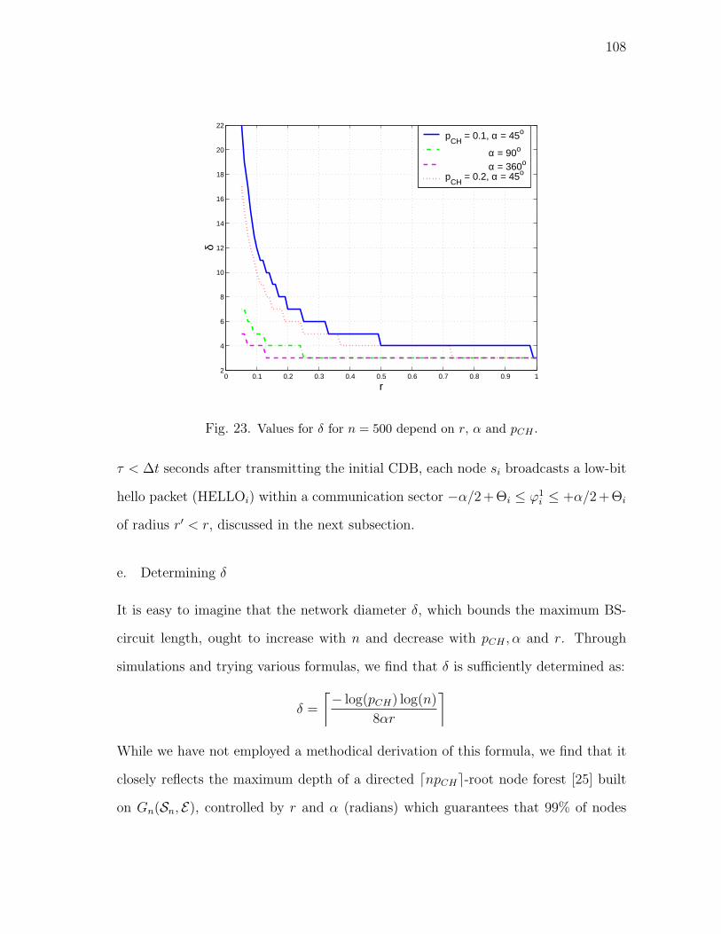
108

0 0.1 0.2 0.3 0.4 0.5 0.6 0.7 0.8 0.9 12

4

6

8

10

12

14

16

18

20

22

r

δ

pCH

= 0.1, α = 45o

α = 90o

α = 360o

pCH

= 0.2, α = 45o

Fig. 23. Values for δ for n = 500 depend on r, α and pCH .

τ < ∆t seconds after transmitting the initial CDB, each node si broadcasts a low-bit

hello packet (HELLOi) within a communication sector −α/2+Θi ≤ ϕ1i ≤ +α/2+Θi

of radius r′ < r, discussed in the next subsection.

e. Determining δ

It is easy to imagine that the network diameter δ, which bounds the maximum BS-

circuit length, ought to increase with n and decrease with pCH , α and r. Through

simulations and trying various formulas, we find that δ is sufficiently determined as:

δ =

⌈− log(pCH) log(n)

8αr

⌉While we have not employed a methodical derivation of this formula, we find that it

closely reflects the maximum depth of a directed dnpCHe-root node forest [25] built

on Gn(Sn, E), controlled by r and α (radians) which guarantees that 99% of nodes

109

are reached by SIRLoS. Figure 23 shows the values of δ for various parameter values.

For example, δ = 12 for pCH = 0.1 and α = 45o, while it is 10 for the same α and

pCH = 0.2. For the omni directional network, δ represents the maximum depth of the

forest the reaches all nodes. Observe also that when pCH = 1, implying that every

node is a cluster head, then δ = 0.

f. Restricted and Compounded Flooding

After re-broadcasting the initially received CDB of cost C0 as described in section d,

a node waits and listens to the channel for a period of δ − C0. This wait enables

the node to receive CDBs from its other predecessors as these beacons may not have

reached it at time t = C0 when it received, processed and forwarded the initial CDB.

A node time stamps each CDB arriving after t = C0 and caches the packet until

the assigned wait period, expires (at time step t = δ). The node then concatenates

all the CDBs it has received during this time, into one compound circuit discovery

beacon (C2DB), and forwards this C2DB to its successors following a simple schedule

of transmission.

Only nodes that received CDBs or C2DBs after the hot potato phase of SIRLoS

may consider transmitting to its successors during the next time step, according to

the scheduling algorithm described in subsection g below. All other nodes continue to

listen for beacons in the channel. Any node that has received and buffered one or more

CDBs or more than one C2DB during its waiting phase, schedules the aggregated

packet for transmission with probability 1. This is because the CDBs within the

network at this time contain new information on the network topology that has not

yet reached the base station. On the other hand, if only one C2DB is received from

a predecessor, it is processed and scheduled for rebroadcast with a probability of

pr = 2/nαr2. Otherwise, the C2DB is dropped. The value of pr is the reciprocal

110

of nαr2/2, which represents the expected number of neighbors of a node 4, thereby

ensuring that the network is not flooded with each node’s C2DB. Similar to the CDB,

the transmission of the C2DB is terminated when it encounters a cluster head, or if

its HT value exceeds δ.

g. Schedule of Transmission

At time step t = δ + 1 only nodes that have a packet scheduled for rebroadcast will

perform the following schedule of transmission algorithm (SA) described in Table VII,

where the phase i is initialized to 1:

Table VII. Schedule of transmission algorithm SA(i).

a) orange: transmit with probability ps = δ−C0

δ;

b) green: for i > 1, transmit with probability 1 if did not transmit in i− 1;

c) red: wait and listen for δ − (C0 + i) time steps;

d) i ++, repeat SA(i + +).

The SA is a stochastic algorithm that mimics the pattern of traffic light schedul-

ing somewhat, by slowing down travel and bunching up packets during the orange

and red steps, and then moving them onto the next intersection with the green step.

Observe that the scheduling algorithm is only executed by nodes that have a buffered

packet waiting to be rebroadcast at t > C0. Figure 24(a) illustrates a sample 13-node

network, and the associated schedule of transmissions for three packets originating

at different cluster heads within the network is depicted in Figure 24(b). We have

assumed that at t = δ = 6 time steps, and observe that C0 is one for both si and sy.

4The average out degree of Gn(Sn, E).

111

After a wait of δ−C0 we observe that si makes the decision (with probability 5/6) to

transmit while sy waits for an additional δ − C0 − 1 and then transmits as proposed

by the scheduling algorithm. In this case, it requires 10 time steps to complete the

transmission of the packets within the network.

Obviously the schedule of transmission observed for si and sy in the example

above may have been reversed, leading to larger overall delays. For example, at

t = δ, if si had chosen (with probability 1/6) to wait for 4 time steps, and sy had

chosen to transmit (which occurs with probability 5/6), and then to wait for 3 time

steps at t = 10, then the overall delay in the network would increase to 13. From

this example, it is obvious that the maximum possible delay incurred by the SIRLoS

algorithm in the network of diameter d is determined as δ(δ − 1). This delay is

observed in the worse case scenario in which each node along a BS-circuit of length

δ is within one downlink hop from a cluster head, and chooses to wait for δ − 1 time

steps during its initial round of the scheduling algorithm. The node furthermost from

the exit cluster head receives an additional packet in the second time step. Recall that

we have assumed time synchronization within the WOSNs, employing the methods

proposed and explored in [9].

112

S*z SySg

SiSh

S*v S*w S*x δ = 6

123

(a) Sample 10 node network.

1 2 3 4 7 8 9

S*v

Sa

Sb

S*z

Sy

S*x

Si

S*w

time t

δ = 6

5 6 6

(b) Time line of packet transmission.

Fig. 24. Illustrating the transmission of various packets within a sample network.

113

Sx

r’

r

ϕ1xϒc(ϕ1

x)

ϕ2x

ϒc(ϕ2x)

Φx

Fig. 25. The centroid of the two regions ϕ1x and ϕ2

x that comprise the communication

sector Φx of node sx. The sector-based communication provides more localized

estimation of the node position and the additional HELLO-phase provides even

finer granularity.

2. Location Estimation

The reception of a CDB provides a node si with knowledge that it lies within the

communication sector φi of the predecessor that forwarded the CDB. To provide

finer granularity to location estimation, we employ the following procedure. After

τ seconds of receiving a CDB from si, sj may determine that its location Υj lies

either within the sector ϕ1i ∈ Φi if it received HELLOi, or otherwise within the

circular segment ϕ2i ∈ Φi as depicted in Figure 25, and then estimates its location

Υestj as the centroid of the corresponding region. The centroid is known to be the

least square error solution [91] given that sj falls with equal probability at any point

within Φi. We consider location estimation in the two possible cases.

Case 1: Node sj concludes that Υj ∈ ϕ1i and determines Υest

j as the centroid

Υc(ϕ1i ) of the sector ϕ1

i given by the well known formula for the centroid of a sector:

Υestj =

(xi

yi

)+

∣∣∣∣2r′ sin(α)

3α

∣∣∣∣ (sin(θi)

cos(θi)

)(4.1)

114

where |.| denotes absolute value, and r′ = r/√

2 is determined to be the optimal

radius of ϕ1 such that A(ϕ1) = A(ϕ2), implying it is equally likely that sj falls within

either part.

Case 2: Node sj concludes that Υj ∈ ϕ2i and determines Υest

j as the centroid

Υc(ϕ2i ) of the sector segment ϕ2

i :

Υestj =

(xi

yi

)+

∣∣∣∣2r sin(α)

3α

∣∣∣∣(

2√

2− 1√2

)(sin(θi)

cos(θi)

), (4.2)

Equation 4.2 is easily derived by employing the formula for the centroid(

xc(Λ)yc(Λ)

)of an

M -part composite shape Λ given as:(xc(Λ)

yc(Λ)

)=

∑Mj=1 A(λj)

(xc(λj)yc(λj)

)∑A(λj)

,

where A(λj) and(

xc(λj)yc(λj)

)represent the area and centroid of the jth individual part of

Λ, respectively. With Φ composed of two parts ϕ1 and ϕ2 as depicted in Figure 25,

it is easy to rearrange the equation above to yield:(xc(ϕ2)

yc(ϕ2)

)=

A(Φ)(

xc(Φ)yc(Φ)

)− A(ϕ1)

(xc(ϕ1)yc(ϕ1)

)A(ϕ2)

Substituting A(ϕ1) = A(ϕ2), yields Υc(ϕ2) = 2Υc(Φ) − Υc(ϕ1), where the formulae

for the centroids Υc(Φ) and Υc(ϕ1) of sectors of radius r and r′ respectively may be

derived from Equation 4.1, easily yielding the expression of Equation 4.2.

If sy hears m > 1 predecessors at time step t ≥ C0, it estimates its location

as the average of the centroid’s of the m regions within which it falls, given as

Υestj = 1

m

∑mq=1 Υc(ϕq

i ). Similarly, it continues to refine its location estimate with

each CDB or HELLO packet it receives from a new predecessor. In this case, Υestj

does not represent the centroid of the overlapping region of the m sectors, but instead

the midpoint of the centroids of the communication sectors of predecessors, which is

115

simply a location within the sectors overlap region. For our method, nodes are not

required to perform range estimation or angle-of-arrival measurements, keeping both

computational and communication overhead low. Our simple and computationally ef-

ficient mechanism for location estimation does not require complex search algorithms

to determine the boundaries of the irregular shaped overlap region, or grid score ta-

bles to find the centroid of the resulting overlap region as was proposed in [91]. While

our simple localization scheme does not perform as well as other hardware based

and computationally intensive schemes such as [91], it serves well as a good first es-

timate of the locations of node, which may be further employed as the initializing

seed for other more complex localization algorithms. For example, with the scheme

proposed in [91], our estimate may be employed to determine the boundaries of a

more conservative grided search region, rather than what has been proposed.

While the centroid-based scheme proposed in [91] yields the least square error

estimate of a node’s location, we justify our approach due to the minimum delay and

computation incurred as it is integrated with the neighborhood discovery scheme.

Our scheme also differs from well known triangulation methods in which each node

must wait to receive beacons from three known-location predecessors to determine its

location. The authors of [9] have proposed a localization scheme for WOSNs based

on triangulation, in which they show that the scheme converges asymptotically, that

is as network density increases to infinity.

3. Secure Base Station Network Topology Reconstruction

The BS is able to reconstruct and estimate Gn(Sn, E′) of Gn(Sn, E) from the BS-

circuits and individual node information available in returned CDBs and C2DBs.

First, it validates each CDB (or parsed CDB contained in a C2DB) received (as

discussed below), and then constructs an adjacency matrix E ′by assuming that a

116

subsequent node in a CDB’s chronologically organized payload entry is a successor of

the previous node. That is, if sj’s entry follows that of si, the BS assumes si → sj

and hence E ′ij = 1. The BS also records (or compares with existing records) the

information vector of each node represented in each received and validated CDB.

To validate a CDB, the BS performs the following security checks:

1. verifies that HT equals the number of appended sections in the payload;

2. verifies the claimed identity and per hop entry of each node si with an input in

the payload, by ensuring that its computed MACKiI(si) |PWi is equivalent

to the signature entry of the node;

3. performs the ROC test for each link represented in the payload;

4. verifies that the final cumulative path nonce η∗t+h included in the CDB for each

h-length path, say s∗1 → s2 → · · · → sh, equals η1t ⊕PW1⊕PW2⊕ · · · ⊕PWh.

If any of the four security checks fail, or the BS observes any discrepancy in the entries

of any CDB, that CDB is discarded, and intrusion detection mechanisms initiated on

the suspicious routes.

4. Updating Nodes Routing Tables

From E ′, the BS constructs both the predecessor routing table PRT(si) and the

successor routing table SRT(si) for each node si. Similar to PRT(si), each of si’s au-

thentic successor’s information vector, associated uplink and path cost is entered into

SRT(si). The BS unicasts the encrypted routing tables EKi[RT(si)] = EKi

[PRT(si)|SRT(si)]

to si, who upon receipt, compares the PRT from the BS with its self-registered PRT.

Any discrepancy observed in entries triggers suspicion and deletion of the correspond-

ing circuit from PRT(si) and a report to the BS. Figure illustrates a sample 12-node

117

Predecessor Data Cost Downlink

sy ϒy θy

ϒw θw

sz

sw

23 sv su

Successor Data Cost Downlink

sa ϒa θa

ϒd θd

sb sc

sd

34 se sf sc

S*c

S*z

Sa

Sy

Sx

Sb

PRT(Sx):

SRT(Sx):

Sw

Sv

Sd

Se

Sf

S*u

Fig. 26. A sample network with the corresponding predecessor and successor routing tables

PRT(si), SRT(si) for node si.

network and the corresponding PRT and SRT for node si. Observe that the size of the

routing tables is dependent on the expected number of predecessors and successors

which is nαr2/2. Nodes that receive valid routing tables conclude the neighborhood

discovery phase by sending an acknowledgement (ACK) to the BS. The BS queries

nodes from which it has not received an ACK within a stipulated time frame. Each

node employs the minimum cost route in its SRT to transmit its sensor data to the

base station by fixing its laser in the direction of the appropriate successor. Figure 26

illustrates a sample network with the corresponding predecessor and successor routing

tables PRT(si), SRT(si) for node si. The optimal downlink and uplink paths is seen

to be via nodes sy and sa respectively.

5. Dynamic Route Setup

Dynamic route establishment for the WOSN entails a node, say si, seeking a secure

and efficient route to any node sj as needed, by leveraging the BS [31]: si sends an

118

encrypted route request RREQ(sj) for sj to the BS, who responds by sending si the

minimum cost path for si sj, and sending sj the minimum cost RETURN link

for sj si, encrypted with Ki and Kj respectively. The BS also includes a unique

pairwise key Keij to enable si and sj establish a secure communication for a session.

6. Route Maintenance

Route Maintenance for SIRLoS aims to discover malfunctioning, dead or subverted

nodes along BS-circuits, and is achieved by leveraging the naturally occurring path

diversity in the network; each node is with high probability, contained in more than

one disjoint BS-circuit, and hence can exploit multiple uplink paths to the base station

in order to alert the network of possible malicious behavior. The expected number

of unique uplinks and downlinks to the base station is equivalent to the expected

number of successors and predecessors respectively. Route maintenance is initiated if

a node does not receive updates to their routing tables from the base station.

A node floods route maintenance request (RMReq) towards the base station via

all its successors uplink paths by scanning its laser. A RMReq is signed and encrypted

with a nodes individual key. Once a base station receives and authenticates a RMReq,

he initiates route maintenance by querying each downlink path to the affected node

by requesting multi-path ‘multi-cast’ returns of his route maintenance query (RM-

Query) packet, similar to flooding. Each node encountering the RMQuery appends its

signature along with its information vector and time stamp on the RMQuery so the

packet accumulates chronological BS-circuit information. Validated circuits whose

RMQuery packets return to the base station are marked as functional. Since flooding

is robust, this process will easily discover non cooperative nodes in a given BS-circuit.

Time stamping a RMQuery may also be employed by the base station to de-

tect nodes that are running malicious code using mechanisms similarly utilized for

119

0 0.02 0.04 0.06 0.08 0.10 0.12 0.14 0.16 0.18 0.20

0.1

0.2

0.3

0.4

0.5

0.6

0.7

0.8

0.9

1

Communication range r (km)

Loca

lizat

ion

Err

or L

E

α = 45 − Sα = 45 − Cα = 90 − Sα = 90 − Cα = 180 − Sα = 180 − Cα = 270 − Sα = 270 − Cα = 360 − Sα = 360 − C

Fig. 27. Simulation results for localization error versus r with pCH = 0.1.

remote entity verification. Aimed at exposing malicious nodes that attempt to avoid

detection by correctly processing RMQuery and similar intrusion detection packets,

the underlying assumption is that, additional time is required for a malicious node to

reload authentic code in memory in order to correctly process a RMQuery, resulting

in a time delay that is longer than normal, thereby exposing the fraudulent node.

C. Performance Evaluation

We employ matlab simulations and analysis to study performance metrics of SIRLoS.

With α, pCH and r preset, n = 300 nodes are randomly positioned and oriented

in a planar square region of unit area 1 km2 according to a uniform distribution.

As predecessor relationships are derived by reversing successor links, it suffices to

populate E by determining successor relationships only, using the ROC test between

each node and every other node. We employ Monte Carlo mechanisms, repeating each

120

0.1 0.2 0.3 0.4 0.5 0

0.05

0.1

0.15

0.2

0.25

0.3

0.35

pCH

Loca

lizat

ion

Err

or L

E

α = 45o

α = 90o

α = 180o

α = 270o

α = 360o

Fig. 28. Simulation results for localization error versus pCH with r = 0.1 km.

simulation scenario 1000 times, and averaging the results over all the trials to yield

an acceptable statistical confidence of obtained results. We study three important

metrics of performance for SIRLoS, including localization error, average hop count

and end-to-end delay of the routing mechanism in the network.

1. Localization Error

With pCH set to 0.1, and r varying from 0 through 0.2 km, we run SIRLoS and

compute the localization error LE =∑n

i=1

√(xi − xc

i)2 + (yi − yc

i )2/n as the mean

squared error between the correct and estimated position vectors (initialized to zero)

of Sn. Figure 27 illustrates plots of LE versus r for SIRLoS denoted “S” which

performs better, compared with the centroid only [91] method (positions are estimated

as the average centroid of the sectors of predecessors) denoted “C”, as r increases

and α decreases. Observe that as r → 0, LE → (1 − pCH) (in this case 0.9), since

121

0 50 100 150 200 250 300 3502

3

4

5

6

7

8

9

10

α (degrees)

Ave

rage

hop

cou

nt

r = 0.1, pCH

= 0.1 p

CH = 0.2

pCH

= 0.3r = 0.2, p

CH = 0.1

pCH

= 0.2 p

CH = 0.3

Fig. 29. Simulation results for average hop count versus α.

the network is almost surely disconnected at small r values and CHs are the only

nodes that determine their positions (accurately) from the BS. Another interesting

observation is the ‘phase transition’ property [19], (LE transitions rapidly from a

maximum to minimum value) which gets more dramatic as α → 2π. As expected,

LE improves for larger α and r, as a greater number of predecessors are available

for location estimation. In a second experiment, we vary pCH from 0.1 through 0.5

and measure LE for various α, with r = 0.1 km. Figure 28 illustrates plots of LE

decreasing with increasing pCH and α.

2. Average Hop Count

To study the communication overhead of SIRLoS, we observe average hop count HT ,

(computed by averaging HT values of CDB’s received by the BS) versus α with r set

to 0.1 and 0.2, and corresponding pCH of 0.1, 0.2 and 0.3, n = 500. We observe from

122

Figure 29, that increasing r yields greater improvements in HT than a corresponding

increase in pCH , showing it more beneficial to focus resources on increasing r and α

rather than pCH .

3. End-to-End Delay Analysis

The hot potato phase of SIRLoS incurs a delay of δ while we previously showed

the worst case delay for the compounded flooding phase to be δ(δ − 1), so that the

worst case end-to-end delay for SIRLoS is δ2. For comparison, we have simulated

the SIRLoS and measure the end-to-end delay compared to the simple-bro/simple-

gather scheme proposed for neighborhood discovery in [9]. In this paper, the authors

proposed three network algorithms for WOSNs, including a localization algorithm

based on trilateration, and two separate neighborhood discovery schemes: the simple-

broadcast for downlink discovery and the simple-gather algorithm for uplink discovery.

While the algorithms are three separate schemes, we have integrated the localization

scheme with the simple-broadcast algorithm in order to achieve the best case delay

performance for comparison with our scheme. Figure 30 depicts the average delay for

neighborhood discovery in terms of number of time steps or iterations required for

SIRLoS compared with the simple-bro/simple-gather scheme, as the network diameter

value δ is varied. From the plots, we observe that SIRLoS always outperforms the

simple-bro/simple-gather scheme, in the worse case by about 30% and in the best case

by more than 100% for the δ values we have observed. The reason for this superior

performance is obvious, since the two neighborhood discovery algorithms proposed

in simple-bro/simple-gather must be executed serially (i.e. they cannot be executed

concurrently since the simple-gather is dependent on the accurate execution of the

simple-broadcast within four time steps). In contrast, SIRLoS integrates both steps

of downlink and uplink discovery into one efficient BS-circuit discovery.

123

2 3 4 5 6 7 8 9 100

10

20

30

40

50Average delay for neighborhood discovery

δ (network diameter)

Num

ber

of it

erat

ions

SIRLoSsimple bro/gather

Fig. 30. Simulation results for average delay required for neighborhood discovery versus

network diameter δ.

Analytical proofs of the convergence of the two neighborhood discovery algo-

rithms are based on asymptotic assumptions for n → ∞. As we found through our

simulations, this assumption unfortunately has practical impacts especially on the

localization scheme for real WOSNs with limited n and small pCH , as it is sometimes

the case that there are no nodes in the first time step that receive CDBs from three or

more cluster heads in order to estimate their locations. In comparing SIRLoS to the

proposed neighborhood discovery in [9], we observe that simple-broadcast algorithm

executes within four iterations, while the simple-gather executes within δ(δ− 1) time

steps completed by 4 of simple-broadcast time steps for each execution of the simple-

gather, as described in the paper. Therefore the total best case end-to-end delay for

the simple-gather/simple-broadcast is δ(δ− 1 + 4) + 4 = δ(δ + 3) + 4 time steps.

Furthermore, the algorithms of [9] have not considered security in their design.

124

4. Byte Overhead

Another performance metric is the byte overhead (the overall number of bytes) gener-

ated by the protocols, which may be used to evaluate, in part, the energy requirements

of the protocols. The following parameter values were utilized: 64 bit key length, 8

bits for the nonce and passwords, the HT field is dlog δe bits, while a nodes ID and

position coordinates are each represented with dlog ne bits. The algorithms complete

execution within 6 time steps, with the SIRLoS’ paradigm of integrating the broad-

casting and gathering steps into one circuit-based step hugely reducing overhead. The

security functionality of SIRLoS does result in additional overhead, which quickly dies

down in time.

Figures 31 (a) - (d) show comparative plots of byte overhead versus number of

rounds of simulation for the two algorithms, for a network size of n = 200, while

varying PCH as 0.1, 0.3, 0.5, and 0.7, respectively. Obviously, the non-secure SIRLoS

always performs better than the other two algorithms as the CDB in this case is not re-

quired to accumulate signatures of per hop nodes. For fewer CHs, security-aware SIR-

LoS starts out with a lower byte overhead than the simple-gather/simple-broadcast,

but soon performs worse as the number of rounds and/or PCH increases.

For all the protocols, byte overhead ramps up to a maximum value, and then

rapidly declines to zero (i.e. no other packets are being transmitted for the neighbor-

hood discovery). This phenomenon is explained by considering that initial broadcast

of the CDB explodes exponentially. However, as the network becomes saturated with

the CDB, and executes the restricted and compounded flooding, the number of CDBs

or C2DBs being sent dips steeply. With increasing PCH all the algorithms converge

faster as shorter length BS-circuits are observed.

125

1 2 3 4 5 60

200

400

600

800

1000

1200

1400

1600

1800

2000

Simulation Round Number

Byt

e O

verh

ead

n = 200, PCH

= 0.1

secure OPSENETnon−secure OPSENETsimple−bro/simple−gather

(a) pCH = 0.1

1 2 3 4 5 60

200

400

600

800

1000

1200

1400

1600

1800

2000

Simulation Round Number

Byt

e O

verh

ead

n = 200, PCH

=0.3

secure OPSENETnon−secure OPSENETsimple−bro/simple−gather

(b) pCH = 0.3

1 2 3 4 5 60

200

400

600

800

1000

1200

1400

1600

1800

2000

Simulation Round Number

Byt

e O

verh

ead

n = 200, PCH

= 0.5

secure OPSENETnon−secure OPSENETsimple−bro/simple−gather

(c) pCH = 0.5

1 2 3 4 5 60

200

400

600

800

1000

1200

1400

1600

1800

2000

Simulation Round Number

Byt

e O

verh

ead

n = 200, PCH

= 0.7

secure OPSENETnon−secure OPSENETsimple−bro/simple−gather

(d) pCH = 0.7

Fig. 31. A comparative plot of byte overhead versus number of rounds of simulation for

SIRLoS, non-secure SIRLoS and simple-bro/simple-gather algorithm, for n = 200

nodes.

126

D. Security Analysis

In this section, we discuss the security features of the cryptographic primitives em-

ployed to mitigate insider and outsider attacks in our algorithm. We earlier classified

attacks as insider and outsider attacks. Following convention, we further classify

routing attacks into two categories; those that target the routing packets, and those

that target the underlying routing protocols. In [11] a further distinction is made

between node class and laptop-class attacks which we will not consider here.

One of the fundamental discoveries of this dissertation is that directionality of

links may be exploited for security gains. This is due mainly to the fact that the

probability that an independently deployed malicious node will exist in both the up-

link and downlink paths of a legitimate node, is negligible. Certainly, this probability

grows with the number of colluding and distributed attackers, however as we will see

this probability is strongly dependent on the value of α. Indeed, we show that as

α → 0, so does this probability. In contrast to the omnidirectional networks, the

added degree of diversity due to directionality in multi-hop routing makes it more

difficult for a malicious node to control both the forward beacon flow, and the paths

followed by their acknowledgement packets. Any attempt at this will easily alert

intrusion detection mechanisms at the base station.

The routing security objectives for WOSNs include message confidentiality, in-

tegrity, availability, freshness, authenticity, robustness to DDoS attacks (i.e., localiz-

ing the effect of a compromised node), described below:

• Message confidentiality ensures that a message enroute from source to desti-

nation is kept secret from intermediate router nodes for whom the data is not

intended. This is often achieved by encrypting the message using an energy

efficient and low complexity algorithm such as TEA or RC5 with a key known

127

only to the source-destination node pair.

• Integrity ensures that a message cannot be arbitrarily modified enroute to the

destination. Three cryptographic primitives - HMAC, digital signatures and

one way HMAC key chains - are widely used for this purpose. For WSNs,

digital signatures requiring public key encryption is often too complex. On the

other hand, HMAC while efficient and affordable requires pairwise keys, and the

lightweight one-way MAC key chain enabling one authenticator to be verified

by a large number of receivers is suitable for broadcast message authentication.

• Authentication, achieved using a signature or a message authentication code

(MAC), enables the destination node to verify that the message was actually

sent from the supposed sender and not an imposter.

• Data Freshness often achieved with a nonce and/or time stamp, ensures that an

original authentic message cannot be stored and then replayed at a later time

to confuse the network.

• Tolerance to node capture so that there is a gradual degradation of security with

node compromise meaning that even if a node is compromised, the attacker

cannot use extracted cryptographic information to compromise other parts of

the WOSN;

• Secure scalability so that nodes may securely join the network without impacting

the underlying routing scheme.

In general, preventive measures eliminate the opportunity for DoS attacks by en-

suring that fabricated routing signals cannot not be injected into the network, routing

messages may not be maliciously altered, loops may not be formed, and routes cannot

128

be maliciously redirected. Several other measures are aim at early attack detection

and robust recovery mechanisms. Interestingly, routing attacks in WSNs have also

been classified in terms of routing packet attacks versus routing algorithm attacks

itself. Routing packet attacks such as selective packet dropping, spoofing, altering

or replaying routing information targets route information exchanged between nodes

in order to create loops, attract or repel network traffic, extend or shorten routes,

generate false error messages, increase end-to-end latency, waste network resources or

create a denial of service (DoS). Altering and spoofing routing packets requires insider

participation, while the replay attack can be easily achieved by an outsider. In the

following sections, we describe opportunities for, and counter measures to possible

security breaches to SIRLoS.

1. Per Hop Authentication and Routing Beacons Alteration

The problem of per hop authentication requires that the base station should be able to

authenticate the participation of every node claimed in each BS-circuit. The rolling

nonce along with individual node’s signatures with their passwords and individual

keys, provides per node authentication while preventing the malicious alteration of

the CDB. In essence, the one-time nonce (different for each entry cluster head) is

cumulatively signed by every node which encounters it. This distinguishing node-

dependence feature strengthens the cryptographic property of our algorithm, some-

what similar in notion to the data-dependent structure that is the mainstay of the

RC5 encryption algorithm. SIRLoS exploits this dependence on descendants, and

link directionality to enhance security (i.e., the CDB will more likely encounter the

base station before it returns to a given node a second time).

Since each node updates a unique nonce with its password, the cumulative value

depends on several unknown entries. Consequently, it is impossible for a subverted in-

129

sider node who encounters a CDB to successfully alter routing information. Consider

for example, two possible cases:

• A malicious node hopes to disrupt routing by deleting the data entry of prior

nodes from the CDB’s payload, and reducing the HT value appropriately. In

this case, it is non-trivial to modify the accumulated nonce value in a way to

extract the passwords of the nodes the attacker hopes to annihilate from the

link, since he cannot decipher a previous node’s password or the original nonce

from the BS. Hence the final nonce will not verify at the base station, resulting

in the discarding of the CDB.

• A malicious node hopes to forge a non existent route by making false node in-

formation entries into the CDB’s payload. In this case, he is unable to correctly

update the nonce or sign the MAC signatures of false entries as the passwords

and individual keys of uncompromised nodes are unknown to it.

a. Problem Case I

In the two attacks enumerated above, an attacker χA say, may succeed in fooling

its descendants (nodes along its uplinks) into making erroneous entries into their

PRTs. This is because a CDB does not get verified until it is returned to the base

station, prior to which nodes have already made entries that might be inaccurate into

their PRTs. However, this falsehood is detected by the base station when the CDB

reaches it, and is detected by the descendant nodes after they receive updated PRTs,

secured with their individual keys from the base station. Each node compares the

PRT received from the base station with the one it recorded during neighborhood

discovery. An aggressive response assumes any inconsistency in PRT entries is due to

a malicious attack. Such entries are deleted from the PRT, and reported to the base

130

Sa Sb

(a) Bi-directional link

SaSb

Sc

(b) Three node insider link

Fig. 32. Depicting the two scenarios in which a vulnerability exists in the security of the

neighborhood discovery scheme.

station thereby serving to initiate intrusion detection on the given BS-circuit.

b. Problem Case II

There are two scenarios under which a vulnerability exists in the security of SIRLoS’

neighborhood discovery scheme as follows:

1. A bidirectional link sa sb say as depicted in Figure 32(a), occurs.

2. A three node insider link occurs such that say, sa sb, sa sc, and sb sc

as depicted in Figure 32(b).

For the first scenario in which a bi-directional link occurs, the first node, say sa,

who receives the CDB would be able to decipher the successor sb’s secret password by

storing the updated cumulative nonce η∗t ⊕PWa when he first sees the CDB it at time

step t, and then XORing it with the updated nonce η∗t+2 = η∗t ⊕PWa⊕PWb it receives

from sb via the bidirectional link at time step t+2, when the CDB returns to it. That

is, PWb = η∗t ⊕PWa⊕ η∗t ⊕PWa⊕PWb. This problem case which occurs in part due

to our choice of employing the simple bitwise ⊕ operation for updating the nonce,

131

sa

ηt* ⊕ PWa

sb sa

ηt* ⊕ PWa⊕ PWb ηt

* ⊕ PWa ⊕ PWb⊕ ηt* ⊕ PWa

t t + 2t + 1time

Fig. 33. Illustrating the bidirectionality vulnerability problem scenario.

is illustrated in Figure 33. To address this “bidirectionality vulnerability”, we again

leverage the security benefits due to directionality, by proving that the probability

that this problem case occurs decreases as α → 0.

Let us consider the probability (1−Pr[0]) that any given node sa has at least

one bidirectional link with a successor (i.e., 1 minus probability Pr[0 ] that the

node has no bidirectional link), and let Za be the random variable (r.v.) counting the

number of sa’s successors. Recall that we previously defined pa as the probability that

a malicious node χA may compromise any authentic network node. We would like to

determine the probability pχA(> 0) that a malicious node χA may compromises sa

which has at least one bidirectional link, as follows:

pχA(> 0) = pa

n−1∑z=0

(1− Pr[0 |Za = z])× Pr[Za = z]

= pa

n−1∑z=0

(1− (1− α

2π)z) e

−nαr2

2

(nαr2

2

)z

z!

= pa

1− e−nαr2

2

n−1∑z=0

(nαr2

2(1− α

2π))z

z!

= pa

(1− e

−nαr2

2 enαr2

2(1− α

2π))

for n →∞

= pa

(1− e

−nα2r2

4π

)(4.3)

132

where as previously discussed in Chapter III, it is known that Za follows a Poisson

distribution of parameter nαr2/2, with αr2/2 as Φa’s area.

We observe from Equation 4.3 that as α → 0, then pχA(> 0 ) → 0. However

as α → 2π which represents the RGG model [19], we see that pχA(> 0 ) →

pa(1−e−nr2). In this case, it is obvious that directionality does not exist and therefore

is no longer be exploited for any security gain as pχA(> 0) rapidly approaches pa.

In Figure 34 (a) and (b), we illustrate the relationship between α and pχA(> 0 )

for various r and pa values with n set to 100 and 500 respectively. This graph reflects

the relationship between α and the probability that any given node will have at least

one bidirectional link.

As expected, the probability that any given node will have a bidirectional link

goes to one as α → 2π, so that pχA(> 0) is upper bounded by pa. It is interesting

to note the trade off between an increase in r and an increase in pa as n → ∞. For

example, for n = 500 with α ≈ 140o yields the same pχA(> 0 ) for parameter

pair values (pa = 0.1, r = 0.10) as for (pa = 0.2, r = 0.05), while for α = 150o

the pχA(> 0 ) is the same for parameter pair values (pa = 0.1, r = 0.15) as for

(pa = 0.2, r = 0.05). Corresponding values of α for similar conditions with n = 100

are 320o and 340o.

We further observe that, even if χA successfully deciphers PWb, without knowl-

edge of Kb, it can only succeed in dropping sb’s entry from the CDB, which may be

acceptable as sa sb represents an unwanted loop. Without the additional knowl-

edge of sb’s individual key Kb for signing the MAC, an attacker cannot masquerade

as the other node, nor can he compromise data confidentiality.

133

0 50 100 150 200 250 300 350 4000

0.02

0.04

0.06

0.08

0.1

0.12

0.14

0.16

0.18

0.2

α (degrees)

prob

abili

ty p

Xa

pa = 0.1, r = 0.05

r = 0.10 r = 0.15p

a = 0.2, r = 0.05

r = 0.10 r = 0.15

(a) n = 100

0 50 100 150 200 250 300 350 4000

0.02

0.04

0.06

0.08

0.1

0.12

0.14

0.16

0.18

0.2

α (degrees)

prob

abili

ty p

Xa

pa = 0.1, r = 0.05

r = 0.10 r = 0.15p

a = 0.2, r = 0.05

r = 0.10 r = 0.15

(b) n = 500

Fig. 34. Probability pχA(> 0) versus α for various r and pa values.

134

As α → 2π, the network tends to the traditional omnidirectional model, and

directionality may no longer be exploited in the security primitives. This becomes

more of the case in which most links are bidirectional with only a small fraction of

directional links, for which several secure routing schemes have been proposed. An

interesting problem involves analyzing the critical value of α at which this transition

occurs for various parameter values. For example, as observed in Figure 34 (b),

for r = 0.15 the critical α is 140o, while it is 200o for r = 0.10. This critical α

value provides a transition point at which previously proposed omnidirectional based

routing schemes are preferred over circuit-based directional routing for WOSNs. That

is, for example, with r set to 0.15, if α < 140o, then SIRLoS may be leveraged,

otherwise, if α > 140o, a smarter approach is to consider traditional omni-directional

routing schemes which have been modified to accommodate a limited number of

directional links.

In the three-node insider link scenario, the final node on the link, sc can decipher

the insider node sb’s secret password as it (as well as sb) would receive a CDB from

sa at time step t, while at time step t + 1, it would receive the same CDB from sb

with its nonce value now updated by PWb. That is, sc can easily decipher PWb =

η∗t ⊕ η∗t+1 = η∗t ⊕ η∗t ⊕PWb. To analyze this scenario, we evaluate the probability that

a three-node insider link occurs as follows:

• Case 1: When α ≤ π/3 the three-node insider link vulnerability reduces to

a case similar to the bi-directional link vulnerability, since we observe that

the probability Pr[sb → sc|sa → sb] that sb → sc exists, given that sa → sb

exists is α/2π. This is true because at α = π/3 the largest inscribed triangle

within Φa is an equilateral triangle with side length r. This implies that the

length of the longest chord the lies within Φa is r, so that d(Υb, Υc) ≤ r and

135

Pr[sb → sc] = α/2π. If we denote as Za be the random variable (r.v.) counting

the number of sa’s successors, the probability that sc may be covered by at least

one of the nodes in Φa, and sc may be compromised by a malicious node χA is

given as:

pχA(> 0) = pa

n−2∑z=1

(1− Pr[0 |Za = z])× Pr[Za = z]

= pa

n−2∑z=1

(1− (1− α

2π)z−1

) e−nαr2

2

(nαr2

2

)z

z!for z > 1

= pa

1− e−nαr2

2

1− α2π

n−2∑z=1

(nαr2

2(1− α

2π))z

z!

= pa

(1− e

−nαr2

2

1− α2π

[e

nαr2

2(1− α

2π) − 1

])for n →∞

= pa

(1− e

−nα2r2

4π + enαr2

2

1− α2π

)(4.4)

• Case 2: When α > π/3 the probability Pr[sb → sc|sa → sb] that sb → sc exists,

given that sa → sb exists is obtained as the product of the probability that two

nodes in Φa are within a distance r, given as r2/2 (α− π/3), and the probability

that given the former condition, Υb ∈ Φc given as α/2π. By the same arguments

employed in Equation 4.4, we derive pχA(> 0) as follows:

pχA(> 0) = pa

n−2∑z=1

(1− (1− αr2

4π(α− π

3))z−1

) e−nαr2

2

(nαr2

2

)z

z!for z > 1

= pa

1− e−nαr2

2

1− αr2(3α−π)12π

n−1∑z=1

(nαr2

2(1− αr2(3α−π)

12π))z

z!

= pa

(1− e

−nαr2

2

1− αr2(3α−π)12π

[e

nαr2

2(1−αr2(3α−π)

12π) − 1

])for n →∞

136

By a similar analysis for the bidirectional vulnerability case, we observe that the

threat due to both the bidirectional and three-node insider vulnerability is enhanced

as α increases, and solutions to mitigate this problem must be further explored. One

possibility is for the base station to periodically and randomly update the passwords

of nodes after the neighborhood discovery phase. The success of this scheme is based

on the assumption that in the early period after deployment, the probability that

malicious nodes have been deployed to compromise authentic network nodes tends to

zero. These password updates may be done along with the unicasting of individual

node’s routing table for uplink updates in the final phase of SIRLoS.

2. Broadcast Authentication and Spoofed Routing Beacons

The goal of broadcast authentication is to ensure that only the base station can ini-

tiate neighborhood discovery. The secure challenge-and-respond protocol employing

individual keys and passwords of cluster heads prevents alien nodes from initiating,

spoofing or fabricating any route discovery communication with the network. The

one-way key chain provides broadcast authentication, as only the base station knows

future keys used to authenticate routing signals, so that no other entity can reveal

this key to a cluster head.

Traditionally, for omnidirectional networks, a malicious (insider or outsider) node

attempting to initiate routing beacons for network discovery aims to fool nodes into

believing he is the base station. If successful, he can gain control of the network as

nodes route their data back to him by the principle of reverse path routing. Due

to the non reversibility of routes, this spoofing attack does not directly apply for

WOSNs. That is, nodes in a WOSN do not route data back in the direction from

which they first received the routing beacon, but forward it along the directed path

until it inadvertently reaches an exit cluster head.

137

Rather, an equivalent attack for CDB spoofing involves a malicious node at-

tempting to establish communication with exit cluster heads, so that routing beacons

end up with it. As previously stated, the challenge-and-respond protocol mitigates

against this attack, i.e., cluster heads do not communicate with unauthenticated part-

ners. Also, this attack is mute due to the fact that cluster heads do not necessarily

advertise their role in order to attract traffic, (i.e., nodes do not advertently forward

data to a cluster head). In the WOSN, a node choosing to be a cluster head does not

attract any more traffic to itself than it would normally receive.

Note that a future key, once revealed in the CDB by the base station appears ex-

posed. An insider attacker who has seen this key may attempt to use this information

in a sophisticated attack. However, due to directionality and because all BS-circuits

must eventually be validated by the base station, an independent attacker does not

benefit from this knowledge.

3. Beacon Freshness and Correlation-based Cryptanalysis

We may employ a time stamp leash on each CDB to bound the BS-circuit discovery

process. The base station allows sufficient time less than the maximum delay tmax

within which all CBDs must either return to it or expire. Any CDB which returns

after tmax (i.e., has been out too long) is suspected of malicious activity, and thus

discarded. This step is important as it is conceivable that given sufficient time, a

malicious node may succeed in cracking the security of the scheme. Consider for

example, the case where an attacker wants to alter the CDB, make the route appear

shorter, and confuse the routing function by removing information input sections of

some of its ancestors from the payload. Given enough time, the attacker can employ

sophisticated measures including for example, colluding with other nodes to sniff the

nonce values at various stages of different BS-circuits. Cryptanalysis on these nonce

138

may reveal the passwords of various nodes, depending on the correlation between

the nodes in the different BS-circuits sniffed. Note that the use of entry cluster

head-dependent nonce greatly strengthens our scheme against such correlation-based

cryptanalysis.

The freshness of the CDBs is assured with the use of a fresh nonce and a new

future key (i.e., the next key in the key chain) for each era that dynamic route

discovery or neighborhood re-discovery is initiated, required for example in case of

topology changes in the network. Suspected malicious nodes are isolated by exclud-

ing them from network re-keying. That is, the base station sends an updated KN

to only the unsuspected network participants. Note that time synchronization and

storing/queuing of routing beacons is not required for our protocol.

4. Unauthorized Alien Node Participation and Traffic Analysis

The cryptographic primitives employed in SIRLoS provides confidentiality and en-

sures that unauthorized alien nodes cannot participate in route establishment. Aliens

do not possess KN and hence cannot decrypt or update routing signals. Encrypting

the CDBs also mitigates against attacks based on traffic analysis. It is noteworthy

that passively observing the geographic direction of routed packets from a single van-

tage point in a WOSN exposes little about the location of the base station or cluster

head.

E. Attack Analysis

In this section, we discuss routing attacks [11] in the context of WOSNs for SIRLoS,

and particularly focus on a novel attack aimed at circumventing and undermining the

security advantage due to path diversity and link directionality in WOSNs, as well as

139

on the wormhole attack.

sxsy sz

χA1 χA2

(a)

[ HT = h | e | Ke | η*h || ….|| sx’s entry || sy’s entry || sz’s entry ]

χA2χA1 PWymodify

delete

(b)

Fig. 35. BS-circuit collusion attack.

1. BS-Circuit Collusion Attack

We introduce a novel attack for the WOSN termed the BS-circuit collusion attack in

which insider nodes collude to place themselves both at the downlink and uplink of

a target node sy, thereby breaking the authenticity of the represented BS-circuit, as

depicted in Figure 35 (a). The motivation for this wormhole-type [77] insider attack

is to disrupt routing by deciphering PWy, as similarly described in problem case II,

and then successfully dropping sy’s entry from any CDB, as illustrated in Figure 35

(b). For tractability, we only consider here the case with two colluding invaders χA1

and χA2 attempting a 2-hop attack targeting sx and sz, both 1-hop from/to node

sy, respectively, with the aim to decipher PWy. We state the collusion attacker’s

140

problem by asking: Given that χA1 has successfully invaded sy’s predecessor sx, what

is χA2’s probability pca of invading a second node sz that is one of sy’successors?

We determine the search region Ωx where χA2 attempts an invasion to be the

locus of points at a fixed distance r from Φx, delineated by the dotted line around

the shaded region in Figures 36 (a) and (b) for α < π and α ≥ π respectively. The

probability pca of χA2 invading node sz ∈ Φy given sy ∈ Φx is:

pca = pa

n−1∑z=0

(1− Pr[sz /∈ Φy|sz ∈ Ωx | Zy = z]).Pr[Zy = z]

= pa

n−1∑z=0

(1− (1− A(Φy)

A(Ωx))z

) e−nαr2

2

(nαr2

2

)z

z!

= pa

(1− e−

nαr2A(Φy)

2A(Ωx)

)for n →∞, (4.5)

where A(λ) is the area of λ. Simplifying steps in Equation 4.5 follow similar steps in

Equation 4.3 and A(Ωk) is obtained as:

A(Ωk) =∑i∈Ωx

A(ωi)

= r2 [2 + α + π] for α < π (4.6)

= r2

[4 + 3α + π − 2

tan(

2π−α2

)] for α ≥ π (4.7)

which is derived as the sum of the (lightly shaded) areas of the six regular-shaped

partitions of the composite shape Ωx as depicted in Figure 36.

141

sx

Ωx

φx

r

α

r

rπ - α

ω1

ω2

ω2

ω3

ω3

ω4

(a) α < π

sx

Ωx

φxr

α

r

r

ω1ω2

ω2

ω5

ω5

ω6

(b) α ≥ π

Fig. 36. Depicting the region of possibility where sx’s successor falls.

142

We have determined the areas of the partitions of Ωx shown in Figure 36 as:

A(ω1) =α(2r)2

2− αr2

2=

3αr2

2

A(ω2) =πr2

4

A(ω3) = r2

A(ω4) =(π − α)r2

2

A(ω5) = r2

[1− 1

tan(

2π−α2

)]

A(ω6) =r2

tan(

2π−α2

)so that, for α < π, A(Ωk) = A(ω1) + 2A(ω2) + 2A(ω3) + A(ω4), and for α ≥ π,

A(Ωk) = A(ω1)+2A(ω2)+2A(ω5)+A(ω6), where simplifying easily yields the results

of Equations 4.6 and 4.7 respectively.

In Figure 37 we show graphs of pca versus α (from Equation 4.5) for r = 0.05, 0.1,

and pa = 0.1, 0.2 with n = 500 and 1000. In essence, the graph describes the vulner-

ability of an individual node to collusion attack with α going from 0 for WOSNs to

2π for the omni-directional network. It is clear that the probability pca of successfully

launching a BS-circuit collision attack increases with the increase in n, r, and α.

Furthermore, we also observe that a linear increase in r produces a more significant

impact on pca compared with a corresponding increase in either n or α further verify-

ing r as a highly sensitive parameter for security. For example, in Figure 37 (a), for

a given α, say 100o, with pa = 0.1, we observe that pca = 0.012 for r = 0.1. Doubling

r to 0.2 results in almost a quadrupling of pca to 0.04. However doubling α to 200o

yields pca = 0.032 which is less than what is achieved by doubling r. Doubling n from

500 to 1000 for the same parameter values, say α = 100o, r = 0.1, pa = 0.1 results in

pca merely increasing from 0.04 to 0.061 as shown in Figures 37 (a) and (b).

143

0 50 100 150 200 250 300 3500

0.02

0.04

0.06

0.08

0.1

0.12

0.14

0.16

0.18

0.2

α (degrees)

prob

abili

ty p

ca

r = 0.05, pa = 0.1

r = 0.05, pa = 0.2

r = 0.10, pa = 0.1

r = 0.10, pa = 0.2

(a) n = 500

0 50 100 150 200 250 300 3500

0.02

0.04

0.06

0.08

0.1

0.12

0.14

0.16

0.18

0.2

α (degrees)

prob

abili

ty p

ca

r = 0.05, pa = 0.1

r = 0.05, pa = 0.2

r = 0.10, pa = 0.1

r = 0.10, pa = 0.2

(b) n = 1000.

Fig. 37. Illustrating the vulnerability to collusion attack with pca versus α.

144

In summary, we note that r is a high sensitivity parameter which directly im-

pacts connectivity while it has an inverse relationship to the security of the WOSN

with regards to its vulnerability to the impact of BS-circuit collusion attacks and

other similar attacks. We have also characterized the relationship that demonstrates

the benefit of directionality for security in WOSNs, as the probability and impact

of a successful BS-circuit collision attack diminishes as α is reduced, as expected.

That is, directionality provides clear advantages for security in ad hoc neioghborhood

discovery and routing for WOSNs.

2. Wormhole Attack

A particularly devastating outsider attack, the wormhole attack, was introduced

in [88], and has been widely studied for omnidirectional sensor networks [11, 90]. The

aim of this attack is to disrupt neighborhood discovery and routing in the network.

Conventionally, the attacker establishes a low metric route between two locations W1

and W2 say, in the network through which he tunnels packets recorded at one end W1

say, of the wormhole to the other end W2 where he replays them in a timely manner.

Recently, two models of the wormhole attack for directional sensor networks have

been identified [91], namely the long range and the short range wormholes.

A wormhole is a powerful attack that disrupts neighborhood discovery and rout-

ing in the network by establishing a low-metric link between two network locations.

The attacker records beacons at one end of the link (typically closer to the base sta-

tion), tunnels them via the wormhole to a colluding node who replays the beacon in

a timely manner at the other link’s end. The tunnel may be established in several

ways, such as a low latency out-of-band channel (e.g., wired link) or high powered

wireless transmission. A tunneled beacon arrives with a much better routing metric

(e.g., faster or lower hop count) than it would if it had followed the normal multi hop

145

Base Station

sb

sa

Attacker

BS

CH

CH

Sa → Sb

Long range wormholeShort range

wormhole

sc

Sa → Scviolates range constraint property

violates orientationconstraint property

sniff

replayreplay

Fig. 38. Illustrating a short range and long range wormhole attack in a WOSN, which

violates geometric connectivity using the range-and-orientation constraint test.

route, thereby fooling nodes in the neighborhood of the tunneled packet by creating

an illusion that they have a direct (one-hop) route via the wormhole, to nodes in the

neighborhood from which the packet was tunneled.

The nature of this attack makes it particularly debilitating because it may be ef-

fectively deployed as an outsider attack, even if the network provides confidentiality,

integrity and broadcast/per hop authentication based on cryptographic primitives.

Once the wormhole is established, the attacker then follows up with other malicious

acts such as a sinkhole (selectively dropping packets), modifying and forwarding pack-

ets, or denial of service attacks. When launched prior to topology discovery, worm-

holes falsify the network’s connectivity graph and thereby introduce erroneous or

nonexistent routes that can be very difficult to recover from.

In a WOSN, a wormhole can violate either the range or the orientation constraint

with either a long range wormhole of tunnel distance much greater than r, or a short

146

range wormhole in which packets from the original sector are replayed in a different

sector within the same disc (see Figure 38 for illustration). The short range wormhole

does not require specialized hardware for low latency or high powered transmissions

by the attacker.

(a) Long Range Wormhole Attack: For tunnel distances much longer than r, the

CDB arrives with a lower HT value than if it followed the normal route, thereby

fooling nodes that receive PW into believing they have a one-hop route (via the

wormhole) to nodes in the neighborhood from which PW was tunneled. Each

node sa performs the range constraint test to detect this attack as follows:

if d(Υesta , Υest

q ) > r ∀sq ∈ Sa ⇒ attack present (4.8)

(b) Short Range Wormhole Attack: For tunnel distances ≤ r the CDB arrives

at W2 with an orientation value Θb of the predecessor sb that differs by more

than α/2 from the accurate orientation. To detect this attack each node sa

performs the orientation constraint test as follows:

if Θa −ΨTab ≥

α

2≥ Θa + ΨT

ab ∀sa ∈ Sa ⇒ attack absent (4.9)

where ΨTab = min [|Θa −Ψab|, |Θa + 2π −Ψab|, |Θa − 2π −Ψab|] represents the an-

gular difference between the direction of sb and the position of sa, with Ψab =

arccos d(ya, yb)/∆ab.

For both models, the location and orientation information included in the CDB

enables the ROC test in SIRLoS, and serves to mitigate this attack. That is, a

wormhole is detected if this geometric connectivity test fails, similar to the method

proposed in [77]. It is conceivable that a desperate attacker may attempt to modify

the location or orientation information of a predecessor’s entry to corroborate its

147

wormhole attack, as this information is in the clear. However, the base station with

its global view of the network topology and connectivity, is able to detect this attack

since the MAC containing the authentic location and orientation entry will fail to

verify. In this dissertation, we have not considered the effects that localization error

will have on the accuracy of detection for the wormhole attacks, but have included it

for future work.

The conventional wormhole attack exploits the structure of reverse path routing

in which link bi-directionality and reverse path routing are assumed, and the uplink

and downlink paths are symmetric involving the same nodes. This does not hold for

the WOSN, thereby invalidating its effect; specifically, because a downlink path of

SIRLoS is different than its uplink path, a wormhole has limited effect in suggesting

an attractive reverse route.

3. Other Common Routing Attacks

In this section, we consider common routing attacks in the WOSN scenario; similar

routing attack analysis for traditional RF sensor networks have been performed in

[43], [56], and [57]. We analyze the following well-known types of DoS attacks that

affect SIRLoS, which we argue are the most significant for routing in sensor networks

because of their inherent nature to disrupt information flow in cooperative networks.

The development of additional attacks targeting the directional framework is a topic

of ongoing research.

a. Type I: Sinkhole Attacks

A sinkhole involves a malicious node striving to illegally attract traffic through itself

by giving other nodes the impression that a high quality route exists through it to the

base station. Once this is accomplished, the corrupt node can then launch selective

148

forwarding, spoofing, packet altering, or eavesdropping. Two well known sinkhole

attack include the wormhole attack previously discussed, and the sybil attack.

• Sybil Attacks: In keeping with its namesake, the popular 1970s book Sybil on

multiple personality disorder, in a Sybil attack [44] a single node presents multiple

(false) identities for the purpose of confusing the routing scheme and leading to a

possible sinkhole. A parallel attack involves identity fabrication or theft. In SIRLoS,

a malicious node may not fabricate or steal any other identity different from its own

since the protocol requires each node to sign a MAC of its appended identity using

its individual key shared with the base station. Furthermore, XORing its password

(known only to itself and the base station) with the cumulative nonce propagating

along the BS-circuit adds another degree of source authentication.

b. Type II: Blackhole Attacks

A blackhole entails a malicious node illegally attracting traffic to a nonexistent route

so that packets attempting to traverse such hops are not received by any node and

are therefore dropped. We discuss three mechanisms a malicious node may employ

to launch a blackhole attack.

• HELLO Flood Attacks: In this attack, malicious nodes broadcast high-powered

long range HELLO packets to deceptively announce themselves as neighbors to a much

larger coverage area than can be attained using the required maximum communica-

tion range of a standard network node. Assuming the opponents to be neighbors,

legitimate nodes will attempt to route data to the base station. In reverse path rout-

ing, this involves legitimate nodes routing data to the base station via the out-of-range

opponents leading to “in air” packet dropping. In SIRLoS, application of this attack

will not have a relevant effect since routing is conducted through successor nodes

that provide an uplink path to the base station. The opponent will be considered

149

a predecessor neighbor who is part of the downlink path not used by the legitimate

node for routing.

• Identity Replication Attacks: Identity replication, in which the same identity

is used many times in multiple locations, can be performed and defended against

by the SIRLoS protocol. By centrally registering each nodes identity and location,

the base station easily detects that the same identity exists in multiple locations.

Another feasible approach is for the base station to centrally count the number of

connections of each node using the networks adjacency matrix, and revoke those with

more connections than an allowable maximum.

• Location Misrepresentation Attacks: Another possible attack by a malicious

node involves misrepresenting its location information to fool the routing and localiza-

tion protocol by causing its neighbors to route data away from legitimately receiving

nodes thereby wasting resources. Such an attack in the WOSN scenario is easily iden-

tifiable by the base station, as the network topology is available to validate a nodes

location. Moreover, such an attack has negative implications that are emergent from

the structure of SIRLoS. In particular, since the uplink and downlink paths of a node

are distinct, the malicious node cannot be selective and stealthy in which neighbors

it misrepresents its position to. Such an attack effectively cuts the malicious node off

from participating in network protocols since its predecessors will assume the incor-

rect orientation of its laser towards the node, obtained from its SRT. SIRLoS’ route

maintenance mechanism detects this link as broken and reroutes data via other links.

c. Type III: Other Denial of Service Attacks

• Neglect and greed: In this attack, the malicious node neglects to route some or all

messages passed to it. The subverted or malicious node can still participate in lower

level protocols such as route maintenance but drops messages on a random or arbitrary

150

basis or may give undue priority to its own messages. Packet acknowledgments are

normally employed to ensure data are appropriately received in unreliable networks.

Such paradigms are also useful for identifying this attack in WOSNs. However, if

a node is stealthy, it may pass so-called acknowledgments to a node whose signals

it has not passed, appeasing it. For unidirectional networks, the success of such an

attack is limited because the malicious node cannot exist in both the uplink and

downlink paths of a legitimate node; this additional level of diversity in multi-hop

routing makes it possible for a malicious node to either control data flow but not

acknowledgments, or vice versa, alerting intrusion detection mechanisms.

• Homing attack: Based on traffic analysis, an attacker sniffs packet headers in

order to decipher where they come from and where they are going. For the WOSN

scenario, such an attack may aim to determine the global network topology by ob-

serving routed packets and use such information to launch more harmful attacks.

Given the passive nature of eavesdropping, such an attack is not easily detectable.

However, in comparison to omnidirectional RF networks where communication is

broadcast-based, FSO beams are physically more inaccessible, requiring that an at-

tacker distribute itself and providing a higher level of effort, possibly deterring such

opponent activity.

• Misdirection attacks: These are similar to (victim-directed) sinkholes in which

the attacker forwards messages along a wrong path with the intention of flooding its

victims link. One way to achieve this is for the attacker to forge replies to route-

discovery requests, including the victims ID in the spoofed routes. SIRLoS guards

against this attack and other route spoofing attacks by requiring that all nodes ap-

pend their ID along with their MACs (encrypted with their individual keys, using the

nonce as freshness). The above analysis gives a flavor of the advantages and novelty

that directional communications provides for routing security. The higher overhead

151

required for directional routing is, in part, offset by its capability to naturally protect

against traditional types of routing attacks based on reverse path routing as well as

traditional eavesdropping due to the directed nature of the communication beam.

In addition, the circuit-based routing anchored at the trusted base station provides

additional security. The base station acts as the watchdog for the network, as it pos-

sesses the global picture of the network topology, and our proposed solutions leverage

redundancy, in part, to mitigate catastrophic network failures, and directionality for

security gains.

4. Summary of Insights

In summarizing the insights gained from our overall connectivity and secure neigh-

borhood discovery analysis for directional WOSNs, we observe the following:

1. A linear change in r produces a much more significant direct impact on the

connectivity of the network, and an inverse impact on the security of the net-

work (with regards to its vulnerability to the impact of insider attacks), than a

corresponding change in either α or n, making r is a high sensitivity parameter.

2. We provide an analytical expression which characterizes the relationship be-

tween α and security in WOSNs, and therefore demonstrates the direct benefits

of directionality for security in WOSNs.

3. We show through performance evaluation, security and attack analysis and syn-

thesis, the fundamental trade off between security and connectivity in WOSNs.

In particular, even though directionality of links yields a sparser network which

negatively impacts on connectivity when compared to omnidirectional networks,

link directionality proves beneficial to security for neighborhood discovery and

routing in WOSNs.

152

CHAPTER V

CONCLUSION

In this dissertation, we have investigated the feasibility of directional wireless opti-

cal sensor networks (WOSNs) for security sensitive broadband applications. In this

regard, we consider the following novel contributions.

First, we addressed the requirements on the physical layer network properties of

node density, transmission radius and beam width for the free space optics (FSO)

signal. We employed a probabilistic approach to analytically determine the relation-

ship between the network properties and the node isolation property for WOSNs and

determine its relationship to the probability of network connectivity. We also consid-

ered this problem within a fading channel framework with attenuation due to adverse

weather and turbulence. This analysis is vital to network engineers striving to de-

termine practical network parameter values in order to achieve a highly connected

network with a given confidence level. Our results are also of significance in the light

of recent research that has shown that the probability that there is no isolated node

provides a tight lower bound to the probability that the network is connected. We

showed how this result applies to the WOSNs as α → 2π. Finally, for this aspect, we

provided analytical insights on the impact of hierarchy and clustering on connectivity

in WOSNs.

Secondly, we have introduced SIRLoS, a lightweight algorithm for integrated

secure network discovery and localization for WOSNs, anchored at the base sta-

tion. SIRLoS exploits link directionality, circuit based routing, and the resources of

a trusted base station to construct a global topology visualization of the WOSN at

the base station, which acts as a watch dog and authenticator for the network. Our

algorithm entails various phases such as the initial hot potato routing, compounded

153

flooding, base station processing, node routing table updates, dynamic route set up

and route maintenance mechanisms. Additionally, we have provided detailed perfor-

mance evaluations, security analysis, and attack analysis and synthesis to illustrate

the various novel features of SIRLoS, including the tangible benefits of directionality

to the security of the neighborhood discovery scheme. Through simulation results and

analysis, we show that SIRLoS yields enhanced performance, compared to previously

proposed route establishment protocols for WOSNs.

A. Future Work

In this section, we identify some ideas that are topics of our ongoing or future research

efforts for WOSNs, including:

• Investigating the impact of more than two colluding attackers in the BS-circuit

collusion attack. Developing additional novel attacks on the WOSN that tar-

get the directional framework. Considering the impact of nodes sending false

information to fool the PRT of its successors.

• A more thorough performance evaluation of SIRLoS such as an investigation

on the effects that quantization will have on the performance metrics such as

localization error, and how propagated localization error will affect the accuracy

of wormhole attack detection. Also, a quantitative assessment of routing attacks

to measure the robustness and degradation of SIRLoS for this emerging WOSN

paradigm.

154

REFERENCES

[1] I. F. Akyildiz, W. Su, Y. Sankarasubramaniam, and E. Cayirci, “A survey on

sensor networks,” IEEE Communications Magazine, vol. 40, no. 8, August 2002,

pp. 102–114.

[2] J. M. Kahn, R. H. Katz, and K. S. J. Pister, “Next century challenges: Mobile

networking for smart dust,” in Proceedings on ACM/IEEE International Con-

ference on Mobile Computing and Networking, Seattle, WA, August 1999, pp.

271-278.

[3] B. Warneke, M. Last, B. Liewbowitz, and K. Pister, “Smart Dust: Communi-

cation with a cubic-millimeter computer,” IEEE Computer, vol 34, no. 1, 2001,

pp. 44–51.

[4] D. Kedar and S. Arnon, “Optical wireless communication in distributed sensor

networks,” SPIE Newsroom, vol. 10, no. 2, 2006, pp. 79–81.

[5] J. Akella, C. Liu, D. Partyka, M. Yuksel, S. Kalyanaraman, and P. Dutta,

“Building blocks for mobile free-space-optical networks,” in Proceedings of

IFIP/IEEE International Conference on Wireless and Optical Communications

Networks (WOCN), Dubai, United Arab Emirates, March 2005, pp. 164–168.

[6] C. Davis, I. Smolyaninov and S. Milner, “Flexible optical wireless links and

networks,” IEEE Communications Magazine, vol. 41, no. 3 March 2003, pp.

51–57.

[7] S. Teramoto and T. Ohtsuki, “Optical wireless sensor network system using

155

corner cube retroreflectors,” EURASIP Journal on Wireless Communications

and Networking, vol. 1, no. 1, 2005, pp. 39–44.

[8] J. Llorca, A. Desai, U. Vishkin, C. Davis, and S. Milner, “Reconfigurable op-

tical wireless sensor networks,” in Proceedings of SPIE Optics in Atmospheric

Propagation and Adaptive Systems VI Conference, J. D. Gonglewski and K.

Stein, Eds., Barcelona, Spain, vol. 5237, February 2004, pp. 136-146.

[9] J. Diaz, J. Petit, and M. Serna, “A random graph model for optical networks

of sensors,” IEEE Transactions on Mobile Computing, vol. 2, no. 3, July–

September 2003, pp. 186-196.

[10] J. Hill, R. Szewczyk, A. Woo, S. Holler, D. Culler and K. Pister, “System

architecture directions for networked sensors,” in Proceedings of the 9th Inter-

national Conference on Architectural Support for Programming Languages and

Operating Systems, 2000, pp. 93–104.

[11] C. Karlof and D. Wagner, “Secure routing in wireless sensor networks: At-

tacks and countermeasures,” in Proceedings of IEEE International Workshop

on Sensor Network Protocols and Applications, May 2003, pp 113–127.

[12] S. Yi and P. Naldurg and R. Kravets, “Security-aware ad hoc routing for wire-

less networks,” in Proceedings of the ACM Symposium on Mobile Ad Hoc

Networking and Computing (MobiHOC 2001), Long Beach, CA, Oct 2001, pp.

299–302.

[13] I. F. Akyildiz, T. Melodia and K. R. Chowdhury, “A survey on wireless multi-

media sensor networks,” Computer Networks Journal, vol. 52, no. 4, 2007, pp.

921–960.

156

[14] H. Willebrand and B. Ghuman, “Free Space Optics: Enabling Optical Connec-

tivity in Todays Networks,” Indianapolis, IN: Sams Publishing, 2002.

[15] U. Ndili Okorafor and D. Kundur, “A secure integrated routing and localization

scheme for broadband mission critical networks,” in Proceedings of IEEE Work-

shop on Mission-Critical Networking, INFOCOM, Phoenix, Az, April 2008, to

appear.

[16] H. Izadpanah, T. ElBatt, V. Kukshya, F. Dolezal and B. Ryu, “High-availability

free space optical and RF hybrid wireless networks,” IEEE Wireless Communi-

cations, vol. 10, no. 2, 2003, pp. 45–53.

[17] J. Derenick, C. Thorne, J. Spletzer, “Hybrid Free-space Optics/radio Frequency

(FSO/RF) Networks for Mobile Robot Teams,” Multi-Robot Systems: From

Swarms to Intelligent Automata, Alan C. Schultz and Lynne E. Parker (eds.),

New York, NY: Springer, 2005.

[18] J. N. Al-Karaki and A. E. Kamal, “Routing techniques in wireless sensor net-

works: a survey,” IEEE Wireless Communications, vol. 11, no. 6, Dec 2004, pp.

6–28.

[19] M. D. Penrose, “On k-connectivity for a geometric random graph,” Random

Structure Algorithms, vol. 15, no. 2, 1999, pp. 145-164.

[20] P. Gupta and P. R. Kumar, “Critical power for asymptotic connectivity in

wireless networks,” Stochastic Analysis, Control, Optimization and Applica-

tions, Volume in honor of W.H. Fleming, W.M. McEneaney, G. Yin and Q.

Zhang (Eds.), Boston, MA, 1998, pp. 547–566.

[21] E. Kranakis, D. Krizanc, and E. Williams, “Directional versus omnidirectional

157

antennas for energy consumption and k-connectivity of networks of sensors,” in

Proceedings of OPODIS, Teruo Higashino (ed.) vol. 3544, 2004, pp. 357–368.

[22] A. Kashyap and M. Shayman, “Routing and traffic engineering in hybrid

RF/FSO networks,” in Proceedings of IEEE International Conference on Com-

munications, vol. 24, no. 4, 2005, pp. 351-365.

[23] U. Ndili Okorafor and D. Kundur, “On the connectivity of hierarchical direc-

tional optical sensor networks, ” in Proceedings of IEEE Wireless Communi-

cations and Networking Conference WCNC - Networking, Hong Kong, March

2007, pp. 3524–3528.

[24] P. Hall, “Introduction to the Theory of Coverage Processes,” New York, NY:

John Wiley & Sons, 1988.

[25] N. Cressie, “Statistics for Spatial Data,” New York, NY: John Wiley & Sons,

1991.

[26] S. Trisno, “Design and analysis of advanced free space optical communication

systems,” PhD. dissertation, University of Maryland, College Park, Department

of Electrical and Computer Engineering. June 2006.

[27] T. Ernst and W. Dabbous, “A circuit-based approach for routing in unidirec-

tional links networks,” INRIA Research Report, no. 3292, November 1997.

[28] A. Harris, M.K. Al Akkoumi, F.N. Beainy, R.C. Huck, P.K. Verma and H.H.

Refai, “Hybrid networks - free space optics to balloon mounted wireless LAN

for remote emergency operations,” in Proceedings on the Wireless and Optical

Communications Conference, Montreal, Canada, May 2007, pp. 867–891.

158

[29] P. Erdos and A. Renyi, “On the evolution of random graphs,” Publication of

Math. Institute of Hungary Academy Science, vol. 5, 1961, pp. 17–61.

[30] H. Chan and A. Perrig, “Security and privacy in sensor networks,” IEEE Com-

puter Magazine, vol. 36, no. 10, October 2003, pp. 103-105.

[31] A. Perrig, R. Szewczyk, V. Wen, D. Culler, and J. D. Tygar, “SPINS: Security

protocols for sensor networks,” in Proceedings of ACM International Conference

on Mobile Computing and Networking, Rome, Italy, July 2001, pp. 189–199.

[32] P. Santi, D. Blough and F. Vainstein, “A probabilistic analysis for the range

assignment problem in ad hoc networks,” in Proceedings on ACM International

Symposium on Mobile Ad Hoc Networking and Computing, Rome, Italy, 2001,

pp. 212–220.

[33] P. Santi, and D. Blough, “The critical transmitting range for connectivity in

sparse wireless ad hoc networks,” IEEE Transactions on Mobile Computing,

vol. 2. no 1. January-March 2003, pp. 25 –39.

[34] A. Clementi and P. Penna and R. Silvestri, “Hardness results for the power

range assignment problem in packet radio networks,” in Proceedings of the

2nd International Workshop on Approximation Algorithms for Combinatorial

Optimization Problems, Berkeley, CA, vol. 1671, 1999, pp. 197–208.

[35] S. Shakkottai, R. Srikant and N. Shroff, “Unreliable sensor grids: Coverage,

connectivity and diameter,” in Proceedings of IEEE INFOCOM, San Francisco,

CA, vol. 2, 2003, pp. 1073–1083.

[36] B. Liu and D. Towsley, “A study of the coverage of large-scale sensor networks,”

159

in Proceedings of the 1st IEEE International Conference on Mobile Ad-Hoc and

Sensor Systems, Fort Lauderdale, FL, October 2004, pp. 475–483.

[37] H. Zhang and J. C. Hou, “Maintaining sensing coverage and connectivity in

large sensor networks,” Wireless Ad Hoc and Sensor Networks: An International

Journal, vol. 1, no. 1–2, January 2005, pp. 89–123.

[38] P. Piret, “On the connectivity of radio networks,” IEEE Transactions on In-

formation Theory, vol. 37, no. 5, September 1991, pp. 1490–1492.

[39] X. Wang, G. Xing, Y. Zhang, C. Lu, R. Pless, C. Gill, “Integrated coverage

and connectivity configuration in wireless sensor networks,” in Proceedings of

the 1st International Conference on Embedded Networked Sensor Systems, Los

Angeles, CA, 2003, pp 28–39.

[40] M. Zavlanos and G. Pappas, “Potential fields for maintaining connectivity of

mobile networks,” IEEE Transactions on Robotics, vol. 23, no. 4, August 2007,

pp. 812–816.

[41] S. Song, D. L. Goeckel and D. Towsley, “An improved lower bound to the

number of neighbors required for the asymptotic connectivity of ad hoc net-

works,” IEEE Transactions on Information Theory , vol. 52, no. 6, June 2005,

pp. 2756–2761.

[42] C. Bettstetter, “On the minimum node degree and connectivity of a wireless

multihop network,” in Proceedings of the 3rd ACM International symposium

on Mobile Ad Hoc Networking & computing, Lausanne, Switzerland, 2002, pp.

80–91.

160

[43] F. Xue and P. R. Kumar, “The number of neighbors needed for connectivity of

wireless networks,” Wireless Networks, vol. 10, no. 2, 2004, pp. 169-181.

[44] E. Gilbert, “Random plane networks,” Journal of the Society of Industrial and

Applied Mathematics, vol. 4, no. 9, 1961, pp. 533–543.

[45] R. Meester and R. Roy, “Continuum percolation,” Cambridge, UK: Cambridge

University Press, 1996.

[46] B. Bollobas, “Modern Graph Theory,” Cambridge, UK: Springer, 2002.

[47] L. Kleinrock and J. Silvester “Optimum transmission radii for packet radio

networks or why six is a magic number,” in Proceedings of IEEE National

Telecommunications Conference, Birmingham, AL, vol. 1, December, 1978, pp.

431–435.

[48] H. Takahi and L. Kleinrock, “Optimal transmission ranges for randomly dis-

tributed packet radio terminals,” IEEE Transactions on Communications, vol.

32, no. 3, March 1984, pp. 246–257.

[49] L. Lazos and R. Poovendran, “Stochastic coverage in heterogeneous sensor net-

works,” ACM Transactions on Sensor Networks, vol. 2, no. 3, August 2006,

pp. 325–358.

[50] K. Kar and S. Banerjee, “Node placement for connected coverage in sensor

networks,” in Proceedings of the Workshop on Modeling and Optimization in

Mobile, Ad Hoc and Wireless Networks, Sophia, Antipolis, France, 2003, pp.

352–361.

[51] E. Kranakis, D. Krizanc and J. Urrutia, “Coverage and connectivity in networks

161

with directional sensors,” in Proceedings of Euro-Par Conference, Pisa, Italy,

vol. 3149, 2004, pp.917–924.

[52] H. Ma and Y. Liu, “On coverage problems of directional sensor networks,” in

Proceedings of the 1st International Conference on Mobile Ad-hoc and Sensor

Networks (MSN), Wuhan, China, vol. 3794, 2005, pp. 721–731.

[53] W. Heinzelman, A. Chandrakasan, and H. Balakrishnan, “Energy-efficient com-

munication protocols for wireless microsensor networks,” in Proceedings of

Hawaiian International Conference on Systems Science, Big Island, Hawaii, vol.

2, January 2000, pp.10-19.

[54] F. Ye, A. Chen, S. Lu, and L. Zhang, “A scalable solution to minimum cost

forwarding in large sensor networks, in Proceedings on the 10th International

Conference on Computer Communications and Networks, Scottsdale, AZ, Oc-

tober 2001, pp. 304–309.

[55] C. Intanagonwiwat, R. Govindan and D. Estrin, “Directed diffusion: A scalable

and robust communication paradigm for sensor networks,” in Proceedings of the

6th Annual International Conference on Mobile Computing and Networking,

Boston, MA, August 2000, pp. 2–16.

[56] J. Heidemann, F. Silva, C. Intanagonwiwat, R. Govindan, D. Estrin, and D.

Ganesan, “Building efficient wireless sensor networks with low-level naming,”

in Proceedings of the 18th ACM symposium on Operating systems principles,

Banff, Canada, October 2001, pp. 146–159.

[57] D. Ganesan and R. Govindan, S. Shenker and D. Estrin, “Highly-resilient,

energy-efficient multipath routing in wireless sensor networks,” Mobile Com-

puter Communications Review, vol. 5, no. 4, 2001, pp. 11–25.

162

[58] R. C. Shah and J. M. Rabaey, “Energy aware routing for low energy ad hoc

sensor networks,” in Proceedings of IEEE Wireless Communications and Net-

working Conference, Orlando, FL, vol. 1, March 2002, pp. 17–21.

[59] C. Shurgers and M. Srivastava, “Energy efficient routing in wireless sensor net-

works,” in Proceedings of IEEE Military Communication Conference, Washing-

ton D.C., vol. 1, October 2001, pp. 357–361.

[60] S. Lindsey and C. S. Raghavendra, “PEGASIS: Power-efficient gathering in

sensor information systems,” in Proceedings of IEEE Aerospace Conference,

Santa Clara CA, vol. 3, 2002, pp. 1125–1130.

[61] S. Lindsey, C. S. Raghavendra and K. Sivalingam, “Data gathering in sensor

networks using the energy-delay metric,” in Proceedings on the Workshop on

Issues in Wireless Networks and Mobile Computing, Valencia, Spain, April 2001,

pp. 188–192.

[62] A. Manjeshwar and D. P. Agarwal, “TEEN: A routing protocol for enhanced

efficiency in wireless sensor networks,” in Proceedings of the 1st International

workshop on Parallel and Distributed Computing: Issues in Wireless Networks

and Mobile Computing, San Fransisco CA, April 2001, pp. 2009–2015.

[63] A. Manjeshwar and D. P. Agarwal, “APTEEN: A hybrid protocol for efficient

routing and comprehensive information retrieval in wireless sensor networks,”

in Proceedings of the International Parallel and Distributed Computing Con-

ference, Fort Lauderdale, FL, June 2002, pp. 195-202.

[64] L. Subramanian and R. H. Katz, “An architecture for building self configurable

systems,” in Proceedings of the IEEE/ACM Workshop on Mobile Ad Hoc Net-

works and Computing, Boston, MA, August 2000, pp. 63–73.

163

[65] Q. Fang, F. Zhao and L. Guibas, “Lightweight sensing and communication

protocols for target enumeration and aggregation,” in Proceedings of the 4th

ACM International Symposium on Mobile Ad Hoc Networking and Computing,

Annapolis MD, June 2003, pp. 165-76.

[66] J. N. Al-Karaki, R. Ul-Mustafa and A. E. Kamal, “Data aggregation in wireless

sensor networks exact and approximate algorithms,” in Proceedings on IEEE

Workshop on High Performance Switching and Routing, Phoenix AZ, April

2004, pp. 241–245.

[67] Q. Li, J. Aslam and D. Rus, “Hierarchical power-aware routing in sensor net-

works,” in Proceedings of the DIMACS Workshop on Pervasive Networking,

Piscataway NJ, May 2001, pp. 420–423.

[68] B. Karp and H. T. Kung, “GPSR: Greedy perimeter stateless routing for wire-

less sensor networks,” in Proceedings of ACM International Conference on Mo-

bile Computing and Networking, Boston MA, August 2000, pp. 243–254.

[69] Y. Yu, D. Estrin, and R. Govindan, “Geographical and energy-aware routing:

A recursive data dissemination protocol for wireless sensor networks,” UCLA

Computer Science Department Technical Report, UCLA-CSD TR-010023, May

2001.

[70] Y. Xu, J. Heidemann, and D. Estrin, ”Geography-informed energy conservation

for ad-hoc routing,” in Proceedings of ACM International Conference on Mobile

Computing and Networking, Rome Italy, August 2001, pp. 70–84.

[71] F. Kuhn, R. Wattenhofer, and A. Zollinger, “Worst-case optimal and average-

case efficient geometric ad-hoc routing,” in Proceedings of the 4th ACM Inter-

164

national Conference on Mobile Computing and Networks, San Diego CA, vol.

37, September 2003, pp. 267-78.

[72] I. Stojmenovic and X. Lin, “GEDIR: Loop-free location based routing in wire-

less networks,” in Proceedings of the International Conference on Parallel and

Distributed Computer and Systems, Boston MA, November 1999, pp. 1025–

1028.

[73] L. Doherty, L.E. Ghaoui, S.J. Pister, “Convex position estimation in wireless

sensor networks,” in Proceedings of the IEEE 20th Annual Joint Conference

of the IEEE Computer and Communications Societies, Anchorage AL, vol. 3,

April 2001, pp. 1655–1663.

[74] T. He, C. Huang, B. M. Blum, “Range-free localization schemes for large-scale

sensor networks,” in Proceedings of the IEEE 9th Annual International Confer-

ence on Mobile Computing and Networking, San Diego CA, September 2003,

pp. 81–95.

[75] N. Bulusu, J. Heidemann, D. Estrin, “GPS-less low cost outdoor localization

for very small devices,” IEEE Personal Communication Magazine, vol. 7, no. 5,

2000, pp. 28–34.

[76] D. Niculescu and B. Nath, “DV-based positioning in ad hoc networks,” Telecom-

munication Systems Magazine, vol. 22, no. 4, 2003, pp. 267–280.

[77] L. Lazos, and R. Poovendran, “SeRLoc: Robust localization for wireless sensor

networks,” ACM Transactions on Sensor Networks, vol. 1, no. 1, August 2005,

pp. 73–100.

[78] Y. Wu, L. Zhang, Y. Wu, and Z. Niu, “Interest dissemination with directional

165

antennas for wireless sensor networks with mobile sinks, ” in Proceedings of the

4th international conference on Embedded networked sensor systems (Sensys

’06), Boulder CO, October-November 2006 pp. 99–111.

[79] D. B. Johnson and D. A. Maltz, “Dynamic source routing in ad hoc wireless

networks,” Mobile Computing, Norwell, MA: Kluwer Academic Publishers, vol.

353, 1996.

[80] L. Bao and J. J. Garcia-Luna-Aceves, “Link-state routing in networks with

unidirectional links,” in Proceedings of International Conference on Computer

Communications and Networks, Boston MA, October 1999, pp. 358-363.

[81] H Huang, G.H. Chen, F.C.M. Lau, and L. Xie, “A distance-vector routing

protocol for networks with unidirectional links,” Computer Communications,

vol. 23, no. 4, 2000, pp. 473–478.

[82] S. Nesargi and R. Prakash“A tunneling approach to routing with unidirectional

links in mobile ad-hoc networks,” in Proceedings of the 9th International Con-

ference on Computer Communications and Networks, Las Vegas NV, October

2000, pp. 522–527.

[83] W. Dabbous, E. Duros, and T. Ernst, “Dynamic routing in networks with

unidirectional links,” in Proceedings of the 2nd Workshop on Satellite-Based

Information Systems, Budapest Hungary, October 1997, pp. 3547.

[84] M. Marina and S. Das, “Routing performance in the presence of unidirectional

links in multihop wireless networks,” in Proceedings of ACM International Sym-

posium on Mobile Ad Hoc Networking and Computing, Lausanne Switzerland,

June 2002, pp. 12-23.

166

[85] R. Prakash, “A routing algorithm for wireless ad hoc networks with unidirec-

tional links,” Wireless Networks, vol. 7, no. 6, 2001, pp. 617-625.

[86] V. Ramasubramanian, R. Chandra, and D. Mosse, “Providing a bidirectional

abstraction for unidirectional ad hoc networks,” in Proceedings of the 21st

Annual Joint Conference of the IEEE Computer and Communications Societies,

New York NY, June 2002, pp. 1258-1267.

[87] W. Lou and J. Wu, “A multi-path routing protocol for unidirectional networks,”

in Proceedings of the International Conference on Parallel and Distributed Pro-

cessing Techniques and Applications, Las Vegas NV, June 2001, pp. 2021-2027.

[88] P. Papadimitratos and Z. Haas, “Secure routing for mobile ad hoc networks,” in

Proceedings of SCS Conference on Communication Networks and Distributed

Systems Modeling and Simulation, San Antonio TX, January 2002, pp. 86–93.

[89] J. Newsome, E. Shi, D. Song, and A. Perrig, “The sybil attack in sensor net-

works: Analysis and defenses,” in Proceedings of the Symposium on Information

Processing in Sensor Networks, Berkeley CA, April 2004, pp 259–268.

[90] Y. Hu, A. Perrig and D.B. Johnson, “Wormhole Attacks in Wireless Networks,”

IEEE Journal on Selected Areas in Communications, vol. 24, no. 2, February

2006, pp. 370–380.

[91] L. Lazos and R. Poovendran, SeRLoc: secure range-independent localization

for wireless sensor networks, in Proceedings of the ACM Workshop on Wireless

Security, Philadelphia PA, October 2004, pp. 21–30.

[92] A. Arora, P. Dutta, S. Bapat,V. Kulathumani, H. Zhang, V. Naik, H. Mittal,

M. Cao, Y. Choi, T. Herman, S. Kulkarni, U. Arumugam, M. Nesterenko,

167

A. Vora and M. Miyashita, “A line in the sand: A wireless sensor network

for target detection, classification, and tracking,” ACM Computer Networks:

Special Issue on Military Communications Systems and Technologies, vol. 46,

no. 5, 2004, pp. 605–634.

[93] A. Leon-Garcia, “Probability and Random Processes for Electrical Engineer-

ing,” Boston, MA: Addison-Wesley, 1993.

[94] A. V. Aho, J. E. Hopcroft and J. D. Ullman, “The design and analysis of

computer algorithms,” Boston, MA: Addison-Wesley, 1974.

[95] T. Cormen, C. E. Leiserson, R. L. Rivest and C. Stein, “Introduction to algo-

rithms, 2nd edition,” Cambridge, MA: The MIT press, 2001.

[96] “Texas A & M University Super Computing Facility,” http://sc.tamu.edu/.

[97] S. Bandyopadhyay and E. J. Coyle, “An energy efficient hierarchical clustering

algorithm for wireless sensor networks,” in Proceedings of the IEEE 22nd An-

nual Joint Conference of the IEEE Computer and Communications Societies,

San Francisco CA, vol. 3, March-April 2003, pp. 1713–1723.

[98] A. Amis and R. Prakash, “Load-balancing clusters in wireless ad hoc networks,”

in Proceedings of 3rd IEEE Symposium on Application-Specific Systems and

Software Engineering Technology, Richardson, TX, April 2000, pp. 25-32.

[99] B. Das and V. Bharghavan, “Routing in ad-hoc networks using minimum con-

nected dominating sets,” in Proceedings of IEEE International Conference on

Communications, Montreal Canada, vol. 1, June 1997, pp. 376–380.

[100] A. Farid, and S. Hranilovic, “Outage capacity optimization for free-space optical

168

links with pointing errors,” IEEE Journal of Lightwave Technology, vol. 25, no.

7, July 2007, pp. 1702–1710.

[101] X. Zhu and J. M. Kahn, “Free-Space Optical Communication through Atmo-

spheric Turbulence Channels,” IEEE Transactions on Communications, vol. 50,

no. 8, August 2002, pp. 1293–1300.

[102] M. Uysal, S. M. Navidpour, and J. Li, “Error rate performance of coded free-

space optical links over strong turbulence channels,” IEEE Communications

Letters, vol. 8, no. 10, October 2004, pp. 635–637.

169

APPENDIX A

NOTATION

Notation Meaning

si the sensor node’s identity

Sn the set of all n nodes

E the adjacency matrix/edge set of the WOSN

G(Sn, E) the directed random graph model of the WOSN

θi the orientation of node si

Υi the point position of node si

Φi the sector centered at Υi, of radius r, angle α, and orientation θi.

δ+i in degree of node si

δ−i out degree of node si

si → sj direct one hop path from si to sj

si sj a path originating at si and ending at sj

Si set consisting of si’s successors

Pi set consisting of si’s predecessors

Pr[N ] the probability that event N occurs

pif Pr[δ+

i > 0]

pib Pr[δ−i > 0]

170

Notation Meaning

pib|f Pr[δ−i > 0|δ+

i > 0]

pid Pr[si is not isolated]

pd Pr[there is no isolated node in G(Sn, E)]

pc Pr[G(Sn, E) is connected]

BS the base station

CH a cluster head

s∗i a node si that is a cluster head

PCH the probability that a node is a cluster head

CH the set of cluster head nodes

UL(si) an uplink path si → BS

DL(si) a downlink path BS → si

171

APPENDIX B

COMPUTING TOROIDAL DISTANCES

The Toroidal distance metric is employed to eliminate border effects [42]. If

d((xi

yi), (xj

yj))

denotes the usual Euclidean distance between two point (xi

yi) and (xj

yj)

on a bounded area [0, xmax][0, ymax]. Then the Toroidal distance dT (s1, s2) between

nodes s1 and s2 is:

min

[d

((xi

yi

),

(xj

yj

)), d

((xi + xmax

yi

),

(xj

yj

)), d

((xi − xmax

yi

),

(xj

yj

)),

d

((xi

yi + ymax

),

(xj

yj

)), d

((xi

yi − ymax

),

(xj

yj

)), d

((xi + xmax

yi + ymax

),

(xj

yj

)),

d

((xi + xmax

yi − ymax

),

(xj

yj

)), d

((xi − xmax

yi + ymax

),

(xj

yj

)), d

((xi − xmax

yi − ymax

),

(xj

yj

))]Note that dT (si, sj) ≤ d(si, sj), and si → sj if dT (si, sj) ≤ r and |Θi −ΨT

ij| ≤ α2.

The sample 15-node graph of figure B.1(a) and its corresponding adjacency ma-

trix depicted in Figure B.1(b) is obtained by employing the Toroidal distance metric.

The ones in the matrix marked with an asterisk indicate links occurring due to the

Toroidal measure (i.e., they would be a zero if a Euclidean distance metric is em-

ployed). It suffices to populate the adjacency matrix by simply inserting one’s for

each node’s successors as a node is a predecessor to all nodes that are its successors.

172

(a) A DSN node graph with 15 nodes,r = 0.334, α = 90o

On Node Isolation and K-connectivity for Directional Sensor Networks · 29

Table V. Pseudo-code of Dijkstra’s Algorithm to find minimum hop downlink for nodes inGn(Sn, E) for a clustered DSN with CH as the set of cluster heads.

Function Dijkstra (Gn(Sn, E), CH)← DOWNLINK

1. for each si ∈ Gn(Sn, E)2. parent[si] = undefined;

d(CH, CH) = 0;d(CH, si) = d(CH, si) if CH → si;else d(CH, si) =∞;

3. Let SDL = empty set (set of all visited vertices)Q[i] = (STATE set of all visited vertices in level i)i = 1, Q[1] = CH (STATE 1 is the CH at level 0)

4. while Q[i] is a nonempty set5. sj := node such that E(CH, j) = 1 and d(CH, sj) is min6. SDL := SDL ∪ sj

7. ∀sk ∈ S+j

8. if E(j, k) = 1 & d(CH, sj) + d(sj , sk) <= d(CH, sk)9. parent[sj ] := sk

10. SDL := SDL ∪ sk

11. repeat step 7 - 9 for all sj ∈ S12. i++, goto step 4.

0BBBBBBBBBBBBBBBBBBBBBBBBB@

0 0 1 0 0 0 0 0 0 0 0 0 0 0 00 0 0 0 1∗ 0 0 0 0 0 0 0 0 0 0

0 1 0 0 0 0 0 0 0 0 0 0 0 0 0

1 0 0 0 0 0 0 0 0 0 0 0 0 0 00 0 0 0 0 0 0 0 0 0 0 0 0 0 1

0 0 0 0 0 0 0 0 0 0 0 0 0 1 0

0 0 0 0 0 0 0 1 0 0 0 0 0 0 00 0 0 0 0 0 0 0 0 0 0 0 0 0 0

0 0 0 0 0 0 0 0 0 0 0 0 0 0 00 0 0 0 0 0 0 0 0 0 0 0 0 0 0

0 0 0 0 0 0 0 0 0 0 0 0 0 1 0

0 0 0 0 0 0 1 0 0 0 0 0 0 0 10 0 0 0 0 1∗ 0 0 0 0 0 0 0 0 0

0 0 0 0 0 0 0 0 0 0 1 1 0 0 1

0 0 0 0 0 0 1 1 0 0 0 0 0 0 0

1CCCCCCCCCCCCCCCCCCCCCCCCCAFig. 16. Sample simulation scenario of node graph using Toroidal distance measure tocompute the adjacency matrix. The directional sensor network has 15 nodes, with r =0.33, α = 90o.

successors, since a node is a predecessor to all nodes that are its successors.ACM Journal Name, Vol. V, No. N, Month 20YY.

(b) Adjacency matrix of the DSN

Fig. B.1. Sample simulation scenario of node graph using Toroidal distance measure to com-

pute the adjacency matrix. The 1s with asterisks indicates the positions affected

by the Toroidal distance metric which would otherwise be a zero.

173

APPENDIX C

KOSARAJU’S ALGORITHM TO FIND SCC OF GN(SN , E)

Function Kosaraju [Gn(Sn, E), BS]

1. Perform DFS of Gn(Sn, E) and number the vertices in order of completion of

the recursive call

2. Construct a new directed graph G′n(Sn, E) by reversing the direction of every

arc in Gn(Sn, E)

3. Perform a DFS on G′n(Sn, E) starting the search from the highest numbered vertex

according to the numbering assigned in step 1.

4. If the DFS does not reach all vertices start the next DFS from the highest numbered

remaining vertices.

5. Each tree in the resulting spanning forest is a strong component of

Gn(Sn, E), and the largest tree is the SCC of Gn(Sn, E)

174

VITA

Unoma Ndili Okorafor received the Ph.D. degree in the Electrical and Computer

Engineering Department, Texas A&M University, College Station, Texas in August

2008. She obtained her M.Sc. degree in Electrical and Computer Engineering De-

partment from Rice University, Houston, Texas in 2001, and the B.Sc. degree in

Electrical Engineering from the University of Lagos, Nigeria in 1998. Her research in-

terests include secure routing and connectivity analysis for directional and broadband

wireless sensor networks. Ms. Okorafor is a Student Member of IEEE, ACM, SWE,

NSEB and SPIE, and she has been the recipient of the Sloan Foundation Fellowship

for minority Ph.D. students and the AAUW Engineering Dissertation Fellowship.

Unoma Ndili Okorafor may be contacted at following address:

214-B Zachry Engineering Center, Mail Stop 61,

Texas A&M University, College Station, Texas 77843-3405.

Email: unondili@ece.tamu.edu.

The typist for this thesis was Unoma Ndili Okorafor.