DRAINAGE PRINCIPLES AND APPLICATIONS - WUR eDepot
374
DRAINAGE PRINCIPLES AND APPLICATIONS III SURVEYS AND INVESTIGATIONS
-
Upload
khangminh22 -
Category
Documents
-
view
0 -
download
0
Transcript of DRAINAGE PRINCIPLES AND APPLICATIONS - WUR eDepot

DRAINAGE PRINCIPLES AND APPLICATIONS
III SURVEYS AND INVESTIGATIONS

V- \t>'[ ib-iw. rib 2 ^ * -
M&Ui ^" t -«»
,•' '• X ^ W*B < i - >.' V
\.t
DRAINAGE PRINCIPLES AND APPLICATIONS
I I N T R O D U C T O R Y SUBJECTS
II T H E O R I E S OF F I E L D D R A I N A G E AND W A T E R S H E D R U N O F F
III SURVEYS AND INVESTIGATIONS
IV D E S I G N AND M A N A G E M E N T OF D R A I N A G E SYSTEMS
Edited from : Lecture notes of the International Course on Land Drainage Wageningen
CENTRALE LANDBOUWCATALOGUS
I 0000 0021 6180
~>
INTERNATIONAL INSTITUTE FOR LAND RECLAMATION AND IMPROVEMENT P.O. BOX 45 WAGENINGEN THE NETHERLANDS 1974

PREFACE (to Volume III)
The International Institute for Land Reclamation and Improvement has been organizing the International Course on Land Drainage in Wageningen, The Netherlands, each year since 1962. In 1969 the Board of the course decided to have the entire lecture notes re-edited and issued by the Institute in a simple four-volume publication. Readers interested in the reasons for this decision are referred to the Preface and Introduction of Volume I, which was issued in 1972, followed by Volume II in 1973. These two volumes deal with introductory subjects and the theories of field drainage and watershed runoff. This book is the third volume in the series and describes the various surveys and investigations required before an artificial field drainage system can be planned and designed. After an introductory chapter on surveys and their sequence (Chapter 17) currently applied methods for the analysis of rainfall data are treated in Chapter 18 and the methods for determining évapotranspiration in Chapter 19. In general, common soil surveys do not provide an adequate factual basis for drainage designs. An additional or special survey is usually necessary to determine such hydro-logical soil properties as infiltration and percolation rates, the storage of water in the soil, and the movement of the groundwater through the soil layers. These aspects are presented in Chapter 20. Chapter 21 describes the basic elements of a groundwater survey for drainage purposes. The assessment of a groundwater balance, presented in Chapter 22, can be regarded as a means of determining the actual cause of the drainage problem. Determining the physical and hydrological properties of a soil (soil moisture tension, soil moisture content, hydraulic conductivity, transmissivity of aquifers, hydraulic resistance of confining layers, and effective porosity) are important subjects in nearly

all land drainage studies. Field and laboratory methods for determining these characteristics are discussed in the remaining Chapters 23 through 26. Although each volume can be used separately reference is often made to the other volumes to avoid repetition. The four volumes complement one another and it is hoped that they will provide a coverage of all the various topics useful to those engaged in drainage engineering. Most of the chapters of this volume underwent minor or major editorial changes, some chapters even being completely revised or rewritten because another lecturer had taken over the subject (Chapter 19) or because the subject matter had to be updated (Chapter 20).
The members of the Working Group who contributed to the editing of Volume III were:
Mr. N. A. de Ridder, Chairman, Editor-in-Chief Mr. Ch. A. P. Takes, Editor Mr. C. L. van Someren, Editor Mr. M. G. Bos, Editor Mr. R. H. Messemaeckers van de Graaff, Editor Mr. A. H. J. Bökkers, Editor Mr. J. Stransky, Subject Index Mrs. M. F. L. Wiersma-Roche, Translator Mr. T. Beekman, Production
I would like to express my thanks to everyone involved - the members of the Working Group, authors, lecturers, and draughtsmen - for their combined efforts in achieving this result. May this volume be received with the same interest as the previous ones.
Wageningen, March 1974 F. E. Schulze Director International Institute for Land Reclamation and Improvement
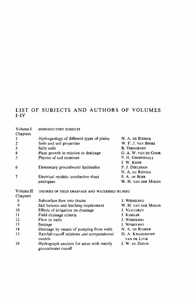
LIST OF SUBJECTS AND AUTHORS OF VOLUMES I-IV
Volume I Chapters 1 2 3 4 5
6
7
INTRODUCTORY SUBJECTS
Hydrogeology of different types of plains Soils and soil properties Salty soils Plant growth in relation to drainage Physics of soil moisture
Elementary groundwater hydraulics
Electrical models : conductive sheet analogues
N. A. DE RIDDER
W. F. J. VAN BEERS
B. VERHOEVEN
G. A. W. VAN DE GOOR
P. H. GROENEVELT
J. W. KIJNE
P. J. DlELEMAN N. A. DE RIDDER
S. A. DE BOER
W . H . V A N D E R M O L E N
Volume II THEORIES OF FIELD DRAINAGE AND WATERSHED RUNOFF Chapters
9 10 11 12 13 14 15
16
Subsurface flow into drains Salt balance and leaching requirement Effects of irrigation on drainage Field drainage criteria Flow to wells Seepage Drainage by means of pumping from wells Rainfall-runoff relations and computational models Hydrograph analysis for areas with mainly groundwater runoff
J. WESSELING
W. H . V A N D E R M O L E N
J. NUGTEREN
J. KESSLER
J. WESSELING
J. WESSELING
N. A. DE RIDDER
D. A. KRAUENHOFF
V A N D E L E U R
J. W. DE ZEEUW
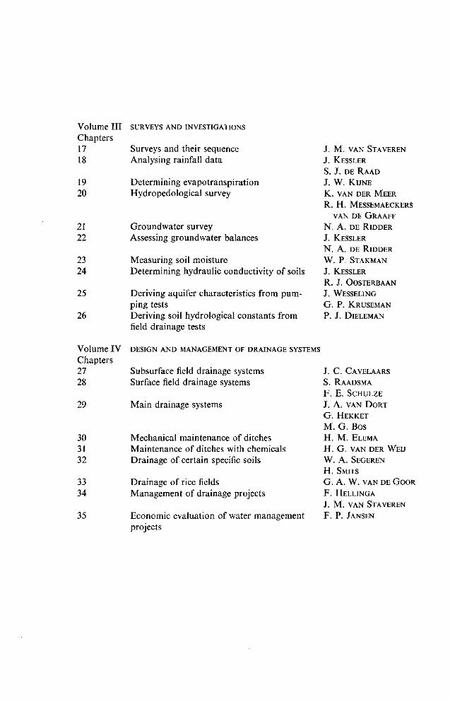
Volume III SURVEYS AND INVESTIGATIONS
Chapters 17 Surveys and their sequence 18 Analysing rainfall data
19 20
21 22
23 24
25
26
Determining évapotranspiration Hydropedological survey
Groundwater survey Assessing groundwater balances
Measuring soil moisture Determining hydraulic conductivity of soils
Deriving aquifer characteristics from pumping tests Deriving soil hydrological constants from field drainage tests
J . M . V A N S T A V E R E N
J. KESSLER
S. J. DE RAAD
J. W. KIJNE
K . V A N D E R M E E R
R. H. MESSEMAECKERS
V A N D E G R A A F F
N. A. DE RIDDER
J. KESSLER
N. A. DE RIDDER
W. P. STAKMAN
J. KESSLER
R. J. OOSTERBAAN
J. WESSELING
G. P. KRUSEMAN
P. J. DIELEMAN
Volume IV DESIGN AND MANAGEMENT OF DRAINAGE SYSTEMS
Chapters 27 Subsurface field drainage systems 28 Surface field drainage systems
29
30 31 32
33 34
35
Main drainage systems
Mechanical maintenance of ditches Maintenance of ditches with chemicals Drainage of certain specific soils
Drainage of rice fields Management of drainage projects
Economic evaluation of water management projects
J. C. CAVELAARS
S. RAADSMA
F. E. SCHULZE
J. A. VAN DORT
G. HEKKET
M. G. Bos H. M. ELEMA
H . G . V A N D E R W E I J
W. A. SEGEREN
H. SMITS
G. A. W. VAN DE GOOR
F. HELLINGA
J. M. VAN STAVEREN
F. P. JANSEN

MAIN TABLE OF CONTENTS
Preface List of subjects and authors of volumes I-IV
SURVEYS AND THEIR SEQUENCE
Objectives and phasing of project surveys The main study phases
ANALYSING RAINFALL DATA
Introduction Frequency analysis of rainfall and recurrence prediction Duration-frequency analysis of rainfall Depth-area analysis of rainfall Survey and measurement Reliability of recurrence predictions Examples of distribution fitting and confidence belts
DETERMINING EVAPOTRANSPIRATION
Introduction Calculation of potential évapotranspiration based on energy considerations
64 19.3 Calculation of potential évapotranspiration based on empirical relationships Measuring evaporation and évapotranspiration Adjustment of évapotranspiration for drying soils Areal variation and frequency of occurrence of évapotranspiration Examples of calculating potential évapotranspiration
HYDROPEDOLOGICAL SURVEY
Introduction Required soil data and maps Hydropedological surveys and investigations Final remarks
153 21 GROUNDWATER SURVEY
155 21.1 Collection of groundwater data 175 21.2 Processing of groundwater data 182 21.3 Evaluation of groundwater data
V VII
1 3 5
13 15 19 27 33 36 39 41
53 55 57
17 17.1 17.2
18 18.1 18.2 18.3 18.4 18.5 18.6 18.7
19 19.1 19.2
66 71 75 77
113 115 118 122 149
19.4 19.5 19.6 19.7
20 20.1 20.2 20.3 20.4
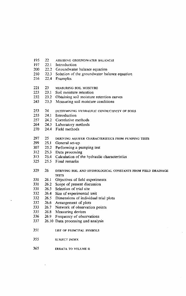
195 197 200 210 216
22 22.1 22.2 22.3 22.4
ASSESSING GROUNDWATER BALANCES
Introduction Groundwater balance equation Solution of the groundwater balance equation Examples
221 23 MEASURING SOIL MOISTURE
223 23.1 Soil moisture retention 232 23.2 Obtaining soil moisture retention curves 243 23.3 Measuring soil moisture conditions
DETERMINING HYDRAULIC CONDUCTIVITY OF SOILS
Introduction Correlative methods Laboratory methods Field methods
DERIVING AQUIFER CHARACTERISTICS FROM PUMPING TESTS
General set-up Performing a pumping test Data processing Calculation of the hydraulic characteristics Final remarks
329 26 DERIVING SOIL AND HYDROLOGICAL CONSTANTS FROM FIELD DRAINAGE
TESTS
Objectives of field experiments Scope of present discussion Selection of trial site Size of experimental unit Dimensions of individual trial plots Arrangement of plots Network of observation points Measuring devices Frequency of observations
26.10 Data processing and analysis
351 LIST OF PRINCIPAL SYMBOLS
355 SUBJECT INDEX
365 ERRATA TO VOLUME II
253 255 257 264 270
297 299 307 312 313 325
24 24.1 24.2 24.3 24.4
25 25.1 25.2 25.3 25.4 25.5
331 331 331 332 332 332 333 335 336 337
26.1 26.2 26.3 26.4 26.5 26.6 26.7 26.8 26.9 26.1(

SURVEYS AND INVESTIGATIONS
17. SURVEYS AND T H E I R SEQUENCE
J. M . V A N S T A V E R E N
Resident Engineer Food and Agriculture Organization Morocco
Lecturers in the Course on Land Drainage
J. M. VAN STAVEREN (1962-1970) International Institute for Land Reclamation and Improvement, Wageningen
A. FRANKE (1971-1973) University of Agriculture, Wageningen

PURPOSE AND SCOPE
Some observations on the phasing of project surveys, with particular reference
to drainage.
CONTENTS
17.1 OBJECTIVES AND PHASING OF PROJECT SURVEYS 3
17.2 THE MAIN STUDY PHASES 5
17.2.1 Reconnaissance survey 5
17.2.2 Semi-detailed survey 8
17.2.3 Detailed survey 9
ANNEX 10
LITERATURE 12

Surveys
17.1 OBJECTIVES AND PHASING OF PROJECT SURVEYS
The cases will be rare where drainage would be the only and exclusive operation
to achieve a project's purposes. Even in temperate humid regions a land improve
ment or reclamation project usually implies a number of combined actions involv
ing water management, infrastructure, land consolidation, agricultural extension,
etc. In arid regions the emphasis will be on the water supply by irrigation,
while the drainage system - although in many cases an essential and integral part
of such projects - is a secondary item in the whole. Elsewhere one may find ex
tensive project areas where a combination of measures is needed in varying inten
sity.
It may occur as well that, in a valley where the original problem was seasonal
waterlogging, the groundwater table is considerably lowered after the introduction
of irrigation by pumping from wells, so that finally drainage provisions can be
disregarded.
These few examples indicate that drainage works have varying degrees of importance
in a land development plan but seldom give rise to a project on their own. It
therefore has limited sense to speak about "drainage projects" as such.
Much of the information needed for considering drainage works is the same as that
needed for any land development project, both requiring geological, topographic,
and soil maps, climatic and agricultural data, and so on. However, the introduction
of drainage involves some specific studies and surveys. It will, for instance,
call for special analyses of climatic data and groundwater balances; it will
require detailed information on hydraulic conductivity and moisture characteristics
of soils; and it presupposes knowledge about the practical application of various
possible drainage systems. Other chapters in these volumes deal with those ques
tions in detail; the present chapter aims only to introduce some organizational
principles concerning the surveys needed.
To arrive at a final answer whether or not a project proposal is technically
feasible and economically sound, a sequence of studies of increasing intensity will
usually be required. Each phase in itself will involve successive actions: the
collection of data, their analysis, the formulation and design of one or more
project proposals, and their evaluation.
As a general rule three phases of study are to be recommended:
- at reconnaissance level
- at semi-detailed level
- at detailed level.
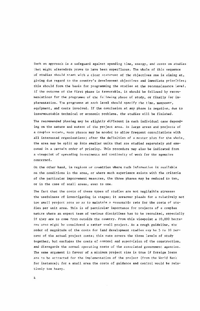
Such an approach is a safeguard against spending time, energy, and costs on studies
that might afterwards prove to have been superfluous. The whole of this sequence
of studies should start with a clear statement of the objectives one is aiming at,
giving due regard to the country's development objectives and immediate priorities;
this should form the basis for programming the studies at the reconnaissance level.
If the outcome of the first phase is favourable, it should be followed by recom
mendations for the programme of the following phase of study, or finally for im
plementation. The programme at each level should specify the time, manpower,
equipment, and costs involved. If the conclusion at any phase is negative, due to
insurmountable technical or economic problems, the studies will be finished.
The recommended phasing may be slightly different in each individual case depend
ing on the nature and extent of the project area. In large areas and projects of
a complex nature, more phases may be needed to allow frequent consultations with
all interested organizations; after the definition of a master plan for the whole,
the area may be split up into smaller units that are studied separately and exe
cuted in a certain order of priority. This procedure may also be indicated from
a viewpoint of spreading investments and continuity of work for the agencies
concerned.
On the other hand, in regions or countries where much information is available
on the conditions in the area, or where much experience exists with the criteria
of the particular improvement measures, the three phases may be reduced to two,
or in the case of small areas, even to one.
The fact that the costs of these types of studies are not negligible stresses
the usefulness of investigating in stages; it moreover pleads for a relatively not
too small project area so as to maintain a reasonable rate for the costs of stu
dies per unit area. This is of particular importance for projects of a complex
nature where an expert team of various disciplines has to be recruited, especially
if they are to come from outside the country. From this viewpoint a 10,000 hecta
res area might be considered a rather small project. As a rough guideline, the
order of magnitude of the costs for land development studies may be 5 to 10 per
cent of the actual project costs; this rate covers the three levels of study
together, but excludes the costs of control and supervision of the construction,
and disregards the normal operating costs of the associated government agencies.
The same argument in favour of a minimum project size is true if foreign loans
are to be attracted for the implementation of the project (from the World Bank
for instance); for a small area the costs of guidance and control would be rela
tively too heavy.
Surveys
17.2 THE MAIN STUDY PHASES
Without claiming completeness the following paragraphs are meant to elaborate the
purpose and the nature of actions for each of the recommended study phases, spe
cial regard being given to their drainage aspects.
17.2.1 RECONNAISSANCE SURVEY
The main objective of a reconnaissance survey is to identify the feasibility of
the proposed project, first of all on technical, but also on economic grounds.
This survey should give an answer to the following questions:
- What area or areas can be considered for improvement?
- What advantages and disadvantages can be expected from the intended change of the existing state?
- What are the alternative possibilities for improvement?
- What technical and organizational measures have to be taken for the alternative solutions?
- What will roughly be the proportion of costs to benefits in each case?
In most cases only part of the advantages and disadvantages can be expressed in
terms of money-value. There are often important imponderable factors which should
also be taken into account, e.g. the creation of new employment possibilities,
the better accessibility of the area or the development of shorter transport
routes, the creation or destruction of attractive landscapes, recreational faci
lities or cultural values; the improvement of public health by the elimination of
breeding grounds of diseases (e.g. malaria and bilharzia by the reclamation of
marshes), etc. Hence the proportion of the costs to the benefits in this stage
is only one of the factors to be considered in taking a decision for or against
moving to the second stage of investigation: the semi-detailed survey.
A study at reconnaissance level will be mainly based on existing information but
includes some limited field work. Documents concerning the area under consideration
should be collected from all agencies which ever worked in the area. Very welcome
are earlier studies, which should be analysed and re-evaluated from the present-
day viewpoint. Other pertinent data are:
- aerial photographs
- all kinds of maps: geological, topographic (scale preferably not smaller than 1/25,000 or 1/50,000), elevation maps of the land surface, road maps, land utilization and ownership maps, etc.
- existing data on soils, surface water, groundwater, climate, crops, crop yields, etc.
The maps should cover the whole of the watershed basin in which the area under
consideration is located. These will serve as the basis for water regime studies
and water balance computations. If the area covers only a small part of the basin
the data should allow estimates to be made of the hydrologie, and possibly other,
consequences of mutual interaction with the other part of the basin.
The field work in this stage is mainly to enable the investigator to familiarize
himself with the general conditions and to collect some complementary information
through inquiries or through incidental observations.
One of the first things to be done is a provisional delimitation of the area to
be identified as a project. For large areas sub-units may be identified and a pri
ority order defined for further studies.
With respect to the drainage features the reconnaissance survey should determine
the extent of excess water occurrence, trace all various causes of this excess,
and try to estimate quantitatively their inputs, frequency, and duration. In this
connection it may be useful to outline the extent of inundated spots as they have
occurred over a series of years, for instance through inquiring of local inhabi
tants. Such data can possibly be related to precipitation or level and discharge
data of near-by rivers. In case of inundations obviously flood protection or
coastal embankment may be more essential than a drainage system, although such
measures are often complementary.
Any indications about depth-to-groundwater-table in relation to precipitation and
near-by surface water levels will be invaluable. If no systematic water table
observations are yet available, inquiries directed to local inhabitants who are
using wells may provide useful information.
For low-lying areas and natural depressions an obstacle to the discharge of excess
water may be the location and condition of the natural "outlet". This item may
need particular attention. For inland areas solutions for gravity discharge are
sometimes found by blowing up a threshold in a river bed or constructing a tunnel
to a near-by lower outlet.
For low-lying coastal land one may take advantage of the tidal effect by means of
tide locks, which discharge during low tide and close automatically when the
outside level rises.
Where the gravity outlet does not offer good prospects, discharge by pumping may
be a possible alternative; a pump installation moreover can advantageously be
installed at a different place than the natural outlet. Being rather decisive for
Surveys
the project, such a solution should be carefully studied at the reconnaissance
level; consideration should be given not only to the installation of the pump but
also to the operational costs, which will require estimates of the volume of water
to be lifted annually and the maximum per day, height of the lift, expenditure on
energy and personnel, etc. Criteria for the water control system and its management
should be established for the proposed cultivation programmes, taking soil condi
tions into account, after which one or more project designs can be developed. Due
attention should also be given in this stage to possible constraints with regard
to water levels, water quality, discharge, or otherwise, which might limit the
choice of solutions or would require special provisions. Some examples are:
- built-up areas and road systems may demand extra deep drainage; in contrast
wooden foundations may need a shallow groundwater level to prevent them from
rotting;
- if polluted water from urban areas is discharged into surface water, pro
visions might have to be made to safeguard the interests of public health, fishe
ries, wildlife, and recreation;
- lowering the phreatic level in the area under consideration by drainage
might adversely affect the hydrologie circumstances of neighbouring areas;
- parts of the area may be situated in different administrative units or
different water districts, and may not be subject to the same regulations.
The reconnaissance survey should devote a substantial part of its investigations
to the collection of hydrologie data on the existing water regime, as this will
provide the basis for future water management.
Hydrologie data, due to their natural variations, will usually be expressed in
terms of probability per time unit and should therefore cover a reasonably long
period to be of any value; a ten years range might be considered a strict
minimum but much depends on their relative variability and the purpose of use.
Correlations can be sought between available climatic data and other data that
may be scarce: for instance between precipitation and river discharges or between
temperature and evaporation. In this manner one may arrive at an estimated longer
range of data. If, however, sufficiently reliable data are not available to allow
an estimate of the water balance components, an immediate programme of appropriate
observations will have to be set up.
Similarly an early verification of the response of proposed crops to the assumed
water management conditions will be needed. If no local experience is available

and no comparison with near-by areas is possible, one might seriously consider
the lay-out of experimental fields for this purpose. Of course, such field experi
ments cannot be completed during the phase of the reconnaissance survey. Hence
conducting such experiments should only be considered seriously if,on other grounds,
there is sufficient evidence for the technical feasibility of the project. Field
experiments, if conducted for a number of consecutive years, will be of invalua
ble help in studying crop response under controlled conditions. A supplementary
advantage of such experimental fields, if used for longer periods, is that they
offer the prerequisites for a demonstration and education centre for the farmers
in the area. The extent and number of the experimental fields should be chosen in
proportion to the size of the project area and the variety of problems to be stu
died: sometimes it is worth-while to include trials with different types of field
drainage systems.
The study at reconnaissance level should conclude with a report which summarizes
all existing knowledge and formulates possible alternative solutions to the problem.
Accompanying the report should be maps showing the borders and sketch-plans of
the area, including the approximate location of the main elements of the water
management system.
Costs and production figures needed for the preliminary appraisal at this stage
can be derived from experience elsewhere (expressed in units of area or length),
if possible adapted to the prevailing local conditions. The most important items
in the report are the recommendations on the next steps to be taken; if one or
more of the proposed alternative solutions are considered to be feasible, it
should be indicated whether or not additional investigations at reconnaissance
level are needed and/or what programmes of surveys and studies are needed in
the semi-detailed phase.
17.2.2 SEMI-DETAILED SURVEY
This study comprises the additional activities needed to work out the alternative
sketch plans retained from the reconnaissance study up to a "semi-detailed"
level (also indicated as "preliminary plans"). The main difference between this
and the earlier stage is that more detail is needed, for which field surveys
(defined in the reconnaissance report) will have to be conducted.
The data to be collected should be sufficiently detailed to permit a design of the
project works, the costs of which can be estimated to an accuracy of some 10 per
cent. At this level the costs and benefits are determined on the basis of calcu
lated quantities and locally checked prices.
Surveys
The topographic and soil maps required at this stage are usually at scales
1/25,000 or 1/10,000; contour lines of 0.25 m maximum interval will be needed.
At the location of projected canals, ditches, and structures, the necessary de
tailed levelling for length and cross-sections should be performed, and all further
surveys needed for the design should be completed. A sample survey outline is
found in National Engineering Handbook, Section 16 (see list of literature).
These semi-detailed studies correspond to the level of what is frequently called
"feasibility studies". This term, introduced by the International Bank for Re
construction and Development (IBRD) and associated bodies, is nowadays widely used
for studies where the Bank is called upon to assist in financing. Guidelines have
been prepared by the Bank for various types of projects, including one for irriga
tion and drainage. To illustrate the approach they take in- judging the viability
of project proposals, the Introduction of the latter document is annexed to this
chapter. For readers interested in more details of a semi-detailed study report,
no better reference could be given at the moment than the above-mentioned "guide
line" prepared by FAO/IBRD (see list of literature).
On the basis of the results of the semi-detailed study, the competent authority
should finally select one of the plans and decide on execution. But here again, it
should be mentioned that the final decision cannot be taken without attention
being paid to the imponderable advantages and disadvantages of the undertaking.
17.2.3 DETAILED SURVEY
The best plan for the area under consideration is chosen after conclusion of the
semi-detailed studies. What remains to be done, if one has decided on implementa
tion, is the final revision and in particular the elaboration - through calcula
tion and drawing - of the details of structures (bridges, culverts, pumping sta
tions, etc.) to complete the "definitive design".
Estimates for construction costs in this stage will not differ greatly from those
estimates made at the semi-detailed level.
The maps now required are at scale 1/10,000 to 1/2,500: structures will require
even larger scales.
The final step is to prepare specifications to be put out to tender.

ANNEX
INTRODUCTION1
As for all types of project, the objective of a feasibility study for an irriga
tion or drainage project is to demonstrate that the project is:
- in conformity with the country's development objectives and immediate
priorities ;
- technically sound, and the best of the available alternatives under
existing technical and other constraints;
- administratively workable;
- economically and financially viable.
In the context of this paper, a feasibility study is a comprehensive document
which will provide all the answers to questions on the above points which might
be put by an appraisal team of the World Bank Group.
In formulating (designing) a project there should be a constant effort to minimize
costs (but not at the expense of safety), maximize returns, and bring about utili
zation of the investment in the quickest possible time. The latter will usually
necessitate a rapid transformation of the farming practices in the project area.
From these considerations stem the main themes of an irrigation project feasibi
lity study:
- A thorough study of the physical resource base, particularly the project
area soils, climate, and water supply, in order to ensure that the cropping pat
terns proposed and the yields predicted can be maintained for a sustained period
and in order to determine the scale of the project.
- A thorough examination of the people likely to be involved in the project
in order to ensure that the proposed development is appropriate to their attitu
des and capacities.
- A thorough study of the engineering alternatives for serving and draining
the project lands, and their phasing, in order to ensure that the most appropriate
economical but safe solution is achieved.
- An adequate preliminary design of, and a construction schedule for, the
works, both project works and on-farm works, in order to demonstrate their suita
bility and to estimate their costs and the phasing of those costs.
Introduction, copied - after approval from editor - from: FAO/IBRD Cooperative Programme. Guidelines for the preparation of feasibility studies for irrigation and drainage projects. Rome, December 1970. Rotaprint. 25 pp.
10

Surveys
- The determination and scheduling of the agricultural pattern (size and
type of farm enterprise, crops and their yields) on the basis of physical and hu
man resources, present land use, market projections and prices.
- The determination and phasing of the various measures and inputs necessary
to achieve the agricultural plan.
- The determination of the management and organization necessary to construct
and implement the project to the time schedules predicted.
- The determination of the economic benefit to the country, the financial
returns to the farmers, the financial results of the operating authority, and the
repayment of project costs by beneficiaries.
It must be stressed that the main themes of the study are not separate exercises.
The finalization of each, and its amalgamation into the whole, is a process of
successive approximation reached after cross-consideration of the interim results
of the others.
No two projects are the same. There is clearly a wide difference between, for
instance, a project using groundwater and sprinklers for the intensive production
of vegetables by sophisticated commercial farmers and a project using a simple
river diversion for surface irrigation of rice by peasant farmers. These projects
are not only different physically, but also in non-physical terms (organization,
markets, need for credit, extension effort, etc.). Therefore, any general guide
line, such as this paper presents, must be used with intelligence and adjusted to
the needs of the particular project under investigation. The guideline is written
on the assumption that the main project works will be constructed and owned by a
public authority. In the case of groundwater projects, the main works (wells and
equipment) may be, and indeed often are, privately owned and financed through a
credit operation. For this type of project the forthcoming guidelines to be pub
lished on agricultural credit projects should be largely used instead of this
guideline.
The guideline does not attempt to deal with special questions of cost allocation
which arise in the case of a multiple-purpose project (e.g. when a reservoir is to
be used for flood control and/or power in addition to its irrigation purposes).
It is assumed in the sections on economic analysis that a cost allocation'to irri
gation has been made of the joint costs of such a project, but it is recognized
that a cost allocation of this nature may itself require a major analytical effort.
11
LITERATURE
FAO/IBRD Cooperative Programme. Guideline for the preparation of feasibility
studies for irrigation and drainage projects. Rome. December 1970.
Rotaprint. 25 pp.
LINSLEY, R.K., FRANZINI, J.B. 1964. Water Resources Engineering. McGraw-Hill
Book Co., New York. 654 pp. (especially Chapter 21, Planning for Water
Resources Development)
National Engineering Handbook. Section 16. Drainage of Agricultural Land,
Chapter 2: Drainage Investigations. US Dept. of Agriculture, Soil Conser
vation Service. May 1971.
12
SURVEYS AND INVESTIGATIONS
18. A N A L Y S I N G R A I N F A L L DATA
J. KESSLER f
Land and Water Management Specialist International Institute for Land Reclamation and Improvement, Wageningen
S. J. DE RAAD
Land drainage engineer Land Development and Reclamation Comp. Grontmij Ltd., De Bilt
Lecturers in the Course on Land Drainage
F. HELLINGA (1962-1964) University of Agriculture, Wageningen
J. KESSLER (1965-1967) International Institute for Land Reclamation and Improvement, Wageningen
S. J. DE RAAD (1968, 1969, 1971) Land Development and Reclamation Comp. Grontmij Ltd., De Bilt
R. J. OOSTERBAAN(1970) International Institute for Land Reclamation and Improvement, Wageningen
PH. TH. STOL (1972, 1973) Institute for Land and Water Management Research, Wagen ingen
PURPOSE AND SCOPE
A description of the statistical techniques for processing rainfall data and
a discussion of some probability distributions.
CONTENTS
18.1 INTRODUCTION 15
18.1.1 Determining a design rainfall 15
18.2 FREQUENCY ANALYSIS OF RAINFALL AND RECURRENCE PREDICTION 19
18.2.1 Frequencies based on depth intervals 19
18.2.2 Frequencies based on depth ranking 21
18.2.3 Recurrence predictions and return periods 25
18.3 DURATION-FREQUENCY ANALYSIS OF RAINFALL 27
18.3.1 Frequency analysis for durations equal to the interval of measurement 28
18.3.2 Frequency analysis for durations composed of two or more intervals of measurement 29
18.3.3 An example of the application of depth-duration-frequency relations to determine a drainage design discharge 30
18.3.4 Generalized depth-duration-frequency relations 31
18.4 DEPTH-AREA ANALYSIS OF RAINFALL 33
18.5 SURVEY AND MEASUREMENT 36
18.5.1 Measurement of point rainfall 36
18.5.2 Network density of raingauges 38
18.6 RELIABILITY OF RECURRENCE PREDICTIONS 39
18.7 EXAMPLES OF DISTRIBUTION FITTING AND CONFIDENCE BELTS 41
18.7.1 Introduction to distribution fitting 41
18.7.2 A logarithmic transformation 42
18.7.3 The normal probability distribution 43
18.7.4 The Gumbel probability distribution 47
LITERATURE 52
14
Rainfall data
18.1 INTRODUCTION
For the design of drainage and flood control works, the amounts of water that
have to be discharged must be known. If possible, these amounts should be assessed
by direct measurements. If not, indirect methods, such as the calculation of
discharges from rainfall data, will have to be used. As rainfall is extremely
variable in time and space, the rainfall data covering long periods and recorded
at various stations will have to be studied. These records can be used in one of
two ways :
- All rainfall data, from moment to moment, are fed into a model of the
natural system, which has rainfall as input and discharge as output (Chap.15,
Vol.11). A design discharge is then selected from the outputs of the model.
- A design rainfall is selected from a range of rainfall values and is then
transformed into a design discharge.
This chapter is mainly concerned with the processing of rainfall data and with
some statistical techniques that enable a proper design rainfall to be selected.
In principle, the same statistical techniques allow a proper design discharge to
be selected.
18.1.1 DETERMINING A DESIGN RAINFALL
The amount of rain that falls on the ground in a certain period is expressed as
a depth P (mm, inches, etc.) to which it would cover a horizontal plane on the
ground. The rainfall depth may be considered a statistical variate, its value
depending on
- the season of the year,
- the duration selected,
- the area under study.
In a design, the frequency, season, and duration chosen depend on the type of
problem under consideration.
The choice of a design frequency
The higher a rainfall, the less often it occurs. Consequently the higher the
design rainfall, implying a more costly project, the less risk there is of failure.
There is, however, a certain point at which the cost of ensuring more safety
outweighs the benefits of a further reduction in the number of failures. Therefore
the choice of a design frequency is an optimization problem.
15
For large-scale flood protection works, where failure may endanger human life or
vital material interests, an average failure of only once in 1000 years or even
10 000 years may be accepted. In this case long-term records have to be available
to allow return periods of exceptionally large floods to be predicted with suf
ficient accuracy by extrapolation (Section 7). If failure is to be understood in
an agricultural sense only, i.e. a loss or reduction in agricultural production
as may occur in irrigation and drainage projects, an average failure of once in
5 or 10 years is generally accepted. Records covering 20 years may suffice in
this case. The statistical techniques to be used may then be relatively simple
and restricted to a frequency analysis (Sections 2 and 3).
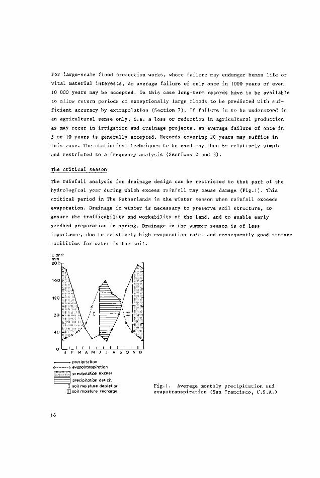
The critical season
The rainfall analysis for drainage design can be restricted to that part of the
hydrological year during which excess rainfall may cause damage (Fig.1). This
critical period in The Netherlands is the winter season when rainfall exceeds
evaporation. Drainage in winter is necessary to preserve soil structure, to
ensure the trafficability and workability of the land, and to enable early
seedbed preparation in spring. Drainage in the summer season is of less
importance, due to relatively high evaporation rates and consequently good storage
facilities for water in the soil.
I I I I I I l _ J L J F M A M J J A S O N D
i precipitation o o évapotranspiration
P^;-:^:ËI precipitation excess
| | precipitation deficit I soil moisture depletion XJ soil moisture recharge
Fig.1. Average monthly precipitation and évapotranspiration (San Francisco, U.S.A.)
16

Rainfall data
In Roumania, where the monthly rainfall and evaporation pattern is similar to
that in The Netherlands, the critical season appears to be the summer season, due
to the very high intensity of summer rainstorms, for which the soil does not offer
sufficient storage.
When the drainage problem concerns surface drainage for crop protection, it is
the growing season that may be critical. If, on the other hand, the problem
concerns surface drainage for erosion control, the off-season may be critical
because of the erosion hazard on bare soils. Unlike drainage, for which maximum
rainfall design values are important, irrigation requires a minimum rainfall
design value (maximum évapotranspiration minus effective rainfall). The critical
season then is the growing season with a rainfall deficit.
The critical duration
The rainfall intensity is expressed as a depth per unit of time. This unit can be
an hour, a day, a month, or a year. The type of problem will decide the duration
to be selected for analysis. In a study of the water availability for crop growing
or of general water excess, monthly rainfall values may suffice (Fig.2). For ir
rigation purposes the critical duration depends on the waterholding capacity of
the soil and crop response to drought, and is of the order of some weeks. In
studies of subsurface drainage, the critical duration depends on the storage capa
city of the soil, the design frequency, and the crop response to waterlogging,
and is of the order of some days. For main drainage systems the critical duration
is often also of the order of some days, depending on the storage allowances of
the system and the discharge intensity of the drainage area. For erosion control
and the drainage of small, steep watersheds or urban areas, the storage capacities
are small; information on hourly rainfalls may then be required.
The analysis of rainfall with respect to duration shows that, with the same
periods of recurrence, rainfall intensities decrease as duration increases (Fig.3).
The area under study
Rainfall is measured at certain points. It is likely that the rainfall in the
vicinity of a point of measurement is approximately the same everywhere, but
farther away from the point this will not be true. It appears that point rainfalls
with high return periods are often considerably higher than the area-average
rainfall with the same return period (Fig.4). Therefore, the design rainfall for
main drainage canals and outlets of large areas can be taken lower than the
corresponding point rainfall.
17

S O N D month
P/t inches/hr 1 Of=
Fig.2. Frequencies of monthly rainfalls (Antalya, Turkey, 15 years)
average return period n years
'100 2 5 N
'IOC ' 2 .
' i I • I
hours F i g . 3 . Depth-dura t ion-f requency r e l a t i o n s (Fresno , C a l i f o r n i a , 1903-1941)
l n r long duration p
short duration
T»2 T return period Fig.4. Schematical presentation of area-depth relations of rainfall. A: Flattening effect of the duration on area-rainfalls as compared with point-rainfalls. B: Flattening effect of size of the area on area-rainfalls of various return periods as compared with point rainfalls
\i

Rainfall data
18.2 FREQUENCY ANALYSIS OF RAINFALL AND RECURRENCE PREDICTION
The frequency of rainfall can be analysed directly, as will be discussed in this
section, or indirectly through adaptation of data to a probability distribution,
as will be discussed in Section 7. The direct frequency analysis is based on the
assignment of a frequency to each measured rainfall or to a group of rainfalls
in an observation record. Two main procedures of frequency assignment can thus be
discerned:
- frequencies based on depth ranking of each measured rainfall; to be used
when there are relatively few data,
- frequencies based on depth intervals (grouping of rainfalls); to be used
when there are many data.
These procedures will be illustrated below with the data given in Table 1, which
presents daily rainfalls for the month of November in 19 consecutive years. This
table will also be the basis for all further examples presented in this chapter.
18.2.1 FREQUENCIES BASED ON DEPTH INTERVALS
The procedure is as follows :
- Select an appropriate number (k) of depth intervals (serial number i,
lower limit a., upper limit b.) of a width suitable to the data series
and the purpose of the analysis,
- Count the number (m.) of data in each interval,
- Divide m. by the total number (n) of data in order to obtain the frequency
(F) of rainfalls in the i-th interval
m. F(a. < P < b.) = — (1)
l i n
The frequency thus obtained is called the frequency of occurrence in a certain
interval.
How this procedure has been applied for the daily rainfalls given in Table 1 is
shown in Table 2, Columns (1), (2), (3), (4), and (5). This last column gives the
frequency distribution of the intervals. It can be seen that the bulk of rainfall
values was either zero or from 0-1 inches. Greater values, which are of more
interest for drainage purposes, are recorded on far fewer days. It appears that
the chosen intervals allow a fairly regular grouping of the data.
19

Table 1. Daily rainfall in inches for the month of November in 19 consecutive years
Date Year
1948
1949
1950
1951
1952
1953
1954
1955
1956
1957
1958
1959
1960
1961
1962
1963
1964
1965
1966
-
-.42
1.14
4.37
----.15
3.64
--
1.61
-2.93
.26
.44
.42
12 13 14 15
.12 .10 1.78 .59 - .04 .21 - - .16 .22
.07 .40 .36 .15 .39 - - - - - - - -
.12 - .07 .50 - .33 1.03 .47 .02 .20 .25 -
.23 3.89 .16 .13 - - - - - - .18 .10 .04
.32 .32 .84 .03 - .44 .43 1.01 .02 - - .01 -
.04 .57 .16 1.28 .10 - .48 - .45 .60 .10
- - - - - - .05 - .05 .21 .04 .26 - .02
.40 - .90 .10 - 1.94 .49 2.25 .06 - .05
.09 .35 - - - .23 .12 - - .09 - - .34
1.61 1.80 - - - - - - .90 .29 .02 .71 .32
.13 - .07 - - - .35 .24 .18 - .52 - - .05
2.55 .76 - 1.38 .13 1.05 .38 .01 .50 1.26 .03 .62 .06
.37 .38 - - - - - - - - -
6.23 .05 - .40 - .23 .43 - - .03 - .26 .02 .52
.34 - .38 - .16 - - .06 .18 - .50 .63 .94 .07
.26 - .06 .14 .39 1.64 .43
.90 .17 - .04 .50 1.16 1.57 .51 .56 .05 .15 -
.50 - .08 - - - .10 - .33 2.21 .13 1.73 .21
.10 - - .06 2.12 2.57 .64 -
1948
1949
1950
1951
1952
1953
1954
1955
1956
1957
1958
1959
1960
1961
1962
1963
1964
1965
1966
16
-
--.04
.97
1.42
-.62
.07
.66
--.46
.26
.05
---
17
1.59
--.01
.84
.14
.70
.56
.14
.85
-.27
.45
-. 15
--.76
18
.49
-.02
---.12
.34
-.12
-. 1 1
--.02
. 12
-.55
19
-
--------.03
-. 12
--.54
.08
. 14
-
20
-
--.18
.07
---.25
.77
--.08
---. 17
-
21
-
--.27
.45
.15
--
1.48
---. 16
7.93
.15
-.07
.36
22
-
--.14
----.13
.78
---
3.71
.32
-. 10
.01
23
-
.29
-.30
.06
-.45
-.54
.28
.04
--.14
----
24
-
. 14
-.09
.72
.04
.14
-.07
.54
--------
25
.01
--
2.10
1 .51
----.03
-1 .10
-.21
-.80
--
26
-
.85
.73
.13
--.02
--.04
-.93
-.02
.80
.17
.44
-
27
-
.20
.20
.23
.18
.13
.02
--.86
-.88
-.46
.20
1 .46
.01
-
28
-
1 .22
.10
.05
.14
-.91
--.04
.28
--.57
-.60
--
29
-
2.65
.81
.13
.29
-.58
-.05
.85
.47
--.01
1.17
.24
-.02
30
-
-1.81
.83
.22
-.07
1. 17
.53
.47
-.32
--.20
.17
-.29
Total
5.31
1.37
8.76
9.54
12.29
9.23
2.51
9.20
3.91
9.06
11 .50
9.52
4.48
10.93
16.57
9.45
9.51
6.66
7.90
20
Rainfall data
From the definition of frequency, it follows that the sum of all frequencies
equals unity.
k k m . I F. = £ — = 1 (2)
. . l . , n i=l 1=1
In hydrology one is often interested in the number or frequency of rainfalls
exceeding a certain value, viz. the design rainfall. The frequency of exceedance
F(P > a.) of the lower limit a. of a depth interval i can be obtained by counting
the number M. of all rainfalls exceeding a., and dividing this number by the total
number of rainfalls (see Table 2, Column 6).
M. F(P > a.) = ̂ , (3)
Frequency distributions are often presented graphically by plotting the frequency
of non-exceedance F(P < x) instead of the frequency of occurrence or exceedance.
The frequency of non-exceedance F(P < a.) of the lower limit a. can be obtained
as the sum of the frequencies over the intervals below a.. The frequency of non-
exceedance is also referred to as the cumulative frequency.
From the fact that the sum of all frequencies over all intervals equals unity, it
can be derived that
F(P > a.) + F(P € a.) = ) (4)
The cumulative frequency distribution, therefore, can be directly derived from the
distribution of the frequency of exceedance (Table 2, Column 7).
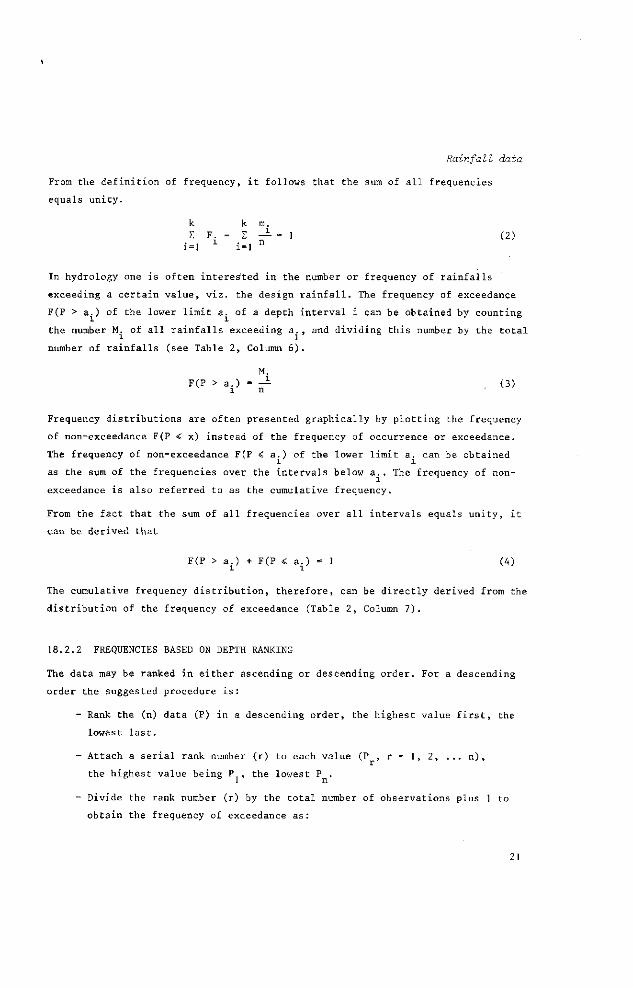
18.2.2 FREQUENCIES BASED ON DEPTH RANKING
The data may be ranked in either ascending or descending order. For a descending
order the suggested procedure is:
- Rank the (n) data (P) in a descending order, the highest value first, the
lowest last.
- Attach a serial rank number (r) to each value (P , r = 1, 2, ... n),
the highest value being P,, the lowest P .
1 n
- Divide the rank number (r) by the total number of observations plus 1 to
obtain the frequency of exceedance as:
21

Xi H
— -<r e n CTi CO OD
O — u~l -3" O ^O CO
CT-. CT\ CTs O
m co m
o o — c - i c o < r i o > j 3
un \0 r-v co o\
22

F(P > P ) r
r n~+7
Calculate the frequency of non-exceedance
F(P «: P ) = 1 - F(P > P ) = 1 r n+1
Rainfall data
(5)
(6)
If the ranking order had b e e n ascending instead of descending, similar relations
as above would have b e e n applicable w i t h an interchange of F(P > P ) and F(P < P ) . r r
A n advantage of using the denominator n+1 instead of n s as in S e c t . 2 . 1 , is that
the results will be identical no matter whether ascending or descending ranking
orders are used.
Table 3 shows how the procedure has b e e n applied for the monthly rainfalls of
Table 1, and Table 4 for the monthly maximum 1-day rainfalls of Table ] .
Table 3. Frequency distributions based on depth ranking of monthly
rainfalls derived from Table ] .
Rank Rainfall
number (descending) F(P > P )
r/(n+l)
F(P § P r )
1-F(P > P ) 1
(5)
(1) (2) (3) (4) (5) (6) (7)
1
2
3
4
5
6
7
8
9
10
11
12
13
14
15
16
17
16.57
12.29
11.50
10.93
9.54
9.52
9.51
9.45
9.23
9.20
9.06
8.76
7.90
6.66
5.31
4.48
3.91
2.51
1.37
n E P
r=l r
275
151
132
119
91
91
91
89
85
85
82
77
62
44
28
20
15
6
2
1962
1952
1958
1961
1951
1959
1964
1963
1953
1955
1957
1950
1966
1965
1948
1960
1956
1954
1949
n = 157.70 E P'
r=l '
0.05
0.10
0.15
0.20
0.25
0.30
0.35
0.40
0.45
0.50
0.55
0.60
0.65
0.70
0.75
0.80
0.85
0.90
0.95
1545
0.95
0.90
0.85
0.80
0.75
0.70
0.65
0.60
0.55
0.50
0.45
0.40
0.35
0.30
0.25
0.20
0.15
0. 10
0.05
20
10
6.7
5.0
4.0
3.3
2.9
2.5
2.2
2.0
1.82
1.67
1.54
1 .43
1 .33
1.25
1.18
1.11
1.05
23
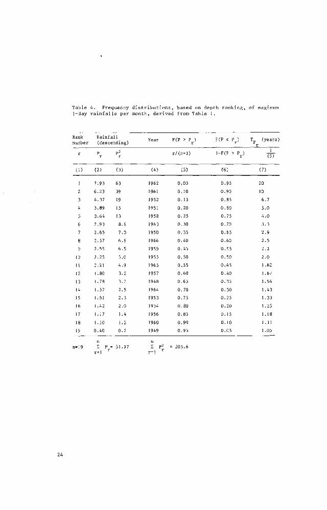
Table 4. Frequency distributions, based on depth ranking, of maximum 1-day rainfalls per month, derived from Table i.
Rank number
r
(0
Rainf (desc
P r
(2)
all ending)
P2
r
(3)
Year
(4)
F(P > P ) r
r/(n+l)
(5)
F(P « P ) r
1-F(P > P )
(6)
TP r
(years)
1 (5)
(7)
! 2
3
4
5
6
7
8
9
10
11
12
13
14
15
16
17
18
19
= 19
7.93
6.23
4.37
3.89
3.64
2.93
2.65
2.57
2.55
2.25
2.21
1.80
1.78
1.57
1.51
1.42
1.17
1.10
0.40
n Ï, P =
r-1 r
63
39
19
15
13
8.6
7.0
6.6
6.5
5.0
4.9
3.2
3.2
2.5
2.3
2.0
1.4
1.2
0.2
51.97
1962
1961
1952
1951
1958
1963
1950
1966
1959
1955
1965
1957
1948
1964
1953
1954
1956
1960
1949
n I P2
r-1 r
0.05
0.10
0.15
0.20
0.25
0.30
0.35
0.40
0.45
0.50
0.55
0.60
0.65
0.70
0.75
0.80
0.85
0.90
0.95
= 203.6
0.95
0.90
0.85
0.80
0.75
0.70
0.65
0.60
0.55
0.50
0.45
0.40
0.35
0.30
0.25
0.20
0.15
0.10
0.05
20
10
6.7
5.0
4.0
3.3
2.9
2.5
2.2
2.0
1 .82
1.67
1.54
1 .43
1 .33
1.25
1.18
1.11
1.05
24

Rainfall data
18.2.3 RECURRENCE PREDICTIONS AND RETURN PERIODS
An observed frequency distribution of rainfalls can be regarded as a sample of
the frequency distribution of the rainfalls that would occur in an infinitely
long observation series (the population). If the sample is representative of the
population, one may expect that future observation periods will reveal frequency
distribution similar to the observed one. Hence an observed frequency distribution
may be used for recurrence predictions.
It is a basic law of statistics that conclusions drawn for the population on
grounds of a sample will be increasingly reliable as the size of the sample
increases. Qualitatively it can be said that the smaller the frequency of occur
rence of an event, the larger is the sample needed to obtain a prediction of the
required accuracy. Referring to Table 2 it can be stated that the observed fre
quency of dry days (50%) will deviate only slightly from the frequency of dry
days to be observed in a future period of at least equal length. The frequency
of daily rainfalls of 3-4 inches (0.5%), however, may be doubled or reduced by
half in the next period of record. A quantitative evaluation of the reliability
of frequency predictions will be given in Sect.6.
Recurrence predictions are often done in terms of return periods (T), which is
the number of new data one has to collect for a certain rainfall to be exceeded
once on the average. The return period is calculated as
T = — (frequency of exceedance) (7) r
In Table 2 the frequency of 1-day rainfalls in the interval of 1-2 inches equals
0.04386. Then the return period is T = — = = any 23 November days. r 0.043bo
In hydrological practice one often works with frequencies of exceedance. The
corresponding return period is symbolized as
Tx = F(P > x) ( 8 )
25
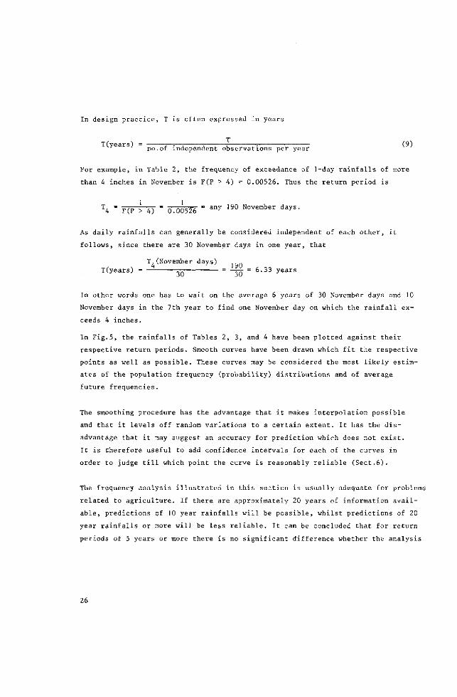
In design practice, T is often expressed in years
T(years) = J-T—3 -,—-—\ -= (9) no.or independent observations per year
For example, in Table 2, the frequency of exceedance of 1-day rainfalls of more
than 4 inches in November is F(P > 4) = 0.00526. Thus the return period is
T4 = F(P > 4) = 0.00526 = a n y 19° N o v e m b e r d*ys-
As daily rainfalls can generally be considered independent of each other, it
follows, since there are 30 November days in one year, that
T,(November days)
T(years) = ^ = ~Jç> = 6'3 3 y e a r s
In other words one has to wait on the average 6 years of 30 November days and 10
November days in the 7th year to find one November day on which the rainfall ex
ceeds 4 inches.
In Fig.5, the rainfalls of Tables 2, 3, and 4 have been plotted against their
respective return periods. Smooth curves have been drawn which fit the respective
points as well as possible. These curves may be considered the most likely estim
ates of the population frequency (probability) distributions and of average
future frequencies.
The smoothing procedure has the advantage that it makes interpolation possible
and that it levels off random variations to a certain extent. It has the dis
advantage that it may suggest an accuracy for prediction which does not exist.
It is therefore useful to add confidence intervals for each of the curves in
order to judge till which point the curve is reasonably reliable (Sect.6).
The frequency analysis illustrated in this section is usually adequate for problems
related to agriculture. If there are approximately 20 years of information avail
able, predictions of 10 year rainfalls will be possible, whilst predictions of 20
year rainfalls or more will be less reliable. It can be concluded that for return
periods of 5 years or more there is no significant difference whether the analysis
26

Rainfall data
is carried out on the basis of all 1-day rainfalls or on maximum 1-day rainfalls
only. This enables the analysis to be restricted to maximum rainfalls only, thus
saving on labour but nevertheless obtaining virtually the same results for longer
return periods.
inc 16
14
12
10
8
6
4
2
hes
^ ^
'- ^ ^ ^
,^^^^^ monthly rainfalls
/ ^ ..'y '
~ * / 7 T--° / intervals — ~~±_
\x
1 _ 1 - d a y rainfalls ^
ximum 1-day rainfalls per month
1 ? 1 1 1 1 1 1 1 1 1 1 1 1 1 0 2 4 6 8 10 12 14 16 18 20
return per iod in years
Fig.5. Depth return period relations derived from Tables 1,2,3, and 4
18.3 DURATION - FREQUENCY ANALYSIS OF RAINFALL
The time analysis is carried out, for the appropriate season, with respect to the
duration of rainfall, which is chosen in accordance with the type of drainage
problem (Sect.2).
The season is a period with fixed date limits at beginning and end, unlike
duration, of which only the length is fixed. For a general determination of
27

critical season, average monthly rainfall values usually provide sufficient
information (Fig.1). For water resources planning, seasonal frequency distributions
may have to be established (Fig.2).
In analyzing the duration of rainfalls one encounters the difficulty of moving or
sliding limits. When a 24-hour rainfall is studied, for example, this does not
necessarily mean the rainfall from 8 o'clock one day till 8 o'clock next day, but
the rainfall of any 24-hour period. If rainfall is measured at fixed intervals
with pluviometers, it may happen that rainstorms are recorded in two parts. The
frequencies of high 24-hour rainfalls will thus be underestimated. The drawback
of interval measurements by pluviometers is avoided by making use of continuously
recording rain gauges (pluviographs).
In the next parts of this section attention will be paid to the duration analysis
for rainfalls which are measured at regular intervals with pluviometers. We
distinguish:
- rainfalls equal to the interval of measurement (e.g.1 day)
- rainfalls of a duration composed of k intervals (k = 1,2, ... n).
Rainfall analysis for durations less than the interval of measurement, which is
of importance for surface drainage of small steep watersheds with short critical
durations, cannot be performed directly. In this case one has to resort to measure
ments with pluviographs or to generalized rainfall-duration relationships, obtained
from pluviographs elsewhere (Sect.3.4).
18.3.1 FREQUENCY ANALYSIS FOR DURATIONS EQUAL TO THE INTERVAL OF MEASUREMENT
From the 1-day rainfalls presented in Table 1, the frequency distribution has
been derived and presented in Table 2. With 30 November days in each year, the
return period has been calculated as
T (days) j T x ( y e a r s ) =
x3 0 = ̂ ( ^ (10)
The frequencies of high 24-hour rainfalls are probably a little higher than for
the 1-day (8 o'clock - 8 o'clock) rainfalls, because a rainstorm may have been
recorded on two consecutive days. It has been found in the U.S.A. and The Nether
lands that this effect can be compensated for by multiplying rainfall depths with
a return period of approximately 10 years with a factor 1.1.
28
Rainfall data
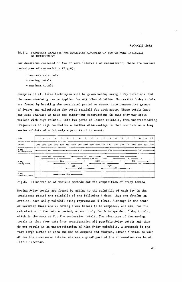
18.3.2 FREQUENCY ANALYSIS FOR DURATIONS COMPOSED OF TWO OR MORE INTERVALS OF MEASUREMENT
For durations composed of two or more intervals of measurement, there are various
techniques of composition (Fig.6):
- successive totals
- moving totals
- maximum totals.
Examples of all three techniques will be given below, using 5-day durations, but
the same reasoning can be applied for any other duration. Successive 5-day totals
are formed by breaking the considered period or season into consecutive groups
of 5-days and calculating the total rainfall for each group. These totals have
the same drawback as have the fixed-hour observations in that they may split
periods with high rainfall into two parts of lesser rainfall, thus underestimating
frequencies of high rainfalls. A further disadvantage is that one obtains a long
series of data of which only a part is of interest.
date
rainfall
5 day succesive totals
5 day moving totals
5 day maximum totals
1
0.02
* 0.60
i 3
0.20
3.82
13.82
' I
4
0.80
5
2.20
; ,
6.40 6.65
•
6
2.60
7
0.85
7.05
7.05
6.25
8
0.60
4.30
4.30
9
0.00
2.10
1 0
0.25
2.30
11
0.40
3.00
12
1.05
3.20
13
1.30
3.05
3.05
14
0.20
2.65
15
0.10
1.60
16 17 i 18 I ,
0.00 ' 0.00 0.00
19 : 20
0.22 0.35
; I :
: ' i
0.30 0 V
.
" I
j
I
Fig.6. Illustration of various methods for the composition of 5-day totals
Moving 5-day totals are formed by adding to the rainfalls of each day in the
considered period the rainfalls of the following 4 days. Thus one obtains an
overlap, each daily rainfall being represented 5 times. Although in the month
of November there are 26 moving 5-day totals to be composed, one can, for the
calculation of the return period, account only for 6 independent 5-day totals,
which is the same as for the successive totals. The advantage of the moving
totals is that they take into consideration all possible 5-day totals and thus
do not result in an underestimation of high 5-day rainfalls. A drawback is the
very large number of data one has to compose and analyse, almost. 5 times as much
as for the successive totals, whereas a great part of the information may be of
little interest.
29

It is for this reason that reduced data series are often used. In these, the data
of less importance, e.g. low rainfalls when drainage projects are being considered,
are omitted, and exceedance series or maximum series only are selected.
Maximum 5-day totals constitute the highest of the 5-day moving totals found for
each year. A straightforward frequency distribution or return period distribution
can then be made with the interval or ranking procedure. However, the second
highest rainfall in a year may exceed the maximum rainfall recorded in some other
years. As a consequence the rainfall depths with return periods of less than
approximately 5 years will be underestimated in comparison with those obtained
from complete or exceedance data series (Sect.7.4). Although, for high return
periods, the difference between maximum series and complete series vanishes (see
Fig.5), it is recommended, for agricultural purposes, not to work exclusively with
maximum series.
Frequency analysis from pluviograph records
If pluviograph records are available in the form of unprocessed recorder charts,
these charts will have to be processed either manually or mechanically to obtain
lists of rainfall depths per unit of time (e.g.5,10,30 min.). When punch tape
recorders are used on the pluviograph the processing can be entirely automated.
Once the lists of rainfall depths for various durations are available, the analysis
can, in principle, be performed along the same lines as was discussed for daily
records. There will, however, be such a mass of data that only maximum series will
be practical.
18.3.3 AN EXAMPLE OF THE APPLICATION OF DEPTH-DURATION-FREQUENCY RELATIONS TO DETERMINE A DRAINAGE DESIGN DISCHARGE
Having analysed rainfalls for both frequency and duration, one arrives at the
depth-duration-frequency relations as illustrated in Fig.3. These relations hold
only for the point where the observations were made, but can be assumed represent
ative of the area surrounding the recording station if the climate in the area is
uniform.
An example of the application of depth-duration-frequency relations is given
below. The data of Table 1 come from a tropical rice growing area. November, when
rice has just been transplanted, is a critical month: an abrupt rise of more than
3 inches of the water standing in the fields is considered harmful. A surface
drainage system is to be designed to prevent this happening too frequently. To
find the design discharge of this surface drainage system, we make use of the
30
Rainfall data
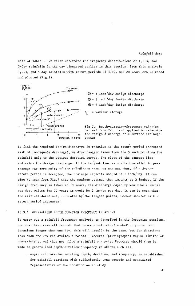
data of Table 1. We first determine the frequency distributions of 1,2,3, and
5-day rainfalls in the way discussed earlier in this section. From this analysis
1,2,3, and 5-day rainfalls with return periods of 5,10, and 20 years are selected
and plotted (Fig.7).
depth inches 10
Tin years
_
© „z-^ / ®^-*—""
- x ^ ^ 2 0 —
—10 —
-/ /* ^f*\ waterstored ^-~-sC^ I u I é^i- / max rise 3"
s m ^ - - " " water d
^-~"7^~-1 inch/day i i Ï
.--^ • ^
ained
i i
— c
•
1 3 4 5 durat ion in days
0 = 1 inch/day design discharge
@ = 2 inch/day design discharge
© = 6 inch/day design discharge
= maximum storage
Fig.7. Depth-duration-frequency relation derived from Tab.1 and applied to determine the design discharge of a surface drainage system
To find the required design discharge in relation to the return period (accepted
risk of inadequate drainage), we draw tangent lines from the 3 inch point on the
rainfall axis to the various duration curves. The slope of the tangent line
indicates the design discharge. If the tangent line is shifted parallel to pass
through the zero point of the coordinate axes, we can see that, if a 5-year
return period is accepted, the drainage capacity should be 1 inch/day. It can
also be seen from Fig.7 that the maximum storage then amounts to 3 inches. If the
design frequency is taken at 10 years, the discharge capacity would be 2 inches
per day, whilst for 20 years it would be 6 inches per day. It can be seen that
the critical durations, indicated by the tangent points, become shorter as the
return period increases.
18.3.4 GENERALIZED DEPTH-DURATION-FREQUENCY RELATIONS
To carry out a rainfall frequency analysis as described in the foregoing sections,
one must have rainfall records that cover a sufficient number of years. For
durations longer than one day, this will usually be the case, but for durations
less than one day the available rainfall records (pluviographs) may be limited or
non-existent, and thus not allow a rainfall analysis. Recourse should then be
made to generalized depth-duration-frequency relations such as :
- empirical formulas relating depth, duration, and frequency, as established
for rainfall stations with sufficiently long records and considered
representative of the location under study
31
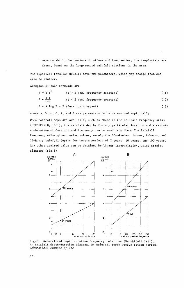
- maps on which, for various durations and frequencies, the isopluvials are
drawn, based on the long-record rainfall stations in the area.
The empirical formulas usually have two parameters, which may change from one
area to another.
Examples of such formulas are
b P = a.t" (t > 2 hrs, frequency constant)
c. t P = T-~7 (t < 2 hrs, frequency constant)
P = A log T + B (duration constant)
(11)
(12)
(13)
where à, b, d, A, and B are parameters to be determined empirically.
When rainfall maps are available, such as those in the Rainfall Frequency Atlas
(HERSHFIELD, 1961), the rainfall depths for any particular location and a certain
combination of duration and frequency can be read from them. The Rainfall
Frequency Atlas gives twelve values, namely the 30-minutes, 1-hour, 6-hours, and
24-hours rainfall depths for return periods of 2 years, 10 years, and 100 years.
Any other desired value can be obtained by linear interpolation, using special
diagrams (Fig.8).
rainfall inches 10 T
f •
._ ,
-
—
- i —
/xn
\
^24
• - •
k D years
years
i i
—\-
I
—
6 12 24 duration in hours
5 10 25 50 100 return period in years
Fig.8. Generalized depth-duration frequency relations (Hershfield 1961). A: Rainfall depth-duration diagram. B: Rainfall depth versus return period. Schematical example of use
32

Rainfall data
Diagram A is used to interpolate between durations of 1-hr and 24-hrs, and
Diagram B is used to interpolate between return periods of 1 year and 100 years.
Diagram A is derived empirically, while Diagram B is based on the Gumbel probabil
ity distribution with a correction for partial-durations when the return period
is less than 10 years.
For the linear interpolation on Diagrams A and B, four key-values only would suf
fice. REICH (1963), in a study on the short-duration rainfall intensities of South
Africa, worked with the key-values: 1-hour and 24-hours duration rainfall depths
for 2-year and 100-year return periods. If the key-values cannot be read directly
from available rainfall maps, empirical relations are suggested to estimate the
key-value from such information as: occurrence of thunder storms, mean of annual
maximum daily rainfalls, and the ratio between 100-year maximum and 2-year maximum
rainfalls as found from neighbouring recorder stations.
18.4 DEPTH-AREA ANALYSIS OF RAINFALL
The analysis of rainfall is understood here to be the analysis of area averages
of point rainfalls or the analysis of the geographical distribution of point
rainfalls. The first type of analysis will be given below, the second type has
been discussed in Sect.3.4.
A rainfall measurement is a point observation and may not a priori be representa
tive of the area. Usually area rainfalls have a smaller variability than point
rainfalls (Fig.4B). For high return periods, this results in area rainfalls which
are smaller than point rainfalls and vice versa. However, area rainfalls will
differ less from point rainfalls if the duration is taken longer. Therefore mean
rainfalls taken over long periods will be approximately equal for points and for
areas, if the area is homogeneous with respect to rainfall. An area-frequency
analysis can be made on the basis of the area averages of point rainfalls for the
chosen duration. Usually one of the following three methods is employed:
- arithmetic mean of rainfall depths at all stations,
- weighted mean of rainfall depths at all stations, the weight being determ
ined by polygons constructed according to the Thiessen method,
- weighted mean of average rainfall depths between isopluvial lines, the
weight being the area enclosed by the isopluvials.
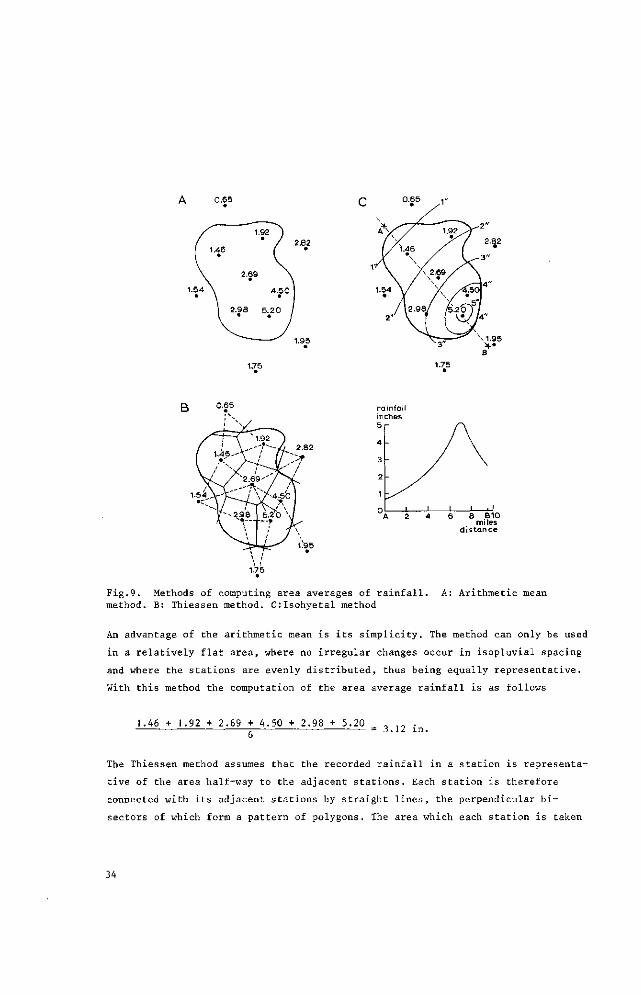
Examples of the above procedures are given in Fig.9.
33
A 0.65 C °-f5 ,v
0.65
Fig.9. Methods of computing area averages of rainfall. A: Arithmetic mean method. B: Thiessen method. C:Isohyetal method
An advantage of the arithmetic mean is its simplicity. The method can only be used
in a relatively flat area, where no irregular changes occur in isopluvial spacing
and where the stations are evenly distributed, thus being equally representative.
With this method the computation of the area average rainfall is as follows
1.46 + 1.92 + 2.69 + 4.50 + 2.98 + 5.20 3.12 in.
The Thiessen method assumes that the recorded rainfall in a station is representa
tive of the area half-way to the adjacent stations. Each station is therefore
connected with its adjacent stations by straight lines, the perpendicular bi
sectors of which form a pattern of polygons. The area which each station is taken
34
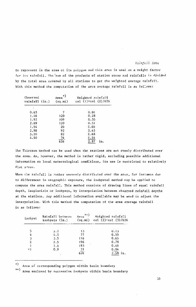
Rainfall data
to represent is the area of its polygon and this area is used as a weight factor
for its rainfall. The'sum of the products of station areas and rainfalls is divided
by the total area covered by all stations to get the weighted average rainfall.
With this method the computation of the area average rainfall is as follows:
Observed Area Weighted rainfall rainfall (in.) (sq.mi) col (l)xcol (2)/626
0.65 7 0.01 1.46 120 0.28 1.92 109 0.35 2.69 120 0.51 1.54 20 0.05 2.98 92 0.45 5.20 82 0.68 4.50 _76 0.54
626 2.87 in.
The Thiessen method can be used when the stations are not evenly distributed over
the area. As, however, the method is rather rigid, excluding possible additional
information on local meteorological conditions, its use is restricted to relatively
flat areas.
When the rainfall is rather unevenly distributed over the area, for instance due
to differences in orographic exposure, the isohyetal method may be applied to
compute the area rainfall. This method consists of drawing lines of equal rainfall
depth, isopluvials or isohyets, by interpolation between observed rainfall depths
at the stations. Any additional information available may be used to adjust the
interpolation. With this method the computation of the area average rainfall
is as follows:
Rainfall between Area Weighted rainfall isonyet i s o h y e t s ( i n - ) (sq.mi) col (2)xCol (3)/626
5 5.1 13 0.10 4 4.5 77 0.55 3 3.5 116 0.65 2 2.5 196 0.78 1 1.5 193 0.46
<] 0.9 _J_1_ 0.04 626 2.58 in.
Area of corresponding polygon within basin boundary
Area enclosed by successive isohyets within basin boundary
35
The area average rainfall is computed from the weighted mean of average rainfalls
between two isohyets, the weight being the enclosed area between the isohyets.
The reliability of the method depends on the accuracy with which the isopluvials
can be drawn.
18.5 SURVEY AND MEASUREMENT
18.5.1 MEASUREMENT OF POINT RAINFALL
Rainfall is measured with rain-gauges, which are provided with a receiver having
a horizontal opening of known area (Fig.10). In principle any open receptacle may
serve as a rain-gauge. Commonly used are receivers with an opening of 200 to
400 cm . The rainfall collected in the gauge is funnelled into a small-diameter
measuring tube, where its depth is amplified so that tenths of a millimeter can be
measured accurately. A distinction can be made between two types of rain-gauges:
self-recording and non-recording.
Non-recording gauges or pluviometers are measured by periodical readings of the
accumulated rainfall. This is generally done every 24 hours. Large capacity
storage gauges, to be used at remote sites, are measured only a few times a year.
Pluviometers have the advantage that they can be made simple and sturdy; con
sequently they are reliable and not very costly.
They have, however, certain disadvantages:
- they require personnel for reading,
- the fixed hour readings may not correspond with the occurrence of rain
storms, which will then be divided over two consecutive intervals (see
Section 3.1),
- the distribution of rainfall within the interval of observation remains
unknown.
Recording gauges or pluviographs give continuous recordings of the rain being
caught in the gauges. They enable the rainfall depth over any period to be read
and are a prerequisite if short duration rainfalls have to be determined. If
recordings are made on punch cards or magnetic tapes, these records can be fed
into electronic computing equipment without further processing.
Their disadvantages are:
- they are more complicated and more expensive than pluviometers,
- they produce an almost unlimited amount of information which may be more
than required, making data selection procedures necessary.
36

Rainfall data
recorder
Ï&.Z7,
Fig.10. Cross-section of the Colenbrander rain-gauge
Although the principle of measuring precipitation is relatively simple, it is
sometimes difficult to obtain accurate measurements. There are various influences
which make rain-gauge readings uncertain, such as
- the wind shelter effect with respect to surrounding objects,
- the wind deformation effect with respect to the rain-gauge itself,
- the evaporation losses.
The wind shelter effect occurs when the rain-gauge is too near a house, a tree,
etc. It may give rise to an excess or deficit in catch. The World Meteorological
Organization (Guide to Hydrometeorological Practices, 1965) gives as a rule of
thumb that the gauge should not be closer to surrounding objects than 4 times the
height of these objects.
The wind deformation effect is due to the fact that wind reduces the amount of
rain caught in the receiver by blowing the rain drops upward over the edge of the
receiver. It has been observed that wind can reduce the catch by more than 10%
(McKay, 1954). The wind deformation effect is determined by the size of the
37

opening and the height of the receiver above the ground surface. Since the wind
deformation effect occurs at the edges of the receiver, it can be reduced by making
a larger opening by which the ratio circumference to surface becomes smaller. The
height of the mouth of receiver above the ground should be as low as possible
because the wind velocity increases with height, but should be high enough to
prevent splashing in. In areas which have little snow and where the surroundings
are such that, even in heavy rain, there is no risk of the ground being covered
by puddles, a height of 30 cm is used. Otherwise a standard height of 1 metre is
advised by the W.M.0. Standard heights in the USSR, the USA, The Netherlands, and
the UK, are 2, 0.75, 0.40, and 0.30 respectively.
The deformation effect can be reduced by choosing the site so that the wind speed
is as low as possible and also by modifying the surroundings of the gauge so
that the airflow across the mouth is made accurately horizontal. This can be
achieved by building a circular turf wall about 3 metres across (English mounting).
The gauge is exposed in the centre of the circle. The inner surface of the wall
should be vertical and the outer surface sloping at an angle of about 15% to the
horizontal. An alternative way is to use shields around the receiver, with the
top of the shield on the same level as the mouth of the receiver. Well known are
the flexible Alter shield and the rigid Nipher shield.
Evaporation losses are likely to occur in hot and dry climates. They can be reduced
by placing oil in the receiver and by preventing the internal temperature of the
receiver from becoming too high. The equipment and practices for rainfall measure
ments are standardized in most countries. It is usually advisable to follow these
standards, even when they would give rise to systematic errors, in order to facili
tate a comparison between newly installed and already existing stations. When more
accurate precipitation data are desirable, as in waterbalance studies, drainage
experiments etc. , a second gauge with a better performance could be installed
next to the standard type, for comparison.
18.5.2 NETWORK DENSITY OF RAIN GAUGES
The required network density of rain gauges depends on the area variability of
rainfall and the required accuracy. A relatively sparse network of stations would
suffice for studies of long-duration rainfalls (e.g.annual). A very dense network
is required to determine the rainfall pattern of thunderstorms. As rainfall
characteristics in mountainous areas are more variable than in flat areas, the
network density has to be higher in the first case than in the second.
38
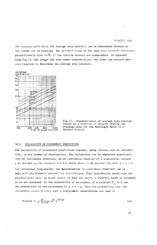
Rainfall data
The accuracy with which the average area rainfall can be determined depends on
the number (n) of stations. The standard error of the mean area rainfall decreases
proportionally with 1/i/n, if the station records are independent. As apparent
from Fig.11, the larger the area under consideration, the lower the network den
sity required to determine the average area rainfall.
percentage standard error 70 60 50
__ .
— v -^
^ ^
- , .-*_
sq.miles^ 500-s' i ^
ioqo„ ^000 4000'
8P00:
^r
—
I I '
s^
s
M i l ' 1 '
- -
1111
3T-TT
T
- •
— I J —
I T
TT _L
100 200 300 500 1000 area per gauge (sq. miles)
Fig.11. Standard error of average area precipitation as a function of network density and drainage area for the Muskingum Basin (U.S. Weather Bureau)
18.6 RELIABILITY OF RECURRENCE PREDICTIONS
The reliability of recurrence predictions depends, among factors such as variabi
lity, on the number of observations. The reliability can be expressed quantitati
vely by confidence intervals. An a% confidence interval of a statistical variate
y is defined as the interval a-b for which there is a% probability that a < y < b.
For calculated frequencies, the determination of confidence intervals can be
made with the binomial probability distribution. This distribution deals with two
possibilities only: an event occurs or does not occur, a rainfall depth is exceeded
or is not exceeded. If the probability of exceedance of a rainfall P is p and
the probability of non-exceedance is q = 1 - p, then the probability that the
exceedance occurs m times when n independent observations are made is
Prob(m) = ml (n-m).'
m (n-m) (14)
39

which is the binomial probability distribution of m, where the symbol .' stands
for factorial according to
n : = n.(n-l).(n-2) .. . 3.2.1
m : = m.(m-1).(m-2) ... 3.2.1
Since the frequency of exceedance is derived from a limited amount of data, it is
only an estimate of the probability of exceedance p. By applying the binomial
confidence interval to the observed frequency of exceedance, one obtains the
interval that covers p at the chosen confidence level. A series of confidence
belts of p is obtained as depicted in Fig.12 for various values of sample
size n.
Fig.12. 95% confidence limits ^ «^ r, .a derived from the binomial distribution 0.40 0.48 , ,, ., t _ „ .. k/n (Pearson, Hartley, 1956)
This figure allows for statements such as:
"It is for 95% likely that the probability of exceedance of a daily rainfall
of 1 inch for which in a sample of size n = 570 the observed frequency of exceed
ance was F(P > 1 inch) = 0.07 (see Table 2) is covered by the interval 0.05
(lower limit) and 0.10 (upper limit)." The return period ranges in this case
from 10 to 20. In literature methods are given for the determination of
confidence intervals for the entire probability distribution.
40

Rainfall data
Recording stations often have lengths of records which are too short for suf
ficiently reliable predictions.
The records may be extended in two ways:
- by relating the record to the records of neighbouring stations with longer
record (e.g. by a linear regression or by the ratio method). This method can
only be successful if there is a good correlation. Further reference on this sub
ject is made to SNEDECOR (1957);
- by adding the records of one or more stations (station year method). This
can only be done if the data are independent, which can be tested, for instance,
by a correlation analysis. Also the stations should be in areas which, from the
point of view of rainfall, are homogeneous. This can be tested by analyzing their
rainfall distributions. Further reference on this subject is made to VEN TE CHOW
(1964).
18.7 EXAMPLES OF DISTRIBUTION FITTING AND CONFIDENCE BELTS
18.7.1 INTRODUCTION TO DISTRIBUTION FITTING
When a frequency distribution has been obtained, it is considered representative
for frequencies in the future. However, a frequency distribution of rainfalls is
obtained from a data series of limited length, which does not contain all possible
rainfall depths (the population). In other words the data series is only a sample
of the population. Thus the frequency distribution of the data series is only an
estimate for the frequency distribution of the population (the probability distri
bution). The degree to which an estimate can deviate from the population value is
dependent on the sample size: the larger the sample, the smaller the deviation
tends to be. This is a fundamental law of statistics.
The probability distribution is, for rainfalls, assumed to be a continuous
function, representing a smooth curve on a graph. A frequency distribution is, as
a consequence of defectiveness of the data, discontinuous and not smooth, A first
step towards finding a smooth probability distribution from a frequency distribu
tion is by plotting the data on a graph against their frequencies (plotting posi
tions) and drawing through the points the best fitting smooth curve (Fig.5).
41
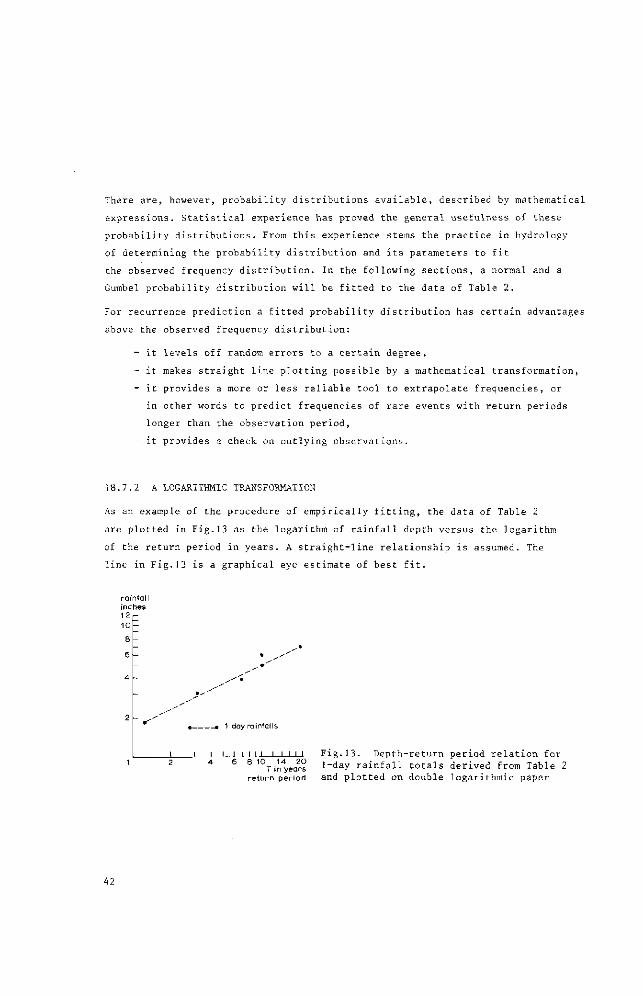
There are, however, probability distributions available, described by mathematical
expressions. Statistical experience has proved the general usefulness of these
probability distributions. From this experience stems the practice in hydrology
of determining the probability distribution and its parameters to fit
the observed frequency distribution. In the following sections, a normal and a
Gumbel probability distribution will be fitted to the data of Table 2.
For recurrence prediction a fitted probability distribution has certain advantages
above the observed frequency distribution:
- it levels off random errors to a certain degree,
- it makes straight line plotting possible by a mathematical transformation,
- it provides a more or less reliable tool to extrapolate frequencies, or
in other words to predict frequencies of rare events with return periods
longer than the observation period,
- it provides a check on outlying observations.
18.7.2 A LOGARITHMIC TRANSFORMATION
As an example of the procedure of empirically fitting, the data of Table 2
are plotted in Fig.13 as the logarithm of rainfall depth versus the logarithm
of the return period in years. A straight-line relationship is assumed. The
line in Fig.13 is a graphical eye estimate of best fit.
rainfall inches
10
8
6
4
2 ^
I
• • 1 day rainfalls
»̂
I I F i g . 1 3 . Dep th - re tu rn per iod r e l a t i o n for 6 81°Tin4yea2r? 1 _ d a y r a i n f a l l t o t a l s der ived from Table 2
return period and p l o t t e d on double l ogar i thmic paper
42

Rainfall data
18.7.3 THE NORMAL PROBABILITY DISTRIBUTION
Theory
The normal probability distribution, also known as the Gauss or the Moivre
distribution, cannot be written directly in terms of probabilities. The analytical
expression is given in the form of a probability density function
_ (x-u)2
f (x) = — — e 2a (15) CT/2TT
where
f(x) = the normal probability density function of x
x = the normal variate (-»̂ x«»)
y = the mathematical expectation of x
a2 = the variance of x
A probability of occurrence in a certain interval can be found by
b Prob (a<x<b) = ƒ f(x) dx (16)
a
Since
+O0
ƒ f(x) dx = 1 (17) —CO
it follows that
Prob (x>a) = 1 - Prob (x^a) (18)
The mathematical expectation of x is given by:
u = ƒ x f(x) dx (19) — 00
The variance,a measure of the variation of x about y, is given by
CO
a2= ƒ (x-y)2 f(x) dx (20)
In Fig.l4A an example is given of a normal probability density function. It can be
seen from the formula that the density function is symmetric about \i. The mode u
(where the function is maximum) coincides with the mean u. The probability of both
exceedance and non-exceedance of y equal {. The median £ therefore also coincides
with the mean. 43
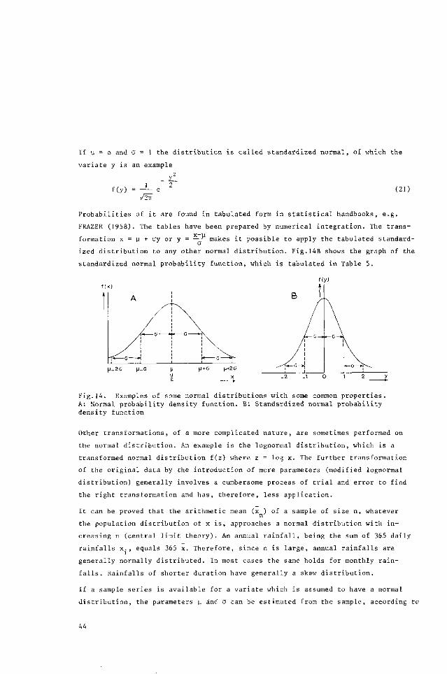
If y = o and O = 1 the distribution is called standardized normal, of which the
variate y is an example
f(y) = 1
/2TF (21)
Probabilities of it are found in tabulated form in statistical handbooks, e.g.
FRAZER (1958). The tables have been prepared by numerical integration. The trans-
formation x = y + Qy or y = — — makes it possible to apply the tabulated standard
ized distribution to any other normal distribution. Fig.l4B shows the graph of the
standardized normal probability function, which is tabulated in Table 5.
L_2G H-o H+o p+2 0
f(
B t
L—Q —
\ J 1
/ 1
y)
— c-A
|—a—ir̂ -̂
- 2 - 1 0 1 2 y
Fig.14. Examples of some normal distributions with some common properties. A: Normal probability density function. B: Standardized normal probability density function
Other transformations, of a more complicated nature, are sometimes performed on
the normal distribution. An example is the lognormal distribution, which is a
transformed normal distribution f(z) where z = log x. The further transformation
of the original data by the introduction of more parameters (modified lognormal
distribution) generally involves a cumbersome process of trial and error to find
the right transformation and has, therefore, less application.
It can be proved that the arithmetic mean (x ) of a sample of size n, whatever
the population distribution of x is, approaches a normal distribution with in
creasing n (central limit theory). An annual rainfall, being the sum of 365 daily
rainfalls x., equals 365 x. Therefore, since n is large, annual rainfalls are
generally normally distributed. In most cases the same holds for monthly rain
falls. Rainfalls of shorter duration have generally a skew distribution.
If a sample series is available for a variate which is assumed to have a normal
distribution, the parameters u and a can be estimated from the sample, according to
44
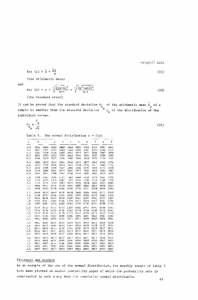
Rainfall, data
E s t ( y ) = x = ^ ( 22 )
(the arithmetic mean)
and
Est (o> - s - f - ^ - V ^ ^ (23)
(the standard error)
It can be proved that the standard deviation a- of the arithmetic mean x of a
x n sample is smaller than the standard deviation a of the distribution of the
x individual values.
o- = -* ( 2 4) n /n
Table 5. The normal distribution y -> f(y)
Ü
0
0 0
0
0
0
0 0
0
] 1
1
! 1
]
]
1 ]
1
2
2 2
2
2.
2
2
2. 2 2
'!, '1.
:i.
'). 3,
V
.0 ,1 ,2
,3
,4
,5
.6 ,7
.8 ,9
.0 ,1
2
,3
,4
,5
,6
,7
,8 ,9
.0 ,1 ,2
,3
,4
,5
,6 ,7
.8 ,9
.0 ,1
,2
,3 ,4
0
5000
4602
4207
3821
3446
3085
2743
2420 2] 19
1841
1587
1357
1151 0968
0808
0668
0 548
0446
03 59 0287
0228
0179 0139
0107 0082
0062
004 7
00 3 5 0026
0019
0013 00 10
0007
0005
0003
1
4960
4562
4168
3783
3409
3050
2709
2389 2090 1814
1562
1335
1 131
09 51
079 3
0655
0537
0436
0351
0281
0222 0174
0136
0104
0080
0060
004 5
0034
0025 0018
00 1 3
0009
0007 1)005
0003
2
4920 4522
4129 3745
3372
3015 2676
2358
2061
1788
1539 1314 1112
0934
0778
0643
0526
0427 0344
0274
0217 0170 0132
0102
0078
00 39 0044
00 33 0024
0018
00 1 3
0009 0006
000 3 000 3
3
4880
4483
4090 3707
3336
2981
2643 2327
2033
1762
1515 1292
109 3
0918 0764
0630
0516
0418 0336
0268
0212 0166
0129
0099
0075
0057
0043 0032
0023 0017
0012
0009
0006 0004
0003
4
4840
4443 4052
3669 3300
2946 2611
2296
2005
1736
1492
1271
1075 0901
0749
0618
0505
0409
0329 0262
0207 0162
0125
0096
0073
0055
0041
00 31
0023 0016
0012
0008
0006
0004
0003
5
4801
4404
4013 3632
3264
2912
2578 2266
1977
1711
1469 1251 1056
0885
0735
0606
0495
0401 0322 0256
0202 0158 0122
0094
0071
0054
0040
0030 0022
0016
001 1
0008
0006
0004
0003
6
4761
4364 3974
3594
3228
2877
2546
2236
1949
1685
1446 1230
1038
0869 0721
0594
0485
0392
0314
0250
0197 0154
01 19
0091 0069
0052
00 39
0029 0021
00 1 5
001 1 0008
0006
0004
000 3
7
4721
4325 3936
3557 3192
2843 2514
2206 1922
1660
1423 1210
1020
0853
0708
0582
0475
0384 0307
0244
0192
0150
01 16
0089
0068
0051
0038
0028 0021
0015
001 1
0008 000 5
0004
0003
8
4681
4286 3897
3520
3156
2810
2483
2177 1894
1635
1401
1190
1003 0838
0694
0571
0465
0375
0301
0239
0188 0146 01 13
0087
0066
0049 0037
0027
0020 0014
0010
0007
000 5
0004
0003
9
4641
4247
3859
3485 3121
2776
2451
2148
1867 161 1
1379 1 170
0985
0823 0681
0559 0455
0367
0294
0233
0183 0143
01 10
0084
0064
0048
00 36
0026
0019 0014
0010
0007
0005
0003 0002
Procedure and example
As an example of the use of the normal distribution, the monthly totals of Table 3
have been plotted on normal probability paper of which the probability axis is
constructed in such a way that the cumulative normal distribution 45
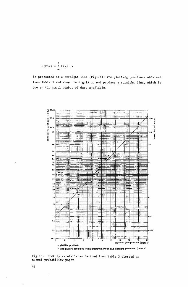
F(P<x) = ƒ f(x) dx co
is presented as a straight line (Fig.15). The plotting positions obtained
from Table 3 and shown in Fig.15 do not produce a straight line, which is
due to the small number of data available.
10005
monthly precipitation (inches) x plotting positions
o straight line estimated from parameters, mean and standard deviation (table 3)
Fig.15. Monthly rainfalls as derived from Table 3 plotted on normal probability paper
46

In order to obtain a straight line, the parameters are estimated as y = P and
CT = s from Table 3, according to
/i S X P 157.70 „ , Est (y) = P = — = — j g — = 8.3
/ N ,/£P - n(P)2 ,/1545 - 19 (8.3)2 , , Est (a) = S p = ]/ ^ - L - =• ^ jg = 3.6
The values P = y - a = 8 . 3 - 3 . 6 =4.7 and P = y + a = 8.3 + 3.6=li.9 are
then plotted against the 16% and 84% non-exceedance probability (see also Fig.14),
whereas the value P = y = 8.3 is plotted against the 50% probability. A straight
line can be drawn through these points.
It is concluded from Fig.15 that the observed monthly total of 16.57 inches is
estimated to have a return period of approximately 100 years instead of the 20
years given as the observed frequency in Table 3. The first estimate (100 years)
depends on the entire sample.
18.7.4 THE GUMBEL PROBABILITY DISTRIBUTION
Theory
The Gumbel distribution (GUMBEL, 1954), also called the distribution of
extreme values can be written as a cumulative probability distribution, viz.
Prob (P < P) = exp {-exp(-y)} (-c»<p<oo) (25)
where
P = the maximum rainfall of a sample of size N,
y = a(P-u) is the reduced Gumbel variate
u = y - c/a = the mode of the Gumbel distribution
y = the population mean
c = Euler constant = 0.57722
TT
a = = the standard deviation of the Gumbel distribution a/6
a = standard deviation of the population
47

The Gumbel distribution is skew to the right with u < \i and the median £ in
between.
For large samples (n > 100, say) the parameters u and a can be estimated
by means of the relationships
Est (a) = -?— (26) sp/6
and
Est (u) =p - law (27)
Introducing P=u into the equation of the Gumbel distribution yields, with
y = a(P-u) = 0
Prob (P < u) = e_1 = 0.37 (28)
Therefore the probability of non-exceedance of the mode u equals 0.37.
It can be proved that the cumulative probability distribution of the maximum value
of a sample of size N approaches asymptotically the Gumbel distribution with
increasing N, if the samples are drawn from a distribution of the exponential
type. In hydrological practice it can be assumed that the asymptotic approach
is realized for N > 10; therefore frequent use is made of the Gumbel distribu
tion in hydrology, mostly for annual or monthly maxima of floods or rainfalls
of short duration (less than —r of year or month resp.).
For the determination of the Gumbel distribution one needs to have several samples
from which to select the maxima, each sample being homogeneous or from the same
population. In this way, annual, monthly, or seasonal maxima series for various
durations can be composed, the duration being such that at least N = 10 indepen
dent data appear from which to choose the maximum.
Observed frequencies of non-exceedance for each of the n maxima selected from
the n x N data can be obtained by using the ranking method (Sect.4.3) yielding
F ( P N < F r ) = ' " F ( P N > P r ) = 1 ~ ÏÏ^T (Pitting position) (29)
where r is the rank number of the selected maxima, when arranged in decreasing
order.
48

Rainfall data
The Gumbel distribution can be written, taking logarithms twice
v - T(P-U) = -log {-log Prob(P < P)} (30)
Gumbel probability paper is constructed in such a way that probabilities of non-
exceedance are plotted on a log log scale to yield a linear relationship. A
straight line of best fit can thus be drawn by eye or can be calculated.
One of the methods for calculation is a linear regression. This regression is based
on the linear relationship between y and P:
y = ai(P-ui) regression of y on P (31)
P = — y + U2 regression of P on y (32)
The coefficients oti and I/M2 are estimated in such a way that the sum of the
squares of the deviations in respectively y and P direction from the straight line
is reduced to a minimum. Setting the geometric mean according to a = V Ctict2, it
can be proved that
s y Est (a) = — and Est (u) = P - " • (33)
s n Est(a)
which determines the straight line for any value of n.
s„ = is the standard deviation of the n maxima P P r
s = is the standard deviation of n reduced variâtes y and depends only on n n (see Table 6) r
P = is the arithmetic mean of the n maxima P n r
y = is the arithmetic mean of n reduced variâtes y n r
and depends only on n (see Table 6)
Procedure and example
As an example of the use of Gumbel distribution to a small sample, the maximum
monthly 1-day rainfalls of Table 1 have been analyzed and are presented in Table
4. The cumulative frequencies have been plotted on Gumbel probability paper in
Fig.16 together with confidence belts as derived from a specific method by Gumbel.
For this example use is made of the regression analysis and Table 5, from which it
follows that
49

and
Est (a) = — SP
Est (u) = P
1.06 1 .84
y„
0.58
2.74 0.52
= 1 .84 n Est(a) ' 0.58
Substitution of the above estimates into the equation y = ot(P-u) gives
y = 0.58 (P - 1.84)
This is an expression for a straight line on Gumbel probability paper. Determi
nation of two arbitrary points gives
y = 0 + P = u = 1.84
y = 3 ^ P = 7 . 0 0
which points have been plotted in Fig.16 and determine the estimate of the Gumbel
distribution by regression.
Table 6. Expected means (y) and standard deviations (s)
of reduced extremes as a function of the sample size (n)
n
10
15
20
25
30
40
50
70
100
CO
s n
3.950
.021
.063
.092
.1 12
. 141
.161
. 185
.206
.282 (
/6
_ y n
0.495
0.513
0.524
0.531
0.536
0.544
0.548
0.555
0.560
0.577 (= c, Euler)
A 1-day rainfall of 8 inches or more as a maximum in the month of November is thus
estimated to have a return period of 38 years instead of 20 according to Table 4.
The confidence belts drawn in Fig.16 by Gumbel's method, however, indicate
that the population value of this return period can be expected to be covered
by the interval given with 68% confidence probability. This interval can be made
smaller only by making more observations.
The Gumbel method allows for such statements as: on an average of once in T years
there is one year with at least one rainfall equalling or exceeding a given depth.
A limitation of the annual-maxima series is that each period is represented by only
50
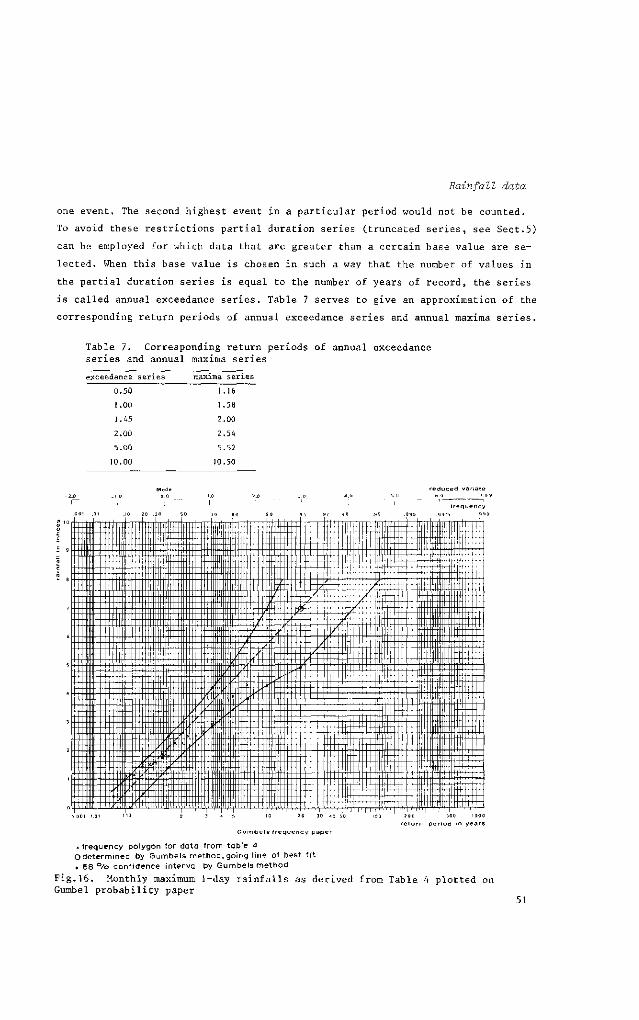
Rainfall data
one event. The second highest event in a particular period would not be counted.
To avoid these restrictions partial duration series (truncated series, see Sect.5)
can be employed for which data that are greater than a certain base value are se
lected. When this base value is chosen in such a way that the number of values in
the partial duration series is equal to the number of years of record, the series
is called annual exceedance series. Table 7 serves to give an approximation of the
corresponding return periods of annual exceedance series and annual maxima series.
Table 7. Corresponding return periods of annual exceedance series and annual maxima series
exceedance series maxima series
0.50
1.00
1.45
2.00
5.00
10.00
1 .16
1.58
2.00
2.54
5.52
10.50
.001 .01
"iftW " ™r :
-41|1 r — H T T T T T I —
MJj
1 'III
'
1 1 III
4JI!)- -1
L-LLIIILLL
.10 .20
jiff *• i 1
III 1
1 1 1
I I I 11 • : l !
1
I i
'M V \\\¥T \ WW \ m\v J
J-JUj-LHllL
.30 SO 7 0
"1 KttltntMrtrflt̂ i
i in ! 1 IL ' 1
l u l l
Il '
' ' 1 ' ' IUI 1
0
ijj'j i 1 1
it 1
' 1 ' / • i ' ¥
1 I KtlJll Irflf
•
/
Lr Ma 1 \X\ 1 1 i l l l l l l l •! I l ! • , 'L-
ivW"W\ '" ' i'i'
*"itn"H III 111 i l l ! Trar__
.'IJMIIIIIi l l l l
QÜ
t "
1 !
"55rt
/.[f .
•fl I vHUl-L E t i t i l IRIi !_ " tttti T IMiL 1 .
lütt* ± D & I effort ' t t t t l 1 ..JILÜ-I-Tttnt-
i ! iL ' li *••
M
-Llil|ll|l|lii
.9'>
.. . ~l
1 . , f l
ii .i j
.9 9
HrjJJiIT--i|| j n~l-
, i
: " 1 _
095 .„'W, j
-flftlp 1 h 1 i I ' r ' i
' ; , in, i ;, , ,
1 i:1'! ! " ' ill'lllllill'lt'tl 1' " ; ' y : \
/ ! • / • iitît*^ W : / I I ' ,
! > " . - y« .
.' -
' f\ • i
TT Ifll -[ |
lïïïïT "
: . ' i ' i
' ' i ' ,
1 I
t -
::::
^ T
T n~T
1
, i M !
i '
i
: 1
" i1' ; ' ' i ' I 'T'i , I ' , ' " ! 1 ' ' '
',i | : j
1 1
1 J
!
1 i i Mli
I'i : 1
NJIlilfflil^U^J per iod in years
Gumbels f requency paper
x frequency polygon for data f rom table 4 Odetermined by Gumbels method.going l ine of best f i t • 6 8 % conf idence interval by Gumbels method
Fig.16. Monthly maximum 1-day rainfalls as derived from Table 4 plotted on Gumbel probability paper
51
LITERATURE
FRAZER, D.A.S. 1958. Statistics. An introduction. John Wiley & Sons Inc.,
New York. Chapman & Hall Ltd., London. 398 pp.
GUMBEL, E.J. 1954. Statistical theory of extreme values and some practical ap
plications. Applied mathematics series 33. U.S.Dept.of Commerce. National
Bureau of Standards.
HERSHFIELD, D.M. 1961. Rainfall frequency atlas of the United States for dura
tions from 30 minutes to 24 hours and return periods from 1 to 100 years.
Technical Paper 40. U.S.Weather Bureau. 115 pp.
McKAY, G.A. 1964. Meteorological measurements for watershed research. Paper
presented at the 4th hydrology symposium on research watersheds. Guelph,
Ontario. 25 pp.
LINSLEY, R.K., KÖHLER, M,A. and PAULHUS, J.L.H. 1949. Applied hydrology. McGraw-
Hill Book Co.New York, Toronto, London. 689 pp.
PEARSON, E.S., and HARTLEY, H.D. 1956. Biometrika. Tables for statisticians.
Vol.1. Cambridge Univ.Press, 238 pp.
REICH, B.M. 1963. Short duration rainfall-intensity estimates and other design
aids for regions of sparse data. J.of Hydrology 3:3-28.
REMENIERAS, G. 1960. L'hydrologie de l'ingénieur. Collection du Laboratoire
national d'hydraulique. Eyrolles. 413 pp.
SNEDEC0R, G.W. 1957. Statistical methods. 5th ed. Iowa State College Press. 534 pp.
VEN TE CHOW (ed.) 1964. Handbook of applied hydrology. McGraw-Hill Book Co.
New York, San Francisco, Toronto, London. 1418 pp.
World Meteorological Organization Guide to Hydrometeorological practices. 1965.
W.M.0. No.168. T.P. 82.
52

SURVEYS AND INVESTIGATIONS
19. D E T E R M I N I N G E V A P O T R A N S P I R A T I O N
J. W. KlJNE Soil Physicist Department of Irrigation and Civil Engineering University of Agriculture, Wageningen
Lecturers in the Course on Land Drainage
P. E. RIJTEMA (1962-1970) Institute for Land and Water Management Research, Wageningen
J. W. KIJNE (1971-1973) University of Agriculture, Wageningen

PURPOSE AND SCOPE
A description of the process of évapotranspiration and some methods for its
calculation.
CONTENTS
19.1 INTRODUCTION 55
19.2 CALCULATION OF POTENTIAL EVAPOTRANSPIRATION BASED ON ENERGY CONSIDERATIONS 57
19.2.1 The energy balance at the soil surface 57
19.2.2 Evaporation from a free water surface 60
19.2.3 Potential évapotranspiration by crops 62
19.3 CALCULATION OF POTENTIAL EVAPOTRANSPIRATION BASED ON EMPIRICAL RELATIONSHIPS 64
19.4 MEASURING EVAPORATION AND EVAPOTRANSPIRATION 66
19.4.1 The water balance method 66
19.4.2 The use of evaporimeters
19.5 ADJUSTMENT OF EVAPOTRANSPIRATION FOR DRYING SOILS 71
19.6 AREAL VARIATION AND FREQUENCY OF OCCURRENCE OF EVAPOTRANSPIRATION 75
19.6.1 Extension from point to areal data
19.6.2 Frequency distribution of évapotranspiration 75
19.7 EXAMPLES OF CALCULATING POTENTIAL EVAPOTRANSPIRATION 77
19.7.1 Formula developed by Penman 78
19.7.2 Formula developed by Turc 83
19.7.3 Formula developed by Jensen and Haise 84
19.7.4 Formula developed by Blaney and Criddle 85
19.7.5 Formula developed by Thornthwaite 86
LITERATURE 96
ANNEX I. 99
Tables for calculating evaporation and évapotranspiration 99
54

Evapotranspiration
19.1 INTRODUCTION
The various processes through which water can be added or removed from the root-
zone of the soil are intimately related to one another because of the physical
requirement of conservation of matter. All additions of water by infiltration
from rainfall or irrigation or by capillary rise from the groundwater table, and
all losses of water by evaporation, transpiration, or deep percolation, need to
be accounted for in a water balance equation. Water balance studies have been
used in water resources investigations, streamflow studies including river fore
casting, irrigation operations, and in the derivation of maps of mean annual
rainfall, runoff, and évapotranspiration. (Evapotranspiration is the combined
effect of evaporation of water from moist soil and transpiration of water
by a growing crop.) In applying the water balance it is usually necessary to make
assumptions with respect to at least one of the variables. In many estimates of
évapotranspiration in irrigated areas, for example, the drainage term is assumed
to be negligible. It is important that these assumptions not be overlooked parti
cularly when methods are being transferred from one field of investigation to
another. Another important consideration is the accuracy with which each term
of the water balance can be evaluated. In this chapter we are concerned with the
évapotranspiration term in the water balance, the objective being to assess the
various methods of estimating or measuring évapotranspiration, in order that some
guidance can be given to those who design drainage systems. The soil, the plants,
and the atmosphere are all components of a physically unified and dynamic system
in which various flow processes occur interdependently like links in a chain
(COWAN, 1965). In this system flow takes place from higher to lower potential
energy, with the concept of water potential being equally valid and applicable
in the plant, soil, and atmosphere (Chap.5, Vol.1). Spontaneous flow is in the
direction of the negative potential gradient, i.e. from places with a relatively
high potential (a smaller negative quantity) to one where the water potential is
relatively low.
The quantity of water transpired daily is large relative to the change in water
content of the plant, so we can treat flow through the plant for short periods
as a steady state process. The potential differences in different parts of the
system are then proportional to the resistance to flow. The resistance is general
ly greater in the soil than in the plant, and greatest in the transition from the
leaves to the atmosphere, where water changes its state from liquid to vapour,
water then moving out of the leaves through the stomata by the process of diffu
sion. The total potential difference between the soil and the atmosphere can
amount to hundreds of bars, and in an arid climate can even exceed 1,000 bar.
55
The potential drop in the soil and plant is generally 'Jess than 10 bar so that
the major portion of the overall potential difference occurs between the leaves
and the atmosphere. Water transport from the leaves to the bulk air occurs as
diffusion of water vapour, which is proportional to the water vapour pressure
gradient. The relative humidity (i.e. the ratio of actual to saturation vapour
pressure), is, in turn, exponentially related to the water potential. A distinc
tion may be made between vapour transfer from a free water surface, from a bare
soil surface, and from transpiring vegetation, but all of these processes are
essentially similar, depending as they do on a supply of water and an energy
source. The nature of the surface, however, does exert some influence on the rate
of vapour loss because of various resistances and "shape" factors associated with
plants, soils, and water bodies. We will return to these differences later.
The following terms are relevant to the discussion in this chapter and need to
be defined:
- potential évapotranspiration, E , is the maximum amount of vapour which
could be transferred from an area to the atmosphere under the existing meteorolo
gical conditions
- actual évapotranspiration, E , is the actual amount of vapour transferred
to the atmosphere, which depends not only on existing meteorological conditions,
but also on the availability of water to meet the atmospheric demand and, in the
case of vegetation, its ability to extract moisture from the soil.
The water loss from a large area in which soil moisture is not a limiting factor
is at the potential rate, and any variations across the area would result from
differences in meteorological conditions, including advective effects. However,
once drying out commences, the picture increases in complexity: the decrease of
the actual évapotranspiration rate below the potential then depends on the avai
lable moisture in the soil, the rooting depth of the crop, and other plant charac
teristics. In extreme cases, the évapotranspiration demand of the atmosphere cannot
be met by the crop even though soil moisture is not limiting. To calculate the
expected amount of deep percolation in drainage design, one is usually interested
in the potential évapotranspiration rate expressed as mm/day, but calculated as
a monthly mean value. This is justified because in irrigated areas with frequent
applications of irrigation water soil moisture deficits exist only for a short
period of time, and on a monthly basis actual évapotranspiration rate, E , differs a
little from potential évapotranspiration rate, E . In humid climates the drainage
design should probably be based on the demand of the wettest period. During this
56

Evapotranspiration
period too E and E will differ little. The designer is then interested in p a
knowing to what extent évapotranspiration can be neglected with respect to rain
fall.
In Section 5 the reduction of E to arrive at E for drying soils is considered. P a
Actual data on évapotranspiration rates are often lacking and hence the design
of drainage systems must be based on estimates of E obtained from meteorological
data. Calculations of E based on energy balance considerations are discussed in
Section 2 and empirical relationships for the calculation of E in Section 3. p Methods of measuring evaporation (pan evaporation) and évapotranspiration (lysi-
meter) are discussed in Section 4. In Sections 5 and 6 some of the consequences
of the assumptions made earlier are considered. Finally, Section 7 gives methods
of calculating E from meteorological data.
19.2 CALCULATION OF POTENTIAL EVAPOTRANSPIRATION BASED ON ENERGY CONSIDERATIONS
19.2.1 THE ENERGY BALANCE AT THE SOIL SURFACE
Evaporation is one of the components of the water balance, but, through the energy
requirement for the phase change of liquid to vapour, evaporation is also one of
the terms of the energy balance at the soil surface. The physical requirement under
lying the energy balance equation is that all incoming energy be accounted for,
because the incoming radiation, the main source of energy, is either reflected,
stored as heat, or used for evaporation or some other energy requiring processes,
for example photosynthesis. Thus H , the net radiation is partitioned as follows o
H = L E + A + G + M (1)
o
where LE is the rate of energy utilization in évapotranspiration (cal/cm2 day),
being the product of the rate of water évapotranspiration and the latent heat of
vaporization, i.e.590 cal/g at about 25 C, A is the energy flux that goes into
heating the air, called sensible heat, G is the rate at which heat is stored in
the soil, the water, and the vegetation, and M represents miscellaneous energy
terms such as photosynthesis and plant respiration. The energy requirement of
these miscellaneous processes is usually smaller than the experimental error in
measuring the major components and is generally ignored. Only under extreme con
ditions of a large mass of active vegetation and a relatively low amount of net
radiation, as when the sky is overcast, can M account for as much as 5-10% of the
net radiation. The net radiation, H , is the overall difference between total in-o
coming and total outgoing radiation (both short-wave and long-wave components)
(Fig.1). Nearly all of the incoming radiation is of the wave-length range of 57
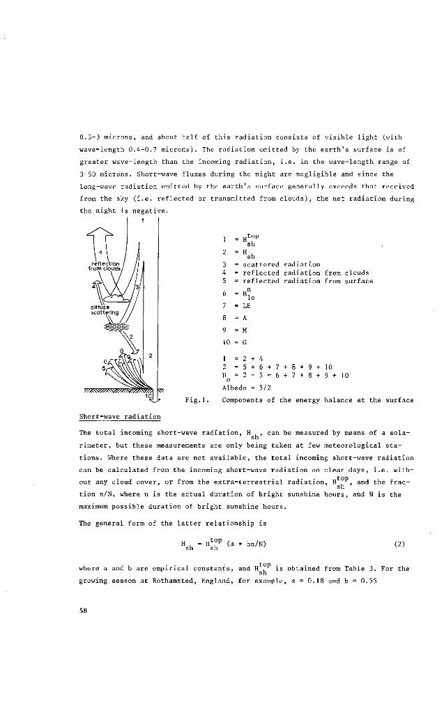
0.3-3 microns, and about half of this radiation consists of visible light (with
wave-length 0.4-0.7 microns). The radiation emitted by the earth's surface is of
greater wave-length than the incoming radiation, i.e. in the wave-length range of
3-50 microns. Short-wave fluxes during the night are negligible and since the
long-wave radiation emitted by the earth's surface generally exceeds that received
from the sky (i.e. reflected or transmitted from clouds), the net radiation during
the night is negative.
= H
= H
top "sh
sh = scattered radiation = reflected radiation from clouds = reflected radiation from surface
lo = LE
Fig.1.
8 = A
9 = M
10 = G
1 = 2 + 4 2 = 5 + 6 + 7 + 8 + 9 + 1 0 H = 2 - 5 = 6 + 7 + 8 + 9 + 10
o Albedo = 5/2
Components of the energy balance at the surface
Short-wave radiation
The total incoming short-wave radiation, H , can be measured by means of a sola-sh
rimeter, but these measurements are only being taken at few meteorological sta
tions. Where these data are not available, the total incoming short-wave radiation
can be calculated from the incoming short-wave radiation on clear days, i.e. without any cloud cover, or from the extra-terrestrial radiation, H top
sh ' and the frac
tion n/N, where n is the actual duration of bright sunshine hours, and N is the
maximum possible duration of bright sunshine hours.
The general form of the latter relationship is
' sh H'"1' (a + bn/N)
sh (2)
where a and b are empirical constants, and H , is obtained from Table 3. For the sh
growing season at Rothamsted, England, for example, a = 0.18 and b = 0.55
58

Evapotranspiration
KOOPMANS (1969) deyeloped two sets of values, one for temperate climates,
a = 0.20 and b = 0.53, and one for tropical climates, a = 0.28 and b = 0.48.
BAARS (1973) studied the regression equations for a number of locations in Jugosla
via, and found that generally the a-values were higher in summer (0.21-0.30) than
in winter (0.14-0.18); the b-values were somewhat lower in summer (0.42-0.47
versus 0.53). Better correlations were obtained when the data for spring and sum
mer were considered separately; then it was found that the a-values were higher
in spring than in summer (about 0.28 versus 0.24). For latitudes cj> < 60 , the
constant a can be approximated by a = 0.29 cos <ji. The calculations presented in
Section 7 are made with the values for a and b as suggested by KOOPMANS (1969).
Where the hours of sunshine are not recorded, the ratio n/N, the actual duration
of bright sunshine as fraction of the maximum possible duration for a cloudless
sky, cannot be calculated. Sometimes this fraction is approximated from cloud
cover estimates, but this leads to poor results, particularly in (subtropical)
areas where high clouds are present.
Long-wave radiation
The net outgoing long-wave radiation, H , can be calculated according to an em
pirical formula in which the following assumptions are made (PENMAN, 1948). The
emission coefficient for a water surface is taken as 1. The absolute temperature
of the radiating surface is assumed to be equal to that of the air. This assump
tion is valid in temperate climates but probably not in arid or semi-arid tropi
cal regions. The net long-wave radiation can then be calculated from
H"O = 118.]0-9 (273 + T 2 )* (0.47 - 0.077 /é7) (0.2 + 0.8n/N) (3)
where T2 is the temperature at a height of 2 m, and e2 is the actual vapour pres
sure (mm Hg) at 2 m. The constants 0.47, 0.077, 0.2 and 0.8 are purely empirical.
BOWEN ratio
BOWEN (1926) recognized that soil heat flux G constitutes only a small fraction of
H when soil moisture is not limiting. He thus partitioned H between LE and A o ° r o
terms. The rate of latent heat transfer by water vapour from the field to the
atmosphere is proportional to the product of the vapour pressure gradient by the
appropriate turbulent transfer coefficient for water vapour. The turbulent trans
fer coefficient is required because the transport of water vapour (and also of
sensible heat) from the field to the atmosphere is affected by the turbulent mo
vement of the air in the atmospheric boundary layer. Turbulent movement of air
59

does not start immediately in the air layer next to the evaporating surface. A
laminar boundary layer of less than 1 mm thick, through which transport occurs by
diffusion, exists next to the surface. Similarly, the sensible heat flux, A, is
proportional to the product of the temperature gradient and the turbulent transfer
coefficient for heat. BOWEN assumed that these transfer coefficients for heat and
water vapour are equal. The ratio of the sensible heat transfer to the latent
heat transport then becomes
T -T „ A 3T/8z s z ,, N ß - L E - = Y 1 W 3 Ï s y r=r ( 4 )
s z
where Y is the psychrometric constant (- 0.66 mbar/ C, or 0.485 mm Hg/ C), the
subscript s indicating a measurement at the surface, and the subscript z a measu
rement at height z.
The validity of the assumption that the transfer coefficients for sensible and
latent heat are equal has been the subject of considerable disagreement among
microclimatologists interested in évapotranspiration studies. However, it can be
shown that the error in LE is considerably smaller than any error in ß if the
assumption of identity between the two coefficients is in error.
The ratio ß is called the BOWEN ratio;ß is rather small when most of the energy
is used for evaporation. This is the situation when the field is moist and the
relative humidity gradient tends to be large and the temperature gradient small.
Conversely when the field is dry the BOWEN ratio can be large because of a small
gradient in vapour pressure and a rather large temperature gradient. Under extre
mely dry conditions LE may tend to zero and ß therefore to infinity.
19.2.2 EVAPORATION FROM A FREE WATER SURFACE
Application of the energy balance equation for the calculation of evaporation
requires measurements of the temperature of the evaporating surface. The tempera
ture of this surface is rather difficult to estimate in case of a free water sur
face and virtually impossible for vegetation. The vapour pressure at a free water
surface is the vapour pressure at saturation for the existing temperature at the
surface (e = e ). So when the surface temperature is known the corresponding
vapour pressure can be obtained from Table 1.
PENMAN (1948) was the first to propose a semi-empirical method for calculating
the evaporation from a water surface. His method is derived from a combination
of the DALTON equation and the energy balance approach. This obviates the need
60

Evapotranepvratxon
to measure surface temperature, but necessitates the introduction of approxima
tions, in particular with regard to the turbulent transfer coefficient. The gene
ral form of the DALTON equation for a free water surface is
LE = f(u) (e - e ) (5) s sat z
where f(u) is a function of the wind speed above the surface, e is the satu-s sat
ration vapour pressure at the temperature of the surface, and e is the vapour
pressure in the air at height z.
Since the temperature and vapour pressure at the surface are not easily measurable,
PENMAN introduced a "standard" value of LE, namely
LE = f(u) (e - e ) (6) x z sat z
where e signifies the saturation vapour pressure of the evaporating surface z sat
for the condition that the surface temperature equals the air temperature, T , z
which is easily determined. The wind function, f(u), according to PENMAN, equals
f(u) = (0.5 + 0.54 u2)0.35 (7)
where u2 is the wind velocity in m/sec at a height of 2 m. The vapour pressure,
e , should also be determined at that height (Sect.7). A major limitation of the
method, perhaps preventing its wide application, is the difficulty of evaluating
the wind function, f(u) = a + bu , since the empirical "constants" a and b, as
used in Eq.7, depend on the nature of the surface. For accurate work this
requires some years of comparison with some standard method of evaluating evapo
ration, such as lysimetry or energy balance measurements.
PENMAN combines the ratio LE /LE (Eqs.5 and 6) with the energy balance (Eq.1) and
the BOWEN ratio (Eq.4), to write LE and A in terms of H , G, and ß only, neglect-o
ing the miscellaneous energy term M in Eq.1 as follows
LE = (H - G)/(l + ß) (8) o
3 n d A = ß(Ho - G)/(l + ß) (9)
PENMAN assumed that G = 0, so Eq.8 could be simplified to
LE = H /(l + ß) (10)
o When Eq.6 is divided by Eq.5 we have, after rearranging terms
61
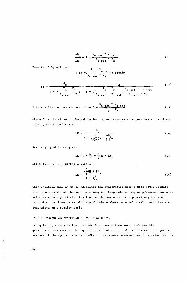
LE e _ - e x _ . _ s sat z sat . >
e - e LE s sat z
From Eq.10 by writing T - T s z
~s sat ~z as Y( z ) w e obtain
LE = (12)
T - T T - T e - e 1 + Y( L. 5—) ] + v( — ? ? )( s s a t z s a t )
e - e a - a " - Q
s sat z
o c Q f" 7 ^ £} t*
Within a limited temperature range A = ——3—= (13) s z
where A is the slope of the saturation vapour pressure - temperature curve. Equa
tion 12 can be written as
LE f — (.4)
1 +Y(})(> - ^ )
Rearranging of terms gives
LE (1 + f} "f V LEx 05)
which leads to the PENMAN equation
(-)H + LE LE - y ° • X (16)
This equation enables us to calculate the evaporation from a free water surface
from measurements of the net radiation, the temperature, vapour pressure, and wind
velocity at one particular level above the surface. The application, therefore,
is limited to those parts of the world where these meteorological quantities are
determined on a routine basis.
19.2.3 POTENTIAL EVAPOTRANSPIRATION BY CROPS
In Eq.16, H refers to the net radiation over a free water surface. The o
question arises whether the equation could also be used directly over a vegetated
surface if the appropriate net radiation term were measured, or if a value for the
62
Evapotranspiration
surface albedo were used. The albedo (i.e. reflectivity averaged over all rele
vant wave-lengths) for plant surfaces is generally much greater than the 0.03 to
0.06 for water surfaces, and varies with the degree of soil coverage, colour, and
hence with the maturity of the crop. Values for cotton range from 0.18 at the
beginning of the growing season to 0.27 for a crop of 115 cm (FRITSCHEN, 1967).
HOUNAM (1971) proposes an albedo value of 0.25 for a green crop to adjust other
radiation measurements or estimates if direct observations of crop H cannot be o
made. According to PENMAN (1956) the potential évapotranspiration rate is deter
mined by the prevailing weather conditions and, for a crop completely covering
the soil surface and never short of water, the rate is about the same, irrespec
tive of plant or soil type. A corollary of this thesis is that évapotranspiration
from a short green cover cannot exceed the evaporation from an open water surface
exposed to the same weather. Recent research into aerodynamic roughness factors
suggests some significant variations between crop types (SLATYER and McILROY,1961,
RIJTEMA, 1966, and ROSENBERG, HART, and BROWN, 1968), and it has been well esta
blished that crop évapotranspiration can exceed free water loss, particularly when
there is appreciable advective transfer of heat (TANNER and PELTON, 1960, PRUITT,
1963). Advection is the horizontal transfer of heat which can contribute energy
for évapotranspiration but is not considered in the energy balance equation where
only vertical fluxes are included. When advection occurs, sensible heat is trans
ferred from the air to the surface, and the BOWEN ratio will be negative during
that portion of the day. The influence of advection can extend to a distance of
about 1 km from the boundary between the heated non-evaporating arid surface and
the irrigated area.
In practice, potential évapotranspiration rate is often estimated from the mea
sured or calculated evaporation rate from a free water surface. A simple correla
tion between the two is then assumed to exist
E = f E (17) P
where E is the potential évapotranspiration rate.
The empirical conversion factor f depends on the reflectivity of the crop, on the
season, the climate, and the size of the cropped area. The table below (VAN DER
MOLEN, 1971) can be used to give a first approximation.
63

Values of the factor f, in E = f E P
Humid Arid or semi-arid
Crop temperate tropical large area small (less than lha)
winter summer winter summer summer
Wet, after rain or irrigation
Short grass 0.7 0.8 0.8 0.8 1.0 1.2
0.9
0.7
0.8
1.0
1.0
0 .8
1.0
1.0
K 0
0.8
4.0
1.2
1.0
0.8
1 .0
1.0
1.2
1.0
1.2
1.3
1 .5
Tall crop (wheat, sugar cane) 0.8 1.0 1.0 1.0 1.2 1.5
Rice 1.0 1.0 1.2 1.0 1.3 1.6
In this table differences in the multiplier f resulting from physiological varia
tion of the crop during the growing season are not considered.
19.3 CALCULATION OF POTENTIAL EVAPOTRANSPIRATION BASED ON EMPIRICAL RELATIONSHIPS
Many empirical methods have been developed for estimating evaporation from open
water surfaces or évapotranspiration from vegetation. Most of these have employed
commonly measured meteorological elements to find a correlation with evaporation
E, or évapotranspiration E , valid for a limited area. The use of these methods
is quite legitimate in such an area provided the period considered is not less
than about 20 days. It is hazardous, however, to use a method in another climate
than that for which it was derived, or to make estimates over short periods.
Methods based on temperature and radiation
In Section 7 two methods of calculating E , both based on temperature and some in
dex of radiation, are presented. These are methods developed by TURC (1954), and
JENSEN and HAISE (1963). Generally it is found that both formulas tend to under
estimate E during spring and overestimate it during summer. This results from
the fact that temperature is given too much weight and radiation not enough in
these formulas. If radiation data are available PENMAN's formula is therefore to
be preferred.
Methods based on temperature and daylength
Also presented in Section 7 are two formulas based merely on temperature and day-
length; these were developed by BLANEY and CRIDDLE (1950) and THORNTHWAITE (1948).
There is evidence that THORNTHWAITE's value can serve a useful purpose in determin
ing water requirements of crops over months and seasons, when mutually high corre
lations exist between mean temperature, net radiation, and évapotranspiration. For
64
Evapotranspiration
shorter periods the method fails principally because mean temperature is not a
suitable physical measure of the energy either available for or used in évapotrans
piration (HOUNAM, 197])- Empirical relationships based solely on temperature have
no practical value as short-term predictors, particularly in a climate of marked
seasonal contrast in atmospheric moisture content (STERN and FITZPATRICK, 1965).
The BLANEY-CRIDDLE procedure was originally developed for estimating seasonal
"consumptive use" (i.e. comparable to seasonal potential évapotranspiration because
of the underlying assumption that water supply to the growing crop never becomes
limiting). Other assumptions are that the length of the growing season is an
index of production and water use by continuously growing crops, and that ferti
lity and water storage of the soil do not differ significantly among areas to be
compared. When the method was used for the prediction of évapotranspiration for
consecutive short periods throughout the growing season, it became necessary to
modify the crop coefficient, C , in Eq.39 (SCS, 1967). One modification requires
the use of climatic coefficients that are directly related to the mean air tempe
rature for each of the short periods which constitute the growing season
C = 0.0312 T + 0.24 (18)
where T is the mean air temperature ( C). The other modification requires the use
of coefficients which reflect the influence of the crop growth stages on E . These
coefficients should ideally be obtained in lysimeter studies. The value of the
coefficients might to some extent be influenced by factors other than the plant
characteristics, and hence it is not expected that the coefficients can be used
universally. The method is widely used, particularly in the U.S.A., where through
the use of the appropriate crop coefficients an estimate of actual rather than
potential évapotranspiration can be obtained when the coefficients are based on
correlation with the existing irrigation practice. As was stated earlier, estimates
obtained by this method may be realistic only for localities and periods for which
the coefficients used were developed. Several comparisons between the various em
pirical approaches are available in literature. VAN BAVEL and WILSON (1952) tested
the THORNTHWAITE, PENMAN, and BLANEY-CRIDDLE methods against evaporation pans and
found fair agreement. HALKIAS et al. (1955) tested the same methods against atmo-
meter evaporation (Sect.4) and gravimetric soil moisture measurement techniques,
and suggested that only soil moisture samples give reliable data on extraction.
HANKS et al. (1971) found that potential évapotranspiration from a lysimeter ex
ceeded the evaporation from a wet surface (PENMAN) by 30% under the advective con
ditions of Northern Utah. A comparison of the methods presented in this chapter
is given in Section 7 for an experimental site in Venezuela.
65

19.4 MEASURING EVAPORATION AND EVAPOTRANSPIRATION
19.4.1 THE WATER BALANCE METHOD
The water balance, referred to in the introduction, may be thought of as a direct
means of measuring potential évapotranspiration, but unfortunately, the degree of
accuracy is rather low except in special cases, such as when lysimeters are used
(Sect.4.2).
The water balance may be written as
A W = P + I - R - D - E (19)
where AW is the change in water content in the rootzone during a certain period,
P is the precipitation in that period, I the irrigation, R the runoff, D the deep
drainage from the rootzone, and E is the combined loss due to transpiration and
evaporation. This is an integral form of the water balance, with the various items
totalled over a certain period of time. The water balance can also be expressed
in differential form, referring to the time rates of the processes, as the rate
at which water flows downwards through the lower boundary of the rootzone, and
the évapotranspiration rate. In differential form, the left hand side of the equa
tion becomes the rate of change of the water content in the rootzone. In irrigated
areas where runoff is negligible, the water balance for periods between irriga
tions (or rainfall) can be reduced to
-AW = D + E (20)
Soil moisture depletion
It is common practice in irrigation to schedule irrigations according to the
degree of deficiency of the total water content of the rootzone. Available water
is then considered to be that held between field capacity and permanent wilting
point. However, with most crops it is not wise to use all of the so-called
available water between irrigations because yields decrease when soil water is
allowed to approach the wilting point. Often irrigations are scheduled when 50%
of the available water has been used. The usual procedure for determining field
capacity is by periodic sampling of a wetted soil that is kept covered to prevent
evaporation. Plants, of course, transpire water between an irrigation and the time
that the field capacity condition is attained (e.g.6 days). This water must be
taken as part of the available water. Deep drainage also occurs and this water
cannot be regarded as being available. In studies of the water balance as given
in Eq.20, depletion of soil water, as calculated from water content changes
66
Evapotranspiration
found from periodic gravimetric sampling of the rootzone, has often been equated
with losses due to évapotranspiration. Very few attempts have been made to parti
tion depletion into évapotranspiration and downward or upward flow of water
through the boundary of the soil layer under study because of insufficient data.
VAN BAVEL et al. (1968), however, measured evaporation losses independently in a
study of the water balance of a soil layer. By combining these direct evaporation
measurements with known depletion figures, they obtained an estimate of the down
ward or upward flux of water. Their data demonstrated that when a bare soil is
irrigated the depletion rate is always more than the true evaporation rate. When
a sorghum crop with a normally developed root system was present, the initial
depletion rates were also greater than the measured evaporation rates, but later,
as water moved upward into the rootzone the depletion rate was an underestimate
of the evaporation rate.
BLACK et al. (1969) successfully predicted the evaporation from a bare sand sur
face for an entire season by using only rainfall and irrigation inputs. They
assumed that each time it rained or the soil was irrigated the evaporation rate
declined as the square root of time and that the cumulative evaporation increa
sed proportionally to the square root of time. The drainage rate was found to be
an exponential function of water storage. This procedure may not be generally
applicable since the relation between the square root of time and evaporation is
applicable for a soil which is wet to an infinite depth. For a finite depth of
wetting the rate drops off more rapidly; this occurs also with heavier textured
soils (KIJNE, 1972).
Soil moisture depletion in the presence of a plant cover
Evaporation from soil under plant canopies or between rows in the case of row
crops cannot be determined by covering the soil surface and subtracting measured
transpiration from the sum of evaporation and transpiration from the uncovered
plot. This is because much of the energy which strikes the covered soil surface
is reflected and results in increased transpiration. BLACK et al. (1970) measured
the energy that is available at the soil surface under snap beans and estimated
the ability of the soil to supply water from the surface water content. They then
assumed that the evaporation was limited by the energy or by the soil-water flux,
whichever was smaller. Independent calculations of transpiration were made based
on leaf-stomatal-resistance values and meteorological measurements within the
canopy. The two independently obtained values of evaporation were in good agree
ment. BRUN et al. (1972) reported a similar study on soybean and sorghum in which
67
again fair agreement was obtained between the two independent estimates of the éva
potranspiration, except under conditions of high evaporative demand when the sum
of calculated soil evaporation and transpiration was less than the lysimetric
estimates of évapotranspiration.
The drainage component of the water balance under ordinary field conditions can be
substantial, as was shown, for example, by the results of the study by BLACK et
al.(1970). In their study évapotranspiration accounted for 170 mm and drainage
for 180 mm of the seasonal precipitation of 320 mm and the 30 mm decrease in wa
ter storage. As changes in soil moisture content are generally only a small
fraction of the total moisture content, the accuracy of determining such changes
will be much lower than that of the soil moisture measurement itself. Even with
considerable effort and elaborate sampling procedures and equipment, good re
sults can rarely be expected over periods of less than a week (Chap.23,Vol.III).The
upward movement of water from the water table should also be considered in stu
dies of the water balance. Some, uncertainty still exists regarding the distance
which water can rise under the influence of hydraulic potential gradients, but
evidence by GARDNER (1965) suggests that rises from a 90 cm water table in sandy
loam are quite feasible. The rate of water extraction depends on the rooting
characteristics of the plant, the soil type, the water potential in the rootzone,
and the depth of the water table (Chap.5, Vol.1).
19.4.2 THE USE OF EVAPORIMETERS
Lysimeters
The most direct way of measuring the components of the water balance as given in
Eqs. 19 or 20 is by means of lysimeters. These are large containers of soil
set in natural surroundings with the least possible discontinuity between the crop
on the lysimeter and that in the surrounding field (Fig.2A). The method by which
the lysimeter is filled with soil can be very important. In some instances, for
example, with a more or less amorphous sandy profile, back fill is satisfactory,
particularly if care is taken to return unit layers of soil in the reverse order
of extraction. However, in heavier soils, particularly where there are disconti
nuities in depth, it is generally necessary to carry out a "monolith" fill ope
ration in which the undisturbed column of soil is fitted into the container
(HOUNAM, 1971). The effective use of lysimeters is limited to situations in which
the vegetation community under study can be simulated within the lysimeter itself,
without, for instance, any restriction of root development. Lysimeters which can
be weighed either by means of pressure transducers or because they float in water
68
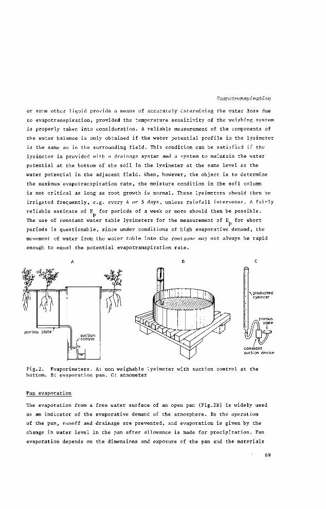
Evapotranspiration
or some other liquid provide a means of accurately determining the water loss due
to évapotranspiration, provided the temperature sensitivity of the weighing system
is properly taken into consideration. A reliable measurement of the components of
the water balance is only obtained if the water potential profile in the lysimeter
is the same as in the surrounding field. This condition can be satisfied if the
lysimeter is provided with a drainage system and a system to maintain the water
potential at the bottom of the soil in the lysimeter at the same level as the
water potential in the adjacent field. When, however, the object is to determine
the maximum évapotranspiration rate, the moisture condition in the soil column
is not critical as long as root growth is normal. These lysimeters should then be
irrigated frequently, e.g. every 4 or 5 days, unless rainfall intervenes. A fairly
reliable estimate of E for periods of a week or more should then be possible. P
The use of constant water table lysimeters for the measurement of E for short P
periods is questionable, since under conditions of high evaporative demand, the
movement of water from the water table into the rootzone may not always be rapid
enough to equal the potential évapotranspiration rate.
\graduated cylinder
constant suction device
Fig.2. Evaporimeters. A: non weighable lysimeter with suction control at the bottom. B: evaporation pan. C: atmometer
Pan evaporation
The evaporation from a free water surface of an open pan (Fig.2B) is widely used
as an indicator of the evaporative demand of the atmosphere. In the operation
of the pan, runoff and drainage are prevented, and evaporation is given by the
change in water level in the pan after allowance is made for precipitation. Pan
evaporation depends on the dimensions and exposure of the pan and the materials
69

from which it has been -constructed, as well as on all the meteorological condi
tions. Because of their ease of operation, pans are widely used throughout the
world, but their -limitations have not always been clearly understood. One factor
to be considered is standardization so that comparisons can be carried out between
results obtained at different locations. The Class A pan of the U.S. Weather
Bureau (4 feet in diameter and 10 inches high) is most widely used as the stan
dard pan. Due co absorption of radiation through the pan wall and transfer of
sensible heat between the air and the pan wall, the above-ground pan receives an
additional amount of energy, which results in higher evaporation rates than are
calculated from meteorological data. Pans are even more susceptible to advection
than are crops, as has been shown by PRUITT et al.(1972). Sunken pans might then
be expected to give more reliable results, but heat exchange between pan wall
and surrounding soil, and surface roughness effects limit the accuracy of results
obtained with them. Empirical correlations are required between the measured eva
poration rate from the pan and either E or E (under standard irrigation practice), p a
whatever may be required.
Atmometers
Reasonable correlations have been found between the évapotranspiration from irri
gated crops and the evaporation from atmometers. Atmometers are instruments with
a porous surface connected to a supply of water in such a way that evaporation
occurs from the porous surface (Fig.2C). A common atmometer is the PICHE atmometer,
made from a flat, horizontal disk of wetted blotting paper with both sides expo
sed to the air; another is the black and white spherical porous ceramic atmometer,
and a third is the BELLANI blackplate atmometer, which consists of a flat, black
porous ceramic plate as the upper face of a non-porous hemisphere. The net ra
diation flux density per unit evaporating surface of an exposed BELLANI is of
the same magnitude as a crop surface whereas that of the other two types is about
one-half because evaporation occurs at both the upper and lower surfaces. Evapo
ration from atmometers is also affected by heat conduction through the water from
the supply system. Furthermore, the transfer of sensible heat from the air is much
greater with atmometers than with vegetation because the atmometer is usually
placed at some height above the crop. Nevertheless, in many instances satisfactory
correlations have been found between the evaporation from the atmometer and po
tential évapotranspiration from crops. For example, KORVEN and WILCOX (1965)
based the irrigation schedule of an irrigated orchard on the evaporation from a
BELLANI atmometer. It has also been found that the difference in evaporation
between black and white spherical atmometers was highly correlated with potential
70
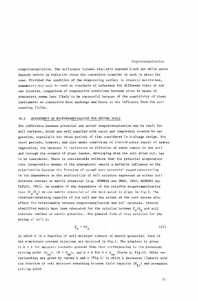
Evapotranspiration
évapotranspiration. The difference between similarly exposed black and white units
depends mainly on radiation since the convective transfer to each is about the
same. Provided the condition of the evaporating surface is properly maintained,
atmometers may well be used as standards of reference for different times at any
one location. Comparison of evaporative conditions between sites by means of
atmometers seems less likely to be successful because of the sensitivity of these
instruments to convective heat exchange and hence to the influence from the sur
rounding fields.
19.5 ADJUSTMENT OF EVAPOTRANSPIRATION FOR DRYING SOILS
The difference between potential and actual évapotranspiration may be small for
soil surfaces, which are well supplied with water and completely covered by ve
getation, especially for those periods of time considered in drainage design. For
short periods, however, and also under conditions of limited water supply or sparse
vegetation, the increase in resistance to diffusion of water vapour in the soil
and through the stomata of plant leaves, developing when the soil dries out, has
to be considered. There is considerable evidence that the potential evaporation
rate (evaporative demand of the atmosphere) exerts a definite influence on the
relationship between the fraction of actual over potential évapotranspiration
in its dependence on the availability of soil moisture expressed as either soil
moisture content or matric potential (e.g. DENMEAD and SHAW, 1962; BAHRANI and
TAYLOR, 1961). An example of the dependence of the relative évapotranspiration
rate (E /E ) on the matric potential of the soil water is given in Fig.3. The a p
moisture-retaining capacity of the soil and the extent of the root system also
affect the relationship between évapotranspiration and soil moisture. Several
simplified models have been advocated for the relation between E /E and soil a p
moisture content or matric potential. The general form of this relation for the
drying of soil is E = kE (21)
a p
in which k is a function of soil moisture content or matric potential. Some of
the k-moisture content relations are depicted in Fig.4. The simplest is given
by k = 1 for moisture contents greater than that corresponding to the permanent wilting point (W ). (W > W ), and k = 0 for W = W (Curve a, Fig.4). Other re-
wp wp wp lationships are given by curves b and c (Fig.4) in which k decreases linearly with
the fraction of soil moisture remaining between field capacity (W. ) and permanent f c
wilting point
71
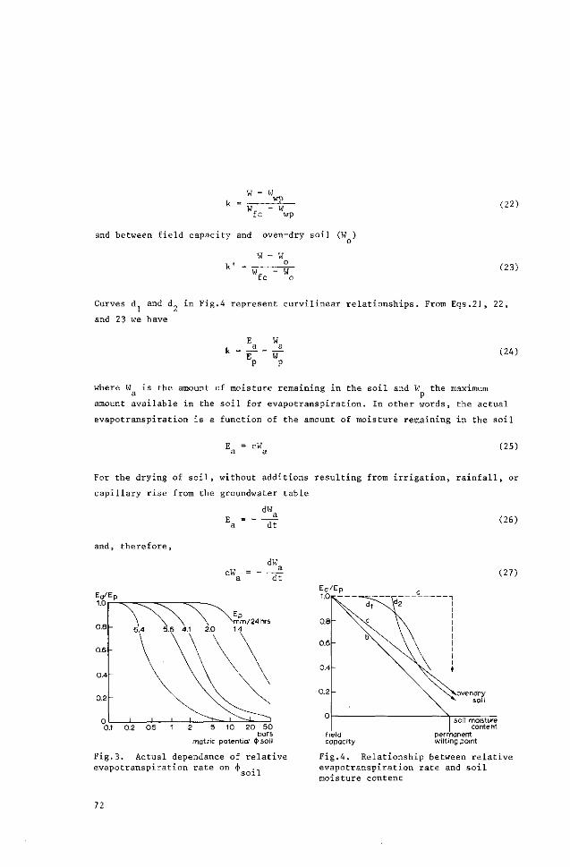
w - w k = wp
IJ =_W fc wp
and between field capacity and oven-dry soil (W ) o
W - W_ k' = W, - W
fc o
(22)
(23)
Curves d and d in Fig.4 represent curvilinear relationships. From Eqs.21, 22,
and 23 we have
(24)
where W is the amount of moisture remaining in the soil and W the maximum 3 . p
amount available in the soil for évapotranspiration. In other words, the actual évapotranspiration is a function of the amount of moisture remaining in the soil
E = cW (25)
For the drying of soil, without additions resulting from irrigation, rainfall, or
capillary rise from the groundwater table
dW (26) E = a
dt
and, therefore,
cW = a
dW a
"dt
0.1 0.2 0.5 10 20 50 bars
mairie potential $soi l
Fig.3. Actual dependance of relative évapotranspiration rate on é
s o i l
(27)
.ovendry soil
soil moisture content
permanent wilting point
Fig.4. Relationship between relative évapotranspiration rate and soil moisture content
72
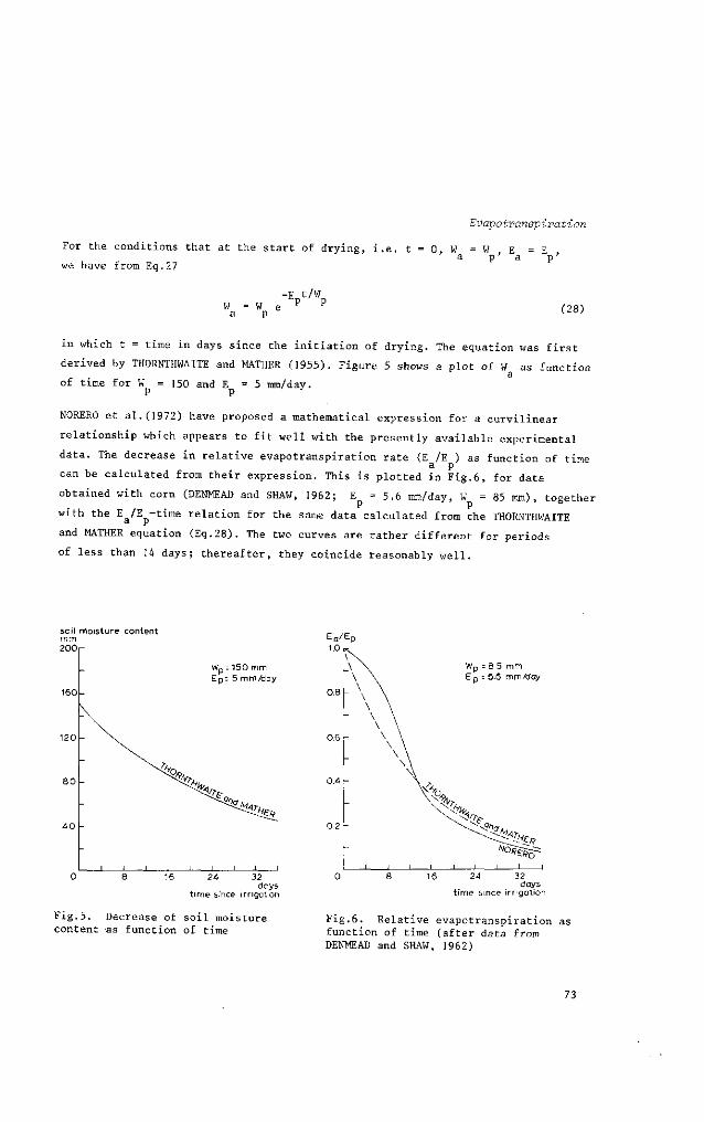
Evapotranspiration
For the conditions that at the start of drying, i.e. t = 0, W = W E a p' a
we have from Eq.27
E , P
-E„t/W„ W e P P
P (28)
in which t - time in days since the initiation of drying. The equation was first
derived by THORNTHWAITE and MATHER (1955). Figure 5 shows a plot of W as function a
of time for W = 1 5 0 and E = 5 mm/day. P P
NORERO et al.(1972) have proposed a mathematical expression for a curvilinear
relationship which appears to fit well with the presently available experimental
data. The decrease in relative évapotranspiration rate (E /E ) as function of time a p
can be calculated from their expression. This is plotted in Fig.6, for data
obtained with corn (DENMEAD and SHAW, 1962; E = 5.6 mm/day, W = 85 m m ) , together
with the Ea/E -time relation for the same data calculated from the THORNTHWAITE
and MATHER equation (Eq.28). The two curves are rather different for periods
of less than 14 days; thereafter, they coincide reasonably well.
soil moisture content mm 20O
160
120
8 0
4 0
" Wp=150mm E p : 5 mm/day
- \ .
- ̂ v i i i i
0 8 16 24 32 days
t ime since irrigation
Fig.5. Decrease of soil moisture content as function of time
W p = 8 5 m m Ep - 5.6 mm/day
32 days
t ime since irrigation
Fig.6. Relative évapotranspiration as function of time (after data from DENMEAD and SHAW, 1962)
73
From the work by NORERO et al.(1972), it may be concluded that for practical
purposes the assumption that E /E is unity when soil moisture storage is at a
maximum and that the ratio is zero when soil moisture storage is zero, is not un
reasonable, especially with a fairly high evaporative demand. When the demand is
low, assuming the ratio to be one, while the average ratio between irrigation ap
plications was only 0.8, would imply an inaccuracy of 20% in the estimate of sto
red water. This, in turn, could mean a considerable contribution to the ground
water tables over an entire season, if irrigation applications were based on the
estimated stored water.
Stage of growth
The stage of growth is also an important factor in the water requirement. Evapo
transpiration increases gradually from planting time to maturity and thereafter
it decreases gradually. The gradual increase can be explained on the basis of
percent cover, which is particularly important for row crops that start out from
a bare soil and approach 100% cover at maturity. Evaporation for most bare soils
decreases rapidly 1 or 2 days after an irrigation or a rain. Under the same condi
tions, transpiration may be maintained at the same level for several weeks. Conse
quently évapotranspiration would increase as the percent cover increases. An ad
ditional effect on plant cover is associated with the reflection coefficient for
incoming radiation, which is lower for bare soil (especially when wet) than for
a dense crop. Low reflection implies that more energy will be absorbed and hence
is available for evaporation and heating. Based on reflection alone évapotranspi
ration would be expected to decrease as the percent cover increases. However, this
effect is far less important than the first, so that a gradual increase in évapo
transpiration is associated with an increase of soil cover. The gradual decrease
with stage of growth at the end of the growing season probably results from plant
physiological factors since it has been found that the decrease of évapotranspira
tion from cotton occurs under conditions of continued irrigation as well as when
the water application is cut down after maturity, as is usual in irrigation prac
tice.
Evaporation from bare soil
Evaporation takes place at nearly the same rate from saturated soil, as may occur
in an irrigated area as from a free water surface, except in the leading edge
where advected heat may result in higher losses. Evaporation from unsaturated
soil decreases rapidly as the soil dries out near the surface. Vapour transfer
across a desiccated surface layer is slow and its rate is determined by tempera
ture gradients within the surface soil (Chap.5, Vol.1).
74
Evapotranspiration
19.6 AREAL VARIATION AND FREQUENCY OF OCCURRENCE OF EVAPOTRANSPIRATION
19.6.1 EXTENSION FROM POINT TO AREAL DATA
Most of the methods discussed in the previous sections give estimates of évapo
transpiration at a single observational site, or over a relatively small area in
the neighbourhood of the sensor. The errors in these estimates are of the order
of 15-30% depending on the length of the period for which the estimate is made.
It is necessary to consider the possibility of integrating a network of point va
lues to give a representative évapotranspiration for an area (HOUNAM, 1971). Me
thods developed for the integration of point values of rainfall (Chap.18, Vol.111)
may be used for this purpose. The most appropriate method for integrating point ob
servations will depend to a considerable extent on the nature of the variation in
évapotranspiration across the area. Spatial variations are due to variations in
radiation load on the vegetation, which may be the result of climatological
variation on a horizontal surface (i.e. temporal variation in cloud cover), and
variation due to slope, orientation, and elevation of the terrain. Additional va
riations result from differences in soil moisture availability and transpiration
characteristics of the vegetation. The reflectivity of a surface has so far been
treated as a constant but it actually varies with the wave-length and, to a cer
tain extent, the angle of incidence. The albedo of a wet surface varies between
0.02 (at zenith sun for the direct beam) and nearly 0.60 at an angle of 85
(LIST, 1966). Since the albedo is only 0.06 at 60°, a constant value of 0.03-0.05
can be used for most computations. Angle of incidence is far less important in the
case of plants, because of variations in leaf shape and orientation, but tempo
ral variations in the growing season and variations amongst crops are considerably
greater than the small change quoted for water. Using the PENMAN equation, HOUNAM
(1971) has calculated, that evaporation increases by about 25% if the surface
albedo is varied from 0.30 to 0.20 (for air temperature 17 C, relative humidity,
h=0.63, 50% cloud cover). In view of the significance of albedo in the evaporation
process, its possible spatial and temporal variations (e.g. due to crop rotations
or the presence of mulches) need to be considered. Apparently wide variation in
évapotranspiration is to be expected, particularly in areas of diversified terrain
and land-use, but many of the spatial and temporal variations have not been quan
tified so far.
19.6.2 FREQUENCY DISTRIBUTION OF EVAPOTRANSPIRATION
Because of lack of information, little attention has been given to frequency dis
tributions of peak water use. In only a few locations in the world have évapo
transpiration data been collected for a single crop over a period of time that is
75

mean évapotranspiration mm/day 10r
30 days
Fig.7. Frequency distribution curves for periods of daily évapotranspiration and means for various lengths of consecutive-day periods up to 30 days in length
adequate for a worthwhile frequency-distribution analysis. One such record comes
from work with the large weighable lysimeter at Davis, California, which has been
continuously cropped to a grass cover since June 1959 (PRUITT et al., 1972). The
actual peak évapotranspiration rates experienced at Davis are unique for the
climate involved, but the general characteristics of the frequency distribution
may be rather widely applicable in the Mediterranean-type hotter climates in many
parts of the world. Cumulative frequency distribution curves for periods of daily
évapotranspiration and means for various lengths of consecutive-day periods illus
trates why long-term mean weather data (e.g.monthly values) are not sufficient
for predicting évapotranspiration demand in the design of irrigation and drainage
projects and/or farm systems. For example, even considering deep-rooted crops
grown in fertile soils, where there might be 15-23 cm of readily available soil
moisture following irrigation, the data from Davis (Fig.7) show that a design
accounting for 7.4 mm per day is required if the system is to cover 95% of the
cases, rather than the 10-year monthly mean for the same period of peak demand
of around 6.6 mm per day. For shallower-rooted crops, or crops otherwise benefiting
from more frequent irrigation, the design value for Davis conditions would run
as high as 8.1 mm per day to handle 95% of the cases, if around 2.5 cm of stored
water could be considered readily available. At the 99% level, the design values
would be considerably higher, but of course, it will seldom be necessary to design
76
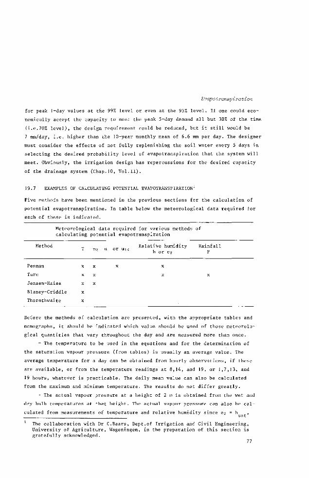
Evapotranspiration
for peak 1-day values at the 99% level or even at the 95% level. If one could eco
nomically accept the capacity to meet the peak 5-day demand all but 30% of the time
(i.e.70% level), the design requirement could be reduced, but it still would be
7 mm/day, i.e. higher than the 10-year monthly mean of 6.6 mm per day. The designer
must consider the effects of not fully replenishing the soil water every 5 days in
selecting the desired probability level of évapotranspiration that the system will
meet. Obviously, the irrigation design has repercussions for the desired capacity
of the drainage system (Chap.10, Vol.11).
19.7 EXAMPLES OF CALCULATING POTENTIAL EVAPOTRANSPIRATION1
Five methods have been mentioned in the previous sections for the calculation of
potential évapotranspiration. In table below the meteorological data required for
each of these is indicated.
Meteorological data required for various methods of calculating potential évapotranspiration
Method „, Relative humidity Rainfall T n2 u or uio , ' _
h or e2 P
x x
x x
Penman
Turc
Jensen-Haise
Blaney-Criddle
Thornthwaite
X
X
X
X
X
X
X
X
Before the methods of calculation are presented, with the appropriate tables and
nomographs, it should be indicated which value should be used of those meteorolo
gical quantities that vary throughout the day and are measured more than once.
- The temperature to be used in the equations and for the determination of
the saturation vapour pressure (from tables) is usually an average value. The
average temperature for a day can be obtained from hourly observations, if these
are available, or from the temperature readings at 8,14, and 19, or 1,7,13, and
19 hours, whatever is practicable. The daily mean value can also be calculated
from the maximum and minimum temperature. The results do not differ greatly.
- The actual vapour pressure at a height of 2 m is obtained from the wet and
dry bulb temperatures at that height. The actual vapour pressure can also be cal
culated from measurements of temperature and relative humidity since e2 = h ,
The collaboration with Dr C.Baars, Dept.of Irrigation and Civil Engineering, University of Agriculture, Wageningen, in the preparation of this section is gratefully acknowledged.
77
where h is the relative humidity. The information on the temperature and relative
humidity should then be available for the same time.
- The wind velocity is required for PENMAN's formula at a height of 2 m. Wind
velocities at other heights (u ) can be converted to a value for 2 m through the
following relationship
, 200 log -r-
----- (29) 100 z
log — - —
In the following sections E and E will now be calculated for July, for a tempera-o
te climate location at 42.5 N, according to the above-mentioned methods.
The meteorological data are as follows
Average air temperature at 2 m (T2) = 23.1 C
Average actual vapour pressure at 2 m (e2) = 12.9 mm Hg
Average wind velocity at 10 m (ujp) = 2.19 m/s
Average duration of bright sunshine (n) = 9.74 hrs/day
For July at 42.5 N we find from Table 9 (Annex I) that the maximum possible du
ration of bright sunshine hours equals 14.96 hours. The relative sunshine dura
tion n/N is then 9.74/14.96 = 0.65.
We find from Table 3 (Annex I) for the H value 961 cal cm 2day l . sh
19.7.1 FORMULA DEVELOPED BY PENMAN
The basic formula for the calculation of evaporation from a free water surface is
as follows
(-)H + LE LE = -^—2 j ^ (30)
1 + (-) Y where '
E = evaporation from a free water surface (mm day •" ; 1 day = 24 hours)
H = net radiation (cal cm 2 day 1)
E = isothermal evaporation (mm day ')
A = slope of the temperature-vapour pressure relationship at temperature T (mm Hg C a )
Y = psychrometric constant (=0.485 mm Hg C l)
latent heat of evaporation of 0.1 cm3 (=59 cal).

Evapotranspiration
The aerodynamic term, E , can be calculated according to PENMAN from the following
equation
E = 0.35(0.5 + 0.54 u2)(e - e2) (31) x sat
where
U2 = wind velocity at 2 m (m sec )
e = saturated vapour pressure (mm Hg) sat
e2 = actual vapour pressure at 2 m (mm Hg)
Calculation by means of tables
Equation 16 can be written in terms of the variables and constants discussed
in Section 2.1
T | 0.94(a+bn/N) H ^ - 1 18.10~9 (273+T2)" (0.47-0.077 /^) (0.2+0.8n/N) E = 59 sh_ +
A + 0.485
0.485 x 0.35(0.5 + 0.54 u2)(e - e2) + . 5££ (32)
A + 0.485
Tables have been prepared by WESSELING (1960) and others for different sections
of Eq.32. BAARS (1973) extended the tables of WESSELING, and these tables have
been used in this paper (see Annex I).
In Table 1, the value of A is given as a function of temperature.
In Table 2, values are given for (a+bn/N) with the constants which KOOPMANS
derived for temperate and tropical climates. The value of (a+bn/N) is given as
a function of n/N.
In Table 3, the extra-terrestrial radiation (H or Angot-value) is given as a
function of latitude, for periods of 10 days and for months of the year. Note
that the table gives values for the Northern and Southern Hemispheres.
In Table 4, values of 118.10 9(273+T2)'t are listed as a function of temperature.
In Table 5, values of 0.47-0.077 Jêî are listed as a function of the actual
vapour pressure at 2m, e2.
In Table 6, values of 0.2+0.8 n/N are listed as a function of n/N.
In Table 7, values are listed of 0.485 x 0.35(0.5+0.54u) for u2(m/sec) measured
at 2 m and for uio(m/sec) as measured at 10 m. It is, therefore, not necessary
79

to convert readings of wind velocity obtained at 10 m to a value for 2 m through
Eq.29 since the appropriate value of the product can be obtained directly
from the Table 7B.
In Table 8, the saturated vapour pressure is given as a function of temperature.
In Tab 1e 9, the maximum possible duration of bright sunshine hours, N, is given
as a function of latitude, for periods of 10 days and for months of the year. Note
that the months for the Southern Hemisphere are listed at the bottom of the table.
Equation 32 can now be rewritten with the values obtained from the tables re
presented by Roman numerals as
•î- (0.94 II x III - IV x V x VI) + VII(VIII - e2)
E = ̂ (33) I + 0.485
Example 1•
As an example, E will now be calculated from the above-mentioned station data.
Using the values in the tables we find the following
For T 2 = 23.1 °C
For n/N = 0.65
For 42.5 °N in July
For T2 = 23.1 °C
For e2 = 12.9 mm Hg
For n/N = 0 . 6 5
For uio = 2.19 m sec 1
For T2 = 23.1 °C
When these values are inserted in Eq.33 we get
1 - 2 8 (0.94 x 0.5445 x 961 - 907 x 0.194 x 0.72) + 0.233(21.19 - 12.90)
I
IIA
III
IV
V
VI
VIIB
VIII
= =
=
= =
=
=
=
1 .28
0.5445
961
907.0
0.194
0.72
0.233
21 .19
E = ^ 1.28 + 0.485
= 5.65 mm day 1 or 31 x 5.65 = 175 mm during July.
80

Evapotranspiration
We can also calculate E from the above-mentioned station data, following the
scheme set out below and using the tables from Annex I.
Calculation scheme Operation Example
1
2
3
4
5
6
7
8
9
10
11
12
13
14
T2
A
L = 59
A/L
n
N
n/N
0.20 + 0.53 n/N
H C °P sh
H , = (0.20 + 0.53 sh
(1-albedo) = 0.94
0.94 H ,_ sh
e sat
e.2 &2 - h e
16 118.10 (273 + T 2 r
17 0.47 - 0.077 / ë 7
18 0.2 + 0.8 n/N
19 H " =118. 1 0 ~ 9 ( 2 7 3 + T O
lo
H = o
21 (A/L) H o
22 y = 0.485
23 U2 or uio
24 Yf(u 2 ) = 0.485 x 0.35(0.5 + 0.54 u2)
25 YE = 0.485 x 0.35(0.5 + 0.54 u 2 ) (e
x 26 (A/L)H + YE
o x
27 A + y
(A/L) H + YE
28 E = mm/day A + Y
(0.2+0.8n/N)
^ - e2) sat
station
Table 1
(59)
2 : 3
station
Table 9
5 : 6
Table 2
Table 3
8 x 9
(0.94)
1 0 x 1 1
Table 8
station
13 - 14
Table 4
Table 5
Table 6
16 x 17
12 - 19
4 x 20
(0.485)
station
Table 7
15 x 24
21 + 25
2 + 22
data
data
data
x 18
data
23.1
1 .28
59
0.022
9.74
14.96
0.65
0.545
961
524
0.94
492
21 .19
12.9
8.29
907
0.194
0.72
127
365
8.04
0.485
2. 19
0.233
1 .86
9.90
1 .765
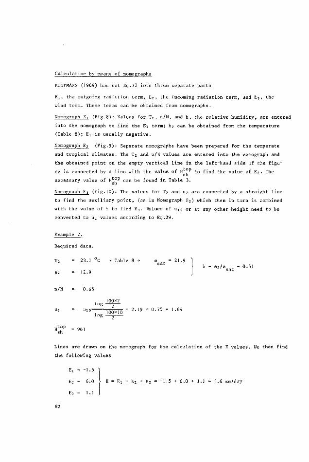
Calculation by means of nomographs
KOOPMANS (1969) has cut Eq.32 into three separate parts
Ei, the outgoing radiation term, E2, the incoming radiation term, and E3, the
wind term. These terms can be obtained from nomographs.
Nomograph Ei (Fig.8): Values for T2 , n/N, and h, the relative humidity, are entered
into the nomograph to find the Ei term; h2 can be obtained from the temperature
(Table 8); Ei is usually negative.
Nomograph E2 (Fig.9): Separate nomographs have been prepared for the temperate
and tropical climates. The T2 and n/N values are entered into the nomograph and
the obtained point on the empty vertical line in the left-hand side of the figu
re is connected by a line with the value of H , " to find the value of E2. The sh
necessary value of H ,P can be found in Table 3. sh
Nomograph E3 (Fig.10): The values for T2 and u2 are connected by a straight line
to find the auxiliary point, (as in Nomograph E2) which then in turn is combined
with the value of h to find E3. Values of ujo or at any other height need to be
converted to u2 values according to Eq.29.
Example 2.
Required data.
h = e2/e _ = 0.61 sat
T2
e 2
n/N
u2
sh
=
=
=
=
23.1 C
12.9
0.65
log u l 0
log
961
•+ Table 8 ->
100x2 2
100X10 ~ "*19
2
e _ = sat
x 0.75 =
21.9
1.64
Lines are drawn on the nomograph for the calculation of the E values. We then find
the following values
Ej = -1.5 "1
E2 = 6.0
E3 = 1.1
82
E = Ei + E2 + E3 = -1.5 + 6.0 + 1.1 = 5.6 mm/day

Evapotranspiration
Nomographs, of course, are less accurate than calculations by means of the tables.
However, when calculating machines are not available the nomographs facilitate the
calculations.
19.7.2 FORMULA DEVELOPED BY TURC
The original formula by TURC is as follows
E = , P + 8° — (mm/10 days) (34) P /, /P+45N2
where
E = potential évapotranspiration (mm/10 days) P
P = precipitation (mm/10 days)
Tc L = evaporative demand of the atmosphere, calculated according to
_ (T + 2) vT~ L • 1 6 — ^ ( 3 5 )
T = average air temperature ( C) at 2 m
H = incoming short-wave radiation (cal cm day 1) sh
Calculation by means of nomograms
Tc Nomograms have been developed for the solution of L and E (Figs.11 and 12).
Tc P Tc These nomograms are valid for L values in excess of 10. Smaller values of L cannot be expected in irrigated regions during the growing season. Figure 12 is not
Tc suitable for L values greater than 40 or for P > 80 mm/10 days. The lines on
the nomogram need to be extrapolated for those cases.
Example 3.
We will use the same location as before, with the added information that the ave
rage rainfall (P) = 1.8 mm/day, or 18 mm/10 days (note that P and E are given
per unit of 10 days). The incoming short-wave radiation can be derived from Table
2A and Table 3: for n/N = 0.65 we have H , = 0.5445 x 961 = 523 cal cm"2 day"1. - - Tc
According to Fig.I 1 for T = 23.1 °C and H = 523 cal cm 2 day 1 we obtain L =36. Tc
Then we read in Fig.12 for L =36 and P = 18 mm/10 days that E = 49 mm/10 days, or 4.9 mm day 1. Later, TURC simplified Eq.34 to
E = 0.40 -ï—r- (H +50) (mm/month) (36) p T+15 sh
83

in case the relative humidity, (h), of the air is greater than 50%, and
E = 0.40 - ^ (H +50) (1 + 52l!l) (mm/month) (37) p T+15 sh 70
in case h is less than 50%.
(Note that E in Eqs.36 and 37 is given in mm/month.)
For our situation we obtain, according to Eq.36
E = 0.40 2 32 ^ | 5 (523+50) = 139 mm for July, or 4.49 mm day"1.
In Sect.7.1 we calculated evaporation rates from open water according to PENMAN
of 5.65 mm day 1 by means of tables and 5.6 mm day 1 by using the nomographs. If
we reduce the evaporation from open water surfaces to the potential évapotranspi
ration by the empirical conversion factor 0.9, we find 0.9 x 5.65 = 5.08 mm day 1,
which is about equal to that calculated according to the original formula by TURC.
The newer formula apparently gives a smaller value.
19.7.3 FORMULA DEVELOPED BY JENSEN AND HAISE
The JENSEN-HAISE formula is as follows
H E = (0.025T + 0.08) -|2- (38)
where
E = potential évapotranspiration (mm/day)
H = incoming short-wave radiation (cal cm day )
T = air temperature ( C)
Example 4.
Required data
T = 23.1 °C
n/N = 0.65 -+ Tables 2A and 3 + H , = 523 cal cm~2day_1
sh
For our example we find that E = (0.025 x 23.1 + 0.08) ̂ ||- =5.83 mm.day"1.
This is considerably higher than the value for the potential évapotranspiration
that was obtained by converting the evaporation from an open water surface with
the factor 0.9.
84
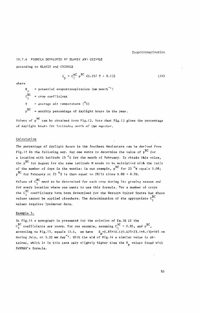
Evapo tvans'pvvati on
19.7.4 FORMULA DEVELOPED BY BLANEY AND CRIDDLE
According to BLANEY and CRIDDLE
E = C^C p B C (0.457 T + 8.13) (39)
where
E = potential évapotranspiration (mm month ')
C = crop coefficient
T = average air temperature ( C)
BC = monthly percentage of daylight hours in the year.
Values of p can be obtained from Fig.13. Note that Fig.13 gives the percentage
of daylight hours for latitudes north of the equator.
Calculation
The percentage of daylight hours in the Southern Hemisphere can be derived from
Fig.13 in the following way. Say one wants to determine the value of p for
a location with latitude 25 S for the month of February. To obtain this value,
the p for August for the same latitude N needs to be multiplied with the ratio RC o
of the number of days in the months: in our example, p for 25 N equals 9.08;
p C for February at 25 °S is then equal to 28/31 times 9.08 = 8.20.
Values of C need to be determined for each crop during its growing season and
for every location where one wants to use this formula. For a number of crops Dp
the C coefficients have been determined for the Western United States but these BC
values cannot be applied elsewhere. The determination of the appropriate C
values requires lysimeter data.
Example 5.
In Fig.14 a nomograph is presented for the solution of Eq.38 if the BC BC BC
C coefficients are known. For our example, assuming C^ = 0.85, and p ,
according to Fig.13, equals 10.4, we have E =0.85x10.4(0.475x23.1+8.13)=165 mm
during July, or 5.32 mm day '. With the aid of Fig.14 a similar value is ob
tained, which is in this case only slightly higher than the E values found with
PENMAN's formula.
85

19.7.5 FORMULA DEVELOPED BY THORNTHWAITE
According to THORNTHWAITE
E =1.6 (-^)a (40) P I
where
E = potential évapotranspiration (cm month J, in months of 30 days, with a day-length of 12 hours)
T = average air temperature ( C), calculated from daily means
I = annual heat index, i.e. the sum of the 12 monthly heat indices, i, where
i=(f) K 5 ] 4 (41)
a = 0.000000675 I3 - 0.000077 I2 + 0.01792 I + 0.49239 (42)
Calculation
The monthly heat index i can be obtained for a given temperature from Table 10.
Summation of the monthly heat indices gives the value of I. This value of I is
entered into Fig.15 on the I scale, and a straight line is drawn through I and
the point of convergence. The mean monthly temperature is then used as argument
for entering the nomograph. For each temperature the corresponding value of the
potential évapotranspiration is found on the x-axis. This is the potential évapo
transpiration for a 30-day month with day-lengths of 12 hours. The correction
factor to be used to convert this, depending on the latitude and month, can be
found in Table 11. Figure 15 cannot be used for temperatures in excess of 26.5 C.
The uncorrected value of the potential évapotranspiration for these higher tem
peratures can be found in Table 12.
Example 6.
We will calculate the potential évapotranspiration according to THORNTHWAITE's
method again for our example at 42.5 N during the month of July. We need to know
the mean air temperature also for the other months in order to calculate the
annual heat index I.

Evccpotvansvivation
January
February
March
April
May
June
July
August
September
October
November
December
Annual heat
T
- 4.8
1.7
5.5
12.0
16.6
21 .3
23.1
24.2
19.2
11.9
11 .2
1.6
index I
i
0
0.20
1.16
3.76
6.15
8.97
10.15
10.89
7.67
3.72
3.39
0.18
= 56.24
The straight line in Fig.15 is drawn through the value of 56.24 for I and the
point of convergence. For a temperature of 23.1 C we find then an uncorrected
value E = 1 1 5 mm. The correction factor found in Table II for 42.5 N in July P
equals 1.28. Hence the potential évapotranspiration E =1.28x115=147 mm or
4.74 mm day , which in this case is only slightly lower than the value calculated
with the aid of PENMAN's formula. Generally, THORNTHWAITE's formula gives values
for the évapotranspiration which are too low. This is also evident from Figs,
16 and 17, in which measured pan evaporation (pans with different exposures) is
compared with the évapotranspiration from a lysimeter (with short grass cover)
and with calculated evaporation values, for Cagua (Venezuela), 10 S, during 1963.
Lysimeter data were available for only one part of the year. During the hottest
months the potential évapotranspiration values based on TURC's and JENSEN and
HAISE's formulas fall considerably short of the open pan evaporation. Even PEN
MAN'S estimate is too low during that period. The formulas by BLANEY and CRIDDLE
and by THORNTHWAITE are clearly not suitable for the monsoon-type climate of
Northern Venezuela.
87

h
0.05 r
El mm/24 hrs
->2
0.1 Oh
0.15
0.2
0.5
0.6
0.7
0.8
0.9
1.0
F i g . 8 . Outgoing r a d i a t i o n , ET

TEMPERATE CLIMATES
n/N 1.0-,
T°C 50
10
0.6-
0.05
cal/cm 24hrs mm/24 hrs 1000-r-10
-9
8
/ " /
^ 6
5
-1.0
-0.9
-0.8
-0.7
-0.6
-0.5
0.3
9 0 0 -
8 0 0 -
100-
TROPICAL CLIMATES
T°C 5 0
-20
0.8-
0.7-
0.6-
Hsh tOP2
cal/cm. 24 hrs mm/24hrs 1000-j
10 Q y 9 00 -
- 8
* " 7 800 -
-1.0
-0.9
•0.8
•0.7
•0.6
-0.5
-0.3
5 0 0 -
400 -
Fig.9. Incoming radiation, E„, for open water

T °C 5 0 -
4 0 -
20H
U; m 10-
J 2 mm/24 hrs m/sec ,^10
4 -
/ /: / -/ /
/ 3-
V
4
/ h / / -2 / / _/
I / -1
- 0 0 .0.1 . 0 2
- 0 . 3
- 0 4
0 5
0 6
|_0.7
- 0 8
-0.05
- 0 9 5
. 0 .96
- 0 9 9
F ig . 10 . Windterm E,
90
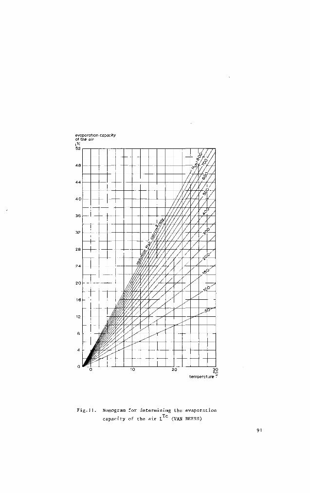
evaporation capacity of the air
52
48
4 0
16
—
- i -
!
-f
- SE
j §§ i*'s
—
-
—
fà W/,
 w 7/ y
- -
r^ / / (/
—
4 /// '//// ///, // V/ />
/ /
-----
*A
*¥/// .$/, /// '/// •'/,
'// //
/// {// 7/
-
#
f / / /
y\
// //
\ /
' / /
y
//, // //
' / ' /
/ /
/ //, 7/ / / v. > / /
^
^ / /
/ /
7/
/ / / / /? /A/ if ' /
/ /
'?/ ', /
r "i
/ V p"°
•fi
&
6
o /
^
°X
0 '
30 °C
temperature T
Fig.11. Nomogram for determining the evaporation
capacity of the air L C (VAN BEERS)
91

o w
•U n j • H
' 4J ><
: " § i o m
c-J
"-• m
• H
\n
a crt n 4-»
o al
> dl
•s o
Q. E , -
-
T
1
!
; i
1
^ , n n-
T
4-T
\-\- : ^
^
L-U-|_
" M
4-u
, ^ ^ 4
M T r̂
^
J??*
<$p C ^ T / / /
IP il
i
h _i
/ ! P"1 ;
"Fi i 4
! _
ii o o o o o o o c
A
Li:
mvx. 777/
.-L- . .-
—
—
i
- —
—
• —
c\j ro n P I
92
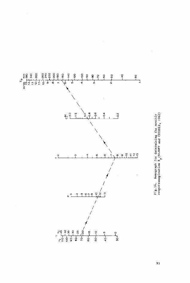
E O E?
K+!
O O O (O T c\j OJ C*J CM
, 1 , J , I ,
o ° ° O) -I—u
\
.-• o I IJ
o o _LJ I L IJ —
e o -S w 0) Q
\
in (D r^ . co O) -J , I . I \ I . I
O ^ oi n • T . T , T , * i
M o e
IJ i« 4-1 S3 0) <
/
J3 E O. O
i in (o f̂ oo ° w m
_ i i i i i y _ i T
•r4 f, fa <U
cjm o m o ir) o o ^- ^ m n c\i cy
_ I, 1,1,1 ,1 /, I Ü.O o o
93
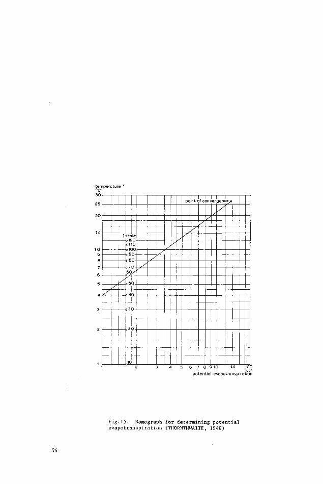
temperature T °C
25
20
10
9
B
7
6
4-
i iCO le
\-r
b110 = 100
6 0 / / I
> SO
I -
, . o 3 0 -
-
3 2 0 i
i y
— . : !__,__
_ i ,10
- - |
po nt c f c onv er
—|—
genceo
—'— —
!
• 4 -
.L 6 7 8 9 10 14 20
cm potential évapotranspiration
Fig.15. Nomograph for determining potential évapotranspiration (THORNTHWAITE, 1948)
94
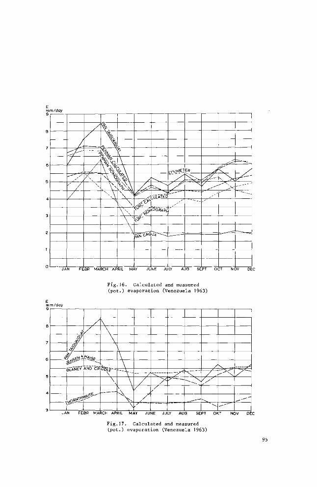
E mm/day 9
^-r
/
<
u. x
%,
fer m.
f"
\ \ \ \ vfev \ \
X \ N \
frW f\ ̂ v x
\ N
//.-" r y
: ^ . -HATED
^ ^
P & > C W
\0GR4PJ:
W"-̂
1,-VSlMEÎ
,''
E/f
^ N r ^ ,
~~~~̂
< V ^ ~ ^ „ - -
'
'"
^ ^ ^f>
t x . > < j
'
— ^ ^
.y^-—'
_----""
~~-~~
JAN FEBR MARCH APRIL MAY JUNE JULY AUG SEPT OCT NOV DEC
Fig.16. Calculated and measured (pot.) evaporation (Venezuela 1963)
E mm/day
<?
/
* • /
#
-f̂ vse
^i^Ü r i
\
• A
V \
/ ' / ' ~
----o
__„_.-\ • " ' "
. /
^^---~
JAN FEBR MARCH APRIL MAY JUNE JULY AUG SEPT OKT NOV DEC
Fig.17. Calculated and measured (pot.) evaporation (Venezuela 1963)
95
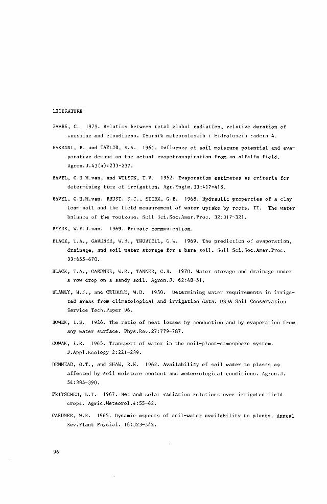
LITERATURE
BAARS, C. 1973. Relation between total global radiation, relative duration of
sunshine and cloudiness. Zbornik meteoroloskih i hidroloskih radora 4.
BAKRANI, B. and TAYLOR, S.A. 1961. Influence of soil moisture potential and eva
porative demand on the actual évapotranspiration from an alfalfa field.
Agron.J.43(4):233-237.
BAVEL, C.H.M.van, and WILSON, T.V. 1952. Evaporation estimates as criteria for
determining time of irrigation. Agr.Engin.33 :417—418.
BAVEL, C.H.M.van, BRUST, K.J., STIRK, G.B. 1968. Hydraulic properties of a clay
loam soil and the field measurement of water uptake by roots. II. The water
balance of the rootzone. Soil Sei.Soc.Amer.Proc. 32:317-321.
BEERS, W.F.J.van. 1969. Private communication.
BLACK, T.A., GARDNER, W.R., THURTELL, G.W. 1969. The prediction of evaporation,
drainage, and soil water storage for a bare soil. Soil Sei.Soc.Amer.Proc.
33:655-670.
BLACK, T.A., GARDNER, W.R., TANNER, C.B. 1970. Water storage and drainage under
a row crop on a sandy soil. Agron.J. 62:48-51.
BLANEY, H.F., and CRIDDLE, W.D. 1950. Determining water requirements in irriga
ted areas from climatological and irrigation data. USDA Soil Conservation
Service Tech.Paper 96.
BOWEN, I.S. 1926. The ratio of heat losses by conduction and by evaporation from
any water surface. Phys.Rev.27 :779-787.
COWAN, I.R. 1965. Transport of water in the soil-plant-atmosphere system.
J.Appl.Ecology 2:221-239.
DENMEAD, O.T., and SHAW, R.H. 1962. Availability of soil water to plants as
affected by soil moisture content and meteorological conditions. Agron.J.
54:385-390.
FRITSCHEN, L.T. 1967. Net and solar radiation relations over irrigated field
crops. Agric.Meteorol.4:55-62.
GARDNER, W.R. 1965. Dynamic aspects of soil-water availability to plants. Annual
Rev.Plant Physiol. 16:323-342.
96
Evapotranspiration
HANKS, R.J., JACOBS, H.S., SCHIMMELPFENNIG, N., NIMAH, M. 1971. Evapotranspira
tion estimates from oats by the energy budget, aerodynamic and combination
methods. Utah Resources Series 53, Utah Agric.Exp.Station.
HALKIAS, N.A., VIEHMEYER, F.J., HENDRIKSON, A.H. 1955. Determining water needs
for crops from climatic data. Hilgardia 24:207-233.
HOUNAM, C.E. 1971. Problems of evaporation assessment in the water balance.
World Meteorol.Org.Techn.Report 13 (WMO 285).
JENSEN, M.E., and RAISE, H.R. 1963. Estimating évapotranspiration from solar
radiation. Amer.Soc.Civ.Eng.Proc.89 (IR 4): 15-41.
KOOPMAN, R.W.R. 1969. De bepaling van de verdamping met behulp van nomogrammen.
Cultuurtechn.Tijdschrift 9(2):76-85.
KORVEN, H.C., and WILCOX, J.C. 1965. Correlation between evaporation from bellani
plates and évapotranspiration from orchards. Canad.J.Plant Sei.45 :132-138.
KIJNE, J.W. 1972. Evaporation from bare soil. In: Physical aspects of soil water
and salts in ecosystems. Springer Verl., pp.221-226.
LIST, R.J. 1966. Smithsonian meteorological tables. 6 ed. Washington,
Smithsonian Inst.
MOLEN, W.H.van der. 1971. Syllabus Agrohydrology. University of Agriculture.
Wageningen.
NORERO, A.L., KELLER, J., ASHCROFT, G.L. 1972. Effect of irrigation frequency
on the average évapotranspiration from various crop-climate-soil systems.
Transact.ASCE 15(4): 662-666.
PENMAN, H.L. 1948. Natural evaporation from open water, bare soil, and grass.
Roy.Soc.London, Proc.Ser.A. 193:120-146.
PENMAN, H.L. 1956. Evaporation: an introductory survey. Neth.J.Agr.Sci.4:9-29 .
Discussions 87-97, 151-153.
PRUITT, W.O. 1963. Application of several energy balance and aerodynamic evapo
ration equations under a wide range of stability. Final rep.to USA EPG.
California, Davis, p. 107-124.
PRUITT, W.O., OETTINGEN, S.von, MORGAN, D.L. 1972. Central California évapotrans
piration frequences. J.Irr.Drain Div.ASCE 98:177-184.
ROSENBERG, N.J., HART, H.E., BROWN, K.W. 1968. Evapotranspiration. Rev.of research.
Univ.of Nebraska, Nebraska Water Resources Res.Inst.Publ.M.P.20.
97

RIJTEMA, P.E. 1966. Transpiration and production of crops in relation to climate
and irrigation. Inst.Land and Water Management Res. Wageningen. Tech.Bull.44.
SLATYER, R.O., and McILROY, I.C. 1961. Practical microclimatology. Unesco. Publ.
by CSIRO, Australia.
STERN, W.R., and FITZPATRICK, E.A. 1965. Calculated and observed evaporation in
a dry monsoonal environment. J.Hydrol.3 :297—311.
SOIL CONSERVATION SERVICE. 1967. Technical Release No.21. Irrigation Water Re
quirements. USDA, Washington.
TANNER, C.B., and PELTON, W.L. 1960. Potential évapotranspiration estimates by
the approximate energy balance method of Penman. J.Geophys.Res.65:3391-3413.
THORNTHWAITE, C.W. 1948. An approach toward a rational classification of climate.
Geogr.Rev.38:55-94.
THORNTHWAITE, C.W., and MATHER, J.K. 1955. The water balance. Publications in
Climatology VIII (1). 104 pp.
TURC, L. 1954. Le bilan d'eau des sols. Relations entre les précipitations,
l'évaporation et l'écoulement. Ann.Agron.6:5—131.
WESSELING, J. 1960. Hulpmiddelen bij de berekening van de verdamping uit een
vrij wateroppervlak. Verslagen en Mededelingen van de Comm. Hydrologisch
Onderzoek TNO, Nr.4:31-45, The Hague.
98

Evapotranspiration
A N N E X I. TABLES FOR CALCULATING EVAPORATION AND EVAPOTRANSPIRATION
Table 1. Values of A (change of saturated vapour pressure with temperature, mm Hg C ), based on data from Handbook of Chemistry and Physics, 49th Ed., pages D-109.
T2
-10 - 9
- 8
- 7
- 6
- 5
- 4
- 3
- 2
- 1
- 0
0 1 2 3 4 5 6 7 8 9
10
11 12 13 14 15 16 17 18 19 20
21 22 23 24 25 26 27 28 29 30
31 32 33 34 35 36 37 38 39 40
T2
,0
0,17
0,18
0,20
0,21
0,22
0,24
0,26
0,27
0,29
0,31
0,33
0,34
0,36
0,38
0,40
0,43
0,45
0,48
0,52
0,55
0,58
0,62
0,66
0,69
0,73
0,78
0,82
0,87
0,92
0,97
I ,03
1,08
1,14
1,21
1 ,28
1,34
1,41
1,49
1,57
1,65
1,74
1,82
1 ,92
2,02
2,12
2,22
2,34
2,45
2,57
2,69
2,82
2,94
,0
,1
0,17
0,18
0,19
0,21
0,22
0,24
0,26
0,27
0,29
0,31
0,33
0,34
0,36
0,38
0,41
0,43
0,46
0,49
0,52
0,55
0,59
0,62
0,66
0,70
0,74
0,78
0,83
0,88
0,93
0,98
1 ,04
1,09
1 ,15
1 ,22
1 ,28
1 ,35
1 ,42
1 ,50
1 ,58
1 ,66
1 ,75
1 ,83
1 ,93
2,03
2,13
2,23
2,35
2,46
2,58
2,70
2,83
2,95
, 1
,2
0,17
0,18
0,19
0,21
0,22
0,24
0,25
0,27
0,29
0,31
0,33
0,34
0,36
0,38
0,41
0,43
0,46
0,49
0,52
0,56
0,59
0,63
0,66
0,70
0,74
0,79
0,83
0,88
0,93
0,98
1,04
1 ,09
1 ,16
1 ,22
1,29
1 ,36
1 ,42
1 ,51
1,59
1 ,67
1 ,76
1 ,84
1 ,94
2,04
2,14
2,24
2,36
2,47
2,59
2,71
2,84
2,97
,2
,3
0,17
0,18
0,19
0,21
0,22
0,24
0,25
0,27
0,29
0,31
0,33
0,34
0,36
0,39
0,41
0,44
0,46
0,49
0,53
0,56
0,59
0,63
0,67
0,71
0,75
0,79
0,84
0,89
0,94
0,99
1 ,05
1,10
1,16
1,23
1,30
1 ,36
1,43
1 ,52
1 ,60
1 ,68
1 ,77
1 ,85
1 ,95
2,05
2,15
2,26
2,37
2,48
2,60
2,72
2,85
2,98
,3
,4
0,17
0,18
0,19
0,20
0,22
0,23
0,25
0,27
0,28
0,30
0,32
0,34
0,36
0,39
0,41
0,44
0,46
0,50
0,53
0,56
0,60
0,64
0,67
0,71
0,75
0,79
0,84
0,89
0,94
0,99
1 ,05
1 ,10
1,17
1 ,24
1 ,30
1,37
1 ,44
1 ,53
1,60
1,69
1 ,78
1,86
1 ,96
2,06
2,16
2,27
2,38
2,49
2,61
2,73
2,86
2,99
,4
,5
0,16
0,18
0,19
0,20
0,22
0,23
0,25
0,27
0,28
0,30
0,32
0,35
0,37
0,39
0,42
0,44
0,47
0,50
0,53
0,57
0,60
0,64
0,68
0,71
0,76
0,80
0,85
0,90
0,95
1 ,00
1 ,06
1,11
1 ,18
1 ,24
1,31
1,38
1 ,45
1,53
1 ,61
1 ,70
1,79
1,87
1 ,97
2,07
2,17
2,28
2,39
2,51
2,63
2,75
2,88
3,00
,5
,6
0,16
0,18
0,19
0,20
0,22
0,23
0,25
0,26
0,28
0,30
0,32
0,35
0,37
0,39
0,42
0,44
0,47
0,50
0,54
0,57
0,60
0,64
0,68
0,72
0,76
0,80
0,85
0,90
0,95
1 ,00
1 ,06
1,12
1 ,18
1 ,25
1 ,32
1 ,38
1 ,46
1,54
1,62
1 ,71 1 ,79
1,88
1 ,98
2,08
2,18
2,29
2,40
2,52
2,64
2,76
2,89
3,01
,6
,7
0,16
0,17
0,19
0,20
0,21
0,23
0,25
0,26
0,28
0,30
0,32
0,35
0,37
0,40
0,42
0,45
0,47
0,51
0,54
0,57
0,61
0,65
0,68
0,72
0,77
0,81
0,86
0,91
0,96
1 ,01
1,07
1 ,12
1,19
1,26
1 ,32
1 ,39
1,47
1,55
1,63
1 ,72
1 ,80
1 ,89
1 ,99
2,09
2,19
2,30
2,41
2,53
2,65
2,78
2,90
3,02
,7
,8
0,16
0,17
0,19
0,20
0,21
0,23
0,24
0,26
0,28
0,30
0,32
0,35
0,37
0,40
0,42
0,45
0,48
0,51
0,54
0,58
0,61
0,65
0,69
0,73
0,77
0,81
0,86
0,91
0,96
1 ,02
1 ,07
1,13
1,20
1,26
1 ,33
1 ,40
1 ,48
1 ,56
1,63
1 ,72
1 ,81
1 ,90
2,00
2,10
2,20
2,31
2,42
2,54
2,66
2,79
2,91
3,04
,8
,9
0,16
0,17
0,18
0,20
0,21
0,23
0,24
0,26
0,28
0,29
0,31
0,35
0,38
0,40
0,43
0,45
0,48
0,51
0,55
0,58
0,62
0,65
0,69
0,73
0,77
0,82
0,87
0,92
0,97
1 ,02
1 ,08
1 ,14
1 ,20
1 ,27
1,34
1 ,40
1 ,49
1 ,57
1 ,64
1 ,73
1 ,81
1 ,91
2,01
2,11
2,21
2,33
2,44
2,55
2,68
2,81
2,93
3,05
,9
T2
-10 - 9
- 8
- 7
- 6
- 5
- 4
- 3
- 2
- 1
- 0
0 1 2 3 4 5 6 7 8 9
10
11 12 13 14 15 16 17 18 19 20
21 22 23 24 25 26 27 28 29 30
31 32 33 34 35 36 37 38 39 40
T2
Read for the comma a decimal -point
99
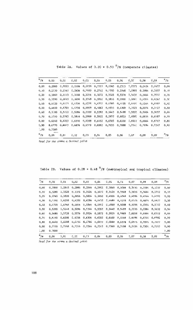
Table 2A. Values of 0.20 + 0.53 /N (temperate c l imates)
" /N
0 ,00
0 ,10
0 ,20
0 ,30
0 ,40
0 ,50
0 ,60
0 ,70
0 ,80
0 ,90
1,00
n /N
0 , 00
0 ,2000
0 ,2530
0 ,3060
0 ,3590
0 ,4120
0 ,4650
0 ,5180
0 ,5710
0 ,6240
0 ,6770
0 ,7300
0 ,00
0 ,01
0 ,2053
0 ,2583
0 , 31 J3
0 ,3643
0 ,4173
0 ,4703
0 ,5233
0 ,5763
0 ,6293
0 ,6823
0 ,01
0 ,02
0 ,2106
0 ,2636
0 ,3166
0 ,3696
0 ,4226
0 ,4756
0 ,5286
0 ,5816
0 ,6346
0 ,6876
0 ,02
0 , 03
0 ,2159
0 ,2689
0 ,3219
0 ,3749
0 ,4279
0 ,4809
0 ,5339
0 ,5869
0 ,6399
0 ,6929
0 , 03
0 ,04
0 ,2212
0 ,2742
0 ,3272
0 ,3802
0 ,4332
0 ,4862
0 ,5392
0 ,5922
0 ,6452
0 ,6982
0 ,04
0 , 05
0 ,2265
0 ,2795
0 ,3325
0 ,3855
0 ,4385
0 ,4915
0 ,5445
0 ,5975
0 ,6505
0 ,7035
0 ,05
0 ,06
0 ,2313
0 ,2848
0 ,3378
0 ,3908
0 ,4438
0 ,4968
0 ,5498
0 ,6023
0 ,6558
0 ,7088
0 ,06
0 ,07
0 ,2371
0 ,2901
0 ,3431
0 ,3961
0 ,4491
0 ,5021
0 ,5551
0 ,6081
0 ,6611
0 ,7141
0 ,07
0 , 08
0 ,2424
0 ,2954
0 ,3484
0 ,4014
0 ,4544
0 ,5074
0 ,5604
0 ,6134
0 ,6664
0,7194
0 ,08
0 ,09
0 ,2477
0 ,3007
0 ,3537
0 ,4067
0 ,4597
0 ,5127
0 ,5657
0 ,6187
0 ,6717
0 ,7247
0 ,09
n /N
0 ,00
0 ,10
0 ,20
0 ,30
0 ,40
0 ,50
0 ,60
0 ,70
0 ,80
0 ,90
n /N
Read for the comma a decimal point
Table 2B. Values of 0.28 + 0.48 /N (subtropical and tropical c l imates)
"/N 0,00 0,01 0,02 0,03 0,04 0,05 0,06 0,07 0,08 0,09 "/N
0,00 0,2800 0,2848 0,2896 0,2944 0,2992 0,3040 0,3088 0,3136 0,3184 0,3232 0,00
0,10 0,3280 0,3328 0,3376 0,3424 0,3472 0,3520 0,3568 0,3616 0,3664 0,3712 0,10
0,20 0,3760 0,3808 0,3856 0,3904 0,3952 0,4000 0,4048 0,4096 0,4144 0,4192 0,20
0,30 0,4240 0,4288 0,4336 0,4384 0,4432 0,4480 0,4528 0,4576 0,4624 0,4672 0,30
0,40 0,4720 0,4768 0,4816 0,4864 0,4912 0,4960 0,5008 0,5056 0,5104 0,5152 0,40
0,50 0,5200 0,5248 0,5296 0,5344 0,5392 0,5440 0,5488 0,5536 0,5584 0,5632 0,50
0,60 0,5680 0,5728 0,5776 0,5824 0,5872 0,5920 0,5968 0,6016 0,6064 0,6112 0,60
0,70 0,6160 0,6208 0,6256 0,6304 0,6352 0,6400 0,6448 0,6496 0,6544 0,6592 0,70
0,80 0,6640 0,6688 0,6736 0,6784 0,6832 0,6880 0,6928 0,6976 0,7024 0,7072 0,80
0,90 0,7120 0,7168 0,7216 0,7264 0,7312 0,7360 0,7408 0,7456 0,7504 0,7552 0,90
1,00 0.7600 1,00
"/N 0,00 0,01 0,02 0,03 0,05 0,08 0,09 '7N
Read for the comma a decimal point
100

Table 4. Values of 118.10 9 (273 + V Evapotranspiration
-10 564
- 9 573
- 8 581
590
599
608
618
627
636
645
655
0
1
2
3
4
5
6
7
8
9
10
I I
12
13
14
15
16
17
18
19
20
21
22
23
24
25
26
27
28
29
30
31
32
33
34
35
36
37
38
39
40
655
665
674
684
694
704
715
725
735
746
756
767
778
789
800
811
823
834
846
857
869
881
893
905
918
930
943
955
994
1007
1021
1034
1048
1061
1075
1089
1103
1118
1132
572,3
581 ,0
589,9
598,8
607,8
617,9
626,3
635,5
645,0
654,4
656,4 666,1 675 ,9 685 ,7 695,7 705 ,8 716 ,0 726 ,3 736 ,8 747 ,3 758 ,0
768 ,7 779 ,6 790 ,6 801 ,6 812 ,9 824 ,3 835 ,8 847 ,4 859,1 870 ,9
882,8
894,9
907,0
919,4
931 ,9
944,4
957,1
969,9
982,8
995,9
1009.1 1010,5
1022.4 1023,8
1035,9 1037,3
1049.5 1050,9
1063,3 1064,7
1077.2 1078,6
1091.2 1092,6
1105.3 1106,7
1119.6 1121,0 1134,0 1135,5
571 ,5 580 ,2 589 ,0 597 ,9 606 ,9 616 ,9 625 ,5 634 ,5 644 ,0 653 ,2
657 ,3 667,1 676 ,9 686 ,7 696,7 706 ,8 717,1 727 ,4 737 ,8 748 ,3 759 ,0
7 69 , 8 780 ,7 791 ,7 802 ,8 814 ,1 825 ,4 836 ,9 848 ,5 860 ,3 872,1
884,0
896,1
908,3
920,6
933,1
945,6
958,4
971 ,2
984,1
997,2
570 ,6 579 ,3 588,1 597 ,0 606 ,0 615 ,8 624 ,6 633 ,6 643,1 652 ,5
658 ,3 668,1 677 ,9 687,7 697,7 707 ,8 718,1 728,4 738,9 749 ,4 760,1
770 ,9 781 ,8 792 ,8 803 ,9 815 ,2 826 ,6 838,1 849 ,7 861 ,4 873 ,3
885 ,2 897 ,3 909 ,5 921 ,9 934 ,4 946 ,9 959 ,6 972 ,5 985 ,4 998 ,5
1011.8 1013,1 1025.1 1026,5
1038,6 1040,0
1052.2 1053,6
1066,0 1067,4
1080,0 1081,3
1094.0 1095,4
1108.1 1109,5
1122,4 1123,9
1136.9 1138,4
569 ,8 578,4 587 ,2 590,1 605 ,1 614 ,8 623 ,8 632 ,7 642,1 651 ,6
659 ,3 669 ,0 678 ,8 688 ,7 698 ,7 708 ,8 719,1 729 ,5 739 ,4 750 ,5 761 ,2
772 ,0 782 ,9 793 ,9 805 ,0 816 ,3 827,7 839 ,2 850 ,9 862 ,6 874 ,5
886 ,4 898 ,5 910 ,7 923,1 935 ,6 948 ,2 960 ,9 973 ,8 986 ,7 999 ,8
568,9 577,6 586,4 595,3 604,2 613,8 623,0 631 ,8 641,2 650,6
660,2 670,0 679,8 689,7 699,7 709,9 720,2 730,5 741 ,0 751 ,6 762,3
773,0 784,0 795,0 806,2 817,5 828,9 840,4 852,1 863,8 875,7
887,8 899,8 912,0 924,4 936,9 949,5 962,2 975,1 988,1
1001,2
1014,4 1027,8 1041,3 1054,9 1068,7 1082,7 1096,8 1110,9 1125,3 1139,8
568,0 576,7 585,5 594,4 603,3 612,8 622,2 630,8 640,2 649,7
661 ,2 671 ,0 680,8 690,7 700,0 710,9 721,2 731 ,5 742,0 752,7 763,3
774,1 785,1 796,1 807,3 818,6 830,0 841 ,8 853,2 865,0 876,8
888,9 901 ,0 913,2 925,6 938,1 950,7 963,5 976,3 989,4
1002,5
1015,8 1029,2 1042,7 1056,4 1070,2 1084,1 1098,2 1112,4 1126,8 1141,3
567,2 575,8 584,6 593,5 602,4 61 1 ,8
621,4
629,9
639,3
648,8
662,2
672,0
681,8
691,7
701,8
711,9
722,2
732,6
743,1
753,8
764,4
775,2
786,2
797,2
808,4
819,7
831 ,2
842,7
854,4
866,2
878,0
890,1
902,2
914,4
926,9
939,4
952,0
964,8
977,6
990,7
1003,8
1016,1
1030,5
1044,0
1057,7
1071,6
1085,5
1099,6
1113,8
1128,2
1142,7
566,
574,
583,
592,
601, 610, 620, 629, 638, 647,
663, 673, 682, 692, 702, 712, 723, 733, 744, 754, 765,
776, 787, 798, 809, 820, 832, 843, 855, 867, 879,
891 ,
903,
915,
9 2 8 ,
9 4 0 ,
953,
966,
978,
992,
1005,
1018,
1031,
1045,
1059,
1073,
1086,
1 101 ,
1 115,
1129,
1144,
565 ,5 574 ,1 582 ,8 591 ,7 600 ,6 609 ,7 619 ,7 628 ,0 637 ,4 646 ,9
664 ,1 674 ,0 683 ,7 693 ,7 703 ,8 714 ,0 724 ,3 734,7 745 ,2 755 ,9 766 ,5
777 ,4 788 ,4 799 ,4 810 ,7 822 ,0 833 ,5 845 ,0 856 ,7 868 ,5 880 ,4
892,5
904,5
916,9
929,4
941 ,9
954,5
967,3
980,2
993,3
1006,5
5 1019,8
9 1033,2
4 1046,7
1 1060,4
0 1074,4
9 1088,4
0 1102,4
3 1116,7
7 1131,1
2 1145,6
-10
- 9
- 8
- 7
- 6
- 5
- 4
- 3
- 2
- 1
- 0
0
1
2
3
4
5
6
7
8
11
12
13
14
15
16
17
18
19
20
21
22
23
24
25
26
27
28
29
30
31
32
33
34
35
36
37
38
39
40
,0 ,1
Head for the comma a decimal point
101

Table 3. Incoming extra-terrestrial radiation, H , (cal cm 2 day 1) (Smithsonian Meteorological Tables, table 132)
N
80
70
60
50
40
30
20
10
0
10
20
30
40
50
60
70
80
8
month 10 d.
10 d. month
10 d. month
10 d. month
10 d. month
10 d. month
10 d. month
10 d. month
10 d. month
10 d. month
10 d. month
10 d. month
10 d. month
10 d. month
10 d. month
10 d. month
10 d. month
10 d. month
10 d. month
I
60
190
335
480
615
745
850
935
995
1035
1050
1040
1020
1040
1090
I
Jan.
II
80 85
215 215
360 365
500 505
635 640
760 760
860 860
935 935
990 990
1025 1020
1025 1020
1010 1005
980 975
985 975
1030 1015
II
Jan.
Ill
110
250
395
535
665
775
870
935
980
1000
990
965
920
900
925
III
I
30
150
300
440
575
695
800
880
935
965
970
950
905
840
780
785
I
Febr.
II
75 75
210 210
355 355
495 495
620 620
730 730
820 820
890 890
930 930
945 945
930 930
895 895
835 835
755 755
660 665
620 620
II
Febr.
Ill
125
270
415
550
665
765
840
895
925
920
890
835
765
665
550
460
III
I
45
185
335
475
600
710
795
860
900
910
890
850
780
690
580
455
325
I
March
II
105 115
260 265
405 405
540 540
655 655
750 750
825 825
875 875
895 895
895 895
860 860
805 800
720 720
620 620
495 495
360 360
210 220
II
March
III
195
345
480
605
710
795
850
890
890
870
825
750
660
545
415
270
125
I [I
I
310
445
565
680
765
835
875
895
880
845
785
700
590
465
330
190
50
I
A p r i l
II
455 460
550 550
655 650
745 745
820 815
875 870
895 895
900 895
870 870
820 820
745 745
645 645
530 530
395 400
255 260
115 120
15
II
April
III
615
650
735
805
865
905
910
895
860
790
700
595
470
335
195
55
III
I
750
740
805
860
905
930
920
895
840
760
665
550
420
285
145
25
T
May
11
865 860
840 830
865 865
910 905
940 935
950 950
930 930
890 890
825 825
735 7 30
630 635
510 515
380 380
240 245
110 110
10
I 1
May
III
960
915
920
945
965
965
935
885
810
715
605
480
340
205
80
III
I
1020
975
955
970
980
970
935
880
800
700
580
455
315
180
60
I
June
II
1050 1045
1010 1000
980 970
985 980
990 985
975 975
935 935
875 875
795 795
690 695
570 575
440 445
305 305
170 170
50 55
II
June
III
1060
1010
975
985
990
975
935
870
790
690
570
440
300
165
50
III
102

EvavotvariBVvvation
(Table 3 cont.)
ii i n i
1033 980 900 795 670 505 355 230 135 65 10 970 655 240 25
980 935 860 770 670 570 470 375 290 2)0 135 80 35 925 670 380 140 10
960 930 885 825 750 670 590 510 430 350 280 215 160 110 85 60 50 50 925 750 510 280 120 55
975 955 920 875 820 760 695 625 555 490 420 360 305 255 220 195 180 180 950 820 625 425 260 185
980 970 940 910 870 825 775 720 665 605 550 495 445 400 360 335 320 320 965 870 720 550 400 325
970 960 950 930 905 875 840 800 755 710 670 620 580 540 510 485 470 470 960 905 800 665 545 475
935 930 925 920 910 895 875 855 830 795 760 725 695 665 640 625 610 610 930 910 855 760 665 615
875 880 880 885 890 890 890 880 870 855 840 820 800 775 760 745 735 735 880 890 880 840 780 740
795 800 815 830 844 855 870 880 885 890 890 885 870 860 855 850 845 845 805 840 880 890 860 845
695 710 725 745 770 800 830 850 875 895 910 920 925 930 930 930 930 930 710 770 850 910 930 930
575 590 615 645 680 720 760 800 840 870 905 930 950 970 980 990 1000 1000 595 680 800 900 965 995
450 470 490 530 570 620 675 725 775 825 870 915 955 985 1010 1030 1040 1040 470 575 725 870 985 1035
305 325 360 400 450 505 565 625 690 750 810 870 925 970 1010 1040 1055 1060 330 450 625 810 970 1050
175 190 220 260 310 370 440 510 585 660 740 810 885 945 995 1030 1050 1055 195 315 510 735 940 1045
55 70 95 130 175 230 300 375 460 550 640 730 820 895 960 1010 1040 1045 75 180 380 640 890 1030
60 230 325 420 525 635 745 860 950 1020 1070 1080 240 525 850 1055
5 1 130
I TT
July
III I II III
August
100
] IT
Sept.
Ill I
420
TI
Oct.
TIT T
880
TI
Nov.
Ill I
] 105
T 1
Dec .
Ill
103

Table 5 . Va lue s o f 0 . 4 7 - 0 . 077 / ê T
e2
0
1
2
3
4
5
6
7
8
9
10
11
!2
13
14
15
16
17
18
19
20
21
22
23
24
25
26
27
28
29
30
e2
>o 0,470
0 ,393
0,361
0 ,337
0 ,316
0 ,298
0,281
0 ,266
0,252
0 ,239
0 ,227
0 ,214
0 ,204
0 ,192
0 ,182
0 ,172
0 ,162
0 ,153
0 ,144
0 ,134
0, 126
0 ,117
0 ,109
0 ,100
0 ,093
0 ,085
0 ,077
0 ,070
0 ,063
0 ,055
0 ,048
,0
,1
0 ,445
0 ,389
0 ,358
0 ,334
0 ,314
0 ,296
0 ,280
0 ,265
0,251
0 ,237
0 ,225
0 ,214
0 ,202
0,191
0 ,180
0 ,170
0,161
0 ,151
0 ,143
0 ,134
0 ,125
0 ,117
0 ,108
0 ,100
0 ,092
0 ,084
0 ,077
0 ,069
0 ,062
0 ,055
0 ,047
,1
,2
0 ,435
0 ,385
0 ,356
0 ,332
0 ,312
0 ,294
0 ,278
0 ,264
0 ,250
0 ,237
0,224
0 ,212
0,201
0 ,190
0 ,180
0 ,170
0 ,160
0 ,150
0,141
0 ,133
0 ,124
0 ,116
0 ,107
0 ,099
0,091
0 ,083
0 ,076
0 ,068
0,061
0 ,054
0 ,047
,2
, 3
0 ,428
0 ,382
0 ,353
0 ,330
0,311
0 ,293
0 ,277
0 ,262
0 ,248
0 ,235
0 ,223
0,211
0 ,200
0 ,189
0 ,179
0 ,169
0 ,159
0 ,150
0 ,140
0 ,132
0 ,123
0 ,114
0 ,107
0 ,098
0 ,090
0 ,083
0 ,075
0 ,068
0 ,060
0 ,053
0 ,047
,3
,4
0 ,421
0 ,379
0,351
0 ,328
0 ,308
0,291
0 ,275
0,261
0 ,247
0 ,234
0,221
0 ,210
0 ,199
0 ,188
0 ,178
0 ,168
0 ,158
0 ,149
0 ,140
0,131
0 ,122
0 ,113
0 ,106
0 ,097
0 ,090
0 ,082
0 ,074
0 ,067
0 ,060
0 ,053
0 ,046
,4
,5
0 ,415
0 ,376
0 ,348
0 ,326
0 ,307
0 ,289
0 ,274
0 ,259
0 ,245
0 ,233
0 ,221
0 ,209
0 ,197
0 ,187
0 ,177
0 ,167
0 ,157
0 ,148
0 ,139
0 ,130
0,121
0 ,113
0 ,105
0 ,097
0 ,089
0 ,081
0 ,073
0 ,067
0 ,059
0 ,052
0 ,045
,5
,6
0 ,411
0 ,373
0 ,346
0 ,324
0 ,305
0 ,288
0 ,272
0 ,257
0 ,244
0 ,231
0 ,219
0 ,207
0 ,197
0 ,186
0 ,176
0 ,166
0 ,157
0 ,147
0 ,138
0 ,129
0 ,120
0 ,1 12
0 ,104
0 ,096
0 ,088
0 ,080
0 ,073
0 ,066
0 ,058
0,051
0 ,044
,6
,7
0 ,405
0 ,370
0 ,344
0 ,322
0 ,303
0 ,286
0 ,271
0 ,257
0 ,243
0,231
0 ,218
0 ,207
0 ,196
0 ,185
0 ,175
0 ,165
0 ,155
0 ,146
0 ,137
0 ,128
0 ,120
0,111
0 ,103
0 ,095
0 ,087
0 ,080
0 ,072
0 ,065
0 ,057
0 ,050
0 ,043
,7
,8
0 ,401
0 ,367
0 ,341
0 ,320
0,301
0 ,284
0 ,269
0 ,255
0,241
0 ,229
0 ,217
0 ,205
0 ,194
0 ,184
0 ,174
0 ,164
0 ,154
0 ,145
0 ,136
0 ,127
0 ,119
0 ,1 10
0 ,103
0 ,094
0 ,087
0 ,079
0,071
0 ,064
0 ,057
0 ,050
0 ,043
, 8
,9
0 ,397
0 ,364
0 ,339
0 ,318
0 ,300
0 ,283
0 ,267
0 ,254
0,241
0 ,227
0 ,216
0 ,204
0 ,194
0 ,183
0 ,173
0 ,163
0 ,154
0 ,144
0 ,135
0 ,127
0 ,118
0 ,110
0,101
0 ,093
0 ,086
0 ,078
0 ,070
0 ,063
0 ,056
0 ,049
0 ,042
,9
ez
0
1
2
3
4
5
6
7
8
9
10
1 1
12
13
14
15
16
17
18
19
20
21
22
23
24
25
26
27
28
29
30
e2
Read for the comma a decimal point
104

Table 6. Values of 0.2 + 0.8 /N
n/N
0,00
0,10
0,20
0,30
0,40
0,50
0,60
0,70
0,80
0,90
1,00
"/N
,00
0,20
0,28
0,36
3,44
0,52
0,60
0,68
0,76
0,84
0,92
1 ,00
,00
,01
0,21
0,29
0,37
0,45
0,53
0,61
0,69
0,77
0,85
0,93
,01
,02
0,22
0,30
0,38
0,46
0,54
0,62
0,70
0,78
0,86
0,94
,02
,03
0,22
0,30
0,38
0,46
0,54
0,62
0,70
0,78
0,86
0,94
,03
,04
0,23
0,31
0,39
0,47
0,55
0,63
0,71
0,79
0,87
0,95
,04
,05
0,24
0,32
0,40
0,48
0,56
0,64
0,72
0,80
0,88
0,96
,05
,06
0,25
0,33
0,41
0,49
0,57
0,65
0,73
0,81
0,89
0,97
,06
,07
0,26
0,34
0,42
0,50
0,58
0,66
0,74
0,82
0,90
0,98
,07
0
0
0
0
0
0
0
0
0
0
08
26
34
42
50
58
66
74
82
90
98
,08
,09
0,27
0,35
0,43
0,51
0,59
0,67
0,75
0,83
0,91
0,99
,09
"/N
0,00
0,10
0,20
0,30
0,40
0,50
0,60
0,70
0,80
0,90
1 ,00
"/N
Evapotranspiration
Read for the comma a
Table 7A. Va lue s
decimal point
of 0 . 4 8 5 x 0 . 35 ( 0 . 5 + 0 . 5 4 u) f o r u (m s e c ' ) measured a t 2
"200 m/sec ,0 ,1 ,3 ,4 ,6 ,7 ,9
u200 m/sec
0
1
2
3
4
5
6
7
8
9
0
0,085
0,177
0,268
0,360
0,452
0,543
0,635
0,727
0,818
0,910
1 ,002
0,094
0,186
0,277
0,369
0,461
0,553
0,644
0,736
0,827
0,919
0,103
0,195
0,286
0,379
0,470
0,562
0,654
0,745
0,836
0,928
0,1 12
0,204
0,295
0,388
0,479
0,571
0,663
0,754
0,845
0,937
0
0
0
0
0
0
0
0
0
0
,121 0 ,131 0 ,140 0 ,149 0 ,158 0 ,167 0
,213 0 ,222 0 ,231 0 ,240 0 ,249 0 ,259 1
,305 0 ,314 0 ,323 0 ,332 0 ,341 0,351 2
,397 0 ,406 0 ,415 0 ,424 0 ,433 0 ,442 3
,488 0 ,497 0 ,507 0 ,516 0 ,525 0 ,534 4
,580 0 ,589 0 ,598 0 ,607 0 ,616 0 ,626 5
,672 0 ,681 0 ,690 0 ,699 0 ,708 0 ,718 6
,763 0 ,772 0 ,781 0 ,790 0 ,799 0 ,809 7
,855 0 ,864 0 ,873 0 ,882 0 ,891 0 ,900 8
,946 0 ,956 0 ,965 0 ,974 0 , 983 0 ,992 9
"200 m/sec
Read for the comma a
Table 7B. Va lue s
decimal point
of 0 . 4 8 5 x 0 . 3 5 ( 0 . 5 + 0 . 5 4 u) f o r u (m s e c " 1 ) measured a t 10
"1000
n/sec ,0 ,1 ,6 ,8
u 1 0 0 0
m/sec
0,085 0 ,092 0 ,098 0 ,105
0 ,153 0 ,160 0 ,166 0 ,173
0 ,221 0 ,227 0 ,234 0 ,241
0 ,288 0 ,295 0 ,302 0 ,309
0 ,356 0 ,363 0 ,370 0 ,377
0 ,424 0 ,431 0 ,438 0 ,444
0 ,492 0 ,499 0 ,505 0 ,512
0 ,560 0 ,567 0 ,573 0 , 580
0 ,628 0 ,634 0 ,641 0 ,648 0
0 ,695 0 ,702 0 ,709 0 ,716
0 ,763
0
0
0
0
0
0
0
0
0
0
1 12
180
248
316
383
451
519
587
655
722
0
0
0
0
0
0
0
0
0
0
,119 0 ,126 0 ,132 0 ,139 0 ,146 0
,187 0 ,193 0 ,200 0 ,207 0 ,214 1
,255 0 ,261 0 ,268 0 ,275 0 ,282 2
,322 0 ,329 0 ,336 0 ,343 0 ,349 3
,390 0 ,397 0 ,404 0 ,411 0 ,417 4
,458 0 ,465 0 ,472 0 ,478 0 ,485 5
,526 0 ,533 0 ,539 0 ,546 0 ,553 6
,594 0 , 600 0 ,607 0 ,614 0 ,621 7
,661 0 ,668 0 ,675 0 ,682 0 ,689 8
,729 0 ,736 0 ,743 0 ,750 0 ,756 9
1000 Ti/sec
1000 m/sec 105
Read for the comma a decimal point
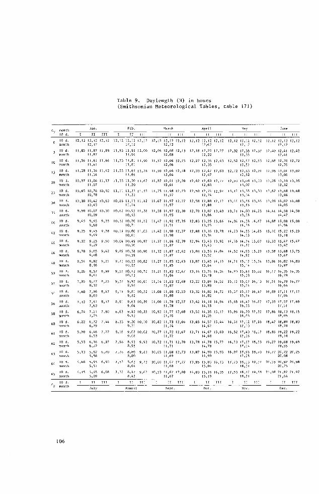
Table 9. Daylength (N) in hours (Smithsonian Meteorological Tables, table 171)
0 N
0
5
10
15
20
25
30
35
40
42
44
46
48
50
52
54
56
58
60
61
62
63
64
65
S
month 10 d.
10 d. month
10 d. month
10 d. month
10 d. month
10 d. month
10 d. month
10 d. month
10 d. month
10 d. month
10 d. month
10 d. month
10 d. month
10 d. month
10 d. month
10 d. month
10 d. month
10 d. month
10 d. month
10 d. month
10 d. month
10 d. month
10 d. month
10 d. month
10 d. month
10 d. month
12
1 1
1 1
1 1
10
10
10
9
9
9
9
8
8
8
7
7
7
6
6
5
5
5
4
4
12
85
56
28
97
65
30
90
45
25
02
78
54
26
95
60
12
74
22
90
53
13
68
15
Jan.
II
12,12 12,12
11,87 1 1,87
1 1 ,61 1 1 ,61
11,34 1 1 ,34
11,06 11,07
10,76 10,78
10,42 10,45
10,07 10,09
9,65 9,68
9,45 9,49
9,25 9,29
9,05 9,08
8,82 8,86
8,57 8,61
8,27 8,32
7,96 8,03
7,61 7,63
7,21 7,25
6,72 6,79
6,46 6,53
6,16 6,22
5,82 5,88
5,45 5,51
5,05 5,09
II
July
III
12,12
1 1,88
11,66
11,42
11,17
10,92
10,63
10,30
9,93
9,78
9,60
9,42
9,21
8,99
8,75
8,47
8,17
7,80
7,44
7,22
6,97
6,70
6,40
6,08
ITT
2
1
1
1
1
1
0
0
0
0
0
9
9
9
9
9
8
8
8
8
7
7
7
7
12
93
73
53
33
11
88
62
32
19
04
89
73
55
37
14
91
63
33
16
98
78
55
32
Feb.
TI
12,12 12,12
11,96 11,96
1 1 ,81 1 1,81
I 1 ,66
1 1 ,66
11,50 11,50
11,33 11,33
11,13 11,14
10,95 10,95
10,70 10,71
10,60 10,61
10,49 10,50
10,38 10,39
10,25 10,27
10,12 10,13
9,97 9,98
9,81 9,82
9,63 9,64
9,42 9,43
9,20 9,21
9,07 9,08
8,93 8,95
8,80 8,80
8,63 8,64
8,47 8,47
II
Angus
III
12,12
12,00
11 ,90
11,78
11,67
11,55
11 ,42
1 1 ,28
11,12
11,05
10,97
10,90
10,82
10,72
10,61
10,52
10,39
10,25
10,10
10,02
9,93
9,83
9,73
9,62
III
T
2,12
2,04
1,97
1,90
1 ,82
1 ,75
1 ,67
1 ,58
1,47
1 ,42
1,37
1 ,32
1 ,27
1 ,21
1,14
1 ,08
1,00
0,92
0,82
0,77
0,72
0,65
0,60
0,53
I
March
II
12,12 12,12
12,08 12,08
12,06 12,06
12,04 12,04
12,01 12,01
11,98 11 ,97
11,97 11,97
11,97 11,95
11,92 1 1 ,91
11,90 11,90
11,86 11,87
11,87 11,87
11,85 1 1,85
11 ,83 11,84
11,83 11,82
11,80 11,80
11,78 11,78
11,77 11,76
11,73 11,74
11,72 11 ,72
11,71 11,71
11 ,68 11,69
11,67 11,68
I 1 ,67 II ,67
II
Sept
III
12,12
12,13
12,15
12,18
12,20
12,23
12,27
12,30
12,35
12,37
12,39
12,42
12,43
12,47
12,49
12,53
12,57
12,60
12,66
12,67
12,70
12,73
12,77
12,80
III
12
12
12
12
12
12
12
12
12
12
12
13
13
13
13
13
13
13
13
13
13
13
13
14
I
12
18
27
33
42
50
58
70
83
88
94
00
07
16
22
32
42
52
65
71
78
87
95
03
April
II
12,12 12 ,-1 2
12,22
12,22
12,35
12,35
12,47
12,47
12,60
12,60
12,74
12,74
12,88
12,88
13,07
13,06
13,25
13,25
13,35
13,34
13,43
13,43
13,53
13,52
13,65
13,64
13,76
13,78
13,89
13,88
14,02
14,02
14,18
14,18
14,35
14,35
14,57
14,62
14,67
14,68
14,78
14,78
14,90
14,90
15,03
15,04
15,18
15,19
II
O c t .
Ill
12,12
12,27
12,43
12,60
12,77
12,97
12,17
13,40
13,66
13,78
13,92
14,04
14,19
14,34
14,52
14,72
14,94
15,17
15,44
15,60
15,77
15,93
16,13
16,35
III
12
12
12
12
12
13
13
13
14
14
14
14
14
14
15
15
15
15
16
16
16
16
17
17
12
32
52
72
93
17
44
71
04
20
35
52
71
90
12
37
65
96
31
52
73
97
23
53
May
II
12,12
12,12
12,35
12,35
12,57
12,57
12,83
12,82
13,08
13,07
13,35
13,34
13,66
13,65
14,00
13,98
14,38
14,36
14,55
14,53
14,74
14,72
14,95
14,92
15,17
15,14
15,41
15,38
15,67
15,64
15,97
15,94
16,47
16,33
16,70
16,66
17,12
17,10
17,40
17,36
17,67
17,64
17,98
17,95
18,33
18,31
18,72
18,71
II
N'ov.
Ill
12,12
12,37
12,63
12,91
13,20
13,50
13,85
14,23
14,67
14,85
15,07
15,29
15,54
15,82
16,13
16,47
16,87
17,32
17,96
18,17
18,53
18,90
19,37
19,88
III
I
12,12
12,40
12,68
12,98
13,28
13,62
13,99
14,41
14,88
15,10
15,33
15,58
15,86
16,17
16,51
16,89
17,35
17,86
18,47
18,85
19,27
19,77
20,35
21,08
I
June
TI
12,12
12,12
12,41
12,41
12,70
12,70
13,01
13,00
13,33
13,32
13,68
13,66
14,07
14,05
14,50
14,47
15,00
14,96
15,22
15,18
15,47
15,42
15,68
15,67
16,02
15,97
16,35
16,29
16,70
16,64
17,11
17,04
17,57
17,51
18,13
18,05
18,80
18,70
19,22
19,10
19,68
19,55
20,22
20,08
20,92
20,75
21 ,87
21 ,64
IT
Dec.
TIT
12,12
12,42
12,72
13,02
13,35
13,68
14,08
14,50
15,00
15,23
15,47
15,75
16,03
16,35
16,72
17,12
17,60
18,15
18,83
19,22
19,69
20,25
20,98
21,97
TTT
106

Evapotranspiration
(Table 9 c on t . )
12
12
12
12
13
13
14
14
14
15
15
15
15
16
16
16
17
17
18
18
19
19
20
21
12
40
68
98
30
63
02
45
92
12
37
62
91
22
56
95
40
92
57
95
40
90
52
30
July
II
12,12
12,12
12,38
12,38
12,64
12,64
12,94
12,92
13,23
13,22
13,56
13,53
13,89
13,88
14,29
14,27
14,74
14,71
14,92
14,90
15,17
15,14
15,40
15,36
15,66
15,62
15,95
15,91
16,27
16,22
16,63
16,58
17,04
16,98
17,52
17,45
18,07
18,01
18,40
18,34
18,77
18,72
19,19
19,13
19,67
19,62
10,16
20,22
II
Jan.
Ill
12,12
12,36
12,60
12,85
13,12
13,41
13,72
14,07
14,48
14,67
14,87
15,07
15,30
15,55
15,83
16,15
16,50
16,91
17,38
17,67
17,98
18,30
18,68
19,10
III
12
12
12
12
12
13
13
13
14
14
14
14
14
15
15
15
15
16
16
16
16
17
17
17
1 1
33
53
73
97
22
49
78
13
29
44
62
82
03
26
52
81
15
52
73
97
23
50
82
August
II
12,10
12,10
12,28
12,28
12,45
12,45
12,62
12,62
12,83
12,81
13,02
13,02
13,23
13,23
13,48
13,47
13,77
13,76
13,90
13,88
14,02
14,01
14,17
14,16
14,32
14,31
14,50
14,48
14,67
14,66
14,88
14,87
15, 12
15,10
15,38
15,37
15,67
15,67
15,83
15,82
16,02
16,01
16,21
16,23
16,42
16,42
16,65
16,66
Tl
F e b r .
Ill
12,10
12,23
12,37
12,50
12,62
12,82
12,96
13,16
13,37
13,46
13,57
13,68
13,80
13,92
14,06
14,21
14,38
14,57
14,81
14,91
15,05
15,25
15,33
15,50
III
12
12
12
12
12
12
12
12
12
12
13
13
13
13
13
13
13
13
13
13
13
14
14
14
1 1
19
27
35
45
55
65
77
91
97
03
1 1
18
27
35
44
55
67
81
89
97
05
1 5
25
Sept
IT
12,11
12,11
12,16
12,16
12,17
12,17
12,22
12,22
12,25
12,26
12,31
12,31
12,34
12,35
12,42
12,42
12,48
12,48
12,51
12,51
12,54
12,53
12,57
12,57
12,61
12,61
12,67
12,66
12,69
12,69
12,74
12,73
12,8!
12,79
12,85
12,85
12,92
12,92
12,93
12,95
13,00
12,98
13,03
13,03
13,08
13,08
13,12
13,12
11
Mur eh
III
12,11
12,10
12,08
12,08
12,07
12,07
12,05
12,07
12,06
12,06
12,03
12,04
12,03
12,03
12,02
12,02
12,02
12,02
12,02
12,02
! 1 ,98
12,00
12,00
12,00
III
I
2,12
2,05
2,00
1 ,95
1 ,88
1,82
1 ,76
1 ,68
1,60
1,57
1 ,54
1 ,51
1 ,46
1 ,41
1 ,37
1 ,32
1 ,26
1 ,20
1 ,12
1 ,07
1 ,03
1 ,00
0,95
0,90
I
O c t .
II
12,12
12,12
12,02
12,02
11,91
11,91
11,82
1 1,81
1 ! ,70
1 1 ,70
11 ,58
1 1 ,58
1 1,47
1 1 ,47
11 ,33
1 1,33
11,18
11,18
11,12
11,12
I 1,04
II ,03
10,97
10,98
10,88
10,89
10,80
10,80
10,70
10,71
10,60
10,61
10,48
10,49
10,37
10,37
10,22
10,22
10,15
10,15
10,05
10,05
9,97
9,97
9,87
9,87
9,77
9,77
T [
A p r i l
ITT
1 2 , 1 2
11,97
11,83
11,67
1 1 ,52
11 ,35
11,18
10,98
10,77
10,67
10,57
10,45
10,33
10,21
10,07
9,91
9,74
9,54
9,33
9,22
9,08
8,95
8,80
8,65
III
12
1 1
1 1
II
1 1
1 1
10
10
10
10
10
9
9
9
9
9
8
8
8
8
8
7
7
7
12
92
75
55
35
12
89
63
33
22
07
92
75
58
39
17
95
68
38
21
03
83
63
40
N o v .
II
12,12
12,12
11,90
11 ,90
I 1,67 II ,67
11,43 1 1,44
11,19 11 ,20
10,93 10,94
10,65 10,67
10,34 10,36
9,98 10,00
9,83 9,86
9,67 9,69
9,48 9,50
9,28 9,30
9,07 9,07
8,82 8,86
8,56 8,59
8,26 8,31
7,93 7,98
7,57 7,60
7,34 7,38
7,12 7,15
6,87 6,89
6,58 6,61
6,27 6,30
TI
Mav
ITI
12,12
11,87
11 ,61
11,35
11 ,07
10,78
10,47
10,10
9,70
9,52
9,32
9,1 !
8,86
8,63
8,37
8,05
7,71
7,32
6,85
6,60
6,30
5,97
5,62
5,22
III
12
1 1
1 1
1 1
10
10
10
9
9
9
9
8
8
8
8
7
7
6
6
5
5
5
4
4
12
85
58
28
97
67
32
93
48
29
07
83
57
30
00
66
26
81
28
98
62
25
82
28
Dec.
II
12,12 12,12
I 1 ,83
II ,83
11 ,54
11 ,55
11 ,22
11 ,25
10,93
10,94
10,60
10,62
10,23
10,26
9,82
9,86
9,35
9,39
9,15
9,20
8,92
8,97
8,68
8,72
8,41
8,45
8, 12
8,17
7,82
7,86
7,42
7,00
7,08
6,52
6,60
5,93
6,04
5,6 1
5,72
5,22
5,34
4,80
4,93
4,30
4,46
3,71
3,88
II
Tune
III
12,13
11,83
1 1 ,54
11,24
10,93
10,60
10,22
9,82
9,35
9,15
8,92
8,65
8,37
8,09
7,77
7,40
6,97
6,48
5,90
5,57
5,18
4,73
4,27
3,65
III
107
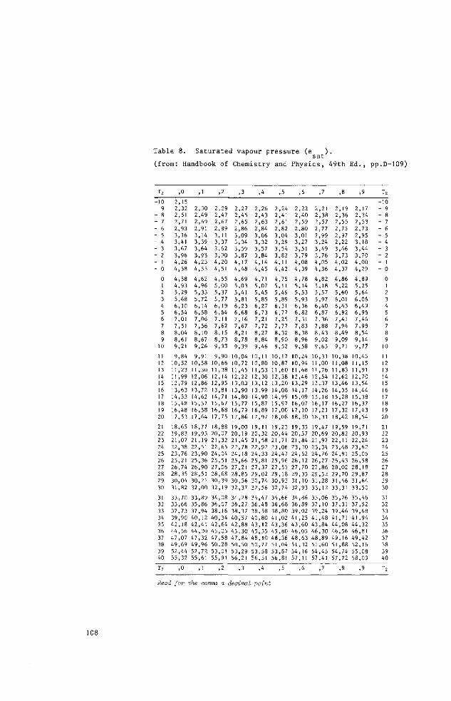
Table 8. Saturated vapour pressure (e ). sa t
(from: Handbook of Chemistry and Phys i c s , 49th Ed . , pp.D-109)
T2
-10 - 9 - 8 - 7 - 6 - 5 - 4 - 3 - 2 - 1 - 0
0 1 2 3 4 5 6 7 8 9
10
11 12 13 14 15 16 17 18 19 20
21 22 23 24 25 26 27 28 29 30
31 32 33 34 35 36 37 38 39 40
T2
.0
2 ,15 2 ,32 2 ,51 2 ,71 2 ,93 3 ,16 3,41 3 ,67 3 ,96 4 ,26 4 ,58
4 ,58 4 , 93 5 ,29 5 ,68 6 ,10 6,54 7,01 7,51 8,04 8,61 9,21
9 ,84 10,52 11 ,23 II ,99 12,79 13 ,63 14,53 15,48 16,48 17,53
18,65 19,83 21,07 22 ,38 23 ,76 25,21 26,74 28 ,35 30,04 31,82
33 ,70 35 ,66 37 ,73 39,90 42 ,18 44 ,56 47 ,07 49 ,69 52 ,44 55 ,32
,0
,1
2 ,30 2 ,49 2 ,69 2 ,91 3 ,14 3 ,39 3 ,64 3 ,93 4 , 23 4 , 55
4 ,62 4 ,96 5 ,33 5 ,72 6 ,14 6 ,58 7 ,06 7 ,56 8 ,10 8,67 9 ,26
9,91 10,58 11,30 12,06 12,86 13,72 14,62 15,57 16,58 17,64
18,77 19,95 21 ,19 22 ,51 23 ,90 25 ,36 26 ,90 28,51 30,21 32 ,00
33 ,89 35,86 37 ,94 40 ,12 42,41 44 ,30 47 ,32 49 ,96 52 ,72 55,61
,1
,2
2 ,29 2 ,47 2 ,67 2 ,89 3,11 3,37 3 .62 3 ,90 4 , 20 4 ,51
4 , 65 5 ,00 5 ,37 5 ,77 6 ,19 6 ,64 7,11 7 ,62 8 ,15 8 ,73 9 ,33
9 ,90 10,66 11 ,38 12,14 12,95 13,81 14,71 15,67 16,68 17,75
18,88 20 ,07 21 ,32 22 ,65 24,04 25,51 27 ,06 28 ,68 30 ,39 32 ,19
34 ,08 36 ,07 38 ,16 40 ,34 42 ,64 45 ,05 47 ,58 50 ,28 53,01 55,91
,2
,3
2 ,27 2 ,45 2 ,65 2 ,86 3 ,09 3 ,34 3 ,59 3 ,87 4 ,17 4 ,48
4 ,69 5 ,03 5,41 5,81 6 ,23 6 ,68 7 ,16 7 ,67 8,21 8 ,78 9 ,39
10,04 10,72 11 ,45 12,22 13 ,03 13,90 14,80 15,77 16,79 17,86
19,00 20 ,19 21 ,45 22 ,78 24 ,18 25 ,66 27,21 28 ,85 30 ,56 32 ,37
34 ,28 36 ,27 38 ,37 40 ,57 42 ,88 45 ,30 47 ,84 50 ,50 53 ,29 56,21
,3
,4
2 ,26 2 , 43 2 ,63 2 , 84 3 ,06 3 ,32 3,57 3 ,84 4 ,14 4 , 45
4 ,71 5 ,07 5 ,45 5 ,85 6 ,27 6 ,73 7,21 7 ,72 8,27 8 ,84 9 ,46
10,11 10,80 11 ,53 12,30 13,12 13,99 14,90 15,87 16,89 17,97
19,11 20 ,32 21 ,58 22 ,92 24 ,33 25,81 27 ,37 29 ,02 30,74 32,56
34 ,47 36 ,48 38 ,58 40 ,80 43 ,12 45 ,55 4 8 , 10 50 ,77 53 ,58 56,51
,4
,5
2 ,24 2 ,41 2 ,61 2 ,82 3 ,04 3 ,29 3 ,54 3 ,82 4 ,11 4 ,42
4 , 75 5 ,11 5 ,49 5 ,89 6,31 6 ,77 7 ,25 7 ,77 8,32 8 ,90 9 ,52
10,17 10,87 11 ,60 12 ,38 13,20 14,08 14,99 15,97 17,00 18,08
19,23 20 ,44 21 ,71 23 ,06 24 ,47 25 ,96 27 ,53 29 ,18 30 ,92 32,74
34,66 36 ,68 38 ,80 41 ,02 43 ,36 45 ,80 48 ,36 51 ,04 53 ,87 56,81
,5
,6
2 ,22 2 ,40 2 ,59 2 ,80 3,01 3 ,27 3,51 3 ,79 4 ,08 4 ,39
4 , 78 5 ,14 5 ,53 5 ,93 6 ,36 6 ,82 7,31 7 ,83 8 ,38 8,96 9 ,58
10,24 10,94 11,68 12,46 13,29 14,17 15,09 16,07 17,10 18,20
19,35 20 ,57 21 ,84 23 ,20 24,62 26,12 27 ,70 29 ,35 31 ,10 32 ,93
34,86 36 ,89 39,02 41 ,25 43 ,60 46 ,05 48 , 63 51 ,32 54 ,16 57 ,1 1
,6
,7
2 ,21 2 ,38 2 ,57 2 ,77 2 ,99 3 ,24 3 ,49 3 ,76 4 , 05 4 ,36
4 ,82 5 ,18 5 ,57 5 ,97 6 ,40 6 ,87 7 ,36 7 ,88 8 ,43 9 ,02 9 ,65
10,31 11 ,00 11 ,76 12,54 13,37 14,26 15,18 16,17 17,21 18,31
19,47 20 ,69 21 ,97 23 ,34 24 ,76 26 ,27 27 ,86 29 ,52 31 ,28 33 ,12
35 ,06 37 ,10 39 ,24 41 , 48 43 ,84 46 ,30 48 ,89 51 ,60 54 ,45 57,41
,7
,8
2 ,19 2 ,36 2 ,55 2 ,75 2 ,97 2 ,22 3 ,46 3 ,73 4 ,02 4 ,32
4 ,86 5 ,22 5 ,60 6,01 6 ,45 6 ,92 7,41 7 ,94 8 ,49 9 ,09 9,71
10,38 11,08 11 ,83 12,62 13,46 14,35 15,28 16,27 17,32 18,42
19,59 20 ,82 22,1 1 23 ,48 24,91 26 ,43 28 ,02 29 ,70 31 ,46 33,31
35,26 37,31 39,46 41 ,71 44 ,08 46 ,56 49 ,16 51 ,88 54,74 57 ,72
,8
,9
2 ,17 2 ,34 2 , 53 2 , 73 2 , 95 3 ,18 3 ,44 3 ,70 4 , 00 4 ,29
4 ,89 5 ,25 5 ,64 6 ,06 6 ,49 6 ,96 7 ,46 7 ,98 8 ,54 9 ,14 9 ,77
10,45 11,15 11,91 12,70 13,54 14,44 15,38 16,37 17,43 18,54
19,71 20 , 93 22 ,24 23 ,62 25 ,06 26 ,58 28 ,18 29 ,87 31 ,64 33 ,50
35 ,46 37 ,52 39 ,68 41 ,94 44 ,32 46 ,81 49 ,42 52 ,16 55 ,08 58 ,03
,9
T2
-10 - 9 - 8 - 7 - 6 - 5 - 4 - 3 - 2 - 1 - 0
0 1 2 3 4 5 6 7 8 9
10
11 12 13 14 15 16 17 18 19 20
21 22 23 24 25 26 27 28 29 30
31 32 33 34 35 36 37 38 39 40
T2
Read for the comma a decimal point
108

Evapotranspiration
Table 10. Value of i (Thornthwaite's monthly heat index)
T°C
0 I 2 3 4 5 6 7 8 9
10
1 1 12 13 14 15 16 17 18 19 20
21 22 23 24 25 26 27 28 29 30
31 32 33 34 35 36 37 38 39 40
,0
,09 ,25 ,46 ,71
1 ,00 1 ,32 1 ,66 2 ,04 2 ,44 2 ,86
3 ,30 3 ,76 4 ,25 4 ,75 5 ,28 5 ,82 6 ,38 6 ,95 7 ,55 8 ,16
8 ,78 9 ,42
10,08 10,75 11,44 12 ,13 12,85 13,58 14,32 15,07
15,84 16,62 17,41 18,22 19,03 19,86 20 ,70 21 ,56 22,42 23 ,30
,1
,10 ,27 ,48 ,74
1 ,03 1 ,35 1 ,70 2 ,08 2 ,48 2 ,90
3 ,34 3,81 4 , 30 4 ,81 5 ,33 5 ,87 6 ,44 7,01 7 ,61 8 ,22
8 ,85 9 ,49
10,15 10,82 11 ,50 12,21 12,92 13,65 14,39 15,15
15,92 16,70 17,49 18,30 19,1 1 19,95 20 ,79 21 ,64 22,51
,2
,01 ,12 ,29 ,51 ,77
1 ,06 1,39 1 ,74 2 ,12 2 ,52 2 ,94
3 ,39 3 ,86 4 , 35 4 , 86 5 ,38 5 ,93 6 ,49 7,07 7 ,67 8 ,28
8,91 9 ,55
10,21 10,39 11,57 12,28 12,99 13,72 14,47 15,22
15,99 16,78 17,57 18,38 19,20 20 ,03 20 ,87 21 ,73 22,59
,3
,01 ,13 ,31 ,53 ,80
1,09 1 ,42 1,77 2 ,15 2 ,56 2 ,99
3 ,44 3,91 4 , 40 4 ,91 5 ,44 5 ,98 6 ,55 7 ,13 7 ,73 8 ,34
8,97 9 ,62
10,28 10,95 11 ,64 12,35 13,07 13,80 14,54 15,30
16,07 16,85 17,65 18,46 19,28 20,11 20 ,96 21 ,81 22 ,68
,4
,02 ,15 ,33 ,56 ,82
1 ,12 1,45 1 ,81 2 ,19 2 ,60 3 ,03
3 ,48 3 ,96 4 , 45 4 ,96 5 ,49 6 ,04 6,61 7 ,19 7 ,79 8,41
9 ,04 9 ,68
10,35 11 ,02 11,71 12,42 13,14 13,87 14,62 15,38
16,15 16 ,93 17 ,73 18,54 19,36 20 ,20 21 ,04 21 ,90 22 ,77
,5
,03 ,16 ,35 ,58 ,85
1,16 1,49 1,85 2 ,23 2 ,64 3 ,08
3 ,53 4 ,00 4 ,50 5,01 5 ,55 6 ,10 6 ,66 7 ,25 7 ,85 8,47
9 ,10 9 ,68
10,41 11,09 11,78 12,49 13,21 13,94 14,69 15,45
16,23 17,01 17,81 18,62 19,45 20 ,28 21 , 13 21 ,99 22 ,86
,6
,04 ,18 ,37 ,61 ,88
1 ,19 1,52 1 ,89 2 ,27 2 ,69 3 ,12
3 ,58 4 ,05 4 , 55 5 ,07 5 ,60 6 ,15 6 ,72 7,31 7 ,91 8 ,53
9 ,17 9 ,75
10,48 11,16 11 , 85 12,56 13,28 14,02 14,77 15 ,53
16,30 17,09 17,89 18,70 19 ,53 20 ,36 21 ,21 22 ,07 22 ,95
,7
,05 ,20 ,39 ,63 ,91
1,22 1,56 1,92 2,31 2 ,73 3 ,16
3 ,62 4 ,10 4 ,60 5 ,12 5 ,65 6,21 6 ,78 7,37 7 ,97 8,59
9 ,23 9 ,82
10,55 11 ,23 11,92 12,63 13,36 14,09 14,84 15,61
16,38 17,17 17,97 18,79 19,61 20 ,45 21 ,30 22 ,16 23 ,03
,8
,06 ,21 M ,66 ,94
1 ,25 1 ,59 1,96 2 ,35 2 ,77 3,21
3 ,67 4 , 15 4 ,65 5 ,17 5,71 6 ,26 6 ,84 7 ,43 8 ,03 8,66
9 ,29 9 ,95
10,62 11 ,30 11 ,99 12,70 13 ,43 14,17 14,92 15,68
16,46 17,25 18.05 18.87 19,69 20 ,53 21 , 38 22 ,25 23 ,12
,9
,07 ,23 ,44 ,69 ,97
1 ,29 1 ,63 2 ,00 2 ,39 2 ,81 3 ,25
3 ,72 4 , 20 4 ,70 5 ,22 5 ,76 6 ,32 6 ,90 7 ,49 8 ,10 8 ,72
9 ,36 10,01 10,68 1 1 ,37 12,06 12,78 13,50 14,24 14,99 15,76
16,54 17,33 1 8 ; ! 3 18.95 19,78 20 ,62 21 ,47 22 ,33 23,21
Read for the conrxa a decimal point
109
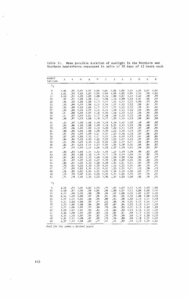
Table 11. Mean possible duration of sunlight in the Northern and Southern hemispheres expressed in units of 30 days of 12 hours each
month/
latitude
0
5
10
15
20
25
26
27
28
29
30
31
32
33
34
35
36
37
38
39
40
41
42
43
44
45
46
47
48
49
50
94 93 91 91 90 89 88 88 88 87 87
87 86 86 85 85 85 84 84 84 83
83 83 82 82 81 81 80 80 79 78
1,04
1 ,03
1,03
1 ,03
1,03
1,03
1,03
1,03
1,03
1,03
1,03
1 ,03
1 ,03
1,03
1,03
1,03
1,03
1,03
1,03
1 ,03
1,03
1,03
1 ,03
1,02
1,02
1,02
1,02
1 ,02
1 ,02
1 ,02
1 ,02
1,01 1
1,02 1
1,03 1
1,04 1
1,05 1
1,06 1
1,06 1
1 ,07 1
1,07 1
1,07 1
1 ,08 1
1,08 1
1,08 1
1 ,09 1
1 ,09 1
1 ,09 1
1,10 1
1,10 1
1,10 1
1,11 1
1,11 1
1,11 1
1,12 1
1,12 1
1,13 1
1,13 1
1,13 1
1,14 1
1,14 1
1,14 1
1,15 1
04 1,
06 1,
08 1,
11 1,
13 1,
15 1 ,
15 1 ,
16 1,
16 1 ,
17 1 ,
18 1,
18 1 ,
19 1,
19 1,
20 1,
21 1,
21 1 , 22 1 ,
23 1 ,
23 I ,
24 1,
25 1,
26 1 ,
26 1 ,
27 1,
28 1 ,
29 1 ,
30 1 ,
31 1, 32 1,
33 1,
01 03 06 08 11 14 15 15 16 16 17
18 19 20 20 21 22 23 24 24 25
26 27 28 29 29 31 32 33 34 36
1 ,04 1
1,06 1
1,08 1
1,12 1
1,14 1
1,17 1
1,17 1
1,18 1
1,18 1
1,19 1
1 ,20 1
1 ,20 1
1 ,21 1
1 ,22 1
1,22 1
1,23 1
1,24 1
1,25 1
1 ,25 1
1 ,26 1
1 ,27 1
1,27 1
1,28 1
1,29 1
1,30 1
1,31 1
1,32 1
1 ,33 1
1,34 1
1 ,35 1
1 ,37 1
,04 ,05 ,07 ,08
,' 1 ,12 ,12 ,13 ,13 ,13 ,14
,14 ,15 ,15 ,16 ,16 ,16
,17 ,17 ,18 ,18
,19 ,19 ,20 ,20 ,21 ,22 ,22 ,23 ,24 ,25
1 ,01
1 ,01
1 ,02
1 ,02
1 ,02
1,02
1 ,02
1,02
1,02
1 ,03
1,03
1,03
1 ,03
1 ,03
1 ,03
1 ,03
1 ,03
1 ,03
1,04
1,04
1,04
1 ,04
1 ,04
1 ,04
1 ,04
1 ,04
1 ,04
1,04
1,05
1,05
1 ,06
04 1
03 ,02 ,01 ,00 ,99 ,99 ,99 ,98 ,98 ,98
,98 ,98 ,97 ,97 ,97 ,97 ,97 ,96 ,96 ,96
,96 ,95 ,95 ,95 ,94 ,94 ,93 ,93 ,93 ,92
01 1,
99 1 ,
98 95 93 91 91 90 90 90 89
89 88 88 87 86 86 85 84 84 83
82 82 81 80 79 79 78 77 76 76
5 10 15 20 25 30 35 40 42 44 46 48 50
1 ,06
1,08
1 ,12
1,14
1,17
1,20
1,23
1,27
1,28
1 ,30
1 ,32
1 ,34
1 ,37
95 1
97 1
98 1
00 1
01 1
03 1
04 1
06 1
07 1
08 1
10 1
11 1
12 1
04 1
05 05 05 05 06 06 07 07 07 07 08 08
00 1
99 1
98 97 96 95 94 93 92 92 91 90 89
02
01 98 96 94 92 89 86 85 83 82 80 77
99 96 94 91 88 85 82 78 76 74 72 70 67
1,02
1,00
,97 ,95 ,93 ,90 ,87 ,84 ,82 ,81 ,79 ,76 ,74
1,03 1
1,01 1
1,00 1
,99 1
,98 1
,96 1
,94 1
,92 1
,92 1
,91 ,90 ,89 ,88
,00
,00
,00
,00
,00
,00
,00
,00
,00
,99
,99
,99
,99
05 06 07 08 10 12 13 15 16 17 17 18 19
1 ,03
1 ,05
1,07
1,09
1,11
1 ,14 1,17
1 ,20
1 ,22
1 ,23
1 ,25
1,27
1 ,29
1 ,06
1 ,10
1 ,12
1 ,15
1,18
1,21
1 ,25
1 ,29
1 ,31
1 ,33
1 ,35
1 ,37
1 ,41
Read for the comma a decimal point
no
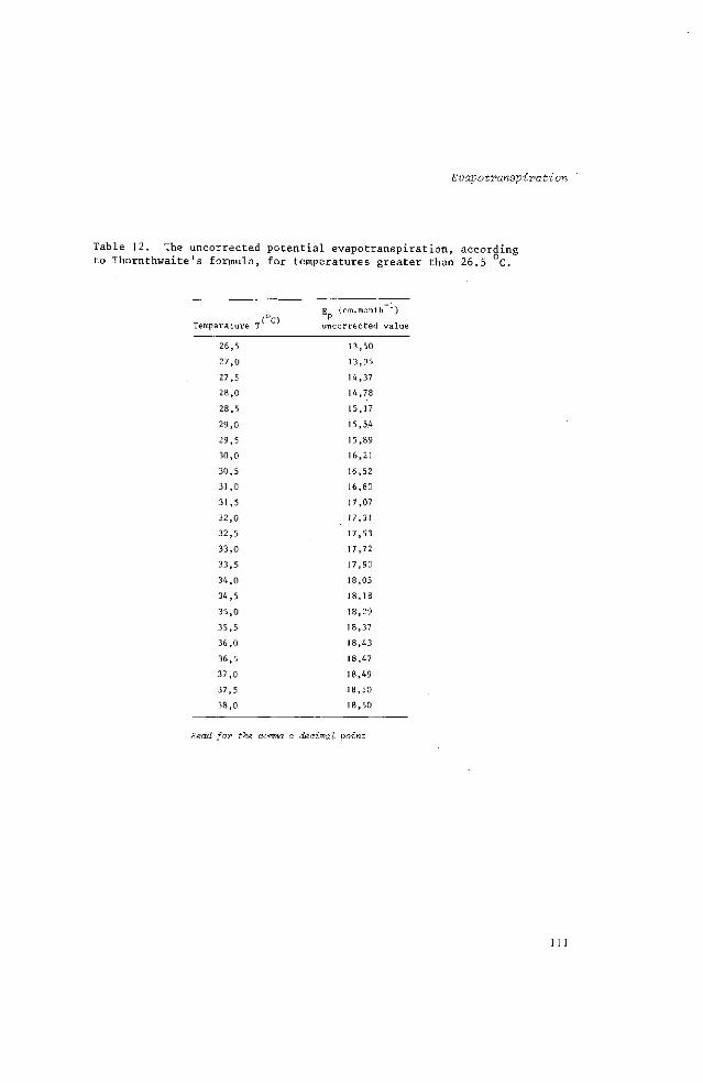
Evapotranspiration
Table 12. The uncorrected potential évapotranspiration, according to Thornthwaite's formula, for temperatures greater than 26.5 °C.
F (cm.month ) (°C) p
Temperature T uncorrected value
26,5 13,50
27,0 13,95
27,5 14,37
28,0 14,78
28,5 15,17
29,0 15,54
29,5 15,89
30,0 16,21
30,5 16,52
31,0 16,80
31,5 17,07
32,0 17,31
32,5 17,53
33,0 17,72
33,5 17,90
34,0 18,05
34,5 18,18
35,0 18,29
35,5 18,37
36,0 18,43
36,5 18,47
37,0 18,49
37,5 18,50
38,0 18,50
Read for the comma a decimal point
1 1 1

SURVEYS AND INVESTIGATIONS
2 0 . H Y D R O P E D O L O G I C A L SURVEY
K . V A N D E R M E E R
Deputy director International Land Consultants ILACO, Arnhem
R. H. MESSEMAECKERS VAN DE GRAAFF
Soil scientist International Institute for Land Reclamation and Improvement Wageningen
Lecturers in the Course on Land Drainage
K. VAN DER MEER (1962-1973) International Land Consultants, ILACO, Arnhem
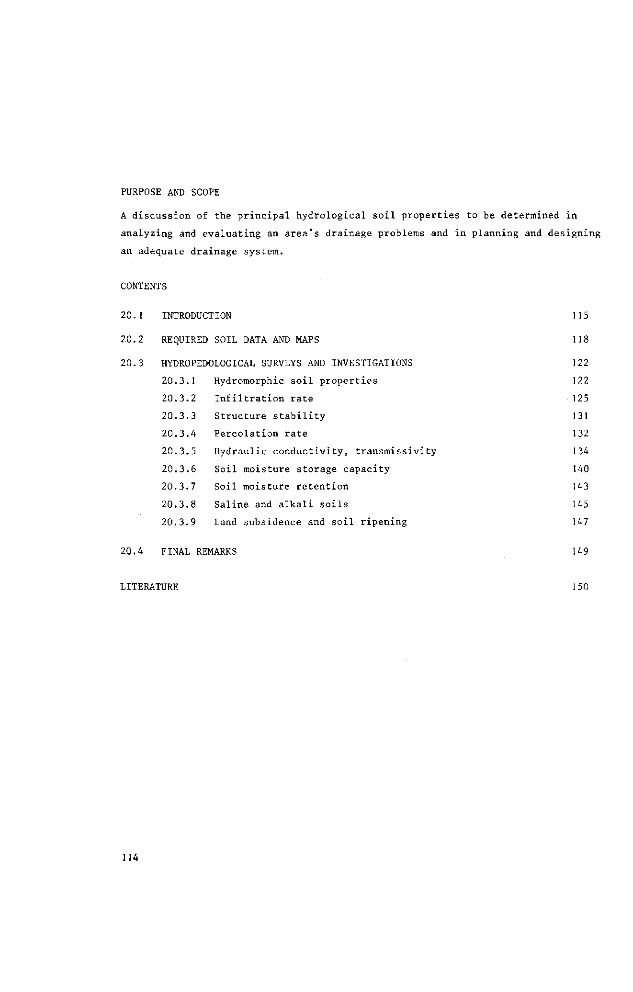
PURPOSE AND SCOPE
A discussion of the principal hydrological soil properties to be determined in
analyzing and evaluating an area's drainage problems and in planning and designing
an adequate drainage system.
CONTENTS
20.1 INTRODUCTION 115
20.2 REQUIRED SOIL DATA AND MAPS 118
20.3 HYDROPEDOLOGICAL SURVEYS AND INVESTIGATIONS 122
20.3.1 Hydromorphic soil properties 122
20.3.2 Infiltration rate 125
20.3.3 Structure stability 131
20.3.4 Percolation rate 132
20.3.5 Hydraulic conductivity, transmissivity 134
20.3.6 Soil moisture storage capacity 140
20.3.7 Soil moisture retention 143
20.3.8 Saline and alkali soils 145
20.3.9 Land subsidence and soil ripening 147
20.4 FINAL REMARKS 149
LITERATURE 150
114

Hydropedological survey
20.I INTRODUCTION
It is the aim of this chapter to define the contribution that a soil scientist can
make to the basic information required to analyse and evaluate an area's drainage
problems and to plan and design an adequate drainage system. The first question to
be answered in any drainage study is what is the soil potential of the area? A
clear statement must be made on whether or not the soils in the area are suitable
for growing the proposed crops. An inventory of the soil resources should there
fore be made, applying modern techniques of soil and land classification mapping.
The conventional soil or land classification maps produced in this way, however,
have only a limited value for drainage purposes because they provide no informa
tion on the layers below 1.20 or 1.50 m. The quantitative hydrological or physical
data required for drainage must be supplied by supplementary investigations that
extend to a depth of 4 to 5 m below ground surface and even deeper. These investi
gations can be grouped under the heading of a hydropedological survey.
A hydropedological survey should throw light on such questions as:
- where do excesses of surface water occur and what are the probable causes?
- which areas suffer from unfavourable groundwater conditions and what is
causing these conditions?
- is excessive wetness of the soils interfering with tillage, crop growth,
and harvesting?
- which areas suffer from unfavourable soil conditions, e.g. salinity, and
what are the relationships, if any, between such conditions and local surface
and groundwater conditions? Can these unfavourable conditions be rectified?
- what properties do the soils of the area possess that will hinder or pro
mote the flow of water through them and will decide whether it is an economic
proposition to control the groundwater table?
- what are the main topographical, physiographical, and relief features of
the area? Will the disposal of excess surface water or drain water be possible
and what are the conditions of the outlet?
- what effect will artificial drainage have on the soils and on their
productivity?
1 15

co
• fel tu k i ÖC Cq 10
O
~~ u 1-J
m < H
O +̂ ' M W
« A i
H W £5 P i
• J i l
a: c
r o
w H P i
w p-,
t a <
2 1 Q M W W P i
p-, 2 ;
w c
H M r -P i O
>-< W M H H O D i U W W < P i PL, p i P -C < P i X P i P-, o C
M Ü P (1) r
p*, 3 O * H
- M C *-* ni n) .
r i M C -H u o
' O O X I
( t , ^1 P , U~i —• Uî
O P H
VJ
CL • -
h w C u O r - t o at > I) 0) •
0 CJ <-)
ca 1-1 0 0 - H a i 0 U Kfi
oc CC X
PL
0 - H en O
C 0J
• a
0 0
u
^ VJ
a i
co
O ^ - .
a) S
C c a i j d
»J - C
0)
u 0)
a i
0
M-i C
0)
_e to a i
T3
• ^
ai c vi 0
S-. i - i P . 3
X ) TD - .-I
QJ ~v
> a -a ^ 3 El
U 00
O
OC G
M 0
S O
3
cr s-ai
« 3 TD
c a 0
*->
1 , - i i - i 03
00 l-i 1-1 O
o d
« 0)
116
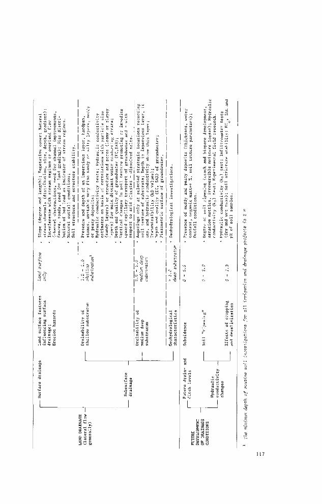
E o o o o
•H 0) T3 O '
e tu o u
CU 3 (fl O
O ni :
V- C W SJ c o o ^ a p P- O O r
M P 4-1 3
^ > p. ai • <U r - l •
13 J3
M C W U
vi t r ^ T i >-, o
) r-t G r
Ö O- V-< ' H C 0) • >> CL ^
i nj eu cu ' r-H R >
•H O
01 j j x :
ai cd o
H l/l M
O T3 J 5
N E cc
at -o
d o
H W K Ü w W < S S Z O P-i M M
w o <J; H a i i J a H P W Q O H > S ^D W fc O [n Q O O
117
20.2 REQUIRED SOIL DATA AMD MAPS
In drainage, a distinction must be made between soil drainage and land drainage.
By soil drainage we mean the ability of the soil to transmit water in a direction
that is mainly vertical. This will take place mainly in the upper 1.20 m of the
soil profile. The components of soil drainage are infiltration, internal drainage,
and water storage above field capacity.
Land drainage covers both surface drainage and subsurface drainage, in both of
which the flow of water is mainly lateral. When speaking of subsurface drainage,
we are usually only interested in that taking place in the upper 5 m of the soil
profile, but sometimes a considerably greater depth is involved.
Each type of drainage survey requires its own set of investigations, although
some observations and measurements are common to all of them. Table 1 lists the
main soil and land features relevant to drainage and the observations and measure
ments required to determine these properties. The task of a soil scientist working
in a drainage project can be derived from a study of this table.
It is not the intention of this chapter to discuss each item of this list; many
of them are self-explanatory while others have been dealt with in detail in other
chapters. In the following pages, only some of the important subjects which have
not yet been covered in other chapters will be discussed.
But first, some remarks on maps and mapping techniques.
Maps are the basis as well as the end result of a hydropedological survey. Hence,
before field work is started, all existing maps of the project area and its sur
roundings should be collected, studied, and, if necessary, transformed. Such maps
include topographical, geological, physiographical, soil, and land classification
maps, and also air photographs. The mapping scale depends on the type of survey
being conducted: reconnaissance, semi-detailed, or detailed. In conventional soil
surveys, one can distinguish various mapping intensities, there being a close re
lationship between survey intensity, mapping scale, and level of mapping units
(see Table 2).
The soil and topographical maps which are used as the basis for a hydropedological
survey are preferably at scales 1:5,000 or 1:10,000.
As already mentioned, conventional soil maps have limited value in land drainage,
especially if a subsurface drainage system is to be installed. The shortcomings
of such maps are listed in Table 3.
118

I l l
u [/)
<u Öl trt U r,i
> <
f f l
H
cri C
<>-i M-l
I M
Ü
<1)
(/) 41 O
(U i—t
^ -U •H 1/5 C <1)
T3
(fl ,£
(/I -Û c
o z M Pi
^ PQ
î-i
; (U I-H j H - r l U \ T-> O ,C j (0 «
1) V-i T M!
^
m
C m a
1 19
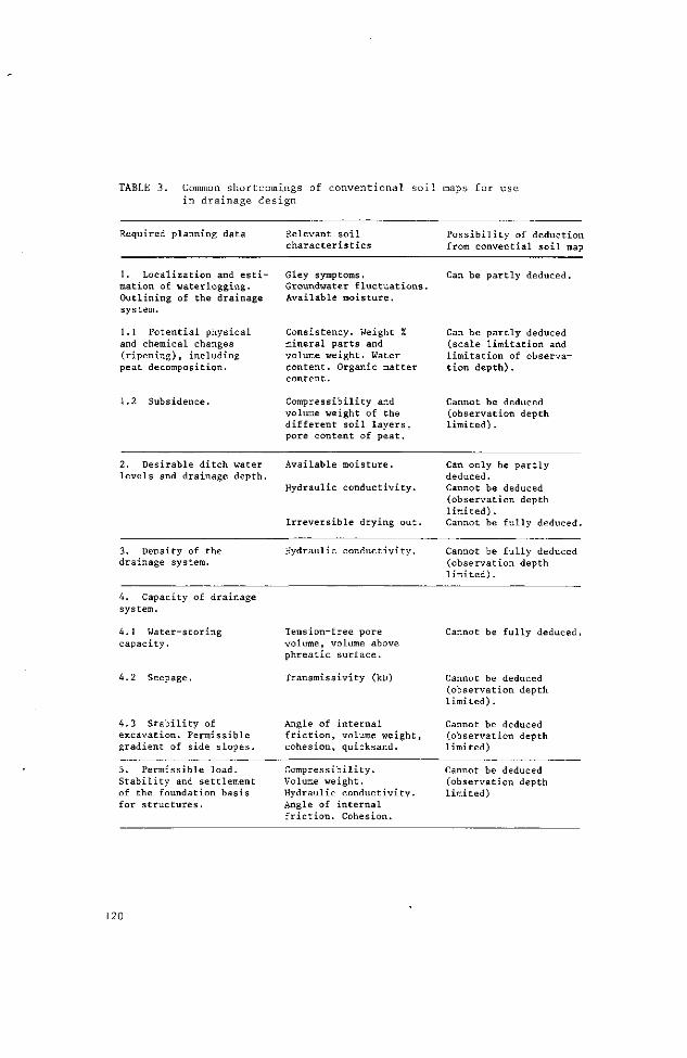
TABLE 3. Common shortcomings of convent ional s o i l maps for use in d ra inage design
Required planning data Relevant soi l charac ter i s t ics
Poss ib i l i ty of deduction from convential soi l map
1. Localization and e s t i mation of waterlogging. Outlining of the drainage system.
1.1 Potential physical and chemical changes (ripening), including peat decomposition.
Gley symptoms. Groundwater fluctuations. Available moisture.
Consistency. Weight % mineral parts and volume weight. Water content. Organic matter content.
Can be partly deduced.
Can be partly deduced (scale limitation and limitation of observation depth).
1 .2 Subsidence. Compressibility and volume weight of the different soil layers, pore content of peat.
Cannot be deduced (observation depth limited).
2. Desirable ditch water levels and drainage depth.
Available moisture.
Hydraulic conductivity.
Irreversible drying out.
Can only be partly deduced. Cannot be deduced (observation depth limited). Cannot be fully deduced.
3. Density of the drainage system.
Hydraulic conductivity. Cannot be fully deduced (observation depth limited).
4. Capacity of drainage system.
4.1 Water-storing capacity.
4.2 Seepage.
4.3 Stability of excavat ion. Permi s s ib1e gradient of side slopes.
Tension-free pore volume, volume above phreatic surface.
Transmissivity (kD)
Angle of internal friction, volume weight, cohesion, quicksand.
Cannot be fully deduced.
Cannot be deduced (observation depth limited).
Cannot be deduced (observation depth limited)
5. Permissible load. Stability and settlement of the foundation basis for structures.
Compressibility. Volume weight. Hydraulic conductivity. Angle of internal friction. Cohesion.
Cannot be deduced (observation depth limited)
120

Hydrovedological survey
The task of a hydropedologist working in land drainage is to produce the following
types of maps, most of which are single value maps:
- a soil texture map of the upper 2 to 5 m, as required
- a contour map of the upper side of the impervious base layer
- a map showing the location, extent, and thickness of coarse sandy or gravelly layers at or below drain depth
- a map showing the thickness of the water-transmitting layer or layers
- a soil salinity map
- a depth-to-water-table map
- a water table fluctuation map, based on soil hydromorphic characteristics (gley)
- a groundwater salinity map
- a hydraulic conductivity map for layers above and below the water table, especially at and below drain depth
- a map showing the magnitude and variations in the rate of infiltration
- a land-use and vegetative-cover map.
Obviously, the hydropedologist will not always be called upon to prepare all of
these maps, nor will he always be able to. If, for example, the impervious base
layer lies deeper than 4 to 5 m below the soil surface, the help of a geologist
will be required to produce a contour map of the surface of this layer. If the
problem is one of watertable control, a vegetative-cover map will not be needed,
whereas in the study of surface drainage problems such a map will be of great
value. Similarly, in areas with very thick peat layers a map showing the thick
ness of the peat can only be made by the hydropedologist if the peat is less
than 5 m thick.
It may happen that within the upper 2 to 4 m of the soil profile a hardpan or
other type of impeding layer is found. If so, it will be necessary to prepare a
map showing the occurrence and lateral extent of such a layer.
The above maps are usually prepared as single value maps, each subject being por
trayed on a single map. It is, however, convenient to reduce the number of these
maps by combining certain subjects; for example, depth to water table and ground
water salinity can often be portrayed on one map, using contour lines for one
subject and hatchings for the other. Similarly, hydraulic conductivity and thick
ness of the water transmitting layer can be combined in one map on which in a
later stage drain discharges, available head, and drain depth can be plotted.
Such a map does not need contour lines for each item, plottings which allow the
direct calculation of drain spacings being sufficient.
121
20.3 HYDROPEDOLOGICAL SURVEYS AND INVESTIGATIONS
As can be seen from Tables 1 and 3, the hydropedological data required for planning
and designing drainage systems are many and manifold. In the following pages we
will limit our discussion to
- hydromorphic soil properties
- infiltration rates
- structure stability
- percolation rates
- hydraulic conductivity
- soil moisture storage
- soil moisture retention
- salinity and alkalinity
- land subsidence and soil ripening.
20.3.1 HYDROMORPHIC SOIL PROPERTIES
As the morphological development of a soil profile is known to be influenced by
many factors (Chap.2, Vol.1), including the groundwater regime, it is logical that
certain morphological features will yield information on groundwater conditions.
This implies that the morphology of the soil has come to some sort of "equilibrium"
with the behaviour of the water table and that the properties of the first truly
reflect the peculiarities of the second. This notion does not always hold and the
processes leading to an equilibrium state can be very complex. In addition to the
groundwater regime, factors like the oxygen content of the groundwater, the che
mical and mineralogical composition of the soil horizons, and the soil temperature
during saturated conditions play an important role in the morphological develop
ment of the soil profile. Hence imprecise (though cheap) information on the beha
viour of the water table can be inferred from hydromorphic soil properties.
Hydromorphic characteristics which allow the natural internal drainage conditions
of soils to be assessed are:
- Soil colour, especially mottling and gley phenomena, which depend on the
presence and oxidation-reduction status of free oxides, primarily iron but also
manganese, and on the presence of organic matter. The colour patterns of mottles
and matrix are directly related to the pattern of translocation of these colouring
agents through the soil mass, and to the differences in accessibility for water
and atmospheric oxygen along cracks, pores, and biogenic channels as compared
with other parts of the soil mass away from these bigger voids.
122

Rydvopedological survey
These visible characteristics have long been in use to classify soils in seven
relative soil-drainage classes (USDA Soil Survey Manual, 1951).
2 +
- Gley soils are grey coloured by active reduction of iron to Fe . The
peculiar property of this grey colour is that it can change rapidly to a brown
colour on exposure to the air. Gley soils do not develop during short periods
of waterlogging, say a few weeks, or at very low temperatures, because, like any
other chemical reaction, gley formation takes time. Hence the absence of gley
phenomena must not be interpreted to mean the absence of waterlogging problems.
On the other hand, mottles may remain visible in soils which have been drained
for a long time. In dense wet soils these phenomena can remain visible for centu
ries. It is difficult to determine whether mottles are "fossil" or recent, but
if they are observed in the profile it is advisable to auger down to see whether
the groundwater table can be reached. Rust coloured mottles may also develop in
unripened soils exposed to drying and atmospheric oxygen. Such mottling is evi
dence of improved aeration rather than of hydromorphism.
- A high content of organic matter or the presence of peaty layers in soils
of humid climates can be regarded as an extreme example of moist soils. If iron
oxide coatings on sand grains in podzol soils just below the B2 horizon are ab
sent, this can be regarded as a sure sign of present or past removal of iron in
a reducing environment. After the removal of the iron, a fluctuating groundwater
table can leave no tell-tale mottling or other colour features indicative of the
height and depth of the water table. Mottling and black manganese concretions in
a grey A2 horizon and in the B2 horizon of Alfisols (soils with high base satura
tion and marked illuvial clay accumulation in the B2 horizon) are signs of a
temporary perched water table in these horizons.
- Finally, an increase in soil salinity towards the surface in regions with
arid and semi-arid climates is a sign of high water table.
In The Netherlands the depth to specific grey mottling (DE BAKKER, 1973) and the
depth to gley horizon were correlated with actual groundwater regimes (SCHELLING,
1960). The behaviour of the water table was characterized in terms of the mean
highest water table (MHW) and the mean lowest water table (MLW). It was found that
in different areas and in soils from different parent materials the relationships
between MHW or MLW and the depth to mottling or gleyed zones were similar but not
identical.
123

Ulli
• • P É P MÊÊÉÊLvmmmm m
f I I m m Il (fi ,11111111,
/
MT%h f i l I P l i i lL >,
/ • • -
/
fin, l>hy (IN.
J L .
LEGEND
Water-table class
MHW
MLW
cm. below surface
< 40
80 -120
< 40
> 120
40 - 80
> 120
80 - 120 > 120
> 200 > 200
a wetter variant of MHW
b drier variant of MHW
1 v not occurring in the
' mapped area
MHW mean highest water table
MLW mean lowest water table
Fig.1. Depth to water table classes distinguished on Dutch soil maps.
124

Hydropedologiaal survey
On Dutch soil maps seven watertable classes are distinguished, based on hydrolo-
gical and hydropedological data (VAN HEESEN, J970; see Fig.1). The duration of
saturated conditions for various depths in the soil profile is not taken into
account and neither are the frequency of low and high water tables or the periods
in the year that they occur.
20.3.2 INFILTRATION RATE
In any drainage project it is essential to have a proper insight into the rate at
which rain or irrigation water enters (infiltrates) into the soil (see also Chap.
5, Sect.4.2, Vol.1 and Chap.15, Sect.4.1, Vol.11 for different approaches to the
phenomenon of infiltration). Water that does not infiltrate creates a nuisance on
the land surface. It is of no use to the crops (excepting rice) and it does not
help to leach any superfluous salts out of the rootzone. Too slow or too fast in
filtration creates problems for the irrigationist. Hence infiltration tests are
required, particularly in planned irrigation projects.
It can often be observed that the infiltration rate - also called intake rate -
decreases with time. One can distinguish different physical quantities that
characterize the whole or parts of the process of infiltration. These are:
- the instantaneous infiltration rate (I. ), which is the volume of water ins
infiltrating through a horizontal unit area of soil surface at any instant (infi
nitely small period of time). It shows, in general, a rapid decline in the begin
ning, followed by a more stable, very slow decline after some 3 to 4 hours of
infiltration. - the cumulative infiltration (I ), which is the total volume of water
cum
that has infiltrated through a unit of horizontal area of soil surface over a
given period of time, measured from the beginning of infiltration.
- the average infiltration rate (I ), which equals the cumulative infiltra
tion divided by the time since infiltration started.
- the basic infiltration rate (I, ), which is the relatively constant rate bas
that develops after some 3 to 4 hours. A good criterion of the term "relatively
constant" would be a change in infiltration rate of less than 10 per cent as
compared with that of the preceding hour, or (I - I ) < 0.1 I (t expressed in
hours). This is the physical quantity commonly used in hydrologie studies and
runoff-erosion work.
125

- the infiltration capacity (I ) which is the maximum rate at which a cap
given soil in a given condition can absorb water. When water is ponded over the soil
during an infiltration test or an irrigation, one always obtains this maximum rate. The (I. )-time relationship is the basis for the design of sprinkler irrigation
systems. In contrast, the (I )-time relationship is the basis for design of cum
surface irrigation systems. The starting point in this reasoning is a crop's
water requirement and a convenient irrigation schedule. However, for the purpose
of this chapter it is necessary to know what portion of the water is removed
"slowly" through the soil and what portion reaches a drainage ditch "rapidly"
over the soil surface. The measured intake characteristics have to be interpreted
in this context. Field measurements on infiltration rate invariably yield data in terms of I
cum Therefore it is much more convenient to derive an expression for I. by differen-
m s tiating the expression for I with respect to time, than to find I by inte-
cum r cum grating I. . For many soils a plot of I as a function of time is described
m s cum by the equation
I = at" (1) cum
where a and n are constants for a given soil and a given moisture content respectively. The constant n is positive but less than unity. From Eq.1 the instantaneous infiltration I. at any time t can be derived by taking the differential
ins with respect to t
dI
cum n-1 . . I. = — j - — = a n t (2) ins dt
A convenient relationship is now
I n I. = ̂ - (3) m s t
From Eq.1 we can also obtain an expression for the average infiltration I by av
dividing I through t cum
T cum n-1 , . I = — — = a t (4) av t
When Eqs.1,2, and 4 are plotted on double logarithmic paper, each one gives a
straight line. Such plots are tantamount to rewriting these equations in loga-
126
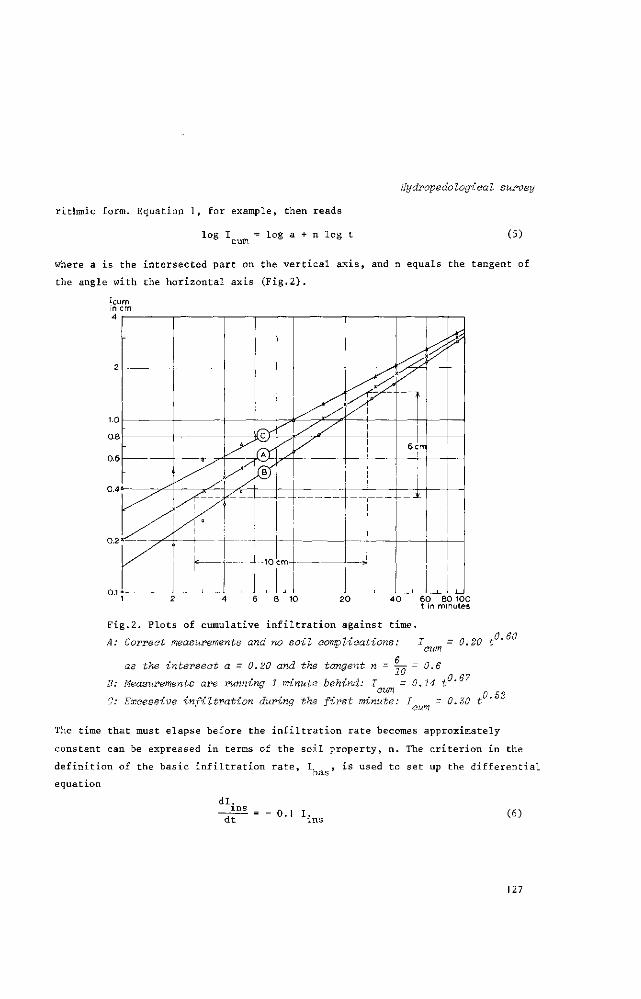
rithmic form. Equation 1, for example, then reads
log I = log a + n log t cum
Hydropedological survey
(5)
where a is the intersected part on the vertical axis, and n equals the tangent of
the angle with the horizontal axis (Fig.2).
60 80 100 t in minutes
cum
0.6
0.20 t
Fig.2. Plots of cumulative infiltration against time
A: Correct measurements and no soil complications: I
as the intersect a - 0.20 and the tangent n = -j
B: Measurements are running 1 minute behind: I =0.14 t' cum
C: Excessive infiltration durinq the first minute: I - 0.30 t J a J cum
0.60
0.67
0.32
The time that must elapse before the infiltration rate becomes approximately
constant can be expressed in terms of the soil property, n. The criterion in the
definition of the basic infiltration rate, I, , is used to set up the differential bas r
equation dl.
ins dt = - 0.1 I.
ins
127

D i f f e r e n t i a t i n g the l e f t -hand term one ob ta ins
d l - , , n - 1 . m s d(a n t ) / ,s t n -2 , , ,
"dt S i t , ( n - , ) , n t ( 7 )
The right-hand term of Eq.6 can also be written as
0.1 I. = 0.1 a n tn_1 (8) ins
Substituting Eqs.7 and 8 into Eq.6 gives
t = 10(l-n) (9)
For a description of infiltration tests, see Chap.24, Vol.111; BERTRAND (1965);
RAISE, DONNAN and others (1956). Usually the data for three tests conducted within
a small area are averaged to characterize a particular type of soil. The three
test results are plotted separately on the same sheet of double logarithmic paper
and, if the points for all three replications are close enough together, an average
curve can be drawn.
In homogeneous soils deviations from a straight line can result from inadvertent
delays in the first readings when the water has already started infiltrating and
from the presence of small cracks and biogenic holes which are filled up very
rapidly in the first minute or so. In Curve B (Fig.2) for example, the observer
measures I for t = 1 when in fact, t = 2. Comparison with Curve A shows that cum
the real I (t = 2) = 0.3 cm, which is 0.1 cm more than the real I (t = 1). cum cum
In this incorrect procedure the observer mistakes this increment of 0.1 cm for the real I (t = 1).
cum
In heterogeneous soils deviations from a straight line are to be expected. Soils
having a strongly developed crack system and large biogenic holes show very high
initial n-values (0.9 or more), which diminish after some time. In very sandy
soils the n-value remains above 0.9 throughout the test. If the subsoil differs
from the top soil in infiltration rate, the curve will show a change of slope
when, after some time, the wetting front passes the boundary between top soil
and subsoil.
In general, the n- and a-values are useful indicators of the infiltration charac
teristics of soils. The a-value in Eq.1 is a measure of the magnitude of infil
tration and, for homogeneous soils, is independent of time. The physical meaning
of the a-value can be illustrated by an example. If I = 0.2 t (I in cm, cum cum
128

Hydropedologieal survey
t in min.), it follows that for t = 1 minute, I = 0.2 cm. For t = 1 hour, one cum
reads the I value at 60 minutes from the graph. The n-value on the other hand cum
reflects the change in infiltration rate with time. In moist soils the a-values
are lower than in dry soils and the n-values are higher.
When dealing with heavy, swelling clay soils the use of cylinder infiltrometers is
likely to yield unrealistic results. If the area of soil enclosed by the cylinder
comprises a large crack interconnected with a system of cracks outside the cylinder,
the infiltration rate will be far too high. If no cracks are enclosed, the infil
tration rate may be almost zero. Yet, the cracks are part of the reality for such
soils; hence basin infiltration tests are indicated (ALLEN and BRAUD, 1966).
For classification purposes, representative infiltration data from the field can
be grouped into distinct families of infiltration curves (S.C.S.National Engineer
ing Handbook, 1964) and each family can be given a class name, such as rapid, mo
derately slow, etc. (see Fig.3).
A classification of basic infiltration rates is suggested by RICKARD and COSSENS
(1965) for irrigated soils in New Zealand:
Class
0 I II III IV
Intake designation
very low low medium high very high
Basic infiltration rate (mm/hour)
less than 2.5 2.5 - 15 1 5 - 2 8 28 - 53 more than 53
VAN BEERS (private communication), stressing the convenience in irrigation of
working with the total amount of time in hours required for the infiltration of
10 cm of water, has put forward a different tentative classification:
Class Time required for 10 cm cumulative intake
marginal (too slow) 20 - 40 hours somewhat unfavourable (slow) 8 - 2 0 favourable 1.5-8 somewhat unfavourable (rapid) 1.5 - 1.0 marginal (too rapid) 1.0 - 0.5
The basic infiltration rate is the most important characteristic for land drainage,
and it should be considered in conjunction with the climate (Chap.18,Vol.Ill ;
Chap.33, Vol.IV).
129
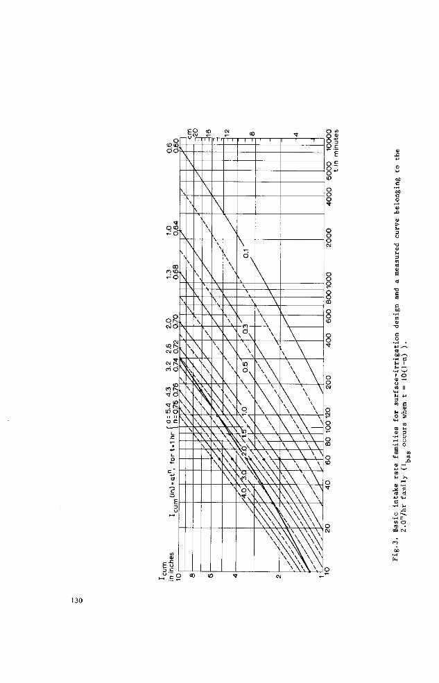
•H c U I u —
U J5 o S
0) M a 4J
c • H
o • H
en
• H
e (0 y- i
u •C
^ O
00 •r-l fa
130

Hydropedological survey
20.3.3 STRUCTURE STABILITY
Agriculturists and soil scientists are interested not only in the structural con
dition (Chap.2, Sect.3.2,Vol.I) of the soil as it affects intake characteristics
during a hydropedological survey or even during a first infiltration test; they
are also vitally interested in the deterioration or improvement of soil structure
as a result of the action of water on the cohesive strength of soil aggregates,
or as a result of future soil management when the area is brought under agricul
tural use. The collapse of soil aggregates when wetted with water is called slaking,
and if the water surrounding the soil becomes turbid the soil is said to disperse.
Upon drying, a slaked surface soil will often form a crust of low permeability,
which may at the same time be so hard that germinating crop seeds cannot break
through it.
If intake characteristics are to be considered favourable, the-majority of soil
aggregates, at least 3/4 by weight, must remain intact, i.e. must not become
smaller than a predetermined size (diameter, say 0.25 mm), when subject to impact
ing raindrops or moving water. Low intake rates on sloping lands results in more
run off, a higher attendant risk of erosion, and a need for more intensive surface
drainage systems. Even salinization of soils can occur, as has happened for example
in parts of the Jessore District of Bangladesh, where only 300 to 400 mm of the
2000 mm precipitation actually infiltrates into the fine, silty, poorly structured
soils of the delta during the wet season. In the dry season, lateral capillary
flow from the flooded depressions causes salt accumulation in a wide zone fringing
these depressions.
Soil aggregate stability can be measured fairly simply in the laboratory. One
somewhat aggressive technique employs wet sieving of air-dry aggregates, followed
by a weighing of the aggregates remaining on the sieve after oven drying (KEMPER
and KOCH, 1966). Another, more passive, technique is based on measuring the loss
of pore volume due to slaking when air-dry aggregates are wetted with water and
vibrated (WILLIAMS, 1963). Agressive methods fail to show differences between
soils whose aggregate stabilities are low to varying degrees. However, one may
first place the soils in broad classes of aggregate stability by a technique which
requires only a set of beakers, some distilled water, and a few other readily
available items (EMERSON, 1967). Once one has a rough idea of the aggregate
stability, one can then choose an appropriate method for making finer distinctions.
The work by Kemper and Koch, which represents numerous soils in the western
U.S. and Canada, indicates that
131
- aggregate stability declines very rapidly when soil organic matter contents
fall below 2%, as is often the case in desert areas
- aggregate stability increases as soil clay contents are higher (about 75%
stable aggregates at 40% clay)
- CaC03 content of the soil has no influence, and
- soils with exchangeable sodium percentages in excess of 20 have no aggre
gate stability at all.
For light sandy loams and silty loams in The Netherlands (BOEKEL, 1965) the risk
of structure deterioration was correlated with the ratio between upper plastic
limit (liquid limit) and moisture content at field capacity (pF = 2) as follows
- > 1.10 little or no slaking will occur r C
- < 0.95 risk of serious slaking during long wet periods
—- < 0.90 risk of serious slaking during short wet periods r C
Between —— = 1,10 and —— = 0.90 the slaking hazards vary markedly with the manner r C r C
and moment of tilling the soil in autumn.
20.3.4 PERCOLATION RATE
Percolation is not synonymous with infiltration. Infiltration refers to the entry
of water at the soil surface; percolation refers to the quantity of water passing
per unit of time through a horizontal unit area at a given depth within the soil
mass. Only in a saturated soil does percolation equal infiltration; in unsatura
ted soil, infiltration equals the sum of percolation and storage.
Some authors, in defining percolation, prefer to think of the time required for
a unit quantity of water to percolate through the soil. Unlike the concept of
infiltration, it is not possible to define percolation in unambiguous physical
terms that would suggest a simple field method of measuring percolation. Perco
lation tests reported in literature are highly empirical because the flow of wa
ter through walls and bottom of test holes takes place under undefined boundary
conditions.
132
Hydropedological survey
The test holes have to be auger holes or dug holes of known diameter and to a
depth at which the percolation rate is to be measured, generally in the layer
thought to have the lowest hydraulic conductivity. The test holes are then filled
with water and one measures the volume of water that flows through the soil.
Several precautions must be taken to ensure the unhindered movement of water
through the walls and bottom of the test holes; for example, the exposed surfaces
of the hole should be sacrified or a layer of gravel added to prevent scouring and
sediment formation. Test holes are also pre-soaked to obtain the more represen
tative percolation rate for wet soils.
To standardize the boundary conditions for the percolation test so that the mea
sured results are quantitative, reproduceable, and physically interprétable, the
test can be done as a normal infiltration test or with the inversed auger hole
method (Chap.24,Vol.Ill) .
With the infiltration method, one uses the normal cylinder infiltrometer, but it
is now installed on the horizontal bottom of an excavation. The excavation should
be made to a depth just above the layer that is suspected of being the least per
vious part of the profile. The cylinder is pushed or hammered some 2 to 5 cm into
this layer and the normal infiltration procedure is followed. The resulting mea
surement will yield information on the hydraulic conductivity of the limiting layer
under nearly saturated conditions (stabilized moisture content).
In land drainage the inversed auger hole method is often applied for layers above
the water table. The hole must be augered to the depth of interest, usually into,
but not through, the layer of limiting hydraulic conductivity. In experimental
fields with subsurface drains and ditches, the ratio of "rapid" to "slow" ditch
discharge, following rain or irrigation, reflects the quantities and rates of
surface flow and percolation.
The macropores in a soil profile play an important role as conduits for water,
and hence largely determine the percolation rate. Pores in a soil profile origi
nate from (decomposed) plant roots and microfauna (ants, worms, molluscs). A single
tubular soil pore (tortuosity = 2, diameter = 1 mm) per m2 horizontal cross-
section can give a hydraulic conductivity of 0.01 m/day. In various studies, counts
of up to 1,500 of the larger, easily visible pores have been reported. Pore counts
have successfully been correlated with reclaimability of saline-alkali soils in
West-Pakistan (ALIM et al., 1971). During a hydropedological survey due attention
should be given to pores visible in profile pits or in undisturbed samples deeper
down. An experienced hydropedologist may even be able to estimate the hydraulic
conductivity so that field measurements can be economized on.
133
Like pores, cracks play a major role as conduits for water. In soils that are com
monly cracked, determining the hydraulic conductivity on small core samples gives
unrealistic results (5 to 25 times too low). In some swelling soils the cracks may
close entirely upon saturation, but in others the cracks remain partially open.
There are reports of clay soils that are permanently below the water table and
yet have wide-open cracks (KALLSTENIUS, 1963; DIELEMAN and DE RIDDER, 1963).
The phenomenon that the cracking of drained and drying soils in the IJsselmeer
polders (The Netherlands) has contributed greatly to the spectacular increase of
hydraulic conductivity is an accepted fact.
The effect of cracks and soil structure on hydraulic conductivity can be calcula
ted, as has been shown by BOUMA and HOLE (1971) and ANDERSON and BOUMA (1973),
but their approach has not yet been applied on a practical scale.
20.3.5 HYDRAULIC CONDUCTIVITY, TRANSMISSIVITY
The hydraulic conductivity of the soil profile at and below drain depth is the most
important soil physical characteristic to be determined in any subsurface drainage
project. The magnitude of the hydraulic conductivity of a soil depends on pore
geometry and the nature of the particle surfaces. Thus it varies with texture,
structure, density of packing of soil grains, and grade of cementation. The effects
of texture, structure, and density are in turn modified by the content of organic
matter of the soil, the degree of saturation with Ca or Na, and the type of clay
minerals (swelling or non-swelling). Some of the factors controlling hydraulic
conductivity can vary considerably over short distances, or at a given site over
short periods of time.
For sandy sediments which have a clay plus silt content of less than 6 per cent,
quick and reliable estimates of hydraulic conductivity can be made on the basis
of particle size distribution or on the specific surface U of the particles (Chap.
24,Vol.III). For the intermediate and heavy textured soils, other factors not
related to particle size generally far outweigh the influences of particle size.
Attempts have been made (Table 2.2 from ZIMMERMAN, 1966; HORN, 1971) to consider
these other factors in arriving more cheaply at usable field estimates of
hydraulic conductivity. The merit of this work is not to be found in any univer
sally applicable relationships but in pointing out the possibility of developing
a fairly consistent local relationship between hydraulic conductivity and easily
observable and measurable soil properties.
134
Hydropedologiaal survey
HORN's (1971) curves (Fig.4) represent the approximate extreme limits of hydraulic
conductivity for natural soils. A highly sorted sand with spherical grains will
have a hydraulic conductivity that is somewhere on or near the theoretical curve,
depending on the particle size. A clay loam, in contrast, could have a K-value
almost anywhere on a horizontal line extending from the point representing its
mean particle diameter. Thus a clay loam with high ESP and swelling clay minerals
may have a K of 0.01 m/day, while one with a good and stable structure may have
a K of 8 m/day.
The common opinion that clays and clay materials always have low hydraulic conduc
tivities is unjustified. In different parts of the world there are heavy clays
whose hydraulic conductivity in natural condition is very high and comparable
with that of coarse sands and gravel. DIELEMAN and DE RIDDER (1963), in studying
the hydraulic conductivity of a 2 m thick heavy clay layer occurring along the
borders of Lake Chad (Central Africa) found values as high as 1000 to 5000 m per
day, the reason being wide cracks and fissures, which had not closed after the
clay had been inundated by the lake water in the geologic past.
Another example is that of the heavy humic clays which occur locally in the Danube
flood plain in Roumania. For these structured clays K values as high as 30 m per
day are reported (FA0 Work Document AGL:UNDP/ROM.1).
It is the hydropedologist's major task to determine the magnitude of the hydraulic
conductivity at and below drain depth and to indicate how it varies within the
boundaries of the project area. Although various methods for measuring hydraulic
conductivity exist, the auger hole method is the one most commonly applied (Chap.
24,Vol.III).
To calculate the spacing of drains, the value of the hydraulic conductivity, K, is
by itself insufficient. Also required is information on the thickness, D, of the
water transmitting layers and on the depth of the impervious base layer. If a con
tinuous layer of heavy clay is found at some depth in a light textured soil profile,
such a clay layer may be regarded as the impervious base of the profile. But an
impervious layer need not be "impervious" in the true sense of the word, i.e. a
layer which does not allow any passage of water. In drainage, "impervious" has
a relative meaning. A base layer whose hydraulic conductivity is 10 times less
than that of the overlying material may be considered impervious in drainage.
In a homogeneous soil, the depth of soil through which the major part of the
groundwater flows towards the drains equals roughly 1/4 of the drain spacing.Hence
it is obvious that a conventional soil survey, which provides information on only
135

I —4 —
- __L_.
1
~ ° r - - a V
. > > * ï
\ s
"V-slS \ o o \ ÓÖ
V 1
\ y E y | ;
ISU . < 5 <D ^
J û Ö Ó
^ 3 < 1/1 "1
o o o
o
>>>
o
\ \ 11
o
a
w O 1
2 S
ÓÓ
~ " o
\ \ 1
, ' o
U ^ i CM(0
o o d o
E î
~ > U £
o o d ó
" ;ä SI
136
~~ r^ o>
~-55 a l o W
—' en ö o
• H 4-»
• r 4
•o a o o
i - H
CD S J
3 u u 3
^ 4J CO
• i-l
O en
-0 C
rt ^ a) 4-J d )
e
3-T - i
Ä Ö-
" f i
S-r - i
-s; t a
•̂ r s ; r £
i
w to Ci
• u
S <s o S H
»
<s
^ 3 + i CJ 3 ?H
+ i
CO
E^tS
E 3
M 'a o co
CO r - i
r O
c <s>
D O
s-. C3
r - i
O
t » S
• r i r - i
r o
« 1
3 co 1 S O C
13 e»
C n + i
r ï
+s • r i
3
co r ^ ï
' r i
O Ü i C n
s es
r S ?
u H cj
es 13
r e t o
• f i
-S"
r c + i V 3
CO r - i
V
es + i
0
Ö
1-0 O
S i r - i
t «
t o • r i
o f « ; rt Co
• r 4
•a
aj r H U
•H 4J H
ffl P.
c CÖ eu
a o 4J
c o
•(-( 4J <o
t—i (U
^
m
ci N V co
O ) r ^
« V + i ! H
t
CO s. 3
+ i O
3
fc -P co
Ss 0
0
a. Ci <K 0 4
«K 0
K 0
• t »
0
co t - ^
• r i
0 co
+ i "Xi u £
1 » r - i
3 " t i
O c
fc 0
« s 0 s
* t
13 co s c» co 0 0
r - i
S i r - i r - i C 0
V s e
r Ç
0 <s E
CO CO
"CS
•g o
s 0
fc V
1
f . co
4 i >
+ i CS E
u V
t n f< O
1
C <t-,T3+ • r 4
>, • U •r-t
> • H 4-1 O 3
• a d o o
CJ •H r-i
3 10 M •a >> X
CO C j
3 + a,
3 i C j 4 i
V r - i
• t i
'S c»
fc £ 1»
a, r - i
c 0
^ - p
CS C o
+ i s ;
co 13 Ä 0
ï -4 0
t o S r i
r - i 1 - ^
0) a
c 3 -Ci CS
O + i
<» 3 -a
co 13
a TS f n
O 'S
<t r C
• M •r-( PU
6-1
• ^
CO CO I N
c» û , CO r i
«> - p
CJ ^ i
3 O O O
-̂ . T3 ' t - ,
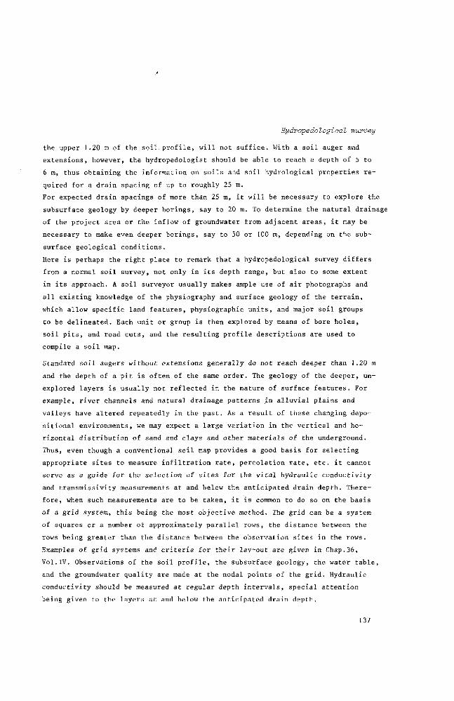
Hydropedological survey
the upper 1.20 m of the soil, profile, will not suffice. With a soil auger and
extensions, however, the hydropedologist should be able to reach a depth of 5 to
6 m, thus obtaining the information on soils and soil hydrological properties re
quired for a drain spacing of up to roughly 25 m.
For expected drain spacings of more than 25 m, it will be necessary to explore the
subsurface geology by deeper borings, say to 20 m. To determine the natural drainage
of the project area or the inflow of groundwater from adjacent areas, it may be
necessary to make even deeper borings, say to 50 or 100 m, depending on the sub
surface geological conditions.
Here is perhaps the right place to remark that a hydropedological survey differs
from a normal soil survey, not only in its depth range, but also to some extent
in its approach. A soil surveyor usually makes ample use of air photographs and
all existing knowledge of the physiography and surface geology of the terrain,
which allow specific land features, physiographic units, and major soil groups
to be delineated. Each unit or group is then explored by means of bore holes,
soil pits, and road cuts, and the resulting profile descriptions are used to
compile a soil map.
Standard soil augers without extensions generally do not reach deeper than 1.20 m
and the depth of a pit is often of the same order. The geology of the deeper, un
explored layers is usually not reflected in the nature of surface features. For
example, river channels and natural drainage patterns in alluvial plains and
valleys have altered repeatedly in the past. As a result of these changing depo-
sitional environments, we may expect a large variation in the vertical and ho
rizontal distribution of sand and clays and other materials of the underground.
Thus, even though a conventional soil map provides a good basis for selecting
appropriate sites to measure infiltration rate, percolation rate, etc. it cannot
serve as a guide for the selection of sites for the vital hydraulic conductivity
and transmissivity measurements at and below the anticipated drain depth. There
fore, when such measurements are to be taken, it is common to do so on the basis
of a grid system, this being the most objective method. The grid can be a system
of squares or a number of approximately parallel rows, the distance between the
rows being greater than the distance between the observation sites in the rows.
Examples of grid systems and criteria for their lay-out are given in Chap.36,
Vol.IV. Observations of the soil profile, the subsurface geology, the water table,
and the groundwater quality are made at the nodal points of the grid. Hydraulic
conductivity should be measured at regular depth intervals, special attention
being given to the layers at and below the anticipated drain depth.
137
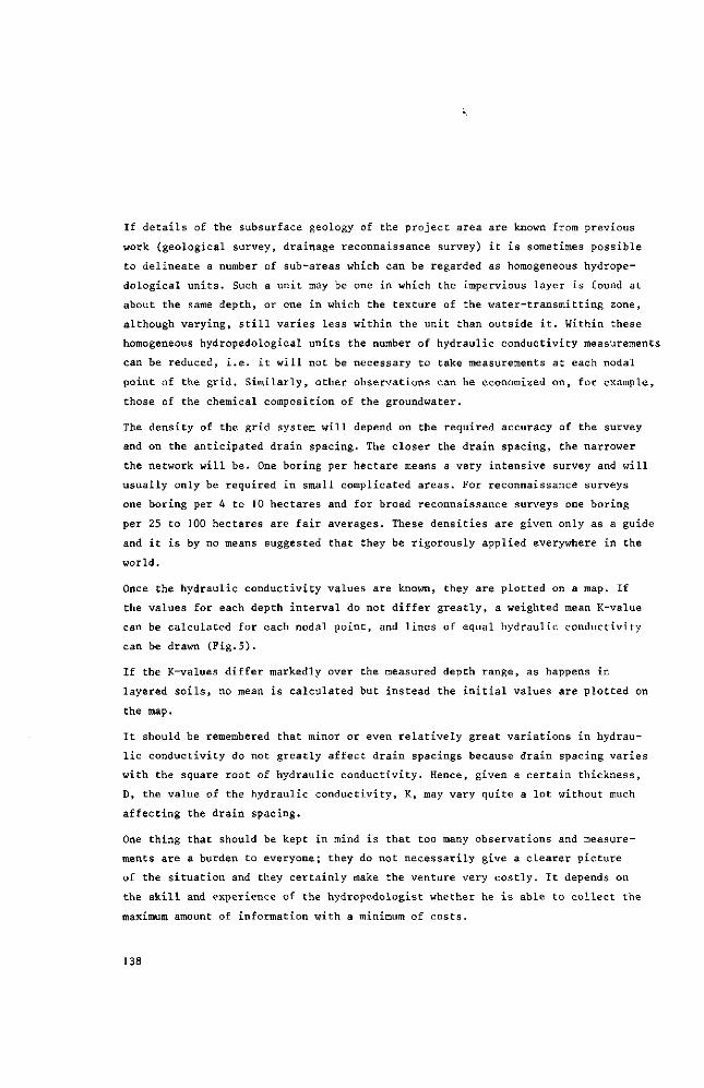
If details of the subsurface geology of the project area are known from previous
work (geological survey, drainage reconnaissance survey) it is sometimes possible
to delineate a number of sub-areas which can be regarded as homogeneous hydrope-
dological units. Such a unit may be one in which the impervious layer is found at
about the same depth, or one in which the texture of the water-transmitting zone,
although varying, still varies less within the unit than outside it. Within these
homogeneous hydropedological units the number of hydraulic conductivity measurements
can be reduced, i.e. it will not be necessary to take measurements at each nodal
point of the grid. Similarly, other observations can be economized on, for example,
those of the chemical composition of the groundwater.
The density of the grid system will depend on the required accuracy of the survey
and on the anticipated drain spacing. The closer the drain spacing, the narrower
the network will be. One boring per hectare means a very intensive survey and will
usually only be required in small complicated areas. For reconnaissance surveys
one boring per 4 to 10 hectares and for broad reconnaissance surveys one boring
per 25 to 100 hectares are fair averages. These densities are given only as a guide
and it is by no means suggested that they be rigorously applied everywhere in the
world.
Once the hydraulic conductivity values are known, they are plotted on a map. If
the values for each depth interval do not differ greatly, a weighted mean K-value
can be calculated for each nodal point, and lines of equal hydraulic conductivity
can be drawn (Fig.5).
If the K-values differ markedly over the measured depth range, as happens in
layered soils, no mean is calculated but instead the initial values are plotted on
the map.
It should be remembered that minor or even relatively great variations in hydrau
lic conductivity do not greatly affect drain spacings because drain spacing varies
with the square root of hydraulic conductivity. Hence, given a certain thickness,
D, the value of the hydraulic conductivity, K, may vary quite a lot without much
affecting the drain spacing.
One thing that should be kept in mind is that too many observations and measure
ments are a burden to everyone; they do not necessarily give a clearer picture
of the situation and they certainly make the venture very costly. It depends on
the skill and experience of the hydropedologist whether he is able to collect the
maximum amount of information with a minimum of costs.
138
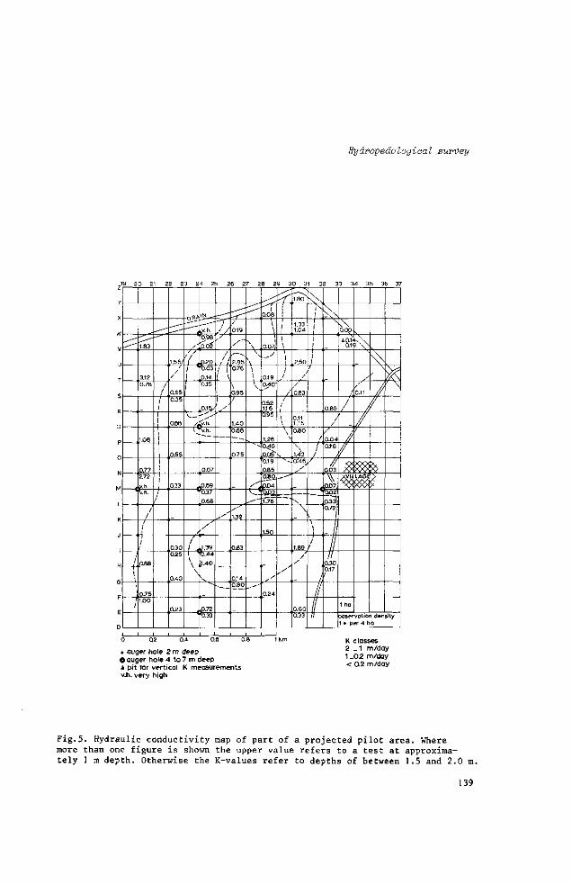
Hydropedologieal .survey
,19 20 21 22 23 24 25 26 27 28 29 30 31 32 33 34 35 36 37
u
T
S
P
L
K
/ / \ 1
/
1.83
3.12 0.78
1.08
0.77 2.72
.v.h.
U. / /
1
1
• ._ 0,88
0.75 1.00
/
I
/
1.56/
/ / 0.55 0.35
0.88
0.55
0.33
030 0.25
0.40
0.?3
r 0 £ i
/'
I
I
\N -
v.h. 0.98
0.20 0.03
0.14 0.15
0.1!},
y.h.
Y-
/
\
0.07
0.69 03 / 0.68
/' J.39 0.44
?.40
.
,0.72 TO.33
/ / S
/ 11 l !
• /
—
—
0.19
y
,—-s
2.85 0./6
0.95
/ 1.40 0.68
0.75
1.32
0.83
0.14 0.80
N
\ \ \
0.08
\ \ 0.07, _J
0.19 0^40
052 1.16 0.9b
1.26 SO46
lo.05~ T0.19 lo65 TOBO.
^ • ' ip j04
-^'
JUXL
150
a24
I I
1 I 1 \ \
1
; / / / /
\ \ \ \
-"' —-
1.80
1.33 1.04
2.60
/ 0.63
0.11 1.16 OSO
\ 1.43 o:46_.
'N
\
1.89 y A. 0.60 0.33
1
/ / /
\
0.85
/ / 0.04 0.16
// °i<p3
ao7, __TQP2
. \ \ /
1
L ƒ II
0.72
-1 II
0.30 0.17
0.00
4 0 .14v \ 0.19 \ \
/ /
} '/
xyiL
1 ha
s
0.11
/
/ 1
LÄbb
' //
'/
'JIZ ' \
observation density 1 • per 4 ha
Q2 0.4
• auger hole 2 m deep O auger hole 4 to 7 m deep A pit for vertical K measurements v.h. very high
K classes 2 _ 1 m/day 1 _0.2 m/day < 0.2 m/day
Fig.5. Hydraulic conductivity map of part of a projected pilot area. Where more than one figure is shown the upper value refers to a test at approximately 1 m depth. Otherwise the K-values refer to depths of between 1.5 and 2.0 m.
139

The results of the 5 m deep borings should also make it possible to prepare
- a contour map of the impervious base (depth contours)
- a map showing any impeding layers
- a map showing any coarse sandy and gravelly layers at or below expected drain depth.
20.3.6 SOIL MOISTURE STORAGE CAPACITY
The storage capacity, i.e. the quantity of moisture that can be stored in the
soil, depends on the pore volume and the depth at which the groundwater table is
found.
The storage coefficient y - also called effective porosity or drainable pore
space - is a measure of the change in water table under given conditions of
recharge or discharge. Hence, it is a soil characteristic that must be determined
in any subsurface drainage project. Two definitions of storage coefficient are in
use, depending on the depth at which the groundwater table occurs:
. _ change in groundwater storage (AS grw) change in groundwater level (Ah)
This applies to soils in which the groundwater occurs at such a depth that fluctu
ations in the moisture content of the upper layers are transmitted to the ground
water only after long delays and with greatly reduced amplitude (Chap.22,Vol.Ill).
change in storage capacity change in moisture content (AS ) 2) y = . . = . 2-
change in groundwater level change in groundwater level (Ah)
This applies to soils in which the groundwater occurs at relatively shallow depth,
so that soil moisture fluctuations in the soil profile or the root zone of crops
are closely reflected in water table changes.
Figure 6 shows the equilibrium moisture distribution above varying groundwater
levels for two homogeneous soils, a sand and a clay. Also shown are the pF curves.
Let us consider the situation where the water table is at a depth of 100 cm. An
equilibrium moisture condition curve DEF can be constructed. If there is equili
brium in the soil profile, the suction of the soil moisture at any point above
the water table equals the height of that point above the water table. Hence the
suction at the surface is 100 cm, corresponding to pF = 2. Projecting F' into
the moisture content axis yields the associated moisture content, F. At and below
H O
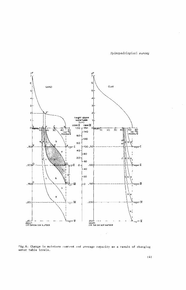
Hydvopedological survey
_250 depth cm below soil surface
250 L
depth cm below soil surface
Fig.6. Change in moisture content and storage capacity as a result of changing water table levels.
141

the water table the sand is fully saturated with 45 per cent moisture content
(point D). In this manner we can find all intermediate moisture contents, which
results in the curve DEF. The area DFSQ represents the total amount of moisture
in the 100 cm layer above the water table, while the area DBF represents the max
imum possible storage capacity if the water table were to rise to the surface.
Let us now consider the situation where the water table has dropped over a distance
Ah to a depth of 150 cm. A new equilibrium moisture condition curve GJ is now
established, whereby part GI of the curve is identical to curve DF, and conse
quently area DBF is identical to the area of GAI. The maximum possible storage is
then represented by the area GBJ.
The areas representing storages in these two situations can be divided into three
sub-areas, a, b, and c, which are always congruent when the soil is homogeneous
in a vertical direction. By lowering the water table from 100 to 150 cm, the
storage capacity is increased by the area GDFJ, which is equal to (a+b+c) and to
the area BJIA.
As the area BJIA is approximately a trapezium, one can write the second definition
of the storage coefficient as
area BJIA _ BJ + IA BJ + BF Ah 2 2
This means that y is equal to the mean soil air content at the soil surface between
the two equilibrium states (II and III). When the water table is deep, the area
BJIA approximates a rectangle, so that for a water table change of Ah
BJ x BA BJ x Ah » = — A h — " ~ T h — = BJ
or y equals the soil air content at the surface. It is clear that y is not constant
but increases with the depth of the groundwater table. However, for water table
changes at depths below 150 cm, y may be taken as a constant value.
Peculiar effects can occur when nearly full capillary soil pores reach to the
soil surface and water tables are at very shallow depths. In such a situation y
will be almost zero and a small excess of precipitation will cause the water
table to rise to the soil surface or very nearly so. Similarly, a small net eva
poration of just a few millimetres may cause the water table to drop several tens
of centimetres.
142
Hydropedologiaal survey
As was shown in Table 1, determining the storage capacities of soils is part of
a soil drainage study, usually concerned with the layers between 0.30 and 1.20 m
below soil surface. This means that a conventional soil map can indicate the pro
per sites to collect undisturbed core samples. Methods of determining typical or
average pF curves of samples are described in Chap.23,Vol.III. The drainable pore
space V can also be measured in a pilot field, but this is only possible if the
water table is not too deep and if all the terms of the water balance are known
quantities (Chaps.22 and 26,Vol.III).
20.3.7 SOIL MOISTURE RETENTION
For soils which show stratification, as many alluvial soils do, there is only one
practical way to obtain a reliable picture of the available water content of the
rootzone; this is at the same time the least sophisticated way. Briefly the method
is as follows:
Close off with planks an area of about 1 m or use a cylindrical section of a
large oil drum. Apply about 15 cm of water (the quantity of water can be adjusted
in line with the desired depth of investigation; dry soil with 50 per cent moisture
retention will be wetted 30 cm deep by 15 cm of water). Note the time required
for infiltration. Cover the surface with plastic film or any other material such
as straw to prevent evaporation. Return after two days, early in the morning if
the days are hot and dry, and take samples at several depths, depending on the
stratification or soil horizons of the profile. Weigh the filled containers soon
after sampling and have the oven-dry weight and the wilting point determined in
the laboratory (Chap.23,Vol.Ill). If one wishes to express the soil moisture
content on a volumetric basis, the bulk density of the core samples must first
be determined (Chap.2,Vol.I).
As a general guideline for irrigation projects, VAN BEERS (1972) suggested the
following rating of total available water capacity for the rootzone:
Class Total available water capacity in mm
favourable more than 150 moderate 150 - 100 marginal not less than 90 mm in the rootzone lower limit not less than 50 mm in the upper 60 cm of depth
The quantity of moisture available in the soil is closely related to soil com
position and structure. SALTER and WILLIAMS (1965; 1967), SALTER et al.(1966),
PETERSEN et al.(1968), PIDGEON (1972) and others have all established relationships
143
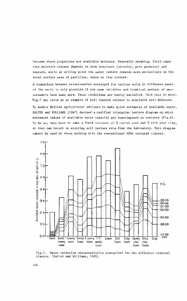
between these properties and available moisture. Generally speaking, field capa
city moisture content depends on both structure (porosity, pore geometry) and
texture, while at wilting point the water content depends more exclusively on the
total surface area of particles, hence on clay content.
A comparison between relationships developed for various soils in different parts
of the world is only possible if the same variables and identical methods of mea
surements have been used. These conditions are rarely satisfied. With this in mind,
Fig.7 may serve as an example of soil texture related to available soil moisture.
To enable British agricultural advisors to make quick estimates of available water,
SALTER and WILLIAMS (1967) devised a modified triangular texture diagram on which
estimated values of available water capacity are superimposed as contours (Fig.8).
To do so, they have to make a field estimate of % coarse sand and % silt plus clay,
or they can resort to existing soil texture data from the laboratory. This diagram
cannot be used by those working with the conventional USDA textural classes.
I -6t—
1 - 4 -
1 - 2 -
1-0 -
0-8 -
0-6 -
S <u •Z 0-4
> <
0-2
0 0
F.C.
-00-33 -00-66 " 0 1 0 0 -02-00
Sand Sand / Loamy Sandy F.sandy V.F. Loam Silt Clay Sandy Silty Clay loamy sand loam loam sandy loam loam clay clay sand loam loam loam
-0400
-0800
15-00 atm
Fig.7. classes.
Water retention characteristics summarized for the different textural (Salter and Williams, 1965)
144

Hydropedologiaal survey
100 0 V
. % 9 0 , ».10 <>
• 2 0 °
T-,80
V-::À-90 . . / \ / \ 7-W \ / \ / \ / \ ' '
oi v 100 90 80 70 60 50 40 30 20 10 O
fine sand °/o ( 0.2.0.02 mm )
Fig.8. Modified triangular co-ordinate diagram. The estimated values of AWC (available water capacity) are superimposed as contours (broken lines) at intervals of 0.5 in./ft. depth. Contours are based on the regression equation: AWC (in./ft.) = 2.17-0.018 (% coarse sand) + 0.0072 (% fine sand). 1 inah/foot= 8.33 vol.%. (Salter and Williams, 1967).
20.3.8 SALINE AND ALKALI SOILS
Salinization of soils may be caused in different ways and under different climato-
logical conditions (Chap.3,Vol.I) , but the main cause is usually poor drainage.
In arid and semi-arid regions salinity symptoms may not always be due to present
poor drainage but could be a result of poor drainage in the geological past.
If saline or alkali soils are suspected, the hydropedologist should give due
attention to
- degree of present soil salinity, if any. This is measured in terms of EC
values for each of the various layers (USDA Handbook 60, 1954)
- severity of present alkali conditions, if any. The concentrations of Na,
Ca, and Mg in the saturation extract are measured for each of the various layers,
and the SAR-values calculated. ESP-values can be determined or estimated from the
SAR-values (USDA Handbook 60, 1954)
- all available field clues as to the source of the salts, the local proces
ses of salinization, and whether these processes are still active and possibly
intensifying, or whether one is dealing with fossil phenomena.
145
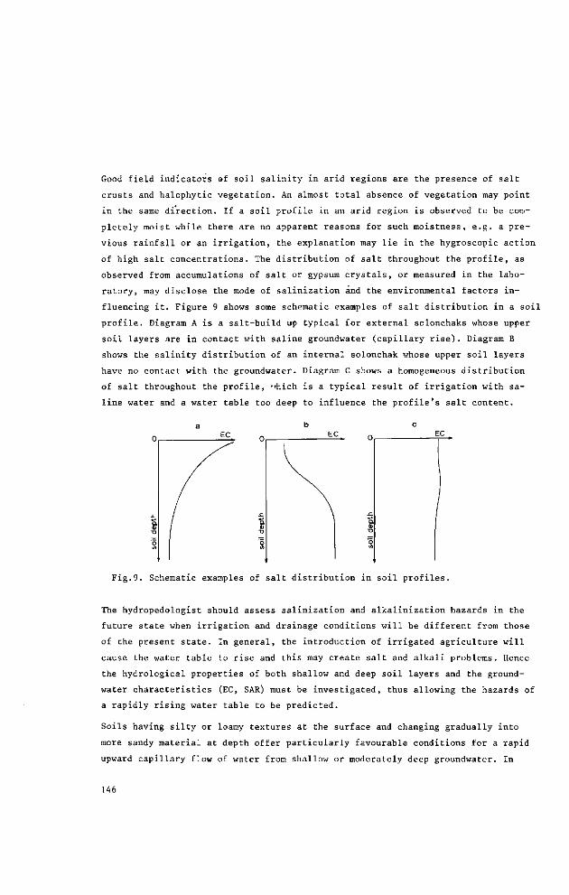
Good field indicators of soil salinity in arid regions are the presence of salt
crusts and halophytic vegetation. An almost total absence of vegetation may point
in the same direction. If a soil profile in an arid region is observed to be com
pletely moist while there are no apparent reasons for such moistness, e.g. a pre
vious rainfall or an irrigation, the explanation may lie in the hygroscopic action
of high salt concentrations. The distribution of salt throughout the profile, as
observed from accumulations of salt or gypsum crystals, or measured in the labo
ratory, may disclose the mode of salinization and the environmental factors in
fluencing it. Figure 9 shows some schematic examples of salt distribution in a soil
profile. Diagram A is a salt-build up typical for external solonchaks whose upper
soil layers are in contact with saline groundwater (capillary rise). Diagram B
shows the salinity distribution of an internal solonchak whose upper soil layers
have no contact with the groundwater. Diagram C shows a homogeneous distribution
of salt throughout the profile, ''hich is a typical result of irrigation with sa
line water and a water table too deep to influence the profile's salt content.
EC
Fig.9. Schematic examples of salt distribution in soil profiles.
The hydropedologist should assess salinization and alkalinization hazards in the
future state when irrigation and drainage conditions will be different from those
of the present state. In general, the introduction of irrigated agriculture will
cause the water table to rise and this may create salt and alkali problems. Hence
the hydrological properties of both shallow and deep soil layers and the ground
water characteristics (EC, SAR) must be investigated, thus allowing the hazards of
a rapidly rising water table to be predicted.
Soils having silty or loamy textures at the surface and changing gradually into
more sandy material at depth offer particularly favourable conditions for a rapid
upward capillary flow of water from shallow or moderately deep groundwater. In
146
Hydropedologïcai survey
arid climates such soils easily develop salinity problems. If there are significant
areas of such soils within a project area they should be mapped.
The gypsum content of the rootzone should be determined because this mineral yields
the Ca which is essential for the reclamation of alkali soils. The soils in arid
climates generally contain gypsum but the hydropedologist should find out whether
there is enough of it in the rootzone to replace a harmful excess of Na. In
semi-arid to sub-humid climates the soils rarely contain sufficient gypsum, so
that special applications are required to prevent the soil structure from deterio
rating.
For a similar reason it is useful to determine the calcium carbonate content of
a soil, particularly if the soil contains no gypsum.
Saline clays containing much montmorillonite are difficult to leach, so it is a
good idea to investigate the clay mineral composition of soils. The salt content
and the Ca/Na ratio of irrigation water used for the leaching of soluble salts
must be known as these qualities affect the drainage criteria. Water that is highly
mineralized has to be applied in greater quantities, so more water will have to be
discharged by the drainage system (Chap.9 ,Vol.II).
Concerning salinization, it is worthwhile to mention that a given regional or
local climate is not identical with the "soil climate" in the same area. In soils
with surface sealing, hardly any water will percolate, but there will be. a great
deal of surface runoff; even if rainfall is adequate, capillary rise from shallow
groundwater will cause (re-)salinization of the topsoil.
20.3.9 LAND SUBSIDENCE AND SOIL RIPENING
Drainage of peat soils and muddy sediments poses specific problems, which are
discussed in detail in Chap.32,Vol.IV. When such soils are drained, this is accom
panied by substantial water losses, an increase in effective stresses, and the
oxidation of organic matter by biochemical action. This results in the land surface
subsiding, which affects the functioning, economics, and hence the design of the
entire drainage system. Irreversible drying of the top layer of peat soils may
form an accessory agricultural problem which also affects the drainage design
because, to prevent it or to cure it, very close control of the water table is
required. If sulphides are present in excess of calcium, their oxidation results
in extreme soil acidity.
147
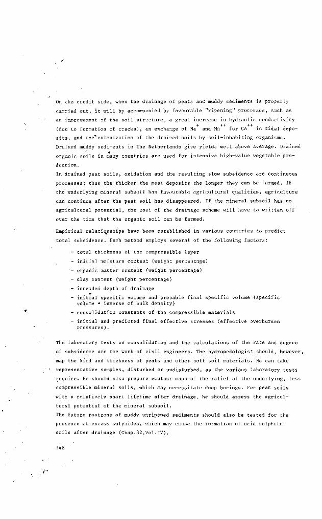
On the credit side, when the drainage of peats and muddy sediments is properly
carried out, it will by accompanied by favourable "ripening" processes, such as
an improvement of the soil structure, a great increase in hydraulic conductivity
+ ++ ++ .
(due to formation of cracks), an exchange of Na and Mn for Ca in tidal depo
sits, and the1* colonization of the drained soils by soil-inhabiting organisms..
Drained muddy sediments in The Netherlands give yields well above average. Drained
organic soils in many countries are used for intensive high-value vegetable pro
duction.
In drained peat soils, oxidation and the resulting slow subsidence are continuous
processes; thus the thicker the peat deposits the longer they can be farmed. If
the underlying mineral subsoil has favourable agricultural qualities, agriculture
can continue after the peat soil has disappeared. If the mineral subsoil has no
agricultural potential, the cost of the drainage scheme will have to written off
over the time that the organic soil can be farmed.
Empirical relationships have been established in various countries to predict
total subsidence. Each method employs several of the following factors:
- total thickness of the compressible layer
- initial moisture content (weight percentage)
- organic matter content (weight percentage)
- clay content (weight percentage)
- intended depth of drainage
- initial specific volume and probable final specific volume (specific volume = inverse of bulk density)
- consolidation constants of the compressible materials
- initial and predicted final effective stresses (effective overburden pressures).
The laboratory tests on consolidation and the calculations of the rate and degree
of subsidence are the work of civil engineers. The hydropedologist should, however,
map the kind and thickness of peats and other soft soil materials. He can take
' representative samples, disturbed or undisturbed, as the various laboratory tests
require. He should also prepare contour maps of the relief of the underlying, less
compressible mineral soils, which may necessitate deep borings. For peat soils
with a relatively short lifetime after drainage, he should assess the agricul
tural potential of the mineral subsoil.
The future rootzone of muddy unripened sediments should also be tested for the
presence of excess sulphides, which may cause the formation of acid sulphate
soils after drainage (Chap.32,Vol.IV).
148
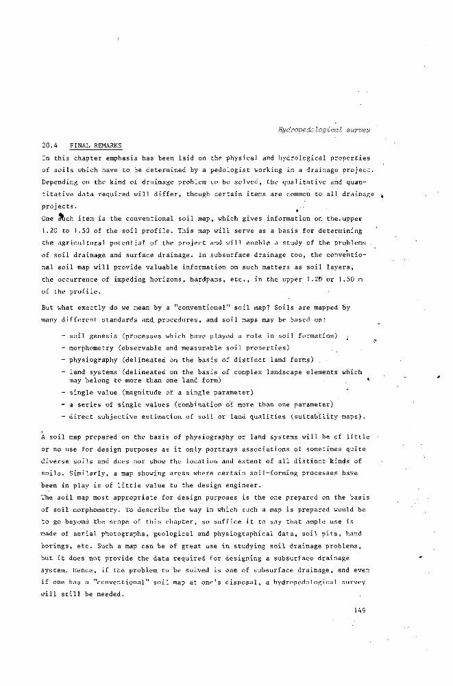
Hydropedological survey
20.4 FINAL REMARKS
In this chapter emphasis has been laid on the physical and hydrological properties
of soils which have to be determined by a pedologist working in a drainage project.
Depending on the kind of drainage problem to be solved, the qualitative and quan
titative data required will differ, though certain items are common to' all drainage
projects.
One sTich item is the conventional soil map, which gives information on the. upper
1.20 to 1.50 of the soil profile. This map will serve as a basis for determining
the agricultural potential of the project and will enable a study of the problems
of soil drainage and surface drainage. In subsurface drainage too, the conventio
nal soil map will provide valuable information on such matters as soil layers,
the occurrence of impeding horizons, hardpans, etc., in the upper 1.20 or 1.50 m
of the profile.
But what exactly do we mean by a "conventional" soil map? Soils are mapped by
many different standards and procedures, and soil maps may be based on:
- soil genesis (processes which have played a role in soil formation)
- morphometry (observable and measurable soil properties)
- physiography (delineated on the basis of distinct land forms)
- land systems (delineated on the basis of complex landscape elements which may belong to more than one land form) *
- single value (magnitude of a single parameter)
- a series of single values (combination of more than one parameter)
- direct subjective estimation of soil or land qualities (suitability maps).
A soil map prepared on the basis of physiography or land systems will be of little
or no use for design purposes as it only portrays associations of sometimes quite
diverse soils and does not show the location and extent of all distinct kinds of
soils. Similarly, a map showing areas where certain soil-forming processes have
been in play is of little value to the design engineer.
The soil map most appropriate for design purposes is the one prepared on the basis
of soil morphometry. To describe the way in which such a map is prepared would be
to go beyond the scope of this chapter, so suffice it to say that ample use is
made of aerial photographs, geological and physiographical data, soil pits, hand
borings, etc. Such a map can be of great use in studying soil drainage problems,
but it does not provide the data required for designing a subsurface drainage
system. Hence, if the problem to be solved is one of subsurface drainage, and even
if one has a "conventional" soil map at one's disposal, a hydropedological survey
will still be needed.
149

LITERATURE
AL IM, M.M., RAFIQ CHOUDRY, M. and BRINKMAN, R. 1971. Land capability classifica
tion in West Pakistan. Project Tech.Guide 11, Soil Survey Proj.of Pakistan,
Lahore. 10 pp.
ALLEN, J.B. and BRAUD, H.J.jr. 1966. Effect of cracks and initial moisture content
on the infiltration rate of Sharkey clay. Bull.Louisiana Agric.Exp.Sta.613,
27 pp.
ANDERSON, J.L. and BOUMA, D. 1973. Relationships between saturated hydraulic
conductivity and morphometric data of an argillic horizon. Soil Sci.Soc.
Am.Proc.37:408-41 3.
BERTRAND, A.R. 1965. Rate of water intake in the field. In: Methods of Soil
Analysis. (Ed.C.A.Black). Am.Soc.Agr.Monogr.9, Part I, Ch.12, 197-209.
BOEKEL, P. 1965. Karakterisering van de slempigheid van zavelgronden door bepa
ling van de consistentie. Landbouwk.Tijdschr.77 :306-311.
BOUMA, D., and HOLE, F.D. 1971. Soil structure and hydraulic conductivity of
adjacent virgin and cultivated pedons at two sites: A typic Argiudoll (silt
loam) and a Typic Eutrochrept (clay). Soil Sei.Soc.Am.Proc.35 :316—319.
BURINGH, P., STEUR, G.CL. and VINK, A.P.A. 1962. Some techniques and methods
of soil survey in The Netherlands. Netherlands J.Agric.Sei.10:157-172.
DE BAKKER, H. 1973. Hydromorphic soils in the system of soil classification for
The Netherlands. Trans.Int.Conf.on Pseudogley and Gley, Stuttgart-Hohenheim,
1971, 405-412.
DIELEMAN, P.J. and DE RIDDER, N.A. 1963. Studies of salt and water movement in
the Bol Guini Polder, Chad Republic. J.Hydrol.1:311-343.
EMERSON, W.W. 1967. A classification of soil aggregates based on their coherence
in water. Aust.J.Soil Res.5:47-57.
FAO. 1971. Etablissement et opérations d'une station pilote d'irrigation dans
la plaine du Danube, Roumanie. Drainage horizontal. Rapport Technique 3 par
P.J.Dieleman et W.Genet. Bucarest 1971.
RAISE, H.R., D0NNAN, W. et al. 1956. The use of cylinder infiltrometer to deter
mine the intake characteristics of irrigated soils. Agric.Res.Serv. and Soil
Cons.Serv. USDA, Washington, D.C
150

llydropedological survey
HORN, M.E. 1971. Estimating soil permeability rates. J.Irrig.Drain.Div., Proc.
A.S.C.E., Vol.97, No.IR 2:263-274.
KALLSTENIUS, T. 1963. Some "structure-forming" processes in clay deposits.
Swedish Geotech.Inst.Proc.No.21, 210 pp.
KEMPER, W.D. and KOCH, E.J. 1966. Aggregate stability of soils from Western
United States and Canada. A.R.S., U.S.D.A., Tech.Bull.1355, 52 pp.
PETERSEN, G.W., CUNNINGHAM, R.L. and MATELSKI, R.P. 1968. Moisture characteristics
of Pennsylvania Soils. I. Moisture retention as related to texture. Soil
Sei.Soc.Am.Proc.32:271-275.
PIDGEON, J.D. 1972. The measurement and prediction of available water capacity
of ferrallitic soils in Uganda. J.Soil Sei.23 :431—441.
RICKARD, D.S. and COSSENS, G.G. 1966. Irrigation investigations in Otago, New
Zealand. I. Description, and physical properties of irrigated soils of the
Ida Valley. N.Z.J.Agric.Res.9 : 197-217.
SALTER, P.J. and WILLIAMS, J.B. 1965. The influence of texture on the moisture
characteristics of soils. II.Available-water capacity and moisture release
characteristics. J.Soil Sei.16:310-317.
SALTER, P.J., BERRY, G. and WILLIAMS, J.B. 1966. The influence of texture on the
moisture characteristics of soils. III. Quantitative relationships between
particle size, composition, and available-water capacity. J.Soil Sei.17:93-98.
SALTER, P.J. and WILLIAMS, J.B. 1967. The influence of texture on the moisture
characteristics of soils. IV. A method of estimating the available water
capacities of profiles in the field. J.Soil Sei.18 :174-181.
SCHELLING, J. 1960. New aspects of soil classification with particular reference
to reclaimed hydromorphic soils. Proc.7th Int.Congress Soil Sei., Part V,
218-224.
SOIL CONSERVATION SERVICE. 1964. National Engineering Handbook. Sec.15: Irrigation.
Chap.1: Soil-plant-water relationships. 72 pp.
SOIL SURVEY MANUAL. 1951. U.S.D.A.Handbook 18, 503 pp.
U.S.SALINITY LABORATORY STAFF. 1954. Diagnosis and Improvement of saline and
alkali soils. U.S.D.A.Agr.Handbook 60, 160 pp.
VAN BEERS, W.F.J. 1973. Private communication.ILRI, P.O.B.45, Wageningen.
151

VAN BEERS, W.F.J. 1972. A reconnaissance survey of the L.S.D.condition of irriga
tion projects (land surface-soil profile-subsurface drainage). Unpublished
draft. ILRI.
VAN HEESEN, H.G. 1970. Presentation of the seasonal fluctuation of the water table
on soil maps. Geoderma 4:257-278.
WILLIAMS, R.J.B. 1963. A new method for determining aggregate stability. Chemi
stry & Industry 25:1032-1033.
ZIMMERMAN, J.D. 1966. Irrigation. John Wiley & Sons, New York. 516 pp.
152

SURVEYS AND INVESTIGATIONS
2 1 .GROUNDWATER SURVEY
N. A. DE RIDDER
Geohydrologist International Institute for Land Reclamation and Improvement Wageningen
Lecturers in the Course on Land Drainage
L. WARTENA (1962) N.V. Heidemij Beheer, Research Department
J. KESSLER (1965-1967) International Institute for Land Reclamation and Improvement, Wageningen
N. A. DE RIDDER (1968, 1970-1973) International Institute for Land Reclamation and Improvement, Wageningen
G. P. KRUSEMAN (1969) International Institute for Land Reclamation and Improvement, Wageningen

PURPOSE AND SCOPE
A brief account of the basic elements of a groundwater survey related to land
drainage.
CONTENTS
21.1 COLLECTION OF GROUNDWATER DATA 155
21.1.1 Preparatory study 156
21.1.2 Survey of groundwater levels 157
21.1.3 Observation network 164
21.1.4 Water level readings 165
21.1.5 Base observation networks 167
21.1.6 Water quality measurements 170
21.2 PROCESSING OF GROUNDWATER DATA 175
21.2.1 Groundwater records 175
21.2.2 Well hydrographs 177
21.2.3 Groundwater maps 177
21.3 EVALUATION OF GROUNDWATER DATA 182
21.3.1 Evaluation of hydrographs 182
21.3.2 Evaluation of groundwater contour maps 184
21.3.3 The use of flow nets 187
21.3.4 Evaluation of other types of groundwater maps 190
LITERATURE 194
154
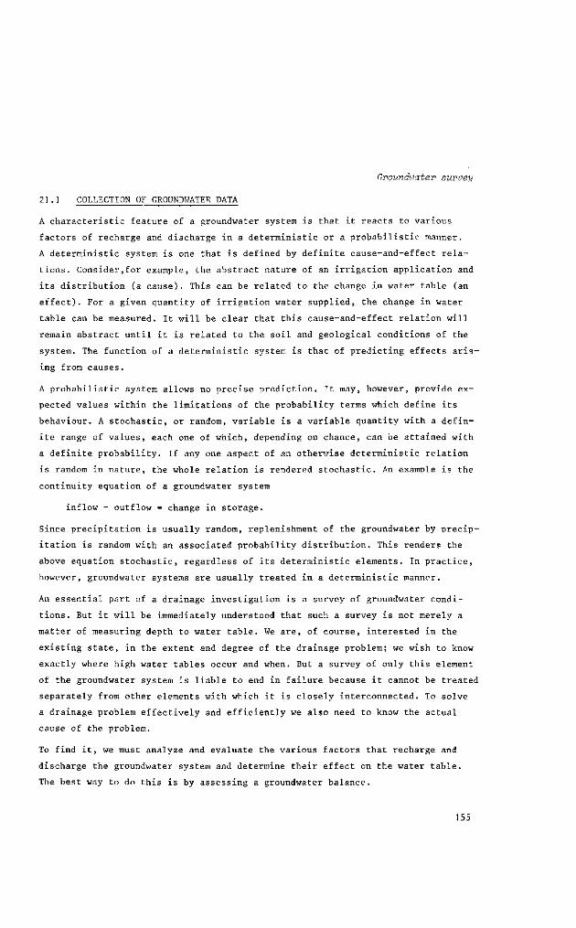
Groundwater survey
21.1 COLLECTION OF GROUNDWATER DATA
A characteristic feature of a groundwater system is that it reacts to various
factors of recharge and discharge in a deterministic or a probabilistic manner.
A deterministic system is one that is defined by definite cause-and-effeet rela
tions. Consider,for example, the abstract nature of an irrigation application and
its distribution (a cause). This can be related to the change in water table (an
effect). For a given quantity of irrigation water supplied, the change in water
table can be measured. It will be clear that this cause-and-effeet relation will
remain abstract until it is related to the soil and geological conditions of the
system. The function of a deterministic system is that of predicting effects aris
ing from causes.
A probabilistic system allows no precise prediction. It may, however, provide ex
pected values within the limitations of the probability terms which define its
behaviour. A stochastic, or random, variable is a variable quantity with a defin
ite range of values, each one of which, depending on chance, can be attained with
a definite probability. If any one aspect of an otherwise deterministic relation
is random in nature, the whole relation is rendered stochastic. An example is the
continuity equation of a groundwater system
inflow - outflow = change in storage.
Since precipitation is usually random, replenishment of the groundwater by precip
itation is random with an associated probability distribution. This renders the
above equation stochastic, regardless of its deterministic elements. In practice,
however, groundwater systems are usually treated in a deterministic manner.
An essential part of a drainage investigation is a survey of groundwater condi
tions. But it will be immediately understood that such a survey is not merely a
matter of measuring depth to water table. We are, of course, interested in the
existing state, in the extent and degree of the drainage problem; we wish to know
exactly where high water tables occur and when. But a survey of only this element
of the groundwater system is liable to end in failure because it cannot be treated
separately from other elements with which it is closely interconnected. To solve
a drainage problem effectively and efficiently we also need to know the actual
cause of the problem.
To find it, we must analyze and evaluate the various factors that recharge and
discharge the groundwater system and determine their effect on the water table.
The best way to do this is by assessing a groundwater balance.
155

Thus the main objectives of a survey of groundwater conditions that forms part of
a drainage survey can be defined as :
- determining the extent, degree, and nature of existing or potential
drainage problems
- analyzing the groundwater system and assessing a water balance from which
the cause(s) of the drainage problem may be understood
- indicating how the groundwater system can be altered artificially so that
the resulting water table will not hamper crop growth.
This chapter is devoted to the collection, processing, and evaluation of ground
water data. The subject of the assessment of groundwater balances will be treated
separately in Chapter 22, Vol.111.
21.1.1 PREPARATORY STUDY
The first step in a survey of groundwater conditions must always be a preparatory
phase. This involves:
- obtaining suitable topographical maps on as large a scale as possible:
1/10 000, 1/20 000, or 1/50 000. These maps should show contours of the land
surface. They are the essential foundation without which no accurate work can be
done. If the area under study is a large one it is also convenient to have a top
ographical map on a reduced scale, say 1/100 000. Specific information can be
transferred to such maps, which greatly facilitates studies in the office. They
are also useful for reporting because there is nothing more annoying than bunches
of maps folded ten times or more;
- obtaining air photographs which can help to make up for any shortcomings
in topographical and geological maps. These photographs may provide useful infor
mation not only on topography and geology but also on hydrogeology and vegetation
cover ;
- obtaining geological maps, showing not only the outcrops of all the geolog
ical formations but also their lithology. These maps and geological cross-sections
allow permeable and less permeable zones to be distinguished, zones of recharge,
transmission, and discharge to be delineated, and the types of aquifers to be
defined (unconfined, semiconfined, Fig.1). From this information the type of land
scape can be determined and thus, in general, the groundwater conditions that can
be expected (see Chapter 1, Vol.1).
156
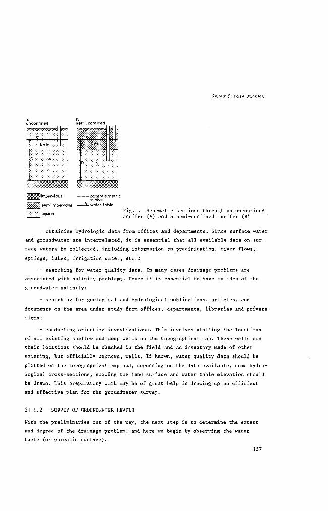
GvounâwateT survey
A unconfined semi-confined
^ impervious
\ semi impervious
1 aquifer
- Potentiometrie surface
- water table Fig.1. Schematic sections through an unconfined aquifer (A) and a semi-confined aquifer (B)
- obtaining hydrologie data from offices and departments. Since surface water
and groundwater are interrelated, it is essential that all available data on sur
face waters be collected, including information on precipitation, river flows,
springs, lakes, irrigation water, etc.;
- searching for water quality data. In many cases drainage problems are
associated with salinity problems. Hence it is essential to have an idea of the
groundwater salinity;
- searching for geological and hydrological publications, articles, and
documents on the area under study from offices, departments, libraries and private
firms ;
- conducting orienting investigations. This involves plotting the locations
of all existing shallow and deep wells on the topographical map. These wells and
their locations should be checked in the field and an inventory made of other
existing, but officially unknown, wells. If known, water quality data should be
plotted on the topographical map and, depending on the data available, some hydro-
logical cross-sections, showing the land surface and water table elevation should
be drawn. This preparatory work may be of great help in drawing up an efficient
and effective plan for the groundwater survey.
21.1.2 SURVEY OF GROUNDWATER LEVELS
With the preliminaries out of the way, the next step is to determine the extent
and degree of the drainage problem, and here we begin by observing the water
table (or phreatic surface).
157
As was mentioned in Chapter J, Vol.1, agricultural land or land that is to be
reclaimed is usually made up of a fine-textured layer whose thickness may vary
from less than 1 m to several metres. Sandy material containing groundwater is
often present underneath this layer and such groundwater may or may not be under
pressure (semiconfined aquifer, Fig.1). If under pressure, the hydraulic head
of the groundwater confined within this sand layer should be observed as well.
For a survey of groundwater levels, observations are made in:
- existing (village) wells
- open bore holes
- piezometers
- surface waters (lakes, streams, canals, etc.).
Existing wells
Existing wells offer ready-made sites for groundwater level observations. In most
villages and on scattered farms or ranches one or more such wells can usually be
found. Although their location may not always fit satisfactorily into the desired
network of observation points (they may be sited on topographical heights only)
it is most useful to include them in the network as they are cheap means of achiev
ing our objective.
It should be noted, however, that a major problem of these wells is the validity
of the observations obtained from them. If the well is hand-dug by the local far
mer, we may be quite certain that the water level measured in the well indeed
represents the water table. Because of its construction by hand the depth of these
wells will seldom be more than about one metre below the lowest water table.
Before the well is included in the network this should, of course, be checked.
Hand-dug wells have a large diameter and thus a large storage capacity. This im
plies that it may take considerable time for the water level in the hole to ad
just to changes of the water table, or to recover when water has been taken from
it in substantial quantities, especially if the hydraulic conductivity of the
water-bearing material is low. Water level readings taken shortly after water has
been withdrawn from such a well are not valid.
A special problem arises if the existing well has been bored or drilled. This type
of well usually has a much greater depth than a hand-dug well. It may penetrate
several aquifers separated from one another by clay layers. Such wells are provid
ed with a casing in which a perforated pipe or screen is fitted at the various
depths where the aquifers occur. Other wells may have casings perforated from top
158
Groundwater survey
to bottom. The water level in these wells certainly does not represent the water
table, but a composite of the various hydraulic heads occurring in the different
aquifers. It must be emphasized therefore that if such wells are used the obser
vations taken from them may not be valid.Before any existing well is included in
the network, information on its depth, type of penetrated layers, casing and
screen should be collected. Only then is it possible to conclude whether the well
penetrates an unconfined aquifer (in which case it may provide valid information
on the water table) or a semiconfined aquifer, or a multiple aquifer system (in
which case it will provide no valid information on the water table).
Open bore holes
Open bore holes without any casing or screen can sometimes be used for watertable
observations. These holes can easily be made with a hand auger as used in soil
surveys, and may be 2 to 3 in. in diameter. The holes should be bored deep enough,
i.e. a few decimetres below the lowest expected watertable depth. Care should be
taken that the holes are provided with a reference point that remains in place
and cannot easily be destroyed. Water table readings are taken from this point,
hence its absolute elevation and elevation above the average land surface should
be measured by a geodetic team. For this purpose a system of bench marks should
be established in the area because contour lines of the land surface are values
too rough to be used for accurate work.
Open bore holes are cheap means of measuring watertable depths. There are, however,
a few troublesome factors. They can easily be destroyed by vandalism. The hole
must therefore be hidden to the eye. Secondly, open bore holes may soon collapse,
especially if they penetrate fine sands. Deepening the hole below the water table
is often impossible because of the movement of these fine sands. In such circum
stances, the hole can only be deepened by installing a casing and using a bailer
to remove the sand. No heavy equipment is needed for this purpose; for holes 2 to
k m deep, thick-walled plastic tubes 3 in. in diameter can be used as casing.
Before the casing is removed, a plastic pipe, 1 or 2 in. in diameter and perfora
ted over the lower 0.3 to 0.5 m, is installed inside the casing (see below).
Piezometers
Piezometers are open-ended pipes driven or jetted into the ground to the depth
at which the hydraulic head is to be measured. The water level in the pipe cor
responds with the hydraulic head at the pipe's lower end. The diameter of the pipe
may vary from 1 to 3 in.
159

When piezometers are used, the following points should be taken into considera
tion. In a homogeneous unconfined aquifer, vertical flow components are usually
lacking or of such minor importance that they can be neglected. Hence at any depth
in an unconfined aquifer, the hydraulic head corresponds to the watertable height
(phreatic level); in other words, in measuring the water table it does not make
any difference how far the piezometer penetrates into the aquifer.
The hydraulic head of the water confined within a homogeneous semiconfined aquifer
usually differs from the head of the phreatic water in the overlying confining
layer. Since it is generally assumed that the flow of groundwater through a semi-
confined aquifer is essentially horizontal and that vertical flow components can
be neglected, the distribution of the head in such an aquifer is essentially the
same everywhere in a vertical plane. The depth to which a piezometer penetrates
into a semiconfined aquifer is therefore of little importance, although its bot
tom end should not be placed too close to either the overlying or underlying clay
bed because of possible leakage effects.
If the hydraulic head in a semiconfined aquifer is higher or lower than the head
of the phreatic water in the overlying semipervious layer, there is an upward or
downward flow through this layer away from or towards the aquifer. The water level
in a piezometer which penetrates into the semipervious covering layer is a
function of its depth of penetration because the flow direction in this layer is
mainly vertical (Fig.2). To measure the water table, the piezometer should there
fore penetrate not more than a few centimeters into the saturated zone; but since
water tables are usually changing during the course of the year, this procedure
is not practical: if the water table is dropping the piezometer will soon fall
dry. For practical purposes, piezometers are therefore, placed somewhat deeper,
i.e. just below the lowest expected watertable depth.
To ensure that the piezometer functions properly, the lower 0.5 m of the nipe may
be perforated. To prevent fine soil particles from entering the pipe or clogging
the tiny holes, some jute or cotton is wrapped around the perforated part and the
lower open end sealed with a plug. The pipe is then placed in the centre of a
bore hole and, over the whole length of the perforated part, the annular space
(space between pipe and wall of the hole) is filled with artificially graded fine
gravel or coarse sand. This gravel pack facilitates the flow of water from the
soil into the pipe and vice versa. The remainder of the annular space is then
carefully filled with fine material (clay, clayey fine sand) whose permeability
is low to prevent leakage along the pipe.
160
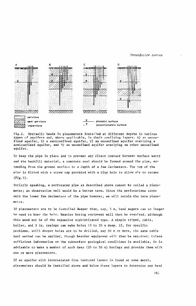
Crvounâhiatev survey
[; ; ;-;-;-; ;-| pervious X/////\ semi pervious
impervious
B
m v/y//,
fi WA
phreatic surface — Potentiometrie surface
Fig.2. Hydraulic heads in piezometers installed at different depths in various types of aquifers and, where applicable, in their confining layers. A) an uncon-fined aquifer, B) a semiconfined aquifer, C) an unconfined aquifer overlying a semiconfined aquifer, and D) an unconfined aquifer overlying an other unconfined aquifer.
To keep the pipe in place and to prevent any direct contact between surface water
and the backfill material, a concrete seal should be formed around the pipe, ex
tending from the ground surface to a depth of a few decimeters. The top of the
pipe is fitted with a screw cap provided with a tiny hole to allow air to escape
(Fig.3).
Strictly speaking, a perforated pipe as described above cannot be called a piezo
meter; an observation well would be a better term. Since the perforations cover
only the lower few decimeters of the pipe however, we will retain the term piezo
meter.
If piezometers are to be installed deeper than, say, 5 m, hand augers can no longer
be used to bore the hole. Heavier boring equipment will then be required, although
this need not be of the expensive sophisticated type. A simple tripod, cable,
bailer, and 3 in. casings can make holes 10 to 20 m deep. If, for specific
problems, still deeper holes are to be drilled, say 50 m or more, the same cable
tool method can be applied, though heavier equipment will then be required. Unless
sufficient information on the subsurface geological conditions is available, it is
advisable to make a number of such deep (20 to 50 m) borings and provide them with
one or more piezometers.
If an aquifer with intercalated fine textured layers is found at some depth,
piezometers should be installed above and below these layers to determine any head
161

gtr escape
completion
jute cover
ravel pack
sand trap
Fig.3. Schematic cross-section through a piezometer.
differences that may exist (Fig.4). Since the diameter of such deep borings is
larger than that of hand borings, perforated clay layers should be properly sealed
with bentonite or fine sandy loam to prevent leakage along the outside of the
piezometer. If the diameter of the bore hole is sufficiently large, several piezo
meters can be placed at different depths in the same hole; here again it is essen
tial that the piezometers be properly isolated.
Surface waters
A survey of the water table is incomplete if the levels of the surface waters that
are in free connection with the groundwater are neglected. The water of a stream
is either fed by the groundwater, the stream thus acting as a drainage channel
(effluent stream), or the stream is feeding the groundwater, in which case it acts
as a recharge channel (influent stream), see Figure 5.
Water levels of streams or other water courses represent local mounds or depres
sions in the water table and consequently are of great importance in a survey
of groundwater conditions. A number of staff gauges should therefore be installed
in these water courses and their absolute elevation measured.
If the water table lies below the bottom of the stream, the water level of the
stream does not represent any point of the groundwater table. The stream is then
losing water that percolates through the unsaturated zone to the deep water table.
162
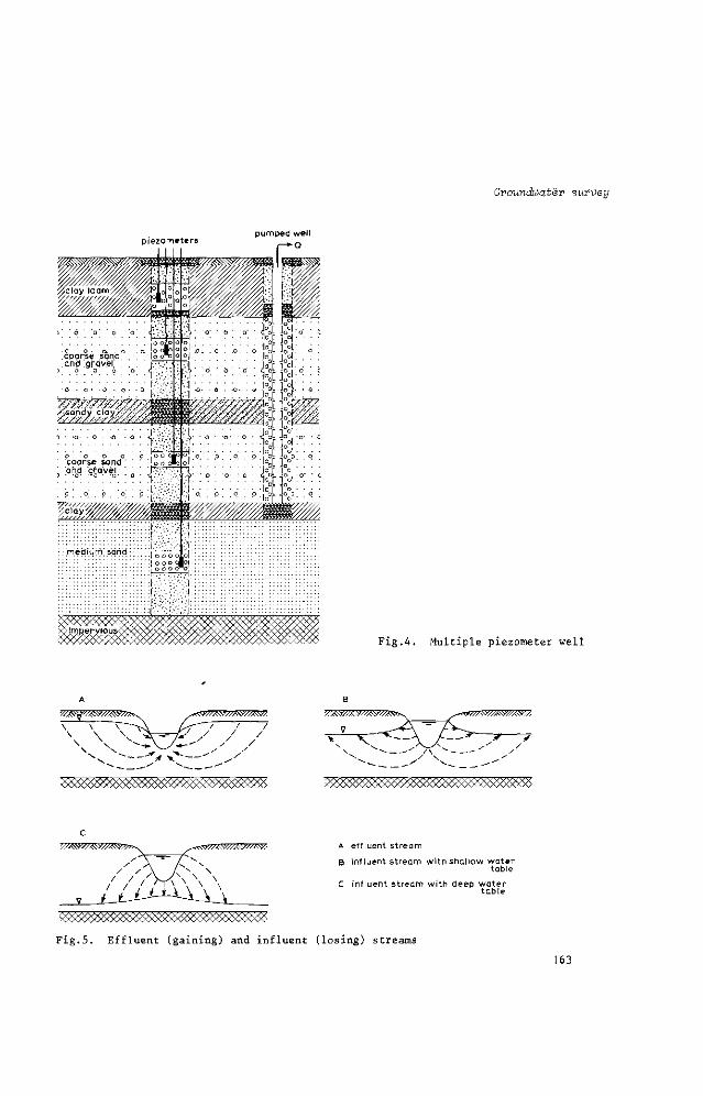
Groundwater survey
piezometers pumped well
O
F i g . 4 . Mul t ip le p iezometer wel l
y//&tf//4m»& V/^V///W/AVx
« Ä Ä W 5 ! » ^ - « W / A W Ä « A effluent stream B influent stream with shallow water
table
C influent stream with deep water table
Fig.5. Effluent (gaining) and influent (losing) streams
163
It thus recharges the groundwater system and a local mound is built up under the
channel. In such a situation the'-e is no need for a staff gauge in the channel
but a piezometer should be installed on its banks.
21.1.3 OBSERVATION NETWORK
A network of observation points provides data on the elevation and variation of
the water table and Potentiometrie surface. These data can be used to determine:
- the configuration of the water table and the Potentiometrie surface
- the direction of the groundwater movement
- the location of recharge and discharge areas.
It will therefore be clear that in planning an observation network an optimal
lay-out of the observation points i.e. one that provides maximum information at
minimum costs, must be the aim. Too many points are as undesirable as too few,
and what counts even more is their proper siting.
The lay-out of an observation network should therefore be based on any information
on topography, geology, hydrology, soils, etc. collected and studied during the
preparatory phase. Observation points will be required (Fig.6):
- along and perpendicular to lines of expected groundwater flow,
- at locations where changes in the slope of the water table (or the Poten
tiometrie surface) can be expected,
- in areas where significant changes in watertable elevation are likely to
occur,
- on the banks of streams and other open water courses and along lines per
pendicular to them, to determine the proper curving of the water table near such
water courses,
- in areas where shallow water tables occur or can be expected in the future
(for example in areas with a relatively high intensity of irrigation, or in seep
age zones).
With regard to the density of the observation network, no strict rule can be given
as this depends entirely on the topographical, geological, and hydrological condi
tions of the area under study, and on the type of survey (reconnaissance,detailed).
As the required accuracy is generally inversely proportional to the size of
The word Potentiometrie replaces the formerly used but incorrect term piezo— metric in such phrases as piezometric head, piezometric surface, in accordance with the recommendations made in U.S.Geol.Survey, Water Supply Paper No.1988, Lohman et al.
164

Groundwater survey
B
Fig.6. Lay-out of a piezometer network for expected groundwater conditions. A: incorrect, B: correct.
the area, the following relation may serve as a rough guide:
Size of area under study
100 ha
1,000 ha
10,000 ha
100,000 ha
number of observ ation points
20
40
100
300
number of observation points per 100 ha
20
4
1
0.3
The spacing of observation points may be increased as they are farther removed
from lines of recharge or discharge (e.g. streams or canals) in approximately
the following sequence: 30, 40, 100, 250, and 500 m, etc., with a maximum of
2000 to 3000 m.
As was mentioned in Chapter 6, Vol.1, groundwater flow problems cannot be solved
unless it is known what happens at the boundaries of the flow system. An observa
tion network must therefore extend somewhat beyond the boundaries of the area
under study so as to determine qualitively and quantitively any inflow from and
outflow to adjacent areas.
21.1.4 WATER LEVEL READINGS
Water level measurements are always taken from a reference point, for example,
the rim of a piezometer or, if hand-dug wells are used, a mark on the wall of the
hole. The height of the reference point above or below the ground surface and its
absolute elevation above or below mean sea level must be known. All waterlevel
observation data can then be converted into:
- depth below ground surface
- absolute elevation above or below mean sea level.
165
Equipment
Water level measurements can be taken in various ways:
- Wetted tape method: A chain or steel tape (with calibration in millimetres)
to which a weight is attached, is lowered into the pipe or bore hole to below the
water level. The lowered length of chain from the reference point is noted. The
chain is then pulled up and the length of its wetted part measured (this is
facilitated by chalking the lower part of the chain). When the wetted length is
subtracted from the total lowered length, this gives the depth to the water level
below the reference point (Fig.7A).
- With a mechanical sounder, consisting of a small piece of steel or copper
tube (0.5 to 1 in. in diameter and 2 to 3 in. long) which is closed at its upper
end and connected to a calibrated steel tape or to a chain. When lowered into the
pipe it produces a characteristic sound upon hitting the water. The depth to the
water level can be read directly from the steel tape or measured afterwards along
the chain (Fig.7B).
- With an electric Water level indicator, consisting of a double electric
wire with two electrodes at the lower ends. The upper ends of the wire are connec
ted to a battery and an indicator device (lamp, mAm meter, sounder). When the wire
is lowered into the pipe and the electrodes touch the water, the electrical
circuit closes, which is shown by the indicator. If the wire is calibrated, the
depth to the water level can be read directly (Fig.7C).
- With a floating level indicator or recorder, consisting of a float and
counterweight attached to an indicator or recorder (Fig.7D). Recorders can
generally be set for different lengths of observation period. They require,
however, relatively wide pipes. New developments are recorders that punch a water
level code in a paper tape (the paper tape can be fed directly to an electronic
computer for processing) and recorders equipped with a radio emitter that at given
times automatically signals the water level to a receiving post at a field office.
- The water levels of open water surfaces are usually read from a staff gauge
or a water level indicator installed at the edge of the water surface.
Frequency of measurements
The frequency at which water level measurements should be taken depends on the
type of study. In a reconnaissance survey, a frequency of once or twice a month
will generally be sufficient. To obtain a representative picture of the position
of the water table (and Potentiometrie surface) in the area under study, all the
166

Groundwater survey
measurements should as far as possible be taken on the same date, for example,
on the 14th and 28th of each month. If this proves impossible for whatever reason,
the water level of the particular date may, under certain conditions, be estimated
by (graphical) interpolation.
If special problems are to be investigated, for example, the effect of heavy
rainfall or excess irrigation on the water table, the frequency of measurements
should be increased to, say, once every hour. If possible an automatic recorder
should also be installed on a representative well. Other problems that require
frequent measurements are: instantaneous or gradual rise or fall of the water
level in open water courses and their effect on the water table in adjacent land,
the transmission of tidal movement in adjacent land (Chap.13, Vol.11), and the
effect on the water table when a well is pumped (Chap.12, Vol.11).
A B
y/A$y/<myAW/AiVy<'A
-insulated cord with calibration
^counter weight
Fig.7. Methods used to determine depth to water in wells and piezometers. A: wetted tape, B: mechanical sounder, C: electric waterlevel indicator, and D: automatic recorder.
21.1.5 BASE OBSERVATION NETWORKS
Once an observation network has been established, water level measurements should
continue for at least a few years, preferably including both wet and dry years.
When sufficient readings are available, the hydrographs of all the observation
points should be systematically analysed. A comparison of these hydrographs
enables us to distinguish different groups of wells and piezometers. Each well or
piezometer belonging to a certain group shows a similar response to the recharge
and discharge pattern of the area. By a similar response we mean that the water
level in these wells and piezometers starts rising at the same time, attains its
maximum value at the same time, and, after recession starts, reaches its minimum
value at the same time. The amplitude of the water level fluctuation in the
167
various wells need not necessarily be the same but should show a great similarity
Areas where such wells and piezometers are sited can then be regarded as hydro-
logical units.
The water level readings of a certain well in a group of wells can be correlated
with those of another well in that group. If the two wells correlate satisfactor
ily, one of the two can be dropped from the network. Such an analysis may lead
to the selection of a number of standard wells only, and the network can thus be
reduced. From the water level readings in these standard wells, which form the
base network, the water level in the other wells that were dropped can be calcul
ated from the established correlation. Another way of reducing the amount of
measuring work is to reduce the frequency of observation in a number of wells;
for example, measurements can be taken once every season instead of twice a month.
To calculate the correlation of two wells or piezometers, the method of linear
regression is used. An advantage of this technique is that gaps in the readings
can be filled by calculation. Such gaps may occur because the well was destroyed
and could not be repaired promptly, or because it fell dry for some months.
The procedure of the linear regression method is as follows:
- Select two wells or piezometers showing a similar trend in water levels
(Fig.8A) and draw a fluctuation diagram by plotting the water levels of one well
against those of the other (Fig.8B). Prepare the first four columns of Table 1.
- Calculate x = — and y = — and prepare the other columns of Table 1.
n n Ca lcu la tes - \ / i ^ and s = J^ÈûL
n-1 y V n-1
Z(Ax.Ay) Calculate the correlation coefficient r
(n-l)s .s x y
The correlation coefficient should be at least 0.85
s y
- Calculate the regression coefficient a = r —*-s x
- Substitute the values of x, y and a into the equation of the regression
line
(y - y) = a (x - x)
which gives the equation
y = ax + b (1)
168
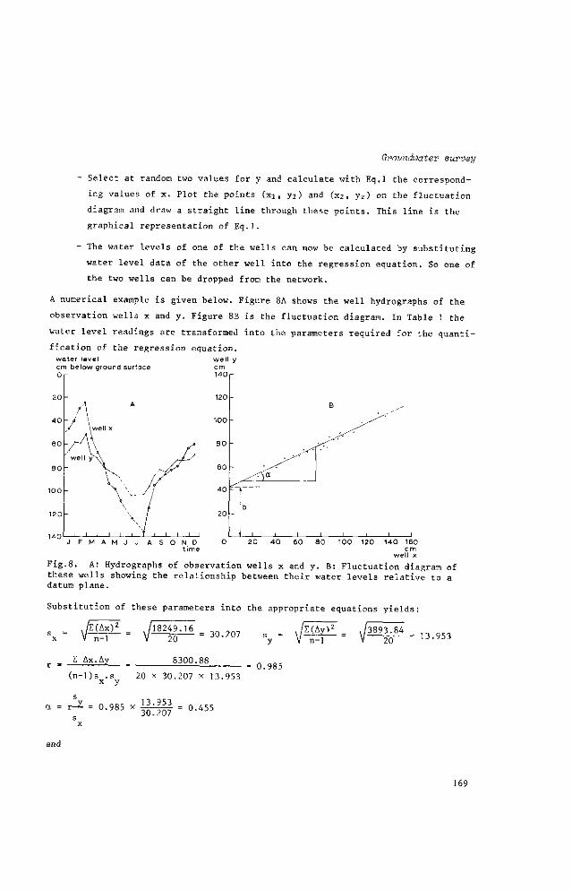
Groundwater survey
- Select at random two values for y and calculate with Eq.1 the correspond
ing values of x. Plot the points (xi, yj) and (x2 , yz) on the fluctuation
diagram and draw a straight line through these points. This line is the
graphical representation of Eq.1.
- The water levels of one of the wells can now be calculated by substituting
water level data of the other well into the regression equation. So one of
the two wells can be dropped from the network.
A numerical example is given below. Figure 8A shows the well hydrographs of the
observation wells x and y. Figure 8B is the fluctuation diagram. In Table 1 the
water level readings are transformed into the parameters required for the quanti
fication of the regression equation. water level cm below ground surface O r
wel l y cm 14U
120
1 0 0
8 0
6 0
4 0
2 0
.
~
^ ^ — - A ~~A
b
i ,
B
y ^ ^
I I
^
I I I
20 40 60 80 100 120 140 160 cm
well x
Fig.8. A: Hydrographs of observation wells x and y. B: Fluctuation diagram of these wells showing the relationship between their water levels relative to a datum plane.
Substitution of these parameters into the appropriate equations yields:
4 T. Ax-Ay
18249.16 20
8300.
= 30.207
(n-l)sx.s 20 x 30.207 x 13.953
y
= 0.985
£(Ay12
n-1 /3893.84
20 13.953
v 13 953 a = r-^ = 0.985 x ^ ^ ~ = 0.455
and
169

78.2 = 0.455 (x - 79.4)
y = 0.455 x + 42.1
Note that:
- The number of simultaneous observations (n) should be at least 20; they
should cover both wet and dry periods.
- The related wells should be located in areas with approximately similar
hydrological conditions and they should possess about the same fluctuation range.
- Wells located in areas with spot-wise irrigation, or in areas subject to
heavy pumping or to unequal rainfall patterns, cannot be related.
- Wells to be dropped from the observation network should have been correl
ated with several other wells of the hydrologie unit area to which they belong.
21.1.6 WATER QUALITY MEASUREMENTS
A survey of groundwater conditions forming part of a drainage survey also involves
the groundwater chemistry. Although the details of groundwater chemistry may be
exceedingly complex, natural variations in groundwater quality should not be
considered random; they are geohydrologically controlled. Hence, to understand
these variations one must have a certain knowledge of the geologic history and
hydrodynamics of the groundwater system.
A survey of groundwater quality is not merely a matter of determining the existing
state. It also involves a study of these natural variations in groundwater qual
ity, why they exist, and how they may change if drainage works are carried out.
Lowering a water table by artificial drainage means that groundwater from adjac
ent lands and from deep layers may start moving to the drained land. If that
groundwater is salty, the drained area and its surface water system will then be
charged daily with considerable amounts of dissolved salts. Hence it is important
to gain an idea of the quality of this groundwater, deep as well as shallow.
Natural variations in groundwater quality are related to the geomorphology of the
terrain. Even minor relief features, as are often found on alluvial plains, usual-
170

Groundwater survey
ly have a clear effect on groundwater quality. Relatively high-lying topographic
al sand ridges, for example, are areas of recharge and consequently contain
groundwater of excellent quality. On its way to adjacent topographical depres
sions the water may gradually be mineralized. Hence in these low-lying areas,
Table 1. Transformation of readings of wells x and y
Rank number
! 2
3
4
5
6
7
8
9
10
11
12
13
14
15
16
17
18
19
20
21
date
14/1
30/1
14/2
28/2
14/3
30/3
14/4
30/4
14/5
30/5
14/6
30/6
14/7
30/7
14/8
30/8
14/9
30/9
14/10
30/10
14/11
30/11
14/12
30/12
1
X
48
41
30
25
56
68
78
95
99
109
130
136
1 16
97
91
87
83
80
73
65
61
668
y
66
59
60
51
69
72
79
83
86
89
105
103
97
88
82
85
78
74
74
74
69
1643
x-x -Ax
-31.4
-38.4
-49.4
-54.4
-23.4
-11 .4
- 1 .4
15.6
19.6
29.6
50.6
56.6
36.6
17.6
11 .6
7.6
3.6
0.6
6.4
-14.4
-18.4
0.6
y-y =Ay
-12.2
-19.2
-18.2
-27.2
- 9.2
- 6.2
0.8
4.8
7.8
10.8
26.8
24.8
18.8
9.8
3.8
6.8
- 0.2
- 4.2
- 4.2
- 4.2
- 9.2
- 0.8
(Ax)2
985.96
1474.84
2440.06
2959.36
547.56
129.96
1.96
243.36
384.16
876.16
2560.36
3203.56
1339.56
309.76
134.56
57.76
12.96
0.36
40.96
207.36
338.56
18249.16
(Ay)2
148.84
368.84
331.24
739.84
84.64
38.44
0.64
23.04
60.84
116.64
718.24
615.04
353.44
96.04
14.44
46.24
0.04
17.64
17.64
17.64
84.64
3893.84
Ax. Ay
383.08
737.28
899.08
1479.68
215.28
70.68
-1.12
74.88
152.88
319.68
1356.08
1403.68
688.08
172.48
44.08
51 .68
- 0.72
- 2.52
26.88
60.48
169.28
8300.88
1668 .,„ . Ey 1643 _ = 7 9 . 4 ; y = - _ = _
171
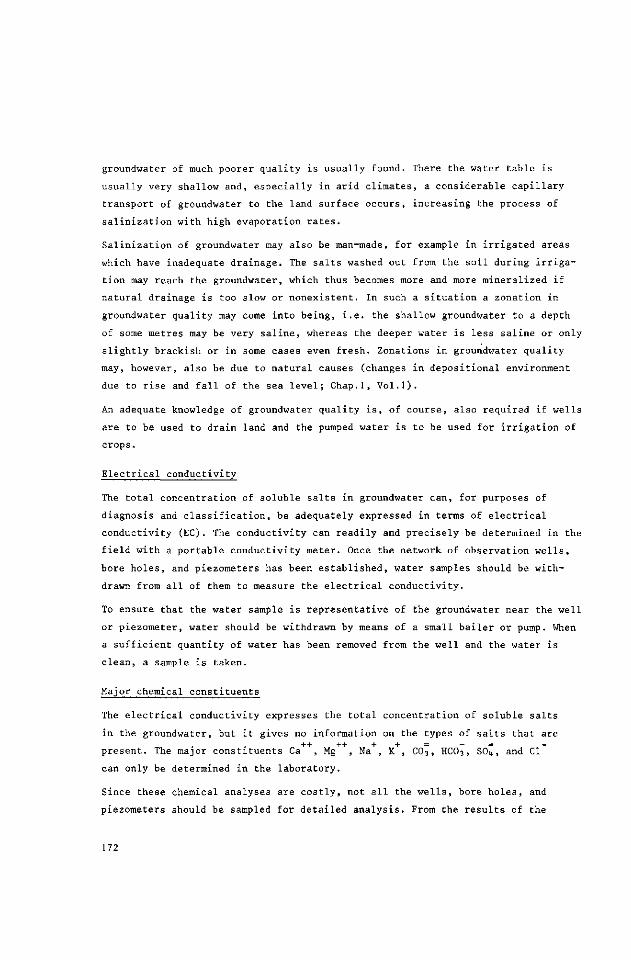
groundwater of much poorer quality is usually found. There the water table is
usually very shallow and, especially in arid climates, a considerable capillary
transport of groundwater to the land surface occurs, increasing the process of
salinization with high evaporation rates.
Salinization of groundwater may also be man-made, for example in irrigated areas
which have inadequate drainage. The salts washed out from the soil during irriga
tion may reach the groundwater, which thus becomes more and more mineralized if
natural drainage is too slow or nonexistent. In such a situation a zonation in
groundwater quality may come into being, i.e. the shallow groundwater to a depth
of some metres may be very saline, whereas the deeper water is less saline or only
slightly brackish or in some cases even fresh. Zonations in groundwater quality
may, however, also be due to natural causes (changes in depositional environment
due to rise and fall of the sea level; Chap.1, Vol.1).
An adequate knowledge of groundwater quality is, of course, also required if wells
are to be used to drain land and the pumped water is to be used for irrigation of
crops.
Electrical conductivity
The total concentration of soluble salts in groundwater can, for purposes of
diagnosis and classification, be adequately expressed in terms of electrical
conductivity (EC). The conductivity can readily and precisely be determined in the
field with a portable conductivity meter. Once the network of observation wells,
bore holes, and piezometers has been established, water samples should be with
drawn from all of them to measure the electrical conductivity.
To ensure that the water sample is representative of the groundwater near the well
or piezometer, water should be withdrawn by means of a small bailer or pump. When
a sufficient quantity of water has been removed from the well and the water is
clean, a sample is taken.
Major chemical constituents
The electrical conductivity expresses the total concentration of soluble salts
in the groundwater, but it gives no information on the types of salts that are
present. The major constituents Ca , Mg , Na , K , C03, HC03, SOi,, and CI
can only be determined in the laboratory.
Since these chemical analyses are costly, not all the wells, bore holes, and
piezometers should be sampled for detailed analysis. From the results of the
172

Groundwater survey
electrical conductivity measurements, certain wells should be selected for de
tailed analysis. These analyses allow other chemical characteristics of the water
to be calculated (SAR and "residual sodium carbonate").
Sodium adsorption ratio
Soil in contact with water that contains sodium may absorb this constituent from
the water. If exchangeable sodium is accumulated, alkali soils characterized by
poor tilth and low permeability, will form.
The sodium-adsorption-ratio is generally used as an index of the sodium or alkali
hazard of the water and is defined by the equation:
SAR = Na / V(Ca + Mg )/2 (2)
where Na , Ca , and Mg represent the concentrations in milliequivalents per
litre of the respective ions.
Classification of waters
Groundwater can be classified in different ways. From a hydrogeological point of
view, groundwater is usually classified on the basis of the dominant ions present.
An example is given in Figure 9. In this diagram the chemical composition of a
water is given as percentage of equivalents per million of the anions and cations
and is plotted as a single point. Waters that plot in Field I are calcium bicar
bonate waters (secondary alkalinity); in Field II sodium carbonate or bicarbonate
water (primary alkalinity); in Field III sulphate, chloride, calcium, magnesium
water (secondary salinity); in Field IV sulphate, chloride, sodium water (primary
salinity); and in Field V no one of the cation-anion pairs exceeds 50 per cent.
A classification of groundwater which is more relevant for drainage and irrigation
purposes is based on the above-mentioned values of SAR and EC. The diagram used for
classification is that given by RICHARDS (1954; see Fig.10). Salinity (C) and
sodium (S) are classed in four groups - low, medium, high, and very high - so
that 16 water types can be distinguished, varying from excellent (CiSj) to very
poor (CtSi,).
It should be noted that these and other classifications should be used with caution
and should never be applied too rigidly. The salt tolerance level of different
crops varies considerably, and so does the drainability of the soil. Irrigation
techniques also differ. If drip irrigation is applied, a much higher salinity
can be accepted than the commonly used maximum EC value of 2250 or 2500 micromhos/
cm. Hence groundwater quality should be considered in relation to crops, soil
drainability, and the irrigation technique applied.
173
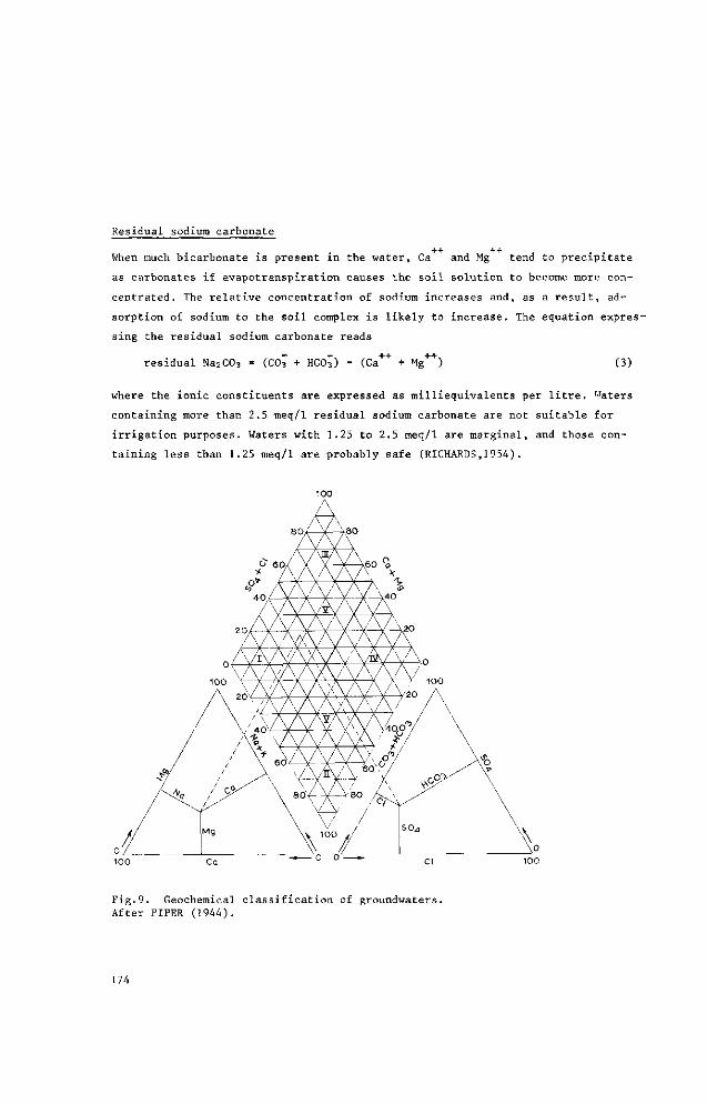
Residual sodium carbonate
++ ++ . .
When much bicarbonate is present in the water, Ca and Mg tend to precipitate
as carbonates if évapotranspiration causes the soil solution to become more con
centrated. The relative concentration of sodium increases and, as a result, ad
sorption of sodium to the soil complex is likely to increase. The equation expres
sing the residual sodium carbonate reads
residual Na2C03 = (C03 + HCO3) - (Ca++ + Mg++) (3)
where the ionic constituents are expressed as milliequivalents per litre. Waters
containing more than 2.5 irieq/1 residual sodium carbonate are not suitable for
irrigation purposes. Waters with 1.25 to 2.5 meq/1 are marginal, and those con
taining less than 1.25 meq/1 are probably safe (RICHARDS,1954).
Fig.9. Geochemical classification of groundwaters. After PIPER (1944).
174
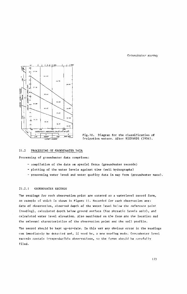
Groundwater survey
SALINITY HAZARD
Fig.10. Diagram for the classification of irrigation waters. After RICHARDS (1954).
21.2 PROCESSING OF GROUNDWATER DATA
Processing of groundwater data comprises:
- compilation of the data on special forms (groundwater records)
- plotting of the water levels against time (well hydrographs)
- presenting water level and water quality data in map form (groundwater maps).
21 .2.1 GROUNDWATER RECORDS
The readings for each observation point are entered on a waterlevel record form,
an example of which is shown in Figure 11. Recorded for each observation are:
date of observation, observed depth of the water level below the reference point
(reading), calculated depth below ground surface (for phreatic levels only), and
calculated water level elevation. Also mentioned on the form are the location and
the relevant characteristics of the observation point and the soil profile.
The record should be kept up-to-date. In this way any obvious error in the readings
can immediately be detected and, if need be, a new reading made. Groundwater level
records contain irreproducible observations, so the forms should be carefully
filed.
175

Fig.11. Example of a water level record form.
GENERAL DATA
MAP NR
MUNICIPALITY.
OWNER
OBSERVATION POINT NR.
COORDINATES: X =
PROVINCE
INSTALLATION DATE
DEPTH SCREENED PART
TYPE1
AQUIFER TYPE2
WELL LOG: FILE NR.
SURFACE ELEVATION
WATER SAMPLES: FILE NR
REFERENCE POINT ELEVATION.
OBSERVATIONS
DATE READING3 ELEVAT I ON1* DEPTH5 REMARKS6
e.g. village well, open bore hole, piezometer* e.g. unconfirmed aquifer, semiconfined aquifer, semipervious covering laver with respect to reference point with respect to general datum, for example mean sea level below ground surface (for vhreatic levels only] data on water samples, irrigation, water at the surface, flow from wells,
water withdrawal (vumving), etc.
176
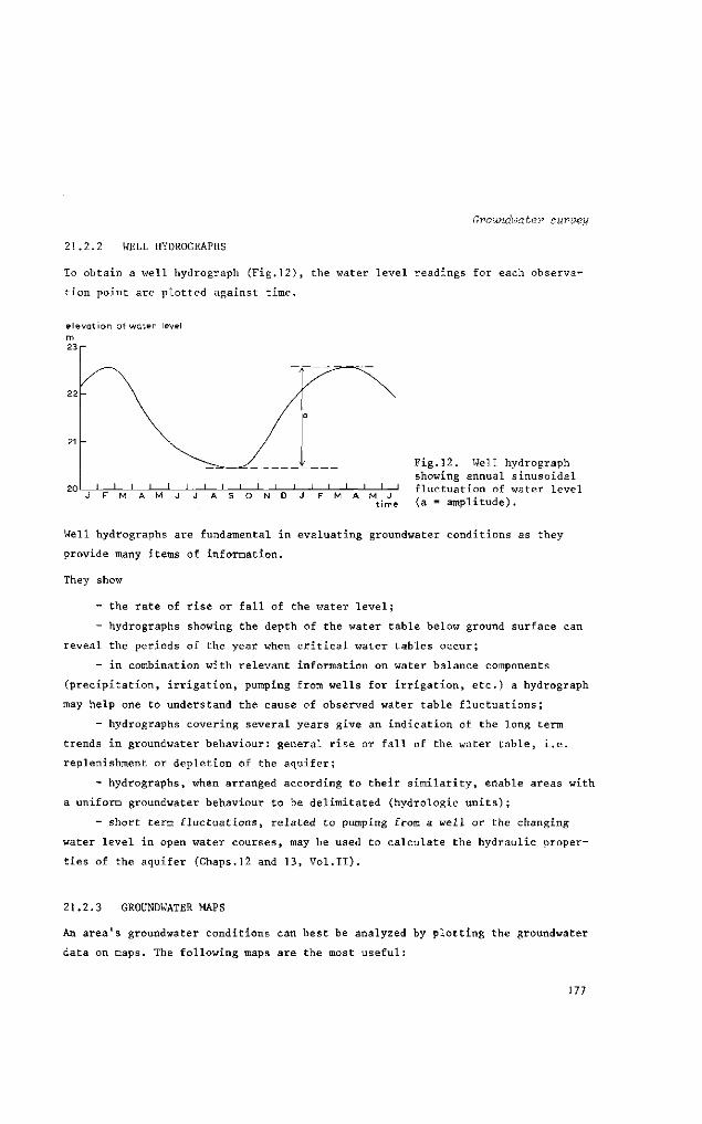
Groundwater survey
21.2.2 WELL HYDROGRAPHS
To obtain a well hydrograph (Fig.12), the water level readings for each observa
tion point are plotted against time.
e leva t i on of water level m 23
Fig.12. Well hydrograph showing annual sinusoidal fluctuation of water level (a = amplitude).
Well hydrographs are fundamental in evaluating groundwater conditions as they
provide many items of information.
They show
- the rate of rise or fall of the water level;
- hydrographs showing the depth of the water table below ground surface can
reveal the periods of the year when critical water tables occur;
- in combination with relevant information on water balance components
(precipitation, irrigation, pumping from wells for irrigation, etc.) a hydrograph
may help one to understand the cause of observed water table fluctuations;
- hydrographs covering several years give an indication of the long term
trends in groundwater behaviour: general rise or fall of the water table, i.e.
replenishment or depletion of the aquifer;
- hydrographs, when arranged according to their similarity, enable areas with
a uniform groundwater behaviour to be delimitated (hydrologie units);
- short term fluctuations, related to pumping from a well or the changing
water level in open water courses, may be used to calculate the hydraulic proper
ties of the aquifer (Chaps.12 and 13, Vol.11).
21.2.3 GROUNDWATER MAPS
An area's groundwater conditions can best be analyzed by plotting the groundwater
data on maps. The following maps are the most useful:
177
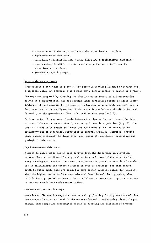
- contour maps of the water table and the Potentiometrie surface,
- depth-to-water-table maps,
- groundwater-fluctuation maps (water table and Potentiometrie surface),
- maps showing the difference in head between the water table and the
Potentiometrie surface,
- groundwater quality maps.
Watertable contour maps
A watertable contour map is a map of the phreatic surface; it can be prepared for
a specific date, but preferably as a mean for a longer period (a season or a year).
The maps are prepared by plotting the absolute water levels of all observation
points on a topographical map and drawing lines connecting points of equal water-
table elevation (equipotential lines, or isohypses, or watertable contour lines).
Such maps enable the configuration of the phreatic surface and the direction and
intensity of the groundwater flow to be studied (see Section 3.2).
To draw contour lines, water levels between the observation points must be inter
polated. This can be done either by eye or by linear interpolation (Fig.13). The
linear interpolation method may cause serious errors if the influence of the
topography and of geological structures is ignored (Fig.14). Therefore contour
lines should preferably be drawn free hand, using all available topographic and
geological information.
Depth-to-water-table maps
A depth-to-water-table map is best derived from the difference in elevation
between the contour lines of the ground surface and those of the water table.
A map showing the depth of the water table below the ground surface is of special
use in delimitating the extent of areas in need of drainage. For that reason
depth-to-water-table maps are drawn for some chosen critical dates, for example,
when the highest water table occurs (deduced from the well hydrographs), when
certain farming operations have to be carried out, or when the crops are expected
to be most sensitive to high water tables.
Groundwater fluctuation maps
Groundwater fluctuation maps are constructed by plotting for a given span of time
the change of the water level in the observation wells and drawing lines of equal
change. These maps are constructed either by plotting the difference in water
178

Groundwater survey
direction of groundwater flow
~—>——56 groundwater
contours
— — r ^—55
54.7 observed water table elevation
Fig,13. Construction of watertable contour lines by linear interpolation.
incorrect: presence of lake ignored correct; presence of lake taken into account
incorrect: fault line ignored correct: fault line taken into account
Fig.14. Two examples of correctly and incorrectly drawn watertable contour lines.
179
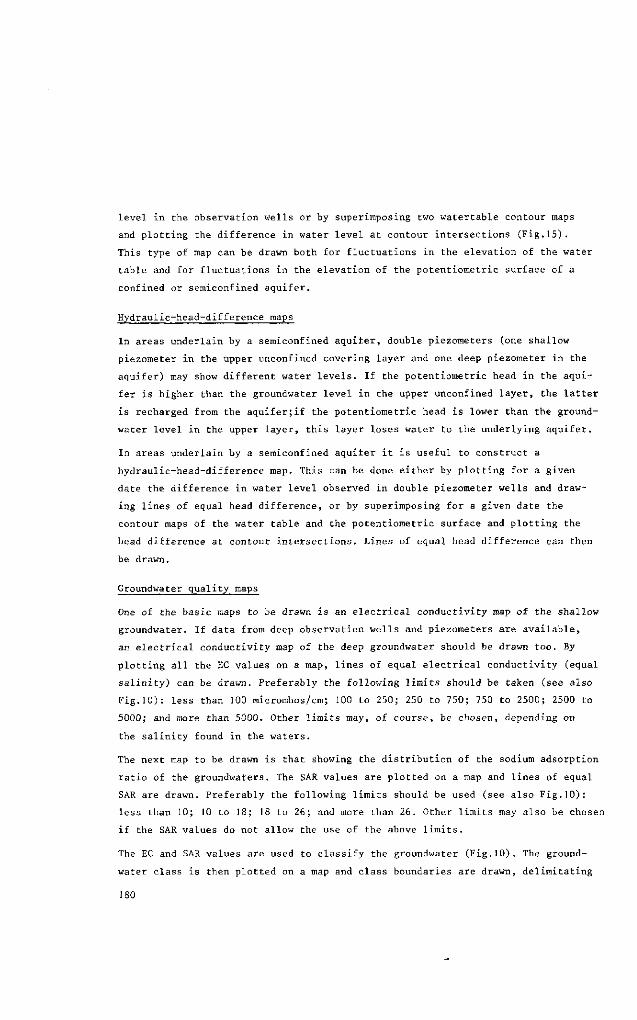
level in the observation wells or by superimposing two watertable contour maps
and plotting the difference in water level at contour intersections (Fig.15).
This type of map can be drawn both for fluctuations in the elevation of the water
table and for fluctuations in the elevation of the Potentiometrie surface of a
confined or semiconfined aquifer.
Hydraulic-head-difference maps
In areas underlain by a semiconfined aquifer, double piezometers (one shallow
piezometer in the upper unconfined covering layer and one deep piezometer in the
aquifer) may show different water levels. If the Potentiometrie head in the aqui
fer is higher than the groundwater level in the upper unconfined layer, the latter
is recharged from the aquifer;if the Potentiometrie head is lower than the ground
water level in the upper layer, this layer loses water to the underlying aquifer.
In areas underlain by a semiconfined aquifer it is useful to construct a
hydraulic-head-difference map. This can be done either by plotting for a given
date the difference in water level observed in double piezometer wells and draw
ing lines of equal head difference, or by superimposing for a given date the
contour maps of the water table and the Potentiometrie surface and plotting the
head difference at contour intersections. Lines of equal head difference can then
be drawn.
Groundwater quality maps
One of the basic maps to be drawn is an electrical conductivity map of the shallow
groundwater. If data from deep observation wells and piezometers are available,
an electrical conductivity map of the deep groundwater should be drawn too. By
plotting all the EC values on a map, lines of equal electrical conductivity (equal
salinity) can be drawn. Preferably the following limits should be taken (see also
Fig.10): less than 100 micromhos/cm; 100 to 250; 250 to 750; 750 to 2500; 2500 to
5000; and more than 5000. Other limits may, of course, be chosen, depending on
the salinity found in the waters.
The next map to be drawn is that showing the distribution of the sodium adsorption
ratio of the groundwaters. The SAR values are plotted on a map and lines of equal
SAR are drawn. Preferably the following limits should be used (see also Fig.10):
less than 10; 10 to 18; 18 to 26; and more than 26. Other limits may also be chosen
if the SAR values do not allow the use of the above limits.
The EC and SAR values are used to classify the groundwater (Fig.10). The ground
water class is then plotted on a map and class boundaries are drawn, delimitating
180

Groundwater survey
areas where high, medium, and low electrical conductivity occurs and where, and
to what extent, a sodium hazard exists.
If the groundwater in most of the area under study is saline, it is also useful
to draw maps showing the distribution of the chloride and sulphate contents of
the groundwater.
The accuracy of groundwater maps depends, amongst other things, on the number of
observation points and their distribution. For this reason each map, whether a
water table map or a water quality map, should clearly show the measuring points
on which it is based. Wells not used for the specific purpose should be dropped
from the map or should be marked differently.
B
/ / / / / °> i ' I ' :
! S i I i i * Si I
I / I ' a I / i ! I
/ ; * I \ i i i
Fig. 15. Construction of waterlevel fluctuation map by superimposing watertable contour maps of two hydrologically different years. A: present water levels, B: past water levels, C: Maps A and B superimposed, and D: resulting waterlevel fluctuation map.
181
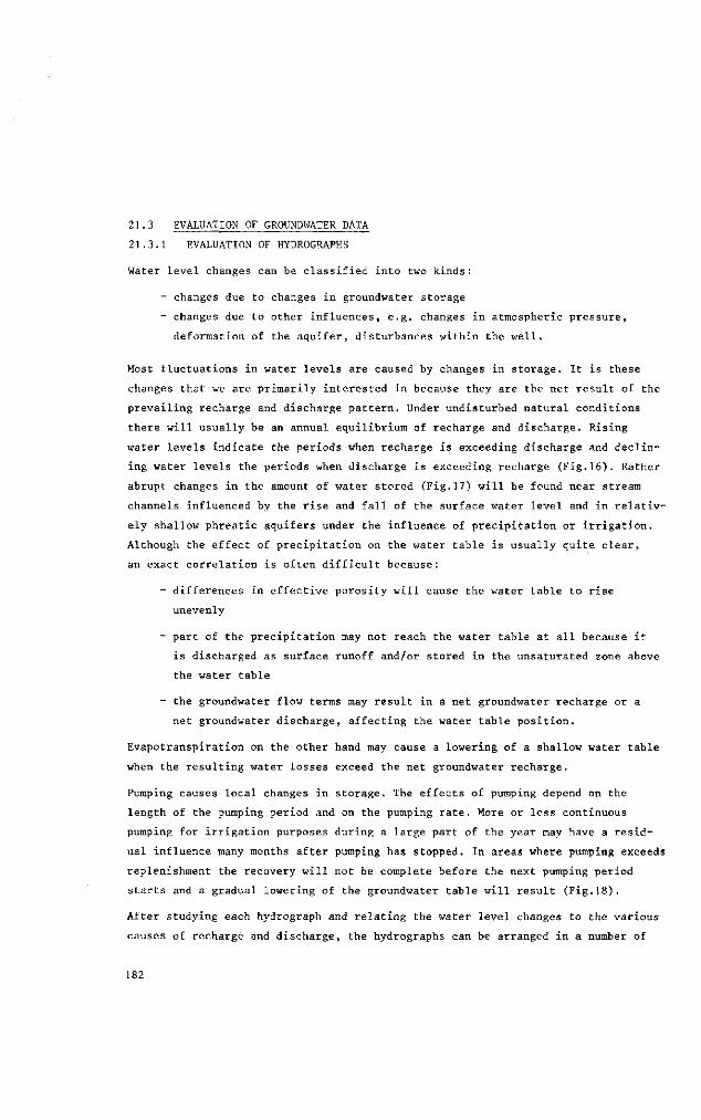
21.3 EVALUATION OF GROUNDWATER DATA
21.3.1 EVALUATION OF HYDROGRAPHS
Water level changes can be classified into two kinds:
- changes due to changes in groundwater storage
- changes due to other influences, e.g. changes in atmospheric pressure,
deformation of the aquifer, disturbances within the well.
Most fluctuations in water levels are caused by changes in storage. It is these
changes that we are primarily interested in because they are the net result of the
prevailing recharge and discharge pattern. Under undisturbed natural conditions
there will usually be an annual equilibrium of recharge and discharge. Rising
water levels indicate the periods when recharge is exceeding discharge and declin
ing water levels the periods when discharge is exceeding recharge (Fig.16). Rather
abrupt changes in the amount of water stored (Fig.17) will be found near stream
channels influenced by the rise and fall of the surface water level and in relativ
ely shallow phreatic aquifers under the influence of precipitation or irrigation.
Although the effect of precipitation on the water table is usually quite clear,
an exact correlation is often difficult because:
- differences in effective porosity will cause the water table to rise
unevenly
- part of the precipitation may not reach the water table at all because it
is discharged as surface runoff and/or stored in the unsaturated zone above
the water table
- the groundwater flow terms may result in a net groundwater recharge or a
net groundwater discharge, affecting the water table position.
Evapotranspiration on the other hand may cause a lowering of a shallow water table
when the resulting water losses exceed the net groundwater recharge.
Pumping causes local changes in storage. The effects of pumping depend on the
length of the pumping period and on the pumping rate. More or less continuous
pumping for irrigation purposes during a large part of the year may have a resid
ual influence many months after pumping has stopped. In areas where pumping exceeds
replenishment the recovery will not be complete before the next pumping period
starts and a gradual lowering of the groundwater table will result (Fig.18).
After studying each hydrograph and relating the water level changes to the various
causes of recharge and discharge, the hydrographs can be arranged in a number of
182

Groundwater survey
groups in conformity with their fluctuation pattern. Each group represents an
area where the changes in water table or Potentiometrie surface are related in
the same way to the recharge and discharge components of the system. From the
hydrographs of each group of piezometers and bore holes, we can read what are the
critical periods of the year in which the water table is too high and needs to be
controlled by artificial drainage. Further we can find from them what components
of recharge (precipitation, water losses from canals, field irrigation losses,
subsurface inflow) the groundwater system is most sensitive to. Hence the effects
of changes in the recharge and discharge pattern may be predicted.
rising l imb re f lects recharge by rain I y gradual decline of ^ ^ ^ wa te r level by
drainage or evaporation
Fig.16. Hydrograph showing rise of water table during recharge by rain and the subsequent decline during drought.
m^ïï^ms^
days
Fig.17. Influence of fluctuations of the water level in a river on the water table in adjacent land. Note that the influence diminishes with increasing distance to the river.
'°ng-«erm t F i n^oT f i ^gTap i r
pumping rate
n n JZL
Fig.18. Hydrograph of a piezometer in a pumped aquifer, and corresponding pumping pattern.
183

21.3.2 EVALUATION OF GROUNDWATER CONTOUR HAPS
The fundamental importance of the water table and the Potentiometrie surface in
groundwater investigations that form part of a drainage study may be outlined by
the following brief summary.
Flow direction. The contour lines of a water table map or a Potentiometrie
surface map are in fact equipotential lines (Chap.6, Vol.1). Hence the direction
of the groundwater flow, being perpendicular to the equipotential lines, can be
directly deduced from these maps (Fig.19).
Hydraulic gradient (dh/dx = i). A water table contour map or a contour map
of the Potentiometrie surface of a semiconfined aquifer is a graphic representation
of the hydraulic gradient of the water table or Potentiometrie surface. The hy
draulic gradients, which can be directly derived from these maps, are the basis
for calculating the rate of groundwater flow through cross-sections, for example,
through project area boundaries. The flow velocity (v) varies directly with the
hydraulic gradient and, at constant flow velocity, the gradient is inversely
related to the hydraulic conductivity (K), or v = Ki (Darcy's law). This is a
fundamental law governing the interpretation of hydraulic gradients of water tables
or Potentiometrie surfaces. If the flow velocity in two cross-sections of equal
depth and width is the same, but one cross-section shows a greater hydraulic
gradient than the other, its hydraulic conductivity must be lower. On the other
hand, small hydraulic gradients (flat watertable slopes) reflect a high hydraulic
conductivity of the water-transmitting material. Hence if in a certain flow
direction the spacing of the contour lines is narrowing (hydraulic gradients becom
ing greater) the hydraulic conductivity of the material becomes lower.
Groundwater mounds. A mound in the water table or Potentiometrie surface is
usually caused by recharge, either from above (for example, by local irrigation),
or from below (for example, by a local upward groundwater flow from deep layers -
see Fig.20). If a local mound in the water table is not due to recharge from ir
rigation or some other surface source of local nature, we can be sure that it is
caused by the upward flow of groundwater from deep layers. Typical examples can
be found in alluvial plains underlain by karstic limestone containing water under
pressure. This water may escape locally through cracks or karstic holes, giving
rise to mounds in the water table or Potentiometrie surface.
Groundwater depressions. A local depression in the water table is usually due
to pumping from wells (Chap.12, Vol.11). If no such pumping occurs and if karstic
limestone exists under the alluvium, groundwater may be lost locally through cracks
or holes in the limestone, causing local depressions in the water table.
184
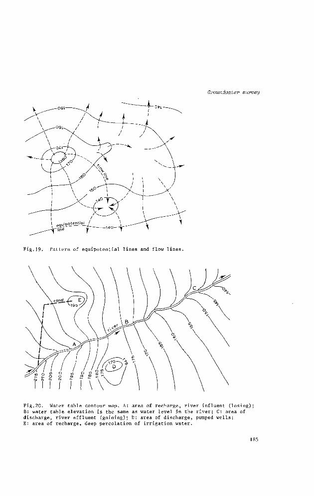
Groundwater survey
Fig.19. Pattern of equipotential lines and flow lines.
Fig.20. Water table contour map. A: area of recharge, river influent (losing B: water table elevation is the same as water level in the river; C: area of discharge, river effluent (gaining); D: area of discharge, pumped wells; E: area of recharge, deep percolation of irrigation water.
185

Influent or effluent streams. The curvature of contour lines of the water
table in the vicinity of streams or other surface water bodies indicates whether
it is an influent (losing) or an effluent (gaining) stream. For streams losing
water, the contour lines bend downstream and for streams gaining water they bend
upstream (Fig.20).
Radial resistance. The bends in contour lines near effluent streams (drainage
channels) may have different shapes due to differences in the radial resistance of
the stream. The concept of radial resistance was introduced by ERNST (1962) as
the resistance that the groundwater has to overcome while flowing into the stream
bed due to the contraction of the flow lines in the vicinity of the stream. Long
and narrow bends indicate a high radial resistance; short and wide bends a low
radial resistance. The radial resistance can be determined from the hydraulic
gradients at some distance on either side of the stream bed (ii and 12) where the
flow is mainly horizontal. If furthermore the transmissivity of the aquifer (KD)
is known, the value of this resistance can be found from the following expression:
Ah q„ = (i! + i2) KD = — Ï (4) o w
where
q = total outflow in a vertical section through the wetted perimeter of
a stream or channel (m2/day)
w = radial resistance of the stream or channel (day/m)
Ah = head difference, difference between water level in the stream and the w
water table elevation (Fig.21), (m)
KD = transmissivity of the water bearing layer (m /day)
i; and i2 = water table gradient on the left and right bank, respectively,
at some distance from the stream where the groundwater flow is still
chiefly horizontal.
A strong flexure of the contour lines near streams indicates a high radial resist
ance, and a minor flexure a low radial resistance. As mentioned before (Section
1.3), to determine the exact shape and size of the flexures in the contour lines
near streams, piezometers should be installed on both the left and right banks
of the stream, and in a row perpendicular to it (Fig.6 and 21). Once the shape
of the flexures in the contour lines has been determined in a few cross-sections,
those of the remaining contour lines can be drawn free hand.
186
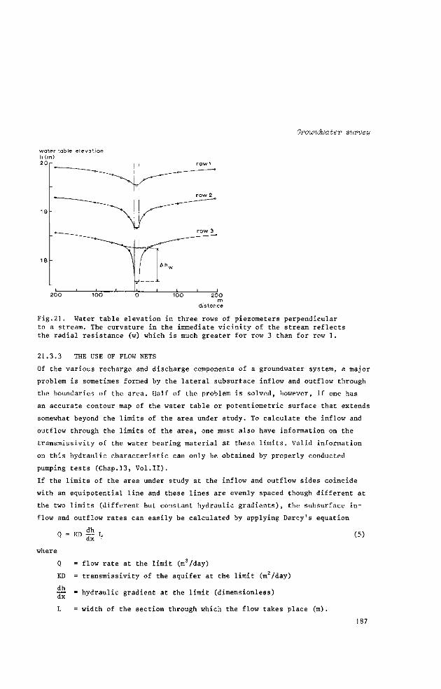
Groundwater suvveu
water table e levat ion h (m) 20
Fig.21. Water table elevation in three rows of piezometers perpendicular to a stream. The curvature in the immediate vicinity of the stream reflects the radial resistance (w) which is much greater for row 3 than for row 1.
21.3.3 THE USE OF FLOW NETS
Of the various recharge and discharge components of a groundwater system, a major
problem is sometimes formed by the lateral subsurface inflow and outflow through
the boundaries of the area. Half of the problem is solved, however, if one has
an accurate contour map of the water table or Potentiometrie surface that extends
somewhat beyond the limits of the area under study. To calculate the inflow and
outflow through the limits of the area, one must also have information on the
transmissivity of the water bearing material at these limits. Valid information
on this hydraulic characteristic can only be obtained by properly conducted
pumping tests (Chap.13, Vol.11).
If the limits of the area under study at the inflow and outflow sides coincide
with an equipotential line and these lines are evenly spaced though different at
the two limits (different but constant hydraulic gradients), the subsurface in
flow and outflow rates can easily be calculated by applying Darcy's equation
Q = KD ̂ L dx (5)
where
Q = flow rate at the limit (m3/day)
KD = transmissivity of the aquifer at the limit (m2/day)
j— = hydraulic gradient at the limit (dimensionless)
L = width of the section through which the flow takes place (m). 187
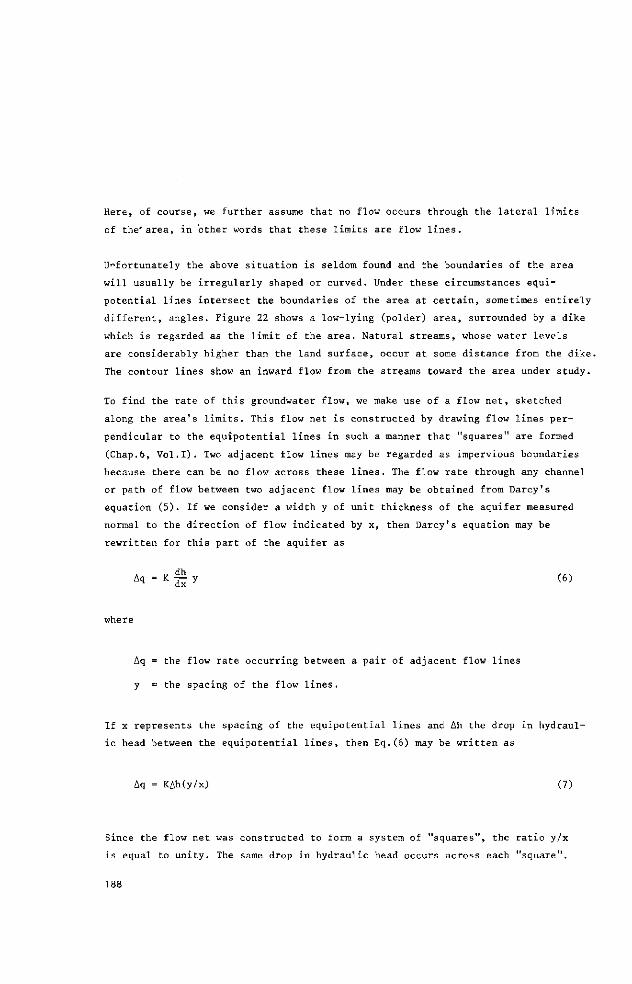
Here, of course, we further assume that no flow occurs through the lateral limits
of the* area, in 'other words that these limits are flow lines.
Unfortunately the above situation is seldom found and the boundaries of the area
will usually be irregularly shaped or curved. Under these circumstances equi-
potential lines intersect the boundaries of the area at certain, sometimes entirely
different, angles. Figure 22 shows a low-lying (polder) area, surrounded by a dike
which is regarded as the limit of the area. Natural streams, whose water levels
are considerably higher than the land surface, occur at some distance from the dike.
The contour lines show an inward flow from the streams toward the area under study.
To find the rate of this groundwater flow, we make use of a flow net, sketched
along the area's limits. This flow net is constructed by drawing flow lines per
pendicular to the equipotential lines in such a manner that "squares" are formed
(Chap.6, Vol.1). Two adjacent flow lines may be regarded as impervious boundaries
because there can be no flow across these lines. The flow rate through any channel
or path of flow between two adjacent flow lines may be obtained from Darcy's
equation (5). If we consider a width y of unit thickness of the aquifer measured
normal to the direction of flow indicated by x, then Darcy's equation may be
rewritten for this part of the aquifer as
Aq = K £ y (6)
where
Aq = the flow rate occurring between a pair of adjacent flow lines
y = the spacing of the flow lines.
If x represents the spacing of the equipotential lines and Ah the drop in hydraul
ic head between the equipotential lines, then Eq.(6) may be written as
Aq = KAh(y/x) (7)
Since the flow net was constructed to form a system of "squares", the ratio y/x
is equal to unity. The same drop in hydraulic head occurs across each "square".
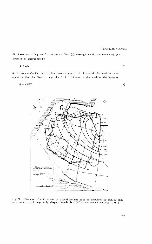
Groundwater survey
If there are n "squares", the total flow (q) through a unit thickness of the
aquifer is expressed by
q = nAq (8)
As q represents the total flow through a unit thickness of the aquifer, the
equation for the flow through the full thickness of the aquifer (D) becomes
nAhKD (9)
^^^^si^ Mr o
Fig.22. The use of a flow net to calculate the rate of groundwater inflow into an area at its irregularly shaped boundaries (after DE RIDDER and WIT, 1967).
189
From Fig.22 it can be seen that there are 16 "squares" along the boundaries of
the area, of which 9 have a Ah = 0.10 m, 6 a Sh = 0.05 m, and 1 a Ah = 0.025 m.
If it is assumed that KD = 4000 m2/day it follows that
Q =[(9 x 0.10) + (6 x 0.05) + (1 x 0.025)]x 4000 = 4900 nrVday
If the area under study covers 692 ha = 692 x ]0"* m2, it follows that
Q = 0.7 mm/day
21.3.4 EVALUATION OF OTHER TYPES OF GROUNDWATER MAPS
Watertable fluctuation maps
The areas of recharge and discharge are easily detected from a watertable fluctua
tion map. Areas characterized by large fluctuations in water table are usually
recharge areas. They generally represent topographical high-lying land with no,
or only few, natural drainage channels.
Areas with minor changes in water table are usually discharge areas. They general
ly represent low-lying lands and topographical depressions which receive continu
ous inflow of groundwater from adjacent higher grounds. Because of this net sub
surface inflow, the water table is high for most of the year and therefore cannot
change much. A denser network of natural drainage channels may be found here than
in the recharge areas.
A change in water table involves a change in the volume of groundwater stored in
the soil. If the effective porosity of the zone in which the water table changes
occur is known, the change in groundwater storage over a given period can be ex
pressed as
AS = uAh (10)
where
AS = change in storage of groundwater over a given period and per unit of
horizontal surface area (m)
y = effective porosity of the soil (dimensionless)
Ah = change in water table elevation over the given period (m)
Hydraulic difference maps
A map showing the difference in hydraulic head between the unconfined and the
semiconfined water of a groundwater system is of fundamental importance for the
analysis and evaluation of the vertical flow through semipervious layers, i.e.
190

Groundwater survey
layers whose hydraulic conductivity is considerably lower than that of sandy
aquifers.
Semiconfined aquifers are a common feature in regions suffering from high water
tables. The water confined in these aquifers is often under pressure and its head
may be found (considerably) above that of the unconfined water in the covering
semipervious layer. This layer is thus recharged from the underlying aquifer. The
flow through the semipervious layer is chiefly vertical.
To calculate the rate of this vertical upward flow of groundwater through the
covering semipervious layer, Darcy's equation can be used:
where
v = rate of vertical flow per unit surface area (m/day)
h = hydraulic head of the water in the semiconfined aquifer (m)
h' = hydraulic head of the phreatic water in the covering semipervious
layer (m)
K' = hydraulic conductivity of the semipervious layer for vertical flow
(m/day)
D' = thickness of the saturated part of the covering semipervious layer (m)
c = D'/K' = hydraulic resistance of the semipervious layer (days).
In this equation h - h' represents the difference in head between the confined
and the unconfined groundwater and can be read from the map. Usually this head
difference is not the same everywhere in the area. It is large close to surface
water bodies whose levels are above the adjacent land (Chap.13, Vol.11) and be
comes smaller farther away from them. Hence it is necessary to distinguish
areas that have approximately the same differences in hydraulic head.
A major problem of this method of calculation is the hydraulic resistance (c).
This characteristic of the semipervious layer usually varies considerably from one
site to another.
In addition to the hydraulic differences map, a hydraulic resistance map is
required showing the areal distribution of c-values. This map is difficult to
obtain as it requires a considerable amount of field work, including borings that
fully penetrate the covering semipervious layer (to find D') and hydraulic conduc
tivity measurements (to find K'). Under favourable conditions pumping tests may
191

yield values of c (Chap. 12, Vol.11; Chap.25, Vol.111) but because of theii Mgh
costs their number must usually be limited. When notwithstanding these drawbacks
sufficient information on this characteristic is available the method can be
applied (DE RIDDER and WIT, 1967).
In irrigated areas a reverse situation can often be found. Because of field irri
gation losses and conveyance losses, water tables are rising. If the hydraulic
head of the water in the underlying semiconfined aquifer is lower than that of
the phreatic water in the covering layer, a vertical downward flow through the
covering semipervious layer comes into being. The rate of this downward flow can
be calculated by applying the same formula (Eq.JJ).
Fig. 23. Chloride concentrations of the groundwater in a semiconfined aquifer at approximately 20 cm below the ground surface (after DE RIDDER and WIT, 1967).
192

Groundwater survey
Groundwater quality maps
Groundwater quality maps are necessary for studying soil salinity and assessing
salt balances and leaching requirements (Chap.3, Vol.1; Chaps.9 and 11, Vol.11).
A groundwater salinity map can be used to convert hydraulic head data from deep
piezometers that are installed in an aquifer containing groundwater of different
salinity (Fig.23). The salt water heads should be converted to fresh water heads
(Chap.6, Vol.1).
In areas with upward vertical flow of groundwater as mentioned in the previous
section, we are interested not only in the rate of flow but also in the amounts
of salt with which the upper layers and drainage channels and surface waters are
charged daily. If the salt concentration of the groundwater that enters the upper
layers is known, a weighted mean salt concentration can be calculated for the
whole area. This value, multiplied with the mean rate of upward groundwater flow,
yields the salt supply to the area (DE RIDDER and WIT, 1967).
193
LITERATURE
DAVIS, S.N. and DE WIEST, R.J.M. 1966. Hydrogeology. John Wiley & Sons, New York.
463 pp.
DE RIDDER, N.A. and WIT, K.E. 1967. Seepage flow analysis of a small polder in
the south-western part of The Netherlands. J.Hydrol.5. North-Holland Publ.
Co. Amsterdam, pp.47-57.
DE WIEST, R.J.M. 1965. Geohydrology. John Wiley & Sons, New York. 366 pp.
DOMENICO, P.A. 1972. Concepts and Models in Groundwater Hydrology. Mc Graw Hill,
New York. 405 pp.
ERNST, L.F. 1967. Grondwaterstromingen in de verzadigde zone en hun berekening
bij aanwezigheid van horizontale evenwijdige open leidingen. (Groundwater
flow in the saturated zone and its calculation when horizontal parallel open
conduits are present.) Thesis, Utrecht. Pudoc, Wageningen, 189 pp.
ERNST, L.F., DE RIDDER, N.A. and DE VRIES, J.J. 1970. A geohydrologic study of
East Gelderland (The Netherlands). Geol.en Mijnb.49, 6, pp.457-488.
PIPER, A.M. 1944. A graphic procedure in the geochemical interpretation of water
analyses. Trans.Amer.Geophys.Union, pp.914-929.
RICHARDS, L.A. 1954. Diagnosis and Improvement of Saline and Alkali Soils.
U.S.Dept. of Agric. Handbook No.60. U.S.Gov.Printing Office, Washington D.C.,
160 pp.
UNESCO. 1967. Methods and techniques of groundwater investigation and development.
Water Resources Series No.33, New York. 206 pp.
194
SURVEYS AND INVESTIGATIONS
22. ASSESSING G R O U N D W A T E R BALANCES
J. KESSLER f
Land and Water Management Specialist International Institute for Land Reclamation and Improvement, Wageningen
N. A. DE RIDDER
Geohydrologist International Institute for Land Reclamation and Improvement, Wageningen
Lecturers in the Course on Land Drainage
N. A. DE RIDDER (1970-1973) International Institute for Land Reclamation and Improvement, Wageningen
PURPOSE AND SCOPE
The assessment of a groundwater balance is of primary importance in studies on
land drainage as it allows the cause(s) of the drainage problem to be determined
in quantitative terms. The balance equation and its various components are
discussed and its application is illustrated by some practical examples.
CONTENTS
22.1 INTRODUCTION 197
22.2 GROUNDWATER BALANCE EQUATION 200
22.2.1 Water balance of the unsaturated zone 202
22.2.2 Water balance of surface-water system 203
22.2.3 Influence of underlying semiconfined aquifer 204
22.2.4 Influence of lateral groundwater flow 205
22.2.5 Change in groundwater storage 207
22.3 SOLUTION OF THE GROUNDWATER BALANCE EQUATION 210
22.3.1 Percolation and capillary rise 212
22.3.2 Net subsurface inflow 214
22.3.3 Groundwater outflow into streams and water losses through stream beds 215
22.3.4 Change in groundwater storage 216
22.4 EXAMPLES 216
LITERATURE 220
196

Groundwater balances
22.1 INTRODUCTION
Groundwater investigations related to land drainage comprise three interrelated
steps :
- an analysis of the groundwater flow system
- an analysis of the groundwater storage
- an analysis of the various components of groundwater recharge and discharge.
The objective of these investigations is to find out how to alter the groundwater
flow system so as to prevent the water table from rising too far into the root
zone of the crops. This might mean increasing the discharge or reducing the
recharge. A common approach to enable decisions on such matters is to assess a
groundwater balance of the area under study.
The water on earth - whether as water vapour in the atmosphere, as surface water
in streams, lakes, and oceans, or as groundwater in the pores of the subsoil -
is not at rest, but is in a continuous circulatory movement. There is a never-
ending transformation from one state to another. The course of events marking the
movement of a particle of water from the atmosphere to the land masses and oceans
and its return to the atmosphere is known as the hydrologie cycle. The hydrologie
cycle, as the word implies, has neither beginning nor end; it represents a closed
system in which no single drop of water can be created or destroyed (Fig.1).
ATMOSPHERE
HYDROSPHERE
LITHOSPHERE
Fig.1. Schematic representation of the hydrologie cycle
In this extremely simplified representation of the hydrologie cycle we have lumped
the atmosphere, the hydrosphere, and the lithosphère into single components, thus
masking the fact that each component is made up of sub-components. A more informa
tive presentation is given in Fig.2, which shows the elements of the hydrologie
cycle and the way they are interrelated by the various moisture inputs and outputs.
The water from the atmosphere falls to the ground as precipitation (Pr), where
part of it may flow overland to streams (runoff, R.off), part will infiltrate into
the soil (Inf) and percolate to the groundwater table (Perc), and part will evapo-
197
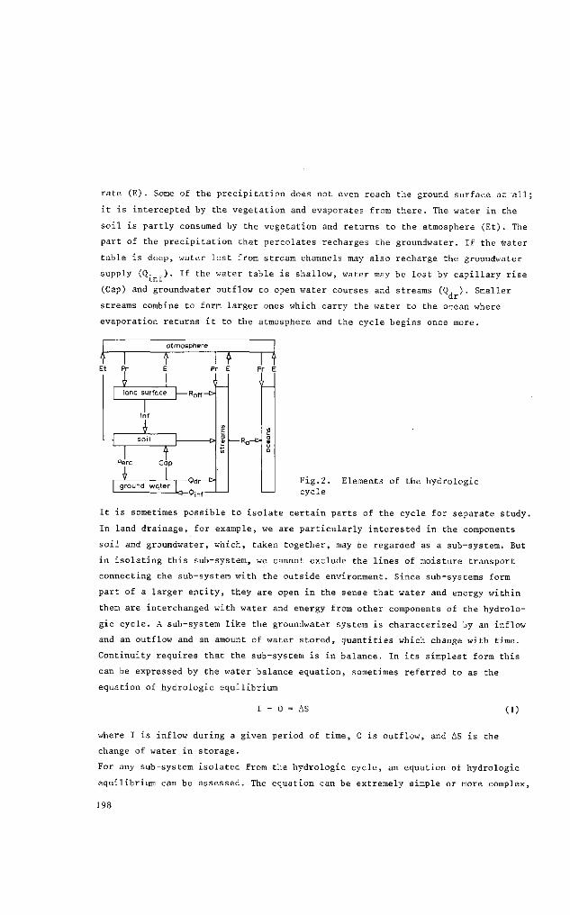
rate (E). Some of the precipitation does not even reach the ground surface at "all;
it is intercepted by the vegetation and evaporates from there. The water in the
soil is partly consumed by the vegetation and returns to the atmosphere (Et). The
part of the precipitation that percolates recharges the groundwater. If the water
table is deep, water lost from stream channels may also recharge the groundwater
supply (Q. ). If the water table is shallow, water may be lost by capillary rise
(Cap) and groundwater outflow to open water courses and streams (Q, ). Smaller dr
streams combine to form larger ones which carry the water to the ocean where
evaporation returns it to the atmosphere and the cycle begins once more.
atmosphere
land surface J— R of f"
Pr E
i
Perc
J_ T Cap
ground water 9 d r -
<?inf-
- I — V d r
-l«-<?in1
E — O a»
Fig.2. Elements of the hydrologie cycle
It is sometimes possible to isolate certain parts of the cycle for separate study.
In land drainage, for example, we are particularly interested in the components
soil and groundwater, which, taken together, may be regarded as a sub-system. But
in isolating this sub-system, we cannot exclude the lines of moisture transport
connecting the sub-system with the outside environment. Since sub-systems form
part of a larger entity, they are open in the sense that water and energy within
them are interchanged with water and energy from other components of the hydrolo
gie cycle. A sub-system like the groundwater system is characterized by an inflow
and an outflow and an amount of water stored, quantities which change with time.
Continuity requires that the sub-system is in balance. In its simplest form this
can be expressed by the water balance equation, sometimes referred to as the
equation of hydrologie equilibrium
0 = AS (0
where I is inflow during a given period of time, 0 is outflow, and AS is the
change of water in storage.
For any sub-system isolated from the hydrologie cycle, an equation of hydrologie
equilibrium can be assessed. The equation can be extremely simple or more complex,
198
Groundwater balances
depending on circumstances. For a rain gauge, for example, it is written as
Pr = AS (2)
which states that the amount of precipitation (Pr) over a given period of time is
equal to the measured increase of water stored in the rain gauge. The quantity
AS in this example has a positive sign.
For a lysimeter, from which all the excess water is drained out during a certain
period of time (Dr), the equation contains more members
Pr + I - Et - Dr = AS (3)
where
Pr = precipitation
I = water added to the lysimeter (irrigation)
Et = évapotranspiration from the lysimeter
Dr = excess water drained out from the lysimeter
AS = change of water stored in the lysimeter, which in this case is equal to AS = change of soil moisture in storage
sm °
The time element cannot be excluded from these equations because the individual
sub-systems are open and should be treated as such by considering the inflow and
outflow over a period of record. A water balance is commonly assessed for a certain
period, which is chosen in such a manner that, with the exception of one, all the
numerical values of the various members of the equation are known. If, for example,
the period is chosen as the time between two irrigation applications, the soil
moisture storage at the beginning and the end of the period is at field capacity.
Hence the change of soil moisture in storage over this period is zero. Since pre
cipitation, amount of water added, and amount of water drained are quantitatively
measured, the unknown quantity of water lost by évapotranspiration can be calcu
lated.
Care should be taken in any water balance study that all the quantities of water
are expressed in the same dimensions and units; for example, in units of dis
charge: mm3/day, litres/sec, etc., or in units of discharge/area: m/day, cm/day,
mm/day.
In the above example the water balance equation was used to calculate one unknown
quantity of the sub-system, viz. Et. It will be clear that the other quantities
should be known with great precision, otherwise the result may be misleading as
inaccuracies in one or more of the known quantities may exceed the magnitude of
199

the unknown quantity. The water balance equation can also be used as a tool to
check whether all the flow components involved have been quantitatively accounted
for, and what components have the greatest bearing on the problem under study.
Thus, taken all round, a water balance assessment is a very useful technique to
apply in any hydrologie study.
The characteristic features of the water balance can be summarized as follows:
- a water balance can be assessed for any sub-system of the hydrologie cycle,
for any size of area, and for any period of time
- a water balance can serve to check whether all flow components involved
have been quantitatively accounted for
- a water balance can serve to calculate the one unknown member of the equa
tion, provided that the other members are quantitatively known with sufficient
accuracy
- a water balance can be regarded as a model of the complete hydrologie pro
cess under study, and consequently can be used to predict the effect that changes
imposed on certain components will have on the other components of the system
or sub-system.
22.2 GROUNDWATER BALANCE EQUATION
The sub-system of soil and groundwater in which the drainage engineer is interested
is shown in its most elaborate form in Fig.3.
Since the sub-system is open in the sense that water is exchanged with the out
side environment, the system's boundaries and the flow components at these bounda
ries must be properly defined.
The situation depicted in Fig.3 shows an unconfined aquifer, also called free
watertable aquifer, bounded above by the land surface and below by a clay bed
whose hydraulic conductivity is low, though not zero. The clay bed in turn rests
on a semiconfined aquifer. The upper, unconfined aquifer is only partly saturated,
the boundary between the saturated zone and the unsaturated zone being formed by
a free water table.A change in storage of water in such an aquifer is reflected
by a change in the height of the water table as measured in open bore holes or
observation wells. For the present purpose of land drainage, we are interested in
assessing a groundwater balance for the system bounded above by the water table
and below by the clay layer and furthermore by the boundaries of the area, shown
as vertical lines on the left and right of the diagram. For this groundwater
sub-system the following inflow and outflow components can be distinguished:
200
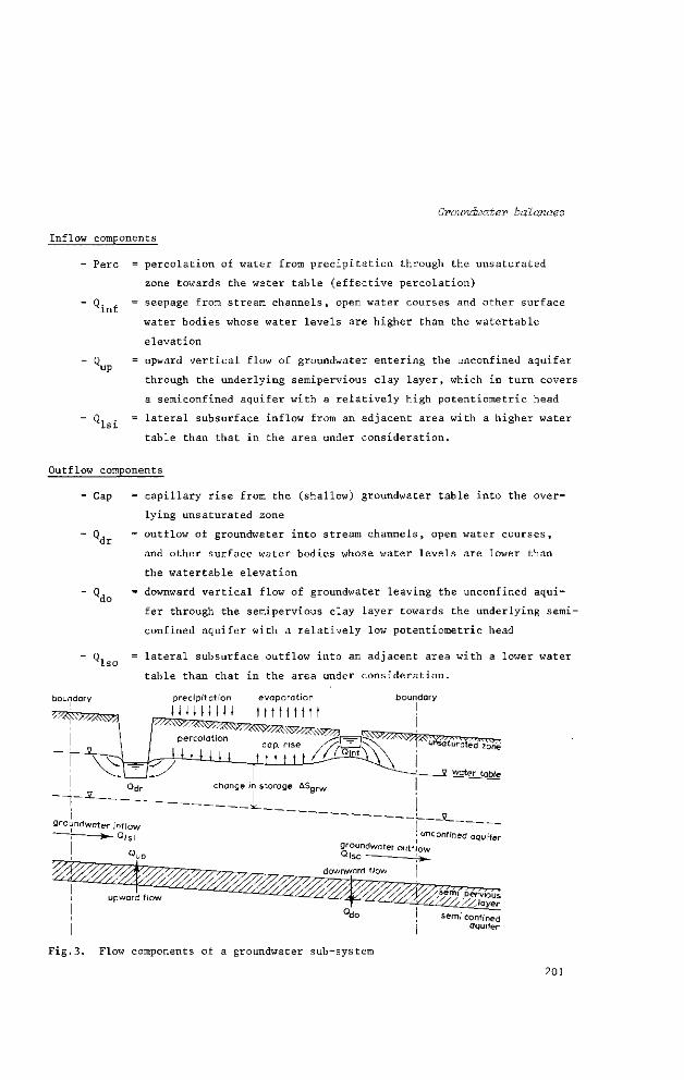
Groundwater balances
Inflow components
- Perc
inf
up
nS i
= percolation of water from precipitation through the unsaturated
zone towards the water table (effective percolation)
= seepage from stream channels, open water courses and other surface
water bodies whose water levels are higher than the watertable
elevation
= upward vertical flow of groundwater entering the unconfined aquifer
through the underlying semipervious clay layer, which in turn covers
a semiconfined aquifer with a relatively high Potentiometrie head
= lateral subsurface inflow from an adjacent area with a higher water
table than that in the area under consideration.
Outflow components
- Cap
"Mr
Mo
lso
capillary rise from the (shallow) groundwater table into the over
lying unsaturated zone
outflow of groundwater into stream channels, open water courses,
and other surface water bodies whose water levels are lower than
the watertable elevation
downward vertical flow of groundwater leaving the unconfined aqui
fer through the semipervious clay layer towards the underlying semi-
confined aquifer with a relatively low Potentiometrie head
lateral subsurface outflow into an adjacent area with a lower water
table than that in the area under consideration.
boundary precip i tat ion
l l l l l l l l l evaporat ion
t t t t t t t t t boundary
semi confined aquifer
Fig.3. Flow components of a groundwater sub-system
201

The balance of these inflow and outflow components equals the change in groundwa
ter storage in the unconfined aquifer. This is expressed by the symbol AS grw
Consequently the groundwater balance equation reads
(Perc + Q + Q. c + CK .) - (Cap + Q, + Q, + Q, ) = AS (4) up inf lsi dr do lso grw
recharge - discharge = change in storage
A more informative presentation can be made by grouping the comparable recharge
and discharge components
(Perc - Cap) + (Q - Q ) + (Q - Q ) + (Q . - Q ) = AS (5) inf dr up do lsi lso grw
The above equation expresses that the changes in groundwater storage are the
result of
- the recharge-discharge conditions determined by the water balance of the
unsaturated zone (member: Perc - Cap)
- the recharge-discharge conditions determined by the position of the water
level in the stream channels and open water courses relative to the water
table (member: Q. , - CK ) inf dr
- the recharge-discharge conditions determined by the Potentiometrie head
in the underlying semiconfined aquifer (member: Q - Q, )
- the recharge-discharge conditions determined by the lateral groundwater
inflow and outflow across the boundaries of the area under consideration
(member: Q. . - Q. ). lsi lso
A brief discussion of the various recharge and discharge components follows.
22.2.1 WATER BALANCE OF THE UNSATURATED ZONE (Perc-Cap)
Precipitation and irrigation (symbols: Pr. and Irr.) result in infiltration of
water into the soil, either completely or partly, because some of the water may
run off over the ground surface into open water courses (surface runoff; symbol
R.off). The infiltrated water will be retained by the soil until the maximum soil
moisture content is attained (field capacity). Any amount of water that infiltra
tes into the soil over and above the field capacity percolates to the water table
(Perc).
202

Groundwater balances
On the other hand, water from the soil-moisture reservoir evaporates from the soil
surface and is transpired by the vegetation cover. If this process of évapotranspi
ration (symbol: Et) is in excess of precipitation and irrigation, the soil-moisture
storage decreases, the moisture content becomes less than the equilibrium moisture
content, and groundwater, if in capillary contact with the root zone, starts
moving upward by capillary flow (Cap).
The members (Perc) and (Cap) are of great importance in any drainage study because
they express the amount of water passing from the unsaturated zone (root zone)
to the saturated zone and vice versa.
The water balance of the unsaturated zone can be written as follows (Fig.4)
(Pr + Irr - R.off) - Et - (Perc - Cap) AS (6)
where AS stands for the change in soil-moisture storage, sm
Soil-moisture storage is here regarded as the amount of water retained by the soil
up to a maximum soil-moisture content equal to field capacity. Near the water
table, in the capillary fringe, water is also retained at higher moisture contents,
but it is assumed that this amount of water remains constant throughout the balance
period. Thus, when the soil-moisture content is at field capacity at the beginning
and at the end of the considered period, AS will be zero, irrespective of any sm
change in the water table height. i r r i g a t i o n precipitation
X\\V//^\^A\^^\V/A\\V/A\\^ inf i l trat ion run of f-
unsaturated zone
percolation percolation change in soil moisture
7 water table
unconfined aquifer saturated zone
A m p e ryjous J ayer <
F i g . 4 . Schematic p r e s e n t a t i o n of the flow components in the unsaturated zone
22.2.2 WATER BALANCE OF SURFACE-WATER SYSTEM (Q. c - Q, )
inf dr
Stream channels, open water courses, and other surface-water bodies such as lakes,
influence the height of the water table to some extent. When the water level of
these water courses is higher than the water table elevation, water is lost to the
underground and the groundwater is thus recharged (Q. ). If, on the other hand, 203
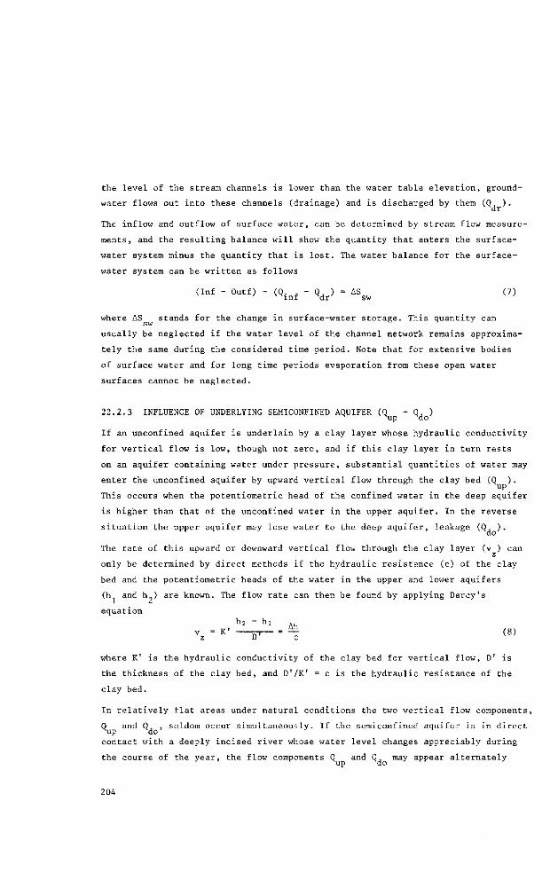
the level of the stream channels is lower than the water table elevation, ground
water flows out into these channels (drainage) and is discharged by them (Q ).
dr
The inflow and outflow of surface water, can be determined by stream flow measure
ments, and the resulting balance will show the quantity that enters the surface-
water system minus the quantity that is lost. The water balance for the surface-
water system can be written as follows (Inf - Outf) - (Q.nf - Qdr) - ASsw (7)
where AS stands for the change in surface-water storage. This quantity can sw
usually be neglected if the water level of the channel network remains approxima
tely the same during the considered time period. Note that for extensive bodies
of surface water and for long time periods evaporation from these open water
surfaces cannot be neglected.
22.2.3 INFLUENCE OF UNDERLYING SEMICONFINED AQUIFER (Q - Q. )
up do
If an unconfined aquifer is underlain by a clay layer whose hydraulic conductivity
for vertical flow is low, though not zero, and if this clay layer in turn rests
on an aquifer containing water under pressure, substantial quantities of water may
enter the unconfined aquifer by upward vertical flow through the clay bed (Q ).
This occurs when the Potentiometrie head of the confined water in the deep aquifer
is higher than that of the unconfined water in the upper aquifer. In the reverse
situation the upper aquifer may lose water to the deep aquifer, leakage (Q ). do
The rate of this upward or downward vertical flow through the clay layer (v ) can z
only be determined by direct methods if the hydraulic resistance (c) of the clay
bed and the Potentiometrie heads of the water in the upper and lower aquifers
(h and h ) are known. The flow rate can then be found by applying Darcy's
equation h2 " hl Ah
Vz = K ' — W - - ^ (8)
where K' is the hydraulic conductivity of the clay bed for vertical flow, D' is
the thickness of the clay bed, and D'/K' = c is the hydraulic resistance of the
clay bed. In relatively flat areas under natural conditions the two vertical flow components,
0 and Q, , seldom occur simultaneously. If the semiconfined aquifer is in direct up Mo
contact with a deeply incised river whose water level changes appreciably during
the course of the year, the flow components Q and Q, may appear alternately up do
204

Groundwater balances
(Chap.13, Vol.11). Under these circumstances the recharge and discharge by verti
cal movement of groundwater may constitute an important, though not constant, fac
tor in the groundwater balance.
Determining these flow components by direct measurements is usually a rather costly
affair, because a network of double piezometers and quite a lot of fieldwork,
including pumping tests, is required, to find the values of the hydraulic resistan
ce, c. Hence it is common practice to derive the order of magnitude of these flow
components indirectly from the groundwater balance. A prerequisite is that the
values of the other members of the balance equation are known with sufficient
accuracy.
22.2.4 INFLUENCE OF LATERAL GROUNDWATER FLOW (Q, . - Q, )
lsi lso
The boundaries of the area under study usually do not represent streamlines, i.e.
they are not perpendicular to the equipotential lines. Hence the lateral flow of
groundwater crossing the area's boundaries must be accounted for in the ground
water balance equation.
If the streams in the area under study are draining (Q ) and none of them is
losing water to the underground (Q. = 0 ) , and if the clay bed underlying the
unconfined aquifer is impervious (Q and Q are zero), and, moreover, if only
periods of long duration are considered (change in groundwater storage, AS is grw
very small), the groundwater balance equation (5) can be replaced by (see Fig.5) (Qlsi - < W = Qdr - (Perc - Cap) (9)
This equation shows how important it is to know the quantity (Q, . - Q, ), n lsi lso
because it represents the difference between the average quantity of water that
has to be drained and the average supply (Perc - Cap).
For the difference between the lateral subsurface inflow and outflow the symbol
I is used, hence ss
I = Q, . - Q, (10) ss lsi lso
Sometimes the term "seepage" is used for the symbol I , but, since this word ss
has different meanings, ERNST, DE RIDDER, and DE VRIES (1970) introduced the term
"net subsurface inflow" as an addition to hydrologie terminology, thus replacing
various other, often confusing, terms currently used. Obviously the net subsurface
inflow (I ) may attain positive or negative values, depending on differences in
water level (and also in ground surface elevation) between the area under consi
deration and the surrounding area.
205

The practical consequences of the value and sign of I are of great importance
in the analysis of the hydrological conditions prevailing in the area. A negative
net subsurface inflow (-1 ) indicates that the supply exceeds the outflow of
groundwater into streams and other open water courses: (Perc - Cap) > Q, . This
means that there is no danger of cumulative salinization of the root zone. This
situation may be found in areas whose land surface and water table elevation are
higher than those of the surrounding area. A positive net surface inflow (+1 )
indicates that the supply is less than the outflow of groundwater into streams and
other open water courses: (Perc - Cap) < Q . This means that the area is receiving
"foreign" water from outside. As a consequence, the water table may rise to heights
very near to, or even at, the ground surface, and artificial drainage will be
required to control the water table and to prevent the root zone from cumulative
salinization. This situation is often found in topographical depressions and in
low-lying valley bottoms.
Et
t f/Mmmm
unconfined aquifer
arbitrary boundary
3lso
Fig.5. Unconfined aquifer with flow components contained in Eq.9
If the water table gradient and the transmissivity of the aquifer are known, the
lateral groundwater inflow and outflow across the project area's boundaries can
be calculated directly, either by using Darcy's equation or a flow net analysis
(Chap.21, Vol.111). To determine the aquifer's transmissivity at the boundaries,
it will be necessary to perform several pumping tests which, because of their
high costs, will usually be limited in number. Without sufficient and reliable
data on the transmissivity, it is impossible to make a direct calculation of the
inflow and outflow across the boundaries. Recourse can then be made to indirect
methods and the net subsurface inflow (I ) can be derived from the groundwater
balance, provided the values of the other members of the equation are known with
sufficient accuracy.
Alluvial plains are seldom entirely flat, but instead show often minor relief
features in the form of topographical ridges, mounds, depressions, etc. In the
special case that a groundwater mound (an area which is surrounded at all sides by
206

Groundwater balances
a lower water table) is found in the area under consideration, the boundary of
the area can be chosen in such a manner that it coincides with the boundary of the
groundwater mound. The area is then an area without any groundwater inflow
(Q, . = 0), and the groundwater outflow from the area is equal to the net sub-lsi
surface inflow (Q, = - I , see Eq.10). If no stream channels occur in the lso ss
area (Q ., = 0), the lateral groundwater outflow will equal the supply dr
(Q = Perc - Cap). Similarly, for an area whose boundaries coincide with those
of a depression in the water table (an area which is surrounded on all sides by
a higher water table), the groundwater outflow is zero (Q = 0). Hence the
groundwater inflow across the boundaries equals the net subsurface inflow which,
in this case, has a positive sign (O. . = + I ). lsi ss
22.2.5 CHANGE IN GROUNDWATER STORAGE (AS )
grw
As a result of the hydrologie cycle, the quantity of groundwater stored in the
unconfined aquifer under discussion constantly increases by inflow of water from
various sources, as discussed previously. At the same time the aquifer loses water
by various types of outflow. In the long run, however, inflow equals outflow and
a near-stationary water table occurs, with seasonal fluctuations around the
average level.
Hence, if a groundwater balance is to be assessed for a relatively short period,
the inflow may not balance the outflow, the difference being accounted for as the
change in groundwater storage. A change in storage of groundwater is reflected
by a rise or fall of the water table (symbol: Ah).
One of the factors influencing the change in water table is the effective porosity
(drainable pore space) of the soil zone in which the water table fluctuations
occur (symbol: u). Since BOUSSINESQ (1903) pointed out that formulas from the
theory of heat conduction in solids can also be used for solving problems of
unsteady flow of groundwater, the following equation has been widely used in
groundwater hydrology (see also Chap.6, Section 5.4, Vol.1)
KD (Üi + i^) = u | £ - R (11) 3x2 3y2 3 t
where
h = Potentiometrie head of groundwater in horizontal flow
x,y = horizontal coordinates
t = time
K = hydraulic conductivity of homogeneous aquifer
207

D = thickness of aquifer
KD = transmissivity of aquifer
R = effective recharge through upper boundary of the considered area
]i = effective porosity.
From this differential equation it follows immediately that the effective porosity
is defined as the ratio of the change in storage of groundwater during a certain
period to the corresponding change in Potentiometrie head, or
The effective porosity is often also defined as the percentage of the total volume
of soil occupied by the ultimate volume of water released from or added to storage
in an unconfined aquifer per unit horizontal area of aquifer and per unit decline
or rise of the water table. The change in groundwater storage over a certain period
and per unit horizontal area is given by
AS = uAh (13) grw
Frequent recordings of the groundwater table taken from a representative network
of observation wells can be used to draw hydrographs from which the value of Ah
can be read for any chosen period.
Equation 13 might suggest that, like hydraulic conductivity, the effective porosity
is a hydrologie constant. This is not entirely true. Firstly, a lowering of the
water table is not accompanied by an instantaneous gravity drainage of the soil
pores. The amount of water drained from the soil increases, though at a diminishing
rate, as the time of drainage increases. Hence the effective porosity increases
as the time of drainage by gravity increases. JOHNSON (1966) reports that a pump
ing test performed near Grand Island (Nebr.) drained the sand and gravel in such
a manner that the computed effective porosity of the material was 9,2 % after
6 hours of pumping, 11,7 % after 12 hours, 16,1 % after 24 hours, 18,5 % after
36 hours, and 20,1 % after 48 hours of pumping. Consequently the values of the
effective porosity of an unconfined aquifer derived from pumping tests data should
be considered with great caution unless pumping is continued for a sufficiently
long time.
Secondly, it has been recognized that the effective porosity changes as the depth
to water table changes. A change in water table elevation is accompanied by a
change in soil moisture content of the entire soil profile, both in the zone in
which the water table fluctuations occur and above this zone. This means that,
208
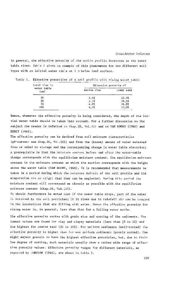
Groundwater balances
in general, the effective porosity of the entire profile decreases as the water
table rises. Table 1 gives an example of this phenomenon for two different soil
types with an initial water table at 1 m below land surface.
Table 1. Effective porosities of a soil profile with rising water table
Total rise in Effective porosity of water table
, v marine clay loamy sand (cm) 30 5,4% 22,3% 50 5,1% 19,5% 70 4,9% 16,8%
100 4,3% 13,0%
Hence, whenever the effective porosity is being considered, the depth of the ini
tial water table should be taken into account. For a further discussion on the
subject the reader is referred to Chap.20, Vol.111 and to VAN H00RN (1960) and
ERNST (1969).
The effective porosity can be derived from soil moisture characteristics
(pF-curves: see Chap.20, Vol.111) and from the (known) amount of water released
from or added to storage and the corresponding change in water table elevation;
a prerequisite is that the moisture content before and after the water-table
change corresponds with the equilibrium moisture content. The equilibrium moisture
content is the moisture content at which the suction corresponds with the height
above the water table (VAN HOORN, 1960). It is recommended that measurements be
taken in a period during which the moisture deficit of the soil profile and thé
evaporation are so slight that they can be neglected. During this period the
moisture content will correspond as closely as possible with the equilibrium
moisture content (Chap.26, Vol.111).
It should furthermore be noted that if the water table drops, part of the water
is retained by the soil particles; if it rises due to rainfall air can be trapped
in the interstices that are filling with water. Hence the effective porosity for
rising water is, in general, less than that for a falling water table.
The effective porosity varies with grain size and sorting of the sediments. The
lowest values are found for clay and clayey materials (less than \7. to 5%) and
the highest for coarse sand (20 to 35%). For uniform sediments (well-sorted) the
effective porosity is higher than for non-uniform sediments (poorly sorted). One
might expect gravels to have the highest effective porosities, but, due to their
low degree of sorting, such materials usually show a rather wide range of effec
tive porosity values. Effective porosity ranges for different materials, as
reported by JOHNSON (1966), are shown in Table 2.
209
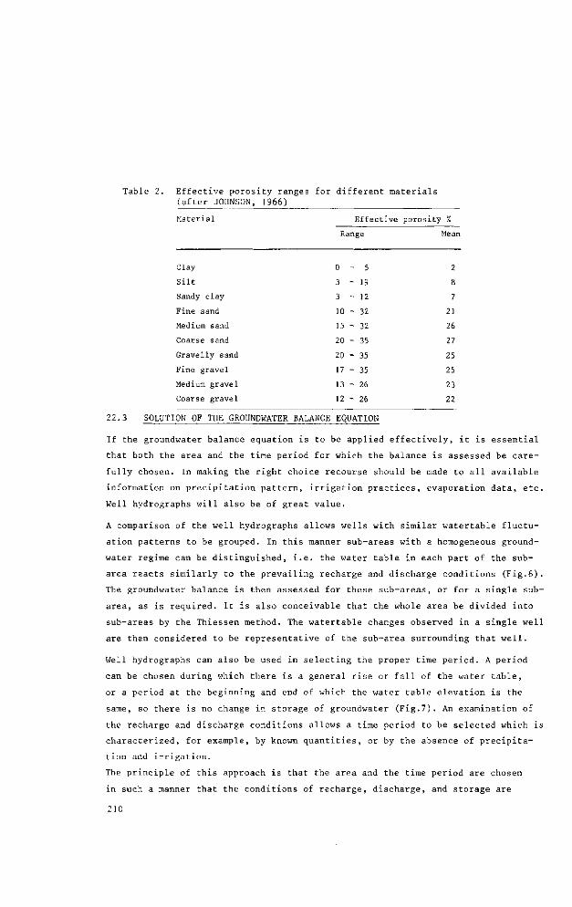
T a b l e 2 . E f f e c t i v e p o r o s i t y r a n g e s f o r d i f f e r e n t m a t e r i a l s ( a f t e r JOHNSON, 1966)
Ma t e r i a l E f f e c t i v e p o r o s i t y 7.
Range Mean
Clay 0 - 5 2
Silt 3 - 1 9 8
Sandy clay 3 - 1 2 7
Fine sand 1 0 - 3 2 21
Medium sand 1 5 - 3 2 26
Coarse sand 20 - 35 27
Gravelly sand 20 - 35 25
Fine gravel 1 7 - 3 5 25
Medium gravel 1 3 - 2 6 23
Coarse gravel 1 2 - 2 6 22
22.3 SOLUTION OF THE GROUNDWATER BALANCE EQUATION
If the groundwater balance equation is to be applied effectively, it is essential
that both the area and the time period for which the balance is assessed be care
fully chosen. In making the right choice recourse should be made to all available
information on precipitation pattern, irrigation practices, evaporation data, etc.
Well hydrographs will also be of great value.
A comparison of the well hydrographs allows wells with similar watertable fluctu
ation patterns to be grouped. In this manner sub-areas with a homogeneous ground
water regime can be distinguished, i.e. the water table in each part of the sub-
area reacts similarly to the prevailing recharge and discharge conditions (Fig.6).
The groundwater balance is then assessed for these sub-areas, or for a single sub-
area, as is required. It is also conceivable that the whole area be divided into
sub-areas by the Thiessen method. The watertable changes observed in a single well
are then considered to be representative of the sub-area surrounding that well.
Well hydrographs can also be used in selecting the proper time period. A period
can be chosen during which there is a general rise or fall of the water table,
or a period at the beginning and end of which the water table elevation is the
same, so there is no change in storage of groundwater (Fig.7). An examination of
the recharge and discharge conditions allows a time period to be selected which is
characterized, for example, by known quantities, or by the absence of precipita
tion and irrigation.
The principle of this approach is that the area and the time period are chosen
in such a manner that the conditions of recharge, discharge, and storage are
210

Groundwater balances
uniform and quantitatively known, except for one flow component. This component
can then be solved from the equation. The component thus found can subsequently
be introduced into the equation for another chosen time period with another un
known item, provided the value of the component remains reasonably constant. In
general, lateral groundwater flows remain rather constant for different time
periods, whereas percolation and capillary rise usually vary during different
parts of the hydrological year. The calculations should preferably be made for
more than one time period in order to have a check on the results obtained.
It is not always possible, nor necessary, to solve all the individual members
of the groundwater balance equation separately. Sometimes, depending on the pro
blem under study, a number of members can be lumped, and their net value only be
taken.
depth to water table (m) 0
Fig.6. Similarly reacting well hydrographs
depth t owa te r table Cm) 0
Fig.7. The use of a well hydrograph to select convenient time periods for assessing groundwater balances
211
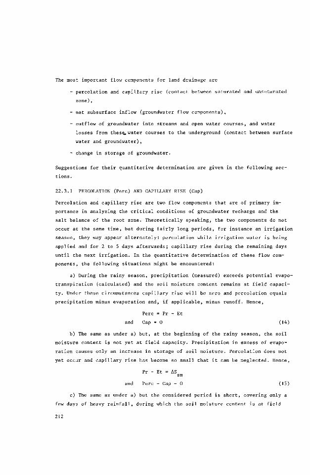
The most important flow components for land drainage are
- percolation and capillary rise (contact between saturated and unsaturated
zone),
- net subsurface inflow (groundwater flow components),
- outflow of groundwater into streams and open water courses, and water
losses from these, water courses to the underground (contact between surface
water and groundwater),
- change in storage of groundwater.
Suggestions for their quantitative determination are given in the following sec
tions.
22.3.1 PERCOLATION (Perc) AND CAPILLARY RISE (Cap)
Percolation and capillary rise are two flow components that are of primary im
portance in analyzing the critical conditions of groundwater recharge and the
salt balance of the root zone. Theoretically speaking, the two components do not
occur at the same time, but during fairly long periods, for instance an irrigation
season, they may appear alternately: percolation while irrigation water is being
applied and for 2 to 5 days afterwards; capillary rise during the remaining days
until the next irrigation. In the quantitative determination of these flow com
ponents, the following situations might be encountered:
a) During the rainy season, precipitation (measured) exceeds potential évapo
transpiration (calculated) and the soil moisture content remains at field capaci
ty. Under these circumstances capillary rise will be zero and percolation equals
precipitation minus evaporation and, if applicable, minus runoff. Hence,
Perc = Pr - Et
and Cap = 0 (14)
b) The same as under a) but, at the beginning of the rainy season, the soil
moisture content is not yet at field capacity. Precipitation in excess of evapo
ration causes only an increase in storage of soil moisture. Percolation does not
yet occur and capillary rise has become so small that it can be neglected. Hence,
Pr - Et = AS sm
and Perc = Cap = 0 (15)
c) The same as under a) but the considered period is short, covering only a
few days of heavy rainfall, during which the soil moisture content is at field
212

Groundwater balances
capacity. Evaporation during this short and wet period can be neglected. The
total rainfall, after reduction for runoff, may be accounted for as percolation.
Hence,
Perc = Pr
and Cap = 0 (16)
d) During the irrigation season percolation 'occurs due to over-irrigation,
i.e. irrigation is in excess of the available soil moisture storage. From irriga
tion flow measurements, or data on the irrigation efficiency, the irrigation losses
can be derived which, in this situation, equal percolation. Hence,
Perc = Irr - AS (17)
sm
If the chosen time period covers only a few days during and after irrigation,
capillary rise can be assumed negligible. For longer periods, capillary rise may
attain considerable values that are not easy to determine by direct methods. In
this situation capillary rise can be derived from the water balance equation it
self (see Section 2.1). Hence, Cap = 0 or Cap = ? (18)
e) For periods during which the water table is at a depth of about 4 m or
more below the ground surface, the capillary rise decreases to negligibly low
values, irrespective of the moisture conditions in the unsaturated zone. Hence,
Cap = 0 (19)
During the dry season, when the soil moisture storage is partly depleted and the
water table is at less than, say, 3 m below ground surface, capillary rise will
not be zero but instead may attain large values, depending on the type of soil
(Chap.I 1, Vol.11).
If the groundwater quality is good and sufficient leaching is provided during
irrigation applications or during the wet season, capillary rise may be considered
a favourable factor, because it represents a supplemental supply of water to the
crops.
If, on the other hand, the groundwater is saline and percolation is limited during
the wet season, capillary rise will constitute the principal factor in the process
of gradual salinization of the root zone.
Capillary rise is difficult to determine directly, and then only on the basis of
experimental field research. However, once sufficiently accurate values of the
effective porosity and the net subsurface inflow have been obtained, it can be
213
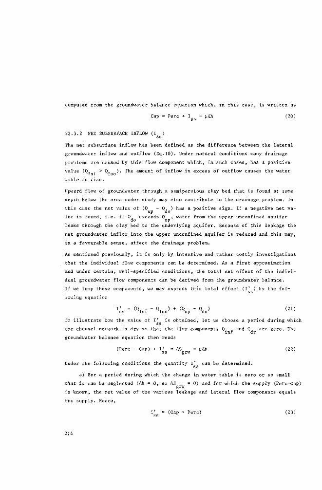
computed from the groundwater balance equation which, in this case, is written as
Cap = Perc + 1 - pAh (20)
22.3.2 NET SUBSURFACE INFLOW (I )
ss
The net subsurface inflow has been defined as the difference between the lateral
groundwater inflow and outflow (Eq.10). Under natural conditions many drainage
problems are caused by this flow component which, in such cases, has a positive value (Q, . > Q. ). The amount of inflow in excess of outflow causes the water
lsi lso table to rise.
Upward flow of groundwater through a semipervious clay bed that is found at some
depth below the area under study may also contribute to the drainage problem. In
this case the net value of (Q - Q ) has a positive sign. If a negative net va-up do
lue is found, i.e. if Q, exceeds Q , water from the upper unconfined aquifer do up
leaks through the clay bed to the underlying aquifer. Because of this leakage the
net groundwater inflow into the upper unconfined aquifer is reduced and this may,
in a favourable sense, affect the drainage problem.
As mentioned previously, it is only by intensive and rather costly investigations
that the individual flow components can be determined. As a first approximation
and under certain, well-specified conditions, the total net effect of the indivi
dual groundwater flow components can be derived from the groundwater balance.
If we lump these components, we may express this total effect (I' ) by the fol
lowing equation
I' = (Q1 . - Q. ) + (Q - Q, ) (21) ss lsi lso up do
To illustrate how the value of I' is obtained, let us choose a period during which ss
the channel network is dry so that the flow components Q. r and Q, are zero. The m f dr
groundwater balance equation then reads (Perc - Cap) + 1 ' = AS = ]iAh (22)
s s grw Under the following conditions the quantity I' can be determined.
ss
a) For a period during which the change in water table is zero or so small
that it can be neglected (Ah = 0, so AS = 0) and for which the supply (Perc-Cap) grw
is known, the net value of the various leakage and lateral flow components equals
the supply. Hence, I' = (Cap - Perc) (23)
214

Groundwater balances
b) If the water table is changing during the chosen period, and if the supply
and the effective porosity are known, the net value of the leakage and lateral
flow components is given by
I' = yAh - (Perc - Cap) (24)
If both percolation and capillary rise are zero (no rainfall or irrigation and a
deep water table) the above equation reduces to
I' = yAh (25) ss
c) If the effective porosity of the soil layer in which the changes in water
table occur is not yet known, both the net value of I' and the effective porosity ss
can be calculated from two different periods for which the supply (Perc - Cap)
and the change in water table (Ah) are known. The solution implies that both I' ss
and y a r e assumed to be constant, a condition which is satisfied if the water
table during the two periods is at the same elevation. The equations read
Ahj (Perc - Cap)i
(26) SS V Atj
Ah 2
Atl
(Perc - Cap) 2
22.3.3 GROUNDWATER OUTFLOW INTO STREAMS AND WATER LOSSES THROUGH STREAM BEDS (V AND (Qinf>
Surface water and groundwater are closely related, irrespective of the moisture
conditions in the unsaturated zone. If there is a surface water system (streams,
canals, ditches, lakes) within the boundaries of the area under study, the outflow
of groundwater to, or the water losses from, the open water courses can be deter
mined from a water balance of the surface water system. For this purpose stream
flow measurements should be taken at properly selected sites.
If only a few small stream channels occur inside the considered area, water losses
from, or outflow of groundwater to, the channels may be so small that they can be
neglected.
In irrigation areas the entire surface-water system may consist of irrigation
canals. If there are no drainage channels, so that Q = 0 , the water losses to
the underground will equal the conveyance losses of the irrigation system, cor
rected for evaporation, if need be.
215

22.3.4 CHANGE IN GROUNDWATER STORAGE (AS )
grw
As follows from Eq.13, the change in groundwater storage over a certain period can
be calculated if the effective porosity and the change in water table are known.
Water table changes can easily be measured in open bore holes or observation wells,
but it is difficult to determine the effective porosity directly. Sufficiently
accurate values of the effective porosity can, however, be derived from the
groundwater balance equation provided that the recharge, discharge, and change in
water table are known precisely. These conditions are usually satisfied in experi
mental fields (Chap.26, Vol.111). If the discharge of such an experimental field
is not measured directly, the time period(s) should be chosen in such a manner
that the discharge components can be assumed to be negligible compared with the
recharge components.
In determining the effective porosity, the following situations might be encounter
ed:
a) Short periods with a high rate of known percolation following intense rain
fall or irrigation. For such a short period the recharge or discharge resulting
from groundwater flow (lateral inflow and outflow) can be neglected. If the change
in water table during this period is measured, the effective porosity can easily
be found from u = Perc/Ah (27)
b) If the outflow of groundwater into open water courses (Q ) has already
been determined during a period in which the water table did not change, longer
periods of irrigation or rainfall may also be used to calculate the effective po
rosity. The formula to be used in this case is
u = (Perc - Qdr)/Ah (28)
22.4 EXAMPLES
The discussion of the groundwater balance will now be illustrated by some examples.
Example 1
Underneath an area of 200 ha is a clay bed 4 m below the ground surface. This bed
is 1.20 m thick and its hydraulic conductivity for vertical flow K' = 5 mm/day.
During a period of 20 days the water table in the sandy layer above the clay bed
is at an average depth of 2.80 m below the ground surface. The Potentiometrie sur
face of the water confined in a sand layer below the clay bed is 1 m below the
ground surface. Calculate the quantity of water that flows during this period from
the deep semiconfined aquifer through the clay bed into the upper unconfined aqui
fer.
216
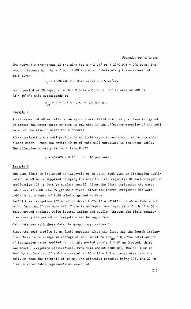
Groundwater balances
The hydraulic resistance of the clay bed c = D'/K' or 1.20/0.005 = 240 days. The
head difference hz - hi = 2.80 - 1.00 = 1.80 m. Substituting these values into
Eq.8 gives
v = 1.80/240 = 0.0075 m/day = 7.5 mm/day z
For a period of 20 days, v = 20 x 0.0075 = 0.150 m. For an area of 200 ha z
(2 x 10⁶m2) this corresponds to
O = 2 x 106 x 0.150 = 300 000 m3. up
Example 2
A rainshower of 40 mm falls on an agricultural field that has just been irrigated.
It causes the water table to rise 40 cm. What is the effective porosity of the soil
in which the rise in water table occurs?
After irrigation the soil profile is at field capacity and cannot store any addi
tional water. Hence the entire 40 mm of rain will percolate to the water table.
The effective porosity is found from Eq.27
V = 40/400 = 0.10 or 10 percent.
Example 3
The same field is irrigated at intervals of 10 days. Each time an irrigation appli
cation of 60 mm is supplied bringing the soil to field capacity. Of each irrigation
application 10% is lost by surface runoff. After the first irrigation the water
table was at 2.00 m below ground surface. After the fourth irrigation the water
table is at a depth of 1.80 m below ground surface.
During this irrigation period of 30 days, there is a rainfall of 45 mm from which
no surface runoff was observed. There is an impervious layer at a depth of 4.00 m
below ground surface, while lateral inflow and outflow through the field bounda
ries during the period of irrigation can be neglected.
Calculate now with these data the évapotranspiration Et.
Since the soil profile is at field capacity after the first and the fourth irriga
tion there is no change in storage of soil moisture (AS = 0). The total amount sm
of irrigation water applied during this period equals 3 x 60 mm (second, third
and fourth irrigation application). From this amount (180 mm), 10% or 18 mm is
lost by surface runoff and the remaining 180 - 18 = 162 mm penetrates into the
soil, as does the rainfall of 45 mm. The effective porosity being 10%, the 20 cm
rise in water table represents an amount of 217

(200 - 180) x o.I = 2 cm or 20 mm
Substituting the above values in Eq.6 gives
45 + 162 - Et - 20 = 0
which gives
Et = J87 mm or 187/30 = 6.2 mm/day
Example 4
The following data covering a 30-day period are available: percolation = 50 mm,
rise in water table Ah = 60 cm. The water table is at such a depth that the capil
lary rise can be neglected (Cap = 0).
For another period, lasting 20 days, a percolation of 20 mm and a rise in water
table Ah = 30 cm is observed. The water table is still at a depth of more than
3 m, so that the capillary rise can be neglected. Calculate the rate of net sub
surface inflow into the area and the effective porosity.
On substitution of the above values into Eq.26 we obtain
I' x 30 = 600 y - (50 - 0) ss
I' x 20 = 300 y - (20 - 0)
After rearranging and solving for I' we find
30 I' = 600 y -ss
40 I' = 600 u -ss
10 I' = 10 ss
- 50
- 40
I' = 1 mm/day ss
Substitution of this value into the equation for the first period, gives
30 x 1 = 600 V -50
600 y = 80
y = 0.13
Note: It will be seen that relatively slight variations in the value of the per
colation of the second period have a great effect on the results of the calcula
tions and may even change the net subsurface inflow into negative values. Hence
it is preferable to choose more than two time periods, which could even be taken
from different years, and to treat them graphically to smooth out inaccuracies of
the individual data.
218

Groundwater balances
Example 5
An agricultural area is irrigated at ]2-day intervals. It is known from irrigation
investigations that during each application approximately 25 mm of irrigation water
is lost to the water table (the sum total of field application losses and seepage
losses from the canal system). The lateral groundwater inflow through the bounda
ries of the field exceeds the lateral outflow by an amount of about 0.5 mm/day
(positive net subsurface inflow I = 0.5 mm/day). The effective porosity of the
soil is 8%. During a period of 36 days (including three irrigation applications)
a 50 cm rise in water table is observed. Calculate the capillary rise.
Substituting the above values into Eq.26, gives
Cap = (3 x 25) + (36 x 0.5) - (0.08 x 500) = 53 mm/36 days
or an average rate of capillary rise of 1.5 mm/day.
219

LITERATURE
BOUSSINESQ, J. 1903. Sur le débit en temps de sécheresse d'une source alimentée
par une nappe d'eaux d'infiltration. C.R.Acad.Sei.Paris 126:1511-1517.
ERNST, L.F. 1969. Determination of storage coefficients from observation of
groundwater levels. Water in the unsaturated zone. Symposium 1966, Proc.
UNESCO/IASH, p.966-989.
ERNST, L.F., DE RIDDER, N.A., and DE VRIES, J.J. 1970. A geohydrologic study
of East Gelderland (The Netherlands). Geol.en Mijnb. 49, 6:457-488.
JOHNSON, A.I. 1966. Specific yield. Compilation of specific yields for various
materials. U.S.Geo1.Survey Open-File Report. Hydrologie Lab.Denver, Col.
Also in: Geol.Surv. Water Supply Paper,1662-B, Washington 1965. 55 p.
VAN HOORN, J.W. 1960. Grondwaterstroming in komgrond en de bepaling van enige
hydrologische grootheden in verband met het ontwateringssysteem. (Ground
water flow in basin clay soil and the determination of some hydrological
factors in relation with the drainage system). With summary in English.
Thesis Univ.of Agric., Wageningen. 134 p.
220
SURVEYS AND INVESTIGATIONS
23. M E A S U R I N G SOIL M O I S T U R E
W. P. STAKMAN
Soil scientist Institute for Land and Water Management Research, Wageningen
Lecturers in the Course on Land Drainage
W. P. STAKMAN (1962-1973) Institute for Land and Water Management Research, Wageningen
PURPOSE AND SCOPE
A discussion of methods of determining soil moisture tensions and soil moisture
contents, with comments on some soil moisture characteristics.
CONTENTS
23.1 SOIL MOISTURE RETENTION 223
23.1.1 Introduction 223
23.1.2 Relation to pore size 223
23.1.3 Moisture retention curves 226
23.1.4 Comments on some soil moisture concepts 228
23.2 OBTAINING SOIL MOISTURE RETENTION CURVES 232
23.2.1 Taking a soil sample 232
23.2.2 Methods of determination 233
23.3 MEASURING SOIL MOISTURE CONDITIONS 243
23.3.1 Gravimetric determination of soil moisture content 243
23.3.2 Tensiometer 244
23.3.3 Electrical resistance units 245
23.3.4 Neutron scattering 247
23.3.5 Gamma-ray attenuation 248
LITERATURE 251
222
Soil moisture
23.1 SOIL MOISTURE RETENTION
23.1.1 INTRODUCTION
Between the soil and its water there exists a continuous energy relationship, the
theoretical background of which has been dealt with in Chap.5, Vol.1.
The potential energy of the soil water is defined as the work that is required
to bring a unit mass of water from a given reference position to a particular
point in the soil. Usually designated as reference position is the phreatic sur
face or the groundwater table. In the zone above the groundwater table the poten
tial - which is numerically equal to the hydrostatic pressure - has a negative
sign. Since the potential is negative in the unsaturated zone it is convenient
to express it in terms of tension or suction (negative pressure) involving only
a change in algebraic sign. In an equilibrium situation the tension in a soil
profile above a water table equals the height above that water table.
The mutual relationship between soil moisture content and soil moisture tension
is to a considerable extent dependent on the size and geometrical arrangement
of the pores in the solid matrix of the soil.
Cohesion forces (forces of attraction between molecules of the same type) and
adhesion forces (forces of attraction between molecules of different type) together
constitute matric forces or capillary forces. Combined with the "osmotic" forces
exerted by the ions adsorbed to the solid phase, they form the binding forces
between solid and liquid phase in a soil. The matric forces can be referred to
as soil moisture tension, soil moisture suction, or matric suction. The dis
solved solutes in the soil water may cause an osmotic solute tension or suction.
The sum of soil moisture tension and solute tension is called total soil moisture
tension.
In sandy soils the soil moisture tension is mainly built up by capillary forces
whereas in clay soils, particularly in the lower water content range, the ad
sorbed ions play an important part.
23.1.2 RELATION TO PORE SIZE
The capillary forces induce a concave water meniscus at the water-air interface.
Under hydrostatic equilibrium conditions (no water flow) the height of capillary
rise in soil pores, which are assumed to have a cylindrical shape, can be cal
culated with the following equation (Fig.1)
223
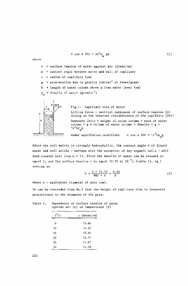
a cos a 2TTr (1)
where
a =
a =
r =
g =
h =
P.. =
surface tension of water against air (dynes/cm)
contact angle between water and wall of capillary
radius of capillary (cm)
acceleration due to gravity (cm/sec or dynes/gram)
length of water column above a free water level (cm)
density of water (gram/cm3)
Fig.1. Capillary rise of water
Lifting force = vertical component of surface tension (a) acting on the internal circumference of the capillary (2irr)
Downward force = weight of water column = mass of water column x g = volume of water column x density x g = irr2hp g
w
Under equilibrium conditions O cos a 2frr = ïïr hp g
Since the soil matrix is strongly hydrophyllic, the contact angle a of liquid
water and soil solids - perhaps with the exception of dry organic soils - will
tend towards zero (cos a = 1). Since the density of water can be assumed to
equal 1, and the surface tension a to equal 72.75 at 20 C (Table 1 ) , Eq.1
reduces to
2 x 72.75 0.30 h 981 x r d
where d = equivalent diameter of pore (cm).
It can be concluded from Eq.2 that the height of capillary rise is inversely
proportional to the diameter of the pore.
(2)
Table 1. Dependence of surface tension of water against air (a) on temperature (T)
T r «
0
10
15
20
25
30
a (dynes/cm)
75.60
74.22
73.50
72.75
71.97
71.18
224
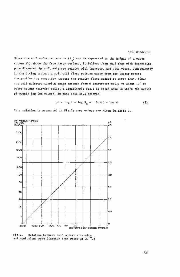
Soil moisture
Since the soil moisture tension (S ) can be expressed as the height of a water
column (h) above the free water surface, it follows from Eq.2 that with decreasing
pore diameter the soil moisture tension will increase, and vice versa. Consequently
in the drying process a soil will first release water from the larger pores;
the smaller the pores the greater the tension force needed to empty them. Since
the soil moisture tension range extends from 0 (saturated soil) to about 10 cm
water column (air-dry soil), a logarithmic scale is often used in which the symbol
pF equals log (cm water). In that case Eq.2 becomes
pF = log h = log S = - 0.523 - log d (3)
This relation is presented in Fig.2; some values are given in Table 2.
soil moisture tension cm water
5000
2000
1000
500
200
100
50
20
10
5
2
1
| / '
/\
i
pF 4.0
3000 1000 500 200 100 50 20 10 5 2 1 equivalent pore diameter (micron)
Fig.2. Relation between soil moisture tension and equivalent pore diameter (for water at 20 °C)
225
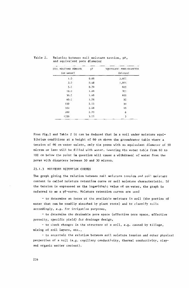
Table 2. Relation between soil moisture tension, pF, and equivalent pore diameter
SOIL MOISTURE TENSION pF EQUIVALENT PORE-DIAMETER
(cm water) (micron)
1.0 0.00 3,000
3.0 0.48 1,000
5.0 0.70 600
10.0 1.00 300
30.0 1.48 100
60.0 1.78 50
100 2.00 30
300 2.48 10
500 2.70 6
1000 3.00 3
From Fig.2 and Table 2 it can be deduced that in a soil under moisture equi
librium conditions at a height of 60 cm above the groundwater table where a
tension of 60 cm water exists, only the pores with an equivalent diameter of 50
micron or less will be filled with water. Lowering the water table from 60 to
100 cm below the point in question will cause a withdrawal of water from the
pores with diameters between 50 and 30 micron.
23.1.3 MOISTURE RETENTION CURVES
The graph giving the relation between soil moisture tension and soil moisture
content is called moisture retention curve or soil moisture characteristic. If
the tension is expressed as the logarithmic value of cm water, the graph is
referred to as a pF-curve. Moisture retention curves are used
- to determine an index of the available moisture in soil (the portion of
water that can be readily absorbed by plant roots) and to classify soils
accordingly, e.g. for irrigation purposes,
- to determine the drainable pore space (effective pore space, effective
porosity, specific yield) for drainage design,
- to check changes in the structure of a soil, e.g. caused by tillage,
mixing of soil layers, etc.,
- to ascertain the relation between soil moisture tension and other physical
properties of a soil (e.g. capillary conductivity, thermal conductivity, clay-
and organic matter content).
226

Soil moisture
Figure 3 shows pF-curves of various soil types.
Fig.3. Moisture retention curves of some soils
Soil type No.
1 2 3 4 5 6 7 8 9 10
Country
Tunesia Brazil Jamaica Senegal Argentina Congo E.Pakistan E.Pakistan India Brazil
Region
Medjerdah Valley Amazon Valley Black River Project Basse Casamana Albardon Lufira Ganges alluvium Ganges alluvium Bombay coastal plain Amazon Valley
Heavy clay Sandy yellow latosol Peat Marine (sal.)clay deposit River levee clay Clay Sandy loam Sand Salty clay Podsol.red fine sandy clay
Depth
40-50 100 0-20
5 20-40
20
40-60 100
Clay soils show a slow and regular decrease in water content with increasing pF
tension (Curves 1, 4, 6 and 9 in Fig.3).
Sandy soils may show only a slight decrease in moisture content in the lower pF
range till the point where only a small rise in pF causes a considerable discharge
of water due to a relatively large number of pores in a particular diameter range
(Curves 5 and 8; range 5-30 and 5-100 micron respectively).
The intersection point of the curves with the volumetric water content axis
(tension: 1 cm water, pF = 0) gives the water content of the soils under nearly
saturated conditions, which means that this point almost indicates the total
pore space percentage (if no air entrapment has taken place). The zero moisture
content is based on the oven-dry condition (105 C), corresponding to a pF of
approximately 7.
227

The total pore space percentage or porosity (e) - defined as the total volume
percentage of the total bulk not occupied by solid particles - can also be
calculated from the dry bulk density and particle density
bulk density (p,) = mass (grams) per unit volume (1 cm3) of soil including pore spaces
particle density (p ) = mass (grams) per unit volume (cm ) of soil solids.
Now the following equation holds
100 x p = (100 - e) x p (4)
d s
or 100 x p
£ = .100 (5)
23.1.4 COMMENTS ON SOME SOIL MOISTURE CONCEPTS
Field capacity
Field capacity is still often defined as the water content remaining in a soil
2 or 3 days after having been saturated and after drainage by gravity forces has
become "negligible". Other definitions have been based on a certain relationship
between the water content at field capacity and a particular soil moisture
tension, e.g. 1/3 atmosphere.
Older literature mentions the "moisture equivalent" as being an indication for
field capacity. The "moisture equivalent" is the weight percentage of water
retained by a previously saturated sample of soil 1 cm in thickness after it has
been subjected to a centrifugal force of one thousand times gravity for 30
minutes and should correspond with a moisture tension of about 1/3 atmosphere.
All these definitions are misleading. The "practically ceased drainage" concept
may only hold for a homogeneous sandy profile having good water-transmitting
properties. The attempts to correlate field capacity with a particular moisture
tension ignore the fact that in a soil profile the moisture condition is not only
dependent on the water-retaining forces but also on the water-transmitting pro
perties over the whole soil profile.
The downward flow (q) of water per unit cross-sectional area is
dS q = K h (^ + .) (6)
228
Soil moisture
where
S = soil moisture tension (cm water) m
z = depth (cm)
It = capillary conductivity (cm/day)
dS The term —r— represents the soil moisture tension gradient, the term ] represents
dz the gravitational gradient and
dS the term — — + 1 represents the total hydraulic gradient.
dz
In a well-drained soil the moisture distribution is relatively uniform. Conse
quently the hydraulic gradient plays a relatively minor role compared with that
of the capillary conductivity, which then mainly determines the drainage rate.
Any correlation between field capacity and a particular moisture tension will be
determined by the capillary conductivity - tension relationship.
For a poorly drained soil the hydraulic gradient is of more importance for the
determination of the field capacity tension value. Moisture equilibrium condi
tions between matric and gravity forces may not be reached even within a long
period of time due to the low drainage rate.
Field capacity expressed as moisture percentage on a dry-weight basis is usually
considered to be the upper limit of the available water in a soil.
If there is no influence of groundwater, the field capacity is assumed to be
roughly approached by a tension of 100 to 200 cm of water (pF 2.0 to 2.3). With
a shallow water table the tension at field capacity (cm water) may equal the
height (cm) above that table (e.g. pF 1.9 at 80 cm above the water level). Hete
rogeneity of the soil profile, impeding layers, fluctuating groundwater levels
complicate the field capacity problem. Therefore, research on field capacity
conditions in the field is preferable to measurements of moisture relationships
in the laboratory.
Wilting point or wilting percentage
In text books on plant physiology the (permanent) wilting percentage is defined
as the soil moisture condition at which the leaves undergo a permanent reduction
of their moisture content (wilting) because of a deficient supply of soil water,
a condition from which the leaves do not recover in an approximately saturated
atmosphere. Only by the addition of water to the soil will the plant recover.
229
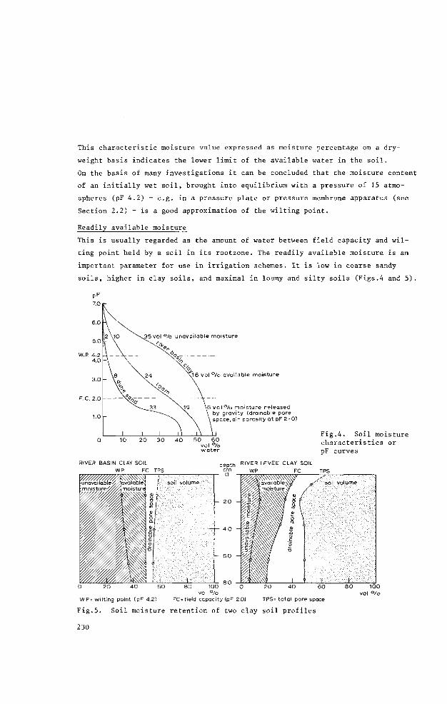
This characteristic moisture value expressed as moisture percentage on a dry-
weight basis indicates the lower limit of the available water in the soil.
On the basis of many investigations it can be concluded that the moisture content
of an initially wet soil, brought into equilibrium with a pressure of 15 atmo
spheres (pF 4.2) - e.g. in a pressure plate or pressure membrane apparatus (see
Section 2.2) - is a good approximation of the wilting point.
Readily available moisture
This is usually regarded as the amount of water between field capacity and wil
ting point held by a soil in its rootzone. The readily available moisture is an
important parameter for use in irrigation schemes. It is low in coarse sandy
soils, higher in clay soils, and maximal in loamy and silty soils (Figs.4 and 5).
16 vol °/o available moisture
6 vo l °/o moisture released by gravi ty (drainable pore space, air porosity at pF 2 -0)
10 20 30 40 50 60 vol °/o w a t e r
Fig.4. Soil moisture characteristics or pF curves
RIVER BASIN CLAY SOIL
WP FC TPS
so i l v o l u m e
d e p t h RIVER LEVEE CLAY SOIL
c rn WP FC TPS
8 0 8 0
^ % % ^ a v a i l a b l e \ ^ > '<yV/y\ mo is tu re sy
mm A
^ M i
a' •'. soil volume / • - ? ' ; : •
r •»•:•-. - - ; ^ i : • ; : > : : - ; . . 100
vol °/o FC= field capacity (pF 2.0)
20 40 60
TPS= total pore space
8 0 100 vol ° /o
WP. wilting point (pF4.2)
F i g . 5 . So i l mois ture r e t e n t i o n of two c lay s o i l p r o f i l e s
230

Soil moisture
Aeration porosity
This is also called air porosity, non-capillary porosity, aeration capacity, or
air capacity. In drainage practices the terms drainable pore space and effective
porosity are also used (see Chap.6.5.3, Vol.1). The first mentioned terms are
defined as the proportion of bulk volume that is filled with air under a speci
fied moisture tension. The aeration porosity is usually taken to be the aggre
gate of large pores, drained by a tension of no more than 100 cm of water.
Generally if the aeration porosity amounts to 10 or 15 vol.% or more at pF = 2.0,
aeration is satisfactory for plant growth. The river basin clay in Figs.4 and 5
is deficient in aeration.
Hysteresis
The relationship between moisture tension and moisture content of a porous mate
rial (e.g. soil) is in general not unique. At a given intermediate tension a soil
will contain less water if that tension is approached by wetting of a dry soil
than if it is approached by drying the same soil starting from a wet state. This
phenomenon is called hysteresis (Fig.6B).
The hysteresis effect may be attributable to
- the fact that pores have a larger diameter than their apertures or necks.
An empty pore system (A in Fig.6A) will only be completely filled with water
to a height inversely proportional to the diameter of its largest pores
(Eq.2). The water-filled pore system (B in Fig.6A) will not lose its water until
the tension has reached a higher value in accordance with the dimensions of its
narrowest apertures,
- variations in packing due to re-arrangement of soil particles by wetting
or drying,
- incomplete water uptake by soils that have undergone irreversible shrink
ing or drying (some clay and peat soils),
- entrapped air.
Due to this hysteresis effect soil moisture-tension relations depend on their
past moisture regime. Since moisture retention curves are generally determined
in the laboratory as desorption curves (from wet to dry conditions), this being
the most efficient procedure, one has to keep in mind that under field conditions
the moisture-tension relationship for a given soil is generally not constant
(Fig.7).
231
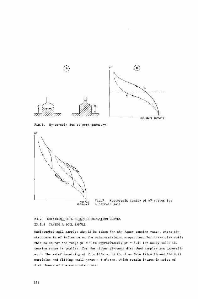
0
moisture content
Fig.6. Hysteresis due to pore geometry
pF
vol °/o Fig-?- Hysteresis family of pF curves for moisture a certain soil
23.2 OBTAINING SOIL MOISTURE RETENTION CURVES
23.2.1 TAKING A SOIL SAMPLE
Undisturbed soil samples should be taken for the lower tension range, where the
structure is of influence on the water-retaining properties. For heavy clay soils
this holds for the range pF = 0 to approximately pF = 3.5; for sandy soils the
tension range is smaller. For the higher pF-range disturbed samples are generally
used. The water remaining at this tension is found as thin films around the soil
particles and filling small pores < 1 micron, which remain intact in spite of
disturbance of the macro-structure.
232
Soil moisture
Undisturbed soil samples for pF-measurements are taken in the field at least in
duplicate. They can be obtained by pushing stainless steel cylinders (inside
diameter 50 mm, height 51 mm, contents 100 cm3) horizontally or vertically into
the distinct profile horizons, exposed by digging a pit and subsequently retriev
ing the filled cylinder. If no pit is dug, an auger in which the same type of
cylinder is fixed can be used.
Care should be taken in transporting the samples to the laboratory as they must
remain intact. In The Netherlands the sample cylinders are usually transported
in wooden boxes lined with foam plastic and rubber plate and each box contains
up to 24 cylinders. A plastic bag is filled with loose soil from each profile
horizon for the determination of pF-values > 3.
23.2.2 METHODS OF DETERMINATION
To construct the moisture retention curve of a sample, the moisture content of
that sample must be measured. This is done by equilibrating the moist soil sample
at a succession of known pF values and each time determining the amount of
moisture that is retained. If the equilibrium moisture content (expressed prefe
rably as volume percentage) is plotted against the corresponding tension (pF), the
moisture retention curve (pF-curve) can be drawn.
There is no single method of inducing the whole range of tensions from pF = - °°
(total saturation) to pF = 7 (oven-dry) but the following two laboratory methods
cover the range satisfactorily.
Porous medium method
The principle of the porous medium method is the equivalence of soil moisture
tension to a positive or negative pressure applied to a water-saturated porous
medium on which the sample is placed in close contact. The equilibrium moisture
content is measured by weighing. This method is the most generally used because
it covers the range pF 0 to 4.2, which is of particular importance in agricultural
practice. The method is technically simple, is inexpensive, and is well suited
for routine analysis.
For the range below 1 atmosphere (pF < 3) it is possible to apply a negative
pressure by using a vacuum pump. In case of low tensions (< 200 cm) a water
column can be suspended from the water in the porous medium.
It makes no difference in the results whether one uses negative or positive
pressure. For the range above 1 atmosphere a positive pressure is applied via
233

a reducing valve with a compressor unit or with a cylinder filled with compressed
air or nitrogen.
The porous medium itself should meet the following requirements:
- it must be possible to apply the required tension or pressure without
reaching the air-bubbling pressure (air entry value). This is the pressure at
which air bubbles start to leak through the medium, which is then no longer
water saturated. The maximum diameter of the pores is the limiting factor for
this pressure;
- the water permeability of the medium has to be as high as possible. This
demands a homogeneous pore size distribution, matching the applied pressure;
- the medium should not be easily damaged.
Types of porous media
Types of porous media used for the determination of moisture retention curves and
the air bubbling pressures of these media are given in Table 3.
Table 3. Maximum tension (cm water or pF) attainable with some water-saturated porous media
MATERIAL
blotting paper
asbestos
Blokzij1 sand
kaolin (China cla
sintered glass
cellulose filters
ceramic
cellophane
sausage casing
:y)
MAXIMUM TENSION
(cm water)
60
150
150
2,500
3,500
10,000
15,000
100,000
MAXIMUM TENSION
(PF)
1.8
2.2
2.2+)
3.4+)
3.5
4.0
4.2
5.0
see Fig.
234

Soil moisture
Commonly used in laboratories in The Netherlands are the following types of
porous media (Fig.8):
- "Blokzijl" sand for the tension range 1 to 100 cm water (pF from 0 to 2.0).
(Blokzijl is a small village in the North East Polder of The Netherlands. The
main fraction of the extremely fine sand found there is between 35 and 75 micron)
- "Blokzijl" sand with a top layer of kaolin for the range 100 to 500 cm
water (pF 2.0 to 2.7)
- Cellophane (Permeable Transparent No.600) for the range 1,000 to 15,000 cm
water (pF 3 to 4.2).
/.u
6.0
5.0
4.0
3.0 2.7
2.0
1.0
\ \ '\ \ \ \
- \ \ \ \
- \
- - _ .KAOLIN
^-IBLOKZIJL' SAND
\ \ \ \ \ \ \ \\ \\
i i i l 20
Fig.8. Moisture retention curves of "Blokzijl"-, o, sand and of kaolin
vol /o moisture
Apparatus for the tension range up to pF 2
The apparatus consists of a box made of stainless steel plate or earthen-ware
with perforated P.V.C. conduit pipes for drainage at the bottom. The box is filled
with Blokzijl sand. With a levelling bottle connected to the outlet of the. drainage
pipes, the "water table" can be adjusted within the range of 0 to 100 cm below
the surface of the sand (Fig.9).
Generally, tensions of successively 3.2, 10, 31.6, and 100 cm of water column are
applied (pF 0.5, 1.0, 1.5 and 2.0). The equilibrium moisture content of the soil
samples, to be determined by weighing, is attained within 3-10 days (heavy clay
soils may require more time).
235
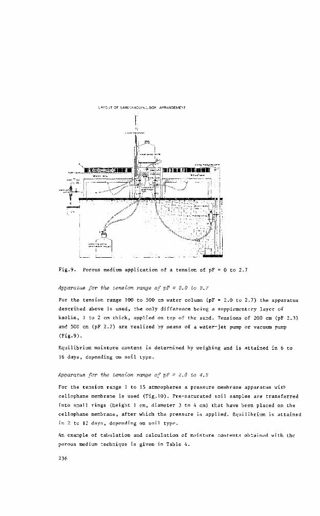
LAYOUT OF SANDtKAOLIN_)_BOX ARRANGEMENT
t . 1 f f l l i i« «JIMBlï
c i
_i>-
_F__£SneF * 1 lïlIllEIlilIHIllllliilIBBfl '
i «
cé
Fig.9. Porous medium application of a tension of pF = 0 to 2.7
Apparatus for the tension range of pF = 2.0 to 2.7
For the tension range 100 to 500 cm water column (pF = 2.0 to 2.7) the apparatus
described above is used, the only difference being a supplementary layer of
kaolin, 1 to 2 cm thick, applied on top of the sand. Tensions of 200 cm (pF 2.3)
and 500 cm (pF 2.7) are realized by means of a water-jet pump or vacuum pump
(Fig.9).
Equilibrium moisture content is determined by weighing and is attained in 6 to
16 days, depending on soil type.
Apparatus for the tension range of pF ~ 3.0 to 4.2
For the tension range 1 to 15 atmospheres a pressure membrane apparatus with
cellophane membrane is used (Fig.10). Pre-saturated soil samples are transferred
into small rings (height 1 cm, diameter 3 to 4 cm) that have been placed on the
cellophane membrane, after which the pressure is applied. Equilibrium is attained
in 2 to 12 days, depending on soil type.
An example of tabulation and calculation of moisture contents obtained with the
porous medium technique is given in Table 4.
236

Soil moisture
Table 4. Example of tabulation and calculation of the weighing data obtained during the determination of moisture retention curves
Dat
24.7.
26.7.
29.7.
31.7.
2.8.
6.8.
9.8.
12.8.
14.8.
19.8.
21.8.
26.8.
28.8.
30.8.
3.9.
5.9.
9.9.
11.9.
16.9.
18.9.
20.9.
23.9.
26.9.
30.9.
e
'63
'63
'63
'63
'63
'63
'63
'63
'63
'63
'63
'63
'63
'63
'63
'63
'63
'63
'63
'63
'63
'63
'63
'63
EXPERIMENTAL FIELD "SINDERHOEVE",
PLOT E n
pF
INITIAL
0.5
1 .0
1 .0
1.0
1 .5
1 .5
1.5
1.5
2.0
2.0
2.0
2.0
2.0
2.3
2.3
2.3
2.3
2.7
2.7
2.7
2.7
2.7
OVEN-DRY WEIGHT
(gram)
WEIGHT OF
CYLINDER (gram)
NET OVEN-DRY
WEIGHT (gram)
BULK DENSITY
pF
INITIAL
0.5
1 .0
1 .5
2.0
2.3
2.7
3.4
4.2
6.0
calculated [vom
SANDY SOIL
RENKUM,
Gross weight (c
Volume of
5-10 cm depth
Nr.of
929
253.0
278.3
277.5
277.4
277.3
272.4
272.2
271 .9
271 .8
263.1
262.9
262.7
262.4
262.4
259.7
258. 1
257.8
257.6
256. 1
255.4
255.2
255.1
255.1
233.7
98.5
135.2
1 .35
19.3
44.6
43.6
38.1
28.7
23.9
21 .4
weight 'i
cylinder
985
251.3
277.0
276.0
276.0
276.0
272.4
272.1
271.9
271.7
261.3
261. 1
260.9
260.5
260.5
257.2
255.4
255.3
255.1
253.7
253.2
252.9
252.7
252.6
231.6
98.9
132.7
1 .33
Volume
19.7
45.4
44.4
40. !
28.9
23.5
21 .0
> of water
THE NETHERLANDS
CROP : WHEAT
ylin
cyl
Mean
134
1
.0
.34
percen
19
45
44
39
28.
23.
21 .
13.
8.
3.
.5
.0
.0
.1
.8
.7
.2
,3+
,4+
1 +
X kul<
[der inc luded) (gram)
inder 100 cm
35-40
Nr.of
943
263.5
287.7
286.3
286.0
285.9
270.4
269.9
269.6
269.6
261.4
261.3
261.2
261.2
261 .2
259.0
257.7
257.4
257.2
256.4
255.9
255.7
255.5
255.4
246.2
100.0
146.2
1 .46
tage of
17.3
41.5
39.7
23.4
15.0
1 1 .0
9.2
densith
cm depth
cylinder
2082
261 .0
285.4
283.6
282.5
282.4
266.8
266.1
265.8
265.6
256.7
256.6
256.5
256.4
256.4
255.3
253.6
253.2
253.2
252.2
251 .8
251 .6
251 .4
251 .4
243.6
91 .8
151 .8
I .52
water
17.4
41 .8
38.8
22.0
12.8
9.6
7.8
Mean
149.0
1 .49
17.4
41 .7
39.3
22.7
13.9
10.3
8.5
3.3 +
2.7 +
0.9+
' (nee Section '/>. 1
237

i VALVE OF GAS CYLINDER
2 ADJUSTING SCREW OF REDUCING VALVE
3 VALVE B E T W E E N CONDUIT P I P E AND A P P A R A T U S
4 OUTLET VALVE
5 PRESSURE-GAUGE
6 BURETTE
Fig.10. Pressure membrane apparatus
Determining the air-bubbling pressure
The air bubbling pressure is the negative or positive pressure at which a water-
saturated porous material starts to transmit air. To examine the tension range
for which a porous medium is suited, the air-bubbling pressure must be ascertained.
This is done by applying a gradually increasing pressure to the pre-saturated
porous medium, which is covered by a thin layer of water (Fig.11).
At the moment air bubbling is discerned the corresponding pressure (h ) is read a
on a manometer. As air will first pass through the pore with the greatest throat,
the equivalent maximum pore diameter (d) can be calculated from Eq.2 as , 3,000 h = — 2 - —
a d
-4 where h is expressed in cm water and d in microns (10 cm).
If the maximum pore diameter of ceramic, sintered glass, steel, and other filters
is stated by the manufacturer, the air bubbling pressure can be calculated directly.
238
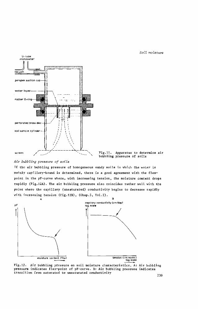
Soil moisture U-tube
manometer
perforated brass disc -
soil sample cy l inder-
Fig. ]J. Apparatus to determine air bubbling pressure of soils
Air bubbling pressure of soils
If the air bubbling pressure of homogeneous sandy soils in which the water is
mainly capillary-bound is determined, there is a good agreement with the flex-
point in the pF-curve where, with increasing tension, the moisture content drops
rapidly (Fig.l2A). The air bubbling pressure also coincides rather well with the
point where the capillary (unsaturated) conductivity begins to decrease rapidly
with increasing tension (Fig.l2B), (Chap.5, Vol.1).
PF capillary conductivity (cm/day) log- scale
moisture content ( ° /o ) tension (cm water) log. scale
Fig.12. Air bubbling pressure on soil moisture characteristics. A: Air bubbling pressure indicates flex-point of pF-curve. B: Air bubbling pressure indicates transition from saturated to unsaturated conductivity
239

Vapour pressure method
The principle of the vapour pressure method is based on the relation between soil
moisture tension and the water vapour pressure (relative humidity) of the sur
rounding atmosphere.
With the porous medium method it is the soil moisture tension equilibrium which
is measured, since the medium is equally permeable for water or for salt ions and
no difference in salt concentration occurs between the released and the retained
water. With the vapour pressure method the total moisture tension equilibrium (S )
is measured as the sum of soil moisture tension (S ) and solute tension (S ), m s
because the dissolved soil solutes influence the equilibrium vapour pressure.
The sample under test is allowed to reach moisture equilibrium with a known humid
ity, transfer of water taking place in the vapour phase. The equilibrium moisture
content of the sample is determined by weighing. Since humidity conditions are
dependent on temperature, accurate temperature control is needed.
When the soil water comes into equilibrium with the water vapour of the sur
rounding atmosphere, the following relation exists
RT e s,- = s + s = _ ^ l n —— O)
t m s gM e sat
where S = total tension of soil solution (cm)
S = soil moisture tension of soil solution (cm) m
S = solute tension of soil solution (cm) s
R = universal gas constant (8.315 x 10 ergs mole K )
T = absolute temperature (°Kelvin) (0 °C = 273 °K)
-2 g = acceleration due to gravity (981 cm sec )
M = molecular weight of water (18.0 g mole )
e = actual vapour pressure
e = saturated vapour pressure at same temperature
Since the relative vapour pressure e/e equals TKK (U being the relative humid-sat 100 ö
ity of the atmosphere expressed in percentage) Eq.7 becomes
c - R T i u - R T 9 ->n i I0° ,Q, St - ~W lnm~ gM 2-3° l0g TT (8)
240
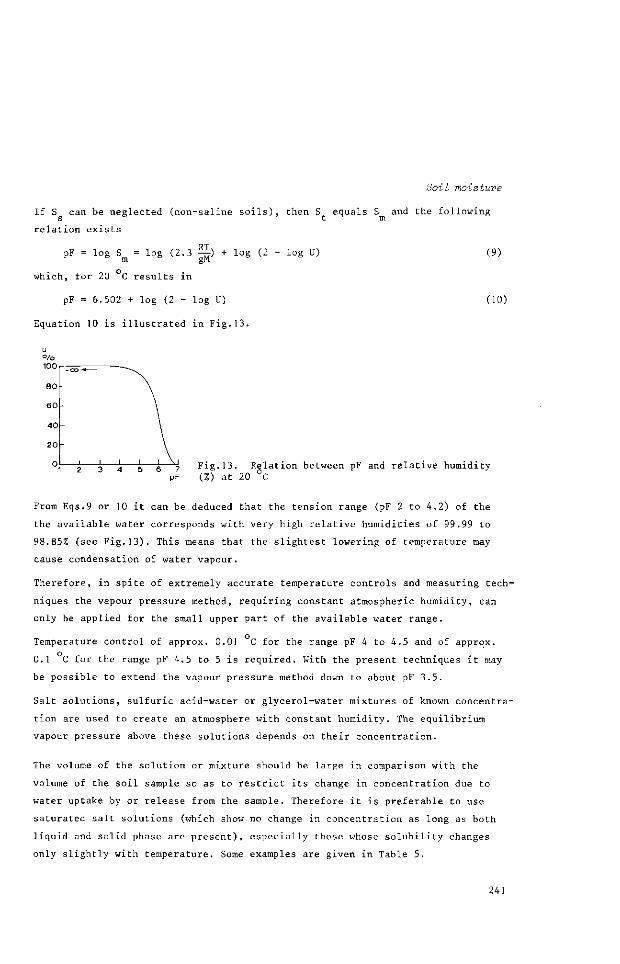
Soil moisture
If S can be neglected (non-saline soils), then S equals S and the following s t m
relation exists
pF = log S = log (2.3 ̂ ) + log (2 - log U) m gM
which, for 20 C results in
pF = 6.502 + log (2 - log U)
Equation 10 is illustrated in Fig.13.
(9)
(10)
0 i ^ J ^ g—^ Fig. 13. Relation between pF and relative humidity pF (%) at 20 °C
From Eqs.9 or 10 it can be deduced that the tension range (pF 2 to 4.2) of the
the available water corresponds with very high relative humidities of 99.99 to
98.85% (see Fig.13). This means that the slightest lowering of temperature may
cause condensation of water vapour.
Therefore, in spite of extremely accurate temperature controls and measuring tech
niques the vapour pressure method, requiring constant atmospheric humidity, can
only be applied for the small upper part of the available water range.
Temperature control of approx. 0.01 C for the range pF 4 to 4.5 and of approx.
0.1 C for the range pF 4.5 to 5 is required. With the present techniques it may
be possible to extend the vapour pressure method down to about pF 3.5.
Salt solutions, sulfuric acid-water or glycerol-water mixtures of known concentra
tion are used to create an atmosphere with constant humidity. The equilibrium
vapour pressure above these solutions depends on their concentration.
The volume of the solution or mixture should be large in comparison with the
volume of the soil sample so as to restrict its change in concentration due to
water uptake by or release from the sample. Therefore it is preferable to use
saturated salt solutions (which show no change in concentration as long as both
liquid and solid phase are present), especially those whose solubility changes
only slightly with temperature. Some examples are given in Table 5.
241
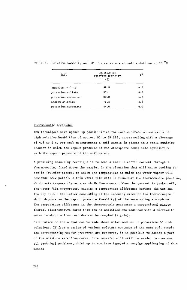
Table 5. Relative humidity and pF of some saturated salt solutions at 20 C
SALT
ammonium oxalate
potassium sulfate
potassium Chromate
sodium chloride
potassium carbonate
EQUILIBRIUM RELATIVE HUMIDITY
(%)
98.8
97.1
88.0
75.8
44.0
pF
4.2
4.6
5.2
5.6
6.0
Thermocouple technique
New techniques have opened up possibilities for more accurate measurements of
high relative humidities of approx. 95 to 99.98%, corresponding with a pF-range
of 4.8 to 2.5. For such measurements a soil sample is placed in a small humidity
chamber in which the vapour pressure of the atmosphere comes into equilibrium
with the vapour pressure of the soil water.
A promising measuring technique is to send a small electric current through a
thermocouple, fixed above the sample, in the direction that will cause cooling to
set in (Peltier-effect) to below the temperature at which the water vapour will
condense (dew-point). A thin water film will be formed at the thermocouple junction,
which acts temporarily as a wet-bulb thermometer. When the current is broken off,
the water film evaporates, causing a temperature difference between the wet and
the dry bulb - the latter consisting of the incoming wires of the thermocouple -
which depends on the vapour pressure (humidity) of the surrounding atmosphere.
The temperature difference in the thermocouple generates a proportional minute
thermal electromotive force that can be amplified and measured with a microvolt-
meter to which a line recorder can be coupled (Fig.14).
Calibration of the output can be made above molar sodium- or potassium-chloride
solutions. If from a series of various moisture contents of the same soil sample
the corresponding vapour pressures are measured, it is possible to assess a part
of the moisture retention curve. More research will still be needed to overcome
all technical problems, which up to now have impeded a routine application of this
method.
242

Soil moisture self recording micro Volt meter
— amplifier
— b a t t e r y 1.5 V
( / ) — m A meter
/WVN 1000 fl
thermo regulated water bath
dry bulb of thermocouple (copper w i res)
we t bulb of thermocouple (e.g.chromel-constantan wires)
soil sample Fig.14. Thermocouple measuring circuit
23.3 MEASURING SOIL MOISTURE CONDITIONS
Several methods of measuring the soil moisture content or tension, either in the
field or in the laboratory, are known. Only the most frequently applied methods
will be discussed.
23.3.1 GRAVIMETRIC DETERMINATION OF SOIL MOISTURE CONTENT
Measuring the water content by the gravimetric method involves weighing the
natural (wet) soil sample, and reweighing it after the water has been removed by
drying to constant weight in an oven at 105 C. The difference in weight indicates
the moisture content and is expressed either as a percentage of the weight or
volume of the oven-dry soil. The weight-percentage of moisture can be calculated
as follows
. , _ . weight wet soil - weight oven-dry soil weight % of moisture = ;—r— j 6 -, l x 100
weight oven-dry soil
grams water grams oven-dry soil
^r x 100
For irrigation, drainage, and other agronomic purposes it is useful to know the
moisture content on a volume basis (vol.% of water = mm of water per 10 cm depth).
If soil samples of known volume are taken, the moisture content expressed as a
percentage of that volume can be calculated as follows
243
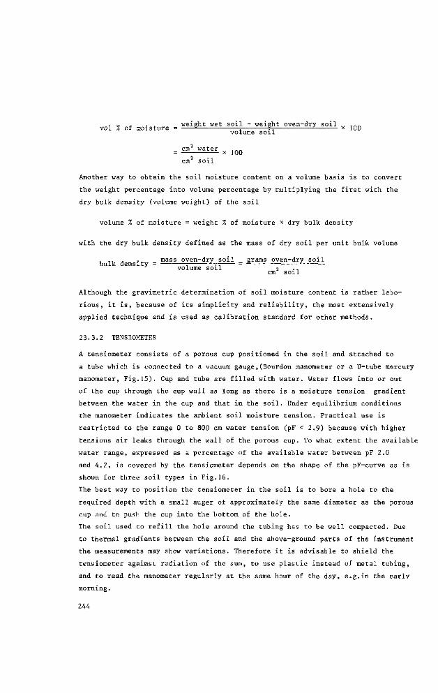
-.„e • - weight wet soil - weight oven-dry soil „ ,_. vol % of moisture = - = T-: x 100
volume soil
= C m 3 W a t e r x 100 cm soil
Another way to obtain the soil moisture content on a volume basis is to convert
the weight percentage into volume percentage by multiplying the first with the
dry bulk density (volume weight) of the soil
volume % of moisture = weight % of moisture x dry bulk density
with the dry bulk density defined as the mass of dry soil per unit bulk volume
, . . . . mass oven-dry soil grams oven-dry soil bulk density = ; ^-rz. = •=— -
volume soil 3 ., cm soil
Although the gravimetric determination of soil moisture content is rather labo
rious, it is, because of its simplicity and reliability, the most extensively
applied technique and is used as calibration standard for other methods.
23.3.2 TENSIOMETER
A tensiometer consists of a porous cup positioned in the soil and attached to
a tube which is connected to a vacuum gauge,(Bourdon manometer or a U-tube mercury
manometer, Fig.15). Cup and tube are filled with water. Water flows into or out
of the cup through the cup wall as long as there is a moisture tension gradient
between the water in the cup and that in the soil. Under equilibrium conditions
the manometer indicates the ambient soil moisture tension. Practical use is
restricted to the range 0 to 800 cm water tension (pF < 2.9) because with higher
tensions air leaks through the wall of the porous cup. To what extent the available
water range, expressed as a percentage of the available water between pF 2.0
and A.2, is covered by the tensiometer depends on the shape of the pF-curve as is
shown for three soil types in Fig.16.
The best way to position the tensiometer in the soil is to bore a hole to the
required depth with a small auger of approximately the same diameter as the porous
cup and to push the cup into the bottom of the hole.
The soil used to refill the hole around the tubing has to be well compacted. Due
to thermal gradients between the soil and the above-ground parts of the instrument
the measurements may show variations. Therefore it is advisable to shield the
tensiometer against radiation of the sun, to use plastic instead of metal tubing,
and to read the manometer regularly at the same hour of the day, e.g.in the early
morning.
244
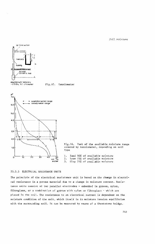
Soil moisture
air free water
Ol tubing
porous ceramic cup
equilibrium tension = = (13.6h (-h) c m w a t e r Fig.15. Tensiometer
available water range tensiometer range
40 50 vol °/o water
Fig.16. Part of the available moisture range covered by tensiometer, depending on soil type
1. Sand 50% of available moisture 2. Loam 75% of available moisture 3. Clay 25% of available moisture
23.3.3 ELECTRICAL RESISTANCE UNITS
The principle of the electrical resistance unit is based on the change in electri
cal resistance in a porous material due to a change in moisture content. Resis
tance units consist of two parallel electrodes - embedded in gypsum, nylon,
fibreglass, or a combination of gypsum with nylon or fibreglass - which are
placed in the soil. The resistance to an electrical current is dependent on the
moisture condition of the unit, which itself is in moisture tension equilibrium
with the surrounding soil. It can be measured by means of a Wheatstone bridge.
245

The electrical resistance of the unit should be calibrated against the soil
moisture tension (Fig.17). Calibration can be done in the field by taking soil
samples for moisture content determination at the same time as resistance
measurements are made. If the moisture retention curve is known, the relation
between resistance and tension can be plotted. For calibration in the laboratory
either the same procedure can be followed or the resistance-tension relation can
be measured on soil samples subjected to tensions by means of the porous medium
method. If the blocks are of standard manufacture, it is not necessary to calibrate
each unit separately.
Resistance readings will be affected by hysteresis phenomena and by the presence
of electrolytes in the soil solution. The lowering of the resistance, due to
electrolytes, is counteracted by the saturated solution of calcium sulphate
present in gypsum blocks. The blocks can therefore be used in slightly saline
soils of which the saturation-extract shows a conductivity of less than approxi
mately 2 mmhos cm . Under wet conditions and in acid soils the gypsum block
will gradually deteriorate. Nylon and fibreglass units are more durable but are
very sensitive to electrolytes.
The electrical resistance method is not suitable for soils showing shrinkage
(contact problems) or for sandy soils with a somewhat horizontal section in the
moisture retention curve for which a slight change in tension would cause a great
change in water content.
Gypsum blocks are recommended for the range of pF 2.3 to 4 (Fig.17), nylon
elements encased in gypsum for the range of pF 1.3 to 2.3.
resistance ohms 10'
pF Fig.17. Electrical resistance (ohms) of gypsum block versus moisture tension
246
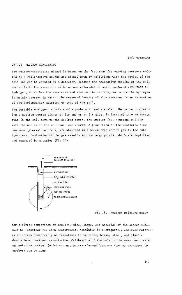
Soil moisture
23.3.4 NEUTRON SCATTERING
The neutron-scattering method is based on the fact that fast-moving neutrons emit
ted by a radio-active source are slowed down by collisions with the nuclei of the
soil and can be counted by a detector. Because the moderating ability of the soil
nuclei (with the exception of boron and chloride) is small compared with that of
hydrogen, which has the same mass and size as the neutron, and since the hydrogen
is mainly present in water, the measured density of slow neutrons is an indication
of the (volumetric) moisture content of the soil.
The portable equipment consists of a probe unit and a scaler. The probe, contain
ing a neutron source either at its end or at its side, is inserted into an access
tube in the soil down to the desired depth. The emitted fast neutrons collide
with the nuclei in the soil and lose energy. A proportion of the scattered slow
neutrons (thermal neutrons) are absorbed in a boron trifluoride gas-filled tube
(counter). Ionization of the gas results in discharge pulses, which are amplified
and measured by a scaler (Fig.18).
scaler and counter recorder
preamplifier
BF3 tube (counter)
access tube
slow neutrons
fast neutrons
radio-active source
Fig.If Neutron moisture meter
For a direct comparison of results, size, shape, and material of the access tubes
must be identical for each measurement. Aluminium is a frequently employed material
as it offers practically no resistance to neutrons; brass, steel, and plastic
show a lower neutron transmission. Calibration of the relation between count rate
and moisture content (which can not be transferred from one type of apparatus to
another) can be done
247
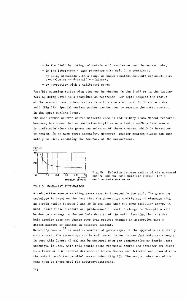
- in the field by taking volumetric soil samples around the access tube;
- in the laboratory - same procedure with soil in a container;
- by using standards with a range of known constant moisture contents, e.g. sand-alum or sand-paraffin mixtures;
- by comparison with a calibrated meter.
Possible counting drifts with time can be checked in the field or in the labora
tory by using water in a container as reference. For depth-samples the radius
of the measured soil sphere varies from 15 cm in a wet soil to 30 cm in a dry
soil (Fig.19). Special surface probes can be used to measure the water content
in the upper surface layer.
The most common neutron source hitherto used is Radium-Beryllium. Recent research,
however, has shown that an Americium-Beryllium or a Plutonium-Beryllium source
is preferable since the gamma ray emission of these sources, which is hazardous
to health, is of much lower intensity. Moreover, greater neutron fluxes can then
safely be used, enhancing the accuracy of the measurement.
radius cm 40
\ X ——'—\— ' '1~^ \ —
0.6 O.S 1.0 g r /cm 3
moisture content
Fig.19. Relation between radius of the measured sphere and the soil moisture content for a neutron moisture meter
23.3.5 GAMMA-RAY ATTENUATION
A radioactive source emitting gamma-rays is inserted in the soil. The gamma-ray
technique is based on the fact that the absorption coefficient of elements with
an atomic number between 2 and 30 is the same when the same radiation energy is
used. Since these elements are predominant in soil, a change in absorption will
be due to a change in the wet bulk density of the soil. Assuming that the dry
bulk density does not change over long periods changes in adsorption give a
direct measure of changes in moisture content. 137 . . . .
Generally Cesium is used as emitter of gamma-rays. If the apparatus is suitably
constructed, the gamma-rays can be collimated in such a way that moisture changes
in very thin layers (1 cm) can be measured when the transmission or double probe
technique is used. With this double-probe technique source and detector are fixed
to a frame at a horizontal distance of 40 cm. Source and detector are lowered into
the soil through two parallel access tubes (Fig.20). The access tubes are of the
same type as those used for neutron-scattering.
248

Soil moisture
Another technique is the scattering technique, where a single probe contains both
source and detector, separated by shielding. With this method, for which one
access tube suffices, an approximately spherical sample with a diameter of 20 to
75 cm, depending on apparatus and soil characteristics, is measured. Therefore the
double-probe technique is better suited for the study of shallow layers in a
soil profile.
A comparison of the merits and limitations of methods mentioned in Sect.3.1 to
3.5 is given in Table 6.
The above enumeration of methods for the determination of soil water is not com
prehensive. The electrical capacitance, the thermal conductivity, and the porous
absorber method have not found wide usage and cannot be recommended at this
time. The same can be said for the freezing-point-depression and the centrifuge
method in the laboratory.
2355
El
y/jsy///Rmmm y/tw*W/,
Fig.20. Set up of gamma ray transmission equipment. l=source, 2=detector, 3= connection frame of detector and source, 4=container, 5=counter, 6=access tube for source, 7=access tube for detector
249

Table 6. Principal merits and limitations of the common methods of soil moisture measurement
METHOD MERITS LIMITATIONS
sampling complete moisture range, not (gravimetric) sensitive to salt and tempe
rature, reliable (used as calibration standard)
not reproducible, high sampling error, volume weight to be known, laborious
tensiometer direct measurement of moisture tension, reproducible
limited tension range, hysteresis effect, contact with soil (particularly in swelling and shrinking soils), apparatus fragile
electrical resistance blocks (gypsum) and nylon units)
practically complete moisture range, reproducible
sensitive to temperature and salt (especially nylon units), hysteresis effect, contact with soil, calibration, limited life in wet, acid soils (particularly gypsum units)
neutron scattering
complete moisture range, reproducible, no salt and temperature influence, relatively large horizontal distance
apparatus fragile and expensive, relatively large vertical distance, deviations due to high amounts of organic matter and uncommon excesses of B, CI, and Fe
gamma radiation adsorption
complete moisture range, reproducible, relatively large horizontal and small vertical distance, no salt and temperature influence
apparatus fragile and expensive, volume weight to be known
250
Soil moisture
LITERATURE
BAVEL, C.H.M.van, et al. 1963. Soil moisture measurement with the neutron method.
U.S.D.A., ARS-41-70. 39 pp.
BAVER, L.D., GARDNER, W.H., and GARDNER, W.R. 1972. Roil physics. 4th ed.,John
Wiley & Sons, Inc. New York, Sydney, London, Toronto. 498 pp.
BLACK, C.A. et al. 1965. Methods of soil analysis. Part I, Agronomy No.9.
Am. Soc. Agronomy. 770 pp.
BUCKMAN, H.O., and BRADY, N.C. 1969. The nature and properties of soils. Macmil-
lan Co., London. 653 pp.
CRONEY, D. et al. 1952. The suction of water held in soil and other porous
materials. Road Res.Techn.Paper,No.24, 42 pp.
GARDNER, W.R. 1967. Water movement in the unsaturated soil profile. Proc.Int.
Soil Water Symposium, I.e.I.D. Praha. Vol.11, 223-236.
HILLEL, D. 1971. Soil and water: Physical principles and processes. Academic Press
Inc.,New York. 288 pp.
HOLMES, J.W. et al. 1967. Measurement of soil water. In: R.M.Hagan et al. (Ed.),
Irrigation of Agricultural Lands, Agronomy No.11, 275-303. Am.Soc.Agron.
KIRKHAM, D. and POWERS, W.L. 1972. Advanced Soil Physics. Wiley-Interscience,
New York. 534 pp.
KOHNKE, H. 1968. Soil Physics. McGraw-Hill Book Co.,New York. 224 pp.
ROSE, C.W. 1966. Agricultural Physics. Pergamon Press, Oxford. 226 pp.
RIJTEMA, P.E. 1969. The calculation of non-parallelism of gamma access tubes,
using soil sampling data. Techn.Bull.67. I.C.W. Wageningen.
RYHINER, A.H. and PANKOW, J. 1969. Soil moisture measurement by the gamma trans
mission method. Techn.Bull.66. I.C.W. Wageningen.
STAKMAN, W.P. 1969. Determination of pore size by the air bubbling pressure method
Mise.Repr.84. I.C.W. Wageningen.
STAKMAN, W.P. et al. 1969. Determination of soil moisture retention curves I.
Sand-box apparatus. II. Pressure membrane apparatus. I.C.W.Wageningen.
TAYLOR, S.A. et al. 1964. Evaluating soil water. Bull.426. Agr.Exp.Stat.,
Utah State Univ. 67 pp.
251

SURVEYS AND INVESTIGATIONS
24. D E T E R M I N I N G H Y D R A U L I C C O N D U C T I V I T Y OF SOILS
J. KESSLER f
Land and Water Management Specialist International Institute for Land Reclamation and Improvement, Wageningen
R. J . OOSTERBAAN
Land Drainage Engineer International Institute for Land Reclamation and Improvement Wageningen
Lecturers in the Course on Land Drainage
W. C. VISSER (1962) Institute for Land and Water Management Research, Wageningen
G. ZIJLSTRA (1963-1966) International Institute for Land Reclamation and Improvement, Wageningen
J. KESSLER (1967) International Institute for Land Reclamation and Improvement, Wageningen
J. G. VAN ALPHEN (1968) International Institute for Land Reclamation and Improvement, Wageningen
R. J. OOSTERBAAN (1969, 1970) International Institute for Land Reclamation and Improvement, Wageningen
C. L. VAN SOMEREN (1971-1973) International Institute for Land Reclamation and Improvement, Wageningen
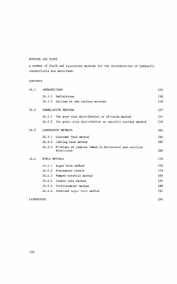
PURPOSE AND SCOPE
A number of field and laboratory methods for the determination of hydraulic
conductivity are described.
CONTENTS
24.1 INTRODUCTION 255
24.1.1 Definitions 255
24.1.2 Outline of the various methods 256
24.2 CORRELATIVE METHODS 257
24.2.1 The pore size distribution or pF-curve method 257
24.2.2 The grain size distribution or specific surface method 259
24.3 LABORATORY METHODS 264
24.3.1 Constant head method 264
24.3.2 Falling head method 266
24.3.3 K-values of samples taken in horizontal and vertical directions 268
24.4 FIELD METHODS 270
24.4.1 Auger hole method 270
24.4.2 Piezometer method 279
24.4.3 Pumped borehole method 283
24.4.4 Double tube method 285
24.4.5 Infiltrometer method 289
24.4.6 Inversed auger hole method 292
LITERATURE 295
254

24.1 INTRODUCTION
24.1.1 DEFINITIONS
The term hydraulic conductivity is the proportionality factor K in Darcy's law
for the flow of water in soil (Chap.6, Vol.1),
v = - Ki (1)
where
v = flow velocity (LT )
K = hydraulic conductivity (LT )
i = -T— = hydraulic potential gradient (dimensionless) dx
It can be seen that for a unit hydraulic gradient the flow velocity equals K. The
factor K usually stands for the hydraulic conductivity of a saturated soil, i.e.
under positive pressure of the soil water. It is considered independent of the
pressure gradient because we assume that the water-conducting porosity does not
change with the pressure gradient. Under unsaturated conditions, however, the
hydraulic conductivity varies with the soil moisture suction, since suction, soil
moisture content, and water-conducting porosity are closely interrelated. K is
then called capillary conductivity and is represented by the symbol K to signify h
the relationship.
The hydraulic conductivity of a soil represents its average water transmitting
properties, which depend mainly on the number and the diameter of the pores present.
If these are uniformly distributed, the soil is said to be homogeneous. In such a
soil the hydraulic conductivity is the same in all directions and the soil is
said to be isotropic.
Soils commonly show a certain stratification so that the hydraulic conductivity
in one direction is greater than in another. A soil in which the hydraulic
conductivity at any point has preferential directions is called anisotropic.
If the anisotropy varies from point to point in a given layer, the layer is said
to be heterogeneous. If, on the other hand, the condition of anisotropy is the
same from point to point in the layer, the layer is still homogeneous.
Apart from porosity, hydraulic conductivity also depends on the viscosity and
density of the soil water. This relationship is expressed in the following
equation (see also Chap.6, Vol.1)
K = K' £-£ (2)
255
where
K = hydraulic conductivity (cm/sec)
K' = intrinsic permeability independent of density and viscosity (cm )
p = mass density of the solution (g/cm )
g = acceleration due to gravity (cm/sec2)
T] = dynamic viscosity of the solution (poise, g/cm sec)
Density and viscosity are determined mainly by the temperature and salt concen
tration of the soil water. Only relatively small variations in these factors are
found in the field,but corrections may be necessary when laboratory data are used.
24.1.2 OUTLINE OF THE VARIOUS METHODS
Hydraulic conductivity, K, can be determined either from soil samples in the
laboratory or from soil bodies in situ. Both methods impose certain flow condi
tions on a soil body, after which discharge is measured and K calculated with
a formula describing the relation between K, the flow conditions, and the dis
charge. An analytical derivation of the formula is possible because flow condi
tions are relatively simple to produce in the laboratory. Flow systems with
known boundaries are obviously more difficult to create in the field. This has
certain implications for the determination and derivation of the geometry factor
(C) which is introduced into the formulas. The field measurements are of two
types, viz. measurements in non-saturated soils (above the water table) and in
saturated soils (below the water table). Examples of the first type are the
double tube method, the infiltrometer method, and the inversed auger hole method,
which are discussed in Sects.4.4, 4.5, and 4.6 respectively.
Methods for measuring K below the water table can be roughly classified into
large-scale field measurements and point measurements. The former are discussed
in Chaps.21, 25, 26, Vol.111. Point measurements below the water table require a
bore hole from which water is removed and the rate of rise of the water level is
observed (augerhole method, Sect.4.1; piezometer method, Sect.4.2), or a bore
hole in which the water table is kept at a certain level by pumping and the water
extraction measured (pumped borehole, Sect.4.3).
Estimation methods, employing the correlation between hydraulic conductivity and
the pore or grain size distribution of the soil are discussed in Sects.2.1 and
2.2 respectively.
256
Hydraulic conductivity
24.2 CORRELATIVE METHODS
24.2.1 THE PORE SIZE DISTRIBUTION OR pF-CURVE METHOD
Principle
This method is based on the laws of Poiseuille and Darcy and describes the relation
between K and the hydraulic gradient for a given cylindrical capillary pore. An
average K value can be estimated with the aid of a moisture retention curve.
Calculations
According to the laws of Poiseuille and Darcy the hydraulic conductivity of a
capillary pore for laminar flow is (Chap.6, Vol.1)
where
K = hydraulic conductivity (cm/sec)
r = radius of cylindrical pore (cm)
p, g, and i"| are as previously defined
The height to which water will rise in a vertical capillary cylinder is (Chap.5,
Vol.1)
h - * L (4)
Pgr where
h = height of capillary rise or capillary pressure (cm)
O = surface tension of water against air (dyne/cm, g/sec2)
p and g are as previously defined.
Combining Eqs.3 and 4 gives
K = - 2 Î - (5) 2pgnh2
For water at 20 C, a = 73 dyne/cm, n = 0.01 poise and pg = 980 g/cmz sec2,
whence
K = 2 7 0 ( 6 )
h2
MARSHALL (1957) determined the pore size distribution using the soil moisture
retention curve (Fig.1). The vertical axis, with the moisture content in vol.%,
257

is divided in n equal intervals. Each interval i represents a number of capil
laries having an average radius equal to the capillary height, h, required to
empty the pores.
Marshall subsequently estimated K from
e2 2i-l K = 270 — Ï, ^ - ± (7)
where n2 i=l h2
l
K = hydraulic conductivity (cm/sec)
e = the porosity of the soil (vol.%)
n = number of intervals on the moisture content axis
h = height of capillary rise (cm)
2i-l = weight factor
moisture content vol ° /o 50
80 100 200 300 500 1000 linear scalel log scale cm
-• *- capilary pressure
Fig.1. Soil moisture retention curve of a sandy soil with average capillary pressure by porosity class and moisture range
Examp le 1
The soil moisture retention curve of a sandy soil has been divided along the
moisture axis in n = 9 equal intervals of 5%. The total porosity of the soil
is assumed to equal the soil moisture content at zero capillary pressure, e = 0.45.
The average capillary pressure required to lower the soil moisture content to the
average moisture content of each interval is given in Fig.1 from which Table 1 is
derived.
The hydraulic conductivity is calculated, according to Eq.7
270 (CL45)2
L41 1_ + ^
2 £-;2 67"
5
852 105" 140'
11
2502
13
4002
15
7302
-3 2.2 x 10 cm/sec or K = 1.9 m/day
258

Hydraulic conductivity
Table 1. Relation between moisture content and capillary pressure
Porosity class
]
2
3
4
5
6
7
8
9
Moisture range
40 -
35 -
30 -
25 -
20 -
15 -
10 -
5 -
0 -
m 45
40
35
30
25
20
15
10
5
Average capillary pressure (cm)
>
41
67
85
105
140
250
400
730
1000
Discussion
The pF-curve method for determining hydraulic conductivity is only applicable to
soils with a single grain structure such as sands. The continuity and regularity
of small pores is probably higher than those of larger pores and to account for
this a weight factor (2i-l)/n2 is introduced in Eq.7 (see for the derivation of
Eq.7 MARSHALL, 1957). It should be noted that when hydraulic conductivity is
calculated from the moisture retention curve only an order of magnitude is obtained
and not an exact value.
24.2.2 THE GRAIN SIZE DISTRIBUTION OR SPECIFIC SURFACE METHOD
Principle
The principle of this method is similar to that of the pore size distribution
technique, the main difference being that the pore size is not related to capil
lary pressure but to the specific surface of the soil particles. The specific
surface (or U figure) is a single parameter by which the grain size distribution
of a sample of sandy soil is expressed.
Calculations
The specific surface (U) is defined as the ratio of the total surface area of the
soil particles to the surface area of an equal quantity, by weight, of spherical
particles of the same material with a diameter of 1 cm.
If we assume w gram of a material whose particles are spheres with a diameter of
d cm and a mass density p , then the number of particles in w gram material is
259

w _ 6w
1/6 ïïd3p ïïd3p
and the t o t a l su r face a rea of t hese p a r t i c l e s
6w 12 6w ? TTd = cm
l d p dp s s
The total surface area of w gram of these particles with a diameter of 1 cm is
therefore 6w/p cm2. The specific surface of the material
6w I 6w _ ]_ dp ' p d
s s
a relation derived by HOOGHOUDT (1934).
(8)
In fact granular soils generally do not consist of uniform particles of one single
diameter, but will contain grains of different sizes, to be grouped in fractions,
each with certain limits of particle size. The relation between fraction size and
U figure is given in Table 2.
Table 2. Sand fractions, their particle size limits, and U figure
Description
Extremely fine sand
Very fine sand
Fine sand
Moderately fine sand
Moderately coarse sand
Coarse sand
Very coarse sand
Extremely coarse sand
Partiel limits
di
16
63
83
125
200
333
500
1000
- size TI i , l (micron) da
d2
63
83
125
200
333
500
1000
2000
d in cm
(625 + 160)
(160 + 120)
(120 + 80)
(80 + 50)
(50 + 30)
(30 + 20)
(20 + 10)
(10 + 5)
IT'
= 390
= 140
= 100
= 65
= 40
= 25
= 15
= 7.5
For a sand sample, consisting of a number of different fTactions,one can calculate
the value of U for the total sample as follows
(9)
where
W. l
U z u.w.
1 1 tot W tot
weight of the fraction i
weight of all the fractions
260
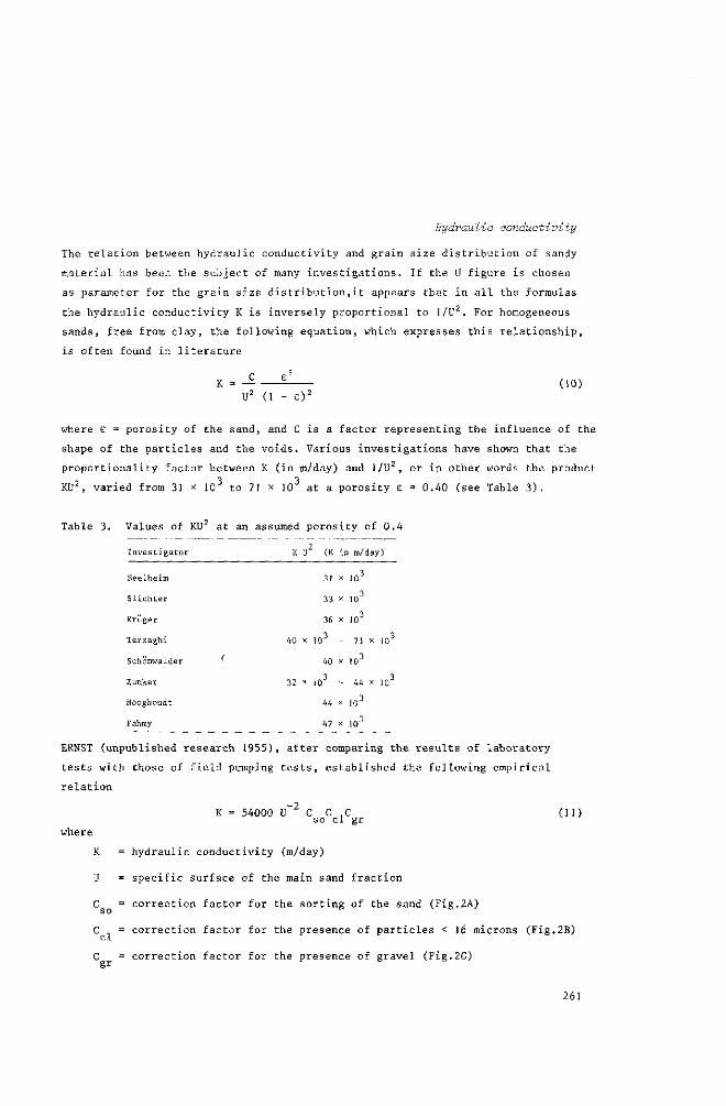
Hydraulic conductivity
The relation between hydraulic conductivity and grain size distribution of sandy
material has been the subject of many investigations. If the U figure is chosen
as parameter for the grain size distribution,it appears that in all the formulas
the hydraulic conductivity K is inversely proportional to 1/U2. For homogeneous
sands, free from clay, the following equation, which expresses this relationship,
is often found in literature
C f3
K = -^ £ (jo) U2 (1 - e ) 2
where e = porosity of the sand, and C is a factor representing the influence of the
shape of the particles and the voids. Various investigations have shown that the
proportionality factor between K (in in/day) and 1/U2, or in other words the product
KU2, varied from 31 x 10 to 71 x 10 at a porosity e = 0.40 (see Table 3).
31
33
36
40 x 103
40
32 x io
44
47
x
x
x
-X
-x
X
io3
io3
io3
71 x
,03
44 x
103
103
,o3
io3
Table 3. Values of KU at an assumed porosity of 0.4
2 Investigator K U (K in m/day)
Seelheim
Slichter
Krüger
Terzaghi
Schonwalder ^
Zunker
Hooghoudt
Fahmy
ERNST (unpublished research 1955), after comparing the results of laboratory
tests with those of field pumping tests, established the following empirical
relation
K = 54000 U~2 C C ,C (11) so cl gr
where
K = hydraulic conductivity (m/day)
U = specific surface of the main sand fraction
C = correction factor for the sorting of the sand (Fig.2A)
so " C , = correction factor for the presence of particles < 16 microns (Fig.2B)
cl C = correction factor for the presence of gravel (Fig.2C)
261
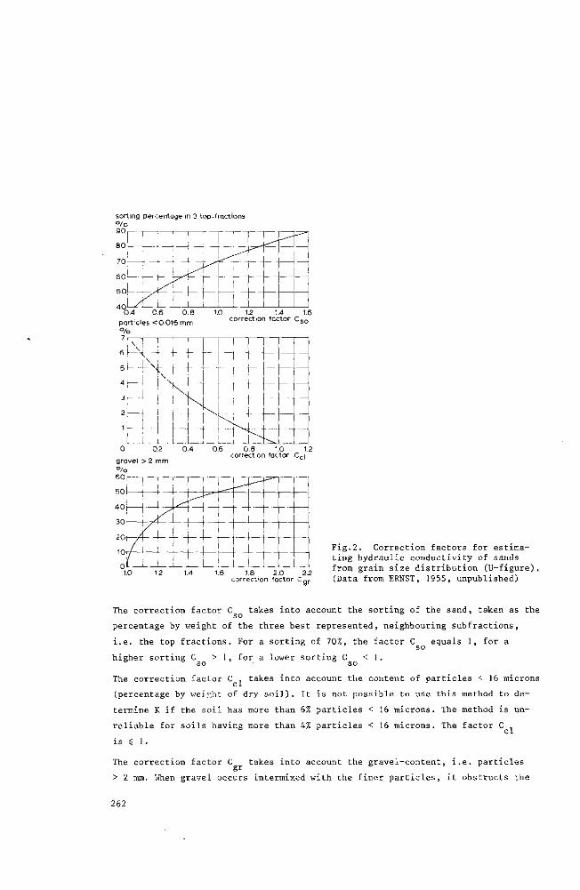
sorting percentage in 3 top-fractions ° /o 90 r
4 0 L ^ ' — 0.4 0.6
particles <0.016 mm °/o
1.0 1.2 1.4 1.6 correction factor C - n
'̂ n— 6 k - \ -4- f-
si-4H t-\ 4 1
3r 'l 2' f-
1 '-• I •
L i .
v
4-
f • — 1
|" r
I
TT-t i— t t-\ •
—
—
—
--
• —
—
—
0 0.2
gravel > 2 mm °/o 60
50 h
0.6 0.8 1.0 1.2 correction factor C c |
4 0 r
30
20r
10
r \ T I . L
L-j
A ! I I ,
-yi--i- 1 i
h 4—
— i —
—
—
1.6 1.8 2.0 2.2 correction factor C n r
Fig.2. Correction factors for estimating hydraulic conductivity of sands from grain size distribution (U-figure). (Data from ERNST, 1955, unpublished)
The correction factor C takes into account the sorting of the sand, taken as the so
percentage by weight of the three best represented, neighbouring subfractions,
i.e. the top fractions. For a sorting of 70%, the factor C equals 1, for a
higher sorting C > 1, for a lower sorting C < 1. so so
The correction factor C . takes into account the content of particles < 16 microns cl
(percentage by weight of dry soil). It is not possible to use this method to de
termine K if the soil has more than 6% particles < 16 microns. The method is un
reliable for soils having more than 4% particles < 16 microns. The factor C
is $ 1.
The correction factor C takes into account the gravel-content, i.e. particles gr
> 2 mm. When gravel occurs intermixed with the finer particles, it obstructs the
262
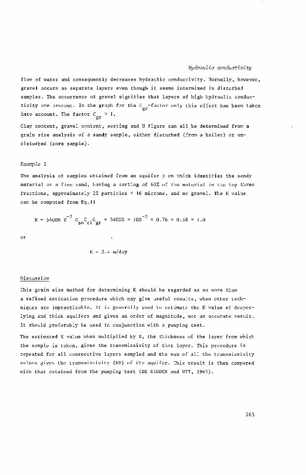
Hydraulic conductivity
flow of water and consequently decreases hydraulic conductivity. Normally, however,
gravel occurs as separate layers even though it seems intermixed in disturbed
samples. The occurrence of gravel signifies that layers of high hydraulic conduc
tivity are present. In the graph for the C -factor only this effect has been taken
into account. The factor C > 1.
gr
Clay content, gravel content, sorting and U figure can all be determined from a
grain size analysis of a sandy sample, either disturbed (from a bailer) or un
disturbed (core sample).
Example 2
The analysis of samples obtained from an aquifer 5 cm thick identifies the sandy
material as a fine sand, having a sorting of 60% of the material in the top three
fractions, approximately 2% particles < 16 microns, and no gravel. The K value
can be computed from Eq.1]
K = 54000 U~2 C C ,C = 54000 x 100~2 x 0.76 x 0.58 x l.o so cl gr
2.4 m/day
Discussion
This grain size method for determining K should be regarded as no more than
a refined estimation procedure which may give useful results, when other tech
niques are impracticable. It is generally used to estimate the K value of deeper-
lying and thick aquifers and gives an order of magnitude, not an accurate result.
It should preferably be used in conjunction with a pumping test.
The estimated K value when multiplied by D, the thickness of the layer from which
the sample is taken, gives the transmissivity of that layer. This procedure is
repeated for all consecutive layers sampled and the sum of all the transmissivity
values gives the transmissivity (KD) of the aquifer. This result is then compared
with that obtained from the pumping test (DE RIDDER and WIT, 1965).
263

24.3 LABORATORY METHODS
Principle
Laboratory measurements of hydraulic conductivity are conducted on soil samples,
contained in cylinders of known dimensions. If the hydraulic conductivity values
are to be representative of a soil in situ, undisturbed samples must be obtained.
Stainless steel cylinders with a thin wall and one sharpened end are used to
extract soil samples above the groundwater table (Kopecky rings usually 100 cm ,
50 mm diameter x 51 mm length, wall thickness 1.5 mm). They are pressed gra
dually and evenly into the face of a profile pit. Care should be exercised to
minimize soil compaction. The soil around the cylinder is then removed and the
cylinder containing the sample is withdrawn. The ends of the sample should not
be cut with a knife but should be removed to expose the natural structure of
the soil. If the profile pit is cut in steps, vertical samples can also be taken.
Undisturbed samples from the zone under the groundwater table can be obtained
by using a coring apparatus in a borehole (Fig.3). A tube is fitted into the
coring apparatus and driven into the soil at the bottom of the borehole. Closing
off the tube above and below the sample with inflatable rubber rings prevents
the loss of material during extraction. These samples can only be taken in a
vertical direction.
The apparatus required for the measurement of hydraulic conductivity is shown
in Fig.4. A constant water level can be maintained in the container and measure
ments can be made under a constant or a falling head. For further details re
ference is made to WIT (1967).
24.3.1 CONSTANT HEAD METHOD
Calculations
The principle of the constant head method for a Kopecky cylinder is illustrated
in Fig.5. A constant head can be created by means of a siphon and an overflow.
The induced steady flow can be measured in a burette.
According to Darcy's law, K can be expressed as (see also Chap.6, Vol.1)
K = ih (12)
where
264
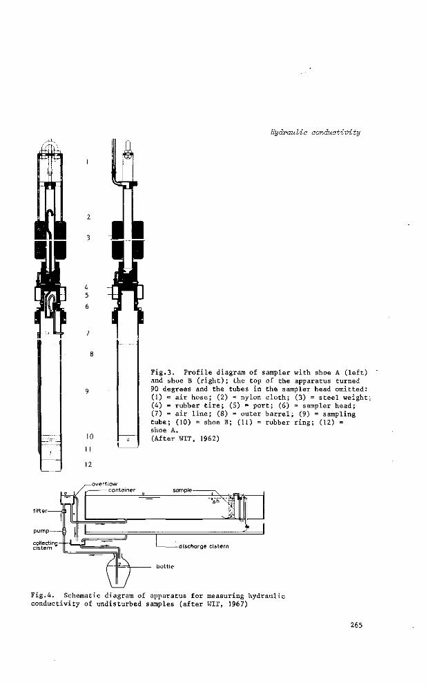
Hydraulic conductivity
L
10
11
12
Fig.3. Profile diagram of sampler with shoe A (left) and shoe B (right); the top of the apparatus turned 90 degrees and the tubes in the sampler head omitted: (1) = air hose; (2) = nylon cloth; (3) = steel weight; (4) = rubber tire; (5) = port; (6) = sampler head; (7) = air line; (8) = outer barrel; (9) = sampling tube; (10) = shoe B; (H) = rubber ring; (12) = shoe A. (After WIT, 1962)
-overflow -container
Fig.4. Schematic diagram of apparatus for measuring hydraulic conductivity of undisturbed samples (after WIT, 1967)
265
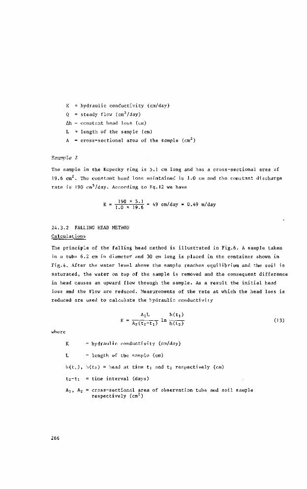
K = hydraulic conductivity (cm/day)
Q = steady flow (cm3/day)
Ah = constant head loss (cm)
L = length of the sample (cm)
A = cross-sectional area of the sample (cm )
Examp le 3
The sample in the Kopecky ring is 5.1 cm long and has a cross-sectional area of
19.6 cm2. The constant head loss maintained is 1.0 cm and the constant discharge
rate is 190 cm3/day. According to Eq.12 we have
K = ,1n°vXio'l = 49 cm/day =0.49 m/day
24.3.2 FALLING HEAD METHOD
Calculations
The principle of the falling head method is illustrated in Fig.6. A sample taken
in a tube 6.2 cm in diameter and 30 cm long is placed in the container shown in
Fig.4. After the water level above the sample reaches equilibrium and the soil is
saturated, the water on top of the sample is removed and the consequent difference
in head causes an upward flow through the sample. As a result the initial head
loss and the flow are reduced. Measurements of the rate at which the head loss is
reduced are used to calculate the hydraulic conductivity
AiL h(tj) K = T—TZ—ITT l n TTT-T (13)
A2(t2-ti) h(t2)
where
K = hydraulic conductivity (cm/day)
L = length of the sample (cm)
h(ti), h(t2) = head at time ti and t2 respectively (cm)
t2-ti = time interval (days)
&i, A2 = cross-sectional area of observation tube and soil sample respectively (cm )
266

Hydraulic conductivity constant level in container
siphon
cylinder holder
O ring
Fig.5. Position of Kopecky ring sample in the apparatus of Fig.4 for measuring hydraulic conductivity under a constant head (after WIT, 1967)
- A,-
htt,) TT h(t2)
Uil
-sample
sieve with gauze Fig.6. Position of sample in the apparatus
of Fig.4 for measuring hydraulic conductivity under a falling head (after WIT, 1967)
267

Examp le 4
A soil sample is taken below the groundwater table in a zinc tube 6.2 cm in
diameter and 30 cm long. After some soil is removed from the top and the bottom, a
soil sample of 25 cm remains. The hydraulic conductivity is determined by the
falling head method as illustrated in Fig.6 (Aj = A2 = A).
At time ti = 0 hours h(ti) measures 1.5 cm
At time ti = 7 hours h(t2) measures 0.9 cm
K is calculated by Eq.13 as
K = j ~ 2.3 log (̂ |) = 43 cm/day = 0.43 m/day
24.3.3 K-VALUES OF SAMPLES TAKEN IN HORIZONTAL AND VERTICAL DIRECTIONS
Samples can be collected above the water table with the Kopecky ring in either a
horizontal or a vertical direction. The measurements will then yield K values in
horizontal or vertical direction, respectively. It is virtually impossible to
collect samples in horizontal direction from deeper soil layers or from layers
below the water table, but soil samples taken vertically can be measured for
their hydraulic conductivity in horizontal direction by using the apparatus shown
in Fig.7.
The base of a sample 30 cm long and 6 cm in diameter is sealed with clay and a
plastic sheet. Two holes 1 cm in diameter are sucked into the top of the sample
and on opposite sides of it. This can be done with a brass tube connected to a
wateriet pump. Two tubes containing filters 10 cm long are then inserted into
the holes. The sample is sealed at the top with a mixture of paraffin and vase
line, after which it is placed in water under vacuum to saturate it. The sample
is then put into the hydraulic conductivity apparatus (Fig.4) and the constant
head procedure is followed. The water flows horizontally through the sample from
one filter to the other. The dimensions of sample and filter tubes are such
that, for the pattern of streamlines and equipotential lines, the following re
lation holds
K = Ähi ( 1 4 )
268
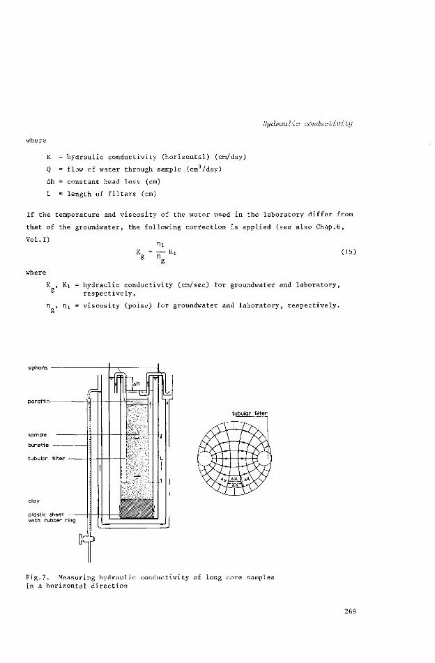
Hydraulic conductivity
where
K = hydraulic conductivity (horizontal) (cm/day)
Q = flow of water through sample (cm /day)
Ah = constant head loss (cm)
L = length of filters (cm)
If the temperature and viscosity of the water used in the laboratory differ from
that of the groundwater, the following correction is applied (see also Chap.6,
Vol.1)
K g = - K l (15)
where
K , Ki = hydraulic conductivity (cm/sec) for groundwater and laboratory, respectively,
T\ , ni - viscosity (poise) for groundwater and laboratory, respectively.
siphons
paraf f in-
sample
burette
tubular f i lter -
clay -
plastic sheet with rubber ring
K?
fl
_ i
tubular f i lter
Fig.7. Measuring hydraulic conductivity of long core samples in a horizontal direction
269
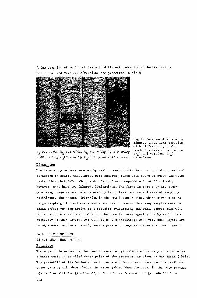
A few examples of soil profiles with different hydraulic conductivities in
horizontal and vertical directions are presented in Fig.8.
EP* .. Ä
:.. «Wij^j-1 Fig.8. Core samples from la-I «"""Sv* ̂ minated tidal flat deposits lv* *"" ' i. with different hydraulic
7 -c n /j 7, -r c /j 7 o -i /j 7 -r /i /j conductivities in horizontal k,-5.0 m/day k.-S.S m/day k=8.1 m/day A:,-5.0 m/day .„ , , . ,.. s h a h h n h " (K.) and vertical (K ) k -2.5 m/day k =0.9 m/day k =8.2 m/day k =1.4 m/day directions v
Discussion
The laboratory methods measure hydraulic conductivity in a horizontal or vertical
direction in small, undisturbed soil samples, taken from above or below the water
table. They therefore have a wide application. Compared with other methods,
however, they have two inherent limitations. The first is that they are time-
consuming, require adequate laboratory facilities, and demand careful sampling
techniques. The second limitation is the small sample size, which gives rise to
large sampling fluctuations (random errors) and means that many samples must be
taken before one can arrive at a reliable evaluation. The small sample size will
not constitute a serious limitation when one is investigating the hydraulic con
ductivity of thin layers. Nor will it be a disadvantage when very deep layers are
being studied as these usually have a greater homogeneity then shallower layers.
24.4 FIELD METHODS
24.4.1 AUGER HOLE METHOD
Principle
The auger hole method can be used to measure hydraulic conductivity in situ below
a water table. A detailed description of the procedure is given by VAN BEERS (1958).
The principle of the method is as follows. A hole is bored into the soil with an
auger to a certain depth below the water table. When the water in the hole reaches
equilibrium with the groundwater, part of it is removed. The groundwater then
270
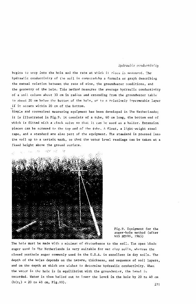
Hydraulic conductivity
begins to seep into the hole and the rate at which it rises is measured. The
hydraulic conductivity of the soil is computed.by a formula or graph describing
the mutual relation between the rate of rise, the groundwater conditions, and
the geometry of the hole. This method measures the average hydraulic conductivity
of a soil column about 30 cm in radius and extending from the groundwater table
to about 20 cm below the bottom of the hole, or to a relatively impermeable layer
if it occurs within 20 cm of the bottom.
Simple and convenient measuring equipment has been developed in The Netherlands;
it is illustrated in Fig.9. It consists of a tube, 60 cm long, the bottom end of
which is fitted with a clack valve so that it can be used as a bailer. Extension
pieces can be screwed to the top end of the tube. A float, a light-weight steel
tape, and a standard are also part of the equipment. The standard is pressed into
the soil up to a certain mark, so that the water level readings can be taken at a
fixed height above the ground surface.
S t <-•;•••:&-r-
Fig.9. Equipment for the auger-hole method (after VAN BEERS, 1965) ••'[-• ' ̂ . •• "•• ,
The hole must be made with a minimum of disturbance to the soil. The open blade
auger used in The Netherlands is very suitable for wet clay soils, whereas the
closed posthole auger commonly used in the U.S.A. is excellent in dry soils. The
depth of the holes depends on the nature, thickness, and sequence of soil layers
and on the depth at which one wishes to determine hydraulic conductivity. When
the water in the hole is in equilibrium with the groundwater, the level is
recorded. Water is then bailed out to lower the level in the hole by 20 to 40 cm
(h(ti) = 20 to 40 cm, Fig.10). 271
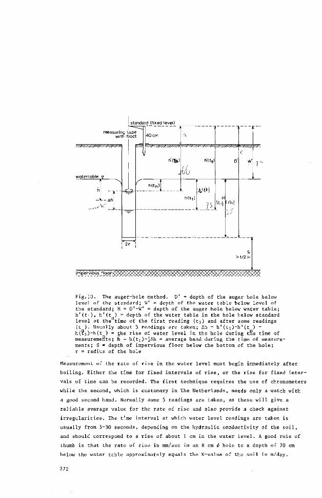
standard (fixed level)
measuring tape w i th f loat
y/m?///J^/Mtm!MS\
watertable y
V _J_
V?7>
a i
1 2r
40 cm
h(tn)|
ft
h'tt,)
tb
h(ti)
^H(ä
c
(UM
s >1/2H
Fig.10. The auger-hole method. D' = depth of the auger hole below level of the standard; W' = depth of the water table below level of the standard; H = D'-W' = depth of the auger hole below water table; h'(ti), h'(t ) = depth of the water table in the hole below standard level at the time of the first reading (ti) and after some readings (t ) . Usually about 5 readings are taken; Ah = h'(ti)-h'(t ) = h(ti)-h(t ) = the rise of water level in the hole during the time of measurements; h = h(ti)~3Ah = average head during the time of measurements; S = depth of impervious floor below the bottom of the hole; r = radius of the hole
Measurement of the rate of rise in the water level must begin immediately after
bailing. Either the time for fixed intervals of rise, or the rise for fixed inter
vals of time can be recorded. The first technique requires the use of chronometers
while the second, which is customary in The Netherlands, needs only a watch with
a good second hand. Normally some 5 readings are taken, as these will give a
reliable average value for the rate of rise and also provide a check against
irregularities. The time interval at which water level readings are taken is
usually from 5-30 seconds, depending on the hydraulic conductivity of the soil,
and should correspond to a rise of about 1 cm in the water level. A good rule of
thumb is that the rate of rise in mm/sec in an 8 cm 6 hole to a depth of 70 cm
below the water table approximately equals the K-value of the soil in m/day.
272

.273 6
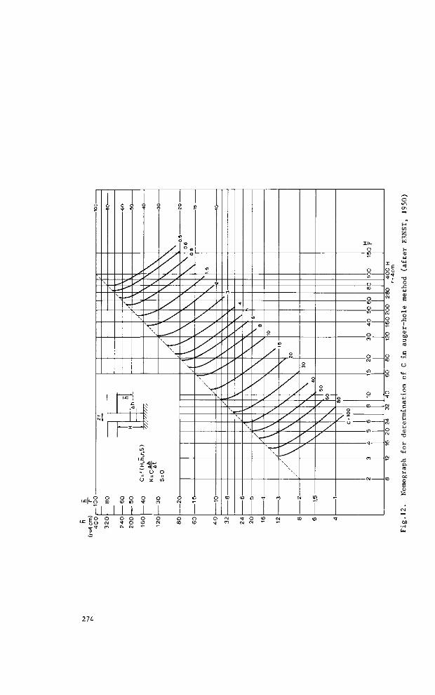
3 J c
\ s^
M
C
N^
1.
T
1.
s
V
) C
x
\
3 C ! 0
u
\ ^
i i r ' si
f LT
H- U O
3 C a 3 3
C <f
3 C 3 t f
c •=5
3 C
r a 3 C
! !
I
,T\1
) If
2 <
IO
< C
\
c
)
^
3
•
\
C
/
\,
3
• f
/
\
(i
y
\
> a
K
\
1 "
O
\^
c
n
o
/
/J
\
T C
O
O
/ /
/ y
1 u
o
/
1
o
o
2 03
O
O if)
O Cl
CM
in
o '""
o
yf ~ U
CO o uO cvj M
•H
274

Care should be taken to complete the measurements before 25% of the volume of
water removed from the hole has been replaced by inflowing groundwater. After that
a considerable funnel shaped watertable develops around the top of the hole.
This increases resistance to the flow around and into the hole. This effect is
not accounted for in the formulas or flow charts developed for the auger hole
method and consequently it should be checked that Ah < | h(ti) (Fig.10).
Calculations (the one layer problem)
ERNST (1950) found that the relation between the hydraulic conductivity of the
soil and the flow of water into the auger hole depends on the boundary conditions.
This relation has been derived numerically by the relaxation technique and is
given as
K = C |£ (16)
where
K = hydraulic conductivity (m/day)
C = geometry factor = f(h,H,r,S). (Figs.10,11,and 12)
j — = rate of rise of water level in the auger hole (cm/sec)
In Fig.11 C is given as a function of h/r and H/r when S > jH, in Fig. 12 a similar
relation applies when S = 0. The use of these figures can be illustrated by the
following example.
Examp le 5
After the readings have been taken, the reliability of the measurements should be
checked. The Ah of each measurement is therefore computed to see whether the con
secutive readings are reasonably consistent. If the value of Ah decreases gradually,
the readings may be averaged up to Ah = j h(t]) or as in the above example, up to
Ah = 7 to 8 cm. Both conditions are satisfied here and therefore K can be computed.
It often happens that Ah is relatively large for the first reading, due to water
dripping along the walls of the hole directly after bailing. If this occurs, the
first measurement should be discarded. Further inconsistency in Ah values may be
caused by the float sticking to the wall or by the wind blowing the tape against
the wall. Consistency can be improved by tapping the tape regularly.
275

No. :
L o c a t i o n :
Da t e :
T e c h n i c i a n :
D'
W'
H
i
1
2
3
4
5
6
= 240
« 114
= D' -
t. l
cm
cm
W'
second
0
10
20
30
40
50
Ah
= 126
h'(t.) l
cm
145.2
144.0
142.8
141.7
140.6
139.6
= 5.6
cm
Ah
cm
-1 .2
1.2
1 .1
1 .1
1.1
5.6
r = 4 cm
S = > j H
At = t6 - t2 = 50 sec
Ah = h'(t]) - h'(t6) = 5.6 cm
h(ti) = h'Ctj) - W' = 145.2 - 114 = 31.2 cm
check Ah < Jh(ti) (5.6 < 7.8)
h = h(tj) - JAh = 31.2 - 2.8 - 28.4 cm
H/r = 31.5 1 £, 7 / C = 6.0 (read from Fig. 11)
Ah/At = -^1 = 0.11
K = C Ah/At = 6.0 x 0.11 = 0.66 m/day
standard (fixed level)
measuring tape with float
y/x^v/^A\w//.<w///^
watertable y
">
v?z
40 cm
' / / A W / A V / / « S
h ' ( t n ) 139.6 cm
h ( t n ) |
W///8*&M% ffy///i m:
h'tt,) 145.2 cm
h ( t i :
D 240 cm
w 114 cm
S >1 /2H
wmmm.. impervious f loor
Fig. 13. Example of measurements for auger-hole method
276
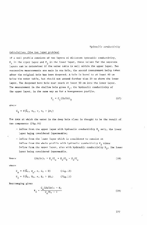
Hydraulic conductivity
Calculations (the two layer problem)
If a soil profile consists of two layers of different hydraulic conductivity,
K in the upper layer and K in the lower layer, these values for the separate
layers can be determined if the water table is well within the upper layer. Two
successive measurements are made in one hole, the second measurement being taken
after the original hole has been deepened. A hole is bored to at least 40 cm
below the water table, but should not extend further than 20 cm above the lower
layer. The deepened bore hole must reach at least 50 cm into the lower layer.
The measurement in the shallow hole gives K , the hydraulic conductivity of
the upper layer, in the same way as for a homogeneous profile.
Kj = C (Ah/At) j (17)
where
Cj = f(hi, Hi, r, Si > iHi)
The rate at which the water in the deep hole rises is thought to be the result of
two components (Fig.14)
- inflow from the upper layer with hydraulic conductivity K only, the lower
layer being considered impermeable;
- inflow from the lower layer which is considered to consist of
inflow from the whole profile with hydraulic conductivity K0 minus
inflow from the upper layer, also with hydraulic conductivity K„, the lower
layer being considered impermeable.
Hence (Ah/At)2 = K,/C + K,/C„ - K./C (18)
1 o I I z o
where
C = f(h2, H , r, Si = 0) (Fig.12)
C2 = f(h2, H2, r, Sz > ^H2) (Fig.11)
Rearranging gives
C (Ah/At)2 - Ki K2 = ° C /C2 - 1 <19>
277
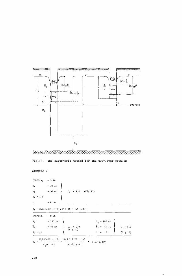
J . 1
',h«n>)2
impervious^
lWti>).
^ ^
hi
• i t ' i ' (f<fn)),
J:
1
.Wtn)),
Fig .14 . The auger -ho le method for the two- layer problem
Example 6
(Ah /At ) , - 0 .16
Hi = 70 cm
h i = 30 cm
Si > J H
r = 4 cm
9 .4 ( P i g . 1 1 )
Ki - C , (Ah /At ) i = 9 .4 x 0 .16 = 1.5 m/day
(Ah /At ) 2 = 0 .26
H,. = 1 5 0 cm
li2 = 40 cm
S2 > iH
C2 = 3 . 9 ( F i g . 1 1 )
H = 100 cm o
h 2 = 40 cm
Si = 0
C (Ah/Ac) 2 - Ki 6 . 3 x 0 .26 - 1.5
C /C 6 . 3 / 3 . 9 - 1 0 .22 m/day
C = 6.3 o
(Fig.12)
278
Hydraulic conductivity
Discussion
Variations in the results of field investigations are less than those obtained
in the laboratory because in the field a larger soil body is measured. The error
of the determination is believed to be of the order of 10-20%. An accompanying
soil profile description is indispensable for further evaluation of the terrain
variability (Sect.5.2).
In stable soils of low hydraulic conductivity, it may be necessary to extend the
augerhole 1 m or more below the water table, and to bail out more than 80 cm of
water to create a measurable rate of rise. In heavy soils the action of the auger
may destroy the soil structure in the vicinity of the wall of the hole. It will
then be necessary to flush the soil and reopen the closed soil pores by bailing
the water out several times. Repeated measurements will reveal that the hydraulic
conductivity gradually improves with time.
In unstable soils, or in soils with a very high hydraulic conductivity, auger holes
deeper than 40 cm or bailings of more than 20 cm of water may produce a rate of
rise too high to be measured. A cave in unstable soils can be prevented by insert
ing a filter into the hole. It is advisable to measure the rate of rise immedia
tely after making the hole, in which case no bailing is required (direct method).
Repeated measurements in an unstable hole, where mud may collect on the bottom,
will reveal a gradual decrease in hydraulic conductivity.
Figs.1] and 12 only differ significantly in the range of small H (depth of the
borehole) values. If one is uncertain of the conductivity of the layers below
the bottom of the hole, Fig.11 may be used (S > 5H) , thus ensuring a conserva
tive estimate of K.
The simplicity of the augerhole method, the fairly large soil body for which K
is measured (about 0.05 to 0.3 m 3 ) , and the presence of relatively high water
tables explain the frequent use of this method in The Netherlands.
24.4.2 PIEZOMETER METHOD
Principle
The principle of this method resembles that of the augerhole method, except
that a tube is inserted into the hole to leave a small cavity at the bottom. The
method is therefore often referred to as the pipe cavity method.
279
The principle is as follows (Fig.15). A hole is augered into the soil to the
depth below the water table at which one wishes to measure the hydraulic con
ductivity. A pipe is inserted into the hole, having a small unprotected cavity
at the bottom. Care should be taken that no leakage occurs along the wall of
the hole. After the water level in the pipe has reached equilibrium with the
groundwater, the water in the pipe is removed. Due to a pressure difference,
water will flow from the surrounding soil into the uncased cavity, causing the
water level in the pipe to rise. The rate of rise is measured and the K value
is calculated with a suitable formula describing the relation between the rate
of rise, the flow conditions and the K value of the soil. The equipment consists
of an auger, a pipe, a pump or bailer, and a water level recorder.
Calculations
The hydraulic conductivity is computed with the following formula (LUTHIN and
KIRKHAM, 1949)
ïï r* h(tj)
K * C(t. - t l ) ln hTETT <20>
where
K = hydraulic conductivity (cm/sec)
r = inside radius of the pipe (cm)
h(ti), h(t.) = depth of water level (cm) in the pipe below equilibrium water level at time ti and t. respectively
t.-tj = time interval of measurement (sec)
C = f(H, r , 1, S), geometry factor
The above formula is similar to the formula used in the falling head laboratory
method (Sect.3.2).
The geometry factor C has been determined with an electric analogue, whereas in
the auger hole method it was determined by relaxation. The result of the electric
analogue experiments is given in Fig.16.
280
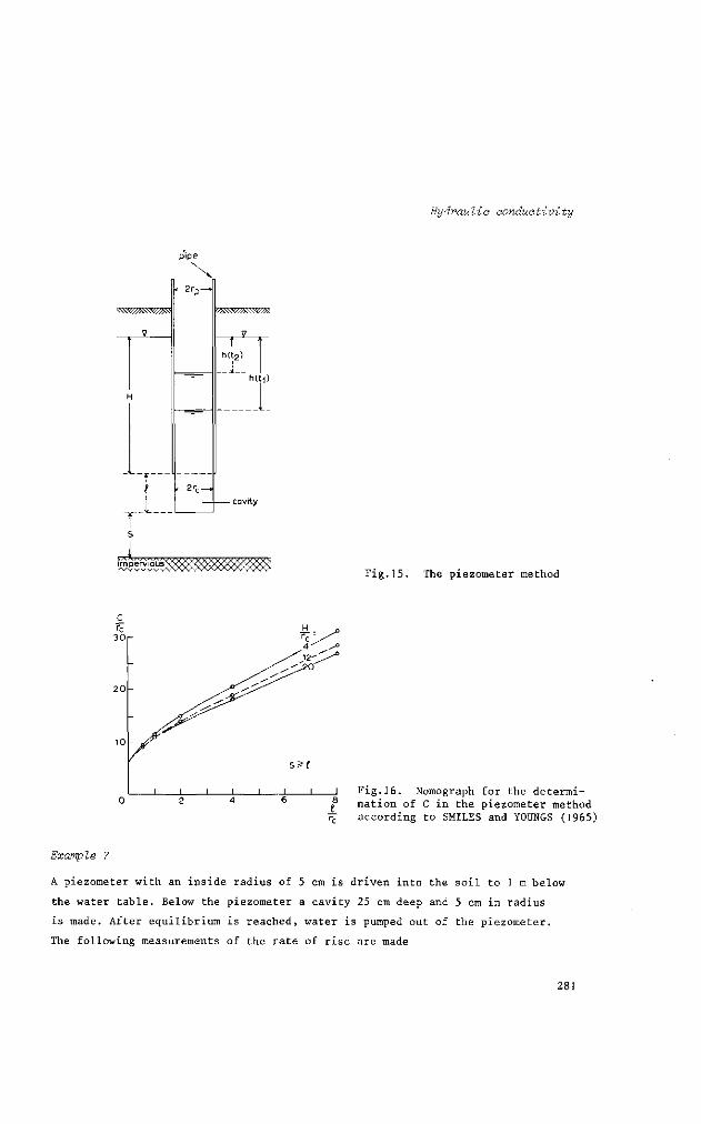
Hydraulic conductivity
_2 , 7
h(t2)
.J. h(t-|
- cavity
Fig.15. The piezometer method
Fig.16. Nomograph for the determination of C in the piezometer method according to SMILES and YOUNGS (1965)
Examp le 7
A piezometer with an inside radius of 5 cm is driven into the soil to 1 m below
the water table. Below the piezometer a cavity 25 cm deep and 5 cm in radius
is made. After equilibrium is reached, water is pumped out of the piezometer.
The following measurements of the rate of rise are made
281

The ratio
i
1
2
3
4
5
t.(sec) l
0
20
40
60
80
h(t.)(' 1
70
65
60
56
52
cm) In h(t-
t. -l
3.68
3.85
3.72
3.71
,)/h(t.)
- t!
10"3
,0"3
10"3
10"3
In h(ti)/h(t.)
is first calculated to check the consistency of the data series. The factor C is
determined from the nomograph Fig.16 with 1/r = 5 and H/r = 20, giving C = 100. c c
The K-value found from Eq.20 will be in cm/sec, and needs to be multiplied by
864 to convert it into m/day.
864 ^ h ( t l ) 8 6 4 x , x 5 2 x 3 - 7 1 x ,0-3 K = c ( t . - t l )
l n MITT
= m = 2-5 m/day
Discussion
The piezometer method is highly suitable for determining the hydraulic conductivity
of individual soil layers or of layers at great depths. Of the hydraulic head,
80% is dissipated in the soil within a distance of one cavity length from the
cavity, and about 90% within two cavity lengths. This method therefore measures
the hydraulic conductivity of the soil within a radius of one or two cavity lengths
from the cavity (0.01 - 0.05 m 3 ) , in a horizontal direction.
It may be necessary to support the cavity with a filter in unstable soil. The
smaller inflow surface of the cavity compared with that provided by the auger
hole method heightens the entrance velocity of the water. This increases the
risk of collapse or deformation of the cavity, and might lead to considerable
error. As with the augerhole method, it may be necessary to flush the cavity
several times in stable clay soils if its walls have been sealed by the action
of the auger.
282

Hydvaulic conductivity
24.4.3 PUMPED BOREHOLE METHOD
Principle
The principle of the method is as follows. A hole is bored into the soil to
below the water table. Water is then pumped from it at a constant rate. When
the water level in the hole has reached equilibrium, the K value is calculated
with a suitable formula expressing the relation between the stabilized water
level in the borehole, the hydraulic conductivity of the surrounding soil, and
the flow conditions.
The equipment consists of an auger, a pump, and a waterlevel recorder (Chap.25,
Vol.11).
Calculation
ZANGAR (1953) has given an analytical solution to the flow problem of a well
penetrating less than 20% into an aquifer. The expression for the hydraulic
conductivity is as follows (Fig.17)
C L r (21)
where
K = hydraulic conductivity (m/day)
Q = steady rate of pumping (m3/day)
r = radius of the borehole (m)
L = H
H = depth of the bottom of the borehole below the initial groundwater table (m)
h = stabilized height of the water level above the bottom of the borehole at equilibrium (m)
C = f(h,r), geometry factor (see Fig.18)
nitial groundwater table
$m5mzz$zzzzzmçmzwzms Fig.17. The pumped borehole method
283
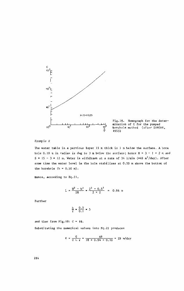
I I I I I I I I I I
Fig.18. Nomograph for the deter-i—L-l mination of C for the pumped
1° borehole method (after ZANGAR, T 1953)
Example 8
The water table in a pervious layer 15 m thick is 1 m below the surface. A bore
hole 0.10 m in radius is dug to 3 m below the surface; hence H = 3 - 1 = 2 m and
S = 15 - 3 = 12 m. Water is withdrawn at a rate of 34 1/min (=49 m3/day). After
some time the water level in the hole stabilizes at 0.50 m above the bottom of
the borehole (h = 0.50 m).
Hence, according to Eq.21,
T H2 - h2 22 - 0.52 . .. L = —;TT; = ~ ., - — = 0.94 m
2H 2 x 2
Further
h = CK_5 r 0.1
= 5
and thus from Fig.18: C = 18.
Substituting the numerical values into Eq.21 produces
K = Q = 49
C L r 18 x 0.94 x 0.10 = 29 m/day
284

Hydraulic conductivity
Discussion
The pumped borehole method is best applied to deep homogeneous phreatic aquifers
of high hydraulic conductivity. The aquifer should be deep enough to satisfy the
condition that no more than 20% penetration occurs (H/D = 0.25), and the hydraulic
conductivity should be high enough to guarantee measurable pumping rates and equi
librium water levels. This indicates the advantage of the pumped borehole in
highly pervious aquifers since under these conditions, the augerhole method, and
to a certain extent the piezometer method, may produce rates of rise of the water
level too high to be measured accurately. The pumped borehole differs from most
other pumping tests in that an additional installation of piezometers is not
required. The K-value of the soil is measured in a direction intermediate between
horizontal and vertical and is representative of a large soil body of several m3.
24.4.4 DOUBLE TUBE METHOD
Principle
The principle of the double tube method is illustrated in Fig.19. In an unsaturated
soil, two concentric tubes are placed at the depth where one wishes to measure
the hydraulic conductivity. First, the soil below and around the tubes is satura
ted by infiltration; note that the infiltration rate must be constant. The tubes
are then filled with water and the rate of fall of the levels in both outer and
inner tube is measured. The tubes are then refilled, the water level in the outer
tube now being kept constant, and the rate of fall in the inner tube being
recorded. Because of a gradually increasing difference between water levels in the
outer and inner tubes, the infiltration from the inner tube will be counteracted
by a gradually increasing hydraulic head from the outer tube. This reduces the
rate of fall in the inner tube, as compared to the rate of fall occurring when
the equal level condition is imposed. The hydraulic conductivity can be computed
with a formula expressing the relation between the difference in fall under equal
level and constant outer level conditions, the flow geometry, and the hydraulic
conductivity. The appropriate equipment for the technique, as developed by
BOUWER (1961, 1962), is schematically described in Fig.20. It consists of a water
reservoir connected by pipes and valves to the inner and outer tubes in such a way
that the conditions of equal level fall and constant outer level can be imposed.
Also required are a large posthole auger and cleaning equipment to return the
disturbed structure of the bottom of the hole to its original condition.
285
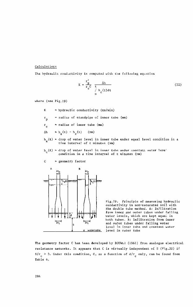
Calculations
The hydraulic conductivity is computed with the following equation
2
Ah K
r C t (22)
h (t)dt c
where (see Fig.19)
K
c
Ah
= hydraulic conductivity (mm/min)
= radius of standpipe of inner tube (mm)
= radius of inner tube (mm)
= h (t) - h (t) (mm)
h (t) = drop of water level in inner tube under equal level condition in a time interval of t minutes (mm)
h (t) = drop of water level in inner tube under constant outer level condition in a time interval of t minutes (mm)
C = geometry factor
A B
Fig.19. Principle of measuring hydraulic conductivity in non-saturated soil with the double tube method. A: Infiltration from inner and outer tubes under falling water levels, which are kept equal in both tubes. B: Infiltration from inner and outer tubes under falling water level in inner tube and constant water level in outer tube
The geometry factor C has been developed by BOUWER (1961) from analogue electrical
resistance networks. It appears that C is virtually independent of S (Fig.20) if
S/r > 3. Under this condition, C, as a function of d/r only, can be found from c c
Table 4.
286
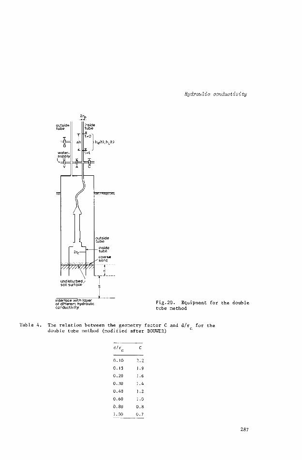
Hydraulic conductivity
outside tube
=*H water-supply
inside tube
i l t .0]
•U-t=t
interface with layer of different hydraulic conductivity
Fig.20. Equipment for the double tube method
Table 4. The relation between the geometry factor C and d/r for the double tube method (modified after BOUWER) c
d / r c
0 . 10
0.15
0.20
0.30
0.40
0.60
0 .80
1.00
C
2.2
1.9
1.6
1.4
1 .2
1.0
0 .8
0 .7
287

Example 9
The double tube method is applied in an auger hole,the bottom of which is 1 m
below the soil surface yet above a water table. The inner tube 62.5 mm in radius
penetrates 10 mm into the bottom of the auger hole. The radius of the standpipe,
in which the observations are made,is 12.5 mm. The results of experiments are
presented in Fig.21.
From the data given in this figure, it follows that
= 12.5, r 62.5 mm,and d = 10 mm
Consulting Table 4 one finds that for d/r = 10/62.5 = 0.16, C is 1.8.
c
Hence, at t = 30 min, Ah = 40 mm, and h (t) = 20 mm. The integral value of Eq.22
is approximated by a triangle with an area
x t x h (t) = J x 30 x 20 300
Inserting the above information into Eq.22 produces
K = Ah
r C t C ƒ h (t)dt
c o
/ i o rr "\ *i / n
en 5 x ] S 300 = "''8 m m / m i n = 0 . 2 6 m/day
|hc(t)dtÄlthc(t)
Fig.21. Graphical analysis of measurements with double-tube method
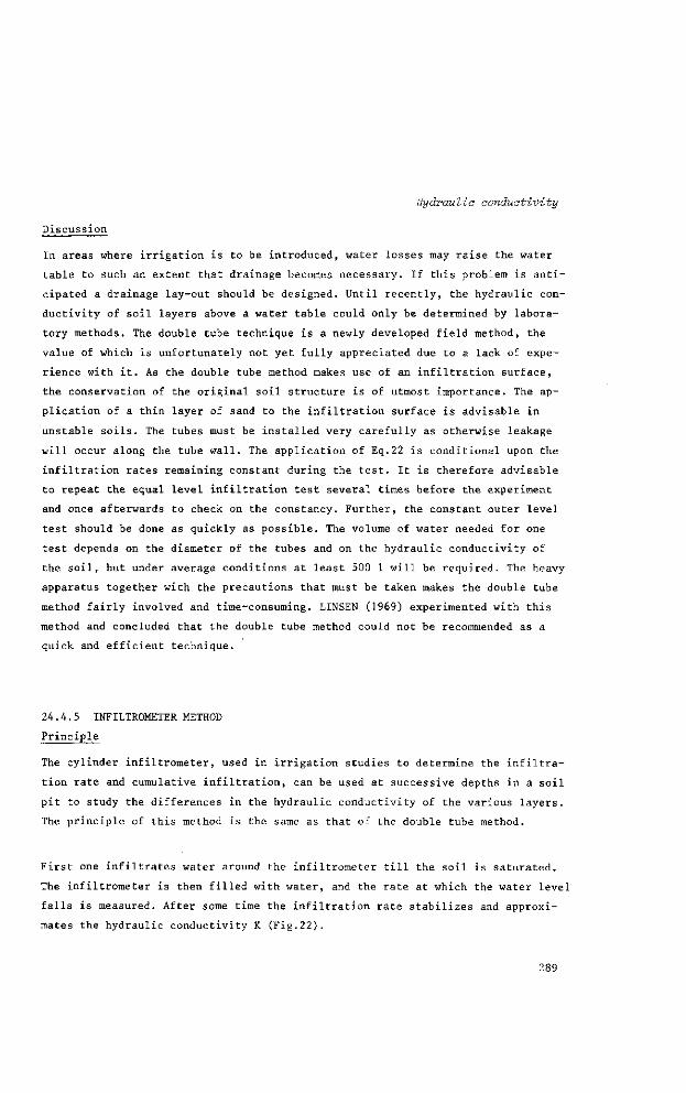
Hydraulic conductivity
Discussion
In areas where irrigation is to be introduced, water losses may raise the water
table to such an extent that drainage becomes necessary. If this problem is anti
cipated a drainage lay-out should be designed. Until recently, the hydraulic con
ductivity of soil layers above a water table could only be determined by labora
tory methods. The double tube technique is a newly developed field method, the
value of which is unfortunately not yet fully appreciated due to a lack of expe
rience with it. As the double tube method makes use of an infiltration surface,
the conservation of the original soil structure is of utmost importance. The ap
plication of a thin layer of sand to the infiltration surface is advisable in
unstable soils. The tubes must be installed very carefully as otherwise leakage
will occur along the tube wall. The application of Eq.22 is conditional upon the
infiltration rates remaining constant during the test. It is therefore advisable
to repeat the equal level infiltration test several times before the experiment
and once afterwards to check on the constancy. Further, the constant outer level
test should be done as quickly as possible. The volume of water needed for one
test depends on the diameter of the tubes and on the hydraulic conductivity of
the soil, but under average conditions at least 500 1 will be required. The heavy
apparatus together with the precautions that must be taken makes the double tube
method fairly involved and time-consuming. LINSEN (1969) experimented with this
method and concluded that the double tube method could not be recommended as a
quick and efficient technique.
24.4.5 INFILTROMETER METHOD
Principle
The cylinder infiltrometer, used in irrigation studies to determine the infiltra
tion rate and cumulative infiltration, can be used at successive depths in a soil
pit to study the differences in the hydraulic conductivity of the various layers.
The principle of this method is the same as that of the double tube method.
First one infiltrates water around the infiltrometer till the soil is saturated.
The infiltrometer is then filled with water, and the rate at which the water level
falls is measured. After some time the infiltration rate stabilizes and approxi
mates the hydraulic conductivity K (Fig.22).
289

/gage index
.engineers scale
welding rod
y T\
Fig.22. The infiltrometer
Calculations
The infiltration rate of water in an unsaturated soil measured by a cylinder
infiltrometer may be expressed in terms of Darcy's law as
v = K, + z + h (23)
where
v = infiltration rate (cm/sec)
K = hydraulic conductivity of the transmission zone (cm/sec)
<|> = suction at the bottom of the transmission zone (cm)
z = depth of the transmission zone below the infiltrometer (cm)
h = height of water in the infiltrometer (cm)
The influence of <j> and h relative to z diminishes as the depth of the transmission
zone and the moisture content of the soil increase. So the hydraulic gradient
,<}> + z + h, z
tends towards 1 in the case of a deep uniform soil profile and the infiltration
rate becomes constant, attaining what is known as the basic infiltration rate.
In that case we may write
v = K„ (24)
290
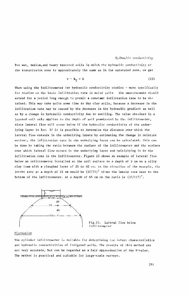
Hydraulic conductivity
For wet, medium,and heavy textured soils in which the hydraulic conductivity of
the transmission zone is approximately the same as in the saturated zone, we get
K„. K (25)
When using the infiltrometer for hydraulic conductivity studies - more specifically
for studies on the basic infiltration rate in moist soils - the measurements should
extend for a period long enough to permit a constant infiltration rate to be ob
tained. This may take quite some time in dry clay soils, because a decrease in the
infiltration rate may be caused by the decrease in the hydraulic gradient as well
as by a change in hydraulic conductivity due to swelling. The value obtained in a
layered soil only applies to the depth of soil penetrated by the infiltrometer,
since lateral flow will occur below if the hydraulic conductivity of the under
lying layer is low. If it is possible to determine the distance over which the
lateral flow extends in the underlying layers by estimating the change in moisture
content, the infiltration rate in the underlying layer can be calculated. This can
be done by taking the ratio between the surface of the infiltrometer and the surface
over which lateral flow occurs in the underlying layer and multiplying it by the
infiltration rate in the infiltrometer. Figure 23 shows an example of lateral flow
below an infiltrometer installed at the soil surface to a depth of 5 cm on a silty
clay loam with a ploughed layer of 20 to 40 cm. In the situation of the example, the
intake rate at a depth of 25 cm would be (37/77)2 times the intake rate near to the
bottom of the infiltrometer. At a depth of 65 cm cm the ratio is (37/117)2.
m\^//AW//^^//fcw^^
Fig.23. Lateral flow below infiltrometer
Discussion
The cylinder infiltrometer is suitable for determining the intake characteristics
and hydraulic conductivities of irrigated soils. The results of this method are
not very accurate, but can be regarded as a fair approximation of the K-value.
The method is practical and suitable for large-scale surveys.
291

24.4.6 INVERSED AUGER HOLE METHOD
Principle
The auger hole test above the water table, described in French literature as the
Porchet method, consists of boring a hole to a given depth, filling it with water,
and measuring the rate of fall of the water level.
Calculations
The calculation is carried out as follows (Fig.24)
A(t.) = 2irr h(t.) + irr2 (26)
where
A(t.) = surface over which water infiltrates into the soil at time t. (cm2)
r = radius of the auger hole (cm)
h(t.) = water level in the hole at time t. (cm)
Supposing that the hydraulic gradient is approximately 1, we may write according
to Darcy's law
Q(t.) = KA(t.) = 2Kirr (h(t.) + r/2) (27)
If during the time interval dt the water level falls over a distance dh, the
quantity of water infiltrated into the soil equals
Q(t ) = - irr2 ̂ (28) l dt
Substituting Eq.27 into Eq.28 gives
2Kïïr ( h ( t . ) + r /2) = - ïïr2 ~ (29) l dt
Integration between the limits
t. = ti, h(t.) = h(ti) and
t. = t , h(t.) = h(t ) gives l n l n
~ (tn-ti) = In (h(ti) + r/2) - In (h(tn) + r/2) (30)
Changing to common logarithms and rearranging gives
log (h(tj) + r/2) - log(h(t ) + r/2) K = 1.15 r = 1.15 r tan a (31)
Cn - Cl
By plotting (h(t.) + r/2) against t. on semilogarithmic paper we obtain a straight
line with a tangent a.
292

Hydraulic conductivity
0&.WAVS»
h(t,)
h(tn)
^ • S ^ ? * s
h'(t,)
h'(tn)
TV*
Fig.24. Inversed augerhole method
Example 10
r = 4 cm
D' = 90 cm
h'(t.) h(t.) h(t.)+r/2 h'(t.) h(t.) h(t.)+r/2
]
2
3
4
5
6
7
8
9
0
40
80
150
250
350
550
750
975
can ai
73
74
75
76
77
78
79
80
81
2 0
17
16
15
14
13
12
11
10
9
19
18
17
16
15
14
13
12
11
1 -1 1200 S e C
0
140
300
500
650
900
1090
1300
1520
71
72
73
74
75
76
77
73
79
tan ci2
19
18
17
16
15
14
13
12
11
2.7 10
1 X 2000
21
20
19
18
17
16
15
14
13
-1 sec
K = 1.15 x 4 x 0.000167 cm/sec
= 0.66 m/day
K = 1.15 x 4 x 0.000135 cm/sec
=0.54 m/day
293
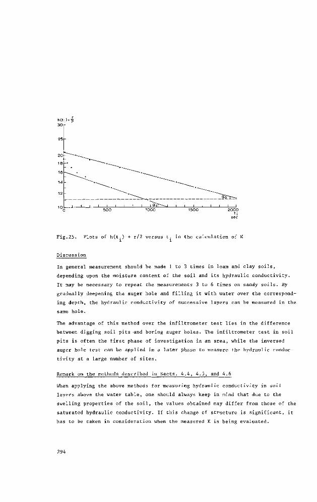
l i l t 30
25
20
18
16
14
12
\)
-
-
2
— ^ ^ ^ ^ ^ ^ - ^
^ ^ • ^ ^
I I I I I
^ ^ ^ ^ ^ ^
^ ^ ^
^ • ^ ^
i i i i i o ïT^^ i i i
^ ^ 3 ^
i i i i i i 2000
tj sec
Fig.25. Plots of h(t.) + r/2 versus t. in the calculation of K ï i
Discussion
In general measurement should be made 1 to 3 times in loam and clay soils,
depending upon the moisture content of the soil and its hydraulic conductivity.
It may be necessary to repeat the measurements 3 to 6 times on sandy soils. By
gradually deepening the auger hole and filling it with water over the correspond
ing depth, the hydraulic conductivity of successive layers can be measured in the
same hole.
The advantage of this method over the infiltrometer test lies in the difference
between digging soil pits -and boring auger holes. The infiltrometer test in soil
pits is often the first phase of investigation in an area, while the inversed
auger hole test can be applied in a later phase to measure the hydraulic conduc
tivity at a large number of sites.
Remark on the methods described in Sects. 4.4, 4.5, and 4.6
When applying the above methods for measuring hydraulic conductivity in soil
layers above the water table, one should always keep in mind that due to the
swelling properties of the soil, the values obtained may differ from those of the
saturated hydraulic conductivity. If this change of structure is significant, it
has to be taken in consideration when the measured K is being evaluated.
294

Hydraulic conductivity
LITERATURE
BOUWER, H. 1961. A double tube method for measuring hydraulic conductivity of
soil in situ above a water table. Proc.Soil Sei. Soc.Am. 25:334-339.
BOUWER, H. 1962. Field determination of hydraulic conductivity above a water
table with the double tube method. Proc.Soil Sei. Soc.Am. 26:330-335.
BOUWER, H. 1969. Planning and interpreting soil permeability measurements.
J.of Irrig.and Drainage Div. Proceedings Am.Soc.Civ.Engrs.95 :391-402.
DE RIDDER, N.A., and WIT, K.E. 1965. A comparative study on the hydraulic
conductivity of unconsolidated sediments. J.of Hydrology 3:180-206.
ERNST, L.F. 1950. A new formula for the calculation of the permeability factor
with the auger hole method. T.N.0. Groningen. Translated from Dutch by
H.Bouwer, Cornell Univ., Ithaca, N.Y. 1955.
ERNST, L.F. and WESTERHOF, J.J. 1956. Le développement de la recherche hydrolo
gique et son application au drainage aux Pays Bas. Publ.No.41 de l'Asso
ciation Internationale d'Hydrologie. Symposia Darcy, Dyon.
HOOGHOUDT, S.B. 1934. Bijdragen tot de kennis van enige natuurkundige grootheden
van de grond. 2.Versl.Landbouwk.Onderz. No.40 B. 's-Gravenhage. 215-345.
JOHNSON, A.I., and RICHTER, R.C. 1967. Selected bibliography on Permeability and
Capillarity testing of rock and soil materials. Special Techn.Publ. No.417.
Am.Soc.Testing Materials. Symposion Permeability and Capillarity of Soils,
pp.176-210.
KESSLER, J. 1970. Determination of soil permeability with the auger hole method
in Iraq. Ministry of Irrigation. FAO report.
LINSSEN, L.P.M. 1969. Verschillende methoden om de doorlatendheid te meten.
Univ.of Agric, Wageningen.
LUTHIN, J.W., and KIRKHAM, D. 1949. A piezometer method for measuring permeabi
lity of soil in situ below a water table. Soil Sei.68:349-358.
MARSHALL, T.J. 1957. Permeability and the size distribution of pores. Nature
180:664-665.
MARSHALL, T.J. 1958. A relation between permeability and size distribution of
pores. J.of Soil Sei. 9, No.1. 8 p.
SMILES, D.E., and YOUNGS, E.G. 1965. Hydraulic conductivity determination by se
veral field methods in a sand tank. Soil Sei.99:83-87.
295

TALSMA, T., and FLINT, S.E. 1958. Some factors determining the hydraulic conduc
tivity of subsoils with special reference to tile drainage problems. J.of
Soil Sei. 85:198-206.
VAN BEERS, W.F.J. 1958. The auger hole method. Bull. No.J. International Inst,
for Land Reclamation and Improvement, Wageningen. 32 p.
WIT, K.E. 1962. An apparatus for coring undisturbed samples in deep bore holes.
J.of Soil Sei. 94:65-70.
WIT, K.E. 1967. Apparatus for measuring hydraulic conductivity of undisturbed
soil samples. Symp. on Permeability and Capillarity of soils. Spec. Techn.
Publ.No.4J7. Am.Soc.Testing Mats.
ZANGAR, C.N. 1953. Theory and problems of water percolation. U.S. Bureau of
Reclamation. Engineering Monograph No.8. Denver, Col. 76 p.
296
SURVEYS AND INVESTIGATIONS
25. D E R I V I N G A Q U I F E R C H A R A C T E R I S T I C S F R O M P U M P I N G TESTS
J. WESSELING
Head of Hydrology Department Institute for Land and Water Management Research, Wageningen
G. P. KRUSEMAN
Geohydrologist Food and Agriculture Organization Libya
Lecturers in the Course on Land Drainage
K. E. WIT (1966-1967) Institute for Land and Water Management Research, Wageningen
G. P. KRUSEMAN (1968-1969) International Institute for Land Reclamation and Improvement, Wageningen
N. A. DE RIDDER (1970-1973) International Institute for Land Reclamation and Improvement, Wageningen

PURPOSE AND SCOPE
The procedure followed in performing pumping tests in unconfined and semi-confined
aquifers is described, together with some methods of analyzing the data obtained
from such tests.
CONTENTS
25.1 GENERAL SET-UP 299
25.1.1 Selection of a pumping test site 299
25.1.2 Discharging well 299
25.1.3 Well development 301
25.1.4 Testing of the pumped well 302
25.1.5 Piezometers and observation wells 303
25.2 PERFORMING A PUMPING TEST 307
25.2.1 Water level measurements 307
25.2.2 Discharge rate measurements 309
25.2.3 Duration of the pumping test 312
25.3 DATA PROCESSING 312
25.4 CALCULATION OF THE HYDRAULIC CHARACTERISTICS 313
25.4.1 Unconfined aquifers, steady flow 314
25.4.2 Unconfined aquifers, unsteady flow 314
25.4.3 Semi-confined aquifers, steady flow 321
25.5 FINAL REMARKS 325
LITERATURE 328
298

Aquifer characteristics 25.1 GENERAL SET-UP
The pumping test is a method widely used to determine the hydraulic characteris
tics of an aquifer. The basic procedure is simple: for a fairly long time and at
a specified rate, water is pumped from a well which has a screen in the aquifer
being tested. The effect of the pumping on the water table or the piezometric
surface is measured both at the face of the well and in a number of observation
wells in the vicinity. The hydraulic characteristics of the aquifer can then be
found by substituting, in an appropriate well-flow formula, the drawdown measured
in these observation wells, their distances from the pumped well, and the well
discharge. In reality, a pumping test is much more difficult to conduct than
might appear from this brief description. As will be shown below, if a pumping
test is to yield reliable information, certain conditions must be satisfied and
a certain skill is required.
In most regional groundwater investigations, the high costs of pumping tests and
the usually limited funds available for this purpose normally allow only a small
number of such tests to be conducted. It is sometimes possible to perform a pump
ing test on an existing well, although conditions may not be as ideal as when
wells have been specially drilled for the purpose. In what follows it will be as
sumed that the pumped well and the observation wells have been specially drilled
for the test.
25.1.1 SELECTION OF A PUMPING TEST SITE
When the test site is being selected, the following conditions should be satis
fied:
- the hydrogeological conditions should be representative of the area under con
sideration, or at least a major part of it;
- manpower and equipment should be able to reach the site easily;
- it must be possible to discharge the pumped water outside the area affected by
the pumping, thus preventing it from re-entering the aquifer;
- the natural gradient of the water table or piezometric surface should be small.
25.1.2 DISCHARGING WELL
The discharging (or pumped) well is a bored or drilled hole of sufficient size
and depth, inside which a well screen is installed in the aquifer's most permeable
layers and connected with a tube to the ground surface. The diameter of the well,
299
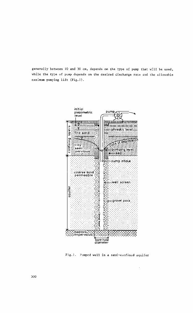
generally between 10 and 30 era, depends on the type of pump that will be used,
while the type of pump depends on the desired discharge rate and the allowable
maximum pumping lift (Fig.1).
initial piezometric level
pump
üfine'sändi:
g/fser 5<^perv ious/ . ft//////////,
CT-
a.
c F c )<
c r "r
s n
e e 0
5(
t If > l e
'^Vllip h rëatï c ' level 1 ^
mmtm CfrnTT^TTTT:-
-:pump' intake:
•^U-^vyell screen •
-gravel pack-;
xbedrock> ximpervioüs<
F i g . 1 . Pumped wel l in a semi-confined aqu i f e r
300
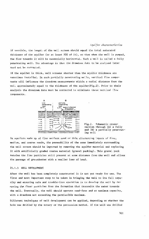
Aquifer ahavaoteristios
If possible, the length of the well screen should equal the total saturated
thickness of the aquifer (or at least 90% of it), so that when the well is pumped,
the flow towards it will be essentially horizontal. Such a well is called a fully
penetrating well. Its advantage is that the drawdown data to be analyzed later
need not be corrected.
If the aquifer is thick, well screens shorter than the aquifer thickness are
sometimes installed. In such partially penetrating wells, vertical flow compo
nents will influence the drawdown measurements within a radial distance from the
well approximately equal to the thickness of the aquifer(Fig.2). Prior to their
analysis the drawdown data must be corrected to eliminate these vertical flow
components.
A B fully I partially penetrating [ penetrating
I r-> *t-~ zone of affected drawdown
„ Fig.2. Schematic cross-nnes * — section through (A) a fully
. , " and (B) a partially pénétrât-
ms^tä&mmmmsmik ing weii In aquifers made up of fine uniform sand or thin alternating layers of fine,
medium, and coarse sands, the permeability of the zone immediately surrounding
the well screen should be improved by removing the aquifer material and replacing
it with artificially graded coarse material (gravel packing). This gravel pack
retains the fine particles still present at some distance from the well and allows
the passage of groundwater with a smaller loss of head.
25.1.3 WELL DEVELOPMENT
After the well has been completely constructed it is not yet ready for use. The
first and most important step to be taken in bringing the well to its full capa
city and ensuring safe and trouble-free operation is to develop the well by re
moving the finer particles from the formation that transmits the water towards
the well. Eventually, the well should operate sand-free and at maximum capacity,
with a drawdown not exceeding the permissible maximum.
Different techniques of well development can be applied, depending on whether the
hole was drilled by the rotary or the percussion method. If the well was drilled
301
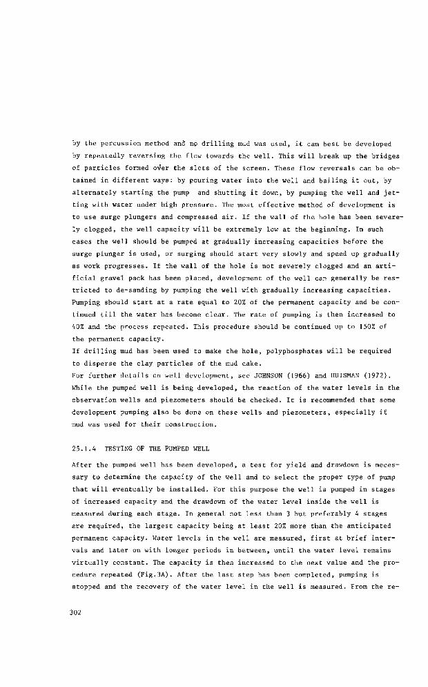
by the percussion method and no drilling mud was used, it can best be developed
by repeatedly reversing the flow towards the well. This will break up the bridges
of particles formed over the slots of the screen. These flow reversals can be ob
tained in different ways: by pouring water into the well and bailing it out, by
alternately starting the pump and shutting it down, by pumping the well and jet
ting with water under high pressure. The most effective method of development is
to use surge plungers and compressed air. If the wall of the hole has been severe
ly clogged, the well capacity will be extremely low at the beginning. In such
cases the well should be pumped at gradually increasing capacities before the
surge plunger is used, or surging should start very slowly and speed up gradually
as work progresses. If the wall of the hole is not severely clogged and an arti
ficial gravel pack has been placed, development of the well can generally be res
tricted to de-sanding by pumping the well with gradually increasing capacities.
Pumping should start at a rate equal to 20% of the permanent capacity and be con
tinued till the water has become clear. The rate of pumping is then increased to
40% and the process repeated. This procedure should be continued up to 150% of
the permanent capacity.
If drilling mud has been used to make the hole, polyphosphates will be required
to disperse the clay particles of the mud cake.
For further details en well development, see JOHNSON (1966) and HUISMAN (1972).
While the pumped well is being developed, the reaction of the water levels in the
observation wells and piezometers should be checked. It is recommended that some
development pumping also be done on these wells and piezometers, especially if
mud was used for their construction.
25.1.4 TESTING OF THE PUMPED WELL
After the pumped well has been developed, a test for yield and drawdown is neces
sary to determine the capacity of the well and to select the proper type of pump
that will eventually be installed. For this purpose the well is pumped in stages
of increased capacity and the drawdown of the water level inside the well is
measured during each stage. In general not less than 3 but preferably 4 stages
are required, the largest capacity being at least 20% more than the anticipated
permanent capacity. Water levels in the well are measured, first at brief inter
vals and later on with longer periods in between, until the water level remains
virtually constant. The capacity is then increased to the next value and the pro
cedure repeated (Fig.3A). After the last step has been completed, pumping is
stopped and the recovery of the water level in the well is measured. From the re-
302
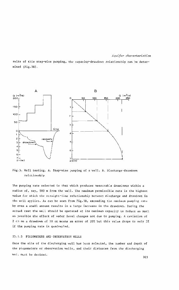
Aquifer characteristics
suits of this step-wise pumping, the capacity-drawdown relationship can be deter
mined (Fig.3B).
B a Crr 2 0 0
150
100
50
0
1
2
3
4
5
6 7
3 /h )
- ^ v
- drawdown
---_
time
recovery ƒ
V ' 7
Q (m3/h) 200 250
Ah (m) Ah(m)
Fig.3. Well testing. A. Step-wise pumping of a well. B. Discharge-drawdown
relationship
The pumping rate selected is that which produces measurable drawdowns within a
radius of, say, 500 m from the well. The maximum permissible rate is the highest
value for which the straight-line relationship between discharge and drawdown in
the well applies. As can be seen from Fig.3B, exceeding the maximum pumping rate
by even a small amount results in a large increase in the drawdown. During the
actual test the well should be operated at its maximum capacity to reduce as much
as possible the effect of water level changes not due to pumping. A deviation of
2 cm on a drawdown of 10 cm means an error of 20% but this value drops to only 5%
if the pumping rate is quadrupled.
25.1.5 PIEZOMETERS AND OBSERVATION WELLS
Once the site of the discharging well has been selected, the number and depth of
the piezometers or observation wells, and their distances from the discharging
well must be decided. 303

A piezometer (Chap.21, Vol.111) is an open-ended unperforated pipe placed in the
ground and extending from the surface to the depth at which the hydraulic head
is to be measured (Fig.4). The term applies equally well to pipes that have a
short screen attached to their lower end. An observation well is an open bore
hole, or a bore hole provided with a pipe which is perforated or slotted over a
relatively great length. The water level in such a well therefore represents the
average hydraulic head over the net length of the bore hole (depth of inflow) or
over the length of the perforated or slotted portion of the pipe. Open bore holes
with or without pipes are used to observe changes in the phreatic level at shal
low depth.
OBSERVATION WEILS PIEZOMETERS PUMPED WELL
groundsurface
aye ra g e j ^j - - vj pïézbmètrïc surface
• - y watertable:
mmm9ßß
Fig.4. Position of screen in observation wells, piezometers, and discharge well
Number and depth
Most methods of analysis require data from at least two piezometers whose lower
ends are located in the aquifer. It is recommended, however, that three or more
be installed. To these should be added, if applicable, some or all of the follow
ing:
- shallow observation wells in the covering layer of semi-confined aquifers, to
check the changes in the phreatic surface;
304
Aquifer characteristics
- piezometers above and below fine-grained intercalations in the aquifer, to
find out whether such intercalations are to be considered resistance layers or
not;
- piezometers in water-bearing layers below the base of the aquifer, to verify
the assumption that this base is impervious;
- a piezometer beyond the radius of influence of the discharge well, to obtain
information on the changes in head not induced by the pumping;
- a piezometer in the gravel pack of the discharge well, to determine whether the
well screen causes significant entrance head losses.
Distances
No fixed rule can be given for the distances at which the observation wells or
piezometers should be installed. The best guide is the experience gained during
pumping tests in comparable aquifers. Nevertheless, the following points should
be considered.
The type of aquifer
In unconfined (phreatic) aquifers the propagation of the head loss is rather slow
because the water released from storage is due mostly to a dewatering of the zone
above the falling water table. The piezometers should therefore not be too far
away from the discharging well.
Semi-confined aquifers react faster (depending on the hydraulic resistance of the
semi-pervious layer) so the distances between piezometers and the pumped well can
be greater.
The value of the hydraulic conductivity K and the storage coefficient S
If K is large and S is small, the cone of depression created by pumping is wide
and flat; if K is small and S is large, the cone is narrow and steep. Thus, in
the first case greater distances are permitted that in the second.
The discharge rate
Pumping at the maximum discharge rate will cause a greater drawdown than pumping
at a low discharge rate. In the first case, therefore, the piezometers can be
placed farther away than in the second.
305
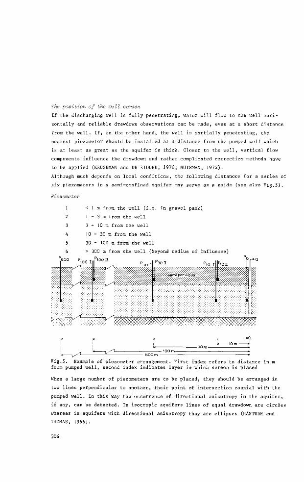
The position of the well screen
If the discharging well is fully penetrating, water will flow to the well hori
zontally and reliable drawdown observations can be made, even at a short distance
from the well. If, on the other hand, the well is partially penetrating, the
nearest piezometer should be installed at a distance from the pumped well which
is at least as great as the aquifer is thick. Closer to the well, vertical flow
components influence the drawdown and rather complicated correction methods have
to be applied (KRUSEMAN and DE RIDDER, 3970; HUISMAN, 1972).
Although much depends on local conditions, the following distances for a series of
six piezometers in a semi-confined aquifer may serve as a guide (see also Fig.5).
Piezometer
1
2
3
4
5
6 r 6 0 0
< 1 m from the well (i.e. in gravel pack]
1 - 3 m from the well
3 - 10 m from the well
10 - 30 m from the well
30 - 100 m from the well
> 300 m from the well (beyond radius of influence) pioon
oO
—H
Fig.5. Example of piezometer arrangement. First index refers to distance in m from pumped well, second index indicates layer in which screen is placed
When a large number of piezometers are to be placed, they should be arranged in
two lines perpendicular to another, their point of intersection coaxial with the
pumped well. In this way the occurrence of directional anisotropy in the aquifer,
if any, can be detected. In isotropic aquifers lines of equal drawdown are circles
whereas in aquifers with directional anisotropy they are ellipses (HANTUSH and
THOMAS, 1966).
306
Aquifer characteristics
25.2 PERFORMING A PUMPING TEST
The measurements to be taken during a pumping test can be divided into two groups:
- measurements of the water levels in the wells and piezometers,
- measurements of the pumping rate.
Since the natural position of the water table will be affected by changes in ba
rometric pressure and in water levels of nearby surface waters, by natural ground
water discharge and by precipitation, these should be measured if the pumping test
is expected to last a long period. Anomalies observed in the drawdown values can
then be explained and corrected.
25.2.1 WATER LEVEL MEASUREMENTS
Measurements prior to and after the pumping test
The natural changes in hydraulic head occurring in the aquifer, i.e. those
changes not induced by pumping, should be known before a pumping test is started.
Hence, for some days prior to the test, the water levels in the observation wells
and/or piezometers should be measured twice a day if a unidirectional change is
expected, or at hourly intervals if a sinusoidal fluctuation pattern is expected.
The latter is a common feature in coastal aquifers and in valleys with river
levels subject to tidal movements.
A hydrograph should be drawn for each observation well, from which the trend and
rate of change in hydraulic head can be read. If the hydrograph indicates that
the trend will not change during the test, pumping can start. When the test is
completed and the water level has been fully recovered, water level readings
should be made in some observation wells once or twice a day for two or three
days. These data complete the well hydrograph and the rate of the natural change
in hydraulic head during the test can then be determined. This information is
used to correct the observed drawdowns into drawdowns induced by pumping alone.
Frequency of observations
The most important part of a pumping test is measuring the depth to water level
in the observation wells, piezometers, and in the pumped well. These measurements
should be taken frequently, and should be as accurate as possible. Since water
levels are dropping fast during the first one or two hours of the test, they
should be recorded at close intervals throughout that period. The time intervals
may be gradually lengthened as the test continues because in the analysis the
307
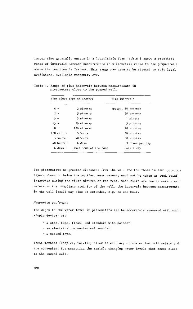
factor time generally enters in a logarithmic form. Table 1 shows a practical
range of intervals between measurements in piezometers close to the pumped well
where the reaction is fastest. This range may have to be adapted to suit local
conditions, available manpower, etc.
Table 1. Range of time intervals between measurements in piezometers close to the pumped well.
Time since pumping started Time intervals
5 -
15 -
50 -
100 min. -
5 hours -
48 hours -
6 days -
2 minutes
5 minutes
15 minutes
50 minutes
100 minutes
5 hours
48 hours
6 days
shut down of the pump
approx. 10 seconds
30 seconds
1 minute
5 minutes
10 minutes
30 minutes
60 minutes
3 times per day
once a day
For piezometers at greater distances from the well and for those in semi-pervious
layers above or below the aquifer, measurements need not be taken at such brief
intervals during the first minutes of the test. When there are two or more piezo
meters in the immediate vicinity of the well, the intervals between measurements
in the well itself may also be extended, e.g. to one hour.
Measuring equipment
The depth to the water level in piezometers can be accurately measured with such
simple devices as :
- a steel tape, float, and standard with pointer
- an electrical or mechanical sounder
- a wetted tape.
These methods (Chap.21, Vol.111) allow an accuracy of one or two millimeters and
are convenient for measuring the rapidly changing water levels that occur close
to the pumped well.
308

Aquifer characteristics
Water level recorders greatly reduce the amount of work required and allow it to
be better organized. When used in piezometers close to the well, however, the
curves obtained will be very steep during the first minutes of the test and can
be interpreted only if the time intervals have been marked by hand on the graph.
Detailed information on automatic recorders, mechanical and electrical sounders
and other equipment is given in such handbooks as JOHNSON (1966), DAVIS and DE
WIEST (1966).
All water level measurements should preferably be noted on pre-printed forms, an
example of which is shown in Fig.6. During the pumping test, time-drawdown curves
for each piezometer are drawn on semi-logarithmic paper (the time in minutes on
the logarithmic scale, and the drawdown in centimetres or millimetres on the
linear scale). Th^se graphs may be helpful in seeing whether the test is running
well and in deciding on the time the pump is to be shut down.
Recovery measurements
When the pump is shut down, the water levels in the pumped well and the piezome
ters will rise rapidly, but as time goes on the rate of rise decreases. Measuring
the rate of rise is called the recovery test. An analysis of the data of such a
test can be used to check the calculations based on the drawdown data.
If the yield of the pumped well was not constant throughout the pumping period,
recovery test data are more reliable than the drawdown data collected during
pumping. The recovery measurements should follow the same schedule as adhered to
during the pumping period.
25.2.2 DISCHARGE RATE MEASUREMENTS
The discharge rate should be measured at least once every hour and adjusted, if
necessary, to keep it constant. Adjustments can be made by means of a valve in
the discharge pipe or by a change in the speed of the pump. The valve, however,
permits a more precise control.
Accurate measurements of the discharge rate can be made with a commercial water
meter of appropriate capacity, if the pipe is running full. To ensure this, the
discharge pipe may be fitted with a U-bend in which the water meter is housed.This
will, however, induce energy losses. If the pumped water is being conveyed through
a channel or small ditch, the discharge rate can be measured by means of a flume
or a weir.A very simple and fairly accurate method is to measure the time required
to fill a container of known volume, e.g. an oil drum. This method, however,
can only be applied if the discharge rates are small.
309

PUMPING TEST:
O B S E R V A T I O N S D U R I N G P U M P I N G / R E C O V E R Y
PIEZOMETER:
PUMPING TEST BY:
PROJECT:
START:
I N I T I A L WATER LEVEL:
REFERENCE LEVEL:
REMARKS:
DEPTH : DISTANCE :
DIRECTED BY:
LOCATION:
STOP:
FINAL WATER LEVEL:
+ M.S.L.1
TIME WATER LEVEL
DRAW DOWN
TIME WATER LEVEL
DRAW DOWN
DISCHARGE RATE
TIME FLOW METER
DISCHARGE RATE
MEAN SEA LEVEL
F i g . 6 . Example of a pumping t e s t obse rva t ion sheet
310

Aquifer characteristics
If none of these methods can be applied, a rough estimate can be obtained by
measuring the dimensions of a stream flowing from either a vertical or horizontal
discharge pipe (JOHNSON, 1966). With a vertical pipe the discharge rate can be
calculated from the height to which the water rises above the top of the pipe and
the diameter of the pipe. The discharge rates for various pipe diameters and
various crest heights are given in Fig.7. With a horizontal pipe, flowing full
crest height in cm 6 0 r
pipe d iameter 2
2 3 4 5 6 8 10 discharge rate in m 3 /dag
Fig.7. Relation between discharge rate, jet flow crest height, and pipe diameter (after JOHNSON, 1966).
f low distance in cm 5 0 i
pipe diameter 2" 3
6 8 icr* discharge rate in m-Vday
Fig.8. Relation between discharge rate, jet flow distance, and pipe diameter for a fall of 30.5 cm (=12") (after JOHNSON, 1966)
311
and allowing a free fall from the discharge opening, the horizontal and vertical
distances from the end of the pipe to a point in the falling stream provide the
basis for calculating the discharge rate. Figure 8 shows the pumping rate for
various pipe diameters and horizontal distances at a given fall.
25.2.3 DURATION OF THE PUMPING TEST
The question of how many hours the well should be pumped is difficult to answer
because the period of pumping depends on the type of aquifer being tested. As al
ready observed, the cone of depression develops rapidly at the beginning of the
test but as pumping continues, it expands and deepens at a decreasing rate because
a larger volume of stored water becomes available with each additional meter of
horizontal expansion. This results in a decrease in drawdown per unit of time,
which may lead to the premature conclusion that the cone has reached a stabilized
position, i.e. that steady-state flow conditions have been reached. In some
aquifers an equilibrium drawdown may be reached a few hours after the start of
pumping. In others it may be reached after a few days or weeks or it may never
be reached. In semi-confined aquifers a steady-state flow situation generally
occurs after 15 to 20 hours of pumping. Since in an unconfined aquifer the cone
of depression expands more slowly, it is common practice to pump such an aquifer
for about three days.
Although methods of analyzing unsteady-state data are available, it is recommended
that pumping be continued till a steady state is reached. This is especially
warranted when accurate information on the aquifer characteristics is required,
for instance when pumping plants for domestic or irrigation water supplies are to
be constructed or when drainage wells are to be installed or other expensive
works are to be carried out. Moreover, a longer period of pumping may reveal the
presence of hydraulic boundaries, previously unknown. The cost of running the
pump a little longer is low compared with the total cost of the test.
25.3 DATA PROCESSING
After the pumping test has been completed and all basic information on well dis
charge, drawdown in the various piezometers and pumped well, trend of the natural
changes in hydraulic head, etc. , has been collected, the data must then be
processed. This comprises:
312

Aquifer characteristics
- compiling the data in the form of graphs;
- correcting the drawdown data for changes of the hydraulic head in the
aquifer not induced by pumping, if applicable;
- determining the type of aquifer that has been pumped.
The field information that consists of time data often given in different units,
(seconds during the first minutes, minutes during the following hours and actual
time later on) and water level observations relative to a reference level, must
be converted into data of a single set of units (for instance time in minutes and
drawdown in metres). These data are then noted on a blank set of observation
sheets (Fig.6), together with all other relevant data.
The drawdowns observed in each piezometer during pumping are plotted versus the
corresponding time data on double logarithmic paper and/or on single logarithmic
paper. The observations made prior to pumping and after complete recovery are
plotted on paper with linear scales to check whether any changes in head have
taken place. In the graph of the "long distance" piezometer the observations made
during the pumping and recovery periods should be included as well. From these
graphs the correction term, i.e. the rate of rise or fall per minute, can be cal
culated. Next, the observed pumping and recovery data are corrected and the time-
drawdown graphs are plotted again, this time with the corrected data.
The type of aquifer is determined from: the bore-hole log, the time-drawdown
curves of the piezometers in the aquifer, and the reaction to pumping observed in
the auxiliary piezometers in the covering layer and in those below the base layer.
If the base layer is impervious (no reaction to pumping in the piezometers below
this layer) and there is a definite covering layer, the drawdowns observed in the
piezometers in the covering layer will help to determine the type of aquifer.
If the drawdown in the shallow observation wells is approximately equal to the
drawdown of the deep piezometers, the aquifer is considered to be unconfined. If
there is an appreciable difference between the drawdowns, the aquifer is considered
to be semi-confined.
25.4 CALCULATION OF THE HYDRAULIC CHARACTERISTICS
In discussing the analysis of pumping tests, we shall restrict our remarks to
horizontal, seemingly infinite, unconfined or semi-confined aquifers. A compre
hensive review of methods of analyzing tests in other types of aquifers is given
by KRUSEMAN and DE RIDDER (1970).
313

25.4.1 ÜNCONFINED AQUIFERS, STEADY FLOW
According to Chap.12, Vol.11, when the flow towards the well was in a steady
state at shut down of the pump, the logarithmic function for this flow around the
well in an unconfined aquifer is written as
Ahl " A h 2 = 2i£D-2-3 0 1°Sr7 (1)
where (see Fig.9)
Ahi, n = steady-state drawdown at distance ri (m),
Ah2, r2 = steady-state drawdown at distance r2 (m),
Q = constant well discharge (m3 day J ) ,
KD = transmissivity of the aquifer (m2 day l).
Substitution of the values Ahi, Ab.2, ri, r2, and Q into Eq.1 yields the value for
KD.
Fig.9. A pumped well and two piezometers in an unconfined aquifer
25.4.2 UNCONFINED AQUIFERS, UNSTEADY FLOW
When the flow towards the well was still unsteady at shut down of the pump, the
analysis of the data is less simple.
Two graphical methods can be followed
- Theis's double-logarithmic method
- Jacob's single-logarithmic method
314

Aquifer characteristics
Theis's double logarithmic method
This method, first described by COOPER and JACOB (1946), is based on the fact
that the unsteady-state drawdown Ah, which is a function of r and t, is propor
tional to another function in r and t, i.e. the well function W(u). According to
Chap.12, Vol.11,
Ah = ̂ 2 _ W(u) (2)
where
r2S (3)
4KDt
S = storage coefficient (dimensionless)
t = time in days
The procedure to be followed in the analysis is as follows:
- Construct, with the aid of Table 2, a 'master-chart' by plotting the values of
u on the horizontal axis of a sheet of double logarithmic paper against the cor
responding values of W(u) on the vertical axis.
- Plot on another sheet of double-logarithmic paper of the same scale, but now
preferably transparent, each observed value of Ah on the vertical axis against
its corresponding value of r /t. If there are n piezometers and m observations in
each piezometer, then m x n observations should be used.
- Place the transparent paper with the plotted observations on the master-chart
and shift till the observed data curve matches the curve on the master-chart.
- Select arbitrarily a match point on the overlapping sheets and determine for
this point the coordinates W(u), u, Ah, and r /t. Note that the match point is
not necessarily located on the curves.
- Substitute the values of W(u), Ah, and Q into Eq.2 and solve for KD.
- Substitute the values of u, r /t, and KD into Eq.3 and solve for S:
Example 1
During a pumping test, 2500 m /day was pumped from a well in an unconfined
aquifer. The following drawdown and time observations were made in two piezome
ters, 10 m and 100 m from the well.
315

Piezometer at 10 m
Ah time since pumping started
0.25 m 57 min. 30 sec. = 0.04 day
0.36 m 3 hours 50 min. = 0.16 day
0.50 m 24 hours = 1 day
100/0.04
100/0.16
100/1
r2/t
= 2500 m2/day
= 625 m2/day
= 100 m2/day
Piezometer at 100 m
0.06 m 6 hours
0.10 m 10 hours 40 min.
0.15m 24 hours
= 0.25 day 10.000/0.25 = 40000 m2/day
= 0.444 day 10.000/0.444 = 22500 m2/day
= 1 day 10.000/1 = 10000 m2/day
Table 2. Values of Theis's well functie
u
0.0001
0.0002
0.0004
0.0006
0.0008
0.001
0.002
0.004
0.006
0.008
0.01
0.02
0.04
0.06
0.08
W(u)
8.63
7.94
7.25
6.84
6.57
6.33
5.64
4.94
4.54
4.26
4.04
3.35
2.68
2.29
2.03
u
0. 10
0.20
0.40
0.60
0.80
1.0
1.2
1.4
1.6
1.8
2.0
2.5
3.0
3.5
4.0
W(u)
1 .82
1 .22
0.702
0.454
0.31 1
0.219
0.158
0.116
0.0863
0.0647
0.0489
0.0249
0.0131
0.00697
0.00378
The observed-data curve and the master-chart curve in matched position are pre
sented in Fig.10. Point A has been selected as match point, its master-chart
coordinates being W(u) = 1 and u = 10 2, and its data-sheet coordinates Ah =
0.076 and r2/t = 1200.
316
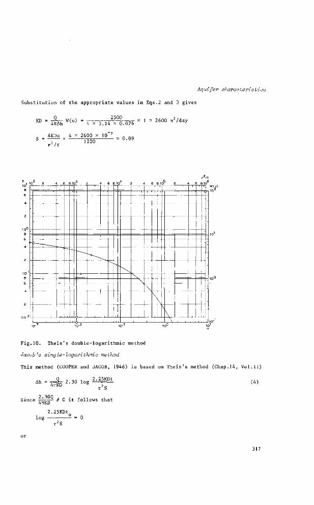
Aquifer characteristics
S u b s t i t u t i o n of t h e a p p r o p r i a t e v a l u e s i n E q s . 2 and 3 g i v e s
Q „ , . . N _ 2500 KD = 4irAh
W(u) 4 x 3 . H x 0.07É
x 1 = 2600 m z / d a y
4KDu 4 x 2600 x 10
llt 1200
0 . 0 9
4 6 8 10 2 4 6 8 1 0 2
~>
1
-
'
-
—
—
-*
-
-
, i . l
,A
1
1 !
. o .
1
' 1 1 1
\ J i
\
i
1
• •
S
, I ,
S
1 1
i
\ i , . ,
~r-r-
\
-
'-
--
-
-1 " I ; ;
, \
Fig.10. Theis's double-logarithmic method
Jacob's single-logarithmic method
T h i s me thod (COOPER and JACOB, 1946) i s b a s e d on T h e i s ' s me thod ( C h a p . 1 4 , V o l . 1 1 )
Ah 4TTKD
Q , , „ , 2 .25KDt -s— 2 . 3 0 l o g (4)
r z S
2 300 Since , ' v ^ 0 i t f o l l o w s t h a t
4TTKD
2.25KDt l o g
r " S
317
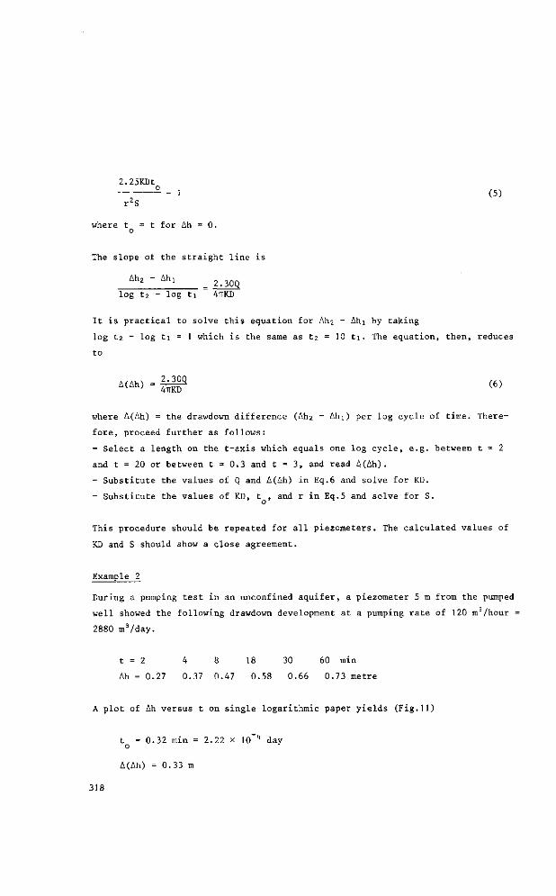
2.25KDt °- = 1 (5)
r2S
where t = t for Ah = 0.
The slope of the straight line is
A h 2 - A h l 2..30Q log t2 - log ti 4ïïKD
It is practical to solve this equation for Ah2 - Ahi by taking
log t2 - log ti = 1 which is the same as t2 = 10 ti. The equation, then, reduces
to
where A(Ah) = the drawdown difference (Ah2 - Ahi) per log cycle of time. There
fore, proceed further as follows:
- Select a length on the t-axis which equals one log cycle, e.g. between t = 2
and t = 20 or between t = 0.3 and t = 3, and read A(Ah).
- Substitute the values of Q and A(Ah) in Eq.6 and solve for KD.
- Substitute the values of KD, t , and r in Eq.5 and solve for S. o
This procedure should be repeated for all piezometers. The calculated values of
KD and S should show a close agreement.
Example 2
During a pumping test in an unconfined aquifer, a piezometer 5 m from the pumped
well showed the following drawdown development at a pumping rate of 120 m /hour =
2880 m3/day.
t = 2 4 8 18 30 60 min
Ah = 0.27 0.37 0.47 0.58 0.66 0.73 metre
A plot of Ah versus t on single logarithmic paper yields (Fig.11)
A(Ah) = 0.33 m
318

Aquifer characteristics
Ah in meters 1.0
0.8
0.2 to"0.32 min
ir ,y-y
y * log eye le
yf\ *y
y
A ( A h l 0.33
1 •n
10" 2 4 6 8 10° 2 4 6 8 10 4 6 810 t in minutes
Fig.II. Jacob's single logarithmic method
Substitution of the appropriate values into Eqs.6 and 5 yields
KD . . l ^ L . , „ 2 ; 3 ? , X „ 2 g ^ = 1600 m a / d a y
S =
47TA(Ah) 4 x 3. 14 x 0.33
o 2.25 x 1600 x 2.22 x 10 5 x 5
0.03
Analysis of recovery data
As was shown in Chap.12, Vol.11, the drawdown development after the pump is shut
down can be found by adding to the drawdown effected by the discharge rate Q, the
(negative) drawdown that would be caused if the pumped well were recharged at the
same rate as it was pumped (Fig.12). Hence, according to Chap.12
Ah- . < L ^ l n *m + _ ^ L l n «Dt: 4TTKD 2 S 4TTKD 2 q
o r , s i nce
4KDt , 4KDt' ln -^^- - In
r 2S r 2S l n ( t / t ' )
Ah' =4ÏÏKÏÏ lnf = 4 4 D 2 - 3 1 ^ ( t / t ' )
where
319

Ah' = the residual drawdown in m, i.e. the difference between the initial water
level prior to pumping and the actual water level at time t' since pumping
stopped
t = time since pumping started, in days
t' = time since pumping stopped, in days
t-
c iAh
0)
t
S
2 c
0 IAH
i 1 * \ E
\ I * \ ~°-
\ a p
^ — y ^
/
f * >- y
pumping period recovery period
Fig. 12. Schematic drawdown development during pumping and recovery period. The broken line indicates the continuing influence of imaginary pumping when imaginary recharge simulates shutdown of pump
Procedure
- Plot for one of the piezometers or for the pumped well, Ah' versus (t/t') on
single logarithmic paper (t/t' on the logarithmic axis) and draw a straight line
through the plotted points. Where this straight line intersects the t/t'-axis,
i.e. the point where Ah' = 0, the point t/t' = 1. Following the same reasoning as
for Jacob's method we get
A(Ah') = 2.30Q 4TTKD
(7)
where A(Ah') is the residual drawdown difference per log cycle of t/t'.
- Substitute the values of A(Ah') and Q into Eq.7 and solve for KD.
Example 3
The pump of a well in an unconfined aquifer is shut down after 24 hours
(= 1440 min) of pumping at a rate Q = 83.5 m3/hour (= 2000 m 3 /day).
The observed decrease of the residual drawdown is as follows
t' (in min)
Ah' (in min)
t/t'
') t = 1440 +
320
t
2 5
0.84 0.78
721 ' 290
15
0.68
97
30
0.58
49
75
0.46
20
150
0.35
10.6
360
0.24
5
720
0.16
3
1440
0.11
2

Aquifer chavaoteristios
A plot of Ah' versus t/t' on single logarithmic paper (Fig.13) yields
A(Ah') = 0.34
Substituting the appropriate values into Eq.7 and solving for KD gives
2.3QQ 2.30 x 2000 .... 2 /, ™ = 4ÏÏÂWY = 4 x 3.14 x 0.34 * 1 1 0° m /day
Äh in meters 1.0
/ s*
s°' _ 1
s ^
A(Äh' ) = 0.
_
3 4 n n
4 6 8 10 4 6 8 10 4 6 810 t /t '
Fig.13. Analysis of recovery data
25.4.3 SEMI-CONFINED AQUIFERS, STEADY FLOW
Two graphical methods will be discussed
- DE GLEE's double-logarithmic method
- HANTUSH-JACOB's single-logarithmic method.
DE GLEE's double-logarithmic method
This method, originally described by DE GLEE (1930), is based on the following
relation (Chap.12, Vol.11)
Ah = 2 Ä V r / ^ (8)
where
321

K (x) = modified Bessel function of the second kind and zero order (Hankel function)
Ah = steady-state drawdown at distance r from the pumped well (m)
c = D'/K' = hydraulic resistance to vertical flow in the semi-pervious layer
(days)
KD = transmissivity of the pervious layer (m2 day l)
Procedure
- Construct, with the aid of Table 3, a master-chart by plotting values of K (x) o
against x on a sheet of double logarithmic paper.
- Plot on another sheet of double logarithmic paper, of the same scale but pre
ferably transparent, the observed steady-state drawdown values against the cor
responding values of r. Each piezometer has only one steady-state drawdown value;
hence, if there are n piezometers then there are also n observations to be used.
- Match both curves and select arbitrarily a point A on the overlapping portion
of the sheets.
- Read the coordinates K (x), x, Ah, and r of Point A.
- Substitute the values of Ah, K (x), and Q into Eq.8 and solve for KD.
Note that , . x = r//KDT (9)
- Substitute therefore the values of x, r, and KD into Eq.9 and solve for c.
Table 3. Values of the modified Bessel function of the second kind and zero order
X
0.01
0.02
0.04
0.06
0.08
0.1
0.2
0.4
0.6
0.8
K (x) 0
4.72
4.03
3.34
2.93
2.65
2.43
1.75
1.11
0.777
0.565
X
1.0
1.2
1.4
1.6
1.8
2.0
2.5
3.0
3.5
4.0
K (x) o
0.421
0.318
0.244
0.188
0. 146
0.114
0.0623
0.0347
0.0196
0.0112
322
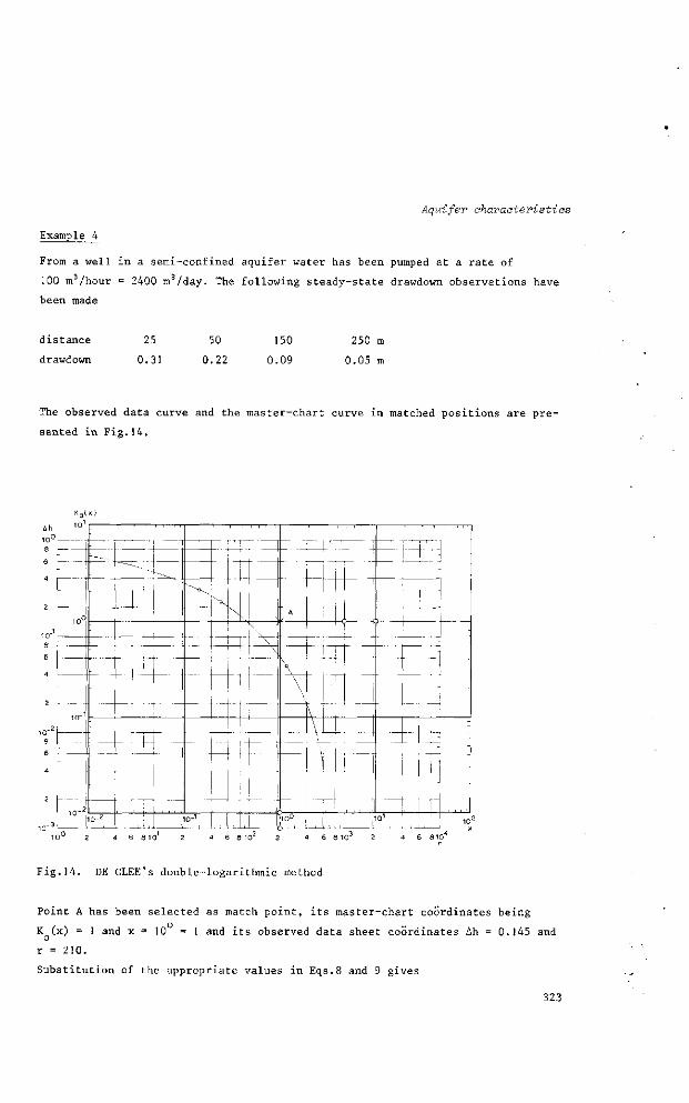
Aquifer characteristics
Example 4
From a well in a semi-confined aquifer water has been pumped at a rate of
100 m /hour = 2400 m3/day. The following steady-state drawdown observations have
been made
distance
drawdown
25
0.31
50
0.22
150
0.09
250
0.05
The observed data curve and the master-chart curve in matched positions are pre
sented in Fig.14.
i H-
! > -
10 2 4 6 8 1 0 2 4 6 8 1 0 2 4 6 8 1 0 2 4 6 8 1 0 r
Fig.14. DE GLEE's double-logarithmic method
Point A has been selected as match point, its master-chart coordinates being
K (x) = 1 and x = 10 = 1 and its observed data sheet coordinates Ah = 0.145 and o r = 210.
Substitution of the appropriate values in Eqs.8 and 9 gives
323
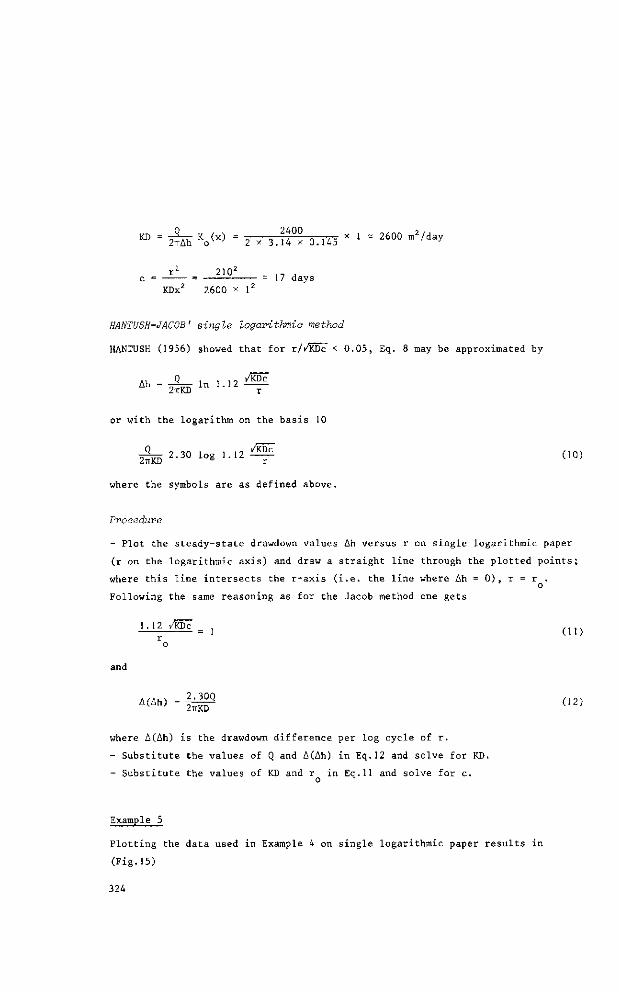
^ - 4 Ko ( x ) = 2 x 3,u°x 0.145 X ' = 2 6 0 ° m 2 / d a ^
210^ „ . , , - 1/ days
KDx 2600 x i*
HANTUSH-JACOB ' single logarithmic method
HANTUSH (1956) showed t h a t f o r r / /KDc < 0 . 0 5 , Eq. 8 may be approximated by
A h = < L l n ,.12 ^Dc 2irKD r
or with the logarithm on the basis 10
_ 2 _ 2.30 log ..12 ̂ (10)
where the symbols are as defined above.
Procedure
- Plot the steady-state drawdown values Ah versus r on single logarithmic paper
(r on the logarithmic axis) and draw a straight line through the plotted points;
where this line intersects the r-axis (i.e. the line where Ah = 0), r = r . o
Following the same reasoning as for the Jacob method one gets
••'2 ^ - ! (11)
and
A(Ah)=|^2 (12)
where A(Ah) is the drawdown difference per log cycle of r.
- Substitute the values of Q and A(Ah) in Eq.12 and solve for KD.
- Substitute the values of KD and r in Eq.11 and solve for c. o
Example 5
Plotting the data used in Example 4 on single logarithmic paper results in
(Fig.15)
324

Aquifer characteristics
r = 320 m o
A(Ah) = 0.285 m
Substitution of the appropriate values into Eqs.11 and 12 yields
2.30O 2.30 x 2400 KD 2irA(Ah) 2 x 3.14 x 0.285
3100 ni /day
• i ?̂ 2 _ _L 320. C " ÎÏÏ ( KÏ2>* • 3ÏÖÖ X (ïfft)2 » 26 da^S
The results with the De Glee method differ from those obtained with the Hantush-
Jacob method, which is illustrative of the inaccuracies inherent to these graphi
cal methods.
ah in meters 0.35
0.20
0.15
A U
I \ \ \
I
ih)=0.20S I I I I
•
m
Y0" 320 n n
4 6 8 10 ' 4 6 8 10 r in meters
Fig.15. Hantush-Jacob's single-logarithmic method
25.5 FINAL REMARKS
Before any of the methods of analysis is applied, attention should be given to
the assumptions underlying that particular method.
The natural conditions nearly always deviate somewhat from the assumed ones.
325

These deviations should be taken into account when the final evaluation of the
calculations is being made. Several methods of analysis, if applicable, should be
used to calculate the hydraulic characteristics. The results should be compared
and weighed by one's professional judgement when the mean values are being calcu
lated.
Sometimes the observed data show unexpected anomalies. Some of them are mentioned
below:
- A great difference between the water levels in the pumped well and at the well
face. This is a common phenomenon due to faulty construction of the well, or its
insufficient development. The result is a high entrance resistance into the well,
which causes the anomalous head loss. This is one of the reasons why piezometer
data, rather than data from the pumped well, are preferred for calculation pur
poses .
- A smaller drawdown in a piezometer close to the discharging well than in one
farther away. This may be due to inhomogeneities of the aquifer which should,
however, have been revealed from the study of the well logs. Other explanations
may be found in the influence of a second pumped well in the vicinity, the lower
ing of the level of a nearby canal, etc.
Variations in the hydraulic resistance of a semi-pervious layer may also have an
effect on piezometer readings.
Variations in the discharge rate will have a greater effect on piezometers near
the pumped well than on those farther away. These influences can easily be traced
by an examination of the measured discharge rate. Faulty piezometers and water-
level indicators and inattentive observers are other sources of deviations from
the expected course of events. Testing of piezometers and equipment during devel
opment pumping and the use of well-trained personnel will largely overcome these
problems.
A report should be written at the conclusion of the pumping test, and should con
tain the following items:
- a map of the pumping test site and surrounding area, including locations of
main well, piezometers, and open water courses, if any;
- a lithological cross-section of the test site, based on data from the borings;
- sheets of the observed field data;
- a description and/or graphs, illustrating the corrections applied to the ob-
326
Aquifer characteristics
served data, if applicable;
- a conclusion regarding the type of aquifer and the considerations that led to
the selection of the analytical methods used;
- graphs of the time-drawdown curves in superposition on the type curves, if
applicable;
- the calculations in an abbreviated form;
- the values of the hydraulic characteristics of the aquifer and confining
layers, as well as a discussion as to their accuracy;
- recommendations for further investigations, if applicable;
- a summary of the results obtained.
327
LITERATURE
COOPER, H.H. and JACOB, C E . 1946. A generalized graphical method evaluating
formation constants and summarizing well field history. Am. Geophys. Univ.
Trans. 27: 526-534.
DAVIS, S.N. and DE WIEST, R.J.M. 1966. Hydrogeology. John Wiley and Sons,
New York, 463 pp.
DE GLEE, G.J. 1930. Over grondwaterstromingen bij wateronttrekking door middel
van putten (Thesis). J. Waltman, Delft. 175 pp.
HANTUSH, S.M. 1956. Analysis of data from pumping tests in leaky aquifers.
Trans. Am. Geophys. Union, 36: 95-100.
HANTUSH, S.M. and THOMAS, R.G. 1966. A method for analyzing a drawdown test in
anisotropic aquifers. Water Resources Res. 2: 281-285.
HUISMAN, L. 1972. Groundwater recovery. MacMillan Civil Eng. Hydraulics. The
MacMillan Press Ltd., London. 336 pp.
JOHNSON, E.E. 1966. Groundwater and wells. Edward E. Johnson Inc., Saint Paul,
Minnesota, U.S.A. 440 pp.
KRUSEMAN, G.P. and DE RIDDER, N.A. 1970. Analysis and evaluation of pumping test
data. Int. Inst, for Land Reclam. and Improvement, Bull.No.11. 200 pp.
328

SURVEYS AND INVESTIGATIONS
26. D E R I V I N G SOIL H Y D R O L O G I C A L CONSTANTS F R O M F I E L D D R A I N A G E TESTS
P. J. DlELEMAN Land Drainage Engineer Food and Agriculture Organization Rome
Lecturers in the Course on Land Drainage
J. WESSELING (1962-1967) Institute for Land and Water Management Research, Wageningen
P. J. DIELEMAN (1968, 1969) International Institute for Land Reclamation and Improvement, Wageningen
J. KESSLER (1970, 1971) International Institute for Land Reclamation and Improvement, Wageningen
C. L. VAN SOMEREN (1972, 1973) International Institute for Land Reclamation and Improvement, Wageningen

PURPOSE AND SCOPE
The layout of experimental fields, the network of observations, and the processing
of measurements with a view to obtaining information on the soil hydraulic conduc
tivity, the transmissivity, the effective porosity, and the groundwater reservoir-
coefficient.
CONTENTS
26.1 OBJECTIVES OF FIELD EXPERIMENTS 331
26.2 SCOPE OF PRESENT DISCUSSION 331
26.3 SELECTION OF TRIAL SITE 331
26.4 SIZE OF EXPERIMENTAL UNIT 332
26.5 DIMENSIONS OF INDIVIDUAL TRIAL PLOTS 332
26.6 ARRANGEMENT OF PLOTS 332
26.7 NETWORK OF OBSERVATION POINTS 333
26.7.1 Drain discharge 333 26.7.2 Watertable depth 334
26.8 MEASURING DEVICES 335
26.8.1 Drain discharge 335
26.8.2 Watertable depth 336
26.9 FREQUENCY OF OBSERVATIONS 336
26.10 DATA PROCESSING AND ANALYSIS 337
26.10.1 Steady state conditions (non-layered soil) 337 26.10.2 Steady state conditions (layered soil) 340 26.10.3 Unsteady state conditions 342
LITERATURE 350
330
Soil hydvologicdl constants
26.1 OBJECTIVES OF. FIELD EXPERIMENTS
The measurement of such hydrologie soil characteristics as hydraulic conductivity
of the upper layer, transmissivity of a phreatic aquifer, and the effective poro
sity has been discussed in Chap.24, Vol.111. It will have been observed that the
volume of soil involved in the measurement is usually small. As an example, when
hydraulic conductivity is measured by the auger hole" method, the soil volume that
3
contributes to the measurement seldom exceeds 0.5 m . The sample sizes for labora
tory methods are even smaller. Due to this limited volume of soil investigated per
observation a large number of measurements is needed to obtain a statistically
reliable average that can be used for the design of the drainage system, but often
a much smaller number is taken in practice. As a consequence, it is often desi
rable - and sometimes even indispensable - to make use of experimental fields to
verify the initial assumptions concerning the hydrological soil properties on which
the design of the drainage system has to be based. In areas where soil conditions
are rather heterogeneous, experimental fields may be the only or most efficient
way to obtain the required information on drainage design factors. Such fields,
moreover, may serve to collect information on individual water balance factors,
the desirable watertable depth, the efficiency of the irrigation system, the
leaching efficiency, etc. They may also be used to test drainage materials, such
as pipes and filter materials, or new techniques of drainpipe installation. Before
constructing the field one should carefully define the problem to be investigated.
The layout of the plots and the network of observations should be such that ade
quate information can be obtained and that as many subjects of interest as possible
are covered.
26.2 SCOPE OF PRESENT DISCUSSION
The present discussion will be limited to the layout of trial fields, the measure
ments and the processing of field data in view of obtaining information on the
hydraulic conductivity and transmissivity of the soil, the effective porosity in
the zone of fluctuating water tables and the groundwater reservoir-coefficient.
The layout and observation systems suggested in the following sections will in
principle be suitable for the other tests above.
26.3 SELECTION OF TRIAL SITE
The site of a experimental field should be chosen in such a way that the ground
water table is only influenced by precipitation, irrigation and evaporation. The
results obtained from experimental fields should be applicable to an area of fair
331
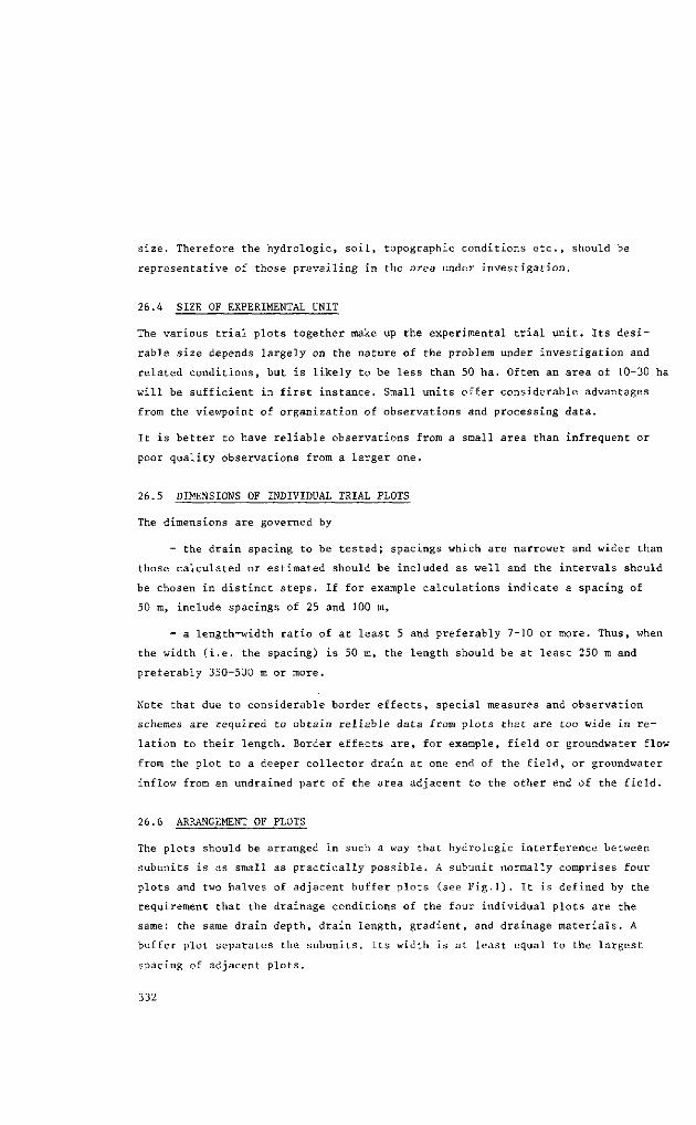
size. Therefore the hydrologie, soil, topographic conditions etc., should be
representative of those prevailing in the area under investigation.
26.4 SIZE OF EXPERIMENTAL UNIT
The various trial plots together make up the experimental trial unit. Its desi
rable size depends largely on the nature of the problem under investigation and
related conditions, but is likely to be less than 50 ha. Often an area of 10-30 ha
will be sufficient in first instance. Small units offer considerable advantages
from the viewpoint of organization of observations and processing data.
It is better to have reliable observations from a small area than infrequent or
poor quality observations from a larger one.
26.5 DIMENSIONS OF INDIVIDUAL TRIAL PLOTS
The dimensions are governed by
- the drain spacing to be tested; spacings which are narrower and wider than
those calculated or estimated should be included as well and the intervals should
be chosen in distinct steps. If for example calculations indicate a spacing of
50 m, include spacings of 25 and 100 m,
- a length-width ratio of at least 5 and preferably 7-10 or more. Thus, when
the width (i.e. the spacing) is 50 m, the length should be at least 250 m and
preferably 350-500 m or more.
Note that due to considerable border effects, special measures and observation
schemes are required to obtain reliable data from plots that are too wide in re
lation to their length. Border effects are, for example, field or groundwater flow
from the plot to a deeper collector drain at one end of the field, or groundwater
inflow from an undrained part of the area adjacent to the other end of the field.
26.6 ARRANGEMENT OF PLOTS
The plots should be arranged in such a way that hydrologie interference between
subunits is as small as practically possible. A subunit normally comprises four
plots and two halves of adjacent buffer plots (see Fig.]). It is defined by the
requirement that the drainage conditions of the four individual plots are the
same: the same drain depth, drain length, gradient, and drainage materials. A
buffer plot separates the subunits. Its width is at least equal to the largest
spacing of adjacent plots.
332
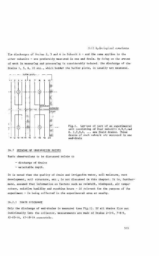
Soil hydrologiaal constants
The discharges of Drains 2, 3 and 4 in Subunit A - and the same applies to the
other subunits - are preferably measured in one end drain. By doing so the amount
of work in measuring and processing is considerably reduced. The discharge of the
Drains 1, 5, 6, 10 etc., which border the buffer plots, is usually not measured.
r- — buffer plots- 1
I t 1 2 3 4 5 * 6 7 8 9 1 0 '
4)
© -0-
11 12 13 14 15 16 17 18 19 20
Fig.1. Lay-out of part of an experimental unit consisting of four subunits A,B,C,and D. 1,2,3,4, ... are field drains. Three drains of each subunit are measured in one end-drain
26.7 NETWORK OF OBSERVATION POINTS
Basic observations to be discussed relate to
- discharge of drains
- watertable depth.
It is noted that the quality of drain and irrigation water, soil moisture, root
development, soil structure, etc., is not discussed in this chapter. It is, further
more, assumed that information on factors such as rainfall, windspeed, air tempe
rature, relative humidity and sunshine hours - if relevant for the purpose of the
experiment - is being collected in the experimental area or nearby.
26.7.1 DRAIN DISCHARGE
Only the discharge of énd-drains is measured (see Fig.1). If all drains flow out
individually into the collector, measurements are made of Drains 2-3-4, 7-8-9,
12-13-14, 17-18-19 separately.
333

Note that the discharge capacity of the collector drain should be large enough to
keep its water level below the field drains during periods of high discharge. If
the end pipes of field drains are submerged, back pressure will occur in the
field drains, whereas discharge measurements will be impossible - unless specific
devices are employed.
26.7.2 WATERTABLE DEPTH
Water table observation wells are installed (Fig.2)
- midway between drains to measure the available hydraulic head,
- near one or more of the drains of each subunit, to observe-the shape of the
water table; wells preferably to be placed at distances of 0.5, 1, 2, 4 and 10 m
from the drain,
- at the upper and/or lower ends of some of the subunits, to observe border
effects,
- on top of drain tubes, to check the functioning of the drains.
Figure 2 illustrates the placement of wells. If problems of malfunctioning arise,
additional wells may be needed.
collector drain
B
f 1
-
~~
JB
•
, A
Ä
dra ned fields !
C J
midway between drains
0 5 10 30m
Fig.2. Example of a network of watertable observation wells; o = observation well
334

Soil hydvological constants
Note that observation wells are open boreholes or boreholes in which perforated
pipes have been placed. It is essential that water can seep in and out of the well
over its entire saturated depth (Fig.3). Piezometers, i.e. pipes with a short
filter at the lower end, may be placed at different depths in cases where a verti
cal flow of groundwater might be of importance. Depending on the purpose of the
experiment, the desired accuracy and the hydrologie heterogeneity of the soil,
adaptations in number or type might be useful. For example when the experiment
serves to check the effect of different types of drainage materials, more emphasis
must be laid on measurements of the loss of hydraulic head in the near vicinity
of the drain lines, which makes the use of piezometers more appropriate. Some wells
must be measured frequently, others need no longer to be measured once the hydro-
logical influence of the surrounding areas is known (Sect.9).
perforated pipe open bor
—
ehole
V
n borehole
si 1 : l i 11 : 1 i'f'
1 IS* . i i
:sl 1 m t: Sil his m i s i 1 'M 1 ! I is.'
1 Is •1 .;! 1
»y/7?
—
Fig.3. Sketch of watertable observation wells
26.8 MEASURING DEVICES
26.8.1 DRAIN DISCHARGE
Drain discharge may be measured by
- buckets of known volume and using a stopwatch; this method is fairly labo
rious, especially during periods of heavy rainfall or during and directly after
irrigation when several measurements are needed to obtain a true picture of dis
charge fluctuations. When a quick reaction to rainfall or irrigation is to be
expected the difficulty to make observations at night will be another disadvantage.
A considerable advantage of the method is its simplicity and low cost,
335

- discharge recorders attached to drain outlets; several types are available;
they offer the advantage that a more reliable picture is obtained of a total or
average discharge rate per day or during shorter periods; disadvantages are: very
expensive compared to a bucket though often more economic when costs for labour,
etc. are taken into account, considerable processing work, though some techniques
are available which allow automatic data processing, the requirement that a free
board of 20 cm or more is necessary between drain outlet and the water level in
the ditch;
- weirs, etc., disadvantages are 20-30 cm headloss and inaccuracy during
periods of low discharge.
It is recommended that at least some recorders are permanently used. They will
be helpful in extrapolating data from non-recording systems.
26.8.2 WATERTABLE DEPTH
Watertable depths can be measured in numerous ways, for example by (Chap.21,Vol.III)
- float and tape
- mechanical sounder
- electrical devices (dependent on batteries, sensitive to dirt)
- watertable depth recorders, which are mounted on the observation wells and
operate with a float with mechanical registration; some recorders make use of
a punched tape.
Also here it is recommended that some automatic recording devices be included
to allow correct extrapolation of measurements by other devices.
26.9 FREQUENCY OF OBSERVATIONS
The frequency of observations should be governed by local conditions and the pur
pose of the trial field. For the experiments discussed in this chapter mostly the
relation discharge - hydraulic head is the subject of investigation and the number
of observations must be adequate to determine this relation, either for steady or
unsteady state conditions. In this respect the drainage intensity of the system
under investigation is a significant property, being a characteristic for the
speed of the discharge of rain or irrigation water. When a quick discharge occurs
after recharge the frequency of observations (of drain discharge and watertable
depth) will have to be at least three times a day or more, whereas intervals can
gradually be enlarged when the changes in discharge and watertable depth slow
down.
336
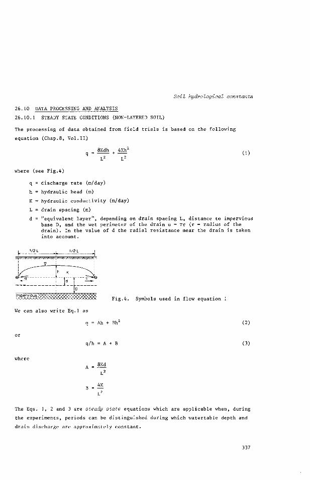
Soil hydrologioal constants
26.10 DATA PROCESSING AND ANALYSIS
26.10.1 STEADY STATE CONDITIONS (NON-LAYERED SOIL)
The processing of data obtained from field trials is based on the following
equation (Chap.8, Vol.11)
8Kdh 4Kh/
T 2 (1)
where (see Fig.4)
q = discharge rate (m/day)
h = hydraulic head (m)
K = hydraulic conductivity (m/day)
L = drain spacing (m)
d = "equivalent layer", depending on drain spacing L, distance to impervious base D, and the wet perimeter of the drain u = TTr (r = radius of the drain). In the value of d the radial resistance near the drain is taken into account.
JZ_ T h K
Fig.4. Symbols used in flow equation 1
We can also write Eq.1 as
q = Ah + Bh2 (2)
q/h = A + (3)
where
A = 8Kd
4K
T2
The Eqs. 1, 2 and 3 are steady state equations which are applicable when, during
the experiments, periods can be distinguished during which watertable depth and
drain discharge are approximately constant.
337

Procedure and example (steady state flow)
Procedure
- convert the observed discharge rate into mm or m per day, plot these versus time
and draw visually a fitting line through the points (Fig.5A)
- convert the observed watertable depths into hydraulic head values (mm or m),
plot these versus time and draw visually a fitting line through the points
(Fig.5B)
- plot discharge rates versus corresponding hydraulic heads from both curves and
obtain the discharge-head relation (Fig.5C).
Note that Fig.5C can be constructed without the aid of Figs.5A and 5B. The latter,
however, are helpful in finding periods during which the hydraulic head and drain
discharge are approximately constant and in showing the degree of regularity and
accuracy of the measurements. Furthermore, if q and h have not been measured on
the same date, interpolations can be made via Figs.5A and 5B.
Fig.5. Relation between q and h as derived from q-t and h-t curves
Analysis
Equation 2
q = Ah + Bh2
shows that the q-h relation will approach a straight line when the value of Bh2
is small compared to the value of Ah(Fig.5C, curve 1). Such a straight line points
338

Soil hyanalogical constants
to a transmissivity of the layers above drain level that is negligible compared
to that of the soil layers below the drain level. As a result, the greater part of
the drainage water will pass through the layers below the drains.
When flow above the drain level is not negligibly small, the q-h line will be
curved. Its actual shape will depend on the relative contribution made by each of
the two parts of the right hand term. The greater the share of the layers above
the drains the stronger the curvature will be.
To facilitate the interpretation of the measured q-h relation it may be helpful
to plot also q/h versus h (Fig.6). This relation is presented by a straight line
making an angle a with the horizontal axis,with(see Eq.3)
4K tan a = —
L2
When the value of is relatively small the q/h-line will be horizontal. L2
q/h
da 16
14
12
/ s -1
1
q 8 K d j 4 K h A I Q . + —rj - A+ Bh
q . S K d
h " L2
l 1 1 0 0.2 0.4 0.6 0.8 1.0
htm) Fig.6. Relation q/h-h, yielding straight lines
Examp le 1
Consider an experimental field which has been drained by pipes with a radius
r = 0.10 m, placed at 2 m depth and at a spacing of 100 m. Discharge rate and
watertable depth have been measured frequently during periods of little change
in watertable position. The observations have been plotted as shown in Figs.5A and
5B and the corresponding values derived are given in Table 1.
Figure 7 shows a plot of q versus h and of q/h versus h. The q-h relation is a
slightly curved line which indicates that the greater part of the excess water
will flow to the drains through the soil layers below drain level.
4K -3 The q/h-h relation is a straight line, whose tangent is B = — = 0.4 x 10
T2
and the value A - = 1.6 x 10 , read from the intersection point on the L2
vertical axis.
339
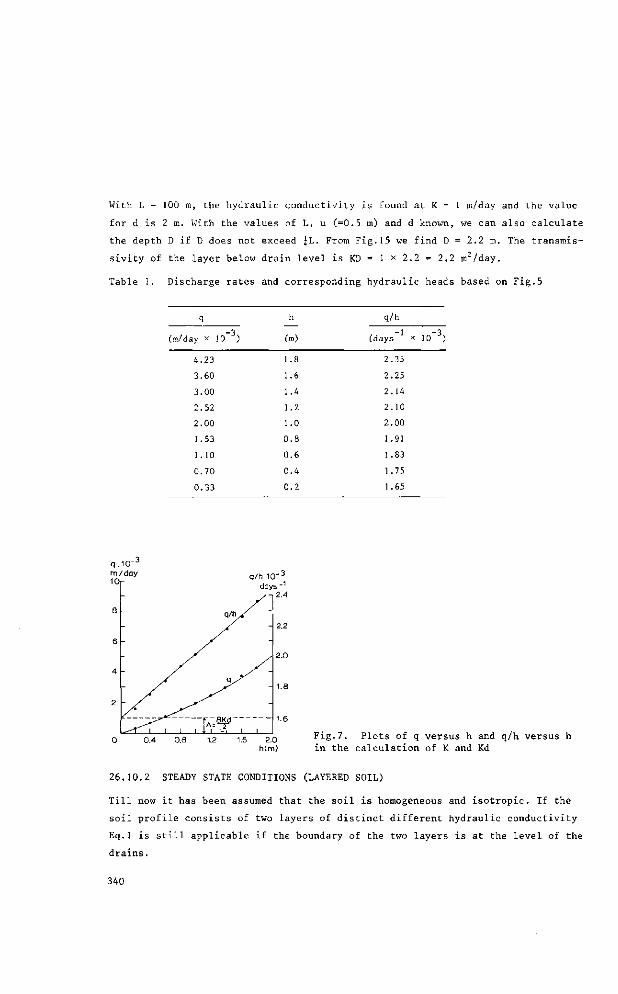
With L = 100 m, the hydraulic conductivity is found at K = 1 m/day and the value
for d is 2 m. With the values of L, u (=0.5 m) and d known, we can also calculate
the depth D if D does not exceed jL. From Fig.15 we find D = 2.2 m. The transmis-
sivity of the layer below drain level is KD = 1 x 2.2 = 2.2 m /day.
Table 1. Discharge rates and corresponding hydraulic heads based on Fig.5
q
(m/day x 1o" )
4 .23
3.60
3.00
2.52
2 .00
1.53
1.10
0.70
0 .33
h
(m)
1.8
1.6
1.4
1.2
1.0
0 .8
0 .6
0 .4
0 .2
q/h
(days x io J)
2.35
2.25
2.14
2.10
2.00
1.91
1.83
1.75
1.65
q .10"
10
8
6
4
2
aay
-
-
. - " T l I i i l l
<VK<
<y>
8 K d " L2,
q/h.10 days
/ -
-
_ -
7 0.4 0.8 1.2 1.6 2.0
h(m)
Fig.7. Plots of q versus h and q/h versus h in the calculation of K and Kd
26.10.2 STEADY STATE CONDITIONS (LAYERED SOIL)
Till now it has been assumed that the soil is homogeneous and isotropic. If the
soil profile consists of two layers of distinct different hydraulic conductivity
Eq. 1 is still applicable if the boundary of the two layers is at the level of the
drains.
340
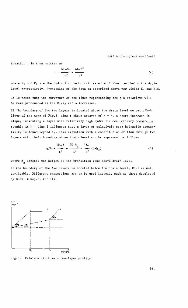
Equation 1 is then written as
8K2dh 4K1h/
q =
Soil hydvologiodl constants
(4)
where Ki and K2 are the hydraulic conductivities of soil above and below the drain
level respectively. Processing of the data as described above now yields Kj and K2d.
It is noted that the curvature of the lines representing the q-h relations will
be more pronounced as the Ki/K2 ratio increases.
If the boundary of the two layers is located above the drain level we get q/h-h
lines of the type of Fig.8. Line 1 shows upwards of h = hj a sharp increase in
slope, indicating a layer with relatively high hydraulic conductivity commencing
roughly at hi ; Line 2 indicates that a layer of relatively poor hydraulic conduc
tivity is found beyond h2. This situation with a contribution of flow through two
layers with their boundary above drain level can be expressed as follows
q/h = 8K2d 4K2h 4Kj
(h-h ) (5)
where h denotes the height of the transition zone above drain level.
If the boundary of the two layers is located below the drain level, Eq.1 is not
applicable. Different expressions are to be used instead, such as those developed
by ERNST (Chap.8, Vol.11).
q /h days-'
2 / 1
^=^r^X-~-
h meters
Fig.8. Relation q/h-h in a two-layer profile
341
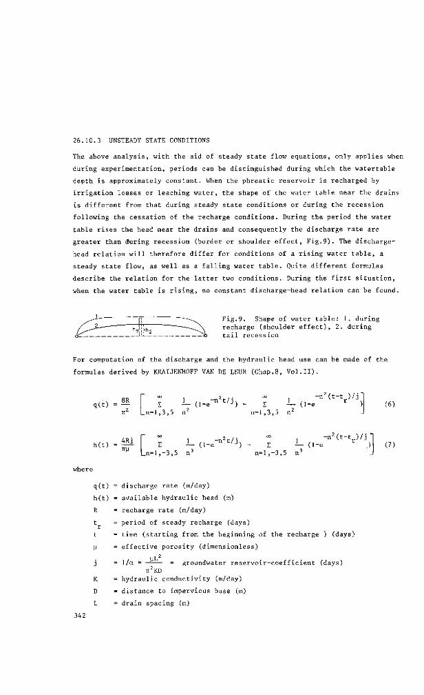
26.10.3 UNSTEADY STATE CONDITIONS
The above analysis, with the aid of steady state flow equations, only applies when
during experimentation, periods can be distinguished during which the watertable
depth is approximately constant. When the phreatic reservoir is recharged by
irrigation losses or leaching water, the shape of the water table near the drains
is different from that during steady state conditions or during the recession
following the cessation of the recharge conditions. During the period the water
table rises the head near the drains and consequently the discharge rate are
greater than during recession (border or shoulder effect, Fig.9). The discharge-
head relation will therefore differ for conditions of a rising water table, a
steady state flow, as well as a falling water table. Quite different formulas
describe the relation for the latter two conditions. During the first situation,
when the water table is rising, no constant discharge-head relation can be found.
Fig.9. Shape of water table: 1. during recharge (shoulder effect), 2. during tail recession
For computation of the discharge and the hydraulic head use can be made of the
formulas derived by KRAIJENHOFF VAN DE LEUR (Chap.8, Vol.11).
q(t) = 8R 1 -n2t/i °° 1 -n2(t-t )/Jl
Ï. — (1-e n t / J ) - I i- (1-e Ln=l,3,5 n2 n=],3,5 n2
(6)
h(t) = 4Rj THi
(l-e-n2t/j) --n2(t-t )/j
-!- (1-e 1,-3,5 nd n=l,-3,5 n*
(7)
where
q(t) = discharge rate (m/day)
h(t) = available hydraulic head (m)
R = recharge rate (m/day)
t = period of steady recharge (days)
t = time (starting from the beginning of the recharge ) (days)
u = effective porosity (dimensionless)
UL2
j = 1/a - = groundwater reservoir-coefficient (days) TT2KD
K = hydraulic conductivity (m/day)
D = distance to impervious base (m)
L = drain spacing (m) 342

Soil hydrologiaal constants
At a certain time t = 0.4 j , after cessation of the recharge, the second and
further terms of the infinite series of Eqs.6 and 7 become very small and are
therefore negligible ("tail recession"). Thus Eqs.6 and 7 reduce to
, . 8R q ( t ) = —
TT 2
h ( t ) 4Rj i n j
( l - e " t / 3 ) - ( 1 - e
( l - e " t / j ) - ( 1 - e
-(t-t J / j
• ( t - t r ) / j (
(8)
(9 )
S u b s t i t u t i n g two v a l u e s t = t i and t = t2 ( t i and t 2 > t +0 .4J ( s e e F i g . 1 0 ) )
one o b t a i n s
q ( t 2 ) = q ( t j ) e " ( t 2 - t i ) / j
' ( t j - t ^ / j h ( t 2 ) = h ( t i ) e
Combining Eq.8 and Eq.9 gives
or (t2-ti)/j = 2.3 log
or (t2-ti)/j = 2.3 log
q(ti)
q(t2)
h(t!)
hltll
or, since
q(t) = | h ( t )
V^
q(t)
TT7 KD
2TTKD h(t)
(10)
(11)
(12)
(13)
(14)
Note that
- the groundwater reservoir-coefficient j may, according to Eqs.10 and 11, be
calculated either from the hydraulic heads, or from the discharge rates; when
using equations for steady state flow both hydraulic head and discharge should be
known,
- strictly speaking, the numerical value of D in Eq.13 is equal to the thick
ness of the aquifer below the drains plus 1/4 (h(ti) + h(t2)}. To apply the equa
tion for unsteady state flow, however, D should be constant. In practice this is
considered to be so if the transmissivity of the part of the phreatic aquifer below
the drains exceeds by far that of the part above the drains,
- to include the radial resistance near the drain the D-value may be replaced
by Hooghoudt's d-value.
343

Equation 14 may then be written as
. . 2irKd q(t) = h(t) (15)
hydraulic head
tl and t 2 > t r»0.4j
Fig.10. Relation between h(t) and t, during recharge and tail recession
Procedure and example (unsteady state flow)
Exanrp le 2
The procedure and analysis is demonstrated by the following example.
Consider an experimental field that has been drained by pipes at a spacing of
30 m. The pipes with a radius r = 0.10 m have been placed at a depth of 1.80 m
(Fig.11).
Soil investigations show a thick layer of clay with a plastic consistence whose
upper boundary is at a depth of 4.80 m below ground surface. From hydraulic conduc
tivity measurements and additional observations on the seasonal fluctuations of
the water table it is concluded that the transmissivity of this layer is very
small compared to that of the overlying soil and may be considered an impervious
floor.
On a certain day 140 mm of water is applied, of which 40 mm percolate below the
rootzone. It is assumed that all of it recharges the phreatic aquifer on that same
day. During the day of recharge and the following days the watertable depth and the
discharge rate are measured several times a day.
344

Soil hydrological constants
The experiment will serve - amongst other things - to find the coefficient (j) and/
or to collect basic information on such individual physical soil characteristics as
hydraulic conductivity (K), transmissivity (KD), and effective porosity (y).
///^/;/s&///!m'//^///^//^//'^^
Fig.11. Drainage conditions of Example 2 (unsteady flow)
Calculation of the groundwater reservoir-coefficient
To arrange the field observations and calculate the groundwater reservoir-
coefficient, proceed as follows
- convert the observed discharge rates into mm or m per day, plot these versus
time and draw visually a fitting line through the points (Fig.12),
- convert the observed watertable depths into hydraulic head values (mm or m ) ,
plot these versus time and draw visually a fitting line through the points (Fig.12),
- read from the two graphs the corresponding values at the end of the days
and compose Table 2.
Table 2. Recharge, discharge rates and corresponding hydraulic heads based on Fie.12
t
R
q(t)
h(t)
= = = =
1
40
14.4
495
2
-5.9
430
3
-4.4
340
4
-3.4
265
5
-2.6
205
6
-2.0
160
7
-1.6
125
8
-I .2
100
days
mm
mm/day
mm
345

- plot q(t) and/or h(t) values from this table versus time on semi-log paper
and obtain the lines of Fig.13,
hydraulic head mm S00
4 0 0
200
discharge rate m m/day
16
Fig.12. Watertable position and discharge rates observed and converted into hydraulic heads (mm) and discharge rates (mm/day).
discharge rate mm/day
20
10 12 14 days
Fig.13. Plots of q(t) versus time and h(t) versus time. Data taken from Table 2
Note that, according to Eqs.10 and 11 - which apply to tail recession - these
lines should be straight and parallel to one another.
- calculate the groundwater reservoir-coefficient (j).
A practical way of calculation is by using the Eqs.10 and 11
2.3 (log h(ti) - log h(tz)} l/j t2 - ti
and
346
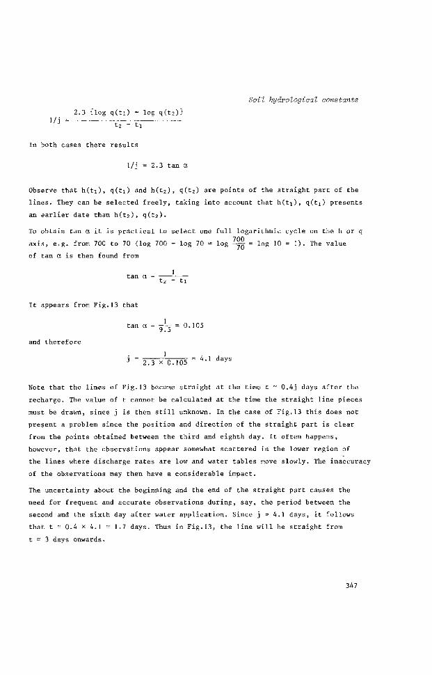
l / j
Soil hydvological constants
2.3 {log q(ti) - log q(t2)}
t2 - ti
In both cases there results
1/j = 2.3 tan a
Observe that h(ti), q(tj) and h(t2), q(t2) are points of the straight part of the
lines. They can be selected freely, taking into account that h(t]), q(tj) presents
an earlier date than h(t2), q(t2).
To obtain tan a it is practical to select one full logarithmic cycle on the h or q
axis, e.g. from 700 to 70 (log 700 - log 70 = log —j=- = log 10 = 1)- The value
of tan a is then found from
1 tan a
t2 - ti
It appears from Fig.13 that
and therefore
tan a = ̂ —r- = 0.105
j = 2.3 x'o.105 = 4-' d a y S
Note that the lines of Fig.13 become straight at the time t = 0.4j days after the
recharge. The value of t cannot be calculated at the time the straight line pieces
must be drawn, since j is then still unknown. In the case of Fig.13 this does not
present a problem since the position and direction of the straight part is clear
from the points obtained between the third and eighth day. It often happens,
however, that the observations appear somewhat scattered in the lower region of
the lines where discharge rates are low and water tables move slowly. The inaccuracy
of the observations may then have a considerable impact.
The uncertainty about the beginning and the end of the straight part causes the
need for frequent and accurate observations during, say, the period between the
second and the sixth day after water application. Since j =4.1 days, it follows
that t = 0.4 x 4.1 - 1.7 days. Thus in Fig.13, the line will be straight from
t - 3 days onwards.
347
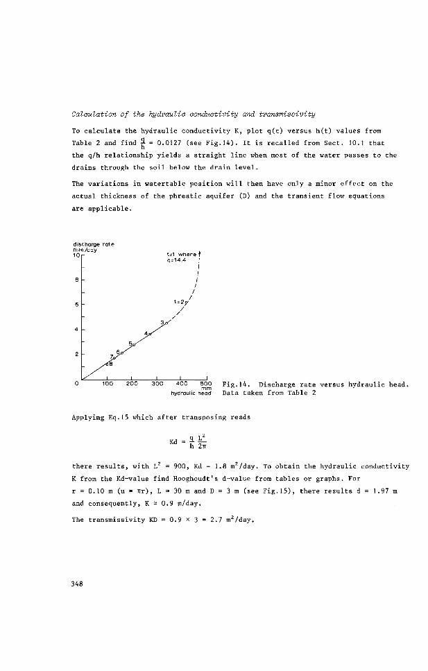
Calculation of the hydraulic conductivity and transmissivity
To calculate the hydraulic conductivity K, plot q(t) versus h(t) values from
Table 2 and find 3.= 0.0127 (see Fig.14). It is recalled from Sect. 10.1 that
the q/h relationship yields a straight line when most of the water passes to the
drains through the soil below the drain level.
The variations in watertable position will then have only a minor effect on the
actual thickness of the phreatic aquifer (D) and the transient flow equations
are applicable.
dis mn 10
8
6
4
2
charge i /day
rate
/•(SB
1
&ft
5a""
1
Ay
3.
1
t q
1 where 1 = 14.4 |
I / ;
1 1 w
/ / /
1 1
300 400 500 Fig.14. Discharge rate versus hydraulic head. hydraulic head Data taken from Table 2
Applying Eq.15 which after transposing reads
h 2ir
there results, with L = 900, Kd = 1.8 m2/day. To obtain the hydraulic conductivity
K from the Kd-value find Hooghoudt's d-value from tables or graphs. For
r = 0.10 m (u = ïïr), L = 30 m and D = 3 m (see Fig.15), there results d = 1.97 m
and consequently, K - 0.9 m/day.
The transmissivity KD = 0.9 x 3 = 2.7 m2/day.
348
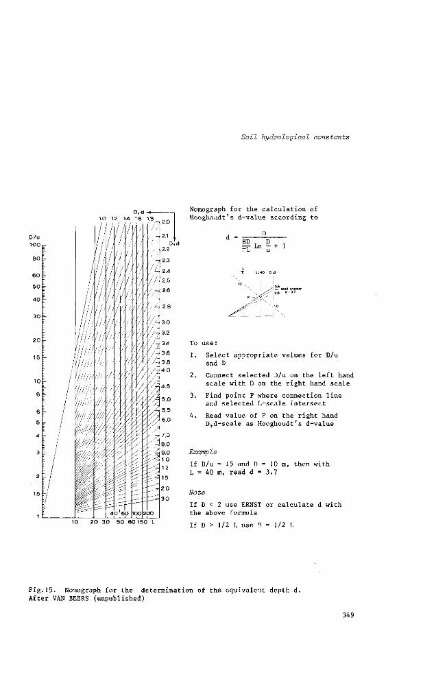
Soil hydrologiaal constants
D,d -«— 1.0 12 14 16 1.8
D/u 100
80
60
50
40
20
15
6
5
X 40 60 100 200
2.0
2.1 , D,
• 2.2
- 2.3
2.4
2.5
2.6
2.8
3.0
3.2
3.4
3.6
3.8
5.0
5.5
6.0
7.0
8.0
9.0
j1 0
• 12
: 15
- 2 0
: 3 0
Nomograph for the calculation of Hooghoudt's d-value according to
8D T D - r L n - t 1 irL U
20 30 50 80 150 L
To use:
1. Select appropriate values for D/u and D
2. Connect selected D/u on the left hand scale with D on the right hand scale
3. Find point P where connection line and selected L-scale intersect
4. Read value of P on the right hand D,d-scale as Hooghoudt's d-value
Example
If D/u = 15 and D = 10 m, then with L = 40 m, read d = 3.7
Note
If D < 2 use ERNST or calculate d with the above formula
If D > 1/2 L use D = 1/2 L
Fig.15. Nomograph for the determination of the equivalent depth d. After VAN BEERS (unpublished)
349

Calculation of the effective porosity
The effective porosity \i may be calculated from
Ti2Kdj A _,„ U = - =0.08
or from Eq.12
U - ^ - 0 . 0 8
or - more roughly - directly from Table 2 or Fig.12 as the change in hydraulic
head during the first day (495 mm) under influence of the recharge of 40 mm
40 U _ = 0 . 0 8
The effective porosity may also be found from the volume (W) of water released
by the soil when the water table drops from position h(ti) to position h(t2) in
a known time interval during the tail recession, according to the expression
W = 0.7U (h(ti) - h(t2)l where W is calculated from the measured discharge rates.
LITERATURE
KRAIJENHOFF VAN DE LEUR, D.A. A study of non-steady groundwater flow with special
reference to a reservoir coefficient. De Ingenieur 70:B87-94.
LUTHIN, J.M. 1967. Drainage engineering. John Wiley & Sons, New York.
VAN BEERS, W.F. 1965. Some nomographs for the calculation of drain spacings.
Bulletin 8. International Institute for Land Reclamation and Improvement,
Wageningen, The Netherlands.
350
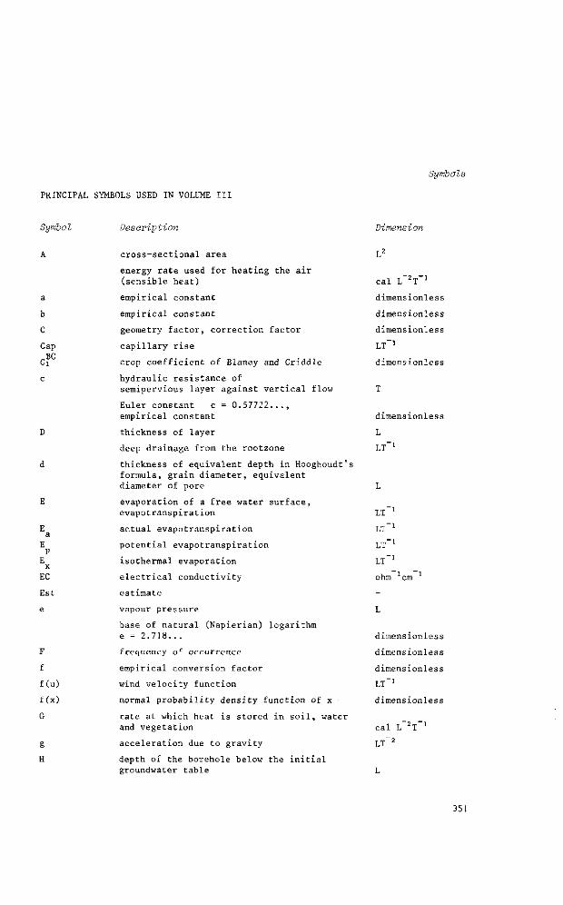
PRINCIPAL SYMBOLS USED IN VOLUME III
Symbols
Symbol Description Dimension
Cap
E x
EC
Est
F
f
f(u)
f(x)
G
cross-sectional area
energy rate used for heating the air (sensible heat)
empirical constant
empirical constant
geometry factor, correction factor
capillary rise
crop coefficient of Blaney and Criddle
hydraulic resistance of semipervious layer against vertical flow
Euler constant c = 0.57722..., empirical constant
thickness of layer
deep drainage from the rootzone
thickness of equivalent depth in Hooghoudt's formula, grain diameter, equivalent diameter of pore
evaporation of a free water surface, évapotranspiration
actual évapotranspiration
potential évapotranspiration
isothermal evaporation
electrical conductivity
estimate
vapour pressure
base of natural (Napierian) logarithm e = 2.718...
frequency of occurrence
empirical conversion factor
wind velocity function
normal probability density function of x
rate at which heat is stored in soil, water and vegetation
acceleration due to gravity
depth of the borehole below the initial groundwater table
dimensionless
dimensionless
dimensionless
LT_1
dimensionless
dimensionless
L
LT_1
LT_1
LT_1
LT_1
LT-1
ohm 1cm '
dimensionless
dimensionless
dimensionless
LT_1
dimensionless
c a l L~~2T~l
LT~2
351
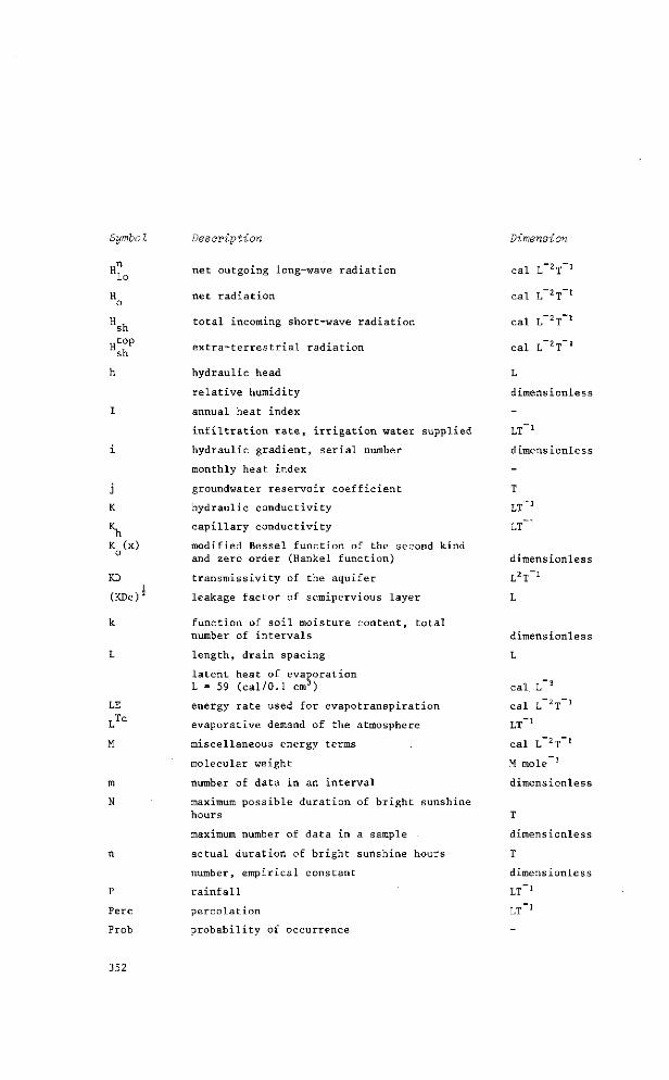
SymboI Description Dimension
lo
sh top sh
\ K (x)
1 KD
(KDc)ä
k
LE , Tc
P
Perc
Prob
net outgoing long-wave radiation
net radiation
total incoming short-wave radiation
extra-terrestrial radiation
hydraulic head
relative humidity
annual heat index
infiltration rate, irrigation water supplied
hydraulic gradient, serial number
monthly heat index
groundwater reservoir coefficient
hydraulic conductivity
capillary conductivity
modified Bessel function of the second kind and zero order (Hankel function)
transmissivity of the aquifer
leakage factor of semipervious layer
function of soil moisture content, total number of intervals
length, drain spacing
latent heat of evaporation L = 59 (cal/0.1 cm3)
energy rate used for évapotranspiration
evaporative demand of the atmosphere
miscellaneous energy terms
molecular weight
number of data in an interval
maximum possible duration of bright sunshine hours
maximum number of data in a sample
actual duration of bright sunshine hours
number, empirical constant
rainfall
percolation
probability of occurrence
cal L Z T
cal L 2 T
cal L ^T
cal L "T
dimensionless
LT '•
dimensionless
LT 1
LT"1
dimensionless
dimensionless
L
cal L~3
cal L~2T_ 1
LT _ 1
cal L _ 2 T _ I
M mole 1
dimensionless
dimensionless
T
dimensionless
LT _ 1
LT 'l
352
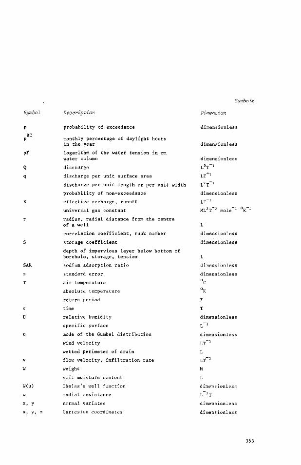
SymboIs
SymboI
P
BC P
pF
Q
q
SAR
W(u)
w
x, y
x, y, z
"1
Description Dimension
probability of exceedance diraensionless
monthly percentage of daylight hours in the year dimensionless
logarithm of the water tension in cm
water column dimensionless
discharge L3T 1
discharge per unit surface area LT l
discharge per unit length or per unit width L2T l
probability of non-exceedance dimensionless
effective recharge, runoff LT
universal gas constant
radius, radial distance from the centre
of a well L
correlation coefficient, rank number dimensionless
storage coefficient dimensionless
depth of impervious layer below bottom of
borehole, storage, tension L
sodium adsorption ratio dimensionless
standard error dimensionless
air temperature C
absolute temperature K
return period T
time T
relative humidity dimensionless
specific surface L l
mode of the Gumbel distribution dimensionless
wind velocity LT 1
wetted perimeter of drain L
flow velocity, infiltration rate LT 1
weight M
soil moisture content L
Theiss's well function dimensionless
radial resistance L :T
normal variâtes dimensionless
Cartesian coordinates dimensionless
353

SymboI Description
angle
regression coefficient, standard deviation of the Gumbel distribution
Bowen ratio
psychrometric constant
Y = 0.66 mbar/°C or 0.485 mm Hg/°C
partial derivative sign
small increment of slope of saturation vapour pressure -temperature curve
porosity, median
dynamic viscosity
effective porosity, storage coefficient, drainable pore space, mathematical expectation of the normal variate
mass density
surface tension of water against air
standard deviation
variance of the normal variate
latitude
suction
factorial
Dimension
degree
dimensionless
dimensionless
L V 1
dimensionless
dimensionless
L V 1
dimensionless
ML"1!"1
dimensionless
ML-3
MT~2
dimensionless
dimensionless
degree
L
dimensionless
354

Subject index
S U B J E C T I N D E X
Actual évapotranspiration relation to potential
évapotranspiration
19.1
Actual vapour pressure 19.7;
Adhesion forces
Advection
Aeration porosity
Aggregate stability
Air temperature of 19.2.2; 19. turbulent movement of 19.
Air bubbling pressure 23.
Air entry value 23.
Air porosity 23.
Albedo 19.2.3;19.
Alkalinity
of the groundwater 21,
Alkalinization of soil 20.
Angot-value 19.
Anisotropic soil 24.
Area rainfall computation of 18. measurement of 18.
Atmometers 19
5
7.1
1.1
2.3
1.4
3.3
7 2.1
2.2
2.2
1.4
6.1
1.6
3.8
7.1
1.1
.4
.5
.4.2
Auger hole method determination of hydraulic conductivity 24.
inversed 20.3.4;24.
Available water capacity values of
Average infiltration rate
20.
20.
2.1 4.6
3.7
3.2
Balance see Groundwater balance
Basic infiltration rate
Bellani atmometer
Binomial probability distribution
20.3.2;24.4.5
19.4.2
18.6
Blaney & Criddle equation 19.7.4
Border effect 26.10.3
Bourdon manometer 23.3.2
Bouwer's geometry factor 24.4.4
Bowen ratio 19.2.1
Buckets measurement of drain
discharge 26.8.1
Bulk density 23.1.3 determination 23.3.1
Capillary forces 23.
Capillary pores see Soil pores
1 .2
Capillary pressure
Capillary rise analyzing groundwater
recharge calculation of relation to pore size
Central limit theory
Cohesion forces
Clay effective porosity of
Confidence belts
24,
23.
22. 22. 23.
18,
23,
22.
18.
.2
,1 ,
,3, ,4 .1,
.7,
.1
,2,
.7,
.1
.2
. 1
.2
,3
. 1
.5
.4
Confidence intervals application of M
Constant head method determination of
hydraulic conductivity 24.
Correlative methods determining of hydraulic
3.1
conductivity
Cracks in soils influence on hydraulic
conductivity
Crops depletion rate by potential évapotranspi
ration by
Cumulative infiltration
24,
20.
19,
19,
20,
.2
,3.
.4,
.2,
.3,
,4
.1
.3
.2
355

Dalton equation 19.2.2
Darcy's equation 21.3.3
De Glee's double-logarithmic method 25.4.3
Depletion of soil water 19.4.1
Depression see Water table depression
Depth-area analysis of rainfall 18.4
Depth-duration-frequency relations 18.3.3
generalized 18.3.4
Depth-to-water-table
map 20.2.3; 20.3.1 ; 21.2.3
Dew point 23.2.2
Discharge-head relation 26.10
Discharge well see Pumped well
Distribution fitting
introduction to 18.7.1
Distribution of extreme values 18.7.4
Double tube method 24.4.4
Downward force 23.1.2
Drainage survey soil data required 20.2
Drain discharge computation of frequency of observations measurement measuring devices steady state conditions
26.10.1 ;26.10.2 unsteady state
conditions
26. 26. 26. 26.
10 9 7.1 8.1
26.10.3
Drainable pore space 23.1.4; as hydropedological data
Drainage see Land drainage, Soil drainage
Drainage capacity determining of
Drainage design hydropedological data
required 20. use of maps 20.
Drainage projects 17 objectives 17. study phases 17.
356
2.5 3.6
18.3.3
Duration-frequency analysis of rainfall 18.3
from pluviograph records 18.3.2
Effective porosity as hydropedological
data calculation of changes in water table definition of determining
Effluent stream 21.1.2;
Electrical conductivity map of the groundwater
Electrical resistance units
Energy balance
23.1.4
20.3.6 26.10.3 22.2.5 22.2.5 22.3.4
21.3.2
21.2.3 21.1.6
23.3.3
at the soil sur application of
Equilibrium moisture as hydropedolog determination
Equipotential lines
Euler constant
Evaporation calculation of
face equation
content ical data
21.2.3;
from a free water surface
from bare soil from the soil measuring
19.2.2;
methods for estimating
19 19,
20 23,
21,
18.
19, 19,
19, 19. 19, 19, 19,
.2.
.2.
.3,
.2.
.3.
,7.
.1
.7.
.7. ,5 .2. .4 .3
,1 ,2
.6
.2
,2
,4
, 1
,1
, 1
Evaporimeters use of 19.4.2
Evapotranspiration see also Actual évapotranspiration, Potential évapotranspiration, Relative évapotranspiration
Evapotranspiration adjustment for drying
soils 19.5 areal variation of 19.6.1 determining 19 frequency distribution of 19.6.2 measuring 19.4 methods for estimating 19.3
Subject index
Experimental fields see also Trial plots
Experimental fields objectives of selection of site size of unit
Falling head method determination of
hydraulic conductivity
Feasibility studies
Field capacity
Field drainage test
deriving soil hydrological constants from
Fisher Tippett type I distribution
Floating level indicator
Flow see also Groundwater flow
Flow nets use
26.1 26.3 26.4
Gley soils waterlogging problems
of
Grain size distribution
Gravel packing
20.3.1
24.2.2
25.1 .2
24.3.2
17.2.2
23.1.4
26
18.7.4
21.1.4
21.3.3
Flow towards the well steady state 25.4.1; unsteady state
Fluctuation diagram
Free watertable aquifer
Frequency distributions cumulative fitting
Frequency of exceedance 18.2.1;
Frequency of non-exceedance
Frequency of occurrence
Frequency of rainfall based on depth intervals based on depth ranking
Fully penetrating well
Gamma-ray attenuation
Gauges
Gauss distribution
Gravimetric method measuring the water
content
Grey mottling 20,
Groundwater see also Water table
Groundwater
maps 21, mounds 21 records 21 . salinization of 21 survey 21
Groundwater balance 22 equation 22, examples 22, of surface-water system 22, of unsaturated zone 22 solution 22, use of well hydrographs 22,
Groundwater contour maps evaluation of
3.1
3.1
2.3 3.2 2.1 1.6
21, 21
25 25
21
22
18 18
18
18
18
18 18
25
23
18
18
4 4
1
2
6 7
6
2
2
2 2
1 1
3
5
7
3 2
5
1
1
1 2
2
5
3
Groundwater data collection of evaluation of processing of
Groundwater flow see also Lateral groundwater f
Groundwater flow direction velocity
Groundwater fluctuation evaluation of
Groundwater level annual sinusoidal
fluctuation changes measurement readings records survey of
Groundwater outflow into streams
Groundwater quality maps
low
map
21 .2
21 21 21
21 21
21 21
21 21 21 21 21 21
22
21 3;21
.1 3
.2
3 3
.2 3
2 3 1 1 2 1
3
1 3
2 2
3 4
2 1 4 4 1 2
3
6 4
357
Groundwater reservoir-factor calculation of 26.10.3
Hysteresis 23.1 .4
Groundwater storage changes in 20.3.6 ;22.2.5 ;22.3.4
Gumbel probability distribution 18.7.4
Hantush-Jacob's single-logarithmic method
Head difference
Heat see also Sensible heat
Heat
advective transfer of
Heterogeneous layer
Homogeneous layer Hydraulic conductivity
as hydropedological data calculation of determination in hori
zontal directions determination of field methods of
determination laboratory measurements relation to soil
properties
25.4.3
21.3.2
19.2.3
24.1.1
24.1.1
21.3.2 20.3.5 26.10.3
24.3.3 24
24.4 24.3
20.3.5
Hydraulic gradient graphic representation of 21.3.2
Hydraulic-head-difference map 21.2.3 evaluation 21.3.4
Hydraulic resistance map 21.3.4
Hydrographs see also Well hydrogvaph
Hydrographs evaluation of
Hydrologie cycle
Hydrologie equilibrium equation
Hydrologie units
Hydromorphic soil properties data for drainage design 20.3.1
Hydropedological survey 20 soil data required 20.2
21.
22,
22.
21.
. 3 .
.1
.1
. 2 .
.1
2
Infiltration capacity
Infiltration classes
Infiltration rate as hydropedological data
Infiltration tests for hydropedological
survey
Infiltrometer method determination of
hydraulic conductivity determination of
percolation rate
Inflow components for the groundwater
sub-system
Influent stream 21.1.2;
Instantaneous infiltration rate
Intake see Infiltration
Inversed augerhole method
Irreversible drying
Isohyetal method computing the area
rainfall
Isohypses
20.3.2
20.3.2
24.4.5 20.3.2
24.4.5
20.3.2
24.4.5
20.3.4
22.2
21 .3.2
20.3.2
24.4.6
20.3.9
18.4
21.2.3
Jacob's single-logarithmic method 25.4.2
Jensen & Haise equation 19.7.3
Koopmans values 19.2.1
Kopecky cylinder 24.3.1
358
Subject index
Land drainage soil features
relevant to
Lateral groundwater flow influence of
Layered soil
drain discharge
Lifting force
Linear interpolation method
Linear regression method
Liquid limit
Loamy sand
effective porosity of
Logarithmic transformation
Lognormal distribution Long-wave radiation
calculation of Luthin & Kirkham formula
Lysimeter equation for
20.2
22.2.4
Meteorological data for calculating évapotranspiration 19.7
Moisture see Soil Moisture
Moivre distribution 18.7.3
26.10.2
23.1.2
21.2.3
21.1.5
20.3.3
22.2.5
18.7.2
18.7.3
19.2.J
24.4.2
19.4.2 22.1
L 1L^ is U U is ri.U ö ü t S U i ü H IfiLs' Is is Is is 1 IL]
Mounds see Groundwater mounds
Net subsurface inflow 22.2.4;
Neutron moisture meter
Neutron scattering
Nomographs calculation of evaporation 19.7.1;
Non-capillary porosity
Non-layered soil drain discharge
Normal probability distribution
22.
23.
23.
19.
23.
26.
18.
,3.2
.3.4
,3.4
.7.2
,1.4
,10.1
,7.3
Maps for groundwater survey
21.1.1; 21.2.3; 21.3.2; 21.3.4 of the pumping test site 25.5
use for hydropedological surveys
use for project surveys
Marine clay effective porosity of
Matric forces
20. 17.
22.
23.
,2 ,2.
,2.
,1 .
, 1
,5
1
Matric potential see Soil moisture content
Maximum permissible rate 25.1.4
Mean highest water table 20.3.1
Mean lowest water table 20.3.1
Measurement of water level equipment 21.1.4
frequency 21.1.4
Measurement of water quality 21.1.6
Mechanical sounder 21.1.4
Observation network 21.1.3 basic 21.1.5
Observation points network of 26.7
Observation wells 25.1.5 hydrograph of 21.1.5 measurement of water
level in 25.2.1 measurement of
watertable depth 26.7.2
Outflow see also Groundwater outflow
Outflow components for the groundwater
sub-system 22.2
Pan evaporation 19.4.2
Partially penetrating well 25.1.2
359

Partiele density
Peat soils
drainage of
Peltier effect
Penman equation
Percolation analyzing ground
water recharge 22
Percolation rate 20
pF curve see also Soil moisture
pF-curve method
23.
20,
23.
19.2.2 ; 19.
.1.
.3
.2,
,7,
.3
.9
.2
.1
Porous media determination of
moisture retention
curves
Porous medium method
Potential évapotranspiration by crops calculation of 19 .2.
23.
23.
19. 19.
;19.
.2,
.2,
.1
.2,
.3
.2
.2
.3
3.1
3.4
24.2.1
Phreatic surface observations 21.1 .2
iezometer effects on readings measurement of water
level in measurement of watertable
depth observation for
groundwater survey observation network
25. 25.
25,
26.
21. 21.
.1,
.5
.2.
.7,
,1. J .
.5
.1
.2
.2
.3
Piezometer method determination of
hydraulic conductivity 24,
Piezometric surface see Potentiometrie surface
Piche atmometer 19,
Pipe cavity method 24,
Plant cover see Crops
Pluviograph 18.3; 18, records 18,
Pluviometer 18.5.1
4.2
4.2
4.2
5 3.2
,5. 1
4.6
Point rainfall
measurement of 18
Porchet method 24
Pore size relation to capillary
rise 23.1.2
Pore size distribution determining hydraulic
conductivity 24.2.1
Pores see Soil pores
examples of calculating 19.7
relation to actual évapotranspiration 19.5
Potentiometrie surface 21.1. map 21.2.3; 21.3. mound in 21.3.
Precipitation influence on water
table
Preliminary plans project surveys
Probability density function 18.7.3;
Probability distribution for rainfalls
logarithmic normal
Probability of exceedance
Project surveys
Psychrometrie constant 19.2.1 ;
Pumped aquifer hydrograph of a
piezometer in
21
17
18,
18, 18, 18,
18,
17,
19,
21,
.3,
.2,
.7.
.7,
.7.
.7,
.6
.1
.7.
.3.
.1
.2
.4
.1
.2
.3
.1
.1
Pumped borehole method 24.4.3
Pumped well 25.1.2 development of 25.1.3 measurement of the
water level in 25.2.1 testing of 25.1 .4
Pumping
effects in storage 21.3.1
Pumping rate measurement of
Pumping test analysis of anomalies of the
observed data data processing
25, 25,
25 25.
25. 25.
.1 ,
.2.
.4
.5
.3
.4 ,2
360

duration of general set-up performing selection of site
Radial resistance
Radiation
Radioactive technique see Gamma-ray attenuation
25
25 25 25
21
19
2
1 2 1
3
2
3
1
2
1
Subje
Relative humidity
Residual sodium carbonate
Return periods average
Rootzone available water capacity
for water content in
ct index
23.2.2
21.1.6
18.2.3 18.6
20.3.7 19.4.1
Rain water table after
Rainfall see also Frequency
Rainfall critical duration depth-area analysis duration-frequency
analysis of frequency of intensity maps measurement of
of
Rain-gauges network density of wind deformation effect
21
18 18
18 18 18 18 18
18 18 18
3
1 4
3 2 J 3 5
5 5 5.
1
1
1 4
2 1
Salinity map of the groundwater
Salinization of soils
Salt tolerance level of crops
Saturation vapour pressure 19.2.2; 19.7.1
21 21
20
21
; 23
Scattering see Neutron-scattering
Sediments effective porosity of 25
3 1
3
1
2
2
4 6
8
6
2
5
Random errors 24.3.3
Readily available moisture see also Soil moisture
Readily available moisture 23.1.4
Reconnaissance soil map 20.2
Reconnaissance survey 17.2.1
Recorders for drain discharge 26.8.1 for watertable depth 26.8.2
Recovery test 25.2.1 analysis of data 25.4.2
Recurrence predictions see also Rainfall
Recurrence predictions 18.2.3 fitted probability
distribution 18.7.1 reliability of 18.6
Reflectivity of plant surfaces 19.2.3; 19.6.1
Relative évapotranspiration rate 19.5
Semi-confined aquifer analysis of pumping test 25, graphical methods for
4.3
steady flow
Sensible heat
Short-wave radiation calculation of
Shoulder effect
Slaking
Sodium adsorption ratio map
Soil aggregates stability of
Soil colour as hydropedological
Soil drainage
data
soil features relevant to
25
19
19
26
20
21 21
20
20
20
4.3
2.1
2.1
10.3
3.3
1.6 2.3
3.3
3
2
Soil hydrological constants deriving from tests 26
Soil maps see also Maps
361

Soil maps for hydropedological
survey 20.2; 20.4 use of 17.2.2; 20.2
Soil moisture characteristic 23.1.3
derivation of effective porosity from 20.3.6;22.2.5
Soil moisture content 20.3.6 gravimetric determi
nation of 23.3.1 methods of measuring 23.3 relation to relative
évapotranspiration 19.5 volumetric 23.3.4
Soil moisture depletion 19.4.1
Soil moisture distribution 20.3.6
Soil moisture retention in relation to texture 20.3.7
Soil moisture retention curves 23.1.3; 24.2.1
determination methods 23.2.2 obtaining 23.2
Soil moisture storage capacity coefficient
22.2.1 20.3.6 20.3.6
Soil moisture tension 23.1.1; 23.1.2 apparatus used 23.2.2 equilibrium measured 23.2.2 methods of measuring 23.3
Soil pores see also Pore size
Soil pores as conduits for water 20.3.4
Soil solution 21.1.6
Soil texture classes water retention
characteristics 20.3.7
Soil water
potential energy of 23.1.1
Soil-drainage classes 20.3
Solute tension 23.2.2
Sounder see Mechanical sounder Specific surface method
determination of hydraulic conductivity 24.2.2
Standardized normal
probability function 18.7.3
Station year method 18.6
Steady state flow analysis of drain
discharge 26.10.1 ; 26.10.2 Storage coefficient see
Soil moisture
Stream beds
water losses through 22.3.3
Structure stability 20.3.3
Subsidence 20.3.9
Suction see Soil moisture tension
Surface drainage system design discharge of 18.3.3
Surface irrigation design
basic intake rate 20.3.3
Surface tension of water 23.1.2
Surface water observations for
groundwater survey 21.1.2 Surface water system
water balance of
Surveys detailed phasing reconnaissance semi-detailed
Tail recession
water table during
Temperature gradient
Tensiometer
22.2.2
17 17.2.3 17.1 17.2.1 17.2.2
26.10.3
19.2.1
23.3.2
Tension see Soil moisture tension Test see Field drainage test,
Pumping test
Texture see Soil texture
Theis's double-logarithmic
method 25.4.2
Thermocouple technique 23.2.2
Thiessen method area-frequency analysis
of rainfall 18.4
362
Subject index
Thornthwaite & Mather equation 19.5
Thornthwaite equation 19.7.5
Total available water capacity 20.3.7
Transfer coefficient
for heat 19.2.1
Transmission zone 24.4.5
Transmissivity as pedohydrological data 20.3.5 calculation of 26.10.3 of the aquifer 24.2.2 of the layer 21 .3.2
Trial plots see also Experimental fields
Trial plots arrangement of 26.6 dimensions of 26.5 frequency of observations 26.9 observation points 26.7 processing of data
from 26.10
Turbulent transfer coefficient 19.2.1
Turc equation 19.7.2
U-figure 24.2.2
Unconfined aquifer analysis of pumping
test 25.4.1 ; 25.4.2 graphical methods for
unsteady flow 25.4.2 groundwater sub-system 22.2 logarithmic function
for steady flow
Unsaturated zone water balance of
Unsteady state flow analysis of drain
discharge equation for of groundwater
Upper plastic limit
Vapour pressure
Vapour pressure method
25.4.1
22.2.1
26.10.3 22.2.5 22.2.5
20.3.3
19.2.2
23.2.2
Water suitability for
irrigation 21.1.6
Water balance see also Groundwater balance
Water balance method measuring évapotrans
piration 19.4.1
Water level measurement in the
wells
Water losses through stream beds
Water table after rain contour maps 21.2 depression in during drought
•3;
effect of precipitation on
fluctuation maps 21.2 fluctuation of 21.2, hydraulic gradient
of mound in
• 3; .2;
25
22
21 21 21 21
21 21 21
21 21
.2.
.3,
.3.
.3.
.3.
.3.
.3.
.3.
.3.
.3.
.3.
.1
.3
.1
.2 ,2 ,1
.1
.4
.1
.2 ,2
Water vapour pressure see Relative humidity
Waterlevel fluctuation map
construction of 21.2.3
Waterlevel indicator 21.1.4
Watertable classes 20.3.1 Watertable depth 20.3.1
computation of 26.10 frequency of
observations 26.9 measurement 26.7.2 measuring devices 26.8.2 steady state
conditions 26.10.1; 26.10.2 unsteady state
conditions 26.10.3
Watertable gradient 21.3.2
Well see also Observation well
Well groundwater level
observations in hydrograph
21. 21.
1 .2 2.2
363
Well hydrographs use of
Well testing
Wetted tape method
22.3
25.1.4
21. J. 4
Wilting point
Wind velocity
23.1.4
19.2.2; 19.7
364
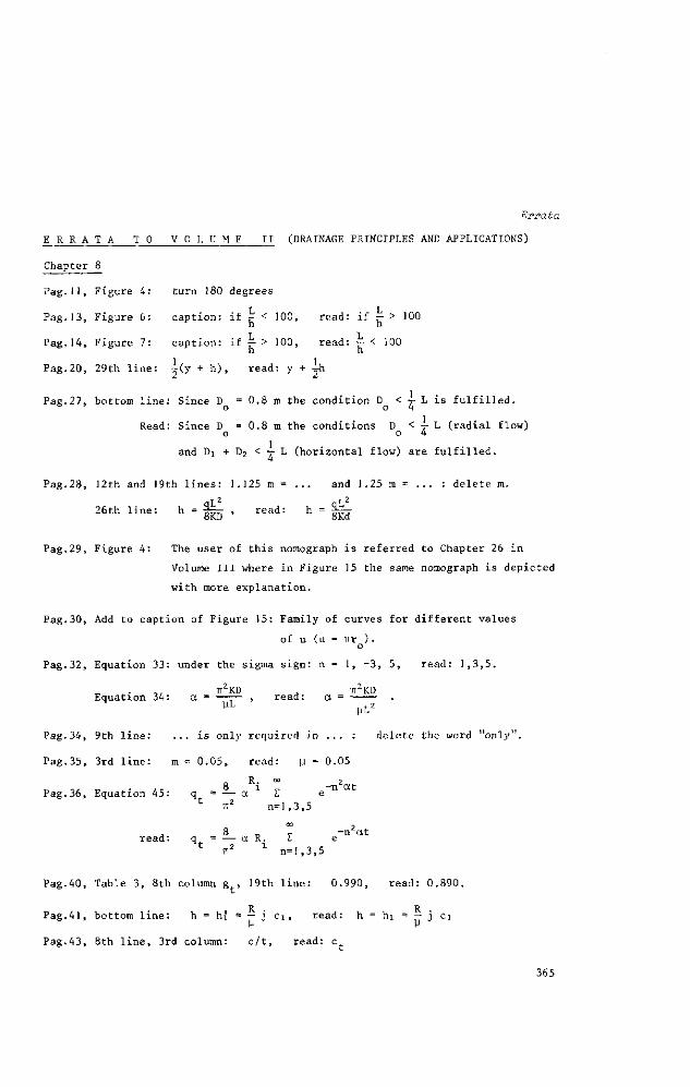
Errata
E R R A T A T O V O L U M E II (DRAINAGE PRINCIPLES AND APPLICATIONS)
Chapter 8
Pag.11, Figure 4: turn 180 degrees
Pag.13, Figure 6: caption: if ̂ < 100, read: if S 100
Pag.14, Figure 7: caption: if ̂ > 100, read: ̂ < 100
Pag.20, 29th line: -ky + h), read: y + |h
Pag.27, bottom line: Since D = 0.8 m the condition D < 7- L is fulfilled. 0 o o 4
Read: Since D = 0.8 m the conditions D < 7- L (radial flow) o o 4
and Dj + D2 < 7- L (horizontal flow) are fulfilled.
Pag.28, 12th and 19th lines: 1.125 m = ... and 1.25 m = ... : delete m.
26th line: h - f g , read: h = ä|_
Pag.29, Figure 4: The user of this nomograph is referred to Chapter 26 in
Volume III where in Figure 15 the same nomograph is depicted
with more explanation.
Pag.30, Add to caption of Figure 15: Family of curves for different values
of u (u = Trr ). o
Pag.32, Equation 33: under the sigma sign: n = 1, -3, 5, read: 1,3,5.
TT2KD , TT2KD Equation 34: a = — - — , read: a =
y L PL2
Pag.34, 9th line: ... is only required in ... : delete the word "only".
Pag.35, 3rd line: m = 0.05, read: u = 0.05 R °° 2
•>/• T. ,.• / r 8 i _ - n a t P a g . 3 6 , E q u a t i o n 4 5 : q = — a I e
Ü ir2 n = l , 3 , 5 co ?
, 8 _ v - n a t r e ad : q — a R. L e
t TT2 1 n = l , 3 , 5
Pag.40, Table 3, 8th column g , 19th line: 0.990, read: 0.890.
R R Pag.41, bottom line: h = h{ = — j ei, read: h = hi = — j ci
Pag.43, 8th line, 3rd column: c/t, read: c
365
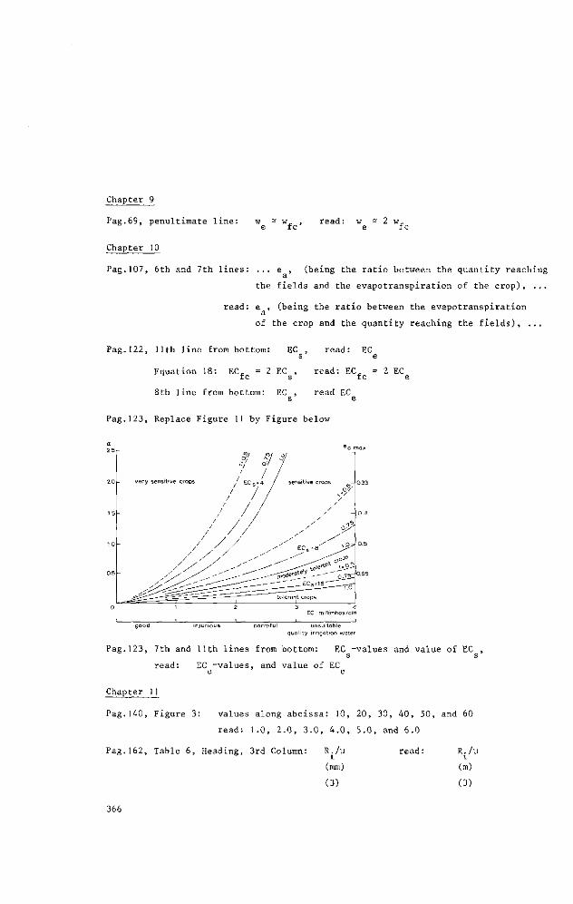
Chapter 9
Pag.69, penultimate line:
Chapter 10
fc' read: w 2 w
fc
Pag.107, 6th and 7th lines: ... e , (being the ratio between the quantity reaching
the fields and the évapotranspiration of the crop), ...
read: e , (being the ratio between the évapotranspiration
of the crop and the quantity reaching the fields), ...
Pag.122, 11th line from bottom: EC , read: EC s e
Equation 18: EC, = 2 EC , read: EC, = 2 EC fc s fc e
8th line from bottom: EC , read EC s e
Pag.123, Replace Figure 11 by Figure below
-
-
-
very sensitive crops
/ / / / / y
<^^<^<^ ^ g S ^ r ^ p S =
/ / /
/ / / / / / / / / /
' y / // ^~ ^^-^,
^ ^ S - ^
VI ?/
V / E C S
/ / / / / / ,
—-~" ^Z
0 /
/ 4 /
^^ _ ^ s -
- - -
/ sensitive crops
/ / / y
ECS^S
^ - < ^ ^ ^fi^-' "" _ _ _ E C S - 1 6 " ^
tolerant crops
<o/ 0 /
\'/ / / y
'_oJS--—To"
EC milltmhos/crr
good injurious harmful unsuitable quality irrigation water
Pag.123, 7th and 11th lines from bottom: EC -values and value of EC s s
read: EC -values, and value of EC e e
Chapter 11
Pag.140, Figure 3: values along abcissa: 10, 20, 30, 40, 50, and 60
read: 1.0, 2.0, 3.0, 4.0, 5.0, and 6.0
Pag.162, Table 6, Heading, 3rd Column: R./u
(mm)
(3)
366
read : R./y l
(m)
(3)

Errata
Chapter 12
Pag. 173, Heading of Table I, 2nd line: Bessel function of the first kind
read: Bessel function of the second kind
Pag. 176, 1st line below Equation 14: where K is a modified Bessel function
(Hankel function) of the first kind ...
read: . . . of the second kind . . .
Pag.184, 6th and 9th lines: a bracket should be placed between 2.3 and
2 25KD log —'- n and one behind the last term on the 9th line
r2S
Chapter 13
Pag.195, 1st line: Substituting this form into Eq.7 yields a = + 1/KDc
read: ... yields a = + 1//KDc
Pag.200, Eq.24: Q = 2irßr [-Cjlj (r/X) - C2Kl(r/X)']
read: Q = 2irßr [-dli (r/X) + C2Ki (r/X)]
Pag.202, Equation 32: behind equal sign, 2trßr, read: 2TT(3R
Pag.208, middle of page: — = -ï- - = % x -^— = 20 u 2 / F u 2 0.1
,. /KD x 1 _ 4 v 1 .. read:./— = = — x yr-r = 20
V y 2/E u 2 0.1
Pag.219, Example 8, 1st and 2nd lines: Assume a ditch with top width B = 3 m,
bottom width b = 1 m, water depth y = 1 m, and h = 4 m above ...
o o
read: Assume a ditch with top width B = 3 m, bottom width b = 1 m,
water depth 1 m, and an impervious layer 4 m below the bottom of the ditch (hence y = 1 + 4 = 5 m).
o
Pag.220, 1st line: B/u = 3/3.82 = 0.76 m, read: B/u = 3/3.82 = 0.76
5th line: hi/y = 4.8/5 = 0.96 m, read: hj/y = 4.8/5 = 0.96
6th line: (B/u > 0.9)f = 1.08, read: (B/u < 0.9)f = 1.08
Chapter 14
noo „ - , ô 2 h <52h - j 5 2 h <52h Pag.228, Equation 1 : = 0, read: + = 0 ox2 ôy2 ôx2 (Sx2
367
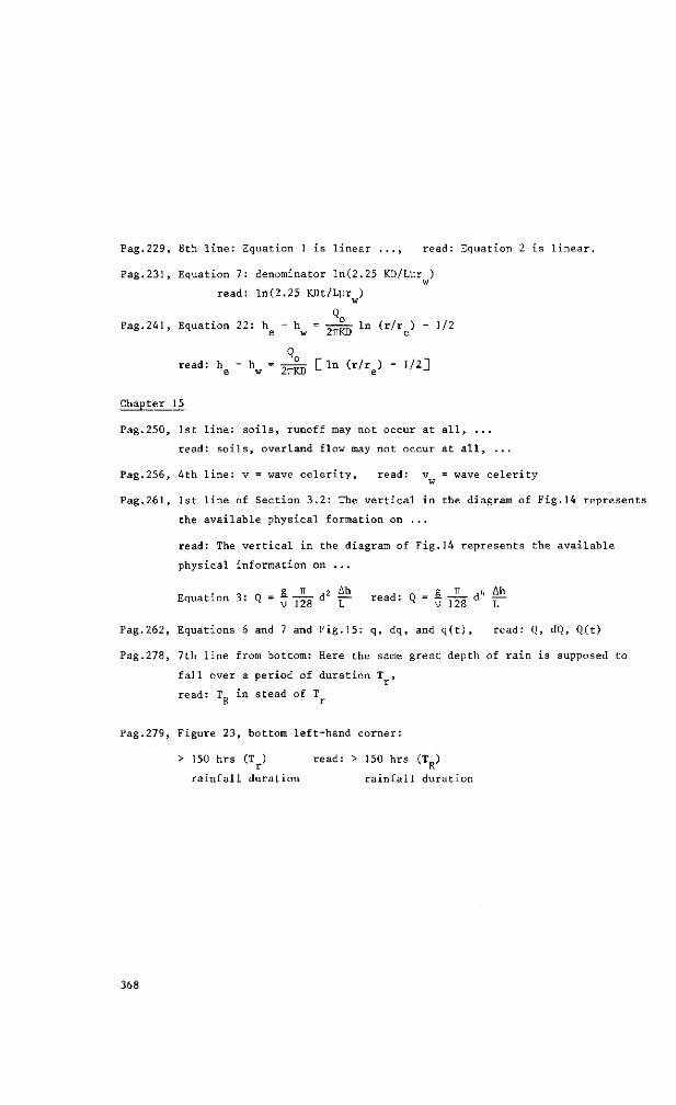
Pag.229, 8th line: Equation 1 is linear ..., read: Equation 2 is linear.
Pag.231, Equation 7: denominator ln(2.25 KD/LUr ) w
read: ln(2.25 KDt/Lyr ) w
Q Pag.241, Equation 22: hg - hw = j ^ In (r/r ) - J/2
r e a d= h e - h w = 2ilD ^l n (r/re> " "^
Chapter 15
Pag.250, 1st line: soils, runoff may not occur at all, ...
read: soils, overland flow may not occur at all, ...
Pag.256, 4th line: v = wave celerity, read: v = wave celerity
Pag.261, 1st line of Section 3.2: The vertical in the diagram of Fig.14 represents
the available physical formation on ...
read: The vertical in the diagram of Fig.14 represents the available
physical information on ...
Equation 3: Q - * ̂ d* f* read: Q - § ̂ d*f*
Pag.262, Equations 6 and 7 and Fig.15: q, dq, and q(t), read: Q, dQ, Q(t)
Pag.278, 7th line from bottom: Here the same great depth of rain is supposed to
fall over a period of duration T , r
read: T„ in stead of T R r
Pag.279, Figure 23, bottom left-hand corner:
> 150 hrs (T ) read: > 150 hrs (T ) r K
rainfall duration rainfall duration
368