UC IrvineUC Irvine Previously Published Works

TitleHORTON'S LAW OF STREAM NUMBERS FOR TOPOLOGICALLY RANDOM CHANNEL NETWORKS

Permalinkhttps://escholarship.org/uc/item/0nz2t3vv

JournalThe Canadian Geographer/Le Géographe canadien, 14(1)

ISSN0008-3658

AuthorWERNER, CHRISTIAN

Publication Date1970-03-01

DOI10.1111/j.1541-0064.1970.tb00006.x

Copyright InformationThis work is made available under the terms of a Creative Commons Attribution License, availalbe at https://creativecommons.org/licenses/by/4.0/ Peer reviewed

eScholarship.org Powered by the California Digital LibraryUniversity of California

HORTON‘S LAW OF STREAM NUMBERS FOR TOPOLOGICALLY RANDOM CHANNEL NETWORKS

CHRISTIAN WERNER

University of California, Irvine

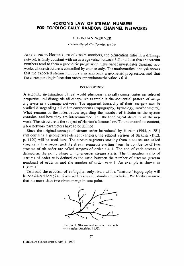
ACCORDING to Horton’s law of stream numbers, the bifurcation ratio in a drainage network is fairly constant with an average value between 3.5 and 4, so that the stream numbers tend to form a geometric progression. This paper investigates drainage net- works whose structure is controlled by chance only. The mathematical analysis shows that the expected stream numbers also approach a geometric progression, and that the corresponding bifurcation ratios approximate the value 3.6 18.

INTRODUCTION

A scientific investigation of real world phenomena usually concentrates on selected properties and disregards all others. An example is the sequential pattern of merg- ing rivers in a drainage network. The apparent hierarchy of their mergers can be studied disregarding all other components (topography, hydrology, morphometry). What remains is the information regarding the number of tributaries the system contains, and how they are interconnected, i.e., the topological structure of the net- work. This structure is the subject of Horton’s famous law. To understand its content, a few network parameters have to be defined.

Since the original concept of stream order introduced by Horton (1945, p. 281) still contains a geometrical element (angles), the refined version of Strahler (1952, p. 1120) will be used here. The stream segments starting from a source are called streams of first order, and the stream segments starting from the confluence of two streams of ith order are called streams of order i + 1 . The end of each stream is defined as the point where a higher-order stream starts. The bifurcation ratio of streams of order m is defined as the ratio between the number of streams (stream numbers) of order m and the number of order m + 1 . An example is shown in Figure 1.

To avoid the problem of ambiguity, only rivers with a “mature” topography will be considered here; i.e., rivers with lakes and islands are excluded. We further assume that no more than two rivers merge in one point.

1

FIGURE 1. Stream orders in a river net- work (after Strahler, 1952).

57

CANADIAN GEOGRAPHER, XIV, 1, 1970

58 THE CANADIAN GEOGRAPHER

FIGURE 2. The set of topologically different channel networks having four sources.

According to Horton (1945, p. 291), “the numbers of streams of different orders in a given drainage basin tend to closely approximate an inverse geometric series in which the first term is unity and the ratio is the bifurcation ratio.” This “Law of Stream Numbers,” which describes an observed regularity in nature but does not explain it, has been reaffirmed in many surveys. But empirical investigations have failed to produce a satisfactory explanation for the “law,” nor have they been able to establish any major correlation between the variation of topological network measures (magnitude, order, bifurcation ratio of streams) and geomorphic or hydro- logic variables by statistical analysis’ (Shreve 1966, p. 18). Scheidegger (1968) has reviewed the various attempts to establish a rational explanation for the Horton law. Most recently, Woldenberg (1969) has tried to derive it from the premise that the set of basin areas in a drainage system somehow corresponds to a hierarchy of nesting hexagons. But, aside from the speculative nature of his assumptions and subsequent reasoning, his method permits the generation of such a vast number of numerical sequences that a “good fit” can easily be found for almost any geometric progression.

The low correlation between observed bifurcation ratios and environmental variables lends itself to the hypothesis that the topological patterns of natural channel networks are the result of a random process, or that these networks are a random sample from the population of all possible network configurations, at least with regard to their topological structure. A general definition and test of topological randomness in line patterns have been suggested by the author (Werner, 1969b). By means of computer simulation Shreve (1966) and later Scheidegger (1967) and Liao and Scheidegger (1 968) have studied large numbers of theoretically possible network configurations, and a statistical comparison with the empirically observed network patterns produced encouraging results. Shreve (1967) and Smart (1968) proceeded to calculate the parameters of the theoretical network distribution. Their deductions are based on the assumption that all channel networks having the same number of sources occur with equal likelihood. Although this seems to be an intuitively appealing approach, it bears implications which might be difficult to accept, if the final goal is to simulate a drainage pattern under random conditions. To demonstrate this point a single example is sufficient. Given four sources producing a single drainage network, all five configurations shown in Figure 2 would have the same chance to occur. Consequently, the merger of the first-order streams B and c would be twice as probable as any of the other three alternatives (A + B / c + D / A + B and c + D). In contrast, this paper assumes that all possible mergers among streams of the same order have the same probability of occurrence. Hence, “topologically random

‘Statistically significant dependences have, however, been established between morphornefric and geologic/hydrologic variables. See, for example, Morisawa (1962).

HORTON’S LAW OF STREAM NUMBERS 59

channel networks” will be defined here as networks in which the mergers among streams of equal order are controlled by chance only; all other mergers are disre- garded.’ It is the purpose of this paper to derive general expressions and numerical values for the expected stream numbers and bifurcation ratios of channel networks, which are topologically random in the predefined sense, and to test them against empirical observations.

COMBlNATORIAL ANALYSlS OF STREAM NUMBERS UNDER RANDOM CONDlTlONS

Assume that there are n streams of order m in a given channel network. The number of streams of order m + 1 in the same network is equal to the number i of mergers of streams of order m. The following theorems determine the number of ways in which n streams of order m can produce i streams of order m + I , and, based on the resulting frequency distribution, the expected value of i, En, assuming that all possible patterns are equally probable. The expected bifurcation ratio is then immediately obtained as the ratio of the numbers of streams of mth and of (rn + 1)th order, i.e., nlE,.

Channel networks are only one example of a wide variety of phenomena resulting from or represented by binary branching processes. The formal structure they share in common is one of the subjects of graph theory and set theory. The theorems will therefore be stated in general mathematical terms before they are applied to the specific case of channel networks.

THEOREM I :3 Let S be an ordered set of n elements. The number P(i, n) of different ways in which one can select i mutually exclusive pairs (1 5 i i n/2) of adjacent elements from S is given by

1 I i 5 n/2.

COROLLARY: The number S,, of different ways in which mutually exclusive pairs of adjacent elements can be selected from a given sequence of n elements is

s,= i = c 1 ( “ T i ) .

THEOREM 1 1 : ~ The integers S,, + 1 = F,,, n = 0, 1 , 2, ..., are the Fibonacci number^.^ ZObviously, this definition focuses on Horton’s law and is insufficient for topological network

problems in general. 3Although there are many related binomial identities I have been unable to locate this theorem in

the literature. A proof is given in the Appendix. My attention has been drawn to a similar lemma by Kaplansky (Ryser, 1963, p. 33), from which Theorem I could be derived: Let f ( n , k) denote the number of ways of selecting k objects, no two consecutive, from n objects arranged in a row. Then

f ( n , k ) = (” - + ’). 4I am grateful to the reviewer who identified this theorem as a special case of a generalized relation-

ship reported by Riordan (1968, p. 89):

where f n ( k ) is the kth convolved Fibonacci number. In our case k = 1.

F.-I + Fn--2 (hence, Fz = 2, F, = 3, F4 = 5 , Fs = 8, etc.). See, for example, Hall (1967, p. 26). ’The Fibonacci numbers F,, are defined by Fo = 1, Fl = 1, and the recursion formula F,, =

60 LE GBOGRAPHE CANADIEN

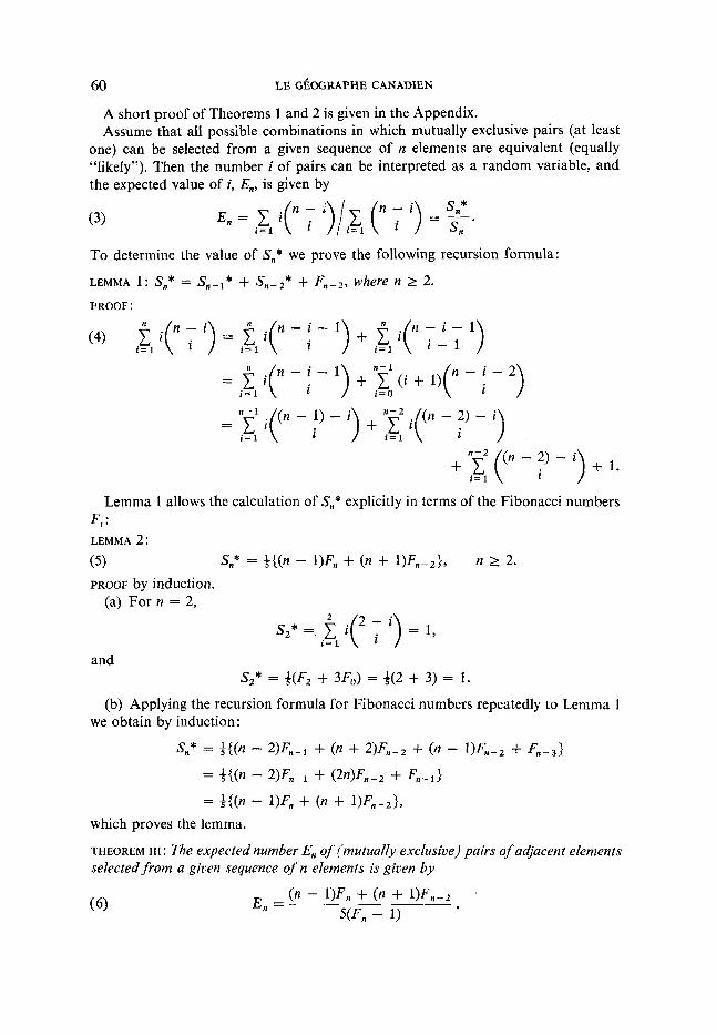
A short proof of Theorems 1 and 2 is given in the Appendix. Assume that all possible combinations in which mutually exclusive pairs (at least

one) can be selected from a given sequence of n elements are equivalent (equally "likely"). Then the number i of pairs can be interpreted as a random variable, and the expected value of i, En, is given by

(3) E,, = c i(" T '),/x (" T i, = Sn* --.

i = l i = 1 Sn

To determine the value of Sn* we prove the following recursion formula:

LEMMA 1: s,,* = s,,-,* + s,,-,* + Fn+, where n 2 2. PROOF :

= '2' - - i) + "i2 i((" - - i ) i = 1 i = 1

+ y ('" - - i ) + 1* i = 1

Lemma 1 allows the calculation of Sn* explicitly in terms of the Fibonacci numbers F, :

( 5 ) PROOF by induction.

(a) For n = 2,

LEMMA 2: S,* = f{(n - l)Fn + (n + l)Fn-z}, n 2 2.

2

i = 1 s,* =, c i(' T i, = 1,

and Sz* = *(Fz + 3Fo) = +(2 + 3) = 1 .

(b) Applying the recursion formula for Fibonacci numbers repeatedly to Lemma 1 we obtain by induction:

S,* = f ( ( n - 2)Fn-, + (n + 2)F,-z + (n - l)Fn-2 + F n - 3 }

= f { ( n - 2)Fn-, + (2n)F,,-, + Fn-l}

= +{(n - l)Fn + (n + l)Fn-2}, which proves the lemma.

THEOREM IN: The expected number En of (mutually exclusive) pairs of adjacent elements selected from a given sequence of n elements is given by

(n - l )Fn + ( n + l)Fn-2 5(F, - 1)

I

E n =

HORTON'S LAW OF STREAM NUMBERS 61

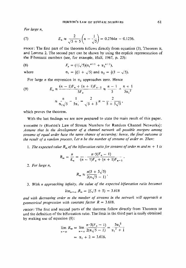
For large n,

(7) 2

E,, x ~ ( n - $) = 0.2764n - 0.1236. J 5 + 5

PROOF: The first part of the theorem follows directly from equation (3), Theorem 11,

and Lemma 2. The second part can be shown by using the explicit representation of the Fibonacci numbers (see, for example, Hall, 1967, p. 23):

(8 ) where

F,, = (1/J5)(al"+' + aZn+'),

a, = +(I + 4 5 ) and a2 = +(I - J5) .

For large n the expression in ctz approaches zero. Hence

( n - l)Fn i- ( n + l)Fn-z n - 1 n + 1 x - + 7 5 5%

En x 5Fn

(9)

n 1 2 2 - a5 - 501, - F 5 It - 5 + 5J5

which proves the theorem.

With the last findings we are now prepared to state the main result of this paper.

THEOREM IV (Horton's Law of Stream Numbers for Random Channel Networks): Assume that in the development of a channel network all possible mergers among streams of equal order have the same chance of occurring; hence, the final outcome is the result of a random process. Let n be the number of streams of order m. Then:

1. The expected value R, of the bifurcation ratio for streams of order m and m + 1 is

n n*5(F,, - 1) E,,

R = - = ( n - 1)F, + ( n + l)Fn-z ' m

2. For large n,

n(5 + 54.5) R , x

2(nJ5 - 1) *

3. With n approaching infinity, the value of the expected bifurcation ratio becomes

R, = t (J5 + 5) = 3.618

and with decreasing order m the number of streams in the network will approach a geometrical progression with constant factor R = 3.618.

PROOF: The first and second parts of the theorem follow directly from Theorem III and the definition of the bifurcation ratio. The limit in the third part is easily obtained by making use of equation ( 8 ) :

= + 2 = 3.618.

62 THE CANADIAN GEOGRAPHER

3 . 8

3.6

3 . 4

3 . 2

3 . 0

2 . 8

2 . 6

2 . 4

2 . 2

2.0

L

0‘ I I

,‘ R = f(n) I

P ‘

I 0 I

I 1

I

I I

I

0

t n 2 4 6 8 1 0 15 20 2 5 30 3s 40

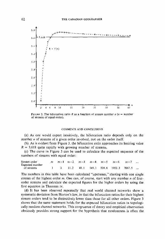
FIGURE 3. The bifurcation ratio R as a function of stream number n (n = number of streams of equal order).

COMMENTS AND CONCLUSIONS

(a) As one would expect intuitively, the bifurcation ratio depends only on the

(b) As is evident from Figure 3, the bifurcation ratio approaches its limiting value

(c) The curve in Figure 3 can be used to calculate the expected sequence of the

number n of streams of a given order involved, not on the order itself.

R = 3.618 quite rapidly with growing number of streams.

numbers of streams with equal order:

Stream order m m-1 m-2 m-3 m-4 m--5 m-6 m-7 ... Expected number

of streams 1 3 11.2 41 .1 149.1 539.8 1953.3 7067.5 ... The numbers in this table have been calculated “upstream,” starting with one single stream of the highest order m. One can, of course, start with any number IZ of first- order streams and calculate the expected figures for the higher orders by using the first equation in Theorem IV.

(d) It has been observed repeatedly that real world channel networks show a systematic deviation from Horton’s law, in that the bifurcation ratios for their highest stream orders tend to be distinctively lower than those for all other orders. Figure 3 shows that the same statement holds for the expected bifurcation ratios in topologi- cally random channel networks. This congruence of theory and empirical observation obviously provides strong support for the hypothesis that randomness is often the

HORTON’S LAW OF STREAM NUMBERS 63

300

200

100

60

40

30

20

10

6

4

3

2

1 ’

Number of Streams

of order j-1

/ . .. . /.*. . , . /

/ /

Number of Streams of order j /;. .a:... ..*‘ *..a* . . . 9

L 2 3 4 6 10 20 30 40 60 100 200 1000

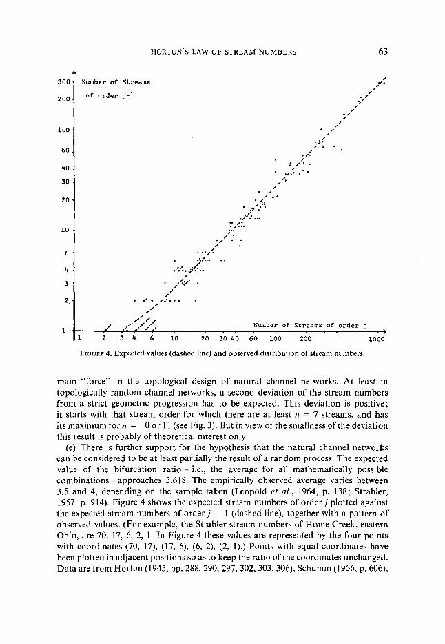
FIGURE 4. Expected values (dashed line) and observed distribution of stream numbers.

main “force” in the topological design of natural channel networks. At least in topologically random channel networks, a second deviation of the stream numbers from a strict geometric progression has to be expected. This deviation is positive; it starts with that stream order for which there are at least n = 7 streams, and has its maximum for n = 10 or 11 (see Fig. 3). But in view of the smallness of the deviation this result is probably of theoretical interest only.

(e) There is further support for the hypothesis that the natural channel networks can be considered to be at least partially the result of a random process. The expected value of the bifurcation ratio - i.e., the average for all mathematically possible combinations - approaches 3.61 8. The empirically observed average varies between 3.5 and 4, depending on the sample taken (Leopold et al., 1964, p. 138; Strahler, 1957, p. 914). Figure 4 shows the expected stream numbers of order j plotted against the expected stream numbers of order j - 1 (dashed line), together with a pattern of observed values. (For example, the Strahler stream numbers of Home Creek, eastern Ohio, are 70, 17, 6, 2, 1. In Figure 4 these values are represented by the four points with coordinates (70, 17), (17, 6), (6, 2), (2, l).) Points with equal coordinates have been plotted in adjacent positions so as to keep the ratio of the coordinates unchanged. Data are from Horton (1945, pp. 288, 290, 297, 302,303, 306), Schumm (1956, p. 606),

64 LE GBOGRAPHE CANADIEN

Smith (1958, p. 1003), and Morisawa (1962, pp. 1036-7). These data do not constitute a random sample and could therefore not be analysed by inferential statistics.

APPENDIX

Proof of Theorem I (by induction) 1. The theorem can easily be verified for n = 2 and i = I . 2. Since equation (1) is a function in two variables, the second part of the induction

will have to treat both i and n independently. (a) Assume that (1) holds for P(i, m), where m < n. Let S = {Pl, . . . , p , } be a

sequence of n elements and i the number of (mutually exclusive) pairs of adjacent elements to be selected from S. The set of all possible combinations in which this can be done can be subdivided into the cases where P, forms a pair with Pn- l , and all other cases. According to the principle of induction, the first subset consists of

combinations, and the second of

('" - - i> P(i, n - 1) =

combinations. Hence,

(10) P(i, n) = P(i - 1, n - 2) + P(i, n - 1)

= (" - i - 1) + (" - j - 1) = ; i) i - 1

(b) Assume that (1) holds for P(j,n), where j < i. Let S = { P I , ..., P,} be a sequence of n elements and i be the number of pairs of adjacent elements to be selected from S. Let K be the set of all possible combinations in which this selection can be done. K can be decomposed into classes c k , where C, consists of all combinations in which the pair farthest to the left is formed by the elements Pk, Pkfl . Obviously, the classification is exhaustive and exclusive. The number of combinations which constitute the class C, is

where k 5 n - 2 i + 1. Consequently, the number of combinations in all classes is given by

n-?+l (,, i n - - 2 i + l ( n - k - i)! (12) P(i, !Z) = ) = k = l c ( i - I)! (n - k - 2Z + I)! h = 1

n - - 2 i + t ( n - i - k + l)! - ( n - i - k ) ! ( n - 2i - k + 1) . _ _ _ _ ~ _ _ _ _ = c k = 1 i! ( n - 2i - k + I)!

HORTON’S LAW OF STREAM NUMBERS 65

1.e.

P( i ,n ) = (” ; i ) - ( i - 1 ) . Since the last of the two binomial coefficients is zero, the proof is completed.

Proof of Theorem II (by induction)

(a) Since (“ i, is defined as zero for n = 0, 1 and is 1 and 2 respectively for i = 1

n = 2 and 3, then F,, = S,, + 1 for values of IZ from 0 to 3.

(b) . ,

(14) S , + 1 = i = C 1 (” ; i, + 1 = (” - ; - 1 ) + iil (” ;: ; 1) + 1.

Since all terms are zero for i > (n - 1)/2 in the first sum and for i > n/2 in the

second sum on the right side of (14), and since 0 ’> = 1, we have

= ( & - I + 1) + (Sn-2 + l ) ,

which proves the theorem.

REFERENCES

HALL, MARSHALL JR. (1967), Combinational Theory (Waltham, Mass.). HARARY, F., ed. (1967), Graph Theory and Theoretical Physics (New York). HORTON, R. E. (1945), “Erosional Development of Streams and Their Drainage Basins: Hydro-

LEOPOLD, L. B., M. G. WOLMAN, and J. P. MILLER (1964), Fluvial Processes in Geomorphology

LIAO, K. H., and A. E. SCHEIDECGER (1968), “A Computer Model for Some Branching-Type

MELTON, M. A. (1959), “A Derivation of Strahler’s Channel-Ordering System,” J. Geoi. 67, 345-6. MORISAWA, M. E. (1962), “Quantitative Geomorphology of Some Watersheds in the Appalachian

RIORDAN, J. (1958), An Introduction to Combinational Analysis (New York).

RYSER, H. J. (1963), Combinatorial Mathematics (Carus Mathematical Monographs, No. 14, New York).

SCHEIDEGGER, A. E. (1966), “Stochastic Branching Processes and the Law of Stream Orders,” Water Resources Res. 2, 199-203.

(1967), “Random Graph Patterns of Drainage Basins,” in Hydrological Aspects of the Utilization of Water (Int. Assoc. Sci. & Hydro]., General Assembly of Bern, Trans.) pp. 417-25.

___ (1968), “Horton’s Law of Stream Numbers,” Wafer Resources Res., 4, 655-8. ScnuMM, S. A. (1956), “Evolution of Drainage Systems and Slopes in Badlands at Perth Amboy,

SHREVE, R. L. (1966), “Statistical Law of Stream Numbers,” J. Geol. 74, 17-39. ___ (1967), “Infinite Topologically Random Channel Networks,” J. Geol. 75, 178-86. SMART, J. S. (1968), Mean Stream Numbers and Branching Ratios for Topologically Random Channel

physical Approach to Quantitative Morphology,” Bull. Geol. Soc. Amer. 56, 275-370.

(San Francisco).

Phenomena in Hydrology,” Bull. Int. Assoc. Sci. & Hydrol.

Plateau,” Bull. Geol. Soc. Amer. 73, 1025-46.

(1968), Combinatorial Identities (New York).

New Jersey,” Bull. Geol. Soc. Amer. 67, 597-646.

Networks (IBM Research Paper, RC 2144).

66 THE CANADIAN GEOGRAPHER

SMITH, K. G. (1958), “Erosional Processes and Landforms in Badlands National Monument, South

STRAHLER, A. N. (1952), “Hypsometric (Area-Altitude) Analysis of Erosional Topography,” Bull. Dakota,” Bull. Geol. SOC. Amer. 69, 975-1008.

Geol. SOC. Amer. 63, 111742. (1957), “Quantitative Analysis of Watershed Geomorphology,” Amer. Geophys. Union,

Trans. 38. 913-20. WERNER, C. (1969a), “Networks of Minimum Length,” Can. Geogr. 13, 47-69.

(1969b), “Topological Randomness in Line Patterns,” Proc. Assoc. Amer. Geogr. 1, 157-62. WOLDENBERG, M. J. (1969), “Spatial Order in Fluvial Systems: Horton’s Law Derived from Mixed

Hexagonal Hierarchies of Drainage Basin Areas,” Bull. Geol. SOC. Amer. 80, 97-1 12.