1

Reproducible determination of dissolved organic matter photosensitivity Alec W. Armstrong1,2, Leanne Powers1, Michael Gonsior1 1University of Maryland Center for Environmental Science, Chesapeake Biological Laboratory, Solomons, Maryland 20688 2Department of Entomology, University of Maryland, College Park, Maryland 20742 5

Correspondence to: Alec W. Armstrong (aarmstr1@umd.edu) and Michael Gonsior (gonsior@umces.edu)

Abstract. Dissolved organic matter (DOM) connects aquatic and terrestrial ecosystems, plays an important role in C and N

cycles, and supports aquatic food webs. Understanding DOM chemical composition and reactivity is key to predict its

ecological role, but characterization is difficult as natural DOM is comprised of a large but unknown number of distinct

molecules. Photochemistry is one of the environmental processes responsible for changing the molecular composition of DOM 10

and DOM composition also defines its susceptibility to photochemical alteration. Reliably differentiating the photosensitivity

of DOM from different sources can improve our knowledge of how DOM composition is shaped by photochemical alteration

and aid research into photochemistry’s role in various DOM transformation processes. Here we describe an approach to

measure and compare DOM photosensitivity consistently based on the kinetics of changes in DOM fluorescence during 20h

photodegradation experiments. We identify several methodological choices that affect photosensitivity measurements and 15

offer guidelines for adopting our methods, including use of a reference material, precise control of conditions affecting photon

dose, leveraging actinometry to estimate photon dose instead of expressing results as a function of exposure time, and frequent

(every 20 minutes) fluorescence and absorbance measurements during exposure to artificial sunlight. We then show that our

approach can generate photosensitivity metrics across several sources of DOM, including freshwater wetlands, a stream, an

estuary, and Sargassum sp. leachate, and observed differences in these metrics that may help identify or explain differences in 20

their composition. Finally, we offer an example applying our approach to compare DOM photosensitivity in two adjacent

freshwater wetlands as seasonal hydrologic changes alter their DOM sources.

1 Introduction

The photochemical reactivity of dissolved organic matter (DOM) is inherently linked to its composition and photochemical

behavior reflects compositional differences between samples. Several authors have discussed the fundamental processes 25

involved in light absorption by DOM and the phenomena that may follow (Miller, 1998; Sharpless et al., 2014) , including

loss of absorbance (Del Vecchio and Blough, 2002), production of new substances (Gonsior et al., 2014; Blough and Zepp,

1995; Bushaw et al., 1996; Moran and Zepp, 1997), and loss of fluorescence (Blough and Del Vecchio, 2002). Absorption

spectra and derived values such as spectral slopes and their ratios have long been used to characterize DOM (Blough and Del

2

Vecchio, 2002; Helms et al., 2008; Twardowski et al., 2004). Fluorescence measurements arise from only a fraction of 30

chromophoric DOM (CDOM) but are sensitive to small variations in DOM chemical composition (Blough and Del Vecchio,

2002). To the extent that photochemical reactivity is a property of DOM chemical composition (Boyle et al., 2009; Cory et al.,

2014; Del Vecchio and Blough, 2004; Gonsior et al., 2013, 2009; Wünsch Urban J. et al., 2017), comparing the potential for

photochemical transformation of different DOM sources or treatments (hereafter called photosensitivity) may be a useful tool

in the continuing effort to characterize DOM composition and to describe its susceptibility to sunlight-induced degradation. 35

Such comparisons require robust methods that are sensitive enough to discern ecologically and chemically relevant differences

between distinct DOM sources.

Research across ecosystem settings has measured changes in optical properties following sunlight or simulated-sunlight

irradiation to infer changes in DOM composition. A general discussion of this approach and its bases has been previously 40

published (Hansen et al., 2016; Kujawinski et al., 2004; Sulzberger and Durisch-Kaiser, 2009). Examples of recent research

using photochemical changes to make ecologically significant distinctions between DOM samples collected in specific

ecosystems have been described in detail elsewhere (Gonsior et al., 2013; Laurion and Mladenov, 2013; McEnroe et al., 2013;

Minor et al., 2007). DOM photodegradation itself has ecological consequences, affecting overall carbon (C) cycling (Anesio

and Granéli, 2003; Obernosterer and Benner, 2004), microbial heterotrophy of DOM (Amado et al., 2015; Cory et al., 2014; 45

Lapierre and del Giorgio, 2014), and algal and submerged plant primary productivity (Arrigo and Brown, 1996; Thrane et al.,

2014).

Experimental approaches connecting DOM chemical composition, its optical properties and their photochemical bases, and

relevant ecological phenomena typically expose natural DOM samples to natural or simulated sunlight and measure the change 50

in optical properties over time. In situ experiments have been used to explore the role of photodegradation relative to other

transformations of DOM in aquatic ecosystems but field studies are difficult if not impossible to reproduce (Cory et al., 2014;

Groeneveld et al., 2016; Laurion and Mladenov, 2013). Laboratory-based irradiation experiments may allow greater

reproducibility and logistical flexibility. Laboratory photodegradation experiments have tested the potential ecological

significance of photodegradation and explored the fundamental photochemical mechanisms involved in photobleaching (Chen 55

and Jaffé, 2016; Del Vecchio and Blough, 2002; Goldstone et al., 2004; Hefner et al., 2006). These experiments usually involve

simultaneous irradiation of DOM in several sample vials under polychromatic or monochromatic light. Vials are then

destructively sampled for DOM measurements at intervals throughout the experiment, or simply compared before and after

light exposure. While powerful, these experiments require a trade off in effort between reproducibility and temporal resolution.

Replicate vials are often sampled to ensure precision and improve reproducibility, but lamp space is finite, limiting temporal 60

sampling resolution.

3

Continuous measurement of a single sample undergoing controlled photoirradiation offers an alternative experimental

approach. The kinetics of DOM fluorescence loss during photoirradiation experiments have been recently described (Murphy

et al., 2018; Timko et al., 2015). These studies leveraged novel time series of frequent measurements (e.g. every 20 minutes) 65

of fluorescence and UV-Vis absorption which allowed modeling of distinct reactive components. Fluorescence losses were

best described by the sum of two exponential decay terms, allowing straightforward and precise modeling of photosensitive

fluorescence signals that degraded quickly, which may reflect chemically distinct processes contributing to fluorescence loss

during photodegradation. This approach may offer the resolution required to compare photosensitivity between samples with

small but ecologically significant differences in DOM composition 70

The goals of this study are to 1.) identify methodological barriers to reproducible determination of DOM photosensitivity and

offer experimental guidelines to improve studies of DOM photodegradation kinetics; 2.) test our approach on samples from

various environmental settings to see if our derived metrics of photosensitivity might respond to variability in DOM

composition; and 3.) analyze photosensitivity differences between different DOM sources in detail to better understand the 75

links between DOM composition, environmental setting, and photochemical degradation processes. In a series of experiments,

we explored potential sources of variability in photodegradation kinetics stemming from experimental conditions and

methodology. We further develop a previously described experimental setup (Timko et al., 2015), showing results are

reproducible under controlled conditions using a common reference material, and suggest a set of best practices for collecting

reproducible and high resolution time series of fluorescence measurements during experimental irradiation of a single sample. 80

Then we apply this approach to several natural DOM sources by building on and exploring new dimensions of an established

modeling framework (Murphy et al., 2018) to identify photosensitivity differences that may be ecologically relevant. Finally,

we thoroughly test DOM from two wetlands to show how these differences in photosensitivity metrics may help us link DOM

composition to ecological phenomena.

2 Materials and procedures 85

2.1 Photoirradiation system

We needed our system to irradiate samples without self-shading even at relatively high CDOM concentrations. The

photoirradiation system circulates an aqueous sample between a mixing reservoir (i.e. equilibration flask), a solar simulator,

and a spectrofluorometer, similar to a system described previously (Timko et al., 2015). A photograph of the system can be

found in Appendix A (Figure A1). Samples were continuously circulated between a central mixing reservoir and system 90

components were connected by PEEK tubing (LEAP PAL Parts & Consumables, 0.0625” OD/0.030” ID). The central reservoir

was a 25 mL borosilicate equilibrator flask with a magnetic stir bar constantly rotating at its bottom, at a speed low enough to

prevent visible bubbles from forming. Sample gently dripping from flow lines into the equilibrator ensured sample remained

oxygenated during photodegradation. A micro gear pump (HNP Mikrosysteme, mzr-4665) was used to pump the sample with

4

almost pulse-less flow through the system at a rate of 1.5+0.1 ml min-1. The spectrophotometer flow cell and equilibrator flask 95

were surrounded by a circulating water jacket set to 25 °C. To prevent contamination or the establishment of microbes that

could degrade DOM during experiments, the system was flushed with 0.1 M NaOH between experiments then thoroughly

flushed with ultrapure water. Ultrapure water for blanks was circulated for at least 10 minutes before checking absorbance and

fluorescence for signs of contamination. If blank contamination persisted after subsequent rinses, the system was flushed with

isopropanol and thoroughly rinsed with ultrapure water before checking for contamination by examining optics and testing 100

[DOC].

Samples were irradiated as they were slowly pumped through a custom-built flow cell (SCHOTT Borofloat borosilicate glass,

Hellma Analytics, 70 to 85% transmission between 300 and 350 nm, 85% transmission at wavelengths >350 nm), with a total

exposure path area of 101 cm2 arranged in an Archimedean spiral and returned to the equilibrator flask. This 20x20 cm 105

borosilicate spiral flow cell had a 1 mm deep x 2 mm wide long flow path covering the irradiation area and was located

underneath a solar simulator (Oriel Sol2A) with a 1,000 W Xe arc lamp equipped with an air mass (AM) 1.5 filter. Lamp

output was checked periodically using an Oriel PV reference cell set to one sun which corresponds here to exactly 1,000 W m-

2 and lamp power was held constant during irradiation experiments using a Newport 68951 Digital Exposure Controller.

Another tubing carried the sample from the equilibrator flask to a temperature-controlled square quartz fluorescence flow cell 110

(1 cm x 1 cm) located within a Horiba Jobin Yvon Aqualog spectrofluorometer.

Total sample exposure varied depending on the total volume in the photodegradation system. We controlled volume by

completely filling the tubing and flow cells (12.2 mL volume) and adjusting volume added to the equilibration flask. We used

nitrite actinometry to calculate photon flux based on the response bandwidth between 330 and 380 nm of the nitrite actinometer 115

(Jankowski et al., 1999, 2000). Briefly, a solution of 1 mM sodium nitrite, 1 mM benzoic acid, and 2.5 mM sodium

bicarbonate was circulated through the irradiation system with regular measurements of fluorescence emission at 410 nm after

excitation at 305 nm. Results are compared against a fluorescence calibration curve using 0-5 µm salicylic acid fluorescence

to calculate formation of salicylic acid from benzoic acid (mediated by hydroxyl radicals formed during photolysis of nitrite)

as a function of time. This is then used to calculate photon exposure as a function of time. Actinometer experiments were 120

repeated with 0.5, 5, and 10 mL of actinometer solution added to the equilibration vessel after filling flow lines. Average July

solar irradiance was modeled using the System for Transfer of Atmospheric Radiation model (Ruggaber et al., 1994)

calculated just below the water surface as described previously (FichotandMiller,2010). With 10 mL volume added to the

equilibrator (our typical experimental conditions), a 20 h irradiation experiment was equivalent to 1.0 day of exposure between

330 – 380 nm at 45 °N latitude in mid-July where one day is ~15.75 h long. For the lowest total volume used here (0.5 mL in 125

the equilibrator, total volume 12.7 mL), photon dose was 1.7 times higher than this estimate. We calculated a mean photon

flux of 3.9x10-5 mol photons m-2s-1 for experiments with 10 mL sample added once flow lines were filled (total sample volume

22.2 mL), based on a mean photon exposure of 0.23 µmol photons cm-2 min-1 (5 trials, standard deviation 0.0045).

5

Past experiments revealed the importance of pH control on DOM fluorescence and photodegradation kinetics (Timko et al., 130

2015). We adjusted initial sample pH to 3.0 (+ 0.2) with HCl but did not control pH by autotitration. At pH 3 natural organic

acids should generally be protonated regardless of compositional differences between DOM sources, which should prevent

solution pH change due to the photoproduction of CO2 (Ritchie and Perdue, 2003). Starting at pH 3 and equilibrating the

sample in an air-filled reaction vessel ensured minimal pH change during irradiation, never changing by more than 0.2 pH

units, in line with expectations from work on mechanisms explaining pH decreases during photooxidation (Xie et al., 2004). 135

2.2 Optical measurements

We used a Horiba Jobin Yvon Aqualog spectrofluorometer to collect time series of UV-Vis absorbance and excitation-emission

matrix (EEM) fluorescence spectra throughout experiments. UV-Vis absorbance was measured at 3 nm intervals between 600

and 230 nm. Fluorescence excitation occurred at the same intervals, and emission spectra were recorded from 600 to 230 nm

at 8 pixel CCD resolution, or approximately 3.24 nm intervals. EEMs integration times were 1 second. Milli-Q water (18.2 140

MW-cm) adjusted to pH 3 with concentrated HCl was circulated through the system and used as a measurement blank

immediately prior to each experiment.

2.3 Experiments

Several sets of experiments explored method reproducibility, sensitivities to experimental conditions, and differences between

DOM sources. For our first goal of identifying methodological barriers to reproducible determination of DOM photosensitivity 145

we varied the concentrations and volumes of SRNOM PPL extracts added to the photodegradation system to test their influence

on degradation kinetics. Different researchers in our group then repeated experiments with SRNOM PPL extracts to test

reproducibility. We explored effects of storage time on filtered water sample photodegradation results. We next compared

SRNOM PPL extracts and SRNOM reference material reconstituted in ultrapure water (RO SRNOM) to test the effect of

extraction on photodegradation kinetics. We approached our second goal – demonstrating the utility of our approach as a 150

measure of DOM photosensitivity – by applying methodological guidelines developed in our tests of SRNOM to PPL extracts

of DOM from a variety of aquatic ecosystem settings and sources (see section 2.4). Finally, we ran experiments comparing

photosensitivity of DOM sampled from two adjacent freshwater sites in different seasons to better understand the links between

DOM composition, environmental setting, and photochemical degradation processes.

155

In each experiment, a sample was exposed to 20 hours of simulated sunlight, and EEM spectra were collected (using the

“Sample Q” feature in Aqualog software) starting immediately before irradiation began with a 17.5 minute interval between

each scan, generating a time series of 60 EEM spectra for each experiment. Where applicable, time of EEM collection was

converted to cumulative photon exposure (mol photon m-2) by multiplying time by calculated photon flux (mol photon m-2 s-

1) using actinometry results generated with the same sample volume. 160

6

2.4 Sample materials

We used Suwannee River natural organic matter (SRNOM) obtained from the International Humic Substances Society as a

reference material (catalog no. 2R101N, isolated by reverse osmosis; Greenetal.,2014). Freeze-dried SRNOM was dissolved

in Milli-Q water and was prepared less than one week prior to use (hereafter called RO SRNOM). Dilutions approximately

corresponded to a dissolved organic carbon (DOC) concentration of 5 mg C l-1.This is well below the [DOC] range found in 165

SRNOM source material before it was extracted, but within the range of other aquatic DOM sources dominated by terrestrially-

derived DOM. Additionally, SRNOM solid phase extracts using the Agilent PPL resin were extracted in May 2012 during the

same time the SRNOM standard material was isolated, and were prepared directly before irradiation experiments (see details

below).

170

Additional water samples were collected across a variety of aquatic ecosystems to explore the range of our approach and to

validate it. Sample sources include two freshwater wetland sites (Caroline County, Maryland, USA), one perennial stream

(Parker’s Creek, Calvert County, Maryland, USA, collected September 2017), one estuary (Delaware Bay, USA, collected

July 2016), and leachate from live Sargassum sp. collected in Bermuda in July 2016 (Powers et al., 2019). These samples were

0.7 µM filtered within 24 hours of collection through combusted (500°C) Whatman GF/F filters and acidified to pH 2 using 175

concentrated HCl (Sigma, 32% pure) before solid-phase extraction. The true pore size used in this pre-filter step was probably

smaller than 0.7 µm (e.g. 0.3 µm in Nayar and Chou, 2003). All samples, whether whole water or solid-phase extracts

redissolved in water, were filtered through syringe-mounted 0.2 µm cellulose acetate filters that were pre-rinsed with > 30 mL

ultrapure C-free water.

180

Samples from the two freshwater wetland sites are used in the more detailed comparison presented in Section 3.3 and hence

these sites merit additional description. Small topographic depressions are common throughout the interior of Delmarva

Peninsula. These depressions persist in this low-elevation, low-relief landscape, and regular seasonal inundation has led to the

development of wetland soils and biota in many of these depressions. Depressions on land not drained for agriculture are

inundated for several months most years. Some do not exchange water through surface flow with perennial stream networks, 185

while others sustain downstream connections through temporary surface channels for several months in the wettest months of

the year (typically late winter-spring). These two sites, referred to as “smaller wetland” and “larger wetland”, are adjacent but

lie within distinct topographic depressions. Their inundated areas expand and contract with water level fluctuations, and both

may go entirely dry at the surface in the summer. If water levels are sufficiently high, their surface waters merge, and a

temporary channel may fill and sustain export flow to the perennial stream network. One sampling site is within the smaller 190

depression, which mostly lacks submerged and emergent vegetation and is hemmed closely by trees. The other site is within a

larger depression, where surface water is more exposed to light and features a variety of herbaceous submerged and aquatic

plants. Experiments were run with DOM from both sites, sampled on three dates (2017-10-05, 2017-12-20, 2018-04-01).

7

Except for RO SRNOM samples used to test the effect of solid phase extraction and wetland samples used for the storage time 195

experiment described below, all samples were solid-phase extracted using a proprietary styrene divinyl benzene polymer resin

(Agilent PPL Bond Elut) following a procedure described previously (Dittmar et al., 2008). PPL extracts were used because

our goal is to develop a reproducible method to compare photochemical behavior of natural organic matter without the

influence of the sample matrix. Extracts allow longer storage, isolate organic matter from potentially photosensitive matrices,

and capture representative photosensitive organic matter fractions (Murphy et al., 2018). While filtration to 0.2 µm should 200

remove most viable microbes, microbial degradation may still be possible in filtered water if ultra-small microorganisms are

present (Brailsford et al., 2017; Luef et al., 2015). Extraction removes this possibility.

Immediately prior to each experiment, 0.5-5 ml of the extract was evaporated under high-purity N2 gas, dissolved in 30 ml

ultrapure C-free Milli-Q water, and diluted to similar CDOM absorbance values to minimize any potential inner filter effects 205

on fluorescence degradation kinetics. Absorbance (A) at 300 nm was used as a benchmark for dilution instead of adjustments

based on measured [DOC] because it could be done quickly on the equipment used for the photochemical experiments and

allowed consistent correction of inner filtering effects. We adjusted all samples (except for those used in the storage time

experiments described below) to a raw absorbance of 0.12 (+ 0.01), which translates to a Napierian absorption coefficient (a)

of 27.6 m-1. Delaware Bay samples were too dilute to generate sufficient volume to fill the photoirradiation system, so several 210

sample extracts from throughout the depth profile of a single sample station were combined prior to evaporation.

2.5 Data analyses

Fluorescence EEM spectra were inner-filter corrected and had 1st order Rayleigh scatter removed by the built-in Aqualog

software (based on Origin). Second order Rayleigh scatter was removed using an in-house Matlab toolbox following methods 215

previously described (Zepp et al., 2004) . EEM spectra were normalized by dividing fluorescence measurements by the area

of the water Raman scatter peak of the water blanks. Data were processed in Matlab R2018a using an in-house toolbox and

the drEEM toolbox (Murphy et al., 2013). Absorbance data were converted to absorption coefficients using Eq. 1:

𝑎(𝜆) = 2.303𝐴(𝜆)/𝑙 (1)

where a is the absorption coefficient at wavelength l, A is raw absorbance at wavelength l, and l is path length in m, here 0.01 220

(Hu et al., 2002).

We fitted a 4-component parallel factor analysis (PARAFAC) model to data from 3 SRNOM PPL extract experiments (60

EEMs each, 180 EEMs total). PARAFAC models with 3, 4, and 5 components were fitted to the 3 SRNOM PPL extract

experiment EEMs. The 4-component model was chosen as it exhibited better component spectral characteristics than the 225

others. Emission spectra from components matched the 4 components identified in similar experiments (Murphy et al., 2018).

8

Split-half validation is often used to validate PARAFAC models fitted to data sets where each EEM represents a different

DOM source but may not be appropriate for data sets where EEMs are not independent. Instead, 4-component models were

fitted from each of the three SRNOM PPL extract experiments individually to confirm each experiment’s data led to the same

PARAFAC model, then the model built from all three experiments was compared to each of these. All comparisons were 230

confirmed using Tucker congruence (rex*rem > 0.99 for all components in all cases. Wavelengths below 270 nm were excluded

due to high leverage on models that led to noisy loading spectra and for ready comparison to the PARAFAC models presented

elsewhere (Murphy et al., 2018). The full data set of EEMs from all degradation experiments was then projected onto the 4-

component model derived from SRNOM PPL. This allowed standardization of the fluorescence signal loss we wished to

model. Fluorescence intensity at the maximum of each component (Fmax) was normalized to the second data point in each 235

degradation experiment time series, as the first points (collected immediately before lamp exposure) were often outliers with

aberrant residuals after modelling fluorescence losses (e.g. Eq. 2 and 3).

Previous studies (Murphy et al. 2018, Del Vecchio and Blough 2002) used a bi-exponential model to describe fluorescence

loss during photo-exposure as described in Eq. 2: 240

𝑓! = 𝑓"𝑒#$!! + 𝑓%"𝑒#$"!! (2)

where ft, total fluorescence normalized to the first EEM collected after the solar simulator lamp shutter opened at time t, is the

sum of two fluorescence fractions (fL and fSL) undergoing decay at different rates (kL and kSL) (Murphy et al., 2018; Timko et

al., 2015).

245

We modified Eq. 2 to replace time t with cumulative photon dose, assuming lamp photon output is constant throughout each

experiment. If it can be properly measured, using cumulative photon exposure instead of time as the independent variable in

models of fluorescence loss may allow better comparison of parameters between experiments, researchers, and experimental

setups. The model is given in Eq. 3:

𝑓& = 𝑓"𝑒#$!& + 𝑓%"𝑒#$"!& (3) 250

where fP is total normalized fluorescence after cumulative photon exposure P (in moles of photons). Other variables are the

same as in Eq. 2. Photon dose estimations from nitrite actinometry can be applied to DOM irradiated under the same conditions

if those conditions allow for optically thin solutions during exposure. The 1 mm pathlength spiral exposure cell we used should

ensure optical thinness even in highly absorbent DOM solutions.

255

Results from fitting Eq. 3 are reported as four separate parameters: fL, kL, fSL, and kSL. However, fL and fSL are not independent

as they should always sum to 1. They are expressed separately in our results because we believe these f values may be useful

for understanding the compositional bases of degradation differences despite the difficulties for interpretation this dependence

presents, and because each f value was fitted separately, so modelled fits not always sum exactly to 1.

260

9

R software (v. 3.6.0) was used to fit bi-exponential models using the nlsLM function from the minpack.lm package, and R was

also used for significance testing and plotting most results.

3 Results and discussion

We stated three goals of this study, claiming we would: 1.) identify methodological barriers to reproducible determination of

DOM photosensitivity and offer experimental guidelines to improve studies of DOM photodegradation kinetics; 2.) test our 265

approach on samples from various environmental settings to see if our derived metrics of photosensitivity might respond to

variability in DOM composition; and 3.) analyze photosensitivity differences between different DOM sources in detail to better

understand the links between DOM composition, environmental setting, and photochemical degradation processes. Our results

are presented and discussed in the same order. Section 3.1 discusses experiments using SRNOM that identify several sources

of experimental variability that influence photodegradation results which are crucial to apply our approach with confidence 270

but also relevant to other methods of experimental DOM photodegradation. Section 3.2 shows that we were able to successfully

apply our method to experiments using several different DOM sources. Finally, Section 3.3 presents a detailed comparison of

experiments using samples from two freshwater wetlands to discuss the ecological relevance of photosensitivity differences

measured with our approach. Sections 3.1 and 3.3 are further divided into topically distinct sub-sections for convenience.

3.1 Method optimization and reproducibility 275

3.1.1 PARAFAC model

Our results confirm many of the findings reported by Murphy et al. (2018) in that the fitted PARAFAC model of SRNOM

PPL photodegradations produced similar components despite the independent data collection and analysis by different

researchers (Fig. 1). Emission maxima for components 1 to 4 were 439, 412, 525, and 452 nm; however, only components 3

and 4 followed the bi-exponential decay pattern. Figure 2 shows an example of fluorescence change in each PARAFAC 280

component during photodegradation of SRNOM PPL. Component 3 in this study corresponds with F520 in Murphy et al., 2018,

while component 4 corresponds to the F450. Matching component spectra to models in the online OpenFluor database confirmed

these matches, with Tucker congruence r values over 0.98 for emission spectra for both components. The weaker match

between component 4 in this study and F450 in Murphy et al. is driven by differences in the excitation spectra (r = 0.949), but

strong correlation between all 4 components in our PARAFAC model and higher information density in low wavelength ranges 285

of excitation spectra could interfere with excitation spectral signal discrimination. Components 1 and 2 in this study did not

exhibit bi-exponential decay during photodegradation. In most experiments component 1 decayed but did not follow a bi-

exponential pattern, while component 2 showed little net change. Differences in PARAFAC component matches and behavior

between this study and Murphy et al. (2018) could arise from operating at a different pH (3 here vs. their minimum pH of 4).

For example, despite spectral differences, component 1 behaves similarly to F420 in Murphy et al. (2018), which showed less 290

10

rapid initial decay and a more linear overall pattern as pH decreased from 8 to 4 (see Fig. S4 in Murphy et al., 2018). Further

results will focus on components 3 and 4 as they are most sensitive to photodegradation.

Figure 1. Spectral loadings and contour plots of PARAFAC components modeled from EEMs of SRNOM PPL extract photodegradation time series. In the top row, dashed lines represent excitation spectra and solid lines show emission spectra in 295 the top. The full dataset of all degradation time series EEMs was projected onto this model.

300 400 500 600Wave. (nm)

0

0.05

0.1

0.15

0.2

0.25Lo

ads:

Mod

el4

300 400 500 600Wave. (nm)

0

0.05

0.1

0.15

0.2

0.25

0.3

300 400 500 600Wave. (nm)

0

0.05

0.1

0.15

0.2

300 400 500 600Wave. (nm)

0

0.05

0.1

0.15

0.2

0.25

11

Figure 2. Example of fluorescence change in PARAFAC components during photodegradation. Data show degradation of SRNOM PPL. 300

3.1.2 SRNOM experiments – experimental conditions and photon dose

Photodegradation kinetics in SRNOM trials were sensitive to many experimental conditions, but most importantly those that

affected cumulative photon exposure. Key influences included volume of sample added to the irradiation system and DOM

concentration, and we also tested for differences in results due to unknown discrepancies between individual researchers.

Measurements made as a function of exposure time could obscure these differences if photon exposure was not instead directly 305

estimated. In this sub-section we describe these methodological influences on results and demonstrate the utility of directly

expressing results as a function of estimated photon exposure instead of exposure time.

● ● ● ● ● ● ● ● ● ● ● ● ● ● ● ● ● ● ● ● ● ● ● ● ● ● ● ● ● ● ● ● ● ● ● ● ● ● ● ● ● ● ● ● ● ● ● ● ● ● ● ● ● ● ● ● ●●

●

0.5

0.6

0.7

0.8

0.9

1.0

1.1

0 1 2Exposure, mol photons m-2

Fluo

resc

ence

inte

nsity

,re

lativ

e to

sta

rt PARAFACcomponent

● 1234

12

Total volume of sample in the system affected degradation kinetics by altering the cumulative photon exposure relative to the

abundance of optically active molecules. Figure 3 shows loss of absorbance at 254 nm and loss of fluorescence intensity of 310

components 3 and 4 relative to starting values in experiments where total volume of sample varied. Sample volume predictably

affects photon dose relative to the quantity of starting material, because in all trials a fixed volume of the total volume is

exposed to light at any time before returning to the mixing vessel. We found that flow rates from 1.5 to 8 mL per minute did

not impact photon dose (data not shown). Removing the magnetic stir bar in the equilibration vessel seemed to have a slight

effect on absorbance and to a lesser degree fluorescence loss, so it was used throughout subsequent experiments. Expressing 315

loss of absorbance and fluorescence as a function of estimated photon exposure rather than a function of time seems necessary

to ensure comparability with other experimental systems, and we will follow this convention where possible.

However, the reader is reminded that actinometers do have limitations (e.g. broadband response measurement) and caveats

exist for their successful interpretation. Because CDOM absorption spectra generally increase exponentially with decreasing 320

wavelengths, many experimental designs may violate the requirement that samples are optically thin when irradiated (Hu et

al. 2002). The irradiation cell used here has a depth of 1 mm, which should prevent self-shading during photo-exposure at all

concentrations tested. Previous work using this system showed that fluorescence loss was independent of SRNOM

concentrations between 25 and 100 mg L-1 (Timko et al. 2015). Concentration dependence in photochemistry is often assumed

to stem from self-shading alone, and past work has shown the importance of working with “optically thin” solutions or properly 325

correcting for inner filter effects when measuring photochemical behavior. All solutions shown here were considered optically

thin at 300 nm and greater wavelengths following the convention that for optically thin solutions,

𝐴' × 𝐿 ≪ 1 (4)

where AT is total (Napierian) absorption coefficient and L is path length in m (Hu et al., 2002). Although inner-filter corrections

can be applied to correct for self-shading in spectrophotometer cells with known geometry (Hu et al. 2002), these corrections 330

cannot be easily applied in other irradiation designs (e.g. vials on their sides and spiral flow cells). The definition for optically

thin solutions (Eq. 4) is somewhat vague, so we also tested the dependence of DOM concentration on photodegradation rates.

13

Figure 3. Photodegradation time series of absorbance at 254 nm and fluorescence intensities of PARAFAC component 3 and 4 relative to starting values. Data are shown from experiments with SRNOM PPL that varied volume of sample added to mixing 335 reactor (after filling flow cell lines). Top panels show values as a function of exposure time, while bottom panels show values as a function of cumulative photon exposure calculated from NO2/NO3 actinometry.

Degradation patterns seemed to be sensitive to DOM concentration as well but the effects were less clear (Fig. 4). In general,

lower concentrations showed greater overall losses of absorbance and fluorescence. For the two most dilute solutions, 340

PARAFAC C3 loss could not be modeled with a bi-exponential model, in contrast to all other samples throughout our study.

Our results suggest either that our solutions experienced self-shading despite meeting the conventional definition of optical

thinness, or some other mechanism links CDOM concentration to absorbance or fluorescence degradation kinetics such as

●●●●●●●●●●●●●●●●●●●●●●●●●●●●●●●●●●●●●●●●●●●●●●●●●●●●●●●●●●●

0.00

0.25

0.50

0.75

1.00

0 5 10 15 20Exposure time, hours

Abso

rban

ce a

t 254

nm

,re

lativ

e to

sta

rt

●●●●●●●●●●●●●●●●●●●●●●●●●●●●●●●●●●●●●●●●●●●●●●●●●●●●●●●●●●●

0.00

0.25

0.50

0.75

1.00

0 5 10 15 20Exposure time, hours

PAR

AFAC

com

pone

nt 3

inte

nsity

, rel

ative

to s

tart

●●●●●●●●●●●●●●●●●●●●●●●●●●●●●●●●●●●●●●●●●●●●●●●●●●●●●●●●●●●

0.00

0.25

0.50

0.75

1.00

0 5 10 15 20Exposure time, hours

PAR

AFAC

com

pone

nt 4

in

tens

ity,re

lativ

e to

sta

rt

● 10 ml5 ml0.5 ml

●●●●●●●●●●●●●●●●●●●●●●●●●●●●●●●●●●●●●●●●●●●●●●●●●●●●●●●●●●●

0.00

0.25

0.50

0.75

1.00

0 1 2 3 4Exposure, mol photons m-2

Abso

rban

ce a

t 254

nm

,re

lativ

e to

sta

rt

●●●●●●●●●●●●●●●●●●●●●●●●●●●●●●●●●●●●●●●●●●●●●●●●●●●●●●●●●●●

0.00

0.25

0.50

0.75

1.00

0 1 2 3 4Exposure, mol photons m-2

PAR

AFAC

com

pone

nt 3

inte

nsity

, rel

ative

to s

tart

●●●●●●●●●●●●●●●●●●●●●●●●●●●●●●●●●●●●●●●●●●●●●●●●●●●●●●●●●●●

0.00

0.25

0.50

0.75

1.00

0 1 2 3 4Exposure, mol photons m-2

PAR

AFAC

com

pone

nt 4

in

tens

ity,re

lativ

e to

sta

rt

● 10 ml5 ml0.5 ml

14

concentration-dependent charge transfer interactions (Sharpless and Blough, 2014). Further work is needed to explain these

findings. 345

Figure 4. Photodegradation time series of absorbance at 254 nm and fluorescence intensities of PARAFAC component 3 and 4 relative to starting values. Data are shown from experiments with SRNOM PPL that varied approximate DOC concentrations. In all experiments 0.5 ml SRNOM PPL solution was added to mixing reactor after filling flow lines.

Two researchers followed the same protocols with the same material (SRNOM PPL) as a test of reproducibility due to sample 350

handling. Agreement between researchers was good and results varied to a similar degree as repeated tests by the same

researcher (Fig. 5). Two-tailed t-tests were not able to distinguish differences in means between trials run by each researcher

for any biexponential model parameters (p-values all greater than 0.10).

●●●●●●●●●●●●●●●●●●●●●●●●●●●●●●●●●●●●●●●●●●●●●●●●●●●●●●●●●●●

0.00

0.25

0.50

0.75

1.00

0 1 2 3 4Exposure, mol photons m-2

Abso

rban

ce, 2

54 n

m,

rela

tive

to s

tart

●●●●●●●●●●●●●

●●●●●●●●●●●●●●●●●●●●●●●●●●●●●●●●●●●●●●●●●●●●●●

0.00

0.25

0.50

0.75

1.00

0 1 2 3 4Exposure, mol photons m-2

PAR

AFAC

com

pone

nt 3

in

tens

ity,re

lativ

e to

sta

rt

●

●

●

●●●●●●●●●●●●●

●●●●●●●●●●●●●●●●●●●●●●●●●●●●●●●●●●●●●●●●●●●

0.00

0.25

0.50

0.75

1.00

0 1 2 3 4Exposure, mol photons m-2

PAR

AFAC

com

pone

nt 4

in

tens

ity,re

lativ

e to

sta

rt

● 18 mg C/L12 mg C/L6 mg C/L3 mg C/L3 mg C/L (no stir)1.5 mg C/L1 mg C/L

15

Figure 5. Photodegradation time series of PARAFAC component 3 and 4 fluorescence intensity, relative to starting values. Data 355 are shown from experiments using SRNOM PPL performed by 2 of the authors to test reproducibility of results.

3.1.3 Effects of solid-phase extraction

Use of extracts vs. whole water samples is another major methodological choice that can affect results. Fluorescence

degradation from reconstituted RO SRNOM and SRNOM PPL extracts generated the same PARAFAC components. However,

the overall loss of modeled components 3 and 4 differed between SRNOM PPL extracts and RO SRNOM, as did kinetics of 360

fluorescence loss (Fig. 6). The differences in fluorescence loss were small but systematic. Two-tailed t-tests of relative

fluorescence loss suggested differences between PPL and RO SRNOM in PARAFAC component 4 (p-value < 0.01) with

limited support for differences in component 3 (p-value = 0.06) and no support for differences in absorbance loss (p-value =

0.3 for 254 nm). Projecting the data onto a PARAFAC model built from RO SRNOM degradation data instead of SRNOM

PPL data did not affect these results. Fitted model parameters from Eq. 3 suggest these differences stem from the kinetics of 365

the semi-labile fluorescence pool, with possible differences in the relative starting abundances of the labile vs. semi-labile

pools (Fig. 7 and Table A1). Rate constants of the labile pool did not vary for either PARAFAC component, suggesting

extraction did not affect behavior of this pool, so studies focusing on this pool should not be affected by PPL extraction.

●●●●

●●●●●●

●●●●●●●●●●●●●●●●●●●●●●●●●●●●●●●●●●●●●●●●●●●●●●●●●

●●●●●●●

●●●●●

●●●●●●●●●●●●●●●●●●●●●●●●●●●●●●●●●●●●●●●●●●●●●●●

●●●●●●●●

●●●

●●●●●●●●●●●●●●●●●●●●●●●●●●●●●●●●●●●●●●●●●●●●●●●●

0.00

0.25

0.50

0.75

1.00

0 1 2Exposure, mol photons m-2

PAR

AFAC

com

pone

nt 3

in

tens

ity, r

elat

ive to

sta

rt●

●●●●●●●●●

●●●●

●●●●●●●●●●●●●●●●●●●●●●●●●●●●●●●●●●●●●●●●●●●●●

●

●

●

●●●●●●●●●●

●●●

●●●●

●●●●●●●●●●●●●●●●●●●●●●●●●●●●●●●●●●●●●●●

●

●

●●●●●●●●●●●●●●●

●●●●●●

●●●●●●●●●●●●●●●●●●●●●●●●●●●●●●●●●●●●

0.00

0.25

0.50

0.75

1.00

0 1 2Exposure, mol photons m-2

PAR

AFAC

com

pone

nt 4

in

tens

ity, r

elat

ive to

sta

rt

Operator

●

12

16

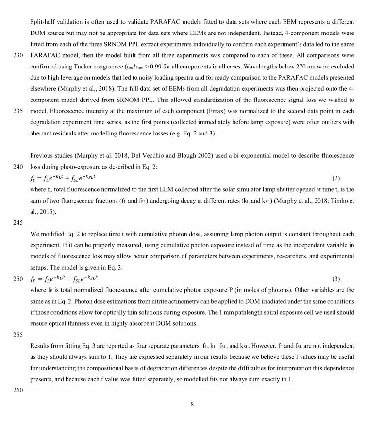
Capturing changes in this pool is one of the explicit advantages of our experimental system, and future work on environmental

photo-reactivity may focus on this time scale as photochemical reactions in the environment are often driven by initial rates 370

(Powers and Miller, 2015). However, slower degradation processes or longer irradiations may be affected by extraction.

Figure 6. Photodegradation time series of PARAFAC component 3 and 4 fluorescence intensity, relative to starting values. Data are shown from 3 replicates of both RO SRNOM and SRNOM PPL.

●●●●●●●●●●●●●●●●●●●●●●●●●●●●●●●●●●●●●●●●●●●●●●●●●●●●●●●●●●●

●●●●●●●●●●●●●●●●●●●●●●●●●●●●●●●●●●●●●●●●●●●●●●●●●●●●●●●●●●●

●●●●●●●●●●●●●●●●●●●●●●●●●●●●●●●●●●●●●●●●●●●●●●●●●●●●●●●●●●●

0.00

0.25

0.50

0.75

1.00

0 1 2Exposure, mol photons m-2

PAR

AFAC

com

pone

nt 3

inte

nsity

,re

lativ

e to

sta

rt●

●●●●●●

●●●●●●●●●●●●●●●●●●●●●●●●●●●●●●●●●●●●●●●●●●●●●●●●●●●●

●●●●●●●●●●

●●●●●●●●●●●●●●●●●●●●●●●●●●●●●●●●●●●●●●●●●●●●●●●●●

●

●●●●●●●

●●●●●●●●●●●●●●●●●●●●●●●●●●●●●●●●●●●●●●●●●●●●●●●●●●●

0.00

0.25

0.50

0.75

1.00

0 1 2Exposure, mol photons m-2

PAR

AFAC

com

pone

nt 4

inte

nsity

,re

lativ

e to

sta

rt

● RO SRNOMSRNOM PPL

17

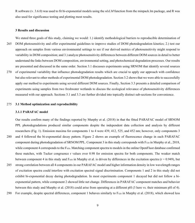
375

Figure 7. Fitted biexponential model parameters (Eq. 3) from the time series of loss of PARAFAC components 3 and 4 in irradiation experiments comparing RO SRNOM to PPL SRNOM (see Fig. 6 for data). f is unitless and k is m2 [mol photons]-1. C3 and C4 denote PARAFAC components 3 and 4. Error bars represent mean + standard deviation from three experiments. Two-tailed t-tests suggest differences in kSL for both components (p = 0.020 in component 3, p = 0.015 in component 4), while fL and fSL may differ (p = 0.065 and 0.058) in component 3. 380

Shared PARAFAC components suggest PPL extraction did not strongly alter the compositional bases of fluorescence

photosensitivity in the RO SRNOM, but the differences in losses suggest researchers should take care when comparing extracts

to original samples in future photodegradation kinetics studies. We are not sure what gave rise to these differences, but the RO

SRNOM likely contains much more highly polar compounds such as (poly)saccharides and related compounds (e.g.

glycosates). Differences between PPL and RO samples here are probably not due to variation in photon dose, as volume and 385

initial absorbance were equal across samples. If concentration of fluorophores affects degradation kinetics, differing

fluorophore concentrations between our PPL extracts and whole SRNOM could explain the discrepancy. Even though we

adjusted all samples to similar starting absorbance, selective enrichment or dilution of absorbing or fluorescing compounds in

extracts could affect the mechanism responsible for any concentration dependence. Differences in electronic coupling and

●

● ●

●

C3 C4

RO PPL RO PPL0

1

2

3

4Fi

tted

valu

e of

kL

●

●

●

●

C3 C4

RO PPL RO PPL0.000.050.100.150.200.25

Fitte

d va

lue

of k

SL

●

●

●●

C3 C4

RO PPL RO PPL0.00

0.05

0.10

0.15

0.20

Fitte

d va

lue

of f L

●

●

●

●

C3 C4

RO PPL RO PPL0.80

0.85

0.90

0.95

1.00

Fitte

d va

lue

of f S

L

18

charge-transfer abilities (Del Vecchio and Blough, 2004; Sharpless and Blough, 2014) could arise in extracts and affect 390

fluorescence degradation kinetics. RO SRNOM may present matrix effects relative to extracted SRNOM PPL, as metals and

other possible interferences are still present (albeit at much lower concentrations relative to DOC than in source water) despite

the cation exchange and desalting treatments that accompanied the original reverse osmosis isolation (Kuhn et al., 2014).

3.1.4 Guidelines for photodegradation fluorescence kinetics experiments

It has been established that initial pH and pH change during photodegradation affects fluorescence photodegradation kinetics 395

(Timko et al., 2015). We chose to conduct experiments at pH 3 because control by autotitration was not possible during these

experiments due to contamination from the pH probe, and starting at pH 3 ensured minimal pH change during

photodegradation. If research goals do not explicitly include understanding effects of pH during photodegradation, we

recommend bringing all samples to the same starting pH and controlling pH during the course of photodegradation

experiments, or starting experiments at pH 3 and ensuring change during the experiment is minimal. 400

Using a reference material allows consistency within and between research labs. We recommend using SRNOM as it has been

widely studied and characterized (Green et al., 2014). Comparing total absorbance and fluorescence loss and degradation

kinetics of SRNOM to DOM sources of interest will allow more meaningful comparison between lab groups. Repeated

experiments with the same standard can identify sources of error and quantify variability due to experimental procedures. 405

Checking this variability against variability among repeated measurements of a sample may allow common variability to be

estimated and thus reduce the need for replication in future runs with similar DOM sources. We also used SRNOM (after solid

phase extraction) as the basis for our PARAFAC model of fluorescence change during photodegradation and projected this

model onto the rest of our data set, standardizing fluorescence losses between DOM sources to the same signal.

410

For research into compositional changes in DOM during photodegradation, test materials should be brought to similar starting

absorbance. We adjusted all samples to a raw absorbance of 0.12 at 300 nm (with a 1 cm path length), but this may be difficult

or less ecologically meaningful with naturally dilute (e.g. ocean) or concentrated (e.g. leachates) DOM sources. If possible,

testing different DOM concentrations for the same sample is recommended in order to establish any concentration dependence

on photochemical rates. In our system, 415

Photon dose obviously affects degradation kinetics. Our experimental system offered several procedural choices that could

affect photon dose, including volume of sample in the system and lamp intensity. Researchers should carefully control these

parameters and ensure their procedures are generating reproducible results by running several replicated experiments with a

reference material. We encourage repeating this process with multiple individuals within a lab to understand the impact of 420

individual methodological choices on results (e.g. gravimetric measurement of volume added vs. pipetting, preparation of

samples). We strongly encourage at least reporting actinometry results or assumed actinometry for the experimental conditions

19

used in order to better compare photon doses across studies and in the environment. While the additional work of actinometry

is not trivial, we believe this represents one way to improve reproducibility of degradation kinetics that avoids the limitations

of using time alone. Even this approach could be improved – our actinometer did not directly measure radiation across the UV 425

spectrum, which could allow more accurate quantification of cumulative photon dose. Striking a balance between effort

required and reproducibility is difficult, but we believe our work illustrates some of the limitations of conventional approaches

where photon exposure cannot be reliably calculated, and we hope our efforts inspire alternative approaches to overcoming

these limitations. Ideally, samples should be irradiated under optically thin conditions when actinometry measurements or

other approaches can be used to estimate photon doses for kinetic modelling (e.g. using Eq. 3 instead of 2). 430

Photodegradation is affected by both DOM composition and matrix conditions. While we found that the same PARAFAC

model captured fluorescence decay in both SRNOM and solid phase extracts of SRNOM (as in (Murphy et al., 2018)),

extraction did affect total fluorescence loss and its kinetics. However, we chose to use extracts for further experiments as in

accordance with our research priorities and because our samples were not stable when stored as whole water samples. 435

Preliminary experiments showed storage of water samples for greater than two weeks led to changes in fluorescence loss

patterns, even when filtered to 0.2 µm (see Appendix B). We believe this could have been due to the high DOC concentrations

in samples used in those experiments, which could have been more susceptible to flocculation (von Wachenfeldt and Tranvik,

2008; Wachenfeldt et al., 2009) or other aggregation processes than dilute samples, but further work would be required to test

this. While other work has found DOM absorbance remained stable in seawater samples after storage at 4° C up to 1 year 440

(Swan et al., 2009), concentrated DOM in inland waters may be unstable in cold storage conditions, affecting its optical

properties or responses to photoirradiation. Further work is required to understand the cause of this behavior, but losses of

DOC and changes to optical properties during cold storage of samples have been reported elsewhere (Peacock et al., 2015).

We recommend using extracts with greater storage stability to allow comparison over time, unless all experiments can be

conducted shortly after sample collection or previous experience shows that the optical properties of the DOM in question are 445

stable for the duration of storage. As our goal was to test photosensitivity arising from DOM composition itself and not the

effects of matrix chemistry, extraction was also conceptually appropriate. The tradeoffs and advantages of using whole water

vs. extracts may be different in other experiments, and comparisons should probably be made to contextualize results when

using extractions. Comparisons of kinetics between extracts and whole water samples should be made with care, but

experiments using such comparisons may help disentangle the role of DOM chemical composition from other matrix effects 450

in determining photodegradation behavior and sensitivity. Matrix effects may be especially important for extrapolating lab

photodegradation findings to inferences at ecosystem scales. For example, if the approach described here is used to investigate

longitudinal changes in DOM photosensitivity along a river network, tying these findings to residence times and photon doses

in the field would be difficult without considering light attenuation by inorganic chromophores and particles. Matrix

constituents may also fundamentally alter the photosensitivity of DOM by participating in charge-transfer processes. We 455

recommend using DOM isolated from its matrix by extraction here not because it is a sufficient approach to understand these

20

phenomena, but as a foundation to explore this complexity. More work is needed to understand the relative influence of DOM

and matrix compositions on photodegradation kinetics.

3.2 Photosensitivity differences between DOM sources 460

After establishing procedures to understand and control experimental influences on DOM photosensitivity, our comparison of

photodegradation of several DOM sources sought to reveal differences in photosensitivity arising from DOM. Figure 8 shows

the degradation of PARAFAC components 3 and 4 relative to starting intensities in samples from different DOM sources. Both

components showed potentially divergent decay patterns among DOM sources, with Sargassum leachate starkly diverging

from bulk DOM sources. Fitted biexponential model parameters of decay in PARAFAC components 3 and 4 are shown in 465

Tables A2 and A3, with parameters from component 4 plotted in Fig. 9 (similar plot for component 3 can be found in Appendix

A, Fig. A2). We did not conduct repeated trials with every DOM source shown here due to logistical constraints, but t-tests on

three trials each with SRNOM and one of the wetland samples supported potential differences in fL and fSL in both PARAFAC

components, and possible differences in kSL in component 3. Notably, these two DOM sources had biexponential parameter

values that were among the most similar compared to other sources (see “Small wetland” and “SRNOM” in Fig. 9), which 470

suggests that our approach is sensitive enough to detect small differences.

21

Figure 8. Photodegradation time series of PARAFAC component 3 and 4 fluorescence intensity, relative to starting values. Data are shown from experiments using PPL extracts from different DOM sources (see Methods for source descriptions). “Large 475 wetland” and “Small wetland” samples use the same symbol for samples from each source, including samples collected on different dates.

●●●●

●●●●●●●

●●●●●●●●

●●●●●●●●●●●●●●●●●●●●●●●●●●●●●●●●●●●●●●●●

●●●●

●●●●●

●●●●●●●●●●●●●●●●●●●●●●●●●●●●●●

●●●●●●●●●●●●●●●●●●●●

●●●●●●●●●

●●●●●●●●●●●●●●●●●●●●●●●●●●●●●●●●●●●●●●●●●●●●●●●●●●

0.00

0.25

0.50

0.75

1.00

0 1 2Exposure, mol photons m-2

PAR

AFAC

com

pone

nt 3

inte

nsity

, rel

ative

to s

tart

●

●●●●●●●●●●●●●

●●●●

●●●●●●●●●●●●●●●●●●●●●●●●●●●●●●●●●●●●●●●●●

●●

●●●●●●●●●

●●●●●●

●●●●●●

●●●●●●●●●●●●●●●●●●●●●●●●●●●●●●●●●●●●

●

●

●●●●●●●●●●●

●●●●●●●

●●●●●●●●●●●●●●●●●●

●●●●●●●●●●●●●●●●●●●●●

0.00

0.25

0.50

0.75

1.00

0 1 2Exposure, mol photons m-2

PAR

AFAC

com

pone

nt 4

inte

nsity

, rel

ative

to s

tart

● SRNOMSmall wetlandLarge wetlandStreamCoastal oceanSargassum

22

Figure 9. Fitted biexponential model parameters (Eq. 3) from the time series of PARAFAC component 4 (see Fig. 9 for data). f is unitless and k is m2 [mol photons]-1. For wetland samples, shapes represent different sampling dates (circles are 2017-10-04, 480 triangles are 2017-12-20, and squares are 2018-04-01).

The outlier in our comparison of DOM sources was Sargassum leachate extract, which was expected given the unique

composition and the presence of phlorotannins (Powers et al., 2019). The natural DOM used in a previous study (Murphy et

al., 2018) that yielded PARAFAC components appearing in all photodegradation experiments did not include leachates, only

natural bulk DOM. Interestingly, this sample alone showed little or very slow semi-labile fluorescence loss with total 485

fluorescence loss of projected PARAFAC components 3 and 4 dominated by rapid initial loss. Future studies using leaf or

soil/sediment leachates, or lysed algal cells, or other putative sources of natural DOM instead of bulk natural DOM itself need

to test this modelling approach more thoroughly to ensure it is appropriate, but using other leachate sources may highlight the

compositional basis of the semi-labile fluorescence decay that seems ubiquitous in bulk natural DOM but absent in Sargassum

leachate here. These experiments demonstrated the general applicability of our method to compositionally distinct DOM 490

sources.

●

●

●●

●●

●

●

●

●

●

●

●●

●

● ●

●●

●

●●●

●

●

●●

●●●

●

●

●●

●

● ●

●●

●

fL fSL

kL kSL

SRNOM

Small wetland

Large wetland

Stream

Coastal ocean

Sargassum

SRNOM

Small wetland

Large wetland

Stream

Coastal ocean

Sargassum

0.0

0.1

0.2

0.3

0.650.700.750.800.850.90

2

3

4

0.10

0.15

0.20

0.25

0.30

DOM source

Fitte

d pa

ram

eter

val

ue,

loss

of P

ARAF

AC c

ompo

nent

4

23

3.3 Photosensitivity and ecological inference

3.3.1 Interpreting biexponential model parameters

Differences in biexponential model parameters between samples may allow reproducible comparisons of natural DOM

photosensitivity. While the differences in parameter values described in Section 3.2 were encouraging, we wanted to know 495

more about the potential ecological relevance of these differences. This approach has been used before given the excellent fit

of this type of model to photodegradation data sets, and biexponential models indeed provided excellent fits to fluorescence

losses in PARAFAC components 3 and 4 in our data sets. The biexponential model represents the sum of two terms, often

referred to as labile and semi-labile to reflect the large relative differences in exponential slopes (kL and kSL in Eq. 2). This

model captures loss of two pools of fluorescence intensity, possibly arising from two pools of DOM fluorophores decreasing 500

in abundance at differing rates, or perhaps a single pool of photoreactive DOM with differing capacities for two types of

reactions contributing to loss of fluorescence (Murphy et al., 2018).

In other studies (e.g. Murphy et al., 2018; Timko et al., 2015) the rate parameters kL and kSL have received the most attention,

as different average rates of change in fluorescence governed by these rate constants may indicate differences in DOM 505

chemical composition, matrix composition, environmental conditions (if experiments are performed in situ), or experimental

conditions, making these values potentially useful metrics of compositional differences between DOM sources. However,

differences in loss of fluorescence between samples may also arise from differing relative abundances of two “pools” of

whatever is responsible for fluorescence at the beginning of the time series. Figure 10 shows degradation time series from two

experiments, along with fitted model parameters. These experiments compare DOM sampled in October 2017 from the two 510

freshwater wetlands in Maryland. Figure 10 shows loss of PARAFAC component 3 (see Fig. A3 in Appendix A for a similar

plot showing loss of component 4). The model fits are shown against the data in upper panels, while the modelled fits for each

of the two terms from Eq. 3 (𝑓"𝑒#$!& and 𝑓%"𝑒#$"!&) are plotted separately against the data in lower panels. This visualization

is useful to weigh the contribution of differing rate parameters (kL and kSL) against the relative abundance of their respective

fractions (fL and fSL) at the onset of the experiment in determining overall differences in photodegradation behavior between 515

samples. Component 3 loss models show similar kL values but different relative fractions of the “fast” pool of fluorescence

loss at the start of the experiment. Differences in these starting fractions between samples may play a role in overall differences

in degradation kinetics in component 4 as well. It is crucial to note that the chemical interpretation of these modelled fits is not

clear. “Pools” of fluorescence in different relative abundances that decay at different rates may not map directly onto different

groups of fluorophores changing in concentration. This behavior may stem from differences in the capacity for two classes of 520

photochemical reactions – where k describes the reaction rates and f describes the relative capacity of the sample to undergo

the corresponding reaction at the outset of the experiment. For example, one possible explanation offered for biexponential

decay in Murphy et al. (2018) invoked reactive species degrading a single pool of fluorophores quickly and direct photolysis

degrading those fluorophores more slowly. Differences in fL may then reflect differing capacity to form or react with triplet

24

excited DOM. Further work is needed to understand what gives rise to relative differences between f terms in different samples, 525

though as noted fL and fSL are not independent in the model presented here. This highlights one of the strengths of our approach

– the ability to capture optical properties of DOM that change very quickly during photodegradation. The modelled labile

portion of fluorescence contributes negligibly to total fluorescence after receiving between 0.5 and 1.2 moles of photons per

square meter, (3-10 hours of irradiation with our experimental setup). Future work relating the photon dose required to reach

this point and the environmental conditions affecting this dose in natural DOM could improve knowledge of DOM origins, 530

residence times, and interactions with other degradation processes.

3.3.2 Linking photosensitivity to DOM sources in dynamic ecosystems

High resolution photodegradation experiments of natural DOM can reveal fundamental photophysical behavior of ecological

importance. We believe the approach described here can help unravel sources or light exposure histories of DOM in natural

settings. One of our overall goals is to determine relative photosensitivity among samples. The biexponential models that fit 535

experimental photodegradation data may help with these comparisons. For example, in the two wetland samples compared in

Fig. 10, distinct patterns of photodegradation suggest distinct DOM composition. DOM fluorescence in the larger wetland had

relatively less “fast” decaying fluorescence in photosensitive PARAFAC components (parameter fL) than the smaller wetland.

These wetlands are depressions located less than 100 m from each other, but with isolated surface water during the October

2017 sampling. They differ in basin size, canopy cover, and vegetation communities. Our data and fitted model parameters 540

suggest that DOM in the larger wetland has either previously been exposed to sunlight that has depleted the potential for “fast”

decaying fluorescence, or that differences in source material or other processing of DOM pools in each wetland have given

rise to relatively less photosensitive material in the larger wetland. In winter, water levels rose in each depression, and

eventually both depressions were connected by surface flow from the larger to smaller wetland. Photosensitivity differences

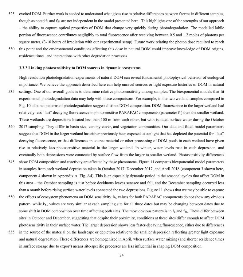
show DOM composition and reactivity are affected by these phenomena. Figure 11 compares biexponential model parameters 545

in samples from each wetland depression taken in October 2017, December 2017, and April 2018 (component 3 shown here,

component 4 shown in Appendix A, Fig. A4). This is an especially dynamic period in the seasonal cycles that affect DOM in

this area – the October sampling is just before deciduous leaves senesce and fall, and the December sampling occurred less

than a month before rising surface water levels connected the two depressions. Figure 11 shows that we may be able to capture

the effects of ecosystem phenomena on DOM sensitivity. kL values for both PARAFAC components do not show any obvious 550

pattern, while kSL values are very similar at each sampling site for all three dates but may be changing between dates due to

some shift in DOM composition over time affecting both sites. The most obvious pattern is in fL and fSL. These differ between

sites in October and December, suggesting that despite their proximity, conditions at these sites differ enough to affect DOM

photosensitivity in their surface water. The larger depression shows less faster-decaying fluorescence, either due to differences

in the source of the material on the landscape or depletion relative to the smaller depression reflecting greater light exposure 555

and natural degradation. These differences are homogenized in April, when surface water mixing (and shorter residence times

in surface storage due to export) means site-specific processes are less influential in shaping DOM composition.

25

These photosensitivity differences may have consequences for other ecosystem processes. For example, if low fL at the time

of sampling reflects high rates of photodegradation in wetland surface water, photopriming may contribute to microbial 560

heterotrophy. Or wetland DOM with high fL may influence downstream ecosystems, if DOM exported to stream networks is

then susceptible to photodegradation which alters its lability to heterotrophs (Judd et al., 2007) or promotes flocculation (Helms

et al., 2013). The sensitivity of our approach may also allow revisiting questions of longitudinal dynamics of light exposure in

stream systems (Larson et al., 2007).

565

We can use this example to justify the effort involved in modeling fluorescence decay kinetics by comparing these inferences

to those possible with simpler approaches. Modeling kinetics of fluorescence loss allows us to resolve processes apparently

occurring at different rates, obvious in the large differences between kL and kSL in any of the samples analyzed. Differences in

fL values between samples provide novel information and are the basis for our comparison of photosensitivity to relatively fast

photochemical processes. These parameters can only be derived from time series of measurements collected frequently. 570

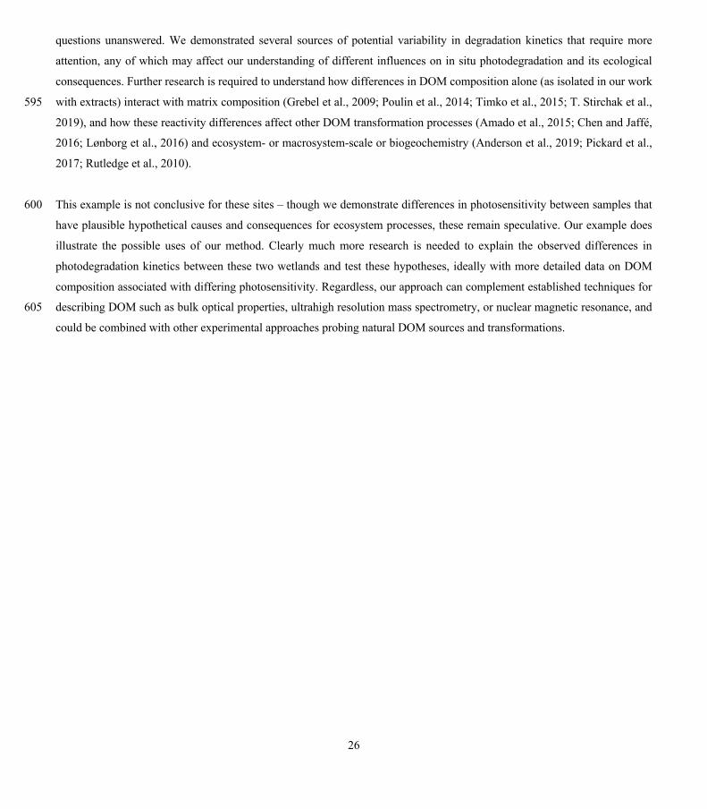
Otherwise our basis of comparison is differences in overall changes to fluorescence and absorbance. In the wetland samples

described here these differences were small or nonexistent and showed no discernible patterns. An example is shown in Figure

12, which shows absorbance spectra before and after irradiation in samples from the two wetlands (using only two of the dates

shown in Figure 11 for visual simplicity). Samples show similar behavior in all cases, or differences due to lack of resolution

producing errors (as in large apparent relative changes in the small wetland Nov. 2017 sample, which arise from small changes 575

near the limit of detection). Additionally such comparisons are difficult to compare between studies – any change is contingent

on photon dose, which would either need to be replicated with identical experimental apparatus or related to only two time

points, making calculations of rate prone to error. It might be possible to glean more information from the absorbance time

series during irradiation, but this would require selecting optimal wavelengths to isolate for modeling losses or modeling losses

at many wavelengths, approaches which to our knowledge have not been developed. Instead we can model kinetics of a 580

tractable number of variables (PARAFAC loadings) for each sample that provide novel information building on existing

approaches to characterize DOM composition. Our approach is not the only way to compare photosensitivity and effects of

photodegradation, nor will it be appropriate for all studies. We encourage all researchers to ensure their approaches address

the methodological issues raised in Section 3.1, but the advantages of the specific data and modeling employed by our method

correspond to our research questions and may not be universal. 585

Photodegradation of DOM extracts in the lab does not replicate in situ photodegradation of DOM in surface waters. However,

in situ photodegradation of DOM in surface water is extremely convoluted – the complexity of DOM chemical composition,

surface water matrix composition, simultaneous ecological processes that also alter DOM composition, and the natural

dynamism of surface water systems are intertwined and make it difficult to understand the role of photodegradation of DOM 590

in surface water ecosystems. Our approach represents one step in the direction of disentangling this story but leaves many

26

questions unanswered. We demonstrated several sources of potential variability in degradation kinetics that require more

attention, any of which may affect our understanding of different influences on in situ photodegradation and its ecological

consequences. Further research is required to understand how differences in DOM composition alone (as isolated in our work

with extracts) interact with matrix composition (Grebel et al., 2009; Poulin et al., 2014; Timko et al., 2015; T. Stirchak et al., 595

2019), and how these reactivity differences affect other DOM transformation processes (Amado et al., 2015; Chen and Jaffé,

2016; Lønborg et al., 2016) and ecosystem- or macrosystem-scale or biogeochemistry (Anderson et al., 2019; Pickard et al.,

2017; Rutledge et al., 2010).

This example is not conclusive for these sites – though we demonstrate differences in photosensitivity between samples that 600

have plausible hypothetical causes and consequences for ecosystem processes, these remain speculative. Our example does

illustrate the possible uses of our method. Clearly much more research is needed to explain the observed differences in

photodegradation kinetics between these two wetlands and test these hypotheses, ideally with more detailed data on DOM

composition associated with differing photosensitivity. Regardless, our approach can complement established techniques for

describing DOM such as bulk optical properties, ultrahigh resolution mass spectrometry, or nuclear magnetic resonance, and 605

could be combined with other experimental approaches probing natural DOM sources and transformations.

27

Figure 10. Data and model fit of PARAFAC component 3 loss in experiments with two wetland samples. Top panels show data and model fit (Eq. 3) while bottom panels decompose the fitted model into its two summed terms, 𝒇𝑳𝒆"𝒌𝑳𝑷 and 𝒇𝑺𝑳𝒆"𝒌𝑺𝑳𝑷, or labile and semi-labile terms. 610

Component 3, small wetland, data and fit

Component 3, small wetland, data and decomposed fit Component 3, large wetland, data and decomposed fit

Component 3, large wetland, data and fit

kL = 2.7fL = 0.03

kSL = 0.19fSL = 0.98

kL = 2.9fL = 0.13

kSL = 0.18fSL = 0.87

Component 3, small wetland, data and decomposed fit

28

Figure 11. Fitted biexponential model parameters (Eq. 3) from the time series of PARAFAC component 3, comparing DOM from large and small wetland sampling sites collected on different dates. f is unitless and k is m2 [mol photons]-1. 615

●

●

●

●

●

●

●

●

●

●

●

●

kL kSL

fL fSL

2017−10−05

2017−12−20

2018−04−01

2017−10−05

2017−12−20

2018−04−01

2017−10−05

2017−12−20

2018−04−01

2017−10−05

2017−12−20

2018−04−01

0.87

0.90

0.93

0.96

0.14

0.16

0.18

0.20

0.025

0.050

0.075

0.100

0.125

2

3

4

5

6

Sampling date

Fitte

d bi

expo

nent

ial

mod

el p

aram

eter

val

ue,

PAR

AFAC

com

p. 3

loss

● Larger wetland

Smaller wetland

29

Figure 12. Changes to absorbance spectra after photodegradation show advantages of high-resolution fluorescence data. Panel A (left side) shows initial vs. final spectra (calculated as absorption coefficients) in photodegradation experiments using samples taken from the two wetlands on two of the dates also shown in Fig. 11. Panel B (right side) shows the same data, but expressed as percent change in absorbance across the spectrum. 620

4 Conclusion

Our research identified several methodological issues that can improve photodegradation experiments and leveraged this

knowledge to show how photosensitivity differences may relate to DOM composition and environmental setting using a case

study. Photodegradation experiments have improved our understanding of the role of DOM light sensitivity in ecological 625

processes. As researchers continue to explore related questions and experiments proliferate, it is important to use approaches

that constrain the influence of experimental conditions and promise reproducible or at least comparable results. Our method

allows reproducible and relatively short experiments that capture photosensitivity differences between varying sources of

natural DOM on time scales relevant for investigating degradation processes in the environment. This approach can be used

Apr. 2018

Nov. 2017

300 400 500

0

20

40

60

0

20

40

60

Wavelength (nm)

Abso

rptio

n co

effic

ient

, m-1

Site sampledLarge wetlandSmall wetland

MeasurementInitialFinal

A

Apr. 2018

Nov. 2017

300 400 500

−100

−75

−50

−25

0

−100

−75

−50

−25

0

Wavelength (nm)

Perc

ent c

hang

e in

abs

orba

nce

Site sampledLarge wetlandSmall wetland

B

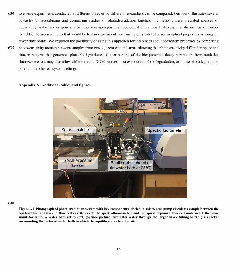
30

to ensure experiments conducted at different times or by different researchers can be compared. Our work illustrates several 630

obstacles to reproducing and comparing studies of photodegradation kinetics, highlights underappreciated sources of

uncertainty, and offers an approach that improves upon past methodological limitations. It also captures distinct fast dynamics

that differ between samples that would be lost in experiments measuring only total changes in optical properties or using far

fewer time points. We explored the possibility of using this approach for inferences about ecosystem processes by comparing

photosensitivity metrics between samples from two adjacent wetland areas, showing that photosensitivity differed in space and 635

time in patterns that generated plausible hypotheses. Closer parsing of the biexponential decay parameters from modelled

fluorescence loss may also allow differentiating DOM sources, past exposure to photodegradation, or future photodegradation

potential in other ecosystem settings.

Appendix A: Additional tables and figures

640 Figure A1. Photograph of photoirradiation system with key components labeled. A micro gear pump circulates sample between the equilibration chamber, a flow cell cuvette inside the spectrofluorometer, and the spiral exposure flow cell underneath the solar simulator lamp. A water bath set to 25°C (outside picture) circulates water through the larger black tubing to the glass jacket surrounding the pictured water bath in which the equilibration chamber sits.

Solar simulator Spectrofluorometer

Equilibration chamber(in water bath at 25°C)

Spiral exposure flow cell

31

Table A1. Fitted biexponential model parameters (Eq. 3) for comparison between RO and PPL SRNOM. p-values are from 645 two-sided t-test of difference in means; n = 3 for both RO SRNOM and SRNOM PPL. f is unitless and k is m2 [mol photons]-1.

PARAFAC component

Biexponential parameter

RO SRNOM Mean (SD)

SRNOM PPL Mean (SD) t-test p-value

3 kL 3.35 (0.252) 2.63 (0.654) 0.18 3 fL 0.0623 (0.00207) 0.0411 (0.0102) 0.065 3 kSL 0.133 (0.0150) 0.177 (0.00792) 0.02 3 fSL 0.936 (0.00113) 0.960 (0.0107) 0.058 4 kL 2.72 (0.110) 2.39 (0.276) 0.16 4 fL 0.155 (0.00717) 0.140 (0.0139) 0.2 4 kSL 0.132 (0.143) 0.191 (0.00346) 0.015 4 fSL 0.838 (0.00897) 0.856 (0.0142) 0.16

Table A2. Fitted biexponential model parameters (Eq. 3) for different DOM sources. f is unitless and k is m2 [mol photons]-1. Where n > 1, means are shown with standard deviations in parentheses. SRNOM PPL trials are three experiments using the 650 same sample source, small wetland trials include three trials with the same sample source (to test non-SRNOM system stability) and two trials with samples from other dates, and large wetland trials include one trial each from three sampling dates. p-values of biexponential model fits all below 1x10-6 except for kSL for Sargassum, p = 0.016. Model parameters for every individual trial can be found in associated data set (Armstrong, 2020).

PARAFAC component

Biexponential parameter

SRNOM PPL (n = 3)

Stream (n = 1)

Coastal ocean (n = 1)

Sargassum (n = 1)

3 kL 2.63 (0.654) 3.17 2.84 5.4

3 fL 0.0411 (0.0102) 0.106 0.135 0.11

3 kSL 0.177 (0.00792) 0.237 0.137 0.0194

3 fSL 0.960 (0.0107) 0.887 0.857 0.889

4 kL 2.39 (0.276) 3.58 4.55 3.68

4 fL 0.140 (0.0139) 0.222 0.229 0.334

4 kSL 0.191 (0.00346) 0.308 0.332 -0.00803

4 fSL 0.856 (0.0142) 0.764 0.762 0.653 655

Table A3. Fitted biexponential model parameters (Eq. 3) for wetland DOM samples. f is unitless and k is m2 [mol photons]-1. Where n > 1, means are shown with standard deviations in parentheses. p-values of biexponential model fits all below 1x10-6. Model parameters for every individual trial can be found in associated data set (Armstrong, 2020).

PARAFAC component

Biexponential parameter

Small wetland, 2017-10-05

(n = 3)

Small wetland, 2017-12-20

(n = 1)

Small wetland, 2018-04-01

(n = 1)

Large wetland, 2017-10-05

(n = 1)

Large wetland, 2017-12-20

(n = 1)

Large wetland, 2018-04-01

(n = 1) 3 kL 2.86 (0.199) 2.37 4.12 2.69 6.01 1.34

3 fL 0.120 (0.00908) 0.126 0.0732 0.0281 0.214 0.0496

3 kSL 0.184 (0.0203) 0.138 0.124 0.185 0.137 0.127

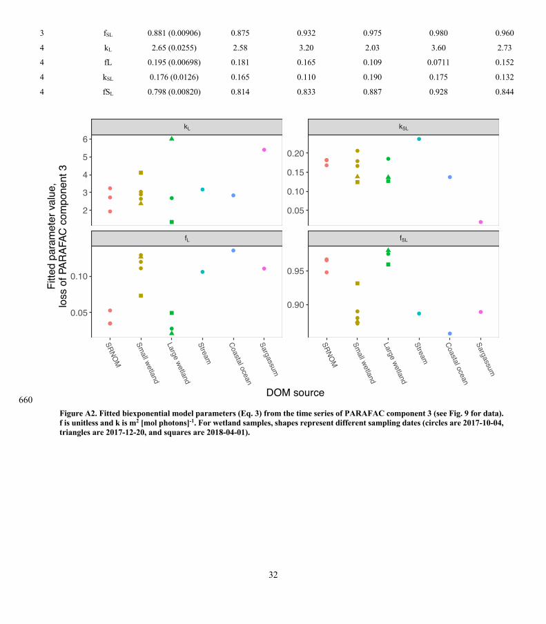
32

3 fSL 0.881 (0.00906) 0.875 0.932 0.975 0.980 0.960

4 kL 2.65 (0.0255) 2.58 3.20 2.03 3.60 2.73

4 fL 0.195 (0.00698) 0.181 0.165 0.109 0.0711 0.152

4 kSL 0.176 (0.0126) 0.165 0.110 0.190 0.175 0.132

4 fSL 0.798 (0.00820) 0.814 0.833 0.887 0.928 0.844

660 Figure A2. Fitted biexponential model parameters (Eq. 3) from the time series of PARAFAC component 3 (see Fig. 9 for data). f is unitless and k is m2 [mol photons]-1. For wetland samples, shapes represent different sampling dates (circles are 2017-10-04, triangles are 2017-12-20, and squares are 2018-04-01).

●●

●

●

●

●●●

●

●

●

●

●●

●●

●

●●

●

● ●

●

●

●

●

●

●●●

●

●

●●

●●

●

●●

●

fL fSL

kL kSL

SRNOM

Small wetland

Large wetland

Stream

Coastal ocean

Sargassum

SRNOM

Small wetland

Large wetland

Stream

Coastal ocean

Sargassum

0.05

0.10

0.15

0.20

0.90

0.95

2

3

4

5

6

0.05

0.10

DOM source

Fitte

d pa

ram

eter

val

ue,

loss

of P

ARAF

AC c

ompo

nent

3

33

Figure A3. Data and model fit of PARAFAC component 4 loss in experiments with two wetland samples. Top panels show data 665 and model fit (Eq. 3) while bottom panels decompose the fitted model into its two summed terms, 𝒇𝑳𝒆"𝒌𝑳𝑷 and 𝒇𝑺𝑳𝒆"𝒌𝑺𝑳𝑷, or labile and semi-labile terms.

AWA1031 data and fit, decomposed

●●●●●●●●●●●●●●●●●●●●●●●●●●●●●●●●●●●●●●●●●●●●●●●●●●●●●●●●●●●

0.0 0.5 1.0 1.5 2.0 2.5

0.0

0.2

0.4

0.6

0.8

1.0

Exposure, mol photons m-2

Rel

ative

fluo

resc

ence

AWA1031 data and fit

●●●●●●●●●●●●●●●●●●●●●●●●●●●●●●●●●●●●●●●●●●●●●●●●●●●●●●●●●●●

0.0 0.5 1.0 1.5 2.0 2.5

0.0

0.2

0.4

0.6

0.8

1.0

Exposure, mol photons m-2

Rel

ative

fluo

resc

ence

AWA1029 data and fit, decomposed

●●●●●●●●●●●

●●●●●●●●●●●●●●●●●●●●●●●●●●●●●●●●●●●●●●●●●●●●●●●●

0.0 0.5 1.0 1.5 2.0 2.5

0.0

0.2

0.4

0.6

0.8

1.0

Exposure, mol photons m-2

Rel

ative

fluo

resc

ence

AWA1029 data and fit

●●●●●●●●●●●

●●●●●●●●●●●●●●●●●●●●●●●●●●●●●●●●●●●●●●●●●●●●●●●●

0.0 0.5 1.0 1.5 2.0 2.5

0.0

0.2

0.4

0.6

0.8

1.0

Exposure, mol photons m-2

Rel

ative

fluo

resc

ence

Component 4, small wetland, data and fit

Component 3, small wetland, data and decomposed fit Component 4, large wetland, data and decomposed fit

Component 4, large wetland, data and fit

kL = 2.0fL = 0.11

kSL = 0.19fSL = 0.89

kL = 2.6fL = 0.20

kSL = 0.17fSL = 0.79

Component 4, small wetland, data and decomposed fit

34

Figure A4. Fitted biexponential model parameters (Eq. 3) from the time series of PARAFAC component 4, comparing DOM from large and small wetland sampling sites collected on different dates. f is unitless and k is m2 [mol photons]-1. 670

●

●

●

●

●

●

●

●

●

●

●

●

kL kSL

fL fSL

2017−10−05

2017−12−20

2018−04−01

2017−10−05

2017−12−20

2018−04−01

2017−10−05

2017−12−20

2018−04−01

2017−10−05

2017−12−20

2018−04−01

0.82

0.86

0.90

0.125

0.150

0.175

0.10

0.15

0.20

2.0

2.5

3.0

3.5

Sampling date

Fitte

d bi

expo

nent

ial

mod

el p

aram

eter

val

ue,

PAR

AFAC

com

p. 4

loss

● Larger wetland

Smaller wetland

35

Figure A5. EEMs of filtered source water samples compared to reconstituted solid phase extracts. A: Large wetland, source water. B: Large wetland, soild phase extract. C: Small wetland, source water. D: Small wetland, solid phase extract. Figure shows samples originally collected 2017-10-05.

675

Appendix B: Storage time experiment

We ran a series of experiments testing effects of storage time on photodegradation kinetics which are relevant to our overall

results but were performed under different conditions. These preceded the other experiments and the experimental setup was

modified based on their results. These used filtered water samples (not extracts) taken from the small and large wetland sites

described above, but were collected in November 2017. They were filtered, stored in the dark at 4°C, and run through the 680

photodegradation system undiluted using a 3x3mm quartz flow cell in the spectrofluorometer instead of the 10x10mm cell

index1

300 350 400 450 500 550 600Ex. (nm)

250

300

350

400

450

500

550Em

. (nm

)

0

0.05

0.1

0.15

0.2

0.25

0.3

index1

300 350 400 450 500 550 600Ex. (nm)

250

300

350

400

450

500

550

Em. (

nm)

0

0.2

0.4

0.6

0.8

1

1.2

1.4

index2

300 350 400 450 500 550 600Ex. (nm)

250

300

350

400

450

500

550

Em. (

nm)

0

0.05

0.1

0.15

0.2

0.25

0.3

index2

300 350 400 450 500 550 600Ex. (nm)

250

300

350

400

450

500

550

Em. (

nm)

0

0.2

0.4

0.6

0.8

1

1.2

A

B

C

D

36

used for all other experiments. Experiments were run after 5-8, 9-13, and 14-16 days of storage. These results are reported as

a function of time rather than photon exposure as no actinometry was collected with an analogous experimental setup.

Figure B1. Time series of photodegradation experiments on whole water wetland samples. Each column represents samples 685 from a different wetland source. Three experiments were run with aliquots drawn from a water sample from each wetland, and results seemed to change with storage time. First experiments with each wetland water source were run 5-8 days after sample collection, second experiments were run 9-13 days after sample collection, and third experiments were run 14-16 days after

●●● ●

●●

●

●●

●●

●

●●

●

●

●●

●

●

●●●●●●●

●●●●●

●

●●●

●●●

●

●

●●

●●●●●

●●

●

●●●

●●●●

●●●

●●●●●●

●●●●●●●●●●●●●●●●●●●●●●●●●●

●●●●●●●●●

●●●●●●●●●●●

Large wetland Small wetland

0 5 10 15 20 0 5 10 15 200.00

0.25

0.50

0.75

1.00

Time (hours)

PAR

AFAC

com

pone

nt 3

in

tens

ity, r

elat

ive to

sta

rt

● 1st trial

2nd trial

3rd trial

●

●●●

●

●●

●

●

●

●●●●

●

●

●

●●●●

●

●●●

●●

●

●●●●●●

●

●

●●●

●●●

●

●

●

●

●

●●

●●●●

●●●

●

●●●●●●●

●●●●●●●●

●●●●●●●●●●●●●●●●●●●●●●●●●●●●●●●●●●●●●●●●●●●

Large wetland Small wetland

0 5 10 15 20 0 5 10 15 200.00

0.25

0.50

0.75

1.00

Time (hours)

PAR

AFAC

com

pone

nt 4

in

tens

ity, r

elat

ive to

sta

rt

● 1st trial

2nd trial

3rd trial

37

collection. The trend in most cases toward lower relative photosensitivity in measured variables and in some cases increasing data noise (or poor PARAFAC model fit) as samples aged informed the decision to use solid phase extracts to improve 690 reproducibility.

Data and code availability

Data and code used in this analysis are available from the Dryad repository at https://doi.org/10.5061/dryad.hmgqnk9d9 (Armstrong, 2020). 695

Author contribution

AA developed the method’s applications for ecological inference, collected the data, analyzed the data, and drafted the

manuscript. LP assisted in the method’s conception, collected the data, assisted with data analysis, and edited the manuscript.

MG conceived the method, designed and optimized the instrument system, assisted with data analysis, and edited the 700

manuscript.

Competing interests

The authors declare they have no conflict of interest.

Acknowledgments

A. Armstrong was supported in part by US National Science Foundation Grant # DBI-1052875 and cooperative agreement # 705

58-1245-3-278 between the United States Department of Agriculture, University of Maryland, and the National Socio-

Environmental Synthesis Center. Dr. Margaret Palmer provided valuable feedback during planning and manuscript

preparation. Katherine Martin provided the sample from Parker’s Creek included in the comparison of DOM source material.

Jessalyn Davis assisted with actinometry measurements. This is contribution xxxx (to be enumerated upon acceptance of

manuscript) of the University of Maryland Center for Environmental Science. 710

References

Amado, A. M., Cotner, J. B., Cory, R. M., Edhlund, B. L., and McNeill, K.: Disentangling the Interactions Between Photochemical and Bacterial Degradation of Dissolved Organic Matter: Amino Acids Play a Central Role, Microb. Ecol., 69, 554–566, https://doi.org/10.1007/s00248-014-0512-4, 2015.

38

Anderson, T. R., Rowe, E. C., Polimene, L., Tipping, E., Evans, C. D., Barry, C. D. G., Hansell, D. A., Kaiser, K., Kitidis, V., 715 Lapworth, D. J., Mayor, D. J., Monteith, D. T., Pickard, A. E., Sanders, R. J., Spears, B. M., Torres, R., Tye, A. M., Wade, A. J., and Waska, H.: Unified concepts for understanding and modelling turnover of dissolved organic matter from freshwaters to the ocean: the UniDOM model, Biogeochemistry, 146, 105–123, https://doi.org/10.1007/s10533-019-00621-1, 2019.

Anesio, A. M. and Granéli, W.: Increased photoreactivity of DOC by acidification: Implications for the carbon cycle in humic lakes, Limnol. Oceanogr., 48, 735–744, https://doi.org/10.4319/lo.2003.48.2.0735, 2003. 720

Arrigo, K. R. and Brown, C. W.: Impact of chromophoric dissolved organic matter on UV inhibition of primary productivity in the sea, Mar. Ecol. Prog. Ser., 140, 207–216, 1996.

Blough, N. V. and Del Vecchio, R.: Chromophoric DOM in the Coastal Environment-Chapter 10, 2002.

Blough, N. V. and Zepp, R. G.: Reactive Oxygen Species in Natural Waters, in: Active Oxygen in Chemistry, edited by: Foote, C. S., Valentine, J. S., Greenberg, A., and Liebman, J. F., Springer Netherlands, Dordrecht, 280–333, 725 https://doi.org/10.1007/978-94-007-0874-7_8, 1995.

Boyle, E. S., Guerriero, N., Thiallet, A., Vecchio, R. D., and Blough, N. V.: Optical Properties of Humic Substances and CDOM: Relation to Structure, Environ. Sci. Technol., 43, 2262–2268, https://doi.org/10.1021/es803264g, 2009.

Brailsford, F. L., Glanville, H. C., Marshall, M. R., Golyshin, P. N., Johnes, P. J., Yates, C. A., Owen, A. T., and Jones, D. L.: Microbial use of low molecular weight DOM in filtered and unfiltered freshwater: Role of ultra-small microorganisms and 730 implications for water quality monitoring, Sci. Total Environ., 598, 377–384, https://doi.org/10.1016/j.scitotenv.2017.04.049, 2017.

Bushaw, K. L., Zepp, R. G., Tarr, M. A., Schulz-Jander, D., Bourbonniere, R. A., Hodson, R. E., Miller, W. L., Bronk, D. A., and Moran, M. A.: Photochemical release of biologically available nitrogen from aquatic dissolved organic matter, Nature, 381, 404–407, https://doi.org/10.1038/381404a0, 1996. 735

Chen, M. and Jaffé, R.: Quantitative assessment of photo- and bio-reactivity of chromophoric and fluorescent dissolved organic matter from biomass and soil leachates and from surface waters in a subtropical wetland, Biogeochemistry, 129, 273–289, https://doi.org/10.1007/s10533-016-0231-7, 2016.

Cory, R. M., Ward, C. P., Crump, B. C., and Kling, G. W.: Sunlight controls water column processing of carbon in arctic fresh waters, Science, 345, 925–928, https://doi.org/10.1126/science.1253119, 2014. 740

Del Vecchio, R. and Blough, N. V.: Photobleaching of chromophoric dissolved organic matter in natural waters: kinetics and modeling, Mar. Chem., 78, 231–253, 2002.

Del Vecchio, R. and Blough, N. V.: On the Origin of the Optical Properties of Humic Substances, Environ. Sci. Technol., 38, 3885–3891, https://doi.org/10.1021/es049912h, 2004.

Dittmar, T., Koch, B., Hertkorn, N., and Kattner, G.: A simple and efficient method for the solid-phase extraction of dissolved 745 organic matter (SPE-DOM) from seawater, Limnol. Oceanogr. Methods, 6, 230–235, 2008.

Fichot, C. G. and Miller, W. L.: An approach to quantify depth-resolved marine photochemical fluxes using remote sensing: Application to carbon monoxide (CO) photoproduction, Remote Sens. Environ., 114, 1363–1377, https://doi.org/10.1016/j.rse.2010.01.019, 2010.

39

Goldstone, J. V., Vecchio, R. D., Blough, N. V., and Voelker, B. M.: A Multicomponent Model of Chromophoric Dissolved 750 Organic Matter Photobleaching¶§, Photochem. Photobiol., 80, 52–60, https://doi.org/10.1111/j.1751-1097.2004.tb00049.x, 2004.

Gonsior, M., Peake, B. M., Cooper, W. T., Podgorski, D., D’Andrilli, J., and Cooper, W. J.: Photochemically Induced Changes in Dissolved Organic Matter Identified by Ultrahigh Resolution Fourier Transform Ion Cyclotron Resonance Mass Spectrometry, Environ. Sci. Technol., 43, 698–703, https://doi.org/10.1021/es8022804, 2009. 755

Gonsior, M., Schmitt-Kopplin, P., and Bastviken, D.: Depth-dependent molecular composition and photo-reactivity of dissolved organic matter in a boreal lake under winter and summer conditions, Biogeosciences, 10, 6945–6956, https://doi.org/10.5194/bg-10-6945-2013, 2013.

Gonsior, M., Hertkorn, N., Conte, M. H., Cooper, W. J., Bastviken, D., Druffel, E., and Schmitt-Kopplin, P.: Photochemical production of polyols arising from significant photo-transformation of dissolved organic matter in the oligotrophic surface 760 ocean, Mar. Chem., 163, 10–18, https://doi.org/10.1016/j.marchem.2014.04.002, 2014.

Grebel, J. E., Pignatello, J. J., Song, W., Cooper, W. J., and Mitch, W. A.: Impact of halides on the photobleaching of dissolved organic matter, Mar. Chem., 115, 134–144, https://doi.org/10.1016/j.marchem.2009.07.009, 2009.

Green, N. W., McInnis, D., Hertkorn, N., Maurice, P. A., and Perdue, E. M.: Suwannee River Natural Organic Matter: Isolation of the 2R101N Reference Sample by Reverse Osmosis, Environ. Eng. Sci., 32, 38–44, https://doi.org/10.1089/ees.2014.0284, 765 2014.

Groeneveld, M., Tranvik, L., Natchimuthu, S., and Koehler, B.: Photochemical mineralisation in a boreal brown water lake: considerable temporal variability and minor contribution to carbon dioxide production, Biogeosciences, 13, 3931–3943, https://doi.org/10.5194/bg-13-3931-2016, 2016.

Hansen, A. M., Kraus, T. E. C., Pellerin, B. A., Fleck, J. A., Downing, B. D., and Bergamaschi, B. A.: Optical properties of 770 dissolved organic matter (DOM): Effects of biological and photolytic degradation, Limnol. Oceanogr., 61, 1015–1032, https://doi.org/10.1002/lno.10270, 2016.

Hefner, K. H., Fisher, J. M., and Ferry, J. L.: A Multifactor Exploration of the Photobleaching of Suwannee River Dissolved Organic Matter Across the Freshwater/Saltwater Interface, Environ. Sci. Technol., 40, 3717–3722, https://doi.org/10.1021/es052513h, 2006. 775

Helms, J. R., Stubbins, A., Ritchie, J. D., Minor, E. C., Kieber, D. J., and Mopper, K.: Absorption spectral slopes and slope ratios as indicators of molecular weight, source, and photobleaching of chromophoric dissolved organic matter, Limnol. Oceanogr., 53, 955–969, 2008.

Helms, J. R., Mao, J., Schmidt-Rohr, K., Abdulla, H., and Mopper, K.: Photochemical flocculation of terrestrial dissolved organic matter and iron, Geochim. Cosmochim. Acta, 121, 398–413, https://doi.org/10.1016/j.gca.2013.07.025, 2013. 780

Hu, C., Muller-Karger, F. E., and Zepp, R. G.: Absorbance, absorption coefficient, and apparent quantum yield: A comment on common ambiguity in the use of these optical concepts, Limnol. Oceanogr., 47, 1261–1267, https://doi.org/10.4319/lo.2002.47.4.1261, 2002.

Jankowski, J. J., Kieber, D. J., and Mopper, K.: Nitrate and Nitrite Ultraviolet Actinometers, Photochem. Photobiol., 70, 319–328, https://doi.org/10.1111/j.1751-1097.1999.tb08143.x, 1999. 785

40

Jankowski, J. J., Kieber, D. J., Mopper, K., and Neale, P. J.: Development and Intercalibration of Ultraviolet Solar Actinometers, Photochem. Photobiol., 71, 431–440, https://doi.org/10.1562/0031-8655(2000)0710431DAIOUS2.0.CO2, 2000.

Judd, K. E., Crump, B. C., and Kling, G. W.: Bacterial responses in activity and community composition to photo-oxidation of dissolved organic matter from soil and surface waters, Aquat. Sci., 69, 96–107, https://doi.org/10.1007/s00027-006-0908-790 4, 2007.

Kuhn, K. M., Neubauer, E., Hofmann, T., von der Kammer, F., Aiken, G. R., and Maurice, P. A.: Concentrations and Distributions of Metals Associated with Dissolved Organic Matter from the Suwannee River (GA, USA), Environ. Eng. Sci., 32, 54–65, https://doi.org/10.1089/ees.2014.0298, 2014.

Kujawinski, E. B., Del Vecchio, R., Blough, N. V., Klein, G. C., and Marshall, A. G.: Probing molecular-level transformations 795 of dissolved organic matter: insights on photochemical degradation and protozoan modification of DOM from electrospray ionization Fourier transform ion cyclotron resonance mass spectrometry, Mar. Chem., 92, 23–37, https://doi.org/10.1016/j.marchem.2004.06.038, 2004.

Lapierre, J.-F. and del Giorgio, P. A.: Partial coupling and differential regulation of biologically and photochemically labile dissolved organic carbon across boreal aquatic networks, Biogeosciences, 11, 5969–5985, https://doi.org/10.5194/bg-11-5969-800 2014, 2014.

Larson, J. H., Frost, P. C., Lodge, D. M., and Lamberti, G. A.: Photodegradation of dissolved organic matter in forested streams of the northern Great Lakes region, J. North Am. Benthol. Soc., 26, 416–425, https://doi.org/10.1899/06-097.1, 2007.

Laurion, I. and Mladenov, N.: Dissolved organic matter photolysis in Canadian arctic thaw ponds, Environ. Res. Lett., 8, 035026, https://doi.org/10.1088/1748-9326/8/3/035026, 2013. 805

Lønborg, C., Nieto-Cid, M., Hernando-Morales, V., Hernández-Ruiz, M., Teira, E., and Álvarez-Salgado, X. A.: Photochemical alteration of dissolved organic matter and the subsequent effects on bacterial carbon cycling and diversity, FEMS Microbiol. Ecol., 92, https://doi.org/10.1093/femsec/fiw048, 2016.

Luef, B., Frischkorn, K. R., Wrighton, K. C., Holman, H.-Y. N., Birarda, G., Thomas, B. C., Singh, A., Williams, K. H., Siegerist, C. E., Tringe, S. G., Downing, K. H., Comolli, L. R., and Banfield, J. F.: Diverse uncultivated ultra-small bacterial 810 cells in groundwater, Nat. Commun., 6, 6372, https://doi.org/10.1038/ncomms7372, 2015.

McEnroe, N. A., Williams, C. J., Xenopoulos, M. A., Porcal, P., and Frost, P. C.: Distinct Optical Chemistry of Dissolved Organic Matter in Urban Pond Ecosystems, PLOS ONE, 8, e80334, https://doi.org/10.1371/journal.pone.0080334, 2013.

Miller, W. L.: Effects of UV Radiation on Aquatic Humus: Photochemical Principles and Experimental Considerations, in: Aquatic Humic Substances: Ecology and Biogeochemistry, edited by: Hessen, D. O. and Tranvik, L. J., Springer Berlin 815 Heidelberg, Berlin, Heidelberg, 125–143, https://doi.org/10.1007/978-3-662-03736-2_7, 1998.

Minor, E. C., Dalzell, B. J., Stubbins, A., and Mopper, K.: Evaluating the photoalteration of estuarine dissolved organic matter using direct temperature-resolved mass spectrometry and UV-visible spectroscopy, Aquat. Sci., 69, 440–455, https://doi.org/10.1007/s00027-007-0897-y, 2007.

Moran, M. A. and Zepp, R. G.: Role of photoreactions in the formation of biologically labile compounds from dissolved 820 organic matter, Limnol. Oceanogr., 42, 1307–1316, https://doi.org/10.4319/lo.1997.42.6.1307, 1997.

41

Murphy, K. R., Stedmon, C. A., Graeber, D., and Bro, R.: Fluorescence spectroscopy and multi-way techniques. PARAFAC, Anal. Methods, 5, 6557, https://doi.org/10.1039/c3ay41160e, 2013.

Murphy, K. R., Timko, S. A., Gonsior, M., Powers, L. C., Wünsch, U. J., and Stedmon, C. A.: Photochemistry Illuminates Ubiquitous Organic Matter Fluorescence Spectra, Environ. Sci. Technol., 52, 11243–11250, 825 https://doi.org/10.1021/acs.est.8b02648, 2018.

Obernosterer, I. and Benner, R.: Competition between biological and photochemical processes in the mineralization of dissolved organic carbon, Limnol. Oceanogr., 49, 117–124, https://doi.org/10.4319/lo.2004.49.1.0117, 2004.

Peacock, M., Freeman, C., Gauci, V., Lebron, I., and D. Evans, C.: Investigations of freezing and cold storage for the analysis of peatland dissolved organic carbon (DOC) and absorbance properties, Environ. Sci. Process. Impacts, 17, 1290–1301, 830 https://doi.org/10.1039/C5EM00126A, 2015.

Pickard, A. E., Heal, K. V., McLeod, A. R., and Dinsmore, K. J.: Temporal changes in photoreactivity of dissolved organic carbon and implications for aquatic carbon fluxes from peatlands, Biogeosciences, 14, 1793–1809, https://doi.org/10.5194/bg-14-1793-2017, 2017.

Poulin, B. A., Ryan, J. N., and Aiken, G. R.: Effects of Iron on Optical Properties of Dissolved Organic Matter, Environ. Sci. 835 Technol., 48, 10098–10106, https://doi.org/10.1021/es502670r, 2014.

Powers, L. C. and Miller, W. L.: Hydrogen peroxide and superoxide photoproduction in diverse marine waters: A simple proxy for estimating direct CO2 photochemical fluxes, Geophys. Res. Lett., 42, 7696–7704, https://doi.org/10.1002/2015GL065669, 2015.

Powers, L. C., Hertkorn, N., McDonald, N., Schmitt‐Kopplin, P., Vecchio, R. D., Blough, N. V., and Gonsior, M.: Sargassum 840 sp. Act as a Large Regional Source of Marine Dissolved Organic Carbon and Polyphenols, Glob. Biogeochem. Cycles, 33, 1423–1439, https://doi.org/10.1029/2019GB006225, 2019.

Ritchie, J. D. and Perdue, E. M.: Proton-binding study of standard and reference fulvic acids, humic acids, and natural organic matter, Geochim. Cosmochim. Acta, 67, 85–96, https://doi.org/10.1016/S0016-7037(02)01044-X, 2003.

Ruggaber, A., Dlugi, R., and Nakajima, T.: Modelling radiation quantities and photolysis frequencies in the troposphere, J. 845 Atmospheric Chem., 18, 171–210, https://doi.org/10.1007/BF00696813, 1994.

Rutledge, S., Campbell, D. I., Baldocchi, D., and Schipper, L. A.: Photodegradation leads to increased carbon dioxide losses from terrestrial organic matter, Glob. Change Biol., 16, 3065–3074, https://doi.org/10.1111/j.1365-2486.2009.02149.x, 2010.

Sharpless, C. M. and Blough, N. V.: The importance of charge-transfer interactions in determining chromophoric dissolved organic matter (CDOM) optical and photochemical properties, Env. Sci Process. Impacts, 16, 654–671, 850 https://doi.org/10.1039/C3EM00573A, 2014.

Sharpless, C. M., Aeschbacher, M., Page, S. E., Wenk, J., Sander, M., and McNeill, K.: Photooxidation-Induced Changes in Optical, Electrochemical, and Photochemical Properties of Humic Substances, Environ. Sci. Technol., 48, 2688–2696, https://doi.org/10.1021/es403925g, 2014.

Sulzberger, B. and Durisch-Kaiser, E.: Chemical characterization of dissolved organic matter (DOM): A prerequisite for 855 understanding UV-induced changes of DOM absorption properties and bioavailability, Aquat. Sci., 71, 104–126, https://doi.org/10.1007/s00027-008-8082-5, 2009.

42

Swan, C. M., Siegel, D. A., Nelson, N. B., Carlson, C. A., and Nasir, E.: Biogeochemical and hydrographic controls on chromophoric dissolved organic matter distribution in the Pacific Ocean, Deep Sea Res. Part Oceanogr. Res. Pap., 56, 2175–2192, https://doi.org/10.1016/j.dsr.2009.09.002, 2009. 860

Thrane, J.-E., Hessen, D. O., and Andersen, T.: The Absorption of Light in Lakes: Negative Impact of Dissolved Organic Carbon on Primary Productivity, Ecosystems, 17, 1040–1052, https://doi.org/10.1007/s10021-014-9776-2, 2014.

Timko, S. A., Gonsior, M., and Cooper, W. J.: Influence of pH on fluorescent dissolved organic matter photo-degradation, Water Res., 85, 266–274, https://doi.org/10.1016/j.watres.2015.08.047, 2015.

T. Stirchak, L., J. Moor, K., McNeill, K., and James Donaldson, D.: Differences in photochemistry between seawater and 865 freshwater for two natural organic matter samples, Environ. Sci. Process. Impacts, 21, 28–39, https://doi.org/10.1039/C8EM00431E, 2019.

Twardowski, M. S., Boss, E., Sullivan, J. M., and Donaghay, P. L.: Modeling the spectral shape of absorption by chromophoric dissolved organic matter, Mar. Chem., 89, 69–88, https://doi.org/10.1016/j.marchem.2004.02.008, 2004.

von Wachenfeldt, E. and Tranvik, L. J.: Sedimentation in Boreal Lakes—The Role of Flocculation of Allochthonous Dissolved 870 Organic Matter in the Water Column, Ecosystems, 11, 803–814, https://doi.org/10.1007/s10021-008-9162-z, 2008.

Wachenfeldt, E. von, Bastviken, D., and Tranvika, L. J.: Microbially induced flocculation of allochthonous dissolved organic carbon in lakes, Limnol. Oceanogr., 54, 1811–1818, https://doi.org/10.4319/lo.2009.54.5.1811, 2009.

Wünsch Urban J., Stedmon Colin A., Tranvik Lars J., and Guillemette François: Unraveling the size‐dependent optical properties of dissolved organic matter, Limnol. Oceanogr., 63, 588–601, https://doi.org/10.1002/lno.10651, 2017. 875

Xie, H., Zafiriou, O. C., Cai, W.-J., Zepp, R. G., and Wang, Y.: Photooxidation and Its Effects on the Carboxyl Content of Dissolved Organic Matter in Two Coastal Rivers in the Southeastern United States, Environ. Sci. Technol., 38, 4113–4119, https://doi.org/10.1021/es035407t, 2004.

Zepp, R. G., Sheldon, W. M., and Moran, M. A.: Dissolved organic fluorophores in southeastern US coastal waters: correction method for eliminating Rayleigh and Raman scattering peaks in excitation–emission matrices, Mar. Chem., 89, 15–36, 880 https://doi.org/10.1016/j.marchem.2004.02.006, 2004.