JOURNAL OF GEOPHYSICAL RESEARCH, VOL. 96, NO. C6, PAGES 10,487-10,506, JUNE 15, 1991

Modeled and Observed Mesoscale Circulation and Wave-Current Refraction

During the 1988 Norwegian Continental Shelf Experiment

PETER M. HAUGAN, GEIR EVENSEN, JOHNNY A. JOHANNESSEN, OLA M. JOHANNESSEN, AND LASSE H. PETTERSSON

Nansen Environmental and Remote Sensing Center, Solheimsvik, Norway

A simple two-layer, quasi-geostrophic model with bottom topography is shown to reproduce several features of the mesoscale circulation on the Norwegian continental shelf between 62øN and 66øN, as observed with in situ and remote sensing instruments during the Norwegian Continental Shelf Experiment (NORCSEX '88). The widening of the shelf, its steplike deepening northeastward along the coast, and the presence of the Haltenbank generate intense eddy activity. Further northeast, Atlantic Water is steered anticyclonically around the Haltenbank, and the Norwegian Coastal Current is squeezed toward the coast. The variability of the modeled and observed near-surface current is shown by ray-tracing calculations to be able to generate significant wave-current refraction. In addition to its importance for wave modeling and prediction, this fact opens possibilities for indirect surface current measurements from directional wave observations, particularly from synthetic aperture radar.

1. INTRODUCTION

The Norwegian Coastal Current (NCC) flows northward along the west coast of Norway as a wedge-shaped current originating primarily form the low-salinity upper layer water from Skagerrak as well as freshwater outflow from the fjords. In the west the current is bounded by the inflow of Atlantic Water (AW) originating from the North Atlantic Current. The AW inflow branches into a northward and

southward current at about 62øN. In turn, a distinct temper- ature front and cyclonic current shear is formed along the boundary to the south. The two currents merge north of the branching point, forming a boundary maintained in both the salinity and temperature fields.

The mesoscale circulation pattern in this current system has been well documented in TIROS/NOAA infrared (IR) satellite images and in direct current measurements [Johan- nessen et al., 1983; Johannessen et al., 1989a]. Ikeda et al. [1989] have also provided a detailed comparison of the circulation pattern based on observations and quasi- geostrophic (QG) numerical model simulations. They con- clude that provided the QG model is regularly updated with observations, it is a simple and useful tool for predicting mesoscale circulation patterns in the NCC.

Observations and model predictions of the mesoscale circulation pattern in the NCC will form an important element in marine monitoring and forecasting services planned under the Norwegian HOV (HavmiljO-Overvfikning og Varsling) establishment [Guddal et al., 1989]. A demon- stration of this was provided by [Johannessen et al. [1989b] during the monitoring and prediction of the toxic algae event in May 1988. However with the IR satellite images fre- quently hampered by cloud cover, regular passive optical satellite observations are not possible. In contrast active microwave sensors such as the synthetic aperture radar (SAR) and radar altimeter to be flown on the European Space Agency remote sensing satellite ERS 1 are weather

Copyright 1991 by the American Geophysical Union.

Paper number 91JC00299. 0148-0227/91/91J C-00299505.00

independent. Their resulting capability to regularly detect mesoscale circulation patterns makes them attractive [Gud- dal et al., 1989].

The Norwegian Continental Shelf Experiment (NORC- SEX '88) conducted off the west coast of Norway centered at 64øN in March 1988, was dedicated as a prelaunch ERS 1 investigation aimed at measuring near-surface wind, waves and currents from active microwave sensors [NORCSEX '88 Group, 1989; Johannessen et al., this issue]. Although the in situ oceanographic data collection (Table 1) was not prima- rily directed at detecting and tracking mesoscale eddy fea- tures, it provides satisfactory data for testing and validation of the QG model.

A summary of the general circulation pattern in the experimental region is given in section 2. The numerical model is presented in section 3, and model results are compared with observations from NORCSEX '88 in section 4. The relevance of SAR and altimeter data in combination

with the model data for detection of mesoscale circulation

pattern is discussed in sections 5 and 6. Conclusions are then given in section 7.

2. GENERAL CIRCULATION PATTERN

The depth and time-averaged currents at each mooring during the NORCSEX '88 period (Figure lb and Table 1) vary from 0.07 m s -• to 0.20 m s -• with a mean northeast- ward direction, except for CM3 located north-northeast of the Haltenbank which shows a south-southeasterly flow direction. These directions are nearly parallel to the iso- baths, documenting significant influence of topographic steering. Minor vertical shear and turning angle of the current are found on all moorings except at CM2 located in the channel east of Haltenbank, where the speed decreases from 0.30 m s -• at 25 m to 0.10 m s -• at 150 m, while the direction remains unchanged.

During winter the NCC is characterized by cold and fresh coastal water with temperature ranging from 2 ø to 5øC and salinity less than 34.8%0, while the AW has a temperature exceeding 6øC and salinity greater than 35%0 [Scetre and LjOen, 1972]. A well-defined frontal boundary forms be-

10,487

10,488 HAUGAN ET AL.' MODELED AND OBSERVED MESOSCALE CIRCULATION IN NORCSEX '88

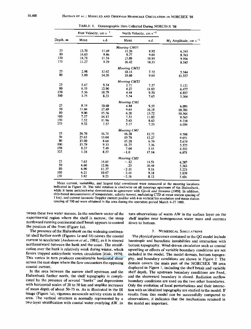
TABLE 1. Oceanographic Data Collected During NORCSEX '88

East Velocity, cm s -1 North Velocity, cm s -1

Depth, m Mean s.d. Mean s.d. M 2 Amplitude, cm s

Mooring CMT1 25 13.70 11.69 11.26 8.92 6.745 80 14.63 9.86 9.77 9.01 8.763

150 14.71 11.24 15.09 10.93 9.936 175 11.27 9.29 16.42 10.33 8.345

Mooring CMT2 25 2.98 12.02 10.14 7.72 5.344 80 3.80 14.26 10.60 9.64 11.557

Mooring CMT3 25 5.47 9.54 2.71 7.27 5.121 80 6.53 12.90 4.27 11.03 6.477

150 5.36 10.79 4.44 9.50 6.937 300 3.75 8.23 5.54 7.65 5.364

Mooring CM1 25 8.19 10.60 4.84 9.55 6.091 50 11.04 17.49 9.61 16.19 10.781 80 9.00 15.56 6.20 13.72 10.364

100 7.37 14.13 7.53 11.82 9.565 150 7.52 11.96 5.63 8.63 8.710 275 9.32 7.57 5.17 7.33 6.094

Mooring CM2 25 26.70 16.71 16.20 12.72 9.588 50 25.63 13.04 19.70 12.27 9.051 80 15.00 8.60 15.20 6.70 5.679

100 15.79 9.13 11.75 7.36 5.575 150 8.37 7.49 7.64 5.11 4.552 325 - 1.24 8.57 - 1.0 17.14 6.071

Mooring CM3 25 7.63 14.61 -.12 11.51 6.287 50 6.60 12.86 -.23 10.48 5.363 80 6.90 11.37 -2.11 9.33 5.223

100 6.21 10.67 -2.41 9.18 5.859 150 5.82 9.23 -2.16 8.12 5.601

Mean current, variability, and largest tidal constituent were measured at the mooring locations indicated in Figure lb. The tidal rotation is clockwise on all moorings upstream of the Haltenbank, while it turns anticlockwise downstream in agreement with Gjevik and Straume [1989]. In addition, ship-based measurements of temperature, salinity (towed, undulating CTD at mean station spacing of 1 km), and current (acoustic Doppler current profiler with 4-m vertical bin resolution and mean station spacing of 700 m) were obtained in the area during the operation period March 4-27 1988.

tween these two water masses. In the southern sector of the

experimental region where the shelf is narrow, the steep northward running continental shelf break appears to control the position of the front (Figure l a).

The presence of the Haltenbank on the widening continen- tal shelf further north (Figures l a and 1 b) causes the coastal current to accelerate [Audunson et al., 1981], as it is steered northeastward between the bank and the coast. The stratifi- cation over the bank is relatively weak during winter, which favors trapped anticyclonic vortex circulation [Eide, 1979]. This vortex in turn produces considerable horizontal shear across the east slope where the flow encounters the opposing coastal current.

In the area between the narrow shelf upstream and the Haltenbank further north, the shelf topography is compli- cated by the presence of several "banks" and depressions with horizontal scales of 20 to 50 km and steplike increases of mean depth of about 50-75 m. As is illustrated in the IR image (Figure l a), vigorous mesoscale activity exists in this area. The vertical structure is normally represented by a two-layer stratification with coastal water overlying AW. In

turn observations of warm AW in the surface layer on the shelf implies near homogeneous water mass and currents down to bottom.

3. NUMERICAL SIMULATIONS

The physical processes contained in the QG model include barotropic and baroclinic instabilities and interaction with bottom topography. Wind-driven circulation such as coastal upwelling or effects of variable boundary conditions are not included in the model. The model domain, bottom topogra- phy, and boundary conditions are shown in Figure 2. The domain covers the main part of the NORCSEX '88 area displayed in Figure 1, including the shelf break and variable shelf depth. The upstream boundary conditions are fixed, and the shoreward boundary is closed. Radiation outflow boundary conditions are used on the two other boundaries. Only the evolution of local perturbations and their interac- tion with an idealized topography are studied in the model. If results from this model can be successfully compared to observations, it indicates that the mechanisms retained in the model are important.

HAUGAN ET AL.' MODELED AND OBSERVED MESOSCALE CIRCULATION IN NORCSEX '88 10,489

66 o - ..... 66 o

. . - "•.•,:•.'

•..

Fig. la. Sea surface temperature on March 25, 1988, from the advanced very high resolution radiometer AVHRR sensor on the NOAA series of satellites, received at Troms0 Satellite Station and processed at Nansen Environmental and Remote Sensing Center. White represents water at 7øC; dark grey represents water at 4øC.

The Model

The model is multilayered with layer thicknesses Hj and densities pj, where j denotes layer number;j = 1 in the upper layer. It is based on a formulation similar to that of lkeda [1981] and Ikeda et al. [1989], used here in a 2«-layer version. The horizontal length scale is the internal Rossby radius of deformation of the upper layer, L 2 = {(P2 - Pi )#Hi }/{p0f2}, where # is the gravitational acceleration, P0 is averaged density, and f is the Coriolis parameter. The characteristic horizontal velocity is denoted U. The pressure scale is Po fUL, and the stream function scale is UL. The nondimen- sional quasi-geostrophic equations are [Pedlosky, 1987]

dj/dt(Wj) = 0 j = 1, 2

where dj/dt = O/Ot + uiO/Ox + viO/Oy, uj = -OPj/Oy, vj = OPj/Ox, and P is the stream function. The coordinate x is alongshore (northeastward) and y is cross-shore; t is time. The potential vorticity in each layer is defined as

W• = •72p• + (P2 - P1)

W2 = •72p2- (H•/H2)(P2- P1) + F

The following physical parameters are used in the simula- tions: H l = 50 m, H 2 = 250 m, P2 - Pl = 1.0 kg m -3, P3 - P2 - 0.5 kg m -3, f = 1.25 x 10 -4 s -1, giving L = 5.4 km. The velocity scale U is 0.3 m s-l, yielding a time scale T = L/U - 0.21 day.

The term F in layer 2 changes across the shelf break. On the shelf (Figure 2), layer 2 is coupled to the bottom topography by using F = RHb/(eH2), where e is the Rossby number (e = U/fL) and Hb is the bottom topography defined so that the total depth is H 1 + H 2 + H b . The QG model breaks down if the dimensionless bottom topography Hb/H 2 is greater than O(e). The real topography at the Haltenbank is such that the maximum (Hb/H2) would be around 0.8. With a small e (0.44 in this case), the topography term would dominate in the equation for layer 2. However, it is well

10,490 HAUGAN ET AL.' MODELED AND OBSERVED MESOSCALE CIRCULATION IN NORCSEX '88

66 •

3 • 20 65 N ,CM

64 N

•2

63 N

6 E

'-."-::-:5" .

... _

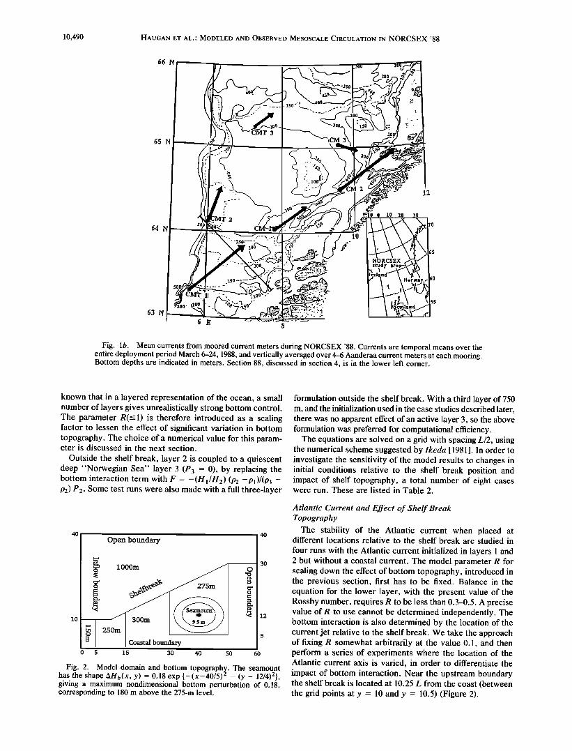
Fig. lb. Mean currents from moored current meters during NORCSEX '88. Currents are temporal means over the entire deployment period March 6-24, 1988, and vertically averaged over 4-6 Aanderaa current meters at each mooring. Bottom depths are indicated in meters. Section 88, discussed in section 4, is in the lower left corner.

known that in a layered representation of the ocean, a small number of layers gives unrealistically strong bottom control. The parameter R(_< 1) is therefore introduced as a scaling factor to lessen the effect of significant variation in bottom topography. The choice of a numerical value for this param- eter is discussed in the next section.

Outside the shelf break, layer 2 is coupled to a quiescent deep "Norwegian Sea" layer 3 (P3 = 0), by replacing the bottom interaction term with F = -(HI/H2) (P2 -Pl)/(P3 - P2) P2. Some test runs were also made with a full three-layer

Open boundary

1000m 0

o 275m rr m o

10

m 250m o 5

• Coastal boundary 0 5 15 30 40 50 60

Fig. 2. Model domain and bottom topograph[. The seamount has the shape AHb(x , y) = 0.18 exp {-(x-40/5) - (y - 12/4)2}, giving a maximum nondimensional bottom perturbation of 0.18, corresponding to 180 m above the 275-m level.

formulation outside the shelf break. With a third layer of 750 m, and the initialization used in the case studies described later, there was no apparent effect of an active layer 3, so the above formulation was preferred for computational efficiency.

The equations are solved on a grid with spacing L/2, using the numerical scheme suggested by Ikeda [1981]. In order to investigate the sensitivity of the model results to changes in initial conditions relative to the shelf break position and impact of shelf topography, a total number of eight cases were run. These are listed in Table 2.

Atlantic Current and Effect of Shelf Break Topography

The stability of the Atlantic current when placed at different locations relative to the shelf break are studied in

four runs with the Atlantic current initialized in layers 1 and 2 but without a coastal current. The model parameter R for scaling down the effect of bottom topography, introduced in the previous section, first has to be fixed. Balance in the equation for the lower layer, with the present value of the Rossby number, requires R to be less than 0.3-0.5. A precise value of R to use cannot be determined independently. The bottom interaction is also determined by the location of the current jet relative to the shelf break. We take the approach of fixing R somewhat arbitrarily at the value 0.1, and then perform a series of experiments where the location of the Atlantic current axis is varied, in order to differentiate the impact of bottom interaction. Near the upstream boundary the shelf break is located at 10.25 L from the coast (between the grid points at y = 10 and y = 10.5) (Figure 2).

HAUGAN ET AL ' MODELED AND OBSERVED MESOSCALE CIRCULATION IN NORCSEX '88 10,491

TABLE 2. Model Cases

Case

Parameter 1 2 3 4 5 6 7 8

Atlantic Current

Axis, upstream y ax 11.5 10.5 9.5 8.5 9.5 9.5 9.5 9.5 e-folding width: Ay 2.5 2.5 2.5 2.5 2.5 2.5 2.5 2.5 Uma x (layers I and 2) 1.0 1.0 1.0 1.0 1.0 1.0 1.0 1.0

Coastal Current

Axis: y ax 4 4 4 4 4 4 4 4 e-folding width: Ay 1.43 1.43 1.43 1.43 1.43 1.43 1.43 1.43 Umax, layer 1 0 0 0 0 1 1 1 1 Umax, layer 2 0 0 0 0 0 0.3 0.6 0.6

Eddy Location (Xe, Y e) ..................... (6, 6.5) Strength, Ap max ..................... 1 e-folding scale, Ar ..................... 1.41

The velocity profiles in the Atlantic and Coastal current jets are given by U(y) = Uma x exp {-[(y - Yax)/Ay]2}. The Atlantic current axis in general follows the shelf break. For cases with nonstandard location of the axis, the shift is the same downstream as upstream. The additional eddy perturbation in case 8 has the shape Zip(x, y) = ziPmax .exp {-[(x - Xe) 2 + (y - ye)2]/Ar2}.

Case 1. The axis of the Atlantic current is located 1.25 L

off the shelf break. This results in a very stable current that is totally controlled by the bottom topography and is flowing along the shelf break (not shown).

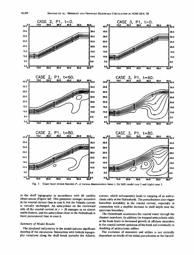
Case 2. The axis of the current is 0.25 L off the shelf

break. This means that a part of the Atlantic current flows over the shelf, interacting with the shelf topography. This results in a weak circulation of AW on the shelf (Figure 3), and some recirculation due to interaction with the seamount.

Case 3. The axis of the current is 0.75 L inside of the

shelf break. This gives strong interaction between the cur- rent and the steps on the shelf, and strong circulation of AW over the shelf. At t - 60 the flow is topographically steered by the seamount and flows around the seamount with deeper water to the left (Figure 3), and at t = 80 an anticyclone is found near the top of the seamount. The modeled flow field is in good agreement with the observed accumulation of AW over the bank and downstream of it, and with coastal water extending seaward upstream of the bank (Figure la).

Case 4. Finally we initialize the current with axis 1.75 L inside the shelf break, which means that most of the current is located on the shelf. This is a rather unphysical situation at the Haltenbank and results in strong instabilities because of interactions with the bottom topography (not shown).

Coastal Current and Effect of Shelf Topography Case 3 described above indicates steered circulation of

AW around the Haltenbank, in agreement with what is expected from observations. In the following cases where the coastal current is included, we therefore use this initial- ization of the Atlantic current. Three runs with different

amplitude of the coastal current in the lower layer, and a fourth case with an initial eddy perturbation upstream are carried out.

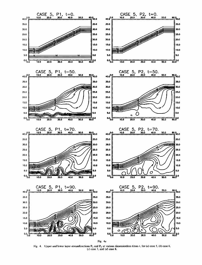
Case 5. In this case we have initialized a baroclinic

coastal current with no current in the lower layer. After a while, the Atlantic current interacts with, and triggers ba- roclinic instability in, the coastal current. Meanders start growing in the entire coastal current, and rather strong meanders are also observed east of the seamount (Figure

4a). The evolution of the Atlantic current remains as in case 3. The mesoscale flow on the shelf thus appears to have minor impact on the AW flow along the shelf break.

An anticyclone evolves in the strong meander at x = 30 from t - 70 to t = 90. It also spins up anticyclonic circulation in layer 2, located exactly above a step in the bottom topography (Figures 2 and 4). The anticyclone propagates offshore with deeper water to the left and with a small downslope component due to the nonlinear effect [Ikeda and Lygre, 1989].

Case 6. A weak barotropic component is included in the coastal current; the current in layer 2 is 30% of the current in layer 1, providing a baroclinic to barotropic component ratio (BC/BT) of 7/3. This ensures stronger topographical control in the coastal current. Early in the run an onshore flow component is established near the inflow boundary due to the flow into regions with deeper water (Figure 4b). These perturbations (in the two layers) grow into meanders as they propagate northward, but they are weaker and do not extend as far seaward as in case 5. At the seamount, most of the coastal current is accelerated and squeezed through the narrow channel to the east of the seamount. We note in

comparison that high velocities, up to 60-70 cm s -1 were observed in this channel during NORCSEX '88. In this case with a barotropic component in the current, the meanders in the channel disappear and the current flows straight through the channel. This is in contrast to the completely baroclinic case (case 5), which allowed stronger meander growth, in agreement with general results of Ikeda et al. [1989].

Case 7. A stronger barotropic component is used in the coastal current; the current in layer 2 is 60% of the upper layer current. Hence the BC/BT ratio decreases to 2/3. The same acceleration of the coastal current and squeezing through the channel east of the seamount as in case 6 is observed. In fact, the solution is similar to case 6 except that three meanders are developed upstream of the Haltenbank instead of two (Figure 4c).

Case 8. This case is the same as case 6 except that a barotropic eddylike perturbation is introduced on the shore- ward side of the Atlantic current close to the upstream step

10,492 HAUGAN ET AL.' MODELED AND OBSERVED MESOSCALE CIRCULATION IN NORCSEX '88

40.00'0

35.0

30.0

25.0

20.0

15.0

10.0

5.0

40.00'0

35.0

30.0

25.0

20.0

15.0

10.0

5.0

40.½ '0

35.0

30.0

25.0

20.0

15.0

10.0

5.0

0,1

CASE 2, 1 o.o 20.0

P1, t-O. CASE 3, P1, t-O. •o.o ,o.o •o.o •o.%. ø ,o.oO.O ,o.o :o.o :o.o 50.0

35.0 35.0

30.0 30.0

25.0 25.0

20.0 20.0

15.0 15.0

lO.O lO.O

5.0 5.0

10.0 20.0 30.0 40.0 50.0 1.0 0'00.0 10.0 20.0 30.0 40.0 50.0

CASE 2, 1 o.o 20.0

P1, t=60. CASE 3, P1, t=60. :o.o •o.o so.o •o.%. o •o. oO.O ,o.o :o.o :o.o •o.o

35.0 35.0

30.0 30.0

25.0 25.0

20.0 20.0

15.0 15.0

10.0 lO.O

5.0 5.0

10.0 20.0 30.0 40.0 50.0 1.0 0'00.0 10.0 20.0 30.0 40.0 50.0

CASE 2, P1, t=80. 10.0 20.0 30.0 40.0

CASE 3, P1, t-80. 50.0 60.%. 0 40.00.0 10.0 20.0 30.0 40.0 50.0

35.0 35.0

30.0 30.0

25.0 25.0

20.0 20.0

o 15.0 15.0

lO.O lO.O

5.0 5.0

,o.o 20.0 •o.o 40.0 •.o •o.o ø'ø ø'øo.o •o.o 20.0 3o.o 40.0 so.o

Fig. 3. Upper layer stream function P] at various dimensionless times t, for (left) model case 2 and (right) case 3.

60'(•10. 0

35.0

30.0

25.0

20.0

15.0

10.0

5.0

60'040.0

35.0

30.0

25.0

20.0

15.0

10.0

5.0

}.0

60'040.0

35.0

30.0

25.0

20.0

15.0

10.0

5.0

1.0

in the shelf topography in accordance with IR satellite observations (Figure 4d). This generates stronger meanders in the coastal current than in case 6, but the Atlantic current is virtually unchanged. An anticyclone on the shoreward side of the coastal current at x = 20 emerges as an almost stable feature, and the anticyclone close to the Haltenbank is more pronounced than in case 6.

Summary of Model Results

The idealized bathymetry in the model induces significant steering of the circulation. Interaction with bottom topogra- phy variations along the shelf break perturbs the Atlantic

current, which subsequently leads to trapping of an anticy- clonic eddy at the Haltenbank. The perturbations also trigger baroclinic instability in the coastal current, especially in connection with a steplike increase in shelf depth near the upstream boundary.

The Haltenbank accelerates the coastal water through the channel nearshore. In addition the trapped anticyclonic eddy at the bank leads to increased growth of offshore meanders in the coastal current upstream of the bank and eventually to shedding of anticyclonic eddies.

The evolution of meanders and eddies is not critically dependent on details of the initial perturbation or the barocli-

40.00'0

35.0

CASE 5, P1, t=0. 10.0 20.0 30.0 40.0 50.0 60'%. 0

35.0 35.0

CASE 5, P2, t=0. 10.0 20.0 30.0 40.0 50.0 60'%. 0

35.0

30.0 30.0 30.0 • 30.0

25.0 25.0 25.0 25.0

20.0 20.0 20.0 20.0

15.0 15.0 15.0 15.0

10.0 1 o.o 1 o.o 10.0

5.0 5.0 5.0 5.0

0.0 0.0 10.0 20.0 30.0 40.0 50.0 6C 10.0 20.0 30.0 40.0 50.0

).0 6C

40.00'0 CASE 5, P1, t-50. 10.0 20.0 30.0 40.0 50.0

CASE 5, P2, t-50. 10.0 20.0 30.0 40.0 60-%. 0

35.0 35.0 35.0 35.0

30.0 30.0 30.0 30.0

25.0 25.0 25.0 25.0

20.0 20.0 20.0 20.0

15.0 15.0 15.0 15.0

10. 0 10.0 10.0 10.0

5.0

10.0 20.0 30.0 40.0 50.0

5.0

).0

5.0 0 O 5.0 ).0

10.0 20.0 30.0 40.0 50.0

40.00'0

35.0

30.0

CASE 5, P1, t=70. 10.0 20.0 30.0 40.0 50.0 60.%. 0

35.0

30.0

CASE 5, P2, t-70. 40 00.0 10.0 20.0 30.0 40.0 50.0 60 0 lllllllllllllllllllllllllllllllllllllllllllllllllllllllll '40.0

30.0 30.0

25.0 25.0 25.0 25.0

20.0 20.0 20.0 20.0

15.0 15.0 15.0 15.0

10.0 1 o.o 1 o.o 10.0

5.0 5.0 5.0 5.0

1.0 10.0 20.0 30.0 40.0 50.0 10.0 20.0 30.0 40.0 50.0

1.0

0.0 40.O

CASE 5, P1, t=90. CASE 5, P2, t-go. ,o.o •o.o •o.o •o.o •o.o •o.%. o •o.oo.o ,o.o •o.o •o.o •o.o 50.0 60'%. 0

35.0 35.0 35.0 35.0

30,0 30.0 30.0 30.0

25.0 25.0 25.0 25.0

20.0 20.0 20.0 20.0

15.0 15.0 15.0 15.0

10.0 lO.O lO.O lO.O

5.0 5.0 5.0 5.0

10.0 20.0 30.0 40.0 50.0 10.0 20.0 30.0 40.0 50.0 1.0

6C

Fig. 4a

Fig. 4. Upper and lower layer streamfunctions P1 and P2 at various dimensionless times t, for (a) case 5, (b) case 6, (c) case 7, and (d) case 8.

10,494 HAUGAN ET AL.' MODELED AND OBSERVED MESOSCALE CIRCULATION IN NORCSEX '88

CASE 6, P1, t-O. CASE 6, P2, t-O. ,0.00.0 ,0.0 20.0 30.0 ,0.0 •0.0 •0.%. 0 •0.00.0 ,0.0 20.0 •0.0 ,0.0 •0.0 •0.%. 0 35.0 35.0 35.0 35.0

50.0 .30.0 30.0 • 30.0

25.0 25.0 25.0 25.0

20.0 20.0 20.0 20.0

15.0 15.0 15.0 15.0

10. 0 1 0.0 1 0.0 1 0.0

0'00.0 10.0 20.0 30.0 40.0 50.0

5.0 5.0 5.0

,.o 0'003 ,o.o 2o.o •o.o ,o.o •o.o ,.o

CASE 6, P1, t=50. CASE 6, P2, t-50. •o.o ø'ø ,o.o 20.0 •o.o •o.o •o.o •o.%. o •o.oO.O ,o.o 20.0 •o.o •o.o •o.o •o.%. o 55.0 35.0 35.0 35.0

30.0 30.0 30.0 30.0

25.0 25.0 25.0 25.0

20.0 20.0 20.0 20.0

15.0 15.0 15.0 15.0

10.0 •a., 10.0 10.0 • 10.0 5.0 5.0 5.0 5.0

0'%.0 10.0 20.0 30.0 40.0 50.0 ,.o ø'øo.• ,o.o 20.0 •o.o ,o.o •o.o ,.o

CASE 6, P1, t-70. CASE 6, P2, t=70. •o.o ø'ø ,o.o 20.0 =o.o •o.o •o.o •o.%. o ,o.oO.O ,o.o 20.0 =o.o •o.o •o.o •o.%. o 35.0 35.0 35.0 35.0

30.0 30.0 30.0 30.0

25.0 25.0 25.0 25.0

20.0 20.0 20.0 20.0

15.0 15.0 15.0 15.0

10.0

5.0

10.0 20.0 50.0 40.0 50.0 6C

1 o.o 1 o.o 1 o.o

•.o 5.0 • •.o

,.o ø'øo.• •o.o •o.o •o.o ,o.o •o.o ,.o

CASE 6, P1, t-90. CASE 6, P2, t-90. •0.00.0 ,0.0 20.0 •0.0 ,0.0 •0.0 •0.%. 0 ,0.00.0 ,0.0 20.0 •0.0 ,0.0 •0.0 •0.%. 0 35.0 35.0 35.0 35.0

30.0 50.0 50.0 30.0

25.0 O 25.0 25.0 25.0 20.0 20.0 20.0 20.0

15.0 15.0 15.0 15.0

10.0 10.0 10.0 10.0

5.0 5.0 5.0 5.0

0.00. 0 10.0 20.0 50.0 40.0 50.0 60.8 '0 0'00.•) 10.0 20.0 50.0 40.0 50.0 61: Fig. 4b

HAUGAN ET AL ' MODELED AND OBSERVED MESOSCALE CIRCULATION IN NORCSEX '88 10,495

CASE 7, P1, t-0. CASE 7, P2, t=0. ,o.oO.O ,o.o =o.o •o.o •o.o •o.o so.%. o ,o.oO.O ,o.o =o.o •o.o •o.o •o.o •o.%. o

35.0 35.0 35.0 35.0

30.0 • 30.0 30.0 • 30.0

25.0 25.0 25.0 25.0

20.0 20.0 20.0 20.0

15.0 15.0 15.0 15.0

10.0 10.0 10.0 10.0

5.0 ,• •------•---5.0 5.0 • 4•• 5.0

0'00.0 10.0 20.0 50.0 40.0 50.0 ).0 10.0 20.0 30.0 40.0 50.0 ).0

CASE 7, P1, t=50. CASE 7, P2, t-50.

4o.oO.O ,o.o :,o.o •o.o ,,o.o •.o eo.O,o.o ,o.oO.O ,.o.o •o.o •o.o ,•;,o, ,,•,o;,o, ,•i.o IIIIII IIIIIIIIIIIIIIIIIIIIIIIIIIII IIII IIIIII 40.0

•.o •.o •.o I •.o •o.o •o.o •o.o • •o.o

•,.o •.o •.o •.o

•o.o •o.o •o.o •o.o

15.0 15.0 15.0 15.0

10.0 10.0 10.0 10.0

5.0 5.0 5.0 5.0

ø'øo.•) ,o.o :,o.o :so.o •.o •o.o ).o 10.0 20.0 30.0 40.0 50.0 ).0

CASE 7, P1, t-70. CASE 7, P2, t-70.

,,o.oO.o ,o.o ,o.o ,o.o ,.o ,o.o ,o.O(o o ,o.oø- i ,o.o ,o.o ,o.o ,.o so.o ß IIIIIIIIIIIIIIII1'11111111 iiiiiiiiiiiiiiiiiiiiiiiiiiiiiiii '40.0

35.0 35.0 35.0 I• 35.0 30.0 30.0 30.0 30.0

25.0 25.0 25.0 25.0

20.0 20.0 20.0 20.0

15.0 15.0 15.0 15.0

10.0 10.0 10.0 10.0

5.0 5.0 5.0 5.0

0'00.0 10.0 20.0 50.0 40.0 50.0 1.0 ø'øo.•) •o.o 20.0 :so.o •.o so.o ec ).o

CASE 7, P1, t-go. CASE 7, P2, t-go. •o.oO.O ,o.o =o.o •o.o •o.o •o.o eo.%. o ,o.oO.O ,o.o =o.o •o.o •o.o •o.o eo.%. o

35.0 35.0 35.0 35.0

30.0 30.0 30.0 30.0

25.0 25.0 25.0 25.0

20.0 20.0 20.0 20.0

15.0 ! 5.0 ! 5.0 ! 5.0

10. 0 10.0 10.0 10.0

5.0 5.0 5.0 5.0

ø'øo.•) •o.o :,o.o •o.o •.o so.o ec ,.o Fig. 4c

10.0 20.0 30.0 40.0 50.0 6C ).0

10,496 HAYGAN ET AL.' MODELED AND OBSERVED MESOSCALE CIRCULATION IN NORCSEX '88

40.00'0 CASE 8,

1 o.o 2o.o P1, t=O. CASE 8, P2, t=O. ,30.0 40.0 50.0 60.%. 0 40.00.0 10.0 20.0 ,30.0 40.0 50.0 60.%. 0

35.0 ,35.0 35.0 ,35.0

,:30.0 ,30.0 50.0 • 30.0

25.0 25.0 25.0 25.0

20.0 20.0 20.0 20.0

15.0 15.0 15.0 15.0

10.0 10.0 10.0 10.0

4.• ,4.• • 5.0 5.0 5.0

10.0 20.0 30.0 40.0 50.0 1.0 0'00.0 1 0.0 20.0 ,30.0 40.0 50.0 1.0

5.0

40.00'0 CASE 8, lO.O 2o.o

P1, t-50. CASE 8, P2, t=50. •o.o 40.0 5o.o 6o.%. o ,o.oO.O •o.o 20.0 •o.o ,o.o 50.0 60.%. 0

,35.0 ,35.0 35.0 35.0

,:30.0 ,30.0 ,30.0 ,30.0

25.0 25.0 25.0 25.0

20.0 20.0 20.0 20.0

15.0 15.0 15.0 15.0

10.0 10.0 10.0 10.0

5.0 5.0 5.0 5.0

30.0 40.0 •0.0 ,.0 ø'ø0.'0 •0.0 20.0 30.0 40.0 •0.0 10.0 20.0

40.00'0 CASE 8, 1 o.o 20.0

P1, t-70. CASE 8, P2, t-70. •o.o ,o.o 50.0 6o.%. o ,o.oO.O •o.o 20.0 •o.o ,o.o 50.0 60.040.0

35.0 ,35.0 35.0 35.0

,30.0 30.0 ,30.0 30.0

25.0 25.0 25.0 25.0

20.0 20.0 20.0 20.0

15.0 15.0 15.0 15.0

10.0 10.0 10.0 10.0

5.0 5.0 5.0 5.0

O.Oo.• ,30.0 40.0 50.0 60.00'0 10.0 20.0 `30.0 40.0 50.0 1.0 10.0 20.0

40.00'0

,35.0

,30.0

25.0

20.0

15.0

10.0

5.0

CASE 8, P1, t=90. 10.0 20.0 ,30.0 40.0

10.0 20.0

50.0 60.%. 0

35.0

CASE 8, P2, t-90. 40.½.0 10.0 20.0 ,30.0 40.0 50.0 60 0 IIIIIIIIIIIIIIIIIIIIIIIIIIIIIIIIIllllllllllllllllllllllll '40.0

35.0 • 1 35.0 ,30.0 50.0

25.0 25.0

20.0 20.0

15.0 15.0

lO.O lO.O

5.0 5.0 5.0

30.0

25.0

20.0

15.0

10.0

30.0 40.0 50.0 60.(• '0 10.0 20.0 30.0 40.0 50.0 1.0 Fig. 4d

HAUGAN ET AL.' MODELED AND OBSERVED MESOSCALE CIRCULATION IN NORCSEX '88 10,497

CMT1

ß

: .... •o .... -• .... •o ....

'•o l• 80

CM1

lO • 8O

CM3

North

t , cm/s East !

10 20 30

Fig. 5. Velocity stick plots from all moorings at 25 m. Data have been smoothed with a 36-hour low-pass filter. Time scale is in Julian days of 1988, so that (for example) March 20 is in the interval 79-80. Features E 1 to E4 indicate eddies which are referred to in the text.

nicity in the coastal current except that propagation of meanders past the Haltenbank is observed only in the pure baroclinic coastal current.

Shelf waves forced by a varying wind field are not in- cluded in the model [Gjevik, 1989]. In reality, these mecha- nisms, as well as tidal rectification over the Haltenbank [Hunkins, 1986], might contribute to the mesoscale flow pattern. In addition, the upstream boundary condition in the model has no variation in time and therefore cannot account

for perturbations that propagate northeastward into the upstream domain. An indication of such a perturbation is seen in the advanced very high resolution radiometer (AVHRR) image in Figure la around 4øE, 63øN. This will be further discussed in section 6.

4. OBSERVATIONS

Moored Current Meter Data

The velocity stick plots from each current meter at 25 m obtained during the sampling interval have been smoothed with a 36-hour low-pass filter to remove the tidal and inertial motions (Figure 5). The filtered currents show large temporal and spatial variations ranging from less than 0.05 m s -• to

0.60 m s -• suggesting a characteristic speed of 0.3 m s -• used in the model. The mean and standard deviation of the

measured current components are shown in Table 1. At mooring CMT1 (placed along the shelf break), and in the upper 150 m at CM2 (placed in the channel), the mean currents are larger than the variability, indicating a relatively strong steady current component at these locations. The stability at these locations occurred in spite of variable winds encountered during NORCSEX '88, including a 2-day period with predominantly northwesterly winds with an average of 10 m s - • on the March 11-13.

CMT2 (at the shelf break) is more variable than CMT1, but it also has a dominating northward component (Table 1 and Figure 5). The measurements from these two moorings are therefore in agreement with the model results of a topo- graphically controlled Atlantic current along the shelf break.

Maximum currents of 0.60-0.70 m s -• are reported at CM2, where the model indicates a directional steering and acceleration of the coastal current northeastward past the Haltenbank. The large temporal changes in the upper 100 m at this mooring (Figure 5), are not apparently correlated with observations at other moorings. These changes are therefore probably not of direct meteorological origin but suggest

10,498 HAUGAN ET AL.' MODELED AND OBSERVED MESOSCALE CIRCULATION IN NORCSEX '88

NORTHWEb•

CURRENT VECTORS

SOUTHEAS•

lOO

SALINITY .... i ........ , ......... ! ......... , ......... . .... ß .... ! ß ß

ffi 40 00 8o lOO

DISTANCE IN KM

Fig. 6. ADCP velocity stick plots at 25 m and 100 m, and SeaSoar salinity structure from section 88. The location of this section is indicated in Figure Ib.

150

baroclinic meanders in the coastal current. According to the model results, well-developed meanders at this location are possible only if the coastal current is strongly baroclinic.

The weak southerly component at CM3 reflects topo- graphic steering by the Haltenbank setting up an anticy- clonic vortex circulation around the bank in agreement with the model results above. This is also in agreement with satellite IR images (Figure l a is one example of this) which show a tendency for Atlantic water to occupy the bank region, implying weak vertical stratification, which in turn favors topographic steering.

In addition to the meandering current reported at CM2, the currents at CMT3 and CM1 also veer from north to

south, showing temporal evolution of several "open and closed" fans. According to Foldvik et al. [1988], such

behavior of the current vectors may be associated with the propagation of eddies past the moorings. Assuming that the eddy propagation is northeastward with the mean current, the "open fan" structure will always reflect the passage of a cyclonic eddy, while the "closed fan" structure always reflects the passage of an anticyclonic eddy. Four eddy features, E 1 to E4 (Figure 5) are clearly identified using this method. E1 and E2 are located in the most meander- and

eddy-rich region predicted by the model.

Ship Data

The simultaneously acoustic Doppler current profiler (ADCP) current measurements and SeaSoar conductivity- temperature-depth (CTD) observations allow a check on the

TABLE 3. ADCP Data Statistics

I•, U, Sil , S U •

Data Set N Nac c cm s- I cm s- 1 cm s- 1 cm s- 1

All (26 m) 10,000 5630 5.9 1.3 23 22 All (102 m) 10,000 5555 4.3 1.3 18 18 Event (26 m) 639 366 7.4 -4.7 20 29 Event (102 m) 639 362 4.7 0.6 15 15

Mean flow and variance at 4-m depth bins centered around 26- and 102-m depth, of the whole NORCSEX ADCP data set and of the subset used in the detailed event description in section 4. N is the total number of data points available, and Nac c is the number of points accepted after the screening described in the appendix; u and v denote the mean flow in the alongshore-cross-shore coordinate system, and s,, S v, are the standard deviations about this mean.

HAUGAN ET AL.' MODELED AND OBSERVED MESOSCALE CIRCULATION IN NORCSEX '88 10,499

c

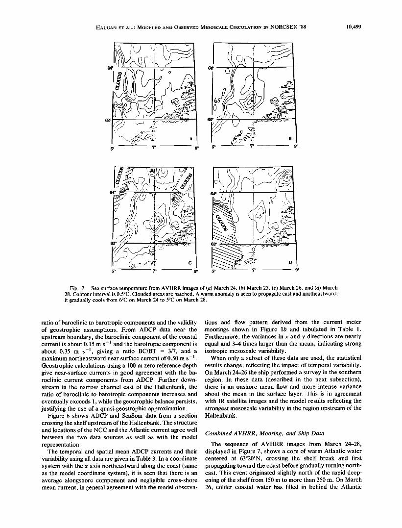
Fig. 7. Sea surface temperature from AVHRR images of (a) March 24, (b) March 25, (c) March 26, and (d) March 28. Contour interval is 0.5øC. Clouded areas are hatched. A warm anomaly is seen to propagate east and northeastward; it gradually cools from 6øC on March 24 to 5øC on March 28.

ratio of baroclinic to barotropic components and the validity of geostrophic assumptions. From ADCP data near the upstream boundary, the baroclinic component of the coastal current is about 0.15 m s -• and the barotropic component is about 0.35 m s -• giving a ratio BC/BT - 3/7, and a maximum northeastward near surface current of 0.50 m s-•. Geostrophic calculations using a 100-m zero reference depth give near-surface currents in good agreement with the ba- roclinic current components from ADCP. Further down- stream in the narrow channel east of the Haltenbank, the ratio of baroclinic to barotropic components increases and eventually exceeds 1, while the geostrophic balance persists, justifying the use of a quasi-geostrophic approximation.

Figure 6 shows ADCP and SeaSoar data from a section crossing the shelf upstream of the Haltenbank. The structure and locations of the NCC and the Atlantic current agree well between the two data sources as well as with the model

representation. The temporal and spatial mean ADCP currents and their

variability using all data are given in Table 3. In a coordinate system with the x axis northeastward along the coast (same as the model coordinate system), it is seen that there is an average alongshore component and negligible cross-shore mean current, in general agreement with the model observa-

tions and flow pattern derived from the current meter moorings shown in Figure lb and tabulated in Table 1. Furthermore, the variances in x and y directions are nearly equal and 3-4 times larger than the mean, indicating strong isotropic mesoscale variability.

When only a subset of these data are used, the statistical results change, reflecting the impact of temporal variability. On March 24-26 the ship performed a survey in the southern region. In these data (described in the next subsection), there is an onshore mean flow and more intense variance

about the mean in the surface layer. This is in agreement with IR satellite images and the model results reflecting the strongest mesoscale variability in the region upstream of the Haltenbank.

Combined A VHRR, Mooring, and Ship Data

The sequence of AVHRR images from March 24-28, displayed in Figure 7, shows a core of warm Atlantic water centered at 63ø20'N, crossing the shelf break and first propagating toward the coast before gradually turning north- east. This event originated slightly north of the rapid deep- ening of the shelf from 150 m to more than 250 m. On March 26, colder coastal water has filled in behind the Atlantic

10,500 HAUGAN ET AL.: MODELED AND OBSERVED MESOSCALE CIRCULATION IN NORCSEX '88

RUEL25

10 kin:

0.5 m/s:

AUEL100

10 kin:

0.5 m/s:

Fig. 8. Optimally estimated ADCP currents at 26-m and 102-m depth. The time of analysis is March 26, 0000 UT. Data were collected from March 25, 1750 UT to March 26, 1500 UT, from north to south along the indicated ship tracks. Analysis parameters are given in the appendix.

water, trapping the intrusion in the coastal current. The migration speed of the core of maximum temperature is estimated from the images to be close to 0.13 m s -• (6 km d-I), in good agreement with the mean current from moor- ings CMT1 and CM1. However, the actual advection speed of the near-surface water mass may be larger than this, since some mixing and cooling is expected to take place at the leading edge of the intrusion.

In accordance with this event, low-pass-filtered currents at mooring CMT1 fight at the shelf break (Figure 1) increase from 0.10-0.20 m s -1 in the first 15 days to more than 0.30 m s- 1 from March 20 until the end of the deployment period on March 23 (Figure 5).

The combined observations from CMT1 and AVHRR

indicate a growing perturbation in the Atlantic current close to CMT1 on March 20-21, which will interact strongly with the bottom topography as discussed in the modeling section (Figures 4b, 4c, and 4d). In turn, this results in eastward flow along the steplike bottom topography around March 23 and finally is advected northwards with the coastal current on March 26-28. On the basis of these results it appears that this flow regime is intermittent and can occur in events with time scales of 4-8 days. Eastward flow along this topographic feature has also been reported from drifter experiment (R. Sartre, Institute of Marine Research Bergen, personal com- munication, 1990).

Gfidded circulation maps are obtained from the ADCP data as shown in Figure 8. The method chosen to construct these maps is based on optimal estimation, usually denoted objective analysis in meteorological and oceanographical

applications [Bretherton et al., 1976; McWilliams et al., 1986]. It requires estimation of the velocity correlation structure. Application of this method to ADCP data is not previously reported in the literature (except briefly by Haugan et al. [ 1989]). Anomalies relative to a mean velocity field are analysed using analytical, homogeneous, isotropic spatial correlation functions, justified and derived from the ADCP observations. A more detailed discussion and speci- fication of our use of this method is given in the appendix.

Eastward flow along the steplike topography and associ- ated with eddies further downstream are observed (Figure 8). This might be compared to the model results in cases 6-8. In agreement with the model results, we have indications that the eddy pattern displayed in these maps originated from an anomaly in the Atlantic current. The strong barotro- pic component of the generated eddies also points to the importance of topographic effects in their further develop- ment.

It is clear that we need more regular synoptic data coverage in order to fully test, validate, and improve models of coastal circulation to be used in the Norwegian HOV. The Seasat SAR was demonstrated to be capable of detecting current patterns independent of clouds [Beal et al., 1981]. Moreover, Johannessen et al. [this issue] documented the relationship between SAR image expressions and mesoscale current boundaries. They also discussed the sensitivity of the SAR imaging capability to wind speed and radar look direction, which favors detection capabilities for certain configurations. On the other hand, as was discussed by Barnett et al. [1989], the SAR can also obtain indirect estimates of the current shear strength and position from imaging of long wave-current refraction. This is further discussed in the next section.

5. SAR AND WAVE-CURRENT REFRACTION

The limitations of SAR imaging capabilities of ocean waves, i.e., to determine wavelength and wave propagation direction, have been documented in several papers to be primarily a result of (1) too high a ratio of radar range (R) to radar velocity (V), and (2) near-azimuth-traveling waves [Hasselmann et al., 1985]. However, under optimal imaging conditions the wave propagation direction detected by SAR across spatial distances of 100 km or more provides oppor- tunities to examine evidence of ocean wave refraction in-

duced by spatial varying bottom depth and surface current [Beal et al., 1981].

According to Shuchman and Kasischke [1981], wave refraction induced by bottom topography can be expected only when the requirement D < L/3, where D is the water depth and L is wavelength, is met. The SAR-derived ocean wave spectra as well as the wave observations from the four NORWAVE/Wavescan directional wave measuring buoys during NORCSEX '88 show that the longest waves exceed 300 m only in a few cases, while the predominant wave propagation direction ranged from easterly to northeasterly [Johannessen et al., this issue]. This implies that even wave-bottom refraction induced by the shallow plateau of about 100 m at the Haltenbank can be ignored.

The wave-current refraction can reflect two kinds of

mesoscale current pattern: (1) current strain rate, 0u/0r • 0 where u are current components in the r direction; and (2) cyclonic (anticylonic) current shear where Vxu % 0.

Strec•r•f•ncti•on P ! T-90 0.0 10.0 20.0 50.0 40.0 50.0 60.0

40.0 i iiii ii iii ii ii ii ii ii ii ii ii iii ii ii ii ii ii il iI ii ii iii i1• 40.0 30,0 •: 30.0

25.0 • •' 25.0 ß

a.•, 20.0 20.0 o.•

15.0 15.0

lO.O lO.O

ß 0 0 10 0 20 0 50 0 40 0 50 0 60 (•.0

40

35

30

20

1,5

10

0 0

lambda=110m, alpha=-90 40 T T r r ,

b 35

30

20

15

10

,5 ß

0 i ,

0 10 20 30 40 50 60

lambda= 1 lorn

i ! i i i

c

Fig. 9. Wave-current refraction' (a) Upper layer stream function used in wave-current refraction calculations, (b) Waves propagating southeasterly, and (c) Waves propagating northeasterly.

10,502 HAUGAN ET AL.' MODELED AND OBSERVED MESOSCALE CIRCULATION IN NORCSEX '88

RMS ANOMAL ES (ALL TRACKS)

Fig. 10. Contours of Geosat-derived rms height.

Using a ray-tracing method [Lyzenga and Bennett, 1988; Mathiesen, 1987; Phillips, 1981], the refraction induced by the modeled and observed mesoscale circulation pattern discussed in section 4 is studied. The action conservation

equation is used to formulate a set of four equations giving the wave ray and wave number characteristics in the r, n plane:

Or/Ot = u + Car

On/Ot = v + Can

Okr/Ot = -krOu/Or- knOv/Or

Southeasterly propagating waves cross the current steered along the shelf break practically without being refracted (Figure 9b). On the other hand, the mesoscale meander and eddy circulation pattern in the coastal current, especially located between 20 and 35, induce wave refractions that lead to focal points and shadow zones near shore. The results are sensitive to the current profile such that the focal points and shadow zones for the southeasterly propagating waves are found behind the regions of maximum offshore and onshore current. In contrast, northeasterly propagating waves are immediately refracted by the upstream Atlantic water and coastal current (Figure 9c). As a result, in turn a zone of focal points start to form at the shelf break centered at 35,15. On the shelf the refractions are more complicated, displaying several areas of focal points and shadow zones, since refractions induced by the meander and eddy circulation pattern are superimposed on the upstream refraction. A particularly large shadow zone is formed downstream from 20,10 (Figure 9c).

As was pointed out by Barnett et al [1989], who inverted the current shear from space shuttle SAR images, their method is based on some assumptions that have clear limitations, especially the assumptions of (1) uniform spatial wind field, (2) small relative wave-current angles, and (3) wave-radar look direction in range configuration. The latter two assumptions were satisfied during the SAR flight on March 20. We are therefore validating the refraction model results to these observations.

The analyses of the SAR wave data are included by Mognard et al. [this issue]. They report on clear evidence of refraction of the swell by local current features. Using their results, the refraction in offshore direction at the shelf break is estimated to about 15ø-20 ø . This is in quantitative agree- ment with the model results shown in Figure 9c. The current

-1 along the shelf break is thus expected to be about 0.20 m s in accordance with the magnitude obtained in the model. In comparison, maximum currents of 0.20-0.25 m s -1 are reported respectively on CMT3 and CMT2 (Figure lb and Figure 5) on March 20. These results suggest that combining a wave-current refraction model and SAR wave field images provides a method to better validate the magnitude of the inverted current.

Okn/Ot = -krOu/On- knOv/On

The variables u and v are the current components in the r

and n directions, Car and Can are the group velocities in the same directions, and k r and kn are the corresponding wave numbers. The equations are scaled so they match the model grid, and the velocity components and derivatives are ob- tained from interpolations of the model solution to the grid points. When the initial wave ray starting points and direc- tions are given, the equations are solved for the wave propagation.

We have selected the modeled stream function obtained

for the baroclinic simulation run, case 6, reproduced in Figure 9a. This shows a strong topographic steering of the Atlantic water along the shelf break as well as significant perturbations of the coastal current including the evidence of topographically steered circulation around the Haltenbank. Wave trains at wavelengths between 100 and 200 m are forced to propagate through this circulation pattern in dif- ferent directions.

6. ALTIMETER SEA SURFACE HEIGHT OBSERVATIONS

In order to construct a horizontal contour map of the residual height, data from the first 62 repeat cycles of the Geosat Exact Repeat Mission were used. Each track is typically a few hundred kilometers long within the box considered, but data gaps occur, leading to variation in the number of points and consequently the extent of the track from one period to the next. A method to compute the mean height which specifically accounts for this problem of han- dling data gaps is proposed by Chelton et al. [1989]. We have employed this method. It involves using the along-track height derivatives (slopes) to obtain the mean. The deriva- tives are estimated for each point using finite differences in height at neighboring points. At each point a mean slope is then calculated using all repeat cycles. The orbit error, essentially having long-wavelength characteristics, will not contaminate this mean slope. The mean height is then estimated by stepwise integration of the mean slope. An initial mean height is selected at the integration starting

HAUGAN ET AL.: MODELED AND OBSERVED MESOSCALE CIRCULATION IN NORCSEX '88 10,503

0 0 0 0 0 0 ß •6 cS v• d • d o o

,,,,,,,, o

o

o

o

1111Lll IIIII111 IIIIIII III!1111 IIIIII!

-o

o

10,504 HAUGAN ET AL.' MODELED AND OBSERVED MESOSCALE CIRCULATION IN NORCSEX '88

.2.

-.4

o 30

Lon-25m-South r-lTrans-25m-South •,Lon - I02- South

Trans -lOP-South

• ' 1 '0 1 '5 2'0 2'5 ' Dis:once (kin)

Fig. 12. Empirical longitudinal and transversal correlation functions at 25-m and 102-m depth, calculated from equation (1) using all pairs of data points from ADCP sections 130-139 with a time separation of less than 0.1 day.

point. (This may introduce a constant bias). In the case of data gaps, a starting point is found for each segment, and the integration is performed.

The results of this analyses are shown in Figure 10. In the QG model domain, rms height anomalies range between 6 and 20 cm. In the nearshore sector from the Haltenbank, an elongated region of high rms occurs in the descending direction almost parallel to the coast. The maximum is located close to the top of the Haltenbank (see bottom topography in Figure lb).

The model-predicted variability, average Geosat rms, and an AVHRR surface expression are compared in Figure 11. The main feature from Geosat in the model domain is the

aforementioned maximum rms, close to the AVHRR front shoreward and upstream of the Haltenbank. In comparison, model case 6 has highest variability upstream of the Halten- bank but also has high variability also in the narrow trench shoreward of the Haltenbank, and a clear maximum between the Haltenbank and the shelf break (Figure 11 b). The Geosat rms also has a maximum at approximately the same location, but relatively much weaker. The (long-term) Geosat data and (short-term, one case) model results have some apparent similarities in location of maxima, but quantitative differ- ences are present. Such differences are to be expected in comparing any single model simulation with a long time series from Geosat.

Seaward of the shelf break, significant variability is appar- ent in both Geosat and AVHRR data upstream, suggesting advection of mesoscale activity into the domain by the Norwegian Atlantic Current. This area is not described by the model, which focuses on the shelf and uses steady inflow boundary conditions. Future model studies should address whether such features may significantly affect shelf variabil- ity. Also variability in the Norwegian Coastal Current up- stream [Johannessen et al., 1989a] may be advected into the area. However, such perturbations would probably be strongly modified by the shelf topography in the domain and therefore strongly resemble the patterns that were generated internally in the present model study.

7. CONCLUDING REMARKS

Observations of fronts and intrusions from NOAA

AVHRR, of mean mesoscale variability from Geosat altim- etry, and of currents and hydrography from moored and

ship-based instruments provide a consistent picture of the mesoscale variability on the Norwegian continental shelf between 62 ø and 66øN. Its dynamics are represented by a simple QG model with bottom topography, to the extent that we may verify it in view of the significant variability that exists on other time and space scales. The strong effect of bottom topography on mesoscale activity is clearly demon- strated.

However, the interaction between different phenomena, including wave-current refraction and wind-generated re- sponse, needs to be better understood if we are ultimately to devise reliable schemes for marine forecasting. The pros- pects are good, particularly if we develop the ability to make use of future multisensor satellite AVHRR, radar altimeter, and SAR observations. SAR-derived wave fields, for exam- ple, can provide useful indirect observations of mesoscale currents, while the SAR's capability to detect mesoscale circulation pattern such as eddies ensures weather indepen- dent monitoring.

APPENDIX

Optimal Estimation of the Velocity Field From ADCP data

The ADCP data collected during NORCSEX '88 consist of a total of 10,000 absolute velocity profiles. To deal with these data, automatic procedures for data screening and combina- tion are required in order to honor the information content and minimize the effects of noise. A screening is performed to remove suspicious data based on the following criteria: ship turning or too high ship speed, too few pings recorded, too low acoustical amplitude or percentage of pings ac- cepted, too high measured ADCP velocities. A statistical evaluation has been carried out of all ADCP data remaining after the screening described above. Table 3 describes some basic characteristics.

Analytical correlation functions after Freeland and Gould [1976] are used. The mean advection is taken into account in the correlation distance, and correlations are assumed to

2 have an exponential time decay. With o's as the signal variance, T as the e-folding time scale of the signal, U as the mean velocity, and f as the spatial correlation function tensor, the covariance tensor between velocity anomaly ui at

HAUGAN ET AL.: MODELED AND OBSERVED MESOSCALE CIRCULATION IN NORCSEX '88 10,505

position ri, time t i, and velocity anomaly uj at position rj, time tj, is taken to be

coy (ui, uj)= •r• exp (Iti-tj[) ,

T

ß f{Iri- [rj + U(t i -- ½]1}

For each analysis point (ri, ti) , a subset of the most correlated (closest) data points (rj, tj) are chosen to contrib- ute to the analysis. The analysis-observation covariance vector and the two point observation covariance matrix are computed from the above formula with the addition of observation noise on the diagonal of the covariance matrix.

To avoid complications due to correlated subgrid-scale noise [Clancy, 1983], a subsampling of the available data points is performed before analysis. Then the analysis is performed over a 5 km x 5 km grid. The first zero crossing of the transversal correlation function, the e-folding time scale T, and the noise to signal ratio, are set at 20 km, 2.5 days, and 0.2, respectively, on the basis of the analysis below.

Statistical Input Parameters to the Optimal Estimation

To calculate the time and space structure of the velocity correlation functions to be used in optimal estimation, the pairs of data points are binned into time and space distance bins taking account of advection as above. For each depth, the spatially homogeneous mean is subtracted from the individual data values. Longitudinal and transversal velocity correlations are then calculated as average products of residual velocity components, each normalized by the cor- responding velocity variance,

Ncor

2 • (Ui, lU/,2) i=l

(1) N½or

Z [(Ui,1) 2 + (tti,2) 2] i=1

where Ui, 1 and Ui, 2 are the appropriate (longitudinal or transversal) components of the residual velocity in the two points in pair number i, and Nco r is the number of pairs of points in the time and space distance bin.

No significant anisotropy was found in the resulting cor- relation function estimates, so results in Figure 12 are shown only for At, Ar bins (not At, Ax, Ay). The transversal correlation function crosses zero at about 20 km. Functions

based on the whole NORCSEX '88 ADCP data set and

functions based on the subset associated with the Atlantic

intrusion event have rather similar shapes and scales. The correlation levels are higher in the smaller data set from the Atlantic intrusion event. This can be partially explained by some data with high noise in the larger data set but is probably also an effect of the use of a homogeneous mean, which may be less appropriate for such a large area.

The noise/signal ratio may be estimated from limar•0 (1 -f)/f, where f is the correlation function, and the limiting operation is to be understood in the light of analysis (->5 km) versus noise length scale. The noise/signal ratio, which is

normally not a very critical input parameter to the results of objective analysis [Carter and Robinson, 1987], is set to 0.2 in the application described in the text, on the basis of the curves in Figure 12.

Both longitudinal and transversal functions are found to have e-folding time scales of about 0.5 days (not shown). The estimate is crude, however, since the ship-based data collection implies that data points with large time separation tend to also have large separation in space. Few data point pairs with large time lag are sufficiently close in (advection- corrected) space to be significantly correlated. Correlation time scales determined from data will also be affected by tidal and inertial oscillations, which have slow spatial vari- ability but rapid temporal variability, and which we actually want to filter out. Correlation time scales longer than 0.5 days are therefore used in analyses.

The objective analysis procedure also gives an estimate of the errors, assuming perfect statistics. It is emphasized that the actual expected error will be higher than this level, since the assumed statistics in the procedure are not perfect. The error estimate, however, provides a consistent way of dis- carding estimates in points where the error is likely to be high. The vectors plotted in Figure 8 all have theoretical error estimates of less than 2 cm s -•.

Acknowledgments. We would like to thank Motoyoshi Ikeda, Bedford Institute of Oceanography, for providing the initial version of the model, and discussion of some cases. Thanks also to Paul Samuel, NERSC, for implementing and running the Geosat analyses package, to Kjell Kloster, NERSC, for processing of the AVHRR images, and to Kjetil Lygre, NERSC, for comments on an earlier version of the manuscript.

REFERENCES

Audunson, T., V. Dalen, H. Krogstad, H. N. Lie, and O. Stein- bakke, Some observations of ocean fronts, waves and currents in the surface along the Norwegian coast from satellite images and drifting buoys, in The Norwegian Coastal Current, Proceedings From Symposium, edited by R. Sartre and M. Mork, pp. 20-57, University of Bergen, Bergen, Norway, 1981.

Barnett, T. P., F. Kelly, and B. Holt, Estimation of the two- dimensional ocean current shear field with a SAR, J. Geophys. Res., 94, 16,087-16,097, 1989.

Beal, R. C., P.S. DeLeonibus, and I. Katz (Eds.). Spaceborne Synthetic Aperture Radar for Oceanography, Johns Hopkins Oceanogr. Stud., vol. 7, 215 pp., Johns Hopkins University Press, Baltimore, Md., 1981.

Bretherton, F. P., R. E. Davis, and C. B. Fandry, A technique for objective analysis and design of oceanographic experiments ap- plied to MODE-73, Deep Sea Res., 23, 559-582, 1976.

Carter E. F., and A. R. Robinson, Analysis models for the estima- tion of oceanic fields, J. Atmos. Oceanic Technol., 4, 49-74, 1987.

Chelton, D., R. deSzoeke, A. Bennett, R. Miller, and L. Fu, Mesoscale and large-scale variability of the Antarctic Circumpo- lar Current, Minutes of the first TOPEX/POSEIDON Science Working Team, Rep. JPL D-6378, Jet Propul. Lab., Pasadena, Calif., April 1989.

Clancy, R. M., The effect of observational error correlations on objective analysis of ocean thermal structure, Deep Sea Res., Part A, 30, (9), 985-1002, 1983.

Eide, L. I., Evidence of a topographically trapped vortex on the Norwegian continental shelf, Deep Sea Res., Part A, 26(6), 601-621, 1979.

Foldvik, A., K. Aagaard, and T. T0rresen, On the velocity field of the East Greenland Current, Deep Sea Res., 35(8), 1335-1354, 1988.

Freeland, H. J., and W. J. Gould, Objective analysis of meso-scale ocean circulation features, Deep Sea Res., 23,915-923, 1976.

Gjevik, B., Model simulations of tides and shelf waves along the

10,506 HAUGAN ET AL..' MODELED AND OBSERVED MESOSCALE CIRCULATION IN NORCSEX '88

shelves of the Norwegian-Greenland-Barents Sea, in Modeling Marine Systems, vol. 1, edited by A.M. Davies pp. 188-219 CRC Press, Boca Raton, Fla., 1989.

Gjevik, B., and T. Straume, Model simulations of the M2 and the K 1 tide in the Nordic seas and the Arctic Ocean, Tellus, 41 A, 73-96, 1989.

Guddal, J., et al. (Eds), HOV: Havmilj0-Overvfikning og Varsling (Marine monitoring and forecasting), report to the Norwegian Dep. of Environ., Oslo, 1989.

Hasselmann, K., et al., Theory of synthetic aperture radar ocean imaging: A MARSEN view, J. Geophys. Res., 90, 4659-4686, 1985.

Haugan, P.M., J. A. Johannessen, K. Lygre, S. Sandven, and O. M. Johannessen, Simulation experiments of the evolution of mesoscale circulation features in the Norwegian coastal current, in Mesoscale/Synoptic Coherent Structures in Geophysical Tur- bulence, Elsevier Oceanogr. Ser., vol. 50, edited by J. C. J. Nihoul and B. M. Jamart, pp. 303-313, Elsevier, New York, 1989.

Hunkins, K. Anomalous tidal current on the Yermak Plateau, J. Mar. Res., 44, 51-69, 1986.

Ikeda, M., Meanders and detached eddies of a strong eastward- flowing jet using a two-layer quasi-geostrophic model, J. Phys. Oceanogr., 11,526-540, 1981.

Ikeda, M., and K. Lygre, Eddy-current interactions using a two- layer quasi-geostrophic model, in Mesoscale/Synoptic Coherent Structures in Geophysical Turbulence, Elsevier Oceanogr. Ser., vol. 50, edited by J. C. J. Nihoul, and B. M. Jamart, pp. 277-291, Elsevier, New York, 1989.

Ikeda, M., J. A. Johannessen, K. Lygre, and S. Sandven, A process study of mesoscale meanders and eddies in the Norwegian Coastal Current, J. Phys. Oceanogr., 19, 20-35, 1989.

Johannessen, J. A., E. Svendsen, S. Sandven, O. M. Johannessen, and K. Lygre, Three-dimensional structure of mesoscale eddies in the Norwegian Coastal Current, J. Phys. Oceanogr., 19, 3-19, 1989a.

Johannessen, J. A., O. M. Johannessen, and P.M. Haugan, Remote sensing and model simulation studies of the Norwegian Coastal Current, Int. J. Remote Sens., 10(12), 1893-1906, 1989b.

Johannessen, J. A., R. A. Shuchman, O. M. Johannessen, K. L. Davidson, and D. R. Lyzenga, Synthetic aperture radar imaging of upper ocean circulation features and wind fronts, J. Geophys. Res., this issue.

Johannessen, O. M., J. A Johannessen, and B. A. Farrelly, Appli- cation of remote sensing for studies, mapping and forecasting of eddies on the Norwegian Continental Shelf, paper presented at

EARSEL/ESA Symposium on Remote Sensing for Environmen- tal Studies, Eur. Assoc. of Remote Sens. Labs., Brussels, 1983.

Lyzenga, D. R., and J. R. Bennett, Full-spectrum modeling of synthetic aperture radar internal wave signatures, J. Geophys. Res., 93, 12,345-12,354, 1988.

Mathiesen, M., Wave refraction by a current whirl, J. Geophys. Res., 92, 3961-3970, 1987.

McWilliams, J. C., W. B. Owens, and B. L. Hua, An objective analysis of the POLYMODE local dynamics experiment, I, Gen- eral formalism and statistical model selection, J. Phys. Ocean- ogr., 16, 483-504, 1986.

Mognard, N.M., J. A. Johannessen, C. E. Livingston, D. Lyzenga, R. Shuchman, and C. Russel. Simultaneous observations of ocean surface wind and waves by Geosat radar altimeter and airborne synthetic aperture radar during the 1988 Norwegian Continental Shelf Experiment, J. Geophys. Res., this issue.

NORCSEX '88 Group, NORCSEX '88: A pre-launch ERS-1 exper- iment, EOS Trans. AGU, 1528-1530, 1538-1539, 1989.

Pedlosky, J., Geophysical Fluid Dynamics, 2nd ed., 710 pp., Spring- er-Verlag, New York, 1987.

Phillips, O. M., The structure of short gravity waves on the ocean surface, Spaceborne Synthetic Aperture Radar for Oceanogra- phy, edited by R. C. Beal, P.S. deLeonibus and I. Katz, Johns Hopkins University Press, Baltimore, Md., 1981.

Rufenach, C. L., R. A. Shuchman, N. P. Malinas, and J. A. Johannessen, Ocean wave spectral distortion in airborne syn- thetic aperture radar imagery during the Norwegian Continental Shelf Experiment of 1988, J. Geophys. Res., this issue.

Shuchman, R. A., and E. S. Kasischke, Refraction of coastal ocean waves, in Spaceborne Synthetic Aperture Radar for Oceanogra- phy, edited by R. C. Beal, P.S. DeLeonibus, and I. Katz, Johns Hopkins University Press, Baltimore, Md., 1981.

Sartre, R., and R. Lj0en, The Norwegian Coastal Current, in Proceedings of the POAC Conference, pp. 514-535, Technical University of Norway, Trondheim, 1972.

G. Evensen, P.M. Haugan, J. A. Johannessen, O. M. Johannes- sen, and L. H. Petterson, Nansen Environmental and Remote Sensing Center, Edvard Griegsvei 3a, N-5037 Solheimsvik/Bergen, Norway.

(Received August 15, 1990; revised December 5, 1990;

accepted November 16, 1990.)