arX

iv:h

ep-t

h/05

1211

6v3

28

Apr

200

6

Hawking emission of gravitons in higher dimensions: non-rotating black holes

Vitor Cardoso∗

Dept. of Physics and Astronomy, The University of Mississippi, University, MS 38677-1848, USA †

Marco Cavaglia‡

Dept. of Physics and Astronomy, The University of Mississippi, University, MS 38677-1848, USA

Leonardo Gualtieri§

Centro Studi e Ricerche E. Fermi, Compendio Viminale, 00184 Rome, Italy andDipartimento di Fisica Universita di Roma “La Sapienza”/Sezione INFN Roma1, P.le A. Moro 2, 00185 Rome, Italy

(Dated: February 1, 2008)

We compute the absorption cross section and the total power carried by gravitons in the evapo-ration process of a higher-dimensional non-rotating black hole. These results are applied to a modelof extra dimensions with standard model fields propagating on a brane. The emission of gravitonsin the bulk is highly enhanced as the spacetime dimensionality increases. The implications for thedetection of black holes in particle colliders and ultrahigh-energy cosmic ray air showers are brieflydiscussed.

PACS numbers: 04.70.Dy, 04.25.Nx, 04.50.+h

I. INTRODUCTION

Models with extra dimensions have emerged as the most successful candidates for a consistent unified theory offundamental forces. The most recent formulation of superstring theory suggests that the five consistent string theoriesand 11-dimensional supergravity constitute special points in the moduli space of a more fundamental nonperturbativetheory, called M -theory [1]. In models of warped or large extra dimensions, standard model fields but the gravitonare confined to a three-dimensional membrane [2, 3]. The observed hierarchy between the electroweak and thegravitational coupling constants is naturally explained by the largeness of the extra dimensions.

The presence of extra dimensions changes drastically our understanding of high-energy physics and gravitationalphysics. Gravity in higher dimensions is much different than in four dimensions. For example, black holes with afixed mass may have arbitrarily large angular momentum [4]. The uniqueness theorem does not hold, allowing higher-dimensional black holes with non-spherical topology. A naive analysis suggests that higher-dimensional black holesshould evaporate [5] more quickly than in four dimensions, due to the larger phase space. Moreover, brane emissionshould dominate over bulk emission because standard model fields carry a larger number of d.o.f. than the graviton[6]. However, a black hole does not radiate exactly as a black body and the emission spectrum depends crucially onthe structure and dimensionality of the spacetime. A large graviton emissivity could reverse the above conclusion; ifthe probability of emitting spin-2 quanta is much higher than the probability of emitting lower spin quanta, the blackhole could evaporate mainly in the bulk [7]. A conclusive statement on this issue can only be reached if the relativeemissivities of all fields (greybody factors) are known. This is particularly relevant for the phenomenology of blackholes in models of low-energy scale gravity [8, 9]. Unequivocal detection of subatomic black holes in particle colliders[10] and ultrahigh-energy cosmic ray observatories [11, 12] is only possible if a consistent fraction of the initial blackhole mass [13, 14] is channeled into brane fields.

If the center-of-mass energy of the event is sufficiently large compared to the Planck scale, quantum gravitationaleffects can be neglected and the black hole can be treated classically. It is commonly accepted that black holes withmasses larger than few Planck masses satisfy this criterion. Under this assumption, if the fundamental gravitationalscale is about a TeV, micro black holes produced at the Large Hadron Collider (center-of-mass energy = 14 TeV) andin ultrahigh-energy cosmic ray showers (center-of-mass energy & 50 TeV) can be considered classical. Throughout thepaper we will assume that this is the case. (See Ref. [12] and references therein for a discussion of the uncertainties

† Also at Centro de Fısica Computacional, Universidade de Coimbra, P-3004-516 Coimbra, Portugal∗Electronic address: vcardoso@phy.olemiss.edu‡Electronic address: cavaglia@phy.olemiss.edu§Electronic address: gualtieri@roma1.infn.it

2

deriving from this assumption.)The relative emissivities per degree of freedom (d.o.f.) of a classical four-dimensional non-rotating black hole are

1, 0.37, 0.11 and 0.01 for spin-0, -1/2, -1 and -2, respectively [15]. In that case, the graviton power loss is negligiblecompared to the loss in other standard model channels. Since brane fields are constrained in four dimensions, therelative greybody factors for these fields approximately retain the above values in higher dimensions. The emissionrates for the fields on the brane have been computed in Ref. [16]. The graviton emission is expected to be larger inhigher dimensions due to the increase in the number of its helicity states. The authors have recently calculated theexact absorption cross section, power and emission rate for gravitons in generic D-dimensions [17]. (See also Ref.[18].) The purpose of this paper is to discuss these results in more detail. The graviton emissivity is found to be highlyenhanced as the spacetime dimensionality increases. Although this increase is not sufficient to lead to a dominationof bulk emission over brane emission, at least for the standard model, a consistent fraction of the higher-dimensionalblack hole mass is lost in the bulk.

The organization of this paper is as follows. In Section II we fix notations and briefly review the basics of gravita-tional perturbations in the higher-dimensional black hole geometry. In Section III we derive the field absorption crosssections from the absorption probabilities. Details of this derivation are included in the Appendix. The low-energyabsorption probabilities and the cross sections for spin-0, -1 and -2 fields in generic dimensions are computed inSection IV. This derivation is valid for scalars, vectors and gravitons in the bulk and generalizes previous results [16].In Section V we prove that the high-energy behavior of the cross section is universal and reduces to the capture crosssection for a point particle. Numerical results for the total power and the emission rates for all known particle speciesare obtained in Section VI. Finally, Section VII contains our conclusions.

II. EQUATIONS AND CONVENTIONS

The formalism to handle gravitational perturbations of a higher-dimensional non-rotating black hole was developedby Kodama and Ishibashi [19] (hereafter, KI). In this section we briefly review their main results.

A. Number of degrees of freedom of gravitational waves

In four dimensions, gravitational waves have two possible helicities [20], corresponding to the number of spatialdirections transverse to the propagation axis. In generic D dimensions, gravitational waves can be described by asymmetric traceless tensor of rank D − 2, corresponding to the representation of SO(D − 2). The number ofhelicities is

N =(D − 2)(D − 1)

2− 1 =

D(D − 3)

2. (2.1)

This representation is decomposed into tensor (T ), vector (V ), and scalar (S) perturbations on the sphere SD−2.These components correspond to symmetric traceless tensors, vectors and scalars, respectively. Tensors and vectorsare divercenceless on SD−2. The number of d.o.f. are

NT =

(

(D − 2)(D − 1)

2− 1

)

− (D − 2) , NV = (D − 2) − 1 , NS = 1 . (2.2)

The perturbations are further expanded in tensor, vector and spherical harmonics on SD−2. The total number ofhelicity states is obtained by considering the multiplicities of these components. A massless particle of spin J in fourdimensions has helicities +J and −J , corresponding to the projections of the spin along the direction of motion.These states provide a representation of the little group SO(D − 2) = SO(2), i.e. the group of spatial rotationspreserving the particle direction of motion. In four dimensions all massless particles have two helicities since allnon-singlet representations of SO(2) have dimension two. The description of spin in D dimensions proceeds similarlyto the four-dimensional case. For instance, in five dimensions there are three directions orthogonal to the direction ofmotion. The little group is SO(3) and the helicities of the 5-dimensional graviton are 2 , 1 , 0 ,−1 ,−2. For a generaldiscussion, see Ref. [21].

B. Metric and master equations for gravitational perturbations

The metric of the higher-dimensional non-rotating spherically symmetric black hole is [4, 22]

ds2 = −fdt2 + f−1dr2 + r2dΩ2D−2 , (2.3)

3

where

f = 1 −rH

rD−3. (2.4)

The mass of the black hole is M = (D−2)ΩD−2 rH/(16πG), where ΩD−2 is the volume of the unit (D−2)-dimensionalsphere with line element dΩ2

D−2 and G is Newton’s constant in D dimensions. Withouth loss of generality, we chooserH = 1. This amounts to rescaling the radial coordinate and ω. Hereafter, ω stands for ω rH .

Let us consider weak perturbations of the geometry (2.3) by external fields. If the field is a scalar, the contributionto the total energy-momentum tensor is negligible. The evolution for the field is simply given by the Klein-Gordonequation in the fixed background. The evolution equations for the electromagnetic field were derived by Crispino,Higuchi and Matsas [23] and more recently by KI in the context of charged black hole perturbations. According tothe KI formalism, the perturbations are divided into vector and scalar perturbations. The gravitational evolutionequations were derived by KI [19] following earlier work by Regge and Wheeler [24] and Zerilli [25] in four dimensions.The gravitational perturbations are divided in scalar, vector and tensor perturbations. Tensor perturbations existonly in D > 4.

The evolution equation for all known fields (scalar, electromagnetic and gravitational) can be reduced to the secondorder differential equation

d2Ψ

dr2∗

+ (ω2 − V )Ψ = 0 , (2.5)

where r is a function of the tortoise coordinate r∗, which is defined by ∂r/∂r∗ = f(r). With the exception ofgravitational scalar perturbations, the potential V in Eq. (2.5) can be written as

V = f(r)

[

l(l + D − 3)

r2+

(D − 2)(D − 4)

4r2+

(1 − p2)(D − 2)2

4rD−1

]

. (2.6)

The constant p depends on the field under consideration:

p =

0 for scalar and gravitational tensor perturbations,2 for gravitational vector perturbations,2/(D − 2) for electromagnetic vector perturbations,2(D − 3)/(D − 2) for electromagnetic scalar perturbations.

(2.7)

For radiative modes, the angular quantum number l takes the integer values

l =

0 , 1 . . . for scalar perturbations,1 , 2 . . . for electromagnetic perturbations,2 , 3 . . . for gravitational perturbations.

(2.8)

The potential for gravitational scalar perturbations is

V = fQ(r)

16r2H(r)2, (2.9)

where

Q(r) = (D − 2)4(D − 1)2x3 + (D − 2)(D − 1) (2.10)

× 4[2(D − 2)2 − 3(D − 2) + 4]m + (D − 2)(D − 4)(D − 6)(D − 1)x2

− 12(D − 2)(D − 6)m + (D − 2)(D − 1)(D − 4)mx + 16m3 + 4D(D − 2)m2 ,

H(r) = m +1

2(D − 2)(D − 1)x , m = l(l + D − 3) − (D − 2) , x ≡

1

rD−3, (2.11)

and l ≥ 2 has been assumed. In four dimensions, the equations for scalar and vector perturbations reduce to theZerilli and Regge-Wheeler equations, respectively. In the limit l → ∞, Eq. (2.5) shows the universal behavior

d2Ψ

dr2∗

+ (ω2 − fl2

r2)Ψ = 0 , l → ∞ . (2.12)

The above equation guarantees that all perturbations behave identically in this limit. The effective potential fortensor perturbations is equal to the potential of a massless scalar field in the higher-dimensional Schwarzschild blackhole background [26].

4

Assuming a harmonic wave eiωt and ingoing waves near the horizon, we impose the boundary condition

Ψ(r) → e−iωr∗ ∼ (r − 1)−iω/(D−3) , r → r+ . (2.13)

At the asymptotic infinity, the wave behavior includes both ingoing and outgoing waves

Ψ(r) → Te−iωr∗ + Reiωr∗ , r∗ → ∞ . (2.14)

The physical picture is a wave with amplitude T scattering on the black hole. Part of this wave is reflected back withamplitude |R|2 and part is absorbed with probability |A|2 = (|T |2 − |R|2)/|T |2.

III. FROM ABSORPTION PROBABILITIES TO ABSORPTION CROSS SECTIONS

The rate of absorbed particles for a plane wave of spin s and flux Φs is

dNs

dt= σsΦs , (3.1)

where σs is the absorption cross section. In Eq. (3.1) we sum over all final states and average over the initial states.The total cross section is obtained by summing the absorption coefficients for each single mode l, As

l , weighted bythe multiplicity factors. For a scalar field, the result is 1

σs=0(D, ω) = Cs=0(D, ω)∑

l

Nl S

∣

∣As=0l,S

∣

∣

2, (3.2)

where the normalization factor is

Cs=0(D, ω) =

(

2π

ω

)D−21

ΩD−2=

(4π)(D−3)/2Γ[(D − 1)/2]

ωD−2, (3.3)

and the multiplicities of the scalar spherical harmonics are

Nl S =(2l + D − 3)(l + D − 4)!

l!(D − 3)!. (3.4)

Equation (3.3) follows from the decomposition of a plane wave in spherical waves. In four dimensions, Eq. (3.4) givesthe well-known result Nl S = 2l + 1.

Spherical harmonics and partial wave expansion are different for vector and tensor fields. This leads to differentexpressions for the normalization and multiplicity factors. (This fact has been overlooked in the literature. See, forinstance, Ref. [9].)

Consider a vector field V µ in the transverse gauge. The decomposition of a transverse plane wave in spherical wavesgives the factor (see the Appendix and Ref. [23])

Cs=1(D, ω) =Cs=0(D, ω)

D − 2. (3.5)

Following KI, we first decompose V µ in the divergence of a scalar field plus a divergenceless vector. These componentsare then expanded in scalar and vector spherical harmonics. The multiplicities of the scalar harmonics are given byEq. (3.4). The multiplicities of the vector harmonics are

Nl V =l(l + D − 3)(2l + D − 3)(l + D − 5)!

(l + 1)!(D − 4)!. (3.6)

The cross section is

σs=1 = Cs=1(D, ω)∑

l

[

Nl S

∣

∣As=1l S

∣

∣

2+ Nl V

∣

∣As=1l V

∣

∣

2]

. (3.7)

1 See, for example, Ref. [27] for the four-dimensional case and the Appendix and Ref. [9, 28] for its D-dimensional generalization.

5

Finally, let us consider the graviton field. The decomposition of a plane wave in spherical waves yields the normalizationfactor (see the Appendix for details)

Cs=2(D, ω) =2

D(D − 3)Cs=0(D, ω) . (3.8)

The gravitational perturbation is first decomposed in scalar, vector and tensor components on the tangent space ofSD−2. These components are then expanded in scalar, vector and tensor harmonics. The corresponding multiplicitiesare Nl S , Nl V and [29]

Nl T =1

2

(D − 1)(D − 4)(l + D − 2)(l − 1)(2l + D − 3)(l + D − 5)!

(l + 1)!(D − 3)!, (3.9)

respectively. The graviton absorption cross section is

σs=2 = Cs=2(D, ω)∑

l

[

Nl S

∣

∣As=2l S

∣

∣

2+ Nl V

∣

∣As=2l V

∣

∣

2+ Nl T

∣

∣As=2l T

∣

∣

2]

. (3.10)

Note that in D = 4, accidentally, the conversion factors do not depend on the spin. The four-dimensional crosssections read

σs(4, ω) =π

ω2

∑

l

(2l + 1)|Asl |

2 , s = 0, 1, 2 . (3.11)

(See also the discussion in Section V below.)

IV. LOW-ENERGY ABSORPTION PROBABILITIES

Since low frequencies (ω ≪ 1) give a substantial contribution to the total power emission, it is worthwhile to derivean analytical expression for this limiting case. The low-energy approximation uses a matching procedure to find asolution on the whole spacetime for any value of p. Let us define the near-horizon region r − 1 ≪ 1/ω and theasymptotic region r ≫ 1. To solve the wave equation in the near-horizon region, we set

Ψ = rβ0/2 Ξ , (4.1)

where β0 = (D − 2)(p + 1). With this substitution, the wave equation (2.5) is cast in the form

f

rβ0∂r

(

frβ0

∂rΞ)

+

[

ω2 +f

r2

(

−l(l + D − 3) +p(D − 3)(D − 2)

2+

p2(D − 2)2

4

)

]

Ξ = 0 . (4.2)

Changing variables to

v = 1 −1

rD−3, (4.3)

Eq. (4.2) reads

(1 − v)2v2(3 − D)2∂2vΞ − (3 − D)v(1 − v)2

(

p(D − 2)v

(1 − v)− (3 − D)

)

∂vΞ +(

(ωr)2 + va)

Ξ = 0 , (4.4)

where

a = −l(l + D − 3) +p(D − 3)(D − 2)

2+

p2(D − 2)2

4. (4.5)

This equation can be put in a standard hypergeometric form by defining

ph =p(D − 2)

D − 3, ωh =

ω

D − 3, ah =

a

(D − 3)2, (4.6)

6

and setting

Ξ = vc1(1 − v)c2F , (4.7)

c1 = −iωh , (4.8)

c2 =1

2(1 + ph − b) =

1

2

β0 − 1 − (D − 3)b

D − 3, (4.9)

b =√

(1 + ph)2 − 4ah − 4ω2h =

1

D − 3

√

(D + 2l − 3)2 − 4ω2 . (4.10)

The result is

v(1 − v)∂2vF + (γ − v(1 + α + β)) ∂vF − αβF = 0 , (4.11)

where

γ = 1 − 2iωh , α =1

2(1 − ph − 2iωh − b) , β =

1

2(1 + ph − 2iωh − b) . (4.12)

The most general solution of Eq. (4.11) in the neighborhood of v = 0 is

F = AF (α, β, γ, v) + B v1−γF (α − γ + 1, β − γ + 1, 2 − γ, v) . (4.13)

Since the second term describes an outgoing wave near the horizon, we set B = 0. The asymptotic behavior of thenear-horizon solution is

Ξ ∼ r−2iω−(β0−1)−(D−3)b/2 ×Γ(γ)Γ(α + β − γ)

Γ(α)Γ(β)+ r−(β0−1)+(D−3)b/2 Γ(γ)Γ(γ − α − β)

Γ(γ − α)Γ(γ − β), (4.14)

where we have used the property of the hypergeometric functions:

F (α, β, γ, v) = (1−v)γ−α−β × Γ(γ)Γ(α+β−γ)Γ(α)Γ(β) F (γ − α, γ − β, γ−α−β+1, 1−v)

+Γ(γ)Γ(γ−α−β)Γ(γ−α)Γ(γ−β) F (α, β,−γ+α+β+1, 1−v) . (4.15)

In the asymptotic region, Eq. (4.2) can be written as

∂2rΞ +

β0

r∂rΞ +

[

ω2 +f

r2

(

−l(l + D − 3) +p(D − 3)(D − 2)

2+

p2(D − 2)2

4

)

]

Ξ = 0 . (4.16)

The solution of this equation is

Ξ = C1r(1−β0)/2Jb/2(ωr) + C2r

(1−β0)/2Yb/2(ωr) , (4.17)

where b =√

(1 − β0)2 − 4a. Expanding Ξ for small ωr, we obtain

Ξ ∼ C1(ω/2)b/2

Γ(1 + b/2)r(1−β0+b)/2 − C2

(2/ω)b/2Γ(b/2)

πr(1−β0−b)/2 . (4.18)

Equation (4.18) is matched to Eq. (4.14). As (D − 3)b ∼ b for ω ≪ 1, we find

Γ(γ − α − β)Γ(α)Γ(β)

Γ(α + β − γ)Γ(γ − α)Γ(γ − β)= −

C1

C2

π(ω2 )b

Γ(1 + b2 )Γ( b

2 ), (4.19)

C1

C2= −

(

2

ω

)D+2l−3 Γ(

l + D−32

)2 (l + D−3

2

)

Γ(γ − α − β)Γ(α)Γ(β)

πΓ(α + β − γ)Γ(γ − α)Γ(γ − β), (4.20)

C1

C2= −

(

2

ω

)D+2l−3 Γ(

l + D−32

)2 (l + D−3

2

)

Γ(

1 + 2lD−3

)2

Γ(β)2(

1 + 2lD−3

)

sin πβ sin 2lπD−3

π2α2 sin παΓ(−α)2. (4.21)

7

It is straightforward to show that the reflection coefficient is

R =R

T=

C1 − iC2

C1 + iC2. (4.22)

Therefore, the absorption probability in the ω ≪ 1 approximation is

|A|2 = 1 − |R|2 = 4π(ω

2

)D+2l−2 Γ(

1 + 2l+p(D−2)2(D−3)

)2

Γ(

1 + 2l−p(D−2)2(D−3)

)2

Γ(

1 + 2lD−3

)2

Γ(

l + (D−1)2

)2 . (4.23)

The result for the scalar waves [16] are obtained by setting p = 0 and l = 0 , 1 . . .. Setting p = 0 (2) and l = 2 , 3 . . .we obtain the low-energy absorption probability for the gravitational tensor (vector) perturbations. The gravitationalscalar perturbation cannot be dealt analytically. Numerical results give

pgrav scalar ∼ 2 + 0.674D−0.5445 . (4.24)

Using Eqs. (3.4), (3.6), (3.8), (3.9) and (4.23) it is straightforward to compute the low-energy absorption cross sectionfor the gravitational waves. For instance, recalling that the four-dimensional absorption probabilities of scalar andvector perturbations are equal [30] and the tensor contribution vanishes, the contribution of the l = 2 mode in fourdimensions is

σl =4π

45ω4 . (4.25)

This result agrees with the well-known result of Ref. [15].

V. HIGH-ENERGY ABSORPTION CROSS SECTIONS

The wave equation can also be solved in the high-energy limit, where the absorption cross section is expected toapproximate the cross section for particle capture. This has been verified in a number of papers for the scalar field.(See Ref. [9] and references therein.) We will now extend this result to spin-1 and -2 fields in any dimension D. Inthe high-l limit, the multiplicities satisfy the relations

Nl ,S =1

D − 2[Nl ,S + Nl ,V ] =

2

D(D − 3)[Nl ,S + Nl ,V + Nl ,T ] , l → ∞ , D > 2 . (5.1)

The above relations also hold for any l when D = 4. In that case, Chandrasekhar [30] showed that Al S = Al V forany l and Nl T (4, 2) = 0. Therefore, in four dimensions the cross section does not depend on the particle spin.

Since high frequencies can easily penetrate the gravitational potential barrier, the absorption probabilities of allfields, |A(D, l, ω)|2, tend to 1 as ω → ∞. A WKB analysis shows that the absorption probability is nonzero forl . ω. Therefore, the cross section in the high-energy limit must include the contribution from all l . ω. The largestcontribution to the cross section when ω → ∞ is given by high-l modes. Since the high-l limit of the wave equationis independent of the kind of perturbation (see Section II B), the wave equation takes a universal form in this limit,i.e. Al S = Al V = Al T . From Eqs. (3.5)-(3.10) and (5.1) it follows that the absorption cross sections for spin-0, -1and -2 fields is equal in the limit ω → ∞.

VI. TOTAL ENERGY EMISSION

The total energy flux for gravitational waves is

dE

dt=

dES

dt+

dEV

dt+

dET

dt=∑

l

∫

dω

2π

ω

eω/TH − 1

(

Nl S |As=2l S |2 + Nl V |As=2

l V |2 + Nl T |As=2l T |2

)

, (6.1)

where the Hawking temperature is TH = (D − 3)/(4π) and the counting of helicities is included in the multiplicityfactors. The total absorption probabilities can be computed numerically. Equation (2.5) is integrated from a pointnear the horizon (typically r−1 ∼ 10−6), where the field behavior is given by Eq. (2.13). The numerical result is then

8

compared to Eq. (2.14) at large r. A better accuracy is achieved by considering the next-to-leading order correctionterms [31]

Ψ(r) → T(

1 +ε

r

)

e−iωr∗ + R(

1 −ε

r

)

eiωr∗ , r∗ → ∞ , (6.2)

where

ε = −il(l + D − 3) + (D − 2)(D − 4)/4

2ω. (6.3)

The emission rates and the total integrated power for various fields are summarized in Tables I-III. For sake ofcomparison with previous works, the values for lower-spin fields are taken from Ref. [9]. (We checked these results withour numerical codes and found agreement within numerical uncertainties.) The results in the tables are normalizedto the four-dimensional values. In four dimensions, the radiated power P is

Ps=0 = 2.9 × 10−4 r−2+ , Ps=1/2 = 1.6 × 10−4 r−2

+ , Ps=1 = 6.7 × 10−5 r−2+ , Ps=2 = 1.5 × 10−5 r−2

+ . (6.4)

The spin-0, -1/2 and -1 values are per d.o.f., whereas the graviton value includes the contribution of the two helicities2. The four-dimensional emission rates are

Rs=0 = 1.4 × 10−3 r−1+ , Rs=1/2 = 4.8 × 10−4 r−1

+ , Rs=1 = 1.5 × 10−4 r−1+ , Rs=2 = 2.2 × 10−5 r−1

+ . (6.5)

The above values for fermions, bosons and graviton agree with Page’s results (See Table I in Ref. [15]). Some features

TABLE I: Total radiated power P into different channels. The first three rows correspond to fields propagating on the brane.The last row gives the power radiated in bulk gravitons normalized to the four-dimensional case.

D 4 5 6 7 8 9 10 11

Scalars 1 8.94 36 99.8 222 429 749 1220

Fermions 1 14.2 59.5 162 352 664 1140 1830

Gauge Bosons 1 27.1 144 441 1020 2000 3530 5740

Gravitons 1 103 1036 5121 2 × 104 7.1 × 104 2.5 × 105 8 × 105

of the numerical results of Table I are worth discussing:

• The relative contributions of the higher partial waves increase with D. For instance, in four dimensions thecontribution of the l = 2 mode is two orders of magnitude larger than the contribution of the l = 3 mode.The l = 2 and l = 3 contributions are roughly equal in D = 8. More energy is channeled in l = 3 mode thanin l = 2 mode for D ≥ 9. (The largest tensor contribution in ten dimensions comes from the l = 4 mode.)Contributions from high l are needed to obtain accurate results for large D. For instance, in ten dimensions thefirst 10 modes must be considered for a meaningful result. Therefore, precise values for very large D require themost CPU-time. The values in Table I have a 5% accuracy.

• The total power radiated in gravitons increases more rapidly with D than the power radiated in lower-spinfields. This is due to the increase in the multiplicity of the tensor perturbations, which is larger than the scalarmultiplicity by a factor D2 at high D. Therefore, the main contribution to the total power comes from tensor(and vector) modes. For instance, in ten dimensions the tensor modes contribute roughly half of the total poweroutput.

Table II gives the fraction of radiated power per d.o.f. normalized to the scalar field. In four dimensions, the gravitonchannel is only about 5% of the scalar channel. Therefore, the power loss in gravitons is negligible compared to thepower loss in lower-spin fields. This conclusion is reversed in higher dimensions. For instance, the graviton loss isabout 35 times higher than the scalar loss in D = 11. Graviton emission is expected to dominate the black holeevaporation at very high D. The particle emission rates per d.o.f. are shown in Table III. The relative emission

2 Since the number of graviton d.o.f. (helicities) depends on the spacetime dimensionality D, here and throughout the paper we give thetotal rate and the total power for the graviton field, rather than the rate and power per d.o.f.

9

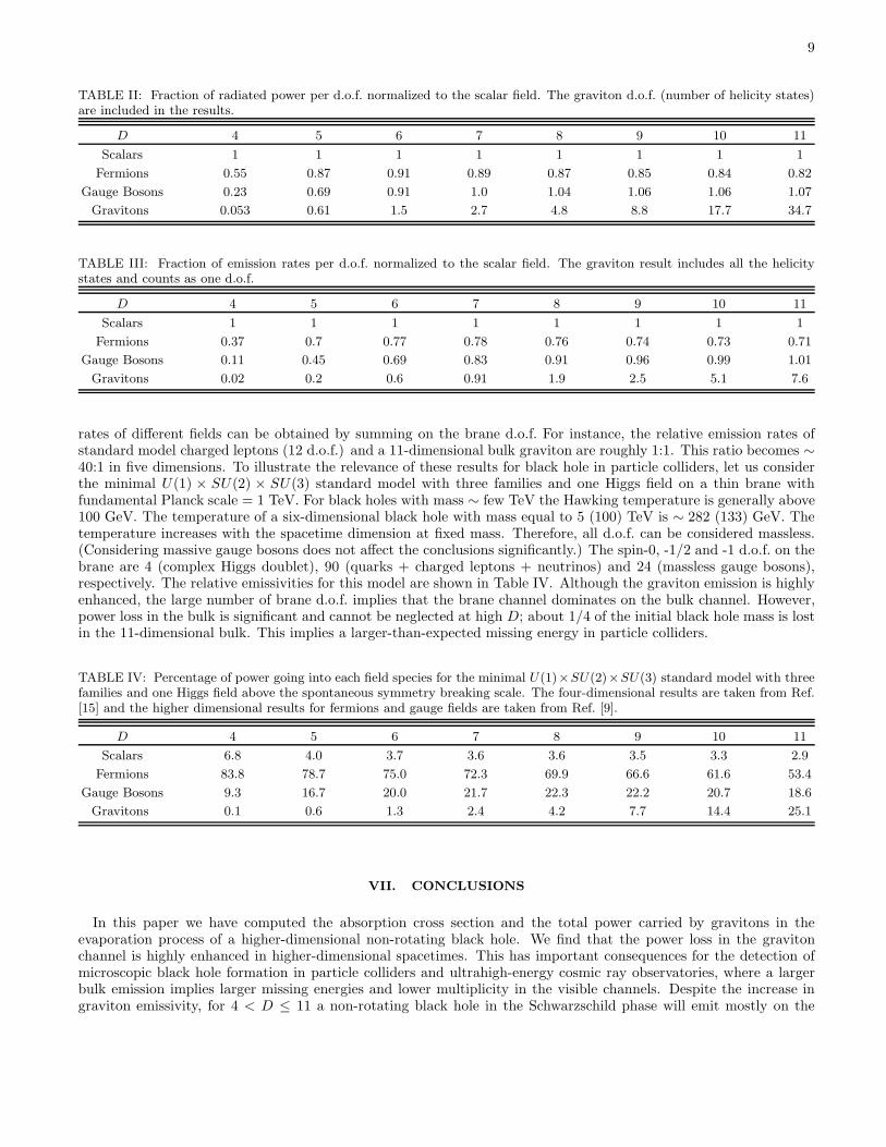
TABLE II: Fraction of radiated power per d.o.f. normalized to the scalar field. The graviton d.o.f. (number of helicity states)are included in the results.

D 4 5 6 7 8 9 10 11

Scalars 1 1 1 1 1 1 1 1

Fermions 0.55 0.87 0.91 0.89 0.87 0.85 0.84 0.82

Gauge Bosons 0.23 0.69 0.91 1.0 1.04 1.06 1.06 1.07

Gravitons 0.053 0.61 1.5 2.7 4.8 8.8 17.7 34.7

TABLE III: Fraction of emission rates per d.o.f. normalized to the scalar field. The graviton result includes all the helicitystates and counts as one d.o.f.

D 4 5 6 7 8 9 10 11

Scalars 1 1 1 1 1 1 1 1

Fermions 0.37 0.7 0.77 0.78 0.76 0.74 0.73 0.71

Gauge Bosons 0.11 0.45 0.69 0.83 0.91 0.96 0.99 1.01

Gravitons 0.02 0.2 0.6 0.91 1.9 2.5 5.1 7.6

rates of different fields can be obtained by summing on the brane d.o.f. For instance, the relative emission rates ofstandard model charged leptons (12 d.o.f.) and a 11-dimensional bulk graviton are roughly 1:1. This ratio becomes ∼40:1 in five dimensions. To illustrate the relevance of these results for black hole in particle colliders, let us considerthe minimal U(1) × SU(2) × SU(3) standard model with three families and one Higgs field on a thin brane withfundamental Planck scale = 1 TeV. For black holes with mass ∼ few TeV the Hawking temperature is generally above100 GeV. The temperature of a six-dimensional black hole with mass equal to 5 (100) TeV is ∼ 282 (133) GeV. Thetemperature increases with the spacetime dimension at fixed mass. Therefore, all d.o.f. can be considered massless.(Considering massive gauge bosons does not affect the conclusions significantly.) The spin-0, -1/2 and -1 d.o.f. on thebrane are 4 (complex Higgs doublet), 90 (quarks + charged leptons + neutrinos) and 24 (massless gauge bosons),respectively. The relative emissivities for this model are shown in Table IV. Although the graviton emission is highlyenhanced, the large number of brane d.o.f. implies that the brane channel dominates on the bulk channel. However,power loss in the bulk is significant and cannot be neglected at high D; about 1/4 of the initial black hole mass is lostin the 11-dimensional bulk. This implies a larger-than-expected missing energy in particle colliders.

TABLE IV: Percentage of power going into each field species for the minimal U(1)×SU(2)×SU(3) standard model with threefamilies and one Higgs field above the spontaneous symmetry breaking scale. The four-dimensional results are taken from Ref.[15] and the higher dimensional results for fermions and gauge fields are taken from Ref. [9].

D 4 5 6 7 8 9 10 11

Scalars 6.8 4.0 3.7 3.6 3.6 3.5 3.3 2.9

Fermions 83.8 78.7 75.0 72.3 69.9 66.6 61.6 53.4

Gauge Bosons 9.3 16.7 20.0 21.7 22.3 22.2 20.7 18.6

Gravitons 0.1 0.6 1.3 2.4 4.2 7.7 14.4 25.1

VII. CONCLUSIONS

In this paper we have computed the absorption cross section and the total power carried by gravitons in theevaporation process of a higher-dimensional non-rotating black hole. We find that the power loss in the gravitonchannel is highly enhanced in higher-dimensional spacetimes. This has important consequences for the detection ofmicroscopic black hole formation in particle colliders and ultrahigh-energy cosmic ray observatories, where a largerbulk emission implies larger missing energies and lower multiplicity in the visible channels. Despite the increase ingraviton emissivity, for 4 < D ≤ 11 a non-rotating black hole in the Schwarzschild phase will emit mostly on the

10

brane due to the higher number of brane d.o.f. 3 However, black hole energy loss in the bulk cannot be neglected inpresence of extra dimensions. Graviton emission is expected to dominate the black hole evaporation at very high D.

Acknowledgements

We are very grateful to De-Chang Dai for pointing out some typos in previous versions. The authors thank AkihiroIshibashi for useful correspondence. VC acknowledges financial support from FCT through the PRAXIS XXI program,and from the Fundacao Calouste Gulbenkian through the Programa Gulbenkian de Estımulo a Investigacao Cientıfica.

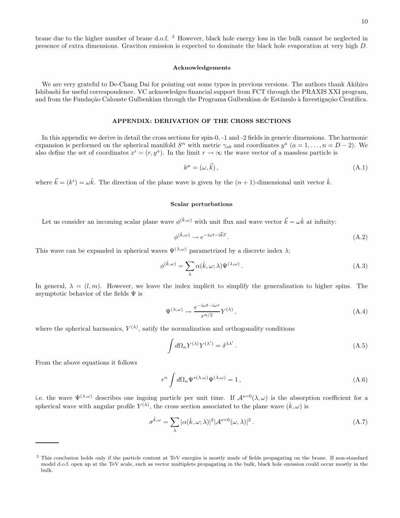
APPENDIX: DERIVATION OF THE CROSS SECTIONS

In this appendix we derive in detail the cross sections for spin-0, -1 and -2 fields in generic dimensions. The harmonicexpansion is performed on the spherical manifold Sn with metric γab and coordinates ya (a = 1, . . . , n = D − 2). Wealso define the set of coordinates xi = (r, ya). In the limit r → ∞ the wave vector of a massless particle is

kµ = (ω,~k) , (A.1)

where ~k = (ki) = ωk. The direction of the plane wave is given by the (n + 1)-dimensional unit vector k.

Scalar perturbations

Let us consider an incoming scalar plane wave φ(k,ω) with unit flux and wave vector ~k = ωk at infinity:

φ(k,ω) → e−iωt−i~k~x . (A.2)

This wave can be expanded in spherical waves Ψ(λ,ω) parametrized by a discrete index λ:

φ(k,ω) =∑

λ

α(k, ω; λ)Ψ(λ,ω) . (A.3)

In general, λ = (l, m). However, we leave the index implicit to simplify the generalization to higher spins. Theasymptotic behavior of the fields Ψ is

Ψ(λ,ω) →e−iωt−iωr

rn/2Y (λ) , (A.4)

where the spherical harmonics, Y (λ), satify the normalization and orthogonality conditions∫

dΩnY (λ)Y (λ′) = δλλ′

. (A.5)

From the above equations it follows

rn

∫

dΩnΨ∗(λ,ω)Ψ(λ,ω) = 1 , (A.6)

i.e. the wave Ψ(λ,ω) describes one ingoing particle per unit time. If As=0(λ, ω) is the absorption coefficient for a

spherical wave with angular profile Y (λ), the cross section associated to the plane wave (k, ω) is

σk,ω =∑

λ

|α(k, ω; λ)|2|As=0(ω, λ)|2 . (A.7)

3 This conclusion holds only if the particle content at TeV energies is mostly made of fields propagating on the brane. If non-standardmodel d.o.f. open up at the TeV scale, such as vector multiplets propagating in the bulk, black hole emission could occur mostly in thebulk.

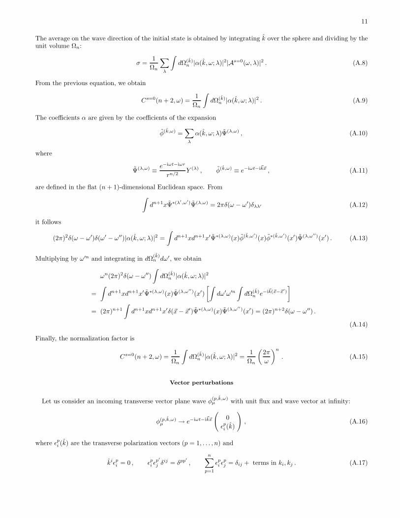
11

The average on the wave direction of the initial state is obtained by integrating k over the sphere and dividing by theunit volume Ωn:

σ =1

Ωn

∑

λ

∫

dΩ(k)n |α(k, ω; λ)|2|As=0(ω, λ)|2 . (A.8)

From the previous equation, we obtain

Cs=0(n + 2, ω) =1

Ωn

∫

dΩ(k)n |α(k, ω; λ)|2 . (A.9)

The coefficients α are given by the coefficients of the expansion

φ(k,ω) =∑

λ

α(k, ω; λ)Ψ(λ,ω) , (A.10)

where

Ψ(λ,ω) ≡e−iωt−iωr

rn/2Y (λ) , φ(k,ω) ≡ e−iωt−i~k~x , (A.11)

are defined in the flat (n + 1)-dimensional Euclidean space. From

∫

dn+1xΨ∗(λ′,ω′)Ψ(λ,ω) = 2πδ(ω − ω′)δλλ′ (A.12)

it follows

(2π)2δ(ω − ω′)δ(ω′ − ω′′)|α(k, ω; λ)|2 =

∫

dn+1xdn+1x′Ψ∗(λ,ω)(x)φ(k,ω′)(x)φ∗(k,ω′)(x′)Ψ(λ,ω′′)(x′) . (A.13)

Multiplying by ω′n and integrating in dΩ(k)n dω′, we obtain

ωn(2π)2δ(ω − ω′′)

∫

dΩ(k)n |α(k, ω; λ)|2

=

∫

dn+1xdn+1x′Ψ∗(λ,ω)(x)Ψ(λ,ω′′)(x′)

[∫

dω′ω′n

∫

dΩ(k)n e−i~k(~x−~x′)

]

= (2π)n+1

∫

dn+1xdn+1x′δ(~x − ~x′)Ψ∗(λ,ω)(x)Ψ(λ,ω′′)(x′) = (2π)n+2δ(ω − ω′′) .

(A.14)

Finally, the normalization factor is

Cs=0(n + 2, ω) =1

Ωn

∫

dΩ(k)n |α(k, ω; λ)|2 =

1

Ωn

(

2π

ω

)n

. (A.15)

Vector perturbations

Let us consider an incoming transverse vector plane wave φ(p,k,ω)µ with unit flux and wave vector at infinity:

φ(p,k,ω)µ → e−iωt−i~k~x

(

0

ǫpi (k)

)

, (A.16)

where ǫpi (k) are the transverse polarization vectors (p = 1, . . . , n) and

kiǫpi = 0 , ǫp

i ǫp′

j δij = δpp′

,

n∑

p=1

ǫpi ǫ

pj = δij + terms in ki, kj . (A.17)

12

We assume xi to be asymptotically Euclidean coordinates for simplicity. The wave can be expanded in sphericalwaves Ψ(λ,ω) parametrized by a discrete index λ, which includes the polarizations:

φ(p,k,ω)µ =

∑

λ

α(p, k, ω; λ)Ψ(λ,ω)µ . (A.18)

The asymptotic fields Ψµ are

Ψ(λ,ω)µ →

e−iωt−iωr

rn/2

0

0

rY(λ)a

, (A.19)

where Y(λ)a satisfy the normalization and orthogonality conditions

∫

dΩnY (λ)a Y

(λ′)b γab = δλλ′

. (A.20)

From the above equation it follows

rn

∫

dΩnΨ∗(λ,ω)µ Ψ(λ,ω)

µ gµν = 1 , (A.21)

i.e. a wave Ψ(λ,ω)µ describes one ingoing particle per unit time. If As=1(λ, ω) is the absorption coefficient for a spherical

wave with angular profile Y(λ)a , the cross section associated to the plane wave (p, k, ω) is

σp,k,ω =∑

λ

|α(p, k, ω; λ)|2|As=1(ω, λ)|2 . (A.22)

The average on the wave direction and polarization of the initial state is obtained by summing on p, integrating kover the sphere and dividing by the unit volume Ωn and the number of polarizations n:

σ =1

nΩn

∑

λ

∫

dΩ(k)n

n∑

p=1

|α(p, k, ω; λ)|2|A(ω,λ)|2 . (A.23)

From the previous equation, we obtain

Cs=1(n + 2, ω) =1

nΩn

∫

dΩ(k)n

n∑

p=1

|α(p, k, ω; λ)|2 . (A.24)

The coefficients α are the coefficients of the expansion

φ(p,k,ω)µ =

∑

λ

α(p, k, ω; λ)Ψ(λ,ω)µ , (A.25)

where

Ψ(λ,ω)i ≡

e−iωt−iωr

rn/2

(

0

rY(λ)

a

)

, φ(p,k,ω)i ≡ e−iωt−i~k~xǫp

i (k) , (A.26)

are defined in the flat (n + 1)-dimensional Euclidean space. From

∫

dn+1xΨ∗(λ′,ω′)i Ψi(λ,ω) = 2πδ(ω − ω′)δλλ′ (A.27)

it follows

(2π)2δ(ω − ω′)δ(ω′ − ω′′)|α(p, k, ω; λ)|2 =

∫

dn+1xdn+1x′Ψ∗(λ,ω)i (x)φi(p,k,ω′)(x)φ

∗(p,k,ω′)j (x′)Ψj(λ,ω′′)(x′) . (A.28)

13

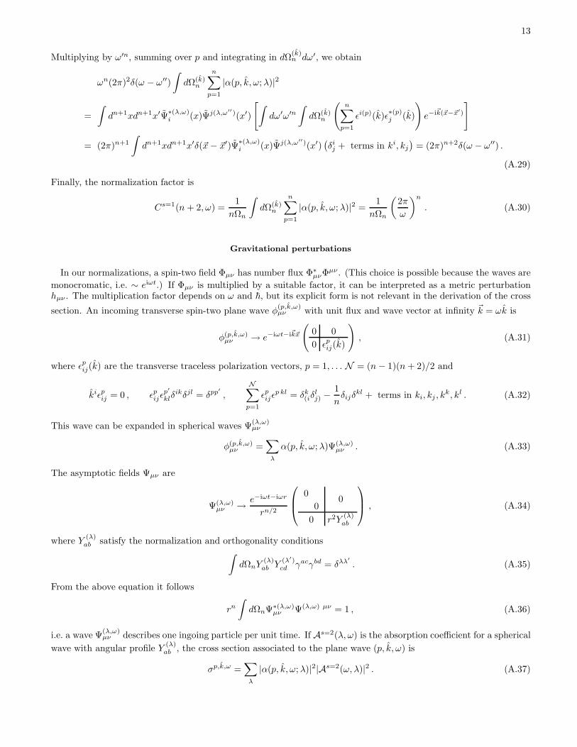
Multiplying by ω′n, summing over p and integrating in dΩ(k)n dω′, we obtain

ωn(2π)2δ(ω − ω′′)

∫

dΩ(k)n

n∑

p=1

|α(p, k, ω; λ)|2

=

∫

dn+1xdn+1x′Ψ∗(λ,ω)i (x)Ψj(λ,ω′′)(x′)

[

∫

dω′ω′n

∫

dΩ(k)n

(

n∑

p=1

ǫi(p)(k)ǫ∗(p)j (k)

)

e−i~k(~x−~x′)

]

= (2π)n+1

∫

dn+1xdn+1x′δ(~x − ~x′)Ψ∗(λ,ω)i (x)Ψj(λ,ω′′)(x′)

(

δij + terms in ki, kj

)

= (2π)n+2δ(ω − ω′′) .

(A.29)

Finally, the normalization factor is

Cs=1(n + 2, ω) =1

nΩn

∫

dΩ(k)n

n∑

p=1

|α(p, k, ω; λ)|2 =1

nΩn

(

2π

ω

)n

. (A.30)

Gravitational perturbations

In our normalizations, a spin-two field Φµν has number flux Φ∗µνΦµν . (This choice is possible because the waves are

monocromatic, i.e. ∼ eiωt.) If Φµν is multiplied by a suitable factor, it can be interpreted as a metric perturbationhµν . The multiplication factor depends on ω and ~, but its explicit form is not relevant in the derivation of the cross

section. An incoming transverse spin-two plane wave φ(p,k,ω)µν with unit flux and wave vector at infinity ~k = ωk is

φ(p,k,ω)µν → e−iωt−i~k~x

(

0 0

0 ǫpij(k)

)

, (A.31)

where ǫpij(k) are the transverse traceless polarization vectors, p = 1, . . . N = (n − 1)(n + 2)/2 and

kiǫpij = 0 , ǫp

ijǫp′

klδikδjl = δpp′

,N∑

p=1

ǫpijǫ

p kl = δk(iδ

lj) −

1

nδijδ

kl + terms in ki, kj , kk, kl . (A.32)

This wave can be expanded in spherical waves Ψ(λ,ω)µν

φ(p,k,ω)µν =

∑

λ

α(p, k, ω; λ)Ψ(λ,ω)µν . (A.33)

The asymptotic fields Ψµν are

Ψ(λ,ω)µν →

e−iωt−iωr

rn/2

0

00

0 r2Y(λ)ab

, (A.34)

where Y(λ)ab satisfy the normalization and orthogonality conditions

∫

dΩnY(λ)ab Y

(λ′)cd γacγbd = δλλ′

. (A.35)

From the above equation it follows

rn

∫

dΩnΨ∗(λ,ω)µν Ψ(λ,ω) µν = 1 , (A.36)

i.e. a wave Ψ(λ,ω)µν describes one ingoing particle per unit time. If As=2(λ, ω) is the absorption coefficient for a spherical

wave with angular profile Y(λ)ab , the cross section associated to the plane wave (p, k, ω) is

σp,k,ω =∑

λ

|α(p, k, ω; λ)|2|As=2(ω, λ)|2 . (A.37)

14

The average on the wave direction and polarization of the initial state is obtained by summing on p, integrating k onthe sphere and dividing by the unit volume Ωn and the number of polarizations N :

σ =1

NΩn

∑

λ

∫

dΩ(k)n

N∑

p=1

|α(p, k, ω; λ)|2|A(ω,λ)|2 . (A.38)

From the previous equation, we obtain

Cs=2(n + 2, ω) =1

NΩn

∫

dΩ(k)n

N∑

p=1

|α(p, k, ω; λ)|2 . (A.39)

The coefficients α are the coefficients of the expansion

φ(p,k,ω)µν =

∑

λ

α(p, k, ω; λ)Ψ(λ,ω)µν , (A.40)

where

Ψ(λ,ω)ij ≡

e−iωt−iωr

rn/2

(

0 0

0 r2Y(λ)ab

)

, φ(p,k,ω)ij ≡ e−iωt−i~k~xǫp

ij(k) (A.41)

are defined in the flat (n + 1)-dimensional Euclidean space. From

∫

dn+1xΨ∗(λ′,ω′)ij Ψij(λ,ω) = 2πδ(ω − ω′)δλλ′ , (A.42)

it follows

(2π)2δ(ω − ω′)δ(ω′ − ω′′)|α(p, k, ω; λ)|2 =

∫

dn+1xdn+1x′Ψ∗(λ,ω)ij (x)φij(p,k,ω′)(x)φ

∗(p,k,ω′)kl (x′)Ψkl(λ,ω′′)(x′) . (A.43)

Multiplying by ω′n, summing over p and integrating in dΩ(k)n dω′, we obtain

ωn(2π)2δ(ω − ω′′)

∫

dΩ(k)n

N∑

p=1

|α(p, k, ω; λ)|2

=

∫

dn+1xdn+1x′Ψ∗(λ,ω)ij (x)Ψkl(λ,ω′′)(x′)

[

∫

dω′ω′n

∫

dΩ(k)n

(

N∑

p=1

ǫij(p)(k)ǫ∗(p)kl (k)

)

e−i~k(~x−~x′)

]

= (2π)n+1

∫

dn+1xdn+1x′δ(~x − ~x′)Ψ∗(λ,ω)ij (x)Ψkl(λ,ω′′)(x′)

(

δ(ik δ

j)l −

1

nδijδkl + terms in ki, kj, kk, kl

)

= (2π)n+2δ(ω − ω′′) .

(A.44)

Finally, the normalization factor is

Cs=2(n + 2, ω) =1

NΩn

∫

dΩ(k)n

N∑

p=1

|α(p, k, ω; λ)|2 =1

NΩn

(

2π

ω

)n

. (A.45)

[1] J. Polchinski, String theory, Vol. 1 and 2 (Cambridge University Press, UK, 1998).[2] N. Arkani-Hamed, S. Dimopoulos and G. R. Dvali, Phys. Lett. B 429, 263 (1998) [arXiv:hep-ph/9803315];

I. Antoniadis, N. Arkani-Hamed, S. Dimopoulos and G. R. Dvali, Phys. Lett. B 436, 257 (1998) [arXiv:hep-ph/9804398];N. Arkani-Hamed, S. Dimopoulos and G. R. Dvali, Phys. Rev. D 59, 086004 (1999) [arXiv:hep-ph/9807344].

[3] L. Randall and R. Sundrum, Phys. Rev. Lett. 83, 4690 (1999) [arXiv:hep-th/9906064];L. Randall and R. Sundrum, Phys. Rev. Lett. 83, 3370 (1999) [arXiv:hep-ph/9905221].

15

[4] R. C. Myers and M. J. Perry, Annals Phys. 172, 304 (1986).[5] S. W. Hawking, Commun. Math. Phys. 43, 199 (1975) [Erratum-ibid. 46, 206 (1976)].[6] R. Emparan, G. T. Horowitz and R. C. Myers, Phys. Rev. Lett. 85, 499 (2000) [arXiv:hep-th/0003118].[7] M. Cavaglia, Phys. Lett. B 569, 7 (2003) [arXiv:hep-ph/0305256].[8] M. Cavaglia, Int. J. Mod. Phys. A 18, 1843 (2003) [arXiv:hep-ph/0210296];

G. Landsberg, arXiv:hep-ph/0211043;R. Emparan, arXiv:hep-ph/0302226;S. Hossenfelder, arXiv:hep-ph/0412265;V. Cardoso, E. Berti and M. Cavaglia, Class. Quant. Grav. 22, L61 (2005) [arXiv:hep-ph/0505125].

[9] P. Kanti, Int. J. Mod. Phys. A 19, 4899 (2004) [arXiv:hep-ph/0402168].[10] T. Banks and W. Fischler, arXiv:hep-th/9906038;

S. B. Giddings and S. Thomas, Phys. Rev. D 65, 056010 (2002) [arXiv:hep-ph/0106219];S. Dimopoulos and G. Landsberg, Phys. Rev. Lett. 87, 161602 (2001) [arXiv:hep-ph/0106295];K. m. Cheung, Phys. Rev. Lett. 88, 221602 (2002) [arXiv:hep-ph/0110163];E. J. Ahn, M. Cavaglia and A. V. Olinto, Phys. Lett. B 551, 1 (2003) [arXiv:hep-th/0201042];E. J. Ahn and M. Cavaglia, Gen. Rel. Grav. 34, 2037 (2002) [arXiv:hep-ph/0205168];M. Cavaglia, S. Das and R. Maartens, Class. Quant. Grav. 20, L205 (2003) [arXiv:hep-ph/0305223];A. Chamblin, F. Cooper and G. C. Nayak, Phys. Rev. D 70, 075018 (2004) [arXiv:hep-ph/0405054];R. Godang et al., Int. J. Mod. Phys. A 20, 3409 (2005) [arXiv:hep-ph/0411248];A. Flachi and T. Tanaka, Phys. Rev. Lett. 95, 161302 (2005) [arXiv:hep-th/0506145].

[11] J. L. Feng and A. D. Shapere, Phys. Rev. Lett. 88, 021303 (2002) [arXiv:hep-ph/0109106];L. A. Anchordoqui, J. L. Feng, H. Goldberg and A. D. Shapere, Phys. Rev. D 65, 124027 (2002) [arXiv:hep-ph/0112247];L. Anchordoqui and H. Goldberg, Phys. Rev. D 65, 047502 (2002) [arXiv:hep-ph/0109242];A. Ringwald and H. Tu, Phys. Lett. B 525, 135 (2002) [arXiv:hep-ph/0111042];M. Kowalski, A. Ringwald and H. Tu, Phys. Lett. B 529, 1 (2002) [arXiv:hep-ph/0201139];E. J. Ahn, M. Ave, M. Cavaglia and A. V. Olinto, Phys. Rev. D 68, 043004 (2003) [arXiv:hep-ph/0306008];A. Mironov, A. Morozov and T. N. Tomaras, arXiv:hep-ph/0311318;E. J. Ahn, M. Cavaglia and A. V. Olinto, Astropart. Phys. 22, 377 (2005) [arXiv:hep-ph/0312249];V. Cardoso et al., Astropart. Phys. 22, 399 (2005) [arXiv:hep-ph/0405056];A. Cafarella, C. Coriano and T. N. Tomaras, JHEP 0506, 065 (2005) [arXiv:hep-ph/0410358];J. I. Illana, M. Masip and D. Meloni, Phys. Rev. D 72, 024003 (2005) [arXiv:hep-ph/0504234];M. Ahlers, A. Ringwald and H. Tu, arXiv:astro-ph/0506698.

[12] E. J. Ahn and M. Cavaglia, arXiv:hep-ph/0511159.[13] D. M. Eardley and S. B. Giddings, Phys. Rev. D 66, 044011 (2002) [arXiv:gr-qc/0201034];

E. Kohlprath and G. Veneziano, JHEP 0206, 057 (2002) [arXiv:gr-qc/0203093];V. P. Frolov and D. Stojkovic, Phys. Rev. D 66, 084002 (2002) [arXiv:hep-th/0206046];V. P. Frolov and D. Stojkovic, Phys. Rev. Lett. 89, 151302 (2002) [arXiv:hep-th/0208102];H. Yoshino and Y. Nambu, Phys. Rev. D 67, 024009 (2003) [arXiv:gr-qc/0209003];H. Yoshino and V. S. Rychkov, Phys. Rev. D 71, 104028 (2005) [arXiv:hep-th/0503171].

[14] V. Cardoso and J. P. S. Lemos, Phys. Lett. B 538, 1 (2002) [arXiv:gr-qc/0202019];V. Cardoso and J. P. S. Lemos, Gen. Rel. Grav. 35, 327 (2003) [arXiv:gr-qc/0207009];V. Cardoso and J. P. S. Lemos, Phys. Rev. D 67, 084005 (2003) [arXiv:gr-qc/0211094].

[15] D. N. Page, Phys. Rev. D 13, 198 (1976). See also D. N. Page, Phys. Rev. D 14, 3260 (1976) for the rotating case.[16] P. Kanti and J. March-Russell, Phys. Rev. D 66, 024023 (2002) [arXiv:hep-ph/0203223];

P. Kanti and J. March-Russell, Phys. Rev. D 67, 104019 (2003) [arXiv:hep-ph/0212199];D. Ida, K. y. Oda and S. C. Park, Phys. Rev. D 67, 064025 (2003) [Erratum-ibid. D 69, 049901 (2004)][arXiv:hep-th/0212108];C. M. Harris and P. Kanti, JHEP 0310, 014 (2003) [arXiv:hep-ph/0309054]; D. Ida, K. y. Oda and S. C. Park,arXiv:hep-ph/0501210;D. Ida, K. y. Oda and S. C. Park, Phys. Rev. D 71, 124039 (2005) [arXiv:hep-th/0503052];C. M. Harris and P. Kanti, arXiv:hep-th/0503010;E. Jung, S. Kim and D. K. Park, Phys. Lett. B 619, 347 (2005) [arXiv:hep-th/0504139];G. Duffy, C. Harris, P. Kanti and E. Winstanley, JHEP 0509, 049 (2005) [arXiv:hep-th/0507274];M. Casals, P. Kanti and E. Winstanley, arXiv:hep-th/0511163.

[17] V. Cardoso, M. Cavaglia and L. Gualtieri, Phys. Rev. Lett., in press (2006); arXiv:hep-th/0512002.[18] A. S. Cornell, W. Naylor and M. Sasaki, arXiv:hep-th/0510009.[19] H. Kodama and A. Ishibashi, Prog. Theor. Phys. 110, 701 (2003) [arXiv:hep-th/0305147];

A. Ishibashi and H. Kodama, Prog. Theor. Phys. 110, 901 (2003) [arXiv:hep-th/0305185];H. Kodama and A. Ishibashi, Prog. Theor. Phys. 111, 29 (2004) [arXiv:hep-th/0308128].

[20] C.W. Misner, K.S. Thorne and J.A. Wheeler, Gravitation (Freeman, San Francisco, 1973).[21] R.C. Slansky, An essay on the role of supergravity in the search for unification: Toward a Unified Theory (Los Alamos

Science, Summer/Fall 1984).[22] F.R. Tangherlini, Nuovo Cim. 27, 636 (1963).[23] L. C. B. Crispino, A. Higuchi and G. E. A. Matsas, Phys. Rev. D 63, 124008 (2001) [arXiv:gr-qc/0011070].

16

[24] T. Regge, J.A. Wheeler, Phys. Rev. 108, 1063 (1957).[25] F. J. Zerilli, Phys. Rev. Lett. 24, 737 (1970).[26] V. Cardoso, O. J. C. Dias and J. P. S. Lemos, Phys. Rev. D 67, 064026 (2003) [arXiv:hep-th/0212168].[27] W. G. Unruh, Phys. Rev. D 14, 3251 (1976).[28] S. S. Gubser, Phys. Rev. D 56, 4984 (1997) [arXiv:hep-th/9704195].[29] A. Chodos and E. Myers, Annals Phys. 156, 412 (1984);

M. A. Rubin and C. R. Ordonez, J. Math. Phys. 25, 2888 (1984);M. A. Rubin and C. R. Ordonez, J. Math. Phys. 26, 65 (1985).

[30] S. Chandrasekhar, in The Mathematical Theory of Black Holes (Oxford University, New York, 1983).[31] E. Berti, M. Cavaglia and L. Gualtieri, Phys. Rev. D 69, 124011 (2004) [arXiv:hep-th/0309203].