Onset and decay of the 1+1 Hawking-Unruh effect:what the derivative-coupling detector saw

Benito A. Juarez-Aubry∗ and Jorma Louko†

School of Mathematical SciencesUniversity of Nottingham

Nottingham NG7 2RDUK

June 2014, revised August 2014‡

Abstract

We study an Unruh-DeWitt particle detector that is coupled to the propertime derivative of a real scalar field in 1+1 spacetime dimensions. Working withinfirst-order perturbation theory, we cast the transition probability into a regulator-free form, and we show that the transition rate remains well defined in the limitof sharp switching. The detector is insensitive to the infrared ambiguity when thefield becomes massless, and we verify explicitly the regularity of the massless limitfor a static detector in Minkowski half-space. We then consider a massless fieldfor two scenarios of interest for the Hawking-Unruh effect: an inertial detectorin Minkowski spacetime with an exponentially receding mirror, and an inertialdetector in (1 + 1)-dimensional Schwarzschild spacetime, in the Hartle-Hawking-Israel and Unruh vacua. In the mirror spacetime the transition rate traces theonset of an energy flux from the mirror, with the expected Planckian late timeasymptotics. In the Schwarzschild spacetime the transition rate of a detectorthat falls in from infinity gradually loses thermality, diverging near the singularityproportionally to r−3/2.

∗pmxbaju@nottingham.ac.uk†jorma.louko@nottingham.ac.uk‡This is an author-created, un-copyedited version of an article published in Class. Quantum Grav. 31,

245007 (2014). IOP Publishing Ltd is not responsible for any errors or omissions in this version of themanuscript or any version derived from it. The Version of Record is available online at doi:10.1088/0264-9381/31/24/245007.

1

arX

iv:1

406.

2574

v3 [

gr-q

c] 2

5 N

ov 2

014

1 Introduction

For quantum fields living on a pseudo-Riemannian manifold, the experiences of observerscoupled to the field depend both on the quantum state of the field and on the worldlineof the observer [1, 2]. A celebrated example is the Unruh effect [3], in which uniformlyaccelerated observers in Minkowski spacetime experience a thermal bath in the quantumstate that inertial observers perceive as void of particles. Other well-studied examplesarise with black holes that emit Hawking radiation [4] and with observers in spacetimesof high symmetry [5].

A useful tool for analysing the experiences of an observer is a model particle detectorthat follows the observer’s worldline and has internal states that couple to the quantumfield. Such detectors are known as Unruh-DeWitt (UDW) detectors [3, 6]. While much ofthe early literature on the UDW detectors focused on stationary situations, including theUnruh effect [7, 8], the detectors remain well defined also in time-dependent situations,where they can be analysed within first-order perturbation theory [9, 10, 11, 12, 13, 14,15, 16, 17, 18, 19, 20, 21] as well as by nonperturbative techniques [22, 23, 24, 25, 26].A review with further references can be found in [27].

In this paper we consider a detector coupled to a quantised scalar field in 1+1spacetime dimensions. A scalar field in 1+1 dimensions has local propagating degreesof freedom, and it exhibits the Hawking and Unruh effects just like a scalar field inhigher dimensions. However, the dynamics of the field in 1+1 dimensions is signifi-cantly simpler than in higher dimensions, especially for a massless minimally coupledfield, for which the field equation is conformally invariant and conformal techniques areavailable. In particular, the evolution of a massles minimally coupled field on a (1+1)-dimensional collapsing star spacetime reduces essentially to that of a massless field on(1+1)-dimensional Minkowski spacetime in the presence of a receding mirror, and thesystem is explicitly solvable [28, 29].

The simplifications in the dynamics in 1 + 1 dimensions come however at a cost:the Wightman function of a minimally coupled field in 1+1 dimensions is infrared di-vergent in the massless limit. While Hadamard states can still can be defined in termsof the short distance expansion of the Wightman function [30], the Hadamard expan-sion contains an additive constant that is not determined by the quantum state. Whilethis undetermined additive constant does not contribute to stress-energy expectationvalues [1, 31, 32], it does contribute to the transition probability of an UDW detectorthat couples to the value of the field at the detector’s location. In stationary situationsthe ambiguous contribution to transition probablities can be argued to vanish, undersuitable assumptions about the switch-on and switch-off [7, 11, 12], but in nonstation-ary situations the ambiguity is more severe and has been found to lead to physicallyundesirable predictions in examples that include a receding mirror spacetime [19].

In this paper we analyse a detector that is insensitive to the infrared ambiguity ofthe (1 + 1)-dimensional Wightman function in the massless minimaly coupled limit: wecouple the detector linearly to the derivative of the field with respect to the detector’sproper time [9, 22, 33, 34], rather than to the value of the field. Working in first-

2

order perturbation theory, the detector’s transition probability involves then the doublederivative of the Wightman function, rather than the Wightman function itself. We showthat the response of the (1+1)-dimensional derivative-coupling detector is closely similarto that of the (3 + 1)-dimensional detector with a non-derivative coupling [14, 15]. Inparticular, the transition probablity can be written as an integral formula that involvesno short-distance regulator at the coincidence limit but contains instead an additive termthat depends only on the switching function that controls the switch-on and switch-off.A consequence is that in the limit of sharp switching the transition probability divergesbut the transition rate remains finite.

We carry out three checks on the physical reasonableness of the derivative-couplingdetector in stationary situations in which the switch-on is pushed to asymptotically earlytimes. First, we verify that the transition rate is continuous in the limit of vanishingmass for an inertial detector in Minkowski space, with the field in Minkowski vacuum,and we show that the same holds also for a static detector in Minkowski half-space withDirichlet and Neumann boundary conditions. This is evidence that the derivative cou-pling manages to remove the infrared ambiguity of the massless field without producingunexpected discontinuities in the massless limit. Second, we show that the transitionrate of a uniformly accelerated detector in Minkowski space, coupled to a massless fieldin Minkowski vacuum, coincides with that of an inertial detector at rest with a thermalbath, being in particular thermal in the sense of the Kubo-Martin-Schwinger (KMS)property [35, 36]. This shows that the derivative-coupling detector sees the usual Unruheffect for a massless field. Third, we show that in a thermal bath of a massless fieldin Minkowski space, the transition rate of an inertial detector that is moving with re-spect to the bath is a sum of two terms that are individually thermal but at differenttemperatures, related to the temperature of the bath by Doppler shifts to the red andto the blue. As these terms stem respectively from the right-moving and left-movingcomponents of the field, the temperature shifts are exactly as one would expect.

After these checks, we focus on the massless minimally coupled field in two nonsta-tionary situations, each of interest for the Hawking-Unruh effect.

We first consider a Minkowski spacetime with a mirror whose exponentially recedingmotion makes the field mimic the late time behaviour of a field in a collapsing starspacetime [1, 28, 29]. We show that at late times the detector’s transition rate is the sumof a Planckian contribution, corresponding to the field modes propagating away fromthe mirror, and a vacuum contribution, corresponding to the field modes propagatingtowards the mirror. While the detector couples to the sum of the two parts, the twoparts can nevertheless be unambiguously identified by considering their dependence onthe detector’s velocity with respect to the rest frame in which the mirror was staticin the asymptotic past. We also show numerical results on how the transition rateevolves from the asymptotic early time form to the asymptotic late time form. Theseproperties of the transition rate are in full agreement with the energy flux emitted bythe mirror [1, 28, 29].

We then consider a detector falling inertially into the (1 + 1)-dimensional Schwarz-

3

schild black hole, with the field in the Hartle-Hawking-Israel (HHI) and Unruh vacua.Starting the infall at the asymptotic infinity, we verify that the early time transition ratein the HHI vacuum is as in a thermal state, in the usual Hawking temperature, whilein the Unruh vacuum it is as in a thermal state for the outgoing field modes and in theBoulware vacuum for the ingoing field modes. The outgoing and ingoing contributionscan again be unambiguously identified by considering their dependence on the detector’svelocity in the asymptotic past. The transition rate remains manifestly nonsingular onhorizon-crossing, and we present numerical evidence of how the thermal properties aregradually lost during the infall. Near the black hole singularity the transition rate di-verges proportionally to r−3/2 where r is the Schwarzschild radial coordinate. Theseresults are in full agreement with the known properties of the HHI and Unruh vacua,including their thermality, their invariance under Schwarzschild time translations andtheir regularity across the future horizon.

We anticipate that the derivative-coupling detector will be a useful tool for probing aquantum field in other situations where the infrared properties raise technical difficultiesfor the conventional UDW detector. One such instance is when the field has zero modes,which typically occur in spacetimes with compact spatial sections [37]. Other instancesmay arise in analogue spacetime systems [38] or in spacetimes where the back-reactiondue to Hawking evaporation is strong (for a small selection of references see [39, 40, 41,42, 43]).

The structure of the paper is as follows. In Section 2 we introduce the derivative-coupling detector, write the transition probability in a regulator-free form and providethe formula for the transition rate in the sharp switching limit. Consistency checksin three stationary situations are carried out in Section 3. Sections 4 and 5 addressrespectively the receding mirror spacetime and the Schwarzschild spacetime. The resultsare summarised and discussed in Section 6. Details of technical calculations are deferredto four appendices.

Our metric signature is (−+), so that the norm squared of a timelike vector isnegative. We use units in which c = ~ = kB = 1, so that frequencies, energies andtemperatures have dimension inverse length. Spacetime points are denoted by SansSerif characters (x) and spacetime indices are denoted by a, b, . . .. Complex conjugationis denoted by overline. O(x) denotes a quantity for which O(x)/x is bounded as x→ 0,o(x) denotes a quantity for which o(x)/x → 0 as x → 0, O(1) denotes a quantity thatis bounded in the limit under consideration, and o(1) denotes a quantity that goes tozero in the limit under consideration.

2 Derivative-coupling detector

In this section we introduce an UDW detector that couples linearly to the proper timederivative of a scalar field [9, 22, 33, 34]. We show, within first-order perturbationtheory, that in (1 + 1) spacetime dimensions the detector’s transition probability andtransition rate are closely similar to those of a (3 + 1)-dimensional UDW detector with

4

a non-derivative coupling [14, 15].

2.1 Derivative-coupling detector in d ≥ 2 dimensions

Our detector is a spatially point-like quantum system with two distinct energy eigen-states. We denote the normalised energy eigenstates by |0〉D and |ω〉D, with the respec-tive energy eigenvalues 0 and ω, where ω 6= 0.

The detector moves in a spacetime of dimension d ≥ 2 along the smooth timelikeworldline x(τ), where τ is the proper time, and it couples to a real scalar field φ via theinteraction Hamiltonian

Hint = cχ(τ)µ(τ)d

dτφ(x(τ)

), (2.1)

where c is a coupling constant, µ is the detector’s monopole moment operator and theswitching function χ specifies how the interaction is switched on an off. We assume thatχ is real-valued, non-negative and smooth with compact support.

Where Hint (2.1) differs from the usual UDW detector [3, 6] is that the interactionis linear in the proper time derivative of the field, rather than in the field itself. Analternative expression is Hint = cχ(τ)µ(τ) xa∇aφ

(x(τ)

), where the overdot denotes d/dτ .

We take the detector to be initially in the state |0〉D and the field to be in a state |ψ〉,which we assume to be regular in the sense of the Hadamard property [30]. After theinteraction has been turned on and off, we are interested in the probability for thedetector to have made a transition to the state |ω〉D, regardless the final state of thefield. Working in first-order perturbation theory in c, we may adapt the analysis of theusual UDW detector [1, 2] to show that this probability factorises as

P (ω) = c2|D〈0|µ(0)|ω〉D|2F(ω) , (2.2)

where |D〈0|µ(0)|ω〉D|2 depends only on the internal structure of the detector but neitheron |ψ〉, the trajectory or the switching, while the dependence on |ψ〉, the trajectory andthe switching is encoded in the response function F . With our Hint (2.1), the responsefunction is given by

F(ω) =

∫ ∞−∞

dτ ′∫ ∞−∞

dτ ′′ e−iω(τ ′−τ ′′) χ(τ ′)χ(τ ′′) ∂τ ′∂τ ′′W(τ ′, τ ′′) , (2.3)

where the correlation function W(τ ′, τ ′′).= 〈ψ|φ

(x(τ ′)

)φ(x(τ ′′)

)|ψ〉 is the pull-back of

the Wightman function 〈ψ|φ(x′)φ(x′′)|ψ〉 to the detector’s world line.From now on we drop the constant prefactors in (2.2) and refer to the response

function as the transition probability.As |ψ〉 is Hadamard and the detector’s worldline is smooth and timelike, the cor-

relation function W is a well-defined distribution on R × R [44, 45, 46, 47]. As χ issmooth with compact support, it follows that F (2.3) is well defined: given a family offunctions Wε that converges to the distribution W as ε → 0+, F is evaluated by first

5

making in (2.3) the replacement W → Wε, then performing the integrals, and finallytaking the limit ε→ 0+. The limit ε→ 0+ may however not necessarily be taken underthe integrals. For the usual UDW detector, for which the response function is given asin (2.3) but without the derivatives, this issue is known to become subtle if one wishesto define an instantaneous transition rate by passing to the limit of sharp switching: thesubtleties start in three spacetime dimensions and increase as the spacetime dimensionincreases and the correlation function becomes more singular at the coincidence limit[14, 15, 16, 17]. We may expect similar subtleties for the derivative-coupling detector,and since the derivatives in (2.3) increase the singularity of the integrand at the coinci-dence limit, we may expect the subtleties to start in lower spacetime dimensions thanfor the usual UDW detector.

We confirm these expectations in subsections 2.2, 2.3 and 2.4 by analysing the re-sponse function (2.3) and the transition rate in (1 + 1) spacetime dimensions.

2.2 (1 + 1) response function: isolating the coincidence limit

We now specialise to (1 + 1) spacetime dimensions. In this subsection we write theresponse function (2.3) in a way where the contribution from the singularity of theintegrand at the coincidence limit has been isolated.

We start from (2.3) and write W = (W −Wsing) +Wsing, where Wsing is the locallyintegrable function

Wsing(τ ′, τ ′′).=

−i sgn(τ ′ − τ ′′)

4− ln |τ ′ − τ ′′|

2πfor τ ′ 6= τ ′′ ,

0 for τ ′ = τ ′′ ,(2.4)

and sgn denotes the signum function,

sgnx.=

1 for x > 0 ,

0 for x = 0 ,

−1 for x < 0 .

(2.5)

We obtain

F(ω) = Freg(ω) + Fsing(ω) , (2.6a)

Freg(ω) =

∫ ∞−∞

dτ ′∫ ∞−∞

dτ ′′ e−iω(τ ′−τ ′′) χ(τ ′)χ(τ ′′) ∂τ ′∂τ ′′[W(τ ′, τ ′′)−Wsing(τ ′, τ ′′)

],

(2.6b)

Fsing(ω) =

∫ ∞−∞

dτ ′∫ ∞−∞

dτ ′′ e−iω(τ ′−τ ′′) χ(τ ′)χ(τ ′′) ∂τ ′∂τ ′′Wsing(τ ′, τ ′′) , (2.6c)

where the derivatives are understood in the distributional sense.

6

Consider first Freg (2.6b). The Hadamard short distance form of the Wightmanfunction [30] implies that bothW(τ ′, τ ′′) and ∂τ ′∂τ ′′

[W(τ ′, τ ′′)−Wsing(τ ′, τ ′′)

]are repre-

sented in a neighbourhood of τ ′ = τ ′′ by locally integrable functions. It follows that theintegral in (2.6b) receives no distributional contributions from τ ′ = τ ′′, and the integralcan hence be decomposed into integrals over the subdomains τ ′ > τ ′′ and τ ′ < τ ′′. Inthe subdomain τ ′ > τ ′′ we write τ ′ = u and τ ′′ = u − s, where u ∈ R and 0 < s < ∞,and in the subdomain τ ′ < τ ′′ we write τ ′′ = u and τ ′ = u − s, where again u ∈ Rand 0 < s < ∞. Using the property W(τ ′, τ ′′) = W(τ ′′, τ ′) and the explicit form ofWsing(τ ′, τ ′′) (2.4), we obtain

Freg(ω) = 2

∫ ∞−∞

du

∫ ∞0

ds χ(u)χ(u− s) Re

[e−iωs

(A(u, u− s) +

1

2πs2

)], (2.7)

where

A(τ ′, τ ′′).= ∂τ ′∂τ ′′W(τ ′, τ ′′) . (2.8)

Note that the integrand in (2.7) is still a distribution, but it is represented by a locallyintegrable function in a neighbourhood of s = 0, and any distributional singularities arehence isolated from s = 0.

We evaluate Fsing (2.6c) in Appendix A. Combining (2.7) and (A.6), we find

F(ω) = −ωΘ(−ω)

∫ ∞−∞

du [χ(u)]2 +1

π

∫ ∞0

dscos(ωs)

s2

∫ ∞−∞

duχ(u)[χ(u)− χ(u− s)]

+ 2

∫ ∞−∞

du

∫ ∞0

ds χ(u)χ(u− s) Re

[e−iωs

(A(u, u− s) +

1

2πs2

)], (2.9)

where A is given by (2.8) and Θ is the Heaviside function,

Θ(x).=

1 for x > 0 ,

0 for x ≤ 0 .(2.10)

An equivalent form, using for Fsing the alternative expression (A.7) given in Appendix A,is

F(ω) = −ω2

∫ ∞−∞

du [χ(u)]2 +1

π

∫ ∞0

ds

s2

∫ ∞−∞

duχ(u) [χ(u)− χ(u− s)]

+ 2

∫ ∞−∞

du

∫ ∞0

ds χ(u)χ(u− s) Re

[e−iωsA(u, u− s) +

1

2πs2

]. (2.11)

The integral over s in the second term in (2.9) and (2.11) is convergent at small s sincethe integral over u produces an even function of s that vanishes at s = 0.

The expression (2.11) for the response function is closely similar to that obtainedin [14, 15] for the usual, non-derivative UDW detector in (3 + 1) dimensions. This

7

happens because of the similarity between the coincidence limit singularities of thetwice differentiated (1 + 1)-dimensional correlation function, appearing in (2.3), andthe undifferentiated (3 + 1)-dimensional correlation function that appears in the similarexpression for non-derivative coupling.

We re-emphasise that the last term in (2.9) and (2.11) may contain distributionalcontributions from s > 0. Similar distributional contributions were not consideredfor the (3 + 1)-dimensional non-derivative UDW detector in [15], but they can occuralso there, and the analysis in [15] can be amended to include these contributions byproceeding as in the present paper. Similar distributional contributions can arise inany spacetime dimension: in (2 + 1) dimensions, examples on the Bandados-Teitelboim-Zanelli black hole were encountered in [17].

2.3 (1 + 1) sharp switching limit: transition rate

In this subsection we consider the sharp switching limit of the derivative-coupling de-tector in (1 + 1) dimensions.

Following [14, 15], we consider a family of switching functions given by

χ(u) = h1

(u− τ0 + δ

δ

)× h2

(−u+ τ + δ

δ

), (2.12)

where τ and τ0 are pararameters satisfying τ > τ0, δ is a positive parameter, and h1

and h2 are smooth non-negative functions such that h1(x) = h2(x) = 0 for x ≤ 0 andh1(x) = h2(x) = 1 for x ≥ 1. In words, the detector is switched on over an interval ofduration δ before time τ0, stays on at constant coupling from time τ0 to time τ , andis finally switched off over an interval of duration δ after time τ . The profile of theswitch-on is determined by h1 and the profile of the switch-off is determined by h2.

We are interested in the limit δ → 0. To begin with, suppose that A(τ ′, τ ′′) (2.8)is represented by a smooth function for τ ′ 6= τ ′′. Given the similarity between (2.11)and the (3 + 1)-dimensional non-derivative response function given by equation (3.16)in [15], we may follow the analysis that led to equations (4.4) and (4.5) in [15]. For theresponse function, we find

F(ω, τ) = −ω∆τ

2+ 2

∫ τ

τ0

du

∫ u−τ0

0

ds Re

[e−iωsA(u, u− s) +

1

2πs2

]+

1

πln

(∆τ

δ

)+ C +O(δ), (2.13)

where ∆τ.= τ − τ0, C is a constant that depends only on h1 and h2, and we have

included in F(ω, τ) the second argument τ to indicate explicitly the dependence on τ .The response function (2.13) hence diverges logarithmically as δ → 0, but the diver-

gent contribution is a pure switching effect, independent of the quantum state and of

8

the detector’s trajectory. The transition rate, defined as F(ω, τ).= ∂

∂τF(ω, τ), remains

finite as δ → 0, and is in this limit given by

F(ω, τ) = −ω2

+ 2

∫ ∆τ

0

dsRe

[e−iωsA(τ, τ − s) +

1

2πs2

]+

1

π∆τ. (2.14)

An equivalent expression, obtained by writing 1 = cos(ωs) + [1 − cos(ωs)] under theintegral in (2.14), is

F(ω, τ) = −ωΘ(−ω) +1

π

[cos(ω∆τ)

∆τ+ |ω| si(|ω|∆τ)

]

+ 2

∫ ∆τ

0

dsRe

[e−iωs

(A(τ, τ − s) +

1

2πs2

)], (2.15)

where si is the sine integral in the notation of [48]. When the switch-on is in theasymptotic past and the fall-off of A(τ, τ − s) is sufficiently fast as large s, the ∆τ →∞limit of (2.15) gives

F(ω, τ) = −ωΘ(−ω) + 2

∫ ∞0

dsRe

[e−iωs

(A(τ, τ − s) +

1

2πs2

)]. (2.16)

The observational meaning of the transition rate relates to ensembles of ensembles ofdetectors (see Section 5.3.1 of [12] or Section 2 of [15]).

When A(τ ′, τ ′′) (2.8) is not represented by a smooth function for τ ′ 6= τ ′′, the esti-mates leading to (2.13) and (2.14) need not hold, and the transition rate need not havea well-defined δ → 0 limit for all τ0 and τ . In particular, if the detector is switched onat a finite time τ0 and A(τ ′, τ ′′) has a distributional singularity at (τ ′, τ ′′) = (τ, τ0), theintegral expressions in (2.14) and (2.15) would not be well defined because the singular-ity occurs at an end-point of the integration. If the switch-on is in the asymptotic past,however, the transition rate formula (2.16) is well defined even when A(τ ′, τ ′′) has dis-tributional singularities for τ ′ 6= τ ′′ provided these singularities are sufficiently isolated.We shall encounter examples of such singularities in subsection 3.1 and Section 4.

Similar remarks about singularities of the correlation function at timelike-separatedpoints apply also to the sharp switching limit of the non-derivative UDW detector in(3 + 1) dimensions. The transition rate results given in [15] for a switch-on at a finitetime hold when no such singularities are present.

2.4 Stationary transition rate

Suppose that the Wightman function is stationary with respect to the detector’s tra-jectory, in the sense that W(τ ′, τ ′′) depends on τ ′ and τ ′′ only through the differenceτ ′ − τ ′′. When the detector is switched on in the asymptotic past, the transition rate

9

(2.16) reduces to

F(ω) = −ωΘ(−ω) + 2

∫ ∞0

dsRe

[e−iωs

(A(s, 0) +

1

2πs2

)]= −ωΘ(−ω) +

∫ ∞−∞

ds e−iωs

[A(s, 0) +

1

2πs2

]= −ωΘ(−ω) +

∫C

ds e−iωs

[A(s, 0) +

1

2πs2

]=

∫ ∞−∞

ds e−iωsA(s, 0) , (2.17)

where we have dropped the second argument τ from F as the transition rate is nowindependent of τ , and A(s, 0) is understood as a distribution everywhere, includings = 0. In (2.17) we have first used the propertiesA(τ ′, τ ′′) = A(τ ′−τ ′′, 0) andA(τ ′, τ ′′) =A(τ ′′, τ ′). Next, we have deformed the real s axis into a contour C in the complex splane, such that C follows the real axis except that it dips into the lower half-planenear s = 0; this deformation is justified by the Hadamard short separation form of theWightman function [30]. In the contour integral over C, we have then separated the twoterms in the integrand, evaluated the integral of the second term by a standard contourtechnique, and noted that in the first term C can be deformed back to the real s axisprovided the integrand is understood as a distribution for all s, including s = 0.

The result (2.17) coincides with the transition rate that one obtains from the responsefunction (2.3) by the usual procedure of setting χ = 1 and formally factoring out theinfinite total detection time [1].

3 Stationary checks: massless limit, the Unruh ef-

fect, and inertial response in a thermal bath

In this section we perform reasonableness checks on the derivative-coupling detectorin three stationary situations. First, we verify that the transition rate is continuousin the massless limit for a static detector in Minkowski space, and also in Minkowskihalf-space with Dirichlet and Neumann boundary conditions. Second, we verify that thedetector sees the usual Unruh effect when the field is massless. Third, we verify thatthe transition rate of an inertial detector in the thermal bath of a massless field sees aDoppler shift when the detector has a nonvanishing velocity in the inertial frame of thebath.

3.1 Static detector in Minkowski (half-)space

Let M be (1 + 1) Minkowski spacetime, with standard Minkowski coordinates (t, x) in

which the metric reads ds2 = −dt2 + dx2, and let M be the submanifold ofM in which

10

x > 0. We consider inM and M a scalar field of mass m ≥ 0, and in M we impose theDirichlet or Neumann boundary condition that the field or its normal derivative vanishat x = 0.

We set the field in M in the Minkowski vacuum |0〉, and the field in M in theMinkowski-like vacuum |0〉 that is the no-particle state with respect to the timelikeKilling vector ∂t.

Now, consider in M and M a detector on the static worldline

x(τ) = (τ, d) , (3.1)

where d is a positive constant. InM the value of d has no geometric significance, but inM d is the distance of the detector from the mirror at x = 0. We take the detector to beswitched on in the asymptotic past, so that the detector’s transition rate is stationaryand given by (2.17). We shall show that the transition rate is continuous in the limitm→ 0.

3.1.1 m > 0

For m > 0, the Wightman function in M is [1]

〈0|φ(x)φ(x′)|0〉 =1

2πK0

[m√

(∆x)2 − (∆t− iε)2], (3.2)

where ∆x = x−x′, ∆t = t−t′, K0 is the modified Bessel function of the second kind [48],and the expression is understood as a distribution in the sense of ε → 0+. The squareroot is positive when x and x′ are spacelike separated and ε→ 0+, and the continuationto general x and x′ is specified by the iε prescription. By the method of images, theWightman function in M is the sum of (3.2) and the image piece

〈0|φ(x)φ(x′)|0〉 − 〈0|φ(x)φ(x′)|0〉 =η

2πK0

[m√

(x+ x′)2 − (∆t− iε)2], (3.3)

where η = −1 for Dirichlet and η = 1 for Neumann.We evaluate the transition rate (2.17) in Appendix B. We obtain

M : F(ω) =ω2

√ω2 −m2

Θ(−ω −m) , (3.4a)

M : F(ω) =ω2[1 + η cos

(2d√ω2 −m2

)]√ω2 −m2

Θ(−ω −m) . (3.4b)

The transition rate is non-negative, and it is nonvanishing only for ω < −m, that is, forde-excitations exceeding the mass gap. These are properties that one would expect of areasonable detector coupled to a massive field.

11

3.1.2 m = 0

OnM, the massive Wightman function (3.2) diverges as m→ 0. However, the quantity〈0|φ(x)φ(x′)|0〉+ 1

2πln[meγ/(2µ)], where γ is Euler’s constant and µ is a positive constant

of dimension inverse length, has at m→ 0 a finite limit, given by [48]

〈0|φ(x)φ(x′)|0〉 .= − 1

2πln[µ√

(∆x)2 − (∆t− iε)2]. (3.5)

We take (3.5) as the definition of the Wightman function for m = 0. The constant µis required for dimensional consistency, and its arbitrariness means that 〈0|φ(x)φ(x′)|0〉(3.5) is unique up to an additive constant. The massless Wightman function on M isthe sum of (3.5) and the image piece

〈0|φ(x)φ(x′)|0〉 − 〈0|φ(x)φ(x′)|0〉 = − η

2πln[µ√

(x+ x′)2 − (∆t− iε)2], (3.6)

where again η = −1 for Dirichlet and η = 1 for Neumann. Note that for η = −1,the massless Wightman function on M is independent of µ and can be obtained as them→ 0 limit of the massive Wightman function on M without introducing a subtractionby hand.

We show in Appendix B that the transition rate is given by

M : F(ω) = −ωΘ(−ω) , (3.7a)

M : F(ω) = −ω [1 + η cos(2dω)] Θ(−ω) . (3.7b)

The transition rate is non-negative, and it is nonvanishing only for de-excitations, asone would expect of a reasonable detector coupled to a massless field.

We see from (3.4) and (3.7) that the massless transition rate is equal to the masslesslimit of the massive transition rate. This is the property that we wished to verify.

3.2 Unruh effect

Let againM be (1 + 1) Minkowski spacetime, and consider inM a massless field in theMinkowski vacuum. We consider a detector on the uniformly accelerated worldline

x(τ) =(a−1 sinh(aτ), a−1 cosh(aτ)

), (3.8)

where the positive constant a is the magnitude of the proper acceleration. The trajectoryis stationary with respect to the boost Killing vector t∂x+x∂t, and |0〉 is invariant underthis Killing vector. With the detector switch-on pushed to the asymptotic past, thetransition rate is independent of time and given by (2.17).

From (2.8), (3.5) and (3.8), we find

A(τ ′, τ ′′) = − a2

8π sinh2(a(τ ′ − τ ′′ − iε)/2

) . (3.9)

12

Substituting (3.9) in (2.17), deforming the contour of s-integration to s = −iπ/a + rwhere r ∈ R, and using formula 3.985.1 in [49], we find

F(ω) =ω

e2πω/a − 1. (3.10)

The transition rate (3.10) satisfies the KMS relation [35, 36],

F(ω) = e−ω/T F(−ω) , (3.11)

with T = a/(2π), and is hence thermal at temperature a/(2π) in the KMS sense. Weconclude that the detector does see the usual Unruh effect [3, 7]. The Planckian formof the transition rate (3.10) is identical to that of a non-derivative detector coupled toa massless field on a uniformly accelerated trajectory in (3 + 1) dimensions [3, 7].

3.3 Inertial detector in a thermal bath

We consider again a massless field in (1 + 1) Minkowski spacetime M, but now in thethermal state |T 〉 of positive temperature T . Working in Minkowski coordinates (t, x)in which the thermal bath is at rest, the thermal Wightman function is obtained fromthe vacuum Wightman function by taking an image sum in t with period i/T [1]. Withthe vacuum Wightman function (3.5), the sum reads

〈T |φ(x)φ(x′)|T 〉 = − 1

4π

∞∑n=−∞

lnµ2[(∆x)2 − (∆t− iε+ in/T )2

], (3.12)

and does not converge. However, differentiation of the sum in (3.12) term by term withrespect to ∆x gives a new sum that converges and can be summed by residues intoan elementary function. We integrate the elementary function with respect to ∆x andfix the ∆t-dependent integration constant by requiring that the massless Klein-Gordonequation is satisfied, and requiring evenness in ∆t for (∆x)2 − (∆t)2 > 0. The outcomeis

〈T |φ(x)φ(x′)|T 〉 .= − 1

4πlnsinh[πT (∆x+ ∆t− iε)]

− 1

4πlnsinh[πT (∆x−∆t+ iε)] , (3.13)

uniquely up to an additive constant, and we take (3.13) as the definition of the thermalWightman function. Note that (3.13) decomposes into the right-mover contribution thatdepends on ∆(x− t) and the left-mover contribution that depends on ∆(x+ t).

We consider the inertial detector worldline

x(τ) = (τ coshλ,−τ sinhλ) , (3.14)

13

where λ ∈ R is the detector’s rapidity parameter with respect to the rest frame of thebath. For later convenience, we have chosen the sign in (3.14) so that a detector withpositive λ is moving towards decreasing x. From (2.8), (3.13) and (3.14) we find

A(τ ′, τ ′′) = − 1

16π

((2πT+)2

sinh2[πT+(τ ′ − τ ′′ − iε)]+

(2πT−)2

sinh2[πT−(τ ′ − τ ′′ − iε)]

), (3.15)

where T±.= e±λT . Taking the detector to be switched on in the asymptotic past, and

proceeding as with (3.9), we find that the transition rate is given by

F(ω) =ω

2

(1

eω/T+ − 1+

1

eω/T− − 1

), (3.16)

simplifying in the special case λ = 0 to

F(ω) =ω

eω/T − 1. (3.17)

The λ = 0 transition rate (3.17) satisfies the KMS relation (3.11) in temperature T ,and it coincides with the transition rate (3.10) of a uniformly accelerated detector whenT = a/(2π). The λ 6= 0 transition rate (3.16) is a sum of the right-mover and left-movercontributions, each satisfying the KMS relation but in the respective Doppler-shiftedtemperatures T±. These are properties that one would expect of a reasonable detector.

3.4 Inertial detector with vacuum left-movers and thermalright-movers

In preparation for the nonstationary situations that will be addressed in Sections 4 and 5,we consider here the inertial detector (3.14) in the state in which the left-movers are inthe Minkowski vacuum but the right-movers are in a thermal bath with temperature T .As the left-movers and the right-movers decouple, the results can be read off from thosegiven above in a straightforward way. Taking the switch-on to the asymptotic past, wefind

F(ω) = −ω2

Θ(−ω) +ω

2 (eω/T+ − 1). (3.18)

The first term in (3.18) is the left-mover contribution, equal to half of the Minkowskitransition rate. The second term is the right-mover contribution, which is Planckian inthe Doppler-shifted temperature T+ = eλT .

4 The receding mirror spacetime

In this section we consider a massless field in (1 + 1)-dimensional Minkowski spacetimewith a receding mirror that asymptotes at late times to a null line, in a fashion that

14

mimics the late time redshift that occurs in a collapsing star spacetime [1, 28, 29].Focusing on a specific mirror trajectory that is asymptotically inertial at early times, andchoosing a vacuum with no incoming radiation from infinity, we compute the transitionrate of an inertial, sharply-switched detector that is turned on in the asymptotic past.We show that the early time transition rate is Minkowskian and the late time transitionrate has the expected form of Planckian radiation emitted from the mirror.

4.1 Mirror spacetime and the in-vacuum

Denoting a standard set of Minkowski coordinates by (t, x), we work in the double nullcoordinates

u = t− x , (4.1a)

v = t+ x , (4.1b)

in which ds2 = −du dv. We take the mirror trajectory to be

v = −1

κln(1 + e−κu) , (4.2)

where κ is a positive constant. When parametrised in terms of the proper time τ , thetrajectory reads

u = −2

κln[sinh(−κτ/2)] , (4.3a)

v = −2

κln[cosh(−κτ/2)] , (4.3b)

where −∞ < τ < 0. The velocity and acceleration are towards decreasing x, and theproper acceleration has the magnitude κ/ sinh(−κτ). At early times the trajectory isasymptotically inertial, asymptoting to x = 0 from the left, with proper accelerationthat vanishes exponentially in τ . At late times the trajectory asymptotes to the null linev = 0 from below, receding to infinity as τ → 0−, and the proper acceleration divergesas −1/τ . A spacetime diagram is shown in Figure 1.

We consider the spacetime that is to the right of the mirror. The mirror is hencereceding, and the constant κ is analogous to the surface gravity in a collapsing starspacetime at late times [1, 28, 29].

We consider a massless scalar field φ with Dirichlet boundary conditions at themirror. As the positive frequency mode functions, we choose [1, 28, 29]

uk = i(4πk)−1/2[e−ikv − e−ikp(u)

], (4.4)

where k > 0 and

p(u) = −1

κln(1 + e−κu) . (4.5)

15

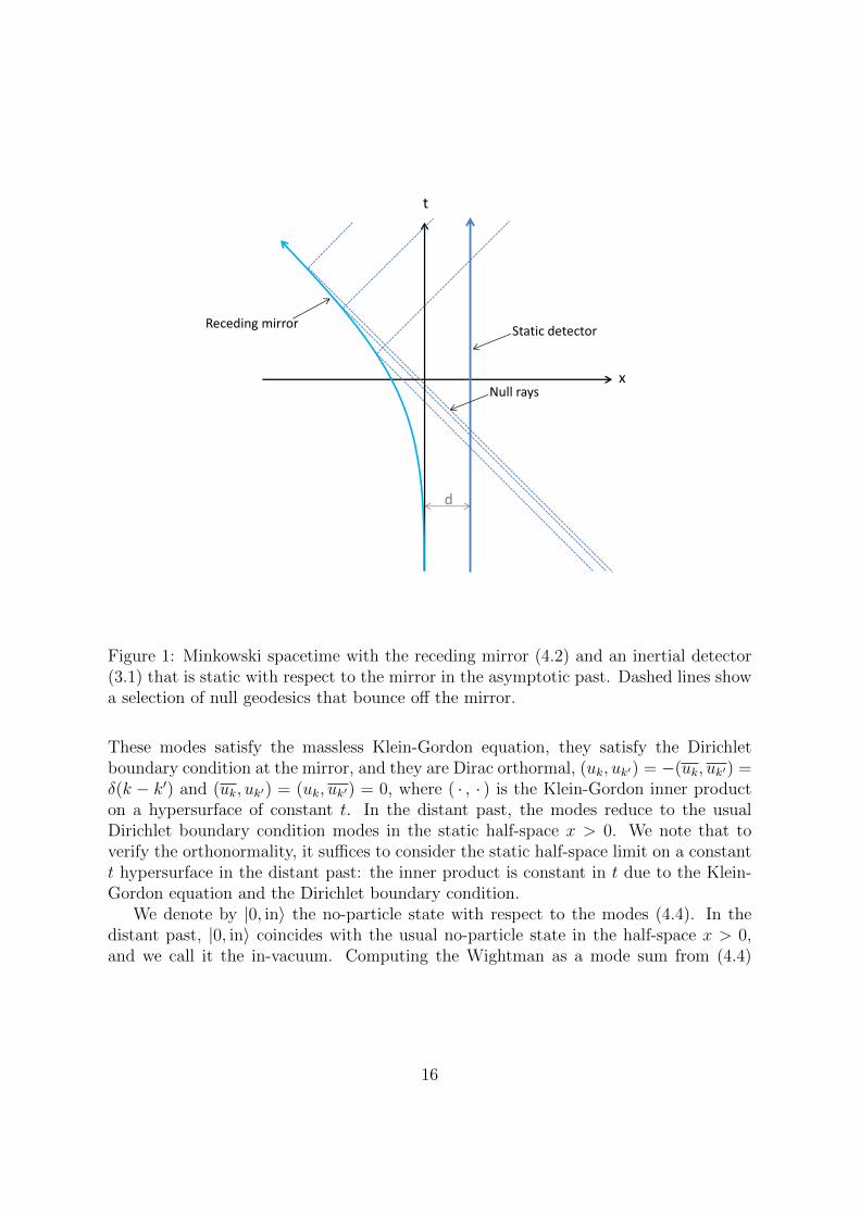
Figure 1: Minkowski spacetime with the receding mirror (4.2) and an inertial detector(3.1) that is static with respect to the mirror in the asymptotic past. Dashed lines showa selection of null geodesics that bounce off the mirror.

These modes satisfy the massless Klein-Gordon equation, they satisfy the Dirichletboundary condition at the mirror, and they are Dirac orthormal, (uk, uk′) = −(uk, uk′) =δ(k − k′) and (uk, uk′) = (uk, uk′) = 0, where ( · , · ) is the Klein-Gordon inner producton a hypersurface of constant t. In the distant past, the modes reduce to the usualDirichlet boundary condition modes in the static half-space x > 0. We note that toverify the orthonormality, it suffices to consider the static half-space limit on a constantt hypersurface in the distant past: the inner product is constant in t due to the Klein-Gordon equation and the Dirichlet boundary condition.

We denote by |0, in〉 the no-particle state with respect to the modes (4.4). In thedistant past, |0, in〉 coincides with the usual no-particle state in the half-space x > 0,and we call it the in-vacuum. Computing the Wightman as a mode sum from (4.4)

16

gives [1]

〈0, in|φ(x)φ(x′)|0, in〉 = − 1

4πln

[ (p(u)− p(u′)− iε

)(v − v′ − iε)(

v − p(u′)− iε)(p(u)− v′ − iε

)] , (4.6)

where iε arises from the conditional ultraviolet convergence as usual. The mode sum isinfrared convergent because of the Dirichlet boundary condition.

4.2 Inertial detector: static in the distant past

We consider a detector on the inertial worldline (3.1), where d is again a positive con-stant. In the asymptotic past, the detector is hence at distance d from a static mirror.We take the detector to be switched on in the asymptotic past, and we take the field tobe in the in-vacuum |0, in〉.

Using (3.1), (4.1) and (4.6), we find

A(τ ′, τ ′′) = − 1

4π

(p′(u′)p′(u′′)

[p(u′)− p(u′′)− iε]2+

1

(v′ − v′′ − iε)2

− p′(u′′)

[v′ − p(u′′)− iε]2− p′(u′)

[p(u′)− v′′ − iε]2

), (4.7)

where u′ = τ ′ − d, v′ = τ ′ + d, u′′ = τ ′′ − d and v′′ = τ ′′ + d. The prime on p denotesderivative with respect to the argument. From (2.16) we then have

F(ω, τ) = F0(ω, τ) + F1(ω, τ) + F2(ω, τ) , (4.8a)

F0(ω, τ) = −ωΘ(−ω) +1

2π

∫ ∞0

ds cos(ωs)

(− p′(τ − d)p′(τ − d− s)

[p(τ − d)− p(τ − d− s)]2+

1

s2

),

(4.8b)

F1(ω, τ) =1

2π

∫ ∞0

dscos(ωs) p′(τ − d− s)

[τ + d− p(τ − d− s)]2, (4.8c)

F2(ω, τ) =1

2π

∫ ∞0

ds Re

(e−iωs p′(τ − d)

[p(τ − d)− τ − d+ s− iε]2

). (4.8d)

In (4.8b) and (4.8c) we have set ε = 0 as the integrand has no singularities. The ε in(4.8d) needs to be kept as the integrand has a singularity, arising because the pointsτ−s and τ on the detector’s trajectory are connected by a null ray that is reflected fromthe mirror, as shown in Figure 1. The integral is well defined despite this singularitysince the switch-on is in the asymptotic past so that the range of s cannot end at thesingularity.

17

We show in Appendix C that the early and late time forms of the transition rate(4.8) are

F(ω, τ) = −ω [1− cos(2dω)] Θ(−ω) +O(eκτ ) as τ → −∞ , (4.9a)

F(ω, τ) = −ω2

Θ(−ω) +ω

2 (e2πω/κ − 1)+ o(1) as τ →∞ . (4.9b)

4.3 Inertial detector: travelling towards the mirror in the dis-tant past

We next consider a detector on the inertial worldline

x(τ) = (τ coshλ,−τ sinhλ) , (4.10)

where λ > 0. In the asymptotic past, where the mirror is static, the detector is movingtowards the mirror with speed tanhλ.

Proceeding as above, we find

F(ω, τ) = F0(ω, τ) + F1(ω, τ) + F2(ω, τ) , (4.11a)

F0(ω, τ) = −ωΘ(−ω) +1

2π

∫ ∞0

ds cos(ωs)

(−p′(eλτ)p′

(eλ(τ − s)

)e2λ[

p(eλτ)− p(eλ(τ − s)

)]2 +1

s2

),

(4.11b)

F1(ω, τ) =1

2π

∫ ∞0

dscos(ωs) p′

(eλ(τ − s)

)[e−λτ − p

(eλ(τ − s)

)]2 , (4.11c)

F2(ω, τ) =1

2π

∫ ∞0

ds Re

(e−iωs p′(eλτ)

[p(eλτ)− e−λ(τ − s)− iε]2

), (4.11d)

and we show in Appendix C that the early and late time forms are

F(ω, τ) = −ω[1− e2λ cos(2τ sinhλ eλω)

]Θ(−ω) +O(τ−1) as τ → −∞ , (4.12a)

F(ω, τ) = −ω2

Θ(−ω) +ω

2 (e2πe−λω/κ − 1)+ o(1) as τ →∞ . (4.12b)

4.4 Onset of thermality

We are now ready to discuss the sense in which the transition rate exhibits the onset ofthermality as the mirror continues to recede.

Consider first the distant past. For the detector (3.1), static with respect to themirror, the transition rate (4.9a) agrees with that (3.7b) of the same detector in the

static half-space M. For the detector (4.10), drifting towards the mirror, the transition

rate (4.12a) can be verified to agree with that of the same detector in M. Compared

18

with (4.9a), the non-Minkowski part of (4.12a) has the static distance d replaced by thetime-dependent distance −τ sinhλ, ω replaced by the blueshifted frequency eλω, and anadditional blueshift factor eλ.

Consider then the distant future. The distant future transition rates (4.9b) and(4.12b) agree with the transition rate (3.18) of an inertial detector in Minkowski spacewhen the left-movers are in the Minkowski vacuum and the right-movers are thermal intemperature κ/(2π). Note that the detector’s velocity shows up by a Doppler blueshiftin the right-mover contribution.

The late time transition rates (4.9b) and (4.12b) can hence be interpreted to consistof a contribution from the left-moving part of the field, undisturbed by the mirror,and and a contribution from the right-moving part of the field, excited by the mirrorto induce a Planckian response. This interpretation is consistent with the fact thatthe stress-energy tensor of the field contains at late times an energy flux to the right[1, 28, 29, 50, 51].

This late time result is consistent with that quoted in [1] for a non-derivative UDWdetector with a mirror trajectory with similar late time asymptotics, in the sense thatthe left-mover contribution was not explicitly written out in [1].

Figures 2 and 3 show numerical plots for the evolution of the transition rate fromearly to late times, for the detector (3.1) that is static with respect to the mirror in thedistant past. The asymptotic late time value is reached via a ring-down of oscillationswhose period equals 2π/κ within the range of the numerical experiments. We have notattempted to examine this oscillation analytically.

5 (1 + 1) Schwarzschild spacetime

In this section we consider a detector in the (1+1)-dimensional Schwarzschild spacetime,obtained by dropping the angular dimensions from the (3+1)-dimensional Schwarzschildmetric [52]. We first establish the notation, recall the definitions of the Boulware, HHIand Unruh vacua [1], and discuss briefly the case of a static detector in the exterior.The main objective is to study a geodesically infalling detector.

5.1 Spacetime and vacua

We write the metric of the (1+1)-dimensional maximally extended Schwarzschild space-time in the notation of [1] as

ds2 = −2Me−r/(2M)

rdu dv , (5.1)

where M > 0 is the Schwarzschild mass parameter, the Kruskal null coordinates u andv increase towards the future and satisfy uv < (4M)2, and r ∈ R+ is the unique solutionto

−uv = (4M)2[r/(2M)− 1]er/(2M) . (5.2)

19

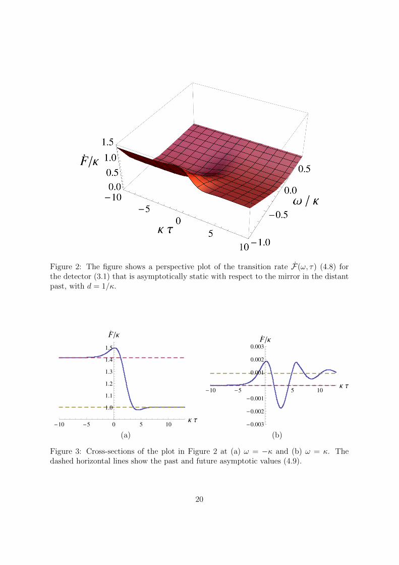
Figure 2: The figure shows a perspective plot of the transition rate F(ω, τ) (4.8) forthe detector (3.1) that is asymptotically static with respect to the mirror in the distantpast, with d = 1/κ.

-10 -5 0 5 10Κ Τ

1.0

1.1

1.2

1.3

1.4

1.5

F Κ

-10 -5 5 10Κ Τ

-0.003

-0.002

-0.001

0.001

0.002

0.003

F Κ

(a) (b)

Figure 3: Cross-sections of the plot in Figure 2 at (a) ω = −κ and (b) ω = κ. Thedashed horizontal lines show the past and future asymptotic values (4.9).

20

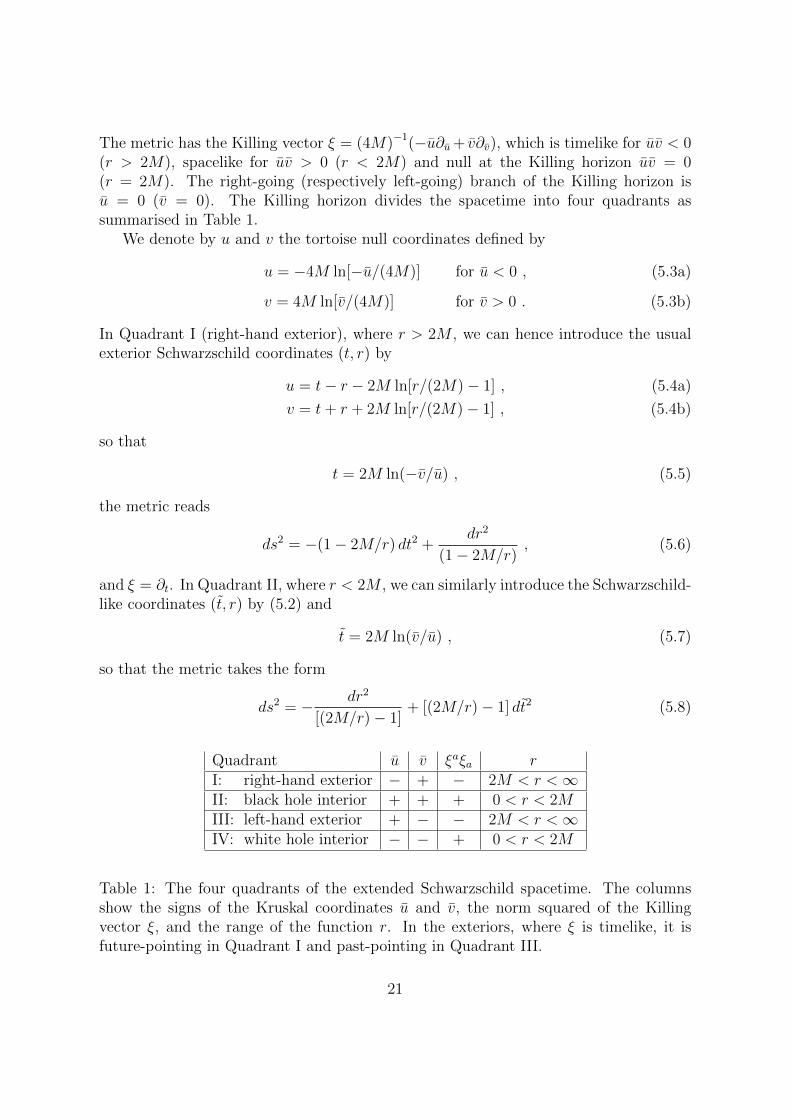
The metric has the Killing vector ξ = (4M)−1(−u∂u+ v∂v), which is timelike for uv < 0(r > 2M), spacelike for uv > 0 (r < 2M) and null at the Killing horizon uv = 0(r = 2M). The right-going (respectively left-going) branch of the Killing horizon isu = 0 (v = 0). The Killing horizon divides the spacetime into four quadrants assummarised in Table 1.

We denote by u and v the tortoise null coordinates defined by

u = −4M ln[−u/(4M)] for u < 0 , (5.3a)

v = 4M ln[v/(4M)] for v > 0 . (5.3b)

In Quadrant I (right-hand exterior), where r > 2M , we can hence introduce the usualexterior Schwarzschild coordinates (t, r) by

u = t− r − 2M ln[r/(2M)− 1] , (5.4a)

v = t+ r + 2M ln[r/(2M)− 1] , (5.4b)

so that

t = 2M ln(−v/u) , (5.5)

the metric reads

ds2 = −(1− 2M/r) dt2 +dr2

(1− 2M/r), (5.6)

and ξ = ∂t. In Quadrant II, where r < 2M , we can similarly introduce the Schwarzschild-like coordinates (t, r) by (5.2) and

t = 2M ln(v/u) , (5.7)

so that the metric takes the form

ds2 = − dr2

[(2M/r)− 1]+ [(2M/r)− 1] dt2 (5.8)

Quadrant u v ξaξa rI: right-hand exterior − + − 2M < r <∞II: black hole interior + + + 0 < r < 2MIII: left-hand exterior + − − 2M < r <∞IV: white hole interior − − + 0 < r < 2M

Table 1: The four quadrants of the extended Schwarzschild spacetime. The columnsshow the signs of the Kruskal coordinates u and v, the norm squared of the Killingvector ξ, and the range of the function r. In the exteriors, where ξ is timelike, it isfuture-pointing in Quadrant I and past-pointing in Quadrant III.

21

and ξ = ∂t. A pair of coordinates that covers Quadrants I and II and the black holehorizon that separates them is (u, v). We shall not need the explicit form of the metricin these coordinates.

We consider a massless minimally coupled scalar field in three distinguished states.First, in Quadrant I we consider the Boulware vacuum |0B〉, defined by the positive andnegative frequency decomposition with respect to ∂t in (5.6) [53]. At the asymptoticallyflat infinity of Quadrant I, |0B〉 reduces to the Minkowski vacuum. Second, on thewhole spacetime we consider the HHI vacuum |0H〉, defined by the positive and negativefrequency decomposition with respect to ∂u and ∂v on the Killing horizon [54, 55]. InQuadrant I, |0H〉 is a thermal equilibrium state with respect to ∂t, at the local Hawkingtemperature

Tloc =1

8πM√

1− 2M/r. (5.9)

Third, in Quadrants I and II and on the black hole horizon that separates them, weconsider the Unruh vacuum |0U〉, defined by the positive and negative frequency de-composition with respect to ∂u and ∂v in the coordinates (u, v) [3]. |0U〉 mimics a statethat results from the collapse of a star at late times when there is initially no incomingradiation from infinity, and it has the left-moving part of the field in a Boulware-likestate and the right-moving part of the field in a HHI-like state.

The Wightman functions for the three vacua are [1]

〈0B|φ(x)φ(x′)|0B〉 = − 1

4πln[(ε+ i∆u)(ε+ i∆v)] , (5.10a)

〈0H |φ(x)φ(x′)|0H〉 = − 1

4πln[(ε+ i∆u)(ε+ i∆v)] , (5.10b)

〈0U |φ(x)φ(x′)|0U〉 = − 1

4πln[(ε+ i∆u)(ε+ i∆v)] , (5.10c)

where ∆u = u − u′ and similarly for the other coordinates. Each of the Wightmanfunctions is unique up to a real-valued additive constant. The Boulware and HHI vacuumWightman functions are invariant under the isometries generated by the Killing vector ξ.The Unruh vacuum Wightman function changes under these isometries by an additiveconstant; however, the Unruh vacuum may nevertheless be considered invariant underthe isometries since the stress-energy tensor and other quantities built from derivatives ofthe Wightman function are invariant [31, 32]. The non-invariance of the Unruh vacuumWightman function is due to the infrared properties of the (1+1)-dimensional conformalfield and has no counterpart in higher dimensions [56].

5.2 Static detector

We consider first a detector in Quadrant I on the static, noninertial trajectory r = R,where R > 2M is a constant. Using (2.17) and (5.10), the calculations are closely similar

22

to those in Section 3, and we omit the detail. We find

FB(ω) = −ωΘ(−ω) , (5.11a)

FH(ω) =ω

eω/Tloc − 1, (5.11b)

FU(ω) = −ω2

Θ(−ω) +ω

2 (eω/Tloc − 1), (5.11c)

for respectively the Boulware, HHI and Unruh vacua, where Tloc is the local Hawkingtemperature (5.9) evaluated at r = R.

These results conform fully to expectations. The Boulware vacuum transition rateis that of an inertial detector in Minkowski space in Minkowski vacuum, while the HHIvacuum transition rate is thermal in the local Hawking temperature (5.9). The Unruhvacuum transition rate is the average of the two, with the two pieces arising respectivelyfrom the left-moving and right-moving parts of the field.

These results are also consistent with what was reported for the non-derivative UDWdetector in [1], in the sense that the left-mover contribution in (5.11c) was not explicitlywritten out in [1]. Finally, the similarity between (5.11c) and our receding mirror space-time results (4.9b) and (4.12b) is an additional confirmation that the Unruh vacuummimics the late time properties of a state created in a collapsing star spacetime [1, 3].

5.3 Interlude: geodesics

We next turn to inertial detectors. In this subsection we recall a convenient parametri-sation for the geodesics. We give the full expressions in a form that applies only toQuadrant I, where the equations of a timelike geodesic in the Schwarzschild coordinates(5.6) take the form

t =E

1− 2M/r, (5.12a)

r2 = E2 − 1 + 2M/r , (5.12b)

where E is a positive constant and the overdot denotes derivative with respect to theproper time τ . The continuation beyond Quadrant I can be done by passing to theKruskal coordinates (u, v).

When E > 1, the geodesic has at infinity the nonvanishing speed√

1− E−2 withrespect to the Killing vector ξ. We consider a geodesic that is sent in from the infinity,

23

so that r < 0. The geodesic can be parametrised as

τ =M

(E2 − 1)3/2(sinhχ− χ) , (5.13a)

r =M

(E2 − 1)(coshχ− 1) , (5.13b)

t =ME

(E2 − 1)3/2

[sinhχ+ (2E2 − 3)χ

]+ 2M ln

(− tanh(χ/2) +

√1− E−2

− tanh(χ/2)−√

1− E−2

), (5.13c)

where the parameter χ takes values in (−∞, 0), so that the trajectory starts at theinfinity in the asymptotic past at χ → −∞ and hits the singularity at χ → 0. Theadditive constant in (5.13a) is chosen so that −∞ < τ < 0. The horizon-crossing occursat χ = χh

.= −2 arctanh

(√1− E−2

). Equation (5.13c) applies only in Quadrant I,

where −∞ < χ < χh.When E = 1, the geodesic has at infinity a vanishing speed with respect to ξ. We

consider again a geodesic that is sent in from the infinity. The geodesic takes the form

r = 2M [−3τ/(4M)]2/3 , (5.14a)

t = τ − 4M [−3τ/(4M)]1/3 + 2M ln

([−3τ/(4M)]1/3 + 1

[−3τ/(4M)]1/3 − 1

), (5.14b)

where −∞ < τ < 0. The horizon-crossing occurs at τ = τh.= −4M/3, and the

singularity is reached as τ → 0. Equation (5.14b) applies only in Quadrant I, where−∞ < τ < τh.

When 0 < E < 1, the geodesic has a maximum value of r. The geodesic can beparametrised as

τ =M

(1− E2)3/2(ϕ+ sinϕ) , (5.15a)

r =M

(1− E2)(1 + cosϕ) , (5.15b)

t =ME

(1− E2)3/2

[sinϕ+ (3− 2E2)ϕ

]+ 2M ln

(1 +√E−2 − 1 tan(ϕ/2)

1−√E−2 − 1 tan(ϕ/2)

), (5.15c)

where the parameter ϕ takes values in (−π, π), so that the trajectory starts at thewhite hole singularity at ϕ → −π and ends at the black hole singularity at ϕ →π. The additive constant in (5.15a) is chosen so that τ = 0 at the moment whenr reaches its maximum value, 2M/(1 − E2). The total proper time elapsed between

the singularities is 2πM(1− E2)−3/2

. The horizon-crossings occur at ϕ = ∓ϕh where

24

ϕh.= 2 arctan

(√E−2 − 1

). Equation (5.15c) applies only in Quadrant I, where −ϕh <

ϕ < ϕh.Finally, there exist also timelike geodesics that pass from the white hole to the black

hole through the horizon bifurcation point u = v = 0, without entering Quadrant I (orQuadrant III). These geodesics take the form

u = v = 4M sin(ϕ/2) exp[

12

cos2(ϕ/2)], (5.16)

where the parameter ϕ takes values in (−π, π), and τ and r are given by (5.15a) and(5.15b) with E = 0. The isometry generated by ξ has been used in (5.16) to set u = vwithout loss of generality.

5.4 Inertial detector

The transition rate of the inertial detector is obtained by inserting the Wightman func-tions (5.10) and the geodesic trajectories of subsection 5.3 into the integral formulasof subsection 2.3. The transition rate is expressible as the integral of an elementaryfunction for all values of E; for E > 1 (respectively E < 1) this is accomplished bywriting the differentiations and the integration in terms of χ (ϕ).

We address the near-infinity and near-singularity limits analytically and the inter-mediate regime numerically.

5.4.1 Near the infinity

We consider the E > 1 trajectories (5.13) and the E = 1 trajectory (5.14), all of whichfall in from the infinity, and we push the switch-on to the infinite past. It is shown inAppendix D that at early times, τ → −∞, we have

FB(ω, τ) = −ωΘ(−ω) + o(1) , (5.17a)

FH(ω, τ) =ω

2 (eω/T− − 1)+

ω

2 (eω/T+ − 1)+ o(1) , (5.17b)

FU(ω, τ) = −ω2

Θ(−ω) +ω

2 (eω/T+ − 1)+ o(1) , (5.17c)

where T±.= e±λ/(8πM) and λ

.= arctanh

(√1− E−2

). For E = 1, we have T+ = T− =

1/(8πM), so that the two terms in (5.17b) are equal and combine to the Planckianresponse.

The asymptotic past results (5.17) conform fully to physical expectations. TheBoulware vacuum transition rate is that in Minkowski vacuum (3.7a), consistently withthe interpretation of the Bouware vacuum as the no-particle state with respect to ξ.The HHI vacuum transition rate is that of an inertial detector in a thermal bath inMinkowski space (3.16), with the temperature given by the Hawking temperature atthe infinity, 1/(8πM), and with each of the two Planckian terms containing a Doppler

25

shift factor that accounts for the detector’s velocity at the infinity. The Unruh vacuumtransition rate sees a Planckian term only in the outgoing part of the field, as confirmedby the Doppler shift to the blue in this term, while the term that corresponds to theingoing part of the field is Minkowski-like.

5.4.2 Near the singularity

We consider the transition rate in the HHI and Unruh vacua in the limit where thedetector approaches the black black hole singularity. We allow all values of the non-negative constant E. We also allow the switch-on moment to remain arbitrary, subjectonly to the condition that for 0 ≤ E < 1 the switch-on in the HHI vacuum takes placeafter the trajectory emerges from the white hole singularity, and the switch-on in theUnruh vacuum takes place after the trajectory crosses the past horizon.

It is shown in Appendix D that in this near-singularity limit we have

F(ω, τ) =1

8πM

[(2M

r(τ)

)3/2

+1 + E2

2

(2M

r(τ)

)1/2]

+O(1) , (5.18)

for both the HHI vacuum and the Unruh vacuum: the differences between the twovacua show up only in the O(1) part. In terms of τ , the leading term in (5.18) is1/[6π(τsing − τ)], where τsing is the value of τ at the black hole singularity.

5.4.3 Intermediate regime: loss of thermality

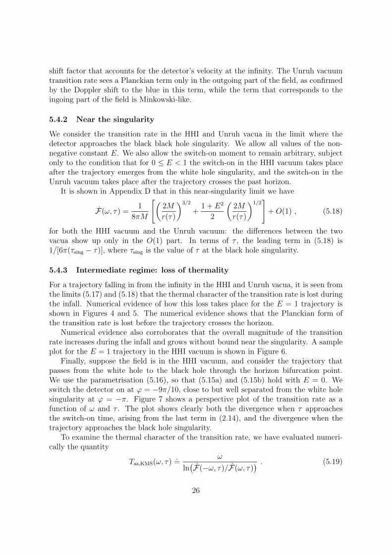
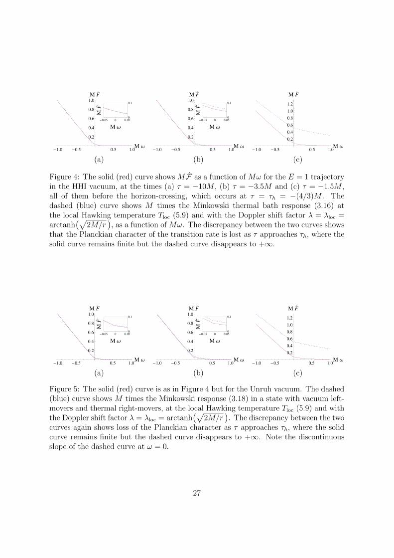
For a trajectory falling in from the infinity in the HHI and Unruh vacua, it is seen fromthe limits (5.17) and (5.18) that the thermal character of the transition rate is lost duringthe infall. Numerical evidence of how this loss takes place for the E = 1 trajectory isshown in Figures 4 and 5. The numerical evidence shows that the Planckian form ofthe transition rate is lost before the trajectory crosses the horizon.

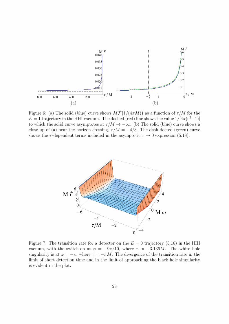
Numerical evidence also corroborates that the overall magnitude of the transitionrate increases during the infall and grows without bound near the singularity. A sampleplot for the E = 1 trajectory in the HHI vacuum is shown in Figure 6.

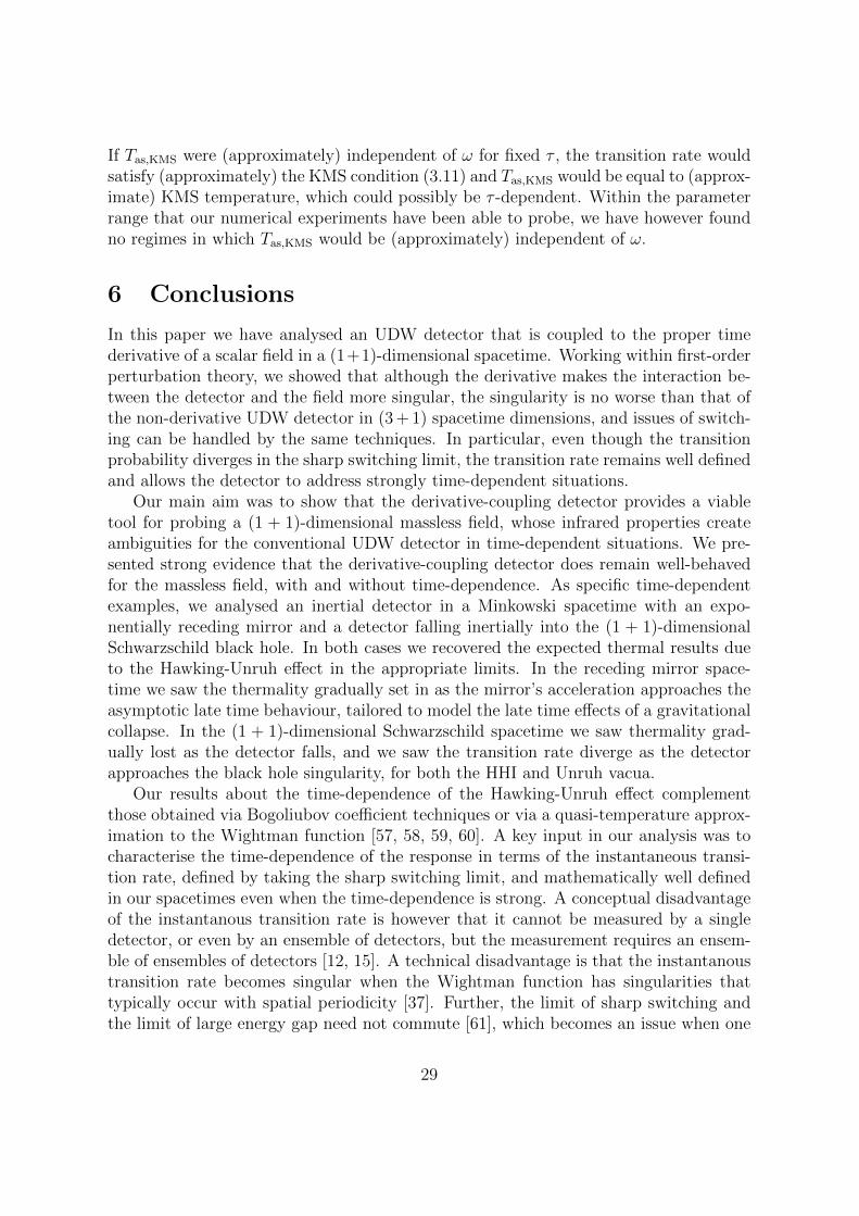
Finally, suppose the field is in the HHI vacuum, and consider the trajectory thatpasses from the white hole to the black hole through the horizon bifurcation point.We use the parametrisation (5.16), so that (5.15a) and (5.15b) hold with E = 0. Weswitch the detector on at ϕ = −9π/10, close to but well separated from the white holesingularity at ϕ = −π. Figure 7 shows a perspective plot of the transition rate as afunction of ω and τ . The plot shows clearly both the divergence when τ approachesthe switch-on time, arising from the last term in (2.14), and the divergence when thetrajectory approaches the black hole singularity.

To examine the thermal character of the transition rate, we have evaluated numeri-cally the quantity

Tas,KMS(ω, τ).=

ω

ln(F(−ω, τ)/F(ω, τ)

) . (5.19)

26

-1.0 -0.5 0.5 1.0M Ω

0.2

0.4

0.6

0.8

1.0

M F

-0.05 0 0.050

0.1

M Ω

MF

-1.0 -0.5 0.5 1.0M Ω

0.2

0.4

0.6

0.8

1.0

M F

-0.05 0 0.050

0.1

M Ω

MF

-1.0 -0.5 0.5 1.0M Ω

0.2

0.4

0.6

0.8

1.0

1.2

M F

(a) (b) (c)

Figure 4: The solid (red) curve shows MF as a function of Mω for the E = 1 trajectoryin the HHI vacuum, at the times (a) τ = −10M , (b) τ = −3.5M and (c) τ = −1.5M ,all of them before the horizon-crossing, which occurs at τ = τh = −(4/3)M . Thedashed (blue) curve shows M times the Minkowski thermal bath response (3.16) atthe local Hawking temperature Tloc (5.9) and with the Doppler shift factor λ = λloc =arctanh

(√2M/r

), as a function of Mω. The discrepancy between the two curves shows

that the Planckian character of the transition rate is lost as τ approaches τh, where thesolid curve remains finite but the dashed curve disappears to +∞.

-1.0 -0.5 0.5 1.0M Ω

0.2

0.4

0.6

0.8

1.0

M F

-0.05 0 0.050

0.1

M Ω

MF

-1.0 -0.5 0.5 1.0M Ω

0.2

0.4

0.6

0.8

1.0

M F

-0.05 0 0.050

0.1

M Ω

MF

-1.0 -0.5 0.5 1.0M Ω

0.2

0.4

0.6

0.8

1.0

1.2

M F

(a) (b) (c)

Figure 5: The solid (red) curve is as in Figure 4 but for the Unruh vacuum. The dashed(blue) curve shows M times the Minkowski response (3.18) in a state with vacuum left-movers and thermal right-movers, at the local Hawking temperature Tloc (5.9) and withthe Doppler shift factor λ = λloc = arctanh

(√2M/r

). The discrepancy between the two

curves again shows loss of the Planckian character as τ approaches τh, where the solidcurve remains finite but the dashed curve disappears to +∞. Note the discontinuousslope of the dashed curve at ω = 0.

27

-800 -600 -400 -200 0Τ M

0.015

0.020

0.025

0.030

0.035

0.040M F

-2 - 4

3 -1 0Τ M

0.1

0.2

0.3

0.4

0.5

0.6M F

(a) (b)

Figure 6: (a) The solid (blue) curve shows MF(1/(4πM)

)as a function of τ/M for the

E = 1 trajectory in the HHI vacuum. The dashed (red) line shows the value 1/[4π(e2−1)]to which the solid curve asymptotes at τ/M → −∞. (b) The solid (blue) curve shows aclose-up of (a) near the horizon-crossing, τ/M = −4/3. The dash-dotted (green) curveshows the τ -dependent terms included in the asymptotic τ → 0 expression (5.18).

Figure 7: The transition rate for a detector on the E = 0 trajectory (5.16) in the HHIvacuum, with the switch-on at ϕ = −9π/10, where τ ≈ −3.136M . The white holesingularity is at ϕ = −π, where τ = −πM . The divergence of the transition rate in thelimit of short detection time and in the limit of approaching the black hole singularityis evident in the plot.

28

If Tas,KMS were (approximately) independent of ω for fixed τ , the transition rate wouldsatisfy (approximately) the KMS condition (3.11) and Tas,KMS would be equal to (approx-imate) KMS temperature, which could possibly be τ -dependent. Within the parameterrange that our numerical experiments have been able to probe, we have however foundno regimes in which Tas,KMS would be (approximately) independent of ω.

6 Conclusions

In this paper we have analysed an UDW detector that is coupled to the proper timederivative of a scalar field in a (1+1)-dimensional spacetime. Working within first-orderperturbation theory, we showed that although the derivative makes the interaction be-tween the detector and the field more singular, the singularity is no worse than that ofthe non-derivative UDW detector in (3 + 1) spacetime dimensions, and issues of switch-ing can be handled by the same techniques. In particular, even though the transitionprobability diverges in the sharp switching limit, the transition rate remains well definedand allows the detector to address strongly time-dependent situations.

Our main aim was to show that the derivative-coupling detector provides a viabletool for probing a (1 + 1)-dimensional massless field, whose infrared properties createambiguities for the conventional UDW detector in time-dependent situations. We pre-sented strong evidence that the derivative-coupling detector does remain well-behavedfor the massless field, with and without time-dependence. As specific time-dependentexamples, we analysed an inertial detector in a Minkowski spacetime with an expo-nentially receding mirror and a detector falling inertially into the (1 + 1)-dimensionalSchwarzschild black hole. In both cases we recovered the expected thermal results dueto the Hawking-Unruh effect in the appropriate limits. In the receding mirror space-time we saw the thermality gradually set in as the mirror’s acceleration approaches theasymptotic late time behaviour, tailored to model the late time effects of a gravitationalcollapse. In the (1 + 1)-dimensional Schwarzschild spacetime we saw thermality grad-ually lost as the detector falls, and we saw the transition rate diverge as the detectorapproaches the black hole singularity, for both the HHI and Unruh vacua.

Our results about the time-dependence of the Hawking-Unruh effect complementthose obtained via Bogoliubov coefficient techniques or via a quasi-temperature approx-imation to the Wightman function [57, 58, 59, 60]. A key input in our analysis was tocharacterise the time-dependence of the response in terms of the instantaneous transi-tion rate, defined by taking the sharp switching limit, and mathematically well definedin our spacetimes even when the time-dependence is strong. A conceptual disadvantageof the instantanous transition rate is however that it cannot be measured by a singledetector, or even by an ensemble of detectors, but the measurement requires an ensem-ble of ensembles of detectors [12, 15]. A technical disadvantage is that the instantanoustransition rate becomes singular when the Wightman function has singularities thattypically occur with spatial periodicity [37]. Further, the limit of sharp switching andthe limit of large energy gap need not commute [61], which becomes an issue when one

29

attempts to identify characteristics of thermal behavour in the response of a detectorthat operates for a genuinely finite interval of time. While we hence do not advocatethe instantaneous transition rate as a definitive quantifier of time-dependence in thedetector’s response, our results strongly suggest that the instantaneous transition rateconveys a physically expected picture about the onset and decay of the Hawking-Unruheffect.

Acknowledgments

We thank Don Marolf and Adrian Ottewill for discussions and correspondence, encour-aging us to look at the derivative-coupling detector. We also thank Chris Fewster, LeeHodgkinson, Bei-Lok Hu, Bernard Kay, Eduardo Martın-Martınez, Suprit Singh andMatteo Smerlak for helpful discussions and comments. A special thanks to Don Pagefor questions that led to the correction of an error in the captions of Figures 4 and 5.BAJA was supported by Consejo Nacional de Ciencia y Tecnologıa (CONACYT), withadditional support from Sistema Estatal de Becas de Veracruz, Mexico. JL was sup-ported in part by STFC (Theory Consolidated Grant ST/J000388/1).

A Evaluation of Fsing (2.6c)

In this appendix we show that Fsing (2.6c) can be written as (A.6) or (A.7).Starting from (2.6c) and integrating the distributional derivatives by parts, we have

Fsing(ω) =

∫ ∞−∞

dτ ′∫ ∞−∞

dτ ′′Q′ω(τ ′)Q′ω(τ ′′)Wsing(τ ′, τ ′′) , (A.1)

where Qω(τ).= e−iωτχ(τ) and the prime denotes derivative with respect to the argu-

ment. Note that the integrand in (A.1) is a locally integrable function, containing nodistributional parts. Using the explicit form of Wsing (2.4), we obtain

Fsing(ω) = Fsing,1(ω) + Fsing,2(ω) , (A.2a)

Fsing,1(ω) = − i

4

∫ ∞−∞

dτ ′∫ ∞−∞

dτ ′′Q′ω(τ ′)Q′ω(τ ′′) sgn(τ ′ − τ ′′) , (A.2b)

Fsing,2(ω) = − 1

2π

∫ ∞−∞

dτ ′∫ ∞−∞

dτ ′′Q′ω(τ ′)Q′ω(τ ′′) ln |τ ′ − τ ′′| . (A.2c)

30

For Fsing,1, integrating over τ ′′ in (A.2b) gives

Fsing,1(ω) = − i

2

∫ ∞−∞

duQ′ω(u)Qω(u)

= − i

2

∫ ∞−∞

du [χ′(u)− iωχ(u)]χ(u)

= −ω2

∫ ∞−∞

du [χ(u)]2 , (A.3)

where we have renamed τ ′ as u, used the definition of Qω, and finally noted that∫∞−∞ duχ

′(u)χ(u) = 12

∫∞−∞ du

ddu

[χ(u)]2 = 0.For Fsing,2, we break the integral in (A.2c) into the subdomains τ ′ > τ ′′ and τ ′ < τ ′′.

In the subdomain τ ′ > τ ′′ we write τ ′ = u and τ ′′ = u− s, where u ∈ R and 0 < s <∞,and in the subdomain τ ′ < τ ′′ we write τ ′′ = u and τ ′ = u− s, where again u ∈ R and0 < s <∞. This gives

Fsing,2(ω) = − 1

π

∫ ∞0

ds ln s

∫ ∞−∞

duRe[Q′ω(u)Q′ω(u− s)

]=

1

π

∫ ∞0

ds ln s

∫ ∞−∞

duRe[Qω(u)Q′′ω(u− s)

]=

1

π

∫ ∞0

ds ln sd2

ds2

∫ ∞−∞

duRe[Qω(u)Qω(u− s)

]=

1

π

∫ ∞0

ds ln sd2

ds2

(cos(ωs)

∫ ∞−∞

duχ(u)χ(u− s))

= − 1

π

∫ ∞0

ds

s

d

ds

(cos(ωs)

∫ ∞−∞

duχ(u)χ(u− s)), (A.4)

where we have first integrated by parts in u, then written the derivatives in Q′′ω(u− s) ass-derivatives outside the u-integral, then used the definition of Qω, and finally integratedby parts in s. The substitution term from s = 0 in the integration by parts vanishesbecause cos(ωs)

∫∞−∞ duχ(u)χ(u − s) is even in s, and the integral over s in the last

expression in (A.4) is convergent at small s for the same reason.In the last expression in (A.4), writing χ(u)χ(u−s) = [χ(u)]2−χ(u)[χ(u)−χ(u−s)]

31

gives

Fsing,2(ω) =ω

π

(∫ ∞−∞

du [χ(u)]2)∫ ∞

0

dssin(ωs)

s

+1

π

∫ ∞0

ds

s

d

ds

(cos(ωs)

∫ ∞−∞

duχ(u)[χ(u)− χ(u− s)])

=|ω|2

∫ ∞−∞

du [χ(u)]2 +1

π

∫ ∞0

dscos(ωs)

s2

∫ ∞−∞

duχ(u)[χ(u)− χ(u− s)] ,

(A.5)

where in the first term we have used the identity∫∞

0ds s−1 sin(ωs) = 1

2π sgnω, and in

the second term we have integrated by parts. The integral over s in the second termis convergent at small s because

∫∞−∞ duχ(u)[χ(u)− χ(u− s)] vanishes at s = 0 and is

even in s.Combining (A.3) and (A.5), we obtain

Fsing(ω) = −ωΘ(−ω)

∫ ∞−∞

du [χ(u)]2

+1

π

∫ ∞0

dscos(ωs)

s2

∫ ∞−∞

duχ(u)[χ(u)− χ(u− s)] . (A.6)

An alternative expression is

Fsing(ω) = −ω2

∫ ∞−∞

du [χ(u)]2 +1

π

∫ ∞0

ds

s2

∫ ∞−∞

duχ(u) [χ(u)− χ(u− s)]

+1

π

∫ ∞−∞

du

∫ ∞0

ds χ(u)χ(u− s) [1− cos(ωs)]

s2, (A.7)

which may be obtained from (A.6) by writing cos(ωs) = 1− [1− cos(ωs)] and using theidentity ∫ ∞

0

ds1− cos(ωs)

s2=π|ω|

2. (A.8)

B Evaluation of the static detector’s transition rate

in Minkowski (half-)space

In this appendix we verify formulas (3.4) and (3.7) for the transition rate of a staticdetector in Minkowski space and Minkowski half-space. We use the Wightman functionsfound in subsection 3.1 and evaluate the transition rate from (2.17).

32

B.1 m = 0

We consider first the massless field, with the Wightman function given by (3.5) and (3.6).In M, we find from (2.8), (3.1) and (3.5) that A(τ ′, τ ′′) = −1/

[2π(τ ′ − τ ′′ − iε)2

].

Evaluating (2.17) as a contour integral gives (3.7a).

In M, we find from (3.6) that the integrand in (2.17) contains the additional piece

∆A(τ ′, τ ′′) = − η

2π

(τ ′ − τ ′′ − iε)2 + 4d2

[(τ ′ − τ ′′ − iε)2 − 4d2]2. (B.1)

Evaluating the contribution to (2.17) as a contour integral leads to (3.7b).We note that ∆A(τ ′, τ ′′) (B.1) has distributional singularities at τ ′− τ ′′ = ±2d. The

geometric reason for these singularities is that the points τ ′ and τ ′′ on the detector’strajectory are connected by a null ray that is reflected from the mirror. As we haveseen, the stationary transition rate is well defined despite these singularities. Were wehowever to consider a detector that operates for a finite duration, the singularities wouldinterfere with the sharp switching limit manipulations that led to (2.14) when ∆τ = 2d.

B.2 m > 0

For the massive field, the Wightman function is given by (3.2) and (3.3). We consider

M and M in turn.

B.2.1 M

In M, we find from (2.8), (3.1) and (3.2) that

A(τ ′, τ ′′) =m2

2πK ′′0[m(ε+ i(τ ′ − τ ′′)

)], (B.2)

where the prime denotes derivative with respect to the argument. From (2.17) we thenobtain

F(ω) =m2

2π

∫C

ds e−iωsK ′′0 (ims) , (B.3)

where the contour C in the complex s plane follows the real axis from −∞ to +∞ exceptthat it drops in the lower half-plane near s = 0, and K0 has its principal branch when sis negative imaginary. We now assume ω 6= −m: it follows then from the asymptotics ofK0 at large imaginary argument [48] that (B.3) is convergent as an improper Riemannintegral.

From (B.3) we obtain

F(ω) =ω2

2π

∫C

ds e−iωsK0(ims)

=ω2

2Im

∫ ∞0

ds e−iωsH(2)0 (ms) , (B.4)

33

where we have first integrated by parts twice, as allowed by the large s behaviour ofthe integrand, then deformed C to the real s axis, as allowed by the merely logarithmicsingularity of the integrand at s = 0, and finally used the Bessel function analyticcontinuation formulas [48]. The integral in (B.4) was encountered in [19] in the contextof a non-derivative detector, and from equations (5.11) and (5.14) therein we have

F(ω) =ω2

√ω2 −m2

Θ(−ω −m) , (B.5)

which is the result (3.4a) used in the main text.

B.2.2 M

In M, we find from (3.3) that the integrand in (2.17) contains the additional piece

∆A(τ, τ ′′) = − η

2π

d2

dτ ′2K0

[m√

4d2 − (τ ′ − τ ′′ − iε)2], (B.6)

where the branch of the square root is as explained in the main text. The additionalpiece in the transition rate (2.17) is hence

∆F(ω) = − η

2π

∫ ∞−∞

ds e−iωs d2

ds2K0

[m√

4d2 − (s− iε)2]

=ηω2

2π

∫ ∞−∞

ds e−iωsK0

[m√

4d2 − (s− iε)2]

=ηω2

πRe

∫ ∞0

ds e−iωsK0

[m√

4d2 − (s− iε)2], (B.7)

again assuming ω 6= −m and integrating by parts twice. The integral in (B.7) wasencountered in [19], and from equations (5.15) and (5.25) therein we have

∆F(ω) =ηω2 cos

(2d√ω2 −m2

)√ω2 −m2

Θ(−ω −m) , (B.8)

which leads to the result (3.4b) in the main text.

C Asymptotic past and future transition rate in the

receding mirror spacetime

In this appendix we find the asymptotic past and future forms (4.9) and (4.12) of thetransition rate of an inertial detector in the receding mirror spacetime of Section 4.

34

C.1 Static in the distant past

We wish to extract the asymptotic behaviour of (4.8) as τ → −∞ and as τ →∞.

C.1.1 τ → −∞

Consider (4.8b). Using (4.5) and letting h.=(1 + eκ(d−τ)

)−1, we have

F0(ω, τ) = −ωΘ(−ω) +1

2π

∫ ∞0

ds cos(ωs)

(1

X+

1

s2

), (C.1)

where

X = −[1− h(1− e−κs)]

κs+ ln[1− h(1− e−κs)]

2

κ2(1− h)2 . (C.2)

The limit τ → −∞ is now the limit h→ 0+.Following the technique used in subsection 5.3 of [13], we make in the integrand of

(C.1) the re-arrangement

1

X+

1

s2=−X − s2

s4

(1 +−X − s2

s2

)−1

. (C.3)

Taylor expanding the numerator of (C.2) to quartic order in h(1− e−κs) shows that thesecond factor in (C.3) is of the form 1 + O(h), uniformly in s, and yields for the firstfactor in (C.3) an estimate that can be applied under the integral over s and whoseleading term is proportional to h. We hence have

F0(ω, τ) = −ωΘ(−ω) +O(h) . (C.4)

Consider then (4.8c). Proceeding similarly, we find

F1(ω, τ) =1

4πd+|ω|2π

[cos(2dω) si(2d|ω|)− sin(2d|ω|) Ci(2d|ω|)

]+O(h) , (C.5)

where si and Ci are the sine and cosine integrals in the notation of [48].Consider finally (4.8d). Integrating by parts once reduces the integral to a form that

can be evaluated exactly in terms of the sine and cosine integrals [48], with the result

F2(ω, τ) =1− h

2π

− 1

B+ |ω|

[sin(B|ω|) Ci(B|ω|)− cos(Bω) si(B|ω|)

]+ 2πω cos(Bω)Θ(−ω)

, (C.6)

35

where B.= 2d− κ−1 ln(1− h). A small h expansion in (C.6) gives

F2(ω, τ) = − 1

4πd+|ω|2π

[sin(2d|ω|) Ci(2d|ω|)− cos(2dω) si(2d|ω|)

]+ ω cos(Bω)Θ(−ω) +O(h) . (C.7)

Combining (C.4), (C.5) and (C.7), we have

F(ω, τ) = −ω [1− cos(2dω)] Θ(−ω) +O(eκτ ) as τ → −∞ . (C.8)

C.1.2 τ →∞

Consider (4.8b). Letting f.= 1/(1 + eκ(τ−d)), and adding and subtracting

κ2 cos(ωs)[8π sinh2(κs/2)]−1 in the integrand, we obtain

F0(ω, τ) = −ωΘ(−ω) +1

2π

∫ ∞0

ds cos(ωs)

(1

s2− κ2

4 sinh2(κs/2)

)

+κ2

2π

∫ ∞0

ds cos(ωs)

(1

4 sinh2(κs/2)− f 2 eκs

[1 + f(eκs − 1)]

ln[1 + f(eκs − 1)]2

).

(C.9)

In the last term in (C.9), the integrand goes to zero pointwise as f → 0, and a monotoneconvergence argument shows that the integral vanishes as f → 0. The second term plushalf of the first term is equal to half of the transition rate encountered in subsection 3.2(with a→ κ) and evaluated to (3.10). We hence have

F0(ω, τ) = −ω2

Θ(−ω) +ω

2 (e2πω/κ − 1)+ o(1) as f → 0 . (C.10)

In (4.8c), a straightforward monotone convergence argument gives F1(ω, τ) = o(1).In (4.8d), (C.6) gives F2(ω, τ) = O(f).

Combining, we have

F(ω, τ) = −ω2

Θ(−ω) +ω

2 (e2πω/κ − 1)+ o(1) as τ →∞ . (C.11)

C.2 Travelling towards the mirror in the distant past

We wish to extract the asmptotic behaviour of (4.11) as τ → −∞ and as τ →∞.

C.2.1 τ → −∞

For (4.11b), proceeding as in (C.1)–(C.4) gives

F0(ω, τ) = −ωΘ(−ω) +O(eeλκτ

). (C.12)

36

For (4.11c), we have

F1(ω, τ) =1

2π

∫ ∞0

cos(ωs) ds(1 + ge−κseλ

) [seλ − 2τ sinhλ+ κ−1 ln

(1 + ge−κseλ

)]2 , (C.13)

where g = eκτeλ . When τ < 0, we may bound the absolute value of F1(ω, τ) by thereplacements cos(ωs)→ 1 and g → 0 in (C.13), and evaluating the integral that ensuesgives F1(ω, τ) = O(τ−1).

For (4.11d), we proceed as with (C.6), obtaining the exact result

F2(ω, τ) =(1− h) e2λ

2π

− 1

C+ |ω|

[sin(C|ω|) Ci(C|ω|)− cos(Cω) si(C|ω|)

]+ 2πω cos(Cω)Θ(−ω)

, (C.14)

where h = g/(1 + g) and C.= −(e2λ − 1)τ − κ−1eλ ln(1 − h). As τ → −∞, we have

C →∞, and using formulas (6.2.17) and (6.12.3) in [48] gives

F2(ω, τ) = e2λ ω cos(2τ sinhλ eλω)Θ(−ω) +O(τ−3) . (C.15)

Combining, we have

F(ω, τ) = −ω[1− e2λ cos(2τ sinhλ eλω)

]Θ(−ω) +O(τ−1) . (C.16)

C.2.2 τ →∞

For (4.11b), proceeding as in (C.9) gives

F0(ω, τ) = −ω2

Θ(−ω) +ω

2 (e2πe−λω/κ − 1)+ o(1) as τ →∞ . (C.17)

For (4.11c), using (C.13) and substituting s = τ + r gives

F1(ω, τ) =κ2

2π

∫ ∞−τ

cos[ω(τ + r)] ds(1 + e−κreλ

) [κτe−λ + ln

(1 + eκreλ

)]2 . (C.18)

We may assume τ > 0. To bound the absolute value of (C.18), we make in the integrandthe replacement cos[ω(τ + r)] → 1 and extend the integration to be over the full realaxis in r. Elementary estimates then show that the contribution from −∞ < r < 0 isO(τ−2) and the contribution from from 0 < r <∞ is O(τ−1). Hence F1(ω, τ) = O(τ−1).

For (4.11d), (C.14) gives F2(ω, τ) = O(e−eλκτ

).

Combining, we have

F(ω, τ) = −ω2

Θ(−ω) +ω

2 (e2πe−λω/κ − 1)+ o(1) as τ →∞ . (C.19)

37

D Near-infinity and near-singularity transition

rates in the (1 + 1)-dimensional Schwarzschild

spacetime

In this appendix we verify the near-infinity and near-singularity transition rate formu-las (5.17) and (5.18) for the inertial detector in the (1 + 1)-dimensional Schwarzschildspacetime.

D.1 Near-infinity transition rate

We consider the E ≥ 1 trajectories (5.13) and (5.14) in Quadrant I. We wish to findthe transition rate in the early time limit, assuming that the detector is switched on inthe asymptotic past.

Using (2.16) and (5.10), we find

FB(ω, τ) = −ωΘ(−ω) + 2

∫ ∞0

ds cos(ωs)

(Au(τ, τ − s) +Av(τ, τ − s) +

1

2πs2

),

(D.1a)

FH(ω, τ) = −ωΘ(−ω) + 2

∫ ∞0

ds cos(ωs)

(Au(τ, τ − s) +Av(τ, τ − s) +

1

2πs2

),

(D.1b)

FU(ω, τ) = −ωΘ(−ω) + 2

∫ ∞0

ds cos(ωs)

(Au(τ, τ − s) +Av(τ, τ − s) +

1

2πs2

),

(D.1c)

where

Au(τ, τ ′) = − u(τ)u(τ ′)

4π[u(τ)− u(τ ′)]2, (D.2a)

Av(τ, τ ′) = − v(τ)v(τ ′)

4π[v(τ)− v(τ ′)]2, (D.2b)

Au(τ, τ ′) = −˙u(τ) ˙u(τ ′)

4π[u(τ)− u(τ ′)]2, (D.2c)

Av(τ, τ ′) = −˙v(τ) ˙v(τ ′)

4π[v(τ)− v(τ ′)]2. (D.2d)

Using (5.13) and (5.14), it is straightforward to verify that as τ → −∞ with fixed

38

positive s, we have

Au(τ, τ − s)→ −1

4πs2, (D.3a)

Av(τ, τ − s)→ −1

4πs2, (D.3b)

Au(τ, τ − s)→ −e2λ

4π(8M)2 sinh2(eλs/(8M)

) , (D.3c)

Av(τ, τ − s)→ −e−2λ

4π(8M)2 sinh2(e−λs/(8M)

) , (D.3d)

where λ = arctanh(√

1− E−2). Taking the τ → −∞ limit under the integrals in (D.1),

justified by the monotone convergence argument given below, and proceeding as insubsection 3.2, leads to the formulas (5.17) in the main text.

What remains is to provide the monotone convergence argument. Let q stand foreither u or v, and note from (5.4) and (5.12) that

r = −√E2 − 1 + 2M/r , (D.4a)

q =1

E + η√E2 − 1 + 2M/r

, (D.4b)

q = − ηM

r2(E + η

√E2 − 1 + 2M/r

)2 , (D.4c)

where η = 1 for q = v and η = −1 for q = u. The expressions∫ ττ−s q(τ

′) dτ ′√q(τ)q(τ − s)

, (D.5a)

sinh(

18M

∫ ττ−s q(τ

′) dτ ′)

√q(τ)q(τ − s)

, (D.5b)

are hence well defined for all s > 0 when τ is sufficiently large and negative. For mono-tone convergence, it suffices to show that each of the expressions in (D.5) is monotonein τ for all s > 0 when τ is sufficiently large and negative. Differentiating (D.5) withrespect to τ , it suffices to show that each of the expressions∫ τ

τ−sq(τ ′) dτ ′ − 2[q(τ)− q(τ − s)]

(q(τ)

q(τ)+q(τ − s)q(τ − s)

)−1

, (D.6a)

tanh

(1

8M

∫ τ

τ−sq(τ ′) dτ ′

)− 1

4M[q(τ)− q(τ − s)]

(q(τ)

q(τ)+q(τ − s)q(τ − s)

)−1

, (D.6b)

39

has a fixed sign for all s > 0 when τ is sufficiently large and negative. Introducing in(D.6) a new integration variable by p′ =

√E2 − 1 + 2M/r(τ ′) , we see that it suffices to

show that each of the functions

f1(p) =1

2

∫ pf

p

dp′

(E + ηp′)[p′2 − E2 + 1]2

− pf − p(E + ηp)[p2

f − E2 + 1]2

+ (E + ηpf )[p2 − E2 + 1]2, (D.7a)

f2(p) = tanh

(1

2

∫ pf

p

dp′

(E + ηp′)[p′2 − E2 + 1]2

)

− pf − p(E + ηp)[p2

f − E2 + 1]2

+ (E + ηpf )[p2 − E2 + 1]2, (D.7b)

defined on the domain√E2 − 1 < p < pf , where pf ∈

(√E2 − 1 , E

)is a parameter,

has a fixed sign when pf is sufficiently close to√E2 − 1.

Consider f1. f ′1 is a rational function whose sign can be analysed by elementarymethods, with the outcome that f ′1 is negative when pf is sufficiently close to

√E2 − 1.

Hence f1 is positive when pf is sufficiently close to√E2 − 1.

Consider then f2. When pf is sufficiently close to√E2 − 1, an elementary analysis

shows that the second term in (D.7b) is negative and strictly increasing, and there isa p1 ∈

(√E2 − 1 , pf

)such that this term takes the value −1 at p = p1. With pf this

close to√E2 − 1, it follows that f2 is negative for p ≤ p1, whereas for p1 < p < pf f2

has the same sign as

f3(p) =1

2

∫ pf

p

dp′

(E + ηp′)[p′2 − E2 + 1]2

− arctanh

(pf − p

(E + ηp)[p2f − E2 + 1]

2+ (E + ηpf )[p2 − E2 + 1]2

). (D.8)

f3 can be analysed by the same methods as f1, with the outcome that f3 is negativewhen pf is sufficiently close to

√E2 − 1. Collecting, we see that f2 is negative when pf

is sufficiently close to√E2 − 1.

This completes the monotone convergence argument.

D.2 Near-singularity transition rate

We consider the trajectories (5.13), (5.14), (5.15) and (5.16), with E ≥ 0, and withthe field in the HHI and Unruh vacua. The switch-off moment τ is assumed to be inQuadrant II. The switch-on-moment τ0 either is finite and in a region of the spacetimewhere the vacuum is regular, or for E ≥ 1 may alternatively be pushed to the asymptoticpast.

40

Let τsing be the value of τ at the black hole singularity, and let τ1 be a constant suchthat the detector is somewhere in Quadrant II at proper time τ1. In the limit τ → τsing

with everything else fixed, we have

FH(ω, τ) = Gu(ω, τ, τ1) +Gv(ω, τ, τ1) +O(1) , (D.9a)

FU(ω, τ, τ1) = Gu(ω, τ, τ1) +Gv(ω, τ, τ1) +O(1) , (D.9b)

where

Gv(ω, τ, τ1) = 2

∫ τ

τ1

dτ ′ cos[ω(τ − τ ′)](Av(τ, τ ′) +

1

4π(τ − τ ′)2

), (D.10a)

Gv(ω, τ, τ1) = 2

∫ τ

τ1

dτ ′ cos[ω(τ − τ ′)](Av(τ, τ ′) +

1

4π(τ − τ ′)2

), (D.10b)

Gu(ω, τ, τ1) = 2

∫ τ

τ1

dτ ′ cos[ω(τ − τ ′)](Au(τ, τ ′) +

1

4π(τ − τ ′)2

), (D.10c)

and Av, Av and Au are given in (D.2).Consider first Gv(ω, τ, τ1), and assume τ1 < τ < τsing. Working in the coordinates

(v, r), well defined in Quadrant II, the equations for the trajectory read

r = −√E2 − 1 + 2M/r , (D.11a)

v =1

E +√E2 − 1 + 2M/r

, (D.11b)

from which it follows that

v = − M

r2(E +

√E2 − 1 + 2M/r

)2 . (D.12)

From (D.2b) and (D.10a) we hence have

Gv(ω, τ, τ1) =1

2πlimτ ′→τ

[cos[ω(τ − τ ′)]

(− v(τ)

v(τ)− v(τ ′)+

1

τ − τ ′

)]+O(1)

=1

16πM

[(2M

r(τ)

)3/2

− E(

2M

r(τ)

)+

1 + E2

2

(2M

r(τ)

)1/2]

+O(1) , (D.13)

where we have first integrated by parts, observing that the new integral term is O(1)by virtue of near-singularity estimates that ensue from (D.11) and (D.12), and thenevaluated the limit using (D.11) and (D.12).

For Gv(ω, τ, τ1) we may proceed similarly, using v = 4M exp[v/(4M)]. The differ-ences from Gv(ω, τ, τ1) turn out to be O(1), so that

Gv(ω, τ, τ1) =1

16πM

[(2M

r(τ)

)3/2

− E(

2M

r(τ)

)+

1 + E2

2

(2M

r(τ)

)1/2]

+O(1) . (D.14)

41

For Gu(ω, τ, τ1) the analysis is as for Gv(ω, τ, τ1) but with E → −E, with the result

Gu(ω, τ, τ1) =1

16πM

[(2M

r(τ)

)3/2

+ E

(2M

r(τ)

)+

1 + E2

2

(2M

r(τ)

)1/2]

+O(1) . (D.15)

Combining (D.9), (D.13), (D.14) and (D.15) yields (5.18).

References

[1] N. D. Birrell and P. C. W. Davies, Quantum Fields in Curved Space (CambridgeUniversity Press, 1982).

[2] R. M. Wald, Quantum field theory in curved spacetime and black hole thermody-namics (University of Chicago Press, Chicago, 1994).

[3] W. G. Unruh, “Notes on black hole evaporation,” Phys. Rev. D 14, 870 (1976).

[4] S. W. Hawking, “Particle creation by black holes,” Commun. Math. Phys. 43, 199(1975) [Erratum-ibid. 46, 206 (1976)].

[5] G. W. Gibbons and S. W. Hawking, “Cosmological event horizons, thermodynam-ics, and particle creation,” Phys. Rev. D 15, 2738 (1977).

[6] B. S. DeWitt, “Quantum gravity: the new synthesis”, in General Relativity: anEinstein centenary survey, edited by S. W. Hawking and W. Israel (CambridgeUniversity Press, Cambridge, 1979) 680.

[7] S. Takagi, “Vacuum noise and stress induced by uniform acceleration: Hawking-Unruh effect in Rindler manifold of arbitrary dimension,” Prog. Theor. Phys. Suppl.88, 1 (1986).

[8] L. C. B. Crispino, A. Higuchi and G. E. A. Matsas, “The Unruh effect and itsapplications,” Rev. Mod. Phys. 80, 787 (2008) [arXiv:0710.5373].

[9] P. C. W. Davies and A. C. Ottewill, “Detection of negative energy: 4-dimensionalexamples,” Phys. Rev. D 65, 104014 (2002) [arXiv:gr-qc/0203003].

[10] S. Schlicht, “Considerations on the Unruh effect: Causality and regularization,”Class. Quant. Grav. 21, 4647 (2004) [arXiv:gr-qc/0306022].

[11] P. Langlois, “Causal particle detectors and topology,” Annals Phys. 321, 2027(2006) [arXiv:gr-qc/0510049].

[12] P. Langlois, “Imprints of spacetime topology in the Hawking-Unruh effect”, PhDThesis, University of Nottingham (2005) [arXiv:gr-qc/0510127].

42

[13] J. Louko and A. Satz, “How often does the Unruh-DeWitt detector click? Reg-ularisation by a spatial profile,” Class. Quant. Grav. 23, 6321 (2006) [arXiv:gr-qc/0606067].

[14] A. Satz, “Then again, how often does the Unruh-DeWitt detector click if we switchit carefully?,” Class. Quant. Grav. 24, 1719 (2007) [arXiv:gr-qc/0611067].

[15] J. Louko and A. Satz, “Transition rate of the Unruh-DeWitt detector in curvedspacetime”, Class. Quant. Grav. 25, 055012 (2008) [arXiv:0710.5671 [gr-qc]].

[16] L. Hodgkinson and J. Louko, “How often does the Unruh-DeWitt detector clickbeyond four dimensions?”, J. Math. Phys. 53, 082301 (2012) [arXiv:1109.4377v3[gr-qc]].

[17] L. Hodgkinson and J. Louko, “Static, stationary and inertial Unruh-DeWitt de-tectors on the BTZ black hole,” Phys. Rev. D 86, 064031 (2012) [arXiv:1206.2055[gr-qc]].

[18] L. C. Barbado and M. Visser, “Unruh-DeWitt detector event rate for tra-jectories with time-dependent acceleration,” Phys. Rev. D 86, 084011 (2012)[arXiv:1207.5525 [gr-qc]].

[19] L. Hodgkinson, “Particle detectors in curved spacetime quantum field theory,” PhDThesis, University of Nottingham (2013) [arXiv:1309.7281v2 [gr-qc]].

[20] L. Hodgkinson, J. Louko and A. C. Ottewill, “Static detectors and circular-geodesicdetectors on the Schwarzschild black hole,” Phys. Rev. D 89, 104002 (2014)[arXiv:1401.2667 [gr-qc]].

[21] K. K. Ng, L. Hodgkinson, J. Louko, R. B. Mann and E. Martın-Martınez,“Unruh-DeWitt detector response along static and circular-geodesic trajectories forSchwarzschild-AdS black holes,” Phys. Rev. D 90, 064003 (2014) [arXiv:1406.2688[quant-ph]].

[22] A. Raval, B. L. Hu and J. Anglin, “Stochastic theory of accelerated detectors in aquantum field,” Phys. Rev. D 53, 7003 (1996) [arXiv:gr-qc/9510002].

[23] S. -Y. Lin and B. L. Hu, “Backreaction and the Unruh effect: New insights fromexact solutions of uniformly accelerated detectors,” Phys. Rev. D 76, 064008 (2007)[gr-qc/0611062].

[24] D. C. M. Ostapchuk, S. -Y. Lin, R. B. Mann and B. L. Hu, “Entanglement Dy-namics between Inertial and Non-uniformly Accelerated Detectors,” JHEP 1207,072 (2012) [arXiv:1108.3377 [gr-qc]].

43

[25] E. G. Brown, E. Martın-Martınez, N. C. Menicucci and R. B. Mann, “Detectorsfor probing relativistic quantum physics beyond perturbation theory,” Phys. Rev.D 87, 084062 (2013) [arXiv:1212.1973 [quant-ph]].

[26] D. E. Bruschi, A. R. Lee and I. Fuentes, “Time evolution techniques for detectors inrelativistic quantum information,” J. Phys. A 46, 165303 (2013) [arXiv:1212.2110[quant-ph]].

[27] B. L. Hu, S. -Y. Lin and J. Louko, “Relativistic quantum information in detectors-field interactions,” Class. Quant. Grav. 29, 224005 (2012) [arXiv:1205.1328 [quant-ph]].

[28] P. C. W. Davies and S. A. Fulling, “Radiation from a moving mirror in two-dimensional space-time conformal anomaly,” Proc. Roy. Soc. Lond. A 348, 393(1976).

[29] P. C. W. Davies and S. A. Fulling, “Radiation from moving mirrors and from blackholes,” Proc. Roy. Soc. Lond. A 356, 237 (1977).

[30] Y. Decanini and A. Folacci, “Hadamard renormalization of the stress-energy tensorfor a quantized scalar field in a general spacetime of arbitrary dimension,” Phys.Rev. D 78, 044025 (2008) [arXiv:gr-qc/0512118].

[31] S. A. Fulling and S. N. M. Ruijsenaars, “Temperature, periodicity and horizons,”Phys. Rept. 152, 135 (1987).

[32] B. S. Kay, “Application of linear hyperbolic PDE to linear quantum fields in curvedspace-times: Especially black holes, time machines and a new semilocal vacuumconcept,” Journees Equations aux derivees partielles, Nantes, 5 au 9 juin 2000,GDR 1151 (CNRS), IX-1 [arXiv:gr-qc/0103056].

[33] D. J. Raine, D. W. Sciama and P. G. Grove, “Does an accelerated oscillator radi-ate?” Proc. Roy. Soc. A 435, 205 (1991).

[34] Q. Wang and W. G. Unruh, “Motion of a mirror under infinitely fluctuating quan-tum vacuum stress,” Phys. Rev. D 89, 085009 (2014) [arXiv:1312.4591 [gr-qc]].

[35] R. Kubo, “Statistical mechanical theory of irreversible processes. 1. General theoryand simple applications in magnetic and conduction problems,” J. Phys. Soc. Jap.12, 570 (1957).

[36] P. C. Martin and J. S. Schwinger, “Theory of many particle systems. 1.,” Phys.Rev. 115, 1342 (1959).

[37] E. Martın-Martınez and J. Louko, “Particle detectors and the zero mode of a quan-tum field,” Phys. Rev. D 90, 024015 (2014) [arXiv:1404.5621 [quant-ph]].

44

[38] P. Anderson, R. Balbinot, A. Fabbri and R. Parentani, “Gray-body factor andinfrared divergences in BEC acoustic black holes,” arXiv:1404.3224 [gr-qc].

[39] S. L. Braunstein, “Black hole entropy as entropy of entanglement, or it’s curtains forthe equivalence principle,” arXiv:0907.1190v1 [quant-ph]; S. L. Braunstein, S. Pi-randola and K. Zyczkowski, “Better Late than Never: Information Retrieval fromBlack Holes,” Phys. Rev. Lett. 110, 101301 (2013) [arXiv:0907.1190v3 [quant-ph]].

[40] S. D. Mathur, “The information paradox: a pedagogical introduction,” Class.Quant. Grav. 26, 224001 (2009) [arXiv:0909.1038 [hep-th]].

[41] A. Almheiri, D. Marolf, J. Polchinski and J. Sully, “Black Holes: Complementarityor Firewalls?,” JHEP 1302, 062 (2013) [arXiv:1207.3123 [hep-th]].

[42] M. Hotta, J. Matsumoto and K. Funo, “Black hole firewalls require huge energy ofmeasurement,” Phys. Rev. D 89, 124023 (2014) [arXiv:1306.5057 [quant-ph]].

[43] A. Almheiri and J. Sully, “An Uneventful Horizon in Two Dimensions,” JHEP1402, 108 (2014) [arXiv:1307.8149 [hep-th]].

[44] C. J. Fewster, “A general worldline quantum inequality,” Class. Quant. Grav. 17,1897 (2000) [arXiv:gr-qc/9910060].

[45] W. Junker and E. Schrohe, “Adiabatic vacuum states on general space-time man-ifolds: Definition, construction, and physical properties,” Ann. Henri Poincare 3,1113 (2002) [arXiv:math-ph/0109010].

[46] L. Hormander, The Analysis of Linear Partial Differential Operators I (DistributionTheory and Fourier Analysis), 2nd Edition (Springer, Berlin, 1990), Theorem 8.2.4.

[47] L. Hormander, “Fourier Integral Operators. I”, Acta Mathematica 127, 79 (1971),Theorem 2.5.11’. Reprinted in: J. Bruning and V. W. Guillemin (Editors), FourierIntegral Operators (Springer, Berlin, 1994).

[48] NIST Digital Library of Mathematical Functions. http://dlmf.nist.gov/, Re-lease 1.0.6 of 2013-05-06.

[49] I. S. Gradshteyn and I. M. Ryzhik, Table of Integrals, Series, and Products , 7thedition (Academic Press, New York, 2007).

[50] R. D. Carlitz and R. S. Willey, “Reflections on moving mirrors,” Phys. Rev. D 36,2327 (1987).

[51] M. R. R. Good, P. R. Anderson and C. R. Evans, “Time dependence of particle cre-ation from accelerating mirrors,” Phys. Rev. D 88, 025023 (2013) [arXiv:1303.6756[gr-qc]].

45

[52] C. W. Misner, K. S. Thorne and J. A. Wheeler, Gravitation (Freeman, San Fran-cisco, 1973).

[53] D. G. Boulware, “Quantum field theory in Schwarzschild and Rindler spaces,” Phys.Rev. D 11, 1404 (1975).

[54] J. B. Hartle and S. W. Hawking, “Path integral derivation of black hole radiance,”Phys. Rev. D 13, 2188 (1976).

[55] W. Israel, “Thermofield dynamics of black holes,” Phys. Lett. A 57, 107 (1976).

[56] C. Dappiaggi, V. Moretti and N. Pinamonti, “Rigorous construction and Hadamardproperty of the Unruh state in Schwarzschild spacetime,” Adv. Theor. Math. Phys.15, 355 (2011) [arXiv:0907.1034 [gr-qc]].

[57] C. Barcelo, S. Liberati, S. Sonego and M. Visser, “Minimal conditions for theexistence of a Hawking-like flux,” Phys. Rev. D 83 (2011) 041501 [arXiv:1011.5593[gr-qc]].

[58] L. C. Barbado, C. Barcelo and L. J. Garay, “Hawking radiation as perceived bydifferent observers,” Class. Quant. Grav. 28 (2011) 125021 [arXiv:1101.4382 [gr-qc]].

[59] L. C. Barbado, C. Barcelo and L. J. Garay, “Hawking radiation as perceived bydifferent observers: An analytic expression for the effective-temperature function,”Class. Quant. Grav. 29 (2012) 075013 [arXiv:1201.3820 [gr-qc]].

[60] M. Smerlak and S. Singh, “New perspectives on Hawking radiation,” Phys. Rev. D88, 104023 (2013) [arXiv:1304.2858 [gr-qc]].

[61] C. J. Fewster, B. A. Juarez-Aubry and J. Louko, in preparation (2014).

46