Grafted Polymer Chains Interacting with Substrates: Computer Simulations and Scaling
25
Grafted Polymer Chains Interacting with Substrates: Computer Simulations and Scaling Radu Descas, * Jens-Uwe Sommer, Alexander Blumen Introduction Polymer chains grafted onto solid surfaces are funda- mental in many applications in colloid and surface science, as well as in biology. [1–4] In this paper, we focus on grafted polymer chains whose monomers get adsorbed to the surface. In a seminal work, using Monte Carlo simulations, Eisenriegler et al. [5] have studied the adsorption behavior of single chains grafted to the surface. It turned out that polymer adsorption is related to a surface phase transition and that in order to describe the situation correctly novel surface exponents must be taken into account. Using these results scaling arguments have been applied to explore the behavior of polymer chains on adsorbing surfaces. [6] In particular, extensions of the classical studies have focused on systems formed from many chains, in which the excluded volume interactions lead to a whole series of features, such as the saturation of the adsorption on the surface and the formation of blob-type structures. [7,8] Some of these features also appear in polymer brushes which form when the surface grafting density gets high. However, the situation there is different due to the lack of attractive monomer/surface interactions. [9,10] A more formal, analytical approach to the problem of polymer adsorption uses field theoretic methods, in particular renormalization group techniques. Now, the presence of the surface converts the infinite space surrounding polymers in solution to a problem in semi- infinite space: it turns out (as in the case of restricted geometries) that the field theoretic methods work less well in the semi-infinite than in the infinite geometry. For instance, for very dilute systems one obtains for the cross- over surface exponent very different values when different methods to evaluate it are used. [11,12] Even more complex is the problem at finite polymer densities; here most of the Feature Article R. Descas, A. Blumen Theoretische Polymerphysik, Universita ¨t Freiburg, Hermann-Herder-Strasse 3, D-79104 Freiburg, Germany Fax: (þ49) 761 203 5906; E-mail: [email protected] J.-U. Sommer Leibniz-Institut fu ¨r Polymerforschung Dresden, Hohe Strasse 6, D-01069 Dresden, Germany We review scaling methods and computer simulations used in the study of the static and dynamic properties of polymer chains tethered to adsorbing surfaces under good solvent conditions. By varying both the grafting density and the monomer/surface interactions a variety of phases can form. In particular, for attrac- tive interactions between the chains and the sur- face the classical mushroom-brush transition known for repulsive substrates splits up into an overlap transition and a saturation transition which enclose a region of semidilute surface states. At high grafting densities oversaturation effects and a transition to a brush state can occur. We emphasize the role of the critical adsorption parameters for a correct description and under- standing of such polymer adsorption phenomena. Macromol. Theory Simul. 2008, 17, 429–453 ß 2008 WILEY-VCH Verlag GmbH & Co. KGaA, Weinheim DOI: 10.1002/mats.200800046 429
-
Upload
tu-dresden -
Category
Documents
-
view
0 -
download
0
Transcript of Grafted Polymer Chains Interacting with Substrates: Computer Simulations and Scaling
Feature Article
Grafted Polymer Chains Interacting withSubstrates: Computer Simulations and Scaling
Radu Descas,* Jens-Uwe Sommer, Alexander Blumen
We review scaling methods and computer simulations used in the study of the static anddynamic properties of polymer chains tethered to adsorbing surfaces under good solventconditions. By varying both the grafting density and the monomer/surface interactions avariety of phases can form. In particular, for attrac-tive interactions between the chains and the sur-face the classical mushroom-brush transitionknown for repulsive substrates splits up into anoverlap transition and a saturation transitionwhich enclose a region of semidilute surfacestates. At high grafting densities oversaturationeffects and a transition to a brush state can occur.We emphasize the role of the critical adsorptionparameters for a correct description and under-standing of such polymer adsorption phenomena.
Introduction
Polymer chains grafted onto solid surfaces are funda-
mental in many applications in colloid and surface science,
as well as in biology.[1–4] In this paper, we focus on grafted
polymer chains whose monomers get adsorbed to the
surface. In a seminal work, using Monte Carlo simulations,
Eisenriegler et al.[5] have studied the adsorption behavior
of single chains grafted to the surface. It turned out that
polymer adsorption is related to a surface phase transition
and that in order to describe the situation correctly novel
surface exponents must be taken into account. Using these
results scaling arguments have been applied to explore the
R. Descas, A. BlumenTheoretische Polymerphysik, Universitat Freiburg,Hermann-Herder-Strasse 3, D-79104 Freiburg, GermanyFax: (þ49) 761 203 5906;E-mail: [email protected]. SommerLeibniz-Institut fur Polymerforschung Dresden,Hohe Strasse 6, D-01069 Dresden, Germany
Macromol. Theory Simul. 2008, 17, 429–453
� 2008 WILEY-VCH Verlag GmbH & Co. KGaA, Weinheim
behavior of polymer chains on adsorbing surfaces.[6] In
particular, extensions of the classical studies have focused
on systems formed from many chains, in which the
excluded volume interactions lead to a whole series of
features, such as the saturation of the adsorption on the
surface and the formation of blob-type structures.[7,8]
Some of these features also appear in polymer brushes
which form when the surface grafting density gets high.
However, the situation there is different due to the lack of
attractive monomer/surface interactions.[9,10]
A more formal, analytical approach to the problem of
polymer adsorption uses field theoretic methods, in
particular renormalization group techniques. Now, the
presence of the surface converts the infinite space
surrounding polymers in solution to a problem in semi-
infinite space: it turns out (as in the case of restricted
geometries) that the field theoretic methods work less well
in the semi-infinite than in the infinite geometry. For
instance, for very dilute systems one obtains for the cross-
over surface exponent very different values when different
methods to evaluate it are used.[11,12] Even more complex
is the problem at finite polymer densities; here most of the
DOI: 10.1002/mats.200800046 429

R. Descas, J.-U. Sommer, A. Blumen
RaduDescasstudied physics inCluj-Napoca,Romania,and obtained his Ph.D. in 2006 in the TheoreticalPolymer Physics group of A. Blumen in Freiburg. Inhis work, he has investigated the adsorption of poly-mers on surfaces using Monte-Carlo simulations andscaling analysis. During his Ph.D. studies he spentseveral months atthe ‘‘Institutde Chimie des Surfaceset Interfaces’’ in Mulhouse with J.-U. Sommer. Since2006 he is a postdoctoral researcher in the group of A.Blumen and he is collaborating with J.-U. Sommer atthe Leibniz-Institute of Polymer Research in Dresden.His research interest is the theory of polymeric sys-tems. Using both analytical and simulation methodshe focuses on adsorption of polymers on surfaces.
Jens-Uwe Sommer studied physics in Merseburg andJenaandobtainedhisPh.D.in1991workinginthegroupofG.Helmisondynamicalmodelsofpolymernetworks.After post-doctoral research in Regensburg and Saclay,he joined the group of A. Blumen in Freiburg were heobtained his Habilitation in 1998. In 2000, he became astaff scientist of the CNRS in France, where he workedat the ‘‘Institut de Chimie des Surfaces et Interfaces’’ inMulhouse. In 2006, he was appointed Full Professor forTheory of Polymers at the Technische Universitat Dres-den and is since then heading a research group at theLeibniz-Institute of Polymer Research in Dresden. Hisresearch is focused on the field of statistical physics ofsoft condensed matter using both analytical and simu-lation methods. His current research interests includepolymersatsurfacesandinterfaces,polymerdynamics,networks, and crystallization and structure formationfar from equilibrium.
AlexanderBlumenstudied physics at the University ofMunich and obtained his doctoral title and his habi-litation in Theoretical Chemistry in G. L. Hofacker’sgroup at the Technical University of Munich. He spentpart of his postdoctoral period at the MassachusettsInstitute of Technology in R. J. Silbey’s group and atExxon Research and Engineering Co., collaboratingwith J. Klafter. He was awarded a Heisenberg Stipendby the DFGin1984,whichheused in1985 fora researchstay at the Max-Planck Institute for Polymer Science inMainz. In 1986, he was appointed Professor for Theor-etical Physics at the University of Bayreuth, where hismain interest were the dynamics of and transportphenomena in molecular crystals. Since 1991 he is FullProfessor for Theoretical Polymer Physics at the Uni-versity of Freiburg. His current research centers onanalytical and numerical work on polymer systems,such as branched macromoleculesand networks, withparticular emphasis on their dynamics. Furthermore,he is interested in modeling stochastic processes insoft matter using continuous-time random walks(CTRW) and fractional integrodifferential equations.Recently, with O. Mulken, he started analyzing quan-tum-mechanical transport features in soft matterusing continuous-time quantum walks (CTQW), anextension of the classical CTRW.
430
Macromol. Theory Simul. 2008, 17, 429–453� 2008 WILEY-VCH Verlag GmbH & Co. KGaA, Weinheim
field theoretic approaches use the analogy between
polymer chains and spin systems close to the critical
point.[13] Much attention has been focused on the chain
conformations and the profile of the adsorbed layer in the
saturated state.[14,15] Here, using scaling arguments, de
Gennes has predicted a power law behavior for the
concentration profile as a function of the distance from the
adsorbing surface, the so-called ‘‘self-similar layer.’’[14]
Densely adsorbed polymer layers have been studied using
variants of self-consistent field theories.[1,15] These meth-
ods have been extended to related problems, such as
polymer layers on curved and disordered surfaces and the
adsorption of polymers in slit-like geometries, where the
interaction between distinct polymer layers is of impor-
tance.[16–18]
Up to now, it is rather difficult to check these results
experimentally, since any convincing test requires very
smooth surfaces, given that one aims at determining (say
by scattering techniques) the density profiles on the
nanometer scale. When using AFM measurements one
must perform cuts of the polymer/substrate interface
without tampering with the polymer profile in the
nanometer range. Even more demanding is to determine
experimentally the behavior of individual chains adsorbed
to the surface.
In such situations computer simulations are an alter-
native method, which is able to explore the properties of
polymeric systems on the nanoscale and hence can
provide a test for the theory (see ref.[19] for a recent
review on the last developments in Monte Carlo simula-
tions of polymer systems on lattices). However, similar to
the field theoretic calculations, computer simulations face
particular problems when used to estimate the critical
exponents of the adsorption transition. A very important
issue here is the possibility to determine the critical
adsorption strength (or, equivalently, the transition
temperature) using calculations based on chains of finite
length.[20–22] As has been shown in ref.,[23] even slight
variations in the estimation of the critical point substan-
tially influence the determination of the surface expo-
nents. In this work, we will compare and discuss various
methods used in the literature in order to obtain such
critical parameters.
Scaling at the critical point of adsorption (CPA) (which is
a special point in the context of field theory) is the
precondition which permits, using simple concepts, to
explore the behavior of polymer layers formed by many
chains. Bouchaud and Daoud[7] have used the results of
ref.[5] to develop a scaling theory for the semidilute surface
state. In ref.,[7] the properties of single chains and the
density profiles above the surface have been determined as
a function of the adsorption strength and of the monomer
concentration on the surface. These properties of the
quasi-2D surface layer have been calculated using argu-
DOI: 10.1002/mats.200800046

Grafted Polymer Chains Interacting with Substrates . . .
ments developed for polymers in the bulk. Of particular
interest for systems formed from many chains is the so-
called semidilute surface state, which is intermediate
between a state in which a single chain is adsorbed and
states in which the surface is saturated with chains. In a
recent work, using computer simulations, the semidilute
surface state has been considered in detail.[24]
Using grafted chains the surface concentration can be
increased beyond the values achievable by only adsorbing
free chains from the solution. For grafted chains one
observes a transition from configurations in which most of
the polymer segments are close to the surface to a brush-
like regime, in which after the formation of a dense surface
layer most polymers end by having an orientation
perpendicular to the surface. The possible arrangements
of grafted polymers on adsorbing substrates can be studied
using scaling arguments: this leads to a phase diagram in a
parameter space spanned by the interaction strength and
by the grafting density, as we will show in the next section
of this work. We mention here that for end-anchored
chains without attraction to the surface there are other
interesting features which appear.[25] In this case, much
recent attention was devoted to the compression of the
end-grafted layers by different mechanisms;[10,26,27] one
also studied entanglements in polymer brushes.[28,29] The
influence of the end-grafted chains on the adsorption of
simple fluids and of spherical molecules on surfaces has
been investigated using density functional approaches
and computer simulations.[30,31]
Another open problem concerns the dynamics of
polymer chains both at the CPA and in the adsorbed
state. Here, simulation studies are rare. Using the results
for single chains in good solvents and in the absence of
hydrodynamic interactions Milchev and Binder[32] have
monitored the diffusion of single monomers and the
correlation functions of the chain ends and have found a
transition from 3D to 2D dynamics. The dynamics of single
chains at the CPA has been investigated previously, and it
has been found that the dynamics of a 3D chain does not
change qualitatively at the adsorption point.[23] This
conclusion was inferred by focusing on the dynamical
exponent which relates the longest relaxation time of the
chain to its length. The dynamics in the adsorbed state can
be understood using dynamic scaling arguments,[33]
results which confirm and extend observations first made
in ref.[32] In the adsorbed state the excluded volume
interaction influences the dynamics of the monomer
fluctuations, so that the dynamics change in the semi-
dilute surface state. Using scaling arguments, the simula-
tion results in this region can be again satisfactorily
explained as a dynamic cross-over from a 2D excluded
volume situation to a Gaussian behavior at long times.
When the grafting density exceeds the saturation point,
another dynamical regime appears, in which brushes form
Macromol. Theory Simul. 2008, 17, 429–453
� 2008 WILEY-VCH Verlag GmbH & Co. KGaA, Weinheim
and the fluctuations become independent of the strength
of the adsorption. We will discuss these features in the
subsequent sections of this work.
Static Properties
In this section, we review the static equilibrium properties
of adsorbed polymers. In the limit of infinite chain length,
N, the adsorption of a single chain can be viewed as being a
surface phase transition, as first pointed out by Eisenrieg-
ler et al.[5] There exists a CPA, denoted as special point in
the context of surface phase transitions, which separates
the adsorbed surface state from the non-adsorbed state. To
see that there is a critical point in the polymer adsorption
problem one has to take into account that an impenetrable
wall suppresses many conformational degrees of freedom
if a chain is located close to it. This results in an effective
(entropic) repulsion of the chain which, in turn, will avoid
the surface region. On the other hand, if the surface
provides a strong enthalpic attraction, e, for the monomers,
the chain will form a flat conformation on the wall. Here,
the number of monomers in contact with the wall is
proportional to the number of monomers in the chain. In
between the repulsive and attractive regimes there exists a
critical strength of adsorption ec where the chain is neither
rejected from wall nor completely adsorbed. This point can
be understood as the CPA. However, the transition from
the bulk to the adsorbed state is only a true (infinitely
sharp) phase transition if the chain length tends to infinity.
In the formal language of field theory the double limit
" ! "c and N ! 1 is called the ‘‘special transition.’’ Many
concepts of the theory of critical phenomena at surfaces
can be used in polymer physics. For finite chains the phase
transition displays a smooth cross-over, which is con-
trolled by a single scaling variable U given by
� ¼ kNf (1)
Now the constant k (which characterizes the strength of
adsorption) can be expressed as a dimensionless quantity:
k � D"="c � ð"� "cÞ="c (2)
where we denoted by e the attraction strength and by ec its
value at the CPA. In Equation (1), f is the cross-over
exponent;[5,11,34] f relates the number of surface contacts
Mc at CPA to the length of the chain N:
Mc � Nf (3)
When the surface is not impenetrable the exponent f
equals f¼ 1� n, a result which has been obtained by de
Gennes[35] using scaling arguments only. The calculation
of the cross-over exponent for impenetrable surfaces via
www.mts-journal.de 431
R. Descas, J.-U. Sommer, A. Blumen
432
analytical approaches (such as field theoretic methods) is
much more difficult; in fact reliable results have been
obtained only recently.[12,36] Also computer simulations do
not yield the cross-over exponent in a simple and
straightforward manner. Here a major problem is to
determine from simulations performed with finite chains,
at the same time both the CPA and also the cross-over
exponent. In ref.[5] a value of about f¼ 0.6 is reported,
value which is much larger than the one found for
penetrable surfaces. Analyses based on chain growth
algorithms[37] lead to f-values which are close to 0.5 and
which lie even below 0.5; such values, however, were
found to lead to rather poor overall scaling results.[38] We
have shown in recent work[23] that even a quite small
change in the estimation of ec leads to a strong change in
the value of f and that both values depend crucially on the
analysis used to determine them. Since f is essential for
the scaling behavior of chains at adsorbing surfaces, we
review in Section ‘‘Single Chains, Critical Parameters, and
the Cross-over Exponent’’ various methods to determine
the set of critical parameters (ec, f).
In Section ‘‘Many Chains and their Phase Diagram,’’ we
turn to the many chain problem, namely to the investigation
of the semidilute surface state. This regime has been
theoretically addressed using scaling arguments by Bou-
chaud and Daoud,[7] but is difficult to reach experimentally.
The reason is that here already small concentrations of
polymers in the bulk are sufficient to saturate the surface,
since in this regime the free energy gain per adsorbed chain
is much larger than the thermal energykT. Using simulation
results, we discuss the consequences of semidilute surface
scaling, an approach which turns out to faithfully reproduce
several features found when the surface concentration
varies. In Section ‘‘Deviations from Semidilute Scaling and
Saturation Scaling,’’ we discuss for higher surface concen-
trations the influence of the excluded volume effect in more
detail. In particular, we show that the excluded volume
interactions influence the stability of the adsorption blobs
and hence lead to corrections of the semidilute surface
scaling. In this section, we demonstrate that introducing a
new scaling variable related to the saturation concentration
helps in understanding the behavior found at high surface
concentrations. Finally, we address in Section ‘‘Oversatura-
tion Effects’’ the problem of oversaturation and the
transition of grafted polymer chains to brush-like config-
urations.
Single Chains, Critical Parameters, and the Cross-OverExponent
For a flexible chain close to a surface the geometrical
restrictions introduced by the presence of the surface (the
fact that a part of the space is no more accessible to the
monomers of the chain) lead to a lower conformational
Macromol. Theory Simul. 2008, 17, 429–453
� 2008 WILEY-VCH Verlag GmbH & Co. KGaA, Weinheim
entropy. Despite this entropic effect, in many cases
polymers still adsorb on the surface because of an
enthalpic gain, usually due to a van der Waals-type
interaction. We will denote by �e the attractive energy
gained by each monomer from getting adsorbed on the
surface. Above the value e¼ ec, i.e., above the CPA, the
polymers change their conformation from a three-dimen-
sional form (a mushroom shape) to a two-dimensional
form (a pancake).[5,13,35] Based on the formal analogy of the
polymer adsorption problem to the problem of critical
phenomena in the n-vector model of a magnet with a free
surface, it was shown[5,34] that for e> ec the adsorbed phase
of the polymer chain corresponds to a situation in which
the surface of the magnet gets ordered before the bulk does
so. Moreover, then ec corresponds to a multi-critical
(special) point of simultaneous bulk and surface order
(see ref.[5,34]).
Order Parameter for Single Chain Adsorption and Scaling
The observable which plays the role of order parameter in
the single chain adsorption transition is the fraction of
monomers in contact with the surface. This quantity is
given by
m ¼ M
N(4)
In Equation (4), M is the number of adsorbed monomers
and N is the chain length. For e> ec (i.e., in the adsorbed
state) m is finite for N ! 1. For e< ec (in the non-adsorbed
state) M grows less than linearly with N and therefore
m ! 0 in the limit N ! 1.
Directly at the CPA, for e¼ ec, the number of adsorbed
monomers is related to the chain length by Equation (3).
The cross-over exponent f has to be considered as a new
(surface) critical exponent which cannot be a priori
obtained from bulk exponents in the case of an
impenetrable surface. Since f plays a key role in the
analysis of polymer adsorption,[6,7,34] its estimation is a
very important task.
According to the theory of critical phenomena, the
partition function Z (Z counts the number of chain
conformations) can be expressed, close to the CPA, in
scaling form.[5] The relevant scaling variable is given by
Equation (1). This implies that also other statistical
variables directly related to Z can be written in scaling
form.[5,7] Alternatively, one can view the scaling variable
as the ratio of two characteristic length scales: one of these
is given by the extension of the free chain, R � Nn, and the
second is controlled by the adsorption strength, L � k�n=f
(see further below).
The scaling behavior of M close to the CPA was
determined theoretically in ref.[5,7,13] Based on these
works, other scaling relations for M follow readily. The
DOI: 10.1002/mats.200800046

Grafted Polymer Chains Interacting with Substrates . . .
number M of adsorbed monomers on the surface can be
written in scaling form as
Macrom
� 2008
M ¼ McfMð�Þ � NffMð�Þ; with fMð0Þ ¼ 1 (5)
where fM is a function of the scaling variable U [see
Equation (1)]. For � � 1, the whole chain is adsorbed on
the surface and the number of surface contacts is
proportional to N. With this remark it follows that
N � M � NffMð�Þ (6)
This proportionality holds only if fM(U) is a power law,
fMð�Þ � ðkNfÞn1 (7)
Equation (6) becomes now
N � M � NfðkNfÞn1 � Nfkn1Nn1f (8)
Comparing the powers of N one finds n1 ¼ (1�f)/f and
from Equation (6) one infers that
M=Nf � ðkNfÞð1�fÞ=f ðfor kNf � 1Þ (9)
In the other limit, when � � 0, the chain is in
mushroom form and M � N0. Following the same line of
thought we obtain
M=Nf � ðkNfÞ�1 ðfor kNf � 1Þ (10)
By considering length scales in the direction perpendi-
cular to the surface it is useful to introduce a new
dimensionless variable z through
z ¼ z=Nn (11)
where z is the distance from the surface.
Scaling Regions of Polymer Adsorption
As a function of the scaling variable U one can distinguish
four cases:
Non-Adsorbed Phase
This phase corresponds to large negative values of U (i.e.,
the case when the wall is repulsive). Then, the tethered
chain is in a mushroom form. The chain extension is
proportional to that of a free chain with the same N, whose
characteristic length, here the radius of gyration Rg0, obeys
Rg0 � Nn; furthermore, the monomer density profile has a
smooth maximum at Rg0.
ol. Theory Simul. 2008, 17, 429–453
WILEY-VCH Verlag GmbH & Co. KGaA, Weinheim
Critical Point of Adsorption and Adsorption Cross-Over
For U¼ 0, the surface appears effectively neutral to the
polymer. For this to happen a non-zero adsorption strength
ec is necessary, since the non-penetrable surface reduces
the conformational entropy of the chain. Now, the chain
conformation, in particular the monomer density profile in
the direction perpendicular to the wall, differs both from
the mushroom state and from the free state. As discussed
by Eisenriegler et al.[5] and by de Gennes and Pincus,[6] in
the presence of a non-penetrable but effectively neutral
surface a singular monomer profile � z�n evolves, where n
is the proximal exponent. A further analysis given by
Eisenriegler reveals a non-trivial cross-over for the shape of
the density profile at the CPA[13] (see also Section ‘‘Analysis
of the Monomer Density Profile’’).
For a finite chain a slight excess of adsorption energy is
necessary in order to localize the chain at the interface (and
to change the density profile). Here, therefore adsorption is
a cross-over phenomenon: in order to adsorb a floating
chain from the solvent and to localize it at the surface the
energy of adsorption, namely Mk, must balance the loss kT
in entropy. Hence, a finite chain is localized at the surface
when k fulfills
Nfk � 1 (12)
Adsorbed State
For � � 1, but small k many of the monomers of the chain
are adsorbed, but the binding energy of each monomer is
low. It is important to note that the adsorption of a single
long chain does not require a strong monomer-interface
attraction in units of ec.
Therefore, although the chain is adsorbed as a whole, a
large number of monomers are located at distances much
larger than a single segment length from the surface. This
situation corresponds to the so-called weak coupling
limit.[14] The adsorbed chain can be viewed as being a
string of adsorption blobs. This string of blobs forms a
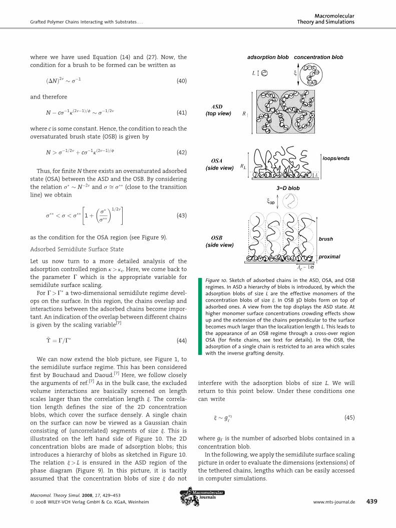
quasi-two-dimensional layer on the surface (see Figure 1).
An adsorption blob is on the verge of adsorption (still
dominated by free conformations).[7] Its characteristic
parameters are the number g of monomers which it
contains and its characteristic length L. Thus, the criteria of
being at adsorption implies
gfk � 1 (13)
whereas L and g are connected through L � gn. It follows
that
L � gn � k�n=f (14)
Each blob carries an adsorption energy of about kT.
www.mts-journal.de 433

R. Descas, J.-U. Sommer, A. Blumen
Figure 2. Scaling plot of M/Nf as a function of jkjNf for e> ec(upper part) and e< ec (lower part).[33] To include both e> ec ande< ec in the same graph we plot the scaling variable as jkjNf, sincefor e< ec, k becomes negative. The different symbols representsimulation results, with N lying between 20 and 200. Scaling isfound for ec¼ 1.01 and f ’ 0:59.
Figure 1. Sketch of an adsorbed chain which can be viewed asbeing a two-dimensional chain composed of adsorption blobs.[24]
The view from the side indicates the localization length L and theclassification of the regions above the surface. The view from thetop shows the two-dimensional self-avoiding chain of adsorptionblobs on the surface.
434
Strong Coupling Limit
For k � 1 each monomer is strongly attracted by the
surface. The density profile in this regime displays a quasi-
exponential decay beyond the length scale of a single
segment. One might consider this case as the limit g ! 1.
Here, scaling analysis breaks down and the chain can be
simply envisaged as being a 2D object. For values larger
than k ’ 10 the adsorption becomes irreversible (see
ref.[39–44]).
The analysis of the first three (scaling) regions requires
exact values for f and for ec (via k). In the following, we
discuss various methods to obtain and assess the
correctness of the set of critical parameters ec and f.
Best Scaling Analysis
Based on the idea that self-similar behavior should be
visible close to the CPA, several observables can be tested
for scaling by varying the two parameters ec and f and by
examining the results.
As an example we present in Figure 2 an analysis[23] of
the scaling behavior of M based on Equation (9) and (10).
Here, the simulation data which correspond to different
values of N and e lie on common curves (master curves)
when one plots M/Nf as a function of jkjNf for
Macrom
� 2008
f ’ 0:59 and "c ¼ 1:01 (15)
To find this optimal pair (f, ec) of values, ec was
systematically varied from 0.8 to 1.1 and f from 0.4 to 0.6
(see ref.[23]).
ol. Theory Simul. 2008, 17, 429–453
WILEY-VCH Verlag GmbH & Co. KGaA, Weinheim
Intersection Method
An alternative way to determine ec was proposed by
Metzger et al.[38] and makes use of the chain’s extension.
Since the presence of the surface breaks the isotropy of the
problem, the parallel and perpendicular components of
position-dependent quantities have to be considered
separately. In the following, we denote by Rgk and by
Rg? the radius of gyration of the polymer chain parallel and
perpendicular to the surface. One has then
Rgkð�Þ ¼ Rgkð0Þfkð�Þ (16)
and
Rg?ð�Þ ¼ Rg?ð0Þf?ð�Þ (17)
with fkð0Þ ¼ 1 and f?ð0Þ ¼ 1. One has at U¼ 0
Rgkð0Þ ¼ rgkNn (18)
and
Rg?ð0Þ ¼ rg?Nn (19)
with rgk and rg? being constants. For � � 1, the chain is
completely adsorbed on the surface and Rg?ð�Þ is
independent of N, thus Rg?ð�Þ � N0. The situation is
different parallel to the surface; here the chain behaves as
a two-dimensional self-avoiding walk; hence, Rgkð�Þ � Nn2
(with n2 being the Flory exponent in two dimensions).
DOI: 10.1002/mats.200800046

Grafted Polymer Chains Interacting with Substrates . . .
Considering now the ratio wð�Þ ¼ Rg?ð�Þ=Rgkð�Þ and
using Equation (18) and (19) together with Equation (16)
and (17) one obtains
Figsymsymatpatarecurestthis
Macrom
� 2008
wð�Þ ¼ wgfrð�Þ (20)
Figure 4. Display of m¼M/N as a function of N in doublelogarithmic scales. This plot renders evident the correlationbetween ec and f, see text for details.
with wg ¼ rgk=rg? and frð�Þ ¼ fkð�Þ=f?ð�Þ. Hence, for U¼ 0
the ratio between both components should be a constant,
independent of N. For different values of N, these curves
must intersect at a single point, which gives ec. This
method to obtain ec was also used in ref.[20–22] The plot
w2 ¼ R2g?=R
2gk versus e is given in Figure 3. In Figure 3, the
curves intersect close to the value e¼ 0.98� 0.03. However,
a zoom of the region around e¼ 0.98 (see the inset of
Figure 3) shows that the curves do not intersect in a single
point. This fact was also reported in ref.[20–22,38] The inset
in Figure 3 shows the full region in which the curves
intersect. We note that the intersection method tacitly
assumes simple scaling at the CPA (it does not consider
corrections to scaling at finite N).
Analysis of the Order Parameter
This method was first used by Eisenriegler et al. in ref.[5] and
is based on an analysis of the order parameterm¼M/N [see
Equation (4)]. For large values ofN,m is expected to obey the
following asymptotic power laws (see also Section ‘‘Order
Parameter for Single Chain Adsorption and Scaling’’):
m �N�1 for k < 0Nf�1 for k ¼ 0N0 for k > 0
8<: (21)
ure 3. Ratio R2g?=R2
gk, plotted as a function of e. Differentbols belong to different values of N, as given in the list ofbols. Since in the simulation box the reflecting wall is located
z¼ 100, for N¼ 200 and small e deviations from the generaltern appear. Therefore, for N¼ 200 only the results for e>0.75included in the plot. The location of the intersection of the
ves (whose variation is given by the width of the bar) allows toimate ec as being ec¼0.98�0.03. The inset presents a zoom of
region.
ol. Theory Simul. 2008, 17, 429–453
WILEY-VCH Verlag GmbH & Co. KGaA, Weinheim
The principle of the method is illustrated in Figure 4.
Here, the order parameter m is displayed in a double
logarithmic plot as a function of the chain length N. As can
be seen from Equation (21), for k 6¼ 0 and N ! 1 only two
types of asymptotic behavior appear, namely M=N ! N0
for k> 0 and M=N ! N�1 for k< 0. Therefore, all these
curves should bend toward their corresponding, asympto-
tic fixed points. A straight line with a slope of f� 1, see
Equation (21), should appear only at k¼ 0 (i.e., at e¼ ec).
However, in the range of 0.98< ec < 1.05 we do not observe
that the curves bend, at least not for the N-values which
we consider here. We can only infer that ec obeys
0.98< ec < 1.05. Here, Figure 4 provides additional infor-
mation about the correlation between ec and f. As can be
learned from Figure 4, smaller values of e are related to
smaller slopes in Figure 4 and thus to smaller values of f.
Analyzing Figure 4, we infer that for ec¼ 1.01 the best
choice is f ’ 0:59, and that for ec ¼ 0.98 it is f ’ 0:5. We
will thus compare in the following the results based on the
two parameter sets (ec, f)¼ (1.01, 0.59) and (ec, f)¼ (0.98,
0.5).
We now turn to study the scaling behavior of M
according to Equation (9) and (10). The expected asympto-
tic power laws correspond in a double logarithmic
representation to straight lines, as indicated in Figure 2
and 5. Figure 2 shows the data obtained for the set (1.01,
0.59), whereas Figure 5 gives the data for the set (0.98, 0.5).
The simulation data follow nicely the expected power laws
for the two regions, e> ec and e< ec. A critical value ec¼ 0.98
is suggested by Figure 3; according to the discussion of
Figure 4 the corresponding cross-over exponent is f ’ 0:5.
The value ec¼ 1.01 is slightly larger, but it is still in the
range of the bar of Figure 3. A closer look at Figure 2 and 5
shows, however, that for the set of parameters (0.98, 0.5)
the scaling behavior is worse than for the set (1.01, 0.59).
www.mts-journal.de 435

R. Descas, J.-U. Sommer, A. Blumen
Figure 5. Same as Figure 2. Here the parameters are ec¼0.98 andf¼0.5. The straight lines indicate the asymptotic behavior of thescaling function[23] according to Equation (9) and (10).
Figure 6. Double logarithmic plot of the normalized free-enddistribution,[23] Z(z), as a function of z/Nn at fixed N¼ 160. Thee-values are as listed. The inset reproduces the plot for e¼0.9,closely below the CPA.
436
Moreover, in Figure 5 the asymptotic slope is not yet
reached. This is similar to observations made in ref.[38]
An analysis of the scaling behavior of the chain’s
extension indicates that this quantity is less sensitive to a
change in the set of critical parameters than the order
parameter. This fact is in line with the results of ref.[23]
Analysis of the Monomer Density Profile
Yet another possibility to find the correct set of critical
parameters is to analyze the distribution of distances of
the end-monomers from the surface and the density
profile of all the monomers. According to ref.,[5] the
number of grafted chains whose free end is at the distance
z from the surface obeys in the vicinity of the CPA a scaling
form which depends on two variables. One has
Macrom
� 2008
ZðzÞ ¼ N�1þnð1�h?ÞFðz;�Þ (22)
whereU is given by Equation (1) and zby Equation (11). Here,
we introduce the surface critical exponentsh? and hk, which
characterize the singularity of the monomer distribution
functions for N ! 1 (see ref.[5]). Namely, at the CPA the
variable� ¼ kNf vanishes andFdepends only onz. For small
z, i.e., for distances smaller than Rg(0), a sharp power-law
behavior near the wall is expected. This power law can be
written (dispensing with N) in the form:[5,36]
Z0ðzÞ � z�Dh ðfor z � 1Þ (23)
where
Figure 7. Double logarithmic plot of the normalized free-enddistribution,[23] Z0(z)Nn, for ec¼ 1.01, given as a function of
Dh ¼ h? � hk (24)
z/Nn. The same data, but in linear scales, are displayed in theinset. The straight line indicates the best fit to the simulationpoints in the region z � 1.
In order to estimate ec one can now analyze the shape of
the free-end monomer distributions as a function of e. At ec
ol. Theory Simul. 2008, 17, 429–453
WILEY-VCH Verlag GmbH & Co. KGaA, Weinheim
the distributions change from mushroom forms with
pronounced peaks at about Rg0 to distributions having
their maxima at the surface. This is illustrated in Figure 6,
where we display the normalized distribution function Z(z)
for N¼ 160. Here, e varies between 0.1 and 1.8.
Note that in the region " ’ "c, but e still below the CPA,
the density profile gets large in the proximal region and
exhibits two peaks (see ref.[5,13,35]). In the inset of Figure 6,
this is visible at the value e¼ 0.9, below ec. According to
Equation (23), at e¼ ec and for small values of z the
distribution function of the free-end monomer should
follow a power law.
By comparing results for different chain lengths it is
possible to check the scaling with respect to N. In Figure 7,
DOI: 10.1002/mats.200800046

Grafted Polymer Chains Interacting with Substrates . . .
we display the results for ec ¼ 1.01 and for three values of
N. From the figure we can determine the exponent Dh, see
Equation (23) and (24), using the singular part of the
profile. By taking a fit to the points in the region z � 1 we
estimate the exponent to be Dh ’ 0:25 [see Equation (23)].
This value is intermediate between the result Dh ¼ 0:11 of
ref.[11,36,45] and the result Dh ¼ 0:47 of ref.[5]
Alternatively, one may use the density profile of
polymer chains to gain information about ec. As has been
discussed by de Gennes and Pincus,[6] see also Section
‘‘Scaling Regions of Polymer Adsorption,’’ at k¼ 0 and
z � 1 the density profile is expected to show scaling,
Figmeec¼z/N
Macrom
� 2008
r0ðzÞ � z�n (25)
where n denotes the proximal exponent,[6] given by
n ¼ 1 þ ðf� 1Þ=n (26)
One should note that the power law of the density
profile is controlled by the cross-over exponent f (see ref.[6]
for details). Hence, this relation can be used to estimate (or
test) the set of critical parameters. An example is given in
Figure 8 for the case ec ¼ 1.01.
A fit to the points in the region z � 1 allows to estimate
the proximal exponent given by Equation (26). We obtain
n¼�0.33, which again agrees very well with a cross-over
exponent of f¼ 0.59.
All the methods described above yield a very good
scaling of various observable quantities at the CPA when
choosing the set of critical parameters according to
Equation (15), a caveat being that the results are based
on moderately long chains. Since infinitely long chains are
neither available in experiments nor in computer simula-
ure 8. Double logarithmic plot of the normalized total mono-r density[23] r0(z), namely r0(z)Nn, as a function of z/Nn for1.01. The straight line is a fit to the simulation points for smalln. The inset presents the same data, but in linear scales.
ol. Theory Simul. 2008, 17, 429–453
WILEY-VCH Verlag GmbH & Co. KGaA, Weinheim
tions, we continue here by using the parameters of
Equation (15), which allows us to further explore the
adsorption of grafted polymer chains.
Many Chains and their Phase Diagram
When grafting many polymer chains on the surface, the
interplay between the grafting density, the adsorption
strength and the excluded volume interaction leads to the
appearance of different regimes. The grafting density is
defined to be
s ¼ 4n
A(27)
where n is the total number of chains in the system and A is
the surface area. In Equation (27), the factor four appears
because in the simulation method which we use (see
Appendix A) a monomer occupies four lattice sites on the
adsorbing surface. Since all polymers are grafted to the
surface, all monomers contribute to the surface layer.
Therefore, the surface excess concentration G (given by the
integral over the surface excess concentration density
profile[7]) is
G ¼ 4nN
A¼ Ns (28)
There exist two characteristic monomer surface con-
centrations. First, the surface concentration, G�, at which
the adsorbed chains start to overlap is
G� ¼ N
R2gk0
(29)
In Equation (29), N represents the number of monomers
per chain and Rgk0 is the extension parallel to the surface of
the radius of gyration of isolated chains ðG ! 0Þ. Now, Rgk0
depends on N and k in the following way:[7,35]
Rgk0 � Nn2kDn=f (30)
with Dn ¼ n2 � n being the difference between the 2D and
the 3D Flory exponent. This expression represents the
extension of a 2D self-avoiding chain composed of
adsorption blobs [see Figure 1 and Equation (13) and
(14)]. Thus, G� can be written as
G� � N1�2n2k�2Dn=f (31)
A second characteristic monomer surface concentration
arises in situations when under an increase in the total
concentration the surface and its vicinity (the proximal
layer) cannot be enriched anymore, because of the
excluded volume interactions between the adsorption
www.mts-journal.de 437

R. Descas, J.-U. Sommer, A. Blumen
438
blobs. In the case of non-grafted chains this characteristic
concentration is called saturation concentration;[7] in our
case we will call it surface saturation concentration and
denote it by G��. Using Equation (14) we obtain
Macrom
� 2008
G�� � g
L2� kð2n�1Þ=f (32)
Figure 9. Phase diagram for grafted chains on adsorbing surfaces.As a function of k and s five different regions could be found.Region M: the tethered chains are in a mushroom-like state.
The Phase Diagram
In order to construct the phase diagram for grafted
polymer chains on adsorbing surfaces we use the grafting
density s¼G/N, see Equation (28), instead of G, since this
quantity can be related more directly to experiments.
Using Equation (31) we can write
Region AD: The adsorbed chains are in a dilute state. Region ASD:The adsorbed chains form a 2D semidilute surface state. RegionOSB: the chains are in an oversaturated brush state. For finitechains a narrow cross-over region OSA appears between ASD ands�ðkÞ ¼ G�
N� N�2n2k�2Dn=f (33)
OSB, which we call adsorbed oversaturated region. Region B: thetethered chains are in a brush state. The small filled circles (red inthe online version) denote adsorption blobs, whereas the largeopen circles represent Alexander-de Gennes blobs.
Let us recall the fact that the surface phase-transition is
very sharp only for infinite chains at k¼ 0 (i.e., at ec ¼ e). As
already discussed in Section ‘‘Scaling Regions of Polymer
Adsorption’’, see Equation (12), for finite chains adsorption
is a cross-over effect with a characteristic value of
kc � N�f (34)
Below kc the chains are only weakly perturbed by the
surface. Inserting now Equation (34) into Equation (33) we
obtain
s� ¼ s�ðkcÞ � N�2n2N2Dn � N�2n (35)
In the case of non-adsorbing surfaces this corresponds to
the cross-over from the mushroom to the brush state, as
first discussed by Alexander and de Gennes.[46,47] We note
that changes in the conformational properties might be
observable only for values of s/s�> 10, as has been
reported recently by Chen et al.[48,49] This implies a rather
broad transition zone. In a similar way, for the case of
adsorbing surfaces and above kc, we have also observed in
our simulations a cross-over region between the adsorbed
semidilute and oversaturated brush regions (see Figure 9
and the explanations below).
Using Equation (32) we obtain as corresponding grafting
density at the saturation limit
s��ðkÞ � N�1kð2n�1Þ=f (36)
At k¼ kc, Equation (36) becomes
s��ðkcÞ � N�1N�ð2n�1Þ � N�2n (37)
which again corresponds to the mushroom-brush transi-
tion. Thus, an adsorbing surface splits s� into two cross-
over lines which open the region of a semidilute surface
state. This is illustrated in Figure 9, where we show the
ol. Theory Simul. 2008, 17, 429–453
WILEY-VCH Verlag GmbH & Co. KGaA, Weinheim
phase diagram whose parameters are the adsorption
strength k and the grafting density s. Note that k is directly
related to the temperature by the relation k¼ (Tc � T)/T,
where Tc corresponds to the temperature at the CPA.
Next, we discuss the various regions which can be
defined in this phase diagram:
For k< kc the polymer chains are not adsorbed. At s� a
transition from a mushroom state (M) to a brush-like state
(B) takes place.
For k> kc the chains are adsorbed and three new regions
can be identified. The adsorbed chains are diluted in the
(AD) region below the ‘‘overlap-line’’ s�(k) [see Equation
(35)]. Above the ‘‘overlap line’’ the adsorbed chains form a
2D semidilute surface state (ASD), which extends up to the
‘‘saturation-line’’ s��(k) [see Equation (36)]. The ‘‘overlap-
line’’ and the ‘‘saturation-line’’ intersect at k¼ kc which
gives s�, the grafting density which triggers the mush-
room-brush transition. If the grafting density is increased
beyond the ‘‘saturation line’’ a brush-like state forms on
the top of the adsorbed layer. We call this region the
oversaturated brush regime OSB, to be explained below.
It is interesting to consider the condition for the cross-
over from the ASD to the OSB region. The number of
monomers available for brush formation is given by
DN ¼ N � Nsat (38)
where Nsat is the number of adsorbed monomers per chain
at the threshold of saturation and is given by
Nsat ¼ðA=L2Þg
n� s�1kð2n�1Þ=f (39)
DOI: 10.1002/mats.200800046
Grafted Polymer Chains Interacting with Substrates . . .
where we have used Equation (14) and (27). Now, the
condition for a brush to be formed can be written as
Macrom
� 2008
ðDNÞ2n � s�1 (40)
and therefore
N � cs�1kð2n�1Þ=f � s�1=2n (41)
where c is some constant. Hence, the condition to reach the
oversaturated brush state (OSB) is given by
N > s�1=2n þ cs�1kð2n�1Þ=f (42)
Thus, for finite N there exists an oversaturated adsorbed
state (OSA) between the ASD and the OSB. By considering
the relation s� � N�2n and s ffi s�� (close to the transition
line) we obtain
s�� < s < s�� 1 þ s�
s��
� �1=2n" #
(43)
Figure 10. Sketch of adsorbed chains in the ASD, OSA, and OSBregimes. In ASD a hierarchy of blobs is introduced, by which theadsorption blobs of size L are the effective monomers of theconcentration blobs of size j. In OSB 3D blobs form on top ofadsorbed ones. A view from the top displays the ASD state. Athigher monomer surface concentrations crowding effects showup and the extension of the chains perpendicular to the surfacebecomes much larger than the localization length L. This leads to
as the condition for the OSA region (see Figure 9).
Adsorbed Semidilute Surface State
Let us now turn to a more detailed analysis of the
adsorption controlled region k> kc. Here, we come back to
the parameter G which is the appropriate variable for
semidilute surface scaling.
For G>G� a two-dimensional semidilute regime devel-
ops on the surface. In this region, the chains overlap and
interactions between the adsorbed chains become impor-
tant. An indication of the overlap between different chains
is given by the scaling variable[7]
the appearance of an OSB regime through a cross-over regionOSA (for finite chains, see text for details). In the OSB, theadsorption of a single chain is restricted to an area which scales
~� ¼ G=G� (44)
with the inverse grafting density.
We can now extend the blob picture, see Figure 1, tothe semidilute surface regime. This has been considered
first by Bouchaud and Daoud.[7] Here, we follow closely
the arguments of ref.[7] As in the bulk case, the excluded
volume interactions are basically screened on length
scales larger than the correlation length j. The correla-
tion length defines the size of the 2D concentration
blobs, which cover the surface densely. A single chain
on the surface can now be viewed as a Gaussian chain
consisting of (uncorrelated) segments of size j. This is
illustrated on the left hand side of Figure 10. The 2D
concentration blobs are made of adsorption blobs; this
introduces a hierarchy of blobs as sketched in Figure 10.
The relation j> L is ensured in the ASD region of the
phase diagram (Figure 9). In this picture, it is tacitly
assumed that the concentration blobs of size j do not
ol. Theory Simul. 2008, 17, 429–453
WILEY-VCH Verlag GmbH & Co. KGaA, Weinheim
interfere with the adsorption blobs of size L. We will
return to this point below. Under these conditions one
can write
j � gG
n2 (45)
where gG is the number of adsorbed blobs contained in a
concentration blob.
In the following, we apply the semidilute surface scaling
picture in order to evaluate the dimensions (extensions) of
the tethered chains, lengths which can be easily accessed
in computer simulations.
www.mts-journal.de 439
R. Descas, J.-U. Sommer, A. Blumen
440
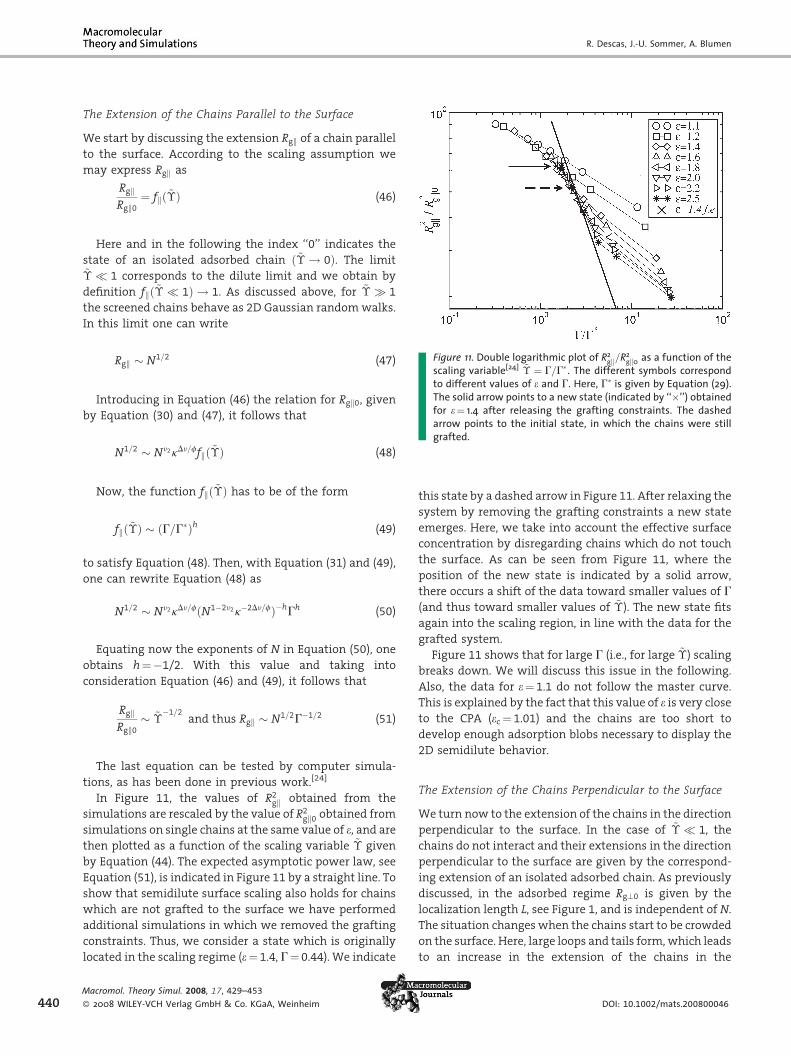
The Extension of the Chains Parallel to the Surface
We start by discussing the extension Rgk of a chain parallel
to the surface. According to the scaling assumption we
may express Rgk as
Macrom
� 2008
RgkRgk0
¼ fkð~�Þ (46)
Here and in the following the index ‘‘0’’ indicates the
state of an isolated adsorbed chain ð~� ! 0Þ. The limit~� � 1 corresponds to the dilute limit and we obtain by
definition fkð~� � 1Þ ! 1. As discussed above, for ~� � 1
the screened chains behave as 2D Gaussian random walks.
In this limit one can write
Figure 11. Double logarithmic plot of R2gk=R
2gk0 as a function of the
scaling variable[24] ~� ¼ G=G�. The different symbols correspond�
Rgk � N1=2 (47)
to different values of e and G. Here, G is given by Equation (29).The solid arrow points to a new state (indicated by ‘‘’’) obtainedfor e¼ 1.4 after releasing the grafting constraints. The dashed
Introducing in Equation (46) the relation for Rgk0, given
by Equation (30) and (47), it follows that
arrow points to the initial state, in which the chains were stillgrafted.N1=2 � Nn2kDn=ffkð~�Þ (48)
Now, the function fkð~�Þ has to be of the form
fkð~�Þ � ðG=G�Þh (49)
to satisfy Equation (48). Then, with Equation (31) and (49),
one can rewrite Equation (48) as
N1=2 � Nn2kDn=fðN1�2n2k�2Dn=fÞ�hGh (50)
Equating now the exponents of N in Equation (50), one
obtains h¼�1/2. With this value and taking into
consideration Equation (46) and (49), it follows that
RgkRgk0
� ~��1=2
and thus Rgk � N1=2G�1=2 (51)
The last equation can be tested by computer simula-
tions, as has been done in previous work.[24]
In Figure 11, the values of R2gk obtained from the
simulations are rescaled by the value of R2gk0 obtained from
simulations on single chains at the same value of e, and are
then plotted as a function of the scaling variable ~� given
by Equation (44). The expected asymptotic power law, see
Equation (51), is indicated in Figure 11 by a straight line. To
show that semidilute surface scaling also holds for chains
which are not grafted to the surface we have performed
additional simulations in which we removed the grafting
constraints. Thus, we consider a state which is originally
located in the scaling regime (e¼ 1.4, G¼ 0.44). We indicate
ol. Theory Simul. 2008, 17, 429–453
WILEY-VCH Verlag GmbH & Co. KGaA, Weinheim
this state by a dashed arrow in Figure 11. After relaxing the
system by removing the grafting constraints a new state
emerges. Here, we take into account the effective surface
concentration by disregarding chains which do not touch
the surface. As can be seen from Figure 11, where the
position of the new state is indicated by a solid arrow,
there occurs a shift of the data toward smaller values of G
(and thus toward smaller values of ~�). The new state fits
again into the scaling region, in line with the data for the
grafted system.
Figure 11 shows that for large G (i.e., for large ~�) scaling
breaks down. We will discuss this issue in the following.
Also, the data for e¼ 1.1 do not follow the master curve.
This is explained by the fact that this value of e is very close
to the CPA (ec ¼ 1.01) and the chains are too short to
develop enough adsorption blobs necessary to display the
2D semidilute behavior.
The Extension of the Chains Perpendicular to the Surface
We turn now to the extension of the chains in the direction
perpendicular to the surface. In the case of ~� � 1, the
chains do not interact and their extensions in the direction
perpendicular to the surface are given by the correspond-
ing extension of an isolated adsorbed chain. As previously
discussed, in the adsorbed regime Rg?0 is given by the
localization length L, see Figure 1, and is independent of N.
The situation changes when the chains start to be crowded
on the surface. Here, large loops and tails form, which leads
to an increase in the extension of the chains in the
DOI: 10.1002/mats.200800046
Grafted Polymer Chains Interacting with Substrates . . .
direction perpendicular to the surface. Finally, at high
surface coverage the loops and tails form an extended
layer, whose characteristic height is that of an unper-
turbed chain. Bouchaud and Daoud have assumed that this
limit is reached in the semidilute surface region. Thus, for~� � 1 one can write[7]
Figas aat anot
Macrom
� 2008
Rg? � Nn (52)
Now, according to the scaling assumption one can write
in general for the extension perpendicular to the surface
Rg?Rg?0
¼ f?ð~�Þ (53)
Making use of the fact that Rg?0 is given by the
localization length L for ~� � 1 and that Rg? is given by
Equation (52) for ~� � 1, one can rewrite Equation (53) as
Nn � k�1f?ð~�Þ (54)
Here, the approximate relation[5,12,23] n ’ f was used.
Now Equation (54) can be satisfied only when the function
f?ð~�Þ obeys a power law. Hence, using the exact result
n2 ¼ 3/4 we obtain
Rg?Rg?0
� ~�2n
and Rg? � k�2nfð2n�1Þ
G2nNn (55)
Figure 12 displays in a double logarithmic plot the
simulation results for the radius of gyration of the chains
in the direction perpendicular to the surface,[24] R2g?,
plotted as a function of the scaling variable ~�. In this figure
ure 12. Same as in Figure 11, only that here R2g?=R2
g?0 is displayedfunction of G/G�. For isolated chains R2
g?0 becomes very smallttraction strengths larger than e> 1.6, so that such results areshown here.
ol. Theory Simul. 2008, 17, 429–453
WILEY-VCH Verlag GmbH & Co. KGaA, Weinheim
R2g? is rescaled by the simulation results obtained for single
chains, R2g?0, at the same value of e. The expected slope is
indicated in the figure by a straight line.
In contrast to the results for the chain’s extension
parallel to the surface Figure 12 displays rather poor
scaling. One can notice only an accumulation of data
points around the asymptotic region given by Equation
(55).
It is important to note that the ASD surface scaling for
Rg? is based on additional assumptions. While the scaling
of Rgk follows the same arguments as for semidilute
solutions in 3D (SD), one has to assume here, a priori, that
Rg? � Nn at G ffi G�. Since G� is difficult to monitor (by
contrast to G��, see ref.[7]) there are no experimental
observations available to prove the relation Rg?ðG�Þ � Nn.
Deviations from Semidilute Scaling and Saturation Scaling
From the analysis of Figure 11 and 12 it turns out that for
large values of G the simulation points do not follow the
master curve according to the power laws obtained from
the scaling analysis in the semidilute surface regime.
As mentioned above, the scaling analysis of the ASD
surface state assumes that the adsorption blobs are not
perturbed by the excluded volume interaction. Now,
excluded volume interactions increase the free energy of
the polymer layer. Let us estimate at the mean-field level
and as a function of concentration the excess free energy
per adsorption blob. The probability that two adsorption
blobs overlap is given by
pover �G
g
� �L2 (56)
In analogy to the situation of concentration blobs in
semidilute solutions,[35] for a mutual penetration of blobs
one needs an energy of at least kT; in fact the free energy
penalty is limited to kT by the self-avoidance of the
adsorption blobs. Hence, we can express the free energy
per blob due to repulsion as
Frep � kTpover � G=G�� (57)
Inserting Equation (56) in Equation (57) and using
Equation (14) the free energy per blob due to repulsion is
Frep � kTGk�ð2n�1Þ=f (58)
where we obtained the last expression by comparing Frep
to Equation (32). The free energy increase due to the dense
packing of the adsorption blobs has to be confronted to the
free energy decrease due to adsorption, which is again
around kT per blob. The dimensionless scaling variable
www.mts-journal.de 441

R. Descas, J.-U. Sommer, A. Blumen
442
which measures this free energy excess is then given by
Macrom
� 2008
~V ¼ G
G�� (59)
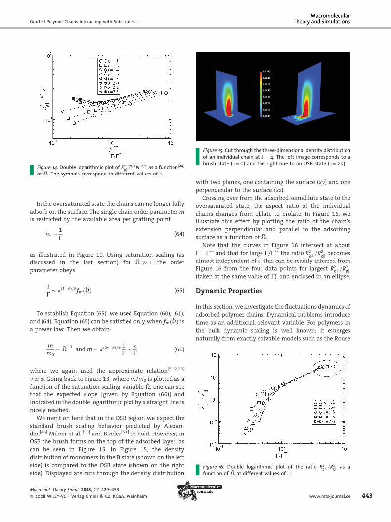
Figure 13. Scaling plot of the chain order parameter assumingsaturation scaling[24] according to Equation (66).
This relation shows that the saturation concentration
G�� controls the balance between concentration blobs and
adsorption blobs.
Thus, semidilute surface scaling is fulfilled in the regime
G� � G � G��, because saturation leads to only weak
perturbations, as already remarked by Bouchaud and
Daoud.[7]
To check the saturation scaling we use the single chain
order parameter m (see Section ‘‘Order Parameter for Single
Chain Adsorption and Scaling’’), which is only weakly
influenced by chain overlap. For G>G�, the formation of
large loops and tails slightly decreases the number of
adsorbed monomers per chain, an effect which hardly
affects the relation M � N. Therefore, only saturation
scaling is expected to change the order parameter and we
assume that
m
m0¼ fmð~VÞ (60)
where m0 is the chain order parameter for G ! 0 and is
given by:[7,23]
m0 � kð1�fÞ=f (61)
In the case of (non-grafted) chains adsorbed from
solution, the limit ~V � 1 is unphysical because G is
limited by G��. In the case of tethered chains, however,
G>G�� can be reached using higher grafting densities, thus
attaining the OSD and OSB regions in the phase diagram of
Figure 9.
Simulation results for the chain order parameter using
saturation scaling are displayed in Figure 13. In this figure
m is rescaled by the m0 value obtained from the simulation
of single chains and is then plotted against the saturation
scaling variable given by Equation (59). One can see that
the different symbols corresponding to different values of eand G follow a common curve. Saturation scaling does not
hold anymore when the size of the adsorption blobs is
comparable to the distance between grafting points. Such
a situation occurs for chains close to the adsorption
threshold, see the data for e¼ 1.1. In this particular case,
the chains are not long enough to form many adsorption
blobs.
Close to G�� the free energy excess due to the repulsion
between adsorption blobs is essential and changes the
scaling behavior also for such observables which follow
semidilute surface scaling (i.e., the chain extensions
parallel to the surface). This was already visible in
ol. Theory Simul. 2008, 17, 429–453
WILEY-VCH Verlag GmbH & Co. KGaA, Weinheim
Figure 11, where the data points for higher values of the
surface concentration deviate from the scaling predictions.
In order to analyze this effect we consider an observable
O in the semidilute surface state. Then, we assume that the
deviations with respect to this reference state are
controlled by saturation scaling, i.e., by the parameter ~V
defined in Equation (59):
O ¼ OASDfOð~VÞ (62)
where the index ‘‘ASD’’ indicates the value of the
observable in the semidilute surface state and fO is a
function of the saturation scaling variable ~V.
A suitable example is the chain extension in the
direction parallel to the surface:
Rgk ¼ RgkASDfkð~VÞ ¼ G�1=2N1=2fkð~VÞ (63)
where for Rgk Equation (51) has been applied. In Figure 14,
we display the simulation results using Equation (63). Only
states with an adsorption energy per monomer greater
than e¼ 1.4 display scaling according to Equation (63). This
observation is in agreement with the one we have reached
by considering the semidilute surface region, see Figure 11,
where we have found that for e< 1.4 the data do not show
the 2D semidilute asymptotic behavior. Furthermore, for
parameter regions which do not reach semidilute scaling,
one also does not see saturation scaling at higher
concentrations.
Oversaturation Effects
As mentioned above, in the case of tethered chains, the
regime for which ~V � 1 can be physical. We call this
region the oversaturation regime. The regime of over-
saturation can be obtained by increasing the grafting
density beyond the saturation line (see Figure 9).
DOI: 10.1002/mats.200800046
Grafted Polymer Chains Interacting with Substrates . . .
Figure 14. Double logarithmic plot of R2gkG1=2N�1=2 as a function[24]
of ~V. The symbols correspond to different values of e.
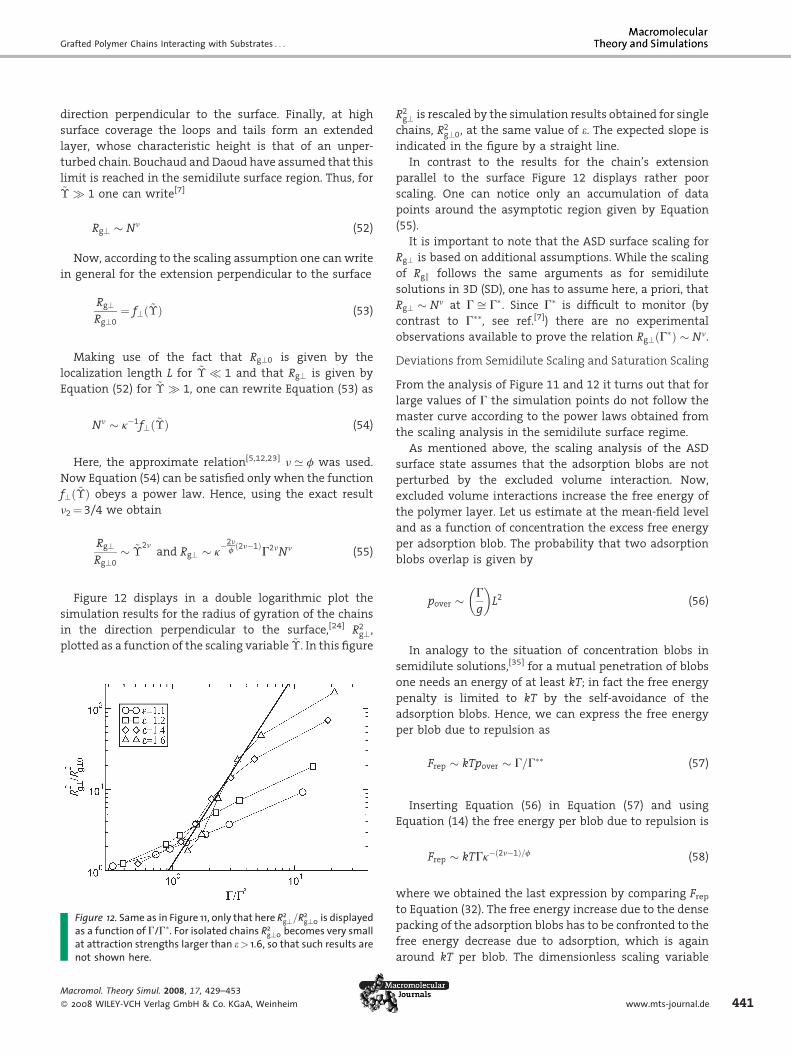
Figure 15. Cut through the three-dimensional density distributionof an individual chain at G¼ 4. The left image corresponds to abrush state (e¼0) and the right one to an OSB state (e¼ 2.5).
In the oversaturated state the chains can no longer fully
adsorb on the surface. The single chain order parameter m
is restricted by the available area per grafting point
Macrom
� 2008
m � 1
G(64)
as illustrated in Figure 10. Using saturation scaling (as
discussed in the last section) for ~V � 1 the order
parameter obeys
1
G� kð1�fÞ=ffmð~VÞ (65)
To establish Equation (65), we used Equation (60), (61),
and (64). Equation (65) can be satisfied only when fmð~VÞ is
a power law. Then we obtain:
m
m0� ~V
�1and m � kð2n�fÞ=f 1
G� k
G(66)
Figure 16. Double logarithmic plot of the ratio R2g?=R2
gk as afunction of ~
V at different values of e.
where we again used the approximate relation[5,12,23]
n ’ f. Going back to Figure 13, where m/m0 is plotted as a
function of the saturation scaling variable ~V, one can see
that the expected slope [given by Equation (66)] and
indicated in the double logarithmic plot by a straight line is
nicely reached.
We mention here that in the OSB region we expect the
standard brush scaling behavior predicted by Alexan-
der,[46] Milner et al.,[50] and Binder[51] to hold. However, in
OSB the brush forms on the top of the adsorbed layer, as
can be seen in Figure 15. In Figure 15, the density
distribution of monomers in the B state (shown on the left
side) is compared to the OSB state (shown on the right
side). Displayed are cuts through the density distribution
ol. Theory Simul. 2008, 17, 429–453
WILEY-VCH Verlag GmbH & Co. KGaA, Weinheim
with two planes, one containing the surface (xy) and one
perpendicular to the surface (xz).
Crossing over from the adsorbed semidilute state to the
oversaturated state, the aspect ratio of the individual
chains changes from oblate to prolate. In Figure 16, we
illustrate this effect by plotting the ratio of the chain’s
extension perpendicular and parallel to the adsorbing
surface as a function of ~V.
Note that the curves in Figure 16 intersect at about
G¼G�� and that for large G/G�� the ratio R2g?=R
2gk becomes
almost independent of e; this can be readily inferred from
Figure 16 from the four data points for largest R2g?=R
2gk
(taken at the same value of G), and enclosed in an ellipse.
Dynamic Properties
In this section, we investigate the fluctuations dynamics of
adsorbed polymer chains. Dynamical problems introduce
time as an additional, relevant variable. For polymers in
the bulk dynamic scaling is well known; it emerges
naturally from exactly solvable models such as the Rouse
www.mts-journal.de 443

R. Descas, J.-U. Sommer, A. Blumen
444
model for ideal chains[52] and from renormalization group
approaches (see ref.[53]). Usually the longest (characteristic)
relaxation time, t controls the dynamical behavior. We
hence introduce as new dimensionless variable
Macrom
� 2008
V ¼ t=t (67)
Concepts of dynamic scaling have been applied to
various polymer systems such as semidilute solutions or
entangled melts (see ref.[35,52])
Close to the CPA and on time scales much larger than the
segmental relaxation time, the dynamical quantities often
depend on the two relevant variables U and V. Directly at
the CPA, of course, U vanishes and the dependence on V is
particularly evident. An important question now is the
dependence of t on N, which, however cannot be simply
inferred from the dynamical behavior of free chains.
We recall that for a free chain t is related to N according
to a power law[35,54,55]
t ¼ t0Na (68)
with a being the dynamical exponent and t0 being the
characteristic relaxation time of a monomer. For flexible
polymer chains in good solvents and in the absence of
hydrodynamic interactions (situation which is realized in
many simulations), a is given by
a ¼ 1 þ 2n ’ 2:176 (69)
We recall, following ref.,[35,54,55] the main arguments
leading to this result. If we regard the chain as being a
system of N identical, diffusing and interacting particles,
but in the absence of any external interaction (such as
hydrodynamic forces or electrodynamic fields), then the
center of mass motion of the considered system is a force-
free diffusion process. The diffusion constant is then
given by
DCOM ¼ D0=N (70)
where D0 is the diffusion constant of a single particle
(monomer). This result requires the cancellation of all
internal forces according to Newton’s third law. Now,
assuming that the characteristic time scale t is given by
the time needed for the polymer chain to move to a
distance comparable to its own size, R � Nn, leads to the
relation t � R2=D � N1þ2n.
Now, the presence of external forces such as the
adsorption potential invalidate the arguments leading to
Equation (70); thus the dynamical exponent a has to be
determined by other means. Given that a unique
dynamical exponent might appear under critical condi-
tions, we will focus in Section ‘‘Single Chains at the Critical
ol. Theory Simul. 2008, 17, 429–453
WILEY-VCH Verlag GmbH & Co. KGaA, Weinheim
Point of Adsorption and the Dynamic Exponent’’ on the
determination of a from the dynamics of chains at the CPA.
Knowing the value of a at the CPA, dynamic scaling
arguments can be applied to provide a basic under-
standing of the dynamics in the adsorbed diluted state;
such arguments and corresponding simulation results are
presented in Section ‘‘Dynamic Scaling in the Adsorbed
State.’’ Finally, in the following sections we consider the
chain dynamics in the semidilute surface state and in the
oversaturated brush-like state.
Single Chains at the Critical Point of Adsorption andthe Dynamic Exponent
In general, an observable O which characterizes some
dynamical property of the system will depend on all
relevant parameters in the scaling limit (length scales
much larger than the segment size and time scales much
larger than the segmental relaxation time). For a single
chain grafted to the surface we thus expect:
O ¼ O0fOðk;VÞ (71)
where O0 denotes some characteristic value of the
observable for given values of k and V. In the mushroom
state dynamical scaling should emulate a bulk chain, apart
from an obvious breaking of symmetry (i.e., the obser-
vables may have different characteristic values with
respect to their direction in space). On the other hand,
for the adsorbed state, k> 0, one can expect the system to
follow the dynamical behavior of a quasi-2D chain.
Indications for a dynamical cross-over from 3D to 2D
behavior during adsorption have already been obtained by
Milchev and Binder.[32] However, in order to explore the
details of the dynamics in the adsorbed state we focus here
on the dynamics of a chain at the CPA. For this one needs in
particular to know the dynamic exponent a.
The End-to-End Vector Correlation Function
An appropriate test of dynamical scaling is provided by the
autocorrelation function of the end-to-end vector in the
direction perpendicular to the surface. This quantity is
given by
C?ðt;N; "Þ ¼ zðtÞ � hzið Þ zð0Þ � hzið Þh ihz2i � hzi2 (72)
In Equation (72), z(t) represents the position of the
monomer at the free end of the chain, in the direction
perpendicular to the surface at time t. Note that for time-
dependent observables averaging has to be carried
out over all the different realizations of the initial
DOI: 10.1002/mats.200800046
Grafted Polymer Chains Interacting with Substrates . . .
conformations of the chain. Thus, dynamic results are very
demanding with respect to computer resources.
At CPA, U vanishes and the behavior is controlled by V
only. Hence, we can write C?ðt;N; "cÞ ¼ f ðt=tÞ. Now, for the
proper choice of the dynamic exponent the explicit N-
dependence of C?ðt;N; "cÞ can be eliminated. Note that the
characteristic value, C0 ¼ C(t¼ 0), is unity and is indepen-
dent of the length of the chain.
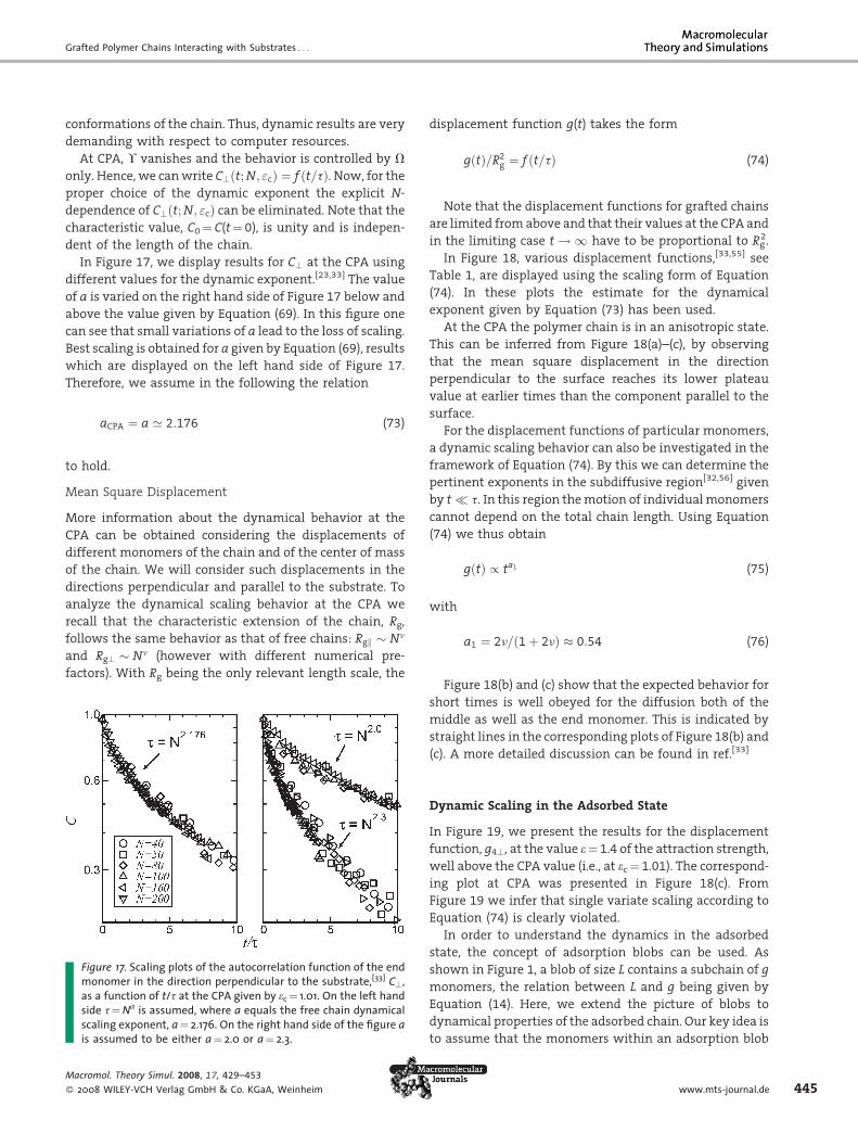
In Figure 17, we display results for C? at the CPA using
different values for the dynamic exponent.[23,33] The value
of a is varied on the right hand side of Figure 17 below and
above the value given by Equation (69). In this figure one
can see that small variations of a lead to the loss of scaling.
Best scaling is obtained for a given by Equation (69), results
which are displayed on the left hand side of Figure 17.
Therefore, we assume in the following the relation
Figmoas asidscais a
Macrom
� 2008
aCPA ¼ a ’ 2:176 (73)
to hold.
Mean Square Displacement
More information about the dynamical behavior at the
CPA can be obtained considering the displacements of
different monomers of the chain and of the center of mass
of the chain. We will consider such displacements in the
directions perpendicular and parallel to the substrate. To
analyze the dynamical scaling behavior at the CPA we
recall that the characteristic extension of the chain, Rg,
follows the same behavior as that of free chains: Rgk � Nn
and Rg? � Nn (however with different numerical pre-
factors). With Rg being the only relevant length scale, the
ure 17. Scaling plots of the autocorrelation function of the endnomer in the direction perpendicular to the substrate,[33] C?,
function of t/t at the CPA given by ec ¼ 1.01. On the left hande t¼Na is assumed, where a equals the free chain dynamicalling exponent, a¼ 2.176. On the right hand side of the figure assumed to be either a¼ 2.0 or a¼ 2.3.
ol. Theory Simul. 2008, 17, 429–453
WILEY-VCH Verlag GmbH & Co. KGaA, Weinheim
displacement function g(t) takes the form
gðtÞ=R2g ¼ f ðt=tÞ (74)
Note that the displacement functions for grafted chains
are limited from above and that their values at the CPA and
in the limiting case t ! 1 have to be proportional to Rg2.
In Figure 18, various displacement functions,[33,55] see
Table 1, are displayed using the scaling form of Equation
(74). In these plots the estimate for the dynamical
exponent given by Equation (73) has been used.
At the CPA the polymer chain is in an anisotropic state.
This can be inferred from Figure 18(a)–(c), by observing
that the mean square displacement in the direction
perpendicular to the surface reaches its lower plateau
value at earlier times than the component parallel to the
surface.
For the displacement functions of particular monomers,
a dynamic scaling behavior can also be investigated in the
framework of Equation (74). By this we can determine the
pertinent exponents in the subdiffusive region[32,56] given
by t � t. In this region the motion of individual monomers
cannot depend on the total chain length. Using Equation
(74) we thus obtain
gðtÞ / ta1 (75)
with
a1 ¼ 2n=ð1 þ 2nÞ � 0:54 (76)
Figure 18(b) and (c) show that the expected behavior for
short times is well obeyed for the diffusion both of the
middle as well as the end monomer. This is indicated by
straight lines in the corresponding plots of Figure 18(b) and
(c). A more detailed discussion can be found in ref.[33]
Dynamic Scaling in the Adsorbed State
In Figure 19, we present the results for the displacement
function, g4?, at the value e¼ 1.4 of the attraction strength,
well above the CPA value (i.e., at ec¼ 1.01). The correspond-
ing plot at CPA was presented in Figure 18(c). From
Figure 19 we infer that single variate scaling according to
Equation (74) is clearly violated.
In order to understand the dynamics in the adsorbed
state, the concept of adsorption blobs can be used. As
shown in Figure 1, a blob of size L contains a subchain of g
monomers, the relation between L and g being given by
Equation (14). Here, we extend the picture of blobs to
dynamical properties of the adsorbed chain. Our key idea is
to assume that the monomers within an adsorption blob
www.mts-journal.de 445

R. Descas, J.-U. Sommer, A. Blumen
Figure 18. Scaling plots at the CPA for various N and various displacement func-tions:[33] (a) parallel and perpendicular components of g3; (b) same for g1; (c) same forg4; (d) parallel components of g1 and g2. In (a)–(c) we introduced for comparison alsothe free chain results for N¼ 50, 100, and 160.
446
obey critical dynamical behavior (this means that the
blobs represent a local state at the verge of adsorption).
Adopting the previous result obtained for the dynamical
scaling exponent a, we rewrite Equation (68) as
Tab
g1
N/2
g2
N/2
g3
the
g4
Macrom
� 2008
tg � g2nþ1 (77)
where t was replaced by tg and N by g. In this way tg, given
by Equation (77), represents the characteristic relaxation
time of a blob.
le 1. Displacement functions gk.
Mean square displacement of the center monomer
Mean square displacement of the center monomer
relative to the center of mass
Mean square displacement of the center of mass of
chain
Mean square displacement of the end monomer(s)
ol. Theory Simul. 2008, 17, 429–453
WILEY-VCH Verlag GmbH & Co. KGaA, Weinheim
To eliminate the unknown variable g,
we use Equation (13) to rewrite Equation
(77):
tg � L2nþ1n � ðR2
?Þ2nþ1
2n (78)
In the last relation, we used as the
characteristic size of a blob the end-to-end
distance R? of a single chain in the
direction perpendicular to the surface.
Note that large loops are very improbable
in the AD region of the phase diagram (see
Figure 9). Therefore, the characteristic
relaxation time in the direction perpendi-
cular to the surface is given directly by tg:
t? / tg (79)
In Figure 20, the data of Figure 19 are
rescaled according to Equation (79).
Obviously, these results are in good
agreement with the scaling argument
given above. However, the validity of the
scaling exponents used here must be taken
with care. It has to be noted that the
relaxation time of the motion perpendi-
cular to the surface is rather short, since
this corresponds to the relaxation of
individual blobs. This short relaxation time
together with the fact that our coarse
graining in time is quite large (5000 MCS,
see the discussion about the simulation
details) already brings us close to the plateau. Therefore,
the scaling region in Figure 20 is rather small and it
extends only over a factor of two to three in the
displacement function.
Assuming that the adsorption blobs are the dynamical
units of the chain, we can extend our scaling analysis to
the motion in the direction parallel to the substrate. The
adsorbed chain is again viewed as a 2D effective chain
made of N/g blobs, where each blob relaxes during the
time tg. Hence, in this case tg replaces the segmental
relaxation time t0 in Equation (68). Using this idea we can
express the characteristic relaxation time for motion
parallel to the surface by using Equation (78) and by
generalizing Equation (69) to 2D:
tk ¼ ðN=gÞ2n2þ1tg � N2n2þ1g�2n2�1L2þ1=n (80)
Furthermore, using Equation (13) we obtain
tk � N2n2þ1L�2n2=n�1=nL2þ1=n � N2n2þ1L�2Dn=n (81)
DOI: 10.1002/mats.200800046

Grafted Polymer Chains Interacting with Substrates . . .
Figure 19. Double logarithmic plot of the reduced displacement ofthe end monomer g4?=N2n as a function of t/t with t¼N2.176, inthe adsorbed regime at e¼ 1.4.
Figure 21. Double logarithmic plot of the motion of the centralmonomer in the direction parallel to the substrate, g1k=R2
1k, as afunction of t=tk, for different values of e in the adsorbedregime.[33] The theoretically expected slope is also plotted. Fora better visualization of the simulation points for differentparameters N and e, some of the data points were left out.
Using the relation between L and k given by Equation(14), one can write
Figponas
Macrom
� 2008
tk � N2n2þ1k2Dn=f (82)
For t � tk the monomer motion is subdiffusive. The
corresponding exponent a12D, see also Equation (76), is now
given by
a2D1 ¼ 2n2=ð1 þ 2n2Þ ¼ 0:6 (83)
Dynamical scaling implies for the displacement func-
tion of the middle monomer
g1kR2
1k¼ f1kðt=tkÞ (84)
ure 20. Double logarithmic plot of the perpendicular com-ent of the reduced end monomer displacement[33] g?=R2
?a function of t/tg at e¼ 1.4.
ol. Theory Simul. 2008, 17, 429–453
WILEY-VCH Verlag GmbH & Co. KGaA, Weinheim
In Equation (84), we use to rescale g1k the average square
distance R21k of the central monomer from the anchor point
in the direction parallel to the surface.
Now, R21k contains the contributions of N and of e in an
implicit form,[7] and thus they do not enter explicitly into
f1k. The corresponding scaling result is displayed in
Figure 21. In this figure, g1k=R21k is plotted versus t=tk for
different N and e values. Figure 21 shows that the
simulation data follow a master curve and that in the
subdiffusive region the slope expected from Equation (83)
is indeed well obeyed. This confirms previously obtained
results by Milchev and Binder.[32] Dynamics of single
polymer chains has been considered also in confined
systems like slits[57] and nanotubes.[58] Moreover, it has
been shown in ref.[57] that the situation of adsorbed
polymers on a surface is similar to that of a polymer
confined in a slit, so that the scaling theory for the
dynamics of the two systems is analogous.
Dynamics in the Semidilute Surface State
We now investigate the dynamics in the region ASD of the
phase diagram (see Figure 9). In this regime, G� � G � G��,
the adsorbed polymer chains overlap strongly. We consider
first the diffusive motion in the direction perpendicular to
the surface. Motivated by the results for the case G ! 0, we
again focus on the time scale tg, which corresponds to the
relaxation of a nearly unrestricted chain of extension R?,
as given by Equation (78). In Figure 22, we present the
simulation results for the displacement g4? of the end-
monomer perpendicular to the surface, using the scaling of
length and time variables at the given values of e and G. For
comparison, we have added the simulation results for
www.mts-journal.de 447

R. Descas, J.-U. Sommer, A. Blumen
Figure 22. Double logarithmic plot of the motion of the endmonomer in the direction perpendicular to the substrate,g4?=R2
?, as a function of t/tg, for different values of e and G inthe semidilute surface regime. The characteristic relaxation timeof the adsorption blob, tg, is given by Equation (78), derived forthe adsorbed state in the dilute surface regime.
Figure 23. Same as in Figure 22, but here for g4k.
448
G ! 0. We observe from Figure 22 that the dynamics of the
blobs largely controls the diffusive motion in the ASD state
and that the displacement perpendicular to the surface is
well characterized by the relaxation dynamics of the blobs
which form the adsorption layer. It is worth noting that in
the ASD region large loops are formed, fact which has been
discussed in Section ‘‘Many Chains and their Phase
Diagram.’’ These chain parts are implicitly taken into
account by using the relevant length scale R? in defining tg
according to Equation (78).
We turn now to the dynamics in the direction parallel to
the surface. As we have discussed in Section ‘‘Many Chains
and their Phase Diagram,’’ in the ASD state a hierarchy of
blobs appears (see Figure 9 and 10). This leads to a complex
dynamics controlled by several parameters. To simplify
the analysis we apply dynamical scaling on the level of
adsorption blobs only.
The simulation results are presented in Figure 23, which
shows that the data can be fit to a master curve. Depending
on G and e, the curves start bending at long times. As
already discussed in Section ‘‘Dynamic Scaling in the
Adsorbed State,’’ dynamic scaling implies a subdiffusive
behavior on time scales smaller than the relaxation times
of the blobs. In the present case this implies for the end
monomer the following power law:
Macrom
� 2008
g4 / t2n=ð1þ2nÞ (85)
In fact we can observe in Figure 23 at small times a
corresponding, subdiffusive behavior. Following the argu-
ments of Section ‘‘Dynamic Scaling in the Adsorbed State,’’
at times larger than tg a slope of 0.6 should be visible; it is
due to 2D excluded volume effects, which control the
statical and dynamical properties on these scales. In the
ol. Theory Simul. 2008, 17, 429–453
WILEY-VCH Verlag GmbH & Co. KGaA, Weinheim
ASD state, however, such a behavior is restricted to the 2D
concentration blobs. On larger scales, the chain statistics is
Gaussian,[52] which leads, instead of Equation (85), to a
subdiffusive behavior with an exponent of a1R¼ 1/2. This
behavior can be indeed observed in Figure 23 at
intermediate times, before the cross-over to a plateau
regime takes place.
From our data, we cannot localize the intermediate
dynamical regime which corresponds to the relaxation of
2D excluded volume blobs. Instead, the 3D relaxation
behavior of Equation (85) seems to cross-over directly into
the subdiffusion regime of ideal chains. A possible reason
for the missing intermediate range could be the fact that in
our simulations the chain lengths are rather short. Another
possible reason for the missing intermediate state may be
due to the relaxation of the large loops formed in the ASD
state. As already noted above, we introduced the
characteristic time scale tg based on the thickness of the
adsorbed layers, a quantity which also accounts for
contributions from large loops. Now, the dynamics of
such loops may interfere with the relaxation of the 2D
excluded volume blobs and may obscure the subdiffusive
regime of an ideal 2D excluded volume chain.
As noted above, the subdiffusive regimes are limited by
the onset of saturation due to grafting. This is visible for
almost all parameters in Figure 23.
Dynamics in the Oversaturated State
For G>G�� the tethered chains interact strongly; thus, by
increasing the concentration first long tails and then a
brush-like state forms above a densely adsorbed layer. In
the following we again consider g4, the mean square
displacement of the end monomer, and monitor its
evolution in time. In Figure 24, we plot the results of
our simulations for several values of e and for two values of
G above the saturation concentration. These values are in
DOI: 10.1002/mats.200800046

Grafted Polymer Chains Interacting with Substrates . . .
Figure 24. Double logarithmic plot of g4 as a function of t. Theresults corresponding to the parallel and to the perpendicularcomponent of g4 are displayed for different values of G and e.
Figure 25. Double logarithmic plot of g4?s as a function of t=tg3D .The various symbols represent simulation results of g4? fordifferent values of G and e.
the region OSB (G¼ 4) and also possibly in OSA (some data
for G¼ 1). Displayed are the results for the components
parallel and perpendicular to the surface. We infer from
Figure 24 that the mean square displacement of the end
monomer is only slightly influenced by e, both for motions
parallel and perpendicular to the surface.
Having in this regime a brush-like state formed on top of
the adsorbed layer, we expect that the dynamics is
controlled by 3D semidilute blobs formed in a similar
way as in the case of ‘‘simple’’ brushes (i.e., where no
attractive interactions between the monomers and the
surface exist). We recall here that the chains of a polymer
brush in a good solvent can be viewed, according to the
picture of Alexander and de Gennes,[46,47] as being linear
coarse-grained chains made out of blobs whose diameter is
around j3D ¼ s�1=2. Inside such 3D blobs the conforma-
tions of the subchains resemble those of single chains in
good solvents. Therefore, denoting the number of mono-
mers in the blob by g3D, the size of the blob scales as
j3D � gn3D. Hence, one can write for the relaxation time of a
blob (see also ref.[9,59,60] which deal with brushes)
Macrom
� 2008
tg3D
� j23D=g3D � s�1�1=2n (86)
see ref.[51] for a summary of the literature on the relaxation
times of chains in polymer brushes. These results are:
t?3D � N3s2=3 (87)
for the motion perpendicular and
Figure 26. Double logarithmic plot of g4k=R2k as a function of
tk3D� N2s�1=6 (88)
t=tk3D. The various symbols represent simulation results of g4kfor different values of G and e.
for the motion parallel to the surface.ol. Theory Simul. 2008, 17, 429–453
WILEY-VCH Verlag GmbH & Co. KGaA, Weinheim
In Figure 25, we present the results of our simulations
for g4 and motion perpendicular to the surface using the
scaling ansatz obtained in the 3D semidilute blob picture.
Hence, we rescale g4? by j3D2 and time by the 3D blob’s
relaxation time given by Equation (86). Scaling turns out to
be reasonable, when one takes into account that the states
corresponding to G¼ 1 (s¼ 0.01) and to 1.2< e< 1.8 are not
in the oversaturated regime (see Figure 16 and its
discussion).
Considering now in Figure 26 the motion parallel to the
surface we rescale g4k by the mean square end-to-end
distance parallel to the surface, R2k , and the time by the
relaxation time tk3D of the chain in the brush regime, given
by Equation (88). The obtained results follow nicely a
master curve for the set of parameters listed in Figure 26.
Finally, we note that experimentally one of the methods
used to investigate the dynamics of end-grafted polymers
www.mts-journal.de 449

R. Descas, J.-U. Sommer, A. Blumen
450
is deuterium nuclear magnetic resonance (2H NMR).[61,62]
This method is sensitive to the anisotropy of the molecular
motion and therefore it has been used to study the
segmental motion under variations of the grafting density
and of the temperature.[62]
Conclusion
Grafted polymer chains usually interact with the substrate
they are tethered to. We have shown that this leads to a
multitude of phases, depending on the interaction
strength (or, equivalently, on the temperature) and on
the grafting density. One of the major results of our work
here is the state diagram presented in Section ‘‘The Phase
Diagram.’’ There we have shown that the simple mush-
room-brush transition splits into distinct phases in the
presence of an adsorbing substrate. In particular, a
semidilute surface state appears when adsorbed polymer
chains start to overlap. In order to understand the static
and dynamical properties of such systems we made use
both of scaling methods and of computer simulations.
While scaling models reveal the dominant geometrical,
thermodynamical, and dynamical features, computer
simulations provide powerful tests in terms of master-
curves; from such simulations several parameters can be
directly read-off, the cross-over thresholds and the
universal cross-over functions can be determined, and
many observables a priori not accessible by scaling can be
obtained.
An important precondition for the investigation of
surface states of polymer chains is the knowledge of the
set of critical parameters, namely of the critical adsorption
strength (i.e., of the CPA) and of the cross-over exponent.
Namely, in scaling analysis the interaction energies of the
system are related to the CPA. The cross-over exponent is
related to the size of the adsorption blob (i.e., to the
correlation length). An accurate estimation of the CPA is
mandatory, since even small changes in this quantity have
a large impact on the results. In this work we have
reviewed various methods to find the set of critical
parameters. The basic problem here is to extract such sets
of parameters, formally defined in the limit of infinitely
long chains, from simulations which use chains of finite
length. Based on the assumption that corrections to scaling
are small for chain lengths in the range of a few hundred
monomers, we have applied a best scaling approach in
order to obtain an optimal set of critical parameters. The
simulation results have been found to be consistent with
the subsequent scaling analysis of various surface states.
For grafting densities intermediate between the overlap
state of adsorbed chains and the saturation density of the
adsorbed layer, a semidilute surface state forms. The
semidilute surface state corresponds to a semidilute
Macromol. Theory Simul. 2008, 17, 429–453
� 2008 WILEY-VCH Verlag GmbH & Co. KGaA, Weinheim
solution in two dimensions. Here, the scaling analysis is
based on a hierarchy of blobs; this hierarchy consists of
adsorption blobs at small length scales and of 2D
concentration blobs (formed by coarse-grained chains
made of adsorption blobs) at large length scales. Using
such multi-blob scaling arguments, one tacitly assumes
the decoupling of the interaction effects responsible for
blob formation on different scales. In the particular case of
the semidilute surface state one implicitly assumes that
excluded volume effects between overlapping adsorbed
chains do not effect the free energy of the individual
adsorption blobs. To go beyond this assumption we have
taken into account the influence of the excluded volume
effect in a mean-field picture and have put forward the
concept of saturation scaling. Observables such as the
order parameter (the relative number of monomers in
contact with the surface) which are invariant with respect
to semidilute scaling can be analyzed using our saturation
scaling approach. The reduction of the order parameter
with increase in surface concentration, as observed in
simulations, can be explained using saturation scaling.
In contrast to the free chains adsorbed from solution, by
increasing the grafting density the grafted chains can
display oversaturation. In the oversaturated state not all
monomers can be accommodated in densely packed
adsorption blobs and a fraction of monomers has to
remain in the non-adsorbed state. We have shown that
there is no direct transition from the saturated surface
state to the brush state, but that there exists a narrow
region in between both states where oversaturation does
not yet cause the stretching of the individual chains in the
direction perpendicular to the surface.
The dynamical properties of grafted chains at attractive
surfaces can also be described using scaling concepts.
Adsorption leads to different time scales: While diffusion
processes in the direction perpendicular to the surface are
limited by the blob dynamics, the lateral diffusion can be
understood based on the 2D conformational properties of
the chains. In particular, the diffusion dynamics in the
direction parallel to the surface can be much slower than
the diffusion dynamics of free chains. If the surface
concentration crosses the saturation threshold, the brush-
like state starts to dominate the dynamics of the chains.
For very high grafting densities one may even envisage the
opposite effect. Then the relaxation times in the direction
perpendicular to the surface may increase, while the
relaxation times in the direction parallel to the surface
may decrease gradually.
The study of substrate interactions on grafted polymer
chains reveals an intimate interplay between adsorption
and concentration effects. By using different solvents this
fact may even be used to switch the polymer layer from
one state to the other. The solvent molecules can namely
change the effective polymer/substrate interactions and
DOI: 10.1002/mats.200800046
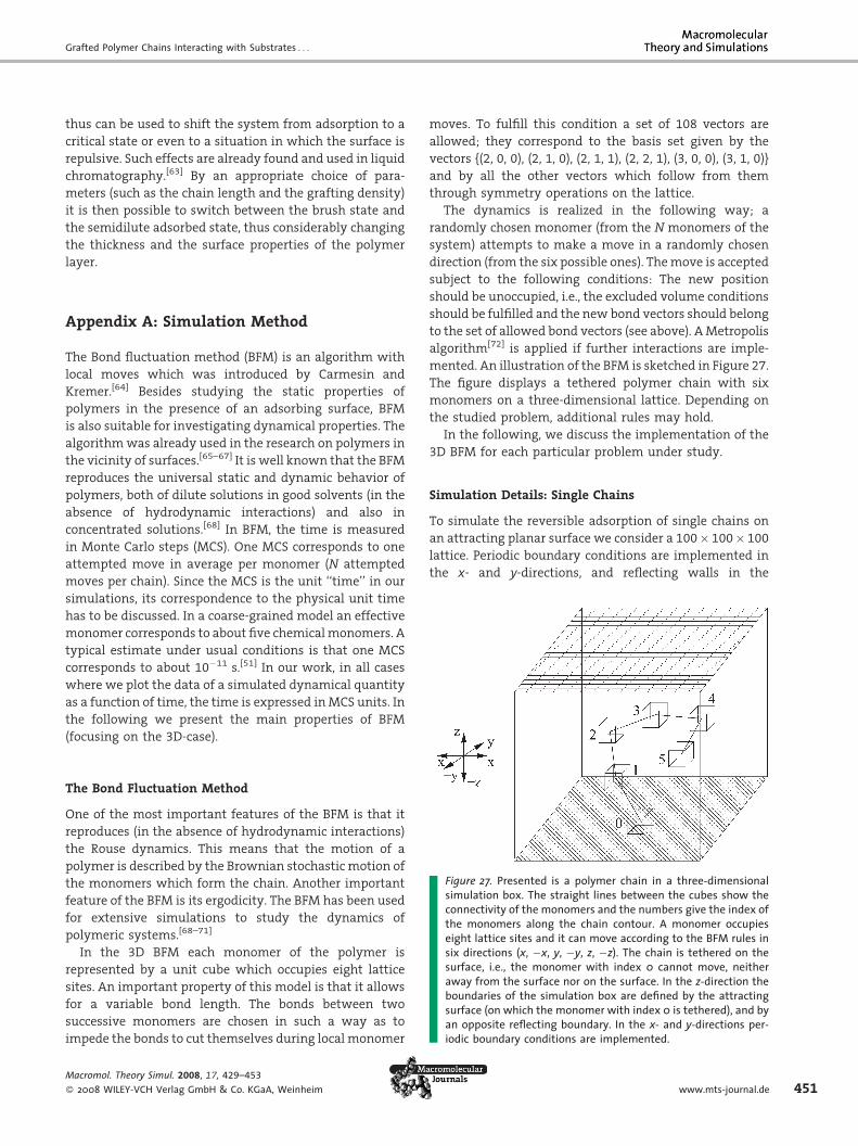
Grafted Polymer Chains Interacting with Substrates . . .
thus can be used to shift the system from adsorption to a
critical state or even to a situation in which the surface is
repulsive. Such effects are already found and used in liquid
chromatography.[63] By an appropriate choice of para-
meters (such as the chain length and the grafting density)
it is then possible to switch between the brush state and
the semidilute adsorbed state, thus considerably changing
the thickness and the surface properties of the polymer
layer.
Appendix A: Simulation Method
The Bond fluctuation method (BFM) is an algorithm with
local moves which was introduced by Carmesin and
Kremer.[64] Besides studying the static properties of
polymers in the presence of an adsorbing surface, BFM
is also suitable for investigating dynamical properties. The
algorithm was already used in the research on polymers in
the vicinity of surfaces.[65–67] It is well known that the BFM
reproduces the universal static and dynamic behavior of
polymers, both of dilute solutions in good solvents (in the
absence of hydrodynamic interactions) and also in
concentrated solutions.[68] In BFM, the time is measured
in Monte Carlo steps (MCS). One MCS corresponds to one
attempted move in average per monomer (N attempted
moves per chain). Since the MCS is the unit ‘‘time’’ in our
simulations, its correspondence to the physical unit time
has to be discussed. In a coarse-grained model an effective
monomer corresponds to about five chemical monomers. A
typical estimate under usual conditions is that one MCS
corresponds to about 10�11 s.[51] In our work, in all cases
where we plot the data of a simulated dynamical quantity
as a function of time, the time is expressed in MCS units. In
the following we present the main properties of BFM
(focusing on the 3D-case).
Figure 27. Presented is a polymer chain in a three-dimensionalsimulation box. The straight lines between the cubes show theconnectivity of the monomers and the numbers give the index ofthe monomers along the chain contour. A monomer occupieseight lattice sites and it can move according to the BFM rules insix directions (x, �x, y, �y, z, �z). The chain is tethered on thesurface, i.e., the monomer with index 0 cannot move, neitheraway from the surface nor on the surface. In the z-direction theboundaries of the simulation box are defined by the attractingsurface (on which the monomer with index 0 is tethered), and byan opposite reflecting boundary. In the x- and y-directions per-iodic boundary conditions are implemented.
The Bond Fluctuation Method
One of the most important features of the BFM is that it
reproduces (in the absence of hydrodynamic interactions)
the Rouse dynamics. This means that the motion of a
polymer is described by the Brownian stochastic motion of
the monomers which form the chain. Another important
feature of the BFM is its ergodicity. The BFM has been used
for extensive simulations to study the dynamics of
polymeric systems.[68–71]
In the 3D BFM each monomer of the polymer is
represented by a unit cube which occupies eight lattice
sites. An important property of this model is that it allows
for a variable bond length. The bonds between two
successive monomers are chosen in such a way as to
impede the bonds to cut themselves during local monomer
Macromol. Theory Simul. 2008, 17, 429–453
� 2008 WILEY-VCH Verlag GmbH & Co. KGaA, Weinheim
moves. To fulfill this condition a set of 108 vectors are
allowed; they correspond to the basis set given by the
vectors {(2, 0, 0), (2, 1, 0), (2, 1, 1), (2, 2, 1), (3, 0, 0), (3, 1, 0)}
and by all the other vectors which follow from them
through symmetry operations on the lattice.
The dynamics is realized in the following way; a
randomly chosen monomer (from the N monomers of the
system) attempts to make a move in a randomly chosen
direction (from the six possible ones). The move is accepted
subject to the following conditions: The new position
should be unoccupied, i.e., the excluded volume conditions
should be fulfilled and the new bond vectors should belong
to the set of allowed bond vectors (see above). A Metropolis
algorithm[72] is applied if further interactions are imple-
mented. An illustration of the BFM is sketched in Figure 27.
The figure displays a tethered polymer chain with six
monomers on a three-dimensional lattice. Depending on
the studied problem, additional rules may hold.
In the following, we discuss the implementation of the
3D BFM for each particular problem under study.
Simulation Details: Single Chains
To simulate the reversible adsorption of single chains on
an attracting planar surface we consider a 100 100 100
lattice. Periodic boundary conditions are implemented in
the x- and y-directions, and reflecting walls in the
www.mts-journal.de 451

R. Descas, J.-U. Sommer, A. Blumen
Table 2. Parameters of the simulation box.
s 10 20 25 30 35 40 60
Lx¼ Ly 100 200 250 300 350 400 600
G 4.0 1.0 0.64 0.44 0.32 0.25 0.11
452
z-direction (see Figure 27). Since we study the behavior of
polymer chains in the presence of an adsorbing surface we
implement a Metropolis algorithm. The monomer/surface
interaction is represented by an attractive, short-ranged
potential e0, acting only at a distance of one lattice unit
from the surface. The Metropolis scheme implies that a
monomer located at the surface (z¼ 0) can leave it only
with a probability
Fig(misur
Macrom
� 2008
p" ¼ expf�"g (A1)
Figure 29. Snapshot of the relaxed tethered system of chains forG¼0.44 (i.e., for s¼ 30) and e¼ 2.2. The lightly colored monomersare in contact with the surface.
where e¼ e0/kT. By setting kT¼ 1 we will focus in the
following only on e. A reflecting wall in the z-direction
implies that the monomers cannot cross the wall and all
moves violating this condition have to be rejected. In our
simulation, we fix (tether) one end of the chain to the surface,
as it has been considered also in previous works.[5,38,73]
We consider fixed values of the chain length N
(20 � N � 200) and fixed values of the surface attraction
e (0:0 � N � 2:0). Before setting e for a given value of N, the
chain is allowed to relax in the absence of any surface
attraction. This, depending on N, requires several hundred
thousands MCS. A snapshot with an equilibrated chain
conformation is presented on the left hand side of
Figure 28. Using the equilibrated state another run is
started, where the interaction e is set to a fixed value. The
chain is allowed to relax again during a period of
(about) 108 MCS. To be sure that the chain conformations
are indeed well equilibrated, for large values of e (e> 1.1)
the equilibration periods were extended up to 109 MCS. In
the middle and on the right hand side of Figure 28
snapshots with equilibrated conformations are presented
for e¼ 0.8 and for e¼ 1.4, respectively. The obtained relaxed
conformations are collected in files in steps of 5000 MCS.
After collecting the simulation data we perform their
analysis and evaluate the quantities of interest.
Simulation Details: Many-Chains Systems
For simulations involving many chains in contact with the
surface we proceed as follows: all chains are anchored at
the adsorbing surface and all of them are made of N¼ 100
monomers. The chains are grown up in a regular square
ure 28. Snapshots of chain conformations with N¼ 100 for e¼0ddle) and for e¼ 1.4 (right). The lightly colored monomers are inface.
ol. Theory Simul. 2008, 17, 429–453
WILEY-VCH Verlag GmbH & Co. KGaA, Weinheim
array of 10 10 chains with a distance of s lattice units
between the grafting points in the xy-plane. To grow up
the chains we use the (0, 0, 2) vector only. In the x- and y-
directions we implement periodic boundary conditions. In
the z-direction we place the adsorbing surface at z¼ 0 and
a reflecting wall at z¼ 210. Note that even totally stretched
chains (reaching the z¼ 200) do not touch this wall. By
varying s the simulations are performed for several
monomer surface concentrations G [see Equation (28)].
The parameters of the simulation box are presented in
Table 2. Here, Lx, and Ly are the (equal) dimensions of the
box in the x- and y-directions.
We equilibrate in the absence of any interaction with
the surface for each fixed value of G every system during
2.5 107 Monte-Carlo steps. After this procedure the
interaction between the monomers and the surface is
turned on. This interaction is introduced in the same way
as for single chains. We set the interaction e to a prescribed
value between 1.1 and 2.5 for each fixed value of G and
allow the chains to relax again during a period of 2.5 107
MCS.
In Figure 29, we present a snapshot of an equilibrated
system for G¼ 0.44 and e¼ 2.2.
(left), for e¼0.8contact with the
Acknowledgements: The support of theDeutsche Forschungsgemeinschaft and of theFonds der Chemischen Industrie is gratefullyacknowledged. R. D. thanks the IPF Dresden forits hospitality during a research stay.
Received: May 20, 2008; Revised: September 4,2008; Accepted: September 10, 2008; DOI:10.1002/mats.200800046
DOI: 10.1002/mats.200800046
Grafted Polymer Chains Interacting with Substrates . . .
Keywords: Adsorption; Monte Carlo simulations; Polymers; Scal-ing; Surfaces
[1] G. J. Fleer, M. A. C. Stuart, J. M. H. M. Scheutjens, T. Cosgrove, B.Vincent, ‘‘Polymers at Interfaces’’, Chapman & Hall, London1993.
[2] D. H. Napper, ‘‘Polymeric Stabilization of Colloidal Disper-sions’’, Academic Press, London 1983.
[3] R. C. Advincula, W. J. Brittain, K. C. Caster, J. Ruhe, PolymerBrushes, Wiley-VCH, Weinheim 2004.
[4] A. Halperin, M. Tirrell, T. P. Lodge,Adv. Polym. Sci. 1992, 100, 31.[5] E. Eisenriegler, K. Kremer, K. Binder, J. Chem. Phys. 1982, 77,
6296.[6] P. G. de Gennes, P. Pincus, J. Phys. (France) Lett. 1983, 44, L241.[7] E. Bouchaud, M. Daoud, J. Phys. (Paris) 1987, 48, 1991.[8] J. Kl�os, J.-U. Sommer, J. Chem. Phys. 2007, 127, 174901.[9] G.-L. He, H. Merlitz, J.-U. Sommer, C.-X. Wu, Macromolecules
2007, 40, 6721.[10] K. Ohno, T. Sakamoto, T. Minagawa, Y. Okabe, Macromol-
ecules 2007, 40, 723.[11] H. W. Diehl, S. Dietrich, Phys. Rev. B 1981, 24, 2878.[12] Z. Usatenko, J. Stat. Mech. 2006, P03009.[13] E. Eisenriegler, ‘‘Polymers near Surfaces’’, World Scientific,
New York 1993.[14] P. G. de Gennes, Macromolecules 1981, 14, 1637.[15] A. N. Semenov, J. Bonet-Avalos, A. Johner, J. F. Joanny, Macro-
molecules 1996, 29, 2179.[16] F. Clement, J. Joanny, J. Phys. II 1997, 7, 973.[17] A. N. Semenov, J. F. Joanny, A. Johner, J. Bonet-Avalos, Macro-
molecules 1997, 30, 1479.[18] K. I. Skau, E. M. Blokhuis, Eur. Phys. J. E 2002, 7, 13.[19] K. Binder, W. Paul, Macromolecules 2008, 41, 4537.[20] M.-B. Luo, J. Chem. Phys. 2008, 128, 044912.[21] J. L. Strathmann, F. Rampf, W. Paul, K. Binder, J. Chem. Phys.
2008, 128, 064903.[22] S. Bhattacharya, H.-P. Hsu, A. Milchev, V. G. Rostiashvili, T. A.
Vilgis, Macromolecules 2008, 41, 2920.[23] R. Descas, J.-U. Sommer, A. Blumen, J. Chem. Phys. 2004, 120,
8831.[24] R. Descas, J.-U. Sommer, A. Blumen, J. Chem. Phys. 2006, 125,
214702.[25] H. Merlitz, G.-L. He, C.-X. Wu, J.-U. Sommer, Macromolecules
2008, 41, 5070.[26] J. U. Kim, M. W. Matsen, Macromolecules 2008, 41, 246.[27] M. D. Whitmore, R. Baranowski, Macromol. Theory Simul.
2005, 14, 75.[28] J. B. Sokoloff, Macromolecules 2007, 40, 4053.[29] R. S. Hoy, G. S. Grest, Macromolecules 2007, 40, 8389.[30] A. Patrykiejew, S. Soko l�owski, R. Tscheliessnig, J. Fischer, O.
Pizio, J. Phys. Chem. 2008, 112, 4552.[31] M. Borowko, W. Rzysko, S. Soko l�owski, T. Staszewski, J. Chem.
Phys. 2007, 126, 214703.[32] A. Milchev, K. Binder, Macromolecules 1996, 29, 343.[33] R. Descas, J.-U. Sommer, A. Blumen, J. Chem. Phys. 2005, 122,
134903.[34] A. J. Bray, M. A. Moore, J. Phys. A 1977, 10, 1927.[35] P. G. de Gennes, ‘‘Scaling Concepts in Polymer Physics’’, Cornell
University Press, Ithaca 1979.[36] H. W. Diehl, M. Shpot, Nucl. Phys. B 1998, 528, 595.
Macromol. Theory Simul. 2008, 17, 429–453
� 2008 WILEY-VCH Verlag GmbH & Co. KGaA, Weinheim
[37] P. Grassberger, J. Phys. A 2005, 38, 323.[38] S. Metzger, M. Muller, K. Binder, J. Baschnagel, Macromol.
Theory Simul. 2002, 11, 985.[39] B. O’Shaughnessy, D. Vavylonis, Eur. Phys. J. E 2003, 11,
213.[40] B. O’Shaughnessy, D. Vavylonis, Phys. Rev. Lett. 2003, 90,
056103.[41] R. Descas, J.-U. Sommer, A. Blumen, J. Chem. Phys. 2006, 124,
094701.[42] A. L. Ponomarev, T. Sewell, C. Durning, Macromolecules 2000,
33, 2662.[43] S. Bhattacharya, A. Milchev, V. G. Rostiashvili, A. Y. Grosberg,
T. A. Vilgis, Phys. Rev. E 2008, 77, 061603.[44] X. Zhang, B. Chen, Z. Wang, J. Colloid Interface Sci. 2007, 313,
414.[45] H. W. Diehl, S. Dietrich, Phys. Lett. A 1980, 80, 408.[46] S. Alexander, J. Phys. (Paris) 1977, 38, 977.[47] P. G. de Gennes, Macromolecules 1980, 13, 1069.[48] W. Y. Chen, J. X. Zheng, S. Z. D. Cheng, C. Y. Li, P. Huang, L. Zhu,
H. Xiong, Q. Ge, Y. Guo, R. P. Quirk, B. Lotz, L. Deng, C. Wu, E. L.Thomas, Phys. Rev. Lett. 2004, 93, 028301.
[49] J. X. Zheng, H. Xiong, W. Y. Chen, K. Lee, R. M. V. Horn, R. P.Quirk, B. Lotz, E. L. Thomas, A.-C. Shi, S. Z. D. Cheng, Macro-molecules 2006, 39, 641.
[50] S. T. Milner, T. A. Witten, M. E. Cates, Macromolecules 1988, 21,2610.
[51] K. Binder, Eur. Phys. J. E 2002, 9, 293.[52] M. Doi, S. F. Edwards, ‘‘The Theory of Polymer Dynamics’’,
Clarendon Press, Oxford 1986.[53] Y. Oono, Adv. Chem. Phys. 1985, 61, 301.[54] A. Milchev, W. Paul, K. Binder, J. Chem. Phys. 1993, 99, 4786.[55] I. Geroff, A. Milchev, K. Binder, W. Paul, J. Chem. Phys. 1993, 98,
6526.[56] K. Kremer, K. Binder, J. Chem. Phys. 1984, 81, 6381.[57] D. I. Dimitrov, A. Milchev, K. Binder, L. I. Klushin, A. M.
Skvortsov, J. Chem. Phys. 2008, 128, 234902.[58] H. Yang, Y. Liu, H. Zhang, Z.-S. Li, Polymer 2006, 47, 7607.[59] P.-Y. Lai, K. Binder, J. Chem. Phys. 1991, 95, 9288.[60] M. Murat, G. S. Grest, Macromolecules 1989, 22, 4054.[61] M. Zeghal, B. Deloche, P. Auroy, Macromolecules 1999, 32,
4947.[62] T. Tajouri, H. Hommel, Magn. Reson. Chem. 2007, 45, 488.[63] S. Orelli, W. Jiang, Y. Wang, Macromolecules 2004, 37,
10073.[64] I. Carmesin, K. Kremer, Macromolecules 1988, 21, 2819.[65] K. Binder, A. Milchev, J. Baschnagel, Ann. Rev. Mater. Sci. 1996,
26, 107.[66] C. Mischler, J. Baschnagel, S. Dasgupta, K. Binder, Polymer
2002, 43, 467.[67] J. S. Shaffer, Macromolecules 1994, 27, 2987.[68] W. Paul, K. Binder, D. W. Heermann, K. Kremer, J. Phys. II 1991,
1, 37.[69] J. Baschnagel, K. Binder, J. Phys. I 1996, 6, 1271.[70] E. Reister, M. Muller, J. Chem. Phys. 2003, 118, 8476.[71] H. P. Wittmann, K. Kremer, K. Binder, J. Chem. Phys. 1992, 96,
6291.[72] N. Metropolis, A. W. Rosenbluth, M. N. Rosenbluth, A. Teller, E.
Teller, J. Chem. Phys. 1953, 21, 1087.[73] S. Metzger, M. Muller, K. Binder, J. Baschnagel, J. Chem. Phys.
2003, 118, 8489.
www.mts-journal.de 453