Directive Antenna Using Metamaterial Substrates

by

Weijen Wang

B. S. in Electrical Engineering and Computer ScienceMassachusetts Institute of Technology, Cambridge, June 2002

Submitted to the Department of Electrical Engineering and Computer Sciencein Partial Fulfillment of the Requirements for the Degree of

Master of Engineering in Electrical Engineering and Computer Science

at the

MASSACHUSETTS INSTITUTE OF TECHNOLOGY

June 2004

@ Massachusetts Institute of Technology 2004. All rights reserved.

Author .............Depadment of Electrical En geering and Computer Science

May 20, 2004

Certified by...........Jin Au Kong

Thesis Supervisor

Accepted by ....... ................Arthur C. Smith

Chairman, Department Committee on Graduate Students

ASSACHUSETTS INST E.OF TECHNOLOGY

EJUL 2 0 200

LIBRARIESBARKER

I

11'

A

2

Directive Antenna Using Metamaterial Substrates

by

Weijen Wang

Submitted to the Department of Electrical Engineering and Computer Scienceon May 20, 2004, in partial fulfillment of the

requirements for the Degree ofMaster of Engineering in Electrical Engineering and Computer Science

Abstract

Using a commercially available software(CST Microwave Studio®), two kinds of sim-ulations have been carried out on different metamaterials in the microwave regime.One is transmission and reflection of a unit cell in a waveguide, and the other isparallel plate slab farfield radiation. The S-parameters are obtained from the wave-guide simulation and are used to retrieve the effective permittivity and permeabilitywith which we can estimate the farfield radiation using analytic method. Thus, bycomparing the farfield radiation from two different methods, analytic and slab simu-lation, we find that the analytic method is able to indicate many major features ofthe slab simulation's farfield results, implying that within a certain frequency range,we can treat the metamaterial as being homogeneous. After comparing the radiationperformance of different metamaterial as antenna substrates, a structure is chosento be optimized in such a way that it improves in radiation power, beamwidth, andbandwidth.

Thesis Supervisor: Jin Au KongTitle: Professor, Department of Electrical Engineering and Computer Science

3

4

Acknowledgments

First, I would like to thank Professor Jin Au Kong for giving me the opportunity to do

research in electromagnetics. I will always remember how his excellent teaching has

inspired me, and helped me in understanding one of the most difficult subjects in the

electrical engineering area. I am also thankful for his kindness and encouragement. I

am indebted to Dr. George A. Kocur, Professor Steven R. Lerman, Dr. V. Judson

Harward, and Professor Ruaidhri M. O'Connor, with whom I have gained valuable

experience as a teaching assistant.

I would also like to thank the CETA group members, namely Benjamin E. Bar-

rowes, Jianbing Chen, Xudong Chen, Tomasz M. Grzegorczyk, May Lai, Jie Lu,

Christopher Moss, Madhusudhan Nikku, Joe Pacheco, Zachary M. Thomas, and Bae-

Ian Wu, for their valuable advice and discussions on various topics. I am grateful for

the friendship and comradeship from my former and current fellow teaching assis-

tants: Sehyun Ahn, Jeffrey M. Bartelma, Liou Cao, Christopher A. Cassa, Curtis R.

Eubanks, Peilei Fan, Abdallah W. Jabbour, Bharath K. Krishnan, Hariharan Laksh-

manan, Jedidiah B. Northridge, Fernando Perez, and Anamika Prasad.

It has been almost six years since I first joined the great minds at the Mas-

sachusetts Institute of Technology. As what the rumors have spread, it has not been

easy surviving in this institution. I still remember being doubtful about my college

choice after meeting several international Math, Physics, Chemistry, and Informatics

Olympiad's medalists during my first day of international orientation. However, the

friendships that I have established at MIT have helped me tremendously throughout

my undergraduate and graduate years. To all my friends, I am thankful for the com-

pany when I stayed up at night, the encouragement when I felt down, the counsel

when I was lost, and mostly, the friendship that they have given me. Special thanks

to Senkodan Thevendran and Felicia Cox, who have accepted me regardless of good

or bad, for their love and patience, and making me a better person. Lastly, I would

like to acknowledge Bae-Ian Wu, who has been both a mentor and a friend, for his

guidance and support without which this thesis would not have been possible.

5

Finally, I would like to thank my parents for always trying to provide me with the

best education opportunities. Without them, I will not be where I am today. They

have never stopped believing in me and giving me the reason and the energy to thrive

at wherever I am. To my brother and sister, thank you for always being there for me

and bringing joy to my life.

I dedicate this thesis to my family and friends.

6

To my family and friends

7

8

Contents

1 Introduction

2 Methodology

2.1 Prior art . . . . . . . . . . . .. . . .

2.2 Simulation ...............

2.2.1 Radiation setup . . . . . . . .

2.2.2 Waveguide setup . . . . . . .

2.3 Analytic method for farfield radiation

2.4 Radiation results and normalization .

3 Comparative Study of Different Metamaterial Substrate

3.1 2-D Smith structure . . . . . . . . . . . . . . . . . . . . .

3.2 1-D Smith structure . . . . . . . . . . . . . . . . . . . . .

3.3 Pendry structure . . . . . . . . . . . . . . . . . . . . . . .

3.4 Omega structure . . . . . . . . . . . . . . . . . . . . . . .

3.5 S structure................ ..... .... ......

3.6 Sum m ary . . . . . . . . . . . . . . . . . . . . . . . . . . .

4 Optimized Metamaterial Structure

4.1 Optimized unit cell's geometry . . .

4.2 Optimization of cell orientation and

4.3 Comparison with analytic method .

4.4 Summary . . . . . . . . . . . . . .

9

. . . . . . . . . .

antenna position

. . . . . . . . . .

. . . . . . . . . .

17

21

22

23

24

26

28

30

37

38

44

49

55

60

66

67

68

70

77

79

5 Conclusion

Bibliography 83

10

81

List of Figures

1-1 Dipole emission in a substrate with n = 0 . . . . . . . . . . . . . . . . 19

2-1 M ethodology chart . . . . . . . . . . . . . . . . . . . . . . . . . . . . 21

2-2 Full size rod structure . . . . . . . . . . . . . . . . . . . . . . . . . . 24

2-3 Mesh for full size rod structure . . . . . . . . . . . . . . . . . . . . . 25

2-4 Slab of metamaterial(rod medium) . . . . . . . . . . . . . . . . . . . 26

2-5 Unit cell rod structure in a waveguide . . . . . . . . . . . . . . . . . . 27

2-6 Retrieval results for rod medium . . . . . . . . . . . . . . . . . . . . . 27

2-7 Radiation configuration of a linesource in an infinite isotropic slab of

thickness d1 + d2 . . . . . . . .. . . . .. . . . . . . . . . . .. . 28

2-8 Radiation plane of interest . . . . . . . . . . . . . . . . . . . . . . . . 30

2-9 Radiated power and normalized radiation from analytic method for

rod structure ........ ............................... 31

2-10 Radiated power and normalized radiation from simulation for rod full

size and slab structure . . . . . . . . . . . . . . . . . . . . . . . . . . 32

2-11 Beamwidth for full size rod medium . . . . . . . . . . . . . . . . . . . 33

2-12 Beamwidth for a slab of rod medium . . . . . . . . . . . . . . . . . . 34

3-1 Unit cell 2-D Smith structure in a waveguide . . . . . . . . . . . . . . 38

3-2 Retrieval results for 2-D Smith structure . . . . . . . . . . . . . . . . 39

3-3 Slab of 2-D Smith structure . . . . . . . . . . . . . . . . . . . . . . . 40

3-4 Mesh for 2-D Smith structure . . . . . . . . . . . . . . . . . . . . . . 40

3-5 Radiated power and normalized radiation from analytic method and

slab simulation for 2-D Smith structure . . . . . . . . . . . . . . . . . 42

11

3-6

3-7

3-8

3-9

3-10

3-11

3-12

3-13

3-14

3-15

3-16

3-17

slab simulation for Pendry structure . . . . . . .

Beamwidth for Pendry structure slab simulation

Unit cell Omega structure in a waveguide . . . .

Retrieval results for Omega structure . . . . . .

Slab of Omega structure . . . . . . . . . . . . .

Mesh for Omega structure . . . . . . . . . . . .

Radiated power and normalized radiation from

slab simulation for Omega structure . . . . . . .

Beamwidth for Omega structure slab simulation

Unit cell S structure in a waveguide . . . . . . .

Retrieval results for S structure . . . . . . . . .

. . . . . . . . . . . . 53

. . . . . . . . . . . . 54

. . . . . . . . . . . . 55

. . . . . . . . . . . . 56

. . . . . . . . . . . . 57

. . . . . . . . . . . . 57

analytic method and

. . . . . . . . . . . . 58

. . . . . . . . . . . . 59

. . . . . . . . . . . . 60

. . . . . . . . . . . . 6 1

3-27 Slab of S structure . . . . .... ......... . . . . . . .. . ... .

3-28 Mesh for S structure . . . . . . . . . . . . . . . . . . . . . . . . . . .

3-29 Radiated power and normalized radiation from analytic method and

slab simulation for S structure . . . . . . . . . . . . . . . . . . . . . .

3-30 Beamwidth for S structure slab simulation . . . . . . . . . . . . . . .

12

Beamwidth for 2-D Smith structure slab simulation . . . . . . . . . .

Unit cell 1-D Smith structure in a waveguide . . . . . . . . . . . . . .

Slab of 1-D Smith structure . . . . . . . . . . . . . . . . . . . . . . .

Retrieval results for 1-D Smith structure . . . . . . . . . . . . . . . .

Mesh for 1-D Smith structure . . . . . . . . . . . . . . . . . . . . . .

Radiated power and normalized radiation from analytic method and

slab simulation for 1-D Smith structure . . . . . . . . . . . . . . . . .

Beamwidth for 1-D Smith structure slab simulation . . . . . . . . . .

Unit cell Pendry structure in a waveguide . . . . . . . . . . . . . . . .

Retrieval results for Pendry structure . . . . . . . . . . . . . . . . . .

Slab of Pendry structure . . . . . . . . . . . . . . . . . . . . . . . . .

Mesh for Pendry structure . . . . . . . . . . . . . . . . . . . . . . . .

Radiated power and normalized radiation from analytic method and

43

44

45

46

46

47

48

49

50

51

52

3-18

3-19

3-20

3-21

3-22

3-23

3-24

3-25

3-26

62

63

64

65

4-1 Unit cell optimized structure in a waveguide . . . . . . . . . . . . . . 68

4-2 Retrieval results for the optimized structure . . . . . . . . . . . . . . 69

4-3 Two different 1-D orientations of unit cells arrangement . . . . . . . . 70

4-4 Mesh for the optimized structure . . . . . . . . . . . . . . . . . . . . 71

4-5 Radiated power and normalized radiation from slab simulation for

Pendry version x and Pendry version y structure . . . . . . . . . . . . 72

4-6 Beamwidth for Pendry version x structure slab simulation . . . . . . 73

4-7 Beamwidth for Pendry version y structure slab simulation . . . . . . 74

4-8 Two different antenna positions . . . . . . . . . . . . . . . . . . . . . 75

4-9 Radiated power and normalized radiation from slab simulation for dif-

ferent antenna positions . . . . . . . . . . . . . . . . . . . . . . . . . 76

4-10 Radiation configuration of a linesource in an infinite anisotropic slab

of thickness d1 + d2 . . . . . . . . . . .. . . .. . . . . .. . . . . 77

4-11 Radiated power and normalized radiation from analytic method for

Pendry version x and Pendry version y structure . . . . . . . . . . . . 78

13

14

List of Tables

3.1 Comparison among different metamaterial substrates . . . . . . . . . 66

15

16

Chapter 1

Introduction

Recently, there has been growing interest in the study of metamaterials both the-

oretically and experimentally. Metamaterials are artificial materials synthesized by

embedding specific inclusions, for example, periodic structures, in the host media [1]-

[17]. Some of these materials exhibit either negative permittivity or negative perme-

ability [2]-[16]. If both permittivity and permeability of such materials are negative at

the same time, then the composite possesses an effective negative index of refraction

[18] and is referred to as a left-handed metamaterial. The name is used because the

electric field, the magnetic field, and the wave vector form a left-handed system [18].

These metamaterials are typically realized artificially as composite structures that are

composed of periodic metallic patterns printed on dielectric substrates. These inclu-

sions affect the macroscopic properties of the bulk composite medium which exhibits

a negative effective permittivity and/or permeability for a certain frequency band.

One of the first theoretical studies was done by Veselago in the 1960's [18]. He

examined the propagation of plane waves in a hypothetical substance with simulta-

neous negative permittivity and permeability. He found that the Poynting vector of

the plane wave is antiparallel to the direction of the phase velocity, which is contrary

to the conventional case of plane wave propagation in natural media. It has been

shown by Pendry et al. that a medium constructed with periodic metallic thin wires

behaves as a homogeneous material with a corresponding plasma frequency when the

lattice constant of the structure and the diameter of the wire are small in compar-

17

ison with the wavelength of interest [2]. Pendry et al. also showed that split ring

resonators can result in an effective negative permeability over a particular frequency

region [3]. Only a couple of years ago, Smith, Schultz, and Shelby from the Univer-

sity of California-San Diego constructed the first left-handed metamaterial in the

microwave regime, and demonstrated experimentally the negative index of refraction

[5].

Many properties and potential applications of metamaterials have been explored

and analyzed theoretically. Pendry proposed that left-handed metamaterials could

be used to build a perfect lens with sub-wavelength resolution [19]. Studies have been

done on backward waves propagation [20, 21], waveguides [22, 23], Cerenkov radiation

[24], resonators [25], and growing evanescent waves [26], etc.

We can view metamaterials as a class of materials broader than left-handed meta-

materials. It is a class of materials that enable us to manipulate the bulk permittivity

and permeability. To this date, such technology in left-handed metamaterials is best

suited for our purpose.

Little research has been done on applications of metamaterials in antenna systems.

Emission in metamaterials using an antenna has been recently presented in 2002 by

Enoch et al. [27]. Two features are of interest regarding the control of emission:

direction and power of emission. Enoch et al. have demonstrated the feasibility of

using a rod medium to direct the emission of an embedded source towards the normal

of the substrate, thus confining the radiated energy to a small solid angle.

The metamaterial they used was a metallic mesh of thin wires. Such medium

can be characterized by a plasma frequency [2]. The effective permittivity can be

expressed as

EP = W- /w2

where w, is the plasma frequency and w is the frequency of the propagating elec-

tromagnetic wave. From this equation, the effective permittivity is negative when

the frequency is below the plasma frequency. When operating at the plasma fre-

quency, the effective permittivity is zero, and hence yields a zero index of refraction

18

air n = 1

n = 0

Figure 1-1: Dipole emission in a substrate with n = 0

(n = jyreC). From Snell's law

sin Ot /sin Oi = ni/nt (1.2)

where i denotes the incident medium and t denotes the transmitted medium, for

ni ~ 0, we obtain a Ot of zero regardless of what 9i is. As shown in Figure 1-1, if we

place a dipole in a substrate with index of refraction n = 0, the exiting ray from the

substrate will be normal to the surface. Therefore, the closer the operating frequency

is to the plasma frequency, the better the directivity. The permittivity just above

the plasma frequency can be positive but still less than one. This will correspond to

an index of refraction of less than one and close to zero. Then for any incident ray

from inside such a medium to free space, the angle of refraction will be close to zero

and the refracted rays will be close to normal. This property can be used to control

the direction of emission. More specifically, We can expect directive radiation when

the absolute value of the index of refraction is less than one and its imaginary part is

small. Inspired by Enoch, we proposed to use left-handed like metamaterial, where

ceff and peff will be zero for certain frequencies. Through the manipulation of a

structure's geometry, where Eeff = 0 and pef f = 0 are can be tuned to the desired

frequencies to produce directional emission in a wider band.

By using a commercially available software called CST Microwave Studio® [28],

studies will be done on a dipole embedded in different metamaterial substrates. In

19

Chapter 2, methodology for studying antenna radiation in metamaterial substrates

will be presented. In Chapter 3, different metamaterials are analyzed for antenna

substrates application. Simulation results are compared with specific focuses on

beamwidth, bandwidth, and power. In Chapter 4, we will show our optimized re-

sults and how other parameters like position of antenna can effect radiation results.

Lastly, Chapter 5 is conclusion.

20

Chapter 2

Methodology

As discussed in the previous chapter, the objective of this thesis is to develop a

methodology to analyze and design metamaterial substrates for directive antenna. In

this chapter, we will present the methodology in detail. The flow chart in Figure 2-1

shows the basic elements in our methodology and the process of analysis. We will

use the rod medium as an example to illustrate how our methodology works and

how it can assist us to optimize a metamaterial structure as a substrate for directive

antenna.

one cellPEC/PMC > S parameterswavegu ide

Metamaterials

Microwave Studio Analytic formulaparallel plate waveguide radiation

radiation Farfield results

Figure 2-1: Methodology chart

As seen in the methodology chart, the metamaterial is the starting point of the

analysis and is usually composed of periodic structures of metal and dielectric for the

microwave region. We can build the structure and perform experiments to determine

21

what its performance is as an antenna substrate, or we can do numerical simulations,

or we can do theoretical studies assuming the substrate is homogeneous. Since exper-

iment is the most expensive and time consuming, we will use numerical simulation

and theoretical studies first to study the properties of different metamaterials, and

later design a metamaterial structure that is good for antenna substrate. Simulating

the real size structure requires a lot of memory and simulation time, therefore we will

use a slice of metamaterial which is placed in a parallel plate waveguide to approxi-

mate the radiation effect. We can also simulate a unit cell of the metamaterial in a

waveguide and extract the S-parameters in order to find the effective E and p for all

frequencies [29]. With the effective permittivity and permeability, we can calculate the

corresponding S-parameters and compare with the ones we obtained from simulation.

Furthermore, we can use analytic formula to obtain farfield results with peff and Eeff.

This theoretical farfield results is faster to acquire than the ones from simulating in a

parallel plate waveguide. Therefore, for optimization, we will use theoretical method

to find a structure with the best theoretical farfield radiation first, then simulate the

metamaterial in the parallel plate waveguide.

2.1 Prior art

Enoch et al. has used metamaterial as antenna substrate[27]. The metamaterial

they used were layers of copper grids separated by foam. The copper grids has a

square lattice with a period of 5.8 mm; each layer has a separation of 6.3 mm. This

metamaterial possesses a microwave plasma frequency at about 14.5 GHz. The source

of excitation used is a monopole antenna fed by a coaxial cable. The emitting part of

the monopole is approximately located at the center of the metamaterial substrate. In

the experiment, a ground plane is added to the metamaterial substrate. At 14.65 GHz,

it was shown to have the best directivity.

The block of metamaterial substrate can be treated as a homogenous material.

Since it has a plasma frequency of _14.5 GHz, the permittivity is closed to zero at

this frequency, which means that the index of refraction is closed to zero as well.

22

From ray theory, the exiting ray from the substrate will be very closed to the normal

of the substrate(as shown in Chapter 1).

Changes in the copper grid metamaterial can only change where ecf = 0 is.

However, for the index of refraction n = 0, we do not necessarily have to make

permittivity zero; we can also have peff = 0. The known technology to manipu-

late both permittivity and permeability of a structure from the study of left handed

metamaterials can be applied. In the next chapter, we will study some known left

handed metamaterials as antenna substrates. However, in this chapter we will use rod

medium as an example, since it is the simplest metamaterial and we have previous

literature to compare our simulation results with. We will use similar aperture size

for all our metamaterial substrates, and keep our region of interest in the microwave

region. Ground planes will not be used in our study; the main effect will be that the

beamwidth will be wider without the ground plane. In the next subsection, we will

show how to simulate metamaterials using CST Microwave Studio®.

2.2 Simulation

For simulation, we use CST Microwave Studio®. It uses Finite Integration Tech-

nique (FIT)[30] for general purpose electromagnetic simulations. FIT applied to

Cartesian grids in the time domain is computationally equivalent with the standard

Finite Difference Time Domain(FDTD) method. For high frequency electromagnetic

applications, time domain simulations methods are highly desirable, especially when

broadband results are needed. FIT therefore shares FDTD's advantageous proper-

ties like low memory requirements and efficient time stepping algorithm. However,

standard FDTD has poor modeling quality for arbitrarily shaped geometries since

it uses staircase approximations. FIT combined with Perfect Boundary Approxima-

tion(PBA) can maintain the convenient structured Cartesian grids and permit an

accurate modeling of curved structures[31].

The solver that we used for all our simulations is a transient solver. For a wide

frequency range, it uses only one computational run for the simulation of a structure's

23

behaviors[31]. The version of CST Microwave Studio@ that we are using is v4.2. We

will be using it for radiation simulation and waveguide simulation.

2.2.1 Radiation setup

Here we will show our simulation setup for getting the farfield radiation. To illustrate

the methodology in detail, a simple rod medium will be used as demonstration, which

is very similar to what Enoch et al. has used[27]. The full size structure setup for

the rod medium is shown in Figure 2-2. Each rod is a cylindrical Perfect Electric

Conductor(PEC) structure that has a radius of 0.2 mm, and a length of 250 mm.

The period in the x direction is 5.8 mm and in the y direction is 6.3 mm. There

are 6 layers of rods in the y direction and 40 repetitions in the x direction. A 50 Q

y

6.3mm x 6

- - ~-~-' ~-~- '250mm

5.8mm x 40

Figure 2-2: Full size rod structure

S-parameter discrete port(dipole) of 1mm in length is placed at the center of the

structure for radiation. Mesh type of PBA(usually staircase type will be used if there

is no curvature in the structure to save simulation time) is used with mesh density set

at 10 lines per wavelength with refinement at PEC edges by 3. The resultant mesh in

the x - y plane is shown in Figure 2-3. How the mesh is setup is very important to the

accuracy of our simulation results. It needs to be fine enough to capture the details

of the metamaterial structure. It is not as essential here for the simple rod medium

as for some other structure which we will encounter later. The open boundary is

24

Figure 2-3: Mesh for full size rod structure

modeled with Perfectly Matched Layer(PML) of 8 layers and a reflection coefficient

of 0.0001. The automatic minimum distance to structure(when using "open(add

space)" as the boundary condition) is one wavelength. Farfield monitors are set up

for frequencies from 11 GHz to 17 GHz. Radiation power are calculated at a distance

10 meters away from the excitation source(dipole in all our cases). These are the

typical parameters we use in all our simulations, except for the mesh parameters and

farfield monitor frequency range. Farfield results are shown in Section 2.4. Simulating

the full size structure takes a lot of memory and as most metamaterial structures are

more complicated than periodic rods, more time and even more memory are needed

for simulation as well. Therefore, we use a slab of metamaterial in a PEC parallel

plate waveguide to approximate the full size structure to save simulation time and

memory. The slab setup is as shown in Figure 2-4. The dipole is again placed at the

center of the structure. Mesh parameters are the same as before with the additional

option of "Merge fixpoints on thin PEC and lossy metal sheet" chosen. All other

parameters stay the same.

25

5.8mm x 40

6.3mm x 6 -

-3.33mm

Figure 2-4: Slab of metamaterial(rod medium)

2.2.2 Waveguide setup

In order to study the metamaterial properties in a waveguide, a unit cell is identified

from the full size structure and placed in a waveguide to collect the S-parameters.

The unit cell for the rod medium is shown in Figure 2-5. The rod here is again

modeled with PEC material, and the background as air. The top and bottom sur-

face has PEC boundary condition, whereas the left and right has perfect magnetic

conductor(PMC) boundary condition, and front and back with open boundary con-

dition. These boundary conditions will be the same for all structures' unit cells that

we presented in this thesis. A waveguide port is placed at the open boundaries. Mesh

density is 10 lines per wavelength; the options of refinement at PEC edges by factor 4

and inside dielectric materials are chosen. With the S-parameter data obtained from

the waveguide simulation, we can retrieve the effective p and E for all frequency[29].

An electric plasma frequency of 13.5 GHz is observed from retrieval(see Figure 2-

6). Therefore, for farfield radiation, we will be interested in the frequencies around

13.5 GHz, as the index of refraction will be close to zero in that region, and thus will

possibly have beam sharpening effect. Using a rod medium, we can only have eeff

to be zero at a certain frequency by changing the periodicity or the radius of the

rods and thus making the index of refraction n = 0 at the corresponding frequency.

Ultimately, our goal is to find a metamaterial structure where we can also get [eff

to be zero at a frequency that is close to where eeff = 0 is, such that the region

26

3.33mm

F.3mm

Figure 2-5: Unit cell rod structure in a waveguide

5432

1

0-1-2

-3-4-5

4321

2 4 6 8 10 12 14 16 18 20f/GHz

U.

-1 -

-2 - - -

-3

.

-4 . -.-.-.

-50 2 4 6 8 10 12 14 16 18 20

f/GHz

54-3-

2-1

0-1

-2 -

-3 .

-4-5

0 2 4 6 8 10 12 14 16 18 2Cf/GHz

5

4- -... Real(e)

3 . . . -.. . Imag(e)3

2--1

-1

- 2 -. -...-

-3 -. . .

- 4 .. .. .. . .. ... I.. ... .

0 2 4 6 8 10f/GH2

12 14 16 18 20

Figure 2-6: Retrieval results for rod medium

27

Real(z)- Imag(z)

----- ------ -

-- Real(n)-Imag n)

........ g (-

-. ...-.

- Real(p)- Imag(p)

I

-

where n ~ 0 can be broadened. Consequently we can potentially have a wider band

where we can expect beam sharpening. Retrieval results (peff and eff) enable us

to relate metamaterials to a homogeneous material, and further assist us to estimate

the radiation characteristic as we will demonstrate in the next section.

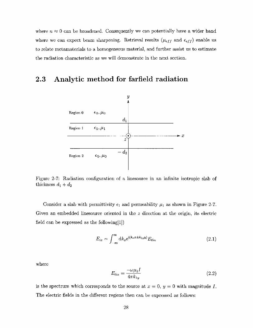
2.3 Analytic method for farfield radiation

y

Region 0 0 , /t0

Region 1 E 1,1A

Xz

Region 2 60, P0- d2 1

Figure 2-7: Radiationthickness d, + d 2

configuration of a linesource in an infinite isotropic slab of

Consider a slab with permittivity c, and permeability p1 as shown in Figure 2-7.

Given an embedded linesource oriented in the z direction at the origin, its electric

field can be expressed as the following[1])

Eiz = J dkxe(kxxiklY)Ein (2.1)

where

E -in = I(2.2)

is the spectrum which corresponds to the source at x = 0, y = 0 with magnitude I.

The electric fields in the different regions then can be expressed as follows:

28

0

In region 0,

Eoz dkxEfin(Tieikoy)eikxx (2.3)

In region 1,

Elz = J dkx Efin(e ±ik1 + Ae iklyy + Be-iky )eikxx (2.4)

In region 2,

E2Z J dkxEin(T2e-ikyy)e ikxx (2.5)

By matching the boundary conditions for the tangential electric and magnetic

fields at y = di and y = -d 2 , we can find the coefficients T1, T2, A, and B.

2ei(kiy-koy)dipo1 (1 + ei2k1yd2(_ +Pi 1) +i P()e ei2kly (d +d2)(~ 1+ poi) 2

-(1 + pol) 2 (26

T2 2ei(klykoy)d2po1 + ei 2 klydi + POO + P01) (2.7)

ei2klY (d+d2)(-1 + P01)2 - (1 +| P01)2

A = - e ei2kid2(- ± P01) (i + ei2kiyd1(_1 + P01) + P01) (28)e i2kiy(d1+d2)(1 + P01)2 _ (1 + Pa) 2

B = - ei2kiyd2(_1 +pi) (i ei2kiyd2( + pi0) ±oi) (2.9)ei2kiy(d1+d2)(-1 + poi) 2 _ (1 + P01) 2

where

pi = k (2.10)pu 1 Aikoy

Using farfield approximation, the electric field in region 0 can be simplified as

follows:

Eo= EnkoyT1] dkx I eikoye ik;X = EeinkoyT1 eikor (211f-00 koy iko

Normalizing this electric field to a free space case, we get

Er = (2.12)Poi

where Er denotes the relative electric field with respect to a dipole in free space.

29

2.4 Radiation results and normalization

In this section, we will show all our different radiation results from different methods

and how we compare them. Radiation results are plotted for the plane of interest,

the x - y plane, as shown in Figure 2-8 using a parallel plate radiation as an example.

Angle # is the angle from the +x axis in the plane of interest. In the frequency band

Yx

Figure 2-8: Radiation plane of interest

where index of refraction n ~~ 0, the main beam(most power) is expected to occur at

0 = 900 or # = 270' or both. We have two different radiation results: simulation and

analytic. These two methods plot different aspects of farfield radiation, and we want

to normalize them in some way such that we can compare our results.

Analytic method shown in Section 2.3 calculates radiation using electric field from

an embedded linesource. The resultant farfield calculation is the ratio of the electric

field in metamaterial to the electric field in free space. It can then be squared to

show the relative power in dB. Simulated farfield radiation calculates the electric

fields or power by using farfield approximation. In order to compare radiation results

from these different methods, we need to find a way to normalize these data first.

We noticed that in all these results, power is involved. In the analytic method, for

each direction, the power of each frequency is divided by the power corresponding

to the free space case. Therefore, for the same frequency, different radiated powers

at different angles will be divided by the same number. However, if the frequency is

different, the powers will be divided with a different number. This tells us that there

is a different scaling factor for different frequency. Hence, our method for normalizing

30

all radiation figures is that for each frequency, we calculate the average power in that

frequency and normalize(divide) all power data in that frequency with this average.

The 3 dB beamwidth calculation will not be affected by this normalization.

Figure 2-9 shows the radiation results obtained from analytic method. From

retrieval as discussed in Section 2.2.2, we expect to see directive radiation around the

electric plasma frequency of 13.5 GHz. The most directive and high power radiation

is seen to center at 13.6 GHz and 13.9 GHz respectively. Shortly after 13.9 GHz, the

main beam starts to divert away from q = 90', and form a "U" shape radiation

pattern.

Radiated Power Normalized Radiation17 5 17 15

16 0 16 10N NM15 -5 M15 5

O 14 -10 C14 0

13 -15 213 -5

12 -20 12 -10

11 -25 11 -150 30 60 90 120 150 180 0 30 60 90 120 150 180

Angle(degree) Angle(degree)

Figure 2-9: Radiated power and normalized radiation from analytic method for rodstructure

Next, lets look at the radiation results acquired from simulation for both the

full size and the parallel plate slab cases in Figure 2-10. For the full size structure

simulation, the most directive beam is centered at around 13.7GHz and the high

power beam is centered at around 14.4GHz. Similarly like what the analytic results

have predicted, the highest power beam takes place after the most directive beam, but

with both these frequencies shifted to a slightly higher frequencies. The parallel plate

slab case exhibits a directive and high power beam at around 13.8 GHz and 13.9 GHz

respectively. The parallel plate slab radiation has higher sidelobes which might be

caused by the addition of the two PEC parallel plates. The two simulations are both

a little bit different from what is predicted from the analytic method, however, they

31

do demonstrate similar behavior of a "U"

case.

Radiated Power(Fullsize)

0 30 60 90 120 150 180Angle(degree)

Radiated Power(Slab)

-45

-50

-55

-60

-65

-70

-75

-45

-50

-55

-60

-65

-70

-75

shape radiation pattern as the analytic

17

16

NM 15

14

13

12

11

17

16,

'15

S14

13

12

11

Normalized Radiation(Fullsize)

*L"\-WIAU17

16

NM 15

c 14

13

12

S1

0 30 60 90 120 150 180 0 30 60 90 12U 1bU 180Angle(degree) Angle(degree)

Figure 2-10: Radiated power and normalized radiation from simulation for rod fullsize and slab structure

Besides power and directivity, we are also interested in the 3 dB beamwidth of

the antenna system. The only beamwidth we are interested in are in the region

where index of refraction n ~ 0, and where the mainlobe of the radiation in one

particular frequency at # = 90 (normal to the substrate). Due to possible numerical

simulation errors/approximations, we allow the main beam to be slightly away from

the normal, given that the beam power at the normal direction is still within the

3 dB range of the main beam. We also allow the beam power to oscillates up and

down as long as it is all within a 3 dB window. The bandwidth is decided by having

the side lobes to be 10 dB lower than the main beam, given that the beam in the

32

0 30 60 90 120 150 180Angle(degree)

Normalized Radiation(Slab)

20

15

10

5

0

-5

17

16

M15

c 14

13U-

12

i1

20

15

10

5

0

-5

-10

-I-7511

a a NV

normal direction is within 3 dB of the main beam. Figure 2-11 shows the maximum

power angle at different frequencies and the corresponding 3 dB beamwidths for the

full size rod structure; interested bandwidths are the regions colored in yellow. The

smallest beamwidth of 200 occurs at 12.8 GHz, and the bandwidth is from 12.8 GHz

to 15 GHz. Figure 2-12 shows the figures for the parallel plate slab case, where the

smallest beamwidth of 6' happens at 13.7 GHz, and the bandwidth is from 13.7 GHz

to 14GHz.

3dB Beamwidthbu

50

M 40(D4)"a 30

20

a)LD

1011 12 13 14 15 16 1

Frequency(GHz)

Max Power Angle100

9 0 - -- -.-.- . -.-

8 0 - - - - - - - - - - - -

7 0 - -- -- -- - - --- -.-

60

12 13 14Frequency(GHz)

15 16

7

17

Figure 2-11: Beamwidth for full size rod medium

In Enoch's experiment[27], the best directivity was observed at 14.65 GHz, and

the beamwidth at this frequency is 8.9 0(Note: the experimental results is based on

an antenna substrate backed with a ground plane, which we did not put in our

analytic method or simulation). Our simulation and analytic results yield similar

results regarding where the antenna system has high power and directivity. The

exact frequencies differ with each other and with Enoch's experimental results can

33

-. .. . .- .. ..-. . ..-.

-...........-. . . . . .. . . . .

................-

- -

11

3dB Beamwidth

12

100

80

(D

60

0'a 40C

20

0

135

120

(D105

S 90()

75

60

451

Figure 2-12:

13 14Frequency(GHz)

Max Power Angle

15 16

.. ... 3. 1. 1

13 14 15 16Frequency(GHz)

Beamwidth for a slab of rod medium

34

12

17

17

- - -.

. . .. . . . . . . . . . . . . . . . . . . . . . . .-

-

- -- -

- - - - -- -

- - -

- - - -

- - -

1

1

.... ..............

.. ................ . .. ... .

.. ... .. ... .. .. ... ..

be contributed from the difference in exact structure setup and excitation source,

simulation's numerical errors/approximations, and experimental noise. We conclude

that with this methodology, we can study how a metamaterial structure perform as

a directive antenna substrate and further make improvement on the metamaterial

structure to yield better results. In the next chapter, we will show how different

metamaterials perform as a substrate, and compare their performance.

35

36

Chapter 3

Comparative Study of Different

Metamaterial Substrate

In this chapter, we will examine different published metamaterial structures as an-

tenna substrate. For each structure, the dimensions of a unit cell will be illustrated.

Next, the effective permittivity and permeability will be obtained from the retrieval

results based on the S-parameter scattering simulation in a waveguide. For paral-

lel plate slab radiation simulation, dimension of the slab and the mesh used will be

shown. Lastly, analytic farfield radiation based on retrieved results and simulated

farfield radiation will be presented and compared.

These structures are all left handed metamaterials, there will be a region where

n < 0 and the index of refraction n = 0 would occur at the frequencies where either

Eeff = 0 or peff = 0. We are going to evaluate these different structures and see which

one would work best for our purposes. Ideally, we would like to find a structure which

is easy for tuning and manufacturing; then, we would optimize the structure such that

it will exhibit higher power, better beamwidth, and wider bandwidth.

At the end of this chapter, a summary of results and comparisons of these different

structures will be presented.

37

3.1 2-D Smith structure

The first classic metamaterial structure is Smith's structure, so we'll first examine

how it works as an antenna substrate. A unit cell 2-D Smith structure can be seen in

Figure 3-1 and the 1-D dimensions is as shown in Figure 3-7. The dimension of this

metamaterial structure is taken from a paper published by Shelby et al. in 2001[12].

The unit cell is then placed in a waveguide to collect the S-parameters scattering

data. Since the waveguide has PEC and PMC boundaries, we need to choose a unit

cell that is as symmetrical as possible.

The metal part of the structure is modeled with PEC. The dielectric is lossless with

a relative permittivity of 4. Background is free space. These parameters will be used

for all the structures we investigate in this chapter and beyond. Figure 3-2 shows the

0.125mm

0.12

3.33mm

Figure 3-1: Unit cell 2-D Smith structure in a waveguide

retrieval results from the unit cell. It is not a very clean results compared to the 1-D

unit cell one as shown in Figure 3-9. From both the 1-D and 2-D retrieval results, we

38

5mm

can estimate that we will see some directive radiation in the normal direction(# = 0)

from around 10 to 11 GHz. The radiation results from analytic method using the 2-D

retrieval data is shown in Figure 3-5. A slab of this 2-D Smith metamaterial substrate

10 10Real(z) - Real(n)

-Imag(z) -- lmag(n)5 -.. . . .-. 5 - -. . -- - -.. . . . . . . . ..

.... .... ..... 5.......

0 0

-5 -- -5 -- -.-

-10, -100 5 10 15 20 0 5 10 15 20

f/GHz f/GHz

10 10- Real(p) -- Real(e)

- Imag(g) Imag(E)5 -5

0 ... ...0.

-5- -5

-101 -10,0 5 10 15 20 0 5 10 15 20

f/GHz f/GHz

Figure 3-2: Retrieval results for 2-D Smith structure

will look like the one shown in Figure 3-3. The period in both the x and y direction is

5 mm. There are a total of 35 layers in the x direction and 5 layers in the y direction.

The excitation dipole is again placed in the center of the substrate. Farfield monitors

are set up for frequencies from 8 GHz to 22 GHz with 0.1 GHz intervals. In order

to get accurate simulation results, the mesh setup is important. Before starting the

radiation simulation, we need to make sure our mesh looks fine enough to capture

the details of the structure. In Figure 3-4, the mesh used for parallel plate radiation

is shown. Mesh line density is 15 lines per wavelength. The mesh type is staircase

mesh. No refinement at PEC edges or inside dielectric. Fixed points are merged for

thin PEC and lossy metal sheets.

39

Figure 3-3: Slab of 2-D Smith structure

Figure 3-4: Mesh for 2-D Smith structure

40

Lastly, the radiation results from both analytic and simulation are shown in Fig-

ure 3-5, and the 3 dB beamwidth from the simulation results are shown in Figure 3-6.

As we mentioned in Chapter 1, we are likely to see directive radiation when Inj < 1

with imaginary part of n being small(small loss). According to the 2-D retrieval

results, we should expect to see directive radiation from about 11.5 GHz to 12GHz,

since in this region, both the real part and the imaginary part of n is small. Therefore,

we see directive radiation in such range in the analytic radiation, but it is obviously

not very sharp beam, as the strength is almost evenly distributed among all the dif-

ferent # angles for one single frequency. This is mainly due to the uncleaned 2-D

retrieval results. In the slab farfield simulation, the directivity is not very strong un-

til higher frequencies are reached, which should correspond to the plasma frequencies

of the rods(vertical metal strips on one side of the dielectric). There are somewhat

directive radiation between 12GHz and 17GHz, however not very strong, which is

probably due to the fact that the loss is still relatively high in that region. The best

directivity starts around 19 GHz, and the best beamwidth is about 290. To conclude,

this structure is relatively isotropic in two directions, but harder to retrieve and hence

harder to predict from analytic method what the radiation figure would look like. As

for its performance as an antenna substrate, it did not improve on what rods alone

could offer us.

41

Normalized Radiation(Analytic)

0 30 60 90 120 150 18CAngle(degree)

Radiated Power(Simulation)

0 30 60 90 120 150 180Angle(degree)

0

-5

-10

-15

-20

-25

-30

-110

-115

-120

-125

-130

-135

-140

22

20

-18M

. 16C

S14Cr

u- 12

10

810

22

20

N 18

'16

2 14

10

8

30 60 90 120 150 18(Angle(degree)

Normalized Radiation(Simulation)

- - -

0 30 60 90 120Angle(degree)

150 18

Figure 3-5: Radiated power and normalized radiation from analytic method and slabsimulation for 2-D Smith structure

42

22

20

'Ri18

S16

Cr2$ 14

u- 12

10

8

22

20

-N18

316

8 14

u. 12

10

8

15

10

5

0

-5

-10

-15

15

10

5

0

-5

-10

-15

Radiated Power(Analytic)

3dB Beamwidth20

00 - -.-.- -

8 0 -- - -.-.-.-.-.-.-

60 - - - - - - -

40 - -

20 -

8 10 12 14 16 18 20 2Frequency(GHz)

Max Power Angle00

90 - - - -

80 - - - -.-.-

70 - - - -

6 0 -- . - -.. . . -.. .. . -.. . -.. . . .. . . . .- -.. . .. . .

50

ji-0

0)

00)C

0)00)0V00)C

2

22

43

1

1

8 10 12 14 16 18 20Frequency(GHz)

Figure 3-6: Beamwidth for 2-D Smith structure slab simulation

I

3.2 1-D Smith structure

2-D metamaterials are nice in the sense that it provides us with a relatively isotropic

material property in the x - y plane. However, construction of a rigid 2-D structure is

hard. Looking at the waveguide transmission/reflection results for 1-D Smith struc-

ture, the S21 has a wide band where its value is close to 0 dB. It suggests that 1-D

Smith might give better radiation power. 1-D structures are easier to fabricate and

construct. The unit cell dimension is as shown in Figure 3-7. The 1-D structure we

investigate here has the dielectric strips aligned in the y direction for slab simulation

and the setup is shown in Figure 3-8. There are 6 unit cells in the y direction and

36 unit cells in the x direction; periodicity in both directions is 5 mm. The materials

used are the same as the ones used for the 2-D structure. The retrieval results are

2.375mm

5mm

Figure 3-7: Unit cell 1-D Smith structure in a waveguide

shown in Figure 3-9 and the corresponding analytic radiation pattern is shown in

44

Figure 3-8: Slab of 1-D Smith structure

Figure 3-11. The radiation mesh setup for this structure is very similar to 2-D Smith;

the main difference is the mesh in the x - z plane(see right half of Figure 3-10). Most

of the mesh parameters are kept the same as the 2-D case, where the main change

is the mesh line density to 18 lines per wavelength from 15. The radiation results

are shown in Figure 3-11. The analytic and simulation results are similar but with

some slight frequency shift. This implies that the retrieval of effective permittivity

and permeability are more accurate for the 1-D case, and hence gave a better ana-

lytic radiation pattern. The radiation power has improved compared to the 2-D case,

however, not the directivity, nor the bandwidth. The radiation beamwidth resulted

from simulation can be seen in Figure 3-12.

45

10-Real(z)-Imag(z)

0

-5 --- --

05 10 15 2(f/GHz

10- Real(g)

- Imag(A)5-

0

0 5 10f/GHz

15 20

5

0

-5

-100 5 10

f/GHz15 20

10- Real(E)- Imag(E)

5

0

-5

~4n0 5 10

f/GHz15 20

Figure 3-9: Retrieval results for 1-D Smith structure

I -

t -

Figure 3-10: Mesh for 1-D Smith structure

46

Real(n)- mag(n)

-.. ..... .... ...

-0

-

SRadiated Power(Analytic)

0 30 60 90 120 150Angle(degree)

5

0

-5

-10

-15

-20

-25180

Radiated Power(Simulation)-30

-35

-40

-45

-50

-55

-600 30 60 90 120 150 180

Angle(degree)

22

20

-N 18

516

S14

u 12

10

80

22

20

218I

16

Cr

0*S2IC

Normalized Radiation(Analytic)

30 60 90 120Angle(degree)

150 180

15

10

5

0

-5

-10

-15

Normalized Radiation(Simulation)

15

-5

-10

-150 30 60 90 120 150 180

Angle(degree)

Figure 3-11: Radiated power and normalized radiation from analytic method andslab simulation for 1-D Smith structure

47

22

20

-18

16

S14

LL 12

10

8

22

20

N 16M

0

8% 1

CS14

LL 12

IC

6

3dB Beamwidth60

5 0 -- - -.-.-.- -

40 - - - -

~30 - -- --- ~

20 - - - -

10 - .--

018 10 12 14 16 18 20 2

Frequency(GHz)

Max Power Angle

150 - -. .. -. -.-.-

12 0 - . . .-.. -.-.-

90 - -. -- 6

3 0 -.-.- ..-.-.--.-.-.

n8 10 12 14 16

Frequency(GHz)18 20

Figure 3-12: Beamwidth for 1-D Smith structure slab simulation

48

00a00aC

00)0

V00)C

22

2

3.3 Pendry structure

Another classic example of metamaterials is the Pendry structure[32]. The unit cell

we used and its dimensions are as illustrated in Figure 3-13. We mainly scaled the

original Pendry structure to work in the microwave regime. With the S-parameters

0.5mm1.17mm

6mm

5.04mm

Figure 3-13: Unit cell Pendry structure in a waveguide

obtained from the PEC-PMC waveguide simulation, retrieval is done and shown in

Figure 3-14. There is a resonant frequency at about 8 GHz. From 8.5 to 12 GHz, index

of refraction n ~ 0, but the imaginary part of n is slightly large. Therefore, instead of

seeing directive radiation for all frequencies between this range, we might only have it

around the two end frequencies. As what we expect, the analytic results as shown in

Figure 3-17 show that there are stronger directivity at around 8.5 GHz and 12 GHz,

but the region in between have a much lower directivity. Pendry structure is one-

dimensional, so we will use the similar radiation simulation setup as the 1-D Smith

49

0 5 10 15 2f/GHz

0 5 10f/GHz

0

IV

5

0

-5

10

inReal(E)

-- Imag(E)5 --

0 -

-5-

15 20

--Real(n)-- Imag n)

0 5 10 15 2f/GHz

0 5 10f/GHz

15 20

Figure 3-14: Retrieval results for Pendry structure

50

5

0

-5

-10

10

5

0

-5

0

- Real(z)-- Imag(z)

-. ..... -.. . . ....

- Real(g)- Imag(s)

.........- -.. ..... -. ...

--.. . . .

-H I

_1 "

structure. We have 6 unit cell repeated in the y direction and 64 unit cell repeated in

the x direction. The periodicity is 5.04 mm in the y direction and 2.84 mm in the x

direction. The mesh setup for this radiation simulation is as seen in Figure 3-16 and

Figure 3-15: Slab of Pendry structure

the radiation results from analytic method and simulation is presented in Figure 3-

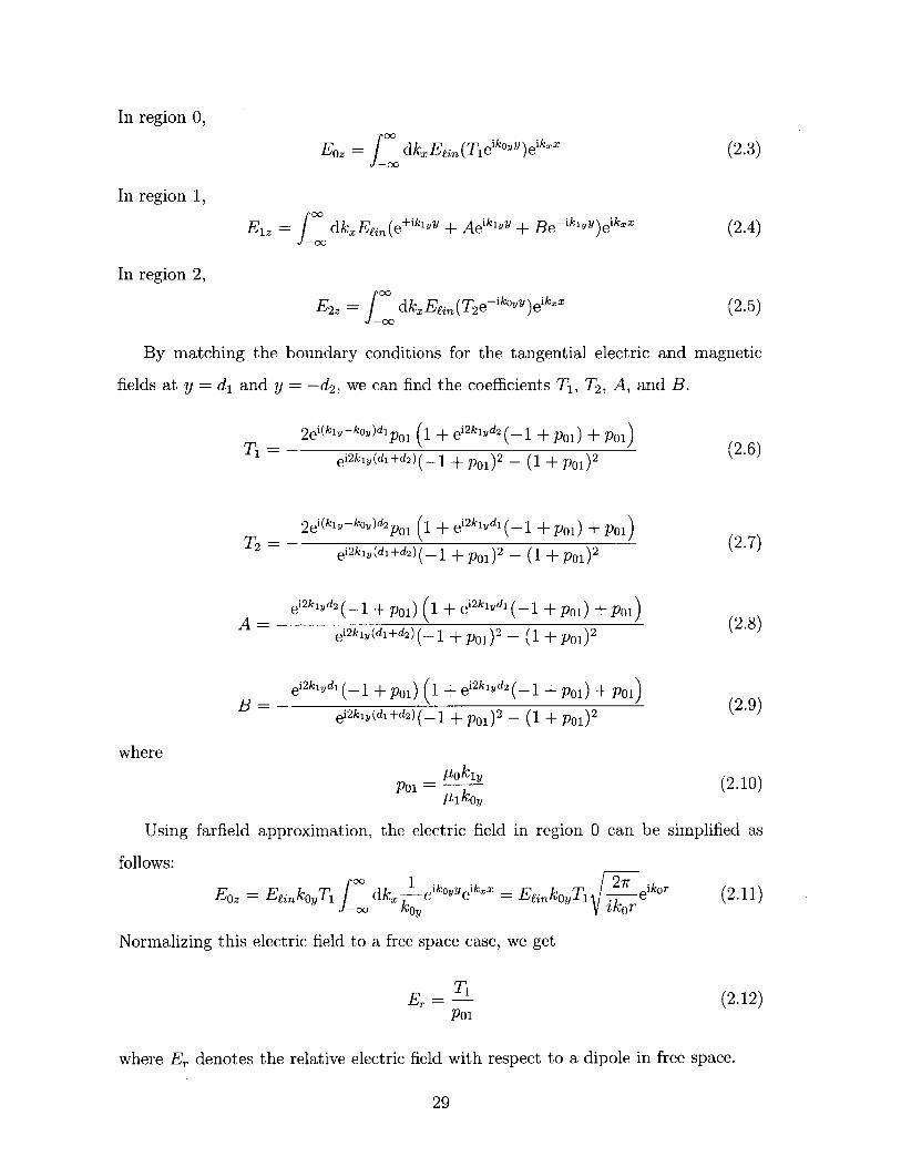
17. The corresponding beamwidth results for simulation is shown in Figure 3-18.

Pendry structure has its maximum beam power mainly directed along the normal

direction(<$ = 900) which is good for our directive antenna purposes. The beamwidth

however is somewhat a bit too large to be ideal. The simulation results is not exactly

what we have predicted from retrieval and analytic method; we do not see two strong

directivity areas. It might be that the loss is too large in the area of interest (8.5 GHz

to 12 GHz), which we can somewhat see in our simulation results.

51

Figure 3-16: Mesh for Pendry structure

52

Normalized Radiation(Analytic)

0 30 60 90 120 150 180Angle(degree)

Radiated Power(Simulation)

22

20

N 18

16

8 14

L 12

10

8

22

20

N 18

16C

S14

LL 12

10

8

10

5

0

-5

-10

-15

-20

-100

-105

-110

-115

-120

-125

-130

22

20

N 18

16

12

10

80

22

20

-18

16C

D 14

LL 12

10

80

30 60 90 120 150 18CAngle(degree)

Normalized Radiation(Simulation)

30 60 90 120 150 18(Angle(degree)

Figure 3-17: Radiated power and normalized radiation from analytic method andslab simulation for Pendry structure

53

0 30 60 90 120 150 180Angle(degree)

15

10

5

0

-5

-10

-15

15

10

5

0

-5

-10

-15

Radiated Power(Analytic)

3dB Beamwidth

8 10 12 14 16 18 2Frequency(GHz)

Max Power Angle

310 12 14 161

- -.-.- - -.. .. .... .. .. ...... .. ..

-.. ... - ...-

-..............-. .....-. .......-. .........-.-.-.-.-.-.

8 10 12 14 16 18Frequency(GHz)

Figure 3-18: Beamwidth for Pendry structure slab simulation

20

54

120

100

80

*560C

40

20

20)a)*0a)0)C

110

100

90

80

70

0

3.4 Omega structure

Recently, there are some new metamaterial structures being explored. One of which

is an Omega-shaped structure[14].The unit cell and its dimensions are presented in

Figure 3-19. The retrieval results for this Omega structure is shown in Figure 3-20.

0.4mm1.05mm

3.33mm

4mm 2.5mm

Figure 3-19: Unit cell Omega structure in a waveguide

We can see that the retrieval results are not very clean for frequencies below 11 GHz.

This might be caused by the increased complexity of the structure, since the rod

are coupled with the rings, which means that the permittivity and permeability are

coupled. However, we see that at around 11.4 GHz and 16.8 GHz, n ~ 0 and the

imaginary part of n is closed to zero, so we should be able to have regions where we

observe directive radiation. The analytic radiation, which is plotted in Figure 3-23,

only has one directive radiation region centered around 17 GHz. We also see that

there are a lot of "ringing" effects from 12 to 14 GHz, which we would not be able to

55

tell from the retrieved data. The slab of metamaterial used for parallel plate radiation

5 10 15 20f/GHz

5 10 15 20f/GHz

Figure 3-20: Retrieval

20

10

0

-10

5 100 5 10

f/GHz

0 5 10f/GHz

results for Omega structure

is shown in Figure 3-21. There are a total of 6 by 72 unit cells with periodicity of 4 mm

and 2.5 mm respectively. Figure 3-22 shows the mesh used for radiation. Due to the

more complicated structure, limited memory, and a big aperture size, the mesh would

have been better if it is even finer, but it is not permitted with the available resource.

However, it should be able to tell us the approximate behavior of such structure as an

antenna substrate. The radiation results from both analytic method and simulation

are shown in Figure 3-23. The corresponding beamwidth from the simulation result

is shown in Figure 3-24. We see some "ringing" effect in our simulation results similar

to the analytic results and there are some relatively high radiation directivity from 16

to 17 GHz and around 14 GHz. However, the beamwidth at these frequencies are too

wide. Therefore, the Omega structure is not a good structure to use as a substrate

for directive antenna.

56

-Real(z)IMag(Z)

-. ... -.. . -.. . -. . -. .10

0

-10

-20

20

10 1

0

-10[

0A

15 20

-_Real(p)- Imag(g)

-.. .. . - .... .

- ... . -.

0

0- Real(E)- Imag(E)

I0

0-

1 0 - - -.. .. . .. . . .

015 20

-- Real(n)-- Imag(n)

. .-.. .-.

V~ - -...- ....

I 2

1

-

2-

Figure 3-21: Slab of Omega structure

Figure 3-22: Mesh for Omega structure

57

Radiated Power(Analytic)5

0

-5

-10

-15

-20

-250 30 60 90 120 150 180

Angle(degree)

Radiated Power(Simulation)

0 30 60 90 120 150Angle(degree)

22

20

18

16C

S14

u- 12

10

8

22

20

18

16C

Cr$ 14

LL 12

10

8

Normalized Radiation(Analytic)

1N18

16

C1a)

LiL 12

10

80 30 60 90 120 150 180

Angle(degree)

Normalized Radiation(Simulation)22

20

'N' 18

316

2 14a'a)

U- 12.

10

80 30 60 90 120 150 180

Angle(degree)

Figure 3-23: Radiated power and normalized radiation from analytic method andslab simulation for Omega structure

58

-50

-55

-60

-65

-70

-75

-80180

15

10

5

0

-5

-10

-15

15

10

5

0

-5

-10

-15

3dB Beamwidth80

4 0 - -. -. .-. ..-. -. . . .-. . ..

120-

08 10 12 14 16 18 20 2

Frequency(GHz)

Max Power Angle10

1 5 0 - - . .. -.. . -.. .. -.. . . . - . . .. .-. .... ..

1 2 0 -.. . .. . .. . . .. . .. . .. . . . .. .

90

60 - - -...

3 0 -.-.. -..-.

8 10 12 14 16Frequency(GHz)

Figure 3-24: Beamwidth for Omega structure slab simulation

59

CC4

0C)0)C)

Vii-0)

2

2218 20

3.5 S structure

0.5mm1mm

5.4mm

0.

4mm 2.5mm

Figure 3-25: Unit cell S structure in a waveguide

Another novel metamaterial is a coupled "S" shaped structure[15]. There are no

obvious ring or rod parts any more, but it still has the properties of having an electric

plasma frequency and an magnetic resonant frequency. The unit cell is shown in Fig-

ure 3-25 and the corresponding retrieval results in Figure 3-26. Since the S structure

does not have any curvature, the retrieval results are relatively clean. Similarly, S also

have two frequencies where loss is low and n ~ 0. They are around 12.2 and 20 GHz,

and index of refraction is approximately zero in between these two frequencies but

the loss is large. Therefore, in the analytic method, we see that in this region there

are relatively high directivity, however, the radiation power is relatively low.

The slab of S structure is as seen in Figure 3-27. Identical to the Omega structure,

the slab is consist of 6 by 72 unit cells with the corresponding periodicity of 4mm and

60

10 10Real(z) - Real(n)Imag(z) - Imag(n)

5 -. -.. . - -. . . .. . . . . . . . 5 -.. . . . .

0 0

-5 -5

-10 -10

0 5 10 15 20 0 5 10 15 20f/GHz f/GHz

10 10-- Real(p) - Real(E)- Imag(p) - Imag(E,)

0

-5 - - -1 -0 - -

-0 5 10 15 20 -10 5 10 15 20f/GHz f/GHz

Figure 3-26: Retrieval results for S structure

61

2.5 mm. The mesh setup for slab simulation is shown in Figure 3-28. In Figure 3-

Figure 3-27: Slab of S structure

29, we show the analytic and simulation results and they display similar radiation

patterns. They both show some "ringing" effects. Furthermore, as predicted in the

analytic method, there are some directivity from about 12 GHz to 20 GHz, but with

low power. The only very high directivity only takes place at higher frequency of

20.2 GHz for the analytic case and 21.3 GHz for the simulation case. The beamwidth

for the slab simulation is shown in Figure 3-30. The best is 180 at 21 GHz.

62

- -~ --I

Figure 3-28: Mesh for S structure

63

24 10 24 15

22 5 22 10

,20 20N N0 I 5

0 18 (D 18

S16 -5 16 0

-10 -5

L 12 L- 12

10 -15 10 -10

8 -20 8 150 30 60 90 120 150 180 0 30 60 90 120 150 180

Angle(degree) Angle(degree)

Radiated Power(Simulation) Normalized Radiation(Simulation)

24 -50 24 15

22 -55 10

-20 9201M -60 I5

C 16 -65 16 -0

-70 -5

L- 12 12

10-75 10 -10

8 -80 8 -- 150 30 60 90 120 150 180 0 30 60 90 120 150 180

Angle(degree) Angle(degree)

Figure 3-29: Radiated power and normalized radiation from analytic method and

slab simulation for S structure

64

Normalized Radiation (Analytic)Radiated Power(Analytic)

3dB BeamwidthIUU I

008 0 -. -. . -.. .. . . . .. . .. ....

60

4 0 - . -.-.-.

20

8 10 12 14 16 18 20 22 2Frequency(GHz)

Max Power Angle17n

150

130

012 110

0)

0

S. 900

50

30

108

4

.- - -... ...

. . . .-. - -.. .... .. -.. .. . . .. ..

-.. - - -.. . .-.

-. . . .. ..

- -.

- - - - - - .

10 12 14 16 18 20 22 24Frequency(GHz)

Figure 3-30: Beamwidth for S structure slab simulation

65

0)R.

-.......

3.6 Summary

From studying and analyzing all these different metamaterial structures, we can con-

clude that a 2-D structure is harder to construct than a 1-D one. Additionally a

1-D structure yield higher power than a corresponding 2-D one. Permittivity and

permeability are coupled in the Omega structure and the S structure, so these two

structures would be harder to tune. The Pendry structure and the Smith structure

differ mainly in the implementation of their rings. The Pendry structure shows better

directional beam and is easier to tune its permeability since its rings are symmetrical.

For example, we can change the Pendry ring dimensions while keeping the same gap

while the Smith ring consists of one bigger ring and one smaller ring, so if we make

the bigger ring smaller then the gap would become smaller too unless we make the

small ring smaller as well. Hence, more parameters are involved in the Smith ring

and therefore harder to tune.

We are interested in the 8 GHz to 18 GHz frequency range, and in Table 3.1, we

summarize how the different metamaterial structure perform as directive antenna

substrate. Beamwidth and power shown will be the best within the bandwidth.

Table 3.1: Comparison among different metamaterial substrates

Structure 2-D Smith 1-D Smith Pendry Omega SAperture size 175 x 3.33 180 x 3.33 181.76 x 6 180 x 3.33 180 x 5.4

(mm x mm)Beamwidth (0) 29 28 42 36, 56 28Bandwidth 10.2-18 12-12.3 16.1-18 13.7-14.1 10.7-10.8(GHz) 15.6-17.2Power (dB) -115 ~ -35 ~ -108 -55 ~ -75

~-65Ease of hard easy easy easy easyconstructionRetrieval unclean clean clean unclean uncleanTunability medium medium easy hard hard

66

Chapter 4

Optimized Metamaterial Structure

From the previous chapter, the Pendry structure has the main beam directed mostly

along the normal direction, which is where we want for a directive antenna. There-

fore, we change some parameters in order to yield a wider band, higher power, and

smaller beamwidth. From experience, if we observe from retrieval that there are two

frequencies which have index of refraction n = 0 and are far from each other, then

the imaginary part of n is usually too large(loss is large) for the frequencies in be-

tween to maintain high power. This is what we see in the retrieval results of the

Pendry structure(Figure 3-14). Changes will be made on top of this Pendry structure

to make the frequencies where E = 0 and p = 0 closer to each other. Therefore,

instead of having two small regions where we see high directivity and high power, we

hope to have one larger region with high directivity and high power. We carry out

the one cell PEC-PMC waveguide simulation, and use the obtained S-parameters to

retrieve the effective permittivity, permeability, and index of refraction, with which

we can calculate the analytic farfield radiation. If the analytic radiation results are

not satisfactory, then the geometries of the unit cell will be further modified until the

analytic radiation exhibits high power in a wider band with high directivity.

67

4.1 Optimized unit cell's geometry

The optimized structure is shown in Figure 4-1. Material properties are the same as

the Pendry structure presented in the previous chapter.

0.5mm

2.m m .24mm

5mm

5mm

Figure 4-1: Unit cell optimized structure in a waveguide

Retrieval results are shown in Figure 4-2. The two frequencies where n = 0 are

very closed to each other. The imaginary part of n is small for all frequencies in

between. Essentially, we have lowered the electric plasma frequency, and increased

the magnetic resonance frequency. The electric plasma frequency is related to the

size of the rod, and its periodicity. The smaller the period, the higher the electric

plasma frequency. Therefore, by increasing the size of the unit cell, we also increase

the spacing between the rods, and hence lower the electric plasma frequency. As for

magnetic resonance frequency, it is related to the dimensions of the ring. Decreasing

the perimeter of the ring will cause an increase in the magnetic resonance frequency.

68

15 20

10

5

0

-5

0 5 10 15 2f/GHz

1- Real()- Image

-5 -. . ..-. .. . ..

10

15 20 5 10f/GHz

Figure 4-2: Retrieval results for the optimized structure

69

10

5

0

-5

0 5

Real(n)-- Imag(n)

010f/GHz

5 10f/GHz

10-Real(g)-Imag(g)

5 -- -. . . .. ..

0

-5

1IA

0 15 200-

-Real(z)-Imag(z)

Here we assume that the material property do not change: metal is still modeled with

PEC, and the dielectric is lossless with a relative permittivity of 4. Changes in the

material properties would cause changes in the effective permittivity and permeability

as well.

4.2 Optimization of cell orientation and antenna

position

After we have decided what the optimized unit cell should be, we need to figure

out how to put these unit cells together(orientation) and where to place the dipole

antenna within the bulk of the metamaterial. After all, the metamaterial substrate

is not homogeneous and radiation results could possibly change depending on how

everything is put together.

Since we are interested in making a 1-D structure, there are two possible arrange-

ments: the dielectric strips align with the x direction or the y direction as shown in

Figure 4-3. We will refer to the one that has the dielectric strips aligned in the x

direction as Pendry version x, and the other as Pendry version y. The mesh setup for

Figure 4-3: Two different 1-D orientations of unit cells arrangement

farfield radiation for both orientations is shown in Figure 4-4.The radiation results

for these two different orientations are presented in Figure 4-5, and the corresponding

beamwidth results are shown in Figure 4-7 and Figure 4-6.

70

o I

Figure 4-4: Mesh for the optimized structure

Comparing to the other substrates we presented in the previous chapter, both of

these metamaterial substrates have shown to have a better combination of radiation

power, beamwidth, and bandwidth. From the radiation figures alone, we can see

that there is an obvious improvement in directivity compared to the original Pendry

structure(region 8 GHz to 13 GHz in Figure 3-17), hence we can expect the beamwidth

to improved as well. In addition, radiation power has substantial improvement of

approximately 20 dB. Between Pendry version x and Pendry version y, it is seen

that Pendry version x has slightly higher power and directivity for a wider frequency

range than Pendry version y. Overall, Pendry version x has a better performance

than Pendry version y as a substrate for directive antenna.

71

Radiated Power(Pendry version x)

0 30 60 90 120 150 18Angle(degree)

Radiated Power(Pendry version y)

-80

-85

-90

-95

-100

-105

-110

18

16Nr

14

12Cr

.2

U-

10

8

18

16N

14

12

10

Normalized Radiation(Pendry version x)18 1

NM

0

C

a)02a)

N7:

0

LL

80 30 60 90 120 150 180

Angle(degree)

15

10

5

0

-5

-10

-1A

Normalized Radiation (Pend ry version y)18 15

16 10

514

012

-5

10 -10

8 -150 30 60 90 120

Angle(degree)150 180

Figure 4-5: Radiated power and normalized radiation from slab simulation for Pendryversion x and Pendry version y structure

72

-80

-85

-90

-95

-100

-105

-11030 60 90 120 150 180

Angle(degree)

800

3dB Beamwidth

8 9 10 11 12 13 14 15 16 17 1Frequency(GHz)

Max Power Angle

. _ -.-. .-.-. .-.- - -.

...-.-.-.-.-.-.-.-..-.-.-.-.- -.-.-.-

-. .... -. ...-. .-. .- . -. .-. .-.-

.......-. . -.. ..... - -.. ...... - -..........

80

70

|60,0)

-50

40

30

20

120

110

100

SO 0)

80

70

0

8

14 15 16 17 18

Figure 4-6: Beamwidth for Pendry version x structure slab simulation

73

8 9 10 11 12 13Frequency(GHz)

-

- ..............-. .-.

........ -. -.. .. -.. .... ..- .- .- -. -. -

-......

-

.......... ..... -

-..-.-.-.-

........... . . .....- -

100

90

80-

3dB Beamwidth

9 10 11 12 13Frequency(GHz)

Max Power Angkc40

3 0 - - - - - - - -.-.- .

20 - - - - -

1 0 - - - -.-.-.-.- . -

j0 -.. -- -.. -.. -...---00-90

80 --- -

08 0 . . . . . . . . .. . . . .. . .. . . . . . . . .. . . .. .._. . .._. . . .. .._. . . .

9 10 11 12 13Frequency(GHz)

14 15 16 17 18

14 15 16 17 18

Figure 4-7: Beamwidth for Pendry version y structure slab simulation

74

- . . .. .. . . . .-. . ...-. . ..-.

-. .. .- ...-. . ... -. .. .

. . . .-. . -.. . -.. .. . . .I . . .. .

-. -.. . . -. . .. . ..-. .

......... . ... .... .. ....

- - . .... . - . ..- .- ... -.. .-

-i p

70

60

50

40

30

20

a)g>

0)

1)

211)

1)

1)

8

- .

Figure 4-8: Two different antenna positions

Is the position of the antenna going to affect our radiation results? This is some-

thing that analytic method cannot tell us. Therefore, we can only run simulations

to find out. For symmetry reason, there are two different antenna positions that we

can explore; they are shown in Figure 4-8. In Figure 4-9, comparison of the farfield

radiation from the two different positions of antenna is shown. One is always con-

sistently 2 dB higher in radiation power than the other(varies between 2.06 dB to

2.37 dB). Therefore, for the metamaterial substrate to output higher radiation power,

it is better to align the antenna with the boundary between two adjacent unit cells,

and not with the rod of an unit cell.

75

Radiated Power(Aligned)

30 60 90 120 150Angle(degree)

Radiated Power(Not Aligned)

-80

-85

-90

-95

-100

-105

-110180

-80

-85

-90

-95

-100

-105

-110

18

16

14

0

cm12

10

810

18

16

14

122.)LL

10

810

Figure 4-9: Radiated power and normalizedent antenna positions

Normalized Radiation(Aligned)18

16N

14

12

0 30 60 90 120 150 1Angle(degree)

Normalized Radiation(Not Aligned)18

16N

214

a).12

10

0 30 60 90 120 150 18Angle(degree)

15

10

5

0

-5

-10

-15

15

10

5

0

-5

-10

-150

radiation from slab simulation for differ-

76

30 60 90 120 150 180Angle(degree)

I

4.3 Comparison with analytic method

y

Region 0 60, P0

di

Region 1 51,771

z

-d2Region 2 Co, Ao

Figure 4-10: Radiation configuration of a linesource in an infinite anisotropic slab ofthickness d, + d2

We have been using an isotropic analytic method up to this point; we can modify

the formulas to include the anisotropic case. Now the figure for anisotropic case(shown

in Figure 4-10) will be slightly different from the one for the isotropic case(Figure 2-

7.) The substrate's permittivity and permeability will be expressed by using tensors

instead of scalar variables, which assumes isotropy. Now the permittivity and perme-

ability take the form

1 0 0

1= 0 Ey 0 (4.1)

0 0 1

0 0

1= 0 1 0 (4.2)

0 0 p1 t

All the equations remain the same as shown in Section 2.3, except the expressions

for Eejn and poi.

E - (4.3)47rklu

77

Poi = pok(44)p1xkoy

Using these anisotropic analytic equations, the radiation patterns for Pendry ver-

sion x and Pendry version y are different as shown in Figure 4-11. Pendry version x

structure yields better radiation power and directivity than Pendry version y structure

over a broader band. The same conclusion were drawn from the simulation results.

If anisotropy is taken into consideration, the analytic method has the capability to

demonstrate the difference between the two different setup of the unit cells.

Radiation Power(Pendry version x)18 10

16 5

014

-5

12-10

10 -15

8 -20

8

0 30 60 90 120 150 18Angle(degree)

Radiation Power(Pendry version y)

0

10

5

0

-5

-10

-15

-20

Normalized Radiation(Pendry versio18

16

14

.120)

LL

10

n x)15

10

5

0

-5

-10

O00 30 60 90 120 150 180

Angle(degree)

Normalized Radiation(Pendry version y)18

16

014C()

.12

10

-I

15

10

5

0

-5

-10

-150 30 60 90 120 150 180 0 30 60 90 120 150 180

Angle(degree) Angle(degree)

Figure 4-11: Radiated power and normalized radiation from analytic method forPendry version x and Pendry version y structure

78

NI(9C.)C0)0~0)U-

14

= 12

10

_1U

1V

1V

E

4.4 Summary

Through the manipulation of a metamaterial's geometry, we can tune its effective

permittivity and permeability to our desired specifications. We can potentially incor-

porate anisotropic properties of the metamaterial into our analytic radiation calcula-

tion. Analytic method has its own constraint, for example, it is unable to tell us if the

difference in antenna positions would affect radiation power. Hence, these metama-

terials are only homogeneous to a certain extent. To summarize, the best structure is

using Pendry version x with the dipole in the "not aligned" position(aligned with the

boundary of two adjacent unit cells). This optimized structure is shown to improve

in radiation power, beamwidth, and bandwidth.

79

80

Chapter 5

Conclusion

After employing our methodology on different metamaterials, we can conclude that it

works reasonably well. Our analytic method is able to help us predict what we might

obtain from the numerical farfield simulation. Furthermore, we can model a metama-

terial as a homogeneous medium for both the waveguide reflection/transmission study

and the farfield radiation study. This has helped us to simplify our design procedure,

because we can use our analytic method to arrive at a good structure first before

proceeding to the time and memory consuming farfield simulation. Additionally, the

analytic method is not limited to using isotropic metamaterial models, but also the

anisotropic ones. However, analytic method always assumes homogeneity, which can-

not incorporate certain details of the antenna system. For example, the position of

the dipole antenna, which does affect the farfield radiation results. If the bulk of the

metamaterial substrate is indeed homogeneous, our radiation pattern should always

be symmetric, which is not the case as seen in Figure 3-5. Therefore, if we look at

the radiation in the # = 180' to # = 3600 range, we would not always expect to see

the same radiation pattern as what we will obtain from the # = 0' to # = 180' range.

Our optimized structure uses both ring and rod elements. Additionally, we are able

to make the electric plasma frequency and the magnetic plasma frequency to be very

closed to each other. This is an improvement over the rod only medium.

81

82

Bibliography

[1] J. A. Kong, "Electromagnetic wave interaction with stratified negative isotropic

media," PIER, vol. 35, pp. 1-52, 2002.

[2] J. B. Pendry, A. J. Holden, D. J. Robbins, and W. J. Stewart, "Low frequency

plasmons in thin-wire structures," J. Physics-Condensed Matter, vol. 10, pp.

4785-4809, 1998.

[3] J. B. Pendry, A. J. Holden, D. J. Robbins, and W. J. Stewart, "Magnetism

from conductors and enhanced nonlinear phenomena," IEEE Trans. Microwave

Theory Tech., vol. 47, no. 11, pp. 2075-2084, Nov. 1999.

[4] D. R. Smith, W. J. Padilla, D. C. Vier, S. C. Nemat-Nasser, and S. Schultz,

"Composite medium with simutaneously negative permeability and permittiv-

ity," Phys. Rev. Lett., vol. 84, no. 18, pp. 4184-4187, May 2000.

[5] R. A. Shelby, Smith D. R., and S. Schultz, "Experimental verification of a

negative index of refraction," Science, vol. 292, pp. 77-79, Apr. 2001.

[6] T. Weiland, R. Schuhmann, R. B. Greegor, C. G. Parazzoli, A. M. Vetter, D. R.

Smith, D. C. Vier, and S. Schultz, "Ab initio numerical simulation of left-handed

metamaterials: Comparison of calculations and experiments," J. Appl. Phys.,

vol. 90, no. 10, pp. 5419-5424, 2001.

[7] C. G Parazzoli, R. B. Greegor, K. Li, B. E. C. Koltenbah, and M. Tanielian,

"Experimental verification and simulation of negative index of refraction using

snell's law," Phys. Rev. Lett., vol. 90, pp. 107401, 2003.

83

[8] R. B. Greegor, C. G Parazzoli, K. Li, and M. Tanielian, "Origin of dissipative

losses in negative index of refraction materials," Appl. Phys. Lett., vol. 82, no.

14, pp. 2356-2358, 2003.

[9] K. Li, J. McLean, R. B. Greegor, C. G Parazzoli, and M. Tanielian, "Free-space

focused-beam characterization of left-handed materials," Appl. Phys. Lett., vol.

82, no. 15, pp. 2535-2537, 2003.

[10] D. R. Smith, P. Rye, D. C. Vier, A. F. Starr, J. J. Mock, and T. Perram, "Design

and measurement of anisotropic metamaterials that exhibit negative refraction,"

JEICE Trans. Electron., vol. E87-C, no. 3, pp. 359-370, 2004.

[11] J. Pacheco, Theory and Application of Left-Handed Metamaterials, Ph.D. thesis,

Massachusetts Institute of Technology, Cambridge, 2004.

[12] R. A. Shelby, Smith D. R., S. C. Nemat-Nasser, and S. Schultz, "Microwave

transmission through a two-dimensional, isotropic, left-handed metamaterial,"

Appl. Phys. Lett., vol. 78, no. 4, pp. 489-491, Jan. 2001.

[13] D. R. Smith, D. C. Vier, N. Kroll, and S. Schultz, "Direct calculation of perme-

ability and permittivity for a left-handed metamaterial," Appl. Phys. Lett., vol.

77, no. 14, pp. 2246-2248, Oct. 2000.

[14] J. Huangfu, L. Ran, H. Chen, X. Zhang, K. Chen, T.M. Grzegorczyk, and J.A.

Kong, "Experimental confirmation of negative refractive index of a metamaterial

composed of Q - like metallic patterns," Appl. Phys. Lett., vol. 84, no. 9, pp.

1537-1539, Mar. 2004.

[15] H. Chen, L. Ran, J. Huangfu, X. Zhang, K. Chen, T.M. Grzegorczyk, and J.A.

Kong, "Left-handed metamaterials composed of only S-shaped resonators," To

Be Published.

[16] P. Marko and C.M. Soukoulis, "Absorption losses in periodic arrays of thin

metallic wires," Optics Letters, vol. 28, pp. 846, May 2003.

84

[17] D. Sievenpiper, High-Impedance Electromagnetic Surfaces, Ph.D. thesis, Univer-

sity of California, Los Angeles, 1999.

[18] V. G. Veselago, "The electrodynamics of substances with simultaneously negative

values of E and p," Soviet Physics USPEKHI, vol. 10, no. 4, pp. 509-514, Jan.-

Feb. 1968.

[19] J. B. Pendry, "Negative refraction makes a perfect lens," Phys. Rev. Lett., vol.

85, no. 18, pp. 3966-3969, Oct. 2000.

[20] I. V. Lindell, S. A. Tretyakov, K. I. Nikoskinen, and S. Ilvonen, "BW-Media

with negative parameters, capable of supporting backward waves," Microwave

Opt. Technol. Lett., vol. 31, no. 2, pp. 129-133, Oct. 2001.

[21] A. Grbic and G. V. Eleftheriades, "Experimental verification of backward-wave

radiation from a negative refractive index metamaterial," J. Appl. Phys., vol.

92, no. 10, pp. 5930-5935, 2002.

[22] B.-I. Wu, T. M. Grzegorczyk, Y. Zhang, and J. A. Kong, "Guided modes with

imaginary transverse wavenumber in a slab waveguide with negative permittivity

and permeability," J. Appl. Phys., June 2003.

[23] C. Caloz, C.-C. Chang, and T. Itoh, "Full-wave verification of the fundamental

properties of left-handed materials in waveguide configurations," J. Appl. Phys.,

vol. 90, no. 11, pp. 5483-5486, 2001.

[24] J. Lu, T. M. Grzegorczyk, Y. Zhang, J. Pacheco, B.-I. Wu, J. A. Kong, and

M. Chen, "Cerenkov radiation in materials with negative permittivity and per-

meability," Optics Express, vol. 11, no. 7, pp. 723-734, Apr. 2003.

[25] N. Engheta, "An idea for thin subwavelength cavity resonators using metamate-

rials with negative permittivity and permeability," IEEE Antennas and Wireless

Propagation Letters, vol. 1, no. 1, pp. 10-13, 2002.

85

[26] A. Grbic and G. V. Eleftheriades, "Growing evanescent waves in negative-

refractive-index transmission-line media," Appl. Phys. Lett., vol. 82, no. 12,

pp. 1815-17, 2003.

[27] S. Enoch, G. Tayeb, P. Sabouroux, N. Guerin, and P. Vincent, "A metamaterial

for directive emission," Phys. Rev. Lett., vol. 89, no. 21, pp. 213902, Nov. 2002.

[28] Microwave Studio is a registered trademark of CST GmbH, Darmstadt, Germany.

[29] X. Chen, T.M. Grzegorczyk, B.-I. Wu, J. Pacheco Jr., and J.A. Kong, "An

improved method to retrieve the constitutive effective parameters of metamate-

rials," To Be Published.

[30] T. Weiland, "Time domain electromagnetic field computation with finite dif-

ference methods," International Journal of Numerical Modelling, vol. 9, pp.

259-319, 1996.

[31] CST-Computer Simulation Technology, CST Microwave Studio® Advanced Top-

ics Version 4, 2002.

[32] S. O'Brien and J. B. Pendry, "Magnetic activity at infrared frequencies in struc-

tured metallic photonic crystals," J. Physics-Condensed Matter, vol. 14, no. 25,

pp. 6383-6394, July 2002.

[33] J. A. Kong, Electromagnetic Wave Theory, EMW, Cambridge, MA, 2000.

[34] S. Enoch, G. Tayeb, and D. Maystre, "Dispersion diagrams of bloch modes

applied to the design of directive sources," PIER, vol. 41, pp. 61-81, 2003.

86