Seediscussions,stats,andauthorprofilesforthispublicationat:https://www.researchgate.net/publication/47454834

AGeneralClassofMetamaterialTransformationSlabs

ArticleinPhysicalreview.B,Condensedmatter·March2010

DOI:10.1103/PhysRevB.81.125124·Source:OAI

CITATIONS

29

READS

26

5authors,including:

G.Castaldi

UniversitàdegliStudidelSannio

202PUBLICATIONS3,473CITATIONS

SEEPROFILE

VincenzoGaldi

UniversitàdegliStudidelSannio

254PUBLICATIONS3,618CITATIONS

SEEPROFILE

AllcontentfollowingthispagewasuploadedbyVincenzoGaldion01December2016.

Theuserhasrequestedenhancementofthedownloadedfile.

A General Class of Metamaterial Transformation Slabs

Ilaria Gallina 1, Giuseppe Castaldi 1, Vincenzo Galdi 1, Andrea Alù 2, and Nader Engheta 3

(1) Waves Group, Department of Engineering, University of Sannio, I-82100, Benevento, Italy

(2) Department of Electrical and Computer Engineering, The University of Texas at Austin,

Austin, TX 78712, USA

(3) Department of Electrical and Systems Engineering, University of Pennsylvania,

Philadelphia, PA 19104, USA

Abstract

In this paper, we apply transformation-based optics to the derivation of a general class of

transparent metamaterial slabs. By means of analytical and numerical full-wave studies, we explore

their image displacement/formation capabilities, and establish intriguing connections with

configurations already known in the literature. Starting from these revisitations, we develop a

number of nontrivial extensions, and illustrate their possible applications to the design of perfect

radomes, anti-cloaking devices, and focusing devices based on double-positive (possibly

nonmagnetic) media. These designs show that such anomalous features may be achieved without

necessarily relying on negative-index or strongly resonant metamaterials, suggesting more practical

venues for the realization of these devices.

PACS number(s): 41.20.Jb, 42.25.Fx, 42.25.Gy

2

1. Introduction

First envisaged in the 1960s within the framework of electromagnetic (EM) wave propagation in

curved space-time or curved-coordinate systems (see, e.g., Refs. 1 and 2), “transformation optics”

(TO) 3-7 (also referred to as “transformation EM”) has only recently become a technologically

viable approach to EM field manipulation, thanks to the formidable advances in the synthesis of

“metamaterials” with precisely controllable anisotropy and spatial-inhomogeneity properties (see,

e.g., Ref. 8).

In essence, TO relies on the formal invariance of Maxwell equations under coordinate

transformations, which enables the design of the desired field behavior in a curved-coordinate

fictitious space, and its subsequent translation in a flat-metric physical space filled up by a suitable

(anisotropic, spatially-inhomogeneous) “transformation medium” which embeds the coordinate-

transformation effects. As a sparse sample of the available application examples, besides the

celebrated invisibility “cloaking” (see, e.g., Refs. 8 and 9), we recall here those pertaining to

super/hyper-lensing, 10-12 field concentrators 13 and rotators, 14 conformal sources, 15 beam shifters

and splitters, 16, 17 retroreflectors, 18, 19 as well as the broad framework of “illusion optics” 20 (see

also Ref. 21, and references therein, for a collection of recent applications).

In this paper, we focus on a general class of TO-inspired metamaterial slabs (henceforth, simply

referred to as “transformation slabs”). Propagation of EM waves in slab-type configurations is a

subject of longstanding interest, which has recently received renewed attention in view of the new

perspectives and degrees of freedom endowed by metamaterials. In particular, low-refractive-index

slabs have been explored in connection with ultrarefraction phenomena, with potential applications

to directive emission, 22 enhanced transmission through subwavelength apertures, 23 and phase-

pattern tailoring. 24 Double-negative (DNG) slabs have attracted a great deal of attention, especially

in connection with superlensing 25 and phase-compensation 26 effects. Superlensing effects have

also been predicted in metamaterial slabs featuring extreme effective parameters, 2729 whereas

anomalous tunneling and transparency phenomena have been studied in connection with single-

negative (SNG) bi-layers made of epsilon-negative (ENG) and mu-negative (MNG) media. 30 Some

of the above effects, attributable to anomalous interactions occurring in DNG/double-positive

(DPS) or ENG/MNG paired configurations, have also been interpreted within the broader context of

“complementary” media. 31

Within this framework, TO has been shown to provide insightful alternative interpretations, and to

enable for nontrivial extensions (see, e.g., Refs. 10 and 3234 for a sparse sampling). For instance,

3

lensing configurations have been interpreted in terms of coordinate-folding, 10 and have been

extended so as to deal with the presence of passive or active objects. 34 More in general, there has

been considerable recent interest in the study of transparency/reflection conditions 3537 in scenarios

involving transformation media.

Against this background, in this paper, we introduce and explore a general class of two-dimensional

(2-D) coordinate transformations capable of yielding transparent metamaterial slabs potentially

useful for image displacement and reconstruction.

First, we show that the proposed class of transformation slabs includes as particular cases several

conventional configurations already known in the literature. Next, we focus on a series of nontrivial

extensions, with possible applications to radome, cloaking/anti-cloaking, and focusing scenarios,

which naturally emerge from the proposed approach. Our results provide further confirmation of the

broad breadth of TO and its intriguing potentials as a general unifying approach to metamaterial

functionalization. Our interest is especially focused in proposing designs that may not require

negative constitutive parameters, but that exploit the inherent anisotropy of the transformation slabs

to achieve anomalous wave interaction within the DPS regime of operation. This may be

particularly attractive to simplify the realization of these devices and to possibly relax some

bandwidth limitations typical of SNG and DNG metamaterials.

Accordingly, the rest of the paper is laid out as follows. In Sec. 2, we outline the problem geometry

and its formulation. In Sec. 3, we illustrate the general analytical solution and some details about

the computational tools utilized. In Sec. 4, we focus on particular reductions corresponding to

configurations already known in the literature. In Sec. 5, starting from these configurations, we

present a number of nontrivial extensions, with applications to perfect radomes, cloaking/anti-

cloaking, and focusing scenarios. Finally, in Sec. 6, we provide some brief conclusions together

with hints for future research.

2. Problem Geometry and Formulation

Referring to the geometry in Fig. 1, we consider a 2-D coordinate transformation between a

fictitious (vacuum) space ( ), ,x y z′ ′ ′ and the slab region x d≤ (embedded in vacuum) in the actual

physical space ( ), ,x y z ,

4

( )

( ) ( )

,

,

,

x au x

yy v x

u x

z z

′ = ′ = + ′ =

ɺ (1)

where a is a real scaling parameter, and ( )u x and ( )v x are arbitrary continuous real functions. In

(1) and henceforth, an overdot denotes differentiation with respect to the argument. We assume that

the derivative ( )u xɺ is continuous and nonvanishing within the slab region, so that the coordinate

transformation in (1) is likewise continuous. Moreover, for reasons that will become clearer

hereafter, we also assume that

( ) 1,u d± =ɺ (2)

so that, apart from a possible (irrelevant) rigid translation, the planar interfaces ( )1,2x d au d′ ′= ≡ ∓

of the (virtual) vacuum slab in the auxiliary space are imaged as the planar interfaces x d= ∓ of the

transformed slab region in the actual physical space (see Fig. 1). Within the TO framework 3-7, the

EM field effects induced by the curved metrics in (1) can be equivalently obtained in a flat,

Cartesian space by filling-up the transformed slab region x d≤ with an anisotropic, spatially

inhomogenous transformation medium described by the relative permittivity and permeability

tensors:

( ) ( ) ( ) ( ) ( )1 1, , det , , , ,T

x y x y J x y J x y J x yε µ − − = = ⋅ (3)

where the superscript T denotes matrix transposition, and

( ) ( )( )

( )

( ) ( )( ) ( )2

0 0

, , 1, 0

, ,

0 0 1

au x

x y z u x yJ x y v x

x y z u x u x

′ ′ ′∂ = = − ∂

ɺ

ɺɺɺ

ɺ ɺ (4)

is the Jacobian matrix. It can be shown (see Appendix A for details) that the constitutive tensors in

(4) are real and symmetric, and hence they admit real eigenvalues, and they can be diagonalized by

an orthogonal matrix. In particular, it is expedient to represent these tensors in their diagonalized

5

forms (εɶ and µɶ , respectively) in the principal reference system ( ), ,zξ υ constituted by their

(orthogonal) eigenvectors, viz.,

( ) ( )( )

( ), 0 0

, , 0 , 0 ,

0 0

x y

x y x y x y

a

ξ

υε µΛ = = Λ

ɶ ɶ (5)

where ,ξ υΛ denote the transverse eigenvalues. It can be shown (see Appendix A for details) that

( ) ( ),sgn , sgn ,x y aξ υ Λ = (6)

and hence, depending on the sign of the scaling parameter a , the constitutive tensors are either both

positive-defined ( )0a > or both negative-defined ( )0a < . Accordingly, the resulting transformation

medium is either DPS ( )0a > or DNG ( )0a < . Moreover, it readily follows from (5) that, for the

particular choice 1a = , the resulting transformation medium is effectively non-magnetic ( )1zµ =ɶ

for transverse-magnetic (TM) polarization (i.e., z-directed magnetic field), and non-electric ( )1zε =ɶ

for transverse-electric (TE) polarization (i.e., z-directed electric field).

Finally, recalling the developments in Ref. 36, we note that the condition (2) (i.e., the fact that at the

transformed-region boundaries x d= ∓ the coordinate mapping in (1) reduces to a rigid translation)

ensures the reflectionless of the transformation slab.

In what follows, without loss of generality, we study the EM response of the above defined

transformation slab excited by a time-harmonic ( )( )exp i tω− , TM-polarized, arbitrary aperture field

distribution located at a source-plane sx x d= < − ,

( ) ( ), .z sH x x y f y= = (7)

3. Generalities on Analytical Derivations and Numerical Simulations

3.1 General solution

6

It can be shown (see Appendix B for details) that, for an observer located at ox d> (i.e., beyond the

transformation slab), the EM response of the system can be viewed as effectively generated by an

equivalent aperture field distribution

( ) ( )0, ,z iH x x y f y y= = − (8)

corresponding to a (virtual or real) image at the plane

( ) ( )2 ,i sx x x d a u d u d= ≡ + − − − (9)

which exactly reproduces the source-plane aperture field distribution in (7), apart from a possible

rigid translation of

( ) ( )0y v d v d= − − (10)

along the y-axis. Note that the image-plane position and the y-displacement do not depend on the

actual form of the mapping function ( )u x and ( )v x in (1), but rather on their values at the slab

interfaces x d= ∓ , thereby leaving ample design freedom. Clearly, for ix d< , a virtual image is

formed, corresponding to a perceived displacement of the source. In particular, for i sx x= and

0 0y = (i.e., zero displacement), the transformation slab behaves like a vacuum slab of same

thickness, thereby acting as a perfect radome. Conversely, for ix d> , a real image is formed, and

the slab ideally behaves like a perfect lens.

3.2 Simulation tools and parameters

Our analytical derivations below are supported by full-wave numerical studies based on a finite-

element solution of the EM problem for Gaussian-beam or plane-wave illuminations. Our

simulations rely on the use of the commercial software COMSOL Multiphysics, 38 based on the

finite-element method (FEM), in view of its ability to deal with arbitrary anisotropic and spatially

inhomogeneous transformation media. In all simulations below, slight material losses (loss-

tangent= 310− ) are assumed, and the slabs are truncated along the y-axis to an aperture of 2L . The

resulting computational domains are adaptively discretized via nonuniform meshing (with element

size which can be locally as small as 404 10 λ−×∼ , with 0λ denoting the vacuum wavelength), and

terminated by perfectly matched layers, resulting into a total number of unknowns 610∼ .

7

4. Particular Cases Already Known in the Literature

In order to illustrate the general character of the proposed class, we begin showing that it includes

as special cases several configurations already known in the literature.

Perhaps the most trivial reduction is obtained by assuming ( ) ( ), 0u x x v x= = , which yields

1 0 0

0 0

0 0

a

a

a

ε µ

− = =

, (11)

which closely resembles the class of nonreflecting birefringent metamaterials considered in Ref. 39

(in connection with perfect lensing for vectorial fields), and also widely used in the design of

perfectly-matched layers for finite-difference-time-domain numerical schemes (see, e.g., Ref. 40).

In this case, (9) and (10) trivially reduce to

( ) 02 1 , 0,i sx x d a y= + − = (12)

corresponding to an orthogonal (with respect to the slab) image displacement, which vanishes only

for 1a = (i.e., when the material trivially reduces to vacuum), and yields Pendry’s perfect lens 22 for

1a = − .

Another interesting reduction is obtained by assuming

( ) ( )1, , ,a u x x v x xα= = = (13)

which yields

2

1 0

1+ 0 .

0 0 1

αε µ α α

− = = −

(14)

It is interesting to note that the above medium (spatially homogeneous, DPS, and non-magnetic for

the assumed TM polarization) is amenable to the tilted uniaxial class considered in Ref. 41. Indeed,

letting

8

R R RR

1= sin cos ,α ε θ θ

ε

−

(15)

and enforcing the condition for omnidirectional total transmission in Eq. (30) of Ref. 41 (assuming

1Lε = ),

2 21sin cos 1,R R R

R

ε θ θε

+ = (16)

the diagonalized constitutive tensors [cf. (5)] in the principal reference system (rotated of an angle

Rθ with respect of the x-axis) become

1

0 0

0 0 ,

0 0 1

R

R

εε µ ε −

= =

ɶ ɶ (17)

and hence completely equivalent (at least for the assumed TM polarization) to that considered in

Eq. (1) of Ref. 41 (taking into account the different reference system utilized). Under these

assumptions, (9) and (10) reduce to

0, 2 ,i sx x y dα= = − (18)

corresponding to a lateral shift which can be tailored in sign and amplitude by tweaking the slab

thickness and constitutive parameters [cf. (15)]. Note that, depending on the incident field and on

the constitutive parameters, the above shift can be induced by positive or negative refraction (see

Ref. 41 for details). As an example, Fig. 2 shows a typical FEM-computed response for a normally-

incident collimated Gaussian beam, which illustrates the lateral shift induced for 0α > . It is worth

pointing out that the coordinate transformation in (13) was also proposed in Ref. 17 for the very

purpose of beam shifting, without, however, establishing the connection with the tilted uniaxial

media in (17) and Ref. 41.

As a final example of well-known configurations included as special cases in our proposed class,

we consider the real-image case ix d> in (9). In this case, assuming ( ) ( )u d u d> − and recalling

that sx d< − , it readily follows from (9) that 0a < , and thus the slab is DNG. Accordingly, this

case belongs to the broad class of DPS-DNG complementary media considered in Ref. 31, and its

further generalizations (see, e.g., Ref. 34).

9

5. Examples of Nontrivial Extensions

5.1 DPS nonmagnetic radomes

As a first example of nontrivial extensions of the above illustrated configurations, we consider a

general class of transparent slabs characterized by

( ) ( ) ( )1, , ,a u x x v d v d= = = − (19)

for which the image displacement is zero, viz.,

0, 0.i sx x y= = (20)

Such slabs exhibit the same EM response of a slab of vacuum of same thickness, and can therefore

be viewed as DPS nonmagnetic “perfect radomes.” The possibly simplest conceivable realization

can be obtained by choosing

( ) ,v x xα= (21)

which, by comparison with (13), is readily realized to correspond to the juxtaposition of two beam

shifters (as in Fig. 2) producing opposite lateral shifts. Figure 3 clearly illustrates the shift-

compensation effect that yields the same transmitted field that a vacuum slab of same size would

produce. Note that, at the interface 0x = separating the two half-slabs, a negative (total) refraction

takes place. Interestingly, a similar “twin-crystal” configuration (involving halfspaces instead of

slabs) was also studied in Ref. 42 in connection with total amphoteric refraction. Again, a similar

configuration was proposed in Ref. 17, in a beam-shifting framework, without establishing the

connection with the twin-crystal case. Our extension above indicates that twin-crystal slabs are

potentially interesting candidates for radome applications, in view of their relatively simple

constitutive properties (which involve only piecewise anisotropic, homogeneous media, with

everywhere finite parameters).

Note that (19) constrains only the boundary values of the function ( )v x , and thus different choices

are possible in principle. For instance, choosing

( ) 2v x xβ= (22)

10

yields an inhomogenous transformation medium, whose constitutive parameters are shown in Fig.

4. It can be observed that this medium still resembles the twin-crystal structure above, but with a

spatial tapering in the constitutive parameters and in the optical-axis direction. The corresponding

response is shown in Fig. 5, from which a phenomenon resembling the beam-shift compensation in

Fig. 3 is still visible.

An alternative perfect-radome condition that does not rely on (global or local) crystal-twinning is

given by

( ) ( ) ( )1, 2 , 0,a u d u d d v x= − − = = (23)

with emphasis placed on the function ( )u x , instead of ( )v x . For instance, the class of functions

satisfying the conditions

( )2

0 1 2 ,n n

x xu x u u u

d d = + +

ɺ (24)

with n even, and

0 1 2

1 2

1,

12 ,

1 2

u u u

nu u

n

+ + = += − +

(25)

provides a possible solution. It can be shown that, unlike the previous cases, the corresponding

constitutive parameters tend to assume extreme values for y → ∞ . However, in view of the

unavoidable slab truncation, this does not constitute a serious practical limitation. Figure 6 illustrate

typical constitutive parameters for this configuration, from which the different structure (as

compared to the twin-crystal-like cases) as well as the tendency towards extreme values are clearly

visible. From the corresponding EM response, shown in Fig. 7, it can be observed that the beam

profile is not subject to any lateral shift inside the slab.

Another interesting class is obtained by choosing 1a = , ( ) 0v x = , and

( ) ( ) ( )2 22 2 2 21, 0,u x x d x

dδ δ δ δ

δ >= ± ± + − + ∆ + − + ∆ < +

(26)

11

where 0δ ≥ is an offset parameter, while ∆ is a small parameter that is eventually let tend to zero.

Note that for 0δ = (and 0∆ → ) the transformation trivially reduces to the identity, while for 0δ >

(and 0∆ → ) the mapping in (26) vanishes at the 0x = plane; in this latter case, it can be shown

that the constitutive parameters tend to exhibit extreme values at the 0x = plane as well as for

y → ∞ . Unlike the transformation slabs obeying to (19) or (23), which ideally behave as vacuum

slabs of same thickness, the above configuration, while still being ideally nonreflecting, induces a

nonzero image displacement along the x-axis [cf. (9)]

( )2 222i sx x d d

dδ δ

δ − = − + − +

. (27)

Figure 8 shows representative constitutive parameter maps, from which the anticipated singular

behavior at the 0x = plane, as well as for y → ∞ , can be observed. The corresponding Gaussian-

beam response, shown in Fig. 9, illustrates (by comparison with Figs. 3, 5, and 7) the image

displacement, with the slight imperfect transmission and reflection effects attributable to the

structure and material parameter truncations.

5.2 DPS cloak/anti-cloak

The last example of radome class is particularly interesting because the underlying transformations

in (26) (intended for each of the half slabs) are directly related to that used in Ref. 13 for designing

an invisibility cloak with square shape. The above results therefore seem to provide the building

block for an “anti-cloaking” device, like those proposed in Refs. 43 and 44, in connection with

cylindrical geometries. Such a device would be capable of allowing field penetration inside the

cloak shell. However, unlike the designs proposed in Refs. 43 and 44 (based on DNG or SNG

media, possibly exhibiting extreme-value parameters), it would involve only DPS media, thereby

removing the most significant technological limitations that prevent their practical realization and

that would cause significant bandwidth restrictions and loss mechanism.

As an illustrative example, we consider the configuration in Fig. 10(a), where four modified

(trapezoidal-shaped, translated and possibly rotated) versions of the transformation slab in (26) are

juxtaposed so as to form a square shell. Referring to the rightmost trapezoidal slab (the other three

being simply obtained via translation and/or rotation), the underlying coordinate transformation

entails ( ) 0v x = and

12

( ) ( )

( )( )

2 2 2 2 2 22 2 1 2 2 1 2

1

2 2 2 2 2 22 3 3 2 3 2 3

3

1, , ,

( )1

, , ,

x x x x x x x y xx

u x

x x x x x x x y xx

− − − ∆ − − ∆ ≤ ≤ ≤= − + ∆ − + ∆ ≤ ≤ ≤

(28)

21

1 22 2 21 2 2

23

2 32 2 23 2 3

, , ,

, , ,

xx x x y x

x xa

xx x x y x

x x

− ≤ ≤ ≤ − − ∆= ≤ ≤ ≤ − + ∆

(29)

with 2,3∆ denoting vanishingly small parameters. At variance with the original transformation slab

in (26), note the two different values of a in (29), both positive (thereby indicating that the media

are still DPS), but 1≠ (thereby indicating that the media exhibit magnetic properties, as required in

perfect cloaking/anti-cloaking transformations). In spite of the different coordinate-transformation

and notation 45 that we utilize, the outer square shell in Fig. 10(a) shares the same spirit as the

square cloak in Ref. 13; in both configurations, in the ideal limit ( 3 0∆ → in our case), a point

(coordinate-system origin) in the fictitious space is mapped into a square [of sidelength 22x in Fig.

10(a)] in the physical space, thereby creating a square “hole” effectively inaccessible by the EM

fields (see, e.g., Fig. 1 in Ref. 13).

Figure 10(b) shows the response for oblique plane-wave incidence in the presence of the outer

(cloak) shell only, from which one observes how the impinging radiation is re-routed, with little

exterior scattering and interior penetration (attributed to the inevitable parameter truncations).

Conversely, as shown in Fig. 10(c), the addition of the inner (anti-cloak) shell renders field

penetration possible, with the restoration of a modal field inside the inner square region, in a fashion

that closely resembles the interactions attainable via a SNG or DNG anti-cloak. 44 The

corresponding material parameters are not shown explicitly, but their qualitative behaviors may be

gathered from the infinite-slab configuration in Fig. 8. In particular, in the ideal limit 2,3 0∆ → , a

singular behavior is expected at the interface separating the cloak and anti-cloak shells.

The above illustrated mechanisms also offer a suggestive idea for partial (i.e., angle-selective)

cloaking. For instance, Fig. 11 shows the response of the cloak/anti-cloak square configuration

above when two trapezoidal anti-cloak elements are removed. It can be observed that, when the

illumination direction is orthogonal to the sides that are missing the anti-cloak elements [Fig. 11(a)],

the cloaking mechanism prevails, and there is still little field penetration. Conversely, strong field

13

penetration is obtained when the illumination direction is orthogonal to the sides corresponding to

the two remaining anti-cloak elements [Fig. 11(b)].

5.3 DPS focusing devices

It was shown in Sec. 4 that the class of transformation slabs under analysis includes as special cases

the perfect lenses based on DNG media. However, from (9), it may appear that a perfect real image

(i.e., ix d> ) can also be formed by a DPS transformation slab (i.e., 0a > ), provided that

( ) ( )u d u d< − . Note that such condition, coupled with the reflectionless condition (2), implies that

the derivative ( )u xɺ must vanish somewhere inside the slab, thereby yielding extreme-value

constitutive parameters and extreme anisotropy. It should be pointed out that under this extreme

condition, the previous analytical derivations (based on the continuity of the coordinate

transformation) break down, and so the seemingly implied “perfect” imaging and phase

compensation are not strictly attainable. Nevertheless, one can still obtain some interesting focusing

effects, which bear a resemblance with those observed in Refs. 2729 in connection with

anisotropic media exhibiting extreme-value parameters along specific directions.

As an example, assuming i sx x d= − > , it can easily be verified that a transformation featuring

1a = , ( ) 0v x = , and

( )3

33

321 3 , 1 ,

2 2 3 2i i i

pi

x x xdu x x x x x

d d x d

± ∆ ± ∆ >= − + ≡ −<

(30)

with ∆ denoting a vanishingly small parameter, would satisfy the above conditions. Figure 12

shows some representative constitutive parameter maps, from which the singular behavior at the

planes px x= ± [where the derivative of ( )u x in (30) vanishes] is evident. The corresponding EM

response for a subwavelength-waisted Gaussian beam excitation, shown in Fig. 13, illustrates the

achievable focusing effects.

5.4 Possible further twists: SNG media via complex mapping

From Eq. (6), it is clear that the transformation media in (3) can only be DPS or DNG, but not SNG.

Interestingly, SNG media can be obtained via a complex-coordinate modification of the

transformation in (1), viz.,

14

( )

( ) ( )

,

,

.

x iau x

yy i iv x

u x

z z

′ = ′ = + ′ =

ɺ (31)

In this case, via straightforward extension of the results in Appendix A, it can be shown that the

constitutive tensors in the principal reference system assume the form

( ) ( )( )

( ), 0 0

, , 0 , 0 ,

0 0

x y

x y x y x y

a

ξ

υε µΛ = = Λ −

ɶ ɶ (32)

while (6) remains still valid. Accordingly, the resulting medium is SNG. Note that the framework

utilized in Sec. 3.1 cannot be directly applied to the study of configurations involving paired

ENG/MNG transformation media, since the coordinate mapping needs to be continuous. However,

more or less straightforward extensions may cover these cases too.

6. Conclusions and Perspectives

In this paper, we have studied a general class of TO-based transparent metamaterial slabs. Via

analytical derivations and numerical-full wave simulations, we have explored the image

displacement and reconstruction capabilities of such slabs, highlighting the wide breadth of

phenomenologies involved. Moreover, starting from those special cases corresponding to

configurations already known in the literature, we have developed some nontrivial extensions, and

illustrated their potential applications to the design of radomes, cloaking and anti-cloaking devices,

and focusing devices based only on DPS anisotropic media.

Our results confirm the power of TO as a systematic approach to the design of application-oriented

metamaterials with prescribed (e.g., DPS, nonmagnetic) constitutive properties.

It should be noted that no attempt was made at this stage to optimize the parametric configurations,

and emphasis was only placed on the illustration of the basic phenomenologies. Parametric

optimization, as well as deeper exploration of certain interactions (especially in connection with the

DPS anti-cloaking and focusing), are currently being pursued. Also worth of interest is the

extension to ENG/MNG paired configurations.

15

Appendix A: Pertaining to (5) and (6)

Substituting (4) into (3) yields

( ) ( )

( )( ) ( ) ( )

( )( ) ( ) ( )

( ) ( ) ( ) ( )( )

2

2 3

222

3 2

10

1, , 0 ,

0 0

r r

u x v x yu x

au x au x

u x v x yu x yu xx y x y au x v x

au x a u x

a

ε µ

− +

− + = = + −

ɺ ɺ ɺɺ

ɺ ɺ

ɺ ɺ ɺɺ ɺɺɺ ɺ

ɺ ɺ (A1)

i.e., real and symmetric tensors, whose eigenvalues can be computed from the characteristic

equation

( ) ( )2 1 , 0,a a x y Λ − Λ + − Ω = (A2)

where

( ) ( ) ( ) ( ) ( ) ( )( )

22

22 2 2 4

1, .

u x v x yu xx y u x

a u x a u x

− + Ω = + +ɺ ɺ ɺɺ

ɺ

ɺ ɺ (A3)

Noting that ( ),x yΩ in (A3) is a sum of squares, and hence always positive, Eq. (6) follows

immediately from (A2) as a consequence of Descartes’ rule of signs.

Appendix B: Pertaining to (8)-(10)

A general expression of the magnetic field in the presence of the transformation slab can be

compactly written as a spectral integral

( ) ( ) ( )1 ˆ, exp , ; ,2z y x y yH x y f k i k k x y dkϕπ

∞

−∞ = ∫ , (B1)

where ( )2 2 20 , Im 0x y xk c k kω= − ≥ is the x-domain wavenumber (with 0c denoting the speed of

light in vacuum),

16

( ) ( ) ( )ˆ expy yf k f x ik y dy∞

−∞= −∫ (B2)

is the plane-wave spectrum of the aperture field distribution in (7), and

( )

( )

( ) ( ) ( ) ( )

( )1

2

, ,

, ; , , , ,

, , .

x s y

x y x s y x y

x y x y

k x x k y x d

yk k x y k au x x k v x k k x d

u x

k x k y k k x d

ϕ ϕ

ϕ

− + < − = − + + + <

+ + >

ɺ (B3)

The phase function in (B3) is derived by solving the straightforward problem in the virtual space

(plane-wave propagation in vacuum) and subsequently translating this solution in the actual

physical space via the continuous coordinate transformation in (1), accounting for the possible

phase displacements ( )1,2 ,x yk kϕ introduced by the reflectionless slab interfaces. Enforcing the field

continuity conditions at these interfaces ( )x d= ∓ yields, after straightforward algebra,

( ) ( ) ( )1 , ,x y x yk k k d au d k v dϕ = − + − − − (B4)

( )2 0, ,x y x i yk k k x k yϕ = − − (B5)

with ix and 0y defined in (9) and (10), respectively. Equation (8) then follows straightforwardly,

by substituting (B4) [with (B5)] in (B1).

17

References

1. J. Plebanski, Phys. Rev. 118, 1396 (1960).

2. E. J. Post, Formal Structure of Electromagnetics (Dover Publications, Inc., New York, 1962).

3. J. B. Pendry, D. Schurig, and D. R. Smith, Science 312, 1780 (2006).

4. U. Leonhardt, Science 312, 1777 (2006).

5. U. Leonhardt and T. G. Philbin, New J. Phys. 8, 247 (2006).

6. V. M. Shalaev, Science 322, 384 (2008).

7. U. Leonhardt and T. G. Philbin, Prog. Opt. 53, 70 (2009).

8. D. Schurig, J. J. Mock, B. J. Justice, S. A. Cummer, J. B. Pendry, A. F. Starr, and D. R. Smith,

Science 314, 977 (2006).

9. I. I. Smolyaninov, Y. J. Hung, and C. C. Davis, Opt. Lett. 33, 1342 (2008).

10. M. Tsang and D. Psaltis, Phys. Rev. B 77, 035122 (2008).

11. A. V. Kildishev and E. E. Narimanov, Opt. Lett. 32, 3432 (2007).

12. I. I. Smolyaninov, Y.-J. Hung, and C. C. Davis, Science 315, 1699 (2007).

13. M. Rahm, D. Schurig, D. A. Roberts, S. A. Cummer, D. R. Smith, and J. B. Pendry, Photonics

and Nanostructures - Fundamentals and Applications 6, 87 (2008).

14. H. Chen, B. Hou, S. Chen, X. Ao, W. Wen, and C. T. Chan, Phys. Rev. Lett. 102, 183903

(2009).

15. N. Kundtz, D. A. Roberts, J. Allen, S. Cummer, and D. R. Smith, Opt. Express 16, 21215

(2008).

16. M. Rahm, S. A. Cummer, D. Schurig, J. B. Pendry, and D. R. Smith, Phys. Rev. Lett. 100,

063903 (2008).

17. M. Y. Wang, J. J. Zhang, H. S. Chen , Y. Luo, S. Xi, L. X. Ran, and J. A. Kong, Progress in

Electromagnetics Research (PIER) 83, 147 (2008).

18. I. Gallina, G. Castaldi, and V. Galdi, IEEE Antennas Wireless Propagat. Lett. 7, 603 (2008).

19. Y. G. Ma, C. K. Ong, T. Tyc, and U. Leonhardt, Nature Materials 8, 639 (2009).

20. Y. Lai, J. Ng, H.-Y. Chen, D. Han, J. Xiao, Z.-Q. Zhang, and C. T. Chan, Phys. Rev. Lett. 102,

253902 (2009).

21. U. Leonhardt and D. R Smith, New J. Phys. 10, 115019 (2008).

22. G. Lovat, P. Burghignoli, F. Capolino, D. R. Jackson, and D. R. Wilton, IEEE Trans. Antennas

Propagat. 54, 1017 (2006).

23. A. Alù, F. Bilotti, N. Engheta, and L. Vegni, IEEE Trans. Antennas Propagat. 54, 1632 (2006).

24. A. Alù, M. G. Silveirinha, A. Salandrino, and N. Engheta, Phys. Rev. B 75, 155410 (2007).

25. J. B. Pendry, Phys. Rev. Lett. 85, 3966 (2000).

18

26. N. Engheta, IEEE Antennas Wireless Propagat. Lett. 1, 10 (2002).

27. J. Elser, R. Wangberg, V. A. Podolskiy, and E. E. Narimanov, Appl. Phys. Lett. 89, 261102

(2006).

28. M. G. Silveirinha, C. A. Fernandes, and J. R. Costa, Phys. Rev. B. 78, 195121 (2008).

29. P. A. Belov, Y. Zhao, Yang Hao, and C. Parini, Opt. Lett. 34, 527 (2009).

30. A. Alù and N. Engheta, IEEE Trans. Antennas Propagat. 51, 2558 (2003).

31. J. B. Pendry and S. A. Ramakrishna, J. Phys.: Condens. Matter 15, 6345 (2003).

32. J. J. Zhang, Y. Luo, S. Xi, H. S. Chen, L. X. Ran, B.-I. Wu, and J. A. Kong, Progress in

Electromagnetics Research (PIER) 81, 437 (2008).

33. X. Zhang, H. Chen, X. Luo, and H. Ma, Opt. Express 16, 11764 (2008).

34. W. Yan, M. Yan, and M. Qiu, Phys. Rev. B 79, 161101(R) (2009).

35. L. Bergamin, Phys. Rev. A 80, 063835 (2009).

36. W. Yan, M. Yan, and M. Qiu, arXiv:0806.3231v1 [physics.optics] (2009).

37. P. Zhang, Y. Jin, and S. He, arXiv:0906.2038v1 [physics.optics] (2009).

38. COMSOL MULTIPHYSICS − User's Guide (COMSOL AB, Stockholm, 2007).

39. A. A. Zharov, N. A Zharova, R. E. Noskov, I. V. Shadrivov, and Y. S. Kivshar, New J. Phys. 7,

220 (2005).

40. Z. S. Sacks, D. M. Kingsland, R. Lee, and J.-F. Lee, IEEE Trans. Antennas Propagat. 43, 1460

(1995).

41. Z. Liu, Z. Lin, and S. T. Chui, Phys. Rev. B. 69, 115402 (2004).

42. Y. Zhang, B. Fluegel, and A. Mascarenhas, Phys. Rev. Lett. 91, 157404 (2003).

43. H. Chen, X. Luo, H. Ma, and C. T. Chan, Opt. Express 16, 14603 (2008).

44. G. Castaldi, I. Gallina, V. Galdi, A. Alù, and N. Engheta, Opt. Express 17, 3101 (2009).

45. Note that, in Ref. 13, at variance with our notation, primed coordinates refer to the physical

space, rather than the fictitious one.

19

(a)

'x1d ′− 2d ′

1r rε µ= =

(b)

xd− d

( ) ( ), ,r rx y x yε µ=

yy′

⋮

⋮

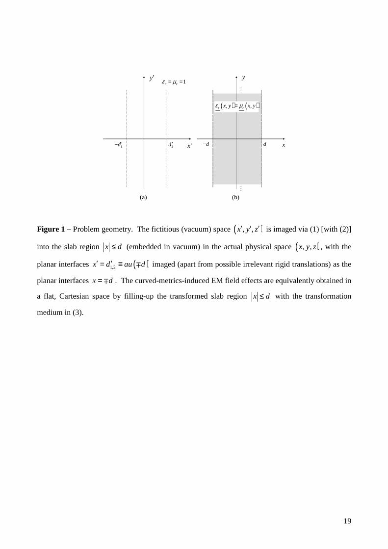
Figure 1 – Problem geometry. The fictitious (vacuum) space ( ), ,x y z′ ′ ′ is imaged via (1) [with (2)]

into the slab region x d≤ (embedded in vacuum) in the actual physical space ( ), ,x y z , with the

planar interfaces ( )1,2x d au d′ ′= ≡ ∓ imaged (apart from possible irrelevant rigid translations) as the

planar interfaces x d= ∓ . The curved-metrics-induced EM field effects are equivalently obtained in

a flat, Cartesian space by filling-up the transformed slab region x d≤ with the transformation

medium in (3).

20

x/λ0

y/λ 0

-4 -2 0 2 4-8

-6

-4

-2

0

2

4

6

8

-1

-0.5

0

0.5

1

x/λ0

y/λ 0

-4 -2 0 2 4-8

-6

-4

-2

0

2

4

6

8

-1

-0.5

0

0.5

1

Figure 2 – (Color online) An example known in the literature, but using the technique presented

here: Geometry as in Fig. 1, with 0d λ= (but truncated along the y-axis to an aperture of 014λ ), and

transformation-slab in (13) with 2α = [i.e., 60Rθ = ° in (15)], assuming a loss-tangent of 310− .

FEM-computed magnetic field map pertaining to a normally-incident collimated Gaussian beam

(with waist of size 02λ , located at 04sx λ= − , i.e., 03λ away from the slab interface), displaying

the lateral beam shift.

x/λ0

y/λ 0

-4 -2 0 2 4-8

-6

-4

-2

0

2

4

6

8

-1

-0.5

0

0.5

1

x/λ0

y/λ 0

-4 -2 0 2 4-8

-6

-4

-2

0

2

4

6

8

-1

-0.5

0

0.5

1

Figure 3 – (Color online) As in Fig. 2, but for the perfect-radome (twin-crystal) configuration in

(21), illustrating the beam-shift compensation.

21

(a) (b)

x/d

y/L

-1 -0.5 0 0.5 1-1

-0.5

0

0.5

1

0.2 0.4 0.6 0.8

x/d-1 -0.5 0 0.5 1

2 3 4 5

(a) (b)

x/d

y/L

-1 -0.5 0 0.5 1-1

-0.5

0

0.5

1

0.2 0.4 0.6 0.8

x/d

y/L

-1 -0.5 0 0.5 1-1

-0.5

0

0.5

1

0.2 0.4 0.6 0.8

x/d-1 -0.5 0 0.5 1

2 3 4 5

x/d-1 -0.5 0 0.5 1

2 3 4 5

Figure 4 – (Color online) Constitutive-parameter maps (transverse components) for the perfect-

radome configuration in (22) (with 1β = ), shown in the principal reference system. As a reference,

the principal axes directions ξ and υ are shown as short segments, in (a) and (b), respectively.

x/λ0

y/λ 0

-4 -2 0 2 4-8

-6

-4

-2

0

2

4

6

8

-1

-0.5

0

0.5

1

x/λ0

y/λ 0

-4 -2 0 2 4-8

-6

-4

-2

0

2

4

6

8

-1

-0.5

0

0.5

1

Figure 5 – (Color online) As in Fig. 2, but for the perfect-radome configuration in (22) (cf. the

constitutive parameters in Fig. 4).

22

(a) (b)

x/d

y/L

-1 -0.5 0 0.5 1-1

-0.5

0

0.5

1

0.2 0.4 0.6 0.8

x/d-1 -0.5 0 0.5 1

20 40 60 80 100 120

(a) (b)

x/d

y/L

-1 -0.5 0 0.5 1-1

-0.5

0

0.5

1

0.2 0.4 0.6 0.8

x/d

y/L

-1 -0.5 0 0.5 1-1

-0.5

0

0.5

1

0.2 0.4 0.6 0.8

x/d-1 -0.5 0 0.5 1

20 40 60 80 100 120

x/d-1 -0.5 0 0.5 1

20 40 60 80 100 120

Figure 6 – (Color online) As in Fig. 4, but for the configuration in (24) and (25) (with 2n = and

2 1u = ).

x/λ0

y/λ 0

-4 -2 0 2 4-8

-6

-4

-2

0

2

4

6

8

-1

-0.5

0

0.5

1

x/λ0

y/λ 0

-4 -2 0 2 4-8

-6

-4

-2

0

2

4

6

8

-1

-0.5

0

0.5

1

Figure 7 – (Color online) As in Fig. 2, but for the perfect-radome configuration in (24) and (25) (cf.

the constitutive parameters in Fig. 6).

23

(a) (b)x 10

3

x/d

y/L

-1 -0.5 0 0.5 1-1

-0.5

0

0.5

1

0.2 0.4 0.6 0.8

x/d-1 -0.5 0 0.5 1

2 4 6 8

(a) (b)x 10

3

x/d

y/L

-1 -0.5 0 0.5 1-1

-0.5

0

0.5

1

0.2 0.4 0.6 0.8

x/d

y/L

x/d

y/L

-1 -0.5 0 0.5 1-1

-0.5

0

0.5

1

0.2 0.4 0.6 0.8

x/d-1 -0.5 0 0.5 1

2 4 6 8

x/dx/d-1 -0.5 0 0.5 1

2 4 6 8

Figure 8 – (Color online) As in Fig. 4, but for the configuration in (26) (with dδ = and

100d∆ = ).

x/λ0

y/λ 0

-4 -2 0 2 4-8

-6

-4

-2

0

2

4

6

8

-1

-0.5

0

0.5

1

x/λ0

y/λ 0

-4 -2 0 2 4-8

-6

-4

-2

0

2

4

6

8

-1

-0.5

0

0.5

1

Figure 9 – (Color online) As in Fig. 2, but for the configuration in (26) (cf. the constitutive

parameters in Fig. 8).

24

cloak

anti-cloak

x

y

1x 2x 3x

(a) (c)(b)

x/λ0

y/λ 0

-4 -2 0 2 4

-4

-2

0

2

4

x/λ0

-4 -2 0 2 4

-1

-0.5

0

0.5

1

cloak

anti-cloak

x

y

1x 2x 3x

cloak

anti-cloak

x

y

1x 2x 3x

(a) (c)(b)

x/λ0

y/λ 0

-4 -2 0 2 4

-4

-2

0

2

4

x/λ0

y/λ 0

-4 -2 0 2 4

-4

-2

0

2

4

x/λ0

-4 -2 0 2 4

-1

-0.5

0

0.5

1

x/λ0

-4 -2 0 2 4

-1

-0.5

0

0.5

1

Figure 10 – (Color online) (a) Square cloak/anti-cloak geometry [cf. (28) and (29)]. (b), (c) FEM-

computed magnetic field maps pertaining to oblique (15°) plane-wave excitation in the presence

and absence, respectively, of the anti-cloak shell (parameters: 1 00.81x λ= , 2 01.30x λ= , 3 01.79x λ= ,

3 1 100x∆ = , 2 31.82∆ = ∆ ). Note that, for computational convenience, the oblique incidence is

simulated using a 15°-rotated (,x y ) coordinate system, where the illuminating wave impinges

along the x -axis.

(b)(a)

x/λ0

y/λ 0

-4 -2 0 2 4

-4

-2

0

2

4

x/λ0

-4 -2 0 2 4

-1

-0.5

0

0.5

1

(b)(a)

x/λ0

y/λ 0

-4 -2 0 2 4

-4

-2

0

2

4

x/λ0

y/λ 0

-4 -2 0 2 4

-4

-2

0

2

4

x/λ0

-4 -2 0 2 4

-1

-0.5

0

0.5

1

x/λ0

-4 -2 0 2 4

-1

-0.5

0

0.5

1

Figure 11 – (Color online) As in Figs. 10(b) and 10(c), but with the two horizontal anti-cloak

elements removed, and plane-wave incidence direction orthogonal (a) and parallel (b) to the

corresponding sides.

25

(a) (b)

x/d

y/L

-1 -0.5 0 0.5 1-1

-0.5

0

0.5

1

0.2 0.4 0.6 0.8

x/d-1 -0.5 0 0.5 1

2 4 6 8 10 12

x 105

(a) (b)

x/d

y/L

-1 -0.5 0 0.5 1-1

-0.5

0

0.5

1

0.2 0.4 0.6 0.8

x/d

y/L

-1 -0.5 0 0.5 1-1

-0.5

0

0.5

1

0.2 0.4 0.6 0.8

x/d-1 -0.5 0 0.5 1

2 4 6 8 10 12

x 105

x/d-1 -0.5 0 0.5 1

2 4 6 8 10 12

x 105

Figure 12 – (Color online) As in Fig. 4, but for the DPS focusing configuration in (30) (with

1.01ix d= and 10d∆ = ).

x/λ0

y/λ 0

-2 0 2

-6

-4

-2

0

2

4

6

-1

-0.5

0

0.5

1

x/λ0

y/λ 0

-2 0 2

-6

-4

-2

0

2

4

6

-1

-0.5

0

0.5

1

Figure 13 – (Color online) As in Fig. 2, but for the DPS focusing configuration in (30) (cf. the

constitutive parameters in Fig. 12), for a very weakly collimated Gaussian beam (with waist of size

0 3λ , located at 1.01sx d= − , i.e., 0 100λ away from the slab interface), displaying the focusing

effects at the image plane i sx x= − .