Light-driven oscillations of entangled nematic colloidal chains
Upload
khangminh22Category
view
1download
0
Michael Schmiedeberg
Colloidal particles onquasicrystalline substrates


Colloidal particles onquasicrystalline substrates
vorgelegt vonDiplom Physiker
Michael Schmiedeberg
geboren in Villingen-Schwenningen
Von der Fakultat II - Mathematik und Naturwissenschaftender Technischen Universitat Berlin
zur Erlangung des akademischen GradesDoktor der Naturwissenschaften (Dr. rer. nat.)
genehmigte Dissertation
Promotionsausschuss:Vorsitzender: Prof. Dr. Martin Schoen
Erster Berichter: Prof. Dr. Holger StarkZweite Berichterin: Prof. Dr. Sabine Klapp
Externer Berichter: Prof. Dr. Hartmut Lowen
Tag der wissenschaftlichen Aussprache: 24.7.2008
Berlin 2008
D 83

1
Contents
1 Introduction 5
2 Optical Matter 9
2.1 Charge-stabilized colloidal suspensions . . . . . . . . . . . . . . . . . . . . 9
2.2 Optical tweezing . . . . . . . . . . . . . . . . . . . . . . . . . . . . . . . . 10
2.3 Previous works with colloids in laser fields . . . . . . . . . . . . . . . . . . 11
3 Quasicrystals and decagonal laser fields 13
3.1 A brief introduction to quasicrystals . . . . . . . . . . . . . . . . . . . . . . 13
3.1.1 History . . . . . . . . . . . . . . . . . . . . . . . . . . . . . . . . . . 13
3.1.2 Tilings . . . . . . . . . . . . . . . . . . . . . . . . . . . . . . . . . . 15
3.1.3 Projection methods . . . . . . . . . . . . . . . . . . . . . . . . . . . 17
3.1.4 Classification of quasicrystals . . . . . . . . . . . . . . . . . . . . . 18
3.2 The number of the golden ratio . . . . . . . . . . . . . . . . . . . . . . . . 19
3.3 Quasicrystalline laser fields . . . . . . . . . . . . . . . . . . . . . . . . . . . 22
3.3.1 Zoo of possible interference patterns . . . . . . . . . . . . . . . . . 22
3.3.2 The standard decagonal potential . . . . . . . . . . . . . . . . . . . 27
3.3.3 Distribution of depths of the minima . . . . . . . . . . . . . . . . . 27
3.3.4 Nearest neighbors in the decagonal potential . . . . . . . . . . . . . 29
3.4 Phonons and Phasons . . . . . . . . . . . . . . . . . . . . . . . . . . . . . . 29
3.4.1 Phasons . . . . . . . . . . . . . . . . . . . . . . . . . . . . . . . . . 30
3.4.2 Hydrodynamic modes . . . . . . . . . . . . . . . . . . . . . . . . . . 31
3.4.3 Examples of phasonic displacements, drifts, and gradient fields . . . 33
3.4.4 Indexing problem . . . . . . . . . . . . . . . . . . . . . . . . . . . . 39
3.5 Induced Quasicrystals . . . . . . . . . . . . . . . . . . . . . . . . . . . . . 41
3.5.1 Quasicrystalline films . . . . . . . . . . . . . . . . . . . . . . . . . . 41
3.5.2 Atomic clouds in quasicrystalline traps . . . . . . . . . . . . . . . . 41
3.5.3 Light-induced quasicrystals in polymer-dispersed liquid-crystal ma-terials . . . . . . . . . . . . . . . . . . . . . . . . . . . . . . . . . . 42
3.5.4 Induced non-linear optical quasicrystal . . . . . . . . . . . . . . . . 42

2 Contents
4 Simulation techniques 434.1 Brownian dynamics simulations . . . . . . . . . . . . . . . . . . . . . . . . 43
4.1.1 The Langevin equation . . . . . . . . . . . . . . . . . . . . . . . . . 434.1.2 Discretized equation and simulation details . . . . . . . . . . . . . . 45
4.2 Monte-Carlo simulations . . . . . . . . . . . . . . . . . . . . . . . . . . . . 464.3 Size of the simulation box . . . . . . . . . . . . . . . . . . . . . . . . . . . 48
4.3.1 Approximations for the 1D quasicrystalline potential . . . . . . . . 494.3.2 Approximations for the decagonal potential . . . . . . . . . . . . . 49
4.4 Parameter values . . . . . . . . . . . . . . . . . . . . . . . . . . . . . . . . 51
5 Theory of Melting in 2D 535.1 Landau-Alexander-McTague theory . . . . . . . . . . . . . . . . . . . . . . 535.2 Density functional theory . . . . . . . . . . . . . . . . . . . . . . . . . . . . 555.3 KTHNY theory . . . . . . . . . . . . . . . . . . . . . . . . . . . . . . . . . 56
6 Colloids in a 1D quasicrystalline potential 616.1 Colloids in a 1D periodic potential . . . . . . . . . . . . . . . . . . . . . . 61
6.1.1 Laser-induced freezing and melting . . . . . . . . . . . . . . . . . . 626.1.2 Landau-Alexander-McTague theory . . . . . . . . . . . . . . . . . . 636.1.3 Density functional theory . . . . . . . . . . . . . . . . . . . . . . . 646.1.4 Laser-induced melting due to fluctuations . . . . . . . . . . . . . . 66
6.2 Motivation for the quasicrystalline potential . . . . . . . . . . . . . . . . . 676.3 Phase behavior . . . . . . . . . . . . . . . . . . . . . . . . . . . . . . . . . 68
6.3.1 Results of Monte-Carlo simulations . . . . . . . . . . . . . . . . . . 696.3.2 Refined Landau-Alexander-McTague theory . . . . . . . . . . . . . 71
6.4 Dynamics: Non-periodic locked phase for large laser intensities . . . . . . . 756.5 Experimental results . . . . . . . . . . . . . . . . . . . . . . . . . . . . . . 796.6 Other quasicrystalline potentials . . . . . . . . . . . . . . . . . . . . . . . . 796.7 Summary and Outlook . . . . . . . . . . . . . . . . . . . . . . . . . . . . . 80
7 Colloidal ordering in a decagonal potential 817.1 Phase behavior . . . . . . . . . . . . . . . . . . . . . . . . . . . . . . . . . 81
7.1.1 Bond orientational order parameter . . . . . . . . . . . . . . . . . . 817.1.2 Low-density case . . . . . . . . . . . . . . . . . . . . . . . . . . . . 837.1.3 Phases with ten or twenty bond directions . . . . . . . . . . . . . . 847.1.4 High-density case . . . . . . . . . . . . . . . . . . . . . . . . . . . . 867.1.5 Archimedean tiling . . . . . . . . . . . . . . . . . . . . . . . . . . . 897.1.6 Pair correlation function and structure factor . . . . . . . . . . . . 94
7.2 Comparison to experimental results . . . . . . . . . . . . . . . . . . . . . . 967.3 Phasonic displacements and drifts . . . . . . . . . . . . . . . . . . . . . . . 99
7.3.1 Rearrangements in a decagonal quasicrystal . . . . . . . . . . . . . 997.3.2 Rearrangements in an Archimedean-like tiling . . . . . . . . . . . . 1007.3.3 Stabilizing the Archimedean-like tiling by a phasonic drift . . . . . 101

Contents 3
7.3.4 Stabilizing the Archimedean-like tiling by a phasonic gradient . . . 1017.4 Summary and Outlook . . . . . . . . . . . . . . . . . . . . . . . . . . . . . 102
8 Brownian particles in a decagonal potential 1058.1 A short introduction to anomalous diffusion . . . . . . . . . . . . . . . . . 1058.2 Brownian motion in static potentials started in non-equilibrium . . . . . . 108
8.2.1 Regular and random square potential . . . . . . . . . . . . . . . . . 1088.2.2 Results of the simulations . . . . . . . . . . . . . . . . . . . . . . . 108
8.3 Random trap model . . . . . . . . . . . . . . . . . . . . . . . . . . . . . . 1138.3.1 Theory . . . . . . . . . . . . . . . . . . . . . . . . . . . . . . . . . . 1138.3.2 Results and comparison to simulations . . . . . . . . . . . . . . . . 117
8.4 Brownian motion started in equilibrium . . . . . . . . . . . . . . . . . . . . 1218.4.1 Experimental results . . . . . . . . . . . . . . . . . . . . . . . . . . 1218.4.2 Simulation results . . . . . . . . . . . . . . . . . . . . . . . . . . . . 121
8.5 Colloidal motion in potentials with phasonic drift . . . . . . . . . . . . . . 1238.5.1 Ballistic motion . . . . . . . . . . . . . . . . . . . . . . . . . . . . . 1238.5.2 Mean square displacement and non-equilibrium steady state . . . . 1258.5.3 Modification of the random trap model . . . . . . . . . . . . . . . . 125
8.6 Non-equilibrium statistics . . . . . . . . . . . . . . . . . . . . . . . . . . . 1288.6.1 Derivation of path-ensemble averages . . . . . . . . . . . . . . . . . 1288.6.2 Examples of path-ensemble averages and fluctuation theorems . . . 1308.6.3 Colloidal motion in potentials with phasonic drift: a non-equilibrium
system . . . . . . . . . . . . . . . . . . . . . . . . . . . . . . . . . . 1338.7 Summary and Outlook . . . . . . . . . . . . . . . . . . . . . . . . . . . . . 134
9 Conclusions 137
List of Publications 139
Bibliography 141
Index 163
Zusammenfassung in deutscher Sprache 171
Danksagung 175

4 Contents

5
Chapter 1
Introduction
Quasicrystals are non-periodic solids that nevertheless exhibit long-range positional andorientational order. They can possess rotational point symmetries, such as five- or ten-fold rotational axes, that are not allowed in periodic crystals. Since their discovery [1]quasicrystals have caused much fascination, mainly because our understanding of whatcrystals are has had to change. Besides the non-crystallographic rotational symmetry,quasicrystals also show other physical properties that cannot exist in periodic crystals.Phasons, for example, are correlated global rearrangements of atoms that, like phonons,are hydrodynamic modes since they do not increase the free energy in the long-wavelengthlimit [2, 3]. Their different features are still a main topic and intensively discussed in thefield [4]. In recent years, increasing research activities have been directed towards thequestion of how atoms order and move on quasicrystalline surfaces [5–19]. The goal ofsuch studies is to understand and control the growth of quasicrystals and their exceptionalmaterial properties.
Colloidal suspensions are dispersions of micron-sized particles in a fluid. They are a well-known model system for statistical physics and for mimicking atomic systems. If subjectedto a laser field, colloids are forced towards the region of highest laser intensity. Therefore amodulated light field can be used as an external potential acting on the particles. Unlike inatomic systems, the interactions between the colloids can be fine-tuned and by using videomicroscopy, the positions and movements of the particles can be observed in experiment.Leaving aside chemical details, colloidal suspensions in laser fields are therefore a veryattractive system to study structural features of particle adsorbates on substrates.
In this work, we study the dynamics and the ordering of particles on quasicrystallinesubstrates. Using different simulation techniques, like Monte-Carlo or Brownian dynam-ics algorithms, as well as analytical theories, we determine the phase behavior and themotion of colloids confined to two dimensions in laser fields with one- or two-dimensionalquasicrystalline symmetry. The one-dimensional potential is a sum of two incommensu-rable modulations in one direction and is constant in the other. The two-dimensional lightfield can be realized as the interference pattern of five laser beams and therefore exhibitsdecagonal symmetry (see figure 1.1).

6 Chapter 1. Introduction
aV
(b)(a)
Figure 1.1: (a) Experimental realization of a laser intensity field with decagonal symmetry. Photo andexperiment by J. Mikhael [20]. (b) Theoretically calculated grey-sale representation of the decagonalinterference pattern of five laser beams. White parts indicate a high laser intensity corresponding tominima of the potential. The bar in the upper right corner marks the wave length aV = 2π/|Gj | associatedwith the modulation vector Gj (see section 3.3).
The phase behavior of two dimensional systems, such as atomic monolayers on a surface,is known to be unique. Without an external potential, melting occurs in a two stageprocess due to the dissociation of different types of defects [21–27]. An external one ortwo-dimensional potential, if commensurable to the colloidal lattice structure, can stabilizeor even induce triangular ordering [28], resulting in interesting non-trivial phase diagrams[29–32].
For colloidal particles in very weak quasicrystalline potentials, we find a triangular ora liquid phase depending on the two-particle interaction strength and the density. Forvery strong laser intensity, the system orders with the same symmetry as the substrate.However, when the strengths of the colloidal interaction and the substrate potential arecomparable, we find interesting and unexpected new phases. The dynamics of particlesin quasicrystalline potentials also reveals surprising phenomena, such as a frustrated non-periodic solid phase in the one-dimensional potential or a crossover from a subdiffusiveregime at intermediate times to asymptotic diffusion for a single Brownian particle in thedecagonal laser field.
Another advantage of considering colloidal suspensions in laser fields as a model systemfor particles in quasicrystalline potentials is that phasonic displacements, gradients, ordrifts can easily be studied. We demonstrate how phasonic rearrangements can be inducedby the laser field and how the motion of a single Brownian particle in a decagonal potentialis affected by a phasonic drift.

7
This work is organized as follows: In chapter 2, we shortly introduce colloidal suspen-sions and demonstrate how light fields can be used to manipulate the particles. Chapter3 gives an overview over history, properties, and construction methods of quasicrystals.Furthermore, we explain in detail how we determine the decagonal potential and introducethe phasonic degrees of freedom. We also shortly introduce examples of systems with in-duced decagonal symmetry, such as adatoms on the surface of quasicrystals. In chapter 4,the simulation techniques and their details are presented. We briefly summarize the mostimportant theories of melting in two dimensions without any external potential in chapter5. In chapter 6, colloidal suspensions in one dimensional laser fields are discussed. First,previous works and their results for periodic modulations are shortly introduced, then wepresent our results for the phase behavior and dynamics of colloids in a one-dimensionalquasicrystalline potential. In chapter 7, the ordering in two-dimensional decagonal laserfields is analyzed, along with examples of induced phasonic rearrangements. In chapter 8,we study the dynamics of a single Brownian particle in a decagonal potential without orwith phasonic drift. We also show how such a system can be used as a model system tostudy non-equilibrium path-ensemble averages. Finally, we conclude in chapter 9.

8 Chapter 1. Introduction

9
Chapter 2
Optical Matter
Colloids are widely used as a model system in statistical physics and often laser beamsare employed to manipulate them. For example, colloidal ordering can be induced bymodulated laser fields, which is called optical matter [33]. In this chapter, we first describethe properties of a charge-stabilized colloidal suspension and then explain how one canmanipulate micron-sized particles with laser beams. Finally, we present some previousworks done with 2D colloidal systems in laser fields.
2.1 Charge-stabilized colloidal suspensions
Colloidal systems consist of small particles dispersed in a continuous solution. Usually,colloids are about 0.01 to 10µm in diameter and therefore can show pronounced Brownianmotion. Typical examples are solid particles in a liquid or gas, like paint or smoke, anddrops dispersed in liquids or air as in milk or fog. Sometimes, air bubbles in liquids orsolids, i.e., aqueous or solid foams, and even liquid or solid particles in solids, e.g., gelatin orglass mixtures, are also called colloidal systems. Here we consider spherical solid particles,usually consisting of plastic material (e.g., polystyrene) or glass, in a liquid solvent. Dueto the attractive van der Waals interaction such colloids stick together and form clusters.To prevent aggregation and to stabilize the colloidal suspension, usually one of the two fol-lowing mechanisms is chosen: In a sterically stabilized suspension surfactants or polymersare added. They adhere to the surface of the colloids and keep them at a large distance,where van der Waals interactions are small. As a consequence, clustering is prevented. Ina charge-stabilized suspension, as we consider here, the colloids are charged and the sign ofthe charge is the same for all colloids. Therefore, there is a repulsive interaction caused bythe Coulomb forces. Due to counter ions in the solvent that accumulate around a colloidalparticle, the interaction is screened. It is given by the pair potential φ(r) according to theDLVO-theory [34,35], named after Derjaguin, Landau, Verwey, and Overbeek:
φ(r) =(Z∗e)2
4πε0εr
(eκR
1 + κR
)2e−κr
r, (2.1)

10 Chapter 2. Optical Matter
D,11F
D,12F
R,11F
R,21F
D,21F
D,22F
R,22F
R,12F
Ftot
Laser intensity
Figure 2.1: Colloidal particle in a laser beam with Gaussian intensity profile. The refraction of the lightrays (full lines) lead to forces pointing in forward and outward direction. A small part of the rays isreflected (dashed lines). Because the rays closer to the beam center line are stronger, the total force actsin forward direction and towards the beam center line.
where r is the distance between two interacting colloids, R the radius of a colloid, Z∗ itseffective surface charge, εr the dielectric constant of water, and κ the inverse Debye screen-ing length. Note that in our simulations we also do not allow the colloids to overlap, whichcorresponds to an additional excluded-volume interaction as for hard spheres. However,the mean particle distance and the screening length are usually much larger than the radiusand therefore the excluded-volume interaction does not play an important role.
2.2 Optical tweezing
Inducing ordering in colloidal suspensions by modulated laser fields is based on the samephenomenon that is also responsible for optical tweezing, which is a widely used techniqueto manipulate micron-sized particles [36–38], but also viruses or bacteria [39], by laserbeams. We therefore shortly introduce the principle of the optical tweezing effect and thenexplain how colloids are affected by laser fields.
We consider a colloidal particle in a laser beam with Gaussian intensity profile (seefigure 2.1). Assuming that the refraction index of a colloid is higher than the one of thesurrounding, light rays are refracted towards the center of the colloid. The deflections of

2.3. Previous works with colloids in laser fields 11
the rays lead to forces in outward forward direction (see forces FD,11, FD,12, FD,21, andFD,22 in figure 2.1). A small part of the rays is reflected at each interface leading tosmall additional forces mainly in forward direction (FR,11, FR,12, FR,21, and FR,22). If thecolloidal particle is displaced out of the center of the beam, the forces acting on the sidecloser to the beam center line, i.e., FD,11, FD,12, FR,11, and FR,12, are much larger thanthose on the outside of the beam (FD,21, FD,22, FR,21, and FR,22). Therefore, the resultingtotal force Ftot acts in forward direction and towards the beam center, i.e., the colloid isforced back into the region of highest intensity. As a consequence, a laser beam can beused to trap and move around particles.
An alternative explanation of the optical tweezing phenomenon considers the energy ofa dielectric particle in an electric field. Because the colloid has a higher dielectric constantthan the surrounding medium, the free energy can be lowered by moving the particle intoregions with a higher electric field, i.e., towards a higher laser intensity.
In an optical tweezer, the force is approximately proportional to the gradient of the laserintensity and is directed towards the highest intensities. Therefore, a colloid confined to aplane perpendicular to the beam can be considered to be in a potential that is proportionalto the intensity of the light field, i.e., a particle in a Gaussian laser beam experiences aGaussian potential. Correspondingly, a modulated laser field affects a two-dimensionalcolloidal suspension: The particles are forced towards the brightest spots of the laserpattern, which act as minima of a potential realized by the light-intensity distribution.
2.3 Previous works with colloids in laser fields
As shown in the previous subsection, modulated laser fields act as external potentials forcolloidal suspensions. Such a set-up is widely used as a model system in statistical physicsto study ordering or dynamics in external potentials (for a recent overview, see e.g. [40]).Here we present some examples of previous works with such systems.
External potentials consisting of periodic arrays of minima or pinning locations werestudied experimentally [41,42] and with Brownian dynamics simulations [43,44]. A specialexample of a periodic potential is the one with triangular symmetry that can be realizedas interference pattern of three laser beams (see also section 3.3). In a triangular potential,interesting new phases were observed, especially for the cases where two or more colloidspopulate each potential minimum [42–44]. For a pair of particles, called dimer, or threecolloids per pinning location, termed trimer, the phase diagram was also determined an-alytically [45, 46] by mapping the problem onto a 3-state Potts model or other Ising-liketheories.
A simple one-dimensional periodic potential can already lead to a surprising phasebehavior. It first induces triangular ordering in a colloidal suspension if the colloidaldensity is chosen appropriately. Then, for increasing potential strength and appropriatecolloidal interactions, the triangular phase melts again. We discuss this so-called laser-induced freezing and reentrant melting in section 6.1.
12 Chapter 2. Optical Matter
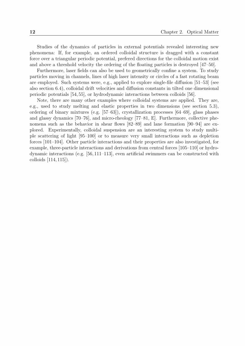
Studies of the dynamics of particles in external potentials revealed interesting newphenomena: If, for example, an ordered colloidal structure is dragged with a constantforce over a triangular periodic potential, prefered directions for the colloidal motion existand above a threshold velocity the ordering of the floating particles is destroyed [47–50].
Furthermore, laser fields can also be used to geometrically confine a system. To studyparticles moving in channels, lines of high laser intensity or circles of a fast rotating beamare employed. Such systems were, e.g., applied to explore single-file diffusion [51–53] (seealso section 6.4), colloidal drift velocities and diffusion constants in tilted one dimensionalperiodic potentials [54,55], or hydrodynamic interactions between colloids [56].
Note, there are many other examples where colloidal systems are applied. They are,e.g., used to study melting and elastic properties in two dimensions (see section 5.3),ordering of binary mixtures (e.g. [57–63]), crystallization processes [64–69], glass phasesand glassy dynamics [70–76], and micro-rheology [77–81, E]. Furthermore, collective phe-nomena such as the behavior in shear flows [82–89] and lane formation [90–94] are ex-plored. Experimentally, colloidal suspension are an interesting system to study multi-ple scattering of light [95–100] or to measure very small interactions such as depletionforces [101–104]. Other particle interactions and their properties are also investigated, forexample, three-particle interactions and derivations from central forces [105–110] or hydro-dynamic interactions (e.g. [56, 111–113], even artificial swimmers can be constructed withcolloids [114,115]).

13
Chapter 3
Quasicrystals and decagonal laserfields
A well-known result of crystallography states that periodic lattices are only compatiblewith 1, 2, 3, 4 or 6-fold rotational symmetry. Quasicrystals possess a perfect long-rangepositional order but nevertheless they are not periodic, i.e., it is not possible to obtainthe same structure after any translation of the system. As a consequence, other rotationalsymmetries with, e.g., five-, eight-, or ten-fold axes are allowed. In addition, quasicrystalshave also other unique properties, such as the so-called phasons, which correspond tospecial atomic rearrangements that do not change free energy. This chapter gives anoverview over the most important properties of quasicrystals and of modulated laser fieldswith quasicrystalline symmetry, which we use in this work.
Section 3.1 is a brief summary of the history of quasicrystals, their construction meth-ods, and their classification. In section 3.2, we present some properties of the number ofthe golden ratio, because it is an important and interesting number often found in pentag-onal and decagonal patterns. Quasicrystalline laser fields are described in detail in section3.3. In section 3.4, the hydrodynamic modes of a quasicrystal are discussed, especially theso-called phasons, which do not exist in periodic crystals. Finally, in section 3.5, we discusssystems, where a quasicrystalline symmetry is induced by a substrate or another externalpotential. Examples are thin films on surfaces of quasicrystals or atomic clouds in opticaltraps with quasicrystalline symmetry.
3.1 A brief introduction to quasicrystals
3.1.1 History
Recently, it was reported that non-periodic, quasicrystalline tilings were used in Islamicarchitecture a long time before they were discovered in the west [116]: Starting around1200 AD some complex, but still periodic patterns were created using non-trivial tilesleading to very large unit cells. Later, in the 15th century, a nearly perfect quasicrystalline

14 Chapter 3. Quasicrystals and decagonal laser fields
tiling, corresponding to the one later constructed by Penrose, was used as decoration onthe Darb-i Imam shrine in Isfahan, Iran. In the west, during the first half of the 19th
century, a standard classification of crystals was developed. It seemed natural that everytwo-dimensional structure with long-range order has to be periodic. Then, only 1, 2, 3, 4,or 6-fold rotational symmetries are possible [117]. An aperiodic tiling was still consideredto be impossible in the early 1960s [118]. However, in 1966 Berger published a proofthat aperiodic 2D-tilings exist [119], i.e., tilings without a translational symmetry but aperfect long-range order. He explicitly invented a tiling that is constructed out of a setof 20426 elementary tiles. A few years later aperiodic tilings consisting of just six tileswere found [120]. The most famous aperiodic tiling of the plane was presented by Penrosein 1974 [121]. This so called Penrose tiling can be constructed by using two elementarytiles (see also section 3.1.2). It has a five-fold rotational symmetry but no translationalsymmetry. Other aperiodic tilings were discovered in the following years (see also section3.1.2), however, they seemed to be only of interest as theoretical models in mathematics.This changed in 1984 when Shechtman et. al. [1] published the observation of sharp ten-fold symmetric Bragg peaks in small metallic grains, which form in fast cooled alloysof Al with 14 at.% Mn. Shortly later, Levine and Steinhardt proposed that this is dueto a quasicrystalline ordering without any translational symmetry [122]. Today, manyquasicrystals with different point symmetries are known. Some quasicrystals are aperiodicin all three directions of space, for example the icosahedral Al-Mn grains in [1], others areperiodic stacks of 8-, 10- or 12-fold symmetric two-dimensional quasicrystalline structures.Quasicrystals are not only observed in metallic alloys but they can even be constructed,e.g., with macromolecules [123].
The interest in quasicrystals is not only due to their non-crystallographic rotationalsymmetry, they also have many new properties that can probably lead to new applicationsin material science (cf. [124]). Because of the aperiodicity it was not obvious, whetherquasicrystals are closer to amorphous or to crystalline materials. The material propertiesof quasicrystals turned out to be unique. For example, quasicrystals have an electronicband structure which contains a special pseudo-gap [125–127] leading to characteristicconductance properties [128,129]. The mechanical properties are also very interesting: Atlow temperatures they are often very brittle [130, 131], whereas they become ductile athigher temperatures [132]. In recent time, there has been much research activity in thefield of photonics and photonic crystals. The idea is to build components similar to elec-tronic semiconductor devices such as transistors working with photons instead of electrons.Similar to the electronic band structure, an optical band structure can be calculated forcrystals [133]. Quasicrystals have a very special optical band structure [134–136] withproperties that may be used to construct photonic devices.
One of the most fascinating new properties of a quasicrystal is the larger numberof independent hydrodynamic modes. Aside from phonons, which also exist in normalcrystals, there are additional modes in quasicrystals called phasons. These new modesare important for elastic properties, the brittleness at low temperatures, and the meltingbehavior of quasicrystals. Phonons and phasons will be introduced in more detail in section3.4.

3.1. A brief introduction to quasicrystals 15
Figure 3.1: Penrose tiling.
3.1.2 Tilings
In this and the next subsection we discuss common methods to construct quasicrystallinepatterns. Probably the most famous quasicrystalline pattern is the Penrose tiling [121]shown in figure 3.1. It has a 5-fold rotational symmetry and perfect long-range order.The Penrose pattern can be constructed by using four triangular elementary tiles [seefigure 3.2(a)]. It is not allowed to combine the tiles in an arbitrary way. There are somematching rules which have to be obeyed. One possibility to implement such rules is tomark the edges of the triangles with arrows. Edges in contact must always have the samenumber of arrows pointing into the same direction [137, 138]. Other elementary tiles forbuilding up Penrose pattern are shown in figures 3.2(b) and (c).
There are a lot of other quasicrystalline patterns that are usually assembled with tiles.Two examples are presented in figure 3.3. However, the matching rules usually are muchmore complicated than those for the Penrose tiling (see e.g. [139–141]).
Often tilings are also constructed by the so-called deflation method [121], which uses theself-similarity of the patterns. In each step of the deflation process every tile is replaced bya set of smaller tiles that cover the same area. This can be done in a way that the matchingrules are obeyed. Therefore, after a few steps of deflation, a perfect quasicrystalline tilingcovers the original starting tile.

16 Chapter 3. Quasicrystals and decagonal laser fields
2π/5
2π/5
π/5
1
1/τπ/5 π/5
τ
3π/51
3π/5
2π/5 2π/5
2π/5
4π/5 2π/5
6π/5
π/5π/5
4π/5
(a)
(b) (c)
Figure 3.2: (a) Tiles of the Penrose pattern. The arrows on the edges symbolize matching rules. If twotriangles are put together, the edges at contact must have the same number of arrows pointing into thesame direction. The triangles can also be combined to (b) two rhombic tiles or (c) a kite and a dart tile,which serve as alternative elementary tiles for constructing a Penrose pattern.
(a) (b)
Figure 3.3: Other examples of quasicrystalline tilings: (a) decagonal Tubingen tiling, (b) octagonal Am-mann tiling.

3.1. A brief introduction to quasicrystals 17
LS
L
L
L
L
L
L
L
L
L
L
L
L
L
S
S
S
S
S
S
S
S
1/τ
Figure 3.4: Projection of a two-dimensional square lattice on a line with slope 1/τ . The limiting, dashedlines of the acceptance region are defined by two vertices of the unit cell. The resulting one-dimensionalsequence of small (S) and long (L) distances corresponds to the Fibonacci chain.
3.1.3 Projection methods
Two-dimensional quasicrystalline patterns can also be constructed by projecting a higherdimensional periodic lattice onto a plane. The Penrose tiling for example can be achieved byprojecting a five-dimensional cubic structure onto a two-dimensional plane [137,138,142].
Here we shortly demonstrate the projection method for constructing a one-dimensionalquasicrystal by starting with a two-dimensional square lattice and projecting the latticepoints onto a line. The projection formalism works as follows: All points of the squarelattice which are within some acceptance region are projected onto the line. If the slopeof the line is an irrational number, the projected points form a non-periodic lattice, whichnevertheless has a perfect long-range ordering and therefore is a quasicrystal. In the ex-ample shown in figure 3.4 we choose the slope 1/τ where τ = (1 +
√5)/2 is the number
of the golden ratio (see section 3.2). The limiting lines of the acceptance region are de-fined by the unit cell of the square lattice in a way, that only one of the two outermostparticles is accepted for the projection (see figure 3.4). The resulting quasicrystal corre-sponds to the so-called Fibonacci chain. A Fibonacci chain is a series of two elements Land S, here representing long and short distances between the points of the quasicrystal.The Fibonacci chain can also be constructed by starting a sequence with L and then re-

18 Chapter 3. Quasicrystals and decagonal laser fields
G
G
G
G
G
0
1
2
3
4
Figure 3.5: Reciprocal lattice vectors of a decagonal quasicrystal. Note that the negative vectors often arealso considered as part of an elementary star of vectors describing the lattice. For the quasicrystalline laserfield described in section 3.3, the vectors shown here correspond to the wave vectors of the laser beamsprojected into the sample plain.
peating the following replacements: L → LS and S → L. The steps towards a longerFibonacci chain therefore are: L, LS, LSL, LSLLS, LSLLSLSL, LSLLSLSLLSLLS,LSLLSLSLLSLLSLSLLSLSL etc. The probability to find the element L at a certainposition in such a chain is calculated in section 3.2.
In another construction method, patterns of parallel lines are drawn in each symmetrydirection, e.g., five sets of parallel lines. The vortices of, e.g., a decagonal pattern then arelocated at positions close to certain line intersections [137,138,143].
3.1.4 Classification of quasicrystals
One way to group quasicrystals is to consider them as projection of a higher-dimensionallattice as introduced in the previous subsection. Using the classification for such regularcrystals and describing the method of projection directly gives a method to characterizequasicrystals (see e.g. [139,144]).
Another possibility is to look at the Fourier representation of a quasicrystal [145,146].The mass density ρ(r) can be written in terms of the Fourier coefficients ρG according to
ρ(r) =∑G
ρG exp (iG · r) , (3.1)
where the sum is over all reciprocal lattice vectors G. For an ordered structure, it is usuallysufficient to consider a small set of vectors G such that their linear combinations generatethe complete set of reciprocal lattice vectors. A set of vectors G that reflects the rotationalsymmetry of the reciprocal lattice forms a star (see e.g. figure 3.5). Note that with a vectorG also its negative belongs to the reciprocal lattice. As a consequence, reciprocal latticesalways display rotational symmetries with m-fold axes where m is even. However, the thecorresponding quasicrystal in real space posses either a m- or m/2-fold symmetry axis.

3.2. The number of the golden ratio 19
1+τ
τ1
Figure 3.6: A division according to the golden ratio. The ratio of length of the complete line and thelength of the longer segment equals the ratio of the lengths of the long and the short segment.
For a quasicrystal the points of the reciprocal lattice lie dense in the reciprocal space.For example, for any given point in the plane a linear combination of the five lattice vectorsshown in figure 3.5 exists that describes a point at an arbitrary small distance. Bragg peaksin experiment correspond to reciprocal lattice points. The intensities of these peaks aregiven by |ρ(G)|2. As a consequence, the diffraction patterns contains spots of differentbrightness and, therefore, displays the symmetry of the reciprocal lattice.
3.2 The number of the golden ratio
The number of the golden ratio τ is an important algebraic irrational number in mathe-matics that also appears in arts and even in some biological systems (see e.g. [147]). It isusually defined as the positive solution of the quadratic equation
τ 2 − τ − 1 = 0, (3.2)
i.e., it is
τ =1 +
√5
2≈ 1.618. (3.3)
Dividing a line according to the golden ratio (see figure 3.6) means that the length of thetotal line 1+τ divided by the length of the longer segment τ equals the length of the longersegment τ divided by the length 1 of the shorter one:
1 + τ
τ=τ
1, (3.4)
which corresponds to equation (3.2). An interesting consequence of such a way of dividinga line is that the ratio of the shorter segment and the difference of the lengths of thesegments is again τ , since
1
τ − 1= τ or
1
τ= τ − 1 (3.5)
again corresponds to equation (3.2).The number of the golden ratio can also be written as continued fraction
τ = 1 +1
1 + 11+ 1
1+...
. (3.6)

20 Chapter 3. Quasicrystals and decagonal laser fields
This implies
τ = 1 +1
τ(3.7)
or again equation (3.2). Another interesting formula uses a continued square root:
τ =
√1 +
√1 +
√1 +
√1 + ..., (3.8)
equivalent to the relationτ =
√1 + τ (3.9)
that also gives the positive solution of equation (3.2).The golden ratio is related to the Fibonacci series, which is given by its first elements
F0 = 0 and F1 = 1 and the recurrence relation
Fn = Fn−2 + Fn−1 for n ≥ 2. (3.10)
Therefore, the first Fibonacci numbers are 0, 1, 1, 2, 3, 5, 8, 13, 21, 34, 55, 89, 144, 233,377 etc. An explicit formula for the Fibonacci numbers exists [148]
Fn =τn − (−τ)−n
√5
. (3.11)
It can be proven by induction: Equation (3.11) is valid for F0 and F1. Furthermore, ifFn−2 and Fn−1 are given by (3.11), one finds
Fn = Fn−2 + Fn−1 =τn−2 − (−τ)−n+2
√5
+τn−1 − (−τ)−n+1
√5
=τn−2 + τn−1 − (−τ)−n+2 − (−τ)−n+1
√5
=τn−1
(1τ
+ 1)− (−τ)−n+1 (−τ + 1)√
5
=τn − (−τ)−n
√5
, (3.12)
where τ = 1/τ + 1 or 1/τ = 1 − τ was used. Now, the golden ratio is the ratio of twosuccessive Fibonacci numbers in the limit n→∞, i.e.,
τ = limn→∞
Fn
Fn−1
, (3.13)
which follows from (3.11):
limn→∞
Fn
Fn−1
= limn→∞
τn − (−τ)−n
τn−1 − (−τ)−n+1= lim
n→∞
τn
τn−1= τ, (3.14)
3.2. The number of the golden ratio 21
1
τ
h
h2
1
(a)
1
h
h2
1
(b)
1
1
1
τ−1
τ−1
3π/5
π/52π/5
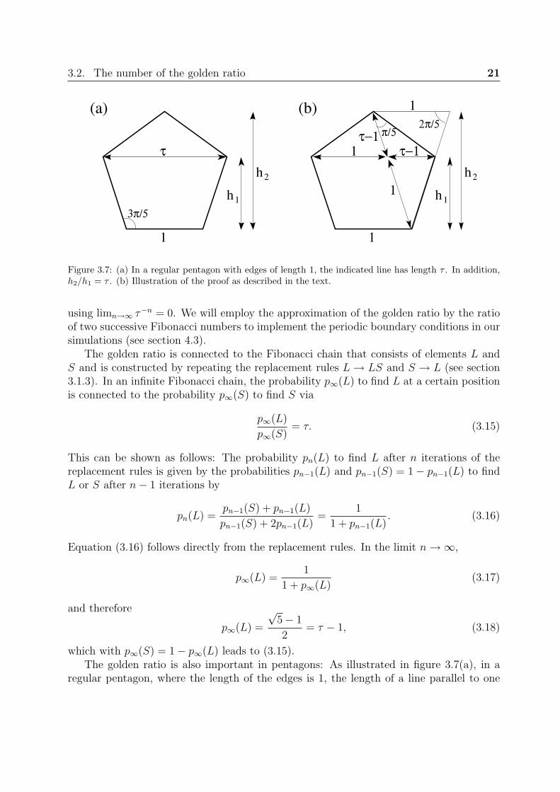
Figure 3.7: (a) In a regular pentagon with edges of length 1, the indicated line has length τ . In addition,h2/h1 = τ . (b) Illustration of the proof as described in the text.
using limn→∞ τ−n = 0. We will employ the approximation of the golden ratio by the ratioof two successive Fibonacci numbers to implement the periodic boundary conditions in oursimulations (see section 4.3).
The golden ratio is connected to the Fibonacci chain that consists of elements L andS and is constructed by repeating the replacement rules L→ LS and S → L (see section3.1.3). In an infinite Fibonacci chain, the probability p∞(L) to find L at a certain positionis connected to the probability p∞(S) to find S via
p∞(L)
p∞(S)= τ. (3.15)
This can be shown as follows: The probability pn(L) to find L after n iterations of thereplacement rules is given by the probabilities pn−1(L) and pn−1(S) = 1− pn−1(L) to findL or S after n− 1 iterations by
pn(L) =pn−1(S) + pn−1(L)
pn−1(S) + 2pn−1(L)=
1
1 + pn−1(L). (3.16)
Equation (3.16) follows directly from the replacement rules. In the limit n→∞,
p∞(L) =1
1 + p∞(L)(3.17)
and therefore
p∞(L) =
√5− 1
2= τ − 1, (3.18)
which with p∞(S) = 1− p∞(L) leads to (3.15).The golden ratio is also important in pentagons: As illustrated in figure 3.7(a), in a
regular pentagon, where the length of the edges is 1, the length of a line parallel to one

22 Chapter 3. Quasicrystals and decagonal laser fields
edge and connecting two vertices of the pentagon is τ . The ratio of the total height h2 tothe partial height h1 is also given by the golden ratio [see figure 3.7(a) for the definitionof h1 and h2]. To proof these properties, we use the geometric relations indicated in figure3.7(b) and the intercept theorem and find
τ − 1 + 1
1=
1
τ − 1. (3.19)
This corresponds to equation (3.2), i.e., τ given in the pentagon is indeed the number ofthe golden ratio. Furthermore, the intercept theorem gives
h2
h1
=1
τ − 1= τ, (3.20)
where we used τ − 1 = 1/τ .The relations for the lengths in a pentagon give us the opportunity to express τ in
terms of trigonometric functions. We find [see figure 3.7(b)]
τ =1
2 cos (2π/5)= 2 cos (π/5) (3.21)
and τ =h1
h2 − h1
=sin (2π/5)
sin (π/5). (3.22)
Equations (3.21) and (3.22) will often be used throughout this work.
3.3 Quasicrystalline laser fields
In this section we introduce methods to obtain laser fields with quasicrystalline symmetry.First, we present different types of patterns that can be produced by varying the numberof laser beams or the polarization. In subsection 3.3.2 we introduce the potential we usein this work. For such a potential the distribution of the depths of the minima is shownin subsection 3.3.3 and finally in subsection 3.3.4 the number and distance of nearestneighbors for the positions of the minima are determined. The results of subsections 3.3.3and 3.3.4 are needed for the random trap model that we develop in section 8.3 to describethe Brownian motion in a decagonal potential.
3.3.1 Zoo of possible interference patterns
To obtain a quasicrystalline laser field in an experiment, a laser beam is split up in n beamsof equal strength. The beams are arranged along the n edges of a prism that is made of aperfect n-sided polygonal base. Finally, the beams are focused onto the sample containingthe colloidal suspension (see figure 3.8 as an example for five beams). In the plane ofthe sample, which in the following will be termed the xy-plane, the beams interfere andform a crystalline or quasicrystalline interference pattern of m-fold rotational symmetry,

3.3. Quasicrystalline laser fields 23
θψ
ψ
ψ
ψ
ψ
Figure 3.8: Five laser beams arranged symmetrically around the vertical axis are focused onto the sample.The polarization vectors are given by the angle ψ, which is measured between the direction of polarizationand the vector pointing outward in radial direction. The opening angle θ is the angle between a beam andthe symmetry axis.
where m = n if the number of beams n is even and m = 2n if n is odd. In theory, theintensity field in the xy-plane can be calculated by summing up the electric fields of allbeams, taking the square of the total electric field to get the intensity, and averaging overone period of the pattern that oscillates with the circular frequency ω of the light. Thecorresponding potential then is (see also e.g. [149]):
V (r) ∝ −∫ T
0
dt
n−1∑j=0
Ej cos [Gj · r + ϕj + ωt]
2
= −∫ T
0
dtn−1∑j=0
n−1∑k=0
Ej · Ek cos [Gj · r + ϕj + ωt] cos [Gk · r + ϕk + ωt]
∝ −∫ T
0
dt
n−1∑j=0
n−1∑k=0
Ej · Ek cos [(Gk −Gj) · r + ϕk − ϕj]
+ cos [(Gk + Gj) · r + ϕk + ϕj + 2ωt]
∝ −n−1∑j=0
n−1∑k=0
Ej · Ek cos [(Gk −Gj) · r + ϕk − ϕj] + const, (3.23)
24 Chapter 3. Quasicrystals and decagonal laser fields
θ=π/2, ψ=π/6: θ=π/2, ψ=π/4: θ=π/2, ψ=π/3:(i)(h)(g)
(a) (b) (c)
(d) (e) (f)θ=π/3, ψ=π/6: θ=π/3, ψ=π/4: θ=π/3, ψ=π/3:
θ=π/4, ψ=π/3:θ=π/4, ψ=π/4:θ=π/4, ψ=π/6:
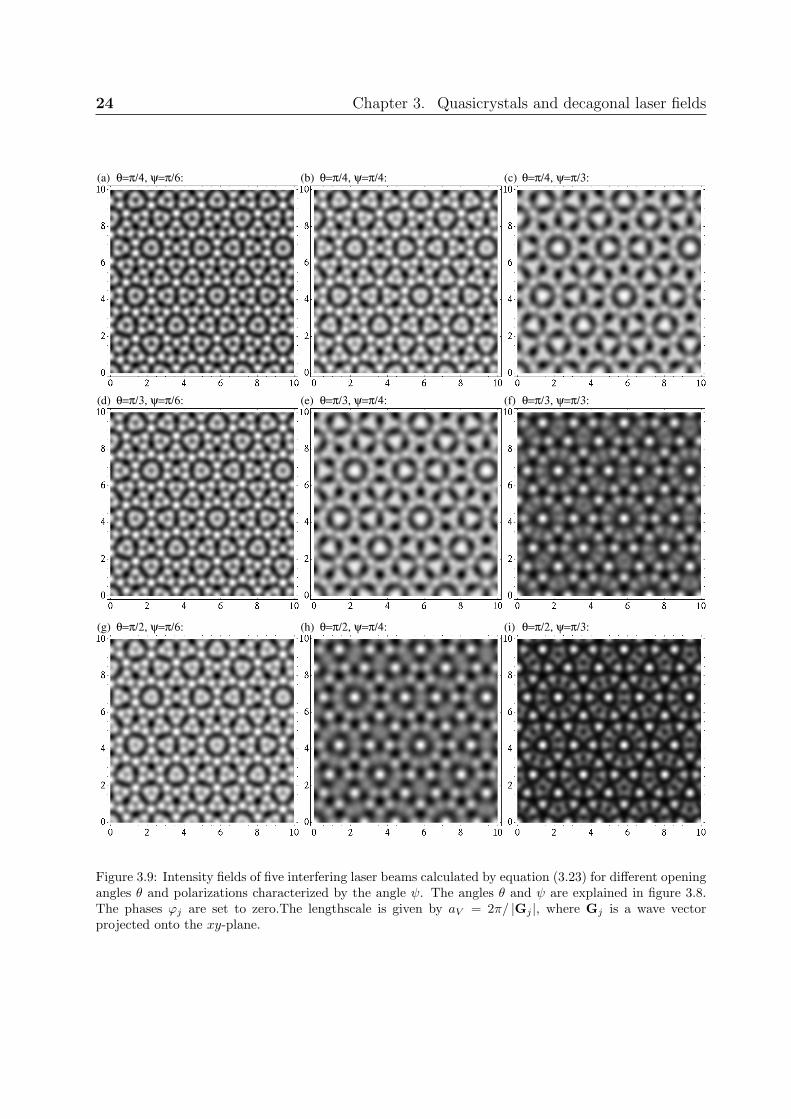
Figure 3.9: Intensity fields of five interfering laser beams calculated by equation (3.23) for different openingangles θ and polarizations characterized by the angle ψ. The angles θ and ψ are explained in figure 3.8.The phases ϕj are set to zero.The lengthscale is given by aV = 2π/ |Gj |, where Gj is a wave vectorprojected onto the xy-plane.

3.3. Quasicrystalline laser fields 25
θ
Figure 3.10: For the standard decagonal laser field, the five laser beams all have the same polarization.The opening angle θ between a beam and the symmetry axis is assumed to be small.
where Gj are the wave vectors projected onto the xy-plane (see figure 3.5) and r = (x, y) isthe position in the xy-plane. A beam has the time period T = 2π/ω, the phase ϕj, and theelectric field vector Ej. To really obtain a perfect rotational symmetry the polarizationsvectors Ej of the beams have to be chosen in a symmetric way (see e.g. figure 3.8). Infigure 3.9 examples of interference patterns that are obtained by five laser beams withoutphase differences are shown for different polarizations and opening angles.
In an experiment, it is easier to realize a configuration, where all beams are polarizedin the same direction (see figure 3.10). For a finite opening angle θ > 0, the resultingintensity pattern no longer has perfect rotational symmetry. However, in experiments, θusually is very small. Therefore, in the following we assume the limit θ → 0 in equation(3.23) and find potentials with perfect rotational symmetry:
V (r) ∝ −n−1∑j=0
n−1∑k=0
cos [(Gk −Gj) · r + ϕk − ϕj] . (3.24)
In figure 3.11 such intensity patterns for different numbers of beams with identical phasesare shown. Note, all patterns have a center of perfect rotational symmetry at (x, y) = (0, 0).

26 Chapter 3. Quasicrystals and decagonal laser fields
(c) 5 beams:(b) 4 beams:(a) 3 beams:
(f) 8 beams:(e) 7 beams:(d) 6 beams:
(i) 11 beams:(h) 10 beams:(g) 9 beams:
Figure 3.11: Interference patterns of different numbers of beams with identical polarization vectors andphases ϕj calculated according to equation (3.24). The length scale is given by aV = 2π/ |Gj |, where Gj
is the projection of the wave vector of a laser beam onto the xy-plane.

3.3. Quasicrystalline laser fields 27
3.3.2 The standard decagonal potential
The decagonal standard potential is obtained by five laser beams with the same polarizationvectors as shown in figure 3.10 in the limit θ → 0 for the opening angle. Using (3.24), wefind
V (r) = −V0
25
4∑j=0
4∑k=0
cos [(Gk −Gj) · r + ϕk − ϕj] , (3.25)
where Gj are the five wave vectors projected onto the xy-plane as shown in figure 3.5 andϕj are the phases of the beams. The prefactor is chosen such that −V0 is the depth of thedeepest potential minimum.
Grey-scale representations as well as a three-dimensional plot of the landscape of thepotential energy are shown in figure 3.12. Some local structures repeatedly occur in thepotential. Examples are a deep minimum surrounded by a broad ring with almost ten-fold rotational symmetry [see left-hand side of figure 3.12(a)] and weak minima forminga pentagon surrounded by another pentagon of deeper minima [right-hand side of figure3.12(a)]. Another striking feature of the potential are perfect lines of low intensity [cf.black lines in figure 3.12(b)] that appear in five directions. If all phases ϕj are set tozero, the decagonal intensity pattern possesses a center of perfect rotational symmetry atx = y = 0. However, the potential contains a lot of points that are very similar to theperfect symmetry center. Therefore, the uniqueness of the perfect center will be neglectedin the following. Furthermore, after certain translations of the intensity pattern, which willbe explained in detail in section 4.3.2, the potential is very similar to the original one. As aconsequence, the actual position where the simulation box of our numerical investigationsis placed within the potential does not affect the results.
In the following, we define the length scale aV of the potential with the help of theprojected wave vectors Gj of the laser beams according to aV = 2π/ |Gj|.
3.3.3 Distribution of depths of the minima
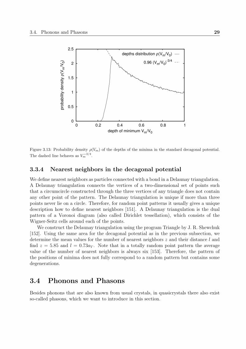
As can be seen in figure 3.12(c), the potential mainly consists of a pattern of wells. Animportant function characterizing the decagonal laser field is the probability to find a wellof a certain depth. We therefore determine the probability density ρ(Vm) for a minimum tohave a potential value between −Vm and −Vm + dVm. The distribution is plotted in figure3.13. In literature it is known that such distributions often are very complicated [150].However, here we find a continuous distribution which, interestingly, for deep minimabehaves like V
−3/4m . Furthermore, minima with depths below Vm/V0 < 0.24 do not exist
indicating that the potential mainly consists of quiet deep wells.
The depths distribution ρ(Vm) is obtained in a rectangular area of the potential byanalyzing all local minima. Because the potential is not periodic, the area has to bechosen in a way, that it well represents the whole potential. We explain the method tofind such an area in section 4.3. We just note that we analyzed 24094 minima in the areagiven by 0 ≤ x < 110aV and 0 ≤ y < 89aV / sin(2π/5).

28 Chapter 3. Quasicrystals and decagonal laser fields
(a)
(c)
(b)
V/V0
Figure 3.12: Standard decagonal potential. The length scale is given by 2π/ |Gj |, where Gj is the projectionof the wave vector of a laser beam onto the xy-plane (see figure 3.5). All phases ϕj are set to zero.
3.4. Phonons and Phasons 29
0
0.5
1
1.5
2
2.5
0 0.2 0.4 0.6 0.8 1
pro
ba
bili
ty d
ensity ρ
(Vm
/V0)
depth of minimum Vm/V0
depths distribution ρ(Vm/V0)
0.96 (Vm/V0)-3/4
Figure 3.13: Probability density ρ(Vm) of the depths of the minima in the standard decagonal potential.The dashed line behaves as V −3/4
m .
3.3.4 Nearest neighbors in the decagonal potential
We define nearest neighbors as particles connected with a bond in a Delaunay triangulation.A Delaunay triangulation connects the vertices of a two-dimensional set of points suchthat a circumcircle constructed through the three vertices of any triangle does not containany other point of the pattern. The Delaunay triangulation is unique if more than threepoints never lie on a circle. Therefore, for random point patterns it usually gives a uniquedescription how to define nearest neighbors [151]. A Delaunay triangulation is the dualpattern of a Voronoi diagram (also called Dirichlet tessellation), which consists of theWigner-Seitz cells around each of the points.
We construct the Delaunay triangulation using the program Triangle by J. R. Shewchuk[152]. Using the same area for the decagonal potential as in the previous subsection, wedetermine the mean values for the number of nearest neighbors z and their distance l andfind z = 5.85 and l = 0.73aV . Note that in a totally random point pattern the averagevalue of the number of nearest neighbors is always six [153]. Therefore, the pattern ofthe positions of minima does not fully correspond to a random pattern but contains somedegenerations.
3.4 Phonons and Phasons
Besides phonons that are also known from usual crystals, in quasicrystals there also existso-called phasons, which we want to introduce in this section.
30 Chapter 3. Quasicrystals and decagonal laser fields
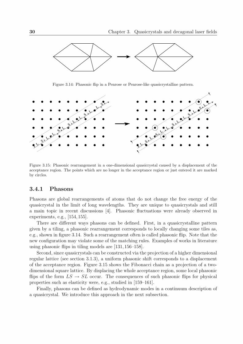
Figure 3.14: Phasonic flip in a Penrose or Penrose-like quasicrystalline pattern.
L
L
L
L
L
S
S
SL
L
S
SL
L
L
L
L
L
L
L
LS
S
S
S
S
Figure 3.15: Phasonic rearrangement in a one-dimensional quasicrystal caused by a displacement of theacceptance region. The points which are no longer in the acceptance region or just entered it are markedby circles.
3.4.1 Phasons
Phasons are global rearrangements of atoms that do not change the free energy of thequasicrystal in the limit of long wavelengths. They are unique to quasicrystals and stilla main topic in recent discussions [4]. Phasonic fluctuations were already observed inexperiments, e.g., [154,155].
There are different ways phasons can be defined. First, in a quasicrystalline patterngiven by a tiling, a phasonic rearrangement corresponds to locally changing some tiles as,e.g., shown in figure 3.14. Such a rearrangement often is called phasonic flip. Note that thenew configuration may violate some of the matching rules. Examples of works in literatureusing phasonic flips in tiling models are [131,156–158].
Second, since quasicrystals can be constructed via the projection of a higher dimensionalregular lattice (see section 3.1.3), a uniform phasonic shift corresponds to a displacementof the acceptance region. Figure 3.15 shows the Fibonacci chain as a projection of a two-dimensional square lattice. By displacing the whole acceptance region, some local phasonicflips of the form LS → SL occur. The consequences of such phasonic flips for physicalproperties such as elasticity were, e.g., studied in [159–161].
Finally, phasons can be defined as hydrodynamic modes in a continuum description ofa quasicrystal. We introduce this approach in the next subsection.

3.4. Phonons and Phasons 31
3.4.2 Hydrodynamic modes
Hydrodynamic modes are excitations in a system that do not change the free energy inthe limit of long wavelengths. Following the work of Socolar et. al. [3], we determine thehydrodynamic modes in a continuum picture where the crystal or quasicrystal is given bya density field ρ(r). We consider an expansion of the free energy F in terms of ρ(r):
F =
∫dA
∞∑k=1
Bkρ(r)k. (3.26)
Bk are coefficients that depend on the details of the actual system and the integration isover the whole plane. With the Fourier series for the density,
ρ(r) =∑
j
ρj exp (−iGj · r) , (3.27)
where Gj are reciprocal lattice vectors and ρj the corresponding Fourier components, thefree energy then is
F =
∫dA
∞∑k=1
Bk
∑j1,...,jk
k∏l=1
ρjlexp
(−i
k∑l=1
Gjl· r
)
= A
∞∑k=1
Bk
∑j1,...,jk
δ
(k∑
l=1
Gjl
)k∏
l=1
ρjl. (3.28)
Here A is the area of the system and the Kronecker symbol δ(∑k
l=1 Gjl
)is 1 if
∑kl=1 Gjl
=
0 and zero in all other cases. Setting ρj = |ρj| exp (iϕj), we find
F = A∞∑
k=1
Bk
∑j1,...,jk
δ
(k∑
l=1
Gjl
)k∏
l=1
|ρjl| exp
(i
k∑l=1
ϕjl
)(3.29)
and realize that the free energy only depends on the sum of all phases∑k
l=1 ϕjl. Therefore,
collective changes in all phases that do not affect the sum of the phases will help to identifyhydrodynamic modes. In the next paragraph, we determine the number of independentlong wavelength excitations that are given by such collective phase changes.
In an ordered system usually only a small set of reciprocal lattice vectors Gj is con-sidered for expansion (3.29) [cf. section 3.1.3]. To construct density fields with the rightpoint symmetry, often stars of lattice vectors such as the ones shown in figures 3.5 or 3.16and their negative vectors are used. The minimal number of vectors in a star is connectedto the number of base vectors of the reciprocal lattice. For example, in periodic crys-tals the minimal number of base vectors to construct the reciprocal lattice is equal to thenumber of dimensions of the system. Therefore, a two-dimensional triangular lattice hastwo base vectors. The star describing triangular ordering contains an additional lattice

32 Chapter 3. Quasicrystals and decagonal laser fields
1G
G
0
2
G
Figure 3.16: Lattice vectors of the triangular phase. For the free energy expansion, the inverse latticevectors −G0, −G1, and −G2 have to be added.
vector obtained by applying simple point symmetry operations to the basis. Including thenegative vectors, the total number of lattice vectors to be considered in the free energyexpansion is, at least, six. Because the density ρ(r) is real, one finds |ρG| = |ρ−G| andϕG = −ϕ−G. Therefore, the total number of independent phases in a triangular lattice isthree. To identify hydrodynamic modes the sum of these phases has to stay constant, i.e.,only two independent hydrodynamic modes exist. For infinite wavelength, they correspondto displacements of the whole lattice in x or y direction. Usually, these modes are calledphonons.
In quasicrystals the number of base vectors needed to obtain all lattice vectors is higherthan the number of dimensions of the system. The minimal set of base vectors is given asprojection of the higher-dimensional lattice if the quasicrystal is obtained by the projectionmethod (see section 3.1.3). Another possibility to find the minimal number nG of reciprocalbase vectors is to look on the number ni of incommensurable length scales in each latticedirection. One finds nG = nid, where d is the number of dimensions [3]. In a decagonalquasicrystal, there are two length scales in the direction of each reciprocal vector (seefigure 3.5). As a consequence, the minimal number of lattice vectors needed is four. Thefree energy expansion (3.29) uses the five vectors shown in figure 3.5 and their inverseones, i.e., there are five independent phases ϕj with j = 0..4. To identify hydrodynamicmodes, the sum of these phases has to stay constant. Therefore, we find four independenthydrodynamic modes in a decagonal quasicrystal.
Usually the hydrodynamic modes are defined by changes of the phases ϕj in the fol-lowing way [2,3]:
ϕj = u ·Gj + w ·G3j mod 5 + γ. (3.30)
Here γ corresponds to a global phase change, which is not a hydrodynamic mode, becauseit affects the sum of all phases ϕj. The vector u = (ux, uy) leads to global displacements ofthe whole crystal along u as can be seen when ρj = |ρj| exp (iu ·Gj) is inserted in (3.27).Therefore, u describes the long wavelength limit of phonons. A uniform vector w =(wx, wy) does also not change the free energy and therefore describes the long wavelengthlimit of two additional hydrodynamic modes. They correspond to global rearrangementsusually termed phasons. Examples will be shown in the next subsection.

3.4. Phonons and Phasons 33
x
x
x
x(a) w =0.05a , w =0 (b) w =0.5a , w =0
(c) w =0, w =0.05a (d) w =0, w =0.5a
V V
V Vyy
y y
Figure 3.17: Decagonal potential for constant phasonic displacements. The arrows between the figuresmark dark horizontal lines, that change their position if wy is increased but not if wx is changed.
3.4.3 Examples of phasonic displacements, drifts, and gradientfields
In this subsection we study phasonic displacements. First we consider only constant dis-placements, later the phasonic displacements depend on time or position. We also showthat phasons can be assigned to some direction and determine how phasonic displacementsare related to shifts of the quasicrystal in real space.
In general, hydrodynamic modes found in the previous subsection depend on the po-sition r and the time t. Therefore, the phases are determined by phononic and phasonicdisplacement fields, u (r, t) and w (r, t), according to
ϕj (r, t) = u (r, t) ·Gj + w (r, t) ·G3j mod 5 + γ, (3.31)
i.e., for any given displacement fields, we can calculate the phases and the standard decago-

34 Chapter 3. Quasicrystals and decagonal laser fields
nal potential by using (3.25). Phononic displacement fields are well known from crystals.Therefore, in this subsection we focus on variations of the phasonic displacement field andchoose u = 0. Note that only differences of the phases enter the decagonal potential (3.25).Therefore, it does not depend on the global phase γ at all.
In figure 3.17 examples of intensity patterns with constant phasonic displacements areshown. The potentials are similar to the one with zero phasonic displacement. However,the center of perfect symmetry no longer is in the point (x, y) = (0, 0). A method todetermine its new position, will be described later in this subsection. Since for our studiesthe position of the symmetry center is not important (cf. subsection 3.3.2), potentials withdifferent constant phasonic displacements do not have to be considered separately.
Interestingly, the direction of a phasonic displacement vector w is connected to direc-tions in real space: For phasonic changes in wx-directions, i.e., for changes of wx withconstant wy, the dark horizontal lines in figure 3.17 do not move or disappear [see arrowsbetween figures 3.17(a) and (b)], whereas the lines in all other direction do so. The horizon-tal lines change if wy is increased [see arrows between figures 3.17(c) and (d)]. In general,lines in the direction defined by the vector (x, y) = (cos(mπ/5), sin(mπ/5)) are not affectedby a phasonic displacement along (wx, wy) = (cos[3mπ/5], sin[3mπ/5]) for m = 0..9.
Now we want to describe the connection between phasonic displacements and shiftsof the quasicrystal in real space. In figures 3.18(a-f) three-dimensional snapshots of thepotential landscape are shown for uniform phasonic displacements wy = jτκ/10 with j =0..5, where τ = (1 +
√5)/2 is the number of the golden ratio (see subsection 3.2) and
κ =1
10
√10− 2
√5)aV =
4
5sin (4π/5) aV . (3.32)
As usual, aV = 2π/Gj and Gj is the length of a wave vector of the laser beam projectedonto the xy-plane. As we will show in the following, phasonic displacements chosen insuch a way reveal interesting properties of their relation to uniform phononic shifts. Theminima in the front, i.e., at y = 0, slowly vanish, however for wy = τκ/2 new minimaappear along a line y = κ/2 [dashed line in figure 3.18(f)]. Furthermore, as shown infigures 3.18(a), (g) and (i), for wy = τκ or wy = 2τκ the potential is identical to theone without phasonic displacement but shifted by κ or 2κ in y-direction, i.e., there is aconnection between potentials with a phasonic displacement and shifted intensity pattern.

3.4. Phonons and Phasons 35
x(a) w =0, w =0 y
x/a
y/a
V/V0
V
V
x/a
y/a
V/V0
V
V
x/a
y/a
V/V0
V
V
x/a
y/a
V/V0
V
V
x/a
y/a
V/V0
V
V
x/a
y/a
V/V0
V
V
x/a
y/a
V/V0
V
V
x/a
y/a
V/V0
V
V
x/a
y/a
V/V0
V
V
x(c) w =0, w = τκ/5y
x(f) w =0, w = τκ/2y
x(i) w =0, w = 2τκy
aV
aV aV
aVaV
aV
aV
aV
x(b) w =0, w = τκ/10y
x(e) w =0, w = 2τκ/5yx(d) w =0, w = 3τκ/10y
x (g) w =0, w = τκy x(h) w =0, w = 3τκ/2y
Figure 3.18: Potential landscape for different phasonic displacements wy. It is τ = (1 +√
5)/2 andκ = 4 sin(4π/5)aV /5. The dashed lines mark rows of minima described in the text.
In general, for the potential Vwx,wy(x, y) with a phasonic displacement wx and wy, we find
Vwx+∆wx,wy+∆wy (x, y) = Vwx,wy (x−∆x, y −∆y) (3.33)
with ∆wx = −9∑
m=0
jmτκ sin (3mπ/5) ,
∆wy =9∑
m=0
jmτκ cos (3mπ/5) ,
∆x = −9∑
m=0
jmκ sin (mπ/5) ,
and ∆y =9∑
m=0
jmκ cos (mπ/5) ,

36 Chapter 3. Quasicrystals and decagonal laser fields
where jm for m = 0..9 are integer numbers. If only one jm is non-zero, the displacement isin a direction perpendicular to dark lines in the intensity pattern. By choosing appropriatenumbers jm, displacements in other direction can be realized. For example a displacementin x-direction is found for non-zero integer numbers j = j7 = j8 or j′ = j6 = j9. Note thedisplacements that can be described by (3.33) lie dense in the plane, i.e., for every givenphasonic or real space displacement, (∆wx,∆wy) or (∆x,∆y), integer numbers jm can bechosen such that the displacement given by these numbers and (3.33) is arbitrarily close to(∆wx,∆wy) or (∆x,∆y). As a consequence, for every positive number ∆V and for everyphasonic displacement, a displacement in real space can be found such that the difference ofthe shifted pattern and the potential with phasonic displacement in every point is smallerthan ∆V . Furthermore, in all potentials with constant phasonic displacements, therealways is a symmetry center which is arbitrarily close to the center of perfect symmetry. Fora phasonic displacement (∆wx,∆wy) given by integers jm and (3.33), a perfect symmetrycenter is located in (∆x,∆y).
In addition, changes of the intensity patterns caused by variations of the phasonic dis-placements can be studied for a simplified potential that one obtains by averaging thedecagonal light field along a direction, where lines of low intensity exist, e.g., along thex-direction. The advantage of such an average is that it only depends on one space co-ordinate. Moreover, since an average along a direction defined by the vector (x, y) =(cos[mπ/5], sin[mπ/5]) (for m = 0..9) corresponds to an average over a phasonic displace-ment along (wx, wy) = (cos[3mπ/5], sin[3mπ/5]), the average one-dimensional potentialonly has one remaining phasonic degree of freedom. For example, 〈V 〉x = 〈V 〉wx onlydepend on y and wy where 〈V 〉x and 〈V 〉wx are obtained by averaging the full potentialover x or wx. Here we study the properties of 〈V 〉x = 〈V 〉wx in more detail. We find
〈V 〉x =V0
25−5− 2 cos (k1 [τwyy])− 2 cos (k2 [wy/τ − y]) (3.34)
with k1 =4π√5τκ
=
√10− 2
√5π
aV
and k2 =4π√5κ
=
√10 + 2
√5π
aV
= τk1.
A minimum of 〈V 〉x corresponds to a row of minima in the two-dimensional potential. Therelation corresponding to (3.33) is
〈Vwy+j∆wy/2 (y)〉x = 〈Vwy (y − j∆y/2)〉x (3.35)
with ∆wy = τκ and ∆y = κ. Note that the allowed displacements here are half ofthose found for the decagonal potential. Figure 3.19 shows 〈V 〉x for different phasonicdisplacements wy. For increasing wy, the minimum originally at y = 0 first becomesshallower, drifts right, and becomes deeper again [see figure 3.19(a)]. This will be importantin section 8.5.1 where we study the Brownian motion of colloids in the decagonal potentialunder the influence of a phasonic displacement that increases at a constant rate in time.The property given by (3.35) is illustrated in figure 3.19(b). At phasonic displacements

3.4. Phonons and Phasons 37
-0.6
-0.5
-0.4
-0.3
-0.2
-0.1
0
-0.2 0 0.2 0.4
<V
>x/V
0
y/aV
wy=0wy=0.1τκ
wy=0.2τκ
wy=0.3τκ
wy=0.4τκ
wy=0.5τκ
-0.6
-0.5
-0.4
-0.3
-0.2
-0.1
0
0 0.5 1 1.5 2 2.5 3
<V
>x/V
0
y/aV
wy=0wy=τκ/2wy=τκ
(a) (b)
Figure 3.19: Average 〈V 〉x = 〈V 〉wxof the decagonal potential over x or wx for different phasonic displace-
ments wy. (a) The minimum originally at y = 0 is moving in y-direction for increasing wy. First it getsshallower, than deeper again (see points and arrows). (b) For wy = j∆wy/2 = jτκ/2 with τ = (1+
√5)/2
and κ = 4 sin(4π/5)aV /5 the averaged potential 〈V 〉x corresponds to the one for wy = 0 displaced byj∆y/2 = jκ/2.
wy = j∆wy/2 the averaged potential 〈V 〉x corresponds to the one for wy = 0 shifted byj∆y/2.
As we have shown for the decagonal laser field as well as for the averaged pattern, thesepotentials change in a very interesting way when the phasonic displacement is increased.To study the behavior of a colloidal suspension in such a varying potential, we will usephasonic displacements that increase at a constant rate in time, i.e., (wx, wy) = (vwxt, vwyt).Because an increase of a phononic displacement ux or uy according to (ux, uy) = (vxt, vyt)results in a drift of the system, we term the corresponding process for phasons a phasonicdrift. The rate of increase (vwx , vwy) is named phasonic drift velocity.
Finally, we consider phasonic displacement fields wx(x, y) and wy(x, y). A special caseis a field that linearly increases along one direction, i.e., a field with constant gradients∇wx(x, y) and ∇wy(x, y), which we call phasonic gradients. Figure 3.20 shows examplesof decagonal light patterns with phasonic gradients. The lines of low intensity are infinitealong a direction of zero phasonic gradient or along a direction given by the phasonicdisplacement vector, the dark lines in other directions only have finite length as indicatedby dashed lines. As we will show in section 7.2, the light field in the experiment usuallycontains phasonic gradients that lead to a prefered direction of the system.

38 Chapter 3. Quasicrystals and decagonal laser fields
xx
x x
x y x y
(a) w =0.005 x, w =0 (b) w =0.015 x, w =0
(d) w =0.15 x, w =0(c) w =0.05 x, w =0
(e) w =0, w =0.005 y (f) w =0, w =0.05 y
y
y y
y
Figure 3.20: Decagonal potential with phasonic gradients. For ∇wx 6= 0 and wy = const. (a-d) or forphasonic displacements that only depend on y (e,f), the horizontal dark lines have infinite length as in thepotential without phasonic displacements. The lines in other directions [see, e.g., white lines in (a) and(b)] only have finite length.

3.4. Phonons and Phasons 39
3.4.4 Indexing problem
The analysis of a quasicrystalline point pattern, for example given by the positions ofcolloids in a decagonal potential, is a very difficult task. Especially, the detection ofphasonic displacements is highly non-trivial. In this subsection, we present a methodhow uniform phasonic displacements can be detected by analyzing a quasicrystalline pointpattern. A widely used ansatz in crystallography considers quasicrystals as projections ofregular crystals in a higher-dimensional space (see section 3.1.3). In principle, one triesto find the point in the high-dimensional space that corresponds to a certain point in thequasicrystalline pattern (see e.g. [162–165]). However, due to problems explained in detailin the following, we do not use the method in this work.
A two-dimensional decagonal quasicrystal can, e.g., be considered as projection of afour-dimensional lattice. A point (x, y) in the 2D pattern is connected to a point in thefour-dimensional space (a1, a2, a3, a4) according to (see e.g. [159])
x = a1v1 + a2v2
y = a3v3 + a4v4, (3.36)
where vj are the typical length scales in the quasicrystal; v1, v2 belong to the x-directionand v3, v4 to the y-direction. If one assumes that the lattice in higher-dimensional spaceis a cubic lattice, the numbers aj for j = 1..4 have to be integers. Typical length scales inthe standard decagonal potential are
in x-direction: v1 = aV and v2 = τaV ,
in y-direction: v3 = aV sin(4π/5) and v4 = aV sin(2π/5) = τv3. (3.37)
As an example, we use the pattern consisting of the positions (x, y) of local minima in thedecagonal potential (see also section 3.3.3). We search for integer numbers that best fulfillthe equations in (3.36). Of course, only a certain range of numbers aj can be scanned. Wechoose a range determined by Fibonacci numbers, because v2/v1 = τ and v4/v3 = τ can beapproximated as ratio of large Fibonacci numbers (see section 3.2). In figure 3.21(a) twocoordinates of the points in four-dimensional space are plotted. The points form elongatedclusters, which correspond to the acceptance regions, i.e., only points in these regions wereprojected onto the two-dimensional plane to obtain the quasicrystalline pattern. Notethat the acceptance regions themselves form a lattice. In the example we introduced insection 3.1.3 to construct a Fibonacci chain (see figure 3.4), the acceptance area was aconnected region consisting of a stripe limited by two lines. To obtain a Fibonacci chaina two-dimensional square lattice was projected. In general, one can also considers othertypes of higher-dimensional lattices or even lattices with a non-trivial basis. It is possible,to map such non-cubic lattices on a cubic one, however a connected acceptance regionin the non-cubic lattice then corresponds to disconnected acceptance areas for the cubiclattice (see e.g. [166–168]). Therefore the disconnected acceptance clusters we find here fora four-dimensional cubic lattice probably corresponds to a connected acceptance region fora non-cubic lattice, possibly also with a non-trivial basis.

40 Chapter 3. Quasicrystals and decagonal laser fields
10
15
20
25
30
0 5 10 15 20
a4
a3
-5
0
5
10
15
20
25
30
35
40
-5 0 5 10 15 20 25 30 35 40
a4
a3
(a) (b)
Figure 3.21: Coordinates a3 and a4 of points in four-dimensional space, whose projection gives the posi-tions of local minima of the decagonal potential (a) without phasonic displacement an (b) for phasonicdisplacements wy = 0 (circles), wy = 0.15aV (squares), and wy = 0.3aV (crosses). A cluster of theacceptance region is marked by lines as guide to the line. Solid lines are used for wy = 0, dashed forwy = 0.15aV , and dotted ones for wy = 0.3aV .
In figure 3.21(b) the coordinates a3 and a4 are shown for different phasonic displace-ments wy. As a guide to the eye a cluster is roughly marked by lines. The acceptanceregions seem to be slightly shifted to the right for increasing phasonic displacement (cf.figure 3.15). In principle, the observed shift can be used to determine the phasonic dis-placement of the original quasicrystalline pattern.
The method presented in this subsection has some severe drawbacks. First, the limita-tion of range for the integers aj is arbitrary and has some influence on the result. Second,the points found in four-dimensional space are scattered even for a perfect pattern given bythe positions of local minima. An analysis of the positions of colloidal particles probablyhas even worse quality due to random fluctuations. Third, the form of the acceptanceregion is not clear, however, to use this method to determine phasonic displacements, thebehavior of the acceptance region has to be known. In summary, the method of indexingpresented here in principal is working, but the quality of the results is to low to be usefulfor the analysis of quasicrystalline colloidal patterns.

3.5. Induced Quasicrystals 41
3.5 Induced Quasicrystals
In this work we consider colloidal suspensions exposed to decagonal laser fields in orderto induce quasicrystalline ordering. Our system is a model system whose behavior can becompared to many other situations. Some examples are given in this section.
3.5.1 Quasicrystalline films
The most important examples for induced quasicrystals are patterns of atoms on the sur-face of quasicrystals [5, 7–13]. Usually the free surfaces of Al-Ni-Co, which has decagonalsymmetry, or of the alloy Al-Pd-Mn with icosahedral symmetry are taken as substrates.Their surfaces act as a five- or ten-fold symmetric potential for the adatoms (see e.g. [5,6]).Often noble gases, such as Ar or Xe, or metallic atoms such as Ag, Au, or Cu were usedas adatoms, i.e., atoms that do not form quasicrystals without substrate. It is very diffi-cult to analyze the local ordering, because the positions of the atoms cannot be observeddirectly. Usually the structure factor is determined, revealing liquid or triangular phasesand sometimes a quasicrystalline ordering with the same symmetry as the substrate, e.g.,decagonal ordering was found on decagonal surfaces. Ledieu et. al. observed an orderingcontaining lines at distances given by a Fibonacci chain [11]. These lines can be part of adecagonal structure or a more complex ordering such as the Archimedean tiling phase thatwill be explained in detail in section 7.1.5. A phase with twenty bond directions, which wedescribe in section 7.1.3, has not been found yet.
There are also grand-canonical simulations of noble atoms on quasicrystalline surfaces[14–17] and recently, works using molecular dynamics simulations have been published[18,19]. As in the experimental works, the ordering is usually determining by the structurefactor, leading to similar results as in the experiments. The local structure has not beenanalyzed yet and a phase with twenty bond directions or an Archimedean tiling phase hasnot been reported.
The behavior of atoms on the surfaces of quasicrystals is important for a large number ofapplications (see also [5,124] for an overview). Quasicrystals can be employed as catalysts,e.g., an AlCuFe quasicrystal efficiently catalyzes the steam reforming of methanol, i.e., thereaction CH3OH + H2O → 3H2 + CO2 that is used to produce hydrogen from methanoland water [169]. The low friction and the good corrosion-resistance of quasicrystals alsolead to possible applications, for instance, the development of new wear-resistant or non-sticky materials [170–172]. Furthermore, the dynamics of adatoms on surfaces probablyinfluences the growth of quasicrystals (see also section 8.7).
3.5.2 Atomic clouds in quasicrystalline traps
Laser beams can also be employed to trap a gas of atoms and to cool it. Usually the beamsare combined with magnetic fields in so-called optomagnetic traps. In such a trap, it ispossible to achieve Bose-Einstein condensation, i.e., a cloud of bosonic atoms, which alloccupy the same quantum mechanical ground state [173]. By using five laser beams, a

42 Chapter 3. Quasicrystals and decagonal laser fields
decagonal potential was applied to an atomic cloud [174] and the diffusion of atoms wasstudied in such a potential [175]. A brief intoduction to atoms in optical lattices in generalis given in [176].
3.5.3 Light-induced quasicrystals in polymer-dispersed liquid-crystal materials
Different laser fields were also used to induce quasicrystalline structures in so-called holo-graphic polymer-dispersed liquid crystal materials [149]. The polymers in such a materialare photopolymers that in combination with a photoinitiator polymerize if exposed to light.If a laser field is applied to a homogeneous mixture of photopolymers, liquid crystal, andphotoinitiator, the polymers polymerize in the brightest regions of the fields and thereforethe liquid crystals diffuse into the dark regions. Finally, most of the liquid crystals are cap-tured in the regions of low intensity of an interference pattern. The system was studied fordifferent numbers of laser beams, achieving quasicrystals with five-, seven-, and nine-foldrotational symmetry [149].
3.5.4 Induced non-linear optical quasicrystal
In a photosensitive nonlinear material, e.g., Sr0.6Ba0.4Nb2O6, the refractive index of light isaffected by the light intensity. Light passing through such a sample can be described by anonlinear equation similar to a nonlinear Schrodinger equation where the time is replacedby the propagation distance. Therefore the evolution of the equation at different points oftime can be studied by analyzing the intensity patterns of the light that passed throughsamples of different thicknesses.
By using the interference pattern of five laser beams, a decagonal quasicrystal can beinduced in the material [177]. If a decagonal interference pattern with a phason-strain fieldis applied, the relaxation of such phasonic strains can be directly observed by looking on thedecagonal pattern for different propagation distances, i.e., for different sample thicknesses[178].

43
Chapter 4
Simulation techniques
In this chapter we present the theoretical background of the simulation techniques anddiscuss the details and tricks used for their implementation. In sections 4.1 Browniandynamics simulations and in section 4.2 Monte-Carlo algorithms are introduced. Becausequasicrystals are not periodic, the choice of the simulation box is not obvious. In section4.3 we present our solution for simulation boxes that fit well to quasicrystals.
4.1 Brownian dynamics simulations
4.1.1 The Langevin equation
Brownian dynamics simulations are used for overdamped systems in contact with a sur-rounding medium which is in thermal equilibrium and therefore has a well-defined tem-perature T . The surrounding medium effectively leads to random thermal forces. Internalparticle-particle interactions or external forces can also be included. The Langevin equationdescribing such a system is derived from Newton’s equation
m∂
∂tv = Ffrict + Fint + Fext + Ftherm, (4.1)
where m is the mass and v the velocity of the particle, Ffrict is the friction force, Fint
the force due to internal interactions, Fext denotes the external and Ftherm the randomthermal forces. Without turbulence, e.g., for small Brownian particles, the friction forcesare proportional to the velocity, i.e., Ffrict = −γv(t) with the friction constant γ. Thefriction constant depends on the size and geometry of the particle and on the viscosity ηof the surrounding liquid, e.g., for small spheres the friction constant according to Stokes’slaw is γ = 6πRη, where R is the radius of the particle. The Langevin equation then is [179](see also e.g. [180])
m∂
∂tv + γv = Fint + Fext + Ftherm. (4.2)

44 Chapter 4. Simulation techniques
The thermal forces have to fulfill the following relations:
〈Ftherm(t)〉 = 0, (4.3)
〈Ftherm,i(t)Ftherm,j(t′)〉 = 2Bδijδ(t− t′), (4.4)
i.e., the average is zero and the thermal forces in different directions or at different timesare totally uncorrelated corresponding to white noise. The strength B is connected to thediffusion constant D of a freely diffusing particle or to the thermal energy kBT and thefriction constant γ. To derive these dependencies, we first calculate the solution of theLangevin equation without interaction or external forces:
v(t) = v(0)e−γm
t + e−γm
t
∫ t
0
dt′1
me
γm
t′Ftherm(t′). (4.5)
By using (4.3) and (4.4), we find the mean square velocity⟨v(t)2
⟩= v(0)2e−2 γ
mt + e−2 γ
mt
∫ t
0
dt′∫ t
0
dt′′1
m2e
γm
(t′+t′′) 〈Ftherm(t′) · Ftherm(t′′)〉
= v(0)2e−2 γm
t +(
1− e−2 γm
t) nBmγ
, (4.6)
where n is the number of dimensions. For long times t m/γ, one finds⟨v(t)2
⟩=nB
mγ. (4.7)
Employing the equipartition theorem m〈v(t)2〉/2 = nkBT/2, a relation of the strength Bto the thermal energy kBT follows:
B = kBTγ. (4.8)
On the other hand, the mean square displacement in the long-time limit is⟨[r(t)− r(0)]2
⟩=
1
γ2
∫ t
0
∫ t
0
dt′dt′′ 〈Ftherm(t′) · Ftherm(t′′)〉
=1
γ2
∫ t
0
∫ t
0
2nBδ(t′ − t′′)dt′dt′′ =2nB
γ2t. (4.9)
The free diffusion constant D is defined by⟨(r(t)− r(0))2⟩ = 2nDt, (4.10)
which givesB = Dγ2. (4.11)
Now, combining (4.8) and (4.11), we find the famous Einstein relation (cf. [181])
D =kBT
γ. (4.12)
4.1. Brownian dynamics simulations 45
In the following, we are only interested in the dynamics of our system on time scalesmuch larger than the very short momentum relaxation time m/γ, which for micron-sizedparticles in water is approximately 10−7s. Then the inertial term m ∂
∂tv(t) is much smaller
than the other terms in (4.1) and can, therefore, be neglected. Such a system is also calledoverdamped.
4.1.2 Discretized equation and simulation details
The overdamped Langevin equation reads
γv = Fint + Fext + Ftherm. (4.13)
For the Brownian dynamics simulations, we discretize equation (4.13). The position attime t+ ∆t is
r(t+ ∆t) = r(t) +∆t
γ(Fint(t) + Fext(t) + Ftherm(t)) . (4.14)
The thermal force is realized by random kicks: At each simulation step a randomly gen-erated number is used as thermal force. The probability distribution of these randomnumbers is not important, as long as (4.3) and (4.4) are satisfied, i.e., if the average of therandom numbers is zero, if the probability distribution does not depend on time or previousrandom numbers, and if the second moment is chosen correctly. The last requirement isrelated to the free diffusion constant that follows from the random numbers: According to(4.14) and for Fint = Fext = 0, the mean square displacement is
⟨(r(t)− r(0))2⟩ =
⟨∆t
γ
t/∆t∑j=0
Ftherm(j∆t)
2⟩
=∆t2
γ2
t/∆t∑j=0
⟨Ftherm(j∆t)2
⟩=
∆t2
γ2
t
∆t
⟨F2
therm
⟩. (4.15)
Here we used the facts that the random forces at different times are uncorrelated, i.e.,〈Ftherm(j∆t) · Ftherm(k∆t)〉 = 0 for j 6= k and that the probability distribution is time-independent 〈Ftherm(j∆t)2〉 = 〈F2
therm〉. From equations (4.15), (4.10), and the Einsteinrelation (4.12), we find that thermal kicks have to comply with
⟨F2
therm
⟩=
2nγkBT
∆t. (4.16)
Gaussian distributed random numbers centered around zero with a second moment of2nγkBT/∆t are a possible choice for simulations. However, generating equally distributedrandom numbers is easier and faster. Therefore, we usually use random kicks in a randomdirection with lengths evenly distributed between 0 and
√12γkBT/∆t, where the prefactor

46 Chapter 4. Simulation techniques
of the upper limit follows from the requirement for the second moment (4.16). We tested ourprogram with Gaussian as well as with evenly distributed random numbers and obtainedthe same results. Without interactions and external forces, we find the constant of freediffusion exactly as predicted by the Einstein relation (4.12).
To produce random numbers, we use a pseudo-random number generator called MersenneTwister mt19937 [182,183] that according to the documentation of the GNU Scientific Li-brary is one of the fastest algorithm appropriate for scientific simulations [184].
The quality and the speed of the simulations depend on the choice of the time stepduration ∆t. The easiest way to accelerate the simulations is to increase ∆t. However, theupper limits of ∆t are:
• The time scale we are interested in when analyzing the results. This time must bemuch larger than a single-step duration so that the results are averaged over enoughrandom kicks.
• If the step duration ∆t is too long, a particle can be kicked over a deep potential well,which then is not recognized in the simulation. Therefore, the step length should besmall compared to the length scale of the potential.
Usually, the second requirement leads to much smaller values of ∆t. In our simulations wechoose an upper limit of ∆t at 0.005βγa2
V for single colloids (in chapter 8) and 0.001βγa2V
for many particle systems (chapters 6 and 7), where β = 1/(kBT ) and aV is the typicallength in the potential, e.g., the modulation length in the one-dimensional potential or inthe decagonal potential (see sections 6.1, 6.3 or 3.3) or the distance between minima inthe square potentials (section 8.2.1). To prevent the occurrence of steps that are too long,we calculate the step length for the case of the maximum possible thermal kick perfectlyaligned with the other forces before every step. If this length is larger than a threshold∆l, we reduce the size of ∆t until the step length is always smaller than ∆l. Therefore, onthe one hand, no important features of the potential are missed. On the other hand, thetime steps are not smaller than necessary. We usually choose ∆l = 0.02aV as thresholdin the decagonal potential (in chapters 7 and 8) and ∆l = 0.1aV in the one-dimensionalquasicrystalline potential (chapter 6). We tested our program with different values of ∆tand ∆l, with constant as well as with adaptive step duration. We found no differencesbetween simulations with our standard procedure and runs with smaller steps in time orlength.
4.2 Monte-Carlo simulations
We use the Monte-Carlo algorithm originally introduced by Metropolis et. al. [185], whichtoday is a standard method in computational physics [186,187]. The Metropolis algorithmallows to treat the system in a canonical ensemble, i.e., the single configurations occur witha probability given by the Boltzmann factor exp(−βE), where E is the total energy of thesystem and β = 1/(kBT ) the inverse of the thermal energy. Therefore, the average of an

4.2. Monte-Carlo simulations 47
observable A, e.g., an order parameter, is determined by calculating A for each configura-tion obtained by the simulation and then by averaging over all these configurations. Theresult is the correctly weighted average 〈A〉 of a canonical ensemble:
〈A〉 =1
N
∑j result of
MC-simulation
Aj =
∑j Aj exp(−βEj)∑
j exp(−βEj), (4.17)
where N is the number of simulated configurations, Ej the energy and Aj the value of theobservable in configuration j.
According to the Metropolis algorithm, in a Monte-Carlo step, first the configurationof the system is changed randomly. Then the energy Enew of the new configuration iscalculated and compared to the energy Eold of the old one. The simulation is continuedwith the new configuration if Enew < Eold. In case of Enew > Eold, the new configuration isaccepted with a probability proportional to exp (−β[Enew − Eold]). If the new configurationis not accepted, the simulation is continued with the old one. The acceptance probabilitiesare chosen this way, because then the transitions between the configurations exploredduring the simulations satisfy detailed balance, i.e., the ratio of the transition probabilitypj→k to get from state j to state k and the probability of the reverse transition pk→j is
pj→k
pk→j
=exp (−βEk)
exp (−βEj). (4.18)
If the system is ergodic and all possible configurations are explored, relation (4.18) guar-antees that the probability to be in configuration j is proportional to exp (−βEj), i.e., weobtain a canonical ensemble of configurations. In a real simulation it is of course impos-sible to explore all possible configurations. For a good implementation of the Metropolisalgorithm it is important to find the configurations with the highest probability, which arethe ones with the lowest energies. Such configurations are usually quiet similar and, there-fore, it is not necessary to consider a completely new configuration at each Monte-Carlostep. It is more convenient to just slightly vary the old one. However, the variation mustbe big enough, at least with some probability, to explore a sufficiently large area of theconfiguration space. The quality of an implementation is mainly given, on the one hand,by the speed of finding the configurations close to the ground state and, on the other hand,by the explored area of the configuration space.
To obtain a new configuration in our implementation of the Metropolis algorithm, wetake a colloid out of the system and place it at a random position. The energy is calculatedand, according to the Metropolis algorithm, it is decided, whether the new position isaccepted or not. To get a sufficient number of accepted new configurations, the colloidusually is placed in an area close to its original position. The size of the area is chosensuch that the acceptance rate is approximately 50%: If it is smaller, the placement areais reduced and therefore the new configurations have a higher probability to be accepted.If the acceptance rate is too large, the area is increased. This procedure guarantees thata large number of configurations close to the lowest energy state is explored very fast.
48 Chapter 4. Simulation techniques
However, with such a local displacement procedure one can get stuck to a region of theconfiguration space with a local minimum in energy. In order to find the global minimum,one also has to allow global replacements. For example, it has to be possible to crosshigh energy barriers. Therefore, in our simulations with a probability of 20% a colloidis not placed locally but is put on some random position anywhere in the sample. Toimplement the Metropolis algorithm, we use the same pseudo-random number generatoras for the Brownian dynamics simulations, i.e., the so-called Mersenne Twister mt19937algorithm [182,183].
In one simulation step, the procedure described above is applied to each colloid of thesample, i.e., after one step about one half of the colloids have been replaced. Usuallya simulation is started in a triangular configuration and one million steps are performedto guarantee that the equilibrium of the canonical ensemble is reached. Of course, wealso tested our program with other starting configurations and other step numbers. Wefound that usually after about 100000 steps the system is already close to equilibriumand after about 500000 steps it is equilibrated no matter what starting configuration wasused. Mean values as in (4.17), e.g., order parameters, are calculated as average over 1000configurations: The first configuration is taken after one million equilibration steps andthen always 100 steps are performed before the next configuration is used. To test thatsuch a result is indeed the one of the canonical ensemble, we ran simulations up to 10million steps before calculating the mean values. However, we never found any substantialdeviations.
Recently, a so-called genetic algorithm was introdued to condensed matter physics[188,189] based on general genetic algorithms originally developed by Holland [190]. As ina Monte-Carlo simulation, a new configuration is created and then it is decided whetherto accept the new configuration (this was termed the selection process for genetic algo-rithms). A so-called fitness function, which usually depends on the free energy or freeenthalpy, leads to an acceptance probability similar to the one in Monte-Carlo simulations.The main difference between genetic algorithms and usual Monte-Carlo simulations is theprocess of finding new configurations. In a genetic algorithm, a new configuration (alsocalled individual of a new generation) is usally not obtained by random displacements ofthe particles as in a Monte-Carlo simulation, but by random changes in an abstract rep-resentation (termed genom) of the individual. Furthermore, a new generation can also becreated by combining different parts of old configurations (called recombination process).Genetic algorithms were also applied to colloidal systems [63, 94]. In this work, we onlyuse conventional Monte-Carlo simulations.
4.3 Size of the simulation box
In our simulations, we use periodic boundary conditions. However, the quasicrystallinepotentials as well as any induced quasicrystal are not periodic. Therefore, these structurescan never fit into any simulation box with periodic boundary conditions. However, we

4.3. Size of the simulation box 49
show in this section that special box sizes exist for which there are only minor distortionsor discontinuities at the boundaries.
4.3.1 Approximations for the 1D quasicrystalline potential
In section 6.3 we apply a one-dimensional quasi-periodic potential to the colloidal suspen-sion. The potential is given as sum of two periodic modulations whose wavelengths differby a factor of τ 2, where τ = (1 +
√5)/2 is the number of the golden ratio (see section 3.2).
However, such a potential is not periodic and therefore does not fit into a simulation boxwith periodic boundary conditions. Therefore, we use approximations for τ to obtain aperiodic potential. To be concrete, in our simulations we use the potential
V (r) = −V0
2[cos (Gα · r) + cos (Gβ · r)] , (4.19)
where Gα = ταG0ex, Gβ = (−1/τβ)G0ex; ex is the unit vector in x-direction, and G0 =π/(
√3aS) is the lattice vector connected to the nearest neighbor particle distance aS in the
triangular starting configuration. The number of the golden mean can be approximated bythe ratio of consecutive Fibonacci numbers (see section 3.2). We choose the approximationsτα = 55/34 and τβ = 34/21. The box size is given by xmax = 34 · 2π/G0 = 34
√3aS/2 in
x-direction and ymax = 34/ sin(π/5) ·√
3aS/2 in y-direction. The number of particles inthe box then is 1054. In x-direction the approximated potential (4.19) is perfectly periodicand fits into the simulation box. The box size in y-direction is selected such that a possiblepentagonal colloidal ordering fits as good as possible into the simulation box. This isfulfilled for our choice of ymax since ymax is an integer multiple of both characteristic lengthscales of a pentagonal quasicrystal in y-direction approximated as 2π/G1,y = ymax/34 and2π/G2,y = τ · 2π/G1,y ≈ ymax/21 (see figure 3.5).
4.3.2 Approximations for the decagonal potential
In case of the decagonal potential (see section 3.3), we leave the potential undistorted.Therefore, a particle crossing the box boundary experiences a discontinuity. However, wechoose the box size in a way that the discontinuity is very small. To obtain an appropriaterectangular box, we have to find translations which leave the potential almost unchanged,i.e., a vector (∆x,∆y) such, that V (x, y) ≈ V (x+∆x, y) and V (x, y) ≈ V (x, y+∆y). Thiscan be realized by choosing ∆x and ∆y to be integer multiples of the length scales, whichare given by 2π/Gj,x and 2π/Gj,y, where Gj,x and Gj,y are the components of the projectedwave vectors (see figure 3.5). Then cos(Gj,x∆x) ≈ 1 and cos(Gj,y∆y) ≈ 1 for j = 0, .., 4.The length scales in x-direction are: aV = 2π/G0, 2π/G1,x = 2aV /τ , −2π/G2,x = τaV /2,where again τ = 2 cos(π/5) is the number of the golden mean, which can be approximatedas ratio of successive Fibonacci numbers (see section 3.2). In y-direction we find the lengthscales 2π/G1,y = aV / sin(π/5) and 2π/Ga,y = τaV / sin(π/5). Therefore, appropriate boxsizes are ∆x = 2naV and ∆y = maV / sin(π/5), where n and m are Fibonacci numbers (1,2, 3, 5, 8, 13, 21, 34, 55, 89, ...). We usually use m to be the Fibonacci number following

50 Chapter 4. Simulation techniques
-1
-0.8
-0.6
-0.4
-0.2
0
0 1 2 3 4 5
V/V
0
x/aV
bottomtop (m= 5)top (m= 8)top (m=13)
-1
-0.8
-0.6
-0.4
-0.2
0
0 1 2 3 4 5
V/V
0
y/aV
leftright (n= 5)right (n= 8)right (n=13)
0
0.05
0.1
0.15
0 1 2 3 4 5
(Vto
p-V
bottom
)/V
0
x/aV
m= 5m= 8m=13
-0.1
0
0.1
0.2
0 1 2 3 4 5
(Vright-V
left)/
V0
y/aV
n= 5n= 8n=13
(a)
(b)
(c)
(d)
Figure 4.1: Value of the decagonal potential (a) at the lower (y = 0) and upper (y = ∆y) boundary ofthe simulation box and (b) at the left (x = 0) and right (x = ∆x) side of the box. In (c) the differencesof the upper and lower, in (d) of the left and right sides of the box are plotted in units of the depth V0 ofthe deepest minimum. The box sizes are chosen according to ∆x = 2naV and ∆y = maV / sin(π/5) withFibbonacci numbers m and n.

4.4. Parameter values 51
on n so that the width and height of the simulation box do not differ to much. Figure 4.1shows the potential values at the boundaries. Obviously even for quiet small Fibonaccinumbers the discontinuities are negligible.
For a fixed particle density, thenumber of colloids depends on the chosen box size. Wetry to select one of the allowed box sizes as determined above such that a simulation boxcontains between 400 and 900 colloids. Therefore, finite-size effects are small and, on theother hand, the simulations are not becoming to slow.
4.4 Parameter values
The colloidal particles are not allowed to overlap and their interaction is given by theDerjaguin-Landau-Verwey-Overbeek-theory [see equation (2.1)] with a large-distance cutoffof the potential at 5aS, where aS is the spacing between the colloids if they form an idealtriangular lattice. The interaction parameters together with the properties of the externalpotential determine the parameter set of our system, i.e., the free parameters usually are:the radius R of a colloid, its effective surface charge Z∗, its friction coefficient in waterγ, the dielectric constant of water εr, the inverse Debye screening length κ, the potentialstrength V0, its typical length scale aV , the absolute temperature T , and the colloidaldensity given by the particle spacing aS.
To study the colloidal behaviour in a one-dimensional potential (see chapter 6), we varythe potential strength V0 and the inverse screening length κ. We employ the same valuesfor the parameters as used by Strepp, Sengupta, and Nielaba in their study of a colloidalsuspension in a commensurate periodic potential [32]: R = 0.535 µm, Z∗ = 7800, εr = 78,and the temperature T = 293.15 K. The density is chosen such that the spacing in an idealtriangular lattice would be aS = 2.53 µm. These parameters are also taken for the case ofa low-density suspension in a two-dimensional potential, where there are less colloids thanminima in the potential (see chapter 7). However, there we vary the potential strengthV0 and the density (given by aS) but choose a constant value for the characteristic lengthaV = 2π/ |Gj| = 2.53 µm and the screening length κ−1 = 0.506 µm = aV /5. For the caseof high densities, i.e., where more colloids than minima occupy the simulation box, we useR = 1.2 µm, Z∗ = 1000, εr = 78, T = 300 K, aV = 5.0 µm, and κ−1 = 0.25 µm = aV /20,which leads to a behavior close to the one observed in experiments by Mikhael et al. [20,191].

52 Chapter 4. Simulation techniques
53
Chapter 5
Theory of Melting in 2D
In this chapter we shortly introduce different widely used theories that describe melting intwo dimensions. The Landau-Alexander-McTague theory presented in section 5.1 is basedon an expansion of the free energy with respect to the order parameter. In section 5.2 abrief introduction to density functional theory is given. The probably most sucessful theoryfor melting in two dimensions is the so called KTNHY-theory, named after Kosterlitz,Thouless, Nelson, Halperlin, and Young. It is based on the dissociation of disclination anddislocation pairs and predicts an interesting new phase between the solid triangular and theliquid phase, termed hexatic. Section 5.3 gives a short overview over the main ideas of theKTNHY-theory also with respect to quasicrystals. The theories presented in this chapterwere also employed to explain the phase behavior in a one-dimensional commensurateperiodic potential (see section 6.1). Furthermore, we use the Landau-Alexander-McTaguetheory to study the phase behavior in a laser field with one-dimensional quasicrystallinesymmetry (section 6.3.2).
5.1 Landau-Alexander-McTague theory
The Landau-theory of phase transitions [192, 193] is based on the expansion of the freeenergy with respect to an order parameter. The order parameter is usually zero in thehigh-symmetry phase, e.g., in a liquid, and non-zero in the low-symmetry phase, which fora two-dimensional colloidal system without external potential is the solid triangular phase.By minimizing the free energy, the value of the order parameter in thermal equilibrium isdetermined and therefore the phase of the system.
The Landau-Alexander-McTague theory was first used in 1978 by Alexander and Mc-Tague to compare the free energy of bcc and fcc crystals [194]. Here we shortly introducethe theory for the triangular to liquid transition in a two-dimensional system. The basicidea is to consider a liquid with a homogeneous density ρ and then expand the free energyF with respect to small variations of the density δρ (r) = ρ (r) − ρ, where ρ (r) is the

54 Chapter 5. Theory of Melting in 2D
density field, e.g., the mass density field, in real space (cf. expansion in section 3.4.2):
F =
∫dA
b′
2[δρ(r)]2 − d
6[δρ(r)]3 +
e
24[δρ(r)]4
. (5.1)
The integration is over the whole plane. The signs are chosen such that the parametersb′, d, and e are positive: e has to be positive to have a stable global minimum of the freeenergy and for other signs of d and b′ no phase transition would occur as will be illustratedbelow. To transform the free energy into reciprocal space we use a Fourier series for thedensity variations:
δρ(r) =∑
j
ρje−iGj ·r, (5.2)
where Gj are the relevant reciprocal lattice vectors and ρj the corresponding Fourier com-ponents. The free energy density in reciprocal space then is
FA
=1
2b′∑
j
|ρj|2 −1
6d∑j,k,l
ρjρkρlδ (Gj + Gk + Gl)
+1
24e∑
j,k,l,m
ρjρkρlρmδ (Gj + Gk + Gl + Gm) , (5.3)
where δ(·) denotes the Kronecker symbol, which is 1 if the argument vanishes and zeroin all other cases. There are three parameters in the free energy expansion: b′, d and e.Because it is possible to rescale the free energy density F/A and the Fourier componentsρj, two parameters can be set to unity. We name the rescaled quantities F/A and ρj,introduce the remaining rescaled parameter b, and then write the rescaled free energy as
FA
=1
2b∑
j
|ρj|2 −1
6
∑j,k,l
ρj ρkρlδ (Gj + Gk + Gl)
+1
24
∑j,k,l,m
ρj ρkρlρmδ (Gj + Gk + Gl + Gm) . (5.4)
Since we want to illustrate the triangular to liquid phase transition, Gj are the threelattice vectors G0, G1, and G2 of the triangular phase as shown in figure 3.16 and the in-verse vectors −G0, −G1, and −G2. The third-order term contains contributions where thethree lattice vectors form triangles. The fourth-order term consists of pairs of antiparallelvectors (e.g. Gk = −Gj and Gm = −Gl). No other non-trivial sum of Gj +Gk +Gl +Gm
vanishes. Due to the six-fold rotational symmetry of the triangular phase, all Fourier com-ponents are the same, i.e., ρ0 = ρ1 = ρ2 = ρ. Counting all the contributions, we finallyfind
FA
= 3bρ2 − 2ρ3 + 4ρ4. (5.5)
For b > 3/32 the free energy only has one minimum at ρ = 0. For b < 3/32 there are twominima, for b > 1/12 the minimum for ρ = 0 is the global minimum, but for b < 1/12

5.2. Density functional theory 55
0
0.002
0.004
-0.1 0 0.1 0.2 0.3
fre
e e
ne
rgy d
en
sity
order parameter
b=19/192b=18/192=3/32b=17/192b=16/192=1/12b=15/192
Figure 5.1: Free energy density F/A for the triangular to liquid phase transition [see equation (5.5)] as afunction of the order parameter ρ. The curves are for different values of the control parameter b.
the second minimum with ρ > 0 is deeper (see figure 5.1). The amplitude ρ is the orderparameter of the system. Since it jumps discontinuously from ρ > 0 to ρ = 0 at b = 1/12,there is a first-order phase transition from a triangular ordering at b < 1/12 into a liquidphase at b > 1/12. The control parameter b is usually identified with the temperature butas we will see below, the inverse screening length of the DLVO potential can also controlthe phase transition.
In section 6.1.2 we shortly present the Landau-Alexander-McTague theory for a two-dimensional system under the influence of an one-dimensional periodic potential as in-troduced by Chowdhury, Ackerson, and Clark [28]. We also use this theory to calculatethe phase diagram for colloids in a one-dimensional quasicrystalline potential (see section6.3.2).
5.2 Density functional theory
The density functional theory in condensed matter physics is a widely used method todescribe phase transitions. For a system consisting of simple spherical particles with purepair interactions it was pioneered by Ramakrishnan and Yussouff in the late 70s [195,196](for reviews see e.g. [197–199]). It is, e.g., used to study freezing in three dimensions[200–203] and in two dimensions [204], and to investigate the liquid-solid interface or thecrystallization behavior [205,206].
The basic idea is to calculate the grand canonical potential or the free energy as afunctional depending on the density field ρ(r). The difference of the grand canonical

56 Chapter 5. Theory of Melting in 2D
potential in the solid compared to the liquid phase is [197]
∆Ω [ρ(r)] = kBT
∫dA ρ(r) [ρ(r)/ρ]− ρ(r) + ρ+ F int [ρ(r)]−F int [ρ] , (5.6)
where ρ is the average density and F int is the interaction free energy. The first term in(5.6) corresponds to the grand canonical potential of an ideal gas.
Using a mean-field approach to approximate the interaction free energy F int and solvinga self-consistency condition for the density (for details see e.g. [196]), one finds:
∆Ω [ρ(r)] = −kBT ln Φ [ρ(r)] +∑
j
ρj
2c1(Gj). (5.7)
Here the functional Φ [ρ(r)] is
Φ [ρ(r)] =1
A
∫A
dA exp
[∑j
ρj exp (iGj · r)
], (5.8)
A is the area of the unit cell of the lattice, j is the index of the reciprocal lattice vectors Gj,and ρj are the corresponding Fourier components (see previous section). The constantsc1(Gj) = ρ g(Gj) denote the peak values of the structure factor g(G), which correspondsto the pair correlation function g(|r− r′|) in Fourier space where g(|r− r′|) is given bythe probability to find two colloids at distance |r− r′|. To determine the phase behavior,∆Ω (or the free energy) has to be minimized. Interestingly, the only free parameters arec1(Gj), which is given by the pair correlation function (or the structure factor).
Finally we note that freezing in two dimensions according to the density functionaltheory is a first-order phase transition [204] as it is for the Landau-Alexander-McTaguetheory.
5.3 KTHNY theory
The KTHNY theory of melting in two dimensions was developed and named after Kosterlitzand Thouless [21], Halperin and Nelson [22–25], and Young [26,27]. The basic idea is thatstarting from a perfect lattice an increasing number of defects appear if the temperatureis raised. The defects destroy the order of the crystal and lead to a two-stage transitioninto the liquid phase. Melting in three dimensions usually starts at the surface of thecrystal, whereas in two dimensions the defects can be easily created in bulk and thereforethe surface is not as important. Defect mediated melting for two-dimensional quasicrystalscorresponding to the KTHNY theory was developed by De and Pelcovits [207–210]. Inthe following, we shortly give an overview of the main ideas of this melting theory fortriangular and for decagonal lattices.
In figure 5.2 defects in a triangular lattice are shown. A dislocation characterizesdefects in the translational order of a lattice whereas a disclination describes defects in the
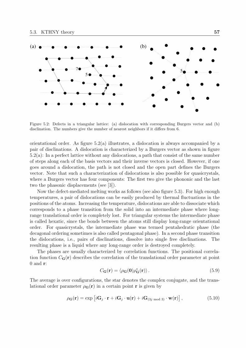
5.3. KTHNY theory 57
(a) (b)
55
7
Figure 5.2: Defects in a triangular lattice: (a) dislocation with corresponding Burgers vector and (b)disclination. The numbers give the number of nearest neighbors if it differs from 6.
orientational order. As figure 5.2(a) illustrates, a dislocation is always accompanied by apair of disclinations. A dislocation is characterized by a Burgers vector as shown in figure5.2(a): In a perfect lattice without any dislocations, a path that consist of the same numberof steps along each of the basis vectors and their inverse vectors is closed. However, if onegoes around a dislocation, the path is not closed and the open part defines the Burgersvector. Note that such a characterization of dislocations is also possible for quasicrystals,where a Burgers vector has four components: The first two give the phononic and the lasttwo the phasonic displacements (see [3]).
Now the defect-mediated melting works as follows (see also figure 5.3). For high enoughtemperatures, a pair of dislocations can be easily produced by thermal fluctuations in thepositions of the atoms. Increasing the temperature, dislocations are able to dissociate whichcorresponds to a phase transition from the solid into an intermediate phase where long-range translational order is completely lost. For triangular systems the intermediate phaseis called hexatic, since the bonds between the atoms still display long-range orientationalorder. For quasicrystals, the intermediate phase was termed pentahedratic phase (thedecagonal ordering sometimes is also called pentagonal phase). In a second phase transitionthe dislocations, i.e., pairs of disclinations, dissolve into single free disclinations. Theresulting phase is a liquid where any long-range order is destroyed completely.
The phases are usually characterized by correlation functions. The positional correla-tion function CG(r) describes the correlation of the translational order parameter at point0 and r:
CG(r) = 〈ρG(0)ρ∗G(r)〉 . (5.9)
The average is over configurations, the star denotes the complex conjugate, and the trans-lational order parameter ρG(r) in a certain point r is given by
ρG(r) = exp[iGj · r + iGj · u(r) + iG(3j mod 3) ·w(r)
], (5.10)

58 Chapter 5. Theory of Melting in 2D
5
5
7
7
5
5
7
7
7
5
(a)
(b)
5
7
Figure 5.3: Dissociation of (a) a dislocation pair and of (b) a dislocation into two disclinations. In bothcases a phase transition takes place.
where u(r) and w(r) are the phononic and phasonic displacement fields at position r, andGj is a lattice vector. Note in a triangular crystal phasons do not occur and w(r) = 0.In a two-dimensional lattice perfect long-range positional order does not exist, i.e., even inthe solid phase CG(r) decays algebraically according to
CG(r) ∝ r−ηG (5.11)
with an exponent ηG that depends on the elastic constants of the lattice (see e.g. [210]).However, perfect long-range orientational correlations can exist in two dimensions. Theorientational correlation function is given by
Cθ,m(r) = 〈ψm(0)ψ∗m(r)〉 , (5.12)
where the bond orientational order parameter ψm(r) in point r is
ψm(r) = exp [imθ(r)] (5.13)
with m = 6 for the triangular and m = 10 in the decagonal lattice; θ(r) is called bondangle field θ(r) and is defined as the angle of a bond between a particle at position r anda nearest neighbor with respect to an arbitrary reference direction (cf. section 7.1.1).

5.3. KTHNY theory 59
Since free dislocations destroy the long-range positional order and free disclinationsalso the long-range orientational order, the correlation functions behave as follows: asalready mentioned, in the solid phase CG(r) decays algebraically whereas Cθ(r) approachesa nonzero constant for r →∞. In the hexatic or pentahedratic phase free dislocations existand CG(r) decays exponentially but Cθ(r) only algebraically. Finally, in the liquid, thefree disclinations lead to an exponential decay of Cθ(r).
By using symmetry arguments, the elastic free energy density up to second order in thestrain variables is given by [2,3]
fel =1
2λuiiuii + µuijuij +
1
2K1wijwij +K2 (wxxwyy − wyxwxy)
+K3 [(uxx − uyy) (wxx + wyy) + 2uxy (wxy − wyx)] , (5.14)
where uij = (∂ui/∂rj + ∂uj/∂ri)/2 and wij = ∂wi/∂rj. The elastic constants are λ, µ, K1,K2 and K3. In a triangular crystal K1 = K2 = K3 = 0. The elastic free energy allowsto calculate the interaction energy between two disclinations or between two dislocations.Therefore, the phase transition temperatures can be determined as unbinding transitions ofthe corresponding defects (see e.g. [25] for triangular crystals and [210] for quasicrystals):The temperature T(m) of the solid to hexatic or pentahedratic transition is given by therelation
c(m),R (λR, µR, K1,R, K2,R, K3,R) =16πkBT(m)
a2S
, (5.15)
where aS is the particle spacing. The transition to the liquid takes place at temperatureT(i) with
c(i),R (λR, µR, K1,R, K2,R, K3,R) = MkBT(i)
π, (5.16)
where M = 72 for the hexatic-liquid and M = 100 for the pentahedratic-liquid tran-sition. Since the interaction between two defects is usually screened by other defectsthe elastic constants have to be renormalized. All constants marked with an index Rare the renormalized quantities of the constants introduced in (5.14). The quantitiesc(m),R (λR, µR, K1,R, K2,R, K3,R) and c(i),R (λR, µR, K1,R, K2,R, K3,R) depend on the elasticconstants; c(i),R (λR, µR, K1,R, K2,R, K3,R) is the Frank constant defined in the free energydensity fθ depending on the variations of the bond angle field θ(r):
fθ =1
2c(i),R (λR, µR, K1,R, K2,R, K3,R)
[(∂θ
∂x
)2
+
(∂θ
∂y
)2]. (5.17)
In certain limits, c(i),R (λR, µR, K1,R, K2,R, K3,R) can be expressed explicitly in terms of λR,µR, K1,R, K2,R, and K3,R depending on the system; c(m),R (λR, µR, K1,R, K2,R, K3,R) is given

60 Chapter 5. Theory of Melting in 2D
by
c(m),R (λR, µR, K1,R, K2,R, K3,R) = 2K1,R
+4K2
3,R (−K2,R + λR + µR) + 2K1,R
[K2
3,R − 2µR (λR + µR)]
K23,R −K1,R (λR + 2µR)
+K1,RK
23,R (−K1,R + 2K2,R) (λR + µR)(
−K23,R +K1,RµR
) [−K2
3,R +K1,R (λR + 2µR)] (5.18)
for quasicrystals and
c(m),R (λR, µR) =4µR (µR + λR)
2µR + λR
(5.19)
for triangular ordering.Nelson and Halperin also predict the phase behavior in commensurate and incommen-
surate potentials as well as on totally disordered substrates [24, 25]. In commensurateperiodic potentials, i.e., triangular substrates with a lattice constant given by the particlespacing, there is a phase transition from a floating solid phase for weak to a pinned solidphase for strong potentials. The floating phase has triangular ordering that is almost notaffected by the substrate and therefore has, like the solid phase without potential, no per-fect long-range positional order. However, in a strong potential the particles are pinnedto the minima and the resulting pinned solid phase displays perfect positional order. In adisordered potential also two different solid phases exist: A floating phase correspondingto the triangular one existing without potential and a pinned disordered phase, where theparticles are just sitting in the minima of the potential. On incommensurable substrates,Nelson and Halperin predict a floating solid phase not affected by the potential, an inter-mediate phase where the orientations of some clusters are locked to the potential, and apinned phase, where the ordering is completely given by the substrate. The intermediatephase exhibits an orientational order given by the smallest common multiplier of the rota-tional order of the substrate and the orientational order that the adsorbed particles wouldhave without potential. Therefore, a colloidal suspension that displays triangular orderingwithout potential would in a square potential posses an intermediate phase with 12-foldorientational order [24,25]. Correspondingly, colloids on a decagonal potential should havea 30-fold bond-orientational symmetry for intermediate potential strengths. However, inour simulations we are not able to identify such a phase (see section 7.1.4).
The KTHNY theory along with its predictions for the elastic properties were also testedexperimentally using, e.g., charged particles [211–214] or supermagnetic colloids, whoseinteraction can be tuned by an external magnetic field [215–220].
In this work we consider quasicrystals induced by an external potential. Therefore themelting properties differ from the ones predicted by the defect mediated melting theoryfor systems that display intrinsic quasicrystalline order.

61
Chapter 6
Colloids in a 1D quasicrystallinepotential
In this chapter we study colloidal ordering and dynamics in a potential that is constantin one direction and quasi-periodically modulated in the other. In literature, the case ofone-dimensional periodic potentials is well known. Therefore, in section 6.1, we give abrief overview of the phase behavior in a periodic laser field. In section 6.2, we introducethe quasicrystalline potential and explain why it is of special interest. By using Monte-Carlo simulations and the Landau-Alexander-McTague theory, we determine the phasediagram in section 6.3. As we will show, it is possible to destroy any periodic ordering byapplying a quasicrystalline laser field with sufficiently large intensity. Therefore, in section6.4, we study colloidal dynamics in the case of very large potential strength and discoveran interesting aperiodic locked phase. We shortly comment on experimental results andon alternative quasicrystalline potentials in sections 6.5 and 6.6, respectively. Finally, wesummarize our results in section 6.7. Some parts of this chapter are published in our letter[A].
6.1 Colloids in a 1D periodic potential
We consider a one-dimensional periodic potential, i.e.,
V (r) = V0 cos (G0 · r) , (6.1)
where G0 = G0ex is a vector of length G0 in x-direction. Usually, we choose a commen-surate potential, i.e., a potential with a wave number G0 that fit the height of a trianglein a perfect triangular lattice. Therefore, in a commensurate laser field G0 = 4π/(
√3aS),
where aS is the particle spacing in the triangular phase. With such a potential triangu-lar ordering can be induced in the system. However, by further increasing the potentialstrength the ordering can be destroyed again depending on the two-particle interaction.We discuss these observations in the next subsection and then present the correspondingtheories to treat them in the subsections 6.1.2 to 6.1.4.

62 Chapter 6. Colloids in a 1D quasicrystalline potential
T (V =0)(m) 0
potential strength
freezinglaser−induced
tem
per
ature
(or
inver
se s
cree
nin
g l
ength
)
∞0
reentrantlaser−induced
melting
triangular
modulated liquid
T (V = )(m)
Figure 6.1: Schematic phase diagram displaying the laser-induced freezing and laser-induced reentrantmelting transitions in a one-dimensional commensurate periodic potential. The transition temperaturesT(m)(V0 = 0) without potential and T(m)(V0 = ∞) in the limit of very large intensities can be determinedusing a defect-mediated melting theory (see section 6.1.4).
6.1.1 Laser-induced freezing and melting
Chowdhury, Ackerson, and Clark discovered that a one-dimensional commensurate peri-odic potential induces two-dimensional triangular ordering [28]. They considered a systemwhich is liquid without external potential but sufficiently close to the freezing point. If thepotential is applied, it first induces a one-dimensional modulation. Accordingly, the newphase is often called modulated liquid. However, at a certain potential strength the systembecomes ordered in both directions, i.e., it freezes into a triangular phase. Chowdhury, Ack-erson, and Clark explained this behavior with the help of the Landau-Alexander-McTaguetheory (see next subsection). The laser induced freezing phenomena was also studied inmore detail experimentally [221], with Monte-Carlo simulations [222], and with a densityfunctional theory [223] (cf. section 6.1.3).
By using more detailed Monte-Carlo simulations, Chakrabarti, Krishnamurthy, Sood,and Sengupta found out that it is also possible to destroy an induced triangular ordering byfurther increasing the potential strength [224]. This phenomena was termed light inducedreentrant melting. Experimentally, it was first observed in a colloidal system by Wei,Bechinger, Rudhardt, and Leiderer [225]. Later, the whole phase behavior was exploredin experiments [29, 30] and with Monte-Carlo simulations [31, 32, 226, 227]. Figure 6.1schematically shows a typical phase diagram. The reentrant melting cannot be explainedby the conventional density functional theory and the predictions of the Landau-Alexander-McTague theory for high laser intensities are probably not correct [223] (see also section6.1.3). Chakrabarti and Sinha added fluctuations to the density functional theory andfound out that these are important for light-induced melting [228]. A full theoreticaldescription of the reentrant melting, based on the KTNHY theory, was developed by Frey,
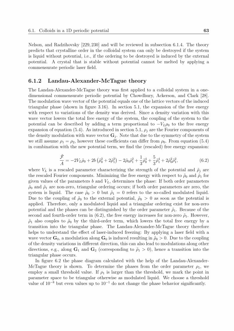
6.1. Colloids in a 1D periodic potential 63
Nelson, and Radzihovsky [229, 230] and will be reviewed in subsection 6.1.4. The theorypredicts that crystalline order in the colloidal system can only be destroyed if the systemis liquid without potential, i.e., if the ordering to be destroyed is induced by the externalpotential. A crystal that is stable without potential cannot be melted by applying acommensurate periodic laser field.
6.1.2 Landau-Alexander-McTague theory
The Landau-Alexander-McTague theory was first applied to a colloidal system in a one-dimensional commensurate periodic potential by Chowdhury, Ackerson, and Clark [28].The modulation wave vector of the potential equals one of the lattice vectors of the inducedtriangular phase (shown in figure 3.16). In section 5.1, the expansion of the free energywith respect to variations of the density was derived. Since a density variation with thiswave vector lowers the total free energy of the system, the coupling of the system to thepotential can be described by adding a term proportional to −VLρ0 to the free energyexpansion of equation (5.4). As introduced in section 5.1, ρj are the Fourier components ofthe density modulation with wave vector Gj. Note that due to the symmetry of the systemwe still assume ρ1 = ρ2, however these coefficients can differ from ρ0. From equation (5.4)in combination with the new potential term, we find the (rescaled) free energy expansion:
FA
= −2VLρ0 + 2b(ρ2
0 + 2ρ21
)− 2ρ0ρ
21 +
1
3ρ4
0 +5
3ρ4
1 + 2ρ20ρ
21, (6.2)
where VL is a rescaled parameter characterizing the strength of the potential and ρj arethe rescaled Fourier components. Minimizing the free energy with respect to ρ0 and ρ1 forgiven values of the parameters b and VL, determines the phase: If both order parametersρ0 and ρ1 are non-zero, triangular ordering occurs; if both order parameters are zero, thesystem is liquid. The case ρ0 > 0 but ρ1 = 0 refers to the so-called modulated liquid.Due to the coupling of ρ0 to the external potential, ρ0 > 0 as soon as the potential isapplied. Therefore, only a modulated liquid and a triangular ordering exist for non-zeropotential and the phases can be distinguished by the order parameter ρ1. Because of thesecond and fourth-order term in (6.2), the free energy increases for non-zero ρ1. However,ρ1 also couples to ρ0 by the third-order term, which lowers the total free energy by atransition into the triangular phase. The Landau-Alexander-McTague theory thereforehelps to understand the effect of laser-induced freezing: By applying a laser field with awave vector G0, a modulation along G0 is induced resulting in ρ0 > 0. Due to the couplingof the density variations in different direction, this can also lead to modulations along otherdirections, e.g., along G1 and G2 (corresponding to ρ1 > 0), hence a transition into thetriangular phase occurs.
In figure 6.2 the phase diagram calculated with the help of the Landau-Alexander-McTague theory is shown. To determine the phases from the order parameter ρ1, weemploy a small threshold value. If ρ1 is larger than the threshold, we mark the point inparameter space to be triangular otherwise as modulated liquid. We choose a thresholdvalue of 10−8 but even values up to 10−1 do not change the phase behavior significantly.
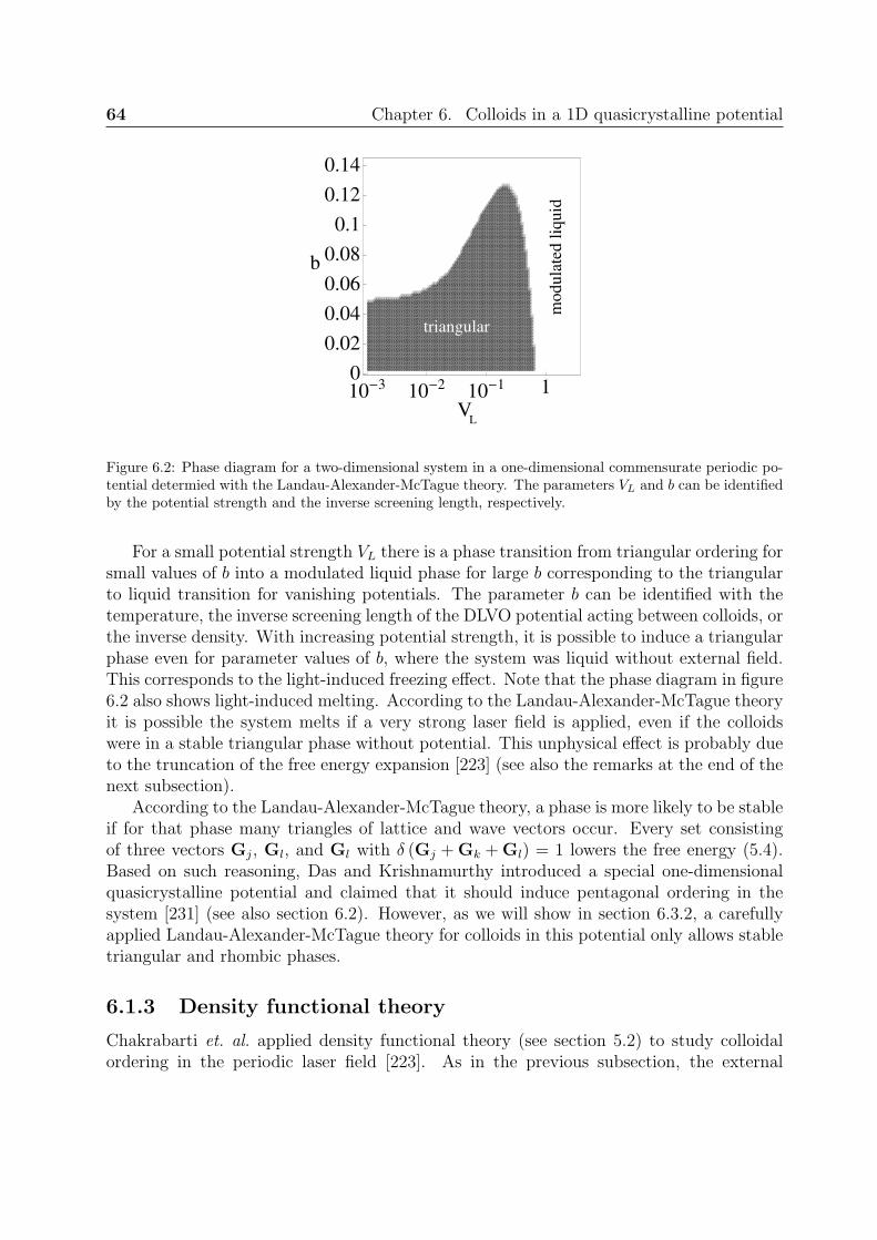
64 Chapter 6. Colloids in a 1D quasicrystalline potential
10-3 10-2 10-1 1
0.02
0.04
0.06
0.08
0.1
0.12
0.14
0
V L
mo
du
late
d l
iqu
id
triangular
b
Figure 6.2: Phase diagram for a two-dimensional system in a one-dimensional commensurate periodic po-tential determied with the Landau-Alexander-McTague theory. The parameters VL and b can be identifiedby the potential strength and the inverse screening length, respectively.
For a small potential strength VL there is a phase transition from triangular ordering forsmall values of b into a modulated liquid phase for large b corresponding to the triangularto liquid transition for vanishing potentials. The parameter b can be identified with thetemperature, the inverse screening length of the DLVO potential acting between colloids, orthe inverse density. With increasing potential strength, it is possible to induce a triangularphase even for parameter values of b, where the system was liquid without external field.This corresponds to the light-induced freezing effect. Note that the phase diagram in figure6.2 also shows light-induced melting. According to the Landau-Alexander-McTague theoryit is possible the system melts if a very strong laser field is applied, even if the colloidswere in a stable triangular phase without potential. This unphysical effect is probably dueto the truncation of the free energy expansion [223] (see also the remarks at the end of thenext subsection).
According to the Landau-Alexander-McTague theory, a phase is more likely to be stableif for that phase many triangles of lattice and wave vectors occur. Every set consistingof three vectors Gj, Gl, and Gl with δ (Gj + Gk + Gl) = 1 lowers the free energy (5.4).Based on such reasoning, Das and Krishnamurthy introduced a special one-dimensionalquasicrystalline potential and claimed that it should induce pentagonal ordering in thesystem [231] (see also section 6.2). However, as we will show in section 6.3.2, a carefullyapplied Landau-Alexander-McTague theory for colloids in this potential only allows stabletriangular and rhombic phases.
6.1.3 Density functional theory
Chakrabarti et. al. applied density functional theory (see section 5.2) to study colloidalordering in the periodic laser field [223]. As in the previous subsection, the external
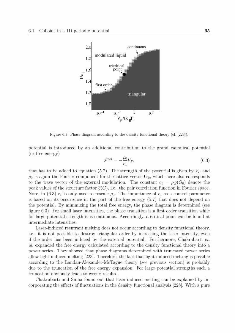
6.1. Colloids in a 1D periodic potential 65
V /(k T)B
11
/c
triangular
point
first order
continuous
modulated liquid
tricritical
F
Figure 6.3: Phase diagram according to the density functional theory (cf. [223]).
potential is introduced by an additional contribution to the grand canonical potential(or free energy)
F ext = −ρ0
c1VF , (6.3)
that has to be added to equation (5.7). The strength of the potential is given by VF andρ0 is again the Fourier component for the lattice vector G0, which here also correspondsto the wave vector of the external modulation. The constant c1 = ρ g(G0) denote thepeak values of the structure factor g(G), i.e., the pair correlation function in Fourier space.Note, in (6.3) c1 is only used to rescale ρ0. The importance of c1 as a control parameteris based on its occurrence in the part of the free energy (5.7) that does not depend onthe potential. By minimizing the total free energy, the phase diagram is determined (seefigure 6.3). For small laser intensities, the phase transition is a first order transition whilefor large potential strength it is continuous. Accordingly, a critical point can be found atintermediate intensities.
Laser-induced reentrant melting does not occur according to density functional theory,i.e., it is not possible to destroy triangular order by increasing the laser intensity, evenif the order has been induced by the external potential. Furthermore, Chakrabarti et.al. expanded the free energy calculated according to the density functional theory into apower series. They showed that phase diagrams determined with truncated power seriesallow light-induced melting [223]. Therefore, the fact that light-induced melting is possibleaccording to the Landau-Alexander-McTague theory (see previous section) is probablydue to the truncation of the free energy expansion. For large potential strengths such atruncation obviously leads to wrong results.
Chakrabarti and Sinha found out that laser-induced melting can be explained by in-corporating the effects of fluctuations in the density functional analysis [228]. With a pure

66 Chapter 6. Colloids in a 1D quasicrystalline potential
mean-field treatment obviously it is not possible to predict laser-induced melting while atheory that includes fluctuations can account for this phenomenon.
Density functional theory can also be applied to a colloidal system in a quasicrystallinepotential. However, the integral in (5.8) is over a unit cell which does not exist for qua-sicrystals. Therefore one has to integrate over large areas similar to the simulation boxesintroduced in section equation 4.3. Because the integration is usually performed numer-ically and is repeated many times during the minimization process, it is not possible todetermine a phase diagram within a reasonable amount of time.
6.1.4 Laser-induced melting due to fluctuations
Frey, Nelson, and Radzihovsky developed a theory of defect-mediated melting in one-dimensional periodic potentials [229, 230], which is in good agreement with the results ofexperiments and simulations (see e.g. [30] for a review). Without potential the meltingtemperature T(m) is given by equations (5.15) and (5.19) obtained from the KTHNY theory,i.e.,
T(m) (V0 = 0) =a2
S
4π
µR (µR + λR)
2µR + λR
, (6.4)
where µR and λR are the renormalized elastic constants of those given by [cf. equation(5.14) with K1 = K2 = K3 = 0]:
fel =1
2λuiiuii + µuijuij. (6.5)
For a system in a potential, Frey, Nelson, and Radzihovsky consider a free energy densityfel,V that takes into account that displacements ux perpendicular to the potential wells aresuppressed by the potential. Therefore, the modes in x-direction are integrated out andone finds
fel,V =1
2
[Bxy (∂xuy)2 +Byy (∂yuy)2] , (6.6)
where Bxy and Byy are effective elastic constants. A calculation similar to the ones em-ployed in the KTHNY theory leads to a relation for the melting temperature:√
BxyByy =8πkBT(m)
a2S
(6.7)
For infinite potential strength, i.e., without any displacements perpendicular to the wellsat all, one finds by comparing (6.6) and (6.5)
Bxy = µR and Byy = 2µR + λR. (6.8)
Therefore, the melting temperature for infinite potential strength is
T(m) (V0 = ∞) =a2
s
8π
√µR (2µR + λR). (6.9)

6.2. Motivation for the quasicrystalline potential 67
As a consequence, there is a limiting melting temperature for V0 →∞, i.e., not all latticescan be melted by increasing the potential. Furthermore, because of T(m) (V0 = ∞) >T(m) (V0 = 0), a crystal stable without laser field cannot be destroyed by applying a periodiccommensurate potential. Note in experiments or simulations often the inverse screeninglength κ is varied. However, qualitatively the results can be compared to the theoreticalresults for varying temperature T .
If one starts at infinite potential strength V0 and then lowers V0, fluctuations perpen-dicular to the wells become important. Therefore, the relations (6.8) that determine theeffective elastic constants in the limit V0 → ∞ are no longer fulfilled. Frey, Nelson, andRadzihovsky found out that due to the fluctuations a range of finite V0 exists, where themelting temperature T(m)(V0) exceeds T(m)(V0 = ∞) [229, 230]. Therefore, at a temper-ature T > T(m) (V0 = ∞) a triangular ordering may be stable for intermediate potentialstrength, however it becomes unstable for V0 → ∞. This corresponds to laser-inducedreentrant melting.
For incommensurate periodic potentials, Frey, Nelson, and Radzihovsky in [229, 230]also predict phases with smectic ordering and floating phases similar to those predictedby Nelson and Halperin for commensurate and incommensurate 2D potentials (see section5.3).
6.2 Motivation for the quasicrystalline potential
In this section we introduce the one-dimensional quasicrystalline potential. It was firstproposed by Das and Krishnamurthy, who claimed that it is possible to induce a phasewith pentagonal symmetry with such a laser field [231]. The quasicrystalline potentialconsists of two modulations whose wavelengths differ by a factor of τ 2 (see figure 6.4),where τ = (1 +
√5)/2 is the number of the golden ratio (see section 3.2):
V (r) = −V0
2[cos (Gα · r) + cos (Gβ · r)] (6.10)
with Gα = τG0ex, Gβ = (−1/τ)G0ex. The vector ex denotes the unit vector in x-directionand G0 is the length of a reciprocal lattice vector that belongs to the ideal triangularconfiguration of the colloids without any external potential. If aS is the particle spacingin this configuration, G0 = 4π/(
√3aS). Within the set of the wave vectors Gα and Gβ
combined with the lattice vectors of the pentagonal phase [see figure 6.5(a)] one can findmany triangles. To be concrete, the following relations hold:
G0 −Gα −Gβ = 0,
G1 + G4 + Gβ = 0,
and G2 + G3 + Gα = 0. (6.11)
These relations can be proven using the special properties of the number of the golden meanτ , e.g., −2G2,x = 1/(2G1,x) = τG0(see also section 3.2). They lead to additional third-order terms in the expansion of the free energy and therefore decrease it (cf. section 6.1.2).

68 Chapter 6. Colloids in a 1D quasicrystalline potential
-1
0
1
0 2 4 6 8 10
-cos(G
α x
)
x/aS
-1
0
1
0 2 4 6 8 10
-cos(G
β x
)
x/aS
-1
0
1
0 2 4 6 8 10
V(x
,y)/
V0
x/aS
+
=
(a)
(b)
(c)
Figure 6.4: (a) One-dimensional quasicrystalline potential consisting of two modulations shown in part (b)and (c). The wavelengths of the modulations differ by a factor of τ2.
Hence, Das and Krishnamurthy claimed that for certain parameters the quasicrystallinepotential (6.10) induces a stable pentagonal (or decagonal) phase [231], i.e., a phase definedby five lattice vectors as shown in figure 6.5(a) and, therefore, exhibiting five- or ten-foldrotational symmetry. However, as we show in the following section, the free energy of thepentagonal phase has to be compared to the free energy of other possible orderings such asthose pictured in figure 6.5(b)-(d). Especially the rhombic-α phase has a lower free energythan the pentagonal ordering. The lattice vector G0 of the rhombic-α or rhombic-β phaseis equal to the wave vector Gα or Gβ, respectively. In both cases, the other wave vector ofthe potential is ignored completely. The length and direction of the lattice vectors G1 andG2 are determined by the following requirements: The sum of the three lattice vectors hasto be zero, i.e., G0 + G1 + G2 = 0 and the density has to equal the density of a triangularlattice, i.e., the corresponding unit cells must have the same area. In the next section,we present complete phase diagrams determined by Monte-Carlo simulations and a refinedLandau-Alexander-McTague theory. We find no pentagonal but only rhombic ordering.
6.3 Phase behavior
In this section we determine the phase behavior in the one-dimensional quasicrystallinepotential. First, we use Monte-Carlo simulations to calculate a complete phase diagram.

6.3. Phase behavior 69
(c) rhombic−α
G=0 αG
GG G
G
G
αβ
G
G3
G
G
G2
Gβ
(b) triangular
G
G
G2
αGβ
G
G
G=−
(d) rhombic−β
βG αGGβ 0
1
2
1
0
1
0
12
4
(a) pentagonal
Figure 6.5: Modulation vectors Gα and Gβ of the one-dimensional quasicrystalline potential together withthe lattice vectors of (a) a pentagonal, (b) a triangular, (c) a rhombic-α, or (d) a rhombic-β ordered phase.
Then we develop a modified Landau-Alexander-McTague theory, which confirms the resultsof the simulations.
6.3.1 Results of Monte-Carlo simulations
The method of Monte-Carlo simulations was shortly introduced in section 4.2. We employthe same parameter values as Strepp, Sengupta, and Nielaba in [32] (see also section 4.4)and use a rational approximation of the potential as explained in section 4.3.1.
In figure 6.6 typical snapshots of the equilibrated system for different values of thepotential strength V0 and the inverse screening length κ of the DLVO potential are shown.We find triangular or rhombic-α ordering as well as the modulated liquid phase. Nopentagonal or decagonal quasicrystal is stable for any set of parameters. On a first glancethe triangular and the rhombic-α phase look quite similar. However, there are easy waysto distinguish the two lattices. The angle between nearest-neighbor bonds is π/3 in thetriangular phase, whereas in the rhombic-α phase it is arctan
(√3τ 2/3
)≈ 0.31π as can
be calculated from the lattice vectors (see figure 6.5 and last paragraph of the previoussubsection). Of course, it is also possible to measure the distances between rows of particlesand compare them to the values expected by the lattice vectors. A very easy way todistinguish the structures, is to look on the orientation of a hexagon that consists ofthe nearest neighbors of a colloid. A hexagon in the rhombic-α phase is rotated by π/2compared to the hexagon in the triangular phase.
We calculated the following order parameter φ(G1) for each of the possible phasesillustrated in figure 6.5:
φ(G1) =1
N〈∑i,j
exp[iG1 · (rj − ri)]〉, (6.12)
where the sum is over all colloidal pairs of nearest neighbors and N is the number of suchpairs; G1 is one of the lattice vectors shown in figure 6.5, it depends on the structure whoseorder parameter one wants to determine. The order parameter looks similar to a Fouriercomponent of a density modulation with wave vector G1, however it only considers nearest

70 Chapter 6. Colloids in a 1D quasicrystalline potential
0
5as
10as
0 5as
10as
0
5as
10as
0 5as
10as
0
5as
10as
0 5as
10as
0
5as
10as
0 5as
10as
0
5as
10as
0 5as
10as
0
5as
10as
0 5as
10as
κ β
κ β κ β
κ β κ
κ β
s s
s s s
s(e) a =12, V =10 (rhombic− )(d) a =12, V =0.1 (triangular)
α
α (f) a =12, V =1000 (mod. liq.)β
0
0 0 0
(b) a =16, V =10 (rhombic− )0 (c) a =16, V =1000 (mod. liq.)0(a) a =16, V =0.1 (mod. liq.)
Figure 6.6: Snapshots of Monte-Carlo simulations for different values of the potential strength βV0 andthe inverse screening length κaS . The potential is plotted in the lower part of the figures. The snapshotsshow just a small region of the simulation box.
neighbors. The simulation box fits best the pentagonal phase (see section 4.3.1), whereasthe triangular and rhombic phases are weakly distorted on a global scale to fit into the box.Therefore, summing over all colloidal pairs in equation (6.12) would not lead to correctresults and the local order parameter defined in (6.12) is more appropriate. It is similarto the one used in [232]. For a triangular and pentagonal lattice a bond orientationalparameter can also be calculated (see section 7.1). However such a parameter is difficultto determine for a rhombic phase, which only has a two fold rotational symmetry.
Figure 6.7 shows the complete phase diagram and the order parameters for the tri-angular and the rhombic-α phase as a function of V0 and κ. For the decagonal and therhombic-β phase, the order parameters always vanish. As one expects, for weak potentialswe find a transition from triangular ordering for small inverse screening lengths κ into aliquid for high values of κ. When the laser strength increases, a transition of the triangularphase into the rhombic-α phase occurs. We also find light induced freezing: Within acertain range of the inverse screening length, the system shows rhombic-α ordering in thelaser field although it is liquid without external potential. Interestingly at very large laserintensities, we do not find any periodic or decagonal ordering at all. In principle, one can

6.3. Phase behavior 71
12
14
16
18
20
10-2
1
102
104
0.30.6
12
14
16
18
20
0.3
10-2 1 10
210
4
12
14
16
18
20
κaS
κaS
G1φ( )
modula
ted l
iquid
triangular rhom
bic
− α
(a) (b)
triangularrh
om
bic
−α
mo
du
late
d l
iqu
id B BV /(k T)
0 0V /(k T)
Figure 6.7: (a) Phase diagram and (b) order parameters as defined in (6.12) depending on the potentialstrength V0 and the inverse screening length κ. The potential strength is given in terms of the thermalenergy kBT and the screening length is normalized by the nearest neighbor distance aS of the triangularstarting configuration. To get the phase diagram in (a), we checked for each possible ordering, if thecorresponding order parameter is larger than 0.1. If none of the order parameters is large enough, wemarked the phase as modulated liquid.
melt the system by applying a strong enough quasicrystalline potential no matter whetherthe colloids form a stable triangular phase without laser field or not. This is different fromthe case of a periodic commensurate potential, where light-induced reentrant melting needsa liquid phase at zero potential strength (see sections 6.1.1 and 6.1.4). A snapshot of asystem melted by a quasicrystalline laser field of high intensity is shown in figure 6.6(f).All particles are located in local minima of the potential, i.e., on lines parallel to the y-axis.The potential wells have an approximate distance of aSτ and their depths are modulatedon the wave length τaS. Therefore, the line density is different in every well. Some wellsare almost empty or at least the probabilities to find a colloid in such wells are very small.Obviously, the potential induces quasicrystalline ordering in x-direction. The ratio of theline densities of neighboring wells is usually irrational. As a consequence, it is impossi-ble to have any periodic ordering along the wells. This explains why there is no periodicphase for sufficiently large potential strengths and why every periodic ordering is destroyedby the quasicrystalline laser field. This is a type of light-induced melting different fromthe fluctuation-driven melting in a periodic commensurate potential. We will study themodulated liquid phase at high laser intensities in more detail in section 6.4.
6.3.2 Refined Landau-Alexander-McTague theory
The usual Landau-Alexander-McTague free energy expansion as in (5.4) [see also section5.1] with some coupling to the potential (cf. section 6.1.2) does not distinguish between therhombic-α and of the rhombic-β phase. This is due to the fact that the same number oftriangles occur for the lattice vectors of these phases. In the following we therefore derive

72 Chapter 6. Colloids in a 1D quasicrystalline potential
an extended expansion of the free energy that also includes the elastic energy needed todeform a lattice, i.e., to change the length of lattice vectors.
The free energy F is expanded with respect to small density variations δρ (r) = ρ (r)−ρ,where ρ (r) is the density field in real space, e.g., of the mass density, and ρ is the averagedensity:.
F =
∫dA
−V (r)δρ(r) +
b′
2[δρ(r)]2 − c1
2[∇δρ(r)]2 +
c22
[∇2δρ(r)
]2−d
6[δρ(r)]3 +
e
24[δρ(r)]4
, (6.13)
As in section 5.1 the integration is over the whole plane and the signs are chosen such thatwith positive parameters b′, c1, c2, d and e a phase transition into some stable ordered phaseoccurs if b′ is sufficiently small. However, extending the free energy used in section 5.1,we now include a coupling −V (r)δρ(r) to the external potential V (r) and in the second-order term we also take into account the first and second derivative of the density field.Using (6.10) for the external potential and the Fourier expansion for the density variationδρ(r) =
∑j ρje
−iGj ·r] where Gj denotes the relevant reciprocal lattice vectors, includingGα and Gβ, the free energy (6.13) is transformed into its representation in reciprocal space:
FA
= −V0 (ρα + ρβ) +∑
j
(b′ − c1G
2j + c2G
4j
)|ρj|2 (6.14)
−d6
∑j,k,l
ρjρkρlδ (Gj + Gk + Gl) +e
24
∑j,k,l,m
ρjρkρlρmδ (Gj + Gk + Gl + Gm) .
In the second-order term, the prefactor of |ρj|2 has a minimum for a certain wave numberwhich we choose to be Gj = G0 so that without external potential we find a phase transitioninto the triangular phase. Therefore, the second-order term is rewritten as∑
j
(b′ − c1G
2j + c2G
4j
)|ρj|2 =
∑j
(b′′ − c′
[G2
j −G20
]2) |ρj|2 , (6.15)
with new positive parameters b′′ and c′. Now, the free energy depends on six free parametersV0, b
′′, c′, d, e, and G0. We rescale the free energy density F/A, the order parameters ρj,and the lengths of the lattice vectors Gj such that only three free parameters VL, b, and cremain
FA
= −VL (ρα + ρβ) +∑
j
(b− c
[G2
j − 1]2)
|ρj|2 (6.16)
−1
6
∑j,k,l
ρj ρkρlδ (Gj + Gk + Gl) +1
24
∑j,k,l,m
ρj ρkρlρmδ (Gj + Gk + Gl + Gm) ,
where we termed the rescaled quantities F/A, ρj, and Gj.

6.3. Phase behavior 73
The parameter space is formed by the three parameters VL, b, and c. Their meaning isexplained in the following:
• VL describes the strength of the potential.
• b is the main control parameter, responsible for the transition into an ordered phasefor small values of b. It can be identified with the temperature, the inverse screeninglength κ, or the inverse density.
• c is a typical elastic constant that distinguishes soft systems with small c from rigidones with large c. This can be seen in the second-order term in (6.16), where any de-viation from the length G0 of the ideal lattice vector of the triangular phase (rescaledto 1) is penalized by an increase of the free energy weighted with the factor c.
To calculate the free energy (6.16) for each of the lattices given by the lattice vectorsin figure 6.5, we need to determine the combinations, where three or four lattice vectorsadd up to zero. In the following, trivial combinations such as G0 −G0 + G1 −G1 are notstated explicitly. For the pentagonal phase shown in figure 6.5(a) we find the followingnon-trivial relations:
G0 −Gα −Gβ = 0,
G1 + G4 + Gβ = 0,
G2 + G3 + Gα = 0.
G0 −Gα + G1 + G4 = 0.
and G0 −Gβ + G2 + G3 = 0. (6.17)
For the triangular phase [see figure 6.5(b)], one finds
G0 + G1 + G2 = 0,
G0 −Gα −Gβ = 0,
and G1 + G2 + Gα + Gβ = 0. (6.18)
For the rhombic-α phase shown in figure 6.5(c) we have only four reciprocal vectors (Gα =G0, G1, G2, and Gβ) and there is only the non-trivial relation
Gα + G1 + G2 = 0. (6.19)
Correspondingly, in the rhombic-β phase [see figure 6.5(d)]
−Gβ + G1 + G2 = 0. (6.20)
For the pentagonal ordering Das and Krishnamurthyn did not consider the non-trivialcombinations of four lattice vectors that appear in the fourth and fifth line of (6.17). Theyalso did not consider any rhombic phases. Therefore, they could predict a stable pentagonalphase [231], which we do not find.

74 Chapter 6. Colloids in a 1D quasicrystalline potential
10-4
10-3
10-2
0.06
0.07
0.08
0.09
0.1
10-4
10-3
10-2
0.06
0.07
0.08
0.09
0.1
0.06
0.07
0.08
0.09
10-3
10-2
10-1
1
10-4
10-2
1
0.06
0.07
10-3
10-2
10-1
1
10-3
10-2
10-1
0.06
0.07
0.08
0.09
0.1
c=10−2
liq
uid
modula
ted
(c)
b
tria
ngula
r αrh
om
bic
−
c=10−4
liq
uid
mo
dula
ted
(d)
rhom
bic
−α
V
b
(a)
triangular
rhombic−α
V
b
c
c=1(b)
tria
ng
ula
rb
modula
ted l
iquid
L
L
Figure 6.8: (a) Phase diagram showing the regions of stable triangular (dark gray) and rhombic-α (lightgray) phase. In all other regions of the parameter space, a modulated liquid is found. (b)-(d) Phasediagrams for (b) rigid systems with c = 1, (c) intermediate crystals with c = 10−2, and (d) soft systemswith c = 10−4.
By using (6.16) together with the relations (6.18) to (6.20), we can formulate the freeenergies for each of the four possible structures. At a given point VL, b, c of the parameterspace, we minimize the free energies with respect to the order parameters ρj. We assumethat the system has the ordering of the structure with the smallest free energy, if all orderparameters are non-zero. If at least one order parameter vanishes, we term the phasemodulated liquid. Figure 6.8(a) shows the full phase diagram for the whole parameterspace. Figures 6.8(b) to (d) present phase diagrams for constant values of the elasticconstant c. For very rigid crystals (large c), we only find a triangular phase that canbe melted by increasing b or the potential strength VL. In contrast, in very soft systemstriangular order only exists for very small strength VL < 10−5. For intermediate laserstrength a rhombic-α phase is induced. This is even possible if the system is liquid withoutany external potential. The situation of intermediate elastic constants c, as shown infigure 6.8(c), is very close to the simulations (see figure 6.7). Though the predictions of

6.4. Dynamics: Non-periodic locked phase for large laser intensities 75
0.01
0.1
1
10
0.01 0.1 1 10 100
mean s
quare
dis
pla
cem
ent <
r2>
/aS
2
time t/(βγ aS2)
κ aS=10 , β V=500κ aS=10.2, β V=500κ aS=10.5, β V=500κ aS=11 , β V=500κ aS=12 , β V=500κ aS=14 , β V=500κ aS=16 , β V=500
~t0.5
~taκ S
Figure 6.9: Time dependence of the mean square displacement.
a Landau-Alexander-McTague theory for large VL are sometimes not reliable (see section6.1.2), here even the phase behavior for large laser intensities is in good agreement withthe simulations. Only the small region in figure 6.8(c) where the triangular phase firstmelts before it crystallizes into the rhombic-α phase by increasing VL is not found in thesimulations. In the next section we study the dynamics of the modulated liquid at largepotential strength.
6.4 Dynamics: Non-periodic locked phase for large
laser intensities
In systems with a commensurate potential Vext(x) = cos(G0x), only crystals producedby light-induced freezing can melt at large laser intensities [229, 230] (see also section6.1.4). In the one-dimensional quasicrystalline potential, light-induced melting is due tothe quasiperiodicity of the potential, which enforces that for very high potential strengthsthe number of colloids is different in every potential well. Therefore, periodic ordering isnot possible, i.e., by increasing the laser intensity all periodic crystalline structures can bedestroyed in a quasicrystalline potential. In this section, we study the properties of theresulting non-periodic phase(s) at high potential strengths.
We perform Brownian dynamics simulations (see section 4.1 for details) of the colloids instrong laser fields (βV0 = 500) and determine the mean square displacement. We considersystems with only 195 particle but averaged over 20 independent runs, i.e., for each runwe first use one million Monte-Carlo steps to find an equilibrium configuration and then

76 Chapter 6. Colloids in a 1D quasicrystalline potential
0
2as
4as
6as
8as
0 2as
4as
6as
8as
10as
0
2as
4as
6as
8as
0 2as
4as
6as
8as
10as
0
2as
4as
6as
8as
0 2as
4as
6as
8as
10as
κ κ β κ βs s sβ(a) a =8, V =500 (locked)0 0 (c) a =12, V =500 (mod. liq.)0(b) a =10, V =500 (locked)
Figure 6.10: Snapshots of simulations with the 1D quasicrystalline laser field for large potential strengths.The potential is shown in the lower parts of the figures.
started the Brownian dynamics simulations. The mean square displacement is determinedaccording to ⟨
r2(t)⟩
=⟨|r(t)− r(0)− 〈r(t)− r(0)〉|2
⟩, (6.21)
i.e., 〈r2(t)〉 is corrected by movements of the center of mass and therefore the randommotion of the whole system does not affect the results. In figure 6.9 the time dependenceof the mean square displacement is shown. There is a crossover from subdiffusion 〈r2〉 ∝ t0.5
on short time scales (reminiscent to single-file diffusion) to normal diffusion 〈r2〉 ∝ t inthe asymptotic long time limit. Single-file diffusion usually occurs for particles, which areconfined in a one-dimensional channel and cannot pass each other (see e.g. [51–53,233,234]).In our system we observe a similar diffusion process on time scales, where colloids inneighboring walls do not pass each other. For very small inverse screening lengths κaS, acrossover into the regime of normal diffusion is not observed, i.e., for small κaS the colloidsdo not pass particles in neighboring wells even on long time scales. Hence, there is atransition into a dynamically locked state. The transition takes place between κaS = 10.2and κaS = 10.3. However, there are no differences visible in snapshots of the modulatedliquid and the locked phase (see figure 6.10). In the locked phase the number of colloidswithin a certain potential well is the same as in the modulated liquid phase. No periodicordering along the wells is possible and the locked phase cannot be crystalline. Perhapsthere is some quasicrystalline order along the wells. However, all differences we have foundso far between the modulated liquid and the locked phase concern their dynamics.
To further study the transition from the modulated liquid into the non-periodic lockedphase, we considered the mean square distance of colloids that were nearest neighbors attime t = 0, i.e.,
⟨r2NN(t)
⟩=
⟨1
N
∑j
1
nNN
∑k∈NNj(t=0)
|rj(t)− rk(t)|2⟩. (6.22)
Note that 〈r2NN(t)〉 is similar to the modified Lindemann parameter [215, 235, 236]: In the

6.4. Dynamics: Non-periodic locked phase for large laser intensities 77
0
1
2
3
4
5
6
0 10 20 30 40 50 60
msd o
f N
N <
r NN
2>
/aS
2
time t/(βγ aS2)
κ aS=10 , β V=500κ aS=10.2, β V=500κ aS=10.5, β V=500κ aS=11 , β V=500κ aS=12 , β V=500κ aS=14 , β V=500κ aS=16 , β V=500
κaS
Figure 6.11: Time dependence of the mean square distance of colloids that were nearest neighbors at timet = 0.
modified Lindemann parameter usually the mean distance between nearest neighbors issubtracted before the distance is squared. Such a substraction does not make sense in oursystem because the nearest neighbor distance is not even close to the mean distance.
In figure 6.11 the time dependence of the mean square distance is shown. In themodulated liquid it grows linearly in time, whereas in the locked phase it stays almostconstant, i.e., nearest neighbors remain nearest neighbors. By linear fits we determined theeffective diffusion constant DNN as defined in 〈r2
NN〉 = 4DNNt. We plot DNN as a functionof the inverse screening length κas in figure 6.12. Obviously, the effective diffusion constantis useful as an order parameter to indicate the transition from the modulated liquid to thelocked phase. It is zero in the locked phase and non-zero in the modulated liquid. This isdifferent from usual order parameters, which are zero in the disordered phase and non-zeroin the low-symmetry phase. Therefore, DNN can also be seen as a disorder parameter. Atthe transition, DNN is continuous in κaS.
Since the phase transition in our system is described by its dynamical properties, itmight resemble the glass transition. However, in our case the locked phase is a real equi-librium phase, whereas in a non-ergodic glass the glassy phase is approached dynamicallyby fast cooling to prevent crystallization. Most glasses are characterized as non-ergodicsystems, i.e., not all possible micro states are approached by the temporal evolution of thesystem. A Monte-Carlo simulation would relax such a glassy system to the equilibriumstate, which usually corresponds to a crystalline state and not to a glassy state. In oursystem it is possible to find the locked state by Monte Carlo simulations. Therefore, thecolloids in a quasicrystalline potential are closer to a geometrical frustrated system, i.e., a
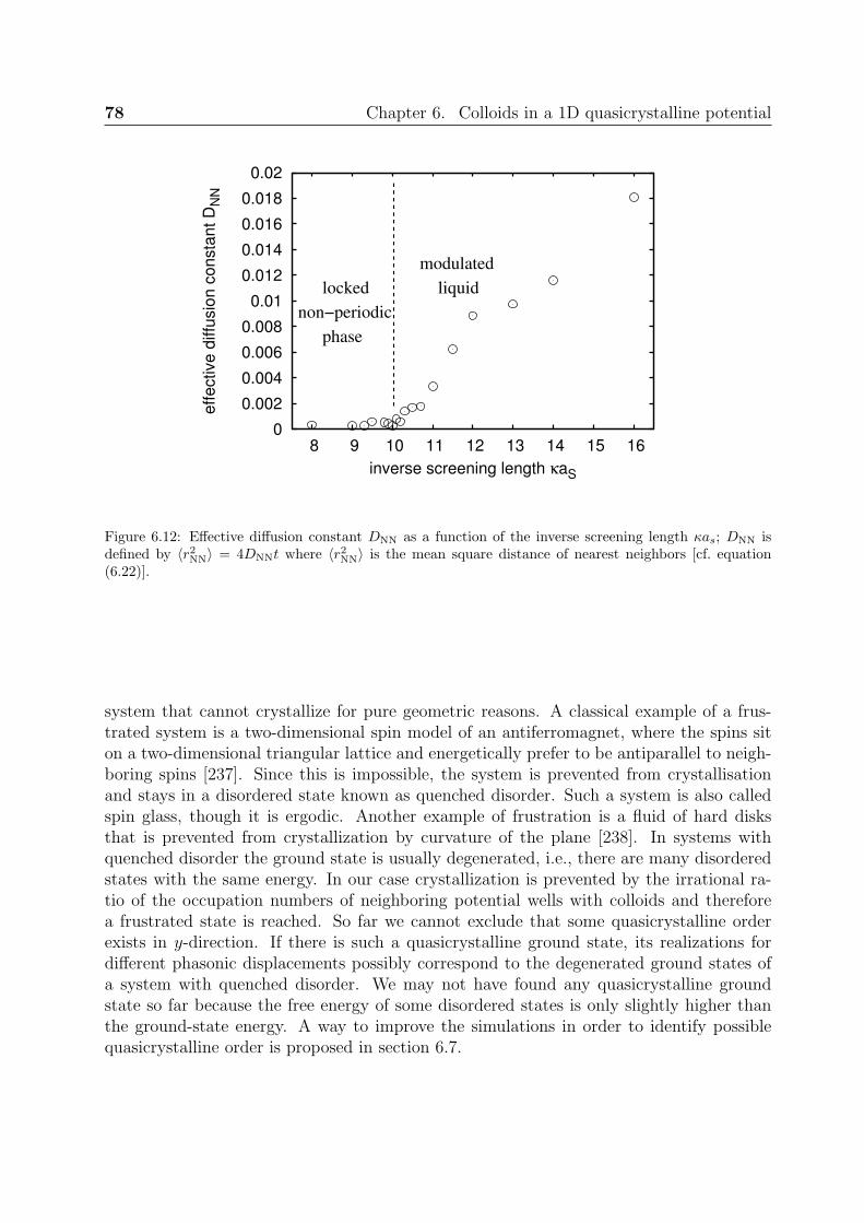
78 Chapter 6. Colloids in a 1D quasicrystalline potential
0
0.002
0.004
0.006
0.008
0.01
0.012
0.014
0.016
0.018
0.02
8 9 10 11 12 13 14 15 16
eff
ective
diffu
sio
n c
on
sta
nt
DN
N
inverse screening length κaS
modulated
liquidlocked
non−periodic
phase
Figure 6.12: Effective diffusion constant DNN as a function of the inverse screening length κas; DNN isdefined by 〈r2NN〉 = 4DNNt where 〈r2NN〉 is the mean square distance of nearest neighbors [cf. equation(6.22)].
system that cannot crystallize for pure geometric reasons. A classical example of a frus-trated system is a two-dimensional spin model of an antiferromagnet, where the spins siton a two-dimensional triangular lattice and energetically prefer to be antiparallel to neigh-boring spins [237]. Since this is impossible, the system is prevented from crystallisationand stays in a disordered state known as quenched disorder. Such a system is also calledspin glass, though it is ergodic. Another example of frustration is a fluid of hard disksthat is prevented from crystallization by curvature of the plane [238]. In systems withquenched disorder the ground state is usually degenerated, i.e., there are many disorderedstates with the same energy. In our case crystallization is prevented by the irrational ra-tio of the occupation numbers of neighboring potential wells with colloids and thereforea frustrated state is reached. So far we cannot exclude that some quasicrystalline orderexists in y-direction. If there is such a quasicrystalline ground state, its realizations fordifferent phasonic displacements possibly correspond to the degenerated ground states ofa system with quenched disorder. We may not have found any quasicrystalline groundstate so far because the free energy of some disordered states is only slightly higher thanthe ground-state energy. A way to improve the simulations in order to identify possiblequasicrystalline order is proposed in section 6.7.

6.5. Experimental results 79
∼0.31 π
π/3
(b)(a)
Figure 6.13: Micrographs of an aqueous colloidal suspension of charged polystyrene spheres (with diameter2.4 µm on a 1D quasicrystalline substrate created with interfering laser beams. The colloids form (a) atriangular lattice for small laser intensities and (b) a rhombic-α-phase for higher potential strength. Thetwo phases can be distinguished by measuring the angles as shown in the figures (see also section 6.3.1).Experiment and micrographs by J. Baumgartl [239].
6.5 Experimental results
Some results of the simulations and the theory were verified experimentally by J. Baumgartl[239], e.g., a transition from a triangular phase for small potential strength [see figure6.13(a)] towards a rhombic-α-phase for higher laser intensities [see figure 6.13(b)] wasfound. However, the non-periodic locked phase for very large potential strengths describedin the last subsection has not been observed yet in experiments since the rhombic-α phaseis kinetically stabilized against the modulated liquid by large potential barriers.
6.6 Other quasicrystalline potentials
We also used other quasicrystalline potentials for the simulations. For example, a potentialwith wells of equal depth and distances corresponding to the Fibonacci chain (see section3.2). In another potential, the wave vectors of the modulation fit to the y-projectionof the decagonal lattice vectors shown in figure 3.5. For all potentials we tried, we didnot find any stable two-dimensional quasicrystalline ordering. Usually for intermediatestrengths of the potential, the colloids order in a rhombic way and only one possible length

80 Chapter 6. Colloids in a 1D quasicrystalline potential
scale of the potential is represented in the ordering, all other length scales are ignored.For large potential strengths, the periodic phases melt into a modulated liquid. Fromthe results of subsection 6.4 we expect that the phase for large laser intensities is also alocked, frustrated phase without any periodicity. This is different for periodic potentials,where rhombic phases are also observed (see section 6.1 or [240] as an example for a non-commensurate potential). However, these are even stable for very large potential strengthssince there frustration does not occur.
6.7 Summary and Outlook
We studied a two-dimensional colloidal system in a one-dimensional quasicrystalline po-tential obtained by the superposition of two modulations characterized by the wave vectorsτG0ex and (−1/τG0)ex, where τ is the number of the golden ratio (see section 3.2) andG0 is related to the nearest neighbor distance aS in a triangular crystal via aS = 2π/G0.We determined the phase diagram by using Monte-Carlo simulations and by applying theLandau-Alexander-McTague theory. We found a triangular to liquid phase transition forweak potentials. For intermediate laser intensities the system is in a rhombic phase, i.e.,the colloids lock to the modulation given by τG0ex and ignore the other one. For largepotential strengths the colloids can only move in the potential wells. Due to the varyingdepths of the wells, the numbers of colloids occupying the wells are different. Usually theratio of these numbers for neighboring wells is irrational and therefore periodic orderingalong the well direction is not possible. Using Brownian dynamics simulations, we found atransition from a modulated liquid at large inverse screening lengths κ into a locked phaseat small κ. In the locked phase the colloids of neighboring wells no longer pass by eachother and system is frustrated since periodic order is impossible.
The Brownian dynamics simulations of the modulated liquid and the locked phase areperformed for a two-dimensional system. Because fluctuations out of the well minimum canbe neglected for large strengths of the potential, a simpler model using particles that canonly move on lines is sufficient to describe the properties at large laser intensities. Such asimplified model should be used in future works. It has the advantage that simulations aremuch faster and therefore the system size can be increased to prevent possible finite-sizeeffects. In addition the statistics is easily improved, which allows to study the behaviorclose to the phase transition in more detail. Furthermore, very long simulation runs mayhelp to reveal any possible quasicrystalline ordering along the wells.
The potential strengths needed to obtain the locked non-periodic phase are usually tolarge for experiments. However, a frustrated locked state can also be achieved in any linepotential (even a periodic one) if the line potential is strong enough to prevent colloids tojump from one line to the other. A non-periodic phase is realized by placing colloids intothe wells in a way that the ratio of the numbers of colloids in neighboring wells is irrational.Note the resulting locked non-periodic phase is not an equilibrium phase then, however itis close to the theoretical equilibrium phase obtained in very strong quasicrystalline laserfields.

81
Chapter 7
Colloidal ordering in a decagonalpotential
In this chapter we study the ordering of colloidal particles in the decagonal potential. Insection 7.1 we present phase diagrams determined by Monte Carlo simulations and discussthe observed phases with ten-fold, twenty-fold, and without bond orientational order anda phase reminiscent to an Archimedean tiling. We compare our findings to experimentalresults in section 7.2 and study the effect of phasonic displacements, drifts, and distortionsin section 7.3. Finally we conclude in section 7.4. Reference [D] is based on some parts ofthis chapter.
7.1 Phase behavior
We usually characterize the phases with the bond orientational order parameter whichwe introduce in subsection 7.1.1. In the following, the density is qualified by the particlespacing aS of the ideal triangular lattice. At a density corresponding to a particle spacingof aS = 0.7aV , the colloids exactly occupy all local minima of the decagonal potential.We use this density to distinguish between the low-density case (aS > 0.7aV ), which westudy in subsections 7.1.2 and 7.1.3, and the high-density case (aS < 0.7aV ) investigated insubsections 7.1.4 and 7.1.5. The parameters for the simulations were given in section 4.4.They are chosen such that for zero potential the phase transition from the solid triangularto the liquid phase is observed in both the low and the high density cases. Finally, insubsection 7.1.6 we determine pair correlation functions to get a deeper insight to thephase behavior.
7.1.1 Bond orientational order parameter
A translational order parameter (like the one used in section 6.3) is not as suitable asan order parameter that measures the orientational symmetry. Here we use the bond

82 Chapter 7. Colloidal ordering in a decagonal potential
θ jk
j
k
Figure 7.1: The bond orientational order parameter uses the directions of bonds between nearest neighbors.A detailed explanation is given in the text.
orientational order parameter
ψm =
⟨∣∣∣∣∣ 1
N
N∑j=1
1
nj
nj∑k=1
eimθjk
∣∣∣∣∣⟩, (7.1)
where the inner sum is over all nj nearest neighbors of colloid j, N is the total number ofparticles, and θjk is the angle of the bond connecting colloids j and k given with respectto some arbitrary reference direction (see figure 7.1). The ensemble average in equation(7.1) is calculated over 1000 configurations taken every 100 steps as described in detail insection 4.2. We are particularly interested in bond orientational order with m = 6, 10, or20, which characterizes phases with nearest neighbor bonds that point, respectively, along6, 10, or 20 equally distributed directions around the central colloid. In the phase diagramsa m-fold bond order is assigned to the phases if ψm > 0.1. In particular, we call phaseswith ψ6 > 0.1 triangular including structures where only domains of triangles occur withthe same orientation. The order parameter ψm in equation (7.1) is defined such that ψm
becomes non-zero if within one configuration the number of bonds in m equally distributeddirections exceeds the number of bonds in other directions. In another direction these mdirections may be different meaning that the configuration is rotated as a whole. However,if within one configuration two or more domains exist with different preferred directions,then ψm vanishes. Therefore, a phase possesses a m-fold bond orientational order onlyif a long-range orientational order exists throughout the colloidal configuration. We alsochecked that the choice of the threshold value 0.1 hardly affects the phase boundaries.
Before we analyze the Monte-Carlo simulations, we calculate the order parameters ψ10
and ψ20 for ideal colloidal patterns created by placing particles directly at the positions oflocal potential minima: First we determine all local minima in a certain region (cf. section3.3.3) and then fill them by first placing a particle in the deepest one. We proceed byplacing further colloids in the deepest unoccupied minima until the requested density is

7.1. Phase behavior 83
0.88
0.92
0.96
1.00
0 1 2 3 4 5 6 7 8 9
bond o
rienta
tional ord
er
para
mete
r ψ
10,
ψ2
0
particle spacing aS/aV
ψ10ψ20
Figure 7.2: Order parameters ψ10 and ψ20 for a pattern of colloids constructed by placing them at thepositions of the deepest minima up to a density corresponding to a triangular lattice with particle spacingaS .
reached. Figure 7.2 shows the order parameters ψ10 and ψ20 as a function of the colloidaldensity given by the particle spacing aS of an ideal triangular lattice. The curve startsat aS ≈ 0.7aV , where all local minima are occupied. Obviously, the value of ψ10 stronglydepends on the density whereas ψ20 is almost constant. For most densities ψ20 > ψ10, i.e.,the potential allows 20 bond directions however 10 of them are preferred. The positionsof neighboring maxima in ψ10 are related to each other by a factor equal to the number ofthe golden ratio τ = (1 +
√5)/2, which reveals some self-similar properties.
7.1.2 Low-density case
Figure 7.3 shows the phase diagram for the low-density case in the parameter space givenby the particle spacing aS versus potential strength V0. For weak potential strengths,i.e., when the colloidal interactions dominate the phase behavior, a phase transition fromthe triangular (ψ6 > 0.1) to the liquid (ψm ≈ 0 for all m) phase is observed. On theother hand, at sufficiently large V0 a decagonal quasicrystalline phase with ten preferredbond directions (ψ10 > 0.1) is favored by the decagonal potential. The interesting phasesoccur for intermediate potential strengths, where a quasicrystalline phase with twenty bonddirections is found, i.e., where ψ20 > 0.1 but ψ10 ≈ 0. It is bounded by the solid and dashedlines. We will study it in more detail in the next subsection. The dotted line indicatesthe border of a triangular-quasicrystalline coexistence region, where we find that both thetriangular and the quasicrystalline order parameters are non-zero.

84 Chapter 7. Colloidal ordering in a decagonal potential
4.0
3.5
3.0
2.5
2.0
1.5
100 50 10 5
part
icle
spacin
g a
S/a
V
potential strength V0/(kBT)
6 bond directions
10 bond directions
20 bond directions
liquid
triangular
(20 bond
directions) directions)
quasicrystallineliquid
coexistencequasicrystalline−triangular
(10 bond
Figure 7.3: Phase diagram for low colloidal densities as a function of the potential strength V0 (in unitsof the thermal energy kBT ) and the particle spacing aS (in units of aV = 2π/|Gj |) in the ideal triangularlattice. The symbols denote the order parameters that are larger than 0.1. If all order parameters areclose to zero a small cross is plotted. The phase boundaries are drawn as guide to the eye. Note there isa coexistence region, where ψ6 and ψ20 or ψ10 are larger than 0.1. A detailed description is given in thetext.
7.1.3 Phases with ten or twenty bond directions
To understand the occurrence of the intermediate phase with 20 bond directions in figure7.3, we draw possible bond directions in the representation of the decagonal potential (seefigure 7.4). The full lines indicate 10 directions where predominantly deep minima arefound. They are occupied for large potential strengths and, therefore, the phase with 10bond directions is stable. If the potential strength is decreased, the colloidal interactionsbecome more important and some particles are pushed to more shallow minima situatedalong the dashed lines in figure 7.4 in order to increase the interparticle distance. Whenthe colloids occupy all 20 bond directions uniformly, ψ10 vanishes and ψ20 > 0.1 indicatesthe 20-fold bond orientational order.
Figure 7.5 shows snapshots of the two quasicrystalline phases. In (b), where 10-foldbond order exists, one can identify lines formed by the particles and oriented along the 10

7.1. Phase behavior 85
aV
Figure 7.4: Bond directions in the decagonal potential. If only the deepest minima are considered, 10 bonddirections exist (solid lines). If also more shallow minima are included, 20 bond directions are possible(solid and dotted lines).
20 bond directions 10 bond directions
S V
5aV
S BV B(a) a /a =2.5, V =8 k T0 (b) a /a =2.5, V =20 k T0
Figure 7.5: Snapshots for particle positions for the two quasicrystalline phases with (a) 20 and (b) 10bond directions. Examples for the bonds are given. In (a) the dashed lines indicate the additional bonddirections of ψ20. In (b) lines formed by particles are visible.
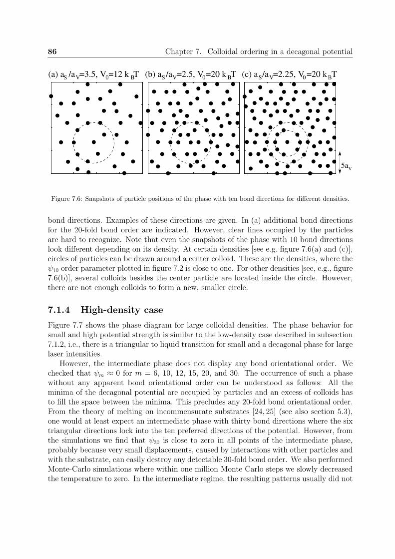
86 Chapter 7. Colloidal ordering in a decagonal potential
5aV
S V VS S V BBB(a) a /a =3.5, V =12 k T0 (b) a /a =2.5, V =20 k T0 (c) a /a =2.25, V =20 k T0
Figure 7.6: Snapshots of particle positions of the phase with ten bond directions for different densities.
bond directions. Examples of these directions are given. In (a) additional bond directionsfor the 20-fold bond order are indicated. However, clear lines occupied by the particlesare hard to recognize. Note that even the snapshots of the phase with 10 bond directionslook different depending on its density. At certain densities [see e.g. figure 7.6(a) and (c)],circles of particles can be drawn around a center colloid. These are the densities, where theψ10 order parameter plotted in figure 7.2 is close to one. For other densities [see, e.g., figure7.6(b)], several colloids besides the center particle are located inside the circle. However,there are not enough colloids to form a new, smaller circle.
7.1.4 High-density case
Figure 7.7 shows the phase diagram for large colloidal densities. The phase behavior forsmall and high potential strength is similar to the low-density case described in subsection7.1.2, i.e., there is a triangular to liquid transition for small and a decagonal phase for largelaser intensities.
However, the intermediate phase does not display any bond orientational order. Wechecked that ψm ≈ 0 for m = 6, 10, 12, 15, 20, and 30. The occurrence of such a phasewithout any apparent bond orientational order can be understood as follows: All theminima of the decagonal potential are occupied by particles and an excess of colloids hasto fill the space between the minima. This precludes any 20-fold bond orientational order.From the theory of melting on incommensurate substrates [24, 25] (see also section 5.3),one would at least expect an intermediate phase with thirty bond directions where the sixtriangular directions lock into the ten preferred directions of the potential. However, fromthe simulations we find that ψ30 is close to zero in all points of the intermediate phase,probably because very small displacements, caused by interactions with other particles andwith the substrate, can easily destroy any detectable 30-fold bond order. We also performedMonte-Carlo simulations where within one million Monte Carlo steps we slowly decreasedthe temperature to zero. In the intermediate regime, the resulting patterns usually did not

7.1. Phase behavior 87
0.68
0.66
0.64
0.62
0.60
0.58
0.56
0.54
100 50 10 5
part
icle
spacin
g a
S/a
V
potential strength V0/(kBT)
6 bond directions
10 bond directions
20 bond directions
no rot. symmetryquasicrystalline
triangular
liquid
solid phase without bondorientational order
Archimedean tiling
Figure 7.7: Phase diagram for large colloidal densities as a function of the potential strength V0 (in unitsof the thermal energy kBT ) and the particle spacing aS (in units of aV = 2π/|Gj |) in the ideal triangularlattice. The symbols denote the order parameters that are larger than 0.1. If all order parameters areclose to zero a small cross is plotted. The phase boundaries are drawn as guide to the eye. The dottedelliptical line marks the region where Archimedean-like tilings are found (see subsection 7.1.5). The dashedtransition line was determined by Brownian dynamics simulations. A detailed description is given in thetext.
reveal any bond orientational order. Therefore, it is not just due to thermal fluctuationsthat prevent any bond orientational symmetry. The potential itself does not seem to allowany orientational order.
In addition, the disordered phase seems to change from a liquid to a solid with increas-ing density. We tried to determine this phase transition by calculating the mean squaredisplacement of the colloids using Brownian dynamics simulations (see figure 7.8). Thedifferences in the time dependence of the mean square displacement are not as pronouncedas for the phase transition from the modulated liquid into the locked non-periodic phasedescribed in section 6.4. The asymptotic regime was not yet reached within our Browniandynamics simulations and we have not found any obvious phase transition so far. Onlywithin the phase with Archimedean-like tiling (see also section 7.1.5) for aS/aV ≈ 0.8, themean square displacement stays very small, indicating that the colloids are firmly bound to

88 Chapter 7. Colloidal ordering in a decagonal potential
0.01
0.1
1
10
0.1 1 10 100
me
an
sq
ua
re d
isp
lace
me
nt
<r2
>/a
V2
time t/(βγ aV2)
V=20 kBT; aS/aV=0.57V=20 kBT; aS/aV=0.58V=20 kBT; aS/aV=0.585V=20 kBT; aS/aV=0.59V=20 kBT; aS/aV=0.595V=20 kBT; aS/aV=0.6
liquid
close to phase tra
nsition?
solid (AT)
solid?
Figure 7.8: Mean square displacement calculated by Brownian dynamics simulations (as described insection 4.1) for systems in the phase with no bond orientational order. There seems to be a phasetransition, perhaps between a solid and a liquid state. The Archimedean-like tiling (see also section 7.1.5)for aS/aV = 0.8 is an extraordinary stable phase.
VS
aV
S VVS(a) a /a =0.8, V =100 k T (b) a /a =0.7, V =100 k T (c) a /a =0.6, V =100 k T0 0 0B B B
Figure 7.9: Snapshots for particle positions of the phase with ten bond directions for different densities.Note, the density in figure (b) corresponds to one particle per minimum. In (a) there are less colloids thanminima, in (c) there are more.
7.1. Phase behavior 89
the lattice positions of the Archimedean-like structure. For other densities, the curves forβV0 = 20 shown in figure 7.8 as well as corresponding curves for other potential strengthsseem to group: For low densities, the colloidal motion is diffusive corresponding to thedynamics of a liquid. For larger densities (below the dashed line in figure 7.7), the meansquare displacement increases much slower. Perhaps this is due to a solid phase where theparticles can diffuse within a region that is large compared to the area around a minimum.For example, colloids can move on circular trajectories in the regions of the shallow wellsthat form rings around the very deep minima. Another possibility is, that some particlesare pinned to the potential while others can float around them. Therefore, the transitionthat we mark as liquid to solid transition can also be a transition between different solid orliquid phases. Studying the dynamics in more detail and extending the Brownian dynamicssimulations to much longer times will be important for future works.
Finally, we want to comment on our observation, that snapshots of the phase withten bond direction sometimes appear very different depending on the density (see alsofigure 7.6 in subsection 7.1.3). For the density of the colloidal patterns shown in figure7.9(a) and (c) almost complete circles formed by particles exist whereas in figure 7.9(b)the most striking structures are pentagons. The circles correspond to circles [figure 7.9(a)]or double circles [figure 7.9(c)] of potential wells around a very deep minimum (cf. section3.3.2). Colloids of a partially filled inner circle [as in figure 7.9(b)] are usually placed ina way that they are located on the edge of large pentagons. Therefore the pentagons areextraordinary conspicuous for densities with partially filled circles.
7.1.5 Archimedean tiling
At densities with particle spacing aS/aV around 0.58 the triangular ordering reaches deepinto the region where bond-orientational order is not expected (see figure 7.7). As wedemonstrate in this section, the extraordinary stability is due to a very special structure.
In figure 7.10 we show the Delaunay triangulation of the colloidal patterns for someof the simulation results. For better visibility, all bonds that are longer than 1.1aS arenot shown. Interestingly, in figures 7.10(c) to (f) domains of a highly ordered structureare visible. This structure corresponds to an Archimedean tiling of type (33.22) [see figure7.11(a)] and consists of rows of squares and triangles. Sometimes there are also two rowsof triangles enclosed by the rows of squares [see figure 7.11(b)]. Archimedean tilings areinteresting complex structures which can also be found on periodic substrates [241,242, C].They are composed of regular polygons and characterized by the number and type ofpolygons that are grouped around one node [143]. For example, in an Archimedean tilingof type (33.22) one finds three triangles and two squares when going around a vertex [seearrow in figure 7.11(a)]. On the decagonal substrate the square rows of the Archimedeantiling of type (33.22) or its modified version with double triangular rows can appear withfive different orientations corresponding to the directions of the lines of low intensities inthe laser fields. Usually a domain with one specific orientation is quiet small and withinone colloidal configuration domains of two or three different orientations coexist.

90 Chapter 7. Colloidal ordering in a decagonal potential
S B(b) a /a =0.56; V =20 k TV
S B(c) a /a =0.577; V =10 k TV
S B(e) a /a =0.58; V =10 k TV
S(h) a /a =0.6; V =20 k TV BS(g) a /a =0.6; V =10 k TV B
S V
S V
no r
ot.
ord
erin
g
tria
ngula
r
no r
ot.
ord
erin
g
no r
ot.
ord
erin
gS V(a) a /a =0.56; V =10 k T 0 B
(d) a /a =0.577; V =20 k T B
(f) a /a =0.58; V =20 k T B
0
00
0 0
00
AT
−li
ke
AT
−li
ke
AT
−li
ke
AT
−li
ke
Figure 7.10: Delaunay triangulation of colloidal patterns obtained by Monte-Carlo simulations. Bondsthat are longer than 1.1aS are not shown. A detailed description of the observed phases is given in thetext.

7.1. Phase behavior 91
(b) modified AT(a) AT of type (3 .4 )23
Figure 7.11: (a) Archimedean tiling (AT) of type (33.22) and (b) modified AT with double rows of triangles.The Archimedean-like tiling observed in our simulations is a combination of these structures (see figure7.12).
For the Archimedean-like tiling the distances between the square rows behave as in aFibonacci chain, i.e., short distances corresponding to a single row of triangles and longdistances due to a double row of triangles are ordered in the same way as the short andlong distances in a Fibonacci chain (see figure 7.12).
Archimedean-like tilings for colloids in decagonal laser fields were first observed inexperiments by Mikhael et. al. [191] (see also section 7.2). Structures found by Ledieuet. al. [11] for Cu atoms on the surface of the icosahedral quasicrystal Al70Pd21Mn9 maycorrespond to such tilings.
By analyzing the Delaunay triangulations of colloidal snapshots, we find the Archimedean-like tiling in a very small density range with 0.577 ≤ aS/aV ≤ 0.585 which is framed bya dotted line in figure 7.7. Triangles dominate these structures and therefore usuallyψ6 > 0.1.
In the following, we calculate the density (or aS/aV ) where an Archimedean-like tilingis expected to fit best in the decagonal potential. The orientations of the rows of theArchimedean-like tiling correspond to the directions of the lines of low intensities in thedecagonal laser fields. As described in section 3.4.3, an average of the decagonal poten-tial over these directions leads to an one-dimensional potential that is the sum of twomodulations [cf. equation (3.34)]. The wavelengths of these modulations are
λ1 =2π
k1
=
√5 +
√5
10aV ≈ 0.851aV
and λ2 =2π
k2
=
√5−
√5
10aV =
λ1
τ≈ 0.526aV , (7.2)
where τ is the number of the golden ratio. The positions of the minima of the averaged

92 Chapter 7. Colloidal ordering in a decagonal potential
S L S L L S
Figure 7.12: Archimedean-like tiling pattern for aS/aV = 0.577 and V0/(kBT ) = 20. The sequence of shortand long distances between the rows of squares corresponds to the sequence of S and L in a Fibonaccichain (cf. section 3.1.3).
potential are roughly given as multiples of λ2, however their exact positions and theirdepths are modulated with λ1. The Archimedean tiling of type (33.22) [see figure 7.11]best fits the potential, if the sum of the heights of one row of triangles and and the heightof one row of squares equals two wavelengths λ2. For the modified Archimedean tiling [seefigure 7.11(b)] the height of two rows of triangles and one row of squares has to be 3λ2.Therefore, the length aAT of the edges of the squares and triangles in the Archimedeantiling are
aAT =2
1 +√
32
λ2 ≈ 0.563aV for an Archimedean tiling of type (33.22)
and amod−AT =3
1 + 2√
32
λ2 ≈ 0.577aV for a modified Archimedean tiling. (7.3)
This corresponds to a density given by the particle spacing aS of the ideal triangular latticewith
aS,AT =4√
3
3
√√
3− 3
2λ2 ≈ 0.585aV for an Archimedean tiling of type (33.22)
and aS,mod−AT =
√3−
√3λ2 ≈ 0.592aV for the modified Archimedean tiling. (7.4)
Since the averaged potential is quasiperiodic, none of the periodic structures describedabove fits the potential very well. In the simulations, we found that the sequence of the dis-tances between the square rows are given by a Fibonacci chain and therefore Archimedean-like tiling that appears in the decagonal potential is a combination of the Archimedean

7.1. Phase behavior 93
S B(b) a /a =0.93; V =20 k TV S B(c) a /a =0.95; V =20 k TVS V 0 0(a) a /a =0.9; V =20 k T B 0
Figure 7.13: Delaunay triangulation of point patterns without bonds longer than 1.1aS . Archimedean-liketiling can be observed. The particle spacing aS is roughly by a factor of τ larger than for the Archimedean-like tilings in figure 7.10. The parameters of the low density case are used (see section 4.4), only the chargeof the colloids is set to Z∗ = 20000.
tiling of type (33.22) and the modified one. In the observed Archimedean-like tiling, theprobability to find double rows of triangles is τ -times the probability to find single rows oftriangles (see section 3.2). Therefore, one finds
afib−AT =3τ + 2(√
3 + 1)τ +
√3/2 + 1
λ2 ≈ 0.573aV
and aS,fib−AT =
√2√
3
3
3τ + 2(√3 + 1
)τ +
√3/2 + 1
λ2 ≈ 0.590aV . (7.5)
The particle spacing aS,fib−AT for the theoretically predicted Archimedean-like tilingtherefore is just slightly larger than the one found in the simulation, which ranges fromapproximately 0.577 to 0.585. The difference probably is due to the imperfections of thepatterns in simulations, which lead to higher densities compared to perfect structures.
Note that the Archimedean-like tiling can also lock to the distance λ1 = τλ2. The idealdensity for such a structure with the characteristics of the Fibonacci chain then is
aS,λ1−fib−AT = τaS,fib−AT ≈ 0.954aV . (7.6)
This structure can be observed in simulations (see figure 7.13) and in experiments [20].No Archimedean-like tilings were found for even more dilute systems corresponding todistances τλ1, i.e., they seem to be restricted to densities determined by the wavelengthsλ1 and λ2.

94 Chapter 7. Colloidal ordering in a decagonal potential
7.1.6 Pair correlation function and structure factor
In figure 7.14 we plot the pair correlation functions g(d) for several colloidal patterns,which is given by the probability to find two colloids with a distance d. In figure 7.14(a)g(d) is plotted when the colloids are only allowed to occupy the potential minima; namelyall of them (full line) or just the deepest one (dotted line). Clearly, in the second casea few distances are preferred. The arrows indicate peak positions that follow from theirleft-hand neighbors by multiplication with the number of the golden ratio τ , which againreveals a self-similar property of the decagonal potential. The pair correlation function[figure 7.14(b)] determined from Monte-Carlo simulations indicates for small V0 a clearpeak close to d = aS = 2aV , as expected for the ideal triangular phase. For increasingpotential strength V0, new peaks start to develop in the quasicrystalline region at positionsof the deepest minima but they are still quite broad so that only ψ20 is non-zero (dashedline). Just crossing the phase boundary to the 10-bond-direction phase, the peaks becomemore pronounced (dotted line) meaning that the colloids settle more and more into thedeepest minima. Furthermore, for densities with aS around 1.85, the quasicrystallinephase with 20 bond directions only exists in a very small range of V0 (cf. figure 7.3). Thisis understandable from the pair correlation functions in figure 7.14(c). They show thatthe main peak in the triangular phase is already close to one pronounced peak of theideal g(d) in figure 7.14(a). As a result, the colloids can settle into the deepest minimaof the decagonal potential without the need of strong rearrangements and, therefore, the20-bond-direction phase hardly occurs.
In figure 7.14(e), we plot the pair correlation function for aS = 0.56 for increasingpotential strengths V0. The most pronounced peak is just determined by the colloidaldensity. During the transition from the triangular (ψ6 > 0.1) to the disordered (ψm < 0.1)phase, g(d) changes so that the other peaks better fit to the ideal pair correlation functionin figure 7.14(a). The pair correlation functions of the Archimedean-like tiling shownin figure 7.7(d), the peaks (besides the highest one) fit very well to the ideal g(d) infigure 7.14(a). Therefore, this ordering is extraordinary stable and the transition into thedisordered phase is delayed to larger V0. The observation that the Archimedean like tilingfits to the decagonal potential very well is also discussed in [191].
Finally, in figure 7.15, we plot the two-dimensional direct correlation functions for theliquid and the phases with 10 or 20 bond directions. We also calculated the correspondingstructure factors, which are the Fourier transformed of the direct correlation functions.The structure factors confirm the long-range order of the quasicrystalline phases. Sincesometimes it is hard to determine the actual symmetry by just calculating the correlationfunctions or the structure factors, the quantitative method that employs the bond orien-tational order parameter is more appropriate to quantitatively analyze colloidal ordering.
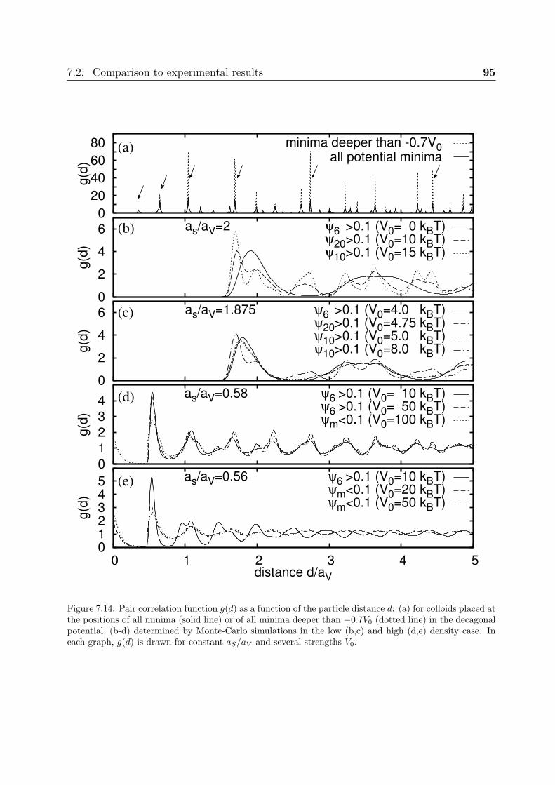
7.2. Comparison to experimental results 95
0
20
40
60
80
g(d
) all potential minima minima deeper than -0.7V0
0
2
4
6
g(d
)
as/aV=2 ψ6 >0.1 (V0= 0 kBT)ψ20>0.1 (V0=10 kBT)ψ10>0.1 (V0=15 kBT)
0
2
4
6
g(d
)
as/aV=1.875 ψ6 >0.1 (V0=4.0 kBT)ψ20>0.1 (V0=4.75 kBT)ψ10>0.1 (V0=5.0 kBT)ψ10>0.1 (V0=8.0 kBT)
0
1
2
3
4
g(d
)
as/aV=0.58 ψ6 >0.1 (V0= 10 kBT)ψ6 >0.1 (V0= 50 kBT)ψm<0.1 (V0=100 kBT)
012345
0 1 2 3 4 5
g(d
)
distance d/aV
as/aV=0.56 ψ6 >0.1 (V0=10 kBT)ψm<0.1 (V0=20 kBT)ψm<0.1 (V0=50 kBT)
(b)
(a)
(c)
(d)
(e)
Figure 7.14: Pair correlation function g(d) as a function of the particle distance d: (a) for colloids placed atthe positions of all minima (solid line) or of all minima deeper than −0.7V0 (dotted line) in the decagonalpotential, (b-d) determined by Monte-Carlo simulations in the low (b,c) and high (d,e) density case. Ineach graph, g(d) is drawn for constant aS/aV and several strengths V0.

96 Chapter 7. Colloidal ordering in a decagonal potential
0 BVS V B0SSliquid (a /a =2.25; V =5 k T)V 0 B
Vy
/a
Vy
/a
Vy
/a
g
/G
y
0
g
/G
y
0
g
/G
y
0
g /G x 0 g /G x 0 g /G x 0
V
(d)
20 bond dir. (a /a =2.25; V =10 k T) 10 bond dir. (a /a =2.25; V =20 k T)
x/a x/aV V
(a) (b) (c)
(e) (f)
x/a
Figure 7.15: (a-c) Two-dimensional direct correlation functions and (d-f) structure factors for (a,d) theliquid for βV0 = 5, (b,e) the phase with 20 bond directions for βV0 = 10, and (c,f) the phase with 10-foldbond orientational order for βV0 = 20. In all cases, the density is given by aS/aV = 2.25. One quadrantfor each of the plots was calculated, the other quadrants are mirror images.
7.2 Comparison to experimental results
In the experiments performed at the University of Stuttgart by J. Mikhael, L. Helden,and C. Bechinger the decagonal laser field (see figure 7.16) is realized by five linearlypolarized laser beams that are arranged along the edges of a prism with pentagonal basisand then interfere to create the potential (cf. section 3.3). The colloidal suspension isconfined between two class plates. By pushing the colloids against the lower glass surfacewith an additional laser beam with a broad focus, they can only move in two dimensions.A boundary is created with the help of a laser beam that rotates along a circle aroundthe region that contains the colloidal system to be studied. By changing the radius ofthe circle, the density can be adjusted. The interaction strength is regulated via theconcentration of counter ions in the suspension. Highly charged polystyrene spheres withradius R = 1.45 µm and a polydispersity of about 4% dispersed in deionized water areused. The mean particle spacing is about aS = 4.6 µm. Usually the laser power is graduallyincreased up to 10 Watts. The positions of the colloids are determined via video microscopy.

7.2. Comparison to experimental results 97
Figure 7.16: Decagonal laser field in experiment. Experiment and photograph by J. Mikhael [20].
In figure 7.17 a micrograph of the decagonal phase at high laser intensities is shown.Archimedean-like tilings were first observed in the experiments (see figure 7.18 and [191])and can be found at different densities probably because the systems locks into the twolength scales λ1 and λ2 introduced in section 7.1.5.
As in the simulations, domains of an Archimedean-like tiling with different orientationsare found in experiments. However, one direction usually seems to be preferred and there-fore large domains of an almost perfect Archimedean-like tiling with just one orientationcan be observed. Very likely, this is caused by a small imperfection in the experimentallycreated potential. If for example not all angles of the laser beams with respect to the sam-ple plane are equal, the lengths of the projected wave vectors Gj may vary. If one of thevectors Gj is slightly different from the others, this corresponds to a gradient in the phase,which is equivalent to a combination of a constant phononic and phasonic strain along acertain direction in the decagonal potential [178]. Because in a potential with such a phasegradient the lines of low intensities are all finite except those in the gradient direction (seefigure 7.19), the orientation along this direction is preferred by the Archimedean-like tiling(see also section7.3.4).

98 Chapter 7. Colloidal ordering in a decagonal potential
Figure 7.17: Decagonal ordering in experiment. Experiment and micrograph by J. Mikhael [20].
Figure 7.18: Archimedean-like tiling in experiment. Experiment and micrograph by J. Mikhael [20].

7.3. Phasonic displacements and drifts 99
x/aV
y/a
V
Figure 7.19: Theoretically calculated decagonal potential with a gradient in the phase ϕ0 attached to wavewith wave vector G0: ϕ0 = 0.2x/aV . It creates a gradient in the phononic and phasonic displacementsalong the x-direction. The lines of low intensity are infinite in x-direction, but finite in all other directions.
7.3 Phasonic displacements and drifts
In this section, we shortly demonstrate how the colloidal system can be used to study theproperties and consequences of phasonic displacements, gradients, and drifts.
7.3.1 Rearrangements in a decagonal quasicrystal
First we demonstrate how a phasonic flip in a decagonal pattern can be induced by achange of the phasonic displacement of the potential.
Figure 7.20 shows patterns within the decagonal phase before and after a phasonicdisplacement, i.e., the phasonic displacement is wx = 0 on the left-hand side and wx =0.1aV on the right; wy is 0 in both cases. The pattern is decagonal independent of thedisplacement, however the orientation of some of the sketched pentagons has changed.It seems that always two neighboring pentagons flip their orientation at the same time.Furthermore, the row of pentagon does not change its y-position, which is probably due to

100 Chapter 7. Colloidal ordering in a decagonal potential
aV
∆x
w =0.1aV
Figure 7.20: Inducing a phasonic flip: Colloidal point patterns within the decagonal phase (aS/aV = 0.65,V0/(kBT ) = 1000) for wx = 0 (left) and wx = 0.1aV (right). The flipping pentagons are marked by dottedcircles.
S L S L L S S L S L S L
∆ yw =0.015aV
Figure 7.21: Inducing a phasonic flip: Delaunay triangulation of colloidal point patterns (without bondslonger than 1.1aS) for the Archimedean-like tiling (aS/aV = 0.577, V0/(kBT ) = 20) for wy = 0 (left) andwy = 0.015aV (right). The flip in the Fibonacci chain is marked by dotted circles.
the fact that the horizontal lines of low laser intensity are not affected by a change of wx
(see section 3.4.3).
7.3.2 Rearrangements in an Archimedean-like tiling
Here we want to demonstrate the consequences of a phasonic displacement on the Archimedean-like tiling. Figure 7.21 shows patterns of the Archimedean-like tiling for different phasonicphases wy. Note a whole row of triangles and a row of squares have interchanged theirposition on the right-hand side of figures 7.21. Therefore, phasonic flips occur in the se-quence of the distances between the square rows that corresponds to a Fibonacci chain (cf.sections 3.1.3 and 3.4.1).
If the phasonic displacement is changed such that the lines of low intensity in thedirection of the square or triangular rows are not shifted, the whole Archimedean-liketiling is not affected by the phasonic displacement.

7.3. Phasonic displacements and drifts 101
Vy/a
0
−0.4 −0.2 0−4
−2
∆
per MC step
xw =10 a−4
V
wx
<V> /V0
Figure 7.22: Stabilization by a phasonic drift: Delaunay triangulation of colloidal point patterns (withoutbonds longer than 1.1aS) for the Archimedean-like tiling (aS/aV = 0.577, V0/(kBT ) = 20) withoutphasonic displacement (left) and in a potential with a phasonic drift of ∆wx = 104aV per Monte-Carlostep (right). The small graph on the right-hand side shows the potential averaged over wx depending ony [see also equation (3.34)].
7.3.3 Stabilizing the Archimedean-like tiling by a phasonic drift
Fluctuations in wx or a steadily growing wx orients the Archimedean-like tiling along thex-direction. This is demonstrated in figure 7.22) for a phasonic drift ∆wx = 104aV perMonte-Carlo step. Domains that are not oriented along the x-direction are reduced becausea change in wx would always displace the rows of squares and triangles in the Archimedean-like tiling except when they are oriented along the x-direction. A colloid in a decagonallaser field with a fast phasonic drift in wx-direction can be considered as a particle in aneffective potential that is the decagonal potential averaged over wx (see right-hand side offigure 7.22). As introduced in section 3.4.3, the average of the decagonal laser field over wx
corresponds to the average over x and does not depend on y. Such an averaged potentialonly supports domains of Archimedean-like tiling oriented in x-direction. In summary,phasonic fluctuations or drifts help to create large domains of Archimedean-like tilings.
7.3.4 Stabilizing the Archimedean-like tiling by a phasonic gra-dient
Another possibility to reduce the domains of Archimedean-like tiling that are not orientedalong the x-direction is to induce a phasonic gradient in x-direction. Such a gradientdestroys all continuous lines of low intensity in the potential landscape, except those inx-direction (see also section 3.4.3). Therefore, in a potential with a phasonic gradient, theArchimedean-like tiling is mainly oriented along the phasonic gradient (see figure 7.23).This very likely is the reason for the very large domains of Archimedean-like tiling foundin experiments that preferentially orientate along the same direction. A phasonic gradientfield is caused when the laser beams are not perfectly adjusted (see also section 7.2).

102 Chapter 7. Colloidal ordering in a decagonal potential
xw /x=0.15
Figure 7.23: Stabilization by a phasonic gradient: Delaunay triangulation of point patterns (without bondslonger than 1.1aS) for the Archimedean tiling like phase (as/al = 0.577, V0/(kBT ) = 20) without phasonicdisplacement (left) and in a potential with a phasonic gradient with wx/x = 0.15 (right).
7.4 Summary and Outlook
In this chapter, we determined the phase behavior of colloids on a 2D decagonal substrate.We found a triangular to liquid phase transition for small laser intensities and decagonalordering in strong potentials. For intermediate intensities, however, where the colloidalordering is influenced by both the colloidal interaction and the substrate potential, weidentify a series of interesting phases: For systems with low densities, where the number ofcolloidal particles is less than the number of potential minima, there is a quasicrystallinephase which exhibits bond orientations in 20 different directions. When the number ofcolloids exceeds the number of potential minima, we usually find a solid phase without anyapparent bond orientational order. However, for certain densities the system locks into ahighly ordered phase that is close to an Archimedean tiling.
We also demonstrated how the system can be used to study the effects of phasonic dis-placements, drifts, or gradients. We showed how phasonic colloidal flips in the Archimedean-like tiling and in the decagonal phase are induced by phasonic displacements in the sub-strate potential. Furthermore, the Archimedean-like tiling orientated along one directionis stabilized with the help of a phasonic drift or gradient.
Interestingly, in experiments the Archimedean-like tilings seem to be extraordinary sta-ble [20]. The density in experiments usually cannot be controlled as easy as in simulations:In Monte-Carlo simulations the density is extremely homogeneous due to possible globalsteps. In experiments, the density often seem to self-adjust right inside the small stabil-ity region of the Archimedean-like tiling. Therefore, Brownian dynamics simulations withopen boundary conditions would give a deeper inside into the stability of Archimedeantilings.
In triangular phases induced by triangular substrates the phonon spectrum was de-termined from simulations, experiments, and analytical calculations [243, 244] (cf. also[245–248]). Such an analysis for the phonon and phason spectra of induced quasicrystalswould be very interesting, however, also extremely difficult due to the problems of splittingup the observed displacements into phononic and phasonic contributions (cf. section 3.4.4).
Finally, as a very general outlook, we discuss the following question: What is reallyneeded to induce quasicrystalline order in a mono-atomic system? Usually, two appro-

7.4. Summary and Outlook 103
priately chosen characteristic lengths are needed to achieve quasicrystalline order, e.g.,quasicrystals are observed for systems with two length scales in the interaction poten-tial [249, 250]. In binary systems studied so far the free energy of periodic and quasicrys-talline states are close [57,61,251,252]. In the most recent work the ground state seems tobe periodic [252]. Patrykiejew and Soko lowski claimed to have found decagonal orderingin a mono-atomic system, where one length scale is given by the particle interactions andanother by a periodic potential [241]. However, the observed phase turned out to be aperiodic Archimedean tiling [242, C]. Probably a promising candidate for mono-atomicquasicrystalline ordering on a periodic potential is a system, where the mean particle spac-ing differs by an irrational factor (e.g. by a factor of τ) from the lattice constant of thesubstrate. A pinned phase for high potential strength therefore usually cannot order pe-riodically (cf. the frustrated non-periodic phase in section 6.4). To study such a phaseis very interesting, especially to find out, whether it exhibits quasicrystalline ordering,perhaps even with some non-crystallographic rotational symmetry. Such a system, i.e.,with a mismatch in the lattice structure of the substrate and the colloidal adsorbate, wasalready studied in [253], however mainly for selected mismatch ratios that lead to periodicstructures.

104 Chapter 7. Colloidal ordering in a decagonal potential

105
Chapter 8
Brownian particles in a decagonalpotential
In this chapter we consider a single colloidal particle moving in decagonal or square poten-tials. In the long-time limit we find conventional diffusion as it is known in literature forsystems whose depth of the potentials is limited. However, for large potential strengthsthe particle needs a very long time to approach its asymptotic diffusive limit. For anintermediate time regime, which can span over several decades, we find subdiffusive mo-tion. To explore this regime, we especially study in this chapter how the diffusive limit inthermal equilibrium is approached. First, in section 8.1 we shortly introduce anomalousdiffusion. We then concentrate on the Brownian motion of a particle in potential land-scapes of different symmetry. In section 8.2 results of Brownian dynamics simulations arepresented, where the colloid is started at an arbitrary position in the potential, i.e., innon-equilibrium. In section 8.3 an analytic theory for this situation is developed, basedon a model where the particle jumps between random trapping sites, and the theory iscompared to the results of the simulations. The motion of a colloid in thermal equilib-rium is discussed in section 8.4 and compared to experimental results. In section 8.5 theBrownian dynamics of particles that are driven out of equilibrium by a phasonic drift isstudied. Relation known in non-equilibrium statistics can be applied to such a system andare, therefore, shortly introduced in section 8.6. Finally we conclude in section 8.7. Partsof this chapter are based on publication [B].
8.1 A short introduction to anomalous diffusion
Free Brownian motion leads to diffusion at time scales where inertia can be neglected and iswell understood since Einstein’s seminal paper [181] (see also section 4.1.1). Conventionaldiffusion of a particle is characterized by its mean square displacement that is proportionalto time: 〈r2〉 ∝ t. However, in systems with anomalous diffusion, one finds
〈r2〉 ∝ tν (8.1)

106 Chapter 8. Brownian particles in a decagonal potential
with an exponent ν 6= 1. For ν < 1 the system is called subdiffusive and for ν > 1superdiffusive. For superdiffusive motion, one also uses the notions subballistic for ν < 2,ballistic for ν = 2, and superballistic for ν > 2. In this section we present some approachesto theoretically address anomalous diffusion as well as important examples of systemswhere it occurs.
Asymptotic anomalous diffusion, i.e., sub- or superdiffusive motion in the long time-limit t→∞, is often explained by using so-called Levy walks (see e.g. [254–258]). These aremodified random walks with special distributions for step length or step duration. Some-times waiting times in between the steps are included. Asymptotic anomalous diffusionoccurs, if the first or second moment of the step length distribution or of the waiting timedistribution is not finite. Note that even if the first and second moment are convergent andtherefore the motion is diffusive in the long time limit, there still can be anomalous diffusionat intermediate times. In modifications of the standard Levy walk model, e.g., in randomwalk models with nontrivial coupling between step length and duration (see e.g. [257]) orin models with a random distribution of velocities [259, H], asymptotic anomalous diffusionis also found.
Diffusion is often characterized by the parabolic differential equation
∂
∂tp(r, t) = D∇2
rp(r, t), (8.2)
where p(r, t) is the probability for the diffusing particle to be at position r at time t andD is the diffusion constant. To construct a generalized equation that describes anomalousdiffusion, we apply a Laplace transformation in time and a Fourier transformation in space:
p(k, s) =
∫ ∞
0
dt
∫dr exp(−st) exp(ik · r)p(r, t). (8.3)
The integration in r is over the whole space. In Fourier-Laplace space equation (8.2) reads(s+Dk2
)p(k, s) = 0. (8.4)
This equation can be generalized by introducing exponents α and β:(sα +D |k|β
)p(k, s) = 0. (8.5)
In real space and time, equations such as (8.5) are often written with fractional derivatives(i.e. ∂α/∂tα) and the corresponding equations for anomalous diffusion are called fractionaldiffusion equations (see e.g. [260, 261]). The mean square displacement for a solutionof equation (8.5) behaves as 〈r2〉 ∝ t2α/β if it is convergent. Obviously, equation (8.5)describes subdiffusive as well as superdiffusive motion if the exponents α and β are chosenappropriately. Sometimes, the mean square displacement is divergent and therefore thescaling in time is studied by considering other moments [260]:
〈|r|δ〉 ∝ tδα/β. (8.6)

8.1. A short introduction to anomalous diffusion 107
However, the is a difference between the scaling of the moments and the (approximate)scaling of p(r, t). furthermore, if p(r, t) does not scale perfectly, the scaling of the momentsdepends on the exponent δ in a non-trivial way [I].
Superdiffusion is not only found in systems with a Levy walker. There are also billiardmodels, i.e., systems where a particle is reflected when hitting the boundary of an obstacle,which exhibit superdiffusion for an ensemble of particles started with random conditions.The path of a particle in such a billiard system is not random but totally determined bythe starting position and direction. A famous example of such a system is the Lorentz gasalso called Sinai billiard, which in two dimensions consists of circular obstacles from whichthe particles are reflected. If there is no straight path of infinite length (finite horizonsystem), the particles behave diffusive [262]. However, if straight paths of infinite lengthexist, the mean square displacement asymptotically is proportional to t ln t, i.e., the systemis superdiffusive [263,264]. There are also other billiard systems like zigzag channels [265]or hexagonal channel systems [F,G,J] that are superdiffusive due to some special paths onwhich the particles travel in one direction for very long times.
Also many subdiffusive systems have been studied in recent years. Examples are many-particle systems such as dense colloidal suspensions close to freezing [266] or other glassysystems (see e.g. [267–269]), where subdiffusion is due to caging from surrounding particlesas demonstrated explicitly in experiments [270–272]. Permanent confinement leads to sub-diffusion as well: many particles that move in narrow channels exhibit anomalous diffusion[233], which recently was also studied for single-file diffusion in colloidal systems [51, 52,234]. Furthermore, particles confined to the space between obstacles forming a Lorentz gasbehave subdiffusively on intermediate time scales [273].
Anomalous diffusion also plays an important role in many biological systems. Exam-ples are the dynamics of molecular motors moving along heterogeneous substrates [274],superdiffusion of migrating cells [275], the subdiffusion of macromolecules in the cell due tocrowding [276], the motion of beats in the cytoskeleton or artificial actin networks [277,278],or the dynamics of fluorescently labeled molecules in cells [279–281] and in membranes [282].
Even the simple Brownian motion of a single particle in a random potential exhibitssubdiffusion. Honkonen and Pis’mak [283] showed that such a motion is subdiffusive onall time scales if the depth of the potential is not limited from below. This was extensivelystudied in many Brownian dynamics simulations, where for overdamped systems indeedasymptotic subdiffusion is observed [284], whereas for low damping also superdiffusion atintermediate times can be found [285–289]. However, if each potential well possesses afinite depth, the motion always becomes diffusive in the long-time limit. Modelling it byjumps between traps with random but finite strengths, the asymptotic diffusion constantcan be calculated (see, e.g., Haus et al. in [290,291]). The random trap model we introducein section 8.3 also leads to diffusive behavior at very long times.

108 Chapter 8. Brownian particles in a decagonal potential
8.2 Brownian motion in static potentials started in
non-equilibrium
Here, the colloidal particles are started at random positions within the potentials. Weperform Brownian dynamics simulations in two dimensions (see section 4.1 for the detailsof the simulations) under the influence of external potentials. We compare the motionof a colloidal particle in a potential with decagonal symmetry (see section 3.3) to itsdiffusive behaviour in regular or random square potentials, which we introduce in the nextsubsection.
8.2.1 Regular and random square potential
We consider regular or random square potentials that consist of wells located on a squaregrid with lattice constant aV . Each well is modeled according to a product of cosines,i.e., within the area given by |x− xm| ≤ aV /2 and |y − ym| ≤ aV /2, the minimum of thepotential at position rm = (xm, ym) is described by
V (r) = −Vm(rm)
2
1 + cos
[2π(x− xm)
aV
]cos
[2π(y − ym)
aV
], (8.7)
where Vm(rm) ist the depth of the minimum. In the regular square potential all minimahave the same depth, i.e., Vm(rm) = V0 = const. For the random square potential, thedepths of the wells are randomly taken from the interval [0, V0] with the same probability.Therefore the distribution of the potential depths for the random square potential is muchsimpler than the one of the decagonal potential (see 3.3.3). As we demonstrate at the endof the next subsection, this leads to differences in the simulation results. Figure 8.1 showsthe potential landscapes of the square and the decagonal potentials, and their grey-scalerepresentations, which correspond to the intensity field of the respective light patterns inexperiments.
8.2.2 Results of the simulations
Here, we calculate the mean square displacement with respect to the starting position r(0)of the random walker according to
〈r2〉 = 〈[r(t)− r(0)]2〉, (8.8)
where the ensemble average is realized with 5000 different runs in the simulations.The particles start at random positions. The left-hand side of figure 8.2 shows the
simulation results for the time dependence of the mean square displacement for all poten-tials. The different curves correspond to different values of the strength V0 of the potentialsnormalized by the thermal energy β−1 = kBT . The characteristic length scale aV is usedto rescale length, the time is plotted in units of βγa2
V , where γ is the friction coefficientof the colloid. For zero potential βV0 = 0 the system is diffusive with 〈r2〉 = 4Dt, where

8.2. Brownian motion in static potentials started in non-equilibrium 109
V/V0
V/V0
V/V0
y
y
y
x
x
x
(a) (b)
(d)
(f)
(c)
(e)
aV
Figure 8.1: (a,c,e) Potential landscapes and (b,d,f) their grey-scale representations for (a,b) a regularsquare, (c,d) a random square, and (e,f) a decagonal potential. The exact definitions of the potentials aregiven in sections 8.2.1 for the square and 3.3 for the decagonal potential. The bar in the lower right cornerof figure (f) indicates the characteristic length aV = 2π/ |Gj |.
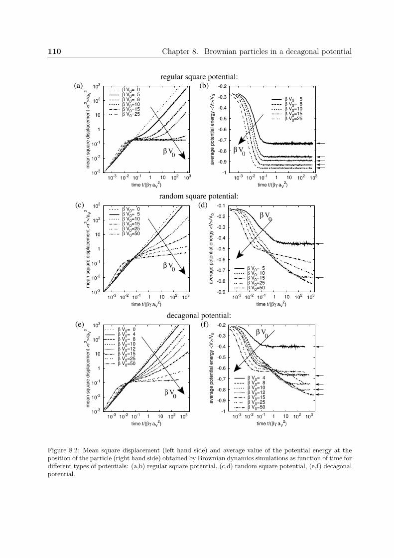
110 Chapter 8. Brownian particles in a decagonal potential
10-3
10-2
10-1
1
10
102
103
10-3
10-2
10-1 1 10 10
210
3
me
an
sq
ua
re d
isp
lace
me
nt
<r2
>/a
V2
time t/(βγ aV2)
β V0= 0β V0= 5β V0= 8β V0=10β V0=15β V0=25
-1
-0.9
-0.8
-0.7
-0.6
-0.5
-0.4
-0.3
-0.2
10-3
10-2
10-1 1 10 10
210
3
ave
rag
e p
ote
ntia
l e
ne
rgy <
V>
/V0
time t/(βγ aV2)
β V0= 5β V0= 8β V0=10β V0=15β V0=25
-0.9
-0.8
-0.7
-0.6
-0.5
-0.4
-0.3
-0.2
-0.1
10-3
10-2
10-1 1 10 10
210
3
ave
rag
e p
ote
ntia
l e
ne
rgy <
V>
/V0
time t/(βγ aV2)
β V0= 5β V0=10β V0=15β V0=25β V0=50
10-3
10-2
10-1
1
10
102
103
10-3
10-2
10-1 1 10 10
210
3
me
an
sq
ua
re d
isp
lace
me
nt
<r2
>/a
V2
time t/(βγ aV2)
β V0= 0β V0= 5β V0=10β V0=15β V0=25β V0=50
-1
-0.9
-0.8
-0.7
-0.6
-0.5
-0.4
-0.3
-0.2
10-3
10-2
10-1 1 10 10
210
3
ave
rag
e p
ote
ntia
l e
ne
rgy <
V>
/V0
time t/(βγ aV2)
β V0= 4β V0= 8β V0=10β V0=12β V0=15β V0=25β V0=50
10-3
10-2
10-1
1
10
102
103
10-3
10-2
10-1 1 10 10
210
3
me
an
sq
ua
re d
isp
lace
me
nt
<r2
>/a
V2
time t/(βγ aV2)
β V0= 0β V0= 4β V0= 8β V0=10β V0=12β V0=15β V0=25β V0=50
Vβ0
Vβ0
Vβ0
Vβ0
Vβ0
Vβ0
(a)
(c)
(e)decagonal potential:
(f)
(d)random square potential:
(b)regular square potential:
Figure 8.2: Mean square displacement (left hand side) and average value of the potential energy at theposition of the particle (right hand side) obtained by Brownian dynamics simulations as function of time fordifferent types of potentials: (a,b) regular square potential, (c,d) random square potential, (e,f) decagonalpotential.

8.2. Brownian motion in static potentials started in non-equilibrium 111
0.2
0.4
0.6
0.8
1.0
1.2
0.01 0.1 1 10 100
loca
l exp
onen
t ν(t
)
time t/(βγ aV2)
βV0= 4βV0= 8βV0=10βV0=12βV0=15
Figure 8.3: Time dependence of the local exponent ν(t) as defined in equation (8.9) for the decagonalpotential.
the diffusion constant D obeys the Einstein relation D = (βγ)−1 [see equation (4.12)]. Fora non-zero potential and at short times, the particles first relax into the nearest minima.For stronger potentials, the relaxation process is faster. Nevertheless, after the short-timerelaxation interestingly all curves for the mean square displacement seem to intersect in acommon point, a behaviour we were not able to explain. In the long-time limit, we findnormal diffusion. The asymptotic diffusion constant decreases with increasing potentialstrength. The behaviour at intermediate times strongly depends on the type of the poten-tial. For the regular square potential [see figure 8.2(a)], the mean square displacement doesalmost not increase and the crossover to diffusion happens already before the mean squaredisplacement has reached a2
V , i.e., as soon as the particle leaves a potential well making astep of length aV , diffusion sets in. By contrast, in a random or decagonal potential thecolloid has to explore an area larger than a2
V and therefore several potential minima, beforethe motion becomes diffusive. The temporal range of the intermediate regime increaseswith increasing potential strength βV0. For very high large V0, the diffusive limit hasnot even been reached within the simulated time range. The motion in the intermediateregime is subdiffusive, i.e., if the mean square displacement is fitted locally by a power law〈r2〉 ∝ tν , the exponent ν is smaller than 1. In figure 8.3 we plot the local exponent ν forthe decagonal potential calculated according to
ν(t) =d log [〈r2(t)〉/a2
V ]
d log [t/ (βγa2V )]
. (8.9)
As expected, for small times the exponent is larger than 1 indicating the superdiffusivemotion while the particle relaxes into the nearest minimum. For intermediate times, the
112 Chapter 8. Brownian particles in a decagonal potential
exponent is smaller than 1 and slowly relaxes towards ν = 1 with increasing time, whichmeans subdiffusive motion that slowly crosses over to conventional diffusion in the longtime limit.
On the right-hand side of figure 8.2 we plot the time dependence of the average potentialenergy at the position of the particle, i.e., if r(t) is the colloidal position the averagepotential energy is
〈V (t)〉 = 〈V (r(t))〉, (8.10)
where the average is taken over an ensemble of particle runs. Since the colloids are startedat random positions the curves start at t = 0 from the mean value of the potential. It canbe calculated analytically by integrating over the whole potential,
〈V (0)〉 = limA→∞
1
A
∫A
dA V (r) , (8.11)
where A is the area of the integration region. We find 〈V (0)〉 = −0.25V0 for the regu-lar, 〈V (0)〉 = −0.125V0 for the random square, and 〈V (0)〉 = −0.2V0 for the decagonalpotential. At small times the particle relaxes into the minima closest to its starting posi-tion. In the regular potential, the colloid then has already reached its asymptotic averagepotential energy. However, in the random square and the decagonal potential it takes upto several decades in time before the long-time value is approached (marked by arrows infigure 8.2). The asymptotic average energies correspond to the canonical ensemble averageof the potential energy of a particle. Interestingly, the long-time limit is reached, whenthe motion of the particle crosses over into the diffusive regime. Therefore, as long as thecolloid has not explored the full variety of possible minima so that it is possible to find apotential well much deeper than the ones the colloid has visited before, the system behavessubdiffusively. As soon as the potential energy of the particle is thermally equilibrated,its motion is diffusive. The relaxation process reveals similarities and differences betweenthe random and the decagonal potential. The curves for both potentials display a kinkat times where the particles have relaxed into nearby minima. Their depth correspondto the mean potential depth 〈Vm〉 = −0.5V0 in the random and 〈Vm〉 = −0.603V0 in thedecagonal potential (see also section 8.3.2). However, beyond the kink and for large laserintensities βV0, the average potential energy stays on an almost constant plateau in caseof the decagonal potential, but clearly decreases in the random potential. The differentbehavior is due to the different distributions ρ(Vm) of the depths of the minima (see sec-tions 3.3.3 and 8.2.1). In the decagonal potential minima with depths smaller than 0.24V0
do not exist and the number of wells decreases with its depth. In contrast, in the randomsquare potential all depths between 0 and V0 occur with the same probability. Therefore,in the decagonal potential it takes longer to find minima much deeper than the averagewell and the potential energy decreases much slower.

8.3. Random trap model 113
8.3 Random trap model
In the following we develop a theory to calculate the time dependence of the mean squaredisplacement. The theory is applicable to all potentials that display clear minima. Insubsection 8.3.2 we compare the theoretical results to the simulations.
8.3.1 Theory
We consider the local minima of the potential as trapping sites for the colloid. The particlesits in a well and after a certain waiting time jumps into a neighboring minimum. Therefore,we consider a theory with a random walker jumping between trapping sites. The probabilityto leave a site is given by a transition rate Γ. Its inverse Γ−1 denotes a typical waitingtime. The mean square displacement is calculated by⟨
r2(t)⟩
=∑
j
p(xj, yj, t)(x2j + y2
j ), (8.12)
where the sum is over all trapping sites, i.e., all local minima of the potential, and p(x, y, t)is the probability for the walker to be at position (x, y) at time t. In the square and alsoin triangular or hexagonal lattices, both the distance between nearest neighbors and thenumber of nearest neighbors is constant. In the decagonal potential this is not the case.Nevertheless, we will develop the theory for regular lattices and will then show that theresults well approximate the random walk in the decagonal potential when mean valuesfor the numbers of nearest neighbors and their distances are chosen.
The dynamics of the probability p(x, y, t) is governed by the rate equation:
d
dtp(xj, yj, t) = −zΓ(xj, yj)p(xj, yj, t) +
∑i∈NNj
Γ(xi, yi)p(xi, yi, t), (8.13)
where the sum is over all nearest neighbors of the minimum j located at xj, yj and z isthe number of its nearest neighbors. Equation (8.13) describes the temporal change of theprobability to be at the trapping site j. The first term on the right-hand side corresponds toparticles leaving the trap and the second term to colloids reaching site j from neighboringtraps. In the following we define a time-dependent diffusion constant D(t) by
D(t) =d
dt
⟨r2(t)
⟩. (8.14)
For normal diffusion this gives the conventional diffusion constant in 〈r2(t)〉 = 4Dt. In-serting equation (8.13) into the time derivative of equation (8.12), the diffusion constantis connected to the transition rates and p(xj, yj, t):
D(t) =1
4
∑j
−zΓ(xj, yj)p(xj, yj, t) +∑
i∈NNj
Γ(xi, yi)p(xi, yi, t)
(x2j + y2
j ). (8.15)
114 Chapter 8. Brownian particles in a decagonal potential
After interchanging the summation∑j
∑i∈NNj
Γ(xi, yi)p(xi, yi, t)(x2j + y2
j ) =∑
i
∑j∈NNi
Γ(xi, yi)p(xi, yi, t)(x2j + y2
j ), (8.16)
the second term in (8.15) can be calculated for a square, triangular, and hexagonal lattice:∑j∈NNi
(x2j + y2
j ) = zx2i + zy2
i + zl2, (8.17)
where l is the jump length (e.g., the lattice constant aV in the square lattice). Thereforewith equations (8.17) and (8.16), equation (8.15) becomes
D(t) =zl2
4
∑j
Γ(xj, yj)p(xj, yj, t). (8.18)
In the long-time limit, this gives
D∞ =zl2
4〈〈Γ〉〉 . (8.19)
Equation (8.19) is a well known result for the time-independent asymptotic diffusion con-stant given, e.g., in reference [291]. The average 〈〈·〉〉 is weighted according to the occupa-tion probabilities of the trapping sites. Note that equation (8.18) is a more general relationsince it is not only valid in the asymptotic long-time regime but for all times, where thediffusion constants generally depend on time.
We now introduce the probability P (Vm, t)dVm for a colloid to be at time t in a minimumwith the depth within the interval [Vm, Vm +dVm]. In the following, we will study diffusionbased on the rate equation for P (Vm, t) instead of using p(x, y, t). However, this is onlypossible if the transition rates Γ do not depend on the location of the trapping sites and,especially, if there are no positional correlations of the transition rates. Therefore we nowassume that the transition rate Γ only depends on the depth of the well Vm = |V (x, y)| atthe trapping site. Later we will show that this assumption is reasonable, if one considersKramer’s rate theory to calculate the transition rate for leaving a minimum.
We replace the average in space in equation (8.18) by an average over all possible depthsVm. Therefore the diffusion constant becomes
D(t) =zl2
4
∫ V0
0
dVmΓ(Vm)P (Vm, t), (8.20)
where the depth Vm is limited to the range between 0 and V0. The rate equation forP (Vm, t) then reads
d
dtP (Vm, t) = −zΓ(Vm)P (Vm, t) + zρ(Vm)
∫ V0
0
dV ′mΓ(V ′
m)P (V ′m, t). (8.21)

8.3. Random trap model 115
The first term on the right-hand side is the probability of a colloid to leave a trapping siteof depth Vm; the second term gives the averaged probability that the colloid jumps intothe potential minimum of this site. The probability density ρ(Vm) introduced in section3.3.3 for the decagonal potential takes into account the distribution of potential depths.Note that the rate equation (8.21) does not depend on the history of the colloidal path.Therefore, it corresponds to a theory with annealed disorder. The simulations, however,correspond to a system with quenched disorder, i.e., the depth of a potential minimum hasnot changed when it is occupied by the colloid for a second time. It is known that theorieswith annealed disorder lead to the same results as theories with quenched disorder if theaverage mean waiting time is finite [292]. This is fulfilled in our system because the depthof our potentials is limited.
We now use the Laplace transform with respect to time:
P (Vm, s) =
∫ ∞
0
dt exp(−st)P (Vm, t). (8.22)
The Laplace transform of equation (8.21) reads
sP (Vm, s)− P0(Vm) = −zΓ(Vm)P (Vm, s) + zρ(Vm)
∫ V0
0
dV ′mΓ(V ′
m)P (V ′m, s), (8.23)
where P0(Vm) = P (Vm, t = 0) is the distribution at t = 0. To solve equation (8.23) wedefine
c(s) =
∫ V0
0
dV ′mΓ(V ′
m)P (V ′m, s), (8.24)
and calculate P (Vm, s) from equation (8.23):
P (Vm, s) =P0(Vm)
zΓ(Vm) + s+
zρ(Vm)
zΓ(Vm) + sc(s). (8.25)
Inserting Eq. (8.25) into (8.24) and solving for c(s) gives
c(s) =
∫ V0
0dV ′
mΓ(V ′
m)P0(V ′m)
zΓ(V ′m)+s
s∫ V0
0dV ′
mρ(V ′
m)zΓ(V ′
m)+s
. (8.26)
Equation (8.26) together with (8.25) represents the Laplace transform of the solution to therate equation (8.21). Since the inverse Laplace transform is too complicated, we calculateapproximate solutions for the limit t→∞.
To determine the long-time behavior of the diffusion constant (8.20), we choose anansatz, where the system relaxes exponentially to the asymptotic diffusion constant D∞on a time scale given by τ :
D(t) = D∞(1 + e−t/τ
). (8.27)

116 Chapter 8. Brownian particles in a decagonal potential
The limit of large times t corresponds to the limit s → 0. We determine the long-timebehavior of D(t) by comparing the expansion for small s of the Laplace transform of ansatz(8.27)
sD(s) ≈ D∞ (1 + sτ) (8.28)
to the Laplace transform of D(t) in equation (8.20):
D(s) =zl2
4
∫ V0
0
dVmΓ(Vm)P (Vm, s). (8.29)
Calculating the expansion of sD(s) for s→ 0 by using equations (8.25), (8.26), and (8.29),we are able to identify the asymptotic diffusion constant
D∞ = limt→∞
D(t) = lims→0
sD(s) =zl2
4∫ V0
0dVm
ρ(Vm)Γ(Vm)
(8.30)
and the time scale
τ =1
z
∫ V0
0dVm
ρ(Vm)Γ(Vm)2∫ V0
0dVm
ρ(Vm)Γ(Vm)
+1
z
∫ V0
0
dVmρ(Vm)− P0(Vm)
Γ(Vm). (8.31)
Equation (8.30) corresponds to the well-known result
D∞ =zl2
4⟨
1Γ(Vm)
⟩ , (8.32)
where the average is taken over all trapping sites (see e.g. [290,291]). However, in additionwe have also determined the time scale τ on which the system relaxes into the diffusiveregime.
to calculate the transition rate Γ(Vm) necessary in equations (8.30) and (8.31), we useKramer’s formula [293]
Γ(Vm) =ωmωb
2πγe−βVm . (8.33)
Here, ωm and ωb are the square roots of the absolute values of the curvatures taken,respectively, at the potential minimum and the maximum of the potential barrier, theparticle tries to overcome. Using equation (8.7), we find for the regular square potential:
Γ(Vm) =πVm
γl2e−βVm . (8.34)
In the random square lattice, the curvature or second derivative of the potential ist notcontinuous at the maximum situated between two minima. However, it is reasonable totake the one-sided value coming from the minimum the particle is trying to leave. Thenωb = ωm and equation (8.34) still holds.

8.3. Random trap model 117
The regular square potential has only one possible minimum value, i.e., ρ(Vm) =V0δ(Vm − V0). So evaluating equations (8.30) and (8.31), we arrive at
D(reg)∞ =
πzV0
4γe−βV0 (8.35)
and
τ (reg) =γl2
πzV0
eβV0 . (8.36)
Next we calculate D∞ and τ for the random square potential. We will also use theseresults as an estimate for the decagonal potential. For βV0 1, the integrals in equations(8.30) and (8.31) are determined by the behavior close to V0 due to the exponential depen-dence of Γ(Vm) on βVm. We therefore expand log[ρ(Vm)/Γ(Vm)] and similar expressionsfor the other integrands around V0 to linear order in V − V0. Using these expansions inthe various integrals of equations (8.30) and (8.31), we arrive at the approximate values
D(rand/deca)∞ ≈ πzβV0
4γρ(V0)e−βV0 (8.37)
and
τ (rand/deca) ≈ γl2
2πzV0
eβV0 . (8.38)
In the decagonal potential the numbers and distances of the nearest neighbors are notconstant. To apply equations (8.37) and (8.38) to the decagonal potential, we use theaverage number z = 5.85 for the nearest neighbors and the average step length l = 0.73aV
as introduced in section 3.3.4. Note that the approximate value of the time scale τ (rand/deca)
is independent of the initial distribution P0(Vm).In the regular square lattice only one characteristic time scale exists and, therefore,
a sharp crossover to conventional diffusion occurs when the particle escapes the potentialminimum in which it has relaxed in the beginning. In contrast, a broad distribution of timescales seems to be important in the random and the decagonal potential. The time scaleτ (rand/deca) is the largest possible time scale of the system since it is associated with thedeepest potential minimum at V0 and therefore with the smallest of all possible Kramer’sescape rates. In a potential, where the minimum value is not limited from below, there isno limiting time scale and the colloidal particle will always exhibit subdiffusion [283–286].
8.3.2 Results and comparison to simulations
We use the random trap model developed in the last subsection to calculate the full timedependence of the mean square displacement. The probability density P (Vm, t) is deter-mined from a discretized version of the rate equation (8.21). We choose P (Vm, 0) = ρ(Vm)as starting condition corresponding to Brownian particles randomly placed into the min-ima. The mean square displacement is calculated from the diffusion constant by integratingequation (8.14), the resulting time dependence is plotted in figures 8.4(a) and (c). The
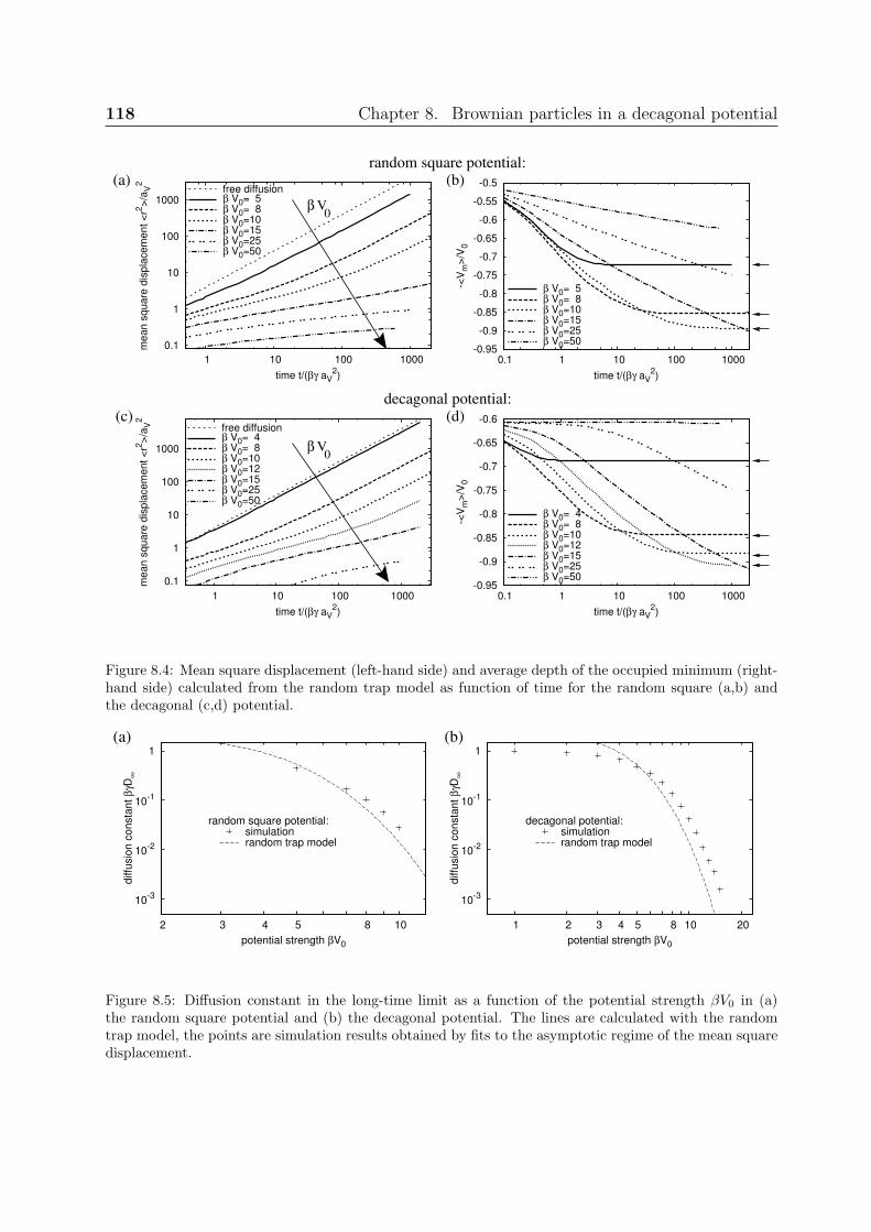
118 Chapter 8. Brownian particles in a decagonal potential
0.1
1
10
100
1000
1 10 100 1000
mean s
quare
dis
pla
cem
ent <
r2>
/aV
2
time t/(βγ aV2)
free diffusionβ V0= 4β V0= 8β V0=10β V0=12β V0=15β V0=25β V0=50
-0.95
-0.9
-0.85
-0.8
-0.75
-0.7
-0.65
-0.6
0.1 1 10 100 1000
-<V
m>
/V0
time t/(βγ aV2)
β V0= 4β V0= 8β V0=10β V0=12β V0=15β V0=25β V0=50
0.1
1
10
100
1000
1 10 100 1000
mean s
quare
dis
pla
cem
ent <
r2>
/aV
2
time t/(βγ aV2)
free diffusionβ V0= 5β V0= 8β V0=10β V0=15β V0=25β V0=50
-0.95
-0.9
-0.85
-0.8
-0.75
-0.7
-0.65
-0.6
-0.55
-0.5
0.1 1 10 100 1000
-<V
m>
/V0
time t/(βγ aV2)
β V0= 5β V0= 8β V0=10β V0=15β V0=25β V0=50
Vβ0
Vβ0
decagonal potential:
random square potential:
(d)
(b)
(c)
(a)
Figure 8.4: Mean square displacement (left-hand side) and average depth of the occupied minimum (right-hand side) calculated from the random trap model as function of time for the random square (a,b) andthe decagonal (c,d) potential.
10-3
10-2
10-1
1
2 3 4 5 8 10
diffu
sio
n c
onsta
nt
βγD
∞
potential strength βV0
random square potential:simulationrandom trap model
10-3
10-2
10-1
1
1 2 3 4 5 8 10 20
diffu
sio
n c
onsta
nt
βγD
∞
potential strength βV0
decagonal potential:simulationrandom trap model
(a) (b)
Figure 8.5: Diffusion constant in the long-time limit as a function of the potential strength βV0 in (a)the random square potential and (b) the decagonal potential. The lines are calculated with the randomtrap model, the points are simulation results obtained by fits to the asymptotic regime of the mean squaredisplacement.

8.3. Random trap model 119
right-hand side of figure 8.4 shows the average depth 〈Vm〉 of the minimum the particleoccupies at time t. The results agree qualitatively with the simulation results (see figure8.2). The crossover from subdiffusion to the asymptotic diffusive regime is clearly visiblefor the mean square displacement. Only the short-time behavior is different in the randomtrap model, because the particles already start in a minimum of the potential and thereforethe short-time relaxation visible in the simulations is not included. Note that the averagedepth 〈Vm〉 of the occupied minimum shown in 8.4(b) and (d) is not the same quantityas the average potential energy plotted on the right-hand side of figure 8.2. Nevertheless,the behavior of the curves is very similar: In the random trap model the particles startin randomly chosen minima, i.e., for t = 0 one has 〈Vm(0)〉 = −0.5V0 in the random and〈Vm(0)〉 = −0.603V0 in the decagonal potential. This corresponds to the positions of thekinks in the simulated curves (see end of section 8.2.2). For intermediate and long timesthe curves are very similar. Especially the plateau for βV0 = 50 is found in theory and inthe simulations for the decagonal potential, whereas in both cases there is no plateau buta decrease for the random potential.
Using equation (8.37), the asymptotic diffusion constant can be calculated for βV0 1. In figure 8.5 we compare the theoretical results to the diffusion constants obtainedby asymptotic fits to the simulated curves. There are differences especially for largerpotential strengths βV0 and our random trap model is only approximately valid. Thisprobably is due to shallow minima in the potential landscape where the particle is notbound to the minimum and during a “jump” between two wells finite-time excursionsoutside the minimum occur. Furthermore, jumps exist that do not take place betweennearest neighbors. Finally, we also neglected spatial correlations in the depths of thepotential wells in our model.
It is difficult to determine the crossover time τ by fits to the curves of the simulationsbecause the resulting values strongly depend on the range of the fit. Therefore, to quan-titatively test our theory, we plot the time dependence of the mean square displacementwhere time is rescaled τ and the mean square displacement by D∞τ . The rescaled curvesare shown in figures 8.6(a) to (c). For the regular square potential the curves perfectlycollapse on a single curve for βV0 1, as can be seen in figure 8.6(a). However, for therandom square and the decagonal potential shown in 8.6(b) and (c), respectively, the col-lapse is not as good. In figure 8.6(d) we plot the curves of the decagonal potential with the
mean square displacement rescaled by D(fit)∞ τ , where D
(fit)∞ is taken from asymptotic fits
to the simulation results. The collapse in figure 8.6(d) is much better, therefore the maindiscrepancies between simulations and theory are the differences between the calculatedasymptotic diffusion constants and the ones obtained by fits to the simulations. Thesedifferences can be seen in figure 8.5 and were already discussed.
Another test for our theory is to compare the distribution P (V, t) in the limit t→∞.Comparing equations (8.20) and (8.30), one finds
P (stat)(Vm) =
ρ(Vm)Γ(Vm)∫ V0
0dV ′
mρ(V ′
m)Γ(V ′
m)
. (8.39)

120 Chapter 8. Brownian particles in a decagonal potential
10-3
10-2
10-1
1
10
102
103
10-6
10-4
10-2 1 10
2mean s
quare
dis
pla
cem
ent <
r2>
/(D
∞(f
it) τ)
time t/τ
β V0= 4β V0= 6β V0= 8β V0=10β V0=12β V0=15
10-3
10-2
10-1
1
10
102
103
10-10
10-8
10-6
10-4
10-2 1 10
210
4
mean s
quare
dis
pla
cem
ent <
r2>
/(D
∞τ)
time t/τ
β V0= 4β V0= 6β V0= 8β V0=10β V0=12β V0=15β V0=20β V0=25
10-2
10-1
1
10
102
103
10-12
10-10
10-8
10-6
10-4
10-2 1 10
2
mean s
quare
dis
pla
cem
ent <
r2>
/(D
∞τ)
time t/τ
β V0= 5β V0= 8β V0=10β V0=15β V0=25
10-3
10-2
10-1
1
10
102
103
10-10
10-8
10-6
10-4
10-2 1 10
2
mean s
quare
dis
pla
cem
ent <
r2>
/(D
∞τ)
time t/τ
β V0= 5β V0=10β V0=15β V0=25
decagonal potential:
regular square potential:
(d)(c)
(a) (b) random square potential:
decagonal potential:
Figure 8.6: Rescaled mean square displacement of the Brownian dynamics simulations in (a) a regularsquare, (b) a random square, and (c,d) in a decagonal potential. The time is rescaled by an factor of1/τ and the mean square displacement by (a-c) 1/(D∞τ) or (d) by 1/(D(fit)
∞ τ), where D(fit)∞ is the fitted
asymptotic diffusion constant.
0
1
2
3
4
5
6
7
0.2 0.3 0.4 0.5 0.6 0.7 0.8 0.9 1
P(s
tat)(V
m/V
0)/ρ
(Vm
/V0)
depth of minimum Vm/V0
theory
simulation
Figure 8.7: Stationary distribution P (stat)(Vm) in the long-time limit for the decagonal potential withβV0 = 8.

8.4. Brownian motion started in equilibrium 121
Note that this distribution is stationary since it does not change with time anymore,ddtP (stat)(Vm) = 0. On the other hand, the distribution in real space p(x, y, t) is not sta-
tionary for infinite systems. It is a big advantage of our approach, which is based on thedistribution P (Vm, t) for finding a particle in a minimum of depth Vm, rather than onthe positional distribution p(x, y, t), that P (Vm, t) relaxes into a stationary long-time limitwhen the transition into the diffusive regime takes place. Figure 8.7 presents P (stat)(Vm) forthe decagonal potential with βV0 = 8 as given by the analytic formula (8.39) and comparesit to the stationary distribution determined in the Brownian dynamics simulations in thelong-time limit. Theory and simulation agree very well.
8.4 Brownian motion started in equilibrium
In section 8.2 the colloidal particles were started at random positions in the potential.In this section we consider the Brownian motion in equilibrium that was also studiedexperimentally. We will discuss the experiment and its results in the next subsection andcompare it to simulations in subsection 8.4.2.
8.4.1 Experimental results
In experiments, the ensemble average is replaced by an average over time, i.e., the meansquare displacement is determined according to
〈r2(exp)(t)〉 = 〈〈[r(t′ + t)− r(t′)]
2〉t′〉, (8.40)
where 〈·〉 denotes the usual average over different runs and 〈·〉t′ is the average over timet′. The results of experiments by J. Baumgartl [244] are shown in figure 8.8. Using videomicroscopy, the trajectories of up to 72 polystyrene spheres with a diameter of 1.8 µmimmersed in water were recorded by taking 30.000 to 100.000 images at a frame rate of10 Hz. The colloidal suspension was highly diluted so that neighboring particles did notinteract during the diffusion process. At a first glance, the experimental results look similarto the simulation results of figure 8.2. However, only dynamics in thermal equilibrium wasmeasured in the experiment. As we will show in the next subsection, the extended non-equilibrium relaxation process we found in theory, is not included in the experimentalresults. Note that as long as the mean square displacement is calculated according to(8.40) such a relaxation process cannot be observed, because most of the time the systemis in equilibrium and possible non-equilibrium dynamics at the beginning of a measurementcan be neglected.
8.4.2 Simulation results
In the simulation we calculate the mean square displacement as an ensemble average fortrajectories started in equilibrium, i.e., with starting positions given by the stationarydistribution of the asymptotic diffusive regime [see equation (8.39)]. In figure 8.9, results
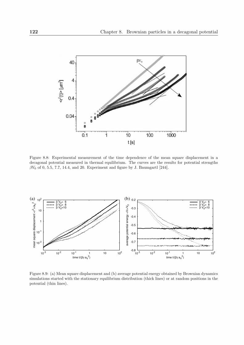
122 Chapter 8. Brownian particles in a decagonal potential
βV0
Figure 8.8: Experimental measurement of the time dependence of the mean square displacement in adecagonal potential measured in thermal equilibrium. The curves are the results for potential strengthsβV0 of 0, 5.5, 7.7, 14.4, and 20. Experiment and figure by J. Baumgartl [244].
10-2
10-1
1
10
102
10-3
10-2
10-1 1 10 10
2
mean s
quare
dis
pla
cem
ent <
r2>
/aV
2
time t/(βγ aV2)
β V0= 6β V0= 8β V0=10
-0.8
-0.7
-0.6
-0.5
-0.4
-0.3
-0.2
10-3
10-2
10-1 1 10 10
2
avera
ge p
ote
ntial energ
y <
V>
/V0
time t/(βγ aV2)
β V0= 6β V0= 8β V0=10
(a) (b)
Figure 8.9: (a) Mean square displacement and (b) average potential energy obtained by Brownian dynamicssimulations started with the stationary equilibrium distribution (thick lines) or at random positions in thepotential (thin lines).

8.5. Colloidal motion in potentials with phasonic drift 123
of Brownian dynamics simulation of the dynamics in thermal equilibrium are plotted withthick lines and compared to the ones obtained by particles started in non-equilibriumshown with thin lines. Obviously, the crossover into the asymptotic diffusive regime occursat much shorter times and on much smaller length scales if the colloids are already inthermal equilibrium. The short-time dynamics is due to the motion within the initialwell. As soon as the first jump into another minimum takes place, the diffusive limit isreached. Unlike in the non-equilibrium case, it is not necessary to explore different potentialminima to relax towards the stationary distribution in thermal equilibrium. Therefore, theexperiments presented in the last subsection do not show the very slow relaxation processof colloids starting in non-equilibrium. The observed small-time dynamics is the crossoverfrom almost free diffusion within a potential well to the asymptotic diffusive regime, wherethe colloid jumps between minima.
8.5 Colloidal motion in potentials with phasonic drift
In this section we study the motion of a particle in a potential subject to a constantphasonic drift, i.e., the phasonic displacement is changed at a constant rate in time (cf.section 3.4.3). First, we determine the mean drift of the colloids induced by the phasonicdrift. Second, we show that the phasonic drift leads to a crossover into a diffusive non-equilibrium state. Finally, we modify the random trap model such that the phasonic driftis included.
8.5.1 Ballistic motion
Colloidal particles in a potential with an imposed phasonic drift perform a drift motionon average, i.e., they move ballistically. To study this motion without including thermalfluctuation, we set the temperature to zero and perform Brownian dynamics simulations.Then the simulations are completely deterministic and the averages are taken over differentstarting conditions. In figure 8.10 the directions of the drift velocity v of the particles as afunction of the directions of the phasonic drift velocity vw are shown. The absolute valueof the phasonic drift velocity is chosen sufficiently small so that the particles are able tofollow the positions of the local minima they occupy. Viscous forces are not yet important.The directional dependence roughly follows a line, where the polar angle αv of the driftvelocity v with respect to the y-direction is related to the angle αw of the phasonic driftvelocity vw via
αv = −3αw. (8.41)
For angles αw that are integer multiplies of π/10, this relation seems to be exact. Theresults of the simulation show a superimposed periodicity with period π/5, which is dueto the symmetry of the potential. The factor 3 in relation (8.41) is probably connected tothe index 3j mod 5 in the definition of the phasonic displacements [cf. equation 3.31].
In figure 8.11 the absolute value of the drift velocity as a function of the phasonic driftvelocity is shown. For small phasonic drift velocities the dependence is linear, indicating
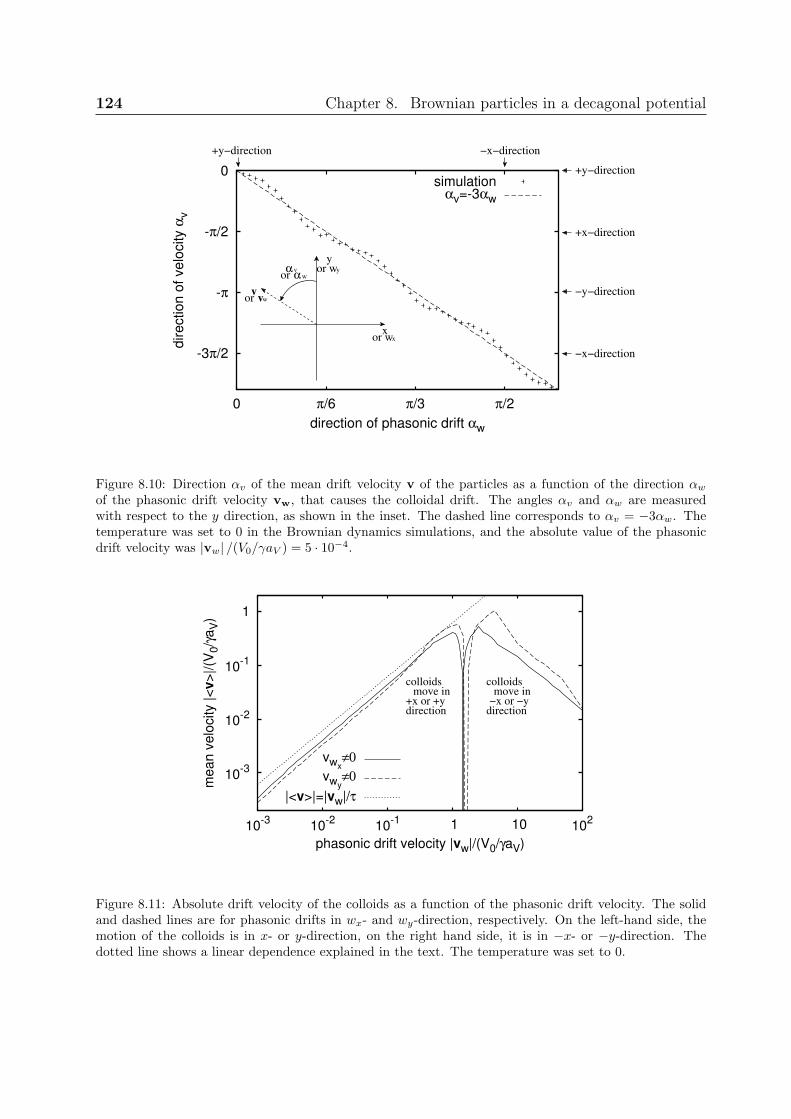
124 Chapter 8. Brownian particles in a decagonal potential
-3π/2
-π
-π/2
0
0 π/6 π/3 π/2
direction o
f velo
city α
v
direction of phasonic drift αw
simulationαv=-3αw
vor w
or w yvα
or w x
−x−direction
−y−direction
+x−direction
+y−direction
x
αw
+y−direction −x−direction
y
or
v
Figure 8.10: Direction αv of the mean drift velocity v of the particles as a function of the direction αw
of the phasonic drift velocity vw, that causes the colloidal drift. The angles αv and αw are measuredwith respect to the y direction, as shown in the inset. The dashed line corresponds to αv = −3αw. Thetemperature was set to 0 in the Brownian dynamics simulations, and the absolute value of the phasonicdrift velocity was |vw| /(V0/γaV ) = 5 · 10−4.
10-3
10-2
10-1
1
10-3
10-2
10-1 1 10 10
2
me
an
ve
locity |<
v>
|/(V
0/γ
aV)
phasonic drift velocity |vw|/(V0/γaV)
vwx≠0
vwy≠0
|<v>|=|vw|/τ
direction+x or +y
move in
direction−x or −y
move incolloidscolloids
Figure 8.11: Absolute drift velocity of the colloids as a function of the phasonic drift velocity. The solidand dashed lines are for phasonic drifts in wx- and wy-direction, respectively. On the left-hand side, themotion of the colloids is in x- or y-direction, on the right hand side, it is in −x- or −y-direction. Thedotted line shows a linear dependence explained in the text. The temperature was set to 0.

8.5. Colloidal motion in potentials with phasonic drift 125
that the particles follow the position of the minimum they occupy. If the motion of thewells corresponds to the motion of the minimum of the averaged potential shown in figure3.19, the drift velocity of the colloids should be [cf. equation 3.33 or 3.35]
|〈v〉| = |vw| /τ, (8.42)
where τ is the number of the golden ratio. Relation (8.42) is plotted in figure 8.11 as dottedline. Even for very small phasonic drift velocities, the values predicted by (8.42) are largerthan the colloidal drift found in the simulations. Therefore, not all local minima moveaccording to the minima in the averaged potential. In fact, most single particle trajectoriesdisplay a zigzag-like shape (cf. minima in figure 3.18), which would lead exactly to relation(8.42). However, a few colloids (or positions of local minima) move in opposite directionand therefore the average velocity is decreased.
For a phasonic drift velocity |vw| /(V0/γaV ) slightly larger than 1 the drift of the parti-cles is suddenly reversed. This is caused by the fact that due to viscous forces the colloidcan no longer follow the position of a minimum for such a large phasonic drift: The relax-ation time, i.e., the time a colloid needs to relax into a local minimum, is roughly givenby γa2
V /V0. Therefore, for |vw| /(V0/γaV ) 1, the time scale of the relaxation process islarger than the time scale aV / |vw| on which the minima of the potential change. For largephasonic drift velocities, the colloidal motion is no longer connected to the motion of thepositions of local minima.
8.5.2 Mean square displacement and non-equilibrium steady state
In figure 8.12 the mean square displacement and the average potential energy obtainedfrom Brownian dynamics simulation is shown for different phasonic drift velocities. Themean square displacement is calculated after subtracting the ballistic motion due to thephason-induced drift [cf. equation (6.21)].
Figure 8.12(a) shows that the crossover into an asymptotic diffusive regime occurs atearlier times if the phasonic drift velocity is increased. The average potential energy weaklyoscillates around an asymptotic energy level. The oscillations are probably due to thealmost periodic decrease and increase of the depths of the potential wells (cf. section 3.4.3).By increasing the phasonic drift velocity, the asymptotic energy level is also increased.Obviously, the phasonic drift acts as a constant influx of energy and therefore keeps thecolloids in a non-equilibrium steady state in the long-time limit. In section 8.6.3 we showthat this system can be used as a model system for studying the properties of the non-equilibrium.
8.5.3 Modification of the random trap model
If a phasonic drift is applied to the potential landscape, the depths of its minima arecontinuously changing. Therefore, the potential energy of a colloid changes either due tojumps into neighboring minima or due to the imposed phasonic drift. The probability

126 Chapter 8. Brownian particles in a decagonal potential
0.01
0.1
1
10
100
1000
0.001 0.01 0.1 1 10 100
mean s
quare
dis
pla
cem
ent <
r2>
/aV
2
time t/(βγ aV2)
free diffusionvwy
/(V0/γaV)=0
vwy/(V0/γaV)=0.00005
vwy/(V0/γaV)=0.0005
vwy/(V0/γaV)=0.005
vwy/(V0/γaV)=0.05
-0.8
-0.7
-0.6
-0.5
-0.4
-0.3
-0.2
0.001 0.01 0.1 1 10 100-<
Vm
>/V
0
time t/(βγ aV2)
vwy/(V0/γaV)=0
vwy/(V0/γaV)=0.00005
vwy/(V0/γaV)=0.0005
vwy/(V0/γaV)=0.005
vwy/(V0/γaV)=0.05
Phasonicdrift
velocity
Phasonicdrift
velocity
(a) (b)
Figure 8.12: (a) Mean square displacement and (b) average potential energy obtained from Browniandynamics simulation in a decagonal potential with βV0 = 20 for different phasonic drift velocities vwy
,given in units of V0/(γaV ).
1
10
100
10 100 1000 10000
me
an
sq
ua
re d
isp
lace
me
nt
<r2
>/a
V2
time t/(βγ aV2)
Dw=0
Dw=0.01
Dw=0.03
Dw=0.1
-0.95
-0.9
-0.85
-0.8
-0.75
-0.7
-0.65
1 10 100 1000 10000
-<V
m>
/V0
time t/(βγ aV2)
Dw=0
Dw=0.01
Dw=0.03
Dw=0.1
Phasonicdrift
velocityPhasonic
driftvelocity
(a) (b)
Figure 8.13: (a) Mean square displacement and (b) average potential energy obtained by the modifiedrandom trap model for different values of the parameter Dw, which in the simulations is controlled by thephasonic drift velocity. The potential strength is kept constant at βV0 = 15.

8.5. Colloidal motion in potentials with phasonic drift 127
0
1
2
3
4
5
6
0.4 0.5 0.6 0.7 0.8 0.9 1
P(n
eq
) (Vm
/V0)
depth of minimum Vm/V0
Dw=0
Dw=0.01
Dw=0.03
Dw=0.1
velocitydrift
Phasonic
Figure 8.14: Probability distribution P (neq)(Vm) to find a particle in a minimum with a depth in [Vm, Vm +dVm] in the asymptotic long time limit for different phasonic drift velocities. The distributions weredetermined by the modified random trap model.
density P (Vm, t) that a colloid occupies a minimum with a depth within [Vm, Vm + dVm]decreases at a rate proportional to P (Vm, t) due to the changing depth of the minimum.However, at the same time it increases by a term proportional to P (Vm−dVm, t) +P (Vm +dVm, t) because some minima of depth Vm − dVm or Vm + dVm will have the depth Vm att + dt. In total, the additional temporal change of P (Vm, t) due to the phasonic drift isproportional to
P (Vm − dVm, t) + P (Vm + dVm, t)− 2P (Vm, t) ∝d2
dV 2m
P (Vm, t). (8.43)
Since the depth of a minimum can be either decrease from Vm to Vm − dVm or increase toVm + dVm we included a factor of 2 in the last term of the left-hand side of (8.43). Hence,the rate equation of the random trap model (8.21) is modified by adding a diffusion term,i.e.,
d
dtP (Vm, t) = −zΓ(Vm)P (Vm, t) + zρ(Vm)
∫ V0
0
dV ′mΓ(V ′
m)P (V ′m, t) +Dw
d2
dV 2m
P (Vm, t),
(8.44)where Dw describes the rate of changes in the depths of the minima. In the simulationsthese changes of the minima are controlled by the phasonic drift velocity vw. We solveequation (8.44) numerically and by using equation (8.20) to determine the diffusion con-stant of the colloids, we then calculate the mean square displacement. In figure 8.13 thetime dependence of the mean square displacement and the average potential energy isshown. There is a good qualitative agreement with the simulation results (cf. figure 8.12).
128 Chapter 8. Brownian particles in a decagonal potential
Figure 8.14 shows the probability distribution P (neq)(Vm) = limt→∞ P (Vm, t) in theasymptotic long time limit. The phasonic drift decreases the occupation of deep minimaand increases P (neq)(Vm) for intermediate Vm.
8.6 Non-equilibrium statistics
In this section, we shortly introduce some central ideas of non-equilibrium statistical the-ories and motivate how they may be applied to our system.
8.6.1 Derivation of path-ensemble averages
Mainly following the work of Crooks [294], we first present a derivation of path-ensembleaverages, i.e., averages of observables over an ensemble of different paths, which a systemperforms with time. Usually the path ensemble is defined by an initial distribution inthermal equilibrium and a time-dependent external perturbation that drives the systemout of equilibrium. We also derive some more general new relations where we do notassume that the equilibrium distribution is given in form of the Boltzmann distribution.The basic idea to derive path-ensemble averages is to split the dynamics of the system intoa part caused by the coupling to the heat bath and a part due to external perturbationssuch as the temporal variation of the external potential, e.g., caused by a phasonic drift.The dynamics due to the coupling to the heat bath is characterized by the fact that it doesnot change an equilibrium distribution, i.e., a system is never driven out of equilibrium.On the other hand, external perturbations change the energies associated with the statesof the system and therefore drive the system out of equilibrium.
We consider a system with discretized states at discretized times and assume that thedynamics is Markovian, i.e., it only depends on the current state but not on its history. Theprobability to be in state x at time t is ρx(t). The external perturbations are characterizedby the time-dependence of the state energy (or a similar quantity) Ex(t). We assume thatEx(t) never is infinite. We now split the dynamics of the system in two parts. First, thetemporal evolution of the system due to the coupling to a heat bath is written as
ρx′(t+ 1) =∑
x
M(t)x′xρx(t), (8.45)
where M(t) is the transition matrix whose element M(t)x′x is the probability to get fromstate x to x′. In the following, we leave away the sum symbol and perform a summationover indices that appear twice. In the second part of the temporal evolution of the system,the new state x′ assumes the energy Ex′(t+ 1).
In equilibrium, there is a stationary distribution πx(t)(E(t)) = ρ(stat)x(t) (t) that usually
is given by the equilibrium distribution of a canonical ensemble. It does not explicitlydepend on time. However, it relies on the states x(t) and the energy E(t) = Ex(t), whichboth may be time-dependent due to the external perturbations (see below). We require
8.6. Non-equilibrium statistics 129
the dynamics described by M to fulfill the following relation:
πx′(E) = M(t)x′xπx(E), (8.46)
i.e., πx(E) has to be invariant under a transition M(t) so that without external pertur-bations a system in equilibrium stays in equilibrium. Equation (8.46) is the central as-sumption to derive path-ensemble averages. It is valid in all systems with detailed balance
M(t)xx′πx′(E) = M(t)x′xπx(E), (8.47)
however, detailed balance is not required here.We assume a path [x] that starts in state x(t0) = x0 and ends in x(tf ) = xf . In the
following we will always use square brackets [·] to denote such a path. The time-reversedpath [x] starts at time tf in state x(t0) = x(tf ) = xf and ends in x(tf ) = x(t0) = x0.
Correspondingly, Ex(t) describes the time-dependence of the energy along the reversedpath. In general, x(t) = x(tf − t). The dynamics of the reverse path is governed by M(t)with
ρx′(t) = M(t)x′xρx(t− 1), (8.48)
where ρx(t) is the probability for the reversed path to be in state x(t) at time t.Let P ([x]|x(t0) = x0) be the probability for a path [x] that starts in state x0 and
P ([x]|x(t0) = xf ) the probability for the reversed path [x] with x(t0) = x(tf ) = xf . Theratio of these probabilities is
P ([x]|x(t0) = x0)
P ([x]|x(t0) = xf )=
tf−1∏t=t0
M(t)x(t+1)x(t)
M(t+ 1)x(t+1)x(t)
. (8.49)
Because∏tf−1
t=t0 πx(t)(E(t)) =∏tf−1
t=t0 πx(t+1)(E(t+ 1)), one finds
P ([x]|x(t0) = x0)
P ([x]|x(t0) = xf )=
tf−1∏t=t0
M(t)x(t+1)x(t)πx(t)(E(t))
M(t+ 1)x(t+1)x(t)πx(t+1)(E(t+ 1))
=πx(t0)(E(t0))
πx(tf )(E(tf ))·
tf−1∏t=t0
M(t)x(t+1)x(t)πx(t)(E(t))
M(t+ 1)x(t+1)x(t)πx(t)(E(t))
=πx(t0)(E(t0))
πx(tf )(E(tf ))·
tf−1∏t=t0
πx(t+1)(E(t))
πx(t)(E(t))
=
tf−1∏t=t0
πx(t+1)(E(t))
πx(t+1)(E(t+ 1))
=
tf−1∏t=t0
πx(t+1)(E(t))
πx(t)(E(t)). (8.50)

130 Chapter 8. Brownian particles in a decagonal potential
To arrive at the third line, we used relation (8.46). Equation (8.50) will be the startingpoint to derive different types of path-ensemble averages and fluctuation theorems in thenext subsection.
Usually the stationary distribution πx(E(t)) is given by the equilibrium distribution ofthe canonical ensemble,
πx(E(t)) =exp (−βEx(t))∑x′ exp (−βEx′(t))
= exp (βF (t)− βEx(t)) , (8.51)
where β = 1/(kBT ), Ex(t) is the energy of state x at time t, and F (t) is the free energy
F (t) = −kBT ln∑x′
exp (−βEx′(t)) . (8.52)
Equation (8.50) then becomes
P ([x]|x(t0) = x0)
P ([x]|x(0) = xf )=
tf−1∏t=t0
exp(βF (t)− βEx(t+1)(t)
)exp
(βF (t)− βEx(t)(t)
)= exp
(−β
tf−1∑t=t0
[Ex(t+1)(t)− Ex(t)(t)
])= exp (−βQ ([x])) , (8.53)
where Q ([x]) =∑tf−1
t=t0
[Ex(t+1)(t)− Ex(t)(t)
]is the total heat exchange with the reservoir,
when the system changes its state from x(t) to x(t+ 1).
8.6.2 Examples of path-ensemble averages and fluctuation theo-rems
We consider a function f([x]) that depends on a path [x] of the system. The average off([x]) over the ensemble of paths is
〈f〉[x] =∑[x]
ρx0 (t0)P ([x]|x(t0) = x0) f([x]). (8.54)
Using equation (8.50), we find
〈f〉[x] =∑[x]
ρx0 (t0)
tf−1∏t=t0
πx(t+1)(E(t))
πx(t)(E(t))P ([x]|x(t0) = xf ) f([x])
=∑[x]
ρx0 (t0)
ρxf(t0)
tf−1∏t=t0
πx(t+1)(E(t))
πx(t)(E(t))ρxf
(t0)P ([x]|x(t0) = xf ) f([x])
=
⟨fρx0 (t0)
ρxf(t0)
tf−1∏t=t0
πx(t+1)(E(t))
πx(t)(E(t))
⟩[x]
. (8.55)

8.6. Non-equilibrium statistics 131
This is one of the most general forms of a path-ensemble average. If the path x and theinverse path x are started in equilibrium, ρx0 (t0) = πx0(E(t0)) and ρxf
(t0) = πxf(E(tf ))
and therefore
〈f〉[x] =
⟨f
tf−1∏t=0
πx(t+1)(E(t))
πx(t+1)(E(t+ 1))
⟩[x]
. (8.56)
If πx(E(t)) is given by (8.51), we find
〈f〉[x] =
⟨f
tf−1∏t=0
exp(βF (t)− βEx(t+1)(t)
)exp
(βF (t+ 1)− βEx(t+1)(t+ 1)
)⟩[x]
=
⟨f exp
(β
F (t0)− F (tf ) +
tf−1∑t=0
[Ex(t+1)(t+ 1)− Ex(t+1)(t)
])⟩[x]
= 〈f exp (β F (t0)− F (tf ) +W ([x]))〉[x] , (8.57)
where W ([x]) is the work performed on the system by the external perturbation W ([x]) =∑tf−1t=t0
[Ex(t+1)(t+ 1)− Ex(t+1)(t)
]. Usually f is replaced by f exp (−βW ([x])) leading to
〈f exp (−βW ([x]))〉[x] = 〈f exp (−β∆F )〉[x] , (8.58)
with ∆F = F (tf ) − F (t0). Equation (8.58) is a convenient and useful relation [294] thatconnects averages over the forward and the backward paths.
For f = 1, equation (8.58) becomes
〈exp (−βW ([x]))〉[x] = exp (−β∆F ) . (8.59)
This is the well known Jarzynski non-equilibrium work relation [295], which is closelyconnected to relations known as integral fluctuation theorems in literature [296]. Usuallythe Jarzynski relation is derived from elementary statistical physics. It connects the freeenergy difference of two equilibrium states to the total work performed on the system whilethe system evolves along the paths. It can be used to determine free energy differences inexperiments (see e.g. [297–299]). The Jarzynski theorem is also valid if the final state is anon-equilibrium steady state even though the free energy F (tf ) is no longer well defined innon-equilibrium: If one considers F (tf ) to be defined by the configuration sum in equation(8.52), the Jarzynski relation can still be used [300,301].
Another important relation is derived from (8.58) with f = δ (βW − βW ([x])), whereδ(·) is the Dirac-δ-function that is non-zero if the work along a paths W ([x]) equals a givenvalue W . One finds
〈δ (βW − βW ([x])) exp (−βW ([x]))〉[x] = 〈δ (βW − βW ([x])) exp (−β∆F )〉[x] . (8.60)
Using W ([x]) = −W ([x]) this is
p[x] (βW ) exp (−βW ) = p[x] (−βW ) exp (−β∆F ) , (8.61)

132 Chapter 8. Brownian particles in a decagonal potential
where p[x] (βW ) = 〈δ (βW − βW ([x]))〉[x] is the probability to perform the work W on theforward path, and p[x] (−βW ) is the corresponding distribution for the backward path. Forp[x] (−βW ) 6= 0, one finds
p[x] (βW )
p[x] (−βW )= exp (βW − β∆F ) . (8.62)
Relation (8.62) connects the work distribution of the forward path to the backward path.Often (8.62) is also rewritten in terms of the dissipated work or the change in entropy [296,302–307]. Because it allows a decrease in entropy with a small probability, it was incorrectlyreferred to as a relation that allows the violation of the second law of thermodynamicswith a certain probability [302,303]. Equation (8.62) or similar ones have also been testedexperimentally [308–310].
Finally, we want to derive a relation which connects a non-equilibrium distributionρ
(neq)x (t) to the distribution πx(E) in equilibrium. We assume an ensemble of paths [x] that
start in states x0 with probabilities given by πx0(E(t0)) and end in non-equilibrium statesx(tf ). Using (8.50), we find
ρ(neq)xf
(tf ) =∑
[x] with x(tf )=xf
πx0(E(t0))P ([x]|x(t0) = x0)
=∑
[x] with x(t0)=xf
πx0(E(t0))P ([x]|x(t0) = xf )
tf−1∏t=t0
πx(t+1)(E(t))
πx(t)(E(t))
=∑
[x] with x(t0)=xf
πxf(E(tf ))P ([x]|x(t0) = xf )
tf−1∏t=t0
πx(t+1)(E(t))
πx(t+1)(E(t+ 1))
= πxf(E(tf ))
⟨tf−1∏t=t0
πx(t+1)(E(t))
πx(t+1)(E(t+ 1))
⟩[x], x(t0)=xf
. (8.63)
The non-equilibrium distribution is therefore related to the distribution that an equilibriumsystem would have at the same time. If πx(E) is given by (8.51), one finds
ρ(neq)xf
(tf ) = πxf(E(tf ))
⟨tf−1∏t=t0
exp(βF (t)− βEx(t+1)(t)
)exp
(βF (t+ 1)− βEx(t+1)(t+ 1)
)⟩[x], x(t0)=xf
= πxf(E(tf )) 〈exp (β −∆F +W ([x]))〉[x], x(t0)=xf
= πxf(E(tf )) exp (−β∆F ) 〈exp (βW ([x]))〉[x], x(t0)=xf
, (8.64)
i.e., the non-equilibrium distribution is connected to the equilibrium distribution via thework performed on the paths into the non-equilibrium (see also [294]).

8.6. Non-equilibrium statistics 133
8.6.3 Colloidal motion in potentials with phasonic drift: a non-equilibrium system
In sections 8.3 and 8.5.3, where we introduced the random trap model, we showed thatthe natural distribution to determine the dynamics of a single colloid in quasicrystallineor random potentials is the probability density P (Vm, t) to find the colloid at time t ina minimum with a depth within [Vm, Vm + dVm]. To calculate path-ensemble averagesfor such a system, we therefore consider the states x to be the positions of the minima,whose actual depths Vm(x, t) correspond to the energies Ex(t) that change in time dueto a phasonic drift. The probability ρx(t) is replaced by P (Vm(x, t), t) and the thermalequilibrium distribution πx(E(t)) is the asymptotic stationary distribution P (stat)(Vm(x, t))as determined in equation (8.39). Note, P (stat)(Vm(x, t)) is given for a canonical ensemblein thermal equilibrium, however, it does not have the form of a conventional Boltzmanndistribution, because Vm(x, t) is the depths of a minimum and not the actual potentialenergy of the colloid. The external perturbation that drives the system out of equilibriumis realized by a phasonic drift or other time-dependent phasonic displacements.
We find the following path-ensemble averages: First, the probabilities for a forwardpath compared to a backward path have to fulfill the relation [cf. equation (8.50)]
P ([x]|x(t0) = x0)
P ([x]|x(t0) = xf )=
tf−1∏t=t0
P (stat)(Vm(x(t+ 1), t))
P (stat)(Vm(x(t), t))(8.65)
=
tf−1∏t=t0
Vm(x(t), t)
Vm(x(t+ 1), t)
ρ(Vm(x(t+ 1), t))
ρ(Vm(x(t), t))eβ[Vm(x(t+1),t)−Vm(x(t),t)],
where for the stationary distribution equations (8.39) and (8.34) were used and ρ(Vm) isthe distribution of the depths of the local minima in the potential (see section 3.3.3).
Second, a path-ensemble average over some function f ([x]) is given by [cf. equation(8.56)]
〈f〉[x] =
⟨f
tf−1∏t=t0
P (stat)(Vm(x(t+ 1), t))
P (stat)(Vm(x(t+ 1), t+ 1))
⟩[x]
(8.66)
=
⟨f
tf−1∏t=t0
Vm(x(t+ 1), t+ 1)
Vm(x(t+ 1), t)
ρ(Vm(x(t+ 1), t))
ρ(Vm(x(t+ 1), t+ 1))eβ[Vm(x(t+1),t)−Vm(x(t+1),t+1)]
⟩[x]
.

134 Chapter 8. Brownian particles in a decagonal potential
Finally, we find a relation for a non-equilibrium distribution [cf. equation (8.63)]:
P (neq)(Vm(xf , tf ), tf ) = P (stat)(Vm(xf , tf ))
⟨tf−1∏t=t0
P (stat)(Vm(x(t+ 1), t))
P (stat)(Vm(x(t+ 1), t+ 1))
⟩[x], x(t0)=xf
=
⟨tf−1∏t=t0
KVm(x(t+1),t),Vm(x(t+1),t+1)
⟩[x], x(t0)=xf
P (stat)(Vm(xf , tf ))
with KV0,V1 =V1
V0
ρ(V0)
ρ(V1)eβ[V0−V1]. (8.67)
In figure 8.14 we already plotted examples for P (neq)(Vm(xf , tf )) in a system with a constantphasonic drift. According to equation (8.67), these distributions are connected to the(known) equilibrium distribution P (stat)(Vm) by a factor that can be calculated if a largenumber of paths towards the non-equilibrium steady state is known.
The path-ensemble averages presented here are still quite complicated. In principle,it is possible to check these relations with simulations. However, since some paths thathave to be included in the path-ensemble average occur with a very small probability, itis almost impossible to simulate a sufficient large number of paths for such a test. For thefuture, it would be interesting to determine the path-ensemble for explicit quantities suchas the diffusion constant as defined in (8.20). This should also give useful relations forpredicting such quantities even in the non-equilibrium.
8.7 Summary and Outlook
We studied the Brownian motion of an ensemble of single colloidal particles in the decago-nal potential and compared it to the motion in a regular square and a random squarepotential. While Brownian motion is naturally treated in equilibrium, we started the en-semble of single Brownian particles from a non-equilibrium distribution and monitor howthey reach thermal equilibrium. Brownian dynamics simulations clearly show that after afast relaxation into local potential minima, the particles in the random square and decago-nal potential pass a wide-stretched subdiffusive regime and then enter thermal equilibriumwhen they start to exhibit normal diffusive motion. While the mean-square displacementas a function of time looks qualitatively the same for both potentials, the temporal evo-lution of the mean potential energy reveals some differences which we explained by thedifferent distributions for the depths of the potential minima.
Furthermore, we developed a random trap model based on the probability distributionP (Vm, t) of finding a particle in a trap with depth Vm. It agrees with the results from theBrownian dynamics simulations, especially the temporal evolution of the average potentialenergy with its characteristic features is reproduced. While an analytic formula derivedwithin the random trap model only approximates the long-time diffusion constant foundin the Brownian dynamics simulations, the analytically given time scale on which the

8.7. Summary and Outlook 135
particle relaxes into the diffusive state fits very well to the simulations. Finally, our modelclearly identifies that normal diffusion is reached when P (Vm, t) approaches its stationarydistribution which corresponds to thermal equilibrium. While conventional treatments ofBrownian motion use a positional distribution p(x, y, t), we here introduced an alternativeapproach that is easier to treat and that might be applicable to other systems whereBrownian motion in an external potential is studied.
If a phasonic drift is applied to the decagonal potential, the colloids no longer reach thethermal equilibrium. However, in the long-time limit, a non-equilibrium steady state ofenhanced diffusion is found. The phasonic drift also induces a colloidal drift that for smalltemperatures and slow phasonic drifts is determined by the motion of the local minima.However, for large phasonic drift the direction of this colloidal motion is reversed.
Finally, Brownian particles in decagonal potential with phasonic drift can be used asa model system to study general properties of systems far from equilibrium. We derivedsome path integral relations that are applicable to our concrete system.
Since single colloids already show a surprising dynamics, we expect the collective motionof many particles in a decagonal potential without or even with a phasonic drift to exhibita lot of interesting features, concerning, e.g., the dynamics of induced phasonic flips orthe collective drift behavior. One can also think of studying the dynamics and ordering ofcolloids driven over a decagonal potential (cf. works for driven particles in periodic systems,e.g. [48, 49,311]).
A central question for atomic quasicrystals is: How does the dynamics of the constituentparticles on the surface of a quasicrystal affect its growth and how is the growth processinfluenced by phasonic fluctuations? Certainly, the diffusion constant is an importantquantity that determines the speed with which new particles find optimal positions onthe surface. We demonstrated here that phasonic drifts enhance diffusion. We expect asimilar behavior for phasonic fluctuations. To elucidate the role of phasonic fluctuations,it is also important to clarify the microscopic details of how quasicrystals grow. recentliterature reports evidences that single particles first form clusters and then stick to thesurface [312,313].

136 Chapter 8. Brownian particles in a decagonal potential

137
Chapter 9
Conclusions
Colloidal particles in light fields created by interfering laser beams are a very useful modelsystem to study the ordering and dynamics of particles on quasicrystalline substrates suchas atoms on the surface of a quasicrystal. With the help of Monte-Carlo and Browniandynamics simulations, we studied a two-dimensional charge-stabilized colloidal suspensionin external potentials with quasicrystalline symmetries in one- and two-dimensions. Wealso developed theoretical models and compared their results to the simulations.
The one-dimensional potential consists of two modulations, whose wavelengths differby a factor of τ , where τ =
(1 +
√5)/2 ≈ 1.618 is the number of the golden ratio. The
two-dimensional potential possesses decagonal symmetry and can be realized in experimentby five interfering laser beams.
In both cases, for weak potentials, a triangular or liquid phase occurs depending onthe strength of the particle interactions and their density. An interesting and unexpectedphase behavior was found when the strength of the substrate potential increases and thetriangular phase has compete with the destabilizing symmetry of the substrate. In theone-dimensional quasicrystalline potential the colloidal density modulations lock to one ofthe potential modulations while ignoring the other and therefore rhombic ordering can beobserved. We explained the occurrence of such a phase with a refined Landau-Alexander-McTague theory. In the decagonal potential and for low particle densities, a quasicrystallinephase is stable with a surprising twenty-fold bond orientational order. On the other hand,at large particle densities, i.e., when the number of colloids exceeds the number of avail-able minima in the substrate potential, no apparent bond orientational order was found.Furthermore, in two narrow ranges of densities, we identified structures that are reminis-cent to Archimedian tilings. Finally, for very large potential strengths a quasicrystallinephase with ten bond directions was observed in decagonal laser fields, whereas colloidsin the one-dimensional potential assemble in lines given by the potential wells. Since theratio of number densities in neighboring wells usually is irrational due to their differentdepths, periodic ordering along the lines is not possible. Therefore, the one-dimensionalquasicrystalline potential destroys any periodic ordering. However, the resulting phaseis not necessarily liquid. By using Brownian dynamic simulations, we found a transition

138 Chapter 9. Conclusions
into a solid-like frustrated state at large particle interactions, where neighboring rows ofparticles cannot pass each other.
Furthermore, we studied the Brownian motion of single colloids on a decagonal sub-strate. From Brownian dynamics simulations and a random trap theory we found thatinitially the particle exhibits subdiffusional motion over several decades in time until itcrosses over to pure diffusion in the long-time limit. We demonstrated that this subdiffu-sion is due to a temporally extended relaxation process towards thermal equilibrium. Wecompared the simulated behavior to Brownian motion in random potentials and developeda random trap model, from which we calculated the crossover time and the asymptoticdiffusion constant analytically.
A big advantage of studying colloidal suspensions in quasicrystalline laser fields is thatphasonic displacements, gradients, and drifts can be applied to the substrate potential bymanipulating the phases of the laser beams in time accordingly. Phasons are unique toquasicrystals. Like phonons they are hydrodynamic modes, i.e., global excitations that donot change free energy in the long-wavelength limit. We demonstrated that phasonic driftsin the substrate potential induce phasonic flips in the colloidal monolayer. Secondly, a pha-sonic gradient or drift stabilizes the Archimedean-like tiling. Thirdly, if a constant phasonicdrift is applied to a laser field while observing the Brownian motion of a single particle, thesystem never relaxes to thermal equilibrium. Instead, it reaches a non-equilibrium steadystate which displays an enhanced diffusive transport. By varying the velocity of the pha-sonic drift, the non-equilibrium motion is controlled in a well-defined manner. Therefore,our system is very interesting for studying properties of the non-equilibrium. We presentedsome path-ensemble relations for future investigations.
In summary, a rich phase behavior was found for a colloidal monolayer on quasicrys-talline substrates. New unexpected phases occur when the strengths of the colloidal in-teraction and the substrate potential are comparable. Studying dynamic aspects revealednovel phenomena such as a frustrated phase in a one-dimensional quasicrystalline potentialor a subdiffusion to diffusion crossover for Brownian particles in laser fields with decagonalsymmetry. We demonstrated how phasonic displacements, gradients, or drifts of the sub-strate affect the colloidal monolayer. This work also contributes to the understanding ofthe ordering and dynamics of adatoms on the surface of quasicrystals and therefore helps toestablish the basis for many new applications such as the development of quasicrystallinecatalysts or new wear-resistant materials.

139
List of Publications
Related to this work:
[A] M. Schmiedeberg, J. Roth, and H. Stark, Freezing and Melting of a Colloidal Adsor-bate on a 1D Quasicystalline Substrate, Phys. Rev. Lett. 97, 158304 (2006).
[B] M. Schmiedeberg, J. Roth, and H. Stark, Brownian particles in random and qua-sicrystalline potentials: How they approach the equilibrium, Eur. Phys. J. E 24, 367(2007).
[C] M. Schmiedeberg and H. Stark, Comment on “Two-Dimensional Quasicrystals ofDecagonal Order in One-Component Monolayer Films”, Phys. Rev. Lett. 100,019601 (2008).
[D] M. Schmiedeberg and H. Stark, Colloidal ordering on a 2D quasicrystalline substrate,submitted to Phys. Rev. Lett. (2008).
Other publications:
[E] M. Schmiedeberg and H. Stark, One-bead microrheology with rotating particles , Eur.Phys. Lett. 69, 629 (2005).
[F] M. Schmiedeberg, MF. Miri, and H. Stark, Photon channelling in foams , Eur. Phys.J. E 18, 123 (2005).
[G] M. Schmiedeberg and H. Stark, Superdiffusion in a honeycomb billiard , Phys. Rev.E 73, 031113 (2006).
[H] V. Yu. Zaburdaev, M. Schmiedeberg, and H. Stark, Random Walks with randomvelocities , Phys. Rev. E 78, 011119 (2008).

140 List of Publications
In preparation:
[I] V. Yu. Zaburdaev, M. Schmiedeberg, and H. Stark, On Moments and Scaling inanomalous random walks , in preparation (2008).
Diploma thesis:
[J] M. Schmiedeberg, Lichttransport in zellularen Strukturen, Diplomarbeit, UniversitatKonstanz (2004).

141
Bibliography
[1] D. Shechtman, I. Blech, D. Gratias, and J. W. Cahn, Metallic Phase with Long-Range Orientational Order and No Translational Symmetry, Phys. Rev. Lett. 53,1951 (1984).
[2] D. Levine, T. C. Lubensky, S. Ostlund, S. Ramaswamym, P. J. Steinhardt, and J.Toner, Elasticity and Dislocations in Pentagonal and Icosahedral quasicrystals, Phys.Rev. Lett. 54, 1520 (1985).
[3] J. E. S. Socolar, T. C. Lubensky, and P. J. Steinhardt, Phonons phasons, and dislo-cations in quasicrystals, Phys. Rev. B 34, 3345 (1986).
[4] C. L. Henley, M. de Boissieu, and W. Steurer, Discussion on clusters, phasons andquasicrystal stabilisation, Phil. Mag. 86, 1131 (2006).
[5] R. McGrath, J. Ledieu, E. J. Cox, and R. D. Diehl, Quasicrystal surfaces: structureand potential as templates, J. Phys.: Condens. Matter 14, R119 (2002).
[6] N. Ferralis, K. Pussi, E. J. Cox, M. Gierer, J. Ledieu, I. R. Fisher, C. J. Jenks,M. Lindroos, R. McGrath, and R. D. Diehl, Structure of the tenfold d-Al-Ni-Coquasicrystal surface, Phys. Rev. B 69, 153404 (2004).
[7] M. Shimoda, T. J. Sato, A. P. Tsai, and J. Q. Guo, Epitaxial crystalline film withpsuedo-tenfold symmetry formed by Au-deposition on a decagonal Al72-Ni12-Co16quasicrystal, Phys. Rev. B 62, 11288 (2000).
[8] K. J. Franke, H. R. Sharma, W. Theis, P. Gille., P. Ebert, and K. H. Rieder,Quasicrystalline Epitaxial Single Element Monolayers on Icosahedral Al-Pd-Mn andDecagonal Al-Ni-Co Quasicrystal Surfaces, Phys. Rev. Lett. 89, 156104 (2002).
[9] V. Fournee, T. C. Cai, A. R. Ross, T. A. Lograsso, J. W. Evans, and P. A. Thiel,Nucleation and growth of Ag films on a quasicrystalline AlPdMn surface, Phys. Rev.B 67, 033406 (2003).
[10] N. Ferralis, R. D. Diehl, K. Pussi, M. Lindroos, I. Fisher, and C. J. Jenks, Low-energy electron diffraction study of Xe adsorption on the ten-fold decagonal Al-Ni-Coquasicrystal surface, Phys. Rev. B 69, 075410 (2004).

142 Bibliography
[11] J. Ledieu, J. T. Hoeft, D. E. Reid, J. A. Smerdon, R. D. Diehl, T. A. Lograsso, A. R.Ross, and R. McGrath, Pseudomorphic Growth of a Single Element QuasiperiodicUltrathin Film on a Quasicrystal Substrate, Phys. Rev. Lett. 92, 135507 (2004).
[12] H. R. Sharma, M. Shimoda, A. R. Ross, T. A. Lograsso, and A. P. Tsai, Real-space observation of quasicrystalline Sn monolayer formed on the fivefold surface oficosahedral Al-Cu-Fe quasicrystal, Phys. Rev. B 72, 045428 (2005).
[13] J. Ledieu, P. Unsworth, T. A. Lograsso, A. R. Ross, and R. McGrath, Ordering ofSi atoms on the fivefold Al-Pd-Mn quasicrystal surface, Phys. Rev. B 73, 012204(2006).
[14] R. A. Tasca, N. Ferralis, R. D. Diehl, and M. W. Cole, The adsorption of Xe and Aron quasicrystalline AlNiCo, J. Phys.: Condens. Matter 16, (2004).
[15] S. Curtarolo, W. Setyawan, N. Ferralis, R. D. Diehl, and M. W. Cole, Evolutionof Topological Order in Xe Films on a Quasicrystal Surface, Phys. Rev. Lett. 95,136104 (2005).
[16] W. Setyawan, N. Ferralis, R. D. Diehl, M. W. Cole, and S. Curtarolo, Xe films on adecagonal Al-Ni-Co quasicrystalline surface, Phys. Rev. B 74, 125425 (2006).
[17] W. Setyawan, R. D. Diehl, N. Ferralis, M. W. Cole, and S. Curtarolo, Noble gas filmson a decagonal AlNiCo quasicrystal, J. Phys.: Condens. Matter 19, 016007 (2007).
[18] B. Bilki, M. Erbudak, M. Mungan, and Y. Weisskopf, Structure formation of a layerof adatoms on a quasicrystalline substrate: Molecular dynamics study, Phys. Rev. B75, 045437 (2007).
[19] M. Mungan, Y. Weisskopf, and M. Erbudak, Deposition of atoms on a quasicrys-talline substrate: Molecular dynamics study in three dimensions, Phys. Rev. B 76,195443 (2007).
[20] J. Mikhael, L. Helden, and C. Bechinger, private communication .
[21] J. M. Kosterlitz and D. J. Thouless, Ordering, metastability and phase transitions intwo-dimensional systems, J. Phys. C 6, 1181 (1973).
[22] B. I. Halperin and D. R. Nelson, Theory of Two-Dimensional Melting, Phys. Rev.Lett. 41, 121 (1978).
[23] D. R. Nelson, Study of melting in two dimensions, Phys. Rev. B 18, 2318 (1978).
[24] D. R. Nelson and B. I. Halperin, Dislocation-mediated melting in two dimensions,Phys. Rev. B 19, 2457 (1979).
[25] D. R. Nelson, Defects and Geometry in Condensed Matter Physics, Cambridge Uni-versity Press, Cambridge (2002).

Bibliography 143
[26] A. P. Young, On the theory of the phase transition in the two-dimensional planarspin model, J. Phys. C: Solid State Phys. 11, (1978).
[27] A. P. Young, Melting and the vector Coulomb gas in two dimensions, Phys. Rev. B19, 1855 (1979).
[28] A. Chowdhury, B. J. Ackerson, and N. A. Clark, Laser-Induced Freezing, Phys. Rev.Lett. 55, 833 (1985).
[29] C. Bechinger, M. Brunner, and P. Leiderer, Phase Behavior of Two-DimensionalColloidal Systems in the Presence of Periodic Light Fields, Phys. Rev. Lett. 86, 930(2001).
[30] C. Bechinger and E. Frey, Phase behaviour of colloids in confining geometry, J. Phys.:Condens. Matter 13, (2001).
[31] W. Strepp, S. Sengupta, and P. Nielaba, Phase transitions of hard disks in externalperiodic potentials: A Monte Carlo study, Phys. Rev. E 63, 046106 (2001).
[32] W. Strepp, S. Sengupta, and P. Nielaba, Phase transitions of soft disks in externalperiodic potentials: A Monte Carlo study, Phys. Rev. E 66, 056109 (2002).
[33] M. M. Burns, J.-M. Fournier, and J. A. Golovchenko, Optical Matter: Crystallizationand Binding in Intense Optical Fields, Science 249, 749 (1990).
[34] B. V. Derjaguin and L. Landau, Theory of stability of highly charged lyophobic solsand adhesion of highly charged particles in solutions of electrolytes, Acta Physic-ochimica (USSR) 14, 633 (1941).
[35] E. J. Verwey and J. T. G. Overbeek, Theory of the Stability of Lyophobic Colloids,Elsevier, Amsterdam (1948).
[36] A. Ashkin, Acceleration and Trapping of Particles by Radiation Pressure, Phys. Rev.Lett. 24, 156 (1970).
[37] A. Ashkin, Applications of Laser Radiation Pressure, Science 210, 1081 (1980).
[38] A. Ashkin, J. M. Dziedzic, J. E. Bjorkholm, and S. Chu, Observation of a single-beamgradient force optical trap for dielectric particles, Opt. Lett. 11, 288 (1986).
[39] A. Ashkin and J. M. Dziedzic, Optical trapping and manipulation of viruses andbacteria, Science 235, 1517 (1987).
[40] G. Gompper and M. Schick (editors), Soft Matter, Volume 3: Colloidal Order: En-tropic and Surface Forces, Wiley-VCH, Weinheim (2007).
[41] K. Mangold, P. Leiderer, and C. Bechinger, Phase Transitions of Colloidal Monolay-ers in Periodic Pinning Arrays, Phys. Rev. Lett. 90, 158302 (2003).

144 Bibliography
[42] M. Brunner and C. Bechinger, Phase Behavior of Colloidal Molecular Crystals onTriangular Light Lattices, Phys. Rev. Lett. 88, 248302 (2002).
[43] C. Reichhardt and C. J. Olsen, Novel Colloidal Crystalline States on Two-Dimensional Periodic Substrates, Phys. Rev. Lett. 88, 248301 (2002).
[44] C. Reichhardt and C. J. Olson Reichhardt, Ordering and melting in colloidal molec-ular crystal mixtures, Phys. Rev. E 71, 062403 (200).
[45] A. Sarlah, T. Franosch, and E. Frey, Melting of Colloidal Crystals on TriangularLattices, Phys. Rev. Lett. 95, 088302 (2005).
[46] A. Sarlah, E. Frey, and T. Franosch, Spin models for orientational ordering of col-loidal molecular crystals, Phys. Rev. E 75, 021402 (2007).
[47] C. Reichhardt and C. J. Olsen, Colloidal Dynamics on Disordered Substrates, Phys.Rev. Lett. 89, 078301 (2002).
[48] C. Reichhardt and C. J. Olsen Reichhardt, Local Melting and Drag for a ParticleDriven through a Colloidal Crystal, Phys. Rev. Lett. 92, 108301 (2004).
[49] C. Reichhardt and C. J. Olsen Reichhardt, Dynamic regimes and spontaneous sym-metry breaking for driven colloids on triangular substrates, Eur. Phys. Lett. 68, 303(2004).
[50] C. Reichhardt and C. J. Olsen Reichhardt, Pinning and dynamics of colloids onone-dimensional periodic potentials, Phys. Rev. E 72, 032401 (2005).
[51] Q.-H. Wei, C. Bechinger, and P. Leiderer, Single-File Diffusion of Colloids in One-Dimensional Channels, Science 287, 625 (2000).
[52] C. Lutz, M. Kollmann, and C. Bechinger, Single-file Diffusion of Colloids in One-Dimensional Channels, Phys. Rev. Lett. 93, 026001 (2004).
[53] C. Lutz, M. Kollmann, P. Leiderer, and C. Bechinger, Diffusion of colloids in one-dimensional light channels, J. Phys.: Condens. Matter 16, S4075 (2004).
[54] S. H. Lee and D. G. Grier, Giant Colloidal Diffusivity on Corrugated Optical Vortices,Phys. Rev. Lett. 96, 190601 (2006).
[55] M. Evstigneev, O. Zvyagolskaya, S. Bleil, R. Eichhorn, C. Bechinger, and P. Reimann,Diffusion of colloidal particles in a tilted periodic potential: Theory versus experi-ment, Phys. Rev. E 77, 041107 (2008).
[56] C. Lutz, M. Reichert, H. Stark, and C. Bechinger, Surmounting Barriers: The Benefitof Hydrodynamic Interactions, Eur. Phys. Lett. 74, 719 (2006).
Bibliography 145
[57] F. Scheffler, P. Maass, J. Roth, and H. Stark, Quasicrystalline order in binary dipolarsystems, Eur. Phys. J. B 42, 85 (2004).
[58] N. Hoffmann, F. Ebert, C. N. Likos, H. Lowen, and G. Maret, Partial Clustering inBinary Two-Dimensional Colloidal Suspensions, Phys. Rev. Lett. 97, 078301 (2006).
[59] K. Franzrahe and P. Nielaba, Entropy versus energy: The phase behavior of a hard-disk mixture in a periodic external potential, Phys. Rev. E 76, 061503 (2007).
[60] J. Baumgartl, R. P. A. Dullens, M. Dijkstra, R. Roth, and C. Bechinger, ExperimentalObservation of Structural Crossover in Binary Mixtures of Colloidal Hard Spheres,Phys. Rev. Lett. 98, 198303 (2007).
[61] L. Assoud, R. Messina, and H. Lowen, Stable crystalline lattices in two-dimensionalbinary mixtures of dipolar particles, Eur. Phys. Lett. 80, .
[62] F. Ebert, P. Keim, and G. Maret, Local crystalline order in a 2D colloidal glassformer, Eur. Phys. J. E 26, 161 (2008).
[63] J. Fornleitner, F. Lo Verso, G. Kahl, and C. N. Likos, Genetic algorithms predictformation of exotic ordered configurations for two-component dipolar monolayers,Soft Matter 4, 480 (2008).
[64] D. J. W. Aastuen, N. A. Clark, L. K. Cotter, and B. J. Ackerson, Nucleation andGrowth of Colloidal Crystals, Phys. Rev. Lett. 57, 1733 (1986).
[65] A. van Blaaderen, R. Ruel, and P. Wiltzius, Template-directed colloidal crystalliza-tion, Nature 385, 321 (1997).
[66] S. Auer and D. Frenkel, Prediction of absolute crystal-nucleation rate in hard-spherecolloids, Nature 409, 1020 (2000).
[67] U. Gasser, E. R. Weeks, A. Schofield, P. N. Pusey, and D. A. Weitz, Real spaceimaging of nucleation and growth in colloidal crystallization, Science 292, 258 (2001).
[68] S. van Teeffelen, C. N. Likos, N. Hoffmann, and H. Lowen, Density functional theoryof freezing for soft interactions in two dimensions, Eur. Phys. Lett. 75, 583 (2006).
[69] S. van Teeffelen, C. N. Likos, and H. Lowen, Colloidal Crystal Growth at ExternallyImposed Nucleation Clusters, Phys. Rev. Lett. 100, 108302 (2008).
[70] P. N. Pusey and W. van Megen, Phase behaviour of concentrated suspensions ofnearly hard colloidal spheres, Nature 320, 340 (1986).
[71] P. N. Pusey and W. van Megen, Observation of a glass transition in suspensions ofspherical colloidal particles, Phys. Rev. Lett. 59, 2083 (1987).

146 Bibliography
[72] W. Gotze and L. Sjogren, Relaxation processes in supercooled liquids, Rep. Prog.Phys. 55, 241 (1992).
[73] M. Fuchs, MCT Results for a simple liquid at the glass transition, Transport Theoryand Statistical Physics 24, 855 (1995).
[74] M. Fuchs, W. Gotze, and M. R. Mayr, Asymptotic laws for tagged-particle motion inglassy systems, Phys. Rev. E 58, 3384 (1998).
[75] W. Gotze, Recent tests of the mode-coupling theory for glassy dynamics, J. Phys.:Condens. Matter 11, A1 (1999).
[76] E. Zaccarelli, H. Lowen, P. P. F. Wessels, F. Sciortino, P. Tartaglia, and C. N. Likos,Is There a Reentrant Glass in Binary Mixtures?, Phys. Rev. Lett. 92, 225703 (2004).
[77] T. G. Mason, K. Ganesan, J. H. van Zanten, D. Wirtz, and S. C. Kuo, ParticleTracking Microrheology of Complex Fluids, Phys. Rev. Lett. 79, 3282 (1997).
[78] A. J. Levine and T. C. Lubensky, One- and Two-Particle Microrheology, Phys. Rev.Lett. 85, 1774 (2000).
[79] A. I. Bishop, T. A. Nieminen, N. R. Heckenberg, and H. Rubinsztein-Dunlop, OpticalMicrorheology Using Rotating Laser-Trapped Particles, Phys. Rev. Lett. 92, 198104(2004).
[80] E. Andablo-Reyes, P. Diaz-Leyva, and J. L. Arauz-Lara, Microrheology from Rota-tional Diffusion of Colloidal Particles, Phys. Rev. Lett. 94, 106001 (2005).
[81] S. Jabbari-Farouji, D. Mizuno, M. Atakhorrami, F. C. MacKintosh, C. F. Schmidt,E. Eiser, G. H. Wegdam, and D. Bonn, Fluctuation-Dissipation Theorem in an AgingColloidal Glass, Phys. Rev. Lett. 98, 108302 (2007).
[82] N. A. Clark and B. J. Ackerson, Observation of the Coupling of Concentration Fluc-tuations to Steady-State Shear Flow, Phys. Rev. Lett. 44, 1005 (1980).
[83] B. J. Ackerson and N. A. Clark, Shear-Induced Melting, 1981.
[84] L. V. Woodcock, Origins of Thixotropy, Phys. Rev. Lett. 54, 1513 (1985).
[85] S. Ramaswamy and S. R. Renn, Theory of Shear-Induced Melting of Colloidal Crys-tals, Phys. Rev. Lett. 56, 945 (1986).
[86] B. J. Ackerson and N. A. Clark, Shear-Induced Order in Suspensions of Hard Spheres,Phys. Rev. Lett. 61, 1033 (1988).
[87] D. J. Pine, J. P. Gollub, J. F. Brady, and A. M. Leshansky, Chaos and threshold forirreversibility in sheared suspensions, Nature 438, 997 (2005).

Bibliography 147
[88] R. Besseling, E. R. Weeks, A. B. Schofield, and W. C. K. Poon, Three-DimensionalImaging of Colloidal Glasses under Steady Shear, Phys. Rev. Lett. 99, 028301 (2007).
[89] L. Corta, P. M. Chaikin, J. P. Gollub, and D. J. Pine, Random organization inperiodically driven systems, Nature Physics 4, 420 (2008).
[90] J. Dzubiella, G. P. Hoffmann, and H. Lowen, Lane formation in colloidal mixturesdriven by an external field, Phys. Rev. E 65, 021402 (2002).
[91] J. Chakrabarti, J. Dzubiella, and H. Lowen, Reentrance effect in the lane formationof driven colloids, Phys. Rev. E 70, 012401 (2004).
[92] M. Koppl, P. Henseler, A. Erbe, P. Nielaba, and P. Leiderer, Layer Reduction inDriven 2D-Colloidal Systems through Microchannels, Phys. Rev. Lett. 97, 208302(2006).
[93] M. Rex and H. Lowen, Lane formation in oppositely charged colloids driven by anelectric field: Chaining and two-dimensional crystallization, Phys. Rev. E 75, 051402(2007).
[94] J. Fornleitner and G. Kahl, Lane formation vs. cluster formation in two-dimensionalsquare-shoulder systems - A genetic algorithm approach, Eur. Phys. Lett. 82, 18001(2008).
[95] P. E. Wolf and G. Maret, Weak Localization and Coherent Backscattering of Photonsin Disordered Media, Phys. Rev. Lett. 55, 2696 (1985).
[96] G. Maret and P. E. Wolf, Multiple light scattering from disordered media. The effectof brownian motion of scatterers, Zeitschrift fr Physik B Condensed Matter 65, 409(1986).
[97] S. Fraden and G. Maret, Multiple Light Scattering from Concentrated InteractingSuspensions, Phys. Rev. Lett. 65, 515 (1990).
[98] G. Maret, Multiple Light Scattering Illuminates Colloid Interaction, Physics World5, 24 (1992).
[99] G. Maret, Diffusing Wave Spectroscopy, Current Opinion in Colloid and InterfaceScience 2, 251 (1997).
[100] M. Storzer, P. Gross, C. Aegerter, and G. Maret, Observation of the critical regimenear Anderson localization of light, Phys. Rev. Lett. 96, 063904 (2006).
[101] D. Rudhardt, C. Bechinger, and P. Leiderer, Direct measurement of depletion po-tentials in mixtures of colloids and non-ionic polymers, Phys. Rev. Lett. 81, 1330(1989).

148 Bibliography
[102] C. Bechinger, D. Rudhardt, P. Leidererm, R. Roth, and S. Dietrich, Understandingdepletion forces beyond entropy, Phys. Rev. Lett. 83, 3960 (1999).
[103] H. H. von Gruunberg, L. Helden, P. Leiderer, and C. Bechinger, Measurement of sur-face charge densities on Brownian particles using total internal reflection microscopy,J. Chem. Phys. 114, 10094 (2001).
[104] C. Hertlein, L. Helden, A. Gambassi, S. Dietrich, and C. Bechinger, Direct measure-ment of critical Casimir forces, Nature 451, 172 (2008).
[105] K. Zahn, G. Maret, C. Ruß, and H. H. von Grunberg, Three-Particle Correlations inSimple Liquids, Phys. Rev. Lett. 91, 115502 (2003).
[106] M. Brunner, J. Dobnikar, H. H. von Grunberg, and C. Bechinger, Direct measurementof three-body interactions, Phys. Rev. Lett. 92, 078301 (2004).
[107] J. Dobnikar, M. Brunner, H. H. von Grunberg, and C. Bechinger, Three-body inter-actions in colloidal systems, Phys. Rev. E 69, 031402 (2004).
[108] C. Bechinger and H. H. von Grunberg, Wenn drei Korper mehr sind als drei Paare,Physik Journal 11, 33 (2004).
[109] C. Russ, M. Brunner, C. Bechinger, and H. H. von Grunberg, Three-body forces atwork:three-body potentials derived from triplet correlations in colloidal suspensions,Eur. Phys. Lett. 69, 468 (2005).
[110] D. Reinke, H. Stark, H. H. von Grunberg, A. B. Schofield, G. Maret, and U. Gasser,Noncentral Forces in Crystals of Charged Colloids, Phys. Rev. Lett. 038301, 98(2007).
[111] M. Reichert and H. Stark, Hydrodynamic coupling of two rotating spheres trapped inharmonic potentials, Phys. Rev. E 69, 031407 (2004).
[112] S. Martin, M. Reichert, H. Stark, and T. Gisler, Direct Observation of HydrodynamicRotation-Translation Coupling between Two Colloidal Spheres, Phys. Rev. Lett. 97,248301 (2006).
[113] H. Stark, Immer in Bewegung bleiben: Die sonderbare Welt der kleinen Reynolds-Zahlen, Physik Journal 11, 31 (2007).
[114] R. Dreyfus, J. Baudry, M. L. Roper, M. Fermigier, H. A. Stone, and J. Bibette,Microscopic artificial swimmers, Nature 437, 862 (2005).
[115] E. Gauger and H. Stark, Numerical study of a microscopic artificial swimmer, Phys.Rev. E 74, 021907 (2006).
[116] P. J. Lu and P. J. Steinhardt, Decagonal and Quasi-Crystalline Tilings in MedievalIslamic Architecture, Science 315, 1106 (2007).

Bibliography 149
[117] M. A. Bravais, Memoirs sur les systemes formes par des point distribues regulierementsur un plan ou dans l’espace, J. Ec. Polytech. (Paris) 33, 1 (1850).
[118] H. Wang, Proving theorems by pattern recognition II, Bell Systems Tech. J. 40, 1(1961).
[119] R. Berger, The undecidability of the domino problem, Memoirs Amer. Math. Soc 66,72 (1966).
[120] R. M. Robinson, Undecidability and nonperiodicity of tilings in the plane, Inv. Math.12, 177 (1971).
[121] R. Penrose, The role of aesthetics in pure and applied mathematical research, Bull.Inst. Math. Appl. 10, 266 (1974).
[122] D. Levine and P. J. Steinhardt, Quasicrystals: A New Class of Ordered Structures,Phys. Rev. Lett. 53, 2477 (1984).
[123] X. Zeng, G. Ungar, Y. Liu, V. Percec, A. E. Dulcey, and J. K. Hobbs, Supramoleculardendritic liquid quasicrystals, Nature 428, 157 (2004).
[124] E. Macia, The role of aperiodic order in science and technology, Rep. Prog. Phys.69, 397 (2006).
[125] X. Wu, S. W. Kycia, C. G. Olson, P. J. Benning, A. I. Goldman, and D. W. Lynch,Electronic Band Dispersion and Pseudogap in Quasicrystals: Angular-Resolved Pho-toemission Studies on Icosahedral Al70Pd21.5Mn8.5, Phys. Rev. Lett. 75, 4540 (1995).
[126] P. A. Thiel and J. M. Dubois, Quasicrystals: Electrons in a strange sea, Nature 406,570 (2000).
[127] E. Rotenberg, W. Theis, K. Horn, and P. Gille, Quasicrystalline valence bands indecagonal AlNiCo, Nature 406, 602 (2000).
[128] S. Martin, A. F. Hebard, A. R. Kortan, and F. A. Thiel, Transport Properties ofAl65Cu15Co20 and Al70Ni15Co15 Decagonal Quasicrystals, Phys. Rev. Lett. 67, 719(1991).
[129] B. Passaro, C. Sire, and V. G. Benza, Anomalous diffusion and conductivity in oc-tagonal tiling models, Phys. Rev. B 46, 13751 (1992).
[130] S. Takeuchi, H. Iwanaga, and T. Shibuya, Hardness of quasicrystals, Jpn. J. Appl.Phys. 30, 561 (1991).
[131] R. Mikulla, J. Stadler, F. Krul, H. R. Trebin, and P. Gumbsch, Crack Propagationin Quasicrystals, Phys. Rev. Lett. 81, 3163 (1998).

150 Bibliography
[132] S. Takeuchi and T. Hashimoto, Plastic Deformation of Al-Pd-Mn Icosahedral Qua-sicrystal, Jpn. J. Appl. Phys. 32, 2063 (1993).
[133] E. Yablonovitch, Inhibited Spontaneous Emission in Solid-State Physics and Elec-tronics, Phys. Rev. Lett. 58, 2059 (1987).
[134] Y. S. Chan, C. T. Chan, and Z. Y. Liu, Photonic Band Gaps in Two DimensionalPhotonic Quasicrystals, Phys. Rev. Lett. 80, 956 (1998).
[135] A. Della Villa, S. Enoch, G. Tayeb, V. Pierro, V. Galdi, and F. Capolino, BandGap Formation and Multiple Scattering in Photonic Quasicrystals with Penrose-TypeLattice, Phys. Rev. Lett. 94, 183903 (2005).
[136] W. Man, M. Megens, P. J. Steinhardt, and P. M. Chaikins, Experimental measure-ment of the properties of icosahedral quasicrystals, Nature 436, 993 (2005).
[137] N. G. de Bruijn, Algebraic theory of Penrose’s nonperiodic tilings of the plane I,Nederl. Akad. Wetensch. Indag. 43, 39 (1981).
[138] N. G. de Bruijn, Algebraic theory of Penrose’s nonperiodic tilings of the plane II,Nederl. Akad. Wetensch. Indag. 43, 53 (1981).
[139] L. Levitov and J. Rhyner, Crystallography of quasicrystals;application to icosahedralsymmetry, J. Phys. 49, 1835 (1988).
[140] S. E. Burkov, Enforcement of matching rules by chemical ordering in the decagonalAlCuCo quasicrytal, Phys. Rev. B 47, 12326 (1993).
[141] R. Klitzing, M. Schlottmann, and M. Baake, Perfect matching rules for undecoratestriangular tilings with 10-, 12- and 8-fold symmetry, Int. J. Mod. Phys. B 7, 1455(1993).
[142] M. Duneau and A. Katz, Quasiperiodic Patterns, Phys. Rev. Lett. 54, 2688 (1985).
[143] B. Grunbaum and G. C. Shepard, Tilings and Patterns, W.H. Freeman, New York(1987).
[144] T. Janssen, Icosahedral Crystals, Quasi-Crystals: new Forms of Incommensuratecrystal Phases, J. Phys. 47, 85 (1986).
[145] D. S. Rokhser, D. C. Wright, and N. D. Mermin, The Two-Dimensional Quasicrys-tallographic Space Groups with Rotational Symmetries less than 23-Fold, Acta Cryst.A 44, 197 (1988).
[146] D. A. Rabson, N. D. Mermin, D. S. Rokhser, and D. C. Wright, The space groups ofaxial crystals and quasicrystals, Rev. Mod. Phys. 63, 699 (1991).

Bibliography 151
[147] M. Livio, The Golden Ratio: the story of phi, the world’s most astonishing number,Broadway Books, New York (2003).
[148] I. N. Bronstein, K. A. Semendjajew, G. Musiol, and H. Muhlig, Taschenbuch derMathematik, Verlag Harry Deutsch, Frankfurt am Main (2000).
[149] S. P. Gorkhali, J. Qi, and G. P. Crawford, Switchable quasi-crystal structures withfive-, seven-, and ninefold symmetries, J. Opt Soc. Am. B 23, 149 (2006).
[150] A. A. Chernikow, R. Z. Sagdeev, D. A. Usikov, and G. M. Zaslavsky, The HamiltonianMethod for Quasicrystal Symmetry, Physics Lett. A 125, 101 (1987).
[151] R. Collins, A geometrical sum rule for two-dimensional fluid correlation functions,J. Phys. C 1, 1461 (1968).
[152] J. R. Shewchuk, Triangle, http://www-2.cs.cmu.edu/˜quake/triangle.html .
[153] J. L. Meijering, Interface area, edge length, and number of vertices in crystal aggre-gates with random nucleation, Philips Res. Rep. 8, 270 (1953).
[154] K. Edagawa, K. Suzuki, and S. Takeuchi, High Resolution Transmission ElectronMicroscopy Observation of Thermally Fluctuating Phasons in Decagonal Al-Cu-Co,Phys. Rev. Lett. 85, 1674 (2000).
[155] S. Francoual, F. Livet, M. de Boissieu, F. Yakhou, F. Bley, A. L’etoublon, R. Cau-dron, and J. Gastaldi, Dynamics of Phason Fluctuations in the i-AlPdMn Quasicrys-tal, Phys. Rev. Lett. 91, 225501 (2003).
[156] M. Reichert, Monte-Carlo-Simulationen zum Clustermodell der Quasikristalle, Diplo-marbeit, Universitat Stuttgart (2001).
[157] F. Gahler and M. Reichert, Cluster Models of Decagonal Tilings and Quasicrystals,J. Alloys Compd. 342, 180 (2002).
[158] M. Reichert and F. Gahler, Cluster Model of Decagonal Tilings, Phys. Rev. B 68,214202 (2003).
[159] U. Koschella, Zur Phason-Phonon-Kopplung in dekagonalen Quasikristallen, Diplo-marbeit, Universitat Stuttgart (2001).
[160] U. Koschella, F. Gahler, J. Roth, and H. R. Trebin, Phason Elastic Constants of aBinary Tiling Quasicrystal, J. Alloys Compd. 342, 287 (2002).
[161] U. Koschella, Phason-elastische Energie in dekagonalen Quasikristallen, Dissertation,Universitat Stuttgart (2005).
[162] V. Elser, Indexing Problems in quasicrystal diffraction, Phys. Rev. B 32, 4892 (1985).

152 Bibliography
[163] F. Lancon, L. Billard, S. Burkov, and M. de Boissieu, On choosing a proper basis fordetermining structures of quasicrystals, J. Phys. I France 4, 283 (1994).
[164] W. Steurer and T. Haibach, The periodic average structure of particular quasicrystals,Acta Cryst. A 55, 48 (1999).
[165] A. Cervillino and W. Steurer, General periodic average structures of decagonal qua-sicrystals, Acta Cryst. A 58, 180 (2001).
[166] F. Lancon and L. Billard, Numerical simulation of quasicrystals, Journal of Non-Crystalline Solids 117, 836 (1990).
[167] F. Lancon and L. Billard, Stability and atomic motifs of quasicrystalline models, J.Phys. France 51, 1099 (1990).
[168] R. V. Moody and J. Petera, Dynamical Generation of Quasicrystals, Letters in Math-ematical Physics 36, 291 (1996).
[169] M. Yoshimura and A. P. Tsai, Quasicrystal application on catalyst, Journal of Alloysand Compounds 342, 451 (2002).
[170] J. M. Dubois, S. S. Kang, and J. Von Stebut, Quasicrystalline low-friction coatings,Journal of Materials Science Letters 10, 537 (1991).
[171] R. P. Matthews, C. I. Lang, and D. Shechtman, Sliding wear of quasicrystallinecoatings, Tribology Letters 7, 179 (1999).
[172] J. Y. Park, D. F. Ogletree, M. Salmeron, R. A. Ribeiro, P. C. Canfield, C. J. Jenks,and P. A. Thiel, Tribological properties of quasicrystals: Effect of aperiodic versusperiodic surface order, Phys. Rev. B 74, 024203 (2006).
[173] M. H. Anderson, J. R. Ensher, M. R. Matthews, C. E. Wieman, and E. A. Cornell,Observation of Bose-Einstein Condensation in a Dilute Atomic Vapor, Science 269,198 (1995).
[174] L. Sanchez-Palencia and L. Santos, Bose-Einstein condensates in optical quasicrystallattices, Phys. Rev. A 72, 053607 (2005).
[175] L. Guidoni, B. Deebret, A. di Stefano, and P. Verkerk, Atomic diffusion in an opticalquasicrystal with five-fold symmetry, Phys. Rev. A 60, R4233 (1999).
[176] M. Greiner and S. Folling, Optical lattices, Nature 453, 736 (2008).
[177] B. Freedman, G. Bartal, M. Segev, R. Lifshitz, D. N. Christodoulides, and J. W.Fleischer, Wave and defect dynamics in nonlinear photonic quasicrystals, Nature440, 1166 (2006).

Bibliography 153
[178] B. Freedman, R. Lifshitz, J. W. Fleischer, and M. Segev, Phason dynamics in non-linear photonic quasicrystals, Nat. Mat. 6, 776 (2007).
[179] P. Langevin, Sur la theorie du mouvement brownien, C. R. Acad. Sci., Paris 146,530 (1908).
[180] W. Paul and J. Baschnagel, Stochastic processes - from physics to finance, SpringerVerlag, Berlin, Heidelberg (1999).
[181] A. Einstein, Uber die von der molekularkinetischen Theorie der Warme geforderteBewegung von in ruhenden Flussigkeiten suspendierten Teilchen, Ann. Phys.(Leipzig) 17, 549 (1905).
[182] M. Matsumoto and T. Nishimura, Mersenne Twister: A 623-dimensionally equidis-tributed uniform pseudorandom number generator, ACM Trans. on Modeling andComputer Simulation 8, 3 (1998).
[183] K. Taketa, http://www.math.sci.hiroshima-u.ac.jp/˜m-mat/MT/VERSIONS/C-LANG/mersennetwister.zip (2005).
[184] Reference Manual of the GNU Scientific Library, http://www.gnu.org/software/gsl/manual/html node/Random-Number-Generation.html .
[185] N. Metropolis, A. W. Rosenbluth, M. N. Rosenbluth, A. H. Teller, and E. Teller,Equation of State Calculations by fast Computing Machines, J. Chem. Phys. 21,1087 (1953).
[186] K. Binder and D. W. Heermann, Monte carlo simulations in Statistical Physics,Springer, Berlin (1988).
[187] M. E. J. Newman and G. T. Barkema, Monte Carlo Methods in Statistical Physics,Oxford University Press, New York (1999).
[188] D. Gottwald, G. Kahl, and C. N. Likos, Predicting equilibrium structures in freezingprocesses, J. Chem. Phys. 122, 204503 (2005).
[189] D.Gottwald, Genetic Algorithms in Condensed Matter Theory, Dissertation, Tech-nische Universiat Wien (2005).
[190] J. H. Holland, Adaptation in Natural and Artificial Systems, The University of Michi-gan Press, Ann Arbor (1975).
[191] J. Mikhael, L. Helden, J. Roth, and C. Bechinger, Archimedean Tiling Structures onDecagonal Quasicrystal Templates, Nature 454, 501 (2008).
[192] L. D. Landau, Zur Theorie der Phasenumwandlungen I, Phys. Z. Sowjet. 11, 26(1937).

154 Bibliography
[193] L. D. Landau, Zur Theorie der Phasenumwandlungen II, Phys. Z. Sowjet. 11, 545(1937).
[194] S. Alexander and J. McTague, Should all Crystals Be bcc? Landau Theory of Solid-ification and Crystal Nucleation, Phys. Rev. Lett. 41, 702 (1978).
[195] T. V. Ramakrishnan and M. Yussouff, Theory of the Liquid-Solid Transition, SolidState Communications 21, 389 (1977).
[196] T. V. Ramakrishnan and M. Yussouff, First-principles order-parameter theory offreezing, Phys. Rev. B 19, 2775 (1979).
[197] Y. Singh, Density-functional theory of freezing and properties of the ordered phase,Phys. Rep. 207, 351 (1991).
[198] H. Lowen, Melting, freezing and colloidal suspensions, Phys. Rep. 237, 249 (1994).
[199] J. Wu and Z. Li, Density-Functional Theory for Complex Fluids, Annual Review ofPhysical Chemistry 58, 85 (2007).
[200] T. V. Ramakrishnan, Density wave theory of freezing and the solid, Pramana 22, 365(1984).
[201] W. A. Curtin and N. W. Ashcroft, Density-functional theory and freezing of simpleliquids, Phys. Rev. Lett. 56, 2775 (1986).
[202] Y. Rosenfeld, Free-energy model for the inhomogeneous hard-sphere fluid mixture anddensity-functional theory of freezing, Phys. Rev. Lett. 63, 980 (1989).
[203] S. Sengupta and A. K. Sood, Theory of liquid-bcc-fcc coexistence in charge-stabilizedcolloidal systems, Phys. Rev. A 44, 1233 (1991).
[204] T. V. Ramakrishnan, Density-Wave Theory of first-Order Freezing in Two dimen-sions, Phys. Rev. Lett. 48, 541 (1982).
[205] A. D. J. Haymet and D. W. Oxtoby, A molecular theory for the solid-liquid interface,J. Chem. Phys. 74, 2559 (1981).
[206] W. Klein and F. Leyvraz, Crystalline Nucleation in Deeply Quenched Liquids, Phys.Rev. Lett. 57, 2845 (1986).
[207] P. De and R. A. Pelcovits, Linear elasticity theory of pentagonal quasicrystals, Phys.Rev. B 35, 8609 (1987).
[208] P. De and R. A. Pelcovits, Disclinations in pentagonal quasicrystals, Phys. Rev. B36, 9304 (1987).

Bibliography 155
[209] P. De and R. A. Pelcovits, Interaction energy of disclinations in pentagonal qua-sicrystals, Phys. Rev. B 38, 5042 (1988).
[210] P. De and R. A. Pelcovits, Defect-mediated meling of pentagonnal quasicrystals, J.Phys. A 22, 1167 (1989).
[211] C. A. Murray and d. H. Van Winkle, Experimental observation of two-stage meltingin a classical two-dimensional screened Coulomb system, Phys. Rev. Lett. 58, 1200(1988).
[212] C. A. Murray and R. A. Wenk, Microscopic particle motions and topological defectsin two-dimensional hexatics and dense fluids, Phys. Rev. Lett. 62, 1643 (1989).
[213] C. A. Murray, W. O. Sprenger, and R. A. Wenk, Comparison of melting in three andtwo dimensions: Microscopy of colloidal spheres, Phys. Rev. B 42, 688 (1990).
[214] O. S. Vaulina, I. E. Drangevski, X. G. Adamovich, O. F. Petrov, and V. E. Fortov,Two-Stage Melting in Quasi-Two-Dimensional Dissipative Yukawa Systems, Phys.Rev. Lett. 97, 195001 (2006).
[215] K. Zahn, R. Lenke, and G. Maret, Two-Stage Melting of Paramagnetic ColloidalCrystals in Two Dimensions, Phys. Rev. Lett. 82, 2721 (1999).
[216] K. Zahn, A. Wille, G. Maret, S. Sengupta, and P. Nielaba, Elastic Properties of 2DColloidal Crystals from Video Microscopy, Phys. Rev. Lett. 90, 155506 (2003).
[217] P. Keim, G. Maret, U. Herz, and H. H. von Grunberg, Harmonic Lattice Behaviorof Two-Dimensional Colloidal Crystals, Phys. Rev. Lett. 92, 215504 (2004).
[218] H. H. von Grunberg, P. Keim, G. Maret, and U. Herz, Elastic Behavior of a Two-Dimensional Crystal Near Melting, Phys. Rev. Lett. 93, 255703 (2004).
[219] P. Keim, Schmelzen und Erstarren in zwei Dimensionen, Dissertation, UniversitatKonstanz (2005).
[220] P. Keim, G. Maret, and H. H. von Gruunberg, Frank’s constant in the hexatic phase,Phys. Rev. E 75, 031402 (2007).
[221] K. Loudiyi and B. J. Ackerson, Direct observation of laser induced freezing, PhysicaA 184, 1 (1992).
[222] K. Loudiyi and B. J. Ackerson, Monte carlo simulation of laser induced freezing,Physica A 184, 26 (1992).
[223] J. Chakrabarti, H. R. Krishnamurthy, and A. K. Sood, Density Functional Theory ofLaser-Induced Freezing in Colloidal Suspensions, Phys. Rev. Lett. 73, 2923 (1994).

156 Bibliography
[224] J. Chakrabarti, H. R. Krishnamurthy, A. K. Sood, and S. Sengupta, Reentrant Melt-ing in Laser Fields Modulated Colloidal Suspensions, Phys. Rev. Lett. 75, 2232(1995).
[225] Q.-H. Wei, C. Bechinger, D. Rudhardt, and P. Leiderer, Experimental Study of Laser-Induced Melting in Two-Dimensional Colloids, Phys. Rev. Lett. 81, 2606 (1998).
[226] C. Das, P. Chaudhuri, A. K. Sood, and H. R. Krishnamurthy, Laser-induced freezingin 2-d colloids, Current Science 80, 959 (2001).
[227] F. Burzle and P. Nielaba, Phase transitions in two-dimensional model colloids in aone-dimensional external potential, Phys. Rev. E 76, 051112 (2007).
[228] J. Chakrabarti and S. Sinha, Effect of Fluctuations on the Freezing of a ColloidalSuspension in an External Periodic Potential, J. Phys. II 7, 729 (1997).
[229] E. Frey, D. R. Nelson, and L. Radzihovsky, Light-Induced Melting of Colloidal Crys-tals in Two Dimensions, Phys. Rev. Lett. 83, 2977 (1999).
[230] L. Radzihovsky, E. Frey, and D. R. Nelson, Novel phases and reentrant melting oftwo-dimensional colloidal crystals, Phys. Rev. E 63, 031503 (2001).
[231] C. Das and H. R. Krishnamurthy, Laser-induced quasicrystalline order in charge-stabilized colloidal systems, Phys. Rev. B 58, (1998).
[232] C. Das, A. K. Sood, and H. R. Krishnamurthy, Bond-orientational ordering andshear rigidity in modulated colloidal liquids, Physica A 270, 237 (1999).
[233] D. G. Levitt, Dynamics of a Single-File Pore: Non-Fickian Behavior, Phys. Rev. A8, 3050 (1973).
[234] M. Kollmann, Single-file Diffusion of Atomic and Colloidal Systems: AsymptoticLaws, Phys. Rev. Lett. 90, 180602 (2003).
[235] V. M. Bedanov, G. V. Gadiyak, and Y. E. Lozovik, On a modified Lindemann-likecriterion for 2D melting, Phys. Lett. A 109, 289 (1989).
[236] K. Zahn and G. Maret, Dynamic Criteria for Melting in Two Dimensions, Phys.Rev. Lett. 85, 3656 (2000).
[237] G. H. Wannier, Antiferromagnetism. The Triangular Ising Net, Phys. Rev. 79, 357(1950).
[238] C. D. Modes and R. D. Kamien, Geometrical frustration in two dimensions: Ideal-izations and realizations of a hard-disk fluid in negative curvature, Phys. Rev. E 77,041125 (2008).
[239] J. Baumgartl and C. Bechinger, private communication .
Bibliography 157
[240] J. Baumgartl, M. Brunner, and C. Bechinger, Locked-Floating-Solid to Locked-Smectic Transition in Colloidal Systems, Phys. Rev. Lett. 93, 168301 (2004).
[241] A. Patrykiejew and S. Soko lowski, Two-Dimensional Quasicrystals of Decagonal Or-der in One-Component Monolayer Films, Phys. Rev. Lett. 99, 156101 (2007).
[242] A. Patrykiejew and S. Soko lowski, Reply, Phys. Rev. Lett. 100, 019602 (2008).
[243] H. H. von Grunberg and J. Baumgartl, Lattice dynamics of two-dimensional colloidalcrystals subject to external light potentials, Phys. Rev. E 75, 051406 (2007).
[244] J. Baumgartl, M. Zvyagolskaya, and C. Bechinger, Tailoring of Phononic Band Struc-tures in Colloidal Crystals, Phys. Rev. Lett. 99, 205503 (2007).
[245] C. Woll, Phonons on Surfaces: The Importance of Structure and Adsorbates, Appl.Phys. A 53, 377 (1991).
[246] Y. N. Ohshima and I. Nishio, Colloidal crystal: bead-spring lattice immersed in vis-cous media, J. Chem. Phys. 114, 8649 (2001).
[247] U. Herz, Berechnungenvon Kompressibilitaten zweidimensionaler, geladener Kol-loidsysteme, Dissertation, Universitat Konstanz (2004).
[248] M. Engel, S. Sonntag, H. Lipp, and h. R. Trebin, Structure factors of harmonic andanharmonic Fibonacci chains by molecular dynamics simulations, Phys. Rev. B 75,144203 (2007).
[249] A. R. Denton and H. Lowen, Stability of Colloidal Quasicrystals, Phys. Rev. Lett.81, 469 (1998).
[250] M. Engel and H. R. Trebin, Self-assembly of monatomic complex crystals and qua-sicrystals with a double-well interaction potential, Phys. Rev. Lett. 98, 225505 (2007).
[251] H. K. Lee, R. H. Swendsen, and M. Widom, Crystalline ground states of an entrop-ically stabilized quasicrystal model, Phys. Rev. B 64, 224201 (2001).
[252] J. Roth, submitted to Philosophical Magazine (2008).
[253] S. Bleil, H. H. von Grunberg, J. Dobnikar, R. Castaneda-Priego, and C. Bechinger,Strain-induced domain formation in two-dimensional colloidal systems, Eur. Phys.Lett. 73, 450 (2006).
[254] T. Geisel, J. Nierwetberg, and A. Zacherl, Accelerated Diffusion in Josephson Junc-tions and Related Chaotic Systems, Phys. Rev. Lett. 54, 616 (1985).
[255] J. Klafter, A. Blumen, and M. F. Shlesinger, Stochastic pathway to anomalous diffu-sion, Phys. Rev. E 35, 3081 (1987).

158 Bibliography
[256] M. F. Shlesinger, B. J. West, and J. Klafter, Levy Dynamics of Enhanced Diffusion:Application to Turbulence, Phys. Rev. Lett. 58, 1100 (1987).
[257] A. Blumen, G. Zumofen, and J. Klafter, Transport aspects in anomalous diffusion:Levy Walks, Phys. Rev. A 40, 3964 (1989).
[258] G. Zumofen and J. Klafter, Scale-invariant motion in intermittent chaotic systems,Phys. Rev. E 47, 851 (1993).
[259] E. Barkai and J. Klafter, Anomalous Diffusion in the Strong Scattering Limit: ALevy Walk Approach, Lecture notes in physics 511, 373 (1988).
[260] R. Metzler and J. Klafter, The random walk’s guide to anomalous diffusion: a frac-tional dynamics approach, Phys. Rep. 339, 1 (2000).
[261] R. Metzler and J. Klafter, The restaurant at the end of the random walk: recentdevelopments in the description of anomalous transport by fractional dynamics, J. ofPhysics A 37, 161 (2004).
[262] J. Machta and R. Zwanzig, Diffusion in a Periodic Lorentz Gas, Phys. Rev. Lett.50, 1959 (1983).
[263] G. Zumofen and J. Klafter, Power spectra for anomalous diffusion in the extendedSinai billiard, Phys. Lett. A 114, 317 (1986).
[264] D. N. Armstead, B. R. Hunt, and E. Ott, Anomalous diffusion in infinite horizonbilliards, Phys. Rev. E 67, 021110 (2003).
[265] D. P. Sanders and H. Larralde, Occurrence of normal and anomalous diffusion inpolygonal billiard channels, Phys. Rev. E 73, 026205 (2006).
[266] A. V. Indrani and S. Ramaswamy, Universal self-diffusion and subdiffusion in colloidsat freezing, Phys. Rev. Lett. 73, 360 (1994).
[267] F. H. Stillinger, A Topographic View of Supercooled Liquids and Glass Formation,Science 267, 1935 (1995).
[268] C. A. Angell, Formation of Glasses from Liquids and Biopolymers, Science 267, 1924(1995).
[269] C. A. Angell and S. R. Nagel, Supercooled Liquids and Glasses, J. Phys. Chem. 100,13200 (1996).
[270] E. R. Weeks, J. C. Crocker, A. C. Levitt, A. Schofield, and D. A. Weitz, Three-Dimensional Direct Imaging of Structural Relaxation Near the Colloidal Glass Tran-sition, Science 287, 627 (2000).

Bibliography 159
[271] E. R. Weeks and D. A. Weitz, Properties of Cage Rearrangements Observed near theColloidal Glass Transition, Phys. Rev. Lett. 89, 095704 (2002).
[272] E. R. Weeks and D. A. Weitz, Subdiffusion and the cage effect studied near thecolloidal glass transition, Chem. Phys. 284, 361 (2002).
[273] F. Hofling, T. Franosch, and E. Frey, Localization Transition of the Three-Dimensional Lorentz Model and Continuum Percolation, Phys. Rev. Lett. 96, 165901(2006).
[274] Y. Kafri, D. K. Lubensky, and D. R. Nelson, Dynamics of Molecular Motors andPolymer Translocation with Sequence Heterogeneity, Biophys. J. 86, 3373 (2004).
[275] P. Dieterich, R. Klages, R. Preuss, and A. Schwab, Anomalous dynamics of cellmigration, PNAS 105, 459 (2008).
[276] M. Weiss, M. Elsner, F. Kartberg, and T. Nilsson, Anomalous Subdiffusion Is aMeasure for Cytoplasmic Crowding in Living Cells, Biophys. J. 87, 3518 (2004).
[277] F. Amblard, Subdiffusion and Anomalous Local Viscoelasticity in Actin Networks,Phys. Rev. Lett. 77, 4470 (1996).
[278] P. Bursac, G. Lenormand, B. Fabry, M. Oliver, D. A. Weitz, V. Viasnoff, J. P. Butler,and J. J. Fredberg, Cytoskeletal remodeling and slow dynamics in the living cell, Nat.Mat. 4, 557 (2005).
[279] P. R. Smith, I. E. Morrison, K. M. Wilson, N. Fernandez, and R. J. Cherry, Anoma-lous diffusion of major histocompatibility complex class I molecules on HeLa cellsdetermined by single particle tracking, Biophys. J. 76, 3331 (1999).
[280] P. Schwille, U. Haupts, S. Maiti, and W. W. Webb, Molecular dynamics in living cellsobserved by fluorescence correlation spectroscopy with one- and two-photon excitation,Biophys. J. 77, 2251 (1999).
[281] I. Golding and E. C. Cox, Physical Nature of Bacterial Cytoplasm, Phys. Rev. Lett.96, 098102 (2006).
[282] T. J. Feder, I. Brust-Mascher, J. P. Slattery, B. Baird, and W. W. Webb, Constraineddiffusion or immobile fraction on cell surfaces: a new interpretation, Biophys. J. 70,2767 (1996).
[283] J. Honkonen and Y. M. Pis’mak, Exact calculation of the anaomalous dimension ofthe diffusion coefficient for a model of a random walk in a random potential, J. Phys.A 22, (1989).
[284] A. H. Romero and J. M. Sancho, Brownian motion in short range random potentials,Phys. Rev. E 58, 2833 (1998).

160 Bibliography
[285] J. M. Sancho, A. M. Lacasta, K. Lindenberg, I. M. Sokolov, and A. H. Romero,Diffusion on a Solid Surface: Anomalous is Normal, Phys. Rev. Lett. 92, 250601(2004).
[286] A. M. Lacasta, J. M. Sancho, A. H. Romero, I. M. Sokolov, and K. Lindenberg, Fromsubdiffusion to superdiffusion of particles on solid surfaces, Phys. Rev. E 70, 051104(2004).
[287] J.-D. Bao and Y. Zhou, Comment on ¨Diffusion on a Solid Surface: Anomalous isNormal¨, Phys. Rev. Lett. 94, 188901 (2005).
[288] J. M. Sancho, A. M. Lacasta, K. Lindenberg, I. M. Sokolov, and A. H. Romero,Reply, Phys. Rev. Lett. 94, 188902 (2005).
[289] Y. Zhou and J.-D. Bao, Time-dependent diffusion in a random correlated potential,Phys. Rev. E 73, 031103 (2006).
[290] J. W. Haus, K. W. Kehr, and J. W. Lyklema, Diffusion in a disordered medium,Phys. Rev. B 25, 2905 (1982).
[291] J. W. Haus and K. W. Kehr, Diffusion in regular and disordered lattices, Phys. Rep.150, 263 (1987).
[292] J.-P. Bouchard and A. Georges, Anomalous Diffusion in Disordered Media: StatisticalMechanisms, Models and Physical Aplications, Phys. Rep. 195, 127 (1990).
[293] P. Hanggi, P. Talkner, and M. Borkovec, Reaction-rate theory: fifty years afterKramers, Rev. Mod. Phys. 62, 251 (1990).
[294] G. E. Crooks, Path-ensemble averages in systems driven far from equilibrium, Phys.Rev. E 61, 2361 (2000).
[295] C. Jarzynski, Nonequilibrium Equality for Free Energy Differences, Phys. Rev. Lett.78, 2690 (1997).
[296] U. Seifert, Entropy Production along a Stochastic Trajectory and an Integral Fluctu-ation Theorem, Phys. Rev. Lett. 95, 040602 (2005).
[297] J. Liphardt, S. Dumont, S. B. Smith, I. Tinoco Jr., and C. Bustamante, Equilib-rium Information from Nonequilibrium Measurements in an Experimental Test ofJarzynski’s Equality, Science 296, 1832 (2002).
[298] O. Braun, A. Hanke, and U. Seifert, Probing Molecular Free Energy Landscapes byPeriodic Loading, Phys. Rev. Lett. 93, 158105 (2004).
[299] V. Blickle, T. Speck, L. Helden, U. Seifert, and C. Bechinger, Thermodynamics ofa Colloidal Particle in a Time-Dependent Nonharmonic Potential, Phys. Rev. Lett.96, 070603 (2006).

Bibliography 161
[300] E. G. D. Cohen and D. Mauzerall, A note on the Jarzynski equality, J. Stat. Mech.P07006 (2004).
[301] C. Jarzynski, Nonequilibrium work theorem for a system strongly coupled to a thermalenvironment, J. Stat. Mech. P09005 (2004).
[302] D. J. Evans, E. G. D. Cohen, and G. P. Morriss, Probability of Second Law Violationsin Shering Steady States, Phys. Rev. Lett. 71, 2401 (1993).
[303] D. J. Evans and D. J. Searles, Equilibrium microstates which generate second lawviolating steady states, Phys. Rev. E 50, 1645 (1994).
[304] G. Gallavotti and E. G. D. Cohen, Dynamical ensembles in Nonequilibrium StatisticalMechanics, Phys. Rev. Lett. 74, 2694 (1995).
[305] D. J. Searles and D. J. Evans, Fluctuation theorem for stochastic systems, Phys. Rev.E 60, 159 (1999).
[306] G. E. Crooks, Entropy production fluctuation theorem and the nonequilibrium workrelation for free energy differences, Phys. Rev. E 60, 2721 (1999).
[307] T. Speck, V. Blickle, C. Bechinger, and U. Seifert, Distribution of entropy productionfor a colloidal particle in a nonequilibrium steady state, Eur. Phys. Lett. 79, 30002(2007).
[308] G. M. Wang, E. M. Sevick, E. Mittag, D. J. Searles, and D. J. Evans, Experimen-tal Demonstration of Violations of the Second Law of Thermodynamics for SmallSystems and Short Time Scales, Phys. Rev. Lett. 89, 050601 (2002).
[309] D. M. Carberry, J. C. Reid, G. M. Wang, E. M. Sevick, D. J. Searles, and D. J. Evans,Fluctuations and Irreversibility: An Experimental Demonstration of a Second-Law-Like Theorem Using a Colloidal Particle Held in an Optical Trap, Phys. Rev. Lett.92, 140601 (2004).
[310] D. Collin, F. Ritort, C. Jarzynski, S. B. Smith, I. Tinoco Jr., and C. Bustamante,Verification of the Crooks fluctuation theorem and recovery of RNA folding free en-ergies, Nature 437, 231 (2005).
[311] J. Tekic, O. M. Braun, and B. Hu, Dynamic phases in the two-dimensional under-damped driven Frenkel-Kontorova model, Phys. Rev. E 71, 026104 (2005).
[312] A. S. Keys and S. C. Glotzer, How do Quasicrystals Grow?, Phys. Rev. Lett. 99,235503 (2007).
[313] P. J. Steinhardt, Solid-state physics: How does your quasicrystal grow?, Nature 452,43 (2008).
References [A] to [J] are listed in the List of Publications on page 139.

162

163
Index
acceptance probability, 47acceptance rate, 47acceptance region, 17, 30, 39adatom, 41aggregation, 9Alexander-McTague theory, see Landau-
Alexander-McTague theoryalgorithm, see Brownian dynamics simula-
tion or Monte-Carlo simulationAmmann tiling, 16amorphous, 14angular correlation function, see orientational
correlation functionannealed disorder, 115anomalous diffusion, see subdiffusion or su-
perdiffusionantifereromagnet, 78aperiodic, see locked non-periodic phase, qua-
sicrystal, or quasicrystalline 1D po-tential
application, 14, 41Archimedean tiling, 89–93, 94, 98, 100–101artificial swimmer, 12asymptotic diffusion constant, 115–117, 119asymptotic diffusive regime, 112, 116, 121,
125AT, see Archimedean tilingatomic cloud, 41–42attractive interaction, 9
ballistic motion, 106, 123–125band structure, 14base vector, 31beam, 10, 22BEC, see Bose-Einstein-condensatebilliard, 107
binary mixtures, 12, 103biological examples, 107Boltzmann factor, 46bond angle, 58, 59, 82bond orientational correlation function, see
orientational correlation functionbond orientational order parameter, 58, 81Bose-Einstein-condensate, 41boundary condition, 48–51box size, see simulation box sizeBragg-peak, 14, 19brittleness, 14Brownian dynamics simulation, 43–46, 75–
78, 87Brownian dynamics step, 45–46Brownian motion, 9, 43–45, 105–135Burgers vector, 57
caging, 107canonical ensemble, 46, 47, 130catalyse, 41center of mass, 76, 125center of symmetry, 25, 27, 34, 36charge, see surface chargecharge-stabilized suspension, 9–10circular frequency, 23circumcircle, 29classification of (quasi-)crystals, see crystal-
lographic classificationcluster, 9colloidal drift, 123–125colloidal interaction, 9colloidal suspension, 9–10, 96commensurate potential, 60, 61, 63, 75complex conjugate, 57conductance, 14

164 Index
configuration sum, 131confinement, 107construction of quasicrystals, 15–18continuous phase transition, 65, 77continuous solution, 9control parameter, 55, 73correlation function, see orientational corre-
lation function, pair correlation func-tion, or positional correlation func-tion
corrosion-resistance, 41Coulomb potential, see screened Coulomb
potentialcounter ion, 9, 96critical point, 65crossover time scale, 76, 115–117, 119crowding, 107crystallization, 12, 135crystallographic classification, 18–19, 39crystals, see crystallographic classificationcurvature, 78cutoff distance, 51
Debye screening length, see screening lengthDebye-Waller correlation function, see posi-
tional correlation functiondecagonal phase, 59, 68, 83, 84, 86decagonal potential, 6, 27–29, 49decagonal symmetry, 16, 27defect, see disclination or dislocationdefect-mediated melting, see KTHNY the-
orydeflation, 15deflection of light rays, 10degeneration, 29, 78Delaunay triangulation, 29dense, 19, 36density, 73, 81density functional theory, 55–56, 64–66density variation, 53, 63, 72depletion forces, 12depths distribution, 27, 108
Derjaguin-Landau-Verwey-Overbeek interac-tion, 9
detailed balance, 47, 129diameter, see radius of a colloiddielectric constant, 10, 11, 51dielectric particle, 11diffraction pattern, 19diffusion constant, see asymptotic diffusion
constant or free diffusion constantdiffusion constant, definition, 44, 106, 113diffusion equation, 106diffusive regime, see asymptotic diffusive re-
gimedimer, 11direct correlation function, one-dimensional,
see pair correlation functiondirect correlation function, two-dimensional,
96direction of a colloidal drift, see colloidal
driftdirection of a phasonic displacement, see pha-
sonic displacementdirection of a phasonic drift, see phasonic
driftDirichlet tessellation, 29disclination, 57discretized Langevin equation, 45dislocation, 57disorder parameter, 77disordered phase, see high-symmetry phase
or liquiddisordered substrate, 60displacement, see phasonic displacement or
phonondissipated work, 132dissociation, 58distance cutoff, 51distance to nearest neighbors, 29, 71, 117distances, distribution of, see pair correla-
tion functiondistribution of minima depths, see depths
distributionDLVO interaction, 9

Index 165
domain, 82, 89, 97, 101drift of colloids, see colloidal driftdrift of phasonic phase, see phasonic driftdual pattern, 29
Einstein relation, 44, 111elastic constant, 59, 66, 73elastic free energy, 59, 66electric field, 11electronic properties, 14energy barriers, 48enthalpy, 48entropy change, 132equilibrium, see asymptotic diffusive regime,
detailed balance, or surrounding me-dium
equilibrium distribution, 119, 128, 130, 132equilibrium starting conditions, 121–123ergodic, 47, 77excluded-volume interaction, 10experimental results, 6, 79, 96–97, 121experimental setup, 22, 25external perturbation, 128, 131external potential, see decagonal potential,
quasicrystalline 1D potential, ran-dom square potential, or regularsquare potential
Fibonacci chain, 17, 21, 79, 91, 100Fibonacci numbers, 20, 39, 49Fibonacci series, 20film, 41finite horizon, 107finite-size effect, 51, 80first-order phase transition, 55, 56, 65fitness function, 48flip, see phasonic flipfloating phase, 60, 67flow, 135fluctuation, 57, 65, 67, 87fluctuation theorem, 128–134foam, see honeycomb billiardforward path, see path
Fourier series, 31, 54, 72Fourier transformation, 18, 31, 54, 72Fourier-Laplace transformation, 106fractional diffusion equation, 106Frank constant, 59free diffusion constant, 44, 106free energy, see elastic free energy or free
energy expansion or free energy ina canonical ensemble
free energy expansion, 31, 54, 63, 65, 72free energy in a canonical ensemble, 130free enthalpy, 48freezing, see laser-induced freezingfriction constant, 43, 51frustration, 78functional, 55
gap, 14Gaussian distributed random numbers, 45generation, 48genetic algorithm, 48genom, 48glass, 12, 77, 107glassy dynamics, see glassglobal Monte-Carlo step, 48golden ratio, 17, 19–22, 34, 49, 67, 83, 91,
94, 125grand canonical potential, 55growth of quasicrystals, 135
hard sphere interaction, 10harmonic elastic energy, see elastic free en-
ergyheat bath, 43, 128heat exchange, 130hexagonal billiard, 107hexatic phase, 57, 59high-density case, 81, 86–93high-symmetry phase, 53, 77history of quasicrystals, 13–14holographic polymer-dispersed liquid-crystal
material, 42honeycomb billiard, 107

166 Index
hopping model, see random trap modelhorizon, 107hydrodynamic interactions, 12hydrodynamic modes, 31–32hydrogen, 41
icosahedral, 14ideal gas, 56incommensurate potential, 60, 80index of refraction, see refractionindexing, 39–40individual, 48inertia, 45infinite horizon, 107integral fluctuation theorem, 131intensity, see potential strengthinteraction, see DLVO interactioninteraction free energy, 56interference pattern, 22–27inverse density, see densityinverse screening length, see screening lengthirrational slope, 17Ising model, 11isotropic phase, see high-symmetry phase or
liquid
Jarzynski non-equilibrium work relation, 131jump duration, see waiting timejump length, see step lengthjump model, see random trap modeljump rate, see transition rate
Kosterlitz-Thouless-Halperin-Nelson-Youngtheory, see KTHNY theory
Kramer’s rate, 116Kronecker symbol, 31, 54KTHNY theory, 56–60, 66
Levy walk, 106Landau-Alexander-McTague theory, 53–55,
63–64, 71–75lane formation, 12Langevin equation, 43–46Laplace transformation, 106, 115
laser beam, 10, 22
laser induced melting, 66
laser intensity, see potential strength
laser interference pattern, see interferencepattern
laser potential, see decagonal potential, qua-sicrystalline 1D potential, randomsquare potential, or regular squarepotential
laser-induced freezing, 62
laser-induced melting, 62–63, 65, 67
lattice spacing, see lengthscale or particlespacing
lattice vector, 18, 31, 31, 54, 56, 58, 63, 69,73
length scale, 27, 28, 39, 46, 49, 51, 109
light field, see decagonal potential, interfer-ence pattern, quasicrystalline 1D po-tential, random square potential, orregular square potential
light ray, 10
light scattering, 12
light-induced freezing, see laser-induced freez-ing
light-induced melting, see laser-induced melt-ing
Lindemann parameter, 76
liquid, 53, 57, 59, 83, 86
liquid-crystal, 42
local minima depths distribution, see depthsdistribution
local minima positions, see positions of localminima
locked non-periodic phase, 75–78
long-range order, 13, 17, 82
long-ranged correlation, see orientational cor-relation function or positional corre-lation function
long-time limit, see asymptotic diffusive regime
Lorentz gas, 107
low-density case, 81, 83–86
low-symmetry phase, 53, 77

Index 167
Markovian dynamics, 128matching rule, 15, 30mean square displacement, 44, 76, 88, 105,
108, 113, 121, 125mean square distance of nearest neighbors,
76melting, see density functional theory,
KTHNY theory, Landau-Alexander-McTague theory, or laser-inducedmelting
melting temperature, 59, 66Mersenne Twister, 46, 48metallic atom, 41methanol, 41Metropolis algorithm, see Monte-Carlo sim-
ulationmicro-rheology, 12micrograph, 79, 98micron-sized particle, 9, 10microscopy, see video microscopyminima depths distribution, see depths dis-
tributionminima positions, see positions of local min-
imamixtures, 12, 103modified Lindemann parameter, 76modified random trap model, 125–128modulated liquid, 62, 63, 71, 74–78modulation vector, 69molecular motor, 107momentum relaxation time, 45Monte-Carlo simulation, 46–48, 69–71, 83–
93Monte-Carlo step, 47, 48multiple scattering of light, 12
nearest neighbor, see Delauney triangulation,distance to nearest neighbors, meansquare distance of nearest neighbors,or number of nearest neighbors
noble gas, 41non-commensurate potential, see incommen-
surate potential
non-equilibrium distribution, 125, 127, 132,134
non-equilibrium starting conditions, 108non-equilibrium statistics, 128–134non-equilibrium steady state, 125, 128, 131,
134non-ergodic, 77non-linear optical quasicrystal, 42non-periodic, see locked non-periodic phase,
quasicrystal, or quasicrystalline 1Dpotential
non-sticky material, 41number of colloids, 49, 51number of nearest neighbors, 29, 113, 117number of the golden ratio, see golden ratio
observable, 46–48octagonal symmetry, 16one-dimensional potential, see periodic 1D
potential or quasicrystalline 1D po-tential
opening angle, 23, 25optical matter, 9–12optical potential, see decagonal potential,
quasicrystalline 1D potential, randomsquare potential, or regular squarepotential
optical quasicrystal, 42optical trap, 41–42optical tweezing, 10–11optomagnetic trap, 41order parameter, 47, 48, 53, 55, 58, 63, 69,
77, 81ordered phase, see decagonal phase, locked
non-periodic phase, low-symmetryphase, rhombic phase, or triangularphase
orientational correlation function, 58orientational order parameter, see bond ori-
entational order parameteroverdamped Langevin equation, 45overdamped system, 45
pair correlation function, 56, 65, 94

168 Index
pair correlation function, two-dimensional,96
parabolic differential equation, 106parameter, see order parameter or simula-
tion parameterparticle spacing, 51, 59, 61, 67, 71, 83, 96path, 129path-ensemble averages, 128–134Penrose tiling, 14, 15pentagon, 21–22pentagonal phase, 68, 69, 73pentagonal potential, see decagonal poten-
tialpentagonal symmetry, 15pentahedratic phase, 57, 59periodic, see translational symmetryperiodic 1D potential, 61–67periodic 2D potential, see regular square po-
tentialperiodic boundary condition, see boundary
conditionphase diagram, 63, 65, 71, 74, 83, 86–89phase of laser beam, 25, 32, 33phase transition, see continuous phase tran-
sition, first order phase transition, orphase diagram
phason, 29–40, 99–101phasonic displacement, 32–37, 99–100phasonic drift, 37, 101, 123–128phasonic flip, 30, 99phasonic gradient, 37, 99, 101phasonic rearrangement, see rearrangementphonon, 31–32photon, 10photonic crystal, 14photonics, 14photopolymer, 42pinned solid, 60plastic, 9point pattern, 70, 76, 85, 86, 88, 100polarization, 23, 25, 25polydispersity, 96polymer-dispersed liquid-crystal material, 42
polystyrene, 9, 96, 121positional correlation function, 57positional order, 13positional order parameter, see translational
order parameterpositions of local minima, 27, 82potential, see decagonal potential, quasicrys-
talline 1D potential, random squarepotential, or regular square potential
potential length scale, see length scalepotential strength, 27, 63, 65, 71, 73, 83, 108Pott model, 11probability to accept, see acceptance proba-
bilityprojection method, 17–18, 18, 30, 39properties of quasicrystals, 13–14pseudo-gap, see gappseudo-random number generator, 46, 48
quasicrystal, 13–19quasicrystalline 1D potential, 49, 67–78quasicrystalline 2D potential, see decagonal
potentialquasiperiodic 1D potential, see quasicrystal-
line 1D potentialquenched disorder, 78, 115
radius of a colloid, 9–10, 51, 96random kicks, 45, 45random number distribution, 45random number generator, 46, 48random square potential, 108random thermal forces, see thermal forcerandom trap model, 113–121, 125–128rate equation, 113, 114rate theory, see random trap modelrational approximation, 48–49ray optics, 10rearrangement, 99–100reciprocal lattice, 19reciprocal lattice vector, see lattice vectorreciprocal space, 19, 54, 72recombination, 48

Index 169
reentrant melting, see laser-induced meltingrefraction, 10regular square potential, 108relaxation time scale, 125renormalization, 59repulsive interaction, 9rescaling, 54, 72reservoir, 43, 128reversed path, 129rheology, 12rhombic phase, 68, 73rotational symmetry, 14, 18, 22, 26
scaling, 105, 106, 111scattering, 12screened Coulomb potential, 9screening, 9, 59screening length, 10, 51, 67, 71, 73second law violation, 132selection, 48self-similarity, 15, 83, 94shear flow, 12simulation, see Monte-Carlo simulation or
Brownian dynamics simulationsimulation box position, 27simulation box size, 48–51simulation parameter, 51simulation snapshot, see point patternSinai billiard, 107single particle dynamics, 105–135single-file diffusion, 76, 107slope, 17, 78smecitc phase, 67snapshot, see point patternsolid phase, see decagonal phase, locked non-
periodic phase, rhombic phase, or tri-angular phase
solution, 9spacing, see particle spacingspin glass, 78spin model, 78square potential, see regular square poten-
tial or random square potential
stabilization, 9starting condition, see equilibrium starting
conditions or non-equilibrium start-ing conditions
stationary distribution, 119, 121, 125, 128,133
stationary distribution in non-equilibrium,see non-equilibrium steady state
steady state, see non-equilibrium steady stateor stationary distribution
steam reforming of methanol, 41step, see Brownian dynamics step, Monte-
Carlo step, or random trap modelstep duration, 46, 106step length, 46, 106, 114, 117sterically stabilized suspension, 9sticky, see non-sticky materialStokes’s law, 43Stokes-Einstein relation, 44, 111strength of the potential, see potential
strengthstructure factor, 41, 56, 65, 96subballistic motion, 106subdiffusion, 106, 111substrate, see decagonal potential, quasicrys-
talline 1D potential, or surfacesuperballistic motion, 106superdiffusion, 106supermagnetic colloid, 60surface, 41surface charge, 10, 51, 93surrounding medium, 9, 11, 43suspension, see colloidal suspensionswimmer, 12symmetry, see rotational symmetry or trans-
lational symmetrysymmetry center, 25, 27, 34, 36
Tubingen tiling, 16temperature, 43, 51, 67, 73thermal equilibrium, see asymptotic diffu-
sive regime, detailed balance, equi-librium distribution, or surrounding

170 Index
mediumthermal force, 44, 45thermal random kicks, see random kicksthree-particle interaction, 12tiling, 15time reversal, 129time scale, see crossover time scaletime-reversed path, 129transition rate, 113, 116transition rate theory, see random trap modeltranslational correlation function, see posi-
tional correlation functiontranslational order parameter, 55, 57, 63,
69, 81translational symmetry, 13trapping time, see waiting timetriangular phase, 32, 53, 55, 59, 62, 63, 69,
73, 83, 86triangular potential, 11trimer, 11tweezing, see optical tweezingtwo-dimensional direct correlation function,
96two-dimensional potential, see decagonal po-
tential, random square potential, orregular square potential
unbinding transition, 58
van der Waals interaction, 9velocity of a colloidal drift, see colloidal driftvelocity of a phasonic drift, see phasonic driftvideo microscopy, 121violation of the second law, 132Voronoi diagram, 29
waiting time, 106, 113wave vector, see lattice vectorwear-resistance, 41white noise, 44Wigner-Seitz cell, 29work, 131work relation, 131
Yukawa potential, see screened Coulomb po-tential
zigzag channel, 107zigzag motion, 125

171
Zusammenfassung
Quasikristalle sind nicht periodische Festkorper, die trotzdem eine weitreichende Ordnungbesitzen. In einige Eigenschaften unterscheiden sich Quasikristalle wesentlich von perio-dischen Kristallen. So sind in zweidimensonalen periodischen Strukturen nur 1-, 2-, 3-,4- oder 6-zahlige Rotations-Symmetrieachsen erlaubt, wo hingen in Quasikristallen zumBeispiel auch 5- oder 10-fache Symmetrien vorkommen konnen. Eine andere Besonder-heit von Quasikristallen sind die sogenannten Phasonen. Dabei handelt es sich wie beiPhononen um hydrodynamische Moden, d.h. globale Umordnungen, die im Grenzfall langerWellenlangen nicht mit einer Erhohung der freien Energie einhergehen [2, 3]. Die Fragen,wie Phasonen tatsachlich in Erscheinung treten und welche Eigenschaften oder Auswirkun-gen sie haben, sind Gegenstand der aktuellen Forschung und vieler Diskussionen [4]. Seiteinigen Jahren wird zunehmend auch die Anlagerung von Atomen an quasikristallinenOberflachen erforscht. Insbesondere die Struktur der sich bildenden Monolagen wird in-tensiv untersucht [5–19]. Ziel dieser Arbeiten ist es, den Wachstumsprozess sowie die ein-zigartigen Materialeigenschaften von Quasikristallen verstehen und beeinflussen zu konnen.
Kolloidale Suspensionen bestehen aus Teilchen mit einem Durchmesser im Mikometer-Bereich, die in einer Flussigkeit dispergiert sind. Da die Teilchenwechselwirkung sehrgenau gesteuert werden kann und da es moglich ist, die Positionen sowie die Bewegungender Teilchen per Video-Mikroskopie experimentell zu beobachten, sind Kolloide ein sehrbeliebtes Modellsystem zur Erforschung und Beschreibung atomarer Prozesse. In einemLaserfeld wirkt auf Kolloide eine Kraft in Richtung der hochsten Intensitat. Deshalblassen sich mit Laserstrahlen ausgezeichnet außere Potentiale fur Kolloidsysteme erzeugen.Interessiert man sich also, unabhangig von chemischen Details, fur Strukturen und Bewe-gungen von Teilchen auf Substraten, so eignen sich kolloidale Suspensionen in Laserfeldernsehr gut als Modellsystem. Im Falle von quasikristallinen Laserfeldern lassen sich außer-dem durch Veranderung der Phasen der Laserstrahlen phasonische Verschiebungen oderGradienten erzeugen und deren Auswirkungen auf die Teilchen untersuchen.
In dieser Arbeit betrachten wir die Struktur und Dynamik von Kolloiden in quasikristalli-nen Potentialen. Die Bewegung der Kolloide ist dabei auf eine Ebene begrenzt. Schmelzenin zwei Dimensionen ist besonders interessant, da es in einem zweistufigen Prozess statt-findet, bei dem schrittweise erst die Positionsordnung und dann die Orientierungsordnungverschwindet [21–27]. In externen Potentialen kann ein sehr komplexes Phasenverhaltenbeobachtet werden. So kann mit einem Potential, welches in eine Richtung konstant undin die andere Richtung kommensurabel periodisch moduliert ist, eine stabile zwei dimen-

172 Zusammenfassung
sionale Dreiecksordnung induziert werden [28]. Wie wir in dieser Arbeit zeigen, tauchenin quasikristallinen Laserfeldern weitere, unerwartete Phasen auf, wobei sich auch dasPhasenverhalten allgemein von dem in periodischen Potentialen unterscheidet.Zunachst untersuchen wir Kolloide in einem eindimensional quasikristallinen Potential,welches in eine Richtung konstant und in die andere Richtung durch zwei Modulationen,deren Wellenlangen sich um τ 2 unterscheiden, geben ist. Dabei ist τ = (1+
√5)/2 ≈ 1, 618
die Zahl des goldenen Schnittes. Mit Monte-Carlo-Simulationen finden wir, abhangig vonder Starke der Teilchenwechselwirkung, eine Dreiecksphase oder eine flussige Phase in einemschwachen Potential. Bei mittlerer Laserintensitat beobachten wir eine rhombische Pha-se, bei der die Kolloide sich gemaß einer Modulation periodisch anordnen und gleichzeitigdie zweite Modulation ignorieren. Mit einer speziell entwickelten Variante der Landau-Alexander-McTague-Theorie kommen wir zu den gleichen Ergebnissen wie in den Simula-tionen. In sehr starken Potentialen ist keine periodische Struktur mehr vorhanden. Dannbefinden sich alle Teilchen auf Linien in den Potentialminima. Da diese unterschiedlicheTiefen und Abstande haben, kann das Verhaltnis der Teilchendichten in benachbarten Mini-ma irrational sein, womit eine periodische Anordnung ausgeschlossen ist. Durch Bown’scheDynamik-Simulationen weisen wir einen Phasenubergang von einer modulierten Flussigkeitbei schwachen Teilchenwechselwirkungen in eine frustrierte, nicht periodische, feste Phasebei starken Wechselwirkungen nach.Das zweidimensional quasikristalline Potential, kann experimentell als Interferenzmustervon funf Laserstrahlen erzeugt werden. Es hat somit dekagonale Symmetrie. Monte-Carlo-Simulationen ergeben einen Dreiecksphase oder Flussigkeit in schwachen Potentialen unddekagonale Ordnung bei hohen Laserintensitaten. Uberraschenderweise gibt es fur mittlerePotentialstarken eine quasikristalline Phase, die sich durch zwanzig Verbindungsrichtungenzwischen nachsten Nachbarn auszeichnet. Im Falle sehr hoher Dichten jedoch, wenn alsoinsbesondere mehr Kolloide als lokale Minima vorhanden sind, geht fur mittlere Laserin-tensitaten jegliche Orientierungsordnung verloren. Außerdem tritt in zwei eng begrenztenDichtebereichen eine Phase auf, deren Struktur sich durch Archimedische Parketierungenbeschreiben lasst. Desweiteren untersuchen wir den Einfluss von phasonischen Verschie-bungen und Gradienten und beobachten insbesondere die dadurch erzeugte Umordnungder Teilchen.Die Bewegung von einzelnen Teilchen in einem dekagonalen Potential untersuchen wirmit Hilfe von Brown’schen Dynamik-Simulationen und einer analytischen Theorie, die aufeiner Ratengleichung fur die Besetzungswahrscheinlichkeit fur Minima einer speziellen Tiefebasiert. Im asymptotischen Grenzfall sehr langer Zeiten ist die Bewegung immer diffusiv,fur mittlere Zeit jedoch kann sie subdiffusiv sein. Wir zeigen, dass der Ubergang vonder Subdiffusion zur Difussion direkt in Zusammenhang mit dem Relaxationsprozess insthermische Gleichgewicht steht. Verwendet man ein Potential mit einer mit konstanterRate anwachsender phasonischen Verschiebung, so tritt der Ubergang zur Diffusion fruherein und die Diffusionskonstante ist wesentlich erhoht. Das System relaxiert nicht mehrins thermische Gleichgewicht sondern gelangt in einen stationaren Nichtgleichgewichtszu-stand. Wir zeigen, dass dieses System deshalb auch als Modellsystem zum Erforschen vonNichtgleichgewichts-Relationen geeignet ist.

Zusammenfassung 173
Teilchen auf quasikristallinen Substraten haben eine interessante Dynamik und ein in vie-lerlei Hinsicht unerwartetes Phasenverhalten. Wie diese Arbeit zeigt, eignen sich Kolloidein quasikristallinen Laserfeldern sehr gut um dies genauer zu untersuchen.

174 Zusammenfassung
175
Danksagung
Mein ganz besonderer Dank gilt Prof. Dr. Holger Stark, der mit viel Rat und einer MengeIdeen die Forschung an diesem Projekt ermoglicht und unterstutzt hat. Seine Anmerkungenund kritischen Fragen, sowie viele Korrektur- und Verbesserungsvorschlage haben entschei-dend beim Erstellen dieser Arbeit geholfen. Er stand jederzeit fur alle Fragen oder Diskus-sionen zur Verfugung und verstand es, fur eine anhaltend hohe Motivation zu sorgen.Ich habe die Zusammenarbeit mit ihm immer sehr genossen. Auch wenn ich mehr Wis-senschaftsstandorte kennenlernen durfte, als ursprunglich gedacht, habe ich es nie bereut,als Teil seiner “Wanderarbeitsgruppe” quer durch Deutschland gezogen zu sein.
Prof. Dr. Sabine Klapp und Prof. Dr. Hartmut Lowen danke ich dafur, dass Sie sich sofortbereit erklart haben, die weiteren Gutachten zu dieser Arbeit anzufertigen. Mein Dankgilt auch Prof. Dr. Martin Schoen, der einverstanden war, den Vorsitz des Promotionsauss-chusses zu ubernehmen.
Ich bedanke mich ebenfalls bei unseren Kooperationspartnern an der Universitat Stuttgart.Experimente an Kolloiden in quasikristallinen Laserfeldern wurden am 2. PhysikalischenInstitut in der Gruppe von Prof. Dr. Clemens Bechinger durchgefuhrt, zunachst vonDr. Jorg Baumgartl, spater von Dr. Laurent Helden und Jules Mikhael. Ich verdankedieser Zusammenarbeit viele neue Ideen und zahlreiche anregende Diskussionen. Es warein Glucksfall fur diese Arbeit, dass theoretische und experimentelle Ergebnisse direktmiteinander verglichen werden konnten.
Desweiteren danke ich Dr. Johannes Roth vom Institut fur Theoretische und AngewandtePhysik der Universitat Stuttgart, ohne den es wahrscheinlich nie zu diesem Projekt gekom-men ware. Mit seinem großem Wissen im Gebiet der Quasikristalle war er außerdem immerzur Stelle, wenn es darum ging, spezifisch quasikristalline Probleme zu losen. Seine zahl-reichen Hinweise und Korrekturvorschlage zu dieser Arbeit haben mir sehr geholfen.
Diese Arbeit wurde am Fachbereich Physik der Universitat Konstanz, in der Abteilungkomplexe Fluide des Max-Planck-Institutes fur Dynamik und Selbstorganisation in Got-tingen und am Institut fur Theoretische Physik der Technischen Universitat Berlin ange-fertigt. An all diesen Standorten habe ich ausgezeichnete Arbeitsbedingungen vorgefundenund bin den entsprechenden Gruppen zu großem Dank fur die Unterstutzung aber auchdie gute Arbeitsatmosphare dankbar.
An der Universitat Konstanz gilt mein Dank insbesondere Prof. Dr. Georg Maret, mitdessen Lehrstuhl unsere Arbeitsgruppe assoziiert war. Insbesondere der von ihm geleiteten“International Research Training Group” zum Thema “Soft Condensed Matter Physics of

176 Danksagung
Model Systems” verdanke ich unter anderem viele sehr interessante Seminare und Kon-takte. In diesem Zusammenhang mochte ich mich bei Prof. Dr. Nicolas Rivier und Prof.Dr. Jorg Baschnagel fur die hilfreichen Diskussionen bedanken. Den Start in Konstanz,sowohl bei meiner Diplom- wie auch bei der Doktorarbeit, insbesondere in Bezug auf desComputersystem und der Simulation Brown’scher Dynamik, wurde mir von Dr. MichaelReichert sehr erleichtert. Matthias Huber, Erik Gauger und Andrej Grimm sorgten fur eineangenehme und nie langweilige Arbeitsatmosphare. Den Mitgliedern des Lehrstuhles vonProf. Dr. Nielaba verdanke ich viele interessante Diskussionen sowie Hilfestellungen zu Pro-grammiertechniken, insbesondere mochte ich Kerstin Franzrahe, Peter Henseler, ChristineKircher und Jorg Neder danken.In Gottingen bin ich Prof. Dr. Stephan Herminghaus und der gesamten Abteilung kom-plexe Fluide zu großem Dank verpflichtet. Ich habe die Zeit am Max-Planck-Institut undinsbesondere die sehr internationale Atmosphare dort sehr genossen. Besonders dankeich Dr. Axel Fingerle fur viele Hinweise in Bezug auf Fluktuationstheoreme. Dr. Mar-tin Brinkmann und Marcus Schwamberger kummerten sich um das Computersystem undrichteten den Rechnercluster ein, der viele Simulationen zu meiner Arbeit wesentlich be-schleunigt hat. Prof. Dr. MirFaez Miri war, wie schon in Konstanz, kurzzeitig Gast unsererArbeitsgruppe und ich danke ihm fur die vielen sehr anregenden Diskussionen insbesondereuber die Brown’sche Bewegung in externen Potentialen.In Berlin bedanke ich mich bei allen Mitgliedern des hervorragend organisierten Institutesfur Theoretische Physik. Neben Prof. Dr. Holger Stark danke ich Dr. Vasily Zaburdaev,der ebenfalls von Gottingen nach Berlin umzog, fur viele hilfreiche Diskussionen und furdie interessante und erfolgreiche Abwechslung durch das Projekt zu “Random Walks withRandom Velocities”. Fur die ausgezeichnete und produktive Arbeitsatmosphare danke ichaußerdem Dr. Mathew Downton, Sebastian Heidenreich, Sareh Nakaie, Dr. Arthur Straubeund Reinhard Vogel. Prof. Dr. Hess verdanke ich einige Ideen und Hinweise. Peter Orlowskisorgt am Institut fur ein immer perfekt funktionierendes Computersystem.Schließlich bedanke ich mich noch bei Prof. Dr. von Grunberg und Prof. Dr. Trebin furinteressante und hilfreiche Diskussionen.
Finanziell unterstutzt wurde diese Arbeit von der “International Research Training Group”an der Universitat Konstanz sowie der Deutschen Forschungsgemeinschaft im Rahmen desProjektes Ro 924/5-1.
Copyright © 2022 FDOKUMEN