applied sciences

Article

Generalized Beam Theory for Thin-Walled Beamswith Curvilinear Open Cross-Sections

Jarosław Latalski 1,† and Daniele Zulli 2,*1 Department of Applied Mechanics, Lublin University of Technology, 20-618 Lublin, Poland;

j.latalski@pollub.pl2 Department of Civil, Construction-Architectural and Environmental Engineering, University of L’Aquila,

Piazzale Pontieri, Loc. Monteluco, 67100 L’Aquila, Italy* Correspondence: daniele.zulli@univaq.it; Tel.: +39-0862-434537† Current address: 36 Nadbystrzycka Str., 20-618 Lublin, Poland.

Received: 16 September 2020; Accepted: 29 October 2020; Published: 3 November 2020

Abstract: The use of the Generalized Beam Theory (GBT) is extended to thin-walled beams withcurvilinear cross-sections. After defining the kinematic features of the walls, where their curvatureis consistently accounted for, the displacement of the points is assumed as linear combination ofunknown amplitudes and pre-established trial functions. The latter, and specifically their in-planecomponents, are chosen as dynamic modes of a curved beam in the shape of the member cross-section.Moreover, the out-of-plane components come from the imposition of the Vlasov internal constraintof shear indeformable middle surface. For a case study of semi-annular cross-section, i.e., constantcurvature, the modes are analytically evaluated and the procedure is implemented for two differentload conditions. Outcomes are compared to those of a FEM model.

Keywords: generalized beam theory (GBT); curved cross-section; thin-walled beam;cross-section deformation

1. Introduction

Thin-walled beams are structural elements with three characteristic dimensions of different ordersof magnitude: the thickness is small when compared to the dimensions of the cross-section, which inturn are small when compared to the beam length.

Starting from the second half of the 19th century, slender thin-walled members have foundapplications in civil and naval engineering as beams, columns, frame-works etc. Later they have beenadopted to the needs of aeronautics and aerospace design, as well as, e.g., turbomachinery industry.They offer a number of advantages over the classical compact section beams. The most importantones are lightweight combined with strong rigidity and loads resistance, lower manufacturing costsdue to reduced resource consumption and labor-saving design, lower transport and maintenanceexpenses etc.. Moreover, thanks to their specific layout they leave to the designer much more flexibilityregarding the choice of the material and cross-section shape to meet any specific design requirements.

The slender thin-walled elements exhibit significantly different kinematic behavior whencompared to solid section beams. In particular the profile warping occurs combined with elasticcouplings involving bending and twisting; other local effects arise as well. Therefore, the recognizedclassical beam theories like Euler–Bernoulli and Timoshenko cannot be trustworthy to analysethin-walled members.

The first successful attempt to model the kinematics of thin-walled beams was done by Vlasov [1].He developed the Theory of Sectorial Area postulating the non-uniform torsion along the beamaxis contributing to out-of-plane warping of the cross-section. This hypothesis was accompanied

Appl. Sci. 2020, 10, 7802; doi:10.3390/app10217802 www.mdpi.com/journal/applsci

Appl. Sci. 2020, 10, 7802 2 of 18

by further assumptions regarding the cross-section being rigid in its own plane and no sheardeformability along the profile mid-line. Vlasov’s analytical model was widely adopted by the researchcommunity and extended over the years to account for other effects like geometric non-linearities inlongitudinal deformations caused by large cross sectional rotation [2], shear deformability along thewall thickness [3], variable cross section specimens (stepped or tapered) [4,5], curved axis beams [6,7]or nonlinear warping effects [8].

A further generalization of Vlasov’s model was proposed by Capurso [9]. He revisited theoriginal assumptions to include shear deformation over the cross-section midline by generalizing thedescription of warping. Later, significant research was focused on modern materials with directionalproperties like composites and laminates. The works by Librescu and Song [10] and VariationalAsymptotic Beam Sectional (VABS) theory developed by Yu and Hodges [11] extending the originalVlasov model are particularly worth noting. Research on the dynamics of composite thin-walledbeams with closed sections was also carried out by Latalski et al. [12,13].

According to the original assumptions on beam profile kinematics the Vlasov theory fails to takeinto account the effects of cross-section distortion and any local in-plane deformations of the walls.In this respect, The Generalized Beam Theory (GBT) is an alternative modeling concept that adds tothe Vlasov’s model the distortion of the cross-section.

The method was originally developed by Schardt [14,15] to deal with buckling stability ofprismatic cross-section columns. In its original formulation the slender thin-walled element wasconsidered as an assembly of plate segments which are free to bend in the plane of the cross-section.The consequence of this assumption were in-plane deformations of the profile. The latter wereassumed to be expressed as the superposition of a series of cross-sectional natural modes whosemagnitudes varied along the member span. As a result the two-dimensional (2D) analysis within theshell framework theory is condensed into one-dimensional (1D) beam theory.

Since the mid 1990s, Schardt’s original theory received significant attention from the researchcommunity and was extended to take into account other cases and effects. Renton [16] proposedto use the Generalized Beam Theory to estimate the shear stiffnesses of various cross-sections asparticular cases of a general analysis embracing torsion, bending, extension and shear of regularprismatic systems. Silvestre and Camotim [17] developed a geometrically nonlinear Generalized BeamTheory to consider large structural deformations. The proposed formulation was used to study thepost-buckling behavior of steel columns with cold-formed thin-walled profiles. The presented analysisshowed, among other things, the need to include shear and transverse extension modes to properlycapture system kinematics. The relevant shear-deformable GBT structural model was elaborated andpresented in authors later research [18,19]. Taig and Ranzi [20] adopted the GBT to study the responseof prismatic thin-walled members stiffened at different cross-sections along their span.

Next, Ranzi and Luongo [21] revisited the standard GBT algorithm for the determination of theconventional modes, in which bending, shear and local modes are evaluated separately. Authorsproposed to use the dynamic modes of an unconstrained planar frame similar in shape to the memberprofile to calculate cross-section in-plane deformation modes. Next, based on the enforcement of shearconditions, the out-of-plane warping component was evaluated.

Piccardo et al. [22–24] proposed the new method to evaluate a suitable basis of modes for theelastic analysis of thin-walled members. The suggested treatment relied on the solution of two distincteigenvalue problems governing the in-plane and the out-of-plane free oscillations of a thin-walledbeam cross-section. The first eigenvalue problem was solved posing an inextensibility condition forthe planar frame beam having the shape of the TWB middle line. In the second eigenvalue analysis thetransverse extension and membrane shear strain of the plate elements forming the cross-section wereaccounted for and modes orthogonal to the inextensional ones were calculated. The efficiency of theproposed method was confirmed by the outcomes of numerical examples.

The research was continued later by the authors to extend the theory to account for nonlineareffects exhibited by elastic thin-walled beams [25]. To this aim, both linear and nonlinear functions

Appl. Sci. 2020, 10, 7802 3 of 18

were used to describe the displacement field of the member cross-section. The admissible set of trialfunctions was determined requiring that the classic Vlasov’s kinematic hypotheses of the linear theory(i.e., (a) transverse inextensibility and (b) unshearability) were satisfied also in the nonlinear sense.An illustrative example of C-lipped cross-section beam with uniform thickness subjected to a uniformvertical pressure load was presented. The accuracy of GBT analytical results was confirmed by theoutcomes of FE simulations.

Studying the invoked above references and other GBT related literature one observes the vastmajority of research deals with polygon-like cross sections while the cases of non-prismatic open orclosed profiles are very scarce. This results from the fact that curved geometries make the problemto find the cross-section deformation modes quite complex. The exception might be tubular beamdesigns studied by Schardt in [14], who presented solutions to the problem of uniform bending ofa closed cylinder specimen. The analysis was enhanced by discussion of solution accuracy whenapproximating the cylinder profile by a regular polygon shape.

In recent years, Silvestre [26] investigated the buckling behavior of circular hollow section(CHS) members. He postulated to extend the cross section analysis and include axisymmetric andtorsional modes apart from the set of classical orthogonal shell-type deformations of the profile.The presented discussion concerned the influence of member length on the critical stress magnitudeand corresponding buckling mode shape. Comparison of the analytical GBT results to FE simulationsby shell elements revealed very good consistency with respect to both local and global structuralbehavior. Afterwards, the author extended his research to account for elliptical cylindrical shells andtubes under compression [27]. The problem of variable curvature along the cross-section mid-line wassolved by introducing parametric functions of tangential angle and their Fourier series expansions toapproximate the local arch radius. The proposed formulation proved to be very effective since onlythree deformation modes (one local-shell, one distortional and one global) were required to accuratelyevaluate the buckling behavior of elliptical members for a wide range of specimen slenderness.The structural behavior of circular cross-section members was studied also by Nedelcu [28]. The authorconsidered conical shells under three different boundary conditions and subjected to buckling load.In the proposed approach the member deformed configuration was approximated by a combination ofthe predetermined shell-type deformation modes.

Thereafter, Luongo and Zulli [29] adopted a GBT framework to analyse the ovalization of a tubularcross-section beam when subjected to bending. In the kinematic analysis of the member cross section,distortional and bi-distortional strains were introduced in addition to the regular strain measures ofrigid cross-section beams. Several cases of static loadings applied at the free end were investigatedfollowed by large-amplitude free vibrations analysis. This research was continued to account fortubular beams with a soft core, possibly made of foam materials [30]. The findings showed the inclusionof a foam core could improve performance of the pipes due to the shifted structural instability limitload. In the subsequent paper [31], Zulli adopted this model to capture the double-layered pipedesigns. New terms representing longitudinal slipping of the two layers were added to the kinematicdescription of the structure profile. Next, a homogenization procedure was applied to obtain thenonlinear, coupled, elastic response function of the beam-like member.

An efficient method to model beams with arbitrary but open cross section shapes withinGeneralized Beam Theory was presented by Gonçalves and Camotim [32]. The core of this approachwas a modified two-stage cross sectional analysis procedure. Within the first step the curved mid-lineof the cross-section was finely approximated by a series of straight segments constituting the polyline.The second stage consisted in selection just a few of natural nodes of this polyline to generate theindependent DOFs for warping analysis while the intermediate nodes of the profile were treated likein classic procedure. By this approach it was possible to describe the cross-section geometry accurately,without generating an excessive number of deformation modes. The method was applied to severalcross-sections with curved walls and it was shown it assured sufficiently accurate results even with

Appl. Sci. 2020, 10, 7802 4 of 18

a rough selection of cross-section DOFs. The method proved to be particularly efficient for polygonalsections with rounded corners.

The presented above discussion and review of thin-walled structures bibliography demonstratesthat the problem of structural behavior of thin-walled beams with curvilinear open profiles has not beencomprehensively studied within the GBT framework. The main purpose of present contribution is tofill this gap and to derive the analytical model of a generic thin-walled curvilinear cross-sections beamwithin the GBT modelling framework. Therefore the outline of the paper is as follows. In Section 2.1the analysis of the profile kinematics is presented and expressions for strains in curvilinear referencesystem are given. The constitutive law is introduced in Section 2.2, and the procedure for settingtrial in-plane and out-of-plane warping functions is explained in Section 2.3. Next, in Section 2.4,the governing equations are derived by means of the Hamilton’s method. In Section 3, the numericalexamples of semi-annular specimen in two loading conditions are presented. The analytical resultsare compared to the outcomes of the FE simulations. Finally, the paper closes in Section 4 with theconcluding remarks.

2. The Beam Model

A thin-walled beam made of isotropic, homogeneous and linearly elastic material is considered.The specimen is initially straight and its cross-sections, which are constituted by curved webs andflanges, are assumed open, while the closed and multi-cell cases are left for future developments.Furthermore, it is assumed that the profile of the beam is constant spanwise with no taper nor pretwist.

First, linear strain-displacement relationship is written and then, following the hypothesis ofplane stress in profile walls, the constitutive law for linear elastic material is used to calculate strainenergy. Finally, Hamilton’s principle is used and the equilibrium equations in terms of kinematicdescriptors are obtained, imposing that the total potential energy attains a minimum in the class ofcompatible displacements. According to GBT framework, the displacements are considered as linearcombinations of pre-established trial functions and kinematic descriptors which change along the axisline of the beam. The adopted cross-section modal shapes describe both rigid displacements, as inclassical beam models, and changes in the shape of the profile characteristic for thin-walled members.

2.1. Geometry and Kinematics

With reference to Figure 1, the axis line of the beam is defined in correspondence of thecross-sections centroids. It is a straight line given as:

x0(x) = 0 + xex (1)

where 0 is the position of the origin, which is the centre of the left tip cross-section, and x is an abscissawhich runs in the interval [0, l], where l is the length of the beam; the unit vectors (ex, ey, ez) areorthogonal to each other and define the canonical (global) basis. The initial position x of a genericpoint P located at the mid-surface of the wall is:

x(x, s) = x0(x) + r(s) (2)

wherer(s) = y(s)ey + z(s)ez (3)

is the vector which defines the mid-curve γ of the cross-section, having curvilinear coordinate s asparameter. Specifically about the mid-curve γ of the cross-section, the parameter s is chosen so that( dy

ds)2

+( dz

ds)2

= 1. Furthermore, it is convenient to set-up a local coordinate system along the curveand given by the tangent, normal and binormal unit vectors (es, en, eb) where—with respect to globalbasis—the relations follow:

Appl. Sci. 2020, 10, 7802 5 of 18

es(s) =dyds

ey +dzds

ez

en(s) = −dzds

ey +dyds

ez

eb(s) = ex

(4)

and the curvature around eb is defined as:

k(s) =dyds

d2zds2 −

dzds

d2yds2 (5)

Through the beam deformation, the point P undergoes a displacement u, which can beexpressed in terms of components on both the global and local bases, namely uxex + uyey + uzez andues + ven + web. According to Equation (4) the two sets of displacements are related as:

u =dyds

uy +dzds

uz

v = −dzds

uy +dyds

uz

w = ux

(6)

(a) (b)axis line

mid-surface of the wall

0

xex

ey

ez

l

γx0

x

r

x0ex ey

ez

esen

eb ≡ ex

s

y

z

r

x

γ

Figure 1. Thin-walled beam in initial configuration (a) and details of the mid-curve γ of thecross-section (b).

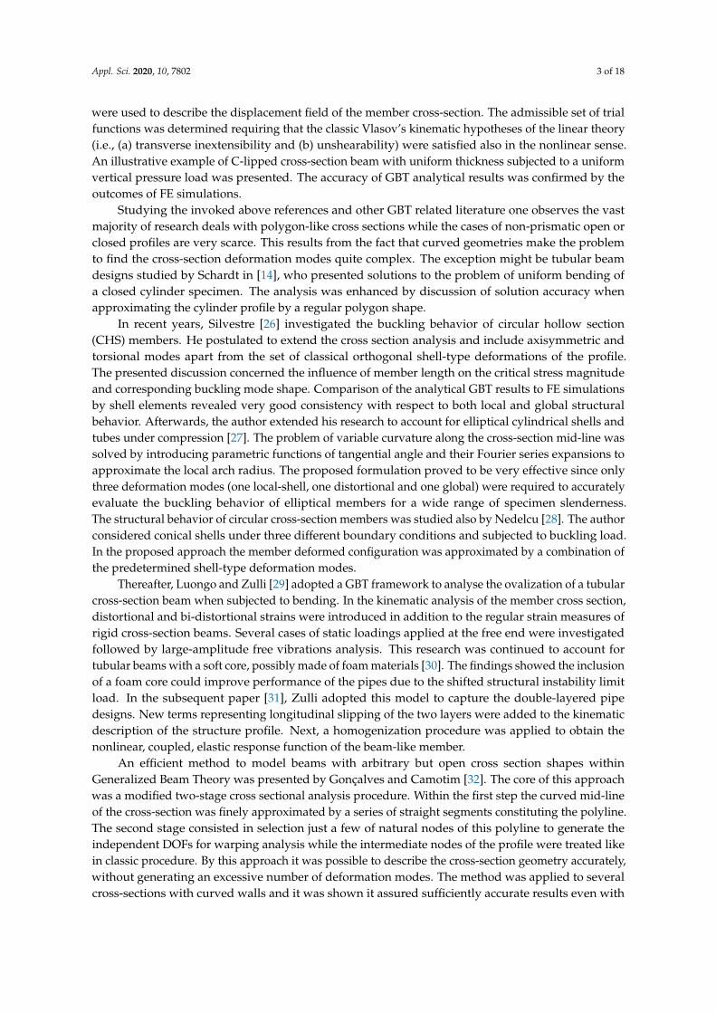
In order to take into account the thickness h of the walls, the webs and flanges are considered assingly curved thin shells, whose mid-surface coincides with γ (Figure 2). The displacements of anygeneric point located off the mid-surface (n 6= 0) are obtained from the mid-surface counterpart onesusing Kirchhoff’s thin plate assumption.

Appl. Sci. 2020, 10, 7802 6 of 18

mid-surface

normal line

eb ≡ ex

es

en

γ

xn

h

Figure 2. Local sketch of the singly curved thin shell.

Thus, every line normal to the mid-surface at x before deformation remains normal after thedeformation and relevant rotations about es and eb directions are:

θs = −∂v∂x

(7)

θb =∂v∂s

+ ku (8)

respectively. It is worth noting how the second term in the right hand side of Equation (8) results fromcross-section curvature about binormal axis [33].

As a consequence, any point out of the mid-surface performs displacement d which has thefollowing components on (es, en, eb):

ds = u− nθb

dn = v

db = w + nθs

(9)

respectively. Substituting Equations (7) and (8) into the above definitions, the local basis displacementcomponents are as follows:

ds = u− n(∂v

∂s+ ku

)dn = v

db = w− n∂v∂x

(10)

The infinitesimal strain components within the curved thin wall are defined as [33]:

εx =∂db∂x

εs =∂ds

∂s− kdn

γxs =∂ds

∂x+

∂db∂s

(11)

where εx, εs are longitudinal strain along x, s, respectively, and γxs is the shear strain. After substitutingEquation (10) in Equation (11), the strain components attain the following expressions:

Appl. Sci. 2020, 10, 7802 7 of 18

εx = εMx + εF

x

εs = εMs + εF

s

γxs = γMxs + γF

xs

(12)

where the pure membrane strain components, i.e., relevant to the mid-surface (n = 0) and indicatedwith superscript M, and the flexural strain components, i.e., proportional to n and indicated withsuperscript F, are:

εMx =

∂w∂x

εMs =

∂u∂s− kv

γMxs =

∂u∂x

+∂w∂s

(13)

and

εFx = −n

∂2v∂x2

εFs = −n

(∂2v∂s2 + k

∂u∂s

+∂k∂s

u)

γFxs = −n

(2

∂2v∂x∂s

+ k∂u∂x

) (14)

Following the idea of the Kantorovitch semi-variational method the individual components of themid-curve γ points displacement are expressed as a linear combination of K triplets of trial functions(Uj(s), Vj(s), Wj(s)), j = 1, . . . , K, and unknown amplitude parameters aj(x):

u(s, x) =K

∑j=1

Uj(s)aj(x)

v(s, x) =K

∑j=1

Vj(s)aj(x)

w(s, x) =K

∑j=1

Wj(s)a′j(x)

(15)

where the prime indicates derivative with respect to x. The functions (Uj(s), Vj(s), Wj(s)) representthe three components of the assumed j− th deformation field, defined on the section profile.

The use of Equation (15) in Equations (13) and (14) allows one to express the strain measures interms of the kinematic descriptors aj(x), for j = 1, . . . , K:

εMx =

K

∑j=1

Wj(s)a′′j (x)

εMs =

K

∑j=1

[dUj(s)ds

− kVj(s)]

aj(x)

γMxs =

K

∑j=1

[Uj(s) +

dWj(s)ds

]a′j(x)

(16)

Appl. Sci. 2020, 10, 7802 8 of 18

and

εFx = −n

K

∑j=1

Vj(s)a′′j (x)

εFs = −n

K

∑j=1

[d2Vj(s)ds2 + k

dUj(s)ds

+dkds

Uj(s)]

aj(x)

γFxs = −n

K

∑j=1

[2

dVj(s)ds

+ kUj(s)]

a′j(x)

(17)

2.2. Constitutive Law

It is assumed that the beam is made of an isotropic, homogeneous and linearly elastic material.Moreover, the plane stress state hypothesis is adopted to a thin shell representing any individual beamwall. For thin-walled structures this assumption is realistic and provides reliable results. Accordingto this formulation, the two-dimensional stresses are functions of solely two coordinates x and s,while all the transverse stresses are negligible:

σn = τsn = τnx = 0 (18)

Thus, the corresponding 3D Hooke’s law is simplified to:

εx =1E(σx − νσs) εs =

1E(σs − νσx) γxs =

τxs

G(19)

where E, G, ν are the material Young’s and Kirchhoff’s moduli, and Poisson ratio, respectively.Equation (19), when solved in terms of stresses, becomes:

σx =E

1− ν2 (εx + νεs)

σs =E

1− ν2 (εs + νεx)

τxs =Gγxs

(20)

Substituting Equation (12) in Equation (20), the expressions of the individual stress componentscan be decomposed to the sum of membrane and flexural related terms, as well:

σx = σMx + σF

x

σs = σMs + σF

s

τxs = τMxs + τF

xs

(21)

Finally, the use of Equations (16) and (17) allows one to express the stress components in (21) interms of the trial functions (Uj(s), Vj(s), Wj(s)) and kinematic descriptors aj(x), j = 1, . . . , K. The finalexpressions are omitted for the sake of brevity.

2.3. Trial Functions and Vlasov’s Constraints

The regular Vlasov’s internal constraints specific for any open cross-section require that the profilemid-curve γ is inextensible and the middle surface of the thin-walled beam is shear indeformable.Thereby two relations follow:

εMs = 0

γMxs = 0

(22)

Appl. Sci. 2020, 10, 7802 9 of 18

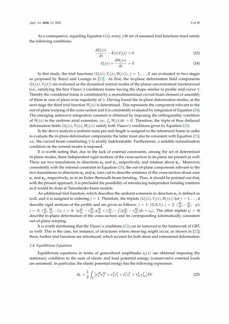
As a consequence, regarding Equation (16), every j-th set of assumed trial functions must satisfythe following conditions:

dUj(s)ds

− k(s)Vj(s) = 0 (23)

Uj(s) +dWj(s)

ds= 0 (24)

In this study, the trial functions (Uj(s), Vj(s), Wj(s)), j = 1, . . . , K are evaluated in two stagesas proposed by Ranzi and Luongo in [21]. At first, the in-plane deformation field components(Uj(s), Vj(s)) are evaluated as the dynamical normal modes of the planar unconstrained inextensional(i.e., satisfying the first Vlasov’s condition) frame having the shape similar to profile mid-curve γ.Thereby the considered frame is constituted by a monodimensional curved beam element or assemblyof them in case of piece-wise regularity of γ. Having found the in-plane deformation modes, at thenext stage the third trial function Wj(s) is determined. This represents the component relevant to theout-of-plane warping of the cross-section and it is consistently evaluated by integration of Equation (24).The emerging unknown integration constant is obtained by imposing the orthogonality conditionof Wj(s) to the uniform axial extension, i.e.,

∫γ Wj(s)ds = 0. Therefore, the triple of thus deduced

deformation fields (Uj(s), Vj(s), Wj(s)) satisfy both Vlasov’s conditions given by Equation (22).In the above analysis a uniform mass per unit length is assigned to the referenced frame in order

to evaluate the in-plane deformation components; the latter must also be consistent with Equation (23),i.e., the curved beam constituting γ is axially indeformable. Furthermore, a suitable normalizationcondition on the normal modes is imposed.

It is worth noting that, due to the lack of external constraints, among the set of determinedin-plane modes, three independent rigid motions of the cross-section in its plane are present as well.These are two translations in directions ey and ez, respectively, and rotation about ex. Moreover,consistently with the internal constraint in Equation (24), the out-of-plane components relevant to thetwo translations in directions ey and ez turn out to describe rotations of the cross-section about axesez and ey, respectively, as in an Euler–Bernoulli beam bending. Thus, it should be pointed out that,with the present approach, it is precluded the possibility of introducing independent bending rotationsas it would be done in Timoshenko beam models.

An additional trial function, which describes the uniform extension in direction ex is defined aswell, and it is assigned to ordering j = 1. Therefore, the triplets (Uj(s), Vj(s), Wj(s)) for j = 1, . . . , 4

describe rigid motions of the profile and are given as follows: j = 1: (0, 0, 1); j = 2: ( dyds ,− dz

ds ,−y);j = 3: ( dz

ds , dyds ,−z); j = 4: (y dz

ds − z dyds , y dy

ds + z dzds ,−

∫(y dz

ds − z dyds )ds + c4). The other triplets (j > 4)

describe in-plane deformation of the cross-section and its corresponding kinematically consistentout-of-plane warping.

It is worth mentioning that the Vlasov’s conditions (22) can be removed in the framework of GBT,as well: This is the case, for instance, of structures where shear-lag might occur, as shown in [22];there, further trial functions are introduced, which account for both shear and extensional deformation.

2.4. Equilibrium Equations

Equilibrium equations in terms of generalized amplitudes aj(x) are obtained imposing thestationary condition to the sum of elastic and load potential energy (conservative external loadsare assumed). In particular, the elastic potential energy has the following expression:

Ue =12

∫V

[σM

x εMx + σF

x εFx + σF

s εFs + τF

xsγFxs]dV (25)

Appl. Sci. 2020, 10, 7802 10 of 18

where V is the total volume of the beam and the differential volume element being dV = dndsdx.In the above the membrane components of strain in tangential direction s and shear mid-surfaceindeformability are omitted according to Vlasov’s conditions Equation (22).

After expressing the stress and strain components in Equation (25) in terms of the unknownamplitudes aj(x), by means of the relevant equations from Sections 2.1 and 2.2, the elastic potentialenergy becomes:

Ue =

l∫0

[12(a ·Aa + a′ · Ba′ + a′′ · Ca′′

)+ a · Fa′′

]dx (26)

where a(x) := (a1(x), . . . , aK(x))T , the dot stands for scalar product, the prime indicates derivativewith respect to x and the expressions of the elements of the individual matrices are:

Ai,j =∫γ

∫ h2

− h2

n2E1− ν2

dds

[dVids

+ kUi

] dds

[dVj

ds+ kUj

]dnds

Bi,j =∫γ

∫ h2

− h2

n2E2(1 + ν)

[2

dVids

+ kUi

][2

dVj

ds+ kUj

]dnds

Ci,j =∫γ

∫ h2

− h2

E1− ν2 [WiWj + n2ViVj]dnds

Fi,j =∫γ

∫ h2

− h2

n2Eν

(1− ν2)

dds

[dVids

+ kUi

]Vjdnds

(27)

It is worth noting that A, B, C are symmetric matrices.The load potential energy is evaluated for a general case of a force per unit area acting in

correspondence of the mid-surface. The generally oriented force is defined by the three componentsvector p(x, s) = pxex + pyey + pzez that yields the energy:

Ul = −∫ l

0

∫γ[pxux + pyuy + pzuz]dsdx (28)

where the displacement components can be expressed in terms of a(x) as well, by means ofEquations (6) and (15).

The minimum of the total potential energy is attained imposing that δ(Ue + Ul) = 0,∀δaj(x), j = 1, . . . , K, where δ is the variation operator, which produces the following set ofEuler-Lagrange equations:

Ca′′′′ + (F + FT − B)a′′ + Aa = f (29)

and boundary conditions in x = 0, l:

a = 0 or −Ca′′′ + (B− FT)a′ = g

a′ = 0 or Ca′′ + FTa = 0(30)

where the elements of f and g are:

f j =∫

γ

[py

(dyds

Uj −dzds

Vj

)+ pz

(dzds

Uj +dyds

Vj

)− p′xWj

]ds

gj =

[ ∫γpxWjds

]x=0,l

(31)

Appl. Sci. 2020, 10, 7802 11 of 18

Equations (29) and (30) represent a linear, ordinary differential boundary value problem withconstant coefficients, governing the evolution of the functions aj(x) along the span of the beam. Even ifit can be analytically solved using the well-known method of variation of constants, which providesthe exact solution, numerical tools capable to solve BVP will be used to find the solution, for practicalpurposes. In spite of this, the outcomes will be referred to as analytical solution in the following partof the paper.

It is noteworthy that the case of branched cross-section can be addressed piecewise evaluatingalong γ the integrals in Equations (27) and (31).

3. Numerical Results

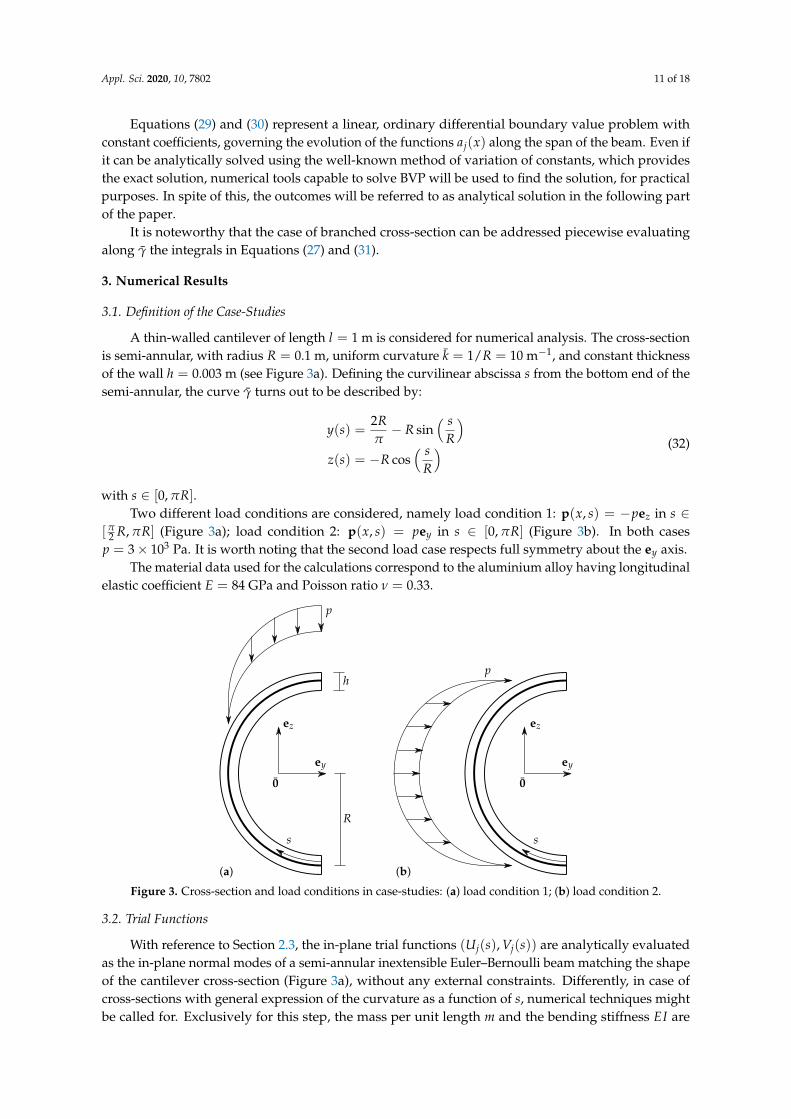
3.1. Definition of the Case-Studies

A thin-walled cantilever of length l = 1 m is considered for numerical analysis. The cross-sectionis semi-annular, with radius R = 0.1 m, uniform curvature k = 1/R = 10 m−1, and constant thicknessof the wall h = 0.003 m (see Figure 3a). Defining the curvilinear abscissa s from the bottom end of thesemi-annular, the curve γ turns out to be described by:

y(s) =2Rπ− R sin

( sR

)z(s) = −R cos

( sR

) (32)

with s ∈ [0, πR].Two different load conditions are considered, namely load condition 1: p(x, s) = −pez in s ∈

[π2 R, πR] (Figure 3a); load condition 2: p(x, s) = pey in s ∈ [0, πR] (Figure 3b). In both cases

p = 3× 103 Pa. It is worth noting that the second load case respects full symmetry about the ey axis.The material data used for the calculations correspond to the aluminium alloy having longitudinal

elastic coefficient E = 84 GPa and Poisson ratio ν = 0.33.

(a) (b)

h

R

ey

ez

s

p

0

ey

ez

0

p

s

Figure 3. Cross-section and load conditions in case-studies: (a) load condition 1; (b) load condition 2.

3.2. Trial Functions

With reference to Section 2.3, the in-plane trial functions (Uj(s), Vj(s)) are analytically evaluatedas the in-plane normal modes of a semi-annular inextensible Euler–Bernoulli beam matching the shapeof the cantilever cross-section (Figure 3a), without any external constraints. Differently, in case ofcross-sections with general expression of the curvature as a function of s, numerical techniques mightbe called for. Exclusively for this step, the mass per unit length m and the bending stiffness EI are

Appl. Sci. 2020, 10, 7802 12 of 18

assumed uniform and, conventionally, their values taken as m = 1 kg/m and EI = 1 Nm2. The normalmodes of the arch beam turn out to be the solutions of the following eigenvalue problem (see [34]):

dUds− kV = 0 (33)

dVds

+ kU −Θb = 0 (34)

kb =dΘbds

(35)

M = EIkb (36)

dNds− kT + mλU = 0 (37)

dTds

+ kN + mλV = 0 (38)

dMds

+ T = 0 (39)

with natural boundary conditions in s = 0, πR:

N = 0

T = 0

M = 0

(40)

where the above represent the normal and shear forces and bending moment, respectively.In particular, Equation (33) states the vanishing of the axial strain of the arch

beam, which corresponds to Vlasov’s condition of profile mid-plane inextensionality(see Equation (23) for comparison); Equation (34) states the vanishing of arch beam shear strain,where Θb is the rotation of the cross-section of the arch about eb—this condition corresponds toformer Kirchhoff’s assumption regarding wall bending. Equation (35) defines the bending curvaturekb about eb, Equation (36) is the classical constitutive law for bending moment M and curvature kb,and Equations (37)–(39) are the balance equations for normal N and shear T forces, and bendingmoment M, respectively. The eigenvalue λ is the square of the circular frequency ω. It is worthnoting that no constitutive law is used for N and T, they being the internal reactive forces to theconstraints (33) and (34).

Assuming an exponential solution of type v(s) = veΩs where v(s) = (U, V, Θb, kb, N, T, M)T ,after usual steps in modal analysis, the following bi-cubic dispersion equation is obtained:

EIΩ6 + 2EIk2Ω4 + (EIk4 −mλ)Ω2 + k2mλ = 0 (41)

Its roots Ωi(λ), i = 1, . . . , 6, after substitution in Equations (33)–(39), allow one to evaluate therelevant eigenvectors vi and build the solution v(s) = ∑i civieΩis, where ci are six undeterminedconstants. The latter expression is substituted in Equation (40) to get the first K natural frequencies(or λ) and, for each of them, five of the six coefficients ci, while the sixth is given by thenormalization condition.

As expected, λ = 0 is a solution of multiplicity 3, giving rise to three in-plane independent rigidmotions. An additional rigid motion, required to describe the uniform displacement in direction ex,is prepended to them as reported at the end of Section 2.3.

Once the modal in-plane components Uj(s), Vj(s), j = 1, . . . , K are obtained, the out-of-plane onesWj(s) are evaluated as well, as described in Section 2.3.

The first four modes, relevant to rigid motions, are shown in Figure 4 where, in the first andsecond row, the in-plane and out-of-plane components are drawn, respectively. In particular, in thefirst line, the in-plane components (Uj(s), Vj(s)) are combined to show the actual displacement of

Appl. Sci. 2020, 10, 7802 13 of 18

the cross-section (in thick solid line), whereas, in the second row, the corresponding normal directioncomponent Wj(s) is plotted (as polar plot, still in thick solid line). Following the same rule, the firstfour in-plane deformation modes (i.e., which correspond to λ 6= 0) are shown in the first row ofFigure 5 and, in the second row, the corresponding out-of-plane components.

I-ip II-ip III-ip IV-ip

I-op II-op III-op IV-op

Figure 4. In-plane (ip) and out-of-plane (op) components of the trial functions, from I to IV(rigid modes). Blue dashed line: initial configuration; black solid line: trial functions.

V-ip VI-ip VII-ip VIII-ip

V-op VI-op VII-op VIII-op

Figure 5. In-plane (ip) and out-of-plane (op) components of the trial functions, from V to VIII(deformation modes). Blue dashed line: initial configuration; black solid line: trial functions.

3.3. Equilibrium Configuration

Using the K = 8 trial functions discussed in Section 3.2, the equilibrium Equation (29) canbe evaluated through Equation (27), and combined to the boundary conditions (30) relevant to thecantilever, i.e., geometric at x = 0 and natural at x = l. The obtained equations are then solved usinga finite difference code based on the three-stage Lobatto IIIa formula, as implemented in the bvp4clibrary command in MATLAB [35], and the solution in terms of aj(x), j = 1, . . . K, is used to calculatedisplacement and stress components in specific points of the thin-walled beam.

In particular, for the two load conditions, plots are shown for: kinematic descriptors aj(x) asfunctions of x ∈ [0, l]; displacement components ux, uy, uz as functions of x for three points of themid-curve γ, i.e., at positions where s = 0 (referred to as position S, i.e., the most southerly point),s = πR

2 (referred to as position W, i.e., the most westerly point), s = πR (referred to as position N,i.e., at the most northern point)—see also Figure A1 in Appendix A for reference; stress component σM

xas a function of x at the same three positions (S,W,N); stress component σx as a function of n ∈ [− h

2 , h2 ]

Appl. Sci. 2020, 10, 7802 14 of 18

at x = 0 in the same three positions. The GBT framework analytical solutions for ux, uy, uz arecompared to the outcomes of a FEM model implemented in the Abaqus software (dotted lines in theplots). Details on the numerical model are given in Appendix A.

For the load condition 1 (load in ez direction), the solution is shown in Figure 6. From Figure 6a,bit can be observed that the component a1, corresponding to uniform extension, is always zero,as expected in a linear problem with structure subjected to transverse loads only. Moreover, amplitudesaj, j = 3, . . . , 6 have at least one order of magnitude larger than the remaining a2, a7, a8, revealingthat global displacement along ey is almost zero and higher modes are actually not required for thiscase (it is verified, even if not reported here for the sake of brevity, that higher modes than K = 8give vanishing contributions for the two analyzed cases). In particular, the components a3, a4, a5

are those which give larger contributions, indicating that besides a rigid motion of the cross-section,a not-negligible deformation component related to a5 (and in minor intensity a6) is present.

In Figure 6c–e, the individual displacement components at the three points of the cross-section(S,W,N) are shown: the component ux comes only from warping of the cross-section and is muchsmaller than uz and uy. Significant in-plane rotation (about ex) and change in shape of the cross-sectionare observed, as related to quite large a4 and a5, respectively, as well as the expected slightly largermaximum displacement in direction ez (direction of the load). These outcomes reveal very goodagreement with the FEM results. Consistently with Vlasov’s theory of non-uniform torsion [1],Figure 6f shows a change in sign of the axial stress component σM

x with respect to the contributionexpected by simple bending: the latter is proportional to a′′3 and would give negative value at S, zerovalue at W and positive value at N (Figure 4—component III-op); however, the change in sign isdue to the large contribution of the out-of-plane distortion proportional to a′′4 (Figure 4—componentIV-op), whereas the non-zero value at position W is mainly due to the contribution of the out-of-planedistortion proportional to a′′5 (Figure 5—component V-op). A not-negligible change in the values of σx

along the thickness of the cross-section is shown at positions N and S in Figure 6g, which contributesto the absolute value of the minimum and maximum stress, respectively.

(a)x (m)

a1a2a3a4

a j(m

)

(b)x (m)

a5a6a7a8

a j(m

)

(c)x (m)

SWN

u x(m

)

(d)x (m)

SWN

u y(m

)

Figure 6. Cont.

Appl. Sci. 2020, 10, 7802 15 of 18

(e)

SWN

x (m)

u z(m

)

(f)

SWN

x (m)

σM x

(Pa)

(g)

SWN

n (m)

σx(

x=

0)(P

a)

Figure 6. Solution for the load condition 1; S: s = 0; W: s = πR2 ; N: s = πR; (a) amplitudes aj,

j = 1, . . . , 4; (b) amplitudes aj, j = 5, . . . , 8; (c) displacement ux; (d) displacement uy; (e) displacementuz; (f) stress component σM

x ; (g) stress component σx at x = 0. Solid lines–analytical solution, dottedlines–FE solution.

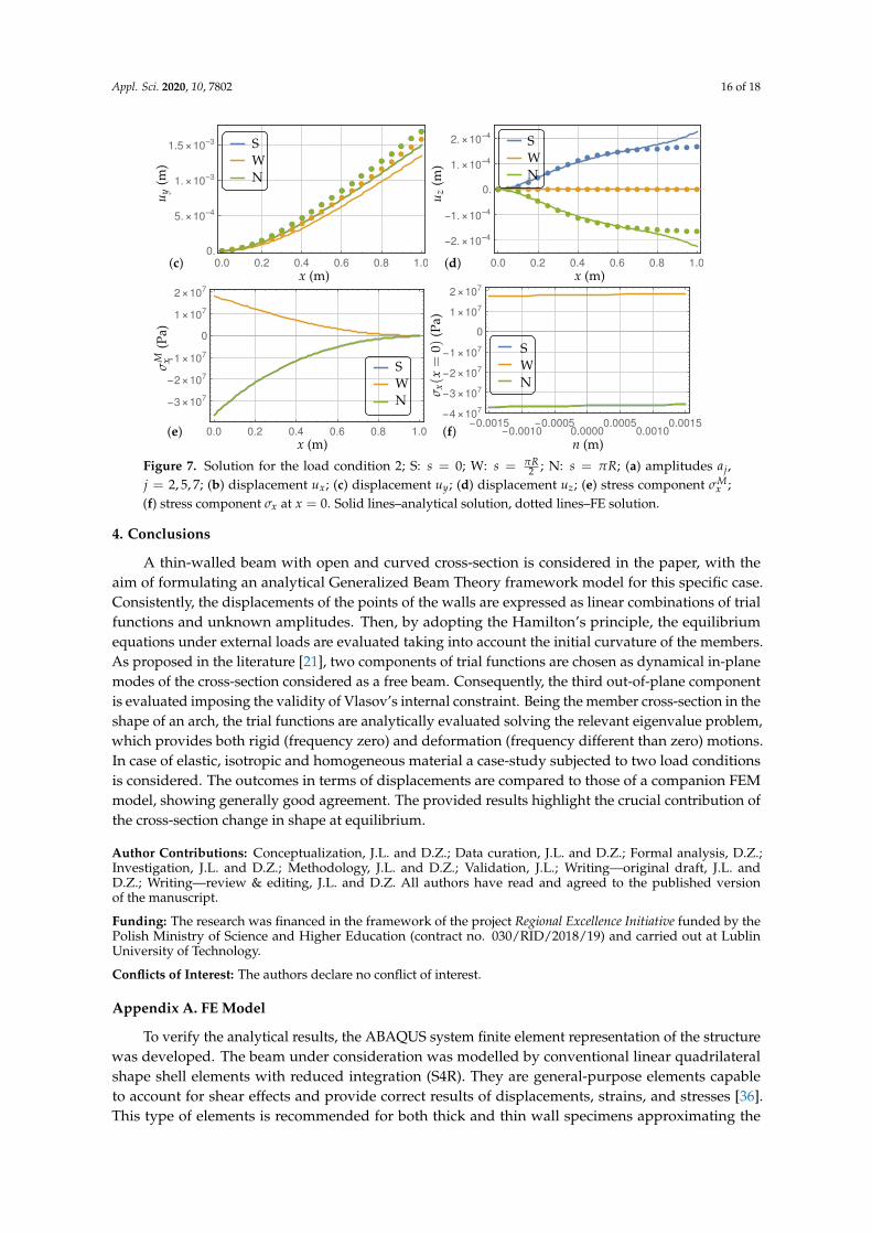
For the load condition 2 (load in ey direction), due to the symmetry of the problem about axis ey,only modes respecting the same symmetry condition are used in the procedure, namely: II, V, VII inFigures 4 and 5. The relevant amplitude components a2, a5, a7 are shown in Figure 7a with clearlydominating role of the component a2 corresponding to rigid motion of the cross-section. Furthermore,among them, a7 is almost negligible as well. In Figure 7b,c, the symmetry of the problem causes theblue and green lines to be superimposed to each other, and satisfying agreement with FEM outcomesis noted. Distortion of the cross-section is evident, as confirmed by the displacement components uz

in Figure 7d, which are opposite in sign for points S and N, respectively, as given by a5 multiplyingthe V-ip trial function in Figure 5. Specifically for this displacement component, a non vanishingdifference of GBT analytical and FEM numerical results is detected at the free tip relevant to positionsN and S. The outcomes are anyway in very good agreement in most of the domain of the beam,i.e., for x ∈ [0, 0.8].

Figure 7e shows the axial stress component σMx . The distribution is fully consistent with the

contribution expected in simple bending test, with stress proportional to a′′2 and multiplying thecomponent II-op in Figure 4. Finally, a vanishing change in the value of resultant σx along the thicknessof the cross-section is shown at positions S and N in Figure 7f. This is due to the fact that the thicknessof the profile wall in these points is perpendicular to the load direction thus the flexural component σF

xis immaterial.

(a)x (m)

a2a5a7

a j(m

)

(b)x (m)

SWN

u x(m

)

Figure 7. Cont.

Appl. Sci. 2020, 10, 7802 16 of 18

(c)x (m)

SWN

u y(m

)

(d)

SWN

x (m)

u z(m

)(e)

SWN

x (m)

σM x

(Pa)

(f)

SWN

n (m)σ

x(x=

0)(P

a)

Figure 7. Solution for the load condition 2; S: s = 0; W: s = πR2 ; N: s = πR; (a) amplitudes aj,

j = 2, 5, 7; (b) displacement ux; (c) displacement uy; (d) displacement uz; (e) stress component σMx ;

(f) stress component σx at x = 0. Solid lines–analytical solution, dotted lines–FE solution.

4. Conclusions

A thin-walled beam with open and curved cross-section is considered in the paper, with theaim of formulating an analytical Generalized Beam Theory framework model for this specific case.Consistently, the displacements of the points of the walls are expressed as linear combinations of trialfunctions and unknown amplitudes. Then, by adopting the Hamilton’s principle, the equilibriumequations under external loads are evaluated taking into account the initial curvature of the members.As proposed in the literature [21], two components of trial functions are chosen as dynamical in-planemodes of the cross-section considered as a free beam. Consequently, the third out-of-plane componentis evaluated imposing the validity of Vlasov’s internal constraint. Being the member cross-section in theshape of an arch, the trial functions are analytically evaluated solving the relevant eigenvalue problem,which provides both rigid (frequency zero) and deformation (frequency different than zero) motions.In case of elastic, isotropic and homogeneous material a case-study subjected to two load conditionsis considered. The outcomes in terms of displacements are compared to those of a companion FEMmodel, showing generally good agreement. The provided results highlight the crucial contribution ofthe cross-section change in shape at equilibrium.

Author Contributions: Conceptualization, J.L. and D.Z.; Data curation, J.L. and D.Z.; Formal analysis, D.Z.;Investigation, J.L. and D.Z.; Methodology, J.L. and D.Z.; Validation, J.L.; Writing—original draft, J.L. andD.Z.; Writing—review & editing, J.L. and D.Z. All authors have read and agreed to the published versionof the manuscript.

Funding: The research was financed in the framework of the project Regional Excellence Initiative funded by thePolish Ministry of Science and Higher Education (contract no. 030/RID/2018/19) and carried out at LublinUniversity of Technology.

Conflicts of Interest: The authors declare no conflict of interest.

Appendix A. FE Model

To verify the analytical results, the ABAQUS system finite element representation of the structurewas developed. The beam under consideration was modelled by conventional linear quadrilateralshape shell elements with reduced integration (S4R). They are general-purpose elements capableto account for shear effects and provide correct results of displacements, strains, and stresses [36].This type of elements is recommended for both thick and thin wall specimens approximating the

Appl. Sci. 2020, 10, 7802 17 of 18

Kirchhoff model as the thickness decreases. Moreover, this element accounts for finite membranestrains and arbitrary large rotations; therefore, it is suitable also for geometrically nonlinear analysis.

Alternatively, one can use continuum shell elements but they require the geometry to modelexplicitly the thickness of the shell, as it would be done with classical 3D solid elements. However,in contrast to the classical shell, continuum shell elements enforce the first order shear deformationconstrains through particular element interpolation functions.

The beam structure was meshed into 100 elements along the span and 30 ones along the profileperimeter. Moreover, the nodal sets required to record the spanwise deflections at most southerly (S),most westerly (W) and most northern (N) positions of the profile were defined as shown in Figure A1.

S set

N set

W set

Figure A1. Meshed FE model of the thin-walled cantilever and nodal points to record displacements.

References

1. Vlasov, V.Z. Thin-Walled Elastic Beams; National Technical Information Service: Jerusalem, Israel, 1961.2. Ghobarah, A.A.; Tso, W.K. A non-linear thin-walled beam theory. Int. J. Mech. Sci. 1971, 13, 1025–1038. [CrossRef]3. Simo, J.C.; Vu-Quoc, L. A geometrically-exact rod model incorporating shear and torsion-warping

deformation. Int. J. Solids Struct. 1991, 27, 371–393. [CrossRef]4. Yang, Y.B.; Yau, J.D. Stability of beams with tapered I—Sections. J. Eng. Mech. 1987, 113, 1337–1357.:9(1337).

[CrossRef]5. De Andrade, A.A.M. One-Dimensional Models for the Spatial Behaviour of Tapered Thin-Walled Bars with

Open Cross-Sections: Static, Dynamic and Buckling Analyses. Ph.D. Thesis, University of Coimbra, Portugal,Coimbra, 2012.

6. Yang, Y.B.; Kuo, S.R. Static stability of curved thin–walled beams. J. Eng. Mech. 1986, 112, 821–841. [CrossRef]7. Gendy, A.S.; Saleeb, A.F. Vibration analysis of coupled extensional/flexural/torsional modes of curved

beams with arbitrary thin-walled sections. J. Sound Vib. 1994, 174, 261–274. [CrossRef]8. Di Egidio, A.; Luongo, A.; Vestroni, F. A non-linear model for the dynamics of open cross-section thin-walled

beams—Part I: Formulation. Int. J. Non-Linear Mech. 2003, 38, 1067–1081. [CrossRef]9. Capurso, M. Influenza delle componenti di scorrimento nella deformazione delle travi di parete sottile con

sezione aperta. G. Genio Civ. 1984, 122, 127–144. (In Italian)10. Librescu, L.; Song, O. Thin-Walled Composite Beams. Theory and Applications; Springer: Berlin/Heidelberg,

Germany, 2006.11. Yu, W.; Hodges, D.H.; Volovoi, V.V.; Fuchs, E.D. A generalized Vlasov theory for composite beams.

Thin-Walled Struct. 2005, 43, 1493–1511. [CrossRef]12. Latalski, J.; Warminski, J.; Rega, G. Bending-twisting vibrations of a rotating hub-thiun-walled composite

beam system. Math. Mech. Solids 2017, 22, 1303–1325. [CrossRef]13. Latalski, J.; Warminski, J. Nonlinear vibrations of a rotating thin-walled composite piezo-beam with

circumferentially uniform stiffness (CUS). Nonlinear Dyn. 2019, 98, 2509–2529. [CrossRef]

Appl. Sci. 2020, 10, 7802 18 of 18

14. Schardt, R. Verallgemeinerte Technische Biegetheorie: Lineare Probleme; Springer: Heidelberg, Germany, 1989.(In German)

15. Schardt, R. Generalized Beam Theory—An adequate method for coupled stability problems. Thin-Walled Struct.1994, 19, 161–180. [CrossRef]

16. Renton, J.D. Generalized Beam Theory applied to shear stiffness. Int. J. Solids Struct. 1991, 27, 1955–1967.[CrossRef]

17. Silvestre, N.; Camotim, D. Nonlinear Generalized Beam Theory for cold-formed steel members. Int. J. Struct.Stab. Dyn. 2003, 3, 461–490. [CrossRef]

18. Silvestre, N.; Camotim, D. Influence of shear deformation on the local and global buckling behaviour ofcomposite thin-walled members. In Thin-Walled Structures—Advances in Research, Design and ManufacturingTechnology; Loughlan, J., Ed.; IOP Publishing Ltd.: Bristol, Italy, 2004; pp. 659–668.

19. Silvestre, N.; Camotim, D. Shear deformable Generalized Beam Theory for the analysis of thin-walledcomposite members. J. Eng. Mech. 2013, 139, 1010–1024. [CrossRef]

20. Taig, G.; Ranzi, G. Generalised Beam Theory (GBT) for stiffened sections. Int. J. Steel Struct. 2014, 14, 381–397.[CrossRef]

21. Ranzi, G.; Luongo, A. A new approach for thin-walled member analysis in the framework of GBT. Thin-WalledStruct. 2011, 49, 1404–1414. [CrossRef]

22. Piccardo, G.; Ranzi, G.; Luongo, A. A complete dynamic approach to the Generalized Beam Theorycross-section analysis including extension and shear modes. Math. Mech. Solids 2014, 19, 900–924. [CrossRef]

23. Piccardo, G.; Ranzi, G.; Luongo, A. A direct approach for the evaluation of the conventional modes withinthe GBT formulation. Thin-Walled Struct. 2014, 74, 133–145. [CrossRef]

24. Ferrarotti, A.; Piccardo, G.; Luongo, A. A novel straightforward dynamic approach for the evaluation ofextensional modes within GBT ’cross-section analysys’. Thin-Walled Struct. 2017, 114, 52–69. [CrossRef]

25. Piccardo, G.; Ferrarotti, A.; Luongo, A. Nonlinear Generalized Beam Theory for open thin-walled members.Math. Mech. Solids 2016, 22, 1907–1921. [CrossRef]

26. Silvestre, N. Generalised Beam Theory to analyse the buckling behaviour of circular cylindrical shells andtubes. Thin-Walled Struct. 2007, 45, 185–198. [CrossRef]

27. Silvestre, N. Buckling behaviour of elliptical cylindrical shells and tubes under compression. Int. J. Solids Struct.2008, 45, 4427–4447. [CrossRef]

28. Nedelcu, M. GBT formulation to analyse the buckling behaviour of isotropic conical shells. Thin-Walled Struct.2011, 49, 812–818. [CrossRef]

29. Luongo, A.; Zulli, D. A non-linear one-dimensional model of cross-deformable tubular beam. Int. J.Non-Linear Mech. 2014, 66, 33–42. [CrossRef]

30. Luongo, A.; Zulli, D.; Scognamiglio, I. The Brazier effect for elastic pipe beams with foam cores.Thin-Walled Struct. 2018, 124, 72–80. [CrossRef]

31. Zulli, D. A one-dimensional beam-like model for double-layered pipes. Int. J. Non-Linear Mech. 2019,109, 50–62. [CrossRef]

32. Gonçalves, R.; Camotim, D. GBT deformation modes for curved thin-walled cross-sections based on amid-line polygonal approximation. Thin-Walled Struct. 2016, 103, 231–243. [CrossRef]

33. Axisa, F.; Trompette, P. Modelling of Mechanical Systems Vol 2 Structural Elements; Elsevier Butterworth-Heinemann:London, UK, 2005.

34. Benedettini, F.; Alaggio, R.; Zulli, D. Nonlinear coupling and instability in the forced dynamics of anon-shallow arch: Theory and experiments. Nonlinear Dyn. 2012, 68, 505–517. [CrossRef]

35. The MathWorks Inc. MATLAB; Version R2019b; The MathWorks Inc.: Natick, MA, USA, 2019.36. Smith, M. ABAQUS/CAE User’s Manual; Dassault Systèmes: Providence, RI, USA, 2020.

Publisher’s Note: MDPI stays neutral with regard to jurisdictional claims in published maps and institutionalaffiliations.

c© 2020 by the authors. Licensee MDPI, Basel, Switzerland. This article is an open accessarticle distributed under the terms and conditions of the Creative Commons Attribution(CC BY) license (http://creativecommons.org/licenses/by/4.0/).