Journal of

Mechanics ofMaterials and Structures

A DIRECT ONE-DIMENSIONAL BEAM MODEL FOR THEFLEXURAL-TORSIONAL BUCKLING OF THIN-WALLED BEAMS

Giuseppe Ruta, Marcello Pignataro and Nicola Rizzi

Volume 1, Nº 8 October 2006

mathematical sciences publishers

JOURNAL OF MECHANICS OF MATERIALS AND STRUCTURESVol. 1, No. 8, 2006

A DIRECT ONE-DIMENSIONAL BEAM MODEL FOR THEFLEXURAL-TORSIONAL BUCKLING OF THIN-WALLED BEAMS

GIUSEPPE RUTA, MARCELLO PIGNATARO AND NICOLA RIZZI

In this paper, the direct one-dimensional beam model introduced by one of the authors is refined totake into account nonsymmetrical beam cross-sections. Two different beam axes are considered, andthe strain is described with respect to both. Two inner constraints are assumed: a vanishing shearingstrain between the cross-section and one of the two axes, and a linear relationship between the warpingand twisting of the cross-section. Considering a grade one mechanical theory and nonlinear hyperelasticconstitutive relations, the balance of power, and standard localization and static perturbation procedureslead to field equations suitable to describe the flexural-torsional buckling. Some examples are given todetermine the critical load for initially compressed beams and to evaluate their post-buckling behavior.

1. Introduction

The flexural-torsional buckling of so-called thin-walled beams is an interesting problem in the field ofthe elastic stability of structural elements. This phenomenon was first investigated in [Wagner 1929]and [Kappus 1937], and since the publication of these pioneering works, many further studies haveappeared on the subject, including [Vlasov 1961; Epstein 1979; Reissner 1983; Simo and Vu-Quoc1991]. More recently, [Di Egidio et al. 2003] investigated modelization aspects, and [Anderson andTrahair 1972; Casciaro et al. 1991; Lanzo and Garcea 1996] presented a search of numerical results forstandard elements. It is remarkable that most of the beam models presented in the literature are derivedby projection of the results of three-dimensional continuum models on shell models (as in Vlasov 1961)or beam models (as in Simo and Vu-Quoc 1991).

In recent years, the authors have considered the direct one-dimensional beam model, originally in-troduced in [Tatone and Rizzi 1991; Rizzi and Tatone 1996]. This model describes the kinematics ofthe beam through the placement of the points of the beam axis, the rotation of the beam cross-sections(which are assumed to be plane in the reference configuration), and a coarse description of the warpingof the beam cross-sections. Using a mechanical theory of grade one (see, for example Germain 1973aand 1973b, and Di Carlo 1996), the interaction of the beam with the surrounding environment is definedas a linear function of the velocities and of their first-order spatial approximations. In this way, themechanical actions naturally appear as dual to the kinematic fields. In particular, actions which spendpower on the warping velocity and on its spatial derivative are interpreted as bi-shear and bi-moment,respectively. As is customary in the literature, two inner constraints are assumed to hold: the shearing

Keywords: thin-walled beams, direct one-dimensional models, flexural-torsional buckling.Giuseppe C. Ruta gratefully acknowledges the financial support of the Progetto giovani ricercatori (2002) of the Università LaSapienza of Rome.

1479

1480 GIUSEPPE RUTA, MARCELLO PIGNATARO AND NICOLA RIZZI

strain between the axis and the cross-section is assumed to vanish, and the coarse warping measure isdirectly proportional to the measure of twist.

In previous papers [Rizzi and Tatone 1996; Pignataro and Ruta 2003; Pignataro et al. 2004], fieldequations in terms of the components of the displacement were obtained, and some flexural-torsionalbuckling cases were investigated. For this purpose, nonlinear hyperelastic constitutive relations wereadopted. However, since no clear distinction was made between the position of the centroid and of theshear center in the plane of the cross-section, it turns out that the results obtained in the above mentionedpapers are precise only for beams with symmetric cross-sections.

The aim of this paper is to overcome this drawback by presenting a refined beam model suitable fordescribing the flexural-torsional buckling of beams with generic, nonsymmetric cross-sections. We willdescribe the strain measures with respect to two beam axes (one passing through the centroids, and theother through the shear centers of the cross-sections). Then, we suitably decompose the power expendedby inner actions, to distinguish clearly between actions applied at each of the two places. Introducingthe same inner constraints as in the papers cited above generates reactive terms that must be added tothe determined part of the contact actions, and those terms account for the geometry of nonsymmetriccross-sections. In this way, we are able to obtain field equations which are more general than thosefound by authors of previous studies. To test the validity of the proposed model, we present some simpleexamples of flexural-torsional buckling and post-buckling phenomena. The results coincide with thosein the literature, for example [Timoshenko and Gere 1961; Grimaldi and Pignataro 1979].

2. A direct one-dimensional beam model

Let E be the standard three-dimensional Euclidean ambient space. The vector space of the translationsof E, here denoted U, is assumed to be equipped with the standard Euclidean norm and scalar (dot)product. Let us consider in E a smooth curve Co and a prototype region R belonging to a plane P. Wethen attach a copy of R to each point of Co, always in correspondence to the same place o ∈ P. Theregion of E occupied by this construction represents the beam. The curve Co corresponds to the axis ofthe beam, and the copies of R are the beam cross sections. With no loss of generality, and only from thepoint of view of introducing constitutive relations, we can imagine that the place o ∈ P is actually thecentroid of the cross-section. Hence, the axis Co is a centroidal axis. Of course, the beam can be equallydescribed using an analogous construction starting from a different curve Cc in E. Again, with no lossof generality, one can imagine that the place c ∈ P is actually the shear center of the cross-sections. Forthe time being, we ignore the question of whether this is the shear center according to Timoshenko orTrefftz. Indeed, for open thin-walled beams the question is immaterial since either definition providesthe same place (see, for example, [Andreaus and Ruta 1998; Ruta 1998]). In this way, we can call thecurve Cc the shear axis, or the axis of the shear centers.

A change of placement is described by the placement of the axes, the rotation of each cross-section withrespect to the attitude in the first placement, and a warping superposed to these two. The transformationsof the axes and the rotations of the cross-sections can be described exactly, but we will limit ourselveswith a coarse description of the warping by using a single scalar parameter. We can suitably definethis parameter as a (possibly weighted) average of the warping over the cross-section, or as the valueof the warping at a particular place of (plane of) the cross-section. A motion is naturally defined as a

A DIRECT ONE-DIMENSIONAL BEAM MODEL FOR FLEXURAL-TORSIONAL BUCKLING 1481

one-parameter family of changes of placements, t ∈ [0, +∞] being the evolution scalar real parameter(the time, for instance).

Let us consider a motion and let S0 be the shape of the beam at t = 0. This may be assumed, with noloss of generality, to be the reference configuration. It is always possible to assume that S0 is such thatthe copies of the prototype plane region R remain plane, that is, the cross-sections undergo no warping.Once a place in E is chosen as origin, the axes of the beam in S0 are described by the regular enoughposition vector fields

qo : ρ ∈ [0, l] → qo(ρ) ∈ U, qc : ρ ∈ [0, l] → qc(ρ) ∈ U,

where ρ is a curvilinear abscissa along one of the axes compatible with the Euclidean metric of theambient space E. The unit vector fields tangent to the axes of the beam are

q′

o(ρ), q′

c(ρ),

where the prime denotes derivation with respect to ρ. With no loss of generality, one can assume that inS0 the relative position of the places o and c in the planes containing the cross-sections does not dependon ρ, so that

q′

o(ρ) = q′

c(ρ), for all ρ ∈ [0, l]. (1)

Let St be the configuration assumed by the beam in the motion we are considering at the present valuet of the evolution parameter. Such a configuration is described by:

• a vector field po(ρ, t) (or, equivalently, pc(ρ, t)), providing the position of the substantial pointidentified by qo(ρ) (or, equivalently, qc(ρ)) in S0;

• a proper orthogonal tensor field R(ρ, t), providing the rotation of the cross-sections when passingfrom S0 to St ;

• a scalar field α(ρ, t), providing a coarse description of the cross-sections’ warping superposed todisplacements induced by the rotation R(ρ, t).

The tensors R(ρ, t) are required to be proper orthogonal to prevent reflections of the cross-sections.Henceforth, the fields po, pc, R, α will be assumed to be regular enough for the analytical developmentswe adopt. Also, for the sake of simplicity of notation, and when no confusion may arise, in the followingthe dependent variables of the indicated fields will be understood and hence omitted, as well as themeasures of integration in the integrals.

The tangent vector fields to the axes of the beam in the present configuration are given by

p′

o(ρ, t), p′

c(ρ, t).

The derivative of a field with respect to t is denoted by a superimposed dot, and skw(U ⊗ U) denotesthe space of skew tensors on U.

The velocity fields for the beam are

wo = po ∈ U, wc = pc ∈ U,

W = RR>∈ skw(U ⊗ U), ω = α ∈ R.

(2)

1482 GIUSEPPE RUTA, MARCELLO PIGNATARO AND NICOLA RIZZI

A rigid, or neutral, change of placement is one such that the rotation of the cross-sections is uniform withrespect to ρ, any vector out of the plane of the cross-sections (for example, either p′

o or p′c) is rotated

according to this uniform rotation, and the warping remains identical to zero.Hence, in a rigid change of placement

R = R0, p′

o = R0q′

o,

p′

c = R0q′

c = R0q′

o, α = 0.(3)

Deformation is the difference between the considered change of placement and a rigid one, and mustvanish if evaluated for a neutral change of placement. Suitable strain measures, pulled back to S0, are

E = R>R′, α, η = α′,

eo = R>p′

o − q′

o, ec = R>p′

c − q′

c = eo + Ec, (4)

where the skew tensor field E provides the change of curvature of one of the beam axes when passingfrom S0 to St . The vector fields eo and ec represent the differences between the tangent to the axes inSt , pulled back to S0, and the tangent to the axes in S0. The vector c defines the position of the place cwith respect to o in the plane of the cross-sections in S0, and c is uniform with respect to ρ because of(1). When the change of placement is neutral, the relations given in (3) imply that the quantities definedby (4) vanish. The strain measures given by (4) are invariant under a change of observer.

With no loss of generality, let S0 be a set of parallel cross-sections orthogonal to the beam axes, eachof which is assumed to be a rectilinear segment of length l. Let us fix a system of orthogonal Cartesiancoordinates with the x1 axis parallel to the beam axes in S0 (ρ ≡ x1). Furthermore, let us consider anorthonormal right-handed vector basis (i1, i2, i3) for U adapted to the introduced coordinate system suchthat

i1 = q′

o = q′

c.

With respect to the introduced basis, consider the decompositions

E = χ1i2 ∧ i3 + χ2i3 ∧ i1 + χ3i1 ∧ i2,

eo = ε1i1 + ε2i2 + ε3i3,

ec = ε1ci1 + ε2ci2 + ε3ci3 = (ε1 + χ2c3 − χ3c2)i1 + (ε2 − χ1c3)i2 + (ε3 + χ1c2)i3,

(5)

where χ1 is the torsion curvature (or twist), χ2 and χ3 are the bending curvatures, ∧ is the exterior productbetween vectors of U which provide skew tensors on U, ε1 is the elongation of the axis of the centroids,ε2 and ε3 are the shearing strains between the axis of the centroids and the cross-sections, and c2 andc3 are the components of c. Equation (5)3 provides, with respect to the shear axis, quantities similar tothose provided by (5)2. In addition, it expresses these last in terms of the components of E and eo (see(4)5).

It is useful to write the strain measures in terms of the displacement field u of the axis of the centroidsstarting from S0 as

u = po − qo = u1i1 + u2i2 + u3i3,

and to decompose the rotation R asR = R3 R2 R1, (6)

A DIRECT ONE-DIMENSIONAL BEAM MODEL FOR FLEXURAL-TORSIONAL BUCKLING 1483

where R1 is a rotation of amplitude ϕ1 about i1, R2 is a rotation of amplitude ϕ2 about R1i2 (that is, theϕ1-transformed of i2), and R3 is a rotation of amplitude ϕ3 about R2R1i3 (that is, the ϕ2 ◦ϕ1-transformedof i3). It can be proved (see [Di Carlo and Tatone 1980]) that the matrix representation (R)0 of R withrespect to the basis (i1, i2, i3) is

(R)0 = (R1)0(R2)1(R3)2, (7)

where (R1)0 is the matrix representation of R1 with respect to the reference basis (i1, i2, i3), (R2)1 isthe matrix representation of R2 with respect to the ϕ1-transformed of the reference basis, and (R3)2 isthe matrix representation of R3 with respect to the ϕ2 ◦ ϕ1-transformed of the reference basis.

Equations (4)–(7) yield expressions of the components of the strain measures in terms of the com-ponents of the displacement of the axis of the centroids starting from the reference configuration S0

asε1 = (1 + u′

1) cos ϕ2 cos ϕ3 + u′

2(cos ϕ1 sin ϕ3 + sin ϕ1 sin ϕ2 cos ϕ3)

+ u′

3(sin ϕ1 sin ϕ3 − cos ϕ1 sin ϕ2 cos ϕ3) − 1,

ε2 = − (1 + u′

1) cos ϕ2 sin ϕ3 + u′

2(cos ϕ1 cos ϕ3 − sin ϕ1 sin ϕ2 sin ϕ3)

+ u′

3(sin ϕ1 cos ϕ3 + cos ϕ1 sin ϕ2 sin ϕ3),

ε3 = (1 + u′

1) sin ϕ2 − u′

2 sin ϕ1 cos ϕ2 + u′

3 cos ϕ1 cos ϕ,

χ1 = ϕ′

1 cos ϕ2 cos ϕ3 + ϕ′

2 sin ϕ3,

χ2 = − ϕ′

1 cos ϕ2 sin ϕ3 + ϕ′

2 cos ϕ3,

χ3 = ϕ′

1 sin ϕ2 + ϕ′

3.

3. Balance of power and balance equations

Let us assume that the interaction of the beam with the environment in its present configuration St isquantified, for each test velocity field attainable by the beam, using a linear functional of the velocityfields, which we will call the external power Pe. Standard representation theorems of linear forms infinite-dimensional vector spaces equipped with a scalar product then let us express external power as

Pe=

∫ l

0(b · wc + B · W + βω) +

∣∣∣∣t · wc + T · W + θω

∣∣∣∣0−

+

∣∣∣∣t · wc + T · W + θω

∣∣∣∣l+

, (8)

where the integral term quantifies the power expended by bulk actions, and the boundary terms quantifythe power expended by contact actions. The vector fields b and t represent external force density (bulkand contact, respectively), the skew tensor fields B and T represent external couple density (bulk andcontact, respectively), and the scalar fields β and θ represent the bulk and contact actions density, respec-tively, which exert power on the warping. It is essential and will be fundamental henceforth that in therepresentation of Pe the velocity used is that of the points of the shear axis.

If we move in the frame of a mechanical theory of grade one (see, for example [Di Carlo 1996]),let us assume that the behavior of any substantial point on the (axis of the) beam is influenced by thesubstantial points contained in one of its neighborhoods. The interaction among different parts of thebeam is then quantified for each test velocity field attainable by the beam, using a linear functional of thevelocity fields and of their first derivatives with respect to x1. This functional, denoted P i , is also called

1484 GIUSEPPE RUTA, MARCELLO PIGNATARO AND NICOLA RIZZI

the internal power. The theorems we used to represent external power Pe enable us to express P i as

P i=

∫ l

0

(c0 · wc + C0 · W + γ0ω + c1 · w′

c + C1 · W′+ γ1ω

′), (9)

where the vector fields c0 and c1 represent self-force and internal force densities, respectively, the skewtensor fields C0 and C1 represent the self-couple and internal couple densities, respectively, and thescalar fields γ0 and γ1 represent the self-action and the internal action densities which spend power onthe warping and on its spatial rate, respectively.

It is natural to assert that P i≡ 0 for any change of placement leaving the beam mechanical state

unaltered, and that is the situation for a the change of placement induced by a neutral velocity field.Substituting (3) into (2) and then into (9), the generality of the kinematic fields present in the integrandleads to the following reduced expression for the internal power

P i=

∫ l

0

(c1 · w′

c − (p′

c ∧ c1) · W + C1 · W′+ γ0ω + γ1ω

′). (10)

Hence, in this beam model the self-force density necessarily vanishes, while the self-couple density isactually the moment of the internal force density with respect to the shear center, as expressed by theterm containing the wedge product in the integrand of Equation (10).

Let us postulate that for any test velocity field attainable by the beam the interactions of the beam withthe environment and of the parts of the beam with each other are such that at any value of the evolutionparameter t the total power vanishes (see [Germain 1973a; 1973b; Di Carlo 1996]), or equivalently,

Pe= P i . (11)

From (11), standard localization procedures under suitable regularity hypotheses yield the law ofaction and reaction∣∣∣∣t · wc + T · W + θω

∣∣∣∣x−

1

= −

∣∣∣∣t · wc + T · W + θω

∣∣∣∣x+

1

, for all x1 ∈ [0, l]. (12)

As a consequence of (12), the boundary terms for the expression of external power (8), can be compactedwith respect to the actions on the positive side of the cross-sections. Applying the fundamental theoremof integral calculus, the balance of power (11) becomes∫ l

0[(t′ + b

)· wc +

(T′

+ p′

c ∧ c1 + B)· W +

(β + θ ′

− γ0)ω

+ (t − c1) · w′

c + (T − C1) · W′+ (θ − γ1) ω′

] = 0. (13)

For generality of the velocity fields and their first spatial derivatives contained in the integrand, (13)yields

c1 = t, C1 = T,

t′ + b = 0, T′+ p′

c ∧ t + B = 0,

γ0 = τ = β + θ ′, γ1 = µ = θ.

(14)

A DIRECT ONE-DIMENSIONAL BEAM MODEL FOR FLEXURAL-TORSIONAL BUCKLING 1485

Equations (14)1,2 represent two identification equations and tell us that in this beam model the inter-nal action densities c1 and C1 actually coincide with contact force and couple densities, respectively.Equations (14)3,4 express the local balance of force and torque. By torque we mean an action whichspends power on an angular velocity, and is hence expressed both by a couple and the moment of aforce. Equation (14)5 is an auxiliary equation for γ0, henceforth denoted τ and interpreted as bishear[Vlasov 1961]. Equation (14)6 is an auxiliary equation for γ1, henceforth denoted µ and interpreted asa bimoment [Vlasov 1961].

The equations in (14) were obtained by the balance of power in the present configuration. In any case,neither the identities in (14)1,2 nor the scalar auxiliary (14)5,6 depend on the configuration. It seemsadvisable, however, to pull back the local balance equations (14)3,4 to the reference configuration. Letus then propose

s = R>t, S = R>TR, a = R>b, A = R>BR,

where s, S, a, and A are the contact and bulk action densities pulled back to S0. Taking into account thedefinitions of ec, E, and Equation (4), the local balance equations (14)3,4, become

s′+ Es + a = 0,

S′+ ES − SE +

(q′

c + ec)∧ s + A = 0,

(15)

while the reduced expression of the internal power (10), and the balance of power (11), become

P i=

∫ l

0

(s · ec + S · E + τω + µω′

)= Pe. (16)

We decompose the contact action densities in S0 as

s = Q1i1 + Q2i2 + Q3i3, S = M1i2 ∧ i3 + M2i3 ∧ i1 + M3i1 ∧ i2. (17)

We now express the strain with respect to the shear axis ec in terms of the strain with respect to thecentroidal axis e, according to (4)3. Then, we can write the full expression of the internal power (16),taking into account the decompositions in (17), as∫ l

0

(Q1ε1 + Q2ε2c + Q3ε3c + M1χ1 + (M2 + c3 Q1)χ2 + (M3 − c2 Q1)χ3 + τω + µω′

). (18)

Equation (18) shows that Q1, interpreted as normal force, spends power on the speed of elongation of thecentroidal axis, while Q2 and Q3, interpreted as shearing forces, spend power on the speed of shearingbetween the cross-sections and the shear axis. That is, we imagine the normal force to be applied at thecentroid of the cross-section, while the shearing forces are applied at the shear center of the cross-section.The twisting couple M1 spends power on the speed of twisting, while the bending torques M2 + c3 Q1

and M3 − c2 Q1, which are composition of a couple and of the moment of a force, respectively, spendpower on the speed of bending. Also, note that the bending torques introduced are thus evaluated withrespect to the centroid of the cross-section.

Substituting (5)3 and (17) into (15), and assuming the bulk actions to vanish as is customary, weobtain the components of the local balance equations for contact force and torque, with all the kinematic

1486 GIUSEPPE RUTA, MARCELLO PIGNATARO AND NICOLA RIZZI

quantities written with respect to the centroid of the cross-sections, as

Q′

1 + χ2 Q3 − χ3 Q2 = 0,

Q′

2 + χ3 Q1 − χ1 Q3 = 0,

Q′

3 + χ1 Q2 − χ2 Q1 = 0,

M ′

1 + χ2 M3 + χ3 M2 + (ε2 − χ1c3)Q3 − (ε3 + χ1c2)Q2 = 0,

M ′

2 + χ3 M1 + χ1 M3 + (ε3 + χ1c2)Q1 − (1 + ε1 + χ2c3 − χ3c2)Q3 = 0,

M ′

3 + χ1 M2 + χ2 M1 + (1 + ε1 + χ2c3 − χ3c2)Q2 − (ε2 − χ1c3)Q1 = 0.

4. Inner constraints and constitutive relations

If the beam is made of homogeneous and elastic material, standard axioms of the constitutive theory[Truesdell and Noll 1965] state that the most general material response function assumes the reducedexpression

S = S(e, E, α, η), (19)

where S represents each of the components of s and S, and τ and µ.Let us now introduce some inner constraints. The first takes into account a standard assumption in

the literature, that is, that warping actually depends on the other strain measures, and vanishes when nostrain is present, as

α = α(e, E), α(0, 0) = 0, (20)

where α is a scalar function independent of the frame of reference, since both e and E are likewiseindependent. On the basis of the literature, it seems natural to postulate the particular expression forEquation (20)

α = ξχ1, ξ ∈ R, η = ξχ ′

1, (21)

where ξ is a numerical constant [Vlasov 1961; Reissner 1983; Simo and Vu-Quoc 1991; Tatone and Rizzi1991; Rizzi and Tatone 1996]. In particular, with reference to [Simo and Vu-Quoc 1991], a possiblekinematic interpretation for α is that of a suitably weighted average of out-of-plane displacement of thepoints initially lying on the same plane cross section.

Furthermore, let us assume that the shearing strains between the cross-sections and the axis of the cen-troids vanishes. This implies that in a neighborhood of the centroid, the cross section remains orthogonalto the axis of the centroids, as

e = ε1q′

o = ε1e1 ⇒ ε2 = ε3 = 0. (22)

Note that this assumption does not imply that the whole of the cross-section remains orthogonal to thebeam axes. Indeed, ε2c and ε3c do not vanish, as is easily obtained from (4)3.

According to the principle of determinism for constrained materials [Truesdell and Noll 1965], in-troducing constraints implies that the contact actions consist of the sum of two contributions. One ofthese is determined by the motion according to a constitutive relation (19), but the other is not. Forthis reason, the former is called active and the latter reactive. The reactive part of the contact actionsis here denoted by the subscript r and is characterized, for so-called smooth constraints [Truesdell andNoll 1965], by spending no power on any velocity field compatible with the introduced constraints. In

A DIRECT ONE-DIMENSIONAL BEAM MODEL FOR FLEXURAL-TORSIONAL BUCKLING 1487

our case, the introduced constraints are those between warping and twist (21), and of vanishing shearingstrain between the cross-sections and the centroidal axis (22). Characterization of smooth constraintsyields

0 =

∫ l

0

(sr · ec + Sr · E + τr α + µr η

)=

∫ l

0

(Q1r ε1 + (M1r − c3 Q2r + c2 Q3r + ξτr )χ1

+ (M2r + c3 Q1r )χ2 + (M3r − c2 Q1r )χ3 + µrξ χ ′

1), (23)

where we used the reduced expression for the internal power (16) and the decompositions of the strainmeasure (4)3 and of the contact actions (17). For generality of the velocity fields and of the domain ofintegration in (23), we obtain

Q1r = 0, Q2r , Q3r ∈ R,

M1r = c3 Q2r − c2 Q3r − ξτr , M2r = M3r = 0,

τr ∈ R, µr = 0.

(24)

Thus, the normal force, the bending couples and the bi-moment are entirely determined by the motion(that is, their reactive part vanishes). On the other hand, the shearing forces and the bi-shear have areactive part entirely undetermined by the motion. If, as is standard in the literature, the shearing forceis assumed to depend only on the shearing strain, the inner constraint on the shearing strain makes theshearing force purely a constraint reaction which is altogether undetermined by the motion. Analogousreasoning can be produced for the bi-shear, to yield

Q2 = Q2r , Q3 = Q3r , τ = τr . (25)

Thus, some actions are purely active, others purely reactive. The exception is the twisting couple, whichhas an active part and a reactive one. The reactive part takes into account reactive bi-shear and shearingforces, which are considered to be applied at the shear center. The presence of bi-shear as a reactivecomponent of the twisting couple is well known in the literature, and was first reported by [Vlasov1961], where it arises from the inner constraint of vanishing shearing strain of the cross-section middleline in its own plane.

To study possible cases of bifurcations of elastic equilibrium, we use a static perturbation technique[Budiansky 1974]. Let us suppose that the contact actions derive from an elastic potential, thus remainingwithin the limits of the standard theory established in [Koiter 1945]. Let us further assume that thematerial of the beam is hyperelastic. Then, we adopt nonlinear constitutive relations for the active partof the contact actions, that is, those determined by the motion. These are denoted by the subscript a and

1488 GIUSEPPE RUTA, MARCELLO PIGNATARO AND NICOLA RIZZI

are

Q1a = Q1 = aε1 +12

dχ21 ,

M1a = (c + dε1 + f2χ2 + f3χ3 + gη)χ1,

M2a = M2 = b2χ2 +12

f2χ21 ,

M3a = M3 = b3χ3 +12

f3χ21 ,

µa = µ = hη +12

gχ21 ,

(26)

where the coefficients a, b j ( j=2, 3), c, h represent the rigidities in extension, bending, torsion, warping,respectively, and d, f j ( j =2, 3), and g take into account the couplings between extension and torsion,bending and torsion, warping and torsion, respectively [Truesdell and Noll 1965; Møllmann 1986]. In(26), only those contact actions which are not entirely reactive have been characterized. Furthermore,the consequences of (24) have been considered, and the coincidence of some of the contact actions withtheir active part has been put into evidence.

If the bulk action β vanishes, which is a standard assumption in continuum mechanics, the Equations(14)5,6, (21), (24)3,5,6, (25), and (26) yield

µ = hξχ ′

1 +12

gχ21 ⇒ τ = µ′

= hξχ ′′

1 + gχ1χ′

1,

M1 = M1a + M1r = (c + dε1 + f2χ2 + f3χ3)χ1 − hξ 2χ ′′

1 + c3 Q2 − c2 Q3.

Comparing Equation (V.1.10)3 in [Vlasov 1961] and our Equation (21)3 we can make the followingcorrespondences:

a = E A, b j = E I j ( j = 2, 3), c = G Ic,

d = E Id , f j = E I f j ( j = 2, 3), hξ 2= E Iω,

where E and G are the elasticity moduli in extension and shear, respectively, A is the area of the cross-section, I j ( j = 1, 2) are the centroidal, principal moments of inertia of the cross-section, Ic is the torsioninertia factor for thin-walled cross-sections, Id is the polar moment of ineria of the cross-section withrespect to the shear center, Iω is the warping inertia (the second moment of the sectorial area with respectto the area of the cross-section), and I f j =

∫R x jr2 ( j = 2, 3), where x j is the coordinate of a point of

the cross-section with respect to the centroid and r the distance of the same point from the shear center.

5. Buckling of compressed beams

Let us consider a beam compressed by a dead load (that is, a force constant in magnitude, direction andsign) of magnitude λ. It is very easy to see by means of elementary considerations that one solution ofthe elastic static problem, called the fundamental equilibrium path, is described by the following fields,

A DIRECT ONE-DIMENSIONAL BEAM MODEL FOR FLEXURAL-TORSIONAL BUCKLING 1489

denoted by the superscript f:

uf= −

λ

ax1i1, Rf

= I, αf= 0,

ef= −

λ

ai1, Ef

= 0, ηf= 0,

sf= − λi1, Sf

= 0, τ f= 0, µf

= 0.

A possible different solution of the same problem, called the bifurcated path, is denoted by the superscriptb, and is then described by the fields

ub= u −

λ

ax1i1, Rb

= R + I, αb= α,

eb= e −

λ

ai1, Eb

= E, ηb= η,

sb= s − λi1, Sb

= S, τ b= τ, µb

= µ.

(27)

From Equation (27) on, symbols of fields without superscripts denote the differences between quantitiesas evaluated in the bifurcated and in the fundamental paths, that is,

(·) := (·)b− (·)f.

In other words, the strain measures, local balance and auxiliary equations and constitutive relationshenceforth will be written in terms of differences. Differences will also be assumed to depend,withregularity sufficient to our scope, on a scalar parameter σ , as

(·) = (·)(σ ), σ ∈ [0, 1], (·)|σ=0 = 0,

that is, the differences are assumed to vanish in the fundamental path, where σ = 0.Since we are using a static perturbation procedure, let us perform a formal σ -power series expansion

of the fields of interest and of the load multiplier λ in a neighborhood of σ = 0. The field equations atthe first order of such a formal expansion are

au1 = 0

b3u′′′′

2 + λ(a − λ

a

)u′′

2 − λc3ϕ′′

1 = 0

b2u′′′′

3 + λ(a − λ

a

)u′′

3 + λc2ϕ′′

1 = 0

hξ 2ϕ′′′′

1 +

(dλ − aca

)ϕ′′

1 + λ(c2u′′

3 − c3u′′

2) = 0

≡ Di j v j = 0, (28)

where a superimposed bar indicates the first-order increment of the indicated quantities with respect tothe perturbation parameter σ . Equation (28) has been written both in extended and in compact form,with v j = (u1, u2, u3, ϕ1) and Di j a symbolic linear differential operator.

Equation (28)1 is independent of Equations (28)2−4, while these last constitute a coupled system ofordinary differential equations with constant coefficients. The equations in (28), along with suitableboundary conditions, form an eigenvalue problem which provides the critical values λci , for i = 1, 2, 3

1490 GIUSEPPE RUTA, MARCELLO PIGNATARO AND NICOLA RIZZI

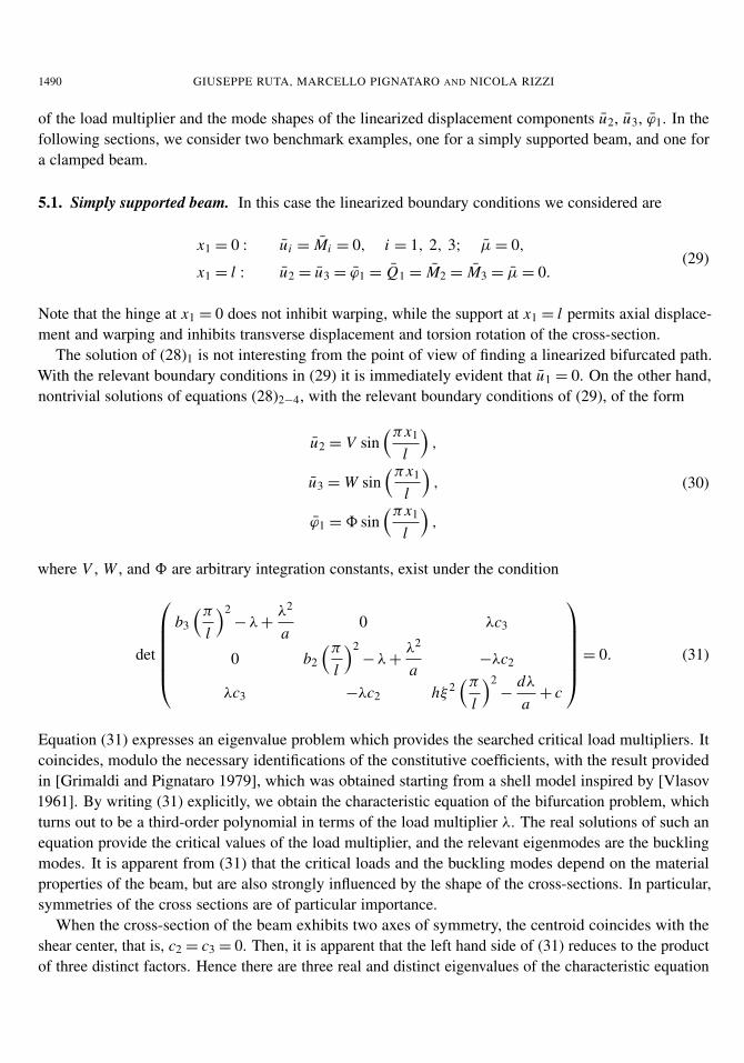
of the load multiplier and the mode shapes of the linearized displacement components u2, u3, ϕ1. In thefollowing sections, we consider two benchmark examples, one for a simply supported beam, and one fora clamped beam.

5.1. Simply supported beam. In this case the linearized boundary conditions we considered are

x1 = 0 : ui = Mi = 0, i = 1, 2, 3; µ = 0,

x1 = l : u2 = u3 = ϕ1 = Q1 = M2 = M3 = µ = 0.(29)

Note that the hinge at x1 = 0 does not inhibit warping, while the support at x1 = l permits axial displace-ment and warping and inhibits transverse displacement and torsion rotation of the cross-section.

The solution of (28)1 is not interesting from the point of view of finding a linearized bifurcated path.With the relevant boundary conditions in (29) it is immediately evident that u1 = 0. On the other hand,nontrivial solutions of equations (28)2−4, with the relevant boundary conditions of (29), of the form

u2 = V sin(πx1

l

),

u3 = W sin(πx1

l

),

ϕ1 = 8 sin(πx1

l

),

(30)

where V , W , and 8 are arbitrary integration constants, exist under the condition

det

b3

(π

l

)2− λ +

λ2

a0 λc3

0 b2

(π

l

)2− λ +

λ2

a−λc2

λc3 −λc2 hξ 2(π

l

)2−

dλ

a+ c

= 0. (31)

Equation (31) expresses an eigenvalue problem which provides the searched critical load multipliers. Itcoincides, modulo the necessary identifications of the constitutive coefficients, with the result providedin [Grimaldi and Pignataro 1979], which was obtained starting from a shell model inspired by [Vlasov1961]. By writing (31) explicitly, we obtain the characteristic equation of the bifurcation problem, whichturns out to be a third-order polynomial in terms of the load multiplier λ. The real solutions of such anequation provide the critical values of the load multiplier, and the relevant eigenmodes are the bucklingmodes. It is apparent from (31) that the critical loads and the buckling modes depend on the materialproperties of the beam, but are also strongly influenced by the shape of the cross-sections. In particular,symmetries of the cross sections are of particular importance.

When the cross-section of the beam exhibits two axes of symmetry, the centroid coincides with theshear center, that is, c2 = c3 = 0. Then, it is apparent that the left hand side of (31) reduces to the productof three distinct factors. Hence there are three real and distinct eigenvalues of the characteristic equation

A DIRECT ONE-DIMENSIONAL BEAM MODEL FOR FLEXURAL-TORSIONAL BUCKLING 1491

λc1 =acd

(1 +

hξ 2π2

cl2

),

λc2 =a2

(1 −

√1 −

4b3π2

al2

),

λc3 =a2

(1 −

√1 −

4b2π2

al2

).

(32)

The three pertaining buckling modes (two purely flexional, one purely torsional) occur separately. Theseresults coincide with those in [Grimaldi and Pignataro 1979] and also those in [Timoshenko and Gere1961; Pignataro and Ruta 2003]. When a → ∞, the two flexional critical loads in (32) reduce to thestandard Euler flexional buckling loads, and no torsional buckling appears. This result can be inferredfrom [Timoshenko and Gere 1961] as well. Indeed, in a nonextensible beam with the centroid coincidentwith the shear center, a compressive dead load cannot produce, even in a buckled shape, a torsion coupleinducing twist. Only flexional buckling modes are possible.

When the cross-section of the beam exhibits one axis of symmetry, for instance, x3, it necessarilyfollows that c2 = 0. Then, the left hand side of (31) is the product of two factors. One provides thesame flexional buckling load λc3 as in (32)3. However, the only real root of the other factor has areally complicated expression which is not reported here for the sake of simplicity. Instead we present asimplified expression, obtained from this complicated one by considering a nonextensible beam, that is,letting a → ∞, yielding

λc1 = λc2 =1

2c23

(√c + hξ 2 π2

l2

√c + hξ 2 π2

l2 + 4b3c23π2

l2 −

(c + hξ 2 π2

l2

)). (33)

Hence we deduce two very interesting results for beams with cross-sections exhibiting one axis of sym-metry. First, there are two only possible buckling modes. One is purely flexional and Euler-like, in theplane described by the axis of the beam and the axis of symmetry of the cross-section (in this case, u3).The other is a coupled flexural-torsional mode (in this case, a combination of u2 and ϕ1). Second, sincethe centroid does not coincide with the shear center, even for nonextensible beams, a torsional (or moreexactly, a flexural-torsional) buckling mode is present. This result clearly coincides with the original oneprovided in [Grimaldi and Pignataro 1979].

When the cross-section exhibits no symmetries, the presence of both coordinates of the shear centerin the characteristic equation (31), yields a single real-valued critical load, providing flexural-torsionalbuckling, and the three modes u2, u3, ϕ1 are coupled and occur together. That is, under the critical loadthe beam bends in both transverse directions and twists. The expression of the critical load, even in thecase of nonextensible beams, is cumbersome and is not reported here for the sake of simplicity. Thisresult also clearly coincides with that in [Grimaldi and Pignataro 1979].

5.2. Clamped beam. In this case the considered linearized boundary conditions are

x1 = 0 : ui = ϕi = 0, i = 1, 2, 3; ϕ′

1 = 0,

x1 = l : Qi = Mi = 0, i = 1, 2, 3; µ = 0. (34)

1492 GIUSEPPE RUTA, MARCELLO PIGNATARO AND NICOLA RIZZI

That is, all the displacements vanish and warping is prevented at the clamped end, while all the contactactions, as well as the bi-moment, are assumed to vanish at the free end. As in the case of the simplysupported beam, here as well the solution of (28)1 is of no interest for determining a linearized bucklingpath, and easily can be proved to be identically equal to zero.

On the other hand, nontrivial solutions of equations (28)2−4, with the relevant boundary conditions inequations (34), of the form

u2 = V[1 − cos

(πx1

2l

)],

u3 = W[1 − cos

(πx1

2l

)],

ϕ1 = 8[1 − cos

(πx1

2l

)],

(35)

where V , W , and 8 are arbitrary integration constants, exist under the condition

det

b3

( π

2l

)2− λ +

λ2

a0 λc3

0 b2

( π

2l

)2− λ +

λ2

a−λc2

λc3 −λc2 hξ 2( π

2l

)2−

dλ

a+ c

= 0. (36)

It is apparent that (36) provides a characteristic equation which has the same form as that provided by(31) for the simply supported beam. The only difference between the two characteristic equations isin the coefficient (2l)2 instead of l2 in the terms multiplying b2, b3 and hξ 2. Hence, apart from thisnumerical difference, it is obvious that all the results obtained for the simply supported beam are thesame of those for the clamped beam. It follows that our analysis and remarks for the simply supportedbeam can be equally reproduced for the clamped beam. The obtained results are then qualitatively thesame as those in [Grimaldi and Pignataro 1979] and for symmetric cross-sections, coincide with thosein [Timoshenko and Gere 1961; Pignataro and Ruta 2003].

6. Post-buckling paths

A fundamental aspect of the study of bifurcation paths is the analysis of the post-buckling behavior ofthe structural element under consideration. That is, it is essential to understand whether the consideredelement has a stable or unstable post-buckling behavior. This also can tell us if the element is sensitiveto imperfection. Another interesting aspect is related to the possibility of interaction between bucklingmodes, which occurs when the geometrical and mechanical characteristics are such that two or morebuckling modes occur under the same critical load.

A DIRECT ONE-DIMENSIONAL BEAM MODEL FOR FLEXURAL-TORSIONAL BUCKLING 1493

To study all these aspects, we must analyze the field equations at the second order of the formal powerseries expansion in terms of σ in a neighborhood of the bifurcation point. These turn out to be

D11 ¯u1 = − 2(

a(u′

2u′′

2 + u′

3u′′

3) + dϕ′

1ϕ′′

1 +a

a−λc

(u′′

2(λcc3ϕ′

1 − b3u′′′

2 ) − u′′

3(λcc2ϕ′

1 + b2u′′′

3 )))

,

D22 ¯u2 + D24 ¯ϕ1 = 2b2(u′′

2ϕ′

1)′′

+ 2 f2(ϕ′

1ϕ′′

1)′

+ 2λcc2(u′

2u′′

3)′

+ 2λcc3(ϕ′

1)2

+2λc(1 −

λca

)u′′

2ϕ1 + 2(c −

dλca

− b3)(

u′′

2ϕ′

1)′

−2b3u′′′

2 ϕ′

1 − 2hξ 2(u′′

2ϕ′′′

1 )′ +2ac3a−λ

(λc

(c3(u′′

2ϕ′

1)′− c2(u′′

3ϕ′

1)′)− b2(u′′

3u′′′

3 )′ − b3(u′′

2u′′′

2 )′)

−2λ

((1 −

λca

)u′′

3 +1

a−λc

(ac2ϕ

′′

1 + b2u′′′′

3))

,

D32 ¯u3 + D34 ¯ϕ1 = −2b3(u′′

3ϕ′

1)′′

+ 2 f3(ϕ′

1ϕ′′

1)′

− 2λcc3(u′

2u′′

3)′

+2λcc2(ϕ′

1)2

+ 2b3u′′′

2 ϕ′

1 + 2hξ 2(u′′

3ϕ′′′

1)′

−2λc

(1 −

λca

)u′′

3ϕ1 − 2(

c −dλca

− b2

)(u′′

3ϕ′

1)′

+2ac2a−λ

(λc

(c3(u′′

2ϕ′

1)′− c2(u′′

3ϕ′

1)′)− b2(u′′

3u′′′

3 )′ − b3(u′′

2u′′′

2 )′)

−2λ

((1 −

λca

)u′′

2 −1

a−λc

(ac3ϕ

′′

1 + b3u′′′′

2))

,

D42 ¯u2 + D43 ¯u3 + D44 ¯ϕ1 = 2hξ 2(u′

2u′′

3)′′′

+ 2(b2 − b3)u′′

2u′

3

+2(dλc

a− c

)(u′

2u′′

3)′+ 2λc(c3u3ϕ1 + c2u′′

2ϕ1)

+2(ϕ′

1(

f3u′′

2 − f2u′′

3))′

+ 2λ(

c3u′′

2 − c2u′′

3 −da

ϕ′′

1

), (37)

where λc is one of the critical values of the load multiplier and the Di j are the components of the symboliclinear differential operator introduced in (28). That is, the field equations at the second order of the formalpower series expansion in terms of σ have the same formal structure of the equations at the first order. Thedifference is that first order equations are homogeneous while second order equations are not (see also[Budiansky 1974; Pignataro et al. 1991]). Hence, since λc is an eigenvalue, that is, the symbolic operatorDi j is singular, a condition of solvability of the system described by equations (37) must be introduced.This turns out to be given by the requirement that the right-hand side of (37) be orthogonal to any ofthe eigensolutions of the first order equations provided by (28). In this case, the dot product yielding anorthogonality condition is given by the integral over the length of the beam of the sum of the productsbetween each right hand side of (37) and the corresponding eigenmode. Such a condition, supplementedby a normalization condition on the buckling modes, will provide the expressions for determining λ, thatis, the slope of the post-buckling path. Roughly speaking, when λ = 0, the considered buckling mode issymmetric, otherwise it is imperfection-sensitive (see also [Budiansky 1974; Pignataro et al. 1991]).

In the following sections, we investigate the case of the simply supported beam considered before.Indeed, since the eigenmodes (35) are qualitatively the same as the eigenmodes (32), the qualitativebehaviour of the clamped beam is the same as this of the simply supported one. Since the equation

1494 GIUSEPPE RUTA, MARCELLO PIGNATARO AND NICOLA RIZZI

for the axial component of the displacement is immaterial for the study of buckling and hence also ofpost-buckling, we will leave it aside, and focus attention on eqs. (37)2,3,4.

We will limit ourselves to examine the case when the cross section exhibits two axes of symmetry, theeigenmodes are provided by equations (30) and the critical load multipliers are given by the equations of(32). Furthermore, in that case we have c2 = c3 = 0 and f2 = f3 = 0. As a consequence, the right-handside of (37) assumes a much simpler form (which is not reported here for the sake of brevity).

For post-buckling behavior in bending, with no loss of generality, let us suppose that the bucklingmode which has taken place is u2 = V sin

(πx1

l

)(see (30)). Once we denote the right-hand side of (37)2

by r2(x1), when u1 = u3 = ϕ1 = 0, the solvability condition yields∫ l

0r2(x1)u2(x1) = 0 ⇒ λ = 0.

That is, the post-buckling path is symmetric, a well known result of Euler-like buckling for symmetricbeams.

For post-buckling behavior in torsion, the eigenmode is ϕ1 = 8 sin(

πx1l

)(see (30)). Once we denote

the right hand side of (37)4 by r4(x1), when u1 = u2 = u3 = 0, the solvability condition yields∫ l

0r4(x1)ϕ1(x1) = 0 ⇒ λ = 0.

Therefore, the post-buckling path in torsion is also symmetric, which is also a well known feature ofsymmetric beams.

7. Conclusions

In this paper we presented a direct, one-dimensional beam model suitable for describing the flexural-torsional buckling of thin-walled beams. The kinematic description makes use of two different beamaxes: the centroids, and the shear centers (we left aside the definition of the latter). Using this, wecan imagine the contact forces applied at different places of the planes of the (unwarped) cross sectionsand the contact torques evaluated with respect to different places of the planes of the (unwarped) crosssections. The constitutive relations are nonlinear and hyperelastic. Two inner constraints are assumed tohold, that is, the (unwarped) cross sections remain orthogonal to the centroidal axis, and the descriptorof the warping is proportional to the twist. This makes it possible to use a static perturbation techniqueto look for bifurcations. Moreover, it is possible to provide a rough description of the quality of thepost-buckling behavior and of the interaction of multiple buckling modes. The qualitative description ofthe phenomena coincides with that obtained with other beam models, yet with all the advantages of adirect model. Further developments of this study will be related to the qualitative analysis of frames.

References

[Anderson and Trahair 1972] J. M. Anderson and N. S. Trahair, “Stability of monosymmetric beams and cantilevers”, J. Struct.Div. ASCE 98 (1972), 269–286.

[Andreaus and Ruta 1998] U. A. Andreaus and G. Ruta, “A review of the problem of the shear centre(s)”, Continuum Mech.Therm. 10:6 (1998), 369–380.

A DIRECT ONE-DIMENSIONAL BEAM MODEL FOR FLEXURAL-TORSIONAL BUCKLING 1495

[Budiansky 1974] B. Budiansky, “Theory of buckling and postbuckling behavior of elastic structures”, pp. 1–65 in Advancesin applied mechanics, vol. 14, edited by C. S. Yih, Academic Press, New York, 1974.

[Casciaro et al. 1991] R. Casciaro, G. Salerno, and A. D. Lanzo, “Finite element asymptotic analysis of slender elastic struc-tures: a simple approach”, Int. J. Numer. Methods Eng. 35:7 (1991), 1397–1426.

[Di Carlo 1996] A. Di Carlo, “A non-standard format for continuum mechanics”, pp. 263–268 in Contemporary research inthe mechanics and mathematics of materials, edited by R. C. Batra and M. F. Beatty, CIMNE, Barcelona, 1996.

[Di Carlo and Tatone 1980] A. Di Carlo and A. Tatone, Analisi numerica della biforcazione dell’equilibrio di travi elastiche in3D, vol. 35, Istituto di Scienza delle Costruzioni, Università di L’Aquila, 1980.

[Di Egidio et al. 2003] A. Di Egidio, A. Luongo, and F. Vestroni, “A non-linear model for the dynamics of open cross-sectionthin-walled beams, I: Formulation”, Int. J. Solids Struct. 38 (2003), 1067–1081.

[Epstein 1979] M. Epstein, “Thin-walled beams as directed curves”, Acta Mech. 33:3 (1979), 229–242.

[Germain 1973a] P. Germain, “La méthode des puissance virtuelles en mécanique des milieux continus, 1ère partie: la théoriedu second gradient”, J. Mécanique 12 (1973), 235–274.

[Germain 1973b] P. Germain, “The method of virtual power in continuum mechanics, II: Microstructure”, SIAM J. Appl. Math.25:3 (1973), 556–575.

[Grimaldi and Pignataro 1979] A. Grimaldi and M. Pignataro, “Postbuckling behavior of thin-walled open cross-section com-pression members”, J. Struct. Mech. 7:2 (1979), 143–159.

[Kappus 1937] R. Kappus, “Drillknicken zentrich gedrückter Stäbe mit offenem profil im elastischen Bereich”, Luftfahrt-forschung 851 (1937), 444–57. Translated in NACA TM 851 (1938).

[Koiter 1945] W. T. Koiter, Over de stabiliteit van het elastisch evenwicht, Thesis, Delft, 1945. translated in NASA TT F-10 vol.833 (1967) and AFFDL Report TR 70-25 (1970).

[Lanzo and Garcea 1996] A. D. Lanzo and G. Garcea, “Koiter’s analysis of thin-walled structures by a finite element approach”,Int. J. Numer. Methods Eng. 39:17 (1996), 3007–3031.

[Møllmann 1986] H. Møllmann, “Theory of thin-walled beams with finite displacements”, pp. 195–209 in EUROMECH Col-loquium 197, edited by W. e. Pietraszkiewicz, Springer-Verlag, New York, 1986.

[Pignataro and Ruta 2003] M. Pignataro and G. C. Ruta, “Coupled instabilities in thin-walled beams: a qualitative approach”,Eur. J. Mech. A Solids 22:1 (2003), 139–149.

[Pignataro et al. 1991] M. Pignataro, N. L. Rizzi, and A. Luongo, Stability, bifurcation and postcritical behaviour of elasticstructures, Elsevier, Amsterdam, 1991.

[Pignataro et al. 2004] M. Pignataro, N. L. Rizzi, and G. C. Ruta, “Buckling and post-buckling in a two-bar frame: a qualitativeapproach”, pp. 337–346 in 4th International Conference on Coupled Instabilities in Metal Structures—CIMS 2004, edited byV. Gioncu et al., ESA, Rome, 2004.

[Reissner 1983] E. Reissner, “On a simple variational analysis of small finite deformations of prismatical beams”, Z. Angew.Math. Phys. 34:5 (1983), 642–648.

[Rizzi and Tatone 1996] N. Rizzi and A. Tatone, “Nonstandard models for thin-walled beams with a view to applications”, J.Appl. Mech. (Trans. ASME) 63 (1996), 399–403.

[Ruta 1998] G. Ruta, “On the flexure of a Saint-Venant cylinder”, J. Elasticity 52:2 (1998), 99–110.

[Simo and Vu-Quoc 1991] J. C. Simo and L. Vu-Quoc, “A geometrically exact rod model incorporating shear and torsion-warping deformation”, Int. J. Solids Struct. 27:3 (1991), 371–393.

[Tatone and Rizzi 1991] A. Tatone and N. Rizzi, “A one-dimensional model for thin-walled beams”, pp. 312–320 in Trends inapplications of mathematics to mechanics, edited by W. ed. Schneider et al., Longman, Avon, 1991.

[Timoshenko and Gere 1961] S. P. Timoshenko and J. M. Gere, Theory of elastic stability, McGraw-Hill, New York, 1961.

[Truesdell and Noll 1965] C. Truesdell and W. Noll, The non-linear field theories of mechanics, vol. 3, Handbuch der Physik,Springer-Verlag, New York, 1965.

[Vlasov 1961] V. Z. Vlasov, Thin-walled elastic beams, Monson, Jerusalem, 1961.

1496 GIUSEPPE RUTA, MARCELLO PIGNATARO AND NICOLA RIZZI

[Wagner 1929] H. Wagner, “Verdrehung und knickung von offenen profilen (Torsion and buckling of open sections)”, in 25thAnniversary Publication, Technische Hochschule, Danzig, 1929. Translated in NACA TM 807 (1936).

Received 13 Jan 2006.

GIUSEPPE RUTA: giuseppe.ruta@uniroma1.itDipartimento di Ingegneria Strutturale e Geotecnica, Università “La Sapienza”, via Eudossiana 18, 00184 Rome,Italyhttp://w3.disg.uniroma1.it/GiusseppeRuta

MARCELLO PIGNATARO: marcello.pignataro@uniroma1.itDipartimento di Ingegneria Strutturale e Geotecnica, Università “La Sapienza”, via Eudossiana 18, 00184 Rome,Italy

NICOLA RIZZI: nlr@uniroma3.itDipartimento di Strutture, Università Roma Tre, via Vito Volterra 62, 00146 Rome, Italy