Flexural performance and cost efficiency of carbon/basalt ...
Upload
khangminh22Category
view
1download
0
FLEXURAL BEHAVIOUR OF FERROCEMENT
by
Abdul Salam A. Alwash, B.Sc. M.Sc.
Thesis submitted
to the
University of Sheffield
for the
degree of Doctor of Philosophy
in the
Faculty of Engineering
Department of Civil and Structural Engineering
February, 1982.

SUMMARY
Ferrocement is often believed to be a form of reinforced concrete.
However, in spite of the similarities between the two materials there are
still major differences, indicating that ferrocement requires a separate
study to establish its structural performances. On the other hand, although
a large amount of research has been carried out on ferrocement, its flexural
behaviour is still not fully understood.
The aim of this investigation is to study the structural behaviour of
ferrocement plates under flexural loading and the influence of the different
variables on the strength and deformation characteristics. The variables
studied were the mesh number, strength, opening and distribution, presence of
steel bars, and the thickness of the section and the mortar cover.
The experimental programme included 49 plates, 1000x300 mm in dimensions,
reinforced with woven type steel wire mesh and tested under two lines load.
Deformation measurements were taken from first application of the load up till
failure and about10000 crack measurements (crack width and spacing) were
recorded.
The crack width data were dealt with statistically. The effect of the
variables on the crack width was studied, quantitatively, by comparing the
rate of growth of crack width of the plates. It was found that ferrocement
cracking behaviour is characterized by almost a full development of the cracks
at relatively early stages of the load (about 30-50% of the ultimate load)
and the crack width is smaller and more uniformly distributed than in reinforced
concrete. The mesh number and yield strength influenced significantly the
crack width and spacing. There was a limit for the mesh number after which
the enhancement in the cracking performance of the plates slowed down
noticeably. Crack width prediction equations were derived from these tests

showed good correlation, whereas the published crack width formulae largely
overestimated or underestimated the measured crack width.
The strength and deformation were influenced mainly by the yield strength
and fraction volume of reinforcement in the loading direction. The deflection
is most likely to exceed the serviceability criteria before the crack width.
For a span-deflection ratio of 180, the mean crack width was mostly below 20
microns, and the load was about 15-30% of the ultimate load.
A procedure is proposed to analyse ferrocement sections under flexural
loading. While application of reinforced concrete theory to predict the
ultimate moment largely underestimated the experimental results, the proposed
procedure predicted closely the experimental moment and deflection at first
cracking, yielding and failure of the tested plates.
ACKNOWLEDGEMENTS
The author wishes to express his appreciation and gratitude
to Dr. R.N. Swamy for his supervision, invaluable advice and
encouragement. He also conveys his thanks to Professor T.H. Hanna
and Professor D. Bond for their concern and for providing the
facilities for this research to be carried out.
The author appreciates his family's help, patience and
encouragement during the course of the work.
The author wishes to acknowledge the assistance of the technical
and secretarial staff of the department of Civil and Structural
Engineering, in particular Mr. R.N. Newman, Mr. G. Wallace,
Mrs. D. Hutson and Miss W. Atkinson. He also wishes to thank
Mrs. J. Czerny, for her patience in typing the thesis.
CONTENTS
PageNo.
Summary.
Acknowledgements.
Contents. iv.
List of Figures. viii.
List of Tables. xi.
List of Plates. xiii.
Notation. xiv.
CHAPTER 1. INTRODUCTION AND BACKGROUND. 1.
1.1 Introduction. 1.
1.2 Aim of the Investigation. 2.
1.3 Layout of the Thesis. 3.
1.4 Review of Literature. 4.
1.4.1 Historical Background. 4.
1.4.2 Definition of Ferrocement. 5.
1.4.3 Ferrocement Constituents. 7.
1.4.3.1 Matrix. 7.
1.4.3.2 Reinforcement. 9.
1.4.4 Mechanical Properties. 11.
1.4.4.1 General. 11.
1.4.4.2 Behaviour Under Tension. 12.
1.4.4.3 Behaviour Under Compression. 18.
1.4.4.4 Behaviour Under Flexure. 19.
1.4.4.5 Behaviour Under Shear and Torsion. 24.
1.4.4.6 Behaviour Under Fatigue and Impact.
1.4.5 Theoretical Models. 27.
1.4.6 Practical Applications. 28.
CHAPTER 2. PROPERTIES OF MATERIALS AND MIX DESIGN. 30.
2.1 Introduction. 30.
2.2 Properties of Reinforcement. 30.
2.2.1 Steel Bars. 31.
2.2.2 Wire Mesh. 31.
2.3 Properties of Mortar Matrix. 35.
2.3.1 Cement. 35.
2.3.2 Fly Ash. 38.
2.3.3 Sand. 38.
2.4 Mix Design. 39.
2.4.1 Experimental Programme. 39.
2.4.2 Discussion of Results. 40.
2.5 Properties of Hardened Mortar. 43.
2.5.1 Compressive Strength. 43.
2.5.2 Flexural Strength.. 43.
2.5.3 Static Modulus of Elasticity. 44.

PageNo.
CHAPTER 3. EXPERIMENTAL PROGRAMME. 45.
3.1 Introduction. 45.
3.2 Variables Studied. 45.
3.3 Type of Test, Size of Test Specimen and ControlSpecimens. 46.
3.4 Details of Experimental Programme. 46.
3.5 Specimen Manufacture. 49.
3.5.1 Casting Mould. 53.
3.5.2 Reinforcement and Preparation for Casting. 55.
3.5.3 Mixing, Casting and Curing. 57.
3.6 Test Equipment. 59.
3.6.1 Testing Rig. 59.
3.6.2 Crack Width Measuring Device. 62.
3.7 Test Measurements and Instrumentation. 62.
3.8 Testing Procedure. 67.
CHAPTER 4. CRACKING BEHAVIOUR. 68.
4.1 Introduction. 68.
4.2 Review of Literature. 69.
4.3 Scope and Experimental Programme. 76.
4.4 Treatment of the Results. 77.
4.5 The Relationship between the Maximum and theAverage Crack Width. 91.
4.6 Cracking Behaviour of Ferrocement. 95.
4.6.1 First Cracking. 95.
4.6.2 Behaviour from First Cracking Till Failure. 97.
4.6.3 Crack Spacing After Failure. 103.
4.6.4 Cracking Mechanism. 114.
4.7 Effect of Variables on the Crack Width. 116.
4.7.1 Effect of Properties of the Reinforcement. 116.
4.7.1.1 Steel Content.
4.7.1.2 Steel Yield Strength. 119.
4.7.1.3 Presence of Reinforcing Bars and Mesh Distribution. 122.
4.7.2 Effect of Mortar Cover. 125.
4.7.3 Effect of the Depth of the Section. 127.
4.8 Crack Width Prediction Equations. 128.
4.9 Comparison of Data with Other Investigators'Equations to Estimate the Crack Width. 132.
4.10 Comparisons of the Derived Equations with OtherInvestigators' Results. 137.
4.11 Conclusions. 140.

PageNo.
CHAPTER 5. LOAD AND DEFORMATION CHARACTERISTICS. 142.
5.1 Introduction. 142.
5.2 Review of Literature. 143.
5.3 Experimental Programme and Test Measurements. 145.
5.4 Behaviour of the Plates Under Loading. 146.
5.5 Load-Deflection Relationship. 147.
5.6 Load-Strain Relationship. 159.
5.7 Relationship between Cracking, Deflection andStrain. 168.
5.8 Effect of Variables on the Load and DeformationCharacteristics. 170.
5.8.1 At First Cracking. 171.
5.8.2 At First Yielding. 177.
5.8.3 At Failure. 189.
5.8.3.1 Ultimate Load. 195.
5.8.3.2 Deflection at Failure. 197.
5.8.3.3 Compressive Strain at Failure. 197.
5.9 Conclusions. 200.
CHAPTER 6. ANALYSIS OF FERROCEMENT IN FLEXURE. 203.
6.1 Introduction. 203.
6.2 Review of Literature. 203.
6.3 Description of the Method of Analysis. 207.
6.3.1 Elastic Stage. 208.
6.3.2 Cracked Stage. 208.
6.3.3 At failure. 214.
6.3.4 Sections with Bar Reinforcement. 217.
6.4 Comparison of Calculated and Experimental MomentCapacity of the Tested Plates. 218.
6.4.1 Cracking Moment. 219.
6.4.2 Moment Capacity at First Yielding. 222.
6.4.3 Ultimate Moment. 226.
6.5 Curvatures and Deflections. 228.
6.6 Prediction of Ultimate moment Using OtherInvestigators' Methods. 234.
6.7 Prediction of Ultimate Moment of OtherInvestigators' Specimens Using the Presented
Method. 235.
6.8 Conclusions. 237.
PageNo.
CHAPTER 7. LIMITATION OF THE WORK, CONCLUSIONS ANDSUGGESTIONS FOR FUTURE WORK. 239.
7.1 Limitation of the Present Work. 239.
7.2 Conclusions. 240.
7.3 Recommendation for Future Work. 243.
References. 244.
APPENDIX A. Typical Calculation of Cracking Moment. 249.
APPENDIX B. Typical Calculation of Moment at FirstYielding. 251.
APPENDIX C. Typical Calculation of Ultimate Moment. 254.

PageNo.
LIST OF FIGURES
TitleFigure No.
102.
1.1 Stress-strain curve for ferrocement under axial tension. 14.
1.2 Stress at first crack vs. specific surface ofreinforcement. 14.
2.1 Details of mesh tensile specimen. 33.
2.2 Stress-strain relationships of the steel bars andmild steel mesh. 37.
2.3 Stress-strain relationship of high tensile steel mesh. 37.
2.4 Relationship between cube compressive strength and ageof mortar. 44.
3.1 Casting mould. 56.
3.2 Schematic diagram for the testing rig. 60.
3.3 Position of strain, deflection and crack width measurement. 65.
4.1 to 4.6 Mean crack width against average tensile strain onthe face of the specimen series 51 to S6. 86.to 88.
4.7 Results of the two methods of analysis of the crackwidth data of specimen S1 C3. 90.
4.8 Standard deviation slope vs. mean crack width slope. 93.
4.9 Load at first crack vs. specific surface of reinforcement. 96.
4.10
Crack width and spacing against percentage of theultimate load for specimens from series Sl. 98.
4.11
Crack width and spacing against percentage of theultimate load for specimens from series S2. 99.
4.12,A,B,C,D. Crack width distribution for specimens reinforced with 100.tosix mesh from series Si and S2. 101.
4.13
Crack width distribution in reinforced concrete oneway slab.
4.14
Crack spacing after failure vs. specific surface.
4.15 Effect of mortar cover and specimen thickness on thecrack spacing after failure.
4.16 Effect of mesh opening on the crack spacing afterfailure.
4.17 Stress distribution in the cracked portion in aferrocement member.

PageNo.
117.
Figure No. Title
4.18
Rate of growth of crack width vs. specific surfaceof reinforcement.
4.19
Rate of growth of crack width vs. fraction volume ofreinforcement. 117.
4.20
Trend of the curves expressing the relationship betweenWm
/Et and S
R for different mesh yield strength. 121.
4.21
Rate of growth of crack width vs. fraction volume ofreinforcement, series S4 and S7. 124.
4.22 Rate of growth of crack width vs. mortar cover. 126.
4.23 Rate of growth of crack width vs. section depth. 126.
4.24 Comparison of predicted and experimental values of meancrack width, SI D2. 135.
4.25 Comparison of predicted and experimental values of meancrack width, S2 D2. 136.
4.26 Comparison of experimental crack width data fromBalaguru et al. and predicted using derived equations,
6.35 mm woven mesh. 139.
4.27 Comparison of experimental crack width data fromBalaguru et al. and predicted using the derived
equations,12.5 mm welded mesh. 139.
5.1 to 5.8
Load-deflection curves, series S1 to S6. 149.to 156.
5.9 Slope of the load-deflection curve at the secondlinear stage against the fraction volume of
reinforcement. 158.
5.10 to 5.13 Load-tensile strain curves, series S1 to S6. 160.to 163.
5.14 to 5.17 Load-compressive strain curves, series Si to S6. 164.to 167.
5.18 Total load at yielding vs. fraction volume ofreinforcement in loading direction. 184.
5.19A and B. Tensile strain at first yielding vs. fraction volumeof reinforcement in loading direction. 186.
5.20 Tensile strain on the face of the specimen vs. fractionvolume of reinforcement in loading direction, S3, S4,
S5, and S6. 188.
5.21 Total ultimate load vs. fraction volume of reinforcementin loading direction, series Sl, S2, S3 and S4. 196.
5.22 Central deflection at ultimate load vs. fraction volumeof reinforcement. 198.

Figure No.
5.23
6.1
6.2
6.3
6.4
6.5
6.6
6.7
6.8
PageNo.
Title
Ultimate compressive strain vs fraction volume ofreinforcement, section thickness and mortar cover.
Different compressive stress blocks.
The ratio of experimental to calculated ultimatemoment vs. the volume of reinforcement (18).
Assumed stress—strain curves in tension andcompression from Paul and Pama (11).
Strain and stress diagrams of ferrocement inflexure.
Composite modulus of elasticity in tension,cracked stage, after Naaman (23).
Stresses carried by the reinforcement after firstyielding.
Strain and stress diagrams at failure of ferrocementin flexure.
Adjustment of the tensile stress diagram to accountfor large mortar cover.
199.
206.
206.
206.
209.
213.
213.
215.
225.
A.1 Strain and stress distribution at first cracking. 249.
B.1 Strain and stress distribution at first yielding. 251.
C.1 Strain and stress distribution at ultimate load. 254.

LIST OF TABLESPage
Table No. Title No.
1.1 Working phases, stresses and strains of ferrocementunder tensile loading. 13.
1.2 Properties of ferrocement under bending/tensile zone. 20.
2.1 Results of reinforcement tensile test. 36.
2.2 Chemical composition of fly ash. 38.
2.3 Sieve analysis results for the sand. 38.
2.4 Properties of trial mixes. 41.
3.1 Details of test programme. 47.
3.2 Details of series Sl, S2,and S3. 50.
3.3 Details of series S4 and S7. 51.
3.4 Details of series S5. 52.
3.5 Details of series S6. 52.
4.1 to Cracking characteristics of specimens of series S1 79. to
4.6 to series S6. 85.
4.7 Results of the linear regression on mean crack widthand average tensile strain. 89.
4.8 Values of Wmax/Wm
for the different series. 94.
4.9 Values of W /W for ferrocement and reinforced concrete. 95.max m
4.10 Reinforcement limits for ferrocement section. 118.
4.11 Predicted and measured mean crack width for specimensof series S3 and S4. 131.
4.12 Comparison of predicted and experimental mean crackwidth. 134.
4.13 Comparison of crack width data from Balaguru et al.and results using derived equations. 138.
5.1 Deflection, cracking and strain relationship. 169.
5.2 to Load and deformation characteristics at first crack, 173. to
5.5 series S1 to S7. 176.
5.6 to Load and deformation at first yielding, series S1 to S7 179. to5.9 182.
5.10 Load and deformation at failure. 191.
Table No.
6.1
6.2
PageNo.
Results of the control specimens and the measuredsection depth. 220.
Calculated and experimental values of crackingmoment. 221.
Title
6.3 Calculated and experimental moment at the assumed firstyielding points. 224.
6.4 Calculated and experimental ultimate moments. 227.
6.5 Calculated and experimental values of centraldeflection. 232.
6.6 Comparison of experimental and calculated ultimatemoment for series Si, using other investigators'methods. 236.
6.7 Comparison of ultimate moment predicted by the givenmethod with the experimental results fromBalaguru, et al. (31). 236.
LIST OF PLATES
TitlePlate No.PageNo.
2.1 Hounsfield Tensometer machine. 34.
2.2 Mesh tensile test. 34.
2.3 Steel plate tensile test to checkgrippings. 34.
3.1 Cut sections of specimens from series Si. 54.
3.2 Reinforcement packed in the mould readyfor casting. 58.
3.3 Casting arrangement. 58.
3.4 Testing rig. 61.
3.5
3.6
4.1 to 4.6
5.1
The microscope and the trolley mounted onthe rig. 63.
Instrumentation on the tensile face of thespecimen. 63.
Cracking intensity at failure of typical
106. tospecimens from series S1 to S6. 111.
Specimen failed by fracture of wire meshin tensile zone. 193.
5.2 Different types of section failure. 194.

NOTATION
AsCross-sectional area of mesh in loading direction.
A tCross-sectional area of steel bars in loading direction.
Width of the plate.
Compressive force in the section.
Mortar cover (clear)
Section depth.
EcModulus of elasticity of the composite.
EfModulus of elasticity of fibres (mesh).
EmModulus of elasticity of the matrix (mortar)
EtModulus of elasticity of the composite in tension.
Assumed modulus of elasticity of the composite during thelinear range of the cracked stage.
. cu Cube compressive strength.
Second moment of area.
Ratio of neutral axis depth from the extreme compressive fibreto the depth of the section.
Plate span.
Moment on a plate or plate resisting moment.
Moment at first cracking.cr
Moment at first yielding.
MuUltimate moment.
fl Modular ratio (E /E ).s m
Ratio of distances to neutral axis from extreme tensile fibreand from outermost mesh in tension.
r, r2Ratios M/14, M /M respectively.cr
Crack spacing.
Specific surface of reinforcement (ratio of reinforcementsurface area to the volume of the composite).
cr
SR

Specific surface of reinforcement in loading direction.RL
Total tensile force of the section.
Tst
Tensile force carried by the steel bars.
VRFraction volume of reinforcement (percentage of the volume
of reinforcement to the total volume of the composite).
3 Fraction volume of reinforcement in loading direction.RL
VmFraction volume of the matrix (mortar).
WmMean crack width.
W /E Rate of growth of crack width.m t
Ec
Composite compressive strain.
Composite yielding compressive strain.cy
cuComposite ultimate compressive strain.
Ef
Strain at a mesh level.
Et
Composite tensile strain.
Composite tensile strain which define the strain limit attcr
which the matrix cracks (equals plain mortar ultimate tensilestrain).
tyComposite yielding tensile strain.
tuComposite ultimate tensile strain.
Standard deviation.
CComposite compressive stress.
• ,a Composite yielding compressive stress and composite ultimatecy Cu
compressive strength, respectively, in flexure (a = a = 0.67 f ).cy cu cu
af Stress in a mesh.
fyMesh yield strength (at 0.005 strain).
amu
Mortar strength in tension.
tComposite tensile stress.
tCr Composite tensile stress at first cracking.

Composite first yielding tensile stress.Gty
a Extra tensile stress carried by the composite after firstt extra
yielding.
Composite ultimate tensile strength.
Ratio of distance of two line load from support to span length.
Deflectionand central deflection, respectively.
Curvature of composite section.
Curvature of composite section at first cracking, first yielding,4)cr2Py2)u( (i and failure, respectively.
atu
U)
C
(I)

CHAPTER 1.
INTRODUCTION AND BACKGROUND
1.1 Introduction.
Plain concrete has low tensile strength, limited ductility, and little
resistance to crack propagation. Flaws or microcracks exist in the material
even before any load is applied, because of its inherent microstructure and
volumetric changes during manufacturing. These flaws lead to a brittle failure
of the material in tension at about one tenth of its compression strength.
In reinforced concrete, although the failure of the composite is ductile
due to the ductile nature of reinforcement, the concrete suffers an extensive
amount of cracking. In the past, working stresses were relatively low.
Consequently, the cracks in the reinforced concrete members were small, and
therefore insignificant. However, the present trends towards more economical
designs, pressed for higher working stresses. This resulted in excessive crack
widths and deflections which impair the appearance of the structure, weakening
the members due to corrosion of steel, and damaging non—structural members.
Thus, the serviceability criteria become more critical than the strength
consideration. The concrete technologist is, therefore, faced with the problem
of improving the inherent weak properties of concrete in order to cater for the
designer's requirements. This, in turn, encouraged the search for new
materials to partially replace reinforced concrete.
It is under such circumstances that ferrocement, among other materials,
has emerged. The reinforcement of ferrocement consists of several layers of
relatively fine wire mesh packed together with or without steel bars in the
middle. Cement mortar is used to fill the gaps between the meshes and
provide the cover for the reinforcement.
The major use of ferrocement has been in the developing countries where
excellent properties of the material and successful field application with

relatively little theoretical basis, were observed. As ferrocement technology
developed, so did the interest of engineers who began to view this material as
a potentially significant material of construction.
The reinforcing mechanism in ferrocement not only improves many of the
'engineering properties of the brittle mortar, such as fracture, tensile and
flexural strength, ductility, and impact resistance,but also provides advantages
in terms of fabrication of products and components. For example, ferrocement
may require less formwork than reinforced concrete. The section thickness of
its members could be as little as 10 mm and due to the flexibility of the
reinforcing mesh it has a high adaptability to complicated shapes and thus,is
very attractive for precast units.
At the same time, the reinforcement in ferrocement is uniformly distributed
in the section and has a high surface area. This results in improved
mechanical properties compared to those of reinforced concrete. Within certain
loading limits, it behaves as a homogeneous elastic material and these limits
are wider than for normal concrete. In addition, because of the subdivision
and distribution of the reinforcement, ferrocement exhibits better crack arrest
mechanism and therefore enhances cracking behaviour.
After this, it is not surprising that ferrocement is receiving extensive
attention both in the field of applications and the study of its properties.
1.2 Aim of the Investigation.
The investigationwas carried out to study experimentally and analytically
the flexural behaviour of ferrocement plates. This included the cracking,
deformation, and strength and the influence of the important parameters on
them.
The parameters studied were the number of meshes, the tensile strength of
the mesh, presence of steel bars, mesh opening and distribution, thickness of
the section and the mortar cover.

The aims of the study, in particular, are:
1. To study the cracking behaviour of ferrocement from a large number of
crack width and spacing measurements, and repeating specimens of the same
variables twice or three times.
2. To establish, quantitatively, the influence of the different parameters
on the crack width and spacing.
3. To develop crack width prediction equation.
4. To investigate the deformation characteristics from first application of
load up till failure and to study the relationship between crack width and
deflection for the serviceability criteria.
5. To develop a method for predicting the strength of ferrocement plate.
6. To use fly ash, as a cheap material, to partially substitute the cement
in the relatively rich mix used in ferrocement and to enhance its cohesiveness
and workability.
1.3 Layout of the Thesis.
The thesis consists of seven chapters. Chapter 1 includes presentation
of the problem, and the background and development of ferrocement.
In Chapter 2, the properties of the materials used and the development of
an economical and suitable mortar mix is reported. The properties of the
hardened mix are also given.
In Chapter 3, the details of the experimental programme, manufacturing
technique, testing equipment, and testing procedure are discussed. The experi-
mental programme consisted of seven series comprising 49 specimens. Special
manufacturing technique was developed to ensure the required distribution of
reinforcement. Also, a special equipment was designed to load the test
specimens.
Chapter 4 is devoted to the study of the cracking behaviour. The
cracking performance of the different specimens ; in terms of the rate of growth

of crack width, is compared. The influence of the variables on the crack
width and spacings were studied and crack width prediction equations are
proposed.
In Chapter 5 the deformation characteristics of the specimens are reported.
The relationship between crack width and deflection was identified and the
behaviour of the plates from first application of load up till failure is
traced. The effect of the variables on the load-deflection and load strain
curves, ductility and stiffness is discussed.
Finally Chapter 6 is devoted to strength characteristics and analysis of
the plates. A method is proposed to analyse the ferrocement section and to
predict its moment capacity and deflection at any level of the load.
1.4 Review of Literature.
1.4.1 Historical Background.
Although other forms of ferrocement may have existed earlier, credit for
using it should go to Joseph Louis Lambot in France, who constructed a rowing
boat from a net of wires and thin bars, and filled with cement mortar. This
type of reinforcement was the one which was first used in reinforced concrete.
However, it never gained much popularity in spite of that early start, and
subsequent reinforced concrete design tended towards the use of heavier bars.
In the First World War, large scale use of ferrocement was in ship building,
using a combination of lightweight reinforced concrete and ferrocement.
In the early 1940's, P.L. Nervi in Italy "rediscovered" this technique.
His reason for it was:
"The fundamental idea behind the new reinforced concrete material
ferro-cemento is the well known and elementary fact that concrete can stand
large strains in the neighbourhood of the reinforcement and that the
magnitude of the strains depends on the distribution and subdivision of the
reinforcement through the mass of the concrete (1).

In addition to the use of ferrocement in boat building, Nervi demonstrated
successfully its use in roofs of buildings and warehouses.
In the 1960's ferrocement began to be used in many countries, not only in
boat building but also in civil engineering structures. Countries like the
Soviet Union, Czechoslovakia and some developing countries used ferrocement
successfully in precast roofs and low cost housing. Because of the universal
availability of the basic component materials of ferrocement and the low skill
needed for the construction of the structural forms, developing countries took
more interest in the material to be used as a general purpose structural
material. The report (2) of the National Academy of Sciences on the uses of
ferrocement in developing countries explored the potentials of ferrocement
and opened many fields of application.
In 1976 an International Ferrocement Information Centre (IFIC) was
established at the Asian Institute of Technology in Bankok, Thailand. The
Journal of Ferrocement which is published by the Centre indicated the amount
of attention drawn worldwide to ferrocement.
In early 1977, the American Concrete Institute (Ad) had set up Committee
549 on ferrocement to review the present state-of-the-art and possibly to
formulate a code of practice for this material. Later, in April, 1978, a
symposium on Ferrocement - Materials & Application was held at the Annual
Convention of the American Concrete Institute in Toronto, Canada, and resulted
in the publication SP-61 by the American Concrete Institute.
It is now clear that ferrocement, a versatile construction material, has
bright prospects and will definitely find better utilization in the near
future.
1.4.2 Definition of Ferrocement.
Although ferrocement has been in use since the 1940's, still, its
definition is not yet established. The reasons for this may be several.
Firstly, the material has been considered as a form of reinforced concrete and
therefore, there was no real need for its definition. Secondly, the lack of
investigation on the material which meant that its potentials and superior
properties are not known. Thirdly, the very many different types of rein-
forcement used in this material led to uncertainty of the established properties.
Until more data is established about the material, ferrocement will have no
exact definition. Ramouldi (3) stated "Among the more pressing problems
relating to the development of ferrocement is the question of its very
definition". In what follows, some of the available definitions of ferrocement
are reviewed.
Bigg (4) reported that ferrocement definition according to the American
Bureau of Shipping is "A thin, highly reinforced shell of concrete in which the
steel reinforcement is distributed widely throughout the concrete, so that the
material under stress, acts approximately as homogeneous material. The
strength properties of the material are to be determined by testing a
significant number of samples ...".
It has been argued that the words thin, highly reinforced, and homogeneous
may suggest different meanings to different people.
The Russians (5) definition, which was also adopted by Bigg (4),
emphasized on the subdivision of the reinforcement. The definition was:
"True Ferrocement is considered to be a mesh reinforced mortar with a
compressive strength of at least 39.3 N/mm2 and a specific surface K (ratio of
surface area of steel wire to the volume of the composite) between 2.0 cm2/cm
2
and 3.0 cm2/cm
3."
This definition seems to lack the description of the material itself.
Moreover, the restriction in the specific surface of reinforcement requires
more experimental verification.

Shah (6) defined ferrocement as a composite material which consists of
wire mesh as reinforcement and mortar as matrix. The basic characteristics
of this reinforcement is the higher bond due to small diameter wire mesh and
higher surface area.
The definition by ACI Committee 549 (7) was: "Ferrocement is a type of
thin wall reinforced concrete construction, where usually a hydraulic cement
is reinforced with layers of continuous and relatively small diameter mesh.
Mesh may be made of metallic materials or other suitable materials". In
this definition, ferrocement is not confined to only steel wire mesh but other
types of meshes as well. However, the definition ignores an important type of
reinforcement currently in use in ferrocement, i.e. the combination of steel
rods and wire mesh. In addition, it does not emphasize the properties of the
mesh reinforcement. These properties, as will be seen later, are important
factors in producing sections of superior properties to reinforced concrete.
It can be seen from the above discussion that research is needed before
reaching a truly representative definition for ferrocement.
1.4.3 Ferrocement constituents.
1.4.3.1 Matrix.
The matrix of ferrocement is usually cement mortar, consisting of cement,
sand, water and perhaps some additive. The matrix should have some or all
of the following requirements, depending on the use of the structure. High
compressive strength, impermeability, hardness, resistance to chemical attack,
low shrinkage, and workability.
Most of the available specifications concerning the properties of the
mortar used in ferrocement depend on observation and practical consideration
of the ferrocement uses, with some aid from the knowledge on concrete
technology. From a concrete technology point of view, the main factors which
affect the properties of the mortar are:

1. Water:cement ratio.
2. Sand:cement ratio.
3. Gradation, shape, maximum size, and purity of sand.
4. Quality, age, and type of cement.
5. Additives.
6. Curing condition.
7. Mixing, placing and compaction.
The limits of the above factors are affected by the requirements of the mortar
which in turn depend on the use of ferrocement. In marine structures more
restrictions are generally required (5,6) than in civil engineering structures.
In most applications, high strength and low shrinkage are required and
therefore low water:cement ratio, between 0.35 to 0.55 (7), should be used.
Workability should be high and therefore a suitable compromise should be
arrived at to increase the water content to take account of the decrease in
strength. Rich cement mortar is required to give compressive strength
between 35 to 50 N/mm2
. Additives have been used to reduce the water content.
Proper gradation (9) of sand could help provide workable mixes. On the other
hand gradation of ordinary sand, light weight sand, expanded shale, or
vermiculite have no effect on the tensile strength of ferrocement (10).
Portland cement type I, II, III and V are all suitable (11), and the
choice depends on the type of structure. The maximum size of sand depends
on the type of reinforcement. Generally passing sieve No. 8 (size 2.4 mm)
is adequate. Compaction and curing should be carefully controlled. All
other factors to give good quality mortar should be considered.
The national Academy of Science (2) reported some of the properties of
mortar required for the use of ferrocement in developing countries. Water:
cement ratio w/c = 0.4 and sand:cement ratio s/c = 2 were recommended.
Gradation is not important other than to produce better workability. Sand
should not have excess of fine particles. Silt and organic materials should
be removed.

1.4.3.2 Reinforcement.
Ferrocement reinforcement is characterized by high surface area as compared
to those used in reinforced concrete. It usually consists of layers of
continuous mesh. These generally result from the assembly of continuous
filaments. Different types of meshes are available almost in every country in
the world. The principal types of wire mesh currently being used are given
below:
1. Hexagonal wire mesh.
2. Welded wire mesh.
3. Woven wire mesh.
4. Expanded metal mesh.
5. Three dimensional mesh (i.e. Watson mesh).
1. Hexagonal or chicken wire mesh: This mesh is readily available in most
countries and it is known to be the cheapest and easiest to handle. The mesh
is fabricated from cold drawn wire which is generally woven into ftexagonal
patterns. Special patterns may include hexagonal mesh with longitudinal wires.
2. Welded wire mesh: In this mesh a grid pattern is formed by welding or
cementing the perpendicular intersecting wires at their intersection. Although
this mesh may have the advantage of easy moulding into the required shape, it
has the disadvantage of the possibility of weak spots at the intersection of
wires resulting from inadequate welding during the manufacture of the mesh (11).
3. Woven Wire mesh: In this mesh, the wires are interwoven to form the
required grid and the intersections are not welded. The wires in this type
of mesh are not straight. They are bent in the shape of zig—zag lines and
large angle of bending might cause cracks along the mesh (12). However,
the moulding performance of this mesh is as good as the hexagonal and the
welded wire mesh (11).

4. Expanded Metal Mesh: This mesh is formed by cutting a thin sheet of
expanded metal to produce diamond shape openings. This type of mesh is not
as popular as the previous three types and weight for weight comparison, it
is not as strong as woven mesh, but on cost to strength ratio, expanded metal
has the advantage (11).
5. Watson Mesh: A specially designed three dimensional space frame mesh.
It consists of straight high tensile wires and a transverse crimped wire which
holds the high tensile wire together. The high tensile wires are placed in
two parallel planes and are separated by mild steel wires transverse to the
high tensile wires. Most of the mesh wires are straight, without twists,
crimps or welds. The result is a very strong mesh, and completely flexible to
conform to any shape.
The above mentioned types of meshes are mainly metallic materials.
Vegetable fibre and glass fibre meshes are also available. At the same
time, there is a wide variation in the properties of each type of mesh.
This includes different mesh size,-strength, ductility, manufacture and
treatment. Research shows that the properties of the resulting ferrocement
product is affected by the properties of the mesh.
Steel rods have been used together with wire mesh in the reinforcement of
ferrocement. The rods could be used for making the frame—work of the structure
upon which layers of mesh are laid. Longitudinal and transverse rods usually
vary in diameter between 4 to 9 mm and they are mainly of mild steel. Steel
rods are sometimes used as main reinforcing component. Bezukladov et al. (5)
reported that the middle third of the mesh in ferrocement members can be
replaced by steel rods without affecting the structural performance of the
member.
Finally, steel fibres have been used (13,14) with wire mesh reinforcement
to enhance some of the properties of ferrocement.
1.4.4 Mechanical Properties.
1.4.4.1 General.
Ferrocement is often thought of as a variation of conventional reinforced
concrete. However, Nervi's (1) description of ferrocement in which he
identifies the material by the high subdivision and distribution of the rein-
forcement may be the basic difference between ferrocement and reinforced
concrete. No theoretical support was provided by Nervi, but later on, the
importance of the subdivision of reinforcement was confirmed by experimental
and theoretical studies (15,16) on closely spaced wire reinforcement. In
addition to the subdivision, the amount of the reinforcement was believed, from
the early experiments on ferrocement, to be very important. Oberti (1) found
that steel content of 120 to 240 kg.1m3 of mortar will not practically enhance
the elongation of the mortar. But increasing it to a range of 480 to 640
kg./m3 increased the elongation to 5 times that of the mortar.
Recently, the subdivision and amount of reinforcement have been described
using the terms specific surface which is defined as the ratio of the surface
area of reinforcement to the volume of the composite, and the fraction volume
which is defined as the percentage of the volume of the reinforcement to the
volume of the composite.
These two terms have been found (5,17,18) to give good correlation to
the load response of ferrocement. Bezukladov (5) found that ferrocement
superior behaviour compared to reinforced concrete can be achieved when the
specific surface of reinforcement exceeds 2.0 cm2/cm
3. However, in most
previous practical uses of ferrocement, the reinforcement had less specific
surface. This, in addition to the many available types of meshes may result
in a confusing picture about the properties of ferrocement.
1.4.4.2 Behaviour under Tension.
1. Elasticity and Stress-Strain Behaviour.
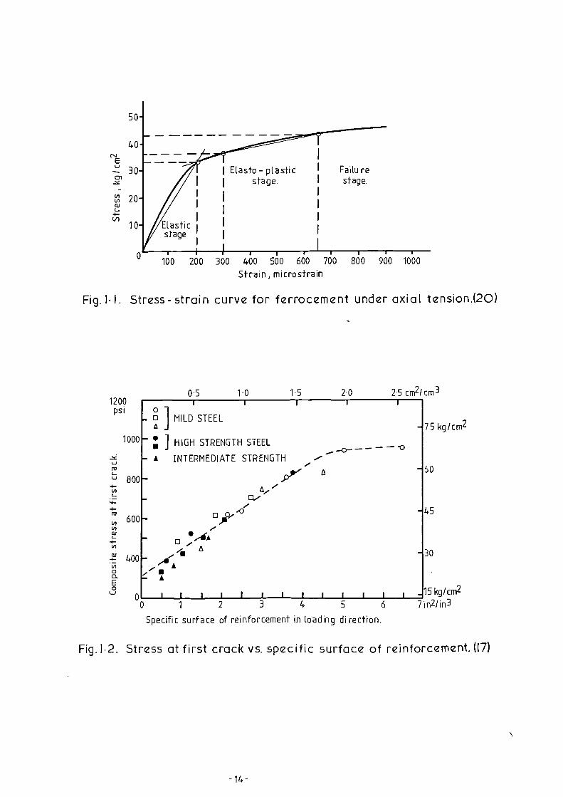
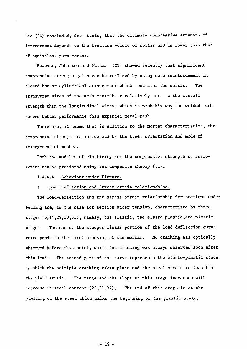
The stress-strain curve is characterized (5,17,19) by three stages, see
Fig.1.1, namely, the elastic stage, the cracked stage, and the yielding stage.
In the elastic stage, both reinforcement and mortar behave elastically and
there is no evidence of crack formation. This stage is followed by a
transitory stage or the quasi-elastic stage (19) which is between the elastic
and the cracked stages. In this stage the cracks propagate and multiply
producing a curvilinear stage, leading to the start of a second linear stage.
The range of quasi-elastic stage in ferrocement is longer than in reinforced
concrete (19). The term first crack, used by many investigators, usually lies
in this stage. In the cracked stage or elasto-plastic stage, the matrix
suffers some plastic strain and cracks increase in number rather than width.
However, the stress in reinforcement is still in the elastic limit. The
yielding stage is characterized by yielding of reinforcement which results in
increasing of the crack width, while the number of cracks has almost reached
its maximum.
A more detailed definition of these three stages, in connection with the
crack width and the tensile strain in the extreme fibre was given by
Walkus (19). Fig.1.1 and Table 1.1 give details of these stages and the
associated crack width and tensile strain values. These values require more
experimental verification, bearing in mind that they are assumed to be the
same for any ferrocement section. Such assumption may not be valid because
of the expected differences in performance of ferrocement sections, depending
on the characteristics of the reinforcement.
The modulus of elasticity, both in the elastic and elasto-plastic stages
has been predicted (17) using the following equations which are based on the
law of composite.

Table 1.1 Working Phases, Stresses and Strains of Ferrocementunder tensile loading (4).
No. ofphase
Strength
Phase
Techno-logicalPhase
Max.width
ofCracks
-3
Stress
KN/m2
UnitElongation
micro-strain
10mm
I Linearly tight - - -Elastic
Ia Quasi 20 3230 200
Elastic .
lb Non-Linearly
noncorrosive
50 3530 290
Elastic
II Elastic-plastic
' 100 4220 645
III Plastic corrosive >100 - -
50
40NJ
30
Li1 20QJ
4-Ul
10 Elasticstage
Failurestage.
Elasto — plasticstage.
05 1•0 1.5 20 25 cm2 / cm3
7 5 kg /cm2
60
45
30
11111 1 11 111 11
1
2
3
4
5
6
100 200 300 400 500 600 700 800 900 1000
Strain, microstrain
Fig. 1 . ). Stress- strain curve for ferrocement under axial tension.(20)
1200PSI
1000
800
600
400
— 0 MILD STEELa
- HIGH STRENGTH STEEL
- A INTERMEDIATE STRENGTH
a,.1:1./
°
--0
15 kg/cm2
7 in2/in3
Specific surface of reinforcement in loading di rection.
- -
Fig. 1 . 2. Stress at first crack vs. specific surface of reinforcement. ((7)

EC Em VM + E. . VRL (elastic stage)
EC RL (elasto—plastic)
(1.2)
where
Elastic modulus of the composite.
EM Modulus of elasticity of mortar.
Elastic modulus of mesh.
VRL
= Volume fraction of longitudinal reinforcement in loading
direction.
V Volume fraction of mortar.
These equations, which take into account only the longitudinal reinforce-
ment underestimate (17) the modulus of elasticity. A detailed analysis taking
into account the orientation of the oblique reinforcing elements seems more
appropriate for reinforcement like hexagonal mesh (11).
The characteristics of the stress—strain relationship are affected mainly
by the characteristics of reinforcement, while rich mortar has no significant
influence on it (5). Increasing the fraction volume of reinforcement (5,17)
increases the modulus of elasticity. Increasing the specific surface
increases (5) the stresses and elongation during crack formation. According
to Bezukladov et al. (5), ferrocement should have specific surface of rein—
forcement between 2 and 3 cm2/cm
3.
The stiffness of ferrocement is largely dependent on the geometry and
ductility of reinforcement and independent of its strength. Cold worked
reinforcement appears to give a stiffer composite than ductile mesh (21).
2. Cracking.
One of the best advantages of ferrocement is its cracking performance.
Higher number of cracks with spacing as little as 5 mm result in smaller
crack width and reflect the superior ferrocement performance compared to
reinforced concrete.

The cracking behaviour was found (5,10,17) to be affected mainly by the
properties of reinforcement including the reinforcement amount, type, ductility,
proof stress, and spacing of transverse wires of the mesh. The specific
surface, as a measure of the bond area, is an important factor. Increasing
it results in smaller crack width and smaller crack spacing after failure
(5,10,17,19,22,23). However,Nathan and Paramasivan (23) suggested that the
cracking behaviour is influenced by the total bond stress between steel and
mortar rather than just the bond area. This means that in addition to the
specific surface, the proof stress of the reinforcement has also an influence
on the cracking behaviour. In addition to the total bond stress, the
ductility of reinforcement and the spacing of the transverse wires of the mesh
affect the cracking behaviour. Increasing the ductility increases the crack
width (10) and higher transverse wires spacing result in less number of
cracks (24). Different types of meshes result in different cracking perform-
ances. For example, expanded metal mesh exhibits superior cracking performance
compared to that of welded mesh.
The cracking behaviour is characterized by two stages. In the first
stage, which follows after first cracking, the cracks increase in number with
increase of load until they reach the ultimate or saturation limit. The
second stage will begin then and is characterized by increase of the crack
width more rapidly.
Based on the above description of cracking behaviour, Naaman (24)
suggested equations to predict the crack width. The end of the above first
stage was called the crack stabilization and the steel stress at the crack
stabilization was calculated using the following equation:
fsta
= 20 SRL
60 KSi (1.3)
where
fsta
= The steel stress at crack stabilization, KSi .
3S = Specific surface of reinforcement,in
2 /in.
RL
The crack width prediction equations are as follows:-
. -1For S
RL g 3m
a) For any steel stress less than fsta
fsta. 1 - 20W
max S ERERRL
Where ER is the modulus of reinforcing system.
b) For steel stress larger than fsta
but less than yield strength
29000 wmax = [6.9 + (f
s - f
sta)]E
R x 10-4
(1.4)
(1.5)
For S > 3 in-1 and, for any stress less than the yield strength or about
RL
- 60 KSi
W = (15.5-3 S) 10-4 �. 0.0004 in.
max RL(1.6)
3. Strength.
The investigations tend to define two strength values in the life of
ferrocement specimen, namely, strength at first crack and strength at failure.
From the previous discussion about the stress-strain relationship in tension,
the first crack takes place in the transitory state which is a later stage
beyond the elastic range. Therefore, the strength in the elasto-plastic
stage has not been considered.
Bezakladov (5) found that the load at first crack increases with the
specific surface of reinforcement up to a total specific surface of
SR = 3.0 to 3.5 cm
2/cm
3 after which reduction in the load takes place.
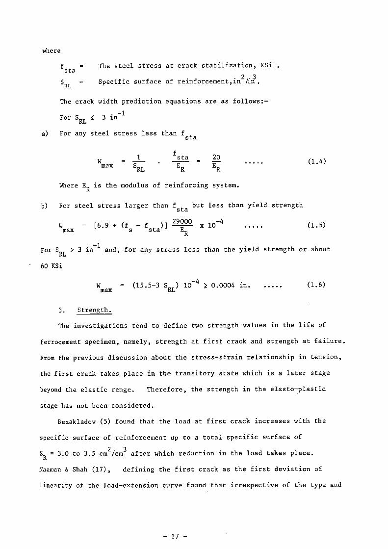
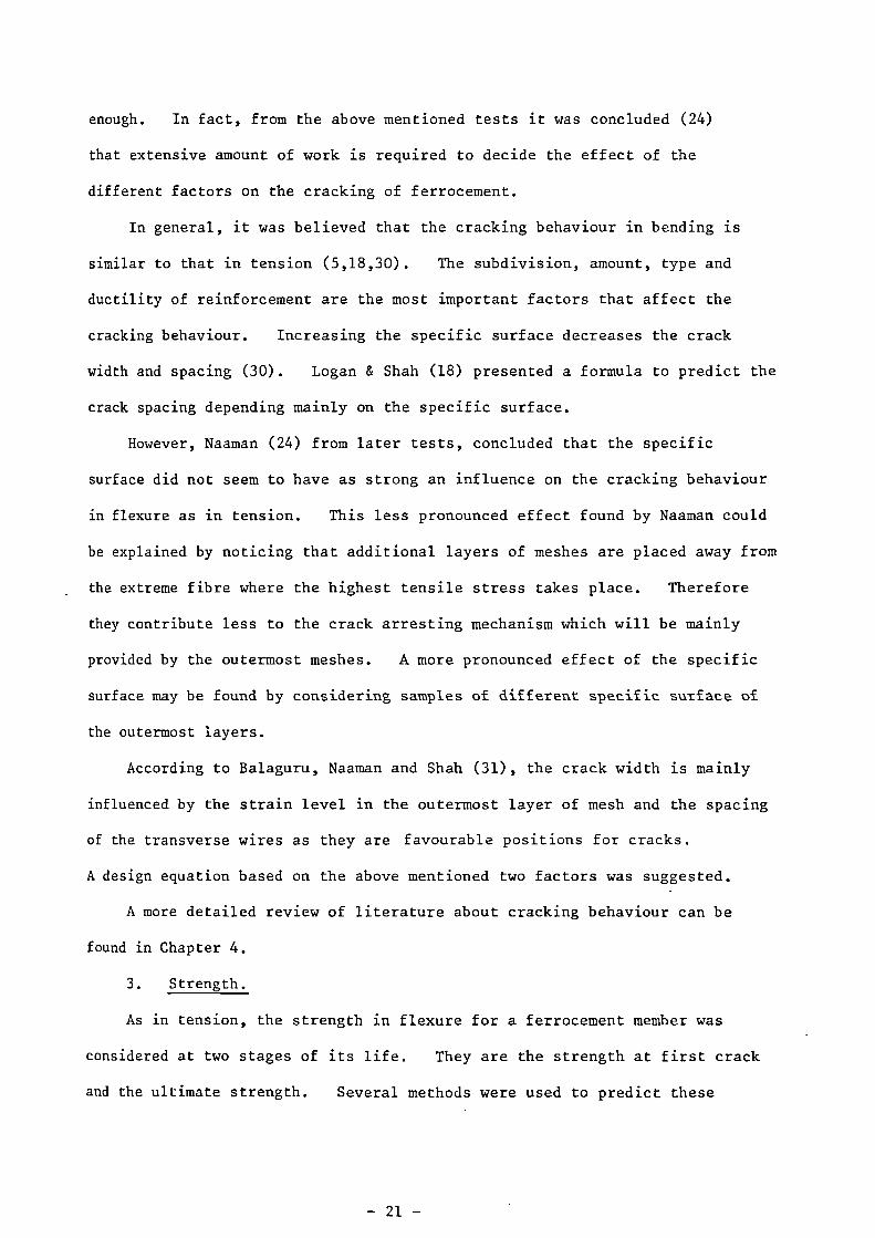
Naaman & Shah (17), defining the first crack as the first deviation of
linearity of the load-extension curve found that irrespective of the type and

size of the mesh the load at the first crack increases linearly with the
specific surface of reinforcement, see Fig.1.2. From the figure it can be
seen that the saturation limit of the specific surface takes place at SL
between 1.5 and 2.0 cm2/cm
3, which is about the same range as that from
Bezukladov. Increasing mortar strength was found (10) to have little effect
on the strength at first crack. Attempts were made (25) to predict the
strength at first crack based basically on the theory of reinforced concrete.
The ultimate strength is found to be dependent on the fraction volume of
reinforcement and is not affected by the degree of dispersion. A one to one
relationship has been reported by many authors (10,17,20,21,22,26) between the
ultimate strength of the mesh and the ferrocement section. The ultimate
strength does not depend on the thickness of the specimen or the strength of
the mortar (21). It seems that it is basically a function of the properties
of the reinforcing mesh and its orientation.
1.4.4.3 Behaviour under Compression.
Ferrocement behaviour in compression is reported (5,26,27,28) to be mainly
affected by the mortar characteristics. Although the modulus of elasticity
increases (28) with increase in the fraction volume of reinforcement, the
ultimate strength is mainly determined by the compressive strength of the
mortar.
Bezukladov et al. (5) reported that the specific surface and the fraction
volume of reinforcement do not exert appreciable influence upon the compressive
strength of ferrocement. Varying steel content from 0.7% to 2.8% increases
compressive strength by 15% and this strength is determined chiefly by the
prismatic strength of the mortar. Rao and Gowder (28) showed that the
increase in the compressive strength with increase in percentage area of
reinforcement is not significant and in any case steel area of more than
2-2.5% was not economical as it results in reduction in strength. Pama and
Lee (26) concluded, from tests, that the ultimate compressive strength of
ferrocement depends on the fraction volume of mortar and is lower than that
of equivalent pure mortar.
However, Johnston and Martar (21) showed recently that significant
compressive strength gains can be realized by using mesh reinforcement in
closed box or cylindrical arrangement which restrains the matrix. The
transverse wires of the mesh contribute relatively more to the overall
strength than the longitudinal wires, which is probably why the welded mesh
showed better performance than expanded metal mesh.
Therefore, it seems that in addition to the mortar characteristics, the
compressive strength is influenced by the type, orientation and mode of
arrangement of meshes.
Both the modulus of elasticity and the compressive strength of ferro-
cement can be predicted using the composite theory (11).
1.4.4.4 Behaviour under Flexure.
1. Load-deflection and Stress-strain relationships.
The load-deflection and the stress-strain relationship for sections under
bending are, as the case for section under tension, characterized by three
stages (5,14,29,30,31), namely, the elastic, the elasto-plastic,and plastic
stages. The end of the steeper linear portion of the load deflection curve
corresponds to the first cracking of the mortar. No cracking was optically
observed before this point, while the cracking was always observed soon after
this load. The second part of the curve represents the elasto-plastic stage
in which the multiple cracking takes place and the steel strain is less than
the yield strain. The range and the slope at this stage increases with
increase in steel content (22,31,32). The end of this stage is at the
yielding of the steel which marks the beginning of the plastic stage.

The load-deflection curve can be idealized (26,29) to a trilinear
curve with each of the above three stages considered as a straight line.
Near ultimate load, the deflection can be approximated by an elastic-
perfectly plastic bilinear analysis. Walkus (20) had divided the behaviour
of ferrocement section under bending, as he did for section under tension,
according to the serviceability and in connection with the crack width, see
Table 1.2 and Fig. 1.1.
Table 1.2-Properties of ferrocement section under bending/tensile zone (20).
Measured valuesTechnological State
TightAnti-
corrosiveI
Anti-corrosive
II
Corrosive
Permissible width ofmicro-cracks (microns)
Stress, a kg/cm2
Unit elongation E. 10-6
Coefficient ofdeformability
10-3 . E, kg/cm
2
0-20
43
130
330
20-50
49.5
325
33
50-100
56
650
20
> 100
-
-
-
2. Cracking.
The cracking behaviour of ferrocement was studied mainly by observing
the crack number at first cracking and at failure and the factors which
influenced them. The more appropriate and systematic approach of measuring
the crack width and separating the influences of the different factors on it,
was neglected. Consequently, there are no experimental data to initiate or
verify crack width prediction equations.
Recently, tests were carried out (24,31) to measure the crack width and
present prediction equations for the crack width in connection with the
factors considered. However, the amount of data in this field is far from
enough. In fact, from the above mentioned tests it was concluded (24)
that extensive amount of work is required to decide the effect of the
different factors on the cracking of ferrocement.
In general, it was believed that the cracking behaviour in bending is
similar to that in tension (5,18,30). The subdivision, amount, type and
ductility of reinforcement are the most important factors that affect the
cracking behaviour. Increasing the specific surface decreases the crack
width and spacing (30). Logan & Shah (18) presented a formula to predict the
crack spacing depending mainly on the specific surface.
However, Naaman (24) from later tests, concluded that the specific
surface did not seem to have as strong an influence on the cracking behaviour
in flexure as in tension. This less pronounced effect found by Naaman could
be explained by noticing that additional layers of meshes are placed away from
. the extreme fibre where the highest tensile stress takes place. Therefore
they contribute less to the crack arresting mechanism which will be mainly
provided by the outermost meshes. A more pronounced effect of the specific
surface may be found by considering samples of different specific surface of
the outermost layers.
According to Balaguru, Naaman and Shah (31), the crack width is mainly
influenced by the strain level in the outermost layer of mesh and the spacing
of the transverse wires as they are favourable positions for cracks.
A design equation based on the above mentioned two factors was suggested.
A more detailed review of literature about cracking behaviour can be
found in Chapter 4.
3. Strength.
As in tension, the strength in flexure for a ferrocement member was
considered at two stages of its life. They are the strength at first crack
and the ultimate strength. Several methods were used to predict these

strengths and they all fall into one of the three theoretical models mentioned
in sec. 1.4.5. A more detailed review of these methods can be found in
Chapter 6. In any case, none of these methods is fully accepted as ration-
alized design method and more work is needed in this context.
The factors which influence the strength at first cracking and at failure
are discussed separately as follows:
a. Strength at first cracking;-
There are several definitions of the first cracking load. Depending
on the definition adopted, first cracking represents a certain point in the
elasto-plastic stage of the life of the section. It is this non-uniqueness
of the first cracking definition which has led to the uncertainty of the factors
affecting it.
Some researchers(12,33) have found that the strength at first cracking
increases with increase in steel content. Logan and Shah (18)concluded
that the strength at first cracking increases with increase in the specific
surface of reinforcement. However, Balaguru, Naaman, & Shah (31) could not
find a clear relationship between the first cracking load and the specific
surface.
It appears that the term first cracking itself is not suitable unless all
are agreed on its definition. If it is defined as the instance of first
movement of the existing flaws, then there is a doubt whether there is a
factor, other than the ultimate tensile strength of the mortar, which will
enhance it. But if it is defined as the instance in which a crack of a
certain width appears, then the factors affecting the cracking behaviour will
be expected to influence it.
It, therefore, follows that the term first cracking whenever used should
be associated closely with its definition.

b. Ultimate Strength:-
The ultimate strength in bending is expected to reflect the combined
influences of factors governing the tensile and compressive strength.
Therefore, and as far as reinforcement is concerned, the amount, type,
orientation and inherent geometry of the reinforcing meshes, in addition to
their position relative to the neutral axis and to each other, are factors
influencing the ultimate strength. As for the mortar,its strength was found to be
of relatively little importance (34) on the ultimate bending moment.
Thus, a mortar of medium compressive strength of 35 to 50 N/mm2 is adequate
(5,34). The thickness of the section has little influence on the ultimate
strength, aside from the influence of depth as expected from analytical
principles (34).
It follows, therefore, that the reinforcement characteristics have the
greatest influence on the ultimate bending strength. Increasing the reinforce-
ment content increases the ultimate strength (5,12,32,33,35), but the specific
surface has no effect on it (5). The type of mesh also affects the ultimate
strength. For example, members reinforced with expanded metal or welded wire
mesh of a given cross-sectional area and used in their normal orientation,
perform better than those reinforced with woven wire mesh or standard bars of
the same cross-sectional area.
Orientation and geometry of the mesh have a significant effect on the
ultimate strength. ACI Committee 549 (7), reported that different meshes
exhibit weaknesses in different directions and therefore orientation becomes
particularly important when strength under biaxial loading is considered.
Expanded metal mesh imparts a considerable weakness in the secondary direction
(34). Welded wire mesh, while having equal strength in both longitudinal
and transverse directions, has weakness along planes at 450 to the directions
of the wires. Large weaving angles in woven wire mesh result in cracks along
the mesh (12). This could result in premature failure.

In ferrocement, unlike in reinforced concrete, uniform distribution of
the mesh along the section gives better ultimate strength than concentrating
them near the fibres (34).
The steel strength was reported (34) to have relatively minor importance
in the ultimate strength and it is controlled by the degree of cold working
employed in the manufacturing process of the mesh. This result seems to be
illogical especially for specimens reinforced with small numbers of meshes
where flexural failure takes place due to fracture of the mesh (12).
1.4.4.5 Behaviour under Shear and Torsion.
Very little information is available about the shear strength of ferrocement,
perhaps because ferrocement is generally used in thin panels where the span-
depth ratio in flexure is large enough so that shear does not govern failure.
In any case, the parallel and longitudinal alignment of the reinforcing layers
in ferrocement precludes the inclusion of shear reinforcement equivalent to the
bent up bars or stirrups used in reinforced concrete, so ferrocement is not
suited to resisting shear.
Cohen & Kirwan (35) reported that the ultimate shear strength increases
with increase in steel content. For the woven wire mesh used, the maximum
shear strength obtained was at steel content of 513 kg/m3 and it was equal to
8.5 N/mm2. Bezukladov et al. (5), from tests on ferrocement plates with in-
plane shearing forces, obtained stress-strain curves which were characterized
by two straight line stages. They found that the shearing modulus in the
first stage was influenced by the specific surface of reinforcement, while in
the second stage it was almost the same for the different series.
Pama et al. (26) suggested analytical expressions, based on the theory of
law of mixture, to calculate the shearing and torsional rigidities. The
experimental results from bending and anticlastic slabs and torsion on
tubes tests were used to support the analytical expressions developed and

to show the success of the approach. They concluded that the elastic
constants in the uncracked range for ferrocement are not much different from
those of the mortar.
1.4.4.6 Behaviour under Fatigue and Impact.
1. Fatigue.
The fatigue behaviour of ferrocement is very important. Most of the
structural members will be subjected to a certain type of repeated loading.
Picard and Lachance reported (36) that the load which causes failure on a
ferrocement member after lx106 cycles was only 27% of the ultimate load. Also,
residual deflection during the unloading of the first cycle was noticed and
this deflection increases with increase in the amplitude of the loading cycle.
It is, therefore, essential to establish enough data on fatigue behaviour of
ferrocement before setting its serviceability criteria.
Preliminary flexural fatigue tests by Wind Boats Limited (37) showed the
following results:
Sample Nominal stress level
kg/cm2
Cycles Remarks
A + 44 to - 38.3 2x10⁶
Cracked
B + 49.3 to - 42.3 2x10⁶
No fracture
C + 77.5 to - 77.5 1x10⁵
Cracked
D + 83.5 to - 83.5 1x10⁵
Cracked
It was reported (11) that Karasudhi, Mathew, and Himityongskul (in their
fatigue tests) showed that the fatigue strength of ferrocement is dependent
on the fatigue properties of the reinforcement including both the wire mesh
and the skeletal steel. The load-cycle curves for ferrocement specimens
reinforced with three different meshes were given in the following form:
Log ic) N = 12.27 - 0.128S (Welded wire mesh) (1.7)
Log i() N = 7.417 - 0.031S (Expanded metal mesh) (1.8)
Log10 N = 9.750 - 0.073S (Hexagonal wire mesh) (1.9)

whereN and S denote the number of cycles to failure and the maximum repeated
load expressed as percentage of the ultimate static load.
Using equation 1.7 (for welded mesh) on data from Picard & Lachance (36)
gave S = 49% while the experimental value was 27%. This indicates that there
are other factors apart from the type of mesh which affect the load—cycle
curves.
McKinnon and Simpson (38) reported that ferrocement specimens reinforced
with ungalvanized welded mesh, and water cured showed better flexural fatigue
results than those reinforced with galvanized welded mesh and steam cured.
The deterioration in the fatigue properties due to galvanization of the
mesh was confirmed by Bannet et al. (39).
Balaguru, Naaman and Shah (40) suggested an analytical model to predict
the fatigue properties of ferrocement from the fatigue properties of its
- constituents, i.e., mortar and reinforcement. Expressions for the increase
in the crack width and deflections, and the deterioration of the flexural
rigidity due to repeated loads, were given. These expressions desparately
require more experimental verification.
Singh (41), recently, from the comparison of his and other investigators'
results, found that performance of ferrocement under repated loading is a
function of such factors as:
1. Amount, type and disposition of reinforcement.
2. Mode and method of testing as well as criterion of failure.
3. Specimen form and size.
4. Type of cement and method of curing.
2. Impact.
Because of the importance of the impact resistance in the application of
the material in marine structures,impact tests were some of the very early
experiments carried out on ferrocement. Impact tests (37) on ferrocement

slabs demonstrated the high impact resistance of the material and showed that
failure did not consist of the development of an actual hole in the slab, but
rather a weakening of the wire mesh and a relatively dispersed breaking away
of the mortar. This property is one of the advantages which encouraged the
use of ferrocement in boat building. Impact tests to compare the performance
of ferrocement with reinforced concrete were carried out by Bezukladov et al.
(5). They found that a 25 mm thick ferrocement plate could give the same
impact strength as 50 mm thick reinforced concrete plate.
Shah and Key (10) carried out impact tests to investigate the effect of
the specific surface and tensile strength of the mesh.The rate of flow of water
through the sample was used to measure the damage in the specimen due to impact
loading. They found that the higher the specific surface or the tensile
strength of the mesh, the lower the damage induced by impact loadings.
Nathan & Paramasivam (23) carried out tests and showed that increasing the
fraction volume of reinforcement increases the absorbed energy required to
cause impact failure. It was reported (13,42,43) that inclusion of short
steel fibres with wire mesh reinforcement in ferrocement greatly enhanced the
impact strength.
1.4.5 Theoretical Models.
The theory governing the ferrocement has not been established yet.
The state of knowledge and the experimental data available about the material
are still in the stage of exploring its different properties. However,
several theoretical models were used in predicting some of the mechanical
properties of ferrocement.. Most of these models fall into one of the following
three main categories:
1. Using the theory of composite materials, mainly developed by
Pama (11,26). This approach was used in predicting several mechanical
properties of ferrocement. It considers ferrocement as composite material

consisting of mesh as reinforcement and mortar as a matrix. The skeletal
bars are usually neglected.
2. Using reinforced concrete analysis. In this approach, the theory
of reinforced concrete is used in analysing the section and mostly to predict
the flexural strength.
3. Models based entirely on experimental results. A typical example
of the use of this approach is that of Walkus (30,44). Section behaviour is
divided into several stages and the mechanical properties found experimentally
were fixed at these stages. This approach has the disadvantage of limitation
inflicted by the limitation of the experimental programme.
None of the above approaches has proved to be fully adequate for the
analysis of ferrocement and many theoretical models developed for the material
still require further experimental confirmation. Therefore, ferrocement
• requires much more work before the development of its theory can be arrived at.
1.4.6 Practical Applications.
During the past ten years, ferrocement application has been extended
widely. This was specially helped by publishing a report on the uses of
the material in developing countries by the National Academy of Sciences (2)
of the United States of America. The report explored the many advantages
of the material like ease of fabrication, low skill and adaptability of the
material for complicated shapes. On the other hand research progress helped
developed countries to find many new potential uses of the material.
In marine applications, it includes a wide range of boat building
varying in size between 10 to 30 m. It also includes (11), docks, buoys,
floating breakwaters, submarine structures, floating and submerged oil
reservoirs, offshore tanker terminals, floating bridges and others.
The in-land applications of the material, both in developing and
developed countries, vary widely. The developing countries, making use of

the low skill required and the availability of the constituents, used the
material in low cost housing, roofing, grain storage bins, agricultural
buildings and similar applications (11,45). In developed countries
applications include shell structures, water tanks, tunnel lining, permanent
formwork, etc.
A good amount of literature is available (46,47,48) on both the possible
applications of ferrocement and its manufacturing techniques. Moreover, it
wculd be expected that the material will find even a greater range of
application when its characteristics and theoretical prediction are fully
established.
CHAPTER 2.
PROPERTIES OF MATERIALS AND MIX DESIGN.
2.1 Introduction.
Ferrocement is a composite material with cement mortar as the matrix and
steel mesh as the reinforcement. The properties of any composite material
are determined by the properties of the reinforcement and the matrix. There-
fore, in order to understand the behaviour of the composite material, it is
essential to establish the properties of its constituents.
In ferrocement, although the properties of the reinforcement have a more
dominating effect on the behaviour of the composite, the properties of the
mortar, such as compressive strength, shrinkage, durability, and permeability
also control important properties of the resulting ferrocement. In addition,
the nature of the reinforcement requires the mortar mix to be very workable in
order to penetrate through the several layers of wire meshes and produce well
compacted elements. On the other hand, the water content should be limited to
reduce shrinkage. Therefore, the mortar mix should be designed carefully.
Although the concrete technology provides extensive knowledge about mortars,
its use in ferrocement requires a flexible approach in the use of that
knowledge. At the same time, research on mortar for ferrocement is
essential to obtain the best product.
• In this Chapter, the properties of the materials used in this study were
established. Several trial mixes were studied to reach the most suitable and
economic mix to be used in the main experimental programme. The properties
of the hardened mortar were then determined from that mix.
2.2 Properties of Reinforcement.
It has been established, in the review of literature, Chapter 1, that
the reinforcement characteristics in ferrocement represent one of the most

influencing factors on the behaviour of the composite material. These
characteristics may include the type, geometry, orientation, and mechanical
properties of the mesh and bar reinforcement. The mechanical properties of
the bar reinforcement can be established from standard tests used in rein-
forced concrete. Unfortunately, there are no such standard tests for the
mesh reinforcement and different investigators used different tests. In
this study, galvanized steel woven wire mesh and steel bars were used as
reinforcement. The properties of the two types of reinforcement are
discussed separately.
2.2.1 Steel Bars.
Mild steel bars 6 mm. in diameter were used. The mechanical properties
were obtained from three tensile specimens tested in an Amsler machine. Fig.
2.2 shows a typical stress—strain curve for the bar. The strain was measured
over a gauge length of 50 mm. using an extensometer placed at the central
portion of the tested bar. Table 2.1 shows the average values for the prop-
erties of the three bar specimens tested.
2.2.2 Wire Mesh.
Three different types of woven steel wire mesh were used. All were
galvanized with wire diameter equal to 0.914 mm. Two of them were of mild
steel with mesh opening of 5.45 and 6.34 mm. respectively. The third type
was of high tensile steel with mesh opening of 5.45 ram.
It was felt that the mechanical properties of the mesh should be
obtained from tensile tests on a piece of mesh rather than a single wire taken
from the mesh. Tests on single wires ignore the effect of the transverse
wires in the mesh. Preliminary tensile tests showed that a single wire
straightened itself completely near failure, while in the mesh test, the
wires in the mesh were still zig—zag shaped, indicating that even at failure
transverse wires prevented complete straightening of the longitudinal wires

and therefore should have an effect on the stress—strain curve.
Three specimens for each type of mesh were cut with the longitudinal
direction along the longitudinal direction of the mesh in the ferrocement
specimen. Hounsfield Tensometer machine (Plate 2.1) was used to perform the
test. The mesh specimen was 300 mm. long and 50 mm. and 100 mm. wide at the
strain measurement portion and at the grips respectively, Fig.2.1.A.
Specially designed grips were used. Each grip consisted of two steel plates
and the mesh specimen was sandwiched between these two plates. Plastic
padding was used to bond the mesh to the grips and ensure uniform loading on
it. The grips were attached to the testing machine with specially made
attachment to ensure axial load on the specimen. Fig.2.1.0 and Plate 2.2
show the gripping details.
To fix the mesh specimen to the grips, a mould (Fig.2.1.B), with the
same dimension as the specimen, was used to ensure axial alignment of the
mesh. One plate of each grip was first placed in position in the mould.
A layer of plastic padding was then applied on each plate. The mesh was
then put in position and the second plate of each grip, covered with a layer
of plastic padding, was tightly pushed on top of its twin plate. A pin was
pushed through the two holes of the twin plates to ensure perfect alignment.
The specimen was left then for a few hours for the plastic padding to set
and be ready for testing.
The strain measurements were taken using a 100 mm. mechanical demec
gauge, with the demec points fixed on the grips as shown in plate 2.2. The
gauge length of the mesh was 95 tam. and, therefore, the strain measurements
from the demec gauges were adjusted by multiplying them by the ratio of the
demec gauge length to the mesh gauge length. Plate 2.1 shows the tensile
specimen mounted on the testing machine. In addition to the load and strain
measurement, the load—extension graph for each test was obtained from the
testing machine.

base plate--.
350mm
-4.0•11-4,#-4,AvAdt-4.1'Po i'or.fiereil-ei'vewtri1:47,-*/
mesh specimen
loomm 4, 100mm 100mm It
E•MEN MEM•••••••• MIM11•111•1••••••••• MOIMMOMM••••••••••••••••••••••••••••••IIIIMIIRMIIIIIIMM•11111M•111101111.t........m.................e.•ommommossm••mmo.......... .........•••••••• ••••••••1••••••111 IIIIIIIII•M
E EE Eo 0LC) 0
a) Shape of mesh test specimen
b) Perspex mould for fixing grips
twin steel plates grips pin attachment of/grips to machine
p astic padding
c) Details of gripping of mesh specimens
F1g2.1 Details of mesh tensile specimen
- 3 3 -

Plate.21. Hounsfield Tensometer machine.
Plate.22. Mesh tensile test.
Plate.2 .3. Steel plate tensile test to check grippings.
-34-

To check the efficiency of the plastic padding in preventing slippage
in the grips of the mesh during testing, a tensile specimen was made by
replacing the mesh with a steel plate. The steel plate was 5 mm thick and
the other dimensions were the same as those of mesh specimen. The steel
plate specimen was tested in the same machine and under the same range of
loads. At different levels of loadings, the strain was measured on the
steel plate and between the grips using mechanical demec gauges, Plate 2.3.
There was no appreciable difference between the two strain readings.
Therefore it was concluded that plastic padding was successful in preventing
mesh slippage from the grips.
It was noticed that in the tensile mesh test, not all the wires of the
mesh were cut simultaneously at failure. Therefore, single wires taken
from each type of mesh were tested for their ultimate loads. The ultimate
strength from the single wire tests was 2 to 4% higher than that obtained
from the mesh tests. Hence the ultimate strength from the two tests
could be considered practically the same.
The average values of some of the mechanical properties for the three
types of meshes are given in Table 2.1. Figs. 2.2 and 2.3 show the stress—
strain curves for these meshes. It is to be noticed that the modulus of
elasticity for the mesh was less than the usual value for steel. This
could be attributed to the nature of the woven mesh, where a certain amount
of the extension under load is due to the straightening of the zig—zag
shaped wires. Naaman (24) reported that the modulus of elasticity of
woven wire mesh varies considerably and the term apparent modulus of elas-
ticity was used instead.
2.3 Properties of Mortar Matrix.
2.3.1 Cement.
Ordinary Portland cement was used throughout the investigation. The
cement was considered to comply with B.S.12 (49).

c•I
0
Z
44-1co0CD1-1
.LJCl)
rla)
• .-1
0Ln •.-10c0 $4
• 4.)0(a
if) 0rn •ri0 00 s-L• 4_,0 m
4-1a)in
14-14-i0
t...ecs1
0
CI)CO0ni
c4
1/40 Ln• •
cn 0 0r1 4-1 c‘lCV CV
cs4 al• •
rl 0 cV.1- 4-1 inCV CV
LriCY'L 0 •1,- 4-/ 1/40cn 0...1•
CV
cn0Cr)
e-1• 0
cn 4-10cn
Ch
CV0cn
C1.1COCt)-Iw›.
•ic
.....1-•co
•—,c.,
kr)-.1_c.,
nI'o.en
a)CO0Cl
irtCs• 0 !
rl 4-1 rlca. 0
cV
C'1 N- 0 r•-•
cV 4-1 COrl c••1CV ('1
r•••• 0 •CO 4-1 el1/40 0('4 ce)
(11cocos-+a)>
<4
r•-•al1-1
r-I
Chr-Ics4
r•••
1.--CO(-V
CLICOg
c2
N. .4-•0 ••
in 4, en
c9 CAr-I
CYL CV•• 0 •
aN 4-1 Lnt-I cnCA C•1
el 0 .4-../. 4_1 %.0Ln Ln
CI)COco$4a)>
•CC
u-)
Ch0CV
Ch
tf)cVcV
enLn
ti.1 ›N0 .6)
• •••1 c••1ca u0 ••-1 9,-ii-1 •••n0 cn Z
"0 ca0 r-1Z W
CICO0RI
r4
e-- enIn LC o
• 0 • r-401 4-/ . X...tco al
cn cnr4 I Ln_, 0C
•
0• ,--.
.1-i '—i°30 X Cs4 Xv-1.--L rt
Cn0
en ,--)0 X,—. 0 ,X 1-i
c. •
n—I cnCM LT.
(NI cn '.o c'•• 0 0 • 0
1-1 .--1 4-1 rn ,-I0< 1-1 XL-.1 cV
CllCOCl)-4a)>
cn0riX
-.7•
CT
cn0riX
ce)•
0
,--1
cn0r4Xri
•CN101
cn-..? 0
• r-Ir's X
0cs)
w 44, L,000 C')E 0
• rl o 04-1 3.4 -••••r-1 4-1 Z0 Ci)
a)COZ
A
r's• 0 •
0 4-) co
^Le-•1...1-cn
VD til• 0 •
.0 4-) r---(NJin
elcn
0 ....7ON 0 0.-4 4, c.,.-4ri
cV aL• 0 •
0.% 4-I
-
01.0 .0-...1- -1-
a)COca$4CU>
<4
1/40•
CO-...7ce)
cn
r-ICnC'l
r--01rlr-I
1/40
011/40....7
JJ0w5al
14-1 CJ0 I-I
0Cl) 14-1g. 0›, • /-1HO)
):4
'Fn ECU
III 0-Zr
w • -Zr,-/ in T.,
• 1-1 ON3 to •
0 0ri • r
CI) 0 •w w Cl4-1 g. • r-1C0 0 '0
1:1 4 a)•••. et p• n-1 la) • rlZ 9 3
4Cl) 0 •C11E- 8
tnw • ...o.3-1 '.0I-I
•• rl 013 to •
0 0ri • ral 0 •a) a) Cl
4-1 0. • rlCn 0 '0
7:1 4 al••-. co $-1• 1-1 0) • f-IZ 9
w$.4
..-13
•1-1a) 0CU
T
.L.J
0 'VI rl01
C.1 in •,--I--.1- 0• ri •
cn Ln •0 ClCD ba • rlH 0 7:1
••-nX 4 0 a)t1.0 Ci) (1) $.1
• r-I 0) gad• v-490 3
•$.4co
c0ro0)a) E.I.JCO 1/40
II7:1 •1-1 Cl• .-4 • rZ 0

300
NEEnzc 200tou)01)
"4-U)
High tensile steel wire meshMesh opening =5-45mm
-
_
400
100
1
Mild steel bar 0=6mm
Mild steel wireMesh opening=6-34mm
Mild steel wire meshMesh opening = 5.45mm
I I
5000 10000 15000 20000 25000 30000Strain in microstrain
Fig 2.2 Stress - strain relationships of the steel bars and mild steel meshes
1200-
1000
NEE 800n
Z
C
(fi 6000a)6.45(
400
200
1
5000 10000 15000 20000 25000 30000 35000
Strain in microstrainFig 2.3 Stress-strain relationship of high tensile steel wire mesh'

2.3.2 Fly Ash.
The fly ash used was obtained from the Ferry Bridge Power Station.
The chemical composition as given by the supplier is shown in Table 2.2.
The figures shown complied with B.S. 3892: 1965 (50) limits.
The fly ash was used in this investigation to replace a certain per-
centage of the cement and sand as will be shown in the section on mix design.
Table 2.2
Chemical composition of fly ash.
Compound Symbol % by weight B.S.3892 limits
Silica SiO2
56.2
_
—
Alumina Al203
26.2 —
Iron Fe203
7.3 —
Titanium TiO2
1.0 —
Phosphate P205
0.3 —
Calcium CaO 1.6 —
Magnesium MgO 0.7 4% Max.
Potassium K20 2.5 —
Sodium Na20 1.3 —
Sulphate SO3
0.7 2.5% Max.
Loss onignition — 2.2 7% Max.
2.3.3 Sand.
Washed natural river sand, of the same delivery batch was used throughout
the investigation. The sand was sieved through sieve No. 14. Table 2.3
gives the sieve analysis results of the sand. All sand was dried thoroughly
in a rotating furnace before use.
Table 2.3 Sieve analysis results for the sand.
B.S. Sieve size Sieve opening Percentage passing
14 1.2 mm 100
25 600 pm 86.5
52 300 pm 25.4
100 150 pm 2.9
200 75 pm 1.2

2.4 Mix Design.
Two main requirements are essential for mortars used in ferrocement.
First, low shrinkage and relatively high strength are desirable which
requires low water:cement (w/c) ratio and relatively high cement content.
Second, high workability is required for the mortar to penetrate through
several layers of wire mesh during casting. High workability can be
achieved by increasing water:cement ratio which defies the first requirement.
Alternatively, additives can be used to enhance the workability of the mix.
In concrete, Fly Ash has been used as an economical material to sub-
stitute a certain percentage of the cement. Swamy and Stavrides (51) have
shown that fly ash increases the workability and cohesiveness of the mix.
Since ferrocement mortars require a relatively high cement content, fly
ash could be suitable as an economical material to substitute partially the
cement in the mix and at the same time to increase its workability. An
experimental programme was set out to investigate the effect of fly ash on
the mortar mixes and to obtain a mix with a cube strength between 35 and 48
N/mm2 and workable enough to penetrate through up to ten mesh layers without
excessive vibration and produce a well compacted product.
2.4.1 Experimental Programme.
The experimental programme consisted of 11 trial mixes. These were
divided into 3 main groups. In the first group, the mixes consisted of
water, cement and sand only. The proportions of the mixes were maried to
study the effect on the workability and the compressive strength of the mix.
In the second group, fly ash was used to replace partially the cement or the
cement and sand content in the mixes. The variables were the mix proportions
and the amount of replaced cement and sand, including the method of calcul-
ating that amount. The cement is usually partially replaced by equal
weight of fly ash. However, the sand could either be replaced by equal
volume or by equal weight. The third group included mixes of approximately
equal w/c and s/c ratios, but with different additives. One had no
additives, the other had fly ash and the third had Febf low as water reducing
agent. Febf low is a brown liquid (S.C. about 1.2), non toxic, containing
no chlorides or nitrates. The manufacturer recommended a dosage of 3.26-
6.7 gm/ Kg of fines (cement or cement + pfa). The amount used in this
study was equal to 3.4 gm/1 Kg of cement. Details of all trial mixes are
given in Table 2.4.
All the mixes were batched in a horizontal pan type mixer. Mixing
procedure was according to ASTM (C305-65) (52) of mixing mortar. Details
of this mixing procedure are given in sec. 3.5.3.
For each mix six 50 mm cubes were cast. The workability of the mix
was observed visually and described according to its suitability for casting
ferrocement specimens. Experience on the required workability was gained
from the casting of the preliminary ferrocement specimens. The cubes were
kept in a fog room until the date of testing. They then were tested in
compression at a stress rate of 15 N/mm2 according to R.S.1881 part 4 (53).
Three of the six cubes were tested at the age of 7 days while the other at the
age of 28 days.
2.4.2 Discussion of Results.
The cube strength results together with observed workability are shown
in Table 2.4.
From the results of trial mixes TMI-4, the following observations can
be made:
1. For mixes with no additive (only cement and sand), better work-
ability was achieved, without increasing w/c, by increasing the amount of
cement in the mix (see results of mixes TMI and TM2). However, this resulted
in undesirable increase in the compressive strength.

Table 2.4 Properties of trial mixes.
TrialMixNo.
Mixproportionsbefore replace-ment by pfa
Amount andmethod ofreplacementby pfa
Mix proportionafter replacement
by pfa
CubeStrength
Nimm2
Work-
ability
w/cCement/Sand
Cement%
Sandw/c
wpfa : C : s
7days
28days.c+pfa
Tml 0.46 1:2.3 - - 0.46 0.46 0:1:2.3 44.2 57.6 •Verylow
TM2 0.46 1:1.75 - - 0.46 0.46 0:1:1.75 54.9 72.7 Good
TM3 0.4 1:1.5 15% byweight
- 0.54 0.46 0.18:1;1.75 44.9 61.5highwatercontent
1
TM4 0.48 1:220% byweight
10% byweight 0.60 0.4 0.50:1:2.25 43.7 58.0
verygood
TM5 0.54 1:1.7530% byweight
20% byweight
0.77 0.4 0.94:12 31.7 46.0good
water canbe reduced
TM6 0.46 1:2.520% byweight
10% byvolume
0.575 0.4 0.44:1:2.8 42.9 54.3 low
TM7 0.52 1:2.520% byweight
20% byvolume
0.65 0.4 0.63:1:2.5 47.6 63.4verygood
TM8 0.45 1:2.5 - - 0.45 0.45 0:1:2.5 46.4 62.0 low
TM9 0.45 1:2.5
_
-
FebFlowadded
- 0.45 0.45 0:1:2.5 44.1 58.8low togood
,
TM10 0.61 1:3 20% byweight
20% byvolume
0.765 0.45 0.7:1:3
.
32.5 49.8verygood
(water canbe reduced)
TM11 0.54 1:3 20% byweight
20% byvolume
0.71 0.42 0.7:1:3 34.2 50.8verygood
2. Introducing pfa to the mixes (mixes TM3 and TM4) enhanced the
workability. Comparison between TM1 and TM4 shows that, at least, no loss
of strength was suffered through addition of pfa.
Therefore the results from the first four mixes demonstrate the
advantage of pfa. However, different investigators (51,54,55) have recom-
mended different percentages of the cement or the cement and sand of concrete
mixes to be replaced by pfa. In mixes TV3 to 7, the percentages of the
replaced cement or cement and sand were varied. Also, two methods to
calculate the weight of the replacing pfa were used. The first method was
by replacing a percentage of the cement or cement and sand by weight. The
second method was by replacing a percentage of the cement by weight and a
percentage of the sand by volume. The second method was suggested by
Jackson and Goodridge (54). They recommended a conversion factor equal to
0.6 which if multiplied by the weight of sand to be replaced will give the
weight of the replacing pfa.
From the results of mixes TM3 to 7 the following observations can be
made.
1. Mix TM5, which has pfa to cement ratio of 0.94 gave relatively low
early strength. However, the high early strength was regained in mixes with
pfa to cement ratio of 0.5 and 0.63 (mixes TM4 and TM7).
2. Replacement of 20% by weight of cement and 20% by volume of sand,
by pfa, mix TM7, gave the best results.
3. Comparing the results of mixes TM1 and TM7 it can be seen that
using pfa did not only enhance considerably the workability but also
increased the compressive strength.
From the results of mixes TM7, TM8, and TM9 it can be seen that addition
of pfa (TM7) gave better results than addition of Febflow (TM9) in both
strength and workability. Also, addition of pfa resulted in an increase

in the strength of the mix compared to that with only cement and sand
(TM8).
Mixes TM10 and TM11 were tried to reach the mix which fullfils the
requirements for this investigation. The required mix was TM11 with
pfa:c:s proportion equal to 0.7:1:3 and w/(c+pfa) = 0.42.
2.5 Properties of the Hardened Mortar.
The mix chosen in the previous section was used throughout the experi-
mental programme of this study. Therefore it was essential to find some of
the properties of the hardened mortar of the mix. These properties
included compressive strength, flexural strength and static modulus of
elasticity.
2.5.1 Compressive strength.
The compressive strength at different ages of the mortar was determined
from 50 mm cubes. Mixing was carried out according to ASTM C305-65 (52).
Casting was carried out on a vibrating table. A fog room was used for
curing of the cubes. Compression test was carried out at stress rate of
15 N/mm2 according to B.S.1881 part 4 (53). At each age, 3 cubes were
tested. The test results are shown in Fig.2.4. From the figure it can
be seen that most of the strength will be gained in the first year and the
ratio of strength at 700 days to that at 28 is about 1.7. The strength at
7 days is about 0.66 of that at 28 days.
2.5.2 Flexural strength.
Six specimens size 500x100x25 mm were cast. Mixing and casting
procedure were the same as that of specimens for compression test. At the
age of 28 days flexural test was carried out under third point loading with
a span equal to 450 mm. The stress rate was equal to 1.6 N/mm2 per min
according to B.S.1881 part 4 (53). The average value of the modulus of
rupture for these specimens was equal to 4.3 N/mm2 and S.D.= 0.53 Nimm2 . To
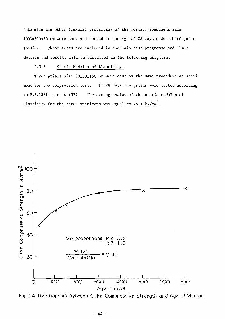
determine the other flexural properties of the mortar, specimens size
1000x300x25 mm were cast and tested at the age of 28 days under third point
loading. These tests are included in the main test programme and their
details and results will be discussed in the following chapters.
2.5.3 Static Modulus of Elasticity.
Three prisms size 50x50x150 mm were cast by the same procedure as speci-
mens for the compression test. At 28 days the prisms were tested according
to B.S.1881, part 4 (53). The average value of the static modulus of
elasticity for the three specimens was equal to 25.1 kN/mm2
.
—
—
—
_Mix proportions: Pfa:C:S
0 . 7: 1 : 3
-Water
Cement+ Pfa- 0•42
I I I I I I I
0 100 200 300 400 500 600 700Age in days
Fig. 2 . 4. Relationship between Cube Compressive Strength and Age of Mortar.
CHAPTER 3.
EXPERIMENTAL PROGRAMME.
3.1 Introduction.
In spite of the extensive amount of work carried out on ferrocement, its
flexural behaviour is far from being clear. The literature review shows that
the work on the flexural behaviour lacks two main aspects — firstly, the study
of its basic features, namely the cracking, deformation and strength in
relation to each other, and secondly, identifying quantitatively the factors
which affect this behaviour. Research in this direction will not only help
the settling of the design theory for ferrocement, but also assist in finding
the optimum form of the material.
As the structural behaviour of the ferrocement section differs according
to the type of the reinforcing mesh, it is essential to study the flexural
behaviour of ferrocement reinforced with each type of mesh separately. In
this study, only woven steel wire mesh was considered.
3.2 Variables Studied.
The objective of the experimental programme is to study the cracking,
deformation, and strength characteristics in flexure of ferrocement section
reinforced with woven type wire mesh. These characteristics included first
cracking, crack width and spacing, deflection, compressive and tensile strains,
and the strength at the elasto—plastic and ultimate stages.
The variables considered were:
1. Number of meshes in the section.
2. Strength of the mesh.
3. Presence of steel bars.
4. Mesh size and mesh distribution in the section.
5. Thickness of mortar cover.
6. Thickness of the section.

All these variables were included in the study of all of the above
mentioned flexural characteristics. Although some of the variables were
specifically selected for one of the characteristics, it was felt that
including them in the study of the others will still provide
important information. This therefore resulted in using one testing
procedure throughout the testing programme All other properties were kept
constant.
3.3 Type of Test, Size of Test Specimen and Control Specimens.
The test chosen to fulfill the requirement of the study was the four
lines loading flexural test. This type of loading arrangement has the
advantages of constant moment zone and zero transverse shear which is not only
essential in the study of cracking, but also provides a larger zone for the
failure unlike the one point loading arrangement.
It was felt that the specimen size should be large enough to avoid the
, effect of scaling down the prototype. Therefore, the specimen chosen was a
plate type 1000 mm in length and 300 mm in width. The supported length was
900 mm and the constant moment zone was 300 mm long.
To help carry out the crack width measurements, the test was arranged
upside down, i.e. tensile face upward.
The control specimens, cast with each specimen, were six cubes, size
50 mm, for compression test and three plates 500x100x25 mm in dimension for
flexural test.
3.4 Details of Experimental Programme.
The experimental programme included casting and testing seven series,
each containing several sets of specimens. The specimens in each set have
identical properties. A total of 49 specimens were cast and tested. The
description of each series is given below, while the details are given in
Table 3.1.

t1)a)
• ,-14-1$41:11
0$.4
1:14
4-10a)6cuU
..1
04-10
11)1:4
4. = Nr-i 4-1 g0 bo= .'"--4 a) Zca $.1
al 4-1Z CI)
.0
00sten
r...
o,,--1,--1
m
r--I
•r)Cfl
VD
CO....7cr)
.
VD
CO...7Cr)
VD
CO...1'M
VD
00-.I'ri
IAro 0Cn • n-1 S(3) 0 SZ a)
0
In
s7
Lel
U'").1-
cr)
..1-rn
VD
lel
.0-
Ln
In .
-../.
If
innI'
Lrl
Lrl-4'
LI)
4..)
0a)E
4-1 CI)OE.)
k
a) oa 4-1›% 0H 4 ,1
a)• $.1
P,140o
4u)CU
6
a)1.4
..-I.
:
--
::
4....
--
r...
,Ia)a))..)Cr)
"o0al Cil
3-14 co
C.1) an
w6
a)l.i
..-1
>1L--10o
4Cl)
a)0CI)w
.1-1
-..
."..
=
:
..
r.
3-10 1.44a) 9w > a.00Z c.)
N N N N N
n0
..t)
-4-
N
cn
a) wE 0
•,-1 ,m 5c.) c.) 9a) •,-)ca..=
Cl) 4..1
LelN
tr)
CNIcr)N
IliN
m
00
l's
,—I
V)
NlriN
En0
;..1 a)a) e
4 44 -,-1IS 0 C.)o a)z ra.
Cl)
COw-A
CO
.
n0 ....7 1/40 -4' VI.
0o
..-1 .C1) 4.1a) 0
$.1 baa) -,-1
En Lna),0
EnNEn
4-11En
...1CO
.
IS)
Enn0Cl)
r-.cn

Series Si: In this series, the number of mild steel wire meshes was
varied from none to the maximum possible number. The purpose
of this series was to study the effect of steel content.
Series S2: This series is similar to Si but using high strength steel
mesh instead of mild steel mesh. The purpose was to study the
effect of reinforcement strength.
Series S3: This series was again similar to Si, but the size of the
mesh was different. The sets of specimens in this series have
equal number of meshes with some of the sets in Si but the
percentage of steel content was different. In addition to the
study of the effect of mesh size, the purpose of this series was
to fill the gaps between steel percentages used in Sl.
The meshes in specimens of series Si, S2, and S3 were uniformly
distributed across the section with mortar cover equal to 2 mm.
Series S4:
In this series, the reinforcements consisted of mild steel
wire mesh and steel bars. The variable was the number of meshes
used with the steel bars.
Series S5: The variable in this series was the thickness of the specimen.
The percentage of steel content was kept constant. It was equal
to the optimum value found from series Si and S3. The reinforce-
ment consisted of mild steel wire meshes uniformly distributed
across the section.
Series S6: This series was the same as S5 but the variable here was the
mortar cover.
Series S7: This series was a continuation of Series S4. The steel bars
were removed but the distribution of the meshes was the same as in
S4, i.e. concentrated near the outer faces.
The specimen designations used in this study were as follows:
1. Each series was given a serial number which follows the letter S,
(S for abbreviation of series). Hence S3 refers to series number three.
2. Each set of specimens was given a letter which follows the series number.
The letter indicates the number of meshes in the specimens of that set.
The letters used were A, B, C, D, E, and F which stand for number of
meshes equal to 0, 2, 4, 6, 8 and 10, respectively. For example, SID
refers to a set of specimens in series one with number of meshes equal
to 6.
3. The serial number of the specimen in the set was given after the letter
which identify the set. The specimens in each set had the same
properties. Therefore S2 Bl refers to specimen number one, of the set
B (two meshes) of the second series.
4. In series S6 a figure was used between the series number and the set
letter. This figure indicates the value of mortar cover thickness of
the specimens. Whenever this figure is not mentioned then the value of
the cover is equal to 2 mm. For example 56 4D1 refers to specimen
number one of the set D (6 meshes) of the series number 6, with mortar
cover equal to 4 mm.
Details of the sets of specimens in each series and the properties of
the section of each set are given in Tables 3.2 to 3.5. It is to be noticed
that the number of specimens in each set of series Si was three. However,
this number was decreased in the subsequent series. The reasons for having
a large number of specimens were firstly to establish the repeatability of
the test results and secondly because of the importance of the results from
series S1 to define the optimum amount of reinforcement which was used in
later tests. Thirdly, the tests gave an idea about the amount of scatter
in the results, especially in the study of cracking. It showed that the
scatter could be very small and the number of repeated specimens in the
subsequent series was reduced depending on the importance of the series itself.
3.5 Specimen Manufacture.
Different investigators have used different techniques in manufacturing
ferrocement specimens. However, the difficulty arises when the mesh distri-
bution is considered important and a specified mortar cover is required. For
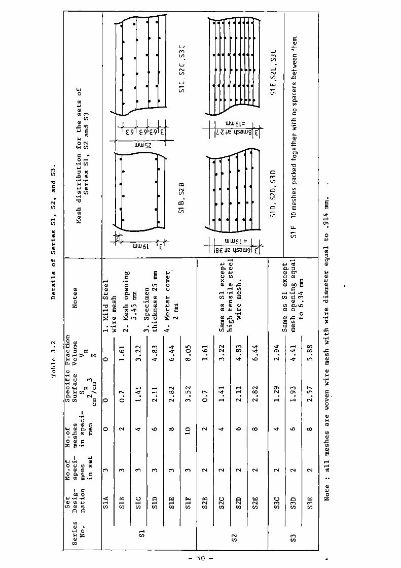
ii-)o
co4-)a)0) C •)
Cl)a).0 'V4-1 g
co
0 N144 V)
g .0 rl
• 14 V)4-10 co
.0 cu• )-1 •,-1
I-4 )44-1 CU
u) CJ)-,-)"a
.0coa)z
a
•
III•
•
•
I
I •
I
•
Ill
111
I
II
.1-
L)rriV)
-L)
Cs.1
V)-
L.)
V)
7)
c0
(71.
111
WW 61 =gsawdel
Illill
v)".
7.
-C4-
:CUQJ
-I-CU
_cacnL._a,4._)roo.IA
0c-c.-
L..=-•-a,ono
4-
-aCU_vL.1roci.IAa,_.ina,E
_L._.--V)
E.9 E9 E9 E L.Z 4e
I tuw 61. =
III
WW SZ
=1'
61. fEr.d,
l18.E 4.e .1591.1J9
Cf10.)4-1oZ
00 wt E
C) g p4ft) )-I > Bs:
044 >
C)• •4 CU44 C.) Cr)• 8-4 C1:1 e
C./ 144 I:4 C.)a) W Cl) •••n•04 0 c‘,
En Cl) 0C.)
I5,-1
C)u) a) 0
4.1 a) 0, 0.)0 4 a 0
• 00 a) 0Z E •,-)
I 4-1
44 • r1 0./0 C.) CO U)• a) g
0 04 CU 0Z O E .r•1
ICOD 0
4.4 ,-1 • r1CU C/) 4-1
Cl) a) raA 0
IAo.) •
• r•1 0/4 Za)
cr)
n-ta)CU
4-1CO .0
ta•10 W.- E•-)Z a.)
W• •,-1
4-4
0
0
o
o")
44Irlcn
elo0
•.-I0a)ra.0
.0U)a)Z
•N
,-i..o
r1
N.
0
N
Cr)
COr-1cn
0g W5 E
..-1Ln c.)••3' a)
• Ci..Min an
Cr)
(NIN
•Crl
r-1....1
•.-4
....7
Crl
C...)rlr.n
1-ICO
g
I=InCV
CI)Ena)0c..)
•,-1• ,c
4-1
enCO
....1
1-11-1Sc,,
VD
Cr)
A1-1Cl)
$.4
a)>0C)
/4al4., 5I-4 00
Z cNi•
...7
...?
...7•
4:)
SICO
•cn1
CO
Cr)
411•••1Cl)
in0
•CO
NIll
•el
0i-4
Cr1
P.)rlCl)
i-14-) CUP. CUcu .I..)C.) CO)Xa.) a)
rl•-i • .-1V) Cf)
C/) CUal 4-Ial ,ca boco •,-1Cl) x
1-1 cs1%0 N
•r4 Cr)
rlIs....1"• •0 i-i
N st
N N
Pc1C...)N NCl) CO
•.0
COa)E
0CUI-I
-,-)3
V)CO
•••1
r-I1-1•Cs.1
%.0
N
r1C-11NCO
NCl)
--.I••••1"
VD
NCO
CV
CO
N
NCO
1-1cn
En
.....tCT
•N
ONN
.rl
.....7
CV
C..)ce)CO
4-l c
c.)a)
CO0)
co
•-)
04 Za) cr•
a)X
tiO 00
•4-1 ......?0 ina)
U) 04 %.0d
o,.0 4J
E cocue,
n-i...1"••..7
C•"1ON
9-1
%.0
N
Aer)CO
CF)Cl)
•
coCO
•Lf)
N.U'l
.N
CO
N
C.4onCO

0.,-1.i..10
4• n-i
14.6)Cl)
•,-(
A4../
0a)Ea)U
W
0
II
•a 0 a
I/
ID
CIDcr)
o
111111
...t1111
IIIi n
.0Li
Ern
co$4al.0,—ia)a)
.6.1CO
0
0
.0
..-13
4-)
04
C..)....1-cn
caCO
a)
ECO
CO
ES ZI. 5.9
I S
Zl. 5
Ill
• 3
•
D
5.9 9 9 5 . 9
4-1 1 0N.0
.1-1'.0
< I IIOil
II•L.-.) cn
C)f:4
-cr)
.....?(1)
• n
d I I •
••••nnn••nnnn••11).....•
Ill V)4... CV ajMco E
4.1..1
• r4. %—i 3
a) .
E co ,z 00W E co 0(1) CO E a) ••-) 0
W %.0 1-1 > CO 0 0 01-1 CO En al N a)0 .0 co 0 0 W Cad 4
4..) p ›, 0 ...s4 II I-0 .1-DV) -.-1 cd f-1 I-I C.) •.-1 -"A co0 3 4 •—I " • •-1 D.4 4C) ca x g w ci)
3 )4co
E •0 ,--I 0 -0 • 4-1 oci > .—i C) 4..) an•,-) cu a) • ,-4 o g 0 W6 0
U) c.) c.) W MI 0 = 0 Ln c.) a) 4 •--Ia) W 61 4-) 0 a) N 4..1 g. a)
4..) fan 0 LO 4-I 0 E $-1 ca 5- ..cr a)0 co 4-1 •,-t E 0 -.4 II ca cil 4-,Z 0 "0 b0 ce) c) 4-) 'LS in co
•—i . ,I T-1 0 0 a) 1-1 1—I -7 cnn—i CU • n••n 0 0 4..1 0. 0 - ,1 • CO.44 p E ,-.1 ,--1 al cn Z Z Lel
WE
• • • • CO1.-4 N c-r) .7 cn
II
,-1 N en ..1- NC4 Lrt ,-1 N. en cn1
> K, • • • 0 .,—I en -.7 VD en
n M 1-4 CV in1a4 CV 0 1-1 co in csl -.7
cn 0 u • • • • 0 •cJ 0 0 .--) CV 1-1
0 ..4 (I)
Ea c.) E4-1 W cc) • ,40 .0 a) c.)
• CO a) 0 t-.1 ...t .0 00 W 0 0.Z 0 - .'l CO
I4-1 . 1-1 .1-/00 CO a)
• a) 0 cf) v—i v—i ,--) v--) N ,—)0 0. a) 0Z ta 0 •1-1
US T Sa a 18S v17s si7s 3i7s CII7S VL S OLS
II
SaT.I9SII
i7S IIll LS

•
0
( LI-I
Ul
Co
p oLII
470
_o• —
• IL4-in .......„.....n"' n,,—.0
•_—-0
4-C
wL.,
LI S w9
E
47EIiE
.1"0....c._cux "----------
LL
II I III I
p pipl..-)
Lrtln
• II • II
---------a—
Li saw+71 1} 1
E wwLL1E1
bo $.1›, 0 a)
,_ ,-4 •r-1
a) 0 0 00)0 WE c)J-J Cl. aEl),. 0 1-1
U) irl Ca 0ul 'W 4 .4- 4-1a) '-E u) • 14
4-1 •,-1 W in 0c.10 Z w Z ZZ H
• • r•I • •1.-1 eV Cr)
Cel CvlCO 00
.
in
-4- -4-
EC)
c4 ---
,-1,--1
..--1,-1
•CI) NJ C•1 Csl
EC.)
Wcna)
I 0 .g.-1 x.,
.....tN.r-I Crl
c.) 0 ua) 0.) • r-1
04 E 4crl .6I
U)I4-1 a)0 4
• V) .1- coOWZ E
I 4.)I4-1 • A a)0 C.) ca En m en• W 0
0 Ow a) 0Z Erl 0 •,1
•
I 0bD 0
4.1 • 1-1 • r•ICD U) •-)
En w cd
0Enco
riltncn
A 0
co
:I=7
-0"—L4-
I/1..17
.1CaiEaJ1-.1
L
0
,IC
. _w
cc
CI.0
.0L/1
{Lisa
• SI
1 1
D
• •
SEMI
tv
I
pp
II
•0
•
SZ
9
II
1 •
II a
S
0
L
0
•
•
n
im-1../Z)1/1
Lisaw9
Cl)a)4-i0Z
Nong if)
il r..1 • .-I (NICU 0 0WO WS I
.i.J cl, 5 0CO ,0 0 0 V3
CO tri •
I
)-1 En'0W 4 -.7 4.10),--1 0 cn • c.) 0..-i a) in W .MZ a) Z CO C.)
H •,1• ,..I • • .0
v-1 CV r).1.)
›' M
re)EC)
c4 ---Er) CV
EC.)
1414Ca a) g4.)1.1000Z
Cl)14-1 a)0 4
• en00)Z E
I 4-14-1 •r-I a)0 CJ up En
• a) 00 0- W 0Z co e .,-1
I oco 0
4-1 • .-1 • 1-1C1) C0 .1-I
CO W ctA 0
C•1 enCO co
.....t -4-
,-1 ,--1i—i r-4
• •C•4 CNI
.3- .0
%.0 vo
c..) EN
I= A..../. %.0%.0 VDCl) c/3
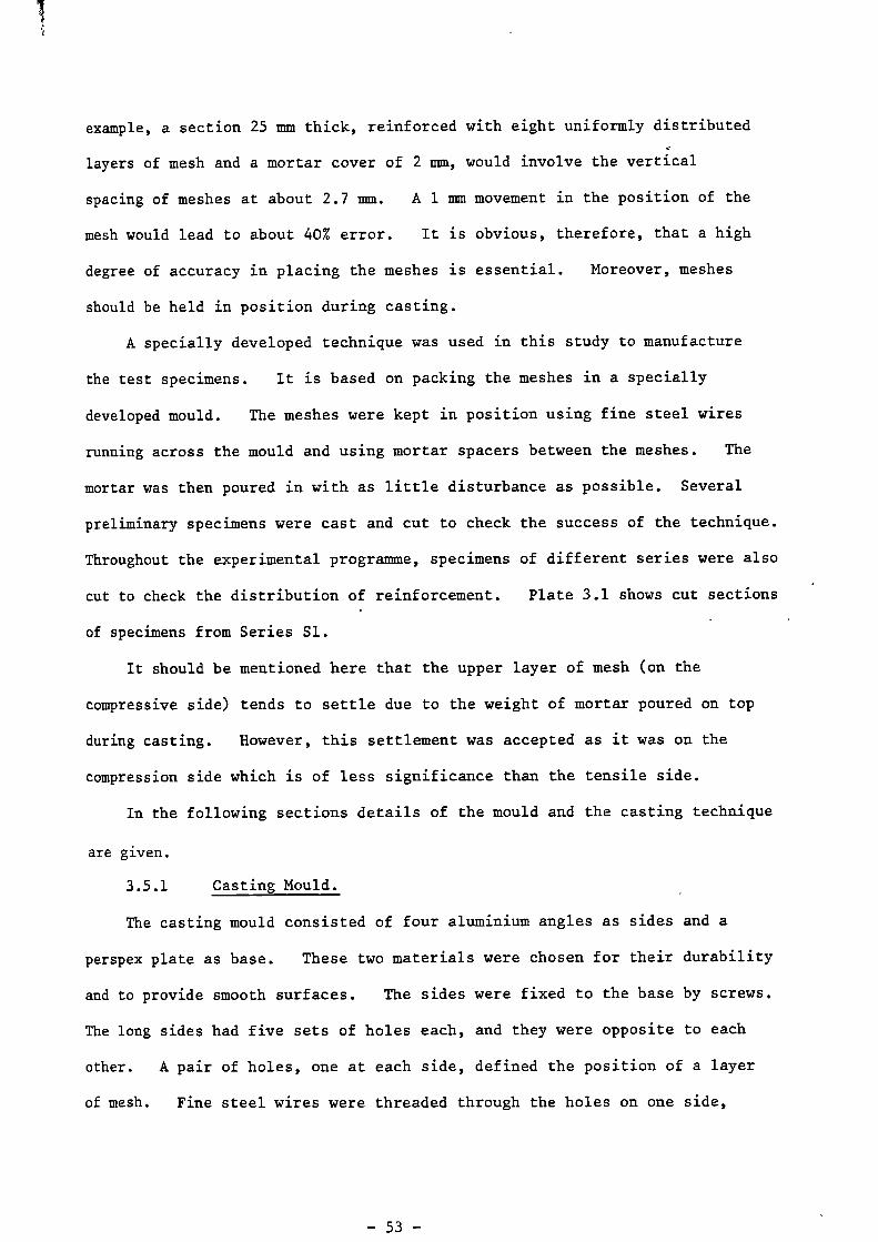
example, a section 25 mm thick, reinforced with eight uniformly distributed
layers of mesh and a mortar cover of 2 mm, would involve the vertical
spacing of meshes at about 2.7 mm. A 1 mm movement in the position of the
mesh would lead to about 40% error. It is obvious, therefore, that a high
degree of accuracy in placing the meshes is essential. Moreover, meshes
should be held in position during casting.
A specially developed technique was used in this study to manufacture
the test specimens. It is based on packing the meshes in a specially
developed mould. The meshes were kept in position using fine steel wires
running across the mould and using mortar spacers between the meshes. The
mortar was then poured in with as little disturbance as possible. Several
preliminary specimens were cast and cut to check the success of the technique.
Throughout the experimental programme, specimens of different series were also
cut to check the distribution of reinforcement. Plate 3.1 shows cut sections
of specimens from Series Sl.
It should be mentioned here that the upper layer of mesh (on the
compressive side) tends to settle due to the weight of mortar poured on top
during casting. However, this settlement was accepted as it was on the
compression side which is of less significance than the tensile side.
In the following sections details of the mould and the casting technique
are given.
3.5.1 Casting Mould.
The casting mould consisted of four aluminium angles as sides and a
perspex plate as base. These two materials were chosen for their durability
and to provide smooth surfaces. The sides were fixed to the base by screws.
The long sides had five sets of holes each, and they were opposite to each
other. A pair of holes, one at each side, defined the position of a layer
of mesh. Fine steel wires were threaded through the holes on one side,
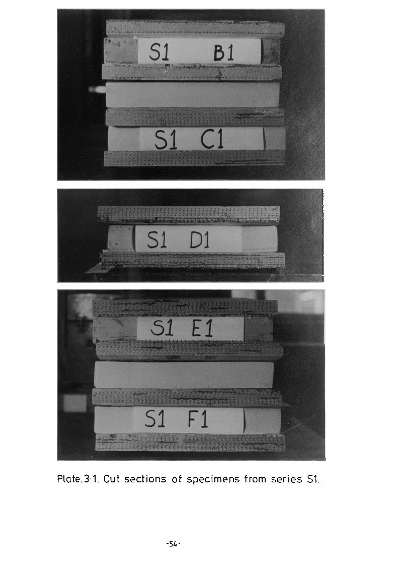
Plate.31. Cut sections of specimens from series Si.

running across the mould and threaded again through the corresponding holes
on the other side. The ends of the wires were fastened to bolts fixed on
the base plate outside the casting area. These wires provided support for
the layer of mesh. Each layer was then supported by five wires. Mortar
spacers, made from the same mortar as that of the specimens, and of a
specified thickness were used to provide the required spacing in areas between
the supporting wires. Fig.3.1 shows a schematic diagram for the details of
the mould.
3.5.2 Reinforcement and Preparation for Casting.
A woven type galvanized steel wire mesh was used in this study. It was
supplied in flat sheets of 1200x1000 mm in dimensions with the least dimension
along the rolling direction (warp). Each sheet was cut into four mesh layers
using shears. The longitudinal direction of the mesh layer was along the
. least dimension of the sheet (i.e. warp direction).
The meshes were cleaned using carbon tetrachloride to remove any oil on
them. They were then straightened to get rid of any warping suffered through
handling of the mesh. This process was essential to ensure a uniform spacing
of the mesh along the test specimen. In specimens which had more than two
meshes, each of the two meshes, separated by mortar spacers, were tied
together using fine steel wire. This was to ensure that the spacing of the
two meshes relative to each other will remain the same and thus cause less
error in the spacing of the meshes.
In the case of specimens with steel bars, the bars were tied to form a
mesh with the required spacing. The placing of the bar mesh in the mould
was carried out in the same way as the wire meshes.
To prepare the mould for casting, it was first oiled. The first set of
wires was threaded through the holes to support the first layer of wire mesh
and provide the required cover. Mortar spacers (one in the middle of the


span of each wire) were used to support these wires. The first layer of
mesh was then placed and another set of wires was threaded to hold it in
position. The next set of wires were fixed to support the next layer of
mesh and mortar spacers were used in the areas between these wires. Equal
number of spacers were used for each layer of mesh and for all the specimens.
The next layer of mesh was then placed. This procedure was continued until
the last set of wires were fixed to hold the last layer of mesh in position.
Plate 3.2 shows the reinforcement packed in the mould, ready for casting.
3.5.3 Mixing, Casting, and Curing.
The mixing was carried out in a horizontal pan type mixer. The mixing
procedure was according to ASTM specification (C305-65) (52) of mixing mortars.
The fly ash, cement, and water were first mixed for 30 seconds. Then, sand
was added while mixing continued for another 30 seconds. Mixing was continued
for a further 30 seconds, after which the mixer was stopped for 90 seconds
for the mixture to settle. During that time, any lumps on the blades were
quickly removed. The mixing was resumed for a further 60 seconds,
after which the mortar was ready for casting.
Casting was carried out on a vibrating table. One specimen was cast at
a time. The specimen mould, with the reinforcement packed in, was placed,
together with moulds for the control specimens, on the vibrating table, see
Plate 3.3. The control specimens consisted of 6 cubes of 50 mm, for
compression tests and 3 plates of 500x100x25 mm in dimension for flexural
tests. Casting was carried out while the vibrating table was in operation.
The mortar was applied in thin layers to reduce the disturbance of the mesh
spacing caused by the weight of mortar. Control specimens were cast at the
same time as the test specimen and these were cast in two layers. All
specimens and control specimens were subjected to the same vibration time,
equal to six minutes. Then, the specimens,after being trowelled, were
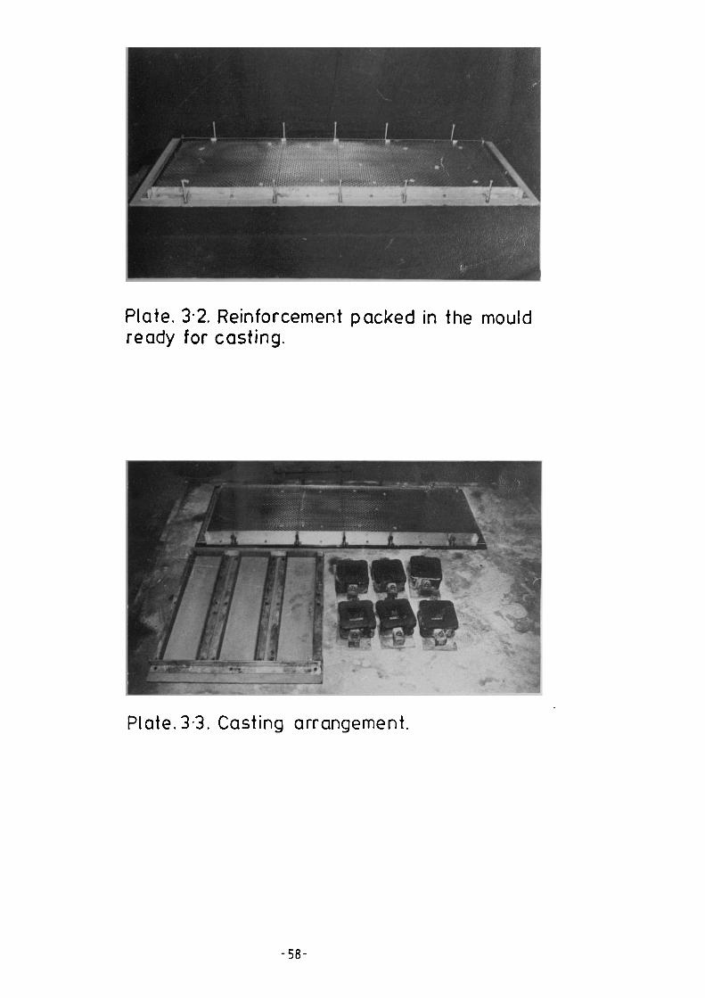
Plate. 3 . 2. Reinforcement packed in the mouldready for casting.
Plate.3 .3. Casting arrangement.

covered with polythene sheets and left on the vibrating table for 24 hours.
All the specimens were then stripped, marked and transferred to the fog
room. The specimens were kept in a fog room where the temperature was 21 0 C
and the humidity was 98%. At the age of 27 days they were transferred to
the laboratory for instrumentation and to be tested the following day.
3.6 Test Equipment.
3.6.1 Testing Rig.
A testing rig was specially designed to carry out the tests in this
investigation. The rig design was based on the following requirements:
1. Four line loading flexural test.
2. Crack width measurements and therefore tensile face of the
specimen upward, with access to it.
3. Large deflection is expected.
4. Free supports to eliminate end restraints.
5. Crack width measuring device is to be mounted on the rig.
The testing rig consisted of a screw jack to supply the load, a proving
ring to measure the load, loading frame to apply the load equally on the two
lines of loading, and supporting frame with roller supports to hold the specimen,
see Fig.3.2. The load is transferred from the proving ring to the loading
frame through a steel bar with a steel ball at each end. The steel bar passes
through a sleeve to direct the load vertically, see Plate 3.4.
Two parallel steel tubes are fixed to the rig to act as rails supporting
the crack width measuring device. They ran parallel to the longitudinal
direction of the specimen.
Preliminary tests were carried out in the rig before starting the programme
of tests for the investigation. The rig was checked under the required range
of loads against movements and stability.

i1.1.19pC.
n
Roller support
Loading-'4'frame
E Rails for crackE width measuringtn° device.N
Proving ring
Screw jack
EE00cn___.E
E00co
Roller
Steel bar
1400 mm
f 300 mm
30 14 mm i, 300mm )(
Testing Rig.
Rubber strip
Details of supports and loading frame.
Fig.3 . 2.Schematic diagram for the testing rig.

- 61-

3.6.2 Crack width Measuring Device.
The crack width measuring device consisted of a micrometer microscope,
a trolley to carry the microscope, and a source of illumination. The micro-
meter microscope had a magnification power of 80 and a least division on the
micrometer of 0.89x10⁻³ mm. The trolley was specially designed to be mounted
on the rig, see Plate 3.5. It is capable of travelling along two steel
tubes, as rails, in the longitudinal direction of the specimen and parallel to
its tensile face. The microscope itself was fixed to a steel base which
sits on two box section steel bars running perpendicular to the longitudinal
direction of the specimen. The microscope can be moved along the steel bars
while the trolley is stationary. Therefore, the microscope can be moved to
any point on the face of the specimen by combination of the trolley movement
and the sliding of the microscope in a plane parallel to the face of the
specimen.
The trolley weighed very little and when not required for crack width
measurements, could be pushed to the side of the constant moment zone or
lifted up from the rig. During crack width measurement, a light source was
attached to the trolley to supply the illumination.
3.7 Test Measurements and Instrumentation.
The measurements required were the loads, strains, and deflection from
first application of the load until failure. In addition, the load at first
cracking and the crack width and spacing at different levels of loading were
also obtained.
The load was measured using a proving ring placed between the screw jack
and the specimen. Two different proving rings were used throughout the test
programme with maximum capacities of 1000 and 2000 kg. respectively. The
1000 kg proving ring was used for specimens with low ultimate load. The use
of two proving rings was to ensure that the measured loads fall within a

Plate. 35. The microscope and the trolley mountedon the rig.
Plate. 3 . 6. Instrumentation on the tensile face ofthe specimen.

reasonable range of the proving ring capacity. Both proving rings were
calibrated using the same machine several times during the period of the experi -
mental programme.
The strain measurements included strains on the compression and tensile
faces and on the side of the specimen. Strains along the lines of crack width
measurements were also obtained. The strain measurements were taken using
Demec gauges and electric resistance strain gauges. Fig.3.3 shows the type
and positions of strain measurements on the two faces of the specimen.
Demec gauges were used to measure the strain on the tensile face (see Plate
3.6). A 100 mm gauge length was used for measuring strains along the lines
of crack width measurement, while for the general tensile strain on the face,
two of 100 mm and two of 50 mm gauge lengths were used. The use of 50 mm
gauge length here is to reduce the error resulting from high curvature near
ultimate load.
All Demec points were stuck to the specimen by first rubbing its place
with emery paper. Then, the place was cleaned using carbon tetrachloride.
Plastic Padding was used to stick the Demec points in position.
Electric resistance foil type strain gauges were used to measure the
strains on the compressive and tensile faces and on the side of the specimen,
see Fig.3.3. On the tensile face, two strain gauges of 5 mm gauge length,
and 2.10 gauge factor, were used for strain measurement mainly within the
elastic limit of the mortar i.e. before cracking. The sensitivity of
electrical resistance strain gauge, is higher than that of the Demec gauge.
So, it was hoped that more accurate readings could be obtained by using them.
In fact the strain reading from the electrical strain gauges were used to
sense the occurrence of first cracking. The mall gauge length was chosen
because of greater possibility of the cracks not crossing the gauges.
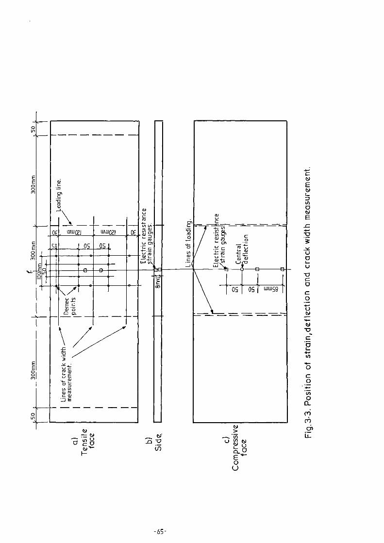
In
a.i
ro0-J U
Li
ro LJ
4a'
7
=
In
II
•::E;
-a
0
szv
C-•n••••
0
0
4-•
0-
•Cr)
Cf:)
WWS9OS
C9-.71
E0
- 65 -
4- • cn= 3V) VI
oe ww OZ I W1110Zi
4-1/1ajcn ro
VI
sn
1.1-1
CU cocn
1.13 Uaj
flj 4-
LJGJ CU CU
OS
OSOS

Therefore,the gauges might give an idea about the strains between cracks.
The electrical resistance strain gauges on the side of the specimen were
similar to those on the tensile face. They were used to give an indication
of the strain distribution along the section of the specimen.
On the compressive face three strain gauges of 20 mm gauge length and
2.10 gauge factor, were used. Higher gauge length was chosen here, since the
higher the gauge length, the better the average strain reading obtained.
From experience of previous work (12) it was found that electrical
resistance strain gauges could give reliable reading of the strains on the
mortar if attention was paid in their attaching process. In this study, the
process of sticking the gauges was by first rubbing well their place on the
mortar with emery paper. This was to remove the relatively soft mortar on
the surface. The surface was then washed with carbon tetrachloride to remove
any loose particles. An adhesive, type P2 was used to seal the mortar
surface. It was applied in a very thin layer and left for at least two hours
to harden. Then, the gauge was stuck on top of it. The adhesive used this
time was an instantaneous adhesive. For curing, this adhesive requires
very light pressure and human body temperature. Therefore, after
removing any excess of adhesive and ensuring that the thin layer of adhesive
under the gauge was free from air bubbles, finger pressure was applied on
the full gauge for 30 seconds. After finishing sticking of all the gauges,
wires were soldered to the gauges to connect them to the strain reading
devices during testing.
It should be mentioned that early in the test programme electrical
resistance crack propagation gauges were used to measure the depth of the
cracks on the side of the specimen. These gauges were abandoned later due
to their unreliable results.

Deflection at mid span was measured using a dial gauge with a least
division equal to 0.025 mm.
3.8 Testing Procedure.
The testing of the specimen was carried out at the age of 28 days. Load
was applied incrementally. For the range from first application of load until
first cracking, the load increments were small, mainly to get more represent-
ative recorded reading of the load at first cracking. The magnitude of the
load increments was increased after that and near failure, the load was
increased continuously until failure. Each test took from twelve to twenty
five load increments. Load, deflection and strains were taken at each
increment of loading. Near failure where the load was applied continuously,
load, deflection and compressive strain were recorded instananeously at
selected stages and at failure.
The load at first cracking was recorded for all specimens. The first
crack was detected using a magnifying glass and with the aid of light source.
The occurrence of the first crack was detected from observing the increments
of deflection and the tensile strain from the electric resistance strain gauges.
Soon after their readings deviate from linearity the first crack appeared. The
width of the first crack was measured for selected specimens.
Crack width and spacing measurements were taken at selected increments
(at least four increments) during the period from first cracking until
shortly after yielding of the specimen. At each of these load increments, all
cracks within the constant moment area and crossed by one of the three grid
lines (see Fig.3.3), were marked and their width and distance from the loading
line were measured.
After failure, the number of cracks, spacing and the maximum crack width
were taken. The specimen was then photographed at the cracked area.
Each test took between four to seven hours a large part of that time
was spent on crack width measurements.
CHAPTER 4.
CRACKING BEHAVIOUR
4.1 Introduction.
Cement mortar in ferrocement, like concrete in reinforced concrete, has
a tensile strength of the order of one tenth of its compressive strength.
The tensile strain at which it cracks is about one hundred microstrain and
this figure is only a fraction of that at ultimate load in the steel which it
surrounds. It is for this reason, and the tendency towards more economical
design that in reinforced concrete, cracking and crack width become very
important as it hinders increasing the allowable stresses. Extensive studies
have been carried out on the cracking behaviour of reinforced concrete. The
factors which affect cracking have been investigated, and equations to
predict the mean and the maximum crack width at any level of load are now
established.
Ferrocement is considered as a form of reinforced concrete. However, it
shows better cracking performance than reinforced concrete. The material
exhibits larger number of cracks and hence smaller crack width. For the
same steel stress, reinforced concrete crack width equations predict
substantially smaller crack width in ferrocement than in reinforced concrete
(18). Therefore, crack width equations developed for reinforced concrete
cannot be used for ferrocement. In addition, the factors found to affect the
cracking behaviour in reinforced concrete are not necessarily the same in
ferrocement. This is due to the different reinforcing mechanism of the two
materials. At the same time, the criteria for the crack width for reinforced
concrete might not be applicable to ferrocement.
It is clear, therefore, that cracking of ferrocement requires a separate
and extensive study. The studies should include the cracking behaviour, the
factors affecting it, and the development of equations to predict the crack
width. Such studies will not only enable a better understanding of ferro-
cement but also put the designer in a better position to decide the level of
allowable stresses and servicability of the material.
4.2 . Review of Literature.
Most of the work carried out on the cracking behaviour of ferrocement
sections in flexure have been limited to the general observation of the
cracking and crack number, and the properties of the section at first cracking.
Instead of studying the crack width and crack spacing throughout the elasto-
plastic and plastic stages, investigators were more concerned with the first
crack which represents only a single moment in the life of the section.
There were also attempts to define the optimum reinforcement amount which
produces ferrocement section, by comparing the load at the first crack of the
section. However, different definitions for the first crack were adopted by
• different investigators, such as those that relate it to the onset of the non-
linearity of the load-deflection curve, to the occurrence of certain crack
widths, or to the establishment of a certain tensile strain in the mortar.
These definitions, depending on the technique of the experimental measurements,
may not represent the same single stage in the life of the section, and
therefore the term first crack in itself does not have much meaning.
Bezukladov et al. (5) compared the cracking behaviour of ferrocement
sections at the first visible crack which corresponds to 0.05 mm in width.
They found that the stresses and relative elongations during crack formation
increased with an increase in the specific surface (SR) of the reinforcement
to a specific limit equalling 3.0 to 3.5 cm2/cm
3 and an increase in S
R above
that will lead to a decrease in the stresses at crack formation. They also
observed that the enhancement in the behaviour of the section as compared to
reinforced concrete starts when SR is more than 2.0 cm
2/cm
3.

Naaman & Shah (17), from tensile tests on ferrocement, found that
increasing the specific surface of reinforcement in the longitudinal direction
(SL) increased the stress at the first crack and the number of cracks at
failure. No increase in the stress was observed when SL exceeded about 2.0
cm2/cm
3.
Shah & Key (10) reported that leakage tests performed on specimens under
tension showed that there was no leakage of water through the specimen up to
a crack width of 0.05 mm. It was observed that the number of cracks at
fracture and the width of cracks were significantly influenced by the specific
surface. The average number of cracks at failure varied linearly with increase
in the specific surface of reinforcement.
Walkus (19,20,30) defined ferrocement as a material with a minimum specific
surface, SL , of 1.0 cm2/cm
3 and an upper limit of 1.5 cm
2/cm
3 due to practical
considerations of placing steel in a given section. Considering the cracking
behaviour of ferrocement in flexure similar to that in tension, Walkus divided
the behaviour of the section into 4 stages according to the crack width and
the servicability. Table 1.2 shows the properties of the section at each stage.
It can be seen that crack width over 0.1 mm are unacceptable.
To Walkus, microcracks are inherent in ferrocement even under no loading.
At the initial stages of loading they are of the order of a few microns, but
when their width enlarges and becomes tens of microns they become practically
significant. This may be why the cracking moment is only a relative term.
One of the first attempts to measure the crack width of ferrocement beams
under flexure was made by Logan & Shah (18). It was found that increasing
the specific surface of mesh reinforcement increases the number of cracks at
failure and decreases the crack width for a given steel stress. The following
equation was given for prediction of the average crack spacing at failure.
It is, essentially the same as that derived for reinforced concrete.
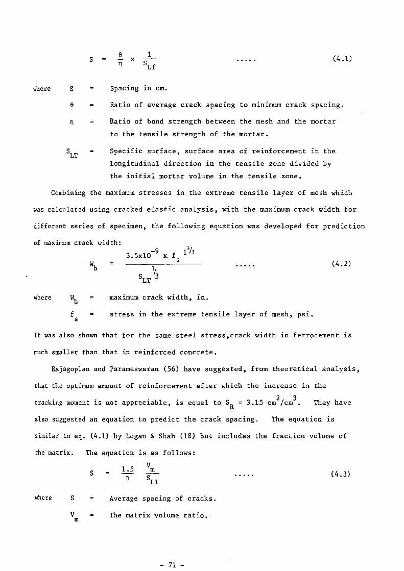
(4.1)
of maximum crack width:
3.5x10⁻⁹ x f
s 113
Wb
SLT
3
(4.2)
where S = Spacing in cm.
6 = Ratio of average crack spacing to minimum crack spacing.
n . Ratio of bond strength between the mesh and the mortar
to the tensile strength of the mortar.
SLT
Specific surface, surface area of reinforcement in the
longitudinal direction in the tensile zone divided by
the initial mortar volume in the tensile zone.
Combining the maximum stresses in the extreme tensile layer of mesh which
was calculated using cracked elastic analysis, with the maximum crack width for
different series of specimen, the following equation was developed for prediction
where Wbmaximum crack width, in.
fsstress in the extreme tensile layer of mesh, psi.
It was also shown that for the same steel stress,crack width in ferrocement is
much smaller than that in reinforced concrete.
Rajagoplan and Parameswaran (56) have suggested, from theoretical analysis,
that the optimum amount of reinforcement after which the increase in the
cracking moment is not appreciable, is equal to SR = 3.15 cm
2/cm
3. They have
also suggested an equation to predict the crack spacing. The equation is
similar to eq. (4.1) by Logan & Shah (18) but includes the fraction volume of
the matrix. The equation is as follows:
1.5Vm
S = (4.3)nLT
wherewhere S = Average spacing of cracks.
Vm = The matrix volume ratio.

Fajagoplan and Parameswaran have also suggested an expression to predict the
maximum crack width. It is based on the assumption that the average crack
spacing multiplied by the steel strain equals the average crack width. The
crack width is then modified to account for the strain gradient in the beam.
The maximum crack width is assumed to be equal to 1.5 times the average crack
width. The expression obtained is given below:
2.25 Vm (
afm-420) (D-a)
n SLT
Ef CD-a)
where:-
Maximum crack width in cm.
Crfin
Stress in the extreme mesh layer, kg./cm2
.
a Depth of neutral axis from extreme compression edge, cm.
Total depth of the ferrocement beam, cm.
1Depth from the extreme compression edge to the last layer
of mesh, cm.
EfModulus of elasticity of the mesh, kg/cm
2.
Paul and Pama (11) derived the following theoretical equation to predict
crack width for ferrocement members under tension. They have suggested that
the equation can also be used for members under flexure.
(4.4)
a * amu7 MU [af - (R+m)]
W = 2S EC. TLfbu
where:-
(4.5)
SL = Specific surface of reinforcement in loading direction.
a mu . Ultimate tensile strength of the mortar.
Cb = Bond correction factor of equivalent aligned fibre.
= Ultimate bond stress,TU
fFibre stress at the crack.
Ratio of area of matrix in the assumed aligned fibre model
to the cross-sectional area of fibre' A
m /Am f
m = Modular ratio, Ef/Em.

It can be seen that equation (4.5) is rather complicated and needs
verification by experimental data.
The first systematic work to measure the crack width of beams under
flexural loading was made by Balaguru, Naaman and Shah (31). They tested beams
reinforced with different numbers of meshes and measured the crack width at
different levels of loads.1 1
The meshes used were /4 in. woven mesh and /2 in.
woven and welded mesh. They concluded that the influence of SR on the cracking
performance of ferrocement in flexure is not as strong as in tension. However,
they found that everything else being equal, specimens reinforced with 1/
i4 n.
mesh gave a better cracking performance than those reinforced with /2 in. mesh.
A linear regression analysis carried out on the crack width measurements and
the tensile strain in the extreme layer of mesh, found from a mathematical model,
yielded the following equations:
For 112 in. welded mesh reinforcement
Wav
0.206 + 0.335 es
1 iFor / n. woven mesh reinforcement
2
Wav
0.353 + 0.42 es
1For
14 in. woven mesh reinforcement
Wav
0.254 + 0.186 Es
where:-
(4.6)
(4.7)
(4.8)
-3 .Wav
The average crack width, 10 in.
Steel strain, 10ES
To study the influence of other variables found important in reinforced
concrete, the regression analysis was repeated with combinations of these
variables and the steel strain. The three other variables considered were:
the cover measured from the cut surfaces, the area of tension zone divided by

number of wires in tension, and the ratio of distance to neutral axis from
extreme tension fibre and from centroid of steel. From the regression analysis,
they found that the standard error was not improved by addition of any of
these three terms. Hence, it was concluded that the maximum crack width would
seem to be primarily dependent on the tensile strain in the extreme layer of
mesh. However, the cover was varied only between 0.4 and 1.7 mm which is
a small range and there were no tests carried out specially to determine the
effect of the cover.
A design equation was suggested by Balaguru et al. (31) based on the
assumption that mortar between cracks is completely free and the number of
cracks equals the number of transverse wires. The equation was in the following
form:
• E s SR
(4.9)
where:
• Average crack width.
Es
•
Tensile steel strain in the extreme layer of
steel.
• Spacing of transverse wires.
• Ratio of distances to neutral axis from extreme
tension fibre and from the outermost layer of mesh.
The equation was found to give upper bound limit for the crack width. This
equation was used (40,57) in crack width prediction for section under static
flexural load which in turn was used in the analysis of crack width for sections
under fatigue load.
Naaman (24) reporting on the experimental work mentioned in Ref. (31),
gave general equations for the average and maximum crack width in terms of
the tensile stress in steel rather than the tensile strain. These equations
are given below:

(4.10)
(4.11)
11-171 0 1S=
IP n SLT
(4.13)
VI
Way.
= (0.271 fs — 3.73) 10-4
Wmax
= (0.324 fs — 4.36) 10-4
and to include the modulus of elasticity of the mesh
23000W
. = (0.271 f
s — 3.73) 10-4
ay . ER
where
(4.12)
W ,W
•
Average and maximum crack width respectively, in.ay . max
fs
•
Steel stress, Ksi.
ER
•
Modulus of reinforcing system, Ksi.
Naaman reported that the number of cracks reached a steady value soon
after occurrence of first crack and the spacing independent of the number of
meshes used is equal to the spacing of transverse wires. He also reported
that the overall average ratio between maximum crack width and the average
• crack width was equal to 1.21 with a standard deviation of 0.14. Naaman,
however, concluded that the exhaustive experimental work combined with scrupulous
analysis are still necessary in ferrocement to better ascertain the influence
of the major parameters and separate their effects.
Recently, Balaguru (58), presented theoretical equations to predict the
crack spacing. The equation is basically the same as that suggested by Logan
and Shah (18) (eq. 4.1), to predict the ultimate crack spacing, but he included
the curvature of the beam as the important factor which controls the cracking.
The equation is:
where* and *u
are the curvature of the beam at the given load and at failure
respectively.
Assuming that the curvature of the beam at ultimate equals the curvature
at yielding and that the average crack width equals the average tensile strain

6 (h-c) Way.
47-117-
y n SLT
(4.14)
in the tension face multiplied by the crack spacing, Balaguru gave the following
equation:
where Wav
= Average crack width..
IP = Curvature of the beam at yielding.Y
h = Total depth of the section.
Depth of neutral axis from compression face.
Balaguru also suggested that the properties of the section required in
eq. 4.14 could be found using linear elastic analysis i the same as that used in
reinforced concrete. This method of analysis may not give accurate results
for the depth of the neutral axis and the curvature of ferrocement beams.
Also, in Balaguru's theoretical model, the assumption * = *u could be
invalid as *u is substantially higher than * (11). In any case, the derived
equations need verification by experimental results.
From the literature review, it can be seen that the cracking behaviour in
flexure and the factors affecting this behaviour are an area which needs more
study, not only for the prediction of the crack width but, perhaps, for
reaching a better understanding of the potential of ferrocement.
4.3 Scope and Experimental Programme.
The following aspects were studied:
(1) Comparison of the cracking performance of specimens reinforced with mild
steel wire mesh, high tensile steel wire mesh, and combination of mild steel
wire mesh and steel bars.
(2) Effect of the number of the steel wire mesh on the crack width and spacing
for specimens reinforced as in (1) above.
(3) Effect of the mesh distribution and the presence of steel bars in the
section on the cracking performance and crack width.
(4) For the same amount of reinforcement, the effect of mortar cover and
thickness of the section on the cracking performance and crack width.
(5) Derivation of crack width prediction equation.
The experimental programme consisted of seven series, comprising 44
specimens. Since cracking is essentially a random phenomenon, specimens with
the same variables were repeated twice or three times. In addition, a large
number of crack width and crack spacing measurements, at each of the selected
stages of loading and for each specimen, were taken. The reason for that was
to establish the repeatability of the tests and to obtain more reliable
results.
Full details of the test programme, instrumentation, and test procedure
are given in Chapter 3.
4.4 Treatment of the Results.
For each specimen, the results included the crack width and spacing,
together with the corresponding tensile strain on the face of the specimen,
recorded for at least four different load stages between the first crack and
soon after yielding. All the cracks in the constant moment zone and crossing
any of the three grid lines, shown in Fig.3.3, were considered. The number of
crack width measurements at each stage varied between 20 and 90, depending on
the type of specimen and level of load. A total number of crack width
measurements of about 10,000 were taken.
A statistical approach was adopted to deal with that large number of crack
width readings. The statistical approach does not only make the comparison
of the data easier, but also gives more reliable results as it deals with the
total population of the cracks rather than single cracks. A statistical
computer programme was used to calculate the following values for each specimen
and at each stage of crack width measurements:—

1. The mean, the maximum measured, the standard deviation and the coefficient
of variation of the total population of the crack width readings.
2. The maximum crack width. Assuming normal distribution, the crack width
with 2.28% chance of being exceeded was calculated.
3. Coefficient of skewness and coefficent kurtosis. These two values
measure the skewness of the distribution from normality.
4. The average of the tensile strain measured (gauge length 100 mm) along
the three lines of crack width measurement.
Tables 4.1 to 4.6 give details of the cracking characteristics at each stage
of crack width measurement and for all specimens.
For each specimen, the mean crack width and the standard deviation were
plotted against the corresponding average tensile strain on the face of the
specimen. A linear regression was carried out and the slope of the best fit
line together with the intercept and the correlation coefficient were found
for all the specimens. Figs. 4.1 to 4.6 show the graphs of the mean crack
width against the average tensile strain relationship and Table 4.7 gives the
characteristics of the equations found from the linear regression for these
relationships.
The slope of the linear relationship between the mean crack width and
the average tensile strain on the face of the specimen, Wm/c
t, will be
referred to as the rate of growth of crack width, because it represents the
rate of increase in the mean crack width with respect to the tensile strain.
It should be noticed that Wm/ct
equals the crack spacing, if the mortar
between cracks is assumed to carry no tensile stress.
Relating the mean crack width to the tensile strain at the level of the
crack is a beneficial approach in studying the effect of the different
variables on the crack width. The tensile strain is a primary factor which
affects the crack width. Moreover, this factor will repeat itself in every

Table 4.1 Cracking Characteristics of Specimens of Series Sl.
Specimen LoadkN
*No. ofcracks
Mean ofcrackwidth
(microns)
Standarddeviation
a(microns)
Coeff.ofvariation
%
Max.Crackwidth(measured)
Averagetensilestrainon the
microns faceeav
micro-strain
S1 Bl 1.176 22 33.9 13.3 39.2 56.3 13231.312 23 46.9 14.5 30.8 71.4 17151.450 23 182.5 78.7 43.2 313.4 6810
**S1 B2 0.9 10 39.3 9.1 23.1 51.8 802
1.16 24 40.6 18.3 45.1 74.1 13151.29 26 64.2 38.5 60 134.8 16081.37 27 181.3 95.1 52.5 321.5 4960
Si B3 0.848 28 11.2 4.5 40.7 25 436
1.018 30 23.2 8.7 37.6 42 858
1.169 31 30.7 10.9 35.6 53.6 11681.305 33 38.2 15.7 41 74.1 1543
S1 Cl 1.230 28 19.6 5.3 26.9 30.4 7401.504 29 29.7 7.5 25.2 44.7 1076
1.777 31 38.3 10.5 27.3 56.3 1425
2.188 34 54.2 19.0 35.0 84.8 2130
2.461 36 73.6 29.9 40.6 125 2924
2.735 37 104.1 45 43.3 195.6 4249
S1 C2 0.957 29 13.2 4.0 30.2 21.4 768
1.552 38 24.8 7.7 31.2 40.2 15742.078 38 39.4 11.7 29.6 68.8 2419
2.557 38 83.8 26.5 31.6 142.9 4895
Si C3 1.271 33 15.2 4.5 29.4 23.2 847
1.668 40 23.2 7.5 32.6 34.8 1338
2.085 42 32.7 11.6 35.5 50.9 1909
2.461 43 52.7 19.4 36.8 88.4 2951
2.741 44 100 40.7 40.8 174.1 5560
Si Dl 1.121 18 8.3 2.3 28.1 13.4 446
1.586 37 14.3 4.1 28.5 23.2 984
2.085 40 23.2 6.6 28.5 37.5 1540
2.680 44 28.9 10.4 35.8 48.2 2178
3.172 46 42.7 13.8 32.3 72.3 - 3182
3.637 46 78.7 24.9 31.6 120.5 5430
Si D2 1.278 36 13.4 4.8 36.2 21.4 884
1.832 44 19.8 8.3 41.8 40.2 1475
2.365 48 27.7 12.2 43.9 52.7 2055
3.097 49 49.5 22.1 44.6 90.2 3512
3.384 49 68.8 29.5 42.9 119.7 4971
Si D3 1.258 48 8.7 3.0 34.6 13.4 703
1.818 59 14.1 5.2 37.3 25 12102.598 63 22.1 8.1 36.8 39.3 1982
3.377 65 38.0 17 44.7 86.6 33563.884 69 66.8 32.4 48.5 144.7 6225
Total number of cracks crossing the three grid lines.**Neglected in the analysis due to inconsistency of results.

Table 4.1 Cracking Characteristics of Specimens of Series Si.
SpecimenLoad._10
*No. ofcracks
Mean ofcrack
.width(microns)
Standarddeviation
a(microns)
Coeff. ofVariation
%
Max.crackwidth
(measured)
Averagetensile
strain onthe face
microns cav
microstrain
Si El 1.271 33 13.4 3.7 28.0 21.4 6842.338 41 25.2 6.2 24.6 35.7 15712.912 42 32.4 8.6 26.5 51.8 20553.418 44 40.4 10.9 27.0 67.0 27403.938 45 54.7 17.7 32.3 93.8 3704
Si E2 2.092 44 13.7 4.5 32.7 23.2 11742.639 53 18.3 5.0 27.1 27.7 15743.193 54 23.6 6.9 29.1 37.5 19883.685 58 28.5 9.9 34.7 47.3 24754.417 60 44.4 15.5 34.9 83.1 3799
S1 E3 1.572 50 11.5 3.6 31.0 21.4 8052.618 55 20.3 6.4 31.4 36.6 15683.671 57 31.9 10.1 31.7 58.0 24904.663 58 63.5 19.6 30.9 109.0 48845.155 58 103.6 31.6 30.5 175.0 7936
Si Fl 1.805 31 10.0 2.6 25.5 15.2 7292.393 47 12.8 4.0 31.3 23.2 10552.953 50 15.5 4.9 31.9 24.1 13603.720 52 20.5 6.9 33.6 33 18225.046 56 33.4 10.0 30.1 56.3 2952
Si F2 1.805 44 9.8 3.1 31.4 17.9 8112.625 55 14.8 5.1 34.5 31.3 13013.460 56 21.1 6.7 31.5 41.1 17484.198 64 26.2 9.9 37.8 58.9 23404.923 66 37.1 14.4 38.9 78.6 3368
Si F3 1.545 37 8.7 2.3 25.7 14.3 6702.625 54 16.1 4.3 27.0 25.9 14053.692 57 24.2 6.6 27.4 36.6 21884.704 58 36.6 10.4 28.5 60.7 33185.689 59 69.6 22.3 32.1 118.8 6410
Total number of cracks crossing the three grid lines.

Table 4.2 Cracking Characteristics of Specimens of Series S2.
SpecimenLoadkN
No. ofcracks
Mean ofcrackwidth
microns
Standarddeviation
amicrons
Coeff. ofvariation
%
Measuredmax,crackwidthW
maxmicrons
Averagetensile
strain on thefaceet
microstrain
S2 B1 0.882 20 15.8 6.8 43.2 28.6 5261.073 29 25.8 8.0 30.8 36.6 12551.244 31 35.5 9.7 27.4 49.1 17321.552 32 47.3 11.8 24.9 65.2 22841.942 33 64 14.3 22.3 87.5 3042
S2 B2 1.217 41 23.9 9.8 40.8 53.6 15321.504 42 35.1 12.7 36.1 70.6 21651.805 42 44.1 14.7 33.3 84.8 28132.321 44 62.3 20.6 33.1 108.1 4036
S2 Cl 1.463 47 16.4 4.1 24.9 26.8 10752.290 50 30.7 7.6 24.7 48.2 21463.104 52 44 10.4 23.7 65.2 31093.665 53 53.9 12.5 23.2 77.7 37904.184 58 60.1 18.5 30.8 90.2 4525
S2 C2 1.482 53 12.0 4.0 33.7 20.5 12532.167 63 20.5 7.1 34.4 37.5 21603.083 70 30.2 11.2 37.1 56.3 3424 **4.010 80 37.8 14.9 39.5 69.7 4782
S2 D1 1.600 40 12.6 3.2 25.7 17.9 10582.74 60 22.9 7.8 34.3 36.6 21783.898 66 33.0 10.3 31.4 57.2 34315.037 73 42.6 14.0 32.9 72.3 46526.130 80 53.4 18.2 34.2 95.6 6083
S2 D2 1.653 46 12.7 4.0 31.0 19.7 10902.704 57 26.2 7.5 28.5 40.2 21603.915 67 37.0 13.5 36.5 61.6 33355.055 71 47.6 16.5 34.6 77.7 4692
S2 El 1.618 45 8.8 2.9 32.5 14.3 7662.775 62 17.4 5.7 32.6 31.3 16273.898 70 23.6 8.2 34.7 45.5 24815.587 76 34.0 10.8 31.8 69.6 3842
S2 E2 1.907 50 10.7 3.1 28.9 18.8 10883.024 65 18.8 5.4 28.7 32.2 20094.683 82 28.0 9.9 35.4 48.2 35026.154 86 37.4 12 32.0 64.3 4879
*Total number of cracks crossing the three grid lines.
**Neglected in the analysis due to inconsistency of the results.

Table 4.3 Cracking Characteristics of Specimens of Series S3.
SpecimenLoadkN
No.of*
cracks
Mean ofcrackwidth
microns
Standarddeviation
amicrons
Coefficientof
variation%
Measuredmax.crack
widthWmax
microns
Averagetensile
strain onthe face
Et
microstrain
S3 Cl 0.977 32 13.4 4.1 30.4 20.5 6481.264 35 22.0 6.6 29.8 31.3 12151.764 38 37.4 12.3 32.8 53.6 20922.250 40 87.5 31.0 35.4 134.8 4260
S3 C2 0.847 28 13.5 5.1 37.7 31.3 5041.285 36 24.4 7.7 31.5 42.9 11661.688 38 35.7 11.4 32.0 56.3 17902.092 39 55.4 19.1 34.5 92.9 26972.311 39 91.8 36.4 39.7 171.5 4263
S3 D1 1.230 33 15.8 4.1 26.1 23.2 8951.805 34 28.2 5.2 18.6 39.3 14952.352 36 40.6 8.2 20.2 58.0 21472.858 36 59.4 11.2 18.8 86.6 30983.336 36 98.0 19.7 20.1 141.9 5022
S3 D2 1.278 31 12.1 4.5 37.2 21.4 7161.811 40 20.8 8.1 39.2 38.4 13282.352 44 29.4 11.8 40.1 58.0 19842.871 45 46.4 19.0 41 100.0 30943.350 46 88.2 38.8 44 205.4 6102
**S3 El 1.230 33 10.6 2.9 27.1 18.8 696
2.092 41 23.9 7.0 29.5 36.6 15042.899 42 39.4 10.1 25.7 63.4 23113.658 42 71.2 18.1 25.4 116.1 4039
S3 E2 1.504 39 9.6 3.4 35.1 17.0 7592.064 51 14.5 5.2 35.7 25.9 12202.865 55 24.0 7.9 33.0 39.3 19103.644 56 40.0 12.4 31.0 71.4 29894.116 56 63.6 19.7 31.0 116.1 4763
*Total number of cracks crossing the three grid lines.
**Neglected due to low ultimate strength.

Table 4.4 Cracking Characteristics of Specimens of Series S4 and S7.
Specimen Load
kN
*No.ofcracks
Mean ofcrackwidth
microns
Standarddeviation
amicrons
Coefficientof
variationat%
Measuredmax.crack
widthWmax
microns
Averagetensile
strain onthe face
et
microstrain
S4 A 1.265 18 16.9 6.2 37.0 33 3002.120 32 25.6 10.2 40.0 47.3 8643.364 33 44.0 13.9 31.6 68.8 1682
S4 B 0.797 17 9.4 3.3 35.1 17.0 3371.057 32 15.1 5.5 36.5 32.2 6611.453 38 20.3 7.9 38.8 45.5 9962.023 46 27.3 10.8 39.7 50.9 15142.699 51 39.5 18.9 48.0 80.4 2325
S4 C 1.323 28 10.4 2.8 26.6 15.2 6401.677 37 12.9 4.5 35.0 19.7 9022.220 42 18.9 6.3 33.2 32.2 13073.10 47 27.50 9.7 35.2 45.5 20144.063 53 42.0 16.3 38.8 75.0 3262
S4 D 1.866 37 9.4 2.7 28.8 14.3 7853.023 61 15.9 5.8 36.4 28.6 15224.14 65 26.1 10.1 38.6 47.3 24495.12 66 51.1 22.1 43.3 90.2 4714
Si C 1.169 36 15.2 4.4 28.7 22.3 7881.665 38 26.6 7.0 26.1 36.6 13472.120 38 40.8 9.9 24.3 56.3 1973**2.462 38 99.3 29.3 29.5 156.3 4025
Total number of cracks crossing the three grid lines.**Neglected due to the inconsistency of the results.

*
Table 4.5 Cracking Characteristics of Specimens of Series S5.
SpecimenLoadkN
No.of*
cracks
Mean ofcrackwidthmicrons
Standarddeviation
amicrons
Coefficientof
variation%
Measuredmax.crack
widthWmax
microns
Averagetensile
strain onthe face
Et
micros train
S5 Cl 1.162 35 12.0 s.6 21.4 17.9 7321.654 43 19.8 4.4 22.3 27.7 12582.256 51 27.2 8.2 30.1 47.3 20093.035 55 46.1 15.5 33.6 90.2 32703.487 55 81.4 28.2 34.6 178.6 5411
S5 C2 1.176 35 13.2 4.4 33.4 20.5 8802.023 48 25.3 8.8 34.7 45.5 17552.830 50 42.8 12.6 29.4 67.9 30863.295 52 69.8 21.8 31.2 114.3 5041
S5 C3 1.203 33 15.1 3.9 25.8 26.8 8801.777 46 22.9 6.8 28.5 41.1 15392.557 48 39.9 11.9 29.9 69.7 2565
S5 El 2.191 29 15.2 3.9 25.6 21.4 6703.9155.049
3536
34.455.2
9.314.9
26.9 ,27.0
53.687.5
15232417
6.071 36 101.3 27.3 26.9 167.0 4271
S5 E2 2.188 29 12.1 3.2 26.1 18.8 6293.336 39 22.9 7.2 31.5 34.8 13314.459 41 35.4 10.4 29.4 56.3 20365.539 41 59.2 17.1 28.9 109.8 3286
S5 E3 2.433 32 14.2 4.6 32.6 20.5 6623.496 37 26.1 7.8 29.9 39.3 12374.530 39 39.8 12.0 30.1 67.0 18875.126 39 60.0 16.3 27.2 105.4 2714
Total number of cracks crossing the three grid lines.
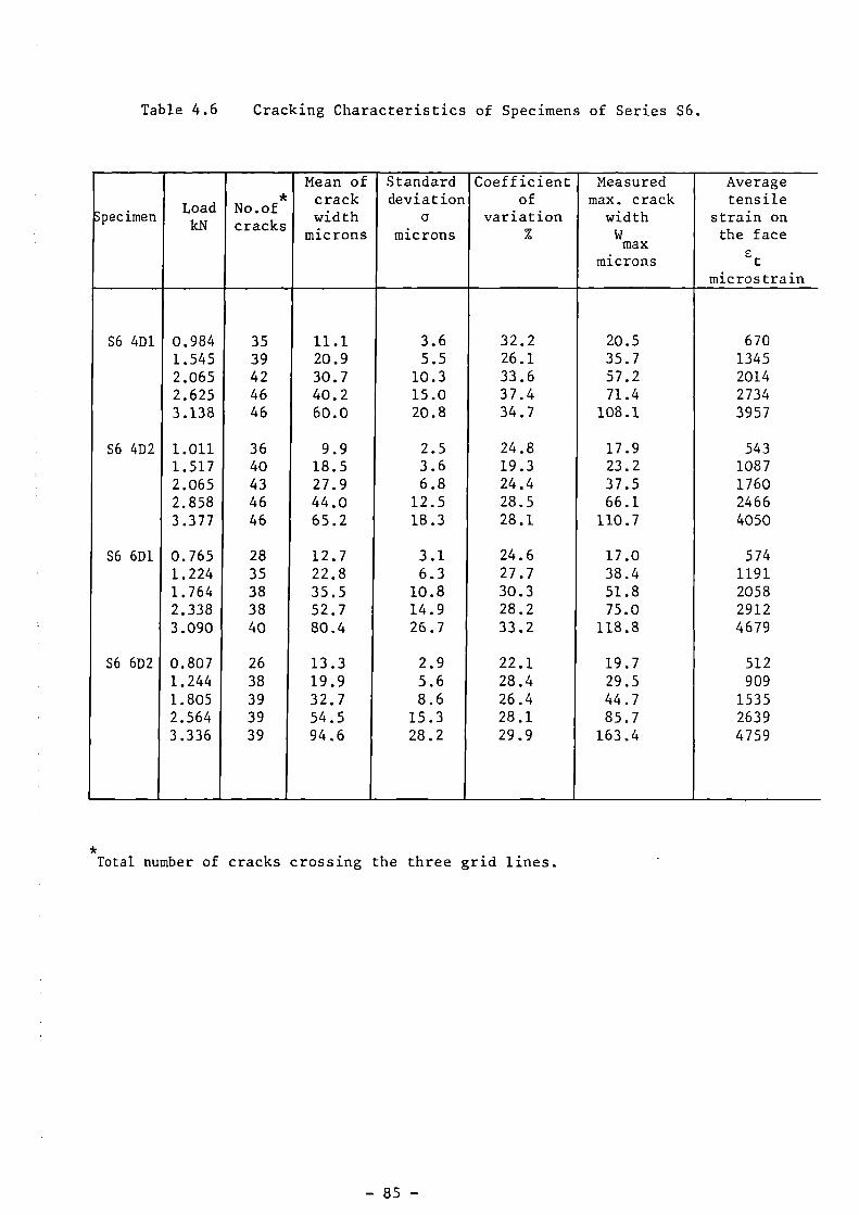
Table 4.6 Cracking Characteristics of Specimens of Series S6.
Specimen Load
kNNo.of
*
cracks
Mean ofcrackwidth
microns
Standarddeviation
amicrons
Coefficientof
variation%
Measuredmax. crack
widthW
max
microns
Averagetensile
strain onthe face
Et
micros train
S6 4D1 0.984 35 11.1 3.6 32.2 20.5 6701.545 39 20.9 5.5 26.1 35.7 13452.065 42 30.7 10.3 33.6 57.2 20142.625 46 40.2 15.0 37.4 71.4 27343.138 46 60.0 20.8 34.7 108.1 3957
S6 4D2 1.011 36 9.9 2.5 24.8 17.9 5431.517 40 18.5 3.6 19.3 23.2 10872.065 43 27.9 6.8 24.4 37.5 17602.858 46 44.0 12.5 28.5 66.1 24663.377 46 65.2 18.3 28.1 110.7 4050
S6 6D1 0.765 28 12.7 3.1 24.6 17.0 5741.224 35 22.8 6.3 27.7 38.4 11911.764 38 35.5 10.8 30.3 51.8 20582.338 38 52.7 14.9 28.2 75.0 29123.090 40 80.4 26.7 33.2 118.8 4679
S6 6D2 0.807 26 13.3 2.9 22.1 19.7 5121.244 38 19.9 5.6 28.4 29.5 9091.805 39 32.7 8.6 26.4 44.7 15352.564 39 54.5 15.3 28.1 85.7 26393.336 39 94.6 28.2 29.9 163.4 4759
*Total number of cracks crossing the three grid lines.

S2C14meshes
x
S1B3 S1C32 meshes 4meshes
S1 E38meshes
S1D36meshes
-S1F3
10meshes
Series Simild steel mesh onlymesh opening =5 -45m-cl
mortar cover =2mm
1 i 1 1 t
1 •i 1i
60
Cu) 60oL..o
-Ec 50
.c'IS3
_)cc.)
2 30c..)coa)2 20
10 -
0 0
inc502c.)._Ec 40._.E
j30_v02o 20C0a)
2 10
1000 2000 3000 4000 5000
Average tensile strain in microst rainFig.4.I. Mean crack width against average tensile strain on the face of
the specimen ,series SI.
S2B12meshes
S2D16meshes
S2E18meshes
Series S2high tensile steel mesh onlymesh opening =5-45mmmortar cover=2mm
1000 2000 3000 4000
5000
Average tensile strain in microstrain
Fig.4 .2. Mean crack width against average tensile stain on the face ofthe specimen ,series 52.

.i.x 30UaL.UC20a(92
10
111
4 meshes onlyS7 C 54B
2 meshes + bars
S4C4 meshe +bars S4 D
6 meshes+bars
Series 54mild steel mesh+barsmesh opening= 5•45mmmortar cover =2mm
S4Abars only
10
-
toc
2u0
60-
S 20c;2
_
60 _
S3 C24 meshes
S3D2meshes S3 E2
8 meshes
Series 53mild steel mesh onlymesh opening. 6-34mmmortar cover. 2mm
I I
1000 2000 3000 4000 5000Average tensile strain in microstrain
Fig.43. Mean crack width against the average tensile strain on the face ofthe specimen ,series 53.
0 I I I I I0 1000 2000 3000 4000 5000
Average tensile strain in microstrain
Fig.4 . 4. Mean crack width against average tensile strain on the face ofthe specimen series 54 and 57.

40:+6
U 30
Ca 20
210
70
60
0
P0
S5EI8 meshes
S5C1 C24 meshes
Series 5555 E thickness = 34 mmS5C " I7-5mmmortar cover = 2mmmild mesh onlymesh opening = 5.45mmSR = 211 cm2/cm3
S5E26 meshe
566D1 564D2566D2
Series 56mortar cover= 4 and 6 mm.mild steel mesh onlymesh opening= 5-45No_ of meshes = 6
C'n
2 50
40
30
2c 20
210
1000 2000 3000 4000 5000
Average tensile strain in microstrains
Fig.45. Mean crack width against average tensile strain on the face of thespecimen,series 55.
S64DI
1000 2000 3000 4000
Average tensile strain in microstrains
Fig.4 . 6. Mean crack width against average tensile strain on the face of thespecimen, series 56.
-88 -
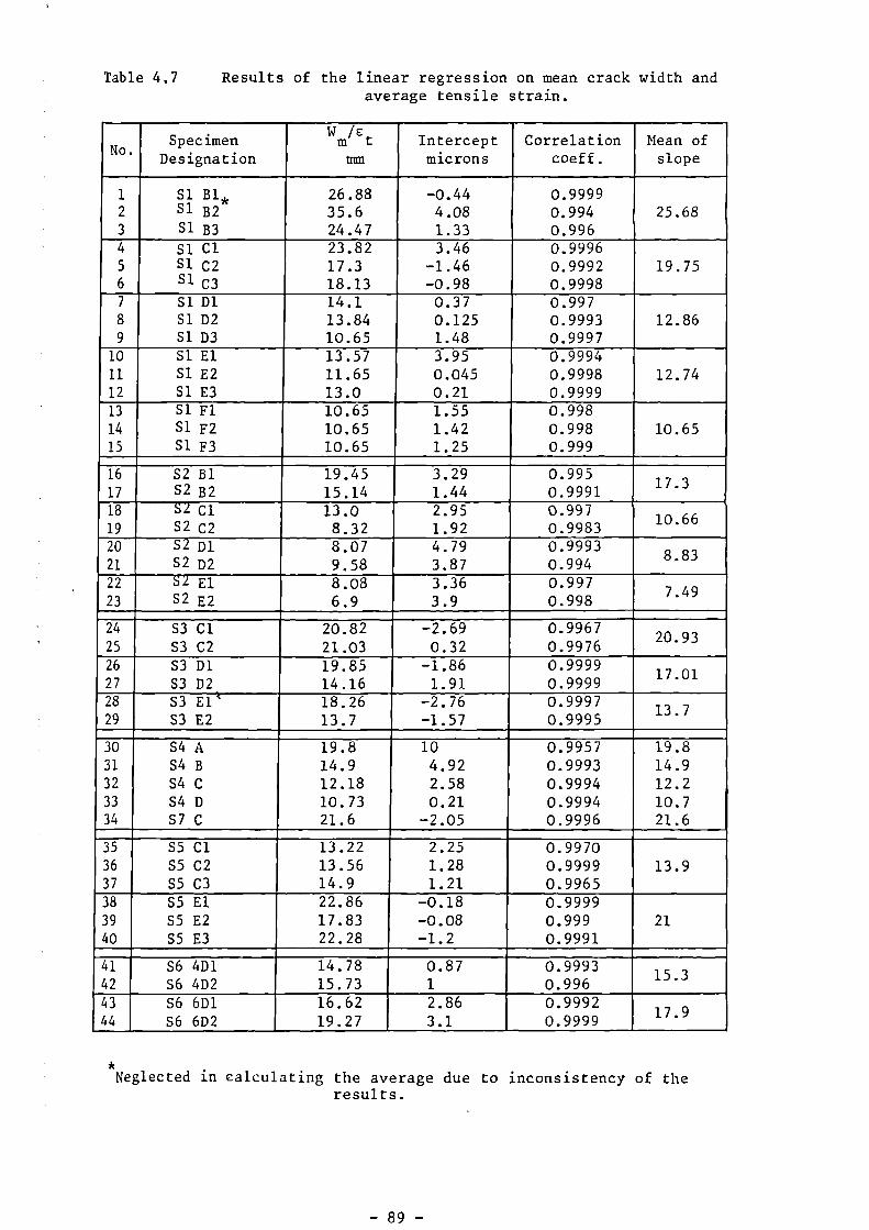
Table 4.7 Results of the linear regression on mean crack width andaverage tensile strain.
N o .Specimen
Designation
Wm
/Et
mmInterceptmicrons
Correlationcoeff.
Mean ofslope
1 Si B1 * 26.88 -0.44 0.99992 Si B2 35.6 4.08 0.994 25.683 Si B3 24.47 1.33 0.9964 Si Cl 23.82 3.46 0.99965 Si C2 17.3 -1.46 0.9992 19.756 Si 0 18.13 -0.98 0.99987 Si D1 14.1 0.37 0.9978 Si D2 13.84 0.125 0.9993 12.869 Si D3 10.65 1.48 0.9997
10 Si El 13.57 3.95 0.999411 Si E2 11.65 0.045 0.9998 12.7412 Si E3 13.0 0.21 0.999913 Si Fl 10.65 1.55 0.99814 Si F2 10.65 1.42 0.998 10.6515 Si F3 10.65 1.25 0.999
16 S2 B1 19.45 3.29 0.99517 S2 B2 15.14 1.44 0.9991
17.3
1819
S2 ClS2 C2
13.08.32
2.951.92
0.9970.9983
10.66
2021
S2 D1S2 D2
8.079.58
4.793.87
0.99930.994
8.83
2223
S2 ElS2 E2
8.086.9
3.363.9
0.9970.998
7.49
2425
S3 ClS3 C2
20.8221.03
-2.690.32
0.99670.9976
20.93
2627
S3 D1S3 D2
19.8514.16
-1.861.91
0.99990.9999
17.01
2829
S3 E0S3 E2
18.2613.7
-2.76-1.57
0.99970.9995
13.7
30 S4 A 19.8 10 0.9957 19.831 S4 B 14.9 4.92 0.9993 14.932 S4 C 12.18 2.58 0.9994 12.233 S4 D 10.73 0.21 0.9994 10.734 S7 C 21.6 -2.05 0.9996 21.6
35 S5 Cl 13.22 2.25 0.997036 S5 C2 13.56 1.28 0.9999 13.937 S5 C3 14.9 1.21 0.996538 S5 El 22.86 -0.18 0.999939 S5 E2 17.83 -0.08 0.999 2140 S5 E3 22.28 -1.2 0.9991
4142
S6 4D1S6 4D2
14.7815.73
0.871
0.99930.996
15.3
4344
S6 6D1S6 6D2
16.6219.27
2.863.1
0.99920.9999 17.9
*Neglected in calculating the average due to inconsistency of the
results.

in(11-- _80
In
1
0
ooo
0
§c,
8-,0
Nr
1 i I i I
if) 0N in
suonp u! Lippn )pa.ij

specimen and therefore cannot be eliminated for the sake of the study of the
effect of the other factors on the crack width. Consequently, replacing the
crack width by the rate of growth of crack width, W m/e t , eliminates the
repeated variable and simplifies the analysis of the effect of the other
factors as they are mainly independent variables.
This approach has been used satisfactorily in dealing with the cracking
in reinforced concrete (59,60,61). It could be even more appropriate for
ferrocement as it has been suggested that for such material (31,70) the
steel strain is the most important factor affecting the crack width. Although
in this study, the tensile strain on the face of the specimen was considered
instead of the steel tensile strain, the strain on the face could be assumed to
be in direct proportion to the steel strain.
It is to be mentioned that an alternative method for finding the rate of
growth of crack width Wm/et was considered. Instead of calculating the
average tensile strain along the three lines of crack width measurement and
relating it to the total population of the crack width, the mean crack width
of the cracks on each line was plotted against the corresponding tensile
strain. Although the values of Wm/e t using this method were practically the
same as those from the first method, the correlation coefficient of the
relationship using the first method was found to be higher. Since in the
first method the considered crack population is larger, and the larger the
population the nearer the distribution to normal (62), therefore the first
method was adopted. Fig.4.7 shows typical results for a specimen calculated
by the two methods.
4.5 The Relationship Between the Maximum and the Average Crack Width.
The relationship between the maximum and the average crack width was
found by two methods. The first method was by calculating the average ratio
of the measured maximum crack width to the mean. The second method was by

using a statistical approach. It depends on the relationship between the
mean and the standard deviation of the population of the crack width readings.
The principles of the second method are as follows:
1. The slopes of the linear relationships between the mean crack width
and the average tensile strain (W /E ) for the different specimens werem t
plotted against the corresponding slopes of the linear relationships between
the standard deviation and the average tensile strain (a/Et), see Fig.4.8.
The best fit line forced through the origin was found. The equation of this
line is
a/et= b W /E
m t
where the slope (b) can be calculated using the following relation (62):
b = E[(a/e t ) (wm/ct)]/Etwm/y2
Thus, the standard deviation is defined in terms of the mean crack width.
2. Assuming a normal distribution, the maximum crack width with 2.28%
chance of being exceeded, is:
Wmax
= Wm +2a
Substituting a in the above equation by its value in terms of Wm, found in
step 1, gives the probabilistic relationship between Wm and W
max.
It is relevant to notice that the slope of the best fit line (b) is
equal to the coefficient of variation divided by 100. The value of this
slope found from analysing the results of all the tested specimens was equal
to 0.354 which gives an overall coefficient of variation equal to 35.4%.
The average value of the coefficient of variation of crack width found at
each loading stage (Tables 4.1 to 4.6) was equal to 32% which is in good
agreement with above one.

WW 4 3/.0 'ZdOIS 11014.DIAZip pmpuols
0:9
(a_0tr)
_c4-,
U
(.)
0
0
0
>-0
-0
0z,f5
IL

The values of W /W for specimens of each series as well as themax m
overall value for all specimens were calculated using the two described methods
and are given in Table 4.8. The overall value of Wmax/Wm
found using the
first method was 1.69 with a standard deviation equal to 0.21, while that
found using the second method was 1.71. The two methods, therefore, gave
comparable results.
To the best of the writer's knowledge, the only other Wmax
/Wm value for
ferrocement found experimentally was reported by Naaman (24). It was equal
to 1.21 with standard deviation equal to 0.14. The procedure used is
similar to that of the first method described above, while the reported value,
as can he seen, is Less than the one obtained from this study. It may be
worth noticing, however, that in Naaman's specimens the zone over which the
cracks were measured was only 125 mm, while in this study the zone was 300 mm.
Thus, higher number of crack width measurements at each loading stage were
taken in this study and hence a more accurate value of the mean crack width
(62) would be expected.
In table 4.9, values of Wmax
/Wm
found for reinforced concrete members
are given. It can be seen that these values are relatively higher than those
for ferrocement, indicating that ferrocement shows a more uniform cracking
performance than reinforced concrete.
Table 4.8
Values of Wmax/Wm
for the different series.
Wmax
/Wm
S1 S2 S3 S4 S5 S6 Overall
-a Average 1.72 1.69 1.72 1.79 1.64 1.58 1.69LI 0(11 4
i4 1.1
,1 elW E
Range(2.28-1.42)
(1.38-2.24)
(1.42-2.33)
(1.46-2.24)
(1.41-1.96)
(1.26-1.86)
(1.26-2.33)
1..-1
...1
1:113.L1,-.
coou - 1.82 1.53 1.68 1.95 1.58 1.66 1.71044.,4
(.1 4-) 0 LI
cu e) w (r)
cn a ...,
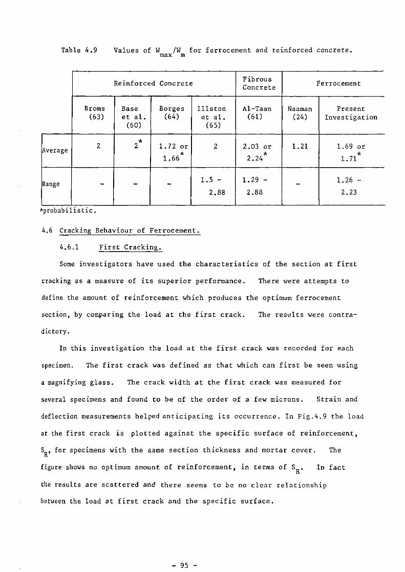
Table 4.9
Values of W /W for ferrocement and reinforced concrete.max m
Reinforced ConcreteFibrousConcrete
Ferrocement
Broms(63)
Baseet al.(60)
Borges(64)
Illstonet al.(65)
Al—Taan(61)
Naaman(24)
PresentInvestigation
Average2
*2 1.72 or
*1.66
2 2.03 or*
2.24
1.21 1.69 or*
1.71
Range — — —1.5 —
2.88
1.29 —
2.88—
1.26 —
2.23
*probabilistic.
4.6 Cracking Behaviour of Ferrocement.
4.6.1 First Cracking.
Some investigators have used the characteristics of the section at first
cracking as a measure of its superior performance. There were attempts to
define the amount of reinforcement which produces the optimum ferrocement
section, by comparing the load at the first crack. The results were contra-
dictory.
In this investigation the load at the first crack was recorded for each
specimen. The first crack was defined as that which can first be seen using
a magnifying glass. The crack width at the first crack was measured for
several specimens and found to be of the order of a few microns. Strain and
deflection measurements helped anticipating its occurrence. In Fig.4.9 the load
at the first crack is plotted against the specific surface of reinforcement,
SR'
for specimens with the same section thickness and mortar cover. The
figure shows no optimum amount of reinforcement, in terms of S R . In fact
the results are scattered and there seems to be no clear relationship
between the load at first crack and the specific surface.

>4<
0
0.1
'1 0
_- = =
z
4100
0 <I X 0
0
0
0(r")
0
C.)
Cr)
CC
c34-•
U")
a_
(J)
-*
a
0
(7)L.
0
4-
4-•
o_
>
00
0 •
a
0
U) in WO
-
0 0 8
•7)
0_J
0 0 0 0 0 6.%0 0
CO0N
0•0
0 •sirIn
- 9 6 -

4.6.2 Behaviour from First Cracking Till Failure.
The development of crack spacing and crack width with load is shown in
Fig.4.10 for specimens reinforced with mild steel mesh (Series Si), and in
Fig.4.11 for specimens reinforced with high tensile steel mesh (Series S2).
The two figures show that the crack width increases linearly with the load.
However, for specimens with mild steel mesh, and at a certain stage of the
load, the crack width starts to increase at a faster rate. This stage of
loading corresponds to the beginning of yielding of the specimen. The
faster increase in the crack width was not observed in specimens with high
tensile steel mesh for the range of crack width measurements taken in this
study.
In terms of the crack number and spacing, the cracking behaviour is
characterized by two stages. The first stage occurs immediately after the
first cracking in which the cracks increase in number rapidly, followed by a
second stage when crack spacing decreases at a much slower rate. The number
of cracks appear to reach almost a saturation limit at a certain stage of loading.
Most of the cracks found after failure are actually formed at about 30-50% of
the ultimate load. The early development of the crack number represents a major
difference in the cracking behaviour of ferrocement and other similar materials.
Al-Taan (61) reported, from tests on conventionally reinforced concrete beams
with steel fibres, that the number of cracks visible at the service load, (35-
45% of the ultimate load) was about half the number near failure.. The full
development of the number of cracks in ferrocement at the early stages of
loading utilizes the advantage of higher crack number and hence less crack
width at the critical stage of loading, i.e. the service load.
Fig.4.12 shows the frequency distribution of the crack width measurements
at different loading stages for four specimens, reinforced with six meshes
each, two specimens with mild steel and the other two with high tensile steel.

30
15
11 1 11 i
_
_
2 mesh4mesh
6mesh
8mesh
10mesh
load atE-----first crack --> mes h8
10
35 _
Mild steel series Si
100
I I I 1
10 20 30 40 50 60 70 80 90 100
%ultimate load
120
co
O 100
.0
Ez- 80
..+P.".3...v 600
019
C 400
(E'
20
• 10 20 30 40 50 60 70 80 90 100
%ultimate load
Fig.4.10 Crack width and spacing against percentageof the ultimate load for specimens from series Si

90 100
2 mesh
4mesh
6 mesh
8 mesh
100Co0-k- 80
Z"6- 60i_x00401
20 -
35,-
High yield steel series S230
10
80010 20 30 40 50 60 70
%ultimate load120-
00 10 20 30 40 50 60 70 80 90 100%ultimate load
Fig.4.11 Crack width and spacing against percentageof ultimate load for specimens from series S2

I ta.°) c-
) U
13 3
0,CONq
viC6
in.. Ee,. 0 No
7- in .
tnm..
0 Em m_'1* .0 Cr)
(T? nC) Cr)a IL
'J.) E=..
0 cynCO -
0 N--NH
.D NH H
EI— >.
-
-
tr)m.. E .0 --n0 r-,%0
0 Li N -— Cr —
H H H
1—.
E
,0 co N'Cr h '<t.
ee li N
IT Z WI— _11) iu
W Ln 3u
..0
0(1)
u .0C.-.u
0b
0c_.u
01._u .
*66
156
O6
46d .
Z Z Z Z
-
_Em..co -
,i)
..o-
E3 -0,.0
I.
n tn tnE
inD.,
0 E
U)E
in E-
a. =..)) C̀.)
0kr) NO11) coci3
00 61
0 m_0 —
(3‘ .i.0 co -0 CO 4.6
4-(7)
" N cr)c\I No N
cm— Ll) — r-,- q 4.) _• o-ä
., u., Ei--
le el II
i-.1' E
ee a a
I— 0 E
le a ll
J Z W ci°c_
(I) (e
t_ C_.3.)
(.0CIt..-
U C..) 0 U-
45
6Z
75
6z
O6z
O6 _z
, I i I i I ill_
it IS1DDJD -o AoLianbaid

b "10
to c
4t-li0
—d (I)
i.,)d• -c__0In
E0
9.-r
N
in
11
Inin -NC Ea u0 2 c\j-,o 0 ,a
k0
CrII
In
u
0 °.- N0\ u
0G" 0
—.
_...inc
C\J— 4- (NJ0 „ci E
" Z
— 011 .- O
(A) Z
—iiE
CNJN
C0L.u
"--E
04.-
_c(7)E.
_c
1
4.- (N
r
I i t I I 0
.0C\J—
coqqq
,c)co
II 11 0Ln
.._ Ein um... 0 M.
U)r_
in o =
Int... coN 0 (5,
— 0 11
II • ,--
cr 0 N
CO w_ CT;)
CO 0 „
II •
in0' C ON
U
0 -C
u2 -L-n'
0
(...7 z...., 0 ELai Z (N E 71
—._N -
10 cv._
E_c "V4._.
q 3 C)..
-I t
9.-
Er
11 i I
000CO (11 —
I I I
( S>IDDJD i.0 0J) buanbaJd

0—0
0U-)co
DU 2) nb Jd

Fig.4.13 shows the frequency distribution of the crack width in a reinforced
concrete slab spanning one way (59). Comparison of the two figures shows that
with the increase in load, the crack width distribution in ferrocement becomes
single peaked, symmetrical, and reasonably uniform, being thus near to normal
distribution. In reinforced concrete as the load increases, more peaks develop
and the distribution deviates more from normality. Also, in reinforced concrete
the highest peak is at the range of smaller crack widths which indicates that
more cracks are developing with the load and this does not seem to slow the
widening of the maximum crack. In ferrocement, as mentioned earlier, full
development of the number of cracks takes place at early stages of the load
thus keeping the maximum crack width relatively small. After that, the cracks
increase in width proportionally and uniformly. This may be the reason why,
from Figs. 4.12 and 4.13, for the same tensile strain on the face of the speci-
mens, the maximum crack width in reinforced concrete is 4-5 times higher than
in ferrocement.
Fig.4.12 shows also the random nature of cracking. For the same tensile
strain, specimens with the same variables have exhibited different numbers of
cracks, Fig.4.12, A and C. This clearly demonstrates the necessity for
repeating the specimens for the same variables and favours the use of statistical
approach in dealing with cracking.
4.6.3 Crack Spacing After Failure.
As mentioned in the previous section, the crack spacing reaches almost a
saturation limit at about 30-50% of the ultimate load and does not decrease
considerably at failure. For this reason, the crack spacing after failure
becomes important as it gives an indication of the crack spacing at stages well
before failure.
In Fig.4.14, the crack spacing after failure (ultimate crack spacing), is
plotted against the specific surface of reinforcement, SR , for the specimens of
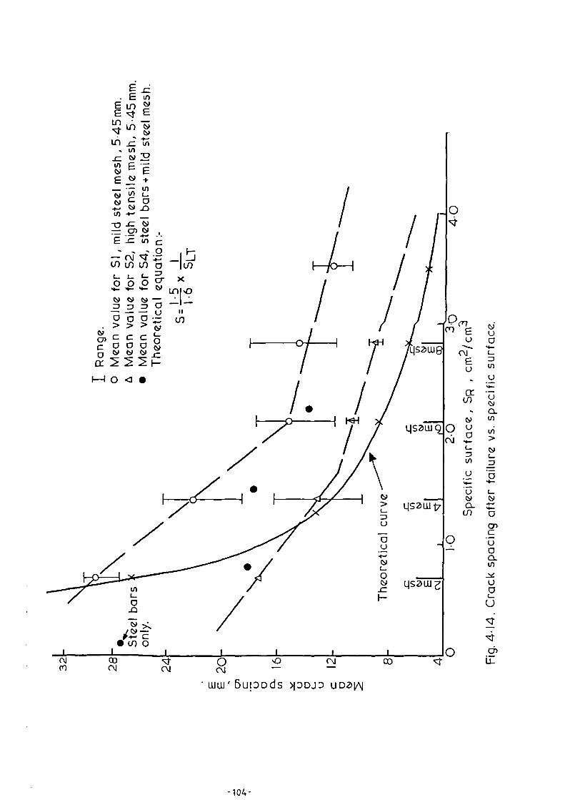
/. i.,,..c +,J0- X0 0 Jo, i. Lnisoi I / /
iqsaw
CC .k.)
(r)
V
I. 1zz
LISZ111
174—Iqs w
_60
zqsaw z
.,
chco .Kr 0 6.--(N (N (N
—
- W W ' 6UpDdS >IDIDJD UDOIAI
Series Si, S2, and S4. The specimens of these series represent three
different types of reinforcement although the size of mesh is the same. These
three types are mild steel mesh only (Series Si), high tensile steel mesh only,
(Series S2), and longitudinal and transverse steel bars spaced at 100 and 300
mm respectively plus varying numbers of meshes (0,2,4,6) placed near the extreme
tensile and compressive fibres (Series S4). The figure shows that, for any
number of meshes, the ultimate spacing for high tensile steel specimens is
less than that for mild steel ones, while those of steel bars and mesh are in
between. The figure also shows that addition of two meshes to the reinforce-
ments of the specimen with steel bars only (in Series S4) resulted in a large
decrease in the ultimate spacing (from 27 mm to 18 mm). This result clearly
demonstrates the advantage of the mesh reinforcement over the conventional
steel bars. However, careful combination of the two reinforcements could be
as effective as the mesh reinforcement alone, see results of Series S4.
A clear feature in Fig.4.14 is that, irrespective of the type of rein-
forcement, increasing the specific surface decreases the ultimate spacing of
cracks. This is also clear in Plates 4.1 to 4.4, where the tensile faces of
typical specimens from Series Si to S4, after failure, are shown. However,
the decrease in the ultimate spacing appears to slow down after a certain
amount of reinforcement, suggesting that increasing the steel content beyond
that amount does not result in appreciable decrease in the ultimate spacing
of cracks.
Naaman (24) reported that, in his tests, the ultimate spacing of cracks
was equal to the spacing of transverse wires of the mesh. In this study, the
smallest ultimate spacing was about two times the spacing of the transverse
wires. Therefore, the basic assumption in Balaguru, Naaman, and Shah crack
width equation (eq. 4.9) could not be verified in this study. Nevertheless,
the transverse wires were still found to be a favourable location for cracks.

I
Plate 4 . 1. Cracking intensity at failure of typicalspecimens from series Si.

Plate. 42. Cracking intensity at failure of typicalspecimens from series 52.

•
53EZ
S3
Plate 4 . 3. Cracking intensity at failure of typicalspecimens from series 53.

Plate.4 . 4. Cracking intensity at failure of typicalspecimens from series S4.
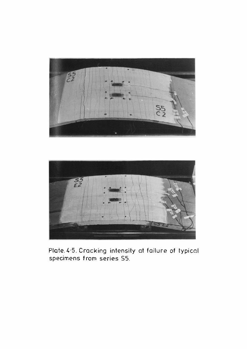
Plate. 45. Cracking intensity at failure of typicalspecimens from series S5.

P1ate.4-6. Cracking intensity at failure of typicalspecimens from series S6 and set Si D.
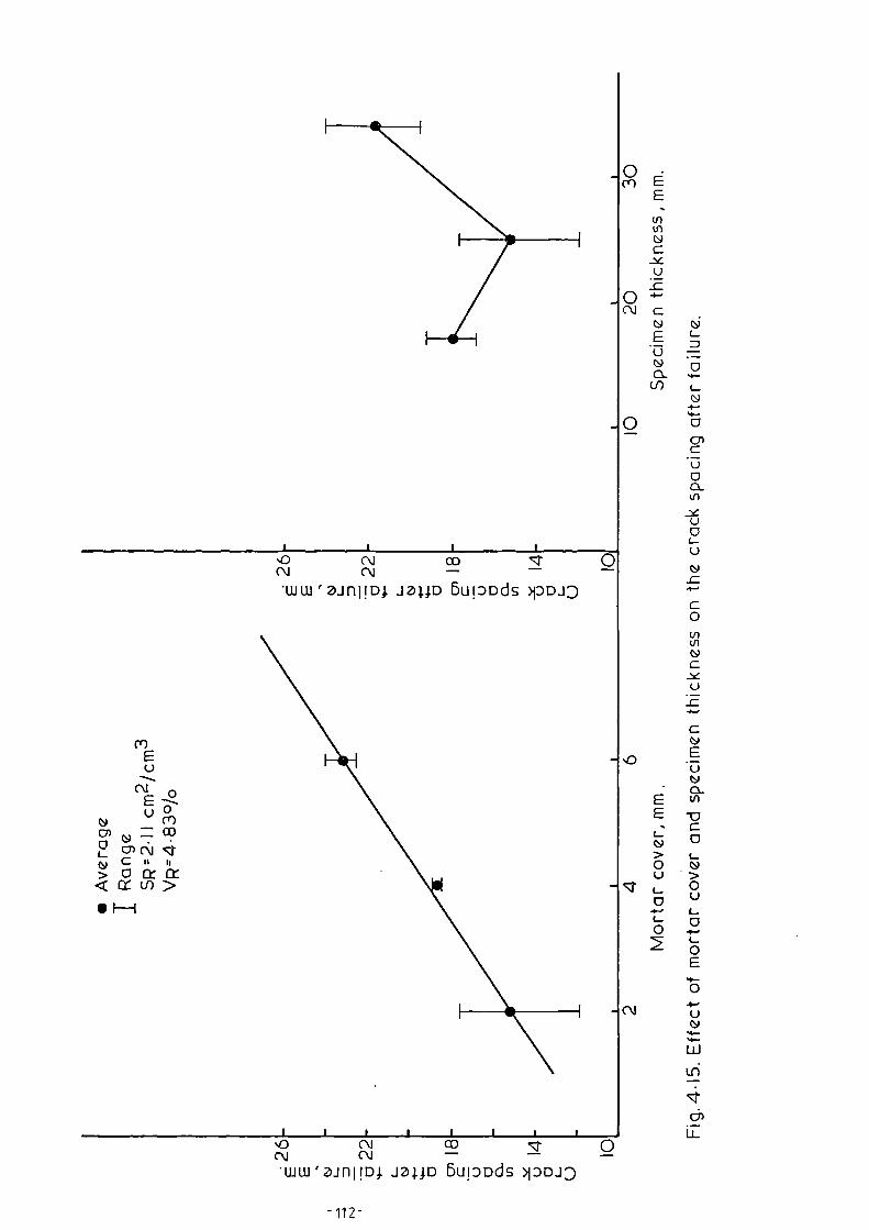
n0 (N CO •Kr 0(N r\I --
'WW ` 2)J111114 J2)140 6UpDdS >IDDJD
•
_
-
%.0
EE(2C9>0U
04-,L-0
2
N
•O N co 7i- 0(N (N
_
'ww i onipj. J31j1D 6UpDdS )10DJ3

-
-
I I I I I
1.41-471
..6_1-6U-
0Cr)•0 N CO CrC\I CV —
_
• WW ' p .m' pl JOI.p 6L1IDDdS rDJD
0

The crack spacing equation 4.1, which was recommended by many
investigators (18,56,58) was used to find the ultimate spacing for the range
of specific surface used in this study. The results are plotted in Fig.4.14.
It can be seen that the predicted values mainly underestimate the experimental
results, and that the equation does not include variables, other than the
specific surface, found important in this study. On the other hand, the
predicted results, although different, show similar trend with respect to
change in the specific surface as those found in this study.
In Fig.4.15, the crack spacing after failure is plotted against the
mortar cover and thickness of the section, for specimens with the same specific
surface and fraction volume of reinforcement. The figure shows that increasing
the mortar cover decreases the final spacing, see Plate 4.5, and the relation
appears to be linear. An increase in the mortar cover from 2 mm to 6 mm
increased the average crack spacing by about 1.5 times.
From Fig.4.15, the section thickness showed no regular effect on the
crack spacing. The crack spacing results for sections 17.5 and 25 mm thick,
are comparable, while those for 34 mm thick were relatively higher.
This might suggest that for the type and amount of reinforcement used in these
tests, the 25 mm thick section gives optimum results.
The effect of the mesh opening on the crack spacing after failure is shown
in Fig.4.16. For the same number of meshes and wire diameter, specimens with
6.34 mesh opening gave relatively higher crack spacing. These results
suggest that the finer the mesh the more the number of cracks that develop.
4.6.4 Cracking Mechanism.
The cracking process in ferrocement could be explained by considering the
tensile stresses in the steel and mortar during cracking of the section.
First cracking takes place when the tensile strain in the extreme fibre of the
section reaches the ultimate tensile strain of the mortar. When this happens,
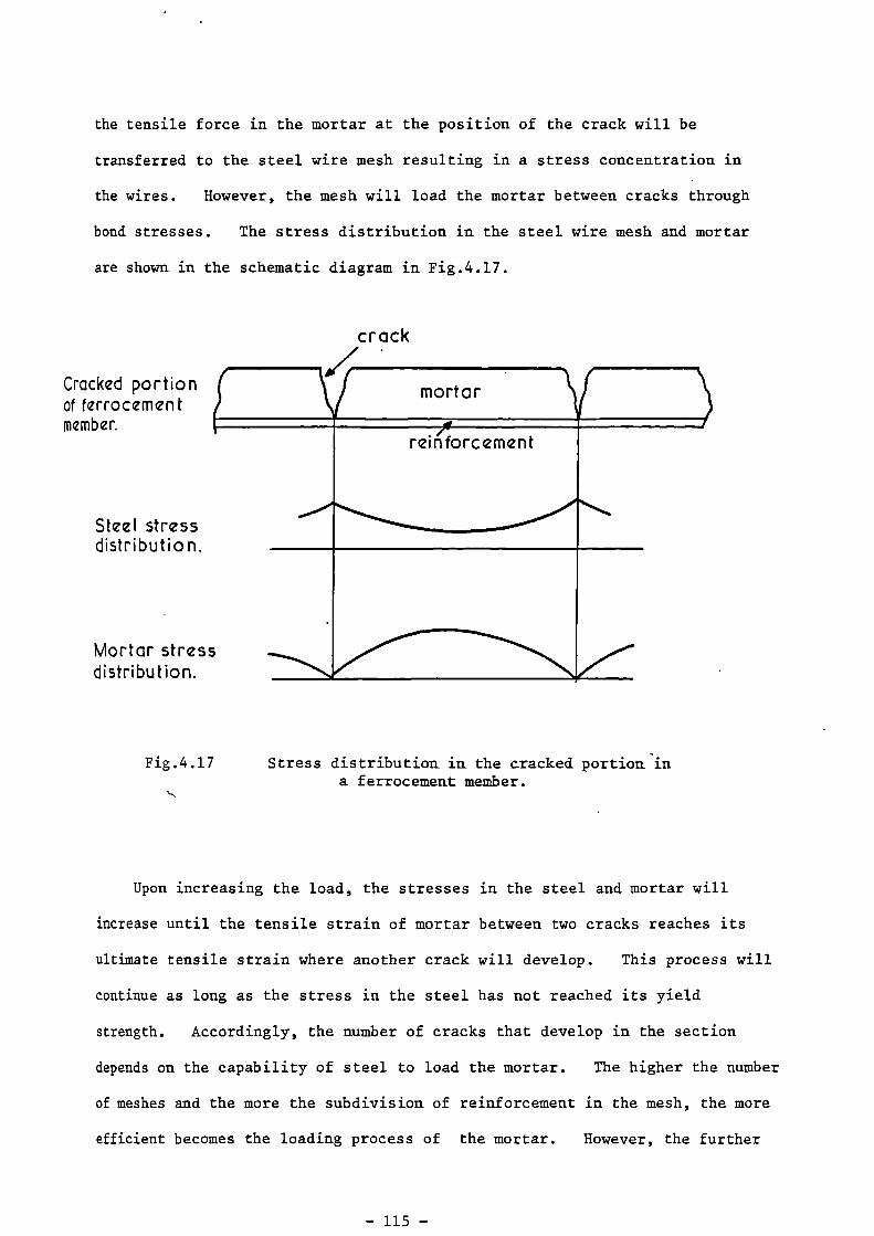
Mortar stressdistribution.
the tensile force in the mortar at the position of the crack will be
transferred to the steel wire mesh resulting in a stress concentration in
the wires. However, the mesh will load the mortar between cracks through
bond stresses. The stress distribution in the steel wire mesh and mortar
are shown in the schematic diagram in Fig.4.17.
Cracked portionof ferrocementmember.
crack
mortar
reinforcement
Steel stressdistribution.
Fig.4.17 Stress distribution in the cracked portion ina ferrocement member.
Upon increasing the load, the stresses in the steel and mortar will
increase until the tensile strain of mortar between two cracks reaches its
ultimate tensile strain where another crack will develop. This process will
continue as long as the stress in the steel has not reached its yield
strength. Accordingly, the number of cracks that develop in the section
depends on the capability of steel to load the mortar. The higher the number
of meshes and the more the subdivision of reinforcement in the mesh, the more
efficient becomes the loading process of the mortar. However, the further

the meshes are from the extreme tensile fibre the less their contribution to
the loading process and it would be expected that after a certain number of
meshes, addition of more meshes will not result in a significant increase in
the crack number. This probably explains the slowing down of the decrease
in the spacing shown in Fig.4.14.
4.7 Effect of Variables on the Crack Width.
The effect of the different variables on the cracking behaviour was
investigated by studying, quantitatively, the effect of these variables on
the crack width. This was achieved by comparing the rate of growth of crack
width, Wm/E t , for the sets of specimens of the different series. For a
certain tensile strain, a higher value of Wm/et
means a higher crack width.
One should notice that in establishing the values of Wm/Et'
the mean crack
'width, Wm, was calculated from the total population of the readings recorded
at each stage of loading. Thus, the value of Wm/Et
defines, statistically,
the trend of the total population of cracks, rather than a single crack.
The variables included the properties of reinforcement (series S1 to S4
and series S7), section depth (series S5), and thickness of the mortar cover
(series S6). The influences of these variables on the cracking behaviour are
discussed separately in the following sections.
4.7.1 Effect of Properties of the Reinforcement.
4.7.1.1 Steel Content.
Most investigators express the steel content in terms of the specific
surface and the fraction volume of reinforcement (SR and V
R' respectively).
The same expressions were used in this study. The average rate of growth of
crack width (Wm
/6t) of the specimens in each of the sets of series S1 to S4
is plotted against the specific surface in Fig.4.18 and against the reinforce-
ment fraction volume in Fig.4.19. These figures show that, in general,
increasing SR and V
R decreases the rate of growth of crack width, hence,
reduces the crack width for a given tensile strain, see Figs. 4.1 to 4.4.

tI-C9
0)
0L.
C9>
< 0 3.5 4-00-5 1.0 1.5 2.0 2.5 3.0
Specific surface in cm2/cm3
Fig. 4 . 18. Rate of growth of crack width vs. specific surface of reinforcement.
0
o Series S IA Series 52x Series 54
o 51
----17----- MildS4
HT52
"trn...............
NN
N
EEc. _
d o Series 51,5 . 45mm mild steel mesh.- -i
A S2,5.45 mm high tensile steel mesh.25 6) 53,6.34mm mild steel mesh.>r x 54,5.45mm mild steel mesh
:49:3
\\\
plus•steel bars.
-6 20x \oL.u 0t 15 Steel bars.... only \._ 0.c
3O \,x,.....„... 0 o SI & 53L '----x 54 001, Io ....6cy ------.5 52
2 3 4 5 6 7Fraction volume of reinforcement P/o
Fig.4 . 19. Rate of growth of crack width vs. fraction volume of reinforcement,series SI ,S2 and 54.

This was the result irrespective of the type of reinforcement. The same
conclusion could be reached, indirectly, by noticing that in Fig.4.14 the
final crack spacing decreases with an increase in SR
. The decrease in
the rate of growth of crack width in Figs. 4.18 and 4.19 appears to slow down
after a certain amount of reinforcement. This amount of reinforcement could
be considered as a saturation limit for the reinforcement at which increasing
the amount of reinforcement does not result in a considerable reduction in
the crack width.
Limits for the amount of reinforcement in ferrocement sections had been
suggested by many investigators (5,18,30,56) and the principles from which
these limits were established differ from one investigator to another. Most
of these limits were established from comparing the enhancement in the loads
or the deformation at first cracking with increase in the specific surface
of reinforcement. The fact that the first cracking represents a certain
moment in the life of the specimen and the difficulty to define it resulted
in unrepeatable results, see Table 4.10. However, in this study the satur-
ation limit of reinforcement has been established by considering the history
of the total population of cracks, rather than considering a single crack or
a single moment in the life of the specimen. Table 4.10 gives the amount
of reinforcement limits found in this study and those suggested by other
investigators.
Table 4.10 Reinforcement limits for ferrocement section.
Rajagoplaintheoretical
Bezukladovet al.
Walkus Loganand
BalaguraNaaman
Present investigator
Author (56) (5) (30) Shah and Shah mild High Mild(18) (31) steel
meshonly
tensilemeshonly
mesh& steelbars
wo m
-cl r=40 VI
(11 IXC)m a)
0 61).--i 0 0
U V) W C.) • ...1 • IAow ctl ...44 4-I J-) $4 „.0 4-1 • 1-1 (.) (1)
$4 0 2.0— En U 4-1 )-+ cd 0
Z a.1 cn 3.15 2.0 s-4 0 • ,-I 0 0 Q)cci 2.1 1.5 1.5m 5 0 3.0 • ri • I-1 • r•1 U) CA C.) al
11) U 4-1 C0 $4
U U "*.. 00 ›... a) U CLI 4-1 C.)
• .-1 N CNI 4-i 0 1-1 cn • .-I W cn 0'40 Ej C0 • ri )-1 CLI 4-1 U $4 • r•I• r1 4-1 UU 0a) • n••1
.M Ca a) • ,1rd U (1) $4 U0 cd 0 U CU
0 • I-1• ,-1 14-1 ,..0
.1..)0.0)
(r) 1.40 $4 • r-1 0 a.
•--1 ci r-1 • ,-1 cn0 4-1 •-1z C‘

The enhanced cracking behaviour with the increase of steel content was
explained in sec. 4.6.3. It was shown that the greater the steel content,
the more are the forces available to load the mortar and therefore creating
more cracks rather than increasing the width of the already established
cracks. It should be noticed that the regression lines in Fig.4.18,
specially those after the steel saturation limit for series Sl, S2, and S4
are parallel. This indicates that the effect of increasing the specific
surface has the same trend in spite of the different type of reinforcement.
In this study, however, the specific surface was increased through increasing
the number of meshes rather than increasing the specific surface of the mesh
itself. Using a mesh with a higher specific surface and then varying the
number of meshes would be expected to produce a curve lower than those in Fig.
4.18 but parallel to them. It may be appropriate, therefore, in studies
which involve the size of mesh as a variable, to define the subdivision of the
reinforcement in the single mesh as well as the subdivision of the total
reinforcement, i.e. SR
. In contrast, the ratio S R/VR seems to define uniquely
the reinforcement subdivision of the single mesh. On the other hand, such
definition may not be necessary when the section is subjected to direct loading.
4.7.1.2 Steel yield strength.
In series Si and S2, the steel mesh used was the same except that of S2
was high tensile steel with ultimate strength of (1197 N/mm2) and yield
strength, at 0.005 strain of (394 N/mm2). While those in Si are mild steel
mesh with ultimate strength (348.6 N/mm2) and yield strength (218.4 N/mm2).
The modulus of elasticity for both meshes are nearly the same, see Table 2.1.
The rates of growth of crack width for specimens of these two series are shown
in Fig.4.18, their final crack spacings in Fig.4.14 and the tension face of
typical specimens from the two series are shown in Plates 4.1 and 4.2.
It can be seen that the high tensile steel specimens (S2) showed a better
cracking performance than the mild steel ones in terms of both the crack width

and spacing. Also, the saturation limit of reinforcement in series S2 is
smaller than that in series Si. It is, therefore, clear that the yield
strength of the mesh has a major influence on the cracking behaviour of
ferrocement.
The curves in Fig.4.18 for both series Si and S2 could be considered
to consist of two segments each. The equations for the four segments of
these two curves were found using linear regression and they are as follows:
1. For mild steel mesh
a - segment (1)
Wm
JEt
•
32.45 - 9.2 SR(4.15)
b - segment (2)
(4.16)Win /€
t
•
16.5 - 1'57 S
R
2. For high tensile steel mesh
a - segment (1)
Wm
/6t
23.9 - 9.4 SR
b - segment (2)
W/E
•
12.79 - 1.88 S
m t R
where
Wm
•
Mean crack width, microns.
(4.17)
(4.18)
t
•
Average tensile strain on the face, 1x10⁻³ mm/mm.
SRTotal specific surface, cm
2/cm
3.
The above four equations represent the relationship between the mean
crack width, tensile strain, and the specific surface for specimens rein-
forced with the mild and high tensile steel woven wire mesh used in this
study. From these equations it can be seen that the slopes of the line
before and after saturation limit for these two curves are similar and the
two curves could be assumed parallel with the pivot axis being the straight
line connecting the saturation limit points, see Fig.4.20. The equation for

Wm,'Et T
Si (mild steel mesh)
••n•n•••
Pivot axis orsaturation limitline.
52(hi h tensile steel mesh)
the pivot axis line was obtained by first solving the above four equations
to find the coordinates of the saturation limit points of the two curves.
The coordinates of these points, together with the corresponding mesh
yield strength are:
For a = 218.4 N/mm2, then S
R = 2.09 cm
2/cm
3 and W
m/E
t = 13.22 mm
For a = 394 N/mm2, then S
R = 1.48 cm
2/cm
3 and W /c = 10.01 mm.
m t
From the above coordinates, the pivot axis can be defined by either of
the following two equations:
SR = 2.85 — 3.5x10
-3 a
(4.19)
wm
/et = 17.2 — 18.3x10
-3 a
(4.20)
where
yield strength of the mesh at 0.005 strain, N/mm2.
Proposed curve for specimens reinforcedwith woven mesh of a yield strengthbetween those of S1 and 52.
SR
Fig.4.20 Trend of the curves expressing the relationship between Wm/Etand S
R for different mesh yield strength.

The better cracking performance of specimens reinforced with high tensile
steel wire mesh compared to specimens reinforced with mild steel wire mesh can
be explained by noticing that, although the initial modulus of
elasticity for both type of meshes are almost equal,the yielding point is higher
for high tensile mesh. Therefore, the range of the stress between the first
cracking and yielding of the mesh is higher for the specimens with high
tensile steel. This, eventually, will allow more cracks to develop rather
than widening of the already existing cracks. This can be seen from comparing
Figs.4.10 and 4.11 in which rapid widening of the cracks took place in
mild steel mesh specimen after about 50% of the ultimate load while those of
high tensile specimen in spite of the fact that their maximum load is higher,
were still increasing in width linearly. The same conclusion can be reached
by comparing the frequency distribution of the crack width for typical
specimens from series Si and S2, shown in Fig.4.12. Up to a tensile strain
on the face equal to 2000 microstrain the two specimens showed fairly similar
=her of cracks and crack width. However, as the load increases, additional
cracks continue to form more substantially in the specimen with the high
tensile mesh. At a tensile strain equal to about 6000 microstrain the
specimen with the mild steel mesh had 69 cracks with mean crack width, Wm
66.8 microns, while that with high tensile mesh had 80 cracks with a mean
crack width of 53.4 microns.
4.7.1.3 Presence of Reinforcing Bars and Mesh Distribution.
Series S4 was designed to study the effect of reinforcing the specimen
with reinforcing bars of 6 mm diameter in addition to steel wire mesh. The
longitudinal bars were spaced at 100 mm, while the transverse bars were spaced
at 300 mm. The steel wire mesh used was the mild steel mesh used in series
Sl. The number of meshes was varied from none to maximum possible of six
meshes equally distributed on both sides of the bars. In specimen S7 C the bars
were removed with the meshes remaining in the same position: this is to find
the effect of reinforcing bars on the behaviour of the section.

Figs. 4.18 and 4.19, show that for the same specific surface S, or theR
same fraction volume of reinforcement, VR, the rate of growth of crack width,
Wake
for the specimens of series S4 are somewhere between those for the
specimens reinforced with high tensile mesh (S2) and those for the specimens
reinforced with mild steel mesh (Si). This indicates that replacing some
of the mild steel meshes in the specimens of series Si, by reinforcing bars,
changed the cracking performance. The presence of the reinforcing bars is
appreciated in Fig.4.19 more than in Fig.4.18, because the bars have, relatively,
low SR but high VR.
In Fig.4.21, the values of Wm/Et for series S4 and S7 are plotted against
V. The following points can be noticed from Figs. 4.18, 4.19 and 4.21:
1. Superior cracking performance of ferrocement compared to that of
reinforced concrete (S4 A) starts in specimens with more than four meshes in
use of mild steel while those with high tensile steel mesh showed better
performance even with two meshes.
2. Enhancement in the cracking behaviour in ferrocement with bars was
not appreciable when the number of meshes increased to more than two at each
side of the bars. The vertical spacing of the meshes in this specimen is the
same as that in specimen S1 D, i.e. 2 mm (Si D gave the steel saturation limit
of series Si).
3. The curve of S4 in Fig.4.19 is nearly parallel, specially after the
saturation limit, to the curves of Si and S2, indicating the similar effect
of increasing the number of meshes on the cracking behaviour in these series.
The saturation limit was smaller than that of Si both in terms of V R and SR.
This may be due to the fact that the yield strength and the modulus of
elasticity of the reinforcing bars were higher than those of mild steel mesh.
4. Removal of the reinforcing bars (as in S7 C and Si B) resulted in
considerable deterioration in the cracking behaviour. Also, from comparing
S7C and Si C, concentration of the meshes near the fibres did not, at least,
enhance the cracking behaviour.
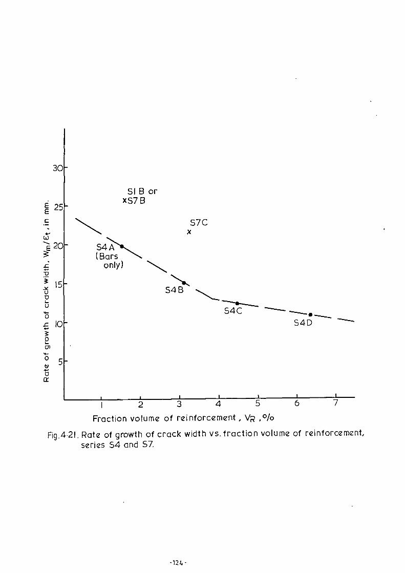
S7Cx
30
SIB orxS7 8
S4A(Bars
only)
S4B.......
-----•,..S4C •
S4D
I 1 I I I I I 2 3 4 5 6 7
Fraction volume of reinforcement, Vp ,o/o
Fig.4 .21. Rate of growth of crack width vs.fraction volume of reinforcement,series 54 and 57.

where
W /Em av
5. The curve for S4 can be assumed to be of the same shape as Si and S2
and its saturation limit falls along the straight line shown in Fig.4.20.
4.7.2 Effect of Mortar Cover.
As in the cracking behaviour of reinforced concrete members the cover has
an effect on the cracking behaviour of ferrocement. Although the cover in
ferrocement is small in value, its percentage of the total depth of the section
is still as high as in reinforced concrete if not more. Because the cover is
of the order of a few millimeters, in practice this value could easily be
doubled and therefore it is important to study the effect of this variable on
the cracking behaviour in ferrocement.
In Fig.4.22, the values of Vet of specimens reinforced with the same
number of meshes are plotted against the mortar cover in these specimens.
Each point in the graph represents the average results from two specimens.
From the figure, it can be seen that the higher the cover, the higher the rate
of growth of crack width and therefore, the higher the crack number and width,
see Plate 4.5. Linear regression on the results gave the following equation:
W /E = 10.3 + 1.27 C (4.21)m av
slope of mean crack width against average tensile
strain pmm x 10-3
cover, mm.
From the above equation, increasing the cover from 2 mm to 4 mm will
result in an increase in the crack width by about 20%. Although this result
might suggest a minor influence, it still shows that cover has an effect on
the determination of the crack width.
It should be noticed here that only one value of steel content was
used in the study of the effect of mortar cover. This value was the
saturation limit for the mild steel wire mesh found from series Si. Specimens
reinforced with high tensile steel mesh were assumed to behave in the same
manner.
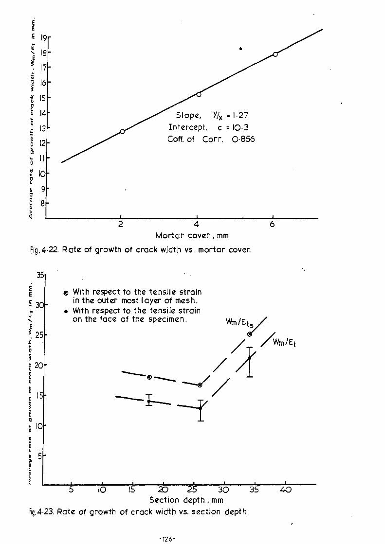
EE
•
-
-
-
oLU 14 - Slope, Y/x =1.27
Intercept, c =10.3
Coff. of Corr. 0•856
-
-
-
-
-
0L AL,o><
-
0 With respect to the tensile strainin the outer most layer of mesh.
• With respect to the tensile strainon the face of the specimen.
Wm / Etes/
//
2
4
6Mortar cover, mm
Fig.4 . 22. Rate of growth of crack width vs. mortar cover.
10 15 20 25 30 35Section depth , mm
Pig, 4 . 23. Rate of growth of crack width vs. section depth.
-126-

To explain the deterioration in the cracking performance with the
increase of the cover, one can see from Fig.4.17 that the further the outmost
layer of mesh from the extreme fibre, the higher the forces in the steel
needed to load the mortar between the cracks to the cracking stress.
4.7.3 Effect of the Depth of the Section.
It was shown in the previous sections that there was a saturation limit
for the amount of reinforcement in the section. That limit was established
by comparing the rate growth of crack width on specimens 25 mm in depth and
reinforced with different numbers of meshes. Practical uses of ferrocement
suggest that the section depth could vary from 10 mm up to 50 mm. Consequently,
two questions can be raised. First, is the saturation limit .of steel content
the same irrespective of the section depth? Second, for the same VR and SR'
what is the effect of the depth of the section on the cracking behaviour?
In this study, only the second question is dealt with. Specimens 17 um,
25 tom and 34 mm in depth and reinforced with the saturation limit of steel as
found from series S1 were tested, see Plate 4.6. In Fig.4.23, Wm/Et values
for these specimens are plotted against the section depth.
Because of the difference in the section depth of the specimens, the
strain gradient of the section may vary from one specimen to another. Thus,
for the same tensile strain at the extreme fibre, the tensile strain at the
outermost mesh would also vary with the section depth. To investigate the
effect of such variation on the rate of growth of crack width, the values of
Wm/6t for the specimens in this series were recalculated with respect to the
tensile strain at the outermost mesh instead of the tensile strain at the
extreme fibre. The strain at the outermost mesh was obtained from the strain
measurements and assuming linear strain distribution in the section. The new
values of Wm/Etswere plotted in Fig.4.23. The figure shows that these values
are in direct proportion with those calculated with respect to the tensile
strain at the extreme fibre of the section. It also shows that the values

of the rate of growth of crack width for the 17 mm and 25 mm deep specimens
are comparable while that of 34 mm is noticably higher. The figure suggests
that, for the same type of reinforcement and for the amount of reinforcement
equal to the saturation limit, Wm/Et values are higher for sections deeper
than 25.
The behaviour may be explained by noticing that to maintain the same
SR and VR' the number of meshes is increased with the increase in the section
depth. Since the vertical spacing of the meshes is the same for the
different sections, the extra meshes added to account for the increase in depth
are placed further away from the faces and therefore they are expected to
contribute less in loading the mortar to bring it to the cracked stage. At
the same time, deeper cracks and thus wider at the face of the specimen, are
expected because of deeper tensile zone. For the smaller section, since the
amount of reinforcement was found to be the optimum, the decrease in the
section depth and consequently the number of meshes, could not enhance the
value of Wm/E t .
It is to be mentioned here that only mild steel mesh was used in this
series and using high tensile steel mesh reinforcement would probably lead to
less significant difference in the values of Wm/Et for deeper section.
4.8 Crack Width Prediction Equations.
General equations were derived to predict the crack width taking into
account the effect of steel content, yield strength of the mesh, mortar cover,
and the value of strain at the level of cracks. The derivation was based on
the observation that the curves representing the relationship between the
specific surface, S R and the rate of growth of crack width Wm /Et for series Si
(mild steel wire mesh) and series S2 (high tensile steel wire mesh) were parallel,
sec. 4.7.1.2. Each curve consisted of two straight line segments, where the
value of SR at the turning point is called the saturation limit of
steel content. SR and Wm /E t at the saturation limit varied with mesh

SR. 2.85 - 3.5x10
-3 a
Y
. 17.2 - 18.3x10⁻⁴ a
yWi / 6in t
(4.19)
(4.20)
yield strength (stress at 0.005 strain) and were assumed to follow a linear
relationship described by the following two relations, see also Fig.4.20.
To derive the general equation for crack width prediction, the slopes of
the parallel segments, given in eqs. 4.15 to 4.18 of the curves SR vs
Wm/6t of
series SI and S2 were averaged. The average slopes were used to define the
general two segments relationship between SR and
Wm/6t for any mesh yield
strength. The equations for these two segments are as follows:
Segment (1)
= C - 9.3 SWm/6
t 1 R
Segment (2)
W/et= C
2 - 1.73 S
m R
(4.22)
(4.23)
To find the values of the constants C1 and C
2' SR and
Wm/6t in eqs. 4.22
and 4.23 were substituted by those in eqs. 4.19 and 4.20. Therefore,
C1= 43.7 - 50.9x10
-3 a
Y
C2= 22.1 - 2.4.4x10
-3 a
Y
Substituting the values of C1 and C 2 above in eqs. 4.22 and 4.23 will
give the equations for segments (1) where SR is less than the saturation limit,
and segment (2) where SR > the saturation limit.
The effect of the mortar cover on the W /6 was derived in sec. 4.7.2 andin t
it was in the following form:-
W /6 = 10.3 + 1.27 C (4.21)m t
Equations 4.22 and 4.23 were based on series S1 and S2 where the mortar
cover was equal to 2 mm. Therefore, the term 1.27 (C-2) should be added to
these equations to account for the effect of mortar cover.
- 129-

Hence, the equation for the mean crack width will be as follows:
For SR < 2.85 - 3.5x10
-3 a
Wm
/Et = 43.7 - 50.9x10
-3 a - 9.3 S
R + 1.27 (C-2) (4.24)
For SR > 2.85 - 3.5x10⁻³ a
w /t = 22.1nit
- 24.4x10⁻³ a - 1.37 SR + 1.27 (C-2) (4.25)
where Wm = Mean crack width, microns.
Et
= Tensile strain on the face, lx10-3 mm.
a . Meshes yield strength (at 0.005 strain), N/mm2.Y
SRTotal specific surface of reinforcement, cm
2/cm
3.
Mortar cover, mm.
To account for section depth higher than 25 mm, the slope of the line
connecting the points of 25 mm and 34 mm section depth in Fig.4.23, were
found. The term 0.92 (D-25) therefore could be added to eqs. 4.24 and 4.25.
The maximum crack width can be obtained using the relation found in sec.4.5;
wmax
1.71 x Wm(4.26)
Equations 4.24 and 4.25 were used to calculate the mean crack width for
the specimens of series Si. The average ratios of predicted to measured mean
crack width for these specimens was equal to 0.95 with standard deviation
equal to 0.13. The derived equations were also used to calculate the mean
crack width for specimens of series S3 and S4. The data from these two series
have not been included in the regression from which the derived equations
were obtained. The calculated and the measured values of the mean crack
width together with the average tensile strain on the face of the specimen
were given in Table 4.11. The table shows the good agreement between the
calculated and the measured values of the mean crack width. It should be
mentioned, however, that for series S4, eq. 4.25 was used for all specimens

Table 4.11 Predicted and measured mean crack width for specimens ofseries S3 and S4.
Specimendesig-nation
Averagetensilestrainmicro-strain
Measuredmean crack
widthmicron
Predictedmean crack
widthmicron
Predicted
Measured
S3 Cl 648 13.4 12.4 0.931215 22 23.3 1.062092 37.4 40.1 1.074260 87.5 81.7 0.93
S3 C2 504 13.5 9.7 0.721166 24.4 22.4 0.921790 35.7 34.3 0.962697 55.4 51.7 0.934263 91.8 81.3 0.89
S3 D1 895 15.8 11.8 0.751495 28.2 19.8 0.72147 40.6 28.4 0.73098 59.4 41 0.695022 98 66 0.67
S3 D2 716 12.1 9.5 0.791328 20.8 17.6 0.851984 29.4 26.3 0.893094 46.4 40.9 0.886102 88.2 80.7 0.92
S3 E2 759 9.6 8.9 0.931220 14.5 14.2 0.981910 24 22.3 0.932989 40 34.9 0.874763 63.6 55.5 0.87
S4 B 337 9.4 4.8 0.51661 15.1 9.5 0.63996 20.3 14.3 0.7
1514 27.3 21.7 0.82325 39.5 33.4 0.85
S4 C 640 10.4 8.7 0.84902 12.9 12.2 0.95
1307 18.9 17.7 0.942014 27.5 27.2 0.993262 42 44.1 1.05
S4 D 785 9.4 9.8 1.041522 15.9 18.9 1.192449 26.1 30.5 1.174714 51.1 58.7 1.15
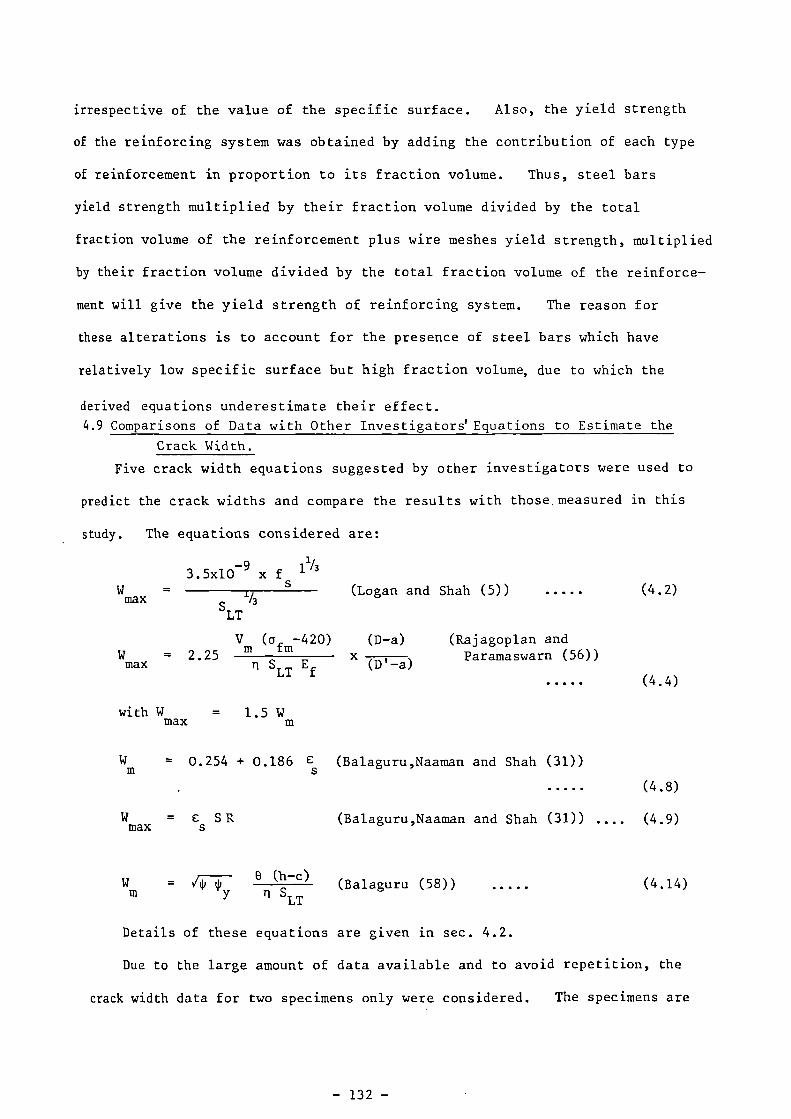
(Logan and Shah (5)) (4.2)max 1/
SLT
(Rajagoplan andParamaswarn (56))
(4. 4)
0 (h-c)Wm
ti,/7-Ep (Balaguru (58))y n s
LT(4.14)
irrespective of the value of the specific surface. Also, the yield strength
of the reinforcing system was obtained by adding the contribution of each type
of reinforcement in proportion to its fraction volume. Thus, steel bars
yield strength multiplied by their fraction volume divided by the total
fraction volume of the reinforcement plus wire meshes yield strength, multiplied
by their fraction volume divided by the total fraction volume of the reinforce-
ment will give the yield strength of reinforcing system. The reason for
these alterations is to account for the presence of steel bars which have
relatively low specific surface but high fraction volume, due to which the
derived equations underestimate their effect.
4.9 Comparisons of Data with Other Investigators'Equations to Estimate the
Crack Width.
Five crack width equations suggested by other investigators were used to
predict the crack widths and compare the results with those. measured in this
. study. The equations considered are:
3.5x10⁻⁹ x f 11/3
Vm (a -420)(D-a)
Wmax
= 2.25n s
LT Ef(D'-a)
with Wmax
= 1 . 5W
Wm= 0.254 + 0.186 es (Balaguru,Naaman and Shah (31))
(4.8)
Wmax
= Es SR
(Balaguru,Naaman and Shah (31)) .... (4.9)
Details of these equations are given in sec. 4.2.
Due to the large amount of data available and to avoid repetition, the
crack width data for two specimens only were considered. The specimens are
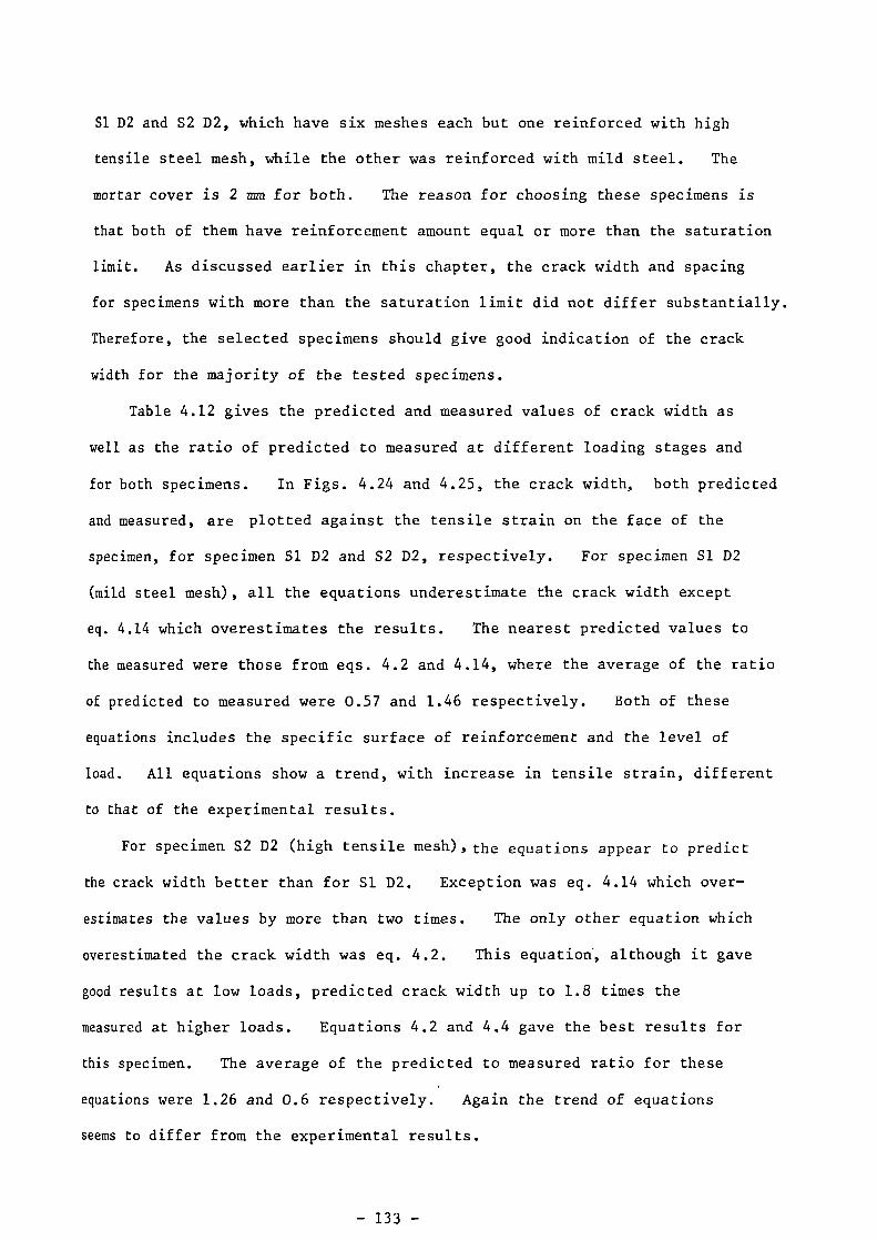
Si D2 and S2 D2, which have six meshes each but one reinforced with high
tensile steel mesh, while the other was reinforced with mild steel. The
mortar cover is 2 mm for both. The reason for choosing these specimens is
that both of them have reinforcement amount equal or more than the saturation
limit. As discussed earlier in this chapter, the crack width and spacing
for specimens with more than the saturation limit did not differ substantially.
Therefore, the selected specimens should give good indication of the crack
width for the majority of the tested specimens.
Table 4.12 gives the predicted and measured values of crack width as
well as the ratio of predicted to measured at different loading stages and
for both specimens. In Figs. 4.24 and 4.25, the crack width, both predicted
and measured, are plotted against the tensile strain on the face of the
specimen, for specimen S1 D2 and S2 D2, respectively. For specimen Si D2
(mild steel mesh), all the equations underestimate the crack width except
eq. 4.14 which overestimates the results. The nearest predicted values to
the measured were those from eqs. 4.2 and 4.14, where the average of the ratio
of predicted to measured were 0.57 and 1.46 respectively. Both of these
equations includes the specific surface of reinforcement and the level of
load. All equations show a trend, with increase in tensile strain, different
to that of the experimental results.
For specimen S2 D2 (high tensile mesh), the equations appear to predict
the crack width better than for S1 D2. Exception was eq. 4.14 which over-
estimates the values by more than two times. The only other equation which
overestimated the crack width was eq. 4.2. This equation ., although it gave
good results at low loads, predicted crack width up to 1.8 times the
measured at higher loads. Equations 4.2 and 4.4 gave the best results for
this specimen. The average of the predicted to measured ratio for these
equations were 1.26 and 0.6 respectively. Again the trend of equations
seems to differ from the experimental results.
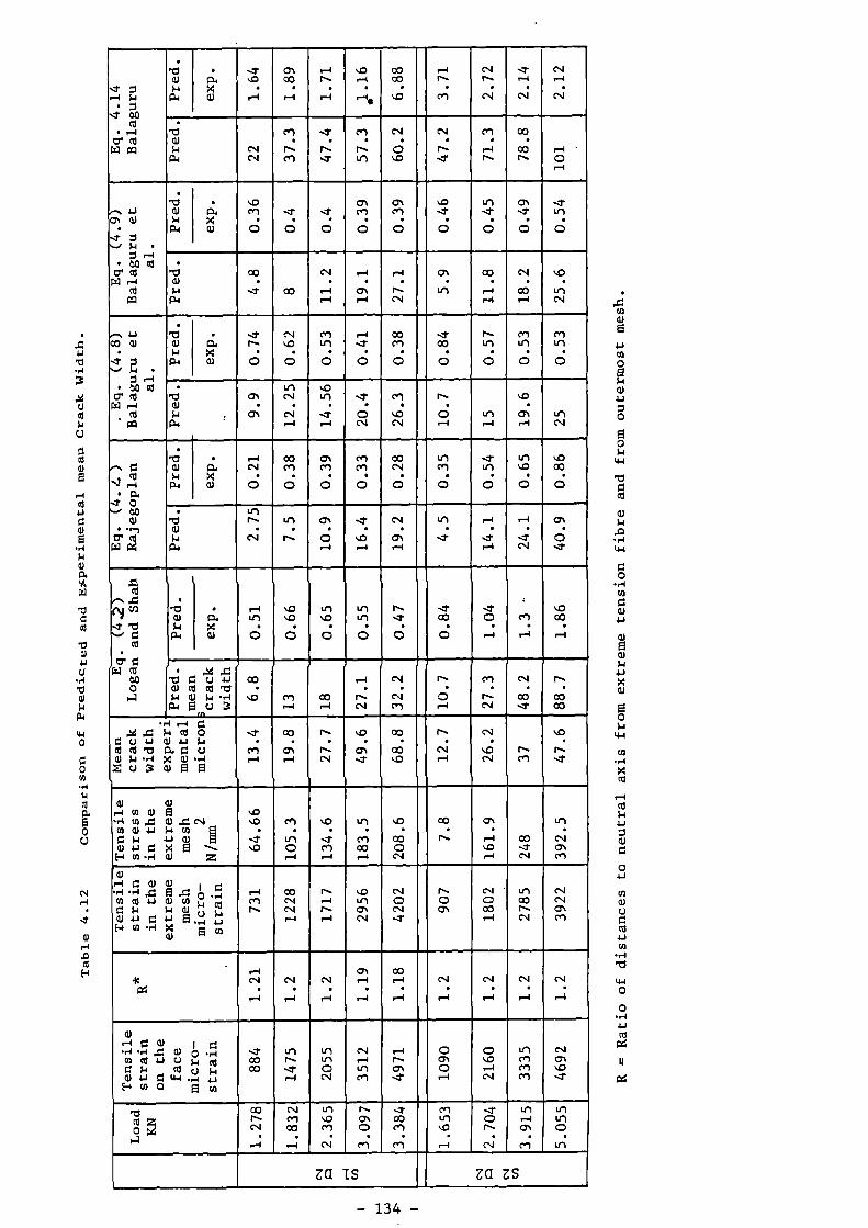
.-
.4' 0rl W
• 0..t OD
0• ,-.1Cr co41 go
•
CIP
;LI
•04>4C1)
....1- 011/40 CO
• •r-I r-I
riN.
•r-I
s,C)rl
•ris
co
CO•
10
1-1
IN•
Cr)
NJN.
•c4
...1-r-I
•C11
CNI
r-4•
NI
•'0aJw
044
ce)•
NI IN.csi cr)
..1••
N....?
Cr)•
r...ul
c'.1•
0
NJ
N.-...t
Cf)
•f--I1-..
CO
oo1-..
i-i .0rI
al a)•
..? 0
.... p0 r-I
• OD 0:1cr a!41 r-1
oPO
•710))4P.
•Ow>40)
.0rel ..t
• •0 0
.1••
0
01ce)
•0
CAcr-)
•0
‘0-1'
•0
Erl-4-
•0
ch...?
•0
.....?in
•0
•noaJ14
P.
co•
-a cocq
•,-)ri
t-i•
cmri
,--)•
N.c•I
cr.U'1
co•
r-Irl
CNI
00re
k0•
irtNI
eN 1.1CO 01
•-4. a.....• )., •
0 ,-I• bp as
0" 041 .--I
. alpl
•"0cl))4
ci•
•M.Xa)
...? cs.1N. 1/4.0
• •0 0
cn111
•0
r-I-4
•0
COcri
•0
...7c0
•0
Is-1Ei
•0
Cr)Lel
•0
Cel
ul•0
•"0a))., :
lie
inCT C11
• •a, csi
ri
voin
•-4-ri
-„,t•
0CNI
cn•
%.0(NI
i•-•
0,--1
Lf1rl
1/40
ONr••1
u-1C*4
.-.. oC0
Nt ,..1
-10..... to
(1)• .,-)
cf ELIW IN
a
wi.I
(.14
•0,X0)
r-.1 COC11 Cr)
• •0 0
ChC•1
•0
Crlre,
•0
COCNI
•0
Li')Cr)
0
.3-itl
•0
it'VD
0
4:3CO
0•
.4•
10O.)3.I
P•1
Lrir".• Ln
• •CC')N-
a.n•
0,-4
....••
N.0.-•
CV•
cr %rl
-
lf)•
I-N
.--1•
-.7,--4
n-I•
- .7C s)
al•o
--1*
-
0n
4-1 C11^0L •0
00
•IV 0
4.1 01o00
i-4
•Cl
•‘01$.
P4
•ca.X0)
-
.I rln %.
00
• •0 0
lf1/4)0
•0
u
if)l
•0
-
1`......1•
•0
-4.CO
0
0•
ri
,
Crl•
ri
CO•,-1
• ,- 4"0 0 C.) 4..•
CD 03 RI •1:1$.4 C1) )4 • ,-Iis• 0 u 3
fa
co•
s.0 Cr)rl
COrl
!
rl•
N.CV
C1I•
c4Cr)
IN
0rl
Cr)•
N.NI
C.4•
CO.../'
N.•
COCO
• 8-1 rl 0-. 4 )4 cd 0
Z C.) .1J 011 •J )4
o al -a 0. 0 u01 34 • ri X CI) • 1-1Z u 3 a.) 0 01
..1*•
cnrl
CO
01r-I
r•-••
INCs1
vo•
01...1-
CO•
COVD
r•••
cnIr-I
c9•
k0NI
N.Cr)
vo•
N..NI'
_
a) a)n-) to 01 e`,4 co 4 0) 4 cgca O 4-I )4 En g0 1.1 4-1 a) aa) 4-1 0 >4 e ---
E..1 03 • r4 01 Z
.0n0
•....1•.o
(41•
iri0ri
40•
.1-oiro
Ln•
cr)corl
n13•
CO0NI
a)
r•••
ON•
r-Iv.orl
CO-...tCs)
un•
NIanCrl
(11•- I O (31 a) i 0' ,-1 •ri 4 EE14 0 .
(4) o 4.1 0) CO 14 00 14 )4 a) „a) 4..) 0 4.1 0 4 4_,
E-4 u) • rl X s rn0)
,-1Enh
coCNIosir--I
N.rih.rl
qoEncr,NI
cg0C-.4...?
-
N.0a,
CV '0corl
inc0hCs)
c..)NI0.Crl
.
•X04
r-IC")
•r-I
C")•
1--1
EN•
rl
01r.
•r-I
COr-i
•r-I
cNI
r-I
cv•
r-I
c.I
rl
cs1•
r-4
01.--1 0 1:11 I 0',I "-I 4 a) o . 1-1
En 0 4-) CJ 5.1 030 )4 0 c.) }.I0) 4.) 0 14.1 .,-1 4..)
E-I ui 0 0 cf)
•••1/41-coCO
inr--...1.r-I
1.41Li,0C11
esi•-.1LnCr)
,.-.1N.aN-.1-
0010rl
010,--4N1
WI("'")cnCrl
c.)CM%.0-4'
•0
2.4
coN.NJ
.••••1
Cn1Cr1Co
r-i
V)n.0c."
•C•i
N.010
•C'')
...I.COm
.Cr')
Cr)it).0
r-I
•-.1'0N.N
•CV
(r11--1a,
C,1
Inin.0
•Lr)
za IS ZG ZS
- 134 -

X
k\
I I I 0 0 0 0 0 0c• in q m (N
• SUOJDN/N 'WM
oooU)

0 •0tr)
SUOJDIW 'W, ylp!m pon uoavl
X
'Ct
0

Equation 4.2 gave the best combined results for specimens Si D2 and S2 D2,
with ratios of predicted to measured crack width of 0.57 and 1.26 respectively.
4.10 Comparisons of the Derived Equations with Other Investigators' Results.
The only data on crack width available in the literature were those of
Balaguru, Naaman & Shah (31). Combining some of the graphs with the tables
in that reference and by assuming the depth of the neutral axis for specimens
reinforced with woven mesh are the same as those reinforced with welded mesh
at the same load, the data in Table 4.13 was found. The derived equation was
used in the following form:
For SR < 2.85 — 3.5x10
-3 a
W /c = 43.7 — 50.9x10⁻³ a — 9.3 S
Rm t
For SR2.85 — 3.5x10
-3 a
Wm/e
t= 22.1 — 24.4x10
-3 a — 1.73 S
R
The effect of the cover was neglected due to insufficient data. The
1 1 iresults for specimens reinforced with / 4 in. woven mesh and /2 n. welded
mesh were tabulated in Table 4.13 and plotted in Figs. 4•26 and 4.27.
From Fig.4.26 it can be seen that the derived equation gave very close
results for the specimens reinforced with woven mesh. The average ratio of
predicted to measured was 1.02. For the welded mesh specimens, although
the derived equation was based on woven mesh it could still predict the mean
crack width reasonably closely (Fig.4.27). The equations overestimate the
results except for the specimens with 6 meshes where they underestimate
and show higher error. However, the experimental results of this specimen
are inconsistent with the other results. The crack width would be expected
to decrease with an increase in number of meshes, while the experimental
results of the 6 mesh specimen showed a higher crack width than the 2 mesh
specimen.

— 138 —
'Vcoa.)U
• H
a)$4
P4
'VtiJW0Cl,00n)Z
.00
•r-I
in en .001 H.I 0
• • •0 l•-n ri
1/40 1/40CT 01
• •0 0
coNI
•1-1
enI-I
•1.--4
en1/40
•1-1
cVN.
•I-4
1/40en
•r-I
NI 00 r--I
• •r-I 1-1
0Crl
•0
Lnin
•0
N.1/40
•0
CO0.) 4E 4J
71 0'V • r4 0a, 3 p
4..i cic.) ..- •,-1
• A C.) E"0 crla) $4W U
114
tn•
encN
....? cv CO• • •
h. LO N.cNi cn-.."
NI rn• •
01 en,--1 en
CT•
LOH.I
CO•
N.NI
Cr,V)
CO
CO 10,-.1
•
N..
...I ...1CV C'n
0
LO
Ill
1/4e1.-I
e1/4.1
st)Cn
0c13al 4
-0-0 • •-I 00.) 3 0w $.4
..- CJJ) CJ • r-irti ti ea) $4Z ci
cv•
cNINI
N. NI•
Co cv or)NI en -.
CO
0...7NI en
NI•
enI-4
1/40•
.....7NI
HA•
1/40Cn
I—I•
tn
N.•
•-1r--I
en••—i •—iNI en
c0
con1-1
•—i
coNI
en
-..i.tr)
0 a) 0• .-1 E • riCOO) eaW 14 4-I4..) 4-1 Q) 4.J
II) >4 4-4 cn(1) ..10 En 0
a) ••-i W -.1.--I 0.1 4.1 C.)• H X • H
CII .1-) E0a) 0
EH • H
0co,..1en
Lr) 0 00 01 LON. CO ..../.
en -7 N.0
0000 0N.) N.C'l Li-)
0-....7....1-•—i
trl1/40enNI
'00NJ0in
1/40n—i•—)
LI')0•—iN
00Ln N.c0 -4-N -4'
en,..0cr.
-.70inNI
0....1-ooin
c1:1)•,-1 E 0
cd a) i-1 •,-4$4 W a) et4.1 a.) p..., Ww X ea a.)
GI I-I U) cri0) W 0
..--1 0) ,a $.4• H ...a CO C.)
Cr1 4-1 CI • .-40 E0)0H -H
0CAN.cs.,
0 0 inin 01 1/40C1/41 CV 1/40cn .....1. in
in 0N. 0CO 0NI in
00NI r-4NI 0r-I NI
00ennI•
I-In0oN
0inN.,-I
0 0CO tr)en N.NI en
0a.N.
0N.0NI
0N.CO-4'
LI-I I00)
U U en•,-+ a) w4-4 u 0 1-)' H CO 4-1 0 pd -...,..CJ LH 0 0.) CO CVa) • r-I E1a• 0 01
co en $.1
EC.)
Ec.)
CY1N.
,--1
01n.0
cv
CO
cz)
1/40
•--I
-.I-.
csi
4.40 0
cr, aJ1-1)1) Eal 4 • ,-14 Cn 0 UE CU • HI G)0 E 0.Z Cl)
-4- 1/40 NI .....1" nO
-0,-14v)W4-10,—.
• H 0.0 0 ON0 • • •-iCI) 0 Cd E
4 k I-1 "-n
CI) Ul 00 COZ.....,
Z .....1-
n.1-
inN.
en•
(NICO--.1•
4.40
.0
Pa a)>1 EFl
17Lis an u anom /ui IlseN Pa Pi aMII
Z4
I.

50
40
- 303
0
20
a
100
0
4 meshes experimental opredicted •
6 50-6 meshes experimental 0
._oL. predicted •eE, 40-
3
t 30
L 20aua ..----------a02 10
0 ' '2000 3000 4000 5000 6000
Tensile strain on the face, is
Fig.4 . 26. Comparison of experimental crack width data from Balaguru et al.(31)and predicted using derived equations, 6 . 35mm woven mesh.
2 meshes (measured Alpredicted A
4 meshes (measured opredicted •
60
1000 2000 3000 4000Tensile strain, microstrain
Fig.4•27. Comparison of experimental crack width data from Balaguru et al.(31)and predicted using the derived equations, 12-5mm welded mesh.

Except for the specimen with 6 welded meshes, the derived equation gave
results of similar trend to the experimental ones.
4.11 Conclusions.
Based on the tests carried out in this investigation, the following
conclusions are drawn:-
1. The cracking behaviour of ferrocement plates is characterized by
almost full development of the number of cracks at relatively early stages
of the load. Most of the cracks found after failure developed at about
30-50% of the ultimate load, and this is a feature which distinguishes ferro-
cement from ordinary reinforced concrete with steel fibres. The major
features which distinguish ferrocement from reinforced concrete are that the
former shows uniform crack width distribution with the peak more or less in
the middle of the range of the crack width, while in reinforced concrete
several peaks form with increase in the load and the highest one is nearer
the smaller range of width of cracks. Also, for the same tensile strain,
the maximum crack width in reinforced concrete can be up to 4 to 5 times
higher than in ferrocement.
2. The mean crack width increases linearly with the average tensile
strain on the face of the specimen. The slope of the linear relationship,
Ve t' is called, appropriately, the rate of growth of crack width, and its
value gives good indication of the cracking performance of the specimen.
3. The mesh yield strength influences strongly the crack width and
gracing. For the same mesh opening, high tensile steel mesh results in
specimens with lower rate of growth of crack width and smaller crack spacing
after failure than those with mild steel mesh.
4. Irrespective of the type of mesh, increasing the number of meshes
in the specimen decreases the rate of growth of crack width, and the spacing

of the cracks before and after failure. This decrease slows down appreciably
at a certain number of meshes. The number of meshes is six for specimens
with mild steel mesh and four for those with high tensile mesh, corresponding
to specific surface of 2.1 and 1.5 cm2/cm
3, respectively. These amounts of
reinforcement are called the saturation limits as the rate of growth of
crack width does not decrease appreciably with further increase in them.
5. The crack width and spacing are influenced by the mortar cover and
the section depth. For 6 mm cover the rate of growth of crack width and
the average crack spacing were about 1.5 and 1.4 respectively, times that
for 2 mm cover. For reinforcement amount equal to the saturation limit of
mild mesh, there appears to be an optimum section thickness which shows the
most favourable cracking behaviour.
6. In terms of the rate growth of crack width, the enhancement in the
• cracking behaviour for specimens reinforced with mild steel wire mesh over
those reinforced with conventional steel bars, and for the amount and type used
in this study, starts when the mesh . number exceeds four. The high tensile
mesh specimens showed better cracking performance even with 2 meshes.
7. Concentration of the meshes near the extreme fibres of the section
does not result in an enhancement in the cracking behaviour over those with
uniformly distributed meshes.
8. Combination of steel bars and mild steel mesh reinforcement gives
a cracking behaviour somewhere between that of mild steel mesh only and high
tensile steel mesh only. Replacement of the middle third of the meshes in
the section by steel bars did not, at least, result in deterioration in the
cracking behaviour.
- 141-

CHAPTER 5.
LOAD AND DEFORMATION CHARACTERISTICS.
5.1 Introduction.
As the interest in ferrocement as a structural material grows, the
demand for understanding, fully, its properties and behaviour grows with it.
On the other hand, ferrocement has been considered, mainly, as a form of
reinforced concrete and many of its strength and deformation characteristics
were assumed to be the same as those of reinforced concrete. But, in spite
of the similarities between the two materials, there are still major
differences between them. These include the subdivision and distribution of
reinforcements, the mesh shape of the reinforcement, the smaller section
depth and mortar cover, the many types of mesh with different geometry,
material and strength properties practically used in ferrocement, etc. These
differences raise the question of whether the behaviour of ferrocement sections
under loading will be different from that of reinforced concrete, and what are
the influences of these differences on the strength and deformation character-
istics of the material.
The most commonly agreed aspect of ferrocement behaviour is its better
cracking performance compared to that of reinforced concrete. This suggests
that the limitation on the crack width for the serviceability purposes will
be less critical. But one cannot conclude that the serviceability load
would be higher than in reinforced concrete unless the deflections prove to
be less critical as well.
It is therefore clear that the tracing of the behaviour of ferrocement
section under load and the study of the load and deformation characteristics
and the relationship between them are very important. It would identify
the differences between this material and reinforced concrete and help
greatly in setting the basis for the design theory of ferrocement.

In this chapter, the influences of the different variables on the load
and deformation characteristics of the ferrocement plates were studied from
first application of the load until failure. The variables included the
reinforcement amount and yield strength, presence of steel bars, mesh opening,
section depth, and mortar cover. The relationship between the load
deflections, strains, and crack width specially during the possible service-
ability range were also investigated.
5.2 Review of Literature.
The work (26,30,31) carried out on ferrocement showed that the behaviour
of the material under load can be divided into three main stages, namely, the
elastic, the elasto—plastic, and the plastic stages. In the elastic stage,
the material is uncracked and Nathan and Paramasivan (23,66) have shown
that it is homogeneous. The end of this stage is marked by the first cracking.
Some investigators (18,25) had suggested expressions to predict the load or
the moment at first cracking directly from the specific surface of reinforce-
ment. However, this could not be verified in this study, see Fig. 4.9.
Nathan and Paramasivan (66) from their tests, concluded that the moment at
first crack in flexure depends on the area of reinforcement, thickness of
the specimen, proof stress of reinforcement and modulus of elasticity of the
conTosite.
The second stage, i.e., the elasto—plastic stage, is characterized by
multiple cracking of the section (31). Bezukladov et al. (5) have found
that the stresses, elongations and modulus of elasticity of ferrocement
during crack formation are affected, mainly, by the amount of reinforcement
expressed in terms of the specific surface and fraction volume. For the same
specific surface, the presence of steel bars did not influence the elongations
at the first visible crack. Bigg (4) reported different design values for

the modulus of elasticity recommended by different investigators. In his
analysis of ferrocement beams, Bigg suggested that in flexure the modulus
of elasticity of the compressive .zone is different from that of the tension
zone. He also gave an expression to predict the modulus of elasticity in
bending from those of the material in compression and in tension and
recommended that expression for the use in establishing the load-deflection
relationship.
The plastic stage is characterized by yielding of the section and rapid
increase in the deformation until failure. Bigg (4) described the failure
offerrocement section as ductile and of a nature similar to that of under
reinforced concrete. However, previous work (12) showed that ferrocement
sections of different amounts of reinforcement exhibited different failures.
The ultimate compressive strain at the outermost fibre of the section is
gieatly higher than the value used in the design of reinforced concrete (12,
18,31), i.e., 0.0035.
Several investigators have developed theoretical procedures to
establish the load-deflection or the moment curvature relationship.
litistriaco et al.(29) have presented an analysis for the inelastic behaviour
of ferrocement slabs in bending. The slabs behave essentially as an .
elastic-strain hardening material with limit surface. Its moment curvature
can be idealized as a trilinear curve. Near ultimate loads, the deflection
of slabs can be approximated by an elastic-perfectly plastic bilinear
analysis. Limited experimental results showed to be in good agreement with the
theoretically predicted values. Balaguru, Naaman and Shah (31) predicted
the load-deflection and moment-rotation relationship for experimentally
tested. beams. Their procedure depends on a non-linear analysis and using
the stress-strain diagrams of the two major constituent materials. Paul
and Pama (11), using the theory of composite materials, have suggested a
procedure for the analysis of ferrocement sections. The load-deflection and
the moment-curvature relationships were again idealized to trilinear behaviours
and developed using the predicted mechanical properties of the composite.
It can be seen, therefore, that a large amount of work has been carried
out on the load-deflection and load-curvature relationship. However, several
other aspects of the deformation characteristics have drawn less attention in
spite of their prime importance. These include tracing of the deformation
characteristics from first application of load until failure and perhaps more
important, a quantitative study of the relationship between the different
aspects of the deformation to establish the serviceability criteria. Also,
the influence of the different variables encountered in ferrocement on the
response of the section to loads needs to be known.
Walkus (30) has made an attempt to relate, quantitatively, some of the
deformation characteristics to each other. He divided the behaviour of the
member according to certain limits of crack width and recommended the
corresponding stresses, strains and modulus of elasticity,(Table 1.2).
However, Walkus generalized these limits and assumed them to be applicable
to ferrocement beams irrespective of the properties of the section and the
reinforcement. Such an assumption, as seen in Chapter 1, is not valid.
It therefore follows that more work is needed to fill the knowledge gap in the
deformation characteristics of ferrocement and if the superior performance
of this material lies in its ability to satisfy the serviceability criteria
at relatively higher loads (67) then there is even more urgent need to find
these criteria and to base the design on them.
5.3 Experimental Programme and Test Measurements.
The deformation measurements from first application of load up till
failure were taken on the specimens of the seven series described in Chapter 3.

The variables in these series are the number, yield strength, and opening of
the mesh, presence of steel bars, section thickness and mortar cover. The
measurements included the tensile and compressive strain on the faces and
sides of the specimens and the central deflection. Full details of the
instrumentation and the test programme are given in Chapter 3.
5.4 Behaviour of the Plates under Loading.
Upon initial application of the load, the plates responded elastically
and were free from any cracks. While the load was increased incrementally,
the first crack was detected visually using a magnifying glass. Near the
first cracking, a small drop in the load was noticed during the loading pro-
cess. This indicates that certain amount of plastic deformation due to
cracking was suffered by the specimen, resulting in some release of the load
in the proving ring. The first crack width was measured for several selected
specimens and found to be as mall as 3 to 6 micron in width. The load at
the first crack varied with the thickness of the specimen as would be
expected. However, for specimens 25 mm in thickness,this load varied between
0.7 to 1.47 kN. The mean ratio of the load at first crack to the load at
failure for all specimens was equal to 0.194 with standard deviation equal
to 0.11. The range varied from 0.08 to 0.6 depending on the type and number
of meshes. This large variation is due, mainly to the variation in the
ultimate load rather than in the first crack load.
Soon after the first cracking, although a small drop in load every time
it was stopped, still takes place, the plate retained partially its elastic
response to the increase in the load. The first cracking was followed by a
rapid increase in number of cracks. The range of the load at which the
number of cracks continued to increase depended on the amount and yield strength of
the reinforcement. In general, most of the cracks found near failure, were
developed at 30 to 50% of the ultimate. After a certain load, the increase
in the number of cracks slowed down considerably accompanied by more rapid
increase in the crack width marking the start of yielding of the specimen.
During the range between first cracking and yielding, all cracks were very
fine and only by a close look could they be identified. Yielding of the
specimen was accompanied by a large amount of deformation. The crack width
increased rapidly but uniformly showing no sign of local yielding. Near
failure a few cracks widened more quickly than the others and one of these
cracks initiated the failure of the specimen.
At failure a compressive strain on the face of the specimen up to 7000
microstrain and central deflection up to 12.5 mm were measured. This value
of compressive strain is twice that used in the design of reinforced concrete.
The measured ultimate compressive strain and ultimate deflections varied
considerably depending on the type and amount of reinforcement which also
seemed to influence the mode of failure. Three types of failure were
observed. These are tensile failure by fracture of the wire mesh,
compressive failure by crushing of the mortar and compressive and tensile
failure by fracture of some of the wires in the mesh accompanied at the same
time by crushing of the mortar. Some specimens suffered premature failure
by splitting of the mortar cover in the tensile and the compressive zones.
The different types of failures will be discussed in detail in section 5.8.3.
However, it is to be mentioned here that Biggs (4) suggestion that ferrocement
beams fail in a similar mode to those of under reinforced section does not
seem to be valid for all specimens. The mode of failure appeared to be
controlled by the amount and yield strength of the reinforcement.
5.5 Load-Deflection Relationship.
The central deflection is plotted against the total load and the curves
are shown, for all specimens in Figs. 5.1 to 5.8. From these figures, the

load-deflection curve for ferrocement can generally be divided into four
stages. In the first stage, the specimens behave elastically, free from
cracks and the load-deflection curve is linear. The range and slope of
the linear relationship was not influenced appreciably by the variables
studied in this investigation. The end of this stage is marked by first
deviation from linearity and the deflection/span ratio at that moment is
mostly less than 1/360.
The second stage of the load-deflection curves corresponds to the elasto-
plastic behaviour of the specimens. The first crack was visible at the
beginning of this stage. The load-deflection relationship was again linear
but with a slope lower than that at the first stage, showing the expected
reduction in the specimen stiffness due to cracking. However, the linearity
of the relationship indicated that the reduction in the stiffness due to
cracking progress through this stage was, at least, not reflected on the load-
deflection characteristics. The cracks, in this stage, increase in number
more rapidly than in width which could be one of the reasons for the less rapid
reduction in the stiffness with increase in load. Linear regression was
carried out on the load and deflection values at the second linear stage.
The slope and the correlation coefficient of the best fit line for the
relationship were found. The correlation coefficient for all specimens
were more than 0.999. This indicated the high degree of linearity of the
relationship and the elastic response of the plate under load. Therefore,
it appears that it is reasonable to assume that the section behaved
elastically in this stage with a reduced modulus of elasticity.
In Fig. 5.9, the slope of the load-deflection curve at the second linear
stage, which could be considered as a measure of the plates stiffness at this
stage, is plotted against the fraction volume of reinforcement in the loading
direction. The results from series Si, S2, S3 and S4 only, were included as
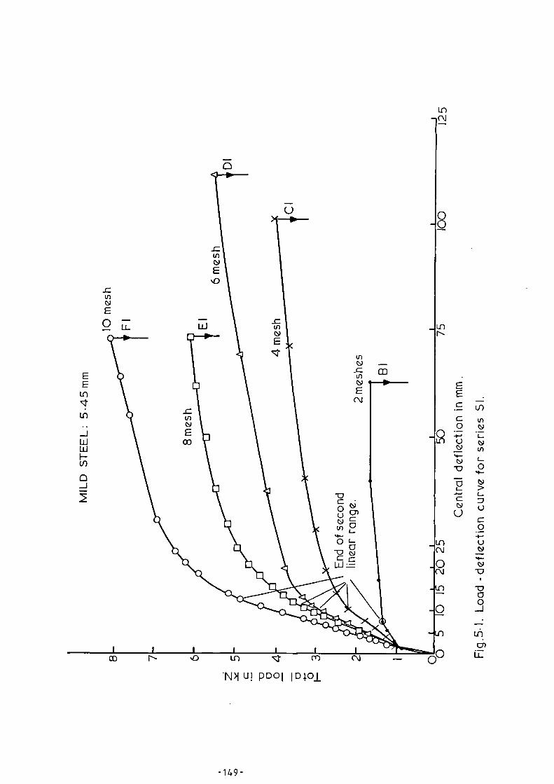
• N Li! ppoi
-E
ao (9
o0:9 cr)4-
0
>c_7
Q.)
0. --4-0
4-0
00

(N
CIO EEC--C0
• -4-U0_
0.0--.0L.
4a.0U
q• N1 u! ppoi plot
-

coU
In-TV—
oo
-000
_J
I I I I I LI-CO N 43 ID Cr Cr) C\ I
-
coco
.N1 u! poi lolcu_

coLL
- I
(J")
In
0 0003UU00Luu_I- CV CV CV CV CNN CV CV
(r) (f) (f) (DU-MU) U")
4DX OxI>X0x
(-.9
0 co N,c) LC) c Cr)
• N>1 u ! ()Doi ploi

_
_
EEa•_a
cv -
• N>1 u! pm)! !Di.oi
00

2
• N1 LI! pDOI

LC) Cr)
• N>1 Li ! ppoi
-155-

• NPI (.1 ! P poi pio±

the specimens of these series have the same section thickness and mortar
cover. The figure shows that the slope of the load deflection curve
increases with the fraction volume of reinforcement in loading direction
and the relationship can be assumed linear. Specimens from series S4,
where the reinforcement consists of wire mesh and steel bars gave, for the
same fraction volume, relatively higher slope values than specimens with
wire mesh only. This could be attributed to the higher modulus of
elasticity of steel bars compared to that of the wire mesh. In general
the stiffness in the elasto—plastic stage does not seem to be influenced
appreciably by the mesh yield strength, specific surface of reinforcement,
or mesh opening.
The load, and maybe to a less extent, the deflection at the end of the
second linear range varied with the studied variables. This variation
will be discussed in section 5.8.2. The end of the second stage is marked by
the deviation of the relationship from linearity. This indicates the start
of yielding of the specimen where the third stage of the load deflection
curve starts. In this stage, the relationship is curvilinear. The
cracks start to increase in width more rapidly, propagate deeper into the
section, and their number reaches almost a saturation limit. This stage
ends when the specimen is fully yielding where the fourth stage starts.
In the fourth stage, the relationship is again linear with the line nearly
horizontal. This stage is characterized by rapid increase in the
deformation, which soon leads to failure. The deflection just before
failure, i.e., ultimate deflection, varied from one specimen to another and
seems to be affected strongly by the mode of failure of the specimen and
this will be discussed in detail in section 5.8.3.

I00co
N00---. 4-,o Go0
0_J-(11L.
<1 \
(7n- N Cr) 'I
X CI)W* O (1)<1
>:
. _4-0c —.-
7)C
Cu
u 0\
0 - CO-0
L.
C0)
(9 U
.0
tr)u
u
<1 7)—
O
—._-,-•c
c
0 00
D c
>
U u
d
\
<1 \ N E o (9u — Uu
O 0
t CS) 4.-
d c E
—c• X c
\
*u- Pt"r....
-0'0 O u
u u
u OE- - E — =
• u —,O 4--• >>
a:
I I I I ,00 0 0 0 LiLC) 0 1.11 0 LnN N _
'ww/N Li! ,Dtyd 2) iuno uo!IDallap -p poi lo adois
CX 0
C
c:;)LE

The part of the load deflection curve after first yielding, i.e.,
after the second linear stage, for specimens of series S2 were different
from the rest of the series. In this series, where the reinforcement
consisted of
high tensile steel mesh, full plastic behaviour was not
realized for specimens with four meshes and more. This is due to the
yielding characteristics of the mesh. As will be discussed later, the
first yielding of the specimens was due to yielding of the mortar in the
compression zone rather than yielding of the mesh in the tension zone.
It therefore follows that the yielding behaviour of the specimens is
determined mainly by the yielding characteristics of the reinforcements.
5.6 Load-Strain Relationship.
In Figs. 5.10 to 5.17, the total load is plotted against the average
strain on the tensile and compressive faces for typical specimens from each
set and for all series. The figures show clearly the different stages of
the specimen behaviour under loading discussed in the previous section.
The first two stages are again shown to be linear. The slope of the first
linear stage is almost the same for all specimens, while the slope of the
second linear stage varies with the amount of reinforcement. This indicates
that the effect of the increase in the amount of reinforcement becomes
significant after the first cracking of the specimens. The slope of the
second linear stage was, as in the load-deflection relationship,
determined mainly by the fraction volume of reinforcement in loading
direction. The specific surface of reinforcement, presence of steel bars,
mesh yield strength, and the mortar cover did not have a significant influence
on it. The plastic stage is clear and distinct for all specimens except
those of series S2 where the reinforcement was high tensile mesh. The
load-compressive strain curves for the specimens of this series were very

dL(:).6a_
,I I 1 I I i
.c) Ln cr co N -
• Nlip poi pio±
-160-

_oo0N
o- 0
O ..0 c• _
0L.—
cl N ul
Ca 0 °I_N 0 uts)
_._LS,
21 E_
-
U")•+-
O0
tnU (9
L.) >cr) 0 L._
9- DUd
_C C4- 0
O c_0o U,_
O c d
(- \.I ' - :-O a•
L.. C
in ty
(9 1O 7-
LT1 -0_0 C 0
O ()) 04.. -I
d05-O (i)(9> 01
I I I I I I I < LEco N .o In q co
CV -
'N>1 ui pool loloi

_
(N1
L11
Cr)U)
-
-
nI
oo9)
N '0 0 ct co
CV -
. i\p, e p D o I 1 Dlcu

rn .0 if) cy
. NPI ' PDOI IDIO±
- -163-

U) ct ol
'N1 ' P p ol 1 DI oi

C•_ag...In0L.U•_E
st cr)
'N>1 1 P D0 1 1D40±
-165 -

Npi t pool ploi
0_ 0
0..(3
ONGO N n0 Ln cr cv -
-
_
_
_

In0)
I I I I I I I I sLE.
ch 03 N ,C) LO 'sr Pi
CNI
N1 ' p poi ioloi
-167-

similar to their load—deflection curves. There was a linear stage and
at the end of it, the failure took place. In the load—tensile strain
curves for this series, the second linear stage extended up to about 6000
microstrain after which the curve started to deviate slightly from
linearity.
For the specimens with mild steel reinforcement the load—deformation
curves are very similar. Increasing the amount of reinforcement in terms
of the fraction volume increases the load at any specific deformation.
5.7 Relationship Between Cracking, Deflection and Strain.
It was shown in previous sections that the reinforcement amount and
their yield strength are the major factors which influence the load and
deformation characteristics. In Table 5.1, the load, tensile strain on
the face of the specimen, mean crack width, and mean crack spacing are given
at different deflection values for specimens with different number of meshes
from series Si and S2. The range of deflection values covers the elasto-
plastic stage and for some specimens covers some of the yielding stage as
well. From the table, it can be seen that for a given deflection, the
man crack width and mean crack spacing decrease as the number of meshes
in the specimen increases and this is true for both types of meshes. The
load was increased with the number of meshes while the tensile strain
did not vary appreciably with the number and yield strength of the mesh.
A comparison of Table 5.1 and Figs. 5.1 and 5.4 shows that the mean
crack width within the elasto—plastic stage remains largely below the value
of 50 microns. If this value of mean crack width is taken as a critical
limit, it would appear that as long as the specimen did not yield then the
crack width is unlikely to exceed this limit. A load of about 0.6 to
0,65, for mild steel mesh, and 0.4 to 0.5 for high tensile mesh, of the

cVCl)
v.r-IWWUU)
•0rl0)
.HPN
400
.H
0;)Cll 10 0 0 0CO rl C•4 • •
• • co 00rI0 rIN
I's CO 0 L.0 1.0rl N \C) • •
• • r.... n.. ..3-MCDH-11-11-1
0 \ Cli 0 CT C•4CO Ca) r'.. • •
• • i.0 ...1. C'l..70NNH.I
i.0 L-4 a r-• C•4OrN in is) • •
• • 1".• Cr) N1.11001C1H4
10
Ln 0 0 .0r`• rH Ln • •
• • rH -Zr NrA CD ,-4 r4 CV
cl, in Lo 1-4 0rn cs1 .../- • •
• • •-.1 CV inCV C) CV CV r-.1
CO in 0 rl COCO cn -4 • •
• • (-I ,--1 ce)01 C) 01 01 ,..4
CT 1C) 0 ill CO0 -Zr ....7 • •
• • .....t CV CVIn C) cl 01 I.H
-Zrco-4-00.0-Zr 1-4 0 • •
• • C) 10 011-1 C) r..I r4 r-I
rAmcomLn- C1I 0 • •
• • Ca) C•4 CON C) CV 01 1-1
001-401.(10CV C'l N • •
• • n.I r"•• CO01 CD 01 -Zr r.4
rHOCDODCDCs4 -Zr 0 • •
• • nO N 10-Zr CD -....t U1 rA
CVIn 01 CD 1/40 01rA CV -Zr • •
• • .--1 Lrl 0r4 0rINM
00 ....7 CD 01 CDrn cn qD • •
. • cv 1`.• COrION.ZN
rH rn CD -Zr. C).7 ..7 C) . •
• • -Zr 0".0NOCni40N
11111
Cl).
NHa)a)UW
-0rl• r4Z
o,A
01 cr% 000,-I (-Ni to • •
• • 0 CV cVCV C) r-i rA Cq
-..i. co 0 in 0.1ON....t VD • •
• • ,-I -Zr r•-•01 C) CV Cq 1-4
LID In 0 0 inin ilD C•4 • •
• • In cn inin C) 01 01 ,--1
11111
coIn co co In •--iN. C•4 04 • •
• • Or--Ln,-10,-1,-iN
0' 000 0,0 in h. • •
• • 0c•40MOcqmcN
cl, in 0 ...1• h•01 1/40 C•4 • •
• •,..70cnMOml-nr-1
11111
1.0in •--1 o c..4 r"-•I's C'l CO • •
• • Oin c•1.-1 0 •-n r-I CNI
-Zr r4 0 CO riCO In .0 • •
• • CV •-n r-4CV 0 C*4 Cn CA
1.n• C•4 0 ...7 C'l...1- 10 0 • •
• • in 0, 0Cn 0 C'") ••4" CNI
e
11111
-.Zrrn 01 CD Cm 001 01 C4 • •
• • 0.% r4 r-H,-I c) cv cn
00 w..4 C) -Zr. CVCD In 04 • •
• • CO en 1".•cs•J 0 e-4 -Zr C11
CV ,-.1 CD CT CVIn VD VD • •
• • 0 N InC•4 0 en 1"••• C•4
11111
NIn in 0 r-I 0r-I n0 0 • •
• • n10 VD 01,-4 0 "-I CV
-Zr. In 0C\ Inc•1 r*-- 0 • •
• • cn -Zr r•••rA C) 1-1 01 C4
CT CO 0 NJ' incq 1--- -Zr • •
• • In rA N-1.-.1 C) r.-1 Zr•• CV
11111
.0U)wZ440
a)
fa.>1H
4coa)ZLH0
•0Z
,
. .0 co
• al E 0ca a • .-IW U44 a it(I) 4 (3.1
•Ii I.i)0.) -0rq . H•,-i Ci
• U) itLIS 0 ..- 3-10 01) U c.)Z ,-I 4.., tt
.- 3-1 a)• )4 CJ 60
. „L.J as al"0r-14-1 0$4ctl $-1 W cll0 0 O) >o4ZZ*.:C
U)
. .0 tt"-E 0WM.•,4W U4.4 a (13U) v- ran
H U)a) "0r4 . H ,14• r4 c.)
'U) RSra 0 .hd )40 (1) L.) c)
z •-•I 4-) cd,._ )-I a)
• W U al. 4.1 cr3 Cri
ID1--14-10Wco o )-4 of a.)0 0 a) p,14Ns.Z.,
,
a0
•,-I 5WM.PH a 5U) ..a
4.1C1) "0 a
e-I • /-I b.1:1•,-1 3 0
•0 if) • rl0 0 ... u0 (1) c..) ct)
Z •--I 4-1 cr, 0,,,.. )4 Lo
• $.1 u"-I CCI ,4
TI,-4.1.J00ca o )4 0 oto 0 C) 1.41-1ZZU
,
...0
• n-i 5Wm.1-i
.1..) . sU) ...0 E
4.10.1 "0 a
1-1 • rl al• al 0
-0 w •,-1(V G .. c.)0 W C) cd
z ,-1 u oi cl,... i.i co
• w u4-I CI .-
1:11-14.10ca 0 1-1 ca al0 0a) S-t
1-INZZU
00
..-14-1C.)
,(/), 0
44a)A
r-I•
in
•0r-I
Cf)•
Ulrl
i'l•0C•4

ultimate load will also satisfy that limit. On the other hand, if
deflections were the governing factor, and assuming an allowable deflection—
span ratio of 1/180, it can be seen from Table 5.1 that at a deflection of
5.1 mm (deflection—span ratio of 1/177) most of the mean crack width values
are less than 20 microns. The load at this deflection value is about 0.28
to 0.33 and 0.14 to 0.23 of the ultimate load for specimens with mild
steel mesh and with high tensile steel mesh, respectively.
It follows, therefore, that the serviceability criteria is most likely
to be governed by the deflection rather than the crack width. If that is
the case then, high tensile mesh is not economical to use in ferrocement
as its higher cost cannot be justified by higher service load. It should
be noticed that if deflections are the governing criteria, then the service
load is about one third of the ultimate load. This is a very small value,
specially if one considered ferrocement's main advantage over reinforced
concrete is its relatively higher service load (67).
It is to be mentioned that the values of mortar tensile strain assumed
by Walkus (30) for different crack width values for ferrocement in bending
(see Table 1.2) are significantly smaller than those found in this study,
Table 5.1. For example, Walkus reported a tensile strain of 650 micro—
strain corresponding to permissible crack width of 50-100 microns, while
from Table 5.1, for such crack width the tensile strain would be more
than 3000 microstrain. Also, according to Walkus (30,38,44), the yielding
stage starts when the crack width exceeds 100 microns, i.e., when the
tensile strain exceeds 650 microstrain and this value of strain is smaller
than the yield strain of the mesh used in this investigation.
5.8 Effect of Variables on the Load and Deformation Characteristics.
The effect of variables on the load and deformation characteristics
was investigated by studying the load and deformation measurements at the
— 170 —

turning points of the load-deflection curve, i.e., at first cracking, at
first yielding, and at ultimate. The first cracking and first yielding
stages were considered, not only because they represent the points of
change in the behaviour of the section, but also they give good indications
of the load and deformation characteristics all through the two linear
ranges of the behaviour. The load and deformation characteristics at each of
thethree points are discussed, separately, in the following sections.
5.8.1 At First Cracking.
The first cracking was defined as the instance when a crack first
became visible with the aid of a magnifying glass. The width of such a
crack was measured and found to be as small as 3-6 microns. The load was
increased incrementally. The first crack was detected and the measurements
were taken at the end of each increment. It therefore follows that the
• measurements at the first cracking are not so reliable as the first crack
could appear during the load increment while the measurements were taken at
the end of it. In addition, as in any other research, there is the
possibility of the investigator's error of not spotting the crack at the
same load increment in which it happened. To reduce the effect of the
above possible errors, the load increments were made as small as 60 N.
Also the occurrence of first crack was anticipated by observing the
deflection and strain measurements which have linear relationships with the
load until the first cracking takes place.
In Tables 5.2 to 5.5, the load central deflection, span-deflection
ratio and the average tensile and compressive strain on the faces of the
specimen, at first crack, are given for all the tested plates. In addition,
the values of M/bD2 (the moment/plate width x square value of the section
depth) are also given. The width and depth of the section are the actually
- 171 -
measured values. The term M/bD2 was calculated to eliminate the effect of
the variation in section dimensions on the load. The tables show that
the load at first crack for ferrocement specimens varied from 0.55 to 1.77
kN, while the ratio M/bD 2 varied from 0.424 to 1.054 N/mm 2 . The central
deflection varied from 0.73 to 2.3 mm which corresponds to a span-deflection
ratio of 391 to 1233. This range of the span deflection ratio is largely
higher than 360, a limit value used as serviceability criteria in
reinforced concrete designs. The tables also show that the average tensile
strain on the face of the specimen varied from 132 to 438 microstrain.
This range of strain is higher than that assumed by Walkus (30). He
reported a tensile strain of 130 microstrain where the crack width is
between 0-20 microns. The average compressive strain varied from 87 to 280
microstrain. The smaller value of the range of the compressive strain
compared to the range of tensile strain and the fact that the sections were
reinforced symmetrically, indicate that a shift in the neutral axis upward
took place before the first crack became visible.
In Tables 5.2 and 5.4, the deformation characteristics at ultimate
load of the plain mortar specimens, SlAl, S1A2, SIA3, S7A1, and S7A2, are
also given. The ultimate tensile strain varied between 85 and 200 micro-
strain with an average value of 134 microstrain. The range of the tensile
strain on the face of the mortar specimens is smaller than that for
ferrocement specimens. The same result applies to the values of compressive
strain (range = 83 - 187 microstrain) and deflections (range of span/
deflection ratio = 692-1111). The range of the value M/bD2 for plain
mortar specimens was 0.423 to 0.958 with the average value equal to 0.656
Nina2 and this value is within the range of values for ferrocement specimens.
It should be noticed that the ultimate load for the plain mortar specimens

Table 5.2 Load and deformation characteristics at first crack,Series Si.
SpecimenLoad
kN
%
Ult.load
M Centraldeflectn.
mm
Span-deflectn.
ratio
Tensi4strainmicro-strain
Compressivestrainmicrostrain
bD 2
2N/mm
Al 0.99 100 0.703 1.09 825 135 140A2 0.68 100 0.503 0.81 1111 95 90
-4
,.4m
A3 0.57 100 0.423 0.9 1000 85 83
Average 0.75 100 0.543 0.93 979 105 104
Bl 1.1 62 0.818 1.27 709 147 120
m B2 0.96 58 0.712 1.1 818 254 215
,..4m
B3 0.82 47 0.602 1.36 661 230 151
Average 0.96 56 0.711 1.24 729 210 162
Cl 1.01 25 0.75 1.87 481 329 240
c.) C2 0.93 23 0.689 1.87 481 293
...,m
C3 0.99 23 0.729 1.75 514 310 219
Average 0.78 24 0.723 1.83 492 320 251
D1 1.2 22 0.894 2.04 441 438 280
n D2 0.9 15 0.666 1.08 833 413 280
,-1m
D3 0.96 12 0.705 1.3 692 384 224
Average 1.02 16 0.755 1.47 655 412 261
El 0.92 15 0.683 1.37 657 246 145E2 1.1 16 0.786 2.11 427 363 223E3 0.96 14 0.711 1.86 484 348 222
-4mAverage 0.99 15 0.727 1.78 523 319 197
Fl 1.48 15 1.054 2.3 391 425 200F2 1.1 14 0.811 2.13 423 366 221
,..,F3 1.1 14 0.84 2.16 417 354 231
m
Average 1.23 14 0.902 2.2 410 382 217
*Strains are the average of the readings on the face of the specimens.

Table 5.3 Load and deformation characteristics at first crack,Series S2.
SpecimenLoad
kN
%
Ult.load
M Centraldeflectn.
MIll
Span—deflectn.
ratio
Tensilestrainn.micro—strain
Compressive. *strain
micro-strain
bD2
N/mm2
Bl 0.88 17 0.653 1.2 750 219 158
mB2 0.88 17 0.652 1.23 732 166 140
C\i
'" Average 0.88 17 0.653 1.22 741 193 149
Cl 0.96 9 0.705 1.35 667 160 150c..) C2 1.07 11 0.787 1.76 511 265 180N0
Average 1.02 10 0.746 1.56 589 213 165
D1 1.06 10 0.784 1.8 500 277 195n D2 0.95 8 0.727 1.48 608 249 186NM
Average 1.01 9 0.756 1.64 554 263 191
El 1.06 9 0.784 1.67 539 260 203
w E2 0.95 9 0.730 1.73 520 288 190
NCl)
Average 1.01 9 0.757 1.7 530 274 196
*Strains are the average of the readings on the face of the specimen.
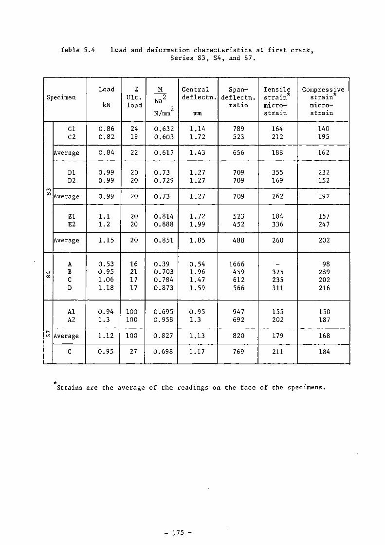
Table 5.4 Load and deformation characteristics at first crack,Series S3, S4, and S7.
SpecimenLoad
kN
%
Ult.load
M Centraldeflectn.
MIR
Span-deflectn.
ratio
Tensils train*
micro-strain
Compressivestrainmicro-strain
bD2
2N/mm
Cl 0.86 24 0.632 1.14 789 164 140C2 0.82 19 0.603 1.72 523 212 195
Average 0.84 22 0.617 1.43 656 188 162
D1 0.99 20 0.73 1.27 709 355 232
mD2 0.99 20 0.729 1.27 709 169 152
° Average 0.99 20 0.73 1.27 709 262 192
El 1.1 20 0.814 1.72 523 184 157E2 1.2 20 0.888 1.99 452 336 247
Average 1.15 20 0.851 1.85 488 260 202
A 0.53 16 0.39 0.54 1666 - 98.1. B 0.95 21 0.703 1.96 459 375 289m
C 1.06 17 0.784 1.47 612 235 202D 1.18 17 0.873 1.59 566 311 216
Al 0.94 100 0.695 0.95 947 155 150
hw
A2 1.3 100 0.958 1.3 692 202 187
Average 1.12 100 0.827 1.13 820 179 168
C 0.95 27 0.698 1.17 769 211 184
*Strains are the average of the readings on the face of the specimens.

Table 5.5 Load and deformation characteristics at first crack,Series S5 and S6.
Specimen
Load
kN
%
Ult.load
M Centraldeflectn.
mm
Spandeflectn.
ratio
Tensilestrain*micro-strain
Compressivestrain*micro-strain
bD2
2N/mm
Cl 0.47 21 0.77 1.68 536 233 173C2 0.47 20 0.818 1.58 570 201 145C3 0.42 20 0.639 1.71 526 218 171
Average 0.45 20 0.742 1.66 544 217 163If
El 1.71 20 0.697 1.11 811 227 195Cl,
E2 1.59 18 0.687 1.11 811 223 188E3 1.77 21 0.766 1.25 720 300 220
Average 1.69 20 0.717 1.16 781 250 201
4D1 0.82 14 0.628 1.57 573 217 1404D2 0.71 13 0.521 1.57 578 206 184
Average 0.77 14 0.575 1.57 573 212 162
6D1 0.68 11 0.424 1.55 1233 215 1686D2 0.77 13 0.489 1.7 857 230 150
Average 0.73 12 0.457 1.62 1045 222 159
*Strains are the average of the readings on the face of the specimens.

varied widely which made the comparison of their results with the results
of ferrocement specimens not very reliable.
The load and deformation at first crack increased slightly with
increase in the number of meshes, see Tables 5.2, 5.3 and 5.4. However,
this increase seems to be insignificant and sometimes inconsistent to draw
a reliable conclusion from it. The mesh yield strength, mesh distribution,
and presence of steel bar did not influence appreciably the load and
deformation at first crack. The load and deflection increased and
decreased, respectively with increase in the section thickness. However,
the ratio M/bD2 did not vary appreciably with the section depth, see results
of series S5. This indicates that the section thickness did not affect the
load at first crack other than the expected increase due to increase in
depth of the section.
Increasing the mortar cover decreased the load and deformation at first
crack, see results of Si D, S6 4D, and S6 6D. For the same number and type
of mesh, increasing the mortar cover from 2 mm to 6 mm decreased the load
by about 40%. The reinforced concrete specimen, S4A, which had the same
mortar cover as that of S6 6D, i.e., 6 mm, gave almost the same load and M/bD2
values. It should be noticed, however, that the value of M/bD2 for these
specimens was smaller than that of the plain mortar specimens.
5.8.2 At First Yielding.
The first yielding was defined as the first deviation from linearity
of the second linear range of the load—deflection curve. The first
yielding points were found for all specimens, and the load and deformations
at these points are given in Tables 5.6 to 5.9. From these tables, the
load varied from 1.15 to 6.4 kN, depending mainly on the number and yield
strength of the mesh and the thickness of the section. The load as a
percentage of the ultimate load varied between 45 to 64% except for specimens
S1B (reinforced with two mild steel mesh) where the average load is equal to
80% of the ultimate load. The span-deflection ratio, again for all speci-
mens except Sin, varied between 54 to 100. This suggests that applying
the deflection limits used in the serviceability criteria for reinforced
concrete, the working load would be within the second linear range, but
less than the first yielding load.
From Table 5.6 (series S1), it can be seen that increasing the number
of meshes increases the load, deflection, and tensile and compressive strain.
Increasing the number of meshes from 2 to 10 mesh, increased the load by a
factor of 3.3, deflection by 1.8, tensile strain by 1.5 and compressive
strain by 1.7. The slow increase in the tensile strain and the continuing
increase in the compressive strain indicates that yielding of the specimen
was initiated by yielding of the mesh.
For the specimens reinforced with the high yield steel mesh, Table 5.7;
the load increased with the number of meshes, but at a slower rate when the
number of meshes was higher than four. The compressive strain increased
when the number of meshes increased from 2 to 4, but remained almost the
same thereafter. The deflection and the tensile strain for 6 and 8 meshes
specimens were less than those with 4 meshes. The observed variation in
the load and deformation suggests that while yielding was controlled by
the mesh in specimens with 2 and perhaps specimens with 4 meshes, it was
controlled by yielding of the mortar in compression, for specimens with 6
and 8 meshes. This seems to be a basic difference between specimens
reinforced with mild steel mesh and high yield mesh. In addition the load
and deformation in series S2 are much higher than in series Si, signifying
the ability of the high yield mesh in carrying higher stresses and loading
the mortar more efficiently.
- 178 -

Table 5.6 Load and deformation at first yielding, Series Sl.
SpecimenLoad
kN
%
Ult.Load
Centraldeflectn.
mm
Span-deflectn.
ratio
Tensillstrainmicro-strain
Compressivestrainmicro-strain
Bl 1.45 82 6.7 134 1715 -B2 1.31 80 7.5 120 1650 6934
-4m
B3 1.37 78 6.9 130 1786 633
Average 1.38 80 7. 128 1717 663
Cl 2.19 53 10.6 85 2130 790C2 2.19 53 9.2 98 2200 906
o C3 2.19 52 9.0 100 1951 783-4mAverage 2.19 53 9.6 94 2094 826
D1 2.79 55 9.5 92 2180 870D2 2.46 45 9.3 97 2212 876
a) D3 2.9 47 9.8 92 2120 785-4mAverage 2.72 49 9.6 94 2170 844
El 3.28 53 10.9 83 2261 940
w E2 3.83 55 12 75 2268 1010
-4En
E3 3.83 56 12.6 71 2704 1170
Average 3.65 55 11.8 76 2411 1040
Fl 4.9 60 12.8 70 2894 995F2 4.35 54 12.6 71 2300 1213
44 F3 4.38 56 12.8 70 2513 1233-4mAverage 4.54 57 12.7 70 2570 1147
*Strains are the average of the readings on the face of the specimens.
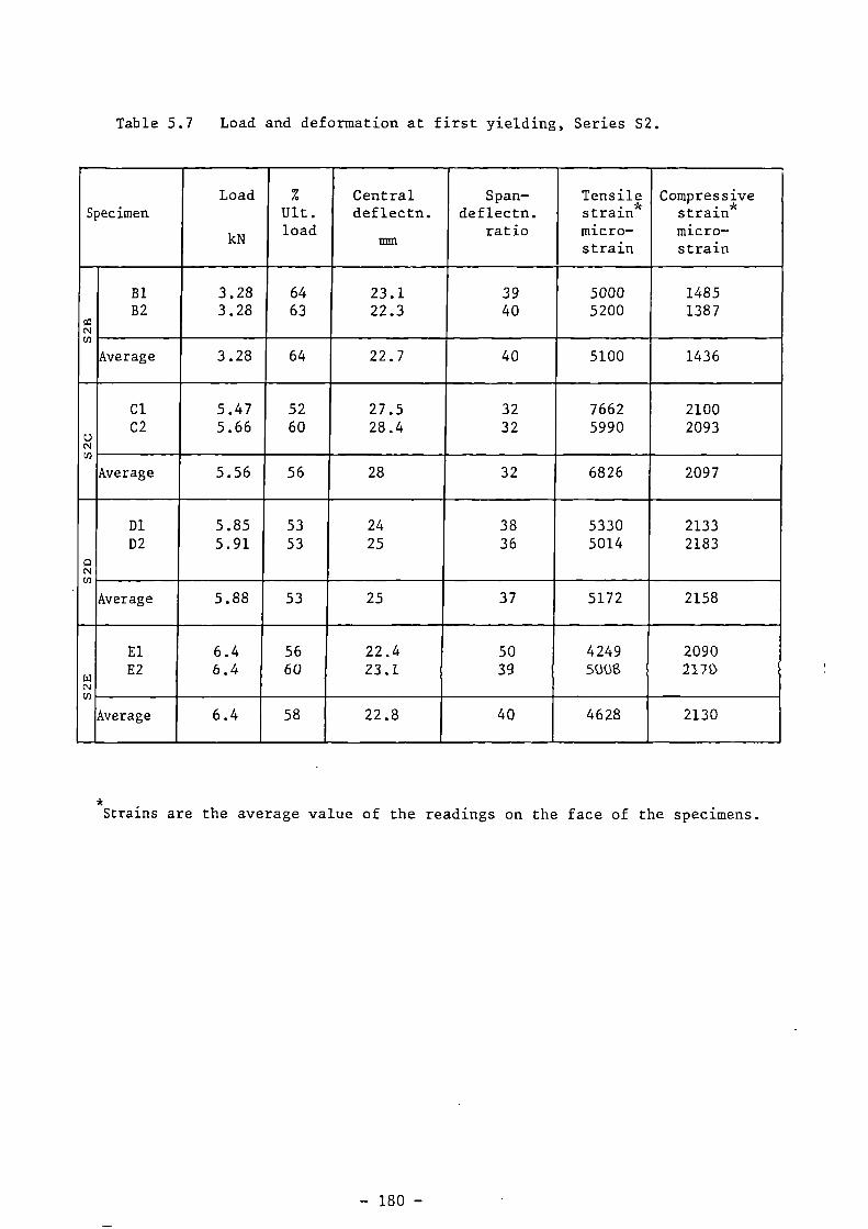
Table 5.7 Load and deformation at first yielding, Series S2.
SpecimenLoad
kN
%
Ult.load
Centraldeflectn.
mm
Span-deflectn.
ratio
Tensilestrainmicro-strain
Compressivestrainmicro-strain
Bl 3.28 64 23.1 39 5000 1485
mB2 3.28 63 22.3 40 5200 1387
Nm
Average 3.28 64 22.7 40 5100 1436
Cl 5.47 52 27.5 32 7662 2100
oC2 5.66 60 28.4 32 5990 2093
NM
Average 5.56 56 28 32 6826 2097
D1 5.85 53 24 38 5330 2133D2 5.91 53 25 36 5014 2183
ANm
Average 5.88 53 25 37 5172 2158
El 6.4 56 22.4 50 4249 2090
w E2 6.4 60 23,1 39 5008 217DNm
Average 6.4 58 22.8 40 4628 2130
*Strains are the average value of the readings on the face of the specimens.

Table 5.8 Load and deformations at first yielding, Series S3, S4and S7.
Specimen
Load
kN
%
Ult.load
Centraldeflectn.
mm
Span—deflectn.
ratio
TensileStrain*micro—strain
CompressiveStrain*micro-strain
Cl 1.83 51 8.9 101 2186 746C2 1.75 50 8.4 107 1596 678
Average 1.79 51 8.7 104 1891 712
D1 2.42 49 9.90 91 1974 926D2 2.46 49 9.6 94 2050 922
mmAverage 2.44 49 9.8 93 2012 924
El 3.01 56 11.7 77 2240 1033E2 2.93 , 54 10.9 83 2050 1026
Average 3.0 55 11.3 80 2145 1030
A 2.02 62 13.5 67 2150 1060B 2.54 58 10.7 84 2220 1003
',71 C 3.87 56 11.1 81 2400 1055D 4.27 63 11.7 77 2600 1160
, C 2.22 63 9.0 100 2150 860m
_
*Strains are the average of the readings on the face of the specimens.

Table 5.9 Load and deformations at first yielding, Series S5,and S6.
Specimen
Load
kN
%
Ult.load
Centraldeflectn.
mm
Span-deflectn.
ratio
Tensilestrain*micro-strain
Compressivestrain*
micro-strain
Cl 1.28 56 16.7 54 2450 973C2 1.16 49 16.3 55 2510 1056C3 1.15 56 16.2 56 2430 940
ow
Average 1.2 54 16.4 55 2463 990
El 4.65 54 8.2 110 1875 936E2 4.59 52 7.8 115 1900 900E3 4.65 54 7.8 115 1911 910
Average 4.63 53 7.9 113 1895 915
4D1 2.74 46 12.2 74 2389 11264D2 2.71 48 11.4 79 2597 1030
Average 2.73 47 11.8 77 2493 1078
.0m 6D1 2.45 47 12.2 74 2690 993
6D2 2.71 52 13.2 68 2950 1035
Average 2.58 45 12.7 71 2820 1014
*Strains are the average of the readings on the face of the specimens.
The results from series S3, Table 5.8, showed that the load and
deformation varied with the number of meshes in a similar manner to that
of series Si. This suggests that for the range of mesh opening used in
this study, the yielding characteristics were not influenced by the size
of the mesh. The same variation in the load as in series Si and S2, was
also observed in series S4, in which the specimens were reinforced with
mild steel mesh and bars. However, the compressive and tensile strain
did not increase as much with increasing the number of meshes in this series.
This is probably due to the presence of steel bars which have a high
fraction volume and the addition of meshes to the reinforcement does not
result in higher strain values unless the meshes are of a higher yield
strength than the steel bars.
The results of specimens of series S6, and specimens Si D indicate that the
mortar cover does not influence significantly the load at first yielding.
But the tensile strain on the face of the specimen increased with increasing
the cover. This was to induce the same tensile strain in the mesh to cause
its yielding. Increasing the section depth (see results of S5C, SID and
S5E) increased the load significantly and decreased the tensile strain
slightly. The average value of the load for these specimens was 1.2, 2.66,
and 4.63 kN corresponding to section thickness 17, 25 and 34 mm, respectively.
These values show a wide variation in the load. However, calculating the
ratio M/bD2, gave very close results (2.1, 2.1, 2.0 N/mm
2)• This indicates
that for the same fraction volume of reinforcement, the load at first
yielding is in direct proportion with the square value of the section depth.
The load at first yielding was found to have a direct relation with
the fraction volume of reinforcement in loading direction. In Fig.5.18,
this relation was plotted for all specimens with the same section depth.
It can be seen that for the specimens reinforced with mild steel, the load

-C\101q‹)ln LI) Ln u) w
x• Oao
^
-
-
• i\pi u! pool Plc)!
C0._4-Uu,:6
cpC
q '6a0
co ---.,
o 4. -•-I Cri u> E
.. dC U
L.0
.- 0
-I-• 4-U C
CY) 0.-
f- 0i-
"0-
C7) 0c u
O DO —
0c >._
C
"a' 0u • -
C\I E.....u
id 0U L--
0
c
-
(-
..... >u
f- 0)c
O :0-
u 779._E >.
--- n 4-•-O °> 77C 0O 0- _4-•U_O 0t_LL 0
I-
CC;_1.1:)
Cr)
Li=
-184 -

varied linearly with fraction volume of reinforcement in loading direction,
irrespective of the mesh opening, presence of steel bars or mortar cover.
For the high tensile steel mesh, Fig.5.18 shows that the load at first
yielding consists of two linear parts depending on the amount of reinforce-
ment. The point which separates the two lines represents the change in
yielding from the mesh in tension to the mortar in compression and the
load increases faster before this point than after it.
Paul and Pama (11) presented a theoretical equation to predict the
composite tensile strain under tension. For square mesh, the equation is
1 1
ty1 [cy
VR
Ef fy
mu2
L
a(5.1)
where Ef and a
fy are the modulus of elasticity and yield strength of the
reinforcement, respectively, a is the mortar strength in tension, and VMU RL
. is the fraction volume of reinforcement in loading direction.
In Fig.5.19, the average tensile strain on the face of the specimen at
first yielding is plotted against the fraction volume of reinforcement in the
loading direction for series Si and 82. Eq. 5.1 was used to calculate the
tensile strain and the results are also included in that figure. From
Fig.5.19, it can be seen that the theoretical strain values are less than
the experimental ones. However, eq. 5.1 is developed for section under
tension. Therefore the equation gives the strain values at the
reinforcement level which are less than the strain at the face of the speci-
men. To find the strain at the specimen face, the theoretical values were
adjusted to account for the strain gradient in the section. The depth of
the neutral axis from the tensile face of the specimens at first yielding
was assumed to be equal to 0.7 times the section depth. This value was
based on calculations of the neutral axis depth at first yielding of the
tested specimens. Hence, the theoretical tensile strain at the specimen

• UpD4SOJD!lli 2,11SUZ4 51D.IZAV
•
-186 -

u 0 U
4n,C9
L. a L..0 001 '4- 1:9
U
(9L.00.1
4".a
4-
0
• UlDJIS0.10!W WIDJ4S ZIISU 2)/. ZEIDJZAV
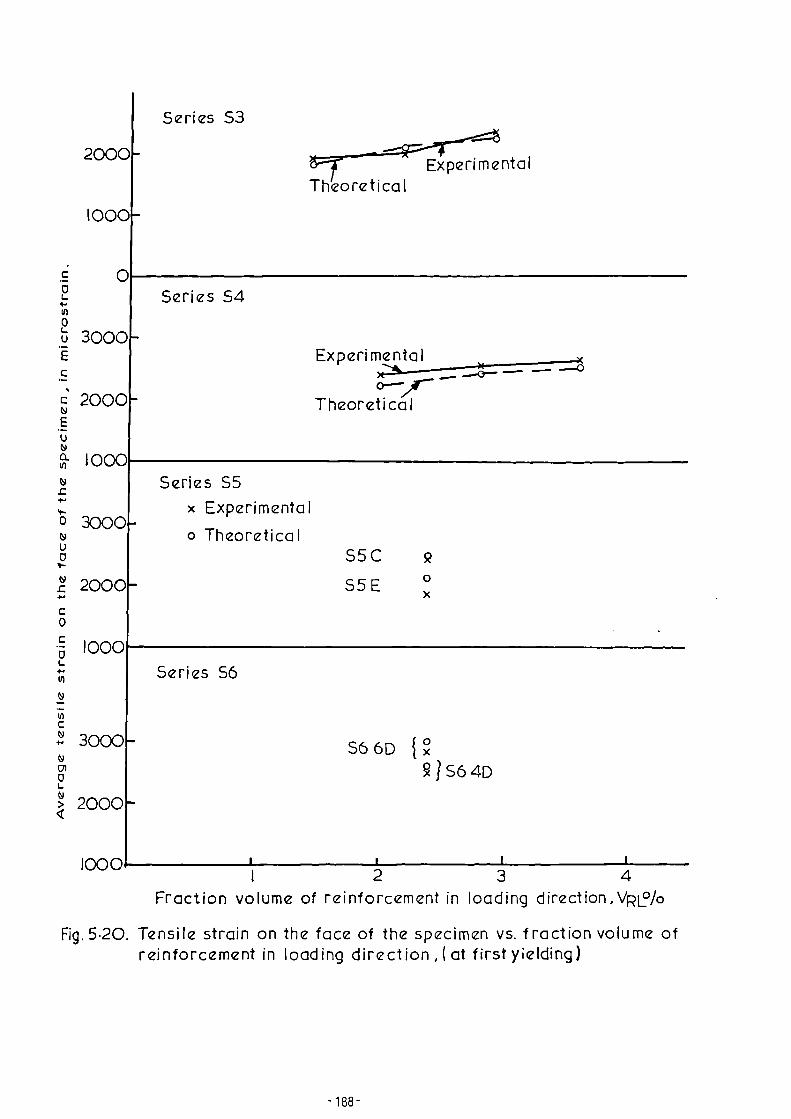
2000 Experimental
1000
Series 54c
.
0 0
In
0u 3000-
c 2000
ft 1000
Theoretical
Series 53
Theoretical
Series S5x Experimental
3000o Theoretical
C S5C 9
2000 55 E
1000Series 56
3000 - S6 6D 1)(3((9
9/564D
> 2000-
10002 3 4
Fraction volume of reinforcement in loading direction,Vp2/0
Fig. 5 .20. Tensile strain on the face of the specimen vs. fraction volume ofreinforcement in loading direction at first yielding)

face was equal to that from eq. 5.1 multiplied by the ratio of the neutral
axis depth from the tensile face to neutral axis depth from the extreme tensile
mesh layer. The adjusted theoretical strain values for series Si are
plotted in Fig. 5.19A. It can be seen that the theoretical and experimental
values for series S1 are very close except for specimen S1B where the number
of meshes was 2. The experimental and the adjusted theoretical values of
tensile strain for series S3, S4, S5, and S6 are plotted against the fraction
volume of reinforcement in Fig.5.20. It can be seen that, again the
theoretical and experimental results are in close agreement.
For series S2, the experimental values of the tensile strain, unlike
in all the other series, decrease when the number of meshes is higher than
4, see Fig.5.19B. As discussed earlier, the decrease is due to the
yielding in these specimens which was by yielding of the compressive zone
and not by yielding of the tensile zone. When calculating the theoretical
values of strain for this series by the same previously discussed procedure,
the theoretical values were much lower than the experimental. However, in
eq. 5.1, a fy was taken at 0.005 strain. While the mild steel mesh when
tested in tension yielded at about this strain value, the high tensile mesh
did not show clear sign of yielding at that strain. Therefore, afy
at
0.005 strain does not give the actual yield strength of the high tensile
mesh. The theoretical values of the tensile strain were calculated again
using the yield strength afy at 0.2% offset. The results are plotted in
Fig.5.19B and are closer to the experimental values than those found by
using afy
at 0.005 strain.
5.8.3 At Failure.
The failure was defined as the point where a sudden release in the
load took place and the section sustained only a fraction of that load. The
release in the load was the result of either failure of the mesh in tension or

failure of the mortar in compression. The measurements were taken just
before the sudden release of the load. They included the load, central
deflection, and compressive strain on the face of the specimen. These
measurements, as well as description of the section failure are given
for all specimens in Table 5.10.
As can be seen in Table 5.10, three types of failed sections were
observed. They were, firstly, sections where the mesh was fractured and
the depth of the compression zone was very small, see Plate 5.1. Secondly
sections in which the mesh was yielded, and in some specimens the extreme
mesh layer was fractured, but the compression zone was deeper than in the
first case. In these sections there was a recognizable compression failure,
see Plate 5.2A. Thirdly, sections with a sudden compression failure, see
plate, 5.2B. The specimen failure could be one of the above three types
depending on the amount of reinforcement and its yield strength. Upon
increasing the number of meshes in the specimens of series Si, the mode of
failure changed from tensile failure to a sudden compression failure. The
same change in the mode of failure was noticed in series S2, where specimens
are reinforced with high tensile mesh. The specimens of series S2 also
exhibited horizontal cracks and spalling of mortar cover in those which
suffered tensile failure (see Plate 5.2C) and buckling of the meshes in
compression and extensive damage to the section in those suffering compression
failure (see Plate 5.2B). In general, specimens reinforced with high
tensile mesh suffered sudden failure, while those with mild steel mesh were
more ductile even for specimens which failed in compression.
For the same fraction volume of reinforcement, the mode of failure did
not change with the section depth or mortar cover. The significant factors
which affect the mode of failure were found to be the reinforcement area and
its yield strength. If the same principles used in the design of reinforced
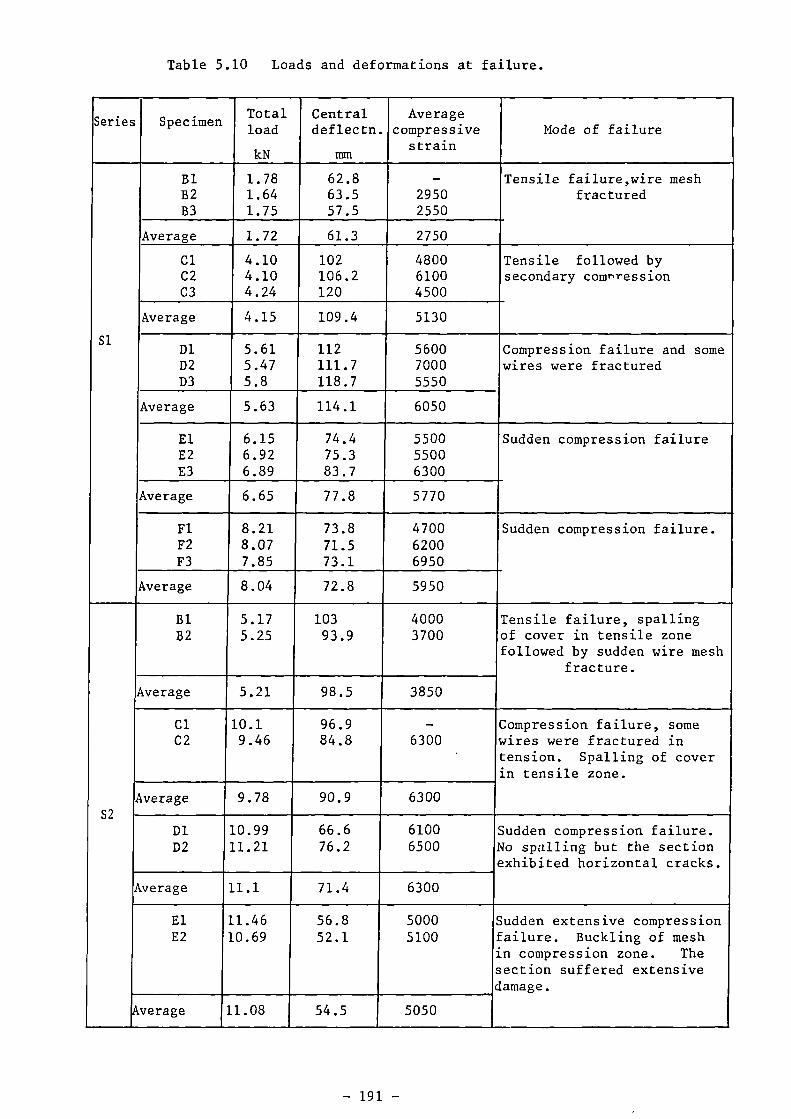
Table 5.10 Loads and deformations at failure.
Series SpecimenTotalload
kN
Centraldeflectn.
mm
Averagecompressive
strainMode of failure
Bl 1.78 62.8 - Tensile failure,wire meshB2 1.64 63.5 2950 fracturedB3 1.75 57.5 2550
Average 1.72 61.3 2750
Cl 4.10 102 4800 Tensile followed byC2 4.10 106.2 6100 secondary comrsressionC3 4.24 120 4500
Average 4.15 109.4 5130
SiD1 5.61 112 5600 Compression failure and someD2 5.47 111.7 7000 wires were fracturedD3 5.8 118.7 5550
Average 5.63 114.1 6050
El 6.15 74.4 5500 Sudden compression failureE2 6.92 75.3 5500E3 6.89 83.7 6300
Average 6.65 77.8 5770
Fl 8.21 73.8 4700 Sudden compression failure.F2 8.07 71.5 6200F3 7.85 73.1 6950
Average 8.04 72.8 5950
B1 5.17 103 4000 Tensile failure, spellingB2 5.25 93.9 3700 of cover in tensile zone
followed by sudden wire meshfracture.
Average 5.21 98.5 3850
Cl 10.1 96.9 - Compression failure, someC2 9.46 84.8 6300
'wires were fractured intension. Spalling of coverin tensile zone.
Average 9.78 90.9 6300
S2D1 10.99 66.6 6100 Sudden compression failure.D2 11.21 76.2 6500 No spalling but the section
exhibited horizontal cracks.
Average 11.1 71.4 6300
El 11.46 56.8 5000 Sudden extensive compressionE2 10.69 52.1 5100 failure. Buckling of mesh
in compression zone. Thesection suffered extensivedamage.
Average 11.08 54.5 5050

Table 5.10 Loads and deformations at failure.•
Series SpecimenTotalload
kN
Centraldeflectn.
mm
AverageCompressive
strain.Mode of failure
Cl 3.61 100.2 4200 Tensile failure, veryC2 3.5 91.0 3800 ductile.
Average 3.56 95.6 4000
D1 4.95 84.1 5800 Compression failure and
S3
D2 4.98 105.8 7000 some wires werefractured. Ductile
failureAverage 4.97 95 6400
*El 5.42 71.3 6100 Compression failure.E2 6.02 86.4 5300
Average 5.72 78.9 5700
A 3.25 93.1 3850 Secondary compression.
S4B 4.41 73.0 4500 Secondary compression,
wire mesh fractured.C 6.32 81.0 4200 Compression failure.D 6.78 93.1 4800 n n
S7 C 3.52 84.0 3150 Tensile failure. Bothtensile mesh fractured.
Cl 2.28 112.9 3700 Secondary compression.C2 2.36 156.4 5500 Wire mesh was yielding.C3 2.06 107.8 3200
S5Average 2.25 125.7 4130
El 8.56 58.4 6200 Secondary compression.E2 8.86 71.9 6700 Wire mesh was yielding.E3 8.56 71.6 6300 One specimen showed
spalling of compressionAverage 8.66 67.3 6400 cover. Another showed
some tensile wiresfractured.
4D1 5.99 137.2 6650 Secondary compression.4D2 5.61 117.1 5400
S6 Average 5.8 127.2 6020
6D1 5.2 95.4 5100 Secondary compression.6D2 5.2 85.4 5000
Average 5.2 90.4 5050._
Specimen neglected due to inconsistent results.

•
—Mk
• • •.1111111111
%VI
•
" -or
0---111111111111111
Plate. 51. Specimen failed by fracture of wire meshin tensile zone.

a) Excessive yielding plus compression failure.
b) Sudden compression failure.
c) Specimen suffered spoiling of the mortar cover.
Plate.5 2. Different types of section failure.

concrete apply to ferrocement then there seems to be a balanced steel ratio
for which the reinforcement in ferrocement members should be less or equal to
avoid the undesirable compression failure.
The ultimate load, deflections, and compressive strains were influenced
greatly by the mode of failure and the influence of the different variables
on each of them will be discussed separately in the following sections.
5.8.3.1 Ultimate load.
In Table 5.10,the ultimate load increased with increase in the amount
of reinforcement. In Fig.5.21, the ultimate load is plotted against the
fraction volume of reinforcement in the loading direction. Each point in
the figure represents the average value of the number of repeated specimens.
The figure shows that the ultimate load for specimens reinforced with mild
steel mesh increases linearly with fraction volume of reinforcement in
loading direction. This was the result irrespective of the difference in
mesh opening or presence of steel bars. It also shows that ultimate load
for specimens reinforced with high tensile mesh is much higher than those
reinforced with mild steel mesh. The load for the high tensile mesh speci-
mens did not increase appreciably when the number of mesh was higher than 4.
The load for specimens with 6 and 8 mesh were the same. This may be due to
the premature failure, as described earlier, caused by buckling of wire
mesh in compression, which was suffered by specimens S2D and S2E.
As in the case of the load at first yielding, the ultimate load
varied linearly with the square value of the section depth. The value of
P/D2 for specimens S5C, S1D, and S5EC section depth 17, 26 and 34 mm) were
8.02, 8.33, 7.83 N/mm2
. The ultimate load also was not affected appreciably
by variation in mortar cover. It appears, therefore, that the ultimate load
is controlled mainly by the fraction volume of reinforcement in loading
direction and the yield strength of the mesh.

_cY,•u) (1)
• 1\1>1 LI ! P D01 apwrlin
0•
L.
0>
N0
o 4-,U0 0
Yo- L-4-
(I)I-. L.
0 -0dE
0 4- U)> 0
X C E "tp0 c
4-•
5.8.3.2 Deflection at Failure.
The values of the deflection at failure is not an important character-
istic as far as the designer is concerned. But it can be used as a measure
for the ductility of ferrocement and gives an idea about the amount of
deformation this material can sustain.
The central deflection is plotted against the total fraction volume of
reinforcement for all series in Fig.5.22. From the figure, it can be seen
that for the mild steel mesh, series Si, the deflection increased with the
fraction volume and then decreased after specimen SlD (6 mesh). In this
series, therefore, there seems to be an optimum amount of reinforcement which
results in the highest ductility. For series S2, the figure shows that the
deflection decreases with the increase in the fraction volume. The
deflections for this series are lower than those of series Si, except for
the specimen with 2 mesh. In series S4, the specimen with steel bars only
(S4A) gave relatively higher deflection than those with mesh and steel bars
which had almost the same deflection. Increasing the section thickness,
as expected decreased noticeably the deflection (series S5). Increasing the
mortar cover would be expected to result in an increase in the deflection
However, the experimental values were inconsistent.
It should be noticed that the deflection at ultimate load reflects
the type of failure the section suffers. Upon increasing the amount of
reinforcement in the section, the failure changesfrom ductile tensile failure
to a less ductile compression failure and the deflection therefore decreases
after that change. Thus the deflection at ultimate load depends on the
amount of reinforcement and its yielding characteristics.
5.8.3.3 Compressive Strain at Failure.
The value of ultimate compressive strain becomes important as this
value is required to calculate the ultimate strength in flexure. In Fig.

SI
.0
(975
.6i! 50
25-
Series S6 (mortar cover)
Series S5(section thickness)
A) Series Si, 52,53 and 54.
•
1 .0 2. 0 3 . 0 40 5. 0 6•0 7 .0 8•0Fraction volume of reinforcement VR cio
B) Series 55 and So.
125
.-c2 100
v75
25
Mortar cover , mm2 4 6
10
20
30Section thickness, mm.
Fig.5 .22. Central deflection at ultimate load vs. fraction volume of reinforcement,mortar cover and section thickness.
-198-

7000r A) Series 51,52,53and 54.
C._0
75 6000o0._E- 5000-
C._2
4000
3000
c9>._0O?- 3000aE0U
o 2000-"iiE.-
5 1 000
6.51)S3 Mild steel mesh.
o 52 High tensile mesho S4 Mesh+steel ball.
-
Series 56(mortar cover)
Series 55 ---(section thicknes
-
1
56I-
1 .0 2.0 3.0 4 . 0 5 . 0 6 .0 7 . 0 8.0oL.. Fraction volume of reinforcement, VR0/0uE B) Series 55 and 56.
C._0
-L-i; 6000u>-VI
(90 50001._aE0
3000Section thickness,mm
200010
I20
I30
I40
Ii I I
2
4 6Mortar cover, mm
Fig. 5 . 23. Ultimate compressive strain vs. fraction volume of reinforcement,section thickness and mortar cover.

5.23, the average measured ultimate compressive strain on the specimen face
is plotted against the fraction volume of reinforcement. The figure shows
that for series S1 the compressive strain increases with the fraction volume
until the value corresponding to 6 meshes (S1D) where it remained almost
constant at 6000 microstrain. For series S2, the strain increased when
VR increased. It reached an optimum value of about 6300 microstrain in
specimens S2C and S2D (4 and 6 meshes) respectively, then decreased for
specimen S2E. This shows as mentioned before, the premature failure of the
specimen due to buckling of the meshes in the compression zone. Except
for specimen S2E, series S2 gave relatively higher compressive strain than
series Si, which shows the ability of the high tensile mesh in utilizing the
high mortar strength. In series S4 the compressive strain is relatively
smaller than those of series S1 and S2 and it seems to increase slightly
with increase in the number of meshes. Increasing the section thickness in
series S5 and decreasing the mortar cover in series S6 increased the
compressive strain. The highest values of strain for these variations were
around 6000 microstrain.
It therefore follows that the average maximum compressive strain is
about 6000 microstrain, and this value is almost the same for all sections
which fail due to failure in the compression zone.
5.9 Conclusions. -
Based on the experimental results of this study, the following
conclusions were drawn:
1. The load-deflection and load-strain curves of ferrocement specimens
can be divided into three ranges. The first two are linear, with the first
cracking and first yielding marking the end of the first and second range,
respectively. In the first range the section is free from cracks and within
the elastic limit of its constituent materials while in the second range the

section is cracked, and is characterized by rapid increase in the number of
cracks. The slopes of the two linear ranges depend mainly on the fraction
volume of reinforcement in loading direction of the specimen. The third
range represents the yielding stage in which the cracks increase rapidly
in width. The yielding characteristics of the section are controlled
by the yielding characteristics of the reinforcing system. Ferrocement
under flexural loading could fail either in tension or in compression
depending on the amount and yield strength of the reinforcement.
2. As far as the deflections and crack width are concerned, the
service load appears to be within the second linear range. As long as the
specimen has not yielded, the mean crack width remains mainly below 50 microns.
For an allowable span—deflection ratio of 180, the mean crack width was mostly
less than 20 microns, and the load was between 15-30% of the ultimate load.
3. The load at first cracking did not vary appreciably with variation
in the amount and yield strength of the mesh, presence of steel bars or the
mesh opening. However, it was in direct proportion with the square of the
section depth.
4. The first yielding of the section could be initiated by either
yielding of the mesh in the tensile zone or yielding of the mortar in the
compressive zone. The load at first yielding increased with amount and
yield strength of the reinforcing system. For the tested specimens, this
load was between 45 and 65% of the ultimate load and it varied linearly with
the fraction volume of reinforcement in loading direction, for specimens in
which their tensile zone yielded first. The tensile strain at first
yielding for such specimens can be predicted closely using the theoretical
equation 5.1, and taking into account the strain gradient in the section.
5. The ultimate load seems to be influenced mainly by the yield
strength and the amount of reinforcement, and depth of the section. It was

not affected appreciably by change in the mesh opening, presence of steel
bars or the variation in the mortar cover. The ultimate load increased
almost linearly with the fraction volume of reinforcement in loading direction
for the specimens with mild steel reinforcement. For the specimens with high
tensile mesh, the ultimate load ceased to increase when the number of mesh
increased to more than 6 meshes. This is probably due to its premature
failure caused by the large transverse tensile stresses which are induced by
the mesh on the mortar because of the zig-zag shape of the mesh wires. These
stresses tend to induce weak planes along the mesh layers.
6. The deflection at failure, as a measure of the ductility, is
influenced by the amount and yielding characteristics of reinforcement, and
the section depth. While there was an optimum value for the ductility for
specimens with mild steel mesh, the deflection at ultimate load decreased
with increase in the number of meshes for specimens with high tensile mesh.
7. The compressive strain at failure was controlled mainly by the
• mode of failure of the section. The average measured ultimate compressive
strain was about 6000 microstrain, and this value was about the same for all
section which failed in compression.
- 202-

CHAPTER 6.
ANALYSIS OF FERROCEMENT IN FLEXURE.
6.1 Introduction.
One of the most important characteristics of ferrocement is the high
degree of dispersion of its reinforcement. Due to this characteristic,
the contribution of the matrix in tension to the stiffness of the section,
during the cracked stage, is more appreciable than in reinforced concrete.
The subdivision of the reinforcement results in increasing its capability of
loading the matrix, through shear bond forces, and thus results in
appreciable tensile force carried by the matrix. This, besides the smaller
mortar cover and section depth ,represents the major differences between ferro-
cement and reinforced concrete. Consequently, the method of analysis used
in reinforced concrete may not apply always satisfactorily to ferrocement.
On the other hand, the need for a simple and reliable analysis method is
becoming more urgent. As the uses of ferrocement as a structural material
widen, the designer's need for a simple and accurate design procedure
increases.
This part of the study is devoted to the development of simple analytical
procedures to predict the moment capacity and deflections at different levels
of the load for ferrocement in flexure. The procedure was applied on
the test programme of this study in which the variables are the number,
yield strength, and opening of the mesh, presence of steel bars, and thickness
of section depth and mortar cover.
6.2 Review of Literature.
There are, mainly, three theoretical approaches used for analysing
ferrocement sections in flexure. The first approach is similar to that of
working stress and ultimate strength theories used in the design of

reinforced concrete members. In this approach the mortar is assumed to
carry no tensile stresses as soon as its strain reaches the ultimate
strain of plain mortar in tension. The second approach is based on
defining ferrocement sections by limiting its amount of reinforcement.
This amount of reinforcement is usually expressed in terms of the specific
surface. The mechanical properties are established experimentally and
assumed to be the same for any ferrocement section having a specific
surface within the specified limits. In the third approach, ferrocement
is treated as a composite material. The law of mixtures is used to find
the mechanical properties of the composite from the properties of its
constituents, i.e., mortar and reinforcement.
Many investigators (18,31,33,34,56) have used the method which is
based on the design theory of reinforced concrete for the prediction of the
ultimate strength, but with some minor differences in their assumptions.
The differences cover mainly two aspects. The first aspect is the linear-
ization of the stress-strain curve for the mesh reinforcement. The second
aspect includes the shape of the compressive stress block and the value of
the ultimate compressive strain. The linearization of the mesh stress-
strain curve results in a certain amount of error, depending on the degree
of linearization. An elastic-perfectly plastic curve is commonly used.
It should be mentioned, however, that the yield point is not always clear
in the mesh stress-strain curve. Hence, this, plus ignoring the strain
hardening of the mesh could lead to a large error in the value of the
predicted ultimate strength. Different compressive stress blocks at ultimate
load have been used. In Fig.6.1, the most common used stress blocks are
given. The stress block shown in Fig.6.1a was used by Logan and Shah (18).
The results of the comparison between the calculated and experimental
values is shown in Fig.6.2. It can be seen from the figure that the ratio
of the experimental to calculated is more than one and that this ratio
increases with the increase in the fraction volume of reinforcements, V.
At -^4 2.5% the ratio is about 1.36RL
The use of other stress blocks by other investigators did not prove
to be much more successful. Johnston and Mowat (34) have showed that using
the reinforced concrete approach, the calculated ultimate moment was changed
by 6.3% when different stress blocks were used, by 0.92% when the ultimate
compressive strain was reduced from 0.38% to 0.31%, and by 8% to 15% when
the mesh stress-strain curve was changed from non linear stress-strain
function to elastic-perfectly plastic. Their results show that the
reinforced concrete approach overestimates the ultimate moment of specimens
reinforced with woven mesh by about 20% to 40%.
Balaguru, Naaman, and Shah (31) used the actual stress-strain curves
for the mortar in compression and the mesh in tension in their non linear
analysis of ferrocement beams. Limited experimental work showed that the
procedure predicts closely the ultimate moment (average ratio of experi-
mental to calculated = 0.92). However, their procedure is rather
complicated for the use in design.
Walkus (30,44) has developed a method for proportioning ferrocement
beams. The method is based on an assumed linearized stress-strain
relationship for the composite under tension. The values of stresses and
strains are simulated from experimental results and assumed to be the same
for any section having a specific surface of reinforcement within 2.0 to
3.0 cm2/cm
3. Walkus method has the disadvantages that the stress-strain
curves are based entirely on simulated experimental results and that it does
not take into account the different types and amount of mesh reinforcement.
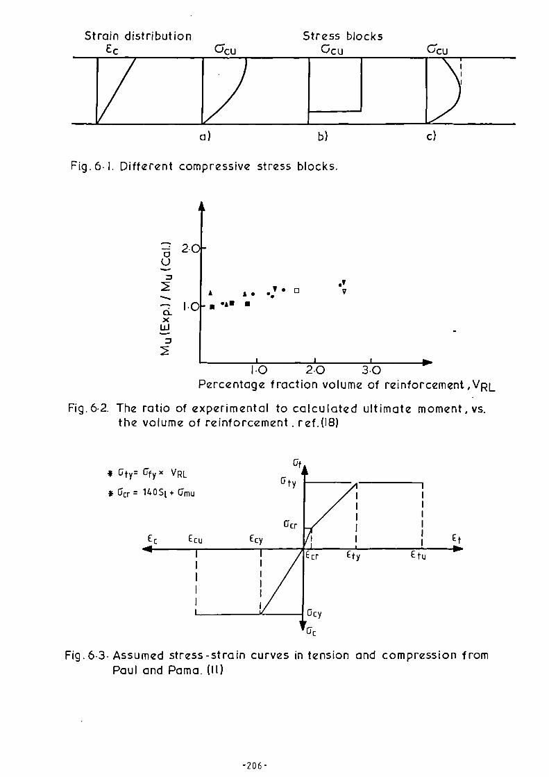
n/Strain distribution
Stress blocksEc
Ccu
Ccu
O'cu
a)
b)
C)
Fig.6 . 1. Different compressive stress blocks.
-a 2-U
=2 T • 0
AV
VA 8 • • •......
1-0 • l'A • •n•n••
1 . 0 2-0 3-0Percentage fraction volume of reinforcement, VRL
Fig.6 . 2. The ratio of experimental to calculated ultimate moment, vs.the volume of reinforcement .ref.(18)
* G ty = Gfy x VRLGt•
Gty
* Gcr = 140S + Gmu
II
Gcr ICc Ccu Ecy I I Ct
4411 . •I I Ecr Et)/ Etu
I
I
1
i
II
1
I
I Gcy
TaC
Fig.6-3 . Assumed stress-strain curves in tension and compression fromPaul and Pama. (11)
•n•n•

ac a V +a Vmm f RL
( 6.1)
The linearized stress-strain curve, as discussed , in section 5.6, could not
be verified from the experimental results of this study.
Several investigators (17,23,26) have predicted successfully some of
the mechanical properties of ferrocement using the law of mixtures.
Paul and Pama (11) have developed a theory in which ferrocement is treated
as a composite material. Its mechanical properties were established from
the properties of its constituents. The theory assumes a bilinear and tri-
linear stress-strain curve for the compressive and tensile zones of the
sections, respectively. Fig. 6.3 shows these curves. Limited experimental
results showed that the theory predicts closely the ultimate strength and the
ultimate deflections. It should be noticed however that the stress-strain
curve of the tensile zone assumes perfectly plastic behaviour after first
yielding. Such assumption, which ignores the strain hardening of the mesh
could lead to conservative results depending on the yielding characteristics
of the mesh. Also, Paul and Pama (11) assumed that the tensile stress at
first cracking increases with the specific surface of reinforcement.
This assumption, as discussed in sec. 4.6.1, could not be verified in this
study.
It can be seen, therefore, that the theory for analysing ferrocement
section in flexure is far from being established. Work is urgently needed
in this area to help set out the design procedure for the material.
6.3 Description of the Method of Analysis.
In a composite material consisting of a matrix and uniformly
dispersed continuous fibres, the stress and the modulus of elasticity of
the composite in direct tension can be written by the law of mixtures as:

(6.3)
(6.4)
and
EcEm Vm Et
VRL (6.2)
where am
and af
are the stress in the matrix and in the fibres respectively,
Vm is the matrix fraction volume
' VRL is the fibres fraction volume in the
loading direction, and Em and E
f are the modulus of the matrix and the fibres,
respectively. As soon as the matrix cracks, its stress will be transferred
to the fibres. Therefore, eqs. 6.1 and 6.2 become:
ac af VRL
EcEf
VRLcr
For ferrocement plates under flexural loading, it was shown in section
5.4, that their behaviour could be divided generally into elastic stage and
cracked stage. The analysis of ferrocement plates in these two stages is
discussed separately.
6.3.1 Elastic Stage.
In the elastic stage, where the plate is free from cracks, both the
mortar and the reinforcement are within their elastic range. The strain
and stress space relationship are linear, as shown in Fig.6.4a. The modulus
of elasticity in the tensile zone is assumed to be equal to that of the
composite in direct tension, i.e., eq. 6.2. The stresses can be found using
(69)the following relation
MCa
where a is the stress at a distance C from the neutral axis, M is the applied
moment, and I is the second moment of area of the equivalent transformed
section.
6.3.2 Cracked Stage.
The cracked stage can be divided mainly into two ranges, namely the linear
range and the yielding range. The stress and strain distribution for these

Ec
Gc
Et
G t . Et x E.
tcr
GyEc> Ecy
tcr
-Et Gt
Tensile zone yielding.
Ec>"Ecy
Et< E ty Gt
Compressive zone yielding.
Gcy
t
Ecy
Etcr
GcEc <Ecy
0-tcr
Gt
a) Elastic Stage.
b) Cracked Stage, linear range.
Et >Ety
Both zones yielding.
c) Yielding range.
Fig. 6-4. Strain and Stress diagrams of ferrocement in flexure.

Ecr
= 1.35 Ef
VRL
(6.5)
two ranges are shown in Fig.6.4. In the linear range, Fig.6.4b, the
mortar and the reinforcement in the compressive zone are still within their
elastic range. The composite in this zone, thus, behaves elastically and
the modulus of elasticity is assumed to be equal to that of plain mortar.
In the tensile zone, the part of the mortar, where £t
> etcr'
is cracked
while the reinforcement all through the zone is still within its elastic
limit. For the cracked depth of the mortar, although the composite stress
is in direct proportion to the strain, the modulus of elasticity of this
part of the section is reduced considerably. According to the law of
mixtures, eq. 6.4 gives the modulus of elasticity in the cracked zone.
However, Naaman and Shah (17), had found from their experimental results that
this equation gives lower bound values. This, perhaps, is due to ignoring
the contribution of the cracked mortar to the rigidity of the section. The
best fit line for Naaman and Shah experimental results, see Fig.6.5, was
found. The equation for it was:
The coefficient 1.35 in the above relation indicates that the modulus of
elasticity for the cracked zone is 35% higher than that calculated taking
into account the effect of reinforcement only. Eq. 6.5 was used, therefore,
instead of eq. 6.4 in the analysis of the plates in this study.
The end of the linear range in the cracked stage is marked by first
yielding of the section. The first yielding of the composite could be due
to yielding of either the tensile or compressive zone, depending on the
properties of the reinforcement and the mortar. Therefore, two cases for
first yielding of the composite can be realized. The first case is when
E > e while c c
< E . The second case is when E < 6 while E Ecy't - ty cy t ty c
where Et and E
c are the composite strain in the extreme tensile and

Ccy 41154115
cu(6.7)
compressive fibres, respectively and Ety
and E are the composite yieldingcy
strain in tension and compression, respectively. The yield tensile strain
for ferrocement under direct tension was derived theoretically by Paul and
Pama (11), and it was given by the following relationship:
amu
e. 1 icy
R)ty Ef ‘ fy 2
(6.6)
where Ef and a
fy are the modulus of elasticity and the yield strength (at
0.005 strain) of the mesh, respectively, amu is the mortar tensile strength
and R 7-1 1/V for a square mesh. It was shown in section 5.8.2 that eq.RL
6.6, after taking into account the strain gradient in the section, predicts
closely the flexural yield tensile strain at the extreme fibre of the tested
Specimens.
The yield strain of the compression zone depends on the compressive
yelding characteristics of the mortar. CP.110 (68) gives the following
relation for the compressive yield strain of concrete:
where f is cube strength. Eq. 6.7 gave reasonably close results whencu
compared with the experimental stress-strain curve of mortar given by Balaguru,
Naaman and Shah (31). Therefore, this equation may be used to predict the
yield strain of the compressive zone of ferrocement.
After first yielding, increasing the load leads eventually to the
yielding of both the compressive and the tensile zones. Fig.6.4c shows the
stress and strain distributions at this stage. In the tensile zone, the
contribution of the mortar to the tensile force after yielding will not
increase appreciably with the progress of the load. This is because the
yielding mesh could not load the mortar between cracks to a significantly
higher level than that at first yielding. Therefore, after C, the mortarty

was assumed to remain carrying the same stress. However, the yielding of
the mesh is not necessarily, perfectly plastic, and the stress is likely
to increase, depending on the yielding characteristics of the mesh, with
the increase in strain. The extra stresses in the meshes after first
yielding were accounted for as shown in Fig.6.6. The extra tensile force
in each mesh is equal to:
(a at Et - a
f at E
ty) x cross-sectional area of mesh.
f
The summation of the extra tensile force of each mesh layer is equal to the
total increase in the tensile force of the section after first yielding.
Alternatively, this increase in the tensile force can be found by assuming a
parabolic increase in the composite tensile stress. By the law of mixtures,
since the contribution of the mortar is neglected, then, the composite
extra stress will be
at extra = (a atat E
t - a
f at E) V
ty RL
where of
is the tensile stress in the mesh, and V is the fraction volumeRL
of the mesh reinforcement in the loading direction.
Using the compatibility and equilibrium of the section, the depth of the
neutral axis at any level of the load during the cracked range, can be found
by iterative procedure if a strain value of the section at that load is given.
The depth of the neutral axis is first assumed. The strain distribution,
thus, can be found from the given strain value and assuming linear strain
distribution. The corresponding stress distribution can be established as
discussed earlier in this section. Therefore, the tensile and compressive
forces in the section can be calculated. To satisfy the equilibrium of the
section, these two forces should be equal. If the computed values of these
forces are not equal or the difference between them is not within 5% of their
- 212-

ca. 1.0
0-8U)2 0.6
15 0.4u.)
-5 0•2-0
• Series L
• Series M
• Series N
Ecr =1 35 Ef VRI
/ •ay.
LOWER BOUND
Ecr = E f VRL
SECTION
0.f2 Extra
Gfl Extra O'f at E f1 —
Gf at Etycity
NA
0 0.5 1.0 1.5 2•0 2.5
Percent fraction volume of reinforcement inloading direction , VRL
Fig. 6 . 5. Composite modulus of elasticity in tension, cracking range. (23)
Gt Extra ( Uf at Et — (if at E ty I VRL
Fig. 6 . 6. Stresses carried by the reinforcement after first yielding.

average, then another value for the neutral axis depth will be assumed.
The tensile and compressive forces will be recalculated and compared. The
iterative procedure is to continue until convergence is achieved. The
resisting moment of the section can be computed by multiplying the average
of the resultants of the tensile and compressive forces at convergence by
the distance between them, i.e.,
M = (T) R
(6.8)
where C and T are the compressive and tensile resultant forces, respectively,
_
and X is the distance between them.
The curvature of the section can be found knowing that,
Ec
. —kD
where (I) is the curvature, Ec
is the compressive strain at the extreme fibre,
and kD is the neutral axis depth from the extreme compressive fibre.
6.3.3 At Failure.
At failure, two cases can be realized. The first case is when the
composite compressive strain Ec attained its ultimate compressive strain
value E , while the composite tensile strain Et
is less than the ultimatecu
tensile strain value, Etu'
which causes the fracture of the mesh reinforcement.
In this case, the section will fail in compression. The second case is when
Ec
< E , while Et = Etu'
then the section will fail in tension. Therefore,cu
the section should be analysed at both cases. The governing case is that
which gives the less resisting moment.
The stress and strain distributions at failure are shown in Fig.6.7.
The compressive stress block is similar to that incorporated in the British
Code. The ultimate compressive strain of the composite is assumed to be 6000
microstrain, and this value was based on the average measured ultimate
(i)(6.9)
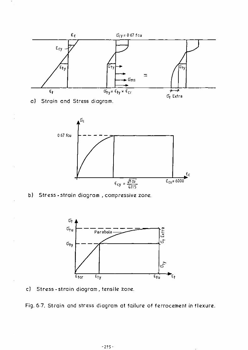
gty
Ec
Ecy
city
Ecu= 6000
O'cy = 067 fcu
UMS
+-4Gt Extra
Et Gty= Etyx Ecr
a) Strain and Stress diagram.
0 67 fcu
Cc
Ccy4115
b) Stress-strain diagram , compressive zone.
c) Stress-strain diagram, tensile zone.
Fig. 6 . 7. Strain and stress diagram at failure of ferrocement in flexure.

compressive strain of the tested specimens of this study and in which the
failure was in compression, (see sec. 5.8.3). A similar value was
reported by Balaguru et al. (31).
The ultimate tensile strain of the composite is determined essentially
by the ultimate tensile strain of the mesh. Its value is equal to the
tensile strain at the extreme fibre of the section when the extreme mesh
layer attained its ultimate tensile strain. For this purpose, however,
the ultimate tensile strain of the mesh, cannot be taken,and specially for
the woven mesh type of reinforcement, equal to the ultimate strain of the
mesh when tested in tension alone, as it is usually assumed (11,18,31).
It was observed that the longitudinal wires of the mesh, having a zig-zag
shape, tend to flatten when the mesh alone is tested in tension. Consequently,
the measured ultimate tensile strain of the tested mesh included the extra
elongation caused by the flattening tendency of the wires. However, when
the mesh is embedded in the mortar, and since complete bond failure did not
take place, the mortar restricted the flattening action of the wires. Thus,
the ultimate tensile strain of the embedded mesh is much less than the
apparent, i.e., measured, ultimate tensile strain of the mesh alone.
A more realistic value of the ultimate tensile strain of the mesh may be
obtained by conducting a tensile test on the composite rather than the
mesh. Moreover, it would be interesting to carry out a study to compare
the values of the ultimate tensile strain obtained from tensile tests
on the mesh and on the composite and flexural test on the composite. Such
a study unfortunately is beyond the scope of this investigation.
The procedure for calculating the moment capacity at failure is the
same as that for finding the moment capacity at the cracked stage
described in the previous section.

6.3.4 Sections with Bar Reinforcement.
So far the analysis included sections where the reinforcement is
uniformly and finely dispersed, i.e., the reinforcement is in the form
of a wire mesh. For sections which include conventional steel bars as
well as wire mesh, the previously described analysis method may not be
appropriate to be used in the given form. It should be noticed that the
available bond area in the bar reinforcement could be as low as 1/10 of the
bond area of an equivalent volume of the mesh reinforcement. Evs,
bar reinforcement cannot be considered as finely dispersed in the section.
Also, the two reinforcements may exhibit different stress-strain curves
and therefore the mechanical properties of the overall reinforcing system
would be somewhere between the individual properties of the two types of
reinforcement.
On the other hand, the described method is still applicable when only
the wire mesh reinforcement is considered. Therefore for sections which
include steel bars as well as wire mesh, the contribution of the bar rein-
forcement could be calculated separately from that of the rest of the
composite, whenever it is necessary.
In the elastic range, the method described in sec. 6.3.1 is applicable.
But, because the bars are not uniformly and finely dispersed and are usually
placed near the centroid of the section, they are neglected in the calculation
of the modulus of elasticity of the composite, but, they are included in the
calculation of the equivalent transformed section.
In the cracked stage, the forces carried by the bars are calculated
separately from those of the wire mesh and the matrix. However, the
yielding of the section is determined by the yielding characteristics of all
the effective reinforcement. Thus, in calculating the tensile yield strain
of the composite (i.e. in eq. 6.6) the bars are included in the term V

direct proportion to their percentage of the fraction volume of the total
reinforcement.
The depth of the neutral axis could be found using the procedure
described in sec. 6.3.2. In calculating the tensile forces, the tensile
force carried by the wire mesh and the matrix (as a composite material)
would be added to the tensile force carried by the bars. The tensile force
carried by the bars can be calculated by finding, from the assumed strain
distribution, the strain value at the level of the bars. Then, the
corresponding stress can be determined from the stress—strain curve of the
bar. Hence, the force carried by the bars is equal to
Tst
=st
x Ast 6.10
where at and A
t are the stress carried by the bars and their cross—
sectional area, respectively.
6.4 Comparison of Calculated and Experimental Moment Capacity of the
Tested Plates.
Three points in the life of the tested plates were selected for the
comparison of the calculated and experimental values of the moment capacity.
These are the first cracking, the first yielding and failure. The first
two points were chosen because they represent the points where the behaviour
of the section changes. At the same time, the result of the comparison at
these two points could be used to judge the performance of the suggested
analytical method all through the elastic stage and the linear range of the
cracked stage, as the method adopts the same procedure for each of these
two ranges. The moment capacity at failure was chosen, obviously, due to
its importance for design purposes.
In the calculations of the moment capacity the average of the actual
(i.e. measured) section depth and cube compressive strength for the specimens

in each set, were used. In Table 6.1, the measured section depth and the
properties of the control specimens for each slab, are given.
6.4.1 Cracking Moment.
The sections were assumed to crack when the tensile strain in the
extreme fibre of the composite attained the value of the ultimate tensile
strain of plain mortar. The value of the ultimate tensile strain of
mortar was established by dividing the average value of the modulus of
rupture of the plain mortar specimens by the modulus of elasticity of plain
mortar in direct compression. This value of tensile strain was found to be
equal to 160 microstrain. The modulus of elasticity for the tensile zone
of the composite was found using the law of mixtures, eq. 6.2. Thus the
cracking stress is equal to:
a x Etcr tcr t
and the cracking moment is equal to
atcr
Cr
where 0 and E are the first cracking tensile stress and strain attcr tcr
the extreme fibre of the section, respectively, Et is the modulus of
elasticity of the composite in tension, M is the cracking moment of thecr
section, and I and C are the second moment of area and the distance from
the neutral axis to the extreme tensile fibre of the transformed section.
For sections which included wire mesh reinforcement only, because of the
symmetrical distribution of the reinforcement in the section, the value of C
was assumed to be equal to half the section depth.
The cracking moment was calculated for all the tested slabs and is
given, together with the experimental cracking moment in Table 6.2. A
sample for the calculations involved is given in Appendix A. The experi-
mental cracking moment of each set is the average value of the cracking
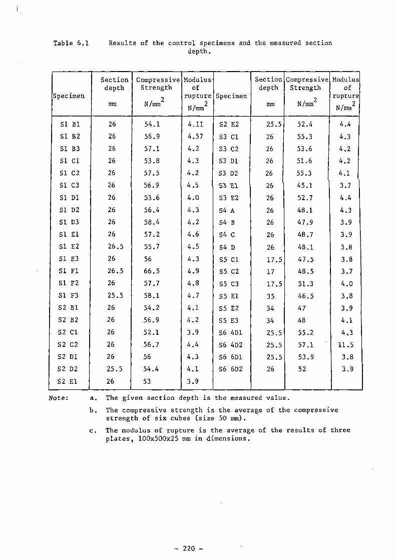
Table 6.1 Results of the control specimens and the measured sectiondepth.
Specimen
Sectiondepth
mm
CompressiveStrength
N/mm2
Modulusof
rupture
N/2
mm
Specimen
Sectiondepth
mmN/mm
2
CompressiveStrength
2N/mm
Modulusof
rupture
Si Bl 26 54.1 4.11 S2 E2 25.5 52.4 4.4
S1 B2 26 56.9 4.57 S3 Cl 26 55.3 4.3
Si B3 26 57.1 4.2 S3 C2 26 53.6 4.2
Si Cl 26 53.8 4.3 S3 D1 26 51.6 4.2
Si C2 26 57.5 4.2 S3 D2 26 55.3 4.1
Si C3 26 56.9 4.5 S3 F.1 26 * 45.1 3.7
Si D1 26 53.6 4.0 S3 E2 26 52.7 4.4
Si D2 26 56.4 4.3 S4 A 26 48.1 4.3
S1 D3 26 58.4 4.2 S4 B 26 47.9 3.9
Si El 26 57.2 4.6 S4 C 26 48.7 3.9
Si E2 26.5 55.7 4.5 S4 D 26 48.1 3.8
Si E3 26 56 4.3 S5 Cl 17.5 47.5 3.8
Si Fl 26.5 66.5 4.9 S5 C2 17 48.5 3.7
Si F2 26 57.7 4.8 S5 C3 17.5 51.3 4.0
Si F3 25.5 58.1 4.7 S5 El 35 46.5 3.8
S2 Bl 26 54.2 4.1 55 E2 34 47 3.9
S2 B2 26 56.9 4.2 S5 E3 34 48 4.1
S2 Cl 26 52.1 3.9 S6 4D1 25.5 55.2 4.3
S2 C2 26 56.7 4.4 S6 4D2 25.5 57.1 11.5
S2 D1 26 56 4.3 S6 6D1 25.5 53.9 3.8
S2 D2 25.5 54.4 4.1 S6 6D2 26 52 3.9
S2 El 26 53 3.9
Note: a. The given section depth is the measured value.
b. The compressive strength is the average of the compressivestrength of six cubes (size 50 mm).
c. The modulus of rupture is the average of the results of threeplates, 100x500x25 mm in dimensions.
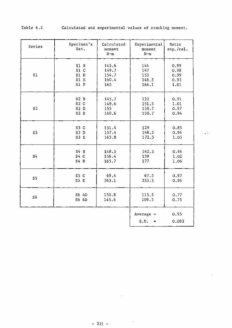
Table 6.2
Calculated and experimental values of cracking moment.
SeriesSpecimen's
Set.CalculatedmomentN-m
ExperimentalmomentN-m
Ratioexp./cal.
S1 B 145.6 144 0.99Si C 149.7 147 0.98
S1 Si D 154.7 153 0.99Si E 160.4 148.5 0.93Si F 165 166.1 1.01
S2 B 145.7 132 0.91S2 C 149.6 151.5 1.01
S2 S2 D 155 150.7 0.97S2 E 160.6 150.7 0.94
S3 C 151.4 129 0.85S3 S3 D 157.4 148.5 0.94
S3 E 163.8 172.5 1.05
S4 B 148.5 142.5 0.96S4 S4 C 156.4 159 1.02
S4 D 165.7 177 1.06
S5 C 69.4 67.5 0.97S5 S5 E 263.1 253.5 0.96
S6S6 4DS6 6D
150.8145.6
115.5109.5
0.770.75
Average = 0.95
S.D. = 0.083
moment of the slabs in that set, except Si F, where the result of slab
Si Fl was neglected due to a high recorded cracking load compared with other
results.
Table 6.2 shows that the calculated values are very close to the
experimental ones, for series Si to S5. The average ratio of experimental
to calculated is equal to 0.97 with the standard deviation equal to 0.052.
The two ratios from the results of series S6 are, however, relatively
lower (average ratio is 0.76). This may be due to, as discussed in sec.
5.8.1, the unexpected low recorded value of the load at first crack for the
specimens of this series. The average value of this load was smaller
than the average ultimate load of the plain mortar specimens. Nevertheless,
the calculated and the experimental values of this series are still close.
The overall ratio of experimental to calculated for all sets of slabs
is equal to 0.95 with a standard deviation of 0.083. This result
indicates that in spite of the variables considered which include number,
yield strength, and opening of the mesh, presence of steel bars, and
thickness of the mortar cover and the section, the suggested method
predicted successfully, the cracking moment of the slabs.
6.4.2 Moment Capacity at First Yielding.
The moment capacity of the section at first yielding was calculated
for all the tested slabs. The first yielding was assumed to take place
when the strain in the extreme fibres of the section attained either the
adjusted value of the tensile strain defined by eq. 6.6 or the value of
the compressive strain given by eq. 6.7, whichever reaches first. The
tensile strain value from eq. 6.6 was adjusted as discussed earlier, to take
into account the strain gradient in the section due to flexural loading.
All the specimens yielded first in the tensile zone except S2 C, S2 D, and S2 E
which yielded in the compressive zone first. A sample for the calculation
of the moment at first yielding is given in Appendix B.
In Table 6.3, the calculated ratio of neutral axis depth from the extreme
compression fibre to the depth of the section, the corresponding tensile
strain in the extreme fibre, and the calculated and experimental moments are
given for each set of specimens. The experimental moments for each set
were obtained by first finding the load corresponding to the assumed tensile
strain for each specimen then averaging moments which correspond to those
loads for the specimens in each set. The number of specimens in each set
of series Sl, S2, S3, S4, S5, and S6 are three, two, two, one, three and two
respectively.
From the values of the ratio of experimental to calculated moments given
in Table 6.3, it can be seen that the described method predicts the moment
capacity of the specimens of series Si and S2 very closely. The mean ratio
of the sets of these two series 1.0 and 1.04 respectively. For the
specimens of series S3, S4, and S5 most of the calculated moment values are
slightly higher than the experimental values (the average ratios of
experimental to calculated are 0.89, 0.94 and 0.97 respectively). The over—
prediction may be because the calculated yield strain is higher than the
experimental ones. Nevertheless, the calculated and the experimental moment
values are still close. For the specimens of series S6, the overprediction
was higher than in the other series (ratio was equal to 0.8). In this
series the variable was the thickness of the mortar cover. Increasing the
mortar cover from 2 mm (specimens Si D) to 4 mm (specimens S6 4D) and to 6 mm
(specimens S6 6D) decreased the ratio of experimental/calculated from 0.99 to
0.83 and to 0.77, respectively. The overprediction can be explained by
noticing that the extreme layer of mesh in the tensile zone becomes less
effective in loading the mortar at the outer side of the section as the depth
of the mortar cover increases. On the other hand, the described method

Table 6.3 Calculated and Experimental moment at the assumed first yieldingpoints.
U'o• ,-i
$4wC"
0oE
• ••I
uwa.
C')
Ratio
*
k
Tensilestrainon theextremefibre
micro-strain
Calculatedmoment
N-m
Experimentalmoment
N-m
Ratio
exp./calc.AverageRatio
S1 B 0.26 1720 210.7 207 0.98 o mID
S1 C 0.28 1930 307.9 314.3 1.02 ,--1 oII
Si D 0.295 2240 417.5 415 0.99 o dco IISi E 0.31 2400 544.6 547.5 1.01 o
$.4 ASi F 0.325 2500 678.5 668.5 0.99 o
> md
S2 B 0.22 5100** 416.3 492 1.18 II n-i
S2 C 0.245 5500** 717 690.6 1.04 oIICIO -.1'
O
cn1
rj.'
S2 DS2 E
0.280.31
4610**4000
801881.6
767.2853.3
0.960.97
CO 0 •• A
CD r-I •
> Cl)•=4
S3 C 0.28 1825 298.1 266.5 0.89 II 00) oN
eelm
S3 DS3 E2
0.30.325
21002250
423539.4
375.4475.9
0.890.89
00 c0 II0 • •i..I 0 AW
C'.)<4 .c)
r.-..S4 B 0.305 2200 432.6 381.5 0.89 II
W0
0-.1•
(n
S4 C 0.33 2425 566 582.5 1.03 tiO -4al aN II
• •S4 D 0.35 2550 693 631.8 0.91 0)0 A•
m(NI
S5 C 0.3 2450 206.8 180.7 0.88 IIW
f-i
In
(/)c
S5 E 0.3 2150 724.9 763.1 1.05 b.° r*-- 0Ctl ON II
P • •0)0 A> •<4 m
S6 4D 0.29or
2580 502or
418.5 0.83or
mco CT• •
.c•0.27 443.6 0.94 o 0
II IIo
m S6 6D 0.28or
3000 553.9or
426.7 0.77or
coCOw
2.6 467 0.9201 34> 0
••4
Overall average = 0.97S.D. = 0.08
*,Ratio of neutral axis depth from extreme compression fibre to the depth ofthe section.
**Governed by yielding of compressive fibre, E = 1800 microstrain.cy

gtcrEtcr
6tyElr
gtcr
y
assumes that the tensile stress for the cracked mortar zone increases
linearly with the strain, i.e., with the depth from the neutral axis. This
assumption seems to be unrealistic in the cover zone, i.e., beyond the
extreme mesh layer when the thickness of this cover is more than 2 mm.
the moment capacity for the specimens of series S6 was therefore recalculated
assuming that the tensile stress remains constant beyond a depth equal to
the depth of the extreme mesh layer plus 2 mm., see Fig.6.8. This adjust-
ment in the method resulted in an increase in the ratio of experimental to
calculated moments from 0.83 and 0.77 for specimens S6 4D and S6 6D to 0.94
and 0.92, respectively.
Ety
Specimen S6 40 Specimen S6 60(mortar cover = 4mm) (mortar cover = 6mm)
Adjustment of the tensile stress diagram to accountfor large mortar cover.
The overall ratio of experimental to calculated was equal to 0.97
with a standard deviation equal to 0.08. This result indicates that the
described method predicts successfully the moment capacity of the ferro-
cement section in the linear range of the cracked stage irrespective of the
number of meshes, mesh yield strength, presence of steel bars, section depth,
and mortar cover.

6.4.3 Ultimate Moment.
From the discussion of sect. 6.3.2, two cases can be realized at
failure:
Case 1. EtEtu
while Ec
< Tensile failure.CU
Case 2 et < etu while E
c6 Compression failurecu
The ultimate moment was calculated for all specimens assuming that they
all follow case 2. Although this assumption as observed experimentally,
may not be true for some specimens, the actual value of the ultimate tensile
strain, Etu
, is not known. Assuming Etu
to be equal to the ultimate tensile
strain of the mesh alone is not correct for specimens reinforced with woven
wire mesh as discussed in sec. 6.3.2. In any case the above assumption
affects only the few specimens where the number of meshes is limited to two
mesh. Moreover, the assumption seems to result in a marginal error in
the calculated ultimate moments, as will be seen later in this section.
To demonstrate the calculation procedure for the ultimate moment, the
calculation for a typical specimen is given in Appendix C.
In Table 6.4, the calculated values of the neutral axis depth and the
ultimate moment are given for all the tested sets of specimens. The
calculated ultimate moments are compared with experimental values which are
obtained from the average of the ultimate moment of the repeated specimen in
each set. From the table, it can be seen that the calculated ultimate moments
are in close agreement with experimental values. The overall average ratio
of experimental to calculated is equal to 1.086 with a standard deviation
equal to 0.109. This result also indicates that the method, in general,
underestimates the ultimate moment. The results of two sets only over-
estimated slightly the experimental values. The two sets are S1 B and S6 6D
(ratio equal to 0.92 and 0.93 respectively). For S1 B, the overestimation
can be attributed to the failure of the specimen in tension and not, as the

Table 6.4 Calculated and experimental ultimate moments.
Series SpecimenRatio*k
Calculatedmoment
N-m
Experimentalmoment
N-m
Ratioexp./cal.
AverageRatio
r,Si B 0.08 280.3 258 0.92 o• mS1 C 0.14 535.5 622.5 1.16 1-1 0
11 •Si Si D 0.2 758.2 844.5 1.11 w o
60 II
Si E 0.24 928.3 997.5 1.08 a3 '$4 MSi F 0.27 1129.2 1206 1.06 cu •
> m
S2
S2 BS2 CS2 D
0.1850.280.32
7511115.81293
78114671665
1.031.311.29
e,t--.,--: cl
it,-1
w 2a) com n
S2 E 0.35 1440 1662 1.1504w .
<4m
-.4-0 cn• c.)
S3S3 CS3 D
0.1450.2
532.6724.8
541.5745.5
1.021.03
,--1 0II •w 0po II
S3 E2 0.27 844.8 903 1.06 m •W qW •> M
•M
csi %.0
S4 A 0.14 447.9 487.5 1.09 r-I ...7
• o
S4S4 BS4 CS4 D
0.1950.250.3
617.5805899.5
661.5948
1017
1.081.181.14
,-4 •II ow 11
to •9p •
w m><4
S5 C 0.23 336.5 337.5 1.0
.4-o• tnt•-n 0
11 •S5 S5 E 0.215 1203.8 1299 1.08 to II9?
M•W AW •> tr)
<4
c-s10
• ("n/
S6S6 4DS6S6 6D
0.2050.225
787.6832.1
870780
1.10.93
ii •w 0to IIm •S-I Ca
w •> m
<4
Overall average ratio = 1.086S.D. = 0.109
*k = ratio of neutral axis depth from extreme compression fibre to the depth
of the section.
6 t kD D(1-k) (6.9)
method assumed, in compression. It can be seen however that the over-
estimation is only minor.
The overestimation in the result of specimen S6 6D (ratio = 0.93), can
be attributed to the assumed value of yield strain which was considered to
be that at the face of the specimen when the specimen first starts
yielding. Such assumption is reasonable if the mortar cover is small.
However, for specimens with 6 mm cover, as was the case in calculating the
moment capacity at first yielding, the yield strain should be considered
to be that at a depth equal to the depth of extreme mesh layer plus 2 mm,
see Fig.6.8.
The difference between the calculated and the experimental ultimate
moments for the high tensile mesh series (S2) (average ratio = 1.19) was
relatively high compared with that of series Sl. This could be explained
by noticing that the high yield mesh did not show a full plastic behaviour.
Thus, the mesh continued to load the mortar in the tensile zone to a higher
level even after the assumed yielding of the specimen. On the other hand
the method does not take into account any increase in mortar tensile stress
beyond that which is calculated at first yielding. The method, therefore,
seems to be reasonable for specimens with mild steel mesh, but gives
slight underestimation for those with high tensile mesh.
6.5 Curvatures and Deflections.
The curvature of the section at any level of the load can be found
knowing that:
The moment-curvature relationship can be established by analysing the
section with incremental increase in the load until failure. Alternatively,
the relationship can be idealized to a trilinear curve and the curvature at

the three turning points of the curve, i.e., first cracking, yielding, and
failure, would be sufficient to establish the linearized moment-curvature
relationship.
The deflection can be calculated from the curvatures. From the
strength of material principles, and using the area-moment method, the
vertical displacement A of point A from the tangent to the elastic curve at
point B is given by
AfB Mxdx
A El
AlsoEl
• A = f Ox dxA
Using an idealized trilinear moment-curvature curve, an idealized tri-
linear load-deflection can be generated. Paul and Pama (11) have given,
using the described principles, the deflection equations for the three
ranges of the idealized load-deflection curve. These equations for the
cracked stage, and for two point load arrangement, are as follows:
For cracked range, first linear range
Ac = (I)c
6 r (wE) 2 (l+r) + ;±.)zi [3 - 4w2 (1+r+r2 )] L2
6.11
For cracked range, yielding range
1A = 4w2cr (r
2+rr2) + 4 cl) (l+r 2
-r2r-r2)1c
+ 4 { 3-4w2 (l+r2+r22 )} L
il26.12
where:
crr = r2 . M
Ac
is central deflection.
cr, , 0, are the moment and the curvature at firsty
cracking, at first yielding, and at the specified load,
respectively.
is the span of the beam.
wL is the distance from the support to the next point load.
To test the performance of the given procedure, the central deflection
of the tested specimens was calculated at two points of their life. These
are the first yielding and the failure. The point of first yielding was
chosen for two reasons. First, the performance of the procedure at this
point could be used to reflect its performance all through the second linear
range as the same equation is proposed to predict the deflection at any point
in this range and that the experimental load-deflection curve is linear there.
It should be noticed that the service load would most likely be within this
range. Second, a close agreement between the calculated and the experi-
mental results would lead, indirectly, to the conclusion that the depth of
the neutral axis obtained by the previously described method of analysis
and on which the values of the curvatures used in the prediction of
deflection depend, should be close to the actual ones. This, in turn
gives another measure, beside that provided by comparing the calculated and
experimental moments, of the success of the suggested analytical procedure
and the assumed stress-strain curves for ferrocement. The deflection at
failure was calculated because of the importance of this value for
ductility purposes.
In Table 6.5, the calculated curvatures, using eq. 6.9, at first
cracking, first yielding, and at failure, are given. These curvature values,
together with the corresponding calculated moments given in Tables 6.2 to
,11,mcr y

6.4 were used in eqs. 6.11 and 6.12 to find the central deflection at
first yielding and at failure for all the sets of specimens. The calculated
and the corresponding experimental deflection are again given in Table 6.5.
From Table 6.5, it can be seen that at first yielding the calculated
deflections are in close agreement with experimental results. The average
ratio of experimental to calculated was equal to 1.07 with the standard
deviation equal to 0.104. The results also show that the calculated
values at this level of the load are mostly less than the experimental
values.
At failure, the calculated deflections are again in close agreement
with experimental results except that of specimens Si B. The high over-
estimation in the deflection of this set of specimens is partly due to
incorrect assumed mode of failure as discussed earlier. This had resulted
in an error in the calculated neutral axis depth and the strain at the
extreme fibre. For sections with very small compression zone at failure,
as is the case with specimen Si B, this error, although it does not affect
the calculated moment significantly, it would lead to a considerable error
in the calculated curvature and in turn in the calculated deflection.
The average ratio of experimental to calculated deflection of all the
sets of specimens, excluding set Si B, is equal to 0.88 with a standard
deviation equal to 0.164. It may be interesting to mention here that
Balaguru et al. (31) had obtained, using a non linear analysis, an average
ratio of calculated to experimental deflection at failure equal to 1.11 with
a standard deviation of 0.318 (ratio range 0.568 to 1.587). Comparing
this result with the result obtained in this study (ratio range 0.58 to 1.19)
suggests that the given method, in spite of being simple, perform equally,
if not better than the method suggested by Balaguru et al. Also, comparison
of the calculated and the experimental deflections at the two selected

a)a.0
,-1• n-icd
L4.4
4•Jcd
00
• ria)C.)a)
r-I4-1a)A
0 •• I-I '`.. 1-14-I • CI3at 0. c..)P4 X
CD
1-1Cr)
•0
tr)CO
•0
CI.,r-I
•r-4
)1-101
•0
co01
•0
r••••
0
inCO
•0
N.•
0
c0In
0
icic,--1cda)0a)0
• 1-1 Ey..a)0.XW
Cr)•
,-110
•..1••
cr.0.—I
r-4•
.....?1-1,--1
CO•
Is.1."•••
CO•
C1Jr••
in•
CO01
al.
0a%
-...t.
1-1rs.
Ln.
Lri
i<-0a)
.I../CI3
v.-I0 EC)
r-Icd
C-)
cr,CAI-I
10••
coCAr-I
...t••
LnCY1
tr)••
,_.03
in•
....tr-
....1-•
0-.1,1-1
r-I•
I".0,-4
00•
CNI0r-I
c0
VI01
CO0
• v-I
r—Ia)
• 1-1›%
Cil$.4
• ri4-1
a)cd
0•ri4-3C.)a)
r-I4-4a)A
0 •• ,-1 --.. r-I4-1 • alal a. oP4 X
a)
.00
•r-i
r-i0
•n-1
Ln0
•r-I
N.0
•r-1
cvr-1
•r-I
Lnc0
0
C•••CA
•0
cn0
•r-4
trl0
•1-I
)c3cr-Ial4-I
A./e
• ri E3.4a)PL.X43
01•
.0
c•I•
co
(r)•
0w-I
co•
,—Iv-I
cn•
C•/r--I
cn•
r••r-I
r•-••
c•1Ni
c,^)•
,--INi
c0•
ONr-I
,it•cla)a)al
1-10ci 0
.-4II
C.)
r-ILn
10
CO0•
CO
Lna'
•CT
100•
r-Ir-I
C110:7%
•••••1,--4
%.0CN1
•0NI
Ni.7
•Cr)Ni
r n•
0Cs.1
co.
03f-1
CAa)$.401-/CO 10> 03.I t-40c.) X
ErlCU a
4-1 -••••CO e-I
r-I0Ci
,—ICO
C..)
CUW
4-1<,-
• .-1co
11-1
......tCO03(NI
0in1.0,—)
cnLnr-In—)
1-1%.001
IllInCO
0LrtNJ"--1
,..1"C1Ico
0C11N.
01/40.0
4..1 ttI)cn 0P •,-1
"014-I 1-1
w4-1 • 1-4-=4 >-,
....T•
cr%co
n—i•
cr)01-4
n-1.
NiCVr--I
c0.
v.-)cnr-I
Lc).
CV-7I-1
Ln
r-IinNI
CNI.
0coC-11
Cr).
10...i.C14
Cr/NJC1I
4-ico
• ri uLH CO
Y41.1 C.)"t
ce)•
0.1v-I
MI•
CAr-I
Cr1•
C11v-I
Cr/•
NJr-I
Cr/•
C11r-1
Crl•
NJr-I
01•
C11g-I
Cr)•
C1.11-1
Cr)•
C1.1f-I
0a)0
• r-I 1.1c..) a)a) cr)Cal
C/1
03
r-iCII
C.,
r-iCI)
A
,--iC/)
PIr-iC/3
44
r-IC/)
PlC11Cl)
0C14Cl)
A
C1,1Cl)
WC13Cl)
— 232 —

a)1-1Z
.-.1• r.Ial
4-1
4-1cd
00
-,-1A-1C)Q)
r-1)44cuq
I-1ccl
00• r-I ---...4-1 •C17 04
X41
,-4es
•0
0ON
•0
0•
1-I
01",
•0
c0CO
•0
,--I••••1
•r-i
%-c)CO
•0
..i.03
•0
Nv--1
•,_.1
r...CO0
4444
•-10
.L.)00)
' S1-1CD0.XW
NO
inCfN
inCT
-4
ioCO
-
en1."..
-
•-•1CO
r-4•
01ON
.
N.•
inCN1•-i
0.1•
N.%.0
.
C4•
N.Csi1-4
.....7•
001
44"0a)
4-10
•--i .E0 EC.)
•-1CAU
in•inen1-1
,-1•
%JD0,-.4
i.D•i.0c0
r-I•
in0I-I
V)•
NON
CO•
enc0
CNJ•
i0-.I*4-1
-
0)•
0o0
N..
en1-11--1
cr)•
....I0
v-I
bO0
• ,-i"0v-Ia)
..-1
4-1Cl)3.4
-.-1144
4-1CO
00
• r-I4.-)c..)a)
•-44-1a)A
•1-40
0 C.)-1-1 "....4-1 •ccl Pw;4 X
Cr)
If )N.
•r-4
rsiN
•1-1
VO,-4
•v-4
MO,-i
•”-I
0•
1-1
N0
•rni
al0
•1n1
NCA
•0
Un1-1•1-.1
r-IN
••-.1
**
,-.1cd4..)0al0
.,-1 i)..1W04X
r..4
Ln
cr,-..t
•,-i•-•I
cc'-,
NJr-.1
Le l
•-.11-I
NO
,-4•-.1
ON•N
r-I
01•
N.r-I
00•
CO
03.
Nr-I
•
L e-1•
V)rvl
4:.0a)
.1-1cd
•-4 gc.)
•-4cd0
n-iN.0
r-
I',01
0.1
NO
0i-4
.
.....1'01
0%
inin1-i•-i
NifON1-1
......ti.0v.1
inin
ON
010
I-1v-I
co
Nr-I
to0)1.10
.1-10
3-I 00 r-Ic.)
X"0al E
.1-1 5CA "-..-
a-I r-40C.)
,--10
C.)
a)L.40
4-) ,-1<4 •rl
CA4-1
0CiNint-4I
0ini-41-4
cpinoo
cn00,--i•-1
enNON
a.%.0N.
0cri-....11-1
,-1Cs)03
Lri0.11-4r-I
LnCN1-01.4
1-1 oDco Z34 • ,-1
• rl '104-1 v-I
a)4..) •.4<4 PN
in•
N.01
-..7•
in,-I,-1
cq
coC11,-i
co
r-IN,-1
EN
01en,-.1
01
0inI-1
00CV
1-I
00,--.11--I
ON
Lncna-I
01•
InLn•--1
.1-1U)
• 1-I C.)14-1
3-14-1 c.)<4
Cr)a
N.-1
01.
N1-1
ce).
N1.--1
en.Nv-I
en.es11-I
en.Nv--I
en.oo1--1
....t.
crien.N•-1
en.Nr-I
0a)E
• v-I .4-1C.) WCll COCa.
CO
C..)
enC./3
A
enEn
W
enCl
faO-..tCl)
C.)
-..tCI)
01
-.I-Cil
c.)
inCl)
W
inCl)
a).4
VDCl)
nO
NDCl)
Q1.04,J
3.40
14-1
0
a)Ett)
$.44.1
0.61
a)
144a)
1-1a) Ea• •.1O 0
W
1-1.L) a)EEI
4-4 XO a)
• Q)cd4.1
a)
.L)
"0 caO 0O 4-'4
CA 73W3.4 4-1O 0
cdC-)
ci
3-1O 0
a) .04-1
COr-I 0O 4-I
1-4CA 0C.) 0
04cl)
4 a)4-3 •
$4 4-k
0 a)O E.) co
"0 4 4w Ei C.)
cd
•
4 a)
g
•
•v-I0 0
.4.4 0U.1-1 • 1-I 0Cr) 4.4 13)
1-1 C.)411 ••4
1-4 044- a)cd a)0
c.) A En-IC 3C
- 233 -

moments of the life of the specimens indicate clearly that the linear-
ization of the moment-curvature and the load-deflection curve does not result
in considerable error in the predicted deflections at these two moments.
It should be mentioned that the contribution of the first term in both
eq. 6.11 and eq. 6.12 to the deflection value obtained from these equations
is only minor. This term corresponds to the deflection at tht end of the
uncracked range and could be ignored in first estimation of the
deflection for design purposes.
6.6 Prediction of Ultimate Moment Using Other Investigators' Methods.
As discussed in the review of literature of this chapter, there are
mainly three different approaches to calculate the flexural strength of
ferrocement. These are, the approach which uses the principles of ultimate
strength analysis of reinforced concrete, the approach which considers ferro-
cement as a composite material with its mechanical properties predicted using
the law of mixtures, and that which limits the amount of reinforcement in
ferrocement and considers its mechanical properties to be the same for any
ferrocement sections. Only the first two approaches were used to calculate
the ultimate strength of some of the specimens tested in this study, as
the disadvantages of the third approach were discussed previously. The
reinforced concrete approach was used with a compressive stress block
similar to that recommended by CP.110 (68). The ultimate compressive strain
was taken to be 6000 microstrain and the actual stress-strain curve of the mesh
was used to find the tensile stress in the reinforcement at the different
strains. The composite material approach is mainly developed by Paul and
Pama (11) and therefore their procedure was used for the calculation of the
ultimate strength.
The ultimate strength of specimens of series Si was calculated using
the above mentioned methods. This series includes five sets of specimens
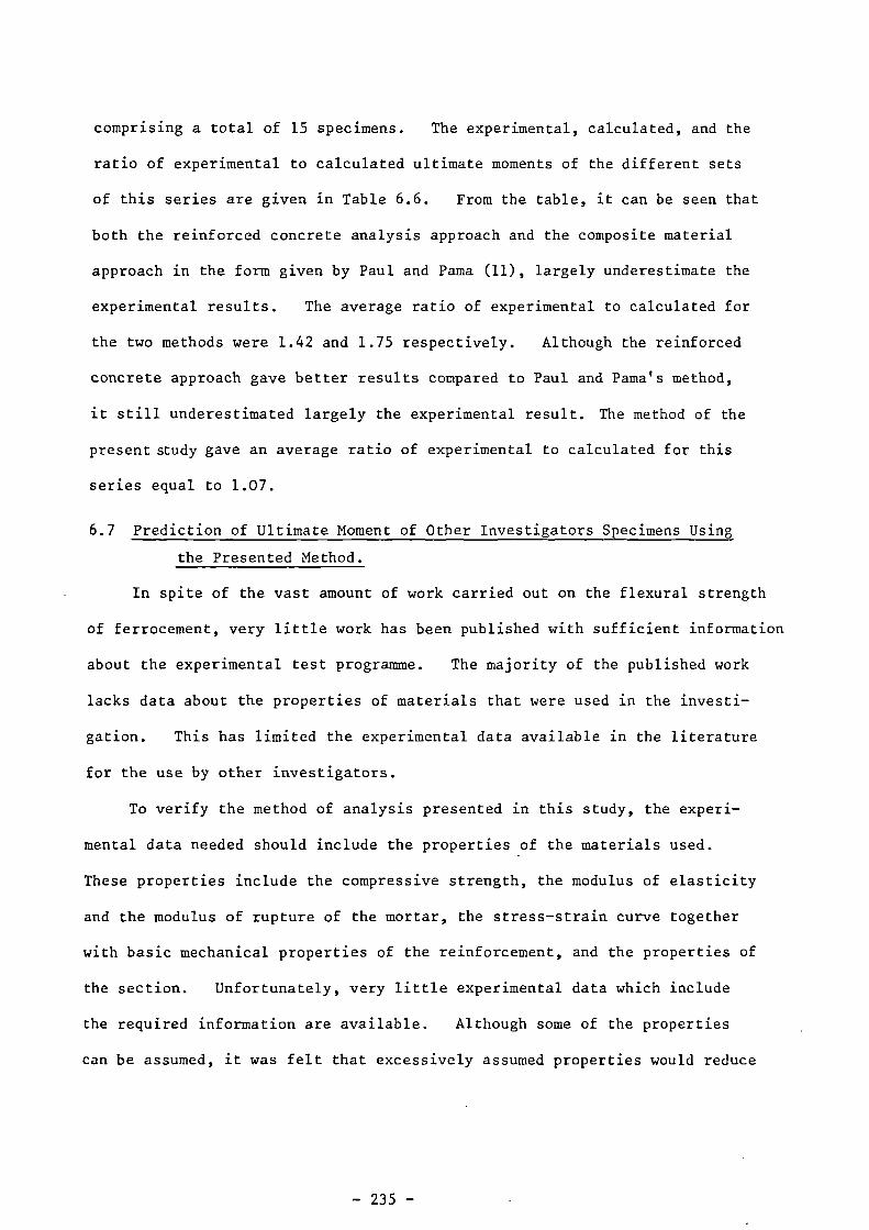
comprising a total of 15 specimens. The experimental, calculated, and the
ratio of experimental to calculated ultimate moments of the different sets
of this series are given in Table 6.6. From the table, it can be seen that
both the reinforced concrete analysis approach and the composite material
approach in the form given by Paul and Pama (11), largely underestimate the
experimental results. The average ratio of experimental to calculated for
the two methods were 1.42 and 1.75 respectively. Although the reinforced
concrete approach gave better results compared to Paul and Pama's method,
it still underestimated largely the experimental result. The method of the
present study gave an average ratio of experimental to calculated for this
series equal to 1.07.
6.7 Prediction of Ultimate Moment of Other Investigators Specimens Using
the Presented Method.
In spite of the vast amount of work carried out on the flexural strength
of ferrocement, very little work has been published with sufficient information
about the experimental test programme. The majority of the published work
lacks data about the properties of materials that were used in the investi-
gation. This has limited the experimental data available in the literature
for the use by other investigators.
To verify the method of analysis presented in this study, the experi-
mental data needed should include the properties of the materials used.
These properties include the compressive strength, the modulus of elasticity
and the modulus of rupture of the mortar, the stress-strain curve together
with basic mechanical properties of the reinforcement, and the properties of
the section. Unfortunately, very little experimental data which include
the required information are available. Although some of the properties
can be assumed, it was felt that excessively assumed properties would reduce
- 235-

Table 6.6 Comparison of experimental and calculated ultimate moment forseries Sl, using other investogators' methods.
SpecimenSet
Ultimate moment in N-mRatio Ratio
Reinforced Paul and Experimental (3)1(1) (3)1(2)Conc.Proced. Pama
(11)(1) (2) (3)
S1 B 277.3 137.2 258 0.93 1.88S1 C 390.9 341.8 662.5 1.69 1.93S1 D 568 480.7 844.5 1.49 1.76S1 E 691 619.9 997.5 1.44 1.61Si F 782.9 765.5 1206 1.54 1.58
Average Average= 1.42 = 1.75
S.D.= 0.288 S.D.=0.156
Table 6.7 Comparison of ultimate moment predicted by the given method withexperimental results from Balaguru, et al. (31).
Type ofmesh
Meshyield
strength
N/mm2
Mesh
modulusof
elastisityN/mm
No.of
mesh
Calculatedultimatemoment
N-m
Experimental
ultimatemoment
N-m
Ratio
Exp./Cal.
1/4 1 'Woven3
2 41.5 32.78 0.79wire dia. 475.8 137.9x10 4 78.6 65.91 0.84=0.635 mm 6 108.7 93.24 0.86
I" Woven 2 52.9 50.09 0.95wire dia. 620.6 200x10
34 132.13 106.73 0.81
= 1.07 mm 6 158.8 155.29 0.98
i n Welded 2 55.1 42.96 0.78wire dia. 482.7 137.9x10
34 101.3 89.51 0.88
=1.07 mm 6 133.7 130.63 0.98
•
Average= 0.874
S.D.=0.079

the significance of the analysis results. Therefore only the beams given
by Balaguru, Naaman, and Shah (31) were considered to calculate the ultimate
strength, as most of the required properties are given. The results are
shown in Table 6.7. It should be mentioned that the moment was calculated
for all the specimens at their actual failure. While the experimental
moment was that which corresponds to a maximum deflection of 25.4 mm or
failure of the specimen. However, only one specimen (2 mesh, 1/4" mesh
specimen) had a deflection at failure higher than the given value.
Table 6.7 shows that the calculated moments are in close agreement
with experimental ones. The overall average ratio of experimental to
calculated was 0.874 with a standard deviation equal to 0.079. The table
also shows that the calculated moments are higher than the experimental
moments. Also, the higher the number of meshes the closer the calculated
value to the experimental results. The overestimation may be attributed
to the value of yield tensile strain which was taken on the face of the
specimen and not on the level of extreme mesh layer. This assumption seems
to result in slightly higher overestimation when the number of meshes is
smaller. It should be noticed however that for specimens with small
section depth, such as those of Balaguru, et al. where D = 12.7 mm, a
difference of 0.3 mm between the nominal and the actual thickness of the
section would result in about 57. variation in the calculated moment.
Therefore the 13% overestimation is acceptable for the given experimental
data.
6.8 Conclusions.
Based on the discussions and results presented in this Chapter, the
following conclusions were drawn:
1. A simple analytical procedure is presented to predict, at any moment
of the life of the member, the moment capacity, curvature and deflection for
ferrocement under flexural loading.

2. The presented procedure predicted closely the moment capacity at
first cracking, at first yielding, and at failure of the ferrocement plates
tested in this study, irrespective of the variables included. The overall
average ratio of experimental to calculated value of the moment capacity at
the mentioned stages were 0.95, 0.97, and 1.086, respectively.
3. The method presented predicted satisfactorily the deflections at first
yielding and at failure of ferrocement plates, assuming idealized trilinear
moment-curvature and load-deflection curves.
4. Reinforced concrete theory and the theory proposed by Paul and Pama (11)
for calculating the ultimate moment, highly underestimated the experimental
results of specimens tested in this investigation (average ratio
experimental/calculated equal to 1.42 and 1.75 respectively).
5. The ultimate moment of the beams given by Balaguru et al. (31) were
predicted satisfactorily using the presented analytical procedure.
6. The use of the assumed stress-strain relationships for the tensile and
compressive zones and the equations for predicting the tensile and
compressive yield strain seem to give satisfactory results.
- 238-

CHAPTER 7.
LIMITATION OF THE WORK, CONCLUSIONS, AND SUGGESTIONS
FOR FUTURE WORK.
The main object of this investigation was to study the strength and
deformation characteristics of ferrocement plates in flexure. There are
several types of mesh reinforcement used in ferrocement. In addition, there
are several parameters involved with each type of mesh. Due to the aim of
achieving significant conclusions with a reasonable amount of work, only one
type of mesh was used, i.e., woven steel wire mesh. Because of this, plus
the fact that in spite of the several parameters considered in this study,
there are others that could affect the behaviour of ferrocement and which
were not included, the present investigation cannot be considered as a complete
study of the flexural behaviour. Nevertheless, the test results have helped
significantly in a clearer understanding of the structural behaviour of ferro-
cement, as well as throwing light on some of the required future research.
7.1 Limitations of the Present Work.
The limitations within which this investigation was carried out can be
summarized as follows:.
1. Only woven type steel wire mesh has been used in the test
programme of this study.
2. Only one mix proportion has been used throughout the investigation.
In that mix, ordinary Portland cement was used and 20% by weight
of the cement and 20% by volume of the sand was replaced by
pulverized fly ash (pfa).
3. For the mild steel mesh reinforcement, two sizes of mesh opening
were considered, i.e., 5.45 mm and 6.35 mm. For the bar
reinforcements, 6 mm mild steel bars were used.
4. For the high tensile reinforcement, steel wire mesh with a mesh
opening of 5.45 mm and ultimate strength of 1197 N/mm2 were used.
5. The effect of the thickness of the section and the mortar
cover were investigated on specimens reinforced with the same
amount of mild steel wire mesh reinforcement.
7.2 Conclusions.
The conclusions presented here are based on and limited by the test
conditions and the test procedures used in this investigation. The con-
clusions derived from each chapter are summarized at the end of that chapter.
The overall general conclusions extracted from the test results are summarized
as follows:
1. Pulverized fly ash can be used successfully, as a cheap material
to substitute part of the cement in the relatively rich mortar
used in ferrocement.
2. The use of pulverized fly ash as a substitute for part of the
cement and part of the sand increased, significantly the work-
ability and increased slightly the compressive strength at 28
days compared to the all cement mix. The compressive strength
at 700 days is about 1.7 times that at 28 days.
3. The developed casting mould and casting technique were simple and
successful in controlling the spacing and distribution of the
reinforcement in the sections.
4. The cracking behaviour of the ferrocement plates is characterized
by small crack width and spacing and by almost full development of
the number of cracks at relatively early stages of the load (at
about 30-50% of the ultimate load). The transverse wires of the
mesh seem to be preferential locations for the cracks, but the
ultimate crack spacing was mostly more than the spacing of the
transverse wires.
5. The overall ratio of maximum to mean crack width was equal to 1.71
and was relatively smaller than in reinforced concrete.
6. For the same tensile strain at the extreme fibre of the member,
the maximum crack width in reinforced concrete can be up to 4 to
5 times that in ferrocement.

7. The mean crack width increases linearly with the tensile strain
at the extreme fibre of the section. The slope of this linear
relationship was called the rate of growth of crack width and its
value was used as a measure of the cracking performance of the
plates.
8. The reinforcement yield strength influences strongly the crack
width and spacing of the ferrocement plates. For the same
number and opening of the mesh, plates reinforced with high
tensile mesh had a lower rate of growth of crack width and smaller
crack spacing after failure than those reinforced with mild steel
mesh.
9. Irrespective of the type of reinforcement, increasing the number
of meshes enhanced appreciably the cracking performance of the
plates. There seems, however, an optimum number of meshes beyond
which the enhancement slows down considerably. The optimum
number of meshes varied with the reinforcement yield strength.
10. Increasing the thickness of the mortar cover decreases the crack
width and spacing.
11. The enhancement in the cracking performance of the plates which
were reinforced with mild steel wire mesh over those reinforced
with conventional steel bars started when the number of meshes
was more than four. The high tensile mesh plates showed better
cracking performance even in plates with two meshes.
12. For the same fraction volume of reinforcement, plates reinforced
with combination of mild steel wire mesh and mild steel bars
showed, if not better, equal cracking performance compared to those
reinforced with mild steel mesh only.
13. Available crack width prediction equations highly underestimate or
overestimate the experimental results of this investigation.
14. The proposed crack width prediction equations are limited by the
experimental results.
15. Based on the load-deflection and load-strain curves, the behaviour
of ferrocement plates under load can be divided into three ranges,
separated by the first cracking and the first yielding. The first
- 241-
two ranges are linear and represent, respectively, the uncracked
stage and the first cracked stage where the cracks multiply in
number rapidly. The third range represents the yielding stage
in which the crack width and deformation increase rapidly.
16. The stiffness of the plates in the linear range of the cracked
stage, measured by the slope of the load-deflection curve, was in
direct proportion with fraction volume of reinforcement in loading
direction.
17. The yielding characteristics of the ferrocement plates is controlled
mainly by the yielding characteristics of the reinforcements.
18. Ferrocement under flexural loading could fail either in tension
or in compression depending on the amount and yield strength of
the reinforcement.
19. For the same type of mesh, increasing the number of meshes in the
plates changed the failure from one in tension to one in
compression.
20. Plates reinforced with high tensile mesh had, generally sudden
and catastrophic failure. The plates were extensively damaged.
Those reinforced with mild steel mesh showed more ductile and
localized failure.
21. The load at first cracking did not vary appreciably with the
studied parameters except that it was in direct proportion to the
square of the section depth.
22. As far as the deflections and crack width are concerned the
service load appears to be within the linear range of the cracked
stage.
23. As long as the plate has not yielded, the crack width remains
mainly below 50 microns.
24. The deflection value seems to be the governing criteria for the
service load. The high tensile mesh therefore is not economical
as its higher cost cannot be justified by a higher service load.
25. The load at first yielding varied between 45-65% of the ultimate
load.
- 242-

26. To satisfy the deflection criteria, the service load could be as
low as 15-30% of the ultimate load.
27. The apparent weakness of ferrocement to satisfy the deflection
criteria suggests strongly that, making use of the good cracking
performance, the material can be used for sandwiched panels or
to be combined with reinforced concrete to produce a composite
material.
28. Simple analytical procedures are presented to predict at any moment
of the life of the specimen, the moment capacity, the curvature,
and the deflection under flexural loading.
7.3 Recommendations for Future Work.
1. More experimental data are needed to investigate the influence of mesh
opening, presence of high tensile bars, and thickness of mortar cover
and section depth on the flexural behaviour of ferrocement plates with
different number of meshes.
2. More 'test data are required to check the validity of the proposed
methods of predicting the crack width, moment capacity and deflection.
Such data will also be useful in refining the proposed equations and
analytical procedures so that they could be used as standard design
methods.
3. More experimental work is required on the optimization of the amount
of reinforcement in the section. Consideration should be given to
combining high tensile steel mesh, mild steel mesh, and steel bars.
4. More experimental work is required to investigate the flexural behaviour
of ferrocement reinforced with other types of mesh. An optimization
study can then be carried out to find the most economical type of mesh.
5. More experimental tests are needed to study the structural behaviour
of full scale ferrocement members under biaxial bending and combined
loading and with different end conditions.
6. Tests and studies are needed to assess the probable economic prospects
of combining ferrocement and reinforced concrete as a composite material,
such as sandwiched panels and the use of ferrocement as a permanent
formwork. for reinforced concrete.

REFERENCES
1. Nervi, P.L., "Structures", Translation by Giuseppina and Mario Salvadori,F.W. Dodge Corporation, 1956, New York.
2. National Academy of Sciences, "Ferrocement: Applications in DevelopingCountries", Washington, February, 1973.
3. Romualdi, J.P., "Research Needs and the Future of Ferrocement", Ref.71,pp.173-177.
4. Bigg, G.W., "An Introduction to Design for Ferrocement Vessels",Vessels and Engineering Division, Industries Development Branch,Fisheries Services, Ottawa, Canada, 1972, pp.224.
5. Bezukladov, V.F., Vanovich, A., "Ship Hulls Made of Reinforced Concrete",Translated from Russian as Navships translation No. 1148, U.S.Department of the Navy, Nov.1968.
6. Shah, S.P., "New Reinforcing Materials in Concrete", J.Amer.ConcreteInstitute, Vol.71, No. 5, May 1974, pp.257-262.
7. ACI Committee 549, "State of the Art", Report on Ferrocement.
8. Kowalski, T.G., Walkus, B.R., "Concrete Technology in the Quality Controlof Ferrocement vessels". Ref. 72, pp.27-32.
9. Raichvarger, Z., and Raphael, M., "Grading Design of Sand for FerrocementMixes", Ref.71, pp.115-132.
10. Shah, S.P., and Key, W.H., "Impact Resistance of Ferrocement", JournalASCE, Struct. Division, Vol.98, No. ST1, Jan. 1972, pp.111-123.
11. Paul,B.K., and Pama, R.P., "Ferrocement" International Ferrocement Centre,IFIC Pub., August, 1978, pp.149.
12. Alwash, A.A., "Flexural Characteristics of Ferrocement", M.Sc. Thesis,College of Engineering, University of Baghdad, Iraq, June, 1974.
13. Atcheson, M., and Alexander, D., "Development of Fibrous Ferrocement",Ref. 71, pp.81-102.
14. Alexander, D., and Atcheson, M., "Fibrous Ferrocement for CommercialVessels", Journal of Ferrocement, Vol.5, No. 2 and 3, March-May,1976,pp.25-48.
15. Ramouldi, J.P., and Batson, G.B., "Mechanics of Crack Arrest in Concrete",Journal ASCE, Vol.89, EM3, June 1963, pp.147.
16. Ramouldi, J.P., and Batson, G.B., "Behaviour of Reinforced Concrete Beamswith Closely Spaced Reinforcement", ACI Journal, Vol.60, No. 6,June 1963, pp.775-790.
17. Naaman, A.E., and Shah, S.P., "Tensile Tests of Ferrocement", ACI Journal,Vol.68, No. 9, Sept. 1971, pp.693-698.

18. Logan, D., and Shah, S.P., "Moment Capacity and Cracking Behaviour ofFerrocement in Flexure", ACI Journal, Vol.70, No. 12, December 1973,pp.799-804.
19. Walkus, R., "State of Cracking and Elongation of Ferrocement Under AxialTensile Load", Buletinul Institutului Politechnic Din lasi, Poland,Part I, Vol.X1V(XVIII) (1968), Part II, Vol.XVI(XX) (1970).
20. Walkus, B.R., and Mackiewicz, A., "Application of Ferrocement Shells inMarine Structures", IASS, Symposium on Industrial Spatial and ShellStructures, Held at Kielec, Poland, June 1973, pp.385-398.
21. Johnston, C.D., and Mattar, S.G., "Ferrocement - Behaviour in Tension andCompression", Journal of the Structural Division, ASCE, Vol.102, No.ST5, May 1976, pp.875-899.
22. Desayi, P., and Jacob, K.A., "Strength and Behaviour of Ferrocement inTension and Flexure", Modern Trends in Civil Engineering, CivilEngineering Department, University of Roorkee, Vol.1, Nov.1972,pp.274-279.
23. Nathan, G.K., and Paramasivam, P., "Mechanical Properties of FerrocementMaterial", First Australian Conference on Engineering Materials, Sydney,August 1974, pp.309.
24. Naaman, A.E., "Design Prediction of Crack Width", Ref.71, pp.25-42.
25. Rajagopalan, K., and Parameswaran, V.S., "Cracking and Ultimate StrengthCharacteristics of Ferrocement in Direct Tension and Pure Bending",Indian Concrete Journal, Vol.48, No. 12, December 1974,pp.387-395.
26. Pama, R.P., Sutharatanachaiyaporn, C., and Lee, S.L., "Rigidities andStrength of Ferrocement", First Australian Conference on EngineeringMaterials, Sydney, August 1974, pp.287-308.
27. Desayi, P., and Joshi, A.D., "Ferrocement Load Bearing Wall Elements",ASCE Journal, Stru. Div., Vol.102, No. ST9, September 1976, pp.1903-1916.
28. Rao, A., and Gowdar, C.S., "A Study of Behaviour of Ferrocement in DirectCompression", Cement and Concrete Journal, Vol.10, No. 3, Oct.-Dec.1969, pp.231-237.
29. Austeriaco, N.C., Lee, S.L., and Pama, R.P., "Inelastic Behaviour ofFerrocement Slabs in Bending", Magazine of Concrete Research, Vol.27,No. 93, December 1975, pp.193-209.
30. Walkus, B.R., "The Behaviour of Ferrocement in Bending", Journal ofStructural Engineering, Vol.3, No. 3, Oct. 1975, pp.113-125.
31. Balaguru, P.N., Naaman, A.E., and Shah, S.P., "Analysis and Behaviourof Ferrocement in Flexure", Journal of the Structural Division,ASCE, Vol.103, No. ST10, Oct.1977, pp.1937-1951.
32. Kamaswadara, A., and Kallapa, C.S., "A Study of the Behaviour of Ferrocementin Flexure", Indian Concrete Journal, April 1971.

33. Surya Kumar, G.V., and Sharma, P.C., "An Investigation of the Ultimateand First Crack Strength of Ferrocement in Flexure", IndianConcrete Journal, Vol.50, No. 11, Nov.1976.
34. Johnston, C.D., and Mowat, D.N., "Ferrocement-Material Behaviour inFlexure", Journal of the Structural Division, ASCE, Vol.100, No. ST10,October 1974, pp.2053-2069.
35. Cohen, L.D.G., and Kirwan, R.S., "Some Notes on the Characteristics ofFerrocement", Civil Engineering and Public Works Review, London, Vol.54,No. 631, Feb.1959, pp.195-196.
36. Picard, A., and LaChance, L., "Preliminary Fatigue Tests on FerrocementPlates", Cement and Concrete Research, Vol.4, No. 6, November 1974,pp.967-978.
37. Thomas, G., "Ferrocement Boats", Indian Concrete Journal, Vol.45, No. 7,July 1971, pp.329-332.
38. McKinnon, E.A., and Simpson, M.G., "Fatigue of Ferrocement", Journal ofTesting and Evaluation, JTEUA, Vol.3, No. 5, Sept. 1975, pp.359-363.
39. Bennett, E.W., Fakhri, N.A., and Singh, G., "Fatigue of Ferrocement inUni-directional Bending", International Symposium on Ferrocement,July 1981, ISMES, Bergamo, Italy, pp.1/37 - 1/47.
40. Balaguru, P.N., Naaman, A.E., and Shah, S.P., "Serviceability of Ferrocementsubjected to Flexural Fatigue", The International Journal of CementComposites, Vol.1, No. 1, May 1979, pp.3-9.
41. Singh, G., "Flexural Response of a Ferrocement to Constant DeflectionRepeated Loading", International Symposium on Ferrocement, July 1981,ISMES, Bergamo, Italy, pp 211 - 216.
42. Surya Kumar, G.V., Narayanaswamy, V.P. and Sharma, P.C., "Ferrocement -A Survey of Experimental Investigations", Journal of StructuralEngineering, Vol.1, No. 4, Jan. 1974.
43. Claman, J.S., "Bending of Ferrocement Plates", M.Sc. Thesis, MassachusettsInstitute of Technology, May 1969.
44. Walkus, B.R., "Proportioning of Ferrocement Elements in Bending TakingAccount of the Crack Width", Journal of Structural Engineering, Vol.3,No. 3, Oct. 1975, pp.127-135.
45. Pama, R.P., et al., (Editor), "Materials of Construction for DevelopingCountries", Proceedings of International Conference, Asian Instituteof Technology, Bangkok Thailand, August 1978, (2 volumes).
46. Pama, R.P., Lee, S.L., and Vietmeyer, N.D., "Ferrocement, A VersatileConstruction Material: Its Increasing Use in Asia", InternationalFerrocement Centre, Asian Institute of Technology, Bangkok,Thailand, 1976.

47. Pama, R.P., and Phromratanaporgse, O., "The Potentials of Ferrocementand Related Materials for Rural Indonesia - A Feasibility Study",Asian Institute of Technology, Bankok, Thailand, October 1977,pp.20.
48. Jorgensen, S.L., "Effect of Multi-Stage Plastering on Ferrocement",M.Sc. Thesis, Sept.1971, Berkeley, U.S.A.
49. British Standards Institute, B.S.12, 1971, "Portland Cement (Ordinaryand Rapid Hardening)".
50. British Standards Institute, B.S.3892, 1965, "PFA For Use in Concrete".
51. Swamy, R.N. and Stavrides, H., "Some Properties of High WorkabilitySteel Fibre Concrete", Proc. of RILEM Symp. on Fibre ReinforcedCement and Concrete, Sept. 1975, Construction Press Ltd., (London),pp.197-208.
52. ASTM (305-65), "Mechanical Mixing of Hydraulic Cement and Mortars ofPlastic Consistency", American Standards of Testing Materials,
1965.
53. British Standards Institute, B.S.1881, Part 4, 1970, "Methods of TestingConcrete".
54. Jackson, A.J.W.,and Goodridge, W.F., "A New Approach to P.F. Ash Concrete",The Contract Journal, March 9th, 1961, pp.1284-1296.
55. Smith, I.A., and Arthur, P.D., "Mix Design for Fly-Ash Concrete", Journalof the Institute of Engineers, (India), Vol.48, No. 1, Sept. 1967,pp.105-128.
56. Rajagoplap, K., and Parameswam, V.S., "Analysis of Ferrocement",Journal of Structural Engineering, Vol.2, No. 4, Jan. 1975, pp.155-164.
57. Balaguru, P.N., Naaman, A.E. and Shah, S.P., "Fatigue Behaviour and Designof Ferrocement Beams", Journal of the Structural Division, ASCE,Vol. 105, No. ST7, July 1979, pp.1333-1346.
58. Balaguru, P.N., "Cracking Behaviour of Ferrocement Beams Under Static andFatigue Loading", International Symposium on Ferrocement, July 1981,ISMES, Bergamo, Italy, pp. 2/127 - 2/138.
59. Beeby, A.W., "An Investigation of Cracking in Reinforced Concrete SlabsSpanning One Way-Static Loading", CIRIA Report No. 21, March 1970,pp. 48.
60, Base, G.D., et al., "An Investigation of the Crack Control Characteristicsof Various Types of Bars in Reinforced Concrete", C and CA ResearchReport, No. 18, Parts 1 and 2, Dec. 1966, 44-32 pp.
61. Al-Taan, S.A., "Structural Behaviour of Conventionally Reinforced ConcreteBeams with Steel Fibres", Ph.D. Thesis, University of Sheffield,July 1978, 339 pp.

62. Davies, O.L., and Goldsmith, P.L., (Editors), "Statistical Methods inResearch and Production", Published for ICI by Oliver and Boyd,Edinburgh, 1972, pp.478.
63. Broms, B.B., and Lutz, L.A., "Effects of Arrangement of Reinforcement onCrack Width and Spacing of Reinforced Concrete Members", ACI Jour.,Proc. Vol.62, No. 11, Nov.1967, pp.1395-1410.
64. Ferry-Borges, J., "Cracking and Deformability of Reinforced ConcreteBeams", Pub. of IABSE, Zurich, Vol.26, 1966, pp.75-95.
65. Illston, J.M., and Stevens, R.F., "Long Term Cracking in ReinforcedConcrete Beams", Proc. of ICE, Vol.53, Dec.1972, pp.445-459.
66. Nathan, G.K., and Paramasivam, P., "Tensile and Flexural CrackingStress of Ferrocement", Engineering Journal of Singapore, Vol.3, No. 1,1976, pp.45-50.
67. Smith, R.B.L., "Design Philosophy for Ferrocement", Ref.46, pp.18-21.
68. C.P.110 - "The Structural Use of Concrete", British Standards Institute,
London, 1972.
69. Ferguson, P.M., "Reinforced Concrete Fundamentals", John Wiley and Sons,Inc., 1965.
70. Weiss, V., "Crack Development in Concrete with Closely-Spaced Reinforcementand in Similar Materials", Cement and Concrete Magazine, Vol.3, No.2,1973.
71. "Ferrocement - Materials and Applications", Proc.International Symposium,Toronto, April 1978, ACI Pub. SP-61, 1979, 195 pp.
72. "FAO Investigates Ferrocement Fishing Craft", Published by Fishing NewsLtd., Surrey, England, 1973, 200 pp.
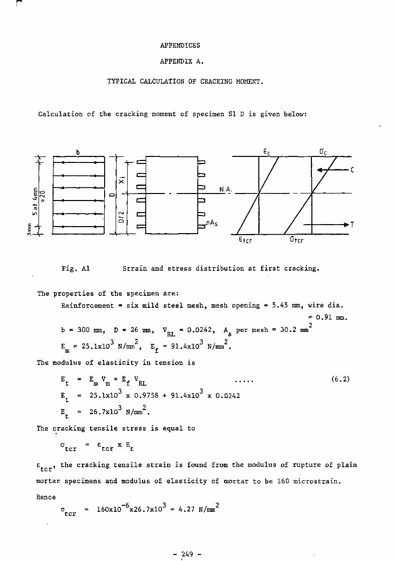
•
E —%-E
•
7
APPENDICES
APPENDIX A.
TYPICAL CALCULATION OF CRACKING MOMENT.
Calculation of the cracking moment of specimen S1 D is given below:
Etcr
c r
Fig. Al Strain and stress distribution at first cracking.
The properties of the specimen are:
Reinforcement = six mild steel mesh, mesh opening = 5.45 mm, wire dia.
= 0.91 mm.
b = 300 mm, D = 26 mm, V = 0.0242, As per mesh = 30.2 mm
2RL
Em = 25.1x10
3 N/mm
2, E
f = 91.4x10
3 N/mm
2.
The modulus of elasticity in tension is
(6.2)Et = E
m Vm Ef VRL
Et = 25.1x10
3 x 0.9758 91.4x10
3 x 0.0242
Et = 26.7x10
3 N/mm
2.
The cracking tensile stress is equal to
a = E x Etcr tcr t
E , the cracking tensile strain is found from the modulus of rupture of plaintcr
mortar specimens and modulus of elasticity of nortar to be 160 microstrain.
Hence
= 160x10-6x26.7x10
3 = 4.27 N/mm2
tcr

The cracking moment is equal to
tnr I
cr
In the above relation, C is the depth of the neutral axis which is
assumed, for sections reinforced with wire mesh only, equal to D/2. I is
the second moment of area of the transformed section. Hence, from the
figure
n. bD
3I 2+E nA X.
12 s 11=1
I = 300x26-3 /12 + (91.4x10³ /25.1x103 ) x 30.2x2(10-2 + 6-2 + 2-2)
I = 470.4x10³ um
4
Hence
4.27x470.4 - 154.5 N.mcr 13

APPENDIX B.
TYPICAL CALCULATION OF YIELD MOMENT CAPACITY.
Calculation of the moment capacity at the assumed first yielding
point for specimen Si D is given below:
b = 300mm
Er 942 us
• .
__ 1Gtcr
E1E
..o E I '
•
c.,ii0
fr)
cip—Er-
I ,,T2I
T
1T3
_ .. ,- ,••••• n
ecrion
ty =LtU JJS Lity= •
Fig.B1 Strain and stress distribution at first yielding.
Mortar : Cube strength, f = 56.1 N/mm , a = 2.3 N/mm2
CU MU
Em = 25.1x10
3
' Etcr
= 160 microstrain
Section : Depth, D = 26 mm, width b = 300 mm, mortar cover
(from the centre of the outermost mesh) = 3 mm.
At first yielding, the tensile strain at the extreme fibre of the section
is obtained from the yield tensile strain of the outermost mesh (eq. 6.6) and
the strain gradient of the section. The strain gradient is obtained by
assuming the depth of neutral axis from the extreme tensile fibre for this
purpose equal to 0.7 D. Knowing that the mortar cover to the centre of the
extreme mesh equal 3 mm, hence the tensile strain at the extreme fibre is:
a1
r 2Vmu
Ety = [7.7— (a, ----)] [0.7 D/(0.7D-3)]tfy
RL
e = 2240 microstrainty
Reinforcement: six mild steel mesh, A per mesh = 30.2 mm2
VL = 0.0242, E = 91.4x10
3 N/mm
2,
sa = 218.4 N/mm2
fR
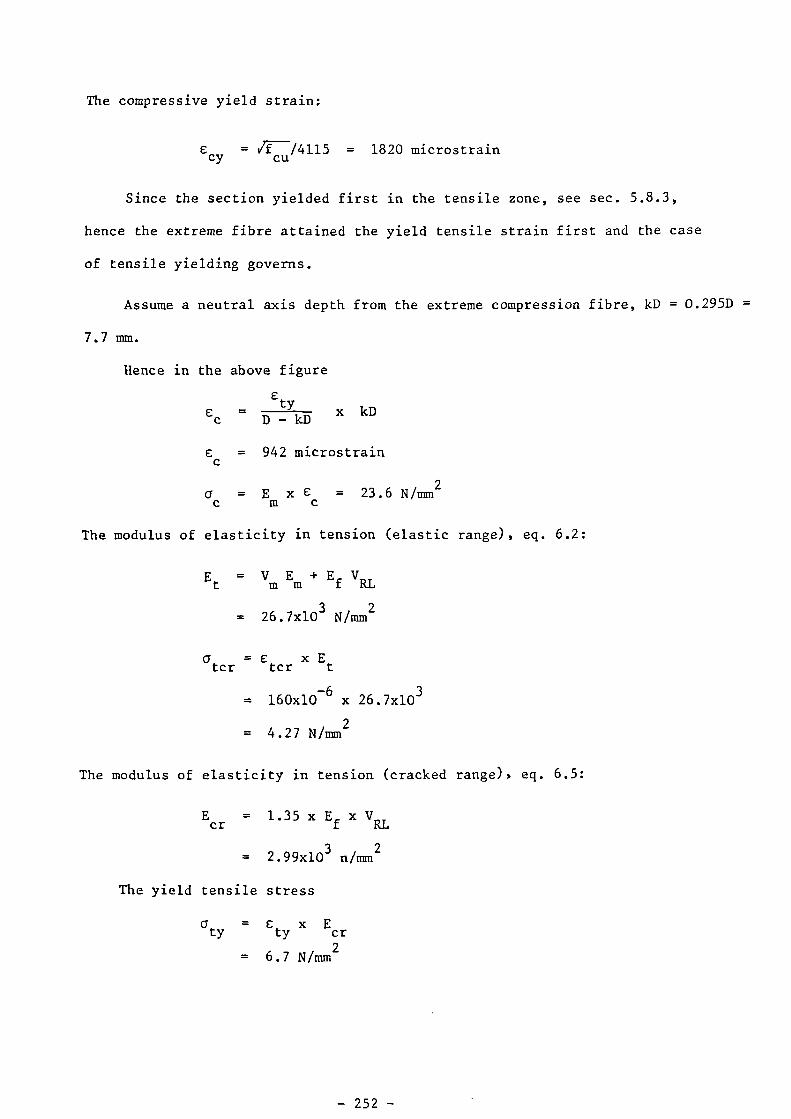
The compressive yield strain:
= /1--/4115 = 1820 microstrainCy Cu
Since the section yielded first in the tensile zone, see sec. 5.8.3,
hence the extreme fibre attained the yield tensile strain first and the case
of tensile yielding governs.
Assume a neutral axis depth from the extreme compression fibre, kD = 0.295D =
7.7 mm.
Hence in the above figure
Ety
ec D — kDkD
Ec = 942 microstrain
ac
= Em x 6 = 23.6 N/mm
2c
The modulus of elasticity in tension (elastic range), eq. 6.2:
Et = Vm Em
+ Ef VRL
= 26.7x10³ N/mm
2
a =c x Ettcr tcr
= 160x10-6 x 26.7x10
3
4.27 N/mm2
The modulus of elasticity in tension (cracked range), eq. 6.5:
E = 1.35 x Ef x VRL
cr
= 2.99x10³ n/mm
2
The yield tensile stress
aty
= Ety
x Ecr
= 6.7 N/mm2
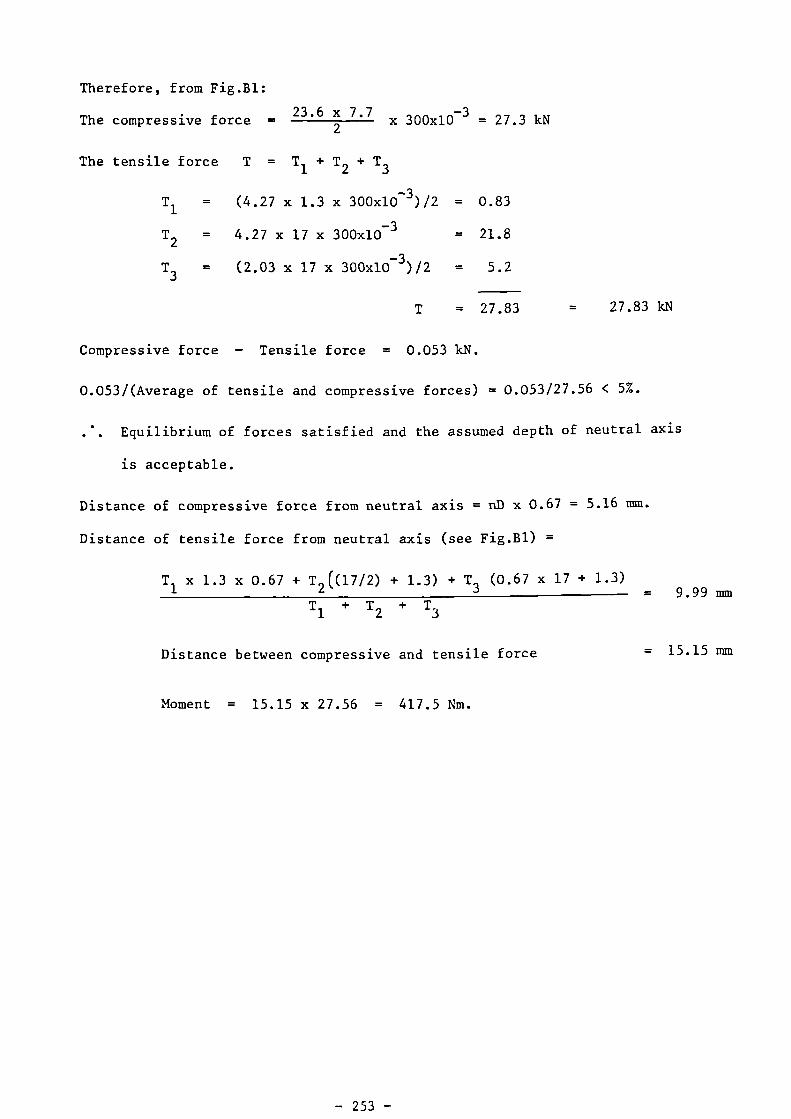
Therefore, from Fig.B1:
23.6 x 7.7 The compressive force - x 300x10
-3 = 27.3 kN
2
The tensile force T = Tl + T
2 + T
3
T1
= (4.27 x 1.3 x 300x10-3
)/2 = 0.83
T2
= 4.27 x 17 x 300x10-3 = 21.8
T3
= (2.03 x 17 x 300x10-3
)/2 = 5.2
T = 27.83 . 27.83 kN
Compressive force - Tensile force = 0.053 kN.
0.053/(Average of tensile and compressive forces) = 0.053/27.56 < 5%.
... Equilibrium of forces satisfied and the assumed depth of neutral axis
is acceptable.
Distance of compressive force from neutral axis = nD x 0.67 = 5.16 mm.
Distance of tensile force from neutral axis (see Fig.B1) =
T1 x 1.3 x 0.67 + T
2 ((17/2) + 1.3) + T3 (0.67 x 17 + 1.3)
T1 + T
2 + T
3
Distance between compressive and tensile force
Moment = 15.15 x 27.56 = 417.5 Nm.
- 9.99 mm
= 15.15 mm

APPENDIX C.
TYPICAL CALCULATION OF ULTIMATE MOMENT.
Calculation of the ultimate moment capacity for specimen Si D is
given below:
LJ — -J V V
EE
....t.1--ro
Ln
--S.—
\
goNJ
II
_
'A)I I
CI
Ecy
so
.75,---
01
c2C
Ety
as%L-,
I
I
1
T
ty
T1>
T2CT
co
,
>T3I
ICT
t
s_.
Fig. Cl Strain and stress distribution at ultimate load.
The properties of the section are given in Appendix B.
Assume neutral axis depth from compression face, kD = 0.2 D
= 5.2 mm.
The specimen is assumed to fail in compression. Hence, the ultimate
compressive strain governs the strain distribution. The ultimate
compressive strain E is assumed 6000 microstrain. Hence in Fig. ClCU
cux 20.8 = 24000 microstrain.
• 5.2
The stresses in the tensile zone are found as follows:
aty
•
E x etycr
As shown in Appendix B:
Ety
•
2240 microstrain
and
Ecr = 1.35 x Ef x V 2.99x10³ N/mm
2
aty
= 6.7 Nimm2

Notice that, to simplify the calculation without affecting,
appreciably, the accuracy of the results, the part of the tensile zone
where et < E
ty is assumed to be all cracked, i.e., not changing the stress
gradient to account for the uncracked tensile zone where Et
< 160 microstrain.
The tensile stress at the extreme tensile fibre at
is (see Fig.C1)
at = a
ty + a
t extra
where at extra
is extra tensile stress carried by the composite due to
the extra stress carried by the mesh after the point of first yielding.
This stress is found as follows:
From the stress-strain curve of the mesh, Fig.2.2,
at tensile strain et
= E = 2240 microstrainty
the mesh stress, af
= 158 N/mm2
and at Et
= tensile strain of the extreme fibre at ultimate load
= 24000 micros train
af
= 293 N/mm2
' . af extra = 293 - 158 = 135 N/mm2
Hence the composite extra stress (see Fig.6.6) is
=a x va t extra f extra RL
= 135 x 0.0242 = 3.27 N/mm
Therefore, the section tensile force T in Fig.C1 is
T = Tl + T
2 + T
3
= 1.9x6.7x0.5x0.3 + 18.9x6.7x0.3 + 0.67x3.27x18.9x0.3
= 1.9 + 38 + 12.4
= 52.3 kN 52.3 kN
2

52.3 kN
me ta t imatecompressives tressa . ..-0.67 f = 37.6 N/mm2cu
Hence, the compressive force C is
C = C1
+ C2
= 3.6 x 37.6 x 0.3 0.67 x 1.6 x 37.6 x 0.3
= 40.6 + 12.1 = 52.7 kN 52.7 kN=======
C - T 0.4 kN
• • C - T < 5% x (C+T)/2
Hence assumed depth of neutral axis is satisfactory.
Distance from the centroid of the tensile force to the N.L.
[1.9x0.67x1.9 + 38(18.9x0.5+1.9) + 12.4(18.9x0.625+1.9)]/52.3
= 11.57 mm
Also, distance from the centroid of the compressive force to the N.A.
= [40.6(3.6x0.5+1.6) + 12.1x0.625x1.61/52.7
= 2.87 mm
Moment arm = 11.57 + 2.87 = 14.47
U (C+T)ltimate moment - x moment arm2
= 52.5 x 14.47 = 758.2 Nm.
Copyright © 2022 FDOKUMEN