An Asymptotic Approach to the Torsion Problem in Thin Walled Beams
28
J Elast (2008) 93: 149–176 DOI 10.1007/s10659-008-9170-4 An Asymptotic Approach to the Torsion Problem in Thin Walled Beams Cesare Davini · Roberto Paroni · Eric Puntel Received: 3 April 2008 / Published online: 10 July 2008 © Springer Science+Business Media B.V. 2008 Abstract A rather straightforward derivation of the -limit of the torsion problem as the thickness goes to zero is obtained for generic thin walled beams. The limit stresses are evaluated and the distributional nature of one of the stress components is clarified. Keywords Saint Venant torsion · Asymptotic approach · Gamma-convergence · Thin walled beams · Bredt’s formulae Mathematics Subject Classification (2000) 74B05 · 74K10 · 49J45 1 Introduction Thin walled beams are widely used in many fields of civil, aeronautical and mechanical engineering. Their broad employ is due to their production method and to their high stiff- ness/weight ratio. The simplified geometry of thin walled sections, composed of joined members whose thickness is negligible with respect to the length of their mid line, has fostered the adoption of approximate formulae in the design practice whenever a closed form analytical solution was not handily available. Such formulae rested, at least in part, on heuristic assumptions; starting from the nineties they were given a mathematical justification by showing their consistency with the limit solution for a profile of vanishing thickness. As- ymptotic methods have thus helped in assessing the validity and applicability of the existing C. Davini ( ) · E. Puntel Dipartimento di Georisorse e Territorio, Università di Udine, via Cotonificio 114, 33100 Udine, Italy e-mail: [email protected] E. Puntel e-mail: [email protected] R. Paroni Dipartimento di Architettura e Pianificazione, Università degli Studi di Sassari, Palazzo del Pou Salit, Piazza Duomo, 07041 Alghero, Italy e-mail: [email protected]
-
Upload
independent -
Category
Documents
-
view
5 -
download
0
Transcript of An Asymptotic Approach to the Torsion Problem in Thin Walled Beams

J Elast (2008) 93: 149–176DOI 10.1007/s10659-008-9170-4
An Asymptotic Approach to the Torsion Problem in ThinWalled Beams
Cesare Davini · Roberto Paroni · Eric Puntel
Received: 3 April 2008 / Published online: 10 July 2008© Springer Science+Business Media B.V. 2008
Abstract A rather straightforward derivation of the �-limit of the torsion problem as thethickness goes to zero is obtained for generic thin walled beams. The limit stresses areevaluated and the distributional nature of one of the stress components is clarified.
Keywords Saint Venant torsion · Asymptotic approach · Gamma-convergence · Thinwalled beams · Bredt’s formulae
Mathematics Subject Classification (2000) 74B05 · 74K10 · 49J45
1 Introduction
Thin walled beams are widely used in many fields of civil, aeronautical and mechanicalengineering. Their broad employ is due to their production method and to their high stiff-ness/weight ratio. The simplified geometry of thin walled sections, composed of joinedmembers whose thickness is negligible with respect to the length of their mid line, hasfostered the adoption of approximate formulae in the design practice whenever a closedform analytical solution was not handily available. Such formulae rested, at least in part, onheuristic assumptions; starting from the nineties they were given a mathematical justificationby showing their consistency with the limit solution for a profile of vanishing thickness. As-ymptotic methods have thus helped in assessing the validity and applicability of the existing
C. Davini (�) · E. PuntelDipartimento di Georisorse e Territorio, Università di Udine, via Cotonificio 114, 33100 Udine, Italye-mail: [email protected]
E. Puntele-mail: [email protected]
R. ParoniDipartimento di Architettura e Pianificazione, Università degli Studi di Sassari, Palazzo del Pou Salit,Piazza Duomo, 07041 Alghero, Italye-mail: [email protected]

150 C. Davini et al.
results. More recently they have been used also to establish or extend lower dimension mod-els, such as beams or plates, to anisotropic, heterogeneous and nonlinear elastic materials(see e.g. [6]).
The present work deals with the De Saint Venant torsion problem in thin walled beams.It is well known that for a rectangular profile the torsional stresses obtained through theapproximate formula account for one half of the actual twisting moment only, as alreadynoticed by Kelvin and Tait [7] who ascribed the remaining half to two concentrated forcessupported on the end sides of the domain. In 1970, Popov [10] extended the result to gener-ally curved simply connected profiles. More recently, the most comprehensive treatment todate of De Saint Venant’s torsion using classical asymptotic techniques is due to Rodriguez,Trabucho and Viaño [12–16, 19]. They recover the limit solution for all possible typologiesincluding domains with junctions and multiply connected ones. Dell’Isola and Rosa [3, 4]have computed further terms of the asymptotic solution by formal expansions, extendingthe applicability of the theory to “moderately” thin sections. The first to compute the limitdistribution of tractions per unit length on the short sides of an open thin domain is, to theauthors’ knowledge, Ruta [17], who employs differential geometry techniques but, similarlyto Dell’Isola and Rosa, lets aside the discussion of the convergence properties.
Here we propose an alternative approach based on �-convergence, which establishes thevalidity of the asymptotic results, stresses included, on a rigorous basis. Moreover it allows arather straightforward derivation of the limit result. Application of �-convergence to singleand multi-cell thin walled beams was first performed by Morassi [8, 9]; another derivation ofDe Saint Venant torsion for thin rectangular profiles by reduction from a three dimensionalsetting using two scaling factors is due to Freddi et al. [5]. Results presented here use onescaling factor only and start from a two dimensional domain but, contrarily to previousworks, they do not use a specific coordinate transformation describing the profile. In thisway all possible extensions, e.g. varying thickness, curved profile, are included within oneunified framework.
The paper outline is as follows. In Sect. 2 a mapping from a rectangle to a broad classof simply connected thin domains without junctions is considered. For the limit problem,the main results concerning the stress function and the stresses are established. Illustrativeexamples are given in Sect. 2.6. Section 3 adapts them to single-hollowed sections andrecovers Bredt’s formulae. Finally Sect. 4 contains the extension to domain with junctions,e.g. ‘T’ or ‘H’ shaped, and multiply-hollowed ones.
2 Torsion in Simply Connected Thin Domains without Junctions
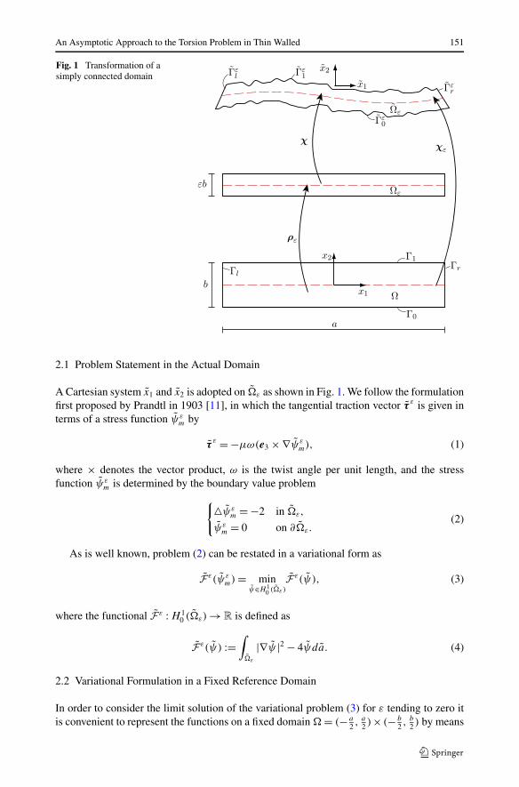
We consider first Saint-Venant’s torsion of a homogeneous, isotropic, linearly elastic beamwith a simply connected cross section �ε , subject to a moment Mε . Domain �ε is regardedas a suitable thickening of order ε of a reference line � dashed in Fig. 1. We assume that �
is a simple Lipschitz curve.Below we denote by μ the shear modulus and assume that there exists a bi-Lipschitz,
orientation preserving, mapping χ : R2 → R
2 that transforms cross section �ε into a rec-tangular domain �ε of length a and constant thickness ε b, as shown in the figure. We notethat transformation χ is independent of ε and that the envisaged case includes both curvedand thickness varying profiles. We are interested in characterizing the asymptotic limit ofthe stress distribution when the parameter ε goes to zero.
An Asymptotic Approach to the Torsion Problem in Thin Walled 151
Fig. 1 Transformation of asimply connected domain
2.1 Problem Statement in the Actual Domain
A Cartesian system x1 and x2 is adopted on �ε as shown in Fig. 1. We follow the formulationfirst proposed by Prandtl in 1903 [11], in which the tangential traction vector τ ε is given interms of a stress function ψε
m by
τ ε = −μω(e3 × ∇ψεm), (1)
where × denotes the vector product, ω is the twist angle per unit length, and the stressfunction ψε
m is determined by the boundary value problem{�ψε
m = −2 in �ε,
ψεm = 0 on ∂�ε.
(2)
As is well known, problem (2) can be restated in a variational form as
F ε(ψεm) = min
ψ∈H 10 (�ε)
F ε(ψ), (3)
where the functional F ε : H 10 (�ε) → R is defined as
F ε(ψ) :=∫
�ε
|∇ψ |2 − 4ψda. (4)
2.2 Variational Formulation in a Fixed Reference Domain
In order to consider the limit solution of the variational problem (3) for ε tending to zero itis convenient to represent the functions on a fixed domain � = (− a
2 , a2 )× (− b
2 , b2 ) by means

152 C. Davini et al.
of a mapping χ ε : � → �ε
χ ε := χ ◦ ρε, (5)
where the transformation ρε : � → �ε , see Fig. 1, contains the explicit dependence on ε
and is given by
ρε(x1, x2) = (x1, εx2). (6)
The boundary segments of � are referred to by means of subscripts l, r , 0, 1
�l :={−a
2
}×(
−b
2,b
2
), �r :=
{a2
}×(
−b
2,b
2
), (7)
�0 :={−b
2
}×(−a
2,a
2
), �1 :=
{b
2
}×(−a
2,a
2
). (8)
Their respective images
�εl := χ ε(�l), �ε
r := χ ε(�r), �ε0 := χ ε(�0), �ε
1 := χ ε(�1) (9)
are analogously indicated.Using the chain rule to differentiate χ ε , we get
∇χ ε = (∇χ) ◦ ρε∇ρε =: GεRε, (10)
where the two factors Gε and Rε are defined by
Gε := (∇χ) ◦ ρε, Rε := ∇ρε =(
1 00 ε
). (11)
We denote by G−1ε and R−1
ε their inverse matrices
G−1ε = (∇χ−1) ◦ χ ε, R−1
ε = (∇ρ−1ε ) ◦ ρε =
(1 00 1/ε
). (12)
Hereafter we assume that Gε strongly converges in L∞(�,R2×2) and we denote the limit
by G.Map χ ε establishes a natural isomorphism between H 1
0 (�ε) and H 10 (�) defined by
ψ := ψ ◦ χ ε, (13)
which is used to represent the stress function ψ on the fixed domain �.From (10)–(13) it follows that
∇ψ ◦ χ ε = (∇χ ε)−T ∇ψ = G−T
ε R−Tε ∇ψ = G−T
ε ∇εψ, (14)
where we have set
∇εψ := R−Tε ∇ψ =
(∂ψ
∂x1,
1
ε
∂ψ
∂x2
). (15)

An Asymptotic Approach to the Torsion Problem in Thin Walled 153
By changing variables and observing that det∇χ ε = ε detGε , the functional F ε becomes
F ε(ψ) =∫
�
(∣∣G−Tε ∇εψ
∣∣2 − 4ψ)
ε |detGε|da =: F ε (ψ) , (16)
which defines a new functional F ε : H 10 (�) → R. It follows that the sought stress function
ψεm = ψε
m ◦ χ−1ε now minimizes the functional F ε , that is,
F ε(ψεm) = min
ψ∈H 10 (�)
F ε(ψ). (17)
2.3 Limit Functional
We shall now study the limit behaviour of the variational problem defined in (16) and (17).Preliminarily, let us state some auxiliary results.
Since χ is bi-Lipschitz it follows that
‖∇χ‖L∞(�ε)< c and
∥∥∇χ−1∥∥
L∞(�ε)< c, (18)
where c does not depend upon ε. Then, by simple calculations and recalling that the deter-minants of Gε and G−1
ε are positive we have that
0 < detGε < c and 0 < detG−1ε < c
with c some other constant independent of ε. It follows that detGε is bounded away fromzero
0 <1
c<
1
detG−1ε
= detGε < c. (19)
By using the continuity of the application: A ∈ R2×2 → detA and the assumption that
Gε → G in L∞(�,R2×2), from (19) we deduce that
1
detGε
→ 1
detGin L∞(�). (20)
Furthermore, from the continuity of the adjugate we deduce that
G−1ε → G−1 in L∞(�,R
2×2). (21)
Lemma 1 (Coercivity) There exists c > 0 independent of ε such that
∫�
∣∣G−Tε ∇εψ
∣∣2 |detGε|da ≥ c
∫�
|∇εψ |2 da
for every ψ in H 10 (�).
Proof Let us first observe that for any vector v we have that
0 < λεm(x) |v|2 ≤ |Gε(x)v|2 ≤ λεM(x) |v|2 < c |v|2 a.e. in �, (22)

154 C. Davini et al.
where λεm and λεM are the lowest and the largest eigenvalues of GTε Gε evaluated at x,
respectively. The last inequality on the right hand side is a consequence of (18)1. In particularwe have that
0 < λεM(x) < c a.e. in �.
Analogously,
0 < λεm(x) |v|2 ≤ ∣∣G−Tε (x)v
∣∣2 ≤ λεM(x) |v|2 < c |v|2 a.e. in �, (23)
where λεm and λεM respectively are the lowest and the largest eigenvalues of G−1ε G−T
ε eval-uated at x. Now, the eigenvalues of G−1
ε G−Tε are the reciprocal of those of GT
ε Gε . Thus,
λεm(x) = 1
λεM(x)>
1
c.
Then, from (23) it follows that
0 <1
c|v|2 ≤ ∣∣G−T
ε (x)v∣∣2 < c |v|2 a.e. in � (24)
which, together with (19), yields the thesis. �
We denote by
W := L2
((−a
2,a
2
);H 1
0
(−b
2,b
2
)), (25)
and endow it with its natural norm
‖ψ‖2W =∫ a
2
− a2
‖ψ‖2L2(− b
2 , b2 )
+∥∥∥∥ ∂ψ
∂x2
∥∥∥∥2
L2(− b2 , b
2 )
dx1. (26)
Lemma 2 (Boundedness) Let {ψε} ⊂ H 10 (�) be a sequence such that supε
F ε(ψε)
ε3 < +∞.Then
supε
∥∥∥∥1
ε
∂ψε
∂x1
∥∥∥∥L2(�)
< +∞ and supε
∥∥∥∥ψε
ε2
∥∥∥∥W
< +∞.
Proof By assumption and by (16)
+∞ >F ε (ψε)
ε3= 1
ε3
∫�
(∣∣G−Tε ∇εψ
ε∣∣2 − 4ψε
)ε |detGε|da.
For a sufficiently small ε, (19) and Lemma 1 yield
+∞ >F ε (ψε)
ε3≥ c
∫�
(1
ε
∂ψε
∂x1
)2
+(
1
ε2
∂ψε
∂x2
)2
− 4|ψε|ε2
da.
By using Young’s inequality: pq ≤ δp2 + 14δ
q2 for all δ > 0, and a Poincaré-like inequality,namely,
‖u‖L2(�) ≤ b
∥∥∥∥ ∂u
∂x2
∥∥∥∥L2(�)
∀u ∈ H 10 (�) , (27)

An Asymptotic Approach to the Torsion Problem in Thin Walled 155
we get
+∞ >F ε (ψε)
ε3≥ c
∫�
(1
ε
∂ψε
∂x1
)2
+ 1
2
(1
ε2
∂ψε
∂x2
)2
+ 1
2b2
(ψε
ε2
)2
− δ
(ψε
ε2
)2
− 4
δda.
By choosing 1/δ = 4b2 we get
C ≥∫
�
(1
ε
∂ψε
∂x1
)2
+ 1
2
(1
ε2
∂ψε
∂x2
)2
+ 1
4b2
(ψε
ε2
)2
da
which implies the thesis. �
From Lemma 2 it follows that
Lemma 3 (Compactness) For any sequence {ψε} ⊂ H 10 (�) satisfying supε
F ε(ψε)
ε3 < +∞,there exist a ψ ∈ W and a subsequence of {ψε}, not relabeled, such that
ψε
ε2⇀ ψ in W and
1
ε
∂ψε
∂x1⇀ 0 in L2 (�) .
Proof By the compactness of L2 and W , respectively, Lemma 2 implies that there are aψ ∈ W and a ξ ∈ L2(�) such that
ψε
ε2⇀ ψ in W and
1
ε
∂ψε
∂x1⇀ ξ in L2 (�) .
Then, ∫�
ξηda = limε→0
∫�
1
ε
∂ψε
∂x1ηda = −lim
ε→0ε
∫�
ψε
ε2
∂η
∂x1da = 0 ∀η ∈ C∞
0 (�) .
Thus, ξ = 0. �
By Lemma 2 the functional F ε
ε3 , thought as a functional of ψε/ε2, is equicoercive withrespect to the weak topology of W . Therefore, we can use the sequential characterization ofthe �-limit, see [1, Proposition 8.10]. That is, F ε
ε3 �-converges to the functional F 0 : W → R
under the convergence ψεj
ε2j
⇀ ψ in W if
F ′′(ψ) ≤ F 0(ψ) ≤ F ′(ψ) for all ψ ∈ W,
where
F ′(ψ) := � − lim infε→0
F ε
ε3(ψ) := inf
{lim infεj →0
F εj
ε3j
(ψεj ) : forψεj
ε2j
⇀ ψ in W
},
F ′′(ψ) := � − lim supε→0
F ε
ε3(ψ) := inf
{lim sup
εj →0
F εj
ε3j
(ψεj ) : forψεj
ε2j
⇀ ψ in W
}.
Theorem 4 (�-convergence). Let F 0 : W → R be defined by
F 0 (ψ) :=∫
�
(∣∣∣∣ ∂ψ
∂x2G−T e2
∣∣∣∣2
− 4ψ
)detGda.

156 C. Davini et al.
Then F ε
ε3 �-converges to F 0 under the convergence ψε
ε2 ⇀ ψ in W .
Proof We start by proving that F 0(ψ) ≤ F ′(ψ) for any ψ ∈ W . Let ψ ∈ W and ψεj /ε2j ⇀
ψ in W . By the argument used in Lemma 3 it follows that
1
εj
∂ψεj
∂x1⇀ 0 in L2(�).
Since detGε and G−Tε converge strongly in L∞ to detG and G−T respectively, by lower
semicontinuity we have
lim infεj →0
F εj
ε3j
(ψεj ) = lim infεj →0
1
ε3j
∫�
(∣∣G−Tεj
∇εjψεj∣∣2 − 4ψεj
)εj
∣∣detGεj
∣∣da
= lim infεj →0
∫�
(∣∣∣∣ 1
εj
∂ψεj
∂x1G−T
εje1 + 1
ε2j
∂ψεj
∂x2G−T
εje2
∣∣∣∣2
− 4ψεj
ε2j
)∣∣detGεj
∣∣da
≥∫
�
(∣∣∣∣ ∂ψ
∂x2G−T e2
∣∣∣∣2
− 4ψ
)detGda = F 0 (ψ) .
To prove F ′′(ψ) ≤ F 0(ψ) let us first assume that ψ ∈ C∞0 (�). Consider the sequence ψεj =
ε2jψ . Then,
limεj →0
F εj
ε3j
(ψεj ) = limεj →0
1
ε3j
∫�
(∣∣G−Tεj
∇εjψεj∣∣2 − 4ψεj
)εj
∣∣detGεj
∣∣da = F 0 (ψ) .
If ψ ∈ W \ C∞0 (�) there is a sequence {ψk} ⊂ C∞
0 (�) converging strongly in W to ψ . Since,by the equation above, F ′′(ψk) ≤ F 0(ψk), the weak lower semicontinuity of F ′′ and thecontinuity of F 0 with respect to the strong convergence in W imply
F ′′(ψ) ≤ lim infk→+∞
F ′′(ψk) ≤ lim infk→+∞
F 0(ψk) = F 0(ψ)
and the proof is concluded. �
2.4 Convergence of the Minimizers
Let εj → 0 and let ψεjm be the minimizer of F εj . Since F εj
ε3j
(ψεjm ) ≤ F εj
ε3j
(0) = 0, by Lemma 2
the sequence {ψεjm /ε2
j } is equibounded in W . Thus there exists a subsequence weakly con-verging to a function ψm in W . By a property of �-convergence, see [1, Corollary 7.17], ψm
is a minimizer of F 0 and
limεj →0
F εj
ε3j
(ψεjm ) = F 0(ψm). (28)
Then, since the minimizer of F 0 is unique, all subsequences have in fact the same limit andhence the full sequence converges. Furthermore, from the strict convexity of the functionalsF ε and arguing as in [2], we deduce that the convergence is indeed strong.
Theorem 5 With the notation above we have
ψεm
ε2→ ψm in W. (29)

An Asymptotic Approach to the Torsion Problem in Thin Walled 157
By imposing the stationarity condition for F 0, ψm is found to be the solution of theboundary value problem⎧⎪⎨
⎪⎩∂
∂x2
(detG∣∣G−T e2
∣∣2 ∂ψm
∂x2
)= −2 detG,
ψm(·,− b2 ) = ψm(·, b
2 ) = 0.
(30)
It is worth noticing that the Dirichlet boundary conditions on the short sides of the rectangle,ψε
m(± a2 , ·) = 0, do not carry over to the limit problem due to the lack of control in F ε
ε3 of theterms containing the derivative of ψε
m/ε2 with respect to x1.In the important case where G does not depend on x2, ψm is parabolic in x2 and is
given by
ψm = − 1
|G−T e2|2(
x22 − b2
4
). (31)
2.5 Limit Stresses
In order to derive the limit stresses, it is first necessary to give a consistent definition of thestresses τ ε
13 and τ ε23 in the reference domain �. Let us define τ ε as the vector field which
satisfies the following relation∫B∩�
τ ε · ∇ηda =∫
χε(B∩�)
τ ε · ∇(η ◦ χ−1ε )da ∀η ∈ H 1(R2), (32)
and for all measurable sets B in R2. Then we have that
τ ε := det∇χ ε
(∇χ−1ε τ ε) ◦ χ ε. (33)
Field τ ε gives a representation of the stress vector field on the fixed domain. It is not difficultto see that τ ε can be regarded as the counterpart of the Piola-Kirchhoff’s stress tensor.
By using (1) and (13) we obtain
τ ε = −μω(e3 × ∇ψε
m
)= μω
(∂ψε
m
∂x2e1 − ∂ψε
m
∂x1e2
). (34)
Taking Theorem 5 into account, we find that τ ε/ε2 converges in an appropriate topology.Indeed, from (29) we immediately deduce that
τ ε13
ε2= μω
1
ε2
∂ψεm
∂x2−→ μω
∂ψm
∂x2=: τ13 in L2(�). (35)
The case of τ ε23 is slightly more involved because the existence of a limit is not di-
rectly assured by the �-convergence theorem. Let H ∗ denote the dual space of H :=H 1((− a
2 , a2 );L2(− b
2 , b2 )). Then,
τ ε23
ε2= −μω
1
ε2
∂ψεm
∂x1−→ τ23 in H ∗, (36)
where τ23 is the element of H ∗ defined by
〈τ23, η〉 = μω
∫�
ψm
∂η
∂x1da ∀η ∈ H. (37)
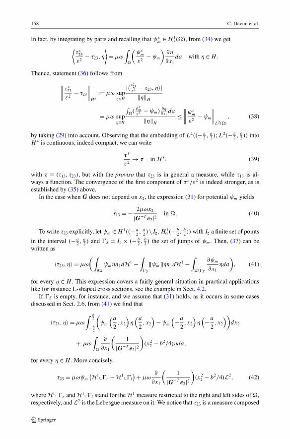
158 C. Davini et al.
In fact, by integrating by parts and recalling that ψεm ∈ H 1
0 (�), from (34) we get⟨τ ε
23
ε2− τ23, η
⟩= μω
∫�
(ψε
m
ε2− ψm
)∂η
∂x1da with η ∈ H.
Thence, statement (36) follows from
∥∥∥∥τ ε23
ε2− τ23
∥∥∥∥H∗
:= μω supη∈H
|〈 τε23ε2 − τ23, η〉|
‖η‖H
= μω supη∈H
∫�(
ψεm
ε2 − ψm)∂η
∂x1da
‖η‖H
≤∥∥∥∥ψε
m
ε2− ψm
∥∥∥∥L2(�)
, (38)
by taking (29) into account. Observing that the embedding of L2((− a2 , a
2 );L2(− b2 , b
2 )) intoH ∗ is continuous, indeed compact, we can write
τ ε
ε2→ τ in H ∗, (39)
with τ ≡ (τ13, τ23), but with the proviso that τ23 is in general a measure, while τ13 is al-ways a function. The convergence of the first component of τ ε/ε2 is indeed stronger, as isestablished by (35) above.
In the case when G does not depend on x2, the expression (31) for potential ψm yields
τ13 = − 2μωx2
|G−T e2|2in �. (40)
To write τ23 explicitly, let ψm ∈ H 1((− a2 , a
2 )\I�;H 10 (− b
2 , b2 )) with I� a finite set of points
in the interval (− a2 , a
2 ) and �S = I� × (− b2 , b
2 ) the set of jumps of ψm. Then, (37) can bewritten as
〈τ23, η〉 = μω
(∫∂�
ψmηn1dH1 −∫
�S
[[ψm]]ηn1dH1 −∫
�\�S
∂ψm
∂x1ηda
), (41)
for every η ∈ H . This expression covers a fairly general situation in practical applicationslike for instance L-shaped cross sections, see the example in Sect. 4.2.
If �S is empty, for instance, and we assume that (31) holds, as it occurs in some casesdiscussed in Sect. 2.6, from (41) we find that
〈τ23, η〉 = μω
∫ b2
− b2
(ψm
(a2, x2
)η(a
2, x2
)− ψm
(−a
2, x2
)η(−a
2, x2
))dx2
+ μω
∫�
∂
∂x1
(1
|G−T e2|2)
(x22 − b2/4)ηda,
for every η ∈ H . More concisely,
τ23 = μωψm
(H1��r − H1��l
)+ μω∂
∂x1
(1
|G−T e2|2)
(x22 − b2/4)L2, (42)
where H1��r and H1��l stand for the H1 measure restricted to the right and left sides of �,respectively, and L2 is the Lebesgue measure on it. We notice that τ23 is a measure composed

An Asymptotic Approach to the Torsion Problem in Thin Walled 159
by a regular part τ a23, which is diffuse over the domain �, and a singular one τ s
23 which issupported at the short sides of the rectangle:
τ a23 := μω
∂
∂x1
(1
|G−T e2|2)
(x22 − b2/4), and τ s
23 := μωψm. (43)
Accordingly, we write
τ23 = τ a23 L2 + τ s
23(H1��r − H1��l),
and
τ = τ13 L2e1 + (τ a23 L2 + τ s
23(H1��r − H1��l))e2 =: τ a L2 + τ s23(H1��r − H1��l)e2. (44)
To deduce the asymptotic tension field τ 0ε on �ε we can rewrite (32) as
∫χε(B∩�)
∇(η ◦ χ−1ε ) · d τ 0ε =
∫B∩�
∇η · dτ , ∀η ∈ H 1(R2) and B ⊂ R2,
which leads to
τ 0ε =(
1
det∇χ ε
∇χ ετa
)◦ χ−1
ε L2 +(
τ s23
∇χ εe2
|∇χ εe2|)
◦ χ−1ε
(H1��ε
r − H1��εl
). (45)
2.6 Examples
We illustrate the above formulae with a few examples. The simplest one is the case in whichthe cross section is a rectangle, that is, �ε = �ε . Then χ is simply the identity map, G isthe identity tensor and the equations above considerably simplify. In particular, we have thatτ a
23 = 0, so that τ23 has only the singular component [2].The resulting limit stress field is illustrated in Fig. 2. Stresses τ13 are linearly distributed
throughout the thickness and independent of x2, while τ23 is a measure supported at the sidesx1 = ± a
2 , where it is parabolically distributed. The two components equally contribute to the
limit value of the rescaled twisting moment: M = limε→0Mε
ε3 , which turns to be μab3
3 ω, asshown in [2].
Another interesting case is for
χ ε =(
x1, εx2
(1 + 1
αsin
(nπ
ax1
))),
with (x1, x2) ∈ � = (0, a) × (− b2 , b
2 ), n ∈ N and α ∈ R, α > 1, see Fig. 3.
Fig. 2 Limit tractions in a thinrectangle

160 C. Davini et al.
Fig. 3 Second example
In this case we have Ge1 = e1 and Ge2 = (1 + 1α
sin( nπa
x1))e2 and
1
|G−T e2|2=(
1 + 1
αsin
(nπ
ax1
))2
.
Taking into account that �ε = (0, a) × (0, εb), we deduce that
τ13 = −2μω
(1 + 1
αsin
(nπ
ax1
))2
x2, and
τ a23 = +2μω
nπ
αacos
(nπ
ax1
)(1 + 1
αsin
(nπ
ax1
))(x2
2 − b2/4).
Note that the larger is n, the larger is τ a23, while for α → +∞ we obtain the results
previously discussed for the rectangle.Finally, let us consider a domain �ε described as follows. Given a Lipschitz curve L
in parametric form x = p(x1), hereafter named reference line, and two pairs of Lipschitzfunctions of unit vectors ν±(x1) and cord lengths b±(x1), let �ε be defined by:
�ε ={
x : x = p(x1) + εx2b±(x1)
bν±(x1), x1 ∈
[−a
2,a
2
], x2 ∈
(−b
2,b
2
)}. (46)
It can be shown that if
dp
dx1× ν±(x1) · e3 > c and b± > c a.e. in
[−a
2,a
2
]
for some consistent c, the regularity requirements on χ ε are satisfied. In (46) the sign ± is tobe chosen according to that of the variable x2, while ε
b±(x1)
2 is the length of the semi-cordsin the upper and lower part of �ε . The situation is illustrated in Fig. 4.
With the notations of Sect. 2.2 we have
Gε =[
dp
dx1+ ε
x2
b
(db±
dx1ν± + b± dν±
dx1
)]⊗ e1 + b±
bν± ⊗ e2. (47)
It is convenient to assume that x1 is the arc length along the reference curve L, so thatt L = dp
dx1turns out to be the unit tangent to the curve. It follows that
G = t L(x1) ⊗ e1 + b±(x1)
bν±(x1) ⊗ e2. (48)

An Asymptotic Approach to the Torsion Problem in Thin Walled 161
Fig. 4 Third example
Thus, G depends upon the sign of x2 only and we will use the notation G = G±(x1) to stressthis in the following. The solution of the stationarity problem (30) will be then given by
ψm = − 1
|(G±)−T e2|2 x22 + c±
1 x2 + c±0 , (49)
where the four integration constants c±1 , c±
0 are determined by the boundary conditions
ψm
(·,−b
2
)= ψm
(·, b
2
)= 0, (50)
and by the matching conditions at x2 = 0
[[ψm]] =[[
detG∣∣G−T e2
∣∣2 ∂ψm
∂x2
]]= 0, (51)
where [[·]] denotes the jump across the reference line. The former follows from the requestthat ψm ∈ L2((− a
2 , a2 ),H 1
0 (− b2 , b
2 )), the latter from the requirement that detG|G−T e2|2 ∂ψm
∂x2be differentiable with respect to x2, cf. (30)1. It is worth noticing that τ a
23 will be non nullwhen G depends upon x1, while the singular part τ s
23 concentrates at the short sides of �,if ψm ∈ H 1(�), while, when it is just piece-wise differentiable there will be concentrationsalso at points of jump, cf. (41).
3 Torsion in Doubly Connected Thin Domains
Let us now consider a doubly connected cross section �ε , having an outer and inner bound-ary �ε
0 and �ε1 respectively, with associated tangential and normal vectors t and n oriented as
in Fig. 5. It is general enough to assume that representation (46) applies, with the additionalrequirement that
p
(−a
2
)= p
(a
2
), ν±
(−a
2
)= ν±(
a
2
)and b±
(−a
2
)= b±(
a
2
)(52)
in order to guarantee that the reference line L is closed and the representation of the actualdomain �ε onto the rectangle �ε of length a and thickness εb is one to one.

162 C. Davini et al.
Fig. 5 Transformation of doublyconnected domain
Again, the aim is to characterize the asymptotic limit of the stress distribution when theparameter ε goes to zero. We shall see that, with due adaptations, it is possible to re-usemuch of the results obtained for the simply connected case.
3.1 Variational Formulation in a Doubly Connected Domain
Unlike the problem established in (2), for a doubly connected domain the stress function hasto be constant at each connected component of the boundary. By linearity it is possible tochoose the constant equal to zero on the outer boundary, while the other one is determinedthrough a monodromy condition that takes the form∫
�ε1
∇ψεm · nds = 2Aε
1, (53)
where Aε1 is the area enclosed by the inner boundary �ε
1 and ∇ψεm · n denotes the derivative
along the external normal n at �ε1 , see [18, pp. 169–171].1 Accordingly, the boundary value
problem becomes ⎧⎪⎨⎪⎩
�ψεm = −2 in �ε,
ψεm = 0 on �ε
0,
ψεm = const on �ε
1,
(54)
where the constant is such that condition (53) is satisfied.The problem (54)–(53) can be restated in a variational form by introducing the functional
F ε(ψ) :=∫
�ε
(|∇ψ |2 − 4ψ)da − 4cψAε1
defined on the admissible function space
Y ε :={ψ ∈ H 1(�ε) : ψ |�ε
0= 0, ψ |�ε
1= cψ , cψ ∈ R
}.
1We observe that here the sign of the term on the right hand side is different from that given in [18, formula(47.10)], due to the different orientation of the normal to the inner boundary �ε
1.

An Asymptotic Approach to the Torsion Problem in Thin Walled 163
Then, ψεm is characterized by the property that
F ε(ψεm) = min
ψ∈Y εF ε(ψ), (55)
as is easily checked.Using definitions (13)–(15) we reformulate problem (55) as a problem on the fixed do-
main � = (− a2 , a
2 ) × (− b2 , b
2 ):
F ε(ψε
m
)= minψ∈Y
F ε (ψ) , (56)
where the domain Y and the functional F ε are given by
Y := {ψ ∈ H 1(�) : ψ |�0= 0,ψ |�1= cψ, cψ ∈ R,ψ |�r = ψ |�l
}, (57)
F ε (ψ) :=∫
�
(∣∣G−Tε ∇εψ
∣∣2 − 4ψ)
ε |detGε|da − 4cψAε1. (58)
Here and below by ψ |�r = ψ |�lwe mean that ψ(− a
2 , x2) = ψ(a2 , x2) for a.e. x2 in (− b
2 , b2 ).
3.2 Limit Functional
Let us now consider a sequence of potentials ψε ∈ Y ε such that functional F ε/ε is bounded.We denote by W� the function space
W� :={ψ ∈ L2
((−a
2,a
2
);H 1
(−b
2,b
2
)): ψ |�0= 0,ψ |�1= cψ
}
endowed with the norm defined by formula (26).
Lemma 6 (Boundedness for doubly connected domains) Let {ψε} ⊂ W� be a sequence suchthat supε
F ε(ψε)
ε< +∞. Then
supε
∥∥∥∥∂ψε
∂x1
∥∥∥∥L2(�)
< +∞ and supε
∥∥∥∥1
ε
∂ψε
∂x2
∥∥∥∥L2(�)
< +∞.
Proof By the assumption and by definition (58),
+∞ >F ε (ψε)
ε=∫
�
(∣∣G−Tε ∇εψ
ε∣∣2 − 4ψε
)|detGε|da − 4
ψε
ε
∣∣∣∣�1
Aε1.
For a sufficiently small ε, (19) and Lemma 1 yield
+∞ >F ε (ψε)
ε≥ c
∫�
[(∂ψε
∂x1
)2
+(
1
ε
∂ψε
∂x2
)2
− 4 |ψε|]
da − 4|ψε|ε
∣∣∣∣�1
Aε1.
Observe that now we have
‖u‖L2(�) ≤ b
∥∥∥∥ ∂u
∂x2
∥∥∥∥L2(�)
and ‖u‖L2(�1) ≤ b12
∥∥∥∥ ∂u
∂x2
∥∥∥∥L2(�)
∀u ∈ W�.

164 C. Davini et al.
Then, by using Young’s inequality: pq ≤ δp2 + 14 δ
q2 for all δ > 0, we get
+∞ >F ε (ψε)
ε≥ c
∫�
[(∂ψε
∂x1
)2
+(
1 − ηbε2 − bδ
a
)(1
ε
∂ψε
∂x2
)2
− 4
η
]da − 4
δ
(Aε
1
)2.
Hence, by choosing δ and η suitably and recalling that Aε1 remains bounded, it follows that
C ≥∫
�
(∂ψε
∂x1
)2
+(
1
ε
∂ψε
∂x2
)2
da,
which implies the thesis. �
From Lemma 6 and proceeding as in Lemma 3 we can prove that
Lemma 7 (Compactness for doubly connected domains) For any sequence {ψε} ⊂ W� sat-isfying supε
F ε(ψε)
ε< +∞, there exist a ψ ∈ W� and a subsequence of {ψε}, not relabeled,
such that
ψε
ε⇀ ψ in W� and
∂ψε
∂x1⇀ 0 in L2 (�) .
Let
A1 = limε→0
Aε1
be the area of the domain bounded by the reference line L of the cross section. Then,a straightforward replica of the proof of Theorem 4 yields that
Theorem 8 (�-convergence for doubly connected domains) Let F 0 : W�(�) → R be de-fined by
F 0 (ψ) :=∫
�
∣∣∣∣ ∂ψ
∂x2G−T e2
∣∣∣∣2
detGda − 4ψ |�1 A1.
Then F ε
ε�-converges to F 0 under the convergence ψε
ε⇀ ψ in W�(�).
3.3 Limit Stresses and Bredt’s Formulae
As a consequence of Theorem 8 the sequence of minimizers ψεm of F ε converges to the
minimizer ψm of F 0 and the convergence is indeed strong
ψεm
ε→ ψm in W�(�), (59)
cf. [2] and Theorem 5.Imposing the stationarity condition for F 0, we find that ψm is the unique solution of the
boundary value problem ⎧⎪⎨⎪⎩
∂
∂x2
(detG∣∣G−T e2
∣∣2 ∂ψm
∂x2
)= 0,
ψm |�0= 0, ψm |�1= cψm,
(60)

An Asymptotic Approach to the Torsion Problem in Thin Walled 165
under the monodromy condition∫�1
detG∣∣G−T e2
∣∣2 ∂ψm
∂x2ds = 2A1. (61)
From (60)1 it follows that
∂ψm
∂x2= g(x1)
detG|G−T e2|2(62)
for some function g = g(x1). Hence, taking account that ψm(x1,− b2 ) = 0 we get
ψm(x1, x2) = g(x1)
∫ x2
− b2
1
detG|G−T e2|2dx2, (63)
where we have taken the freedom to use the same symbol for the variable of integration andthe upper extreme of integration. Furthermore, the conditions at �1 yield
g(x1)
∫ b2
− b2
1
detG|G−T e2|2dx2 = cψm. (64)
Lemma 9 Let t L = dpdx1
be the running unit tangent to the reference line: x = p(x1), then
detG∣∣G−T e2
∣∣2 = 1
|t L × ν±|b
b± a.e. in[−a
2,a
2
]. (65)
Proof Recalling (48), we have
G = t L ⊗ e1 + b±
bν± ⊗ e2.
Thus,
detG = b±
b|t L × ν±|,
and the thesis follows noticing, as proved below, that since
detGG−T e2 = e3 × Ge1 (66)
we have
|detG G−T e2| = |e3 × t L| = 1.
To prove (66) let a be any linear combination of e1 and e2 and observe that
detG(e2 · a) = detG(e3 × e1 · a) = Ge1 × Ga · e3 = GT (e3 × Ge1) · a.
Hence by the arbitrariness of a it follows that
detGe2 = GT (e3 × Ge1),
which is equivalent to (66). �

166 C. Davini et al.
Note that |t L × ν±| = sin θ±, with θ± ∈ (0,π) the angle between the cords having direc-tions ν± and the reference line. Therefore,
b±(x1)|t L(x1) × ν±(x1)|is twice the length of the projection of those cords onto the normal to the reference line atpoint x = p(x1).
By substituting (65) into (64) we get
g(x1) = 1
bn(x1)cψm (67)
with
bn(x1) ≡ 1
2(b+(x1)|t L(x1) × ν+(x1)| + b−(x1)|t L(x1) × ν−(x1)|),
where quantity εbn represents, within higher order terms, the actual thickness of the wall atx1 measured in the direction of the normal to the reference line.
By (67), the monodromy condition∫ a2
− a2
g(x1)dx1 = cψm
∫ a2
− a2
1
bn(x1)dx1 = 2A1
yields the value of the constant cψm
cψm = 2A1∫L
1bn(s)
ds, (68)
where we have indicated by s the arc length along the reference line L.From (68), (64) and (63) we get
ψm = 2A1∫L
1bn(s)
ds
∫ x2
− b2
1
detG|G−T e2|2 dx2
∫ b2
− b2
1
detG|G−T e2|2 dx2
. (69)
In many cases, for instance when using the normal system of coordinates with respectto the mean line and the mean line is smooth, the expression detG|G−T e2|2 turns to beindependent of x2. Therefore, ψm is given by
ψm = 2A1∫L
1bn(s)
ds
1
b
(x2 + b
2
). (70)
Defining τ ε by (1) and τ ε by (33), from (59) we have thatτε
13ε
→ τ13 = μω∂ψm
∂x2in L2(�).
Furthermoreτε
23ε
→ τ23 in the dual space of
H :={η ∈ H 1
((−a
2,a
2
);L2
(−b
2,b
2
)), η |�r = η |�l
},
with τ23 defined as in (37). However, with ψm as in (70), it turns out that
〈τ23, η〉 = μω
∫ b2
− b2
ψm
[η(a
2, x2
)− η(−a
2, x2
)]dx2 = 0 ∀η ∈ H, (71)

An Asymptotic Approach to the Torsion Problem in Thin Walled 167
because η |�r = η |�l. So, we find
τ ε
ε→ τ = μω
∂ψm
∂x2e1 in H ∗, (72)
where the convergence of the first component of τ ε
εis indeed in L2(�).
It is possible to evaluate τ23 without making use of (70), but for brevity we omit this. Itis however worth saying that the singular part of τ23 vanishes under more general conditionsthan those envisaged in (70), whereas there may be a diffuse component of τ23.
Let us now evaluate the limit twisting moment with respect to the origin of the axes inthe physical space. From
Mε =∫
�ε
x × τ εda and τ ε = −μωe3 × ∇ψε
m,
by applying Green formula and taking the boundary conditions into account it follows that
Mε = 2μω
∫�ε
ψεmda − μωψε
m |�1e3 ·∫
�1
x × tds.
Or also,
Mε = 2μωε
∫�
ψεm detGεda + μω2Aε
1ψεm |�1 .
Hence, by rescaling the moment and passing to the limit,
M ≡ limε
Mε
ε= μω2A1cψm = μ
4A21∫
�1
1bn(s)
dsω. (73)
Let τ 0ε be the limit stress field represented on �ε . Recalling (33) and (45),
τ 0ε =(
1
ε detGε
μω∂ψm
∂x2Gεe1
)◦ χ−1
ε = μω2A1∫
�1
1bn(s)
ds
1
εb
(1
detGε
Gεe1
)◦ χ−1
ε (74)
with Gε defined in (47).From (72) we deduce that τ ε and ετ 0ε have the same asymptotic behavior. We write this
as τ ε ≈ ετ 0ε .For cross sections with a C2 mid reference line L, we may choose ν± coinciding with
the normal to L. In this case, b+n = b−
n ≡ bn(s) and dν±dx1
= − 1ρt L , where 1
ρstands for the
curvature of L. Then, for slowly variable thickness, (47) and the above formulae yield
τ ε ≈ μω2A1∫
L1
εbn(s)ds
1
εbn
(1 − 1
ρεx2
)t L with x2 ∈
(−bn
2,bn
2
). (75)
Quantity εbn is the actual thickness of the wall. In particular, the asymptotic stress islinearly variable through the wall, although this is a higher order effect. If we ignore it, wehave
τ ε ≈ μω2A1∫
L1
εbn(s)ds
1
εbn
t L, (76)

168 C. Davini et al.
which expresses the stress field in a way that does not depend upon the special representationof the domain �ε .
By means of the above equations we may now derive Bredt’s formulae. From (73) itfollows that
Mε ≈ μ4A2
1∫L
1εbn(s)
dsω (Bredt’s second formula) (77)
and, by using this expression in (76),
τ ε ≈ Mε
2A1
1
εbn
t L (Bredt’s first formula). (78)
4 Extension to Thin Domains with Junctions and Multiply Connected
The proposed approach can be extended to domains �ε which cannot be mapped into asingle rectangular domain by a bi-Lipschitz transformation. To handle these cases we de-compose �ε in n domains �iε such that �ε = ∪n
i=1�iε and such that each �iε is the imageof a fixed rectangular domain �i through a function χ iε . Functions χ iε , χ i , ρiε and their gra-dients Giε and Riε are defined as for simply connected domains under the same assumptionsof Sect. 2. In particular, we assume that each Giε strongly converges to Gi in L∞(�,R
2×2).Below, additional continuity prescriptions for χ iε on common internal boundaries of dif-ferent �i -s are specifically addressed for the various treated cases. Hereafter, we denote by�ε
ij = ∂�iε ∩ ∂�jε , by �εi = ∂�iε ∩ ∂�ε and �
(i)ij := χ−1
iε (�εij ).
4.1 Torsion in Simply Connected Thin Domains with Junctions
In the present section we consider a “T” shaped domain �ε which we decompose into threesubdomains �iε as in Fig. 6. Each �iε is the image of a rectangular reference domain �i =(−ai/2, ai/2) × (− b
2 , b2 ) via the map χ iε , satisfying
χ iε |�
(i)ij
= χ jε |�
(j)ij
.
For ψ ∈ H 10 (�ε) we denote by
ψi := ψ ◦ χ iε ∈ H 1(�i),
for i = 1,2,3. Note that, since ψ ∈ H 10 (�ε), it follows that ψi ◦χ−1
iε = ψj ◦χ−1jε on �ε
ij , and
ψi ◦ χ−1iε = 0 on ∂�ε, for i, j = 1,2,3. With this notation we have that
F ε(ψ) =:3∑
i=1
F εi (ψi) =: F ε (ψ1,ψ2,ψ3) (79)
where F ε is defined in (4), F εi is the functional
F εi (ψ) :=
∫�i
(|G−Tiε ∇εψ |2 − 4ψ)ε |detGiε|da, (80)

An Asymptotic Approach to the Torsion Problem in Thin Walled 169
Fig. 6 Transformation ofdomain with junctions
and the domain of functional F ε is
Aε :={
(ψ1,ψ2,ψ3) ∈3∏
i=1
H 1(�i) : for i, j = 1,2,3, ψi ◦ χ−1iε = 0 on ∂�ε,
and ψi ◦ χ−1iε = ψj ◦ χ−1
jε on �εij
}. (81)
Let
A :=3∏
i=1
L2
((−ai
2,ai
2
);H 1
0
(−b
2,b
2
)),
and F 0 : A → R be defined by
F 0(ψ1,ψ2,ψ3) :=3∑
i=1
F 0i (ψi) :=
3∑i=1
∫�i
(∣∣∣∣∂ψi
∂x2G−T
i e2
∣∣∣∣2
− 4ψi
)detGida.
An easy adaptation of Theorem 4 yields
Theorem 10 (�-convergence for domains with junctions) As ε → 0+, the sequence offunctionals F ε
ε3 �-converges to the functional F 0 under the convergence ψεj
i /ε2j ⇀ ψi in
L2((− ai
2 ,ai
2 );H 10 (− b
2 , b2 )), for i = 1,2,3.

170 C. Davini et al.
We observe that in the limit problem no continuity of the traces of the stress functionis prescribed on the inner boundaries. Therefore we can refer to the results for the singledomain without junctions to compute the limit stress function, see (30).
Hereafter, relying on the notation and the results of Sect. 2.5, we briefly discuss theconvergence of the stresses.
For i = 1,2,3, we define τ εi as the stress vector field which allows us to rewrite the
internal work in the configuration �i . More precisely, we require τ εi to satisfy the following
relation
Wεi (B,η) :=
∫B∩�i
τ εi · ∇ηda =
∫χ iε(B∩�i)
τ ε · ∇(η ◦ χ−1iε )da, ∀η ∈ H 1(R2) and B ⊂ R
2.
Proceeding as in Sect. 2.5 we find that the limit, in the appropriate topology, of τ εi is a
measure τ i , with support on the closure of �i , given by an expression similar to (42). The“image” τ 0ε
i of τ i , defined as in (45), is a measure with support on the closure of �iε . Wethus deduce
limε→0
Wεi (B,η) =: Wi(B,η) =
∫B∩�i
∇η · dτ i =:∫
χ iε(B∩�i)
∇(η ◦ χ−1iε ) · d τ 0ε
i .
Let (η1, η2, η3) ∈ Aε and B1,B2 and B3 be three measurable subsets of R2. Let ηε be the
function whose restriction to �iε is ηi ◦ χ−1iε , for i = 1,2,3. The total work at level ε is
3∑i=1
Wεi (Bi, ηi) =
3∑i=1
∫χ iε(Bi∩�i)
∇(ηi ◦ χ−1iε ) · τ ε
da =∫
χ iε(Bi∩�i)
∇ηε · τ εda,
while at the limit is
3∑i=1
Wi(Bi, ηi) =3∑
i=1
∫χ iε(Bi∩�i)
∇(ηi ◦ χ−1iε ) · d τ 0ε
i =:∫
χ iε(Bi∩�i)
∇ηε · d τ 0ε,
where we have set
τ 0ε :=3∑
i=1
τ 0εi ,
and where the τ 0εi are meant to denote measures with support in the closure of �iε . Therefore
we have that
τ 0ε��εij = τ 0ε
i ��εij + τ 0ε
j ��εij , (82)
for i, j = 1,2,3.
4.2 Examples
We start with an example which shows that the stress may concentrate along the junctionsbetween domains with different thickness, see Fig. 7.
Let �ε = (−a,0] × (−εb, εb) ∪ [0, a) × (−ε b2 , ε b
2 ). Then denoting by �1 = (−a,0] ×(−b, b) and �2 = (0, a) × (− b
2 , b2 ) and using (42) we find
τ 1 = −2μωx2 L2 e1 − μω(x22 − b2)
(H1�{x1 = 0} ∩ ∂�1 − H1�{x1 = −a} ∩ ∂�1
)e2,

An Asymptotic Approach to the Torsion Problem in Thin Walled 171
Fig. 7 Junction of rectangleswith different thickness
Fig. 8 L-shaped domain with stress concentration
and
τ 2 = −2μωx2 L2e1 − μω
(x2
2 − b2
4
)(H1�{x1 = a} ∩ ∂�2 − H1�{x1 = 0} ∩ ∂�2
)e2.
Hence τ = τ 1 + τ 2 restricted to {x1 = 0} ∩ ∂�2 gives
τ�{x1 = 0} ∩ ∂�2 = +3b2
4μωH1�{x1 = 0} ∩ ∂�2 e2.
The next examples instead shows that the stress may concentrate even if the thicknesshas no discontinuity. For brevity we shall simply calculate the linear stress at the junction.
Let us consider an L-shaped domain �ε as in Fig. 8. Domain �ε is thought of as theunion of an horizontal trapezoid �1ε and of a vertical trapezoid �2ε with a junction �ε
12
parallel to ν. With the coordinate axis as in Fig. 8 let
χ1ε(x1, x2) = x1e1 + εx2b1(x1)
bν1(x1), χ2ε(x1, x2) = −x1e2 + εx2
b2(x1)
bν2(x1),
where να are Lipschitz functions with values on the set of unit vectors such that ν1(0) =ν2(0) = ν, ν1(a1) = e2 and ν2(−a2) = e1 and where bα denote the rescaled length of thecord directed as να . In particular note that b1(0) = b2(0) =: bν. We then find
G1 = e1 ⊗ e1 + b1
bν1 ⊗ e2, G2 = −e2 ⊗ e1 + b2
bν2 ⊗ e2.

172 C. Davini et al.
Then, from (31),
ψ1m(x1, x2) = −b1(x1)2(ν1(x1) · e2)
2
b2
(x2
2 − b2
4
),
and
ψ2m(x1, x2) = −b2(x1)2(ν2(x1) · e1)
2
b2
(x2
2 − b2
4
).
In particular, at the junction x1 = 0 we find
ψ1m(0, x2) = −b2ν(ν · e2)
2
b2
(x2
2 − b2
4
), ψ2m(0, x2) = −b2
ν(ν · e1)2
b2
(x2
2 − b2
4
).
Namely, from (82) and (45), we obtain
τ 0ε1 ��ε
12 = −μωψ1m(0, ·) ◦ χ−11ε νH1��ε
12, τ 0ε2 ��ε
12 = μωψ2m(0, ·) ◦ χ−12ε νH1��ε
12,
thus
τ 0ε��ε12 = μω[ψ2m(0, ·) − ψ1m(0, ·)] ◦ χ−1
ε νH1��ε12,
where χ−1ε denotes the restriction of χ−1
1ε and of χ−12ε to �ε
12. We therefore see that τ 0ε��ε12
is a null measure if and only if ψ1m(0, ·) = ψ2m(0, ·). This requires that |ν · e1| = |ν · e2|,i.e., that the junction line bisects the angle at the corner of �ε .
The above example could have been studied within the framework of Sect. 2. In thiscase, the stress concentration at the junction emerges directly from (41) since the jump[[ψm]] across the junction is in general different from zero, as it follows if one calculates theterm on the right hand side of (31).
4.3 Torsion in Multiply Connected Thin Domains
In the case of a multiply connected thin domain the analysis of Sect. 3 can be similarlyadapted. Let us consider the case depicted in Fig. 9 by the sake of illustration. We decom-pose it into doubly connected subdomains �iε that are the image of rectangular referencedomains �i of length ai and thickness b
2 under the maps χ iε . The maps χ iε are assumedto be periodic: χ iε(− ai
2 , ·) = χ iε(ai
2 , ·). Furthermore, as it is always possible, we assumethat the restriction of these maps to the dotted line in Fig. 9 keeps the arclength, so thatcorresponding pairs of points in the representation domains �i are easily recognized.
As before we set �εij = ∂�iε ∩ ∂�jε , �
(i)ij = χ−1
iε (�εij ) ⊂ ∂�i and �i = χ−1
iε (�εi ), with
�εi = ∂�iε ∩∂�ε . Consistently with Sect. 3.1 the area enclosed by �ε
i is named Aεi . Similarly
Ai is the limit of Aεi for ε → 0. We also denote by χ j i : �
(i)ij → �
(j)
ji the map defined by
χ j i = χ−1
jε |�εji
◦ χ iε|�(i)ij
.
The functional to be studied in this case is F ε : Y ε → R defined by
F ε(ψ) :=∫
�ε
(|∇ψ |2 − 4ψ)da − 4ψ |�ε1Aε
1 − 4ψ |�ε2Aε
2,
with admissible function space
Y ε :={ψ ∈ H 1(�ε) : ψ |�ε
3= 0, ψ |�ε
1= c1, ψ |�ε
2= c2
},

An Asymptotic Approach to the Torsion Problem in Thin Walled 173
Fig. 9 Transformation ofmultiply connected domain
where by ψ |�εα= cα we mean that the trace of ψ on �ε
α is constant.
For ψ ∈ Y ε we denote by
ψi := ψ ◦ χ iε ∈ H 1(�i),
for i = 1,2,3. Then arguing as in the previous section we find
F ε(ψ) =:3∑
i=1
F εi (ψi) =: F ε(ψ1,ψ2,ψ3) (83)
where F εi is defined by
F εi (ψi) :=
∫�i
(∣∣G−Tiε ∇εψi
∣∣2 − 4ψi
)ε |detGiε|da − 4ψi |�i
Aεi , (84)
and the domain of the functional F ε is
Aε :={
(ψ1,ψ2,ψ3) ∈3∏
i=1
H 1(�i) :
ψ3 = 0 on �3, ψi = ci on �i, i = 1,2,
ψi |�(i)l
= ψi |�(i)r
for i = 1,2,3 and ψi = ψj ◦ χ j i on �(i)ij , i �= j
}. (85)
Let
A :={
(ψ1,ψ2,ψ3) ∈3∏
i=1
L2
((−ai
2,ai
2
);H 1
(0,
b
2
)):

174 C. Davini et al.
ψ3 = 0 on �3, ψi = ci on �i, i = 1,2 and ψi = ψj ◦ χ j i on �(i)ij i �= j
}(86)
and F 0 : A → R be defined by
F 0 (ψ1,ψ2,ψ3) :=3∑
i=1
F 0i (ψi) :=
3∑i=1
∫�i
∣∣∣∣∂ψi
∂x2G−T
i e2
∣∣∣∣2
detGida − 4ψi |�iAi.
Theorem 11 (�-convergence for multiply connected domains) As ε → 0+, the sequence offunctionals F ε
ε�-converges to the functional F 0 under the convergence ψ
εj
i /εj ⇀ ψi inL2((− ai
2 ,ai
2 );H 1(0, b2 )), i = 1,2,3.
The minimizer (ψ1m,ψ2m,ψ3m) of F 0 is the solution of the following boundary valueproblem ⎧⎪⎪⎪⎪⎪⎪⎪⎪⎪⎪⎪⎪⎪⎪⎪⎨
⎪⎪⎪⎪⎪⎪⎪⎪⎪⎪⎪⎪⎪⎪⎪⎩
∂
∂x2
(detGi |G−T
i e2|2 ∂ψim
∂x2
)= 0 in �i, i = 1,2,3,∫
�β
detGi |G−Ti e2|2 ∂ψim
∂x2ds = 2Aβ, β = 1,2,
ψ3m = 0 on �3, ψβm = cβ on �β, β = 1,2,
detGi |G−Ti e2|2 ∂ψim
∂x2+(
detGj |G−Tj e2|2 ∂ψjm
∂x2
)◦ χ j i = 0
on �(i)ij , i, j = 1,2,3,
ψim = ψjm ◦ χ j i on �(i)ij , i �= j and i, j = 1,2,3.
(87)
After integration, from (87)1 it follows that
ψm(x1, x2) = gi(x1)
∫ x2
− b2
1
detGi |G−Ti e2|2
dx2 + gi0(x1) i = 1,2,3 (88)
with gi and gi0 functions defined on the interval (− ai
2 ,ai
2 ) to be determined by using bound-ary and junction conditions. Also, by arguing as in Lemma 9, it is found that
detGi
∣∣G−Ti e2
∣∣2 = b
bni
,
with bni being twice the running thickness of domain �iε rescaled by 1ε.
The analysis of the other conditions in problem (87) provides then
g3 ={ − 1
bnc1 x1 ∈ (− a3
2 ,0),
− 1bn
c2 x1 ∈ (0,a32 ),
(89)
the negative and the positive interval corresponding to points of the lines L1 := �ε31 and
L2 := �ε32 in the physical domain �ε respectively, cf. Fig. 9. Furthermore,
gα ={ 1
bn(cα − cβ) |x1| ≤ d
2 , β �= α,
1bn
cαd2 ≤ |x1| ≤ aα
2
(90)

An Asymptotic Approach to the Torsion Problem in Thin Walled 175
with α = 1,2. Here the first formula applies to points of the line L12 := �ε12, while the second
to those of Lα . In (89) and (90) bn denotes the rescaled running thickness of the walls in thephysical domain �ε , respectively defined as bn := bn3+bnα
2 and bn := bn1+bn22 .
By taking (90) into account the monodromy conditions:∫
�αgαds = 2Aα , for α = 1,2,
can be written as ⎧⎪⎪⎨⎪⎪⎩
(∫L1∪L12
1bn
ds)
c1 −(∫
L12
1bn
ds)
c2 = 2A1,
−(∫
L12
1bn
ds)
c1 +(∫
L2∪L12
1bn
ds)
c2 = 2A2.
(91)
The above system of equations yields the value of the constants cα and thence provides thesolution of our problem.
We conclude with two remarks that give account of well known features of the torsionproblem for multicell cross sections.
First, let ∫L1
1
bn
ds =∫
L2
1
bn
ds and A1 = A2.
Then, the system of equation becomes symmetric and thence we find that c1 = c2. It followsfrom (90)1 that gα = 0 in the wall separating the two cells, thus ψαm = const and there is nostress there. The cross section behaves like a doubly connected one, composed just by theexternal walls.
Second, let ∫L12
1
bn
ds �∫
Lα∪L12
1
bn
ds
and let A1 and A2 be comparable. Then,
cα = 2Aα∫Lα∪L12
1bn
ds,
which corresponds to the case where the two cells work in parallel, contributing to the totaltwisting moment proportionally to their twisting stiffness.
Acknowledgements This work has been done within the project COFIN-2005083412. The support of theItalian Ministry for University and Scientific Research is gratefully acknowledged. We are also indebted toan anonymous referee for pointing out a mistake in one of the examples. His remark prompted us to add afurther example, which we hope clarifies the results of the paper.
References
1. Dal Maso, G.: An Introduction to �-convergence. Progress in Nonlinear Differential Equations and theirApplications, vol. 8. Birkhäuser, Boston (1993)
2. Davini, C., Paroni, R., Puntel, E.: An asymptotic approach to the torsion problem in thin rectangulardomains. Meccanica (2008). doi:10.1007/sl1012-007-9106-2
3. Dell’Isola, F., Rosa, L.: An extension of Kelvin and Bredt formulas. Math. Mech. Solids 1(2), 243–250(1996)
4. Dell’Isola, F., Rosa, L.: Perturbation methods in torsion of thin hollow Saint-Venant cylinders. Mech.Res. Commun. 23(2), 145–150 (1996)
5. Freddi, L., Morassi, A., Paroni, R.: Thin-walled beams: the case of the rectangular cross-section. J. Elast.76(1), 45–66 (2004)

176 C. Davini et al.
6. Freddi, L., Murat, F., Paroni, R.: Anisotropic inhomogeneous rectangular thin-walled beams. SIAM J.Math. Anal. (submitted)
7. Kelvin, W.T., Tait, P.G.: Treatise on Natural Philosophy. Cambridge University Press, Cambridge (1912)8. Morassi, A.: Torsion of thin tubes—a justification of some classical results. J. Elast. 39(3), 213–227
(1995)9. Morassi, A.: Torsion of thin tubes with multicell cross-section. Meccanica 34(2), 115–132 (1999)
10. Popov, E.P.: Kelvin’s solution of the torsion problem. J. Eng. Mech. Div. ASCE 96, 1005–1012 (1970)11. Prandtl, L.: Zur torsion von prismatischen stäben. Phys. Z. 4, 758–759 (1903)12. Rodriguez, J.M., Viaño, J.M.: Asymptotic analysis of Poisson equation in a thin domain—application
to thin-walled elastic beams torsion theory. 1. Domain without junctions. C.R. Acad. Sci. Ser. I Math.317(4), 423–428 (1993)
13. Rodriguez, J.M., Viaño, J.M.: Asymptotic analysis of Poisson equation in a thin domain—application tothin-walled elastic beams torsion theory. 2. Domain with junctions. C.R. Acad. Sci. Ser. I Math. 317(6),637–642 (1993)
14. Rodriguez, J.M., Viaño, J.M.: Asymptotic general bending and torsion models for thin-walled elasticrods. In: Ciarlet, P.G., Trabucho, L., Viaño, J.M. (eds.) Asymptotic Methods for Elastic Structures, pp.255–274. Walter de Gruyter, Berlin (1995)
15. Rodriguez, J.M., Viaño, J.M.: Asymptotic analysis of Poisson’s equation in a thin domain. Applicationto thin-walled elastic beams. In: Ciarlet, P.G., Trabucho, L., Viaño, J.M. (eds.) Asymptotic Methods forElastic Structures, pp. 181–193. Walter de Gruyter, Berlin (1995)
16. Rodriguez, J.M., Viaño, J.M.: Asymptotic analysis of Poisson’s equation in a thin domain and its appli-cation to thin-walled elastic beams and tubes. Math. Methods Appl. Sci. 21(3), 187–226 (1998)
17. Ruta, G.C.: On Kelvin’s formula for torsion of thin cylinders. Mech. Res. Commun. 26(5), 591–596(1999)
18. Sokolnikoff, I.S.: Mathematical Theory of Elasticity, 2nd edn. McGraw-Hill, New York (1956)19. Trabucho, L., Viaño, J.M.: Mathematical modelling of rods. In: Ciarlet, P.G., Lions, J.L. (eds.) Handbook
of Numerical Analysis, vol. IV, pp. 487–974. North Holland, Amsterdam (1996)