Einstein-Cartan Theory and Cosmologywith Torsion

Dimitrios Kranas

Supervisor: prof. Christos Tsagas

Section of Astrophysics, Astronomy and Mechanics,

Aristotle University of Thessaloniki

Abstract

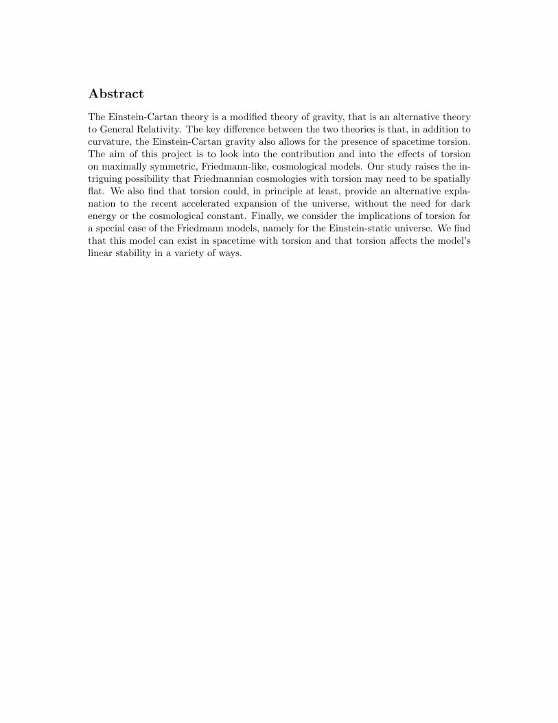
The Einstein-Cartan theory is a modified theory of gravity, that is an alternative theoryto General Relativity. The key difference between the two theories is that, in addition tocurvature, the Einstein-Cartan gravity also allows for the presence of spacetime torsion.The aim of this project is to look into the contribution and into the effects of torsionon maximally symmetric, Friedmann-like, cosmological models. Our study raises the in-triguing possibility that Friedmannian cosmologies with torsion may need to be spatiallyflat. We also find that torsion could, in principle at least, provide an alternative expla-nation to the recent accelerated expansion of the universe, without the need for darkenergy or the cosmological constant. Finally, we consider the implications of torsion fora special case of the Friedmann models, namely for the Einstein-static universe. We findthat this model can exist in spacetime with torsion and that torsion affects the model’slinear stability in a variety of ways.

“Everybody is a genius. But if you judge a fish by its ability to climba tree, it will live its whole life believing that it is stupid.”

—Albert Einstein

Contents

1 Introduction 11.1 Conventions . . . . . . . . . . . . . . . . . . . . . . . . . . . . . . . . . . . 31.2 Spacetime connection and the torsion tensor . . . . . . . . . . . . . . . . . 31.3 The contortion tensor . . . . . . . . . . . . . . . . . . . . . . . . . . . . . 41.4 1+3 covariant decomposition . . . . . . . . . . . . . . . . . . . . . . . . . 51.5 Kinematic quantities and curvature in Riemann-Cartan space . . . . . . . 51.6 Field equations . . . . . . . . . . . . . . . . . . . . . . . . . . . . . . . . . 7

2 Cosmology with torsion 82.1 The Friedmann equation . . . . . . . . . . . . . . . . . . . . . . . . . . . . 92.2 The Raychaudhuri equation . . . . . . . . . . . . . . . . . . . . . . . . . . 102.3 Bianchi identities . . . . . . . . . . . . . . . . . . . . . . . . . . . . . . . . 112.4 Spin formalism . . . . . . . . . . . . . . . . . . . . . . . . . . . . . . . . . 12

3 Torsion in FRW-type cosmology 133.1 The torsion ansatz . . . . . . . . . . . . . . . . . . . . . . . . . . . . . . . 133.2 Bianchi identities and symmetry . . . . . . . . . . . . . . . . . . . . . . . 153.3 The continuity equation . . . . . . . . . . . . . . . . . . . . . . . . . . . . 163.4 Compatibility issues and the flatness problem . . . . . . . . . . . . . . . . 173.5 Splitting the energy-momentum tensor . . . . . . . . . . . . . . . . . . . . 18

4 Cosmological implications of torsion 194.1 Recent accelerated expansion . . . . . . . . . . . . . . . . . . . . . . . . . 204.2 Focusing theorem and singularities . . . . . . . . . . . . . . . . . . . . . . 214.3 Scalar fields in spacetime with torsion . . . . . . . . . . . . . . . . . . . . 234.4 Solutions of the Friedmann equations . . . . . . . . . . . . . . . . . . . . . 25

5 Einstein static universe and its stability 275.1 Einstein static universe without torsion . . . . . . . . . . . . . . . . . . . 275.2 Einstein static universe in spacetimes with torsion . . . . . . . . . . . . . 29

6 Conclusions-Discussion 31

A Detailed calculations 34A.1 Friedmann equation . . . . . . . . . . . . . . . . . . . . . . . . . . . . . . 34A.2 Raychaudhuri equation . . . . . . . . . . . . . . . . . . . . . . . . . . . . . 36A.3 Bianchi identities . . . . . . . . . . . . . . . . . . . . . . . . . . . . . . . . 38A.4 Energy-momentum tensor decomposition . . . . . . . . . . . . . . . . . . . 40

B Sign of physical quantities under the signature transformation 44

1 Introduction

The Einstein-Cartan (EC) theory is an extension of General Relativity (GR) that ac-counts for the presence of spacetime torsion. The theory was first introduced by ElieCartan (1922), in an attempt to propose torsion as the macroscopic manifestation of theintrinsic angular momentum (spin) of the matter [1]. However, his suggestion precededthe discovery of spin and therefore, the theory did not receive much attention. Later on,the inclusion of the matter spin in general relativity was resuggested independently byKibble and Sciama. Since then, the EC theory (also known as ECKS) has been generallyestablished and received much more recognition, as it is probably the most straightfor-ward, classical extension of general relativity.

According to the EC theory, the spacetime affine connection is asymmetric, in con-trast to the symmetric Christoffel symbols of the Riemannian space. Mathematically,the torsion is defined as the antisymmetric part of the non-Riemannian affine connection[1]. Therefore, in addition to the metric tensor, there is also an independent torsionalfield, which is used to describe the gravitational field. Dynamically, the intrinsic angularmomentum (spin) of the matter is responsible for the presence of torsion as the presenceof matter is responsible for the spacetime curvature. This analogy arises from the twofield equations coming from the least action principle1.

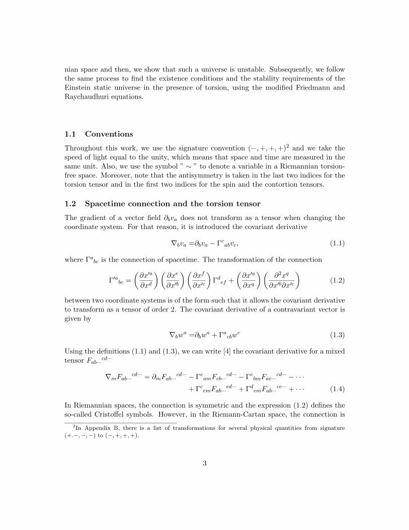
The physical interpretation of the spacetime curvature is that the parallel transportof a vector around a closed loop depends on the followed path (see figure 1). On theother hand, the torsion results in the twisting of the worldlines (see figure 2). In otherwords, a closed loop in a torsion-free spacetime does not close in a spacetime that in-cludes a torsion field. Another example [3] that helps to illustrate torsion is to considerthe spacetime as a thin, elastic rob. Curving the spacetime is equivalent to bending therob, whereas twisting the rob is equivalent to spacetime torsion.

Despite the successes of classical GR, several (cosmological) problems remain still un-solved. The formation of singularities, the origin of the recent accelerated expansion, theflatness problem, the nature of dark matter and dark energy are some of the topics thatneed to be answered. The ECKS theory seems to be a promising candidate theory tosolve some of these problems and several attempts [2, 3] have been made towards thatdirection. An additional merit of the ECKS theory is that it extends GR associating aspacetime property (torsion) with a quantum notion (spin) connecting, somehow, the twomost successful theories of the past century, namely General Relativity and QuantumMechanics.

Yet, there is no experimental evidence that supports either the predictions of the ECKStheory or the existence of spacetime torsion. The reason is that the ECSK theory devi-

1see subsection 1.6 for more details

1

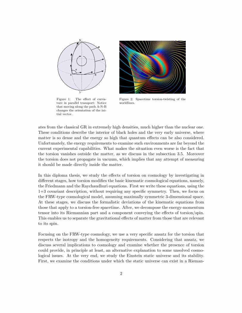
Figure 1: The effect of curva-ture in parallel transport: Noticethat moving along the path A-N-Bchanges the orientation of the ini-tial vector.

Figure 2: Spacetime torsion-twisting of theworldlines.

ates from the classical GR in extremely high densities, much higher than the nuclear one.These conditions describe the interior of black holes and the very early universe, wherematter is so dense and the energy so high that quantum effects can be also considered.Unfortunately, the energy requirements to examine such environments are far beyond thecurrent experimental capabilities. What makes the situation even worse is the fact thatthe torsion vanishes outside the matter, as we discuss in the subsection 3.5. Moreoverthe torsion does not propagate in vacuum, which implies that any attempt of measuringit should be made directly inside the matter.

In this diploma thesis, we study the effects of torsion on cosmology by investigating indifferent stages, how torsion modifies the basic kinematic cosmological equations, namely,the Friedmann and the Raychaudhuri equations. First we write these equations, using the1+3 covariant description, without requiring any specific symmetry. Then, we focus onthe FRW-type cosmological model, assuming maximally symmetric 3-dimensional space.At these stages, we discuss the formalistic deviations of the kinematic equations fromthose that apply to a torsion-free spacetime. After, we decompose the energy-momentumtensor into its Riemannian part and a component conveying the effects of torsion/spin.This enables us to separate the gravitational effects of matter from those that are relevantto its spin.

Focusing on the FRW-type cosmology, we use a very specific ansatz for the torsion thatrespects the isotropy and the homogeneity requirements. Considering that ansatz, wediscuss several implications to cosmology and examine whether the presence of torsioncould provide, in principle at least, an alternative explanation to some unsolved cosmo-logical issues. At the very end, we study the Einstein static universe and its stability.First, we examine the conditions under which the static universe can exist in a Rieman-

2

nian space and then, we show that such a universe is unstable. Subsequently, we followthe same process to find the existence conditions and the stability requirements of theEinstein static universe in the presence of torsion, using the modified Friedmann andRaychaudhuri equations.

1.1 Conventions

Throughout this work, we use the signature convention (−,+,+,+)2 and we take thespeed of light equal to the unity, which means that space and time are measured in thesame unit. Also, we use the symbol ” ∼ ” to denote a variable in a Riemannian torsion-free space. Moreover, note that the antisymmetry is taken in the last two indices for thetorsion tensor and in the first two indices for the spin and the contortion tensors.

1.2 Spacetime connection and the torsion tensor

The gradient of a vector field ∂bva does not transform as a tensor when changing thecoordinate system. For that reason, it is introduced the covariant derivative

∇bva =∂bva − Γcabvc, (1.1)

where Γabc is the connection of spacetime. The transformation of the connection

Γ′abc =

(∂x′a

∂xd

)(∂xe

∂x′b

)(∂xf

∂x′c

)Γdef +

(∂x′a

∂xq

)(∂2xq

∂x′b∂x′c

)(1.2)

between two coordinate systems is of the form such that it allows the covariant derivativeto transform as a tensor of order 2. The covariant derivative of a contravariant vector isgiven by

∇bwa =∂bwa + Γacbw

c (1.3)

Using the definitions (1.1) and (1.3), we can write [4] the covariant derivative for a mixedtensor Fab···

cd···

∇mFab···cd··· = ∂mFab···cd··· − ΓeamFeb···

cd··· − ΓebmFae···cd··· − · · ·

+ ΓcemFab···ed··· + ΓdemFab···

ce··· + · · · (1.4)

In Riemannian spaces, the connection is symmetric and the expression (1.2) defines theso-called Cristoffel symbols. However, in the Riemann-Cartan space, the connection is

2In Appendix B, there is a list of transformations for several physical quantities from signature(+.−,−,−) to (−,+,+,+).

3

asymmetric and thus, it can be decomposed into a symmetric and an antisymmetric part:Γabc = Γa(bc) + Γ[bc]. The latter one defines the torsion tensor

Sabc = Sa[bc] ≡ Γa[bc] (1.5)

Generally, a tensor with 3 indices in 4-dimensions consists of 64 components. Yet, con-sidering the antisymmetry property, the torsion tensor is made out of 20 independentcomponents. Taking all the possible contractions of (1.5), we find:

Sbab = Sa = −Sbba, Sabb = 0

The first of the above equations defines the torsion vector, which consists of 4 independentcomponents. Note also that, contraction between antisymmetric indices is always zero.

1.3 The contortion tensor

We wish now to correlate the asymmetric connection of the general metric space withthe Cristoffel symbols of the Riemaniann space. To achieve that, we start by taking thecovariant derivative of the metric tensor:

∇cgab = ∂cgab − gadΓdbc − gdbΓdac (1.6)

Successive permutations of (1.6) leads to

∇cgab +∇agbc −∇bgca =∂cgab + ∂agbc − ∂bgca − 2gadΓd

[bc]

− 2gbdΓd

(ac) + 2gcdΓd

[ab] (1.7)

In a Riemannian space, the symmetric connection (Christoffel symbols) is given by

Γabc =1

2gab(∂cgdb + ∂bgdc − ∂dgbc) (1.8)

Furthermore, in order to preserve the dot product, and consequently the magnitude ofa vector, invariant, we require the metricity condition ∇cgab = 0. Taking all these intoaccount and using Γa(bc) = Γabc − Γa[bc], after some straightforward algebra, equation(1.7) transforms into

Γabc = Γabc + Sabc + Sbca + Scb

a (1.9)

Relation (1.9) expresses the decomposition of the connection of the Riemann-Cartanspace into the Riemannian connection and the contribution of torsion. The latter definesthe contortion tensor

Kabc = Sabc + Sbc

a + Scba (1.10)

4

At this point we should note that the symmetric part of the generalized connection isnot equal to the Christoffel symbols, as equation (1.9) shows, since the contortion tensoralso contributes in symmetry, and therefore

Γa(bc) = Γabc +Ka(bc) ⇒

Γa(bc) = Γabc + 2S(bc)a (1.11)

One can easily find the symmetries/antisymmetries that the contortion tensor satisfiesby considering the definition of torsion (1.10). Indeed,

Kabc = −Kbac, Ka(bc) = 2S(bc)a, Ka[bc] = Sabc,

K(a|b|c) ≡1

2(Kabc +Kcba) = −2S(ac)b,

K[a|b|c] ≡1

2(Kabc −Kcba) = −Sbac

Also, the possible contractions of (1.10) are

Kbab = 2Sa = −Kab

b, Kbba = 0

1.4 1+3 covariant decomposition

We locally split the spacetime into the 3-dimensional instantaneous rest space of theobserver and the worldlines of the observer, which are perpendicular to the 3-dimensionalhypersurface. To project along the direction of time, we use the 4-velocity vector, definedby: ua = dxa/dτ , where τ is the proper time of the observer. The 4-velocity is tangentto the worldlines, determines the direction of time and satisfies: uaua = −1. To projectonto the 3-dimensional rest hypersurface of the observer, we consider the 3-dimensionalmetric tensor hab = gab+uaub. To describe the observers’ motion we use the 1+3 splittingof the covariant derivative of the 4-velocity [5]

∇bua =1

3Θhab + σab + ωab −Aaub = Dbua −Aaub, (1.12)

where Dbua = 13Θhab + σab + ωab is the 3-dimensional covariant derivative of the 4-

velocity, Θ = ∇aua = Daua is the volume expansion/contraction scalar, σab = D〈bua〉 =

D(bua) − 13Θhab is the shear tensor, ωab = D[bua] is the vorticity and Aa = ua ≡ ub∇bua

is the 4-acceleration. The 3-metric tensor, the shear tensor, the rotation tensor andthe 4-acceleration lie in the 3-dimensional hypersurface of the observer. That implies:habu

b = 0 = σabub = ωabu

b = Aaua.

1.5 Kinematic quantities and curvature in Riemann-Cartan space

The torsion contributes in the kinematic quantities in various ways. To find this con-tribution one has to split each quantity into its Riemannian part and additional terms,

5

which reflect the effect of the torsion. We have already seen how the connection decom-poses into its Riemannian part (Christoffel symbols) and the contortion tensor (equation1.9). Therefore, using (1.1) and (1.9), we can find the decomposition of the covariantderivative of a covariant vector:

∇bua = ∇bua − Scabuc − 2S(ab)cuc, (1.13)

where ∇a is the Riemannian covariant derivative with respect to the Christoffel symbols.Additionally, the spatial covariant derivative breaks into

Dbua = Dbua − hachbdSecdue − 2hachb

dS(cd)eue (1.14)

From the latter expression, we find how the expansion volume, the shear tensor, therotation tensor and the 4-acceleration split. We respectively obtain,

Θ = Θ + 2Saua (1.15)

σab = σab − 2h〈achb〉

dScdeue (1.16)

ωab = ωab − h[achb]

dSecdue (1.17)

Aa = Aa + 2S(bc)aubuc, (1.18)

where Θ = ∇aua = Daua, σab = D〈bua〉, ωab = D[bua] and Aa = ub∇bua are the corre-

sponding kinematic quantities of the Riemannian space.

We now want to find how the dynamical quantities, and particularity the curvatureand its contraction, split into the Rieamannian and the non-Riemannian components.This specific decomposition will be largely instrumental in our analysis, since in the longrun it will be the starting point for our attempt to specify the participation of spin inthe energy density and pressure (see subsection 3.5 for more). Generally, the curvaturetensor is defined by the so-called Ricci identities

∇c∇bua −∇b∇cua = Rdabcud − 2Γd[bc]∇dua (1.19)

and satisfies the relation

Rabcd = ∂cΓabd − ∂dΓabc + ΓebdΓ

aec − ΓebcΓ

aed (1.20)

By substituting (1.9) into (1.20), we obtain [6]

Rabcd =Rabcd + ∂cKabd − ∂dKa

bc + ΓaecKebd − ΓebcK

aed

− ΓaedKebc + ΓebdK

aec +Ke

bdKaec −Ke

bcKaed (1.21)

Contractions of the above relation produce the Ricci tensor

Rab = Rab + ∂cKcab − ∂bKc

ac + ΓdcdKcab − ΓcadK

dcb

− ΓdcbKcad + ΓcabK

dcd +Kc

abKdcd −Kc

adKdcb (1.22)

6

and the Ricci scalar

R = R+ gab∂cKcab − gab∂bKc

ac + ΓcacKabb − ΓabcK

cab

− ΓcabKabc + gabΓcabK

dcd +Kab

bKcac −Kab

cKcab, (1.23)

where the Riemannian curvature tensor is given by a similar to (1.20) relation, adjustedto the Riemaniann space, namely

Rabcd = ∂cΓabd − ∂dΓabc + ΓebdΓ

aec − ΓebcΓ

aed (1.24)

The Riemannian Ricci tensor and scalar are given respectively by

Rab = Rcacb, R = Raa (1.25)

Exploiting equations (1.19) and (1.20) one can prove that, in the Riemann-Cartan space-time, the curvature tensor satisfies

Rabcd = −Rbacd, Rabcd = −Rabdc (1.26)

However, it does not satisfy the summetric property of the Riemmanian curvature Rabcd =Rcdab. In other words, Rabcd 6= Rcdab. Consequently, the Ricci tensor in asymmetric,namely: Rab 6= Rba.

1.6 Field equations

The principle of least action is used extensively in several theories in physics. In GeneralRelativity, it is used to derive the field equations. Particularly, we consider the Einstein-Hilbert action

S =

∫ [1

2κ(R− 2Λ) + LM

]√−gd4x, (1.27)

where κ = 8πGc4

.

Varying for the metric tensor leads to the Einstein-Cartan field equations:

Gab ≡ Rab −1

2Rgab = κTab − Λgab, (1.28)

where Tab ≡ −2√−g

δ(√−gLM )δgab

is the canonical energy-momentum tensor that describes thematter.

The Einstein tensor Gab and the energy momentum tensor Tab are also asymmetric,G[ab] 6= 0 and T[ab] 6= 0, as the asymmetry in the Ricci tensor implies.

7

Varying for the torsion tensor leads to the Cartan field equations:

Sabc = −κ4

(2sbca + gcasb − gabsc), (1.29)

where sabc ≡ −2√

−gδ(√−gLM )

δ(Kabc)

is the spin tensor. Note that the spin tensor is antisymmetric

in the first two indices: sabc = s[ab]c. Contracting the spin tensor produces the spin

vector sa = sbab. Due to its antisymmetry, the spin tensor consists of 20 independentcomponents and the spin vector consists of 4 (just like the torsion tensor and torsionvector). Taking the contraction of the Cartan field equations (1.29) produces

Sa = −κ4sa (1.30)

Furthermore, we can solve the Cartan field equations for the spin tensor by combining(1.29) and (1.30). The result is

sabc =2

κ(Scba − gacSb + gcbSa), (1.31)

Equations (1.28) express the connection between matter and curvature and they areformalistically exactly the same with the Einstein field equations of the classical GR.However, the Ricci tensor, the Ricci scalar and the energy-momentum tensor are effec-tive quantities, that is they include the contribution of torsion and they are not identicalto their Riemannian counterparts. In addition, the Ricci and energy-momentum tensorsare now asymmetric.

The ECKS theory includes an additional set of field equations; the Cartan equations(1.29). These equations express the connection between the spin and the torsion. Notethat there is a similarity between the Einstein-Cartan and the Cartan field equations.Relation (1.28) states that matter is the source of the spacetime curvature, while re-lation (1.29) suggests that spin is the source of the spacetime torsion3. According to(1.28), if the matter is spinless (the spin tensor and vector vanish), the torsion disap-pears. Moreover, the Cartan field equations are linear and algebraic, which implies thattorsion does not propagate in vacuum. Hence, the ECKS theory reduces to the classicalGR in vacuum. The effects of torsion could be detectable inside the matter and theybecome significant in sufficiently high densities.

2 Cosmology with torsion

In this section, we first express the two most important kinematic equations for a cosmo-logical model; the Friedmann and the Raychaudhuri equations in the Riemann-Cartanspace. Then we focus on extracting the conservation laws. Initially, we express theserelations as generally as possible and then we impose symmetry restrictions.

3However, cases where the torsion arises from sources without spin are also investigated [7]

8

2.1 The Friedmann equation

The objective of this subsection is to produce the Friedmann equation in spacetime thatallow for the presence of spacetime torsion. One can derive this equation, using theRobertson-Walker line element and the field equations. In this analysis however, westart from the 3-curvature tensor and we take two consecutive contractions to find thegeneral Friedmann-equation. Then, considering the case of the maximally symmetric3-dimensional space, we eliminate the anisotropic terms and we find the correspondingFriedmann equation for a Friedmann-type cosmological model.

The 3-dimensional curvature tensor <abcd is defined by the following expression:

<abcd = haqhb

shcfhd

pRqsfp −DcuaDdub +DduaDcub, (2.1)

where:

Dbua =1

3Θhab + σab + ωab (2.2)

The 3-curvature tensor <abcd describes the intrinsic curvature of the 3-dimensional spatialhypersurface of the observer, while the tensor Dbua denotes the extrinsic curvature.Furthermore, the 4-dimensional curvature of spacetime splits into the Weyl tensor Cabcdand a series of products of the Ricci tensor Rab, the Ricci scalar R and the metric tensorof the 4-dimensional space gab, as follows:

Rabcd = Cabcd +1

2(gacRbd + gbdRac − gbcRad − gadRbc)−

R

6(gacgbd − gadgbc) (2.3)

The Weyl tensor represents gravitational waves and tidal forces. On the other hand, theRicci tensor and scalar express the local gravitational field, produced by the presence ofmatter in that region. The combination4 of equations (1.28), (2.1), (2.2) and (2.3) yields:

<abcd =haqhb

shcfhd

pCqsfp +1

3(Λ− κT − 1

3Θ2)(hachbd − hadhbc)

+κ

2Tqf (hachb

qhdf + hbdha

qhcf − hbchaqhdf − hadhbqhcf )

− 1

3Θ[hac(σbd + ωbd) + hbd(σac + ωac)− had(σbc + ωbc)− hbc(σad + ωad)]

− (σac + ωac)(σbd + ωbd) + (σad + ωad)(σbc + ωbc) (2.4)

Taking the contraction of the above relation, we acquire:

<ab =hqfhashb

pCqsfp +2

3(Λ− κT − 1

3Θ2)hab +

κ

2(ha

qhbf + habh

qf )Tqf

−1

3Θ(σab + ωab) + (σac + ωac)(σ

cb + ωcb) (2.5)

4see Appendix 1

9

Equation (2.5) is the Gauss-Codacci equation. Making one more step, we can producethe 3-Riemann mean curvature scalar by taking the trace of the Gauss-Codacci equation:

< = 2(κT(ab)uaub + Λ− 1

3Θ2 + σ2 − ω2) (2.6)

Requiring the 3D space to be maximally symmetric, that is to be homogeneous andisotropic, we can write: < = 6K

α2 , where a is the scale factor and K is the curvatureparameter, which takes the values: K = 0,±1. Note that K = 0 indicates a flat,Euclidean space, K = −1 denotes an open hyperboloid and K = +1 indicates a closedsphere. Considering also that H = Θ/3 and that σ = 0 = ω for a maximally symmetricspace, we can derive the Friedman equation for FRW-type models:

H2 =κ

3T(ab)u

aub − K

α2+

Λ

3(2.7)

At this point we should mention that (2.7) is formalistically exactly the same equationwith the Friedmann equation in a Rieamannian space. However, the Hubble parameterand the energy-momentum tensor are effective quantities, that is, they include the effectof torsion and they differ from their Riemannian counterparts. In the case of the energy-momentum tensor, we can interpreter the effect of torsion as the contribution of the spinof matter in the total energy of the fluid.

2.2 The Raychaudhuri equation

The second necessary equation for the kinematic description of the universe, is the Ray-chaudhuri equation. The Raychaudhuri equation describes the propagation of the scalarvolume Θ and, in spacetime with torsion, it is given by [6]

Θ =− 1

3Θ2 −R(ab)u

aub − 2(σ2 − ω2) +DaAa +AaA

a

+2

3ΘSau

a − 2S〈ab〉cσabuc + 2S[ab]cω

abuc − 2S(ab)cuaubAc, (2.8)

where σ2 = 12σabσ

ab and ω2 = 12ωabω

ab. A detailed derivation of the Raychaudhuri equa-tion can be found in Appendix A.

In FRW-type models, the shear tensor σab, the rotation tensor ωab and the 4-accelerationAa vanish. Therefore, the Raychaudhuri equation reads

Θ =− 1

3Θ2 −R(ab)u

aub +2

3ΘSau

a, (2.9)

10

where Sa = Sbab is the torsion vector. Using the Einstein-Cartan field equations (1.28)and switching the volume scalar with the Hubble parameter from Θ = 3H, one canrewrite the Raychaudhuri equation as follows

H = −H2 − 1

3κTabu

aub − 1

6κT +

1

3Λ +

2

3HSau

a (2.10)

The Friedmann equation is formalistiacally exactly the same with that in the torsion-freeFRW cosmology, with the difference that the energy momentum is effective and thereforeit includes the contribution of torsion. However, in the Raychaudhuri equation the torsionappears both implicitly, since the kinematic quantities and the energy-momentum tensorand scalar are effective, and explicitly with the term 2HSau

a.

2.3 Bianchi identities

The most famous conservation in physics, is the conservation of energy. In the contextof general relativity, this conservation can be derived from the divergence of the energy-momentum tensor. To find that expression, we start from the Bianchi identities.

The Bianchi identities for spacetime where the effects of torsion are not negligible are:

∇[eRabcd] = 2Rabf [eS

fcd] (2.11)

Ra[bcd] = −2∇[bSacd] + 4Sae[bS

ecd] (2.12)

Taking the contraction of (2.11) and (2.12), we get respectively:

∇bGba = 2RbcScba +RbcdaS

dcb (2.13)

G[ab] =1

2(Gab −Gba) = ∇aSb −∇bSa +∇cScab − 2ScScab (2.14)

Generally, the Einstein tensor is not symmetric in spacetimes with torsion. Thus, we cancombine (2.13) and (2.14) to find:

∇bGab = ∇bGba + 2(∇b∇aSb −∇b∇bSa +∇b∇cScab)− 4∇b(ScScab) (2.15)

Using the Einstein-Cartan fields equations (1.28), we can extract the conservation lawsfrom relations (2.13 and 2.15)

∇bTba =1

κ(2RbcS

cba +RbcdaS

dcb) (2.16)

∇bTab = ∇bTba +1

κ

[2(∇b∇aSb −∇b∇bSa +∇b∇cScab)− 4∇bScScab

](2.17)

These two equations express the conservation laws in the Riemann-Cartan spacetime andthey are general equations, since we did not assume any spacifit type of matter in orderto extract them. In contrast to the classical GR, the divergent of the energy-momentumtensor is not zero because of the presence of torsion.

11

2.4 Spin formalism

For completeness, we express our results with respect to the spin, replacing the torsiontensor with the spin tensor and the torsion vector with the spin vector from the Cartanfield equations (1.29) and their contraction (1.30), respectively. Indeed, the Raychaudhuriequation becomes [6]

Θ =− 1

3Θ2 − κT(ab)u

aub − 1

2κT − 2(σ2 − ω2) +DaA

a +AaAa

− 1

6κΘsau

a +1

2κsaA

a − κsa(bc)Aaubuc − κsa〈bc〉uaσbc − κsa[bc]u

aωbc, (2.18)

and for isotropic space,

Θ = −1

3Θ2 − κT(ab)u

aub − 1

2κT − 1

6κΘsau

a (2.19)

The conservation laws expressed in terms of spin, recast into

∇bTba = Rbcsabc +

1

2Rsa −

1

4Rbcdas

cbd −Rbasb (2.20)

∇bTab = ∇bTba −∇b∇csabc −κ

2∇bscsabc (2.21)

Furthermore, combining the Einstein-Cartan fileds equation with the Cartan field equa-tions and relation (2.14), we obtain

T[ab] =1

2(Tab − Tba) = −1

2∇csabc −

κ

4scsabc (2.22)

The relation (2.22) states that the source of the antisymmetry in the energy-momentumtensor is the existence of spin. In the very special case of totally antisymmetric spintensor, the spin vector vanishes and the equation (2.22) reads

∇csabc = Tba − Tab (2.23)

Proceeding further, one can write the energy-momentum tensor as

Tab = T(ab) + T[ab] (2.24)

The antisimmetric part is given by (2.22), while the symmetric part can decomposes intoits irreducible pieces as

T(ab) = %uaub + phab + 2u(aqb) + πab (2.25)

(2.26)

12

where

% = Tabuaub, is the effective energy (matter) density (2.27)

p =1

3Tabh

ab, is the effective isotropic pressure (2.28)

qa = −habTbcuc, is the effective total energy-flux vector (2.29)

πab = h〈achb〉

dTcd, is the effective anisotropic stress tensor (2.30)

The previous analysis consists a very general description of the energy-momentum tensorand applies to matter that describes an imperfect fluid with nonzero spin. However, fromnow on, we will focus our analysis on FRW-type models and we will try to find the effectsof the torsion in cosmology, considering that the matter behaves as a perfect fluid.

3 Torsion in FRW-type cosmology

In the previous section, we presented the Friedmann and Raychaudhuri equations andwe discussed how they transform in order to preserve isotropy. Although we canceledout the anisotropic terms, we did not make any assumptions regarding the form of tor-sion that may be compatible with an FRW-type cosmological model. In this section, wepropose such an ansatz for the torsion tensor and we apply it in the set of the Friedmann-Raychaudhuri equations. Furthermore, we employ our ansatz to the conservation laws toextract the continuity equation of this particular model and we discuss its consistency.

At the very end of this section, we make one more step. In particular, we try to findthe intrinsic contribution of torsion/spin to the energy-momentum tensor of the perfectfluid and therefore to decompose it into its purely general-relativistic piece and the tor-sion/spin related part. That will allow us to re-express the Friedmann and Raychaudhuriequations and make further discussions.

3.1 The torsion ansatz

To preserve homogeneity and isotropy in a maximally symmetric 3-dimensional space weintroduce the following ansatz [8] for the torsion tensor:

Sabc = φ(habuc − hacub) (3.1)

Recalling that hab = gab + uaub, it is straightforward to show that

Sabc = φ(gabuc − gacub) (3.2)

Quantity φ is a scalar one that can be either a constant or can only depend on time,namely φ = φ(t). If φ was a function of spatial coordinates, the homogeneity require-ment would not be satisfied. Any dependence on spatial coordinates is forbidden by the

13

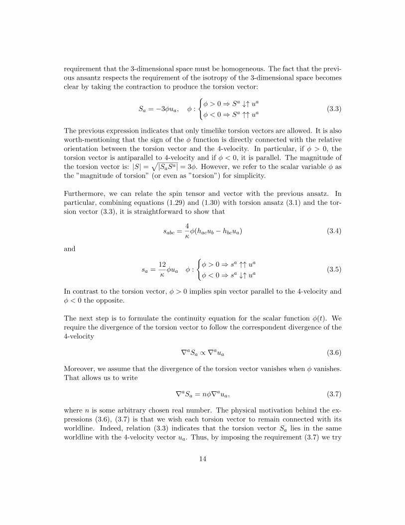
requirement that the 3-dimensional space must be homogeneous. The fact that the previ-ous ansantz respects the requirement of the isotropy of the 3-dimensional space becomesclear by taking the contraction to produce the torsion vector:

Sa = −3φua, φ :

φ > 0⇒ Sa ↓↑ ua

φ < 0⇒ Sa ↑↑ ua(3.3)

The previous expression indicates that only timelike torsion vectors are allowed. It is alsoworth-mentioning that the sign of the φ function is directly connected with the relativeorientation between the torsion vector and the 4-velocity. In particular, if φ > 0, thetorsion vector is antiparallel to 4-velocity and if φ < 0, it is parallel. The magnitude ofthe torsion vector is: |S| =

√|SaSa| = 3φ. However, we refer to the scalar variable φ as

the ”magnitude of torsion” (or even as ”torsion”) for simplicity.

Furthermore, we can relate the spin tensor and vector with the previous ansatz. Inparticular, combining equations (1.29) and (1.30) with torsion ansatz (3.1) and the tor-sion vector (3.3), it is straightforward to show that

sabc =4

κφ(hacub − hbcua) (3.4)

and

sa =12

κφua φ :

φ > 0⇒ sa ↑↑ ua

φ < 0⇒ sa ↓↑ ua(3.5)

In contrast to the torsion vector, φ > 0 implies spin vector parallel to the 4-velocity andφ < 0 the opposite.

The next step is to formulate the continuity equation for the scalar function φ(t). Werequire the divergence of the torsion vector to follow the correspondent divergence of the4-velocity

∇aSa ∝ ∇aua (3.6)

Moreover, we assume that the divergence of the torsion vector vanishes when φ vanishes.That allows us to write

∇aSa = nφ∇aua, (3.7)

where n is some arbitrary chosen real number. The physical motivation behind the ex-pressions (3.6), (3.7) is that we wish each torsion vector to remain connected with itsworldline. Indeed, relation (3.3) indicates that the torsion vector Sa lies in the sameworldline with the 4-velocity vector ua. Thus, by imposing the requirement (3.7) we try

14

to ensure that the two vectors will continue to belong to the same worldline. That isto say, the torsion vector field should behave similarly to the corresponding vector fieldof the 4-velocity. In any case, equation (3.7) is quite general and includes other morespecific conditions, such as ∇aSa = 0. However, our analysis in the two following sectionsis based on (3.7) and we do not require anything more specific.

We can make one extra step by combining (3.3) and (3.7) to receive

φ = −(n+ 3)φH ⇒ φ = −νφH (3.8)

or

φ = −(n+ 3)φa

a⇒ φ = −νφa

a(3.9)

One can integrate the previous relation, to find

φ = φiaνi

1

aν, (3.10)

where φi and ai are initial values. For convenience we set ν = n+ 3. As one can see, theparameter φ is related with the scale factor by the power law φ ∝ a−ν .

Finally, we employ the ansatz (3.1) to rewrite the Raychaudhuri equation (2.10) in termsof the parameter φ, as follows

H = −H2 − 1

3κTabu

aub − 1

6κT +

1

3Λ + 2φH (3.11)

3.2 Bianchi identities and symmetry

At this subsection, we use the Bianchi identities to discuss the symmetry properties ofthe Ricci and energy-momentum tensors and to derive the conservation laws and thecontinuity equation for FRW-type models with torsion employing the ansatz (3.1).

As we found in the previous section, the contractions of the Bianchi identities (2.11)and (2.12) are respectively,

∇bGba = 2RbcScba +RbcdaS

dcb (3.12)

G[ab] =1

2(Gab −Gba) = ∇aSb −∇bSa +∇cScab − 2ScScab, (3.13)

Using relations (3.1), (3.3) and considering that the isotropy and homogeneity imply:∇bua = 1

3Θhab, ∇aφ = −φua, we find that

∇bSa = 3φuaub − φΘhab = ∇aSb (3.14)

ScScab = −3φ2(:0

uchcaub −:0

uchcbua) = 0 (3.15)

15

To calculate the term ∇cScab, it is faster to use relation (3.2), exploiting the metricityrequirement ∇cgab = 0. Therefore,

∇cScab = ∇cφ(∇aub −∇bua)⇒

= −φuc(1

3Θhab −

1

3Θhab)⇒

= 0 (3.16)

Thus, combining equations (3.14)-(3.16), we obtain

G[ab] = 0 = R[ab] = T[ab] :

Gab = Gba

Rab = Rba

Tab = Tba

(3.17)

Hence, in FRW-type models, the Einstein, the Ricci and the energy-momentumtensors are symmetric.

However, the effect of torsion in the latter quantities is not absent. It affects theirsymmetric part, as equation (1.22) suggests. The antisymmetric piece (2.14) is producedpurely by the presence of torsion and seems to destroy the isotropy, according the theprevious analysis. This result is significant by its own means; however, it will also allowus to use the simplest type of matter, namely the perfect fluid.

3.3 The continuity equation

From the Einstein-Cartan field equations (1.28) and the ansatz (3.1), the geometricalrelation (2.13) transforms into the conservation law:

∇bTab = −4φ(Tabub − Λ

κua) (3.18)

To receive the conservation of energy, we multiply by the 4-velocity vector:

ua∇bTab = −4φ(Tabuaub +

Λ

κ) (3.19)

To proceed further and extract the continuity equation, we need an expression for theenergy-momentum tensor. The isotropy and homogeneity restrict the energy-momentumtensor to be that of the perfect fluid:

Tab = %uaub + phab, (3.20)

where % and p are the effective density and the effective pressure of the matter respec-tively, since they include the torsion/spin. Substituting the expression (3.20) into (3.19),produces the continuity equation:

%(I) = −3H(%+ p) + 4φ(%+Λ

κ), (3.21)

16

3.4 Compatibility issues and the flatness problem

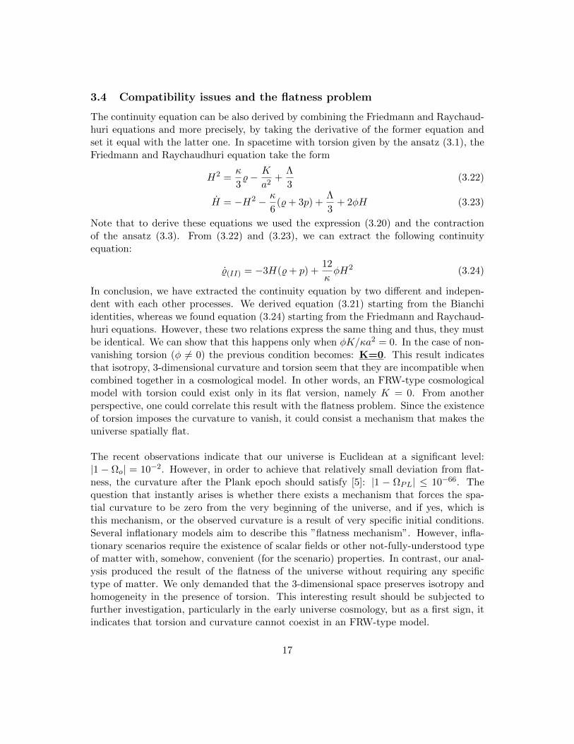
The continuity equation can be also derived by combining the Friedmann and Raychaud-huri equations and more precisely, by taking the derivative of the former equation andset it equal with the latter one. In spacetime with torsion given by the ansatz (3.1), theFriedmann and Raychaudhuri equation take the form

H2 =κ

3%− K

a2+

Λ

3(3.22)

H = −H2 − κ

6(%+ 3p) +

Λ

3+ 2φH (3.23)

Note that to derive these equations we used the expression (3.20) and the contractionof the ansatz (3.3). From (3.22) and (3.23), we can extract the following continuityequation:

%(II) = −3H(%+ p) +12

κφH2 (3.24)

In conclusion, we have extracted the continuity equation by two different and indepen-dent with each other processes. We derived equation (3.21) starting from the Bianchiidentities, whereas we found equation (3.24) starting from the Friedmann and Raychaud-huri equations. However, these two relations express the same thing and thus, they mustbe identical. We can show that this happens only when φK/κa2 = 0. In the case of non-vanishing torsion (φ 6= 0) the previous condition becomes: K=0. This result indicatesthat isotropy, 3-dimensional curvature and torsion seem that they are incompatible whencombined together in a cosmological model. In other words, an FRW-type cosmologicalmodel with torsion could exist only in its flat version, namely K = 0. From anotherperspective, one could correlate this result with the flatness problem. Since the existenceof torsion imposes the curvature to vanish, it could consist a mechanism that makes theuniverse spatially flat.

The recent observations indicate that our universe is Euclidean at a significant level:|1 − Ωo| = 10−2. However, in order to achieve that relatively small deviation from flat-ness, the curvature after the Plank epoch should satisfy [5]: |1 − ΩPL| ≤ 10−66. Thequestion that instantly arises is whether there exists a mechanism that forces the spa-tial curvature to be zero from the very beginning of the universe, and if yes, which isthis mechanism, or the observed curvature is a result of very specific initial conditions.Several inflationary models aim to describe this ”flatness mechanism”. However, infla-tionary scenarios require the existence of scalar fields or other not-fully-understood typeof matter with, somehow, convenient (for the scenario) properties. In contrast, our anal-ysis produced the result of the flatness of the universe without requiring any specifictype of matter. We only demanded that the 3-dimensional space preserves isotropy andhomogeneity in the presence of torsion. This interesting result should be subjected tofurther investigation, particularly in the early universe cosmology, but as a first sign, itindicates that torsion and curvature cannot coexist in an FRW-type model.

17

3.5 Splitting the energy-momentum tensor

The long expressions (1.21-1.23) can be written in a more compact way [3, 9]

Rabcd = Rabcd + ∇cKabd − ∇dKa

bc +KebdK

aec −Ke

bcKaed (3.25)

Rab = Rab + ∇cKcab − ∇bKc

ac +KdabK

cdc −Kd

acKcdb (3.26)

R = R− 2∇aKbab −Kba

bKcac +Kab

cKcba, (3.27)

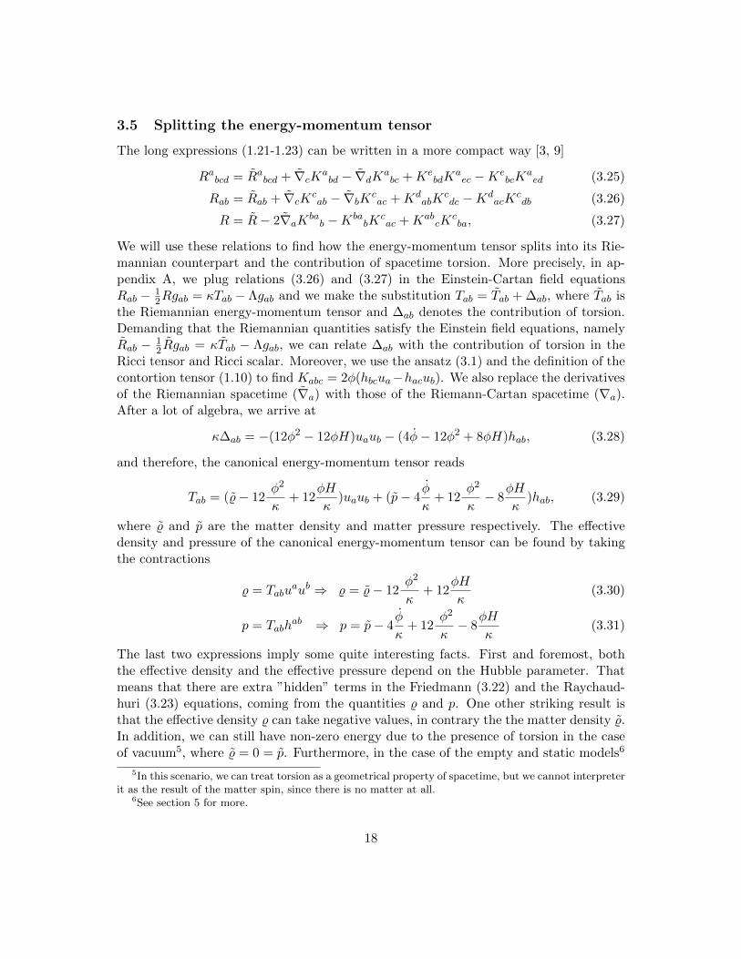
We will use these relations to find how the energy-momentum tensor splits into its Rie-mannian counterpart and the contribution of spacetime torsion. More precisely, in ap-pendix A, we plug relations (3.26) and (3.27) in the Einstein-Cartan field equationsRab − 1

2Rgab = κTab − Λgab and we make the substitution Tab = Tab + ∆ab, where Tab isthe Riemannian energy-momentum tensor and ∆ab denotes the contribution of torsion.Demanding that the Riemannian quantities satisfy the Einstein field equations, namelyRab − 1

2Rgab = κTab − Λgab, we can relate ∆ab with the contribution of torsion in theRicci tensor and Ricci scalar. Moreover, we use the ansatz (3.1) and the definition of thecontortion tensor (1.10) to find Kabc = 2φ(hbcua−hacub). We also replace the derivativesof the Riemannian spacetime (∇a) with those of the Riemann-Cartan spacetime (∇a).After a lot of algebra, we arrive at

κ∆ab = −(12φ2 − 12φH)uaub − (4φ− 12φ2 + 8φH)hab, (3.28)

and therefore, the canonical energy-momentum tensor reads

Tab = (%− 12φ2

κ+ 12

φH

κ)uaub + (p− 4

φ

κ+ 12

φ2

κ− 8

φH

κ)hab, (3.29)

where % and p are the matter density and matter pressure respectively. The effectivedensity and pressure of the canonical energy-momentum tensor can be found by takingthe contractions

% = Tabuaub ⇒ % = %− 12

φ2

κ+ 12

φH

κ(3.30)

p = Tabhab ⇒ p = p− 4

φ

κ+ 12

φ2

κ− 8

φH

κ(3.31)

The last two expressions imply some quite interesting facts. First and foremost, boththe effective density and the effective pressure depend on the Hubble parameter. Thatmeans that there are extra ”hidden” terms in the Friedmann (3.22) and the Raychaud-huri (3.23) equations, coming from the quantities % and p. One other striking result isthat the effective density % can take negative values, in contrary the the matter density %.In addition, we can still have non-zero energy due to the presence of torsion in the caseof vacuum5, where % = 0 = p. Furthermore, in the case of the empty and static models6

5In this scenario, we can treat torsion as a geometrical property of spacetime, but we cannot interpreterit as the result of the matter spin, since there is no matter at all.

6See section 5 for more.

18

(% = 0, H = 0), the torsion field has equation of state p = −% and thus, it behaves asa slowly rolling field. This is an interesting case that can be used to study inflationarymodels, without assuming scalar fields.

We can now see the ’hidden” contribution of torsion in the Friedmann and Raychaudhuriequations by substituting (3.30) and (3.31) into (3.22) and (3.23)

H2 =κ

3%− K

a2+

Λ

3+ 4φH − 4φ2 (3.32)

H = −H2 − κ

6(%+ 3p) +

Λ

3+ 4φH − 4φ2 + 2φ (3.33)

Using (3.32), the Raychaudhuri equation can be dramatically simplified to

H = −κ2

(%+ p) + 2φ (3.34)

Moreover, we can decompose the Hubble parameter into the ”Riemannian” Hubble pa-rameter and the extra contribution of torsion. In particular, from the ansatz (3.3) andthe relation (1.15), we get

H = H + 2φ, (3.35)

where we took Θ = 3H and Θ = 3H. Also, taking the derivative of (3.35), one can find

H = ˙H + 2φ (3.36)

Relation (3.35) states explicitly that positive values of φ enhance the (effective) Hub-ble parameter whereas, negative ones weaken it. Thus, torsion vector antiparallel tothe 4-velocity vector results in an increased Hubble parameter H, in comparison to theRiemannian one H, while the parallel orientation between the two vectors indicate theopposite.

What is more, expressions (3.34) and (3.36) suggest that, the ordinary matter tendsto decrease the rate of the expansion. In contrast, the contribution of torsion (expressedvia the scalar φ) depends on sign of the derivative of φ. An increasing torsion (φ > 0) en-hances the rate of expansion (or weakens the rate of contraction), whereas, a decreasingtorsion (φ < 0) does the opposite. In the case where the magnitude of torsion remainsconstant, namely φ = 0, the Raychaudhuri equation reduces its classical form.

4 Cosmological implications of torsion

In the present section, we discuss the effects of the application of torsion to severalcosmological topics. In particular, we study the recent accelerated expansion, the focusing

19

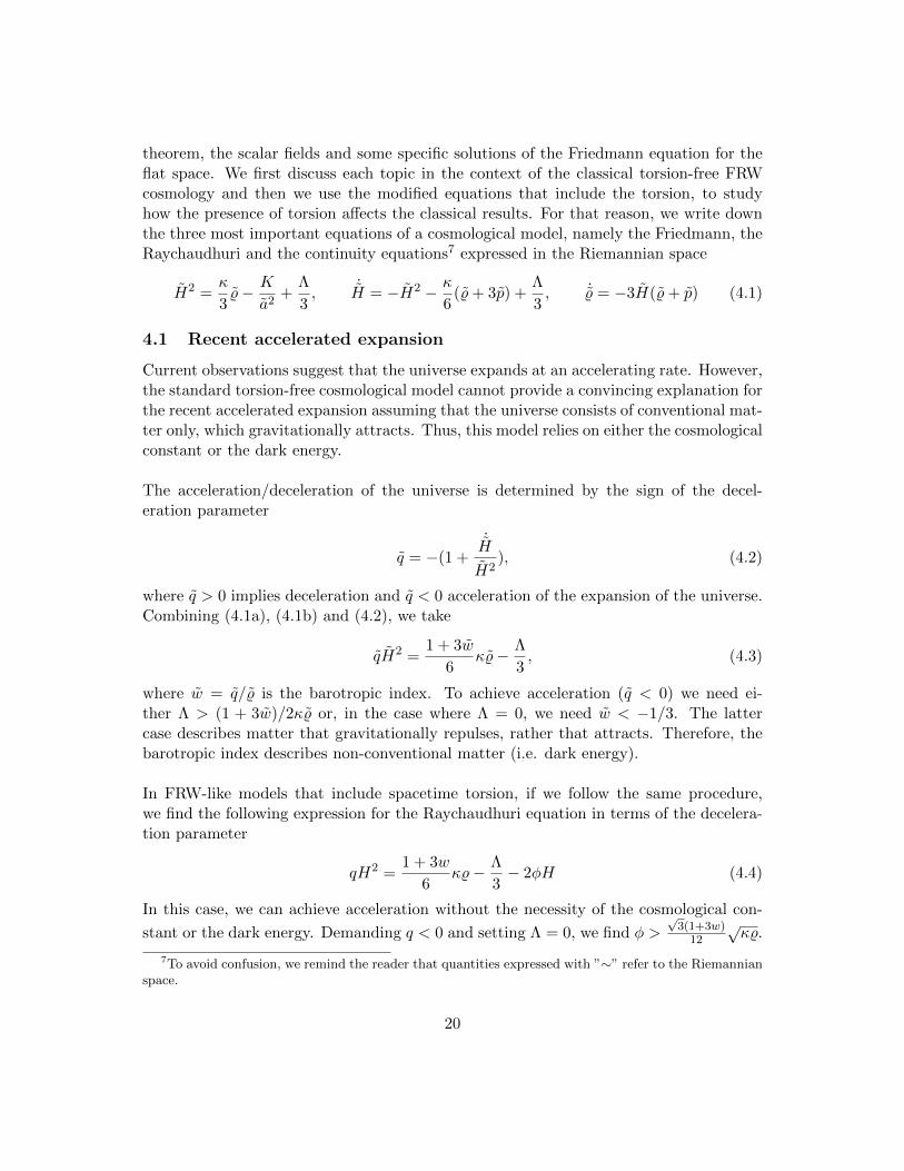
theorem, the scalar fields and some specific solutions of the Friedmann equation for theflat space. We first discuss each topic in the context of the classical torsion-free FRWcosmology and then we use the modified equations that include the torsion, to studyhow the presence of torsion affects the classical results. For that reason, we write downthe three most important equations of a cosmological model, namely the Friedmann, theRaychaudhuri and the continuity equations7 expressed in the Riemannian space

H2 =κ

3%− K

a2+

Λ

3, ˙H = −H2 − κ

6(%+ 3p) +

Λ

3, ˙% = −3H(%+ p) (4.1)

4.1 Recent accelerated expansion

Current observations suggest that the universe expands at an accelerating rate. However,the standard torsion-free cosmological model cannot provide a convincing explanation forthe recent accelerated expansion assuming that the universe consists of conventional mat-ter only, which gravitationally attracts. Thus, this model relies on either the cosmologicalconstant or the dark energy.

The acceleration/deceleration of the universe is determined by the sign of the decel-eration parameter

q = −(1 +˙H

H2), (4.2)

where q > 0 implies deceleration and q < 0 acceleration of the expansion of the universe.Combining (4.1a), (4.1b) and (4.2), we take

qH2 =1 + 3w

6κ%− Λ

3, (4.3)

where w = q/% is the barotropic index. To achieve acceleration (q < 0) we need ei-ther Λ > (1 + 3w)/2κ% or, in the case where Λ = 0, we need w < −1/3. The lattercase describes matter that gravitationally repulses, rather that attracts. Therefore, thebarotropic index describes non-conventional matter (i.e. dark energy).

In FRW-like models that include spacetime torsion, if we follow the same procedure,we find the following expression for the Raychaudhuri equation in terms of the decelera-tion parameter

qH2 =1 + 3w

6κ%− Λ

3− 2φH (4.4)

In this case, we can achieve acceleration without the necessity of the cosmological con-

stant or the dark energy. Demanding q < 0 and setting Λ = 0, we find φ >√

3(1+3w)12

√κ%.

7To avoid confusion, we remind the reader that quantities expressed with ”∼” refer to the Riemannianspace.

20

Substituting the effective density with the Hubble parameter from the Friedmann equa-tion and for matter with vanishing effective pressure (w = 0) in a flat 3-dimensionalspace, the condition for acceleration reads: φ > H

4 . The latter outcome suggests that inorder to achieve accelerated expansion without the existence of either the cosmologicalconstant or the dark energy, the quantity φ, which expresses the magnitude of torsion,must be at least greater than the 25% of the Hubble parameter. Apart from that, weshould also note that φ must be positive, which consequently implies that the torsionvector must be antiparallel to the 4-velocity vector.

4.2 Focusing theorem and singularities

Considering a congruence of timilike geodesics, the focusing theorem states [10] that: aninitially diverging (H > 0) congruence will diverge less rapidly in the future, while aninitially converging (H < 0) congruence will converge more rapidly in the future. Inour analysis, we first study the focusing of the worldlines in the context of the classicalcosmology in a Riemannian space. For what follows, we ignore the cosmological constantand we assume that the strong energy condition holds: Rabu

aub = %+ 3p > 0. In otherwords, we assume that the universe consists of conventional matter, which gravitationallyattracts. In that case (4.1b) reads

˙H ≤ −H2 ⇒ dH

H2≤ −dt⇒

∫ Hf

Hi

dH

H2≤ −

∫ tf

ti

dt⇒ tf − to ≤1

Hf

− 1

Hi

, (4.5)

where ti refers to a initial moment and tf refers to the final moment. Since we move backin the past, we have H ≤ 0. According to the focusing theorem, the initially convergingcongruence will converge more rapidly in the future and therefore Hf → −∞ at time tf .Thus,

∆t = tf − ti ≤1

|Hi|(4.6)

In conclusion, supposing that the universe converges, the worldlines develop a causticpoint (i.e. a singularity) in time no more than 1/|Hi|. Moreover, according to that the-orem, any physical process or structure in the universe has to be no older than 1/|Hi|.

A viable way to discuss the avoidance of the initial singularity, could suggest violation ofthe strong energy-condition [11]. That can be possible in the period when slowly rollingscalar fields dominate, which obey the equation of state p(ψ) = −%(ψ) (see subsection 4.3for more). According to that equation of state, Rabu

aub < 0 the inequality changes to˙H ≥ −H2, giving ∆t ≥ 1/|Hi|. That condition, does not reveal the prevention of the

formation of singularity by itself, rather it states that there is no indication about theformation of a caustic point. However, if we start from a static state Hi = 0, the lattercondition becomes ∆t ≥ +∞. This result shows that starting from a static state, it

21

would take worldlines an infinite amount of time to reach to an end and form a causticpoint.

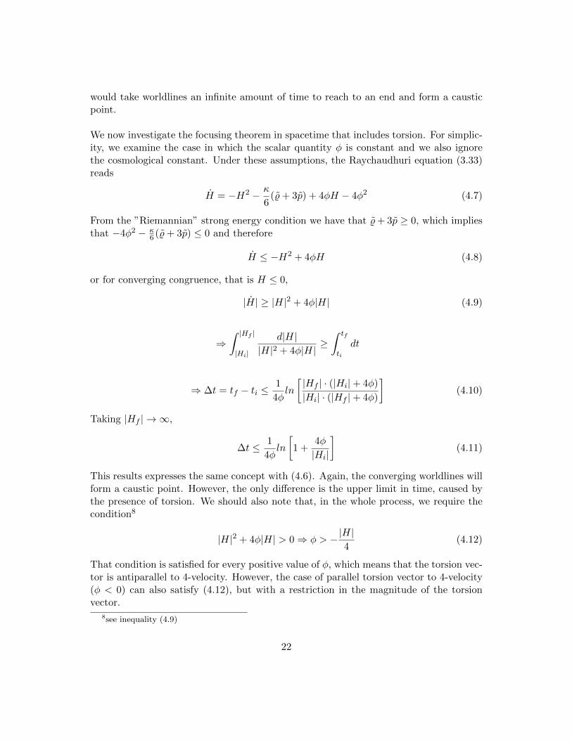
We now investigate the focusing theorem in spacetime that includes torsion. For simplic-ity, we examine the case in which the scalar quantity φ is constant and we also ignorethe cosmological constant. Under these assumptions, the Raychaudhuri equation (3.33)reads

H = −H2 − κ

6(%+ 3p) + 4φH − 4φ2 (4.7)

From the ”Riemannian” strong energy condition we have that %+ 3p ≥ 0, which impliesthat −4φ2 − κ

6 (%+ 3p) ≤ 0 and therefore

H ≤ −H2 + 4φH (4.8)

or for converging congruence, that is H ≤ 0,

|H| ≥ |H|2 + 4φ|H| (4.9)

⇒∫ |Hf ||Hi|

d|H||H|2 + 4φ|H|

≥∫ tf

ti

dt

⇒ ∆t = tf − ti ≤1

4φln

[|Hf | · (|Hi|+ 4φ)

|Hi| · (|Hf |+ 4φ)

](4.10)

Taking |Hf | → ∞,

∆t ≤ 1

4φln

[1 +

4φ

|Hi|

](4.11)

This results expresses the same concept with (4.6). Again, the converging worldlines willform a caustic point. However, the only difference is the upper limit in time, caused bythe presence of torsion. We should also note that, in the whole process, we require thecondition8

|H|2 + 4φ|H| > 0⇒ φ > −|H|4

(4.12)

That condition is satisfied for every positive value of φ, which means that the torsion vec-tor is antiparallel to 4-velocity. However, the case of parallel torsion vector to 4-velocity(φ < 0) can also satisfy (4.12), but with a restriction in the magnitude of the torsionvector.

8see inequality (4.9)

22

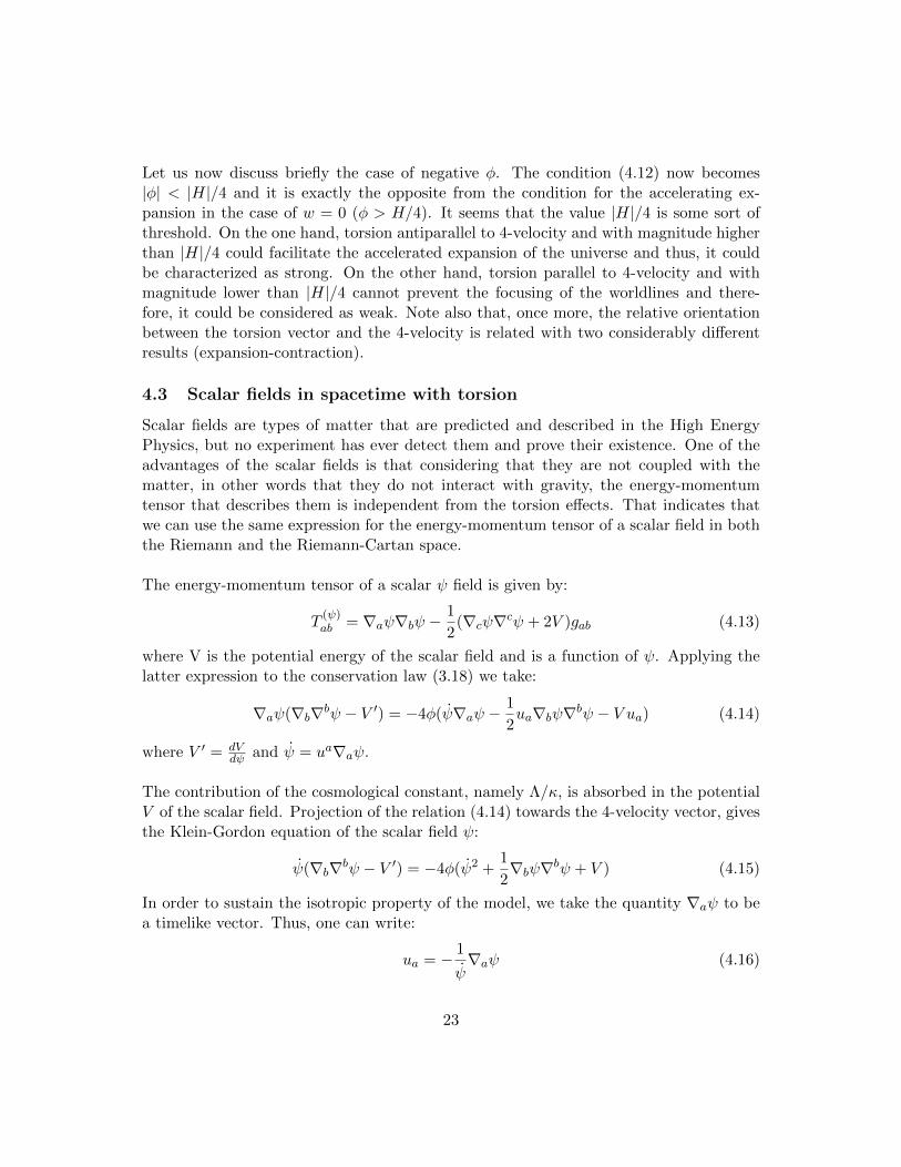
Let us now discuss briefly the case of negative φ. The condition (4.12) now becomes|φ| < |H|/4 and it is exactly the opposite from the condition for the accelerating ex-pansion in the case of w = 0 (φ > H/4). It seems that the value |H|/4 is some sort ofthreshold. On the one hand, torsion antiparallel to 4-velocity and with magnitude higherthan |H|/4 could facilitate the accelerated expansion of the universe and thus, it couldbe characterized as strong. On the other hand, torsion parallel to 4-velocity and withmagnitude lower than |H|/4 cannot prevent the focusing of the worldlines and there-fore, it could be considered as weak. Note also that, once more, the relative orientationbetween the torsion vector and the 4-velocity is related with two considerably differentresults (expansion-contraction).

4.3 Scalar fields in spacetime with torsion

Scalar fields are types of matter that are predicted and described in the High EnergyPhysics, but no experiment has ever detect them and prove their existence. One of theadvantages of the scalar fields is that considering that they are not coupled with thematter, in other words that they do not interact with gravity, the energy-momentumtensor that describes them is independent from the torsion effects. That indicates thatwe can use the same expression for the energy-momentum tensor of a scalar field in boththe Riemann and the Riemann-Cartan space.

The energy-momentum tensor of a scalar ψ field is given by:

T(ψ)ab = ∇aψ∇bψ −

1

2(∇cψ∇cψ + 2V )gab (4.13)

where V is the potential energy of the scalar field and is a function of ψ. Applying thelatter expression to the conservation law (3.18) we take:

∇aψ(∇b∇bψ − V ′) = −4φ(ψ∇aψ −1

2ua∇bψ∇bψ − V ua) (4.14)

where V ′ = dVdψ and ψ = ua∇aψ.

The contribution of the cosmological constant, namely Λ/κ, is absorbed in the potentialV of the scalar field. Projection of the relation (4.14) towards the 4-velocity vector, givesthe Klein-Gordon equation of the scalar field ψ:

ψ(∇b∇bψ − V ′) = −4φ(ψ2 +1

2∇bψ∇bψ + V ) (4.15)

In order to sustain the isotropic property of the model, we take the quantity ∇aψ to bea timelike vector. Thus, one can write:

ua = − 1

ψ∇aψ (4.16)

23

or

∇aψ = −ψua (4.17)

Exploiting the latter equation, one can rewrite equation (4.13) as

T(ψ)ab = ψ2uaub −

1

2(−ψ2 + 2V )gab (4.18)

or

T(ψ)ab = (

1

2ψ2 + V )uaub + (

1

2ψ2 − V )hab (4.19)

The quantity 12 ψ

2 can be interpreted as the kinetic energy of the scalar field. Restrictingthe scalar field in an isotropic space, we can express the energy-momentum tensor of thescalar field in a term that is the coefficient of uaub and a term that is coefficient of thespacelike metric tensor hab, as shown below

T(ψ)ab = ρ(ψ)uaub + p(ψ)hab (4.20)

Comparing (4.19) and (4.20) implies that:

ρ(ψ) =1

2ψ2 + V (4.21)

p(ψ) =1

2ψ2 − V (4.22)

which are the effective density and the effective pressure of the scalar field respectively.The cases of the slowly rolling scalar field, that is ψ2 << V , and the vacuum energy,where ψ = 0, lead to the state equation p(ψ) = −ρ(ψ), as one can find from equations(4.21) and (4.22). According to the same equations, one can show that a fast rollingscalar field (ψ >> V ) has state equation p(ψ) = ρ(ψ).

Taking into account the expression (4.17), the Klein-Gordon equation takes the followingform:

ψψ + (3H − 2φ)ψ2 + V ′ψ − 4φV = 0 (4.23)

Setting φ→ 0, one can take the Klein-Gordon equation in the classical limit

ψ + 3Hψ + V ′ = 0 (4.24)

The differential equation (4.23) describes the evolution in time of the scalar field ψ ina space that includes torsion. To solve it analytically, we need to specify the potentialenergy of the scalar field and to know how the scalar torsion φ and the Hubble parameterchange in time, but this is something beyond the scope of this thesis.

24

4.4 Solutions of the Friedmann equations

Knowing the relation between the Hubble parameter and the time allows us to makepredictions and investigate several cosmological epochs. In FRW torsion-free cosmology,this relation generally obeys the inverse law H ∝ 1/t. More precisely, one can use (4.1a) and (4.1 b) for K = 0 and % = wp, to find the solution9

H =2

3(1 + w)t(4.25)

The scale factor goes as a ∝ t2/3(1+w). The barotropic index w determines the type ofmatter and takes the value: w = 0 for dust, w = 1/3 for the electromagnetic field andw = −1 for the cosmological constant (or the slowly rolling scalar field).

We now wish to find the evolution of H in time including the presence of torsion. We con-sider the case of the flat universe (K = 0), where the cosmological constant dominates.From (4.1), we take

H =

√Λ

3(4.26)

That brings equation (3.35) into

H = 2φ+

√Λ

3(4.27)

Differentiating the latter expression produces

H = 2φ, (4.28)

which, via (3.9) recasts into

H = −2νφH (4.29)

Then, applying (4.27) and (4.28) to the latter expression, gives

φ = −2νφ2 − ν√

Λ

3φ (4.30)

By separation of variables we can solve this differential equation, as follows

dφ

2νφ2 + ν√

Λ3 φ

= −dt⇒ (4.31)

9To derive this result we considered that the cosmological constant is included in the total density %and total pressure p. In other words, % = %matter + Λ

κand p = pmatter − Λ

κ

25

∫ φ

φi

dφ∗

2νφ∗2 + ν√

Λ3 φ∗

= −∫ t

0dt∗ ⇒ (4.32)

1

ν√

Λ3

ln

φ(2νφi + ν√

Λ3 )

φi(2νφ+ ν√

Λ3 )

= −t⇒ (4.33)

φ(t) =ν√

Λ3(

νφi

√Λ3 + 2ν

)eν√

Λ3t − 2ν

(4.34)

Finally, we can derive the Hubble parameter as a function of time, considering relations(4.27) and (4.34). Thus,

H(t) =ν√

Λ3(

ν√

Λ3

Hi−√

Λ3

+ 2ν

)eν√

Λ3t − 2ν

+

√Λ

3, (4.35)

where Hi = φi+√

Λ3 is the initial value of the Hubble parameter corresponding to t = 0.

We now examine two different cases depending on the sign of ν10 for t→∞. For ν > 0we have

limt→∞

φ(t) = 0, limt→∞

H(t) =

√Λ

3(4.36)

and for ν < 0, we take

limt→∞

φ(t) = −1

2

√Λ

3, lim

t→∞H(t) =

1

2

√Λ

3(4.37)

The case of positive ν states that φ vanishes as time goes to infinity, while the Hubbleparameter takes a constant, and more precisely positive, value. Hence, the effect of tor-sion becomes negligible after a long time, something which is consistent with the factthat current observations fail to detect the presence of torsion11.

An interesting, however perhaps less reasonable, result is produced when ν < 0. Inthis case, we find that torsion takes asymptotically a negative value as time increases.This solution implies that the torsion does not vanish and the torsion vector ends upparallel to the 4-velocity. Moreover, it is worth mentioning that the final value of torsionis exactly the opposite from that of the Hubble parameter φf = −Hf .

10We remind that φ ∝ a−ν .11As we have discussed in the introduction, the effects of torsion become significant in extremely high

energy densities.

26

5 Einstein static universe and its stability

The Einstein static universe is considered the type of universe that neither expands norcontracts. By definition, H ≡ a

a = 0 and H = 0. It was proposed by Albert Ein-stein in 1917, who applied his field equations to the universe as a whole. In order tocounterbalance the attractive effects of the conventional matter, Einstein introduced asupplementary term in the field equations; the cosmological constant, which behaves asa repulsive force. Solving the field equations and considering positive cosmological con-stant, he found that static solution could only exist for positive curvature, which meansclosed universe. However, observations by Edwin Hubble showed that the universe ex-pands, making Einstein to characterize the cosmological constant an unfortunate mistake.

Despite the fact that the Einstein static model is not compatible with the present viewof our universe, it still receives much attention, since it is connected with inflationarymodels and the very early universe [11]. In all these considerations, the stability of theEinstein static model plays a key role. In classical GR, Eddington showed [12] that themodel is unstable against spatially homogeneous and isotropic perturbations. In the fol-lowing analysis, we first examine the classical case and we also prove instability againstfirst order perturbation in the scale factor. Moving on to the ECKS theory and consid-ering torsion, we examine the case of the spatially flat static model and we investigateits stability.

5.1 Einstein static universe without torsion

Setting H = 0 = ˙H in (4.1a) and (4.1b), we take

0 =κ

3%− K

a2+

Λ

3(5.1)

0 = −κ6

(%+ 3p) +Λ

3(5.2)

The first equation implies that K = +1 in order to counterbalance the contribution ofthe matter and the cosmological constant. Thus, the Einstein static universe in the clas-sical cosmology must be closed. The flat version (K = 0) can only exist in the trivialcase of the empty universe, where there is neither matter nor cosmological constant inthe model. The second equation suggests that only matter with w = %/p > −1/3 canparticipate in the static model.

If we solve (5.1) for % and substitute the result into (5.2), we find the solution to theEinstein static universe:

ao =

√1 + 3w

(1 + w)Λ, (5.3)

27

where ao is the radius of the Einstein static universe.

We now return to (4.1a)-(4.1b) and we make the substitutions p = w%, H = ˙a/a Inparticular solving equation (4.1a) in terms of % and equation (5.3) in terms of Λ and plugthem into (4.1b), produces

a¨a = −1 + 3w

2˙a2 +

1 + 3w

2ao

2

− 1 + 3w

2(5.4)

To test the stability of the Einstein static universe, we perturb the scale factor around thesolution: a = ao + δa, δa << ao. Holding only first-order terms, relation (5.4) becomes

(δa) =1 + 3w

a2o

δa (5.5)

The solution of the latter differential equation tells us whether the equilibrium point(ao, 0) is stable or not. Although it is very easy to solve that differential equation, we usethe linear stability technique in order to test the stability around the equilibrium point.First, we parameterize the differential equation as follows:

x = bx, (5.6)

where x = δa and b = 1+3wa2o

. This is an autonomous differential equation of order 2,

which is equivalent to a system of two differential equations of order 1. This system canbe described by the equations:

x = f(x, y) = y (5.7)

y = g(x, y) = bx (5.8)

The table of the linearized system is

A =

∂f∂x

∂g∂x

∂f∂y

∂g∂y

o

=

(0 b1 0

)(5.9)

The eigenvalues of table A are:

λ1 = −√b, λ2 = +

√b (5.10)

The two eigenvalues are real numbers with different sign. In this case, the equilibriumpoint is a saddle point and therefore unstable. For completeness we present the solutionof (5.4):

δa(t) = C1e√

(1+3w)/a2o t + C2e

−√

(1+3w)/a2o t, (5.11)

28

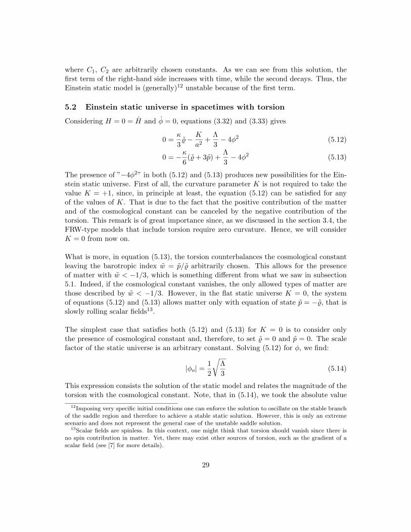
where C1, C2 are arbitrarily chosen constants. As we can see from this solution, thefirst term of the right-hand side increases with time, while the second decays. Thus, theEinstein static model is (generally)12 unstable because of the first term.

5.2 Einstein static universe in spacetimes with torsion

Considering H = 0 = H and φ = 0, equations (3.32) and (3.33) gives

0 =κ

3%− K

a2+

Λ

3− 4φ2 (5.12)

0 = −κ6

(%+ 3p) +Λ

3− 4φ2 (5.13)

The presence of ”−4φ2” in both (5.12) and (5.13) produces new possibilities for the Ein-stein static universe. First of all, the curvature parameter K is not required to take thevalue K = +1, since, in principle at least, the equation (5.12) can be satisfied for anyof the values of K. That is due to the fact that the positive contribution of the matterand of the cosmological constant can be canceled by the negative contribution of thetorsion. This remark is of great importance since, as we discussed in the section 3.4, theFRW-type models that include torsion require zero curvature. Hence, we will considerK = 0 from now on.

What is more, in equation (5.13), the torsion counterbalances the cosmological constantleaving the barotropic index w = p/% arbitrarily chosen. This allows for the presenceof matter with w < −1/3, which is something different from what we saw in subsection5.1. Indeed, if the cosmological constant vanishes, the only allowed types of matter arethose described by w < −1/3. However, in the flat static universe K = 0, the systemof equations (5.12) and (5.13) allows matter only with equation of state p = −%, that isslowly rolling scalar fields13.

The simplest case that satisfies both (5.12) and (5.13) for K = 0 is to consider onlythe presence of cosmological constant and, therefore, to set % = 0 and p = 0. The scalefactor of the static universe is an arbitrary constant. Solving (5.12) for φ, we find:

|φo| =1

2

√Λ

3(5.14)

This expression consists the solution of the static model and relates the magnitude of thetorsion with the cosmological constant. Note, that in (5.14), we took the absolute value

12Imposing very specific initial conditions one can enforce the solution to oscillate on the stable branchof the saddle region and therefore to achieve a stable static solution. However, this is only an extremescenario and does not represent the general case of the unstable saddle solution.

13Scalar fields are spinless. In this context, one might think that torsion should vanish since there isno spin contribution in matter. Yet, there may exist other sources of torsion, such as the gradient of ascalar field (see [7] for more details).

29

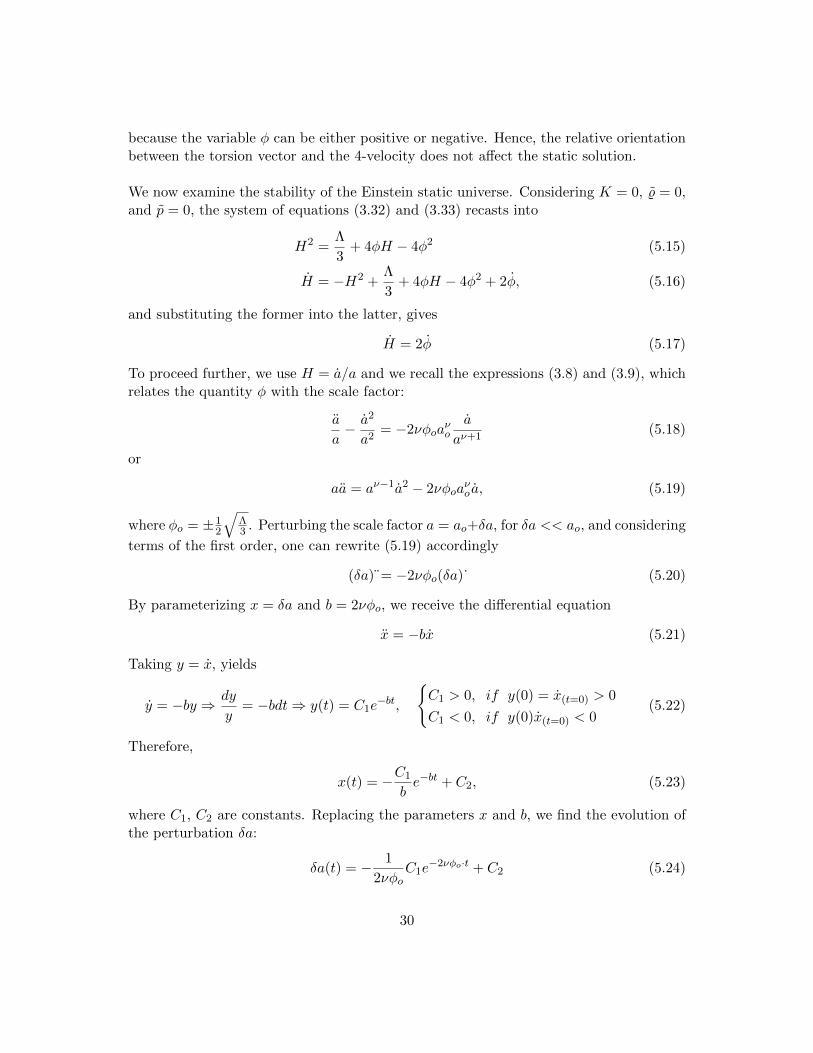
because the variable φ can be either positive or negative. Hence, the relative orientationbetween the torsion vector and the 4-velocity does not affect the static solution.

We now examine the stability of the Einstein static universe. Considering K = 0, % = 0,and p = 0, the system of equations (3.32) and (3.33) recasts into

H2 =Λ

3+ 4φH − 4φ2 (5.15)

H = −H2 +Λ

3+ 4φH − 4φ2 + 2φ, (5.16)

and substituting the former into the latter, gives

H = 2φ (5.17)

To proceed further, we use H = a/a and we recall the expressions (3.8) and (3.9), whichrelates the quantity φ with the scale factor:

a

a− a2

a2= −2νφoa

νo

a

aν+1(5.18)

or

aa = aν−1a2 − 2νφoaνo a, (5.19)

where φo = ±12

√Λ3 . Perturbing the scale factor a = ao+δa, for δa << ao, and considering

terms of the first order, one can rewrite (5.19) accordingly

(δa) = −2νφo(δa)˙ (5.20)

By parameterizing x = δa and b = 2νφo, we receive the differential equation

x = −bx (5.21)

Taking y = x, yields

y = −by ⇒ dy

y= −bdt⇒ y(t) = C1e

−bt,

C1 > 0, if y(0) = x(t=0) > 0

C1 < 0, if y(0)x(t=0) < 0(5.22)

Therefore,

x(t) = −C1

be−bt + C2, (5.23)

where C1, C2 are constants. Replacing the parameters x and b, we find the evolution ofthe perturbation δa:

δa(t) = − 1

2νφoC1e

−2νφo·t + C2 (5.24)

30

However, for t = 0, we have δa(0) = 0, (δa) (t=0) = (δa) o and from (5.24), we find

C1 = (δa) o (5.25)

C2 =C1

2νφo, (5.26)

The sign of C1 depends on the sign of (δa) o at t = 0. Yet, (δa) o represents the initialspeed of the perturbation and we examine the case in which it is positive, which in turnimplies that C1 > 0. The solution for the perturbation becomes

δa(t) =C1

2νφo(1− e−2νφo·t), (5.27)

and for the scale factor, a(t) = ao + δa(t), reads

a(t) = ao +C1

2νφo(1− e−2νφo·t), (5.28)

That is the final result, which describes the perturbation in scale factor as a function oftime. The stability of the static universe depends on the sign of the product ”νφo”. Ifthis product is negative, then from (5.27), we see that the perturbation goes to +∞ whent→ +∞. In that case, the Einstein static model is unstable. On the other hand, takingνφo > 0, the exponential decays as t → +∞ and the perturbation takes the terminalvalue δa = C1/2νφo. This means that the scale factor increases from ao to ao+C1/2νφo.That is to say that the perturbed initial static universe goes asymptotically to a finalstatic state with increased scale factor.

Intuitively, it makes more sense to assume that ν is positive in the expression φ ∝ 1/aν .Since φ is a quantity associated with some sort of energy density (i.e. the torsion/spinenergy density), it is reasonable to expect that φ decreases when the universe expandsand increases when the universe contracts. On that ground, the case of parallel torsionvector to 4-velocity (φo < 0) implies instability of the Einstein static universe, whereas,the case of antiparallel torsion to 4-velocity (φo > 0) implies asymptotic stability withincreased scale factor.

6 Conclusions-Discussion

The main objective of my diploma thesis was to familiarize myself with the Einstein-Cartan theory by analyzing the contribution of torsion in cosmology, focusing particu-larly on the FRW-type models. The motivation for studying FRW-type cosmologies is,from one perspective, the fact that the basic kinematic equations (i.e. the Friedmannand the Raychaudhuri) are oversimplified dramatically. From another perspective theFRW-type cosmological models comes naturally into consideration, since the isotropyand homogeneity these models imply in large scales, are supported by the current data.

31

Perhaps, the most noticeable outcome of our analysis is the incompatibility amongisotropy, curvature and torsion. The roots of this incompatibility lie in the direct com-parison between the continuity equation derived from the Bianchi identities, with thecorresponding one derived from the Friedmann and Raychaudhuri equations. It seemsthat the maximally symmetric FRW-type cosmology is so restrictive that, by allowing forthe presence of both curvature and torsion, it loses its symmetry properties. On the otherhand, this observation may be used for proposing the theory of torsion as an alternativeto inflationary scenarios, since as we already have mentioned, the K = 0 requirementcan be associated with the flatness problem. In particular, when the effect of torsion isconsidered, the symmetry properties impose the spatial 3-dimensional curvature to van-ish. However, this is only an indication and further and more profound research couldbe enlightening.

Moreover, arguments regarding isotropy and homogeneity produced another remarkableresult. Using the torsion ansatz (3.1), we proved that the Einstein and, consequently,the Ricci and the energy-momentum tensors must be symmetric in the FRW-type mod-els that include the spacetime torsion, which in turn simplified our calculations. It isstraightforward to prove that this statement also holds true vice versa; that is to sayif the Einstein tensor is not symmetric then, the 3-dimensional space loses its isotropy.Indeed, the antisymmetry in those tensors is associated with the existence of spacelikecomponents of the torsion/spin vector, which of course is something that destroys the3-dimensional isotropy.

One of our greatest efforts was to decompose the energy-momentum tensor, and con-sequently, the effective energy density and pressure, in order to understand better thecontribution of torsion in matter. Indeed, this attempt seems to be ubiquitous in everyrecent work that involves the ECKS theory. Many authors [6, 13] use the Weyssenhofffluid to describe the matter imposing the Frenkel14 condition. The Weyssenhoff fluid isa perfect fluid with spin where the spin of the matter fields is the source of torsion inan Einstein-Cartan framework. Another approach for generating the energy-momentumsplitting, which motivated ours, is presented in [2, 3, 9], where the author finds a mod-ification of the energy-momentum tensor which is quadratic in the torsion tensor, andthen, assuming the Belinfante-Rosefeld identity, he presents such a decomposition for theenergy-momentum tensor.

However, the previous approaches seem to be incompatible with the homogeneity andisotropy of an FRW-type cosmology, since their analysis allows the existence of spacelikecomponents. For that reason we followed another approach. In particular, we consideredthe ansatz (3.1) and knowing the decomposition in curvature, we calculated the modi-

14The Frenkel condition demands the intrinsic spin to be spacelike and that the torsion is traceless.

32

fied part of the energy-momentum tensor. According to our decomposition, the effectivedensity and pressure, apart from a quadratic term of φ, they also include a coupling termbetween φ and the Hubble parameter.

The implications of torsion in the Einstein static universe are also noteworthy. Theanalysis followed in section 5 shows that, in the context of the classical GR, a positivecosmological constant implies conventional matter and closed universe (K = +1) in orderto achieve static solution. In the Riemann-Cartan space, the Einstein universes, takinginto account the flatness requirement, we need matter with equation of state p = −%.Performing a first order perturbation in the scale factor, we managed to prove that thestatic universe is, generally, unstable in the classical GR. However, we found that, in theRiemann-Cartan spacetime, the flat static universe consisting of only the cosmologicalconstant and the torsion field can be stable. More precisely, perturbing the universe fromits initial static state can drive it in a final state with different value of the scale factor.

Many of our results depend on the relative orientation between the torsion (or spin)vector15 and the 4-velocity. The physical interpretation is of great importance and itprovides the motives for further and more profound investigation. However, we couldbriefly summarize a few simple thoughts. First of all, there is an analogy between thetimelike 4-spin and the z-component of the quantum mechanical spin. According toquantum mechanics, there are two preferable directions for each one of the three spincomponents: spin up and spin down. Similarly, the 4-spin can be either parallel or an-tiparallel to 4-velocity. The difference is that the axis of the 4-velocity represents thedirection of (proper) time, whereas the z-axis is spatial.

Furthermore, in particle physics, the helicity of a particle is a notion that relates themomentum of the particle with its spin. In particular, a particle is said to be right-handed if its spin is parallel to its momentum, and left-handed if they are antiparallel.Extending the comparison, we can define the 4-helicity as the relativistic product of the4-momentum and the 4-spin vector of the particle. However, the 4-momentum vectorpoints at the same direction as the 4-velocity vector. Hence, if the 4-spin is parallel tothe 4-velocity, that is φ > 0, we could say that the universe consists of “right-handed”particles. Otherwise, the universe consists of “left-handed” particles. In any case, thefact that the matter consists of either ”right-handed” (φ > 0) or ”left-handed” (φ < 0)particles implies an symmetry, which could be related to other asymmetries found innature, such as the dominance of the matter over the antimatter, or the fact that thecosmic time flows only in one direction. Therefore, the interpretation of the direction ofspin along the worldlines and its additional effects in cosmology could be an interestingextension of the topics discussed in this diploma thesis.

15The torsion vector is antiparallel to the spin vector as the equation (1.30) suggests. Therefore, if thetorsion vector is parallel to the 4-velocity, the spin vector is antiparallel to the 4-velocity and vice versa.

33

A Detailed calculations

A.1 Friedmann equation

The curvature tensor of the 3-dimensional space of the observer can be expressed by thefollowing equation

<abcd = haqhb

shcfhd

pRqsfp −DcuaDdub +DduaDcub, (A.1)

where:

Dbua =1

3Θhab + σab + ωab (A.2)

In addition, the curvature of the 4-dimensional space satisfies

Rabcd = Cabcd +1

2(gacRbd + gbdRac − gbcRad − gadRbc)−

R

6(gacgbd − gadgbc) (A.3)

We first calculate the term haqhb

shcfhd

pRqsfp of (A.1), using (A.3). In particular,

haqhb

shcfhd

pRqsfp =haqhb

shcfhd

pCqsfp

+1

2ha

qhbshc

fhdp(gqfRsp + gspRqf − gsfRqp − gqpRsf )

−R6ha

qhbshc

fhdp(gqfgsp − gqpgsf )

⇒ haqhb

shcfhd

pRqsfp =haqhb

shcfhd

pCqsfp

+1

2Rqf (hachb

qhdf + hbdha

qhcf − hbchaqhdf − hadhbqhcf )

−R6

(hachbd − hadhbc)

From the Einstein-Cartan field equations (1.28), we have Rab = κTab + (Λ − κ2T )gab,

R = 4Λ− κT . Thus,

haqhb

shcfhd

pRqsfp =haqhb

shcfhd

pCqsfp

+1

2κTqf (hachb

qhdf + hbdha

qhcf − hbchaqhdf − hadhbqhcf )

+1

2(Λ− κT

2)gqf (hachb

qhdf + hbdha

qhcf − hbchaqhdf − hadhbqhcf )

−1

6(4Λ− κT )(hachbd − hadhbc)⇒

haqhb

shcfhd

pRqsfp =haqhb

shcfhd

pCqsfp

+1

2κTqf (hachb

qhdf + hbdha

qhcf − hbchaqhdf − hadhbqhcf )

+(Λ− κT

2)(hachbd − hadhbc)−

1

6(4Λ− κT )(hachbd − hadhbc)⇒

34

haqhb

shcfhd

pRqsfp =haqhb

shcfhd

pCqsfp

+1

2κTqf (hachb

qhdf + hbdha

qhcf − hbchaqhdf − hadhbqhcf )

+(Λ

3− κT

3)(hachbd − hadhbc) (A.4)

Applying (A.2) to the second term of the right-hand side of equation (A.1), gives

DcuaDdub =(1

3Θhac + σac + ωac)(

1

3Θhbd + σbd + ωbd)

=1

9Θ2hachbd +

1

3Θ [hac(σbd + ωbd) + hbd(σac + ωac)]

+ (σac + ωac)(σbd + ωbd) (A.5)

Likewise,

DduaDcub =1

9Θ2hadhbc +

1

3Θ [had(σbc + ωbc) + hbc(σad + ωad)]

+ (σad + ωad)(σbc + ωbc) (A.6)

Plugging (A.4), (A.5) and (A.6) into (A.1), leads to

<abcd =haqhb

shcfhd

pCqsfp +1

3(Λ− κT − 1

3Θ2)(hachbd − hadhbc)

+κ

2Tqf (hachb

qhdf + hbdha

qhcf − hbchaqhdf − hadhbqhcf )

− 1

3Θ[hac(σbd + ωbd) + hbd(σac + ωac)− had(σbc + ωbc)− hbc(σad + ωad)]

− (σac + ωac)(σbd + ωbd) + (σad + ωad)(σbc + ωbc)

We multiply by gac to take the contraction and, considering that σaa = 0, ωaa = 0, weacquire:

<cbcd =hcqhbshc

fhdpCqsfp +

1

3(Λ− κT − 1

3Θ2)(

>3

hcchbd − hcdhbc)

+κ

2Tqf (

>3

hcchbqhd

f + hbdhcqhc

f − hbchcqhdf − hcdhbqhcf )

− 1

3Θ[>

3hcc(σbd + ωbd) + hbd(

>0

σcc +>

0ωcc)− hcd(σbc + ωbc)− hbc(σcd + ωcd)]

− (>

0σcc +

>0

ωcc)(σbd + ωbd) + (σcd + ωcd)(σbc + ωbc)⇒

<bd =hqfhbshd

pCqsfp +1

3(Λ− κT − 1

3Θ2)(3hbd − hbd)

+κ

2Tqf (3hb

qhdf + hbdh

qf − hbqhdf − hbqhdf )

− 1

3Θ[3(σbd + ωbd)− (σbd + ωbd)− (σbd + ωbd)] + (σcd + ωcd)(σbc + ωbc)⇒

35

<bd =hqfhbshd

pCqsfp +2

3(Λ− κT − 1

3Θ2)hbd +

κ

2Tqf (hb

qhdf + hbdh

qf )

− 1

3Θ(σbd + ωbd) + (σcd + ωcd)(σbc + ωbc)

and replacing b with a and d with b,

<ab =hqfhashb

pCqsfp +2

3(Λ− κT − 1

3Θ2)hab +

κ

2(ha

qhbf + habh

qf )Tqf

−1

3Θ(σab + ωab) + (σac + ωac)(σ

cb + ωcb)

Multiplying by gab,

<aa = < =hqfhashapCqsfp +

2

3(Λ− κT − 1

3Θ2)

*3ha

a +κ

2(ha

qhaf +*3

haahqf )Tqf

−1

3Θ(

*0σa

a +*0

ωaa) + (σac + ωac)(σ

ca + ωca)⇒

< =hqfhspCqsfp + 2(Λ− κT − 1

3Θ2) +

κ

2(hqf + 3hqf )Tqf

+ σacσca +

:0ωacσ

ca +:0

σacωca + ωacω

ca

The cancellations were due to multiplications between symmetric and antisymmetrictensors. Furthermore, using hab = gab + uaub and the fact that the Weyl tensor istraceless, we can show that

hqfhspCqsfp =(gqf + uquf )(gsp + usup)Cqsfp = (A.7)

=*

0Cf sfq +

:0

u(quf)Cqs[fp] +*0

Cqpfp +

:0

u(sup)C[qs]fp (A.8)

= 0 (A.9)

Also, recalling that σ2 = 12σabσ

ab and ω2 = 12ωabω

ab, we find

< = 2(κT(ab)uaub + Λ− 1

3Θ2 + σ2 − ω2) (A.10)

A.2 Raychaudhuri equation

To derive the Raychaudhuri equation in spacetime with torsion, we begin from the Ricciidentities, considering however, the effect of torsion

∇a∇buc −∇b∇auc = Rdcbaud − 2Γd[ba]∇duc (A.11)

36

Multiplying the relation (A.11) by gbc and taking into account that ∇cgab = 0, we obtain:

∇a∇bub −∇b∇aub =gbcRdcbaud − 2gbcSdba∇duc

=− gbcRcdbaud − 2Sdba∇dub

=−Rbdbaud − 2Sdba∇dub ⇒∇a∇bub −∇b∇aub =−Rbaub − 2Scba∇cub (A.12)

Projecting in the direction of the 4-velocity, we have:

ua∇a∇bub = ua∇b∇aub −Rabuaub − 2Scbaua∇cub (A.13)

By definition:

Θ = ua∇a∇bub (A.14)

To proceed further, it is necessary to relate ua∇b∇aub with the kinematic variables(Θ, σab, ωab, Aa). To do so, we use the product property of derivation:

∇b(ua∇aub) =ua∇b∇aub + (∇bua)(∇aub)⇒∇bAb =ua∇b∇aub + (∇bua)(∇aub)⇒

ua∇b∇aub =∇aAa − (∇bua)(∇aub) (A.15)

From the definition of the spatial covariant derivative,

DbAa =hbcha

d∇cAd ⇒DaAa =hab∇bAa = (gab + uaub)∇bAa = ∇aAa + uaub∇bAa =

=∇aAa + ub∇b:0

(uaAa)−Aaub∇bua ⇒∇aAa =DaAa +AaA

a (A.16)

Considering also equation (1.12) and taking into account the symmetric and antisym-metric properties of the several kinematic quantities, one can write:

(∇bua)(∇aub) =(1

3Θhab + σab + ωab −Aaub)(1

3Θhba + σba + ωba −Abua) =

=1

9Θ2habhba + σabσba + ωabωba

=1

3Θ2 + 2(σ2 − ω2) (A.17)

Combining equations (A.16) and (A.17) with (A.15), yields

ua∇b∇aub = DaAa +AaAa − 1

3Θ2 − 2(σ2 − ω2) (A.18)

37

In addition:

2Sabcuc∇aub = 2Sabcu

c∇aub

= 2Sabcuc(

1

3Θhab + σab − ωab −Abua)

=2

3ΘSabch

abuc + 2Sabcσabuc − 2Sabcω

abuc − 2SabcuaAbuc

= −2

3ΘSau

a + 2S〈ab〉cσabuc − 2S[ab]cω

abuc + 2S(ab)cuaubAc, (A.19)

where we took Sa[bc]uaubuc = 0 because of the antisymmetry of torsion in the last two

indices. Substituting relations (A.14), (A.18) and (A.19) in (A.13), we find the Raychad-huri equation

Θ =− 1

3Θ2 −R(ab)u

aub − 2(σ2 − ω2) +DaAa +AaA

a

+2

3ΘSau

a − 2S〈ab〉cσabuc + 2S[ab]cω

abuc − 2S(ab)cuaubAc (A.20)

A.3 Bianchi identities

The Bianchi identities are

∇[eRabcd] = 2Rabf [eS

fcd] (A.21)

Ra[bcd] = −2∇[bSacd] + 4Sae[bS

ecd] (A.22)

Using (A.21), one can find

∇eRabcd +∇cRabde +∇dRabec −∇eRabdc −∇cRabed −∇dRabce =

2(RabfeSfcd +RabfcS

fde +RabfdS

fec −RabfeSf dc −RabfcSf ed −RabfdSf ce)

Considering that Rabcd = −Rabdc and that Sabc = −Sacb, we have

∇eRabcd +∇cRabde +∇dRabec = 2(RabfeSfcd +RabfcS

fde +RabfdS

fec) (A.23)

We now contract the previous relation with respect to indices a and c. Multiplying bygca, produces

∇eRcbcd +∇cRcbde +∇dRcbec = 2(RcbfeSfcd +RcbfcS

fde +RcbfdS

fec)

However, Rcacb = Rab and Rabcd = −Rbacd = −Rabdc. Thus

∇eRbd +∇cRcbde −∇dRbe = 2(RcbfeSfcd −RbfSf de +RcbfdS

fec) (A.24)

38

One more contraction, multiplying by gdb and considering also that Raa = R, gives

∇eRdd +∇cRcdde −∇dRde = 2(RcdfeSfcd −RdfSf de +RcdfdS

fec)⇒

∇eR−∇cRce −∇dRde = 2(RcdfeSfcd −RdfSf de +RcfS

fec)⇒

∇eR− 2∇cRce = 2(RcdfeSfcd −RdfSf de +RcfS

fec)

Bearing in mind that Sabc = −Sacb, leads to

∇eR− 2∇cRce = 2(RcdfeSfcd −RdfSf de −RcfSf ce)⇒

∇eR− 2∇cRce = 2(RcdfeSfcd − 2RdfS

fde)⇒

∇eR− 2∇cRce = 2(RcdfeSfcd − 2RdfS

fde)

Since we are allowed to change the name of the indices without affecting the generality,we can write

∇aR− 2∇bRba = 2(RbcdaSdbc − 2RbcS

cba)⇒

gba∇bR− 2∇bRba = 2(RbcdaSdbc − 2RbcS

cba)⇒

∇bRba −1

2gba∇bR = 2RbcS

cba −RbcdaSdbc ⇒

∇bGba = 2RbcScba +RbcdaS

dcb, (A.25)

where Gba ≡ Rba− 12gabR is the Einstein tensor. That is equation (2.13), from which we

derive the conservation laws, replacing Gab with the energy-momentum tensor from theEInstein-Cartan field equations.

We can find the antisymmetric part of the Einstein tensor (equation (2.14)) from equation(A.22), as follows:

Ra[bcd] = −2∇[bSacd] + 4Sae[bS

ecd] ⇒

Rabcd +Racdb +Radbc −Rabdc −Racbd −Radcb =

− 2(∇bSacd +∇cSadb +∇dSabc −∇bSadc −∇cSabd −∇dSacb)+ 4(SaebS

ecd + SaecS

edb + SaedS

ebc − SaebSedc − SaecSebd − SaedSecb)⇒

Rabcd +Racdb +Radbc =− 2(∇bSacd +∇cSadb +∇dSabc)+ 4(SaebS

ecd + SaecS

edb + SaedS

ebc) (A.26)

Multiplying by gca and bearing in mind that Sbab = Sa = −Sbba, we take

Rcbcd +:0

Rccdb +Rcdbc =− 2(∇bSccd +∇cScdb +∇dScbc)+ 4(ScebS

ecd + ScecS

edb + ScedS

ebc)⇒

39

Rbd −Rdb =− 2(−∇bSd +∇cScdb +∇dSb)+ 4(ScebS

ecd + SeS

edb + ScedS

ebc)⇒

Rbd −Rdb =− 2(−∇bSd +∇cScdb +∇dSb)+ 4(

ScebSecd + SeS

edb −

SecdSceb)⇒

Rab −Rba = 2(∇aSb −∇bSa +∇cScab)− 4ScScab ⇒

G[ab] = ∇aSb −∇bSa +∇cScab − 2ScScab (A.27)

A.4 Energy-momentum tensor decomposition

The decomposition of the Ricci tensor and scalar are given by

Rab = Rab + ∇cKcab − ∇bKc

ac +KdabK

cdc −Kd

acKcdb (A.28)

R = R− 2∇aKbab −Kba

bKcac +Kab

cKcba (A.29)

With ∇, we indicate the covariant derivative with respect to the Cristoffel symbols.

We want to find how the torsion/spin affects the energy. For that reason, we assume

Tab = Tab + ∆ab (A.30)

where Tab is the energy-momentum tensor, Tab is the ”Rieamannian part”,16 which de-scribes the perfect fluid in spacetime with a Riemannian connection, and ∆ab is thecontribution of torsion/spin. The presence of torsion is expressed by the the quantity φaccording the the ansatz (3.1). One tool we have to calculate ∆ab is the Einstein-Cartanfield equations (1.28)

Rab −1

2Rgab = κTab − Λgab

Since we know how the Ricci tensor and scalar decomose, we try to correlate their ad-ditional terms with the correction term of the energy momentum tensor. Substituting(A.28), (A.29) and (A.30) into the Einstein-Cartan field equations yields

Rab −1

2Rgab +Qab −

1

2Qgab = κ(Tab + ∆ab)− Λgab (A.31)

where

Qab =∇cKcab − ∇bKc

ac +KdabK

cdc −Kd

acKcdb (A.32)

Q =− 2∇aKbab −Kba

bKcac +Kab

cKcba (A.33)

16Note that Tab = Tba.

40

However, the Riemannian quantities satisfy the Einstein field equations

Rab −1

2Rgab = κTab − Λgab (A.34)

Thus, if we subtract these terms from (A.31), we can calculate ∆ab:

κ∆ab =Qab −1

2Qgab ⇒ (A.35)

κ∆ab =∇cKcab − ∇bKc

ac +KdabK

cdc −Kd

acKcdb

− 1

2(−2∇aKba

b −KbabK

cac +Kab

cKcba)gab (A.36)

To calculate the right-hand side of (A.32) and (A.33), we express the Contorsion tensorin terms of φ by plugging (3.1) into (1.10):

Kabc = 2φ(hbcua − hacub) = 2φ(gbcua − gacub) (A.37)

Taking one contraction yields the contortion vector

Kbab = Ka = −6φua (A.38)

In addition, we need to replace the Riemannian covariant derivatives with those of thegeneralized spacetime that includes the torsion. The covariant derivative of the Contor-tion tensor in the Riemann-Cartan space can be found by (1.4)

∇dKcab = ∂dK

cab + ΓcedK

eab − ΓeadK

ceb − ΓebdK

cae (A.39)

and using (1.9), (1.10), we get

∇dKcab =∂dK

cab + ΓcedK

eab − ΓeadK

ced − ΓebdK

cae

KcedK

eab −Ke

adKceb −Ke

bdKcae (A.40)

However

∇dKcab = ∂dK

cab + ΓcedK

eab − ΓeadK

ceb − ΓebdK

cae (A.41)

Combining the latter two expressions leads to

∇dKcab = ∇dKc

ab −KcedK

eab +Ke

adKceb +Ke

bdKcae (A.42)

and multiplying by gcd, we receive

∇cKcab = ∇cKc

ab −KcdcK

dab +Kd

acKcdb +Kd

bcKcad

41

and after some rearrangement in the indices,

∇cKcab = ∇cKc

ab +KcdcKadb +Ka

dcKdcb +KbdcKacd (A.43)

We use (A.37) to calculate

∇cKcab = ∇cKcab =2(∇cφ)(gabuc − gcbua) + 2φ(gab∇cuc − gcb∇cua)

=− 2φuc(gabuc − gcbua) + 2φ(gabΘ−1

3Θhab)

=− 2φΘuaub + (2φ+4

3φΘ)hab, (A.44)

where we considered that ∇aφ = −φua, ∇bua = 13Θhab and hab = gab+uaub. In addition,

bearing in mind that habub = 0, we have

KcdcKadb = −6φud · 2φ(hdbua − habud) = −12φ2hab (A.45)

KadcKdcb = 2φ(hdcua − hacud) · 2φ(hcbud − hdbuc) = 4φ2hab (A.46)

KbdcKacd = 2φ(hdcub − hbcud) · 2φ(hcdua − haduc) = 12φ2uaub (A.47)

Considering relations (A.44-A.47), expression (A.43) recasts into

∇cKcab = (12φ2 − 2φΘ)uaub + (2φ− 8φ2 +

4

3φΘ)hab (A.48)

The second term of the right-hand side of (A.32) can be rewritten, via (A.42), as follows

∇bKcac = ∇bKc

ac −KcebK

eac +Ke

abKcec +Ke

cbKcae (A.49)

We now calculate separately each one of the terms of the relation above:

∇bKcac = −6(∇bφ)ua − 6φ∇bua = 6φuaub − 2φΘhab (A.50)

KcebK

eac = 2φ(hebu

c − hcbue) · 2φ(hacue − hecua) = 4φ2hab (A.51)

KeabK

cec = 2φ(habu

e − hebua) · (−6φue) = 12φ2hab (A.52)

KecbK

cae = 2φ(hcbu

e − hebuc) · 2φ(haeuc − hceua) = 4φ2hab (A.53)

Plugging equations (A.50-A.53) into (A.49), we receive

∇bKcac = 6φuaub + (12φ2 − 2φΘ)hab (A.54)

The last two terms of (A.32) are

KdabK

cdc = 2φ(habu

d − hdbua) · (−6φud) = 12φ2hab (A.55)

KdacK

cdb = 2φ(hacu

d − hdcua) · 2φ(hdbuc − hcbud) = 4φ2hab (A.56)

42

Finally, the combination (A.48), (A.54), (A.55) and (A.56) can transform expression(3.26) into

Qab = −(6φ− 12φ2 + 2φΘ)uaub + (2φ− 12φ2 +10

3φΘ)hab (A.57)

The scalar quantity Q is given by the contraction of (A.57)

Q = 12(φ− 4φ2 + φΘ) (A.58)

If we substitute (A.57) and (A.58) into (A.35), we acquire

κ∆ab = −(12φ2 − 4φΘ)uaub − (4φ− 12φ2 +8

3φΘ)hab, (A.59)

or, from Θ = 3H,

κ∆ab = −(12φ2 − 12φH)uaub − (4φ− 12φ2 + 8φH)hab, (A.60)

Considering matter as a perfect fluid, we can write

Tab = %uaub + phab (A.61)

where % and p are the density and pressure of the matter respectively. Therefore, thecanonical (or effective) energy-momentum tensor reads

Tab = (%− 12φ2

κ+ 12

φH

κ)uaub + (p− 4

φ

κ+ 12

φ2

κ− 8

φH

κ)hab (A.62)

We can relate the matter density % and pressure p with the effective ones by

% = %− 12φ2

κ+ 12

φH

κ(A.63)

p = p− 4φ

κ+ 12

φ2

κ− 8

φH

κ(A.64)

At this point we should note that there is a faster way to extract the decomposition ofthe effective density (A.63) and pressure (A.64). Specifically, taking the square of (3.35),we find: H2 = H2 − 4Hφ − 4φ2. Then, if we substitute equations (3.22) and (4.1a) inthe previous relation, considering that the FRW-type model with torsion implies K = 0,we obtain the result (A.63). In addition, plugging equations (3.22)17, (3.23), and (4.1b)in (3.36), we receive the decomposition of the effective pressure (A.64).

Although the latter path is way easier, I preferred to present, in more details, the deriva-tion of (A.63) and (A.64) starting from the decomposition of the Ricci tensor and scalarin the Einstein-Cartan field equations because on the one hand, this was my initial ap-proach to that problem and on the other, I feel it consists a more complete and, in someway, more formal analysis. In any case, the fact that we derived the same splitting forthe effective density and the effective pressure from two independent processes enhancesthe validity of our results.

17Once more, we set K = 0.

43

B Sign of physical quantities under the signature transfor-mation

This appendix is taken from [13] and supplemented with a few more transformations. Itis a very useful tool that allows one to switch from signature (+,−,−,−) to (−,+,+,+).

gab → −gab, gab → −gab, gab → ga

b, hab → −habhab → −hab ha

b → hab ua → ua, ua → −ua,

∂a → ∂a, ∇a → ∇a, Da → Da, Θ→ Θ,H → H Aa → −Aa, σab → −σab, ωab → −ωabRabcd → −Rabcd, Rabcd → Rabcd, Rab → Rab, R→ −R,Cabcd → −Cabcd, Tab → Tab, T → T Sabc → SabcSabc → −Sabc Sa → Sa sabc → sabc sabc → −sabcsa → sa Ka

bc → Kabc Kabc → −Kabc Ka → Ka

Raising or lowering an index goes with a ”−” in the corresponding transformation. Forexample, the covariant Ricci tensor tranforms as Rab → Rab, but the mixed Ricci tensortranforms as Ra

b → −Rab.

44

Acknowledgments

I would like to thank my supervisor Prof. Christos Tsagas for his continuous guidance,support and encouragement during this thesis. Furthernore, I would like to thank Dami-anos Iosifidis for the constractive conversations and suggestions. Last but not least, Iam grateful to my parents, Thomas and Maria, and my two younger sisters, Niki andDespoina, for their love and encouragement throughout my undergraduate studies.

45

References

[1] E. Cartan, C.R. Acad. Sci. (Paris) 174, 593 (1922); Ann. Sci. Ec. Norm. Super. 40,325 (1923); 41, 1 (1924); 42, 17 (1925).

[2] N.J. Poplawski, Phys. Lett. B 694, 181 (2010).

[3] N.J. Poplawski, Cosmological consequences of gravity with spin and torsion, Astro-nomical Review, 8:3, 108-115 (2013) , DOI: 10.1080/21672857.2013.11519725.

[4] C.G. Tsagas, Στοιχεία Τανυστικής Ανάλυσης και Γεωμετρίας Riemann, σημειώσειςπροπτυχιακού μαθήματος Γενικής Θεωρίας της Σχετικότητας.

[5] C.G. Tsagas, Εισαγωγή στη Σχετικιστική Κοσμολογία, σημειώσεις προπτυχιακού μα-θήματος Κοσμολογίας.

[6] K. Pasmatsiou, C.G. Tsagas and J.D. Barrow, Phys. Rev. D 95, 104007 (2017).

[7] S. Capozziello, G. Lambiase and C. Stornaiolo (2001), arXiv:gr-qc/0101038.

[8] Damianos Iosifidis, Department of Physics, Aristotle University of Thessaloniki (Pri-vate Communication).

[9] N.J. Poplawski (2009), arXiv:0911.0334v1 [gr-qc].

[10] E. Poisson, A Relativist’s Toolkit (Cambridge University Press, Cambridge, 2004

[11] Ellis G F R and Maartens R (2002) Preprint gr-qc/0211082 90, pp. 668-678.

[12] A.S. Eddington, On the stability of Einstein’s spherical world (1930), MNRAS.

[13] S D Brechet, M P Hobson and A N Lasenby, et al 2007 Class. Quantum Grav. 246329, DOI: 10.1088/0264-9381/24/24/011.

46